About the background distribution in MR data: a local variance study

Available online at www.sciencedirect.com

Magnetic Resonance Imaging 28 (2010) 739–752

About the background distribution in MR data: a local variance studySantiago Aja-Fernández⁎, Gonzalo Vegas-Sánchez-Ferrero, Antonio Tristán-Vega

LPI, ETSI Telecomunicacion, Universidad de Valladolid, Valladolid, Spain

Received 21 May 2009; revised 6 November 2009; accepted 9 February 2010

Abstract

A model for the distribution of the sample local variance (SLV) of magnetic resonance data is proposed. It is based on a bimodal Gammadistribution, whose maxima are related to the signal and background areas of the image. The model is valid for single- and multiple-coilsystems. The proposed distribution allows us to characterize some signal/background properties in MR data. As an example, the model isused to study the effect of the background size over noise estimation techniques and a method to test the validity of background-based noiseestimators is presented.© 2010 Elsevier Inc. All rights reserved.

Keywords: Background; MRI models; Sample local variance; Noise estimation

1. Introduction

Noise is known to be one of the main sources of qualitydeterioration in magnetic resonance (MR) data. Not onlyvisual inspection but also processing techniques such assegmentation, registration or tensor estimation in diffusiontensor MRI (DT-MRI) will be affected or biased due to thepresence of noise [1–3]. In High Angular ResolutionDiffusion Imaging (HARDI) for instance, to achieve aspeedup in the acquisition time the temporal averaging isreduced; as a consequence, the noise power is increasedproportionally to the square root of the speedup.

Noise in the k-space in MR data is usually assumed to be azero-mean uncorrelated complex Gaussian process in eachscanner coil, with equal variance in both the real and imaginaryparts. As a result, in single-coil systems, magnitude data inthe spatial domain is modeled using a Rician distribution [2,4],which reduces to a Rayleigh in the background. In the sameway, the composite magnitude signal in coils systems withmultiple channels under some assumptions may be modeledas noncentral chi distributed [5,6]. In the background, thisdistribution reduces to a central chi.

⁎ Corresponding author.E-mail addresses: [email protected] (S. Aja-Fernández),

[email protected] (G. Vegas-Sánchez-Ferrero), [email protected](A. Tristán-Vega).

0730–725X/$ – see front matter © 2010 Elsevier Inc. All rights reserved.doi:10.1016/j.mri.2010.02.006

The characterization of background and signal areas inMR data is an important source of information that has beenused in a myriad of applications, such as segmentation [7],noise estimation [8–10], quantification of geometric distor-tions in tissues [11] and nonstationarity tests of the data [12].

In the current article, a study of the relation betweensignal areas and background is carried out. It is based on theproperties of the distribution of the sample local variance(SLV) in both regions, since it keeps important informationabout the structural content in the image. The distribution ofthe SLV has been previously used in the image processingand analysis field as a way to study the image structure [13],to estimate the level of noise [14–16], to predict spatialpatterns of textures [17] or as the keystone for image qualityassessment methods [18].

The particular features of signal and noise in MR datamake the SLV a powerful source of information aboutnoise, background and structure. A study of the propertiesof the SLV in MR data is carried out in the article for bothsingle- and multiple-coil systems. The probability distribu-tion of the SLV is well known for certain kinds of data[19,20]; the SLV of Gaussian random variables behaveslike a Gamma distribution (or chi-square for normalizedvariables). However, for other parent distributions,this probability density function (PDF) can only beapproximated [20–23]. A preliminary study of SLV forsingle-coil MR data can be found in Ref. [16]. In this

mailto:[email protected]



http://dx.doi.org/10.1016/j.mri.2010.02.006

740 S. Aja-Fernández et al. / Magnetic Resonance Imaging 28 (2010) 739–752

article, a simplified model based on a bimodal Gammadistribution is proposed for MR data.

As a practical application of the proposed approach, amethod to test the validity of noise estimation techniques ispresented. Many different ways to accurately estimate thenoise power from MR data have been proposed in theliterature. Most of them rely on a statistical model forthe signal/background areas. The assumption of a homo-geneous noisy background is the keystone of these methodsand also one of their main drawbacks: the models need acertain amount of background pixels to perform theestimation. Conversely, new scanning techniques andsoftware eliminate most part of the noisy background,drastically reducing the number of points available forestimation. Thus, many estimation techniques may nolonger be valid. The method proposed here, based on theproperties of the distribution of the previously introducedSLV, will check whether the number of availablebackground pixels is enough to carry out the estimationwith a particular method.

2. Theory

2.1. Statistical noise model in single- and multiple-coilMR signal

For a single-coil acquisition, the complex spatial MR datais typically modeled as a complex Gaussian process, wherethe real and imaginary parts of the original signal arecorrupted with uncorrelated Gaussian noise with zero meanand equal variance σn

2. The magnitude signal M(x) is theRician-distributed envelope of the complex signal [2] withPDF [4]:

pM M jA; rnð Þ = M

r2ne−M2 + A2

2r2n I0AM

r2n

� �u Mð Þ; ð1Þ

with A=A(x) being the original signal if no noise is present,I0 (.) the 0th-order modified Bessel function of the first kindand u(.) the Heaviside step function. For high signal-to-noiseratio (SNR), the Rician distribution approaches a Gaussiandistribution.

In the image background, where the SNR is zero due tothe lack of water-proton density in the air, the Rician PDFsimplifies to a Rayleigh distribution with PDF

pM M jrnð Þ = Mr2n

e− M2

2r2nu Mð Þ: ð2Þ

In a multiple-coil MR acquisition system, the acquiredsignal in the complex spatial domain in each coil may also bemodeled as the original signal corrupted with complexadditive Gaussian noise, with zero mean and equal varianceσn2. If no subsampling is done in the k-space, the composite

magnitude image may be obtained using methods such as thesum of squares (SoS) [5,24]. Assuming the noise compo-nents to be independent and identically distributed (IID), the

envelope of the magnitude signal ML(x) will follow anoncentral chi distribution with PDF [5]:

pML ML jAL; rn; Lð Þ = A1 − LL

r2nML

L e−

M2L

+ A2L

2r2n IL−1ALML

r2n

� �u MLð Þ;

ð3Þ

with L being the number of coils and AL xð Þ =ffiffiffiffiffiffiffiffiffiffiffiffiffiffiffiffiffiffiffiffiffiffiffiffiPLl =1

jA xð Þ j 2s

the original signal. Eq. (3) reduces to the Rician distributionfor L=1. In the background, this PDF simplifies to a centralchi distribution with PDF:

pML ML jrn; Lð Þ = 21−L

C Lð ÞM2L − 1

L

r2Lne−

M2L

2r2nu MLð Þ; ð4Þ

which reduces to Rayleigh for L=1.The latter statistical model is the usual one for the

composite magnitude signal in phased array coils andparallel imaging assuming that no subsampling is done inthe k-space and the image is reconstructed using the SoSmethod. However, one of the aims of parallel imaging isprecisely to accelerate the acquisition process by subsam-pling k-space data in each coil. In these cases, reconstruc-tion methods have to be used in order to suppress thealiasing and underlying artifacts created by the subsam-pling. Dominant among such methods are SENSE [25] andGRAPPA [26], reviews of which can be found in Refs.[27,28]. From a statistical point of view, the reconstructionwill affect the stationarity of the noise in the reconstructeddata, i.e., the spatial distribution of the noise across theimage [29]. As a result, the statistics of the compositemagnitude signal are not strictly stationary. In addition,when reconstructed with GRAPPA, σn

2 may also vary fromcoil to coil and therefore Eq. (3) does not exactly hold, sinceit assumes that σn

2 is the same for every coil. In practicalsituations, if the variance of noise is homogeneous enoughacross pixels and coils, data are usually considered tofollow a noncentral chi distribution if reconstructed withGRAPPA and SoS [6].

2.2. A model for the SLV of MR data

The (biased) SLV of an image M(x) is defined as

^Var M xð Þð Þ = 1

jg xð Þ jX

pag xð ÞM 2 pð Þ − 1

jg xð Þ jX

pag xð ÞM pð Þ

0@

1A

2

ð5Þwith η(x) being a neighborhood centered in x. For the sakeof simplicity in notation, let us denote |η(x)|=N. We definethe random variable V =

^Var M xð Þð Þ, whose moments are

studied in Appendix A. Moments of the distributions usedhereafter may be found in Appendix B.

741S. Aja-Fernández et al. / Magnetic Resonance Imaging 28 (2010) 739–752

Let us first consider the Rayleigh/Rice MR model. Thedistribution of the SLV for Rayleigh data may be accuratelyapproximated1 by the distribution of the difference of twodependent chi-square random variables with the samedegrees of freedom [16,31]. For x≥0 and an even numberof degrees of freedom, the PDF becomes

pV xð Þ = jx jN −1exp − 14 a

þx� �

C Nð Þ 2r212r22 1−q2ð Þg−

� �N XN −1

k =0

C N + kð ÞC k + 1ð ÞC N − kð Þ

2

g− jx j� �k

ð6Þ

with

g− =r22−r

21

� �2+ 4r21r

22 1−q2ð Þ

h i1=2r21r

22 1 − q2ð Þ ð7Þ

aþ = g− +r22 − r21

r21r22 1 − p2ð Þ ; ð8Þ

r21 =r2nN ; r22c

r2nN

p4 and ρ is the correlation coefficient, which

for large N may be approximated as

qcp

4ffiffiffiffiffiffiffiffiffiffiffiffiffiffiffiffiffiffiffiffiffi16p − 4p2

p c0:95 ð9Þ

Although Eq. (6) is an accurate approximation of the PDFof the actual distribution, the whole expression is not usefulto work with. In addition, structural properties cannot beeasily extracted from the expression. Likewise, the SLV ofthe Rician data may be approximated by the distribution ofthe difference of two dependent noncentral chi-squaredistributions [16]. To avoid the use of such involvedPDFs, an alternative simplified model will be considered.

In the case of N IID normalized Gaussian variables,Cochran's theorem shows that the SLV follows a chi-squaredistribution with N−1 degrees of freedom [19], whichbecomes a Gamma distribution for nonnormalized variables.The resultant distribution does not depend on the mean of theoriginal Gaussian variables. For other variables, however,the exact distribution of the SLV cannot be achieved, and ithas to be approximated. In Ref. [21], a Gaussian PDF is used,whereas in Ref. [22] a more general approximation isproposed, based on a chi-square distribution.

In MR data, when the SNR is high enough, it is a commontask to approximate the Rician distribution by a Gaussian. Asa consequence, the SLV of the Rician area of an MR imagecan be approximated by a Gamma distribution. In the Resultssection, we will check the goodness of these approximations.Taking into account this result together with the approxi-mation in Ref. [22], one can also think of the Gamma

1 Note that to obtain the final PDF of V, it is necessary to calculate thePDF of the sum of Rayleigh variables. This is a classic hard-to-findproblem in communications. Some approximations are usually employedHere, the simplified one in Refs. [16,30] is considered.

.

distribution as a proper candidate to approximate the SLV ofother distributions.

We will assume that the SLV of both Rician and Rayleighdata follows a Gamma distribution, with PDF:

pV xð Þ = xki −1e− x=hi

C kið Þhkii: ð10Þ

Parameters ki and θi may be estimated from the mean E{V}and variance σn

2 of the actual distribution (which will bederived next) as

ki =E2 Vf gr2V

hi =r2V

E Vf g :

The mean and the variance of the SLV for eachdistribution are estimated using the moments derived inAppendix A. For the Rayleigh case, assuming N is large,they become:

E Vf g = 2r2n 1 −p4

N − 1N

� �c2r2n 1 −

p4

ð11Þ

r2V =r4nN

4 + 2p − p2 + O1N

� ��

cr4nN

4 + 2p − p2� � : ð12Þ

Another interesting parameter in MR-related distributionis the mode. It has been previously used as a way to estimatenoise parameters and to identify different regions [16]. Wewill use it later to identify the noise and backgroundcontributions. The mode of a Gamma distribution iscalculated as

mode Vf g = E Vf g − r2VE Vf g

= r2n 2 −p2−

1N

5p2 − 16p2p − 8

� �+ O 1 = N2

� �� cr2n 2 −

p2

which fits the value derived in Ref. [16].For the Rician data, in order to approximate the mean and

the variance, a series expansion of the Laguerre polynomialsis considered, assuming N is large and A2≫σn

2. For x = A2

2r2n,

the mean and variance of the SLV will be

E Vf g =N − 1ð Þr2n

N1 −

14x

−18x2

+ O x−3� ��

cN − 1ð Þr2n

N

ð13Þ

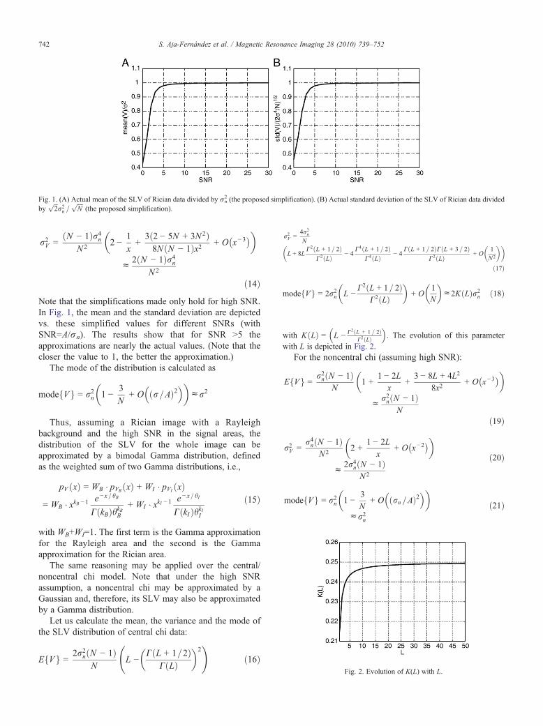
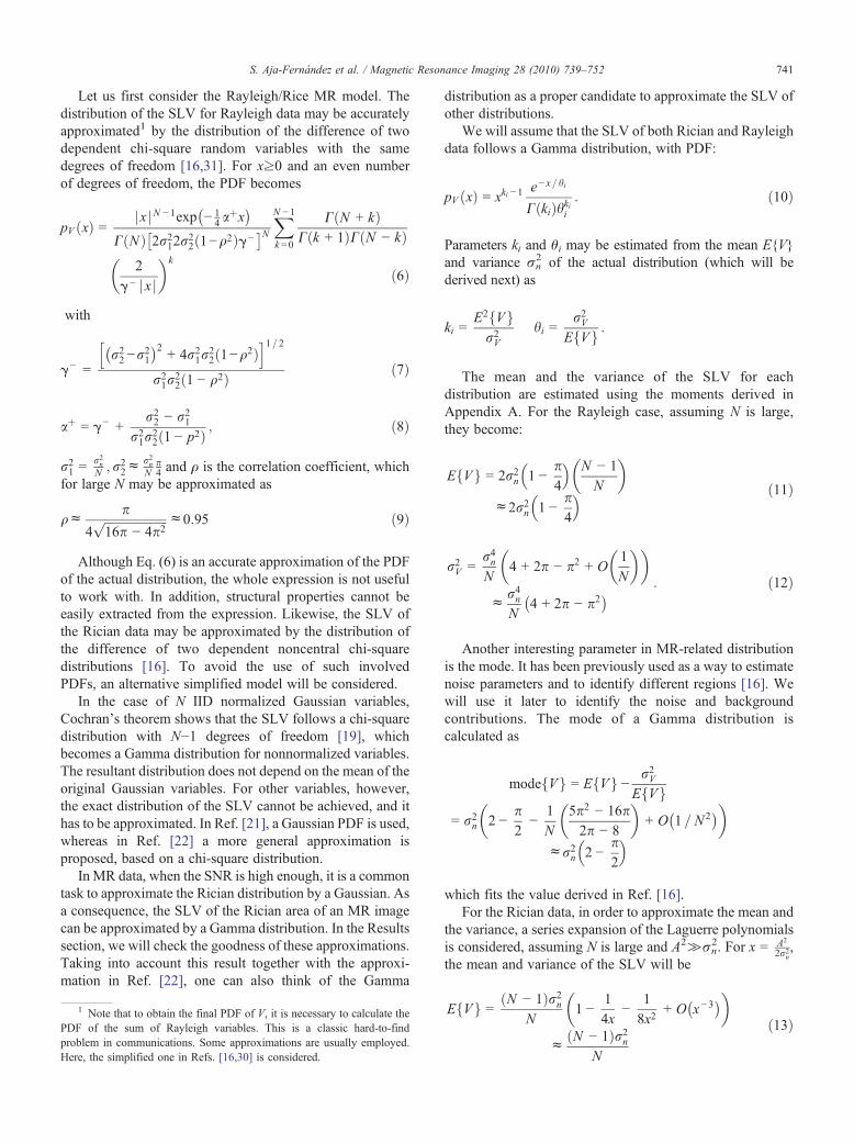
Fig. 1. (A) Actual mean of the SLV of Rician data divided by σn2 (the proposed simplification). (B) Actual standard deviation of the SLV of Rician data divided

byffiffiffi2

pr2n =

ffiffiffiffiN

p(the proposed simplification).

Fig. 2. Evolution of K(L) with L.


r2V =N − 1ð Þr4n

N22 −

1x+

3 2 − 5N + 3N2ð Þ8N N − 1ð Þx2 + O x− 3

� ��

c2 N − 1ð Þr4n

N 2

ð14ÞNote that the simplifications made only hold for high SNR.In Fig. 1, the mean and the standard deviation are depictedvs. these simplified values for different SNRs (withSNR=A/σn). The results show that for SNR N5 theapproximations are nearly the actual values. (Note that thecloser the value to 1, the better the approximation.)

The mode of the distribution is calculated as

mode Vf g = r2n 1 −3N

+ O r=Að Þ2 � �

cr2

Thus, assuming a Rician image with a Rayleighbackground and the high SNR in the signal areas, thedistribution of the SLV for the whole image can beapproximated by a bimodal Gamma distribution, definedas the weighted sum of two Gamma distributions, i.e.,

pV xð Þ = WB � pVB xð Þ + WI � pVI xð Þ= WB � xkB −1 e− x=hB

C kBð ÞhkBB+ WI � xkI −1 e− x= hI

C kIð ÞhkIIð15Þ

with WB+WI=1. The first term is the Gamma approximationfor the Rayleigh area and the second is the Gammaapproximation for the Rician area.

The same reasoning may be applied over the central/noncentral chi model. Note that under the high SNRassumption, a noncentral chi may be approximated by aGaussian and, therefore, its SLV may also be approximatedby a Gamma distribution.

Let us calculate the mean, the variance and the mode ofthe SLV distribution of central chi data:

E Vf g =2r2n N − 1ð Þ

NL −

C L + 1=2ð ÞC Lð Þ

� �2 !

ð16Þ

r2V =4r2nN

L m 8LC2 L + 1= 2ð Þ

C2 Lð Þ − 4C4 L + 1= 2ð Þ

C4 Lð Þ − 4C L + 1= 2ð ÞC L + 3= 2ð Þ

C2 Lð Þ + O1

N2

� �� ð17Þ

mode Vf g = 2r2n L −C2 L + 1 = 2ð Þ

C2 Lð Þ� �

+ O1N

� �c2K Lð Þr2n ð18Þ

with K Lð Þ = L − C2 L + 1 = 2ð ÞC2 Lð Þ

. The evolution of this parameter

with L is depicted in Fig. 2.For the noncentral chi (assuming high SNR):

E Vf g =r2n N − 1ð Þ

N1 +

1 − 2Lx

+3 − 8L + 4L2

8x2+ O x−3

� ��

cr2n N − 1ð Þ

Nð19Þ

r2V =r4n N − 1ð Þ

N22 +

1 − 2Lx

+ O x−2� ��

c2r4n N − 1ð Þ

N2

ð20Þ

mode Vf g = r2n 1 −3N

+ O rn =Að Þ2 � �

cr2n

ð21Þ

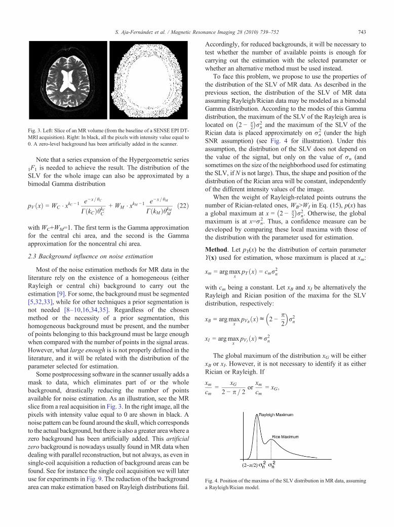
Fig. 4. Position of the maxima of the SLV distribution in MR data, assuminga Rayleigh/Rician model.

Fig. 3. Left: Slice of an MR volume (from the baseline of a SENSE EPI DT-MRI acquisition). Right: In black, all the pixels with intensity value equal to0. A zero-level background has been artificially added in the scanner.


Note that a series expansion of the Hypergeometric series1F1 is needed to achieve the result. The distribution of theSLV for the whole image can also be approximated by abimodal Gamma distribution

pV xð Þ = WC � xkC −1 e− x=hC

C kCð ÞhkCC+ WM � xkM −1 e− x=hM

C kMð ÞhkMMð22Þ

withWC+WM=1. The first term is the Gamma approximationfor the central chi area, and the second is the Gammaapproximation for the noncentral chi area.

2.3 Background influence on noise estimation

Most of the noise estimation methods for MR data in theliterature rely on the existence of a homogeneous (eitherRayleigh or central chi) background to carry out theestimation [9]. For some, the background must be segmented[5,32,33], while for other techniques a prior segmentation isnot needed [8–10,16,34,35]. Regardless of the chosenmethod or the necessity of a prior segmentation, thishomogeneous background must be present, and the numberof points belonging to this background must be large enoughwhen compared with the number of points in the signal areas.However, what large enough is is not properly defined in theliterature, and it will be related with the distribution of theparameter selected for estimation.

Some postprocessing software in the scanner usually adds amask to data, which eliminates part of or the wholebackground, drastically reducing the number of pointsavailable for noise estimation. As an illustration, see the MRslice from a real acquisition in Fig. 3. In the right image, all thepixels with intensity value equal to 0 are shown in black. Anoise pattern can be found around the skull, which correspondsto the actual background, but there is also a greater areawhere azero background has been artificially added. This artificialzero background is nowadays usually found in MR data whendealing with parallel reconstruction, but not always, as even insingle-coil acquisition a reduction of background areas can befound. See for instance the single coil acquisition we will lateruse for experiments in Fig. 9. The reduction of the backgroundarea can make estimation based on Rayleigh distributions fail.

Accordingly, for reduced backgrounds, it will be necessary totest whether the number of available points is enough forcarrying out the estimation with the selected parameter orwhether an alternative method must be used instead.

To face this problem, we propose to use the properties ofthe distribution of the SLV of MR data. As described in theprevious section, the distribution of the SLV of MR dataassuming Rayleigh/Rician data may be modeled as a bimodalGamma distribution. According to the modes of this Gammadistribution, the maximum of the SLV of the Rayleigh area islocated on 2 − p

2

� �r2n and the maximum of the SLV of the

Rician data is placed approximately on σn2 (under the high

SNR assumption) (see Fig. 4 for illustration). Under thisassumption, the distribution of the SLV does not depend onthe value of the signal, but only on the value of σn (andsometimes on the size of the neighborhood used for estimatingthe SLV, if N is not large). Thus, the shape and position of thedistribution of the Rician area will be constant, independentlyof the different intensity values of the image.

When the weight of Rayleigh-related points outruns thenumber of Rician-related ones, WBNWI in Eq. (15), p(x) hasa global maximum at x = 2 − p

2

� �r2n. Otherwise, the global

maximum is at x=σn2. Thus, a confidence measure can be

developed by comparing these local maxima with those ofthe distribution with the parameter used for estimation.

Method. Let pY(x) be the distribution of certain parameterY(x) used for estimation, whose maximum is placed at xm:

xm = argmaxx

pY xð Þ = cmr2n

with cm being a constant. Let xB and xI be alternatively theRayleigh and Rician position of the maxima for the SLVdistribution, respectively:

xB = argmaxx

pVB xð Þc 2 −p2

r2n

xI = argmaxx

pVI xð Þcr2n

The global maximum of the distribution xG will be eitherxB or xI. However, it is not necessary to identify it as eitherRician or Rayleigh. If

xmcm

=xG

2 − p = 2or

xmcm

= xG;

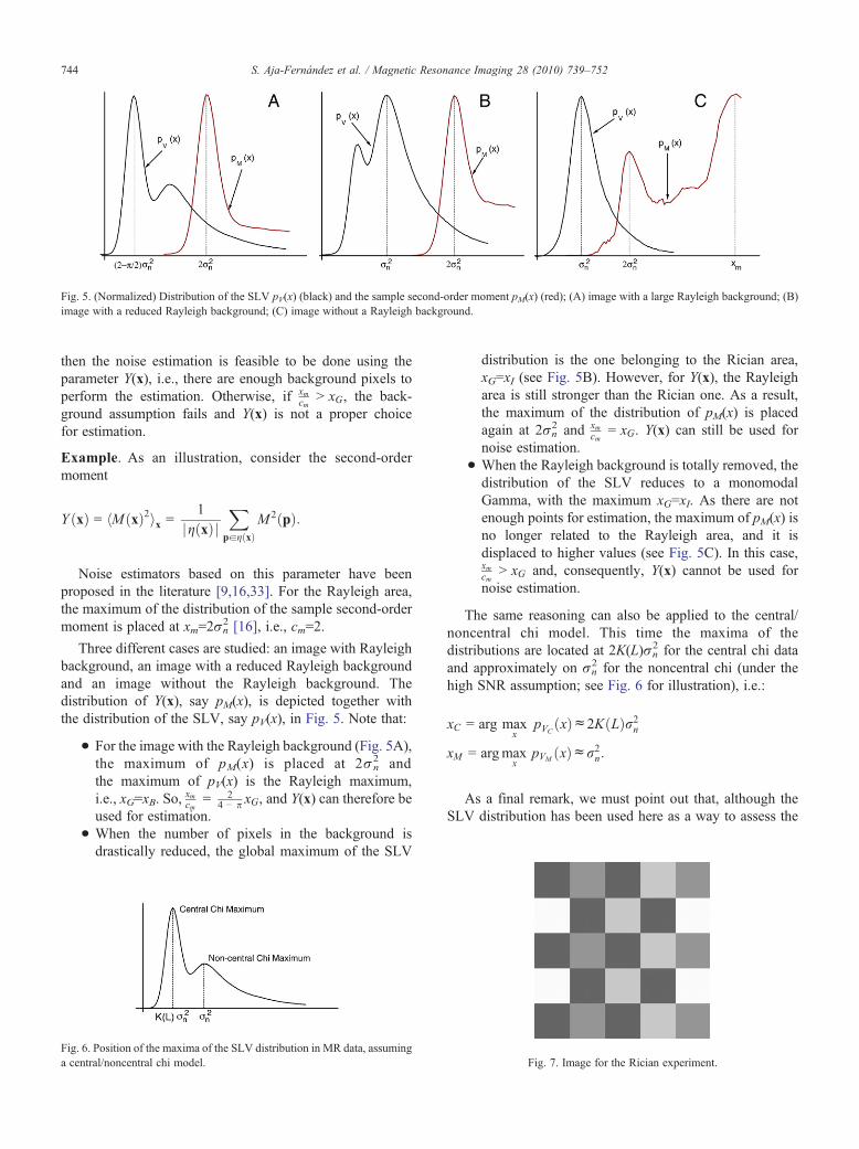
Fig. 5. (Normalized) Distribution of the SLV pV(x) (black) and the sample second-order moment pM(x) (red); (A) image with a large Rayleigh background; (Bimage with a reduced Rayleigh background; (C) image without a Rayleigh background.


then the noise estimation is feasible to be done using theparameter Y(x), i.e., there are enough background pixels toperform the estimation. Otherwise, if xm

cmN xG, the back-

ground assumption fails and Y(x) is not a proper choicefor estimation.

Example. As an illustration, consider the second-ordermoment

Y xð Þ = hM xð Þ2ix =1

jg xð Þ jX

pag xð ÞM 2 pð Þ:

Noise estimators based on this parameter have beenproposed in the literature [9,16,33]. For the Rayleigh area,the maximum of the distribution of the sample second-ordermoment is placed at xm=2σn

2 [16], i.e., cm=2.

Three different cases are studied: an image with Rayleighbackground, an image with a reduced Rayleigh backgroundand an image without the Rayleigh background. Thedistribution of Y(x), say pM(x), is depicted together withthe distribution of the SLV, say pV(x), in Fig. 5. Note that:

• For the image with the Rayleigh background (Fig. 5A),the maximum of pM(x) is placed at 2σn

2 andthe maximum of pV(x) is the Rayleigh maximum,i.e., xG=xB. So,

xmcm

= 24 − p xG, and Y(x) can therefore be

used for estimation.• When the number of pixels in the background isdrastically reduced, the global maximum of the SLV

Fig. 6. Position of the maxima of the SLV distribution in MR data, assuminga central/noncentral chi model. Fig. 7. Image for the Rician experiment.

)

distribution is the one belonging to the Rician area,xG=xI (see Fig. 5B). However, for Y(x), the Rayleigharea is still stronger than the Rician one. As a result,the maximum of the distribution of pM(x) is placedagain at 2σn

2 and xmcm

= xG. Y(x) can still be used fornoise estimation.

• When the Rayleigh background is totally removed, thedistribution of the SLV reduces to a monomodalGamma, with the maximum xG=xI. As there are notenough points for estimation, the maximum of pM(x) isno longer related to the Rayleigh area, and it isdisplaced to higher values (see Fig. 5C). In this case,xmcm

N xG and, consequently, Y(x) cannot be used fornoise estimation.

The same reasoning can also be applied to the central/noncentral chi model. This time the maxima of thedistributions are located at 2K(L)σn

2 for the central chi dataand approximately on σn

2 for the noncentral chi (under thehigh SNR assumption; see Fig. 6 for illustration), i.e.:

xC = arg maxx

pVCxð Þc2K Lð Þr2n

xM = argmaxx

pVM xð Þcr2n:

As a final remark, we must point out that, although theSLV distribution has been used here as a way to assess the

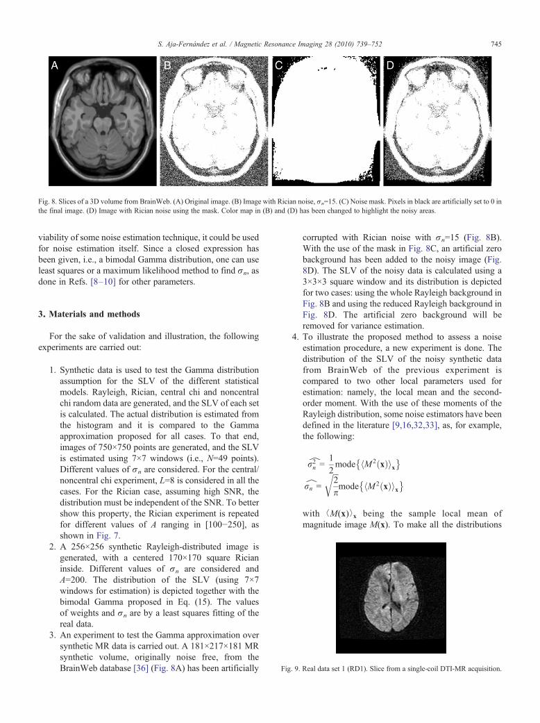
Fig. 8. Slices of a 3D volume from BrainWeb. (A) Original image. (B) Image with Rician noise, σn=15. (C) Noise mask. Pixels in black are artificially set to 0 inthe final image. (D) Image with Rician noise using the mask. Color map in (B) and (D) has been changed to highlight the noisy areas.


viability of some noise estimation technique, it could be usedfor noise estimation itself. Since a closed expression hasbeen given, i.e., a bimodal Gamma distribution, one can useleast squares or a maximum likelihood method to find σn, asdone in Refs. [8–10] for other parameters.

Fig. 9. Real data set 1 (RD1). Slice from a single-coil DTI-MR acquisition

3. Materials and methods

For the sake of validation and illustration, the followingexperiments are carried out:

1. Synthetic data is used to test the Gamma distributionassumption for the SLV of the different statisticalmodels. Rayleigh, Rician, central chi and noncentralchi random data are generated, and the SLV of each setis calculated. The actual distribution is estimated fromthe histogram and it is compared to the Gammaapproximation proposed for all cases. To that end,images of 750×750 points are generated, and the SLVis estimated using 7×7 windows (i.e., N=49 points).Different values of σn are considered. For the central/noncentral chi experiment, L=8 is considered in all thecases. For the Rician case, assuming high SNR, thedistribution must be independent of the SNR. To bettershow this property, the Rician experiment is repeatedfor different values of A ranging in [100−250], asshown in Fig. 7.

2. A 256×256 synthetic Rayleigh-distributed image isgenerated, with a centered 170×170 square Ricianinside. Different values of σn are considered andA=200. The distribution of the SLV (using 7×7windows for estimation) is depicted together with thebimodal Gamma proposed in Eq. (15). The valuesof weights and σn are by a least squares fitting of thereal data.

3. An experiment to test the Gamma approximation oversynthetic MR data is carried out. A 181×217×181 MRsynthetic volume, originally noise free, from theBrainWeb database [36] (Fig. 8A) has been artificially

corrupted with Rician noise with σn=15 (Fig. 8B).With the use of the mask in Fig. 8C, an artificial zerobackground has been added to the noisy image (Fig.8D). The SLV of the noisy data is calculated using a3×3×3 square window and its distribution is depictedfor two cases: using the whole Rayleigh background inFig. 8B and using the reduced Rayleigh background inFig. 8D. The artificial zero background will beremoved for variance estimation.

4. To illustrate the proposed method to assess a noiseestimation procedure, a new experiment is done. Thedistribution of the SLV of the noisy synthetic datafrom BrainWeb of the previous experiment iscompared to two other local parameters used forestimation: namely, the local mean and the second-order moment. With the use of these moments of theRayleigh distribution, some noise estimators have beendefined in the literature [9,16,32,33], as, for example,the following:

^r2n =

12mode hM 2 xð Þix

� �^rn =

ffiffiffi2p

rmode hM 2 xð Þix

� �

with ⟨M(x)⟩x being the sample local mean ofmagnitude image M(x). To make all the distributions

.

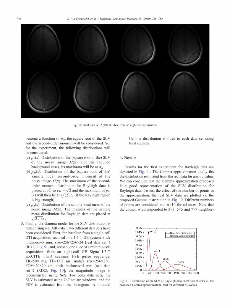
Fig. 10. Real data set 2 (RD2). Slice from an eight-coil acquisition.

Fig. 11. Distribution of the SLV of Rayleigh data. Real data (black) vs. theproposed Gamma approximation (red) for different σn values.


become a function of σn, the square root of the SLVand the second-order moment will be considered. So,for the experiment, the following distributions willbe considered:(a) pV(x): Distribution of the (square root of the) SLV

of the noisy image M(x). For the reducedbackground cases, its maximum will be at σn.

(b) pM(x): Distribution of the (square root of the)sample local second-order moment of thenoisy image M(x). The maximum of the second-order moment distribution for Rayleigh data isplaced at σ2

n, so cM =ffiffiffi2

pand the maximum of pM

(x) will then be atffiffiffiffiffiffiffi2ð Þprn (if the Rayleigh region

is big enough).(c) pA(x): Distribution of the sample local mean of the

noisy image M(x). The maxima of the samplemean distribution for Rayleigh data are placed atffiffiffiffiffiffiffiffiffiffi

2= pp

rn.5. Finally, the Gamma model for the SLV distribution is

tested using real MR data. Two different data sets havebeen considered. First, the baseline from a single-coilDTI acquisition, scanned in a 1.5-T GE system, slickthickness=5 mm, size=256×256×24 [real data set 1(RD1); Fig. 9]; and, second, one slice of a multiple-coilacquisition, from an eight-coil GE Signa 1.5-TEXCITE 11m4 scanner, FSE pulse sequence,TR=500 ms, TE=13.8 ms, matrix size=256×256,FOV=20×20 cm, slick thickness=5 mm [real dataset 2 (RD2); Fig. 10]; the magnitude image isreconstructed using SoS. For both data sets, theSLV is estimated using 7×7 square windows, and thePDF is estimated from the histogram. A bimodal

Gamma distribution is fitted to each data set usingleast squares.

4. Results

Results for the first experiment for Rayleigh data aredepicted in Fig. 11. The Gamma approximation totally fitsthe distribution estimated from the real data for any σn value.We can conclude that the Gamma approximation proposedis a good representation of the SLV distribution forRayleigh data. To test the effect of the number of points inthe approximation, the real SLV data are plotted vs. theproposed Gamma distribution in Fig. 12. Different numbersof points are considered and σ=10 for all cases. Note thatthe chosen N corresponded to 3×3, 5×5 and 7×7 neighbor-

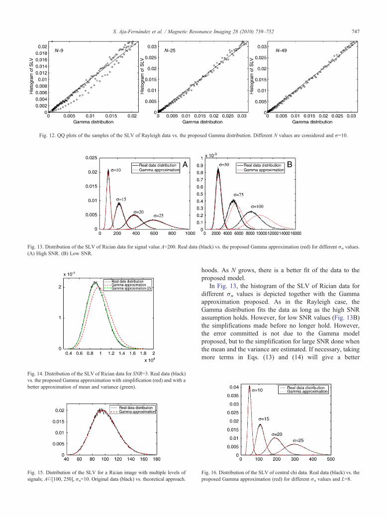
Fig. 13. Distribution of the SLV of Rician data for signal value A=200. Real data (black) vs. the proposed Gamma approximation (red) for different σn values.(A) High SNR. (B) Low SNR.

Fig. 12. QQ plots of the samples of the SLV of Rayleigh data vs. the proposed Gamma distribution. Different N values are considered and σ=10.

Fig. 14. Distribution of the SLV of Rician data for SNR=3. Real data (black)vs. the proposed Gamma approximation with simplification (red) and with abetter approximation of mean and variance (green).

Fig. 15. Distribution of the SLV for a Rician image with multiple levels ofsignals; A∈[100, 250], σn=10. Original data (black) vs. theoretical approach.


hoods. As N grows, there is a better fit of the data to theproposed model.

In Fig. 13, the histogram of the SLV of Rician data fordifferent σn values is depicted together with the Gammaapproximation proposed. As in the Rayleigh case, theGamma distribution fits the data as long as the high SNRassumption holds. However, for low SNR values (Fig. 13B)the simplifications made before no longer hold. However,the error committed is not due to the Gamma modelproposed, but to the simplification for large SNR done whenthe mean and the variance are estimated. If necessary, takingmore terms in Eqs. (13) and (14) will give a better

Fig. 16. Distribution of the SLV of central chi data. Real data (black) vs. theproposed Gamma approximation (red) for different σn values and L=8.

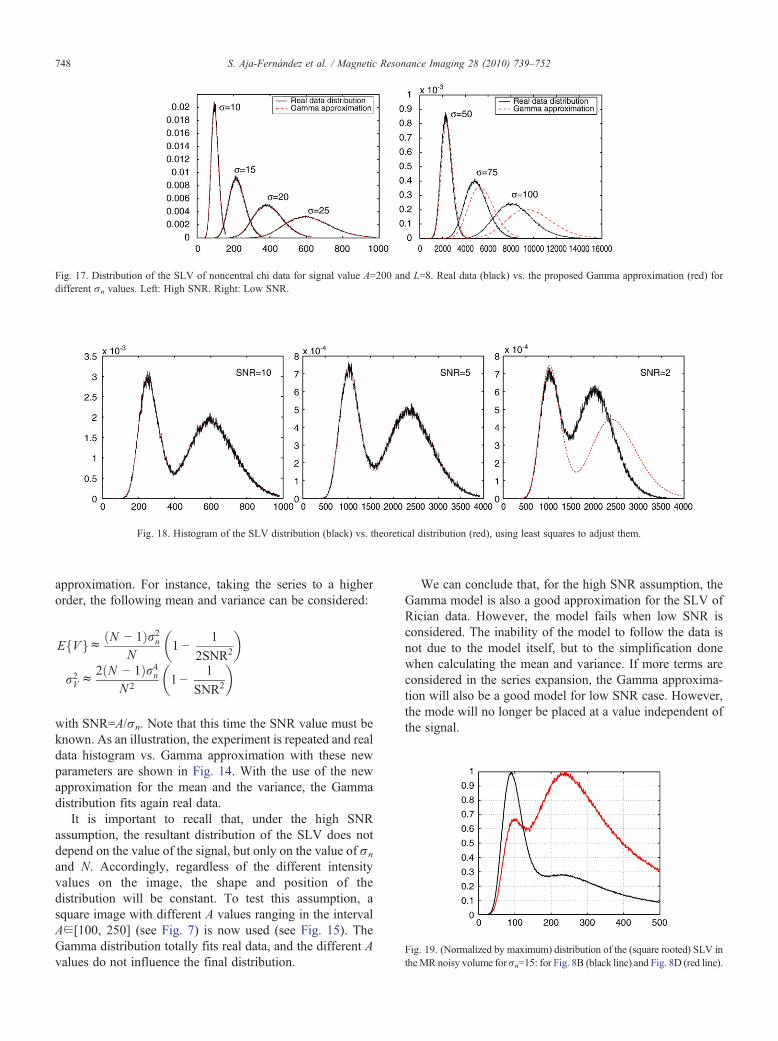
Fig. 17. Distribution of the SLV of noncentral chi data for signal value A=200 and L=8. Real data (black) vs. the proposed Gamma approximation (red) fordifferent σn values. Left: High SNR. Right: Low SNR.

Fig. 18. Histogram of the SLV distribution (black) vs. theoretical distribution (red), using least squares to adjust them.

Fig. 19. (Normalized by maximum) distribution of the (square rooted) SLV intheMR noisy volume forσn=15: for Fig. 8B (black line) and Fig. 8D (red line).


approximation. For instance, taking the series to a higherorder, the following mean and variance can be considered:

E Vf gc N − 1ð Þr2nN

1 −1

2SNR2

� �

r2Vc2 N − 1ð Þr4n

N 21 −

1

SNR2

� �

with SNR=A/σn. Note that this time the SNR value must beknown. As an illustration, the experiment is repeated and realdata histogram vs. Gamma approximation with these newparameters are shown in Fig. 14. With the use of the newapproximation for the mean and the variance, the Gammadistribution fits again real data.

It is important to recall that, under the high SNRassumption, the resultant distribution of the SLV does notdepend on the value of the signal, but only on the value of σn

and N. Accordingly, regardless of the different intensityvalues on the image, the shape and position of thedistribution will be constant. To test this assumption, asquare image with different A values ranging in the intervalA∈[100, 250] (see Fig. 7) is now used (see Fig. 15). TheGamma distribution totally fits real data, and the different Avalues do not influence the final distribution.

We can conclude that, for the high SNR assumption, theGamma model is also a good approximation for the SLV ofRician data. However, the model fails when low SNR isconsidered. The inability of the model to follow the data isnot due to the model itself, but to the simplification donewhen calculating the mean and variance. If more terms areconsidered in the series expansion, the Gamma approxima-tion will also be a good model for low SNR case. However,the mode will no longer be placed at a value independent ofthe signal.

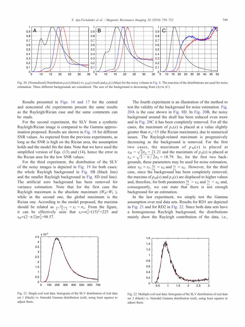
Fig. 20. (Normalized) Distribution pV(x) (black) vs. pM(x) (red) and pA(x) (blue) for the noisy volume in Fig. 8. The maxima of the distributions are used for noiseestimation. Three different backgrounds are considered. The size of the background is decreasing from (A) to (C).


Results presented in Figs. 16 and 17 for the centraland noncentral chi experiments present the same resultsas the Rayleigh/Rician case and the same comments canbe made.

For the second experiment, the SLV from a syntheticRayleigh/Rician image is compared to the Gamma approx-imation proposed. Results are shown in Fig. 18 for differentSNR values. As expected from the previous experiments, aslong as the SNR is high on the Rician area, the assumptionholds and the model fits the data. Note that we have used thesimplified version of Eqs. (13) and (14), hence the error inthe Rician area for the low SNR values.

For the third experiment, the distribution of the SLVof the noisy images is depicted in Fig. 19 for both cases:the whole Rayleigh background in Fig. 8B (black line)and the smaller Rayleigh background in Fig. 8D (red line).The artificial zero background has been removed forvariance estimation. Note that for the first case theRayleigh maximum is the absolute maximum (WBNWI ),while in the second one, the global maximum is theRician one. According to the model proposed, the maximashould be related as xB

2 − p = 2 = xI = rn. From the figure,it can be effectively seen that xI≈σn

2=(15)2=225 andxB≈(2−π/2)σn

2=98.57.

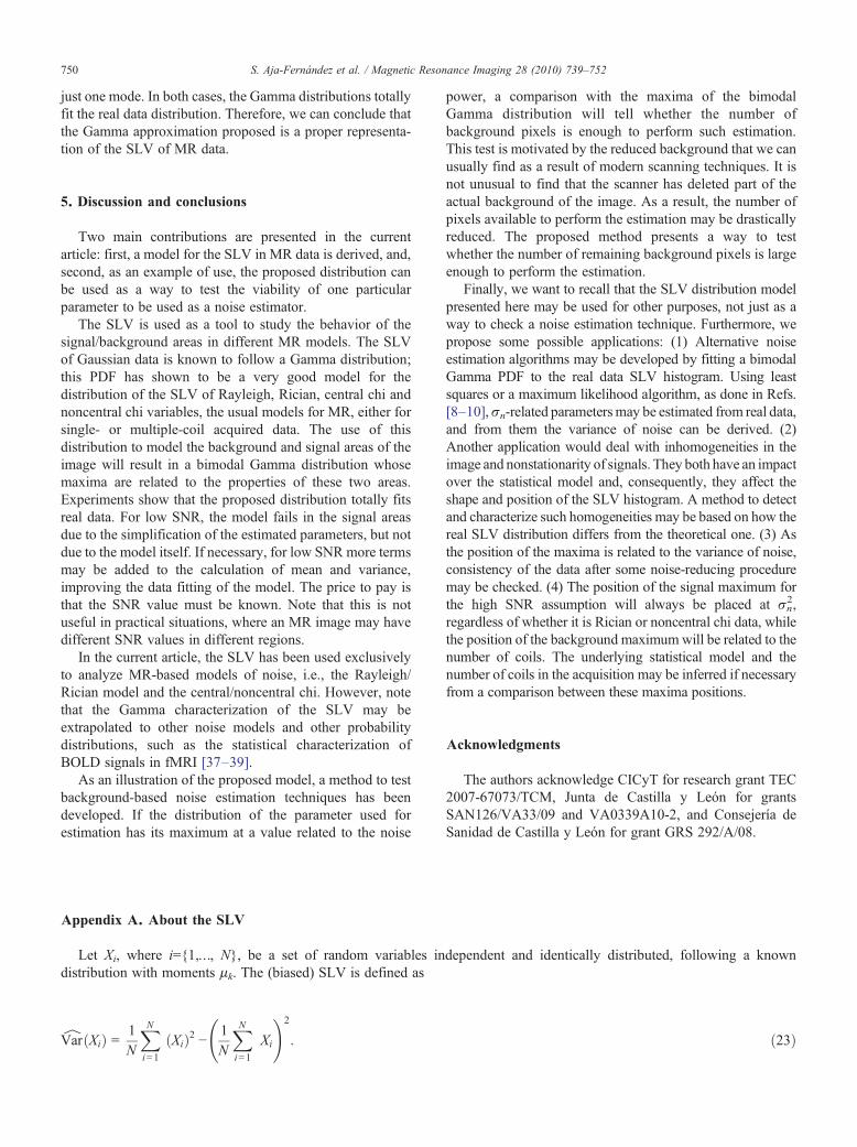
Fig. 21. Single-coil real data: histogram of the SLV distribution of real dataset 1 (black) vs. bimodal Gamma distribution (red), using least squares toadjust them.

The fourth experiment is an illustration of the method totest the validity of the background for noise estimation. Fig.20A is the case shown in Fig. 8D. In Fig. 20B, the noisybackground around the skull has been reduced even moreand in Fig. 20C it has been completely removed. For all thecases, the maximum of pV(x) is placed at a value slightlygreater than σn=15 (the Rician maximum), due to numericalissues. The Rayleigh-related maximum is progressivelydecreasing as the background is removed. For the firsttwo cases, the maximum of pM(x) is placed atxM =

ffiffiffi2

prn = 21:21 and the maximum of pA(x) is placed at

xA =ffiffiffiffiffiffiffiffiffiffiffiffiffiffiffiffiffi2 − p = 2

prn = 18:79. So, for the first two back-

grounds, these parameters may be used for noise estimation,since xG = xI ;

xMcM

= xG and xAcA

= xG. However, for the thirdcase, since the background has been completely removed,the maxima of pM(x) and pA(x) are displaced to higher valuesand, therefore, for both parameters xM

cMN xG and xA

cAN xG and,

consequently, we can state that there is not enoughbackground for an estimation.

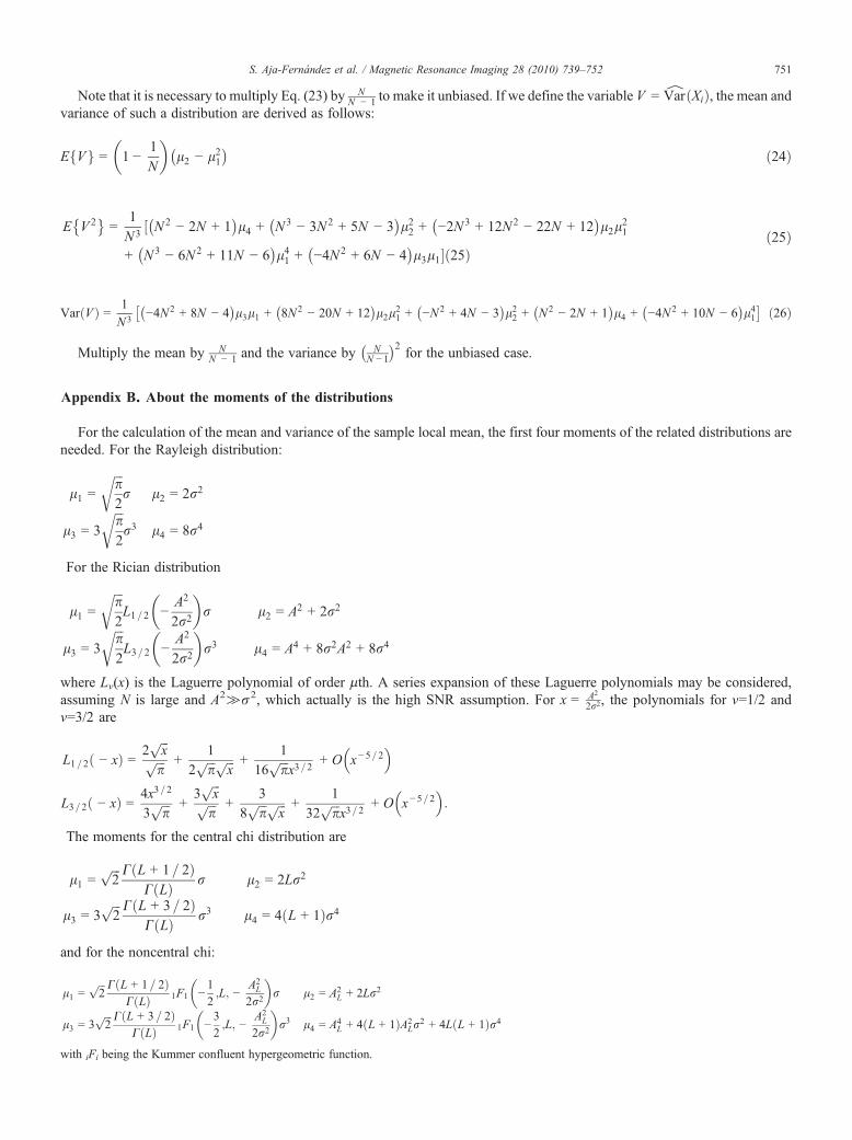
In the last experiment, we simply test the Gammaassumption over real data sets. Results for RD1 are depictedin Fig. 21 and for RD2 in Fig. 22. Since both data sets havea homogeneous Rayleigh background, the distributionsmainly show the Rayleigh contribution of the data, i.e.,

Fig. 22. Multiple coil real data: histogram of the SLV distribution of real dataset 2 (black) vs. bimodal Gamma distribution (red), using least squares toadjust them.


just one mode. In both cases, the Gamma distributions totallyfit the real data distribution. Therefore, we can conclude thatthe Gamma approximation proposed is a proper representa-tion of the SLV of MR data.

5. Discussion and conclusions

Two main contributions are presented in the currentarticle: first, a model for the SLV in MR data is derived, and,second, as an example of use, the proposed distribution canbe used as a way to test the viability of one particularparameter to be used as a noise estimator.

The SLV is used as a tool to study the behavior of thesignal/background areas in different MR models. The SLVof Gaussian data is known to follow a Gamma distribution;this PDF has shown to be a very good model for thedistribution of the SLV of Rayleigh, Rician, central chi andnoncentral chi variables, the usual models for MR, either forsingle- or multiple-coil acquired data. The use of thisdistribution to model the background and signal areas of theimage will result in a bimodal Gamma distribution whosemaxima are related to the properties of these two areas.Experiments show that the proposed distribution totally fitsreal data. For low SNR, the model fails in the signal areasdue to the simplification of the estimated parameters, but notdue to the model itself. If necessary, for low SNR more termsmay be added to the calculation of mean and variance,improving the data fitting of the model. The price to pay isthat the SNR value must be known. Note that this is notuseful in practical situations, where an MR image may havedifferent SNR values in different regions.

In the current article, the SLV has been used exclusivelyto analyze MR-based models of noise, i.e., the Rayleigh/Rician model and the central/noncentral chi. However, notethat the Gamma characterization of the SLV may beextrapolated to other noise models and other probabilitydistributions, such as the statistical characterization ofBOLD signals in fMRI [37–39].

As an illustration of the proposed model, a method to testbackground-based noise estimation techniques has beendeveloped. If the distribution of the parameter used forestimation has its maximum at a value related to the noise

power, a comparison with the maxima of the bimodalGamma distribution will tell whether the number ofbackground pixels is enough to perform such estimation.This test is motivated by the reduced background that we canusually find as a result of modern scanning techniques. It isnot unusual to find that the scanner has deleted part of theactual background of the image. As a result, the number ofpixels available to perform the estimation may be drasticallyreduced. The proposed method presents a way to testwhether the number of remaining background pixels is largeenough to perform the estimation.

Finally, we want to recall that the SLV distribution modelpresented here may be used for other purposes, not just as away to check a noise estimation technique. Furthermore, wepropose some possible applications: (1) Alternative noiseestimation algorithms may be developed by fitting a bimodalGamma PDF to the real data SLV histogram. Using leastsquares or a maximum likelihood algorithm, as done in Refs.[8–10],σn-related parametersmay be estimated from real data,and from them the variance of noise can be derived. (2)Another application would deal with inhomogeneities in theimage and nonstationarity of signals. They both have an impactover the statistical model and, consequently, they affect theshape and position of the SLV histogram. A method to detectand characterize such homogeneities may be based on how thereal SLV distribution differs from the theoretical one. (3) Asthe position of the maxima is related to the variance of noise,consistency of the data after some noise-reducing proceduremay be checked. (4) The position of the signal maximum forthe high SNR assumption will always be placed at σn

2,regardless of whether it is Rician or noncentral chi data, whilethe position of the background maximumwill be related to thenumber of coils. The underlying statistical model and thenumber of coils in the acquisition may be inferred if necessaryfrom a comparison between these maxima positions.

Acknowledgments

The authors acknowledge CICyT for research grant TEC2007-67073/TCM, Junta de Castilla y León for grantsSAN126/VA33/09 and VA0339A10-2, and Consejería deSanidad de Castilla y León for grant GRS 292/A/08.

Appendix A. About the SLV

Let Xi, where i={1,…, N}, be a set of random variables independent and identically distributed, following a knowndistribution with moments μk. The (biased) SLV is defined as

^Var Xið Þ = 1

N

XNi=1

Xið Þ2 − 1N

XNi=1

Xi

!2

: ð23Þ


Note that it is necessary to multiply Eq. (23) by NN − 1 to make it unbiased. If we define the variable V =

^Var Xið Þ, the mean and

variance of such a distribution are derived as follows:

E Vf g = 1 −1N

� �l2 − l21� � ð24Þ

E V 2� �

=1N3

½ N 2 − 2N + 1� �

l4 + N3 − 3N 2 + 5N − 3� �

l22 + −2N 3 + 12N2 − 22N + 12� �

l2l21

+ N3 − 6N 2 + 11N − 6� �

l41 + −4N 2 + 6N − 4� �

l3l1�ð25Þð25Þ

Var Vð Þ = 1N 3

−4N 2 + 8N − 4� �

l3l1 + 8N 2 − 20N + 12� �

l2l21 + −N 2 + 4N − 3

� �l22 + N 2 − 2N + 1

� �l4 + −4N 2 + 10N − 6

� �l41

� � ð26Þ

Multiply the mean by NN − 1 and the variance by N

N −1

� �2for the unbiased case.

Appendix B. About the moments of the distributions

For the calculation of the mean and variance of the sample local mean, the first four moments of the related distributions areneeded. For the Rayleigh distribution:

l1 =

ffiffiffip2

rr l2 = 2r2

l3 = 3

ffiffiffip2

rr3 l4 = 8r4

For the Rician distribution

l1 =

ffiffiffip2

rL1=2 −

A2

2r2

� �r l2 = A2 + 2r2

l3 = 3

ffiffiffip2

rL3=2 −

A2

2r2

� �r3 l4 = A4 + 8r2A2 + 8r4

where Lν(x) is the Laguerre polynomial of order μth. A series expansion of these Laguerre polynomials may be considered,assuming N is large and A2≫σ2, which actually is the high SNR assumption. For x = A2

2r2, the polynomials for ν=1/2 andν=3/2 are

L1=2 − xð Þ = 2ffiffiffix

pffiffiffip

p +1

2ffiffiffip

p ffiffiffix

p +1

16ffiffiffip

px3=2

+ O x−5=2

L3=2 − xð Þ = 4x3=2

3ffiffiffip

p +3ffiffiffix

pffiffiffip

p +3

8ffiffiffip

p ffiffiffix

p +1

32ffiffiffip

px3=2

+ O x−5=2

:

The moments for the central chi distribution are

l1 =ffiffiffi2

p C L + 1= 2ð ÞC Lð Þ r l2 = 2Lr2

l3 = 3ffiffiffi2

p C L + 3= 2ð ÞC Lð Þ r3 l4 = 4 L + 1ð Þr4

and for the noncentral chi:

l1 =ffiffiffi2

p C L + 1= 2ð ÞC Lð Þ 1F1 −

12;L; −

A2L

2r2

� �r l2 = A2

L + 2Lr2

l3 = 3ffiffiffi2

p C L + 3= 2ð ÞC Lð Þ 1F1 −

32;L; −

A2L

2r2

� �r3 l4 = A4

L + 4 L + 1ð ÞA2Lr

2 + 4L L + 1ð Þr4

with iFi being the Kummer confluent hypergeometric function.


References

[1] McGibney G, Smith M. Unbiased signal-to-noise ratio measure formagnetic resonance images. Med Phys 1993;20(4):1077–8.

[2] Gudbjartsson H, Patz S. The Rician distribution of noisy MRI data.Magn Reson Med 1995;34(6):910–4.

[3] Aja-Fernández S, Niethammer M, Kubicki M, Shenton ME, Westin C-F. Restoration of DWI data using a Rician LMMSE estimator. IEEETrans Med Imaging 2008;27(10):1389–403.

[4] Drumheller D. General expressions for Rician density and distributionfunctions. IEEE Trans Aerosp Electron Syst 1993;29(2):580–8.

[5] Constantinides C, Atalar E, McVeigh E. Signal-to-noise measurementsin magnitude images from NMR based arrays. Magn Reson Med1997;38:852–7.

[6] Dietrich O, Raya J, Reeder SB, Ingrisch M, Reiser M, Schoenberg SO.Influence of multichannel combination, parallel imaging and otherreconstruction techniques on MRI noise characteristics. Magn ResonImaging 2008;26:754–62.

[7] Otsu N. A threshold selection method from gray-scale histogram. IEEETrans Syst Man Cybern 1979;9(1):62–6.

[8] Brummer M, Mersereau R, Eisner R, Lewine R. Automatic detectionof brain contours in MRI data sets. IEEE Trans Med Imaging 1993;12(2):153–66.

[9] Aja-Fernández S, Tristán-Vega A, Alberola-López C. Noise estimationin single and multiple coil MR data based on statistical models. MagnReson Imaging 2009;27:1397–409.

[10] Sijbers J, Poot D, den Dekker AJ, Pintjenst W. Automatic estimation ofthe noise variance from the histogram of a magnetic resonance image.Phys Med Biol 2007;52:1335–48.

[11] Sumanaweera T, Glover G, Song S, Adler J, Napel S. QuantifyingMRIgeometric distortion in tissue. Magn Reson Med 2005;31(1):40–7.

[12] Kisner SJ, Talavage TM. Testing the distribution of nonstationary MRIdata. Proc of the IEEE EMBS, San Francisco (CA); 2004. p. 1888–91.

[13] Sendur L, Selesnick I. Bivariate shrinkage with local varianceestimation. IEEE Signal Process Lett 2002;9(12):438–41.

[14] Aja-Fernández S, Alberola-Lóez C. On the estimation of the coefficientof variation for anisotropic diffusion speckle filtering. IEEE TransImage Process 2006;15(9):2694–701.

[15] Aja-Fernández S, Vegas-Sánchez-Ferrero G, Martín-Fernández M,Alberola-López C. Automatic noise estimation in images using localstatistics. Additive and multiplicative cases. Image Vis Comput2009;27(6):756–70.

[16] Aja-Fernández S, Alberola-López C, Westin C-F. Noise and signalestimation in magnitude MRI and Rician distributed images: aLMMSE approach. IEEE Trans Image Proccess 2008;17(8):1383–98.

[17] Coops N, Culvenor D. Utilizing local variance of simulated highspatial resolution imagery to predict spatial pattern of forest stands.Remote Sens Environ 2000;71(3):248–60.

[18] Aja-Fernández S, San-José-Estépar R, Alberola-López C, Westin C-F.Image quality assessment based on local variance. Proc of the 28thIEEE International Conference of the Engineering in Medicine andBiology Society (EMBC), New York; 2006. p. 4815–8.

[19] Papoulis A. Probability, Random Variables and Stochastic Processes.New York (NY): Mc-Graw Hill; 1991.

[20] Royen T. Exact distribution of the sample variance from a gammaparent distribution, Math.ST (Eprint: arXiv/0704.1415); 2007.p. 1–16.

[21] Mudholkarand GS, Madhusudan CT. A Gaussian approximation to thedistribution of the sample variance for nonnormal populations. J AmStat Assoc 1981;76:479–85.

[22] Solomon H, Stephens MA. An approximation to the distribution of thesample variance. Can J Stat 1983;11(2):149–54.

[23] Bentkus V, Zuijlen MV. Bounds for tail probabilities of the samplevariance. J Inequal Appl 2009:1–20.

[24] Roemer P, Edelstein W, Hayes C, Souza S, Mueller O. The NMRphased array. Magn Reson Med 1990;16:192–225.

[25] Pruessmann KP, Weiger M, Scheidegger MB, Boesiger P. SENSE:Sensitivity encoding for fast MRI. Magn Reson Med 1999;42(5):952–62.

[26] Griswold MA, Jakob PM, Heidemann RM, Nittka M, Jellus V, WangJ, et al. Generalized autocalibrating partially parallel acquisitions(GRAPPA). Magn Reson Med 2002;47(6):1202–10.

[27] Hoge WS, Brooks DH, Madore B, Kyriakos WE. A tour of acceleratedparallel MR imaging from a linear systems perspective. ConceptsMagn Reson Part A 2005;27A(1):17–37.

[28] Larkman DJ, Nunes RG. Parallel magnetic resonance imaging. PhysMed Biol 2007;52:15–55 invited Topical Review.

[29] Thnberg P, Zetterberg P. Noise distribution in SENSE- and GRAPPA-reconstructed images: a computer simulation study. Magn ResonImaging 2007;25:1089–94.

[30] Beaulieu NC. An infinite series for the computation of thecomplementary probability distribution function of a sum ofindependent random variables and its application to the sum ofRayleigh random variables. IEEE Trans Commun 1990;38(9):1463–73.

[31] Simon MK. Probability Distributions Involving Gaussian RandomVariables. New York: Springer; 2002.

[32] Nowak R.Wavelet-based Rician noise removal for magnetic resonanceimaging. IEEE Trans Image Process 1999;8(10):1408–19.

[33] Sijbers J, den Dekker A, Van Audekerke J, Verhoye M, Van Dyck D.Estimation of the noise in magnitude MR images. Magn ResonImaging 1998;16(1):87–90.

[34] van Kempen GMP, van Vliet LJ. Background estimation in nonlinearimage restoration. J Opt Soc Am A 2000;17(3):425–33.

[35] Sijbers J, den Dekker AJ, Poot D, Verhoye M, Van Camp N, Van derLinden A. Robust estimation of the noise variance from backgroundMR data. Proc. of SPIE. Medical Imaging 2006: Image Processing,Vol. 6144; 2006. p. 2018–28.

[36] Collins D, Zijdenbos A, Killokian V, Sled J, Kabani N, Holmes C,Evans A. Design and construction of a realistic digital brain phantom.IEEE Trans Med Imaging 1998;17(3):463–8.

[37] Hanson S, Bly B. The distribution of BOLD susceptibility effects in thebrain is non-Gaussian. Neuroreport 2001;12(9):1971–7.

[38] Chena C-C, Tylera C, Baselera HA. Statistical properties of BOLDmagnetic resonance activity in the human brain. Neuroimage 2003;20(2):1096–109.

[39] Wink A, Roerdink JBTM. BOLD noise assumptions in fMRI. Int JBiomed Imaging 2006:1–11.

About the background distribution in MR data: a local variance study

Documents

Transcript of About the background distribution in MR data: a local variance study