A viscoplastic SANICLAY model for natural soft soils - CORE
64
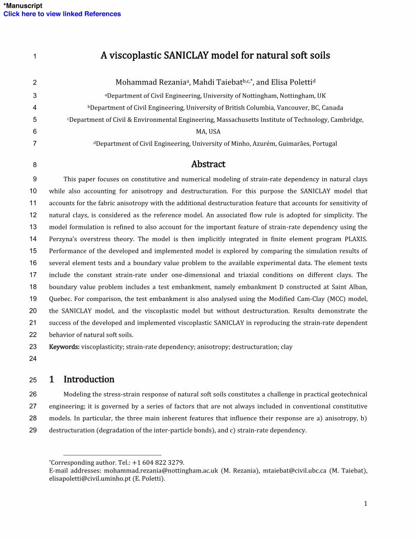
1 A viscoplastic SANICLAY model for natural soft soils 1 Mohammad Rezania a , Mahdi Taiebat b,c,* , and Elisa Poletti d 2 a Department of Civil Engineering, University of Nottingham, Nottingham, UK 3 b Department of Civil Engineering, University of British Columbia, Vancouver, BC, Canada 4 c Department of Civil & Environmental Engineering, Massachusetts Institute of Technology, 5 Cambridge, MA, USA 6 d Department of Civil Engineering, University of Minho, Azurém, Guimarães, Portugal 7 Abstract 8 This paper focuses on constitutive and numerical modeling of strain-rate dependency in natural clays 9 while also accounting for anisotropy and destructuration. For this purpose the SANICLAY model that 10 accounts for the fabric anisotropy with the additional destructuration feature that accounts for sensitivity 11 of natural clays, is considered as the reference model. An associated flow rule is adopted for simplicity. 12 The model formulation is refined to also account for the important feature of strain-rate dependency using 13 the Perzyna’s overstress theory. The model is then implicitly integrated in finite element program 14 PLAXIS. Performance of the developed and implemented model is explored by comparing the simulation 15 results of several element tests and a boundary value problem to the available experimental data. The 16 element tests include the constant strain-rate under one-dimensional and triaxial conditions on different 17 clays. The boundary value problem includes a test embankment, namely embankment D constructed at 18 Saint Alban, Quebec. For comparison, the test embankment is also analysed using the Modified Cam- 19 Clay (MCC) model, the SANICLAY model, and the viscoplastic model but without destructuration. 20 Results demonstrate the success of the developed and implemented viscoplastic SANICLAY in 21 reproducing the strain-rate dependent behavior of natural soft soils. 22 Keywords: viscoplasticity; strain-rate dependency; anisotropy; destructuration; clay 23 24 * Corresponding author. Tel.: +1 604 822 3279. E-mail addresses: [email protected] (M. Rezania), [email protected] (M. Taiebat), [email protected] (E. Poletti).
-
Upload
khangminh22 -
Category
Documents
-
view
1 -
download
0
Transcript of A viscoplastic SANICLAY model for natural soft soils - CORE
1
A viscoplastic SANICLAY model for natural soft soils 1
Mohammad Rezaniaa, Mahdi Taiebatb,c,*, and Elisa Polettid 2
aDepartment of Civil Engineering, University of Nottingham, Nottingham, UK 3 bDepartment of Civil Engineering, University of British Columbia, Vancouver, BC, Canada 4 cDepartment of Civil & Environmental Engineering, Massachusetts Institute of Technology, 5
Cambridge, MA, USA 6 dDepartment of Civil Engineering, University of Minho, Azurém, Guimarães, Portugal 7
Abstract 8
This paper focuses on constitutive and numerical modeling of strain-rate dependency in natural clays 9
while also accounting for anisotropy and destructuration. For this purpose the SANICLAY model that 10
accounts for the fabric anisotropy with the additional destructuration feature that accounts for sensitivity 11
of natural clays, is considered as the reference model. An associated flow rule is adopted for simplicity. 12
The model formulation is refined to also account for the important feature of strain-rate dependency using 13
the Perzyna’s overstress theory. The model is then implicitly integrated in finite element program 14
PLAXIS. Performance of the developed and implemented model is explored by comparing the simulation 15
results of several element tests and a boundary value problem to the available experimental data. The 16
element tests include the constant strain-rate under one-dimensional and triaxial conditions on different 17
clays. The boundary value problem includes a test embankment, namely embankment D constructed at 18
Saint Alban, Quebec. For comparison, the test embankment is also analysed using the Modified Cam-19
Clay (MCC) model, the SANICLAY model, and the viscoplastic model but without destructuration. 20
Results demonstrate the success of the developed and implemented viscoplastic SANICLAY in 21
reproducing the strain-rate dependent behavior of natural soft soils. 22
Keywords: viscoplasticity; strain-rate dependency; anisotropy; destructuration; clay 23
24
*Corresponding author. Tel.: +1 604 822 3279. E-mail addresses: [email protected] (M. Rezania), [email protected] (M. Taiebat), [email protected] (E. Poletti).
2
1 Introduction 25
Modeling the stress-strain response of natural soft soils constitutes a challenge in practical 26
geotechnical engineering; it is governed by a series of factors that are not always included in conventional 27
constitutive models. In particular, the three main inherent features that influence their response are a) 28
anisotropy, b) destructuration (degradation of the inter-particle bonds), and c) strain-rate dependency. 29
Since modeling the full anisotropy of natural clay behavior is not practical due to the number of 30
parameters involved, efforts have been mainly focused on development of models with reduced number of 31
parameters while maintaining the capacity of the model [1]. Historically, for practical model development 32
purposes, the initial orientation of soil fabric is considered to be of cross-anisotropic nature, which is a 33
realistic assumption as natural soils have been generally deposited only one-dimensionally in a vertical 34
direction. It is also a well-established fact that the yield surfaces obtained from experimental tests on 35
undisturbed samples of natural clays are inclined in the stress space due to the inherent fabric anisotropy 36
in the clay structure (e.g., [2-4]). Based on the above, a particular line of thought has become popular in 37
capturing the effects of anisotropy on clayey soil behavior, by development of elasto-plastic constitutive 38
models involving an inclined yield surface that is either fixed (e.g., [2]), or can changed it inclination by 39
adopting a rotational hardening (RH) law in order to simulate the development or erasure of anisotropy 40
during plastic straining (e.g., [5-6]). For obvious reasons a model accounting for both inherent and 41
evolving anisotropy would be more representative of the true nature of response in clays; hence, since the 42
first proposal of such model by Dafalias [5-6] similar framework has been adopted by a number of other 43
researchers for development of anisotropic elasto-plastic constitutive models (e.g., [7-11]). Based on the 44
original model, Dafalias et al. [12] proposed what they called SANICLAY model, altering the original RH 45
law and introducing a non-associated flow rule. A destructuration theory was later applied to the 46
SANICLAY model [13] to account for both isotropic and frictional destructuration processes. In these 47
works, the SANICLAY has been shown to provide successful simulation of both undrained and drained 48
rate-independent behaviour of normally consolidated sensitive clays, and to a satisfactory degree of 49
accuracy of overconsolidated clays. 50
Past experimental studies have also shown that soft soils exhibit time-dependent response (e.g., [14-51
17]). Time-dependency is usually related to the soil viscosity that could lead to particular effects such as 52
creep, stress relaxation, and strain-rate dependency of response. Time-dependency of soil response can be 53
observed experimentally by means of creep tests, stress relaxation tests, or constant rate of strain (CRS) 54
tests [18]. Rate-sensitivity is a particular aspect of time effect that has been investigated extensively; it 55
3
influences both strength and stiffness of soils. Various studies using CRS tests have shown how faster 56
strain rates for a certain strain level lead to higher effective stresses; also, the general observation, 57
particularly in soft soils, is that higher undrained strengths can be achieved by increasing the loading rate 58
(e.g., [16-17,19-20]). The reported observations from laboratory studies all imply that consideration of soil 59
viscosity effects could be key for correct prediction of long term deformations in field conditions; although, 60
neglecting soil viscosity seemingly provide sufficiently correct predictions in short-term [21]. Landslides or 61
long-term deformations of tunnels and embankments on soft soils are examples of common practical 62
problems where a sustainable remediation and/or design solution can only be achieved if time-dependent 63
behavior of soil is taken into consideration. 64
In order to account for the time-dependency of soft clays’ behavior, various frameworks can be found 65
in the literature. Among a number of popular frameworks such as the isotache theory of Šuklje [22] or the 66
non-stationary surface theory of Naghdi and Murch [23], the overstress theory of Perzyna [24-25] is a 67
common framework often used in geomechanics for this purpose due to its relative simplicity. The first 68
overstress-type viscoplastic models were based on isotropic Cam-Clay or modified Cam-Clay models (e.g., 69
[26-32]). More recently, several models accounting for either only the fabric anisotropy (e.g., [33]), or both 70
anisotropy and destructuration [34] have also been introduced. A shortcoming of these models is the 71
absence of bounds for the evolution of rotational hardening variables which could eventually lead to an 72
excessive rotation of the yield surface for loading at very high values of stress-ratio [35-36]. Furthermore, 73
destructuration theories have so far only addressed isotropic destructuration (usually constituting a 74
mechanism of isotropic softening of the yield surface with destructuration), neglecting frictional 75
destructuration. 76
In this paper, a new Elasto-ViscoPlastic Simple ANIsotropic CLAY plasticity (EVP-SANICLAY) 77
model is proposed. The model is a new member of the SANICLAY family of models, which are based on 78
the classical modified Cam-Clay model and include rotational hardening and destructuration features for 79
simulation of anisotropy and sensitivity, respectively. Perzyna’s overstress theory [24-25] is employed to 80
account for soil viscosity effects. Being based on the SANICALY model, the new viscoplastic model 81
restricts the rotation to within bounds necessary to guarantee the existence of real-valued solutions for 82
the analytical expression of the yield surface [12]. In the following sections, the theoretical formulation of 83
the model will be discussed, followed by the details of its numerical implementation based on an 84
algorithm proposed by Katona [28]. The validation of the new model is done by comparing the model 85
simulation results against several experimental data at the element level and also field measurements for a 86
4
boundary value problem. In particular, at element level the measured behavior observed from CRS and 87
undrained triaxial tests over a number of different soft clays are used. Within these examples, 88
determination of model parameter values is also discussed. For the boundary value problem, a well-89
studied test embankment, namely St. Alban embankment, is modeled and the predicted deformations 90
using the EVP-SANICLAY model are compared with the recorded in-situ values. In order to better 91
highlight the merits of the newly proposed constitutive model, the simulation results are also compared 92
with those obtained using the MCC model, the SANCILAY model, and also the EVP-SANICLAY model 93
but without the destructuration feature. Note that in this paper all stress components are effective 94
stresses and as usual in geomechanics, both stress and strain quantities are assumed positive in 95
compression. 96
97
2 EVP-SANICLAY 98
2.1 Model formulation 99
According to Perzyna’s theory, the total strain increment, ∆!, associated with a change in effective 100
stress, ∆!, during a time increment of ∆!, is additively decomposed to elastic and viscoplastic parts 101
∆! = ∆!! + ∆!!" (1)
where the superscripts ! and !" represent the elastic and the viscoplastic components, respectively. The 102
elastic strain increment, ∆!!, is time-independent; whereas, the viscoplastic strain increment, ∆!!", is 103
irreversible and time-dependent. Adopting the isotropic hypoelastic relations for simplicity [12], the elastic 104
part of the total strain can be shown as 105
∆!! = !!!:∆! (2)
where ! is the elastic stiffness matrix with more details presented in the Appendix, and symbol : in 106
implies the trace of the product of two tensors. 107
The time-dependent viscoplastic strain increment is evaluated as 108
∆!!" = !!" ∙ ∆! (3)
where !!" is the viscoplastic strain rate tensor (a superposed dot denotes the time derivative), and 109
following the original proposal by Perzyna [24-25], it can be defined as 110
!!" = ! ∙ Φ ! ∙ !"!! (4)
5
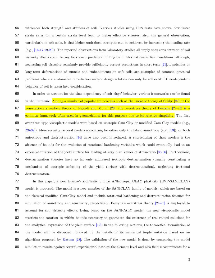
where ! is referred to as the fluidity parameter, ! is the viscoplastic potential function represented by the 111
dynamic loading surface (DLS - explained in the sequel), and Φ ! is the so-called overstress that is the 112
normalised distance between the current static yield surface (SYS) and the DLS (see Figure 1). The 113
application of Macauley brackets in Equation (4) ensures that 114
Φ ! = 0!!!!!!!!!!for!!Φ ! ≤ 0Φ ! !!for!!Φ ! > 0! (5)
Several different relationships for Φ ! have been proposed in the literature (e.g. [26,37]). In this 115
work the following exponential function proposed by Fodil et al. [38] is employed 116
Φ ! = exp!(!) − 1 = exp ! !!!!!!− 1 − 1 (6)
where !!! and !!! are the size of the SYS and the DLS, respectively (see Figure 1), ! is the strain-rate 117
coefficient that together with ! are the two viscous parameters of this model. 118
119
120
Figure 1. Graphical representation of the EVP-SANICLAY model in the stress space 121
122
This specific choice of Φ ! ensures that its value is always greater or equal to zero. Thus, from 123
Equation (7) it is evident that if the stress state lies on or inside the SYS, the soil response would be 124
purely elastic. If the stress state lies outside the SYS, viscoplastic strain will be developed proportional to 125
its distance from the current SYS. 126
In this work the elliptical surface of the SANICLAY model [12] is adopted as the SYS. The 127
SANICLAY model was originally proposed with a non-associated flow rule; however, for simplicity 128
purposes an associated flow rule is adopted here for its elastic-viscoplastic extension. In the general stress 129
space, the SYS function can be expressed as 130
!! = 32 ! − !! : ! − !! − !∗ ! ! − 32!:! !!∗! − ! ! = 0 (7)
6
In the above expression, ! = ! − !! is the deviatoric component of stress tensor ! (! being the fourth 131
order identity tensor). ! is the deviatoric fabric tensor that accounts for anisotropy by coupling the 132
deviatoric and volumetric plastic strain rates. !!∗! = !!!!! defines the size of the structured SYS where 133
!! ≥ 1 is an isotropic destructuration factor and !!! is the size of the intrinsic SYS. !∗ ! = !!! ! where 134
!! ≥ 1 is a frictional destructuration factor and ! ! is the critical stress-ratio that in the general stress 135
space its value is interpolated between !! and !! by means of a Lode angle !. In the stress space 136
illustrated in Figure 1 the scalar ! = (3/2)!!:! defines the rotation of the SYS and DLS. As shown in 137
Figure 1, the DLS has the same shape and orientation as the smaller SYS, and following the adoption of 138
associate flow rule it coincides the viscoplastic potential surface too. A summary of the hardening 139
equations and the Lode angle formulation are presented in the Appendix for the sake of completeness. 140
The model constants of EVP-SANICLAY can be divided into 4 categories: (1) the elasticity 141
constants ! and ! and the critical state constants !!, !! and ! which are the same as those in the MCC 142
model (with the exception that in MCC we have !! = !!); (2) the rotational hardening (RH) constants ! 143
and !, which are specific to the SANICLAY model; (3) the destructuration constants !!, !! and !; and 144
(4) the viscosity parameters ! and !, which constitute the two new additional parameters of the EVP-145
SANICLAY and they can be determined as discussed in Yin and Hicher [31]. Furthermore, similar to the 146
SANICLAY, ! and !!! constitute the hardening internal variables in the EVP-SANICLAY model. It 147
should be noted that despite the large number of model parameters, they have clear physical meaning and 148
can be determined following straightforward processes. The detailed procedure for evaluating the initial 149
values of the model state variables, and hardening and destructuration parameters can be found in 150
Taiebat et al. [13]. 151
152
2.2 Numerical Integration 153
The numerical solution algorithm for the elasto-viscoplastic model can be developed by using a step-154
by-step time integration algorithm with a Newton-Raphson iteration procedure [28]. In this scheme it is 155
assumed at the beginning of a certain defined time interval and strain increment, the values of stresses, 156
strains, and state variables are known. The objective is to determine the subsequent elastic and 157
viscoplastic strain components, which in turn allow finding the subsequent stresses and internal variables. 158
From Equations (1,2) the incremental constitutive relationship for a time step can be expressed as 159
Δ! = ! Δ! − Δ!!" (8)
7
For approximation of Δ!!", a finite difference scheme is employed as: 160
Δ!!" = Δ! 1 − ! !!!" + !!!!!!!" (9)
where !!!" is the value of viscoplastic strain rate at time t, and ! is a time interpolation parameter 161
(0 ≤ ! ≤ 1); ! = 0 represents an explicit forward (Euler) interpolation,!! = 0.5 represents central (Crank-162
Nicolson) interpolation, and ! = 1 implies an implicit backward interpolation. Lewis and Schrefler [39] 163
showed that in this scheme the solution is conditionally stable for 0 ≤ ! < 0.5 and ! = 1, and 164
unconditionally stable for 0.5 ≤ ! < 1. Substituting Equation (9) into Equation (8) and rearranging the 165
terms give: 166
!!!!!!!! + Δ! ∙ ! ∙ !!!!!!" = Δ! − Δ! ∙ 1 − ! !!!" + !!!!! (10)
where the terms on the right hand side are known (at time !), while the left hand side terms are 167
unknowns (at time!! + Δ!) and they are to be solved in an iterative procedure. A Modified Newton-168
Raphson approach is used for the iterative solution of Equation (10). To do this, a limited Taylor series is 169
applied to the unknown quantities !!!!! and !!!!!!" : 170
!!!!! = !! + !!!
!!!!!!" = !!!" +!!!!"!! !!!
(11a)
(11b)
171
Note that subscript ! refers to the !-th iteration at the current time step. Substituting Equations 172
(11a) and (11b) into Equation (10) and successive rearrangements result in the following form for 173
computation of stress increment: 174
!!! = !!! + ∆! ∙ ! ∙ !!!!"
!!!!: Δ! − Δ! ∙ 1 − ! !!!" + !!!:!! − !!!!! + ∆! ∙ ! ∙ !!!" (12)
If it is assumed that function ! represents the term Δ! − Δ! ∙ 1 − ! !!!" + !!!!! with known 175
quantities remaining constant during the iteration, and that function ! represents the iterative term 176
!!!!! + ∆! ∙ ! ∙ !!!" , then Equation (12) can be presented in a short form as: 177
!!! =!"!!
!!∙ !! − !! (13)
The most efficient solution scheme for continuum problems using overstress-type elasto-viscoplastic 178
constitutive equations can be obtained with ! = 0.5 [40]; hence, this value is adopted for the time 179
interpolation parameter in the present work. For the solution algorithm, at every time step Equation (13) 180
is iteratively solved. At each iteration !!! is calculated and subsequently !! is updated as !! = !!!! +181
!!!. When convergence is achieved (i.e. when !!! < tolerance~10!!), the iterative procedure stops and 182
8
the incrementally accumulated stress values will become the stresses at the corresponding time step (i.e., 183
!!!!!); subsequently, viscoplastic strain tensor can be calculated as !!!∆!!" = !!!∆! − !!!!!!!!. The 184
implementation makes it possible to apply the whole strain increment through a number of sub-185
increments, not all at once. After the completion of the integration process at a time increment the 186
procedure advances to the next time step. 187
The EVP-SANICLAY model has been implemented into PLAXIS finite element program as a user-188
defined soil model in order to be used for both element level and boundary value problem simulations. In 189
the following, first the performance of the model is validated by simulation of a number of element test 190
data on various clays. The model is then used for settlement study of a real instrumented test 191
embankment and the simulation results are discussed in detail. The embankment simulation also aims to 192
compare details of the predicted response using the proposed model and also using an isotropic and rate-193
independent model that is often used in practice. 194
195
3 Model validation based on element level tests 196
For the element test simulations the implemented user-defined model has been employed through the 197
PLAXIS Soil Test application [41] to simulate several undrained triaxial shear and CRS test data on four 198
different soft soils reported in the literature, namely Kawasaki clay, Haney clay, St. Herblain clay, and 199
Batiscan clay [14,16,42-43]. The values of model constants and state variables used for the four soil types 200
analysed in this paper are summarised in Tables 1 and 2. In accordance with the natural or reconstituted 201
state of the clay sample being simulated the destructuration feature of the model has been switched on or 202
off by setting respective values to the structuration parameters. 203
204 205
9
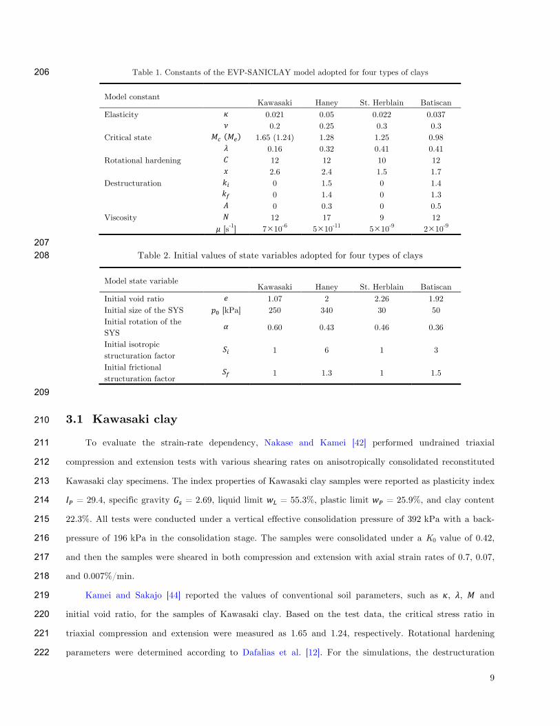
Table 1. Constants of the EVP-SANICLAY model adopted for four types of clays 206
Model constant
Kawasaki Haney St. Herblain Batiscan Elasticity ! 0.021 0.05 0.022 0.037 ! 0.2 0.25 0.3 0.3 Critical state !! !! 1.65 (1.24) 1.28 1.25 0.98 ! 0.16 0.32 0.41 0.41 Rotational hardening ! 12 12 10 12 ! 2.6 2.4 1.5 1.7 Destructuration !! 0 1.5 0 1.4 !! 0 1.4 0 1.3 ! 0 0.3 0 0.5 Viscosity ! 12 17 9 12 ! [s-1] 7!10-6 5!10-11 5!10-9 2!10-9
207 Table 2. Initial values of state variables adopted for four types of clays 208
Model state variable
Kawasaki Haney St. Herblain Batiscan Initial void ratio ! 1.07 2 2.26 1.92 Initial size of the SYS !! [kPa] 250 340 30 50 Initial rotation of the SYS
! 0.60 0.43 0.46 0.36
Initial isotropic structuration factor
!! 1 6 1 3
Initial frictional structuration factor
!! 1 1.3 1 1.5
209
3.1 Kawasaki clay 210
To evaluate the strain-rate dependency, Nakase and Kamei [42] performed undrained triaxial 211
compression and extension tests with various shearing rates on anisotropically consolidated reconstituted 212
Kawasaki clay specimens. The index properties of Kawasaki clay samples were reported as plasticity index 213
!! = 29.4, specific gravity !! = 2.69, liquid limit !! = 55.3%, plastic limit !! = 25.9%, and clay content 214
22.3%. All tests were conducted under a vertical effective consolidation pressure of 392 kPa with a back-215
pressure of 196 kPa in the consolidation stage. The samples were consolidated under a K0 value of 0.42, 216
and then the samples were sheared in both compression and extension with axial strain rates of 0.7, 0.07, 217
and 0.007%/min. 218
Kamei and Sakajo [44] reported the values of conventional soil parameters, such as !, !, ! and 219
initial void ratio, for the samples of Kawasaki clay. Based on the test data, the critical stress ratio in 220
triaxial compression and extension were measured as 1.65 and 1.24, respectively. Rotational hardening 221
parameters were determined according to Dafalias et al. [12]. For the simulations, the destructuration 222
10
feature of the model was switched off by setting !! = !! = 1, as the soil specimens were reconstituted. 223
Viscosity parameters were determined through calibration based on data from tests at only two strain-224
rates. 225
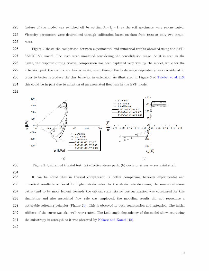
Figure 2 shows the comparison between experimental and numerical results obtained using the EVP-226
SANICLAY model. The tests were simulated considering the consolidation stage. As it is seen in the 227
figure, the response during triaxial compression has been captured very well by the model, while for the 228
extension part the results are less accurate, even though the Lode angle dependency was considered in 229
order to better reproduce the clay behavior in extension. As illustrated in Figure 3 of Taiebat et al. [13] 230
this could be in part due to adoption of an associated flow rule in the EVP model. 231
232
(a) (b)
Figure 2. Undrained triaxial test: (a) effective stress path; (b) deviator stress versus axial strain 233
234 It can be noted that in triaxial compression, a better comparison between experimental and 235
numerical results is achieved for higher strain rates. As the strain rate decreases, the numerical stress 236
paths tend to be more lenient towards the critical state. As no destructuration was considered for this 237
simulation and also associated flow rule was employed, the modeling results did not reproduce a 238
noticeable softening behavior (Figure 2b). This is observed in both compression and extension. The initial 239
stiffness of the curve was also well represented. The Lode angle dependency of the model allows capturing 240
the anisotropy in strength as it was observed by Nakase and Kamei [42]. 241
242
11
3.2 Haney clay 243
Vaid and Campanella [14] carried out undrained triaxial tests on undisturbed saturated sensitive 244
marine clay known as Haney clay. It is a silty clay with !! = 44%, !! = 26% and a sensitivity within the 245
range of 6 to 10. All test samples were normally consolidated, with an all-around confining pressure of 246
515 kPa. Consolidation was allowed for a period of 36 hr after which the samples were left undrained for 247
12 hr under the consolidation stresses prior to shearing. In order to study the rate dependency of 248
undisturbed clay response, the undrained shearing stage of the tests was performed at different constant 249
strain rates, varying from 10-3 to 1.1% /min. 250
Values of conventional soil parameters listed in Tables 1 and 2 were reported by Vermeer and Neher 251
[45]. After determination of the initial value of !, the values of anisotropy constants,!! and !, were 252
obtained via curve fitting. Destructuration parameter values were also calibrated via trial runs. 253
Structuration factor and destructuration constants influence the softening behavior after peak strength, 254
and to a lesser degree, the shear strength achieved. Figure 3a and 3b show the influence of frictional 255
destructuration in soft clay behavior. An increase of the frictional structuration factor leads to a larger 256
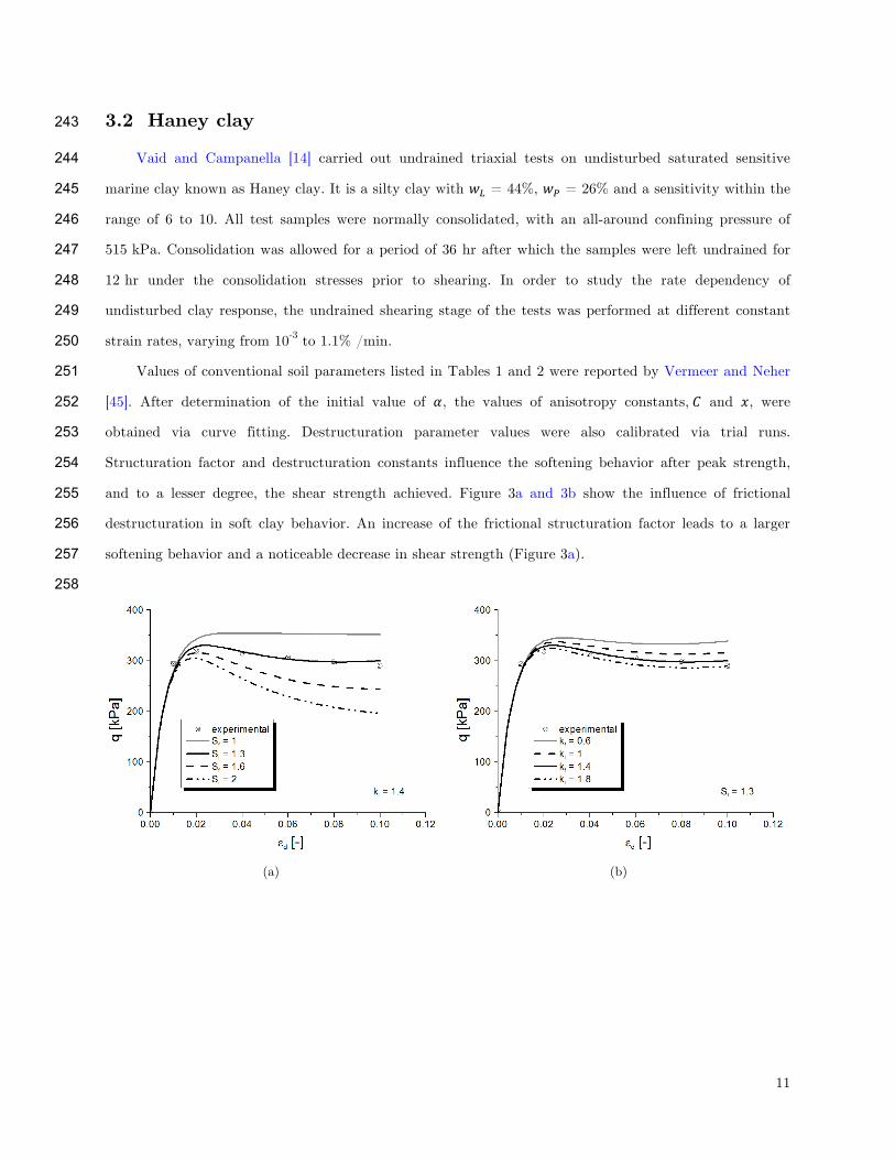
softening behavior and a noticeable decrease in shear strength (Figure 3a). 257
258
(a) (b)
12
(c)
Figure 3. Calibration of structuration and viscosity parameters for Haney clay: (a) influence of frictional 259
structuration parameter !! for a constant rate !! = 1.4; (b) influence of rate of frictional destructuration 260
!! for a constant value of !! = 1.3; (c) combined influence of viscosity parameters ! and ! 261
262
A similar, if less marked, behavior is seen in relation to the rate of frictional destructuration (Figure 263
3b), with larger softening observed for higher destructuration rates. Viscosity parameter values were 264
calibrated based on the results of two tests (i.e. at two strain rates) only. As it is shown in Figure 3c, 265
viscosity parameters play an important role in the overall calibration of the model, particularly with 266
regards to the shear strengths achieved. In order to obtain an improved match with the experimental 267
results, instead of the default value of 0.5, a value of 0.3 was adopted for the destructuration parameter 268
!. 269
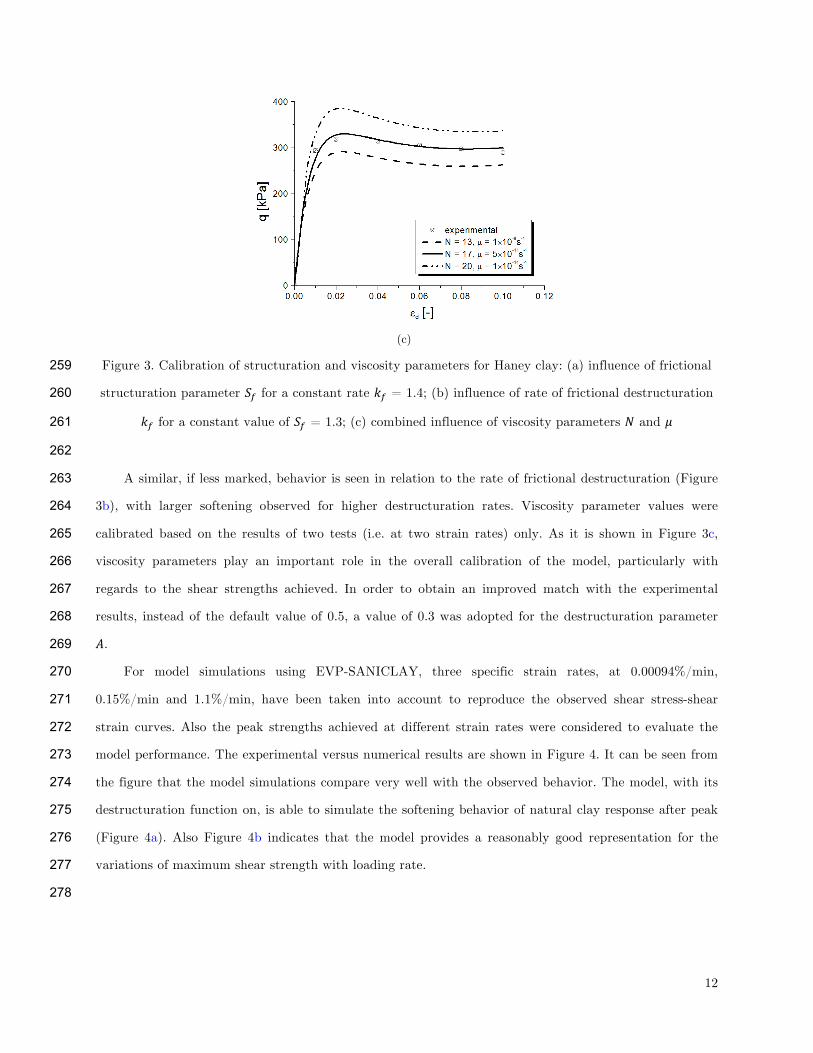
For model simulations using EVP-SANICLAY, three specific strain rates, at 0.00094%/min, 270
0.15%/min and 1.1%/min, have been taken into account to reproduce the observed shear stress-shear 271
strain curves. Also the peak strengths achieved at different strain rates were considered to evaluate the 272
model performance. The experimental versus numerical results are shown in Figure 4. It can be seen from 273
the figure that the model simulations compare very well with the observed behavior. The model, with its 274
destructuration function on, is able to simulate the softening behavior of natural clay response after peak 275
(Figure 4a). Also Figure 4b indicates that the model provides a reasonably good representation for the 276
variations of maximum shear strength with loading rate. 277
278
13
(a) (b)
Figure 4. Undrained triaxial compression tests: (a) deviator stress versus axial strain; (b) evolution of 279
maximum deviator stress with strain rate 280
281
3.3 St. Herblain clay 282
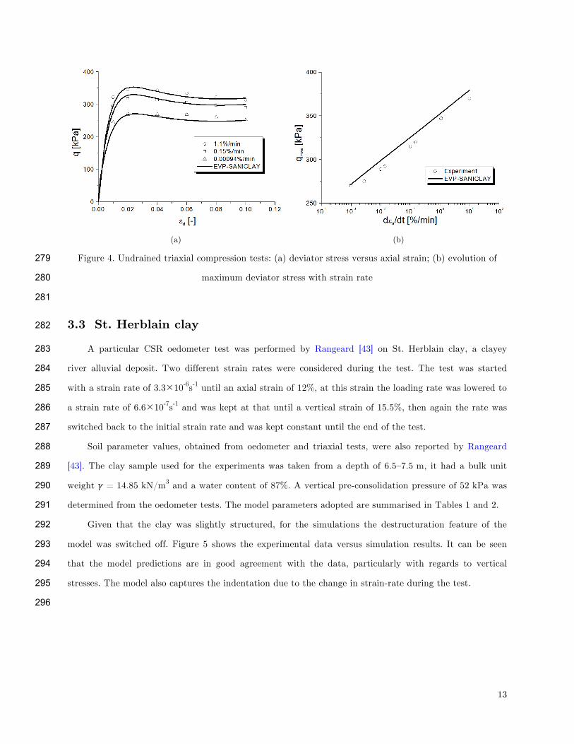
A particular CSR oedometer test was performed by Rangeard [43] on St. Herblain clay, a clayey 283
river alluvial deposit. Two different strain rates were considered during the test. The test was started 284
with a strain rate of 3.3!10-6s-1 until an axial strain of 12%, at this strain the loading rate was lowered to 285
a strain rate of 6.6!10-7s-1 and was kept at that until a vertical strain of 15.5%, then again the rate was 286
switched back to the initial strain rate and was kept constant until the end of the test. 287
Soil parameter values, obtained from oedometer and triaxial tests, were also reported by Rangeard 288
[43]. The clay sample used for the experiments was taken from a depth of 6.5–7.5 m, it had a bulk unit 289
weight ! = 14.85 kN/m3 and a water content of 87%. A vertical pre-consolidation pressure of 52 kPa was 290
determined from the oedometer tests. The model parameters adopted are summarised in Tables 1 and 2. 291
Given that the clay was slightly structured, for the simulations the destructuration feature of the 292
model was switched off. Figure 5 shows the experimental data versus simulation results. It can be seen 293
that the model predictions are in good agreement with the data, particularly with regards to vertical 294
stresses. The model also captures the indentation due to the change in strain-rate during the test. 295
296
14
Figure 5. Simulations of CRS oedometer test results over St. Herblain clay 297
298
3.4 Batiscan clay 299
CSR oedometer tests were performed on Batiscan clay by Leroueil et al. [16]. The clay samples were 300
taken from a depth of 7.25 - 7.46 m; the samples reportedly had a water content of 80%, liquidity index !! 301
= 2.7, !! = 21, and ! = 17.5 kN/m3. The pre-consolidation pressure, determined from conventional 302
oedometer tests, was evaluated as 88 kPa. The strain-rates for the CRS tests varied between 1.7!10-8 s-1 303
and 4!10-5 s-1. The initial vertical effective stress was taken equal to 65 kPa, corresponding to a size of 304
the initial yield surface of 50 kPa. Conventional soil parameter values reported in Tables 1 and 2 were 305
obtained from Leroueil et al. [16] and Rocchi et al. [46]. 306
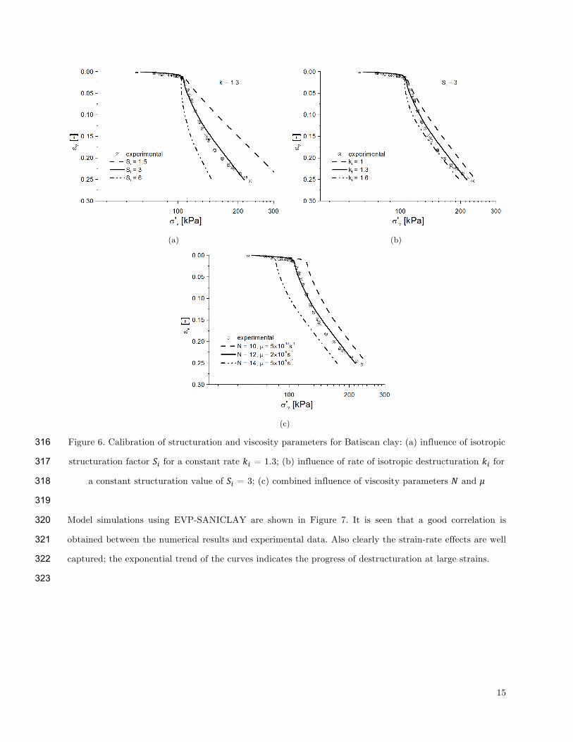
Combinations of initial degree of structuration and rate of destructuration have been studied and the 307
best coupled values were chosen for the numerical simulations. As it is shown in Figure 6a, larger values 308
of initial structuration Si result in a larger reduction of final vertical stress due to the higher softening 309
occurring. For a constant value of Si, the value of the rate of destructuration does not appear to have as 310
much influence, but it follows the same trend (Figure 6b), with higher rates leading to a higher vertical 311
stress reduction. Viscosity parameters are typically obtained from long-term oedometer tests via curve 312
fitting. The calibration of the coupled values is showed in Figure 6c. Note that viscosity parameters 313
greatly change the stress value at the end of the initial stiff elastic regime. The calibrated model 314
parameter values are summarised in Tables 1 and 2. 315
15
(a) (b)
(c)
Figure 6. Calibration of structuration and viscosity parameters for Batiscan clay: (a) influence of isotropic 316
structuration factor !! for a constant rate !! = 1.3; (b) influence of rate of isotropic destructuration !! for 317
a constant structuration value of !! = 3; (c) combined influence of viscosity parameters ! and ! 318
319
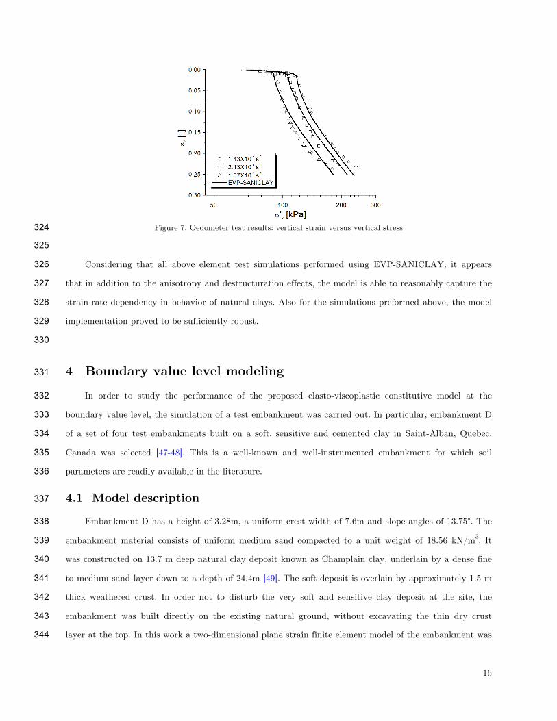
Model simulations using EVP-SANICLAY are shown in Figure 7. It is seen that a good correlation is 320
obtained between the numerical results and experimental data. Also clearly the strain-rate effects are well 321
captured; the exponential trend of the curves indicates the progress of destructuration at large strains. 322
323
16
Figure 7. Oedometer test results: vertical strain versus vertical stress 324
325
Considering that all above element test simulations performed using EVP-SANICLAY, it appears 326
that in addition to the anisotropy and destructuration effects, the model is able to reasonably capture the 327
strain-rate dependency in behavior of natural clays. Also for the simulations preformed above, the model 328
implementation proved to be sufficiently robust. 329
330
4 Boundary value level modeling 331
In order to study the performance of the proposed elasto-viscoplastic constitutive model at the 332
boundary value level, the simulation of a test embankment was carried out. In particular, embankment D 333
of a set of four test embankments built on a soft, sensitive and cemented clay in Saint-Alban, Quebec, 334
Canada was selected [47-48]. This is a well-known and well-instrumented embankment for which soil 335
parameters are readily available in the literature. 336
4.1 Model description 337
Embankment D has a height of 3.28m, a uniform crest width of 7.6m and slope angles of 13.75°. The 338
embankment material consists of uniform medium sand compacted to a unit weight of 18.56 kN/m3. It 339
was constructed on 13.7 m deep natural clay deposit known as Champlain clay, underlain by a dense fine 340
to medium sand layer down to a depth of 24.4m [49]. The soft deposit is overlain by approximately 1.5 m 341
thick weathered crust. In order not to disturb the very soft and sensitive clay deposit at the site, the 342
embankment was built directly on the existing natural ground, without excavating the thin dry crust 343
layer at the top. In this work a two-dimensional plane strain finite element model of the embankment was 344
17
created using PLAXIS AE [41], and taking advantage of the symmetry, only half of the embankment was 345
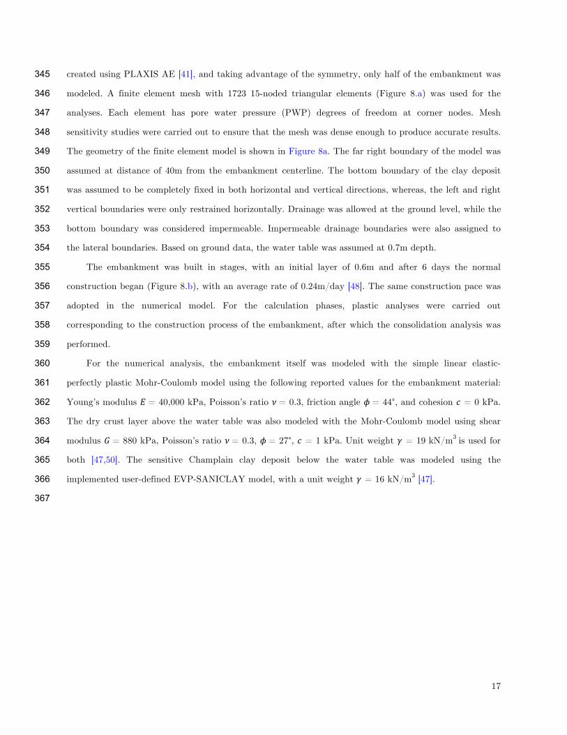
modeled. A finite element mesh with 1723 15-noded triangular elements (Figure 8.a) was used for the 346
analyses. Each element has pore water pressure (PWP) degrees of freedom at corner nodes. Mesh 347
sensitivity studies were carried out to ensure that the mesh was dense enough to produce accurate results. 348
The geometry of the finite element model is shown in Figure 8a. The far right boundary of the model was 349
assumed at distance of 40m from the embankment centerline. The bottom boundary of the clay deposit 350
was assumed to be completely fixed in both horizontal and vertical directions, whereas, the left and right 351
vertical boundaries were only restrained horizontally. Drainage was allowed at the ground level, while the 352
bottom boundary was considered impermeable. Impermeable drainage boundaries were also assigned to 353
the lateral boundaries. Based on ground data, the water table was assumed at 0.7m depth. 354
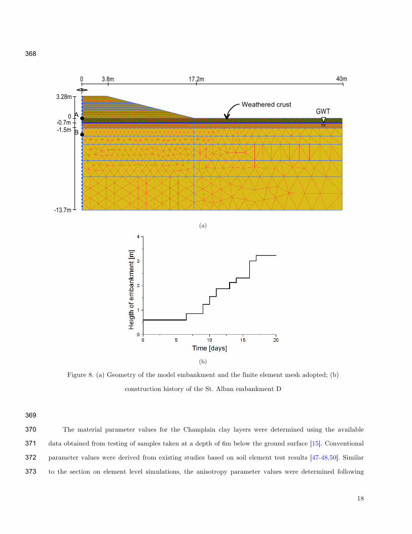
The embankment was built in stages, with an initial layer of 0.6m and after 6 days the normal 355
construction began (Figure 8.b), with an average rate of 0.24m/day [48]. The same construction pace was 356
adopted in the numerical model. For the calculation phases, plastic analyses were carried out 357
corresponding to the construction process of the embankment, after which the consolidation analysis was 358
performed. 359
For the numerical analysis, the embankment itself was modeled with the simple linear elastic-360
perfectly plastic Mohr-Coulomb model using the following reported values for the embankment material: 361
Young’s modulus !!= 40,000 kPa, Poisson’s ratio !!= 0.3, friction angle !!= 44°, and cohesion ! = 0 kPa. 362
The dry crust layer above the water table was also modeled with the Mohr-Coulomb model using shear 363
modulus !!= 880 kPa, Poisson’s ratio !!= 0.3, !!= 27°, ! = 1 kPa. Unit weight ! = 19 kN/m3 is used for 364
both [47,50]. The sensitive Champlain clay deposit below the water table was modeled using the 365
implemented user-defined EVP-SANICLAY model, with a unit weight ! = 16 kN/m3 [47]. 366
367
18
368
(a)
(b)
Figure 8. (a) Geometry of the model embankment and the finite element mesh adopted; (b)
construction history of the St. Alban embankment D
369
The material parameter values for the Champlain clay layers were determined using the available 370
data obtained from testing of samples taken at a depth of 6m below the ground surface [15]. Conventional 371
parameter values were derived from existing studies based on soil element test results [47-48,50]. Similar 372
to the section on element level simulations, the anisotropy parameter values were determined following 373
GWT
3.8m 0 17.2m 40m
3.28m
0 -0.7m -1.5m
-13.7m
Weathered crust
B
A
19
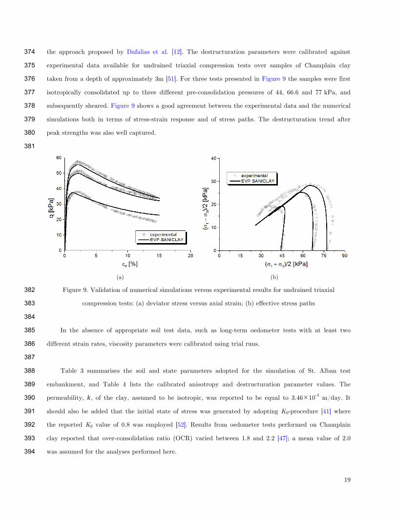
the approach proposed by Dafalias et al. [12]. The destructuration parameters were calibrated against 374
experimental data available for undrained triaxial compression tests over samples of Champlain clay 375
taken from a depth of approximately 3m [51]. For three tests presented in Figure 9 the samples were first 376
isotropically consolidated up to three different pre-consolidation pressures of 44, 66.6 and 77 kPa, and 377
subsequently sheared. Figure 9 shows a good agreement between the experimental data and the numerical 378
simulations both in terms of stress-strain response and of stress paths. The destructuration trend after 379
peak strengths was also well captured. 380
381
(a) (b)
Figure 9. Validation of numerical simulations versus experimental results for undrained triaxial 382
compression tests: (a) deviator stress versus axial strain; (b) effective stress paths 383
384
In the absence of appropriate soil test data, such as long-term oedometer tests with at least two 385
different strain rates, viscosity parameters were calibrated using trial runs. 386
387
Table 3 summarises the soil and state parameters adopted for the simulation of St. Alban test 388
embankment, and Table 4 lists the calibrated anisotropy and destructuration parameter values. The 389
permeability, !, of the clay, assumed to be isotropic, was reported to be equal to 3.46!10-4 m/day. It 390
should also be added that the initial state of stress was generated by adopting K0-procedure [41] where 391
the reported K0 value of 0.8 was employed [52]. Results from oedometer tests performed on Champlain 392
clay reported that over-consolidation ratio (OCR) varied between 1.8 and 2.2 [47]; a mean value of 2.0 393
was assumed for the analyses performed here. 394
20
395
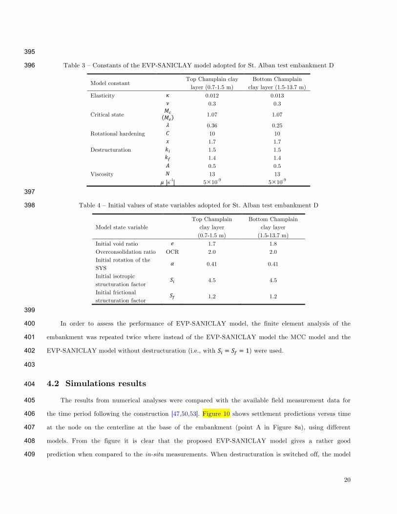
Table 3 – Constants of the EVP-SANICLAY model adopted for St. Alban test embankment D 396
Model constant Top Champlain clay layer (0.7-1.5 m)
Bottom Champlain clay layer (1.5-13.7 m)
Elasticity ! 0.012 0.013 ! 0.3 0.3
Critical state !! !! 1.07 1.07
! 0.36 0.25 Rotational hardening ! 10 10 ! 1.7 1.7 Destructuration !! 1.5 1.5 !! 1.4 1.4 ! 0.5 0.5 Viscosity ! 13 13 ! [s-1] 5!10-9 5!10-9
397
Table 4 – Initial values of state variables adopted for St. Alban test embankment D 398
Model state variable Top Champlain
clay layer (0.7-1.5 m)
Bottom Champlain clay layer
(1.5-13.7 m) Initial void ratio ! 1.7 1.8 Overconsolidation ratio OCR 2.0 2.0 Initial rotation of the SYS
! 0.41 0.41
Initial isotropic structuration factor
!! 4.5 4.5
Initial frictional structuration factor
!! 1.2 1.2
399
In order to assess the performance of EVP-SANICLAY model, the finite element analysis of the 400
embankment was repeated twice where instead of the EVP-SANICLAY model the MCC model and the 401
EVP-SANICLAY model without destructuration (i.e., with !! = !! = 1) were used. 402
403
4.2 Simulations results 404
The results from numerical analyses were compared with the available field measurement data for 405
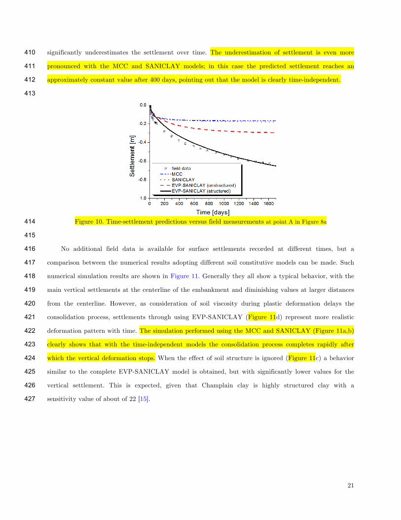
the time period following the construction [47,50,53]. Figure 10 shows settlement predictions versus time 406
at the node on the centerline at the base of the embankment (point A in Figure 8a), using different 407
models. From the figure it is clear that the proposed EVP-SANICLAY model gives a rather good 408
prediction when compared to the in-situ measurements. When destructuration is switched off, the model 409
21
significantly underestimates the settlement over time. The underestimation of settlement is even more 410
pronounced with the MCC and SANICLAY models; in this case the predicted settlement reaches an 411
approximately constant value after 400 days, pointing out that the model is clearly time-independent. 412
413
Figure 10. Time-settlement predictions versus field measurements at point A in Figure 8a 414
415
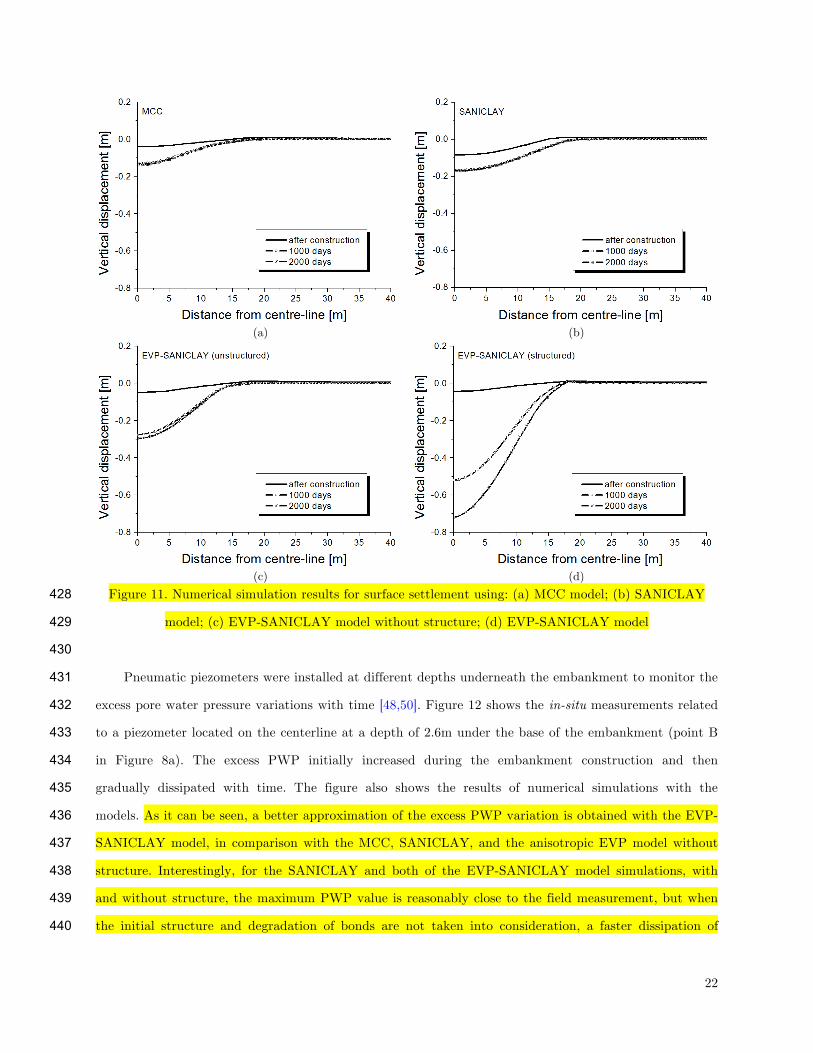
No additional field data is available for surface settlements recorded at different times, but a 416
comparison between the numerical results adopting different soil constitutive models can be made. Such 417
numerical simulation results are shown in Figure 11. Generally they all show a typical behavior, with the 418
main vertical settlements at the centerline of the embankment and diminishing values at larger distances 419
from the centerline. However, as consideration of soil viscosity during plastic deformation delays the 420
consolidation process, settlements through using EVP-SANICLAY (Figure 11d) represent more realistic 421
deformation pattern with time. The simulation performed using the MCC and SANICLAY (Figure 11a,b) 422
clearly shows that with the time-independent models the consolidation process completes rapidly after 423
which the vertical deformation stops. When the effect of soil structure is ignored (Figure 11c) a behavior 424
similar to the complete EVP-SANICLAY model is obtained, but with significantly lower values for the 425
vertical settlement. This is expected, given that Champlain clay is highly structured clay with a 426
sensitivity value of about of 22 [15]. 427
22
(a) (b)
(c) (d)
Figure 11. Numerical simulation results for surface settlement using: (a) MCC model; (b) SANICLAY 428
model; (c) EVP-SANICLAY model without structure; (d) EVP-SANICLAY model 429
430
Pneumatic piezometers were installed at different depths underneath the embankment to monitor the 431
excess pore water pressure variations with time [48,50]. Figure 12 shows the in-situ measurements related 432
to a piezometer located on the centerline at a depth of 2.6m under the base of the embankment (point B 433
in Figure 8a). The excess PWP initially increased during the embankment construction and then 434
gradually dissipated with time. The figure also shows the results of numerical simulations with the 435
models. As it can be seen, a better approximation of the excess PWP variation is obtained with the EVP-436
SANICLAY model, in comparison with the MCC, SANICLAY, and the anisotropic EVP model without 437
structure. Interestingly, for the SANICLAY and both of the EVP-SANICLAY model simulations, with 438
and without structure, the maximum PWP value is reasonably close to the field measurement, but when 439
the initial structure and degradation of bonds are not taken into consideration, a faster dissipation of 440
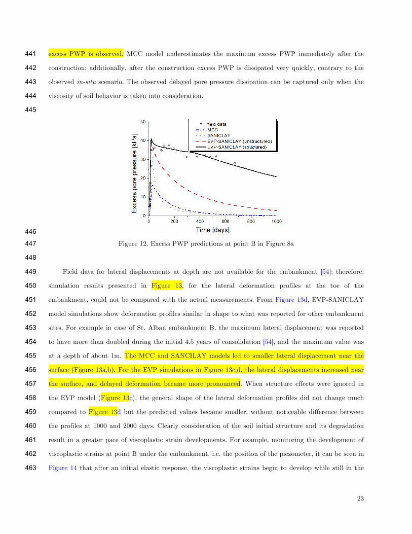
23
excess PWP is observed. MCC model underestimates the maximum excess PWP immediately after the 441
construction; additionally, after the construction excess PWP is dissipated very quickly, contrary to the 442
observed in-situ scenario. The observed delayed pore pressure dissipation can be captured only when the 443
viscosity of soil behavior is taken into consideration. 444
445
446
Figure 12. Excess PWP predictions at point B in Figure 8a 447
448
Field data for lateral displacements at depth are not available for the embankment [54]; therefore, 449
simulation results presented in Figure 13, for the lateral deformation profiles at the toe of the 450
embankment, could not be compared with the actual measurements. From Figure 13d, EVP-SANICLAY 451
model simulations show deformation profiles similar in shape to what was reported for other embankment 452
sites. For example in case of St. Alban embankment B, the maximum lateral displacement was reported 453
to have more than doubled during the initial 4.5 years of consolidation [54], and the maximum value was 454
at a depth of about 1m. The MCC and SANCILAY models led to smaller lateral displacement near the 455
surface (Figure 13a,b). For the EVP simulations in Figure 13c,d, the lateral displacements increased near 456
the surface, and delayed deformation became more pronounced. When structure effects were ignored in 457
the EVP model (Figure 13c), the general shape of the lateral deformation profiles did not change much 458
compared to Figure 13d but the predicted values became smaller, without noticeable difference between 459
the profiles at 1000 and 2000 days. Clearly consideration of the soil initial structure and its degradation 460
result in a greater pace of viscoplastic strain developments. For example, monitoring the development of 461
viscoplastic strains at point B under the embankment, i.e. the position of the piezometer, it can be seen in 462
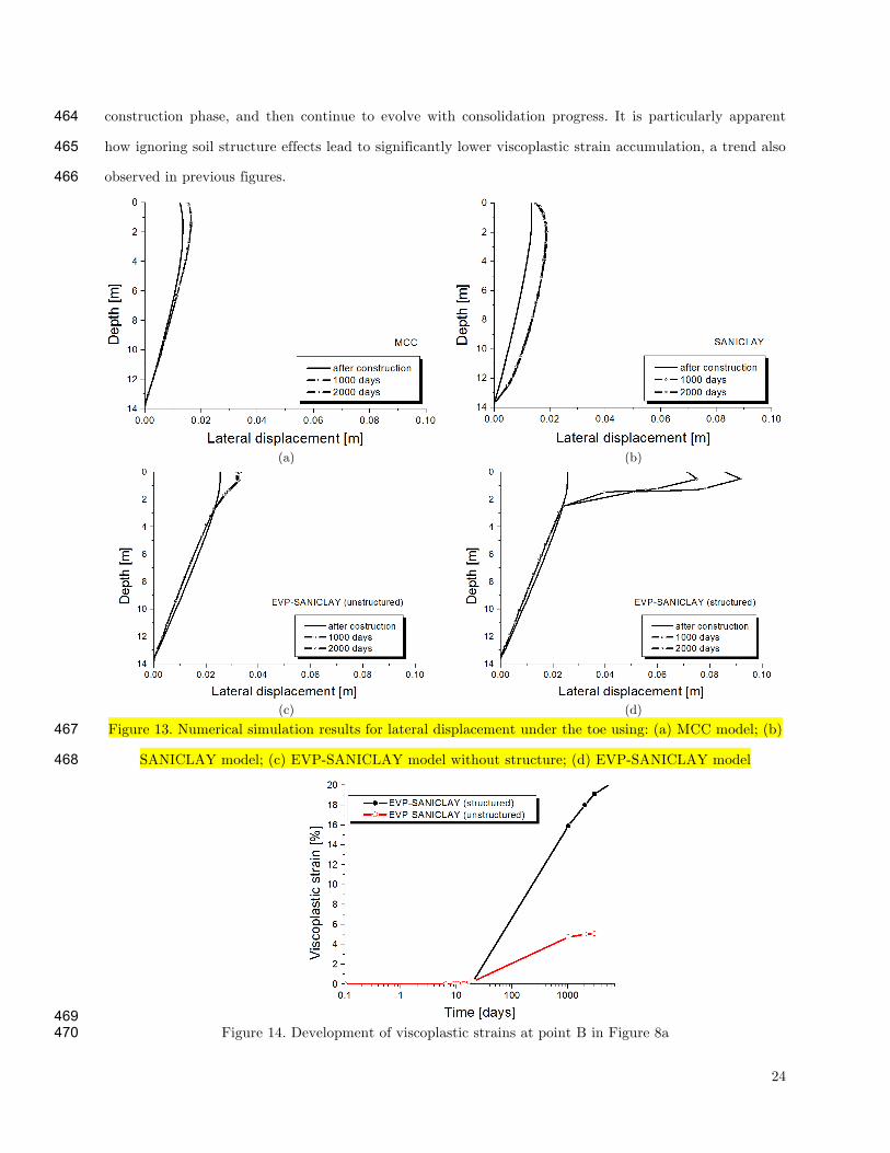
Figure 14 that after an initial elastic response, the viscoplastic strains begin to develop while still in the 463
24
construction phase, and then continue to evolve with consolidation progress. It is particularly apparent 464
how ignoring soil structure effects lead to significantly lower viscoplastic strain accumulation, a trend also 465
observed in previous figures. 466
(a) (b)
(c) (d)
Figure 13. Numerical simulation results for lateral displacement under the toe using: (a) MCC model; (b) 467
SANICLAY model; (c) EVP-SANICLAY model without structure; (d) EVP-SANICLAY model 468
469 Figure 14. Development of viscoplastic strains at point B in Figure 8a 470
25
4.3 Non-uniqueness of viscosity parameters 471
As already mentioned, calibration of viscosity parameters ! and ! has been done directly on the 472
embankment model as no appropriate test data has been available for the foundation soil. It should be 473
pointed out that the Perzyna-type viscosity parameters for a particular clay are not necessarily a unique 474
set and more than one combination of the two viscosity parameters can be found for a clay, depending on 475
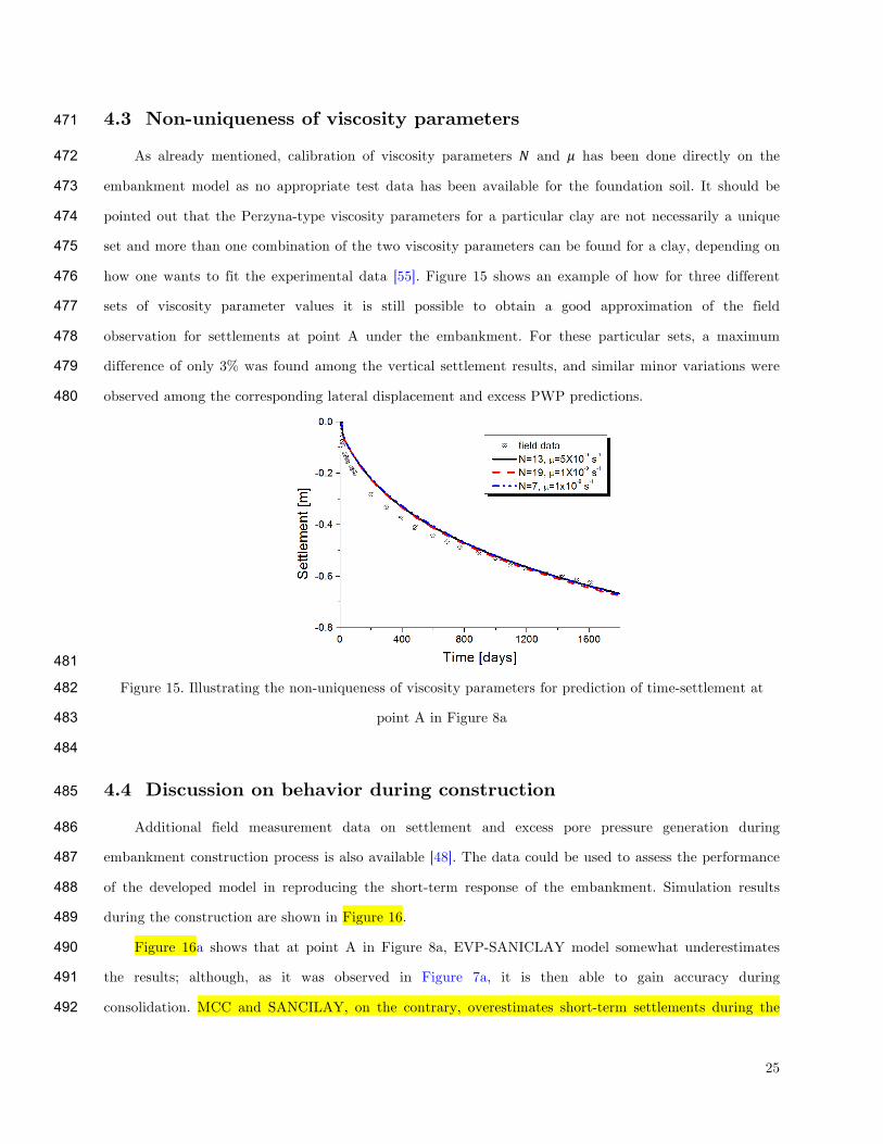
how one wants to fit the experimental data [55]. Figure 15 shows an example of how for three different 476
sets of viscosity parameter values it is still possible to obtain a good approximation of the field 477
observation for settlements at point A under the embankment. For these particular sets, a maximum 478
difference of only 3% was found among the vertical settlement results, and similar minor variations were 479
observed among the corresponding lateral displacement and excess PWP predictions. 480
481
Figure 15. Illustrating the non-uniqueness of viscosity parameters for prediction of time-settlement at 482
point A in Figure 8a 483
484
4.4 Discussion on behavior during construction 485
Additional field measurement data on settlement and excess pore pressure generation during 486
embankment construction process is also available [48]. The data could be used to assess the performance 487
of the developed model in reproducing the short-term response of the embankment. Simulation results 488
during the construction are shown in Figure 16. 489
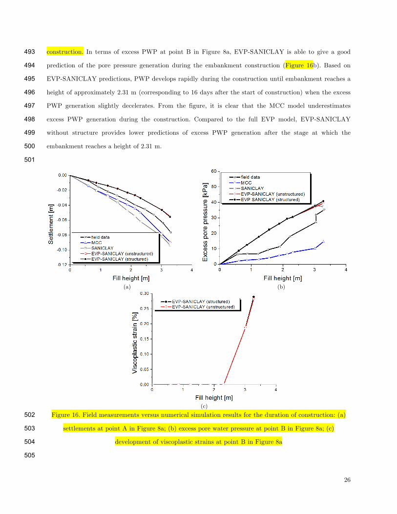
Figure 16a shows that at point A in Figure 8a, EVP-SANICLAY model somewhat underestimates 490
the results; although, as it was observed in Figure 7a, it is then able to gain accuracy during 491
consolidation. MCC and SANCILAY, on the contrary, overestimates short-term settlements during the 492
26
construction. In terms of excess PWP at point B in Figure 8a, EVP-SANICLAY is able to give a good 493
prediction of the pore pressure generation during the embankment construction (Figure 16b). Based on 494
EVP-SANICLAY predictions, PWP develops rapidly during the construction until embankment reaches a 495
height of approximately 2.31 m (corresponding to 16 days after the start of construction) when the excess 496
PWP generation slightly decelerates. From the figure, it is clear that the MCC model underestimates 497
excess PWP generation during the construction. Compared to the full EVP model, EVP-SANICLAY 498
without structure provides lower predictions of excess PWP generation after the stage at which the 499
embankment reaches a height of 2.31 m. 500
501
(a) (b)
(c)
Figure 16. Field measurements versus numerical simulation results for the duration of construction: (a) 502
settlements at point A in Figure 8a; (b) excess pore water pressure at point B in Figure 8a; (c) 503
development of viscoplastic strains at point B in Figure 8a 504
505
27
Figure 16c shows the development of viscoplastic strains at point B under the embankment (i.e. at 506
the position of the pneumatic piezometer considered). The figure shows that the viscoplastic strains start 507
to develop when the embankment reaches a height of about 2.31m, which approximately corresponds to 508
the time when excess pore pressure generation changes its pace. 509
510
5 Conclusions 511
The response of natural soft soil is governed by anisotropy, structure and time-dependency. In this 512
work, in order to concurrently account for these advanced features of soil behavior a time-dependent 513
elasto-viscoplastic extension of a well-established anisotropic clay model, namely SANICLAY, has been 514
proposed. The model is numerically implemented in finite element program PLAXIS using an implicit 515
integration scheme. The performance of the model at the element-level has been validated against 516
experimental data obtained from testing four different clays at both structured and un-structured states. 517
Furthermore the time-dependent behavior of St. Alban embankment D on the well-structured Champlain 518
clay was analysed using the proposed EVP-SANICLAY model. The paper presented the results for 519
settlements, lateral deformations, and excess PWP variations during the construction and the subsequent 520
consolidation, comparing model predictions with the field measurements where available. It was observed 521
that the developed model considers the delayed excess pore pressure dissipation following the completion 522
of the embankment construction reasonably well; hence it is able to yield more realistic predictions of the 523
long-term vertical and horizontal deformations. The boundary value problem simulation results also 524
illustrated that considering clay initial structure and subsequent destructuration effects significantly 525
improve the accuracy of predictions, particularly when dealing with a highly sensitive soft clay such as 526
Champlain clay. Furthermore, the model also predicted the immediate displacements as well as the 527
development of excess pore pressures during early stages of construction with reasonable accuracy. 528
In general, EVP-SANICLAY proved to be able to much better predict both short- and long-term 529
behavior of natural clay behavior when compared with a commonly used critical state based model such 530
as MCC, and also the SANCILAY model. 531
532
28
Acknowledgements 533
Support to conduct this study is provided by the University of Nottingham’s Dean of Engineering 534
award, and the Natural Sciences and Engineering Research Council of Canada (NSERC). 535
536
Appendix 537
For the sake of completeness of presentation, some of the key components of the SANICLAY model 538
that are not presented in the main body of this paper are summarized here. Both stress and strain 539
quantities are assumed positive in compression (as is common in geomechanics), and the effect of this sign 540
convention has been considered on the model equations. All stress components in this paper should be 541
considered as effective stress. Finally, in terms of notation, tensor quantities are denoted by bold-faced 542
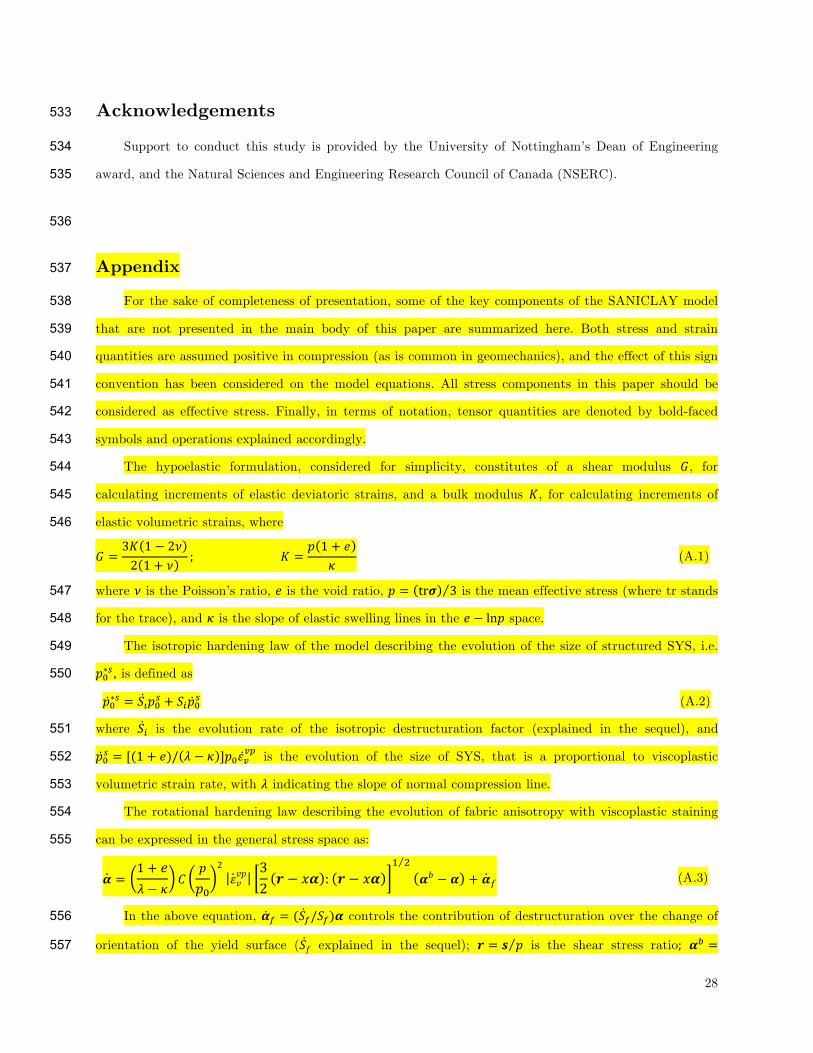
symbols and operations explained accordingly. 543
The hypoelastic formulation, considered for simplicity, constitutes of a shear modulus !, for 544
calculating increments of elastic deviatoric strains, and a bulk modulus !, for calculating increments of 545
elastic volumetric strains, where 546
! = 3! 1 − 2!2 1 + ! ; !!!!!!!!!!!!!!!!!!!!!!!!!!!!!! = ! 1 + !
! (A.1)
where ! is the Poisson’s ratio, ! is the void ratio, ! = tr! 3 is the mean effective stress (where tr stands 547
for the trace), and ! is the slope of elastic swelling lines in the ! − ln! space. 548
The isotropic hardening law of the model describing the evolution of the size of structured SYS, i.e. 549
!!∗!, is defined as 550
!!∗! = !!!!! + !!!!! (A.2)
where !! is the evolution rate of the isotropic destructuration factor (explained in the sequel), and 551
!!! = [(1 + !)/ ! − ! ]!!!!!" is the evolution of the size of SYS, that is a proportional to viscoplastic 552
volumetric strain rate, with ! indicating the slope of normal compression line. 553
The rotational hardening law describing the evolution of fabric anisotropy with viscoplastic staining 554
can be expressed in the general stress space as: 555
! =1 + !! − ! !
!!!
2!!!"
32 ! − !! : ! − !!
! !!! − ! + !! (A.3)
In the above equation, !! = (!!/!!)! controls the contribution of destructuration over the change of 556
orientation of the yield surface (!! explained in the sequel); ! = ! ! is the shear stress ratio; !! =557
29
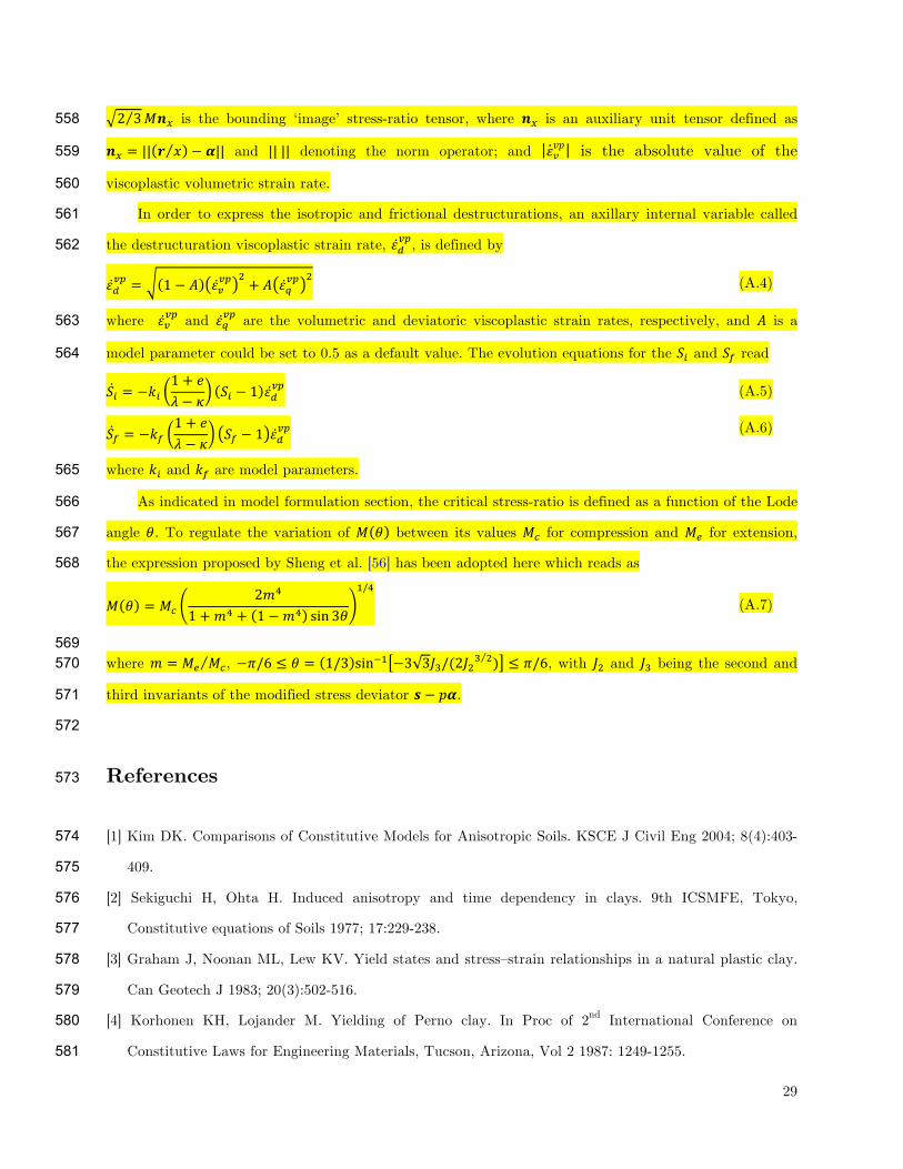
2 3!!! is the bounding ‘image’ stress-ratio tensor, where !! is an auxiliary unit tensor defined as 558
!! = || ! ! − !|| and ||!|| denoting the norm operator; and !!!" is the absolute value of the 559
viscoplastic volumetric strain rate. 560
In order to express the isotropic and frictional destructurations, an axillary internal variable called 561
the destructuration viscoplastic strain rate, !!!", is defined by 562
!!!" = 1 − ! !!!"! + ! !!!"
! (A.4)
where !!!" and !!!" are the volumetric and deviatoric viscoplastic strain rates, respectively, and ! is a 563
model parameter could be set to 0.5 as a default value. The evolution equations for the !! and !! read 564
!! = −!!1 + !! − ! !! − 1 !!!" (A.5)
!! = −!!1 + !! − ! !! − 1 !!!" (A.6)
where !! and !! are model parameters. 565
As indicated in model formulation section, the critical stress-ratio is defined as a function of the Lode 566
angle !. To regulate the variation of ! ! between its values !! for compression and !! for extension, 567
the expression proposed by Sheng et al. [56] has been adopted here which reads as 568
! ! = !!2!!
1 +!! + 1 −!! sin 3!!/!
(A.7)
569 where ! = !! !!, −!/6 ≤ ! = 1/3 sin!! −3 3!!/(2!!! !) ≤ !/6, with !! and !! being the second and 570
third invariants of the modified stress deviator ! − !!. 571
572
References 573
[1] Kim DK. Comparisons of Constitutive Models for Anisotropic Soils. KSCE J Civil Eng 2004; 8(4):403-574
409. 575
[2] Sekiguchi H, Ohta H. Induced anisotropy and time dependency in clays. 9th ICSMFE, Tokyo, 576
Constitutive equations of Soils 1977; 17:229-238. 577
[3] Graham J, Noonan ML, Lew KV. Yield states and stress–strain relationships in a natural plastic clay. 578
Can Geotech J 1983; 20(3):502-516. 579
[4] Korhonen KH, Lojander M. Yielding of Perno clay. In Proc of 2nd International Conference on 580
Constitutive Laws for Engineering Materials, Tucson, Arizona, Vol 2 1987: 1249-1255. 581
30
[5] Dafalias YF. An anisotropic critical state soil plasticity model. Mech Res Commun 1986; 13(6):341-582
347. 583
[6] Dafalias YF. An anisotropic critical state clay plasticity model. In Proceedings of the 2nd international 584
conference on constitutive laws for engineering materials. Tucson, US, 1987:513-521. 585
[7] Thevanayagam S, Chameau JL. Modelling anisotropy of clays at critical state. J Eng Mech-ASCE 586
1992; 118(4):786–806 587
[8] Whittle AJ, Kavvadas MJ. Formulation of MIT-E3 constitutive model for overconsolidated clays. J 588
Geotech Eng 1994; 120(1):173-198. 589
[9] Newson TA, Davies MCR. A rotational hardening constitutive model for anisotropically consolidated 590
clay. Soils Found 1996; 36(3):13–20 591
[10] Wheeler SJ, Karstunen M, Näätänen A. Anisotropic hardening model for normally consolidated soft 592
clay. In Proc. 7th Int. Symp. on Numerical Models in Geomechanics (NUMOG VII), Graz, 1999, 33- 593
40. A.A. Balkema. 594
[11] Wheeler SJ, Näätänen A, Karstunen M, Lojander M. An anisotropic elasto-plastic model for soft 595
clays. Can Geotech J 2003; 40(2):403-418. 596
[12] Dafalias YF, Manzari MT, Papadimitriou AG. SANICLAY: simple anisotropic clay plasticity model. 597
Int J Numer Anal Meth Geomech 2006; 30:1231-1257. 598
[13] Taiebat M, Dafalias YF, Peek R. A destructuration theory and its application to SANICLAY model. 599
Int J Numer Anal Meth Geomech 2010; 34:1009-1040. 600
[14] Vaid YP, Campanella RG. Time-dependent behaviour of undisturbed clay. J Geotech Eng-ASCE 601
1977; 103(7):693-709. 602
[15] Tavenas F, Leroueil S, La Rochelle P, Roy M. Creep behavior of an undisturbed lightly 603
overconsolidated clay. Can Geotech J 1978; 15(3):402–423. 604
[16] Leroueil S, Kabbaj M, Tavenas F, Bouchard R. Stress–strain–strain-rate relation for the 605
compressibility of sensitive natural clays. Géotechnique 1985; 35(2):159–180. 606
[17] Lefebvre G, Leboeuf D. Rate effects and cyclic loading of sensitive clays. J Geotech Eng-ASCE 1987; 607
113(5):476–489. 608
[18] Augustesen A, Liingaard M, Lade PV. Evaluation of Time-Dependent Behavior of Soils. Int J 609
Geomech 2004; 4(3):137-156. 610
[19] Vaid YP, Robertson PK, Campanella RG. Strain rate behavior of Saint-Jean-Vianney clay. Can 611
Geotech J 1979; 16:34–42. 612
31
[20] Díaz-Rodríguez JA, Martínez-Vasquez JJ, Santamarina JC. Strain-rate effects in Mexico City soil. J 613
Geotech Geoenviron Eng 2009; 135(2):300–305 614
[21] Leroueil S. The isotache approach. Where are we 50 years after its development by Professor Šuklje?. 615
2006 Prof. Šuklje’s Memorial Lecture, XIII Danube-European Geotechnical Engineering Conference, 616
29th–31st May 2006, Ljubljana, Slovenia. 617
[22] Šuklje L. The analysis of the consolidation process by the isotache method. Proc. 4th Int. Conf. on 618
Soil Mech and Found. Engng., London 1957; 1:200-206. 619
[23] Naghdi PM, Murch, SA. On the mechanical behavior of viscoelastic/plastic solids. J Applied 620
Mechanics 1963; 30(3):321-328. 621
[24] Perzyna P. The constitutive equations for work-hardening and rate sensitive plastic materials. In 622
Proc. Vibration Problems Warsaw 1963; 3:281-290. 623
[25] Perzyna P. Fundamental problems in viscoplasticity. Adv Appl Mech 1966; 9:244–377. 624
[26] Adachi T, Oka F. Constitutive equations for normally consolidated clay based on elasto-625
viscoplasticity. Soils Found 1982; 22(4):57-70. 626
[27] Nova R. A viscoplastic constitutive model for normally consolidated clay. In Proceedings of IUTAM 627
Conference on Deformation and Failure of Granular Materials, Delft, The Netherlands, 1982, 287–295. 628
[28] Katona MG. Evaluation of Viscoplastic Cap Model. J Geotech Eng-ASCE. 1984; 110:1106-1125. 629
[29] Kaliakin VN, Dafalias YF. Theoretical aspects of the elastoplastic-viscoplastic bounding surface 630
model for cohesive soils. Soils Found 1990; 30(3):11-24 631
[30] Yin JH, Zhu JG, Graham J. A new elastic viscoplastic model for time-dependent behaviour of 632
normally and overconsolidated clays: theory and verification. Can Geotech J 2002; 39:157–173 633
[31] Yin ZY, Hicher PY. Identifying parameters controlling soil delayed behavior from laboratory and in 634
situ pressuremeter testing. Int J Num Anal Meth Geomech 2008; 32:1515-1535 635
[32] Martindale H, Chakraborty T, Basu B. A Strain-Rate Dependent Clay Constitutive Model with 636
Parametric Sensitivity and Uncertainty Quantification. Geotech Geol Eng 2013; 31:229–248 637
[33] Leoni M, Karstunen M, Vermeer P. Anisotropic creep model for soft soils. Géotechnique 2008; 638
58(3):215-226. 639
[34] Yin Z-Y, Karstunen M. Modelling strain-rate-dependency of natural soft clays combined with 640
anisotropy and destructuration. Acta Mechanica Solida sinica, Vol. 24, No 3, June 2001. Published by 641
AMSS Press, Wuhan, China. 642
32
[35] Dafalias YF, Taiebat M. Anatomy of Rotational Hardening in Clay Plasticity. Geotechnique 2013; 643
63(16):1406-1418. 644
[36] Dafalias YF, Taiebat M. Rotational hardening with and without anisotropic fabric at critical state. 645
Geotechnique 2014; 64(6): 507-511. 646
[37] Shahrour I, Meimon Y. Calculation of marine foundations subjected to repeated loads by means of 647
the homogenization method. Comput Geotech 1995; 17(1):93-106. 648
[38] Fodil A, Aloulou W, Hicher PY. Viscoplastic behaviour of soft clay. Géotechnique 1997; 47(3):581-649
591. 650
[39] Lewis RW, Schrefler BA. The Finite Element Method in the Static and Dynamic Deformation and 651
Consolidation of Porous Media. 2nd Ed.: John Wiley & Sons, ISBN: 978-0-471-92809-6; 1998. 652
[40] Hinchberger SD. The behaviour of reinforced and unreinforced embankments on soft rate-sensitive 653
foundation soils. Ph.D. thesis, Department of Civil Engineering, The University of Western Ontario, 654
London, Ont. 1996. 655
[41] Brinkgreve RBJ, Engin E, Swolfs WM. Plaxis 2014 reference manual, Plaxis, Delft, Netherlands; 656
2014. 657
[42] Nakase A, Kamei T. Influence of strain rate on undrained shear characteristics of K0-consolidated 658
cohesive soils. Soils Found 1986; 26(1):85-95. 659
[43] Rangeard D. Identification des caractéristiques hydro-mécaniques d’une argile par analyse inverse des 660
essais pressiométriques. Thèse de l’Ecole Centrale de Nantes et l’Université de Nantes, 2002. 661
[44] Kamei T, Sakajo S. Evaluation of undrained shear behaviour of K0-consolidated cohesive soils using 662
elasto-viscoplastic model. Comput Geotech 1995; 17:397-417. 663
[45] Vermeer PA, Neher HP. A soft soil model that accounts for creep. In: Proc. Plaxis Symposium 664
‘Beyond 2000 in Computational Geotechnic’, Amsterdam 1999: 249-262. 665
[46] Rocchi G, Fontana M, Da Prat M. (2003). Modelling of natural soft clay destruction processes using 666
viscoplasticity theory. Géotechnique 2003; 53(8):729-745. 667
[47] La Rochelle P, Trak B, Tavenas F, Roy M. Failure of a test embankment on a sensitive Champlain 668
clay deposit. Can Geotech J 1974; 11(1):142-164. 669
[48] Tavenas FA, Chapeau C, La Rochelle P, Roy M. Immediate settlements of three test embankments 670
on Champlain clay. Can Geotech J 1974; 11(1):109-141. 671
[49] Leroueil S, Tavenas F, Trak B, La Rochelle P, Roy M. Construction pore water pressures in clay 672
foundations under embankments. Part I: the Saint-Alban test fills. Can Geotech J 1978; 15:54–65. 673
33
[50] Karim MR, Oka F, Krabbenhoft K, Leroueil S, Kimoto S. Simulation of long-term consolidation 674
behavior of soft sensitive clay using an elasto-viscoplastic constitutive model. Int J Numer Anal Meth 675
Geomech 2013; 37:2801–2824. 676
[51] Tavenas F, Leroueil S. Effects of stresses and time on yielding of clays. In Proceedings of the 9th 677
International Conference on Soil Mechanics and Foundation Engineering, Toyko, Japan, 1977. 678
[52] Oka F, Tavenas F, Leroueil S. An elasto-viscoplastic fem analysis of sensitive clay foundation beneath 679
embankment. In Computer Method and Advances in Geomechanics, Vol. 2, Beer G, Booker JR, 680
Carter JP (eds). Balkema: Brookfield, 6-10 May 1991; 1023–1028. 681
[53] Morissette L., St-Louis MW, McRostie GC. Empirical settlement predictions in overconsolidated 682
Champlain Sea clays. Can Geotech J 2001; 38:720–731. 683
[54] Tavenas F, Mieussens C, Bourges F. Lateral displacements in clay foundations under embankments. 684
Can Geotech J 1979; 16(3):532-550. 685
[55] Karstunen M, Rezania M, Sivasithamparam N, Yin ZY. Comparison of Anisotropic Rate-Dependent 686
Models for Modeling Consolidation of Soft Clays. Intl J Geomech 2012, DOI: 687
10.1061/(ASCE)GM.1943- 5622.0000267. 688
[56] Sheng D, Sloan SW, Yu HS. Aspects of finite element implementation of critical state models. 689
Computational mechanics 2000; 26(2):185-196. 690
691
692
1
A viscoplastic SANICLAY model for natural soft soils 1
Mohammad Rezaniaa, Mahdi Taiebatb,c,*, and Elisa Polettid 2
aDepartment of Civil Engineering, University of Nottingham, Nottingham, UK 3 bDepartment of Civil Engineering, University of British Columbia, Vancouver, BC, Canada 4
cDepartment of Civil & Environmental Engineering, Massachusetts Institute of Technology, Cambridge, 5
MA, USA 6 dDepartment of Civil Engineering, University of Minho, Azurém, Guimarães, Portugal 7
Abstract 8
This paper focuses on constitutive and numerical modeling of strain-rate dependency in natural clays 9
while also accounting for anisotropy and destructuration. For this purpose the SANICLAY model that 10
accounts for the fabric anisotropy with the additional destructuration feature that accounts for sensitivity of 11
natural clays, is considered as the reference model. An associated flow rule is adopted for simplicity. The 12
model formulation is refined to also account for the important feature of strain-rate dependency using the 13
Perzyna’s overstress theory. The model is then implicitly integrated in finite element program PLAXIS. 14
Performance of the developed and implemented model is explored by comparing the simulation results of 15
several element tests and a boundary value problem to the available experimental data. The element tests 16
include the constant strain-rate under one-dimensional and triaxial conditions on different clays. The 17
boundary value problem includes a test embankment, namely embankment D constructed at Saint Alban, 18
Quebec. For comparison, the test embankment is also analysed using the Modified Cam-Clay (MCC) model, 19
the SANICLAY model, and the viscoplastic model but without destructuration. Results demonstrate the 20
success of the developed and implemented viscoplastic SANICLAY in reproducing the strain-rate dependent 21
behavior of natural soft soils. 22
Keywords: viscoplasticity; strain-rate dependency; anisotropy; destructuration; clay 23
24
1 Introduction 25
Modeling the stress-strain response of natural soft soils constitutes a challenge in practical geotechnical 26
engineering; it is governed by a series of factors that are not always included in conventional constitutive 27
models. In particular, the three main inherent features that influence their response are a) anisotropy, b) 28
destructuration (degradation of the inter-particle bonds), and c) strain-rate dependency. 29
*Corresponding author. Tel.: +1 604 822 3279. E-mail addresses: [email protected] (M. Rezania), [email protected] (M. Taiebat), [email protected] (E. Poletti).
*ManuscriptClick here to view linked References
2
Since modeling the full anisotropy of natural clay behavior is not practical due to the number of 30
parameters involved, efforts have been mainly focused on development of models with reduced number of 31
parameters while maintaining the capacity of the model [1]. Historically, for practical model development 32
purposes, the initial orientation of soil fabric is considered to be of cross-anisotropic nature, which is a 33
realistic assumption as natural soils have been generally deposited only one-dimensionally in a vertical 34
direction. It is also a well-established fact that the yield surfaces obtained from experimental tests on 35
undisturbed samples of natural clays are inclined in the stress space due to the inherent fabric anisotropy in 36
the clay structure (e.g., [2-4]). Based on the above, a particular line of thought has become popular in 37
capturing the effects of anisotropy on clayey soil behavior, by development of elasto-plastic constitutive 38
models involving an inclined yield surface that is either fixed (e.g., [2]), or can changed it inclination by 39
adopting a rotational hardening (RH) law in order to simulate the development or erasure of anisotropy 40
during plastic straining (e.g., [5-6]). For obvious reasons a model accounting for both inherent and evolving 41
anisotropy would be more representative of the true nature of response in clays; hence, since the first 42
proposal of such model by Dafalias [5-6] similar framework has been adopted by a number of other 43
researchers for development of anisotropic elasto-plastic constitutive models (e.g., [7-11]). Based on the 44
original model, Dafalias et al. [12] proposed what they called SANICLAY model, altering the original RH law 45
and introducing a non-associated flow rule. A destructuration theory was later applied to the SANICLAY 46
model [13] to account for both isotropic and frictional destructuration processes. In these works, the 47
SANICLAY has been shown to provide successful simulation of both undrained and drained rate-independent 48
behaviour of normally consolidated sensitive clays, and to a satisfactory degree of accuracy of 49
overconsolidated clays. 50
Past experimental studies have also shown that soft soils exhibit time-dependent response (e.g., [14-51
17]). Time-dependency is usually related to the soil viscosity that could lead to particular effects such as 52
creep, stress relaxation, and strain-rate dependency of response. Time-dependency of soil response can be 53
observed experimentally by means of creep tests, stress relaxation tests, or constant rate of strain (CRS) tests 54
[18]. Rate-sensitivity is a particular aspect of time effect that has been investigated extensively; it influences 55
both strength and stiffness of soils. Various studies using CRS tests have shown how faster strain rates for a 56
certain strain level lead to higher effective stresses; also, the general observation, particularly in soft soils, is 57
that higher undrained strengths can be achieved by increasing the loading rate (e.g., [16-17,19-20]). The 58
reported observations from laboratory studies all imply that consideration of soil viscosity effects could be 59
key for correct prediction of long term deformations in field conditions; although, neglecting soil viscosity 60
seemingly provide sufficiently correct predictions in short-term [21]. Landslides or long-term deformations 61
of tunnels and embankments on soft soils are examples of common practical problems where a sustainable 62
remediation and/or design solution can only be achieved if time-dependent behavior of soil is taken into 63
consideration. 64
In order to account for the time-dependency of soft clays’ behavior, various frameworks can be found in 65
the literature. Among a number of popular frameworks such as the isotache theory of Šuklje [22] or the non-66
3
stationary surface theory of Naghdi and Murch [23], the overstress theory of Perzyna [24-25] is a common 67
framework often used in geomechanics for this purpose due to its relative simplicity. The first overstress-68
type viscoplastic models were based on isotropic Cam-Clay or modified Cam-Clay models (e.g., [26-32]). More 69
recently, several models accounting for either only the fabric anisotropy (e.g., [33]), or both anisotropy and 70
destructuration [34] have also been introduced. A shortcoming of these models is the absence of bounds for 71
the evolution of rotational hardening variables which could eventually lead to an excessive rotation of the 72
yield surface for loading at very high values of stress-ratio [35-36]. Furthermore, destructuration theories 73
have so far only addressed isotropic destructuration (usually constituting a mechanism of isotropic softening 74
of the yield surface with destructuration), neglecting frictional destructuration. 75
In this paper, a new Elasto-ViscoPlastic Simple ANIsotropic CLAY plasticity (EVP-SANICLAY) model is 76
proposed. The model is a new member of the SANICLAY family of models, which are based on the classical 77
modified Cam-Clay model and include rotational hardening and destructuration features for simulation of 78
anisotropy and sensitivity, respectively. Perzyna’s overstress theory [24-25] is employed to account for soil 79
viscosity effects. Being based on the SANICALY model, the new viscoplastic model restricts the rotation to 80
within bounds necessary to guarantee the existence of real-valued solutions for the analytical expression of 81
the yield surface [12]. In the following sections, the theoretical formulation of the model will be discussed, 82
followed by the details of its numerical implementation based on an algorithm proposed by Katona [28]. The 83
validation of the new model is done by comparing the model simulation results against several experimental 84
data at the element level and also field measurements for a boundary value problem. In particular, at element 85
level the measured behavior observed from CRS and undrained triaxial tests over a number of different soft 86
clays are used. Within these examples, determination of model parameter values is also discussed. For the 87
boundary value problem, a well-studied test embankment, namely St. Alban embankment, is modeled and the 88
predicted deformations using the EVP-SANICLAY model are compared with the recorded in-situ values. In 89
order to better highlight the merits of the newly proposed constitutive model, the simulation results are also 90
compared with those obtained using the MCC model, the SANCILAY model, and also the EVP-SANICLAY model 91
but without the destructuration feature. Note that in this paper all stress components are effective stresses 92
and as usual in geomechanics, both stress and strain quantities are assumed positive in compression. 93
94
2 EVP-SANICLAY 95
2.1 Model formulation 96
According to Perzyna’s theory, the total strain increment, , associated with a change in effective stress, 97
, during a time increment of , is additively decomposed to elastic and viscoplastic parts 98
(1)
where the superscripts and represent the elastic and the viscoplastic components, respectively. The 99
elastic strain increment, , is time-independent; whereas, the viscoplastic strain increment, , is 100
4
irreversible and time-dependent. Adopting the isotropic hypoelastic relations for simplicity [12], the elastic 101
part of the total strain can be shown as 102
(2)
where is the elastic stiffness matrix with more details presented in the Appendix, and symbol in implies 103
the trace of the product of two tensors. 104
The time-dependent viscoplastic strain increment is evaluated as 105
(3)
where is the viscoplastic strain rate tensor (a superposed dot denotes the time derivative), and following 106
the original proposal by Perzyna [24-25], it can be defined as 107
(4)
where is referred to as the fluidity parameter, is the viscoplastic potential function represented by the 108
dynamic loading surface (DLS - explained in the sequel), and is the so-called overstress that is the 109
normalised distance between the current static yield surface (SYS) and the DLS (see Figure 1). The 110
application of Macauley brackets in Equation (4) ensures that 111
or or
(5)
Several different relationships for have been proposed in the literature (e.g. [26,37]). In this work 112
the following exponential function proposed by Fodil et al. [38] is employed 113
e p e p
(6)
where and are the size of the SYS and the DLS, respectively (see Figure 1), is the strain-rate 114
coefficient that together with are the two viscous parameters of this model. 115
116
117 Figure 1. Graphical representation of the EVP-SANICLAY model in the stress space 118
119
This specific choice of ensures that its value is always greater or equal to zero. Thus, from Equation 120
(7) it is evident that if the stress state lies on or inside the SYS, the soil response would be purely elastic. If the 121
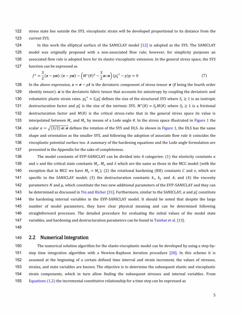
5
stress state lies outside the SYS, viscoplastic strain will be developed proportional to its distance from the 122
current SYS. 123
In this work the elliptical surface of the SANICLAY model [12] is adopted as the SYS. The SANICLAY 124
model was originally proposed with a non-associated flow rule; however, for simplicity purposes an 125
associated flow rule is adopted here for its elastic-viscoplastic extension. In the general stress space, the SYS 126
function can be expressed as 127
(7)
In the above expression, is the deviatoric component of stress tensor ( being the fourth order 128
identity tensor). is the deviatoric fabric tensor that accounts for anisotropy by coupling the deviatoric and 129
volumetric plastic strain rates. defines the size of the structured SYS where is an isotropic 130
destructuration factor and is the size of the intrinsic SYS. where is a frictional 131
destructuration factor and is the critical stress-ratio that in the general stress space its value is 132
interpolated between and by means of a Lode angle . In the stress space illustrated in Figure 1 the 133
scalar defines the rotation of the SYS and DLS. As shown in Figure 1, the DLS has the same 134
shape and orientation as the smaller SYS, and following the adoption of associate flow rule it coincides the 135
viscoplastic potential surface too. A summary of the hardening equations and the Lode angle formulation are 136
presented in the Appendix for the sake of completeness. 137
The model constants of EVP-SANICLAY can be divided into 4 categories: (1) the elasticity constants 138
and and the critical state constants , and which are the same as those in the MCC model (with the 139
exception that in MCC we have ); (2) the rotational hardening (RH) constants and , which are 140
specific to the SANICLAY model; (3) the destructuration constants , and ; and (4) the viscosity 141
parameters and , which constitute the two new additional parameters of the EVP-SANICLAY and they can 142
be determined as discussed in Yin and Hicher [31]. Furthermore, similar to the SANICLAY, and constitute 143
the hardening internal variables in the EVP-SANICLAY model. It should be noted that despite the large 144
number of model parameters, they have clear physical meaning and can be determined following 145
straightforward processes. The detailed procedure for evaluating the initial values of the model state 146
variables, and hardening and destructuration parameters can be found in Taiebat et al. [13]. 147
148
2.2 Numerical Integration 149
The numerical solution algorithm for the elasto-viscoplastic model can be developed by using a step-by-150
step time integration algorithm with a Newton-Raphson iteration procedure [28]. In this scheme it is 151
assumed at the beginning of a certain defined time interval and strain increment, the values of stresses, 152
strains, and state variables are known. The objective is to determine the subsequent elastic and viscoplastic 153
strain components, which in turn allow finding the subsequent stresses and internal variables. From 154
Equations (1,2) the incremental constitutive relationship for a time step can be expressed as 155
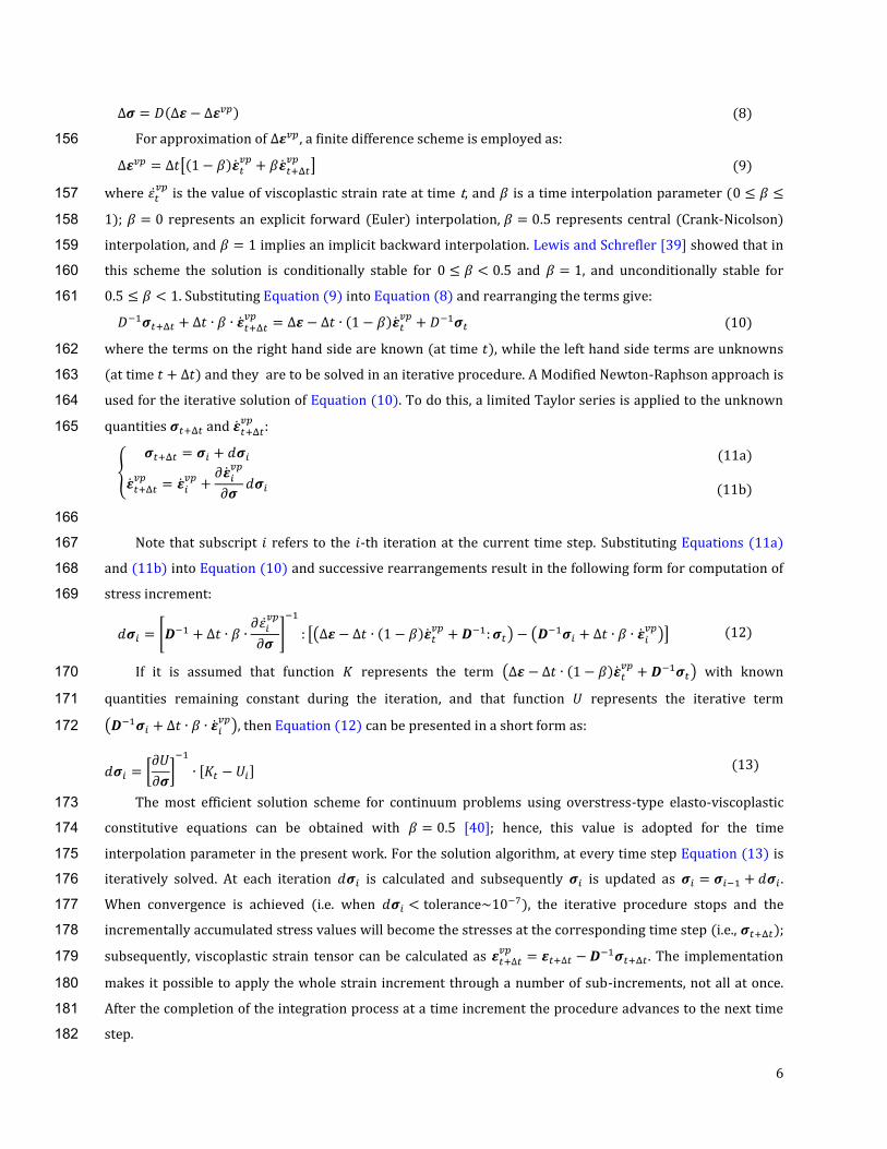
6
(8)
For approximation of , a finite difference scheme is employed as: 156
(9)
where is the value of viscoplastic strain rate at time t, and is a time interpolation parameter ( 157
); represents an explicit forward (Euler) interpolation, . represents central (Crank-Nicolson) 158
interpolation, and implies an implicit backward interpolation. Lewis and Schrefler [39] showed that in 159
this scheme the solution is conditionally stable for . and , and unconditionally stable for 160
. . Substituting Equation (9) into Equation (8) and rearranging the terms give: 161
(10)
where the terms on the right hand side are known (at time ), while the left hand side terms are unknowns 162
(at time ) and they are to be solved in an iterative procedure. A Modified Newton-Raphson approach is 163
used for the iterative solution of Equation (10). To do this, a limited Taylor series is applied to the unknown 164
quantities and : 165
(11a)
(11b)
166
Note that subscript refers to the -th iteration at the current time step. Substituting Equations (11a) 167
and (11b) into Equation (10) and successive rearrangements result in the following form for computation of 168
stress increment: 169
(12)
If it is assumed that function represents the term with known 170
quantities remaining constant during the iteration, and that function represents the iterative term 171
, then Equation (12) can be presented in a short form as: 172
(13)
The most efficient solution scheme for continuum problems using overstress-type elasto-viscoplastic 173
constitutive equations can be obtained with . [40]; hence, this value is adopted for the time 174
interpolation parameter in the present work. For the solution algorithm, at every time step Equation (13) is 175
iteratively solved. At each iteration is calculated and subsequently is updated as . 176
When convergence is achieved (i.e. when tolerance ), the iterative procedure stops and the 177
incrementally accumulated stress values will become the stresses at the corresponding time step (i.e., ); 178
subsequently, viscoplastic strain tensor can be calculated as . The implementation 179
makes it possible to apply the whole strain increment through a number of sub-increments, not all at once. 180
After the completion of the integration process at a time increment the procedure advances to the next time 181
step. 182
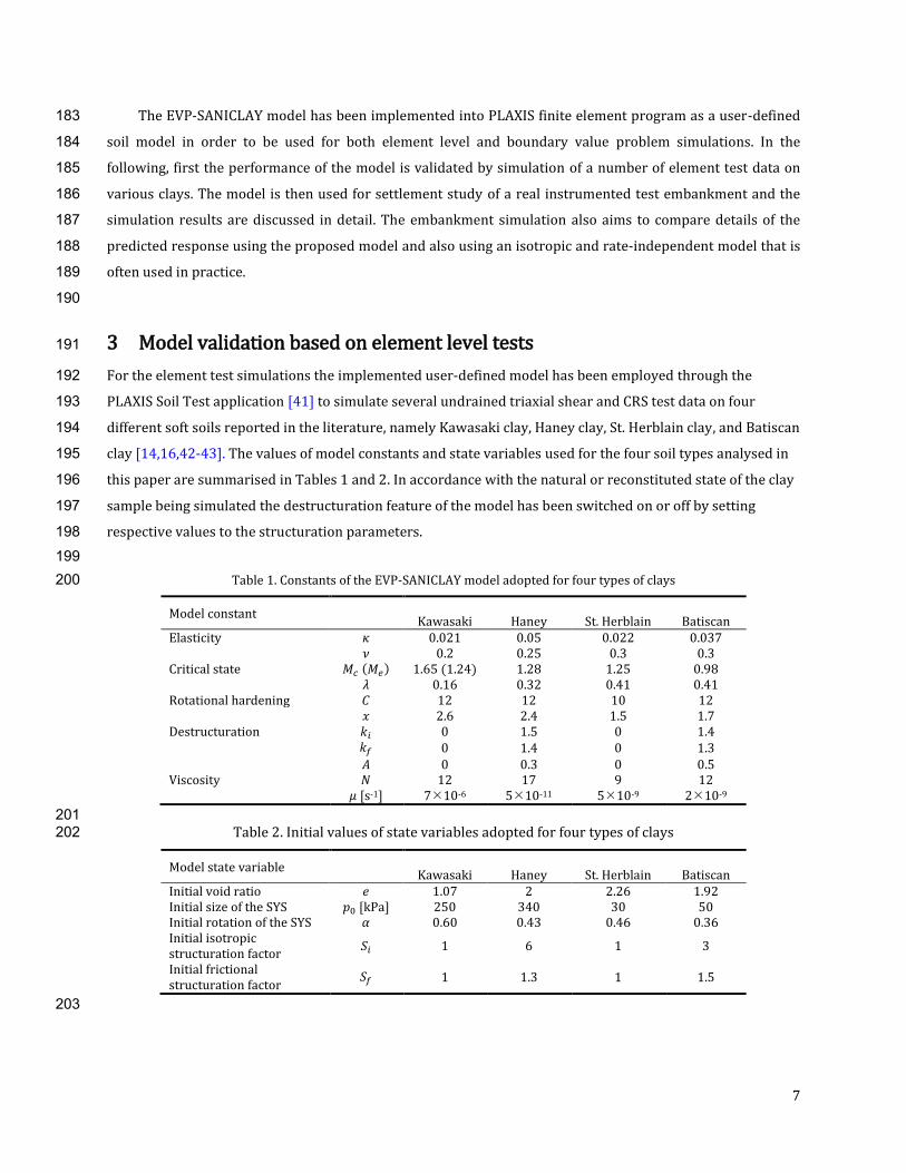
7
The EVP-SANICLAY model has been implemented into PLAXIS finite element program as a user-defined 183
soil model in order to be used for both element level and boundary value problem simulations. In the 184
following, first the performance of the model is validated by simulation of a number of element test data on 185
various clays. The model is then used for settlement study of a real instrumented test embankment and the 186
simulation results are discussed in detail. The embankment simulation also aims to compare details of the 187
predicted response using the proposed model and also using an isotropic and rate-independent model that is 188
often used in practice. 189
190
3 Model validation based on element level tests 191
For the element test simulations the implemented user-defined model has been employed through the 192
PLAXIS Soil Test application [41] to simulate several undrained triaxial shear and CRS test data on four 193
different soft soils reported in the literature, namely Kawasaki clay, Haney clay, St. Herblain clay, and Batiscan 194
clay [14,16,42-43]. The values of model constants and state variables used for the four soil types analysed in 195
this paper are summarised in Tables 1 and 2. In accordance with the natural or reconstituted state of the clay 196
sample being simulated the destructuration feature of the model has been switched on or off by setting 197
respective values to the structuration parameters. 198 199
Table 1. Constants of the EVP-SANICLAY model adopted for four types of clays 200
Model constant Kawasaki Haney St. Herblain Batiscan
Elasticity 0.021 0.05 0.022 0.037 0.2 0.25 0.3 0.3 Critical state 1.65 (1.24) 1.28 1.25 0.98 0.16 0.32 0.41 0.41 Rotational hardening 12 12 10 12 2.6 2.4 1.5 1.7 Destructuration 0 1.5 0 1.4 0 1.4 0 1.3 0 0.3 0 0.5 Viscosity 12 17 9 12 [s-1] 7¯10-6 5¯10-11 5¯10-9 2¯10-9
201 Table 2. Initial values of state variables adopted for four types of clays 202
Model state variable Kawasaki Haney St. Herblain Batiscan
Initial void ratio 1.07 2 2.26 1.92 Initial size of the SYS [kPa] 250 340 30 50 Initial rotation of the SYS 0.60 0.43 0.46 0.36 Initial isotropic structuration factor 1 6 1 3
Initial frictional structuration factor 1 1.3 1 1.5
203
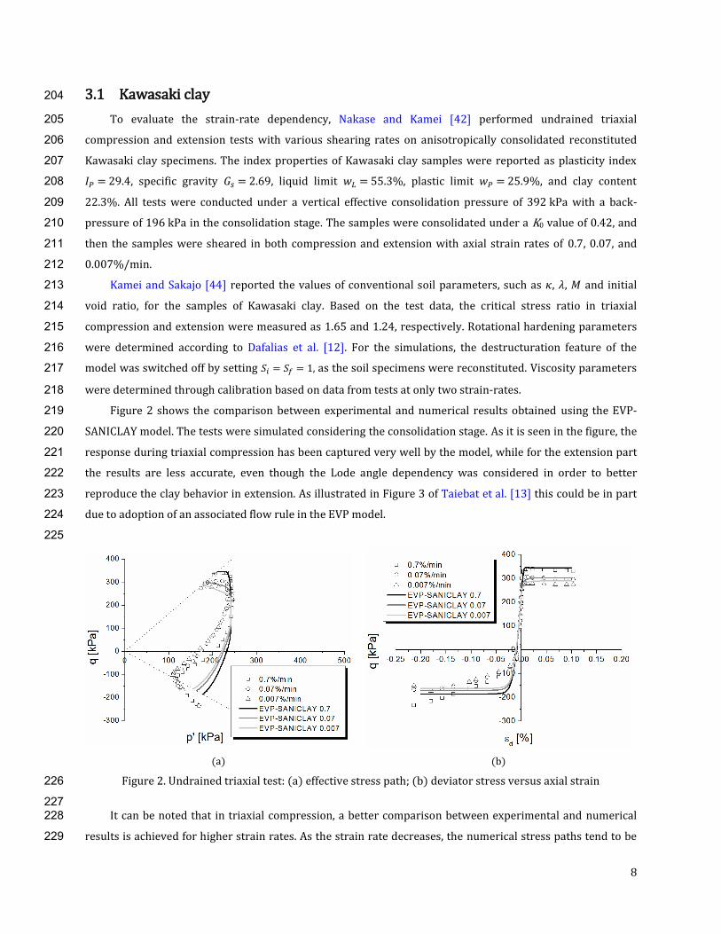
8
3.1 Kawasaki clay 204
To evaluate the strain-rate dependency, Nakase and Kamei [42] performed undrained triaxial 205
compression and extension tests with various shearing rates on anisotropically consolidated reconstituted 206
Kawasaki clay specimens. The index properties of Kawasaki clay samples were reported as plasticity index 207
= 29.4, specific gravity = 2.69, liquid limit = 55.3%, plastic limit = 25.9%, and clay content 208
22.3%. All tests were conducted under a vertical effective consolidation pressure of 392 kPa with a back-209
pressure of 196 kPa in the consolidation stage. The samples were consolidated under a K0 value of 0.42, and 210
then the samples were sheared in both compression and extension with axial strain rates of 0.7, 0.07, and 211
0.007%/min. 212
Kamei and Sakajo [44] reported the values of conventional soil parameters, such as , , and initial 213
void ratio, for the samples of Kawasaki clay. Based on the test data, the critical stress ratio in triaxial 214
compression and extension were measured as 1.65 and 1.24, respectively. Rotational hardening parameters 215
were determined according to Dafalias et al. [12]. For the simulations, the destructuration feature of the 216
model was switched off by setting , as the soil specimens were reconstituted. Viscosity parameters 217
were determined through calibration based on data from tests at only two strain-rates. 218
Figure 2 shows the comparison between experimental and numerical results obtained using the EVP-219
SANICLAY model. The tests were simulated considering the consolidation stage. As it is seen in the figure, the 220
response during triaxial compression has been captured very well by the model, while for the extension part 221
the results are less accurate, even though the Lode angle dependency was considered in order to better 222
reproduce the clay behavior in extension. As illustrated in Figure 3 of Taiebat et al. [13] this could be in part 223
due to adoption of an associated flow rule in the EVP model. 224
225
(a) (b)
Figure 2. Undrained triaxial test: (a) effective stress path; (b) deviator stress versus axial strain 226
227 It can be noted that in triaxial compression, a better comparison between experimental and numerical 228
results is achieved for higher strain rates. As the strain rate decreases, the numerical stress paths tend to be 229
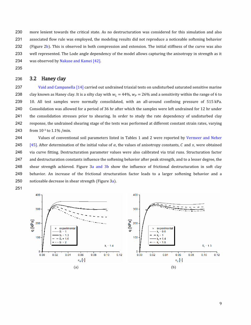
9
more lenient towards the critical state. As no destructuration was considered for this simulation and also 230
associated flow rule was employed, the modeling results did not reproduce a noticeable softening behavior 231
(Figure 2b). This is observed in both compression and extension. The initial stiffness of the curve was also 232
well represented. The Lode angle dependency of the model allows capturing the anisotropy in strength as it 233
was observed by Nakase and Kamei [42]. 234
235
3.2 Haney clay 236
Vaid and Campanella [14] carried out undrained triaxial tests on undisturbed saturated sensitive marine 237
clay known as Haney clay. It is a silty clay with = 44%, = 26% and a sensitivity within the range of 6 to 238
10. All test samples were normally consolidated, with an all-around confining pressure of 515 kPa. 239
Consolidation was allowed for a period of 36 hr after which the samples were left undrained for 12 hr under 240
the consolidation stresses prior to shearing. In order to study the rate dependency of undisturbed clay 241
response, the undrained shearing stage of the tests was performed at different constant strain rates, varying 242
from 10-3 to 1.1% /min. 243
Values of conventional soil parameters listed in Tables 1 and 2 were reported by Vermeer and Neher 244
[45]. After determination of the initial value of , the values of anisotropy constants, and , were obtained 245
via curve fitting. Destructuration parameter values were also calibrated via trial runs. Structuration factor 246
and destructuration constants influence the softening behavior after peak strength, and to a lesser degree, the 247
shear strength achieved. Figure 3a and 3b show the influence of frictional destructuration in soft clay 248
behavior. An increase of the frictional structuration factor leads to a larger softening behavior and a 249
noticeable decrease in shear strength (Figure 3a). 250
251
(a) (b)
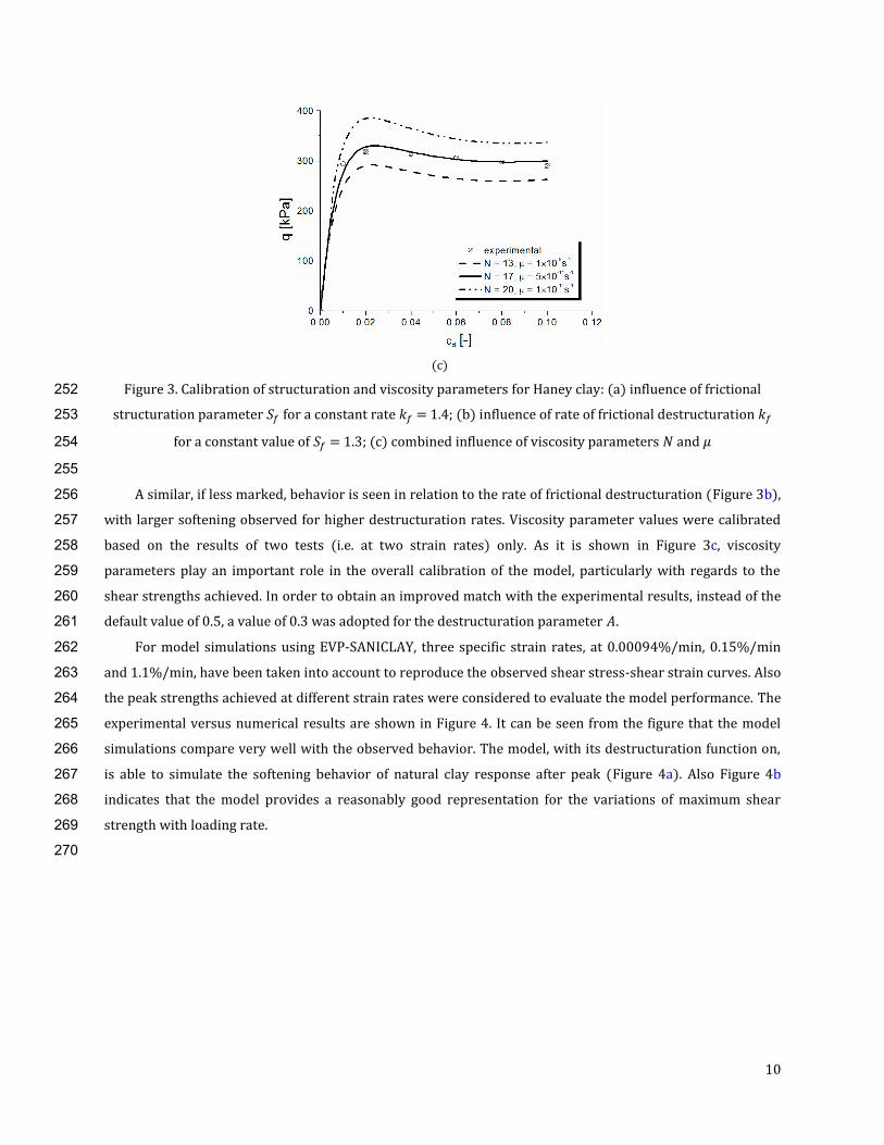
10
(c)
Figure 3. Calibration of structuration and viscosity parameters for Haney clay: (a) influence of frictional 252
structuration parameter for a constant rate = 1.4; (b) influence of rate of frictional destructuration 253
for a constant value of = 1.3; (c) combined influence of viscosity parameters and 254
255
A similar, if less marked, behavior is seen in relation to the rate of frictional destructuration (Figure 3b), 256
with larger softening observed for higher destructuration rates. Viscosity parameter values were calibrated 257
based on the results of two tests (i.e. at two strain rates) only. As it is shown in Figure 3c, viscosity 258
parameters play an important role in the overall calibration of the model, particularly with regards to the 259
shear strengths achieved. In order to obtain an improved match with the experimental results, instead of the 260
default value of 0.5, a value of 0.3 was adopted for the destructuration parameter . 261
For model simulations using EVP-SANICLAY, three specific strain rates, at 0.00094%/min, 0.15%/min 262
and 1.1%/min, have been taken into account to reproduce the observed shear stress-shear strain curves. Also 263
the peak strengths achieved at different strain rates were considered to evaluate the model performance. The 264
experimental versus numerical results are shown in Figure 4. It can be seen from the figure that the model 265
simulations compare very well with the observed behavior. The model, with its destructuration function on, 266
is able to simulate the softening behavior of natural clay response after peak (Figure 4a). Also Figure 4b 267
indicates that the model provides a reasonably good representation for the variations of maximum shear 268
strength with loading rate. 269
270
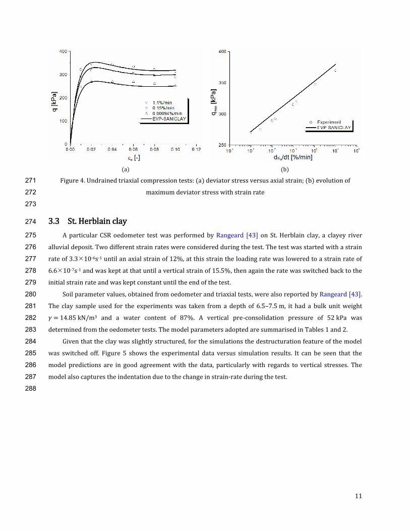
11
(a) (b)
Figure 4. Undrained triaxial compression tests: (a) deviator stress versus axial strain; (b) evolution of 271
maximum deviator stress with strain rate 272
273
3.3 St. Herblain clay 274
A particular CSR oedometer test was performed by Rangeard [43] on St. Herblain clay, a clayey river 275
alluvial deposit. Two different strain rates were considered during the test. The test was started with a strain 276
rate of 3.3¯10-6s-1 until an axial strain of 12%, at this strain the loading rate was lowered to a strain rate of 277
6.6¯10-7s-1 and was kept at that until a vertical strain of 15.5%, then again the rate was switched back to the 278
initial strain rate and was kept constant until the end of the test. 279
Soil parameter values, obtained from oedometer and triaxial tests, were also reported by Rangeard [43]. 280
The clay sample used for the experiments was taken from a depth of 6.5–7.5 m, it had a bulk unit weight 281
= 14.85 kN/m3 and a water content of 87%. A vertical pre-consolidation pressure of 52 kPa was 282
determined from the oedometer tests. The model parameters adopted are summarised in Tables 1 and 2. 283
Given that the clay was slightly structured, for the simulations the destructuration feature of the model 284
was switched off. Figure 5 shows the experimental data versus simulation results. It can be seen that the 285
model predictions are in good agreement with the data, particularly with regards to vertical stresses. The 286
model also captures the indentation due to the change in strain-rate during the test. 287
288
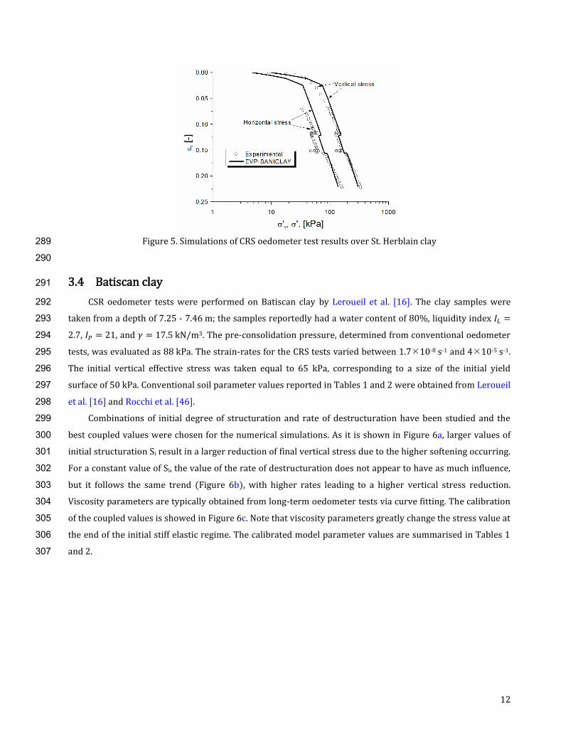
12
Figure 5. Simulations of CRS oedometer test results over St. Herblain clay 289
290
3.4 Batiscan clay 291
CSR oedometer tests were performed on Batiscan clay by Leroueil et al. [16]. The clay samples were 292
taken from a depth of 7.25 - 7.46 m; the samples reportedly had a water content of 80%, liquidity index = 293
2.7, = 21, and = 17.5 kN/m3. The pre-consolidation pressure, determined from conventional oedometer 294
tests, was evaluated as 88 kPa. The strain-rates for the CRS tests varied between 1.7¯10-8 s-1 and 4¯10-5 s-1. 295
The initial vertical effective stress was taken equal to 65 kPa, corresponding to a size of the initial yield 296
surface of 50 kPa. Conventional soil parameter values reported in Tables 1 and 2 were obtained from Leroueil 297
et al. [16] and Rocchi et al. [46]. 298
Combinations of initial degree of structuration and rate of destructuration have been studied and the 299
best coupled values were chosen for the numerical simulations. As it is shown in Figure 6a, larger values of 300
initial structuration Si result in a larger reduction of final vertical stress due to the higher softening occurring. 301
For a constant value of Si, the value of the rate of destructuration does not appear to have as much influence, 302
but it follows the same trend (Figure 6b), with higher rates leading to a higher vertical stress reduction. 303
Viscosity parameters are typically obtained from long-term oedometer tests via curve fitting. The calibration 304
of the coupled values is showed in Figure 6c. Note that viscosity parameters greatly change the stress value at 305
the end of the initial stiff elastic regime. The calibrated model parameter values are summarised in Tables 1 306
and 2. 307
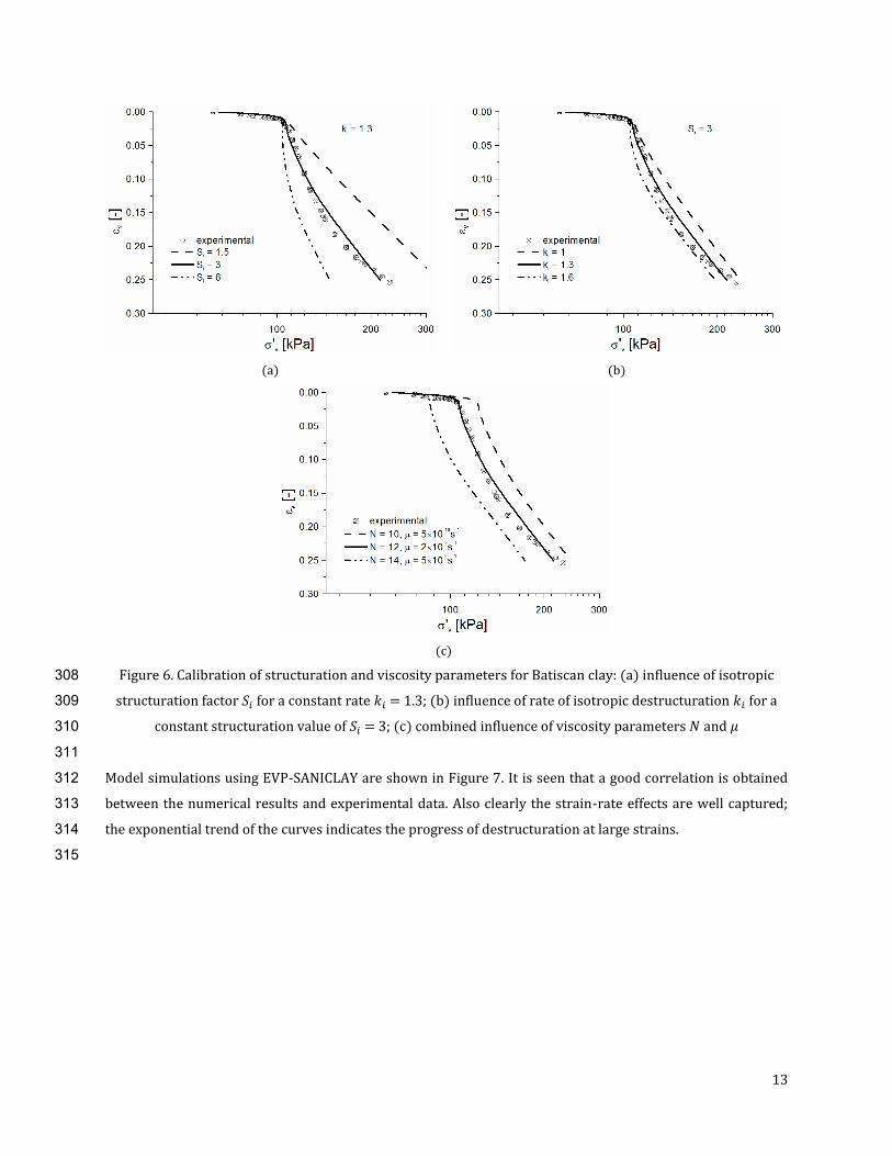
13
(a) (b)
(c)
Figure 6. Calibration of structuration and viscosity parameters for Batiscan clay: (a) influence of isotropic 308
structuration factor for a constant rate = 1.3; (b) influence of rate of isotropic destructuration for a 309
constant structuration value of = 3; (c) combined influence of viscosity parameters and 310
311
Model simulations using EVP-SANICLAY are shown in Figure 7. It is seen that a good correlation is obtained 312
between the numerical results and experimental data. Also clearly the strain-rate effects are well captured; 313
the exponential trend of the curves indicates the progress of destructuration at large strains. 314
315
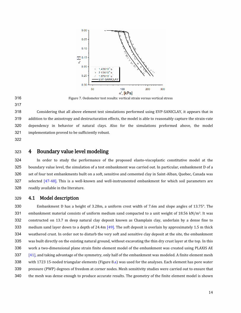
14
Figure 7. Oedometer test results: vertical strain versus vertical stress 316
317
Considering that all above element test simulations performed using EVP-SANICLAY, it appears that in 318
addition to the anisotropy and destructuration effects, the model is able to reasonably capture the strain-rate 319
dependency in behavior of natural clays. Also for the simulations preformed above, the model 320
implementation proved to be sufficiently robust. 321
322
4 Boundary value level modeling 323
In order to study the performance of the proposed elasto-viscoplastic constitutive model at the 324
boundary value level, the simulation of a test embankment was carried out. In particular, embankment D of a 325
set of four test embankments built on a soft, sensitive and cemented clay in Saint-Alban, Quebec, Canada was 326
selected [47-48]. This is a well-known and well-instrumented embankment for which soil parameters are 327
readily available in the literature. 328
4.1 Model description 329
Embankment D has a height of 3.28m, a uniform crest width of 7.6m and slope angles of 13.75°. The 330
embankment material consists of uniform medium sand compacted to a unit weight of 18.56 kN/m3. It was 331
constructed on 13.7 m deep natural clay deposit known as Champlain clay, underlain by a dense fine to 332
medium sand layer down to a depth of 24.4m [49]. The soft deposit is overlain by approximately 1.5 m thick 333
weathered crust. In order not to disturb the very soft and sensitive clay deposit at the site, the embankment 334
was built directly on the existing natural ground, without excavating the thin dry crust layer at the top. In this 335
work a two-dimensional plane strain finite element model of the embankment was created using PLAXIS AE 336
[41], and taking advantage of the symmetry, only half of the embankment was modeled. A finite element mesh 337
with 1723 15-noded triangular elements (Figure 8.a) was used for the analyses. Each element has pore water 338
pressure (PWP) degrees of freedom at corner nodes. Mesh sensitivity studies were carried out to ensure that 339
the mesh was dense enough to produce accurate results. The geometry of the finite element model is shown 340
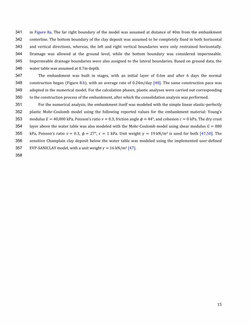
15
in Figure 8a. The far right boundary of the model was assumed at distance of 40m from the embankment 341
centerline. The bottom boundary of the clay deposit was assumed to be completely fixed in both horizontal 342
and vertical directions, whereas, the left and right vertical boundaries were only restrained horizontally. 343
Drainage was allowed at the ground level, while the bottom boundary was considered impermeable. 344
Impermeable drainage boundaries were also assigned to the lateral boundaries. Based on ground data, the 345
water table was assumed at 0.7m depth. 346
The embankment was built in stages, with an initial layer of 0.6m and after 6 days the normal 347
construction began (Figure 8.b), with an average rate of 0.24m/day [48]. The same construction pace was 348
adopted in the numerical model. For the calculation phases, plastic analyses were carried out corresponding 349
to the construction process of the embankment, after which the consolidation analysis was performed. 350
For the numerical analysis, the embankment itself was modeled with the simple linear elastic-perfectly 351
plastic Mohr-Coulomb model using the ollowing reported values or the embankment material Young’s 352
modulus = 40,000 kPa, Poisson’s ratio = 0.3, friction angle = 44°, and cohesion = 0 kPa. The dry crust 353
layer above the water table was also modeled with the Mohr-Coulomb model using shear modulus = 880 354
kPa, Poisson’s ratio = 0.3, = 27°, = 1 kPa. Unit weight = 19 kN/m3 is used for both [47,50]. The 355
sensitive Champlain clay deposit below the water table was modeled using the implemented user-defined 356
EVP-SANICLAY model, with a unit weight = 16 kN/m3 [47]. 357
358
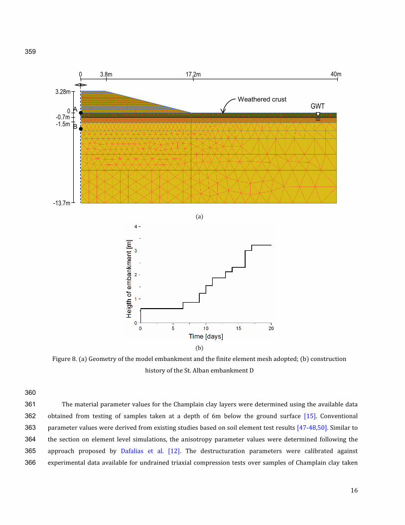
16
359
(a)
(b)
Figure 8. (a) Geometry of the model embankment and the finite element mesh adopted; (b) construction
history of the St. Alban embankment D
360
The material parameter values for the Champlain clay layers were determined using the available data 361
obtained from testing of samples taken at a depth of 6m below the ground surface [15]. Conventional 362
parameter values were derived from existing studies based on soil element test results [47-48,50]. Similar to 363
the section on element level simulations, the anisotropy parameter values were determined following the 364
approach proposed by Dafalias et al. [12]. The destructuration parameters were calibrated against 365
experimental data available for undrained triaxial compression tests over samples of Champlain clay taken 366
GWT
3.8m 0 17.2m 40m
3.28m
0 -0.7m -1.5m
-13.7m
Weathered crust
B
A
17
from a depth of approximately 3m [51]. For three tests presented in Figure 9 the samples were first 367
isotropically consolidated up to three different pre-consolidation pressures of 44, 66.6 and 77 kPa, and 368
subsequently sheared. Figure 9 shows a good agreement between the experimental data and the numerical 369
simulations both in terms of stress-strain response and of stress paths. The destructuration trend after peak 370
strengths was also well captured. 371
372
(a) (b)
Figure 9. Validation of numerical simulations versus experimental results for undrained triaxial compression 373
tests: (a) deviator stress versus axial strain; (b) effective stress paths 374
375
In the absence of appropriate soil test data, such as long-term oedometer tests with at least two different 376
strain rates, viscosity parameters were calibrated using trial runs. 377
378
379
18
Table 3 summarises the soil and state parameters adopted for the simulation of St. Alban test 380
embankment, and Table 4 lists the calibrated anisotropy and destructuration parameter values. The 381
permeability, , of the clay, assumed to be isotropic, was reported to be equal to 3.46¯10-4 m/day. It should 382
also be added that the initial state of stress was generated by adopting K0-procedure [41] where the reported 383
K0 value of 0.8 was employed [52]. Results from oedometer tests performed on Champlain clay reported that 384
over-consolidation ratio (OCR) varied between 1.8 and 2.2 [47]; a mean value of 2.0 was assumed for the 385
analyses performed here. 386
387
388
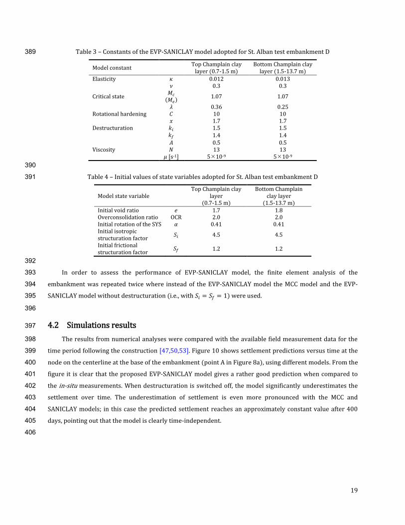
19
Table 3 – Constants of the EVP-SANICLAY model adopted for St. Alban test embankment D 389
Model constant Top Champlain clay layer (0.7-1.5 m)
Bottom Champlain clay layer (1.5-13.7 m)
Elasticity 0.012 0.013 0.3 0.3
Critical state
1.07 1.07
0.36 0.25 Rotational hardening 10 10 1.7 1.7 Destructuration 1.5 1.5 1.4 1.4 0.5 0.5 Viscosity 13 13 [s-1] 5¯10-9 5¯10-9
390
Table 4 – Initial values of state variables adopted for St. Alban test embankment D 391
Model state variable Top Champlain clay
layer (0.7-1.5 m)
Bottom Champlain clay layer
(1.5-13.7 m) Initial void ratio 1.7 1.8 Overconsolidation ratio OCR 2.0 2.0 Initial rotation of the SYS 0.41 0.41 Initial isotropic structuration factor 4.5 4.5
Initial frictional structuration factor 1.2 1.2
392
In order to assess the performance of EVP-SANICLAY model, the finite element analysis of the 393
embankment was repeated twice where instead of the EVP-SANICLAY model the MCC model and the EVP-394
SANICLAY model without destructuration (i.e., with ) were used. 395
396
4.2 Simulations results 397
The results from numerical analyses were compared with the available field measurement data for the 398
time period following the construction [47,50,53]. Figure 10 shows settlement predictions versus time at the 399
node on the centerline at the base of the embankment (point A in Figure 8a), using different models. From the 400
figure it is clear that the proposed EVP-SANICLAY model gives a rather good prediction when compared to 401
the in-situ measurements. When destructuration is switched off, the model significantly underestimates the 402
settlement over time. The underestimation of settlement is even more pronounced with the MCC and 403
SANICLAY models; in this case the predicted settlement reaches an approximately constant value after 400 404
days, pointing out that the model is clearly time-independent. 405
406
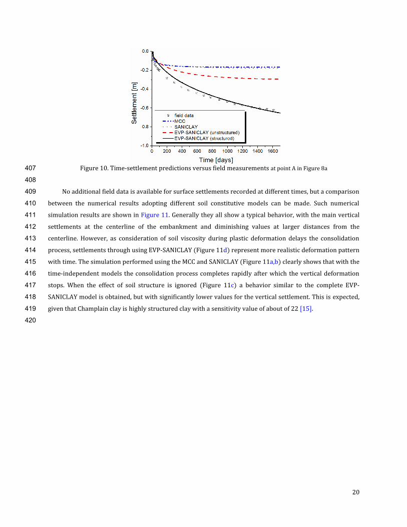
20
Figure 10. Time-settlement predictions versus field measurements at point A in Figure 8a 407
408
No additional field data is available for surface settlements recorded at different times, but a comparison 409
between the numerical results adopting different soil constitutive models can be made. Such numerical 410
simulation results are shown in Figure 11. Generally they all show a typical behavior, with the main vertical 411
settlements at the centerline of the embankment and diminishing values at larger distances from the 412
centerline. However, as consideration of soil viscosity during plastic deformation delays the consolidation 413
process, settlements through using EVP-SANICLAY (Figure 11d) represent more realistic deformation pattern 414
with time. The simulation performed using the MCC and SANICLAY (Figure 11a,b) clearly shows that with the 415
time-independent models the consolidation process completes rapidly after which the vertical deformation 416
stops. When the effect of soil structure is ignored (Figure 11c) a behavior similar to the complete EVP-417
SANICLAY model is obtained, but with significantly lower values for the vertical settlement. This is expected, 418
given that Champlain clay is highly structured clay with a sensitivity value of about of 22 [15]. 419
420
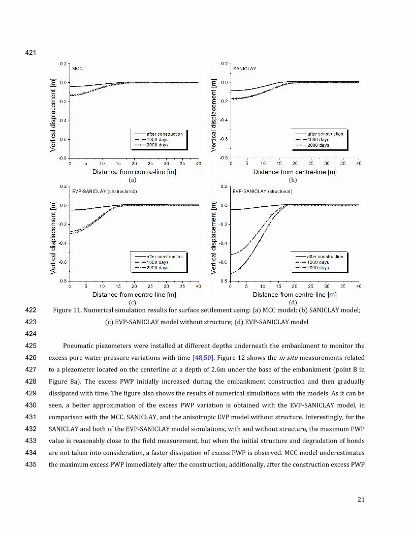
21
421
(a) (b)
(c) (d)
Figure 11. Numerical simulation results for surface settlement using: (a) MCC model; (b) SANICLAY model; 422
(c) EVP-SANICLAY model without structure; (d) EVP-SANICLAY model 423
424
Pneumatic piezometers were installed at different depths underneath the embankment to monitor the 425
excess pore water pressure variations with time [48,50]. Figure 12 shows the in-situ measurements related 426
to a piezometer located on the centerline at a depth of 2.6m under the base of the embankment (point B in 427
Figure 8a). The excess PWP initially increased during the embankment construction and then gradually 428
dissipated with time. The figure also shows the results of numerical simulations with the models. As it can be 429
seen, a better approximation of the excess PWP variation is obtained with the EVP-SANICLAY model, in 430
comparison with the MCC, SANICLAY, and the anisotropic EVP model without structure. Interestingly, for the 431
SANICLAY and both of the EVP-SANICLAY model simulations, with and without structure, the maximum PWP 432
value is reasonably close to the field measurement, but when the initial structure and degradation of bonds 433
are not taken into consideration, a faster dissipation of excess PWP is observed. MCC model underestimates 434
the maximum excess PWP immediately after the construction; additionally, after the construction excess PWP 435
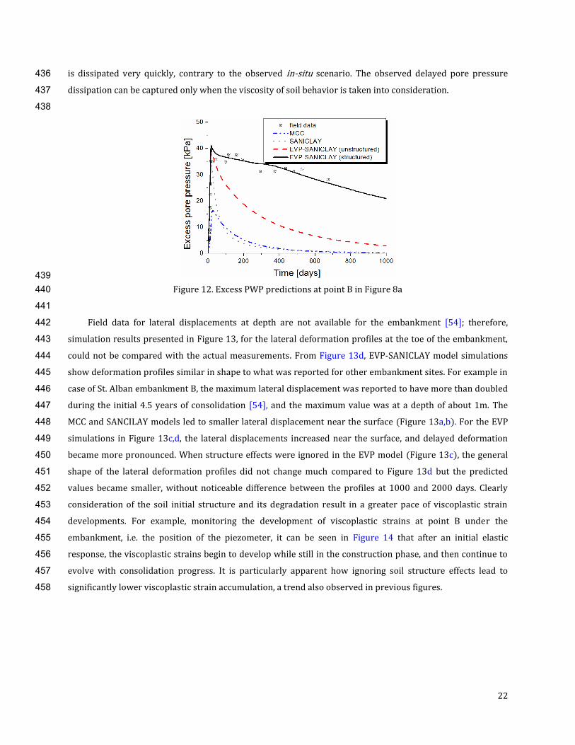
22
is dissipated very quickly, contrary to the observed in-situ scenario. The observed delayed pore pressure 436
dissipation can be captured only when the viscosity of soil behavior is taken into consideration. 437
438
439 Figure 12. Excess PWP predictions at point B in Figure 8a 440
441
Field data for lateral displacements at depth are not available for the embankment [54]; therefore, 442
simulation results presented in Figure 13, for the lateral deformation profiles at the toe of the embankment, 443
could not be compared with the actual measurements. From Figure 13d, EVP-SANICLAY model simulations 444
show deformation profiles similar in shape to what was reported for other embankment sites. For example in 445
case of St. Alban embankment B, the maximum lateral displacement was reported to have more than doubled 446
during the initial 4.5 years of consolidation [54], and the maximum value was at a depth of about 1m. The 447
MCC and SANCILAY models led to smaller lateral displacement near the surface (Figure 13a,b). For the EVP 448
simulations in Figure 13c,d, the lateral displacements increased near the surface, and delayed deformation 449
became more pronounced. When structure effects were ignored in the EVP model (Figure 13c), the general 450
shape of the lateral deformation profiles did not change much compared to Figure 13d but the predicted 451
values became smaller, without noticeable difference between the profiles at 1000 and 2000 days. Clearly 452
consideration of the soil initial structure and its degradation result in a greater pace of viscoplastic strain 453
developments. For example, monitoring the development of viscoplastic strains at point B under the 454
embankment, i.e. the position of the piezometer, it can be seen in Figure 14 that after an initial elastic 455
response, the viscoplastic strains begin to develop while still in the construction phase, and then continue to 456
evolve with consolidation progress. It is particularly apparent how ignoring soil structure effects lead to 457
significantly lower viscoplastic strain accumulation, a trend also observed in previous figures. 458
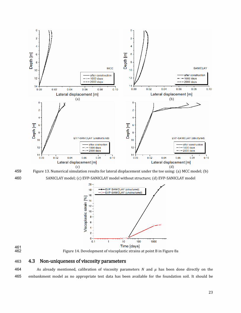
23
(a) (b)
(c) (d)
Figure 13. Numerical simulation results for lateral displacement under the toe using: (a) MCC model; (b) 459
SANICLAY model; (c) EVP-SANICLAY model without structure; (d) EVP-SANICLAY model 460
461 Figure 14. Development of viscoplastic strains at point B in Figure 8a 462
4.3 Non-uniqueness of viscosity parameters 463
As already mentioned, calibration of viscosity parameters and has been done directly on the 464
embankment model as no appropriate test data has been available for the foundation soil. It should be 465
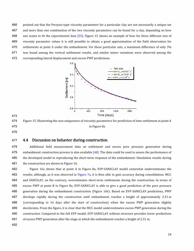
24
pointed out that the Perzyna-type viscosity parameters for a particular clay are not necessarily a unique set 466
and more than one combination of the two viscosity parameters can be found for a clay, depending on how 467
one wants to fit the experimental data [55]. Figure 15 shows an example of how for three different sets of 468
viscosity parameter values it is still possible to obtain a good approximation of the field observation for 469
settlements at point A under the embankment. For these particular sets, a maximum difference of only 3% 470
was found among the vertical settlement results, and similar minor variations were observed among the 471
corresponding lateral displacement and excess PWP predictions. 472
473 Figure 15. Illustrating the non-uniqueness of viscosity parameters for prediction of time-settlement at point A 474
in Figure 8a 475
476
4.4 Discussion on behavior during construction 477
Additional field measurement data on settlement and excess pore pressure generation during 478
embankment construction process is also available [48]. The data could be used to assess the performance of 479
the developed model in reproducing the short-term response of the embankment. Simulation results during 480
the construction are shown in Figure 16. 481
Figure 16a shows that at point A in Figure 8a, EVP-SANICLAY model somewhat underestimates the 482
results; although, as it was observed in Figure 7a, it is then able to gain accuracy during consolidation. MCC 483
and SANCILAY, on the contrary, overestimates short-term settlements during the construction. In terms of 484
excess PWP at point B in Figure 8a, EVP-SANICLAY is able to give a good prediction of the pore pressure 485
generation during the embankment construction (Figure 16b). Based on EVP-SANICLAY predictions, PWP 486
develops rapidly during the construction until embankment reaches a height of approximately 2.31 m 487
(corresponding to 16 days after the start of construction) when the excess PWP generation slightly 488
decelerates. From the figure, it is clear that the MCC model underestimates excess PWP generation during the 489
construction. Compared to the full EVP model, EVP-SANICLAY without structure provides lower predictions 490
of excess PWP generation after the stage at which the embankment reaches a height of 2.31 m. 491
492
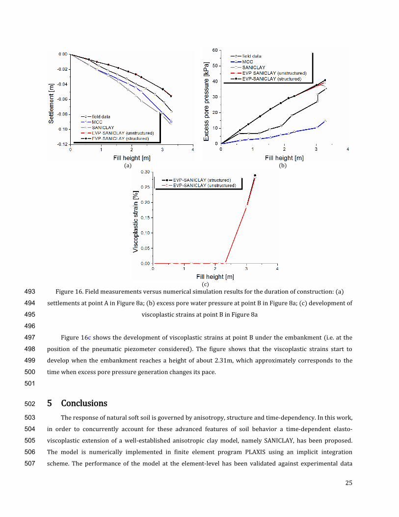
25
(a) (b)
(c)
Figure 16. Field measurements versus numerical simulation results for the duration of construction: (a) 493
settlements at point A in Figure 8a; (b) excess pore water pressure at point B in Figure 8a; (c) development of 494
viscoplastic strains at point B in Figure 8a 495
496
Figure 16c shows the development of viscoplastic strains at point B under the embankment (i.e. at the 497
position of the pneumatic piezometer considered). The figure shows that the viscoplastic strains start to 498
develop when the embankment reaches a height of about 2.31m, which approximately corresponds to the 499
time when excess pore pressure generation changes its pace. 500
501
5 Conclusions 502
The response of natural soft soil is governed by anisotropy, structure and time-dependency. In this work, 503
in order to concurrently account for these advanced features of soil behavior a time-dependent elasto-504
viscoplastic extension of a well-established anisotropic clay model, namely SANICLAY, has been proposed. 505
The model is numerically implemented in finite element program PLAXIS using an implicit integration 506
scheme. The performance of the model at the element-level has been validated against experimental data 507
26
obtained from testing four different clays at both structured and un-structured states. Furthermore the time-508
dependent behavior of St. Alban embankment D on the well-structured Champlain clay was analysed using 509
the proposed EVP-SANICLAY model. The paper presented the results for settlements, lateral deformations, 510
and excess PWP variations during the construction and the subsequent consolidation, comparing model 511
predictions with the field measurements where available. It was observed that the developed model 512
considers the delayed excess pore pressure dissipation following the completion of the embankment 513
construction reasonably well; hence it is able to yield more realistic predictions of the long-term vertical and 514
horizontal deformations. The boundary value problem simulation results also illustrated that considering 515
clay initial structure and subsequent destructuration effects significantly improve the accuracy of predictions, 516
particularly when dealing with a highly sensitive soft clay such as Champlain clay. Furthermore, the model 517
also predicted the immediate displacements as well as the development of excess pore pressures during early 518
stages of construction with reasonable accuracy. 519
In general, EVP-SANICLAY proved to be able to much better predict both short- and long-term behavior 520
of natural clay behavior when compared with a commonly used critical state based model such as MCC, and 521
also the SANCILAY model. 522
523
Acknowledgements 524
Support to conduct this study is provided by the University of Nottingham’s Dean of Engineering award, 525
and the Natural Sciences and Engineering Research Council of Canada (NSERC). 526
527
Appendix 528
For the sake of completeness of presentation, some of the key components of the SANICLAY model that 529
are not presented in the main body of this paper are summarized here. Both stress and strain quantities are 530
assumed positive in compression (as is common in geomechanics), and the effect of this sign convention has 531
been considered on the model equations. All stress components in this paper should be considered as 532
effective stress. Finally, in terms of notation, tensor quantities are denoted by bold-faced symbols and 533
operations explained accordingly. 534
The hypoelastic formulation, considered for simplicity, constitutes of a shear modulus , for calculating 535
increments of elastic deviatoric strains, and a bulk modulus , for calculating increments of elastic volumetric 536
strains, where 537
(A.1)
where is the Poisson’s ratio, is the void ratio, tr is the mean effective stress (where tr stands for 538
the trace), and is the slope of elastic swelling lines in the ln space. 539
27
The isotropic hardening law of the model describing the evolution of the size of structured SYS, i.e. , is 540
defined as 541
(A.2)
where is the evolution rate of the isotropic destructuration factor (explained in the sequel), and 542
is the evolution of the size of SYS, that is a proportional to viscoplastic 543
volumetric strain rate, with indicating the slope of normal compression line. 544
The rotational hardening law describing the evolution of fabric anisotropy with viscoplastic staining can 545
be expressed in the general stress space as: 546
(A.3)
In the above equation, controls the contribution of destructuration over the change of 547
orientation of the yield surface ( explained in the sequel); is the shear stress ratio 548
is the bounding ‘image’ stress-ratio tensor, where is an auxiliary unit tensor defined as 549
and denoting the norm operator; and is the absolute value of the viscoplastic volumetric strain 550
rate. 551
In order to express the isotropic and frictional destructurations, an axillary internal variable called the 552
destructuration viscoplastic strain rate, , is defined by 553
(A.4)
where and
are the volumetric and deviatoric viscoplastic strain rates, respectively, and is a model 554
parameter could be set to 0.5 as a default value. The evolution equations for the and read 555
(A.5)
(A.6)
where and are model parameters. 556
As indicated in model formulation section, the critical stress-ratio is defined as a function of the Lode 557
angle . To regulate the variation of between its values for compression and for extension, the 558
expression proposed by Sheng et al. [56] has been adopted here which reads as 559
sin
(A.7)
560 where , sin , with and being the second and 561
third invariants of the modified stress deviator . 562
563
28
References 564
[1] Kim DK. Comparisons of Constitutive Models for Anisotropic Soils. KSCE J Civil Eng 2004; 8(4):403-409. 565
[2] Sekiguchi H, Ohta H. Induced anisotropy and time dependency in clays. 9th ICSMFE, Tokyo, Constitutive 566
equations of Soils 1977; 17:229-238. 567
[3] Graham J, Noonan ML, Lew KV. Yield states and stress–strain relationships in a natural plastic clay. Can 568
Geotech J 1983; 20(3):502-516. 569
[4] Korhonen KH, Lojander M. Yielding of Perno clay. In Proc of 2nd International Conference on Constitutive 570
Laws for Engineering Materials, Tucson, Arizona, Vol 2 1987: 1249-1255. 571
[5] Dafalias YF. An anisotropic critical state soil plasticity model. Mech Res Commun 1986; 13(6):341-347. 572
[6] Dafalias YF. An anisotropic critical state clay plasticity model. In Proceedings of the 2nd international 573
conference on constitutive laws for engineering materials. Tucson, US, 1987:513-521. 574
[7] Thevanayagam S, Chameau JL. Modelling anisotropy of clays at critical state. J Eng Mech-ASCE 1992; 575
118(4):786–806 576
[8] Whittle AJ, Kavvadas MJ. Formulation of MIT-E3 constitutive model for overconsolidated clays. J Geotech 577
Eng 1994; 120(1):173-198. 578
[9] Newson TA, Davies MCR. A rotational hardening constitutive model for anisotropically consolidated clay. 579
Soils Found 1996; 36(3):13–20 580
[10] Wheeler SJ, Karstunen M, Näätänen A. Anisotropic hardening model for normally consolidated soft clay. 581
In Proc. 7th Int. Symp. on Numerical Models in Geomechanics (NUMOG VII), Graz, 1999, 33- 40. A.A. 582
Balkema. 583
[11] Wheeler SJ, Näätänen A, Karstunen M, Lojander M. An anisotropic elasto-plastic model for soft clays. Can 584
Geotech J 2003; 40(2):403-418. 585
[12] Dafalias YF, Manzari MT, Papadimitriou AG. SANICLAY: simple anisotropic clay plasticity model. Int J 586
Numer Anal Meth Geomech 2006; 30:1231-1257. 587
[13] Taiebat M, Dafalias YF, Peek R. A destructuration theory and its application to SANICLAY model. Int J 588
Numer Anal Meth Geomech 2010; 34:1009-1040. 589
[14] Vaid YP, Campanella RG. Time-dependent behaviour of undisturbed clay. J Geotech Eng-ASCE 1977; 590
103(7):693-709. 591
[15] Tavenas F, Leroueil S, La Rochelle P, Roy M. Creep behavior of an undisturbed lightly overconsolidated 592
clay. Can Geotech J 1978; 15(3):402–423. 593
[16] Leroueil S, Kabbaj M, Tavenas F, Bouchard R. Stress–strain–strain-rate relation for the compressibility of 594
sensitive natural clays. Géotechnique 1985; 35(2):159–180. 595
[17] Lefebvre G, Leboeuf D. Rate effects and cyclic loading of sensitive clays. J Geotech Eng-ASCE 1987; 596
113(5):476–489. 597
29
[18] Augustesen A, Liingaard M, Lade PV. Evaluation of Time-Dependent Behavior of Soils. Int J Geomech 598
2004; 4(3):137-156. 599
[19] Vaid YP, Robertson PK, Campanella RG. Strain rate behavior of Saint-Jean-Vianney clay. Can Geotech J 600
1979; 16:34–42. 601
[20] Díaz-Rodríguez JA, Martínez-Vasquez JJ, Santamarina JC. Strain-rate effects in Mexico City soil. J Geotech 602
Geoenviron Eng 2009; 135(2):300–305 603
[21] Leroueil S. The isotache approach. Where are we 50 years after its development by Pro essor Šuklje?. 604
Pro . Šuklje’s Memorial Lecture, XIII Danube-European Geotechnical Engineering Conference, 29th–605
31st May 2006, Ljubljana, Slovenia. 606
[22 Šuklje L. The analysis o the consolidation process by the isotache method. Proc. 4th Int. Conf. on Soil 607
Mech and Found. Engng., London 1957; 1:200-206. 608
[23] Naghdi PM, Murch, SA. On the mechanical behavior of viscoelastic/plastic solids. J Applied Mechanics 609
1963; 30(3):321-328. 610
[24] Perzyna P. The constitutive equations for work-hardening and rate sensitive plastic materials. In Proc. 611
Vibration Problems Warsaw 1963; 3:281-290. 612
[25] Perzyna P. Fundamental problems in viscoplasticity. Adv Appl Mech 1966; 9:244–377. 613
[26] Adachi T, Oka F. Constitutive equations for normally consolidated clay based on elasto-viscoplasticity. 614
Soils Found 1982; 22(4):57-70. 615
[27] Nova R. A viscoplastic constitutive model for normally consolidated clay. In Proceedings of IUTAM 616
Conference on Deformation and Failure of Granular Materials, Delft, The Netherlands, 1982, 287–295. 617
[28] Katona MG. Evaluation of Viscoplastic Cap Model. J Geotech Eng-ASCE. 1984; 110:1106-1125. 618
[29] Kaliakin VN, Dafalias YF. Theoretical aspects of the elastoplastic-viscoplastic bounding surface model for 619
cohesive soils. Soils Found 1990; 30(3):11-24 620
[30] Yin JH, Zhu JG, Graham J. A new elastic viscoplastic model for time-dependent behaviour of normally and 621
overconsolidated clays: theory and verification. Can Geotech J 2002; 39:157–173 622
[31] Yin ZY, Hicher PY. Identifying parameters controlling soil delayed behavior from laboratory and in situ 623
pressuremeter testing. Int J Num Anal Meth Geomech 2008; 32:1515-1535 624
[32] Martindale H, Chakraborty T, Basu B. A Strain-Rate Dependent Clay Constitutive Model with Parametric 625
Sensitivity and Uncertainty Quantification. Geotech Geol Eng 2013; 31:229–248 626
[33] Leoni M, Karstunen M, Vermeer P. Anisotropic creep model for soft soils. Géotechnique 2008; 58(3):215-627
226. 628
[34] Yin Z-Y, Karstunen M. Modelling strain-rate-dependency of natural soft clays combined with anisotropy 629
and destructuration. Acta Mechanica Solida sinica, Vol. 24, No 3, June 2001. Published by AMSS Press, 630
Wuhan, China. 631
[35] Dafalias YF, Taiebat M. Anatomy of Rotational Hardening in Clay Plasticity. Geotechnique 2013; 632
63(16):1406-1418. 633
30
[36] Dafalias YF, Taiebat M. Rotational hardening with and without anisotropic fabric at critical state. 634
Geotechnique 2014; 64(6): 507-511. 635
[37] Shahrour I, Meimon Y. Calculation of marine foundations subjected to repeated loads by means of the 636
homogenization method. Comput Geotech 1995; 17(1):93-106. 637
[38] Fodil A, Aloulou W, Hicher PY. Viscoplastic behaviour of soft clay. Géotechnique 1997; 47(3):581-591. 638
[39] Lewis RW, Schrefler BA. The Finite Element Method in the Static and Dynamic Deformation and 639
Consolidation of Porous Media. 2nd Ed.: John Wiley & Sons, ISBN: 978-0-471-92809-6; 1998. 640
[40] Hinchberger SD. The behaviour of reinforced and unreinforced embankments on soft rate-sensitive 641
foundation soils. Ph.D. thesis, Department of Civil Engineering, The University of Western Ontario, London, 642
Ont. 1996. 643
[41] Brinkgreve RBJ, Engin E, Swolfs WM. Plaxis 2014 reference manual, Plaxis, Delft, Netherlands; 2014. 644
[42] Nakase A, Kamei T. Influence of strain rate on undrained shear characteristics of K0-consolidated 645
cohesive soils. Soils Found 1986; 26(1):85-95. 646
[43] Rangeard D. Identification des caractéristiques hydro-mécaniques d’une argile par analyse inverse des 647
essais pressiométriques. Thèse de l’Ecole Centrale de Nantes et l’Université de Nantes, . 648
[44] Kamei T, Sakajo S. Evaluation of undrained shear behaviour of K0-consolidated cohesive soils using 649
elasto-viscoplastic model. Comput Geotech 1995; 17:397-417. 650
[45] Vermeer PA, Neher HP. A soft soil model that accounts or creep. In Proc. Pla is Symposium ‘Beyond 651
in Computational Geotechnic’, Amsterdam 999 49-262. 652
[46] Rocchi G, Fontana M, Da Prat M. (2003). Modelling of natural soft clay destruction processes using 653
viscoplasticity theory. Géotechnique 2003; 53(8):729-745. 654
[47] La Rochelle P, Trak B, Tavenas F, Roy M. Failure of a test embankment on a sensitive Champlain clay 655
deposit. Can Geotech J 1974; 11(1):142-164. 656
[48] Tavenas FA, Chapeau C, La Rochelle P, Roy M. Immediate settlements of three test embankments on 657
Champlain clay. Can Geotech J 1974; 11(1):109-141. 658
[49] Leroueil S, Tavenas F, Trak B, La Rochelle P, Roy M. Construction pore water pressures in clay 659
foundations under embankments. Part I: the Saint-Alban test fills. Can Geotech J 1978; 15:54–65. 660
[50] Karim MR, Oka F, Krabbenhoft K, Leroueil S, Kimoto S. Simulation of long-term consolidation behavior of 661
soft sensitive clay using an elasto-viscoplastic constitutive model. Int J Numer Anal Meth Geomech 2013; 662
37:2801–2824. 663
[51] Tavenas F, Leroueil S. Effects of stresses and time on yielding of clays. In Proceedings of the 9th 664
International Conference on Soil Mechanics and Foundation Engineering, Toyko, Japan, 1977. 665
[52] Oka F, Tavenas F, Leroueil S. An elasto-viscoplastic fem analysis of sensitive clay foundation beneath 666
embankment. In Computer Method and Advances in Geomechanics, Vol. 2, Beer G, Booker JR, Carter JP 667
(eds). Balkema: Brookfield, 6-10 May 1991; 1023–1028. 668
[53] Morissette L., St-Louis MW, McRostie GC. Empirical settlement predictions in overconsolidated 669
Champlain Sea clays. Can Geotech J 2001; 38:720–731. 670
31
[54] Tavenas F, Mieussens C, Bourges F. Lateral displacements in clay foundations under embankments. Can 671
Geotech J 1979; 16(3):532-550. 672
[55] Karstunen M, Rezania M, Sivasithamparam N, Yin ZY. Comparison of Anisotropic Rate-Dependent Models 673
for Modeling Consolidation of Soft Clays. Intl J Geomech 2012, DOI: 10.1061/(ASCE)GM.1943- 674
5622.0000267. 675
[56] Sheng D, Sloan SW, Yu HS. Aspects of finite element implementation of critical state models. 676
Computational mechanics 2000; 26(2):185-196. 677
678
679