Quasi-Ordered Rings: a uniform Study of

Orderings and Valuations

Dissertation zur Erlangung des

akademischen Grades eines Doktors der

Naturwissenschaften

vorgelegt von

Müller, Simon

an der

Mathematisch-naturwissenschaftliche Sektion

Fachbereich Mathematik & Statistik

Konstanz, 2020

Konstanzer Online-Publikations-System (KOPS) URL: http://nbn-resolving.de/urn:nbn:de:bsz:352-2-22s99ripn6un3

Tag der mündlichen Prüfung: 10.07.2020

1. Referentin: Prof. Dr. Salma Kuhlmann

2. Referent: Prof. Dr. Tobias Kaiser

Abstract

The subject of this thesis is a systematic investigation of quasi-ordered rings. Aquasi-ordering �, sometimes also called preordering, is usually understood to be abinary, reflexive and transitive relation on a set. In his note Quasi-Ordered Fields([19]), S. M. Fakhruddin introduced totally quasi-ordered fields by imposing axiomsfor the compatibility of � with the field addition and multiplication. His main resultstates that any quasi-ordered field (K,�) is either already an ordered field or thereexists a valuation v on K such that x � y ⇔ v(y) ≤ v(x) holds for all x, y ∈ K.Hence, quasi-ordered fields provide a uniform approach to the classes of orderedand valued fields.

At first we generalise quasi-orderings and the result by Fakhruddin that we justmentioned to possibly non-commutative rings with unity. We then make use ofit by stating and proving mathematical theorems simultaneously for ordered andvalued rings. Key results are:

(1) We develop a notion of compatibility between quasi-orderings and valua-tions. Given a quasi-ordered ring (R,�), this yields, among other things,a characterisation of all valuations v on R such that � canonically inducesa quasi-ordering on the residue class domain Rv. Moreover, it leads to auniform definition of the rank of (R,�).

(2) Given a valued ring (R, v), we characterise all v-compatible quasi-orderingson R in terms of the quasi-orderings on Rv by establishing a Baer-Krulltheorem for quasi-ordered rings. From this, we also derive such a theoremfor ordered rings, respectively valued rings.

(3) We equip the set of all quasi-orderings on a ring R with a coarsening relation≤, which is defined as follows:

�1≤�2 :⇔ ∀x, y ∈ R : (0 �1 x �1 y ⇒ x �2 y)

That way, we unify three different notions at once, namely coarseningsof valuations, inclusions of orderings, and compatibility of orderings andvaluations. We prove that the set of all quasi-orderings on R with fixedsupport forms a rooted tree with respect to ≤, i.e. a partially ordered setwith a unique maximal element such that for each such quasi-ordering allits coarsenings are linearly ordered.

As an application of this tree structure theorem we deduce that the setof all quasi-orderings on R, partially ordered by a slight modification ofthe coarsening relation ≤, is a spectral set, i.e. order-isomorphic to thespectrum of some commutative ring.

(4) We develop a notion of the quasi-real spectrum of a ring, in analogy to thereal spectrum as known from real algebraic geometry. For that purpose, wegeneralise both the Harrison and the Tychonoff topology to the space of allquasi-orderings on a given ring. We establish the results that this space isa spectral space with respect to the Harrison topology and a Boolean spacewith respect to the Tychonoff topology.

Furthermore, we introduce partially quasi-ordered rings and show that they providea uniform approach to strict partial valuations and division closed partial orderings.Last but not least, we give a model-theoretic application of quasi-orderings. Wesubsume the results that the theories of algebraically closed valued fields and realclosed fields adjoined with a convex valuation admit quantifier elimination.

Deutsche Zusammenfassung (German Summary)

Gegenstand dieser Thesis ist das Studium quasiangeordneter Ringe. Gemeinhinversteht man unter einer Quasianordnung�, auch Praordnung genannt, eine binare,reflexive und transitive Relation auf einer Menge. In seinem Paper Quasi-OrderedFields ([19]) fuhrt S. M. Fakhruddin total quasiangeordnete Korper ein, indem erAxiome fur die Vertraglichkeit von � mit Addition und Multiplikation formuliert.Sein Hauptresultat besagt, dass jeder quasiangeordnete Korper (K,�) entwederschon ein angeordneter Korper ist, oder eine Bewertung v auf K existiert, so dassx � y ⇔ v(y) ≤ v(x) fur alle x, y ∈ K gilt. Somit bieten quasiangeordnete Korpereinen einheitlichen Zugang zu angeordneten und bewerteten Korpern.

In dieser Arbeit verallgemeinern wir Quasianordnungen und das eben beschriebeneResultat zunachst auf moglicherweise nicht-kommutative Ringe mit Eins. Diesmachen wir uns zu Nutze, um mathematische Satze simultan fur angeordnete undbewertete Ringe zu beweisen. Zentrale Ergebnisse dieser Arbeit sind:

(1) Wir entwickeln einen Begriff von Kompatibilitat zwischen Quasianordnun-gen und Bewertungen. Ist (R,�) ein quasiangeordneter Ring, so fuhrt unsdies unter anderem zu einer Charakterisierung all derjenigen Bewertungenv auf R, fur die � kanonisch eine Quasianordnung auf dem RestklassenringRv induziert. Ferner leiten wir hieraus eine einheitliche Definition fur denRang eines quasiangeordneten Rings (R,�) ab.

(2) Fur einen bewerteten Ring (R, v) charakterisieren wir die v-kompatiblenQuasianordnungen auf R durch die Quasianordnungen auf Rv mittels einesBaer-Krull Theorems. Hieraus leiten wir dann entsprechende Theoreme furangeordnete Ringe, beziehungsweise bewertete Ringe, ab.

(3) Wir versehen den Raum aller Quasianordnungen auf einem Ring R miteiner Vergroberungs-Relation ≤, welche wie folgt definiert ist:

�1≤�2 :⇔ ∀x, y ∈ R : (0 �1 x �1 y ⇒ x �2 y)

Auf diese Weise vereinheitlichen wir drei unterschiedliche Sachverhalte aufeinmal, namlich Vergroberungen von Bewertungen, Inklusionen von Anord-nungen sowie Kompatibilitat zwischen Anordnungen und Bewertungen.Wir beweisen, dass die Menge aller Quasianordnungen auf R mit festemSupport eine Baumstruktur bezuglich ≤ besitzt, d.h. eine partiell ange-ordnete Menge mit einem Maximum bildet, so dass zu jedem Element dieMenge all seiner Vergroberungen linear angeordnet ist.

Als eine Anwendung dieses Baumstruktur-Theorems erhalten wir, dass dieMenge aller Quasianordnungen auf R, versehen mit einer leichten Modi-fizierung der Vergroberungs-Relation ≤, eine spektrale Menge bildet, d.h.ordnungsisomorph zum Spektrum eines kommutativen Rings ist.

(4) Wir entwickeln den Begriff des quasi-reellen Spektrums eines Rings, inAnalogie zu dem aus der reellen algebraischen Geometrie bekannten reellenSpektrum. Hierzu verallgemeinern wir die Harrison und die TychonoffTopologie auf den Raum aller Quasianordnungen eines Rings. Wir be-weisen, dass dies bezuglich der Harrison Topologie ein spektraler Raumund bezuglich der Tychonoff Topologie ein boolscher Raum ist.

Zudem fuhren wir partielle Quasianordnungen auf Ringen ein und zeigen, dass diesestrikte partielle Bewertungen und divisionsabgeschlossene partielle Anordnungenvereinheitlichen. Schließlich fassen wir mittels Quasianordnungen die Resultatezusammen, dass die Theorien der algebraisch abgeschlossenen bewerteten Korperund der reell abgeschlossenen Korper mit konvexer Bewertung Quantorenelimina-tion besitzen.

Contents

Introduction. . . . . . . . . . . . . . . . . . . . . . . . . . . . . . . . . . . . . . . . . . . . . . . . . . . . . . . . . . . . . . . 9

1. The Notion of Quasi-Ordered Rings . . . . . . . . . . . . . . . . . . . . . . . . . . . . . . . . . . . 15

1.1. Introduction of Quasi-Ordered Rings . . . . . . . . . . . . . . . . . . . . . . . . . . . . . . 20

1.2. The Dichotomy of Quasi-Ordered Rings - Commutative Case . . . . . . 23

1.3. The Dichotomy of Quasi-Ordered Rings - General Case . . . . . . . . . . . . 26

1.4. Special Quasi-Orderings . . . . . . . . . . . . . . . . . . . . . . . . . . . . . . . . . . . . . . . . . . . 29

1.5. Manis Quasi-Orderings and the Inverse Property . . . . . . . . . . . . . . . . . . 31

2. On the Interplay of Quasi-Orderings and Valuations . . . . . . . . . . . . . . . . . . . 35

2.1. Compatibility of Quasi-Orderings and Valuations . . . . . . . . . . . . . . . . . . 36

2.2. The Rank of a Quasi-Ordered Ring . . . . . . . . . . . . . . . . . . . . . . . . . . . . . . . . 44

3. Baer-Krull Theorems for Quasi-Ordered Fields and Rings. . . . . . . . . . . . . . 47

3.1. A Baer-Krull Theorem for Quasi-Ordered Fields . . . . . . . . . . . . . . . . . . . 48

3.2. A Baer-Krull Theorem for Quasi-Ordered Rings . . . . . . . . . . . . . . . . . . . 54

3.3. A Baer-Krull Theorem for Ordered Rings. . . . . . . . . . . . . . . . . . . . . . . . . . 59

3.4. A Baer-Krull Theorem for Valued Rings . . . . . . . . . . . . . . . . . . . . . . . . . . . 61

4. The Tree Structure of Quasi-Orderings . . . . . . . . . . . . . . . . . . . . . . . . . . . . . . . . 63

4.1. A Coarsening Relation for Quasi-Orderings . . . . . . . . . . . . . . . . . . . . . . . . 63

4.2. The Tree Structure Theorem for Quasi-Ordered Rings . . . . . . . . . . . . . 65

4.3. The Tree Structure of Special and Manis Quasi-Orderings . . . . . . . . . 71

4.4. Applications of the Tree Structure Theorem . . . . . . . . . . . . . . . . . . . . . . . 72

4.4.1. On Spectral Sets of Quasi-Orderings. . . . . . . . . . . . . . . . . . . . . . . . . . . 72

4.4.2. Dependency of Quasi-Orderings . . . . . . . . . . . . . . . . . . . . . . . . . . . . . . . 74

4.4.3. Digression on the Topology Induced by a Quasi-Ordering . . . . . . 75

5. The Quasi-Real Spectrum of a Ring . . . . . . . . . . . . . . . . . . . . . . . . . . . . . . . . . . . 77

5.1. The Quasi-Real Spectrum as a Set . . . . . . . . . . . . . . . . . . . . . . . . . . . . . . . . 79

5.2. The Quasi-Real Spectrum as a Topological Space . . . . . . . . . . . . . . . . . . 80

6. Partial Quasi-Orderings on Rings . . . . . . . . . . . . . . . . . . . . . . . . . . . . . . . . . . . . . . 87

6.1. Partial Valuations and Partial Orderings . . . . . . . . . . . . . . . . . . . . . . . . . . 87

6.2. Partially Quasi-Ordered Rings. . . . . . . . . . . . . . . . . . . . . . . . . . . . . . . . . . . . . 89

6.3. The Dichotomy of Partially Quasi-Ordered Rings . . . . . . . . . . . . . . . . . . 92

6.4. Extending Partial Quasi-Orderings . . . . . . . . . . . . . . . . . . . . . . . . . . . . . . . . 94

7. Quasi-Real Closed Fields and Quantifier Elimination . . . . . . . . . . . . . . . . . . 97

Acknowledgements . . . . . . . . . . . . . . . . . . . . . . . . . . . . . . . . . . . . . . . . . . . . . . . . . . . . . . . . 100

References . . . . . . . . . . . . . . . . . . . . . . . . . . . . . . . . . . . . . . . . . . . . . . . . . . . . . . . . . . . . . . . . 101

List of Symbols . . . . . . . . . . . . . . . . . . . . . . . . . . . . . . . . . . . . . . . . . . . . . . . . . . . . . . . . . . . 104

9

Introduction

Goals. The purpose of the present thesis is to provide a systematic and uniformstudy of the classes of ordered and valued rings. At this point we cannot put enoughemphasis on the word uniformity, since we will treat orderings and valuations onrings with multiplicative identity simultaneously throughout the entire thesis - notonly when formulating our results, but also when proving them. This is achieved bythe notion of quasi-orderings, which provides an axiomatic subsumption of orderingsand valuations.

Quasi-ordered fields were introduced in 1987 by Fakhruddin in his note [19]. LetK be a field and � a binary, reflexive, transitive and total relation on K. Writex ∼� y if x � y � x, and otherwise x �� y. Then (K,�) is called a quasi-orderedfield if the following axioms are satisfied for all x, y, z ∈ K :

(Q1) If x ∼� 0, then x = 0.

(Q2) If x � y and 0 � z, then xz � yz.(Q3) If x � y and z �� y, then x+ z � y + z.

Fakhruddin’s main theorem states that any quasi-ordered field (K,�) is either anordered field or else there is a valuation v on K such that x � y ⇔ v(y) ≤ v(x)for all x, y ∈ K ([19, Theorem 2.1]). Slightly adapting these axioms, we will showthat this dichotomy generalises to the class of all possibly non-commutative ringswith unity. While Fakhruddin left his investigation on quasi-ordered fields at thesaid result, we are building upon it and develop the theory of quasi-ordered ringswithout exploiting their dichotomous nature. In this manner, we are able to treatordered rings and valued rings simultaneously and uniformly.

The main goal of our research on quasi-ordered rings is to unify the theories of or-dered and valued rings as much as possible. To this end, we consider various resultsfrom both disciplines, real algebra and valuation theory, and try to formulate andestablish them for quasi-ordered rings. That way, we demonstrate that numerousconcepts and results in these theories are essentially very similar to one anotherand can be dealt with simultaneously.

A beautiful example of this is the notion of special valuations, which was introducedin [35] by Knebusch and D. Zhang. A valuation v on a ring R can be proven tobe special if and only if for any x ∈ R\v−1(∞) there exists some y ∈ R such thatv(xy) ≤ 0. Evidently, via the relationship x � y ⇔ v(y) ≤ v(x), this characterisa-tion may be literally generalised to quasi-ordered rings by demanding that for anyx ∈ R, which is not on the same level as 0, there is some y ∈ R such that 1 � xy.Replacing the quasi-ordering with an ordering, this yields precisely Krivine’s notionof pseudo-fields ([36]), or equivalently, orderings that are maximal elements in thereal spectrum of R. Therefore, special valuations and pseudo-fields turn out to betheir respective counterparts in terms of quasi-orderings.

Likewise, if �1 and �2 are quasi-orderings on a ring R, the condition

∀x, y ∈ R : 0 �1 x �1 y ⇒ x �2 y

even unifies three different notions at once: depending on whether �1 and �2 areorderings or valuations, this means either that the valuation �2 is coarser thanthe valuation �1, or that the ordering �2 contains the ordering �1, or that thevaluation �2 is compatible with the ordering �1 .

10

Throughout this thesis, we will encounter much more such similarities of orderedand valued rings, and develop a whole theory of quasi-ordered rings without makinguse of their dichotomy. An extensive description of the contents of this thesis isgiven in the reader’s guide below.

Motivation and literary background. There are two main reasons why wedo study quasi-ordered rings. First the great importance of both, orderings andvaluations, in various mathematical areas, and second the close relationship betweenthese two classes.

According to Roquette’s survey on the history of valuation theory ([67]), valuationswere first axiomatically defined on fields by Kurschak in 1912 ([42]) as what todayis called an absolute value. For the time being, valuations were primarily utilisedin algebraic number theory. Kurschak himself introduced them for studying thep-adic fields Qp that Hensel had discovered before. Major results of that time arethe classification of all valuations on Q by Ostrowski, the local-global principle byHasse-Minkowski and Hensel’s lemma. In 1932, Krull gave a crucial generalisationof Kurschak’s notion of valuation by replacing the value group R with an arbitraryordered abelian group ([37]). Thereafter, valuations have found many applicationsin various other mathematical areas such as algebraic geometry, real algebra, modeltheory and functional analysis.

In the sixties, Bourbaki ([9]) and Manis ([52]) were the first to introduce valuationson rings. Among other things, Manis established an approximation theorem forthis class in the sense of the respective result by Artin and Whaples for absolutevalues on fields ([5]). Since then, there have been numerous publications on valuedrings, for instance the works of Grater on the approximation theorem ([22],[23]),the development of the valuation spectrum by Huber and Knebusch ([28], [29]), thestudy of ring valuations in real algebra by Marshall ([53]), Powers ([61]) and others,and the books of Knebusch and D. Zhang ([35]), respectively Knebusch and Kaiser([32]), on Manis valuations and Prufer extensions.

The theory of formally real fields and real closed fields was developed in the twentiesby the groundbreaking works of Artin and Schreier ([3], [4]), Artin solving Hilbert’s17-th problem on the representation of non-negative polynomials in R[X] as sumof squares over R(X). Afterward, ordered fields were considered in model theory,resulting in the famous Tarski-Seidenberg theorem ([71], [69]). Orderings wereextensively studied from the seventies onwards, leading to the foundation of modernreal algebraic geometry. The latter studies polynomials and semialgebraic setsover real closed fields. Major results in that area, amongst others, are the Po-sitivstellensatze of Schmudgen ([68]) and Putinar ([66]). In the eighties, the area ofo-minimality arose (cf. [15]). The last-mentioned subject deals with certain orderedstructures in a model-theoretic way and can in some sense be seen as a generalisationof real algebraic geometry. Orderings also appear in further mathematical areassuch as optimisation (e.g. semidefinite programming).

Shortly after and independently of the works of Artin and Schreier, Baer and Krulldiscovered that there is a strong relationship between orderings and valuations([6], [37]). They showed that any ordering P on a field K canonically induces avaluation vP on K, the so-called natural valuation associated to P, that describesthe ordering in terms of its Archimedean equivalence classes. More precisely, thevaluation ring of vP consists of all elements of K which are not infinitely large withrespect to P, and its valuation ideal of all infinitely small elements. From there on,the relationship between orderings and valuations, and the search for a commonfoundation for these two classes have been a reoccurring theme in the literature.

11

We believe that our research on quasi-ordered rings makes a valuable contributionto that matter and provides a better understanding of the relationship of orderingsand valuations.

Let us give a (presumably incomplete) overview of what has been done before inthat regard, where we focus on attempts to unify these objects. In 1966, Harrisonstudied the class of maximal preprimes of a commutative ring R, where a preprimeis a non-empty subset S of R fulfilling the axioms S + S ⊆ S, SS ⊆ S and −1 /∈ S.Harrison proved that any maximal preprime of R canonically induces a Manisvaluation on R and vice versa ([26, Proposition 2.5]). These maximal preprimes,also called Harrison primes, were further investigated in various publications, e.g.by Becker in 1979 ([7], cf. Theorem 5.3).

In 1974, van Maaren studied the class of pseudo-orders on fields, which properlycontains the class of field orderings. Van Maaren showed that pseudo-orders whichsatisfy a certain condition are generated by valuations ([51, Theorem 2.13]).

A different approach was taken by Dress in 1977. He proved the trichotomy thatany subset T of a field K satisfying the conditions

(1) 1 ∈ T,(2) 1− T ⊆ T,(3) a, b ∈ T ⇒ ab ∈ T,(4) (ab)/(a+ b− 1) ∈ T ⇒ a ∈ T or b ∈ T,(5) a, b ∈ T, ab 6= 0⇒ a/b ∈ T or b/a ∈ T,

is either a valuation ring in K, or a [0, 1]-interval with respect to some ordering of K(and therefore uniquely determines this ordering), or the set {0, 1} ([14, Corollaryto Theorem 2]). Eight years later, Fakhruddin introduced quasi-ordered fields andshowed the dichotomy that any quasi-ordering is either an ordering or a valuation([19, Theorem 2.1]; see also the first part of this introduction).

Unrelated to the work of Fakhruddin, D. Zhang axiomatically introduced quasi-ordered fields and rings in a different way in 2002 ([74]). For him, a quasi-orderingon a field K is a binary, reflexive, transitive and total relation ≤ on K such thatfor all x, y, z ∈ K the axioms

(1) x ≤ y ⇒ xz ≤ yz,(2) x ≥ 1, y ≥ 1⇒ x+ y ≥ 1,(3) 1 < 0,

are fulfilled. Zhang deduced that the map v 7→≤v is a bijection between the set ofall quasi-orderings on K and the set of all valuations on K ([74, Proposition 2.3]),where - in analogy to Fakhruddin’s quasi-orderings (except for the non-reversingof the ordering) - x ≤v y ⇔ v(x) ≤ v(y). The special feature of this notion isthat if one exchanges + with · and 0 with 1 in these axioms above, this yields anatural axiomatisation of non-reduced ordered fields, i.e. ordered fields except thatanti-symmetry may possibly fail.

In 2007, Efrat took a very pragmatic approach by simply defining localities on afield to be either orderings or valuations ([16, Chapter 7]). Hence, localities andFakhruddin’s quasi-orderings refer to the very same objects, the only differencebeing that localities are not defined axiomatically. Via localities, Efrat was able tostate and prove numerous results simultaneously for ordered and valued fields - as amatter of fact we will refer to quite a few of them within this thesis. However, due tothe localities’ nature, Efrat frequently needs to distinguish whether a given localityis an ordering or a valuation. In fact, our research on quasi-orderings only differsin two aspects from his research on localities, namely our demand for uniformityand that we are rather interested in rings than fields.

12

Very recently, in 2019, Anscombe, Dittmann and Fehm picked up this notion ofEfrat and proved approximation theorems for spaces of localities ([2]).

In the past years, quasi-orderings in the sense of Fakhruddin were reconsidered.Around 2016, Lehericy derived a notion of quasi-ordered groups from the respectivenotion for fields. Instead of a strict dichotomy, he obtained that quasi-orderingson abelian groups are a hybrid of orderings and valuations ([47]), behaving likean ordering on an initial segment and like a valuation elsewhere. In a furtherpublication, S. Kuhlmann and Lehericy managed to establish a Baer-Krull theoremfor quasi-ordered groups ([39]). Next, in 2017, S. Kuhlmann, Matusinski and Pointderived a notion of rank for quasi-ordered fields ([40]). Also in 2017, the author ofthis thesis introduced quasi-ordered rings ([60]). They were studied in more detailin further publications by S. Kuhlmann and him ([41], [59]). Their respective resultson quasi-ordered rings are all included in this thesis.

Readers’ guide. Chapter 1 is devoted to the introduction of quasi-ordered ringsand to establishing the fundamental result of this thesis, namely that any quasi-ordered ring (R,�) is either an ordered ring or else a valued ring (R, v) such thatx � y ⇔ v(y) ≤ v(x) holds for all x, y ∈ R. We give two different proofs. If thering under consideration is commutative, we derive it directly from the respectiveresult of Fakhruddin ([19, Theorem 2.1]) by exploiting that any commutative quasi-ordered ring is naturally associated to a quasi-ordered field. For the general casewe adapt and slightly improve Fakhruddin’s proof. Furthermore, we introducespecial and Manis quasi-orderings and show that they yield a uniform approach tospecial valuations and pseudo-fields, respectively Manis valuations and orderingson skew-fields.

In the second chapter we study the relationship of quasi-orderings and valuationsby introducing different compatibility notions. Given a quasi-ordered ring (R,�),we call a valuation v on R for instance strongly �-compatible, if

∀x, y ∈ R : 0 � x � y ⇒ v(y) ≤ v(x).

This coincides with the usual notion of compatibility of orderings and valuationsif � is an ordering, while it means that v is coarser than w if � is induced by avaluation w on R. The main results of this chapter describe all the valuations on Rthat are (strongly)�-compatible. Among other things, this yields a characterisationof when a quasi-ordering � on a ring R canonically induces a quasi-ordering on theresidue class domain Rv induced by a given valuation v on R. Moreover, strongcompatibility enables us to introduce the natural valuation of a quasi-ordering,eventually leading to a uniform definition of the rank of a quasi-ordered ring.

Chapter 3 seamlessly continues the investigation of strong �-compatibility betweenquasi-orderings and valuations. Given a valued ring (R, v), we characterise thequasi-orderings on R for which v is strongly �-compatible in terms of the quasi-orderings on the residue class domain Rv induced by v. To this end, we establisha so-called Baer-Krull theorem for quasi-ordered rings. Moreover, we give variousapplications of this result and also derive Baer-Krull theorems for ordered rings,respectively valued rings.

In the following two chapters we move from studying quasi-ordered rings (R,�) tostudying the set Q(R) of all quasi-orderings on R. In the fourth chapter, we equipthis set with a coarsening relation ≤ defined as follows:

�1≤�2 :⇔ ∀x, y ∈ R : 0 �1 x �1 y ⇒ x �2 y.

13

Note that ≤ arises from strong compatibility by replacing the valuation v witha quasi-ordering. The main result of this chapter states that the set of all quasi-orderings on R with fixed support forms a rooted tree with respect to the coarseningrelation ≤, i.e. a partially ordered set admitting a unique maximal element suchthat for any member the set of all its coarsenings is linearly ordered. This improvesthe original result by Efrat ([16, Corollary 7.3.6]) on two levels - first by generalisingit from fields to arbitrary rings with unity, and second by providing a uniformdefinition of the coarsening relation on the one hand, and a uniform proof of thestatement itself on the other hand.

As the main application of this tree structure theorem we obtain that (Q(R),≤′)is a spectral set, where ≤′ is a slight modification of ≤ . In other words, there isa commutative ring S such that (Q(R),≤′) is order-isomorphic to the set of allprime ideals of S, the so-called spectrum of S, partially ordered by inclusion. Weprove that the same result also applies to the set of all special quasi-orderings,respectively Manis quasi-orderings, of a ring. As a further consequence of the treestructure theorem we obtain that dependency is an equivalence relation on theset of all quasi-orderings with fixed support, where two quasi-orderings are calleddependent if they admit a non-trivial common coarsening.

In Chapter 5 we consider Q(R) as a topological space. We equip it with (theanalogue of) the Harrison topology as known from the real spectrum of a ring, i.e.with the topology generated by all sets of the form

U(a, b) := {�∈ Q(R) : a ≺ b} (a, b ∈ R)

In analogy to the real spectrum, we obtain that Q(R) is a spectral space withrespect to the Harrison topology, and that Q(R) is a Boolean space with respectto the the corresponding constructible topology, i.e. the topology generated by thesets U(a, b) and

V (a, b) := {�∈ Q(R) : a � b} (a, b ∈ R)

as an open subbasis.

So far we have only dealt with totally quasi-ordered rings. The subject of Chapter 6is the development of partial quasi-orderings. We axiomatically introduce partiallyquasi-ordered rings and establish the dichotomy, that any partial quasi-ordering iseither a division closed partial ordering (cf. [20, p. 165]) or a strict partial valuation([73, Definition 1.1.1]). In a further step, we show that any partial quasi-ordering� on a field extends to a quasi-ordering, if all squares are non-negative with respectto � .

Chapter 7 is about the model theory of quasi-ordered fields. We uniformly definequasi-real closed fields and the quasi-real closure of a quasi-ordered field (K,�). Theformer subsumes the classes of real-closed fields and algebraically closed fields, whilethe latter coincides with the real closure of (K,�) (if � is an ordering), respectivelythe algebraic closure of K (if � is a valuation). Exploiting Fakhruddin’s dichotomy,we then deduce that the theory of quasi-real closed fields adjoined with a non-trivialcompatible valuation admits quantifier elimination. Moreover, we obtain that thistheory is model complete and the model companion of the theory of quasi-orderedfields adjoined with a non-trivial compatible valuation.

To make this thesis easier to read, most chapters begin with a preliminary section,where relevant basic definitions and results are recalled. Moreover, a symbol indexis attached at the very end of this thesis.

15

1. The Notion of Quasi-Ordered Rings

In the present chapter we introduce quasi-ordered rings and prove that they providean axiomatic unification of the classes of ordered and valued rings. This establishesthe basis for all our further results within this thesis.

Section 1.1 serves the purpose of defining quasi-ordered rings. Moreover, we verifythat any ordered ring and any valued ring is a quasi-ordered ring. The Sections 1.2and 1.3 are devoted to proving the converse, namely that any quasi-ordered ring iseither an ordered ring or a valued ring. In the former section it is shown that forcommutative rings this result may be derived from the respective result for fields([19, Theorem 2.1]), while in the latter section we give a proof for arbitrary rings.

We continue by introducing special (Section 1.4) and Manis quasi-orderings (Section1.5). Special quasi-orderings yield a uniform approach to special valuations on theone hand, and orderings that are maximal elements in the real spectrum of thegiven ring on the other hand. Manis quasi-orderings provide a unification of Manisvaluations and orderings with maximal support, if the ring is commutative. Ingeneral, they subsume Manis valuations with support {0} and skew-field orderings.

Preliminaries on ordered rings, valued rings and quasi-ordered fields.

Here, we briefly recall the notions of ordered and valued rings (including weak,special and Manis valuations), and give a few examples of these classes. Moreover,we summarise Fakhruddin’s work on quasi-ordered fields, which yields an axiomaticsubsumption of ordered and valued fields.

Convention Throughout the entire thesis, the term ring shall always refer to apossibly non-commutative ring with multiplicative identity 1 6= 0. Furthermore, theterm domain shall always include non-commutative rings without zero-divisors.

Definition 1.1. Let R be a ring and ≤ a binary, reflexive, transitive and totalrelation on R. Then (R,≤) is called an ordered ring if for all a, b, x, y, z ∈ R thefollowing holds:

(OR1) 0 < 1

(OR2) If x ≤ y and 0 ≤ a, b, then axb ≤ ayb.(OR3) If xy ≤ 0, then x ≤ 0 or y ≤ 0.

(OR4) If x ≤ y, then x+ z ≤ y + z.

Remark 1.2.

(1) The corresponding positive cone P := P≤ := {x ∈ R : 0 ≤ x} satisfies theaxioms P + P ⊆ P, PP ⊆ P, P ∪ −P = R, and

qP := P ∩ −P = {x ∈ R : 0 ≤ x ≤ 0}is a prime ideal of R, the so-called support of P. In fact, qP is a two-sidedcompletely prime ideal ([48, Theorem 1.2]), i.e. a proper two-sided idealsuch that xy ∈ qP implies x ∈ qP or y ∈ qP for all x, y ∈ R. Therefore,R/qP is a domain.

(2) The orderings on R with support q are in natural 1:1 correspondence withthe orderings on R/q with support {0}. If R is commutative, then theorderings on R/q with support {0} are in natural 1:1 correspondence withthe orderings on K := Quot(R/q) (cf. [54, Proposition 5.1.1], [55, p. 3764]).

16

(3) If R is a division ring, then the axioms (OR1) and (OR3) in Definition1.1 may be replaced with the condition that ≤ is antisymmetric. For thecorresponding positive cone P≤ this means qP = {0}.

Example 1.3. The ordering in (4) will turn out to be a Manis ordering, whereasthe ordering in (6) is special and not Manis (see Section 1.4 and 1.5).

(1) If (D,≤) is an ordered skew-field and R ⊆ D a subring, then (R,≤) is anordered domain with support {0}.

(2) Let K be a field and G an ordered abelian additive group. Equipped withobvious operations + and ·, the set of all formal series

K((G)) :=

∑g∈G

s(g)tg | s : G→ K such that supp(s) is well-ordered

is a field ([25]), where supp(s) := {g ∈ G : s(g) 6= 0}. It is called a field ofgeneralised power series. If ≤ is an ordering on K, then

s > 0 :⇔ s(min(supp(s))) > 0

defines an ordering on K((G)). By (1), this gives rise to an ordering on anysubring of K((G)).

(3) Consider the polynomial ring Q[X], and let r ∈ R. Then 0 ≤ f :⇔ 0 ≤ f(r)w.r.t. the ordering on R defines an ordering on Q[X].(a) If r is algebraic, this is an Archimedean ordering with support (f),

where f = MinPol(r|Q).(b) If r is transcendental, this is an Archimedean ordering with support{0}. The former is because Q is dense in R.

(4) Consider the commutative ring R = C([0, 1],R) of all continuous mapsf : [0, 1]→ R with pointwise addition and multiplication, and let x ∈ [0, 1].Then f ≤ g :⇔ f(x) ≤ g(x) defines an ordering on R.

(5) (cf. [44, Ex. 17.2]) Any free algebra K〈Xi : i ∈ I〉 over a formally real fieldK can be ordered.

(6) (cf. [44, Ex. 17.3]) Consider the Weyl algebra

R := R〈X,Y 〉/(XY − Y X − 1).

We write x and y for the residue classes of X and Y, respectively. Sinceyx = xy − 1, any r ∈ R can be written in the canonical form

r = r0(x) + r1(x)y + . . .+ rn(x)yn

for some n ∈ N0, where ri ∈ R[X] for all 0 ≤ i ≤ n. The chain

R < x < x2 < . . . < y < xy < x2y < . . . < y2 < xy2 < x2y2 < . . .

defines a non-Archimedean ordering on R.

Definition 1.4. ([9], [56]) Let R be a ring, (Γ,+,≤) a totally ordered monoid and∞ a symbol such that γ <∞ and ∞ =∞+∞ = γ +∞ =∞+ γ for all γ ∈ Γ.A surjective map v : R→ Γ∪{∞} is called a weak valuation on R if for all x, y ∈ Rthe following holds:

(VR1) v(0) =∞,(VR2) v(1) = 0,

(VR3) v(xy) = v(x) + v(y),

(VR4) v(x+ y) ≥ min{v(x), v(y)}.

17

Γv := Γ is called the value monoid, and qv := v−1(∞) = {x ∈ R : v(x) = ∞} thesupport of v. A weak valuation v is called trivial, if Γv is the trivial monoid {0}.Definition 1.5. A weak valuation v on a ring R is said to be a

(1) a valuation, if (Γv,+,≤) is cancellative, i.e. if a+ x+ b ≤ a+ y+ b impliesx ≤ y for all a, b, x, y ∈ Γv.

(2) a Manis valuation, if Γv is even a group (cf. [52]).

Remark 1.6.

(1) Valuations on commutative rings are usually defined by demanding thatv maps into the group generated by v(R\qv). In this case, a valuation iscalled Manis if it is surjective. Note that these two definitions of valuationsare equivalent. Indeed, if R is commutative and if v is a valuation on Rin the sense of Definition 1.5, then Γv embeds in an ordered group ([31,Corollary 1]). Conversely, v(R\qv) is a monoid for any map v on R thatsatisfies the above axioms (VR1) - (VR4).

However, as was proven by Mal’cev, Chihata and Vinogradov, there areordered cancellative monoids which cannot be embedded in any orderedgroup (cf. [45, Theorem 9.8]). Consequently, whenever we consider possiblynon-commutative valued rings, we stick to Definition 1.5. For valuationson commutative rings, we occasionally suppose that v maps into the groupΓv for the sake of convenience.

(2) If R is a division ring, then the axioms (VR1) and (VR2) may be subsumedby the condition v(x) =∞ if and only if x = 0. In this case the notions ofweak valuation, valuation and Manis valuation all coincide.

Later on, we also work with special valuations, respectively special quasi-orderings.

Definition 1.7. ([35, Chapter I]) Let R be a commutative ring and v a valuationon R with value group Γ (see Remark 1.6(1)).

(1) The characteristic subgroup cv(Γ) of Γ is the smallest convex subgroup ofΓ containing all elements v(x) such that x ∈ R and v(x) ≤ 0, i.e.

cv(Γ) = {γ ∈ Γ: v(x) ≤ γ ≤ −v(x) for some x ∈ R with v(x) ≤ 0}.(2) v is called special, if cv(Γ) = Γ.

Lemma 1.8. (cf. [35, Proposition I.2.2]) Let R be a commutative ring and let v bea valuation on R. Then

(1) qv ⊆ {r ∈ R : v(xr) > 0 for all x ∈ R}(2) The following are equivalent:

(i) v is special,

(ii) qv = {r ∈ R : v(xr) > 0 for all x ∈ R}.Proof. The proof of (1) is trivial. For (2) first suppose that v is special, and letr ∈ R such that v(xr) = v(x) + v(r) > 0 for all x ∈ R. This implies v(r) > −v(x)for all x ∈ R. Thus, v(r) /∈ cv(Γ). Since v is special, it follows r ∈ qv.

For the converse, suppose that (ii) holds and assume that v is not special. Then wefind some γ ∈ Γ\cv(Γ), w.l.o.g. γ ∈ v−1(R\qv). Let r ∈ R such that v(r) = γ. Sinceγ /∈ cv(Γ), we know that v(r) > 0. We claim that v(xr) > 0 for all x ∈ R. By (ii),this yields r ∈ qv, the desired contradiction. So let x ∈ R, w.l.o.g. v(x) < 0 < v(r).From v(r) /∈ cv(Γ), it follows −v(x) < v(r). Hence, 0 < v(xr). �

The previous lemma yields a generalisation of special valuations to possibly non-commutative rings. We further show that we do not have to distinguish betweenleft and right special valuations.

18

Lemma 1.9. Let R be a ring, v a valuation on R and x, y ∈ R. Then v(xy) ≤ 0 ifand only if v(yx) ≤ 0.

Proof. Let w.l.o.g. x, y /∈ qv. By cancellation in Γv, we obtain

v(x) + v(y) ≤ 0⇔ v(y) + v(x) + v(y) ≤ v(y)⇔ v(y) + v(x) ≤ 0.

�

Definition 1.10. Let R be a ring and let v be a valuation on R. We call v special,if qv = {r ∈ R : v(xr) > 0 for all x ∈ R}.

Remark 1.11. Let R be a ring.

(1) By definition and Lemma 1.9, a valuation v on R is

(a) special, if and only if for any x ∈ R\qv we find some y ∈ R such thatv(xy) ≤ 0, or equivalently, v(yx) ≤ 0.

(b) Manis, if and only if for any x ∈ R\qv we find some y ∈ R such thatv(xy) = 0, or equivalently, v(yx) = 0.

(2) Evidently, any Manis valuation is a special valuation, any special valuationa valuation, and any valuation a weak valuation.

In Lemma 1.12 and Remark 1.13 we observe first similarities between ordered ringsand valued rings.

Lemma 1.12. Let R be a ring and v a weak valuation on R. Then qv is a two-sidedcompletely prime ideal of R.

Proof. By (VR1) and (VR2) we obtain 0 ∈ qv and 1 /∈ qv. Now let x, y ∈ qv. Thenv(x + y) ≥ min{v(x), v(y)} = ∞ by (VR4), i.e. v(x + y) = ∞. Thus, x + y ∈ qv.Next, let x ∈ qv and r ∈ R. Then v(xr) = ∞ + v(r) = ∞ by (VR3), so xr ∈ qv.Analogously, it follows rx ∈ qv. Hence, qv is a proper two-sided ideal. Finally,suppose that xy ∈ qv and y /∈ qv. Then ∞ = v(xy) = v(x) + v(y) and v(y) < ∞.Thus, v(x) =∞, so x ∈ qv. This proves that qv is also completely prime. �

Remark 1.13. By the previous lemma, R/qv is a domain. The valuations on Rwith support q are in natural 1:1 correspondence with the valuations on R/q withsupport {0}. If R is commutative, then the valuations on R/q with support {0} arein natural 1:1 correspondence with the valuations on K := Quot(R/q) (cf. [61, p.256]).

Lemma 1.14. Let R be a ring, v a weak valuation on R, and x, y ∈ R such thatv(x) 6= v(y). Then v(x+ y) = min{v(x), v(y)}.

Proof. As in the case of valued fields, see for instance [18, p. 20, (1.3.4)]. �

Example 1.15.

(1) If (D, v) is a valued skew-field and R ⊆ D a subring, then (R, v) is a valueddomain with support {0}.

(2) Consider the field K((G)) of generalised power series (see Example 1.3(2))for some field K and some ordered abelian additive group G. Then theassignment vmin(f) = min(supp(s)) for s 6= 0 defines a valuation onK((G)).By (1), vmin yields a valuation on any subring of K((G)).

(3) Let R be a ring and q a two-sided completely prime ideal of R. Then thetrivial valuation

vq : R→ {0,∞}, x 7→{

0, x /∈ q∞, x ∈ q

with support q is a Manis valuation.

19

(4) Let R be a domain. Then the map

v : R[X,Y ]→ Z ∪ {∞}, 0 6=∑i,j

aijXiY j 7→ min{i− j : aij 6= 0}

is a Manis valuation (see Proposition 1.16 below).

(5) Consider some free algebra R := S〈Xi : i ∈ I〉 over a domain S. Then theassignment f 7→ −deg(f) defines a special valuation on R, which is notManis. Here, deg(f) refers to the total degree of f.

(6) (R[[X]], vmin) (see Example (2) above) is a valued ring such that vmin is notspecial.

(7) Let R be a domain and −∞ a symbol such that −∞+n := −∞ =: n+(−∞)for all n ∈ N0 ∪ {−∞}, and −∞+∞ :=∞ =:∞+ (−∞), and −∞ < N0.Set Γ := N0 ∪ {−∞}. Then the map

v : R[X,Y ]→ Γ ∪ {∞}, 0 6=∑i,j

aijXiY j 7→ min{i+ j(−∞) : aij 6= 0},

is a weak valuation. It is not a valuation, because v(Y ) ≤ v(Y ) +v(Y ), butv(0) > v(Y ), whence the value monoid Γ is not cancellative.

The following result gives rise to a whole class of valued rings and is later used toproduce (counter-)examples. Inductively, it generalises to arbitrary many variables.

Proposition 1.16. Let R be a ring, u : R → Γu ∪ {∞} a valuation, Γu ⊆ Γ anordered cancellative monoid, and γ ∈ Γ ∪ {∞}. For f =

∑ni=0 aiX

i ∈ R[X] define

v(f) =

{∞ if f = 0,

min0≤i≤n

{u(ai) + iγ} otherwise.

Then v : R[X]→ Γv ∪ {∞} is a valuation that extends u.

Proof. Completely analogue to the field case, see e.g. [18, Theorem 2.2.1]. �

We conclude our discussion on valued rings by giving a binary description of (weak)valuations, which is due to D. Zhang.

Definition 1.17. Let R be a ring. Two weak valuations v, w on R are said to beequivalent, if

∀x, y ∈ R : v(x) ≤ v(y)⇔ w(x) ≤ w(y).

Following the convention from the literature, we identify equivalent weak valuations.

Remark 1.18. [74, Definition 2.3, Theorem 2.1] Let R be a commutative ring.D. Zhang has shown that (the equivalence class of) a weak valuation v on R is abinary, reflexive, transitive and total relation � on R such that for all x, y, z ∈ R :

(1) 0 ≺ 1

(2) If x � y, then xz � yz.(3) If x � y, then x+ y � y.

More precisely, the map v 7→�v is a natural bijective correspondence betweenthe set of all weak valuations on R and the set of all such relations on R, wherex �v y :⇔ v(y) ≤ v(x) for all x, y ∈ R.Adjoining the axiom

(4) If xz � yz and 0 ≺ z, then x � y,we obtain that v 7→�v is a natural bijection between the set of all valuation on Rand the set of all relations on R satisfying these conditions. By Remark 1.11, wemay further generalise Zhang’s result to special valuations and Manis valuations.

20

Finally, we recall quasi-ordered fields.

Definition 1.19. Let S be a set. A (total) quasi-ordering on S is a binary, reflexive,transitive and total relation � on S. If � is a quasi-ordering on S, we call (S,�) aquasi-ordered set.

Lemma 1.20. Let (S,�) be a quasi-ordered set. Then

x ∼� y :⇔ x � y and y � xdefines an equivalence relation on S.

Proof. Symmetry is clear. Reflexivity and transitivity follow from the respectiveproperties of � . �

Notation 1.21. If (S,�) is a quasi-ordered set, then ∼ := ∼� shall always denotethe equivalence relation from Lemma 1.20. For x ∈ S we denote by

E(x) := E�(x) := {y ∈ S : y ∼ x}the equivalence class of x w.r.t. ∼ . Furthermore, we define

x ≺ y :⇔ x � y and y 6� x,x 6∼ y :⇔ x ≺ y or y ≺ x.

Definition 1.22. ([19]) Let K be a field and � a quasi-ordering on K. Then (K,�)is called a quasi-ordered field, if for all x, y, z ∈ K the following holds:

(Q1) If x ∼ 0, then x = 0.

(Q2) If x � y and 0 � z, then xz � yz.(Q3) If x � y and z � y, then x+ z � y + z.

The purpose of quasi-ordered fields is to subsume the classes of ordered fields andvalued fields, as displayed in the following theorem:

Theorem 1.23. ([19, Theorem 2.1]) Any quasi-ordered field (K,�) is either anordered field or there is a valuation v on K such that x � y ⇔ v(y) ≤ v(x) for allx, y ∈ K.Proof sketch: Fakhruddin first shows that ∼ is preserved under multiplication.From this, he deduces that E(x) 6= {x} if and only if E(1) 6= {1} for any x ∈ K×([19, Proposition 3.2]).

The quasi-orderings with E(1) = {1} correspond to orderings, unless char(K) = 2,and the proof of this is rather straightforward ([19, Theorem 3.3]). In the casewhere E(1) 6= {1}, the valuation v inducing � is constructed as follows: the valuegroup is given by Γ := K×/E(1) and the map v assigns 0 6= x to its equivalenceclass E(x). It remains to verify that this indeed yields a valuation on K that induces� . The details are worked out in the more general setting of rings in Section 1.3.There we take a simpler approach by distinguishing whether −1 ≺ 0 or 0 ≺ −1.

1.1. Introduction of Quasi-Ordered Rings.

We begin this section by giving the central definition of the entire thesis, namelythat of a quasi-ordered ring (R,�) (Definition 1.24). In analogy to orderings andvaluations, we obtain that the support q� := {x ∈ R : x ∼ 0} of a quasi-ordering� on a ring R is a two-sided completely prime ideal of R (Proposition 1.30). Thisobservation will play a crucial role in Section 1.2. Next, we show that our notionof quasi-ordered rings is consistent with Fakhruddin’s notion of quasi-ordered fields(Proposition 1.31). At the end of this section we prove that any ordered ring andany valued ring is a quasi-ordered ring (Proposition 1.32 and Proposition 1.33).

21

Definition 1.24. Let R be a ring and � a quasi-ordering on R (see Definition1.19 and also Notation 1.21). Then (R,�) is called a quasi-ordered ring if for alla, b, x, y, z ∈ R the following holds:

(QR1) 0 ≺ 1

(QR2) If x � y and 0 � a, b, then axb � ayb.(QR3) If axb � ayb and 0 ≺ a, b, then x � y.(QR4) If x � y and z � y, then x+ z � y + z.

The set q� := {x ∈ R : x ∼ 0}, is called the support of � .In a first naive attempt of finding the right notion of quasi-ordered rings, we simplytook the axioms of an ordered ring (see Definition 1.1) and adjusted the axiom ofaddition in the sense of Fakhruddin, i.e. by additionally demanding that z � y. Infact, this leads to a slightly different dichotomy involving Marshall’s and Y. Zhang’snotion of weak valuations ([56, p. 193] or Definition 1.4 above), as we will see inSection 1.3. Therefore, we also define:

Definition 1.25. A weakly quasi-ordered ring is a quasi-ordered ring except thatthe axiom (QR3) is replaced with the axiom

(QR3’) If xy � 0, then x � 0 or y � 0.

Weak quasi-orderings will play a minor role in this thesis. They only appear in thepresent section and in Section 1.3.

Lemma 1.26. Any quasi-ordered ring is a weakly quasi-ordered ring.

Proof. Let xy � 0. If x 6� 0, then the totality of � implies 0 ≺ x. So we may apply(QR3) and obtain y � 0. Thus, (QR3’) is fulfilled. �

The converse is not true. Consider for instance R = R[X,Y ]. We define a relation�′ on R as follows: first declare 0 ≺′ r for all r ∈ R\{0}. For monomials f = rXiY j

and g = sXmY n in R\{0} define

f �′ g :⇔

{either 0 < n,

or j = n = 0 and i ≤ m.

So the relation �′ can be described by the chain

0 ≺′ 1 ≺′ X ≺′ X2 ≺′ X3 ≺′ . . . ≺′ Y ∼ XY ∼ X2Y ∼ . . . ∼ Y 2 . . .

and the rule rf ∼ f for all monomials f and all r ∈ R\{0}. Extend �′ to the wholeof R by declaring for 0 6= f, g ∈ R :

f � g :⇔ the �′ -greatest monomial of f is smaller than or equivalent to the one

of g.

Proposition 1.27. (R,�) as just defined is a weakly quasi-ordered ring, but not aquasi-ordered ring.

Proof. Clearly, � is reflexive, transitive, total and satisfies (QR1). Moreover, it isevident that �′ is preserved under multiplication, whence � fulfils (QR2). For theproof of (QR3’) note that R is an integral domain and that 0 ≺ x for all x 6= 0. Itfollows that fg � 0 implies f = 0 or g = 0. Hence, f � 0 or g � 0. Last but notleast, we verify axiom (QR4). Suppose that f � g and h � g. The condition h � gparticularly ensures, that the greatest �′-monomial of h is not the additive inverseof the greatest �′-monomial of g. From this it is easy to see that f + h � g + h.Hence, (R,�) is a weakly quasi-ordered ring.

However, since X2Y � XY and 0 ≺ Y, (QR3) implies the contradiction X ≺ X2.Therefore, (R,�) is not a quasi-ordered ring. �

22

Next, we show that the support q� of a weak quasi-ordering � on a ring R is atwo-sided completely prime ideal of R (see Proposition 1.30). In a retrospect, thiswill be a first little example of a uniform treatment of ordered and valued rings (seeRemark 1.2(1), respectively Lemma 1.12).

Lemma 1.28. Let (R,�) be a weakly quasi-ordered ring and let x, y ∈ R such thatx � 0 and y ∼ 0. Then x+ y ∼ x. In particular, y ∼ 0 if and only if −y ∼ 0.

Proof. Since x � 0 and y ∼ 0, we obtain x � y. So from y � 0 we deduce thatx+ y � x, and from 0 � y we deduce that x � x+ y. Thus, x+ y ∼ x.If y ∼ 0, then −y � 0 implies 0 = (−y) + y ∼ −y � 0, a contradiction. Therefore,−y ∼ 0. The converse is obviously also true for symmetry reasons. �

Lemma 1.29. Let (R,�) be a weakly quasi-ordered ring and let x ∈ R such thatx ≺ 0. Then 0 ≺ −x.

Proof. By Lemma 1.28 we get x,−x � 0. Hence, (QR4) implies 0 ≺ −x. �

Proposition 1.30. Let (R,�) be a weakly quasi-ordered ring. The support q� isa two-sided completely prime ideal of R.

Proof. Clearly, 0 ∈ q�. Now let x, y ∈ q�, and assume that x+ y /∈ q�. So we havex+ y � 0, but −y ∼ 0 by Lemma 1.28. The same lemma yields the contradiction

0 ∼ x = (x+ y)− y ∼ x+ y � 0.

Next, suppose that x ∈ q� and r ∈ R. If 0 � r, then evidently xr ∈ q� by (QR2).If r ≺ 0, then Lemma 1.29 and Lemma 1.28 imply 0 ≺ −r and −x ∼ 0. Therefore,xr = (−x)(−r) ∼ 0, so again xr ∈ q�. Analogously, it follows that rx ∈ q�. Thus,q� is a two-sided ideal of R.

It remains to show that q� is completely prime. Axiom (QR1) states that 1 /∈ q�,i.e. q� 6= R. Finally, assume that xy ∈ q�, but x, y /∈ q�. By Lemma 1.28, also−xy ∈ q�. So we may w.l.o.g. assume that 0 ≺ x, y as if for instance x ≺ 0, then0 ≺ −x (Lemma 1.29). But if 0 ≺ x, y, then also 0 ≺ xy by (QR3’), contradictingthe fact that xy ∈ q�. Hence, q� is completely prime. �

The next result proves that our definition of quasi-ordered rings is consistent withFakhruddin’s definition of quasi-ordered fields (see Definition 1.22).

Proposition 1.31. If (R,�) is a weakly quasi-ordered ring such that R is a field,then (R,�) is a quasi-ordered field. Conversely, any quasi-ordered field is a com-mutative quasi-ordered ring.

Proof. Let (R,�) be a weakly quasi-ordered ring such that R is a field. Proposition1.30 tells us that q� = {0}, so (Q1) is fulfilled. All the other axioms of a quasi-ordered field are also imposed on weakly quasi-ordered rings.

Now let (K,�) be a quasi-ordered field. We only have to verify (QR1) and (QR3).First assume that 1 � 0. By (Q1) and (Q3) we obtain 0 � −1. So (Q2) impliesthat also 0 � 1, a contradiction to (Q1). Hence, 0 ≺ 1. Next, let 0 ≺ z. Note thatif z−1 ≺ 0, then (Q2) yields the contradiction 1 � 0. So we have 0 ≺ z−1. Thus, ifxz � yz and 0 ≺ z, then we get x � y by (Q2). �

We conclude this section by establishing the two main (and in fact only) examplesof quasi-ordered rings, namely that of ordered rings (see Definition 1.1) and thatof valued rings (see Definition 1.5).

Proposition 1.32. Any ordered ring (R,≤) is a quasi-ordered ring.

23

Proof. We only have to verify axiom (QR3) (see Definition 1.1 and Definition 1.24).So let axb ≤ ayb and 0 < a, b. Then a(x− y)b ≤ 0 by axiom (O2). So from axiom(O3) it follows that x− y ≤ 0, i.e. that x ≤ y. Thus, (QR3) holds. �

Proposition 1.33. Let (R, v) be a (weakly) valued ring. Then (R,�) is a (weakly)quasi-ordered ring with support qv, where x � y :⇔ v(y) ≤ v(x).

Proof. First let (R, v) be a weakly valued ring. Clearly, � is reflexive, transitive andtotal, since the ordering ≤ on the value monoid of v has these properties. Furthernote that v(1) = 0 <∞ = v(0), so 0 ≺ 1. This shows that (QR1) is fulfilled. Next,we establish (QR2). From x � y it follows that v(y) ≤ v(x). Hence,

v(ayb) = v(a) + v(y) + v(b) ≤ v(a) + v(x) + v(b) = v(axb),

and therefore axb � ayb. For the verification of (QR3’) suppose that xy � 0, i.e.∞ ≤ v(xy). Then Lemma 1.12 implies v(x) =∞ or v(y) =∞. Consequently, x � 0or y � 0. Axiom (QR4) is shown via proof by cases. So let x � y and z � y. Wedeal with the case z ≺ y, the case y ≺ z is proven similarly. Then v(y) < v(z).Moreover, v(y) ≤ v(x). Applying Lemma 1.14 yields

v(y + z) = v(y) ≤ min{v(x), v(z)} ≤ v(x+ z),

whence x+ z � y + z. Thus, (R,�) is a weakly quasi-ordered ring.

Now let (R, v) be a valued ring. It remains to verify (QR3). So suppose thaty ≺ x, and let 0 ≺ a, b, i.e. v(x) < v(y) and v(a), v(b) <∞. Then v(axb) ≤ v(ayb).Moreover, equality cannot hold, because then cancellation in Γv implies v(x) = v(y),a contradiction. Hence, v(axb) < v(ayb), and therefore ayb ≺ axb. Thus, (R,�) isa quasi-ordered ring.

Finally, note that x ∈ q� if and only if v(x) = v(0) =∞, i.e. if and only if x ∈ qv.Consequently, q� = qv. �

Remark 1.34. Let (R,�) be a weakly quasi-ordered ring. If � is an ordering,then E(x) = x+ q� for all x ∈ R. If � is induced by a weak valuation v on R, thenE(x) ⊇ x + q� and −x ∈ E(x) for all x ∈ R, since v(x) = v(−x). Furthermore,v(x) ≤ ∞ = v(0), and therefore 0 � x for any x ∈ R.Hence, the quasi-orderings obtained in Proposition 1.32 (LHS) and Proposition 1.33(RHS) can be displayed by the following number rays:

−1 + q� q� 1 + q� q� E(1) 3 −1

1.2. The Dichotomy of Quasi-Ordered Rings - Commutative Case.

Let (R,�) be a commutative quasi-ordered ring. In this section, we first prove that� canonically induces a quasi-ordering E on the field K := Quot(R/q�) (Corollary1.38). By applying Fakhruddin’s dichotomy (see Theorem 1.23) to (K,E), we thendeduce that � is either an ordering or a valuation on R (Theorem 1.40). The proofpresented here was already published in 2018 by the author of this thesis ([60]).

A more general proof of the dichotomy, which also applies to non-commutative ringsand weak quasi-orderings, is given in the following section. We decided to includethe present one since it takes a very different approach and, more importantly, itskey ingredients (Lemma 1.35, Proposition 1.37, Corollary 1.38) will play a majorrole later on in this thesis.

24

Lemma 1.35. Let (R,�) be a quasi-ordered ring and I ⊆ q� a two-sided ideal ofR. Then (R/I,�′) is also a quasi-ordered ring, where x �′ y :⇔ x � y.If I = q�, then (R/I,�′) is a quasi-ordered domain with support

{0}.

Proof. Let a ∈ I ⊆ q� and let r ∈ R. Then Lemma 1.28 (if r /∈ q�), respectivelyProposition 1.30 (if r ∈ q�), tells us that a + r ∼ r. Hence, if x � y and c, d ∈ I,these results imply

x+ c ∼ x � y ∼ y + d.

Thus, �′ is well-defined. It is clear that �′ is reflexive, transitive and total. Alsothe axioms (QR1) – (QR4) are easily verified. Finally, if I = q�, then Proposition1.30 implies that R/I is a domain. In that case the support of �′ is trivial, since

x ∈ q�′ ⇔ x ∼ 0⇔ x ∼ 0⇔ x ∈ q� ⇔ x = 0.

�

Lemma 1.36. Let (R,�) be a quasi-ordered ring and let x ∈ R. Then 0 � x2.Moreover, if x ∈ R\q�, then 0 ≺ x2.Proof. By Lemma 1.29, we know that 0 � x or 0 � −x for all x ∈ R. Applying(QR2) results in 0 � x2. The second assertion follows from Proposition 1.30. �

In the proof of the following proposition we will frequently make use of the previouslemma without mentioning it explicitly all the time.

Proposition 1.37. Let (R,�) be a commutative quasi-ordered ring and S ⊆ R amultiplicative set such that S ∩ q� = ∅. Then � uniquely extends to a quasi-orderingE on the localisation Rs as follows:

∀a, x ∈ R, ∀b, y ∈ S : ab−1 E xy−1 :⇔ aby2 � xyb2.Moreover, qE = RSq�.

Proof. In this proof we always assume for any fraction that the nominator lies inR and that the denominator lies in S, the latter being a multiplicative set withoutzero-divisors according to Proposition 1.30.

We first show that E is well-defined. So suppose that ab−1 E pq−1, and let ab−1 andxy−1 be equal fractions, i.e. ay = bx. Note that ab−1 E pq−1 means abq2 � pqb2.(QR2) implies abq2y2 � pqb2y2. By the equality ay = bx, we get b2q2xy � pqb2y2.Since 0 ≺ b2, applying (QR3) yields xyq2 � pqy2. Hence, xy−1 E pq−1. Analogously,it is proven that pq−1 may be replaced with any equal fraction.

Reflexivity and totality of E are clear, as well as the fact that E extends � . Next,we verify transitivity. So let ab−1 E xy−1 and xy−1 E pq−1, i.e. aby2 � xyb2 andxyq2 � pqy2. This implies aby2q2 � xyb2q2 and xyb2q2 � pqy2b2. Transitivity of �yields aby2q2 � pqy2b2, so (QR3) tells us abq2 � pqb2. Thus, ab−1 E pq−1.

It remains to establish the axioms (QR1) - (QR4). The fact that 01 /

11 follows

immediately from 0 ≺ 1 and the definition of E . Thus, (QR1) is fulfilled.

Next, we prove (QR2). So suppose that ab E

xy and 0

1 Epq . Then aby2 � xyb2 and

0 � pq. The latter yields 0 � pq3. Multiplying pq3 on both sides of the inequalityaby2 � xyb2 implies aby2pq3 � xyb2pq3. Consequently, ap

bq Expyq .

For the proof of (QR3) let 01 /

xy and ax

by Epxqy , i.e. 0 ≺ xy and abxy3q2 � pqxy3b2.

Since 0 ≺ xy and 0 ≺ y2, we may cancel xy3 in the second inequality via (QR3).That way, we obtain abq2 � pqb2. Hence, a

b /pq .

Last but not least, we prove that E fulfils (QR4). Suppose that ab E

xy and p

q �xy ,

i.e. aby2 � xyb2 and pqy2 � xyq2. We have to show aq+bpbq E xq+yp

yq , i.e.

(aq + bp)bqy2q2 � (xq + yp)yqb2q2,

25

or equivalently

aq4by2 + b2pq3y2 � xq4yb2 + py2q3b2.

From aby2 � xyb2, it follows aby2q4 � xyb2q4. If we show py2q3b2 � xq4yb2, thenwe are done by axiom (QR4). But this is an easy consequence of the assumptionpqy2 � xyq2 and axiom (QR3) applied to b2q2 � 0.

So far we have shown that (RS ,E) is a quasi-ordered ring. If E′ is another extensionof � to RS , then

a

bE′

x

y⇔ aby2

1E′

xyb2

1⇔ aby2 � xyb2 ⇔ a

bEx

y,

where in the first equivalence we utilised Lemma 1.36 and (QR2), respectivelyLemma 1.36 and (QR3). This shows that E is the unique extension of � to RS .Finally,

r

s∈ qE ⇔

r

s∼E

0

1⇔ rs ∼� 0⇔ r ∈ q�

by Proposition 1.30 and the fact that S ∩ q� = ∅. �

Corollary 1.38. If (R,�) is a commutative quasi-ordered ring, then (K,E) is aquasi-ordered field, where K := Quot(R/q�) and E is given by

∀a, x ∈ R, ∀b, y ∈ R\{0} : ab−1 E xy−1 :⇔ aby2 � xyb2.

Proof. By Lemma 1.35, (R/q�,�′) is a quasi-ordered domain with support{

0}.

Proposition 1.37 implies that (Quot(R/q�),E) is a quasi-ordered ring. Accordingto Proposition 1.31, it is a quasi-ordered field. �

Definition 1.39. Let (R,�) be a commutative quasi-ordered ring. We call thepair (K,E) from Corollary 1.38 the quasi-ordered field associated to (R,�).

We are now in a position to generalise Fakhruddin’s dichotomy (see Theorem 1.23)to commutative quasi-ordered rings.

Theorem 1.40. Let R be a commutative ring and let � be a binary relation onR. Then (R,�) is a quasi-ordered ring if and only if it is either an ordered ring orthere is a unique valuation v on R such that x � y ⇔ v(y) ≤ v(x) for all x, y ∈ R.Moreover, the support of the quasi-ordering � coincides with the support of theordering, respectively the support of the valuation.

Proof. One of these two implications was already shown in Proposition 1.32 andProposition 1.33. Now let (R,�) be a commutative quasi-ordered ring and (K,E)its associated quasi-ordered field. By Fakhruddin’s dichotomy (Theorem 1.23), weobtain that E is either an ordering on K or is induced by a valuation on K.

First suppose that there is a valuation ν : K → Γ∪ {∞} such that x E y ⇔ ν(y) ≤ν(x) for all x, y ∈ K. The restriction v′ of ν to R/q� is obviously a valuation onR/q� with support

{0}

and the same value group such that x �′ y ⇔ v′(y) ≤ v′(x)for all x, y ∈ R/q�. Define v : R→ Γ ∪ {∞} by v(x) = v′(x). Then v is easily seento be a valuation as well. Moreover,

x ∈ qv ⇔ v(x) =∞⇔ v′(x) =∞⇔ x = 0⇔ x ∈ q�,

i.e. the supports of � and v coincide. By Lemma 1.35, it follows:

∀x, y ∈ R : v(y) ≤ v(x)⇔ v′(y) ≤ v′(x)⇔ x �′ y ⇔ x � y.

Moreover, if w is another valuation on R that induces �, then

v(x) ≤ v(y)⇔ y � x⇔ w(x) ≤ w(y)

for all x, y ∈ R, so v and w are equivalent, i.e. equal.

26

If E is an ordering on K, then the restriction (R/q�,�′) is an ordered ring withsupport {0}. Recall from Lemma 1.35 that x �′ y ⇔ x � y. From this, it is easy tosee that (R,�) is an ordered ring with support q�.

Finally, note that −1 ≺ 0 if � is an ordering, whereas 0 ≺ −1 if � is induced bysome valuation on R. This establishes that � is either an ordering or comes from avaluation on R. �

Remark 1.41. Fakhruddin’s proof easily generalises to division rings. Nonethe-less, we cannot deduce an analogue of Theorem 1.40 for possibly non-commutativerings from it in the way we did for commutative rings. In fact, not every ordereddomain can be embedded in a division ring (cf. [45, Theorem 9.11]), which is whyProposition 1.37 does not apply to arbitrary quasi-ordered rings.

However, the latter result does hold whenever the set S is a right denominator set(cf. [45, Definition 10.5]), i.e. both right permutable (rS ∩ sR 6= ∅ for any r ∈ Rand any s ∈ S) and right reversible (for any r ∈ R, if s′r = 0 for some s′ ∈ S,then rs = 0 for some s ∈ S). By [45, Theorem 10.6], then and only then the rightring of fractions RS−1 exists with the following definitions of equality of fractions,addition and multiplication:

(1) (r, s) ∼ (r′, s′) in R× S :⇔ ∃b, b′ ∈ R : sb = s′b′ ∈ S and rb = r′b′ ∈ R,

(2) r1s1

+ r2s2

= r1s+r2rt , where t = s1s = s2r for some s ∈ S and r ∈ R,

(3) r1s1· r2s2 = r1r

s2s, where s1r = r2s for some s ∈ S and r ∈ R.

So let (R,�) be a quasi-ordered ring and S ⊆ R a multiplicative right denominatorset such that S ∩ q� = ∅. For r1, r2 ∈ R and s1, s2 ∈ S, w.l.o.g. 0 ≺ s1, s2, thequasi-ordering � extends to a quasi-ordering E on RS−1 as follows:

r1s−11 E r2s

−12 :⇔ r1s � r2r and s1s = s2r for some r ∈ R and s ∈ S.

Indeed, by right permutability of S, we may choose some r ∈ R and some s ∈ Ssuch that s1s = s2r, i.e. such that s1 = s2rs

−1. Consequently,

r1s−11 E r2s

−12 ⇔ r1 E r2s

−12 s1

⇔ r1 E r2rs−1

⇔ r1s � r2r.Alternatively, we may also choose some r ∈ R and some s ∈ S such that r2s = s1r.The same arguing then yields the following definition of E:

r1s−11 E r2s

−12 :⇔ r1r � r2s and r2s = s1r for some r ∈ R and s ∈ S.

Proving that E indeed defines a quasi-ordering on RS−1, however, is very tedious.Therefore, we take a whole different approach in the following section in order toestablish Theorem 1.40 for possibly non-commutative quasi-ordered rings.

1.3. The Dichotomy of Quasi-Ordered Rings - General Case.

In the present section we give a proof of the dichotomy of quasi-ordered rings thatapplies to possibly non-commutative rings, and also takes weak quasi-orderings intoconsideration (Theorem 1.50). While we exploited Fakhruddin’s dichotomy in theprevious section, here we alter and simplify his proof such that it no longer relies onthe existence of multiplicative inverses. This is achieved by distinguishing whether−1 ≺ 0 or 0 ≺ −1, instead of whether E(1) is trivial or not. That way, we also getrid of the pathological case of characteristic 2 (cf. [19, Theorem 3.3]).

27

Lemma 1.42. Let (R,�) be a weakly quasi-ordered ring with −1 ≺ 0. Then 0 � xif and only if −x � 0 for any x ∈ R. Moreover, if x ∈ R\q�, then either x ≺ −xor −x ≺ x.

Proof. If x � 0, then 0 � −x by Lemma 1.29 or Proposition 1.30. If 0 � x, then−x � 0 by the assumption −1 ≺ 0 and axiom (QR2). The moreover statement isobvious, since either −x ≺ 0 ≺ x or x ≺ 0 ≺ −x. �

Proposition 1.43. Any weakly quasi-ordered ring (R,�) with −1 ≺ 0 is an orderedring.

Proof. We only have to verify axiom (OR4). So suppose that x � y. Then x−y � 0.Indeed, either −y ∼ 0, and then x − y ∼ x � y � 0 by Lemma 1.28; or −y 6∼ 0,and then −y 6∼ y by Lemma 1.42, whence x− y � 0 follows from x � y via axiom(QR4). With the same argument we get that x− y � 0 implies x+ z � y + z. �

Remark 1.44. According to Lemma 1.26, Proposition 1.32, and Proposition 1.43the following are equivalent:

(1) (R,�) is a weakly quasi-ordered ring with −1 ≺ 0,

(2) (R,�) is a quasi-ordered ring with −1 ≺ 0,

(3) (R,�) is an ordered ring.

It remains to show that any (weak) quasi-ordering � on a ring R with 0 ≺ −1 isinduced by a (weak) valuation on R.

Lemma 1.45. Let (R,�) be a weakly quasi-ordered ring such that 0 ≺ −1. Then0 � x for any x ∈ R.

Proof. By Lemma 1.29 we know that 0 � x or 0 � −x for all x ∈ R. Since 0 ≺ −1,(QR2) implies 0 � x for any x ∈ R. �

Corollary 1.46. Let (R,�) be a weakly quasi-ordered ring such that 0 ≺ −1.

(1) If x � y, then ax � ay for all a, b, x, y ∈ R.(2) x ∼ −x for all x ∈ R.

Proof. (1) is trivial by Lemma 1.45 and (QR2). For (2), note that −1 � 1 or1 � −1 by the totality of � . Applying (QR2) with 0 ≺ −1 yields that the conversealso holds, whence −1 ∼ 1. Since ∼ is preserved under multiplication according to(1), this implies −x ∼ x for all x ∈ R. �

For the rest of this section let (R,�) be a weakly quasi-ordered ring with 0 ≺ −1.Define H := (R\q�)/∼. We equip H with the addition [x] + [y] := [xy] and theordering [x] ≤ [y] :⇔ y � x.

Lemma 1.47. (H,+,≤) is a totally ordered monoid. Moreover, if (R,�) is aquasi-ordered ring, then (H,+,≤) is cancellative.

Proof. We first show that + is well-defined. So suppose that [x] = [x′] and [y] = [y′],i.e. x ∼ x′ and y ∼ y′. From x ∼ x′ it follows xy′ ∼ x′y′, and from y ∼ y′ it followsxy ∼ xy′ by Corollary 1.46(1). Hence, xy ∼ xy′ ∼ x′y′, and therefore

[x] + [y] = [xy] = [x′y′] = [x′] + [y′].

By axiom (QR1), 1 ∈ R\q�, and [1] ∈ H is easily seen to be the neutral element ofH. It is also clear that + is associative, whence (H,+) is a monoid.

Next, we show that H is totally ordered by ≤ . We first prove that ≤ is well-defined.So let [x] ≤ [y], and let a ∈ [x] and b ∈ [y], i.e. a ∼ x and b ∼ y. Then

[x] ≤ [y]⇔ y � x⇔ b � a⇔ [a] ≤ [b].

28

It is clear that ≤ is reflexive, transitive and total. For anti-symmetry suppose that[x] ≤ [y] and [y] ≤ [x]. Then x ∼ y, i.e. [x] = [y]. Finally, notice that if y � x, thenyz � xz for any z ∈ R by Corollary 1.46(1). Consequently, [xz] ≤ [yz] follows from[x] ≤ [y]. Hence, (H,+,≤) is a totally ordered monoid.

For the moreover statement suppose that [axb] ≤ [ayb] in H. Then ayb � axb.Furthermore, 0 ≺ a, b by Corollary 1.46(1), so (QR3) yields y � x, i.e. [x] ≤ [y].Consequently, (H,+,≤) is cancellative whenever (R,�) is a quasi-ordered ring. �

We will verify in Proposition 1.49 below that � is induced by the (weak) valuation

v : R→ H ∪ {∞}, x 7→{

[x], x ∈ R\q�∞, x ∈ q�

Lemma 1.48. Let (R,�) be a weakly quasi-ordered ring such that 0 ≺ −1. Thenx+ y � max{x, y} for all x, y ∈ R.

Proof. Completely analogue to the field case, see ([19, Lemma 4.1]). �

Proposition 1.49. Let (R,�) be a (weakly) quasi-ordered ring with 0 ≺ −1. Thenthere is a (weak) valuation v on R such that x � y if and only if v(y) ≤ v(x) forall x, y ∈ R. Moreover, v is unique and q� = qv.

Proof. Let (R,�) be a weakly quasi-ordered ring. We first show that the map vthat we defined above is a weak valuation. By construction, v is surjective. Nowlet us verify the axioms (VR1) - (VR4). Obviously, v(0) =∞ and v(1) = [1] = 0Hby definition of v, so (VR1) and (VR2) are fulfilled. For (VR3) note that xy ∈ q�if and only if x ∈ q� or y ∈ q� (Proposition 1.30), so let w.l.o.g. x, y /∈ q�. Then

v(xy) = [xy] = [x] + [y] = v(x) + v(y),

as desired. Axiom (VR4) is immediately implied by Lemma 1.48. Hence, v is aweak valuation.

If (R,�) is a quasi-ordered ring and v(a) + v(x) + v(b) ≤ v(a) + v(y) + v(b) ∈ Γv,then ayb � axb in R with 0 ≺ a, b. So (QR3) yields y � x, i.e. v(x) ≤ v(y). Thus,(H,+,≤) is cancellative, whence v is a valuation.

Now let x, y ∈ R, w.l.o.g. x, y /∈ q�. Then

v(x) ≤ v(y)⇔ [x] ≤ [y]⇔ y � x.

If w is another such weak valuation, then

w(x) ≤ w(y)⇔ y � x⇔ [x] ≤ [y]⇔ v(x) ≤ v(y),

for all x, y ∈ R, so v and w are equivalent, i.e. equal. Finally,

x ∈ qv ⇔ v(x) = v(0)⇔ x ∼ 0⇔ x ∈ q�,

so qv = q�. This finishes the proof. �

Proposition 1.32, Proposition 1.33, Proposition 1.43 and Proposition 1.49 prove thefollowing generalisation of Theorem 1.40:

Theorem 1.50. Let R be a ring and let � be a binary relation on R. Then (R,�)is a (weakly) quasi-ordered ring if and only if it is either an ordered ring or there isa unique (weak) valuation v on R such that x � y ⇔ v(y) ≤ v(x) for all x, y ∈ R.Moreover, the support of the (weak) quasi-ordering � coincides with the support ofthe ordering, respectively the support of the (weak) valuation.

29

1.4. Special Quasi-Orderings.

In the preliminaries we derived a definition of special valuations on possibly non-commutative rings (see Definition 1.10). Here, we go one step further by introducingspecial quasi-orderings (Definition 1.54). That way, we obtain a notion of specialorderings, which coincides with Krivine’s notion of pseudo-fields ([36]). Hence,special quasi-orderings unify the classes of special valuations and pseudo-fields.Further characterisations of special quasi-orderings are provided (Proposition 1.57,Proposition 1.58). Special quasi-orderings will reappear in Chapter 4.

In Remark 1.11(1), we pointed out that a valuation v on a ring R is special if andonly if for any x ∈ R\qv we find some y ∈ R such that v(xy) ≤ 0 = v(1), i.e.such that 1 �v xy. That is precisely the condition, which we will impose on (right)special quasi-orderings. As in the valued case, left and right special quasi-orderingscoincide, as we will see in Proposition 1.53 below.

Lemma 1.51. Let (R,�) be a quasi-ordered ring and let x, y, z ∈ R. If x � y andz � 0, then yz � xz and zy � zx.

Proof. For symmetry reasons, it suffices to show that yz � xz. We may assumethat z /∈ q�. Moreover, if y ∈ q�, then x, z � 0, whence 0 � −x,−z by Lemma1.29. Thus, by (QR2), yz ∼ 0 � xz. So we may further assume that y /∈ q�. Nowx � y and 0 � −z implies −xz � −yz. We claim that yz � −yz. Once this isshown, it follows from −xz � −yz that yz − xz � 0. The latter implies yz � xz.Indeed, either x � 0 and therefore xz � 0 (Proposition 1.30), so that we can apply(QR4); or x ∼ 0, and therefore yz − xz ∼ yz � 0 ∼ xz (Lemma 1.28).

Assume for the sake of a contradiction that yz ∼ −yz. This yields 0 � yz,−yz(Lemma 1.29). As y /∈ q�, either 0 ≺ y or 0 ≺ −y. So via (QR3) we deduce fromeither 0 � yz (if 0 ≺ y) or 0 � −yz (if 0 ≺ −y) that 0 � z. Hence z ∼ 0, the desiredcontradiction. �

Lemma 1.52. Let (R,�) be a quasi-ordered ring and let x, y, z ∈ R. If xz � yz(respectively zx � zy) and z ≺ 0, then y � x.

Proof. Suppose that xz � yz and z ≺ 0. Assume that x ≺ y. Then Lemma 1.51yields yz � xz, whence xz ∼ yz. Since 0 ≺ −z (Lemma 1.29), we obtain via (QR3)that −x ∼ −y. By (QR2) (if 0 ≺ −1), respectively Lemma 1.51 (if −1 ≺ 0), itfollows that x ∼ y, a contradiction. Thus, y � x. �

Proposition 1.53. (see Lemma 1.9) Let (R,�) be a quasi-ordered ring and letx, y ∈ R. Then 1 � xy if and only if 1 � yx.

Proof. Let 1 � xy. If x ≺ 0, then Lemma 1.51 implies xyx � x. Consequently,Lemma 1.52 yields 1 � yx. If 0 ≺ x, then we just apply axiom (QR2) instead ofLemma 1.51, and axiom (QR3) instead of Lemma 1.52. �

Definition 1.54. Let R be a ring. We call a quasi-ordering � on R special, if forany x ∈ R\q� there is some y ∈ R such that 1 � xy (or equivalently, 1 � yx).

Special valuations were formally introduced in [35] by Knebusch and D. Zhang.These are precisely the valuations that admit no proper primary specialisation inthe valuation spectrum of a commutative ring (cf. [29]). Krivine showed that apreordering T on a real ring R is a maximal preordering if and only if R/T is special,respectively a pseudo-field ([36, Theorem 6]). Furthermore, special orderings arethe maximal elements in the real spectrum of a commutative ring (cf. [13, Theorem13.2.8], see also Remark 4.36).

30

Example 1.55.

(1) In Example 1.3(6) we considered the Weyl algebra R equipped with theordering < that is uniquely determined by the chain

R < x < x2 < . . . < y < xy < x2y < . . . < y2 < xy2 < x2y2 < . . .

This ordering is special, since 1 ≤ r(ry) for any r ∈ R\{0}.(2) The unique ordering on R = R[X] such that 0 < X < R>0 is not special,

since |Xr| < 1 for any r ∈ R.We conclude this section by giving characterisations of special quasi-orderings.

Definition 1.56. Let (R,�) be a quasi-ordered ring and let M ⊆ R be an additivesubgroup of R. Then M is convex (w.r.t. �), if 0 � x � y ∈ M implies x ∈ M forall x, y ∈ R.If �=�v for some valuation v on R, this is the usual notion of v-convexity (see forinstance [52], [35, Definition I.1.8]).

Proposition 1.57. (cf. [34, Theorem 4.8] or [13, Proposition 13.2.7])Let (R,�) be a quasi-ordered ring. The following are equivalent:

(1) � is special,

(2) q� is the only proper two-sided �-convex ideal of R.

Proof. First suppose that (1) holds, and assume that there is a proper two-sidedconvex ideal I of R such that I 6= q�. Then q� ( I, since q� is obviously thesmallest convex subgroup of R. Let x ∈ I\q�. By (1), we find some y ∈ R suchthat 0 ≺ 1 � xy ∈ I, so by convexity also 1 ∈ I, a contradiction. Hence, q� is theonly such ideal of R.

Conversely, assume that there is some x ∈ R\q� such that xy ≺ 1 for all y ∈ R.Consider I := {y ∈ R : yr ≺ 1 for all r ∈ R}. Then q� ( I ( R, since x ∈ I\q�and 1 ∈ R\I. We conclude by showing that I is a two-sided convex ideal, which isa contradiction to (2). Clearly, 0 ∈ I and IR ⊆ I. Proposition 1.53 tells us thatalso RI ⊆ I. Moreover, I + I ⊆ I follows from Lemma 1.48 if 0 ≺ −1, whereas it isan easy consequence of Proposition 1.43 if −1 ≺ 0. Thus, I is a two-sided ideal. Itis convex, since if 0 � a � b ∈ I and r ∈ R, then either ar � br � 1 by (QR2), orar � 0 ≺ 1 by Lemma 1.51. �

In Proposition 1.57, we may also state in (2) that q� is the only proper convex left,respectively right ideal of R. This is evident from the proof and Proposition 1.53.

Proposition 1.58. (cf. [13, Proposition 13.2.7])Let (R,�) be a commutative quasi-ordered ring and let (K,E) be its associatedquasi-ordered field. Then the following are equivalent:

(1) � is special,

(2) �′ is special,

(3) R/q� is cofinal in K.

Proof. The equivalence of (1) and (2) is trivial by Lemma 1.35. Now let �′ bespecial and let x/y ∈ K, w.l.o.g. 0 ≺′ x, y. By (2), we find some a ∈ R/q� suchthat 1 �′ ya. Therefore, x �′ yax. Since 0 ≺ y, we obtain by (QR2) that x/y E ax.Hence, (2) implies (3).

Conversely, let R/q� be cofinal in K. We show that �′ is special. Let 0 6= x ∈ R/q�,and assume that xy ≺′ 1 for all y ∈ R/q�. Then y / 1/x2 for all y ∈ R/q�, acontradiction to (2). Thus, �′ is special. �

31

1.5. Manis Quasi-Orderings and the Inverse Property.

We conclude Chapter 1 by introducing a further class of quasi-orderings, namelyManis quasi-orderings. Just like special quasi-orderings, they arise from the respec-tive notion from valuation theory. In 1969, Manis generalised valuations from fieldsto commutative rings, transferring various results in the process. He demandedthat valuations shall map onto groups ([52]), making his definition stronger thanthe usual definition of a valuation (see Definition 1.5). Amongst others, Manisestablished an approximation theorem for Manis valued rings. The key tool forthat is the so-called inverse property, which ever since was subject to numerouspublications on valued rings (e.g. [1], [17], [22], [23], [32]).

In the present section we will first derive a definition of Manis quasi-ordered rings(Definition 1.63). We then prove the following dichotomy: if R is a ring and � abinary relation on R, then � is a Manis quasi-ordering if and only if � is eithera Manis valuation or R/q� is an ordered division ring (Theorem 1.65). Thus,Manis quasi-orderings unify support {0} Manis valuations and skew-field orderings(Corollary 1.66). Finally, we introduce the inverse property for families of Manisquasi-orderings (Definition 1.68), and prove that it applies to any family of Manisorderings (Proposition 1.77). Manis quasi-orderings will reappear in Chapter 4.

In Remark 1.11(1), we saw that a valuation v on a ring R is Manis if and only iffor any x ∈ R\qv we find some y ∈ R such that v(xy) = v(1). Hence, (right) Manisquasi-orderings shall be quasi-orderings such that

∀x ∈ R\q�, ∃y ∈ R : xy ∼ 1.

As for special quasi-orderings, we first show that left Manis quasi-orderings andright Manis quasi-orderings coincide, i.e. that xy ∼ 1 if and only if yx ∼ 1 for anyquasi-ordered ring (R,�), see Corollary 1.62 below. This relies on the fact that ∼is stable under multiplication, as well as under cancellation.

Lemma 1.59. Let (R,�) be a quasi-ordered ring and let x, y ∈ R. If x ∼ y, thenx ∼ −y or 0 ∼ x− y.

Proof. If x, y ∼ 0, then x ∼ −y, as q� is an ideal. So suppose that x, y � 0,and assume that x � −y. We show that 0 ∼ x − y. Note that y � x � −y. Thus,0 � x−y by (QR4). Likewise, x � y ∼ x � −y, so y � −y, and therewith x−y � 0.Hence, 0 ∼ x− y. �

Corollary 1.60. Let (R,�) be a quasi-ordered ring. Then ∼ is preserved undermultiplication, i.e. if x ∼ y, then also axb ∼ ayb for all x, y, a, b ∈ R.

Proof. We show that x ∼ y implies ax ∼ ay, the proof of right multiplication beinganalogue. The cases 0 � a (axiom (QR2)) and x, y in q� (q� is an ideal) are bothtrivial. So suppose that 0 � a and x, y � 0. Then 0 � −a. Lemma 1.59 gives riseto a proof by cases.

First suppose 0 ∼ x−y. Since −x � 0, we have −x � x−y. Hence, 0 ∼ x−y yields−x ∼ −y by (QR4). Because of 0 � −a, axiom (QR2) implies ax ∼ ay.Now suppose 0 � x − y. Then also 0 � y − x. Thus, Lemma 1.59 implies x ∼ −yand y ∼ −x. Therefore, −x ∼ y ∼ x ∼ −y. So we have −x ∼ −y and 0 � −a,whence the claim follows by applying (QR2). �

Corollary 1.61. Let (R,�) be a quasi-ordered ring. Then ∼ is preserved undercancellation, i.e. if axb ∼ ayb and 0 6∼ a, b, then also x ∼ y for all x, y, a, b ∈ R.

32

Proof. Due to symmetry, we may w.l.o.g. assume that b = 1. If 0 ≺ a, the claimfollows immediately by (QR3). If a ≺ 0, then 0 ≺ −a (Lemma 1.29), so ax ∼ ayimplies −x ∼ −y. By Corollary 1.60 we get x ∼ y. �

Corollary 1.62. Let (R,�) be a quasi-ordered ring and let x, y ∈ R. Then xy ∼ 1if and only if yx ∼ 1.

Proof. Due to symmetry, it suffices to show that xy ∼ 1 implies yx ∼ 1. So letxy ∼ 1. Then Corollary 1.60 yields yxy ∼ y. Since xy ∼ 1, we know that y � 0.Therefore, yxy ∼ y implies yx ∼ 1 (Corollary 1.61). �

Definition 1.63. Let R be a ring. A quasi-ordering � on R is called Manis, if forany x ∈ R\q� there is some y ∈ R such that 1 ∼ xy (or equivalently, 1 ∼ yx).

Remark 1.64. Alternatively, we may define Manis quasi-orderings on a ring R asquasi-orderings such that

(1) (QR3) is omitted and

(2) For any x ∈ R\q� there is some y ∈ R such that both, xy ∼ 1 and yx ∼ 1.

This relies on the observation that ∼ is preserved under multiplication, even if(QR3) fails - in fact, Corollary 1.60 only requires Lemma 1.59 and that q� is anideal. Now suppose that axb � ayb and 0 ≺ a, b. If � satisfies condition (2), thenwe find some c, d ∈ R�0 such that ca ∼ 1 and bd ∼ 1. Corollary 1.60 and (QR2)imply

x ∼ caxbd � caybd ∼ y.Thus, (QR3) follows from (2) and the other axioms of a quasi-ordered ring.

Manis quasi-orderings give rise to the following dichotomies (Theorem 1.65 andCorollary 1.66):

Theorem 1.65. Let (R,�) be a quasi-ordered ring. Then � is Manis if and onlyif either (R/q�,�′) is an ordered division ring or there is a unique Manis valuationv on R such that x � y ⇔ v(y) ≤ v(x) for all x, y ∈ R.

Proof. By Theorem 1.50, � is either an ordering or induced by a unique valuationv on R. In the latter case, v is obviously a Manis valuation by Remark 1.11(1) andDefinition 1.63. So suppose from now on that � is an ordering on R. Hence, for allx, y ∈ R we have x ∼ y if and only if x = y + c for some c ∈ q�.

First suppose that � satisfies the Manis property, and let 0 6= x ∈ R/q�. Then wefind some y ∈ R such that xy ∼ 1, i.e. xy = 1 + c for some c ∈ q�. Hence, xy = 1.Analogously, we obtain yx = 1. Therefore, (R/q�,�′) is an ordered division ring.

Conversely, let R/q� be a division ring and let 0 6= x ∈ R/q�. Then we find somey ∈ R/q� such that xy = 1, whence xy ∼ 1 by Lemma 1.28. Thus, � has theManis property. �

Consequently, if R is a commutative ring, a Manis quasi-ordering on R is eithera Manis valuation or an ordering whose support is a maximal ideal of R. In thespecial case where q� = {0}, we obtain:

Corollary 1.66. Let (R,�) be a quasi-ordered ring with support {0}. Then � isManis if and only if either (R,�) is an ordered division ring or there is a uniqueManis valuation v on R with support {0} such that x � y ⇔ v(y) ≤ v(x) for allx, y ∈ R.

Proof. This follows immediately from Theorem 1.65. �

33

Example 1.67.

(1) In Example 1.3(4) we considered the ring R = C([0, 1],R), chose somex ∈ [0, 1], and ordered R by f ≤ g :⇔ f(x) ≤ g(x). This is a Manisordering. Indeed, if f ∈ R such that f(x) = r 6= 0, then the constant mapg(x) = 1/r is also in R and fg ∼ 1.

(2) The ordering on the Weyl algebra R from Example 1.3(6) is not Manis,since for any r ∈ R either ry < 0 or ry > 1.

Finally, we generalise the inverse property to families of Manis quasi-orderings.

Definition 1.68. ([52]) Let R be a ring and F = (�i : i ∈ I) a family of Manisquasi-orderings on R. Then F has the inverse property, if for every x ∈ R there issome y ∈ R such that xy ∼�i

1 for all i ∈ I with x /∈ q�i.

We first establish some very basic results on the inverse property. Thereafter, weprove that it applies to any family of Manis orderings.

The first result yields a reformulation of the inverse property in such a way, thatwe do not have to restrict to those i ∈ I for which x /∈ q�i

.

Lemma 1.69. (cf. [32, Chapter II, Remark 3.2]) A family F = (�i: i ∈ I) ofManis quasi-orderings on a ring R has the inverse property if and only if for everyx ∈ R there is some y ∈ R such that x2y ∼�i

x for all i ∈ I.

Proof. First suppose that F has the inverse property, and let x ∈ R. Then thereexists some y ∈ R such that xy ∼�i

1 for all i ∈ I with x /∈ q�i. Since ∼�i

ispreserved under multiplication (Corollary 1.60), this implies x2y ∼�i x for all i ∈ Iwith x /∈ q�i . Moreover, if x ∈ q�i for some i ∈ I, then x2y ∼�i 0 ∼�i x.

Conversely, suppose that x2y ∼�i x for all i ∈ I. Then it follows immediately fromCorollary 1.61 that xy ∼�i 1 for all i ∈ I such that x /∈ q�i . �

Lemma 1.70. (cf. [32, Chapter II, Remark 3.4]) Let (�i: i ∈ I) be a family ofManis quasi-orderings on a ring R, and J a two-sided ideal of R such that J ⊆ q�i

for all i ∈ I. The following are equivalent:

(1) (�i : i ∈ I) has the inverse property,

(2) (�′i : i ∈ I) has the inverse property.

Proof. This follows immediately from Lemma 1.35 and Lemma 1.69, because wehave x2y �i x⇔ x2y �′i x for all x, y ∈ R and all i ∈ I. �

For the next result, we introduce a coarsening relation ≤ on the set of all quasi-orderings on a ring R. It will be the central object of Chapter 4, where we establisha tree structure theorem for the set of all quasi-orderings on R equipped with ≤ .

Definition 1.71. Let R be a ring, and let �1 and �2 be quasi-orderings on R. Wesay that �2 is coarser than �1 (or �1 finer than �2), written �1≤�2, if

∀x, y ∈ R : 0 �1 x �1 y ⇒ x �2 y.

Remark 1.72. Definition 1.71 unifies three different notions at once:

(1) either the ordering �2 contains the ordering �1,

(2) or the valuation �2 is strongly compatible with the ordering �2,

(3) or the valuation �2 is coarser than the valuation �1 .

The details for (2) and (3) are worked out in Section 2.1. Because of (3), Corollary1.74 below is a generalisation of [52, Proposition 9].

Lemma 1.73. Let R be a ring and let �1≤�2 be quasi-orderings on R. If x ∼�1y,

then also x ∼�2y for all x, y ∈ R.

34

Proof. If 0 �1 x ∼�1y, this is an immediate consequence of Definition 1.71. If

x ≺1 0, then we obtain 0 �1 −x ∼�1−y by Lemma 1.29 and Corollary 1.60.

Hence, −x ∼�2 −y. Again applying Corollary 1.60 yields x ∼�2 y. �

Corollary 1.74. Let R be a ring and let (�i: i ∈ I) and (�j : j ∈ J) be families ofManis quasi-orderings on R such that

(1) (�i: i ∈ I) has the inverse property,

(2) For every j ∈ J there is some i ∈ I such that �i≤�j .Then (�j : j ∈ J) has also the inverse property.

Proof. Let x ∈ R. By Lemma 1.69 we find some y ∈ R such that x2y ∼�ix for

all i ∈ I. For j ∈ J let ij ∈ I such that �ij ≤�j . Then Lemma 1.73 tells us that

x2y ∼�jx. Hence, it follows from Lemma 1.69 that (�j : j ∈ J) also has the inverse

property. �

Lastly, we consider the inverse property for families of Manis orderings.

Lemma 1.75. Let R be a ring, ≤1 and ≤2 orderings on R with equal support, sayq, and x, y ∈ R. Then xy ∼≤1

1 if and only if xy ∼≤21.

Proof. We obtain

xy ∼≤11⇔ xy + c = 1 for some c ∈ q

⇔ xy ∼≤21.

�

Lemma 1.76. Let R be a ring and let ≤1,≤2 be Manis orderings on R such thatq≤1 6= q≤2 . Then q≤1 and q≤2 are coprime.

Proof. Since the supports are different, there exists (w.l.o.g.) some x ∈ q≤1\q≤2

.Hence, x 6= 0 in R/q≤2

. By Theorem 1.65, we find some y ∈ R/q≤2such that

xy = 1 in R/q≤2. Thus, xy + c = 1 for some c ∈ q≤2

. Note that xy ∈ q≤1, so we

have 1 ∈ q≤1+ q≤2

. Therefore, q≤1+ q≤2

= R, i.e. q≤1and q≤2

are coprime. �

Proposition 1.77. Let R be a ring and F = (≤i: i ∈ I) a family of Manis orderingson R. Then F has the inverse property.

Proof. Let x ∈ R. By definition of the inverse property and Lemma 1.75 it sufficesto consider the maximal subfamily G of F such that the Manis orderings in G havepairwise distinct supports not containing x, say G = (≤j : j ∈ J) for some J ⊆ I.By Lemma 1.76, the supports of the elements in G are pairwise coprime. Moreover,the supports q�j

are two-sided ideals of R. Hence, the Chinese remainder theoremyields

R/∩j∈J q≤j∼=∏j∈J

R/q≤j .

By Theorem 1.65 and the fact that x /∈ q≤jfor all j ∈ J, it follows that (xq≤j )j∈J

is invertible. Thus, x∩j∈Jq≤j is also invertible, whence we find some y ∈ R suchthat

xy∩j∈Jq≤j = 1∩j∈Jq≤j .

Consequently, xy + c = 1 for some c ∈ ∩j∈Jq≤j, which implies xy ∼�j

1 for allj ∈ J. It follows that G, and hence also F , has the inverse property.

�

35

2. On the Interplay of Quasi-Orderings and Valuations

We have seen in Chapter 1 that a quasi-ordering on a ring is either an ordering ora valuation (Theorem 1.50). In the present chapter we give first explicit examplesof how this yields a uniform treatment of ordered and valued rings. In Section 2.1we introduce two different compatibility notions for quasi-orderings and valuations.Given a quasi-ordered ring (R,�), the first one gives rise to a characterisation of allvaluations v on R such that � canonically induces a quasi-ordering on the residueclass domain Rv of v. The second one unifies the usual notion of compatibility oforderings and valuations on the one hand (see Preliminaries below), and the coars-ening relation of valuations on the other hand. In Section 2.2, we first introducethe natural valuation v� of a quasi-ordering � . Following the approach in [40], wethen derive a uniform notion for the rank of a quasi-ordered ring.

Many of the results presented here were published by S. Kuhlmann and the authorof this thesis in [41].

Preliminaries on the compatibility of orderings and valuations.

Here, we introduce our notations for the valuation ring, valuation ideal and residueclass domain of a valued ring (R, v). They are not only used in this chapter, butalso for the rest of this thesis. Moreover, given an ordered field (K,≤), we recallthe characterisation of all ≤-compatible valuations on K (see Theorem 2.3).

Notation 2.1. Given a valued ring (R, v), we denote by Rv := {x ∈ R : v(x) ≥ 0}the valuation ring of v, and by Iv := {x ∈ R : v(x) > 0} the valuation ideal of v.Moreover, we define Uv := Rv\Iv = {x ∈ R : v(x) = 0}. Last but not least, werefer to Rv := Rv/Iv as the residue class domain of v. The latter is justified by thefollowing observation:

Lemma 2.2. Iv is a two-sided completely prime ideal of Rv.

Proof. The fact that Iv is a proper two-sided ideal of Rv is easily deduced from theaxioms of a ring valuation. Furthermore, if xy ∈ Iv, then 0 < v(xy) = v(x) + v(y),and therefore v(x) > 0 or v(y) > 0. Hence, x ∈ Iv or y ∈ Iv. �

In the theory of real valued fields, there is a well-established notion of compatibilitybetween orderings and valuations - a valuation v on a field K is said to be compatiblewith an ordering ≤ on K, if

∀x, y ∈ K : 0 ≤ x ≤ y ⇒ v(y) ≤ v(x).

This condition can also be expressed in terms of the valuation ring Kv, the valuationideal Iv, or the residue class field Kv, as the following characterisation shows (cf.e.g. [46, Theorem 2.3, Proposition 2.9], [62, Lemma 7.2], [18, Proposition 2.2.4]):

Theorem 2.3. Let (K,≤) be an ordered field, and let v be a valuation on K. Thenthe following are equivalent:

(1) v is compatible with ≤,(2) Kv is convex,

(3) Iv is convex,

(4) Iv < 1,

(5) ≤ canonically induces an ordering ≤∗ on Kv via

x+ Iv ≤∗ y + Iv :⇔ ∃c1, c2 ∈ Iv : x+ c1 ≤ y + c2.

36

We are particularly interested in the push-down of quasi-orderings, i.e. an analogueof condition (5). It will play an essential role in Chapter 3, where we prove a Baer-Krull theorem for quasi-ordered rings.

2.1. Compatibility of Quasi-Orderings and Valuations.

The main goal of this section is to establish an analogue of Theorem 2.3 for quasi-ordered rings. To begin with, we derive a compatibility notion for quasi-orderingsand valuations on rings by taking the one for orderings and valuations on fields (seePreliminaries), and replacing the ordering ≤ with a quasi-ordering � (Definition2.4). We deduce that if � is a valuation, then � is compatible with v if and onlyif v is a coarsening of � as valuations (Proposition 2.7).

Unfortunately, Theorem 2.3 utterly fails if we just replace the ordered field (K,≤)with a quasi-ordered ring (R,�), even if R is commutative (Example 2.9, Remark2.18). In response, we first alter the definition of compatibility (Definition 2.10).This results in a characterisation of those quasi-orderings, which push down to theresidue class domain of the valuation under consideration, i.e. in criteria of whencondition (5) of Theorem 2.3 applies to quasi-orderings (Theorem 2.15). Afterward,we prove that the said theorem holds for quasi-ordered rings with the exception ofcondition (4), if we only consider Manis valuations (Theorem 2.19). Next, we showthat for local valuations Theorem 2.3 applies to quasi-ordered rings in full generality(Proposition 2.25). A fortiori, we obtain that we may replace the ordered field(K,≤) in the said theorem with a quasi-ordered field (K,�) (Theorem 2.27).

Definition 2.4. Let (R,�) be a quasi-ordered ring and let v be a valuation on R.We say that v is strongly compatible (abbr. s-compatible) with �, if

∀x, y ∈ R : 0 � x � y ⇒ v(y) ≤ v(x).

Remark 2.5. Strong compatibility is a specialisation of our coarsening relationfrom Definition 1.71, where the valuation v is replaced with a quasi-ordering.

If �=�w for some valuation w on R, then v is strongly compatible with �w if andonly if w(x) ≤ w(y) implies v(x) ≤ v(y) for all x, y ∈ R. This leads to the notionof coarsenings of valuations.

Definition 2.6. Let R be a ring, and let v and w be some valuations on R. Thenv is said to be coarser than w (or w finer than v), written w ≤ v, if there exists anorder-preserving homomorphism ϕ : Γw → Γv such that v = ϕ ◦ w.

Note that in the literature w ≤ v is often times understood as w is coarser than v(cf. [16], [24], [55], [61]), whereas other authors use our notation (cf. [32],[52]).

Proposition 2.7. Let R be a ring, and let v and w be some valuations on R. Thefollowing are equivalent:

(1) v is strongly �w-compatible,

(2) v is a coarsening of w.

Proof. We first show that (1) implies (2). The homomorphism ϕ : Γw → Γv fromDefinition 2.6 is uniquely determined by the equality v(x) = ϕ(w(x)) for all x ∈ R,since w is surjective. By (1), ϕ is well-defined and order-preserving. Moreover,ϕ(0) = ϕ(w(1)) = v(1) = 0 and

ϕ(x+ y) = ϕ(w(a) + w(b)) = ϕ(w(ab)) = v(ab) = v(a) + v(b)

= ϕ(w(a)) + ϕ(w(b)) = ϕ(x) + ϕ(y),

where a, b ∈ R are chosen such that w(a) = x and w(b) = y. Consequently, ϕ is anorder-preserving homomorphism, whence v is coarser than w.

37

Conversely, if w(x) ≤ w(y), then v(x) = ϕ(w(x)) ≤ ϕ(w(y)) = v(y). �

Example 2.8. Let (R,≤) be an ordered ring. We introduce the natural valuationof ≤, which we will need later on. For x, y ∈ R define

x ∼+ y :⇔ ∃n ∈ N : n|x| ≥ |y| and n|y| ≥ |x|,the so-called Archimedean equivalence relation, and

x <<+ y :⇔ ∀n ∈ N : n|x| < |y|.We equip Γ := (R\q≤)/∼+ with the addition [x] + [y] := [xy] and the ordering[x] < [y] :⇔ y <<+ x, where [x] denotes the equivalence class of x with respect to∼+ . It is easy to verify that the map v : R 7→ (Γ,+, <),

x 7→{

[x], x ∈ R\q≤∞, else

defines a valuation on R with support q≤.

Its valuation ring Rv = {x ∈ R : x ∼+ 1 or x <<+ 1} is the convex hull of Z in R,and its valuation ideal is given by Iv = {x ∈ R : x <<+ 1}.The valuation v is s-compatible with ≤ . If x, y ∈ R with 0 < x ≤ y, then x <<+ yor x ∼+ y. Hence, [y] ≤ [x], and therefore v(y) ≤ v(x). It is the finest such valuationon R. Indeed, let w be another strongly ≤-compatible valuation on R, and supposethat v(x) ≤ v(y) for some x, y ∈ R, w.l.o.g. 0 ≤ x, y. Since v(x) ≤ v(y), we findsome n ∈ N such that 0 ≤ y ≤ nx. By s-compatibility of w with ≤, this impliesw(x) = w(nx) ≤ w(y). Therefore, w is a coarsening of v.

Convexity with respect to some quasi-ordering was already defined in Section 1.4(see Definition 1.56(2)), whence we may consider Theorem 2.3 for quasi-orderedrings. As the following examples show, it fails if we replace the field K with a ringR and the ordering ≤ with a quasi-ordering �, even if R is commutative.

Example 2.9.

(i) Let (R,≤) be some ordered ring. We equip the polynomial ring R[X] withthe ordering 0 ≤ f :⇔ 0 ≤ f(0) and the valuation v(f) = −deg(f). ThenRv = R and Iv = {0}, so obviously the conditions (4) and (5) of Theorem2.3 are fulfilled. However, the inequalities 0 ≤ X ≤ 0 imply that neither Ivnor Rv is convex with respect to ≤ . Moreover, we have 0 ≤ X+ 1 ≤ 1, butv(X + 1) = −1 < 0 = v(1), so (1) is also not satisfied.

(ii) Let p be a prime number and v the p-adic valuation on Z. Moreover, let≤ be the unique ordering on Z. Then Rv = Z is convex, so (2) holds.However, it is easy to see that all the other conditions of Theorem 2.3 arenot satisfied.

(iii) For 0 6= f =∑i aiX

i ∈ Z[X] consider the valuations v, w on Z[X] given byv(f) = −deg(f), respectively w(f) = min{i : ai 6= 0} (see Proposition 1.16)Then (1) and (2) are false, whereas (3) - (5) are fulfilled.

Hence, Theorem 2.3 fails for (commutative) quasi-ordered rings, no matter if thequasi-ordering is an ordering or a valuation. In fact, none of these conditions areequivalent anymore for quasi-ordered rings. We will give an complete overview inRemark 2.18.

In what follows, we introduce a weaker compatibility notion, which is necessary andsufficient for a quasi-ordering on R to canonically induce a quasi-ordering on theresidue class domain Rv of a �-compatible valuation v on R. Thereafter, in orderto establish an analogue of Theorem 2.3 for quasi-ordered rings, we strengthen theassumption on v by demanding that it is a Manis valuation.

38

Definition 2.10. Let (R,�) be a quasi-ordered ring, and let v be a valuation onR. Then v is said to be compatible with �, if Iv is a convex subset of Rv, i.e. if0 � x � y ∈ Iv implies x ∈ Iv for all x, y ∈ Rv.Remark 2.11. If R is a ring and if v and w are valuations on R, then v is �w-compatible if and only if w(x) ≥ w(y), and v(y) > 0, and v(x) ≥ 0 all togetherimply v(x) > 0. From this, we may easily derive that Iv ⊆ Iw.

Proof. Assume that there is some y ∈ Iv\Iw. Then w(1) ≥ w(y), and v(y) > 0, andv(1) ≥ 0. Hence, v(1) > 0, a contradiction. Thus, Iv ⊆ Iw. �

Example 2.12. Let (R,≤) be some ordered ring with support q≤ = {0}.We extend≤ to R[X] by declaring 0 6=

∑i aiX

i > 0 :⇔ ak > 0, where k := min{j : aj 6= 0}.Moreover, we equip R[X] with the valuation v(f) = −deg(f). Then v is not strongly≤-compatible, since 0 ≤ X ≤ 1, but v(X) = −1 < 0 = v(1). However, v is ≤-compatible, because 0 ≤ f ≤ g ∈ Iv = {0} implies f = 0 ∈ Iv.Lemma 2.13. Let (R,�) be a quasi-ordered ring.

(1) Any strongly �-compatible valuation is �-compatible. The converse of thisstatement is false.

(2) If v is a Manis valuation on R, then v is compatible with � if and only ifit is strongly compatible with � .

Proof. We first prove (1). So let v denote a strongly �-compatible valuation onR, and suppose that 0 � x � y ∈ Iv. Then 0 < v(y) ≤ v(x), and therefore alsox ∈ Iv. Hence, v is �-compatible. In Example 2.12 we have shown that not any�-compatible valuation is strongly �-compatible.

Now let v be a Manis valuation that is �-compatible, and suppose 0 � x � y.We have to show that v(y) ≤ v(x). So we may assume that x /∈ qv. Since v isManis and x /∈ qv, we find some a ∈ R, w.l.o.g. 0 � a (Lemma 1.29), such thatv(a) = −v(x). Via (QR2), we obtain 0 � ax � ay with ax ∈ Uv ⊆ Rv. If ay ∈ Iv,then the �-compatibility of v yields ax ∈ Iv, a contradiction. Hence, ay /∈ Iv, i.e.v(ay) ≤ v(ax). By cancellation in Γv, this implies v(y) ≤ v(x). �

Also note that if (R,�) is a quasi-ordered ring and v a strongly �-compatiblevaluation on R, then q� ⊆ qv. If v is just �-compatible, this is not necessarily true(see Example 2.12).

Our next aim is to give a characterisation of all valuations v on R, such that v is�-compatible for some quasi-ordering � . This will be exactly these valuations, forwhich � canonically induces a quasi-ordering on the residue class domain Rv.

Lemma 2.14. Let (R,�) be a quasi-ordered ring, v a �-compatible valuation andu ∈ Uv.

(1) If c ∈ Iv, then c 6∼ u.(2) If 0 ≺ u, then 0 ≺ u+ c for all c ∈ Iv.(3) If u ≺ 0, then u+ c ≺ 0 for all c ∈ Iv.

Proof. For (1), assume that c ∼ u for some c ∈ Iv, w.l.o.g. 0 ≺ u. Then we knowthat 0 � u � c ∈ Iv and u ∈ Rv, whence the �-compatibility of v yields u ∈ Iv, acontradiction. Thus, c 6∼ u for all c ∈ Iv.Next, we show that (2) holds. So let 0 ≺ u, and assume that u + c � 0 for somec ∈ Iv. This implies c /∈ q�, as otherwise u ∼ u+c (Lemma 1.28). Hence, we obtainu � −c by (QR4). Therefore, 0 ≺ u � −c. The �-compatibility of v implies u ∈ Iv,a contradiction. So we have 0 ≺ u+ c.

Finally, we prove (3) by contraposition. Suppose that 0 � u + c for some c ∈ Iv.By Lemma 1.14 we know that u+ c ∈ Uv, whence (1) yields 0 ≺ u+ c. So it followsfrom (2) that 0 ≺ (u+ c)− c = u. �

39

In the following theorem, the equivalence of (1) and (4) is our main interest. Itwas previously shown for fields in a non-uniform way by Efrat ([16, Proposition7.2.1(a)]).

Theorem 2.15. Let (R,�) be a quasi-ordered ring and let v be a valuation on R.The following are equivalent:

(1) v is �-compatible,

(2) I�0v is an initial segment of R�0v ,

(3) U�0v is a final segment of Rv,

(4) � canonically induces a quasi-ordering �∗ on Rv via

x+ Iv �∗ y + Iv :⇔ ∃c1, c2 ∈ Iv : x+ c1 � y + c2.

Proof. The equivalence of (1), (2) and (3) is clear by definition of �-compatibility,the fact that R�0v is the disjoint union of U�0v and I�0v , and Lemma 2.14(1).

Next, we show that (4) implies (1). So let 0 � x � y ∈ Iv with x ∈ Rv. Then0 �∗ x �∗ y = 0. Since the support of �∗ is trivial, this yields x = 0, and thereforex ∈ Iv.Finally, we prove that (1) implies (4). First of all we verify that �∗ is well-defined.So suppose that x �∗ y, and let x = x1 and y = y1, say x = x1 + c1 and y = y1 + c2for some c1, c2 ∈ Iv. Then there exist some c3, c4 ∈ Iv such that x + c3 � y + c4.But then also x1 + (c1 + c3) � y1 + (c2 + c4), so we get x1 �∗ y1.Evidently, �∗ is reflexive and total. Next, we show transitivity. So suppose thatx �∗ y and y �∗ z, i.e. x+c1 � y+c2 and y+d1 � z+d2 for some c1, c2, d1, d2 ∈ Iv.If y ∈ Uv, then −c2 + d1 6∼ y + c2 by Lemma 2.14(1). So from x + c1 � y + c2 itfollows via (QR4) that

x+ c1 − c2 + d1 � y + c2 − c2 + d1 = y + d1 � z + d2,

and therefore x �∗ z. If y ∈ Iv, then y + c2 ∈ Iv and y + d1 ∈ Iv. By Lemma 2.14,this means that x is either in U≺0v or in Iv, and that z is either in U�0v or in Iv. Weonly consider the case where both elements are in Iv, the other ones being trivial.So let x, z ∈ Iv. Then x+ (z − x) � z + 0, and therefore x �∗ z.Now we prove that q�∗ =

{0}. So let x ∼ 0. Then there exist c1, c2, d1, d2 ∈ Iv

such that x + c1 � c2 and d1 � x + d2. Assume that x ∈ Rv\Iv = Uv. If 0 ≺ x,then Lemma 2.14 yields 0 ≺ x + c1 − c2, whence c2 ≺ x + c1, a contradiction tox + c1 � c2. Likewise, if x ≺ 0, then Lemma 2.14 yields x + d2 − d1 ≺ 0, whencex + d2 ≺ d1, a contradiction to d1 � x + d2. Therefore, x ∈ Iv, i.e. x = 0. Thus,q�∗ =

{0}.

It remains to verify the axioms (QR1) - (QR4). Obviously, (QR1) is fulfilled. For(QR2) we only show that x �∗ y and 0 �∗ z implies xz �∗ yz, the proof of left-multiplication being analogue. We may assume that z ∈ Uv. So Lemma 2.14 implies0 � z. Moreover, x �∗ y means that x+ d1 � y+ d2 for some d1, d2 ∈ Iv. So (QR2)yields xz + d1z � yz + d2z, and therefore xz �∗ yz.For (QR3), we only prove right-cancellation, the proof of left-cancellation followsdue to symmetry reasons. So let xz �∗ yz and 0 ≺∗ z. We have to show thatx �∗ y. By Lemma 2.14, we know that 0 ≺ z. So if xz � yz, then x � y by (QR3),whence x �∗ y. So we may assume that yz ≺ xz. Further note that z ∈ Uv. Next,we show that we may also assume that x, y ∈ Uv.First suppose that x = 0 and y ≺∗ 0. Then yz �∗ 0 by (QR3). But equality cannothold, because neither z ∈ Iv, nor y ∈ Iv. Thus, yz ≺∗ 0 = xz, a contradiction tothe assumption xz �∗ yz. Likewise, if y = 0 and 0 ≺∗ x, then yz = 0 ≺ xz, again acontradiction. Hence, suppose from now on that x, y ∈ Uv.

40

Since x, y, z ∈ Uv, also xz ∈ Uv and yz ∈ Uv. Hence, it follows from xz �∗ yz thatthere is some c ∈ Iv such that xz � yz + c. So we have yz ≺ xz � yz + c. The restof the proof is done by case distinction.

If 0 ≺ −1, then all elements are non-negative by Lemma 1.45. Since yz is in Uv andIv ⊆ Rv is convex, this implies c ≺ yz (otherwise, 0 ≺ yz � c ∈ Iv yields yz ∈ Iv).From Lemma 1.48, it follows that yz ≺ yz+c � max{yz+c} = yz, a contradiction.Therefore, x �∗ y.Finally suppose that −1 ≺ 0. Consider the inequalities yz ≺ xz � yz + c. ByLemma 2.14(2) and (3), yz, yz + c, and therefore also xz all have the same sign,which is contrary to the sign of −yz. So we may add −yz to these two inequalitiesand obtain 0 � (x − y)z � c. Since v is �-compatible, this yields (x − y)z ∈ Iv.Thus, the facts that Iv is completely prime and z /∈ Iv imply x = y, This finishesthe proof of (QR3).

Last but not least, we verify axiom (QR4). So let x �∗ y and z 6∼ y. Then we findsome c1, c2 ∈ Iv such that x + c1 � y + c2. Moreover, y 6∼ z implies that eithery + e1 ≺ z + e2 for all e1, e2 ∈ Iv or z + e1 ≺ y + e2 for all e1, e2 ∈ Iv. Either way,z 6∼ y+ c2. But then x+ z+ c1 � y+ z+ c2 by (QR4), whence x+ z �∗ y + z. �

As a supplement to Theorem 2.15(4), we obtain:

Proposition 2.16. Let (R,�) be a quasi-ordered ring and v a valuation on R suchthat v is �-compatible.

(1) If � is an ordering, then �∗ is an ordering.

(2) If � is a valuation, then �∗ is a valuation. More precisely, if �=�w, then�∗ is the quotient valuation (cf. e.g. [16, p.56], [18, p.45])

w/v : Rv → Γw/v, a+ Iv 7→

{w(a) if a ∈ Uv,∞ if a ∈ Iv.

Proof. First suppose that � is an ordering. It suffices to show that x �∗ y impliesx+ z �∗ y + z. From x �∗ y, it follows x + c1 � y + c2 for some c1, c2 ∈ Iv. Since� is an ordering, we get x+ z + c1 � y + z + c2. Thus, x+ z �∗ y + z.

Now suppose that � = �w for some valuation w on R. We first verify that w/v iswell-defined. So let a ∈ Uv and c ∈ Iv. We have to prove that w(a) = w(a+ c). ByLemma 1.14, it suffices to show that w(a) < w(c). If not, then w(a) ≥ w(c) withc ∈ Iv and a ∈ Rv. So the �w-compatibility of v implies a ∈ Iv, a contradiction.Hence, w(a) < w(c), and therefore w(a) = w(a+ c).

It is easy to see that w/v satisfies the axioms (VR1) and (VR2) of Definition 1.4, andalso that Γw/v is cancellative, as Γw ⊇ Γw/v has this property. For (VR3) note thatab ∈ Iv if and only if a ∈ Iv or b ∈ Iv, since Iv is a completely prime ideal of Rv (seeLemma 2.2). Thus, w/v(ab+Iv) =∞ if and only if w/v(a+Iv)+w/v(b+Iv) =∞.From this observation (VR3) is easily deduced. The proof of (VR4) is done by asimilar case distinction. Therefore, w/v defines a valuation on Rv. Its support is{0}, since x ∈ Rv ∩ qw implies 0 �w x �w 0 with x ∈ Rv, whence x ∈ Iv by the�w-compatibility of v. Moreover, for x, y ∈ Uv (i.e. x, y 6= 0) we have

x �∗w y ⇔ x+ c1 �w y + c2 for some c1, c2 ∈ Iv⇔ w(y + c2) ≤ w(x+ c1) for some c1, c2 ∈ Iv⇔ w(y) ≤ w(x)

⇔ w/v(y) ≤ w/v(x),

where the third equivalence follows exactly as in the proof of the well-definition ofw/v above. �

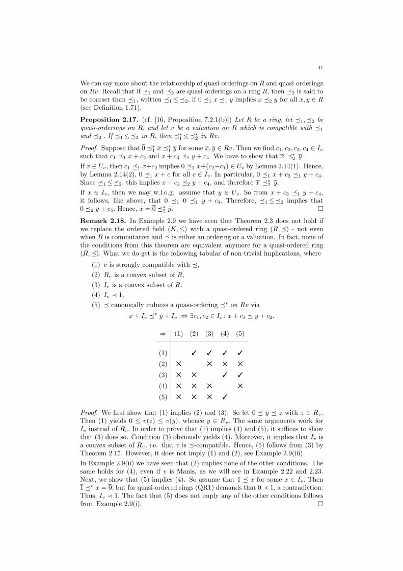
41

We can say more about the relationship of quasi-orderings on R and quasi-orderingson Rv. Recall that if �1 and �2 are quasi-orderings on a ring R, then �2 is said tobe coarser than �1, written �1≤�2, if 0 �1 x �1 y implies x �2 y for all x, y ∈ R(see Definition 1.71).

Proposition 2.17. (cf. [16, Proposition 7.2.1(b)]) Let R be a ring, let �1,�2 bequasi-orderings on R, and let v be a valuation on R which is compatible with �1

and �2 . If �1≤�2 in R, then �∗1≤�∗2 in Rv.

Proof. Suppose that 0 �∗1 x �∗1 y for some x, y ∈ Rv. Then we find c1, c2, c3, c4 ∈ Ivsuch that c1 �1 x+ c2 and x+ c3 �1 y + c4. We have to show that x �∗2 y.

If x ∈ Uv, then c1 �1 x+c2 implies 0 �1 x+(c2−c1) ∈ Uv by Lemma 2.14(1). Hence,by Lemma 2.14(2), 0 �1 x + c for all c ∈ Iv. In particular, 0 �1 x + c3 �1 y + c4.Since �1≤�2, this implies x+ c3 �2 y + c4, and therefore x �∗2 y.

If x ∈ Iv, then we may w.l.o.g. assume that y ∈ Uv. So from x + c3 �1 y + c4,it follows, like above, that 0 �1 0 �1 y + c4. Therefore, �1≤�2 implies that0 �2 y + c4. Hence, x = 0 �∗2 y. �

Remark 2.18. In Example 2.9 we have seen that Theorem 2.3 does not hold ifwe replace the ordered field (K,≤) with a quasi-ordered ring (R,�) - not evenwhen R is commutative and � is either an ordering or a valuation. In fact, none ofthe conditions from this theorem are equivalent anymore for a quasi-ordered ring(R,�). What we do get is the following tabular of non-trivial implications, where

(1) v is strongly compatible with �,(2) Rv is a convex subset of R,

(3) Iv is a convex subset of R,

(4) Iv ≺ 1,

(5) � canonically induces a quasi-ordering �∗ on Rv via

x+ Iv �∗ y + Iv :⇔ ∃c1, c2 ∈ Iv : x+ c1 � y + c2.

⇒ (1) (2) (3) (4) (5)

(1) 3 3 3 3

(2) 5 5 5 5

(3) 5 5 3 3

(4) 5 5 5 5

(5) 5 5 5 3

Proof. We first show that (1) implies (2) and (3). So let 0 � y � z with z ∈ Rv.Then (1) yields 0 ≤ v(z) ≤ v(y), whence y ∈ Rv. The same arguments work forIv instead of Rv. In order to prove that (1) implies (4) and (5), it suffices to showthat (3) does so. Condition (3) obviously yields (4). Moreover, it implies that Iv isa convex subset of Rv, i.e. that v is �-compatible. Hence, (5) follows from (3) byTheorem 2.15. However, it does not imply (1) and (2), see Example 2.9(iii).

In Example 2.9(ii) we have seen that (2) implies none of the other conditions. Thesame holds for (4), even if v is Manis, as we will see in Example 2.22 and 2.23.Next, we show that (5) implies (4). So assume that 1 � x for some x ∈ Iv. Then1 �∗ x = 0, but for quasi-ordered rings (QR1) demands that 0 ≺ 1, a contradiction.Thus, Iv ≺ 1. The fact that (5) does not imply any of the other conditions followsfrom Example 2.9(i). �

42

However, with the additional assumption that v is Manis, we get very close to ananalogue of Theorem 2.3.

Theorem 2.19. Let (R,�) be a quasi-ordered ring and let v be a Manis valuationon R.

(a) The following are equivalent:

(1) v is compatible with �,(2) v is strongly compatible with �,(3) Iv is a convex subset of R,

(4) � canonically induces a quasi-ordering �∗ on Rv via

x+ Iv �∗ y + Iv :⇔ ∃c1, c2 ∈ Iv : x+ c1 � y + c2.

Moreover, any of these conditions implies that Rv is convex subset of R.

(b) If v is non-trivial, then

(5) Rv is a convex subset of R

is equivalent to the conditions (1)− (4).

Proof. We have already seen that (1), (2) and (4) are equivalent (Lemma 2.13(2)and Theorem 2.15). Moreover, clearly (3) implies (1). Next, we show that (2)implies (3). So let 0 � x � y ∈ Iv. Then 0 < v(y) ≤ v(x) by (2), and thereforex ∈ Iv. Hence, the assertions (1) - (4) are equivalent. We conclude part (a) byproving that (2) implies that Rv is a convex subset of R. Again, 0 � x � y ∈ Rvimplies 0 ≤ v(y) ≤ v(x), and therefore x ∈ Rv.In order to prove that (b) is fulfilled, it suffices to show that (5) implies (1). Solet 0 � x � y ∈ Iv and x ∈ Rv. Assume that x ∈ Uv. We choose some z ∈ R�0such that v(z) = −v(y) < 0. Then 0 � xz � yz with v(xz) < 0 and v(yz) = 0,i.e. xz /∈ Rv and yz ∈ Rv. However, (5) yields xz ∈ Rv, a contradiction. Thus,x ∈ Rv\Uv = Iv. �

Remark 2.20.

(1) The assumption in (b) that v is non-trivial is crucial, no matter which kindof a quasi-ordering � is.

In the ordered case consider Z with its unique ordering and the trivialvaluation v mapping the even integers to ∞ and the odd integers to 0.Then Rv = Z is a convex subset of Z, whereas Iv = 2Z is not.

In the valued case consider again Z with the valuation v as before, andlet w be the p-adic valuation on Z for some prime number p > 2. ThenRv = Z is again obviously a convex subset of itself. However, we obtain0 = w(2) ≤ w(1) = 0, but v(1) = 0 < v(2), so (2) is not satisfied.

(2) Instead of v being non-trivial we may as well demand that qv = q� in part(b), i.e. that the supports of v and � coincide. In that case if y ∈ qv, thenalso x ∈ qv ⊆ Iv. Otherwise, if y /∈ qv, we may argue just as in the proof ofTheorem 2.19(b).

While the condition on the supports is consistent with the field case (cf.Theorem 2.3), the assumption that v is non-trivial seems less restraining.

(3) Iv ≺ 1 (see Theorem 2.3) is an easy consequence of the conditions statedin Theorem 2.19. It follows for instance immediately from (3).

Proposition 2.7 and Theorem 2.19 yield a characterisation of all Manis valuationson a ring, which are coarser than a given valuation.

43

Proposition 2.21. Let R be a ring and let v and w be valuations on R such thatv is non-trivial and Manis. Then v is a coarsening of w if and only if one of thefollowing equivalent conditions is satisfied for all x, y ∈ R :

(1) w(x) ≤ w(y)⇒ v(x) ≤ v(y),

(2) w(x) ≤ w(y) ∧ 0 ≤ v(x)⇒ 0 ≤ v(y),

(3) w(x) ≤ w(y) ∧ 0 < v(x)⇒ 0 < v(y),

(4) w/v : Rv → Γw/v ∪{∞}, x+ Iv 7→

{∞ if x ∈ Ivw(x) else

defines a valuation

with support {0}.

Proof. This follows immediately from Proposition 2.7 and Theorem 2.19(2) - (5)in the case where the quasi-ordering � comes from a valuation w on R. Moreover,Proposition 2.16(2) was used for the explicit representation of w/v in (4). �

The following examples show that Iv ≺ 1 is not equivalent to all the other conditionsof Theorem 2.19, regardless of whether � is a valuation (Example 2.22) or anordering (Example 2.23), even if v is a non-trivial Manis valuation.

Example 2.22. Let vp : Q→ Z∪ {∞} denote the p-adic valuation for some primenumber p ∈ N. Apply Proposition 1.16 with γ = 0 to extend vp to a valuationv : Q[X] → Z ∪ {∞}. The valuation v is Manis, since vp is Manis and Γv = Γvp .We do the same procedure with w instead of v, except that this time γ = 1. Thenv = w on Q, and w(f) = v(f) + i for some i ≥ 0 if f ∈ Q[X]\Q. This impliesIv ≺w 1. Indeed, f ∈ Iv means v(f) > 0. But then also w(f) > 0 = w(1), andtherefore f ≺w 1. However, v is not s-compatible with �w . For instance we havev(X2) = v(X), but w(X) < w(X2).

Example 2.23. Let v be the trivial valuation on Z with support {0}, i.e. v(x) = 0for all x 6= 0. Extend v via Proposition 1.16 to a valuation on Z[X,Y ] with γ = 1for X and γ = −1 for Y. So for any 0 6= f =

∑i,j aijX

iY j ∈ Z[X,Y ], we have

v(f) = min{i− j : aij 6= 0}. Then v is a Manis valuation with value group Z, sinceevidently v(Xm) = m or v(Y −m) = m for any m ∈ Z. Order Z[X,Y ] by declaringf ≥ 0 :⇔ f(0) ≥ 0. Then v(f) ≤ 0, if a00 6= 0. Therefore, Iv ⊆ 〈X,Y 〉 = q≤, soIv < 1. However, Iv is not a convex subset of R, since 0 ≤ Y ≤ 0, but Y /∈ Iv.

We conclude this section by imposing a suitable extra condition on v, such thatIv ≺ 1 becomes equivalent to the conditions (1) - (4) of Theorem 2.19.

Definition 2.24. (cf. [24], [35, Ch. I, Definition 5]) Let R be a commutative ring.A valuation v on R is called local, if the pair (Rv, Iv) is local, i.e. if Iv is the uniquemaximal ideal of Rv.

A characterisation of local valuations is given in [35, Ch. I, Proposition 1.3] and [24,Proposition 5], respectively. Valuations on fields are always local Manis valuations.

Proposition 2.25. Let (R,�) be a commutative quasi-ordered ring and v a localManis valuation on R. The following are equivalent:

(1) v is compatible with �,(2) Iv ≺ 1.

Proof. Clearly, (1) implies (2). Now suppose that (2) holds and let 0 � x � y ∈ Ivwith x ∈ Rv. If x /∈ Iv, then x is a unit in Rv. Moreover, 0 � x implies that also0 � x−1. Hence, x � y yields 1 � yx−1 and v(yx−1) = v(y) > 0, i.e. yx−1 ∈ Iv.This is a contradiction to (2). Consequently, x ∈ Iv, so v is �-compatible. �

44

Corollary 2.26. Let v, w be valuations on a commutative ring R such that v isManis and local. Then v is coarser than w if and only if Iv ⊆ Iw.

Proof. This is an immediate consequence of Proposition 2.7 and Proposition 2.25in the case where � = �w . �

By what we have shown so far, we obtain that Theorem 2.3 applies in full generalityto quasi-ordered fields.

Theorem 2.27. (cf. [40, Theorem 2.2]) Let (K,�) be a quasi-ordered field and va valuation on K. Then the following are equivalent:

(1) v is compatible with �,(2) Kv is convex,

(3) Iv is convex,

(4) Iv ≺ 1,

(5) � canonically induces a quasi-ordering �∗ on Kv via

x+ Iv �∗ y + Iv :⇔ ∃c1, c2 ∈ Iv : x+ c1 � y + c2.

Proof. This is an immediate consequence of Theorem 2.19, Remark 2.20(2), andProposition 2.25, since any field valuation is Manis and local. �

2.2. The Rank of a Quasi-Ordered Ring.

In this section we give a uniform definition of the rank of a quasi-ordered ring. Tothis end, we first define the natural valuation v� of a quasi-ordering � to be thefinest valuation of support q� that is strongly �-compatible (Definition 2.32). Therank of (R,�) is then defined as the order type of the set of all strict coarseningsof v� (Definition 2.34). We show that this definition is consistent with the rank ofa quasi-ordered field as developed in [40] (Corollary 2.36).

Simply said, the rank serves as a measure for the size of a given structure. The rankof a valued field (K, v) is the order type of all non-trivial valuation rings Kw suchthat w is coarser than v, i.e. the order type of all non-trivial coarsenings of v. Therank of an ordered field (K,≤) is the order type of all non-trivial valuation ringsKw such that w is ≤-compatible, or equivalently the order type of all non-trivialconvex subrings of K with respect to ≤ . In other words, the rank of (K,≤) is therank of (K, v), where v denotes the natural valuation induced by ≤ .In [40], S. Kuhlmann, Matusinki and Point established Theorem 2.27 by exploitingFakhruddin’s dichotomy, and derived a definition of the rank of a quasi-orderedfield as follows:

Proposition 2.28. Let (K,�) be a quasi-ordered field. Then the �-compatiblevaluations on K are linearly ordered by the coarsening relation ≤ .

Proof. If v and w are �-compatible, then Theorem 2.27(2) yields Kv ⊆ Kw or viceversa, whence v ≤ w or w ≤ v. �

Hence, to any quasi-ordering � on K there is a finest valuation v� on K that is�-compatible. If �= v is a valuation, then v = v�. If �=≤ is an ordering, thenv� is the natural valuation of ≤ . Either way, the rank of (K, v�) coincides withthe rank of (K, v), respectively (K,≤).

In the following we first prove an analogue of Proposition 2.28 for quasi-orderedrings. Afterward, we generalise the rank to this class.

45

Notation 2.29. For a ring R we denote by V(R) the set of all valuations on R. If qis a two-sided completely prime ideal of R, we define Vq(R) := {v ∈ V(R) : qv = q}.

Lemma 2.30. Let (R,�) be a quasi-ordered ring and v the trivial valuation withsupport q�. Then v is strongly �-compatible.

Proof. Let 0 � x � y. If y ∈ q�, then so is x, whence v(x) = v(y) =∞. Otherwise,v(y) = 0 ≤ v(x). �

Proposition 2.31. Let (R,�) be a quasi-ordered ring. Then the set

{v ∈ Vq�(R) : v is strongly � -compatible}is linearly ordered by the coarsening relation ≤ .

Proof. (cf. [56, Lemma 4.2]) Otherwise, we find strongly �-compatible valuationsv1, v2 ∈ Vq�(R) and ai, bi ∈ R such that v1(a1) ≤ v1(a2), but v2(a2) < v2(a1),and v2(b1) ≤ v2(b2), but v1(b2) < v1(b1). Consequently, v1(a1b2) < v1(a2b1) andv2(a2b1) < v2(a1b2). By Lemma 1.29 and the fact that vi(x) = vi(−x) for all x ∈ R,we may w.l.o.g. assume that 0 � ai, bi, and therefore 0 � a1b2 and 0 � a2b1.But then the contraposition of vi being strongly �-compatible implies that both,a2b1 ≺ a1b2 and a1b2 ≺ a2b1, a contradiction. Hence, this set is linearly ordered. �

So if (R,�) is a quasi-ordered ring, then Lemma 2.30 and Proposition 2.31 yield afinest valuation v ∈ Vq�(R) that is strongly �-compatible, namely the intersectionof all strongly �-compatible valuations.

Definition 2.32. Let (R,�) be a quasi-ordered ring. We call the finest strongly�-compatible valuation v ∈ Vq�(R) the natural valuation of �, and we denote itby v�.

Remark 2.33. Let (R,�) be a quasi-ordered ring.

(1) If � is induced by a valuation v, then v� = v.

(2) If � is an ordering, then v� is the natural valuation in the usual sense (seeExample 2.8).

Proposition 2.31 particularly implies that for a valued ring (R, v) the coarseningsof v of support qv are linearly ordered. Therefore, we may define the rank of aquasi-ordered ring in terms of valuations as follows:

Definition 2.34. The rank of a quasi-ordered ring (R,�), written rk(R,�), is theorder type of the linearly ordered set {v ∈ Vq�(R) : v� < v}, i.e. the order type ofthe set of all strict coarsenings of v�.

Next, we show that the rank of a commutative quasi-ordered ring is equal to therank of its associated quasi-ordered field.

Given a valuation v on a commutative ring R, we denote by v′ the valuation on R/qvdefined by v′(x) := v(x), and by ν the unique extension of v′ to K := Quot(R/qv).

Lemma 2.35. Let (R,�) be a commutative quasi-ordered ring and v a valuationon R with support q�. The following are equivalent:

(1) v is strongly compatible with �,(2) v′ is strongly compatible with �′,(3) ν is (strongly) compatible with E .

Proof. The equivalence of (1) and (2) easily follows from the definition of �′ andv′, respectively. We conclude by showing that (2) and (3) are equivalent. It isclear that strong compatibility in K implies strong compatibility in R/q�, as it isa universal statement. Conversely, let 0 E x

y Eab . Then 0 �′ xyb2 �′ aby2. By

46

strong �′-compatibility of v′, we obtain that v′(aby2) ≤ v′(xyb2), and thereforev′(ay) ≤ v′(xb). Thus, ν(ab ) ≤ ν(xy ). �

Corollary 2.36. The rank of a commutative quasi-ordered ring (R,�) coincideswith the rank of its associated quasi-ordered field (K,E).

Proof. By Lemma 2.35 we know that v = v� if and only if ν = νE, where E and νdenote the unique extensions of � and v to Quot(R/q�). Moreover, by Lemma 2.35and Remark 1.13, v� and νE have the same number of strict coarsenings. Hence,(R,�) and (K,E) have the same rank. �

Corollary 2.37. Let (R, v) be a commutative valued ring. Then the rank of (R, v)coincides with the rank of the value group Γv.

Proof. This is because the ranks of (R, v) and (K, ν) coincide (Corollary 2.36), thelatter being equal to the rank of Γν = Γv. �

Obviously, a valued ring (R, v) has rank 0 if and only if v is a trivial valuation. Weconclude this section by considering ordered rings of rank 0.

If (R,≤) is an ordered ring, we call an element 0 < r ∈ R infinitely large if r > nfor all n ∈ N, and infinitely small if nr < 1 for all n ∈ N.

Lemma 2.38. ([43, Lemma 17.20]) Let (R,≤) be an ordered ring. The followingare equivalent:

(1) For any a, b > 0 in R, there exists an integer n ≥ 1 such that na > b.

(2) R admits neither infinitely large nor infinitely small elements.

Proof. We first show that (1) implies (2). So let 0 < r ∈ R be arbitrary. Thenr < n · 1 = n for some n ∈ N, whence r is not infinitely large. Likewise, mr > 1 forsome m ∈ N, so r is not infinitely small either.

Now suppose that (2) holds and let 0 < a, b. Then we find some m,n ∈ N suchthat na > 1 and m > b, since a is not infinitely small and b is not infinitely large.Therefore, mna > m > b. �

Definition 2.39. [43, p. 282] An ordered ring (R,≤) is called Archimedean, if itsatisfies one of the equivalent conditions from Lemma 2.38.

Example 2.40. Let (R,≤) be an ordered ring. Then (Rv≤,≤∗) is an Archimedeanordered domain, because Rv≤ contains no infinitely large elements and Iv≤ consistsprecisely of all infinitely small elements (see Example 2.8).

Corollary 2.41. (to Lemma 2.38) An ordered ring (R,≤) has rank 0 if and onlyif it is Archimedean.

Proof. (R,≤) has rank 0 if and only if the natural valuation v≤ is trivial (Lemma2.30). The latter is equivalent to the fact that the Archimedean equivalence relation∼+ (Example 2.8) on R\q� is trivial, which is precisely the statement of Lemma2.38(1). �

For a further discussion on the rank of quasi-ordered fields we refer the interestedreader to [40].

47

3. Baer-Krull Theorems for Quasi-Ordered Fields and Rings

In Chapter 2 we fixed a quasi-ordered ring (R,�) and characterised the valuationson R, which are (strongly) �-compatible. In the present chapter we turn thesituation around - given a valued ring (R, v), we characterise the quasi-orderings� on R such that v is strongly �-compatible. For that purpose we establish aBaer-Krull theorem for commutative quasi-ordered rings. This theorem describesthe said quasi-orderings on R in terms of the quasi-orderings on the residue classdomain Rv.

For the sake of convenience, we first prove the Baer-Krull theorem for quasi-orderedfields (Section 3.1). Afterward, in Section 3.2, we generalise it to commutativequasi-ordered rings and give a few applications. We conclude this chapter by de-ducing and discussing Baer-Krull theorems for commutative ordered rings in Section3.3, respectively for commutative valued rings in Section 3.4.

Quite a few of the results presented here, including a Baer-Krull theroem for quasi-ordered rings, were already published by S. Kuhlmann and the author of this thesisin [41].

Preliminaries on the Baer-Krull theorem for ordered fields.

In the present chapter, we use the following notation (the notation introduced in(4) will also play an important role in the following chapters):

Notation 3.1. Let (R, v) be a commutative valued ring and q a prime ideal of R.

(1) As before, Γv denotes the value group (see Remark 1.6(1)), qv the support,Rv the valuation ring, Iv the valuation ideal, and Rv = Rv/Iv the residueclass domain of v (see Notation 2.1).

(2) A quadratic system of representatives of R w.r.t. v (cf. [18, p. 37]) is a

family {πi : i ∈ I} ⊆ R\qv such that the elements v(πi) form an F2-basis ofΓv := Γv/2Γv. Such a system exists for any commutative valued ring (R, v),since for any γ ∈ Γv we have γ ∈ v(R) or −γ ∈ v(R). We set γi := v(πi).

(3) Given a quasi-ordering � on R such that v is strongly �-compatible, wedenote by �∗ the induced quasi-ordering on Rv (see Theorem 2.19(4)). Byη� we denote the map I → {−1, 1} defined by η�(i) = 1 if and only if0 � πi.

(4) We denote by Q(R) the set of all quasi-orderings, by O(R) the set of allorderings, and by V(R) the set of all valuations on R. We add q as subscriptto restrict to quasi-orderings (resp. orderings, or valuations) with supportq, and we add v as exponent to restrict to quasi-orderings (resp. orderings,or valuations) which are strongly compatible with v.

So for example Qvq(R) denotes the set of all quasi-orderings � on R withsupport q such that v is strongly �-compatible.

Our goal is to generalise the following theorem, the so-called Baer-Krull theorem,to the class of quasi-ordered rings. Based upon the works of Baer ([6]) and Krull([37]), we follow its exposition given by Engler and Prestel in [18, Theorem 2.2.5].

Theorem 3.2. Let (K, v) be a valued field and {πi : i ∈ I} a quadratic system ofrepresentatives of K w.r.t. v. Then the map

ψ : Ov(K)→ {−1, 1}I ×O(Kv), ≤ 7→ (η≤,≤∗)is a bijective correspondence.

48

3.1. A Baer-Krull Theorem for Quasi-Ordered Fields.

The sole aim of this section is to prove a Baer-Krull theorem for quasi-orderedfields (Theorem 3.7 and Corollary 3.8). Even though we are ultimately interestedin quasi-ordered rings, it is more convenient to first establish the said theorem forquasi-ordered fields, and then deduce it for rings by exploiting the fact that strongcompatibility of quasi-orderings and valuations is preserved when moving on to thequotient field (see Lemma 2.35). In fact, when we gave a direct proof for quasi-ordered rings in [41], we required that the valuation v is Manis - in Section 3.2,however, we will be able to replace the Manis property with a weaker condition onthe valuation v.

Further note that we cannot expect the map ψ from Theorem 3.2 to be a bijection,if we replace Ov(K) with Qv(K), and O(Kv) with Q(Kv). Recall that if a quasi-ordering � is induced by a valuation, then 0 � x for any x (Lemma 1.45). Hence,in that case η� is the constant map η = 1. For that reason what we may and whatwe will get for quasi-ordered fields is that the map

ψ : Qv(K)→ {−1, 1}I ×O(Kv) t {1}I × V(Kv), � 7→ (η�,�∗)is a bijection. Thus, there is some non-uniformity, which, however, will only play aminor role in the following exposition.

Let us now establish a Baer-Krull theorem for quasi-ordered fields. For that purposewe fix a valued field (K, v), a quadratic system {πi : i ∈ I} of representatives of Kw.r.t. v (see Notation 3.1), and a tuple

(η×,�×) ∈ {−1, 1}I ×O(Kv) t {1}I × V(Kv).

The main part of the proof of the Baer-Krull theorem is to construct a quasi-ordering on K that is mapped to (η×,�×) under the analogue of the map ψ fromTheorem 3.2. To this end, adapting the proof given in [18], we define a binaryrelation � on K as a function of �× and η× as follows: for x, y ∈ K such thatx ∈ K× or y ∈ K×, we consider

γ := γx,y := max{−v(x),−v(y)} ∈ Γv.

Then there is a unique representation γ =∑i∈Ix,y

γi of γ in Γv/2Γv. Hence,

γ =∑i∈Ix,y

γi + 2v(ax,y) = v

∏i∈Ix,y

πia2x,y

for some unique subset Ix,y ⊆ I, and some ax,y ∈ K×, which is unique up toits value, i.e. instead of ax,y we may have chosen any other element bx,y ∈ Kwith v(bx,y) = v(ax,y). In what follows, we will just write

∑i,∏i and a instead of∑

i∈Ix,y,∏i∈Ix,y

and ax,y, respectively, whenever x and y are clear from the context.

Lemma 3.3. Let (K, v) be a valued field and x, y ∈ K. With the above notation,x∏i πia

2, y∏i πia

2 ∈ Kv. Moreover, x∏i πia

2 ∈ Iv if and only if v(x) > v(y).

Proof. We have

v

(x∏i

πia2

)= v(x) +

∑i

v(πi) + 2v(a) = v(x) + γ

= v(x) + max{−v(x),−v(y)} ≥ 0,

and analogously for y∏i πia

2, so both are in Kv. Moreover,

x∏i

πia2 ∈ Iv ⇔ v(x) + max{−v(x),−v(y)} > 0⇔ v(x) > v(y).

�

49

In particular, we can always take residues of both, x∏i πia

2 and y∏i πia

2. Themoreover statement of Lemma 3.3 will be of great importance in the proof of thefollowing result:

Main Lemma 3.4. Let (K, v) be a valued field. Using the above notation, wedefine for x, y ∈ K with x ∈ K× or y ∈ K×, that

x � y :⇔

either x∏i πia

2 �× y∏i πia

2 and∏i η×(i) = 1,

or y∏i πia

2 �× x∏i πia

2 and∏i η×(i) = −1.

Moreover, we declare 0 � 0. Then � defines a quasi-ordering on K such that v is�-compatible.

Proof. For the sake of convenience and uniformity, we treat �× and η× as anarbitrary quasi-ordering on Kv, respectively an arbitrary map from I to {−1, 1},for as long as possible. The distinction whether �× is an ordering or a valuation(in which case η× is trivial) is only necessary when verifying axiom (Q3).

First of all we show that � is well-defined. Recall that a ∈ K× is only unique upto its value. So let b ∈ K× such that v(a) = v(b), and suppose that

x∏i

πia2 �× y∏i

πia2.

Define z = ba−1. Then v(z) = 0, so Lemma 1.36 implies 0 ≺× z2. Applying (Q2)yields

x∏i

πib2 �× y∏i

πib2.

Obviously, � is reflexive and total. Next we prove transitivity. So let x � y andy � z, w.l.o.g. x ∈ K× or z ∈ K×. The proof is done by distinguishing four cases.First suppose that v(p) = v(q) ≤ v(r) with p, q, r ∈ {x, y, z} pairwise distinct. Thenγx,y = γx,z = γy,z ∈ Γv all coincide, so Ix,y = Ix,z = Iy,z and ax,y = ax,z = ay,z.Hence, transitivity of � follows immediately from transitivity of �× . It remains toverify the cases where there is a unique smallest element among v(x), v(y) and v(z).First suppose that v(x) < v(y), v(z). Then γx,y = −v(x) = γx,z, i.e. Ix,y = Ix,z andax,y = ax,z. We only consider the subcase

∏i∈Ix,y

η×(i) = −1, since the opposite

one is dealt with analogously. From x � y and v(x) < v(y) it follows

y∏i∈Ix,y

πia2x,y = 0 �× x∏i∈Ix,y

πia2x,y

(Lemma 3.3). Now v(x) < v(z) and again Lemma 3.3 imply

z∏i∈Ix,y

πia2x,y = 0 �× x∏i∈Ix,y

πia2x,y.

Thus, x � z. Next, suppose that v(y) < v(x), v(z). Then γx,y = −v(y) = γy,z, i.e.Ix,y = Iy,z and ax,y = ay,z. Again, we only deal with the case

∏i∈Ix,y

η×(i) = −1.

From v(y) < v(x) and x � y it follows

y∏i∈Ix,y

πia2x,y �× x∏i∈Ix,y

πia2x,y = 0.

Likewise, v(y) < v(z) and y � z implies

z∏i∈Ix,y

πia2x,y = 0 �× y∏i∈Ix,y

πia2x,y.

50

Therefore,

y∏i∈Ix,y

πia2x,y = 0.

On the other hand, v(y) < v(x) yields via Lemma 3.3 that y∏i∈Ix,y

πia2x,y /∈ Iv, a

contradiction. The case v(z) < v(x), v(y) is proven exactly like the case where v(x)is the unique smallest value.

It remains to verify the axioms (Q1) - (Q3) and compatibility of � and v. For theproof of (Q1) assume that there is some x ∈ K× such that x ∼ 0. Then

0 �× x∏i

πia2 �× 0,

whence x∏i πia

2 ∈ Iv. However, from v(x) < v(0) and Lemma 3.3, it follows thatx∏i πia

2 /∈ Iv, a contradiction. Hence, (Q1) is fulfilled.

Next, we verify (Q2), i.e. we show that x � y and 0 � z implies xz � yz. We mayw.l.o.g. assume that z ∈ K×, and that x ∈ K× or y ∈ K×. Therefore,

γxz,yz = max{−v(xz),−v(yz)} = max{−v(z),−v(0)}+ max{−v(x),−v(y)}= γ0,z + γx,y ∈ Γv.

Hence, Ixz,yz is the (w.l.o.g.) disjoint union of Ix,y and I0,z, which implies∏i∈Ixz,yz

η×(i) =∏i∈Ix,y

η×(i) ·∏i∈I0,z

η×(i).

Moreover, axz,yz = ax,ya0,z.

First consider the case∏i∈I0,z η

×(i) = 1. This implies 0 �× z∏i∈I0,z πia

20,z.

If∏i∈Ix,y

η×(i) = −1 =∏i∈Ixz,yz

η×(i), then

y∏i∈Ix,y

πia2x,y �× x∏i∈Ix,y

πia2x,y.

Applying (Q2) yields

yz∏

i∈Ixz,yz

πia2x,ya20,z �× xz

∏i∈Ixz,yz

πia2x,ya20,z,

whence xz � yz. The subcase∏i∈Ix,y

η×(i) = 1 =∏i∈Ixz,yz

η×(i) is proven analo-

gously. The proof of the case∏i∈I0,z η

×(i) = −1 is also almost the same, we just

apply Lemma 1.52 instead of axiom (Q2).

The proof of axiom (Q3) is divided into five cases. First suppose that v(x) < v(z)

or v(y) < v(z). Then γx,y = γx+z,y+z. Moreover, z∏i∈Ix,y

πia2x,y = 0 by Lemma

3.3. Thus, clearly x � y implies x + z � y + z. Further note that if �× is anordering and x ≺ y, then we obtain x+ z ≺ y+ z, because orderings preserve strictinequalities under addition. We will exploit this fact below.

If v(z) < v(x) and v(z) < v(y), then γx,z = γy,z = γx+z,y+z. Lemma 3.3 implies

x∏i∈Ix,z

πia2x,z = 0 = y∏i∈Iy,z

πia2y,z.

From this, it is easy to see that x+z � y+z. Now suppose that v(x) = v(z) < v(y).Then γx,y = γy,z = γx+z,y+z. We distinguish two subcases. If

∏i∈Ix,y

η×(i) = 1,

then x � y yields

x∏i∈Ix,y

πia2x,y �× y∏i∈Ix,y

πia2x,y.

51

As z � y, one may add z∏i∈Ix,y

πia2x,y on either side. If∏i∈Ix,y

η×(i) = −1, then

η× 6= 1, whence �× is an ordering. Thus, one may add z∏i∈Ix,y

πia2x,y on either

side as well. This proves the present case. The case v(y) = v(z) < v(x) is provenanalogously. Finally, suppose that

v(x) = v(y) = v(z) ∈ Γv.

Thenγx+z,y+z = max{−v(x+ z),−v(y + z)} ≤ −v(z).

First suppose that equality holds. Then max{−v(x + z),−v(y + z)} = −v(z), i.e.all γ′s coincide. If

∏i η×(i) = 1, the claim follows immediately by applying axiom

(Q3). If∏i η×(i) = −1, then �× must be an ordering and we may add z

∏i πia

2

to either side anyway.

Last but not least assume that < holds, i.e. max{−v(x+ z),−v(y + z)} < −v(z).

Then v(z) < v(x+z), v(y+z). By Lemma 3.3, p∏i∈Ix,y

πia2x,y 6= 0 for p ∈ {x, y, z},whereas

(x+ z)∏i∈Ix,y

πia2x,y = 0 = (y + z)∏i∈Ix,y

πia2x,y.

Therefore,

x∏i∈Ix,y

πia2x,y = y∏i∈Ix,y

πia2x,y = −z∏i∈Ix,y

πia2x,y.

In particular, we may assume that �× is an ordering, since for a valuation

y∏i∈Ix,y

πia2x,y ∼ −y∏i∈Ix,y

πia2x,y = z∏i∈Ix,y

πia2x,y,

a contradiction to the assumption y � z. We claim that x + z ∼ 0 ∼ y + z, whichclearly implies x+ z � y+ z. Assume for the sake of a contradiction that x+ z � 0.If x + z ≺ 0, it follows from the case “v(x) < v(z)” above (where x + z plays therole of x, 0 the one of y and −z the one of z; recall that v(x + z) < v(z)) andthe fact that �× is an ordering, that x ≺ −z. However, this contradicts the factthat x ∼ −z. Likewise, if 0 ≺ x + z, it follows from the case “v(y) < v(z)” that−z ≺ x, again a contradiction. Therefore x + z ∼ 0. The same reasoning showsthat y + z ∼ 0 as well. Hence, (Q3) is satisfied.

Finally, we show that v is �-compatible. By Theorem 2.27(4) it suffices to showthat Iv ≺ 1. So let x ∈ Iv. Then

γx,1 = max{−v(x),−v(1)} = 0.

Therefore, Ix,1 = ∅,∏i∈Ix,1

η×(i) = 1, and we may choose ax,1 = 1. Consequently,

we obtain x ≺ 1⇔ 0 = x ≺× 1. Since �× is a quasi-ordering, the RHS is fulfilled,whence x ≺ 1. So v is �-compatible. �

Remark 3.5.

(1) Let � denote the quasi-ordering from the Main Lemma 3.4. If x ∈ Uv andy ∈ Rv, or vice versa, then

x � y ⇔ x �× y.This is because, as we just witnessed at the very end of the previous proof,in this case γx,y = 0, whence Ix,y = ∅ and v(ax,y) = 0. The former factyields

∏i∈Ix,y

η×(i) = 1. Moreover, we may choose ax,y = 1, since ax,y is

only unique up to its value.

(2) The main lemma can be proven for commutative quasi-ordered rings, if thevaluation v is Manis (cf. [41, Main Lemma 4.5]).

52

For the proof of the Baer-Krull theorem we require one more lemma. It will beused to compare the size of two quasi-orderings on K. For the sake of generality,we prove it for arbitrary quasi-ordered rings.

Recall from Notation 1.21 that

E(x) = E�(x) = {y ∈ S : x ∼ y},

where (S,�) is a quasi-ordered set.

Lemma 3.6. Let (R,�) be a quasi-ordered ring. Then E(0) + {x} ⊆ E(x) for anyx ∈ R. Moreover, if E(0) + {x} ( E(x), then E(x) = −E(x).

Proof. The first statement is an easy consequence of Lemma 1.28. For the moreoverpart, let z ∈ E(x) be arbitrary and y ∈ E(x)\(E(0) + {x}). We will show that−y ∈ E(x). From z ∼ x ∼ y and Corollary 1.60 it then follows −z ∼ −y ∼ x. Thisimplies −z ∈ E(x), and therefore E(x) = −E(x).

So assume for the sake of a contradiction that −y /∈ E(x). Recall that y ∈ E(x).So we have y ∼ x 6∼ −y. By (QR4), we obtain x− y ∈ E(0), i.e. y ∈ E(0) + {x}, acontradiction. Hence, −y ∈ E(x), as desired. �

We can finally prove a Baer-Krull theorem for quasi-ordered fields. Its formulationrelies on Notation 3.1.

Theorem 3.7. (Baer-Krull theorem for quasi-ordered fields I )Let (K, v) be a valued field and {πi : i ∈ I} a quadratic system of representatives ofK w.r.t. v. Then

ψ : Qv(K)→ {−1, 1}I ×Q(Kv), � 7→ (η�,�∗)

is a well-defined map such that the restriction ψ � ψ−1(A) : ψ−1(A) → A is abijection, where A := {−1, 1}I ×O(Kv) t {1}I × V(Kv).

Proof. By Theorem 2.27(5) the map ψ is well-defined. Now let (η×,�×) ∈ A bearbitrary. We first prove that ψ maps the quasi-ordering � constructed in theMain Lemma to the tuple (η×,�×). First we verify that η� = η×. Note thatγπi,0 = −v(πi) = −γi, whence γπi,0 = v(πia

2) for some a ∈ K× according to theconstruction in the beginning of this chapter. Thus, 0 � πi if and only if either0 �× (πia)2 and η×(i) = 1, or (πia)2 �× 0 and η×(i) = −1. However, the secondcase cannot occur, since non-zero squares are always strictly positive (Lemma 1.36).Altogether, we obtain

η�(i) = 1⇔ 0 � πi ⇔ η×(i) = 1,

and therefore η� = η×.

Next, we prove that �∗=�× . So let x, y ∈ Kv, w.l.o.g. not x and y in Iv. Thenalso x + c and y + d are not both in Iv for all c, d ∈ Iv, so Remark 3.5(1) tells usthat x+ c � y + d⇔ x+ c �× y + d. Thus,

x �∗ y ⇔ ∃c1, c2 ∈ Iv : x+ c1 � y + c2

⇔ ∃c1, c2 ∈ Iv : x+ c1 �× y + c2

⇔ x �× y.

This shows that the map ψ � ψ−1(A) : ψ−1(A)→ A is surjective.

We conclude by showing that this map is also injective. So let �1 ∈ ψ−1(A) bearbitrary, and denote by �2 the quasi-ordering on K defined by η�1

and �∗1 viaour Main Lemma. We prove that �1 =�2 . First we show the inclusion �1⊆�2 .So let x and y in K, w.l.o.g. not both equal to 0, and let I, πi and a be as in the

53

definition of the quasi-ordering �2 with respect to x and y. If∏i η�1

(i) = −1, then∏i πia

2 ≺1 0, so we obtain by Lemma 1.51 and Lemma 1.52 that

x �1 y ⇔ y∏i

πia2 �1 x

∏i

πia2

⇒ y∏i

πia2 �∗1 x∏i

πia2

⇔ x �2 y.

Likewise, if∏i η�1(i) = 1, we may apply (Q2) instead of the Lemmas and get the

same result. Thus, �1⊆�2 . For the rest of the proof we distinguish the cases−1 ��2

1 and −1 ∼�21.

If −1 ��21, then also −x ��2

x for any x ∈ K×, since ∼�2is preserved under

multiplication ([19]; or Corollary 1.60). Thus, E�2(x) 6= −E�2

(x) for all x ∈ K×.From Lemma 3.6, it follows E�2

(x) = {x} for all x ∈ K. Therefore, no quasi-ordering can be properly contained in�2, whence�1⊆�2 already implies�1 =�2 .So suppose for the rest of this proof that −1 ∼�2 1. We distinguish the subcasesv(x) 6= v(y) and v(x) = v(y).

If v(x) 6= v(y), then Lemma 3.3 states that x∏i πia

2 ∈ Uv and y∏i πia

2 ∈ Iv, orvice versa. We show �1 = �2 by proving that the only implication⇒ above is alsoan equivalence. First suppose that x

∏i πia

2 ∈ Uv and y∏i πia

2 ∈ Iv, and assumefor the sake of a contradiction that

0 = y∏i

πia2 �∗1 x∏i

πia2, but x∏i

πia2 ≺1 y

∏i

πia2.

By definition of �∗1, along with Lemma 2.14(1), we find some c ∈ Iv such thatc �1 x

∏i πia

2 ≺1 y∏i πia

2. This is a contradiction to Lemma 2.14(2) and (3),since either u ≺1 Iv or Iv ≺1 u for any u ∈ Uv. Likewise, if x

∏i πia

2 ∈ Iv andy∏i πia

2 ∈ Uv, and if the only implication ⇒ above is not an equivalence, then

y∏i

πia2 + c1 �1 x

∏i

πia2 + c2 ≺1 y

∏i

πia2

for some c1, c2 ∈ Iv. Taking residues yields y∏i πia

2 = 0, a contradiction.

So finally suppose that v(x) = v(y), and assume for the sake of a contradiction thatx ∼�2 y, but x ≺1 y. Choose some a ∈ K× such that 0 ≺1 a (and hence 0 ≺2 a)and v(a) = −v(x). By axiom (Q2), ax ≺1 ay if and only if x ≺1 y, and by Corollary1.60 ax ∼�2

ay if and only if x ∼�2y. So we may replace x and y with ax and

ay. In other words, we may w.l.o.g. assume that v(x) = v(y) = 0. So from y �2 xand Remark 3.5(1) it follows y �∗1 x. Thus, there exist some c1, c2 ∈ Iv such thaty + c1 �1 x + c2, respectively, y �1 x + c for c := c2 − c1 (Lemma 2.14(1)). Since−1 ∼�2 1, also −1 ∼�1 1. Otherwise −1 �1 0, but −1 �2 0, contradicting thefact that �1⊆�2 . Therefore, Lemma 1.45 tells us that 0 ≺1 x for all x ∈ K×. Inparticular, c ≺1 y, since 0 �1 y �1 c would imply y ∈ Iv by Theorem 2.27. So [19,Lemma 4.1], respectively Lemma 1.48, implies the contradiction

y �1 x+ c �1 max{x, c} ≺1 y.

Hence, �1 =�2 . This finishes the proof of the Baer-Krull theorem. �

For the sake of uniformity, we so far did not make use of the dichotomy that everyquasi-ordered field is either an ordered or a valued field (see Theorem 1.23). Takingthis result into consideration, the Baer-Krull theorem simplifies as follows:

54

Corollary 3.8. (Baer-Krull theorem for quasi-ordered fields II )Let (K, v) be a valued field and {πi : i ∈ I} a quadratic system of representatives ofK w.r.t. v. Then the map

ψ : Qv(K)→ A, � 7→ (η�,�∗)

is a bijection, where A := {−1, 1}I ×O(Kv) t {1}I × V(Kv).

Proof. Theorem 1.23 (resp. [19, Theorem 2.1]) and Proposition 2.16 imply thatψ−1(A) coincides with the domain of ψ, whence the statement follows immediatelyfrom Theorem 3.7. �

3.2. A Baer-Krull Theorem for Quasi-Ordered Rings.

In this main section of Chapter 3 we establish two Baer-Krull theorems for com-mutative quasi-ordered rings (R, v). The first one (Theorem 3.9) is weaker in both,the assumption and the conclusion. It imposes no condition on the valuation v, butcharacterises the set Qvqv

(R) in terms of the quasi-orderings on Kν instead of Rv,where K denotes the quotient field of R/qv and ν the unique extension of v fromR to K. The second one (Theorem 3.13) applies only to what we call C-valuations(see Definition 3.11), but characterises Qvqv

(R) in terms of the quasi-orderings onRv.

As an application of the Baer-Krull theorem we obtain that if (R, v) ⊆ (S,w) is animmediate extensions of commutative valued rings, then any �∈ Qvqv

(R) uniquelyextends to a quasi-ordering in Qwqw

(S) (Proposition 3.22). We conclude this sectionby transferring a result from Efrat, stating that the same conclusion holds if thering extension is integral instead of immediate (Proposition 3.25). As throughoutthe entire chapter we refer to Notation 3.1.

Theorem 3.9. (Baer-Krull theorem for commutative quasi-ordered rings I)Let (R, v) be a commutative valued ring, {πi : i ∈ I} a quadratic system of repre-sentatives of R w.r.t. v, and ν the unique extension of v to K := Quot(R/qv).Then the map

ψ : Qvqv(R)→ A, � 7→ (ηE,E

∗)

is a bijection, where A := {−1, 1}I ×O(Kν) t {1}I × V(Kν).

Proof. We have Γv = Γν , so {πi : i ∈ I} is also a quadratic system of represenativesof K w.r.t. ν. Applying Corollary 3.8 to (K, ν) yields the bijective correspondence

ϕ : Qv(K)→ A, E 7→ (ηE,E∗).

From Corollary 1.38 and the uniqueness stated in Proposition 1.37, it follows that� 7→ E defines a bijection between the set Qqv (R) of all quasi-orderings on R withsupport qv, and the set Q(K) of all quasi-orderings on K. Moreover, Lemma 2.35implies that � is strongly v-compatible if and only if E is strongly ν-compatible.Hence, we know that

λ : Qvqv(R)→ Qν(K), � 7→ E .

is a bijection. Therefore, ψ = ϕ ◦ λ is also a bijection. �

In a further step we want to replace the residue class field Kν in the co-domain ofthe map ψ from Theorem 3.9 with the residue class domain Rv induced by v. Notethat if (R, v) is a commutative valued ring, we can first consider the quotient fieldK := Quot(R/qv), and then take the residue class domain Kν, where ν denotesthe unique extension of v from R to K. However, we can also first take the residueclass domain Rv, and then consider its quotient field L := Quot(Rv).

55

Lemma 3.10. Let (R, v) be a commutative valued ring, and let ν denote the uniqueextension of v to K = Quot(R/qv). Then L := Quot(Rv) is a subfield of Kν.

Proof. We consider the canonical map

ϕ : Rv → Kν, x 7→ x+ qv1 + qv

+ Iν .

Note that

x ∈ ker(ϕ)⇔ x+ qv1 + qv

∈ Iν ⇔ x+ qv ∈ Iv′ ⇔ x ∈ Iv,

where v′ denotes the valuation on R/qv defined by v′(x) = v(x) (see Lemma 1.35).Therefore, the homomorphism theorem tells us that the field Kν contains the do-main Rv = Rv/Iv. Hence, it also contains its quotient field L. �

Definition 3.11. ([72, p. 975]) Let (R, v) be a commutative valued ring, andlet ν denote the unique extension of v to K := Quot(R/qv). We say that v is acommuting valuation (abbr. C-valuation) if Quot(Rv) = Kν.

Remark 3.12. In [72], Valente calls these valuations special. We renamed themhere, because they do not coincide with special valuations as introduced in [35] byKnebusch and D. Zhang. Commuting refers to the fact that taking the quotientfield and taking the residue class domain commutes for such valuations.

Theorem 3.13. (Baer-Krull theorem for commutative quasi-ordered rings II)Let R be a commutative ring, v a C-valuation on R, and {πi : i ∈ I} a quadraticsystem of representatives of R w.r.t. v. Then the map

Qvqv(R)→ A, � 7→ (η�,�∗)

is a bijection, where A := {−1, 1}I ×O0(Rv) t {1}I × V0(Rv).

Proof. Let K := Quot(R/qv), and denote by ν the unique extension of v to K.Since v is a C-valuation, restriction E∗ 7→�∗ is a bijective correspondence betweenthe quasi-orderings on Kν = Quot(Rv) and the quasi-orderings on Rv with support{0} (see Proposition 1.37). Moreover, ηE = η�, since πi ∈ R for all i ∈ I. Therefore,the claim follows immediately from Theorem 3.9. �

S. Kuhlmann and the author of this thesis already proved the previous theorem in[41, Corollary 4.11], except that they demanded v to be a Manis valuation insteadof a C-valuation. The next result implies that Theorem 3.13 is a generalisation oftheir result.

Proposition 3.14. ([72, Proposition 2.2]) Let R be a commutative ring. AnyManis valuation on R is a C-valuation. The converse may be false.

Proof. We first show that any Manis valuation is a C-valuation. So let v be aManis valuation on R. By Lemma 3.10, it suffices to show that Kν is a subfieldof Quot(Rv), where K := Quot(R/qv) and ν the unique extension of v to K. Weargue again via the homomorphism theorem. This time, we consider the map

ϕ : Kν → Quot(Rv),x+ qvy + qv

7→ x+ Ivy + Iv

.

Since qv ⊆ Iv, the choice of representatives in the domain does not matter. Toshow that ϕ is well-defined, we additionally have to prove that ϕ maps any elementx+qv

y+qv∈ Kν to an element in Quot(Rv). The fact that this element lies in Kν implies

that v′(y + qv) ≤ v′(x + qv), and therewith v(y) ≤ v(x). Since v is Manis, we findsome a ∈ R such that v(a) = −v(y), i.e. v(ay) = 0 ≤ v(ax). Thus, ay ∈ Uv andax ∈ Rv, so ax+Iv

ay+Iv∈ Quot(Rv). Therefore, also x+Iv

y+Iv∈ Quot(Rv), as this fraction

equals ax+Ivay+Iv

.

56

It is easy to see that ϕ is a ring homomorphism. It remains to show that Iν is thekernel of ϕ. We have

x+ qvy + qv

∈ ker(ϕ)⇔ v(x) > v(y)⇔ v′(x+ qv) > v′(y + qv)⇔ ν

(x+ qvy + qv

)> 0,

so indeed ker(ϕ) = Iν . Applying the homomorphism theorem implies that v is aC-valuation. Consequently, any Manis valuation is a C-valuation.

For the converse consider R = Z[X] and v : R → Z ∪ {∞}, f 7→ − deg(f). Thenv(R) = −N0, whence v is not Manis. However, Quot(Rv) = Q = Kν. Hence, v is aC-valuation. �

Also any p-adic valuation vp on Z is a C-valuation, as Quot(Rvp) = Fp = Kνp.Valente claims that not any valuation is a C-valuation ([72]).

We continue our investigation by considering our second Baer-Krull theorem forquasi-ordered rings under further assumptions. First suppose that the value groupΓv of v is 2-divisible. Then Γv = Γv/2Γv = ∅, whence also I = ∅ (see Notation3.1(2)). Thus, Theorem 3.13 implies:

Proposition 3.15. Let R be a commutative ring and v a C-valuation on R suchthat Γv is 2-divisible. Then the map

Qvqv(R)→ Q0(Rv), � 7→ �∗

is a bijection.

Remark 3.16.

(1) The 2-divisibility of the value group Γv erases precisely the non-uniformcomponent {−1, 1}I of the set A in Theorem 3.13.

(2) In the same way, 2-divisibility of Γv also simplifies all our other versions ofthe Baer-Krull theorem, i.e. Theorem 3.7, Corollary 3.8, Theorem 3.9, andthe ones yet to be derived for commutative ordered rings.

Next, we study the connection between our Baer-Krull theorem and immediateextensions of valued rings.

Definition 3.17. An extension (R, v) ⊆ (S,w) of commutative valued rings iscalled immediate if v(R) = w(R) and Rv = Sw, i.e. if their value groups andresidue class domains coincide.

Example 3.18. Let R be some commutative ring. Then R[X] ⊆ R[[X]] is animmediate extension w.r.t. the valuation 0 6=

∑aiX

i 7→ mini{ai 6= 0}.

Lemma 3.19. If (R, v) ⊆ (S,w) is an immediate extension of commutative valuedrings such that w is a C-valuation, then v is also a C-valuation.

Proof. Since the extension is immediate, we have Quot(Rv) = Quot(Sw).Moreover,since w is a C-valuation, we also have Quot(Sw) = Lω, where L denotes the quotientfield of S/qw, and ω the unique extension of w to L. Correspondingly, let K denotethe quotient field of R/qv, and ν the unique extension of v to K. Then

Quot(Rv) = Quot(Sw) = Lω ⊇ Kν ⊇ Quot(Rv),

where the first inclusion is deduced by applying the homomorphism theorem to thecanonical map ϕ : Kν → Lω, and the second one is implied from Lemma 3.10.

Thus, Quot(Rv) = Kν, so v is a C-valuation. �

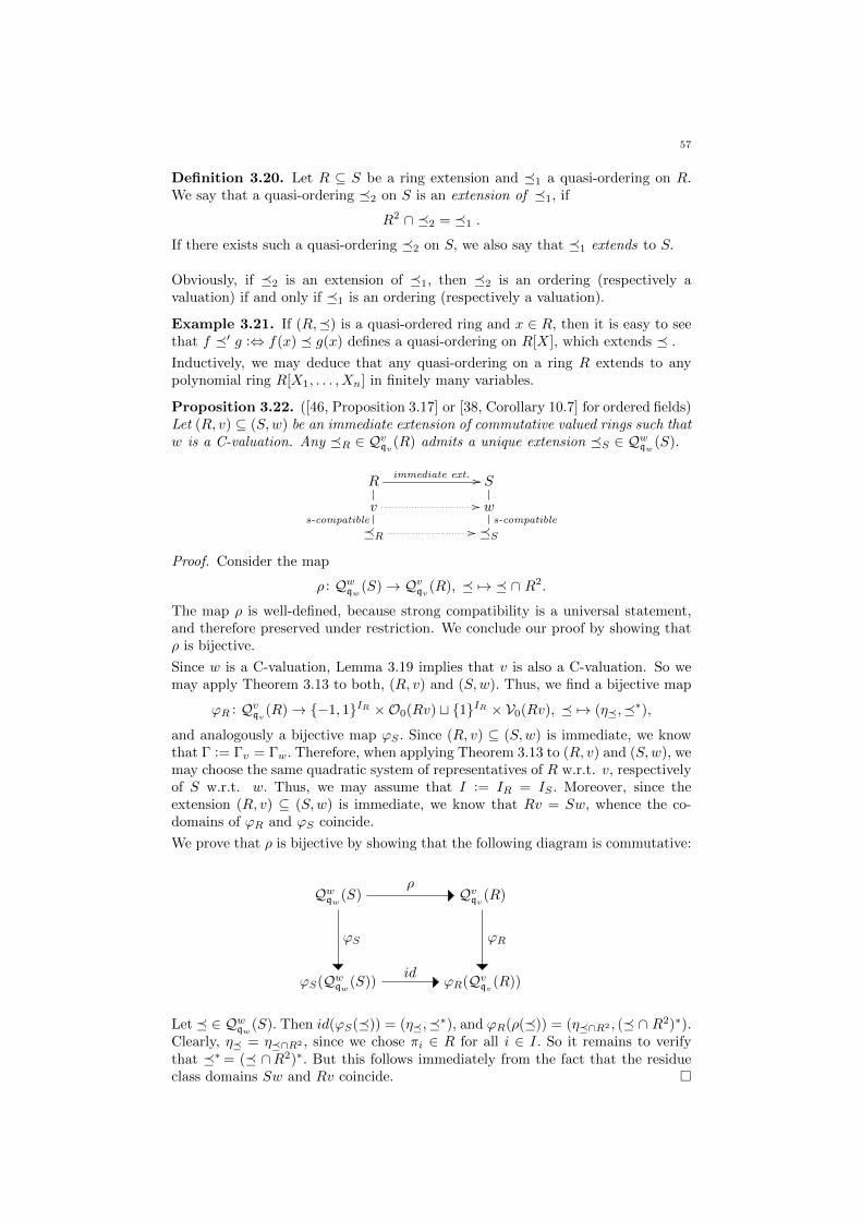
57

Definition 3.20. Let R ⊆ S be a ring extension and �1 a quasi-ordering on R.We say that a quasi-ordering �2 on S is an extension of �1, if

R2 ∩ �2 = �1 .

If there exists such a quasi-ordering �2 on S, we also say that �1 extends to S.

Obviously, if �2 is an extension of �1, then �2 is an ordering (respectively avaluation) if and only if �1 is an ordering (respectively a valuation).

Example 3.21. If (R,�) is a quasi-ordered ring and x ∈ R, then it is easy to seethat f �′ g :⇔ f(x) � g(x) defines a quasi-ordering on R[X], which extends � .Inductively, we may deduce that any quasi-ordering on a ring R extends to anypolynomial ring R[X1, . . . , Xn] in finitely many variables.

Proposition 3.22. ([46, Proposition 3.17] or [38, Corollary 10.7] for ordered fields)Let (R, v) ⊆ (S,w) be an immediate extension of commutative valued rings such thatw is a C-valuation. Any �R ∈ Qvqv

(R) admits a unique extension �S ∈ Qwqw(S).

Rimmediate ext. // S

vs-compatible

// ws-compatible

�R // �S

Proof. Consider the map

ρ : Qwqw(S)→ Qvqv

(R), � 7→ � ∩ R2.

The map ρ is well-defined, because strong compatibility is a universal statement,and therefore preserved under restriction. We conclude our proof by showing thatρ is bijective.

Since w is a C-valuation, Lemma 3.19 implies that v is also a C-valuation. So wemay apply Theorem 3.13 to both, (R, v) and (S,w). Thus, we find a bijective map

ϕR : Qvqv(R)→ {−1, 1}IR ×O0(Rv) t {1}IR × V0(Rv), � 7→ (η�,�∗),

and analogously a bijective map ϕS . Since (R, v) ⊆ (S,w) is immediate, we knowthat Γ := Γv = Γw. Therefore, when applying Theorem 3.13 to (R, v) and (S,w), wemay choose the same quadratic system of representatives of R w.r.t. v, respectivelyof S w.r.t. w. Thus, we may assume that I := IR = IS . Moreover, since theextension (R, v) ⊆ (S,w) is immediate, we know that Rv = Sw, whence the co-domains of ϕR and ϕS coincide.

We prove that ρ is bijective by showing that the following diagram is commutative:

Qwqw(S) Qvqv

(R)

ϕS(Qwqw(S)) ϕR(Qvqv

(R))

ρ

ϕRϕS

id

Let � ∈ Qwqw(S). Then id(ϕS(�)) = (η�,�∗), and ϕR(ρ(�)) = (η�∩R2 , (� ∩ R2)∗).

Clearly, η� = η�∩R2 , since we chose πi ∈ R for all i ∈ I. So it remains to verifythat �∗= (� ∩R2)∗. But this follows immediately from the fact that the residueclass domains Sw and Rv coincide. �

58

In [16, Theorem 20.1.1(a)], Efrat proves a result for localities on algebraic fieldextensions that is very similar to Proposition 3.22. There, �S is given and theexistence and uniqueness of the valuation w is derived, such that w extends v and�S ∈ Qwqw

(S).

Due to this similarity, we transfer Efrat’s result to commutative quasi-ordered ringshere, even though it does not rely on the Baer-Krull theorem at all. This is achievedby arguing via the associated quasi-ordered field (see Definition 1.39).

Lemma 3.23. Let R ⊆ S be an extension of commutative rings, let �R be a quasi-ordering on R, and �S a quasi-ordering on S. Then the following are equivalent:

(1) �S extends �R from R to S,

(2) �′S extends �′R from R/q�Rto S/q�S

,

(3) ES extends ER from K := Quot(R/q�R) to L := Quot(S/q�S

).

Proof. In the following, given a quasi-ordering �, we write (x, y) ∈� for x � y.First, we show that (1) implies (2). By Lemma 1.35 we get:

(x, y) ∈ (R/q�R)2 ∩ �′S ⇔ (x, y) ∈ R2 ∩ �S

⇔ (x, y) ∈ �R⇔ (x, y) ∈ �′R .

Likewise, (3) follows from (2) via Proposition 1.37:(ab−1, xy−1

)∈ K2 ∩ ES ⇔

(aby2, xyb2

)∈ (R/q�R

)2 ∩ �′S

⇔(aby2, xyb2

)∈ �′R

⇔(ab−1, xy−1

)∈ ER .

It remains to show that (1) follows from (3). Like above, we obtain:

(x, y) ∈ R2 ∩ �S ⇔ (x/1, y/1) ∈ K2 ∩ ES⇔ (x/1, y/1) ∈ ER⇔ (x, y) ∈ �R .

�

Remark 3.24. For the proof of the next proposition, we also require the followingbasic facts:

(1) If R ⊆ S is an integral extension of commutative rings, p ∈ Spec(R) andq ∈ Spec(S) such that R ∩ q = p, then R/p ⊆ S/q is an integral extensionof commutative domains.

(2) If R ⊆ S is an integral extension of commutative domains, then the fieldextension Quot(S)|Quot(R) is algebraic.

Proposition 3.25. Let R ⊆ S be an integral extension of commutative rings, v avaluation on R, and �R ∈ Qvqv

(R) such that �R extends to a quasi-ordering �S onS. Then there is a unique valuation w on S extending v such that �S ∈ Qwqw

(S).

Proof. Since �S is an extension of �R, we know that q�R= R ∩ q�S

. Hence, Re-mark 3.24(1) tells us that R/q�R

⊆ S/q�Sis an integral extension of commutative

domains. Let K and L denote the quotient fields of R/q�R, respectively S/q�S

.Then L|K is an algebraic field extension by Remark 3.24(2). Moreover, Corollary1.38 implies that �R and �S extend to quasi-orderings ER and EL on K and L,respectively. Furthermore, Lemma 3.23 tells us that ES is an extension of ER .

59

Finally, Lemma 2.35 implies ER ∈ Qν(K), where ν denote the unique extension ofv from R to K.

Therefore, we may apply [16, Theorem 20.1.1(a)]. Thus, there is a unique valuationω on L extending ν such that ES ∈ Qω(L). Let w be the restriction from L to S.Then it follows again by Lemma 2.35 and Lemma 3.23 that w is still an extension ofv such that�S ∈ Qwqw

(S). The valuation w is unique, because any other valuation onS with these properties would extend to L, and therefore contradict the uniquenessestablished in [16, Theorem 20.1.1(a)]. �

3.3. A Baer-Krull Theorem for Ordered Rings.

In this section we derive from Theorem 3.13 a Baer-Krull theorem for commutativeordered rings (Theorem 3.26), and give various applications. Proposition 3.29 andProposition 3.31 describe the relationship between non-Archimedean orderings onR and real valuations on R, while Proposition 3.32 transfers Proposition 3.22 andProposition 3.25 from quasi-ordered rings to ordered rings.

Theorem 3.26. (Baer-Krull theorem for commutative ordered rings)Let R be a commutative ring, v a C-valuation on R, and {πi : i ∈ I} a quadraticsystem of representatives of R w.r.t. v. Then the map

Ovqv(R)→ {−1, 1}I ×O0(Rv), ≤ 7→ (η≤,≤∗)

is a bijection.

Proof. We have already seen in Proposition 2.16 that � is an ordering if and only�∗ is an ordering, whence the claim follows immediately from Theorem 3.13. �

If R is a field, then this result obviously coincides with Theorem 3.2. Furthernote that if Γv is 2-divisible, then Theorem 3.26 simplifies in the same manner asTheorem 3.13 (see Remark 3.16).

Proposition 3.27. Let R be a commutative ring and v a C-valuation on R suchthat Γv is 2-divisible. Then the map

Ovqv(R)→ O0(Rv), � 7→ �∗

is a bijection.

Proof. This is proven exactly like Proposition 3.15. �

By imposing extra conditions on the residue class domain Rv, we may also eliminateO0(Rv) from the co-domain of our bijection in Theorem 3.26.

Proposition 3.28. Let R be a commutative ring, v a C-valuation on R, and{πi : i ∈ I} a quadratic system of representatives of R w.r.t. v. Further supposethat 0 is not a sum of non-zero squares in Rv, and that for each a ∈ Rv there issome 0 6= b ∈ Rv such that either ab2 or −ab2 is a sum of squares in Rv.Then the map

Ovqv(R)→ {−1, 1}I , ≤ 7→ η≤

is a bijection.

Proof. It suffices to show that Rv is uniquely ordered. The claim then followsimmediately from Theorem 3.26. Note that Rv is uniquely ordered if and only ifQuot(Rv) = Kν is uniquely ordered, where K := Quot(R/qv) and ν denotes theunique extension of v to K. Further note that Kν is uniquely ordered if and onlyif for any a ∈ (Kν)× either a or −a is a sum of squares in Kν.

60

So let xy−1 ∈ (Kν)× with x, y ∈ Rv. Then xy ∈ Rv, whence there exists some

0 6= b ∈ Rv such that (w.l.o.g.) xyb2 is a sum of squares in Rv, say xyb2 =∑pi

2

for some pi ∈ Rv. Then

xy−1 =∑i

(pi(yb)−1

)2is a sum of squares in Kν. Moreover, −xy−1 is not a sum of squares in Kν, sinceotherwise 0 would be a sum of non-zero squares in Rv. �

Conversely, if a domain is uniquely ordered, then it satisfies the conditions imposedon Rv in the previous proposition.

In the remainder of this chapter, we give a few applications for Theorem 3.26. Thefirst two deal with the relationship between non-Archimedean orderings and realvaluations on a commutative ring R, where a valuation v on R is called real if theresidue class domain Rv is real, i.e. if Rv admits an ordering.

Proposition 3.29. Let R be a commutative ring.

(1) If v is a real C-valuation on R, then Ovqv(R) 6= ∅.

(2) If v additionally admits negative values (i.e. v(a) < 0 for some a ∈ R),then any ≤∈ Ovqv

(R) is non-Archimedean. More precisely, any a ∈ R withv(a) < 0 is infinitely large w.r.t. to any such ordering.

Proof. Statement (1) is an immediate consequence of Theorem 3.26 - take thepreimage of the given ordering on Rv and the map η = 1 under the bijectivecorrespondence of the said theorem.

For the proof of (2) let ≤ ∈ Ovqv(R) be arbitrary and suppose that there is some

a ∈ R such that v(a) < 0. Since v(a) = v(−a) and q≤ = qv, we may assume that0 < a. Hence, we have 0 < a, and v(a) < 0 ≤ v(n) for all n ∈ N. So the fact that vis strongly ≤-compatible implies n < a for all n ∈ N. Thus, ≤ is a non-Archimedeanordering on R, and a is infinitely large. �

Remark 3.30. We may also prove Proposition 3.29(2) by considering the naturalvaluation of ≤, say w (see Example 2.8). Note that v(a) < 0 yields w(a) < 0, sincew is the finest strongly ≤-compatible valuation on R. Now a /∈ Rw implies that ais infinitely large.

The next result may be considered as a converse of Proposition 3.29. However,note that the following proposition involves valuations that are possibly not C-valuations.

Proposition 3.31. Let R be a commutative ring. Then O(R) is the union of theArchimedean orderings on R and the sets Ov(R), where v : R→ Γv ∪ {∞} is somenon-trivial real valuation

Proof. Let ≤ be a non-Archimedean ordering on R, and let v denote the naturalvaluation of ≤ . Then v is strongly ≤-compatible (Example 2.8). Furthermore, v isnon-trivial, since ≤ is non-Archimedean (Lemma 2.38). It remains to show that vis real. By Theorem 3.9 and Proposition 2.16 we know that Kν is real. But thenso is the subring Rv ⊆ Kν (Lemma 3.10). Hence, ≤∈ Ov(R) for some non-trivialreal valuation v on R. �

We conclude this section by formulating Proposition 3.22 and Proposition 3.25 fororderings.

61

Proposition 3.32.

(1) Let (R, v) ⊆ (S,w) be an immediate extension of commutative valued ringssuch that w is a C-valuation. Any ≤R ∈ Ovqv

(R) admits a unique extension≤S ∈ Owqw

(S).

(2) Let R ⊆ S be an integral extension of commutative rings, v a valuation onR, and ≤R ∈ Ovqv

(R) such that ≤R extends to an ordering ≤S on S. Thenthere is a unique valuation w on S extending v such that ≤S ∈ Owqw

(S).

Proof. Both these results follow immediately from Proposition 3.22, respectivelyProposition 3.25, since any extension of an ordering is again an ordering. �

3.4. A Baer-Krull Theorem for Valued Rings.

In this final section of Chapter 3 we establish a Baer-Krull theorem for valued rings(Theorem 3.33). Moreover, we derive an analogue statement for Manis valuations(Corollary 3.36). Finally, we establish Proposition 3.22 and Proposition 3.25 alsofor valuations (Proposition 3.37 and Proposition 3.38).

Theorem 3.33. (Baer-Krull theorem for commutative valued rings)Let R be a commutative ring and v a C-valuation on R. Then the map

ψ : Vvqv(R)→ V0(Rv), w 7→ w/v

is an order-preserving bijection with respect to the coarsening relation.

Proof. Immediately from Theorem 3.13 we obtain that

ψ : Vvqv(R)→ V0(Rv), w 7→ w∗

is a bijection. Moreover, Proposition 2.16(2) implies w∗ = w/v. Finally, it followsfrom Proposition 2.17 that ψ is indeed order-preserving. �

Remark 3.34.

(1) According to Proposition 2.7, Theorem 3.33 characterises the refinementsw of the given C-valuation v.

(2) Theorem 3.33 was already established for valued fields by Efrat (cf. [16,Proposition 7.2.1(d)])

We may also formulate a Baer-Krull theorem for commutative Manis valued rings.Recall from Definition 1.5 that a valuation v on a ring R is called Manis, if Γv is agroup, i.e. if Γv is closed under additive inverses.

Lemma 3.35. Let (R, v) be a valued ring, and let w ∈ Vvqv(R). Then w is Manis

if and only if v and w/v are Manis.

Proof. First suppose that w is Manis. Then v is Manis as a coarsening of a Manisvaluation (cf. [32, Remark II.1.3]). Now let γ ∈ Γw/v. Then γ = w/v(a) for somea ∈ Uv, and w/v(a) = w(a). Since w is Manis, we find some b ∈ R such thatw(ab) = 0. By strong �w-compatibility of v we obtain that also v(ab) = 0. Thus,a ∈ Uv, implies b ∈ Uv, whence w/v(b) = w(b) = −γ ∈ Γw/v.

Now let v and w/v be Manis, and γ ∈ Γw. Then γ = w(a) for some a ∈ R\qw, anda /∈ qv because qv = qw. Since v is Manis, we find some y ∈ R such that ay ∈ Uv. Sow/v(ay) = w(ay) =: γ1 ∈ Γw/v. Since w/v is also Manis, there is some z ∈ R suchthat w(z) = w/v(z) = −γ1 ∈ Γw/v. Therefore, w(z) = −w(ay) = −w(a) − w(y).This yields −γ = −w(a) = w(yz) ∈ Γw. �

62

Corollary 3.36. (Baer-Krull theorem for commutative Manis valued rings)Let R be a commutative ring and v a Manis valuation on R. Then the map

ψ : {w ∈ Vvqv(R) : w Manis} → {u ∈ V0(Rv) : u Manis}, w 7→ w/v

is an order-preserving bijection with respect to the coarsening relation.

Proof. By Proposition 3.14, v is a C-valuation. Thus, the claim follows immediatelyfrom Theorem 3.33 and Lemma 3.35. �

Last but not least, we may of course also establish Proposition 3.22 and Proposition3.25 for valuations.

Proposition 3.37.

(1) Let (R, v) ⊆ (S,w) be an immediate extension of commutative valued ringssuch that w is a C-valuation. Any v′ ∈ Vvqv

(R) (i.e. any refinement of vwith same support) admits a unique extension w′ ∈ Vwqw

(S).

(2) Let R ⊆ S be an integral extension of commutative rings, v a valuation onR, and v′ ∈ Vvqv

(R) such that v′ extends to a valuation w′ on S. Then thereis a unique valuation w on S extending v such that w′ ∈ Vwqw

(S).

Proof. This follows immediately from Proposition 3.22 and Proposition 3.25, sinceany extension of a valuation is again a valuation. �

Part (1) of the previous proposition was proven by Efrat for algebraic extensions ofvalued fields, cf. [16, Theorem 20.1.1(b)]. We conclude this whole chapter by alsotransferring this result to integral extensions of commutative valued rings.

Proposition 3.38. Let (R, v) ⊆ (S,w) be an integral extension of commutativevalued rings, and let v′ ∈ Vvqv

(R). Then there is a unique valuation w′ ∈ Vwqw(S)

extending v′.

Proof. As in the proof of Proposition 3.25, we derive the result by consideringquotient fields. Since w extends v from R to S, Lemma 3.23 states that ω extendsν from K := Quot(R/qv) to L := Quot(S/qw), where ω and ν denote the uniqueextensions of w and v to L and K, respectively. Moreover, ν′ ∈ Vν(K) by Lemma2.35, where ν′ denotes the unique extension of v′ to K. Finally, by Remark 3.24,the field extension L|K is algebraic, since R ⊆ S is an integral extension.

Hence, by [16, Theorem 20.1.1(b)], there is a unique valuation ω′ on L extending ν′

such that ω′ ∈ Vω(L). Going back from K to R and from L to S via Lemma 2.35and Lemma 3.23, we obtain a valuation w′ ∈ Vwqw

(S) extending v′. The uniquenessof w′ follows from the uniqueness stated in [16, Theorem 20.1.1(b)] and the factthat any other such valuation extends to a valuation on L. �

A similar result was proven by Manis ([52, Proposition 8(iii)]). There, a slightlyweaker statement is derived for Manis valuations without the assumption that thering extension is integral.

63

4. The Tree Structure of Quasi-Orderings

Let K be a field. In [16, Chapter 7], Efrat defines localities on K to be the disjointunion of all orderings and valuations on K, i.e. localities and quasi-orderings onfields are the same object, except that the former class provides no underlying setof axioms. Any locality λ induces a subgroup Gλ of K×, namely

Gλ =

1 + Iv, if λ = v is a valuation,

P\{0}, if λ = P is an ordering.

Based on this, Efrat defines a coarsening relation ≤ on the set of all localities onK by declaring

λ1 ≤ λ2 :⇔ Gλ2≤ Gλ1

.

His main result from [16, Chapter 7] states that the set of all localities on a givenfield, equipped with this coarsening relation, forms a rooted tree (cf. [16, Corollary7.3.6]), i.e. a partially ordered set admitting a maximum such that for any localityλ the set {λ′ : λ ≤ λ′} is linearly ordered.

The aim of the present chapter is to uniformly establish Efrat’s tree structuretheorem for quasi-ordered rings and to study some of its consequences. Let R be aring. In Section 4.1, we show that the coarsening relation ≤ introduced in Chapter1 (Definition 1.71) defines a partial ordering on the set of all quasi-orderings onR, which coincides with Efrat’s coarsening relation. The main result of Section 4.2states that the set Qq(R) of all quasi-orderings on R with fixed support q forms arooted tree with respect to ≤, thereby generalising Efrat’s result from above. InSection 4.3 we prove that the set of all special quasi-orderings (respectively Manisquasi-orderings) on a ring R is the ordered disjoint union of the rooted trees of allspecial quasi-orderings (respectively Manis quasi-orderings) with fixed support.

Section 4.4 deals with applications of the tree structure theorem. As main applica-tion we obtain that Qq(R) is a spectral set, i.e. order-isomorphic to the spectrum ofsome commutative ring partially ordered by inclusion. The same applies to the setof all special quasi-orderings, respectively Manis quasi-orderings on R (Subsection4.4.1). In Subsection 4.4.2 we introduce a dependency relation on Q(R) and deducefrom the tree structure theorem that it defines an equivalence relation on Qq(R).Finally, we derive the same result in Subsection 4.4.3 by considering the topologyinduced by a quasi-ordering.

4.1. A Coarsening Relation for Quasi-Orderings.

In this section we first recall the coarsening relation on quasi-orderings that wealready introduced in Section 1.4 (Definition 1.71) and verify that it generalisesEfrat’s respective notion from above (see also [16, Chapter 7.1]). We then showthat it defines a partial ordering on the set Q(R) of all quasi-orderings on a givenring R (Proposition 4.5).

Recall 4.1. Let R be a ring, and let �1 and �2 be quasi-orderings on R. We saythat �2 is coarser than �1 (or �1 finer than �2), written �1≤�2, if

∀x, y ∈ R : 0 �1 x �1 y ⇒ x �2 y.

Moreover, we call the quasi-orderings�1 and�2 comparable, if�1≤�2 or�2≤�1 .Otherwise, we call �1 and �2 incomparable.

64

Note that if �2 is induced by a valuation, then this coarsening relation coincideswith our notion of strong compatibility between quasi-orderings and valuations(Definition 2.4). Depending on the kind of the quasi-orderings, the coarseningrelation yields the following possible cases:

(1) If both quasi-orderings are orderings, we obtain �1⊆�2, i.e. that the finerordering �1 is contained in the coarser ordering �2 .

(2) If both quasi-orderings are valuations, we obtain that �2 is a coarsening of�1 in the sense of Definition 2.6 (see Proposition 2.7).

(3) The case where �1 is a valuation and �2 is an ordering cannot occur;0 �1 0 �1 −1 would imply 0 �2 −1, a contradiction. Hence, a valuation isnever finer than an ordering.

(4) If �1 is an ordering and �2 a valuation, we obtain that �2 is strongly�1-compatible (Definition 2.4).

Therefore, our coarsening relation subsumes three different notions at once. More-over, it is a uniform generalisation of Efrat’s coarsening relation (cf. [16, p.69]). Infact, our definition yields a significant improvement. According to us, an orderingP is coarser than an ordering Q if and only if Q ⊆ P, while for Efrat it is theother way round. Since he works over fields, inclusion of orderings implies equalityanyway. In the ring case, however, there are proper inclusions of orderings, whence,in analogy to valuation rings, the finer ordering should be contained in the coarserone.

Remark 4.2. Quasi-orderings admit a uniform definition of the set Gλ that Efratintroduced (see the beginning of this chapter, or [16, Chapter 7.1]). Indeed, for aquasi-ordered field (K,�) we have

G� = {x ∈ K× : 1− x ≺ 1} ≤ K×.

However, this set G� is inconvenient to work with in a uniform way. Moreover,Efrat’s approach does not apply to rings for various reasons.

We conclude this section by showing that ≤ defines a partial ordering on the setQ(R) of all quasi-orderings on a given ring R

Lemma 4.3. Let R be a ring and �1,�2 ∈ Q(R). Then the following are equivalent:

(1) �1≤�2,

(2) ∀x, y ∈ R : 0 �1 x �1 y ⇒ 0 �2 x �2 y.

Proof. Obviously, (2) implies (1). For the converse let �1≤�2 and 0 �1 x �1 y.Then x �2 y. Moreover, 0 �1 0 �1 x yields 0 �2 x. Thus, 0 �2 x �2 y. �

Lemma 4.4. Let (R,�) be a quasi-ordered ring and x, y ∈ R. If x � y ≺ 0, then0 ≺ −y � −x.

Proof. Clearly 0 ≺ −x,−y by Lemma 1.29. It remains to show that −y � −x.Assume that −x ≺ −y. We know that y ≺ 0 ≺ −x,−y, and therefore −x 6∼ y andy 6∼ −y. Via (QR4), it follows from x � y that 0 � y − x and from −x � −ythat y − x � 0. Thus, y − x ∈ q�. This implies −y ∼ −x (see Lemma 1.28), acontradiction. Hence, −y � −x. �

Proposition 4.5. Let R be a ring. Then (Q(R),≤) is a partially ordered set.

Proof. Obviously, ≤ is reflexive. Next, suppose that �1≤�2≤�3, and let x, y ∈ Rsuch that 0 �1 x �1 y. From �1≤�2 and Lemma 4.3 it follows 0 �2 x �2 y. Thus,�2≤�3 yields x �3 y. This shows �1≤�3, whence ≤ is transitive.

65

Last but not least, we prove that ≤ is anti-symmetric. So suppose that �1≤�2 and�2≤�1 . Then Lemma 4.3 implies that 0 �1 x �1 y ⇔ 0 �2 x �2 y for all x, y ∈ R,in particular 0 �1 x ⇔ 0 �2 x. So if �1 6=�2, there exist some x, y ∈ R such that(w.l.o.g.) x �1 y ≺1 0, but y ≺2 x ≺2 0. Lemma 4.4 tells us that 0 ≺1 −y �1 −x,and 0 ≺2 −x �2 −y. Now if −x ∼2 −y, then Corollary 1.60 implies that x ∼2 y, acontradiction. Hence, 0 ≺1 −y �1 −x but −x ≺2 −y, contradicting the assumptionthat �1≤�2 . Therefore, �1 =�2 . �

4.2. The Tree Structure Theorem for Quasi-Ordered Rings.

In the present section we establish the main theorem of this chapter, stating thatfor any ring R and any two-sided completely prime ideal q of R, the set (Qq(R),≤)of all quasi-orderings on R with support q, equipped with the coarsening relation≤, is a rooted tree (Theorem 4.14). From this we deduce a partial ordering ≤′,which canonically partitions Q(R) into the trees Qq(R) (Corollary 4.15). Next, weshow that a quasi-ordering � on R is comparable with a quasi-ordering of supportq if and only if q is �-convex (Proposition 4.23). This gives rise to the result thatthe set of all valuations with support q and all orderings for which q is convex,partially ordered by ≤, is a rooted tree (Proposition 4.27).

In this section, let R always be a ring and q a two-sided completely prime ideal ofR. We use the notation introduced in Notation 3.1(4), i.e. Q(R) denotes the set ofall quasi-orderings on R, and Qq(R) the set of all quasi-orderings on R with supportq. Moreover, ≤ always denotes the coarsening relation introduced in Definition 1.71(see also Recall 4.1).

Definition 4.6.

(1) A partially ordered set (S,≤) is called a tree if for all s, s1, s2 ∈ S withs ≤ s1, s2, the elements s1 and s2 are comparable, i.e. s1 ≤ s2 or s2 ≤ s1.

(2) A rooted tree is a tree that admits a maximum.

(3) A branch Si of a tree S is a maximal chain in S.

(4) The length of a branch Si is the order type of Si.

Remark 4.7. Compared to the usual definition of a (rooted) tree we reversed theordering in Definition 4.6. This is because we want coarse valuations to be largeelements with respect to our coarsening relation. In particular, trivial valuationsshall be maximal elements.

Unfortunately, as we will see below (Lemma 4.25), the whole set (Q(R),≤) is ingeneral neither a tree, nor admits a maximum. We first show that (Qq(R),≤) isalways a rooted tree (see Theorem 4.14 below).

Lemma 4.8. Let �1,�2 ∈ Qq(R) such that �1≤�2 and −1 �2 0. Then 0 �1 x ifand only if 0 �2 x.

Proof. The only-if-implication is trivial. For the if-implication suppose that 0 �2 x,and assume for the sake of a contradiction that x ≺1 0. Then 0 ≺1 −x, so fromthe assumption �1≤�2 and the fact that the supports of these quasi-orderingscoincide, we obtain 0 ≺2 −x. Applying (QR3) on 0 �2 x with −x yields 0 �2 −1,a contradiction to the assumption that −1 �2 0. Thus, 0 �1 x. �

Lemma 4.9. Let 0 ≺ x � y and 0 � a ≺ b. Then ax ≺ by and xa ≺ yb.Proof. Using (QR2) and (QR3), we obtain from a ≺ b and 0 ≺ x that ax ≺ bx.Moreover, from x � y and 0 � b, it follows via (QR2) that bx � by. Therefore,ax ≺ by. The same arguing shows that also xa ≺ yb. �

66

In the first part of the proof of the following proposition, we adapt the proof givenfor Proposition 2.31.

Proposition 4.10. Let �,�1,�2 ∈ Qq(R) such that �≤�1,�2 . Then �1 and�2 are comparable.

Proof. First suppose that 0 ≺i −1 for i = 1, 2. By Lemma 1.45 and Corollary1.46(2), we know that 0 �i x and x ∼�i

−x for all x ∈ R. Assume for the sake ofa contradiction that �1 and �2 are incomparable. Then we find ai, bi ∈ R\q suchthat 0 ≺1 a1 �1 a2 but 0 ≺2 a2 ≺2 a1, and 0 ≺2 b1 �2 b2 but 0 ≺1 b2 ≺1 b1. Since0 ≺i −1, we may w.l.o.g. assume that 0 ≺ ai, bi (otherwise replace ai with −ai,respectively bi with −bi). Lemma 4.9 implies a1b2 ≺1 a2b1 and a2b1 ≺2 a1b2. Sinceall ai, bi are positive w.r.t. �, the contraposition of �≤�i yields a1b2 ≺ a2b1 anda2b1 ≺ a1b2, a contradiction. Hence, �1 and �2 are comparable.

Next, suppose that −1 ≺i 0 for some i. Then also −1 ≺ 0, because �≤�i . Lemma4.8 implies 0 � x ⇔ 0 �i x. Together with Lemma 1.42 (if y /∈ q), respectivelyLemma 1.28 (if y ∈ q), this yields

x � y ⇔ x− y � 0⇔ x− y �i 0⇔ x �i y,whence �=�i . Since �≤�1,�2, this finishes the proof. �

Definition 4.11. A quasi-ordering � on R is called trivial if R/∼� has exactlytwo elements.

Remark 4.12. If � is some trivial quasi-ordering on a ring R, then E(0) = q� andE(1) = R\q� by (QR1), i.e. x ∼ y for all x, y ∈ R\q�. There is a unique trivialquasi-ordering with support q, namely the one induced by the trivial valuation withsupport q. We denote it by �q .

Proposition 4.13. The trivial quasi-ordering �q is the maximum of (Qq(R),≤).

Proof. Let � ∈ Qq(R), and let x, y ∈ R such that 0 � x � y. If x ∈ q, thenx �q y by Remark 4.12. If x /∈ q, then also y /∈ q since 0 � x � y. Consequently,x ∼�q

1 ∼�qy. Therefore, �≤�q, so �q is the maximum of Qq(R). �

Theorem 4.14. (the tree structure theorem)Let R be a ring and q a two-sided completely prime ideal of R. Then (Qq(R),≤) isa rooted tree.

Proof. By Proposition 4.5, (Qq(R),≤) is a partially ordered set. Proposition 4.10implies that, given a quasi-ordering �∈ Qq(R), its coarsenings inQq(R) are linearlyordered. Moreover, Qq(R) admits a maximum, namely the trivial quasi-orderingwith support q (Proposition 4.13). Thus, (Qq(R),≤) is a rooted tree. �

Corollary 4.15. Let R be a ring. Then the partial ordering

�1≤′�2 :⇔�1≤�2 and q�2⊆ q�1

yields a partition of Q(R) into the rooted trees Qq(R), where q runs over all two-sided completely prime ideals of R. Moreover, (Q(R),≤′) is a tree.

Proof. Note that �1≤′�2 if and only if �1≤�2 and q�1 = q�2 . Therefore, bothclaims easily follow from Theorem 4.14. �

We will see in Section 4.3 that this partition comes naturally, if we only considerspecial quasi-orderings, respectively Manis quasi-orderings.

In case where R is commutative, and at the cost of uniformity, we could have easilyderived Theorem 4.14 from Efrat’s result that the set of all localities on a field formsa rooted tree (cf. [16, Corollary 7.3.6]). This is due to the following generalisationof Lemma 2.35:

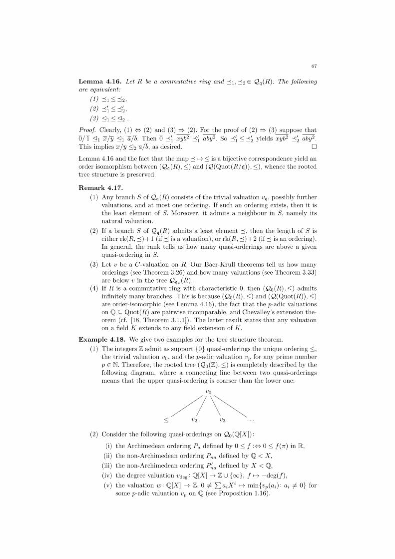
67

Lemma 4.16. Let R be a commutative ring and �1,�2 ∈ Qq(R). The followingare equivalent:

(1) �1≤�2,

(2) �′1≤�′2,(3) E1≤E2 .

Proof. Clearly, (1) ⇔ (2) and (3) ⇒ (2). For the proof of (2) ⇒ (3) suppose that

0/ 1 E1 x/y E1 a/b. Then 0 �′1 xyb2 �′1 aby2. So �′1≤�′2 yields xyb2 �′2 aby2.This implies x/y E2 a/b, as desired. �

Lemma 4.16 and the fact that the map � 7→E is a bijective correspondence yield anorder isomorphism between (Qq(R),≤) and (Q(Quot(R/q)),≤), whence the rootedtree structure is preserved.

Remark 4.17.

(1) Any branch S of Qq(R) consists of the trivial valuation vq, possibly furthervaluations, and at most one ordering. If such an ordering exists, then it isthe least element of S. Moreover, it admits a neighbour in S, namely itsnatural valuation.

(2) If a branch S of Qq(R) admits a least element �, then the length of S iseither rk(R,�)+1 (if � is a valuation), or rk(R,�)+2 (if � is an ordering).In general, the rank tells us how many quasi-orderings are above a givenquasi-ordering in S.

(3) Let v be a C-valuation on R. Our Baer-Krull theorems tell us how manyorderings (see Theorem 3.26) and how many valuations (see Theorem 3.33)are below v in the tree Qqv (R).

(4) If R is a commutative ring with characteristic 0, then (Q0(R),≤) admitsinfinitely many branches. This is because (Q0(R),≤) and (Q(Quot(R)),≤)are order-isomorphic (see Lemma 4.16), the fact that the p-adic valuationson Q ⊆ Quot(R) are pairwise incomparable, and Chevalley’s extension the-orem (cf. [18, Theorem 3.1.1]). The latter result states that any valuationon a field K extends to any field extension of K.

Example 4.18. We give two examples for the tree structure theorem.

(1) The integers Z admit as support {0} quasi-orderings the unique ordering ≤,the trivial valuation v0, and the p-adic valuation vp for any prime numberp ∈ N. Therefore, the rooted tree (Q0(Z),≤) is completely described by thefollowing diagram, where a connecting line between two quasi-orderingsmeans that the upper quasi-ordering is coarser than the lower one:

v0

≤ v2 v3 . . .

(2) Consider the following quasi-orderings on Q0(Q[X]) :

(i) the Archimedean ordering Pa defined by 0 ≤ f :⇔ 0 ≤ f(π) in R,(ii) the non-Archimedean ordering Pna defined by Q < X,

(iii) the non-Archimedean ordering P ′na defined by X < Q,(iv) the degree valuation vdeg : Q[X]→ Z ∪ {∞}, f 7→ −deg(f),

(v) the valuation w : Q[X] → Z, 0 6=∑aiX

i 7→ min{vp(ai) : ai 6= 0} forsome p-adic valuation vp on Q (see Proposition 1.16).

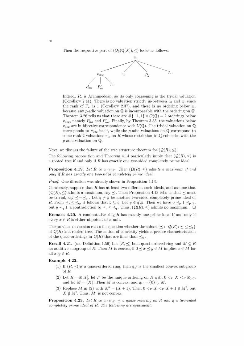
68

Then the respective part of (Q0(Q[X]),≤) looks as follows:

v0

vdeg w Pa. . .

Pna P ′na. . .

Indeed, Pa is Archimedean, so its only coarsening is the trivial valuation(Corollary 2.41). There is no valuation strictly in-between v0 and w, sincethe rank of Γw is 1 (Corollary 2.37), and there is no ordering below w,because any p-adic valuation on Q is incomparable with the ordering on Q.Theorem 3.26 tells us that there are #{−1, 1}×O(Q) = 2 orderings belowvdeg, namely Pna and P ′na. Finally, by Theorem 3.33, the valuations belowvdeg are in bijective correspondence with V(Q). The trivial valuation on Qcorresponds to vdeg itself, while the p-adic valuations on Q correspond tosome rank 2 valuations wp on R whose restriction to Q coincides with thep-adic valuation on Q.

Next, we discuss the failure of the tree structure theorem for (Q(R),≤).

The following proposition and Theorem 4.14 particularly imply that (Q(R),≤) isa rooted tree if and only if R has exactly one two-sided completely prime ideal.

Proposition 4.19. Let R be a ring. Then (Q(R),≤) admits a maximum if andonly if R has exactly one two-sided completely prime ideal.

Proof. One direction was already shown in Proposition 4.13.

Conversely, suppose that R has at least two different such ideals, and assume that(Q(R),≤) admits a maximum, say � . Then Proposition 4.13 tells us that � mustbe trivial, say �=�q . Let q 6= p be another two-sided completely prime ideal ofR. From �p≤�q, it follows that p ( q. Let y ∈ q\p. Then we have 0 �p 1 �p y,but y ≺q 1, a contradiction to �p≤�q . Thus, (Q(R),≤) admits no maximum. �

Remark 4.20. A commutative ring R has exactly one prime ideal if and only ifevery x ∈ R is either nilpotent or a unit.

The previous discussion raises the question whether the subset {�∈ Q(R) : � ≤�q}of Q(R) is a rooted tree. The notion of convexity yields a precise characterisationof the quasi-orderings in Q(R) that are finer than �q .

Recall 4.21. (see Definition 1.56) Let (R,�) be a quasi-ordered ring and M ⊆ Ran additive subgroup of R. Then M is convex, if 0 � x � y ∈M implies x ∈M forall x, y ∈ R.

Example 4.22.

(1) If (R,�) is a quasi-ordered ring, then q� is the smallest convex subgroupof R.

(2) Let R = R[X], let P be the unique ordering on R with 0 <P X <P R>0,and let M = (X). Then M is convex, and qP = {0} (M.

(3) Replace M in (2) with M ′ = (X + 1). Then 0 <P X <P X + 1 ∈ M ′, butX /∈M ′. Thus, M ′ is not convex.

Proposition 4.23. Let R be a ring, � a quasi-ordering on R and q a two-sidedcompletely prime ideal of R. The following are equivalent:

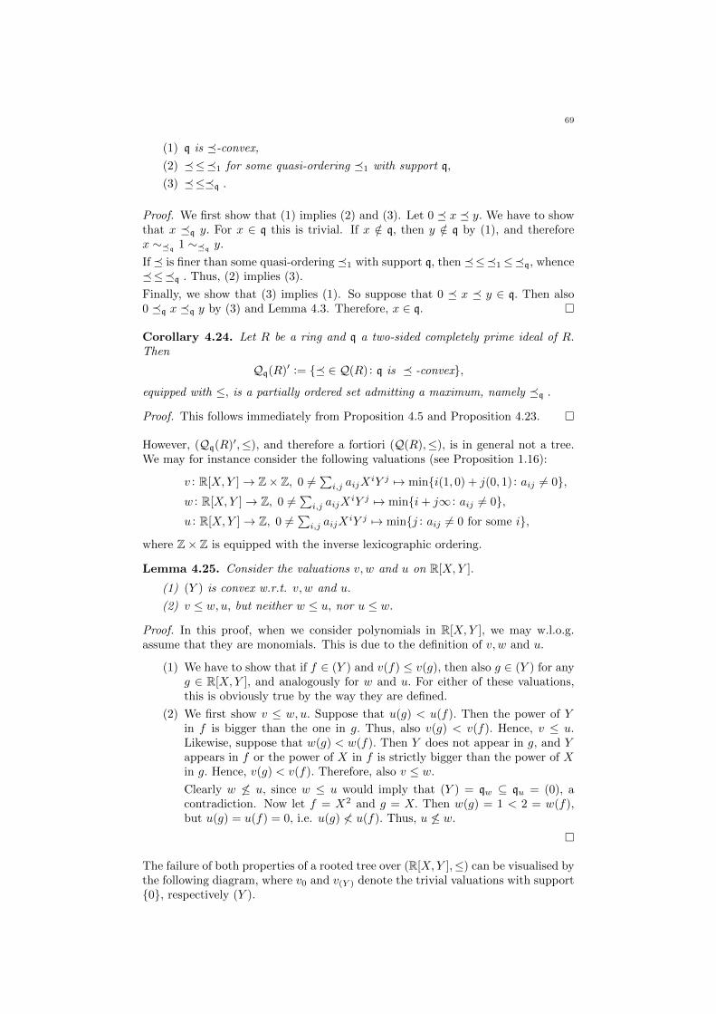
69

(1) q is �-convex,

(2) �≤�1 for some quasi-ordering �1 with support q,

(3) �≤�q .

Proof. We first show that (1) implies (2) and (3). Let 0 � x � y. We have to showthat x �q y. For x ∈ q this is trivial. If x /∈ q, then y /∈ q by (1), and thereforex ∼�q

1 ∼�qy.

If � is finer than some quasi-ordering �1 with support q, then �≤�1≤�q, whence�≤�q . Thus, (2) implies (3).

Finally, we show that (3) implies (1). So suppose that 0 � x � y ∈ q. Then also0 �q x �q y by (3) and Lemma 4.3. Therefore, x ∈ q. �

Corollary 4.24. Let R be a ring and q a two-sided completely prime ideal of R.Then

Qq(R)′ := {� ∈ Q(R) : q is � -convex},

equipped with ≤, is a partially ordered set admitting a maximum, namely �q .

Proof. This follows immediately from Proposition 4.5 and Proposition 4.23. �

However, (Qq(R)′,≤), and therefore a fortiori (Q(R),≤), is in general not a tree.We may for instance consider the following valuations (see Proposition 1.16):

v : R[X,Y ]→ Z× Z, 0 6=∑i,j aijX

iY j 7→ min{i(1, 0) + j(0, 1) : aij 6= 0},w : R[X,Y ]→ Z, 0 6=

∑i,j aijX

iY j 7→ min{i+ j∞ : aij 6= 0},u : R[X,Y ]→ Z, 0 6=

∑i,j aijX

iY j 7→ min{j : aij 6= 0 for some i},

where Z× Z is equipped with the inverse lexicographic ordering.

Lemma 4.25. Consider the valuations v, w and u on R[X,Y ].

(1) (Y ) is convex w.r.t. v, w and u.

(2) v ≤ w, u, but neither w ≤ u, nor u ≤ w.

Proof. In this proof, when we consider polynomials in R[X,Y ], we may w.l.o.g.assume that they are monomials. This is due to the definition of v, w and u.

(1) We have to show that if f ∈ (Y ) and v(f) ≤ v(g), then also g ∈ (Y ) for anyg ∈ R[X,Y ], and analogously for w and u. For either of these valuations,this is obviously true by the way they are defined.

(2) We first show v ≤ w, u. Suppose that u(g) < u(f). Then the power of Yin f is bigger than the one in g. Thus, also v(g) < v(f). Hence, v ≤ u.Likewise, suppose that w(g) < w(f). Then Y does not appear in g, and Yappears in f or the power of X in f is strictly bigger than the power of Xin g. Hence, v(g) < v(f). Therefore, also v ≤ w.Clearly w 6≤ u, since w ≤ u would imply that (Y ) = qw ⊆ qu = (0), acontradiction. Now let f = X2 and g = X. Then w(g) = 1 < 2 = w(f),but u(g) = u(f) = 0, i.e. u(g) 6< u(f). Thus, u 6≤ w.

�

The failure of both properties of a rooted tree over (R[X,Y ],≤) can be visualised bythe following diagram, where v0 and v(Y ) denote the trivial valuations with support{0}, respectively (Y ).

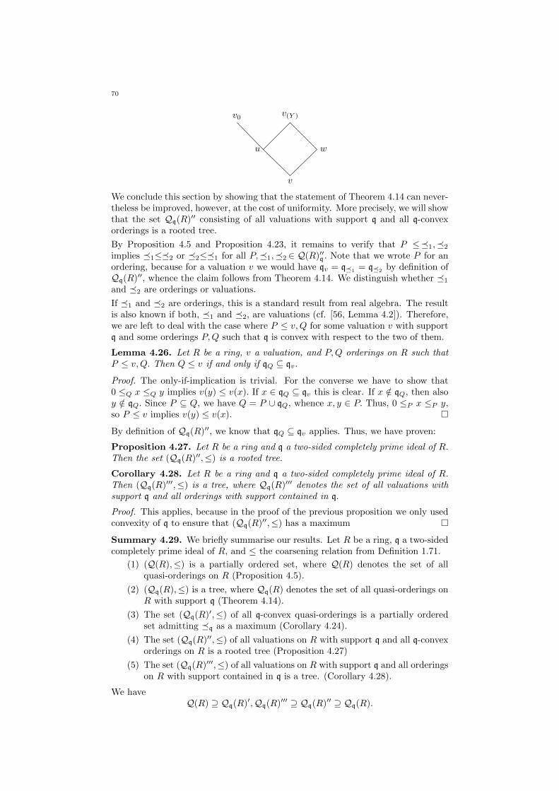
70

v

u w

v0 v(Y )

We conclude this section by showing that the statement of Theorem 4.14 can never-theless be improved, however, at the cost of uniformity. More precisely, we will showthat the set Qq(R)′′ consisting of all valuations with support q and all q-convexorderings is a rooted tree.

By Proposition 4.5 and Proposition 4.23, it remains to verify that P ≤�1,�2

implies �1≤�2 or �2≤�1 for all P,�1,�2 ∈ Q(R)′′q . Note that we wrote P for anordering, because for a valuation v we would have qv = q�1

= q�2by definition of

Qq(R)′′, whence the claim follows from Theorem 4.14. We distinguish whether �1

and �2 are orderings or valuations.

If �1 and �2 are orderings, this is a standard result from real algebra. The resultis also known if both, �1 and �2, are valuations (cf. [56, Lemma 4.2]). Therefore,we are left to deal with the case where P ≤ v,Q for some valuation v with supportq and some orderings P,Q such that q is convex with respect to the two of them.

Lemma 4.26. Let R be a ring, v a valuation, and P,Q orderings on R such thatP ≤ v,Q. Then Q ≤ v if and only if qQ ⊆ qv.

Proof. The only-if-implication is trivial. For the converse we have to show that0 ≤Q x ≤Q y implies v(y) ≤ v(x). If x ∈ qQ ⊆ qv this is clear. If x /∈ qQ, then alsoy /∈ qQ. Since P ⊆ Q, we have Q = P ∪ qQ, whence x, y ∈ P. Thus, 0 ≤P x ≤P y,so P ≤ v implies v(y) ≤ v(x). �

By definition of Qq(R)′′, we know that qQ ⊆ qv applies. Thus, we have proven:

Proposition 4.27. Let R be a ring and q a two-sided completely prime ideal of R.Then the set (Qq(R)′′,≤) is a rooted tree.

Corollary 4.28. Let R be a ring and q a two-sided completely prime ideal of R.Then (Qq(R)′′′,≤) is a tree, where Qq(R)′′′ denotes the set of all valuations withsupport q and all orderings with support contained in q.

Proof. This applies, because in the proof of the previous proposition we only usedconvexity of q to ensure that (Qq(R)′′,≤) has a maximum �

Summary 4.29. We briefly summarise our results. Let R be a ring, q a two-sidedcompletely prime ideal of R, and ≤ the coarsening relation from Definition 1.71.

(1) (Q(R),≤) is a partially ordered set, where Q(R) denotes the set of allquasi-orderings on R (Proposition 4.5).

(2) (Qq(R),≤) is a tree, where Qq(R) denotes the set of all quasi-orderings onR with support q (Theorem 4.14).

(3) The set (Qq(R)′,≤) of all q-convex quasi-orderings is a partially orderedset admitting �q as a maximum (Corollary 4.24).

(4) The set (Qq(R)′′,≤) of all valuations on R with support q and all q-convexorderings on R is a rooted tree (Proposition 4.27)

(5) The set (Qq(R)′′′,≤) of all valuations on R with support q and all orderingson R with support contained in q is a tree. (Corollary 4.28).

We haveQ(R) ⊇ Qq(R)′,Qq(R)′′′ ⊇ Qq(R)′′ ⊇ Qq(R).

71

4.3. The Tree Structure of Special and Manis Quasi-Orderings.

In Chapter 1 we introduced special quasi-orderings (Definition 1.54) and Manisquasi-orderings (Definition 1.63), that way generalising the respective notions fromvaluation theory. Here, we establish the result that the set QSq (R) of all specialquasi-orderings with support q on a ring R is a rooted subtree of Qq(R), and thatthe set QS(R) of all special quasi-orderings on R is the ordered disjoint union ofthe rooted trees QSq (R) (Theorem 4.34). We conclude this section by proving thatthe same applies to Manis quasi-orderings (Theorem 4.37).

Notation 4.30. Let R be a ring and q a two-sided completely prime ideal of R.We denote by QS(R) the set of all special quasi-orderings on R, and by QSq (R) theset of all special quasi-orderings on R with support q.

The sets QM (R) and QMq (R) are defined analagously for Manis quasi-orderings.

Definition 4.31. A (rooted) subtree of a tree (S,≤S) is a (rooted) tree (T,≤T )such that

(1) T ⊆ S and ≤T = ≤S ∩ T 2,

(2) T is upward closed under ≤S , i.e. if s, t ∈ S and T 3 t ≤S s, then s ∈ T.

Condition (1) of the previous Definition is obviously satisfied by the subsets QSq (R)

and QMq (R) of Qq(R) The following Lemma shows that (2) also applies.

Lemma 4.32. Let R be a ring, and let �1≤�2 be quasi-orderings on R.

(1) If �1 is special, then �2 is special.

(2) If �1 is Manis, then �2 is Manis.

Proof. We show (1), the proof of (2) being analogue. From �1≤�2 it immediatelyfollows that q�1

⊆ q�2. Now let x ∈ R\q2. Then also x ∈ R\q1. So we find some

y ∈ R such that 0 ≺1 1 �1 xy. Thus, �1≤�2 implies that 1 �2 xy, i.e. that �2 isspecial. �

Definition 4.33. If a partially ordered set (X,≤X) is the disjoint union of partiallyordered sets (Xi,≤Xi)i∈I , we say that X is the ordered disjoint union of the setsXi, if for all x, y ∈ X :

x ≤X y ⇔ ∃i ∈ I : x, y ∈ Xi and x ≤Xiy.

Theorem 4.34. Let R be a ring, and let q be a two-sided completely prime idealof R. Then

(1) (QSq (R),≤) is a rooted subtree of (Qq(R),≤).

(2) (QS(R),≤) is the ordered disjoint union of the rooted trees (QSq (R),≤).

Proof. The set QSq (R) = QS(R) ∩ Qq(R) is clearly a rooted tree, since Qq(R)is a rooted tree (Theorem 4.14), and since the trivial quasi-ordering �q is special.Moreover, by Lemma 4.32(1), QSq (R) is upward closed under ≤ . Hence, (QSq (R),≤)is a rooted subtree of (Qq(R),≤).

Evidently, QS(R) is the disjoint union of the treesQSq (R). Now let �1≤�2 ∈ QS(R).

We have to show that �1,�2 ∈ QSq (R) for some two-sided completely prime idealq of R. By Proposition 1.57, q := q�1

is the only two-sided completely prime idealof R that is �1-convex. According to Proposition 4.23, �1 only compares to quasi-orderings with support q. Thus, �1 and �2 both lie in QSq (R). Therefore, QS(R)

is the ordered disjoint union of the rooted subtrees QSq (R) of Qq(R). �

The last part of the previous proof may also be shown straight-forward (i.e. withoutexploiting convexity) as follows:

72

Lemma 4.35. Let R be a ring and let �1,�2 be quasi-orderings on R such that�1 is a special quasi-ordering. If �1≤�2, then q�1

= q�2.

Proof. Assume not. Then q�1 ( q�2 . So we find some x ∈ q�2\q�1 . Since �1

is special, there is some y ∈ R such that 0 ≺1 1 �1 xy. Hence, �1≤�2, implies1 �2 xy. On the other hand, xy ∼�2

0, since x ∈ q�2, a contradiction. Therefore,

q�1= q�2

. �

Remark 4.36. Lemma 4.35 particularly implies that special orderings are maximalelements in the real spectrum (cf. [36, Theorem 6], [13, Theorem 13.2.8] also for theconverse implication). Note that unlike us, the cited authors do not allow specialquasi-orderings to have non-trivial support, whence they consider the ring R/q�.

With the very same methods as in the proof of Theorem 4.34, we also get:

Theorem 4.37. Let R be a ring and let q be a two-sided completely prime ideal ofR. Then

(1) (QMq (R),≤) is a rooted subtree of (QSq (R),≤), respectively (Qq(R),≤).

(2) (QM (R),≤) is the ordered disjoint union of the rooted trees (QMq (R),≤).

The Theorems 4.34 and 4.37 are an improvement over Corollary 4.15 in the sensethat for special and Manis quasi-orderings the partition into the rooted treesQSq (R),

respectively QMq (R), comes naturally. Recall that in the said corollary, the partialordering ≤′ artificially enforced the supports to be equal.

4.4. Applications of the Tree Structure Theorem.

As the main application of the tree structure theorem (Theorem 4.14) we obtainthat the trees (Qq(R),≤), (Q(R),≤′), (QS(R),≤), and (QM (R),≤) are all spectralsets (Corollary 4.41, Corollary 4.42, Theorem 4.44), i.e. isomorphic to the spectrumof a commutative ring, partially ordered by inclusion. Hence, even if we start offwith a non-commutative ring R, its quasi-orderings, respectively its special andManis quasi-orderings, can be realised by the prime ideals of some commutativering.

Another, very immediate, application of Theorem 4.14 is that dependency is anequivalence relation on each of the setsQq(R),QS(R) andQM (R) (Proposition 4.46and Corollary 4.47), where two quasi-orderings are called dependent if they admita non-trivial common coarsening. We take this as an opportunity to introduce thetopology induced by a quasi-ordering. While this is not related to the tree structuretheorem, it gives rise to an alternative proof that dependency is an equivalencerelation on the set Qq(R).

4.4.1. On Spectral Sets of Quasi-Orderings.

Let us first define spectral sets.

Definition 4.38. A partially ordered set (X,≤) is called spectral, if it is order-isomorphic to (Spec(S),⊆) for some commutative ring S.

It is a known result that any finite partially ordered set is spectral (cf. [27], [50,Theorem 2.10]). In [49, Corollary 3.3], Lewis and Ohm even showed that a partiallyordered set (X,≤) is spectral, if for any x ∈ X there are only finitely many y ∈ Xsuch that y ≤ x, respectively x ≤ y. This immediately implies:

Proposition 4.39. Let R be a ring and X ⊆ Q(R) such that any quasi-ordering�∈ X has only finitely many coarsenings and refinements. Then (X,≤) is spectral.

73

In the general case, our work relies on a further result by these authors. Theyalso showed that a partially ordered set (X,≤) is a tree satisfying Kaplansky’sproperties (cf. [30], [50, Ch. 3], or (K1) and (K2) from Proposition 4.40 below) ifand only if (X,≤) is isomorphic to the spectrum of a Bezout domain ([49, Theorem4.2]), i.e. a commutative domain in which the sum of two principal ideals is againa principal ideal.

Proposition 4.40. Let R be a ring and let q be a two-sided completely prime idealof R. The tree Qq(R) has the following properties:

(K1) Every chain in Qq(R) has a supremum and an infimum.

(K2) If �1<�2 ∈ Qq(R), then we find elements �3,�4 ∈ Qq(R) such that

(i) �1≤�3<�4≤�2,

(ii) there is no element in Qq(R) lying strictly in-between �3 and �4 .

Proof. We first prove (K1). Let (�i)i∈I be a chain in Qq(R), w.l.o.g. #I ≥ 2. Itis easy to see that the supremum is given by the union of all quasi-orderings suchthat 0 ≺i −1 (i.e. such that �i is a valuation), and the infimum either by the onlyordering (if (�i)i∈I contains an ordering) or else by the intersection of all �i .For (K2) let �1<�2 ∈ Qq(R). Define

A := {� ∈ Qq(R) : �1<�≤�2}.

Then (A,≤) is a non-empty partially ordered set. Moreover, note that any �∈ A isa valuation, since it is coarser than �1 . Hence, for any chain in A, its intersectionis a lower bound in A, Thus, by Zorn’s lemma, there is a minimal element � ∈ A.Consequently, the choice �3 = �1 and �4 = � fulfils condition (K2). �

Corollary 4.41. Let R be a ring and q a two-sided completely prime ideal of R.Then (Qq(R),≤) is a spectral set and anti-isomorphic to the spectrum of a Bezoutdomain.

Proof. The second statement follows from Theorem 4.14, Proposition 4.40 and [49,Theorem 4.2]. Recall that in our definition of a tree we reversed the ordering (seeRemark 4.7), which is why we obtain an anti-isomorphism.

Now [27, Proposition 8] states that a partially ordered set (X,≤) is spectral if andonly if (X,≤0) is spectral, where x ≤0 y :⇔ y ≤ x. Therefore, the first claimimmediately follows from the second one. �

Corollary 4.42. Let R be a ring Then (Q(R),≤′) is a spectral set, where ≤′denotes the partial ordering introduced in Corollary 4.15. Moreover, (Q(R),≤′) isanti-isomorphic to the spectrum of a Bezout domain.

Proof. This is proven exactly like Corollary 4.41, since Proposition 4.40 obviouslyalso applies to the tree (Q(R),≤′). �

Example 4.43.

(1) The tree (Q0(Z),≤) of all quasi-orderings on Z with support 0 (see Example4.18(1)) is anti-order-isomorphic to the spectrum (Spec(Z),⊆) of the Bezoutdomain Z.

(2) The proof of [50, Theorem 3.1] is constructive, i.e. for any tree (T,≤) (inthe usual sense) satisfying (K1) and (K2), an explicit Bezout domain canbe constructed such that its spectrum is order-isomorphic to (T,≤). Theconstruction is as follows (cf. [50] and [21, Theorem 18.6]):

74

(a) Define T× := {t ∈ T | ∃q ∈ T : q << t}, where q << t means thatthere is no element in T, which lies strictly in-between q and t. Then(T×,≤) is also a tree.

(b) Define A := {f : T× → Z |f(t) = 0 for all but finitely many t ∈ T×}.For f ∈ A, denote

MS(f) := {t ∈ T : f(t) 6= 0 and f(t′) = 0 for all t′ < t}.Set A+ := {f ∈ A : f(p) > 0 for all p ∈ MS(f)}. Then (A,A+) is alattice ordered group.

(c) Choose some field K and let D be the group ring of A over K. ThenD is an integral domain. The map

w : D → G ∪ {∞}, 0 6= f =

n∑i=1

aiXgi 7→ inf{gi}ni=1

is a demivaluation, whence it admits a unique extension to a demival-uation v on L := Quot(D).

(d) The demivaluation ring Dv is the Bezout domain we are looking for.

Proposition 4.40 is easily seen to apply to the trees (QS(R),≤) and (QM (R),≤) aswell. Therefore, we further obtain:

Theorem 4.44. Let R be a ring. Then the trees (QS(R),≤) and (QM (R),≤) arespectral sets and anti-isomorphic to the spectrum of a Bezout domain

Proof. This is proven just like Corollary 4.41. �

The previous theorem also applies to (QSq (R),≤), respectively (QMq (R),≤). Moregenerally, it applies to any tree of quasi-orderings that fulfils the two Kaplanskyconditions (K1) and (K2).

4.4.2. Dependency of Quasi-Orderings.

We continue by introducing a dependency relation on the set Q(R). As an easyconsequence of the tree structure theorem (Theorem 4.14) we obtain that it definesan equivalence relation on Qq(R) for any two-sided completely prime ideal q of R(Proposition 4.46). The same applies to the sets QS(R) and QM (R) (Corollary4.47). The dependency relation is further considered in Subsection 4.4.3.

Definition 4.45. Let R be a ring. Two quasi-orderings �1,�2 on R are calleddependent, written �1∼�2, if there is a non-trivial quasi-ordering � on R suchthat �1,�2≤�, or if �1 =�2 is trivial. Otherwise, we call them independent.

Proposition 4.46. Let R be a ring and q a two-sided completely prime ideal of R.Then dependency is an equivalence relation on Qq(R).

Proof. Reflexivity and symmetry are both trivial. For transitivity suppose that�1∼�2 and �2∼�3, w.l.o.g. all non-trivial. Then there are non-trivial quasi-orderings �,�′ ∈ Qq(R) such that �1,�2≤� and �2,�3≤�′ . Hence, �2≤�,�′ .Theorem 4.14 implies that (w.l.o.g.) �≤�′ . Thus, �1,�3≤�′, i.e. �1∼�3 . �

Corollary 4.47. Let R be a ring. Then dependency is an equivalence relation onQS(R) and QM (R).

Proof. This follows immediately from Lemma 4.35 and Proposition 4.46. �

75

4.4.3. Digression on the Topology Induced by a Quasi-Ordering.

We conclude Chapter 4 by introducing the topology induced by a quasi-ordering.This yields an alternative proof of Proposition 4.46, if the ring R is commutative(Corollary 4.55). It is perhaps the more usual approach to obtain the said resultand was for instance taken by Eggert for Manis valuations on commutative rings(cf. [17, p.187]).

In [19, Remark 4.2], Fakhruddin defines quasi-intervals for quasi-ordered fields.Taking the same definition for rings yields:

Definition 4.48. Let (R,�) be a quasi-ordered ring, and let a, b ∈ R. The quasi-interval of length b around a is defined by

(a− b, a+ b)� = {x ∈ R | ∃y ∈ R : 0 � y ≺ b and − y � x− a � y}.

Remark 4.49. If �=≤ is an ordering on R, then

(a− b, a+ b)≤ = {x ∈ R : − b < x− a < b} = {x ∈ R : a− b < x < a+ b},

which is just the usual notion of open intervals in ordered rings, and therefore anopen basis for the order topology on R.

If �= v is a valuation on R, then

(a− b, a+ b)v = {x ∈ R | ∃y ∈ R : v(b) < v(y) and v(x− a) = v(y)}= {x ∈ R : v(x− a) > v(b)}=: Bv(b)(a).

As for valued fields, the set B := {Bv(b)(a) : a, b ∈ R} forms an open basis for aHausdorff topology on R (cf. [18, p. 45]).

Lemma 4.50. Let (R, v) be a valued ring. Then B forms an open basis for atopology on R. If v has trivial support, then this topology is Hausdorff.

Proof. Obviously, the elements of B cover R. Now let Bv(b1)(a1), Bv(b2)(a2) ∈ B bearbitrary, and denote by B their intersection. We may w.l.o.g. assume that B isnon-empty, so in particular that b1, b2 /∈ qv. For z ∈ B define

B3 := Bγ(z) = {x ∈ R : v(x− z) > γ} ∈ B,

where γ := max{v(b1), v(b2)} ∈ Γv. Clearly, z ∈ B3. So it remains to show thatB3 ⊆ B. Let y ∈ B3. Then v(y − z) > γ ≥ v(b1). We compute

v(y − a1) = v((y − z) + (z − a1)) ≥ min{v(y − z), v(z − a1)} > v(b1).

Thus, y ∈ Bv(b1)(a1). Analogously, we obtain y ∈ Bv(b2)(a2), so y ∈ B. Hence, B isindeed an open basis for a topology on R.

Now suppose that v has trivial support, and let y, z ∈ R such that y 6= z. Thenv(y−z) ∈ Γv. It is easy to see that the open sets Bv(y−z)(y) and Bv(y−z)(z) separatey and z. Therefore, the topology induced by B is Hausdorff. �

Consequently, Fakhruddin’s notion of quasi-intervals provides a uniform open basisfor the topology induced by a quasi-ordering on R.

Notation 4.51. Let (R,�) be a quasi-ordered ring. We denote by

T� := {(a, b)� : a, b ∈ R}

the topology on R induced by � .

76

Unfortunately, these quasi-intervals are very inconvenient to work with - which maybe a reason why Fakhruddin never deepened his work on quasi-ordered fields.

In [16, Ch. 8 and 10], Efrat studies the topologies induced by localities on fields, andtheir interplay with the dependency relation. While his approach is non-uniformright away, he manages to simultaneously formulate results for topologies inducedby orderings, respectively valuations.

We conclude this chapter by transferring two of them to commutative quasi-orderedrings via quotient fields. They will give rise to an alternative proof of Proposition4.46. As usual, given a quasi-ordered ring (R,�), we denote by (K,E) its associatedquasi-ordered field (see Definition 1.39).

Lemma 4.52. Let R be a commutative ring and let �1,�2 ∈ Qq(R) for some primeideal q of R. The following are equivalent:

(1) �1∼�2 in R,

(2) �′1∼�′2 in R/q,

(3) E1∼E2 in K.

Proof. This is an immediate consequence of Lemma 4.16. �

Proposition 4.53. (cf. [16, Lemma 8.1.3])Let R be a commutative ring, �1,�2 ∈ Qq(R), and �∈ Qq(R) a non-trivial com-mon coarsening for some prime ideal q of R. Then TE1 = TE2 .

Proof. By assumption �1,�2≤� . Hence, Lemma 4.16 implies that E1,E2≤E inK = Quot(R/q). By [16, Lemma 8.1.3], we obtain TE1 = TE = TE2 . �

Proposition 4.54. (cf. [16, Corollary 10.1.4])Let R be a commutative ring and let �1,�2 be non-trivial quasi-orderings on Rwith same support. If TE1

⊆ TE2, then �1∼�2 .

Proof. Let q be the common support of �1 and �2 . Then E1 and E2 are non-trivialquasi-orderings on K := Quot(R/q) such that TE1

⊆ TE2. By [16, Corollary 10.1.4],

E1∼E2, i.e. we find some non-trivial quasi-ordering E on K such that E1,E2≤E .Going back to R again yields via Lemma 4.16 that �1,�2≤� . Moreover, � is non-trivial, since E is non-trivial. Thus, �1 and �2 are dependent. �

Corollary 4.55. Let R be a commutative ring. Then dependency is an equivalencerelation on Qq(R) for any prime ideal q of R.

Proof. Obviously, reflexivity and symmetry are both fulfilled. For transitivity, let�1,�2,�3 ∈ Qq(R), w.l.o.g. all non-trivial, such that �1∼�2 and �2∼�3 . ThenTE1

= TE2= TE3

by Proposition 4.53. Now TE1= TE3

implies via Proposition 4.54that �1∼�3 . Hence, ∼ is an equivalence relation on Qq(R). �

77

5. The Quasi-Real Spectrum of a Ring

The subject of Chapter 4 was to study the quasi-orderings on a ring R as a partiallyordered set. In the present chapter we consider Q(R) as a topological space. Forthat purpose we develop a notion of quasi-real spectrum, that way unifying thenotions of real spectrum and valuation spectrum (see Preliminaries below).

In Section 5.1 we first introduce the quasi-real spectrum of a commutative ring R asthe set of all tuples (q,E), where q is a prime ideal ofR andE a quasi-ordering on thefield Quot(R/q). We then show that this set is in a natural bijective correspondencewith the set Q(R) of all quasi-orderings on R. The latter result enables us to definethe quasi-real spectrum for arbitrary rings.

In Section 5.2 we generalise the Harrison topology H and the Tychonoff topology Tfrom the real spectrum to the quasi-real spectrum Q(R). Our main results are that(Q(R), T ) is a Boolean space, and that (Q(R),H) is a spectral space. We concludethis section by briefly introducing and discussing a third topology on Q(R), namelythe one induced by our coarsening relation ≤ (see Definition 1.71).

The derivation and study of the quasi-real spectrum is achieved in almost completeanalogy to the real spectrum, respectively valuation spectrum. Therefore, it is aperfect example of how quasi-orderings provide a uniform treatment of ordered andvalued rings.

Preliminaries on the real spectrum and the valuation spectrum.

The real spectrum, related to the Zariski spectrum of a ring, was introduced forcommutative rings by Coste and Roy around 1979 ([10]), and later also consideredfor possibly non-commutative rings by Leung, Marshall, and Y. Zhang ([48]). Itplays an important role in real algebraic geometry for the study of semi-algebraicsets, and for establishing Nullstellen- and Positivstellensatze (cf. e.g. [64, Ch. 4],[54, Ch. 5], [33, Kap. 3]).

Definition 5.1. Let R be a commutative ring. The real spectrum r-Spec(R) of Ris the set

{(q,E) : q ∈ Spec(R), E∈ O(Quot(R/q))}.

The real spectrum of R is in a natural bijective correspondence with the set O(R)of all orderings on R, and therefore identified with this set. It is equipped with twocanonical topologies, namely the Harrison topology and the Tychonoff topology.The former is that of primary interest, while the latter is rather a tool for a betterunderstanding of the Harrison topology - that will also be the case in the quasi-realspectrum, see Section 5.2 below.

Definition 5.2. Let R be a commutative ring.

(1) The Harrison topology (or spectral topology) H on O(R) is the topologygenerated by the sets U(a) as open subbasis, where

U(a) := {≤∈ O(R) : 0 < a} (a ∈ R)

(2) The Tychonoff topology (or patch topology, or constructible topology) T onO(R) is the topology generated by the sets U(a) and V (a) as open subbasis,where

V (a) := {≤∈ O(R) : 0 ≤ a} (a ∈ R)

It can be shown that (O(R),H) is a spectral space, and that (O(R), T ) is a Booleanspace (cf. e.g. [54, Proposition 6.3.3]).

78

Definition 5.3. A topological space (X, τ) is called a Boolean space, if it is quasi-compact, Hausdorff, and totally disconnected.

Definition 5.4. [27] A topological space (X, τ) is called a spectral space, if

(1) it is T0,

(2) it is quasi-compact,

(3) quasi-compact open subsets are closed under finite intersections,

(4) quasi-compact open subsets form an open basis,

(5) every non-empty irreducible closed subset A ⊆ X has a generic point, i.e.a point whose closure is all of A.

Hochster showed in [27] that a topological space is spectral if and only if it ishomeomorphic to the spectrum of a commutative ring equipped with the Zariskitopology. Therefore, the notion of spectral spaces corresponds to the one of partiallyordered spectral sets (see Definition 4.38). In fact, there is a strong relation betweenpartially ordered sets and topological spaces.

Definition 5.5. Let (X, τ) be a topological space and let x, y ∈ X. Then y is called

a specialisation of x (or x a generalisation of y), denoted by x ≤τ y, if y ∈ {x}.

If (X, τ) is a T0 space, then ≤τ defines a partial ordering on X. Conversely, if ≤is a partial ordering on X, then (X, τ≤) is a T0 space, where τ≤ is the topologygenerated by the closed subbasis {y ∈ X : y ≥ x} (cf. [49]).

Remark 5.6. (cf. [49]) If (X1, τ1), (X2, τ2) are homeomorphic T0 spaces, then(X1,≤τ1) and (X2,≤τ2) are order-isomorphic. The converse of this statement maybe false.

Inspired by the real spectrum, the notion of valuation spectrum was independentlydeveloped by de la Puente ([65]) and Huber ([28]), and then further investigatedby Huber and Knebusch ([29]). While de la Puente was interested in applicationsrelated to affine algebraic varieties, Huber and Knebusch were looking for analogiesbetween semi-algebraic geometry and rigid analytic geometry. Nevertheless, theyderived the same topologies on the valuation spectrum.

Definition 5.7. Let R be a commutative ring. The valuation spectrum v-Spec(R)of R is the set

{(q, ν) : q ∈ Spec(R), ν ∈ V(Quot(R/q))}.

In analogy to the real case, this set is in a natural bijective correspondence withthe set V(R) of all valuations on R, and therefore identified with this set. Thevaluation spectrum is canonically equipped with the topologies generated by thefollowing sets (cf. [29]):

(1) τ := {v ∈ V(R) : v(a) ≥ v(b) 6=∞} (a, b ∈ R)

(2) τ ′ := {v ∈ V(R) : v(a) > v(b)} (a, b ∈ R)

(3) τ ′′ := the topology generated by τ ∪ τ ′.

In [29] it is shown that V(R) is a spectral space with respect to either of thesetopologies.

Via quasi-orderings, it is easy to see that the topology τ ′ on the valuation spectrumcorresponds to the Harrison topology on the real spectrum. Moreover, the topologyτ ′′ resembles the Tychonoff topology. We will make use of this in Section 5.2.

79

5.1. The Quasi-Real Spectrum as a Set.

Here, we introduce the notion of the quasi-real spectrum qr-Spec(R) of a ring R.As for orderings and valuations, we first define it for commutative rings to be theset of all tuples (q,E), where q is a prime ideal of R and E a quasi-ordering onthe field Quot(R/q) (Definition 5.8). Thereafter, we prove that qr-Spec(R) may beidentified with the set Q(R) of all quasi-orderings on R (Corollary 5.10), resulting ina definition of the quasi-real spectrum which also applies to non-commutative rings(Definition 5.11). We conclude this section by describing the quasi-real spectrumof R in terms of ring homomorphisms (Proposition 5.14).

Definition 5.8. Let R be a commutative ring. We call

qr-Spec(R) := {(q,E) : q ∈ Spec(R), E∈ Q(Quot(R/q))}the quasi-real spectrum of R.

Our first aim is to derive a definition of the quasi-real spectrum that applies topossibly non-commutative rings.

Proposition 5.9. Let R be a ring, I a two-sided ideal of R and S ⊆ R a multi-plicative set.

(1) There is a bijective correspondence

ϕ : {� ∈ Q(R) : q� ⊇ I} → Q(R/I)

given by the assignment � 7→ �′ .(2) There is a bijective correspondence

ϕ : Qq�(R)→ Q0(R/q�)

given by the assignment � 7→ �′ .(3) If R is commutative, there is a bijective correspondence

ψ : {� ∈ Q(R) : q� ∩ S = ∅} → Q(RS)

given by the assignment � 7→ E .

Proof.

(1) By Lemma 1.35, the map ϕ is well-defined. Moreover, since x � y ⇔ x �′ y,ϕ is easily seen to be bijective.

(2) This is precisely (1) in the case where I = q�.

(3) We have already seen in Proposition 1.37 that the map ψ is well-definedand injective. Moreover, if E is a quasi-ordering on RS , then the restriction� := R ∩ E is a quasi-ordering on R such that ψ(�) = E holds. Hence, ψis bijective.

�

Corollary 5.10. Let R be a commutative ring. The map

ρ : Q(R)→ qr-Spec(R), � 7→ (q�,E)

is a bijection.

Proof. Let q be a prime ideal of R. Applying Proposition 5.9(2) and (3) with thechoice S = (R/q)\{0} implies that ψ ◦ϕ : � 7→ E is a bijection between Qq(R) andQ(Quot(R/q)). From this it is easy to see that the map ρ from the claim is also abijection. �

Because of Corollary 5.10, we may identify the quasi-real spectrum qr-Spec(R)of a commutative ring R with Q(R). This enables us to generalise the quasi-realspectrum to possibly non-commutative rings.

80

Definition 5.11. Let R be a ring. We call

Q(R) = {� ⊆ R2 : � is a quasi-ordering on R}the quasi-real spectrum of R.

Remark 5.12. Consequently, Proposition 5.9(1) and (3) yield a description ofthe quasi-real spectrum of both, the quotient ring R/I and the localisation RS , assubsets of the quasi-real spectrum of R.

We conclude the current section with a further description of the quasi-real spec-trum Q(R) of a commutative ring R (see Proposition 5.14 below).

Lemma 5.13. Let R,S be rings, ϕ : R→ S a ring homomorphism and �S a quasi-ordering on S. Then x �R y :⇔ ϕ(x) �S ϕ(y) defines a quasi-ordering on R withsupport q�R

= {x ∈ R : ϕ(x) ∈ q�S}.

Proof. Showing that �R defines a quasi-ordering on R with support ϕ−1(q�S) is

done straight-forward, which is why we only showcase that (QR4) applies. So letx, y, z ∈ R such that x �R y and z ��R

y. Then ϕ(x) �S ϕ(y) and ϕ(z) ��Sϕ(y).

Via (QR4) it follows that

ϕ(x+ z) = ϕ(x) + ϕ(z) �S ϕ(y) + ϕ(z) = ϕ(y + z),

and therefore x+ z �R y + z. �

By abuse of notation, we denote the quasi-ordering �R from the previous lemmaby ϕ−1(�S). Evidently, ϕ−1(�S) is an ordering (respectively a valuation) if andonly if �S is an ordering (respectively a valuation).

Proposition 5.14. Let R be a commutative ring and � ⊆ R2. The following areequivalent:

(1) � ∈ Q(R),

(2) There is a quasi-ordered field (K,E) and a ring homomorphism ϕ : R→ Ksuch that �= ϕ−1(E).

Proof. We have already shown in Lemma 5.13 that (2) implies (1). For the converse,let� ∈ Q(R). Then� uniquely extends to a quasi-orderingE onK := Quot(R/q�).Now consider the canonical homomorphism ϕ : R → K, x 7→ x / 1. We obtain byLemma 1.35 and Proposition 1.37 that

x � y ⇔ x �′ y ⇔ x / 1 E y / 1,

i.e. that x � y if and only if ϕ(x) E ϕ(y). Hence, (K,E) is a quasi-ordered fieldsuch that � = ϕ−1(E). �

By imposing a suitable equivalence relation on the set of all such homomorphisms,the real spectrum of a commutative ring can also be introduced via the previousproposition (cf. [8, Ch. 7]).

5.2. The Quasi-Real Spectrum as a Topological Space.

In this section we generalise the Harrison topology H and the Tychonoff topologyT from the real spectrum to the quasi-real spectrum of a ring (Definition 5.15,Definition 5.22), and show that many of their properties are preserved. In fact,almost all results presented here are well-known to hold for the real spectrum ofcommutative rings with identical proofs.

Our first main result of the present section states that (Q(R), T ) is a Boolean spacefor any ring R (Theorem 5.24). The latter implies that (Q(R),H) is a spectralspace (Theorem 5.26). This provides a uniform proof of the fact that (O(R),H)

81

and (V(R),H) are also spectral spaces (Corollary 5.27). We further show thatthe Harrison topology is completely determined by the Tychonoff topology andthe partial ordering ≤H (Corollary 5.31, respectively Corollary 5.32). Finally, webriefly discuss a third topology on Q(R), which we call tree topology (Definition5.33). It is the topology induced by the coarsening relation ≤ .

Definition 5.15. Let R be a ring.

(1) For a, b ∈ R we define the set

U(a, b) := {� ∈ Q(R) : a ≺ b}.

(2) The topology H on Q(R) generated by the open subbasis

{U(a, b) ⊆ Q(R) : a, b ∈ R}

is called the Harrison topology (or spectral topology).

If not mentioned otherwise, we always equip Q(R) with this topology H.

Remark 5.16. The restriction of H to O(R) is obviously the usual Harrison topol-ogy on the real spectrum. If we restrict Q(R) to V(R), then H coincides with thetopology τ ′ introduced in [29, 1.3] (see also the preliminaries above).

Example 5.17.

(1) Exploiting the dichotomy (Theorem 1.50), it is easy to see that O(R) isopen and closed with respect to the Harrison topology. Indeed,

O(R) = U(−1, 0),

so O(R) is open. Moreover, (O(R))C

= V(R) = U(0,−1) is also open,whence O(R) is closed.

(2) The set V(R) of all valuations on R is also open and closed. This followsimmediately from (1).

(3) The bijections from Proposition 5.9 can be shown to be homeomorphisms.

We begin our discussion of the Harrison topology with a small observation on therelationship of the quasi-real spectrum and the spectrum of rings.

Lemma 5.18.

(a) Let R be a commutative ring. The support map

supp : Q(R)→ Spec(R), � 7→ q�

is continuous.

(b) Let R,S be rings and ϕ : R→ S a ring homomorphism. Then the map

q-Sperϕ : Q(S)→ Q(R), � 7→ ϕ−1(�)

is continuous.

Proof. First consider the support map. Let r ∈ R and D(r) = {q ∈ Spec(R) : r /∈ q}be a basic open set of the spectrum of R. Then

supp−1(D(r)) = {�∈ Q(R) : r /∈ q�}= {�∈ Q(R) : 0 ≺ r or r ≺ 0}= U(0, r) ∪ U(r, 0),

is an open set, whence supp is continuous.

82

By Lemma 5.13, the map q-Sperϕ is well-defined. Now let A = {�∈ Q(R) : a ≺ b}be a subbasic open set for some a, b ∈ A. Then

(q-Sperϕ)−1(A) = {�∈ Q(S) : q-Sperϕ(�) ∈ A}= {�∈ Q(S) : (a, b) ∈ ϕ−1(�) and (b, a) /∈ ϕ−1(�)}= {�∈ Q(S) : ϕ(a) ≺ ϕ(b)}= U(ϕ(a), ϕ(b))

where (a, b) ∈� :⇔ a � b. Hence, q-Sperϕ is continuous as well. �

Corollary 5.19. Let R,S be commutative rings, ϕ : R→ S a ring homomorphismand Specϕ : Spec(S)→ Spec(R), p 7→ ϕ−1(p). Then

Q(S) Q(R)

Spec(S) Spec(R)

q-Sperϕ

suppsupp

Specϕ

is a commutative diagram of continuous maps.

Proof. We have already seen that all these maps are continuous. Now let �∈ Q(S).Then

Specϕ(supp(�)) = Specϕ(q�) = ϕ−1(q�) = supp(ϕ−1(�))

= supp(q-Sperϕ(�)).

�

We now want to study the properties of the space (Q(R),H), eventually provingthat it is a spectral space (see Theorem 5.26).

Lemma 5.20. Let R be a ring and �1,�2 ∈ Q(R). Then

�2 ∈ {�1} ⇔ �1⊆�2,

i.e. ≤H = ⊆ (see Definition 5.5).

Proof. Let N�2denote the set of all open neighbourhoods of �2 . We deduce

�1⊆�2 ⇔ ∀a, b ∈ R(a �1 b⇒ a �2 b)

⇔ ∀a, b ∈ R(b ≺2 a⇒ b ≺1 a)

⇔ ∀N ∈ N�2: N ∩ {�1} 6= ∅

⇔ �2 ∈ {�1}.�

Corollary 5.21. Let R be a ring. Then (Q(R),H) is a T0 space.

Proof. Two quasi-orderings �1,�2 ∈ Q(R) are topologically indistinguishable if

and only if �1 ∈ {�2} and vice versa. Consequently, by Lemma 5.20, if and onlyif �1 = �2 . Hence, (Q(R),H) is T0. �

For a further study of the Harrison topology we introduce the Tychonoff topologyon Q(R).

83

Definition 5.22. Let R be a ring.

(1) For a, b ∈ R we define the set

V (a, b) := {� ∈ Q(R) : a � b}.(2) The topology T on Q(R) generated by the open subbasis

{U(a, b) ⊆ Q(R) : a, b ∈ R} ∪ {V (a, b) ⊆ Q(R) : a, b ∈ R}is called the Tychonoff topology (or constructible topology, respectively patchtopology).

Remark 5.23.

(1) On O(R), the topology T obviously coincides with the usual Tychonofftopology on the real spectrum. For the valuation spectrum, however, Huberand Knebusch consider {v ∈ V(R) : v(a) ≥ v(b) 6=∞} instead of V (a, b) fortheir corresponding topology τ ′′ (cf. [29, 1.3]).

(2) Immediately by definition, the Tychonoff topology is finer than the Harrisontopology, i.e. H ⊆ T .

Theorem 5.24. Let R be a ring. Then (Q(R), T ) is a Boolean space.

Proof. We first show that this space is quasi-compact. Any quasi-ordering � on Ris uniquely determined by the map

f� : R2 → {0, 1}, (a, b) 7→

{1, a � b0, b ≺ a

Hence, we may consider Q(R) as a subset of F := {0, 1}R2

. We equip {0, 1} withthe discrete topology, which makes it a quasi-compact space. So by the Tychonofftheorem, F is also quasi-compact with respect to the product topology. An opensubbasis is given by the sets

Hε(a, b) := {f : R2 → {0, 1}, (a, b) 7→ ε} (a, b ∈ R, ε ∈ {0, 1}).Therefore, we may identify Q(R) as a subspace of F . We show that it is a closedsubspace, which implies that (Q(R), T ) is quasi-compact. So let f ∈ F be notinduced by some quasi-ordering on R, i.e. the induced binary relation on R doesnot satisfy one of the axioms of a quasi-ordering. If for instance axiom (QR4) fails,then we find some x, y, z ∈ R such that f(x, y) = 1 and f(y, z) = 0 = f(y+z, x+z),respectively f(z, y) = 0 = f(y + z, x + z). Thus, f is separated from Q(R) by theopen set

H1(x, y) ∩ (H0(y, z) ∪H0(y, z)) ∩H0(y + z, x+ z),

whence s /∈ Q(R). The same arguing applies to all the other axioms. Therefore,Q(R) is a closed subspace of F , implying that (Q(R), T ) is quasi-compact.

Next, we show that (Q(R), T ) is Hausdorff. So let �1,�2 ∈ Q(R) with �1 6= �2 .Then there exist (w.l.o.g.) some a, b ∈ R such that a �1 b and b ≺2 a. Consequently,�1 ∈ V (a, b)\U(b, a) and �2 ∈ U(b, a)\V (a, b). This shows that (Q(R), T ) fulfils theHausdorff property.

Finally, assume that there is some connected component X ⊆ Q(R) such that|X| ≥ 2, and let �1 6=�2 ∈ X. Then we find some a, b ∈ R such that (w.l.o.g.)a �1 b and b ≺2 a. Thus,

X = (X ∩ V (a, b)) ∪ (X ∩ U(b, a)),

is a union of two disjoint non-empty open sets. This contradicts the connectednessof X. Hence, (Q(R), T ) is totally disconnected. Altogether, we have shown that(Q(R), T ) is a Boolean space. �

84

Remark 5.25.

(1) Any Boolean space is homeomorphic to the real spectrum of a field (cf. [12]or [11, Theorem 5]; see also [62, Theorem 6.9]).

(2) The Hausdorff property implies that all singletons {�} are closed. Hence,the partial ordering onQ(R) induced by the Tychonoff Topology is equality,i.e. �1 ≤T �2 ⇔ �1 = �2 .

Theorem 5.26. Let R be a ring. Then (Q(R),H) is a spectral space.

Proof. We have already proved that (Q(R),H) is a T0 space (Corollary 5.21), andthat (Q(R), T ) is a compact space (Theorem 5.24). Moreover, the sets U(a, b) areboth open and closed with respect to T , and an open subbasis of H. Therefore, [27,Proposition 7] tells us that (Q(R),H) is a spectral space. �

Corollary 5.27. Let R be a ring. Then (O(R),H) and (V(R),H) are both spectralspaces.

Proof. This is an easy consequence of Theorem 5.26 and Example 5.17, since closedsubsets of spectral spaces are again spectral spaces (cf. [13, Theorem 2.1.3]). �

The previous corollary may be as well deduced from Theorem 5.26 via [13, Theorem2.4.3], since Q(R) is easily seen to be the topological sum of O(R) and V(R). Thecited result also yields that Corollary 5.27 implies Theorem 5.26.

Corollary 5.28. Let R be a ring. Then (Q(R),⊆) is a spectral set.

Proof. By Theorem 5.26, (Q(R),H) is a spectral space. Hence, there is a com-mutative ring S such that (Q(R),H) is homeomorphic to (Spec(S),Z), where Zdenotes the Zariski topology. According to [49], this implies that Q(R) and Spec(S)are order-isomorphic with respect to the induced partial orderings ≤H, respectively≤Z . Thus, (Q(R),⊆) ∼= (Spec(S),⊆), whence (Q(R),⊆) is spectral. �

Next, we generalise the result that H is completely determined by T and ≤H fromthe real to the quasi-real spectrum (cf. [33, Ch. III.4] or [54, Proposition 6.3.4]).

Lemma 5.29. Let R be a ring and (Ai)i∈I a family of T -closed subsets of Q(R)such that

⋂i∈I Ai = ∅. Then there is a finite index set J ⊆ I such that

⋂j∈J Aj = ∅.

Proof. From⋂i∈I Ai = ∅ follows thatQ(R) =

⋃i∈I A

Ci is an open cover ofQ(R). By

quasi-compactness, there is a finite J ⊆ I such that Q(R) =⋃j∈J A

Cj . Therefore,⋂

j∈J Aj = ∅. �

Proposition 5.30. Let R be a ring and Y ⊆ Q(R) a closed subset with respect tothe Tychonoff topology. Then

Y =⋃�∈Y

{�} = {�′ ∈ Q(R) : �≤H�′ for some �∈ Y }

with respect to the Harrison topology.

Proof. The second equality follows immediately from Lemma 5.20. Furthermore,clearly Y ⊇

⋃�∈Y {�}. Conversely, let �∈ Y be arbitrary and {Ui : i ∈ I} the

family of all basic open neighbourhoods of � with respect to the Harrison topology.Then Y ∩ Ui is non-empty and T -closed for all i ∈ I. Therefore, Lemma 5.29 impliesthat

⋂i∈I Y ∩ Ui is also non-empty. So let �′ ∈

⋂i∈I Y ∩ Ui. Then �′ is contained

in every basic open neighbourhood of � with respect to the Harrison topology,whence �∈ {�′}. �

Corollary 5.31. Let R be a ring. A subset Y ⊆ Q(R) is H-closed if and only if itis T -closed and stable under specialisation w.r.t. H.

85

Proof. First let Y be H-closed. Then Y is also T -closed, since H ⊆ T . Now let�1 ∈ Y and �1≤H�2 . Then we obtain �2 ∈ {�1} ⊆ Y = Y. Thus, Y is stableunder specialisation.

Conversely, suppose that Y is T -closed and stable under specialisation. Then weget

Y = {�∈ Q(R) : �′≤H� for some �′ ∈ Y } = Y,

where the first equality follows from Proposition 5.30 and the second one from theassumption that Y is stable under specialisation. Hence, Y is H-closed. �

Corollary 5.32. Let R be a ring. A subset Y ⊆ Q(R) is H-open if and only if itis T -open and stable under generalisation w.r.t. H.

Proof. Making use of Corollary 5.31, the proof goes as follows:

Y is H-open⇔ Y C is H-closed

⇔ Y C is T -closed and stable under specialisation

⇔ Y is T -open and stable under generalisation.

�

We conclude this chapter by introducing a third topology on Q(R), which arisesfrom the coarsening relation ≤ that we studied in Chapter 4. Recall from Lemma4.3 that if �1,�2 ∈ Q(R), then

�1≤�2 ⇔ ∀a, b ∈ R : 0 �1 a �1 b⇒ 0 �2 a �2 b.

Definition 5.33. Let R be a ring.

(1) For a, b ∈ R we define the set

W (a, b) := {� ∈ Q(R) : 0 � a � b}.(2) We call the topology τT on Q(R) generated by the closed subbasis

{W (a, b) ⊆ Q(R) : a, b ∈ R}the tree topology.

The corresponding open subbasis of τT is given by the sets

W (a, b)C = {� ∈ Q(R) : b ≺ a or a ≺ 0}.

Remark 5.34.

(1) If we restrict Q(R) to valuations, we obtain

W (a, b)C ∩ V(R) = {v ∈ V(R) : b ≺v a} = U(b, a) ∩ V(R),

i.e. for valuations our Harrison and our tree topology coincide.

(2) If we restrict Q(R) to orderings, we obtain

U(a, b) ∩ O(R) = {≤ ∈ O(R) : a− b < 0}= {≤ ∈ O(R) : a− b < 0 or 0 < 0}= W (0, a− b)C ∩ O(R),

and conversely

W (a, b)C ∩ O(R) = (U(b, a) ∩ O(R)) ∪ (U(a, 0) ∩ O(R)).

Hence, the Harrison and the tree topology also coincide on O(R).

Lemma 5.35. Let R be a ring, let �1,�2 ∈ Q(R), and let ≤ denote the coarseningrelation on Q(R). Then

�2 ∈ {�1} ⇔ �1≤�2,

w.r.t. τT , i.e. ≤τT =≤ .

86

Proof. This is proven just like Lemma 5.20. So let N�2denote the set of all open

neighbourhoods of �2 w.r.t. τT . We obtain

�1≤�2 ⇔ ∀x, y ∈ R : (0 �1 x �1 y ⇒ 0 �2 x �2 y)

⇔ ∀x, y ∈ R : (y ≺2 x or x ≺2 0⇒ y ≺1 x or x ≺1 0)

⇔ ∀N ∈ N�2: N ∩ {�1} 6= ∅

⇔ �2 ∈ {�1}.�

Remark 5.36. A singleton {�} is τT -closed if and only if � is a trivial quasi-ordering. This is an immediate consequence of Lemma 5.35 and the fact that the≤-maximal elements are precisely the trivial quasi-orderings.

So unlike H and T , the tree topology admits that a valuation lies in the closure ofan ordering. Conversely, an ordering cannot be in the closure of a valuation, sincean ordering is never coarser than a valuation (see Section 4.1).

We conclude our discussion of the quasi-real spectrum with the following result:

Corollary 5.37. Let R be a ring. Then (Q(R), τT ) is a T0 space.

Proof. We may argue just like in the proof of Corollary 5.21. Two quasi-orderings�1,�2 ∈ Q(R) are topologically indistinguishable if and only if �1 ∈ {�2} and

�2 ∈ {�1}, i.e. if and only if �1≤�2≤�1 with respect to the coarsening relation≤ . Anti-symmetry of ≤ yields �1 =�2 . Thus, (Q(R), τT ) is T0. �

87

6. Partial Quasi-Orderings on Rings

In the present chapter we develop a notion of partially quasi-ordered rings andestablish an analogue of the dichotomy proven for totally quasi-ordered rings inChapter 1 (see Theorem 1.50). Moreover, we deal with the question under whichconditions partial quasi-orderings extend to total quasi-orderings.

While there is a rich theory on various kinds of partial orderings on rings, amongothers preorderings, preprimes and quadratic modules, little attention has been paidto a development of partial valuations. The only such notion, as far as the authorof this thesis can tell, is that of (strict) partial valuations on division rings as elabo-rated on in [73]. Building upon this one, it turns out that the right counterparts inthe sense of a dichotomy are division closed partial orderings, i.e. partial orderingsthat are compatible with addition and multiplication in the usual sense and admitdivision, respectively cancellation. These classes are the subject of Section 6.1.

In Section 6.2 we axiomatically introduce partially quasi-ordered rings and provethat all strictly partially valued rings and all division closed partially ordered ringsare contained in this class. The subject of Section 6.3 is to show that the conversealso applies, i.e. to establish a dichotomy for partial quasi-orderings in analogy tothe total case. The proof of this result essentially follows the one that we presentedin Section 1.3 for total quasi-orderings. Finally, in Section 6.4, we introduce thenotion of quadratic partial quasi-orderings and prove that any quadratic partialquasi-ordering on a field extends to a total quasi-ordering.

6.1. Partial Valuations and Partial Orderings.

In this section we briefly introduce the notions of partially and strictly partiallyvalued rings on the one hand (Definition 6.2), and partially ordered rings (Definition6.6), respectively division closed partially ordered rings (Definition 6.8), on theother hand.

Remark 6.1. Throughout this chapter we only consider partial valuations andpartial orderings with support {0}. For the sake of convenience and by abuse ofnotation, we will just call them partial valuations and partial orderings, i.e. notmention all over again that the supports are always trivial. The reader should keepthis in mind, since otherwise the following is partly inconsistent with our previouswork on total quasi-orderings.

Combining the notion of valuations on rings (see Definition 1.5) with the notion ofpartial valuations on division rings (cf. [73, Definition 1.1.1]) results in the followingdefinition of partially valued rings:

Definition 6.2.

(a) Let (Γ,+,≤) be a partially ordered cancellative monoid. A partial valuationon a ring R is a surjective map v : R→ Γ∪{∞}, where∞ is a symbol suchthat γ < ∞ and γ +∞ = ∞ = ∞ + γ for all γ ∈ Γ, such that for allx, y, z ∈ R :

(PV1) v(x) =∞⇔ x = 0,

(PV2) v(xy) = v(x) + v(y),

(PV3) If v(z) ≤ v(x), v(y), then v(z) ≤ v(x+ y).

We call Γv := Γ the value monoid of v.

(b) A strict partial valuation is a partial valuation that satisfies:

88

(PV4) If v(z) < v(x), v(y), then v(z) < v(x+ y).

Remark 6.3.

(1) Any partially valued ring is in fact a domain, for if xy = 0 for some x, y ∈ R,then v(x) + v(y) =∞ by (PV1) and (PV2), whence x = 0 or y = 0.

(2) Definition 6.2 may be generalised by replacing axiom (PV1) with the weakeraxiom (PV1’) v(0) =∞ and v(1) = 0 (see Definition 1.4).In analogy to (total) valuations, the support qv := {x ∈ R : v(x) = ∞} ofv then would be a two-sided completely prime ideal of R, and the mappingv′ : R/qv → Γv, x 7→ v(x) would be a partial valuation on R/q� in thesense of Definition 6.2. Moreover, v is strict if and only if v′ is strict.

Lemma 6.4. Let R be a ring, v a partial valuation on R and x, y ∈ R.(1) If v(x) and v(y) are comparable, then v(x+ y) ≥ min{v(x), v(y)}.(2) If v is strict and if v(x) and v(y) are strictly comparable (i.e. v(x) < v(y)

or vice versa), then v(x+ y) = min{v(x), v(y)}.

Proof. We first show that (1) holds. By assumption, v(x) and v(y) are comparable,whence γ := min{v(x), v(y)} exists. Since γ ≤ v(x), v(y), axiom (PV3) impliesγ ≤ v(x+y). For the proof of (2) suppose that v(x) and v(y) are strictly comparable,say v(x) < v(y). By (1), we obtain v(x + y) ≥ v(x). Assume for the sake of acontradiction that v(x+y) > v(x). Then v(x) < v(y) = v(−y) and v(x) < v(x+y).Hence, (PV4) implies v(x) < v(x + y − y) = v(x), a contradiction. Consequently,v(x+ y) = v(x) = min{v(x), v(y)}. �

Lemma 6.4(1) tells us that a partial valuation is a valuation if and only if its valuemonoid is totally ordered. The second part of the lemma is crucial to establish thatan analogue of axiom (QR4) holds for the relation induced by a partial valuationv via x � y ⇔ v(y) ≤ v(x) (see our proof of Proposition 1.33). For that reason weare eventually only interested in strict partial valuations.

Example 6.5.

(1) Let p, q ∈ N be prime, p 6= q. Consider the map

v := (vp, vq) : Z→ N0 × N0, x 7→ (vp(x), vq(x)),

where vp and vq denote the p-adic, respectively q-adic valuation, and N0×N0

is equipped with the natural (i.e. componentwise/coordinatewise) partialordering. Then v is a partial valuation, which is not strict. For instancev(1) < v(p), v(q), but v(1) = v(p+ q).

If p = q, then v as above is a strict partial valuation, the value monoidbeing the diagonal {(n, n) : n ∈ N0} ⊆ N0 × N0.

(2) More generally, it may be shown that any product (vi)i∈I of valuations(with support {0}) on a ring R is a partial valuation, which is strict if allvi coincide.

(3) Let D be a division ring and R a subring of D which is stable, i.e. invariantunder inner automorphisms. Then R is local if and only if R = Dv for somestrict partial valuation v on D, where Dv := {x ∈ D : v(x) ≥ 0} denotesthe valuation ring induced by v ([73, Proposition 1.1.6]).

(4) ([73, Example 1.1.7]) Consider R = Z(p)[[X]] as subring of K = Q((X)).Then R is local and stable. Hence, there is a strict partial valuation v onK such that Kv = R. Moreover, v is not a valuation. Indeed, since neitherpX−1 ∈ R nor p−1X ∈ R holds, Kv is not a valuation ring.

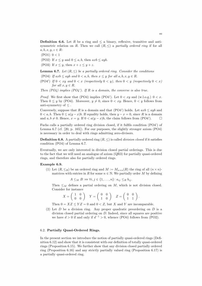
89

Definition 6.6. Let R be a ring and ≤ a binary, reflexive, transitive and anti-symmetric relation on R. Then we call (R,≤) a partially ordered ring if for alla, b, x, y, z ∈ R :

(PO1) 0 < 1

(PO2) If x ≤ y and 0 ≤ a, b, then axb ≤ ayb.(PO3) If x ≤ y, then x+ z ≤ y + z.

Lemma 6.7. Let (R,≤) be a partially ordered ring. Consider the conditions

(PO4) If axb ≤ ayb and 0 < a, b, then x ≤ y for all a, b, x, y ∈ R.(PO4′) If 0 < xy and 0 < x (respectively 0 < y), then 0 < y (respectively 0 < x)

for all x, y ∈ R.Then (PO4) implies (PO4’). If R is a domain, the converse is also true.

Proof. We first show that (PO4) implies (PO4’). Let 0 < xy and (w.l.o.g.) 0 < x.Then 0 ≤ y by (PO4). Moreover, y 6= 0, since 0 < xy. Hence, 0 < y follows fromanti-symmetry of ≤ .Conversely, suppose that R is a domain and that (PO4’) holds. Let axb ≤ ayb and0 < a, b. Then 0 ≤ a(y− x)b. If equality holds, then y− x = 0, since R is a domainand a, b 6= 0. Hence, x = y. If 0 < a(y − x)b, the claim follows from (PO4’). �

Fuchs calls a partially ordered ring division closed, if it fulfils condition (PO4’) ofLemma 6.7 (cf. [20, p. 165]). For our purposes, the slightly stronger axiom (PO4)is necessary in order to deal with rings admitting zero-divisors.

Definition 6.8. A partially ordered ring (R,≤) is called division closed if it satisfiescondition (PO4) of Lemma 6.7.

Eventually, we are only interested in division closed partial orderings. This is dueto the fact that we will need an analogue of axiom (QR3) for partially quasi-orderedrings, and therefore also for partially ordered rings.

Example 6.9.

(1) Let (R,≤R) be an ordered ring and M := Mn×n(R) the ring of all (n×n)-matrices with entries in R for some n ∈ N. We partially order M by defining

A ≤M B :⇔ ∀i, j ∈ {1, . . . , n} : aij ≤R bij .

Then ≤M defines a partial ordering on M, which is not division closed.Consider for instance

X =

(1 00 0

)Y =

(0 01 0

)Z =

(0 01 1

).

Then 0 = XZ ≤ Y Z = 0 and 0 < Z, but X and Y are incomparable.

(2) Let D be a division ring. Any proper quadratic preordering on D is adivision closed partial ordering on D. Indeed, since all squares are positivewe have d > 0 if and only if d−1 > 0, whence (PO4) follows from (PO2).

6.2. Partially Quasi-Ordered Rings.

In the present section we introduce the notion of partially quasi-ordered rings (Defi-nition 6.12) and show that it is consistent with our definition of totally quasi-orderedrings (Proposition 6.15). We further show that any division closed partially orderedring (Proposition 6.16) and any strictly partially valued ring (Proposition 6.17) isa partially quasi-ordered ring.

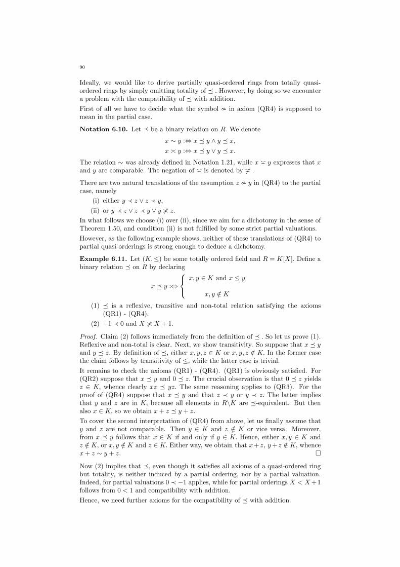
90

Ideally, we would like to derive partially quasi-ordered rings from totally quasi-ordered rings by simply omitting totality of � . However, by doing so we encountera problem with the compatibility of � with addition.

First of all we have to decide what the symbol � in axiom (QR4) is supposed tomean in the partial case.

Notation 6.10. Let � be a binary relation on R. We denote

x ∼ y :⇔ x � y ∧ y � x,x � y :⇔ x � y ∨ y � x.

The relation ∼ was already defined in Notation 1.21, while x � y expresses that xand y are comparable. The negation of � is denoted by 6� .

There are two natural translations of the assumption z � y in (QR4) to the partialcase, namely

(i) either y ≺ z ∨ z ≺ y,(ii) or y ≺ z ∨ z ≺ y ∨ y 6� z.

In what follows we choose (i) over (ii), since we aim for a dichotomy in the sense ofTheorem 1.50, and condition (ii) is not fulfilled by some strict partial valuations.

However, as the following example shows, neither of these translations of (QR4) topartial quasi-orderings is strong enough to deduce a dichotomy.

Example 6.11. Let (K,≤) be some totally ordered field and R = K[X]. Define abinary relation � on R by declaring

x � y :⇔

x, y ∈ K and x ≤ y

x, y /∈ K

(1) � is a reflexive, transitive and non-total relation satisfying the axioms(QR1) - (QR4).

(2) −1 ≺ 0 and X 6� X + 1.

Proof. Claim (2) follows immediately from the definition of � . So let us prove (1).Reflexive and non-total is clear. Next, we show transitivity. So suppose that x � yand y � z. By definition of �, either x, y, z ∈ K or x, y, z /∈ K. In the former casethe claim follows by transitivity of ≤, while the latter case is trivial.

It remains to check the axioms (QR1) - (QR4). (QR1) is obviously satisfied. For(QR2) suppose that x � y and 0 � z. The crucial observation is that 0 � z yieldsz ∈ K, whence clearly xz � yz. The same reasoning applies to (QR3). For theproof of (QR4) suppose that x � y and that z ≺ y or y ≺ z. The latter impliesthat y and z are in K, because all elements in R\K are �-equivalent. But thenalso x ∈ K, so we obtain x+ z � y + z.

To cover the second interpretation of (QR4) from above, let us finally assume thaty and z are not comparable. Then y ∈ K and z /∈ K or vice versa. Moreover,from x � y follows that x ∈ K if and only if y ∈ K. Hence, either x, y ∈ K andz /∈ K, or x, y /∈ K and z ∈ K. Either way, we obtain that x+ z, y+ z /∈ K, whencex+ z ∼ y + z. �

Now (2) implies that �, even though it satisfies all axioms of a quasi-ordered ringbut totality, is neither induced by a partial ordering, nor by a partial valuation.Indeed, for partial valuations 0 ≺ −1 applies, while for partial orderings X < X+1follows from 0 < 1 and compatibility with addition.

Hence, we need further axioms for the compatibility of � with addition.

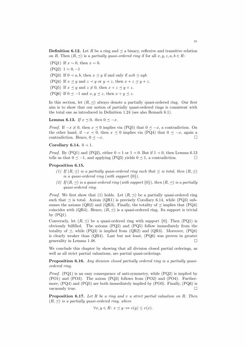
91

Definition 6.12. Let R be a ring and � a binary, reflexive and transitive relationon R. Then (R,�) is a partially quasi-ordered ring if for all x, y, z, a, b ∈ R :

(PQ1) If x ∼ 0, then x = 0.

(PQ2) 1 � 0,−1

(PQ3) If 0 ≺ a, b, then x � y if and only if axb � ayb.(PQ4) If x � y and z ≺ y or y ≺ z, then x+ z � y + z.

(PQ5) If x � y and z 6� 0, then x+ z � y + z.

(PQ6) If 0 � −1 and x, y � z, then x+ y � z.

In this section, let (R,�) always denote a partially quasi-ordered ring. Our firstaim is to show that our notion of partially quasi-ordered rings is consistent withthe total one as introduced in Definition 1.24 (see also Remark 6.1).

Lemma 6.13. If x � 0, then 0 � −x.

Proof. If −x 6� 0, then x � 0 implies via (PQ5) that 0 � −x, a contradiction. Onthe other hand, if −x ≺ 0, then x � 0 implies via (PQ4) that 0 � −x, again acontradiction. Hence, 0 � −x. �

Corollary 6.14. 0 ≺ 1.

Proof. By (PQ1) and (PQ2), either 0 ≺ 1 or 1 ≺ 0. But if 1 ≺ 0, then Lemma 6.13tells us that 0 � −1, and applying (PQ3) yields 0 � 1, a contradiction. �

Proposition 6.15.

(1) If (R,�) is a partially quasi-ordered ring such that � is total, then (R,�)is a quasi-ordered ring (with support {0}).

(2) If (R,�) is a quasi-ordered ring (with support {0}), then (R,�) is a partiallyquasi-ordered ring.

Proof. We first show that (1) holds. Let (R,�) be a partially quasi-ordered ringsuch that � is total. Axiom (QR1) is precisely Corollary 6.14, while (PQ3) sub-sumes the axioms (QR2) and (QR3). Finally, the totality of � implies that (PQ4)coincides with (QR4). Hence, (R,�) is a quasi-ordered ring. Its support is trivialby (PQ1).

Conversely, let (R,�) be a quasi-ordered ring with support {0}. Then (PQ1) isobviously fulfilled. The axioms (PQ2) and (PQ5) follow immediately from thetotality of �, while (PQ3) is implied from (QR2) and (QR3). Moreover, (PQ4)is clearly weaker than (QR4). Last but not least, (PQ6) was proven in greatergenerality in Lemma 1.48. �

We conclude this chapter by showing that all division closed partial orderings, aswell as all strict partial valuations, are partial quasi-orderings.

Proposition 6.16. Any division closed partially ordered ring is a partially quasi-ordered ring.

Proof. (PQ1) is an easy consequence of anti-symmetry, while (PQ2) is implied by(PO1) and (PO3). The axiom (PQ3) follows from (PO2) and (PO4). Further-more, (PQ4) and (PQ5) are both immediately implied by (PO3). Finally, (PQ6) isvacuously true. �

Proposition 6.17. Let R be a ring and v a strict partial valuation on R. Then(R,�) is a partially quasi-ordered ring, where

∀x, y ∈ R : x � y :⇔ v(y) ≤ v(x).

92

Proof. We obtain x ∼ 0 ⇔ v(x) = v(0) = ∞ ⇔ x = 0 by (PV1). Thus, (PQ1)applies. Clearly, 0 ≺ 1 ∼ −1, whence (PQ2) holds. Next, we verify (PQ3). So let0 ≺ a, b. If x � y, then v(y) ≤ v(x). Therefore,

v(ayb) = v(a) + v(y) + v(b) ≤ v(a) + v(x) + v(b) = v(axb),

which means axb � ayb. For the converse, suppose that 0 ≺ a, b and axb � ayb.The former yields v(a), v(b) ∈ Γv, whence we may apply that Γv is cancellative. Sov(a) + v(y) + v(b) ≤ v(a) + v(x) + v(b) implies v(y) ≤ v(x), i.e. x � y.For (PQ4), let x, y, z ∈ R such that x � y, and y ≺ z or z ≺ y, i.e. v(y) ≤ v(x) andv(z) < v(y) or v(y) < v(z). We first deal with the case v(y) < v(z). Then

v(y + z) = v(y) ≤ v(x), v(z)

by Lemma 6.4(2). Thus, v(y + z) ≤ v(x+ z) by (PV3), i.e. x+ z � y + z.Likewise, if v(z) < v(y), we obtain

v(y + z) = v(z) ≤ v(x), v(z),

so by (PV3) we get v(y + z) ≤ v(x+ z), i.e. again x+ z � y + z.

The axiom (PQ5) is vacuously true, while (PQ6) and (PV3) coincide. �

6.3. The Dichotomy of Partially Quasi-Ordered Rings.

The aim of this section is to generalise the dichotomy from the total case (Theorem1.50) to partially quasi-ordered rings (Theorem 6.28). For that purpose we showthat any partially quasi-ordered ring with −1 ≺ 0 is a division closed partiallyordered ring (Proposition 6.23), and that any partially quasi-ordered ring with0 ≺ −1 is a strictly partially valued ring (Proposition 6.27). The proof essentiallyfollows the one that we gave in Section 1.3.

Let (R,�) again always denote a partially quasi-ordered ring.

Lemma 6.18. Either −1 ≺ 0 or 0 ≺ −1.

Proof. Assume that −1 6� 0. Then 0 ≺ 1 (Corollary 6.14) implies via (PQ5) that−1 � 0, a contradiction. Hence, −1 � 0. Furthermore, (PQ1) yields −1 6∼ 0. �

We first deal with the ordered case, i.e. the case −1 ≺ 0 (see Proposition 6.23below).

Lemma 6.19. Let x ∈ R. Then x � 0 if and only if −x � 0.

Proof. Let x � 0, and assume that −x 6� 0. Then it follows from x � 0 or 0 � xthat 0 � −x or −x � 0. Hence, −x � 0, a contradiction. �

Corollary 6.20. Let x ∈ R such that x 6� 0. Then E(x) = {x}.

Proof. Let y ∈ E(x). By the previous lemma −x 6� 0, whence (PQ5) implies that0 � y − x follows from x � y, and that y − x � 0 follows from y � x. Therefore,y − x = 0 by (PQ1), i.e. y = x. Thus, E(x) = {x}. �

Lemma 6.21. Let x ∈ R, and suppose that −1 ≺ 0. Then 0 � x if and only if−x � 0. Moreover, −x ≺ x or x ≺ −x for any 0 6= x ∈ R such that x � 0.

Proof. If x � 0, then 0 � −x by Lemma 6.13. Conversely, if 0 ≺ x, then −x � 0by the assumption −1 ≺ 0 and axiom (PQ3). The moreover statement follows via(PQ1), because either −x ≺ 0 ≺ x or x ≺ 0 ≺ −x. �

Corollary 6.22. Let x ∈ R such that x � 0, and suppose that −1 ≺ 0. ThenE(x) = {x}.

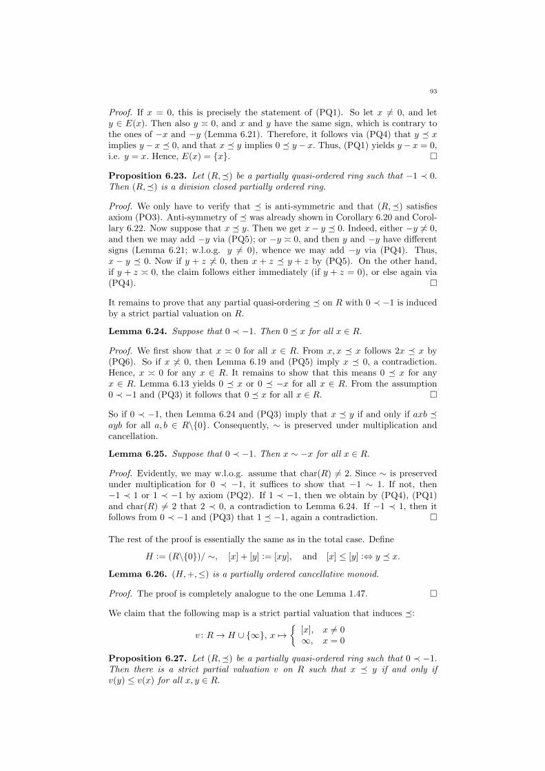
93

Proof. If x = 0, this is precisely the statement of (PQ1). So let x 6= 0, and lety ∈ E(x). Then also y � 0, and x and y have the same sign, which is contrary tothe ones of −x and −y (Lemma 6.21). Therefore, it follows via (PQ4) that y � ximplies y− x � 0, and that x � y implies 0 � y− x. Thus, (PQ1) yields y− x = 0,i.e. y = x. Hence, E(x) = {x}. �

Proposition 6.23. Let (R,�) be a partially quasi-ordered ring such that −1 ≺ 0.Then (R,�) is a division closed partially ordered ring.

Proof. We only have to verify that � is anti-symmetric and that (R,�) satisfiesaxiom (PO3). Anti-symmetry of � was already shown in Corollary 6.20 and Corol-lary 6.22. Now suppose that x � y. Then we get x− y � 0. Indeed, either −y 6� 0,and then we may add −y via (PQ5); or −y � 0, and then y and −y have differentsigns (Lemma 6.21; w.l.o.g. y 6= 0), whence we may add −y via (PQ4). Thus,x − y � 0. Now if y + z 6� 0, then x + z � y + z by (PQ5). On the other hand,if y + z � 0, the claim follows either immediately (if y + z = 0), or else again via(PQ4). �

It remains to prove that any partial quasi-ordering � on R with 0 ≺ −1 is inducedby a strict partial valuation on R.

Lemma 6.24. Suppose that 0 ≺ −1. Then 0 � x for all x ∈ R.

Proof. We first show that x � 0 for all x ∈ R. From x, x � x follows 2x � x by(PQ6). So if x 6� 0, then Lemma 6.19 and (PQ5) imply x � 0, a contradiction.Hence, x � 0 for any x ∈ R. It remains to show that this means 0 � x for anyx ∈ R. Lemma 6.13 yields 0 � x or 0 � −x for all x ∈ R. From the assumption0 ≺ −1 and (PQ3) it follows that 0 � x for all x ∈ R. �

So if 0 ≺ −1, then Lemma 6.24 and (PQ3) imply that x � y if and only if axb �ayb for all a, b ∈ R\{0}. Consequently, ∼ is preserved under multiplication andcancellation.

Lemma 6.25. Suppose that 0 ≺ −1. Then x ∼ −x for all x ∈ R.

Proof. Evidently, we may w.l.o.g. assume that char(R) 6= 2. Since ∼ is preservedunder multiplication for 0 ≺ −1, it suffices to show that −1 ∼ 1. If not, then−1 ≺ 1 or 1 ≺ −1 by axiom (PQ2). If 1 ≺ −1, then we obtain by (PQ4), (PQ1)and char(R) 6= 2 that 2 ≺ 0, a contradiction to Lemma 6.24. If −1 ≺ 1, then itfollows from 0 ≺ −1 and (PQ3) that 1 � −1, again a contradiction. �

The rest of the proof is essentially the same as in the total case. Define

H := (R\{0})/ ∼, [x] + [y] := [xy], and [x] ≤ [y] :⇔ y � x.

Lemma 6.26. (H,+,≤) is a partially ordered cancellative monoid.

Proof. The proof is completely analogue to the one Lemma 1.47. �

We claim that the following map is a strict partial valuation that induces �:

v : R→ H ∪ {∞}, x 7→{

[x], x 6= 0∞, x = 0

Proposition 6.27. Let (R,�) be a partially quasi-ordered ring such that 0 ≺ −1.Then there is a strict partial valuation v on R such that x � y if and only ifv(y) ≤ v(x) for all x, y ∈ R.

94

Proof. We prove that the map v that we just defined fulfils the claim. Evidently, vis surjective and satisfies (PV1). Now let x, y ∈ R, w.l.o.g. x, y 6= 0. Then

v(xy) = [xy] = [x] + [y] = v(x) + v(y),

so (PV2) is also fulfilled. Since 0 ≺ −1, (PV3) is precisely (PQ6). Next, we prove(PV4). So we have to show that v(z) < v(x), v(y) implies v(z) < v(x+ y), i.e. thatx, y ≺ z implies x + y ≺ z. Because of 0 ≺ −1, (PQ6) yields x + y � z. Assumefor the sake of a contradiction that x + y ∼ z. Clearly, −x ≺ −z by Lemma 6.25and the assumption that x ≺ z. It suffices to show that x+ z ≺ −z. Then we maydeduce from −x ≺ −z via (PQ4) that

z = −x+ (x+ z) � −z + (x+ z) = x,

the desired contradiction, whence (PV4) holds. So let us verify that x + z ≺ −z.We know that −z ∼ z ∼ x + y. Moreover, −x ∼ x ≺ z ∼ −z. So we have−z ∼ x+ y and −x ≺ −z, x+ y. So (PQ4) tells us that −x− z ∼ y. Hence, indeedx+ z ∼ −x− z ∼ y ≺ z ∼ −z. Thus, v is a strict partial valuation.

Moreover, if x, y ∈ R\{0}, then

x � y ⇔ [y] ≤ [x]⇔ v(y) ≤ v(x).

The same obviously applies if x = 0 or y = 0. �

Our results give rise to the following dichotomy in the sense of Fakhruddin:

Theorem 6.28. Let R be a ring and � a binary relation on R. Then (R,�) isa partially quasi-ordered ring if and only if it is either a division closed partiallyordered ring or there is a strict partial valuation v on R such that x � y if and onlyif v(y) ≤ v(x) for all x, y ∈ R.

Proof. This is an immediate consequence of Proposition 6.16, Proposition 6.17,Lemma 6.18, Proposition 6.23 and Proposition 6.27. �

6.4. Extending Partial Quasi-Orderings.

In this section we introduce quadratic partially quasi-ordered rings (Definition 6.29).Theorem 6.28 yields the dichotomy that any quadratic partially quasi-ordered fieldis either a preordered field or a strictly partially valued field (Theorem 6.31). Fromthis result we derive that any quadratic partial quasi-ordering on a field K extendsto a quasi-ordering on K (Theorem 6.34).

Definition 6.29. We call a partially quasi-ordered ring (R,�) quadratic, if 0 � x2for all x ∈ R.

Example 6.30.

(1) Any strict partial valuation on a ring R is a quadratic partial quasi-ordering.This was shown in Proposition 6.17 and Lemma 6.24.

(2) The partial ordering from Example 6.9(2) is quadratic.

(3) Any quadratic partial ordering on a division ring is a preordering and viceversa, where in this section preordering shall always mean proper quadraticpreordering. This follows from Theorem 6.28 and the fact that preorderingsover division rings are division closed (see Example 6.9(3)).

As an immediate consequence of Theorem 6.28 and Example 6.30(1) and (3), weobtain the following dichotomy:

95

Theorem 6.31. Let K be a field and � a binary relation on K. Then (K,�) is aquadratic partially quasi-ordered field if and only if it is either a preordered field orthere is a strict partial valuation v on K such that x � y if and only if v(y) ≤ v(x)for all x, y ∈ K.

In what follows let (K,�) always denote a quadratic partially quasi-ordered field.We define the set

Σ� := {�′⊆ K2 : �′ is a quadratic partial quasi-ordering s.t. ∀x, y ∈ K :

x � y ⇒ x �′ y and x ≺ y ⇒ x ≺′ y}.We claim that Σ� admits a maximal element and that any of its maximal elements isa quasi-ordering on K extending � . For the proof, we need the notion of dominanceof local rings.

Definition 6.32. Let A and B be local rings with maximal ideals mA, respectivelymB . Then B dominates A, written A ≤ B, if

A ⊆ B andmB ∩A = mA.

If K is a field and v a strict partial valuation on K, then Kv = {x ∈ K : v(x) ≥ 0}is a local ring with maximal ideal Iv = {x ∈ K : v(x) > 0} ([73, Proposition 1.1.6]).Moreover, the valuation rings on K are precisely the maximal local subrings of Kw.r.t. ≤ . (cf. [57, Theorem 10.2]).

Proposition 6.33. Let K be a field, and let v and w be strict partial valuationson K. The following two conditions are equivalent:

(1) (i) If v(x) ≤ v(y), then w(x) ≤ w(y) for all x, y ∈ K and(ii) If v(x) < v(y), then w(x) < w(y) for all x, y ∈ K.

(2) Kw dominates Kv.

Proof. We first show that (1) implies (2). From (i) it is easy to see that Kv ⊆ Kw.Now let x ∈ Iw∩Kv. Then v(x) ≥ 0. If v(x) = 0, then w(x) = 0 by (i), contradictingthe fact that x ∈ Iw. Hence, v(x) > 0, i.e. x ∈ Iv. Conversely, let x ∈ Iv ⊆ Kv.Then v(x) > 0, whence also w(x) > 0 by (ii). Thus, x ∈ Iw ∩Kv.

For the converse, first suppose that v(x) < v(y). Then y/x ∈ Iv ⊆ Iw by (2).Therefore, w(x) < w(y), so (ii) is satisfied. Next, suppose that v(x) ≤ v(y). Thecase v(x) < v(y) was already dealt with, so we may assume that v(x) = v(y). Thenx/y and y/x ∈ Kv ⊆ Kw. Consequently, also w(x) = w(y). �

By exploiting the dichotomy from Theorem 6.31, we may prove:

Theorem 6.34. Let (K,�) be a quadratic partially quasi-ordered field. Then �extends to a quasi-ordering on K.

Proof. Consider the set Σ� from above. Obviously, �∈ Σ, whence Σ� 6= ∅. Wepartially order Σ� by inclusion. For any chain (�i)i∈I in Σ�, it is routine to checkthat

⋃i∈I �i ∈ Σ is an upper bound for this chain. Hence, Zorn’s lemma states

that Σ� has a maximal element, say �′ . By definition of Σ�, we know that �′ isa quadratic partial quasi-ordering on K extending � .If −1 ≺ 0, then � is a preordering and �′ a maximal preordering containing � .Hence, �′ is an ordering on K extending � (cf. e.g. [64, Proposition 4.1.4]).

If 0 ≺ −1, then � and �′ are induced by strict partial valuations on K, say �=�vand �′=�w for some strict partial valuations v, w on K ([73, Proposition 1.1.6]).By definition of Σ� and Proposition 6.33, the valuation ringKv is dominated byKw.We show that Kw is a maximal element under the dominance relation. Then Kw isa valuation ring ([57, Theorem 10.2]) containing Kv, whence w is a valuation on K

96

extending v. So let A be a local ring dominating Kw. Then A also dominates Kv.However, by Proposition 6.33, the choice of �′ and the fact that local subrings of Kare in bijective correspondence with strict partial valuations on K ([73, Proposition1.1.6]), we know that Kw is a maximal element among all local rings dominatingKv, whence A = Kw. Thus, w is a valuation on K extending v. �

Remark 6.35.

(1) We considered fields in order to exploit the fact that maximal local rings arevaluation rings. Moreover, the proof of Theorem 6.34 relies on the resultthat for division rings there is a bijective correspondence between strictpartial valuations and stable local subrings (cf. [73, Proposition 1.1.6]).

(2) For an alternative, possibly uniform proof of Theorem 6.34 it would sufficeto show that the maximal element �′ of Σ� is total. We may then concludeby applying Proposition 6.15.

97

7. Quasi-Real Closed Fields and Quantifier Elimination

In the present chapter we first introduce quasi-real closed fields (Definition 7.2, seealso Proposition 7.8), that way subsuming the classes of algebraically closed fieldsand real closed fields (Corollary 7.4). By referring to the respective results for alge-braically closed valued fields and real closed valued fields, we then deduce that thetheory of quasi-real closed fields adjoined with a non-trivial compatible valuationadmits quantifier elimination (Theorem 7.9). As an immediate consequence, weobtain that this theory is model complete. Moreover, it is the model companion ofthe theory of quasi-ordered fields adjoined with a non-trivial compatible valuation(Corollary 7.11).

To begin with, we introduce a notion of quasi-real closed fields. This is achievedby generalising the characterisation of real closed fields from Artin and Schreier.

Remark 7.1. ([4]) An ordered field (K,P ) is real closed if and only if one of thefollowing equivalent conditions is fulfilled:

(1) P does not extend to any proper algebraic extension of K.

(2) (K,P ) satisfies:

(i) every a ∈ P has a square root in K,

(ii) every polynomial f ∈ K[X] of odd degree has a root in K.

We will exploit both of these conditions. The first condition is suitable to develop anotion of quasi-real closure, while (2) has the crucial advantage that it is expressiblein the language of quasi-ordered fields.

Definition 7.2. A quasi-ordered field (K,�) is called quasi-real closed, if � doesnot extend to any proper algebraic extension of K.

Lemma 7.3. Let K be a field. The following are equivalent:

(1) K is algebraically closed,

(2) (K, v) is quasi-real closed for some valuation v on K,

(3) (K, v) is quasi-real closed for any valuation v on K.

Proof. If K is algebraically closed, then K admits no proper algebraic extension,whence (K, v) is quasi-real closed for any valuation v on K. Consequently, (1)implies (3). Moreover, since any field admits a valuation, clearly (3) implies (2).

Finally, suppose that (2) holds. Note that the valuation v on K extends to anyfield extension L of K by Chevalley’s Extension Theorem (cf. [18, Theorem 3.1.1]).Since (K, v) is quasi-real closed, this means that K does not admit any properalgebraic extension, i.e. that K is algebraically closed. Thus, (2) implies (1). �

Corollary 7.4. A quasi-ordered field (K,�) is quasi-real closed if and only if �is either an ordering and (K,�) a real closed field, or � is a valuation and K analgebraically closed field.

Proof. This follows from the dichotomy of quasi-ordered fields (Theorem 1.23),Remark 7.1(1) (if � is an ordering), and Lemma 7.3 (if � is a valuation). �

Definition 7.5. Let (K,�) be a quasi-ordered field. A quasi-ordered field (L,�′)is called a quasi-real closure of (K,�), if

(1) (L,�′) is a quasi-real closed field,

(2) L|K is an algebraic field extension,

(3) �′ is an extension of �, i.e. K ∩ �′=� .

98

Proposition 7.6. Any quasi-ordered field (K,�) admits a quasi-real closure.

Proof. Applying Zorn’s lemma to the set

{(L,�′) : (L,�′) is a quasi-ordered field, L|K algebraic,K ∩ �′=�},

partially ordered by

(L1,�′1) ≤ (L2,�′2) :⇔ L1 ⊆ L2 and L1 ∩ �′2 = �′1,

yields a quasi-ordered field (L,�′) that is a maximal algebraic field extension of(K,�). Hence, (L,�′) is quasi-real closed and a quasi-real closure of (K,�). �

Exploiting Fakhruddin’s dichotomy (Theorem 1.23), we could further deduce thatthe quasi-real closure of a quasi-ordered field is unique up to K-isomorphism.

Our next aim is to establish that quasi-real closed fields adjoined with a compatiblevaluation admit quantifier elimination. To this end, we refer to the respective resultsthat are known for real closed valued and algebraically closed valued fields.

Theorem 7.7. (cf. [63, Theorem 4.4.2, Theorem 4.5.1]).

(1) The theory of algebraically closed fields adjoined with a non-trivial valuationv admits quantifier elimination in the language of fields adjoined with �v .

(2) The theory of real closed fields adjoined with a non-trivial compatible valu-ation v admits quantifier elimination in the language of ordered fields ad-joined with �v .

In order to subsume these results, we now work with a different characterisation ofquasi-real closed fields.

Proposition 7.8. A quasi-ordered field (K,�) is quasi-real closed if and only ifthe following two conditions are satisfied:

(i) every x ∈ K with 0 � x has a square root in K.

(ii) every polynomial f ∈ K[X] of odd degree has a root in K.

Proof. If � is an ordering, this follows from Remark 7.1(2) and Corollary 7.4. Solet � be a valuation. If (K,�) is quasi-real closed, then K is algebraically closedaccording to Corollary 7.4, whence (i) and (ii) are both fulfilled.

Conversely, suppose that (i) and (ii) hold. Since � is a valuation, we obtain by (i)that all elements in K have a square root in K. In particular,

√−1 ∈ K. Along with

condition (ii), this implies that K is algebraically closed according to [70, Theorem2]. Hence, (K,�) is quasi-real closed. �

Proposition 7.8 enables us to formalise quasi-real closed fields in a first order lan-guage. As our language of quasi-ordered fields with a compatible valuation v we fixL = {+, ·,−,�,�v, 0, 1}. Moreover, we denote by Σ the following set of L-sentences:

(1) the axioms that (K,+, ·,−) is a field.

(2) the axioms that (K,�) is a quasi-real closed field.

(3) the axioms that (K,�v) is a non-trivially valued field.

(4) the following sentences that determine the relationship of � and �v:(i) 0 ≺ −1→ (∀x, y : 0 � x � y ↔ x �v y)

(ii) −1 ≺ 0→ (∀x, y : 0 � x � y → x �v y)

The last two sentences state that �=�v if � is a valuation, and that v is �-compatible if � is an ordering. That way, we have unified the languages of realclosed valued fields and algebraically closed valued fields (see Theorem 7.7).

99

We refer to the theory of Σ as the theory of quasi-real closed fields adjoined with anon-trivial compatible valuation. Exploiting the dichotomy of quasi-ordered fieldsand Theorem 7.7, we obtain:

Theorem 7.9. The theory of quasi-real closed fields adjoined with a non-trivialcompatible valuation admits quantifier elimination.

Proof. Let Σ denote this theory. Then any model of Σ is either an algebraicallyclosed field adjoined with a non-trivial valuation or a real closed field adjoined witha non-trivial compatible valuation (Corollary 7.4). Therefore, the claim followsfrom the fact that these two classes admit quantifier elimination, see [63, Theorem4.4.2], respectively [63, Theorem 4.5.1]. �

Definition 7.10. Let Σ ⊆ Sent(L) for a given language L. A set Σ∗ ⊆ Sent(L) iscalled a model companion of Σ, if

(1) every model of Σ∗ is a model of Σ,

(2) every model of Σ can be extended to a model of Σ∗,

(3) Σ∗ is model complete.

Corollary 7.11. (cf. [63, Corollary 4.4.3], [63, Corollary 4.5.4])The theory of quasi-real closed fields adjoined with a non-trivial compatible valuationis model complete. It is the model companion of the theory of quasi-ordered fieldsadjoined with a non-trivial compatible valuation.

Proof. The model completeness follows immediately from the quantifier eliminationthat we obtained in Theorem 7.9. It remains to show that condition (2) of Definition7.10 holds in our setting, both (1) and (3) being obviously satisfied.

So let (K,�,�v) be some quasi-ordered field adjoined with a non-trivial compatiblevaluation, and let (L,�′) be a quasi-real closure of (K,�) (Proposition 7.6). Then(L,�′) is a quasi-real closed field. Moreover, L|K is algebraic, whence Proposition3.25 yields a unique extension �′ν of �v from K to L such that ν is compatiblewith �′ . If � is a valuation (i.e. �v =�), then the uniqueness tells us that also�′ν =�′ . Furthermore, ν is non-trivial since v is non-trivial. Hence, (L,�′,�′ν)is an extension of (K,�,�v) and a model of the theory of quasi-real closed fieldsadjoined with a non-trivial compatible valuation. �

Remark 7.12.

(1) The theory of quasi-real closed fields adjoined with a non-trivial compati-ble valuation is easily seen not to be complete. For example the sentence∃x : x2+1 = 0 is false for any real closed field, but true for any algebraicallyclosed field. Consequently, not all models of our theory Σ are elementaryequivalent.

(2) Our notion of quasi-real closure might also provide a partly uniform proofof Theorem 7.9. In fact, the existence (see Proposition 7.6) and uniquenessof the algebraic closure, respectively real closure, plays an important rolein the proof of [63, Theorem 4.4.2], respectively [63, Theorem 4.5.1].

100

Acknowledgements

First and foremost, I would like to thank my supervisor Prof. Dr. Salma Kuhlmannfor proposing this project to me and for her dedicated support through all theseyears. I am especially grateful for her inspiring me with her passion and enthusiasm,and for her continuously encouraging me to share my research results with others,be it by giving talks and presenting posters at various conferences and seminars,or by submitting these results to journals. Last but not least, she supported myparticipation at numerous events and helped me to get in touch with many otherresearchers.

Furthermore, I wish to thank Prof. Dr. Victor Vinnikov, who I could always ask foradvice on problems regarding non-commutative algebra. Most notably, he enabledme to participate in a workshop on free noncommutative functions at the FieldsInstitute in Toronto.

Besides, I am very grateful to both, Dr. Nicolaas Verhulst and Dr. Tom-Lukas Kriel.With Nicolaas I had various helpful discussions on the notions of partial valuationsand partial quasi-orderings. With Tom I was already very good friends long beforeI started my Ph.D., which may be the reason why I considered him such a pleasantoffice mate. Moreover, every now and then he gave me some helpful advice on myresearch problems.

Last but not least I would like to express my gratitude to all those people thatsupported me during these years on a non-mathematical level. Foremost, I wouldlike to mention my family, in particular my mother Gaby Wetzel and my brotherStefan Muller. It is reassuring to know that they always stand by me and wouldimmediately offer me their help whenever needed. Moreover, I wish to thank nu-merous of my former roommates from the Thomas Blarer Haus, where I not onlylived during all of my bachelor’s and master’s studies, but also for two thirds ofmy Ph.D. These guys did a great job in not letting me get too worked up aboutmathematics, some of them still being good friends of mine.

Finally, I am grateful to my former schoolmate Christopher Trondle. Right after thetwo of us finished high school, we had a random encounter at the public swimmingpool in my home town Bad Sackingen. Back then, Christopher said to me thatI would certainly study mathematics, would I not? As a matter of fact that wasan idea that strangely enough had not come to my mind before. Even though noone knows what would have happened otherwise, I am tempted to call this someexcellent advice. Thank you, Christopher!

101

References

[1] J. Alajbegovic and J. Mockor, Approximation Theorems in Commutative Algebra, Classical

and Categorical Methods, Mathematics and Its Applications (East European Series) 59, Kluwer

Academic Publishers Group, Dordrecht, 1992.

[2] S. Anscombe, P. Dittmann and A. Fehm, Approximation theorems for spaces of localities, to

appear in Mathematische Zeitschrift, 2020.

[3] E. Artin, Uber die Zerlegung definiter Funktionen in Quadrate, Abh. Math. Sem. Univ. Ham-

burg 5 (1927), 100-115.

[4] E. Artin and O. Schreier, Algebraische Konstruktion reeller Korper, Abh. Math. Sem. Univ.

Hamburg 5 (1927), 85-99.

[5] E. Artin and G. Whaples, Axiomatic characterization of fields by the product formula for

valuations, Bull. Amer. Soc. 51 (1945), 469-492.

[6] R. Baer, Uber nicht-archimedisch geordnete Korper, Sitz. Ber. der Heidelberger Akad. Abh. 8

(1927), 3-13.

[7] E. Becker, Partial orders on a field and valuation rings, Comm. Algebra 7 (1979),1933-1976.

[8] J. Bochnak, M. Coste and M.-F. Roy, Geometrie Algebrique Reelle, Ergeb. Math. Grenzgebiete

(3rd series) 12, Springer, Berlin Heidelberg New York, 1987.

[9] N. Bourbaki, Algebre commutative, Chap. 1-7, Hermann Paris, 1961-1965.

[10] M. Coste and M.-F Roy, La topologie du spectre reel, Contemp. Math. 8 (1982), 27-59.

[11] T. Craven, The Boolean space of orderings of a field, Trans. Amer. Math. Soc. 209 (1975),

225-235.

[12] T. Craven, The topological space of orderings of a rational function field, Duke Math. J. 41

(1974), 339-347.

[13] M. Dickmann, N. Schwartz and M. Tressl, Spectral Spaces, New Mathematical Monographs

35, Cambridge Univ. Press, Cambridge, 2019.

[14] A. Dress, On orderings and valuations of fields, Geom. Dedicata 6 (1977), 259-266.

[15] L. van den Dries, Tame Topology and O-minimal Structures, London Math. Soc. LNS 248,

Cambridge Univ. Press, Cambridge, 1988.

[16] I. Efrat, Valuations, Orderings and Milnor K-Theory, Mathematical Surveys and Mono-

graphs 124, American Mathematical Society, 2006.

[17] N. Eggert, Dependence of valuations, J. Reine Angew. Math. 253 (1972), 186-192.

[18] A. J. Engler and A. Prestel, Valued Fields, Springer Monographs in Mathematics, Springer-

Verlag, Berlin, 2005.

[19] S. M. Fakhruddin, Quasi-ordered fields, J. Pure Appl. Algebra 45 (1987), 207-210.

[20] L. Fuchs, Teilweise geordnete algebraische Strukturen, Studia Mathematica-Mathematische

Lehrbucher Band XIX, Ubersetzt aus dem Englischen von Eva Vas Vandenhoeck & Ruprecht,

Gottingen 1966.

[21] R. Gilmer, Multiplicative Ideal Theory, Queen’s Papers in Pure and Applied Mathematics

90, Queen’s University, Kingston, ON, 1992.

[22] J. Grater, Der allgemeine Approximationssatz fur Manisbewertungen, Monatsh. Math. 93

(1982), 277–288.

[23] J. Grater, Der Approximationssatz fur Manisbewertungen, Arch. Math. (Basel) 37 (1981),

335–340.

[24] M. Griffin, Valuations and Prufer Rings, Can. J. Math. 26 (1974), 412-429.

[25] H. Hahn, Uber die nichtarchimedischen Großensysteme, S.-B. Akad. Wiss. Wien, IIa, 116

(1907), 601-655.

[26] D.K. Harrison, Finite and infinite primes for rings and fields, Mem. Amer. Math. Soc. 68,

1966.

102

[27] M. Hochster, Prime ideal structure in commutative rings, Trans. Amer. Math. Soc. 142

(1969), 43-60.

[28] R. Huber, Bewertungsspektrum und rigide Geometrie, Regensburger Mathematische Schriften

23, Universitat Regensburg, FB Mathematik, Regensburg, 1993.

[29] R. Huber and M. Knebusch, On Valuation Spectra, Contemp. Math. 155 (1994), 167-206.

[30] I. Kaplansky, Commutative Rings, Allyn and Bacon, Boston, 1970.

[31] N. Kehayopulu and M. Tsingelis, The embedding of some ordered semigroups into ordered

groups, Semigroup Forum 60 (200), 344-350.

[32] M. Knebusch and T. Kaiser, Manis Valuations and Prufer Extensions II, LNM 2103,

Springer, 2014.

[33] M. Knebusch and C. Scheiderer, Einfuhrung in die reelle Algebra, Vieweg Studium: Auf-

baukurs Mathematik 63, Friedr. Vieweg & Sohn, Braunschweig, 1989.

[34] M. Knebusch and D. Zhang, Convexity, valuations and Prufer extensions in real algebra,

Doc. Math. 10 (2005), 1-109.

[35] M. Knebusch and D. Zhang, Manis Valuations and Prufer Extensions I - A New Chapter in

Commutative Algebra, LNM 1791, Springer-Verlag Berlin, 2002.

[36] J.-L. Krivine, Anneaux preordonnes, J. Analyse Math. 12 (1964), 307–326.

[37] W. Krull, Allgemeine Bewertungstheorie, J. Reine Angew. Math. 167 (1932), 160-196.

[38] F.-V. Kuhlmann, Book on Valuation Theory, in preparation.

[39] S. Kuhlmann and G. Lehericy, A Baer-Krull theorem for quasi-ordered groups, Order 35

(2018), 283-291.

[40] S. Kuhlmann, M. Matusinski and F. Point, The valuation difference rank of a quasi-ordered

difference field, Groups, modules, and model theory - surveys and recent developments, 399-414,

Springer, Cham, 2017.

[41] S. Kuhlmann and S. Muller, Compatibility of quasi-orderings and valuations: a Baer-Krull

theorem for quasi-ordered rings, Order 36 (2019) 249–269.

[42] J. Kurschak, Uber Limesbildung und allgemeine Korpertheorie, J. Reine Angew. Math. 142

(1913), 211-253.

[43] T. Y. Lam, A First Course in Noncommutative Rings, Second edition, Graduate texts in

mathematics 131, Springer-Verlag, New York, 1991.

[44] T. Y. Lam, Exercises in Classical Ring Theory, Second edition, Problem Books in Mathe-

matics, Springer-Verlag, New York, 2003.

[45] T. Y. Lam, Lectures on Modules and Rings, Graduate Texts in Mathematics 189, Springer-

Verlag, New York, 1998.

[46] T. Y. Lam, Orderings, Valuations and Quadratic Forms, CBMS Regional Conf. Ser. Math.

52, published by AMS, Providence, 1983.

[47] G. Lehericy, A structure theorem for abelian quasi-ordered groups, J. Pure Appl. Algebra

223 (2019), 3238-3261.

[48] K. H. Leung, M. Marshall and Y. Zhang, The Real Spectrum of a Noncommutative Ring, J.

Algebra 198 (1997), 412-427.

[49] W. J. Lewis and J. Ohm, The Ordering of Spec R, Can. J. Math. 28 (1976), 820-835.

[50] W. J. Lewis, The Spectrum of a Ring as a Partially Ordered Set, J. Algebra 25 (1973),

419-434.

[51] H. van Maaren, Pseudo-ordered fields, Nederl. Akad. Wetensch. Proc. Ser. A 77 (1974),

463-476.

[52] M. Manis, Valuations on a commutative ring, Proc. Amer. Math. Soc. 20 (1969), 193-198.

[53] M. Marshall, Orderings and Real Places on Commutative Rings, J. Algebra 140 (1991),

484-501.

[54] M. Marshall, Spaces of Orderings and Abstract Real Spectra, LNM 1636, Springer-Verlag,

Berlin, 1996.

103

[55] M. Marshall and Y. Zhang, Orderings and valuations on twisted polynomial rings, Comm.

Algebra 28 (2000), 3763-3776.

[56] M. Marshall and Y. Zhang, Orderings, Real Places, and Valuations on Noncommutative

Integral Domains, J. Algebra 212 (1999), 190-207.

[57] H. Matsumura, Commutative ring theory, translated from the Japanese by M. Reid, Second

edition, Cambridge Studies in Advanced Mathematics, 8. Cambridge Univ. Press, Cambridge,

1989.

[58] M. Matusinski and S. Muller, Quasi-real closed fields and quantifier elimination, to appear

in C. R.Acad.Sci.Paris, arXiv Number 2005.12681, 2020.

[59] S. Muller, On the Tree Structure of Orderings and Valuations on arbitrary unital Rings, to

appear in Ark. Mat., arXiv Number 1807.11251, 2018.

[60] S. Muller, Quasi-ordered rings - A uniform approach to orderings and valuations, Comm.

Algebra 46 (2018), 4979-4985.

[61] V. Powers, Valuations and Higher Level Orders in Commutative Rings, J. Algebra 172

(1995), 255-272.

[62] A. Prestel, Lectures on Formally Real Fields, LNM 1093, Springer-Verlag, Berlin, 1984.

[63] A. Prestel and C. Delzell, Mathematical Logic and Model Theory - A Brief Introduction,

Universitext, Springer, London, 2011.

[64] A. Prestel and C. Delzell, Positive Polynomials. From Hilbert’s 17th problem to real algebra,

Springer Monographs in Mathematics, Springer-Verlag, Berlin, 2001.

[65] M. de la Puente, Riemann surfaces of a ring and compactifications of semi-algebraic sets,

Ph.D. Thesis, Stanford University, 1988.

[66] M. Putinar, Positive Polynomials on Compact Semi-Algebraic Sets, Indiana Univ. Math. J.

42 (1993), 969–984.

[67] P. Roquette, History of valuation theory, Part I, in: F.-V. Kuhlmann et al., eds., Valuation

Theory and its Applications, vol. I, Fields Inst. Commun. 32 (2002), 291-355.

[68] K. Schmudgen, The K-moment problem for compact semi-algebraic sets, Math. Ann. 289

(1991), 203–206.

[69] A. Seidenberg, A new decision method for elementary algebra, Ann. of Math. 60 (1954),

365-374.

[70] J. Shipman, Improving the Fundamental Theorem of Algebra, Math. Intelligencer 29 (2007),

9-14.

[71] A. Tarski, A decision method for elementary algebra and geometry, RAND Corp. 1948, UC

Press, Berkeley, 1951; announced in Ann. Soc. Pol. Math. 9 (1931), 206-207; and in Fund. Math

17 (1931), 210-239.

[72] K. G. Valente, On Orderings, Valuations and 0-Primes of a Commutative Ring, Rocky Moun-

tain J. Math. 19 (1989), 973-984.

[73] N. Verhulst, Non-commutative generalisations of valuations and places, Ph.D. thesis, Uni-

versiteit Antwerpen.

[74] D. Zhang, The M-Valuation Spectrum of a Commutative Ring, Comm. Algebra 30 (2002),

2883-2896.

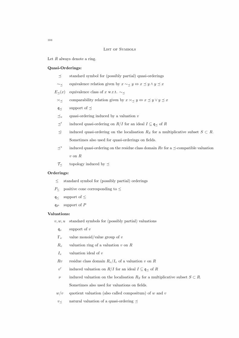
104

List of Symbols

Let R always denote a ring.

Quasi-Orderings:

� standard symbol for (possibly partial) quasi-orderings

∼� equivalence relation given by x ∼� y ⇔ x � y ∧ y � x

E�(x) equivalence class of x w.r.t. ∼�

�� comparability relation given by x �� y ⇔ x � y ∨ y � x

q� support of �

�v quasi-ordering induced by a valuation v

�′ induced quasi-ordering on R/I for an ideal I ⊆ q� of R

E induced quasi-ordering on the localisation RS for a multiplicative subset S ⊂ R.

Sometimes also used for quasi-orderings on fields.

�∗ induced quasi-ordering on the residue class domain Rv for a �-compatible valuation

v on R

T� topology induced by �

Orderings:

≤ standard symbol for (possibly partial) orderings

P≤ positive cone corresponding to ≤

q≤ support of ≤

qP support of P

Valuations:

v, w, u standard symbols for (possibly partial) valuations

qv support of v

Γv value monoid/value group of v

Rv valuation ring of a valuation v on R

Iv valuation ideal of v

Rv residue class domain Rv/Iv of a valuation v on R

v′ induced valuation on R/I for an ideal I ⊆ q� of R

ν induced valuation on the localisation RS for a multiplicative subset S ⊂ R.

Sometimes also used for valuations on fields.

w/v quotient valuation (also called compositum) of w and v

v� natural valuation of a quasi-ordering �

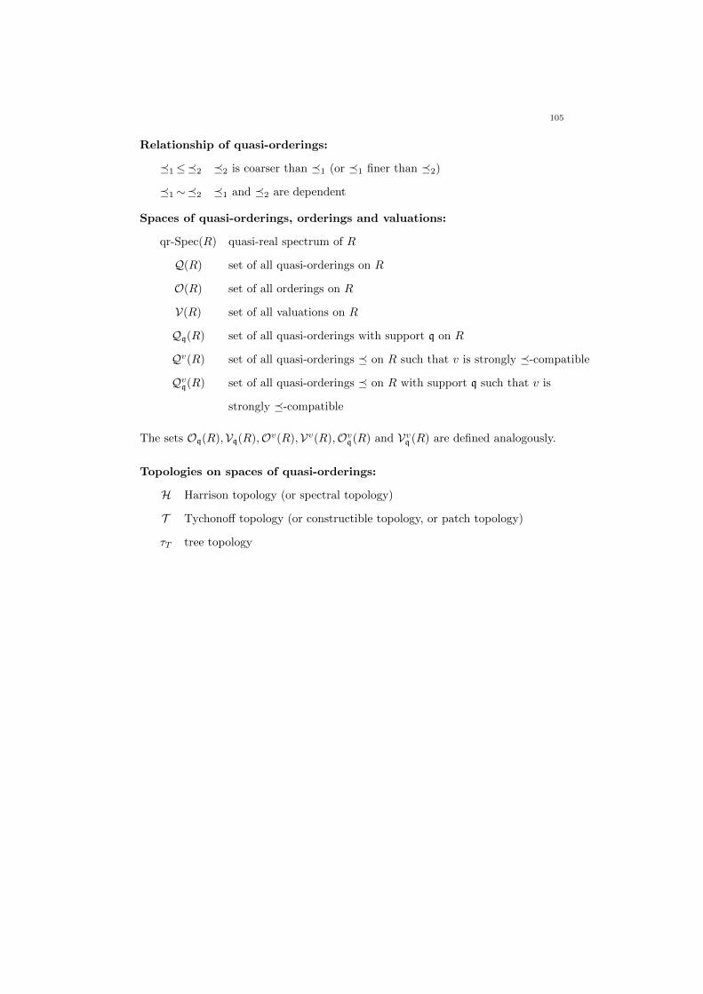
105

Relationship of quasi-orderings:

�1≤�2 �2 is coarser than �1 (or �1 finer than �2)

�1∼�2 �1 and �2 are dependent

Spaces of quasi-orderings, orderings and valuations:

qr-Spec(R) quasi-real spectrum of R

Q(R) set of all quasi-orderings on R

O(R) set of all orderings on R

V(R) set of all valuations on R

Qq(R) set of all quasi-orderings with support q on R

Qv(R) set of all quasi-orderings � on R such that v is strongly �-compatible

Qvq(R) set of all quasi-orderings � on R with support q such that v is

strongly �-compatible

The sets Oq(R),Vq(R),Ov(R),Vv(R),Ovq(R) and Vvq (R) are defined analogously.

Topologies on spaces of quasi-orderings:

H Harrison topology (or spectral topology)

T Tychonoff topology (or constructible topology, or patch topology)

τT tree topology