electronics

Article

A Torque Vectoring Control for Enhancing VehiclePerformance in Drifting

Michele Vignati * , Edoardo Sabbioni and Federico Cheli

Politecnico di Milano, Department of Mechanical Engineering, via la Masa 1, 20156 Milan (MI), Italy;edoardo.sabbioni@polimi.it (E.S.); federico.cheli@polimi.it (F.C.)* Correspondence: michele.vignati@polimi.it; Tel.: +39-02-2399-8466

Received: 30 October 2018; Accepted: 3 December 2018; Published: 5 December 2018�����������������

Abstract: When dealing with electric vehicles, different powertrain layouts can be exploited.Among them, the most interesting one in terms of vehicle lateral dynamics is represented by theone with independent electric motors: two or four electric motors. This allows torque-vectoringcontrol strategies to be applied for increasing vehicle lateral performance and stability. In this paper,a novel control strategy based on torque-vectoring is used to design a drifting control that helpsthe driver in controlling the vehicle in such a condition. Drift is a particular cornering condition inwhich high values of sideslip angle are obtained and maintained during the turn. The controller isapplied to a rear-wheel drive race car prototype with two independent electric motors on the rearaxle. The controller relies only on lateral acceleration, yaw rate, and vehicle speed measurement.This makes it independent from state estimators, which can affect its performance and robustness.

Keywords: torque-vectoring; drift; power-slide; vehicle dynamics; electric vehicles

1. Introduction

In recent years, the interest in hybrid and electric vehicles has led to the possibility of redesigningseveral vehicle subsystems, particularly the powertrain, which can be redesigned to exploit all thefeatures offered by electric motors [1].

Moreover, the use of multiple motors on the vehicle allows, for example, the allocation of onemotor per wheel. This makes it possible to control each wheel independently, and it becomes easy toapply torque-vectoring-based control strategies ([2]).

Torque-vectoring control (TVC) consists of applying different longitudinal forces on the wheels ofthe same axle. This results in a yaw moment that can be used to control the vehicle’s lateral dynamics.

In particular, this paper presents a new control strategy: a torque-vectoring control strategyaiming to help the driver in controlling the vehicle during drift maneuvers.

Drift, or power-slide, is a particular condition of the vehicle in which high values of sideslipangle can be achieved and maintained during the turn. Usually, drift is associated with a counter-steerwhich means that the steering angle is opposite to the direction of the turn and the rear tires are almostsaturated, see Figure 1. Such a condition is usually an unstable vehicle condition that can be controlledby the driver via the steering wheel and the accelerator pedal. This condition is mainly used by rallydrivers in order to perform high-curvature turns.

Hoffman and others ([3]) have explored control strategies for high-sideslip cornering through acombination of experimental data analysis and control design to drift a vehicle. This work suggeststhat the coordination of steering and rear drive torque inputs plays a critical role in drifting. A primaryunderstanding of how the available steering and drive force inputs can be used to control the vehiclestate to a drift equilibrium was necessary for the discussion. This can be done by comparing the direct

Electronics 2018, 7, 394; doi:10.3390/electronics7120394 www.mdpi.com/journal/electronics

Electronics 2018, 7, 394 2 of 18

effect of the steering and rear drive force inputs upon the vehicle’s dynamics for different types ofoperating conditions.

Figure 1. Typical cornering vs. drift cornering.

The analysis in [4] reveals that the rear drive force input has a greater direct influence on thelateral dynamics at drift equilibria than at typical cornering equilibrium. This is due to the couplingbetween lateral and longitudinal forces on the rear tires, which is especially important in drift wherethe tire experiences high slippages κ together with high slip angles due to large values of sideslip angleβ. In fact, direct lateral control authority through the rear drive force input is comparable to that of thesteering input when β is large.

In light of the fact that steering and rear drive force can both be used to control the lateral dynamicsof a vehicle around a drift equilibrium, different steering-based and drive force-based controllers werestudied in order to highlight the capabilities and limitations of each input.

Velenis [5] designed a sliding-mode control scheme stabilizing steady-state cornering conditions,using only longitudinal control inputs (i.e., accelerating/braking torques applied at the front and/orrear wheels).

Both Edelmann et al. [6] and Velenis et al. [7] developed controllers for a rear-wheel drive (RWD)vehicle by coordinating front steering and rear drive torques in order to drift a vehicle.

In both cases, the controller was designed by linearizing a vehicle model at one of its driftequilibria and using full state feedback to compute steering and rear drive torque inputs thatstabilize the linearized model in closed-loop. Gain selection was accomplished using multiple-inputmultiple-output (MIMO) design techniques, specifically pole placement in [6] and linear quadraticregulator (LQR) techniques in [7]. When implemented on nonlinear systems, both controllerssuccessfully stabilized a neighborhood around the desired equilibrium, although their design couldonly tolerate moderate disturbances.

Werling [8] presented a power-slide control strategy for rear-wheel-driven sports cars capable oftracking a course angle reference signal while stabilizing large vehicle sliding angles. Owing to smallslip angles at the front wheels compared to the ones at the sliding rear wheels and the precise yaw ratemeasurement, a fairly simple control strategy can be proposed. It assigns the course angle trackingto the electric power steering. The remaining yaw motion is regulated by a first-order sliding-modethrottle controller, so that the vehicle drifts steadily at a given slip angle. The main advantage of theproposed algorithm is that mainly geometric vehicle parameters and only the measurements of thestandard stock sensors are required. The performance was demonstrated on a drive-by-wire capableseries production car. The problem associated with this type of controller is that it modifies the driverinputs, which can lead to undesired driver feeling.

Electronics 2018, 7, 394 3 of 18

Nakano [9] proposed a very simple control strategy based on a two-level controller for a remotelydriven car with four independent motors. The first level controller tracks the references of speed andyaw rate, while the second level tracks a reference sideslip angle.

The present paper proposes a different approach. The aim of the proposed control strategy is nolonger to modify driver inputs by summing the controller contribution, but to assist the driver duringa drift maneuver by applying a suitable yaw moment to the vehicle thanks to torque-vectoring (TV)applied to the rear-driven wheels. As an additional feature, the proposed control is only based onmeasured quantities (i.e., lateral acceleration, yaw rate, and wheel speed) and does not require anyestimator (e.g., sideslip angle or friction).

2. Simulation Models

The designed control strategy was tested in a simulated environment with Matlab/Simulink.The simulation model accounted for:

• Vehicle (14 d.o.f.);• Tire;• Electric motor;• Driver; and• Control strategy.

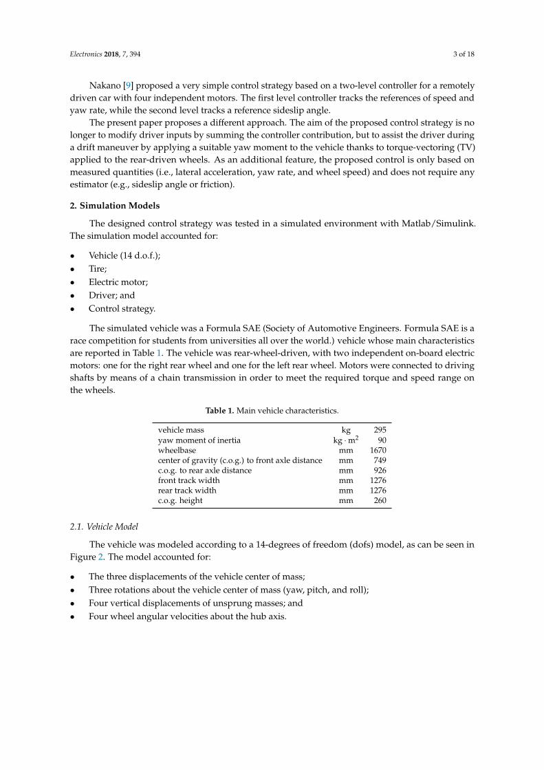
The simulated vehicle was a Formula SAE (Society of Automotive Engineers. Formula SAE is arace competition for students from universities all over the world.) vehicle whose main characteristicsare reported in Table 1. The vehicle was rear-wheel-driven, with two independent on-board electricmotors: one for the right rear wheel and one for the left rear wheel. Motors were connected to drivingshafts by means of a chain transmission in order to meet the required torque and speed range onthe wheels.

Table 1. Main vehicle characteristics.

vehicle mass kg 295yaw moment of inertia kg ·m2 90wheelbase mm 1670center of gravity (c.o.g.) to front axle distance mm 749c.o.g. to rear axle distance mm 926front track width mm 1276rear track width mm 1276c.o.g. height mm 260

2.1. Vehicle Model

The vehicle was modeled according to a 14-degrees of freedom (dofs) model, as can be seen inFigure 2. The model accounted for:

• The three displacements of the vehicle center of mass;• Three rotations about the vehicle center of mass (yaw, pitch, and roll);• Four vertical displacements of unsprung masses; and• Four wheel angular velocities about the hub axis.

Electronics 2018, 7, 394 4 of 18

Figure 2. Fourteen degrees of freedom (14 dofs) vehicle model.

2.2. Tire Model

The contact forces between tires and road were modeled according to an exponential tiremodel ([10]):

Fi = Z(Aize−biz + Bi(1− e−biz))sign(z) (1)

where Z is the vertical force, i is x or y for longitudinal and lateral forces, respectively, z is κ (slippage)in the case of longitudinal forces, while it is α (slip angle) in the case of lateral forces. The coefficientswere than computed according to the following equation:

Ax = px0epx1Z′ epx2α + px3α,

Bx = (px4 − px5Z′)(px6 − px7α),

bx = px8e−px9∗α,

Ay = py0epy1Z′ epy2κ + py3κ,

By = (py4 − py5Z′)(py6 − py7κ),

by = py8e−py9∗κ ,

(2)

where pi,j are fixed coefficients and Z′ is the normalized vertical load Z′ = Z/1000. In this way,the tire model accounted for combined slip effect. The resulting forces of the described model arereported in Figure 3. This model was used because of its simplicity in deriving various terms forvehicle equilibria computation. The computation of phase plots and controllability requires a smoothlyanalytic differentiable tire model which delivers reasonably simple terms in the Jacobian. Therefore,the model in [10] was used. The coefficients reported in the model were tuned by minimizing theroot mean square error with respect to Pacejka tire model (For details on the comparison betweenthe adapted model and the MF Tire model, the reader is referred to [10].). Of course, other modelscould be used (e.g., [11,12]), but this one was preferred for its simplicity and its good representation ofcombined slip effect when compared with the Pacejka MF Tire model.

Figure 3. Tire forces given by the exponential tire model as function of slip κ and slip angles α.

Electronics 2018, 7, 394 5 of 18

2.3. Electric Motor Model

The electric motors (EMs) were modeled accounting for the torque-speed characteristic, seeFigure 4, giving upper and lower bounds to the available motor torque while the dynamics of themotor was accounted for by means of a first-order time lag transfer function

TFmot =1

τmots + 1, (3)

where τmot is the time constant, which also accounts for electronic drive dynamics. A rate limiterfunction was also included to model the electronic drive latency.

Figure 4. Electric motor characteristic curve and efficiency map.

2.4. Driver Model

Since the drift equilibrium is an unstable one, the driver has the objectives of following the desiredtrajectory and keeping the vehicle stable. Acting on the demanded driving torque of the rear axleand on the steering wheel, the driver is able to maintain the vehicle in drift, following curves withdifferent curvatures.

2.5. Close Loop Driver Model

The close-loop driver model indicated in Figure 5 was modeled as a proportional integralderivative (PID) controller that acts on the steering wheel angle δSW as a function of the curvature ρ

error (ερ = ρre f − ρ)

δSW =3

∑i=1

Wi

(kP,δε + kI,δ

∫ε + kD,δ ε

). (4)

Similarly, the driver also acts on the throttle, changing the required driving torque Tr as

Tr =3

∑i=1

WikP,γ

(kP,γε + kI,γ

∫ε + kD,γ ε

). (5)

Such a control law on driving torque is dictated by the fact that, since we are in drift condition,we are in limit adherence conditions. This means that the friction is fully exploited by longitudinaland lateral forces (both present at the same time). Since the adherence is fully exploited, by increasingthe driving torque (and so the longitudinal force), the lateral force on the drive axle (rear in thiscase) reduces. If the lateral force on the rear axle reduces, then the trajectory curvature increases.Conversely, when the driving force reduces, the lateral force of the rear axle increases and the curvaturetrajectory decreases.

The reference curvature was then evaluated at three different distances li in order to simulate thepreview capability of the driver. These distances are a function of vehicle speed

li = vti, (6)

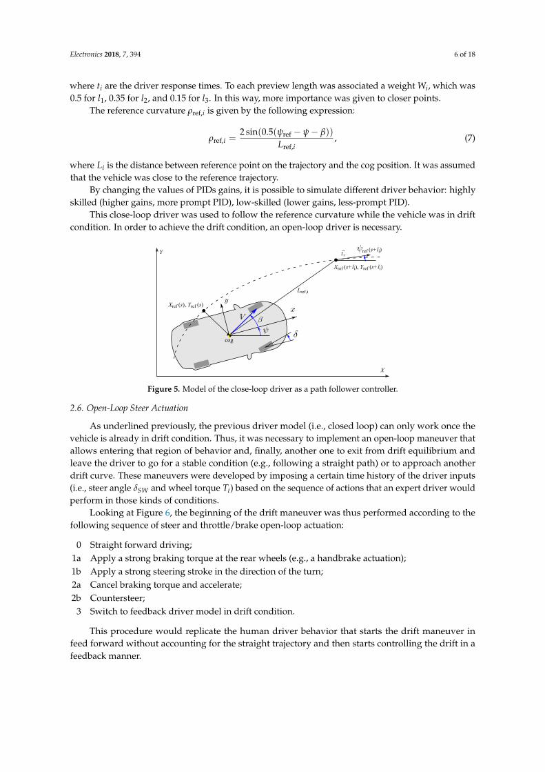
Electronics 2018, 7, 394 6 of 18

where ti are the driver response times. To each preview length was associated a weight Wi, which was0.5 for l1, 0.35 for l2, and 0.15 for l3. In this way, more importance was given to closer points.

The reference curvature ρref,i is given by the following expression:

ρref,i =2 sin(0.5(ψref − ψ− β))

Lref,i, (7)

where Li is the distance between reference point on the trajectory and the cog position. It was assumedthat the vehicle was close to the reference trajectory.

By changing the values of PIDs gains, it is possible to simulate different driver behavior: highlyskilled (higher gains, more prompt PID), low-skilled (lower gains, less-prompt PID).

This close-loop driver was used to follow the reference curvature while the vehicle was in driftcondition. In order to achieve the drift condition, an open-loop driver is necessary.

cog

Xref (s), Yref (s)

Xref (s+li), Yref (s+li)

X

Y ref (s+li)

Lref,i

Figure 5. Model of the close-loop driver as a path follower controller.

2.6. Open-Loop Steer Actuation

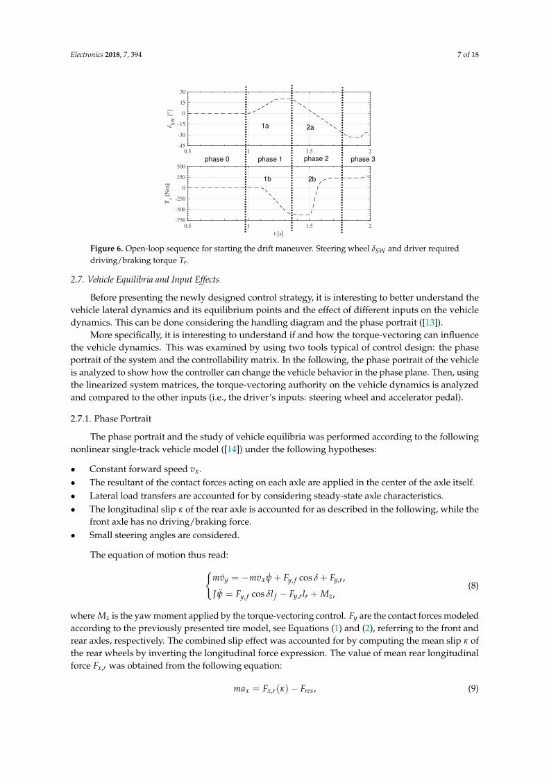
As underlined previously, the previous driver model (i.e., closed loop) can only work once thevehicle is already in drift condition. Thus, it was necessary to implement an open-loop maneuver thatallows entering that region of behavior and, finally, another one to exit from drift equilibrium andleave the driver to go for a stable condition (e.g., following a straight path) or to approach anotherdrift curve. These maneuvers were developed by imposing a certain time history of the driver inputs(i.e., steer angle δSW and wheel torque Ti) based on the sequence of actions that an expert driver wouldperform in those kinds of conditions.

Looking at Figure 6, the beginning of the drift maneuver was thus performed according to thefollowing sequence of steer and throttle/brake open-loop actuation:

0 Straight forward driving;1a Apply a strong braking torque at the rear wheels (e.g., a handbrake actuation);1b Apply a strong steering stroke in the direction of the turn;2a Cancel braking torque and accelerate;2b Countersteer;

3 Switch to feedback driver model in drift condition.

This procedure would replicate the human driver behavior that starts the drift maneuver infeed forward without accounting for the straight trajectory and then starts controlling the drift in afeedback manner.

Electronics 2018, 7, 394 7 of 18

0.5 1 1.5 2-45

-30

-15

0

15

30

SW

[°]

0.5 1 1.5 2

t [s]

-750

-500

-250

0

250

500T

r [N

m]

phase 0 phase 1 phase 2 phase 3

1a

1b 2b

2a

Figure 6. Open-loop sequence for starting the drift maneuver. Steering wheel δSW and driver requireddriving/braking torque Tr.

2.7. Vehicle Equilibria and Input Effects

Before presenting the newly designed control strategy, it is interesting to better understand thevehicle lateral dynamics and its equilibrium points and the effect of different inputs on the vehicledynamics. This can be done considering the handling diagram and the phase portrait ([13]).

More specifically, it is interesting to understand if and how the torque-vectoring can influencethe vehicle dynamics. This was examined by using two tools typical of control design: the phaseportrait of the system and the controllability matrix. In the following, the phase portrait of the vehicleis analyzed to show how the controller can change the vehicle behavior in the phase plane. Then, usingthe linearized system matrices, the torque-vectoring authority on the vehicle dynamics is analyzedand compared to the other inputs (i.e., the driver’s inputs: steering wheel and accelerator pedal).

2.7.1. Phase Portrait

The phase portrait and the study of vehicle equilibria was performed according to the followingnonlinear single-track vehicle model ([14]) under the following hypotheses:

• Constant forward speed vx.• The resultant of the contact forces acting on each axle are applied in the center of the axle itself.• Lateral load transfers are accounted for by considering steady-state axle characteristics.• The longitudinal slip κ of the rear axle is accounted for as described in the following, while the

front axle has no driving/braking force.• Small steering angles are considered.

The equation of motion thus read:{mvy = −mvxψ + Fy, f cos δ + Fy,r,

Jψ = Fy, f cos δl f − Fy,rlr + Mz,(8)

where Mz is the yaw moment applied by the torque-vectoring control. Fy are the contact forces modeledaccording to the previously presented tire model, see Equations (1) and (2), referring to the front andrear axles, respectively. The combined slip effect was accounted for by computing the mean slip κ ofthe rear wheels by inverting the longitudinal force expression. The value of mean rear longitudinalforce Fx,r was obtained from the following equation:

max = Fx,r(κ)− Fres, (9)

Electronics 2018, 7, 394 8 of 18

which represents the vehicle longitudinal dynamic equilibrium in which ax is imposed to be equal to 0.Fres is the total resistance force which accounts for rolling resistance and aerodynamic drag force.

Equation (8) can thus be written in short form as

z = f (z, u), (10)

where z is the state vectorz = {vy ψ}T , (11)

while u is the inputs vectoru = {vx δ Mz}T . (12)

The fixed points could be found by imposing

f (z, u) = 0. (13)

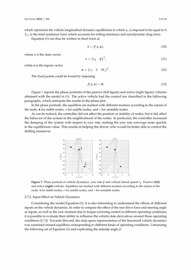
Figure 7 reports the phase portraits of the passive (left figure) and active (right figure) vehiclesobtained with the model in (8). The active vehicle had the control law described in the followingparagraphs, which anticipate the results in the phase plot.

In the phase portraits, the equilibria are marked with different markers according to the nature ofthe node: • for stable nodes, ? for saddle nodes, and ◦ for unstable nodes.

As can be noticed, the controller did not affect the position or stability of nodes, but it did affectthe behavior of the system in the neighborhood of the nodes. In particular, the controller increasedthe damping of the system with respect to yaw rate, making the yaw rate converge more quicklyto the equilibrium value. This results in helping the driver, who would be better able to control thedrifting maneuver.

-10 -5 0 5 10-40

-30

-20

-10

0

10

20

30

40

-10 -5 0 5 10-40

-30

-20

-10

0

10

20

30

40

1

2

Figure 7. Phase portrait of vehicle dynamics: yaw rate ψ and vehicle lateral speed vy. Passive (left)and active (right) vehicles. Equilibria are marked with different markers according to the nature of thenode: • for stable nodes, ? for saddle nodes, and ◦ for unstable nodes.

2.7.2. Input Effect on Vehicle Dynamics

Considering the model Equation (8), it is also interesting to understand the effects of differentinputs on the vehicle dynamics. In order to compare the effect of the rear drive force and steering angleas inputs, as well as the yaw moment due to torque-vectoring control at different operating conditions,it is possible to evaluate their ability to influence the vehicle state derivatives around those operatingconditions ([13]). Towards this end, the state space representation of the linearized vehicle dynamicswas examined around equilibria corresponding to different kinds of operating conditions. Linearizingthe following set of Equation (8) and explicating the sideslip angle β:

Electronics 2018, 7, 394 9 of 18

β =

1mV

(Fy f cos δ + Fy,r

)− ψ,

ψ =1J

(Fy, f cos δl f − Fy,rlr

)+

Mz

J.

(14)

The combined slip effect is accounted for thanks to the previously presented tire model and bycomputing the mean slip κ of the rear wheels by inverting the longitudinal force expression. The valueof mean rear longitudinal force Fx,r is obtained from the following equation:

max = Fx,r(κ)− Fres, (15)

which represents the vehicle longitudinal dynamic equilibrium in which ax is imposed to be equal to 0.Fres is the total resistance force which accounts for rolling resistance and aerodynamic drag force.

The linearized system, about one of the equilibrium points, takes the form

∂x = [A]∂x + [B]∂u, (16)

where x is the state vector∂x = {∂β ∂ψ} (17)

and [A] the plant state matrix

[A] =

∂β∂vy

∂β∂ψ

∂ψ∂vy

∂ψ∂ψ

=

[a11 a12

a21 a22

]. (18)

Since the inputs to the system, i.e., steering angle δ, accelerator pedal γ, and torque-vectoring yawmoment Mz, are of different nature and thus of different orders of magnitude:

δ (rad) −0.17 < δ < 0.17,γ () 0 < γ < 1,

Mz (Nm) −300 < Mz < 300,

(The considered value of Mz was 50% of the maximum exploitable yaw moment when considering themaximum longitudinal force that can be applied on the inner rear wheel. This value was computedconsidering also the load transfer in a turn with maximum lateral acceleration (µg)) it is moreconvenient to study the perturbation effects due to the contact forces which are directly affectedby the driver’s and TV inputs:

• ∂Fy f —front lateral force, which is directly affected by the steering angle;• ∂Fxr—rear longitudinal force, which is directly controlled by gas pedal γ;• ∂∆Fxr—the difference in left and right rear longitudinal forces induced by yaw moment Mz.

In this way, the input matrix [B] can be written as

[B] =

∂β∂Fy f

∂β∂Fxr

∂β∂∆Fxr

∂ψ∂Fy f

∂ψ∂Fxr

∂ψ∂∆Fxr

=

[b11 b12 b13

b21 b22 b23

]. (19)

Considering the different equilibrium points of the vehicle under different driving conditions, itis thus possible to evaluate the influence of the inputs upon the sideslip angle and yaw rate dynamics.Note that Fxr does not appear explicitly inside the equations, but it does affect the rear cornering forcedue to the coupling effect in combined slip condition. The terms b12 and b22 of matrix [B] are thusdifferent from zero when the coupling between longitudinal and lateral forces becomes evident (i.e.,in the case of high values of slip and slip angles). Considering a constant speed vx of 8 m/s, threedifferent driving conditions were analyzed: straight driving, typical cornering, and drift cornering.The computed matrices are reported in Table 2. Specifically, the matrices were respectively obtained bylinearizing the system in the neighborhood of three equilibrium points:

Electronics 2018, 7, 394 10 of 18

• Straight driving: δ = 0, β = 0, ψ = 0;• Typical cornering: point 1 in Figure 7 left;• Drift cornering: point 2 in Figure 7 left.

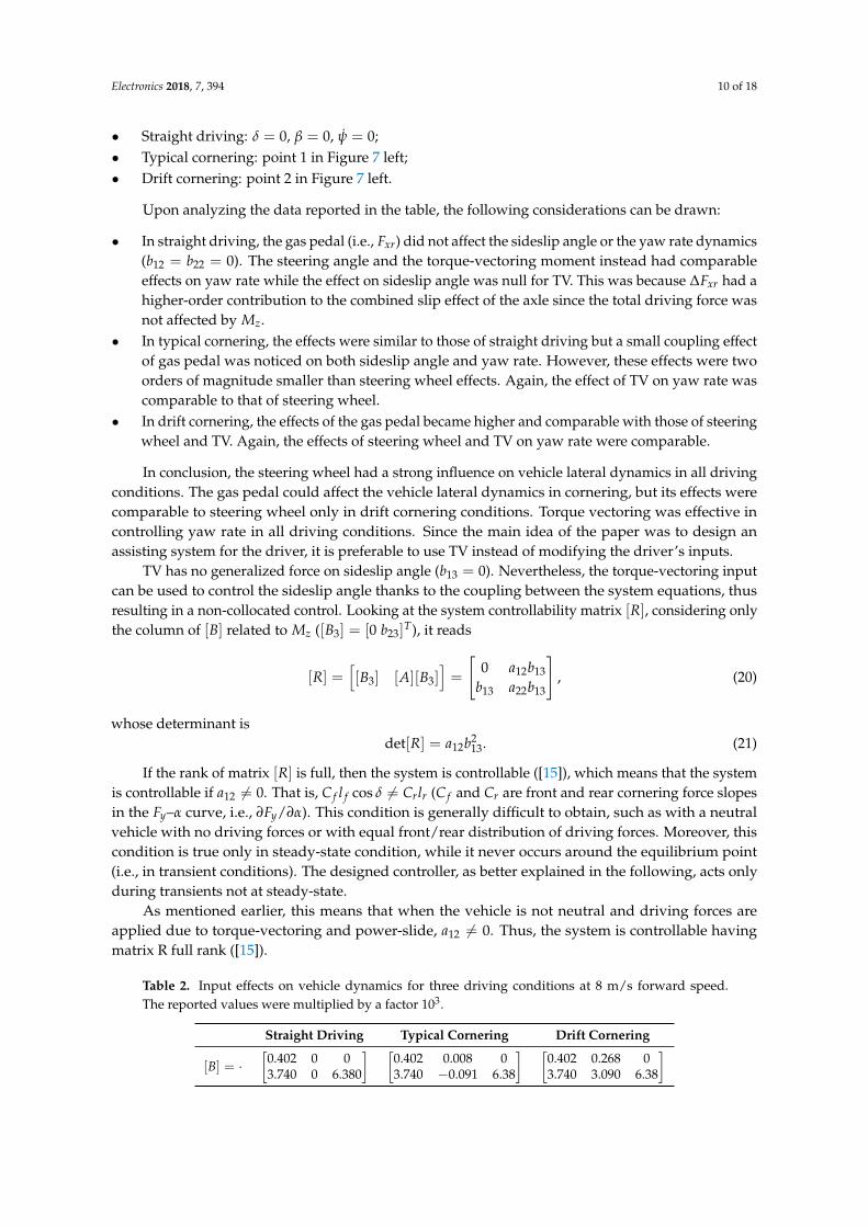
Upon analyzing the data reported in the table, the following considerations can be drawn:

• In straight driving, the gas pedal (i.e., Fxr) did not affect the sideslip angle or the yaw rate dynamics(b12 = b22 = 0). The steering angle and the torque-vectoring moment instead had comparableeffects on yaw rate while the effect on sideslip angle was null for TV. This was because ∆Fxr had ahigher-order contribution to the combined slip effect of the axle since the total driving force wasnot affected by Mz.

• In typical cornering, the effects were similar to those of straight driving but a small coupling effectof gas pedal was noticed on both sideslip angle and yaw rate. However, these effects were twoorders of magnitude smaller than steering wheel effects. Again, the effect of TV on yaw rate wascomparable to that of steering wheel.

• In drift cornering, the effects of the gas pedal became higher and comparable with those of steeringwheel and TV. Again, the effects of steering wheel and TV on yaw rate were comparable.

In conclusion, the steering wheel had a strong influence on vehicle lateral dynamics in all drivingconditions. The gas pedal could affect the vehicle lateral dynamics in cornering, but its effects werecomparable to steering wheel only in drift cornering conditions. Torque vectoring was effective incontrolling yaw rate in all driving conditions. Since the main idea of the paper was to design anassisting system for the driver, it is preferable to use TV instead of modifying the driver’s inputs.

TV has no generalized force on sideslip angle (b13 = 0). Nevertheless, the torque-vectoring inputcan be used to control the sideslip angle thanks to the coupling between the system equations, thusresulting in a non-collocated control. Looking at the system controllability matrix [R], considering onlythe column of [B] related to Mz ([B3] = [0 b23]

T), it reads

[R] =[[B3] [A][B3]

]=

[0 a12b13

b13 a22b13

], (20)

whose determinant isdet[R] = a12b2

13. (21)

If the rank of matrix [R] is full, then the system is controllable ([15]), which means that the systemis controllable if a12 6= 0. That is, C f l f cos δ 6= Crlr (C f and Cr are front and rear cornering force slopesin the Fy–α curve, i.e., ∂Fy/∂α). This condition is generally difficult to obtain, such as with a neutralvehicle with no driving forces or with equal front/rear distribution of driving forces. Moreover, thiscondition is true only in steady-state condition, while it never occurs around the equilibrium point(i.e., in transient conditions). The designed controller, as better explained in the following, acts onlyduring transients not at steady-state.

As mentioned earlier, this means that when the vehicle is not neutral and driving forces areapplied due to torque-vectoring and power-slide, a12 6= 0. Thus, the system is controllable havingmatrix R full rank ([15]).

Table 2. Input effects on vehicle dynamics for three driving conditions at 8 m/s forward speed.The reported values were multiplied by a factor 103.

Straight Driving Typical Cornering Drift Cornering

[B] = ·[

0.402 0 03.740 0 6.380

] [0.402 0.008 03.740 −0.091 6.38

] [0.402 0.268 03.740 3.090 6.38

]

Electronics 2018, 7, 394 11 of 18

3. Drift Torque-Vectoring Active Control

Based on the previous study, thanks to torque-vectoring it is possible to design an advanceddriver-assistance system (ADAS) which helps the driver to control the vehicle during drift withoutmodifying the driver’s inputs (i.e., steering wheel and accelerator/brake pedals).

The controller was designed in order to leave the driver free to define vehicle attitude.The controller generates a yaw moment according to the following equation:

Mz = kY · IY, (22)

where kY is the controller gain and IY is the yaw index expressed as

IY =ay

vx− ψ, (23)

where ay is the vehicle lateral acceleration, vx is the vehicle forward velocity, and ψ is the yaw rate.Controlling IY means to control the time derivative of lateral velocity vy. Considering that the

lateral acceleration ay can be written as

ay = vy + vxψ, (24)

rearranging the equation, we obtainvy

vx=

ay

vx− ψ, (25)

which means that the controller generates a yaw moment that prevents lateral velocity from excessiveincrease. This makes the vehicle more straight-forward for the driver, who can control the vehiclemore smoothly.

3.1. Control Activation Conditions

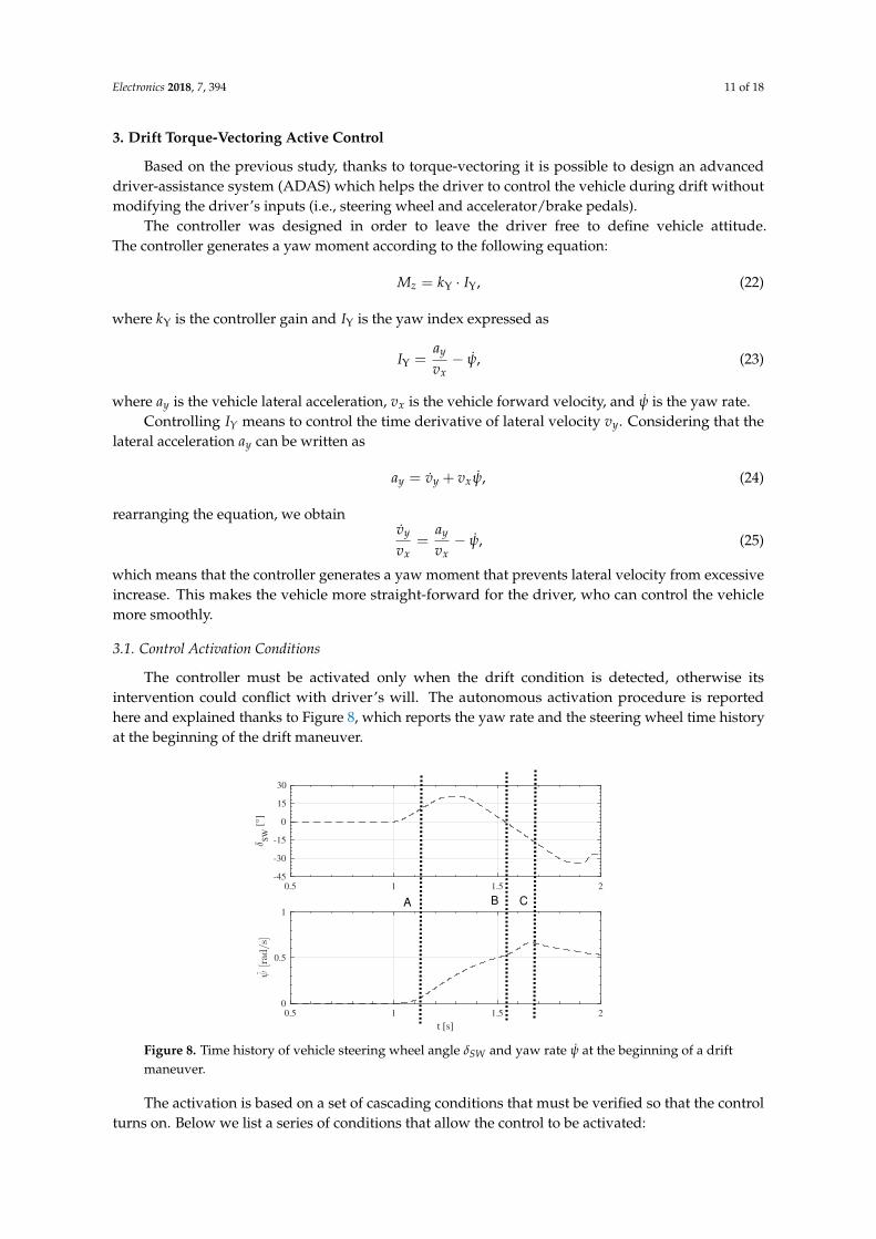
The controller must be activated only when the drift condition is detected, otherwise itsintervention could conflict with driver’s will. The autonomous activation procedure is reportedhere and explained thanks to Figure 8, which reports the yaw rate and the steering wheel time historyat the beginning of the drift maneuver.

0.5 1 1.5 2-45

-30

-15

0

15

30

SW

[°]

0.5 1 1.5 2

t [s]

0

0.5

1A B C

Figure 8. Time history of vehicle steering wheel angle δSW and yaw rate ψ at the beginning of a driftmaneuver.

The activation is based on a set of cascading conditions that must be verified so that the controlturns on. Below we list a series of conditions that allow the control to be activated:

Electronics 2018, 7, 394 12 of 18

Condition A identifies the entrance in a turn by looking at the yaw rate of the vehicle. A smallthreshold is used to avoid intervention due to measurement noise. Condition A reads:

|ψ| > ψlim. (26)

Condition B identifies the beginning of the counter-steering action by the driver. Condition B thusreads:

sgn(δ) 6= sgn(ψ). (27)

Condition C identifies the beginning of the drift due to the permanence of the steering wheel incounter-steer condition:

δ · sgn( ¯ψ) < 0, (28)

where for robustness both δ and ψ are accounted for by means of their average value evaluated(δ and ¯ψ) with a moving average window of 0.5 s.

3.2. Control Deactivation Conditions

The controller is then deactivated when the drift maneuver is ended by the driver. This conditionis identified by a reduction, or a change in sign if the vehicle oscillates, of the yaw rate

|ψ| < ψlim (29)

orψk · ψk−1 < 0. (30)

4. Simulation Results

The control strategy was tested according to the following maneuver, which consists of aconstant-speed U-turn on different adherence road surfaces and for different drivers. The two modeleddrivers were a highly skilled driver and a low-skilled driver. The difference in the two drivers was inthe value of PID gains, as described previously.

The vehicle started from straight line condition with velocity V = 18 m/s. The turn had aradius R of 38 m. The following simulation results report the following quantities related to vehicledynamics behavior:

• Vehicle yaw rate ψ;• Vehicle lateral acceleration ay;• Vehicle sideslip angle β;• Driver required driving torque Tr;• Steering wheel angle δSW ;• Vehicle speed V.

The sign convention is consistent with Figure 2.

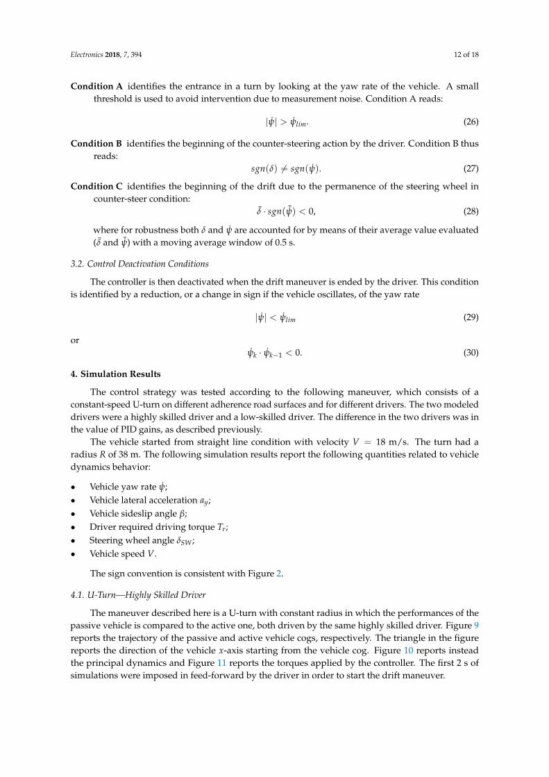
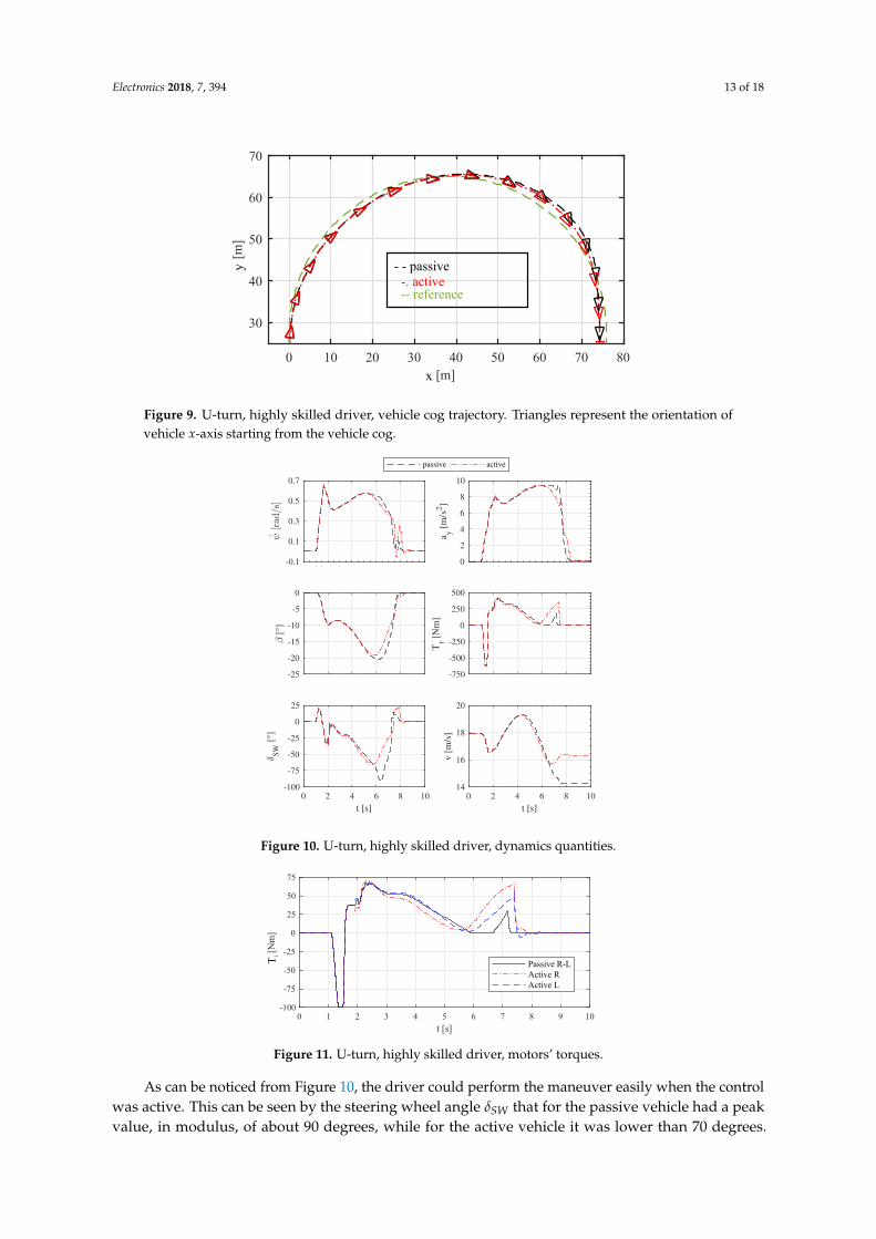
4.1. U-Turn—Highly Skilled Driver

The maneuver described here is a U-turn with constant radius in which the performances of thepassive vehicle is compared to the active one, both driven by the same highly skilled driver. Figure 9reports the trajectory of the passive and active vehicle cogs, respectively. The triangle in the figurereports the direction of the vehicle x-axis starting from the vehicle cog. Figure 10 reports insteadthe principal dynamics and Figure 11 reports the torques applied by the controller. The first 2 s ofsimulations were imposed in feed-forward by the driver in order to start the drift maneuver.

Electronics 2018, 7, 394 13 of 18

0 10 20 30 40 50 60 70 80

[m]

30

40

50

60

70

[m]

-- reference-. active

- - passivey

x

Figure 9. U-turn, highly skilled driver, vehicle cog trajectory. Triangles represent the orientation ofvehicle x-axis starting from the vehicle cog.

-0.1

0.1

0.3

0.5

0.7

passive active

0

2

4

6

8

10

ay [

m/s

2]

-25

-20

-15

-10

-5

0

[°]

-750

-500

-250

0

250

500

Tr [

Nm

]

0 2 4 6 8 10

t [s]

-100

-75

-50

-25

0

25

SW

[°]

0 2 4 6 8 10

t [s]

14

16

18

20

v [

m/s

]

Figure 10. U-turn, highly skilled driver, dynamics quantities.

0 1 2 3 4 5 6 7 8 9 10

t [s]

-100

-75

-50

-25

0

25

50

75

[Nm

]

Passive R-L

Active R

Active L

Ti

Figure 11. U-turn, highly skilled driver, motors’ torques.

As can be noticed from Figure 10, the driver could perform the maneuver easily when the controlwas active. This can be seen by the steering wheel angle δSW that for the passive vehicle had a peakvalue, in modulus, of about 90 degrees, while for the active vehicle it was lower than 70 degrees.

Electronics 2018, 7, 394 14 of 18

Additionally, the dynamics of the car improved: the sideslip angle had a smaller peak value. Finally,the final speed of the vehicle v was higher for the active vehicle by about 2 m/s (7.2 km/h).

4.2. U-Turn—Low-Skilled Driver

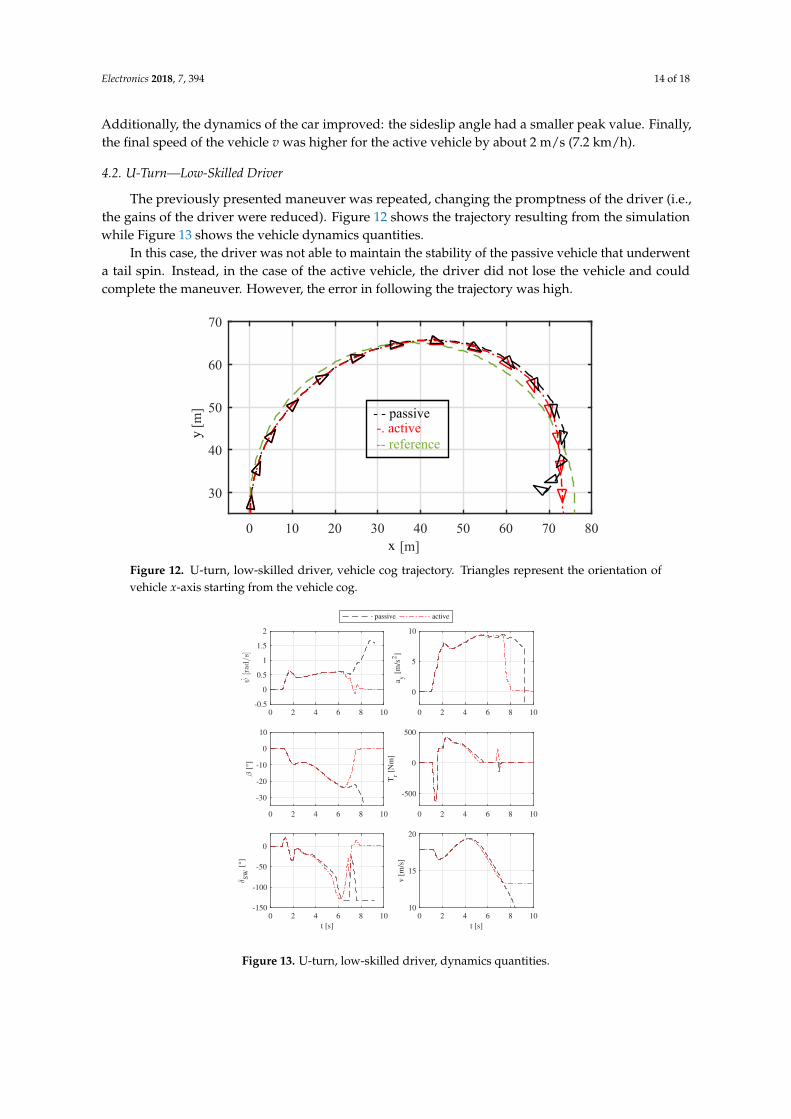
The previously presented maneuver was repeated, changing the promptness of the driver (i.e.,the gains of the driver were reduced). Figure 12 shows the trajectory resulting from the simulationwhile Figure 13 shows the vehicle dynamics quantities.

In this case, the driver was not able to maintain the stability of the passive vehicle that underwenta tail spin. Instead, in the case of the active vehicle, the driver did not lose the vehicle and couldcomplete the maneuver. However, the error in following the trajectory was high.

Figure 12. U-turn, low-skilled driver, vehicle cog trajectory. Triangles represent the orientation ofvehicle x-axis starting from the vehicle cog.

0 2 4 6 8 10-0.5

0

0.5

1

1.5

2

0 2 4 6 8 10

0

5

10

a y [

m/s

2]

0 2 4 6 8 10

-30

-20

-10

0

10

[°]

0 2 4 6 8 10

-500

0

500

Tr [

Nm

]

0 2 4 6 8 10

t [s]

-150

-100

-50

0

SW

[°]

0 2 4 6 8 10

t [s]

10

15

20

v [

m/s

]

passive active

Figure 13. U-turn, low-skilled driver, dynamics quantities.

Electronics 2018, 7, 394 15 of 18

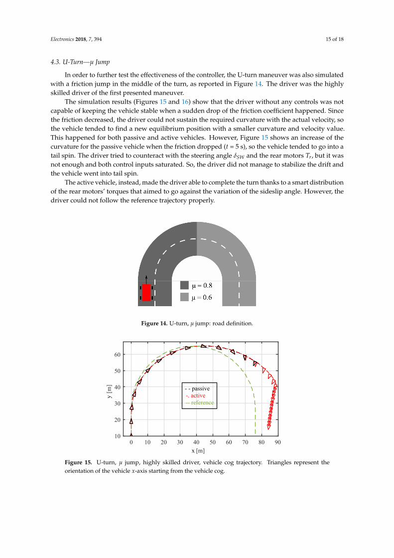
4.3. U-Turn—µ Jump

In order to further test the effectiveness of the controller, the U-turn maneuver was also simulatedwith a friction jump in the middle of the turn, as reported in Figure 14. The driver was the highlyskilled driver of the first presented maneuver.

The simulation results (Figures 15 and 16) show that the driver without any controls was notcapable of keeping the vehicle stable when a sudden drop of the friction coefficient happened. Sincethe friction decreased, the driver could not sustain the required curvature with the actual velocity, sothe vehicle tended to find a new equilibrium position with a smaller curvature and velocity value.This happened for both passive and active vehicles. However, Figure 15 shows an increase of thecurvature for the passive vehicle when the friction dropped (t = 5 s), so the vehicle tended to go into atail spin. The driver tried to counteract with the steering angle δSW and the rear motors Tr, but it wasnot enough and both control inputs saturated. So, the driver did not manage to stabilize the drift andthe vehicle went into tail spin.

The active vehicle, instead, made the driver able to complete the turn thanks to a smart distributionof the rear motors’ torques that aimed to go against the variation of the sideslip angle. However, thedriver could not follow the reference trajectory properly.

Figure 14. U-turn, µ jump: road definition.

0 10 20 30 40 50 60 70 80 90

[m]

10

20

30

40

50

60

[m]

-. active

-- reference

- - passive

x

y

Figure 15. U-turn, µ jump, highly skilled driver, vehicle cog trajectory. Triangles represent theorientation of the vehicle x-axis starting from the vehicle cog.

Electronics 2018, 7, 394 16 of 18

0 2 4 6 8 10 12-1

0

1

2

passive active

0 2 4 6 8 10 12-5

0

5

10

a y[m

/s2]

0 2 4 6 8 10 12-100

-50

0

50 [

°]

0 2 4 6 8 10 12

-100

0

100

SW

[°]

0 2 4 6 8 10 12

t [s]

0

5

10

15

20

V [

m/s

]

0 2 4 6 8 10 12

t [s]

-1000

-500

0

500

[Nm

]

Figure 16. U-turn, µ jump, highly skilled driver, dynamics quantities.

5. Conclusions

The paper presents a control strategy that can help the driver in high-sideslip maneuvers, namely,in drift condition. The control inputs are the torques on the rear wheels, which are independentthanks to electric motors. A torque-vectoring-based control strategy is then set up and tested inMatlab-Simulink simulation environments.

Note that the developed control strategy relies only on measured quantities (i.e., lateralacceleration, yaw rate, and wheel speed). This makes the controller robust and independent fromstate estimators.

Results demonstrated that it was possible to help the stabilization of drift cornering, withoutmaking use of the driver’s inputs but thanks to a smart distribution of rear motor torques. This type ofcontrol allows a collaboration between the driver and the control logic, so that the control does notreplace the driver entirely. Especially, it is shown that the presented control allows even less skilleddrivers to keep the vehicle stable in drift cornering, which would be very difficult without it.

Author Contributions: The following statements should be used conceptualization, M.V. and E.S.; methodology,F.C.; software, M.V.; validation, M.V. and E.S.; formal analysis, F.C.; investigation, M.V. and E.S.; resources, E.S.;data curation, M.V.

Funding: This research received no external funding.

Conflicts of Interest: The authors declare no conflict of interest.

Electronics 2018, 7, 394 17 of 18

Abbreviations

The following abbreviations are used in this manuscript:

ADAS advanced driver assistance systemc.o.g. center of gravitydof degree of freedomEM electric motorPID proportional integral derivativeSAE Society of Automotive EngineersTV torque-vectoringax vehicle longitudinal accelerationay vehicle lateral accelerationC f front axle cornering stiffnessCr rear axle cornering stiffnessFx longitudinal forceFx f longitudinal force of the front axleFxr longitudinal force of the rear axleFy lateral forceFy f lateral force of the front axleFyr lateral force of the rear axleJ vehicle yaw moment of inertiam vehicle massMz torque-vectoring yaw momentvx vehicle longitudinal velocity componentvy vehicle lateral velocity componentV vehicle velocity modulusα slip angleα f slip angle of front axleαr slip angle of rear axleβ sideslip angleγ accelerator pedalδ steering angleψ yaw angle

References

1. Vignati, M.; Sabbioni, E.; Tarsitano, D.; Cheli, F. Electric powertrain layouts analysis for controlling vehiclelateral dynamics with torque-vectoring. In Proceedings of the 2017 International Conference of Electricaland Electronic Technologies for Automotive, Torino, Italy, 15–16 June 2017; pp. 1–5. [CrossRef]

2. Dizqah, A.M.; Lenzo, B.; Sorniotti, A.; Gruber, P.; Fallah, S.; De Smet, J. A Fast and Parametric TorqueDistribution Strategy for Four-Wheel-Drive Energy-Efficient Electric Vehicles. IEEE Trans. Ind. Electron. 2016,63, 4367–4376. [CrossRef]

3. Hoffman, R.C.; Stein, J.L.; Louca, L.S.; Huh, K. Using the Milliken Moment Method and dynamic simulationto evaluate vehicle stability and controllability. Int. J. Veh. Des. 2008, 48, 132. [CrossRef]

4. Edelmann, J.; Plöchl, M. Analysis of controllability of automobiles at steady-state cornering consideringdifferent drive concepts. In Dynamics of Vehicles on Roads and Tracks; CRC Press: London, UK, 2018.

5. Velenis, E.; Frazzoli, E.; Tsiotras, P. Steady-state cornering equilibria and stabilisation for a vehicle duringextreme operating conditions. Int. J. Veh. Auton. Syst. 2010, 8, 217–241, doi:10.1504/IJVAS.2010.035797.[CrossRef]

6. Edelmann, J.; Plöchl, M. Handling characteristics and stability of the steady-state powerslide motion of anautomobile. Regul. Chaotic Dyn. 2009, 14, 682–692. [CrossRef]

7. Velenis, E.; Katzourakis, D.; Frazzoli, E.; Tsiotras, P.; Happee, R. Steady-state drifting stabilization of RWDvehicles. Control Eng. Pract. 2011, 19, 1363–1376. [CrossRef]

Electronics 2018, 7, 394 18 of 18

8. Werling, M.; Reinisch, P.; Gröll, L. Robust power-slide control for a production vehicle. Int. J. Veh. Auton. Syst.2015, 13, 27. [CrossRef]

9. Nakano, H.; Okayama, K.; Kinugawa, J.; Kosuge, K. Control of an electric vehicle with a large sideslip angleusing driving forces of four independently-driven wheels and steer angle of front wheels. In Proceedings ofthe 2014 IEEE/ASME International Conference on Advanced Intelligent Mechatronics, Besancon, France,8–11 July 2014; pp. 1073–1078. [CrossRef]

10. Best, M.C. Exploring Assumptions and Requirements for Continuous Modification of Vehicle Handling UsingNonlinear Optimal Control and a New Exponential Tyre Model; Loughborough University: Loughborough, UK,2010; pp. 79–84.

11. Hindiyeh, R.Y.; Gerdes, J.C. Design of a Dynamic Surface Controller for Vehicle Sideslip Angle DuringAutonomous Drifting. IFAC Proc. Vol. 2010, 43, 560–565. [CrossRef]

12. Bobier-Tiu, C.G.; Beal, C.E.; Kegelman, J.C.; Hindiyeh, R.Y.; Gerdes, J.C. Vehicle control synthesis usingphase portraits of planar dynamics. Veh. Syst. Dyn. 2018, 3114, 1–20. [CrossRef]

13. Hindiyeh, R.Y.; Gerdes, J.C. Equilibrium Analysis of Drifting Vehicles for Control Design. In Proceedingsof the ASME 2009 Dynamic Systems and Control Conference, Hollywood, CA, USA, 12–14 October 2009;Volume 1, pp. 181–188. [CrossRef]

14. Rossa, F.; Gobbi, M.; Mastinu, G.; Piccardi, C.; Previati, G. Bifurcation analysis of a car and driver model.Veh. Syst. Dyn. 2014, 52, 142–156. [CrossRef]

15. Ogata, K. Modern Control Engineering, 5th ed.; Pearson: London, UK, 2010; p. 912.

c© 2018 by the authors. Licensee MDPI, Basel, Switzerland. This article is an open accessarticle distributed under the terms and conditions of the Creative Commons Attribution(CC BY) license (http://creativecommons.org/licenses/by/4.0/).