A topology of services expenditure by poor and rich households in developing countries
323
SERVICES, TRADE AND DEVELOPMENT UNITED NATIONS CONFERENCE ON TRADE AND DEVELOPMENT
Transcript of A topology of services expenditure by poor and rich households in developing countries

SERVICES,
TRADE AND
DEVELOPMENT
U N I T E D N AT I O N S C O N F E R E N C E O N T R A D E A N D D E V E L O P M E N T
U N I T E D N AT I O N S C O N F E R E N C E O N T R A D E A N D D E V E L O P M E N T
SERVICES,
TRADE AND
DEVELOPMENT
New York and Geneva, 2011
MINA MASHAYEKHI
MARCELO OLARREAGA
GUIDO PORTO

ii SERVICES, TRADE & DEVELOPMENT
DISCLAIMER
The designations employed and the presentation of the material in this publication do not imply the expression
of any opinion whatsoever on the part of the Secretariat of the United Nations concerning the legal status of any
country, territory, city or area, or of its authorities, or concerning the delimitation of its frontiers or boundaries.
Symbols of United Nations documents are composed of capital letters combined with figures. Mention of such
a symbol indicates a reference to a United Nations document.
Material in this publication may be freely quoted or reprinted, but acknowledgement is requested. A copy of the
publication containing the quotation or reprint should be sent to the UNCTAD secretariat at: Palais de Nations,
CH 1211 Geneva 10, Switzerland.
The views expressed in this publication are those of the authors and do not necessarily reflect the views of the
United Nations Secretariat.
For further information on the Trade Negotiations and Commercial Diplomacy Branch and its activities,
please contact:
Ms. Mina MASHAYEKHI
Head, Trade Negotiations and
Commercial Diplomacy Branch
Division of International Trade in Goods and
Services, and Commodities
Tel: +41 22 917 56 40
Fax: +41 22 917 00 44
E-mail: [email protected]
www.unctad.org/tradenegotiations
Copyright © United Nations, 2011
All rights reserved. Printed in Switzerland
UNCTAD/DITC/TNCD/2010/5
iiiFOREWORD
FOREWORD
In recent years, notwithstanding the set-back caused by the economic and financial crisis, global demand for
services and international services trade has regularly increased, making the services economy and trade in
services and important component of the development agenda, at the national and international levels. In 2008,
the services economy was identified in the Accra Accord - the document adopted in Accra, Ghana, at the
UNCTAD XII quadrennial conference, setting out UNCTAD´s mandate - as a new frontier for expanding trade,
productivity and competitiveness. However, the Accra Accord also noted that positively integrating developing
countries, especially LDCs, into the global services economy and increasing their participation in services trade,
particularly in modes and sectors of export interest to them, remained a major development challenge.
The objective of this publication is to fill the knowledge and information gap on the impacts of various services
sector and trade reforms on growth, development and poverty reduction. It is intended to provide policy makers
and other affected stakeholders in developing countries and economies with policy analysis and case studies on
services sector on the policy, regulatory and institutional options that can enable a country to promote economic
growth, poverty eradication and sustainable development.
Two broad focuses were chosen for the publication. The first is the importance of policy, regulatory and institutional
frameworks for the services sector. Regulatory failures, including the most recent failure to shield economies
against excessive risk-taking in the financial system which led to the 2008 financial crisis, has drawn the attention
of policy-makers but also of the general public to the need for adequate regulation. Governments have learned
from past regulatory failures the importance of developing best-fit policies, supported by adequate regulatory
and institutional frameworks, adapted to each country’s local circumstances. However, the recent crisis in
the financial sector has highlighted the nature of regulatory challenges which are continuously evolving and
dynamic, not something to be solved once and for all. Because today’s competitive markets are characterized
by innovation, new business models and new product trends, regulators needed to adapt their regulation so as
to avoid failures and crises. In this context, the role of the State - including that of reviewing, and where necessary
renewing, policies, regulations and institutions on a regular basis - has become increasingly evident.
The second focus of the publication is on infrastructure services, a broad group of activities which includes
services such as electricity, financial, telecommunication, transport and water services. In the context of the
ongoing recovery and attempts to better prepare countries for future crises the international community has
highlighted the importance of infrastructure services.. One notable example is the identification by the G20
of the need to secure financing for key infrastructure projects, which can unleash the growth potential of the
developing countries. . This has led the G20 to set up a High Level Panel for Infrastructure Investment to
produce recommendations in order to scale up and diversify financing for infrastructure needs, and identify,
with multilateral development banks, a list of concrete regional initiatives. In a similar vein the recent UN LDC-IV
Conference, which was held from 9 to 13 May, 2011 in Istanbul, Turkey produced a Programme of Action for the
Least Developed Countries (LDCs) for the Decade 2011-2020, which refers in several instances to infrastructure
services. It states that one of the major challenges facing LDCs is the lack of adequate physical infrastructure,
and emphasizes that reliable and affordable infrastructure services are essential for existing productive assets
and enterprises in LDCs to operate efficiently, thereby attracting new investment, connecting producers to market,
assuring meaningful economic development and promoting regional integration. In light of this assessment it
is suggested that LDCs take a number of actions on infrastructure including developing and implementing
comprehensive national policies and plans for infrastructure development and maintenance, encompassing
all modes of transportation and ports, communications and energy. It is also suggested that development
partners could also contribute inter alia by providing enhanced financial and technical support for infrastructure
development in line with LDCs’ sectoral and development needs and priorities. This report therefore devotes
particular attention to these two themes in its various chapters and case studies.

It is our hope that this publication will not only provide policy makers, trade negotiators and the broader trade
community with new research and analysis on the increasingly important role of services for today’s economies
but also spark the interest of academics, research institutions and other interested stake-holders in further
investigating the nexus surrounding services-related economic and social reforms, trade and development.
I would like to take this opportunity to thank the International Development Research Centre (IDRC) for its
invaluable support in carrying out this research project.
Supachai PanitchpakdiSecretary-General of UNCTAD

vACKNOWLEDGMENTS
ACKNOWLEDGEMENTS
The publications has been edited by Mina Mashayekhi, Head of the Trade Negotiations and Commercial
Diplomacy Branch (TNCDB), Division on International Trade in Goods and Services, and Commodities, UNCTAD,
by Marcelo Olarreaga, University of Geneva and Centre for Economic Policy Research, and by Guido Porto,
Universidad Nacional de La Plata, with the assistance of Martine Julsaint-Kidane, Economic Affairs Officer, and
Liping Zhang, Senior Economic Affairs Officer, both from the Trade Negotiations and Commercial Diplomacy
Branch (TNCDB), Division on International Trade in Goods and Services, and Commodities, UNCTAD.
The publication was prepared by the UNCTAD secretariat with the aid of a grant from the International Development
Research Centre (IDRC), Ottawa, Canada, under the UNCTAD project “Development Implications of Services
Trade Liberalization” (INT/0T/7AF), for which UNCTAD is thankful.
The authors of the various chapters are as follows:
Chapter I “Promoting sustainable growth and poverty alleviation in developing countries through their integration
in the global services economy” was prepared by Mina Mashayekhi, Head, Martine Julsaint-Kidane, Economic
Affairs Officer, and Liping Zhang, Senior Affairs Officer, all from the Trade Negotiations and Commercial Diplomacy
Branch (TNCDB), Division on International Trade in Goods and Services, and Commodities, UNCTAD. The
authors are grateful to other members of TNCDB for their inputs and comments, including Andrea Nascimento-
Muller.
Chapter II “Managing the interface between regulation and trade in infrastructure services” was prepared by
Mina Mashayekhi, Head, and Martine Julsaint-Kidane, Economic Affairs Office, both from the Trade Negotiations
and Commercial Diplomacy Branch (TNCDB), Division on International Trade in Goods and Services, and
Commodities, UNCTAD. The authors are grateful to other members of TNCDB for their inputs and comments.
Chapter III “Trade in financial services, financial crisis and development implications: what is important and what
has changed?” was prepared by Mina Mashayekhi, Head, and Deepali Fernandes, Economic Affairs Officer,
both from the Trade Negotiations and Commercial Diplomacy Branch (TNCDB), Division on International Trade
in Goods and Services, and Commodities. The authors are grateful to Kern Alexander, Andrew Cornford, Ugo
Panizza, Taisuke Ito and Mesut Saygili for their comments, inputs and views, and to Babette Ancery and Bo
Young Lin for their contributions, research assistance and comments. Special thanks go to Dr. Y. V. Reddy,
former Governor of the Reserve Bank of India, whose views the authors benefitted from.
Chapter IV “Services rules in Economic Parnership Agreeements: the movement of persons and establishment”
was prepared by Elisabeth Tuerk, Legal Expert, Division on Investment and Enterprise, UNCTAD, and by Marie
Wilke, Programme Officer for International Trade Law at the International Centre for Trade and Sustainable
development (ICTSD). The authors thank Denisse Rodriguez Blanco for her research assistance, and Hasso
Anwer, Martine Julsaint-Kidane, Mina Mashayekhi, Liping Zhang and Wamkele Meme, for their comments.
Chapter V “A topology of services expenditure by poor and rich households in developing countries” was
prepared by Marcelo Olarreaga, University of Geneva and Centre for Economic Policy Research, by Mario
Piacentini, OECD and University of Geneva, and by Guido Porto, Pablo Gluzmann and Mariana Marchionni, all
from Universidad Nacional de La Plata.
Chapter VI “An overview of access to finance and poverty in the developing world” was prepared by Guido Porto,
Natalia Porto, both from Universidad Nacional de La Plata, and by Marcelo Olarreaga, University of Geneva and
Centre for Economic Policy Research. The authors are grateful to Martine Julsaint-Kidane, Mmatlou Kalaba,
Mina Mashayekhi and Myriam Velia for their helpful and constructive comments on earlier version. They are also
grateful to Laurence Bonapera for the logistics.

vi SERVICES, TRADE & DEVELOPMENT
Chapter VII “Distributional incidence of access to services in Latin America” was prepared by Guido Porto,
Pablo Gluzmann and Mariana Marchionni, from Universidad Nacional de La Plata, and by Marcelo Olarreaga,
University of Geneva and Centre for Economic Policy Research. The authors are grateful to many colleagues
at Universidad Nacional de la Plata for their contributions at different stages of this project. The authors would
also like to thank Martine Julsaint-Kidane, Mmatlou Kalaba, Mina Mashayekhi, Myriam Velia, and Liping Zhang
for their helpful and constructive comments.
Chapter VIII “Trade in services and poverty: services, farm export participation and poverty in Malawi and
Uganda” was prepared by Jorge Balat, Yale University, and Guido Porto, University of La Plata.
Chapter IX “Privatization, competition and complementary services in rural Zambia” was prepared by Irene
Brambilla and Guido Porto, Universidad Nacional de la Plata.
Chapter X “Brazil: postal services for financial inclusion and trade” was prepared by José Ansón, Laia Bosch
Gual and Justin Caron, all from the Universal Postal Union.
Chapter XI “Services ownership and access to safe water: water nationalization in Uruguay” was prepared
by Fernando Borraz, University of Montevideo, and Marcelo Olarreaga, University of Geneva and Centre
for Economic Policy Research. The authors wish to thank Dra. María del Carmen Papramborda and Leticia
Rodríguez for kindly providing data. They are also grateful to Cristián González, Guido Porto, Mina Mashayekhi
and Liping Zhang for their helpful and constructive discussions.
Chapter XII “Road infrastructure and agricultural contracting services impact on rural production in Argentina” was
prepared by Agustín Lódola and Rafael Brigo, both from Universidad Nacional de La Plata. The authors thank
Roman Fossati and Fernando Morra for their assistance and Guido Porto for his comments and suggestions.
Chapter XIII “Child labour and services FDI: evidence from Vietnam” was prepared by Marcelo Olarreaga,
University of Geneva and Centre for Economic Policy Research, Mario Piacentini, OECD and University of
Geneva, and Nguyen Viet Cuong, National Economics University of Hanoi. The authors are grateful to Guido
Porto and Liping Zhang for their helpful and constructive comments.
The design of the cover and the desktop publishing were carried out by Laurence Duchemin and
Laura Moresino-Borini. Administrative and logistic support was provided by Faustina Attobra-Wilson. The
publication was edited by John Pappas.
viiCONTENTS
CONTENTS
Disclaimer................................................................................................................................................................ ii
Foreword .................................................................................................................................................................iii
Acknowledgements ................................................................................................................................................. v
Overview ................................................................................................................................................................. xi
CHAPTER I: PROMOTING SUSTAINABLE GROWTH AND POVERTY ALLEVIATION IN DEVELOPING COUNTRIES THROUGH THEIR INTEGRATION IN THE GLOBAL SERVICES ECONOMY ..................................... 1
1. Introduction .........................................................................................................................................................2
2. Development gains from international trade in services .....................................................................................7
3. Supplementary measures for achieving development-enhancing services trade:
The need for adequate regulatory and institutional frameworks and flanking policies ....................................11
4. The GATS’ and other regimes’ contribution to the integration of developing countries
in services trade ................................................................................................................................................14
5. Improving the GATS regime ..............................................................................................................................19
6. Conclusion ........................................................................................................................................................28
Notes .....................................................................................................................................................................30
CHAPTER II: MANAGING THE INTERFACE BETWEEN REGULATION AND TRADE IN INFRASTRUCTURE SERVICES ........331. Introduction .......................................................................................................................................................34
2. The evolution of ISS regulation .........................................................................................................................34
3. Key regulatory and institutional issues ..............................................................................................................35
4. Developing countries’ constraints in ISS regulation .........................................................................................40
5. The interface between trade agreements and ISS regulation ..........................................................................41
6. Conclusion ........................................................................................................................................................44
Notes .....................................................................................................................................................................45
CHAPTER III: TRADE IN FINANCIAL SERVICES, FINANCIAL CRISIS AND DEVELOPMENT IMPLICATIONS: WHAT IS IMPORTANT AND WHAT HAS CHANGED? ................................................................................... 47
1. Introduction .......................................................................................................................................................48
2. Importance of the financial sector and its development implications ..............................................................48
3. Global market trends .........................................................................................................................................52
4. Financial crisis: Causes, implications and policy responses ...........................................................................57
5. Regulation .........................................................................................................................................................59
6. Post crisis developments in the financial regulatory landscape .......................................................................61
7. Financial services and trade: the trade agenda and arising issues in respect of the crisis .............................68
8. Conclusions ......................................................................................................................................................71
Notes .....................................................................................................................................................................72
CHAPTER IV: SERVICES AND INVESTMENT DISCIPLINES IN ECONOMIC PARTNERSHIP AGREEMENTS: THE MOVEMENT OF PERSONS AND ESTABLISHMENT ................................................................................ 79
1. Intruduction .......................................................................................................................................................80
2. Services and investment rules in the CARIFORUM EPA: An overview .............................................................81
3. Mode 4: EU Commitments to facilitate the movement of Caribbean service suppliers ...................................82
4. Mode 3: Rules for attracting investment and reaping attendant development benefits ..................................85
5. Conclusions ......................................................................................................................................................88
Notes .....................................................................................................................................................................30

viii SERVICES, TRADE & DEVELOPMENT
CHAPTER V: A TOPOLOGY OF SERVICES EXPENDITURE BY POOR AND RICH HOUSEHOLDS IN DEVELOPING COUNTRIES ................................................................................................... 93
1. Introduction ....................................................................................................................................................... 94
2. Measuring services expenditure by poor and rich households ........................................................................96
3. A methodology to analyse the distribution of services expenditure .................................................................99
4. Latin America .................................................................................................................................................. 100
5. Sub-Saharan Africa ......................................................................................................................................... 104
6. Asia .................................................................................................................................................................. 107
7. Conclusions .................................................................................................................................................... 110
Notes ................................................................................................................................................................... 155
CHAPTER VI: ACCESS TO AND USE OF FINANCIAL SERVICES IN DEVELOPING COUNTRIES .......................................... 157
1. Introduction ..................................................................................................................................................... 158
2. A first look on micro-data of financial variables ..............................................................................................158
Notes ................................................................................................................................................................... 159
CHAPTER VII: DISTRIBUTIONAL INCIDENCE OF ACCESS TO SERVICES IN LATIN AMERICA ........................................... 163
1. Introduction ..................................................................................................................................................... 164
2. Distributional incidence of access to services in Latin America.. ...................................................................164
3. Extension to other Latin American countries ..................................................................................................167
4. Conclusions .................................................................................................................................................... 167
Notes ................................................................................................................................................................... 187
CHAPTER VIII: TRADE IN SERVICES AND POVERTY: SERVICES, FARM EXPORT PARTICIPATION AND POVERTY IN MALAWI AND UGANDA ......................................................................................................... 189
1. Introduction ..................................................................................................................................................... 190
2. Export participation, income gains and poverty .............................................................................................191
3. Main determinants of agricultural market participation ..................................................................................198
4. Services for exports and poverty alleviation: Intermediaries and tobacco clubs ...........................................206
5. Conclusions .................................................................................................................................................... 212
Appendix ............................................................................................................................................................. 214
Notes ................................................................................................................................................................... 215
CHAPTER IX: TRADE IN SERVICES AND POVERTY: PRIVATIZATION, COMPETITION AND COMPLEMENTARY SERVICES IN RURAL ZAMBIA ......................................................................................217
1. Introduction ..................................................................................................................................................... 218
2. Privatization of cotton in Zambia .....................................................................................................................218
3. Competition policies in Zambian cotton .........................................................................................................222
4. Impacts of cotton reforms ............................................................................................................................... 224
5. Conclusions .................................................................................................................................................... 232
Appendix 1: Mathematical formulation ...............................................................................................................234
Appendix 2: Sensitivity analysis .......................................................................................................................... 237
Notes ................................................................................................................................................................... 238

ixCONTENTS
CHAPTER X: BRAZIL: POSTAL SERVICES FOR FINANCIAL INCLUSION AND TRADE .....................................................239
1. Introduction ..................................................................................................................................................... 240
2. Mapping financial and trade exclusion in Brazil: A quantitative and geographical assessment ...................241
3. Inclusion policies in Brazil during the early part of 2000: Increasing access to finance and
trade infrastructure through postal and delivery networks .............................................................................245
4. From exclusion to integration in finance and trade: testing the impact of the post in
delivering pro-inclusion policies ...................................................................................................................... 246
5. Conclusions .................................................................................................................................................... 254
Appendix 1: Evaluating financial inclusion policies ............................................................................................256
Appendix 2: Evaluating trade inclusion policies .................................................................................................263
Notes ................................................................................................................................................................... 264
CHAPTER XI: SERVICES OWNERSHIP AND ACCESS TO SAFE WATER: WATER NATIONALIZATION IN URUGUAY ........265
1. Introduction ..................................................................................................................................................... 266
2. The water system in Uruguay .......................................................................................................................... 267
3. Child mortality in Maldonado and Canelones .................................................................................................269
4. Methodology ................................................................................................................................................... 272
5. Results ............................................................................................................................................................. 275
6. Conclusions .................................................................................................................................................... 279
Notes ................................................................................................................................................................... 281
CHAPTER XII: ROAD INFRASTRUCTURE AND AGRICULTURAL CONTRACTING SERVICESCIMPACT ON RURAL PRODUCTION IN ARGENTINA ........................................................................................................283
1. Introduction ..................................................................................................................................................... 284
2. Literature review .............................................................................................................................................. 285
3. The data .......................................................................................................................................................... 287
4. Road infrastructure, contracting services and agricultural output ..................................................................290
5. Conclusion ...................................................................................................................................................... 294
Appendix: Analysis domains ............................................................................................................................... 296
Notes ................................................................................................................................................................... 297
CHAPTER XIII: CHILD LABOUR AND FDI: EVIDENCE FROM VIETNAM ...............................................................................299
1. Introduction ..................................................................................................................................................... 300
2. FDI and child labour: A review of the evidence ..............................................................................................301
3. FDI, structural changes and labour supply in Viet Nam: Descriptive evidence .............................................303
4. Industrialization, FDI and child employment: Methodology and empirical results .........................................307
5. Conclusions .................................................................................................................................................... 315
Notes ................................................................................................................................................................... 315
xiOVERVIEW
This publication consists of twelve chapters. Chapters
I to IV focused on issues concerning services
trade policy-making (including trade liberalization
at bilateral, regional and multilateral levels) and
related development challenges, and regulatory and
institutional dimensions of infrastructure services in
particular the financial services sector. Chapters V
to XIII are cases studies. These case studies have
addressed the interface between services, trade and
development in developing countries, in particular the
linkages between services on one hand and poverty
reduction, improved agricultural production and export
performance, trade facilitation for SMEs, financial
inclusion, reduction in child labour and improvement in
health care on the other. The impact of various services
reforms is analyzed in an in-depth manner with detailed
description of methodology and data used. An attempt
has been made to conduct quantitative analyses
in different techniques combining econometrical
modeling (regression analysis, matching, etc.) and
household and enterprise surveys.
In Chapter I “Promoting Sustainable Growth and Pover-
ty Alleviation in Developing Countries Through their Inte-
gration in the Global Services Economy”, services trade
and its liberalization is examined from a developmental
perspective. While recognizing the positive benefits that
trade liberalization brings to developing countries, it is
suggested that flanking policies, including proper regu-
latory and institutional frameworks, should accompany
liberalization efforts at both multilateral and regional lev-
els and to correct some of the negative externalities and
impacts that occur in the case of increased services
trade and economic growth. The paper gives particular
focus on the General Agreement on Trade in Services
(GATS) of the WTO in achieving beneficial integration
of developing and least developed countries into the
services economy. It evaluates the level of success of
this Agreement in light of the broader developmental
objectives stipulated in the agreement as well as in light
of alternative liberalization regimes (i.e. RTAs). Then it
discusses approaches for improving the GATS frame-
work to better promote the integration of developing
countries in the global services economy by reviewing
measures supporting the sustainable development of
developing countries, including provisions for special
flexibilities for developing countries, progressive liberal-
ization, as well as for technical assistance.
The second chapter on “Managing the interface be-
tween Regulators and Trade in Infrastructure services”
discusses the regulatory and institutional frameworks
fro infrastructure services (e.g. telecommunications,
transport, energy and financial services). It explores
how to improve the design and performance of regula-
tory and institutional frameworks in developing coun-
tries. It particularly examines challenges for develop-
ing countries and suggests capacity-building options
for them. In concluding that there is no “one-size-
fits-all” model in terms of regulatory and institutional
frameworks, it suggests that “best-fit-approaches”
should take into account local country context of eco-
nomic and social development, which should change
over time in line with development levels.
Chapter III discusses various aspects relating to the fi-
nancial services. It examines the impacts of the finan-
cial crisis on financial services development in devel-
oping countries. The impact of the financial crisis on
negotiations in liberalizing financial services, in partic-
ular in the GATS context is also analyzed. Particular at-
tention is given to Basel III and its impact on develop-
ing countries. It concludes that for financial services
reform and liberalization to generate pro-development
outcomes, they should be supported by appropriately
designed, paced and sequenced policies composed
of macroeconomic, prudential, regulatory and super-
visory elements, to be determined only on a case-by-
case basis adapted to the specificity of each country.
For many Developing countries, this remains a chal-
lenge, which is further compounded by difficulties
of properly managing capital-account liberalization.
Since the development of proper regulatory systems
is a long-term process, developing countries should
be allowed sufficient time to adopt and implement
their respective legislation and regulations catering to
their specific needs.
Chapter IV analyzes the liberalization of movement of
natural persons (mode 4) in the context of economic
partnership agreement negotiations between EU and
ACP countries with a view to indentifying the develop-
ment benefits of EPAs for developing countries (in this
case CARIFORUM). It finds that the CARIFORUM-EU
EPA signed in 2008 provides improved market access
in mode 4 for CARIFORUM especially for contractual
services suppliers (CSS) and independent profes-
sionals (IP) delinked from mode 3. For CSS and IP, the
OVERVIEW
xii SERVICES, TRADE & DEVELOPMENT
EU undertook commitments in more sub-sectors than
in the WTO with more improvements for CSS than for
IP. It concluded that EPAS would have produced more
benefits to CARIFORUM countries if mode 4 , a prior-
ity for these countries had been addressed in a more
meaningful manner by including more sub-sectors of
their export interest and lowering the conditions for the
entry of services suppliers.
Chapters V, VI and VII conduct an assessment of con-
sumer expenditure of education, health, transport,
financial services and other infrastructure services
such as telecommunications was conducted in order
to capture the relative importance of services expen-
diture in poor and rich households’ total expenditure
and explore its variation across countries, regions
and services subsectors, as well as their correlation
with GDP per capita, FDI flows, openness to trade
and other aggregate variables. Results suggest that
poor households may be relatively more affected by
reforms in social services (education and health) than
reforms in infrastructure services such as telecommu-
nications and transport. They are also less exposed
to changes in the price and quality of services associ-
ated with reforms in services trade policy. Poor house-
holds in Latin America and Asia have a relatively larger
share of services expenditure than in Sub-Saharan
Africa. A study on the distributional incidence of ac-
cess to services in Latin America in an effort to explain
the relatively higher shares of services expenditure by
the rich in that region finds that the distribution of ac-
cess to services is not an important determinant of the
relatively higher shares of services expenditure by the
rich, except in some services such as telecommuni-
cations. In most of the other sectors, even though a
pro-rich pattern is observed in access to services, it
remains relatively weak and it seems to be often ex-
plained mainly by “access” to high quality services.
Chapter VIII is a case study on the implication of certain
services reform on cropping exports and poverty
reduction in Malawi and Uganda. The case illustrates
that the potential gains from trade arising from
production of export crops destined to international
markets depends to a large extent on the availability
of “services” (such as transport services, marketing
services and credit access services). These services
facilitate farmers in those two countries to grow
export crops, which positively contributes to poverty
reduction in rural areas.
Chapter IX examines the cotton sector in Zambia and
reaches the same conclusion as in the case studies
for Malawi and Uganda that financial services (credit
access services), transport services, marketing
services and information provided by cotton
purchasing firms to farmers through contract farming
play an important role in the reduction of poverty,
especially in rural areas in Africa. It is also found that
more competition among such firms leads to higher
costs for farmers via higher credit prices negatively
impacting on cotton farmers, suggesting that there is
a need to delve deep into the details when considering
the poverty reduction impact of services reforms.
Chapter X studies the Brazilian postal services. The
study reveals that postal network could be used to
implement financial inclusion policies and facilitate
trade for SMEs in relatively poor municipalities located
in the rural and peri-urban areas. It also highlights the
close link between access to finance and participation
in export markets.
Chapter XI shows the importance of proper regulation
in water supply sector is illustrated in the case study on
water nationalization in Uruguay. In the case of natural
monopolies, privatization itself is not sufficient to meet
the essential needs of population for safe and affordable
water. Regulating privatized firms is crucial to ensure an
increase in the quality of water supply services.
Chapter XII examines the services role in Argentina’s
agricultural production. It finds that provision of road
infrastructure services has a positive and statistically
significant effect on agricultural productivity.
Compared with other farmers, farmers benefiting from
road investment have more productivity in expected
value partly because available road infrastructure
enables their access to agricultural services such as
contracting farm services. Farmers who have access
to agricultural services enjoy productivity higher
than those who do not. Either road infrastructure
or agricultural services has a direct and differential
impact on the rural sector in Argentina.
Finally, Chapter XIII analyses the impact of FDI in the
services sector on child labour has been found to be
positive in the case of Vietnam based on repeated
household and enterprise surveys. The marginal im-
pact of entry by a foreign firm in the services sector
on child labour supply is larger than that in the manu-
facturing sector, despite that the overall impact of FDI
in the services sector on child labour has so far been
smaller than that in the manufacturing sector partly
due to the fact that FDI in services in Vietnam has
been much smaller than in manufacturing.

PROMOTING SUSTAINABLE GROWTH AND POVERTY ALLEVIATION IN DEVELOPING
COUNTRIES THROUGH THEIR INTEGRATION IN THE GLOBAL SERVICES ECONOMY
2 SERVICES, TRADE & DEVELOPMENT
1. Introduction
Given the potential for development-enhancing and
poverty-alleviating trade in services, including as
promoted through the General Agreement on Trade in
Services (GATS) the better integration of developing
countries (DCs) in the global services economy
should be of priority for governments across the
world and the international community as a whole.
The gains stemming from the liberalization of services
could potentially be larger than in all other areas of
international trade. It is now widely recognized that
carefully designed and prepared liberalization can
contribute to improve the economic performance of
DCs through their integration in the world economy.
This improved performance is, among other things,
the result of increased competitiveness and market
opportunities for DC exports and accompanying
transfers of skills, information and technology.
However, in order for broader development, social,
and equity objectives to be achieved in DCs, it is
important that trade liberalization is coordinated with
policies to promote domestic supply capacity and
related regulatory and institutional reform.
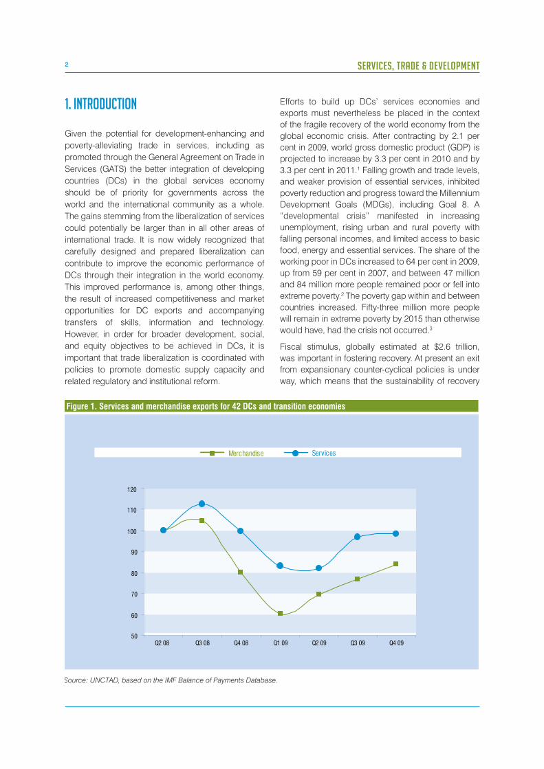
Figure 1. Services and merchandise exports for 42 DCs and transition economies
Source: UNCTAD, based on the IMF Balance of Payments Database.
50
60
70
80
90
100
110
120
Q2 08 Q3 08 Q4 08 Q1 09 Q2 09 Q3 09 Q4 09
Merchandise Services
Efforts to build up DCs’ services economies and
exports must nevertheless be placed in the context
of the fragile recovery of the world economy from the
global economic crisis. After contracting by 2.1 per
cent in 2009, world gross domestic product (GDP) is
projected to increase by 3.3 per cent in 2010 and by
3.3 per cent in 2011.1 Falling growth and trade levels,
and weaker provision of essential services, inhibited
poverty reduction and progress toward the Millennium
Development Goals (MDGs), including Goal 8. A
“developmental crisis” manifested in increasing
unemployment, rising urban and rural poverty with
falling personal incomes, and limited access to basic
food, energy and essential services. The share of the
working poor in DCs increased to 64 per cent in 2009,
up from 59 per cent in 2007, and between 47 million
and 84 million more people remained poor or fell into
extreme poverty.2 The poverty gap within and between
countries increased. Fifty-three million more people
will remain in extreme poverty by 2015 than otherwise
would have, had the crisis not occurred.3
Fiscal stimulus, globally estimated at $2.6 trillion,
was important in fostering recovery. At present an exit
from expansionary counter-cyclical policies is under
way, which means that the sustainability of recovery

3
CHAPTER I: PROMOTING SUSTAINABLE GROWTH AND POVERTY ALLEVIATION IN DEVELOPING COUNTRIES THROUGH THEIR INTEGRATION IN THE GLOBAL SERVICES ECONOMY
increasingly depends on private demand and
structural factors. Unfortunately, high and persistent
unemployment continues to hinder private demand
growth. Moreover, the root causes of the crisis are
yet to be effectively addressed, such as financial
regulatory weaknesses, inequalities within and among
countries, global imbalances and the incoherence of
global governance.
The crisis affected services trade differently from
merchandise trade. Fluctuations in services exports
exhibited less synchronicity across countries,
experienced lower magnitudes of decline, and
recovered more completely. Even so, countries
dependent on services exports were adversely
impacted. Demand contracted more particularly in
income-sensitive services – including tourism and
travel, financial services, construction, retail and
services related to merchandise trade, including
transport – than in energy, health, education,
telecommunications and some business and
professional services which are regarded as
necessities. While the lower volatility of total services
exports highlighted the relative “resilience” of services
trade to the crisis, gains associated with trade in
services should not be considered automatic.
In the context of the ongoing recovering and attempts
to better prepare countries for future crises the
importance of services, and particularly infrastructure
services, has been highlighted by the international
community. The G20 Nations, for example, have
determined as a key element for inclusion today’s
development agenda the need to identify and
secure financing for key infrastructure projects
that could help unleash the growth potential of the
developing countries. As a concrete step to look into
ways to harness investment in infrastructure in the
countries that need it most the G20 set up a High
Level Panel for Infrastructure Investment to produce
recommendations in order to scale up and diversify
financing for infrastructure needs, including from
public, semi-public and private sector sources, and
identify, with multilateral development banks, a list of
concrete regional initiatives. The panel is to produce
its recommendations by the end of 2011. Similarly the
recent UN LDC IV conference which was held on 9 to 13
May, 2011 in Istanbul,Turkey produced a Programme
of Action for the Least Developed Countries for the
Decade 2011-2020, which refers in several instances
to infrastructure services, stating that one of the major
challenges facing least developed countries is the lack
of adequate physical infrastructure, and emphazing
that reliable and affordable infrastructure services are
essential for efficient operation of existing productive
assets and enterprises in least developed countries,
attracting new investment, connecting producers to
market, assuring meaningful economic development
and promoting regional integration. In light of this
assessment the document suggests that LDC take a
number of action on infrastructure including to develop
and implement comprehensive national policies and
plans for infrastructure development and maintenance
encompassing all modes of transportation and ports,
communications and energy. It is also suggested
that development partners could also contribute inter
alia by providing enhanced financial and technical
support for infrastructure development in line with
least developed countries’ sectoral and development
needs and priorities.
Developing and least developed countries’ (LDC)
experience with liberalization has been mixed and
some countries have remained marginalized in
the world economy.4 Certain preconditions may be
necessary in order for countries to benefit fully from
the opportunities offered by participation in the global
services economy. These include coherent domestic
services and development strategies; adequate
regulatory, institutional and competition frameworks;
as well as the necessary infrastructure. There may also
be room for improving the multilateral trading system
(MTS) to make it more supportive of DCs. Among
the reforms of the system that can be imagined
are a greater focus on the liberalization of services
sectors and modes of supply of export interest to
DCs; full operationalization and improvement of
the special flexibilities in favour of developing and
least developed countries (LDCs); the inclusion of
measures effectively addressing developing and
least developed countries’ supply constraints; and
the completion of the GATS framework (i.e. the GATS
Rules and domestic regulation provisions) in a manner
which is supportive of development.
However, even if the MTS were functioning perfectly
this would not necessarily eliminate the negative
environmental, social and gender impacts that are
sometimes associated with privatization, liberalization
and increased services trade. Liberalization should
be tailored to produce not only positive economic
results but also social and human development gains.
Liberalization strategies and policies need to be
formulated in such a manner as to minimize negative

4 SERVICES, TRADE & DEVELOPMENT
externalities and maximize gains, while ensuring that
all population sectors, in particular the poorest, benefit
from them. In addition to reforms and improvements
that can be brought to MTS and to GATS more
specifically, there is need for adequate regulatory
and institutional frameworks (RIFs), adapted to each
country’s circumstances, as well as flanking policies
to accompany liberalization efforts.
Therefore DC integration in the global services
economy needs to be evaluated not only in economic
and trade terms but also according to the criteria
developed by the international community for what
liberalization of trade in services should achieve (that
is, sustainable development). This vision is embodied
in landmark declarations and documents including:
the Millennium Declaration of the United Nations and
the MDGs; the Doha WTO Ministerial Declaration; the
Declaration and Plan of Implementation emerging
from the World Summit on Sustainable Development
(WSSD); the Monterrey Consensus on Financing for
Development; the São Paulo Consensus and Spirit
of São Paulo (developed in the context of UNCTAD
XI); the findings and recommendations of the UN
Millennium Project Task Force; the 2005 UN Secretary-
General Report “In Larger Freedom”; and the Accra
Accord adopted by UNCTAD Member States in the
context of UNCTAD XII in 2008
The Millennium Declaration for example, cites as
the central challenge for the world today to ensure
that globalization becomes a positive force for all
people. The declaration recognizes the opportunities
offered by globalization while acknowledging that
benefits are often unevenly shared and that costs
are unevenly distributed. The Declaration therefore
recommends that globalization be rendered fully
inclusive and equitable, including through policies
and measures which correspond to the needs of
DCs and which are formulated and implemented with
their effective participation. Among the fundamental
values endorsed by the Declaration are: equality
(no individual or nation be denied the opportunity to
benefit from development as well as the equal rights
and opportunities of women and men); solidarity
(global challenges be managed in a way that
distributes the costs and burdens fairly); respect for
nature (the precepts of sustainable development be
used to correct the current unsustainable patterns
of production and consumption); and shared
responsibility (responsibility for managing worldwide
economic and social development be shared among
the States of the world). Several services sectors,
including education, health and services linked to
the provision of safe drinking water are specifically
identified in the Declaration as key elements for
achieving globalization that benefits all.
Development and poverty eradication are central
objectives identified in the Millennium Declaration.
This basically implies the need to devote all efforts to
freeing men, women and children from extreme poverty
and making the right to development a reality for
everyone. Success in meeting this objective depends,
among other things, on achieving an open, equitable,
rule-based, predictable and non-discriminatory
multilateral trading system. The Declaration further
emphasizes the need to assist DCs in mobilizing
required resources needed to finance their sustained
development and addressing the special needs of the
LDCs. As can be seen from the above description, the
Declaration goes well beyond simple economic and
trade gains to encompass a much broader notion of
sustainable development through trade.
The UN Millennium Project Task Force published
(early 2005) a report titled ‘Investing in Development,
A Practical Plan to Achieve the Millennium
Development Goals’. The report contains a series
of findings and makes recommendations for the
achievement of the MDGs. One of the group of
experts’ key recommendations held that high-income
countries open their markets to DC exports through
the Doha Trade Round and assist LDCs raise export
competitiveness through investments in critical
trade-related infrastructure, including electricity,
roads and ports. With respect to services the Task
Force advocated that liberalization of the movement
of labour be adopted as a high priority in the Doha
Round. It also proposed that DCs take commitments
in Modes 1 and 3 in exchange for “real” offers of Mode
4 by developed countries.
As acknowledged at the High-level Plenary Meeting
of the sixty-fifth session of the General Assembly
on the Millennium Development Goals (September
2010), while there has been some progress toward
the achievement of the MDGs (that is, the share of
poor people is declining) successes are nuanced
(the absolute number of poor in certain regions such
as South Asia and sub-Saharan Africa is increasing
and the number of people living in extreme poverty
and hunger surpasses 1 billion). Moreover, impacts
of the recent energy, food, financial and economic
crises have led to setbacks with respect to poverty
5
CHAPTER I: PROMOTING SUSTAINABLE GROWTH AND POVERTY ALLEVIATION IN DEVELOPING COUNTRIES THROUGH THEIR INTEGRATION IN THE GLOBAL SERVICES ECONOMY
eradication. Furthermore, a weak recovery will continue
to compromise efforts toward meeting MDGs. In that
context participating Governments reiterated that an
effective use of trade and investment opportunities
can help countries fight poverty. They also addressed
the trade-off issue between benefits of accepting
international rules and commitments in the areas of
trade, investment and international development and
constraints posed by the loss of policy space.5
The preamble of the Doha Declaration recalls that
WTO Members seek to place the needs and interests
of DCs at the heart of the Doha Work Programme.
Positive efforts, including enhanced market
access, balanced rules, well targeted, sustainably
financed technical assistance and capacity-building
programmes, be made to ensure that DCs, and in
particularly LDCs among them, secure a share in the
growth of world trade commensurate with the needs
of their economic development. The Declaration
also states WTO Members’ determination that the
Organization plays its part in securing LDCs’ beneficial
and meaningful integration into the MTS and the
global economy. The great emphasis WTO Members
placed on developmental aspects of the current
round of negotiations throughout the Declaration is
an indicator that the trade community acknowledged
the need to have development at the heart of its
initiatives and negotiations. However, the failure to
conclude the Round, within the nine years since the
Doha Ministerial Conference, indicates the difficulty of
moving past noble objectives and hortatory language
to negotiated and commercially meaningful trade
outcomes. One recent report by UNDP identified
the failure of the world’s largest economies on
their promise to put in place a trading environment
conducive to the achievement of MDGs as one of
the gaps in formulating the Global Partnership for
Development.6
The WSSD developed targets, timetables and
commitments to aid the fight against poverty and a
continually deteriorating natural environment. The
Conference was based on the premise that progress
in implementing sustainable development has been
extremely disappointing since the 1992 Earth Summit,
with poverty deepening and environmental degradation
worsening and that a new programme for production
and consumption was needed. Commitments were
made in Johannesburg – on expanding access to
water and sanitation, on energy, improving agricultural
yields, managing toxic chemicals, protecting
biodiversity and improving ecosystem management
– that would serve as the yardstick of success or
failure in achieving sustainable development. The
Conference concluded a global deal recommending
free trade and increased development assistance but
also commitment to good governance as well as a
better environment.
The Monterrey Consensus (which emerged from the
UN Conference on Financing for Development), also
offers insight on the holistic approach that needs
to be taken, in order to promote the sustainable
development of DCs. The Consensus highlights
that in pursuing the goal of eradicating poverty,
achieving sustained economic growth and promoting
sustainable development, it is necessary to address
challenges of financing development. This observation
is based on current estimates of dramatic shortfalls in
resources required to achieve internationally agreed
development goals, including those contained in the
United Nations Millennium Declaration. Indeed, while
globalization offers opportunities and challenges,
DCs face special difficulties in responding to them.
Domestic and international resources must be
mobilized and international trade promoted as
engines for development. Increasing international
financial and technical cooperation for development;
sustainable debt financing and external debt relief; and
enhanced coherence and consistency amongst the
international monetary, financial and trading systems
should also contribute to the sustainable financing of
development. The Declaration recognizes trade and
services and more particularly the movement of natural
persons, as one of the key issues of concern to DCs in
international trade to enhance their capacity to finance
their development. The Consensus also points to a
number of specific services which are supportive of
development. These include social, health, education,
as well as financial services, (including banking,
insurance and financial intermediation services) which
are crucial for the financing of development.
The São Paulo Consensus and Spirit of São Paulo7
recall that if globalization does offer new perspectives
for the integration of DCs into the world economy and
can contribute to improving the overall performance
of DC economies, it has also brought new challenges
for growth and sustainable development. Developing
countries have been facing special difficulties in
responding to these challenges. The role of the
international community and of its organizations is
therefore to explore how globalization can support

6 SERVICES, TRADE & DEVELOPMENT
development, and how appropriate development
strategies should be formulated and implemented
in support of a strategic integration of developing
economies into the global economy. This will, in
particular, come from a greater understanding of
the mutuality of interest between developed and
developing economies in sustained and sustainable
development. Moreover, the São Paulo Consensus
re-emphasizes that trade is not an end in itself, but
a means to growth and development. Trade and
development policies are important instruments
inasmuch as they are integrated in development
plans and poverty reduction strategies aimed at such
broad goals as growth, diversification, employment
expansion, poverty eradication, gender equity, and
sustainable development. Coherence and consistency
among trade and other policies for maximizing
development gains should be pursued at the national,
regional and multilateral levels by all countries. In this
context, the Consensus underscores the existence of
new trading opportunities in niche services sectors
where DCs have potential comparative advantages.
Moreover, it emphasizes the contribution that access
to essential services can have in terms of poverty
reduction, growth and sustainable development.
The Consensus also recalls the fact that DCs have
continuously emphasized the important of effective
liberalization of temporary movement of natural
persons under Mode 4 of GATS to them. Finally,
the Consensus underscores that efforts need to be
directed at identifying and promoting environmental
goods and services of actual and potential export
interest to DCs, as well as monitoring environmental
measures affecting their exports.
The Accra Accord8 recognizes that “the services
economy is the new frontier for the expansion of trade,
productivity and competitiveness, and for the provision
of essential services and universal access.” It points
out that despite of the growing services sector in the
world economy and trade, positively integrating DCs,
especially LDCs, into the global services economy
and increasing their participation in services trade,
particularly in modes and sectors of export interest to
them remains to be a major development challenge.
Finally, in the context of global carbon emission
cuts promoted by the UN Framework Convention
on Climate Change (UNFCCC) and the 2009
Copenhagen Conference, social and economic
development and poverty eradication in DCs were
acknowledged as the first and overriding priorities.
However, countries also agreed that a low-emission
development strategy is indispensable to sustainable
development.9 The unavoidable move toward less
carbon intensive economies will have impacts in
terms of countries’ competitiveness and by extension
on international trade. Developing countries have
already voiced concerns regarding the emergence
of burdensome technical standards linked to
process and production methods. Nevertheless, the
liberalization of environmental goods and services as
well as of climate-friendly services can be instrumental
to achieving global climate change objectives.
In discussing what can or should be done to promote
better integration of DCs into the global services
economy this chapter adopts the broader sustainable
development perspective adopted by the international
community in these declarations rather than place
focus on pure economic and trade issues. The
chapter will be organized as follows.
Section II considers development gains that can be
achieved through the liberalization of trade in services
and the implications of such trade for the three pillars
of sustainable development (economic, social and
environmental). Section III examines flanking policies
that must accompany the liberalization process in
order to correct negative externalities and impacts
that occur in the case of increased services trade
and economic growth. It also surveys regulatory and
institutional frameworks that are essential for services,
particularly as a means to address market failures and
promote various policy objectives. Section IV focuses
on the GATS’ and other regime contributions toward the
integration of DCs in world services trade. The success
of the GATS in achieving the beneficial integration of
developing and least developed countries into the
services economy is evaluated in light of alternative
liberalization regimes but also in light of broader
developmental objectives that the GATS should seek
to achieve as set out in the Preamble of the GATS
and Article IV. Section V contemplates approaches
for improving the GATS framework to better promote
integration of DCs in the global services economy.
Measures supporting the sustainable development
of DCs are reviewed, including provisions for special
flexibilities for DCs, progressive liberalization, as well
as technical assistance. The chapter then offers some
concluding remarks.

7
CHAPTER I: PROMOTING SUSTAINABLE GROWTH AND POVERTY ALLEVIATION IN DEVELOPING COUNTRIES THROUGH THEIR INTEGRATION IN THE GLOBAL SERVICES ECONOMY
Box 1: The contribution of services to competitiveness of economies
The role of services as inputs into other sectors of the economy is crucial. Services have an important role to play in terms of their
contribution to manufacturing output growth and productivity and a positive relationship has been found between the level of
per capita income and the intensity of use of services in manufacturing industries. Part of the gains comes from the outsourcing
of indirect production activities but also from certain structural changes in manufacturing industries, which raise their demand
for services as intermediate input. This leads to lower operating costs and increased productivity. But the extent to which a
manufacturing firm will use, in the production process, services procured from outside also depends on: (1) the pressures
on the firm to improve its competitiveness, which in turn depends on the domestic and international competition it is facing,
(2) the availability of services, which depends on the level of development of the services sector in the economy [and on the
openness of the economy to imports of foreign services], and (3) the relative cost of in-house provision of services as against
their procurement from outside agencies.12
The case of India is illustrative of this. Though service inputs contributed little to production of the registered manufacturing
sector in India during the 1980s, this contribution increased dramatically during the 1990s from about 1 per cent in the 1980s to
about 25 per cent in the 1990s. The services sector has increased its own demand by raising output growth and productivity of
the manufacturing sector in the post-reforms period which should help the services sector, to a certain extent, sustain its growth
performance. Trade reforms and liberalization undertaken in the 1990s played an important role in increasing the use of services
in the manufacturing sector. Indeed, trade which increased competition in the domestic market was found to be responsible to
a certain extent for the increase in the intensity of use of services in the manufacturing sector. This points to the possibility that
the Indian services sector might not only succeed in sustaining its own growth but might also help in improving the growth rate
of industrial sector in the near future.13
Single services sectors can also contribute significantly to the development of an economy. Tourism is one of the typical examples.
The worldwide contribution of tourism to GDP exceeds 5 per cent and its annual turnover has been growing at a faster pace than
GDP.14 It has become a useful means to promote economic diversification and strengthen DC economies owing to its linkages
with related services, manufacturing and agriculture sectors of an economy.15 In the Seychelles, for example, tourism services
not only generate income, foreign exchange, and employment but also serve as a catalyst for other economic activities such as
agriculture, fisheries, crafts and manufacture. Tourism is also the source of government revenues which are used to finance a
range of welfare services to citizens at low or very low cost and the development of infrastructure used by the whole community.
Finally, tourism justifies and allows paying for the preservation of the natural environment and cultural heritage of the country. All
of this contributes to making the Seychelles’ economy globally more competitive.16 For countries such as Cape Verde, Maldives
and Samoa, tourism has been a decisive factor supporting their graduation from LDC status.
2. DEVELOPMENT GAINS FROM INTERNATIONAL
TRADE IN SERVICES
Over the last decades the services economy has
gained in importance, contributing a growing share to
gross domestic product (GDP) and employment in all
countries. In 2008 services accounted for 66 per cent
of world GDP and 39 per cent of world employment.10
Services constitute 50 per cent of GDP and 35 per
cent of employment in DCs. Infrastructure services –
financial, transport, telecommunications, water and
energy – are fundamental for development, including
in providing universal access to essential services
for attaining the MDGs on water, energy, health and
education. Services have become a fundamental
economic activity and play a key role in infrastructure
building, competitiveness and trade facilitation.
Indeed, an UNCTAD study on the determinants of
export performance of merchandise goods points to
the important role that services relating to the internal
transport infrastructure can have in addressing supply
constraints, thereby promoting countries’ export
performance. This is particularly more important at the
early stages of development of the external sector.11
UNCTAD services database shows that the share
of services in total world trade has been increasing
steadily with average annual growth rate of world
services exports at 13.5 per cent between 2000 and
2008 – almost equal to that of merchandise exports
at 13.6 per cent during the same period. Developing
country exports expanded at a faster pace (15.6
per cent) than developed countries (12.6 per cent),
resulting in their increased share of world exports in
services from 22.8 per cent to 25.9 per cent. Least
developed countries share remained stagnant at 0.5
per cent. In 2008 trade in services accounted for over

8 SERVICES, TRADE & DEVELOPMENT
20 per cent of total world trade with world exports of
services nearing $3.9 trillion.
During the financial crisis and subsequent global re-
cession in 2008 to 2009, trade in services, as reflected
in balance of payments, contracted less and recov-
ered faster than trade in goods. Its relative “resilience”
in the crisis implies that a strong services sector is con-
ducive to building-up domestic economic resilience
to external shocks. Many DCs including China and
South Africa have thus incorporated the development
of this sector into their post-crisis growth strategies.
The sector can be particularly important for LDCs and
small, structurally weak and vulnerable States. Spe-
cialization is important with regard to growing, resilient
and employment-generating services sectors.
There are, however, differences in the development
of the services economy and infrastructure services
across countries and regions. According to UNCTAD
database, services in 2008 accounted, on average,
for 50 per cent of GDP in DCs, while for developed
countries accounted for 73 per cent. Developing
countries generally remained net importers of
commercial services. The same database shows that
the share of DCs in world total exports of services
was 25 per cent in 2008 compared with 23.1 per cent
in 2000. Average annual growth rates for services
exports of developed countries increased from 4 per
Box 2: Gains through the movement of natural persons
Multilateral liberalization of temporary movement of natural persons – through commercially meaningful GATS commitments –
can contribute to balance, predictability and equity in the multilateral trading system and thereby lead to increased development
opportunities for DCs. Recent studies have shown that gains from the liberalization of the movement of natural persons could be
larger than total gains expected from all the other negotiating items under current WTO negotiations. World welfare gains from
liberalization of the movement of workers could amount to $156 billion per year if developed countries increased, by 3 per cent,
their quota for the entry of workers from DCs.17
Another study computed gains of some $200 billion annually provided a temporary work visa scheme was designed and adopted
multilaterally.18 While a significant portion of movements currently taking place is from DCs to developed countries, there is
also considerable movement of workers between DCs and some movement from developed countries to DCs. Remittances
from workers are a major source of capital inflow for many DCs. In 20 transition economies and DCs including LDCs such as
Haiti, Nepal, Lesotho and Samoa, remittances – a proxy measure of benefits from cross-border movement of natural persons
– accounted for over 10 per cent of GDP.19 In 2008, remittances to DCs reached $328 billion, equivalent to 2.3 per cent of
aggregate DC GDP20 while in 2003 it amounted to $93 billion. The total amount of resources remitted could, however, be two
or three times higher, since a large number of transactions are realized through informal channels. During the recent financial
and economic crisis breaking out in the second half of 2008, remittances remained relatively resilient compared to aid and other
private capital inflows with officially recorded remittance flows to DCs amounting to $316 billion in 2009,21 thus providing a buffer
against economic shocks and important source of financing for development.
Remittances improve the ability of countries to finance development objectives, the foremost of which are poverty reduction
and improvement of human capital. Their positive role is particularly pronounced for LDCs – for many low-income countries,
remittances as a share share of GDP and imports are larger than in the case of middle-income countries. Middle- and lower-
skilled workers tend to remit a higher proportion of their income. Policies are needed to support technology transfer that facilitates
remittances or investments by making such transfers less costly.
A recent UNCTAD study22 quantitatively analysed the extent to which remittances reduce poverty in DCs. Using panel data for
77 DCs (for the period 1980 to 2008), remittances were found to significantly reduce poverty in recipient countries. For a given
level of GDP, a 10 per cent increase in remittances reduces the poverty headcount ratio by about 3.1 per cent and the poverty
gap by about 3 per cent to 5 per cent.
Concerns abound that the movement of workers may result in sending countries to lose some scarce resources. Countries
have been experimenting with unilateral, bilateral and multilateral mechanisms to prevent and alleviate brain drain.23 However,
empirical studies suggest that there is an “optimal level of migration” that stimulates pursuit of higher education at home and
spurs economic growth. Scarce employment opportunities and the limited capacity for collecting income taxes may limit the
actual costs for the individual and the home economy. “Brain circulation” is therefore probably a more appropriate term to
describe the exchange of skills in international trade in services. Despite what is often stated, wages are not likely to decline in
the host economy, as foreign services providers will not be perfect substitutes for national ones. Mode 4 liberalization is also
possibly one of the best ways to reduce permanent or illegal migration and maximize gains for sending and receiving countries.
9
CHAPTER I: PROMOTING SUSTAINABLE GROWTH AND POVERTY ALLEVIATION IN DEVELOPING COUNTRIES THROUGH THEIR INTEGRATION IN THE GLOBAL SERVICES ECONOMY
cent during the period 1995 to 2000 to over 14 per cent
during the period 2003 to 2008. For DCs, this latter
figure was 18 per cent, compared to 3 per cent for the
1995 to 2000 period. In 2008 exports of services from
DCs grew at 13.5 per cent compared with 10.6 per
cent for developed countries. Developing countries’
share in global imports of services has increased from
24 per cent in 2000 to 31 per cent in 2008. During the
same period, developed countries share has declined
from 71.04 per cent in 2000 to 65.37 per cent in 2008.
Least developed countries have continued to build
up export capacities in services, which grew at an
average annual rate of 7.9 per cent during 2003 and
2008 compared to 3 per cent during 2000 and 2003.
Nevertheless, they still face substantial difficulties in
participating in services trade, and their exports are
particularly vulnerable to external shocks. In 2008,
LDCs accounted for 0.5 per cent of world trade in
services, (consisting primarily in transport and travel
services) –their comparative advantage is in the
export of labour-intensive services.
The above figures attest to the economic gains that
can accrue from trade in services. Services can,
however, also be viewed as important contributors
to a sustainable economy. They can favour poverty
reduction, including through the informal services
sectors, which continue to play an important role in
most DCs. Services can also contribute to gender
equity, as many services firms are traditional
employers of women. Moreover, certain specific
services activities have direct favourable impact on
health (services by doctors, nurses, midwives, as well
as hospital services), the environment (sewage, refuse
disposal, and sanitation services), and on the general
welfare of the population (education, social services,
sporting, and recreational services). Services trade,
which allows for consumption beyond what can be
produced locally, has the added effect of multiplying
these different impacts. For example, in the case of
DCs, trade in services through Mode 4, is considered
to hold the potential for positively contributing to
development through remittances that workers send
back home.
The impact of other services sectors could, however,
appear more problematic in terms of sustainable
development if activities are not conducted in an
appropriate and regulated context. Two such examples
are in the transport services (with the pollution that
can be associated with increased movements of
products and people), and in the financial services
(with the negative social impacts of economic
crises in the absence of prudential regulation).
Coordination and sequencing of regulatory reform
and trade liberalization will go a long way in pursuing
development and poverty alleviation through the
growth of services sectors.
Services activities do not necessarily produce either
all positive or negative results. Most often they tend to
produce a mix of both and it will be for the authorities
to ensure that gains outweigh any negative impacts.
Similarly, the impact on the environment can be
complex. The fundamental paradox that underlies the
environmental aspect of tourism is that most forms of
tourism depend on either a built or natural environment
(which will probably lead to increased investment and
spending in these areas), but excessive tourism can
degrade that same environment through pressures on
natural resources such as water and energy, pollution
and waste generation and damage to ecosystems.26
Box 3: The tourism sector in DCs
Many DCs have an important interest in tourism.24 The sector contributes to economic diversification and job creation through
linkages with the rest of the economy. The worldwide contribution of tourism to GDP exceeds 5 per cent.25 Tourism is the main
source of foreign exchange for one-third of DCs and one-half of LDCs, accounting for 40 per cent of GDP. It contributed to
graduation from LDC status of Cape Verde and Maldives. Many WTO Members seek liberal commitments addressing remaining
sectoral and modal barriers such as in Mode 3 (commercial presence) and in Mode 4 and anti-competitive practices.
For example, tourism and tourism-related services have the potential to positively contribute to such varied objectives such
as: rural development, agricultural transformation; community enrichment, social empowerment (particularly for women), and
preservation of cultural and heritage traditions. At the same time, there can also be negative social outcomes from tourism
activities including: increased incidence of crime; spread of drugs and diseases, including HIV/AIDS; change or loss of
indigenous identity and values; culture clashes; and ethical issues (child labour, prostitution and sex tourism).

10 SERVICES, TRADE & DEVELOPMENT
It also poses a growing threat to preservation of
cultural resources.27 Guidelines, principles and codes
of behaviour at the local, national and international
levels are therefore helpful to ensure that tourism
activities lead to sustainable development. Proper
capacity planning, zoning, redesigning the tourism
product to promote ecotourism and cultural tourism,
environmental regulations, and cultural preservation
initiatives have become increasingly important as the
sector matures.28
The impact of services on a sustainable economy will
not depend only on the availability of services but also
on who is providing the services and in what context.
In the case of health and education for example, there
may be significantly different impacts depending on
whether a government is the main provider (in which
case considerations such as universal access may be
determinant) or whether the main provider consists of
a combination of public and private interests.
Similarly, in cases where foreign competition is vibrant,
gains that accrue to the DCs may be reduced (in the
case of tourism, a substantial proportion of gains
are realized by developed country tour operators as
opposed to the countries of tourist destination). The
overall impact of these services on the sustainability
of DC development will, therefore, largely depend on
the underlying characteristics of the markets (type
of services being provided, type of consumers and
type of service suppliers) as well as on the regulatory
and institutional frameworks in place in DCs. The
impact of services may also depend on the mode of
supply through which they are being supplied (with
the exception of a few financial services, cross-border
supply can be considered particularly interesting
from a sustainable perspective, as it may constitute a
valuable alternative to both the movement of persons
to supply services and the supply of services through
goods). Therefore, a better understanding and grasp
of these elements is crucial in assessing the potential
for services trade as positive contributor to growth
and sustainable development.
While countries can harness services trade for both
economic growth and sustainable development, DCs
Box 4: New trading opportunities for DCs through cross-border supply and outsourcing of services
The development and spread of modern information and communications technology has allowed for an increasing share of
international trade in services to take place through cross-border supply.
Linked to this phenomenon, recent technological developments in computer and related services are rendering the outsourcing
of many services an increasingly efficient option for firms. Outsourcing is used by enterprises seeking to take advantage of low-
wage countries, focus on core activities in fewer locations in order to save costs, and take advantage of productivity gains and
access to additional skills. This is giving rise to new trading opportunities for DCs. Outsourcing has become an important source
of export earnings for countries such as India whose commercial services exports currently account for as much as 25 per cent
of total exports. China is also posting notable success in outsourcing services – in 2008 the value of implemented outsourcing
contracts amounted to $4.69 billion and formalised new outsourcing contracts were valued at $5.84 billion. To accommodate
this surge approximately 100,000 trained workers were employed, resulting as an important source of job creation (particularly
for young graduates from colleges and universities who currently account for 82.9 per cent of the employees in this sector).
Globally, outsourcing services demonstrate resilience in the times of crisis. In spite of the unprecedented post World War II
economic crisis of 2008 and 2009, global outsourcing expenditures in 2009 were estimated to have reached $373 billion – a
14.4 per cent increase over 2008.29 However, the fear that growth of services outsourcing may lead to employment losses in
developed countries has given rise to protectionist tendencies, which may prevent firms from taking advantage of the gains to
be made from outsourcing.
Overall, the trade of outsourced services is taking place between developed and DCs, as well as within each group, with DCs
strongly involved in the rise of outsourcing. The gains for receiving countries could be enormous, given that the export earnings
derived from outsourcing are often accompanied by a number of related advantages, including FDI, human capital formation
and knowledge spillovers.
In order to capture the new trading opportunities from outsourcing, DCs can implement a number of domestic policies, relating
among other things to infrastructure development; legal and regulatory framework improvements; human resource development;
and so forth (international policies can also help). In addition, a moratorium could be placed on any restrictive policies relating
to outsourcing (such as government procurement). In all these areas, there is need to explore options for the best way to arrive
at meaningful liberalization.

11
CHAPTER I: PROMOTING SUSTAINABLE GROWTH AND POVERTY ALLEVIATION IN DEVELOPING COUNTRIES THROUGH THEIR INTEGRATION IN THE GLOBAL SERVICES ECONOMY
need to ensure that the multiple characteristics of
service sectors (potential for contributing positively to
the economy while not losing sight of the negative
externalities that may result) are taken into account
and that adequate regulations, institutions and
policies are in place to achieve the desired outcomes.
Authorities must acknowledge that there exist certain
interdependencies between trade and development
policies which will not always lead to easy policy
choices. Indeed, it may be difficult to allocate resources
to trade-related objectives when faced with pressing
development priorities (pandemics and widespread
poverty) just as it may be difficult to allocate resources
to long-term sustainable development objectives
in the presence of more concrete and short-term
economic rewards from trade.
There is a need to strike a balance between the
objectives of efficiency and equity. Both the State
and the market have an important role to play in the
development process, and as such must streamline
their respective roles in a complementary manner.
Furthermore, as development of the private sector
is critical for economic growth, the State is vital
for designing and implementing development
strategies, reducing poverty and attaining equitable
income distribution, building physical and human
infrastructure, addressing market failures where they
occur, ensuring consumer protection, employment
safety nets, and providing enabling macroeconomic
conditions and a sound regulatory framework.
3. SUPPLEMENTARY MEASURES FOR ACHIEVING
DEVELOPMENT-ENHANCING SERVICES TRADE:
THE NEED FOR ADEQUATE REGULATORY AND
INSTITUTIONAL FRAMEWORKS AND
FLANKING POLICIES
In many respects, the various regimes for liberalizing
trade in services are not enough to guarantee DCs’
broader developmental objectives for building a
competitive domestic supply and trade in services
are achieved. Benefits are not automatic and there
may be a number of burdensome costs associated
with trade in services, arising principally from market
failures. Regulatory and institutional frameworks
(regulation and regulatory institutions) are essential
tools for responding to market failures and mitigating
economically and socially undesirable results
while promoting development of services sectors.
Regulation aims at achieving other key domestic
policy objectives (development of domestic supply,
consumer protection, climate change mitigation,
as well as contributing to poverty alleviation, by
ensuring universal access to essential services). The
crisis exemplified the importance of regulatory and
institutional frameworks. The financial market boom
preceding the crisis was not matched by adequate
national and global market regulations. The regulatory
failure in the deregulated environment became
manifest with regard to control of product safety for
complex and high-risk financial products, consumer
protection, risk management and leverage, regulation
of non-traditional financial institutions, credit-rating
agencies, assessment of systemic risk, capital
adequacy regulation, moral hazard and incentive
structure for compensation systems. Sound national
regulations and institutional frameworks adapted
to individual country conditions and capacities, and
international regulatory cooperation, are essential in
preventing future crises. However, regulatory systems
also entail costs, through administrative and human
resources required for their implementation and for
businesses who have to comply with them.
Institutions and procedures are amongst the central
determinants for the quality of regulations. Although
various institutional approaches exist, perhaps the
most prudent would be to adopt the “best-fit” system
as it depends on specific services sectors economic
attributes; technological considerations; as well
as a country’s economic, social, institutional and
political endowment and human and administrative
resources. Moreover, formally establishing regulatory
and institutional frameworks is not sufficient in itself as
credibility and stability will only come with experience
and institutional strengthening. Also, broader policy
and legal environments will have an impact on how
functional regulatory systems can be.
Flanking policies can be seen as a tool to ensure that
not only the economic effects of trade in services
are taken into account by policy makers but also
the cultural, social, environmental and distributional
impacts. Flanking policies must accompany
liberalization in order to ensure that sustainable
development is achieved. Measures need to be put
in place at both the domestic and at the international
level.30
12 SERVICES, TRADE & DEVELOPMENT
The type of costs or impacts that flanking policies
will need to address include unemployment, raising
prices of services, anticompetitive practices and a
whole range of negative social and environmental
externalities. Policies will have to be designed
with the objective of, among other things, meeting
development costs, limiting the risk of crowding-out
of local players and potential job losses, ensuring
safety nets, guaranteeing universal access to certain
essential services or at least making services available
to a greater proportion of the population, ensuring
competition, maintaining health and safety standards,
limiting urban sprawl, contributing to regionally
balanced socioeconomic development, and reducing
poverty, to name but a few.
Flanking measures can also be used to address
supply-side constraints and ensure competitive
outcomes. Addressing supply-side constraints
involves, among other things, addressing DCs’ lack of
access to finance and new technologies, the high cost
and low quality of distribution and transport services,
the lack of requisite infrastructure services generally,
and the lack of supporting institutions, including for
SME-specific measures. Among the measures that
can lead to increased competitiveness, of the services
economy in DCs, are measures aiming to create an
enabling environment for investment, technology
and enterprise development; measures providing
for the adoption and financing of information and
communication technology (ICT); as well as measures
for efficient transport facilities and trade facilitation
Box 5: Providing universal access to essential and infrastructure services
Essential services can serve as an example of services where flanking policies must accompany privatization and liberalization.
Several services are in the general interest of the public and, indeed, essential for human life (health, education and the provision
of water).
Consequently, governments must ensure the adequate provision of such services (including to the poor and marginalized).
While traditionally, the provision of such services has rested within the public domain, the last decades have seen a trend
of opening up essential services sectors to domestic and foreign competition. However, this has produced mixed results,
sometimes increasing the price of services for the poor or entailing considerable adjustment costs.31
The same can be said for several key infrastructure services. Privatization without creating conditions of competition, or the
increase of entry in sensitive sectors (financial) without adequate prudential supervision and full competition serve as examples.32
If the transition process had been adequately managed and regulated, it would – in theory – have been possible to fully reap
the benefits of privatization and liberalization policies. Research has been devoted to identifying the delicate combination of
competition and regulation, required to make privatization and liberalization contribute positively to development. One policy
recommendation that has come out of this research is the need for increased competition and for complementary regulations
with a social purpose. A non-discriminatory universal service obligation is one example of such regulations. Some countries have
successfully experimented with regulations to ensure universal services, with subsidy schemes or universal service obligations
being possible options. Chile, in the case of telecommunications, has adopted a scheme involving several elements: a universal
service levy (1 per cent) to generate finances, and a competitive bidding process to allocate funds. The latter should encourage
operators to adopt the best technology and cost-saving practices. Ultimately, this system has allowed Chile to significantly
increase the number of household telephones with a minimum level of subsidies.33 Ghana established a fund – The Ghana
Investment Fund for Telecommunications (GIFTEL), in operation since 2005 – with the aim to make telecommunication easily
accessible across the country by developing the communications infrastructure in rural areas and thereby contributing to
meeting Millennium Development Goals. To establish funds, the Government of Chile charges every licensed or authorized
operator 1 per cent of contribution from their revenues. GIFTEL facilitates investment for eligible projects in under-served areas
where commercially viable telecommunication services are not available. Funds are allocated on a competitive basis through
an open bidding process based on the successful assessment of a plan’s long-term financial sustainability. This assessment
also reflects how inclusive the plan is with regard to local stakeholders, and in particular for those who are at a disadvantage.
Specific obligations may be placed on licensed operators in order to help facilitate policy objectives, which include specific
interconnection responsibilities. According to the Government of Ghana’s 2009 Budget Statement, under GIFTEL, 39 “common
telecom facilities” were completed, which enabled the extension of service to 273 communities.34
Not all countries have been as successful though. India’s experience in telecoms highlights the difficulties that can arise when
implementing universal service obligations for private sector providers. While targets were set and stipulated in various license
agreements, it was not possible to meet them. Inadequate enforcement mechanisms and overly ambitious targets were among
the reasons for failure.

13
CHAPTER I: PROMOTING SUSTAINABLE GROWTH AND POVERTY ALLEVIATION IN DEVELOPING COUNTRIES THROUGH THEIR INTEGRATION IN THE GLOBAL SERVICES ECONOMY
arrangements which help to reduce overall transaction
costs. Among the more specific measures that can
be considered in this context are subsidies and other
support measures to service suppliers, incentives
for consumers to choose domestically produced
services and temporary safeguard mechanisms. The
first will ensure that the suppliers can grow beyond
infancy status and move on to become more efficient
producers even when faced with foreign competition.
Incentives for consumers to choose domestic goods
are an indirect means of providing domestic services
suppliers with a (captive) market large enough to allow
them to expand their production. The third category of
measures provides services suppliers with temporary
relief from competition from foreign services suppliers
in order to allow for adjustment. However, as
discussed later, trade liberalizing commitments under
international agreements may put certain limits on a
country’s ability to use these measures.
Competition issues are equally crucial in DCs as
anti-competitive measures considerably reduce the
positive effects of trade liberalization for consumers
and enterprises, particularly SMEs. Competition law,
institutions and authorities should be established
in order to safeguard DCs against anti-competitive
behaviour in their markets. Indeed, where adequate
regulatory framework for competition is not in place,
liberalization may imply the replacement of domestic
monopolies and dominant players by foreign
monopolies and dominant players.
By using flanking policies authorities attempt
to integrate developmental, cultural, social,
environmental and even national security perspectives
in addition to the economic perspective in trade
policymaking and economic planning. The overall
objective is to strike a balance between different types
of considerations. Flanking policies can either limit:
trade activities (zoning regulations, operating hours,
and so forth) or place conditions on the exercise of
these activities (local content requirements, local
materials, suppliers and services); requirements for the
creation of employment opportunities, introduction of
advanced technology, upgrading of local technology,
or skills development; qualification requirements
and technical standards, with the view to achieving
specific economic, social and environmental results.
This can be considered an important step toward
managing the interaction between trade and broader
development policies at the national level.
Countries without the necessary flanking policies may
not reap the full benefits from liberalization and the
costs of integration in world services economy may
outweigh benefits. However, flanking policies should
not be viewed as the panacea for all development
related challenges linked to trade liberalization. There
are certain limits to this approach.
Indeed, the emergence of various rule-based regimes
for international trade means that the space for national
economic policy – the scope for domestic policies –
is now often restricted by international disciplines,
commitments and global market considerations.
Such trends can be exemplified by the inclusion
of services in the multilateral trading system which
brings domestic regulatory issues within the ambit of
the WTO. This is in marked contrast with the GATT’s
focus on border measures. Article XXVIII of the GATS
defines the very broad nature of measures covered
by the Agreement which includes “any measure by
a Member, whether in the form of a law, regulation,
rule, procedure, decision, administrative action, or
any other form”. This new focus of GATS on domestic
regulations may lead in certain cases to the difficulty of
Members to change, adapt or improve their regulatory
frameworks relating to services subject to scheduled
commitments. Indeed, the extent of the ‘right to
regulate’ a particular service sector contained in the
preamble of the GATS, (Guidelines and Procedures
for the Negotiations on Trade in Services) as well
as the Doha Ministerial Declaration is related to a
particular Member’s liberalization commitments
From a DCs perspective, it is crucial to retain sufficient
flexibility for regulatory and institutional building.
Indeed, DCs will not always be in a position to adopt
the type of frameworks or upgrade their institutions to
the levels that may exist in more developed economies.
For this reason, it is important that a wide range of
policy options still remain available to governments
in the course of liberalizing services sectors under
GATS or other international arrangements. If
international commitments were shown to constrain
DCs developmental policy options it would prove
particularly negative given the many policies (for
supporting growth, poverty reduction, re-distribution,
protection of the environment, and other social
objectives) that need to be put in place in order for
these countries to achieve a sustainable development
of their economies. For example, strengthened and
globally coordinated financial market regulations
are important to address structural flaws in financial
14 SERVICES, TRADE & DEVELOPMENT
regulatory systems precipitating the crisis. The
Basel III higher banking capital requirement will be
implemented by end 2012. But tighter financial sector
regulations and increased high-income sovereign
borrowing are estimated to reduce DCs’ growth rates
by 0.2 per cent to 0.7 per cent for a five-to-seven-year
period.35
However, even where policy space is available, the
policy mix necessary to produce desired results will
be determined on the basis of ‘trial and error’ and on
concrete experiences of what works and what does
not work in each country. For example, not all options
may be practical to implement, particularly for DCs.
Since an adequate policy response will depend on
country-specific national development potentials
and socio-economic circumstances, as well as
different initial conditions in terms of size, resource
endowment, economic structure and location no easy,
one-size-fits all approach can be developed. To date,
a lack of understanding exists over exact functioning
of various policy suggestions. Moreover there is even
less understanding of how these options may play
out in different economic and social scenarios and
how different reforms should be sequenced. In order
for privatization and liberalization to deliver expected
benefits, more analytical work is required toward
identifying ways of ensuring coherence between
regulation and trade liberalization (how to create
regulatory and trade agendas mutually supportive,
and how to reconcile trade, development, social
and equity objectives). Regulatory and institutional
frameworks are crucial for allowing countries to
balance multiple objectives pursued by governments
and to ensure the involvement of all stakeholders.
This is particularly important in the case of poverty
alleviation as it is now acknowledged that there are
important synergies among the MDGs. For example,
gender and women’s empowerment, more specifically,
have large multiplier effects on poverty eradication.
This relation stems from the strong correlation found
between the gender gap, economic development and
national competitiveness. Similarly, integrating climate
change and poverty reduction policies will become
ever more important, in an era where adaptation and
low-carbon development and diversification (toward
services and other activities more respectful of the
environment) are becoming essential components of
countries’ broader development strategies.
4. THE GATS’ AND OTHER REGIMES’
CONTRIBUTION TO THE INTEGRATION OF
DEVELOPING COUNTRIES IN SERVICES TRADE
It should be noted that liberalization of trade in
services through the GATS is but one among
many policy options available to governments for
developing, regulating and liberalizing services sector.
Broadly, options for countries range from domestic
reform measures aimed at developing the local
services industry (including through privatization)
and autonomous liberalization (decided either
independently or in the context of broader reforms,
including under the aegis of the international financial
institutions), to bilateral and regional economic
integration or trade agreements. The GATS, and its
contribution to integrating DCs into the global services
economy, can therefore be evaluated in comparison
to these alternative means for achieving liberalization.
GATS
The GATS is the first multilateral framework of
principles and rules for progressive liberalization of
trade in services and as such can be considered
an important tool for achieving the integration of
countries into the global services economy. Indeed,
GATS allows WTO Members to negotiate reciprocal
benefits in exchange for locking-in policy reforms in
the services sector.
It is difficult to clearly determine and evaluate the
impact of the results of the Uruguay Round GATS
negotiations and their effect on the integration of
DCs in the global services economy and on their
development. Isolating the impact of the Uruguay
Round negotiations from the impacts of other
measures and regimes for liberalizing services is an
arduous task.
Given the difficulty of assessing the value of
commitments in terms of trade balance or
development impact the coverage of trade
commitments by WTO Members has often been
used as a proxy measure and only very general
and qualitative analyses have been undertaken at
this stage. Members’ specific commitments vary
widely in sectoral and modal coverage, extent of
limitations to market access and national treatment. In
general, there is a correlation between the degree of
development of the services sector and the coverage
of the sectors offered. However, it should be noted
15
CHAPTER I: PROMOTING SUSTAINABLE GROWTH AND POVERTY ALLEVIATION IN DEVELOPING COUNTRIES THROUGH THEIR INTEGRATION IN THE GLOBAL SERVICES ECONOMY
that this does not necessarily mean that DCs with an
interest in developed country markets are well served
since developed countries have largely excluded
some important services sectors, for example audio-
visual, maritime services, and specific sub-sectors
in business services, as well as Mode 4 from their
commitments. The emphasis of most commitments
put forward by all countries, including developed
countries, is on commercial presence mode of supply
and movement of persons in the form of intra-corporate
transferees. Until recently perhaps, most DCs were not
in a position to benefit from the commercial presence
mode of supply given the high cost of establishment
in developed countries and the weaknesses of DCs’
firms in terms of financial and human capital and
access to distribution networks, information channels
and technology. Sectors of particular interest to DCs in
Mode 4 such as tourism-related services, construction
and engineering, business services, health-related
services and maritime transport, are included in the
commitments of many developed countries. However,
only top-management personnel are allowed to move
to provide these services while DCs’ interests reside
in natural persons with medium-to lower-skill levels.
The Mode of supply through movement of natural
persons has been committed in nearly all schedules
by “horizontal” commitments in the limited categories
of intra-corporate transferees (managers, specialists,
executives) and business visitors. The commitments
do not indicate sectoral specificity or specific occupa-
tional categories. The value of these commitments is
limited in light of their connection with Mode 3 com-
mercial presence commitments. Moreover, it should
be noted that national treatment in most cases is left
unbound. Finally, most of the commitments in Mode 4
are still subject to economic needs test (ENTs). Eco-
nomic needs test could act as quota restrictions.
The Uruguay Round commitments of both developed
countries and DCs can generally be considered to
have been mainly status quo commitments. Whilst DCs
may acknowledge that the consolidation of the status
quo has guaranteed security of access, which can
favourably impact on trade and investment in services,
the potential of the Uruguay Round commitments
for significantly increasing their integration into the
global services economy can be considered relatively
limited. Indeed, even where market access and natural
treatment has been granted, DC services and services
suppliers may not be able to out-compete more efficient
competitors from developed countries. However,
from the DC position, status quo commitments have
represented a higher level of concession as they
reflected recent reforms, supported among other
things, by the international financial institutions.
Given the complexities associated with quantifying
barriers and limitations to market access or national
treatment and the bindings on different modes of
supply of services the development of quantifiable
criteria has not been as equable as in the case of
goods trade. While identifying quantifiable values,
either for the existing level of market access or for the
proposed liberalization, remains a challenge. Several
attempts are being directed to improve available data
and analysis of the services economy.36
An attempt is possible to assess the success of the
current Round in achieving the integration of DCs into
the global services economy (based on the views of
DCs).37 The initial 71 offers and 31 revised offers that
have, to date, been submitted already allow for a
preliminary assessment of the current negotiations’
potential for increasing DC participation in trade in
services. Such an analysis is useful to defer waiting
until the end of the Round to assess whether the stated
developmental objectives are achieved. Moreover,
Negotiating Guidelines and Procedures for the
Negotiations specifically provide that – in addition to
the on-going assessment exercise the results of which
should allow to adjust the negotiations (Paragraph
14) – there shall be regular review of progress in
negotiations to consider the extent to which Article IV
is being implemented and to suggest ways and means
of promoting the goals established therein (Paragraph
15). In general, offers do not show considerable
increase in sectoral coverage. They also only show
modest improvement in the level of liberalization
commitments. Minimal progress has been shown in
liberalizing modes and sectors of export interest to
DCs. Several of the initial offers and revised offers
seem to negate previous commitments taken or to
produce no real change in the level of commitment
(even where modifications have been introduced). This
is done either by redefining the sector or sub-sector to
which a commitment applies or by moving from one
partial commitment to another one.
A review of the offers in Mode 4 demonstrates that while
commitments to provide market access for new cate-
gories of persons are offered (that is, persons entering
for career development purposes, graduate trainees,
contractual service suppliers and independent profes-
sionals) by a few countries, offers have far fallen short
16 SERVICES, TRADE & DEVELOPMENT
of expectations from DCs and LDCs in terms of sec-
toral coverage, quota removal and economic needs
test or labour market test. There is no indication of real
progress in the liberalization of Mode 4 in skill levels of
interest to DCs – due mainly to importing country con-
cerns over implications of liberalizing Mode 4 for their
labour market. In some cases, a few limitations are
removed, new categories of services suppliers are in-
troduced or the definition of professionals broadened.
However, these changes remain limited to highly skilled
professionals related to Mode 3. More efforts are need-
ed to expand the scope of categories delinked from
Mode 3 as requested by a group of DCs and LDCs in
their respective collective requests submitted in 2006
in accordance with the decision of the 6th WTO Ministe-
rial Conference in Hong Kong. Furthermore, there is no
indication of an attempt to streamline or increase the
efficiency of processing mechanisms for visa and work
permits and making them transparent to facilitate en-
tries of Mode 4 services suppliers. Negotiations to set
disciplines for domestic regulatory measures, includ-
ing qualification requirements and procedures which
have a direct bearing on Mode 4, have been on-going
for many years and Mode 4-related regulatory meas-
ures are unlikely to be placed under strong disciplines
due to concern from importing countries. This implies
that liberalization commitments in Mode 4 may not be
very ‘meaningful’ from the perspective of many DCs.
With development of information and communica-
tions technology, more and more DCs have shown
interest in exporting outsourcing services, mainly
through cross-border supply. In services relevant to
outsourcing such as business services, telecommuni-
cations services and financial services, existing offers
show some progress with improved commitments
and an increase in new commitments. Still there is
ample room to improve offers, in particular given the
low level of offered bindings on Mode 1. Barriers in-
clude commercial presence required under Mode
1 or outright prohibition on outsourcing. Therefore
commitments could range from substantial liberaliza-
tion to binding existing liberalized markets. Develop-
ing countries have particular interest in tourism as it
is a major component of world trade, ranking fourth
after fuels, chemicals and automotive products and
accounting for over 30 per cent of world commercial
services exports in 2008. One of the most promising
features of the tourism sector’s strong performance
in recent years is that growth in arrivals is greatest in
DCs. In many small DCs and LDCs, tourism domi-
nates their services exports. In over 150 countries,
tourism is among the five top-export earners, and in
60 countries it accounts for the number one export. It
is the main source of foreign exchange for one-third
of DCs and for one-half of foreign exchange of LDCs,
accounting for up to 40 per cent of GDP. Although this
is the sector with most commitments in the Uruguay
Round, many barriers exist, such as: limitations on for-
eign capital thresholds; discrimination against foreign
franchises; lack of means to facilitate temporary entry
of skilled personnel; procedures used for formulating
and administering travel warnings; and anti-competi-
tive practices (including abuse of market dominance,
and discriminatory use of information networks). This
sector has attracted relatively more offers in the Doha
Round and improvements have been offered by
some Members. Nevertheless, additional efforts are
required to address existing barriers requested for re-
moval by DCs.
While most favoured nation treatment (MFN) is
considered to be the fundamental principle and pillar
of the multilateral trading system, few initial offers and
revised offers indicate that countries are abandoning
MFN exemptions. S meagre 10 per cent of the over
400 existing MFN exemptions have been offered to
be removed. There are worries regarding a substantial
number of MFN exemptions to be maintained at the
end of the Round. This can be cause for concern
as the impact of the exemptions has not yet been
assessed and potential negative repercussions on
DCs deflected. Finally, in the cover pages to their
offers certain WTO Members refer to the notion of
reciprocity.
Most DCs are still at the early stage of services devel-
opment and their domestic supply and export capaci-
ty require development through proactive government
policies. While the GATS request-offer process natu-
rally builds upon bargaining and exchange processes,
flexibility should be maintained for DCs and reciproc-
ity should not be requested of them. The exemption of
LDCs from making liberalization commitments in the
Doha Round not only relieves them from such burden-
some requests and offer negotiating process, it also
ensures that they will have more autonomy in regulat-
ing and developing their services sectors in line with
their own situation and needs.
Autonomous domestic reforms
Domestic measures to develop the local services
industry, (though they can be elaborated before
liberalization of trade in services by themselves)
17
CHAPTER I: PROMOTING SUSTAINABLE GROWTH AND POVERTY ALLEVIATION IN DEVELOPING COUNTRIES THROUGH THEIR INTEGRATION IN THE GLOBAL SERVICES ECONOMY
may have widespread impact on liberalization once
it occurs. Indeed, measures that will affect such
elements as the domestic competitive environment,
access to finance and development of skills and know-
how will, at a later stage, impact positively or hinder
the ability of domestic services and services suppliers
to compete in international markets. The advantage
of such domestic policies, as of autonomous
liberalization, is that they can pass through a stage of
regulatory and institutional experimental trial and error
and can ultimately be reversed if authorities realize
that intended results are not being achieved.
The choice of reform policies for services sector
ranges from preserving the role of the government in
the provision of services, and more particularly those
with public goods characteristics, to full privatization
and liberalization of the sector. All these may be
viable, or not depending on the prevailing economic
and social conditions in a country and in international
markets.
Regional trade agreements
While domestic choices and domestic environment
are crucial in allowing countries to reap the benefits of
trade in services, the different regional or international
regimes for the liberalization on trade and services are
also key enabling environments for a DCs’ successful
integration into the world economy. The most
interesting among alternative regimes is possibly that
of regional trade agreements (RTAs).38 The last years
have seen a proliferation of RTAs covering trade in
services. Some agreements are signed only among
developed or DCs, while others have a combination
of signatories. Some of these agreements follow the
GATS approach toward market opening (the positive-
list hybrid approach)39 while others use the North
American Free Trade Agreement- (NAFTA) inspired
negative-list approach.40 Similarly, with regard to
content, they either represent standstill commitments
(which is closer to what the GATS model described
earlier) or real liberalization. In terms of the substantive
provisions, some RTAs simply mirror the GATS (with
respect to domestic regulation or recognition issues),
others go beyond it (so-called GATS plus agreements,
with respect to a priori transparency.41 Also, some
RTAs exist that fall short of relevant GATS provisions
(parts of NAFTA-type agreements, excluding the local
level from the coverage of the agreements).42
Multiple negotiating processes have resulted in an
increasingly complex and overlapping network of
rules, where obligations differ in various aspects.
Multi-layered rules have posed immense challenges
to the administration capacity of DCs participating in
various RTAs. Therefore, it is difficult to assess whether
regional agreements go beyond the multilateral
trading system in achieving the integration of DCs in
the global services economy (even though in the case
of North-South RTAs, the liberalization envisaged is
possibly deeper and faster than the one achieved at
the multilateral level).
Where RTA negotiations follow a negative list
approach towards liberalization, they tend to result
in DCs binding their market opening at a stage more
liberal than their multilateral commitments under
GATS. Such far-reaching commitments may not
always positively impact on DCs’ integration in the
international trade in services, particularly if they are
negotiated in asymmetrical conditions, e.g. between
a Northern country and a South- South regional
grouping, with the latter not having completed its
own integration process. In fact, such circumstances
could impede South-South trade from growing, as
it may be overtaken by the respective North-South
imports. Thus, questions whether, how, and with
whom to pursue services liberalization in a regional
context, are crucial. They need to be taken carefully,
and on the basis of the countries specific, economic,
social and developmental situation and objectives. A
step-by-step approach beginning with South-South
regional liberalization before moving to the multilateral
arena may allow for more sustainable introduction of
the domestic industry to foreign competition.
On a more positive note, DCs may also use
RTAs proactively – with a view to furthering their
developmental objectives. For example, for RTAs
among a smaller subset of countries, more headway
on certain issues of developmental importance is
possible than for negotiations at the multilateral level,
where convergence is slower in materializing. Certain
aspects of regulatory coordination and harmonization
are a point in case. In the case of the Andean Community
for example, certain regulations concerning transport,
financial, and telecommunications services are being
harmonized. In other areas, RTAs might also allow for
lessons to be learnt for the multilateral trading system.
The movement of natural persons might serve as an
example.43 For instance, several regional agreements,
including the Caribbean Community (CARICOM)44

18 SERVICES, TRADE & DEVELOPMENT
and NAFTA45 have achieved more liberalization in
the movement of natural persons than under GATS.
Indeed, to date, GATS-like liberalization of trade in
services through Mode 4 has not led to commercially
meaningful commitments for movement of DC
service providers. These examples are illustrative
of how RTAs may in some cases achieve a better
integration of DCs than that of the multilateral trading
system. Thus, RTAs, including North-South RTAs,
can be helpful insofar as they are pursued with clear
developmental objectives. Moreover, they may result
in the negotiation of operational, development oriented
obligations and cooperation mechanisms to build
services supply capacity, particularly in infrastructure
services.47 Another advantage is that RTA negotiations
can provide negotiating countries with a reason to
undertake an overall and comprehensive assessment
of the condition of their services trade, their regulatory
environment as well as their sectoral performance.
Ultimately, information obtained through this process
can also feed into the countries’ negotiating positions
in the GATS negotiations. Finally, South-South RTAs
can enhance cooperation and collaboration amongst
DCs. Such cooperation can span a wide array of
forms, ranging from cooperation between services
regulators, to broader forms of cooperation, including
for infrastructure, competition or trade-facilitation
related purposes.
This section endeavoured to show that in many
respects it is possible to envisage going beyond
what GATS provides for, particularly when seeking to
achieve meaningful liberalization of trade in services
with a view to achieving better integration of DCs in the
global services economy, including through alternative
trade negotiating fora. It nonetheless makes sense to
seek to improve the results of liberalization achieved
in the multilateral trading system by influencing the
domestic environment in which such liberalization
will take place. This can be achieved (as indicated
previously) prior to liberalization measures or at the
same time, including through adequate flanking
policies which ensure that liberalization leads not
only to economic growth but also allows for the kind
of results called for in the Millennium Declaration and
São Paulo Consensus.
In addition to flanking policies and reform policies in
the services sector, measures could also be put in
place in the GATS or broader WTO context. There is
some concern that the current developmental aspects
of the GATS, as in other WTO agreements, are not
leading to expected results. With this in mind the follow
Box 6: SADC negotiations for a RTA on trade in services
The Southern African Development Community (SADC) negotiations, as contained in the Maseru Ministerial Declaration adopted
in June 2000 follow a three-track implementation plan utilizing the GATS-Plus approach, SADC approach and the consolidation
of the two approaches to develop a regional negotiating strategy. The following services sectors are earmarked for liberalization
commitments: communications; transport; financial; tourism; construction; and energy.
Under the GATS-Plus approach, sectors subject to commitments at the WTO level become the starting point of negotiations.
The main advantage with this approach is that negotiators will be able to rely on experience they have already acquired under
the GATS negotiations and to utilize the GATS guidelines and procedures, where appropriate. The SADC approach involves the
analysis and implementation of work already undertaken by the relevant SADC sector coordinating units dealing with services
sectors. This also entails the involvement of all stakeholders in the negotiations so that the necessary expertise and particularities
of a sector or country are taken into consideration during the negotiations. The consolidation of these two approaches, GATS-
Plus and SADC, leads to the identification of the progress already achieved and the level of binding commitments at the WTO of
the countries in the region. The level of work already undertaken, at the national, regional and multilateral level, can subsequently
be used as the basis for regional negotiations and decisions then taken at the regional level will act as a means for developing
proposals, requests or offers for the multilateral negotiations.
To initiate discussions and make comparable assessments between Member States, data on laws and regulations affecting
trade in services at the national level have been collected and recorded in an agreed template format. The templates basically
give the status quo of the sector and serve as the basis for negotiations. Member States will also utilize templates in developing
their schedules of commitments. SADC Member States have agreed to the elements for an annex to the trade protocol on
trade in services. The annex serves as the framework for liberalizing trade in services at the SADC level. The ultimate aim of the
liberalization process is that each Member State will treat the services emanating from other Member States, and the suppliers
of such services, in the same way as its own services suppliers, and the services they supply.46
19
CHAPTER I: PROMOTING SUSTAINABLE GROWTH AND POVERTY ALLEVIATION IN DEVELOPING COUNTRIES THROUGH THEIR INTEGRATION IN THE GLOBAL SERVICES ECONOMY
section reviews existing developmental provisions of
the GATS. Discussion is centred on current attempts
being carried out in the Committee on Trade and
Development to render certain SDT provisions of the
GATS more effective and operational, as well as the
pros and cons of this approach. Finally, suggestions
are made for developmental provisions that could be
included in new negotiating areas under the GATS.
5. IMPROVING THE GATS REGIME
The section examines whether the GATS Agreement
allows countries to fully benefit from opportunities
offered by participation in the global services
economy and if the Agreement is in need of
improvement. As indicated earlier, one of the main
questions in this context is whether the Agreement
preserves the fundamental rights of DCs to regulate
their services economy and whether it allows them to
put in place relevant domestic regulations pertaining
to liberalization of trade in services and development.
In order to answer this question, main obligations
of the GATS that could affect policy flexibility of the
GATS are discussed. Given the bottom-up nature of
the GATS, the more constraining obligations are not
the general obligations which cover such elements as
most-favoured nation treatment and transparency but
rather the specific commitments on market access,
national treatment and additional commitments.
Articles XVI, XVII and XVIII as constraints to policy flexibility?
Articles XVI (Market Access) and XVII (National
Treatment) provides for the obligations that WTO
Members should assume vis-à-vis foreign services
and services suppliers, in specific sectors, sub-
sectors, and modes inscribed in their schedules.
Such obligations could raise problems as concerns
countries’ policy flexibility.49 More specifically, Article
XVI prevents Members from imposing a number
of limitations on market access granted to foreign
Box 7: ACP-EU economic partnership agreements (EPAs)
The Cotonou Agreement (2000) between ACP countries and the EU which replaces the Lomé Convention establishes
a comprehensive framework for ACP-EU relations. Among the objectives at the heart of the Agreement are: economic
development; the reduction and eradication of poverty; and the smooth and gradual integration of ACP States into the world
economy. One means for achieving these objectives will come from the conclusion between groups of ACP countries and
the EU of WTO-compatible trading arrangements. The EPA negotiations should also contribute to capacity building, including
measures to enhance competitiveness, strengthen regional integration and upgrade infrastructure. An EPA should build upon
and strengthen the regional integration process and complement and support national strategies, policies of adjustment and
structural transformation. While there is no firm obligation under the Cotonou Agreement to liberalize trade in services, Parties
have agreed on the objective of extending their partnership to encompass liberalization of services (Article 41(4)). Services
liberalization should be progressive, in principle based on the positive-list approach, and adapted to the level of development of
ACP countries and regions concerned both in overall terms and in terms of their services sectors and sub-sectors and to their
specific constraints. They should also be underpinned by the principles of special and differential treatment (SDT), asymmetry
and positive regional discrimination. Given the importance of a sound regulatory framework, it is agreed that Parties would retain
the right to regulate, and to introduce new regulations on the supply of services within their territories in order to meet national
policy objectives.
The Economic Partnership Agreement (2008) between the Caribbean Forum of ACP States (CARIFORUM) and European
Community provides improved rules for the temporary movement of natural persons (Mode 4). It categorizes services providers
accessing the other Party’s market by length of stay allowed, skill levels, and according to their link to a legal entity or self-
employment. Economic partnership agreements under Mode 4 commitments are strengthened by rules, cooperation, and
dialogue on tourism, “infrastructure” services, such as telecommunications and maritime transport, and e-commerce.
In addition, the European Commission made WTO-Plus market access commitments on contractual service suppliers (CSS) in
29 services sub-sectors. Of the 29 commitments for CSS, 22 activities have no restriction on market access, national treatment,
or economic needs tests.48
While governments in the region implement the relevant legislative instruments, business must increase export capabilities and
ensure that service suppliers are eligible for entry under the EPA.
20 SERVICES, TRADE & DEVELOPMENT
services and services suppliers, unless these are
specified in the schedule of commitments. The Article
provides the following lists of prohibited measures:
limitations on the number of service suppliers;
limitations on the total value of service transactions
or assets; limitations on the total number of service
operations or on the total quantity of service output;
limitations on the total number of natural persons
that may be employed in a particular service sector;
measures which restrict or require specific types of
legal entity or joint venture through which a service
supplier may supply a service; and limitations on the
participation of foreign capital.
Article XVII does not provide a specific list of prohibited
measures but indicates that “in the sectors inscribed
in its Schedule, and subject to any conditions and
qualifications set out therein, each Member shall
accord to services and service suppliers of any other
Member, in respect of all measures affecting the
supply of services, treatment no less favourable than
that it accords to its own like services and service
suppliers.”(Emphasis added).
WTO Members retain the largest policy flexibility when
they take no specific commitments in a given sector.
When they do decide to take commitments under Ar-
ticles XVI, XVII and XVIII they can still retain flexibility
by putting limitations and conditions to their commit-
ments. However, this requires that countries have a
good understanding not only of the measures that
they are currently implementing but also insight on the
measures that they may wish to impose in the future.
A recent dispute settlement case relating to services
exemplified the type of constraints that can bear
on Members’ policy flexibility on the basis of the
provisions for specific commitments. In the United
States gambling case50 the exact scope of Article XVI
was interpreted by the Appellate Body (AB). Indeed,
in assessing whether the United States regulation
banning internet gambling was a prohibited measure
under Article XVI.2 the AB ruled that the prohibition
in Paragraph (a) of the Article of Numerical Quotas
should be understood to include any restriction that
has the effect of a quota. Similarly, the limitation on
the total number of services operations or on the total
quantity of services output in Paragraph (c) prohibits
Members from applying measures that results in a zero
quota. This interpretation substantively expands the
scope of Article XVI which was previously considered
as relatively straightforward since it provides a list
of the prohibited market access restrictions. The
Article must now be viewed as more complex and as
covering not only quantitative restrictions per se, but
also substantive and qualitative restrictions.51
This ruling seems to indicate that other measures
covered by Article XVI could also be interpreted in
such a broad manner. Therefore, WTO Members
should review their domestic legislation to assess
whether they are maintaining measures that have
the effect of the prohibited measures listed by Article
XVI. The case also highlights once again the need for
careful drafting of schedules of specific commitments.
It is possible to consider that the interpretation of
Article XVII could lead to similarly broad interpretations
by a panel or the AB given the similarity in the structure
of the two articles (both indicate what measures
Members may not maintain unless specified in their
schedules). Article XVII may even be more difficult to
implement given that it does not provide a list of the
prohibited measures.
In the Mexico-Telecom case52 several of the issues
that the panel had to take a decision on were linked
to Article XVIII (Additional Commitments) as they dealt
with obligations that Mexico was said to have taken
under the Reference Paper on Telecommunications.
The panel’s finding that Mexico had failed to fulfil its
commitments under the Reference Paper highlights
that even where Members accept to take part of, or all
of the additional undertakings of the Reference Paper
on a voluntary basis,53 it may still be relatively difficult
for them to ensure that their domestic regulation will
be found to be in compliance with these obligations.
For example, the panel found that actions by services
suppliers that were required by Mexico’s Federal
Telecommunications Commission were inconsistent
with that country’s GATS commitments under the
Reference Paper. It seems unlikely that Mexico would
have taken additional commitments if it had not
intended to abide by them. This illustrates the fact
that countries may not always realize, when taking on
commitments, the extent to which these will limit their
future policy options.
The case also underscores the need for countries
taking commitments to have sufficient foresight on
the type of policies that they may wish to take in the
future. Indeed, Mexico tried to justify imposing higher
interconnection rates on foreign services suppliers in
order to strengthen its domestic infrastructure and
services capacity. This is indeed provided for by
Paragraph 5(g) of the annex on Telecommunications
21
CHAPTER I: PROMOTING SUSTAINABLE GROWTH AND POVERTY ALLEVIATION IN DEVELOPING COUNTRIES THROUGH THEIR INTEGRATION IN THE GLOBAL SERVICES ECONOMY
– “a developing country Member may, consistent with
its level of development, place reasonable conditions
on access to and use of public telecommunications
transport networks and services necessary to
strengthen its domestic telecommunications
infrastructure and service capacity and to
increase its participation in international trade in
telecommunications services.” However, for this
option to remain available, WTO Members must
schedule conditions to the commitments. The annex
adds that “such conditions shall be specified in the
Member’s Schedule”, which Mexico had not done,
forgoing in this manner any opportunity to use this
possibility in the future.54
Capital account management, control and financial liberalization commitments under GATS
The financial crisis originated in developed countries
in late 2008 due to financial regulatory failure was
transmitted to DCs through cross-border movement
of capital, adversely impacting their economic and
social development. This fact points to the importance
of having facility for DCs to regulate cross-border
movement of short term capital. Capital account
management can be effective for them to weather
such crisis, especially when combined with prudential
regulation of financial intermediaries. However, certain
types of financial liberalization commitments under
GATS may make it difficult to exercise such control.
Article XI.2 of GATS requires that a WTO Member “shall
not impose restrictions on any capital transactions
inconsistently with its specific commitments regarding
such transactions”, except for balance of payments
reasons. Footnote 8 to Article XVI adds that Members
are obliged to permit capital to flow freely to the extent
that such capital movement is “essential” for cross-
border supply of a financial service or “related” to the
services provided through commercial presence. This
implies that Members having undertaken financial
liberalization commitments under Mode 1 and Mode
3 are required to simultaneously open their capital
account, although they are not required to entirely
open their capital account. In other words, if a country
makes a commitment to liberalize trade in a particular
financial service in the GATS, “it is also making a
commitment to liberalize most capital movements
associated with the trade liberalization commitment.”55
Examples of some financial services supplied across
border are: acceptance of deposits; lending; and
trading in securities.
The strength of the link between financial liberalization
commitments and liberalization of capital movement
seems to be determined by definitions of “essential”
and “related” capital flows under Mode 1 and Mode 3.
However, GATS does not contain their definitions. In
the absence of such definitions in the GATS itself, they
remain to be clarified through future dispute settlement
cases. For countries who have made financial
liberalization commitments under Mode 1 and Mode
3, the only possibilities for them to use capital account
management and control is to invoke prudential
carve-out or balance of payments difficulties. In either
case, certain criteria must be met. Thus, in order to
preserve flexibilities for use in the future, coherence
between trade negotiators and financial regulators
are important in making commitments on financial
liberalization under GATS.
The permanent nature of GATS commitments
Another challenging element for WTO Members is
that their GATS commitments are quasi irreversible.
GATS Article XXI provides the conditions and the
mechanisms for the modification and withdrawal of
Members’ scheduled commitments. To date, only
three WTO Members (EU, United States and Bolivia)
have initiated such a procedure. The EU invoked this
procedure in order to harmonize the commitments
of the recently acceded States to the community’s
commitments. The United States decided to withdraw
gambling services from its schedule of commitments
after losing the case brought against it by Antigua and
Barbuda. Bolivia requested to withdraw the previous
Government’s commitment to open up its hospitals
and health care sector to foreign corporations. It can
nonetheless be questioned whether more flexibility
would not be needed in the case where a Member
realizes that its scheduling does not allow for it to
maintain all the measures that it deems necessary
to reach its policy objectives. A solution that could
be considered is to have commitments (possibly in
the most sensitive sectors of a Member’s offer) first
go through an initial ‘trial phase’ of five years (until
the following negotiating round) and then either be
confirmed or suspended (this would be a one-time
opportunity for Members to do this). This solution
would need to be carefully considered, including
determining what would need to be done in the case
of Mode 3 commitments where foreign enterprises
had already established their presence in the
domestic market. The situation of these firms could
be considered separately from that of firms located

22 SERVICES, TRADE & DEVELOPMENT
in other countries which would not face the same
losses in terms of investments (by the grandfathering
of those firms already present in the market).56
The difficulties arising from the lock-in nature of the
commitments also evolve from fast technological
changes that can occur in the area of services and
notably in the manner in which they are delivered. This
may point to the need for flexibility in modifying com-
mitments in light of technological change. Since the
Uruguay Round negotiations, trade in services actu-
ally taking place through Mode 1 has certainly grown
to levels that are in no way reflected by Members’
levels of commitments. Development of telecommu-
nications networks, advances in information technol-
ogy and the advent of electronic commerce have all
contributed to a dynamic new environment for trade in
services which has led to a boost in trade, including in
sectors where commitments were previously consid-
ered technically infeasible.
Some WTO Members consider that the principle of
technological neutrality is sufficient to deal with this
issue and GATS jurisprudence has adopted a liberal
pro-trade stance in dealing with this issue. In the
gambling case between United States and Antigua
and Barbuda, both the panel and AB concluded that
cross-border on-line gambling services were covered
by the United States commitments as United States
did not explicitly exclude this type of delivery means.
In the United States vs. China case on audio-visual
products, the same interpretation was repeated.57
In both cases, the panels and AB appear to have
expanded interpretations of scheduled commitments
in a way not envisaged by Members. Indeed, Members
developed an understanding on this principle
during the telecommunications negotiations held
subsequent to the Uruguay Round which basically
imply that a commitment (in basic telecoms) applies
regardless of the means used to supply that service
or the form in which it is supplied – unless specified in
the commitment that it only covers a particular means
or form of supply. However, there is no agreement
between Members on whether this principle can be
applied to their Uruguay Round commitments or any
new commitments or whether this should be the case
for any sectors other than basic telecommunication
services. Indeed, the point could be made that
the understanding reached in the context of basic
telecommunications does not have a binding legal
status and should not be confused with application
of such a concept to all GATS commitments in all
sectors, past and future. Such automatic extension
of commitments is not necessarily in line with the
notion of progressive liberalization and the positive
list approach at the heart of the GATS. Moreover, it
may even be detrimental if technological innovations
led to opportunities for DCs to develop certain new
domestic services industries – process for which
certain policy flexibility may be necessary. It could be
preferable to have a review mechanism that could
be initiated between rounds when Members feel that
technological changes warrant a re-listing or extension
of GATS commitments
The fact that modifying commitments seems almost
impossible may lead countries wishing to retain policy
Box 8: The development provisions of the GATS
The different development provisions of the GATS respectively:
�� State that liberalization of trade in services should aim to achieve the development of DCs;
�� Recognize the right of Members, and particularly DCs, to regulate, and to introduce new regulations, on the supply of
services within their territories;
�� Call on the facilitation of the increasing participation of DCs in trade in services and the expansion of their service exports
including, inter alia, through the strengthening of their domestic services capacity and its efficiency and competitiveness;
�� Call for liberalization in priority in sectors and modes of interest to DCs;
�� Request that special priority be given to the least-developed country Members;
�� Indicate that the process of liberalization should take place with due respect for national policy objectives and the level of
development of individual Members, with appropriate flexibility for individual developing country Members; and
�� Provide for technical assistance to DCs, including by making available information on recent developments in ICT and
assisting in transfer of technology, training and other activities.

23
CHAPTER I: PROMOTING SUSTAINABLE GROWTH AND POVERTY ALLEVIATION IN DEVELOPING COUNTRIES THROUGH THEIR INTEGRATION IN THE GLOBAL SERVICES ECONOMY
flexibility in specific areas to take no or very limited
specific commitments. The question can be raised as
to whether or not it would be preferable to allow for
certain flexibility to delist or re-list commitments rather
than to oblige them to adopt such cautious position.
Implementing and improving GATS provisions for development
While the above may be the more constraining
Articles of the Agreement, other GATS Articles were
included with the specific intention of favouring DCs.
These include the GATS Preamble and Articles IV
(Increasing Participation of Developing Countries),
XIX (Negotiation of Specific Commitments), Article
XXV (Technical Cooperation) and other provisions
providing for technical cooperation such as the annex
on Telecommunications.
Negotiating documents for this current Round have
also been drafted with the inclusion of developmental
elements. The Guidelines and Procedures
for the Negotiations on Trade in Services (the
“Negotiating Guidelines”) begin by recalling the main
developmental provisions of the GATS. Nevertheless,
these guidelines also provide, that to ensure the
effective implementation of Articles IV and XIX.2, the
Council for Trade in Services in Special Session, when
Box 9: Modalities for the special treatment for LDC members in the services negotiations
The main elements of development flexibility included in the Modalities can be summarized as follows:
�� Particular account shall be taken of the serious difficulty of LDCs in undertaking negotiated specific commitments;
�� LDCs are facing serious difficulty in addressing a number of complex issues simultaneously, and lack institutional and
human capacities to analyse and respond to offers and requests – this should be factored into the negotiating process;
�� Members shall exercise restraint in seeking commitments from LDCs, they shall generally not seek the removal of conditions
which LDCs may attach when making access to their markets available to foreign services;
�� There shall be flexibility for LDCs for opening fewer sectors, liberalizing fewer types of transactions, and progressively
extending market access in line with their development situation. Least developed countries shall not be expected to
offer full national treatment, nor are they expected to undertake additional commitments under Article XVIII of the GATS on
regulatory issues which may go beyond their institutional, regulatory, and administrative capacities;
�� Members shall give special priority to providing effective market access in sectors and modes of supply of export interest
to LDCs, through negotiated specific commitments;
�� Members shall take measures, in accordance with their individual capacities, aimed at increasing the participation of LDCs
in trade in services. Such measures could include: i) strengthening programs to promote investment in LDCs; ii) reinforcing
export/import promotion programs; iii) promoting the development of LDCs’ infrastructure and services exports through
training, technology transfer, enterprise level actions and schemes, intergovernmental cooperation programs, and where
feasible, financial resources; and iv) improving the access of LDCs’ services and service suppliers to distribution channels
and information networks, especially in sectors and modes of supply of interest to LDCs;
�� LDCs have indicated that Mode 4 is one of the most important means of supplying services. Members shall, to the extent
possible, consider undertaking commitments to provide access in Mode 4, taking into account all categories of natural
persons identified by LDCs in their requests;
�� LDCs shall be granted appropriate credit for their autonomous trade liberalization. In addition, Members shall refrain from
requesting credits from LDCs;
�� In developing any multilateral rules and disciplines, Members shall take into account the specific interests and difficulties
of LDCs;
�� Targeted and coordinated technical assistance and capacity building programmes shall continue to be provided to LDCs.
Technical assistance shall also be provided to LDCs to carry out national assessments of trade in services.
It is important that LDCs and other WTO Members ensure that they are effectively being implemented. Regular reporting on
the implementation of the modalities to the Special Session of the Council for Trade in Services (CTS) could be one means of
ensuring that they do not remain simply words on paper but actually contribute to the strengthening of the weakest Members of
the multilateral trading system.

24 SERVICES, TRADE & DEVELOPMENT
reviewing progress in negotiations, shall consider the
extent to which Article IV is being implemented and
suggest ways and means of promoting the goals
established therein. The Negotiating Guidelines
also introduce concrete elements to address DCs
constraints – the requirement for the needs of smaller
delegations to be taken into account, for example
through the scheduling of meetings in sequence
rather than in parallel. Finally, the Modalities for the
Special Treatment for Least Developed Countries
similarly provide specific elements for the treatment
of LDCs.
While these provisions and guidelines are very
important, they may remain good intentions unless
DCs regularly monitor their implementation by
WTO Members. One way to successfully monitor
implementation and contribute to the review of
negotiations would be through the use of benchmarks.
Indeed, additional trade and development
benchmarks could be elaborated in the context of the
services negotiations in order to assess how effectively
negotiations are contributing to DCs’ integration in
the international trading system and the benefits that
they are deriving from negotiations. The benchmarks
could attempt to measure the negotiations’ expected
contribution to: i) the development of DCs supply
capacity and competitiveness; ii) Developing
countries’ increasing share in world services trade;
iii) the openness international markets to developing
country exports and the openness of DC markets to
foreign imports; iv) the reduction of poverty and gender
inequality; and v) contribution to other sustainable
development objectives, including employment
generation, skills development, technological
innovation, and improved use of environmental
resources. Additionally, improving existing measures
for development flexibility – where their implementation
has proven unsatisfactory in the past – is one
possibility for achieving the increased participation of
DCs in world trade in services. Finally, it may also be
useful to consider including developmental elements
in new areas, currently still under negotiations. These
could touch upon areas of market access (and the
recognition of qualifications necessary to make
such access commercially meaningful), domestic
regulation, safeguard measures, and disciplines
for subsidies. These latter two approaches will be
discussed in more detail.
When seeking to favour the increased participation
of DCs in the global services economy, progress can
be sought with respect to the operation of provisions
providing for different treatment for DCs and LDCs.
The GATS, similar to other WTO agreements, contains
development-related flexibilities in favour of DCs.
However, as with many of the other SDT provisions
under WTO agreements, countries have raised
concerns that the provisions do not necessarily
lead to desired results. The Doha Work Programme
includes a mandate for WTO Members to review
all SDT provisions with a view to strengthening
them and making them more precise, effective and
operational. More specifically, the Doha Declaration,
Box 10: Improving the development-related provisions of the GATS
The following are among the mechanisms that could be envisaged to make development-related provisions of the GATS more
effective:
i) The setting of benchmarks on financial and technical cooperation and other arrangements in favour of DCs;
ii) Notifications by developed country Members regarding how they are contributing to the objectives enshrined in the
developmental provisions, of the GATS;
iii) Monitoring by the CTS and possibly the CTD as to whether the provisions are leading to the desired outcomes;
iv) Effect market access, including through quotas or preferential access, for DC and LDC services suppliers (particularly in
Mode 4 and Mode 1); and
iv) The inclusion of developmental provisions in the new GATS rules to be developed (for domestic regulation, safeguards
and subsidies).
In any event, of importance is whatever provisions are finally adopted, they be targeted to address the interests and
constraints of DCs, commensurate with their level of development, regulatory and institutional preparedness, and drafted in
clear and enforceable language.
25
CHAPTER I: PROMOTING SUSTAINABLE GROWTH AND POVERTY ALLEVIATION IN DEVELOPING COUNTRIES THROUGH THEIR INTEGRATION IN THE GLOBAL SERVICES ECONOMY
in conjunction with the Decision on Implementation-
Related Issues and Concerns, mandates the
Committee on Trade and Development to identify
which of those SDT provisions are mandatory, and
to consider the implications of making mandatory
those which are currently non-binding. This mandate
is being carried out by the Committee on Trade and
Development (CTD) in special sessions, although part
of the work has also been passed on to relevant WTO
bodies (the CTS in the case of the proposals relating
to services).58 The “July Framework” adopted by the
WTO General Council in 2004 provided that the CTS
would come forth with recommendations on specific
proposals by July 2005. The timeline was not met and
there has been little discussion on this issue in the
services negotiations since then.
Proposals on SDT under GATS that were submitted
principally dealt with GATS Articles VI and V and
market access for DCs and LDCs.59 The proposals
strive to render developmental aspects of the GATS
more precise, effective and operational. For example,
The African Group submitted a proposal for the
development of periodic benchmarks for financial and
technical cooperation by developed country Members
designed to achieve the objectives of Article IV.
Developed country Members would also be obliged
to report twice yearly on their level of compliance
to targets set out by the Committee on Trade and
Development for the operationalization of Article IV.
The African Group also suggested that developed
country Members reserve quotas for the supply of
services by DC suppliers and also suggested that
developed countries not adopt horizontal limitation
with respect to the movement of natural persons
from DCs. The group of LDC WTO Members also put
forth a proposal for multilaterally agreed criteria to be
established for giving priority to LDC under Article IV.3
as well as a timeline for developing further disciplines
and obligations under the Agreement.60
While efforts to make existing provisions precise, ef-
fective and operational are a worthy endeavour, the
question nevertheless remains whether the current
GATS framework is sufficient for embracing a broad-
er developmental approach which goes beyond the
objective of increasing DCs’ participation in trade in
services toward taking into account social, environ-
mental and human welfare factors. Since the existing
GATS framework could be construes as still falling
short of addressing all dimensions of development, it
may be useful to assess whether new developmental
provisions could be introduced in the course of cur-
rent negotiations with a view to assist DCs integrat-
ing successfully into the global economy and reaping
greater benefits from globalization. The following are
some, but by no means exhaustive, suggestions of
areas where improvements could be sought.
Preferential measures in favour of DCs
More effort needs to be devoted toward devising
methods in which developed countries can provide
preferential treatment to DCs under the various
regimes for services liberalization. Among the
envisaged mechanisms at the multilateral level are the
following: i) within market access quotas, preferential
allocation for services and service suppliers of
DCs; ii) special provisions in developed countries’
procurement regimes according preference to DCs’
services suppliers (including to their small- and
medium-sized suppliers); iii) support for regulatory
development and institution building (including
through financing, technical assistance, information
exchange and partnership between institutions
and other collaborative projects at government
and association level); iv) elimination of ENTs vis-à-
vis services and services suppliers of DCs; and v)
assistance to DCs services suppliers for meeting the
various (visa, language and other) requirements for
supplying services in their markets.
Least developed countries have proposed for a MFN
waiver in order to allow non-LDC Members to “give
special priority to providing effective market access
in sectors and modes of supply of export interest
to LDCs” provided for in Article IV and in the LDC
modalities. This waiver will permit non-LDC Members
to grant preferential market access to LDCs without
extending the same treatment to other Members.
Such preference is expected to facilitate effective
access of services and services suppliers from
LDCs to foreign markets, including Mode 4 (which is
identified to be the major export interest of LDCs in
the Doha Round). Similar consideration could also be
given to DCs’ request for preferential market access
so as to increase their participation in international
trade in services.
It is important to note that there may be even more
scope for preferential treatment for DCs and LDCs at
the regional level. For example, in the context of the
EU-ACP EPAs preferential treatment could be granted
to the various groups of countries negotiating with the
26 SERVICES, TRADE & DEVELOPMENT
EU. In the context of services more specifically, it is
envisaged that the EU would be in a position to provide
preferential treatment more readily to these groups of
countries rather than make GATS commitments that
will be multilateral to all WTO Members. Among the
specific areas where such preferential treatment could
be granted are: market access in various sensitive
services sectors; increased liberalization and specific
quotas for supply of services through Mode 4; and
facilitation of the recognition of qualifications of
service suppliers from DCs.
Introducing policy flexibility in the future disci-plines on domestic regulation
Though in some cases, obligations Members accept
to undertake are clear, (as shown previously) in other
situations the exact scope of obligations are not well
defined. The fact that GATS is still a relatively new
agreement and that many provisions have not been
tested, may make some countries fear that taking
binding commitments will prevent them from adopt-
ing policies that they feel are necessary for their devel-
opment. Moreover, the GATS negotiations in certain
areas may reduce governments’ policy space further.
Among the areas currently under negotiation where
such concerns may be particularly relevant are in
negotiations for disciplines on domestic regulations
according to GATS Article VI.4. Article VI.4 mandates
the development of necessary disciplines to ensure
measures relating to qualification requirements
and procedures, technical standards and licensing
requirements and procedures do not constitute
unnecessary barriers to trade in services. In pursuing
this mandate, one objective of WTO Members could
be to ensure that DCs’ export interests are not hindered
by overly burdensome qualification and licensing
requirements and procedures as well as technical
standards. Given DCs export potential under Mode 4,
questions relating to where and how effectively visa
issues are dealt with are particularly important. For
example, some DCs have had negative experiences
with administrative procedures for obtaining visas and
entry permits. They are thus determine to ascertain
to what extent disciplines under Article VI.4 could
help address and overcome these difficulties,61 or
to ascertain what alternatives exist – transparency
being one such option (in the case of professionals
as service providers, making readily available in
a consolidated form, information on all measures
pertaining to the movement of natural persons).
Whatever the form of disciplines adopted, DCs need
to take into account asymmetry in regulation and
institution development between them and more
developed countries. The right to regulate is of
particular importance for DCs, as many of them do
not yet have an optimal regulatory and institutional
framework in place. Thus, DCs must ensure that
any possible future disciplines do not prejudge their
flexibility to undertake regulatory and institutional
reform or their ability to meet public policy objectives.
Financial regulatory failure leading to the global crisis,
unprecedented in the post-World War II period and the
proposed regulatory reform agenda in G20, indicate
the paramount importance of adequate regulatory
autonomy to effectively respond to evolving economic
and social needs. Specific consideration may need
to be given to DCs’ need for flexibility and ways of
implementation (regarding concepts of transparency,
less trade restrictiveness, or national policy objectives
currently in discussion under the Article VI.4 mandate)
and technical assistance in the context of regulatory
reform. Ultimately, to maximize developmental gains,
future disciplines on domestic regulation should
facilitate DC exports, particularly through mouvement
of natural persons.
Emergency safeguard mechanism, subsidies and government procurement as instruments for preserving policy space
Another area where the importance of preserving
policy space appears clearly is in negotiations for
an emergency safeguard mechanism. Indeed,
discussions on an emergency safeguard mechanism
(ESM) draw attention to the need for countries
to preserve the flexibility and the possibility of
implementing measures to address adjustment
costs of liberalization. Major changes that often
accompany trade liberalization call for governments
to monitor, re-evaluate, and sometimes re-regulate
sectors in function of evolving market realities. The
same realities that justify the need for an emergency
safeguard mechanism (difficulty in predicting impact
of liberalization commitments, sector prone to
unforeseen developments) account for the need for
policy space. The adoption of an emergency safeguard
mechanism, possibly in addition to the introduction
of other measures, could contribute to embrace
liberalization and its gains with the assurance that
they will be able to adjust to changes brought about
by liberalization in a satisfactory manner. Negotiations
on possible ESM have been identified as areas of
27
CHAPTER I: PROMOTING SUSTAINABLE GROWTH AND POVERTY ALLEVIATION IN DEVELOPING COUNTRIES THROUGH THEIR INTEGRATION IN THE GLOBAL SERVICES ECONOMY
developmental importance, albeit characterized by
lack of consensus on the key issues of the desirability
and feasibility of such measures. There are several
grounds on which to justify ESM in services.
The nature of services trade renders it prone to
developments which may not have been foreseen
by governments in conducting liberalization
commitments, and a safety belt could assist countries
in their liberalization efforts. It could also help address
adjustment costs and losses due to liberalization and
reform (unemployment) within a particular window of
time. Such safeguard mechanisms could generally be
considered a favourable element for DCs. Measures
to be taken could include such considerations as the
subsidization of affected sectors or the imposition
of quantitative restrictions. Moreover, ESMs could
contain SDT provisions for DCs, among other things
with a view to preventing the number of suppliers
from DCs from decreasing below a certain level or
average level from a recent representative period if a
quantitative restriction is imposed on Mode 4 suppliers
or by granting the right to seek an extension of an
ESM application period only to DCs. Nonetheless, a
number of concerns would remain which would be in
need of addressing such as: fear of abuse; the fact
that Mode 4 is possibly the easiest target; and the risk
of creating an overly burdensome mechanism.
Subsidies have been used and are still being used
to achieve economic, social or environmental
objectives. Many governments subsidize services
sectors such as air, maritime, public railway transport,
telecommunications, utilities, (water and electricity)
and public-good-type services (education and
health).62 There are 107 Members extending subsidies
to transport (of which 32 subsidize maritime, 22 air
transport and 16 road transport). Forty-nine Members
extend subsidies to financial services, 28 Members
to telecommunication services, and 22 Members
to energy services.63 During the crisis, the hardest
affected countries extended massive subsidies to
their financial services sector.
Studies have found evidence that in many cases
countries provide export support to services suppliers
(companies and natural persons).64 Export support
in services is either granted in general to all services
exports, or is granted to some specific services.65
Many countries extend support measures available
for trade in goods to services activities, and also
implement particular programmes to support services
exports.66 Available figures confirm that the amount of
aid provided is far from negligible.67 Such subsidies
to services industries can have a detrimental effect
on international trade, in particular to DC exports.
Negotiating disciplines to address trade-distortive
effects of subsidies, mandated by Article XV of the
GATS, could result in a more favourable situation
for DCs. Unfortunately, negotiations have for now
not moved beyond the exchange of information,
principally in relation to examples of services-
related State-support measures. Few countries have
provided information to the WTO. In order to further
the work in this area Members were called upon to
provide information on their services subsidies by the
end of August 2010, but as of the publication of the
publication not a single Member has done so. The
lack of a definition of services subsidies has been said
to pose difficulty in information exchange. However,
the genuine reason seems to be a lack of interest from
Members to discipline subsidies in services, including
export subsidies.
Discussions have also relied largely on information
contained in trade policy reviews. The preliminary
discussions on definitions and principles, have
sought to draw on the Agreement on Subsidies and
Countervailing Measures and the Agreement on
Agriculture, while keeping in mind specificities of
services.
Developing countries and developed countries differ in
their use of export subsidies, the former tending to rely
on a more selective approach and the latter tending to
use, among other things, export promotion regimes,
export financing and export guarantees.68 These
two groups of countries also differ in their capacity
to subsidize. Negotiations on subsidies disciplines
must pay attention to the special concerns of DCs,
subsidies aimed at building competitiveness in priority
service sectors and meeting social and development
objectives and the priority removal of trade-distorting
subsidies of developed countries. This would
contribute to a more equitable and non-discriminatory
multilateral trading system. Notification of developed
countries’ subsidy programmes, including those
implemented under regional integration schemes,
must be encouraged.
Government procurement is another policy tool
widely used. Traditionally governments use “buy
national” or domestic preference measures to build
supply capacity of local industries and SMEs as
well as to pursue such objectives as promotion
of disadvantaged community, ethnic groups,
28 SERVICES, TRADE & DEVELOPMENT
environmental and social protection. In their efforts
to mitigate the adverse impact of the recent financial
and economic government procurement has become
a spotlight in various economic stimulus packages.
WTO Members’ views remain divergent on the issue
of including market access and non-discriminatory
(MFN and National Treatment) treatment into the
framework of GATS and discussions on government
procurement have not led to any convergence of such
positions. Given the strategic importance government
procurement has proven to have in the economic
development history, DCs may need to consider the
extent of policy flexibilities they wish to preserve in
the negotiations on government procurement under
GATS.
Continued need for targeted and effective technical assistance
Devising provisions for development flexibility may
not be sufficient as many DCs still face difficulty
in implementing trade agreements due to lack of
financial, human and technical resources. Flexibilities
such as longer time-frames for implementing certain
rules must be supplemented with technical and
financial assistance to DCs for implementing their
commitments, devising appropriate policies for
the development of the local services industry and
infrastructure, and strengthening their domestic
regulatory and institutional frameworks. Capacity
building will also be needed for participating in
regional and multilateral negotiations as well as in the
work of standard-setting organizations.
Increasing substantially aid for trade with effective
delivery can help developing countries to build
trade-related infrastructures and competitive supply
capacities, including at the sectoral level. However,
aid for trade currently remains concentrated, with
the top ten recipients accounting for 45 per cent of
total aid for trade commitments while least developed
countries received 25 per cent.
During the negotiations on future disciplines for
domestic regulation, several concrete proposals for
granting targeted and effective technical assistance
to DCs were put forth (in 2006).69 The following are
among some of the proposals:
i) Technical assistance on mutually agreed terms
and conditions (credits, grants, training in
necessary technical and administrative skills
and technology transfer in the form of computer-
based administrative functions) regarding
the establishment and strengthening of DCs’
capacities to regulate the supply of services to
meet national policy objectives and implement
multilaterally-agreed disciplines on domestic
regulation;
ii) Technical assistance on mutually agreed terms
and conditions, including comprehensive advice
on ways and means, aimed at assisting DC
services suppliers meet relevant requirements
and procedures in export markets;
iii) Technical assistance to encourage and facilitate
active participation of DCs in relevant international
standards-setting organizations. Moreover, the
operation and implementation of these measures
be periodically examined by the Council for Trade
in Services.
6. CONCLUSION
Developing a sustainable services sector is vital for all
countries. Given its relative resilience, and economic
importance, the development of the services sector,
particularly infrastructure services, is indispensable for
realizing robust economies, higher economic growth
and welfare improvement. Infrastructure and other
dynamic sectors can contribute to poverty alleviation
and human development, thereby furthering the
achievement of the Millennium Development Goals
(MDGs). Developing country integration in the global
services economy, through new export opportunities,
needs to be supported and facilitated. Coherence
and consistency among trade and other policies
implemented at the national, bilateral, regional and
multilateral levels by countries are equally important
in maximizing contributions of such policies toward
development. The economic crisis has challenged
prevailing economic orthodoxies and policy
prescriptions, and shifted policy focus from a narrow
perspective of external balances and price stability
to accelerated growth and structural rebalancing,
as well as addressing persistent unemployment and
growing poverty. This calls for a redefinition of growth
strategies, including services-related ones, for all
countries.
Preconditions for ensuring development gains include
measures aimed at the appropriate sequencing and
pace of reform, domestic supply capacity building
and increased competitiveness, and universal access
29
CHAPTER I: PROMOTING SUSTAINABLE GROWTH AND POVERTY ALLEVIATION IN DEVELOPING COUNTRIES THROUGH THEIR INTEGRATION IN THE GLOBAL SERVICES ECONOMY
by all, especially the poorest, to essential services.
Services trade can create employment opportunities
and promote poverty alleviation and human
development. Adopting a participatory multi-
stakeholder approach (involving trade negotiators,
regulators, legislators, professional associations
and civil society) in the formulation of policies and
appropriate regulatory frameworks would ensure that
particular concerns are taken into account. It must be
recognized that regulatory reform entails adjustment
costs and necessitates regulatory capacity and
institution building, as well as technical assistance.
Assessment of trade in services and policy reform can
help DCs improve their national policy frameworks
and to negotiate more effectively at the international
level. Moreover, knowledge of the economy gained
from the assessment exercise would allow tailoring
the process of integration into the world economy to
the level of economic development of each country
and the capacity of its institutions and enterprises.
Indeed, experience of DCs reveals that, for positive
outcomes to result liberalization must proceed at a
constant speed, commensurate with local actors and
conditions. Moreover, the regulatory framework and
social safety net must be adequate, with a competitive
business environment and suitable accompanying
policies to ensure that economies enhance capacity
to integrate beneficially into the world economy.
From a sustainable development perspective it
is important that governments and international
organizations keep in mind the wide-range of impacts
that can and should be measured in determining
the type of assessment to carry out. When deciding
to embark on assessment in the context of trade
negotiations, governments should not only determine
the policy priorities but should also determine the type
and manner of impact they deem most crucial to the
determination of their negotiating position and future
trade policy. They will also have to decide on whom
to involve in the process. In order to allow for the
broadest range of concerns and interests to be dealt
with in the assessment, governments should consider
adopting a participatory, multi-stakeholder approach.
Among the possible focuses for assessment are the
following:
�� Economic and financial impacts;
�� Human development and poverty impacts;
�� Human rights impacts;
�� Health and the health care system impacts;
�� Sustainability of the economy impacts;
�� Employment impacts; and
�� Education and cultural policy impacts.
Finally, a repeated or recurring process may be
necessary as opposed to one-time assessment.
These options are not mutually exclusive, but rather
can be combined to complement each other. The
importance of sequencing reforms is well established
in theory, but the specific content of this sequencing
is less clear, and having a number of benchmarks on
how to proceed would facilitate decision-making. It
should be recognized that there is no “one size fits
all” policy framework, either across services sectors
or across countries.
Trade policies of DCs should suit their needs
and circumstances, be integrated into broader
development policies and aimed at reducing poverty,
supporting growth, sustainable development as
well as gender equality. In implementing national
trade and trade-related policies, DCs must pursue a
strategic and appropriately sequenced approach to
liberalization after careful analysis and assessment of
their domestic services economy.
Overall, DCs should be able to arrive at a point
where their participation in world services trade leads
to economic gains that outweigh costs (including
adjustments costs), accompanied by net social and
net environmental gains. The challenge is to elucidate
what policy framework should be used for what
sectors and under what national and international
conditions in order for services to contribute positively
in DCs to the three pillars of sustainable development.
Given that development is said to be at the heart of
the Doha Work Programme, and in order to implement
the MDGs, GATS negotiations should seek to ensure
better prospects for DCs in terms of a more balanced
and equitable distribution of benefits from trade
liberalization. Liberalization in Mode 4 and sectors
of particular interest to DCs will be the litmus test in
this respect. The review and evaluation of the services
negotiations – which shall determine the extent to
which Article IV is being implemented – will also prove
crucial for assuring development gains.
30 SERVICES, TRADE & DEVELOPMENT
NOTES
1 .. World Bank (2010). Global Economic Prospects.2 .. DESA (2010). World Economic Situation and Prospects 2010 (WESP 2010).3 .. IMF/World Bank (2010). The MDGs after the Crisis.4 .. It is important to note that there are marked differences in the development of the services economies of the different DCs.
There appears to be trend toward growing concentration of services exports in a few DCs. In 2008, twelve DCs including China, India, The Republic of Korea, Malaysia, Thailand, Mexico, Egypt and Brazil accounted for 73 per cent of service exports of all DCs, compared to 69 per cent in 2004. UNCTAD Handbook of Statistics 2009.
5 .... See General Assembly Document A/65/L.1 Keeping the Promise: United to Achieve the Millennium Development Goals, adopted by consensus 22 September 2010.
6 ..UNDP, 2010, What Will It Take to Achieve the Millennium Development Goals? - An International Assessment.7 .. Outcome of the eleventh United Nations Conference on Trade and Development, held in São Paulo, Brazil on 13–18 June
2004.8 .. Outcome of the twelfth session of the United Nations Conference on Trade and Development, held in Accra, Ghana on
20–25 April 2008.9 .. Copenhagen Accord. of 18 December 2009.10 .UNCTAD Handbook of Statistics 2009.11 . Marco Fugazza, Export Performance and Its Determinants: Supply and Demand Constraints, Policy Issues in International
Trade and Commodities Study Series No. 26, New York and Geneva, UNCTAD, 2004.12 . Banga, Rashmi and Bishwanath Goldar, Contribution of Services to Output Growth and Productivity in Indian Manufacturing:
Pre And Post Reforms, New Delhi, Indian Council For Research on International Economic Relations, Working Paper no. 139, 2004.
13 . Ibid.14 . National Services Policy Review of Nepal, New York and Geneva, UNCTAD, 2011.15 .TD/B/C.I/8, UNCTAD (2010).16 . Michel, Rosalie, “Tourism and Social Development in Seychelles”, in Development Bulletin 60, December 2002.17 . Alan Winters et al., Negotiating the Liberalization of the Temporary Movement of Natural Persons, Commonwealth
Secretariat,March 2002. See also, UNU/WIDER, Efficiency Gains From the Elimination of Global Restrictions on Labour Mobility, 2003.
18 . See Dani Rodrik, Centre for Economic Policy Research, 2002; skilled and unskilled workers from DCs would be allowed employment (quota set at 3 per cent of developed countries’ labour force) in developed countries for 3-5 years and be replaced on their return.
19 .Migration and Development Brief 12, World Bank, April 23, 2010. 20 . UNCTAD, Report of the Ad-Hoc Expert Meeting on Contribution of Migrants to Development: Trade, Investment and
Development Linkages held on 29 July 2009, page 6.21 .World Bank (2010c). Migration and Remittances Factbook 2011.22 . Impact of Remittances on Poverty in Developing Countries: the Case Study of India. UNCTAD (2010).23 . Among the mechanisms that countries have envisaged or used are return programmes that fund the return of workers and
help them to establish in their home country; compensations paid by receiving countries or the emigrants to the source countries; and tax holidays for returnees. For a detailed description of the different mechanisms see B. Lidsay Lowell, Policy Responses to the International Mobility of Skilled Labour, International Migration Papers 45, International Migration Branch, Geneva, ILO 2001.
24 .Note by the UNCTAD Secretariat on the Contribution to Tourism and Development (TD/B/C.I/8).25 .World Tourism Organization, 2010.26 . Rashad Cassim, Wendy Jackson and Lucille Gavera (eds.), International Trade in Services andSustainable Development:
The Case of Tourism in South Africa, Trade Knowledge Network, 2004.27 . TD/B/C.I/8, UNCTAD (2010).28 . Ibid.29 . Estimated by XMG, a Canadian-based ICT Research and Advisory Firm at http://www.xmg-global.com/cidver/press_
releases/varticle.html?id=31&aid=4 accessed on 10 July 201030 . Note by the UNCTAD secretariat on Universal Access to Services (TD/B/COM.1/EM.30/2).31 . Notes by the UNCTAD secretariat on Services, development and trade: the regulatory and institutional trade4 opportunities
for developing countries (TD/B/C.I/MEM.3/8).32 . Indeed, while countries retain the main responsibility for their economic and social policies, domestic measures need to
be complemented and supported by an enabling global environment, which is essential for DCs to integrate successfully into the world economy. Among the measures that need to be achieved at the international level is the coherence and consistency of different economic and trade measures.

31
CHAPTER I: PROMOTING SUSTAINABLE GROWTH AND POVERTY ALLEVIATION IN DEVELOPING COUNTRIES THROUGH THEIR INTEGRATION IN THE GLOBAL SERVICES ECONOMY
33 .Aaditya Mattoo, Economics and Law of Trade in Services, 2004, World Bank.34 . Universal Access and Service Funds, 2009 update from Intelecom, available at http://www.inteleconresearch.com/pages/
documents/UASFFunds2009update-Oct2009.pdf.35 . UNCTAD (2010), Evolution of the international trading system and of international trade from a development perspective:
The impact of the crisis-mitigation measures and prospects for recovery, TD/B/57/3.36 . The void in statistics on trade in services is not total and several existing statistical domains can be used as a starting
point for the compilation of data on trade in services. Among the useful sources are the: IMF Balance of Payments (BOP) data; Foreign Affiliates Trade in Services (FATS) data; and Manual on Statistics of International Trade in Services (MSITS). However, none of these cover services trade comprehensively implying that assessment of trade in services will continue to rely on qualitative information to supplement the quantitative data and to resort to proxy measures.
37 See for example Proposed Liberalization of Mode 4 Under GATS Negotiations, Communication from Argentina, Bolivia, Chile, China, Colombia, Dominican Republic, Egypt, Guatemala, India, Mexico, Pakistan, Peru, Philippines and Thailand, TN/S/W/14, 3 July 2003 and Review of Progress in Negotiations, Including Pursuant to Paragraph 15 of the Guidelines for Negotiations, Tourism Services, Communication from Brazil, Colombia, Dominican Republic, El Salvador, India, Indonesia, Nicaragua, the Philippines and Thailand, TN/S/W/23, 29 September 2004.
38 Luis Abugattas Majluf, Swimming in the Spaghetti Bowl: Challenges for Developing Countries under the “New Regionalism”, New York and Geneva, UNCTAD, 2004, (UNCTAD/ITCD/TAB/28).
39 For example MERCOSUR, ASEAN or the EU-Mexico FTA.40 For example ANZERTA or the Andean Community.41 Negative-list agreements may serve as another example, as they tend to result in greater degree of liberalization than that
currently enshrined in the GATS.42 Similarly, some agreements allow countries to exclude whole sectors from their coverage (as opposed to the GATS, which
does not consider a priori exclusion), while others tend to contain sectoral exclusions that are wider than those in the GATS. Moreover, RTAs have generally made little progress in developing disciplines on non-discriminatory domestic regulation, potentially affecting trade in services, and also slight progress on addressing safeguards and subsidies.
43 For example for North-North (ANZERTA) and South-South (CARICOM, the Andean Community), as well as for North-South RTAs (NAFTA).
44 Towards SADC Services Liberalization: Balancing Multiple Imperatives, New York and Geneva, UNCTAD, 2009.45 These are business visitors, professionals, intra-corporate transferees and traders and investors.46 These categories are: (i) persons engaging in non-wage earning activities of a commercial, industrial, agricultural,
professional or artisanal nature, non-wage is defined as self-employed; (ii) managerial, technical and supervisory staff of economic enterprises, including the spouses and immediate dependent family; (iii) temporary services-providers; and (iv) university graduates, media-workers, sportspersons, artist and musicians.
47 The negotiation of a RTA entails a series of challenges for DCs. Imbalances in negotiating strength and capacities may create pressures and result in the adoption of far-reaching obligations, which – ultimately – do not reflect the particular country’s development priorities.
48 Natalie Rochester, “Turning Mode 4 commitments into business: The CARIFORUM - European Community EPA”, in Trade Negotiations Insights, Volume 7, Number 10, December 2008/January 2009.
49 . WTO Members retain the largest policy flexibility when they take no specific commitments in a given sector. When they do decide to take commitments under Articles XVI, XVII and XVIII they can still retain flexibility by putting limitations and conditions to their commitments. However, this requires that countries have a good understanding not only of the measures that they are currently implementing but also insight on the measures that they may wish to impose in the future.
51. United States – Measures Affecting the Cross-Border Supply of Gambling and Betting Services, WT/DS285/AB/R.52 Pauwelyn, Joost, “WTO Softens Earlier Condemnation of U.S. Ban on Internet Gambling, but Confrims Broad Reach into
Sensitive Domestic Regulation”, ASIL Insight, April 2005. Some commentators feel, however, that this interpretation of the range of measures covered by Article XVI may be broader than the drafters may have anticipated and that the ruling blurs the line between measures covered by Article XVI and by Article VI (Domestic Regulation). See WorldTradLawn.net Dispute Settlement Commentary.
53 .Mexico – Measures Affecting Telecommunications Services, WT/DS204/R.53 . Though the Reference Paper is a document agreed upon by Members each country can decide which obligations it wishes
to take.54 This is similar to the case of a number of other policy tools (subsidies and universal service/universal access obligations to
service providers) which remain available to WTO Members. However, in order for DCs to use them in the interest of their domestic service suppliers and consumers, they must schedule conditions and limitations to market access and national treatment in all sectors where they take GATS commitments.
55 .S/C/W/312, S/FIN/W/73, WTO (2010). 56 For a similar approach see for example Thailand’s commitments for banking and other financial services where a measure
relating to foreign equity participation may be envisaged for a period of up to 10 years, with foreign shareholders who enter in this period being grandfathered thereafter with respect to the absolute amount of their equity holding.
32 SERVICES, TRADE & DEVELOPMENT
57 . “China – Measures Affecting Trading Rights and Distribution Services for Certain Publications and Audio-visual Entertainment Products” (WT/DS363/AB/R, 2009).
58 In early 2003, the Chairman of the General Council suggested an approach for addressing agreement specific proposals on SDT. The proposals were divided into three distinct categories: category I is composed of those proposals on which there appears to be a greater likelihood of reaching an agreement; category II consists of proposals under negotiation and which are being considered by different WTO bodies so as to elicit a better response within the framework of negotiations or at the technical level; category III groups all proposals on which Members have wide divergences of views. See General Council Chairman’s Proposal on an Approach for Special and Differential Treatment (JOB (03)/68). Category I include 4 proposals relating to the GATS (for Articles IV.3, XXV, IV, and Paragraph 6 of the annex on Telecommunications). Category II includes 3 proposals relating to the GATS (for Articles IV, IV.3, and V.3). Category III contains no GATS-related proposals.
59 .See the proposal by the African Group, TN/CTD/W/3/Rev.2 and the proposal by the LDCs, TN/CTD/W/4/Add.1.60 .See respectively WTO documents TN/CTD/W/3/Rev.2 and TN/CTD/W/4/Add.1.61 .Communications from Colombia (July 2004).62 .Subsides and Trade in Services, S/WPGR/W/9.63 .Source: WTO Secretariat, S /WPGR/W/25/ADD.5, 200764 .Refer to UNCTAD forthcoming study on subsidies.65 . The first case would, for example, be the regime in place in Brunei Dar as Salaam where all services exports benefit from
preferential tax treatment. Refer to APEC (2003) op.cit.66 ECLAC (2003), Francisco Prieto: Fomento y Diversificación de las Exportaciones de Servicios, Serie Comercio Internacional,
División de Comercio Internacional e Integración, Santiago de Chile, Diciembre.67 In the case of Australia, for example, for which the latest TPRM Report provides disaggregate data, assistance to exporters
of services amounted to A$1.35 billion in the five years from 1997 until 2002, being granted to almost every services sector through direct financial assistance, funding to institutions and tax expenditures available to exporters. This amount is almost 30 per cent of all support to services reported during the same period. (WTO S/WPGR/W/25/Add.4 page 7)
68 E. Brau et al., Officially Supported Export Credits: Developments and Prospects, IMF, 1995; IMF, World Economic and Financial Surveys, 1995. In the case of the United States, the Department of Commerce lists 161 export programmes administered by different agencies. The situation is similar in EC and other OECD countries, which employ multiple programmes. OECD, Export Credit Financing Systems in OECD Member and Non-Member Countries, 2002 Supplement.
69... Elements for Draft Disciplines on Domestic Regulation”, Communication from Brazil, Colombia, Dominican Republic, Peru and the Philippines, Room Document; Trade-related Concerns of Small, Vulnerable Economies in the Working Party on Domestic Regulation, communication from the SVE Group, Job(06)/66/Rev.1; Pro-development Principles for GATS Article VI:4 Negotiations, communication from the ACP Group, Job(06)/136/Rev.1; Proposed Disciplines on Domestic Regulation under Article VI.4 of the GATS, communication from China and Pakistan, Job(06)/158.

MANAGING THE INTERFACE BETWEENREGULATION AND TRADE
IN INFRASTRUCTURE SERVICES
34 SERVICES, TRADE & DEVELOPMENT
1. Introduction
Infrastructure services sectors (ISS) such as
telecommunications, transport, energy and financial
services (FS) are fundamental for the efficiency,
growth and competitiveness of economies, for human
development and for the attainment of the Millennium
Development Goals (MDGs). Vibrant ISS can catalyse
economic diversification and enhance domestic
supply capacity and competitiveness, while providing
opportunities for employment, investment and trade.
In increasingly competitive and liberalized economic
environments, governments must focus on how key
developmental, social, environmental and other
national policy objectives may be achieved through
regulatory and institutional frameworks (RIFs) for
ISS. Trade, industrial, services and macroeconomic
policies should be carefully tuned to achieve the
desired combination of goals associated with the
development of ISS.
Infrastructure services sectors are closely linked to,
and are central inputs for other economic activities,
including industrial uses and households. They also
constitute important economic sectors by themselves,
as world ISS markets are extremely large and are
expanding rapidly in response to growing population
and climbing income levels, particularly in developing
countries (DCs). In recent years, the global demand
for ISS has expanded rapidly in response to growing
population and climbing income levels, particularly in
DCs. The combined annual revenue of ISS services
has been estimated at $14.5 trillion or 20 per cent of
total world (GDP) in 2008.1 In the United States, ISS
directly contribute $3.8 trillion or 37 per cent of total
US GDP.2 Transport, storage and communications
services in DCs represented about 7 per cent of
GDP while wholesale, retail trade, restaurants and
hotels accounted for 13 per cent of GDP in 2008. In
this regard, ISS do not only exercise a fundamental
support function on the overall economy but also
represent an important component of the worldwide
GDP in itself. Infrastructure services sectors are a
major source of employment, accounting directly
for roughly 10 per cent of worldwide employment
(telecoms 0.5 per cent; electricity and water together 1
per cent; transportation 6 per cent, and FS 3 per cent
of world employment). Trade in ISS is substantial and
continues to increase. Together, ISS account for over
35 per cent of global services trade: transportation
representing 22.5 per cent; financial services 10.2 per
cent; telecommunications 2.3 per cent, and electricity
and water over 2 per cent (2007).
Among the key characteristics of some ISS are
the fact that they are network services; natural
monopolies and the backbone of economic
development. Some ISS are public goods or feature
specific characteristics (that is, economies of scale or
scope). Many are highly capital-intensive, with sunken
assets that cannot be easily redeployed in other
activities. In selected ISS, technological progress has
diffused these characteristics (that is, novel telecoms
services). Financial services, while not typical network
services or natural monopolies, deserve particular
attention, because of the importance of viable and
stable financial systems for economic growth and
development.
2. The Evolution of ISS Regulation
Historically, many ISS were provided by governments.
Three decades ago a global trend emerged toward
increasing commercialization and privatization
(including public–private partnerships (PPPs),
concessions or built-operate-transfer contracts
(BOTs)), competition and trade in ISS. In some
cases, the participation of foreign services suppliers
was encouraged through trade liberalization policies
so as to supplement domestic supply when there
was insufficient national presence or as a means to
increasing access to more efficient suppliers and
best technologies. The reasons behind these shifts
are several, including insufficient financial capacity of
governments or the need to redirect budgets to other
needs, less than optimal services management, as
well as attempts to increase productivity and access
to new technologies. Countries developed national
regulatory systems as important components of these
reforms. Regulatory systems include both regulatory
measures, namely legislation, directives, standards
and procedures that direct market transactions toward
desired results (that is, regulatory substance), and
regulatory institutions that have the responsibility of
developing, implementing, monitoring and enforcing
regulations (that is, regulatory governance).
Effective policy, legal and regulatory frameworks,
backed by institutional support, contribute to efficient
provision of ISS and higher social welfare by promoting
development of services sectors, responding to

35CHAPTER II: MANAGING THE INTERFACE BETWEEN REGULATION AND TRADE IN INFRASTRUCTURE SERVICES
market failures and mitigating economically and
socially undesirable results. A country’s ability to
provide effective RIFs for ISS is central for overall
economic performance. Frequently, the establishment
of independent regulatory agencies (IRAs) is central
to such reforms. However, the infrastructure reforms
to increase the quality and efficiency of ISS which
many DCs and countries with economies in transition
embarked on in the 1990s led to mixed outcomes.
Regulatory systems were not successful or sufficient
in all countries, and significant gaps remain regarding
the quality and availability of ISS between developing
and developed countries. The recent financial crisis
is the latest example of international risk, even for
those countries with strong and sophisticated RIFs
of experiencing regulatory failures. This underlines
the need for a rethink and proper design of RIFs
and points to the enabling and developmental role
governments continue to assume.
3. Key Regulatory and Institutional
Issues
Infrastructure services sectors regulation can
be organized into several broad and sometimes
overlapping categories, including technical regulation,
economic regulation and competition regulation.
Technical regulation is often specific to each sector.
It involves setting and enforcing production and
process standards dealing with issues such as safety
and security, quality, reliability, customer relations or
environment and climate change. Technical standards
tend to be linked to physical aspects and the
maintenance of infrastructure networks and services.
Economic regulation aims at ensuring competitive
market structures in industries characterized by
market failures (information asymmetries, natural
monopolies, externalities) and at creating stable and
competitive market environments which encourage
investment, private participation and efficient ISS
provision. It also aims at achieving other key domestic
policy objectives, such as protecting consumers,
developing domestic supply capacity, protecting the
environment, mitigating climate change and ensuring
universal access to essential services.
Price regulation, for example, has implications
for market structures, inter-firm competition, and
investment and consumer welfare. The challenge lies
in determining prices that strike a socially acceptable
balance between the interests of investors and
consumers. Sufficient rates of return would allow
transnational corporations (TNCs) to implement
sustained physical investment programmes to serve
future consumers. Price regulation is at the core
of ISS regulation. In the past, under-pricing, while
required for public policy reasons including universal
access, was a common policy issue, often resulting
in under-supply, sub-optimal quality of services
and government subsidies. The two main pricing
approaches are (a) rate of return (RoR) and (b) price
caps. There is also a hybrid approach in which some
cost changes are automatically passed through to
tariffs. Existing research shows that the type of pricing
regime has a bearing on overall ISS performance.
With RoR regulation, prices are set to cover firms’
capital and operating costs and an agreed “fair” return
on investment. The cost estimation is based on past
costs and future forecasts adjusted for inflation. For the
regulated company, this method provides predictability
and stability for future levels of profit. For the regulator,
the approach allows it to attract investors as returns
are subject to less risk than those of an average firm.
Nevertheless, RoR regulation has been questioned
on several grounds: it could create a negative public
opinion of regulators as the regulated companies may
seek to maintain high profits; it could underestimate
capital depreciation, which is problematic in industries
needing to adapt to exogenous technological
progress (telecommunications); and it could create
incentives to inflate costs to raise revenues.
With price cap regulation, prices for services are set
up-front and firms’ returns vary according to the level
of incurred capital and operating costs. This approach
is used in industries that regularly need to adapt to
exogenous technological changes. In this case,
the approach provides better incentives for capital
replacement. It has proven effective in sectors where
information asymmetry is prevalent between the
regulator and the regulated. Price caps can promote
cost reduction and productive efficiency. The main
challenge is designing an incentive that motivates a
cost-reducing attitude and an optimal level of effort
during the whole period of the concession. This
aspect is particularly relevant for monopolies.
A third and more sophisticated methodology of
“revenue cap” puts a ceiling on the revenue that
operators may obtain over a given period. This
methodology is based on cost, but the revenue
36 SERVICES, TRADE & DEVELOPMENT
is adjusted for end-use efficiency gains. Energy
saving by consumers is therefore encouraged by the
operator. Out of the three pricing options, revenue cap
may appear to be the most attractive, as it promotes
demand-side efficient use of utilities. Presently this
feature is particularly relevant as climate change has
become a central concern for all. No rule of thumb
exists, however, as to which pricing approach is most
suitable for any given country.
With price regulation a key operational challenge
remains limited data availability. Regulators are
faced with the problem of information asymmetry
between them and the service providers while data
requirements for determining the appropriate tariffs
are demanding. One means to address this situation
is by measures promoting enhanced transparency,
through independent reporting or auditing.
Universal access regulation aims at enhancing
access to essential services for the poor, remote and
marginalized. Frequently, poor consumers remain left
out of network services and hence, a key policy choice
addresses the balance between connecting the
unconnected and making services more affordable
for those already connected. Sometimes, additional,
new providers in the market can help expand services
delivery to the un-served. Often, regulation is required
in order to support community-based initiatives;
subsidies; and universal service obligations (USOs)
imposed on the service provider to expand service
delivery to certain un-served areas or to deliver at
affordable prices. The allocation of subsidies toward
or the imposition of universal service obligations
on, service providers to extend services delivery at
an affordable price to otherwise un-served remote
areas or poorer segments of the population are
among the means to achieve universal access. Many
countries have opted to create a fund to help advance
universal access objectives. Such funds are often
used to provide subsidy support to firms to undertake
additional investment in extending infrastructure and
improving maintenance operations in poor urban
and rural areas. A large proportion of subsidies in
ISS are captured by the energy sector. Governments
subsidize those sectors or activities that exhibit
positive externality such as high potential to boost
economy-wide productivity growth, technological
progress or support human development. Subsidies
can have negative side effects given their fiscal
implications and the inherent risk of unduly favouring
some groups at the expense of other groups. A key
issue, in developing countries, is targeting subsidies
toward those that are in need. Subsidies are allocated
in ISS markets either in the form of consumption
subsidies or access subsidies. Problems arise due
to the regressive properties of subsidies – larger
subsidy proportions is allocated to richer users and
as it is difficult to measure the consumption of poorer
users, these users are unable to take advantage of
subsidies based on quantities consumed. Therefore,
not accurately targeting access subsidies is a major
problem.
Universal service obligations are central when, under
normal commercial profitability considerations,
suppliers do not provide the service. If they are
to provide workable solutions, USOs should:
be realistic and clearly defined; leave sufficient
incentives for implementation; be adaptable – though
not arbitrary; and, take account of technological
changes. In addition, procedural aspects including:
multi-stakeholder processes for developing USOs;
consumer protection; proper monitoring of targets;
and, information requirements are also important.
Challenges relate to funding and financing USOs
through transfer programmes, including subsidies,
universal service funds, welfare payments or special
budget allocations. Universal service obligations raise
many concerns, including: doubts over their efficiency
and effectiveness; belief that they may impede
competition in markets; impact on companies’ financial
viability (when firms cannot recover investments); or,
their failure to protect consumers. Implementation
difficulties relate to inadequate enforcement
mechanisms and overly ambitious targets. Therefore,
DCs require flexibilities and the possibility of trial and
error implications when implementing USOs.
Competition-related considerations aim at introducing
competitive market structures in industries
characterized by market failures resulting from
economies of scale or scope, information asymmetries,
externalities, natural monopolies and attendant income
and wealth distribution effects. In most ISS, reforms
(such as privatization, corporatization, and break-up of
vertically integrated state-owned-utilities) have led to
increased need for competition policy and regulation.
In markets where competition is unlikely to develop
(natural monopolies), price and services regulation
becomes particularly important. The unbundling of
services and technological innovations often allows
for competition in most segments of the value chain.
In some ISS, ensuring access to bottleneck facilities is
37CHAPTER II: MANAGING THE INTERFACE BETWEEN REGULATION AND TRADE IN INFRASTRUCTURE SERVICES
a key challenge to be addressed through competition
regulation. In a number of countries, telecoms
regulation is almost entirely applied competition policy
(EU telecoms directives are based on EU competition
policy rules). In FS, competition concerns relate to
switching costs (consumer finance); externalities
(e-finance); access to network services (payments,
distribution and information systems) and challenges
arising from trends toward mergers and acquisitions
(M&As) and from more complex and global FS
markets. Cross-cutting concerns arise from firms that
charge excessive prices or adopt tactics to prevent
new competitors from entering the market.
The main challenges with investment policies and
regulations relate to: size of infrastructure investment
needs; gaps in financing; and, the need for balancing
different policy objectives to ensure that investment
positively contributes to host countries (that is
their productive capacities). Costs and benefits of
transnational corporation (TNC) participation depend
on host country policies and regulations (including
Box 1: The importance of ISS Regulation – the case of FS
The global financial crisis exemplified the paramount importance of adequate RIFs in financial services where the cost of market
and regulatory failure can be extremely high. Reasons for regulating include addressing market failures; avoiding moral hazard;
achieving prudent objectives of ensuring the viability, integrity and stability of financial systems; pursuing domestic development
objectives, including UA; and other objectives. Financial deregulation took place among broader trends, including intensifying
financial globalization; integration and consolidation of FS suppliers; proliferation of financial instruments often beyond control
and understanding of regulators; growing equity markets and innovation in information technology. The attendant challenges
resulted in a parallel trend to adopt new regulations – so called “re-regulation” – with focussed instruments, institutions and
practices that have become more important in the new deregulated environment. Rapid developments have made it difficult for
both developed and DC regulators to keep up, as highlighted by the current crisis. Many cite regulatory and institutional failures as
major reasons for the current financial crisis (that is, lack of effective regulation for new, complex and opaque financial products,
hedge funds and credit rating agencies; excessive leverage creating vulnerabilities). Use of derivatives to spread financial risk
was largely unregulated and not transparent. Weak underwriting standards combined with unsound risk management added to
the problem. Even in advanced countries, policymakers, regulators and supervisors did not appreciate and address the build-
up of risks, spurring calls for proper reform, regulation and oversight. Some point to what they perceive as other weaknesses
of regulatory systems: moral hazard –regulators shying away from setting strict industry standards and instead opting for self-
regulation; excessive trust in the corrective forces of the market and consequent pursuit of policies of minimum interference with
open markets and international trade; and overly close relations between FS suppliers and regulators (distorting and reducing the
effectiveness of regulation). The current crisis also shows deficiencies of the international FS governance system. Challenges are
particularly serious for DCs and countries with economies in transition, given their special needs regarding financial development
and stability. However, it is these countries which may have the greatest difficulty in developing the institutional and regulatory
frameworks for their FS. Even in successful industrialized countries, establishing these frameworks requires considerable
resources and a great deal of time. The various reform options are mainly aimed at bringing about a more stable financial sector
which can provide long-term financing to productive investment projects. Many also seek to achieve a more socially efficient
and equitable market through regulation. There is a need for international coordination, sharing of information, and for regulators
to aim at similar standards to avoid a race to the bottom in financial regulations. However it would be a mistake to impose a
common regulatory standard given there is no single regulatory system that is right for all countries. Countries with different
levels of development and regulatory capacity need to adopt different regulatory approaches. By increasing the participation of
developing countries in various agencies responsible for financial regulation and for guaranteeing international financial stability,
those agencies may develop a better understanding of different regulatory requirements.
price regulations). While foreign direct investment (FDI)
and other TNC participation can complement DCs’
domestic infrastructure services firms. Transnational
corporation participation can also bring new
regulatory challenges (that is: increasing the number
of stakeholders under regulation; market power;
crowding-out; State monopolies turned into foreign
private monopolies; renegotiation of concession
contracts; TNC withdrawal). While particularly
pronounced in DCs, more advanced regulatory
systems also face similar challenges. Adequate
RIFs are required to enhance TNC participation and
generate optimal outcomes regarding affordability,
access and other pro-development outcomes.
Consumer protection regulations address, among
other things: answering and resolving consumer
complaints; offering fair billing/payment options;
number portability (telecoms); quality of service
and universal service; installation or repair time; or,
service cancellation conditions. Frequently, consumer
protection regulations are cross-cutting, relating to the
38 SERVICES, TRADE & DEVELOPMENT
purchase of numerous goods and services, and hence
to infrastructure services as well. Specific instruments
can enhance consumers’ participation in regulation,
such as in citizen report cards allowing consumers
to express their opinion on service provisions (price,
quality, efficiency, adequacy of services).
While the case for regulating ISS is widely
acknowledged, less agreement exists over what
constitutes good regulation. For regulation to promote
economic growth, social welfare and environmental
sustainability and to result in outcomes that meet
the expectations of key stakeholders (consumers,
operators, investors) it needs to be effective
(achieve planned goals) and efficient (achieve goals
at minimum cost). Effectiveness depends on two
aspects: the first concerns regulations – the quality of
regulatory decisions; the second relates to institutions
and procedures – the quality of regulatory governance.
Efficiency and effectiveness need to be pursued in
the context of other public policy objectives, such
as health and safety, poverty eradication, universal
access, environmental quality, and cultural or ethical
goals.
Technology and innovations, leading to more
complex and new services, have altered the context
and content of ISS regulation. In the information and
communication technology (ICT) sector, for example,
rapid technological evolution has acted as a driver
and enabler of reform. Voice-over-Internet-Protocol
(VoIP) services have gradually replaced traditional
public switchboard telephone networks, requiring
technological neutrality of regulatory practices. In FS,
e-finance and technological advances have reduced
the role of financial intermediaries, facilitated cross-
border trade and spurred innovative retail financial
products (that is, derivatives, swaps, and so forth)
and financial entities (hedge funds). While attractive,
(higher yields) these products are also more risky,
requiring regulators to adapt to these new realities.
Several approaches and criteria have been identified
to assess RIFs’ effectiveness including: (a) autonomy
from political authorities; (b) transparency before
institutional and non-institutional stakeholders;
(c) accountability to the executive, legislative and
judiciary; and (d) tools for institutional development.
Several institutional factors are prone to regulatory
failure. These comprise (i) limited regulatory
capacity; (ii) limited accountability (leading to the
risk of collusion between various interested parties);
(iii) limited commitment (often evidenced by the
recurrence of contract renegotiation); and (iv) limited
fiscal efficiency. Institutional capacities of national
regulatory authorities can considerably compromise
regulatory process and outcome.
Institutions and procedures (regulatory governance)
are amongst the central determinants for the quality
of regulations. Specific institutions for implementing
and supervising sectoral policies and regulations are
novel – until the 1990s, the majority of infrastructure
services were public and self-regulated or regulated
by a ministry. Policies and tariffs reflected political
concerns more than efficiency and economic
sustainability considerations.
There are two main institutional approaches: regulation
by contract; and regulation by agency. The two can also
be combined. Under the first, objectives are pursued
through the establishment of contracts outsourcing
service provision, often by way of tenders or PPPs.
Under the second, a regulatory agency or institution
is established to oversee the functioning of a given
sector. The choice of the “best-fit” system depends
on the sector’s economic attributes, technological
considerations, the host country’s economic, social,
Box 2: Regulatory impact assessments
An important tool for improving the competence, credibility and legitimacy of regulatory institutions are regulatory impact
assessments (RIAs). These can be performed on an ex ante or ex post basis. In the first case RIAs contribute to refining
regulatory reforms by systematically assessing benefits and costs of regulations, usually prior to implementation. Such ex ante
RIAs are promoted by in OECD States through the OECD Guiding Principles for Regulatory Quality and Performance. They are
also increasingly used in DCs and can support capacity-building. Ex post reviews are pre-scheduled, periodic, independent
reviews of regulatory performance and impact, which look at both substantive and governance-related issues. Such reviews,
particularly when they involve the publication of recommendations, can offer important lessons learned. For example, the reviews
of the Presidency and National Treasury in South Africa, have evaluated the national electricity regulatory authority, concluding
that it had not yet implemented a robust approach to price regulation. Questions have been raised whether complex and
resource intensive ex ante RIAs are the best use of DCs’ scarce human and administrative resources. Ex post assessments and
attendant lessons learned can provide useful and pro-development alternatives.

39CHAPTER II: MANAGING THE INTERFACE BETWEEN REGULATION AND TRADE IN INFRASTRUCTURE SERVICES
institutional and political endowment and human and
administrative resources.
Regulatory contracts (including PPPs, service
contracts, management contract, leases, affermages
and concessions) are typically used in the context of
private sector participation, but can also help improve
the performance of state-owned utilities. When
regulating by contract, investment decisions are
directly made by the government, requiring a good
understanding of the functioning of the market and
anticipation of different situations that may arise. Given
the difficulty of providing for all possible scenarios,
contracts should include re-opener clauses. Contract
implementation and enforcement require monitoring
which can pose capacity-related problems in DCs.
Difficulties in regulating by contract without pre-
existing regulatory agencies were experienced in Latin
America and the Caribbean. Key challenges relate
to possibilities that investors behave strategically. In
the case of PPPs it is particularly important that the
private partner’s objective (that is, to maximize profits)
be aligned with the government’s objective to deliver
efficient and effective services. This can be done by
the government specifying the quantity and quality
of the services it requires, and by the two parties
agreeing upon the price of the services concerned
when concluding the contract. Various forms of PPPs
can be considered, including through management
contracts or investment funds. However, there may
also be some trends across sectors. PPPs have
yielded good results in telecommunications, but less
so in electricity and water.3
When regulating by agency, a government establishes
a legally defined process by which terms of supply
(including prices) are formulated and enforced.
The regulatory agency has the capacity to adapt to
changing conditions, and as a result, there is less
need to anticipate all eventualities. The responsibility
of institutions’ regulators varies between advisory and
decision-making powers, over few or many issues
and regulating private or public entities. Sometimes
regulators are closely linked to policy-making, with
regulators determining – together with government
– the right “policy mix” for achieving a particular
“objective mix”.
Some IRAs have been in place for several decades,
while others were established recently. Generally,
IRAs are established to facilitate private participation
in ISS. Many IRAs have had positive sector results,
particularly in telecoms and electricity, but less so
in water and transport. Formally establishing IRAs
is not sufficient. Instead, what matters is credibility
and stability, and recently established IRAs must
begin by building their role and reputation and
overcoming institutional fragility. It can take time
to effectively build and entrench governance,
management and organizational systems and
practices, particularly in DCs that lack qualified staff,
funding, and legal traditions supporting IRAs. Large
gaps can exist between “law” and “practice”, that is,
regarding regulatory independence. High turnover
of commissioners suggests evidence for political
expediency undermining regulatory independence.
RIFs entail costs, through administrative and human
resources required for their implementation and for
businesses that must comply with them. Governments
face numerous choices when establishing IRAs. One
such choice is between a single-sector and a multi-
sector regulator (for two or more sectors). Benefits
cited for multi-sector regulators include: the potential
to take advantage of commonalities in different ISS,
leading to similar regulatory issues; economies of
scope in regulating sectors together; better use of
scarce human and financial resources shared across
sectors; effective management of firms operating in
more than one sector; greater facility in addressing
linkages between sectors; and, better ability to resist
political interference (because broader constituencies
give IRAs greater independence from sectoral
ministries). Moreover, focussing on a single sector can
prove difficult as sectors are interlinked and mutually
influence each other. Given resource constraints,
particularly in professional and human capital, DCs
might benefit from multi-sector regulators. Other
choices relate to establishing functional regulators
(dealing with functional issues such as universal
service across sectors instead of numerous issues
specific for a particular industry); industry-specific
regulators (infrastructure regulators regulating only
infrastructure); or, infrastructure and content regulator.
Coordination between regulators and between
competition authorities and other regulatory
authorities is important for achieving coherence
and improvements to ISS. The case of Indonesia’s
commission for the supervision of business
competition (KPPU) demonstrates the relevance
of harmonizing competition law and regulation
governing the sector and signing a memorandum
of understanding to facilitate cooperation between
competition authorities, regulatory agencies and
40 SERVICES, TRADE & DEVELOPMENT
the Government of Indonesia. The memorandum of
understanding can be used to raise sector regulators’
awareness of the existence of competition law and
allow early involvement by the competition authority in
the drafting of regulations to ensure compliance with
the competition law. KPPU also took the initiative of
monitoring implementation of the competition-related
provisions after the regulations had entered into
force. Regular interaction and collaboration between
services policymakers, regulators, trade negotiators
and civil society are essential to improve regulatory
outcomes.
Countries’ broader policy and legal realities matter,
as even well-staffed IRAs have difficulties operating in
environments where courts, commercial law systems
and other governmental institutions are dysfunctional.
Moreover, regulators can be driven into policy debates
and policy development, leading to further strains for
fragile institutions.
4. Developing Countries’ Constraints in
ISS Regulation
The quality and credibility of regulatory decisions
largely depend on the competence of regulatory staff.
The greater the discretion enjoyed by the regulator,
the greater the need for trained, experienced and
competent staff. Scarcity of qualified staff is among
the most serious constraints faced by regulators.
Capacity-building and high-quality, relevant training
are thus vital for improving regulatory performance.
A recent global survey of regulators identified lack of
specialized skills as a major problem (30 per cent of
respondents cited insufficient training as a significant
constraint, and 61 per cent viewed training as deficient
and lacking continuity).4 ISS regulators often require
significant numbers of highly skilled professional
staff, including accountants, economists, lawyers
and engineers. However, the problem of certain low-
income and small countries is not only finding sufficient
staff but also having staff-related costs which are in
line with the number of consumers to which services
are provided. A study of 13 Asian countries found that
80 per cent of regulators had no access to training
and that regulatory offices were usually understaffed. 5 Properly staffing regulatory institutions carries high
fixed costs, particularly for small, low-income DCs,
and is difficult to achieve. Skills and experience
required for regulators are highly specific, and the
most competent and qualified staff are often attracted
to the private sector. Targeted training and human
capacity-building, attractive employment conditions
and hiring from diverse backgrounds can help attract
such staff.
Training and capacity-building are central to
developing the human capital of DCs. Often, curricula
with trainers from industrialized countries and little
opportunity for subsequent learning and ongoing
professional networking give insufficient attention to
the specific needs of DC regulators. Regional training
centres (such as South Asia Forum for Infrastructure
Regulation; African Forum for Utility Regulators
(AFUR); and, Regional Electricity Regulators
Association (RERA)) can help.
Outsourcing regulatory functions to external
contractors is common in developed countries and
DCs alike, with regulators sometimes dedicating up
to one-third of their budgets to it. According to a 2004
World Bank survey, most regulators (75 per cent)
outsource regulatory tasks and plan to continue doing
so.6 Of regulators that do not yet outsource, 90 per cent
plan to do so. Outsourcing can enhance institutional
effectiveness by improving regulatory competence,
independence and legitimacy. Decisions regarding
which functions to outsource can vary over time.
Outsourced functions include: consulting or technical
support for regulators; advisory services or expert
panels; performance auditing; preparation of public
consultation documents; and, dispute resolution
to name but a few. Outsourcing, including to expert
panels, can be particularly attractive in the short to
medium term, but can also be politically sensitive. It
requires sound contract management and effective
skill transfer, and should complement rather than
substitute the building of local regulatory capacity.
Twinning involves pairing regulatory institutions and
staff with similar mandates and goals. It can promote
effective institutional capacity-building and has been
used by different bilateral cooperation agencies since
the early 1980s. Twinning has proved successful for
cross-country transfer of technical skills, knowledge
and best practices. Twinning commonly occurs on a
North-South basis but is also increasingly common
on a South-South basis, as exemplified the twinning
arrangement between Jamaica and the United
Republic of Tanzania on utilities regulation.

41CHAPTER II: MANAGING THE INTERFACE BETWEEN REGULATION AND TRADE IN INFRASTRUCTURE SERVICES
Combining international and local expertise: Many
DCs rely on international consultants for drafting new
regulations based on elements of RIFs that are suc-
cessfully applied across countries. Instead of replicat-
ing key structural attributes of other countries’ RIFs,
DCs benefit from adapting solutions to national hu-
man and institutional capacities, varied market struc-
tures and different degrees of government participa-
tion. In some cases, required local expertise is lacking
and in need of development. For example, Costa Rica
developed local expertise by including training for its
government and industry personnel encompassing
the terms of reference of external consultants.
If combined with a phased approach, hybrid
approaches allow for experimentation and a gradual
build-up of human and institutional capacity. Many
African countries initially establish hybrid regulatory
structures, often linked to sectoral ministries. Such
structures then tend to evolve into fully independent
and effective regulatory agencies. Hybrid approaches
are also implemented in price-setting: Thailand
successfully combined price-caps and rate-of-return
approaches.
Adopting a gradual approach: At times, regulators
begin with the minimum RIF necessary to achieve
certain objectives. This allows DCs to establish
a regulatory agency which initially enjoys limited
regulatory discretion and outsources certain functions.
As staffs become more experienced, monitoring
capacities are developed and credibility acquired, the
regulator gradually takes on further responsibilities.
Research shows that effective RIFs can be greater
determinants of ISS performance than ownership or
management style. So both state-owned enterprises
(SOEs) and the private sector provision can be relevant
for specific infrastructure services depending on the
sector and specific country condition. However, differ-
ential regulation may be required in each case. There-
fore it is important adequate attention be given to de-
veloping and monitoring the institutional dimensions of
regulation. The corollary to the need for regulations to
be best fit to prevailing national conditions is the need
to constantly adapt the institutional structure and proc-
ess to new conditions. Regulators are faced with the
challenge of maintaining a predictable environment in
times of unpredictable economic, social, technological
and environmental changes. The institutional design of
the regulator needs to be flexible enough to adapt to
market and other realities while not compromising its
credibility.
5. The Interface between Trade
Agreements and ISS Regulation
Regulation exists at different levels – national, regional
and international. The global trend toward regionalism
also manifests itself in ISS, with regional trade in
infrastructure services increasing (including South–
South) and regional trade agreements (RTAs) covering
ISS (particularly through services and, or investment
liberalization chapters). Many RTAs contain specific
provisions on regulatory and institutional issues,
including cooperative mechanisms, training, regional
centres of excellence, and so forth. In EU integration,
capacity-building and technical assistance are offered
to assist new or future Members implement the
“acquis communautaire”, which covers key aspects
of ISS regulations and institutions in a more liberalized
and competitive environment. Regional cooperation
continues to play an important role in building effective
RIFs. Regional regulation is often associated with
regional integration, harmonization and cooperation.
The development of cross-border infrastructure
networks, or infrastructure sharing, often occurs at the
regional level underpinning regional integration.
Pooling resources regionally also occurs for regional
training centres that disseminate local knowledge
in regional context. They can help create networks
of regulators and improve understanding of local
challenges and problems through research and
training on sector reforms and regulatory trends to
ensure relevance to the needs of regulators in the
region. Successful examples include the Southern
Africa Development Community (SADC), the South
Asian Telecommunications Regulators’ Council, and
the Latin American Inter-American Telecommunication
Commission.
Regional expert panels allow for more efficient use of
scare resources and greater continuity and consistency
in technical assistance. They can assist with the devel-
opment of harmonized regulatory regimes in support
of regional integration. There are also regional asso-
ciations of regulators. SADC actively pursues regional
cooperation in IS regulation. In the telecoms sector, na-
tional telecom regulatory authorities cooperate through
the Telecommunication Regulators’ Association of
Southern Africa on regulatory harmonization and on
capacity-building through a regional training network.
A framework for developing capacity of the regulator at
both national and regional levels is therefore important.

42 SERVICES, TRADE & DEVELOPMENT
International regulatory cooperation and cooperative
mechanisms are important in addressing cross-
border externalities, and overcoming regulatory
and institutional constraints, including resource
and capacity constraints at the national level. The
substantial majority of countries today are engaged
in some form of bilateral, regional or international
cooperation. Formal and informal cooperation
focuses on “hard” infrastructure facilities and policies
and regulations. “Softer” forms of cooperation
include regional regulatory agencies, expert panels
and associations, information exchange, regional
training and research, and “twinning” activities.
These forms of cooperation are not an alternative to
regulation. An UNCTAD survey using questionnaires
covering 66 regulatory authorities in ISS shows that
information exchange and participation in international
associations are the most frequently used forms of
such cooperation, followed by participation in regional
agencies and expert panels.7
There are close linkages between international rules
to liberalize services trade and RIFs for ISS. Typically,
barriers to services trade are not tariffs, but rather
domestic regulations. Hence, when liberalizing trade
in services, multilateral and regional negotiations
directly address countries’ regulatory measures.
The inclusion of services in the multilateral trading
system and regional trade agreements (RTAs) has
raised concerns over the potential conflict between
the liberalization and regulation of services and the
impact of trade rules on national regulatory autonomy
– that is, whether trade agreements limit regulators’
ability to regulate, if so to what extent and whether
such interaction is justifiable.
The General Agreement on Trade in Services (GATS)
recognizes a governments right to regulate (RtR) in
numerous places, included in the Preamble and
Article XIX (progressive liberalization), both stressing
the particular need of DCs to exercise this right. Also,
the GATS’ positive list approach of taking market
access and national treatment commitments and a
Members right to attach conditions and limitations to
commitments can help preclude undue constraints on
sovereignty and regulatory prerogatives.
Further issues regarding the RtR arise from the GATS’
coverage of key regulatory tools (“laws, regulations, rules,
procedures, decisions, administrative actions, or measure
of any other form”) and institutions (central, regional or
local governments and authorities; non-governmental
bodies in the exercise of powers delegated by central,
regional or local governments or authorities) and
provisions for specific institutions (Telecommunications
Reference Paper (RP) requiring IRAs). The GATS also
affects regulatory flexibilities – including for dynamic
evolvement of RIFs – through market access and national
treatment commitments. Nevertheless, experience with
modifying commitments and attendant compensation
requirements remains limited.
Box 3: Regulatory issues in the two GATS disputes
Several core issues rose in the only two GATS dispute settlement cases – the Mexican Telecommunications (Telmex) case
and the United States Betting and Gambling case – and also relate to the impact of GATS on national regulation. In the first
dispute the United States contended, amongst other things, that Mexico failed to ensure that Telmex, (the largest operator,
interconnected US cross-border suppliers of services on cost-oriented) sufficiently unbundled charges as required by the
Telecom Reference Paper which Mexico had adopted. The Panel concluded that the difference between the costs presented
to it and the settlement rates was “unlikely to be within the scope of regulatory flexibility allowed by the notion of cost-oriented
rates” of the Reference Paper8. Only costs related to interconnection itself can be reflected in prices and costs for general
development of the network and for universal service programmes were not considered relevant to determining the cost basis for
interconnection rates. While it was acknowledged that a Member State’s regulator can choose from several pricing approaches
to regulate interconnection rates and the requirement for reasonable, cost-oriented and unbundled rates suggests a limited
flexibility in terms of the ultimate results of the pricing approach selected. The case illustrates the need for governments to involve
their trade and telecommunications authorities to work closely together to make sure the trade commitments under the GATS are
consistent with realistic telecommunications reform agendas
The United States Gambling case which focussed, among other things, on whether the United States measures fell within the
scope of GATS Article XIV’s General Exceptions relating to the protection of public morals and, or public order and whether
these measures were a disguised restriction on trade in services demonstrated that specific commitments on market access
preclude even non-discriminatory (regulatory) prohibitions. This second case also points to the need for regulatory authorities to
pay attention to their country’s WTO commitments when designing or implementing regulatory measures in sectors liberalized
under the GATS.

43CHAPTER II: MANAGING THE INTERFACE BETWEEN REGULATION AND TRADE IN INFRASTRUCTURE SERVICES
GATS obligations can guide toward good regulatory
practices. Provisions on transparency (Article III),
to avoid arbitrariness (Article VI.1 on administering
measures in a reasonable, objective and impartial
manner); for due process (Article VI on judicial,
arbitral or administrative tribunals or procedures for
prompt review of administrative decisions affecting
trade in services – albeit subject to compatibility
with constitutions) serve as examples. Some GATS
provisions go beyond procedural and institutional
elements and also address the substance of
regulatory measures (FS understanding requiring
access for new FS).
As part of the Doha Round, negotiations are underway
for the establishment of multilateral disciplines on
domestic regulations regarding licensing requirements
and procedures, qualification requirements and
procedures and technical standards, so as to
ensure that they are, among other things, consistent
with the criteria listed above and do not constitute
unnecessary barriers to trade in services. One
outstanding issue deals with whether there should be
a “necessity test”, which some consider likely to pose
greater strains on national regulatory autonomy, and,
if so, whether it should apply to all services sectors
where liberalization commitments are made, or only
to specific sectors (such as accounting). Special
and differential treatment (SDT) would be part of
disciplines, (transition periods). Developing countries
have expressed that they need more room for adapting
their regulation to changing circumstances given their
lower levels of development of domestic regulation,
effective SDT and support in building their RIFs.
Some bilateral and multilateral liberalization requests
focusing on the telecoms sector contain regulatory
elements and a call for commitments to all provisions
of the RP, and that there be no limitations on the
establishment or number of service suppliers (for
example quotas, exclusive service suppliers or
geographic restrictions within a Member State’s
territory). Negotiations on market access, rules
(subsidies and government procurement) and
domestic regulations all need to provide flexibility and
policy space for DCs’ regulatory experimentation and
RtR.
Many South–South and North–South Agreements
include provisions relating to RIFs, including
cooperative mechanisms. The EU–CARIFORUM
Economic Partnership Agreement (EPA) –
particularly the telecoms and financial chapters
– contains regulatory provisions (transparency,
public participation, multi-stakeholder approach to
regulation, international harmonization, definitions for
“regulatory authority” and suggestions for designating
UA policies). South–South Agreements, (Andean Free
Trade Agreement and MERCOSUR) contain sector-
specific regulatory frameworks (for the telecoms
sector) which complement liberalization.
While barriers to international trade in services appear
to stem largely from the differences in regulatory
systems the emphasis of trade agreements and
focus of policy-makers should not be on a reduction
of regulations per se, but on the management of
regulatory diversity reflecting each country’s legal
traditions on the content and form of its regulations.
This fact makes the harmonization of services
regulation through trade agreements, especially at the
multilateral level, difficult and raises questions about
its desirability. Close collaboration between regulatory
authorities (including competition authorities in charge
of sector regulations) and trade ministries including
policy advice and assistance for RIFs in relation to
trade liberalization negotiations is crucial.
Addressing the interface between trade and
regulatory issues goes beyond the analysis of
how trade agreements affect regulation and policy
Box 4: Temporary movement of persons to supply ISS
The liberalization of the temporary movement of natural persons (mode 4) in such professional categories as accountants,
engineers and technicians could be particularly relevant for the development of ISS. However, managing this liberalization may
remain a challenge as long as national laws and regulations dealing with immigration and labour do not distinguish between
mode 4 categories and the general pool of immigration. Moreover, where market access exists it is often rendered meaningless
by the non-recognition of the qualifications of services suppliers. Mexico’s experience with its free trade agreements (FTAs) in
relation to professional services illustrated how trade agreements can contribute to liberalizing the movement of categories of
persons relevant for supplying ISS. It also reveals that developing countries should encourage their professionals in various
sectors to form strong national associations to express their interest in the FTA negotiations.9
44 SERVICES, TRADE & DEVELOPMENT
space. It requires the coordination of services trade
liberalization and regulatory reforms and the promotion
of information exchange and dialogue between
the trade and regulatory communities. Irrespective
of whether the impetus is provided by a trade
negotiation (at bilateral, regional or multilateral level)
or by a regulatory reform initiated autonomously by a
government, in ISS, it is essential that policy-makers
and, or regulators consider the trade implications
of regulation and for trade negotiators to assess
the impact of trade commitments on policy space.
This leads to the need for policy-makers, regulators,
and trade negotiators to “learn to speak the same
language”. For some this will require moving beyond
a sole focus on market access and non-discrimination
while for others this will imply learning to integrate
trade-related impacts in a cost-benefit analysis of
regulatory reforms.
International regulatory and trade cooperation can
play an important role in support of national efforts
to create effective, efficient and workable RIFs in
developing countries.
6. Conclusion
For reform of, and trade in ISS to generate pro-
development outcomes, they need to be accompanied
by appropriate policies and RIFs. The latter must
be credible, sustainable and able to face multiple
challenges arising from the increasingly heterogenic
and complex characteristics of infrastructure services
markets. Hence, government has a primordial role to
play.
RIFs need to be adapted to local realities. A RIF’s
success depends on its compatibility with a country’s
needs and circumstances, and institutional and
human resource endowment. DCs may wish to
select from different regulatory options, creating
hybrid models that are appropriate for their individual
country contexts. Effectively adapting best-practice
blueprints to local needs requires local expertise
and knowledge. Best-fit models can change over
time, as regulatory independence and capacity are
built, turning gradualism and experimentalism into
key success factors. It is also essential that RIFs be
securely located within the political, constitutional
and legal arrangements of individual countries.
Complementarities between different institutional
arrangements make it difficult to alter national
systems in a piecemeal fashion. Unorthodox, home-
grown solutions, as suggested by Rodrik,10 could
achieve desired outcomes at lower costs for DCs.
Multi-stakeholder consultations, including on poverty
aspects and involving civil society, consumer groups
and the private sector, are also important.
International trade agreements affect RIFs, by
removing regulatory measures, placing constraints
on governments’ regulatory prerogatives or
inducing good regulatory practices. The suitability
of international commitments for local economic,
social and regulatory specificities is decisive for
overall outcomes. Concerns arise when international
obligations mandate one particular approach that
might not be well-suited for all. Developing Countries
require flexibilities for choosing commitments that
best suit them. As RIFs evolve, trade rules might
lag behind and include outdated obligations.
Accordingly, agreements would need to be sensitive
to countries’ specific regulatory, economic and
social requirements. Regular interaction and cross-
fertilization between trade negotiators and services
policymakers, regulators and civil society can help
improve regulatory and pro-development outcomes.
Additional research is needed to assist developing
countries to identify and implement RIFs that can best
deliver development gains. Focus areas could include:
identifying the different policy regimes required for
regulating privately and publicly owned enterprises,
understanding how RIFs need to evolve as countries
move along the development path and clarifying
whether trade liberalization commitments in ISS have
impacted economic and regulatory developments.
45CHAPTER II: MANAGING THE INTERFACE BETWEEN REGULATION AND TRADE IN INFRASTRUCTURE SERVICES
NOTES
1 UNCTAD (2010a). TD/B/C.I/MEM.3/5. 2 US ITC (2010).3 Report of the Multi-year Expert Meeting on Services, Development and Trade: the Regulatory and Institutional Dimension on
its first session, held at the Palais des Nations, Geneva, from 17 to 19 March 2009, TD/B/C.I/MEM.3/3.4 Tremolet, Sophie, and Niraj Shah (2005). “Wanted! Good Regulators for Good Regulation: An Evaluation of Human and
Financial Resource Constraints for Utility Regulation.” Report by Environmental Resources Management and Tremolet Consulting for the World Bank, Washington, D.C.
5 Study cited in Parker, D et al. (2008). Infrastructure regulation and poverty reduction in developing countries: A review of the evidence and a research agenda. The Quarterly Review of Economics and Finance 48: 177–188.
6 Trémolet, S. (2007). Outsourcing Regulation: When Does It Make Sense and How Do We Best? 7 Manage It? PPIAF Working Paper No. 5. Washington, D.C., World Bank.8 Survey conducted in the context of the UNCTAD Multi-year expert meeting on services, development and trade: the
regulatory and institutional dimension. The Report on the UNCTAD Survey of Infrastructure Services Regulators is available at: http://www.unctad.org/Templates/Page.asp?intItemID=5376&lang=1.
9 WT/DS204/R, para. 7.203.10 Report of the Multi-year Expert Meeting on Services, Development and Trade: the Regulatory and Institutional Dimension on
its second session, held at the Palais des Nations, Geneva, from 17 to 19 March 2010, TD/B/C.I/MEM.3/6.11 See for example, Dani Rodrik and Arvind Subramanian (2003), The Primacy of Institutions (and what this does and does
not mean). Finance & Development. June.

TRADE IN FINANCIAL SERVICES, FINANCIAL CRISIS AND FINANCIAL SERVICES TRADE:
WHAT IS IMPORTANT AND WHAT HAS CHANGED?

48 SERVICES, TRADE & DEVELOPMENT
1. Introduction
Financial Services are a key infrastructure component
of trade in goods and services. An efficient financial
services (FS) sector is crucial for economic
development, and a central infrastructural sector with
strong backward and forward linkages with the overall
economy. It can leverage economic development
by improving productivity, facilitating domestic and
international transactions, broadening the availability
of credit for small- and medium-enterprises (SMEs)
and households, channelling domestic savings,
facilitating firm entry and competition, attracting FDI,
and enhancing efficiency. The sector is also closely
linked to trade (obtaining letters of credit and insurance
in international financial network) as well as to the
supply of other services sectors. Insurance services,
for instance, have the capacity to not only mobilize and
channel savings, but at an individual level to improve
the quality of life of individuals and increase social
stability. Within the services economy, the financial
services sector is one of the more developed but
also more complicated services sectors in terms of
heterogeneity, sophistication of products, regulatory
development and the emergence of new issues.
Previous financial crisis in Asia, Argentina, the
Russian Federation and the ENRON debacle clearly
demonstrate the cost of failure in the FS sector. The
World Bank called the Asian crisis one of the most
acute periods of financial instability this century
in terms of the loss of output and its implications
for poverty and unemployment.1 More recently the
financial crisis whose origins were in the United States
sub-prime mortgage have drawn media attention to
this sector, specifically the importance of regulatory
and supervisory frameworks.2 The collapse of a
global housing bubble in 2007 and the ensuing global
economic crisis caused the values of securities tied to
real estate pricing to plummet leading to the failure of
major financial institutions (both private and public) in
the United States and Europe. The IMF estimates that
large United States and European banks lost more
than $1 trillion on toxic assets and bad loans from
January 2007 to September 2009.3
Given the importance of the sector, the impact of the
financial crisis and the lessons that can be learnt,
ensuring national and global financial stability to
support economic stability is a global public good.4
This chapter attempts to give an overview of the
importance of and recent developments in the FS
sector, specifically as they relate to the interests of
developing countries. This chapter draws on UNCTAD’s
work in the FS sector including observations made by
experts during UNCTAD meetings on financial and
insurance services and the regulatory and institutional
aspects of infrastructure services.
This note considers in Part I the importance of
the financial sector and its role in the national
economy. In particular it weighs the arguments for
and against financial liberalization including capital
account liberalization. Part II provides an overview
of financial markets, tracing developments prior
to and subsequent to the financial crisis. It focuses
on global market trends, specifically the potential
of microfinance, South-South trade in financial
services, outsourcing in the financial services sector
and Islamic finance. Part III takes a closer look at the
financial crisis in terms of its causes, costs, potential
impact on developing countries and more broadly
policy implications for the financial sector as a whole.
Part IV considers briefly the role and importance of
regulation. In particular it examines the kinds of
approaches countries adopt toward regulation in the
FS sector and the formulation and implications of
adopting international standards. Part V looks at the
post crisis development in the financial regulatory
landscape specifically developments in the US, EU
and Basel Committee on Banking and Supervision. It
then sets out the possible implications this evolving
regulatory landscape could have for global co-
operation and developing countries. Part VI focuses
on the trade aspects of financial services. It looks
at financial services trade liberalization in the World
Trade Organization and at a bilateral and regional
level. It then examines possible interlinkages between
financial services, trade commitments, and the bail
out packages and financial sector interventions made
in light of the financial crisis.
2. IMPORTANCE OF THE FINANCIAL SECTOR
AND ITS DEVELOPMENT IMPLICATIONS
According to some authors there are two, possibly co-
existing relationships between the financial sector and
economic growth. One such relationship occurs when
the financial sector has a supply-leading relationship
with growth, and where economic growth can be
induced through the supply of financial services.

49
CHAPTER III: TRADE IN FINANCIAL SERVICES, FINANCIAL CRISIS AND DEVELOPMENT IMPLICATIONS: WHAT IS IMPORTANT AND WHAT HAS CHANGED?
The other relationship is characterized by a demand-
following relationship whereby the demand for financial
services can induce growth of financial institutions
and their assets. Developing countries (DCs) have
supply-leading patterns of causality of development
and have considered locally incorporated insurance
institutions or State-owned monopolies an essential
element of economic development.
The FS sector in many DCs can be characterized
by isolation from global capital market, high levels
of government intervention, restrictive regulations,
limited product differentiation and shallow domestic
markets. During DCs early development phases,
relatively closed banking sectors served them quite
well (such as India and China). Subsequently, with
economies becoming more complex, their FS system
also gradually became more open to trade and foreign
direct investment (FDI). Financial sector reform has
generated much discussion specifically the issues
of capital account liberalization and liberalization of
trade in financial services. Financial liberalization
is broadly the removal of distortions in domestic
financial systems that impede efficient allocation of
capital. It includes elements of domestic deregulation,
internationalization of financial services and capital-
account opening.
2.1. Liberalization of the domestic financial services sector
The 1990s saw a move toward greater privatization
and liberalization undertaken either autonomously or
as a result of bilateral, regional and, or, international
obligations. Largely as a result of this liberalization,
there has been an expansion of financial markets
and increasing financial depth.5 The central challenge
faced by regulators in developing countries revolves
around how to manage the relationship between
commercial objectives of private operators on the one
hand and development objectives of governments on
the other hand.
Arguments for liberalization include the introduction of
greater competition, including foreign entry benefiting
the consumer, increasing efficiency, and transferring
management skills and technologies. Foreign firms
can help re-capitalize failing domestic firms. Inefficient
domestic banking structures serve as an important
motivation for FS liberalization – as has been seen
in Asia and Latin America. More recently, opening
securities exchanges to foreigners has increased
inward capital flows, thus catalysing economic growth.
At the theoretical level, there are many arguments
in favour of adopting the liberalization of FS trade.
Nevertheless, debates circulating over the relative
virtues of openness and protection, in FS, raise
concerns that must be addressed. These concerns
include:
a) Consideration of the role which foreign FS
providers would play in the domestic economy.
Following from the strategic function of FS for
countries’ economic and social development,
the suggestion is to avoid the postulation that the
domestic FS system is dominated solely by foreign
providers – possibly allowing for abuse of market
dominance. On the other hand weaknesses of
the domestic financial system are best improved
through importing foreign know-how and allowing
foreign banks to establish;
b) Foreign FS providers are likely to impact national
providers – entry of foreign firms can lead to a
decline in profitability of existing firms. Some
governments may wish to maintain a certain
national presence in the domestic market or to
provide temporary support to national suppliers.
At the same time, national competitors could be
much less advanced compared to foreign FS
providers entering the market, especially in niche
segments;
c) Universal Access to FS (UA) related concerns also
prevail. Concerns exist that foreign FS providers
will engage in “cherry-picking”,6 operating only
in profitable market segments, neglecting other
important sectors of the economy (such as retail
banking in rural areas). In parallel, to the above
there are also real concerns that internationalization
– through lower profit margins and pressure to cut
costs – could result in the closing or streamlining
of branches;
d) Structural concerns relate to fears that opening-
up to foreign FS providers may lead to capital
flows abroad and the risk of worsening a country’s
balance of-payments position. Foreign FS
providers are more likely to invest in domestic
savings abroad rather than in the local economy,
and in so doing may exacerbate difficulties
regarding domestic savings;
e) Concerns also relate to the difficulty of properly
managing the liberalization process – in many
developing countries, weaknesses of institutions
50 SERVICES, TRADE & DEVELOPMENT
and domestic regulatory frameworks make
it difficult to monitor more complex financial
institutions and regulate international transactions
and operations in international FS markets. This
concern has become more acutely emphasized
with the on-going financial crisis.
For privatization and liberalization to have a successful
outcome, it is important to define their objectives
at the outset – in line with national development
objectives – and to ensure more effective regulatory
and supervisory regimes, as a prerequisite in the
context of liberalization of FS sectors.7 More recently,
during discussions at the UNCTAD Multi-year Expert
Meeting on Services 2010, there was a broadly
expressed view that the magnitude of the economic
and social implications of the crisis was such that it
had led to a rethinking of the orthodox paradigm that
liberalization and deregulation of financial services is
always the optimal choice. In the wake of the crisis,
many countries that had deregulated their markets are
now seeking to re-regulate them, in order to restore to
their financial markets and the economy.
The financial crisis has challenged assumptions on
which previous regulatory approaches were largely
built, and in particular the theory of rational and
self-correcting markets.8 The realization that in this
globalized world “shocks” emanating from a single
segment of the financial sector of a country can
be transmitted to others and have economy wide
effects, has raised fundamental questions about the
wisdom of global financial integration of developing
countries.9 It has been pointed out that financial
market liberalization at multilateral and bilateral level
may limit the ability of developing countries to regulate
financial institutions and instruments, manage capital
flows, or protect themselves from the effects of
financial market protectionism in ways which support
financial stability, economic growth, and the welfare of
vulnerable consumers and investors.10
An IMF Report, 200911 echoes these sentiments,
by highlighting the complex implications that
globalization of financial institutions has for the
financial stability of developing countries. From the
perspective of individual institutions, globalization
can help diversify risks and improve financial
stability. However, as recent events indicate, severe
crises more easily be transmitted across borders.
To address wider systemic risk, a comprehensive
approach to prudential supervision and market
regula tion is needed. Emerging and developing
countries are thus presented with new chal lenges to
strengthen institutions and improve coordination.12
The experience of this financial crisis also supports
the case for a more fundamental rethinking of global
financial governance with a view to stabilizing trade
and finance.
In any event while the pros and cons of liberalization of
financial services trade has its own set of opponents
and proponents, UNCTAD’s discussions and findings
have clearly highlighted that in order for the FS sector
to generate pro-development outcomes, it requires
to be supported by appropriate macroeconomic,
prudential, regulatory and supervisory frameworks
and adjustment policies. For many developing
countries, designing and implementing such policies
continues to remain a challenge, further compounded
by the difficulties of properly managing capital-
account liberalization.13
2.2. Capital account liberalization
The increase of capital flows between countries can
make national financial systems more vulnerable to
external shocks and macroeconomic conditions.
Experiences with capital-account liberalization
emphasize the importance of preconditions for
liberalization to generate benefits.14 The most
controversial issues surrounding capital account
liberalization is the relationship between financial
liberalization, crises and long-term economic
development. There tends to be a disconnect between
economic theory and actual world events.
Substantial empirical evidence suggests a close link
between liberalizing a financial system and economic
and financial crises particularly in developing
countries.15 Kaminsky and Reinhart’s (1999)16 paper,
while exploring the links between banking crises,
exchange rate crises and financial liberalization, found
that banking crises and currency crises are closely
related and that banking crises are often preceded
by financial liberalization.17 Demirguc-Kunt and
Detragiache (1998) found that where banking systems
are not sufficiently developed, with capital account
liberalization, banks become vulnerable to external
economic shocks. Further financial liberalization could
lead to an intensification of competition among banks
and hence to greater moral hazard and risk-taking
than before. Vulnerability is reduced with institutional
development and strengthening of the banking
system through prudential regulation.18 Empirical

51
CHAPTER III: TRADE IN FINANCIAL SERVICES, FINANCIAL CRISIS AND DEVELOPMENT IMPLICATIONS: WHAT IS IMPORTANT AND WHAT HAS CHANGED?
research shows that there has been a sharp increase
in banking and exchange rate crises since the 1980s,19
the most recent being the crisis that originated in the
United States sub-prime mortgage market.
The Asian crisis provided a first-hand observation of
the role of capital account liberalization in causing
or exacerbating that region’s severe economic
downturn. Most economists would now agree that
even if premature financial liberalization without
adequate prudential regulation was not the root cause
of the crises in countries such as Thailand, Republic
of Korea and Indonesia, nevertheless, it greatly
contributed to the occurrence of the crisis and to its
depth. Indeed, the economic fundamentals prior to
the crisis of the affected countries were better than
those of India, which was spared the crisis because
of its control over capital account. Similarly, China
managed to avoid the crisis as it had not liberalized
its capital account,20 and also continued to have fast
economic growth.
Over the last two decades the volatility and the pro-
cyclicality of private capital flows to developing
countries is a reasonably pronounced feature of
international capital movements.21 Such in-flows
come in surges, often bearing little relationship to the
economic fundamentals of the country and leave the
country when they are most needed (in a downturn).22
In developing countries, volatile capital flows can
have a greater relevance given factors such as weak
domestic financial systems, frequent economic
shocks and the possibility of bullish market runs.
In analysing capital account liberalization it is
customary to distinguish between short-term capital
flows (portfolio flows and short-term bank loans) and
long-term capital flows (FDI). In light of the recent deep
economic and financial crises in Asia, Latin America
and the Russian Federation, many economists today
accept that free short-term capital flows could have
seriously adverse consequences for developing
countries. Particularly, as these flows are often volatile
subject to surges and sudden withdrawals. While
long-term capital flows, particularly FDI, are regarded
as more stable and could have a positive influence
on long-term economic development,23 some hold
the view that the inter-relationship between FDI and
capital account liberalization is also a sensitive one.24
In a broad sense those in favour of capital account
liberalization argue that it would lead to global
economic efficiency and optimal allocation of world
savings, thereby enhancing social welfare. Capital
account liberalization could facilitate the diversification
of investment and savings portfolios enabling
corporations to raise capital in international markets
at a lower cost. For instance free capital movements
could help increase world welfare through transferring
resources from ageing populations and lower rates of
return in developed countries to younger populations
and higher rates of return in newly industrializing
countries.
The theoretical case against unfettered capital
movements for maximizing the gains from trade and
world economic welfare has been made by a number
of economists from different schools of thought. Within
the neoclassical tradition, Stiglitz (2000) argues that the
concept of free movements of capital is fundamentally
different from that of free trade in goods. The theory
that financial liberalization leads to global economic
efficiency, based on the analogy with free trade in
goods, is flawed on several counts. Capital flows are
subject to asymmetric information, agency problems,
adverse selection and moral hazard. Although such
problems may also occur also in trade in goods and
services, they are intrinsic to financial flows and are
far more important. There are also diverging views
about the price formation process in asset markets
such as stock markets and currency markets. Price
formation in asset markets may often be dominated
by speculators.
This viewpoint has been strengthened by
developments post the financial crisis. Post the
financial crisis capital flows to emerging markets
have increased as a result of improved fundamental
and growth prospects in these economies and loose
monetary policy in advanced economies. The main
recipients are Asian and Latin American emerging
markets, South Africa and Turkey. These inflows have
been characterized by a predominance of volatile
portfolio investments.25 Associated concerns include
that massive inflows are temporary, can lead to strong
exchange rate appreciations and inflate asset price
bubbles.
In an attempt to stabilize short term volatile capital
inflows, several countries have deployed capital
controls in the run up to and in the wake of the crisis,
including Brazil, Colombia, Indonesia, South Korea,
Taiwan and Thailand. A 2010 IMF Staff Position which
reviewed evidence on capital controls concluded:
“capital controls—in addition to both prudential and
macroeconomic policy—is justified as part of the

52 SERVICES, TRADE & DEVELOPMENT
policy toolkit to manage inflows.”26 A 2011 IMF report
further sets out a set of guidelines for when nations
should (and should not) deploy such measures and
what form they should take.27
3. GLOBAL MARKET TRENDS
3.1. Financial services trade: what has been happening in financial markets?
To have an accurate picture of global financial
markets, consideration must be given to global
financial markets in terms of size and trends prior
to and subsequent to the 2007 financial crisis. A
major cause of the financial crisis was the build-up
of excessive risk in the financial system over many
years, made possible by new financial instruments
that obscured debtor-creditor relations, many of which
were praised as enhancing financial efficiency when
in fact they were delinked from income generation
in the real sector of the economy. Inappropriate risk
assessment, based on inadequate models, resulted
in lax financial control and encouraged risky financial
practices.28 While sufficient data, post crisis, is difficult
to come across at this early stage, it is possible to
discern a few directional trends.
Pre crisis (up to 2007)
Accounting for 90 per cent of global FS exports
in 2005, developed countries dominated this fast
growing market while DCs accounted for only 10 per
cent (about $18 billion). In 2006, total global value of
all quoted FS companies grew by 26 per cent to $10.7
trillion. Emerging markets were important drivers of
growth, representing 29 per cent of increase in total
market value over the previous five years.29 In terms
of FS trade, developed countries were net exporters,
with their exports nearly doubling (from $97 billion to
$182 billion from 2000 to 2005). The United Kingdom
is the largest exporter of FS, followed by the United
States, Luxembourg and Switzerland.
Although developing country trading volumes are
smaller, some countries or territories (such as Hong
Kong, China; Singapore; Taiwan Province of China;
Brazil; South Africa; India; and Republic of Korea) are
active in FS.30 Developing countries’ performance in
FS trade varies considerably by region and country.
Countries in East Asia and the Pacific, Latin America
and the Caribbean account for the major share of
developing countries’ FS trade.
Banks from developing countries tend to enter smaller
developing countries with weak institutions, where
high income country banks are reluctant to go to.
As far as the insurance sector is concerned global
insurance premiums stood at $3.3 trillion in 2005,
life insurance contributing 58 per cent and non-life-
insurance 30 per cent. There is a positive correlation
between a country’s level of development and
insurance coverage. Industrialized countries dominate
the world insurance market, with an 88 per cent share
as opposed to emerging markets (12 per cent). While
collective premiums of developed country markets
were higher than those of emerging markets, overall
real growth rate of these markets were 2 per cent and
8 per cent, respectively, indicating significant demand
in emerging markets.31
Post crisis
However, subsequent to the financial crisis, some of
this picture may have changed, it is difficult to measure
the exact impact in terms of trade flows of financial
services, but certain initial observations provide some
perspective. IMF estimates indicate that large United
States and European banks lost more than $1 trillion
in toxic assets and from bad loans from January 2007
to September 2009.32 The IMFs base case scenario is
that American and European banks have shed some
$10 trillion of assets or an equivalent of 13.5 per cent
of their stock of bank credit in 2009.
Stock markets across the world – developed and
developing countries – dropped substantially since May
2008. The Russian Federation stock market had to stop
trading twice, the Indian stock market dropped by 8 per
cent in one day at the same time as stock markets in the
United States and Brazil plunged. A study on the impact
of the global financial crisis in DCs which covered 10
countries in Africa, Asia and Latin America found
that there was evidence of reduction and pull-out of
portfolio flows and significant drops in equity markets.33
Portfolio investment flows experienced a dramatic drop
in 2008 in most countries, shifting sometimes to large
net outflows34 as well as significant drops in equity
markets in 2008 and into 2009. There is evidence of
increased credit tightening conditions for bank lending
in Cambodia, Ghana and Zambia, where FDI has been
less affected, but this impact varied across countries.35

53
CHAPTER III: TRADE IN FINANCIAL SERVICES, FINANCIAL CRISIS AND DEVELOPMENT IMPLICATIONS: WHAT IS IMPORTANT AND WHAT HAS CHANGED?
The African financial sector has, for the most part,
been left relatively unscathed by the global crisis.
This was primarily due to the fact that changes in
ownership structure and integration of African banks
into the global financial market were slow. Yet African
countries have not been immune to the financial
havoc. The Nigerian stock exchange – All Share Index
– fell 37 per cent in 2009 (the steepest quarterly decline
in more than a decade and the sharpest decline in
the world). The Johannesburg Stock Exchange – the
largest in the region – ended 2008 with a 25.7 per
cent loss. In Asian territories and countries, such as
Hong Kong and Republic of Korea, foreign portfolio
investment represented approximately 30 per cent to
30 per cent of money invested in financial markets. As
investors sold shares to cover severe liquidity needs
in western markets, capital moved out of many Asian
financial markets. In China, where the financial system
was largely insulated from the toxic assets crippling
other economies, the most dramatic development
was the current severe contraction in world trade.
Given the risks to financial stability, policy intervention
by governments on an unprecedented scale helped
improve financial conditions and real activity, money
markets have stabilized, equity markets have
rebounded, and the credit cycle looks to be entering
an upswing.37 Together with real and financial activity,
cross border financial flows from advanced to emerging
economies have picked up, reflecting a recovery from
2008. Equity and bond flows have accelerated since
the end of 2008, although syndicated loan issuance
remains below pre-crisis levels.38 In China, as also
in other parts of emerging Asia, credit and some
asset markets are booming.39 Data from the Bank for
International Settlements (BIS) Consolidated Banking
Statistics point to a drop of more than 13 per cent in
international banks’ claims to developing countries
in March 2009 compared with June 2008 (when they
reached their highest level). From March 2009 to
September 2009 there was modest evidence pointing
to a slight recovery.
3.2. Global market trends
The era of financial globalization (up to 2007) was
characterized by greater privatization, liberalization and
financial sophistication, wider access to information,
technology and communication, offshoring, growth
of Islamic-finance, and microfinance institutions
(MFIs). In the aftermath of the financial crisis, the
exact impact on broad trends in the financial markets
is still evolving and likely to be strongly driven by
the regulatory overhaul being undertaken in the
United States and Europe. Two clear trends have
emerged: the move toward deeper regulation; and
the increasing importance of Asian markets. While
some trends could potentially enhance the system’s
efficiency, they could also make it more vulnerable to
failure. The question remains as to how these trends
will develop and to what extent will they cater to the
needs of developing countries (an area where further
research and monitoring is required).40
3.2.1. Globalization of financial markets
The global FS market is marked by continuing
privatization and liberalization – undertaken
either autonomously or as a result of international
obligations. Largely, as a result of this liberalization,
financial markets have expanded. Moreover, financial
depth (the value of financial assets expressed as a
percentage of GDP) has risen substantially.
3.2.2. Integration and consolidation
Financial services integration occurs by way of
consolidation of FS (within and across FS subsectors
as for instance in the case of bancassurance
and universal banking) as well as mergers and
acquisitions (M&As). As markets become increasingly
internationalized, open and admit competition, the FS
sector has seen a process of M&As, largely driven by
the need for economic efficiency from economies of
scale and consolidating capital and human resources.
This scenario is particularly marked in the European
Union, where a Pan European regulatory environment,
excess capital and increased competition has created
a small group of pan-European giants dominating the
European landscape. It appears that the financial crisis
has continued this process of consolidation, albeit in
a different manner and rationale. Rescue acquisitions
and bargain hunting on the part of relatively stronger
banks is likely to be the dominant motivation for
bank mergers, spurred on by the likely market exit of
several failing banking institutions. In terms of the kind
of M&A, the focus is likely to turn towards domestic
deals as a result of national governments general
preference of domestic consolidation and likely re-
nationalisation as a consequence of new ownership
structures, regulation, and general market sentiment –
making cross-border activities relatively less attractive
for banks.41 The financial landscape has undergone
a change, with a number of banks going into or
verging on bankruptcy, leading to hectic M&A activity,
54 SERVICES, TRADE & DEVELOPMENT
government ownership and to the disappearance of
independent investment banks. For instance Lehman
Brothers is bankrupt, Bear Stearns and Merrill Lynch
have been bought by commercial banks, Goldman
Sachs and Morgan Stanley have changed their status
to commercial banks, and a further five European
banks have failed. Within the space of a month, two
American mortgage giants Freddie Mac and Fannie
Mae were nationalized as was AIG the world’s largest
insurance company and $700 billion of toxic mortgage
related assets were absorbed by the Government of
the United States.
3.2.3. Growth of equity markets
Liberalization and globalization of FS turned the
equity markets into an essential source of capital
for investment, growth and development (replacing
traditional sources of finance, such as sovereign
borrowing and bank lending). In 2005, equities
accounted for nearly half of the growth in global
financial assets. While this trend was mainly seen
in Europe, the United States and Japan, DCs had
also seen growth of equity markets, resulting in new
patterns of foreign and domestic finance. In 2005,
emerging market equities accounted for more than
half of the emerging markets growth in financial assets
(an increase of $1.7 trillion). However, the financial
crisis halted a nearly three-decade-long expansion of
global capital markets, after nearly quadrupling in size
relative to GDP since 1980, world financial assets –
including equities, private and public debt, and bank
deposits – fell by $16 trillion to $178 trillion in 2008,
the largest setback on record.42 Post crisis, Asian and
Latin American countries have received an impetus to
their financial markets.
3.2.4. Proliferation of financial instruments
Industry dynamism, needs of new consumers
(including from emerging markets) and investors,
aging populations (pension plan funding changing
from government-led to individual-led) and
technology-led to the creation of innovative retail
financial products (such as derivatives and swaps)
and financial entities (hedge funds). While attractive,
these financial products also entail higher risks,
especially when traded over the counter (OTC) and not
subject to stringent regulation. Derivative instruments
raise the possibility of potential risk for domestic and
international financial systems.
Following five years of 20 per cent average annual
growth, in 2003 an estimated 7,000 global hedge
funds held assets of $1.3 trillion. The sector remained
lightly regulated for a short duration and concerns of
DCs (mainly Asian) resulting from the late 1990s crises
remain unaddressed. The unregulated operations
of hedge funds and new financial products, such
as collateral debt obligations (CDOs), have been
highlighted as causes for the recent financial
collapses. This in turn has raised concern and interest
in more stringent regulation for hedge funds.43
3.2.5. Continuing opportunities in emerging markets
Emerging markets remain attractive for domestic and
foreign players, particularly for consumer finance
products, due to strong economic growth, increasing
personal disposable income, and large populations,
specifically post crisis. Financial services providers
are pursuing these opportunities through M&As, joint-
ventures or the establishment of new operations.
However, even though capital flows to emerging
markets are growing, they still account for just 10
per cent of global capital flows; 80 per cent of global
capital flows are between the United States, the United
Kingdom, and the Euro zone.44
3.2.6. Offshoring and outsourcing
For DCs, offshoring and outsourcing in the FS sector
offer potential gains, as exports move up the value
chain. By 2010, it was estimated that more than 20
per cent of the FS industry’s global cost base could
have shifted offshore. In 2005, 70 per cent of financial
institutions used outsourcing, compared to 26 per
cent in 2003. The types of FS offshored has, over a
period of time, evolved from basic IT processing and
back-office activities to more value added services,
including front office functions. Offshore finance
centres (OFCs) aim to draw international business
through attractive legislative environments, good
infrastructural facilities, tax concessions and liberal
incorporation requirements.
Post crisis concerns relate to the sustainability of the
offshoring trend, particularly in the financial services
sector. To begin with, FS institutions were some of
the main clients of IT offshoring, for instance, more
than 30 per cent of Indian IT and business services
exports were delivered to banks and other financial
outsourcing activities which have been impacted
in the wake of the financial crisis.45 This situation
has been compounded by protectionist tendencies

55
CHAPTER III: TRADE IN FINANCIAL SERVICES, FINANCIAL CRISIS AND DEVELOPMENT IMPLICATIONS: WHAT IS IMPORTANT AND WHAT HAS CHANGED?
arising out of growing crisis related unemployment in
an industry which was already facing a protectionist
backlash, thus, putting pressure on governments to
retain jobs domestically.46 This has, and will impact
services exports of countries such as India, Sri Lanka,
the Philippines, and even China which plans to build
its domestic IT services industry with particular focus
on offshoring.47 At the same time, a possible converse
trend of the need to reduce costs and improve profits
is likely to push many companies to restructure
production globally, with the result of increased
foreign outsourcing.
3.2.7. South-South financial services
The share of developing country banks out of total
banks operating in DCs (South-South banks) stood
at 30 per cent. Banks from developing countries
tend to enter smaller DCs with weak institutions,
where high income country banks are reluctant to
go to.48 In the Middle East, Bahrain, Dubai and Qatar
have emerged as aspiring global financial centres,
developing dedicated financial districts governed
by international accounting standards. However
the Dubai crisis indicated the need for government
intervention.489Some issues that have arisen include
regulation in DCs to facilitate outward investment
and home and host country sharing of regulatory
responsibilities in the context of South-South provision
of FS.
3.2.8. The role of the new emerging economies50 – including in the context of sovereign wealth funds (SWF)
As the distribution of economic power around the
world changes, financial power also seems to
be changing. Oil-rich countries and Asian central
banks are now among the world’s largest sources
of capital. Regulatory concerns relate to how (what
kind of financial products or services i.e. derivatives,
bonds), with whom, (hedge funds, banks, other
financial entities) and where (EU, United States,
China) these assets are placed. . This is especially
relevant in the context of the current financial crisis.
For instance, Sovereign Wealth Funds (SWF) must
protect themselves against the risks posed by hedge
funds and private-equity funds. In particular, they need
tools and incentives to measure and monitor their
exposure accurately and to maintain enough capital
and collateral to cover these risks. Regulators in
developed countries also tend to be wary of SWF – by
requiring them to publicly state their investment goals.
This is true especially in the context of government
owned SWF. Policy makers in developed countries
should base any regulatory response to the activities
of the new power brokers on an objective appraisal
of the facts. Rating agencies and investors alike must
raise their risk-assessment game.
3.2.9. Islamic financing
Islamic finance (IF) is one of the fastest growing
segments in global financial services, while it currently
represents only 1 per cent of global assets, it has been
growing by over 20 per cent annually since 2000. Its
combined revenue was $53 billion in 2007 and is
expected to reach $120 billion by 2012. Key principles
include: ban on interest (riba)51 and uncertainty; risk-
sharing and profit-sharing; ethical investments that
enhance society;52 and, asset backing.53 Several
UAE-based Islamic banks such as Emirates Islamic
Bank, Dubai Islamic Bank and Abu Dhabi Islamic
Bank have branches in each of the Northern Emirates
and provide fully Sharia-compliant retail, business
and corporate banking services. Dubai aims to
become a major centre for product innovation for
Islamic investors and borrowers. Earlier this year,
Dubai International Financial Centre Investments
LLC, the investment arm of the Dubai International
Financial Centre Investments announced the issue of
a $1.25 billion sukuk (“Sukuk”, is a Sharia compliant
alternative to interest-bearing investment certificates
or fixed income securities commonly referred to as
Islamic bonds.), the highest rated and the largest
straight sukuk to come out of the region.54
Substantial potential does exist particularly
subsequent to the financial crisis, where IF has been
touted as an alternative to pre-crisis approaches in
financial markets as it offers a more realistic reflection
of the real economy.55 The lack of exposure to certain
types of assets associated with the crisis – and
the asset-based and risk-sharing nature of Islamic
finance – shielded Islamic financing from the crisis.
Islamic financial institutions, which are subject to
Sharia regulations, are forbidden from investing in
such derivative instruments. Moreover, the holding
of shares or the investments in conventional financial
institutions which are involved in usury or riba’ are
not permitted. While conventional intermediation
is largely debt-based and allows for risk transfer,
Islamic intermediation, in contrast, is asset-based,
and centres on risk sharing. The combination of
these factors minimized the impact of the financial

56 SERVICES, TRADE & DEVELOPMENT
crisis.56 Furthermore, these features make investment
activities more closely related to the real economy
and tend to reduce their contribution to excesses and
bubbles.57
However, the market is still underdeveloped and
fragmented – considerations such as how the market
in Islamic financial services can be monitored and
regulated in a uniform manner across countries
and sectors are essential. While the objectives of
the regulator in IF remains the same – ensuring the
viability and integrity of the financial system in a
Sharia compatible manner – added objectives include
achieving social justice and economic prosperity of
the whole community.58 Islamic finance typically has a
Sharia supervisory board,59 which approves financial
practices and investments as being Sharia compliant.
The transformation of conventional financial products60
into corresponding IF analogues has important
implications for their regulation and supervision.
Where a dual system of conventional and IF61 is
followed, the regulatory framework of conventional
financial services is applied to the extent possible.
Regulatory concerns arising from the dual operation
include: definitions of Islamic financial products; an
applicable regulatory framework;62 role of the Sharia
supervisory board in a secular country; and the
competence of a Sharia scholar to act as director.63
Various lending structures generate different risk and
balance sheet exposures for Islamic banks, requiring
monitoring and management.64 Differences between
balance sheet structures of Islamic and conventional
banks have implications for accounting and financial
reporting. Treatment of profits and losses has conse-
quences for the balance sheet structure requiring ad-
justments to meet minimal prudential requirements.65
Greater standardization reduces Sharia arbitrage,
sets minimal standards and increases marketability
of Islamic products.66 Many leading IF centres around
the world have adopted international Sharia-compli-
ant financing regulation standards. The Islamic Finan-
cial Services Board (IFSB) and the Accounting and
Auditing Organisation for Islamic Financial Institutions
(AAOIFI) are working toward standardization in IF. The
IFSB puts forth standards for supervision and regula-
tion67 and has adopted globally accepted prudential
standards which integrate IF with the conventional
financial system.68 The AAOIFI issues international
standards on accounting, auditing, and corporate
governance.69
3.2.10. Banking the Unbanked: the Growth of alternative and micro financial institutions
One of the key problems in developing countries
has been the need to reach out to poorer, rural
or “unbanked” segments of the population. MFIs
are successful in providing small loans to the poor.
While No systematic effort to map the distribution
of microfinance has yet been undertaken. A 2003
study on ‘alternative financial institutions’70 counted
approximately 665 million client accounts at over
3,000 institutions that are serving people who are
poorer than those served by the commercial banks.
Of these accounts, 120 million were with institutions
normally understood to practice microfinance. Others
included postal savings banks (318 million accounts),
state agricultural and development banks (172 million
accounts), financial cooperatives and credit unions
(35 million accounts) and specialized rural banks (19
million accounts).
Due to high operating margins, microfinance is viable
from a business perspective, creating increasing
interest by commercial banks and private investors
(including funds) aiming to exploit the market. Policies
are needed to support and regulate the MFI sector. In
the United Republic of Tanzania in 2002, for example,
MFIs reached approximately 6 per cent of the
population and held approximately 60 per cent of total
commercial bank deposits and 11 per cent of credits.
Similarly MFIs play an important role in the Kenyan
financial services sector. A marked occurrence
subsequent to financial reform in Kenya was the
absence of deposit taking institutions willing to handle
small sums arising from low income households
and those in the rural areas. The scarcity of financial
services to the rural poor has seen the emergence of
MFIs and credit co-operatives such as the Savings
and Credit Cooperative Organizations (SACCOs).
The SACCOs gained importance and increased size
when they stepped in during the banking sector crisis
to open branches in areas where banks had retreated
and today constitute a critical part of the financial
system.
Regulation of MFIs has followed a pattern in which
institutions relying on other people’s money are
legally registered, but not regulated or supervised.
Institutions leveraging members’ money credit
unions) are overseen by a non-financial cooperatives
authority. Institutions mobilizing the general public’s
money (banks) are subject to prudential regulation
and supervision.71

57
CHAPTER III: TRADE IN FINANCIAL SERVICES, FINANCIAL CRISIS AND DEVELOPMENT IMPLICATIONS: WHAT IS IMPORTANT AND WHAT HAS CHANGED?
The objective of microfinance regulation varies
depending on local conditions, level of development72
in the sector and the kind of microfinance entity.73
Regulatory approach varies based on structure of
MFI liabilities or their source of funding.74 Generally,
however, governments are moving toward sustainable,
market-based microfinance through three specific
roles: (1) eliminating unfair competition from public
institutions; (2) undertaking regulatory reform; and
(3) improving the business environment.75 Formally
established and regulated microfinance providers are
still relatively few, and microcredit services tend to be
provided by informal and semi-formal entities mostly
not regulated and often not registered.76
4. FINANCIAL CRISIS: CAUSES, IMPLICATIONS
AND POLICY RESPONSES
4.1. Causes
The current financial crisis can be attributed to a
combination of factors including the predominance of
finance over productive sectors of the economy where
real wealth is generated, excessive deregulation and
an underestimation of risk and excessive leveraging
in the years before the crisis.77 This is not the first
time that the failure of financial markets to perform
essential functions has led to severe losses of wealth
and an economic recession.78
A larger question looms over whether governmental
intervention would have prevented or minimized the
impact of the current financial crisis. If the answer to
this is in the affirmative then the follow-up question
would revolve around what kind of governmental
intervention would have been appropriate and at what
point in time should it have been put into place.
4.2. Costs
Given the risks to financial stability, policy intervention
by governments on an unprecedented scale helped
improve financial conditions and real activity, money
markets have stabilized, equity markets have
rebounded, and the credit cycle may be turning up.79
Over 2009 to 2010 many developed countries and
some emerging economies put in place significant
economic stimulus and financial rescue packages.80
The aggregate United States support programmes
have been estimated at $12 trillion,81 and those of
the European Union at $8 trillion. Several emerging
economies, including Brazil, China, and the Russian
Federation, have implemented large economic
stimulus packages, of which China’s is reputed to be
the largest. The major share, by far, of these public
sector interventions has been in financial rescue
packages. According to IMF estimates up-front
government financing and support to the financial
sector82 for developed countries ranged from 0.8
per cent to 18.9 per cent of GDP while on average
for emerging economies it was 0.3 per cent.83 This
indicates considerably more government financial
support for advanced economies as opposed to DCs.
The manner and kind of specific interventions
in the financial sector have varied ranging from
recapitalization of banks, to central bank provision of
loans, credit lines and purchase of illiquid assets from
financial assets, guarantees and deposit insurance.
As far as the insurance sector is concerned the
current crisis affected the insurance sector differently
from the banking sector. The insurance sector had a
comparatively limited involvement in the credit crisis.
Those insurance companies that were affected had
operations as financial guarantors, operating less as
insurance companies than as owners and investors
in a different type of business. Insurers were not
subject to the same systemic issues as banks, nor
had they contributed to global financial instability,
showing instead resilience in the face of adverse
market conditions (liquidity squeeze) and acting
as a stabilizing factor. The resistance of insurance
operators to liquidity problems that had impacted
the banking sector and the impact of expected credit
losses arising from exposure to credit derivative
swaps stemmed from a combination of the insurance
business model vis-à-vis liquidity constraints,
prudence exhibited by most operators following past
experiences and tight supervision of the sector.84
4.3. Potential impacts on DCs
Depending on the level and kind of integration into
global financial markets, DCs have been impacted
differently as far as the FS sector is concerned. While
for many developing countries, the FS sector has
not been hard hit by toxic assets, those with more
integrated financial markets have been unable to
avoid the economic fallout from the troubles of Europe
and the United States, including plummeting stock
58 SERVICES, TRADE & DEVELOPMENT
markets, weakened currencies and foreign portfolio
investment. Other more long-term impacts, depending
on the reality and extent of economic recession are
likely to be a fall in demand and therefore production,
and the possibility of millions slipping back below the
poverty line.
Mature financial markets may be headed for slower
growth in the years to come. In a few developed
economies, rising public deficits and debt have
contributed to a sharp increase in sovereign risk
premiums, creating spillovers into other economies
and markets. At the same time, constraints on bank
capital and sluggish non-financial credit growth
continue to impair the supply of credit, and issuance
of corporate bonds. Bank capital is likely to remain
a constraint, particularly in Europe.85 Nevertheless,
the IMF notes that in developed economies, the
tightening of bank lending standards is ending and
credit appears to be bottoming out.86 Estimates for
actual and prospective bank write-downs and loss
provisions over the period 2007 to 2010 must also be
lowered.87 For emerging markets, the current crisis is
likely to be no more than a temporary interruption in
financial market development, due to the underlying
sources of growth remaining strong.88
The crisis has led to a drop in bond and equity
issuances and to the sell-off of risky assets in
developing countries. The average volume of bond
issuances by developing countries was only $6 billion
between July 2007 and March 2008, down from $15
billion over the same period in 2006. Between January
and March 2008, equity issuance by DCs stood at
$5 billion – its lowest level in five years. As a result,
World Bank research suggests some 91 International
public offerings have been withdrawn or postponed
in 2008.89
Furthermore, without calling into question the
necessity of financial rescue packages an issue which
is considered in greater depth in Part VI of this chapter,
an inevitable question is their effects on international
trade in FS90 and in particular the participation of
financial suppliers from DCs in the financial markets
of more industrialized countries.
While the crisis originated in financial markets, it
reached the real economy in which SMEs operate.
Being at the end of the payment chain, SMEs typically
experienced extended delays for payments, forcing
a growing number of insolvencies and defaults.
Further small- and medium- enterprises experienced
difficulties in accessing financing, due to credit
tightening by banks. In some countries, governments
responded by assisting export oriented SMEs through
various financial schemes, increasing amounts of
public guarantee for loans given to specific companies
or sectors, as well as assisting SMEs to cope with
payment delays.
Emerging and developing countries are presented
with new challenges to strengthen institutions
and improve coordination especially in light of
regulatory developments internationally and in the
G-20 countries. To address wider systemic risk, a
comprehensive approach to prudential supervision
and market regulation is needed.91
4.4. Policy implications more broadly of the financial crisis
During the crisis, in many countries, the financial
system failed to perform vital functions of managing
risk, allocating capital, and mobilizing savings,
becoming instead an ends in themselves rather than
a means to a more productive economy.92 The need
and scale of rescue operations has revealed that
profits and incomes earned from financial activities
over the past few years have been disproportional
to the macroeconomic and social usefulness of the
financial sector.93 A logical consequence of this is
that the balance between private activity and State
involvement in the financial sector beyond the crisis
may need to be fundamentally revised.94 Further the
crisis has made it clear that more finance and more
financial products are not always better, and a more
sophisticated financial system does not necessarily
make a greater contribution to social welfare.95
The realization that in a globalized world, shocks
emanating from a single segment of the financial sector
in one country can be transmitted to the economy
more broadly and other countries, has raised some
fundamental questions about the wisdom of global
financial integration of DCs.96 It has been pointed out
that financial market liberalization at multilateral and
bilateral level may limit the ability of DCs to regulate
financial institutions and instruments, manage capital
flows, or protect themselves from the effects of
financial market protectionism in ways which support
financial stability, economic growth, and the welfare of
vulnerable consumers and investors.97 The fallout from
this financial crisis also supports the case for a more
fundamental rethinking of global financial governance

59
CHAPTER III: TRADE IN FINANCIAL SERVICES, FINANCIAL CRISIS AND DEVELOPMENT IMPLICATIONS: WHAT IS IMPORTANT AND WHAT HAS CHANGED?
with a view to stabilizing trade and finance. Finally
financial policy should include incentives for provision
of credit to certain underserved groups or create
institutions that focus on long-term development
impacts rather than on short-term capital gains.98
At an international level, the crisis also revealed
deficiencies of the international FS governance
system. While international bodies formulated
numerous international standards and guidelines,
they did not help prevent the crisis. Internationally
concerted actions, such as the G-20 Heads of
States agreeing on measures to address the
turmoil and suggestions to improve the international
financial architecture, have emerged. These actions
include: intensifying international cooperation
among regulators and strengthening international
standards; defining systemically important institutions
and determining their appropriate regulation and
oversight functions reforming International Financial
Institutions governance, particularly as regards
Bretton Woods institutions and the Financial Stability
Forum;; advancing the IMF’s monitoring agenda and
reviewing its lending role.
A clear aspect of financial policy reform is the generally
accepted need for strengthening financial regulation
and supervision.99
5. REGULATION
5.1. Regulatory issues
The global financial system, as seen today, owes
its evolution over the past three decades to three
mechanisms – deregulation, technological and
financial innovation and the growing international
mobility of capital. The 1980s saw an accelerating
trend toward financial deregulation within domestic
financial systems and through the internationalization
of FS (eliminating barriers to trade, and reducing
capital-account restrictions). Deregulation included:
elimination of restrictions on intra-sectoral activities
(removing barriers between products and markets)
and between countries; withdrawal of government
intervention (through privatizing State-owned banks,
and leaving interest rates market-determined); and,
elimination of competition-restraining regulation.100
Deregulatory trends in turn, combined with
technological advances, created challenges and
resulted in a parallel or sub-sequent trend of “re-
regulation” (adapting exiting and adopting new
regulations) with a number of objectives (prudential,
competition-enhancing, social policy, good corporate
governance). The trend toward re-regulation has been
given further impetus by the on-going financial crisis.
Today regulators face challenges, arising from the
heterogenic and increasingly complex nature of the FS
sector, technological innovations and newer financial
products. This rapid development of FS has made it
difficult for regulators to keep up with the changes in
the structure of the industry. While earlier, the focus of
regulation used to be on banking (specifically deposit-
taking) and investment businesses (securities),
recently regulation has been introduced to control the
conduct of trusts, company services providers, and
curb financial crimes. Thus, even though economic
liberalization in the twentieth century caused an
unprecedented level of cohesion amongst national
financial systems – to the extent that it can be said that
there now exists a single global financial marketplace
– that marketplace is diverse.
Regulatory and institutional frameworks in countries
vary depending on the objectives of regulation,
circumstances within the financial market and the size
of the FS sector. Across countries, the regulation and
supervision of the FS sector is far from consistent,
this, despite recent efforts of international standard
setting bodies. Developing countries are faced with
additional difficulties as not only are their financial
systems more vulnerable and deeply impacted by
external shocks including financial crisis,101 but their
financial infrastructure is often minimal or inadequate
leading to a gaps in their financial regulatory
frameworks Even among developed countries there
are great differences, for instance, with regard to
capital adequacy and reinsurance supervision.102
Further, given the increasingly high mobility of capital
and a changing financial market place, regulators and
supervisors are ill-equipped to monitor the financial
strength and risk profiles of FS providers. This in turn,
can have negative implications for financial stability,
the recent the sub-prime mortgage crisis being a
good example.
Although a unified theory of financial services regulation
does not exist, certain common key objectives,103 such
as ensuring the viability, integrity and stability of the
financial system; promoting confidence in financial
infrastructure and the economy as whole; avoiding
the possibility of failures; preventing anti-competitive

60 SERVICES, TRADE & DEVELOPMENT
practices to protect financial services businesses as
investors and from malpractice by some consumers;
and maintaining consumer confidence in the financial
system underpin financial services regulation
globally.104
In terms of the approach to be followed, financial
services regulation may be principles-based or
rules-based. Principles-based regulation --followed
for instance in the United Kingdom-- sets broad
behavioural standards expected of services suppliers,
allowing the market to determine the best manner in
which regulatory objectives can be satisfied. While it
reduces the cost and burden of regulation it requires
pro-active supervision and enforcement flexibility.
Benefits of principles-based regulation comprise the
flexibility to rapidly respond to changes in the financial
marketplace. Moreover, implementation of principles
is supported by comprehensive and prescriptive
rules.105 Benefits of a rules-based approach --followed
for instance in the United States -- comprise legal
predictability, by ensuring that regulatory discretion
is circumscribed by specific rules. Rules-based or
prescriptive regulation covers specific situations or
problems, and may result in regulatory arbitrage
and, a compliance culture, of box ticking. According
to the UK Financial Services Authority,106 prescriptive
standards are unable to address changing market
circumstances and practices at all times, leading to
delays, inability to prevent misconduct and becoming
a burden for the regulator and industry. An effective
regulatory system should therefore combine the
two.107
5.2. International approaches to regu-lation of the FS sector
Regulatory initiatives in the FS sector are increasingly
taking place at the international level. The international
financial order has particular characteristics These
include: loosely connected and decentralized
structure of international governance (the international
FS landscape is composed of numerous institutions,
entities and informal networks of national officials
and authorities); the legal nature of rules (hardly
legally binding, instead policy recommendations
and international guidelines); implementation of
rules (informally monitored, with attendant variations
in level of compliance); content and substance of
rules (covering a wide variety of issues sometimes
sector-specific and sometimes functional); and
specificity of rules (mostly setting broad principles
and best practices, granting flexibility for adjusting
them to the specificities of individual countries). By
establishing clear rules, international standards can
help improve the functioning of the market, perform
an important guiding function for domestic reform
processes and facilitate liberalization and integration
of FS markets. Broadly, four elements have been
highlighted as key to a global approach to regulation
in the financial services sector: rules and standard-
setting; surveillance; cooperation and coordination;
and enforcement.108
International regulatory and standards setting bodies
in the financial sector include: Bank for International
Settlements (BIS, 1930); Basel Committee on Banking
Supervision (BCBS, 1973); International Association of
Insurance Supervisors (IAIS, 1993); and International
Organization of Securities Commissions (IOSCO,
1983). These bodies aim to enhance cooperation
and exchange of experiences, the development
of standards, guidelines, best practices and
surveillance mechanisms. The Organization for
Economic Cooperation and Development (OECD)
hosts the Financial Action Task Force (FATF, 1989,
established by the G7), and the IMF plays an informal
role in monitoring the process of work and national
implementation of FS-related international standards
(through multilateral and bilateral surveillance and the
Financial Sector Appraisal Programs (FSAPs)). Other
joint bodies also exist, such as the Financial Stability
Forum, convened in 1999. This Financial Stability
Forum brings together senior representatives of
financial authorities, international financial institutions,
international regulatory and supervisory groupings,
central bank experts and the European Central Bank.
While the number and contents of international
standards and codes of conduct in the FS sector
are varied, detailed and especially during this
period of the financial crisis changing, they pose
a specific set of difficulties for DCs. A first difficulty
lies in defining international standards as they relate
to FS and ensuring the interest of DCs as well as
the status of their FS sectors which are reflected in
the development of these international standards.
This includes recognition by standard setters that
different countries are at different levels of economic
development with varying institutional capacities. In
this process country ownership, appropriateness and
representation is important.109 A second difficulty is in
ensuring acceptance at the national level particularly
through the implementation and enforcement of
61
CHAPTER III: TRADE IN FINANCIAL SERVICES, FINANCIAL CRISIS AND DEVELOPMENT IMPLICATIONS: WHAT IS IMPORTANT AND WHAT HAS CHANGED?
these standards, which in turn could necessitate
creation of further legislation and the need to match
international standards with national circumstances.
(e.g. commercial law is a necessary prerequisite for
the implementation of the IOSCO standards, as is
an independent judiciary for ensuring enforcement).
When looking for the right mix between global and
local, ideally, principles should be international but
they should be implemented locally – in a parallel
but ethnocentric manner. In the banking sector
for instance the Basel core principles for effective
banking supervision represent a useful starting
point for DCs.110 A third difficulty relates to the
need for transition periods, to match liberalization
commitments undertaken by way of international
trade commitments at the WTO or in regional or
bilateral trade agreements. Liberalization of FS and
in particular capital account liberalization require
central banks to have effective regulatory, supervisory,
enforcement and informational structures in place.111
Other DC concerns relate to the need for financial,
technical and human resources for implementation of
regulations and the establishment of institutions.
6. POST CRISIS DEVELOPMENTS IN THE
FINANCIAL REGULATORY LANDSCAPE112
The global financial crisis has demonstrated critical
shortcomings and gaps in national and international
financial regulatory framework. Given that the financial
services sector is a backbone of all economic
activities, the social cost of regulatory failure in the
sector can be, and has during the course of the crisis
been, economy-wide with cross-border spill-over
effects. The crisis challenged assumptions on which
previous regulatory approaches were largely built,
including the rational and self correcting financial
market hypothesis, stressing the role of the State
in ensuring sound regulation and oversight in the
financial sector.
The financial regulatory architecture is currently
under extensive reformation at both the national and
international levels. The major thrust of reform strives to
transform the regulatory and supervisory structure from
a system focussed on micro-prudential supervision
of individual banks into a more holistic system with
a strong and inclusive emphasis on macro-prudential
supervision of the entire system, so as to identify and
control systemic risks. In regulatory terms, market
entry and technical regulations (including competition
and consumer protection) are at the core of these
efforts. The reform agenda pertains to market entry
regulation in that it redefines financial conditions and
requirements for financial institutions to (continue
to) operate in the market by redefining bank capital
adequacy and liquidity requirements. It also pertains
to technical regulations by defining the quality of FS
and products, consumer protection, systemic risks to
the financial systems and real economies. Proposed
regulatory approaches have been largely price-based
in that economic incentives are being modified for
banks to change their risk-taking behaviour while
certain “activity restricting” quantitative approaches
have also been proposed and pursued such as
outright prohibition of certain activities regarded as
detrimental including bans on proprietary trading by
deposit-taking banks (“Volcker Rule”) and on banks’
ownership of hedge funds or private equity.
Substantive changes required of the regulatory
framework have necessitated corresponding changes
in institutional settings and their functions. The
regulatory focus given to macro-prudential regulations
and systemic risks have implied significant changes in
national institutional frameworks, particularly given that
in many cases an institution with regulatory oversight
over the financial system as a whole did not exist.
Extending regulatory perimeters to sectors thus far
excluded from tighter banking regulations have meant
a reallocation of regulatory competencies across
different regulatory agencies (between banking,
insurance and securities), as well as creating dedicated
“one on” macro-prudential supervision. Further, the
macro-prudential focus of the reform proposals has
necessitated consideration of macroeconomic policy
implications, including macroeconomic surveillance
and analysis (such as business cycles, credit growth
and money supply), thereby blurring the lines between
fiscal and monetary policies, and financial regulations.
This requires central banks and regulators to enhance
their regulatory toolkit for assessing systemic risks,
and devise institutional mechanisms to link financial
and macroeconomic conditions.
United States regulatory landscape
In July 2010, the Congress of the United States passed
some of the stiffest restrictions on banks and Wall
Street since the Great Depression (“Dodd Frank-Act”).
The restrictions ushers progress in three critical areas:

62 SERVICES, TRADE & DEVELOPMENT
regulatory oversight; derivatives; and dealing with
troubled banks that are “too big to fail”.113 The Dodd
Frank-Act creates the Consumer Financial Protection
Bureau, empowered to write and enforce regulations
covering mortgages, credit cards and other financial
products. Lenders face new restrictions on the type
of mortgages they write, and borrowers must provide
evidence they can repay loans.
Oversight will be the responsibility of a 10-member
council of regulators led by the Treasury Secretary
which will monitor threats to the financial system
and decide which companies are “too big” or
interconnected to fail, thereby requiring tougher
regulation and if need be liquidation. The most
important provision is the resolution authority under
which federal regulators can seize any financial
company whose failure threatens the financial system,
and quickly pay off secured creditors while imposing
losses on shareholders and unsecured creditors.
Such resolution authority already exists for banks,
but for large companies such as Lehman Brothers
and American International Group, regulators faced
a choice of either bailing out the company and its
creditors or letting it go bankrupt.114 The United
States Federal Reserve System will lead the oversight
of big interconnected companies, and face more
scrutiny from the Government Accountability Office –
Congress’ investigative arm.
In terms of capital requirements big banks will have to
reserve as much money as small banks do to protect
against future losses. Under current law, derivatives
have been traded out of sight of regulators. The new
law would require such trade to be carried out on more
transparent exchange basis. A proposal to stop banks
trading derivatives was scaled back.115 Banks may
continue trading derivatives related to interest rates,
foreign exchange, gold and silver. Riskier derivatives
shall require running through affiliated companies with
segregated finances.116
Companies that own commercial banks shall no
longer make speculative bets for their own profit.
Banks will be allowed to invest up to 3 per cent of their
Tier 1 capital in private equity and hedge funds. Credit
rating agencies that provide recklessly bad advice
shall be legally liable for investor losses. Moreover,
they will be required to register with the Securities and
Exchange Commission.117
EU Regulatory changes
The European Commission adopted on September
23, 2009 an important package of draft legislation to
strengthen supervision of the financial sector.118 The
enhanced cooperative arrangements are designed to
reinforce financial stability throughout the EU.119 It pro-
vides for a European Systemic Risk Board, whose role
is to monitor and assess threats to financial stability
in the EU, identify and prioritise such risks and issue
warnings, where appropriate, to policymakers and su-
pervisors. ESRB recommendations may be general,
or concern individual member states and will be non-
binding. The EC proposal endorsed the creation of
a European System of Financial Supervisors (ESFS)
with the three fold aim of upgrading quality of supervi-
sion at the national level, strengthening oversight of
cross-border groups; and moving towards a single
rulebook for all EU financial institutions by removing
key differences in national legislation.120
The ESFS consists of a network of national financial
supervisors working in tandem with new European
Supervisory Authorities (European Banking
Authority, European Insurance and Occupational
Pensions Authority and a European Securities and
Markets Authority) created by the transformation
of existing Committees for the banking securities,
insurance and occupational pensions sectors. New
powers and responsibilities include: to develop
binding harmonised technical standards (subject
to endorsement by the Commission); make
recommendations to a national supervisor to correct
a manifest divergence from binding EU requirements;
power to settle matters by binding decision; power to
adopt emergency decisions in a crisis; responsibility
for authorisation and supervision of specific entities
with pan-European reach (e.g. credit rating agencies,
EU central counterparty clearing houses).
The role of colleges of supervisors within the EU
has been formalised and extended as a result of
recent changes made to the Capital Requirements
Directive.121
Basel Committee
Since the onset of the crisis, discussions on international
regulatory reform and coordination have evolved
around the Financial Stability Board (FSB), G-20 and
specific to banking sector the Basel Committee on
Banking Supervision (Basel Committee). Traditionally
the Basel Committee has issued recommendations
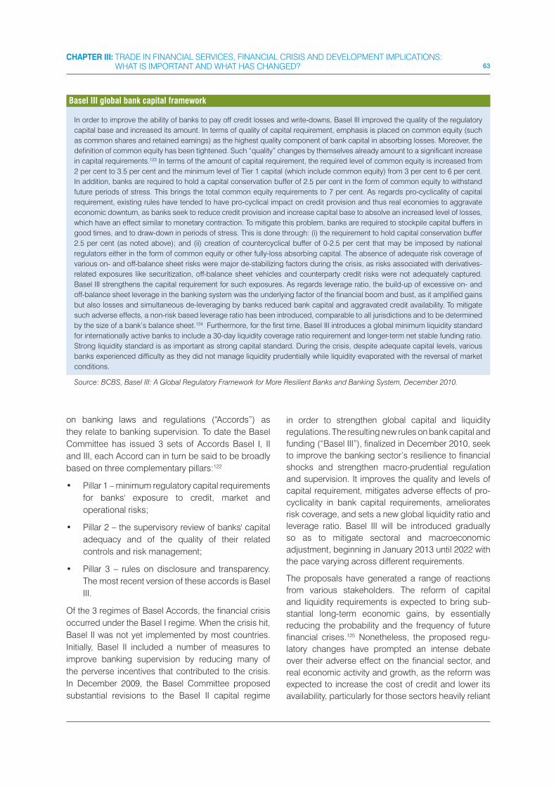
63
CHAPTER III: TRADE IN FINANCIAL SERVICES, FINANCIAL CRISIS AND DEVELOPMENT IMPLICATIONS: WHAT IS IMPORTANT AND WHAT HAS CHANGED?
on banking laws and regulations (“Accords”) as
they relate to banking supervision. To date the Basel
Committee has issued 3 sets of Accords Basel I, II
and III, each Accord can in turn be said to be broadly
based on three complementary pillars:122
�� Pillar 1 – minimum regulatory capital requirements
for banks' exposure to credit, market and
operational risks;
�� Pillar 2 – the supervisory review of banks' capital
adequacy and of the quality of their related
controls and risk management;
�� Pillar 3 – rules on disclosure and transparency.
The most recent version of these accords is Basel
III.
Of the 3 regimes of Basel Accords, the financial crisis
occurred under the Basel I regime. When the crisis hit,
Basel II was not yet implemented by most countries.
Initially, Basel II included a number of measures to
improve banking supervision by reducing many of
the perverse incentives that contributed to the crisis.
In December 2009, the Basel Committee proposed
substantial revisions to the Basel II capital regime
in order to strengthen global capital and liquidity
regulations. The resulting new rules on bank capital and
funding (“Basel III”), finalized in December 2010, seek
to improve the banking sector’s resilience to financial
shocks and strengthen macro-prudential regulation
and supervision. It improves the quality and levels of
capital requirement, mitigates adverse effects of pro-
cyclicality in bank capital requirements, ameliorates
risk coverage, and sets a new global liquidity ratio and
leverage ratio. Basel III will be introduced gradually
so as to mitigate sectoral and macroeconomic
adjustment, beginning in January 2013 until 2022 with
the pace varying across different requirements.
The proposals have generated a range of reactions
from various stakeholders. The reform of capital
and liquidity requirements is expected to bring sub-
stantial long-term economic gains, by essentially
reducing the probability and the frequency of future
financial crises.125 Nonetheless, the proposed regu-
latory changes have prompted an intense debate
over their adverse effect on the financial sector, and
real economic activity and growth, as the reform was
expected to increase the cost of credit and lower its
availability, particularly for those sectors heavily reliant
Basel III global bank capital framework
In order to improve the ability of banks to pay off credit losses and write-downs, Basel III improved the quality of the regulatory
capital base and increased its amount. In terms of quality of capital requirement, emphasis is placed on common equity (such
as common shares and retained earnings) as the highest quality component of bank capital in absorbing losses. Moreover, the
definition of common equity has been tightened. Such “quality” changes by themselves already amount to a significant increase
in capital requirements.123 In terms of the amount of capital requirement, the required level of common equity is increased from
2 per cent to 3.5 per cent and the minimum level of Tier 1 capital (which include common equity) from 3 per cent to 6 per cent.
In addition, banks are required to hold a capital conservation buffer of 2.5 per cent in the form of common equity to withstand
future periods of stress. This brings the total common equity requirements to 7 per cent. As regards pro-cyclicality of capital
requirement, existing rules have tended to have pro-cyclical impact on credit provision and thus real economies to aggravate
economic downturn, as banks seek to reduce credit provision and increase capital base to absolve an increased level of losses,
which have an effect similar to monetary contraction. To mitigate this problem, banks are required to stockpile capital buffers in
good times, and to draw-down in periods of stress. This is done through: (i) the requirement to hold capital conservation buffer
2.5 per cent (as noted above); and (ii) creation of countercyclical buffer of 0-2.5 per cent that may be imposed by national
regulators either in the form of common equity or other fully-loss absorbing capital. The absence of adequate risk coverage of
various on- and off-balance sheet risks were major de-stabilizing factors during the crisis, as risks associated with derivatives-
related exposures like securitization, off-balance sheet vehicles and counterparty credit risks were not adequately captured.
Basel III strengthens the capital requirement for such exposures. As regards leverage ratio, the build-up of excessive on- and
off-balance sheet leverage in the banking system was the underlying factor of the financial boom and bust, as it amplified gains
but also losses and simultaneous de-leveraging by banks reduced bank capital and aggravated credit availability. To mitigate
such adverse effects, a non-risk based leverage ratio has been introduced, comparable to all jurisdictions and to be determined
by the size of a bank’s balance sheet.124 Furthermore, for the first time, Basel III introduces a global minimum liquidity standard
for internationally active banks to include a 30-day liquidity coverage ratio requirement and longer-term net stable funding ratio.
Strong liquidity standard is as important as strong capital standard. During the crisis, despite adequate capital levels, various
banks experienced difficulty as they did not manage liquidity prudentially while liquidity evaporated with the reversal of market
conditions.
Source: BCBS, Basel III: A Global Regulatory Framework for More Resilient Banks and Banking System, December 2010.

64 SERVICES, TRADE & DEVELOPMENT
on bank credit. Estimates by the BCBS suggest that
the impact on GDP of higher capital standards would
be relatively moderate both in short- and long-terms,
and distributed through time, though effects could be
larger were banks to rush to attain the new standards
ahead of the deadline.126 On the cost of regulatory im-
plementation front, some estimates suggest that the
effect of domestic legislation alone could amount to
16 per cent of bank profits in 2013 and European bank
profits in 2012 could fall by 37 per cent because of the
proposed regulation. Interim estimates by the Finan-
cial Industry Group (Institute of International Finance)
indicated that regulatory reform would subtract an an-
nual average of as much as 0.6 per cent from the path
of real GDP growth over 2011 to 2015 for the United
States, EU and Japan, and an average of 0.3 per cent
over 2011to 2020 with particularly significant effects in
the Euro area where the banking system is relatively
important in economy and debt financing.127 Findings
point to the importance of gradual implementation of
tight capital requirements, as a longer implementa-
tion period would likely lead both, to more adjustment
through raising capital by retaining earnings and is-
suing equity rather than through cutting lending, and
increasing interest rates. Furthermore, despite the
transitory measures, market pressures and reputation
considerations could force banks to front-load capital,
racing ahead of required timeframes, in which case
the impact would be more noticeable.
Proposed reforms to Basel III still rely heavily on bank
economic capital models with limited distributions of
data that are not correlated to macroeconomic risk
factors. Countercyclical capital requirements should
be rules-based and linked to a common definition of
the economic cycle across countries.128
The implementation of Basel III and the Basel Accords
more broadly, while providing an important starting
point for effective regulation of DC financial services
sectors, pose specific concerns for DCs. The financial
sector in most DCs, differ substantially-- smaller
banking systems and less developed capital markets--
from those in industrialized countries. Accordingly,
interests and needs generally vary, including between
and among DC financial systems. The standards and
recommendations of the Basel Accords or for that
matter any global reform agenda in the financial services
sector would need to adequately reflect the specific
characteristics and issues of DC financial sectors.
The strains on national supervisory capacity of
introducing Basel III are multiple and more severe in
DCs due to less adequate supervisory capacity, less
developed internal controls within banks, shortage of
information and information collection systems and
the inadequate regulatory infrastructure.129 Pressure
to implement may lead to failure to meet proper
validation standards for external data and models. It
would be important in this regard that they are able
to adjust the rules to national circumstances so that
implementations of the new rules do not risk their
financial system stability or broader developmental
objectives.130 Moreover, the shift from a supervisory
environment that is traditionally compliance-driven
to a more discretionary and judgmental framework
will stretch scarce supervisory resources. Related to
this is the cost of implementing the new framework,
is the significant investment required to upgrade IT
infrastructure and financial software and the need for
training of both bankers and supervisors.
Another concern for DCs is the potential impact on
the composition of domestic lending and, implicitly,
on access to credit for various sectors of the
economy. Basel III is likely to influence how credit
will be allocated to the real economy. For example,
while a lower-risk weighting for residential mortgage
lending provides an incentive to expand housing
finance – provided banks can raise long-term finance
– financing for SMEs and for project finance are
likely to become more costly given their higher risk
weight, and therefore sectors that are key drivers of
economic growth and employment might be severely
hampered.131
Possible national policy responses include a
sequential and tailor made approach to Basel III,
coupled with the need for implementation linked
technical and financial assistance.
Broader post crisis implications of financial services
regulatory developments for global co-operation and
developing countries.
The debate on the changing financial regulatory
landscape linked to the financial crisis has developed
primarily in developed economies – hit hardest by the
crisis.132 Many DCs were relatively de-coupled from
the financial crisis as they had pursued a prudent
regulatory approach domestically and (or) they were
not fully integrated in the global financial markets.
The ensuing regulatory and policy responses have,
however, raised issues relating to the need for global
regulatory co-operation and potential implications for
developing countries.
65
CHAPTER III: TRADE IN FINANCIAL SERVICES, FINANCIAL CRISIS AND DEVELOPMENT IMPLICATIONS: WHAT IS IMPORTANT AND WHAT HAS CHANGED?
New liquidity standards may challenge long-term
bank funding for banks in emerging markets. Higher
liquidity requirements and capital buffers will increase
the cost of banking in developed countries, including
the cost of holding minority interest in emerging
markets banks, and thus could reduce cross-border
investment and lending133 owing to unfavourable risk-
weights assigned to DCs requiring higher capital.
Subsidiaries of cross-border banks in developed
countries have often large and dominant positions in
DCs, and the changes in regulatory regime applying
to parent banks in developed countries will thus
be affected by a significant fall in trade financing
for DCs.134 New regulatory environments aimed
at securing financial transaction, including more
stringent information requirements on counter-party in
low-rated countries are increasing the cost of doing
businesses.135 Moreover, using credit aggregates in
determining the necessary credit buffers for mitigating
pro-cyclicality may constrain financial deepening and
economic growth in DCs.136
The existing variation in regulatory regimes for
the financial services sector may induce financial
companies to resort to “jurisdiction shopping” in their
search for looser financial regulations.137 Large cross-
border banks could move from large branches toward
fire-walled subsidiaries in emerging economies.138 This
could result in increased exports of financials services
from DCs, but could also increase risks and volatility
of the financial sector in some DCs. Therefore, cross-
border banking needs to be regulated collectively
through enhanced coordination. At the same time,
possible contraction of foreign banks’ involvement in
DCs, due to general downsizing effects of reforms may
create room for growth of financial institutions in DCs.
The crisis has made it clear that more finance and
more financial products are not always better.139
Regulating innovations in financial products requires
sophisticated technical and market skill sets, the scale
of which may be lacking in developing countries. It
has been suggested that developing countries could
maintain a positive list of permitted financial products,
based on whether they have been proven to be non
toxic in advanced economies.140
A major outstanding issue yet to be fully addressed
in international financial regulatory reform is the moral
hazard created by systemically important financial
institutions (“too big to fail” banks). These banks are
as large and interconnected as not to be allowed to
go into bankruptcy, and therefore benefit from implicit
government guarantee. As a consequence, they have
an incentive to take excessive risks and benefit from a
competitive edge in terms of subsidized funding costs
over other market participants. The crisis has further
exacerbated the problem, as massive public funds
were injected at the expense of taxpayers, and market
concentration increased, thereby distorting production
and trade patterns in the sector. Various regulatory
approaches are being tested and considered to
address the problem. One approach is to require higher
capital requirements for such banks so as to reflect the
greater risks they pose to the global financial system.
Another is to put in place ex ante safe, rapid and
effective “resolution” regimes, including on a cross-
border scale, in case of insolvency. Such procedures
would define how losses may be distributed among
creditors and counterparties, so as not to disturb the
financial system and expose taxpayers to the risk
of loss. Improving intensity and effective regulatory
supervision of such banks would also be essential.
Other on-going international regulatory reform
processes address, expanding the scope of
regulations to shadow the banking sector, improving
the OTC derivatives market, strengthening accounting
standards, strengthening adherence to international
supervisory and regulatory standards, compensatory
standards, and developing macro-prudential
frameworks. Regulatory harmonization throughout
different segments of financial system is needed.
Otherwise, strengthened bank regulations will
encourage shifting risk to other parts of the financial
sector, such as insurance and pension funds, hedge
funds, and credit rating agencies. At an institutional
level this would necessitate greater and more
frequent coordination among regulatory agencies and
between the government, central bank and regulatory
agencies. It has been suggested that the Central
Bank in particular has a key role to play particularly
in times of crisis.141 For developing countries with a
small financial sector and limited skills set the Central
Bank can perform several regulatory functions.142
Trading OTC derivatives contracts on exchanges
would improve their transparency and avoid the build-
up of unreported risk in the system. It is also necessary
to address the issue of non-cooperative jurisdictions
so as to ensure a level international playing field.
Compensatory practices of firms should be aligned
with prudential risk taking.
Another issue that has been to the forefront of
regulatory reform debate is the creation of a “solidarity
66 SERVICES, TRADE & DEVELOPMENT
mechanism” which would require the financial sector
to reimburse governments and societies for some of
the social costs of financial risk taking (including in
the form of financial taxes that can generate revenue
to pay for the direct and indirect costs of State and
central bank support and to pay for public goods). This
form of burden sharing will require the financial sector
to pay for more of the costs of its risk-taking and can
provide a basis for building solidarity mechanisms
between those who have benefited greatly from
financial globalization and those who have suffered
the costs of excessive financial risk taking.143
It is expected that such a “solidarity mechanism” or
“financial transaction tax” would in turn tax excessive
risk-taking, allocate resources productively and
provide sustainable revenue to governments so
that they can pay for the direct and indirect costs of
financial crisis and to provide for an innovative source
of financing for global development aid and global
public goods (such as for MDGs and climate change
mitigation and adaptation).Various forms of such
taxes are being considered, such as tax on foreign
exchange transactions, tax on exchange-traded and
centrally cleared derivatives and related financial
products, and tax on bank balance sheets, amongst
others. It has been argued that such taxes levied at a
very low level (0.005 per cent on currency transaction
is estimated to generate $33 billion annually) would not
significantly distort financial markets while providing
significant source of revenue.144
7. FINANCIAL SERVICES AND TRADE: THE
TRADE AGENDA AND ARISING ISSUES
IN RESPECT OF THE CRISIS
7.1. Developments in Financial Services Trade Liberalization
On the trade front, liberalization in FS is continuously taking
place through different avenues, autonomously, through
the WTO General Agreement on Trade in Services (GATS)
and regional and bilateral trade agreements (RTAs).
Financial Services Liberalization in GATS
GATS provides for progressive liberalization of serv-
ices trade. Financial services-related provisions are
included in the GATS Agreement, in the annex on FS,
Understanding on Commitments (the Understanding)
in FS and individual Members’ schedules of specific
commitments. Financial services have been the sub-
ject of extended sectoral negotiations after the Uru-
guay Round. Among the 11 services sectors covered
by W/120 (WTO’s sectoral classification list), the FS
sector ranks second, with regard to the numbers of
commitments. As of July 2007, 121 Member States
had commitments in at least one of the FS subsectors
(counting European Union Member States individual-
ly), representing 80.66 per cent of WTO membership.
Member FS commitments exhibit interesting
patterns. After tourism, FS is the sector with the most
commitments. In many cases, DC commitments
enshrined recent FS reforms and liberalization. Mode
3 is the mode in which Members prefer allowing
access to domestic markets for direct insurance
services and, apart from Asia, also for banking. The
preference for Mode 3145 over Mode 1 could originate
in expectations that:
a) Positive effects of liberalization may be weaker in
Mode 1 than in Mode 3;
b) Mode 1 liberalization may create more risks for
domestic financial systems (that is, regulatory
control is easier for banks established within
borders);
c) Implementing Mode 1 commitments may require
cross-border capital flows.
Recently acceded countries made FS commitments
in nearly all subsectors, the breadth and depth of
which raise questions as to their implementation and
sustainability, particularly in light of these countries’
comparatively weak regulatory frameworks, practices
and institutions. Some Members adopted “pre-” or
“phased-in” commitments, committing to market-
opening in the future. In so doing they create a certain
incentive or pressure toward domestic reform, while at
the same time gaining time to develop the necessary
regulatory and supervisory mechanisms, and prepare
industry for enhanced competition. Some Members
use a particularly flexible type of phase-in approach,
making market access dependent on the existence of
a particular regulatory framework, such as by Japan
and Mauritius for new financial products.
In making FS commitments, Members use two
scheduling approaches:
a) Positive-listing of commitments – choosing any
number of subsectors or modes of supply and

67
CHAPTER III: TRADE IN FINANCIAL SERVICES, FINANCIAL CRISIS AND DEVELOPMENT IMPLICATIONS: WHAT IS IMPORTANT AND WHAT HAS CHANGED?
scheduling any type of market access or national
treatment (MA/NT) limitations;
b) Understanding on FS – offering an alternative
mechanism for deeper commitments by giving
details about the sectoral/modal scope/nature
of commitments and by containing additional
obligations (such as standstill, government-
procurement, new FS, transfer and processing
of information and non-discriminatory measures).
Two DCs employ this approach.
Paragraph 7 of the Understanding requires Members
to permit any Mode 3 FS supplier to offer any new
FS. Given the proliferation and rapid development of
new financial products and post the financial crisis
the role of new financial products such as CDOs,
concerns have arisen as to the need to anticipate
the exact scope of commitments. The Understanding
also addresses Mode 3, providing for temporary
entry of senior managerial personnel and specialists
in the operation of the FS supplier, and – associated
with commercial presence – specialists regarding
computer, telecommunication, accounting, actuarial
and legal services.
Other GATS provisions central for Members’ financial
systems include Articles XI (payments/transfer for
current transactions relating to specific commitments)
and XII (balance of payments exception). According
to Article XI, Members shall not impose restrictions on
any capital transaction inconsistent with their specific
commitments.
Appropriate regulatory and supervisory frameworks
are prerequisites for successfully opening up FS,
reflected in the “prudential carve-out”, in paragraph
2(a) of the annex on FS. Members have different
views regarding the carve-out, some suggesting that
it is too broadly defined (and a more precise definition
would be required) and others fearing that this would
erode Member rights to impose prudential measures.
Post the financial crisis the scope of the “prudential
carve-out” has once again come up for discussion,
in the light of the “bail out” packages and other policy
responses initiated by some WTO members. Some
schedules contain explicit references to prudential
measures. In negotiations on domestic regulation,
developing countries (such as the African, Caribbean
and Pacific Group of States) have suggested that
future disciplines should explicitly affirm the right to
prudential measures. In light of post financial crisis
developments, it is likely that the “prudential carve-
out” will remain unchanged in order to ensure flexibility
as required.
In the ongoing Doha round of Negotiations, FS
negotiations saw a number of bilateral requests and
one plurilateral request (February 2006), coordinated
by Canada. The plurilateral request was submitted
by 10 countries with strong FS sectors, directed
mostly toward DCs (Argentina, Brazil, India, China,
Association of South-East Asian Nations (ASEAN),
Egypt and South Africa). Bilateral and plurilateral
requests exhibit similar features, calling for enhanced
commitments on: Modes 1 and 2 (for all subsectors
mentioned in the annex, for a specific set of sectors,
or for a minimum cluster of commitments as per the
Understanding); Mode 3 (eliminating certain sectoral
and horizontal limitations); and Mode 3 (seeking
greater freedom for intra-corporate transferees
and contractual service suppliers). Despite their
far-reaching nature, numerous countries have also
requested DCs to subscribe to some parts, if not all,
of the Understanding or to use the Understanding as
a reference point for commitments.
Interestingly, the FS plurilateral request does not refer
to the Understanding. Suggestions have also been
made on regulatory issues such as transparency
requirements. The plurilateral request on FS flags
transparency in development and application of laws
and regulations – transparent and speedy licensing
procedures have been suggested.
In terms of Offers, only a few introduce significant
changes, and many including those of developed
countries, do not match actual openness. Some add
new FS subsectors; reduce foreign-equity limitations
(India rose limits in transferable securities from 39
to 73 per cent), or requirements for juridical form
(India allows wholly-owned subsidiaries as legal
entities); eliminate residency requirements (Canada
for dealers, brokers, advisors in trading of securities
and commodity futures and to a limited degree also
for citizenship and residence requirements for boards
of directors); relax exchange-regime limitations
(European Union); remove Mode 2 limitations (Japan);
and increase numbers of licenses (India, now 15
bank licenses). In addition, the United States offers
liberalization of interstate branching and acquisitions.
Offers introduce greater precision on Mode 3.
Possible linkages between FS liberalization and capi-
tal-account liberalization are important considerations
in negotiating FS commitments.. While GATS rules
and obligations are designed to decouple the liberali-

68 SERVICES, TRADE & DEVELOPMENT
zation of trade in FS from the liberalization of capital
account transactions, certain practical linkages exist.
These include situations where capital-account trans-
actions are crucial for complying with GATS commit-
ments. For example, the effective implementation of
certain FS commitments in Mode 1, (deposit services),
can require capital-account liberalization the scope
and extent of which are hard to anticipate. Liberal-
izing capital accounts prematurely without adequate
institutions and prudential regulations in place can in-
duce economic and social distress as well as financial
crises. Unlike trade in goods, capital flows are more
subject to information asymmetry, agency problems,
adverse selection and moral hazard (Stiglitz, 2000).
Financial Services Liberalization in Regional Trade Agreements
FS commitments in regional or free trade agreements
(RTAs or FTAs) tend to be more far-reaching than
those in GATS. At times, FS commitments in RTAs
may exceed not only offers made in the context of
the Doha Round (e.g. certain US FTAs) but they also
match and exceed demands made in multilateral
requests. For instance, Latin American and Caribbean
FTAs tend to have significant additional liberalization
FS commitments compared to GATS. Some FTAs
tend to reflect liberalization provisions contained in
the WTO Understanding. Many exhibit increased
commitments for cross-border supply of FS, often
beyond the traditional concept of GATS Mode 1, to
include Mode 2 and in some cases even Mode 3
(Republic of Korea–Chile and the North American
Free Trade Agreement (NAFTA), which defines cross-
border trade in services to include three of the four
GATS modes – cross-border supply, consumption
abroad and the movement of natural persons).
In terms of regulatory disciplines, RTAs echo GATS
provisions on domestic regulation and the prudential
carve-out. For example, EU–Mexico provides for
parties to regulate FS supply on a non-discriminatory
basis and contain a GATS-style prudential carve-
out. The India–Singapore Comprehensive Economic
Cooperation Agreement contains provisions for
domestic regulation. The NAFTA contains “good
government” disciplines (to ensure reasonable,
objective and impartial administration). Other
provisions relate to freezing of existing regulatory
regimes and ratcheting by automatically locking
in any liberalization. In some cases they focus on
regional consolidation of mechanisms.146 Africa
exhibits several (not always fully operational) initiatives
for regional integration of financial markets. Regional
cooperation on regulatory and institutional issues
could help address DC capacity constraints. Regional
initiatives in the financial services sector, particularly
South-South ones, show sensitivity to local conditions
and effective ownership and help reconcile different
national needs and objectives.147 Some RTAs establish
institutional arrangements to address implement FS
related aspects of the RTA. In the 1990s, following
the financial crises in the 1980s, The Economic and
Monetary Community of Central Africa and the West
African Economic and Monetary Union implemented
regional approaches to FS regulation (a regional
banking commission), not all of which were effectively
implemented. NAFTA provides for a FS committee.
With negotiations over the Doha Round stalled, coun-
tries have shown a preference for pursuing regional
and bilateral trade arrangements, many of which in-
cluded substantial services provisions. Several of
these agreements include some manner of financial
services coverage, ranging from considerable to brief
references.148 Regional arrangements can be lever-
aged particularly during financial crisis to build intra-
regional trade and investment including in the South-
South context, strengthen local and regional financial
markets and given the focus in the current financial
crisis on infrastructure needs, leveraged to build re-
gional infrastructure network services. A regional ap-
proach to regulation and institution in the financial
services sector is likely to be cost effective, promote
growth and stability and facilitate regional integration
more broadly. Post financial crisis calls were made for
the establishment of regional financial institutions and
development of regional bond markets.149
7.2. Financial Services, financial crisis, trade commitments and crisis related financial sector intervention – The Interlinkages
The current crisis has necessitated governments
particularly in developed countries to take action to
support their financial sector and more broadly their
economies. The focus of these actions has been to
guard against systemic risk posed to the economy.
Specific interventions in the financial sector have
varied. Many countries have recapitalized their banks,
particularly the systemically important ones. For the
advanced G-20 countries, the average outlay in 2009

69
CHAPTER III: TRADE IN FINANCIAL SERVICES, FINANCIAL CRISIS AND DEVELOPMENT IMPLICATIONS: WHAT IS IMPORTANT AND WHAT HAS CHANGED?
was projected at 3.2 per cent of GDP, with considerable
variation across countries.150 Governments and
some central banks have provided substantial direct
loans and purchased illiquid assets from financial
institutions. Amounts involved range widely, with the
United Kingdom, Japan, and Norway accounting for
over 10 per cent of GDP. The advanced G-20 average
is 3.3 per cent of GDP.151 Central bank support with
or without direct treasury funding has been provided
primarily through credit lines to financial institutions,
purchase of asset-backed securities and commercial
paper, and asset swaps. Guarantees for financial
sector liabilities have been provided for bank
deposits, interbank loans and, in some cases, bonds.
Deposit insurance limits have been raised in almost all
countries.152 In emerging economies financial sector
support has been limited. Main measures announced
include: bank recapitalization in Hungary, Poland,
and Ukraine; liquidity provision in Hungary, India,
Mexico, the Russian Federation, Turkey, and Ukraine.
These countries have extended (or committed to
extend) liquidity facilities to banks or to State-owned
or managed enterprises. Some countries have
announced the provision of guarantees: blanket
coverage provided in Egypt and Saudi Arabia; several
other countries (Hungary, Indonesia, Mexico, Poland,
and the Russian Federation) have committed to
provide more limited guarantees.
A key concern among DCs is that a type of “financial
protectionism” may arise, whereby governments may
direct banks that have received capital injections to
lend more domestically rather than internationally. Fur-
ther, borrowing by the Treasury of the United States to
finance the growing budget deficit also pulls in funds
from around the world and could crowd out borrowers
from countries also seeking to cover their deficits.153
Without calling into question the necessity of financial
rescue packages in the exceptional circumstances that
have prevailed since the onset of the financial crisis,
their sheer size in relation to the share of GDP of the FS
sectors of OECD economies inevitably gives reason to
questions as to their effects on international trade in
FS.154 Similar kinds of responses are beyond the means
of most DCs affected by the crisis.155 For example, if
financial rescue packages had not been provided
in Europe and North America, it is not clear whether
competing FS suppliers in other countries would
have been presented with profitable new investment
opportunities in markets suddenly left under-supplied,
or whether they would have been submerged in a
meltdown of the global financial system.156
The measures used and the scale of bailouts vary, as
do their effectiveness. Some of the impacts of the bail-
outs in the financial sector have been that uncompeti-
tive or even insolvent financial institutions have been
kept in operation at the expense of foreign competi-
tors, thereby distorting the market, and reducing trade
in FS.157 However, under current circumstances, this
may be viewed as secondary to the objective of re-
ducing systemic risk, maintaining stability and restor-
ing credit for the global economy as a whole.
As discussions in the WTO’s Committee on Trade
in Financial Services indicate, the financial rescue
measures have brought to the forefront trade and
competition effects, as well as their implications for
GATS commitments and rules including the “right
to regulate”. Current developments in the FS sector
primarily raise two questions: are actions WTO
compliant; what is the likely coherence of existing WTO
GATS disciplines with a global financial regulatory
landscape that is likely to change.
The answer to these questions vary depending on
financial services commitments made by individual
Members, the specific kind of financial services under
consideration (insurance, banking, securities amongst
others), and specific measures being addressed
(financial bailout, recapitalization, equity purchase) ,
read with GATS disciplines. Broadly, however, some of
the issues which could arise are set out below.
Commitments arising from the Understanding on FS
Many of the countries offering bailout packages are
signatories to the Understanding on FS which offers
an alternative mechanism for deeper commitments.158
In the current context of the financial crisis, this raises
certain issues particularly regarding the evolving FS
regulatory landscape. The Understanding allows
FS suppliers of any other Member established in its
territory to offer within its territory any new financial
services. Given that the crux of the financial crisis
has been CDOs, derivatives and other such “newer
financial products”, this may become an issue when
greater regulatory attention is given to financial product
safety, consumer protection and risk management,
in terms restrictions on the kind of legal form that
is permitted to provide new financial products,
outright bans on certain kinds of financial products
amongst others. Furthermore, the Understanding’s

70 SERVICES, TRADE & DEVELOPMENT
“standstill provision” requiring the non-creation of
new regulations (or reverse liberalization) for the list
of FS appear to be in conflict with various proposals
to limit risky investment instruments, such as certain
types of derivatives. Some of these obligations may
be replicated in regional and bilateral agreements and
would warrant closer attention.
Subsidies in financial services
The bailout packages offer a range of measures in-
cluding soft-loans, capital purchase and credit guar-
antees among others. This raises a first question as to
whether these measures amount to a subsidy and a
second question as to whether the subsidy is prohib-
ited. The WTO, in its World Trade Report of 2006 “Ex-
ploring the Links Between Subsidies, Trade and the
WTO”, recognizes the use of subsidy-like measures in
both developed and DCs during the process of priva-
tization as well as where there is a threat of systemic
risk. The kinds of subsidy-like measures the Report
considers in the financial sector include State guar-
antees, equity participation, soft loans, credit guaran-
tees and tax exemptions.159 The bailout of banks and
insurance companies through the investment of large
sums in “unequityworthy” companies appears to fall
in the category of a subsidy-like measure.
However, the GATS does not contain any disciplines
on subsidies in the services sectors and for that matter
any definition as to what constitutes subsidies in the
services sector. This is an issue under negotiations and
WTO Members have for some time been in the process
of exchanging information on subsidy measures
undertaken by them in various services sectors. In the
absence of clear GATS disciplines on subsides there is
unlikely to be a case for WTO dispute settlement.
Financial services commitments
A determination would have to be made as to whether
the bailouts have: (a) been made in a sector where
a FS commitment has been undertaken to provide
market access; or (b) favour domestic banks and
discriminate against foreign banks, thereby resulting
in a violation of market access and national treatment
commitments. It would also raise a larger question
as to whether foreign-owned or foreign-controlled FS
supplier would be eligible for bailout benefits.
Financial services negotiations
Specifically, for negotiations on the FS sector, DCs are
uncertain as to whether and how to proceed if at all,
given that the global financial landscape has changed
and the uncertainty in global financial markets. The
FS sector is the sector with the largest number of
commitments – 121 schedules contain commitments
particularly in Mode 3, in at least one FS sector with
relatively extensive coverage of core commercial
bank services (deposit taking and lending) and a
fewer commitments in capital market (related services
such as trading). The on-going reform and economic
rationales underpinning it could affect FS liberalization
under the Doha Round with some countries calling for
cautious approach.160 Most DCs were isolated from
the full impact of the financial crisis on their financial
markets either due to more prudent and cautious
regulatory policies or the fact that they were not
entirely integrated into global financial markets.
Further the theoretical assumptions on the basis
of which conditions are decided for the granting of
market access and national treatment to foreign FS
providers has changed. During the Uruguay Round
of WTO negotiations on FS, which ended in 1997,
the ruling assumption was that financial regulation
in developed countries was not only adequate but
also a model for that of DCs. Post financial crisis,
such rationale is being re-evaluated, which may have
implications for countries’ future negotiating stances
in the WTO.161
It has been argued that without the disciplining effects
of subsidies, further liberalization could expose DC
operators to unfair competition, and large financial
operations in DCs may act as vectors of contagion,
as for instance where there is a large foreign bank
presence. There is a greater focus in DCs to allow
establishment through the creation of a subsidiary
(entailing legal personality) rather than direct branching,
and by seeking assurances from subsidiary parent
institutions as to the financial soundness of branches
and subsidiaries. Further conditions to negotiations
in the FS sector may include the distribution of costs
between home and host countries in the event of
cross-border insolvencies of financial firms. This is an
area on which general international guidelines are still
lacking, despite clear agreement on their need.162
Implications of Capital Account Liberalization
Concern arises from capital account opening implied
by GATS commitments. Since certain FS entail capital
movement by their very nature (deposit taking, lend-
ing or securities through Mode 1), GATS requires free
capital movements associated with such commit-

71
CHAPTER III: TRADE IN FINANCIAL SERVICES, FINANCIAL CRISIS AND DEVELOPMENT IMPLICATIONS: WHAT IS IMPORTANT AND WHAT HAS CHANGED?
ments, although liberalization in payments and capital
transfer are not an obligation. This could potentially
constrain DC ability to manage and control capital
flows to insulate them from the excessive financial vol-
atility while sensible capital account management has
gained increased acceptability. The recent episode of
capital controls (tax on foreign purchase of domestic
assets) introduced by several countries (such as Bra-
zil) to counter increased capital inflows lends further
support to capital account management.
Reference to international standards in the finan-cial services sector
In the current arena of regulatory reform within global
financial markets, certain vigilance on the part of
DCs is necessary concerning possible incorporation
of features of the outcome of work on the reform
agenda in IMF conditionality and in rules or standards
proposed in international negotiations elsewhere.
This is because standards may not be appropriate
for countries at earlier stages of development or may
place a disproportionate burden on the administrative
capacity of their governments and the management
of their enterprises.163
It has been suggested that international codes and
standards might be used as part of determining a
country’s scope of flexibility under the prudential
carve-out of the GATS annex on FS regarding
imposition of prudential measures with implications
for international trade in financial services.164
According to the prudential carve-out “a Member shall
not be prevented from taking measures for prudential
reasons, including for the protection of investors,
depositors, policy holders to whom a fiduciary duty is
owed by a financial service supplier, or to ensure the
integrity and stability of the financial system.” Behind
the proposal to limit countries flexibility under this
provision lies a judgment as to the relative importance
of prudential regulation, on the one hand, and a
liberal cross-border regime for financial services, on
the other hand. The recent crisis has emphasized
the importance for many governments in particular
those of DCs of the need to maintain this balance in a
reasonable manner.165
8. Conclusions
Emerging markets are those in greatest need of
economic and social benefits of financial development
and stability. However for many Developing countries,
this remains a challenge, further compounded by
difficulties of properly managing capital-account
liberalization, achieving macroeconomic stability and
developing institutional and regulatory frameworks in
parallel with rapid changes in the financial system.
Many of these difficulties have been brought to the
fore as a result of the recent financial crisis.
The process of financial development needs to
go hand-in-hand with better and broader financial
regulation and supervision. Regulatory reforms
cannot be implemented overnight. For FS reform and
liberalization to generate pro-development outcomes,
it needs to be supported by appropriately designed,
paced and sequenced policies (e.g. macroeconomic,
prudential, regulatory and supervisory), to be
determined on a case-by-case basis and adapted
to the specificity of each country. There is therefore a
case for coherent but not common regulatory structure
adapted to national circumstances. FS reform and
liberalization must be holistic and take into account
micro and macro prudential elements. Further it is
important to ensure linkage between real economy,
financial sector and development objectives.
Furthermore, since financial markets and
circumstances differ from country to country, optimal
regulation and regulatory structures differ. However, as
financial markets become global, global coordination
of regulation is also important. In this context global
regulatory bodies, need to be representative of and
reflect the concerns of DCs. International regulatory
initiatives in the financial services sector can provide
a useful tool to address issues of cross-border
insolvency; expansion of consolidated firms and the
lack of tools for facing new complex financial products,
technologies, and management techniques. However
developing countries need to effectively participate in
such international regulatory initiatives to ensure their
priority concerns are reflected.
A developmental approach to FS liberalization in
GATS is needed. Developing countries should
carefully choose the extent of their bindings in
international agreements pertaining to financial
services liberalization according to the maturity
of their financial and regulatory systems, their
development needs, existing gaps in their domestic
financial services sectors and most suitable fora for
financial liberalization whether autonomous, regional
or multilateral.
72 SERVICES, TRADE & DEVELOPMENT
NOTES
1 World Bank, “Global Development Finance: Building Coalitions for Effective Development Finance,” Page 73, 2001, The World Bank, Washington, DC.
2 With reference to the post 2007 global financial crisis, the terminology, crisis, current crisis, financial crisis maybe used interchangeably during the course of this paper. The terms financial services or financial services sector, unless otherwise specified, refers broadly to the banking, insurance and securities sectors.
3 Bloomberg-U.S. European Bank Write downs & Losses-November 5, 2009.4 Report of the Commission of Experts of the President of the United Nations General Assembly on Reforms of the International
Monetary and Financial System, September 21, 2009 - Stiglitz Report.5 Value of financial assets expressed as a percentage of GDP.6 Cherry-picking would also arise on the human resources side, with foreign companies hiring the best managers and
personnel away from local employers.7 UNCTAD background note and report of expert meeting on financial services (2007), UNCTAD note and report of as hoc
expert meeting on insurance services (2005).8 Lord Turner, Chairman of the UK Financial Services Authority, The Turner Review. Financial Services Authority, A regulatory
response to the global banking crisis March 2009.9 Report of the Commission of Experts of the President of the United Nations General Assembly on Reforms of the International
Monetary and Financial System, September 21, 2009 - Stiglitz Report.10 Report of the Commission of Experts of the President of the United Nations General Assembly on Reforms of the International
Monetary and Financial System, September 21, 2009 - Stiglitz Report.11 IMF Global Monitoring Report 2009, Global Financial Crisis and its Impact on Developing Countries.12 IMF Global Monitoring Report 2009, Global Financial Crisis and its Impact on Developing Countries.13 See Report and background note of UNCTAD expert meeting on trade and development implications for financial services
2007, Report and background note of UNCTAD multi-year expert meeting on Services, development and trade: the regulatory and institutional dimension, 2009, 2010, UNCTAD Trade and Development Report 2009.
14 Report of UNCTAD Expert Meeting on Financial Services (2007).15 Developed countries, including the United States, the United Kingdom and Scandinavian countries, have also been
subject to such crises, but compared with developing countries, the incidence has been relatively low and the social costs correspondingly smaller.
16 Kaminsky Gracila and Reinhart Carmen, The Twin Crises: The Causes of Banking and Balance-of-Payments Problems, American Economic Review, June 1999.
17 In a sample study of twenty countries covering the period 1970-1995, fourteen were developing countries.18 The study examined banking crises during the period 1980-1984 for a sample of 53 developed and developing countries.19 Singh Ajit (2003); Kaminsky/Reinhart (1999); Demirguc-Kunt/Detragiache (1998)20 Singh Ajit, Capital account liberalization, free long-term capital flows, financial crises and economic development, ESRC
Centre for Business Research, University of Cambridge, Working Paper No. 245, December 2002.21 Williamson and Drabek (1999).22 In a country such as Chile which was deeply integrated with the world financial markets, private foreign capital suddenly
withdrew in the event of a fall in copper prices.23 Even Joseph Stiglitz who has been a fierce critic of precipitate capital account liberalization in developing countries appears
to favour free FDI flows, Stiglitz (2000).24 Singh Ajit, Capital account liberalization, free long-term capital flows, financial crises and economic development, ESRC
Centre for Business Research, University of Cambridge, Working Paper No. 245, December 2002.25 IMF Paper prepared by Strategy, Policy, and Review Department, Recent Experiences in Managing Capital Inflows—Cross-
Cutting Themes and Possible Policy Framework, February 14, 2011.26 Jonathan D. Ostry, Atish R. Ghosh, Karl Habermeier, Marcos Chamon, Mahvash S. Qureshi, and Dennis B.S. Reinhardt”Capital
Inflows the Role of Capital, IMF Staff Position Paper, February 2010.27 IMF Paper prepared by Strategy, Policy, and Review Department, Recent Experiences in Managing Capital Inflows—Cross-
Cutting Themes and Possible Policy Framework, February 14, 2011.28 UNCTAD Trade and Development Report 2009, Chapter 3.29 Mercer Oliver Wyman, “State of the Financial Services Industry, 2007”, Source: DataStream financial services index.30 UNCTAD Globestat 2007, based on available data, not all countries reporting for all commercial financial services excluding
insurance.31 See also UNCTAD document on Insurance, UNCTAD/DITC/TNCD/2005/15.32 Bloomberg-U.S. European Bank Write downs & Losses-November 5, 2009.33 Overseas development institute, The Global Financial Crisis and Developing Countries: Preliminary Synthesis of Ten Draft
73
CHAPTER III: TRADE IN FINANCIAL SERVICES, FINANCIAL CRISIS AND DEVELOPMENT IMPLICATIONS: WHAT IS IMPORTANT AND WHAT HAS CHANGED?
Country Reports, April 2009.34 In Indonesia, Uganda and Zambia there was a significant decline in foreign portfolio investment especially in Q2 and
Q3 of 2008. Bangladesh experienced net outflows worth $48 million over the period July-December 2008, while Kenya experienced net portfolio outflows of about $48 million in June 2008 and $12 million in October 2008.
35 Overseas development institute, The Global Financial Crisis and Developing Countries: Preliminary Synthesis of Ten Draft Country Reports, April 2009.
36 Shimelse Ali, Impact of the Financial Crisis on Africa, International Economic Bulletin, Carnegie Endowment, April 2009.37 IMF World Economic Outlook, 2010.38 IMF World Economic Outlook, 2010.39 IMF World Economic Outlook, 2010.40 The request for monitoring and analysis has been raised by both developing and developed countries within the WTO and
UNCTAD.41 Deutsche Bank Research, Financial Market Special, EU Monitor 67, June 15, 200942 Mckinsey Global Institute Report, Global capital markets: entering a new era, September, 2009.43 In London, G-20 Leaders agreed that “hedge funds or their managers will be registered and will be required to disclose
appropriate information on an ongoing basis to supervisors or regulators, 2 April 2009, In Pittsburgh, G-20 Leaders agreed that “standardized OTC derivative contracts should be traded on exchanges.and cleared through central counterparties” and that all OTC derivative contracts should be reported to trade repositories, September 24 – 25, 2009.
44 Meyer Thomas, Economic Crisis Complicates Offshoring of Services, YaleGlobal , 9 February 2009.45 Meyer Thomas, Economic Crisis Complicates Offshoring of Services, Global recession and other problems challenge
China’s plans to extend its offshoring reach into services, Yale Global, February 9, 2009.46 U.S. administration has signalled an end to tax breaks for companies that outsource abroad and promised tax credits to
companies that maintain or increase U.S. workers relative to those abroad.47 Initiatives include the current 11th Five-Year Plan (2006-2010), the Information Strategy (2006-2010), as well as the Thousand-
Hundred-Ten Program of the Chinese Ministry of Commerce.48 Neeltje/Van Horen, Foreign Banking in Developing Countries, Origin Matters, in Emerging Markets Review 8 (2007).49 Bahrain is looking to open the Bahrain Financial Harbor development in 2007. Dubai created the Dubai International
Financial Centre in 2004. Most recently, in May 2005, Qatar established the Qatar Financial Centre. Beyond these special economic zones, the first independent credit agency, Emcredit, was launched in UAE in 2006, providing further evidence of the region’s maturing financial services infrastructure
50 Diana Farrell and Susan Lund, The world’s new financial power brokers, Mckinsey Global Institute Report The new power brokers: How oil, Asia, hedge funds, and private equity are shaping global capital markets, December 2007.
51 Conventional finance makes a distinction between acceptable interest and usurious interest, under Islamic law, however any level of interest is considered usurious and prohibited.
52 Investment in industries that are prohibited by the Qur’an, such as alcohol, pornography, gambling, and pork-based products, are discouraged.
53 Each financial transaction must be tied to a “tangible, identifiable underlying asset.54 A Sukuk is the equivalent of an Islamic bond and is issued in accordance with Islamic principles and investment.55 IFSB, IDB, IRI (2010). Islamic Finance and Global Financial Stability.56 IFSB, IDB, IRI (2010). Islamic Finance and Global Financial Stability.57 Hasan and Dridi (2010), The Effects of the Global Crisis on Islamic and Conventional Banks: A Comparative Study.58 Michael Ainley, Ali Mashayekhi. Robert Hicks, Arshadur Rahman, Ali Ravalia, Islamic Finance in the UK: Regulation and
challenges, November 2007, UK Financial Services Authority.59 Juan Solé, “Introducing Islamic Banks into Conventional Banking Systems,” IMF working Paper, July 2007.60 Sharia compliant current and saving accounts, free loans (Quard-Hassan), Murabaha (Cost-plus sale) – Murabaha
essentially is undertaking a trade with a markup, Ijara (Leasing), Musharaka (Equity Participation), Mudaraba (Partnership Financing), Istinaa (Commissioned Manufacture), Sukuk (Islamic Bond), Takaful (Mutual Insurance).
61 In some countries, such as the Islamic Republic of Iran and Pakistan, Islamic banks are the only mainstream financial institutions. In others, Islamic finance institutions exist alongside conventional banking.
62 For instance, the accommodation of Islamic products within the UK’s Regulated Activities Order.63 For instance, in the UK, a person acting as a Director of an authorised firm must be registered under the FSA and follow the
Approved Persons Rule, which include competence and capability qualification.64 John Taylor Under Secretary, US Treasury for International Affairs, Understanding and Supporting Islamic Finance: Product
Differentiation and International Standards, Forum on Islamic Finance, Harvard University, May 2004.65 John Taylor Under Secretary, US Treasury for International Affairs, Understanding and Supporting Islamic Finance: Product
Differentiation and International Standards, Forum on Islamic Finance, Harvard University, May 2004.66 Shayerah Ilias, Islamic Finance: Overview and Policy Concerns, CRS Report for the US Congress, July 29, 2008.67 Information about standards issued by the IFSB are available at [http://ifsb.org]
74 SERVICES, TRADE & DEVELOPMENT
68 Heiko Hesse Andreas Jobst Juan Solé, Quo vadis Islamic finance?, 24 November 2008, VOX commentary, Website: http://www.voxeu.org/index.php?q=node/2593.
69 Heiko Hesse Andreas Jobst Juan Solé, Quo vadis Islamic finance?, 24 November 2008, VOX commentary, Website: http://www.voxeu.org/index.php?q=node/2593
70 Van Greuning, Gallardo and Randhawa, 1998.71 Robert Peck Christen, Richard Rosenberg & Veena Jayadeva. Financial institutions with a double-bottom line: implications
for the future of microfinance. CGAP Occasional Paper, July 2004.72 Worldwide success that MFIs and microfinance programmes have achieved in making financial services accessible to the
poor and microenterprises has spawned initiatives to expand them.73 NGOs, Credit unions, cooperatives, commercial banks, and small informal groups are important players in microfinance.74 See van Greuning, Gallardo and Randhawa, 1998 for a more complete classification.75 Ashley Hubka and Rida Zaidi , Pact of Government Regulation on Microfinance, Prepared for the World Development Report
2005: Improving the Investment Climate for Growth and Poverty Reduction.76 Joselito Gallardo, Korotoumou Ouattara, Bikki Randhawa and William Steel, Comparative Review of Microfinance Regulatory
Framework Issues in Benin, Ghana and Tanzania, Word Bank Working Paper, April 2005.77 UNCTAD Trade and Development Report 2009.78 Report of the Commission of Experts of the President of the United Nations General Assembly on Reforms of the International
Monetary and Financial System, September 21, 2009 - Stiglitz Report.79 IMF World Economic Outlook, 2010.80 UNCTAD, Report of Multi Year Expert meeting on Services, development and trade: the regulatory and institutional
dimension, 2009.81 Gary Hufbauer, Luca Rubini and Yee Wong, “Swamped by Subsidies: Averting a US-EU Trade War after the Great Crisis”,
Policy Note, 24 July 2009.82 As of May 19, 2009; in per cent of 2008 GDP.83 IMF Staff Position paper, Fiscal Implications of the Global Economic and Financial Crisis, Fiscal Affairs Department,
SPN/09/13, June 9, 2009.84 See also UNCTAD, Report of Multi Year Expert meeting on Services, development and trade: the regulatory and institutional
dimension, 2009.85 IMF World Economic Outlook, 2010.86 IMF World Economic Outlook, 2010.87 IMF Global Financial Stability Report, April 2010.88 Mckinsey Global Institute Report, Global capital markets: entering a new era, September, 2009.89 Dirk Willem te Velde Effects of the Global Financial Crisis on Developing Countries and Emerging Markets: Policy responses
to the crisis, INWENT/DIE/BMZ conference in Berlin, 11 December 2008.90 WTO Annual Report of the Director-General, Overview of Developments in the International Trading Environment, WT/TPR/
OV/12, 18 November 2009.91 IMF Global Monitoring Report 2009, Global Financial Crisis and its Impact on Developing Countries.92 Report of the Commission of Experts of the President of the United Nations General Assembly on Reforms of the International
Monetary and Financial System, September 21, 2009 - Stiglitz Report.93 UNCTAD Trade and Development Report 2009.94 UNCTAD Trade and Development Report 2009.95 UNCTAD Trade and Development Report 2009, Chapter 3.96 Report of the Commission of Experts of the President of the United Nations General Assembly on Reforms of the International
Monetary and Financial System, September 21, 2009 - Stiglitz Report97 Report of the Commission of Experts of the President of the United Nations General Assembly on Reforms of the International
Monetary and Financial System, September 21, 2009 - Stiglitz Report.98 Report of the Commission of Experts of the President of the United Nations General Assembly on Reforms of the International
Monetary and Financial System, September 21, 2009 - Stiglitz Report.99 UNCTAD, Background Note of Multi Year Expert meeting on Services, development and trade: the regulatory and institutional
dimension, 2010.100 UNCTAD Note on Financial Services, 2007.101 Developed countries have also faced failures including the current sub-prime mortgage crisis. Other examples include
Australia’s experience with HiH, the country’s second largest non-life insurer (the company’s failure led to the halting of construction projects and bankruptcy of small businesses), or Japan’s experience with accelerated financial deregulation in the late 1980s which led to the collapse of eight mid-sized life insurers during 1997 to 2001, the Republic of Korea’s experience post the 1997 financial and currency crisis which resulted in massive nonperforming loans, in both banks and insurance companies.
102 For instance, supervisory practices vary considerably even within the European Union, even while efforts toward
75
CHAPTER III: TRADE IN FINANCIAL SERVICES, FINANCIAL CRISIS AND DEVELOPMENT IMPLICATIONS: WHAT IS IMPORTANT AND WHAT HAS CHANGED?
harmonization especially post crisis are being undertaken.103 See UNCTAD background note on Financial Services, 2007 and UNCTAD background note on Insurance Services 2005,
DT L Llewellyn, Institutional Structure of Financial Regulation and Supervision: the Basic Issues, in Aligning Financial Supervisory Structures with Country Needs, World Bank Institute 2004.
104 For a more detailed explanation of the different kinds, approaches and trends in financial services regulation, see UNCTAD Note and Report of the Expert Meeting on Financial Services, 2007.
105 Report of UNCTAD Expert Meeting on Financial Services, 2007.106 See also UK Financial Services Authority “Focusing on the Outcomes that matters”, April 2007.107 UK Financial Services Authority “Focusing on the Outcomes that matters”, April 2007.108 See Report of UNCTAD Expert Meeting on Financial Services, 2007.109 Schneider Benu, Issues in Implementing Standards and Codes, June 2002.110 Report of UNCTAD Expert Meeting on Financial Services, 2007.111 See Schneider Benu, Issues in Implementing Standards and Codes, June 2002.112 Five bodies have issued enough recommendations including the Financial Stability Board, the Basel Committee on Banking
Supervision, the International Organization of Securities Commissions, the International Accounting Standards Board and the International Monetary Fund, and G20. Other key reports which present recommendations include the G30 Report – Volcker Report – on Financial Reform: A Framework for Financial Stability, the De Larosière’s Report on EU Financial Regulation and the Turner Review.
113 The Economist, Financial Reform in America: A Decent Start, July 1st 2010.114 The Economist, Financial Reform in America: A Decent Start, July 1st 2010.115 Volcker Rule, limiting banks’ ability to trade on their own account.116 Beck Thorsten, The US Financial Reform Bill: Hit or Flop?, 16 June 2010.117 Beck Thorsten, The US Financial Reform Bill: Hit or Flop?, 16 June 2010.118 As explained in Cornford, Andrew. “Basel 2 At a Time of Financial Peril”. Financial Markets Center, TWN Global Economy
Series, March 2008.119 EU News Report, European Commission Adopts Legislative proposals to strengthen Financial Supervision in Europe, EU/
NR 38/09: 23 September 2009120 COM(2009)499 final, 2009/0140(COD), http://ec.europa.eu/internal_market/finances/committees/index_en.htm121 I P/09/1582, the proposal was under consideration by the European Council and Parliament. Creation of the new authorities
is envisaged for the end of 2010.122 IP/09/1120, http://ec.europa.eu/internal_market/bank/regcapital/index_en.htm123 Westlake (2010), Basel 3 – tough requirements; generous implementation timetable.124 Alexander, Eatwell, Persaud and Reoch (2010).125 BCBS, An Assessment of the Long-term Economic Impact of Stronger Capital and Liquidity Requirements, August 2010.126 BCBS, Assessing the Macroeconomic Impact of the Transition to Stronger Capital and Liquidity Requirements (interim
report), August 2010.127 IIF, Interim Report on the Cumulative Impact on the Global Economy of Proposed Changes in the Banking Regulatory
Framework, June 2010.128 Alexander, Eatwell, Persaud, Reoch, 2010.129 For a good discussion on likely impacts on developing countries of the Basel Accords, see Cornford, Andrew. “Some
Questions and Answers on Basel 2”, Presentation for the XXVII Technical Group of the Group of 24, Geneva, 8 September 2008.
130 Cornford, Estimating the macroeconomic effects of Basel 3, TWN SUNS, November 19, 2010.131 Calice Pietro, A Preliminary Assessment of the Implication of the Financial Regulatory Reform for African Countries, Policy
Brief on the Financial Crisis, African Development Bank, 2010.132 See, for example, discussions and proposals put forward by Brunnermeier et al (2009); de Larosiere Group (2009); Group
of Thirty (2009); Turner Review (2009); and Warwick Commission (2009).133 IIF (2010), Interim Report on the Cumulative Impact on the Global Economy of Proposed Changes in the Banking Regulatory
Framework and Otker-Robe and Pazarbasoglu, (2010). Impact of Regulatory Reforms on Large and Complex Financial Institutions.
134 For 21 sub-Saharan African countries, foreign banks account for more than 60 per cent of total banking system assets.135 WTO, WT/TPR/OV/13.136 Deputy Governor of the RBI Usha Thorat’s speech, 8 February 2010.137 Mirow (President of the EBRD) speech, Berlin, 19/20 May 2010.138 Beck (2010), Regulatory reform After the Crisis: Opportunities and Pitfalls.139 UNCTAD Trade and Development Report 2009, Chapter 3.140 Alexander, Eatwell, Persaud, Reoch, Crisis management, burden sharing and solidarity mechanism in the EU Study

76 SERVICES, TRADE & DEVELOPMENT
prepared for the European Parliament, June 2010.
141 Reddy YV, Trends in Financial Regulation : Developing Country Perspectives, Speech made at UNCTAD Multi Year Expert
Meeting on Services, Development and Trade: the Regulatory and Institutional Dimension, April 2011.
142 Reddy YV, Trends in Financial Regulation : Developing Country Perspectives, Speech made at UNCTAD Multi Year Expert
Meeting on Services, Development and Trade: the Regulatory and Institutional Dimension, April 2011.
143 Reddy YV, Trends in Financial Regulation : Developing Country Perspectives, Speech made at UNCTAD Multi Year Expert
Meeting on Services, Development and Trade: the Regulatory and Institutional Dimension, April 2011.
144 GATS terminology refers to 4 modes through which services are traded, Mode 1 or Cross Border trade in services, Mode 2
consumption abroad, Mode 3 commercial presence and Mode 4 movement of natural persons.
145 Alexander, Eatwell, Persaud, Reoch, Crisis management, burden sharing and solidarity mechanism in the EU Study
prepared for the European Parliament, June 2010.
146 ASEAN discussed the roadmap for financial services integration aimed at strengthening regional self-help and support-
mechanisms.
147 Report of UNCTAD Expert Meeting on Financial Services, 2007.
148 UNCTAD note on Services and RTAs, 2006.
149 Thailand urged the creation of an Asian version of the International Monetary Fund, to be capitalized with $350 billion.
Leaders from the Philippines and the Republic of Korea offered similar proposals and urged broader currency-swap
arrangements.
150 IMF Staff Position paper, Fiscal Implications of the Global Economic and Financial Crisis, SPN/09/13, June 9, 2009
151 IMF Staff Position paper, Fiscal Implications of the Global Economic and Financial Crisis, SPN/09/13, June 9, 2009.
152 Guarantees provided in Ireland, the Netherlands, Sweden, the United Kingdom, and the United States are particularly large,
relative to GDP.
153 Dick K. Nanto, Coordinator Specialist in Industry and Trade, The Global Financial Crisis: Analysis and Policy Implications,
Report for Congress, April 2009.
154 WTO Annual Report of the Director-General, Overview of Developments in the International Trading Environment, WT/TPR/
OV/12, 18 November 2009.
155 UNCTAD, Report of Multi Year Expert meeting on Services, development and trade: the regulatory and institutional
dimension, 2009.
156 WTO Annual Report of the Director-General, Overview of Developments in the International Trading Environment, WT/TPR/
OV/12, 18 November 2009.
157 Speech WTO Deputy Director General, at the WTO workshop to commemorate the 10th anniversary of the financial service
protocol, March 2009.
158 By giving details about the sectoral/modal scope/nature of commitments and by containing additional obligations (standstill,
government-procurement, new FS, transfer/processing of information and non-discriminatory measures.
159 WTO World Trade Report “Exploring the Links Between Subsidies, Trade and the WTO”, 2006.
160 The Financial Express, WTO ministerial meet likely by Jan-Feb ‘10, May 15, 2009, quoting Commerce secretary G K Pillai
said at a FICCI seminar. Pillai said a new dimension on financial services offers has now surfaced following the post-July
2008 global financial crisis. While no liberalization of financial services seems possible after the outbreak of the financial
crisis, many countries may withdraw the current offers, forcing a re-look at the financial services offers.
161 Remarks of Andrew Cornford, Observatoire de la Finance XXIX Technical Group of the Group of Twenty-Four Geneva,
Questions and Answers on Basel 2 and the Agenda for Regulatory Reform 7-8 September 2009.
162 See G20 Pittsburgh Declaration, September 2009.
163 Remarks of Andrew Cornford, Observatoire de la Finance XXIX Technical Group of the Group of Twenty-Four Geneva,
Questions and Answers on Basel 2 and the Agenda for Regulatory Reform 7-8 September 2009.
164 See, for example, Communication from Switzerland, WTO Document S/CSS/W/71, 4 May 2001.
165 See UNCTAD Report of Expert Meeting on Financial Services, 2007.
77
CHAPTER III: TRADE IN FINANCIAL SERVICES, FINANCIAL CRISIS AND DEVELOPMENT IMPLICATIONS: WHAT IS IMPORTANT AND WHAT HAS CHANGED?
BIBLIOGRAPHY
Alexander, Eatwell, Persaud, Reoch, Crisis management, burden sharing and solidarity mechanism in the EU Study prepared for the European Parliament, June 2010
Cornford Andrew, Observatoire de la Finance XXIX Technical Group of the Group of Twenty-Four Geneva, Questions and Answers on Basel 2 and the agenda for regulatory reform 7-8 September 2009
BCBS, Assessing the Macroeconomic Impact of the Transition to Stronger Capital and Liquidity Requirements (interim report), August 2010
Demirguc-Kunt and Enrica Detragiache, The Determinants of Banking Crises in Developing and Developed Countries, IMF Staff Paper, Volume 45, Number 1, March 1998
Deutsche Bank Research, Financial Market Special, EU Monitor 67, June 15, 2009
EU News Report, European Commission Adopts Legislative proposals to strengthen Financial Supervision in Europe, EU/NR 38/09: 23 September 2009
EU Communications COM(2009) 499 final, 2009/0140 (COD), http://ec.europa.eu/internal_market/finances/committees/index_en.htm, IP/09/1582,
Gallardo Joselito, Korotoumou Ouattara, Bikki Randhawa and William Steel, Comparative Review of Microfinance Regulatory Framework Issues in Benin, Ghana and Tanzania, Word Bank Working Paper, April 2005
Heiko Hesse Andreas Jobst Juan Solé, Quo vadis Islamic finance?, 24 November 2008, VOX commentary, Website: http://www.voxeu.org/index.php?q=node/2593
Hufbauer Gary, Luca Rubini and Yee Wong, “Swamped by Subsidies: Averting a US-EU Trade War after the Great Crisis”, Policy Note, 24 July 2009
International Actuarial Association, The Global Financial Crisis – What Next?, July 2009
IMF Global Monitoring Report 2009, Global Financial Crisis and its Impact on Developing Countries
IMF Staff Position paper, Fiscal Implications of the Global Economic and Financial Crisis, SPN/09/13, June 9, 2009
IMF Global Financial Stability Report, April 2010
Institute of International Finance, Interim Report on the Cumulative Impact on the Global Economy of Proposed Changes in the Banking Regulatory Framework, June 2010
Islamic Financial Services Board, Islamic Development Bank, Islamic Research Institue, Islamic Finance and Global Financial Stability, April 2010
Kaminsky Gracila and Reinhart Carmen, The Twin Crises: The Causes of Banking and Balance-of-Payments Problems, American Economic Review, June 1999
Leaman Alan, The new financial services landscape, Financial world Online, October, 2009
Levine Ross, An Autopsy of the U.S. Financial System:Accident, Suicide, or Negligent Homicide? , Journal of Economic Law, April 2010
Liedtke Patrick, Insurance and the Crisis Resolution, Insurance and Finance volume No. 5, Geneva Association, September, 2009
Mckinsey Global Institute Report, Global capital markets: entering a new era, September, 2009
Singh Ajit, Capital account liberalization, free long-term capital flows, financial crises and economic development, ESRC Centre for Business Research, University of Cambridge, Working Paper No. 245, December 2002
Stiglitz Joseph, Lessons from the global financial crisis. In Global Financial Crises: Lessons from Recent Events, J. R. Bisignano, William C. Hunter and George G. Kaufman, eds., pp. 89–107. Boston, Massachusetts, Dordrecht, Netherlands, and London:Kluwer Academic, 2000
Stiglitz Report, Report of the Commission of Experts of the President of the United Nations General Assembly on Reforms of the International Monetary and Financial System, September 21, 2009
Taylor John, Under Secretary, US Treasury for International Affairs, Understanding and Supporting Islamic Finance: Product Differentiation and International Standards, Forum on Islamic Finance, Harvard University, May 2004
Turner Review. Financial Services Authority, A regulatory response to the global banking crisis March 2009
Reddy Y V, India and the Global Financial Crisis: Managing Money and Finance, Orient Blackswan, 2009
UNCTAD Background Note and Report of the Ad hoc Expert Meeting on Insurance Services, UNCTAD/DITC/TNCD/2005/15
UNCTAD, Note “Trade and Development Implications of Financial Services”, TD/B/COM.1/EM.33/3, 3 August 2007
UNCTAD, Report of the expert meeting on trade and development implications of financial services and commodity exchanges, TD/B/COM.1/EM.33/4, November 15, 2007
UNCTAD Trade and Development Report 2009
78 SERVICES, TRADE & DEVELOPMENT
UNCTAD Secretariat Note, Services, development and trade: the regulatory and institutional dimension, on its First session, TD/B/C.I/MEM.3/2 , 6th January 2009
UNCTAD Report of Multi-Year Expert Meeting on Services, Development and Trade: the Regulatory and Institutional Dimension on its First session, TD/B/C.I/MEM.3/3/Corr.1, April 16, 2009
UNCTAD Secretariat Note, Services, development and trade: the regulatory and institutional dimension, on its Second session, TD/B/C.I/MEM.3/5, 6th January 2010
UNCTAD, Report of Multi-Year Expert Meeting on Services, Development and Trade: the Regulatory and Institutional Dimension on its Second session, TD/B/C.I/MEM.3/6 , 8th April, 2010
Williamson, J., and Z. Drabek, (1999), Whether and When to Liberalize Capital Account and Financial Services. Staff Working Paper ERAD-99-03. World Trade Organization, Economic Research and Analysis Division
WTO Deputy Director General, at the WTO workshop to commemorate the 10th anniversary of the financial service protocol, March 2009
WTO Annual Report of the Director-General, Overview of Developments in the International Trading Environment, WT/TPR/OV/12, 18 November 2009

SS
SERVICES RULES IN ECONOMIC PARTNERSHIP AGREEMENTS:
THE MOVEMENT OF PERSONS AND ESTABLISHMENT
80 SERVICES, TRADE & DEVELOPMENT
1. INTRODUCTION
December 2007 saw the end of the Cotonou trade
regime, triggered by the expiration of the WTO waiver
for African, Caribbean and Pacific Group (ACP) states
permitting the European Union (EU) preferential trade
regime for goods originating in the ACP.1 In an attempt
to ensure the continuation of preferential market
access while complying with World Trade Organisation
(WTO) rules, the EU proposed negotiations on
comprehensive, reciprocal, economic partnership
agreements (EPA) or respective interim agreements.2
As of 2011, only one complete EPA has been
signed by Caribbean countries3 (CARIFORUM EPA,
signed by one LDC and 14 non-LDCs).4 Moreover,
African and Pacific countries have signed a total of
six Interim Agreements, while the signatures of nine
individual countries that initialled EPAs are pending.5
Negotiations for a further six comprehensive EPAs are
currently ongoing.6
EPAs, similar to other regional trade agreements
must comply with WTO rules – most importantly,
Article XXIV of the General Agreement on Tariffs and
Trade (GATT), requiring the elimination of all duties
on “substantially all trade” in a “reasonable length
of time.” While significant controversy7 remains over
the interpretation of these requirements – in particular
the necessary scope of coverage – it is generally
acknowledged that there is no legal requirement that
EPAs should include any rules on trade in services.
However, the Cotonou Partnership Agreement8
strongly endorsed the inclusion of trade related issues,
such as government procurement, investment and
services, once ACP countries have gained sufficient
experience with these issues at the multilateral level.9
In that context, the Cotonu Agreement recognises
services’ “growing importance and their major
contribution to economic and social development.”
Importantly, for parties undertaking negotiations on
services trade, the respective EPA must meet the
standards of the GATT Article XXIV services equivalent
– that is, Article V of the General Agreement on Trade
in Services (GATS). Along these lines, several EU
EPAs negotiating proposals include ambitious and
comprehensive services chapters.
ACP countries face the challenge of negotiating
asymmetrical yet reciprocal agreements. This is
particularly challenging in the area of services trade,
where negotiations involve a highly complex interplay
of actors and institutions, against the backdrop of
limited data and information on individual countries’
services sectors. Moreover, concerns have been
voiced over developmental implications of such
negotiations, including concerns over the lack of policy
preparedness by ACP countries, the nascent status of
their regulatory and institutional frameworks, as well
as the limited capacities of their services suppliers.
Likewise, some negotiators and experts have pointed
to a potential lack of balance in future trade gains that
could result from eventual agreements, particularly
given the relatively small export capacities and
interests of ACP services firms when compared to
their European counterparts.
Nonetheless, several ACP regions agreed to
negotiating a comprehensive EPA including
commitments on trade in services. This is the case
for the concluded CARIFORUM EPA where services
trade was an area of particular interest for both
negotiating partners. For Caribbean countries, for
example, services trade was considered the sector
with the greatest value-added potential – particularly
knowledge-based services. Services were considered
to represent the most viable option for CARIFORUM
global diversification. Accordingly, the Caribbean
countries favoured the inclusion of services trade into
EPA, with a view to gaining the much desired “beyond
GSP benefits”. 10
Moreover, Pacific States, the Economic Community
of West African States (ECOWAS), Eastern and
Southern Africa (ESA), and the Southern African
Development Community (SADC) likewise agreed to
the EU proposal and in the cases of ESA and SADC
included a mandate for continuous negotiations on
trade in services and other trade related issues after
the conclusion of a goods focused EPA. On this basis,
ESA and SADC are currently engaged in respective
negotiations and attempting to structure these around
their own comprehensive negotiation drafts on
services, in order to ensure that their particular needs
and interests are sufficiently addressed
EPA services negotiations are taking place against
the backdrop of the already finalized CARIFORUM
EPA and its comprehensive services chapters.
As the first concluded EPA, the CARIFORUM EPA
is frequently referred to as a model agreement
establishing a benchmark that will influence and direct
future negotiations. Accordingly, such a benchmark
function would also apply to the services market
access commitments completed by the EU and the

81
CHAPTER IV: SERVICES IN ECONOMIC PARTNERSHIP AGREEMENTS:THE MOVEMENT OF PERSONS AND ESTABLISHMENT
Caribbean countries. While the first gives information
on the threshold of commitments the EU is willing
to agree on, the second sheds light on the scope of
liberalization considered necessary by the EU – both
for meeting the requirements of Article V GATS and for
meeting own expectations.
However, in such a context, it is important to keep in
mind that remaining ACP regions may have offensive
and defensive interests that differ considerably from
those of the Caribbean countries. The high level of
commitments included in the CARIFORUM EPA,
both in terms of sectoral coverage and depth of
commitment might not be suitable for or desired by
other EPA negotiating groups. Accordingly, a real need
exists for developing individually designed proposals
rather than simply pursuing CARIFORUM’s approach
without amendment. This would include levels of
commitments targeted to a country’s individual level
of development, as well as operational and effective
provisions on technical assistance and capacity
building, including supply side capacity building. It
has to be noted, that it is frequently pointed out that
the EU proposals do, indeed, take into account the
possibilities and abilities of each negotiating party and
allow a certain degree of asymmetry in the depths of
commitments.
This chapter aims to contribute to such endeavours
by providing policy analysis of the CARIFORUM
EPA provisions on services trade and investment.
A brief review of the EPA’s services and investment
rules is presented, followed by an examination
of the movement of natural persons (MNP) and
investment disciplines. Both hold potentially important
development implications, as evidenced by the
identification of core interests within numerous ACP
countries. While the temporary movement of persons
is an area of main export interest, the attraction
of sustainable foreign investment can contribute
to developing services sectors and generating
related development gains. This chapter concludes
by examining the broader context and presenting
considerations of possible services and investment
chapters of future EPAs and their application.
2. SERVICES AND INVESTMENT RULES IN THE
CARIFORUM EPA – AN OVERVIEW
The 2008 CARIFORUM EPA targets the progressive,
reciprocal and asymmetric liberalization of services
and investment. Title II on “Investment, Trade in
Services and E-commerce” contains, amongst others,
rules for national treatment (NT), market access
(MA) and transparency. Chapters 2 and 3 address
commercial presence/investment (Mode 3) and
Box 1. The identification of interests
With a view to achieving meaningful and development enhancing services commitments from the EPA, the Caribbean Regional
Negotiating Machinery (CRNM) – with assistance of member countries – carried out a process to identify (i) priority, (ii) sensitive
and (iii) flexibility sectors.
For the liberalization commitments of the EPA, CARIFORUM formulated two core objectives:
(i) In its own schedules, Mode 3 commitments that would encourage sustainable investment in selected sectors; and
(ii) In the EU schedule, commitments that extend market access to sectors not scheduled or not fully committed under GATS.a
In terms of “offensive” interests, the region as such – in addition to the individual countries – had a strong interest in obtaining
market access in Mode 2 and Mode 4 and in professional services, cultural practitioners and tourism services. With tourism
and travel related services comprising approximately 60 per cent of all CARIFORUM services exports to the EU, the sector had
continuously been in the spotlight of negotiations.
In order to create a strong negotiation position and pursue the identified interests, CRNM requested its Member States to also
identify sectors that could be utilized to create flexibility in the negotiation process – so called “throw-aways”.
This process required extensive analysis and research as well as extensive consultative work on industry priorities as well as
existing regulatory and institutional frameworks. This task was complicated by the lack in resources and disaggregated statistical
data.b
a Caribbean Regional Negation Machinery (CRNM), The Treatment of Professional Services in the EPA, February 2008, p.2. b Allyson Francis, Heidi Ullrich, “CARIFORUM EPA and beyond: Recommendations for negotiations on Services and Trade
related issues in EPAs”, Deutsche Gesellschaft für Technische Zusammenarbeit, 2008, p. 28.

82 SERVICES, TRADE & DEVELOPMENT
cross-border supply of services (Mode 1 and Mode
2) respectively. Chapter 4 contains rules on the MNP,
(Mode 4) including rules on key personnel, graduate
trainees, business services sellers, contractual
services suppliers, independent professionals,
and short-term visitors for business purposes. The
Protocol on Cultural Cooperation includes provisions
on the entry and temporary stay of artists and cultural
professionals not covered under Title II. Finally,
Chapter 6 and Chapter 7 address regulatory issues
on e-commerce and cooperation respectively.
In terms of liberalization, the EU commitments
relevant for Title II (investment, trade in services
and e-commerce) cover around 94 per cent of all
W/120-list services sectors,11 indicating an increase
compared to earlier trade agreements. Liberalization
commitments on entertainment services are the
broadest ever offered by the EU.
CARIFOUM countries made significant commitments
showing strong increase in liberalization compared to
GATS commitments.12 The CRNM database indicates
that the less developed13 and more developed14
CARIFORUM States made commitments in 65 per cent
and 75 per cent of all services sectors respectively.15
Furthermore, negotiations for further liberalization are
scheduled to begin as early as five years after the entry
into force of the CARIFORUM Agreement.16 These
commitment levels imply a considerable increase of
liberalization compared to GATS. For instance, the
sectoral coverage in Guyana increased from 19 per
cent to 82 per cent while that of St. Kitts and Nevis
increased from 5 per cent to 65 per cent. Moreover,
the Dominican Republic committed to open 90 per
cent thus following the EU example which liberalized
approximately 94 per cent of all sectors.17
Although the extensive opening of Caribbean services
sectors is expected to spur development in certain
areas, such deep commitments may also challenge
CARIFORUM services providers, particularly where
regulatory and institutional frameworks continue to
be weak. It is widely acknowledged, that services
trade liberalization needs to be preceded by the
development of sound regulatory and institutional
frameworks.18 Moreover, despite the asymmetric
character of commitments (65 per cent and 75 per
cent by CARIFORUM compared to approximately
90 per cent by the EU) the relatively small size of
CARIFORUM services exporters, together with the
fact that export competitiveness remains limited to
selected sectors, might – in practice – result in certain
imbalances with respect to the export opportunities
granted by EPA.
In the following, this paper will proceed to discuss the
development, policy and negotiating challenges of
two concrete examples, namely Modes 4 and 3.
3. MODE 4: EU COMMITMENTS TO FACILITATE
THE MOVEMENT OF CARIBBEAN SERVICE
SUPPLIERS
Mode 4 has long been considered the area of prime
interest for services exports of the developing world.
Also CARIFORUM identified Mode 4 as a priority area
(box 1). As such, it is important to analyse, to which
extent EU commitments under the CARIFORUM EPA
grant effective and meaningful market access for the
MNP, with a view to informing the implementation and
application of existing agreements and the negotiation
of further EPAs.19
However, any such analysis must be seen against the
backdrop of services negotiations in the WTO and
uncertainties about the extent of further liberalization
that can be expected from this process. Regional
trade agreement (RTA) commitments are seen to
derive value from going beyond liberalization granted
either under the GSP or envisaged under offers made
in multilateral negotiations. To the extent that the
prospects of far-reaching GATS commitments are
diminishing, also RTA commitments that stop short of
GATS offers would yield benefits.
The value of MNP commitments is derived particularly
from the categories of movement covered under a
country’s schedule. In this context, attention must
be given to: (i) the legal design of commitments; (ii)
the definition of the “categories of movement”; (iii)
the addition of sub-sectors into the schedule; and
(iv) the substance of the commitments, including the
conditions for entry and stay for each “category” (see
box 2 for scheduling formats).
Categories of movement20
In terms of the categories of movement, the EU has
made commitments in the following professional
categories: key personnel (including business visitors
(BVs) responsible for establishing a commercial
presence (CP) and intra-corporate transfers (ICTs)

83
CHAPTER IV: SERVICES IN ECONOMIC PARTNERSHIP AGREEMENTS:THE MOVEMENT OF PERSONS AND ESTABLISHMENT
(including managers, specialists)); graduate
trainees (GTs); business services sellers (BSS);
contractual service suppliers (CSS); and independent
professionals (IPs). These categories – and their
definitions – are largely the same as in the EU GATS
offer (the categories have mainly been re-ordered).
However, the EU has also included the new category
of “short term visitors for business purposes (STVBP)”
(Article 84). The CARIFORUM EPA defines this
category and outlines a series of activities which
STVBP can undertake in receiving countries.21 This
includes activities related to: research and design;
marketing research; training seminars; trade fairs
and exhibitions; sales;22 purchasing; and, tourism.
The provision includes a best endeavour obligation to
facilitate access for STVBPs.
While interesting in approach, this category’s actual
commercial value for ACP countries’ Mode 4 exports
remains to be seen. Importantly, the activities
mentioned must not to be confused with the specific
sub-sectors of services provision and with actual
“trade in services” of these sectors. For example, the
reference to marketing does not cover the supply of
marketing services to a consumer in the receiving
country, but instead it covers the conduct of marketing
activities in the receiving country on behalf of a supplier
established in the sending country.23 While indeed,
these activities could be useful for business people
to establish contacts and prepare the ground for
future services sales, it is important to acknowledge
that in themselves, STVBP do not engage in “sale of
services”.
The CARIFORUM EPA also stops short of establishing
clear market access obligations for natural persons
in the STVBP category. Instead, it provides for: (i)
a best-endeavour statement that the parties “...
shall endeavour to facilitate, in conformity with their
respective legislation, the entry and temporary stay
in their territories of short-term visitors for business
purposes” from the other Party; and (ii) a provision
stating that “this entry and temporary stay into their
territories, when allowed, shall be for a period of up to
90 days in any twelve month period.”
The above could still be useful for natural persons
facing difficulties in the context of visa requirements
and procedures – recognizing, however, that the
facilitation of entry is subject to being in conformity with
the receiving country’s respective legislation. Hence,
this would merely address issues such as the arbitrary
implementation of visa requirements and procedures,
not the burdensome or discriminatory nature of such
requirements or procedures themselves.
Additional sub-sectors
This sector-specific analysis looked at commitments
of selected EU Member States in specific services
sub-sectors (reviewing both, the additions of sub-
sectors and the conditions/limitations attached to any
Box 2. Scheduling formats
Any comparison between the EU CARIFORUM EPA and the GATS schedules is rendered complicated by the fact that the EU
used different scheduling techniques under the two agreements.
In the CARIFORUM EPA, the EU included short definitions of the categories in the main text of the EPA and further definitions and
conditions for entry and stay in the introductory notes to the respective schedules (there are two schedules/lists of reservations
– one for key personnel, graduate trainees and business services sellers, and one for contractual services suppliers and
independent professionals). The lists of reservations describe the market access reservations for individual EU Member States.
There is also the possibility for EU wide reservations (as in the case of the EU Directive on Recognition or entries related to
nationality requirements).
GATS schedules, in turn, contain horizontal and sectoral commitments. For Mode 4, the standard practice is to include specific
“categories of movement” in the horizontal commitment. In the sectoral part of the schedule, countries then commit market
access (MA) and national treatment (NT) for (some of) these categories, on a sub-sector by sub-sector basis.
In its effort to simplify the drafting of own commitments, CARIFORUM insisted on the use of the GATS scheduling technique. This
enabled it to make use of the knowledge and experiences gained during prior GATS negotiations.
For countries with limited capacities however, different scheduling formats may render analysis and direct comparisons difficult.
Moreover, novel scheduling formats can also raise interpretative questions and challenges.

84 SERVICES, TRADE & DEVELOPMENT
market access granted). The analysis focuses on five
potential receiving countries: Germany, the United
Kingdom, France, Spain and Sweden. It looks at all
the respective sub-sectors in the categories of CSS
and IP. In both schedules, the select countries have
comparatively more open schedules than countries
which more recently became EU Member States.
For the categories of Contractual Service Suppliers
(CSS) and Independent Providers (IP), the EU schedule
under the CARIFORUM EPA contains specific sectoral
commitments in a higher number of sub-sectors than
in the EU GATS context, as evidenced by the following
points:
· Looking at the "list of sectors", for CSS, the EU
CARIFORUM schedule includes commitments in
29 sub-sectors,24 of which slightly more than ten
are not in the GATS offer. The additions include:
medical and dental; veterinary; midwives; nurses;
market research; opinion polling; maintenance
and repair of equipment; chef de cuisine; fashion
model; site investigation; and tourist guide
services;
· For IPs, the EU CARIFORUM schedule includes
commitments in 11 sub-sectors,25 of which very
few are not in the GATS offer. The additions
include: research and development services;
market research and opinion polling; and services
related to management consulting.
However, it should be noted, that some of the sub-
sector-specific entries in the EU CARIFORUM
schedule are quite disaggregated, into sub-
categories at a higher digit level than those used in
W/120. For example, in the CARIFORUM EPA nurses
and midwives are two sub-sectors while in the GATS
they are one single sector. Moreover, not all the EU
modifications in the GATS offer are transcribed to the
CARIFORUM EPA – with respect to construction and
services related to the sale of construction equipment,
the EU schedule in CARIFORUM stops short of
including sectors, which are included in the GATS
offer.
While there is, indeed, value added in the inclusion
of these sub-sectors, particularly sectors such as
chefs, fashion models, midwives, nurses, tourist
guide services, among others, the following caveats
are necessary:
· The commitments are complemented with
numerous conditions and limitations, detailed
in both the EU’s horizontal part of the schedules
(that is the list of conditions attached to the
two categories in the introductory note to the
schedule)26 and their country and sector specific
schedules (see below);
· Most of the movement by individuals in the
respective sub-sectors may not actually take
place in the CSS or IP mode. Other categories of
movement may be more important, for example,
Individuals working as chef who hardly move in
the manner as it is covered by contractual service
suppliers - that is, as part of a juridical person
established in an ACP country, exporting services
on the basis of a contractual arrangement other
than contracts (placement and supply of services
of personnel to Europe);
· Questions remain over the actual export
competitiveness of ACP countries in sectors
such as research and development (R&D) and
management consulting.
Substance of specific commitments, conditions for entry and stay
The differences between the EU commitment in the
CARIFORUM EPA and the EU offer in the GATS appear
rather limited, with only very few comprehensive
changes (from “unbound” in EU GATS offer to “none”
in EU CARIFORUM schedule27 or from “unbound”
in GATS offer to “economic needs tests” (ENT)” in
CARIFORUM schedule).28
One issue regarded as a major EU concession to
CARIFORUM, is that the EU CARIFORUM text waives
requirements for university degrees and professional
qualifications for three sub-sectors – namely for chefs
de cuisine; fashion models; and entertainment services
(other than audiovisual services). However, a realistic
assessment, considering the underlying economic
realities in these sub-sectors, reveals the very limited
nature of this concession.29 Moreover, respective EU-
wide limitations allow countries to require specific
technical qualifications and to make use of economic
needs tests. For instance, a chef de cuisine may be
required to have an advanced technical qualification
and at least 6 years of demonstrable work experience
at the level of chef de cuisine; there is also a limitation
for an economic needs test.
Finally, some of the benefits Caribbean countries
might have expected from an easier movement for
their artists (musicians, actors, amongst others) may

85
CHAPTER IV: SERVICES IN ECONOMIC PARTNERSHIP AGREEMENTS:THE MOVEMENT OF PERSONS AND ESTABLISHMENT
be limited by the entertainment services carve-out
related to audio visual services.
Conclusion
With respect to the categories of movements, EU
commitments under the CARIFORUM EPA stop short
of offering significant, meaningful market access that
extends beyond the EU offer under the GATS. Also
with respect to conditions for entry and stay (time-
frame for temporary stay for particular categories)
the EU schedule in the CARIFORUM EPA provides
rather limited value added. However limited in nature,
though, the commitments granted may gain greater
relevance in light of the progress – or lack thereof –
made in the WTO Doha Round (see above).
4. MODE 3: RULES FOR ATTRACTING
INVESTMENT AND REAPING ATTENDANT
DEVELOPMENT BENEFITS
Countries negotiate investment rules with a view to
attracting development-enhancing foreign direct
investment (FDI). Amongst others, FDI can help build
an economy’s productive capacities and improve
its infrastructure (e.g. by delivering better energy,
transport, and telecommunication networks). By
means of facilitating logistics and trade, FDI can
support economic growth as well as generate spill-
over effects by increasing domestic demand and
encouraging domestic entrepreneurship to supply
FDI-receiving industries. This can lead to a cycle of
additional domestic employment, which generates
further domestic demand, triggering sustained
economic growth. Moreover, low-carbon investment
can assist countries in combating climate change.
International investment agreements (IIAs) are
seen as one possible tool to help attract FDI.
Typically, IIAs address three different objectives –
liberalization, protection, and investment promotion
– all of which can have development implications.
Along these lines, a second major objective of
CARIFORUM countries, when negotiating services
disciplines in the EPA, encompassed designing a
comprehensive investment chapter to promote and
attract development enhancing investment. In order
to achieve this, CARIFORUM supports greater legal
predictability and security for investors, enhanced
market access and pre-establishment rights; and
creates an investment regime conducive to the
technological development and social transformation
in the region.30 Against this backdrop, CARIFORUM
sought a comprehensive investment regime covering
market access, pre-establishment and protection.
However, it should be noted that other ACP countries
hold different views about the type of investment
disciplines to be included in a possible EPA. For
example, ESA countries have doubts over economic
benefits that could be derived from comprehensive
investment liberalization in sectors other than services.
Amongst other concerns, they consider that: 1) the
region was not yet ready for comprehensive investment
liberalization; 2) the countries lacked experiences with
such a comprehensive approach in the North-South
context; 3) the negotiating texts put forward by the EU
would go beyond the technical negotiating capacity of
the ESA region, and 4) neither the Cotonou Agreement
nor the WTO Agreement required the negotiation
of investment liberalization in sectors other than
services.31 Similarly, the SADC region’s negotiating
proposal for investment stopped short of covering
issues related to pre-establishment or protection, and
instead, focused only on cooperation.32
The following section examines selected aspects
related to the development dimension of the
CARIFORUM EPA’s investment rules. While there
are numerous references to investment throughout
the EPA (all of which can have significant bearing
on the investment commitments and attendant
development implications) a comprehensive review
is beyond the scope of this chapter. Instead, the
following examination focuses on three aspects: the
scope and definition of the investments covered;
how the agreement addresses pre-establishment
issues; and, the extent to which the EPA includes
other development-enhancing elements (such as
cooperation and technical assistance).33
Scope and definition of investments covered
In terms of scope and definition, the EPA follows the
tradition of earlier EU EPAs and of the GATS, by using
an investment definition focusing on commercial
presence, instead of the asset-based or enterprise-
based investment definition commonly found in
bilateral investment treaties (BITs). More specifically,
the CARIFORUM EPA defines investment by
specifying it involves “...perform(ing) of an economic
activity through setting up a commercial presence.”

86 SERVICES, TRADE & DEVELOPMENT
In terms of sectoral scope, the EPA moves beyond
GATS as it covers all economic activities, including
also those other than services. Accordingly,
specific country commitments on investment
include agriculture, hunting and forestry, fishing and
aquaculture, mining and quarrying, manufacturing
and production, and transmission and distribution on
own account of electricity, gas, steam and hot water.
There are however, certain limitations to the EPA’s
broad scope and definition of covered investments.
The agreement specifies that “acquisition or owner-
ship” shall be understood to include “capital partici-
pation in a juridical person with a view to establishing
or maintaining lasting economic links.”34 This clarifica-
tion explicitly exempts short-term speculative invest-
ment35 thus limiting the scope of application to FDI-
like investment (that is, the type of investment that is
considered more development-enhancing).36
Other important limitations of the EPAs’ scope of
coverage include typical GATS-type exclusions of
activities in governmental authority and immigration
measures related to employment markets. Moreover,
the EPA explicitly excludes subsidies and makes clear
that it shall not be construed to require the privatiza-
tion of public undertakings or to impose any obliga-
tion with respect to government procurement. Finally,
the EPA does not apply to specific, sensitive sectors,
such as activities related to nuclear materials, arms,
munitions and war materials, audio-visual services,
national maritime cabotages, and certain air transport
services (Article 66).
Pre-establishment and market access
Important development implications also arise from
the extent to which the EPA covers pre-establishment
rights.37 For example, countries may wish to retain cer-
tain regulatory flexibilities as to the specific investment
projects that will be permitted in their territory. While
the Agreement does not explicitly refer to pre-estab-
lishment rights, several of its provisions contain lan-
guage that points to pre-establishment-type of issues.
For instance, the provision on national treatment re-
fers to “all measures affecting commercial presence”
hence also covering entry and establishment type is-
sues. Similarly, the market access clause addresses
issues such as “limitations on the participation of for-
eign capital” and “measures which restrict or require
specific types of establishment ... or joint ventures”,
all of which are closely linked to establishment-type
questions.
It is also important to note that EPA provisions on
national treatment and market access are subject
to certain limitations. In addition to the carve-out for
sensitive sectors of Article 66, market access and
national treatment apply only to the extent countries
have made commitments. Commitments may
include conditions and limitations (conditionalities)
and differ across countries, depending on their
level of development and other policy priorities. The
Dominican Republic, for instance, (the Caribbean
nation with the deepest commitments in the services
sector) is the only country that has agreed to market
access in certain sensitive sectors, such as the
transmission and distribution of electricity, gas,
steam and hot water. However, even the Dominican
Republic’s commitments are subject to several
limitations.
Belize, on the other hand, has by far the most
comprehensive conditions attached to its market
access commitments. Amongst others, it retains
policy space for joint venture and transfer of
technology requirements for accounting, architectural
and engineering services. For professional services,
Belize as well as other CARIFORUM countries,
provide policy space for joint ventures and for
transfer of technology requirements. Such rules can
prove critical for generating development gains and
ensuring that investment commitments support the
growth of sustainable services sectors and enhance
supply capacities within the countries.
Although comprehensive in terms of sectoral
coverage, CARIFORUM’s investment commitments
appear to stop short of bringing far-reaching
investment liberalization, combined with an important
caveat that reserves “...the right to set out in the
schedule, within two years of the date of entry into
force of this Agreement, any existing non-conforming
measures existing at the time of the signature of this
Agreement not herein under listed.”
Cooperation
Investment provisions of the EPA are complemented
by numerous provisions on “cooperation”.38 Indeed,
effective cooperation can offer an important
contribution to ensuring development benefits
from investment liberalization and provisions on
cooperation are increasingly included into IIAs,
particularly IIAs other than BITs and double taxation
treaties (DTTs). Cooperation can cover many areas,
including:
87
CHAPTER IV: SERVICES IN ECONOMIC PARTNERSHIP AGREEMENTS:THE MOVEMENT OF PERSONS AND ESTABLISHMENT
- a country’s financial environment where
cooperation can, amongst others, help improve the
overall financial environment of the participating
countries in terms of the development and
expansion of the financial sector, diversification
of financial instruments, establishment of risk
insurance funds, creation of financial instruments
adapted to SMMEs, provision of long-term
financial resources, including risk capital and help
to mobilize domestic and foreign capital for this
purpose;
- investment promotion, which can range from
taking measures to create and enhance conducive
investment and business environments,
establishing and strengthening appropriate
administrative structures (establishing national
contact points and advisory services), improving
the exchange of information on investment
opportunities (sponsoring sectoral investment to
promote partnerships and foreign investment),
or supporting capacity building for investment
promotion agencies and institutions involved in
promoting;
- private sector development, which may include
promoting private sector business dialogue
and partnerships, creating business or advisory
councils, promoting SMMEs and SMEs or
promoting industrial linkages between TNCs and
SMEs for the purposes of skills and technology
transfer. At an enterprise level, cooperation can
also encourage the private sector of one party
to invest and to provide specific assistance to
its counterparts in the other country or to form
partnerships through joint ventures and encourage
venture capital financing for Greenfield investment;
- the building of regulatory and institutional
frameworks, including through twinning
programmes and exchange of experiences and
lessons sharing;
- the encouragement of strategic alliances which
can address, for example, build-operate-transfer
and build-operate-own activities between investors
among the parties; or
- the development of programmes to improve
investment on research and development on
information and industrial technology.
Frequently, cooperation also includes technical
assistance and capacity building. International
investment agreements can also encourage the
signatory parties to foster the deepening of cooperation
on inter-regional and intra-regional investment.39
In the CARIFORUM context, Article 60, for example,
sets out that “...parties agree to cooperate, including
by providing support for technical assistance, training
and capacity building in [...] establishing mechanisms
for promoting investment and joint ventures
between services suppliers of the EU Party and of
the Signatory CARIFORUM State and enhancing
the capacities of investment promotion agencies in
CARIFORUM States.” While it has to be noted that
these provisions are of a mere declaratory character,
a periodic review, such as the one undertaken by the
CARIFORUM-EU Trade and Development Committee,
can possibly help to facilitate and or induce their
implementation.40 However, though limited in scope,
coverage and depth, the pro-development clauses in
the CARIFORUM EPA can still be viewed rather strong
in particular compared to EU Member States’ BITs.
In that context, it is worth noting that the negotiating
text the SADC group developed for EPA investment
negotiations deals almost exclusively with cooperation,
in the absence of liberalization and/or protection
issues. Cooperation was also identified as a major
point of interest by the ESA and ECOWAS countries.
Outlook
This section considers the challenges faced by
ACP countries in terms of negotiating investment
disciplines in current EPA negotiations. Moreover, to
what extent can they build on – or at least refer to –
the development provisions Caribbean countries
managed to negotiate?
At a first glance, achieving similar pro-development
elements or concessions in the outstanding EPAs
might prove difficult. Comparing the CARIFORUM text
with the EU proposal to the SADC group, for example,
suggests that the above and other pro-development
clauses are not included there. Moreover, the EU
proposal to SADC is more or less identical with the EU’s
standard negotiating text, raising questions about the
extent to which the EU negotiating approach reflects
regional specificities and development considerations
and sensitivities.41
This can be seen as problematic, however, as
investment in the services sector is highly sensitive,
and requires country- and sector- specific approaches
aimed at maximizing development benefits from
88 SERVICES, TRADE & DEVELOPMENT
investment. Hence, carefully designed “treatments/
roadmaps” that allow for a development-friendly
process of liberalization could prove beneficial. The
importance of regional differences is apparent in the
“preparedness for liberalisation” which differs across
sectors and countries. Flexibility regarding the use of
a negotiating template would be particularly beneficial
in cases where the counterpart has developed its own
negotiating text. Indeed, some ACP regions such as
the SADC or the ESA regions have already done so.
Important issues also arise regarding the region’s
negotiating leverage. Though interested in strong
cooperation commitments, the remaining EPA regions
may be in a considerably weaker negotiation position
than the CARIFORUM countries, possibly facing
difficulties in achieving similar results. Moreover,
CARIFORUM, also acted as a “demandeur” on
services market access and investment protection
rules, which allowed them to make concessions and
trade-offs which the other EPA regions may not be
able to replicate.
A further dynamic that may substantially influence
current EPA negotiations on investment disciplines
is the shift of competence for FDI from EU member
States to the EU level. At the time of the CARIFORUM
negotiations, the EU did not have competence to
enter into fully fledged investment agreements that
would cover post-establishment protection. Rather,
this competence remained with individual Member
States that entered into BITs.
Meanwhile, the ratification of the Lisbon Treaty in late
2009 transferred FDI related competences to the
EU as part of its common commercial policy. While
questions remain over the extent to which future EU
IIAs will cover portfolio investments and protection
disciplines, (that is, expropriation, fair and equitable
treatment, investor-State dispute settlement) it
cannot be ruled out that the EU may include BITs-like
provisions in upcoming EPA investment proposals.
Such a scenario would not only go beyond what the
CARIFORUM EPA contains, but – as the discussion
above has shown – would go beyond what is currently
envisaged for future EPA investment chapters. ACP
countries that are cautious about far-reaching
investment disciplines may wish to carefully consider
how to respond to a possible novel scenario, should
it occur.
More broadly, the shift in competence may raise novel
considerations for developing countries negotiating
with the EU. As ACP countries would be facing a
partner with increased political clout and strength,
EPA regions may wish to carefully consider the
approach to future negotiations. Issues that would
need to be taken into account include the new role
of the European Parliament, and issues of clarity and
transparency, particularly in the negotiation of mixed
agreements. The latter is relevant in so far as the scope
of competences remains unclear (and potentially
fragmented), leading to a complex interplay of actors,
that could create challenges for negotiating partners.
However, the competence shift may also offer
opportunities by encouraging a novel approach
toward IIA rule-making and the operationalization
of the development dimension. Importantly, the
principles and objectives that shall constitute the
context for future European investment rule-making
require that the EU ”shall seek to develop relations
and build partnerships with third countries” and in so
doing, “encourage the integration of all countries into
the world economy…and promote an international
system based on stronger multilateral cooperation and
good global governance.”42 The new competencies of
the Parliament could further strengthen this approach.
African, Caribbean and Pacific States might want to use
this as a point of entry to argue for strong cooperation
clauses (e.g. as envisioned by SADC countries). Such
rules on cooperation could be potentially critical for
strengthening domestic services sectors and supply
capacities of individual countries thus activating
potential gains from increasing investment flows,
the share of services trade in economic growth and
sustainable development.
5. Conclusions
EPAs are negotiated with a view to fostering sustainable
development in participating ACP countries. However,
the extent to which EPAs will do that, including by
offering ACP countries value-added (that is, in terms
of meaningful services market access commitments
or development enhancing investment cooperation)
remains to be seen.
Regarding services commitments the threshold
established in the CARIFORUM EPA may possibly
create difficulties for those ACP regions, where
services sectors are less developed. For example,
CARIFROUM’s sectoral coverage and depth of

89
CHAPTER IV: SERVICES IN ECONOMIC PARTNERSHIP AGREEMENTS:THE MOVEMENT OF PERSONS AND ESTABLISHMENT
commitments on financial services43 would appear to
be ill-suited for some of the remaining EPA regions.
Importantly, the CARIFORUM services market is
considerably more developed than that of many other
ACP countries, thus benefiting from stronger and
better developed regulatory institutions and domestic
mechanisms. In some of the remaining EPA regions,
policy, regulatory and institutional frameworks are
considered continually weak, while limited capacities
of service suppliers – and relatively small export
capacities – might result in a lack of balance in future
trade gains. In that regard, cooperation and assistance
for developing the supply capacity of the services
industry is of critical importance – one option being
the cooperation clauses analysed previously. Finally,
trade in services is of much greater importance for the
CARIFORUM market than for any other EPA country.
Accordingly, any considerations about the extent to
which remaining EPA groups should reproduce the
CARIFORUM services rules should be viewed with
caution.
Also with respect to investment rules, the CARIFORUM
group, with its ambitions, differs substantially from the
remaining EPA regions. For example, ESA and SADC
have both underlined that liberalization of investment
disciplines is currently not considered a key priority.
Instead, they hold that extensive cooperation is required
in order to support the region’s development of strong
regulatory and institutional frameworks potentially
allowing for a gradual opening to foreign investment.
Moreover, international investment rule-making is
increasingly taking place in a new environment, with
novel challenges at the global and domestic levels,
including challenges related to the global financial and
economic crisis as well as environmental challenges,
such as climate change. This is accompanied by
increased recognition that investment rules must be
designed in a manner allowing for proper interaction
and coherence between investment and other public
policy objectives and for promoting predictability and
stability without opening the door to un-anticipated –
and partly contradictory – interpretations by investor-
State arbitration tribunals.44
In the EPA context, this has even greater importance,
particularly in case any EU shift of competence could
result in broader, more far-reaching negotiating
ambitions. Accordingly, careful attention is paramount
in the drafting and design of any future investment rules,
aiming to ensure that they contribute to sustainable
development for both, home and host countries. A
solid and considerate negotiating process, preceded
by appropriate assessments, fact finding, including
through stakeholder consultations, and technical
assistance, play a key role in this context.
90 SERVICES, TRADE & DEVELOPMENT
NOTES
1 The special EU-ACP relations date back to the origins of the European Union in 1957, when countries and territories of some of the founding EU Member States were associated with the Community in order to “establish close economic relations between the countries and the Community as a whole” (Treaty of Rome, Article 131). The size and composition of the group of African, Caribbean and Pacific States has changed over the years. At present 78 ACP countries are signatories to the Cotonou Agreement: 48 African, 15 Caribbean and 15 Pacific States.
2 EPAs and interim EPAs permit provisionally applied quotas and duty free access of ACP goods (but sugar and rice) from January 2008 onward. For the 33 LDC and ten non-LDC ACP countries currently not covered by any EPA or interim EPA, the duty and quota free market access offered under the Everything but Arms (EBA) initiative for LDCs or respective preferential rules under the Generalised System of Preferences (GSP) for non-LDCs apply.
3 The CARIFORUM group includes: Antigua and Barbuda, the Commonwealth of the Bahamas, Barbados, Belize, the Commonwealth of Dominica, the Dominican Republic, Grenada, the Republic of Guyana, the Republic of Haiti, Jamaica, Saint Christopher and Nevis, Saint Lucia, Saint Vincent and the Grenadines, the Republic of Suriname, and the Republic of Trinidad and Tobago.
4 EPA between the CARIFORUM Member States and the European Community and its Member States, 15 October 2008, signed by the EU and Antigua and Barbuda, Bahamas, Barbados, Belize, Dominica, Dominican Republic, Grenada, Guyana, Haiti (signed in 11 December 2009), Jamaica, St. Kitts and Nevis, St. Lucia, St. Vincent and the Grenadines, The Republic of Surinam, and Trinidad and Tobago.
5 Interim Agreements have been concluded with countries in the following six regions: Southern African Development Community (SADC) (Botswana, Lesotho, Swaziland, Mozambique, signature from Namibia is pending), signed in June 2009; East African Community (EAC) (Burundi, Kenya, Rwanda, Tanzania, Uganda) signed in November 2007; Eastern and Southern Africa (ESA) (Madagascar, Mauritius, Seychelles, Zimbabwe, signature from Comoros and Zambia is still pending) signed in November and December 2007 and in August 2009 (Zimbabwe); Pacific Region (Papua New Guinea, Fiji Islands) signed in October and December 2009; West Africa (Cote d’Ivoire, separate negotiations have been initialled with Ghana) signed in November 2008; Central Africa (Cameroon) signed in January 2009. Not all countries that are formally part of the EPA regions and that negotiate towards full EPAs have negotiated and/or signed Interim Agreements. In particular in Western and Central Africa most countries have refrained from signing Interim Agreements. Also, in the case of SADC, South Africa has decided not to join the Interim Agreement.
6 Negotiations toward a full EPA continue with West Africa (negotiations conducted by the Economic Commission of Western African States), Central Africa (negotiations conducted by the Communauté Economique et Monétaire de l’Afrique Centrale, CEMAC), EAC, Eastern and Southern Africa, SADC and the Pacific Region.
7 For an introduction to the controversies see El Hadji Diouf, “The ACP Advantage: Interpreting GATT Article XXIV and Market Access Implications for EPAs”, Trade Negotiations Insights, Vol. 8, No 7, September 2009.
8 Partnership Agreement between the Members of the African, Caribbean and Pacific Group of States and the European Community and its Members, 23 June 2000.
9 Cotonou Agreement, Art 41 (4). “The Parties further agree on the objective of extending under the economic partnership agreements, and after they have acquired some experience in applying the Most Favoured Nation (MFN) treatment under GATS, their partnership to encompass the liberalization of services in accordance with the provisions of GATS and particularly those relating to the participation of developing countries in liberalization agreements.” It has to be noted, however, that some LDCs’ services schedules under the WTO are of a rather limited nature, suggesting that these countries have not yet obtained experience in applying the MFN treatment under the GATS.
10 “Beyond GSP benefits” refer to a situation where the agreements bring about deeper and more sustainable benefits than those offered under the Generalized System of Preferences (GSP) of the EU – a scheme under which numerous developing and least developing countries receive preferential market access to the EU. As many African nations currently engaged in EPA negotiations would be eligible to make use of these schemes, benefits offered under an EPA need to be greater than those under the GSP in order to bring about real gains. Pierre Sauve, Denis Audet, “The services trade component of an economic Partnership Agreement: Implications for the Common Market of eastern and Southern Africa”, International Trade Centre, 2009, p. 8.
11 The W/120-list refers to an official WTO document providing a list of all 120 sectors that can be negotiated under the GATS. The taxonomy is often used for reference or statistical purposes.
12 For a comprehensive comparison see for instance: Allyson Francis, Heidi Ullrich, “CARIFORUM EPA and Beyond: Recommendations for Negotiations on Services and Trade Related Issues in EPAs”, Deutsche Gesellschaft für Technische Zusammenarbeit, 2008; Pierre Sauve, Natasha Ward, “The EC CARIFORUM Partnership Agreement: Assessing the outcome on services and investment”, European Centre for International Political Economy, 2008, available at: http://www.ecipe.org/publications/ecipe-working-papers/the-ec-cariform-economic-partnership-agreement-assessing-the-outcome-on-services-and-investment, accessed in March 2010; Mario Marconini, “Revisiting Regional Trade Agreements and Their Impact on Services Trade”, ICTSD EPAs and Regionalism Programme, Issue Paper No 4, December 2009.
13 The revised Treaty of Chaguaramas divides the CARICOM members into less developed and more developed countries based on their economic and development level. Less developed countries are: Antigua and Barbuda, Belize, Dominica,
91
CHAPTER IV: SERVICES IN ECONOMIC PARTNERSHIP AGREEMENTS:THE MOVEMENT OF PERSONS AND ESTABLISHMENT
Grenada, Haiti, St. Kitts and Nevis, St. Lucia, and St. Vincent and the Grenadines. 14 See above, more developed countries are: Bahamas, Barbados, Guyana, Jamaica, Suriname, and Trinidad and Tobago. 15 Caribbean Regional Negotiation Machinery, “Highlights: Services and Investment in the CARIFORUM-EU Economic
Partnership Agreement”, database online, available at:http://www.crnm.org/documents/ACP_EU_EPA/epa_agreement?dec%2018-Web-Services&%20Investment%20EPA.pdf.
16 CARIFORUM EPA, Title II, Chapter 1, Article 62. 17 CRNM, op cit. 18 “Services, development and trade: the regulatory and institutional dimension”. Note by the UNCTAD Secretariat on the
Multi-year Expert Meeting on Services, Development and Trade: the Regulatory and Institutional Dimension. Geneva, 17–19 March 2010. http://www.unctad.org/en/docs/c1mem3d5_en.pdf.
19 UNCTAD mimeo, on file with the authors, based on a comparison of Mode 4 commitments in a) the EU schedule in the CARIFORUM EPA; b) the EU schedule in the GATS (consolidated schedule for EU, S/C/W/273, 9 October 2006) and c) the EU offer under the GATS (TN/S/O/EEC/Rev.1 from 29 June 2005).
20 Important questions also arise with respect to the legal design of the commitments, notably the linkages between commitments under different modes.
21 The text describes the category mainly by explaining what STVBP “do not do”. For example, they are not engaged in selling their goods or services to the general public or in supplying their goods or services themselves; they do not on their own behalf receive any remuneration from a source located within the EU Party or the Signatory CARIFORUM State where they are staying temporarily.
22 Defined as “sales representative and agents taking order for negotiating contracts for goods for a company located in the territory of the other Party, but not delivering goods.”
23 Similarly, the entry on tourism, does not cover the actual delivery of tourism related services, but instead covers the participation in tourism conventions or tourism exhibitions – hence it is related to the consumption of travel services by ACP professionals attending tourism events, rather than supplying tourism services in the EU.
24 The 29 include: legal advisory services in respect of international public law and foreign law (that is, non-EU law); accounting and book-keeping services; taxation advisory services; architectural services; urban planning and landscape architecture services; engineering services; integrated engineering services; medical and dental services; veterinary services; midwives services; services provided by nurses, physiotherapists and paramedical personnel; computer and related services; research and development services; advertising services; market research and opinion polling; management consulting services; services related to management consulting; technical testing and analysis services; services relating to scientific and technical consulting services; maintenance and repair of equipment, including transportation equipment, notably in the context of an after sales or after lease services contract; chef de cuisine services; fashion model services; translation and interpretation services; site investigation work; higher education services (only privately-funded services); environmental services; travel agencies and tour operators’ services; tourist guides services; entertainment services other than audiovisual services.
25 The 11 include: legal advisory services in respect of international public law and foreign law; architectural services; urban planning and landscape architecture services; engineering services; computer and related services; research and development services; market research and opinion polling; management consulting services; services related to management consulting; translation; and interpretation services.
26 Amongst the (horizontal) conditions for CSS are: three years of relevant professional experience (after age of majority); a university degree or a qualification demonstrating knowledge of an equivalent level and professional qualifications (where required pursuant to the law/regulations of receiving country). Amongst the (horizontal) conditions for IP are six years relevant professional experience and similar qualification requirements as for CSS.
27 For the 5 countries analysed, this change in CSS only occurred in travel agencies and tour operators, and market research and opinion polling; for less than 5 countries it occurred, amongst others, in research and development; two sub-sectors of maintenance and repair; for IPs, and all 5 countries, this change only occurred for research and development, and market research and opinion polling.
28 For the category of IP for example, this change only occurred once. For further information, see UNCTAD mimeo, on file with the authors.
29 How many chefs de cuisine in the world have a university degree?30 A. Cunningham, “The CARIFORUM States and Economic Partnership Negotiations: A Glance at Negotiating Strategies and
Negotiating Outcomes”, (GTZ, 2008). Generally, see UNCTAD (2009). The Role of International Investment Agreements in Attracting Foreign Direct Investment to Developing Countries. UNCTAD Series on Issues in International Investment Agreements. United Nations publication. New York and Geneva. http://www.unctad.org/en/docs/diaeia20095_en.pdf.
31 The EU Proposal to the ESA Region; Services, Investment and E-Commerce, on file with the authors. 32 SADC negotiating text, on file with the authors. 33 It should be noted that there are numerous other issues impacting the development impact of an IIA. Particularly with
respect to bilateral investment agreements (BITs), important issues arise from investor-State dispute settlement and attendant interpretative questions.
34 See footnote 5 of the legal text.

92 SERVICES, TRADE & DEVELOPMENT
35 See also explanation on the type of loans that would be covered (footnote 6 of EPA). The footnote also specifically addresses long-term loans, specifying long-term loans of a participating nature are loans for a period of more than five years which are made for the purpose of establishing or maintaining lasting economic links; the main examples being loans granted by a company to its subsidiaries or to companies in which it has a share and loans linked with a profit-sharing arrangement
36 UNCTAD (2011), Scope and Definition. UNCTAD Series on Issues in International Investment Agreements. United Nations publication. New York and Geneva. http://www.unctad.org/en/docs//diaeia20102_en.pdf
37 See UNCTAD (2011) Scope and Definition, op cit.38 See chapter 7 of the EPA. 39 For a discussion of IIAs provisions on investment promotion see UNCTAD (2008), Investment Promotion Provisions in
International Investment Agreements. UNCTAD Series on International Investment Policies for Development. United Nations publications. New York and Geneva.
40 According to Part V, Article 4, the CARIFORUM-EU Trade and Development Committee shall, amongst others, undertake certain cooperation and review related functions in the areas of trade and development. Regarding trade, it shall supervise and be responsible for the implementation and proper application of the provisions of the Agreement and discuss and recommend cooperation priorities in this regard. Regarding development it shall assist the Joint CARIFORUM-EU Council in the performance of its functions regarding development cooperation related matters falling under this Agreement: monitor the implementation of the cooperation provisions laid down in the Agreement and to coordinate such action with third party donors; make recommendations on trade-related cooperation between the Parties; keep under periodic review the cooperation priorities set out in this Agreement; and make recommendations on the inclusion of new priorities, as appropriate.
41 Note that this statement applies to the legal text, as thus far, information about possible commitments is not yet available. 42 UNCTAD, World Investment Report 2010, Chapter III.43 “GATS plus” commitments on financial services, for instance, might pose a great burden for developing countries. Amongst
others, the CARIFORUM EPA includes novel provisions on new financial services and data processing – both areas that will require deep structural reforms within the CARIFORUM countries including the implementation of the CARICOM Financial Services Agreement (CFSA). Article 106, for example, states that the parties shall permit suppliers to provide services that have not yet been introduced in that market, in like circumstances, to its own services suppliers. The criticism that this could prevent reforms effectively regulating new products in the interest of the stability of the market and consumer protection has increased immensely in these times of financial and economic crisis.
44 UNCTAD, World Investment Report 2010, Chapter III.
A TOPOLOGY OF SERVICES EXPENDITURE BY POOR AND RICH HOUSEHOLDS IN
DEVELOPING COUNTRIES
The objective of this chapter is to provide an assessment of consumer
expenditure on four broad services sectors (education, health, transport
and infrastructure) by rich and poor households in Latin America, Africa
and Asia. Using data from various household surveys of these regions,
different indicators have been constructed in order to capture the relative
importance of services expenditure in poor and rich households’ total
expenditure and to explore its variation across countries, regions and
services subsectors, as well as their correlation with GDP per capita,
foreign direct Investment (FDI) flows, openness to trade and other
aggregate variables. Results suggest that poor households tend to
spend a smaller share of their total expenditure on services than rich
households. They are therefore, in principle, less exposed to changes
in the price and quality of services associated with reforms in services
trade policy. There is some interesting heterogeneity across countries,
regions and sectors. Poor households have a relatively larger share
of services expenditure in Latin America (LAC) and Asia than in
Sub-Saharan Africa (SSA). They also tend to have a relatively larger
expenditure share in social services – such as education and health –
than in transport, and in particular telecommunication services when
compared to rich households. This suggests that poor households
may be relatively more affected by reforms in social services than
reforms in telecommunications or infrastructure services.
94 SERVICES, TRADE & DEVELOPMENT
1. INTRODUCTION
If all individuals are identical (in terms of preferences,
endowments and technology),1 then it would be easy
to show that in the presence of perfectly functioning
markets there are gains from trade. However, these
gains from trade are not ensured if individuals are
heterogeneous in the sense that they have different
preferences, endowments or technologies. Trade
reforms will make some individuals better off and
others worse off. How then does one add up individuals
change in welfare? Attempts to show gains from trade
using a Pareto approach or a Bergson-Samuelson
social welfare function are not very convincing.2 A way
out of this problem is to assume that governments
have access to transfer mechanisms through which
it can tax those individuals who are better off and
transfer revenue to those that are worse off. If such a
mechanism was put in place it would then be possible
to show that all individuals could potentially win from
opening up to trade.3 However, these mechanisms
require a lot of information and are very costly to set
up, making them less likely to be put in place in poor
developing countries with weak institutions. Thus, at
the end of the day, trade reforms will have different
impacts on different individuals. And poverty may
increase or decline depending on the composition
of the consumption and production bundle of poor
households (see Winters et al., 2004).
The recent empirical literature on trade reforms and
poverty has explored this heterogeneity. It generally
concludes that trade reforms have mostly benefitted
poor households, even though they have led to
increases in income inequality in some cases (see
for example Hoekman and Olarreaga, 2008, Nicita,
2009 and Porto, 2006 and 2009). However, all of these
papers focus exclusively on reforms that affected
goods trade.
While the share of services in GDP has been growing
rapidly over the last two decades, the literature on trade
in services and poverty and other related outcomes is
non-existent. One problem with a broad analysis of
services trade reforms is that the trade restrictiveness
of services trade policies requires measurements,
which take many different forms within a same sector
and have the propensity to affect different sectors. The
measurement and aggregation problems are non-
trivial. There exist some attempts (see for example
Gootiiz and Mattoo, 2009), but generally the level of
aggregation at which these studies are undertaken
remains too broad to match the consumption and
production data available at the household level.
The objective of this chapter is to partially fill this gap.
As such the impact of services reforms on poverty shall
not be assessed in this chapter, but rather shall stop
one step earlier at describing the pattern of services
consumption across different types of households.
This can be seen as a first step toward the evaluation
of services reform on poverty. It will thus provide an
assessment of the exposure of poor households to
reforms in the services sector. As the price and qual-
ity of services changes, the consumption bundle of
different households (rich and poor) will be affected
differently, resulting in changes in relative welfare. A
second step would require the evaluation of the expo-
sition of different households on the income (or pro-
duction) side and the matching of these consumption
and production bundles with services trade policy. In
a series of companion papers, the impact of services
reforms on poverty and other related outcomes were
explored using specific case studies.4
Within this more modest objective, this chapters
analysis is undertaken for four broad types of services:
education; health; transport; and telecommunication
(although in the case of Latin America information
at higher levels of disaggregation or for other types
of services exists that is also explored.5 First, using
household level data an index of relative services
expenditure by the poor (RSEBP) was created that
captures the extent to which poor households tend
to consume certain types of services relatively more
than rich households. The RSEBP can be thought
of as a measure of the relative exposure of poor
households to changes in services prices and quality
that may be affected by services trade reforms. The
higher the RSEBP, the greater will be the gains of poor
households relative to rich households following a
decline in services prices. After describing the indices’
sector and regional patterns, they are then correlated
with aggregate economic and social variables in
an attempt to disentangle some patterns across
countries and regions. Finally, a detailed analysis of
services expenditure within countries in each region
is provided. The analysis first considers patterns
of services consumption across income quintiles,
which provide the basis for the construction of the
RSEBP index. Finally services consumption across
households is explored and correlated with household
characteristics such as income and education within
each country.

95CHAPTER V: A TOPOLOGY OF SERVICES EXPENDITURE BY POOR AND RICH HOUSEHOLDS IN DEVELOPING COUNTRIES
Results suggest that poor households tend to spend
a smaller share of expenditures on services relative to
rich households, and therefore are in practicality less
exposed to changes in the price and quality of servic-
es associated with services trade policy reforms. This
pattern is less pronounced in LAC and Asia than in
SSA. More generally the share spent by poor house-
holds relative to rich households increases as coun-
tries become more affluent. Thus, on average, services
liberalization is more likely to affect poverty in middle
income countries than in low income countries. This
may be due to lower levels of access in poorer coun-
tries. Thus, the above could be seen as referring to
changes in welfare conditional on access and should
obviously not be taken to imply that lack of access
is positive for welfare.6 The relative exposure of poor
households in terms of their consumption bundle to
services reform is also greater in countries which: are
more open to FDI; have a larger share of the economy
in the service sector; account for a smaller share in
the agricultural sector; and have more households
with access to running water.
When correlating the measure of poor household
consumption exposure in services with a measure of
the restrictiveness of the trade policy regimes, a larger
bias in services expenditure by the poor in countries with
a more restrictive trade policy regime was observed,
suggesting that the poor spend a greater share of
their income purchasing services in countries with a
restrictive trade policy regime. This may be partly due
to higher prices under more restrictive regimes, and
relatively inelastic demand for some services such as
health and education. Although the opposite pattern
was observed in the case of telecommunication, more
restrictive trade regimes were associated with a lower
share of expenditure by poor households compared
to rich households. This again could be explained
by higher prices in more restrictive trade regimes,
but also a more elastic demand for services such as
telecommunications by poor households leading to a
smaller overall expenditure when facing higher prices.
Interestingly, the general bias in services expenditure
toward rich households was less pronounced in social
services, such as education and health compared
to transport and telecommunication services.
Moreover, there seemed to be no correlation (or a
small negative correlation) between indices of relative
services expenditure bias by the poor on education
and health services and GDP per capita, whereas
there was a strong positive correlation for other
services (telecommunications and transport). These
results suggest that if poverty is a concern, particular
attention should be paid to the liberalization of social
services such as education and health, particularly in
poor countries.
These results are confirmed by the within-country
analysis performed, with only a few exceptions.
For example in LAC the transport sector showed a
very high index of RSEBP in some countries such
as Mexico, Colombia and Ecuador. Moreover, in
Latin America infrastructure services (such as gas,
electricity and water for which data was not available
for in other regions) tended to also show a strong bias
in services expenditure by the poor even though they
represent a relatively smaller share of household’s
total expenditure.
Regarding determinants of services expenditure,
it was found that the income elasticity of services
expenditure shares is positive in most countries (with
a few exceptions) generally in social services (and
infrastructure services in LAC). Thus higher income
generally led to a higher expenditure on services.
Other household characteristics that were considered
potential determinants of services expenditure
included: household location (rural versus urban);
gender of the household head; and size of the
household. There were some interesting differences
across regions in the impact of these different
household characteristics on services expenditure.
For example, rural households, female headed
households, and small household tended to have a
larger services expenditure share in LAC and Asia, but
a smaller expenditure share in SSA.
There are some obvious shortcomings to the
approach that require highlighting at this stage. First,
the question of access to services was not included.
The main reason was the lack of consistent data on
access to services across countries and regions. This
was less so in the case of LAC (a companion piece
Porto et al. (2009) looks at the distributional incidence
of access to services in almost all LAC. The omission
of access in this chapter is not without consequences.
In some instances the expenditure shares by the
poor were small not because high prices and elastic
demand, but simply because they did not have access
to certain services.
Second, services consumption subsidies may some-
times target the poor resulting in lower expenditure
shares for households at the bottom of the income

96 SERVICES, TRADE & DEVELOPMENT
distribution. Information on subsidized consumption
was not available and therefore was not included.
However, a recent study of 32 programmes for water
and electricity in developing countries suggests that
80 per cent of subsidy schemes are strongly regres-
sive (Komive et al., 2005). Poor households captured
only half of what they would get if these targeted sub-
sidies were randomly distributed.7 Thus, subsidies
actually tend to reduce the actual expenditure share
of rich households by more than of poor households.
Finally, the analysis is inherently static, and assumes
that consumption bundles do not adjust. Thus, when
explaining the impact of reforms an important part
will not be dealt with – individuals will respond to
market incentives. Important trade-offs that may exist
between price and quality of services will also not be
addressed (although partly addressed in Porto et al.,
2009). Only services expenditure is observed, but with
the unfortunate provision that there is no data on the
price and quality of the service purchased.
With all these caveats in mind, the remainder of this
chapter is organized as follows. Section 2 describes
the construction of indices of poverty bias in services
consumption, and their correlation with country
economic and social characteristics. Section 3
describes the methodology which is followed to
describe the patterns of services expenditure across
income quintiles in each country. Section 4 presents
the results for eight LAC.8 Section 5 presents the
results for 23 SSA countries.9 Section 6 presents the
results for nine Asian countries.10 Finally, section 7
provides concluding remarks.
2. MEASURING SERVICES EXPENDITURE BY POOR AND RICH HOUSEHOLDS
It should be noted that the researchers encountered
some issues. First, expenditure information was
not necessarily homogeneous among countries.
For instance, for some countries (Asia and SSA),
expenditures on health services did not include health
insurance costs but did for LAC. Second, in order to
proxy household welfare, household expenditure per
capita was used, but was not completely comparable
among all countries as national statistical offices use
different methodological strategies to build them.
Thus, the international comparisons undertaken and
the results obtained must be considered with care.
It will be important to contrast the results in this
section to the within-country results obtained in
sections 4 to 6.
The first question which was addressed was whether
the expenditure exposure of poor households to
changes in services prices or quality is relatively
stronger than the exposure of rich households.
Therefore, it was necessary to construct an index
of relative services expenditure bias by the poor
(RSEBP) defined as the difference between the share
of expenditure in the bottom two quintiles and the
share of expenditure in the top two quintiles of the
income distribution:
� � � �5421 qqqqRSEBP ���� (1)
Where 21 q and q are the average expenditure shares
in a given service of households in the first and
second income quintiles (poor households), whereas
54 q and q are the expenditure share in the fourth
and fifth quintiles (rich households). A large RSEBP
indicates that poor households spend a larger share
of their income in services, whereas a low value
signals that rich households spend a larger share of
their income in services. Thus the larger the RSEBP
the more sensitive poor households will be relative to
rich households, particularly sensitive to changes in
the price and quality of services. Units of RSEBP are
percentage points of expenditure share.
A problem with RSEBP is that share of services
expenditure may increase (or decrease) with GDP per
capita or other country or household characteristics
making the absolute difference in expenditure shares
a function of the overall expenditure on services. To
control for this the following computation was added:
� � � �� �54321
5421
qqqqq
qqqq*RSEBP
����
����
(2)
An additional helpful property of *RSEBP is that it is
bounded between -1 and 1. Positive values indicate
a bias toward poor households (higher exposure of
poor households to changes in the price and quality
of services), whereas negative values indicate a bias
toward rich households.11
The expenditure shares by income quintile by
country and broad services sector are reported and
discussed in sections 4 to 6 for countries in LAC,
SSA and Asian samples. The average RSEBP for
total services expenditure is -0.11, signalling that rich
households have a larger share of expenditure on
97CHAPTER V: A TOPOLOGY OF SERVICES EXPENDITURE BY POOR AND RICH HOUSEHOLDS IN DEVELOPING COUNTRIES
services than poor households. The average *RSEBP
is -0.29 indicating that after controlling for total
services expenditure in each country, rich households
still spent a larger share of their income on services
than poor households. When using the expenditure in
each of the four services sub-categories (education,
health, transport and communication), as the unit of
observation and not total services expenditure, the
values of RSEBP and *RSEBP are -0.02 and -0.37
respectively, indicating that richer households tend
to spend a larger share of their income on services
than did poor households. After controlling for the
total share of expenditure on services in the economy,
the value of *RSEBP suggests that the difference
in the share of services expenditure between poor
households and rich households represents on
average 37 per cent of the total services expenditure
in each country. This may seem an impressive number
but the value of RSEBP signals that on average there
is only a 2 percentage point difference between the
share of expenditure on services by poor and rich
households. Thus the large value of *RSEBP is driven
by differences in items that represent a small share
of household expenditures. Nevertheless results
suggest that on average poor households spend a
smaller fraction of their income on services.
There are however some countries and/or sectors
where RSEBP and *RSEBP took positive values
suggesting a relatively higher services expenditure by
the poor. At the aggregate level four out of forty coun-
tries (China, Ecuador, Gambia (the) and Mexico) had
positive RSEBP and *RSEBP . At the disaggregate
level 40 out of 143 observations had a positive value.
A majority of these observations occurred in social
services (education and health), but there was also a
large number (14) in telecommunications and trans-
port. Half of these cases were in SSA but SSA rep-
resented 60 per cent of the sample, so were actually
under-represented among those observations with a
positive RSEBP and *RSEBP . A quarter of the obser-
vations with a positive RSEBP and *RSEBP were in
LAC, and another quarter in Asia, but taken together
represented less than 25 per cent of the countries in
the sample, suggesting that they are over-represent-
ed among the countries where poor households tend
to be more exposed to changes in prices and quality
of services.
In order to disentangle regional differences, table 1
provides the results of regressions of RSEBP and *RSEBP on regional dummies. The first two columns
provide results for services as a whole (weighted sum
of all services expenditures), and the last two columns
provide results where observations corresponded to
each of the four broad services categories (education,
health, transport and telecommunications). All
coefficients were negative and statistically different
from zero at the 1 per cent level, suggesting that in
all regions rich households tended to spend a larger
share of their expenditure on services than did poor
households. However, there were some interesting
regional differences. The estimated RSEBP and *RSEBP in SSA was significantly larger than the
estimates for LAC and Asia. Estimates for LAC
were generally larger than those for Asia, but not
statistically so regardless of whether the difference
at the aggregate or disaggregated level was
measured. An important point is that these results
were preserved after controlled for the type of services
in the disaggregated regression (that is, after the
introduction of sector dummies). This suggests that
the composition of services consumption in different
regions did not drive the ranking results, or the fact
that rich households spent a larger share of their
income on services than poor households.
Differences across the four broad sectors are also
explored. Table 2 presents results for a regression
of RSEBP and *RSEBP on sectoral dummies.
Again all coefficients were negative and statistically
different from zero, suggesting that on average rich
households tended to spend a larger share of income
in each service than poor households – this result
holds regardless of whether PPSEB or *PPSEB was
used to measure the bias.
Some interesting differences were seen across
sectors. Social services such as education and health
tended to have a larger RSEBP and *RSEBP then
telecommunication and transport services, suggesting
that poor households on average were more sensitive
to changes in the quality and price of education and
health services than changes in the quality and price
of transport and telecommunication services. In the
case of *RSEBP the estimates for telecommunication
and transport were statistically greater than the
estimates for health and education, whereas between
these two broad groups of services the differences
were not statistically different from zero.
In sum, the share of services in total household ex-
penditure was generally larger for rich households,
particularly in the case of SSA in the telecommunica-
tion and transport sector. Poor households will be
98 SERVICES, TRADE & DEVELOPMENT
relatively more sensitive to changes in the price and
quality of services in LAC and Asia, particularly when it
came to social services such as education and health.
2.1. Variation by sector and country
Before moving on to the within-country analysis in
following sections, it is important to check whether
differences exist in the RSEBP and *RSEBP estimates
across sectors and regions that could provide for
a more detailed analysis. Table 3 summarizes the
results of regressions of RSEBP and *RSEBP on
regional dummies at the sector level, confirming broad
patterns. Poor households tended to spend relatively
less than rich households on services, although this
bias was smaller in education and health services.
However, new estimates not statistically different from
zero were evident (mostly in Asia), suggesting the
absence of bias.
More importantly, there were some interesting
differences within regions. In LAC for example, the
transport sector had the largest *RSEBP , while
the education sector had the largest in Asia, and
the health sector in SSA. In SSA the *RSEBP for
telecommunications was not statistically different
from -1 suggesting the hypothesis that only the
rich (top two quintiles) tended to consume
telecommunication services could not be rejected.
These differences are likely to be present within
regions at the country level in the analysis in sections
4 to 6. They underscore the important heterogeneity
hidden behind some of these averages.
2.2. Relative services expenditure bias by the poor and country characteristics
From the above analysis it seems that a country’s
(or region’s) level of income of will matter in terms
of the exposure of poor households to services
reforms. Moreover, the relationship between GDP per
capita and the exposure of poor households was not
necessarily homogeneous across sectors. To further
explore this, a regression of *RSEBP on the log of
GDP per capita was run for each sector. The largest
coefficients were found in the telecommunications
and transport services. A smaller and statistically
insignificant coefficient was found for education
services and a negative coefficient in health services
was seen. Thus the exposure of poor households
to services reforms increases with GDP per capita
in the telecommunications and transport sector.
Nevertheless, this did not seem to be the case for
education and health services, where poor household
exposure may actually decline as countries become
richer.12 Access of course may be an issue which is
explored in the within-country regional analysis below.
Figure 1 provides the partial plots of *RSEBP on log
of GDP per capita for total services expenditure, as
well as for the four sub-sectors.
Consideration was also directed to the partial correla-
tion between *RSEBP measured with aggregate serv-
ices expenditures and several other country charac-
teristics (results are reported in figure 2). The number
of observations varied in each quadrant because of
data constraints.13 As before, there was a positive and
statistically significant relationship between *RSEBP
and the log of GDP per capita (shown in the first
quadrant). The relationship between *RSEBP and
economic size (measured by the log of GDP) was
positive but not statistically significant. The share of
FDI in GDP, the share of the population with access
to running water, and the share of services in GDP
were also all positively correlated with *RSEBP . On
the other hand the share of agriculture in GDP was
negatively correlated with *RSEBP .
Thus, as countries become richer, open up to FDI,
provide more households with access to water,
increase the overall share of services in GDP and
decrease the importance of the agricultural sector, the
more likely it is that poor households rather than rich
households will be affected by changes in the price
and quality of services.
Finally, the partial correlation between *RSEBP and a
measure of services trade restrictiveness by Gootiiz
and Mattoo (2009) is explored. Their measure of
trade restrictiveness of applied trade policies was
based on surveys of local law firms familiar with the
services sector in each country. To capture the broad
restrictiveness of services trade policies a summary of
key restrictions was prepared for each sector and the
four modes of delivery.14 Unfortunately the study only
included 32 developing countries in the database,
and only 14 of those countries were included in this
database, resulting in correlations with very few
degrees of freedom and therefore not very precisely
measured.
Figure 3 reports the correlation between the aggregate
services trade restrictiveness index of Gootiiz and
Mattoo (2009) making this chapter’s index of poverty
99CHAPTER V: A TOPOLOGY OF SERVICES EXPENDITURE BY POOR AND RICH HOUSEHOLDS IN DEVELOPING COUNTRIES
bias in services expenditure ( *RSEBP ) conditional
on the level of GDP per capita in each country. The
first panel for total services expenditure showed a
positive relationship between the two suggesting that
in countries with a more restrictive trade policy regime
in services, poor household spent a larger share of
their budget on services than rich households did.
This result can partly be explained partly explained by
the fact that in more restrictive regimes higher prices
were expected (for a given quality).15 If demand for
services is relatively inelastic (in particular for health
and education services) then higher prices are likely
to lead to a larger share spent by poor households
on services.
The remaining four panels of figure 3 correlate the four
sector specific *RSEBP with the aggregate measure
of services trade restrictiveness by Gootiiz and Mattoo
(2009). For social services (education and health) and
transport a similar pattern as for total services was
observed, partly reflecting the importance of social
services and transport in total services expenditure.
However, in the case of telecommunications a differ-
ent pattern emerged. A more restrictive trade policy
regime in telecommunication services is associated
with a lower share of expenditure by poor households
when compared to rich households.16 This can be
partly explained by the fact that the demand for tel-
ecommunication services was more elastic for poor
than for rich households. In the case of poor house-
holds telecommunication services such as a mobile
phones are considered a luxury good, whereas in the
case of rich households mobile phones are consid-
ered a basic need. In this case higher prices led to
an important reduction in quantities consumed in poor
households and a smaller reduction in rich house-
holds. Therefore total expenditure on telecommunica-
tions by poor households declined more sharply than
expenditure by rich households.
It should be noted that all the correlations presented
in this section were instrumental in describing the
evolution of the index of relative services expenditure
bias by the poor. These correlations obviously do not
imply any causality. For example, it can simply be
stated that in rich countries poor households tend to
have relatively higher services expenditure compared
to rich households. This does not imply that having a
relatively higher share of services expenditure by the
poor will cause an increase in income per capita.
3. A METHODOLOGY TO ANALYSE THE DISTRIBUTION OF SERVICES EXPENDITURE
The methodological approach is similar to the one
used to study the distributional incidence of public
expenditure. When studying government expendi-
ture one objective was to identify the beneficiaries of
spending and classify them according to their stand-
ard of living. This helps evaluate and quantify the
impact of public spending on the distribution of well-
being within a country.17
This chapter applies the traditional incidence analysis
methodology to study households’ expenditures on
services. It is thus important to gauge and understand
the way services are used by the population, especially
the poorest segments. As such, the distribution of
expenditures on services using per capita household
expenditure as the variable that determines levels of
individual well-being was studied.18
The analysis of the distribution of expenditures was
performed by means of descriptive statistics disag-
gregated by total expenditure (or income) quintiles,
concentration curves and concentration indices. Con-
centration curves measure the cumulative percentage
of aggregate household expenditures on a service
corresponding to each poorest p% of the popula-
tion. For a particular service, if expenditures did not
vary across households, the distribution of expendi-
tures would be represented by a straight 45 per cent
degree concentration curve, henceforth the perfect
equality line. A distribution that exhibited services ex-
penditures biased in favour of rich households was
characterized by a concentration curve located to the
right (or below) the perfect equality line.
Concentration indices summarize the information
given by concentration curves. They are similar to the
Gini Coefficient for the distribution of total expenditure,
but they measure the degree of inequality on the
distribution of services expenditures. The higher the
value of the index in absolute terms the greater the
degree of concentration of services expenditures.
In order to complete the analysis of distributional
incidence of expenditures, focus was directed to
how expenditures on services as a percentage of
total household expenditure, or simply expenditure
shares, evolved as a household’s level of total
expenditure increased. Expenditure shares increased
100 SERVICES, TRADE & DEVELOPMENT
with a household’s total expenditure per capita if –
and only if – its concentration curve was always to the
right of the total expenditure (or income) concentration
curve, commonly known as the Lorenz curve.19
A well known indicator to measure this concept is the
Kakwani Index.20 For a particular service, the Kakwani
Index was computed as the difference between the
concentration index for the distribution of household
expenditures per capita and the Gini Coefficient for the
distribution of total household expenditure per capita.
Thus, positive values for the Kakwani Index indicate that
services expenditures were more concentrated among
rich households than total expenditures.21 The Kakwani
index is computed from the following regression:
iiii2 R
ys2 �����
�
� �
��
��
�
Where is is the expenditure on a given service by
household i, and � its mean; iy is household i total
expenditure and � its mean; iR is the household
fractional rank in the income distribution and � the
variance of the fractional rank. The OLS estimate of �
is the Kakwani Index (or rather weighted least squares
using survey weights which are also used to compute
means and variances). The following sections report
the value of the Kakwani Indices multiplied by 100.
Throughout, this study computes concentration curves
and indices, Lorenz Curves, and Kakwani Indices to
describe the distribution of household expenditures
on services and to assess the distributional impact of
potential reforms. For instance, suppose the price of
a particular service was expected to decrease as a
consequence of trade liberalization. If expenditure on
that service showed a bias toward rich households,
and keeping total expenditure fixed, aggregate
savings would come mostly from rich households.
Nevertheless, such change may decrease or
increase inequality depending on the way shares
varied as household well-being increased. If shares
decreased on average with family consumption, that
is, expenditure on a service was less pro-rich than
household consumption, inequality would fall, and
vice versa. Of course, the opposite would hold if the
price of the service was to increase. Therefore, positive
values for the Kakwani Index mean that if the price of
the service decreases, inequality would increase.22
The relationship between shares and per capita
household total expenditure after controlling for other
socioeconomic variables, such as education, gender,
age, and civil status (all corresponding to the head
of household), household size, and area of residence
(rural or urban region) was also examined. To this
end, estimated shares equations were made for each
service and country, taking into account that shares
could be interpreted as corner solution outcomes,
that is, for some households the optimal expenditure
level, and thus the share level, would be zero, which
is the corner solution. Therefore, the shares models
correspond to the type I Tobit specification following
Amemiya´s Taxonomy (1985). The regression analy-
sis was also instrumental in assessing whether, after
controlling for other potentially relevant factors, the
relationship between shares and household’s total
expenditure was significant, and presenting the same
sign as in the unconditional analysis.
4. LATIN AMERICA
A distributional incidence analysis as the one
described in section 3, requires micro-data at the
household level containing information on household
expenditure on (and access to) services, any measure
of household well-being (total expenditure or income),
and household size. Other household characteristics
such as education, age, gender, civil status, and area
of residence, are also required to perform the above
conditioned regression analysis.
For LAC the services which were considered include:
(a) social services; education and health; (b) infra-
structure services – water, electricity, gas, and public
transport; and (c) telecommunication services – fixed
and mobile telephone, internet connection, and other
telecommunication services. Therefore, information
on expenditures on and access to each one of these
services was required.
Datasets processed at Centro de Estudios Distributivos
Laborales y Sociales (CEDLAS 2007) were used as
part of the Socio-Economic Database for LAC and
the Caribbean project (SEDLAC project) carried
out by CEDLAS and the World Bank’s LAC Poverty
Group (LCSPP), with the help of the Program for the
Improvement of Surveys and the Measurement of
Living Conditions in Latin America and the Caribbean
(MECOVI).23 Based on this data set, the information
needed to perform the distributional incidence analysis
was available for only eight LAC countries: Bolivia,
Colombia, Ecuador, El Salvador, Mexico, Nicaragua,
Panama, and Peru. All these countries had updated
information on expenditure on and access to services,
101CHAPTER V: A TOPOLOGY OF SERVICES EXPENDITURE BY POOR AND RICH HOUSEHOLDS IN DEVELOPING COUNTRIES
and total household consumption or expenditure. The
remaining countries of the region lacked expenditure
data, either because it did not exist, it did exist but was
incomplete, or it was not updated.
Table 4 presents cross-household average service
expenditure shares for each service and country
(henceforth expenditure shares, services shares
or simply shares are taken as synonymous). The
highest shares of total expenditures were found in
Colombia and Ecuador, with the lowest shares in
Peru and Panama. The table also provides the sector
decomposition of household’s services shares, but
are better illustrated in figure 4. In most LAC, the three
services with the highest participation on household
total consumption were education, health, and
transport, representing more than 50 per cent and
up to 74 per cent of total expenditures on services.
If electricity is added, figures range from 72 per cent
to 83 per cent. The highest expenditure share in
education was found in El Salvador (8.2 per cent of
total expenditure); for health was found in Ecuador
(8 per cent); for transport was found in Colombia
(10 per cent), and for telecommunications was found
in Colombia (5 per cent).
In order to get to distributional issues of services ex-
penditure, tables 5 to 13 present information on the
distribution of household expenditures on services
(panel a), and average shares (panel b) across in-
come quintiles for each services. Panel a depicts how
pro-rich or pro-poor the distribution of services ex-
penditures are, that is, whether services expenditure
tend to be concentrated among rich or poor house-
holds. Concentration index for services expenditures
are reported in panel a. The numbers in panel b are
the same as those used in section 2 to construct
RSEBP* leading to the question of whether the im-
portance of services expenditures in total expenditure
is stronger among poor or rich households. Kakwani
Indices are also reported in panel b and allow for the
measurement the degree of bias in the relative service
expenditure along the entire distribution of services
consumption.
Figures 5 to 13 illustrate the concentration curves for
services expenditure (labelled concentration curve)
and total expenditure (labelled Lorenz curve). Based
on these tables and figures, it will be possible to
discern how observed expenditures and shares vary
along the consumption distribution for each service,
as well as how biased services consumption is toward
poor or rich households.
Expenditure on education (table and figure 5)
The distribution of household expenditures on edu-
cation is pro-rich (that is, a larger share of education
expenditure was undertaken by rich households), as
indicated by positive and moderate concentration co-
efficients (ranging from 32.3 to 52.4), and concentra-
tion curves located to the right of the perfect equality
line. This means that the participation on aggregate
expenditure on education increased with household
per capita consumption: from between 3.5 per cent
and 6.9 per cent for the poorest quintile and from be-
tween 39.5 per cent and 57.8 per cent for the richest
quintile.
Depending on the country, the national (total) educa-
tion share on total household consumption ranges
from 4 per cent to 6.6 per cent, but shares vary con-
siderably across consumption quintiles. In fact, for all
countries with the exception of Colombia, the Kakwani
Index took a positive value indicating that expendi-
tures on education was more concentrated than total
expenditure or income, that is, there was a pro-rich
bias. In figure 5, this causes the Lorenz Curves, which
illustrate the concentration in household’s total ex-
penditure or income, to be closer to the perfect equal-
ity line than the concentration curves, capturing the
concentration in household’s services expenditure.24
Expenditure on health (table and figure 6)
The distributions of shares and expenditures on health
were similar to those of education, both in qualitative
and quantitative terms. Depending on the country, the
distribution of expenditures was characterized by a
pro-rich concentration, with concentration coefficients
ranging from 33.5 to 51.6. The poorest quintile
participation on national expenditure on education
was between 2.4 per cent and 8.7 per cent, while the
richest quintile participation ranged from 43.4 per cent
to 55.9 per cent.
Shares increased markedly along the consumption
distribution, ranging from between 0.9 per cent and
8.5 per cent for the first quintile, and to between 2.8
per cent and 10.9 per cent for the last one, with an
average at the national level ranging from 1.8 per
cent to 8 per cent, depending on the country. The
Kakwani Index was positive and moderate in all
countries, except Ecuador where it was negative, but
not statistically different from zero.25

102 SERVICES, TRADE & DEVELOPMENT
Expenditure on Fixed and Mobile Telephone (tables and figures 7 and 8)
Household expenditures on fixed telephone had
a pro-rich distribution, which is very concentrated
in some countries. For instance, the concentration
index reached 71.4 in Bolivia, 60.5 in Peru, and 55.5
in Panama. Depending upon the Country, the poorest
quintile participation on national expenditure ranged
from 0.1 per cent to 3.9 per cent, while the richest
quintile participation ranged from 40 per cent to 75.7
per cent. In figure 7 this fact is reflected through
concentration curves far to the right of the perfect
equality line.
Moreover, shares increased markedly as consumption
increased, and consequently the Kakwani Indices
were positive and high for most countries.26 As figure
7 shows, concentration curves are located to the right
of the Lorenz Curves for household consumption.
Depending on the country, the national share of fixed
phone expenditures ranged from 0.5 per cent to 3.8 per
cent, indicating that the participation of expenditures
on this service on household total consumption was
low on average, at least when compared to the social
services discussed earlier.
The distributions of shares and expenditures on the
mobile telephone service presented similar character-
istics to those of the fixed phone. Concentration co-
efficients ranged from 41.2 to 64.3 indicating a high
pro-rich concentration, corresponding to concentra-
tion curves located far to the right of the perfect equal-
ity line as figure 8 shows. Depending on the country,
participation of the first quintile on national expendi-
ture on mobile phones ranged from 0.8 per cent to 5.5
per cent. Participation of the last quintile was much
higher, ranging from 47.2 per cent to 68.4 per cent.
National average shares varied between 0.4 per
cent and 1.9 per cent across countries, and Kakwani
Indices were positive and usually high, indicating that
shares increase considerably as per capita household
consumption increases.
Expenditure on Total Telecommunication Services (table and figure 9)
Household expenditures on telecommunication were
composed mainly by fixed and cell phone expendi-
tures, but also included expenditures on other items
such as postal services and internet connection.
Depending on the country, fixed and mobile phones
represented, on average, from 67 per cent to 96 per
cent of total household telecommunication expendi-
tures.27 Therefore, it is likely that the distributions of
shares and expenditures on total telecommunication
would be similar to those of telephone services.
In fact, the distribution of total telecommunication ex-
penditures had a very concentrated pro-rich distribu-
tion, with concentration coefficients ranging from 40.4
to 65.0 corresponding to concentration curves located
far to the right of the perfect equality line. The poorest
quintile participation on national expenditure on total
telecommunication services was between 0.3 per cent
and 4.1 per cent, while the richest quintile participation
ranged from 44.2 per cent to 66.3 per cent.
Depending on the country, the national telecommuni-
cation share on total household consumption ranged
from 1.4 per cent to 5 per cent, but shares increased
significantly with consumption. Kakwani Indices were
positive and high; indicating that expenditure on tel-
ecommunication was more concentrated than total
household expenditure in the upper quintiles.
Expenditure on Public Transport (table and figure 10)
Household expenditures on public transport were
characterized by a pro-rich distribution but much less
concentrated than expenditures on the social and
telecommunication services described above. Con-Con-
centration coefficients ranged from 12.6 to 40.8, and
the corresponding concentration curves were located
closer to the perfect equality line.
This can be explained based on the fact that public
transport services include a wide range of very
heterogeneous services, from urban busses and
trains to international flights. It is likely that poorer
households are the main users of the cheaper means
of public transport, and that they use them on a daily
basis, while more expensive means of transport are
almost exclusively used by some households from the
richest quintiles.
Consequently, in some countries like Mexico, Ecuador,
and Colombia, Kakwani Indices were negative and
rather high in absolute values, and concentration
curves were located between the perfect equality line
and the Lorenz curve. This suggests a pro-poor bias in
services expenditure on transport in these countries.
For the other three countries for which there is data
was available, the Kakwani coefficients were positive
but small (even though statistically significant), with
concentration curves to the right but close to the
Lorenz curve.
103CHAPTER V: A TOPOLOGY OF SERVICES EXPENDITURE BY POOR AND RICH HOUSEHOLDS IN DEVELOPING COUNTRIES
Expenditure on Water (table and figure 11)
The distribution of household expenditures on water
was pro-rich, as indicated by positive and moderate
concentration coefficients (ranging from 20.3 to 41.4),
and concentration curves located to the right of the
perfect equality line. The participation on aggregate
expenditure on water increased with household per
capita consumption: from between 3.1 per cent and
10.6 per cent for the poorest quintile to between 30.6
per cent and 43.5 per cent for the richest quintile.
Water represents a small percentage of total household
consumption. Depending on the country, the national
water share on total household consumption ranged
from 0.7 per cent to 2.4 per cent. Water shares did
not exhibit clear patterns across the consumption
distribution: shares slightly increased or decreased
as per capita household consumption increased. As
a result, Kakwani Indices were positive or negative,
but usually small (although statistically significant) in
absolute value, indicating that the concentration of
expenditures on water was similar to that of household
total consumption. Kakwani Indices were slightly
negative in Colombia, Ecuador, El Salvador, Mexico
and Panama indicating a pro-poor bias and slightly
positive in Bolivia, Nicaragua and Peru indicating a
pro-rich bias.
Expenditure on Electricity (table and figure 12)
Similar to the case of water, the distribution of
household expenditures on electricity had a relatively
moderate pro-rich concentration, where concentration
indices increased from 26 to 46.7. The poorest quintile
participation on national expenditure ranged from 3.4
per cent to 9.2 per cent, while that corresponding to
the richest quintile increased from 34.2 per cent to
49.7 per cent.
Depending on the country, the national electricity
share on total household consumption ranged
from 1.7 per cent to 5 per cent. For some countries
shares increased with consumption while other
shares exhibited the opposite pattern. Consequently,
Kakwani Indices were positive (Bolivia, Nicaragua,
Panama and Peru) or negative (Colombia, Ecuador,
El Salvador and Mexico), but mild to moderate in
absolute value.
Expenditure on Gas (table and figure 13)
Compared to the other services, the distribution of
household expenditures on gas was the most equally
distributed. Though it was still pro-rich, concentration
coefficients were rather small (a cross country median
of 24.4), going from 5.4 to 42.8. This fact caused
Kakwani Indices to be negative and high in absolute
values (only telecommunication services presented
higher values). The fact that Kakwani Indices were all
negative, except in Nicaragua, suggests a significant
pro-poor bias in gas expenditures relative to total
household expenditure. However, the participation of
gas on total household consumptions was relatively
modest. Depending on the country, national average
shares varied between 0.7 per cent and 2.7 per cent.
Summing up the distributional analysis
Expenditures on all the services considered present
pro-rich distributions, that is, the rich tend to represent
a larger share of total expenditure on services. But this
was not unexpected as rich households have higher
income and therefore tend to consume more.
Perhaps more interestingly a check was also made
on whether there was a pro-poor or pro-rich bias
in services expenditure shares, or whether the
concentration of services expenditures was lower or
higher than the concentration of total expenditure.
The highest concentration in services expenditure
and Kakwani Indices were found for the distribution of
expenditures on telecommunication services, where
cross-country median Kakwani Indices were 19.1 for
fixed phone, 22.6 for mobile phone, and 20.5 for total
telecommunication. Education and Health services
presented a moderate concentration, with median
Kakwani Indices close to 11. Median Kakwani Indices
for most infrastructure services were small in absolute
values: 1.9 for electricity, -3.5 for water, and –3.1 for
public transport. The exception was gas, with a rather
high and negative median Kakwani coefficient of -14.
Table 14 describes the distribution of total expenditure
on services along the distribution of total expenditure,
and figure 14 illustrates the corresponding
concentration curves for total services expenditure
and total expenditure. Results suggest a mild pro-
poor bias in consumption in Colombia, Ecuador and
Mexico mainly driven by expenditure on transport
and infrastructure services, and a mild pro-rich bias
in Bolivia, El Salvador, Nicaragua, Panama and Peru
mainly driven by expenditure on telecommunications
but also health, education and other infrastructure
services (with the exception of El Salvador which
generally showed a pro-poor bias in infrastructure
services).
104 SERVICES, TRADE & DEVELOPMENT
Explaining expenditure shares with household characteristics
As explained earlier it is important to examine whether
the conditional relationship between expenditure
shares and per capita household consumption was
significant and continued to present the same sign
as the unconditional relationship described by the
Kakwani Indices reported in tables 5 to 13. Moreover,
by so doing, an assessment can be made on how
other household characteristics affect services
expenditure shares.
The regression analysis also allows for an estimate
of the partial per capita consumption elasticity of
expenditure shares and for an assessment of the
significance of other variables in explaining the
participation of services in total family budget.
The results of the estimation of shares equations
using the Tobit Method to control for the fact that
shares are necessarily within a 0-1 range are shown
in tables 15 to 23. Reported figures corresponded to
the estimated marginal effects on expenditure shares.
The first goal was to compare the partial per capita
consumption elasticity of expenditure shares (first line
in the tables) to the Kakwani Indices, in terms of their
signs and statistical significance.
The regression analysis revealed that, in general, esti-
mated marginal effects of household consumption on
expenditure shares were statistically significant even
after controlling for other variables.28 Besides, mar-
ginal effects were of the same sign as the correspond-
ing Kakwani Indices. There were only a few cases
where signs differ, but at least one of the coefficients
(regression estimated effect or Kakwani Index) is not
significant.29 The only exception was for water. Unlike
other services, expenditures on water were much more
related to household characteristics and geographi-
cal location as defined in rural and urban terms,30
particularly because of the existence of limited access
to water networks. Therefore, other factors besides per
capita consumption were controlled; it was found that
conditioned shares behaved significantly different than
unconditioned ones across consumption quintiles.
This was the case for Bolivia, Ecuador, Nicaragua, and
Peru, where the sign of the Kakwani Index was differ-
ent from that of the regression coefficient of log per
capita household consumption, and both estimates
were statistically significant.
In order to garner an idea of the range of variation
of the elasticity of services shares with respect to
total expenditure, the estimated partial per capita
consumption elasticity of expenditure shares is
briefly described. The effect of a one- rural and urban
increase in per capita household consumption is to
increase education shares by one percentage point
in Bolivia, and to decrease it in a similar amount in
Colombia. Estimated effects for the other countries
were all positive, significant, and close to one.
Similar but rather stronger effects were found in the
case of health and telecommunication services. The
larger effects of a one-per cent rise in per capita
household consumption had a 3.44 percentage-point
increase in the health share of Nicaragua, and a 1.91
percentage-point increase in the telecommunication
share of El Salvador. In the case of public transport,
strong effects were found – either positive or negative
depending on the country. For instance, the estimated
elasticity in Nicaragua was 3.2, while it was close to -2
in Ecuador and Colombia.
For the other infrastructure services (water, electricity,
and gas), effects were weaker and usually negative.
However, there were negative and strong elasticities
on gas and electricity in Colombia, and on water in
El Salvador and Colombia, and a positive and strong
elasticity on electricity in Panama.
Concerning the other variables, in general, they
were individually statistically significant to explain
inter-household variations in shares. In most cases
(across services and countries) expenditure shares
were higher (ceteris paribus) in rural households
(except for infrastructure services); in female headed
households (especially in education and health
where the elasticities are very large); if civil status
of the household head was married; and in families
with more educated household heads. Conversely,
expenditure shares were lower as the family size
was greater. The effect of the age of the household
on shares was positive or negative depending on the
service. For instance, and as expected, education
shares increased and health shares decreased as
household heads (and very likely, all other household
members) became older.
5. SUB-SAHARAN AFRICA
The analysis of the distribution of services expenditure
in SSA was undertaken for twenty three countries.
The countries were selected based on existence of
reliable household surveys with complete information
105CHAPTER V: A TOPOLOGY OF SERVICES EXPENDITURE BY POOR AND RICH HOUSEHOLDS IN DEVELOPING COUNTRIES
on expenditures. Most of the utilised datasets
were obtained from the Development Data Platform
(the DDP) – a large dataset of household surveys
maintained by the World Bank. Although the DDP
was a very valuable source of survey data, some
information was not fully up to date. Therefore in some
cases with existing household surveys exist; they
were not available in the development data platform.
In these cases, data collection efforts targeted the
official statistical offices of those countries.
The product of this exhaustive search effort is
based on a set of 23 household surveys for the SSA
countries listed in table 24. The table also presents
a few basic characteristics of those surveys. Sample
sizes range from over 25 thousand households
in Ethiopia and South Africa to below 5 thousand
households in Guinea-Bissau and Zambia. The share
of the population residing in rural areas was often
high. The highest shares, over 82 per cent, were
observed in countries including Rwanda and Kenya,
while the lowest shares at around 35 per cent were in
United Republic of Tanzania and Cameroon. For most
countries, the rural share exceeded 50 per cent. The
last two columns show the estimated total number
of households in a country and the share of those
interviewed in the survey.
All of the twenty-three available household surveys
had expenditure information for some of the four broad
services categories that were considered – education,
health, telecommunications and transport – as well
as total expenditure including auto-consumption
evaluated at market prices. They all have the usual
household data information such as age, gender and
education of household head, number of household
members, urban or rural location of the household,
amongst others. Table 25 lists demographic
characteristics, such as a country’s total population,
age structure, and gender structure, at the national
level as well as at the rural and urban areas. The share
of the rural population was above 50 per cent except
in South Africa. Nevertheless, there were not any
striking differences in terms of average age or gender
across countries and regions.
Table 26 presents cross-household average shares
for each service and country. The average SSA
households spent around 11 per cent of their income
on services, although there were some important
country differences. The highest shares of total
expenditures were found in Togo, and the lowest
in Madagascar. The table also provides the sector
decomposition of household services shares (also
clearly illustrated in figure 15). In most SSA countries,
the two services with the highest participation on
household total consumption were education and
health, together representing more than 50 per cent of
total services expenditure, except in Ethiopia, Rwanda
and South Africa. Transport services were also
relatively important in SSA countries and generally
had much greater importance than LAC. Transport
expenditures on average accounted for more than
20 per cent of total services expenditure in SSA, but
reached 40 per cent in Gambia, South Africa and
Zambia. As in other countries, telecommunications
expenditure remained relatively small accounting for
an average of 5 per cent of total services expenditure.
Tables 27 to 31 present information on the distribution
of services expenditure shares across quintiles.
Concentration index for services expenditures and the
corresponding Kakwani Indices are also reported.
Expenditure on Education (table 27)
Education shares tend to increase with total
expenditure, but only moderately suggesting a
moderate pro-rich bias in education expenditure.
As shown in table 27 some countries had education
shares almost constant across quintiles (Cameroon,
Malawi and Senegal for example) and even tended to
decline with total expenditure (Burundi). The average
value for RSEBP* in education in SSA was -0.11
confirming a small pro-rich bias.
However, once the within-quintile heterogeneity was
controlled using the Kakwani Indices it was found that
on average there was a small pro-poor bias (although it
was mostly statistically insignificant across countries).
Of the 19 countries having education expenditure data
in SSA, 12 had a Kakwani Index not statistically differ-
ent from zero. Of the remaining six two had a negative
and relatively large Kakwani Index and the other four
had a positive and moderate Kakwani Index. Again
it is important to highlight the negative and relatively
large Kakwani Index in Burundi suggesting a strong
pro-poor bias in education expenditure with poor
households spending disproportionately larger shares
of their income than rich did households on education.
However, for SSA as a whole a clear trend in terms of
expenditure bias in education was not discerned.
Expenditure on Health (table 28)
Health shares show a similar pattern with a decline in
total expenditure in Burundi, relatively constant values

106 SERVICES, TRADE & DEVELOPMENT
in Cameroon, Togo and South Africa and a very mild
pro-rich bias in the rest of SSA.
The Kakwani Index describes a similar pattern with
the exception of Burundi and Malawi where the
bias in services expenditure by the poor is large
and statistically different from zero (note that of the
22 countries for which health expenditure data was
available only 4 had a Kakwani Index statistically
different from zero).
Expenditure on Telecommunications (table 29)
Telecommunication shares were very modest in SSA
as illustrated by the small numbers in table 29. Thus a
strong pro-rich or pro-poor bias in telecommunications
did not significantly affect the overall relative welfare
of poor households. Nevertheless telecommunication
expenditures tended to exhibit a strong pro-rich bias
in SSA with an average RSEBP* around -0.55. With
the exception of Burundi and Uganda all Kakwani
Indices were positive, large and generally statistically
different from zero, confirming a relatively strong
pro-rich bias in telecommunications expenditure in
SSA.
Expenditure on Transport (table 30)
Transport expenditure shares were relatively large
compared with what was observed in LAC. They
also showed a much stronger pro-rich bias than
in LAC. Transport shares tended to increase with
total expenditure in all SSA countries. The average
RSEBP* was around -0.34 with a few countries with
values around -0.70 (Madagascar and Mozambique).
The countries with the lowest RSEBP* were South
Africa and Cameroon. Thus again not as pronounced
a pro-rich bias as observed in telecommunications
but much larger than that observed in health and
education in SSA countries.
This finding was confirmed by the estimation of
Kakwani Indices which showed a mild pro-rich bias
on average with a mean value across SSA of 16.2.
It was negative in only 3 countries (Burundi, Uganda
and South Africa), and when positive it was generally
not very large, but statistically different from zero.
Summing up Sub-Saharan Africa’s distributional analysis
Services expenditure tended to have a pro-rich bias in
SSA as well. The pro-rich bias was relatively moderate
in social services such as education and health, but
very strong in telecommunications. However, the share
of telecommunications in total household expenditure
was small and therefore the strong pro-rich bias did
not influence overall distribution.
Table 31 provides the share of total services expendi-
ture in total household expenditure by income quintile. It
includes the expenditure on the four services described
above, but also other services expenditure which may
not be homogenous across countries. However in all
cases it was found that the share of total services ex-
penditure tends to increase with total expenditure (that
is, it increased as progression is made up income
quintiles). The RSEBP* estimates suggest a moderate
pro-rich bias in all countries. This was confirmed by the
Kakwani Index estimates which were negative in only
a few countries (Burundi, Benin, Guinea Bissau and
Uganda), and when positive it was generally not very
large, but statistically different from zero.
Explaining expenditure shares with household characteristics
It is important to examine the relationship between
shares and per capita household consumption after
controlling for other demographic and social factors
such as education, gender, age, and civil status
of the head of household, household size, and
geographic region (rural or urban). The aim was to
assess whether the conditional relationship between
shares and per capita household consumption was
significant and continue to present the same sign as
the unconditioned relationship described previously.
Tables 32 to 36 present the results of the estimation
of services shares equation on the log of per capita
expenditure of the household, household size, the
number of years of education of the household head,
whether the household head is married, the gender
and age of the household head, as well as a dummy
variable that takes the value 1 if the household is
based in a rural area.
By and large the estimation results confirm that
services expenditure shares tend to increase with
household expenditure: richer households spent a
greater share of income on services. There were a
few exceptions. In the transport sector only Mali had
a negative elasticity. In the education and health sec-
tor there were other exceptions: Benin, Burkina Faso,
Cameroon, Senegal and Uganda had a negative elas-
ticity for education expenditure and Burundi, Gambia,
Mozambique, Niger and Uganda had a negative
107CHAPTER V: A TOPOLOGY OF SERVICES EXPENDITURE BY POOR AND RICH HOUSEHOLDS IN DEVELOPING COUNTRIES
elasticity for health expenditure. In terms of total serv-
ices expenditure only Cameroon, Niger and Uganda
had a negative and statistically significant elasticity of
total expenditure. Thus, the broad pattern described
above has been confirmed. Services expenditure
tended to have a pro-rich bias in SSA, particularly in
telecommunications and transport expenditures.
In terms of the other determinants of household serv-
ices expenditures, (tables 32 to 36) household size
generally led to a larger share of services expendi-
ture (with a slightly stronger impact in education ex-
penditure as may be expected). Rural households
had smaller shares except perhaps in terms of health
expenditure, perhaps signalling more difficult living
conditions in rural areas. Female headed households
tended to also have a smaller share of services ex-
penditure. Higher levels of education for the house-
hold head, as well as an older household head tended
to be positively correlated with higher shares of servic-
es expenditure. Married households tended to spend
relatively more in health, although there was no clear
pattern for other services. From these conditional cor-
relations it could be concluded that those most likely
to be exposed to services reforms (changes in price
and quality of services) are rich households in urban
areas headed by a male with high levels of education
and relatively old. Nevertheless, this conclusion hides
some important heterogeneity across countries that
should be considered when undertaking case studies
of services reforms.
6. ASIA
The analysis of the distribution of services expenditure
was performed for nine Asian countries. As was
the case before, the countries were chosen on the
basis that available datasets contain information
on household expenditure on services as well as
some measure of household welfare such as total
expenditure or income. The choice of the services
sub-sectors remained the same as in SSA – health,
education, transport and telecommunication. In
order to perform the same analysis for Asia as
was done for LAC and SSA, reliable data was
retrieved from World Bank’s DDP platform and the
International Household Survey Network (http://www.
internationalsurveynetwork.org/home/). For China,
data came from China Income Project, Rural and
Urban samples of 1995. For India, data came from
the Indian Human Development Survey of 2005. For
Indonesia, data from the Indonesia Family Survey
of 2000 was used. For the Russian Federation, data
came from the Russia Longitudinal Monitoring Survey,
Round 12 of 2003. For Taiwan Province of China data
came from the Taiwan Family Income and Expenditure
Survey of 2003. For Tajikistan data came from the
Tajikistan Living Standard Survey of 2003. For Timor-
Leste, data came from Timor-Leste Living Standards
Measurement Survey of 2001. Finally, for Viet Nam,
data came from the Household Living Standard
Survey of 2002.
As for other regions, the share of services expenditure
by sector in total household expenditure was
constructed. As shown in table 37 the highest shares
of services expenditures were found in Taiwan Province
of China. Conversely the lowest shares of services
expenditures were found in Timor-Leste. The table also
provides the sector decomposition of household’s
services shares (also better detailed in figure 16).
In most Asian countries, the two services with the
highest participation on household total consumption
were education and health, representing more than
60 per cent of total expenditure consumption. In Viet
Nam and Timor-Leste they accounted for more than
90 per cent of services expenditure. The country
with the largest transport share was the Russian
Federation, accounting for more than one third of
total services expenditure. Thailand had the largest
telecommunications participation accounting for
more than one third of total services expenditure.
As in section 4, tables 38 to 42 present information on
the distribution of household expenditures on services
(panel a), and average shares (panel b) across income
quintiles for each of the services. Concentration
indices for services expenditures are reported in
panel a, and Kakwani Indices are reported in panel b.
Figures 17 to 21 illustrate the concentration curves for
services expenditure (labelled concentration curve)
and total expenditure (labelled Lorenz curve).
Expenditure on Education (table 38 and figure 17)
The concentration indices on education expenditure
were moderately high in most countries with India
and Indonesia showing the largest concentration
of education expenditures: almost 60 per cent of
total education services were undertaken by the top
expenditure quintile. The countries with the lowest
concentration indices were Taiwan Province of China
and Tajikistan (see table 38 panel a).
108 SERVICES, TRADE & DEVELOPMENT
Education expenditure shares tended to increase with
household income except in China and Timor-Leste,
but the trends were overall relatively modest. This was
captured by Kakwani Indices that tended to be posi-
tive (except in China and Timor-Leste) but relatively
modest as well, suggesting education expenditure
was not either more or less concentrated than over-
all expenditure. However, even if the Kakwani Indices
were not very large they were statistically different
from zero, indicating a slight pro-poor bias in educa-
tion expenditure (where the education expenditure
curve was slightly above the total expenditure Lorenz
Curve in figure 17), and a slight pro-rich bias in the
other seven Asian countries (where the education ex-
penditure curve was slightly below the total expendi-
ture Lorenz curve).
Expenditure on Health (table 39 and figure 18)
In terms of health expenditure, a similar trend was
observed for education expenditure with moderately
high levels of expenditure concentration particularly
in Indonesia, India and Thailand. Taiwan Province
of China and Viet Nam had the lowest levels of
concentration of health expenditure in the region (see
table 39 panel a).
However, this large degree of concentration in health
expenditure does not necessarily translate into a
strong pro-rich bias as captured by low and even
negative Kakwani Indices in panel b of table 39.
Indeed, Indonesia with the highest degree of health
expenditure concentration had a negative Kakwani
Index even though it was not statistically different from
zero. This was due to the very high level of concentration
in total expenditure in Indonesia, implying that relative
unequal health expenditure is not necessarily pro-
rich. The highest pro-rich biases were found in India,
Thailand and Tajikistan where health expenditures
tended to be more concentrated than total expenditure,
and where the curve of the cumulative share of health
expenditures laid significantly below the Lorenz curve
of total expenditure (figure 18). Nevertheless, the
Kakwani Indices were overall low – and in fact lower
than for education.
Expenditure on Telecommunications (table 40 and figure 19)
The concentration of telecommunication expenditure
was very high in all countries with the exception
perhaps of China and Taiwan Province of China. In
Timor-Leste and Viet Nam the concentration index
was above 0.8 with more than 80 per cent of total
telecommunication expenditure in these two countries
undertaken by individuals in the top expenditure
quintile (see table 40 panel a).
This resulted in very high levels of Kakwani Indices
in all countries. Interestingly China had the strongest
Kakwani Index suggesting that it had a strong pro-
rich bias in total telecommunication expenditures, but
as shown in table 5.2.1 telecommunications repre-
sented less than 10 per cent of total Chinese services
expenditure. Taiwan Province of China displayed the
lowest pro-rich bias, with a Kakwani Index not statisti-
cally different from zero. As can be seen from figure
19 the Lorenz Curve of total expenditure and the con-
centration curve for telecommunication expenditure
cannot be distinguished from each other, whereas the
latter always laid significantly below the former in all
other countries.
Expenditure on Transport (table 41 and figure 20)
In the case of transport the concentration of expenditure
was similar to that observed for health and education
services. That is the levels of concentration were
moderately high, but significantly lower than what
was observed for telecommunications. The highest
index of concentration was found in Timor-Leste and
Tajikistan. The lowest level of concentration was in
transport expenditure for Viet Nam and Indonesia.
In terms of pro-poor or pro-rich bias, the Kakwani
Indices were relatively small, similar to the ones
observed for health. The countries with the strongest
pro-rich bias were Tajikistan and Timor-Leste. The
countries with the strongest pro-poor bias were Timor-
Leste and Viet Nam.
Summing up Asia’s distributional analysis
Expenditures on all the considered services reflected
a pro-rich distribution, that is, the rich households
tended to represent a larger share of total expenditure
on services. This was not unexpected as rich
households have higher income and therefore tend to
consume more.
Perhaps of more interest was the examination of
whether the concentration of services expenditures
is lower or higher than the concentration of total
expenditure using Kakwani Indices. The highest con-
centration in services expenditure and Kakwani Indi-
ces were found for the distribution of expenditures
on telecommunication services, with a cross-country
109CHAPTER V: A TOPOLOGY OF SERVICES EXPENDITURE BY POOR AND RICH HOUSEHOLDS IN DEVELOPING COUNTRIES
median for Kakwani Indices at 0.28. Education, health
and transport services had a moderate concentration,
with median Kakwani Indices between 0 for transport
and 0.10 for education.
Finally, the services sector as a whole was consid-
ered. Table 42 describes the distribution of total ex-
penditure on services along the distribution of total
expenditure, and figure 21 illustrates the correspond-
ing concentration curves for total services expenditure
and total expenditure. The share of total household
expenditure spent on services generally tended to in-
crease each progressive step up the income quintile,
with the exception of China which had a larger share
of services consumption in the bottom quintile than
in any other quintile (although from the second to the
fifth quintile there was a steady progression). Results
suggest a mild pro-poor bias in consumption in Timor-
Leste mainly driven by expenditure on education, and
a mild pro-rich bias in total services expenditure in the
other countries, with the exception of China where the
very large Kakwani Index for telecommunications led
to a large Kakwani Index for total services expenditure
even if the Kakwani Indices were relatively modest in
the three other sectors.
Explaining expenditure shares with household characteristics
Regression analysis was used to the estimate of
the expenditure elasticity of services expenditure
shares, as well as to assess the importance of other
household characteristics in determining services
expenditure shares. The results of the estimation of
shares equations by the Tobit Method are shown in
tables 43 to 47. Reported figures correspond to the
estimated marginal effects on expenditure shares.
The first objective involved comparing the sign and
size of expenditure elasticity of services shares to
the Kakwani Indices. Estimates suggest that in gen-
eral, marginal effects of household consumption
on expenditure shares were statistically significant
even after controlling for other variables, except in
a few cases for health and transport (Viet Nam and
Taiwan Province of China). Marginal effects tended
to be of the same sign as the corresponding Kak-
wani Indices, suggesting that after controlling for
other household characteristics the same type of
relationship between income and services expendi-
ture was observed. There were however a few cases
where signs differed. These include China, Timor-
Leste and Tajikistan for education services, but only
Timor-Leste’s estimates were statistically significant
at the 1 per cent level in both cases. This implies
that in the case of Timor-Leste, expenditure tended
to be pro-poor prior to controlling for other house-
hold characteristics. After the control there tended
to be a pro-rich bias in Timor-Leste’s education ex-
penditure. In the case of health there were also a few
differences but none of them statistically significant.
In telecommunication expenditures the partial elas-
ticities and the Kakwani Index perfectly match, and
thus highly significant, suggesting again a strong
pro-rich bias. In the case of transport the relatively
strong pro-poor bias in Indonesia was confirmed
by the regression analysis, although China and
Timor-Leste’s pro-poor bias was reversed to a pro-
rich bias after a controlling for some household char-
acteristics, also Viet Nam’s pro-poor bias became
statistically insignificant. Thus, after controlling for
other household characteristics it seemed that the
pro-rich bias in services consumption tended to
accentuate.
Concerning the other variables, they were, in general,
individually statistically significant explaining inter-
household variations in shares. In most cases
(across services and countries) expenditure shares
were higher (ceteris paribus) in urban households
(except for infrastructure services), in male headed
households, married, more educated and with a
large number of household members.
However, there were some interesting sector dif-
ferences. The share of health expenditure was
larger in urban areas even after controlling for total
expenditure per capita (income), which could sig-
nal more difficult living conditions in rural areas in
Asia. In China, India and Thailand rural households
also tended to have a larger share of total expen-
ditures for transport services, perhaps signalling
more common off-the farm employment. Another
surprising difference was that households headed
by more educated individuals tended to spend a
smaller share of their total expenditures on health
services, perhaps suggesting some complementa-
rities between education and health, implying that
education reforms may have had positive health
outcomes in Asia (it should be noted that this was
also observed in some LAC, such as Ecuador and
Bolivia and in some SSA countries such as Burkina
Faso).
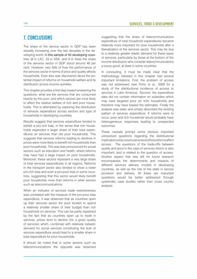
110 SERVICES, TRADE & DEVELOPMENT
7. CONCLUSIONS
The share of the service sector in GDP has been
steadily increasing over the last decades in the de-
veloping world. In this sample of 40 developing coun-In this sample of 40 developing coun-
tries (8 in LAC, 23 in SSA, and 9 in Asia) the share
of the services sector in GDP stood around 48 per
cent. However, very little of how the performance of
the services sector in terms of price and quality affects
households. Even less was discovered about the po-
tential impact of reforms on household welfare and its
distribution across income quintiles.
This chapter provides a first step toward answering the
questions: what are the services that are consumed
heavily by the poor; and which sectors are most likely
to affect the relative welfare of rich and poor house-
holds. This is attempted by exploring the distribution
of services expenditure across sectors and type of
households in developing countries.
Results suggest that services expenditure tended to
exhibit a pro-rich bias, in the sense that rich house-
holds expended a larger share of their total expen-
ditures on services than did poor households. This
suggests that services reforms leading to declines in
prices were more likely to benefit rich households than
poor households. This was less pronounced for social
sectors such as education and health, where reforms
may have had a large impact on poor households.
Moreover, these sectors represent a very large share
of total services expenditures in all regions. Reforms
in the transport sector also tended to show a lower
pro-rich bias and even a pro-poor bias in some coun-
tries, suggesting that this sector would likely benefit
poor households more than reforms in other sectors
such as telecommunications.
When an indicator of services trade restrictiveness
was correlated with the measure of the pro-poor bias
expenditure, it was observed that as countries open
up their services sector the poor tended to spend
a relatively smaller share of their budget than rich
households on services. This can be partly explained
by the fact that as countries open up to trade in
services, prices tend to decline (for a given quality
of services) which, combined with relatively inelastic
demand for social services constituting the bulk of
services expenditure would lead to a smaller share in
total expenditure for poor households.
It should be noted that in some sectors such as
telecommunications the opposite was observed
suggesting that the share of telecommunications
expenditure of total household expenditures became
relatively more important for poor households after a
liberalization of the services sector. This may be due
to a relatively greater elastic demand for these types
of services, particularly by those at the bottom of the
income distribution who consider telecommunications
a luxury good, at least in some countries.
In concluding, it must be made clear that the
methodology followed in this chapter had several
important limitations. First, the problem of access
was not addressed (see Porto et al., 2009 for a
study of the distributional incidence of access to
services in Latin America). Second, the expenditure
data did not contain information on subsidies which
may have targeted poor (or rich) households and
therefore may have biased the estimates. Finally the
analysis was static and simply described the existing
pattern of services expenditure. If reforms were to
occur, poor and rich household would probably have
heterogeneous responses leading to unexpected
outcomes.
These caveats prompt some obvious important
unresolved questions regarding the distributional
implications of access to services and how reforms affect
access. The questions of the trade-offs between
quality and price in the case of services reform is also
important, and is related to the question of access.
Another aspect that was left for future research
encompasses the determinants and impacts of
different services delivery models in developing
countries, as well as the role of the state in service
provision and delivery. All these are important
questions would be better addressed through
systematic case studies rather than cross country
analysis.

111CHAPTER V: A TOPOLOGY OF SERVICES EXPENDITURE BY POOR AND RICH HOUSEHOLDS IN DEVELOPING COUNTRIES
RSEBP(disaggregated services expenditure)
RSEBP*(disaggregated services expenditure)
Telecommunications-.025a
(.003)-.771a
(.055)
Transport-.023a
(.005)-.381a
(.058)
Education-.017a
(.004)-.199a
(.046)
Health-.015a
(.006)-.163a
(.037)
R2 0.331 0.698
Number of observations 143.000 143.000
Note: All regressions are ordinary least squares and robust standard errors are provided in parenthesis. Superscript “a” stands for statistical significance at the 1 per cent level and “b” stands for statistical significance at the 5 per cent level.
Table 2. Indices of pro-poor-services-expenditure-biases across services
RSEBP RSEBP*
LAC SSA Asia LAC SSA Asia
Telecommunication-052a
(.003)-013a
(.002)-023b
(.010)-594a
(.094)-932a
(.061)-.583a
(.115)
Transport.001
(.021)-037a
(.004)-.008
(.007)-.059
(.099)-561a
(.060)-.174a
(.099)
Education-034a
(.011)-011b
(.005)-.015
(.009)-.166a
(.057)-270a
(.074)-.076
(.068)
Health-029b
(.013)-.012
(.008)-.012
(.012)-.193a
(.065)-185a
(.056)-.086
(.054)
Note: All regressions are ordinary least squares and robust standard errors are provided in parenthesis. A regression is run for each sector and index. Superscript “a” stands for statistical significance at the 1 per cent level and “b” stands for statistical significance at the 5 per cent level.
Table 3. Indices of pro-poor-services-expenditure-biases across services and sectors
RSEBP(aggregate services
expenditure)
RSEBP*(aggregate services
expenditure)
RSEBP(disaggregated
services expenditure)
RSEBP*(disaggregated
services expenditure)
Latin America-.117a
(.042)-.150a
(.006)-.030a
(.007)-.272a
(.056)
Sub-Saharan Africa-.121a
(.014)-.383a
(.048)-.019a
(.003)-.472a
(.042)
Asia-.008a
(.024)-.163a (.036)
-.014a
(.005)-.220a
(.044)
R2 0.670 0.730 0.331 0.542
Number of observations 40.000 40.000 143.000 143.000
Note: All regressions are ordinary least squares and robust standard errors are provided in parenthesis. Superscript “a” stands for statistical significance at the 1 per cent level and “b” stands for statistical significance at the 5 per cent level.
Table 1. Indices of pro-poor-services-expenditure-biases across regions

112 SERVICES, TRADE & DEVELOPMENT
Figure 1. Pro-poor-services-expenditure bias by sector and GDP per capita
Telecommunication services Total services
Education servicesTransport services
Health services
CIV
IND
BDI
GNB
ETH
TJK
RWA
MWI
BFA
MDG
UGA
MOZ
GHA
NER
NGA
MLI
TGO
GMB
KEN
ZMB
VNM
SEN
TLS
IND
NIC
IDN
CIV
CMR
BOL
CHN
ECU
PER
COL
RUS
THAZAF
MEX BDI
ETH
GNB
NER
MWI
TJK
BFA
NGA
UGA
TGO
GHA
GMB
BEN
ZMB
IND
MLISEN
CIVKEN
CMR
VNMIDNNICBOL
TLSCHN
ECU
PER
COL
THA
ZAF
PANRUS
MEX
BDI
ETH
MWI
GNB
TJKRWA
NER
MOZ
BFA
MDGKEN
GMB
MLI
TGO
UGA
BEN
TLS
ZMB
GHAVNM
NGA
SEN
IND
CIV
CHN
NIC
CMR
BOL
IDN
ECU
THAPERCOL
RUS
ZAF
PAN
MEX
BDI
ETH
MOZ
TJK
NER
GNB
RWA
MWI
TGO
MLI
UGA
BFAMDG
GHA
TZA
ZMB
GMB
NGA
BEN
VNM
KEN
IDN
CMR
NIC
SEN
CHN
BOL
ECU
RUS
SLV
COL
PER
THA
PAN
MEX
ZAF
BDI
ETH
MWI
NERMOZ
MDG
RWA
UGA
TGO
GHA
TJK
VNM
BFA
IND
MLIZMB
NGA
CMR
CIV
NIC
BOL
SLV
CHN
ECU
PER
THA
RUS
COL
PAN
ZAF
MEX
SEN
-.4
-.2
0.2
.4.6
-.4
-.2
0.2
.4
e( P
PS
EB2
| X
)
-2 -1 0 1 2
e( lgnic | X )
coef = .09778138, (robust) se = .03470804, t = 2.82
-.4
-.2
0.2
.4.6
e( P
PS
EB2
| X
)
-2 -1 0 1 2
e( lgnic | X )
coef = .18957929, (robust) se = .03006759, t = 6.31
-.5
0.5
e( P
PS
EB2
| X
)
-2 -1 0 1 2
e( lgnic | X )
coef = .09778138, (robust) se = .03470804, t = 2.82
-.1
-.5
0.5
e( P
PS
EB2
| X
)
-2 -1 0 1 2
e( lgnic | X )
e( P
PS
EB2
| X
)
-2 -1 0 1 2
coef = .09778138, (robust) se = .03470804, t = 2.82
e( lgnic | X )
coef = .18957929, (robust) se = .03006759, t = 6.31
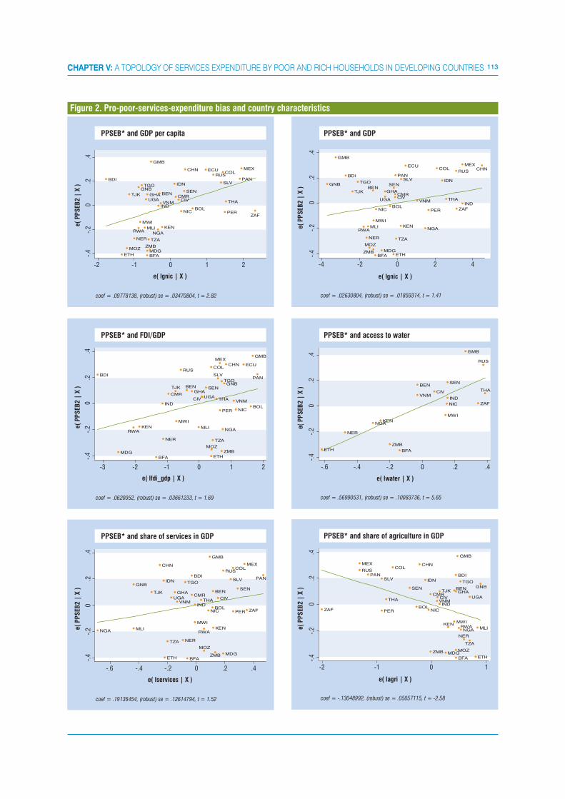
113CHAPTER V: A TOPOLOGY OF SERVICES EXPENDITURE BY POOR AND RICH HOUSEHOLDS IN DEVELOPING COUNTRIES
Figure 2. Pro-poor-services-expenditure bias and country characteristics
PPSEB* and GDPPPSEB* and GDP per capita
PPSEB* and access to waterPPSEB* and FDI/GDP
PPSEB* and share of agriculture in GDP PPSEB* and share of services in GDP
BDI
MDG
RWAKEN
BFA
IND
NER
CMR
TJK
MWI
RUS
BEN
GHA
MLI
UGACIV
SEN
COL
ETH
MOZ
TZA
SLV
MEX
PER
ZMB
TGO
NGA
GNB
CHN
VNM
NIC
ECU
BOL
GMB
PAN
NGA
GNB
MLI
TJK
CHN
IDN
ETH
TZA
UGA
GHA
VNM
NER
TGO
BFA
CMR
BDI
MWI
THA
RWA
MOZ
NIC
GMB
BOL
BEN
KEN
ZMB
CIV
MDG
RUS
SLV
COL
PER
SEN
MEX
ZAF
PAN
GNB
GMB
BDI
TJK
TGO
RWA
NER
MLI
MOZ
BEN
ZMB
MWI
BFA
NIC
MDG
UGA
GHA
BOL
ETH
SEN
CIVCMR
PAN
TZA
KEN
SLV
ECU
VNM
NGA
PER
COL
IDN
THA
RUS
ZAF
MEX
IND
CHN
NER
ZMB
BFA
VNM
BEN
CIV
MWI
NIC
IND
SEN
GMB
ZAF
RUS
THA
ZAF
RUS
MEX
PANSLV
PER
THA
COL
SEN
BOL
CHN
IDN
NIC
CMR
ZMB
VNMCIV
TJK
IND
MDG
KEN
BEN
MWI
MOZ
GHA
BDI
BFA
RWA
TGO
NGA
NER
UGA
TZA
ETH
MLI
GNB
GMB
BDI
ETH
MOZ
TJK
NER
GNB
RWA
MWI
TGO
MLI
UGA
BFAMDG
GHA
TZA
ZMB
GMB
NGA
BEN
VNM
KEN
IDN
CMR
NIC
SEN
CHN
BOL
ECU
RUS
SLV
COL
PER
THA
MEX
ZAF
-.4
-.2
0.2
.4
e( P
PS
EB2
| X
)
-2 -1 0 1 2
e( lgnic | X )
coef = .09778138, (robust) se = .03470804, t = 2.82e(
PP
SEB
2 |
X )
e( lgnic | X )
coef = .02630804, (robust) se = .01859314, t = 1.41
e( P
PS
EB2
| X
)
e( lwater | X )
coef = .0620052, (robust) se = .03661233, t = 1.69
e( P
PS
EB2
| X
)
e( lfdi_gdp | X )
e( P
PS
EB2
| X
)
coef = .19136454, (robust) se = .12614794, t = 1.52
e( lservices | X )
coef = .56990531, (robust) se = .10083736, t = 5.65
e( lagri | X )
e( P
PS
EB2
| X
)
coef = -.13048992, (robust) se = .05057115, t = -2.58
-.4
-.2
0.2
.4
-3 -2 -1 0 1 2
-.4
-.2
0.2
.4
-.6 -.4 -.2 0 .2 .4
-.4
-.2
0.2
.4
-4 -2 0 2 4
-.4
-.2
0.2
.4
-.6 -.4 -.2 0 .2 .4
-.4
-.2
0.2
.4
-2 -1 0 1
PAN
CIV
IND
THA
NGAKEN
ETH
IND

114 SERVICES, TRADE & DEVELOPMENT
Figures 3 Pro-poor-services-expenditure bias and services trade restrictiveness
Communication servicesTotal services
Education servicesHealth services
Transport services
e( P
PS
EB2
| X
)
e( lpol | X )
coef = .07872074, (robust) se = .08455104, t = .93 coef = -.0397855, (robust) se = .09017064, t = -.44e(
PP
SEB
2 |
X )
e( lpol | X )
e( P
PS
EB2
| X
)
e( lpol | X )
coef = .06020301, (robust) se = .09522246, t = .63
e( P
PS
EB2
| X
)
e( lpol | X )
e( P
PS
EB2
| X
)
coef = .14895047, (robust) se = .10464982, t = 1.42
e( lpol | X )
coef = .06834599, (robust) se = .11554118, t = .59
GHA
SEN
ECU
PER
ZAF
NGAKEN
TZA
COL MEXIDN
THA
CHN
IND
-.2
0.2
.4
-1 -.5 0 .5 1
ZAF
PER
ECU
GHA
SEN
NGA
COL
MEX
THA
CHN
IND
-.3
-.2
-.1
0.1
.2
-.5 0 .5 1
PER
ZAF
GHA
SEN
ECU
NGA
KEN
COL
MEX
THA
IDN
CHN
IND
-.4
-.2
0.2
.4
-.5 0 .5 1
ZAF
PER
GHA
ECU
SEN
NGA
KENCOL
IDN
THA
CHN
IND
-.6
-.4
-.2
0.2
.4
-.5 0 .5 1
ZAF
PER
ECU
GHA
SEN
NGA
KEN
COLMEX
THA
IDN
CHN
IND
-.4
-.2
0.2
.4
-.5 0 .5 1
MEX
Source : Authors’ calculations using Gootiz and Mattoo (2009) measures of services trade restrictiveness.

115CHAPTER V: A TOPOLOGY OF SERVICES EXPENDITURE BY POOR AND RICH HOUSEHOLDS IN DEVELOPING COUNTRIES
Country
Telecommunication (%) Infrastructure services (%)
Education HealthFixed phone
Cell phone
TotalPublic
transportWater Electricity Gas Total
Bolivia (Plurinational State of)
6.5 1.8 0.5 1.0 1.8 3.9 1.2 2.8 1.4 19.4
Colombia 4.0 5.5 3.8 1.0 5.0 10.4 2.4 5.0 2.7 34.8
Ecuador 6.6 8.0 1.0 1.9 3.8 8.6 1.3 2.6 0.7 31.5
El Salvador 8.2 1.2 2.2 1.1 3.3 3.7 2.3 4.4 0.9 24.0
Mexico 5.3 2.6 1.6 1.1 3.1 5.0 0.7 2.3 1.9 20.9
Nicaragua 4.8 7.3 NA NA 1.5 4.3 1.2 2.0 1.1 22.1
Panama 5.3 5.6 1.3 0.9 2.3 0,8 1.0 2.6 0.7 18.2
Peru 4.2 3.4 0.8 0.4 1.4 5,3 1.0 1.7 1.1 18.1
Source: Authors’ calculations based on SEDLAC (CEDLAS and The Wodd Bank).
Table 4. Expenditure on services as a percentage of total expenditure in Latin America
Figure 4. Expenditures on each service as a percentage of total expenditures on services
Bolivia
(Plur
inatio
nal
State o
f)
Colom
bia
Ecua
dor
El Salv
ador
Mex
ico
Nicara
gua
Panam
aPer
u
Education Health Telecommunication Transport Water Electricity Gas
0
10
20
30
40
50
60
70
80
90
100
Per
cent
age
Source: Authors’ calculations based on SEDLAC (CEDLAS and The World Bank).
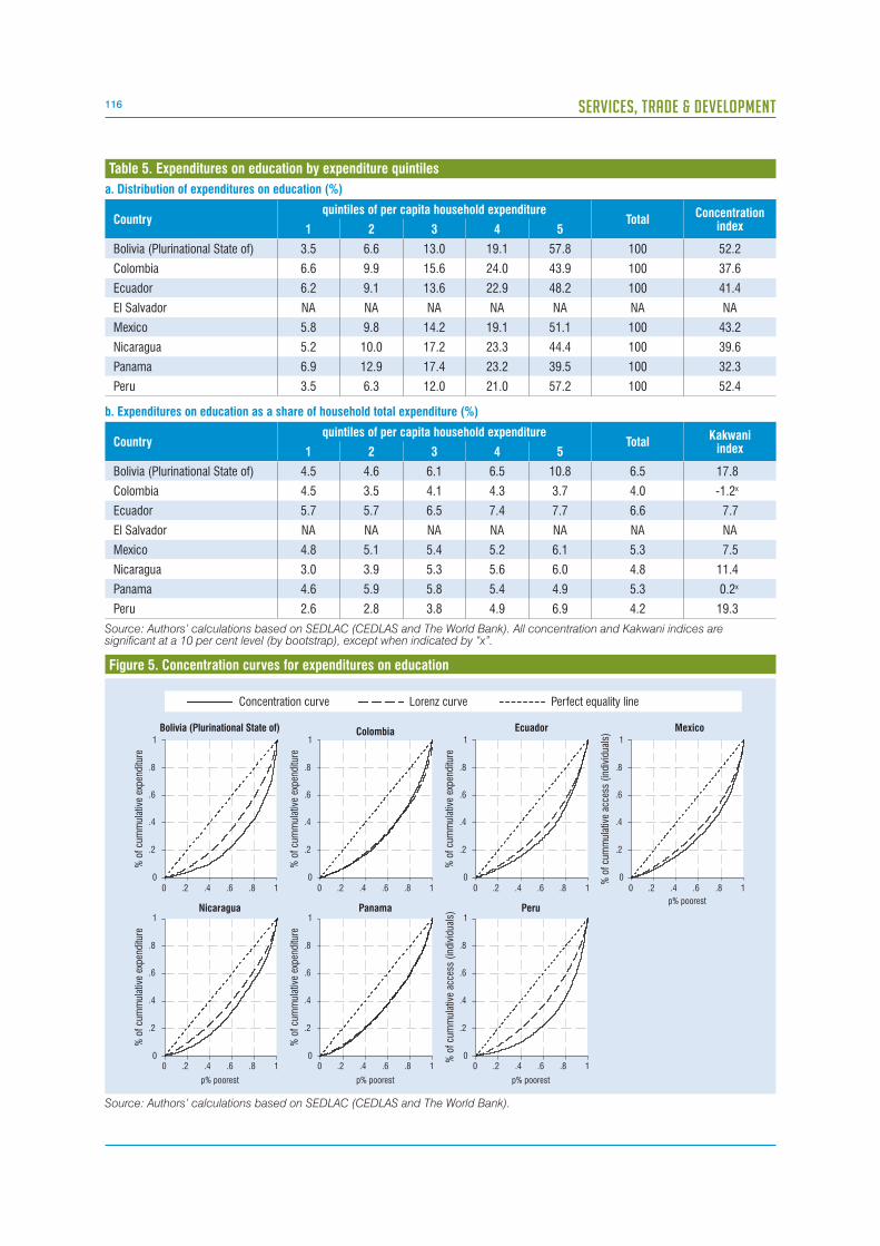
116 SERVICES, TRADE & DEVELOPMENT
a. Distribution of expenditures on education (%)
Countryquintiles of per capita household expenditure
TotalConcentration
index1 2 3 4 5
Bolivia (Plurinational State of) 3.5 6.6 13.0 19.1 57.8 100 52.2
Colombia 6.6 9.9 15.6 24.0 43.9 100 37.6
Ecuador 6.2 9.1 13.6 22.9 48.2 100 41.4
El Salvador NA NA NA NA NA NA NA
Mexico 5.8 9.8 14.2 19.1 51.1 100 43.2
Nicaragua 5.2 10.0 17.2 23.3 44.4 100 39.6
Panama 6.9 12.9 17.4 23.2 39.5 100 32.3
Peru 3.5 6.3 12.0 21.0 57.2 100 52.4 b. Expenditures on education as a share of household total expenditure (%)
Countryquintiles of per capita household expenditure
TotalKakwani
index1 2 3 4 5
Bolivia (Plurinational State of) 4.5 4.6 6.1 6.5 10.8 6.5 17.8
Colombia 4.5 3.5 4.1 4.3 3.7 4.0 -1.2x
Ecuador 5.7 5.7 6.5 7.4 7.7 6.6 7.7
El Salvador NA NA NA NA NA NA NA
Mexico 4.8 5.1 5.4 5.2 6.1 5.3 7.5
Nicaragua 3.0 3.9 5.3 5.6 6.0 4.8 11.4
Panama 4.6 5.9 5.8 5.4 4.9 5.3 0.2x
Peru 2.6 2.8 3.8 4.9 6.9 4.2 19.3
Source: Authors’ calculations based on SEDLAC (CEDLAS and The World Bank). All concentration and Kakwani indices are significant at a 10 per cent level (by bootstrap), except when indicated by “x”.
Table 5. Expenditures on education by expenditure quintiles
Figure 5. Concentration curves for expenditures on education
0
.2
.4
.6
.8
1
% o
f cu
mm
ulat
ive
expe
nditu
re
0 .2 .4 .6 .8 1
Bolivia (Plurinational State of)
0
.2
.4
.6
.8
1
% o
f cu
mm
ulat
ive
expe
nditu
re
0 .2 .4 .6 .8 1
Colombia
0
.2
.4
.6
.8
1
% o
f cu
mm
ulat
ive
expe
nditu
re
0 .2 .4 .6 .8 1
Ecuador
0
.2
.4
.6
.8
1
% o
f cu
mm
ulat
ive
acce
ss (
indi
vidu
als)
0 .2 .4 .6 .8 1
Mexico
0
.2
.4
.6
.8
1
% o
f cu
mm
ulat
ive
expe
nditu
re
0 .2 .4 .6 .8 1
p% poorest
Panama
0
.2
.4
.6
.8
1
% o
f cu
mm
ulat
ive
expe
nditu
re
0 .2 .4 .6 .8 1
p% poorest
Nicaragua
0
.2
.4
.6
.8
1
% o
f cu
mm
ulat
ive
acce
ss (
indi
vidu
als)
0 .2 .4 .6 .8 1
p% poorest
p% poorestPeru
Concentration curve Lorenz curve Perfect equality line
Source: Authors’ calculations based on SEDLAC (CEDLAS and The World Bank).
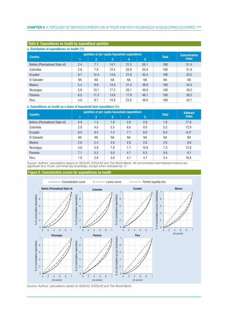
117CHAPTER V: A TOPOLOGY OF SERVICES EXPENDITURE BY POOR AND RICH HOUSEHOLDS IN DEVELOPING COUNTRIES
a. Distribution of expenditures on health (%)
Countryquintiles of per capita household expenditure
TotalConcentration
index1 2 3 4 5
Bolivia (Plurinational State of) 2.4 7.1 14.1 21.2 55.1 100 51.4
Colombia 2.8 7.9 12.5 20.9 55.9 100 51.6
Ecuador 8.7 12.4 14.6 21.0 43.4 100 33.5
El Salvador NA NA NA NA NA NA NA
Mexico 5.4 9.6 13.9 21.4 49.8 100 44.3
Nicaragua 5.8 10.1 17.3 20.1 46.8 100 40.2
Panama 8.5 11.3 13.6 17.9 48.7 100 38.2
Peru 4.0 8.7 15.8 23.6 48.0 100 43.7 b. Expenditures on health as a share of household total expenditure (%)
Countryquintiles of per capita household expenditure
TotalKakwani
index1 2 3 4 5
Bolivia (Plurinational State of) 0.9 1.3 1.9 2.0 2.8 1.8 17.0
Colombia 2.9 4.5 5.5 6.6 8.0 5.5 12.8
Ecuador 8.5 8.5 7.2 7.7 8.0 8.0 -0.2x
El Salvador NA NA NA NA NA NA NA
Mexico 2.0 2.4 2.6 2.9 3.0 2.6 8.6
Nicaragua 4.8 5.9 7.8 7.1 10.9 7.3 12.0
Panama 7.1 5.2 5.0 4.7 6.3 5.6 6.1
Peru 1.9 2.8 3.6 4.1 4.7 3.4 10.6
Source: Authors’ calculations based on SEDLAC (CEDLAS and The World Bank). All concentration and Kakwani indices are significant at a 10 per cent level (by bootstrap), except when indicated by “x”.
Table 6. Expenditures on health by expenditure quintiles
Figure 6. Concentration curves for expenditures on health
0
.2
.4
.6
.8
1
% o
f cu
mm
ulat
ive
expe
nditu
re
0 .2 .4 .6 .8 1
Bolivia (Plurinational State of)
0
.2
.4
.6
.8
1
% o
f cu
mm
ulat
ive
expe
nditu
re
0 .2 .4 .6 .8 1
Colombia
0
.2
.4
.6
.8
1
% o
f cu
mm
ulat
ive
expe
nditu
re
0 .2 .4 .6 .8 1
Ecuador
0
.2
.4
.6
.8
1
% o
f cu
mm
ulat
ive
acce
ss (
indi
vidu
als)
0 .2 .4 .6 .8 1
Mexico
0
.2
.4
.6
.8
1
% o
f cu
mm
ulat
ive
expe
nditu
re
0 .2 .4 .6 .8 1
p% poorest
Panama
0
.2
.4
.6
.8
1
% o
f cu
mm
ulat
ive
expe
nditu
re
0 .2 .4 .6 .8 1
p% poorest
Nicaragua
0
.2
.4
.6
.8
1
% o
f cu
mm
ulat
ive
acce
ss (
indi
vidu
als)
0 .2 .4 .6 .8 1
p% poorest
Peru
Concentration curve Lorenz curve Perfect equality line
p% poorest
Source: Authors’ calculations based on SEDLAC (CEDLAS and The World Bank).
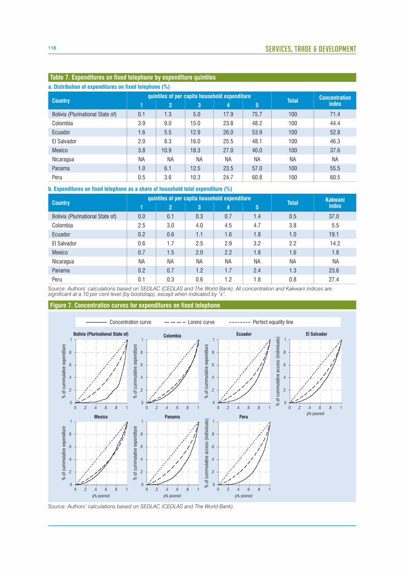
118 SERVICES, TRADE & DEVELOPMENT
Figure 7. Concentration curves for expenditures on fixed telephone
0
.2
.4
.6
.8
1
% o
f cu
mm
ulat
ive
expe
nditu
re
0 .2 .4 .6 .8 1
Bolivia (Plurinational State of)
0
.2
.4
.6
.8
1
% o
f cu
mm
ulat
ive
expe
nditu
re
0 .2 .4 .6 .8 1
Colombia
0
.2
.4
.6
.8
1
% o
f cu
mm
ulat
ive
expe
nditu
re
0 .2 .4 .6 .8 1
Ecuador
0
.2
.4
.6
.8
1
% o
f cu
mm
ulat
ive
acce
ss (
indi
vidu
als)
0 .2 .4 .6 .8 1
El Salvador
0
.2
.4
.6
.8
1
% o
f cu
mm
ulat
ive
expe
nditu
re
0 .2 .4 .6 .8 1
p% poorest
Panama
0
.2
.4
.6
.8
1
% o
f cu
mm
ulat
ive
expe
nditu
re
0 .2 .4 .6 .8 1
p% poorest
Mexico
0
.2
.4
.6
.8
1
% o
f cu
mm
ulat
ive
acce
ss (
indi
vidu
als)
0 .2 .4 .6 .8 1
p% poorest
Peru
Concentration curve Lorenz curve Perfect equality line
p% poorest
Source: Authors’ calculations based on SEDLAC (CEDLAS and The World Bank).
a. Distribution of expenditures on fixed telephone (%)
Countryquintiles of per capita household expenditure
TotalConcentration
index1 2 3 4 5
Bolivia (Plurinational State of) 0.1 1.3 5.0 17.9 75.7 100 71.4
Colombia 3.9 9.0 15.0 23.8 48.2 100 44.4
Ecuador 1.6 5.5 12.9 26.0 53.9 100 52.8
El Salvador 2.0 8.3 16.0 25.5 48.1 100 46.3
Mexico 3.8 10.9 18.3 27.0 40.0 100 37.6
Nicaragua NA NA NA NA NA NA NA
Panama 1.0 6.1 12.5 23.5 57.0 100 55.5
Peru 0.5 3.6 10.3 24.7 60.8 100 60.5 b. Expenditures on fixed telephone as a share of household total expenditure (%)
Countryquintiles of per capita household expenditure
TotalKakwani
index1 2 3 4 5
Bolivia (Plurinational State of) 0.0 0.1 0.3 0.7 1.4 0.5 37.0
Colombia 2.5 3.0 4.0 4.5 4.7 3.8 5.5
Ecuador 0.2 0.6 1.1 1.6 1.8 1.0 19.1
El Salvador 0.6 1.7 2.5 2.9 3.2 2.2 14.2
Mexico 0.7 1.5 2.0 2.2 1.8 1.6 1.8
Nicaragua NA NA NA NA NA NA NA
Panama 0.2 0.7 1.2 1.7 2.4 1.3 23.6
Peru 0.1 0.3 0.6 1.2 1.8 0.8 27.4
Source: Authors’ calculations based on SEDLAC (CEDLAS and The World Bank). All concentration and Kakwani indices are significant at a 10 per cent level (by bootstrap), except when indicated by “x”.
Table 7. Expenditures on fixed telephone by expenditure quintiles

119CHAPTER V: A TOPOLOGY OF SERVICES EXPENDITURE BY POOR AND RICH HOUSEHOLDS IN DEVELOPING COUNTRIES
a. Distribution of expenditures on mobile telephone (%)
Countryquintiles of per capita household expenditure
TotalConcentration
index1 2 3 4 5
Bolivia (Plurinational State of) 1.4 6.1 13.3 21.8 57.4 100 55.7
Colombia 1.1 4.1 8.7 17.7 68.4 100 64.3
Ecuador 5.5 9.8 14.2 23.3 47.2 100 41.2
El Salvador 3.0 7.1 10.5 18.3 61.2 100 55.2
Mexico 4.1 8.6 15.3 22.8 49.2 100 44.3
Nicaragua NA NA NA NA NA NA NA
Panama 2.3 6.9 12.6 21.7 56.5 100 54.4
Peru 0.8 4.2 10.1 21.2 63.8 100 62.2 b. Expenditures on mobile telephone as a share of household total expenditure (%)
Countryquintiles of per capita household expenditure
TotalKakwani
index1 2 3 4 5
Bolivia (Plurinational State of) 0.2 0.6 1.0 1.3 1.7 1.0 21.3
Colombia 0.4 0.5 0.8 1.2 2.2 1.0 25.5
Ecuador 1.3 1.7 1.9 2.2 2.2 1.9 7.5
El Salvador 0.5 0.8 0.9 1.1 2.0 1.1 23.1
Mexico 0.6 0.9 1.1 1.3 1.5 1.1 8.6
Nicaragua NA NA NA NA NA NA NA
Panama 0.3 0.7 0.9 1.1 1.6 0.9 22.6
Peru 0.1 0.2 0.3 0.5 0.9 0.4 29.2
Source: Authors’ calculations based on SEDLAC (CEDLAS and The World Bank). All concentration and Kakwani indices are significant at a 10 per cent level (by bootstrap), except when indicated by “x”.
Table 8. Expenditures on mobile telephone by expenditure quintiles
Figure 8. Concentration curves for expenditures on mobile telephone
0
.2
.4
.6
.8
1
% o
f cu
mm
ulat
ive
expe
nditu
re
0 .2 .4 .6 .8 1
Bolivia (Plurinational State of)
0
.2
.4
.6
.8
1
% o
f cu
mm
ulat
ive
expe
nditu
re
0 .2 .4 .6 .8 1
Colombia
0
.2
.4
.6
.8
1
% o
f cu
mm
ulat
ive
expe
nditu
re
0 .2 .4 .6 .8 1
Ecuador
0
.2
.4
.6
.8
1
% o
f cu
mm
ulat
ive
acce
ss (
indi
vidu
als)
0 .2 .4 .6 .8 1
El Salvador
0
.2
.4
.6
.8
1
% o
f cu
mm
ulat
ive
expe
nditu
re
0 .2 .4 .6 .8 1
p% poorest
Panama
0
.2
.4
.6
.8
1
% o
f cu
mm
ulat
ive
expe
nditu
re
0 .2 .4 .6 .8 1
p% poorest
Mexico
0
.2
.4
.6
.8
1
% o
f cu
mm
ulat
ive
acce
ss (
indi
vidu
als)
0 .2 .4 .6 .8 1
p% poorest
Peru
Concentration curve Lorenz curve Perfect equality line
p% poorest
Source: Authors’ calculations based on SEDLAC (CEDLAS and The World Bank).

120 SERVICES, TRADE & DEVELOPMENT
Figure 9. Concentration curves for expenditures on total telecommunication
0
.2
.4
.6
.8
1
% o
f cu
mm
ulat
ive
expe
nditu
re
0 .2 .4 .6 .8 1
Bolivia (Plurinational State of)
0
.2
.4
.6
.8
1
% o
f cu
mm
ulat
ive
expe
nditu
re
0 .2 .4 .6 .8 1
Colombia
0
.2
.4
.6
.8
1
% o
f cu
mm
ulat
ive
expe
nditu
re
0 .2 .4 .6 .8 1
Ecuador
0
.2
.4
.6
.8
1
% o
f cu
mm
ulat
ive
acce
ss (
indi
vidu
als)
0 .2 .4 .6 .8 1
Mexico
0
.2
.4
.6
.8
1
% o
f cu
mm
ulat
ive
expe
nditu
re
0 .2 .4 .6 .8 1
p% poorest
Panama
0
.2
.4
.6
.8
1
% o
f cu
mm
ulat
ive
expe
nditu
re
0 .2 .4 .6 .8 1
p% poorest
Nicaragua
0
.2
.4
.6
.8
1
% o
f cu
mm
ulat
ive
acce
ss (
indi
vidu
als)
0 .2 .4 .6 .8 1
p% poorest
Peru
Concentration curve Lorenz curve Perfect equality line
p% poorest
Source: Authors’ calculations based on SEDLAC (CEDLAS and The World Bank).
a. Distribution of expenditures on telecommunication (%)
Countryquintiles of per capita household expenditure
TotalConcentration
index1 2 3 4 5
Bolivia (Plurinational State of) 1.1 4.2 9.9 19.5 65.2 100 62.2
Colombia 3.0 7.4 12.6 21.2 55.7 100 51.4
Ecuador 4.0 8.5 14.0 24.5 48.9 100 44.9
El Salvador 2.4 7.9 13.9 22.8 53.0 100 49.7
Mexico 4.1 10.0 16.8 24.9 44.2 100 40.4
Nicaragua 0.3 3.0 8.8 21.5 66.3 100 65.0
Panama 1.6 6.5 12.0 21.8 58.2 100 55.6
Peru 0.6 3.4 9.1 21.7 65.3 100 63.9 b. Expenditures on telecommunication as a share of household total expenditure (%)
Countryquintiles of per capita household expenditure
TotalKakwani
index1 2 3 4 5
Bolivia (Plurinational State of) 0.4 0.9 1.5 2.3 4.0 1.8 27.8
Colombia 3.0 3.7 4.9 5.8 7.5 5.0 12.7
Ecuador 1.9 3.0 3.9 4.9 5.1 3.8 11.2
El Salvador 1.1 2.5 3.4 4.1 5.3 3.3 17.6
Mexico 1.6 2.7 3.5 3.9 3.7 3.1 4.6
Nicaragua 0.1 0.5 1.0 2.1 4.0 1.5 36.8
Panama 0.5 1.5 2.3 3.0 4.4 2.3 23.5
Peru 0.1 0.5 1.0 1.9 3.3 1.4 30.8
Source: Authors’ calculations based on SEDLAC (CEDLAS and The World Bank). All concentration and Kakwani indices are significant at a 10 per cent% level (by bootstrap), except when indicated by “x”.
Table 9. Expenditures on total telecommunication by expenditure quintiles

121CHAPTER V: A TOPOLOGY OF SERVICES EXPENDITURE BY POOR AND RICH HOUSEHOLDS IN DEVELOPING COUNTRIES
Figure 10. Concentration curves for expenditures on public transport
0
.2
.4
.6
.8
1
% o
f cu
mm
ulat
ive
expe
nditu
re
0 .2 .4 .6 .8 1
Bolivia (Plurinational State of)
0
.2
.4
.6
.8
1
% o
f cu
mm
ulat
ive
expe
nditu
re
0 .2 .4 .6 .8 1
Colombia
0
.2
.4
.6
.8
1
% o
f cu
mm
ulat
ive
expe
nditu
re
0 .2 .4 .6 .8 1
Ecuador
0
.2
.4
.6
.8
1
% o
f cu
mm
ulat
ive
acce
ss (
indi
vidu
als)
0 .2 .4 .6 .8 1
Mexico
0
.2
.4
.6
.8
1
% o
f cu
mm
ulat
ive
expe
nditu
re
0 .2 .4 .6 .8 1
p% poorest
Peru
0
.2
.4
.6
.8
1
% o
f cu
mm
ulat
ive
expe
nditu
re
0 .2 .4 .6 .8 1
p% poorest
Nicaragua
Concentration curve Lorenz curve Perfect equality line
p% poorestp% poorest
Source: Authors’ calculations based on SEDLAC (CEDLAS and The World Bank).
a. Distribution of expenditures on public transport (%)
Countryquintiles of per capita household expenditure
TotalConcentration
index1 2 3 4 5
Bolivia (Plurinational State of) 4.3 8.6 17.2 25.0 45.0 100 40.8
Colombia 7.7 13.6 19.7 25.2 33.7 100 26.7
Ecuador 12.7 16.3 19.2 22.8 29.1 100 16.8
El Salvador NA NA NA NA NA NA NA
Mexico 11.5 19.0 22.6 23.2 23.7 100 12.6
Nicaragua 5.1 11.4 19.2 24.9 39.3 100 34.8
Panama NA NA NA NA NA NA NA
Peru 4.3 10.4 18.3 25.0 42.1 100 38.9 b. Expenditures on public transport as a share of household total expenditure (%)
Countryquintiles of per capita household expenditure
TotalKakwani
index1 2 3 4 5
Bolivia (Plurinational State of) 2.5 3.1 4.1 4.8 4.9 3.9 6.3
Colombia 11.0 10.6 11.6 10.9 7.9 10.4 -12.1
Ecuador 10.9 9.7 8.9 7.8 5.6 8.6 -16.9
El Salvador NA NA NA NA NA NA NA
Mexico 5.7 6.2 5.8 4.6 2.7 5.0 -23.1
Nicaragua 2.2 3.6 4.8 5.4 5.7 4.3 6.6
Panama NA NA NA NA NA NA NA
Peru 3.0 4.7 6.2 6.5 5.9 5.3 5.9
Source: Authors’ calculations based on SEDLAC (CEDLAS and The World Bank). All concentration and Kakwani indices are significant at a 10 per cent level (by bootstrap), except when indicated by “x”.
Table 10. Expenditures on public transport by expenditure quintiles

122 SERVICES, TRADE & DEVELOPMENT
a. Distribution of expenditures on water (%)
Countryquintiles of per capita household expenditure
TotalConcentration
index1 2 3 4 5
Bolivia (Plurinational State of) 3.1 9.5 15.1 28.9 43.5 100 41.4
Colombia 7.5 13.6 17.2 22.4 39.3 100 32.4
Ecuador 7.6 12.9 18.4 23.2 37.9 100 30.1
El Salvador 8.3 14.1 18.6 24.1 34.9 100 27.2
Mexico 10.6 15.9 20.5 22.4 30.6 100 20.3
Nicaragua 4.9 13.0 17.9 24.6 39.5 100 35.1
Panama 6.1 15.3 18.7 24.1 35.9 100 31.1
Peru 4.5 10.9 18.3 25.0 41.3 100 37.1 b. Expenditures on water as a share of household total expenditure (%)
Countryquintiles of per capita household expenditure
TotalKakwani
index1 2 3 4 5
Bolivia (Plurinational State of) 0.7 1.1 1.2 1.7 1.5 1.2 7.0
Colombia 2.7 2.5 2.4 2.3 2.1 2.4 -6.5
Ecuador 1.1 1.3 1.4 1.3 1.2 1.3 -3.5
El Salvador 2.7 2.4 2.3 2.2 1.9 2.3 -4.9
Mexico 0.8 0.8 0.8 0.7 0.5 0.7 -15.5
Nicaragua 0.6 1.2 1.3 1.4 1.3 1.2 6.9
Panama 0.7 1.1 1.0 1.1 0.9 1.0 -1.5x
Peru 0.6 0.9 1.1 1.1 1.1 1.0 4.1
Source: Authors’ calculations based on SEDLAC (CEDLAS and The World Bank). All concentration and Kakwani indices are significant at a 10 per cent level (by bootstrap), except when indicated by “x”.
Table 11. Expenditures on water by expenditure quintiles
Figure 11. Concentration curves for expenditures on water
0
.2
.4
.6
.8
1
% o
f cu
mm
ulat
ive
expe
nditu
re
0 .2 .4 .6 .8 1
Bolivia (Plurinational State of)
0
.2
.4
.6
.8
1
% o
f cu
mm
ulat
ive
expe
nditu
re
0 .2 .4 .6 .8 1
Colombia
0
.2
.4
.6
.8
1
% o
f cu
mm
ulat
ive
expe
nditu
re
0 .2 .4 .6 .8 1
Ecuador
0
.2
.4
.6
.8
1
% o
f cu
mm
ulat
ive
acce
ss (
indi
vidu
als)
0 .2 .4 .6 .8 1
El Salvador
0
.2
.4
.6
.8
1
% o
f cu
mm
ulat
ive
acce
ss (
indi
vidu
als)
0 .2 .4 .6 .8 1
Peru
0
.2
.4
.6
.8
1
% o
f cu
mm
ulat
ive
expe
nditu
re
0 .2 .4 .6 .8 1
p% poorest
Nicaragua
0
.2
.4
.6
.8
1
% o
f cu
mm
ulat
ive
expe
nditu
re
0 .2 .4 .6 .8 1
p% poorest
Mexico
0
.2
.4
.6
.8
1
% o
f cu
mm
ulat
ive
acce
ss (
indi
vidu
als)
0 .2 .4 .6 .8 1
p% poorest
Panama
Concentration curve Lorenz curve Perfect equality line
p% poorest
Source: Authors’ calculations based on SEDLAC (CEDLAS and The World Bank).

123CHAPTER V: A TOPOLOGY OF SERVICES EXPENDITURE BY POOR AND RICH HOUSEHOLDS IN DEVELOPING COUNTRIES
a. Distribution of expenditures on electricity (%)
Countryquintiles of per capita household expenditure
TotalConcentration
index1 2 3 4 5
Bolivia (Plurinational State of) 3.6 9.9 17.2 26.3 43.0 100 39.9
Colombia 9.0 13.9 18.6 24.3 34.2 100 26.0
Ecuador 7.3 12.3 17.0 24.4 38.8 100 31.8
El Salvador 6.4 13.5 19.2 24.3 36.6 100 30.4
Mexico 9.2 14.1 17.5 22.4 36.9 100 27.4
Nicaragua 3.4 8.9 15.3 22.6 49.7 100 46.7
Panama 4.2 11.6 16.6 22.2 45.4 100 40.6
Peru 3.4 8.8 16.9 25.5 45.5 100 43.0 b. Expenditures on electricity as a share of household total expenditure (%)
Countryquintiles of per capita household expenditure
TotalKakwani
index1 2 3 4 5
Bolivia (Plurinational State of) 1.7 2.6 3.0 3.6 3.2 2.8 5.5
Colombia 6.3 5.0 5.2 4.9 3.5 5.0 -12.7
Ecuador 2.3 2.6 2.7 2.9 2.5 2.6 -1.9
El Salvador 3.8 4.6 4.9 4.5 4.1 4.4 -1.7
Mexico 2.6 2.5 2.4 2.3 1.9 2.3 -8.4
Nicaragua 0.8 1.6 2.1 2.5 3.0 2.0 18.5
Panama 1.3 2.6 2.9 2.9 3.1 2.6 8.4
Peru 0.9 1.4 1.9 2.2 2.2 1.7 9.9
Source: Authors’ calculations based on SEDLAC (CEDLAS and The World Bank). All concentration and Kakwani indices are significant at a 10 per cent level (by bootstrap), except when indicated by “x”.
Table 12. Expenditures on electricity by expenditure quintiles
Figure 12. Concentration curves for expenditures on electricity
0
.2
.4
.6
.8
1
% o
f cu
mm
ulat
ive
expe
nditu
re
0 .2 .4 .6 .8 1
Bolivia (Plurinational State of)
0
.2
.4
.6
.8
1
% o
f cu
mm
ulat
ive
expe
nditu
re
0 .2 .4 .6 .8 1
Colombia
0
.2
.4
.6
.8
1
% o
f cu
mm
ulat
ive
expe
nditu
re
0 .2 .4 .6 .8 1
Ecuador
0
.2
.4
.6
.8
1
% o
f cu
mm
ulat
ive
acce
ss (
indi
vidu
als)
0 .2 .4 .6 .8 1
El Salvador
0
.2
.4
.6
.8
1
% o
f cu
mm
ulat
ive
acce
ss (
indi
vidu
als)
0 .2 .4 .6 .8 1
Peru
0
.2
.4
.6
.8
1
% o
f cu
mm
ulat
ive
expe
nditu
re
0 .2 .4 .6 .8 1
p% poorest
Nicaragua
0
.2
.4
.6
.8
1
% o
f cu
mm
ulat
ive
expe
nditu
re
0 .2 .4 .6 .8 1
p% poorest
Mexico
0
.2
.4
.6
.8
1
% o
f cu
mm
ulat
ive
acce
ss (
indi
vidu
als)
0 .2 .4 .6 .8 1
p% poorest
Panama
Concentration curve Lorenz curve Perfect equality line
p% poorest
Source: Authors’ calculations based on SEDLAC (CEDLAS and The World Bank).
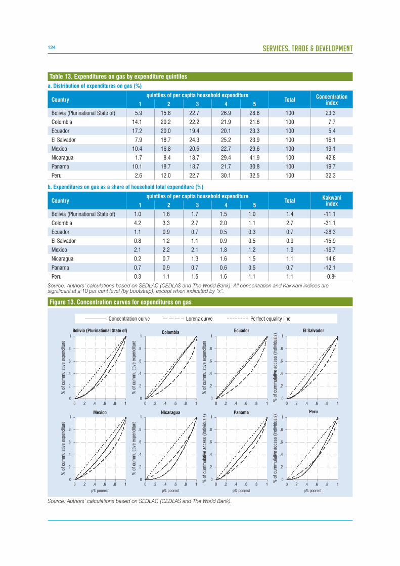
124 SERVICES, TRADE & DEVELOPMENT
a. Distribution of expenditures on gas (%)
Countryquintiles of per capita household expenditure
TotalConcentration
index1 2 3 4 5
Bolivia (Plurinational State of) 5.9 15.8 22.7 26.9 28.6 100 23.3
Colombia 14.1 20.2 22.2 21.9 21.6 100 7.7
Ecuador 17.2 20.0 19.4 20.1 23.3 100 5.4
El Salvador 7.9 18.7 24.3 25.2 23.9 100 16.1
Mexico 10.4 16.8 20.5 22.7 29.6 100 19.1
Nicaragua 1.7 8.4 18.7 29.4 41.9 100 42.8
Panama 10.1 18.7 18.7 21.7 30.8 100 19.7
Peru 2.6 12.0 22.7 30.1 32.5 100 32.3 b. Expenditures on gas as a share of household total expenditure (%)
Countryquintiles of per capita household expenditure
TotalKakwani
index1 2 3 4 5
Bolivia (Plurinational State of) 1.0 1.6 1.7 1.5 1.0 1.4 -11.1
Colombia 4.2 3.3 2.7 2.0 1.1 2.7 -31.1
Ecuador 1.1 0.9 0.7 0.5 0.3 0.7 -28.3
El Salvador 0.8 1.2 1.1 0.9 0.5 0.9 -15.9
Mexico 2.1 2.2 2.1 1.8 1.2 1.9 -16.7
Nicaragua 0.2 0.7 1.3 1.6 1.5 1.1 14.6
Panama 0.7 0.9 0.7 0.6 0.5 0.7 -12.1
Peru 0.3 1.1 1.5 1.6 1.1 1.1 -0.8x
Source: Authors’ calculations based on SEDLAC (CEDLAS and The World Bank). All concentration and Kakwani indices are significant at a 10 per cent level (by bootstrap), except when indicated by “x”.
Table 13. Expenditures on gas by expenditure quintiles
Figure 13. Concentration curves for expenditures on gas
0
.2
.4
.6
.8
1
% o
f cu
mm
ulat
ive
expe
nditu
re
0 .2 .4 .6 .8 1
Bolivia (Plurinational State of)
0
.2
.4
.6
.8
1
% o
f cu
mm
ulat
ive
expe
nditu
re
0 .2 .4 .6 .8 1
Colombia
0
.2
.4
.6
.8
1
% o
f cu
mm
ulat
ive
expe
nditu
re
0 .2 .4 .6 .8 1
Ecuador
0
.2
.4
.6
.8
1
% o
f cu
mm
ulat
ive
acce
ss (
indi
vidu
als)
0 .2 .4 .6 .8 1
El Salvador
0
.2
.4
.6
.8
1
% o
f cu
mm
ulat
ive
acce
ss (
indi
vidu
als)
0 .2 .4 .6 .8 1
Peru
0
.2
.4
.6
.8
1
% o
f cu
mm
ulat
ive
expe
nditu
re
0 .2 .4 .6 .8 1
p% poorest
Nicaragua
0
.2
.4
.6
.8
1
% o
f cu
mm
ulat
ive
expe
nditu
re
0 .2 .4 .6 .8 1
p% poorest
Mexico
0
.2
.4
.6
.8
1
% o
f cu
mm
ulat
ive
acce
ss (
indi
vidu
als)
0 .2 .4 .6 .8 1
p% poorest
Panama
Concentration curve Lorenz curve Perfect equality line
p% poorest
Source: Authors’ calculations based on SEDLAC (CEDLAS and The World Bank).
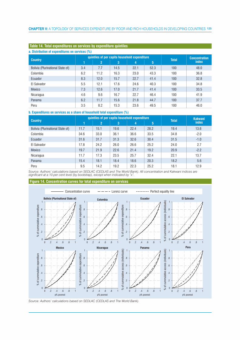
125CHAPTER V: A TOPOLOGY OF SERVICES EXPENDITURE BY POOR AND RICH HOUSEHOLDS IN DEVELOPING COUNTRIES
a. Distribution of expenditures on services (%)
Countryquintiles of per capita household expenditure
TotalConcentration
index1 2 3 4 5
Bolivia (Plurinational State of) 3.4 7.7 14.5 22.1 52.3 100 48.0
Colombia 6.2 11.2 16.3 23.0 43.3 100 36.8
Ecuador 8.3 12.0 15.7 22.7 41.4 100 32.8
El Salvador 5.5 12.1 17.6 24.6 40.3 100 34.8
Mexico 7.3 12.6 17.0 21.7 41.4 100 33.5
Nicaragua 4.6 9.6 16.7 22.7 46.4 100 41.9
Panama 6.2 11.7 15.6 21.8 44.7 100 37.7
Peru 3.5 8.2 15.3 23.6 49.5 100 46.0 b. Expenditures on services as a share of household total expenditure (%)
Countryquintiles of per capita household expenditure
TotalKakwani
index1 2 3 4 5
Bolivia (Plurinational State of) 11.7 15.1 19.6 22.4 28.2 19.4 13.6
Colombia 34.6 33.0 36.1 36.6 33.5 34.8 -2.0
Ecuador 31.6 31.7 31.3 32.6 30.4 31.5 -1.0
El Salvador 17.8 24.2 26.0 26.6 25.2 24.0 2.7
Mexico 19.7 21.9 22.6 21.4 19.2 20.9 -2.2
Nicaragua 11.7 17.3 23.5 25.7 32.4 22.1 13.7
Panama 15.4 18.1 18.4 18.6 20.3 18.2 5.6
Peru 9.5 14.2 19.2 22.3 25.2 18.1 12.9
Source: Authors’ calculations based on SEDLAC (CEDLAS and The World Bank). All concentration and Kakwani indices are significant at a 10 per cent level (by bootstrap), except when indicated by “x”.
Table 14. Total expenditures on services by expenditure quintiles
Figure 14. Concentration curves for total expenditure on services
0
.2
.4
.6
.8
1
% o
f cu
mm
ulat
ive
expe
nditu
re
0 .2 .4 .6 .8 1
Bolivia (Plurinational State of)
0
.2
.4
.6
.8
1
% o
f cu
mm
ulat
ive
expe
nditu
re
0 .2 .4 .6 .8 1
Colombia
0
.2
.4
.6
.8
1
% o
f cu
mm
ulat
ive
expe
nditu
re
0 .2 .4 .6 .8 1
Ecuador
0
.2
.4
.6
.8
1
% o
f cu
mm
ulat
ive
acce
ss (
indi
vidu
als)
0 .2 .4 .6 .8 1
El Salvador
0
.2
.4
.6
.8
1
% o
f cu
mm
ulat
ive
acce
ss (
indi
vidu
als)
0 .2 .4 .6 .8 1
Peru
0
.2
.4
.6
.8
1
% o
f cu
mm
ulat
ive
expe
nditu
re
0 .2 .4 .6 .8 1
p% poorest
Nicaragua
0
.2
.4
.6
.8
1
% o
f cu
mm
ulat
ive
expe
nditu
re
0 .2 .4 .6 .8 1
p% poorest
Mexico
0
.2
.4
.6
.8
1
% o
f cu
mm
ulat
ive
acce
ss (
indi
vidu
als)
0 .2 .4 .6 .8 1
p% poorest p% poorest
Panama
Concentration curve Lorenz curve Perfect equality line
Source: Authors’ calculations based on SEDLAC (CEDLAS and The World Bank).

126 SERVICES, TRADE & DEVELOPMENT
Bolivia (Plurinational
State of)+Colombia+ Ecuador Mexico Nicaragua Panama Peru
Log per capita household consumption
1.0163a
(0.1905)-1.1178a
(0.0784)1.0123."(0.1168)
0.9063a
(0.0766)1.0014a
(0.1111)0.8597."(0.1411)
0.8645a
(0.0586)
Household size-1.3010a
(0.2587)-2.1908a
(0.1468)-0.9605a
(0.1535)-0.5720a
(0.1142)-0.9687a
(0.1343)-0.6374a
(0.1819)-1.0916a
(0.0750)
Female head of household
1.8834a
(0.3454)1.1130a
(0.1464)3.0278a
(0.2352)1.9212a
(0.1474)1.2113a
(0.1904)2.0341a
(0.2388)1.3174a
(0.1060)
Married head of household
-1.2847a
(0.3459)-0.0802
(0.1507)1.2627a
(0.2283)1.0938a
(0.1534)0.2597
(0.1941)0.9516a
(0.2384)0.8498a
(0.1020)
Age of head of household
-0.0274a
(0.0079)-0.0410a
(0.0037)-0.0680a
(0.0048)-0.0689a
(0.0036)-0.0104b
(0.0042)-0.0574".(0.0059)
-0.0300a
(0.0023)
Education of head of household
0.2810a
(0.0276)0.3789a
(0.0132)0.2757a
(0.0171)0.2114a
(0.0122)0.2456a
(0.0165)0.2138a
(0.0224)0.2311a
(0.0083)
Rural household 1.5342a
(0.0629)1.3810a
j0.0337)1.6785a
(0.0390)1.4139a
(0.0286)0.6856a
(0.0260)1.1992a
(0.0404)0.8716a
(0.0166)
Log likelihood -11 223.0000 -59 636.0000 -28 856.0000 -47 002.0000 -17 880.0000 -15 454.0000 -51 836.0000
Sigma11.0115(0.1560)
13.9626(0.0895)
9.2570(0.0798)
12.3708(0.0920)
6.8375(0.0718)
10.1867(0.1240)
6.4797(0.0390)
Observations with share=0
1 351.0000 9 431.0000 3 390.0000 10 001.0000 1 959.0000 2 510.0000 5 874.0000
Observations with share>0
2 722.0000 13 400.0000 7 326.0000 10 525.0000 4 925.0000 3 745.0000 14 699.0000
Source: Authors’ estimates based on SEDLAC (CEDLAS and The World Bank).
Note: Dependent variable is service share on household total consumption. In “+” service as a share of household total expenditure. Standard errors in parentheses: “a” p<0.01, ”b” p<0.05, “c” p<0.1.
Table 15. Marginal effects on education shares: Tobit estimates
Bolivia (Plurinational
State of)+Colombia+ Ecuador Mexico Nicaragua Panama Peru
Log per capita household consumption
1.5065a
(0.1343)0.8628a
(0.0990)-0.1448
(0,2425)1.0462a
(0.0483)3.4428a
(0.2623)0.0130
(0.3557)1.4865a
(0.0563)
Household size0.0221
(0.1785)-3.4009a
(0.2006)0.6473b
(0.3228)0.4197a
(0.0721)1.7461a
(0.3180)0.2963
(0.4631)-0.5098a
(0.0717)
Female head of household
0.1112(0.2387)
0.0448(0.1802)
2.4767a
(0.4692)0.5458a
(0.0906)0.3271
(0.4420)3.6984a
(0.5933)0.4707a
(0.0985)
Married head of household
0.5163b
(0.2377)0.8955a
(0.1850)2.8342a
(0.4532)0.8433a
(0.0933)0.2611
(0.4479)3.6174a
(0.5891)0.8941a
(0.0944)
Age of head of household
0.0236a
(0.0053)0.1315a
(0.0045)0.0664a
(0.0095)0.0065a
(0.0021)0.0662a
(0.0096)0.0837a
(0.0142)0.0177a
(0.0022)
Education of head of household
-0.0466b
(0.0191)0.4467a
(0.0165)0.1007a
(0.0363)-0.0442a
(0:0078)-0.1449a
(0.0395)0.1275b
(0.0572)0.0002
(0.0080)
Rural household0.1905a
(0.0420)0.2354a
(0.0428)-0.1773b
(0.0794)0.2226a
(0.0175)0.5318a
(0.0600)0.2770a
(0.1001)0.3060a
(0.0154)
Log likelihood -9 887.0000 -65 246.0000 -44 529.0000 -51 918.0000 -25 252.0000 -21 420.0000 -53 347.0000
Sigma10.4247(0.1560)
17.1750(0.1070)
21.5147(0.1550)
7.4239(0.0465)
18.2480(0.1750)
31.6252(0.3570)
6.5181.0000(0.0390)
Observations with share=0
1 711.0000 8 723.0000 971.0000 6 760.0000 1 265.0000 2 138.0000 5 615.0000
Observations with share>0
2 362.0000 14 108.0000 9 745.0000 13 766.0000 5 619.0000 4 117.0000 14 958.0000
Source: Authors’ estimates based on SEDLAC (CEDLAS and The World Bank).
Note: Dependent variable is service share on household total consumption. In “+” service as a share of household total expenditure. Standard errors in parentheses: “a” p<0.01, ”b” p<0.05, “c” p<0.1.
Table 16. Marginal effects on health shares: Tobit estimates
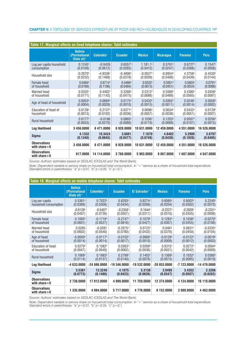
127CHAPTER V: A TOPOLOGY OF SERVICES EXPENDITURE BY POOR AND RICH HOUSEHOLDS IN DEVELOPING COUNTRIES
Bolivia (Plurinational
State of)+Colombia+ Ecuador Mexico Nicaragua Panama Peru
Log per capita household consumption
0.1245a
(0.0109)-0.0426
(0.0612)0.6557a
(0.0265)1.181.1a
(0.0412)0.5761a
(0.0247)0.6727a
(0.0368)0.1547a
(0.0056)
Household size-0.2670a
(0.0232)-4.9338a
(0.1488)-0.4806a
(0.0378)-0.9527a
(0.0509)-0.8954a
(0.0406)4.3756a
(0.0439)-0.4520a
(0.0144)
Female head of household
0.0484a
(0.0169)0.8714a
(0.1106)0.4466a
(0.0484)0.9332a
(0.0673)0.5951a
(0.0451)0.5603a
(0.0554)0.0791a
(0.0088)
Married head of household
0.0325c
(0.0171)0.4402a
(0.1142)0.3266a
(0.0475)0.5312a
(0.0686)0.5560a
(0.0466)0.4380a
(0.0565)0.0456a
(0.0087)
Age of head of household0.0053a
(0.0004)0.0694a
(0.0028)0.0175a
(0.0010)0.0432a
(0.0015)0.0362a
(0.0011)0.0246a
(0.0014)0.0056a
(0.0002)
Education of head of household
0.0128a
(0.0013)0.2137a
(0.0102)0.0371a
(0.0036)0.0696a
(0.0057)0.0634a
(0.0038)0.0432a
(0.0051)0.0129a
(0.0007)
Rural household 0.0177a
(0.0033)-0.0196
(0.0270)0.0865a
(0.0086)0.1036a
(0.0119)0.1203a
(0.0089)0.0567a
(0.0107)0.0256a
(0.0015)
Log likelihood 3 456.0000 8 471.0000 6 928.0000 10 631.0000 12 459.0000 4 551.0000 16 526.0000
Sigma4.1332
(0.1340)10.3424(0.0645)
3.6881(0.0477)
7.1670(0.0749)
4.8402(0.0430)
5.2900(0.1020)
3.8797(0.0495)
Observations with share=0
3 456.0000 8 471.0000 6 928.0000 10 631.0000 12 459.0000 4 551.0000 16 526.0000
Observations with share>0
617.0000 14 114.0000 3 788.0000 5 903.0000 8 067.0000 1 687.0000 4 047.0000
Source: Authors’ estimates based on SEDLAC (CEDLAS and The World Bank).
Note: Dependent variable is service share on household total consumption. In “+” service as a share of household total expenditure. Standard errors in parentheses: “a” p<0.01, ”b” p<0.05, “c” p<0.1.
Table 17. Marginal effects on fixed telephone shares: Tobit estimates
Bolivia (Plurinational
State of)+Colombia+ Ecuador El Salvador+ Mexico Panama Peru
Log per capita household consumption
0.5361a
(0.0368)0.7022a
(0.0308)0.8293a
(0.0434)0,8274a
(0.0266)0.6085a
(0.0204)0.6002a
(0.0302)0.2240a
(0.0070)
Household size-0.6128a
(0.0497)-0.5407a
(0.0736)-0.2358a
(0.0567)0.1644a
(0.0317)-0.2227a
(0.0310)-0.2828a
(0.0355)-0.2331a
(0.0098)
Female head of household
0.1005a
(0.0601)-0.1710a
(0.0527)-0.2747a
(0.0816)0.1079b
(0.0427)0.1283a
(0.0367)0.1036b
(0.0455)-0.0270b
(0.0108)
Married head of household
0.0265(0.0602)
-0.0261(0.0540)
-0.2075a
(0.0780)0.0723a
(0.0432)0.0461
(0.0376)0.0831a
(0.0450)-0.0335a
(0.0104)
Age of head of household
-0.0050a
(0.0014)-0.0117a
(0.0014)-0.0152a
(0.0017)-0.0060a
(0.0010)-0.0129a
(0.0009)-0.0122a
(0.0012)-0.0019a
(0.0003)
Education of head of household
0.0270a
(0.0047)0.1082a
(0.0049)0.0363a
(0.0062)0.0269a
(0.0036)0.0315a
(0.0031)0.0272a
(0.0042)0.0094a
(0.0009)
Rural household0.1068a
(0.0114)0.1883a
(0.0137)0.2789a
(0.0140)0.1402a
(0.0076)0.1369a
(0.0074)0.1032a
(0.0085)0.0360a
(0.0019)
Log likelihood -4 633.0000 -24 886.0000 -19 346.0000 -19 532.0000 -28 853.0000 -7 123.0000 -14 479.0000
Sigma3.5361
(0.0773)13.3240(0.1480)
4.1075(0.0423)
5.3138(0.0626)
3.9495(0.0347)
3.4352(0.0587)
2.3266(0.0282)
Observations with share=0
2 738.0000 17 812.0000 4 999.0000 11 759.0000 12 374.0000 4 124.0000 16 110.0000
Observations with share>0
1 335.0000 4 994.0000 5 717.0000 4 776.0000 8 152.0000 2 089.0000 4 463.0000
Source: Authors’ estimates based on SEDLAC (CEDLAS and The World Bank).
Note: Dependent variable is service share on household total consumption. In “+” service as a share of household total expenditure. Standard errors in parentheses: “a” p<0.01, ”b” p<0.05, “c” p<0.1.
Table 18. Marginal effects on mobile telephone shares: Tobit estimates
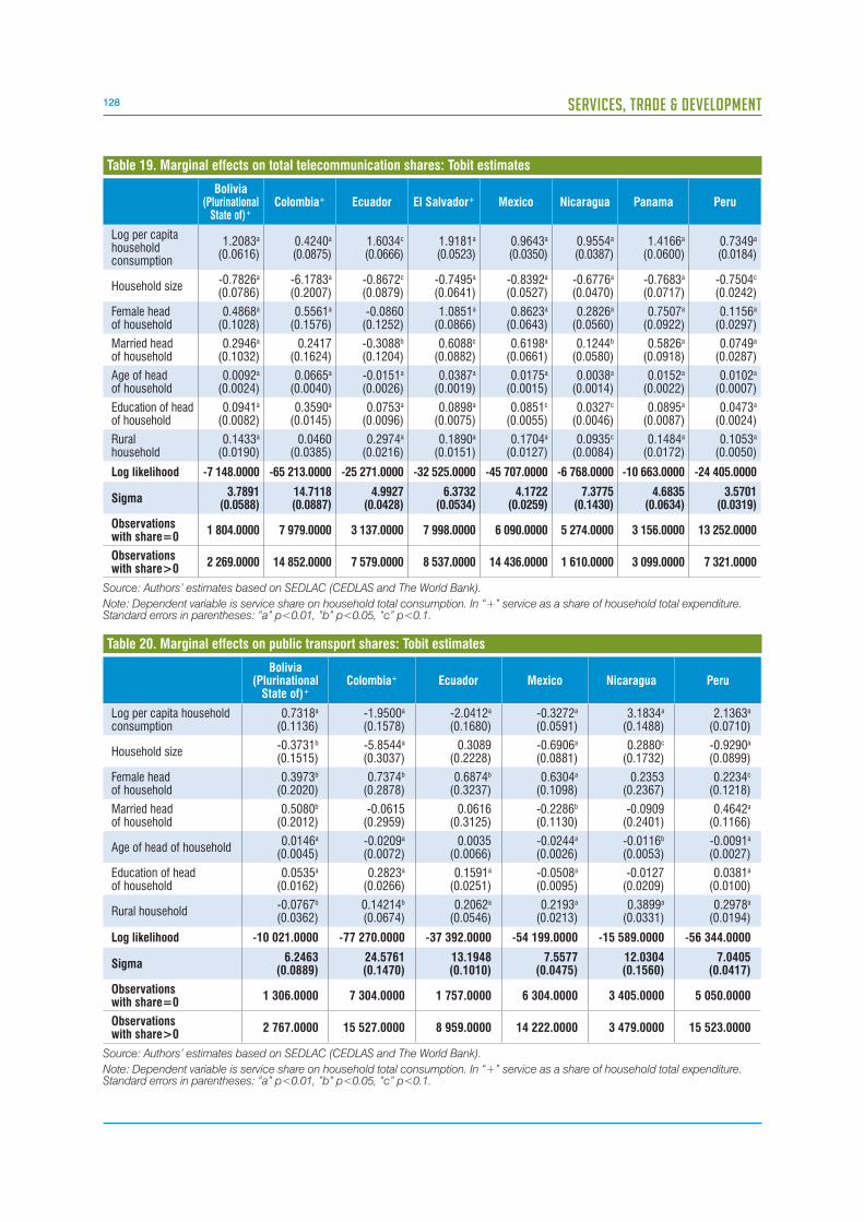
128 SERVICES, TRADE & DEVELOPMENT
Bolivia (Plurinational
State of)+Colombia+ Ecuador El Salvador+ Mexico Nicaragua Panama Peru
Log per capita household consumption
1.2083a
(0.0616)0.4240a
(0.0875)1.6034c
(0.0666)1.9181a
(0.0523)0.9643a
(0.0350)0.9554a
(0.0387)1.4166a
(0.0600)0.7349a
(0.0184)
Household size-0.7826a
(0.0786)-6.1783a
(0.2007)-0.8672c
(0.0879)-0.7495a
(0.0641)-0.8392a
(0.0527)-0.6776a
(0.0470)-0.7683a
(0.0717)-0.7504c
(0.0242)
Female head of household
0.4868a
(0.1028)0.5561a
(0.1576)-0.0860
(0.1252)1.0851a
(0.0866)0.8623a
(0.0643)0.2826a
(0.0560)0.7507a
(0.0922)0.1156a
(0.0297)
Married head of household
0.2946a
(0.1032)0.2417
(0.1624)-0.3088b
(0.1204)0.6088c
(0.0882)0.6198a
(0.0661)0.1244b
(0.0580)0.5826a
(0.0918)0.0749a
(0.0287)
Age of head of household
0.0092a
(0.0024)0.0665a
(0.0040)-0.0151a
(0.0026)0.0387a
(0.0019)0.0175a
(0.0015)0.0038a
(0.0014)0.0152a
(0.0022)0.0102a
(0.0007)
Education of head of household
0.0941a
(0.0082)0.3590a
(0.0145)0.0753a
(0.0096)0.0898a
(0.0075)0.0851c
(0.0055)0.0327c
(0.0046)0.0895a
(0.0087)0.0473a
(0.0024)
Rural household
0.1433a
(0.0190)0.0460
(0.0385)0.2974a
(0.0216)0.1890a
(0.0151)0.1704a
(0.0127)0.0935c
(0.0084)0.1484a
(0.0172)0.1053a
(0.0050)
Log likelihood -7 148.0000 -65 213.0000 -25 271.0000 -32 525.0000 -45 707.0000 -6 768.0000 -10 663.0000 -24 405.0000
Sigma3.7891
(0.0588)14.7118(0.0887)
4.9927(0.0428)
6.3732(0.0534)
4.1722(0.0259)
7.3775(0.1430)
4.6835(0.0634)
3.5701(0.0319)
Observations with share=0
1 804.0000 7 979.0000 3 137.0000 7 998.0000 6 090.0000 5 274.0000 3 156.0000 13 252.0000
Observations with share>0
2 269.0000 14 852.0000 7 579.0000 8 537.0000 14 436.0000 1 610.0000 3 099.0000 7 321.0000
Source: Authors’ estimates based on SEDLAC (CEDLAS and The World Bank).
Note: Dependent variable is service share on household total consumption. In “+” service as a share of household total expenditure. Standard errors in parentheses: “a” p<0.01, ”b” p<0.05, “c” p<0.1.
Table 19. Marginal effects on total telecommunication shares: Tobit estimates
Bolivia (Plurinational
State of)+Colombia+ Ecuador Mexico Nicaragua Peru
Log per capita household consumption
0.7318a
(0.1136)-1.9500a
(0.1578)-2.0412a
(0.1680)-0.3272a
(0.0591)3.1834a
(0.1488)2.1363a
(0.0710)
Household size-0.3731b
(0.1515)-5.8544a
(0.3037)0.3089
(0.2228)-0.6906a
(0.0881)0.2880c
(0.1732)-0.9290a
(0.0899)
Female head of household
0.3973b
(0.2020)0.7374b
(0.2878)0.6874b
(0.3237)0.6304a
(0.1098)0.2353
(0.2367)0.2234c
(0.1218)
Married head of household
0.5080b
(0.2012)-0.0615
(0.2959)0.0616
(0.3125)-0.2286b
(0.1130)-0.0909
(0.2401)0.4642a
(0.1166)
Age of head of household0.0146a
(0.0045)-0.0209a
(0.0072)0.0035
(0.0066)-0.0244a
(0.0026)-0.0116b
(0.0053)-0.0091a
(0.0027)
Education of head of household
0.0535a
(0.0162)0.2823a
(0.0266)0.1591a
(0.0251)-0.0508a
(0.0095)-0.0127
(0.0209)0.0381a
(0.0100)
Rural household-0.0767b
(0.0362)0.14214b
(0.0674)0.2062a
(0.0546)0.2193a
(0.0213)0.3899a
(0.0331)0.2978a
(0.0194)
Log likelihood -10 021.0000 -77 270.0000 -37 392.0000 -54 199.0000 -15 589.0000 -56 344.0000
Sigma6.2463
(0.0889)24.5761(0.1470)
13.1948(0.1010)
7.5577(0.0475)
12.0304(0.1560)
7.0405(0.0417)
Observations with share=0
1 306.0000 7 304.0000 1 757.0000 6 304.0000 3 405.0000 5 050.0000
Observations with share>0
2 767.0000 15 527.0000 8 959.0000 14 222.0000 3 479.0000 15 523.0000
Source: Authors’ estimates based on SEDLAC (CEDLAS and The World Bank).
Note: Dependent variable is service share on household total consumption. In “+” service as a share of household total expenditure. Standard errors in parentheses: “a” p<0.01, ”b” p<0.05, “c” p<0.1.
Table 20. Marginal effects on public transport shares: Tobit estimates

129CHAPTER V: A TOPOLOGY OF SERVICES EXPENDITURE BY POOR AND RICH HOUSEHOLDS IN DEVELOPING COUNTRIES
Bolivia (Plurinational
State of)+Colombia+ Ecuador El Salvador+ Mexico Nicaragua Panama Peru
Log per capita household consumption
-0.1718a
(0.0332)-0.7147a
(0.0400)0.0569b
(0.0255)-0.7248a
(0.0295)-0.0746a
(0.0136)-0.0560b
(0.0250)-0.0282
(0.0242)-0.0416a
(0.0126)
Household size-1.1500a
(0.0457)-2.4873a
(0.0780)-0.6722a
(0.0347)-1.1452a
(0.0393)-0.4706a
(0.0210)-1.1295a
(0.0317)4.4258a
(0.0314)-1.0529a
(0.0173)
Female head of household
0.0947(0.0591)
0.1806b
(0.0736)0.2056a
(0.0490)0.2032a
(0.0528)0.0714a
(0.0253)0.1650a
(0.0411)0.1254a
(0.0398)0.0874a
(0.0216)
Married head of household
-0.0543(0.0589)
-0.0387(0.0756)
0.2397a
(0.0475)0.0703
(0.0538)0.0838a
(0.0261)0.0778c
(0.0421)0.0197
(0.0391)0.0221
(0.0209)
Age of head of household
0.0059a
(0.0013)0.0401a
(0.0018)0.0091a
(0.0010)0.0206a
(0.0012)0.0032a
(0.0006)0.0116a
(0.0009)0.0093a
(0.0010)0.0057a
(0.0005)
Education of head of household
0.0172a
(0.0048)0.0900a
(0.0068)0.0030
(0.0038)0.0607a
(0.0047)0.0038c
(0.0022)0.0273a
(0.0037)0.0107a
(0.0039)0.0062a
(0.0018)
Rural household-0.0678a
(0.0107)-0.1458a
(0.0173)-0.0014
(0.0084)-0.2331a
(0.0091)-0.0168a
(0.0050)-0.0392a
(0.0060)4.0413a
(0.0069)-0.0277a
(0.0035)
Log likelihood -6 711.0000 -55 828.0000 -17 691.0000 -36 141.0000 -30 824.0000 -8 973.0000 -9 032.0000 -26 697.0000
Sigma1.7656
(0.0236)5.9149
(0.0335)2.3686
(0.0226)3.0762
(0.0197)2.2776
(0.0165)2.0000
(0.0263)1.4393
(0.0162)1.5883
(0.0111)
Observations with share=0
1 080.0000 4 952.0000 4 311.0000 3 480.0000 9 546.0000 3 484.0000 1 508.0000 8 882.0000
Observations with share>0
2 993.0000 16 368.0000 6 398.0000 13 054.0000 10 980.0000 3 393.0000 4 355.0000 11 691.0000
Source: Authors’ estimates based on SEDLAC (CEDLAS and The World Bank).
Note: Dependent variable is service share on household total consumption. In “+” service as a share of household total expenditure. Standard errors in parentheses: “a” p<0.01, ”b” p<0.05, “c” p<0.1.
Table 21. Marginal effects on water shares: Tobit estimates
Bolivia (Plurinational
State of)+Colombia+ Ecuador El Salvador+ Mexico Nicaragua Panama Peru
Log per capita household consumption
-0.0664(0.0744)
-1.3953a
(0.0651)0.0061
(0.0487)-0.3549a
(0.0514)-0.1971a
(0.0328)0.5447a
(0.0449)0.6542a
(0.0577)-0.0415b
(0.0192)
Household size-2.3082a
(0.1018)-1.7830a
(0.1237)-0.2364a
(0.0652)-1.4889a
(0.0680)-0.5535a
(0.0498)-1.6430a
(0.0549)-0.9962a
(0.0726)-1.4176a
(0.0253)
Female head of household
0.3880a
(0.1327)0.1805
(0.1197)0.6245a
(0.0942)1.0179a
(0.0918)0.0905
(0.0615)0.3871a
(0.0728)0.8622a
(0.0929)0.2384a
(0.0336)
Married head of household
0.0952(0.1323)
0.0729(0.1230)
0.7132a
(0.0912)0.8725a
(0.0936)0.2030a
(0.0632)0.2267a
(0.0745)0.8217a
(0.0919)0.1820a
(0.0323)
Age of head of household
0.0221a
(0.0030)0.0687a
(0.0030)0.0277a
(0.0019)0.0416a
(0.0020)0.0194a
(0.0015)0.0187a
(0.0017)0.0226a
(0.0023)0.0168a
(0.0008)
Education of head of household
0.0597a
(0.0107)0.1462a
(0.0110)0.0381a
(0.0073)0.0497a
(0.0081)0.0295a
(0.0053)0.0539a
(0.0065)0.0570a
(0.0090)0.0547a
(0.0028)
Rural household
-0.0923a
(0.0239)-0.2209a
(0.0280)-0.0427a
(0.0160)-0.3209a
(0.0158)-0.0086
(0.0120)-0.0030
(0.0105)0.0058
(0.0166)-0.0327a
(0.0054)
Log likelihood -8 739.0000 -73 783.0000 -23 842.0000 -44 693.0000 -44 211.0000 -11 403.0000 -12 981.0000 -33 476.0000
Sigma3.7399
(0.0519)9.6287
(0.0499)3.6843
(0.0314)4.8306
(0.0295)4.5205
(0.0300)3.3176
(0.0407)3.3444
(0.0369)1.9865
(0.0127)
Observations with share=0
1 189.0000 3 456.0000 2 919.0000 2 346.0000 7 426.0000 3 141.0000 1 678.0000 6 854.0000
Observations with share>0
2 884.0000 19 273.0000 7 797.0000 14 187.0000 13 100.0000 3 740.0000 4 484.0000 13 719.0000
Source: Authors’ estimates based on SEDLAC (CEDLAS and The World Bank).
Note: Dependent variable is service share on household total consumption. In “+” service as a share of household total expenditure. Standard errors in parentheses: “a” p<0.01, ”b” p<0.05, “c” p<0.1.
Table 22. Marginal effects on electricity shares: Tobit estimates
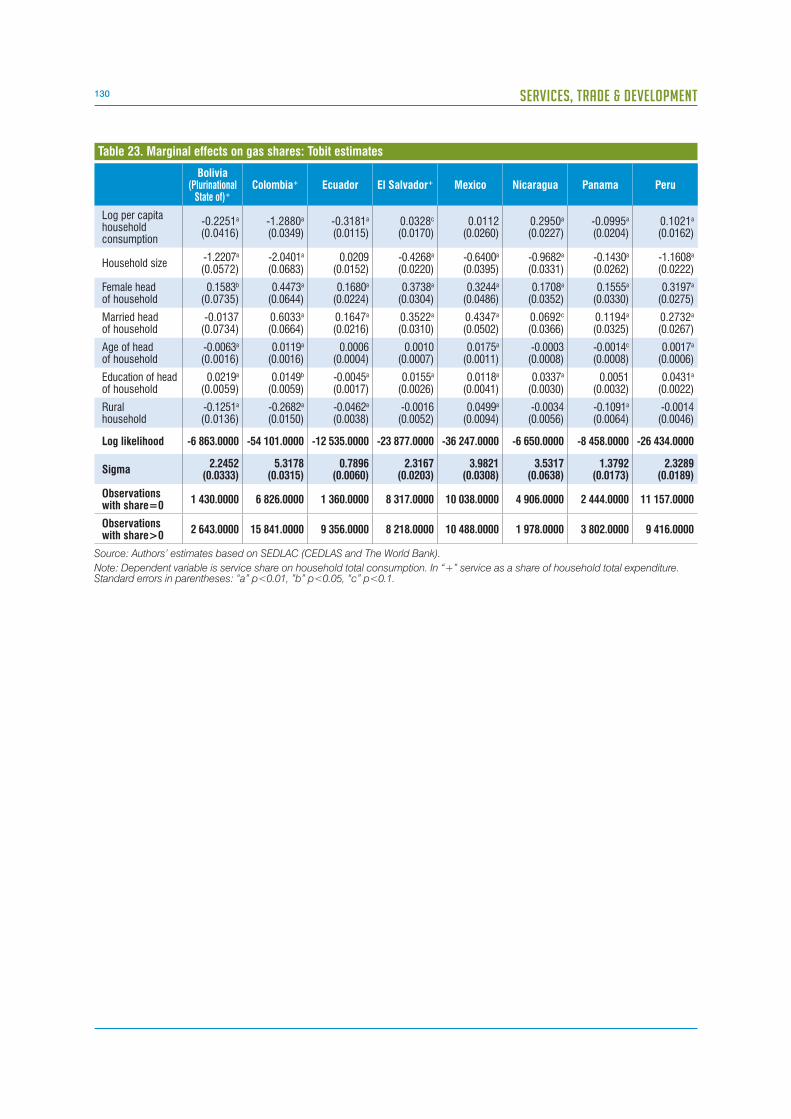
130 SERVICES, TRADE & DEVELOPMENT
Bolivia (Plurinational
State of)+Colombia+ Ecuador El Salvador+ Mexico Nicaragua Panama Peru
Log per capita household consumption
-0.2251a
(0.0416)-1.2880a
(0.0349)-0.3181a
(0.0115)0.0328c
(0.0170)0.0112
(0.0260)0.2950a
(0.0227)-0.0995a
(0.0204)0.1021a
(0.0162)
Household size-1.2207a
(0.0572)-2.0401a
(0.0683)0.0209
(0.0152)-0.4268a
(0.0220)-0.6400a
(0.0395)-0.9682a
(0.0331)-0.1430a
(0.0262)-1.1608a
(0.0222)
Female head of household
0.1583b
(0.0735)0.4473a
(0.0644)0.1680a
(0.0224)0.3738a
(0.0304)0.3244a
(0.0486)0.1708a
(0.0352)0.1555a
(0.0330)0.3197a
(0.0275)
Married head of household
-0.0137(0.0734)
0.6033a
(0.0664)0.1647a
(0.0216)0.3522a
(0.0310)0.4347a
(0.0502)0.0692c
(0.0366)0.1194a
(0.0325)0.2732a
(0.0267)
Age of head of household
-0.0063a
(0.0016)0.0119a
(0.0016)0.0006
(0.0004)0.0010
(0.0007)0.0175a
(0.0011)-0.0003
(0.0008)-0.0014c
(0.0008)0.0017a
(0.0006)
Education of head of household
0.0219a
(0.0059)0.0149b
(0.0059)-0.0045a
(0.0017)0.0155a
(0.0026)0.0118a
(0.0041)0.0337a
(0.0030)0.0051
(0.0032)0.0431a
(0.0022)
Rural household
-0.1251a
(0.0136)-0.2682a
(0.0150)-0.0462a
(0.0038)-0.0016
(0.0052)0.0499a
(0.0094)-0.0034
(0.0056)-0.1091a
(0.0064)-0.0014
(0.0046)
Log likelihood -6 863.0000 -54 101.0000 -12 535.0000 -23 877.0000 -36 247.0000 -6 650.0000 -8 458.0000 -26 434.0000
Sigma2.2452
(0.0333)5.3178
(0.0315)0.7896
(0.0060)2.3167
(0.0203)3.9821
(0.0308)3.5317
(0.0638)1.3792
(0.0173)2.3289
(0.0189)
Observations with share=0
1 430.0000 6 826.0000 1 360.0000 8 317.0000 10 038.0000 4 906.0000 2 444.0000 11 157.0000
Observations with share>0
2 643.0000 15 841.0000 9 356.0000 8 218.0000 10 488.0000 1 978.0000 3 802.0000 9 416.0000
Source: Authors’ estimates based on SEDLAC (CEDLAS and The World Bank).
Note: Dependent variable is service share on household total consumption. In “+” service as a share of household total expenditure. Standard errors in parentheses: “a” p<0.01, ”b” p<0.05, “c” p<0.1.
Table 23. Marginal effects on gas shares: Tobit estimates
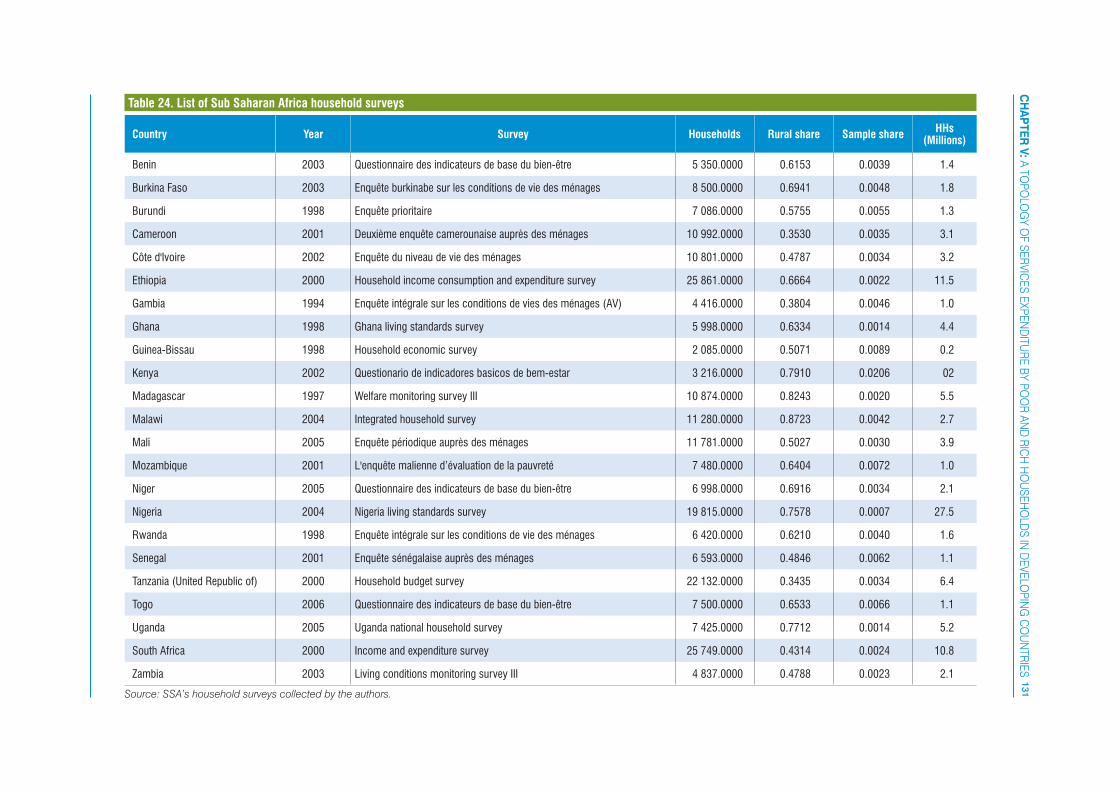
131
CH
AP
TE
R V
: A TO
PO
LOG
Y OF
SE
RV
ICE
S E
XP
EN
DITU
RE
BY P
OO
R A
ND
RIC
H H
OU
SE
HO
LDS
IN D
EV
ELO
PIN
G C
OU
NTR
IES
Country Year Survey Households Rural share Sample shareHHs
(Millions)
Benin 2003 Questionnaire des indicateurs de base du bien-être 5 350.0000 0.6153 0.0039 1.4
Burkina Faso 2003 Enquête burkinabe sur les conditions de vie des ménages 8 500.0000 0.6941 0.0048 1.8
Burundi 1998 Enquête prioritaire 7 086.0000 0.5755 0.0055 1.3
Cameroon 2001 Deuxième enquête camerounaise auprès des ménages 10 992.0000 0.3530 0.0035 3.1
Côte d'Ivoire 2002 Enquête du niveau de vie des ménages 10 801.0000 0.4787 0.0034 3.2
Ethiopia 2000 Household income consumption and expenditure survey 25 861.0000 0.6664 0.0022 11.5
Gambia 1994 Enquête intégrale sur les conditions de vies des ménages (AV) 4 416.0000 0.3804 0.0046 1.0
Ghana 1998 Ghana living standards survey 5 998.0000 0.6334 0.0014 4.4
Guinea-Bissau 1998 Household economic survey 2 085.0000 0.5071 0.0089 0.2
Kenya 2002 Questionario de indicadores basicos de bem-estar 3 216.0000 0.7910 0.0206 02
Madagascar 1997 Welfare monitoring survey III 10 874.0000 0.8243 0.0020 5.5
Malawi 2004 Integrated household survey 11 280.0000 0.8723 0.0042 2.7
Mali 2005 Enquête périodique auprès des ménages 11 781.0000 0.5027 0.0030 3.9
Mozambique 2001 L'enquête malienne d’évaluation de la pauvreté 7 480.0000 0.6404 0.0072 1.0
Niger 2005 Questionnaire des indicateurs de base du bien-être 6 998.0000 0.6916 0.0034 2.1
Nigeria 2004 Nigeria living standards survey 19 815.0000 0.7578 0.0007 27.5
Rwanda 1998 Enquête intégrale sur les conditions de vie des ménages 6 420.0000 0.6210 0.0040 1.6
Senegal 2001 Enquête sénégalaise auprès des ménages 6 593.0000 0.4846 0.0062 1.1
Tanzania (United Republic of) 2000 Household budget survey 22 132.0000 0.3435 0.0034 6.4
Togo 2006 Questionnaire des indicateurs de base du bien-être 7 500.0000 0.6533 0.0066 1.1
Uganda 2005 Uganda national household survey 7 425.0000 0.7712 0.0014 5.2
South Africa 2000 Income and expenditure survey 25 749.0000 0.4314 0.0024 10.8
Zambia 2003 Living conditions monitoring survey III 4 837.0000 0.4788 0.0023 2.1
Source: SSA’s household surveys collected by the authors.
Table 24. List of Sub Saharan Africa household surveys
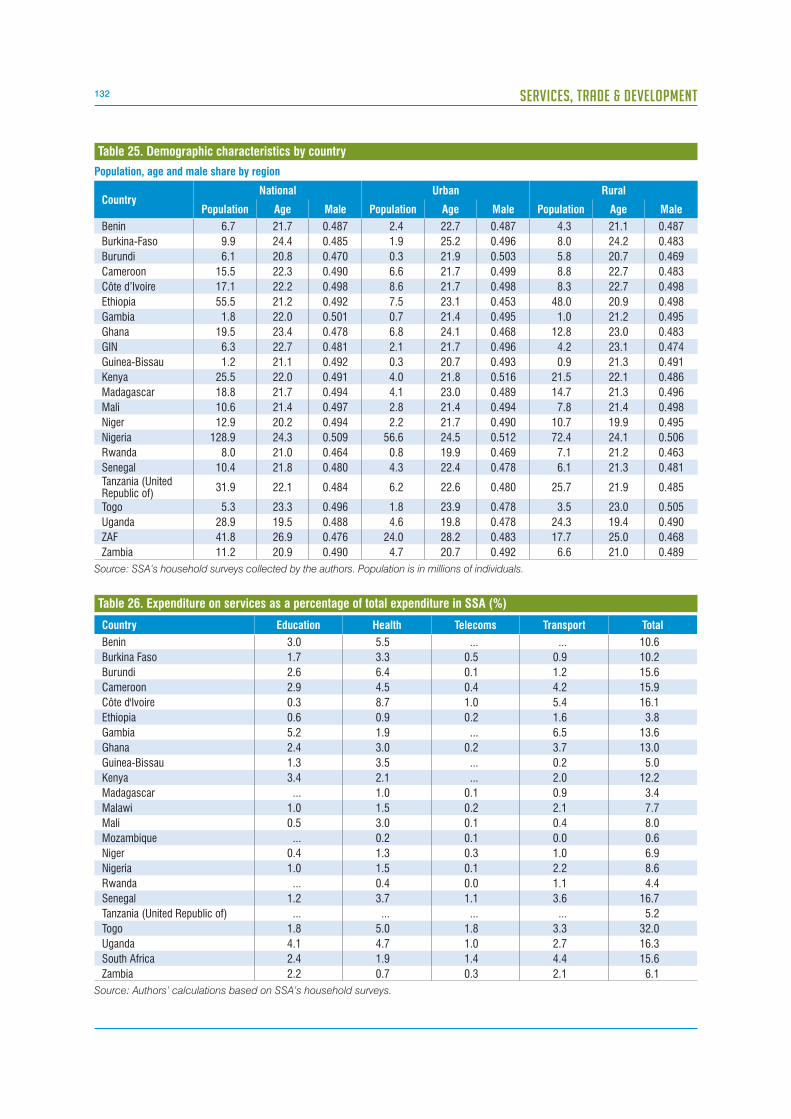
132 SERVICES, TRADE & DEVELOPMENT
Population, age and male share by region
CountryNational Urban Rural
Population Age Male Population Age Male Population Age Male
Benin 6.7 21.7 0.487 2.4 22.7 0.487 4.3 21.1 0.487
Burkina-Faso 9.9 24.4 0.485 1.9 25.2 0.496 8.0 24.2 0.483
Burundi 6.1 20.8 0.470 0.3 21.9 0.503 5.8 20.7 0.469
Cameroon 15.5 22.3 0.490 6.6 21.7 0.499 8.8 22.7 0.483
Côte d’Ivoire 17.1 22.2 0.498 8.6 21.7 0.498 8.3 22.7 0.498
Ethiopia 55.5 21.2 0.492 7.5 23.1 0.453 48.0 20.9 0.498
Gambia 1.8 22.0 0.501 0.7 21.4 0.495 1.0 21.2 0.495
Ghana 19.5 23.4 0.478 6.8 24.1 0.468 12.8 23.0 0.483
GIN 6.3 22.7 0.481 2.1 21.7 0.496 4.2 23.1 0.474
Guinea-Bissau 1.2 21.1 0.492 0.3 20.7 0.493 0.9 21.3 0.491
Kenya 25.5 22.0 0.491 4.0 21.8 0.516 21.5 22.1 0.486
Madagascar 18.8 21.7 0.494 4.1 23.0 0.489 14.7 21.3 0.496
Mali 10.6 21.4 0.497 2.8 21.4 0.494 7.8 21.4 0.498
Niger 12.9 20.2 0.494 2.2 21.7 0.490 10.7 19.9 0.495
Nigeria 128.9 24.3 0.509 56.6 24.5 0.512 72.4 24.1 0.506
Rwanda 8.0 21.0 0.464 0.8 19.9 0.469 7.1 21.2 0.463
Senegal 10.4 21.8 0.480 4.3 22.4 0.478 6.1 21.3 0.481Tanzania (United Republic of)
31.9 22.1 0.484 6.2 22.6 0.480 25.7 21.9 0.485
Togo 5.3 23.3 0.496 1.8 23.9 0.478 3.5 23.0 0.505
Uganda 28.9 19.5 0.488 4.6 19.8 0.478 24.3 19.4 0.490
ZAF 41.8 26.9 0.476 24.0 28.2 0.483 17.7 25.0 0.468
Zambia 11.2 20.9 0.490 4.7 20.7 0.492 6.6 21.0 0.489
Source: SSA’s household surveys collected by the authors. Population is in millions of individuals.
Table 25. Demographic characteristics by country
Country Education Health Telecoms Transport Total
Benin 3.0 5.5 ... ... 10.6
Burkina Faso 1.7 3.3 0.5 0.9 10.2
Burundi 2.6 6.4 0.1 1.2 15.6
Cameroon 2.9 4.5 0.4 4.2 15.9
Côte d'Ivoire 0.3 8.7 1.0 5.4 16.1
Ethiopia 0.6 0.9 0.2 1.6 3.8
Gambia 5.2 1.9 ... 6.5 13.6
Ghana 2.4 3.0 0.2 3.7 13.0
Guinea-Bissau 1.3 3.5 ... 0.2 5.0
Kenya 3.4 2.1 ... 2.0 12.2
Madagascar ... 1.0 0.1 0.9 3.4
Malawi 1.0 1.5 0.2 2.1 7.7
Mali 0.5 3.0 0.1 0.4 8.0
Mozambique ... 0.2 0.1 0.0 0.6
Niger 0.4 1.3 0.3 1.0 6.9
Nigeria 1.0 1.5 0.1 2.2 8.6
Rwanda ... 0.4 0.0 1.1 4.4
Senegal 1.2 3.7 1.1 3.6 16.7
Tanzania (United Republic of) ... ... ... ... 5.2
Togo 1.8 5.0 1.8 3.3 32.0
Uganda 4.1 4.7 1.0 2.7 16.3
South Africa 2.4 1.9 1.4 4.4 15.6
Zambia 2.2 0.7 0.3 2.1 6.1
Source: Authors’ calculations based on SSA’s household surveys.
Table 26. Expenditure on services as a percentage of total expenditure in SSA (%)

133CHAPTER V: A TOPOLOGY OF SERVICES EXPENDITURE BY POOR AND RICH HOUSEHOLDS IN DEVELOPING COUNTRIES
Figure 15. Expenditures on each service as a percentage of total expenditures on services
Education Health Telecommunication Transport
0 10 20 30 40 50 60 70 80 90 100
Burundi
Benin
Burkina Faso
Côte d’Ivoire
Cameroon
Ethiopia
Ghana
Gambia
Guinea-Bissau
Kenya
Madagascar
Mali
Mozambique
Malawi
Niger
Nigeria
Rwanda
Senegal
Togo
Uganda
South Africa
Zambia
Percentage
Source: Authors’ calculations based on Asia’s household surveys

134 SERVICES, TRADE & DEVELOPMENT
Countryquintiles of per capita total expenditure (%) Kakwani
indexq1 q2 q3 q4 q5
Benin 4.3 5.3 5.5 6.2 6.2 -4.5x
Burkina-Faso 0.9 2.3 3.3 4.2 5.9 4.9x
Burundi 12.5 7.1 5.4 3.5 3.2 -48.3
Cameroon 4.2 4.5 4.7 4.8 4.4 -4.9x
Côte d'Ivoire 7.1 8.0 8.9 9.2 10.6 7.6x
Ethiopia 0.5 0.7 1.0 1.2 1.1 23.2
Gambia 3.2 2.0 1.4 1.4 1.6 -9.9x
Ghana 2.2 2.8 3.2 3.3 3.6 -17.1
Guinea-Bissau 2.9 3.5 3.8 3.6 3.9 0.4x
Kenya 1.4 1.7 2.1 2.2 3.3 9.4x
Madagascar 0.6 0.8 1.1 1.3 1.4 ...
Malawi 1.5 1.6 1.6 1.5 1.4 10.0
Mali 1.3 2.6 2.9 3.4 4.9 12.4x
Mozambique 0.2 0.1 0.2 0.1 0.3 ...
Niger 0.8 0.9 1.0 1.4 2.5 21.6
Nigeria 0.6 1.2 1.5 1.8 2.2 19.7
Rwanda 0.3 0.3 0.4 0.5 0.4 ...
Senegal 3.9 3.8 3.7 3.5 3.7 15.8Tanzania (United Republic of)
... ... ... ... ... ...
Togo 2.5 3.9 7.7 5.5 5.5 -10.9x
Uganda 4.5 4.9 5.5 5.5 2.9 -43.1x
South Africa 0.9 1.0 1.2 2.1 4.1 -1.0x
Zambia 0.3 0.6 0.7 0.9 1.0 11.7x
Table 27. Share of education on total expenditure by total expenditure quintiles
Countryquintiles of per capita total expenditure (%) Kakwani
indexq1 q2 q3 q4 q5
Benin 2.6 2.6 3.2 3.3 3.3 -3.6x
Burkina-Faso 0.8 1.1 1.6 2.1 2.8 8.1x
Burundi 4.1 2.9 2.1 1.5 2.1 -48.6
Cameroon 2.2 3.0 3.2 3.1 2.7 -0.2x
Côte d'Ivoire 0.3 0.3 0.4 0.4 0.4 7.3x
Ethiopia 0.2 0.3 0.6 0.9 1.2 1.3x
Gambia 8.5 4.7 4.0 4.9 4.1 -1.9x
Ghana 1.6 2.9 2.8 2.8 1.6 -2.2x
Guinea-Bissau 0.9 1.0 1.2 1.6 1.7 -3.7x
Kenya 2.6 3.3 3.5 3.9 3.9 11.6x
Madagascar ... ... ... ... ... 0.1x
Malawi 0.8 0.9 0.8 0.9 1.6 -17.8
Mali 0.3 0.4 0.4 0.5 0.8 15.7x
Mozambique ... ... ... ... ... 20.0x
Niger 0.1 0.1 0.3 0.5 0.9 6.5x
Nigeria 0.1 0.4 0.7 1.4 2.3 3.7x
Rwanda ... ... ... ... ... ...
Senegal 0.9 0.7 0.9 1.1 2.2 1.2x
Tanzania (United Republic of)
... ... ... ... ... ...
Togo 1.8 1.3 1.9 2.0 2.2 -24.3x
Uganda 2.6 3.4 3.8 5.5 5.0 -62.0x
South Africa 2.7 1.9 1.9 2.6 2.8 11.4
Zambia 0.7 1.5 2.1 2.5 4.3 2.9x
Note: All Kakwani and concentration indices are statistically different from zero unless it is indicated with an “x” next to the coefficient.
Table 28. Share of health on total expenditure by total expenditure quintiles

135CHAPTER V: A TOPOLOGY OF SERVICES EXPENDITURE BY POOR AND RICH HOUSEHOLDS IN DEVELOPING COUNTRIES
Countryquintiles of per capita total expenditure (%) Kakwani
indexq1 q2 q3 q4 q5
Benin ... ... ... ... ... ...
Burkina-Faso 0.0 0.0 0.1 0.4 1.9 29.1
Burundi 0.0 0.0 0.0 0.0 0.6 -43.2
Cameroon 0.0 0.1 0.2 0.5 1.0 28.1
Côte d'Ivoire 0.3 0.6 0.9 1.1 1.9 19.4
Ethiopia 0.0 0.0 0.1 0.3 0.7 58.5
Gambia ... ... ... ... ... ...
Ghana 0.0 0.0 0.1 0.2 0.6 26.4
Guinea-Bissau ... ... ... ... ... ...
Kenya ... ... ... ... ... ...
Madagascar 0.0 0.0 0.0 0.0 0.4 47.2
Malawi 0.0 0.0 0.0 0.1 1.0 42.0
Mali 0.0 0.0 0.1 0.1 0.5 39.9x
Mozambique 0.0 0.0 0.0 0.1 0.4 40.2
Niger 0.0 0.0 0.1 0.3 1.1 41.6
Nigeria 0.0 0.0 0.0 0.1 0.3 35.1
Rwanda 0.0 0.0 0.0 0.0 0.1 30.4x
Senegal 0.2 0.4 0.7 1.3 2.7 31.6Tanzania (United Republic of)
... ... ... ... ... ...
Togo 1.1 1.6 1.6 2.2 2.8 44.7x
Uganda 0.2 0.5 1.0 1.6 1.8 -33.9x
South Africa 0.7 1.1 1.4 1.7 2.0 4.3x
Zambia 0.0 0.0 0.0 0.1 1.2 36.0x
Table 29. Share of telecommunications on total expenditure by total expenditure quintiles
Countryquintiles of per capita total expenditure (%) Kakwani
indexq1 q2 q3 q4 q5
Benin ... ... ... ... ... 0.0
Burkina-Faso 0.1 0.4 0.8 1.2 2.1 16.2
Burundi 0.7 0.6 0.8 1.0 2.8 -34.3
Cameroon 2.9 3.8 4.5 4.8 5.1 5.5
Côte d'Ivoire 3.2 4.2 5.1 6.3 8.0 9.5
Ethiopia 0.2 0.7 1.4 2.1 3.3 34.9
Gambia 7.6 4.7 5.2 5.6 9.4 15.0
Ghana 2.3 3.0 3.8 4.2 5.1 4.9x
Guinea-Bissau 0.1 0.2 0.2 0.2 0.4 26.5x
Kenya 0.8 1.4 1.9 2.3 3.6 13.1
Madagascar 0.1 0.2 0.4 0.8 3.1 34.7
Malawi 0.4 0.8 1.6 2.7 4.9 19.5
Mali 0.1 0.2 0.3 0.4 0.9 28.9x
Mozambique 0.0 0.0 0.0 0.0 0.1 43.9x
Niger 0.3 0.5 0.6 1.2 2.2 16.3
Nigeria 0.6 1.4 1.9 2.7 4.4 11.9
Rwanda 0.1 0.3 0.7 1.6 2.6 20.4x
Senegal 2.4 2.6 3.0 3.6 6.4 21.2Tanzania (United Republic of)
... ... ... ... ... ...
Togo 1.8 1.3 3.9 3.7 5.6 85.6x
Uganda 1.3 2.3 2.9 3.5 3.6 -41.1x
South Africa 3.1 3.8 4.8 5.4 4.8 -0.8x
Zambia 0.4 0.9 1.4 2.2 5.6 24.8x
Note: All Kakwani and concentration indices are statistically different from zero unless it is indicated with an “x” next to the coefficient.
Table 30. Share of transport on total expenditure by total expenditure quintiles
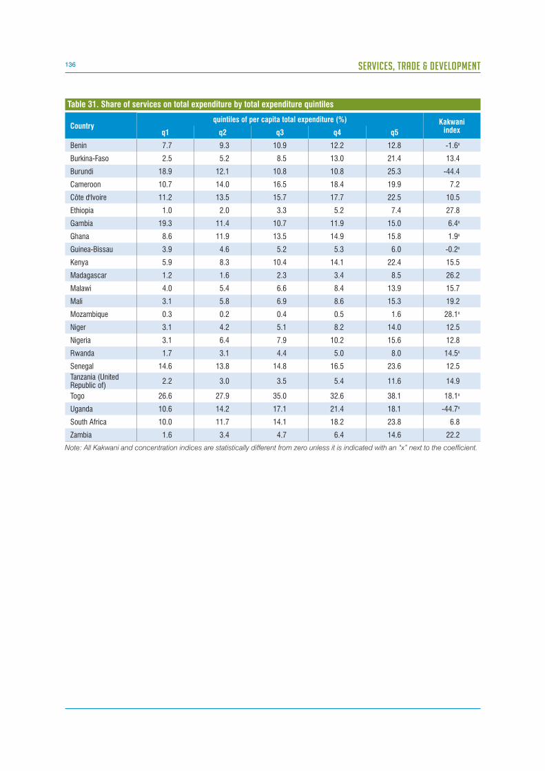
136 SERVICES, TRADE & DEVELOPMENT
Countryquintiles of per capita total expenditure (%) Kakwani
indexq1 q2 q3 q4 q5
Benin 7.7 9.3 10.9 12.2 12.8 -1.6x
Burkina-Faso 2.5 5.2 8.5 13.0 21.4 13.4
Burundi 18.9 12.1 10.8 10.8 25.3 -44.4
Cameroon 10.7 14.0 16.5 18.4 19.9 7.2
Côte d'Ivoire 11.2 13.5 15.7 17.7 22.5 10.5
Ethiopia 1.0 2.0 3.3 5.2 7.4 27.8
Gambia 19.3 11.4 10.7 11.9 15.0 6.4x
Ghana 8.6 11.9 13.5 14.9 15.8 1.9x
Guinea-Bissau 3.9 4.6 5.2 5.3 6.0 -0.2x
Kenya 5.9 8.3 10.4 14.1 22.4 15.5
Madagascar 1.2 1.6 2.3 3.4 8.5 26.2
Malawi 4.0 5.4 6.6 8.4 13.9 15.7
Mali 3.1 5.8 6.9 8.6 15.3 19.2
Mozambique 0.3 0.2 0.4 0.5 1.6 28.1x
Niger 3.1 4.2 5.1 8.2 14.0 12.5
Nigeria 3.1 6.4 7.9 10.2 15.6 12.8
Rwanda 1.7 3.1 4.4 5.0 8.0 14.5x
Senegal 14.6 13.8 14.8 16.5 23.6 12.5
Tanzania (United Republic of)
2.2 3.0 3.5 5.4 11.6 14.9
Togo 26.6 27.9 35.0 32.6 38.1 18.1x
Uganda 10.6 14.2 17.1 21.4 18.1 -44.7x
South Africa 10.0 11.7 14.1 18.2 23.8 6.8
Zambia 1.6 3.4 4.7 6.4 14.6 22.2
Note: All Kakwani and concentration indices are statistically different from zero unless it is indicated with an “x” next to the coefficient.
Table 31. Share of services on total expenditure by total expenditure quintiles

137CHAPTER V: A TOPOLOGY OF SERVICES EXPENDITURE BY POOR AND RICH HOUSEHOLDS IN DEVELOPING COUNTRIES
CountryRural
householdAge of head of household
Female head of household
Married head of household
Education of head of household
Log of per capita
expenditure
Household size
Benin -0.021a
(0.003)0.001a
(0.000)0.042a
(0.004)0.009b
(0.004)0.007a
(0.000)-0.011a
(0.002)0.012a
(0.001)
Burkina Faso
-0.046a
(0.002)0.000a
(0.000)-0.027a
(0.004)0.006b
(0.003)0.004a
(0.000)-0.005a
(0.001)0.005a
(0.000)
Burundi 0.136a
(0.015)0.001a
(0.000)-0.052a
(0.008)0.005
(0.008)0.005a
(0.001)0.001
(0.002)0.026a
(0.001)
Cameroon-0.007a
(0.001)0.001a
(0.000)-0.019a
(0.002)-0.002
(0.002)0.005a
(0.000)-0.008a
(0.001)0.005a
(0.000)
Côte d'Ivoire0.037a
(0.009)0.003a(0.000)
0.019(0.017)
0.012(0.013)
0.003a
(0.001)0.019a
(0.005)0.011a
(0.001)
Ethiopia-0.006a
(0.001)0.000a
(0.000)-0.006a(0.001)
0.000(0.001)
0.001a
(0.000)0.003a
(0.000)0.003a
(0.000)
Gambia-0.011
(0.021)0.002a
(0.001)-0.059a
(0.022)-0.022
(0.025)0.007a
(0.002)-0.001
(0.010)0.009a
(0.002)
Ghana-0.030a
(0.003)0.000
(0.000)-0.033a(0.003)
0.018a
(0.003)...
0.008a
(0.002)0.013a
(0.001)
Guinea-Bissau-0.025a
(0.002)0.000a
(0.000)-0.012a
(0.003)-0.008a
(0.002)0.002a
(0.000)0.000
(0.001)0.002a
(0.000)
Kenya-0.004
(0.003)0.001a
(0.000)-0.038a
(0.003)0.027a(0.003)
0.004a
(0.000)0.020a
(0.002)0.016a
(0.000)
Madagascar ... ... ... ... ... ... ...
Malawi-0.006a
(0.001)0.000a
(0.000)-0.013a
(0.002)-0.007a
(0.002)0.002a
(0.000)0.004a
(0.001)0.009a
(0.000)
Mali-0.022a
(0.002)0.000
(0.000)0.000
(0.004)... ...
0.008a
(0.001)0.001a
(0.000)
Mozambique ... ... ... ... ... ... ...
Niger-0.019a
(0.004)0.000a
(0.000)-0.019b
(0.009)0.000
(0.007)0.002a
(0.000)0.000
(0.001)0.006a
(0.001)
Nigeria-0.176a
(0.008)0.002a
(0.000)-0.082a
(0.012)0.027a
(0.011)0.004a
(0.001)0.154a
(0.006)0.023a
(0.001)
Rwanda ... ... ... ... ... ... ...
Senegal-0.005a
(0.001)0.000a
(0.000)-0.008a
(0.001)0.005a
(0.001)0.002a
(0.000)-0.001b
(0.001)0.001a
(0.000)
Tanzania (United Republic of)
... ... ... ... ... ... ...
Togo0.000
(0.007)0.000
(0.000)0.004
(0.008)-0.003
(0.008)0.000
(0.001)0.006b
(0.003)0.001
(0.002)
Uganda-0.050a
(0.003)0.001a
(0.000)-0.045a
(0.004)0.005
(0.004)0.006a
(0.000)-0.005a
(0.001)0.014a
(0.000)
South Africa-0.003b
(0.001)0.000a
(0.000)-0.020a
(0.001)0.004a
(0.001)0.002a
(0.000)0.004a
(0.001)0.011a
(0.000)
Zambia -0.015a
(0.002)0.001a
(0.000)-0.020a
(0.003)0.001
(0.003)0.004a
(0.000)0.011a
(0.001)0.009a
(0.000)
Source: Authors’ own estimates based on national household surveys.
Note: Dependent variable is the service share on total household expenditure. Standard errors are in squared brackets and a stands for significance “a” the 1 per cent level and “b” for statistical significance at the 5 per cent level.
Table 32. Marginal effects on education expenditure shares: Tobit estimates
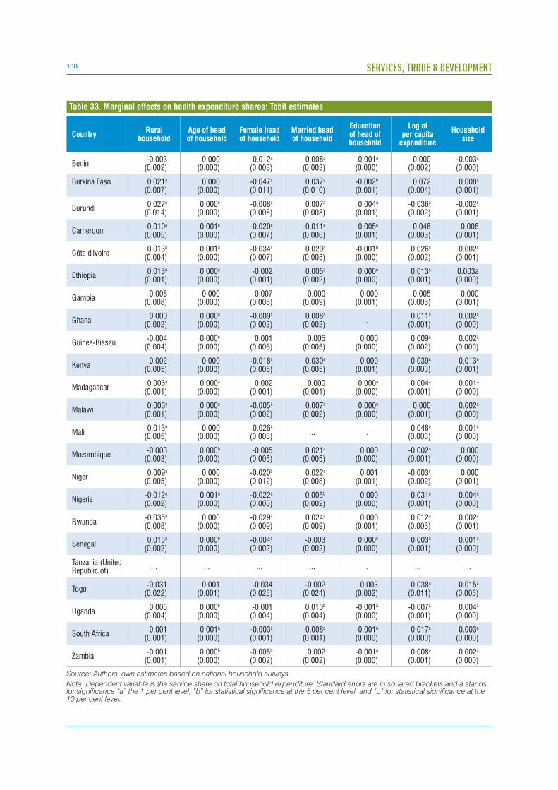
138 SERVICES, TRADE & DEVELOPMENT
CountryRural
householdAge of head of household
Female head of household
Married head of household
Education of head of household
Log of per capita
expenditure
Household size
Benin -0.003
(0.002)0.000
(0.000)0.012a
(0.003)0.008a
(0.003)0.001a
(0.000)0.000
(0.002)-0.003a
(0.000)
Burkina Faso
0.021a
(0.007)0.000
(0.000)-0.047a
(0.011)0.037a
(0.010)-0.002b
(0.001)0.072
(0.004)0.008a
(0.001)
Burundi 0.027c
(0.014)0.000c
(0.000)-0.008a
(0.008)0.007a
(0.008)0.004a
(0.001)-0.036a
(0.002)-0.002c
(0.001)
Cameroon-0.010a
(0.005)0.001a
(0.000)-0.020a
(0.007)-0.011a
(0.006)0.005a
(0.001)0.048
(0.003)0.006
(0.001)
Côte d'Ivoire0.013a
(0.004)0.001a
(0.000)-0.034a
(0.007)0.020a
(0.005)-0.001b
(0.000)0.026a
(0.002)0.002a
(0.001)
Ethiopia0.013a
(0.001)0.000a
(0.000)-0.002
(0.001)0.005a
(0.002)0.000c
(0.000)0.013a
(0.001)0.003a(0.000)
Gambia0.008
(0.008)0.000
(0.000)-0.007
(0.008)0.000
(0.009)0.000
(0.001)-0.005
(0.003)0.000
(0.001)
Ghana0.000
(0.002)0.000a
(0.000)-0.009a
(0.002)0.008a
(0.002)...
0.011a
(0.001)0.002a
(0.000)
Guinea-Bissau-0.004
(0.004)0.000c
(0.000)0.001
(0.006)0.005
(0.005)0.000
(0.000)0.009a
(0.002)0.002a
(0.000)
Kenya0.002
(0.005)0.000
(0.000)-0.018a
(0.005)0.030a
(0.005)0.000
(0.001)0.039a
(0.003)0.013a
(0.001)
Madagascar0.006a
(0.001)0.000a
(0.000)0.002
(0.001)0.000
(0.001)0.000a
(0.000)0.004a
(0.001)0.001a
(0.000)
Malawi0.006a
(0.001)0.000a
(0.000)-0.005a
(0.002)0.007a
(0.002)0.000a
(0.000)0.000
(0.001)0.002a
(0.000)
Mali0.013a
(0.005)0.000
(0.000)0.026a
(0.008)... ...
0.048a
(0.003)0.001a
(0.000)
Mozambique-0.003
(0.003)0.000b
(0.000)-0.005
(0.005)0.021a
(0.005)0.000
(0.000)-0.002a
(0.001)0.000
(0.000)
Niger0.009a
(0.005)0.000
(0.000)-0.020b
(0.012)0.022a
(0.008)0.001
(0.001)-0.003c
(0.002)0.000
(0.001)
Nigeria-0.012a
(0.002)0.001a
(0.000)-0.022a
(0.003)0.005b
(0.002)0.000
(0.000)0.031a
(0.001)0.004a
(0.000)
Rwanda-0.035a
(0.008)0.000
(0.000)-0.029a
(0.009)0.024a
(0.009)0.000
(0.001)0.012a
(0.003)0.002a
(0.001)
Senegal0.015a
(0.002)0.000b
(0.000)-0.004c
(0.002)-0.003
(0.002)0.000c
(0.000)0.003a
(0.001)0.001a
(0.000)
Tanzania (United Republic of)
... ... ... ... ... ... ...
Togo-0.031
(0.022)0.001
(0.001)-0.034
(0.025)-0.002
(0.024)0.003
(0.002)0.038a
(0.011)0.015a
(0.005)
Uganda0.005
(0.004)0.000b
(0.000)-0.001
(0.004)0.010b
(0.004)-0.001a
(0.000)-0.007a
(0.001)0.004a
(0.000)
South Africa0.001
(0.001)0.001a
(0.000)-0.003a
(0.001)0.008a
(0.001)0.001a
(0.000)0.017a
(0.000)0.003a
(0.000)
Zambia-0.001
(0.001)0.000b
(0.000)-0.005b
(0.002)0.002
(0.002)-0.001a
(0.000)0.008a
(0.001)0.002a
(0.000)
Source: Authors’ own estimates based on national household surveys.
Note: Dependent variable is the service share on total household expenditure. Standard errors are in squared brackets and a stands for significance “a” the 1 per cent level, “b” for statistical significance at the 5 per cent level, and “c” for statistical significance at the 10 per cent level.
Table 33. Marginal effects on health expenditure shares: Tobit estimates
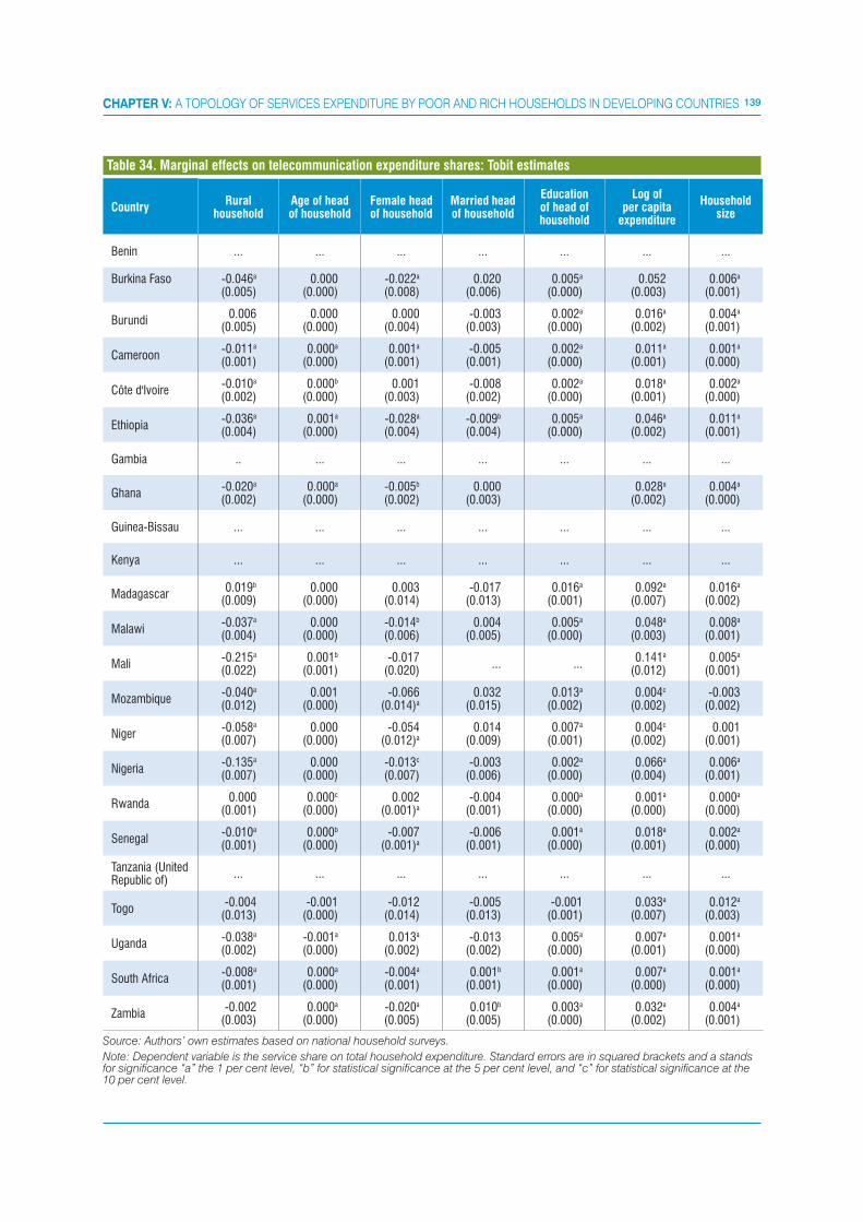
139CHAPTER V: A TOPOLOGY OF SERVICES EXPENDITURE BY POOR AND RICH HOUSEHOLDS IN DEVELOPING COUNTRIES
CountryRural
householdAge of head of household
Female head of household
Married head of household
Education of head of household
Log of per capita
expenditure
Household size
Benin ... ... ... ... ... ... ...
Burkina Faso
-0.046a
(0.005)0.000
(0.000)-0.022a
(0.008)0.020
(0.006)0.005a
(0.000)0.052
(0.003)0.006a
(0.001)
Burundi 0.006
(0.005)0.000
(0.000)0.000
(0.004)-0.003
(0.003)0.002a
(0.000)0.016a
(0.002)0.004a
(0.001)
Cameroon-0.011a
(0.001)0.000a
(0.000)0.001a
(0.001)-0.005
(0.001)0.002a
(0.000)0.011a
(0.001)0.001a
(0.000)
Côte d'Ivoire-0.010a
(0.002)0.000b
(0.000)0.001
(0.003)-0.008
(0.002)0.002a
(0.000)0.018a
(0.001)0.002a
(0.000)
Ethiopia-0.036a
(0.004)0.001a
(0.000)-0.028a
(0.004)-0.009b
(0.004)0.005a
(0.000)0.046a
(0.002)0.011a
(0.001)
Gambia .. ... ... ... ... ... ...
Ghana-0.020a
(0.002)0.000a
(0.000)-0.005b
(0.002)0.000
(0.003)0.028a
(0.002)0.004a
(0.000)
Guinea-Bissau ... ... ... ... ... ... ...
Kenya ... ... ... ... ... ... ...
Madagascar0.019b
(0.009)0.000
(0.000)0.003
(0.014)-0.017
(0.013)0.016a
(0.001)0.092a
(0.007)0.016a
(0.002)
Malawi-0.037a
(0.004)0.000
(0.000)-0.014b
(0.006)0.004
(0.005)0.005a
(0.000)0.048a
(0.003)0.008a
(0.001)
Mali-0.215a
(0.022)0.001b
(0.001)-0.017
(0.020)... ...
0.141a
(0.012)0.005a
(0.001)
Mozambique-0.040a
(0.012)0.001
(0.000)-0.066
(0.014)a0.032
(0.015)0.013a
(0.002)0.004c
(0.002)-0.003
(0.002)
Niger-0.058a
(0.007)0.000
(0.000)-0.054
(0.012)a0.014
(0.009)0.007a
(0.001)0.004c
(0.002)0.001
(0.001)
Nigeria-0.135a
(0.007)0.000
(0.000)-0.013c
(0.007)-0.003
(0.006)0.002a
(0.000)0.066a
(0.004)0.006a
(0.001)
Rwanda0.000
(0.001)0.000c
(0.000)0.002
(0.001)a-0.004
(0.001)0.000a
(0.000)0.001a
(0.000)0.000a
(0.000)
Senegal-0.010a
(0.001)0.000b
(0.000)-0.007
(0.001)a-0.006
(0.001)0.001a
(0.000)0.018a
(0.001)0.002a
(0.000)
Tanzania (United Republic of)
... ... ... ... ... ... ...
Togo-0.004
(0.013)-0.001
(0.000)-0.012
(0.014)-0.005
(0.013)-0.001
(0.001)0.033a
(0.007)0.012a
(0.003)
Uganda-0.038a
(0.002)-0.001a
(0.000)0.013a
(0.002)-0.013
(0.002)0.005a
(0.000)0.007a
(0.001)0.001a
(0.000)
South Africa-0.008a
(0.001)0.000a
(0.000)-0.004a
(0.001)0.001b
(0.001)0.001a
(0.000)0.007a
(0.000)0.001a
(0.000)
Zambia -0.002
(0.003)0.000a
(0.000)-0.020a
(0.005)0.010b
(0.005)0.003a
(0.000)0.032a
(0.002)0.004a
(0.001)
Source: Authors’ own estimates based on national household surveys.
Note: Dependent variable is the service share on total household expenditure. Standard errors are in squared brackets and a stands for significance “a” the 1 per cent level, “b” for statistical significance at the 5 per cent level, and “c” for statistical significance at the 10 per cent level.
Table 34. Marginal effects on telecommunication expenditure shares: Tobit estimates

140 SERVICES, TRADE & DEVELOPMENT
CountryRural
householdAge of head of household
Female head of household
Married head of household
Education of head of household
Log of per capita
expenditure
Household size
Benin ... ... ... ... ... ... ...
Burkina Faso
0.064a
(0.009)-0.001b
(0.000)-0.024a
(0.014)0.023a
(0.012)0.003a
(0.001)0.088a
(0.005)0.010a
(0.001)
Burundi 0.038a
-(0.008)0.000b
(0.000)-0.024a
(0.006)0.008
(0.006)0.002b
(0.001)0.021a
(0.002)0.004
(0.209)
Cameroon-0.010a
(0.005)0.001c
(0.000)-0.020a
(0.007)-0.011a
(0.006)0.005a
(0.001)0.048
(0.003)0.006c
(0.001)
Côte d'Ivoire-0.015a
(0.004)0.000
(0.000)0.005
(0.005)-0.022a
(0.004)0.004a
(0.000)0.019a
(0.002)0.003a
(0.001)
Ethiopia-0.019a
(0.001)0.000
(0.000)0.000
(0.001)0.002
(0.002)0.002a
(0.000)0.022a
(0.001)0.003a
(0.000)
Gambia0.017
(0.017)0.000
(0.001)0.015
(0.018)0.017
(0.020)0.002
(0.002)0.039a
(0.009)0.004a
(0.001)
Ghana-0.010a
(0.002)0.000a
(0.000)-0.001
(0.002)0.001
(0.002)...
0.016a
(0.001)0.002a
(0.000)
Guinea-Bissau-0.009a
(0.003)0.000
(0.000)0.003
(0.004)-0.004
(0.003)0.000c
(0.000)0.012a
(0.002)0.001a
(0.000)
Kenya-0.021a
(0.003)0.000a
(0.000)0.004
(0.003)0.001
(0.003)0.002a
(0.000)0.034a
(0.002)0.005a
(0.000)
Madagascar0.097a
(0.006)0.000
(0.000)-0.018c
(0.011)0.037a
(0.010)0.013a
(0.001)0.101a
(0.005)0.008a
(0.001)
Malawi-0.018a
(0.006)-0.001a
(0.000)0.009
(0.008)0.019a
(0.007)0.001b
(0.001)0.094a
(0.003)0.018a
(0.001)
Mali-0.411a
(0.136)0.007
(0.005)0.020
(0.202)... ...
-0.418a
(0.088)-0.024a
(0.008)
Mozambique0.235
(0.145)0.000
(0.005)-0.235
(0.165)0.020
(0.161)0.016
(0.017)0.024
(0.022)-0.025
(0.024)
Niger-0.004
(0.004)0.000
(0.000)-0.018c
(0.010)-0.022a
(0.006)0.004a
(0.000)0.000
(0.002)-0.001
(0.001)
Nigeria-0.056a
(0.002)0.000a
(0.000)-0.004
(0.003)-0.008a
(0.003)0.001a
(0.000)0.052a
(0.001)0.002a
(0.000)
Rwanda-0.104a
(0.008)0.000
(0.000)0.003
(0.008)-0.014
(0.009)0.003a
(0.001)0.027a
(0.003)0.007a
(0.001)
Senegal0.011a
(0.002)0.000
(0.000)0.006a
(0.002)-0.007a
(0.002)0.001a
(0.000)0.022a
(0.001)0.001a
(0.000)
Tanzania (United Republic of)
... ... ... ... ... ... ...
Togo-0.004
(0.031)0.002c
(0.001)-0.019
(0.032)0.026
(0.032)0.001
(0.003)0.065a
(0.015)0.010
(0.007)
Uganda-0.022a
(0.003)0.000a
(0.000)0.014a
(0.003)-0.014a
(0.003)0.004a
(0.000)0.006a
(0.001)0.001a
(0.000)
South Africa-0.010a
(0.001)0.000c
(0.000)0.005a
(0.001)0.001
(0.001)0.001a
(0.000)0.000
(0.000)0.001a
(0.000)
Zambia 0.005
(0.004)0.000a
(0.000)0.007
(0.007)0.002
(0.006)0.000
(0.001)0.055a
(0.003)0.007a
(0.001)
Source: Authors’ own estimates based on national household surveys.
Note: Dependent variable is the service share on total household expenditure. Standard errors are in squared brackets and a stands for significance “a” the 1 per cent level, “b” for statistical significance at the 5 per cent level, and “c” for statistical significance at the 10 per cent level.
Table 35. Marginal effects on transport expenditure shares: Tobit estimates
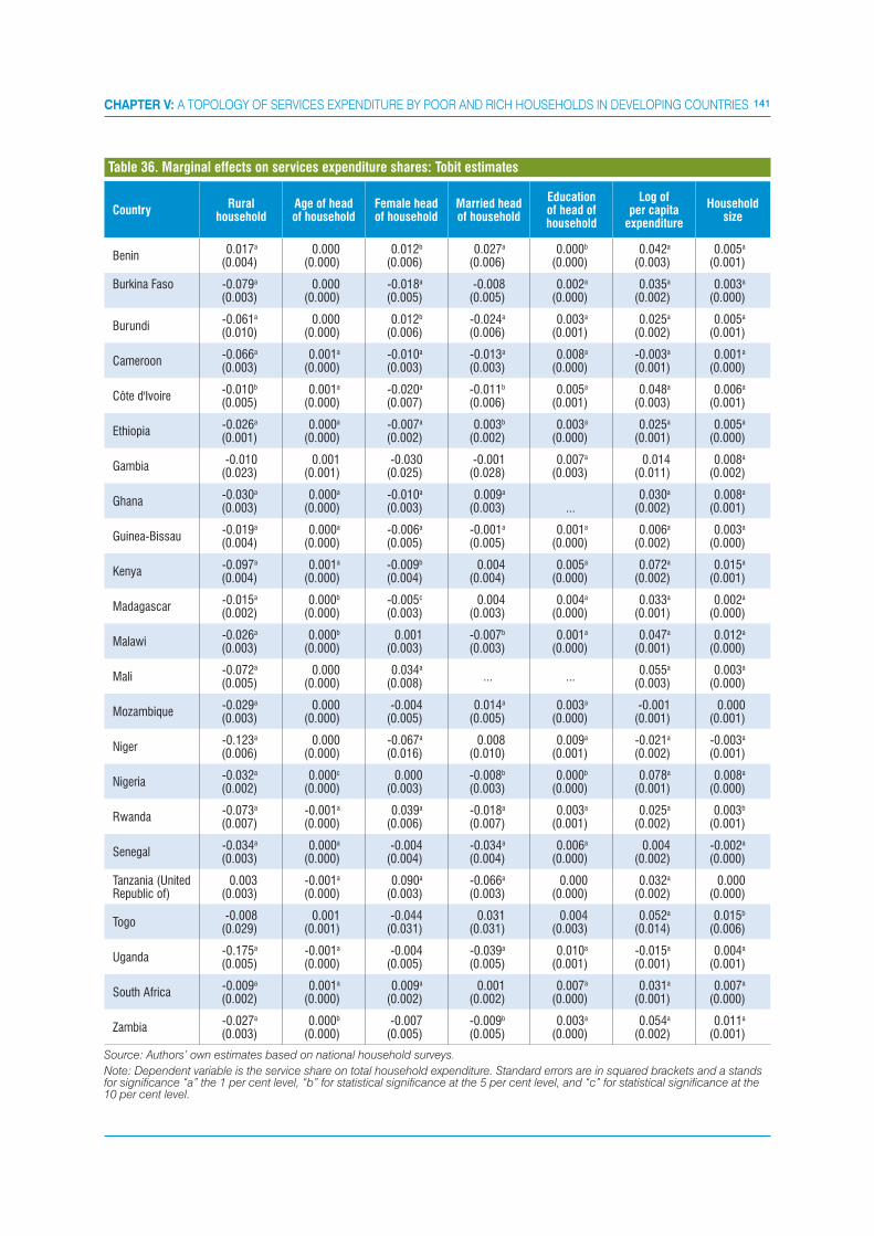
141CHAPTER V: A TOPOLOGY OF SERVICES EXPENDITURE BY POOR AND RICH HOUSEHOLDS IN DEVELOPING COUNTRIES
CountryRural
householdAge of head of household
Female head of household
Married head of household
Education of head of household
Log of per capita
expenditure
Household size
Benin 0.017a
(0.004)0.000
(0.000)0.012b
(0.006)0.027a
(0.006)0.000b
(0.000)0.042a
(0.003)0.005a
(0.001)
Burkina Faso
-0.079a
(0.003)0.000
(0.000)-0.018a
(0.005)-0.008
(0.005)0.002a
(0.000)0.035a
(0.002)0.003a
(0.000)
Burundi -0.061a
(0.010)0.000
(0.000)0.012b
(0.006)-0.024a
(0.006)0.003a
(0.001)0.025a
(0.002)0.005a
(0.001)
Cameroon-0.066a
(0.003)0.001a
(0.000)-0.010a
(0.003)-0.013a
(0.003)0.008a
(0.000)-0.003a
(0.001)0.001a
(0.000)
Côte d'Ivoire-0.010b
(0.005)0.001a
(0.000)-0.020a
(0.007)-0.011b
(0.006)0.005a
(0.001)0.048a
(0.003)0.006a
(0.001)
Ethiopia-0.026a
(0.001)0.000a
(0.000)-0.007a
(0.002)0.003b
(0.002)0.003a
(0.000)0.025a
(0.001)0.005a
(0.000)
Gambia-0.010
(0.023)0.001
(0.001)-0.030
(0.025)-0.001
(0.028)0.007a
(0.003)0.014
(0.011)0.008a
(0.002)
Ghana-0.030a
(0.003)0.000a
(0.000)-0.010a
(0.003)0.009a
(0.003)
... 0.030a
(0.002)0.008a
(0.001)
Guinea-Bissau-0.019a
(0.004)0.000a
(0.000)-0.006a
(0.005)-0.001a
(0.005)0.001a
(0.000)0.006a
(0.002)0.003a
(0.000)
Kenya-0.097a
(0.004)0.001a
(0.000)-0.009b
(0.004)0.004
(0.004)0.005a
(0.000)0.072a
(0.002)0.015a
(0.001)
Madagascar-0.015a
(0.002)0.000b
(0.000)-0.005c
(0.003)0.004
(0.003)0.004a
(0.000)0.033a
(0.001)0.002a
(0.000)
Malawi-0.026a
(0.003)0.000b
(0.000)0.001
(0.003)-0.007b
(0.003)0.001a
(0.000)0.047a
(0.001)0.012a
(0.000)
Mali-0.072a
(0.005)0.000
(0.000)0.034a
(0.008)... ...
0.055a
(0.003)0.003a
(0.000)
Mozambique-0.029a
(0.003)0.000
(0.000)-0.004
(0.005)0.014a
(0.005)0.003a
(0.000)-0.001
(0.001)0.000
(0.001)
Niger-0.123a
(0.006)0.000
(0.000)-0.067a
(0.016)0.008
(0.010)0.009a
(0.001)-0.021a
(0.002)-0.003a
(0.001)
Nigeria-0.032a
(0.002)0.000c
(0.000)0.000
(0.003)-0.008b
(0.003)0.000b
(0.000)0.078a
(0.001)0.008a
(0.000)
Rwanda-0.073a
(0.007)-0.001a
(0.000)0.039a
(0.006)-0.018a
(0.007)0.003a
(0.001)0.025a
(0.002)0.003b
(0.001)
Senegal-0.034a
(0.003)0.000a
(0.000)-0.004
(0.004)-0.034a
(0.004)0.006a
(0.000)0.004
(0.002)-0.002a
(0.000)
Tanzania (United Republic of)
0.003(0.003)
-0.001a
(0.000)0.090a
(0.003)-0.066a
(0.003)0.000
(0.000)0.032a
(0.002)0.000
(0.000)
Togo-0.008
(0.029)0.001
(0.001)-0.044
(0.031)0.031
(0.031)0.004
(0.003)0.052a
(0.014)0.015b
(0.006)
Uganda-0.175a
(0.005)-0.001a
(0.000)-0.004
(0.005)-0.039a
(0.005)0.010a
(0.001)-0.015a
(0.001)0.004a
(0.001)
South Africa-0.009a
(0.002)0.001a
(0.000)0.009a
(0.002)0.001
(0.002)0.007a
(0.000)0.031a
(0.001)0.007a
(0.000)
Zambia-0.027a
(0.003)0.000b
(0.000)-0.007
(0.005)-0.009b
(0.005)0.003a
(0.000)0.054a
(0.002)0.011a
(0.001)
Source: Authors’ own estimates based on national household surveys.
Note: Dependent variable is the service share on total household expenditure. Standard errors are in squared brackets and a stands for significance “a” the 1 per cent level, “b” for statistical significance at the 5 per cent level, and “c” for statistical significance at the 10 per cent level.
Table 36. Marginal effects on services expenditure shares: Tobit estimates

142 SERVICES, TRADE & DEVELOPMENT
Country/EconomyEducation
(%)Health
(%)Telecoms
(%)Transport
(%)Total(%)
China 3.2 2.6 0.7 0.6 7.1
India 3.7 8.2 2.8 1.7 16.5
Indonesia 6.1 1.8 1.7 ... 9.6
Russian Federation 0.9 4.3 3.0 0.6 8.7
Taiwan Province of China
10.9 13.7 1.4 3.1 29.0
Tajikistan 4.4 4.8 2.0 0.3 11.5
Thailand 2.2 2.1 1.6 3.4 9.3
Timor-Leste 0.7 0.7 0.0 0.0 1.5
Viet Nam 4.5 5.2 0.5 0.4 10.6
Source: Authors’ calculations based on Asia’s household surveys.
Table 37. Expenditure on services as a percentage of total expenditure in Asia
Figure 16. Expenditures on each service as a percentage of total expenditures on services
China
India
Indon
esia
Russia
n
Fede
ratio
n
Taiw
an P
rovin
ce
of C
hina
Tajik
istan
Taila
nd
Timor
-Les
te
Viet
Nam
0
10
20
30
40
50
60
70
80
90
100
Education Health Telecommunication Transport
Per
cent
age
Source: Authors’ calculations based on Asia’s household surveys.
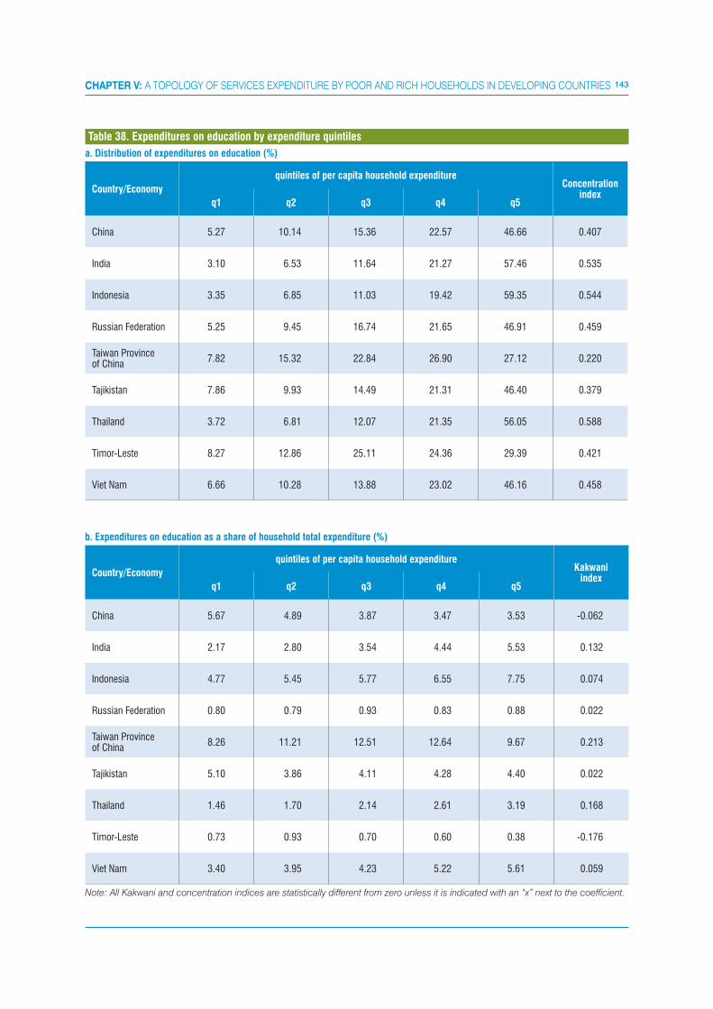
143CHAPTER V: A TOPOLOGY OF SERVICES EXPENDITURE BY POOR AND RICH HOUSEHOLDS IN DEVELOPING COUNTRIES
a. Distribution of expenditures on education (%)
Country/Economy
quintiles of per capita household expenditureConcentration
indexq1 q2 q3 q4 q5
China 5.27 10.14 15.36 22.57 46.66 0.407
India 3.10 6.53 11.64 21.27 57.46 0.535
Indonesia 3.35 6.85 11.03 19.42 59.35 0.544
Russian Federation 5.25 9.45 16.74 21.65 46.91 0.459
Taiwan Province of China
7.82 15.32 22.84 26.90 27.12 0.220
Tajikistan 7.86 9.93 14.49 21.31 46.40 0.379
Thailand 3.72 6.81 12.07 21.35 56.05 0.588
Timor-Leste 8.27 12.86 25.11 24.36 29.39 0.421
Viet Nam 6.66 10.28 13.88 23.02 46.16 0.458
Table 38. Expenditures on education by expenditure quintiles
b. Expenditures on education as a share of household total expenditure (%)
Country/Economy
quintiles of per capita household expenditureKakwani
indexq1 q2 q3 q4 q5
China 5.67 4.89 3.87 3.47 3.53 -0.062
India 2.17 2.80 3.54 4.44 5.53 0.132
Indonesia 4.77 5.45 5.77 6.55 7.75 0.074
Russian Federation 0.80 0.79 0.93 0.83 0.88 0.022
Taiwan Province of China
8.26 11.21 12.51 12.64 9.67 0.213
Tajikistan 5.10 3.86 4.11 4.28 4.40 0.022
Thailand 1.46 1.70 2.14 2.61 3.19 0.168
Timor-Leste 0.73 0.93 0.70 0.60 0.38 -0.176
Viet Nam 3.40 3.95 4.23 5.22 5.61 0.059
Note: All Kakwani and concentration indices are statistically different from zero unless it is indicated with an “x” next to the coefficient.

144 SERVICES, TRADE & DEVELOPMENT
Figure 17. Concentration curves for education
Lorenz % cumulative share Line of equality
0.2
.4.6
.81
cum
ulat
ive
expe
nditu
re
0 .2 .4 .6 .8 1
China
0.2
.4.6
.81
cum
ulat
ive
expe
nditu
re
0 .2 .4 .6 .8 1
% poorest
Indonesia
0.2
.4.6
.81
cum
ulat
ive
expe
nditu
re
0 .2 .4 .6 .8 1
% poorest
Russian Federation
0.2
.4.6
.81
cum
ulat
ive
expe
nditu
re
0 .2 .4 .6 .8 1
% poorest
Taiwan Province of China
0.2
.4.6
.81
cum
ulat
ive
expe
nditu
re
0 .2 .4 .6 .8 1
% poorest
Thailand
0.2
.4.6
.81
cum
ulat
ive
expe
nditu
re
0 .2 .4 .6 .8 1
% poorest
Timor-Leste
0.2
.4.6
.81
cum
ulat
ive
expe
nditu
re
0 .2 .4 .6 .8 1
% poorest
Viet Nam
0.2
.4.6
.81
cum
ulat
ive
expe
nditu
re
0 .2 .4 .6 .8 1
% poorest
India
0.2
.4.6
.81
cum
ulat
ive
expe
nditu
re
0 .2 .4 .6 .8 1
% poorest
Tajikistan
% poorest

145CHAPTER V: A TOPOLOGY OF SERVICES EXPENDITURE BY POOR AND RICH HOUSEHOLDS IN DEVELOPING COUNTRIES
a. Distribution of expenditures on health (%)
Country/Economy
quintiles of per capita household expenditureConcentration
indexq1 q2 q3 q4 q5
China 4.54 8.77 14.71 22.45 49.53 0.448
India 3.63 7.33 11.97 19.60 57.47 0.543
Indonesia 2.78 6.12 10.55 19.97 60.58 0.573
Russian Federation 5.92 10.30 13.39 21.49 48.89 0.430
Taiwan Province of China
11.87 15.46 17.37 21.19 34.11 0.217
Tajikistan 4.40 8.67 13.26 22.10 51.56 0.457
Thailand 3.72 7.14 11.44 19.29 58.41 0.549
Timor-Leste 6.26 7.27 17.47 22.14 46.86 0.421
Viet Nam 7.78 11.92 16.02 22.06 42.23 0.392
Table 39. Expenditures on health by expenditure quintiles
b. Expenditures on health as a share of household total expenditure (%)
Country/Economy
quintiles of per capita household expenditureKakwani
indexq1 q2 q3 q4 q5
China 3.46 3.04 2.66 2.47 2.62 -0.021
India 5.62 7.11 8.22 9.27 10.99 0.141
Indonesia 1.32 1.57 1.77 2.16 2.32 -0.105x
Russian Federation 5.08 4.31 3.74 4.06 4.09 -0.006x
Taiwan Province of China
15.49 14.60 13.31 12.80 12.25 -0.043
Tajikistan 3.27 4.03 4.55 5.43 6.63 0.100
Thailand 1.46 1.77 2.03 2.34 3.08 0.120
Timor-Leste 0.74 0.87 0.49 0.74 0.74 0.018
Viet Nam 4.20 4.90 5.42 5.63 6.01 -0.006
Note: All Kakwani and concentration indices are statistically different from zero unless it is indicated with an “x” next to the coefficient.
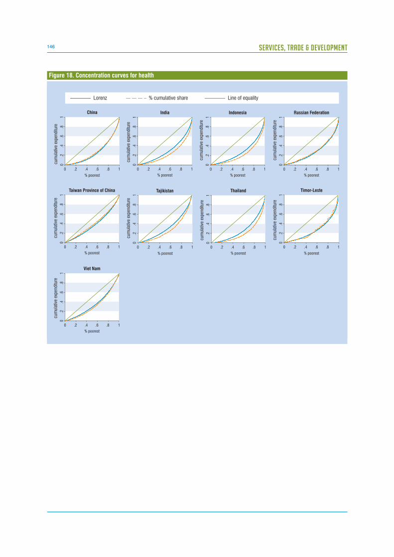
146 SERVICES, TRADE & DEVELOPMENT
Figure 18. Concentration curves for health
Lorenz % cumulative share Line of equality
0.2
.4.6
.81
cum
ulat
ive
expe
nditu
re
0 .2 .4 .6 .8 1
Indonesia
0.2
.4.6
.81
cum
ulat
ive
expe
nditu
re
0 .2 .4 .6 .8 1
% poorest
Russian Federation
0.2
.4.6
.81
cum
ulat
ive
expe
nditu
re
0 .2 .4 .6 .8 1
% poorest
Taiwan Province of China
0.2
.4.6
.81
cum
ulat
ive
expe
nditu
re
0 .2 .4 .6 .8 1
% poorest
0.2
.4.6
.81
cum
ulat
ive
expe
nditu
re
0 .2 .4 .6 .8 1
% poorest
Thailand
0.2
.4.6
.81
cum
ulat
ive
expe
nditu
re
0 .2 .4 .6 .8 1
% poorest
Timor-Leste
0.2
.4.6
.81
cum
ulat
ive
expe
nditu
re
0 .2 .4 .6 .8 1
% poorest
Viet Nam
0.2
.4.6
.81
cum
ulat
ive
expe
nditu
re
0 .2 .4 .6 .8 1
% poorest
India
Tajikistan
0.2
.4.6
.81
cum
ulat
ive
expe
nditu
re
0 .2 .4 .6 .8 1
% poorest
China
% poorest
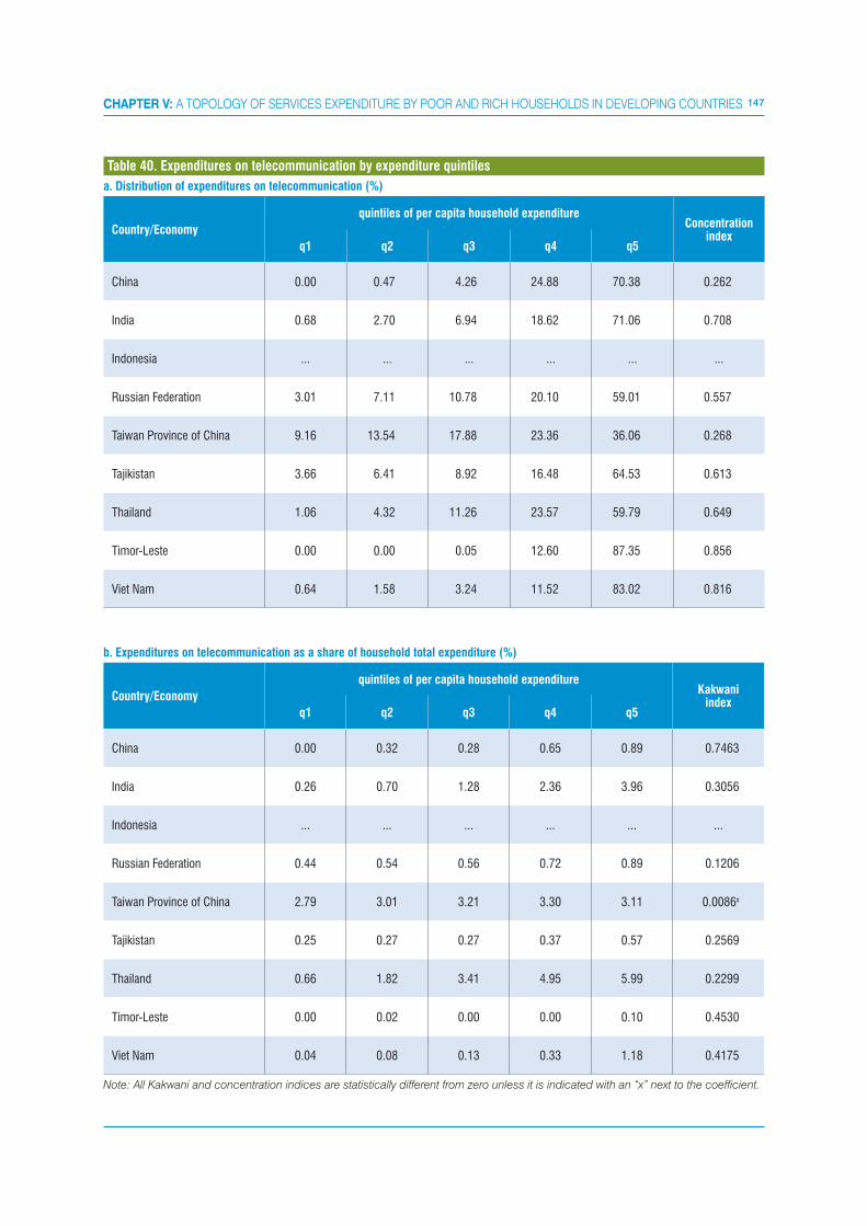
147CHAPTER V: A TOPOLOGY OF SERVICES EXPENDITURE BY POOR AND RICH HOUSEHOLDS IN DEVELOPING COUNTRIES
a. Distribution of expenditures on telecommunication (%)
Country/Economy
quintiles of per capita household expenditureConcentration
indexq1 q2 q3 q4 q5
China 0.00 0.47 4.26 24.88 70.38 0.262
India 0.68 2.70 6.94 18.62 71.06 0.708
Indonesia ... ... ... ... ... ...
Russian Federation 3.01 7.11 10.78 20.10 59.01 0.557
Taiwan Province of China 9.16 13.54 17.88 23.36 36.06 0.268
Tajikistan 3.66 6.41 8.92 16.48 64.53 0.613
Thailand 1.06 4.32 11.26 23.57 59.79 0.649
Timor-Leste 0.00 0.00 0.05 12.60 87.35 0.856
Viet Nam 0.64 1.58 3.24 11.52 83.02 0.816
Table 40. Expenditures on telecommunication by expenditure quintiles
b. Expenditures on telecommunication as a share of household total expenditure (%)
Country/Economy
quintiles of per capita household expenditureKakwani
indexq1 q2 q3 q4 q5
China 0.00 0.32 0.28 0.65 0.89 0.7463
India 0.26 0.70 1.28 2.36 3.96 0.3056
Indonesia ... ... ... ... ... ...
Russian Federation 0.44 0.54 0.56 0.72 0.89 0.1206
Taiwan Province of China 2.79 3.01 3.21 3.30 3.11 0.0086x
Tajikistan 0.25 0.27 0.27 0.37 0.57 0.2569
Thailand 0.66 1.82 3.41 4.95 5.99 0.2299
Timor-Leste 0.00 0.02 0.00 0.00 0.10 0.4530
Viet Nam 0.04 0.08 0.13 0.33 1.18 0.4175
Note: All Kakwani and concentration indices are statistically different from zero unless it is indicated with an “x” next to the coefficient.
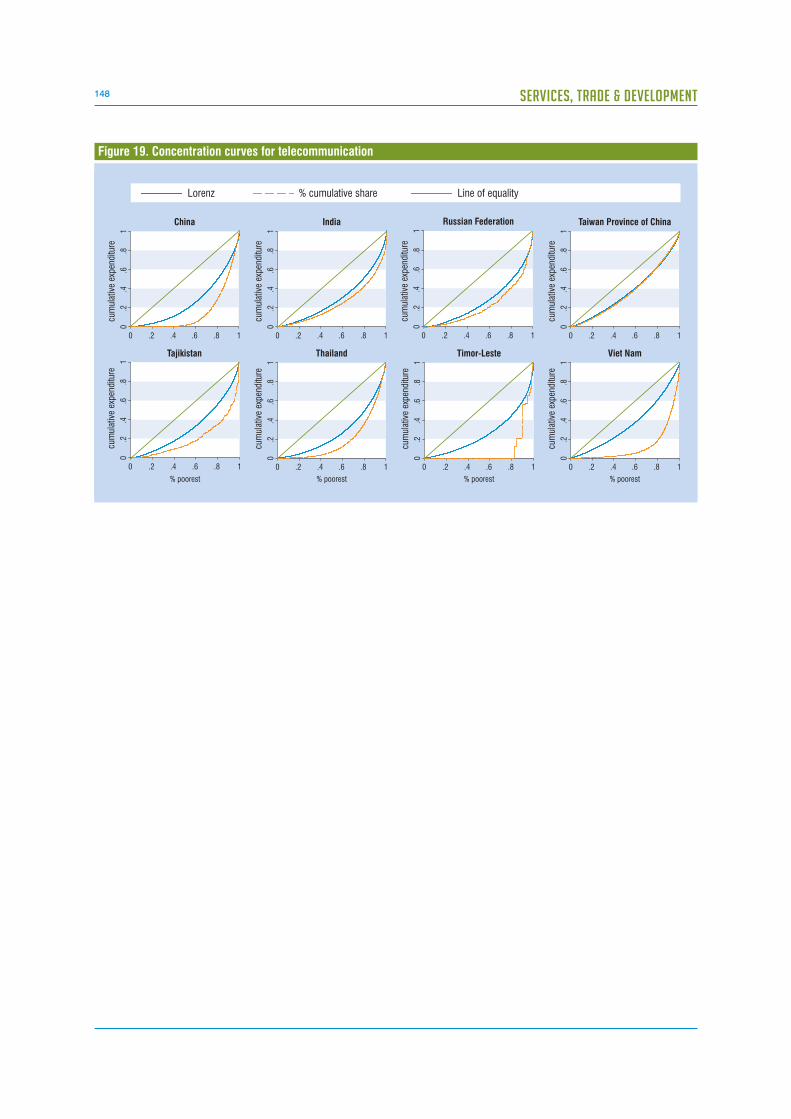
148 SERVICES, TRADE & DEVELOPMENT
Figure 19. Concentration curves for telecommunication
Lorenz % cumulative share Line of equality
0.2
.4.6
.81
cum
ulat
ive
expe
nditu
re
0 .2 .4 .6 .8 1
Viet Nam
0.2
.4.6
.81
cum
ulat
ive
expe
nditu
re
0 .2 .4 .6 .8 1
% poorest
Timor-Leste
0.2
.4.6
.81
cum
ulat
ive
expe
nditu
re
0 .2 .4 .6 .8 1
% poorest
Thailand
0.2
.4.6
.81
cum
ulat
ive
expe
nditu
re
0 .2 .4 .6 .8 1
% poorest
0.2
.4.6
.81
cum
ulat
ive
expe
nditu
re
0 .2 .4 .6 .8 1
Taiwan Province of China
0.2
.4.6
.81
cum
ulat
ive
expe
nditu
re
0 .2 .4 .6 .8 1
Russian Federation
0.2
.4.6
.81
cum
ulat
ive
expe
nditu
re
0 .2 .4 .6 .8 1
China
0.2
.4.6
.81
cum
ulat
ive
expe
nditu
re
0 .2 .4 .6 .8 1
India
Tajikistan
% poorest

149CHAPTER V: A TOPOLOGY OF SERVICES EXPENDITURE BY POOR AND RICH HOUSEHOLDS IN DEVELOPING COUNTRIES
a. Distribution of expenditures on transport (%)
Country/Economy
quintiles of per capita household expenditureConcentration
indexq1 q2 q3 q4 q5
China 4.60 8.95 14.67 24.24 47.54 0.441
India 4.81 8.05 11.98 18.05 57.11 0.481
Indonesia 7.55 12.31 16.71 23.67 39.76 0.322
Russian Federation 3.35 7.17 10.93 16.73 61.82 0.573
Taiwan Province of China
9.09 12.28 16.95 22.64 39.04 0.288
Tajikistan 2.06 5.37 11.23 18.84 62.50 0.564
Thailand 4.18 8.81 15.88 26.91 44.23 0.498
Timor-Leste 0.45 4.96 1.87 7.20 85.51 0.589
Viet Nam 9.09 14.77 19.97 24.26 31.90 0.299
Table 41. Expenditures on transport by expenditure quintiles
b. Expenditures on transport as a share of household total expenditure (%)
Country/Economy
quintiles of per capita household expenditureKakwani
indexq1 q2 q3 q4 q5
China 1.470 1.39 1.17 1.16 1.07 -0.028x
Indonesia 2.150 1.86 1.69 1.55 1.15 -0.147
India 2.560 2.60 2.75 2.83 3.35 0.078
Russian Federation 2.360 2.73 2.76 2.86 4.11 0.130x
Taiwan Province of China
1.320 1.24 1.35 1.43 1.48 0.066x
Thailand 1.010 1.35 1.73 2.04 1.76 0.078
Tajikistan 0.730 1.23 1.90 2.32 3.87 0.207
Timor-Leste 0.004 0.01 0.02 0.01 0.09 0.188
Viet Nam 0.400 0.52 0.59 0.56 0.42 -0.099
Note: All Kakwani and concentration indices are statistically different from zero unless it is indicated with an “x” next to the coefficient.
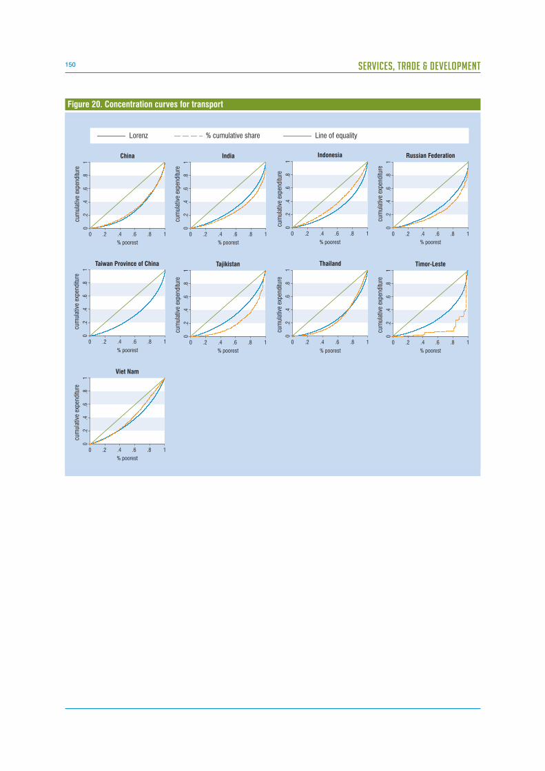
150 SERVICES, TRADE & DEVELOPMENT
Figure 20. Concentration curves for transport
Lorenz % cumulative share Line of equality
0.2
.4.6
.81
cum
ulat
ive
expe
nditu
re
0 .2 .4 .6 .8 1
China
0.2
.4.6
.81
cum
ulat
ive
expe
nditu
re
0 .2 .4 .6 .8 1
% poorest
India
0.2
.4.6
.81
cum
ulat
ive
expe
nditu
re
0 .2 .4 .6 .8 1
% poorest
Russian Federation
0.2
.4.6
.81
cum
ulat
ive
expe
nditu
re
0 .2 .4 .6 .8 1
% poorest
0.2
.4.6
.81
cum
ulat
ive
expe
nditu
re
0 .2 .4 .6 .8 1
% poorest
Tajikistan
0.2
.4.6
.81
cum
ulat
ive
expe
nditu
re
0 .2 .4 .6 .8 1
% poorest
Thailand
0.2
.4.6
.81
cum
ulat
ive
expe
nditu
re
0 .2 .4 .6 .8 1
% poorest
Timor-Leste
0.2
.4.6
.81
cum
ulat
ive
expe
nditu
re
0 .2 .4 .6 .8 1
% poorest
Viet Nam
Taiwan Province of China
0.2
.4.6
.81
cum
ulat
ive
expe
nditu
re
0 .2 .4 .6 .8 1
% poorest
Indonesia
% poorest
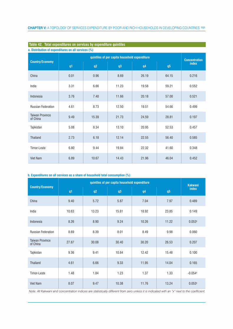
151CHAPTER V: A TOPOLOGY OF SERVICES EXPENDITURE BY POOR AND RICH HOUSEHOLDS IN DEVELOPING COUNTRIES
a. Distribution of expenditures on all services (%)
Country/Economy
quintiles of per capita household expenditureConcentration
indexq1 q2 q3 q4 q5
China 0.01 0.96 8.69 26.19 64.15 0.216
India 3.31 6.66 11.23 19.58 59.21 0.552
Indonesia 3.76 7.40 11.66 20.18 57.00 0.521
Russian Federation 4.61 8.73 12.50 19.51 54.66 0.499
Taiwan Province of China
9.49 15.39 21.73 24.59 28.81 0.197
Tajikistan 5.08 8.34 13.10 20.95 52.53 0.457
Thailand 2.73 6.18 12.14 22.55 56.40 0.585
Timor-Leste 6.80 9.44 19.84 22.32 41.60 0.348
Viet Nam 6.89 10.67 14.43 21.96 46.04 0.452
Table 42. Total expenditures on services by expenditure quintiles
b. Expenditures on all services as a share of household total consumption (%)
Country/Economy
quintiles of per capita household expenditureKakwani
indexq1 q2 q3 q4 q5
China 9.40 5.72 5.87 7.04 7.97 0.489
India 10.63 13.23 15.81 18.92 23.85 0.149
Indonesia 8.26 8.90 9.24 10.26 11.22 0.053x
Russian Federation 8.69 8.39 8.01 8.49 9.98 0.060
Taiwan Province of China
27.87 30.08 30.40 30.20 26.53 0.207
Tajikistan 9.36 9.41 10.84 12.42 15.48 0.100
Thailand 4.61 6.66 9.33 11.95 14.04 0.165
Timor-Leste 1.48 1.84 1.23 1.37 1.33 -0.054x
Viet Nam 8.07 9.47 10.38 11.76 13.24 0.053x
Note: All Kakwani and concentration indices are statistically different from zero unless it is indicated with an “x” next to the coefficient.
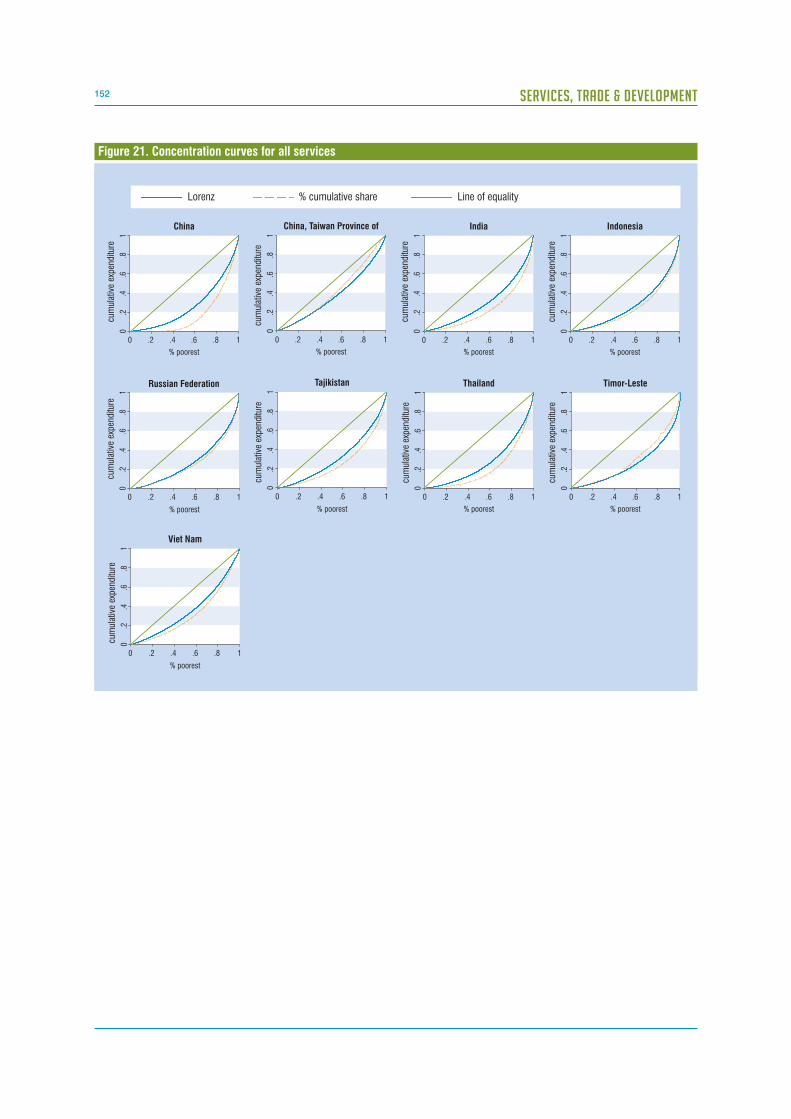
152 SERVICES, TRADE & DEVELOPMENT
Figure 21. Concentration curves for all services
Lorenz % cumulative share Line of equality
0.2
.4.6
.81
cum
ulat
ive
expe
nditu
re
0 .2 .4 .6 .8 1
Indonesia
0.2
.4.6
.81
cum
ulat
ive
expe
nditu
re
0 .2 .4 .6 .8 1
% poorest
India
0.2
.4.6
.81
cum
ulat
ive
expe
nditu
re
0 .2 .4 .6 .8 1
% poorest
China
0.2
.4.6
.81
cum
ulat
ive
expe
nditu
re
0 .2 .4 .6 .8 1
% poorest
0.2
.4.6
.81
cum
ulat
ive
expe
nditu
re
0 .2 .4 .6 .8 1
% poorest
China, Taiwan Province of
0.2
.4.6
.81
cum
ulat
ive
expe
nditu
re
0 .2 .4 .6 .8 1
% poorest
Tajikistan
0.2
.4.6
.81
cum
ulat
ive
expe
nditu
re
0 .2 .4 .6 .8 1
% poorest
Thailand
0.2
.4.6
.81
cum
ulat
ive
expe
nditu
re
0 .2 .4 .6 .8 1
% poorest
Timor-LesteRussian Federation
0.2
.4.6
.81
cum
ulat
ive
expe
nditu
re
0 .2 .4 .6 .8 1
% poorest
Viet Nam
% poorest
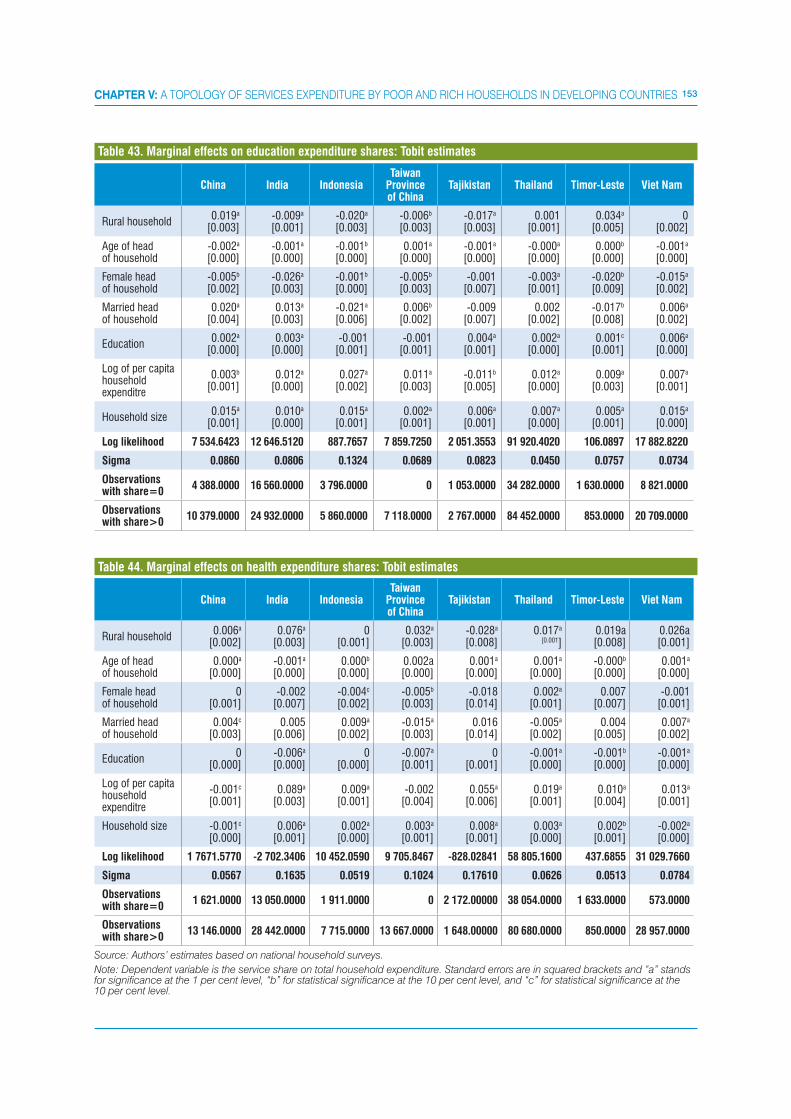
153CHAPTER V: A TOPOLOGY OF SERVICES EXPENDITURE BY POOR AND RICH HOUSEHOLDS IN DEVELOPING COUNTRIES
China India IndonesiaTaiwan
Province of China
Tajikistan Thailand Timor-Leste Viet Nam
Rural household0.019a
[0.003]-0.009a
[0.001]-0.020a
[0.003]-0.006b
[0.003]-0.017a
[0.003]0.001
[0.001]0.034a
[0.005]0
[0.002]
Age of head of household
-0.002a
[0.000]-0.001a
[0.000]-0.001b
[0.000]0.001a
[0.000]-0.001a
[0.000]-0.000a
[0.000]0.000b
[0.000]-0.001a
[0.000]
Female head of household
-0.005b
[0.002]-0.026a
[0.003]-0.001b
[0.000]-0.005b
[0.003]-0.001
[0.007]-0.003a
[0.001]-0.020b
[0.009]-0.015a
[0.002]
Married head of household
0.020a
[0.004]0.013a
[0.003]-0.021a
[0.006]0.006b
[0.002]-0.009
[0.007]0.002
[0.002]-0.017b
[0.008]0.006a
[0.002]
Education0.002a
[0.000]0.003a
[0.000]-0.001
[0.001]-0.001
[0.001]0.004a
[0.001]0.002a
[0.000]0.001c
[0.001]0.006a
[0.000]
Log of per capita household expenditre
0.003b
[0.001]0.012a
[0.000]0.027a
[0.002]0.011a
[0.003]-0.011b
[0.005]0.012a
[0.000]0.009a
[0.003]0.007a
[0.001]
Household size 0.015a
[0.001]0.010a
[0.000]0.015a
[0.001]0.002a
[0.001]0.006a
[0.001]0.007a
[0.000]0.005a
[0.001]0.015a
[0.000]
Log likelihood 7 534.6423 12 646.5120 887.7657 7 859.7250 2 051.3553 91 920.4020 106.0897 17 882.8220
Sigma 0.0860 0.0806 0.1324 0.0689 0.0823 0.0450 0.0757 0.0734
Observations with share=0
4 388.0000 16 560.0000 3 796.0000 0 1 053.0000 34 282.0000 1 630.0000 8 821.0000
Observations with share>0
10 379.0000 24 932.0000 5 860.0000 7 118.0000 2 767.0000 84 452.0000 853.0000 20 709.0000
Table 43. Marginal effects on education expenditure shares: Tobit estimates
China India IndonesiaTaiwan
Province of China
Tajikistan Thailand Timor-Leste Viet Nam
Rural household0.006a
[0.002]0.076a
[0.003]0
[0.001]0.032a
[0.003]-0.028a
[0.008]0.017a
[0.001]0.019a[0.008]
0.026a[0.001]
Age of head of household
0.000a
[0.000]-0.001a
[0.000]0.000b
[0.000]0.002a[0.000]
0.001a
[0.000]0.001a
[0.000]-0.000b
[0.000]0.001a
[0.000]
Female head of household
0[0.001]
-0.002[0.007]
-0.004c
[0.002]-0.005b
[0.003]-0.018
[0.014]0.002a
[0.001]0.007
[0.007]-0.001
[0.001]
Married head of household
0.004c
[0.003]0.005
[0.006]0.009a
[0.002]-0.015a
[0.003]0.016
[0.014]-0.005a
[0.002]0.004
[0.005]0.007a
[0.002]
Education0
[0.000]-0.006a
[0.000]0
[0.000]-0.007a
[0.001]0
[0.001]-0.001a
[0.000]-0.001b
[0.000]-0.001a
[0.000]
Log of per capita household expenditre
-0.001c
[0.001]0.089a
[0.003]0.009a
[0.001]-0.002
[0.004]0.055a
[0.006]0.019a
[0.001]0.010a
[0.004]0.013a
[0.001]
Household size
-0.001c
[0.000]0.006a
[0.001]0.002a
[0.000]0.003a
[0.001]0.008a
[0.001]0.003a
[0.000]0.002b
[0.001]-0.002a
[0.000]
Log likelihood 1 7671.5770 -2 702.3406 10 452.0590 9 705.8467 -828.02841 58 805.1600 437.6855 31 029.7660
Sigma 0.0567 0.1635 0.0519 0.1024 0.17610 0.0626 0.0513 0.0784
Observations with share=0
1 621.0000 13 050.0000 1 911.0000 0 2 172.00000 38 054.0000 1 633.0000 573.0000
Observations with share>0
13 146.0000 28 442.0000 7 715.0000 13 667.0000 1 648.00000 80 680.0000 850.0000 28 957.0000
Source: Authors’ estimates based on national household surveys.
Note: Dependent variable is the service share on total household expenditure. Standard errors are in squared brackets and “a” stands for significance at the 1 per cent level, “b” for statistical significance at the 10 per cent level, and “c” for statistical significance at the 10 per cent level.
Table 44. Marginal effects on health expenditure shares: Tobit estimates

154 SERVICES, TRADE & DEVELOPMENT
China India IndonesiaTaiwan
Province of China
Tajikistan Thailand Timor-Leste Viet Nam
Rural household00
-0.019a
[0.001]...
-0.001[0.001]
-0.027a
[0.003]-0.002a
[0.001]0.014a
[0.002]-0.002a
[0.000]
Age of head of household
0.000a
[0.000]0.000a
[0.000]...
-0.000a
[0.000]0.000b[0.000]
0[0.000]
0.000a
[0.000]0.000a
[0.000]
Female head of household
-0.001[0.001]
-0.012a
[0.003]...
0.001[0.001]
-0.008c
[0.004]-0.001
[0.001]-0.071a
[0.002]-0.002a
[0.001]
Married head of household
0.002[0.002]
0.003[0.002]
...
0.002a
[0.001]0.001
[0.004]-0.002
[0.001]0.411a
[0.002]0.002b
[0.001]
Education0.001a
[0.000]0.003a
[0.000]...
0[0.000]
0.002a
[0.000]0.001a
[0.000]0
[0.000]0.001a
[0.000]
Log of per capita household expenditre
0.017a
[0.001]0.031a
[0.001]...
0.002a
[0.001]0.011a
[0.002]0.041a
ae200.042a
[0.000]0.015a
[0.001]
Household size 0.004a
[0.001]0.002a
[0.000]...
0[0.000]
0.001a
[0.000]0.005a
[0.000]0.003a
[0.000]0.002a
[0.000]
Log likelihood 4 664.9910 1 099.8350 ... 32 091.1150 732.6328 65 476.3190 342.00460 20 673.4590
Sigma 0.0265 0.0523 ... 0.0197 0.0344 0.0476 0.00003 0.0178
Observations with share=0
3 769.000025
192.0000... 0 2 935.0000 44 765.0000 2 432.00000 18 477.0000
Observations with share>0
3 004.0000
16 300.0000
... 13 617.0000 885.0000 73 969.0000 51.00000 11 053.0000
Table 45. Marginal effects on telecommunication expenditure shares: Tobit estimates
China India IndonesiaTaiwan
Province of China
Tajikistan Thailand Timor-Leste Viet Nam
Rural household0.022a
[0.002]0.002a
[0.001]-0.003a
[0.000]-0.001
[0.000]-0.025a
[0.004]0.021a
[0.001]0.000b
[0.000]0.005a
[0.000]
Age of head of household
0[0.000]
0[0.000]
-0.000a
[0.000]0.000a
[0.000]-0.000c
[0.000]-0.000a
[0.000]0
[0.000]-0.000a
[0.000]
Female head of household
0[0.001]
0.002c
[0.001]-0.001c
[0.001]-0.002a
[0.000]0.002
[0.006]-0.011a
[0.001]0
[0.000]0
[0.000]
Married head of household
-0.001[0.002]
-0.001[0.001]
0.002a
[0.001]0
[0.000]0.005
[0.006]0.017a
[0.002]0
[0.000]0
[0.001]
Education0.001a
[0.000]0.000a
[0.000]0
[0.000]0.000b
[0.000]0
[0.000]0.001a
[0.000]0.000b
[0.000]-0.000a
[0.000]
Log of per capita household expenditre
0.009a
[0.001]0.003a
[0.001]-0.005a[0.000]
0[0.000]
0.044a
[0.004]0.025a
ae200.002a
[0.000]0.004a
[0.000]
Household size0.002a
[0.000]0
[0.000]-0.000a
[0.000]-0.001a
[0.000]0.005a
[0.001]0.007a
[0.000]0.000a
[0.000]0.001a
[0.000]
Log likelihood 16 758.9260 64 491.1430 24 485.3240 31 221.2830 650.6808 -9 548.4601 3 350.7127 23 331.0390
Sigma 0.0419 0.0360 0.0159 0.0160 0.0779 0.0786 0.0043 0.0201
Observations with share=0
3 700.0000 3 357.0000 465.0000 0 2 162.0000 80 391.0000 1 462.0000 16 119.0000
Observations with share>0
11 067.0000 38 135 .0000 9 174.0000 12 160.0000 1 658.0000 38 343.0000 1 021.0000 13 411.0000
Source: Authors’ estimates based on national household surveys.
Note: Dependent variable is the service share on total household expenditure. Standard errors are in squared brackets and “a” stands for significance at the 1 per cent level, “b” for statistical significance at the 10 per cent level, and “c” for statistical significance at the 10 per cent level.
Table 46. Marginal effects on transport expenditure shares: Tobit estimates

155CHAPTER V: A TOPOLOGY OF SERVICES EXPENDITURE BY POOR AND RICH HOUSEHOLDS IN DEVELOPING COUNTRIES
China India IndonesiaTaiwan
Province of China
Tajikistan Thailand Timor-Leste Viet Nam
Rural household00
0.026a
[0.002]-0.020a
[0.002]0.018a
[0.005]-0.042a
[0.005]-0.018a
[0.001]0.008b
[0.003]0.026a
[0.002]
Age of headof household
-0.000b
[0.000]-0.000a
[0.000]-0.000a
[0.000]0.001a
[0.000]-0.009
[0.010]0.000a
[0.000]0.000c
[0.000]0.001a
[0.000]
Female head of household
0[0.002]
-0.020a
[0.005]0.002
[0.004]-0.018a
[0.004]-0.001
[0.009]-0.005a
[0.001]-0.013c
[0.007]-0.014a
[0.002]
Married head of household
0.011a
[0.004]0.010b
[0.005]-0.015a
[0.004]-0.004
[0.003]0.005a
[0.001]0.013a
[0.002]-0.007
[0.005]0.012a
[0.002]
Education0.001a
[0.000]-0.001a
[0.000]0
[0.000]-0.004a
[0.001]0.033a
[0.005]0.002a
[0.000]0.001
[0.000]0.003a
[0.000]
Log of per capita household expenditre
0.019a
[0.003]0.089a
[0.002]0.015a
[0.002]-0.002
[0.005]0.008a
[0.001]0.051a
ae200.011a
[0.003]0.024a
[0.001]
Household size
0.011a
[0.001]0.006a
[0.000]0.006a
[0.000]0.010a
[0.001]-0.082a
[0.023]0.010a
[0.000]0.004a
[0.001]0.005a
[0.000]
Log likelihood 8 029.9853 18 933.0570 8 279.7116 5 436.4159 1 781.4311 90 696.1210 1 847.5940 26 609.4910
Sigma 0.0704 0.1318 0.1002 0.0901 0.1274 0.0783 0.0559 0.0934
Observations with share=0
147.0000 478.0000 109.0000 0 319.0000 4 751.0000 728.0000 200.0000
Observations with share>0
6 626.0000 41 014.0000 9 512.0000 6 504.0000 3 501.0000 113 983.0000 1 755.0000 29 330.0000
Source: Authors’ estimates based on national household surveys.
Note: Dependent variable is the service share on total household expenditure. Standard errors are in squared brackets and “a” stands for significance at the 1 per cent level, “b” for statistical significance at the 10 per cent level, and “c” for statistical significance at the 10 per cent level.
Table 47. Marginal effects on total services expenditure shares: Tobit estimates
NOTES1 Alternatively one can assume identical and homothetic preferences, in which case there is no need for identical factor
endowments. In all these cases, to obtain the social utility function one can simply add up the quantities consumed by each individual (of each good).
2 The Pareto approach would stipulate that free trade is Pareto-superior if all individuals are better off under free-trade, that
is, � � � �Aii
Fii cucu � for all individuals i in the economy, where ic is the consumption bundle of individual i, and superscripts
F stands for free-trade and A for autarky. This is a very simple criterion, and it does not require any inter-individual utility comparisons. It is also transitive. However, as argued above, it is unlikely that trade will bring gains to everyone in an economy with heterogeneous individuals. The Bergson-Samuelson social welfare function assumes the existence of a social welfare function of the form W=w(u
1 , u
2 , u
3 ,…, u
i) and establishes that free trade is preferred to autarky if WF> WA.
The problem with this approach is that there is not a unique definition of the social welfare function, so it is possible to rank two situations differently according to the social welfare function that one chooses.
3 See Dixit and Norman (1986) or Kemp and Wan (1986).4 It is important to note that omitting the effect on the production side can obviously reverse welfare results. This would
be the case if for example rich households have a larger share of services expenditure than poor households, but also a much larger share of their income linked to the services sector. An increase in the price of services will hurt rich households on the consumption side more than poor households, but will also benefit them more on the production side. Nevertheless, and keeping this caveat in mind, it is believed that the type of information obtained by focusing exclusively on the consumption side is useful. To assess the poverty implications of services reforms in different countries, it will be necessary to assess the patterns of services consumption of rich and poor households. This necessary step is the aim of this study.
5 Data on financial services is much more difficult and homogeneous across survey to be included in the overview chapter. However in a companion paper (Porto, Porto, and Olarreaga 2009) some first steps toward an analysis of access to finance in developing countries is provided.
156 SERVICES, TRADE & DEVELOPMENT
6 In a companion paper the extent to which lack of access to these different services can explain the observed expenditure patterns in LAC is considered (see Porto et al., 2009). The broad conclusion is that lack of access can only explain a small share of the patterns found in this chapter. In the case of financial services, however, the question of access seems to be relatively more important (see Porto, Porto and Olarreaga, 2009).
7 This is partly because of lack of access by the poor.8 Bolivia, Colombia, Ecuador, El Salvador, Mexico, Nicaragua, Panama, and Peru.9 Burundi, Benin, Burkina Faso, Cote d’Ivoire, Cameroon, Ethiopia, Ghana, Gambia, Guinea-Bissau, Kenya, Madagascar,
Mali, Mozambique, Malawi, Niger, Nigeria, Rwanda, Senegal, Togo, United Republic of Tanzania, Uganda, South Africa and Zambia.
10 China, Indonesia, India, the Russian Federation, Thailand, Tajikistan, Timor-Leste, Taiwan Province of China, and Viet Nam.11 An alternative that uses the information over the entire expenditure distribution is the Kakwani progressivity index, defined as
twice the area between the Lorenz curve for services expenditure (conditional on the ranking of total household expenditure) and the Lorenz curve for total household expenditure (Kakwani, 1977). Therefore, it can be calculated as the difference between the Concentration index of services expenditure and the Gini coefficient of total expenditure.
12 Note that poverty here is a relative concept within a country. Households in the bottom quintile of one country with a very high GDP per capita can potentially be richer than households in the top quintile of another country with a very low GDP per capita.
13 The source of country characteristics data are the World Bank’s World Development Indicators. For each variable we took the average for the period 1999-2006.
14 The sectors considered in the services trade restrictiveness index are financial services, telecommunications, retail distribution, transportation, and selected professional services. Thus, they do not fully correspond to the sectors included in our surveys of household expenditure.
15 Otherwise there is no reason to restrict trade as foreign services would come at higher prices, and consumers will not purchase them. This may oversimplify the demand structure for services where product heterogeneity and preferences exhibiting desire for variety may be important.
16 Note that none of these correlations are statistically different from zero and are undertaken for only 14 observations.17 There is wide economic literature related to incidence analysis. Recent contributions include Bourguignon and Pereira da
Silva (2003), and Van de Walle (2003), among others. 18 There are numerous arguments for using expenditure rather than income as the variable to indicate well-being. (see Deaton
and Zaidi (2002) for general arguments). 19 This result comes from the Jakobsson and Fellman theorem (see Lambert, 2001).20 The Kakwani Index is usually known as the Kakwani Progressivity Index. In the traditional incidence analysis literature, a
public programme is said to be progressive if the benefit it generates (measured as a proportion of total expenditure per capita) diminishes as household total expenditure per capita increases. Throughout this chapter, where the interest lies on the distribution of household (instead of public) expenditures, the terms progressive and regressive is not used in order to avoid confusion.
21 The Kakwani Indices can be seen as an alternative to RESBP* developed in section 2. The advantage of Kakwani Indices is that it takes the information along the entire distribution of expenditure instead of calculating averages for each income quintile as in the calculation of RESBP* which then ignores the degree of inequality or bias within each quintile. The correlation between the Kakwani Index and RESBP* is -0.61 in our sample, which indicates that as expected large values of the Kakwani Index are associated with small values for RESBP*. The correlation is the strongest in LAC with a value of -0.93 which indicates that intra-quintile heterogeneity may be less important than in other regions. Within sectors the highest correlations are found for health, education and transport signaling less within quintile heterogeneity than in telecommunications or overall services expenditure. A simple OLS regression of RESBP* on the Kakwani Index yields a coefficient equal to -1.02 and a standard error of 0.10 with an R2 of 0.37.
22 Throughout, this chapter refers to low, moderate and high concentration and Kakwani Indices to establish a ranking within the set of services under analysis. There is no particular definition of low, moderate and high, as they are used relatively to the values in other sectors.
23 For more information see: www.cedlas.org24 Exceptions are Colombia and Panama, where Kakwani Indices were not significant (based on bootstrap). 25 Except Ecuador, where it is negative but not significant (by bootstrap).26 All Kakwani Indices are statistically different from zero.27 Average national shares of fixed and cell phones on household total telecommunication expenditure are: 67 per cent in
Bolivia, 96 per cent in Colombia, 79 per cent in Ecuador, 80 per cent in Mexico, 92 per cent in Panama, and 88 per cent in Peru.
28 Marginal effects are calculated at the mean of the independent variables.29 This is the case in El Salvador and Mexico, when analyzing gas services, and Bolivia, Ecuador, and Peru when studying
expenditures on electricity. 30 Note that some countries, e.g., South Africa, do not have a formal/agreed upon definition of “urban” and “rural”, and that
as with other variables the definition of “rural” and “urban” varies by country/survey.

AN OVERVIEW OF ACCESS TO FINANCE AND POVERTY
IN THE DEVELOPING WORLD
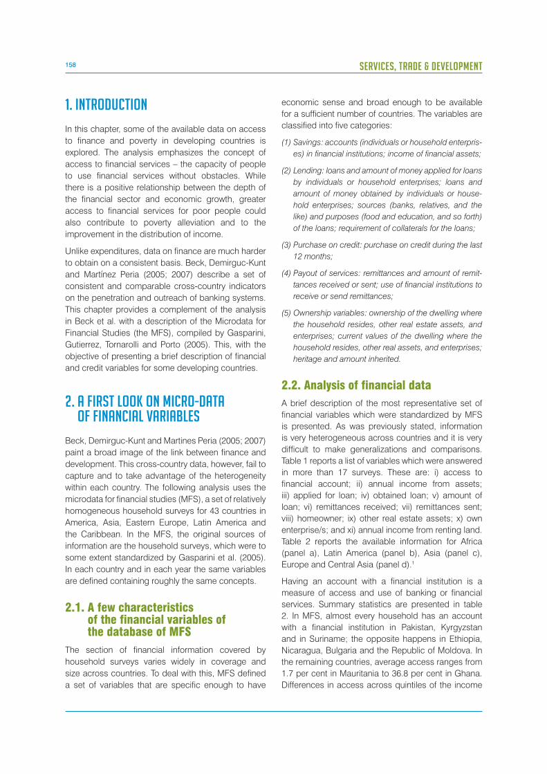
158 SERVICES, TRADE & DEVELOPMENT
1. INTRODUCTION
In this chapter, some of the available data on access
to finance and poverty in developing countries is
explored. The analysis emphasizes the concept of
access to financial services – the capacity of people
to use financial services without obstacles. While
there is a positive relationship between the depth of
the financial sector and economic growth, greater
access to financial services for poor people could
also contribute to poverty alleviation and to the
improvement in the distribution of income.
Unlike expenditures, data on finance are much harder
to obtain on a consistent basis. Beck, Demirguc-Kunt
and Martínez Peria (2005; 2007) describe a set of
consistent and comparable cross-country indicators
on the penetration and outreach of banking systems.
This chapter provides a complement of the analysis
in Beck et al. with a description of the Microdata for
Financial Studies (the MFS), compiled by Gasparini,
Gutierrez, Tornarolli and Porto (2005). This, with the
objective of presenting a brief description of financial
and credit variables for some developing countries.
2. A FIRST LOOK ON MICRO-DATA OF FINANCIAL VARIABLES
Beck, Demirguc-Kunt and Martines Peria (2005; 2007)
paint a broad image of the link between finance and
development. This cross-country data, however, fail to
capture and to take advantage of the heterogeneity
within each country. The following analysis uses the
microdata for financial studies (MFS), a set of relatively
homogeneous household surveys for 43 countries in
America, Asia, Eastern Europe, Latin America and
the Caribbean. In the MFS, the original sources of
information are the household surveys, which were to
some extent standardized by Gasparini et al. (2005).
In each country and in each year the same variables
are defined containing roughly the same concepts.
2.1. A few characteristics of the financial variables of the database of MFS
The section of financial information covered by
household surveys varies widely in coverage and
size across countries. To deal with this, MFS defined
a set of variables that are specific enough to have
economic sense and broad enough to be available
for a sufficient number of countries. The variables are
classified into five categories:
(1) Savings: accounts (individuals or household enterpris-
es) in financial institutions; income of financial assets;
(2) Lending: loans and amount of money applied for loans
by individuals or household enterprises; loans and
amount of money obtained by individuals or house-
hold enterprises; sources (banks, relatives, and the
like) and purposes (food and education, and so forth)
of the loans; requirement of collaterals for the loans;
(3) Purchase on credit: purchase on credit during the last
12 months;
(4) Payout of services: remittances and amount of remit-
tances received or sent; use of financial institutions to
receive or send remittances;
(5) Ownership variables: ownership of the dwelling where
the household resides, other real estate assets, and
enterprises; current values of the dwelling where the
household resides, other real assets, and enterprises;
heritage and amount inherited.
2.2. Analysis of financial data
A brief description of the most representative set of
financial variables which were standardized by MFS
is presented. As was previously stated, information
is very heterogeneous across countries and it is very
difficult to make generalizations and comparisons.
Table 1 reports a list of variables which were answered
in more than 17 surveys. These are: i) access to
financial account; ii) annual income from assets;
iii) applied for loan; iv) obtained loan; v) amount of
loan; vi) remittances received; vii) remittances sent;
viii) homeowner; ix) other real estate assets; x) own
enterprise/s; and xi) annual income from renting land.
Table 2 reports the available information for Africa
(panel a), Latin America (panel b), Asia (panel c),
Europe and Central Asia (panel d).1
Having an account with a financial institution is a
measure of access and use of banking or financial
services. Summary statistics are presented in table
2. In MFS, almost every household has an account
with a financial institution in Pakistan, Kyrgyzstan
and in Suriname; the opposite happens in Ethiopia,
Nicaragua, Bulgaria and the Republic of Moldova. In
the remaining countries, average access ranges from
1.7 per cent in Mauritania to 36.8 per cent in Ghana.
Differences in access across quintiles of the income

159CHAPTER VI: AN OVERVIEW OF ACCESS TO FINANCE AND POVERTY IN THE DEVELOPING WORLD
distribution are also examined. As expected, access
to finance is much higher at the upper quintiles. For
example, in Guatemala, Paraguay and Haiti, between
28 per cent and 46 per cent of households at the top
quintile have an account with a financial institution
while lower descending values correspond to the rest
of the quintiles.
Information about annual income of financial assets
(interests, dividends, and royalties) is available in al-
most every survey. These data reveal some features
of savings behaviour. Income from financial assets
accounts for less than 10 per cent of total household
income in countries like Mexico, Peru, Kyrgyzstan,
and Ukraine. In the majority of countries, including
the Plurinational State of Bolivia, Brazil, Colombia, El
Salvador, Haiti, Panama, Paraguay, Uruguay, Bang-
ladesh, the Republic of Moldova and Romania, the
share of income from financial assets ranges from
15 per cent to 35 per cent. The highest shares are in
Mauritania, Zambia, Bolivarian Republic of Venezuela
and Armenia (between 40 per cent and 65 per cent).
In some cases, the share of income from financial
assets grows across quintiles (Uganda, Argentina,
Plurinational State of Bolivia, Panama, Paraguay, and
Uruguay). In some other countries, these shares in-
stead decline across quintiles (Zambia, Brazil, Ja-
maica, Bolivarian Republic of Venezuela, Bangladesh,
and Pakistan).
Information on loan application is very scarce. In the
11 surveys with data containing this information, less
than 10 per cent of the households applied for a loan
in Madagascar, Mauritania, Paraguay, and Bulgaria. At
the same time, less than 10 per cent of the households
actually received a loan in Cote D’Ivoire, Gambia,
Kenya, Jamaica, Mexico, Paraguay and Bulgaria;
between 15 per cent and 35 per cent received a loan
in Ghana, Ecuador, Zambia, Suriname, Moldova and
Ukraine; and more than 80 per cent received a loan
in Madagascar, Uganda, Guatemala, Pakistan and
Kyrgyzstan (table 2).
The share of the income obtained from the loan and
total household income (excluding the loan) varies
greatly across countries. These shares are lower than
10 per cent in Cote D’Ivoire, Gambia, Ghana, Mada-
gascar, Uganda, Peru, Pakistan, Kyrgyzstan, Romania
and Ukraine. In contrast, loans as a percentage of to-
tal household income are more than 100 per cent in
Zambia, Armenia, and Moldova. Intermediate shares,
of between 15 per cent and 30 per cent, are observed
in Mauritania, Ecuador, Guatemala and Bulgaria (ta-
ble 2). In general, the share of loan income declines
across quintiles.
Unlike loan data, information on “payment of services’’
(which gives some insight into the likely use of financial
instruments) is widespread across household
surveys. Almost every survey asks about remittances
sent or received, specifying the amount. Burkina
Faso, Cote D’Ivoire, Ghana, Madagascar, Uganda,
Ecuador, Jamaica, Nicaragua, Peru, Bangladesh,
Viet Nam and Armenia are examples in which
between 25 per cent and 45 per cent of households
have received remittances. Remittances are a very
important source of income in Gambia, Plurinational
State of Bolivia, and Bulgaria (table 2). Considering
the income distribution, remittances income as a
share of total income, decreases across quintiles
in Cote D’Ivoire, Mauritania, Mexico, Pakistan and
Bulgaria, and conversely increases across quintiles in
Ethiopia, Uganda, Guatemala, Haiti, Honduras, Peru,
Bangladesh, and Moldova.
Considering “remittances sent”, it is observed that
between 10 per cent and 50 per cent of households
sent remittances in Burkina Faso, Gambia, Ghana,
Kenya, Madagascar, Mauritania, Uganda, Ecuador,
Jamaica, Armenia, Kyrgyzstan and Moldova. Sending
remittances is widespread in Cote D’Ivoire (50 per
cent) and Bulgaria (75 per cent). In most cases,
sending remittances increases with income.
In ending, a brief description of measures of collateral
as an indirect measure of the potential for a sound
financial sector is provided. On average, more than
80 per cent of the population owns the dwelling
where the household reside in Asia and Europe and
Central Asia. For the rest of the countries, values
range from 34 per cent (Ghana) to 82 per cent
(Burkina Faso), with average values of around 70
per cent in Gambia, Kenya, Madagascar, Mauritania,
Uganda, Argentina, Brazil, Ecuador, Guatemala, Haiti,
Honduras, Nicaragua, Paraguay, Peru, Suriname,
Uruguay, and Bolivarian Republic of Venezuela (table
2). Lastly, ownership of other real estate assets and
enterprise(s) ownership are much less prevalent than
homeownership.
NOTES1 It should be stressed that, because the coverage of
financial variables is very different across household surveys, there are several missing cells in table 6.

160 SERVICES, TRADE & DEVELOPMENT
Africa Americas AsiaEurope
and Central AsiaTotal
Financial account 4 8 3 5 20
Annual income from assets 5 18 4 6 33
Loan applied 4 4 1 2 11
Loan obtained 7 10 3 6 26
Loan amount 8 5 4 6 23
Remittances received 10 14 4 7 35
Remittances sent 9 5 3 6 23
House dwelling owner 10 19 4 8 41
Other real estate assets 10 7 4 8 29
Own enterprise/s 7 4 5 6 22
Annual income from renting land 8 17 4 8 37
Table 1. Available variables by continent
UgandaCôte
d’IvoireGhana Zambia Madagascar Mauritania Gambia Ethiopia Burkina Kenya
Financial account ... ... 0.368 0.242 ... 0.017 ... 0.011 ... ...
Annual income from assets
0.115 ... ... 0.415 ... 0.602 ... 0.125 ... ...
Loan applied 0.183 0.998 ... ... 0.052 0.019 ... ... ... ...
Loan obtained 0.887 0.039 0.351 0.174 1.000 ... 0.019 ... ... 0.039
Loan amount 0.017 0.002 0.058 2.451 0.020 0.274 0.009 ... ... ...
Remittances received
0.313 0.322 0.399 0.169 0.258 0.173 0.980 0.011 0.371 ...
Remittances sent 0.387 0.629 0.429 1.000 0.347 0.117 0.275 ... 0.125 0.147
House dwelling owner
0.796 0.497 0.339 0.671 0.697 0.755 0.792 ... 0.829 0.757
Other real estate assets
0.732 0.537 0.264 0.049 0.513 ... 0.373 ... 0.910 ...
Own enterprise/s 0.903 1.000 0.854 0.673 ... 0.424 0.790 ... ...
Annual income from renting land
0.176 0.181 0.047 1.996 ... 0.383 ... 0.141 ... ...
Table 2a. Variable’s average by country for Africa
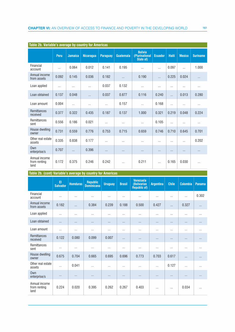
161CHAPTER VI: AN OVERVIEW OF ACCESS TO FINANCE AND POVERTY IN THE DEVELOPING WORLD
El Salvador
HomdurasRepublic
DominicanaUruguay Brasil
Venezuela(Bolivarian Republic of)
Argentina Chile Colombia Panama
Financial account
... ... ... ... ... ... ... ... ... 0.302
Annual income from assets
0.182 ... 0.384 0.239 0.188 0.500 0.427 ... 0.327 ...
Loan applied ... ... ... ... ... ... ... ... ... ...
Loan obtained ... ... ... ... ... ... ... ... ... ...
Loan amount ... ... ... ... ... ... ... ... ... ...
Remittances received
0.122 0.080 0.099 0.007 ... ... ... ... ... ...
Remittances sent
... ... ... ... ... ... ... ... ... ...
House dwelling owner
0.675 0.704 0.665 0.695 0.696 0.773 0.703 0.617 ... ...
Other real estate assets
... 0.041 ... ... ... ... ... 0.127 ... ...
Own enterprise/s
... ... ... ... ... ... ... ... ... ...
Annual income from renting land
0.224 0.020 0.395 0.262 0.267 0.403 ... ... 0.034 ...
Peru Jamaica Nicaragua Paraguay GuatemalaBolivia
(Plurinational State of)
Ecuador Haiti Mexico Suriname
Financial account
... 0.064 0.012 0.141 0.195 ... ... 0.097 ... 1.000
Annual income from assets
0.092 0.145 0.036 0.182 ... 0.190 ... 0.225 0.024 ...
Loan applied ... ... ... 0.037 0.132 ... ... ... ... ...
Loan obtained 0.137 0.048 ... 0.037 0.877 0.116 0.240 ... 0.013 0.280
Loan amount 0.004 ... ... ... 0.157 ... 0.168 ... ... ...
Remittances received
0.377 0.322 0.435 0.187 0.137 1.000 0.321 0.219 0.048 0.224
Remittances sent
0.556 0.186 0.021 ... ... ... 0.105 ... ... ...
House dwelling owner
0.731 0.559 0.776 0.753 0.715 0.659 0.746 0.710 0.645 0.701
Other real estate assets
0.335 0.838 0.177 ... ... ... ... ... ... 0.202
Own enterprise/s
0.707 ... 0.396 ... ... ... ... ... ... ...
Annual income from renting land
0.172 0.375 0.246 0.242 ... 0.211 ... 0.165 0.030 ...
Table 2b. Variable’s average by country for Americas
Table 2b. (cont) Variable’s average by country for Americas

162 SERVICES, TRADE & DEVELOPMENT
Kyrgyzstan Moldova Romania Armenia Bulgaria Albania Ukraine
Financial account 1.000 0.003 0.177 ... 0.002 ... ...
Annual income from assets 0.033 0.220 0.318 0.640 0.995 ... 0.076
Loan applied 0.052 ... 0.002 ... ... ... ...
Loan obtained 1.000 0.229 0.132 0.471 0.041 ... 0.373
Loan amount 0.004 1.282 0.004 3.445 0.171 ... 0.017
Remittances received ... 0.103 0.088 - 0.375 0.872 0.242 ...
Remittances sent 0.474 0.129 0.081 0.159 0.850 0.073 ...
House dwelling owner 0.919 0.875 0.960 0.917 0.889 0.926 0.847
Other real estate assets 0.957 0.749 0.536 0.414 0.282 0.438 ...
Own enterprise/s 1.000 0.025 ... 0.153 ... 0.563 0.008
Annual income from renting land 0.032 0.517 0.278 0.640 0.403 0.129 0.023
Table 2d. Variable’s average by country for Europe and Central Asia
Pakistan Bangladesh Viet Nam Indonesia
Financial account 1.000 ... 0.141 ...
Annual income from assets 0.118 0.209 ... ...
Loan applied ... ... ... ...
Loan obtained 1.000 ... 0.491 ...
Loan amount 0.054 ... ... ...
Remittances received 0.175 0.264 0.268 ...
Remittances sent 0.018 0.035 ...
House dwelling owner 0.915 0.813 0.936 0.842
Other real estate assets 0.838 0.320 0.033 0.413
Own enterprise/s 0.476 ... ... 0.313
Annual income from renting land 0.230 0.673 ... ...
Table 2c. Variable’s average by country for Asia

DISTRIBUTIONAL INCIDENCE OF ACCESS TO SERVICES
IN LATIN AMERICA
The objective of this chapter is to provide information regarding the
distributional incidence of access to services in Latin America, and
in particular how it can help explain the relatively higher shares of
services expenditure by the rich observed by Olarreaga et al. (2009).
There is an examination on whether there is a higher concentration
of services expenditure in rich household that can be explained by a
lack of access to services by poor households. Using concentration
curves that look at the concentration in the access to different services,
a conclusion is reached that the distribution of access to services is
not an important determinant of the relatively higher share of services
expenditure by the rich, except in some services sub-sectors such as
telecommunications. In most of the other sub-sectors, even though a
pro-rich pattern in access to services is observed, it remains relatively
weak and seems to mainly be explained by “access” to high quality
services.
164 SERVICES, TRADE & DEVELOPMENT
1. INTRODUCTION
When studying the distributional incidence of
expenditure, the question of access to consumption is
important, in particular when analysing the expenditure
for basic services such as water and electricity. To
illustrate this, assume that service coverage varies
by geographic area, being higher in rich areas (that
is, areas inhabited by richer households). A pro-rich
distribution of expenditure and shares that increase
with household total expenditure per capita will be
observed because poor households living in poor
regions have no, or limited, access to the service.
Thus, a necessary complement to the analysis of
the expenditure distribution and share patterns in
Olarreaga et al. (2009) is to analyse how access to
services is distributed along income levels.1 Access
patterns are hidden behind expenditure patterns.
Therefore the understanding of who access different
services should help explain the distribution of
services expenditure. 2
It should be noted that for some services, such as
primary education, health insurance coverage or
mobile telephone, it is not entirely appropriate to
talk about access since there usually are no access
restrictions other than prices. Despite this, and for
simplicity, “access” shall be referred to as meaning
that the service is consumed. Possibly, the three main
reasons to explain why some households decide not
to access those services are: (1) they are too poor
to afford them (prices are too high compared to
their income or to other prices); (2) they face higher
opportunity costs; or (3) they have low preference for
those services.
The analysis is restricted to Latin America due to data
restrictions not allowing for a systematic undertaking
of this type of study using surveys of other regions.
Results suggest that the concentration of access to
services explains little of the high concentration and
pro-rich bias observed in services expenditure. Even
though most services show some pro-rich bias in the
access to services, (suggesting that rich households
tend to have a higher level of access to services
than poor households) this bias remains relatively
small and cannot explain some of the strong pro-
rich biases observed in services expenditure. The
exception is perhaps in telecommunications where a
strong pro-rich bias in access is evident, which could
help explain the strong pro-rich bias observed for
telecommunications expenditure.
In most of the other services sub-sectors, even
though there is some pro-rich bias, it is not sufficiently
significant enough to explain in a meaningful way the
pro-rich bias observed in services expenditure. There
is, however, evidence that the bias in access to high
quality services (such as private education, or private
health insurance) is more unequal, and therefore
access to quality, rather than simple access may be
more of an issue. But here, lack of access could be
explained by high prices that the poor are unable to
afford, rather than to a lack of infrastructure.
The rest of this chapter is organized as follows. Section
2 provides an analysis of the distributional incidence
of access for the eight Latin American countries
studied in section 4 of Olarreaga et al. (2009).
Section 3 expands the analysis to other countries in
Latin America for which data is available. Section 4
concludes.
2. DISTRIBUTIONAL INCIDENCE OF ACCESS TO SERVICES IN LATIN AMERICA
The analysis of access is performed for the same
sectors as was the case in Olarreaga et al. (2009):
education; health; telecommunications; transport;
water; electricity; and gas. In addition, home and
internet connections are also looked at and within
these sub-sectors a further differentiation is made
along important dimensions that were not undertaken
earlier. For example, in the case of education, a
differentiation will be made between primary and
secondary education, as well as private and public
education. The methodology closely follows the one
developed in section 3 (Olarreaga et al. 2009), and
basically consists of the calculation of concentration
curves for access to different services. It is important
to note that contrary to the analysis on services
expenditure shares in Olarreaga et al. (2009), where
concentration curves are calculated in terms of
access, it will be nonsensical to compare them to
Lorenz curves of total expenditure or income. Thus,
there is no equivalent to the Kakwani indices that
were calculated in Olarreaga et al. (2009). A simple
comparison of the concentration curves to the perfect
equality line will be made, implying that access
to services is the same across the entire income
distribution.
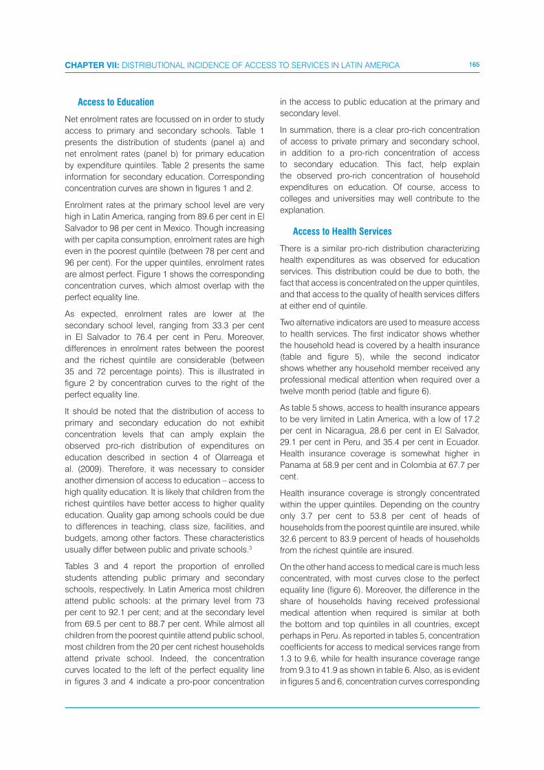
165CHAPTER VII: DISTRIBUTIONAL INCIDENCE OF ACCESS TO SERVICES IN LATIN AMERICA
Access to Education
Net enrolment rates are focussed on in order to study
access to primary and secondary schools. Table 1
presents the distribution of students (panel a) and
net enrolment rates (panel b) for primary education
by expenditure quintiles. Table 2 presents the same
information for secondary education. Corresponding
concentration curves are shown in figures 1 and 2.
Enrolment rates at the primary school level are very
high in Latin America, ranging from 89.6 per cent in El
Salvador to 98 per cent in Mexico. Though increasing
with per capita consumption, enrolment rates are high
even in the poorest quintile (between 78 per cent and
96 per cent). For the upper quintiles, enrolment rates
are almost perfect. Figure 1 shows the corresponding
concentration curves, which almost overlap with the
perfect equality line.
As expected, enrolment rates are lower at the
secondary school level, ranging from 33.3 per cent
in El Salvador to 76.4 per cent in Peru. Moreover,
differences in enrolment rates between the poorest
and the richest quintile are considerable (between
35 and 72 percentage points). This is illustrated in
figure 2 by concentration curves to the right of the
perfect equality line.
It should be noted that the distribution of access to
primary and secondary education do not exhibit
concentration levels that can amply explain the
observed pro-rich distribution of expenditures on
education described in section 4 of Olarreaga et
al. (2009). Therefore, it was necessary to consider
another dimension of access to education – access to
high quality education. It is likely that children from the
richest quintiles have better access to higher quality
education. Quality gap among schools could be due
to differences in teaching, class size, facilities, and
budgets, among other factors. These characteristics
usually differ between public and private schools.3
Tables 3 and 4 report the proportion of enrolled
students attending public primary and secondary
schools, respectively. In Latin America most children
attend public schools: at the primary level from 73
per cent to 92.1 per cent; and at the secondary level
from 69.5 per cent to 88.7 per cent. While almost all
children from the poorest quintile attend public school,
most children from the 20 per cent richest households
attend private school. Indeed, the concentration
curves located to the left of the perfect equality line
in figures 3 and 4 indicate a pro-poor concentration
in the access to public education at the primary and
secondary level.
In summation, there is a clear pro-rich concentration
of access to private primary and secondary school,
in addition to a pro-rich concentration of access
to secondary education. This fact, help explain
the observed pro-rich concentration of household
expenditures on education. Of course, access to
colleges and universities may well contribute to the
explanation.
Access to Health Services
There is a similar pro-rich distribution characterizing
health expenditures as was observed for education
services. This distribution could be due to both, the
fact that access is concentrated on the upper quintiles,
and that access to the quality of health services differs
at either end of quintile.
Two alternative indicators are used to measure access
to health services. The first indicator shows whether
the household head is covered by a health insurance
(table and figure 5), while the second indicator
shows whether any household member received any
professional medical attention when required over a
twelve month period (table and figure 6).
As table 5 shows, access to health insurance appears
to be very limited in Latin America, with a low of 17.2
per cent in Nicaragua, 28.6 per cent in El Salvador,
29.1 per cent in Peru, and 35.4 per cent in Ecuador.
Health insurance coverage is somewhat higher in
Panama at 58.9 per cent and in Colombia at 67.7 per
cent.
Health insurance coverage is strongly concentrated
within the upper quintiles. Depending on the country
only 3.7 per cent to 53.8 per cent of heads of
households from the poorest quintile are insured, while
32.6 percent to 83.9 percent of heads of households
from the richest quintile are insured.
On the other hand access to medical care is much less
concentrated, with most curves close to the perfect
equality line (figure 6). Moreover, the difference in the
share of households having received professional
medical attention when required is similar at both
the bottom and top quintiles in all countries, except
perhaps in Peru. As reported in tables 5, concentration
coefficients for access to medical services range from
1.3 to 9.6, while for health insurance coverage range
from 9.3 to 41.9 as shown in table 6. Also, as is evident
in figures 5 and 6, concentration curves corresponding

166 SERVICES, TRADE & DEVELOPMENT
to health insurance coverage are much further from
the perfect equality line than those corresponding to
access to medical services.
At first glance, this seems to suggest that access to
health services is not really a problem in Latin America.
However access to private health insurance and
therefore high quality private medical services is much
more concentrated. Thus, as in the case of education,
taking into account differences in the quality of health
services accessed by poorer and richer households
may help explain the observed expenditure patterns.
Access to Fixed and Mobile Telephones
Access to fixed-line telephone services (fixed phone)
is rather limited in Latin America. As shown in table 7,
the percentage of households with access to a fixed
phone ranges from 14.2 per cent in Nicaragua to a
maximum of 54.6 per cent in Colombia. Moreover,
the distribution of telephone access is extremely
concentrated on the upper quintiles. For example,
only 1 per cent of households have a fixed phone
among Peru’s bottom quintile compared to almost 70
per cent of households from the richest quintile. Thus,
the corresponding concentration curves are located
far to the right of the perfect equality line, as can be
seen in figure 7.
This high pro-rich concentration in the distribution of
access also clarifies the high pro-rich concentration of
expenditures on fixed phones (discussed in section 4).
The distribution of access to mobile phone services
(mobile phones) is described in table 8 and figure 8.
Access to mobile phones varies between 17.5 per cent
in Colombia to 68.2 per cent in Ecuador. Considering
median values of coverage across countries,
approximately 36 per cent of households have fixed
phones and mobile phones. As previously pointed
out, Colombia has the highest fixed phone access
(54.6 per cent), but also has the lowest mobile phone
coverage (17.5 per cent). Although this suggests
some kind of substitution in the consumption of the
two services, the case of Colombia seems to be the
exception. The remaining Latin American countries
have wider fixed phone coverage as well as wider
mobile phone coverage (Spearman´s rank correlation
equals 64 per cent).
Although access to mobile phones is concentrated on
the upper quintiles, the use of mobile phones is more
common among poor households than their access
to fixed phones.
Access to Home Internet Connection
In addition to fixed phones and mobile phones, total
household telecommunication expenditures include
other services such as postal services and internet.
While surveys lack information on postal services use,
there is available data on home internet connection.
Table 9 and figure 9 describe the distribution of internet
access along the per capita household consumption
distribution.
Access to home internet is very rare throughout Latin
America. Mexico has the highest coverage at 8.4 per
cent, followed by Colombia at 5.3 per cent, Panama
at 5.0 per cent, and Peru at 4.7 per cent. As expected,
internet access is extremely pro-rich concentrated,
with virtually no households from the poorer quintiles
with home internet connection.
Access to Transport Services (Public and Private)
As mentioned earlier, available information on the use
of transport services does not exist for most Latin
American countries. Therefore, access is substituted
by an indicator of positive household expenditure
on transport services, both private and public.
Under this definition, the lack of access to transport
services means that a family does not report positive
expenditures on any means of transport, presumably
because it does not use any.
As table 10 shows, depending on the country, between
65.2 per cent and 90.9 per cent of households
use either public or private transport services. The
distribution of access exhibits a slight pro-rich
concentration (see figure 10), but still access varies
markedly by quintiles. For example, in Peru, Colombia
and Ecuador, at least 50 per cent of families from the
poorest quintile do not pay for the use of transport
services, while more than 80 per cent of the families
from the richest quintile do pay for transport services.
Access to Water
Two alternative indicators of access to water services
are used. According to the first indicator, a household
has access to water if it has a source of (presumably)
drinkable water in its terrain or dwelling. According
to the second indicator, a household has access to
water if it is connected to a water network. Clearly, if
a household has access to water based on the latter
definition, then it also has access to water based on
the former. Tables 11 and 12 describe the distribution
of access to water across consumption quintiles
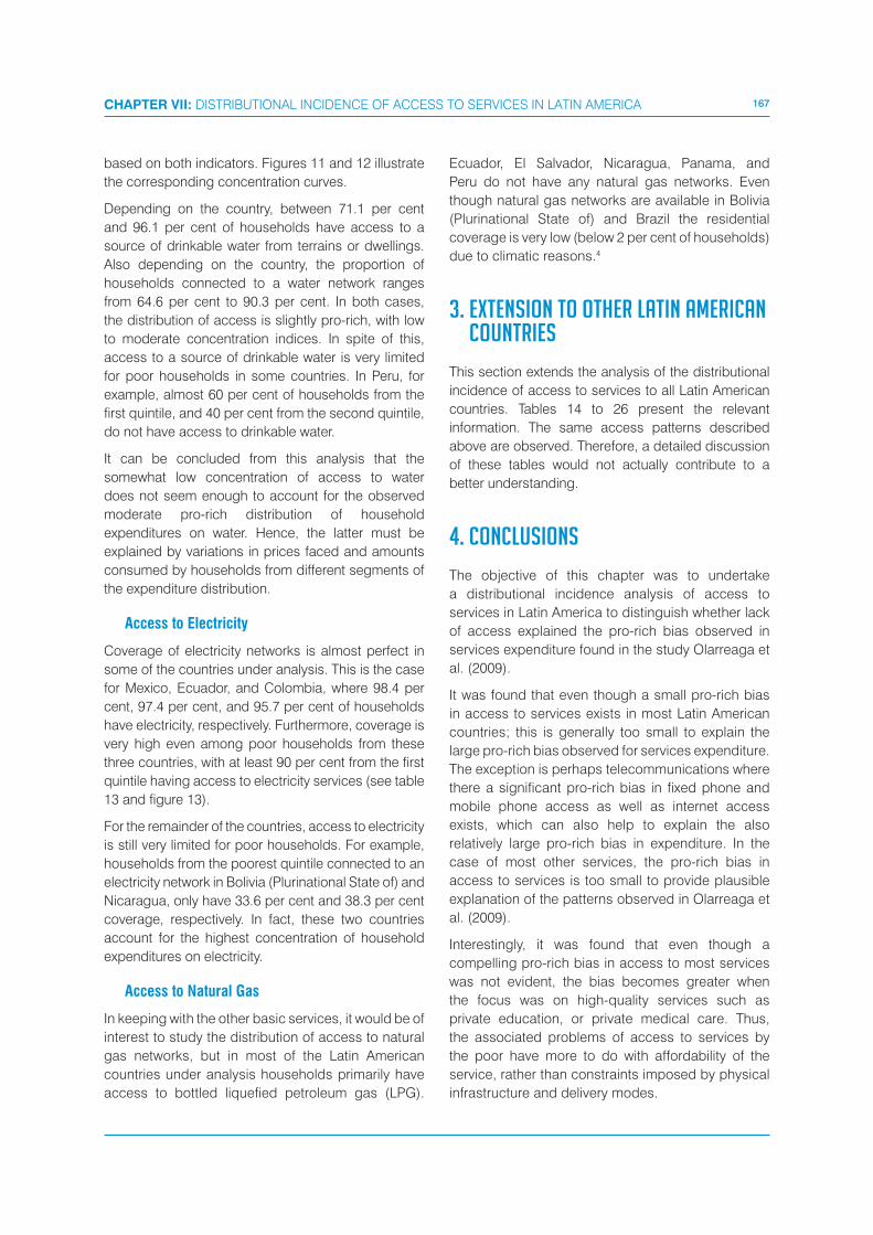
167CHAPTER VII: DISTRIBUTIONAL INCIDENCE OF ACCESS TO SERVICES IN LATIN AMERICA
based on both indicators. Figures 11 and 12 illustrate
the corresponding concentration curves.
Depending on the country, between 71.1 per cent
and 96.1 per cent of households have access to a
source of drinkable water from terrains or dwellings.
Also depending on the country, the proportion of
households connected to a water network ranges
from 64.6 per cent to 90.3 per cent. In both cases,
the distribution of access is slightly pro-rich, with low
to moderate concentration indices. In spite of this,
access to a source of drinkable water is very limited
for poor households in some countries. In Peru, for
example, almost 60 per cent of households from the
first quintile, and 40 per cent from the second quintile,
do not have access to drinkable water.
It can be concluded from this analysis that the
somewhat low concentration of access to water
does not seem enough to account for the observed
moderate pro-rich distribution of household
expenditures on water. Hence, the latter must be
explained by variations in prices faced and amounts
consumed by households from different segments of
the expenditure distribution.
Access to Electricity
Coverage of electricity networks is almost perfect in
some of the countries under analysis. This is the case
for Mexico, Ecuador, and Colombia, where 98.4 per
cent, 97.4 per cent, and 95.7 per cent of households
have electricity, respectively. Furthermore, coverage is
very high even among poor households from these
three countries, with at least 90 per cent from the first
quintile having access to electricity services (see table
13 and figure 13).
For the remainder of the countries, access to electricity
is still very limited for poor households. For example,
households from the poorest quintile connected to an
electricity network in Bolivia (Plurinational State of) and
Nicaragua, only have 33.6 per cent and 38.3 per cent
coverage, respectively. In fact, these two countries
account for the highest concentration of household
expenditures on electricity.
Access to Natural Gas
In keeping with the other basic services, it would be of
interest to study the distribution of access to natural
gas networks, but in most of the Latin American
countries under analysis households primarily have
access to bottled liquefied petroleum gas (LPG).
Ecuador, El Salvador, Nicaragua, Panama, and
Peru do not have any natural gas networks. Even
though natural gas networks are available in Bolivia
(Plurinational State of) and Brazil the residential
coverage is very low (below 2 per cent of households)
due to climatic reasons.4
3. EXTENSION TO OTHER LATIN AMERICAN COUNTRIES
This section extends the analysis of the distributional
incidence of access to services to all Latin American
countries. Tables 14 to 26 present the relevant
information. The same access patterns described
above are observed. Therefore, a detailed discussion
of these tables would not actually contribute to a
better understanding.
4. CONCLUSIONS
The objective of this chapter was to undertake
a distributional incidence analysis of access to
services in Latin America to distinguish whether lack
of access explained the pro-rich bias observed in
services expenditure found in the study Olarreaga et
al. (2009).
It was found that even though a small pro-rich bias
in access to services exists in most Latin American
countries; this is generally too small to explain the
large pro-rich bias observed for services expenditure.
The exception is perhaps telecommunications where
there a significant pro-rich bias in fixed phone and
mobile phone access as well as internet access
exists, which can also help to explain the also
relatively large pro-rich bias in expenditure. In the
case of most other services, the pro-rich bias in
access to services is too small to provide plausible
explanation of the patterns observed in Olarreaga et
al. (2009).
Interestingly, it was found that even though a
compelling pro-rich bias in access to most services
was not evident, the bias becomes greater when
the focus was on high-quality services such as
private education, or private medical care. Thus,
the associated problems of access to services by
the poor have more to do with affordability of the
service, rather than constraints imposed by physical
infrastructure and delivery modes.
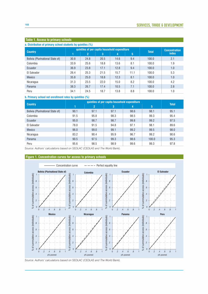
168 SERVICES, TRADE & DEVELOPMENT
b. Primary school net enrollment rates by quintiles (%)
Countryquintiles of per capita household expenditure
Total1 2 3 4 5
Bolivia (Plurinational State of) 90.1 97.1 97.1 98.6 98.1 95.1
Colombia 91.5 95.8 98.3 98.5 99.3 95.4
Ecuador 95.0 98.7 98.7 99.8 99.2 97.5
El Salvador 78.0 91.5 94.8 97.1 98.1 89.6
Mexico 96.0 99.0 99.1 99.2 99.5 98.0
Nicaragua 83.2 90.4 95.9 96.7 99.2 90.6
Panama 90.5 97.5 99.3 98.6 100.0 95.3
Peru 95.6 98.5 98.9 99.6 99.3 97.8
Source: Authors’ calculations based on SEDLAC (CEDLAS and The World Bank).
a. Distribution of primary school students by quintiles (%)
Countryquintiles of per capita household expenditure
TotalConcentration
index1 2 3 4 5
Bolivia (Plurinational State of) 30.8 24.8 20.5 14.6 9.4 100.0 2.1
Colombia 33.9 25.6 18.8 13.6 8.1 100.0 1.9
Ecuador 36.9 23.8 17.1 12.8 9.4 100.0 1.0
El Salvador 26.4 25.3 21.5 15.7 11.1 100.0 5.3
Mexico 35.8 25.0 18.8 12.3 8.1 100.0 1.0
Nicaragua 31.3 23.5 22.0 15.0 8.2 100.0 4.2
Panama 38.3 26.7 17.4 10.5 7.1 100.0 2.8
Peru 34.1 24.5 18.7 13.8 8.8 100.0 1.0
Table 1. Access to primary schools
Figure 1. Concentration curves for access to primary schools
Concentration curve Perfect equality line
0
.2
.4
.6
.8
1
% o
f cu
mm
ulat
ive
acce
ss (
indi
vidu
als)
0 .2 .4 .6 .8 1
Bolivia (Plurinational State of)
0
.2
.4
.6
.8
1
% o
f cu
mm
ulat
ive
acce
ss (
indi
vidu
als)
0 .2 .4 .6 .8 1
Colombia
0
.2
.4
.6
.8
1
% o
f cu
mm
ulat
ive
acce
ss (
indi
vidu
als)
0 .2 .4 .6 .8 1
Ecuador
0
.2
.4
.6
.8
1
% o
f cu
mm
ulat
ive
acce
ss (
indi
vidu
als)
0 .2 .4 .6 .8 1
El Salvador
0
.2
.4
.6
.8
1
% o
f cu
mm
ulat
ive
acce
ss (
indi
vidu
als)
0 .2 .4 .6 .8 1
p% poorest
Nicaragua
0
.2
.4
.6
.8
1
% o
f cu
mm
ulat
ive
acce
ss (
indi
vidu
als)
0 .2 .4 .6 .8 1
p% poorest
Mexico
0
.2
.4
.6
.8
1
% o
f cu
mm
ulat
ive
acce
ss (
indi
vidu
als)
0 .2 .4 .6 .8 1
p% poorest
Panama
0
.2
.4
.6
.8
1
% o
f cu
mm
ulat
ive
acce
ss (
indi
vidu
als)
0 .2 .4 .6 .8 1
p% poorest
Peru
Source: Authors’ calculations based on SEDLAC (CEDLAS and The World Bank).
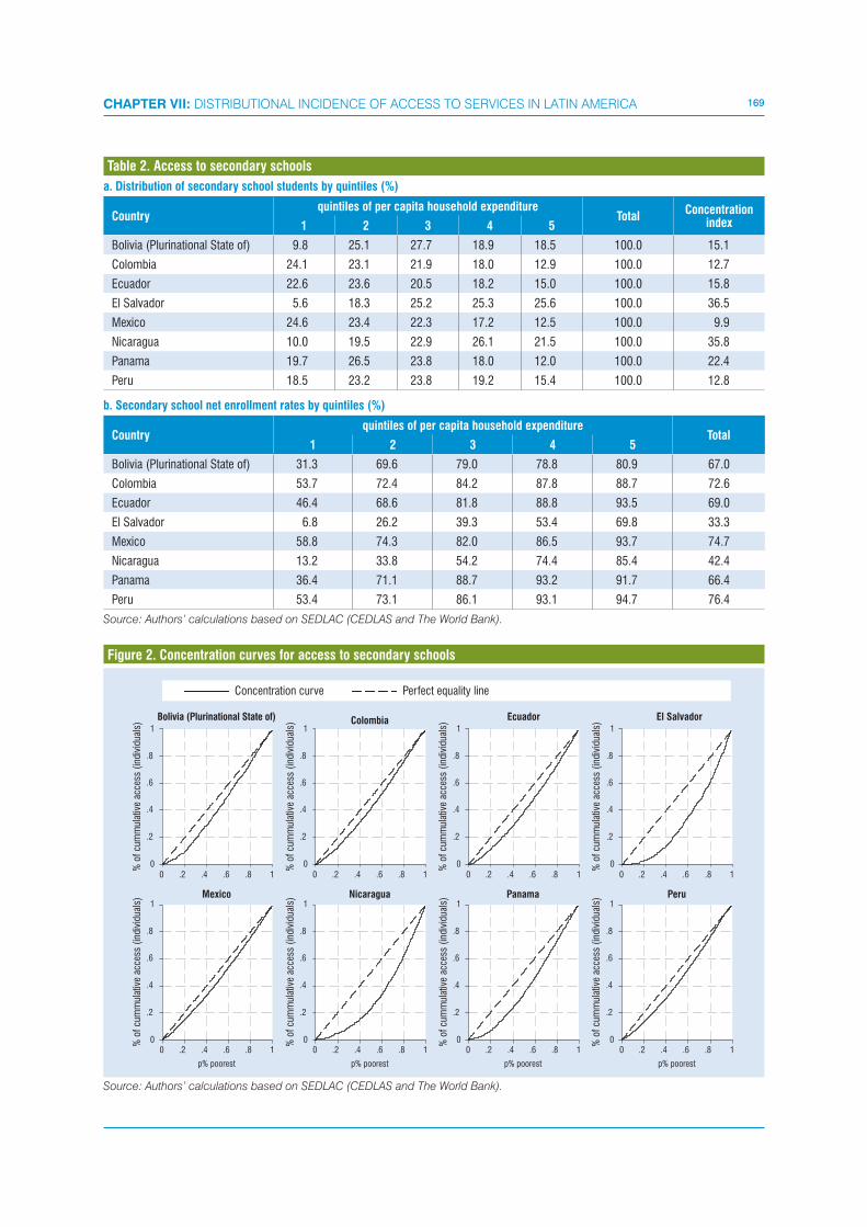
169CHAPTER VII: DISTRIBUTIONAL INCIDENCE OF ACCESS TO SERVICES IN LATIN AMERICA
a. Distribution of secondary school students by quintiles (%)
Countryquintiles of per capita household expenditure
TotalConcentration
index1 2 3 4 5
Bolivia (Plurinational State of) 9.8 25.1 27.7 18.9 18.5 100.0 15.1
Colombia 24.1 23.1 21.9 18.0 12.9 100.0 12.7
Ecuador 22.6 23.6 20.5 18.2 15.0 100.0 15.8
El Salvador 5.6 18.3 25.2 25.3 25.6 100.0 36.5
Mexico 24.6 23.4 22.3 17.2 12.5 100.0 9.9
Nicaragua 10.0 19.5 22.9 26.1 21.5 100.0 35.8
Panama 19.7 26.5 23.8 18.0 12.0 100.0 22.4
Peru 18.5 23.2 23.8 19.2 15.4 100.0 12.8 b. Secondary school net enrollment rates by quintiles (%)
Countryquintiles of per capita household expenditure
Total1 2 3 4 5
Bolivia (Plurinational State of) 31.3 69.6 79.0 78.8 80.9 67.0
Colombia 53.7 72.4 84.2 87.8 88.7 72.6
Ecuador 46.4 68.6 81.8 88.8 93.5 69.0
El Salvador 6.8 26.2 39.3 53.4 69.8 33.3
Mexico 58.8 74.3 82.0 86.5 93.7 74.7
Nicaragua 13.2 33.8 54.2 74.4 85.4 42.4
Panama 36.4 71.1 88.7 93.2 91.7 66.4
Peru 53.4 73.1 86.1 93.1 94.7 76.4
Source: Authors’ calculations based on SEDLAC (CEDLAS and The World Bank).
Table 2. Access to secondary schools
Figure 2. Concentration curves for access to secondary schools
Concentration curve Perfect equality line
0
.2
.4
.6
.8
1
% o
f cu
mm
ulat
ive
acce
ss (
indi
vidu
als)
0 .2 .4 .6 .8 1
Bolivia (Plurinational State of)
0
.2
.4
.6
.8
1
% o
f cu
mm
ulat
ive
acce
ss (
indi
vidu
als)
0 .2 .4 .6 .8 1
Colombia
0
.2
.4
.6
.8
1
% o
f cu
mm
ulat
ive
acce
ss (
indi
vidu
als)
0 .2 .4 .6 .8 1
Ecuador
0
.2
.4
.6
.8
1
% o
f cu
mm
ulat
ive
acce
ss (
indi
vidu
als)
0 .2 .4 .6 .8 1
El Salvador
0
.2
.4
.6
.8
1
% o
f cu
mm
ulat
ive
acce
ss (
indi
vidu
als)
0 .2 .4 .6 .8 1
p% poorest
Nicaragua
0
.2
.4
.6
.8
1
% o
f cu
mm
ulat
ive
acce
ss (
indi
vidu
als)
0 .2 .4 .6 .8 1
p% poorest
Mexico
0
.2
.4
.6
.8
1
% o
f cu
mm
ulat
ive
acce
ss (
indi
vidu
als)
0 .2 .4 .6 .8 1
p% poorest
Panama
0
.2
.4
.6
.8
1
% o
f cu
mm
ulat
ive
acce
ss (
indi
vidu
als)
0 .2 .4 .6 .8 1
p% poorest
Peru
Source: Authors’ calculations based on SEDLAC (CEDLAS and The World Bank).

170 SERVICES, TRADE & DEVELOPMENT
a. Distribution of primary school students attending public schools by quintiles (%)
Countryquintiles of per capita household expenditure
TotalConcentration
index1 2 3 4 5
Bolivia (Plurinational State of) 33.4 26.7 21.3 13.8 4.8 100.0 -6.6
Colombia 39.3 28.3 18.3 10.7 3.5 100.0 -10.7
Ecuador 46.0 26.0 16.4 8.8 2.8 100.0 -15.9
El Salvador 30.7 28.7 22.1 13.2 5.2 100.0 -11.0
Mexico 38.8 26.8 19.4 11.0 3.9 100.0 -6.7
Nicaragua 34.6 25.5 22.9 12.9 4.2 100.0 -8.0
Panama 42.2 29.1 17.8 8.5 2.4 100.0 -8.4
Peru 38.0 27.9 19.1 11.4 3.6 100.0 -10.1 b. Proportion of primary school students attending public schools by quintiles (%)
Countryquintiles of per capita household expenditure
Total1 2 3 4 5
Bolivia (Plurinational State of) 99.1 98.1 94.8 86.3 46.9 91.3
Colombia 97.5 92.8 81.9 65.9 35.6 84.0
Ecuador 91.6 79.7 69.6 49.7 21.8 73.0
El Salvador 98.2 96.0 86.9 71.2 39.9 84.5
Mexico 99.8 98.7 95.2 82.7 44.6 92.1
Nicaragua 99.6 97.4 92.8 76.2 46.2 89.7
Panama 99.6 97.9 91.8 72.6 30.1 90.0
Peru 99.0 98.1 88.4 70.7 36.0 87.3
Source: Authors’ calculations based on SEDLAC (CEDLAS and The World Bank).
Table 3. Access to public primary schools
Figure 3. Concentration curves for access to public primary schools
Concentration curve Perfect equality line
0
.2
.4
.6
.8
1
% o
f cu
mm
ulat
ive
acce
ss (
indi
vidu
als)
0 .2 .4 .6 .8 1
Bolivia (Plurinational State of)
0
.2
.4
.6
.8
1
% o
f cu
mm
ulat
ive
acce
ss (
indi
vidu
als)
0 .2 .4 .6 .8 1
Colombia
0
.2
.4
.6
.8
1
% o
f cu
mm
ulat
ive
acce
ss (
indi
vidu
als)
0 .2 .4 .6 .8 1
Ecuador
0
.2
.4
.6
.8
1
% o
f cu
mm
ulat
ive
acce
ss (
indi
vidu
als)
0 .2 .4 .6 .8 1
El Salvador
0
.2
.4
.6
.8
1
% o
f cu
mm
ulat
ive
acce
ss (
indi
vidu
als)
0 .2 .4 .6 .8 1
p% poorest
Nicaragua
0
.2
.4
.6
.8
1
% o
f cu
mm
ulat
ive
acce
ss (
indi
vidu
als)
0 .2 .4 .6 .8 1
p% poorest
Mexico
0
.2
.4
.6
.8
1
% o
f cu
mm
ulat
ive
acce
ss (
indi
vidu
als)
0 .2 .4 .6 .8 1
p% poorest
Panama
0
.2
.4
.6
.8
1
% o
f cu
mm
ulat
ive
acce
ss (
indi
vidu
als)
0 .2 .4 .6 .8 1
p% poorest
Peru
Source: Authors’ Scalculations based on SEDLAC (CEDLAS and The World Bank).

171CHAPTER VII: DISTRIBUTIONAL INCIDENCE OF ACCESS TO SERVICES IN LATIN AMERICA
a. Distribution of primary school students attending public schools by quintiles (%)
Countryquintiles of per capita household expenditure
TotalConcentration
index1 2 3 4 5
Bolivia (Plurinational State of) 11.5 28.7 30.1 19.2 10.4 100.0 -10.2
Colombia 29.3 26.2 22.7 15.3 6.5 100.0 -12.2
Ecuador 27.5 27.1 22.0 16.9 6.5 100.0 -13.1
El Salvador 7.9 23.3 27.9 23.9 17.0 100.0 -15.3
Mexico 27.1 25.5 22.9 16.4 8.0 100.0 -7.3
Nicaragua 13.1 23.3 25.3 24.7 13.6 100.0 -13.0
Panama 22.4 29.7 25.4 16.9 5.6 100.0 -10.0
Peru 23.2 26.8 25.8 17.0 7.2 100.0 -11.8 b. Proportion of primary school students attending public schools by quintiles (%)
Countryquintiles of per capita household expenditure
Total1 2 3 4 5
Bolivia (Plurinational State of) 100.0 97.9 93.4 87.2 48.9 85.8
Colombia 96.1 90.6 82.7 67.7 40.3 79.6
Ecuador 86.1 81.3 75.7 65.7 30.6 70.8
El Salvador 97.3 90.0 77.0 65.2 45.9 69.5
Mexico 98.4 96.5 91.1 84.4 56.7 88.7
Nicaragua 95.3 86.1 81.0 69.9 45.5 72.8
Panama 98.0 97.7 92.1 80.8 40.1 86.5
Peru 98.5 96.5 91.4 78.6 40.1 83.9
Source: Authors’ calculations based on SEDLAC (CEDLAS and The World Bank).
Table 4. Access to public primary schools
Figure 4. Concentration curves for access to public secondary schools
Concentration curve Perfect equality line
0
.2
.4
.6
.8
1
% o
f cu
mm
ulat
ive
acce
ss (
indi
vidu
als)
0 .2 .4 .6 .8 1
Bolivia (Plurinational State of)
0
.2
.4
.6
.8
1
% o
f cu
mm
ulat
ive
acce
ss (
indi
vidu
als)
0 .2 .4 .6 .8 1
Colombia
0
.2
.4
.6
.8
1
% o
f cu
mm
ulat
ive
acce
ss (
indi
vidu
als)
0 .2 .4 .6 .8 1
Ecuador
0
.2
.4
.6
.8
1
% o
f cu
mm
ulat
ive
acce
ss (
indi
vidu
als)
0 .2 .4 .6 .8 1
El Salvador
0
.2
.4
.6
.8
1
% o
f cu
mm
ulat
ive
acce
ss (
indi
vidu
als)
0 .2 .4 .6 .8 1
p% poorest
Nicaragua
0
.2
.4
.6
.8
1
% o
f cu
mm
ulat
ive
acce
ss (
indi
vidu
als)
0 .2 .4 .6 .8 1
p% poorest
Mexico
0
.2
.4
.6
.8
1
% o
f cu
mm
ulat
ive
acce
ss (
indi
vidu
als)
0 .2 .4 .6 .8 1
p% poorest
Panama
0
.2
.4
.6
.8
1
% o
f cu
mm
ulat
ive
acce
ss (
indi
vidu
als)
0 .2 .4 .6 .8 1
p% poorest
Peru
Source: Aauthors’ calculations based on SEDLAC (CEDLAS and The World Bank).
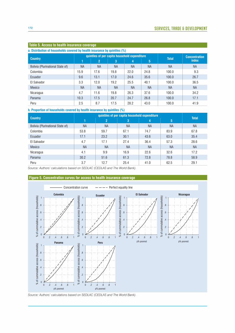
172 SERVICES, TRADE & DEVELOPMENT
Figure 5. Concentration curves for access to health insurance coverage
Concentration curve Perfect equality line
0
.2
.4
.6
.8
1
% o
f cu
mm
ulat
ive
acce
ss (
hous
ehol
ds)
0 .2 .4 .6 .8 1
Colombia
0
.2
.4
.6
.8
1
% o
f cu
mm
ulat
ive
acce
ss (
hous
ehol
ds)
0 .2 .4 .6 .8 1
Ecuador
0
.2
.4
.6
.8
1
% o
f cu
mm
ulat
ive
acce
ss (
hous
ehol
ds)
0 .2 .4 .6 .8 1
El Salvador
0
.2
.4
.6
.8
1
% o
f cu
mm
ulat
ive
acce
ss (
hous
ehol
ds)
0 .2 .4 .6 .8 1
Nicaragua
0
.2
.4
.6
.8
1
% o
f cu
mm
ulat
ive
acce
ss (
hous
ehol
ds)
0 .2 .4 .6 .8 1
p% poorest
Peru
0
.2
.4
.6
.8
1
% o
f cu
mm
ulat
ive
acce
ss (
hous
ehol
ds)
0 .2 .4 .6 .8 1
p% poorest
Panama p% poorest p% poorest
Source: Authors’ calculations based on SEDLAC (CEDLAS and The World Bank).
a. Distribution of households covered by health insurance by quintiles (%)
Countryquintiles of per capita household expenditure
TotalConcentration
index1 2 3 4 5
Bolivia (Plurinational State of) NA NA NA NA NA NA NA
Colombia 15.9 17.6 19.8 22.0 24.8 100.0 9.3
Ecuador 9.6 13.1 17.0 24.6 35.6 100.0 26.7
El Salvador 3.3 12.0 19.2 25.5 40.1 100.0 36.5
Mexico NA NA NA NA NA NA NA
Nicaragua 4.7 11.6 19.8 26.3 37.6 100.0 34.2
Panama 10.3 17.5 20.7 24.7 26.8 100.0 17.1
Peru 2.5 8.7 17.5 28.2 43.0 100.0 41.9 b. Proportion of households covered by health insurance by quintiles (%)
Countryquintiles of per capita household expenditure
Total1 2 3 4 5
Bolivia (Plurinational State of) NA NA NA NA NA NA
Colombia 53.8 59.7 67.1 74.7 83.9 67.8
Ecuador 17.1 23.2 30.1 43.6 63.0 35.4
El Salvador 4.7 17.1 27.4 36.4 57.3 28.6
Mexico NA NA NA NA NA NA
Nicaragua 4.1 9.9 16.9 22.6 32.6 17.2
Panama 30.2 51.6 61.3 72.8 78.8 58.9
Peru 3.7 12.7 25.4 41.0 62.5 29.1
Source: Authors’ calculations based on SEDLAC (CEDLAS and The World Bank).
Table 5. Access to health insurance coverage
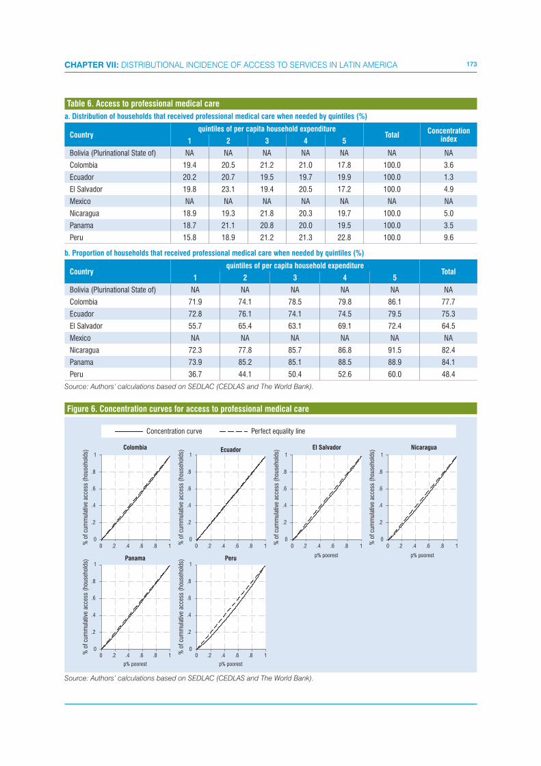
173CHAPTER VII: DISTRIBUTIONAL INCIDENCE OF ACCESS TO SERVICES IN LATIN AMERICA
a. Distribution of households that received professional medical care when needed by quintiles (%)
Countryquintiles of per capita household expenditure
TotalConcentration
index1 2 3 4 5
Bolivia (Plurinational State of) NA NA NA NA NA NA NA
Colombia 19.4 20.5 21.2 21.0 17.8 100.0 3.6
Ecuador 20.2 20.7 19.5 19.7 19.9 100.0 1.3
El Salvador 19.8 23.1 19.4 20.5 17.2 100.0 4.9
Mexico NA NA NA NA NA NA NA
Nicaragua 18.9 19.3 21.8 20.3 19.7 100.0 5.0
Panama 18.7 21.1 20.8 20.0 19.5 100.0 3.5
Peru 15.8 18.9 21.2 21.3 22.8 100.0 9.6 b. Proportion of households that received professional medical care when needed by quintiles (%)
Countryquintiles of per capita household expenditure
Total1 2 3 4 5
Bolivia (Plurinational State of) NA NA NA NA NA NA
Colombia 71.9 74.1 78.5 79.8 86.1 77.7
Ecuador 72.8 76.1 74.1 74.5 79.5 75.3
El Salvador 55.7 65.4 63.1 69.1 72.4 64.5
Mexico NA NA NA NA NA NA
Nicaragua 72.3 77.8 85.7 86.8 91.5 82.4
Panama 73.9 85.2 85.1 88.5 88.9 84.1
Peru 36.7 44.1 50.4 52.6 60.0 48.4
Source: Authors’ calculations based on SEDLAC (CEDLAS and The World Bank).
Table 6. Access to professional medical care
Figure 6. Concentration curves for access to professional medical care
Concentration curve Perfect equality line
0
.2
.4
.6
.8
1
% o
f cu
mm
ulat
ive
acce
ss (
hous
ehol
ds)
0 .2 .4 .6 .8 1
Colombia
0
.2
.4
.6
.8
1
% o
f cu
mm
ulat
ive
acce
ss (
hous
ehol
ds)
0 .2 .4 .6 .8 1
Ecuador
0
.2
.4
.6
.8
1
% o
f cu
mm
ulat
ive
acce
ss (
hous
ehol
ds)
0 .2 .4 .6 .8 1
El Salvador
0
.2
.4
.6
.8
1
% o
f cu
mm
ulat
ive
acce
ss (
hous
ehol
ds)
0 .2 .4 .6 .8 1
Nicaragua
0
.2
.4
.6
.8
1
% o
f cu
mm
ulat
ive
acce
ss (
hous
ehol
ds)
0 .2 .4 .6 .8 1
p% poorest
Peru
0
.2
.4
.6
.8
1
% o
f cu
mm
ulat
ive
acce
ss (
hous
ehol
ds)
0 .2 .4 .6 .8 1
p% poorest
Panama p% poorest p% poorest
Source: Authors’ calculations based on SEDLAC (CEDLAS and The World Bank).

174 SERVICES, TRADE & DEVELOPMENT
a. Distribution of households with fixed telephone by quintiles (%)
Countryquintiles of per capita household expenditure
TotalConcentration
index1 2 3 4 5
Bolivia (Plurinational State of) 0.3 3.4 10.8 31.4 54.0 100.0 55.4
Colombia 6.4 14.1 22.1 26.2 31.2 100.0 25.5
Ecuador 3.7 9.4 17.5 28.8 40.6 100.0 38.7
El Salvador 3.6 12.2 19.9 27.5 36.8 100.0 34.2
Mexico 7.8 15.5 21.5 25.7 29.5 100.0 22.5
Nicaragua 0.0 2.3 9.2 25.3 63.2 100.0 63.3
Panama 1.7 10.4 18.3 27.5 42.1 100.0 41.0
Peru 0.9 5.6 14.8 29.4 49.4 100.0 50.4 b. Proportion of households with fixed telephone by quintiles (%)
Countryquintiles of per capita household expenditure
Total1 2 3 4 5
Bolivia (Plurinational State of) 9.3 3.0 9.4 27.2 47.0 17.4
Colombia 17.6 38.4 60.4 71.4 85.2 54.6
Ecuador 7.2 18.2 33.7 55.5 78.2 38.6
El Salvador 7.3 24.8 40.3 55.9 74.6 40.6
Mexico 19.9 39.9 55.2 66.1 75.7 51.4
Nicaragua 0.0 1.7 6.5 18.0 45.0 14.2
Panama 2.8 17.1 30.2 45.4 69.4 33.0
Peru 1.2 7.8 20.6 40.9 68.7 27.8
Source: Authors’ calculations based on SEDLAC (CEDLAS and The World Bank).
Table 7. Access to fixed telephone
Figure 7. Concentration curves for access to fixed phone
Concentration curve Perfect equality line
0
.2
.4
.6
.8
1
% o
f cu
mm
ulat
ive
acce
ss (
hous
ehol
ds)
0 .2 .4 .6 .8 1
Bolivia (Plurinational State of)
0
.2
.4
.6
.8
1
% o
f cu
mm
ulat
ive
acce
ss (
hous
ehol
ds)
0 .2 .4 .6 .8 1
Colombia
0
.2
.4
.6
.8
1
% o
f cu
mm
ulat
ive
acce
ss (
hous
ehol
ds)
0 .2 .4 .6 .8 1
Ecuador
0
.2
.4
.6
.8
1
% o
f cu
mm
ulat
ive
acce
ss (
hous
ehol
ds)
0 .2 .4 .6 .8 1
El Salvador
0
.2
.4
.6
.8
1
% o
f cu
mm
ulat
ive
acce
ss (
hous
ehol
ds)
0 .2 .4 .6 .8 1
p% poorest
Nicaragua
0
.2
.4
.6
.8
1
% o
f cu
mm
ulat
ive
acce
ss (
hous
ehol
ds)
0 .2 .4 .6 .8 1
p% poorest
Mexico
0
.2
.4
.6
.8
1
% o
f cu
mm
ulat
ive
acce
ss (
hous
ehol
ds)
0 .2 .4 .6 .8 1
p% poorest
Panama
0
.2
.4
.6
.8
1
% o
f cu
mm
ulat
ive
acce
ss (
hous
ehol
ds)
0 .2 .4 .6 .8 1
p% poorest
Peru
Source: Authors’ calculations based on SEDLAC (CEDLAS and The World Bank).
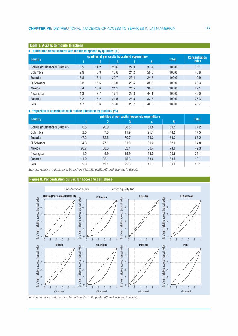
175CHAPTER VII: DISTRIBUTIONAL INCIDENCE OF ACCESS TO SERVICES IN LATIN AMERICA
a. Distribution of households with mobile telephone by quintiles (%)
Countryquintiles of per capita household expenditure
TotalConcentration
index1 2 3 4 5
Bolivia (Plurinational State of) 3.5 11.2 20.6 27.3 37.4 100.0 35.1
Colombia 2.9 8.9 13.6 24.2 50.5 100.0 46.8
Ecuador 13.8 18.4 20.7 22.4 24.7 100.0 10.9
El Salvador 8.2 15.6 18.0 22.5 35.6 100.0 26.3
Mexico 8.4 15.6 21.1 24.5 30.3 100.0 22.1
Nicaragua 1.3 7.7 17.1 29.8 44.1 100.0 45.0
Panama 5.2 15.2 21.5 25.5 32.6 100.0 27.3
Peru 1.7 8.6 18.0 29.7 42.0 100.0 42.7 b. Proportion of households with mobile telephone by quintiles (%)
Countryquintiles of per capita household expenditure
Total1 2 3 4 5
Bolivia (Plurinational State of) 6.5 20.9 38.5 50.8 69.5 37.2
Colombia 2.5 7.8 11.9 21.1 44.2 17.5
Ecuador 47.2 62.6 70.7 76.2 84.3 68.2
El Salvador 14.3 27.1 31.3 39.2 62.0 34.8
Mexico 20.7 38.6 52.1 60.4 74.6 49.3
Nicaragua 1.5 8.9 19.9 34.5 50.9 23.1
Panama 11.0 32.1 45.3 53.6 68.5 42.1
Peru 2.3 12.1 25.3 41.7 59.0 28.1
Source: Authors’ calculations based on SEDLAC (CEDLAS and The World Bank).
Table 8. Access to mobile telephone
Figure 8. Concentration curves for access to cell phone
Concentration curve Perfect equality line
0
.2
.4
.6
.8
1
% o
f cu
mm
ulat
ive
acce
ss (
hous
ehol
ds)
0 .2 .4 .6 .8 1
Bolivia (Plurinational State of)
0
.2
.4
.6
.8
1
% o
f cu
mm
ulat
ive
acce
ss (
hous
ehol
ds)
0 .2 .4 .6 .8 1
Colombia
0
.2
.4
.6
.8
1
% o
f cu
mm
ulat
ive
acce
ss (
hous
ehol
ds)
0 .2 .4 .6 .8 1
Ecuador
0
.2
.4
.6
.8
1
% o
f cu
mm
ulat
ive
acce
ss (
hous
ehol
ds)
0 .2 .4 .6 .8 1
El Salvador
0
.2
.4
.6
.8
1
% o
f cu
mm
ulat
ive
acce
ss (
hous
ehol
ds)
0 .2 .4 .6 .8 1
p% poorest
Nicaragua
0
.2
.4
.6
.8
1
% o
f cu
mm
ulat
ive
acce
ss (
hous
ehol
ds)
0 .2 .4 .6 .8 1
p% poorest
Mexico
0
.2
.4
.6
.8
1
% o
f cu
mm
ulat
ive
acce
ss (
hous
ehol
ds)
0 .2 .4 .6 .8 1
p% poorest
Panama
0
.2
.4
.6
.8
1
% o
f cu
mm
ulat
ive
acce
ss (
hous
ehol
ds)
0 .2 .4 .6 .8 1
p% poorest
Peru
Source: Authors’ calculations based on SEDLAC (CEDLAS and The World Bank).

176 SERVICES, TRADE & DEVELOPMENT
a. Distribution of households with internet connection by quintiles (%)
Countryquintiles of per capita household expenditure
TotalConcentration
index1 2 3 4 5
Bolivia (Plurinational State of) 0 1.0 2.3 18.8 78.9 100.0 77.2
Colombia 0.6 1.1 4.6 13.3 80.4 100.0 74.2
Ecuador 0 1.0 3.2 10.5 85.3 100.0 80.0
El Salvador 1.9 0 1.8 8.1 88.2 100.0 81.0
Mexico 0.3 2.7 9.4 22.2 65.4 100.0 64.4
Nicaragua 0 0 0 25.1 74.9 100.0 81.4
Panama 0 1.2 1.8 10.8 86.3 100.0 79.1
Peru 0 0 1.8 12.3 85.5 100.0 80.7 b. Proportion of households with internet connection by quintiles (%)
Countryquintiles of per capita household expenditure
Total1 2 3 4 5
Bolivia (Plurinational State of) 0 0 0.4 2.9 12.4 3.1
Colombia 0.2 0.3 1.2 3.6 21.5 5.3
Ecuador 0 0.1 0.5 1.5 12.2 2.9
El Salvador 0.2 0 0.2 0.9 9.5 2.1
Mexico 0.1 1.1 4.0 9.3 27.5 8.4
Nicaragua 0 0 0 0.2 0.6 0.1
Panama 0 0.3 0.5 2.7 21.6 5.0
Peru 0 0 0.4 2.9 20.1 4.7
Source: Authors’ calculations based on SEDLAC (CEDLAS and The World Bank).
Table 9. Access to home internet connection
Figure 9. Concentration curves for access to home internet connection
Concentration curve Perfect equality line
0
.2
.4
.6
.8
1
% o
f cu
mm
ulat
ive
acce
ss (
hous
ehol
ds)
0 .2 .4 .6 .8 1
Bolivia (Plurinational State of)
0
.2
.4
.6
.8
1
% o
f cu
mm
ulat
ive
acce
ss (
hous
ehol
ds)
0 .2 .4 .6 .8 1
Colombia
0
.2
.4
.6
.8
1
% o
f cu
mm
ulat
ive
acce
ss (
hous
ehol
ds)
0 .2 .4 .6 .8 1
Ecuador
0
.2
.4
.6
.8
1
% o
f cu
mm
ulat
ive
acce
ss (
hous
ehol
ds)
0 .2 .4 .6 .8 1
El Salvador
0
.2
.4
.6
.8
1
% o
f cu
mm
ulat
ive
acce
ss (
hous
ehol
ds)
0 .2 .4 .6 .8 1
p% poorest
Nicaragua
0
.2
.4
.6
.8
1
% o
f cu
mm
ulat
ive
acce
ss (
hous
ehol
ds)
0 .2 .4 .6 .8 1
p% poorest
Mexico
0
.2
.4
.6
.8
1
% o
f cu
mm
ulat
ive
acce
ss (
hous
ehol
ds)
0 .2 .4 .6 .8 1
p% poorest
Panama
0
.2
.4
.6
.8
1
% o
f cu
mm
ulat
ive
acce
ss (
hous
ehol
ds)
0 .2 .4 .6 .8 1
p% poorest
Peru
Source: Authors’ calculations based on SEDLAC (CEDLAS and The World Bank).
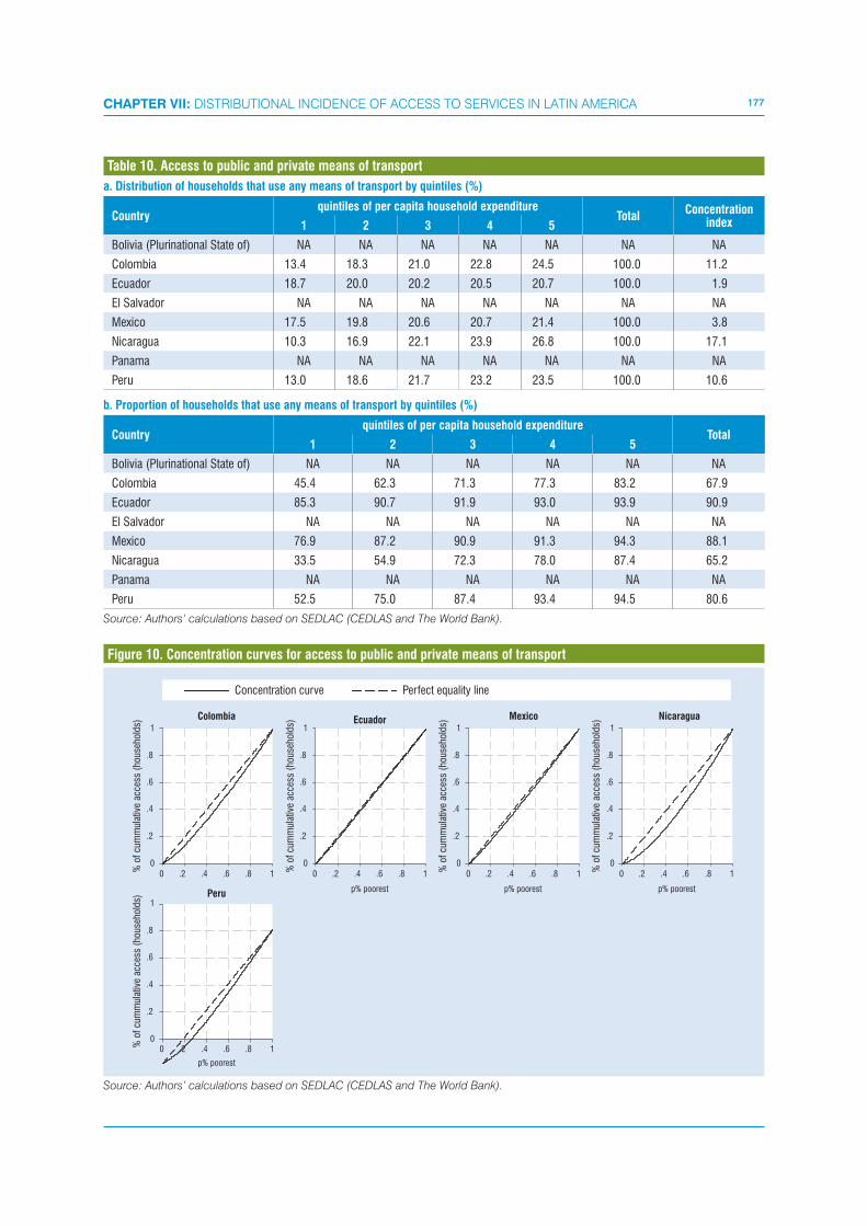
177CHAPTER VII: DISTRIBUTIONAL INCIDENCE OF ACCESS TO SERVICES IN LATIN AMERICA
a. Distribution of households that use any means of transport by quintiles (%)
Countryquintiles of per capita household expenditure
TotalConcentration
index1 2 3 4 5
Bolivia (Plurinational State of) NA NA NA NA NA NA NA
Colombia 13.4 18.3 21.0 22.8 24.5 100.0 11.2
Ecuador 18.7 20.0 20.2 20.5 20.7 100.0 1.9
El Salvador NA NA NA NA NA NA NA
Mexico 17.5 19.8 20.6 20.7 21.4 100.0 3.8
Nicaragua 10.3 16.9 22.1 23.9 26.8 100.0 17.1
Panama NA NA NA NA NA NA NA
Peru 13.0 18.6 21.7 23.2 23.5 100.0 10.6 b. Proportion of households that use any means of transport by quintiles (%)
Countryquintiles of per capita household expenditure
Total1 2 3 4 5
Bolivia (Plurinational State of) NA NA NA NA NA NA
Colombia 45.4 62.3 71.3 77.3 83.2 67.9
Ecuador 85.3 90.7 91.9 93.0 93.9 90.9
El Salvador NA NA NA NA NA NA
Mexico 76.9 87.2 90.9 91.3 94.3 88.1
Nicaragua 33.5 54.9 72.3 78.0 87.4 65.2
Panama NA NA NA NA NA NA
Peru 52.5 75.0 87.4 93.4 94.5 80.6
Source: Authors’ calculations based on SEDLAC (CEDLAS and The World Bank).
Table 10. Access to public and private means of transport
Figure 10. Concentration curves for access to public and private means of transport
Concentration curve Perfect equality line
0
.2
.4
.6
.8
1
% o
f cu
mm
ulat
ive
acce
ss (
hous
ehol
ds)
0 .2 .4 .6 .8 1
Colombia
0
.2
.4
.6
.8
1
% o
f cu
mm
ulat
ive
acce
ss (
hous
ehol
ds)
0 .2 .4 .6 .8 1
Ecuador
0
.2
.4
.6
.8
1
% o
f cu
mm
ulat
ive
acce
ss (
hous
ehol
ds)
0 .2 .4 .6 .8 1
Mexico
0
.2
.4
.6
.8
1
% o
f cu
mm
ulat
ive
acce
ss (
hous
ehol
ds)
0 .2 .4 .6 .8 1
Nicaragua
p% poorest
0
.2
.4
.6
.8
1
% o
f cu
mm
ulat
ive
acce
ss (
hous
ehol
ds)
0 .2 .4 .6 .8 1
p% poorest
Peru p% poorest p% poorest
Source: Authors’ calculations based on SEDLAC (CEDLAS and The World Bank).

178 SERVICES, TRADE & DEVELOPMENT
a. Distribution of households with drinkable water by quintiles (%)
Countryquintiles of per capita household expenditure
TotalConcentration
index1 2 3 4 5
Bolivia (Plurinational State of) 13.4 19.0 21.4 22.7 23.4 100.0 9.8
Colombia 16.1 18.9 21.1 21.7 22.2 100.0 6.1
Ecuador 15.4 18.4 20.4 22.1 23.7 100.0 8.4
El Salvador 14.4 18.0 20.2 22.5 24.9 100.0 10.0
Mexico 18.8 19.9 20.2 20.4 20.6 100.0 1.8
Nicaragua 14.8 18.2 21.0 22.4 23.6 100.0 9.2
Panama 17.2 19.9 20.6 20.9 21.3 100.0 3.9
Peru 11.7 17.1 21.3 23.8 26.2 100.0 14.9 b. Proportion of households with drinkable water by quintiles (%)
Countryquintiles of per capita household expenditure
Total1 2 3 4 5
Bolivia (Plurinational State of) 54.0 76.3 86.2 91.3 94.2 80.4
Colombia 69.0 81.1 90.6 93.0 94.9 85.7
Ecuador 62.9 74.7 83.0 90.0 96.3 81.4
El Salvador 53.4 65.8 73.3 80.7 88.6 72.5
Mexico 90.5 95.7 97.2 98.1 99.2 96.1
Nicaragua 60.0 73.9 85.0 90.8 95.6 81.1
Panama 78.8 91.4 94.6 96.0 97.5 91.7
Peru 41.5 60.7 75.6 84.8 93.1 71.1
Source: Authors’ calculations based on SEDLAC (CEDLAS and The World Bank).
Table 11. Access to a drinkable water source in terrain or dwelling
Figure 11. Concentration curves for access to a drinkable water source in terrain or dwelling
Concentration curve Perfect equality line
0
.2
.4
.6
.8
1
% o
f cu
mm
ulat
ive
acce
ss (
hous
ehol
ds)
0 .2 .4 .6 .8 1
Bolivia (Plurinational State of)
0
.2
.4
.6
.8
1
% o
f cu
mm
ulat
ive
acce
ss (
hous
ehol
ds)
0 .2 .4 .6 .8 1
Colombia
0
.2
.4
.6
.8
1
% o
f cu
mm
ulat
ive
acce
ss (
hous
ehol
ds)
0 .2 .4 .6 .8 1
Ecuador
0
.2
.4
.6
.8
1
% o
f cu
mm
ulat
ive
acce
ss (
hous
ehol
ds)
0 .2 .4 .6 .8 1
El Salvador
0
.2
.4
.6
.8
1
% o
f cu
mm
ulat
ive
acce
ss (
hous
ehol
ds)
0 .2 .4 .6 .8 1
p% poorest
Nicaragua
0
.2
.4
.6
.8
1
% o
f cu
mm
ulat
ive
acce
ss (
hous
ehol
ds)
0 .2 .4 .6 .8 1
p% poorest
Mexico
0
.2
.4
.6
.8
1
% o
f cu
mm
ulat
ive
acce
ss (
hous
ehol
ds)
0 .2 .4 .6 .8 1
p% poorest
Panama
0
.2
.4
.6
.8
1
% o
f cu
mm
ulat
ive
acce
ss (
hous
ehol
ds)
0 .2 .4 .6 .8 1
p% poorest
Peru
Source: Authors’ calculations based on SEDLAC (CEDLAS and The World Bank).
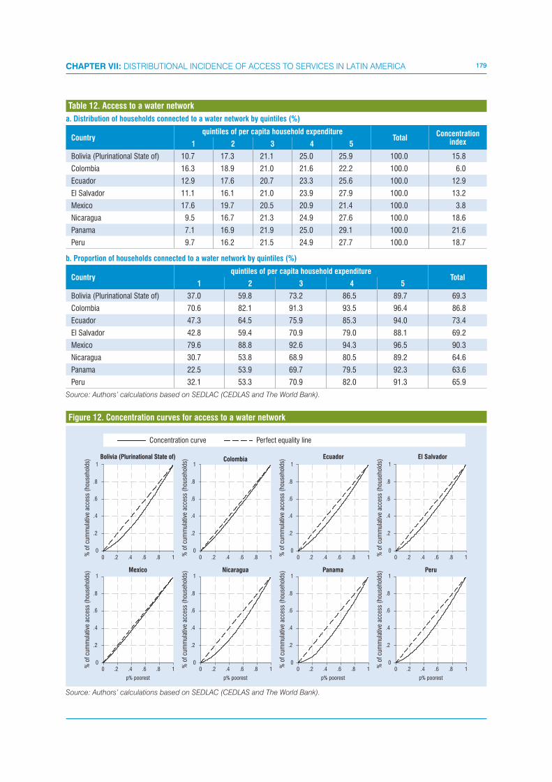
179CHAPTER VII: DISTRIBUTIONAL INCIDENCE OF ACCESS TO SERVICES IN LATIN AMERICA
a. Distribution of households connected to a water network by quintiles (%)
Countryquintiles of per capita household expenditure
TotalConcentration
index1 2 3 4 5
Bolivia (Plurinational State of) 10.7 17.3 21.1 25.0 25.9 100.0 15.8
Colombia 16.3 18.9 21.0 21.6 22.2 100.0 6.0
Ecuador 12.9 17.6 20.7 23.3 25.6 100.0 12.9
El Salvador 11.1 16.1 21.0 23.9 27.9 100.0 13.2
Mexico 17.6 19.7 20.5 20.9 21.4 100.0 3.8
Nicaragua 9.5 16.7 21.3 24.9 27.6 100.0 18.6
Panama 7.1 16.9 21.9 25.0 29.1 100.0 21.6
Peru 9.7 16.2 21.5 24.9 27.7 100.0 18.7 b. Proportion of households connected to a water network by quintiles (%)
Countryquintiles of per capita household expenditure
Total1 2 3 4 5
Bolivia (Plurinational State of) 37.0 59.8 73.2 86.5 89.7 69.3
Colombia 70.6 82.1 91.3 93.5 96.4 86.8
Ecuador 47.3 64.5 75.9 85.3 94.0 73.4
El Salvador 42.8 59.4 70.9 79.0 88.1 69.2
Mexico 79.6 88.8 92.6 94.3 96.5 90.3
Nicaragua 30.7 53.8 68.9 80.5 89.2 64.6
Panama 22.5 53.9 69.7 79.5 92.3 63.6
Peru 32.1 53.3 70.9 82.0 91.3 65.9
Source: Authors’ calculations based on SEDLAC (CEDLAS and The World Bank).
Table 12. Access to a water network
Figure 12. Concentration curves for access to a water network
Concentration curve Perfect equality line
0
.2
.4
.6
.8
1
% o
f cu
mm
ulat
ive
acce
ss (
hous
ehol
ds)
0 .2 .4 .6 .8 1
Bolivia (Plurinational State of)
0
.2
.4
.6
.8
1
% o
f cu
mm
ulat
ive
acce
ss (
hous
ehol
ds)
0 .2 .4 .6 .8 1
Colombia
0
.2
.4
.6
.8
1
% o
f cu
mm
ulat
ive
acce
ss (
hous
ehol
ds)
0 .2 .4 .6 .8 1
Ecuador
0
.2
.4
.6
.8
1
% o
f cu
mm
ulat
ive
acce
ss (
hous
ehol
ds)
0 .2 .4 .6 .8 1
El Salvador
0
.2
.4
.6
.8
1
% o
f cu
mm
ulat
ive
acce
ss (
hous
ehol
ds)
0 .2 .4 .6 .8 1
p% poorest
Nicaragua
0
.2
.4
.6
.8
1
% o
f cu
mm
ulat
ive
acce
ss (
hous
ehol
ds)
0 .2 .4 .6 .8 1
p% poorest
Mexico
0
.2
.4
.6
.8
1
% o
f cu
mm
ulat
ive
acce
ss (
hous
ehol
ds)
0 .2 .4 .6 .8 1
p% poorest
Panama
0
.2
.4
.6
.8
1
% o
f cu
mm
ulat
ive
acce
ss (
hous
ehol
ds)
0 .2 .4 .6 .8 1
p% poorest
Peru
Source: Authors’ calculations based on SEDLAC (CEDLAS and The World Bank).
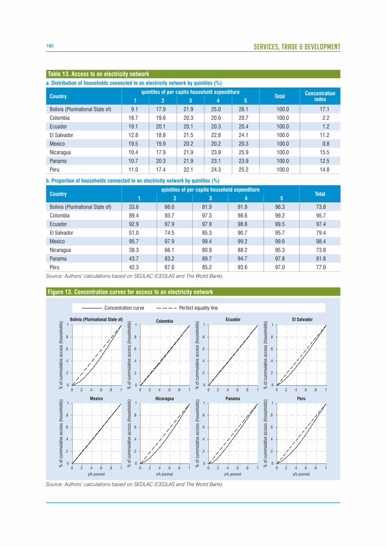
180 SERVICES, TRADE & DEVELOPMENT
Figure 13. Concentration curves for access to an electricity network
Concentration curve Perfect equality line
0
.2
.4
.6
.8
1
% o
f cu
mm
ulat
ive
acce
ss (
hous
ehol
ds)
0 .2 .4 .6 .8 1
Bolivia (Plurinational State of)
0
.2
.4
.6
.8
1
% o
f cu
mm
ulat
ive
acce
ss (
hous
ehol
ds)
0 .2 .4 .6 .8 1
Colombia
0
.2
.4
.6
.8
1
% o
f cu
mm
ulat
ive
acce
ss (
hous
ehol
ds)
0 .2 .4 .6 .8 1
Ecuador
0
.2
.4
.6
.8
1
% o
f cu
mm
ulat
ive
acce
ss (
hous
ehol
ds)
0 .2 .4 .6 .8 1
El Salvador
0
.2
.4
.6
.8
1
% o
f cu
mm
ulat
ive
acce
ss (
hous
ehol
ds)
0 .2 .4 .6 .8 1
p% poorest
Nicaragua
0
.2
.4
.6
.8
1
% o
f cu
mm
ulat
ive
acce
ss (
hous
ehol
ds)
0 .2 .4 .6 .8 1
p% poorest
Mexico
0
.2
.4
.6
.8
1
% o
f cu
mm
ulat
ive
acce
ss (
hous
ehol
ds)
0 .2 .4 .6 .8 1
p% poorest
Panama
0
.2
.4
.6
.8
1
% o
f cu
mm
ulat
ive
acce
ss (
hous
ehol
ds)
0 .2 .4 .6 .8 1
p% poorest
Peru
Source: Authors’ calculations based on SEDLAC (CEDLAS and The World Bank).
a. Distribution of households connected to an electricity network by quintiles (%)
Countryquintiles of per capita household expenditure
TotalConcentration
index1 2 3 4 5
Bolivia (Plurinational State of) 9.1 17.9 21.9 25.0 26.1 100.0 17.1
Colombia 18.7 19.6 20.3 20.6 20.7 100.0 2.2
Ecuador 19.1 20.1 20.1 20.3 20.4 100.0 1.2
El Salvador 12.8 18.8 21.5 22.8 24.1 100.0 11.2
Mexico 19.5 19.9 20.2 20.2 20.3 100.0 0.8
Nicaragua 10.4 17.9 21.9 23.9 25.9 100.0 15.5
Panama 10.7 20.3 21.9 23.1 23.9 100.0 12.5
Peru 11.0 17.4 22.1 24.3 25.2 100.0 14.8 b. Proportion of households connected to an electricity network by quintiles (%)
Countryquintiles of per capita household expenditure
Total1 2 3 4 5
Bolivia (Plurinational State of) 33.6 66.0 81.9 91.9 96.3 73.8
Colombia 89.4 93.7 97.3 98.6 99.2 95.7
Ecuador 92.9 97.9 97.9 98.8 99.5 97.4
El Salvador 51.0 74.5 85.3 90.7 95.7 79.4
Mexico 95.7 97.9 99.4 99.2 99.6 98.4
Nicaragua 38.3 66.1 80.9 88.2 95.3 73.8
Panama 43.7 83.2 89.7 94.7 97.8 81.8
Peru 42.3 67.0 85.2 93.6 97.0 77.0
Source: Authors’ calculations based on SEDLAC (CEDLAS and The World Bank).
Table 13. Access to an electricity network

181CHAPTER VII: DISTRIBUTIONAL INCIDENCE OF ACCESS TO SERVICES IN LATIN AMERICA
Countryquintiles of per capita household income (%)
Total1 2 3 4 5
Argentina 99.1 98.9 99.9 99.4 99.8 99.2
Bolivia (Plurinational State of) 92.6 95.0 95.6 97.9 98.6 95.1
Brazil 96.4 97.2 98.3 99.5 99.5 97.6
Chile 98.4 99.2 98.8 99.7 99.5 99.0
Colombia 92.0 95.3 97.8 99.1 99.0 95.5
Costa Rica 97.7 98.7 99.4 99.3 100.0 98.7
Dominican Republic 96.6 97.5 97.9 99.1 98.6 97.6
Ecuador 95.5 97.5 99.1 99.3 99.2 97.5
El Salvador 83.6 89.2 92.5 95.7 97.4 89.6
Guatemala 84.7 90.2 93.1 94.0 98.8 90.2
Honduras 88.9 94.0 95.2 97.3 96.2 93.3
Mexico 96.1 99.0 98.9 99.1 99.0 98.0
Nicaragua 85.2 90.8 93.8 94.4 98.3 90.6
Panama 92.2 95.3 98.1 99.2 99.5 95.3
Paraguay 92.2 95.8 97.8 97.6 99.7 95.6
Peru 95.9 98.3 98.5 99.1 99.9 97.8
Uruguay 99.4 99.7 99.8 100.0 100.0 99.6
Venezuela 95.3 97.4 98.3 98.8 99.2 97.2
Source: Authors’ own calculations based on SEDLAC (CEDLAS and The World Bank).
Table 14. Primary school net enrolment rates
Countryquintiles of per capita household income (%)
Total1 2 3 4 5
Argentina 70.1 83.4 90.0 95.0 96.0 81.1
Bolivia (Plurinational State of) 42.0 66.6 76.5 83.1 72.8 67.0
Brazil 30.4 47.1 59.4 73.8 87.5 53.5
Chile 73.0 80.8 86.3 88.9 92.6 81.8
Colombia 56.1 70.2 80.1 88.0 92.1 72.7
Costa Rica 44.1 59.8 61.3 75.9 91.3 61.2
Dominican Republic 33.2 48.2 57.1 65.6 80.1 52.4
Ecuador 52.9 65.1 73.3 84.0 91.6 69.1
El Salvador 14.9 24.9 41.0 50.2 61.9 33.4
Guatemala 18.5 30.8 43.5 56.9 76.9 40.2
Honduras 23.1 40.9 55.4 67.1 77.8 49.3
Mexico 63.9 73.7 75.0 83.1 90.3 74.6
Nicaragua 16.4 36.4 46.1 63.6 87.4 42.4
Panama 43.1 67.9 82.6 83.1 93.4 66.4
Paraguay 49.3 66.3 71.8 83.8 85.7 67.3
Peru 56.3 71.8 84.3 91.3 94.4 76.4
Uruguay 61.5 78.6 87.4 92.8 96.2 75.7
Venezuela 63.6 70.3 73.9 78.1 82.7 72.0
Source: Authors’ own calculations based on SEDLAC (CEDLAS and The World Bank).
Table 15. Secondary school net enrolment rates

182 SERVICES, TRADE & DEVELOPMENT
Countryquintiles of per capita household income (%)
Total1 2 3 4 5
Argentina 92.3 74.5 57.0 43.1 25.9 74.6
Bolivia (Plurinational State of) 98.6 97.1 93.9 89.4 50.5 91.3
Brazil 97.0 91.6 84.7 69.2 35.5 84.3
Chile 99.1 98.6 97.5 94.0 65.9 94.2
Colombia 96.4 92.9 85.0 65.8 35.4 83.8
Costa Rica 99.2 97.4 95.2 87.9 55.3 92.3
Dominican Republic 92.8 80.9 72.7 60.0 33.9 76.2
Ecuador 89.9 80.4 68.1 53.2 29.2 73.0
El Salvador 96.4 93.1 82.4 72.2 47.6 84.4
Guatemala 96.4 93.3 87.2 72.7 41.2 85.6
Honduras NA NA NA NA NA NA
Mexico 99.7 b8.1 94.8 87.9 47.0 92.1
Nicaragua 98.2 96.0 89.2 81.9 56.3 89.6
Panama 98.8 97.3 88.8 76.2 39.8 90.0
Paraguay 94.7 89.1 82.2 69.0 39.0 82.4
Peru 98.5 96.7 88.9 71.3 39.5 87.3
Uruguay 98.0 90.8 77.5 55.1 25.8 86.0
Venezuela NA NA NA NA NA NA
Source: Authors’ own calculations based on SEDLAC (CEDLAS and The World Bank).
Table 16. Percentage of primary school students attending public schools
Countryquintiles of per capita household income (%)
Total1 2 3 4 5
Argentina 88.3 77.6 63.2 48.3 33.2 71.2
Bolivia (Plurinational State of) 97.7 96.1 91.9 84.6 52.3 85.8
Brazil 95.3 92.5 88.9 78.7 37.6 78.8
Chile 99.0 98.4 97.3 93.3 64.1 93.0
Colombia 95.8 89.7 83.8 66.4 37.4 79.6
Costa Rica 96.4 96.8 94.2 85.5 59.6 88.5
Dominican Republic 90.6 79.7 74.2 59.5 33.3 67.6
Ecuador 81.8 83.4 77.3 63.3 31.0 70.8
El Salvador 90.8 77.2 72.7 66.7 47.2 69.4
Guatemala 75.3 61.5 58.9 47.2 21.8 50.7
Honduras NA NA NA NA NA NA
Mexico 98.2 94.5 91.2 87.0 58.1 88.7
Nicaragua 87.7 82.5 85.7 69.6 46.7 72.9
Panama 95.8 96.0 88.4 84.2 42.1 86.5
Paraguay 95.6 84.1 82.8 74.0 48.7 79.1
Peru 98.1 95.3 89.0 77.9 42.9 83.9
Uruguay 99.0 95.0 87.0 65.7 28.7 84.3
Venezuela NA NA NA NA NA NA
Source: Authors’ own calculations based on SEDLAC (CEDLAS and The World Bank).
Table 17. Percentage of secondary school students attending public schools
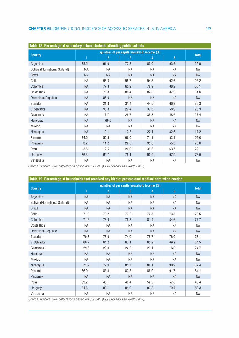
183CHAPTER VII: DISTRIBUTIONAL INCIDENCE OF ACCESS TO SERVICES IN LATIN AMERICA
Countryquintiles of per capita household income (%)
Total1 2 3 4 5
Argentina 28.5 61.0 77.3 85.0 93.8 69.0
Bolivia (Plurinational State of) NA NA NA NA NA NA
Brazil NA NA NA NA NA NA
Chile NA 96.8 95.7 94.5 92.6 95.2
Colombia NA 77.3 65.9 78.9 88.2 68.1
Costa Rica NA 79.3 83.4 84.5 87.2 81.6
Dominican Republic NA 85.0 NA NA NA NA
Ecuador NA 21.3 31.4 44.5 66.3 35.3
El Salvador NA 93.8 27.4 37.6 58.9 28.9
Guatemala NA 17.7 28.7 35.8 48.6 27.4
Honduras NA 69.0 NA NA NA NA
Mexico NA NA NA NA NA NA
Nicaragua NA 9.1 17.8 22.1 32.6 17.2
Panama 24.6 50.5 66.0 71.1 82.1 59.0
Paraguay 3.2 11.2 22.6 35.8 55.2 25.6
Peru 3.5 12.5 26.0 39.6 63.7 29.1
Uruguay 36.3 62.7 78.1 90.9 97.9 73.5
Venezuela NA NA NA NA NA NA
Source: Authors’ own calculations based on SEDLAC (CEDLAS and The World Bank).
Table 18. Percentage of secondary school students attending public schools
Countryquintiles of per capita household income (%)
Total1 2 3 4 5
Argentina NA NA NA NA NA NA
Bolivia (Plurinational State of) NA NA NA NA NA NA
Brazil NA NA NA NA NA NA
Chile 71.3 72.2 73.2 72.5 73.5 72.5
Colombia 71.6 73.9 78.3 81.4 84.6 77.7
Costa Rica NA NA NA NA NA NA
Dominican Republic NA NA NA NA NA NA
Ecuador 70.5 75.9 74.9 75.7 78.9 75.1
El Salvador 60.7 64.2 67.1 63.2 69.2 64.5
Guatemala 29.6 29.0 24.3 23.1 16.0 24.7
Honduras NA NA NA NA NA NA
Mexico NA NA NA NA NA NA
Nicaragua 71.9 79.9 85.7 86.1 90.9 82.4
Panama 76.0 83.3 83.8 86.9 91.7 84.1
Paraguay NA NA NA NA NA NA
Peru 39.2 45.1 49.4 52.2 57.8 48.4
Uruguay 84.6 83.1 84.9 83.3 79.4 83.3
Venezuela NA NA NA NA NA NA
Source: Authors’ own calculations based on SEDLAC (CEDLAS and The World Bank).
Table 19. Percentage of households that received any kind of professional medical care when needed
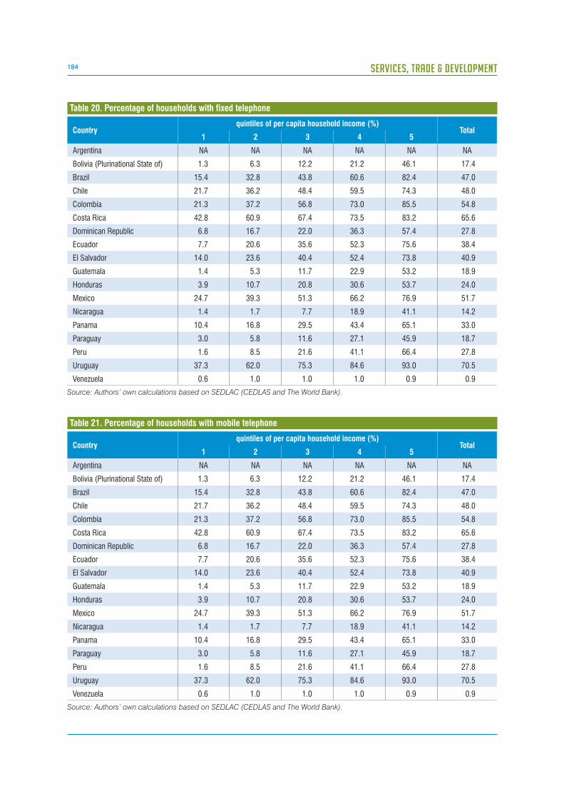
184 SERVICES, TRADE & DEVELOPMENT
Countryquintiles of per capita household income (%)
Total1 2 3 4 5
Argentina NA NA NA NA NA NA
Bolivia (Plurinational State of) 1.3 6.3 12.2 21.2 46.1 17.4
Brazil 15.4 32.8 43.8 60.6 82.4 47.0
Chile 21.7 36.2 48.4 59.5 74.3 48.0
Colombia 21.3 37.2 56.8 73.0 85.5 54.8
Costa Rica 42.8 60.9 67.4 73.5 83.2 65.6
Dominican Republic 6.8 16.7 22.0 36.3 57.4 27.8
Ecuador 7.7 20.6 35.6 52.3 75.6 38.4
El Salvador 14.0 23.6 40.4 52.4 73.8 40.9
Guatemala 1.4 5.3 11.7 22.9 53.2 18.9
Honduras 3.9 10.7 20.8 30.6 53.7 24.0
Mexico 24.7 39.3 51.3 66.2 76.9 51.7
Nicaragua 1.4 1.7 7.7 18.9 41.1 14.2
Panama 10.4 16.8 29.5 43.4 65.1 33.0
Paraguay 3.0 5.8 11.6 27.1 45.9 18.7
Peru 1.6 8.5 21.6 41.1 66.4 27.8
Uruguay 37.3 62.0 75.3 84.6 93.0 70.5
Venezuela 0.6 1.0 1.0 1.0 0.9 0.9
Source: Authors’ own calculations based on SEDLAC (CEDLAS and The World Bank).
Table 20. Percentage of households with fixed telephone
Countryquintiles of per capita household income (%)
Total1 2 3 4 5
Argentina NA NA NA NA NA NA
Bolivia (Plurinational State of) 1.3 6.3 12.2 21.2 46.1 17.4
Brazil 15.4 32.8 43.8 60.6 82.4 47.0
Chile 21.7 36.2 48.4 59.5 74.3 48.0
Colombia 21.3 37.2 56.8 73.0 85.5 54.8
Costa Rica 42.8 60.9 67.4 73.5 83.2 65.6
Dominican Republic 6.8 16.7 22.0 36.3 57.4 27.8
Ecuador 7.7 20.6 35.6 52.3 75.6 38.4
El Salvador 14.0 23.6 40.4 52.4 73.8 40.9
Guatemala 1.4 5.3 11.7 22.9 53.2 18.9
Honduras 3.9 10.7 20.8 30.6 53.7 24.0
Mexico 24.7 39.3 51.3 66.2 76.9 51.7
Nicaragua 1.4 1.7 7.7 18.9 41.1 14.2
Panama 10.4 16.8 29.5 43.4 65.1 33.0
Paraguay 3.0 5.8 11.6 27.1 45.9 18.7
Peru 1.6 8.5 21.6 41.1 66.4 27.8
Uruguay 37.3 62.0 75.3 84.6 93.0 70.5
Venezuela 0.6 1.0 1.0 1.0 0.9 0.9
Source: Authors’ own calculations based on SEDLAC (CEDLAS and The World Bank).
Table 21. Percentage of households with mobile telephone
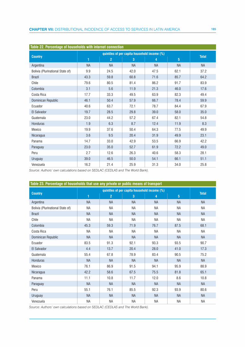
185CHAPTER VII: DISTRIBUTIONAL INCIDENCE OF ACCESS TO SERVICES IN LATIN AMERICA
Countryquintiles of per capita household income (%)
Total1 2 3 4 5
Argentina NA NA NA NA NA NA
Bolivia (Plurinational State of) 9.9 24.5 42.0 47.5 62.1 37.2
Brazil 43.3 59.8 60.8 71.6 85.7 64.2
Chile 79.6 80.5 81.4 86.2 91.7 83.9
Colombia 3.1 5.6 11.9 21.3 46.0 17.6
Costa Rica 17.7 33.3 49.5 63.9 82.3 49.4
Dominican Republic 46.1 50.4 57.9 66.7 78.4 59.9
Ecuador 40.6 63.7 72.1 78.7 84.4 67.9
El Salvador 19.7 28.5 29.8 39.0 58.0 35.0
Guatemala 23.0 44.2 57.2 67.4 82.1 54.8
Honduras 1.9 6.3 8.7 12.4 11.9 8.3
Mexico 19.9 37.6 50.4 64.3 77.5 49.9
Nicaragua 3.6 9.5 20.4 31.9 49.9 23.1
Panama 14.7 33.0 42.9 53.5 66.9 42.2
Paraguay 23.0 35.0 52.7 61.9 72.2 49.0
Peru 2.7 12.6 26.3 40.6 58.3 28.1
Uruguay 39.0 46.5 50.0 54.1 66.1 51.1
Venezuela 16.2 21.4 25.9 31.3 34.0 25.8
Source: Authors’ own calculations based on SEDLAC (CEDLAS and The World Bank).
Table 22. Percentage of households with internet connection
Countryquintiles of per capita household income (%)
Total1 2 3 4 5
Argentina NA NA NA NA NA NA
Bolivia (Plurinational State of) NA NA NA NA NA NA
Brazil NA NA NA NA NA NA
Chile NA NA NA NA NA NA
Colombia 45.3 59.3 71.9 76.7 87.5 68.1
Costa Rica NA NA NA NA NA NA
Dominican Republic NA NA NA NA NA NA
Ecuador 83.5 91.3 92.1 93.3 93.5 90.7
El Salvador 4.4 13.7 20.4 28.0 41.0 17.3
Guatemala 55.4 67.8 78.9 83.4 90.5 75.2
Honduras NA NA NA NA NA NA
Mexico 76.1 86.9 91.5 94.1 95.9 88.9
Nicaragua 42.2 58.6 67.5 75.5 81.8 65.1
Panama 11.1 10.8 11.7 12.0 8.6 10.8
Paraguay NA NA NA NA NA NA
Peru 55.1 76.1 85.5 92.3 93.9 80.6
Uruguay NA NA NA NA NA NA
Venezuela NA NA NA NA NA NA
Source: Authors’ own calculations based on SEDLAC (CEDLAS and The World Bank).
Table 23. Percentage of households that use any private or public means of transport

186 SERVICES, TRADE & DEVELOPMENT
Countryquintiles of per capita household income (%)
Total1 2 3 4 5
Argentina 96.0 99.2 99.4 99.9 100.0 98.9
Bolivia (Plurinational State of) 55.7 76.6 85.6 90.8 93.0 80.4
Brazil 80.6 92.6 94.9 97.1 99.4 93.1
Chile 93.6 95.7 96.8 97.8 98.6 96.5
Colombia 71.0 81.6 89.5 92.0 94.6 85.7
Costa Rica 95.6 99.0 99.1 99.3 99.6 98.5
Dominican Republic NA NA NA NA NA NA
Ecuador 60.2 75.9 84.4 90.9 95.1 81.3
El Salvador 55.7 66.0 72.9 78.3 89.3 72.6
Guatemala 76.9 87.9 90.7 94.7 95.7 89.2
Honduras 67.9 77.7 86.9 90.5 95.4 83.7
Mexico 89.4 96.2 97.3 98.8 99.0 96.1
Nicaragua 60.2 77.2 83.4 91.3 93.0 81.0
Panama 82.1 89.9 94.6 95.5 96.3 91.7
Paraguay 85.9 94.5 94.6 97.4 98.9 94.3
Peru 42.9 62.8 74.4 83.0 92.5 71.1
Uruguay 81.8 91.4 95.5 97.4 98.7 93.0
Venezuela 80.0 86.2 91.4 94.6 96.9 89.8
Source: Authors’ own calculations based on SEDLAC (CEDLAS and The World Bank).
Table 24. Percentage of households with access to a drinkable water source in their terrains or dwellings
Countryquintiles of per capita household income (%)
Total1 2 3 4 5
Argentina 79.5 82.9 87.3 90.3 93.8 86.8
Bolivia (Plurinational State of) 36.8 62.0 74.5 83.9 88.9 69.2
Brazil 69.3 80.9 84.3 86.9 92.5 82.9
Chile 89.5 92.2 93.8 95.5 96.6 93.5
Colombia 72.7 82.6 90.4 92.6 95.8 86.8
Costa Rica 86.7 93.1 94.8 97.0 98.0 93.9
Dominican Republic 54.6 65.9 71.9 78.9 88.1 71.9
Ecuador 45.9 66.6 76.7 85.5 92.0 73.3
El Salvador 46.9 60.1 69.8 76.3 88.7 69.3
Guatemala 60.5 70.6 76.2 84.1 90.3 76.4
Honduras 67.5 76.8 86.3 89.9 94.8 83.1
Mexico 79.1 88.7 92.6 95.3 96.1 90.4
Nicaragua 33.7 55.9 68.8 80.7 83.8 64.6
Panama 33.3 49.0 69.5 77.0 89.3 63.6
Paraguay 43.8 59.9 63.6 71.9 77.3 63.3
Peru 33.8 56.0 69.7 80.0 90.2 65.9
Uruguay 77.9 85.4 89.9 92.6 95.2 88.2
Venezuela 59.3 65.2 74.0 80.8 87.3 73.3
Source: Authors’ own calculations based on SEDLAC (CEDLAS and The World Bank).
Table 25. Percentage of households with access to a water network
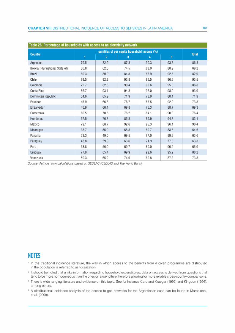
187CHAPTER VII: DISTRIBUTIONAL INCIDENCE OF ACCESS TO SERVICES IN LATIN AMERICA
Countryquintiles of per capita household income (%)
Total1 2 3 4 5
Argentina 79.5 82.9 87.3 90.3 93.8 86.8
Bolivia (Plurinational State of) 36.8 62.0 74.5 83.9 88.9 69.2
Brazil 69.3 80.9 84.3 86.9 92.5 82.9
Chile 89.5 92.2 93.8 95.5 96.6 93.5
Colombia 72.7 82.6 90.4 92.6 95.8 86.8
Costa Rica 86.7 93.1 94.8 97.0 98.0 93.9
Dominican Republic 54.6 65.9 71.9 78.9 88.1 71.9
Ecuador 45.9 66.6 76.7 85.5 92.0 73.3
El Salvador 46.9 60.1 69.8 76.3 88.7 69.3
Guatemala 60.5 70.6 76.2 84.1 90.3 76.4
Honduras 67.5 76.8 86.3 89.9 94.8 83.1
Mexico 79.1 88.7 92.6 95.3 96.1 90.4
Nicaragua 33.7 55.9 68.8 80.7 83.8 64.6
Panama 33.3 49.0 69.5 77.0 89.3 63.6
Paraguay 43.8 59.9 63.6 71.9 77.3 63.3
Peru 33.8 56.0 69.7 80.0 90.2 65.9
Uruguay 77.9 85.4 89.9 92.6 95.2 88.2
Venezuela 59.3 65.2 74.0 80.8 87.3 73.3
Source: Authors’ own calculations based on SEDLAC (CEDLAS and The World Bank).
Table 26. Percentage of households with access to an electricity network
NOTES1 In the traditional incidence literature, the way in which access to the benefits from a given programme are distributed
in the population is referred to as focalization.2 It should be noted that unlike information regarding household expenditures, data on access is derived from questions that
tend to be more homogeneous than the ones on expenditure therefore allowing for more reliable cross-country comparisons.3 There is wide ranging literature and evidence on this topic. See for instance Card and Krueger (1992) and Kingdon (1996),
among others.4 A distributional incidence analysis of the access to gas networks for the Argentinean case can be found in Marchionni,
et al. (2008).
TRADE IN SERVICES AND POVERTY: SERVICES, FARM EXPORT PARTICIPATION
AND POVERTY IN MALAWI AND UGANDA
This chapter examines the link between trade, services access and
poverty by first exploring the link between poverty and export cropping
in Africa and then the link between the provision and access to various
services (with varying degrees of tradability) and export cropping.
Evidence is provided supporting the idea that poverty is lower among
households and farms engaged in export cropping. Using data from
Malawi and Uganda, a strong negative correlation is found between the
extent of cash export cropping and poverty. Evidence is also provided
of the role various services have on cash cropping and agricultural
productivity. In Uganda, it was found that transportation services and
marketing services for exports (intermediaries) facilitate the adoption of
export crops. In the case of Malawi, transportation services were found
to be not as important as in Uganda, however, marketing services and
credit are. This chapter highlights the complementarities between
the role of services, services reforms, and trade in poverty reduction,
in particular as they relate to Africa. The exercises illustrate that the
potential gains from trade arising from the production of export crops
destined to international markets depends to a large extent on the
availability of services such as transportation and marketing. Services
reforms that reduce trade costs and encourage marketing activities in
rural areas may be useful to facilitate exports and reduce poverty.

190 SERVICES, TRADE & DEVELOPMENT
1. INTRODUCTION
Given the overwhelming role of agriculture in Sub-
Saharan Africa (for the poor and the non-poor alike),
poverty reduction strategies have been oriented to
increase agriculture productivity among the poor.
Beginning in the mid 1980s, most Sub-Saharan
countries have engaged in structural reforms of
the agricultural sector. This development strategy,
suggested and fostered by the World Bank (World
Bank, 1994) and other development agencies, has
focused on the gradual deregulation of export crop
markets as a key instrument for poverty alleviation
(Peters, 1997; Takane, 2005; HIID, 1994). Export
crop liberalization was regarded as the single best
channel to accelerate the growth of smallholder
agriculture and through this, the entire rural economy
(Donovan, 1993). The removal of long-standing legal
and institutional constraints was supposed to induce
small farmers to switch away from food crops and
to find better income opportunities by growing high
return crops. Moreover, as long as export crops
tended to be more labour-intensive, the reforms were
expected to increase the demand for hired labour as
well (Masanjala, 2005). Furthermore, the prospect of
higher income was supposed to alleviate household’s
food security.
However, market liberalization has been a very limited
mechanism for broad-based poverty alleviation (Orr,
2000). The number of poor farmers switching to export
crops has been far from massive. Even though the
proportion of smallholders in the production of export
crops increased (Takane, 2005), the share of land
dedicated to grow export crops remained very low.
In addition, poor households have been incapable of
profiting from the cash crops as much as the wealthier
households (World Bank, 2002). This has generated
a genuine policy necessity to understand why poor
farmers have failed in taking advantage of available
economic opportunities.
The objective of this chapter is to explore the role
of services for export crops as facilitators of export
market participation and poverty reduction. To gauge
this, Malawi and Uganda Malawi were chosen as
case studies. Entry into commodity export markets
(tobacco, cotton, coffee, tea, vanilla, pineapple, fish,
and exotic fruit) usually requires special attributes
of the households such as skills, knowledge, credit,
start-up capital, and labour supply. In the presence
of imperfect markets, wide margins in the differential
returns of export agriculture and subsistence
agriculture may arise in equilibrium among otherwise
similar households. Faced with higher tobacco prices,
for instance, some farmers may be unable to enter the
market if they do not have appropriate access to credit
or wealth to cover start-up costs (in seeds, fertilizers,
and so forth). Similarly, faced with higher coffee prices,
farmers may be unable to expand current coffee
production if family labour supply is limited and rural
labour markets are thin. In addition, lack of services,
such as road infrastructure, transportation, health
facilities, land, and market availability can impede
market participation and lead to increases in poverty.
This theme is explored with two case studies of Malawi
and Uganda. The first task requires a link description
between market participation and poverty. Section 2,
utilizes data from the Uganda National Household
Survey and the Malawi Integrated Household Survey,
to estimate the overall relationship between market
involvement and poverty in the two countries are
closely examined. In the case of Malawi, income gains
from export agriculture to provide supplementary
evidence supporting the notion that higher export
participation is associated with lower poverty.
Sections 3 and 4, considers the role of services.
Section 3, performs a simple regression analysis
to establish relevant correlations between various
services and export market participation in the target
countries, focusing on both individual as well as
aggregate (village-level) explanatory variables. The
type of services covered in the analysis includes
infrastructure, transportations, health, education,
credit, and market access (both for outputs and for
inputs). These correlations are intended to reveal
the role of various services in facilitating export
market participation and in alleviating poverty. The
correlations, together with the prevalence of poverty
and the lack of services revealed in the data, suggest
the need for services reforms to benefit the poor.
In Section 4, a closer examination of two specific
types of services is carried out – one for Malawi and
another one for Uganda. In the case of Uganda, the
role of marketing services (that is, market access via
increased competition among intermediaries and
transportation) in the adoption of coffee, tea, cotton
and fruits among smallholders is explored. In the
Malawi case, the role of the services provided by the
tobacco clubs (such as market access, input access,
credit, transportation services) in increasing tobacco
sales and yields as well as tobacco adoption among
191CHAPTER VIII: TRADE IN SERVICES AND POVERTY: SERVICES, FARM EXPORT PARTICIPATION AND POVERTY IN MALAWI AND UGANDA
tobacco farmers is investigated.
In this chapter, the link between trade, services and
poverty comes from the combination of exportable
crops (coffee, tea, cotton, tobacco) with various
services, including transportation, market access for
outputs and inputs, credit, and insurance. The value of
this chapter is the role of these services in the context
of a profound process of reforms affecting export
agriculture. Concretely, these two African countries
strongly liberalized their agricultural exports (in Malawi,
smallholders were not allowed to farm tobacco at all
before 1994; in Uganda, the overall agricultural sector
was heavily distorted). In consequence, this chapter
illustrate how services at the grassroots, complement
export agricultural liberalization to reduce poverty in
Africa.
2. EXPORT PARTICIPATION, INCOME GAINS AND POVERTY
This section describes how poverty is related to export
market participation in Malawi and Uganda, and
characterizes income gains in commodity exports.
The maintained hypothesis is that households can
escape from poverty by devoting resources to high-
yield export related crops instead of to food crops
for home consumption. This has been the basis of
the deregulation process of export crop markets
carried out by many Sub-Saharan countries, where
subsistence agriculture is widespread. In switching
their production to market oriented crops, poor
farmers would be able to get higher proceeds from
the sales of export crops, allowing them to buy the
subsistence food no longer produced by themselves,
and to dispose of additional cash. It is believed that
the fact that farmers cannot enjoy those income gains
from export agriculture is an indication of the lack of
services needed to successfully participate in export
markets.
To support this hypothesis it is necessary to first show
that a link between poverty and the production of
exportable crops exists. After proving this existence,
quantification will be made of the gains (in monetary
terms) of producing the latter types of crops.
The analysis is based on household survey data for,
Malawi and Uganda. In the case of Malawi, the Ma-
lawi Integrated Household Survey (IHS) of 2004/05 is
utilized. This is a comprehensive, national, household
survey with two questionnaires: a household question-
naire, and a community questionnaire. In the case of
Uganda, we utilize The Uganda National Household
Survey (UNHS) of 1999/2000 is utilized. There are also
two sets of data in the UNHS, household data and
community data.
In both countries, the household questionnaires cover
characteristics such as education, health, housing,
agriculture, consumption and income, among other
topics. Sample statistics of key variables are displayed
in table 1. The proportion of males in the sample is the
same for both countries at 49 per cent; the average
household size is slightly over 4.5 individuals in
Malawi while in Uganda is between 5 to 6 members;
around two-thirds of the households have a male
head in both countries; in Malawi the percentage of
adults between 18 and 45 years old is 37 per cent and
in Uganda 30 per cent (this is counterbalanced with a
smaller percentage of sample population of 12 and 18
year olds in Malawi). In Malawi, over 60 per cent of the
household heads can read and write in Chichewa (the
national language), and about 30 per cent in English.
The national poverty rate in Malawi was 53 per cent
using the head count ratio, which is the proportion of
people below the poverty line, while it was of 35 per
cent in Uganda (Appleton, 1999).
The module on agriculture of both countries is very
detailed and comprises land use, production, sales,
home-consumption, and input use amongst others,
from an extensive list of food and cash crops. The
composition of these two groups of crops is not the
same in the two countries. In Malawi, for instance,
the main cash crops are tobacco, groundnuts and
cotton.1 The main cash crops in Uganda are cotton,
coffee, tea, pineapples and exotic fruit. Throughout
the chapter, the terms commodity exports, export
crops, high-yield crops, commercialized crops, or
cash crops, referring to these recently described
sets of crops are used interchangeably. On the other
hand, the terms food crops for own-consumption, or
subsistence agriculture, refer to crops such as maize,
cassava, potatoes, matooke, beans, millet, sorghum,
and some others grown by the household for own
usage. Table 2 presents key summary statistics from
the agriculture module. Average total land holding
is 5.6 acres in Malawi and 2.6 acres in Uganda. The
distribution of land between food and cash crops
is very similar in both countries. The main farming
activity is food production for own-consumption,
accounting for 92 per cent of the land holdings of
a typical farmer. The remaining 8 per cent of land is

192 SERVICES, TRADE & DEVELOPMENT
devoted to commercialization activities (cash crops).
In Malawi, the main cash crop, in terms of land
allocation, is tobacco, with a 5 per cent land share,
followed by groundnuts and cotton. In Uganda, the
main cash crops are cotton, coffee, tea, pineapple
and other exotic fruit to a lesser extent.
The community questionnaires collect information that
is common to all households in a given area, defined
here as the village or urban location surrounding the
enumerator area. It contains information on access to
basic services and infrastructure. Table 3 shows some
summary statistics. In Malawi, nearly 30 per cent of
the communities have a daily market, and also 30
per cent have a weekly larger market; the main type
of roads are maintained dirt roads, and, on average,
the distance to an asphalt road is 2 kilometres. This
picture is not completely mirrored in Uganda, where
76 per cent of the enumerator areas of a district have
markets for food products; the average distance
to asphalt roads is 26 kilometres, suggesting that
transportation costs are more important hindrance to
commercialization than in Malawi; only 12 per cent of
Malawi Uganda
Average Standard deviation Average Standard deviation
Agriculture
Total land holdings (acre) 5.6 154.0 2.6 3.5
Land Shares
Food crops 92.1 16.9 92.8 18.0
Cash crops 7.9 16.7 7.2 17.1
Note: Authors’ calculations based on Malawi integrated household survey (2004/2005) and Uganda national household survey (1999/2000).
Table 2. Summary statistics: Agriculture characteristics (%)
Malawi Uganda
Average Standard deviation Average Standard deviation
Household characteristics
Household size 4.61 2.35 5.67 3.05
Sex of head (1=male) 0.77 0.42 0.74 0.44
Proportionof males 0.49 0.23 0.49 0.22
Proportion age 0-12 0.36 0.17 0.41 0.18
Proportion age 12-18 0.11 0.16 0.13 0.16
Proportion age 18-45 0.37 0.27 0.30 0.23
Proportion age 46+ 0.16 0.27 0.16 0.26
Head literacy (Chichewa) 0.62 0.48 ... ...
Head literacy (English) 0.30 0.46 ... ...
Income and poverty
Poverty rate: individuals (%) 52.60 ... 0.35 0.48
Poverty rate: households (%) 44.30 ... ... ...
Remittances ... ... 0.48 0.50
Non-farm income ... ... 0.35 0.48
Number of observations
Rural 9 840.00 6 554.00
Note: Authors’ calculations based on Malawi integrated household survey (2004/2005) and Uganda national household survey (1999/2000).
Table 1. Summary statistics: Household characteristics (%)
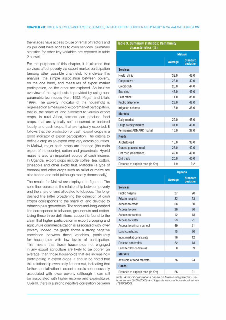
193CHAPTER VIII: TRADE IN SERVICES AND POVERTY: SERVICES, FARM EXPORT PARTICIPATION AND POVERTY IN MALAWI AND UGANDA
the villages have access to use or rental of tractors and
26 per cent have access to oxen services. Summary
statistics for other key variables are reported in table
2 as well.
For the purposes of this chapter, it is claimed that
services affect poverty via export market participation
(among other possible channels). To motivate this
analysis, the simple association between poverty,
on the one hand, and measures of export market
participation, on the other are explored. An intuitive
overview of the hypothesis is provided by using non-
parametric techniques (Fan, 1992; Pagan and Ullah,
1999). The poverty indicator of the household is
regressed on a measure of export market participation,
that is, the share of land allocated to various export
crops. In rural Africa, farmers can produce food
crops, that are typically self-consumed or bartered
locally, and cash crops, that are typically exported. It
follows that the production of cash, export crops is a
good indicator of export participation. The criteria to
define a crop as an export crop vary across countries.
In Malawi, major cash crops are tobacco (the main
export of the country), cotton and groundnuts. Hybrid
maize is also an important source of cash income.
In Uganda, export crops include coffee, tea, cotton,
pineapple and other exotic fruit. Matooke (a type of
banana) and other crops such as millet or maize are
also traded and sold (although mostly domestically).
The results for Malawi are displayed in figure 1. The
solid line represents the relationship between poverty
and the share of land allocated to tobacco. The long-
dashed line (after broadening the definition of cash
crops) corresponds to the share of land devoted to
tobacco plus groundnuts. The short-and-long-dashed
line corresponds to tobacco, groundnuts and cotton.
Using these three definitions, support is found to the
claim that higher participation in export cropping and
agriculture commercialization is associated with lower
poverty. Indeed, the graph shows a strong negative
correlation between these variables, particularly
for households with low levels of participation.
This means that those households not engaged
in any export agriculture are likely to be poorer, on
average, than those households that are increasingly
participating in export crops. It should be noted that
this relationship eventually flattens out, indicating that
further specialization in export crops is not necessarily
associated with lower poverty (although it can still
be associated with higher income and expenditure).
Overall, there is a strong negative correlation between
Malawi
AverageStandard deviation
Services
Health clinic 32.0 46.0
Cooperative 23.0 42.0
Credit club 26.0 44.0
Bus stop 43.0 49.0
Post office 14.0 35.0
Public telephone 23.0 42.0
Irrigation scheme 15.0 36.0
Markets
Daily market 29.0 45.0
Large weekly market 31.0 46.0
Permanent ADMARC market 16.0 37.0
Roads
Asphalt road 15.0 36.0
Graded graveled road 23.0 42.0
Dirt road (maintained) 42.0 49.0
Dirt track 20.0 40.0
Distance to asphalt road (in Km) 1.9 0.2
Uganda
AverageStandard deviation
Services
Public hospital 27 20
Private hospital 32 23
Access to credit 68 30
Access to oxen 26 36
Access to tractors 12 18
Access to water 53 21
Access to primary school 49 21
Land constrains 15 20
Input market constraints 16 12
Disease constrains 22 18
Land fertility constrains 8 9
Markets
Available of food markets 76 24
Roads
Distance to asphalt road (in Km) 26 21
Note: Authors’ calculations based on Malawi integrated house-hold survey (2004/2005) and Uganda national household survey (1999/2000).
Table 3. Summary statistics: Community characteristics (%)

194 SERVICES, TRADE & DEVELOPMENT
poverty and export crop participation. The relationship
between poverty and a locally commercialized crop
such as hybrid maize is much weaker.
The case of Uganda, exhibited in figure 2, confirms the
hypothesis. The solid line represents the relationship
between the poverty indicator of the household and
the share of land devoted to Uganda’s major export
crops (coffee, tea, cotton, pineapple and fruit). Similar
to Malawi, higher participation in export cropping and
agriculture commercialization leads to lower poverty
was also found in Uganda. This conclusion persists
after broadening the definition of cash crops to
include matooke and maize (the long-dashed curve).
However, when the list of crops is further extended to
include food crops such as millet, sorghum, beans,
groundnuts, sweet potatoes, and cassava, the
negative association between poverty and agriculture
commercialization vanishes (the short dashed curve).
A possible explanation of this last result is that the list of
crops included in this definition is too comprehensive
and thus there are no significant differences in the
average poverty rates at different levels of land shares.
Income gains in commodity exports
Figures 1 and 2 illustrate (unconditional) correlations
between market participation and poverty but
imply potential income gains from the adoption of
commercialized export crops. To see this in greater
detail, Malawi income gains are estimated.
The estimate is based on the income differential from
export cropping when compared to the production of
own-consumption goods using matching methods.
Therefore, some measure of the return to the
different agricultural activities is required. The IHS
data contains information on the value of outputs
and inputs used for different crops, as well as on the
land allocation. Thus, the measure of returns is the
per acre yield net of inputs. By netting out inputs, the
measure of return reflects profits are more certain.
Also, when dividing by land allocation, a comparable
unit of measure across crops is possible. The overall
idea of the matching method is to compare two sets
of households, one that produces for subsistence and
the other that produces for the market. The key insight
is that these sets of households must be relatively
Figure 1. Poverty and market participation in Malawi
Pove
rty
Land share
0 .2 .4 .6 .8 1
0.30
0.35
0.40
0.45
0.50
Note: The graph reports the non-parametric regression of poverty on export crop participation (share of land allocated). The estimates are obtained with a Fan (1992), locally linear non-parametric regression. The solid line corresponds to the share of land allocated to tobacco; the long-dashed line to tobacco plus groundnuts; the short-and-long-dashed line refers to tobacco, cotton and groundnuts; and the short-dashed line corresponds to hybrid maize share of land.
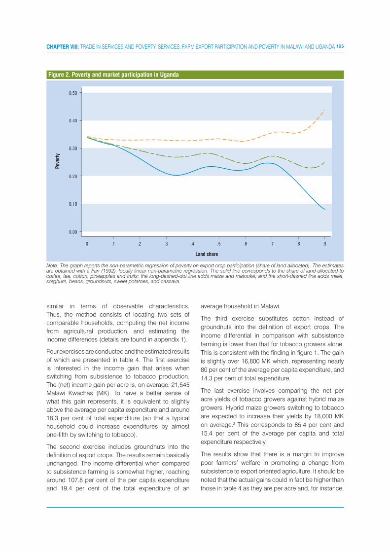
195CHAPTER VIII: TRADE IN SERVICES AND POVERTY: SERVICES, FARM EXPORT PARTICIPATION AND POVERTY IN MALAWI AND UGANDA
similar in terms of observable characteristics.
Thus, the method consists of locating two sets of
comparable households, computing the net income
from agricultural production, and estimating the
income differences (details are found in appendix 1).
Four exercises are conducted and the estimated results
of which are presented in table 4. The first exercise
is interested in the income gain that arises when
switching from subsistence to tobacco production.
The (net) income gain per acre is, on average, 21,545
Malawi Kwachas (MK). To have a better sense of
what this gain represents, it is equivalent to slightly
above the average per capita expenditure and around
18.3 per cent of total expenditure (so that a typical
household could increase expenditures by almost
one-fifth by switching to tobacco).
The second exercise includes groundnuts into the
definition of export crops. The results remain basically
unchanged. The income differential when compared
to subsistence farming is somewhat higher, reaching
around 107.8 per cent of the per capita expenditure
and 19.4 per cent of the total expenditure of an
average household in Malawi.
The third exercise substitutes cotton instead of
groundnuts into the definition of export crops. The
income differential in comparison with subsistence
farming is lower than that for tobacco growers alone.
This is consistent with the finding in figure 1. The gain
is slightly over 16,800 MK which, representing nearly
80 per cent of the average per capita expenditure, and
14.3 per cent of total expenditure.
The last exercise involves comparing the net per
acre yields of tobacco growers against hybrid maize
growers. Hybrid maize growers switching to tobacco
are expected to increase their yields by 18,000 MK
on average.2 This corresponds to 85.4 per cent and
15.4 per cent of the average per capita and total
expenditure respectively.
The results show that there is a margin to improve
poor farmers’ welfare in promoting a change from
subsistence to export oriented agriculture. It should be
noted that the actual gains could in fact be higher than
those in table 4 as they are per acre and, for instance,
Figure 2. Poverty and market participation in Uganda
Pove
rty
Land share
0 .1 .2 .3 .4 .5 .6 .7 .8 .9
0.00
0.10
0.20
0.30
0.40
0.50
Note: The graph reports the non-parametric regression of poverty on export crop participation (share of land allocated). The estimates are obtained with a Fan (1992), locally linear non-parametric regression. The solid line corresponds to the share of land allocated to coffee, tea, cotton, pineapples and fruits; the long-dashed-dot line adds maize and matooke; and the short-dashed line adds millet, sorghum, beans, groundnuts, sweet potatoes, and cassava.

196 SERVICES, TRADE & DEVELOPMENT
a farmer could actually increase the production of
export crops by more than one acre.
A somewhat different matching exercise is performed
that will allow for a better understanding of how the
gains from subsistence to export cropping can be
accrued. The conceptual difference in this exercise
is related to the arbitrariness in the definition of a
tobacco grower. The simple matching methods
used in the previous 4 exercises (whereby farmers
were classified as export producers or subsistence
��������� � ��� ������ ��� �������� ��� ��� ���������
terminology) are extended allowing for more than one
category of treatment. In particular, an estimate of
the average income gains of different types of export
growers depending on their degree of specialization
(in comparison with subsistence farmers) is sought.
To proceed, households are divided by the share of
land allocated to tobacco, and build five categories:
subsistence farmers (tobacco share of land equal to
zero); tobacco growers with a share of land of more
than zero but less than 20 per cent; from 20 per cent
to 40 per cent; from 40 per cent to 75 per cent; and
from 75 per cent to 100 per cent. Subsequently,
comparable households are found in these different
categories and an estimate is made of the average
income differential (technical details are found in
appendix 1).
The results of the estimated average outcomes,
after sub classifying on the balancing score to
adjust for covariate differences across categories,
are presented in figure 3. Yields per acre are found
to increase as farmers become more specialized
in tobacco. It should be pointed out that there is no
difference in the outcome if a household switches to
tobacco on only a small fraction of its available land.
This may be because the scale is not sufficient to fully
exploit the gains when both planting and selling the
produce. The yields per acre start to increase when
a farmer devotes more than 20 per cent of his land
(in terms of land area, this represents, on average,
roughly 1.5 acres of a typical tobacco grower).3 For
the 40 per cent to 75 per cent category, the expected
yield is higher than for any of the previous three
categories. Furthermore, the difference in outcomes
with the purely subsistence and the 0 per cent to 20
per cent groups is statistically significant. It should
also be noted that the gain in yield per acre is in
line with the one estimated in table 4. The outcome
is also higher for the group of most specialized
farmers, than for the group of subsistence farmers
and the least specialized tobacco growers. The main
conclusion here still remains the same: there is room
for improvement on poor farmers’ welfare and these
gains are increasing with participation in tobacco
production. It seems that some level of specialization
is required in order to realise gains.
Lastly, the final exercise includes groundnuts into the
definition of cash crops. Figure 4 depicts this exercise.
The results remain unchanged and the magnitudes
of the gains are more or less the same as those in
figure 3. Overall, it seems that tobacco is the key crop
associated with higher net yield and income gains in
Malawi.4
Gain(in MK)
% of expenditure
Total Per capita
Tobacco vs. subsistence21 545.0(5 346.0)
102.0 18.3
Tobacco & groundnuts vs. subsistence22 770.0(4 902.0)
107.8 19.4
Tobacco & cotton vs. subsistence16 826.0(3 307.0)
79.6 14.3
Tobacco vs. hybrid maize 18 040.0(6 491.0)
85.4 15.4
Note: Income gains were calculated with a propensity score matching kernel estimator. Standard errors in parenthesis were estimated with bootstrap methods. A farmer is considered to be a tobacco grower if 50 per cent or more of his total available land is allocated to tobacco, and similarly for tobacco plus groundnuts, tobacco plus cotton, subsistence and hybrid maize growers.
Table 4. Export cropping and income gains (per acre)
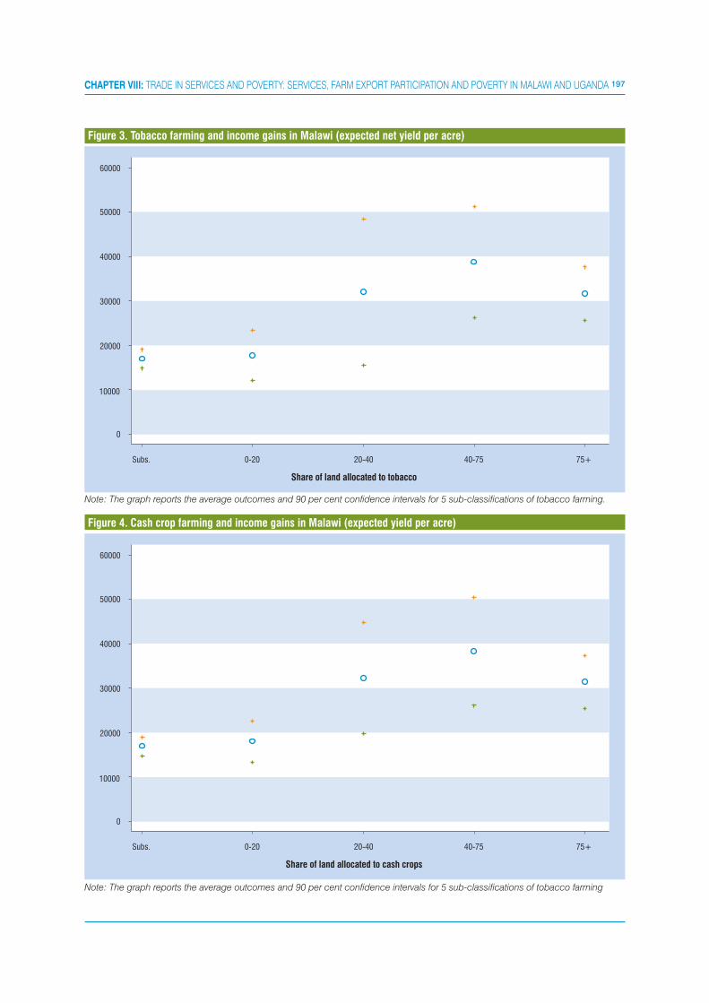
197CHAPTER VIII: TRADE IN SERVICES AND POVERTY: SERVICES, FARM EXPORT PARTICIPATION AND POVERTY IN MALAWI AND UGANDA
Figure 3. Tobacco farming and income gains in Malawi (expected net yield per acre)
Subs. 0-20 20-40 40-75 75+
0
10000
20000
30000
40000
50000
60000
Share of land allocated to tobacco
Note: The graph reports the average outcomes and 90 per cent confidence intervals for 5 sub-classifications of tobacco farming.
Figure 4. Cash crop farming and income gains in Malawi (expected yield per acre)
Subs. 0-20 20-40 40-75 75+
0
10000
20000
30000
40000
50000
60000
Share of land allocated to cash crops
Note: The graph reports the average outcomes and 90 per cent confidence intervals for 5 sub-classifications of tobacco farming

198 SERVICES, TRADE & DEVELOPMENT
3. MAIN DETERMINANTS OF AGRICULTURAL MARKET PARTICIPATION
Observing higher returns in export agriculture raises
the question of why farmers do not switch activities
into the more profitable ones. Even when part of the
income differential surely compensates for special
characteristics required to produce such export
crops, another part may be due to large distortions
in the economy. To unveil the reasons it is necessary
to explore the main determinants of participation into
export commodities. As such it is essential to identify
key constraints to agriculture that may prevent farmers
from entering high-return markets, thus locking them
into poverty. To this end a regression model is set
up that includes two sets of regressors: household
controls and district controls,. The model takes the
following form:
Where is the share of land allocated to export crops
by household in community.
Since UNHS and the IHS are not identical, the list
of explanatory variables is not the same for Uganda
and Malawi. For instance, in Malawi’s regressions it
is possible to include, among the covariates different
services provided by tobacco clubs that do not have
an exact parallel in Uganda’s regressions. Likewise,
the questionnaire of Uganda includes relevant
variables at both the household and village levels
that are not found in the Malawi survey. However,
the bulk of controls remain the same in both cases.
Hence, even when the results for each country are
not strictly comparable due to these slight differences
in the control list, they pretty much capture the same
forces governing the participation in agriculture
commercialization.
In the case of Malawi, only tobacco is included
in the definition of export crops. Six models are
considered: Model 1 only includes essential
household demographic variables such as household
size, demographic composition, and educational
attainments of the head. Model 2 includes district level
characteristics. Model 3 is equal to Model 2 but adds
district dummies to control for district fixed effects.
Model 4 includes a dummy that equals 1 if the farmer
belongs to a tobacco club. Model 5 includes an
alternative definition of access to transportation along
with variables to capture assets’ possessions. Model
6 replaces the tobacco club dummy with dummies of
different benefits the farmer obtains from the tobacco
club (if he belongs to one).
Export agriculture in Uganda includes coffee, tea,
cotton, pineapple and exotic fruit. Five models are
explored in this case: Model 1 includes only essential
household demographic variables like household
size, demographic composition, and educational
attainments. Model 2 adds land tenure. Model 3
includes the availability of food markets. Models 4
and 5 include health indicators, assets and non-
agricultural income variables, and village controls.
Model 4 includes monetary measures of assets
(animals and equipment) and of non-farm income
(remittances and non-farm income). Model 5 includes
dummy indicators of whether the household has
different assets or received/earns different types of
non-agricultural income.
Individual determinants in Malawi
As a first step, the household level determinants of
export crops farming are discussed. The results
displayed in table 5 suggest that household
characteristics do matter. For instance, if the head of
the household is male, there is a positive effect on the
share of land allocated to tobacco. Also the marital
status of the head is important: the tobacco share of
land is greater when the head is married.
Household size has a positive effect even though it
is weak. This result goes in line with the hypothesis
that larger households have a larger labour supply
and thus face lower constrains to commercialization.
On the other hand, it could be argued that larger
households will try and secure food needs prior to
venturing into commercialization. Nevertheless, the
household structure needs to be taken into account
as well. For example, in terms of labour supply and
food security, a household with 8 members of which
6 members range between 1 and 8 year olds, is
completely different than a household with 8 members
of which all are over 18 years old.
The way to interpret the household age composition
coefficients is the following. Each variable (age 0-7, age
8-12, etc.) represents the proportion of total members
in that age bracket. In the regression, the omitted
category is the proportion of members between 18
and 45 years old. Therefore, if the coefficient of, for
example, age 0-7 is negative (positive) this should be
interpreted as raising the share of family members in
the 0 to 7 age group, and at the same time decreasing

199CHAPTER VIII: TRADE IN SERVICES AND POVERTY: SERVICES, FARM EXPORT PARTICIPATION AND POVERTY IN MALAWI AND UGANDA
the share of family members in the 18 to 45 age group
by the same amount. Leaving the rest of the shares
constant, will decrease (increase) the share of land
devoted to tobacco. The results are as expected.
Substituting adults between 18 and 45 years old with
younger or older members has a negative effect on
the share of land. Two forces are at play and they go
in the same direction. Having more children raises
the food security concern and at the same time
restricts the available labour force, therefore, limiting
commercialization activities.
Another component of the household structure is the
proportion of males. In this case, there seems to be no
effect on export activities to a change in the proportion
of males after controlling by household size and age
composition. This may indicate that women are also
engaged in the production of tobacco.
There is no clear association between commercializa-
tion and the education or literacy status of the head.
In model 1, only those heads with completed primary
or junior secondary education seem to have larger
areas of planted tobacco than those without primary
or secondary education. One possible explanation is
that education is extremely low across the population,
so that there is no sufficient variability to capture the
effects of education.
It is surprising to find that the health status of the
household (measured as the proportion of sick
members) does not seem to affect the decision to
participate in export activities. This is also true for the
health status of the household head. This evidence
does not support the notion that sick members,
including the head, reduce effective labour, or that
sick children compromise the effort of women in
agriculture. The reason may be that these variables
cannot distinguish between chronic and short-term
sickness.
Possession of household assets such as beds, tables,
chairs, fans, radios, amongst others, has a positive
effect. The possession of agricultural tools also has a
positive effect (hoe or sickle). The existence of food
markets in a village is associated with higher export
agriculture, which supports a recent hypothesis (de
Janvry et al. 1991). If food markets are thin, households
Figure 5. Marketing services availability and export market participation Uganda
0.00
0.05
0.10
0.15
Expo
rt p
artic
ipat
ion
Services availabilty
0 .2 .4 .6 .8 1
Note: The graph reports the non-parametric regression of export crop participation on measure of market availability. The solid line corresponds to the share of land allocated to export crops suchas coffee, cotton, tea, pineapples, and fruits. The broken line corresponds to the share of income derived from those crops. The estimates are obtained with a locally weighted linear regression with Gaussian kernel and bandwidth equal to 0.15”.
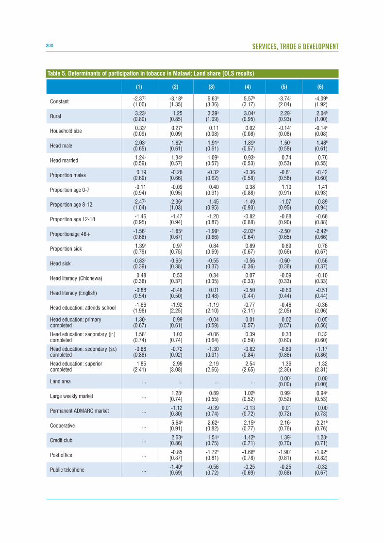
200 SERVICES, TRADE & DEVELOPMENT
(1) (2) (3) (4) (5) (6)
Constant-2.37b
(1.00)-3.18b
(1.35)6.63b
(3.36)5.57b
(3.17)-3.74b
(2.04)-4.09b
(1.92)
Rural3.23a
(0.80)1.25
(0.85)3.39a
(1.09)3.04a
(0.95)2.29b
(0.93)2.04b
(1.00)
Household size0.33a
(0.09)0.27a
(0.09)0.11
(0.08)0.02
(0.08)-0.14c
(0.08)-0.14c
(0.08)
Head male2.03a
(0.65)1.82a
(0.61)1.91a
(0.61)1.89a
(0.57)1.50a
(0.58)1.48b
(0.61)
Head married1.24b
(0.59)1.34b
(0.57)1.09b
(0.57)0.93c
(0.53)0.74
(0.53)0.76
(0.55)
Proportion males0.19
(0.69)-0.26
(0.66)-0.32
(0.62)-0.36
(0.58)-0.61
(0.58)-0.42
(0.60)
Proportion age 0-7-0.11
(0.94)-0.09
(0.95)0.40
(0.91)0.38
(0.88)1.10
(0.91)1.41
(0.93)
Proportion age 8-12-2.47b
(1.04)-2.36b
(1.03)-1.45
(0.95)-1.49
(0.93)-1.07
(0.95)-0.89
(0.94)
Proportion age 12-18-1.46
(0.95)-1.47
(0.94)-1.20
(0.87)-0.82
(0.88)-0.68
(0.90)-0.66
(0.88)
Proportionage 46+ -1.56b
(0.68)-1.85a
(0.67)-1.99a
(0.66)-2.02a
(0.64)-2.50a
(0.65)-2.42a
(0.66)
Proportion sick1.39c
(0.79)0.97
(0.75)0.84
(0.69)0.89
(0.67)0.89
(0.66)0.78
(0.67)
Head sick-0.83b
(0.39)-0.65c
(0.38)-0.55
(0.37)-0.56
(0.36)-0.60c
(0.36)-0.56
(0.37)
Head literacy (Chichewa)0.48
(0.38)0.53
(0.37)0.34
(0.35)0.07
(0.33)-0.09
(0.33)-0.10
(0.33)
Head literacy (English)-0.88
(0.54)-0.48
(0.50)0.01
(0.48)-0.50
(0.44)-0.60
(0.44)-0.51
(0.44)
Head education: attends school-1.66
(1.98)-1.92
(2.25)-1.19
(2.10)-0.77
(2.11)-0.46
(2.05)-0.36
(2.06)
Head education: primary completed
1.30c
(0.67)0.99
(0.61)-0.04
(0.59)0.01
(0.57)0.02
(0.57)-0.05
(0.56)
Head education: secondary (jr.) completed
1.58b
(0.74)1.03
(0.74)-0.06
(0.64)0.39
(0.59)0.33
(0.60)0.32
(0.60)
Head education: secondary (sr.) completed
-0.88(0.88)
-0.72(0.92)
-1.30(0.91)
-0.82(0.84)
-0.89(0.86)
-1.17(0.86)
Head education: superior completed
1.85(2.41)
2.99(3.08)
2.19(2.66)
2.54(2.65)
1.36(2.36)
1.32(2.31)
Land area ... ... ... ...0.00b
(0.00)0.00
(0.00)
Large weekly market ...1.28c
(0.74)0.89
(0.55)1.02b
(0.52)0.99c
(0.52)0.94c
(0.53)
Permanent ADMARC market ...-1.12
(0.80)-0.39
(0.74)-0.13
(0.72)0.01
(0.72)0.00
(0.73)
Cooperative ...5.64a
(0.91)2.62a
(0.82)2.15c
(0.77)2.16b
(0.76)2.21b
(0.76)
Credit club ...2.63a
(0.86)1.51a
(0.75)1.42b
(0.71)1.39b
(0.70)1.23c
(0.71)
Post office ...-0.85
(0.87)-1.72b
(0.81)-1.68b
(0.78)-1.90b
(0.81)-1.92c
(0.82)
Public telephone ...-1.40b
(0.69)-0.56
(0.72)-0.25
(0.69)-0.25
(0.68)-0.32
(0.67)
Table 5. Determinants of participation in tobacco in Malawi: Land share (OLS results)

201CHAPTER VIII: TRADE IN SERVICES AND POVERTY: SERVICES, FARM EXPORT PARTICIPATION AND POVERTY IN MALAWI AND UGANDA
(1) (2) (3) (4) (5) (6)
Health clinic ...-0.48
(0.74)0.37
(0.60)0.28
(0.56)0.41
(0.55)0.43
(0.55)
Irrigation scheme ...-0.84
(0.75)-0.71
(0.75)-1.06
(0.70)-0.86
(0.72)-0.76
(0.73)
Graded graveled road ...2.83c
(0.89)0.69
(0.79)0.73
(0.76)0.45
(0.79)0.46
(0.79)
Dirt road (maintained) ...2.05c
(0.77)1.26
(0.66)1.00
(0.62)0.64
(0.63)0.69
(0.64)
Dirt track ...1.18
(0.89)0.91
(0.79)0.78
(0.75)0.43
(0.80)0.44
(0.80)
Distance to urban center ... ... ... ...-0.00
(0.00)-0.00
(0.00)
Distance to asphalt road ... ... ... ...0.01
(0.02)0.01
(0.02)
Remoteness ... ... ... ...0.82
(1.34)0.90
(1.37)
Household assets ... ... ... ...0.43
(0.39)0.43
(0.39)
Bicycle ... ... ... ...1.24a
(0.32)1.30a
(0.33)
Other mean of transp. ... ... ... ...1.78
(2.04)1.91
(2.00)
Oxcart ... ... ... ...6.17a
(1.33)7.05a
(1.33)
Wheelbarrow ... ... ... ...1.31
(1.15)1.24
(1.15)
Hoe ... ... ... ...0.60
(0.97)0.43
(0.95)
Sickle ... ... ... ...1.13a
(0.28)1.11a
(0.28)
Tobacco club member ... ... ...17.46a
(1.45)16.23a
(1.51)
Club benefit: credit ... ... ... ... ...8.93a
(1.97)
Club benefit: inputs at lower price
... ... ... ... ...-1.45
(2.71)
Club benefit: better tobacco prices
... ... ... ... ...-0.20
(2.83)
Club benefit: extension service ... ... ... ... ...0.96
(2.22)
Club benefit: quota access ... ... ... ... ...6.23a
(2.18)
Club benefit: transport to market
... ... ... ... ...4.37b
(2.18)
Observations 9 764.00 9 429.00 9 429.00 9 429.00 9 429.00 9 429.00
R-squared 0.03 0.08 0.19 0.24 0.24 0.25
Note: Standard errors in parenthesis. “a”, “b”, and “c” denote statistically significant at 1, 5, and 10 per cent, respectively. Models 3 to 6 also include district dummies, not reported in this table. The age category omitted is the one that correspond to 18 to 45 years old. The roads category omitted is asphalt.
Table 5 (cont.). Determinants of participation in tobacco in Malawi: Land share

202 SERVICES, TRADE & DEVELOPMENT
will be reluctant to engage in commercialization and
will face potentially high prices as a consequence of
low food supplies. In this case, farmers will choose
to focus on food production for home consumption.
Instead, if food markets are available, households
may face, in the end, a lower risk of engaging in export
crops.
It should also be noted that the presence of the
Agricultural Development and Marketing Corporation
(ADMARC), which was originally a government mar-
keting board has no effect. In a recent study (Nthara
2002), one of the findings was that ADMARC does
not play a role as a buyer of agricultural produce. This
is the case as producers obtain higher prices when
selling to private traders and at local markets, also
ADMARC buys farmers produce very late in the year
and in some areas tends to run out of cash. There-
fore, producers are forced to sell to other buyers when
cash is in need.
Individual determinants in Uganda
Uganda’s case confirms several of the same results
found for Malawi (see table 6): households with
a larger proportion of males are more likely to be
engaged in export agriculture; households with a
larger proportion of members in the 12 to 18, 18 to
45 and over 45 age categories are more likely to be
engaged in commercialization; a clear association
between commercialization and the education of
the head is not evident; the health status of different
family members does not seem to affect the decision
to participate in export commercialization; and the
existence of food markets in a village induces export
agriculture.
However, there are some differences between the
two countries. The gender and the marital status
of the household head do not seem to matter for
participation in export commercialization in Uganda
while they have a positive effect in Malawi. It also
appears that larger households are less engaged in
agriculture commercialization (although this result is
weak, and sometimes mixed (see models 1 to 3 for
export participation). However, in the more complete
model with assets and non-agriculture income, the
coefficient of household size is negative. This result
would favour the hypothesis that larger households
will try and secure food needs before engaging in
commercialization. The counter-hypothesis would
argue that larger households are endowed with a
larger supply of labour and thus face lower constraints
to commercialization. Overall, food security and risk
coping seems to dominate the labour supply effect
in Uganda.
In addition, households endowed with a larger
plot size are more likely to participate in export
and extended commercialization (model 2). Two
interpretations of this finding are: first, by having more
land, households are able to allocate enough land to
food and have additional land resources to devote
to commercialization (food security and household
resource interpretation); and second, allowing
households to obtain cheaper credit to finance any
investment that commercialization requires (land can
work as collateral for loans and is thus an indication
of household assets interpretation). It is also possible
that farmers with higher land endowments are
more willing to take more risk and be engaged in
commercialization.
Regarding income from sources other than agriculture,
it was found that receiving remittances has a slightly
positive (but only marginally significant) relationship
with agriculture commercialization. Instead, having non-
agriculture income sources affects commercialization
negatively. One interpretation of this finding is that
non-agricultural activities crowd out resources
(labour) that thus cannot be used for production for
commercialization. Overall, households endowed
with agricultural equipment (animals or other tools)
are more likely to be involved in commercialization.
The interpretation lies on the complementary of these
capital goods with commercialization activities.5
Aggregate determinants in Malawi
Considering the aggregate (district level) determinants,
an interesting finding is that credit plays a significant
role in determining the share of land dedicated
to grow export crops (table 5). The presence of a
credit club in a village has a strong positive effect on
commercialization activities. If a farmer is a member of
a tobacco club and if he receives credit from the club
the effect on the share of land allocated to tobacco is
positive and quite large (model 6). This implies that
in conjunction with having credit available meeting
the requirements to obtain credit plays an important
role. This finding supports the start-up investment
hypothesis.
The presence of a cooperative in a village also has a
positive effect on farming of export crops, although not
as effective as the effects of belonging to a tobacco

203CHAPTER VIII: TRADE IN SERVICES AND POVERTY: SERVICES, FARM EXPORT PARTICIPATION AND POVERTY IN MALAWI AND UGANDA
(1) (2) (3) (4) (5)
Household size0.003a
3.0600.002b
2.2400.002b
2.310-0.003-1.480
-0.002-1.020
Sex head (male)0.012c
1.7000.013c
1.7500.004r0.670
0.0070.970
0.0060.840
Married head0.008c
1.9400.009b
2.0400.0061.500
0.0061.510
0.0051.400
Proportion of males0.030a
2.8000.029a
2.7300.027b
2.5400.024b
2.3300.023b
2.270
Proportion members 12-180.041a
2.6500.037b
2.2900.041a
2.8100.096a
4.2300.098a
4.200
Proportion members 18-450.0010.070
-0.003-0.190
00.030
0.046b
2.4200.050b
2.510
Proportion members over 450.069a
3.2000.063a
2.9900.062a
2.9500.111a
4.2900.105a
4.000
Proportion members 6-120.0241.210
0.0231.160
0.033c
1.8500.031c
1.7300.032c
1.710
Head attends school?-0.001-0.020
-0.001-0.040
0.0010.050
-0.011-0.550
-0.006c
-0.210
Literacy of head0.023b
2.1500.023b
2.1500.0161.750
0.0141.590
0.0161.750
Primary incomplete-0.010-1.000
-0.012-1.130
-0.017-1.600
-0.017c
-1.740-0.016-1.600
Primary complete0.0100.370
0.0060.240
0.0050.200
0.0070.260
0.0080.300
Junior incomplete-0.021-0.890
-0.022-0.940
-0.027-1.200
-0.025-1.120
-0.022-0.950
Junior complete0.0131.040
0.0100.810
0.0040.290
0.0030.260
0.0050.410
Senior incomplete-0.029c
-1.800-0.038b
-2.250-0.041b
-2.380-0.044a
-2.680-0.040b
-2.380
Senior complete0.0020.030
-0.014-0.350
-0.031-0.700
-0.036-0.690
-0.022-0.500
University degree-0.046-0.870
-0.062-1.250
-0.076-1.490
-0.084-1.510
-0.068-1.320
Household head sick0.0081.090
0.001.090
0.0040.660
0.0111.660
0.0101.520
Land ...0.004b
2.0800.003b
2.0500.003b
2.0400.004b
2.120
Food markets ... ...0.109a
3.2300.109a
3.1700.107a
3.110
Number of sick members ... ... ...-0.022-1.280
-0.021-1.220
Proportion sick children ... ... ...0.0121.560
0.0121.640
Number of children ... ... ...0.011a
3.1300.010a
2.940
Mother sick (with children) ... ... ...0
0.0600
0.060
Remittances (yes/no) ... ... ... ...0.01
1.540
Non-farm income (yes/no) ... ... ... ...-0.012-1.990
Table 6. Determinants of participation in export crops in Uganda: Land share (OLS results)
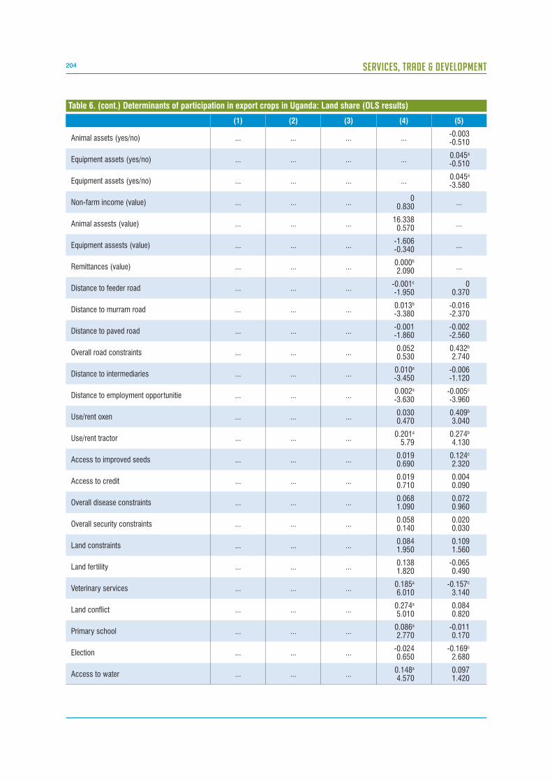
204 SERVICES, TRADE & DEVELOPMENT
(1) (2) (3) (4) (5)
Animal assets (yes/no) ... ... ... ...-0.003-0.510
Equipment assets (yes/no) ... ... ... ...0.045a
-0.510
Equipment assets (yes/no) ... ... ... ...0.045a
-3.580
Non-farm income (value) ... ... ...0
0.830...
Animal assests (value) ... ... ...16.3380.570
...
Equipment assests (value) ... ... ...-1.606-0.340
...
Remittances (value) ... ... ...0.000b
2.090...
Distance to feeder road ... ... ...-0.001c
-1.9500
0.370
Distance to murram road ... ... ...0.013b
-3.380-0.016-2.370
Distance to paved road ... ... ...-0.001-1.860
-0.002-2.560
Overall road constraints ... ... ...0.0520.530
0.432b
2.740
Distance to intermediaries ... ... ...0.010a
-3.450-0.006-1.120
Distance to employment opportunitie ... ... ...0.002a
-3.630-0.005c
-3.960
Use/rent oxen ... ... ...0.0300.470
0.409b
3.040
Use/rent tractor ... ... ...0.201a
5.790.274b
4.130
Access to improved seeds ... ... ...0.0190.690
0.124c
2.320
Access to credit ... ... ...0.0190.710
0.0040.090
Overall disease constraints ... ... ...0.0681.090
0.0720.960
Overall security constraints ... ... ...0.0580.140
0.0200.030
Land constraints ... ... ...0.0841.950
0.1091.560
Land fertility ... ... ...0.1381.820
-0.0650.490
Veterinary services ... ... ...0.185a
6.010-0.157c
3.140
Land conflict ... ... ...0.274a
5.0100.0840.820
Primary school ... ... ...0.086a
2.770-0.0110.170
Election ... ... ...-0.0240.650
-0.169c
2.680
Access to water ... ... ...0.148a
4.5700.0971.420
Table 6. (cont.) Determinants of participation in export crops in Uganda: Land share (OLS results)

205CHAPTER VIII: TRADE IN SERVICES AND POVERTY: SERVICES, FARM EXPORT PARTICIPATION AND POVERTY IN MALAWI AND UGANDA
club. If a farmer is a member of such a club, the share
of land devoted to tobacco increases significantly as
previously shown (model 5). It is also interesting to
disentangle the aggregated effects tobacco clubs
toward the benefits its members accrue. This is
reported in model 6, where the tobacco club dummy
is replaced by dummies of the different benefits the
members receive from the club. As mentioned earlier,
credit plays a very important role in the decision of
farmers to engage in the production of export oriented
crops. A farmer is also motivated to produce tobacco
as there is always a ready market to sell it in order
to obtain cash to later be able to buy food and other
goods. In this sense, the availability of traders or
produce markets is a crucial condition. This is why
the quota access to auction floors has a big positive
effect on motivating farmers to grow tobacco.
The district road variables included in the regressions
seem to have little impact on the measure of commer-
cialization when controlling by the rest of the covari-
ates. This is true for two different measures of road
infrastructure, which is an indication of transportation
services: dummies for different types of roads (mod-
els 2 to 4), and distance to asphalt road in kilometres
(models 5 and 6). There exist three reasons why this
means roads are not important.
Firstly, it should be kept in mind that some of the
measures of road access are dummies indicating the
main type of road in the district. Asphalt roads are
the omitted category in the regressions thus, the right
interpretation of the sign and significance of the road
dummies is that the different qualities of roads have
no further effect on participation. Different road access
specifications are experimented with in appendix 1.
Secondly, even though effects of different road
access and distance on the share of land allocated
to tobacco were not found, what was found is that
access for the transport of bales to market is linked
to higher participation in export agriculture. This is
an important result as it implies that the presence of
intermediaries linking farmers with markets facilitates
participation. In other words, these services create
markets for commercial crops and act as impulses
toward participation.
Third, a household having a bicycle or an oxcart has
a positive effect on participation. These two means of
transport are used by tobacco farmers to carry their
produce to the selling point. This indicates that even
though a positive effect for different types of access to
roads is not found, there are positive and significant
effects of services related to transport.
In conclusion, the type of road access available to
a farmer does not seem to be a great constraint to
agriculture, provided roads (asphalt, gravelled) do
exist and are maintained, and provided farmers are
endowed with the means to reach selling points, have
access to intermediaries or other marketing channels,
and have transport facilities through, for instance,
tobacco clubs.
Aggregate determinants in Uganda
As was the case with Malawi, road infrastructure
(again, taken as in indicator of transport services) is
also important for commercialization in Uganda. Table
6 reports the coefficients for three different measures
of road infrastructure (distance to feeder roads,
distance to murram roads, and distance to tarred
roads). It is interesting to note the findings indicate
that the most significant effects come from asphalt
and murram roads. The evidence suggests that better
road infrastructure is necessary to assist the poor to
participate in agricultural commercialization and thus
accrue gains.6
Table 6. (cont.) Determinants of participation in export crops in Uganda: Land share (OLS results)
(1) (2) (3) (4) (5)
Public hospital0.155a
4.820-0.165c
2.550
Private hospital0.0160.610
0.0551.180
Observations 6 554.00 6 554.00 6 554.00 6 513.00 6 554.00
R-squared 0.02 0.03 0.05 0.06 0.06
Note: Standard errors in parenthesis. “a”, “b”, and “c” denote statistically significant at 1, 5, and 10 per cent, respectively. All Models include district dummies, not reported in this table.

206 SERVICES, TRADE & DEVELOPMENT
Table 6 revealed that farmers residing in villages
served by truck and pickup services are more likely
to participate in export commercialization. This is
important as the presence of intermediaries linking
farmers with markets facilitate participation. In other
words, these services create markets for commercial
crops and increase impetus toward participation. This
is consistent with the findings regarding market costs
in export agriculture (Balat, Brambilla and Porto 2009).
Another interesting result emerges from the presence
of formal employment opportunities in a given area.
Farmers located far from factories are more likely to
be engaged in agriculture commercialization. One
reason being, that employment opportunities in rural
areas often allow workers to earn higher wages. For
instance, a recent study found income differences of
up to 100 per cent between rural employment and
other agricultural activities in Zambia (Balat and Porto
2007). Therefore, when higher earnings employment
opportunities are available, farmers (or at least a
family member) may opt out of household agriculture
and commercialization.
The bottom of table 6 includes additional results
for several other measures of infrastructure and
access to services. In these cases, results are less
robust than for variables included in the first panel. A
strong relationship exists between access to tractor
services and commercialization. A somewhat weaker
link exists between access to improved seeds, oxen
use, and access to water. Overall, though, access
to agricultural services seems to be a positive
determinant of commercialization. Land constraints,
such as access to land, conflict, and land fertility are
also important, particularly for export crops, but less
than expected, in terms of land fertility. One plausible
explanation is that land is readily available for use,
(either privately or communally), and soil and climate
conditions are relatively good for growing crops such
as maize, matooke, coffee and tea).
4. SERVICES FOR EXPORTS AND POVERTY ALLEVIATION: INTERMEDIARIES AND TOBACCO CLUBS
This section provides additional insights on the role of
services as a vehicle for poverty reduction by exploring
two examples of services for exports in Uganda and
Malawi – the role of marketing services in Uganda and
the role of tobacco clubs in Malawi.
4.1. Marketing services and poverty in Uganda
The chapter has thus far shown the negative
correlation between export market participation and
poverty in Uganda, as well as that a lack of services
can be a hindrance to export crop adoption and thus
impede the process of poverty reduction in Africa.
This section, explores the role of one specific service
with the aim of deriving general lessons for services,
trade in services, and services reforms as vehicles
toward poverty alleviation.
The role of marketing services in export agriculture is
investigated. Due to insufficient infrastructure, export
commercialization requires intermediaries that work
as bridges between international markets and the
farmers, throughout Africa. In rural areas, the lack of
intermediation activity acts as an effective barrier to
exports. The following case study quantifies these
effects using UNHS.
Marketing services are associated with the presence
of various outlets where farmers can sell their
export crops. There are three different types of such
markets in rural Uganda. First, the most widespread
way of marketing export crops is through export
intermediaries. These are agents that purchase output
from farmers, store the production and then transport
the agricultural produce with pick-ups or small trucks
to Kampala, the capital of Uganda. Second, typical
outlets for cash crop are district markets or stalls
along the road to Kampala. Third, an additional
channel to sell agricultural produce is through large
commercial plantations, particularly coffee and
tea. These plantations often purchase the output of
neighbour farmers thereby constituting additional
channels of market availability. Most plantations are
run by foreign firms. The community module of the
UNHS provides information on the availability of these
three types of outlets for each community; these data
are aggregated at the district level. Nationally, the
average marketing service is 0.37, meaning that in 37
per cent of the communities there is at least one outlet
for agricultural produce (intermediaries, export crop
stalls, or local large plantations).
Figure 5 shows the relationship between marketing
services and export participation. The solid line
corresponds to the share of land allocated to export
crops and the broken line, to the share of export crops
in income. Clearly, the availability of marketing services
for agriculture exports is positively linked to export

207CHAPTER VIII: TRADE IN SERVICES AND POVERTY: SERVICES, FARM EXPORT PARTICIPATION AND POVERTY IN MALAWI AND UGANDA
cropping. In turn, figure 6 establishes the negative
link between poverty and marketing services. This
relationship is negative, with lower poverty associated
with a higher availability of services for exports.
These graphs corroborate that services, and in par-
ticular marketing services, are important for poverty
reduction. Ugandan farmers facing abundant mar-
keting services are less likely to be poor because the
availability of marketing services allows them to adopt
more profitable exports crops such as coffee, cotton
or tea.
The graphical representation of the relationship
between availability of services, export cropping,
and poverty is a descriptive tool. In consequence, it
cannot provide causal evidence. For such evidence
the following formal regression analysis is utilized.
Estimation and results
Poverty regressions are begun with. Let be a dichoto-
mous variable that indicates the poverty status of
household in district. A household is poor if its per
capita expenditure falls below the official poverty line.
is regressed on the measure of marketing services,
which includes the three types of outlets discussed
above. The model also includes a number of addition-
al controls, such as household characteristics, (size,
demographic composition, age and gender of the
household head, the level of education and literacy
of the head, and the health status of the head) and
district characteristics. These characteristics include
access to credit, roads, equipment such as oxen or
tractors, inputs, and extension services, indicators of
major agricultural constraints (land quality and land
availability), input availability, disease, and education,
medical, sanitary and veterinary infrastructure, and
prevalence of security and conflicts. To account for
possible reverse causality (from poverty to marketing
services), the model is estimated with instrumental
variables. The instrument is the transportation costs
from the district centre to Kampala.7
The main results are shown in table 7. In the top panel,
estimates from linear IV regressions are reported. The
first column corresponds to a simple linear model that
Figure 5. Marketing services availability and export market participation Uganda
0.00
0.05
0.10
0.15
Expo
rt p
artic
ipat
ion
Services availabilty
0 .2 .4 .6 .8 1
Note: The graph reports the non-parametric regression of export crop participation on measure of market availability. The solid line corresponds to the share of land allocated to export crops suchas coffee, cotton, tea, pineapples, and fruits. The broken line cor-responds to the share of income derived from those crops. The estimates are obtained with a locally weighted linear regression with Gaussian kernel and bandwidth equal to 0.15”.
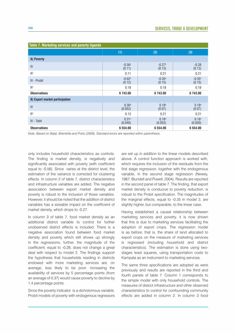
208 SERVICES, TRADE & DEVELOPMENT
only includes household characteristics as controls.
The finding is market density, is negatively and
significantly associated with poverty (with coefficient
equal to -0.56). Since varies at the district level, the
estimation of the variance is corrected for clustering
effects. In column 2 of table 7, district characteristics
and infrastructure variables are added. The negative
association between export market density and
poverty is robust to the inclusion of these variables.
However, it should be noted that the addition of district
variables has a sizeable impact on the coefficient of
market density, which drops to -0.27.
In column 3 of table 7, food market density as an
additional district variable to control for further
unobserved district effects is included. There is a
negative association found between food market
density and poverty which still shows up strongly
in the regressions; further, the magnitude of the
coefficient, equal to -0.28, does not change a great
deal with respect to model 2. The findings support
the hypothesis that households residing in districts
endowed with more marketing services are, on
average, less likely to be poor: increasing the
availability of services by 5 percentage points (from
an average of 0.37) would cause poverty to decline by
1.4 percentage points.
Since the poverty indicator is a dichotomous variable,
Probit models of poverty with endogenous regressors
are set up in addition to the linear models described
above. A control function approach is worked with,
which requires the inclusion of the residuals from the
first stage regression, together with the endogenous
variable, in the second stage regression (Newey,
1987; Blundell and Powell, 2004). Results are reported
in the second panel of table 7. The finding, that export
market density is conducive to poverty reduction, is
robust to the Probit specification. The magnitudes of
the marginal effects, equal to -0.35 in model 3, are
slightly higher, but comparable, to the linear case.
Having established a causal relationship between
marketing services and poverty, it is now shown
that this is due to marketing services facilitating the
adoption of export crops. The regression model
is as before; that is, the share of land allocated to
export crops on the measure of marketing services
is regressed (including household and district
characteristics). The estimation is done using two-
stages least squares, using transportation costs to
Kampala as an instrument to marketing services.
The same three specifications are adopted as were
previously and results are reported in the third and
fourth panels of table 7. Column 1 corresponds to
the simple model with only household controls. The
measures of district infrastructure and other observed
characteristics to control for confounding community
effects are added in column 2. In column 3 food
(1) (2) (3)
A) Poverty
IV-0.56a
(0.11)-0.27b
(0.13)-0.28
(0.13)
R2 0.11 0.21 0.21
IV - Probit-0.62a
(0.12)-0.35a
(0.15)-0.35a
(0.15)
R2 0.18 0.18 0.18
Observations 6 743.00 6 743.00 6 743.00
B) Export market participation
IV0.30a
(0.052)0.18a
(0.07)0.18a
(0.07)
R2 0.13 0.21 0.21
IV - Tobit0.31a
(0.040)0.18a
(0.052)0.18a
(0.050)
Observations 6 554.00 6 554.00 6 554.00
Note: Based on Balat, Brambilla and Porto (2009). Standard errors are reported within parenthesis.
Table 7. Marketing services and poverty Uganda

209CHAPTER VIII: TRADE IN SERVICES AND POVERTY: SERVICES, FARM EXPORT PARTICIPATION AND POVERTY IN MALAWI AND UGANDA
market density is added as a control. Strong evidence
is found that higher export market density induces
farmers to participate more in export agriculture. This
result holds for all specifications. This is an important
result: improved trade facilitation and lower export
marketing costs matter for export crop participation.
The point estimate is equal to 0.18 – an increase in
export market density of 5 percentage points would
cause the average land share devoted to export crops
to increase by 0.9 percentage points, equivalent to 13
per cent of the average export participation (roughly
7 per cent).
Since the two measures of export participation are
shares that are left censored at 0 and right censored
at 1, Tobit models are estimated with a control function
approach (to account for the endogeneity of export
market availability). As was the case before, this
requires that inclusion of the estimated residuals from
the first stage regression along with the endogenous
variable and the other exogenous regressors in a
standard Tobit model. The bottom panel of table 7
demonstrates that the findings are robust to censoring
of the export participation variables. The coefficients
on market density are positive and highly significant.
Furthermore, the marginal effect of the Tobit estimates
(the change in the unconditional average land share)
is 0.18, the same as the IV estimate in the first panel.
4.2. Tobacco Clubs in Malawi
A different source of services for exports in Africa is
the Malawi Tobacco Clubs. Tobacco is the largest
commodity export of Malawi and is also one of the
major sources of cash income for Malawi farmers. In
an attempt to reduce poverty and foster smallholder
tobacco production, the Government of Malawi
started in the early 1990s a gradual process of
liberalization of the tobacco sector. The reform
comprised several steps. One was the amendment of
the Special Crop Act that precluded participation of
small farmers by allowing cultivation of tobacco only
on leasehold and freehold land, and the allocation
of an increasing share of the national burley quota
to smallholder farmers. Another was the introduction
of a programme of intermediate buyers to facilitate
the logistics of bringing the smallholder’s output to
auction floors. Finally, a major feature of the reforms
was the creation of “burley tobacco clubs”– groups of
10 to 30 smallholders that gathered together to grow
tobacco and jointly perform critical farming activities.
The tobacco club initiative was a success. According
to the Tobacco Control Commission (TCC), the number
of clubs grew to 23,843 in the 2006/2007 season
from a few thousands in the early 1990s. In turn,
smallholder production of tobacco grew hand in hand
with the spread of burley clubs. Figure 7 depicts, both
the number of clubs and the volume of smallholder
burley production experienced a steady growth after
market liberalization in 1992. Nevertheless, the total
quantity of tobacco produced in Malawi underwent
little variation over the same period. In the end, the
participation of smallholders in total production and
exports of tobacco grew as well.
The services delivered by the clubs increase the
performance of members in key stages of the farming
process. In order to document them, we use two
sources of data. Some pieces of evidence come from
the Tobacco Clubs Survey of 2007. This is a survey of
clubs put together by Negri and Porto (2009). Other
pieces of evidence come from the tobacco module of
the Malawi IHS (2004 and 2005). Table 8 summarizes
the evidence.
Institutional access has traditionally represented the
major incentive for smallholder membership. For
many years, tobacco clubs constituted almost the
only way to access auction floors and fetch higher
prices. Upon registration with the Ministry of Agricul-
ture, the club was allocated a burley quota and a li-
cense to sell tobacco at the auction floor (Orr, 2000).
Instead, non-members had to sell their tobacco either
to intermediate buyers or across the border in Zam-
bia or Mozambique, at a lower price. Although quo-
tas have practically to all intents and purposes been
abolished, tobacco clubs are still an efficient vehicle
to reach output markets. The IHS and the TCS provide
different complementary evidence, reported in panel
A of table 8, on institutional access. On the one hand,
IHS reveals that 73 per cent of the clubs acknowledge
easier access to the auction floor. On the other hand,
according to TCS, only 33 per cent of the clubs actu-
ally obtain better prices at the auction floors. Both IHS
and TCS agree that tobacco clubs provide preferen-
tial institutional access to official extension support. In
table 8, 90 per cent and 69 per cent of the surveyed
clubs in TCS and IHS, respectively, claim to have re-
ceived better training and technical advisory services
from official extension workers.
Burley clubs have a major role as facilitators of collective
actions. One example is debt repayment monitoring.
In the absence of collateral, credit institutions use
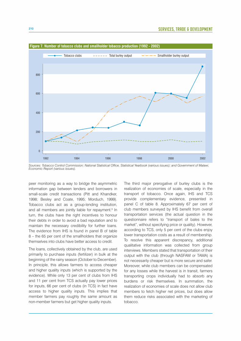
210 SERVICES, TRADE & DEVELOPMENT
peer monitoring as a way to bridge the asymmetric
information gap between lenders and borrowers in
small-scale credit transactions (Pitt and Khandker,
1998; Besley and Coate, 1995; Morduch, 1999).
Tobacco clubs act as a group-lending institution,
and all members are jointly liable for repayment.8 In
turn, the clubs have the right incentives to honour
their debts in order to avoid a bad reputation and to
maintain the necessary credibility for further loans.
The evidence from IHS is found in panel B of table
8 – the 65 per cent of the smallholders that organize
themselves into clubs have better access to credit.
The loans, collectively obtained by the club, are used
primarily to purchase inputs (fertilizer) in bulk at the
beginning of the rainy season (October to December).
In principle, this allows farmers to access cheaper
and higher quality inputs (which is supported by the
evidence). While only 13 per cent of clubs from IHS
and 11 per cent from TCS actually pay lower prices
for inputs, 66 per cent of clubs (in TCS) in fact have
access to higher quality inputs. This implies that
member farmers pay roughly the same amount as
non-member farmers but get higher quality inputs.
The third major prerogative of burley clubs is the
realization of economies of scale, especially in the
transport of tobacco. Once again, IHS and TCS
provide complementary evidence, presented in
panel C of table 8. Approximately 67 per cent of
club members surveyed by IHS benefit from overall
transportation services (the actual question in the
questionnaire refers to “transport of bales to the
market”, without specifying price or quality). However,
according to TCS, only 5 per cent of the clubs enjoy
lower transportation costs as a result of membership.
To resolve this apparent discrepancy, additional
qualitative information was collected from group
interviews. Members stated that transportation of their
output with the club (through NASFAM or TAMA) is
not necessarily cheaper but is more secure and safer.
Moreover, while club members can be compensated
for any losses while the harvest is in transit, farmers
transporting crops individually had to absorb any
burdens or risk themselves. In summation, the
realization of economies of scale does not allow club
members to fetch higher net prices, but does allow
them reduce risks associated with the marketing of
tobacco.
Figure 7. Number of tobacco clubs and smallholder tobacco production (1992 - 2002)
800
600
400
200
0
1992 1994 1996 1998 2000 2002
Tobacco clubs Total burley output Smallholder burley output
Sources: Tobacco Control Commission; National Statistical Office, Statistical Yearbook (various issues); and Government of Malawi, Economic Report (various issues).

211CHAPTER VIII: TRADE IN SERVICES AND POVERTY: SERVICES, FARM EXPORT PARTICIPATION AND POVERTY IN MALAWI AND UGANDA
Another major service provided by the clubs is as a
support networks and safety net. This has significant
implications in terms of labour supply, effort,
absorption of negative shocks and externalities from
positive shocks. The evidence from TCS is in panel D
of table 8.9
Clubs allow for peer to peer extension support as
members visit each other’s fields and sometimes
jointly grade tobacco. In addition, club members are
expected to assist colleagues with farming activities
and other social support in the event of sickness. This
is to ensure sufficient tobacco production at the end
������������������������������������� �������������
event must be covered by the club. As a result, the
clubs create an environment characterized by both,
learning by doing and learning from others (Munshi,
2004). Almost all clubs interviewed by TCS (98 per
cent) acknowledged having enhanced their farming
ability due to member advice. Also, around 65 per
cent of club members provide labour assistance to
fellow members in farming activities such as baling,
grading, harvesting or shade building. In contrast,
only 44 per cent of respondents claimed to have
actually received labour assistance from fellow club
members. Almost half of the club members get
advice in diverse issues such as personal matters and
health matters and other tips on how to spend any
extra income generated by tobacco. In fact, tobacco
clubs represent an alternative to the farmer’s informal
network of family and friends, and thus diversify a
farmer’s social network. In the end, these support
networks provide the needed motivation and identity
to withstand the hard work required to grow tobacco.
Overall, 96 per cent of respondents felt more motivated
to work harder after membership in a tobacco clubs.
Clearly, the study of the tobacco clubs is relevant for
the trade in services and poverty agenda for a number
of reasons. The tobacco clubs work as instruments
to provide various services needed for efficient
tobacco farming. The clubs facilitate access to credit
and inputs, improve the proper use of those inputs,
spread knowledge, reduce labour constraints, reduce
Malawi IntegratedHousehold Survey (IHS)
Tobacco Clubs Survey(TCS)
Yes No Yes No
A) Institutional access
Improved access to auction floor 73 2 ... ...
Higher prices ... ... 33 67
Better and more extension advice(a) 69 31 90 10
B) Collective actions
Improved access to credit 65 3 ... ...
Lower prices for inputs 13 87 11 89
Better input quality ... ... 66 34
C) Economies of scale
Transport of bales to auction floors 67 3 ... ...
Lower transport cost to auction floors ... ... 5 95
D) Supporting network
Enhanced farming ability due to fellow advice ... ... 98 2
Provision of labour assistance to club members ... ... 65 35
Assistance on farming activities from club members ... ... 44 56
Advice on non-farm activities from club members ... ... 49 51
Motivation to work harder ... ... 96 4
Notes: The table shows weighted averages computed from the Malawi Integrated Household Survey of 2004/2005 and the Tobacco Clubs Survey of June 2007. In the Malawi Integrated Household Survey (2004/2005), 280 club members answered the question: “Which of the following benefits did you enjoy from membership in a tobacco club?” In the TCS, 240 clubs responded specific questions on the prerogative of clubs. See Aappendix 1. (a): refers to visits from government officers or people from NASFAM/TAMA/etc.
Table 8. Benefits of tobacco club membership (Percentage of respondents)
212 SERVICES, TRADE & DEVELOPMENT
risks associated with transportation, secure higher
output prices, and promote economic coordination
among smallholders in liberalized markets. Tobacco
clubs thus provide farmers with incentives to exert
the required effort and to maintain the motivation
essential for profitable tobacco farming. In addition,
the tobacco clubs were created as one of the building
blocks of the tobacco liberalization. It follows that
these clubs are a manifestation of the process of
agricultural liberalization in Africa.
The impact of tobacco clubs
This exploration is geared toward generating evidence
on the impact of tobacco clubs on tobacco farming in
Malawi. The analysis is based on data from IHS. The
estimating equation is:
Where denotes an outcome of household, a tobacco
grower; is a binary variable that indicates whether the
person in charge of cropping activities in the household
(usually, but not necessarily, the household head) has
ever been a member of a tobacco club in the last
5 years; is a vector of additional controls including
characteristics of the person who makes cropping
decisions, such as gender, education, age, marital
status and health, as well as characteristics of the
household such as size, demographic composition,
and land holdings. In some specifications, the vector
also includes tobacco related variables such as
tobacco experience, fertilizer use, baling procedures,
and temporary work (ganyu). The equation also
includes district dummies to control for differences
in district infrastructure, local institutions, and
demographic-cultural factors (such as the matrilineal
or patrilineal nature of the district). Finally, the
residuals capture other unobservable factors that
affect the outcomes y and that may be correlated with
club participation.10
Several outcomes y are explored including output per
acre, (which is a measure of land productivity) and
sales per acre. On the one hand, low productivity
in agriculture is often the major reason behind the
prevalence of poverty in rural Africa; while on the
other hand, sales of cash crops such as tobacco
often provide the income opportunities needed to
escape poverty. There are two additional tobacco
outcomes of interest – tobacco participation and unit
values. A first question deals with whether farmers in
clubs allocate higher shares of their land to tobacco
than non-members. Low export participation is often
cited as another major reason behind low household
income and poverty traps. A second question deals
with whether clubs allow members to fetch higher unit
values for their tobacco. This is an important question
because higher prices and higher quality, both
associated with higher unit values, are also vehicles
toward poverty reduction.
There is an obvious endogeneity problem in the
simple model. The need to minimize the risk of default
forces them to select trustworthy and able farmers to
produce a sufficient amount tobacco. Among those
likely to be denied membership are newcomers to the
village, farmers with very little land, and farmers who
have behaved badly in the past. Club membership
is thus an endogenous variable and using OLS will
produce biased estimates of. In consequence, is
estimated with matching methods (see appendix 1 for
details).
Results from the matching exercises are reported
in table 9. The major finding is that club members
are around 40 per cent more productive than
non-members. The result is robust to the use of
three different matching estimators, named Kernel
matching (column 1), stratification matching (column
2), and nearest neighbour matching (column 3). The
matching estimates also reveal higher sales (per acre)
for members than for non-members. In the Kernel
matching in column 3, the club premium in sales (per
acre) is 45 per cent (also similar to the unconditional
mean difference).
The land share allocated to tobacco is positively
affected by club membership, but only marginally so.
Furthermore, even though club membership makes
farmers more productive and allows them to earn
more income through sales, members do not fetch
better prices – the unit values from tobacco sales do
not show significant differences between members
and non-members. This explains why the difference in
sales per acre is roughly comparable to the difference
in output per acre. This result is not really surprising
due to the fact there are only a few buyers at the
auction floors and tobacco clubs are not big enough
to counterbalance their market power.
5. CONCLUSIONS
In this case study, the link between trade, services
access and poverty have been tackled by first exploring
the link between poverty and export cropping in Africa
and secondly exploring the link between the provision
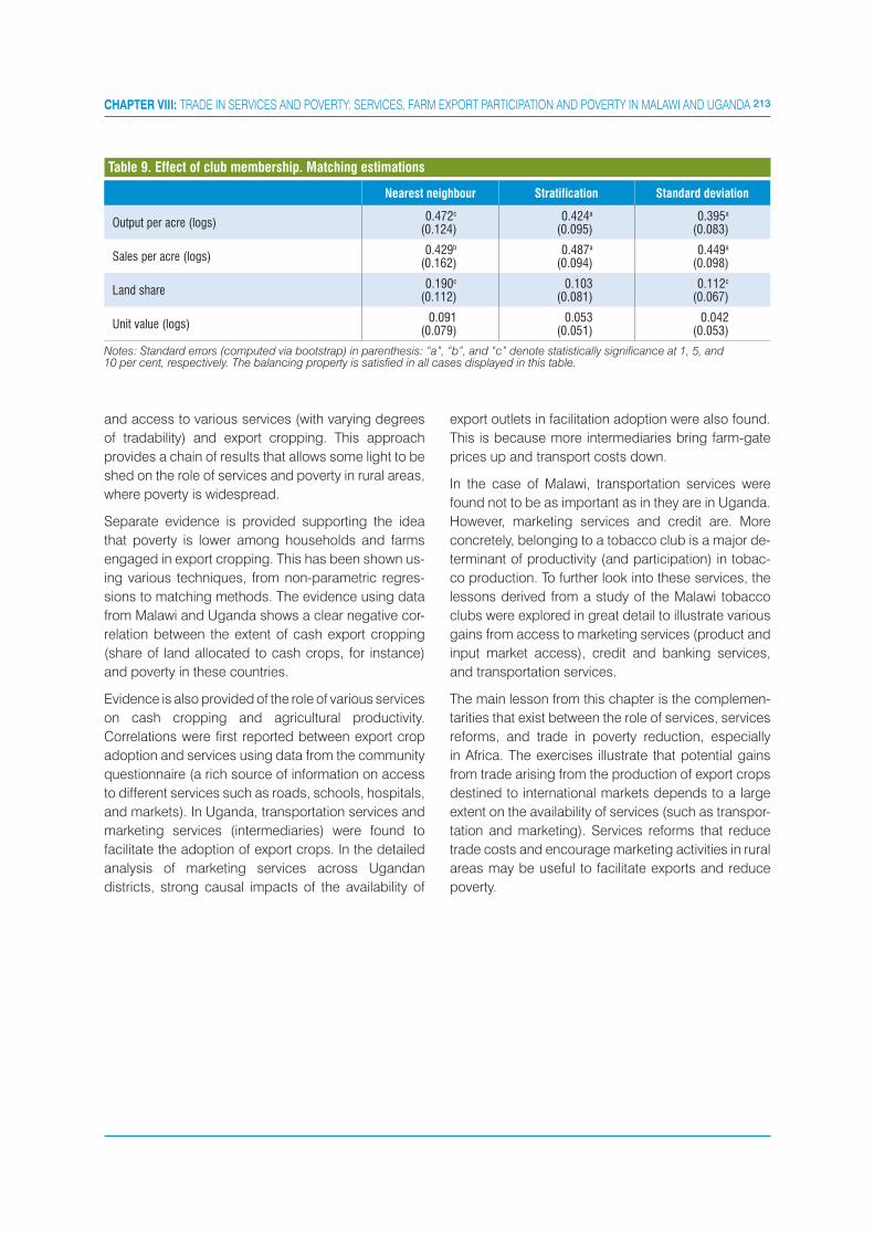
213CHAPTER VIII: TRADE IN SERVICES AND POVERTY: SERVICES, FARM EXPORT PARTICIPATION AND POVERTY IN MALAWI AND UGANDA
and access to various services (with varying degrees
of tradability) and export cropping. This approach
provides a chain of results that allows some light to be
shed on the role of services and poverty in rural areas,
where poverty is widespread.
Separate evidence is provided supporting the idea
that poverty is lower among households and farms
engaged in export cropping. This has been shown us-
ing various techniques, from non-parametric regres-
sions to matching methods. The evidence using data
from Malawi and Uganda shows a clear negative cor-
relation between the extent of cash export cropping
(share of land allocated to cash crops, for instance)
and poverty in these countries.
Evidence is also provided of the role of various services
on cash cropping and agricultural productivity.
Correlations were first reported between export crop
adoption and services using data from the community
questionnaire (a rich source of information on access
to different services such as roads, schools, hospitals,
and markets). In Uganda, transportation services and
marketing services (intermediaries) were found to
facilitate the adoption of export crops. In the detailed
analysis of marketing services across Ugandan
districts, strong causal impacts of the availability of
export outlets in facilitation adoption were also found.
This is because more intermediaries bring farm-gate
prices up and transport costs down.
In the case of Malawi, transportation services were
found not to be as important as in they are in Uganda.
However, marketing services and credit are. More
concretely, belonging to a tobacco club is a major de-
terminant of productivity (and participation) in tobac-
co production. To further look into these services, the
lessons derived from a study of the Malawi tobacco
clubs were explored in great detail to illustrate various
gains from access to marketing services (product and
input market access), credit and banking services,
and transportation services.
The main lesson from this chapter is the complemen-
tarities that exist between the role of services, services
reforms, and trade in poverty reduction, especially
in Africa. The exercises illustrate that potential gains
from trade arising from the production of export crops
destined to international markets depends to a large
extent on the availability of services (such as transpor-
tation and marketing). Services reforms that reduce
trade costs and encourage marketing activities in rural
areas may be useful to facilitate exports and reduce
poverty.
Nearest neighbour Stratification Standard deviation
Output per acre (logs)0.472c
(0.124)0.424a
(0.095)0.395a
(0.083)
Sales per acre (logs)0.429b
(0.162)0.487a
(0.094)0.449a
(0.098)
Land share0.190c
(0.112)0.103
(0.081)0.112c
(0.067)
Unit value (logs)0.091
(0.079)0.053
(0.051)0.042
(0.053)
Notes: Standard errors (computed via bootstrap) in parenthesis: “a”, “b”, and “c” denote statistically significance at 1, 5, and 10 per cent, respectively. The balancing property is satisfied in all cases displayed in this table.
Table 9. Effect of club membership. Matching estimations
214 SERVICES, TRADE & DEVELOPMENT
APPENDIX
Propensity Score Estimation
Let be the yield (net of inputs) per acre in market
agriculture of household. In the empirical exercise
that follows, market agriculture is defined as tobacco
farming (based on figure 1). Let be the net yield per
acre from subsistence agriculture for household.
Define also an indicator variable, set to 1 if the
household is a tobacco producer or 0 if it is a producer
of food for own-consumption.
Before proceeding there is one caveat. Few farmers
fully specialized in one crop, say tobacco or hybrid
maize. As mentioned earlier, production of food for
own-consumption is widespread. Therefore, there is
no evident division between subsistence and cash
crops producers. In fact, the characterization problem
faced is a continuum. While this problem is tackled
later, at this moment, a farmer is defined as having
specialization for a given crop (food crops, hybrid
maize or tobacco) if the household devotes more than
50 per cent of its land to that crop.
Interest is focused on estimating the expected income
differential of farmers engaged into export crops,
The problem is that for each farmer only or is
observed. This is exactly the paramount obstacle of
non-experimental data. The difference can be rapidly
calculated as, but this is a potentially biased estimator
of. The problem is that if treated and controls, in this
literature terminology, systematically differ in their
characteristics, then observing for the control group
is not a good estimate of for the treated group. To
sort this problem out, matching methods based on
the propensity score are used. There is abundant
literature on matching methods. Original pieces
include Rubin (1977) and Rosembaun and Rubin
(1983). More recently, Heckman, Ichimura and Todd
(1997) and (1998), and Heckman, Ichimura, Smith
and Todd (1996) extended and assessed these
methods. Dehejia and Wahba (2002) provided a
practical examination of propensity score matching
methods using the data in Lalonde (1986).
The main assumption of this method is that, in this
chapter’s case, the participation into market oriented
farming can be based on observables. More formally,
this is the “ignorability” of treatment assignment and
can be stated as (Rubin 1977). As such it is possible to
control for differences in observed characteristics by
grouping the observations into subclasses based on
those observed characteristics, thus reducing the bias
due to imbalances in the covariates. The drawback
is that when the number of covariates increases,
the number of subclasses grows exponentially, and
potentially the cells will not contain both treated and
control units jeopardizing the comparison between.
Fortunately, there exists a scalar function of the
covariates (the propensity score) that reduces the
dimensionality problem and can be used to balance
the distribution of the covariates, as proposed by
Rosenbaum and Rubin (1983, 1985a, b).
The propensity score is defined as the conditional
probability of participating in market oriented crops
Thus, this methodology requires estimating, for
example, a Probit model of participation into export
agriculture, which will then define the propensity
score, for a given vector of observables. When the
propensity score is a balancing one,. This is an
important property because as shown by Rosenbaum
and Rubin (1983, 1985a, b) it implies that
In other words, observations with a given propensity
score have the same distribution of observables
for households involved in market agriculture as in
subsistence. Importantly, the balancing condition
can and should be checked. In all of the exercises,
these balancing conditions were tested following the
procedure suggested by Dehejia and Whaba (2002).
Thereafter, subsistence farmers are matched with
market farmers based on this propensity score, and the
income differential is estimated using kernel methods.
In the exercises that follow the vector of observable
covariates include household characteristics such as
household demographics (household size, age and
sex composition) and health status of its members;
household head characteristics, and district dummies
to capture district level fixed effects.
Further Technical Issues
Let index each of the 5 categories. In this case
interest is on the average outcome, the net yield per
acre, for each one of the 5 categories of tobacco
growers. As before, the problem with just taking
averages within each category is that if the farmers
across the categories differ systematically in their
characteristics the results may not be directly
comparable. Differences between the may be caused
by differences on the observed covariates and not
only due to differences on the exposure level of the
treatment, that is, the specialization level in tobacco

215CHAPTER VIII: TRADE IN SERVICES AND POVERTY: SERVICES, FARM EXPORT PARTICIPATION AND POVERTY IN MALAWI AND UGANDA
production. In fact, a similar problem is faced as the
one with only 2 categories.
The approach here is conceptually similar to the
one used above but has been modified slightly to
accommodate multiple treatment doses (Lu et. al.
2001; Imbens 2000; Imai and van Dyk 2003). The
sample is sub classified by the estimated propensity
score assigning each observation into a small number
of subclasses or strata.
The estimation of the propensity score is more
complicated because there are more than two
categories. Fortunately, a scalar propensity score can
be modelled using an ordinal logit (McCullagh 1980).
In this case, the distribution of categories (or different
doses of treatment) for household, given the set of
observed covariates, is modelled with a proportional
odds model.
Where is the cut point of. In this model the 5 cut points
and the intercept cannot be estimated, and therefore
set the constant to zero.
The important feature of this model is that the
distribution of categories given the covariates
depends on the observed covariates only through, so
that the observed covariates and the categories are
conditionally independent given the scalar. Therefore,
is a balancing score.
The next step is to verify that the balancing condition
is held, meaning that the distribution of covariates
is balanced across categories, and after that the
expected outcome for each one of the 5 categories
can be estimated.
Let be the estimated mean outcome for farmers with
grade of tobacco specialization. These estimates can
be computed as the weighted average
Where is the observed mean outcome among farmers
with specialization level and balancing score strata,
and the weights equal the number of farmers in strata
divided by the total number of farmers.
NOTES1 Sugar cane, tea and coffee are also cash crops produced in Malawi, but these are mainly grown by large estates. Therefore,
for smallholders, they are of much less importance than tobacco or cotton, and there is no sufficient data to take them into account in the analysis.
2 The income gain per acre from producing hybrid maize has also been estimated instead of subsistence farming, and this gain is positive though not statistically significant.
3 It should be noted that for the 20 per cent to 40 per cent category, the differences with the first two categories are not statistically significant.
The standard errors of the gains in figure 4 are smaller; one reason for this may be the increased number of observations now included into each category.
5 In the case of Uganda, some variations to the original model were explored as a way to check for robustness. Instead of using the share of land devoted to commercialized crops as dependent variable, an attempt was made to use the share of income derived from the sales of those same crops. The results and main conclusions were found, (for individual and aggregate determinants) not to be affected by the choice of independent variables used to measure commercialization. Regression results were also explored using the broader definition of commercialization. Overall, results are consistent across specifications. These results are not reported for sake of simplicity in the presentation of the findings.
6 The regressions include other distances reported in the community questionnaire such as distance to hospitals, post office, or banks. These variables are used as controls in the regressions, to take account of other village effects.
7 In Uganda, (a landlocked country) most international shipments must pass through the capital, Kampala. The out-of-district transportation costs are proxied with district level data on transportation costs from the centre of each district to Kampala. These costs are reported in the community questionnaire of UNHS as the monetary cost of reaching Kampala by car or truck (for more detail see Balat, Brambilla, and Porto 2009).
8 The loan is later repaid when tobacco is sold at the auction floor by deducting the amount of the loan, plus interest, from the amount of the sale of tobacco (the difference is deposited directly into the club’s bank account).
9 No information on this theme is available in IHS.10 The model is estimated only on the sample of tobacco growers during the 2004/2005 season and not on the whole sample.
Therefore, the estimates of represent the causal effects of burley club membership on those farmers who have moved into tobacco. Since unobservable factors partially guide selection into different cropping activities, the estimates will not identify the impacts on a random farmer. Thus the average treatment effect on the treated as opposed to the average treatment effect on the population is identified.
TRADE IN SERVICES AND POVERTY:PRIVATIZATION, COMPETITION AND
COMPLEMENTARY SERVICES IN RURAL ZAMBIA
Services can play an important role in the eradication of poverty,
especially in rural areas of Africa. Key services include financial
services (access to credit), transportation services, marketing services
(access to markets), and information. The objective of this chapter is to
generate evidence on the likely impact of services reforms on poverty
in Africa. The analysis explores reforms in the Zambian cotton sector.
The appealing feature of the cotton reforms is that they implicitly
embed services reforms due to the outgrower contracts. There is a
strong business relationship between cotton firms and farms closely
interacting through contract farming arrangements. In this arrangement
firms provide credit, transport services, information services, and
marketing services to the farmers. A major factor in this approach is the
intertwined competition and the provision of these services. Greater
competition among cotton firms is generally associated with higher
farm-gate prices paid to cotton farmers, which has poverty reducing
impacts. However, when firms also provide services, such as credit, the
direct link between competition and poverty may break down because
due to increased competition making it more difficult to sustain the
institution of contract farming. Using simulation models and household
survey data, it is shown that while more competition, indeed leads to
higher prices, it can also lead to higher costs by way of higher credit
prices and lower market access to farmers. This highlights the need to
delve deep into the details when considering the poverty impacts of
services reforms.

218 SERVICES, TRADE & DEVELOPMENT
1. INTRODUCTION
This chapter explores the poverty impacts of
privatization and competition policies in export
agriculture in Africa, and in particular focuses on
cotton in Zambia. This is an interesting case study
due to the dynamics of the sector. The cotton sector
was traditionally controlled by the marketing agency,
Lintco (Lint Company of Zambia) until its privatization
in 1994. At first, the privatization process led to some
improvements in cotton farming (especially in adoption
and yields). However, the market later collapsed
primarily due to the failure of the outgrower scheme.
Cotton farming in Zambia was conducted by way of
outgrower contracts, whereby the firms gave inputs
on loans to the farmers, which were repaid at harvest
time. Unregulated entry into the market quite often led
to a farmer’s default as a result of higher interest rates
and credit prices. This spiralled out of control which
finally led to collapse of the system. In 2001, cotton
buyers improved the outgrower arrangements and
made contracts more efficient. As a result the sector
became reinvigorated and is currently vibrant and
growing, all within this decade.
The first part of the chapter investigates privatization
impacts of the cotton sector on farm productivity,
defined as yields per hectare. Increases in productivity
are a straightforward mechanism toward poverty
alleviation. To this end, reforms of the Zambia cotton
sector are reviewed. This review includes the initial
privatization of the cotton marketing board as well
as the subsequent competition, entry and exit of
the sector. These market dynamics greatly affected
the availability of complementary services to the
farmer, including credit, transportation, marketing,
and information, thus acting as a de facto indirect
liberalization of various services for exports. The
evolution of participation in cotton farming and cotton
productivity through the different phases of the
liberalization will then be tracked.
The second part of the chapter provides a simulation
analysis of the poverty reducing impacts of competition
policies in the cotton sector. A theoretical model of
export agriculture including farmers, ginneries and
retailers are developed and, based on parameters
that characterize the sector, poverty simulations are
performed. The simulations explore the impacts
of increases in competition at different levels of the
cotton value chain and the subsequent competition,
as well as entry and exit into the sector by domestic
and or foreign firms (such as Dunavant, Cargill,
Zambia-China Mulungushi, to name but a few).
This case study should allow for a better understanding
of the impact of different forms of services liberalization
on poverty, which may provide answers to the following
two questions: (i) Were Zambia’s cotton farmers
assisted by the introduction of more competition in
the marketing and distribution sector; (ii) Was foreign
entry and the accompanying technology responsible
for transforming the cotton sector? Understanding
the mechanisms through which services liberalization
affect the poor is crucial, particularly if Zambia is to
consider other services liberalization schemes for the
telecommunications, water, and electricity sectors
(Mattoo and Payton, 2007).
Results suggest that if privatization of the cotton mar-
keting and distribution sector was accompanied by
an increase in the level of competition (due in part to
entry by foreign firms), the effects may have been det-
rimental resulting from market failures not possible to
address through privatization or increased competi-
tion. In the absence of a well functioning legal system,
there is a need to strictly regulate entry into the market
to ensure outgrower contract enforcement. It is be-
lieved applying the experience of the cotton sector in
Zambia can help in designing better services reforms.
2. PRIVATIZATION OF COTTON IN ZAMBIA
Poverty is a severe phenomenon in Zambia (table 1).
Fifty six per cent of the national population is poor
(that is, it has a level of expenditure which is below the
poverty line). As expected, poverty is more pervasive
and widespread in rural than in urban areas. While in
urban areas the poverty rate is 45.3 per cent, 61.8 per
cent of the rural population is poor.1
Poverty rates vary significantly across provinces. The
highest poverty rates are observed in the Northern,
Luapula, and North-Western province. The lowest
poverty rates are observed in Lusaka and Southern
province. The poverty gap is a measure of how far the
poor are from the poverty line. Intuitively, it is the share
of the poverty line that would be “necessary” to put
the poor out of poverty. It is of interest to note that rural
Lusaka has a relatively “moderate” poverty rate of 63
per cent but has one of the largest poverty gaps in
the country. This means that, even though the number
of poor individuals is relatively small, they are farther
away from the poverty line.
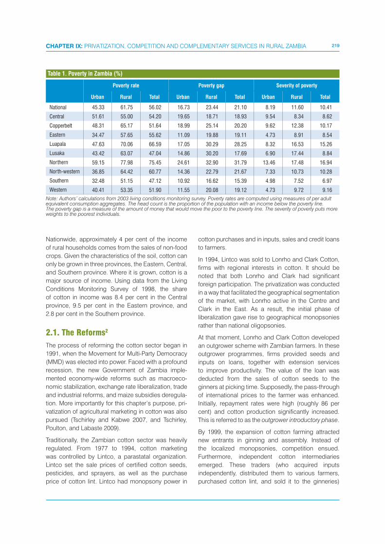
219CHAPTER IX: PRIVATIZATION, COMPETITION AND COMPLEMENTARY SERVICES IN RURAL ZAMBIA
Nationwide, approximately 4 per cent of the income
of rural households comes from the sales of non-food
crops. Given the characteristics of the soil, cotton can
only be grown in three provinces, the Eastern, Central,
and Southern province. Where it is grown, cotton is a
major source of income. Using data from the Living
Conditions Monitoring Survey of 1998, the share
of cotton in income was 8.4 per cent in the Central
province, 9.5 per cent in the Eastern province, and
2.8 per cent in the Southern province.
2.1. The Reforms2
The process of reforming the cotton sector began in
1991, when the Movement for Multi-Party Democracy
(MMD) was elected into power. Faced with a profound
recession, the new Government of Zambia imple-
mented economy-wide reforms such as macroeco-
nomic stabilization, exchange rate liberalization, trade
and industrial reforms, and maize subsidies deregula-
tion. More importantly for this chapter’s purpose, pri-
vatization of agricultural marketing in cotton was also
pursued (Tschirley and Kabwe 2007, and Tschirley,
Poulton, and Labaste 2009).
Traditionally, the Zambian cotton sector was heavily
regulated. From 1977 to 1994, cotton marketing
was controlled by Lintco, a parastatal organization.
Lintco set the sale prices of certified cotton seeds,
pesticides, and sprayers, as well as the purchase
price of cotton lint. Lintco had monopsony power in
cotton purchases and in inputs, sales and credit loans
to farmers.
In 1994, Lintco was sold to Lonrho and Clark Cotton,
firms with regional interests in cotton. It should be
noted that both Lonrho and Clark had significant
foreign participation. The privatization was conducted
in a way that facilitated the geographical segmentation
of the market, with Lonrho active in the Centre and
Clark in the East. As a result, the initial phase of
liberalization gave rise to geographical monopsonies
rather than national oligopsonies.
At that moment, Lonrho and Clark Cotton developed
an outgrower scheme with Zambian farmers. In these
outgrower programmes, firms provided seeds and
inputs on loans, together with extension services
to improve productivity. The value of the loan was
deducted from the sales of cotton seeds to the
ginners at picking time. Supposedly, the pass-through
of international prices to the farmer was enhanced.
Initially, repayment rates were high (roughly 86 per
cent) and cotton production significantly increased.
This is referred to as the outgrower introductory phase.
By 1999, the expansion of cotton farming attracted
new entrants in ginning and assembly. Instead of
the localized monopsonies, competition ensued.
Furthermore, independent cotton intermediaries
emerged. These traders (who acquired inputs
independently, distributed them to various farmers,
purchased cotton lint, and sold it to the ginneries)
Poverty rate Poverty gap Severity of poverty
Urban Rural Total Urban Rural Total Urban Rural Total
National 45.33 61.75 56.02 16.73 23.44 21.10 8.19 11.60 10.41
Central 51.61 55.00 54.20 19.65 18.71 18.93 9.54 8.34 8.62
Copperbelt 48.31 65.17 51.64 18.99 25.14 20.20 9.62 12.38 10.17
Eastern 34.47 57.65 55.62 11.09 19.88 19.11 4.73 8.91 8.54
Luapala 47.63 70.06 66.59 17.05 30.29 28.25 8.32 16.53 15.26
Lusaka 43.42 63.07 47.04 14.86 30.20 17.69 6.90 17.44 8.84
Northern 59.15 77.98 75.45 24.61 32.90 31.79 13.46 17.48 16.94
North-western 36.85 64.42 60.77 14.36 22.79 21.67 7.33 10.73 10.28
Southern 32.48 51.15 47.12 10.92 16.62 15.39 4.98 7.52 6.97
Western 40.41 53.35 51.90 11.55 20.08 19.12 4.73 9.72 9.16
Note: Authors’ calculations from 2003 living conditions monitoring survey. Poverty rates are computed using measures of per adult equivalent consumption aggregates. The head count is the proportion of the population with an income below the poverty line. The poverty gap is a measure of the amount of money that would move the poor to the poverty line. The severity of poverty puts more weights to the poorest individuals.
Table 1. Poverty in Zambia (%)

220 SERVICES, TRADE & DEVELOPMENT
made competition even more aggressive. Without
any regulatory framework to control entry, the system
entered a vicious cycle and failed. Those firms that
were not using outgrower schemes, as well as some
cotton intermediaries, had incentive to offer higher
net cotton prices to farmers who had already signed
outgrower contracts with other firms (mostly Lonrho
and Clark). This caused repayment problems and
increased the rate of loan defaults. The loan repayment
rate, for instance, dropped to approximately 60 per
cent to 65 per cent. In turn, firms raised loan prices
and non-defaulting farmers ended up receiving lower
net prices for their cotton production. The sector
collapsed. This is referred to as the outgrower scheme
failure phase.3
Partly as a result of the failure of outgrower schemes,
Lonrho exited the market and was acquired by Duna-
vant Zambia Limited (part of a United States of America
multinational corporation). Dunavant and Clark Cotton
actively worked to improve and expand the outgrow-
er schemes.4 Two innovations took place. First, firms
adopted identifying labels on the cotton bags given to
farmers to store production after harvest and commit-
ted them to only purchase cotton bags with their own
labels. This helped eliminate most of the independ-
ent traders that contaminated the market during the
failure phase. Second, Dunavant introduced the “Dis-
tributor System.” The firms provided inputs which were
allocated to farmers by a distributor, an independent
agent (not a firm employee), that grew cotton himself.
He prepared individual contracts with the farmers, was
in charge of assessing reasons for loan defaults (be-
ing able, in principle, of condoning default in special
cases), and renegotiated contracts in future seasons.
The Distributor had discretion on the number of farm-
ers under his control. Clark kept the more traditional
agent/employee-based system but worked to extend
coverage. Both Dunavant and Clark (and others) ex-
panded the production network, thus facilitating ac-
cess for a wider array of smallholders. Both systems
worked well, and repayment rates increased from 65
per cent to 90 per cent (Tschirley and Kabwe, 2007).
The sector advanced significantly. This is referred to as
the outgrower scheme success phase.
From 2002 to the present, the cotton sector performed
well. It is vibrant and the market is dynamic, with entry,
exit, and acquisition taking place---for instance, Cargill
bought Clark Cotton in 2006. Although the outgrower
scheme works well, it is in need of constant monitoring
due to potential deviations from the contract system
by (occasional) new entrants.
2.2. Trends in Cotton Production
In the following, data from the Post Harvest Survey
(PHS) is utilized to look at the correlation between
cotton adoption and cotton yields with the different
phases of reforms. The PHS data are collected by the
Zambian Central Statistical Office (CSO). It is a repeat-
ed cross-section (not a panel). Annual cross-sections
are only available for the period 1997 to 2002. The Post
Harvest Surveys include data on land tenure, land al-
location, output in physical units, limited input data,
and household characteristics such as demographic
composition, age of head, and housing infrastructure.
Table 2 provides an overview of the relevant sample
sizes, by year and by province. In a given survey,
around 600 to 700 households were interviewed in
Province 1997 1998 1999 2000 2001 2002
Central 654 674 648 795 663 701
Eastern 1 225 1 197 1 255 1 437 1 248 1 292
Southern 895 828 835 961 835 850
Lusaka 246 252 243 244 185 182
Copperbelt 370 349 379 464 367 372
Luapula 803 775 799 869 760 761
Northern 1 211 1 190 1 348 1 551 1 293 1 376
North-western 409 423 429 543 435 431
Western 706 648 725 835 699 733
Total 6 519 6 336 6 661 7 699 6 485 6 698
Note: Authors’ calculations based on the post harvest surveys 1997-2002.
Table 2. Post harvest survey (sample sizes)
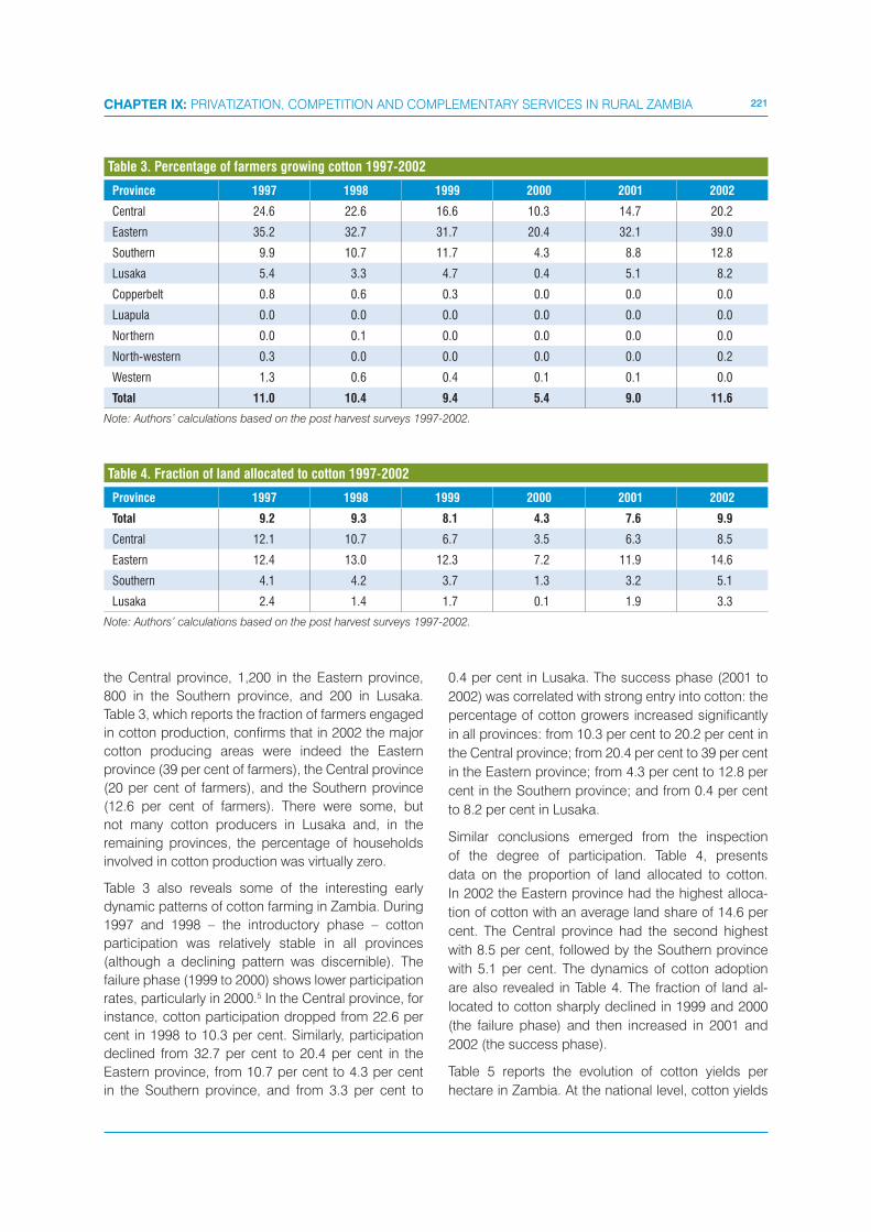
221CHAPTER IX: PRIVATIZATION, COMPETITION AND COMPLEMENTARY SERVICES IN RURAL ZAMBIA
the Central province, 1,200 in the Eastern province,
800 in the Southern province, and 200 in Lusaka.
Table 3, which reports the fraction of farmers engaged
in cotton production, confirms that in 2002 the major
cotton producing areas were indeed the Eastern
province (39 per cent of farmers), the Central province
(20 per cent of farmers), and the Southern province
(12.6 per cent of farmers). There were some, but
not many cotton producers in Lusaka and, in the
remaining provinces, the percentage of households
involved in cotton production was virtually zero.
Table 3 also reveals some of the interesting early
dynamic patterns of cotton farming in Zambia. During
1997 and 1998 – the introductory phase – cotton
participation was relatively stable in all provinces
(although a declining pattern was discernible). The
failure phase (1999 to 2000) shows lower participation
rates, particularly in 2000.5 In the Central province, for
instance, cotton participation dropped from 22.6 per
cent in 1998 to 10.3 per cent. Similarly, participation
declined from 32.7 per cent to 20.4 per cent in the
Eastern province, from 10.7 per cent to 4.3 per cent
in the Southern province, and from 3.3 per cent to
0.4 per cent in Lusaka. The success phase (2001 to
2002) was correlated with strong entry into cotton: the
percentage of cotton growers increased significantly
in all provinces: from 10.3 per cent to 20.2 per cent in
the Central province; from 20.4 per cent to 39 per cent
in the Eastern province; from 4.3 per cent to 12.8 per
cent in the Southern province; and from 0.4 per cent
to 8.2 per cent in Lusaka.
Similar conclusions emerged from the inspection
of the degree of participation. Table 4, presents
data on the proportion of land allocated to cotton.
In 2002 the Eastern province had the highest alloca-
tion of cotton with an average land share of 14.6 per
cent. The Central province had the second highest
with 8.5 per cent, followed by the Southern province
with 5.1 per cent. The dynamics of cotton adoption
are also revealed in Table 4. The fraction of land al-
located to cotton sharply declined in 1999 and 2000
(the failure phase) and then increased in 2001 and
2002 (the success phase).
Table 5 reports the evolution of cotton yields per
hectare in Zambia. At the national level, cotton yields
Province 1997 1998 1999 2000 2001 2002
Central 24.6 22.6 16.6 10.3 14.7 20.2
Eastern 35.2 32.7 31.7 20.4 32.1 39.0
Southern 9.9 10.7 11.7 4.3 8.8 12.8
Lusaka 5.4 3.3 4.7 0.4 5.1 8.2
Copperbelt 0.8 0.6 0.3 0.0 0.0 0.0
Luapula 0.0 0.0 0.0 0.0 0.0 0.0
Northern 0.0 0.1 0.0 0.0 0.0 0.0
North-western 0.3 0.0 0.0 0.0 0.0 0.2
Western 1.3 0.6 0.4 0.1 0.1 0.0
Total 11.0 10.4 9.4 5.4 9.0 11.6
Note: Authors’ calculations based on the post harvest surveys 1997-2002.
Table 3. Percentage of farmers growing cotton 1997-2002
Province 1997 1998 1999 2000 2001 2002
Total 9.2 9.3 8.1 4.3 7.6 9.9
Central 12.1 10.7 6.7 3.5 6.3 8.5
Eastern 12.4 13.0 12.3 7.2 11.9 14.6
Southern 4.1 4.2 3.7 1.3 3.2 5.1
Lusaka 2.4 1.4 1.7 0.1 1.9 3.3
Note: Authors’ calculations based on the post harvest surveys 1997-2002.
Table 4. Fraction of land allocated to cotton 1997-2002
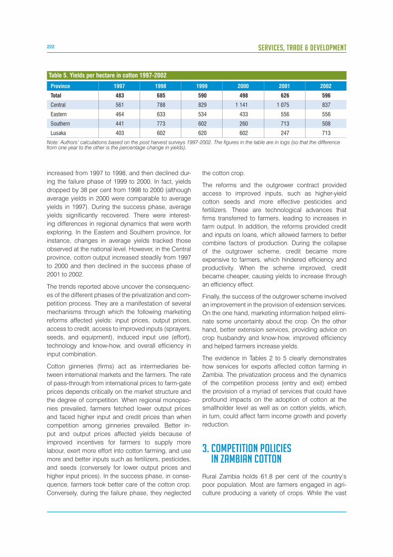
222 SERVICES, TRADE & DEVELOPMENT
increased from 1997 to 1998, and then declined dur-
ing the failure phase of 1999 to 2000. In fact, yields
dropped by 38 per cent from 1998 to 2000 (although
average yields in 2000 were comparable to average
yields in 1997). During the success phase, average
yields significantly recovered. There were interest-
ing differences in regional dynamics that were worth
exploring. In the Eastern and Southern province, for
instance, changes in average yields tracked those
observed at the national level. However, in the Central
province, cotton output increased steadily from 1997
to 2000 and then declined in the success phase of
2001 to 2002.
The trends reported above uncover the consequenc-
es of the different phases of the privatization and com-
petition process. They are a manifestation of several
mechanisms through which the following marketing
reforms affected yields: input prices, output prices,
access to credit, access to improved inputs (sprayers,
seeds, and equipment), induced input use (effort),
technology and know-how, and overall efficiency in
input combination.
Cotton ginneries (firms) act as intermediaries be-
tween international markets and the farmers. The rate
of pass-through from international prices to farm-gate
prices depends critically on the market structure and
the degree of competition. When regional monopso-
nies prevailed, farmers fetched lower output prices
and faced higher input and credit prices than when
competition among ginneries prevailed. Better in-
put and output prices affected yields because of
improved incentives for farmers to supply more
labour, exert more effort into cotton farming, and use
more and better inputs such as fertilizers, pesticides,
and seeds (conversely for lower output prices and
higher input prices). In the success phase, in conse-
quence, farmers took better care of the cotton crop.
Conversely, during the failure phase, they neglected
the cotton crop.
The reforms and the outgrower contract provided
access to improved inputs, such as higher-yield
cotton seeds and more effective pesticides and
fertilizers. These are technological advances that
firms transferred to farmers, leading to increases in
farm output. In addition, the reforms provided credit
and inputs on loans, which allowed farmers to better
combine factors of production. During the collapse
of the outgrower scheme, credit became more
expensive to farmers, which hindered efficiency and
productivity. When the scheme improved, credit
became cheaper, causing yields to increase through
an efficiency effect.
Finally, the success of the outgrower scheme involved
an improvement in the provision of extension services.
On the one hand, marketing information helped elimi-
nate some uncertainty about the crop. On the other
hand, better extension services, providing advice on
crop husbandry and know-how, improved efficiency
and helped farmers increase yields.
The evidence in Tables 2 to 5 clearly demonstrates
how services for exports affected cotton farming in
Zambia. The privatization process and the dynamics
of the competition process (entry and exit) embed
the provision of a myriad of services that could have
profound impacts on the adoption of cotton at the
smallholder level as well as on cotton yields, which,
in turn, could affect farm income growth and poverty
reduction.
3. COMPETITION POLICIES IN ZAMBIAN COTTON
Rural Zambia holds 61.8 per cent of the country’s
poor population. Most are farmers engaged in agri-
culture producing a variety of crops. While the vast
Province 1997 1998 1999 2000 2001 2002
Total 483 685 590 498 626 596
Central 561 788 829 1 141 1 075 837
Eastern 464 633 534 433 556 556
Southern 441 773 602 260 713 508
Lusaka 403 602 620 602 247 713
Note: Authors’ calculations based on the post harvest surveys 1997-2002. The figures in the table are in logs (so that the difference from one year to the other is the percentage change in yields).
Table 5. Yields per hectare in cotton 1997-2002

223CHAPTER IX: PRIVATIZATION, COMPETITION AND COMPLEMENTARY SERVICES IN RURAL ZAMBIA
majority of households in rural areas produce food for
home consumption, the number of farmers engaged
in commercial agriculture such as cotton is much low-
er. It has long been recognized that, under the right
circumstances, commercial agriculture, in particular
cotton cultivation, can work as an effective vehicle
for poverty alleviation (Balat and Porto, 2007). This is
because commercial crops often show higher returns
(per unit of inputs) than home consumption crops.
However, as has previously been shown, cotton com-
mercialization takes place along a value chain where
intermediaries, exporters, downstream producers and
upstream producers interact with farmers.
Farmers produce cotton seed which is the basic in-
put of the cotton value chain, involving international
markets and exports. The farming sector itself is
composed of many atomistic smallholders. Instead,
the lower-level of the chain is usually dominated by
a small number of firms. Farmers may thus suffer
from the non-competitive behaviour of agents at other
levels of the chain. In this scenario, changes in the
structure of these levels, for example by increas-
ing downstream competition, will affect the prices
received by farmers and therefore their income and
earnings. The main purpose of this analysis is to
estimate impacts, at the farm level, of changes in the
cotton value chain on household income.
The household analysis at the farm level is quite broad.
To begin with, it is important to discover how the in-
come of an average farmer already participating in
the cotton chain will respond to changes in the struc-
ture of that chain. These farmers are most likely to be
affected by any changes in the commercialization of
cotton. At the same time, it is necessary to shed some
light on the income responses of those smallholders
who are initially not participating in the chain. If these
are the poorest or most vulnerable households, larger
impacts on poverty should be expected when these
farm responses are included in the analysis.
To address these questions, the analysis proceeds
in two stages. In the first stage, the changes in farm-
gate prices of cotton given hypothetical changes in
the structure of the chain are simulated. The second
stage utilizes these price changes to estimate house-
hold income responses using household survey data.
To compute the price changes that would be generat-
ed by changes in the value chain, a theoretical model
of a cotton sector with a vertical structure and different
layers in the value chain was set up. The theoretical
model commences with a basic model in which atom-
istic farmers produce cotton that is sold to an oligopo-
listic exporter. The basic model is then expanded to in-
clude two layers along the chain in order that farmers
interact with both upstream and downstream produc-
ers and or retailers. Based on data on the elasticity of
demand in the different layers, the elasticity of supply
of cotton, the number of firms operating in each layer
and other relevant information, price changes caused
by changes in the main parameters of the model that
characterize the cotton value chain are simulated. The
simulations involve the re-evaluation of the solution
to the theoretical model under different assumptions
about the value of those parameters. Two markets
were explored: the market for cotton lint, where farm-
ers sell cotton seed to the ginneries, and the ginner-
ies export cotton lint; and the market for cotton yarn,
where farmers sell cotton seed to the ginneries, the
ginneries in turn sell to the retailers, who export yarn.
In the second stage, price changes for cotton calcu-
lated in the first stage are fed into household survey
data. The available household surveys have informa-
tion on the structure of income derived from various
agricultural activities. Faced with a change in farm-
gate cotton prices, the effect on farm income can
be studied by exploring the income shares (Deaton,
1989; Deaton, 1997). This methodology provides an
evaluation of the income responses of those house-
holds already participating in the value chain. By in-
specting the distribution of the income shares along
the income distribution, it will be possible to identify
which farmers will benefit more from the price changes
and whether the poor will enjoy any of these benefits.
The analysis takes a further step and evaluates the
likely responses of those farmers initially not involved
in the value chain. This is an important addition to
the more standard analysis, since those farmers that
are out of the chain are likely to be the poorest or
the most vulnerable households. In order to conduct
this evaluation four steps were required. First, based
on information from the household survey, a Probit
model of cotton participation is estimated, allowing
for a prediction of the probability of participation
for all farmers in the household survey sample.
Second, using the simulated price changes from the
first stage, aggregate supply responses at the farm
level are calculated. Third, these supply responses
are allocated to the farmers in proportion to the
estimated Probit probabilities. It should be noted that
this method allows these supply responses to affect
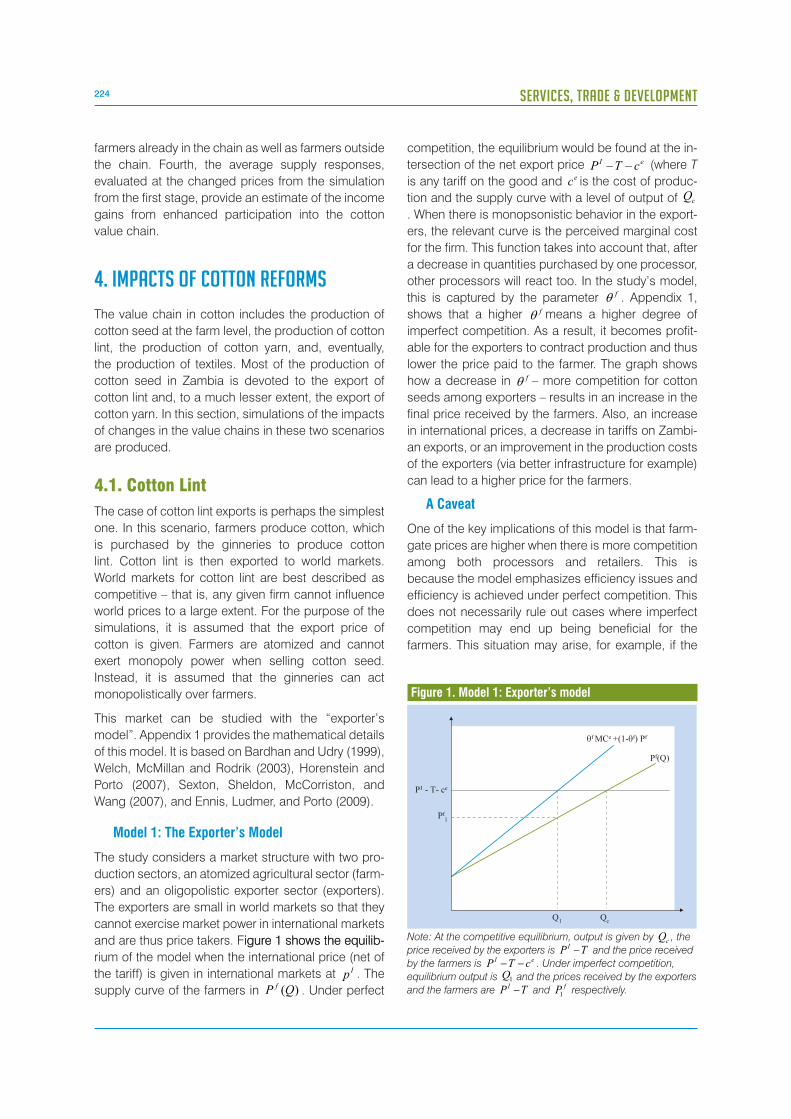
224 SERVICES, TRADE & DEVELOPMENT
farmers already in the chain as well as farmers outside
the chain. Fourth, the average supply responses,
evaluated at the changed prices from the simulation
from the first stage, provide an estimate of the income
gains from enhanced participation into the cotton
value chain.
4. IMPACTS OF COTTON REFORMS
The value chain in cotton includes the production of
cotton seed at the farm level, the production of cotton
lint, the production of cotton yarn, and, eventually,
the production of textiles. Most of the production of
cotton seed in Zambia is devoted to the export of
cotton lint and, to a much lesser extent, the export of
cotton yarn. In this section, simulations of the impacts
of changes in the value chains in these two scenarios
are produced.
4.1. Cotton Lint
The case of cotton lint exports is perhaps the simplest
one. In this scenario, farmers produce cotton, which
is purchased by the ginneries to produce cotton
lint. Cotton lint is then exported to world markets.
World markets for cotton lint are best described as
competitive – that is, any given firm cannot influence
world prices to a large extent. For the purpose of the
simulations, it is assumed that the export price of
cotton is given. Farmers are atomized and cannot
exert monopoly power when selling cotton seed.
Instead, it is assumed that the ginneries can act
monopolistically over farmers.
This market can be studied with the “exporter’s
model”. Appendix 1 provides the mathematical details
of this model. It is based on Bardhan and Udry (1999),
Welch, McMillan and Rodrik (2003), Horenstein and
Porto (2007), Sexton, Sheldon, McCorriston, and
Wang (2007), and Ennis, Ludmer, and Porto (2009).
Model 1: The Exporter’s Model
The study considers a market structure with two pro-
duction sectors, an atomized agricultural sector (farm-
ers) and an oligopolistic exporter sector (exporters).
The exporters are small in world markets so that they
cannot exercise market power in international markets
and are thus price takers. Figure 1 shows the equilib-igure 1 shows the equilib-
rium of the model when the international price (net of
the tariff) is given in international markets at Ip . The
supply curve of the farmers in )(QP f . Under perfect
Figure 1. Model 1: Exporter’s model
PI - T- ce
�f MCe +(1-�f) Pf
Pf1
Pf(Q)
QcQ1
Note: At the competitive equilibrium, output is given by cQ , the
price received by the exporters is TP I � and the price received
by the farmers is eI cTP �� . Under imperfect competition,
equilibrium output is 1Q and the prices received by the exporters
and the farmers are TP I � and fP1 respectively.
competition, the equilibrium would be found at the in-
tersection of the net export price eI cTP �� (where T
is any tariff on the good and ec is the cost of produc-
tion and the supply curve with a level of output of cQ
. When there is monopsonistic behavior in the export-
ers, the relevant curve is the perceived marginal cost
for the firm. This function takes into account that, after
a decrease in quantities purchased by one processor,
other processors will react too. In the study’s model,
this is captured by the parameter f� . Appendix 1,
shows that a higher f� means a higher degree of
imperfect competition. As a result, it becomes profit-
able for the exporters to contract production and thus
lower the price paid to the farmer. The graph shows
how a decrease in f� – more competition for cotton
seeds among exporters – results in an increase in the
final price received by the farmers. Also, an increase
in international prices, a decrease in tariffs on Zambi-
an exports, or an improvement in the production costs
of the exporters (via better infrastructure for example)
can lead to a higher price for the farmers.
A Caveat
One of the key implications of this model is that farm-
gate prices are higher when there is more competition
among both processors and retailers. This is
because the model emphasizes efficiency issues and
efficiency is achieved under perfect competition. This
does not necessarily rule out cases where imperfect
competition may end up being beneficial for the
farmers. This situation may arise, for example, if the

225CHAPTER IX: PRIVATIZATION, COMPETITION AND COMPLEMENTARY SERVICES IN RURAL ZAMBIA
realization of monopoly profits allows for the creation
of new goods and markets that use farm outputs as
key inputs. In other words, in cases where monopoly
profits allow firms to create new markets for the poor,
it may be desirable to allow for imperfect competition
at different layers of the value chain. The analysis
does not accommodate these cases. However, in the
simulations below, cases are considered where the
presence of a few firms allows for the success of the
outgrower scheme in cotton. This is then an instance
where imperfect competition, to some degree at least,
may be desirable.
Micro econometric Model: Household Impacts
The numerical solution to the “exporters’ model”
deliver market prices and quantities in equilibrium.
These solutions can be shocked to simulate price
and quantity responses from a baseline situation
to a proposed scenario. With this simulation and
the household survey, the next task was to estimate
welfare effects. To be as comprehensive as possible,
first order effects and second order effects which
include supply responses, were included.
First order effects are the direct impact, caused by
those price changes, over current cotton producers.
First order effects are computed as the cotton share
in total household income multiplied by the per cent
change in cotton prices. For example, if a household
earns 50 per cent of its income from cotton and the
price of cotton increases by 50 per cent, then the first
order effect of this price change would be equivalent
to 25 per cent of the (initial) household income. These
effects represent the short term impacts of the price
changes, before any production response.
The analysis also accounts for supply responses.
Therefore, when prices go up, farmers are allowed to
expand production and even switch to other crops.
These comprise second order effects of the price
change, which are a measure of the benefit from
adjusting production. Changes in production levels
are calculated with the “exporters’ model” of value
chains. To allocate these quantity changes among
farmers, a procedure was adopted that assigned
responses in proportion to the likelihood of being a
cotton producer. This probability can be estimated
with the relative propensity score as follows.
First, the propensity score )(xp is defined as the prob-
ability of producing cotton as a function of a vector
of characteristics x . The estimating equation of the
propensity score is )|1=(=)( ii DPp xx where D is
an indicator function of whether the household is a
producer of the agricultural product and x is the set
of relevant characteristics.6
Next, these probabilities are re-scaled by the sum of
the individual propensity scores
.)(
)(=~
i
i
i
xp
xpp
�
This re-scaling transforms the estimated propensity
score into weights that can be used to allocate the
increased production predicted by the “exporters’s
model.”
Simulations
First, a baseline scenario was calibrated, based on
information on the number of firms in each sector and
on their market shares. In the case of cotton, measures
of market shares are built based on the available data
on processing capacity. There are six major players
in cotton: Dunavant (44 per cent), Cargill (32 per
cent), Amaka (13 per cent), Mulungushi (6 per cent),
Continental (5 per cent) and Mukuba (1 per cent).
Minor changes in these shares are not likely to affect
the results. A key parameter of the model, in contrast,
is the elasticity of supply of cotton at the farm level.
Estimates of the elasticity of supply are generally hard
to obtain. In principle, this elasticity should be quite
low, particularly in the short run. Based on estimates
available in the literature and also based on personal
interviews with cotton farmers in Zambia, a baseline
elasticity of supply of 0.75 was used. To explore how
robust results are, a full set of sensitivity results were
carried out (appendix 2). Five different competition
configuration scenarios were then simulated: “Leader
splits”; “Small entrant”; “Leaders merge + Small
entrant”; “Leaders merge”; “Exit of the largest”;
“Equal market shares”; and “Competition”. These
simulations describe several possible mergers, splits
and new entrants in the industry.
Table 6 presents the simulation results for each compe-
tition scenario by different rural population groups. The
exercise shows that the change in cotton prices ranged
from 34 per cent (in cases of increased market power)
to 42 per cent (in cases of increased competition).
The main conclusion from Table 6 is that competi-
tion at the cotton processing level is good for the
farmers. In the model, more competition among
processors translates into higher farm-gate prices.

226 SERVICES, TRADE & DEVELOPMENT
As a result, either entry or split of incumbents gener-
ates welfare gains for the farmers. This can be seen,
for example, in simulation 1 (“Leader splits”) and sim-
ulation 2 (“Small entrant”), both involving an increase
in competition. On the other hand, further market con-
centration leads to lower farm income and generates
losses for the farmers. This can be seen, for example,
in simulation 3 (“Leaders merge + Small entrant”) and
simulation 4 (“Leaders merge”), both involving a de-
crease in competition.
Small changes in the value chains are not likely to
generate large impacts on farmers. For instance, sim-
ulation 2 (“Small entrant”) shows very small impacts
on farm income; in contrast, large changes in com-
petition such as simulation 1 (“Leader splits”) cause
much larger effects. Similar remarks can be made
about decreases in competition. Small changes in
market power generate relatively small impacts at the
farm level – demonstrated when comparing simula-
tion 3 with simulation 4.
For a given simulation, the average per cent income
change is much larger for cotton (household) produc-
ers than for non-cotton producers. For example, in
simulation 1 (“Leader Splits”), the increase in farm-gate
prices was 12.53 per cent. This generates an increase
in the average income of rural households of 0.49 per
cent, an effect that is quite small from a practical point
of view. However, the income of a cotton producer
increased by 4.30 per cent. This is a sizable income
effect, especially for the poor. The impacts on the en-
tire rural population were smaller because of two main
factors. First, only 8.4 per cent of households were
cotton producers and, second, their average spe-
cialization rate was 35.5 per cent. This means that the
increase in cotton prices would only affect a relatively
small fraction of an average farmer’s income.
Another way to see this is by comparing the first and
second order impacts of the price change. The first
order effects reveal the impacts at a given level of
production (without any adjustments). The second
order impacts allow farmers to respond to new prices
as well. In other words, second order effects allow for
supply responses and increased farmer participation
in cotton. The simulations clearly show that the first
order effects account for most of the change in
household income.
Simulation
1 2 3 4 5 6 7
����� 0.1253 0.0221 -0.3049 -0.3429 -0.0937 0.1955 0.4237
Total 0.0049 0.0008 -0.0074 -0.0080 -0.0029 0.0082 0.0227
1st order 0.0043 0.0008 -0.0104 -0.0116 -0.0032 0.0066 0.0144
2nd order 0.0006 0.0000 0.0030 0.0037 0.0003 0.0016 0.0083
Producers 0.0430 0.0075 -0.1004 -0.1126 -0.0314 0.0677 0.1515
1st order 0.0424 0.0075 -0.1033 -0.1161 -0.0317 0.0662 0.1435
2nd order 0.0006 0.0000 0.0028 0.0035 0.0003 0.0015 0.0079
Poor 0.0047 0.0007 -0.0067 -0.0072 -0.0027 0.0080 0.0224
1st order 0.0040 0.0007 -0.0098 -0.0111 -0.0030 0.0063 0.0137
2nd order 0.0007 0.0000 0.0031 0.0039 0.0003 0.0017 0.0088
Non-Poor 0.0052 0.0008 -0.0085 -0.0092 -0.0032 0.0086 0.0232
1st order 0.0046 0.0008 -0.0112 -0.0126 -0.0034 0.0072 0.0156
2nd order 0.0006 0.0000 0.0027 0.0034 0.0003 0.0014 0.0076
Note: Authors’ calculations based on the exporter’s model and household data from the 2003 living conditions monitoring surveys.
Simulation 1: “Leader splits”Simulation 2: “Small entrant”Simulation 3: “Leaders merge +Small entrant”Simulation 4: “Leaders merge”Simulation 5: “Exit of the largest”Simulation 6: “Equal market shares” (imperfect competition)Simulation 7: “Competition”
Table 6. Changes in income (%)

227CHAPTER IX: PRIVATIZATION, COMPETITION AND COMPLEMENTARY SERVICES IN RURAL ZAMBIA
It is interesting to note that the previous result is true
even in the presence of supply responses. The reason
being that, in the case of supply responses, higher
cotton prices are only enjoyed by marginal units.
However, even though the second order effects are
small, they are very important for “non-producers.”
While the second order impacts on producers account
for a small fraction of their overall gains, they account
for all the benefits accruing to non-producers.
Another important result is that the benefits for the poor
and the non-poor are similar in magnitude. On the
one hand, results show that the benefits of increased
competition in the value chain do not concentrate
on the non-poor. On the other hand, the fact that
the impacts on both groups are small indicates that
cotton participation is low across all levels.
One concern often encountered in practice is to better
understand the implications of exit, particularly of
the largest firm. This is the grounds for conducting
simulation 5. In the case of cotton, the exit of Dunavant
led to a decrease of competition among firms and
thus to a decline in farm-gate prices by 9.37 per cent.
This caused income losses for farmers, equivalent to
0.29 per cent for an average farmer (not necessarily
producing cotton to begin with) and to 3.14 per cent
for an average cotton producer.
Two additional simulations attempting to quantify the
largest potential gains for the farmers were run. In
the first case (simulation 6, “Equal Market Shares,”),
the assumption was that imperfect competition
remains in place (so that the processors retain market
power over farmers). It was also assumed that the
benchmark firms alter their market shares to reach
equal market participation (that is, if production were
relocated from big companies to small ones). This
scenario would reveal an upper bound increase in
income under imperfect competition. In this case,
farm-gate prices increased by 19.55 per cent, due
to increased competition among cotton firms. Higher
prices translate into higher household income: 0.82
per cent for an average producer and 6.77 per cent
for a cotton producer. This scenario produced large
impacts on household income.
The final simulation assumed perfect competition
among processors (simulation 7). This maximizes
overall efficiency. Farm-gate prices could be 42.37 per
cent higher than in the current situation. This implies
large increases in household incomes. An average
farmer would enjoy benefits of up to 2.27 per cent
and, in contrast, a typical cotton producer would enjoy
gains of 15.15 per cent, on average. This situation led
to the largest possible gains for the farmers (but is
probably unlikely).
Outgrower Schemes: Adverse Competition Effects
Small farmers can receive financing from processors
(in the form of inputs) in exchange for future production
through the outgrower scheme. In the absence of
enforcement mechanisms, however, processors
would not have incentives to provide input in advance.
If contracts cannot be enforced, farmers could default
on their debt and sell all the production to the best
buyer (thus depriving processors from investment
returns). Importantly, the degree of failure of the
outgrower contract can, at least in part, be linked to
increased competition.
The failure of the outgrower programme could be
thought of as increases in the firms’ costs. There
are a number of mechanisms that could prevent
farmers from not honouring contracts. Social norms,
reputation, monitoring, price controls, collusion and
specific storage devices are some examples. Although
some of these mechanisms demand no active role
of processors, in practice firms spend resources to
reduce farmer fraud. An increase in the degree of
competition in the processor sector could induce
an adverse effect because these contract-enforcing
expenses are likely to rise with the number of firms.
This would probably translate into lower output prices
for farmers. More importantly, it is believed that the
failure of the outgrower programme would increase
the price of inputs faced by firms. This increases the
costs of production of the farmers and thus reduces
household income.
Table 7 incorporates the impacts of increases in the
cost of a farmer’s production. It is assumed that these
costs increase with competition in proportion to the
decrease in �. More concretely, a farmers cost, when
there is perfect competition, is 10 per cent higher than
in the baseline situation. This factor of proportionality
is kept constant in all intermediate simulations. While
arguably this is an arbitrary setting, the idea of this
exercise is to exemplify the type of potential hazards
associated with increases in competition in the
presence of an outgrower scheme.
As the results in Table 7 show, this effect reduces
a farmer’s potential gains and losses because the
impacts of more competition and of higher costs move
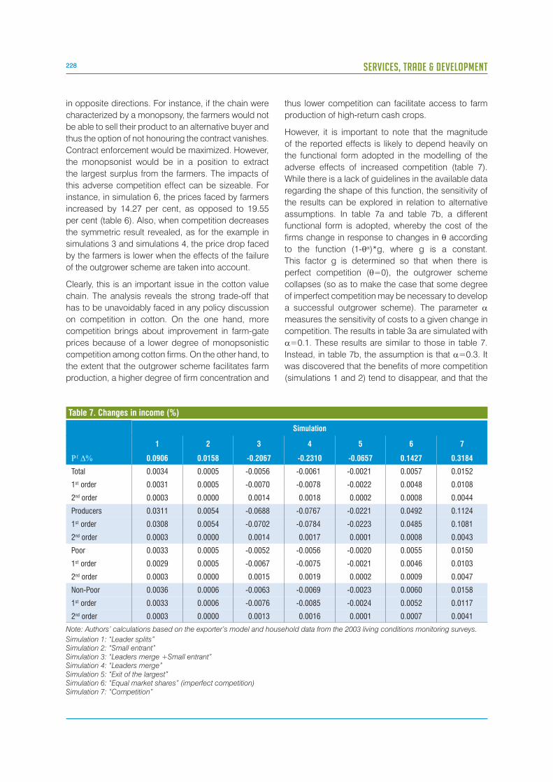
228 SERVICES, TRADE & DEVELOPMENT
in opposite directions. For instance, if the chain were
characterized by a monopsony, the farmers would not
be able to sell their product to an alternative buyer and
thus the option of not honouring the contract vanishes.
Contract enforcement would be maximized. However,
the monopsonist would be in a position to extract
the largest surplus from the farmers. The impacts of
this adverse competition effect can be sizeable. For
instance, in simulation 6, the prices faced by farmers
increased by 14.27 per cent, as opposed to 19.55
per cent (table 6). Also, when competition decreases
the symmetric result revealed, as for the example in
simulations 3 and simulations 4, the price drop faced
by the farmers is lower when the effects of the failure
of the outgrower scheme are taken into account.
Clearly, this is an important issue in the cotton value
chain. The analysis reveals the strong trade-off that
has to be unavoidably faced in any policy discussion
on competition in cotton. On the one hand, more
competition brings about improvement in farm-gate
prices because of a lower degree of monopsonistic
competition among cotton firms. On the other hand, to
the extent that the outgrower scheme facilitates farm
production, a higher degree of firm concentration and
thus lower competition can facilitate access to farm
production of high-return cash crops.
However, it is important to note that the magnitude
of the reported effects is likely to depend heavily on
the functional form adopted in the modelling of the
adverse effects of increased competition (table 7).
While there is a lack of guidelines in the available data
regarding the shape of this function, the sensitivity of
the results can be explored in relation to alternative
assumptions. In table 7a and table 7b, a different
functional form is adopted, whereby the cost of the
firms change in response to changes in � according
to the function (1-�)*g, where g is a constant.
This factor g is determined so that when there is
perfect competition (�=0), the outgrower scheme
collapses (so as to make the case that some degree
of imperfect competition may be necessary to develop
a successful outgrower scheme). The parameter
measures the sensitivity of costs to a given change in
competition. The results in table 3a are simulated with
=0.1. These results are similar to those in table 7.
Instead, in table 7b, the assumption is that =0.3. It
was discovered that the benefits of more competition
(simulations 1 and 2) tend to disappear, and that the
Simulation
1 2 3 4 5 6 7
����� 0.0906 0.0158 -0.2067 -0.2310 -0.0657 0.1427 0.3184
Total 0.0034 0.0005 -0.0056 -0.0061 -0.0021 0.0057 0.0152
1st order 0.0031 0.0005 -0.0070 -0.0078 -0.0022 0.0048 0.0108
2nd order 0.0003 0.0000 0.0014 0.0018 0.0002 0.0008 0.0044
Producers 0.0311 0.0054 -0.0688 -0.0767 -0.0221 0.0492 0.1124
1st order 0.0308 0.0054 -0.0702 -0.0784 -0.0223 0.0485 0.1081
2nd order 0.0003 0.0000 0.0014 0.0017 0.0001 0.0008 0.0043
Poor 0.0033 0.0005 -0.0052 -0.0056 -0.0020 0.0055 0.0150
1st order 0.0029 0.0005 -0.0067 -0.0075 -0.0021 0.0046 0.0103
2nd order 0.0003 0.0000 0.0015 0.0019 0.0002 0.0009 0.0047
Non-Poor 0.0036 0.0006 -0.0063 -0.0069 -0.0023 0.0060 0.0158
1st order 0.0033 0.0006 -0.0076 -0.0085 -0.0024 0.0052 0.0117
2nd order 0.0003 0.0000 0.0013 0.0016 0.0001 0.0007 0.0041
Note: Authors’ calculations based on the exporter’s model and household data from the 2003 living conditions monitoring surveys.
Simulation 1: “Leader splits”Simulation 2: “Small entrant”Simulation 3: “Leaders merge +Small entrant”Simulation 4: “Leaders merge”Simulation 5: “Exit of the largest”Simulation 6: “Equal market shares” (imperfect competition)Simulation 7: “Competition”
Table 7. Changes in income (%)
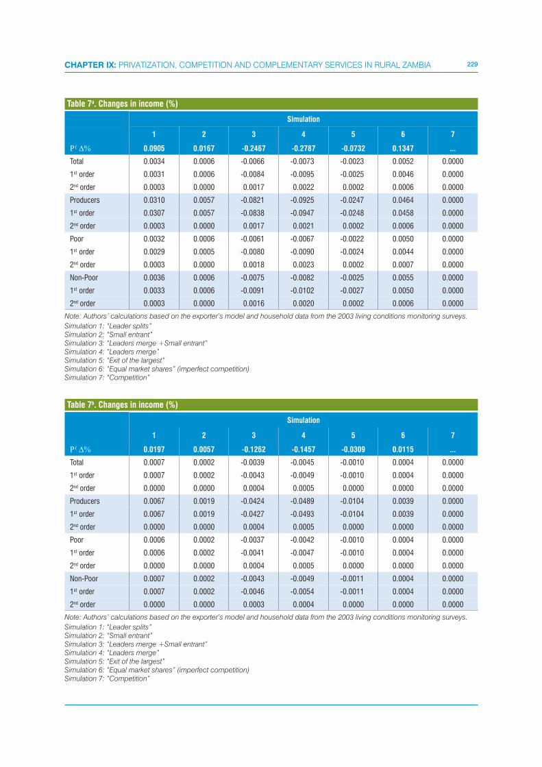
229CHAPTER IX: PRIVATIZATION, COMPETITION AND COMPLEMENTARY SERVICES IN RURAL ZAMBIA
Simulation
1 2 3 4 5 6 7
����� 0.0905 0.0167 -0.2467 -0.2787 -0.0732 0.1347 ...
Total 0.0034 0.0006 -0.0066 -0.0073 -0.0023 0.0052 0.0000
1st order 0.0031 0.0006 -0.0084 -0.0095 -0.0025 0.0046 0.0000
2nd order 0.0003 0.0000 0.0017 0.0022 0.0002 0.0006 0.0000
Producers 0.0310 0.0057 -0.0821 -0.0925 -0.0247 0.0464 0.0000
1st order 0.0307 0.0057 -0.0838 -0.0947 -0.0248 0.0458 0.0000
2nd order 0.0003 0.0000 0.0017 0.0021 0.0002 0.0006 0.0000
Poor 0.0032 0.0006 -0.0061 -0.0067 -0.0022 0.0050 0.0000
1st order 0.0029 0.0005 -0.0080 -0.0090 -0.0024 0.0044 0.0000
2nd order 0.0003 0.0000 0.0018 0.0023 0.0002 0.0007 0.0000
Non-Poor 0.0036 0.0006 -0.0075 -0.0082 -0.0025 0.0055 0.0000
1st order 0.0033 0.0006 -0.0091 -0.0102 -0.0027 0.0050 0.0000
2nd order 0.0003 0.0000 0.0016 0.0020 0.0002 0.0006 0.0000
Note: Authors’ calculations based on the exporter’s model and household data from the 2003 living conditions monitoring surveys.
Simulation 1: “Leader splits”Simulation 2: “Small entrant”Simulation 3: “Leaders merge +Small entrant”Simulation 4: “Leaders merge”Simulation 5: “Exit of the largest”Simulation 6: “Equal market shares” (imperfect competition)Simulation 7: “Competition”
Table 7a. Changes in income (%)
Simulation
1 2 3 4 5 6 7
����� 0.0197 0.0057 -0.1262 -0.1457 -0.0309 0.0115 ...
Total 0.0007 0.0002 -0.0039 -0.0045 -0.0010 0.0004 0.0000
1st order 0.0007 0.0002 -0.0043 -0.0049 -0.0010 0.0004 0.0000
2nd order 0.0000 0.0000 0.0004 0.0005 0.0000 0.0000 0.0000
Producers 0.0067 0.0019 -0.0424 -0.0489 -0.0104 0.0039 0.0000
1st order 0.0067 0.0019 -0.0427 -0.0493 -0.0104 0.0039 0.0000
2nd order 0.0000 0.0000 0.0004 0.0005 0.0000 0.0000 0.0000
Poor 0.0006 0.0002 -0.0037 -0.0042 -0.0010 0.0004 0.0000
1st order 0.0006 0.0002 -0.0041 -0.0047 -0.0010 0.0004 0.0000
2nd order 0.0000 0.0000 0.0004 0.0005 0.0000 0.0000 0.0000
Non-Poor 0.0007 0.0002 -0.0043 -0.0049 -0.0011 0.0004 0.0000
1st order 0.0007 0.0002 -0.0046 -0.0054 -0.0011 0.0004 0.0000
2nd order 0.0000 0.0000 0.0003 0.0004 0.0000 0.0000 0.0000
Note: Authors’ calculations based on the exporter’s model and household data from the 2003 living conditions monitoring surveys.
Simulation 1: “Leader splits”Simulation 2: “Small entrant”Simulation 3: “Leaders merge +Small entrant”Simulation 4: “Leaders merge”Simulation 5: “Exit of the largest”Simulation 6: “Equal market shares” (imperfect competition)Simulation 7: “Competition”
Table 7b. Changes in income (%)
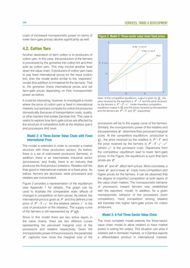
230 SERVICES, TRADE & DEVELOPMENT
costs of increased monopsonistic power (in terms of
lower farm-gate prices) decline significantly as well.
4.2. Cotton Yarn
Another destination of farm cotton is to producers of
cotton yarn. In this case, the production of the farmers
is processed by the ginneries into cotton lint and then
sold as cotton yarn. This may involve another level
down the value chain. If producers of cotton yarn have
to pay fixed international prices for the input (cotton
lint), then the model works similar to the “exporters”
model (this addition is immaterial for the farmers). That
is, the ginneries check international prices and set
farm-gate prices depending on their monopsonistic
power as before.
It could be interesting, however, to investigate a model
where the price of cotton yarn is fixed in international
markets, but spinners compete for cotton lint produced
domestically (because of transportation costs, quality,
or other barriers that isolate Zambian lint). This case is
useful to explore how farm-gate prices are affected by
the structure of competition both at the retailers (yarn)
and processors (lint) level.
Model 2: A Three-Sector Value Chain with Fixed International Price
The model is extended in order to consider a market
structure with three production sectors. As before,
there is a set of cottonseed producers (farmers); in
addition, there is an intermediate industrial sector
(processors); and finally, there is an industry that
produces the final product (retailers). Retailers sell the
final good in international markets at a fixed price. As
before, farmers are atomized, while processors and
retailers are concentrated.
Figure 2 provides a representation of the equilibrium
(see Appendix 1 for details). The graph can be
used to illustrate the comparative static effects of
changes in competition on farm prices. As before, the
international price is given at IP and this defines a net
price of rI cTP �� for the retailers (where rc is the
cost of production of the retailers). The supply curve
of the farmers is still represented by )(QP f .
Since in this model there are two active layers in
the value chains, there are two different curves
representing the perceived marginal cost of the
processors and retailers respectively. Given the
monopsonistic power of the processors, the parameter f� captures how close the marginal cost of the
processors will be to the supply curve of the farmers.
Similarly, the monopsonistic power of the retailers and
the parameters p� determine their perceived marginal
costs. At the competitive equilibrium, production is
cQ , the price received by the retailers is TP I � and
the price received by the farmers is prI ccTP ���
(where pc is the processor cost). Departures from
the competitive equilibrium lead to lower farm-gate
prices. In the Figure, the equilibrium is such that farm
prices are fP1.
Both f� and p� affect farm prices. More concretely, a
lower p� and a lower f� imply more competition and
higher prices for the farmers. It can be observed that
the degree of imperfect competition at both layers of
the value chain matters. The monopsonistic behavior
of processors toward farmers was established
with the exporters’ model. In addition, for a given
monopsonistic behavior of the processors (even
competition), more competition among retailers
will translate into higher farm-gate prices for cotton
producers.
Model 3: A Full Three-Sector Value Chain
The most complete model extends the three-sector
value chain model to allow retailers to have market
power in selling the output. This situation can arise if
retailers sell in domestic markets, or if Zambia exports
a differentiated product in international markets.
Figure 2. Model 2: Three-sector value chain fixed prices
Note: At the competitive equilibrium, output is given by cQ , the
price received by the exporters is TP I � and the price received
by the farmers is eI cTP �� . Under imperfect competition,
equilibrium output is 1Q and the prices received by the exporters
and the farmers are TP I � and fP1 respectively.
PI - T- cp-cr
QcQ1
�f MCp +(1-�f) Pf
Pf1
Pf(Q)
�p MCr +(1-�p) Pp
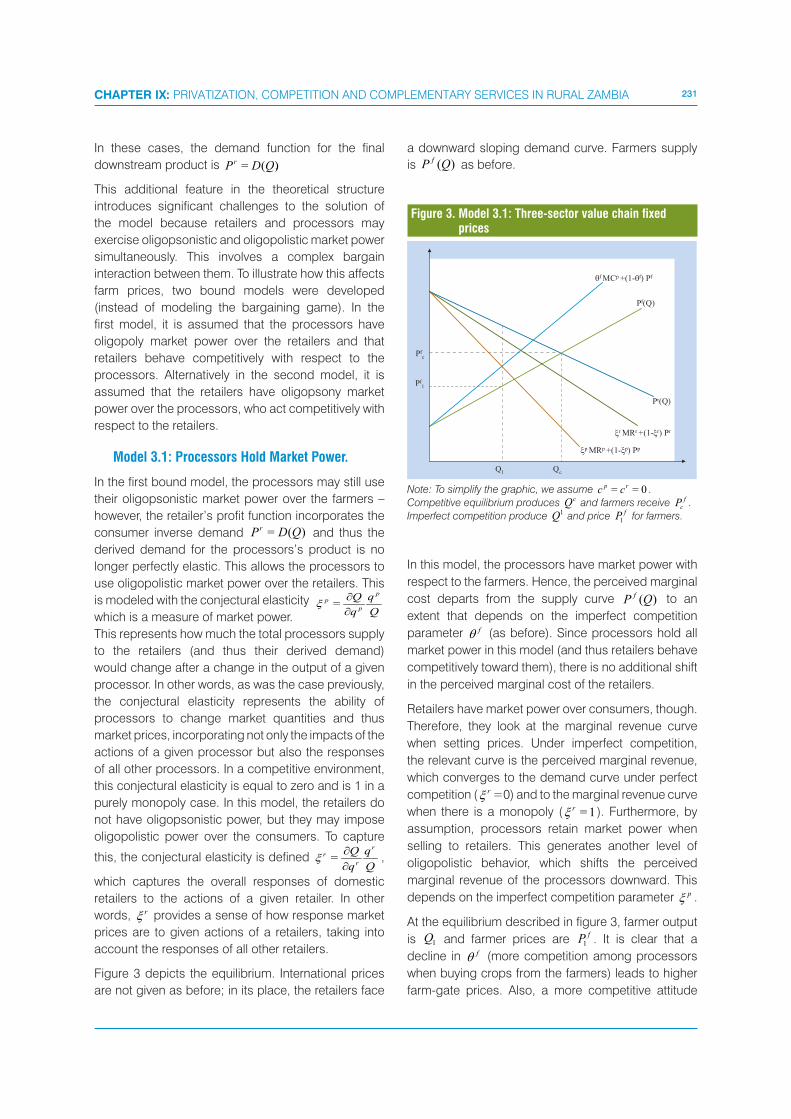
231CHAPTER IX: PRIVATIZATION, COMPETITION AND COMPLEMENTARY SERVICES IN RURAL ZAMBIA
In these cases, the demand function for the final
downstream product is ).(= QDP r
This additional feature in the theoretical structure
introduces significant challenges to the solution of
the model because retailers and processors may
exercise oligopsonistic and oligopolistic market power
simultaneously. This involves a complex bargain
interaction between them. To illustrate how this affects
farm prices, two bound models were developed
(instead of modeling the bargaining game). In the
first model, it is assumed that the processors have
oligopoly market power over the retailers and that
retailers behave competitively with respect to the
processors. Alternatively in the second model, it is
assumed that the retailers have oligopsony market
power over the processors, who act competitively with
respect to the retailers.
Model 3.1: Processors Hold Market Power.
In the first bound model, the processors may still use
their oligopsonistic market power over the farmers –
however, the retailer’s profit function incorporates the
consumer inverse demand )(= QDP r and thus the
derived demand for the processors’s product is no
longer perfectly elastic. This allows the processors to
use oligopolistic market power over the retailers. This
is modeled with the conjectural elasticity Q
q
q
Q p
p
p
��
=�
which is a measure of market power.
This represents how much the total processors supply
to the retailers (and thus their derived demand)
would change after a change in the output of a given
processor. In other words, as was the case previously,
the conjectural elasticity represents the ability of
processors to change market quantities and thus
market prices, incorporating not only the impacts of the
actions of a given processor but also the responses
of all other processors. In a competitive environment,
this conjectural elasticity is equal to zero and is 1 in a
purely monopoly case. In this model, the retailers do
not have oligopsonistic power, but they may impose
oligopolistic power over the consumers. To capture
this, the conjectural elasticity is defined Q
q
q
Q r
r
r
��
=� ,
which captures the overall responses of domestic
retailers to the actions of a given retailer. In other
words, r� provides a sense of how response market
prices are to given actions of a retailers, taking into
account the responses of all other retailers.
Figure 3 depicts the equilibrium. International prices
are not given as before; in its place, the retailers face
a downward sloping demand curve. Farmers supply
is )(QP f as before.
QcQ1
Pr(Q)
�f MCp +(1-�f) Pf
Pf(Q)
�p MRp +(1-�p) Pp
�r MRr +(1-�r) Pr
Pf1
Pfc
Note: To simplify the graphic, we assume 0== rp cc .
Competitive equilibrium produces cQ and farmers receive f
cP .
Imperfect competition produce 1Q and price
fP1 for farmers.
Figure 3. Model 3.1: Three-sector value chain fixed prices
In this model, the processors have market power with
respect to the farmers. Hence, the perceived marginal
cost departs from the supply curve )(QP f to an
extent that depends on the imperfect competition
parameter f� (as before). Since processors hold all
market power in this model (and thus retailers behave
competitively toward them), there is no additional shift
in the perceived marginal cost of the retailers.
Retailers have market power over consumers, though.
Therefore, they look at the marginal revenue curve
when setting prices. Under imperfect competition,
the relevant curve is the perceived marginal revenue,
which converges to the demand curve under perfect
competition ( r� =0) and to the marginal revenue curve
when there is a monopoly ( 1=r� ). Furthermore, by
assumption, processors retain market power when
selling to retailers. This generates another level of
oligopolistic behavior, which shifts the perceived
marginal revenue of the processors downward. This
depends on the imperfect competition parameter p� .
At the equilibrium described in figure 3, farmer output
is 1Q and farmer prices are fP1 . It is clear that a
decline in f� (more competition among processors
when buying crops from the farmers) leads to higher
farm-gate prices. Also, a more competitive attitude
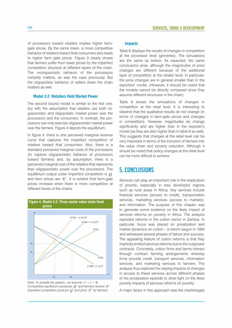
232 SERVICES, TRADE & DEVELOPMENT
of processors toward retailers implies higher farm-
gate prices. By the same token, a more competitive
behavior of retailers toward final consumers also leads
to higher farm gate prices. Figure 3 clearly shows
that farmers suffer from lower prices by the imperfect
competition structure at different layers of the chain.
The monopsonistic behavior of the processors
certainly matters, as was the case previously. But
the oligopolistic behavior of sellers down the chain
matters as well.
Model 3.2: Retailers Hold Market Power
The second bound model is similar to the first one,
but with the assumption that retailers use both oli-
gopsonistic and oligopolistic market power over the
processors and the consumers. In contrast, the pro-
cessors can only exercise oligopsonistic market power
over the farmers. Figure 4 depcits the equilibrium.
In figure 4, there is one perceived marginal revenue
curve that captures the imperfect competition of
retailers toward final consumers. Also, there is a
standard perceived marginal costs of the processors
(to capture oligopsonistic behavior of processors
toward farmers) and, by assumption, there is a
perceived marginal cost of the retailers that represents
their oligopsonistic power over the processors. The
equilibrium output under imperfect competition is 1Q
and farm prices are fP1. It is evident that farm-gate
prices increase when there is more competition at
different levels of the chains.
Impacts
Table 8 displays the results of changes in competition
at the processor level (ginneries). The simulations
are the same as before. As expected, the same
conclusions arise, although the magnitudes of price
changes are different because of the additional
layer of competition at the retailer level. In particular,
the price changes are in general smaller than in the
exporters’ model. (However, it should be noted that
the models cannot be directly compared since they
assume different structures in the chain).
Table 9 shows the simulations of changes in
competition at the retail level. It is interesting to
observe that the qualitative results do not change (in
terms of changes in farm-gate prices and changes
in competition). However, magnitudes do change
significantly and are higher than in the exporter’s
model (as they are also higher than in table 8 as well).
This suggests that changes at the retail level can be
very important in terms of the inclusion of farmers into
the value chain and poverty reduction. Although it
should be noted that policy changes at the retail level
can be more difficult to achieve.
5. CONCLUSIONS
Services can play an important role in the eradication
of poverty, especially in less developed regions
such as rural areas in Africa. Key services include
financial services (access to credit), transportation
services, marketing services (access to markets),
and information. The purpose of this chapter was
to generate some evidence on the likely impact of
services reforms on poverty in Africa. The analysis
exploited reforms in the cotton sector in Zambia. In
particular, focus was placed on privatization and
market dynamics on cotton – a reform begun in 1994
and witnessed several phases of failure and success.
The appealing feature of cotton reforms is that they
implicitly embed services reforms due to the outgrower
contracts. Concretely, cotton firms and farms interact
through contract farming arrangements whereby
firms provide credit, transport services, information
services, and marketing services to farmers. The
analysis thus explored the varying impacts of changes
in access to these services across different phases
of the privatization episode to shed light on the likely
poverty impacts of services reforms on poverty.
A major factor in this approach was the interlinkages
Pr(Q)
QcQ1
�f MCp +(1-�f) Pf
Pf1
Pf(Q)
Pfc
�r MRr +(1-�r) Pr
�p MCr +(1-�p) Pp
Note: To simplify the graphic, we assume 0== rp cc .
Competitive equilibrium produces cQ and farmers receive f
cP .
Imperfect competition produce 1Q and price fP1 for farmers.
Figure 4. Model 3.2: Three-sector value chain fixed prices

233CHAPTER IX: PRIVATIZATION, COMPETITION AND COMPLEMENTARY SERVICES IN RURAL ZAMBIA
Simulation
1 2 3 4 5 6 7
����� 0.0581 0.0100 -0.1254 -0.1394 -0.0409 0.0924 0.2123
Total 0.0022 0.0003 -0.0033 -0.0036 -0.0013 0.0037 0.0104
1st order 0.0020 0.0003 -0.0043 -0.0047 -0.0014 0.0031 0.0072
2nd order 0.0002 0.0000 0.0009 0.0011 0.0001 0.0006 0.0031
Producers 0.0199 0.0034 -0.0417 -0.0463 -0.0138 0.0319 0.0751
1st order 0.0197 0.0034 -0.0426 -0.0474 -0.0139 0.0314 0.0721
2nd order 0.0002 0.0000 0.0009 0.0011 0.0001 0.0005 0.0030
Poor 0.0021 0.0003 -0.0031 -0.0033 -0.0012 0.0036 0.0102
1st order 0.0019 0.0003 -0.0041 -0.0045 -0.0013 0.0030 0.0069
2nd order 0.0002 0.0000 0.0010 0.0012 0.0001 0.0006 0.0033
Non-Poor 0.0023 0.0004 -0.0038 -0.0041 -0.0014 0.0039 0.0107
1st order 0.0021 0.0004 -0.0046 -0.0051 -0.0015 0.0034 0.0078
2nd order 0.0002 0.0000 0.0008 0.0010 0.0001 0.0005 0.0029
Note: Authors’ calculations based on the exporter’s model and household data from the 2003 living conditions monitoring surveys.
Simulation 1: “Leader splits”Simulation 2: “Small entrant”Simulation 3: “Leaders merge +Small entrant”Simulation 4: “Leaders merge”Simulation 5: “Exit of the largest”Simulation 6: “Equal market shares” (imperfect competition)Simulation 7: “Competition”
Table 8. Changes in income (%)
Simulation
1 2 3 4 5 6 7
����� 0.1559 0.0279 -0.4037 -0.4571 -0.1200 0.2412 0.5109
Total 0.0059 0.0010 -0.0107 -0.0118 -0.0038 0.0097 0.0249
1st order 0.0053 0.0009 -0.0137 -0.0155 -0.0041 0.0082 0.0174
2nd order 0.0006 0.0000 0.0030 0.0037 0.0003 0.0015 0.0076
Producers 0.0535 0.0095 -0.1342 -0.1516 -0.0405 0.0833 0.1808
1st order 0.0529 0.0095 -0.1371 -0.1552 -0.0407 0.0819 0.1735
2nd order 0.0006 0.0000 0.0029 0.0036 0.0003 0.0014 0.0073
Poor 0.0057 0.0009 -0.0099 -0.0109 -0.0036 0.0094 0.0246
1st order 0.0051 0.0009 -0.0131 -0.0148 -0.0039 0.0078 0.0166
2nd order 0.0006 0.0000 0.0032 0.0039 0.0003 0.0015 0.0080
Non-Poor 0.0063 0.0010 -0.0121 -0.0134 -0.0041 0.0102 0.0257
1st order 0.0057 0.0010 -0.0148 -0.0168 -0.0044 0.0089 0.0188
2nd order 0.0005 0.0000 0.0027 0.0034 0.0003 0.0013 0.0069
Note: Authors’ calculations based on the exporter’s model and household data from the 2003 living conditions monitoring surveys.
Simulation 1: “Leader splits”Simulation 2: “Small entrant”Simulation 3: “Leaders merge +Small entrant”Simulation 4: “Leaders merge”Simulation 5: “Exit of the largest”Simulation 6: “Equal market shares” (imperfect competition)Simulation 7: “Competition”
Table 9. Changes in income (%)
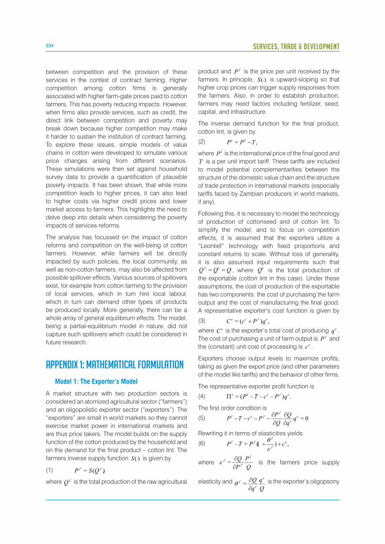
234 SERVICES, TRADE & DEVELOPMENT
between competition and the provision of these
services in the context of contract farming. Higher
competition among cotton firms is generally
associated with higher farm-gate prices paid to cotton
farmers. This has poverty reducing impacts. However,
when firms also provide services, such as credit, the
direct link between competition and poverty may
break down because higher competition may make
it harder to sustain the institution of contract farming.
To explore these issues, simple models of value
chains in cotton were developed to simulate various
price changes arising from different scenarios.
These simulations were then set against household
survey data to provide a quantification of plausible
poverty impacts. It has been shown, that while more
competition leads to higher prices, it can also lead
to higher costs via higher credit prices and lower
market access to farmers. This highlights the need to
delve deep into details when considering the poverty
impacts of services reforms.
The analysis has focussed on the impact of cotton
reforms and competition on the well-being of cotton
farmers. However, while farmers will be directly
impacted by such policies, the local community, as
well as non-cotton farmers, may also be affected from
possible spillover effects. Various sources of spillovers
exist, for example from cotton farming to the provision
of local services, which in turn hire local labour,
which in turn can demand other types of products
be produced locally. More generally, there can be a
whole array of general equilibrium effects. The model,
being a partial-equilibrium model in nature, did not
capture such spillovers which could be considered in
future research.
APPENDIX 1: MATHEMATICAL FORMULATION
Model 1: The Exporter’s Model
A market structure with two production sectors is
considered an atomized agricultural sector (“farmers”)
and an oligopolistic exporter sector (“exporters”). The
“exporters” are small in world markets so they cannot
exercise market power in international markets and
are thus price takers. The model builds on the supply
function of the cotton produced by the household and
on the demand for the final product – cotton lint. The
farmers inverse supply function )(�S is given by
(1) ),(= ff QSP
where fQ is the total production of the raw agricultural
product and fP is the price per unit received by the
farmers. In principle, )(�S is upward-sloping so that
higher crop prices can trigger supply responses from
the farmers. Also, in order to establish production,
farmers may need factors including fertilizer, seed,
capital, and infrastructure.
The inverse demand function for the final product,
cotton lint, is given by
(2) ,= TPP Ie �
where IP is the international price of the final good and
T is a per unit import tariff. These tariffs are included
to model potential complementarities between the
structure of the domestic value chain and the structure
of trade protection in international markets (especially
tariffs faced by Zambian producers in world markets,
if any).
Following this, it is necessary to model the technology
of production of cottonseed and of cotton lint. To
simplify the model, and to focus on competition
effects, it is assumed that the exporters utilize a
“Leontief” technology with fixed proportions and
constant returns to scale. Without loss of generality,
it is also assumed input requirements such that
QQQ ef == , where eQ is the total production of
the exportable (cotton lint in this case). Under these
assumptions, the cost of production of the exportable
has two components: the cost of purchasing the farm
output and the cost of manufacturing the final good.
A representative exporter’s cost function is given by
(3) ,)(= efee qPcC �
where eC is the exporter’s total cost of producing eq .
The cost of purchasing a unit of farm output is fP and
the (constant) unit cost of processing is ec .
Exporters choose output levels to maximize profits,
taking as given the export price (and other parameters
of the model like tariffs) and the behavior of other firms.
The representative exporter profit function is
(4) .)(= efeIe qPcTP ����
The first order condition is
(5) 0.=ee
ffeI q
q
Q
Q
PPcTP
��
��
����
Rewriting it in terms of elasticities yields
(6) ,)(1= e
f
ffI cPTP ���
��
where Q
P
P
Q f
f
f
��
=� is the farmers price supply
elasticity and Q
q
q
Q e
e
f
��
=� is the exporter’s oligopsony

235CHAPTER IX: PRIVATIZATION, COMPETITION AND COMPLEMENTARY SERVICES IN RURAL ZAMBIA
market power conjectural elasticity. The supply
elasticity is a measure of how responsive farmer
output is to prices. The conjectural elasticity f� is
a measure of the exporter’s oligopsonistic market
power and shows how equilibrium output Q responds
to a change in the production level of an individual
exporter. In perfect competition, 0=f� because each
individual exporter would be too small to affect the
market; in the case of a monopsony, 1=f� since the
exporter is the only buyer and eqQ = . In the case of
imperfect competition, f� lies between 0 and 1, being
closer to 0 when the “exporters” are less concentrated
and closer to 1 when they are more concentrated.
The first order condition (6) has a simple interpretation.
As usual, profit maximization requires the equalization
of the marginal revenue from the production of an
additional unit of exports (the international price net of
the tariff given by the left hand side) with the marginal
cost. This is given by the unit processing cost ec and
the price paid to farmers fP , taking into account the
supply response and the conjectural elasticity. Several
interesting cases emerge.
Consider first the case where there is competition
among exporters in the value chain. In this case,
0=f� so that the first order condition implies
(7) .= eIf cTPP ��
In this case, there is no strategic behavior of the
exporters and therefore the price paid to the farmer
is just the difference between the net price of exports
and the cost of processing. Since exporters do not
have market power over farmers, the price paid
adjusts to eliminate profits among exporters.
The opposite case arises when there is only one
exporter, who thus acts as a monopsonist over the
farmers. In this case, the price paid to the farmer
is actually lower than the net price of the exporter
( TcP eI �� ), a fact that reveals monopsonistic
behavior. Intuitively, by reducing the price below this
level, the exporter realizes a gain not only on the
marginal unit but also on the inframarginal units. This
makes price reductions – from the competitive level –
profitable for the exporter. In consequence, the price
paid to the farmer is lower than the competitive price
and the extent of this wedge depends on the elasticity
of supply of farm output. Intuitively, the higher the
elasticity of supply f� , the higher the price received
by the farmers. When the processors decide to cut fP (from, say, the competitive equilibrium), farmers
respond by decreasing quantities to an extent given
by f� . When f� is high, farmers respond a lot to given
price cut and this reduces the profitability of further
price cuts leading, in the end, to higher equilibrium
prices.
Finally, for a given elasticity of supply, the price
paid to the farmers increases when the competition
among exporters is more intense. In the model, this is
captured by a lower value of f� , the parameter that
describes the competitive nature of the model and
that depends on the number of firms and their relative
size. A low f� means that a given exporter expects
little reaction from other exporters. This translates into
higher farm-gate prices fP . Conversely, a higher f�
means less competition (more monopsonistic power)
and lower farm-prices.
Model 2: A Three-Sector Value Chain with Fixed International Price
As before, the building blocks of the model are the
supply of farm output and the demand of the final
product. The farmers inverse supply function is given
by equation 1 and the final product inverse demand
function is given by equation 2. The cost functions of
the processors and retailers are, respectively
(8) pfpp qPcC )(= �
(9) ,)(= rprr qPcC �
where pc and rc are fixed per unit production costs
and pP and fP are the processor price and the
farmers price, respectively. Let T be a per unit tariff.
The profit functions are, thus
(10) pfppp qPcP )(= ���
(11) .)(= rprIr qPcTP ����
The first order conditions from profit maximization are
(12) 0=rr
pprI q
q
Q
Q
PPcTP
��
��
����
for the retailers and
(13) 0,=p
p
ffpf q
q
Q
Q
PPcP
��
��
���
for the processors.
As before, it is useful to rewrite these expressions in
terms of elasticities. This yields
(14) =)(1 r
p
ppI TcPP
��
���
(15) .=)(1 p
f
ffp cPP
��
��
Market equilibrium in this case is determined by
equations (1), (2), (14) and (15) where Q
P
P
Q p
p
p
��
=�

236 SERVICES, TRADE & DEVELOPMENT
is the derived supply elasticity of “processors” and
Q
P
P
Q f
f
f
��
=� is the supply elasticity of “farmers”.
The competition parameters are Q
q
q
Q r
r
p
��
=� and
Q
q
q
Q p
p
f
��
=� which measure the oligopsonistic
market power of “retailers” and “processors”
respectively. When 0=},{ fp� , downstream firms are
small to affect market volumes and therefore are
competitive; instead, when 1=},{ fp� both firms have
monopsonist power. Intermediate parameter values of
� capture different degrees of imperfect competition.
Equation 14 is the retailer first order condition. It states
that the retailer chooses to produce a quantity such
that the international price IP equals the sum of the
unit import tariff (T ), the unit production cost ( rc ), and
the marginal cost of getting a unit of processed input
( pq ). This marginal cost depends on the competition
parameter p� (the ability to affect other retailers
production), on the supply elasticity of processors
( p� ), and on the equilibrium processor price. This
equation determines the processor price, which, in
equilibrium, is a wedge on the net price received by
the retailers. This wedge depends on p� and p� ;
the intuition and mechanisms are exactly as before,
in Model 1. In particular, more competition among
retailers (i.e., a lower p� ) brings the processor price
closer to the competitive price level )( TcP rI �� , and
a higher p� (more monopsonistic power of retailers)
reduces pP .
Equation (15) summarizes an analog condition for the
processor optimization and implicitly defines the farm
price, given the equilibrium producer price pP . Farm
prices are, once again, a wedge on producer prices pP and this wedge depends on f� and f� in exactly
the same manner as in Model 1. However, it should
be noted that this model has a prediction of how fP
responds to imperfect competition at the retailer level.
This is because p� determines pP , which in turn
determines fP . More concretely, more competition at
the retail level (a low p� ) implies a higher producer
price pP and thus, via (15), higher farm prices.
Model 3: A Full Three-Sector Value Chain
Model 3.1: Processors Hold Market Power
In this model, the demand function for the downstream
product is
(16) ).(= QDP r
The first order conditions for this model are
0=r
r
rprr q
q
Q
Q
PPcTP
��
��
����
(17) 0.=p
p
fp
p
pfpf q
q
Q
Q
Pq
q
Q
Q
PPcP
��
��
���
��
���
These yield the following equilibrium conditions
(18) rp
r
rr TcPP =)(1
��
���
(19) p
f
ff
p
pp cPP =)(1)(1
��
��
���
Equation (18) is the first order condition for profit
maximization of the retailers. Production level rq is
chosen to equate marginal revenue ( )(1r
rrP
��
� ) with
the sum of the per unit tariff (T ), the per unit cost ( rc )
and the input price ( pP ). This equation has a standard
monopoly pricing interpretation. Concretely, the price
charged by retailers rP is a markup on marginal costs.
The markup depends on the (inverse) of the elasticity
of demand r� (so that a more inelastic demand leads
to higher equilibrium prices) and on the competition
parameter r� . When there is perfect competition
( 0=r� ), price is just equal to marginal cost. Under
imperfect competition, a higher r� (so that the actions
of a given retailer trigger significant responses from
the competitor retailers) leads to higher equilibrium
prices.
Equation 19 summarizes the first order condition
of the processors. Since processors may use both
oligopsonistic and oligopolistic power, the optimization
condition takes into account the whole set of upstream
and downstream reactions measured by f� , r� and f� (as well as on the demand elasticity p� and the
supply elasticity f� ). Equilibrium farm prices are a
wedge on the net producer prices, as before. Although
there are now several additional mechanisms to
explore, the basic intuition is similar to that in Models
1 and 2. For example, farm prices respond to the
processor monopsonistic power parameter ( f� ) and
the supply elasticity ( f� ) in exactly the same way as
before. In addition, farm prices respond to changes
in the oligopoly parameter of processors toward
retailers ( p� ). If there is no oligopolistic behavior and
processors behave competitively when selling the
output to retailers, then the pricing condition is closer
to the simpler models previously discussed. Notice
also that the producer price depends on the oligopoly
parameter of the retailers in the downstream sector.
Hence, changes in ( r� ) affect producer prices and
thus farm prices as well.
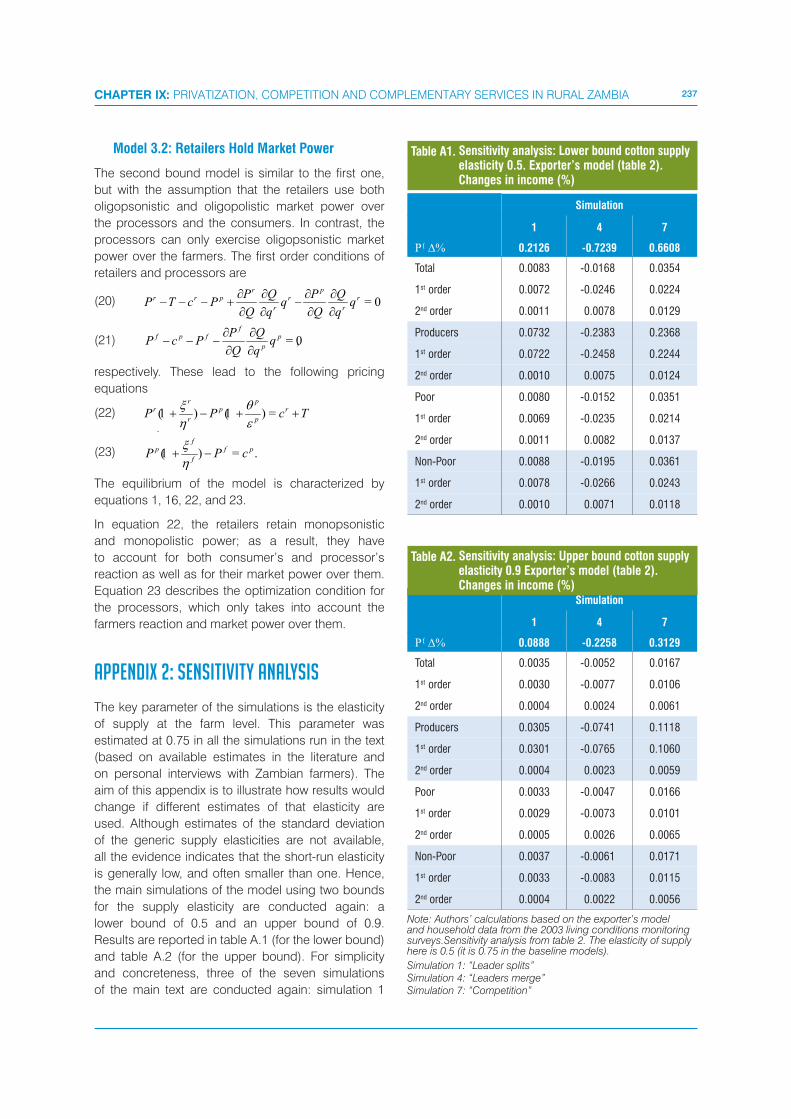
237CHAPTER IX: PRIVATIZATION, COMPETITION AND COMPLEMENTARY SERVICES IN RURAL ZAMBIA
Model 3.2: Retailers Hold Market Power
The second bound model is similar to the first one,
but with the assumption that the retailers use both
oligopsonistic and oligopolistic market power over
the processors and the consumers. In contrast, the
processors can only exercise oligopsonistic market
power over the farmers. The first order conditions of
retailers and processors are
(20) 0=rr
pr
r
rprr q
q
Q
Q
Pq
q
Q
Q
PPcTP
��
��
���
��
����
(21) 0,=p
p
ffpf q
q
Q
Q
PPcP
��
��
���
respectively. These lead to the following pricing
equations
(22) =)(1)(1 r
p
pp
r
rr TcPP ����
��
��
(23) .=)(1 pf
f
fp cPP ��
��
�
The equilibrium of the model is characterized by
equations 1, 16, 22, and 23.
In equation 22, the retailers retain monopsonistic
and monopolistic power; as a result, they have
to account for both consumer’s and processor’s
reaction as well as for their market power over them.
Equation 23 describes the optimization condition for
the processors, which only takes into account the
farmers reaction and market power over them.
APPENDIX 2: SENSITIVITY ANALYSIS
The key parameter of the simulations is the elasticity
of supply at the farm level. This parameter was
estimated at 0.75 in all the simulations run in the text
(based on available estimates in the literature and
on personal interviews with Zambian farmers). The
aim of this appendix is to illustrate how results would
change if different estimates of that elasticity are
used. Although estimates of the standard deviation
of the generic supply elasticities are not available,
all the evidence indicates that the short-run elasticity
is generally low, and often smaller than one. Hence,
the main simulations of the model using two bounds
for the supply elasticity are conducted again: a
lower bound of 0.5 and an upper bound of 0.9.
Results are reported in table A.1 (for the lower bound)
and table A.2 (for the upper bound). For simplicity
and concreteness, three of the seven simulations
of the main text are conducted again: simulation 1
Simulation
1 4 7
����� 0.2126 -0.7239 0.6608
Total 0.0083 -0.0168 0.0354
1st order 0.0072 -0.0246 0.0224
2nd order 0.0011 0.0078 0.0129
Producers 0.0732 -0.2383 0.2368
1st order 0.0722 -0.2458 0.2244
2nd order 0.0010 0.0075 0.0124
Poor 0.0080 -0.0152 0.0351
1st order 0.0069 -0.0235 0.0214
2nd order 0.0011 0.0082 0.0137
Non-Poor 0.0088 -0.0195 0.0361
1st order 0.0078 -0.0266 0.0243
2nd order 0.0010 0.0071 0.0118
Table A1. Sensitivity analysis: Lower bound cotton supply elasticity 0.5. Exporter’s model (table 2). Changes in income (%)
Simulation
1 4 7
����� 0.0888 -0.2258 0.3129
Total 0.0035 -0.0052 0.0167
1st order 0.0030 -0.0077 0.0106
2nd order 0.0004 0.0024 0.0061
Producers 0.0305 -0.0741 0.1118
1st order 0.0301 -0.0765 0.1060
2nd order 0.0004 0.0023 0.0059
Poor 0.0033 -0.0047 0.0166
1st order 0.0029 -0.0073 0.0101
2nd order 0.0005 0.0026 0.0065
Non-Poor 0.0037 -0.0061 0.0171
1st order 0.0033 -0.0083 0.0115
2nd order 0.0004 0.0022 0.0056
Note: Authors’ calculations based on the exporter’s model and household data from the 2003 living conditions monitoring surveys.Sensitivity analysis from table 2. The elasticity of supply here is 0.5 (it is 0.75 in the baseline models).
Simulation 1: “Leader splits”Simulation 4: “Leaders merge”Simulation 7: “Competition”
Table A2. Sensitivity analysis: Upper bound cotton supply elasticity 0.9 Exporter’s model (table 2). Changes in income (%)
238 SERVICES, TRADE & DEVELOPMENT
NOTES1 See Balat and Porto (2007) and World Bank (2007) for a more thorough analysis of poverty in Zambia.2 This section is based on Brambilla and Porto (2009).3 See Kranton and Swamy (2008) for a theoretical model of firm hold-up and farmer debt renegation, and for a discussion
of similar cases in textiles and opium in India.4 Some of the other minor players that had recently entered the market also used outgrower schemes, although they arguably
free-rode on the schemes successfully developed by the major players, Dunavant (Lonrho) and Clark.5 While these correlations suggest a link between the different phases of the reforms and cotton participation rates, causality
does not necessarily follows. Among other things, there might be other variables that may contaminate any causal relationship. One key such variable is the international price of cotton, which showed a declining trend during this period.
6 In the empirical applications, these characteristics include household size, distance to the market, production assets, housing ownership, number of farm workers, province dummies, and others. See the discussion below.
(increase in competition); simulation 2 (decrease in
competition); and simulation 7 (perfect competition).
The main observation from this sensitivity analysis
was that results can be quite sensitive to the elasticity
of supply. In table A.1, the price changes from the
same baseline are larger (in absolute value). In table
A.2, the price changes are smaller. For example, while
in simulation 1 (increase in competition) the price
faced by farmers increased by 12.53 per cent with
an elasticity of 0.75, it increased by 21.26 per cent
with an elasticity of 0.5 and by 8.88 per cent with an
elasticity of 0.9. Naturally, the sign of the change is not
affected by the elasticity of supply, but the magnitude
of the price changes, and therefore of the income and
poverty impacts, do depend critically to that elasticity.
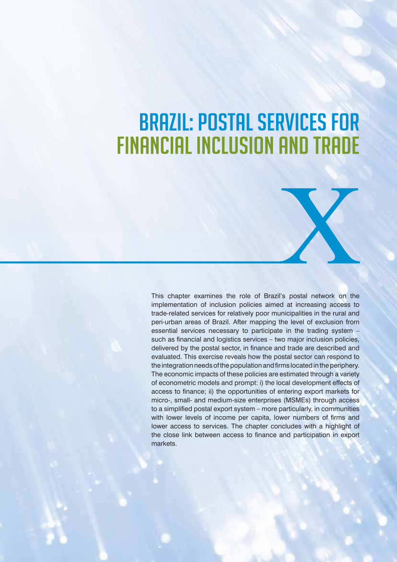
BRAZIL: POSTAL SERVICES FOR FINANCIAL INCLUSION AND TRADE
This chapter examines the role of Brazil’s postal network on the
implementation of inclusion policies aimed at increasing access to
trade-related services for relatively poor municipalities in the rural and
peri-urban areas of Brazil. After mapping the level of exclusion from
essential services necessary to participate in the trading system –
such as financial and logistics services – two major inclusion policies,
delivered by the postal sector, in finance and trade are described and
evaluated. This exercise reveals how the postal sector can respond to
the integration needs of the population and firms located in the periphery.
The economic impacts of these policies are estimated through a variety
of econometric models and prompt: i) the local development effects of
access to finance; ii) the opportunities of entering export markets for
micro-, small- and medium-size enterprises (MSMEs) through access
to a simplified postal export system – more particularly, in communities
with lower levels of income per capita, lower numbers of firms and
lower access to services. The chapter concludes with a highlight of
the close link between access to finance and participation in export
markets.

240 SERVICES, TRADE & DEVELOPMENT
1. INTRODUCTION
Posts have facilitated trade and international
exchanges for many centuries, supplying essential
communication and logistic services to businesses
and states of all types.1 With the surge of new
information and communication technologies, the role
and relevance of the postal services in the twenty-first
century is uncertain. Could access to physical retail
networks ease the provision of basic services for the
poor and help them integrate into the international
trading system? Moreover, what is the economic
impact of supplying a wider range of postal services
to rural and peri-urban populations in emerging and
developing countries? Can the observations drawn
from Latin America, particularly from the Brazil study
be applied to other developing or emerging countries?
Whatever form future mail communications take, posts
are characterized by two main potential assets for
their development. The first is by ubiquitous physical
networks in all industrialized countries and in many
developing and emerging nations – connecting over
660,000 world-wide post offices. The second is that
they have people’s trust in the performance of their
services. Albeit, this second characteristic may hold
less true in many Latin America countries which did
not pursue clear sectoral policies in the late twentieth
century and de facto left postal exchanges to fully
deregulated markets. As a consequence, a process of
destructive competition – a somewhat counterintuitive
phenomenon for economists – is observed in the
region. Compared to peers in other regions this
destructive competition resulted in a smaller number
of postal exchanges as well as a lower quality of
service negatively affecting the public trust.
Brazil’s postal services on the other hand faced different
developments. Although not the only exception in Latin
America with a harmonious development of postal
services, Brazil is increasingly cited as a best practice
case and referred to in reforms of postal services
in other developing and emerging countries. Thus,
this chapter measures the Brazilian postal sector’s
contribution to better access of essential services for
the development of trade, namely access to finance
and logistics. It also estimates the sectors’ economic
impact in terms of local economic development.
In Brazil, postal and delivery services enterprises
are key trade facilitators. The country provides non-
discriminatory access to simplified customs and
trade procedures to all postal and express carriers,
having heavily invested in and enhancing delivery
and logistics networks in the last twenty years. The
Government of Brazil as well as the postal incumbent
was also instrumental in enhancing the postal sector
through regular investment and offering universal
access to postal, express and basic financial
services through the national network of 6,000 post
offices (approximately one third of which are under
franchising agreements with private agents).
This chapter evaluates recent policies aimed at
including more exporters in the trading system,
particularly MSMEs. It also assesses the extent to which
universal access, provided by the Brazilian postal
incumbent, and has made a difference, particularly,
in terms of trade inclusion to provide a first export
opportunity to many small firms located in relatively
poorer municipalities, where the density of firms is
lower and the access to a wide range of services
limited. Moreover, the chapter highlights the postal
networks inclusion power in access to basic finance
– payments and financial transactions paramount to a
smooth handling of trade transactions and to deliver
the second largest anti-poverty programme in Brazil,
that is, the payment of pension benefits.
By examining these initiatives it is possible to test
whether there is a need to balance greater economic
and geographic concentration, resulting from
economic development and trade openness (World
Bank, 2008), with more integration of the periphery and
the less well-off parts of society. Econometric results
regarding the impacts of these initiatives are very much
consistent with what was expected in terms of poverty
alleviation. After showing that the rural and peri-urban
poor suffered from a lack of access to services prior
to the introduction of the abovementioned policies,
the great untapped demand for financial and logistics
services by these segments of the population is
highlighted. The extended use of these services
reveals the needs of marginalized populations and
enterprises in terms of access to essential services for
trade. Moreover, the provision of services through the
Brazilian postal sector triggered important economic
impacts on local development, particularly in relatively
deprived communities. These impacts ranged from
facilitating first time entry into export markets to
creating new micro and small enterprises that would
have otherwise not existed or traded.
Section 2 maps financial and trade exclusion in rural
and peri-urban areas of Brazil. Section 3 describes
two historical inclusion policies that resulted in

241CHAPTER X: BRAZIL: POSTAL SERVICES FOR FINANCIAL INCLUSION AND TRADE
pro-active and extensive use of the postal network
toward achieving greater economic integration.
Section 4 tests the postal networks impact on the
delivery of inclusion policies, both in terms of improved
access to services, increased use of services and
local development effects. Section 5 concludes.
2. MAPPING FINANCIAL AND TRADE EXCLUSION IN BRAZIL: A QUANTITATIVE AND GEOGRAPHICAL ASSESSMENT
Relatively high levels of income inequality have
historically characterized Brazil. Inequality is often
linked to a lack of access to basic infrastructure and
services, of which finance and trade heavily depend on.
This section provides some measurement of exclusion
from access to finance and trade infrastructure in Brazil
prior to a number of pro-inclusion reforms initiated over
the last decade.
In the early years of 2000, many instances of exclusion
from basic finance and international trade infrastructure
were evident. Much of the population did not have open
banking access, even in light of accelerating economic
developments. Over forty per cent of municipalities
were without a bank branch, particularly in rural and
peri-urban areas. Relative to peer countries, Brazil had
only a small number of enterprises – and barely any
MSMEs – involved with export markets. High levels of
income inequality were persistent over time.
In terms of exclusion from financial infrastructure, the
Figure 1. Brazilian municipalities without any bank branch in 2002 (grey areas)
None
Source: Authors’ calculation; data from the Brazilian Central Bank.

242 SERVICES, TRADE & DEVELOPMENT
map of the Brazilian municipalities (figure 1) identifies
locations without bank branches in 2002. Regional
disparities in terms of geographic access to finance
were wide ranging from 8,100 inhabitants per bank
branch in the South to 20,100 inhabitants per bank
branch in the North (tables 1 to 3). For instance, in
order for a pensioner to collect his pension benefit
from a city far from where he resided, equated to
roughly $30, or approximately forty per cent of the
benefit and two-days travel.
By relating financial infrastructure exclusion to
population or wealth, the picture became clear.
Financial institutions – not surprisingly – were
disproportionally concentrated among high population
and wealth areas (tables 1 to 3). In some cities, such
as Autazes in the north, distances to reach a bank
could easily exceed 100 kilometres, translating into a
14-hour boat ride to cover part of the 140 kilometres
before reaching the first available bank. Financial
access figures by region – credit per GDP, deposit per
GDP – reflect this situation (table 3).
Region PopulationGDP
(in million BRL)GDP per capita
(in BRL)Industry
share (%)Agricultural share (%)
Service share (%)
Number of firms
Central/west 13 014.333 190.000 14 599.29 14.35 36.31 49.34 43 419
Northeast 51 016.525 280.000 5 488.42 13.02 20.38 66.60 952 466
North 14 698.878 107.000 7 279.47 13.57 30.04 56.38 214 720
Southeast 78 444.032 1 210.000 15 425.01 20.21 20.77 59.02 3 041.597
South 26 973.511 356.000 13 198.13 19.18 28.27 52.55 1 416.670
Total 184 147.279 2 143.000 11 637 ... ... ... 6 059.651
Source: Authors’ calculation; data from IBGE.
Table 1. Socio-demographic regional differences (2005 values)
RegionExported value (in million USD
FOB)
Totalexporters
DSE exported value
(in USD)
EF exported value
(in BRL)
EF number
of exporters
EF value per exporter
Central/west 4 922 828 1 666.735 796.579 76 10 481.31
Northeast 10 520 1 380 6 824.055 1 459.181 223 6 543.41
North 7 192 840 8 956.397 13 200.000 25 528 000.00
Southeast 68 890 10 565 160 400.000 24 700.000 1 780 13 876.40
South 26 770 5 902 42 997.365 3 047.839 347 8 783.40
Total 118 294 19 515 220 844.552 43 203.599 2 451 17 626.93
Source: Authors’ calculation; data from IBGE and Ministry of Economic Development.
Table 2. Exporting activity regional differences (2005 values)
RegionBanco Postal
agenciesBank
agenciesBanking
correspondentsCredits perGDP (%)
Deposits perGDP (%)
Central/west 537 1 253 3 366 129.30 20.23
Northeast 1 687 2 539 8 914 41.25 15.32
North 481 693 1 204 37.48 14.80
Southeast 1 855 9 624 18 744 78.99 23.10
South 1 007 3 575 7 178 118.53 20.92
Total 5 567 17 684 39 406 ... ...
Note: Credits and deposits refer to both public and private.
Source: Authors’ calculation; data from IBGE.
Table 3. Financial access regional differences (2006 values)

243CHAPTER X: BRAZIL: POSTAL SERVICES FOR FINANCIAL INCLUSION AND TRADE
Figure 2. Need for simplified export processes (2005)
Source: Authors’ calculations; data from Correios (ECT) and MDIC.
Note: RE is the abbreviation for Registry of Exports, where exports following the usual export procedures are registered in Brazil. DSE is related to simplified export declarations for exports following the simplified procedure. EF is the abbreviation for “Exporta Facil”, the Brazilian postal incumbent’s programme for simplified export also using DSE regulations.
Figure 2 highlights municipalities not exclusively using
conventional export procedures, and thus: excluded
from international export trade (not “RE only” in yellow
ink); without a single firm participating in the export
markets (“NONE” in grey ink); and MSMEs in need
of alternative simplified export procedures to start
exporting (“EF” in green ink or “DSE only” in orange
ink, and in some cases “DSE and RE” in red ink).
A depiction of the concentration of exporters in the
south and south-eastern regions is also presented.
Trade and financial exclusion are closely related. In
2002, there were 2,302 municipalities without a single
bank branch. Out of these, 2,101 municipalities were
not exporting at all, that is only nine per cent had at
least one exporter. This situation differed considerably
DSE and RENone RE only DSE only EF
Brazil’s exporting municipalities - with EF - 55mu1000gc (exportst_1)
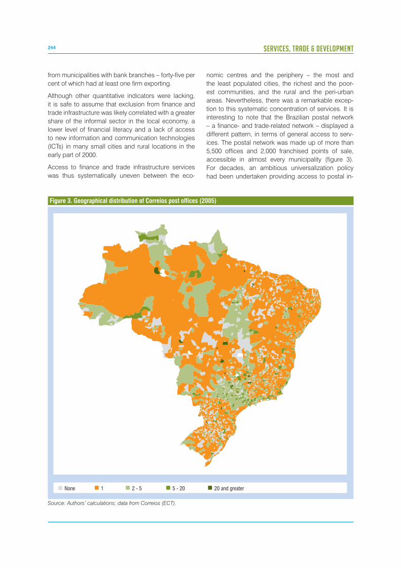
244 SERVICES, TRADE & DEVELOPMENT
from municipalities with bank branches – forty-five per
cent of which had at least one firm exporting.
Although other quantitative indicators were lacking,
it is safe to assume that exclusion from finance and
trade infrastructure was likely correlated with a greater
share of the informal sector in the local economy, a
lower level of financial literacy and a lack of access
to new information and communication technologies
(ICTs) in many small cities and rural locations in the
early part of 2000.
Access to finance and trade infrastructure services
was thus systematically uneven between the eco-
nomic centres and the periphery – the most and
the least populated cities, the richest and the poor-
est communities, and the rural and the peri-urban
areas. Nevertheless, there was a remarkable excep-
tion to this systematic concentration of services. It is
interesting to note that the Brazilian postal network
– a finance- and trade-related network – displayed a
different pattern, in terms of general access to serv-
ices. The postal network was made up of more than
5,500 offices and 2,000 franchised points of sale,
accessible in almost every municipality (figure 3).
For decades, an ambitious universalization policy
had been undertaken providing access to postal in-
Figure 3. Geographical distribution of Correios post offices (2005)
Source: Authors’ calculations; data from Correios (ECT).
1None 2 - 5 5 - 20 20 and greater

245CHAPTER X: BRAZIL: POSTAL SERVICES FOR FINANCIAL INCLUSION AND TRADE
frastructure services. Moreover, Correios – the Brazil-
ian Post – had been ranked at the top of the most-
trusted institutions or companies in Brazil several
times. In fact, only the family and firemen closely fol-
lowed, while banks and telecommunications compa-
nies held distant rankings. This trust made the postal
network an ideal hub for distributing financial and
trade facilitation services to the entire population, and
by so doing served poverty alleviation policies.
3. INCLUSION POLICIES IN BRAZIL DURING THE EARLY PART OF 2000: INCREASING ACCESS TO FINANCE AND TRADE INFRASTRUCTURE THROUGH POSTAL AND DELIVERY NETWORKS
This section describes how the Government of Brazil
closely associated and guided its postal network in
adopting pro-inclusion policies over the last decade.
In so doing, it had a pivotal impact on Correios, mak-
ing it one of the most innovative postal networks in the
world. Two such pro-inclusion policies are introduced
below. The first deals with improving access to basic
finance, and the second with trade facilitation for MS-
MEs. In each case, the general policy is presented
prior to specifying the role played by Correios in this
context. The possible impacts on poverty alleviation
are highlighted.
3.1. Access to finance: general policy and role of the post
It was not until the 1990s that the development of
other forms of financial institutions, especially micro-
finance institutions and credit cooperatives, started
to increase in addition to traditional banking in Brazil.
At that time, the Government of Brazil strengthened its
innovative approach for supplying financial services
and incrementing access to finance through a system
of correspondent banks (considered a form of micro-
finance institutions).
Banking correspondents acting as agents for banks
are ultimately responsible for financial transactions vis-
à-vis, its customers. The rationale behind this form of
banking uses the large capillary of networks (typically
lottery kiosks, post offices, pharmacies, supermarkets
and other retailers) to achieve a universal provision of
financial services. The interest to financial institutions
of operating through such large retail networks was
related to sharing fixed costs, benefiting from econo-
mies of scale and reaching more customers.
In this framework, Banco Postal (BP) – a special
postal financial service provided by the Brazilian
Post, through its agent Empresa de Correios e Telé-
grafos (ECT) – acts as a correspondent for a private
bank, namely Bradesco (the principal). Banco Postal
founded in 2001 as a result of a governmental auc-
tion won by Bradesco, bid 200 million BRL to operate
until 2009 in the ECT agencies. The general princi-
ples of BP were established by the Brazil Ministry of
Communication and reflected the institution’s social
inclusion objectives. These objectives stipulated that
priority be given to municipalities without a bank in
order to provide them with a first access to financial
services. Indeed, the establishment of BP agencies
was designed to achieve specific timetable objectives
– to serve at least 1,000 municipalities by the end of
2002 and to reach all of Brazil’s financially unattended
municipalities by the end of 2003. In order to achieve
this goal, Correios had to first resolve important con-
nectivity problems. Points of sales (POS) terminals
and V-Sat antennas, sometimes relying on solar en-
ergy, had to be set up and installed in many locations.
As continuous communication between Correios and
Bradesco data centres was paramount, numerous
postal employees were trained to ensure this new
service. Finally, Bradesco organized a fail-safe and
timely manner in which to transport cash to thousands
of new point of sales (POS).
Each BP agency provided a range of payment, sav-
ings and lending services (including microcredit),
although the partner bank remained responsible for
approving any transaction. Banco Postal offered sim-
plified bank accounts with easy and affordable fees
structure. Unlike private banks, it did not require a
substantial deposit to open an account. These fea-
tures contributed to make deposits attractive for low-
income people with relatively low levels of financial
literacy. A wider access to finance can be better lever-
aged in terms of poverty reduction when a specific
offer toward lower-income groups is designed. More
precisely, in the case of the simplified account “Conta
Fácil”, as long as deposited money remained in the
account for more than thirty days, it earned interest
so as to automatically convert stable deposits into
savings. The monthly fee in this account was lower
than that of the Bradesco fee with only a minimum
amount of 5 BRL required.2 Loans and micro credits
246 SERVICES, TRADE & DEVELOPMENT
were first granted in 2002 and 2003 respectively. As
Credit risks were completely assumed by Bradesco,
BP’s employees were not responsible for ensuring
lower-income groups pay back loans3.
3.2. Access to trade: general policy and role of the post
For its size, Brazil’s share of total global trade is low
(1.14 per cent in 2007)4. Moreover, most of its exports
are concentrated in hands of large exporting firms. In
1999, MSMEs only contributed 2.3 per cent to total
exports.5 This can partially be explained by increased
delays and costs created by an export-specific bu-
reaucracy that were unbearable to smaller firms which
exported objects of low value.
To offset this, in 1999, the Government of Brazil
instituted new procedures enabling the export of
low-valued objects without going through normal
formalities thereby, reducing the number of export
procedures from twenty-three to only three. In the same
year, different government ministries teamed up to
create a new legislation introducing a simplified export
form called “Declaração Simplificada de Exportação”
(DSE)6 which applied to the export of objects whose
value was less than $10,000 (this limit was raised to
$20,000 in 2006, and to $50,000 in 2008). This form
presented a number of advantages greatly simplifying
export procedures. As with the product features of
BP described above, simplicity was a key factor to
increase the possible leverage of the initiative on
relatively poor entrepreneurs. The usage of the DSE
was open to all logistics intermediaries – among them
postal operators and other express operators falling
into the postal sector – as defined by the Brazilian
Ministry of Communication.
Exporta Fácil was launched by Correios in November
2000 after the introduction of DSE in 1999. However,
the service was not intended to simply take advantage
of this simplified export form. Correios’ goal was to
provide universal and easy access to export markets,
by making the service available in more than 8,000
Brazilian post offices (in almost every municipality),
theoretically permitting the inclusion of remote towns
and villages that would, without the capillarity of the
designated postal operator’s network, have been ge-
ographically excluded from accessing a carrier to ex-
port. Exporta Fácil relied on Correios’ traditional inter-
national package services and permitted shipments
of up to 30 kilograms through the EMS (express mail
services) system and of 20 kilograms through stand-
ard package sending, to upward of 200 countries.
4. FROM EXCLUSION TO INTEGRATION IN FINANCE AND TRADE: TESTING THE IMPACT OF THE POST IN DELIVERING PRO-INCLUSION POLICIES
This section evaluates the extent to which the postal
network was efficient in delivering pro-inclusion
policies outlined in section 3, in response to the lack of
initial access to basic finance and trade infrastructure
described in section 2. A common database was built
to analyse the economic impacts of both policies at
the municipality level. Financial inclusion through BP
was evaluated in terms of access, use and impact on
local economic development. The trade facilitation
programme, Exporta Fácil, was analysed over a
time-period to better identify its users’ characteristics
and whether it enabled small firms to enter export
markets. This empirical evaluation assess whether
the outcomes of these initiatives were supportive of
poverty alleviation goals. More methodological and
estimation details can be found in Ansón and Bosch
Gual (2008) and Ansón and Caron (2008).
4.1. Empirical approach for evaluating two pro-inclusion policies through the postal network: data
Both evaluations are mainly based on municipality-
level data covering the period 1999 to 2007. This data
being the most disaggregated level, permitted the
researchers to exploit the huge variations in the size
and income of Brazil’s municipalities – defined as the
smallest political administrative unit after a state and,
although the number of municipalities changed only
slightly during the period, a total 5,561 municipalities
remained static throughout the time frame. Cognizant
of the fact that there was considerable heterogeneity
within municipalities, especially for the big cities where
disparities between slums and rich neighbourhoods
made it dubious to consider them as uniform areas,
a solution was used to reduce the potential statistical
bias arising from this lack of information – the
availability of within-municipality inequality measures
(Gini indices).
247CHAPTER X: BRAZIL: POSTAL SERVICES FOR FINANCIAL INCLUSION AND TRADE
4.2. Access to basic finance: testing the impact of the post in delivering inclusion and local economic development
First, municipalities were dived by semi-deciles of their
GDP per capita and population in order to provide a
concise picture of BP’s location and use, and to com-
pare it with that of bank agencies and correspondents
(Boldron et al. 2006). Second, in order to examine
whether financial intermediation through BP exerted a
causal impact on local development, the opening of a
BP agency in a municipality in 2002 was considered a
“treatment” for the municipality, and also use propen-
sity score matching methods to estimate the impact
of such an opening on the post-intervention economic
state of the municipality (Ansón and Bosch Gual 2008).
Evaluating and comparing access provided by different channels
The first BP branch was opened in March 2002 and, by
the end of 2006, a total of 5,567 BP agencies were in
operation after a progressive opening of point of sales.
A way to analyse the distribution of financial interme-
diaries is by grouping municipalities according to their
population or their wealth. It can be inferred from ta-
bles A.1.1 to A.2.2 (appendix 1) that BP agencies, oth-
er correspondents and traditional bank agencies all
presented different network topographies. Municipali-
ties with higher overall GDP per capita and population
tended to have a denser network of financial interme-
diaries. However, a comparison of these networks at
different levels of income and population revealed that
they complemented each other in some cases and
overlapped in others, possibly creating some com-
petitive pressure.
Bank agencies tend to cluster in wealthier and densely
populated areas as a result of their rational and profit-
maximizing behaviour. Such a clear concentration
does not appear in the case of BP agencies because
their introduction was proportional to the more
evenly distributed postal network. Consequently,
the distribution of BP agencies was quite constant
across different levels of wealth and population.
Other correspondents seem to have behaved
similarly to bank agencies, locating in wealthier and
densely populated areas and in all probability where
the density of other networks, such as supermarkets
or pharmacies, was also higher.
In 2002, 20 per cent of municipalities with the lowest
number of inhabitants, representing less than 2 per
cent of Brazil’s total population, corresponded to very
different percentages of each network’s outlets – 8.55
per cent of all BP agencies or 1.78 per cent of all bank
agencies and 0.5 per cent of all correspondents (ta-
ble A.1.1). In 2006, BP agencies stood at 13.41 per
cent but only accounted for 1.53 per cent of all bank
branches and approximately 1 per cent of all corre-
spondents in these same municipalities. It was also
found that in only 60 per cent of the largest municipali-
ties that the average number of correspondents was
greater than that of BP agencies (table A.1.2). For
bank agencies, it was only from the median munici-
pality that their average number became larger than
that of BP agencies.
A similar, though less striking, phenomenon was seen
with the same analysis of municipalities’ income level
(tables A.2.1 and A.2.2). The average number of BP
agencies increased with wealth, but not as dramatically
for traditional bank agencies. The biggest difference
in BP distribution occurred between the lowest and
the highest semi-decile; the poorest 5 per cent of
municipalities had, on average, roughly 2.8 times
fewer agencies than the richest 5 per cent. On the
other hand, the distribution in the bank agency network
according to level of income was even more skewed
– the difference in the average number of agencies
between the richest and poorest municipalities was
by a factor of about 60. Approximately 32 per cent
of the banking network was concentrated in the 278
richest municipalities. Alternatively, 58 per cent of their
network was concentrated in the 278 most populated
municipalities.
To sum up, in 2002, there was less than one bank
agency in the 35 per cent of the poorest municipalities
and in the 55 per cent of the least populated
municipalities. This result improved four years later,
when “only” 30 per cent of the poorest and 33 per
cent of the least populated municipalities had less
than one traditional bank branch on average.
The fact that BP agencies were homogeneously
distributed throughout the territory, regardless of the
municipalities’ level of economic development and
population, also reflects the institution’s desire for
social and financial inclusion.
Evaluating use by previously excluded customers
The three main components of financial services
provided by BP are savings, credit and payment
248 SERVICES, TRADE & DEVELOPMENT
services. Savings accounts are important for they help
buffer emergencies to which poorer segments of the
population are more vulnerable.7 Access to credit for
segments of the population with more modest incomes
is often viewed as a way to enhance small business
development. Lastly, access to payment services
such as money transfers, social security payments
or international remittances, is also important to the
less well-off rural inhabitants, who often rely on these
payments.
The population’s relative participation in BP services
was gauged by exploring how these components
were utilized in each region and in each group of
municipalities (divided into semi-deciles of population
and GDP per capita).
Tables A.3.1 and A.3.2 present the distribution of
different BP services and products across semi-
deciles. Table A.3.1 presents the number of current
deposits and savings deposits and the number of
withdrawals8. At first glance, it seems that wealth and
the per capita demand for BP services and products
were not proportionally related. In fact, those living in
the poorest 50 per cent municipalities, representing
less than one third of the population (29 per cent)
accounted for some 50 per cent of all BP deposits.
This is a very positive result as regards financial
inclusion, as it indicates that there were more BP
deposits in poorer municipalities.
Access to credit is one of the most quoted constraints
to business development by the self-employed and
micro entrepreneurs. Micro enterprises accounted for
the vast majority of all Brazilian firms and contributed
substantially to employment and GDP. Brazil’s 4.5
million micro and small enterprises accounted for
44 per cent of all employment and more than 60
per cent of urban jobs (Kumar et al., 2001). From its
creation up to the end of 2006, BP granted 1.93 million
loans, including micro-credits, loans and e-loans.
On average, in 2006, a BP agency granted some
200 loans in the north and central west, while in the
northeast and southeast the average number of loans
per BP agency was half that amount. The difference
was more striking in the south, where a typical BP
agency granted four times fewer loans on average
than in the north or central west.
Table A.3.2, presents an analysis of credit services,
including micro-credits, loans and e-loans.9 The
micro-credits, loans and e-loans granted by BP
were disproportional. In 2005, 10 per cent of the
total population, was concentrated in the 20 per cent
poorest municipalities and received some 20 per cent
of all micro-credits. Conversely, the richest semi-decile,
containing some 20 per cent of the population, received
less than 10 per cent of all micro-credits granted.
This disproportionality was even more apparent with
regular loans. Nearly one quarter of all loans were
granted to the poorest two deciles, while only some
4 per cent of loans were granted to the wealthiest 5
per cent throughout all municipalities, accounting for
10 per cent and 20 per cent of the total population
respectively. These figures confirm the evidence of a
North-South pattern in BP lending services.
Local economic development
The analysis of the treatment effect of a BP branch
opening in 2002 is based on seven outcome
variables: i) number of new firms; ii) variation in the
level of employment; iii) growth in the average number
of employees per firm; iv) growth in proportion of
salaried employees; v) number of new bank agencies;
vi) number of new correspondents; and vii) growth in
real GDP. All the outcome variables are presented as
the difference in their values between 2001 (before
the BP treatment) and 2005 (after the BP treatment).
The results are presented in tables A.4 to A.5.3 in
appendix 1.
The number of firms was used to study the impact of
a BP branch opening on local entrepreneurship. The
level of employment was used to assess job creation.
To determine BP impact on the size of the firms, the
average number of employees per firm was utilized.
Furthermore, in order to understand the effect of a
new BP branch on the level of formalization of the la-
bour market, the proportion of salaried people com-
pared with all employees was applied. To determine
whether the launch of BP generated positive exter-
nality on other financial intermediaries, (whether it at-
tracted bank agencies and other correspondents) the
change in the number of other correspondent agen-
cies and bank branches was looked at. Lastly, any BP
impact on local economic growth was considered.
The average outcome for the treated groups and for
the control (non-treated) groups is summarized in col-
umns i and ii of tables A.4 to A.5.3 respectively. Column
iii presents the difference between columns i and ii.
This can be interpreted as the average treatment effect
on the treated (ATT). A positive (negative) difference
means that the average affects on the treated group is
greater (smaller) than on the non-treated group.

249CHAPTER X: BRAZIL: POSTAL SERVICES FOR FINANCIAL INCLUSION AND TRADE
The estimates given in table A.4 reveal that the
launch of a BP agency in a municipality in 2002 had
significant average causal effects on most of the
outcome variables concerned. In a four-year period
(2002 to 2005), the municipalities that had received
the treatment experienced a formalization of their
labour market and attracted more bank agencies and
correspondents. In concrete terms, the increase in the
number of bank agencies (other correspondents) was
56 per cent higher in municipalities with a BP agency
compared to peers without BP. Another positive impact
brought about by BP was the average 37 additional
new firms per municipality with BP compared to peers
without BP in four years.
The results in table A.4 make no allowance for other
sources of variation in outcome, such as differences
attributed to regions per se. For example, some
regions may have had a more formalized labour
market or an industrial structure highly dependent
on external financing, which could bias the results.
To deal with the intrinsic regional effects or structural
regional differences, regional dummies were included
in a new set of estimations, the results of which are
summarized in table A.5.10 This might have reduced
the region-specific bias (which, despite the inclusion
of all relevant control variables, is a difficult, if not
impossible task). The addition of regional dummies
attenuate coefficients and raise standard errors,
rendering it impossible to reject the null hypothesis of
a zero BP effect on outcome variables, except in the
case of enterprise creation. However, these statistical
results are more likely to be simply due to the fact
that most BP branches were first opened in the north
and north east regions – the municipalities without a
bank. Therefore, it can be inferred from table A.5 that
the average treatment effect of a BP agency launch
in 2002 was the creation of an estimated average
of 29 additional new firms per municipality with BP
compared to peers without BP in four years.
The underlying heterogeneity could be utilized better
by conditioning the municipalities on their level of
banking penetration prior to treatment. Tables A.4.1
to A.4.3 report the estimation results of the baseline
model using three conditioning information sets. The
first set includes only municipalities without a bank
in 2001. The second includes municipalities with at
least one, but fewer than six, bank branches. The third
includes only those municipalities with more than five
bank agencies. These sets represent 42.4 per cent,
51.9 per cent and 5.7 per cent of all municipalities
respectively. The ATT was conditioned to determine
where the causal effect was more pronounced. In
other words, the treatment was conditioned to use
the level of access. Furthermore, conditioning was
based on the level of banking penetration – a proxy
for financial literacy – and adds regional dummies in
tables A.5.1 to A.5.3.
It can be concluded from table A.5.2, that taking into
account regional differences and specific levels of
financial access, the opening of a BP agency in 2002
had a causal impact on the creation of 20 additional
new firms in municipalities as well as some level of
financial competition and literacy (from one to five
bank agencies) compared to peers without BP. It
can also be concluded that treated municipalities
with some level of financial competition and literacy
in 2001 experienced a 17 per cent higher growth in
the number of additional new firms than non-treated
municipalities.
Although BP led to the creation of enterprises, the
average size of the firms remained virtually unchanged.
This can probably be explained by the fact that most
newly created firms had a small number of employees
on average.
As regards the effects on the labour market, it was
discovered that, once regional differences were taken
into account, jobs were created in municipalities
already benefiting from some degree of financial
intermediation. This result could well highlight a
greater impact of the financial inclusion policy under
study in communities with people already being
financially literate to some extent in 2001 (table
A.5.2). Interestingly, in municipalities with low levels
of financial literacy – for instance in municipalities
that were initially un-banked – significant BP effects
are only found on the formalization of the labour
market. On average, municipalities that were initially
un-banked experienced relatively more growth in the
proportion of salaried workers than other initially un-
banked municipalities not benefiting from a BP launch
in 2002.
Furthermore, the first wave of BP branch openings did
not have any medium-term effect on local GDP per
capita growth in 2005. A plausible explanation is that
financial inclusion is above all a matter of numbers
rather than value. While many individuals and small
firms were financially included through BP, it is intuitive
to understand that the monetary added value of all
transactions was not large enough so as to have an

250 SERVICES, TRADE & DEVELOPMENT
impact on a macroeconomic aggregate – such as
GDP – which is measured in value terms. The result is
the same when comparing these transactions to the
overall financial system. Yet, this constitutes further
tangible proof of the inclusion power of BP, for if many
new firms had been created locally thanks to BP (as
tested econometrically) while the value aggregate
(GDP) remained largely unaffected, this in turn means
that the newly created economic activities have mostly
involved the less well-off segments of the population
– low-income households and micro enterprises. The
positive macroeconomic local impact of BP is to be
found at the extensive rather than at the intensive
margin.11 Thus confirming BP was an important factor
of integration for those segments of the population
– mostly rural or living in small cities – at a time of
stronger concentration of economic activities in large
centres due to economic development and greater
trade openness. More concentration also calls for
more integration in order to prevent the periphery from
becoming a de-stabilizing factor and jeopardizing the
sustainability of economic development (World Bank
WDR 2008).
Ultimately the treatment did attract other bank
agencies, but only in municipalities already with bank
agencies in 2001. Treated municipalities, with at least
one bank agency in 2001, had more than three times
as many bank agencies as non-treated municipalities
with the same level of financial access through bank
agencies.
4.3. Trade facilitation for all: testing the impact of the post in delivering access to export markets for first-time exporters
After demonstrating the impacts of providing access
to finance through a postal network, the extent to which
the Brazilian postal sector was equally successful for
easing access to export markets to those formerly
“excluded” firms from the international trading system
was examined.
4.3.1. Evolution of DSE exports
How have low-valued exports evolved since the intro-
duction of simplified export procedures (DSE) in 1999?
Figure 4 illustrates three important and revealing
trends. The first trend, illustrates the clear upward
evolution of the value of low-valued exports through
DSE to $387 million in 2007. A particularly large
Figure 4. Evolution of DSE exported value
1999
2001
2000
2002
2003
2004
2005
2006
2007
Non-postal Other postal sector Exporta facil
0
50'000
100'000
150'000
200'000
250'000
300'000
350'000
400'000
1000
$ F
OB
Source: Authors’ compilation; data from MDIC / MC / Correios.
increase was noticed between 2005 and 2006, which
can be explained in part by the increase in the maximum
exportable value from $10,000 to $20,000 taking place
at that time. The second trend concerning total DSE
exports include postal exports carried out by what the
Brazilian Ministry of Communications defines as the
postal sector – the historical operator Correios, but
also eight other express carriers, including the usual
global players. Exports through the postal sector had
continuously grown, encompassing about one half of
total DSE exports. This leads to the conclusion that
the postal sector as a whole has an important role to
play in the delivery of low-valued exports. The third
trend revealed by this graph concerns the evolution
of Exporta Fácil exports: they represented a relatively
small share of the total small export market and their
importance, both in absolute and in relative terms,
was decreasing in 2006 and 2007.
4.3.2. Evolution of Exporta Fácil
Figures 5 to 7 illustrate the evolution of, Exporta Fácil
exported values, the number of exporters having
used Exporta Fácil, and the number of objects sent
through Exporta Fácil, respectively. All three measures
followed the same trend: a rapid increase in the
years following Exporta Fácil’s launch in late 2000,
followed by a clear peak around 2004 after which
usage declined. Three explanations can be provided.
One is not specific to the programme but attributable
to Correios’ general performance in the outgoing
international shipment of packages. Advertising
for these services was unexpectedly temporarily
interrupted between 2005 and 2007 (more recent
provisional figures show renewed growth). The reason
for this interruption is that it coincided with a review

251CHAPTER X: BRAZIL: POSTAL SERVICES FOR FINANCIAL INCLUSION AND TRADE
of the public procurement process at Correios. As
figure 8 illustrates, Exporta Fácil followed the same
declining trend as the rest of Correios’ international
shipments. This trend reveals a marketing structural
problem, especially when it is confronted to the
general growth of Brazilian exporting activity during
the same period. Furthermore, Correios was handling
an ever-increasing number of incoming international
packages showing that the reliability of its services
was not a concern. The second explanation is related
more to the implementation of the Exporta Fácil
programme itself. Correios underestimated the fact
that repeat exports were not the rule but the exception
in international trade (Besedes and Prusa (2004),
or Braidford et al. 2003). It did not sufficiently renew
its customer base in terms of new small exporters
holding the belief that repeat purchases would be
as high as for other products or services delivered
through the postal network. Maintaining and growing
this customer base would have required greater effort
and coordination with local chambers of commerce
and small firm organisations. It is interesting to
note that other Latin American countries replicating
Exporta Fácil through an IIRSA programme– such as
the Post in Peru – learned from Correios experience
and have made efforts to secure a constant inflow
of new exporters. The third explanation is related to
competition exerted by foreign couriers and express
companies, which were also allowed to access DSE.
These operators have offered end-to-end integrated
services from the originating to the destination country
for several decades, while historical postal operators
have only recently started to develop greater
interconnectivity and integration of their services –
making international postal regulations more flexible
in terms of parcel sizes and weights, or adding
reliable international track-and-trace options for their
customers.
4.3.3. Econometric analysis: the determinants of low-value exports
The data allows for further investigation into what
drives exporting activity at the municipality level, by
econometric methods. It is thus possible to estimate
the impact of socio-economic and demographic
variables on exported value and number of exporters
for RE, DSE, and Exporta Fácil exports.
Figure 5. EF exported values
Value of EF exports in million BRL
Value of EF exports in million USD
0
5
10
15
20
25
30
35
40
45
50
2001
2000
2002
2003
2004
2005
2006
2007
Source: Correios (ECT).
Figure 6. EF number of exporters
0
500
1000
1500
2000
2500
3000
2001
2000
2002
2003
2004
2005
2006
2007
Source: Correios (ECT).
Figure 7. EF number of objects
2001
2000
2002
2003
2004
2005
2006
2007
0
5000
10000
15000
20000
25000
30000
Source: Correios (ECT).

252 SERVICES, TRADE & DEVELOPMENT
Figure 8. Exporta Fácil vs. all Correios international shipments
Number of objects EF 9.5 Service international - expedition
0
5000
10000
15000
20000
25000
30000
0
50000
100000
150000
200000
250000
300000
350000
400000
2001
2000
2002
2003
2004
2005
2006
2007
Source: Correios (ECT).
Table 4 displays the estimated effect of the differ-
ent explanatory variables, by export channel, on the
number of exporters and exported value, respectively.
To make interpretation easier, only the sign (positive =
“+”, negative = “-”) of the effect is displayed here for
statistically significant coefficients. A lack of statistical
significance for the variable coefficient is reported with
“0”. It is to be noted that all explanatory variables are
not used at the same time in the econometric estima-
tion due to multi co- linearity problems. The full coef-
ficients as well as more detailed technical considera-
tions can be found in Anson and Caron (2008).
The first test conducted relates to geographic inclusion.
All other effects being controlled for, both transport
cost to São Paulo and transport cost to nearest capital
either negatively affected or did not affect low-valued
(DSE and Exporta Fácil) exports. Hence, neither DSE
(which was expected) nor Exporta Fácil (which was
not expected) had promoted geographical inclusion.
It is interesting, then, to analyse which variables affect
their usage, and if there are some explaining DSE
exports but not RE exports.
The following factors seem to consistently explain all
types of exporting activity in a municipality: share of
industrial sector (positively); labour participation rate
(positively); and education level – as defined by the
median number of years of schooling, (positively). This
gives an insight into the necessary prerequisites for
exporting activity in a municipality – it has to be indus-
trialized, educated and with a high labour participation
rate (likely to increase access to a variety of produc-
tion factors). The total number of firms in a municipality
explains positively the number of exporters but not the
exported value (for both the DSE and the RE).
More interestingly, some factors influence low-valued
exports (DSE including Exporta Fácil) differently than
normal ones (RE). As can be seen, population (in
log form) affected positively DSE and Exporta Fácil
exports, but not RE exports, whereas the log of GDP
affected RE exports and the number of DSE exporters,
but not its value and not Exporta Fácil exports. This
implies that low-valued exports (particularly Exporta
Fácil) depend more on population and less on wealth
than regular exports. Moreover, it appears that the
share of the services (tertiary) sector explains positively
DSE exports, meaning that low-valued exports were
more intensely used in service-oriented cities. Finally,
it looks as if the average size of firms (in employees)
affected negatively the value of DSE exports. These
two last results taken together appear to indicate that
cities with a concentration of small firms where the
service sector plays a larger role will generate a higher
usage of DSE and Exporta Fácil exports.

253CHAPTER X: BRAZIL: POSTAL SERVICES FOR FINANCIAL INCLUSION AND TRADE
The results demonstrate that most municipality-
level characteristics explaining Exporta Fácil usage
are not much different from those explaining overall
DSE exports. However, three variables, (log GDP, the
share of the service sector, and the number of firms)
exerting a positive influence on the total number of
DSE exporters had no significant effect on Exporta
Fácil exports. These variables together represent a
proxy for the level of wealth and economic structure
of a municipality. This is important in the sense that it
tends to prove that, (geographical location controlled
for) Exporta Fácil exports were less affected by
wealth, access to numerous services, and the number
of existing firms than other DSE exports. This may well
be indicative of the real inclusion value of Exporta
Fácil – answering the needs and facilitating trade to
small exporters irrespective of their municipality’s
income level, access to services or existence of a rich
industrial structure. If trade is to alleviate poverty, then
Exporta Fácil programmes seem to be needed by
such communities (relatively poor, with few firms, and
little access to services).
Trade creation? A panel analysis
A crucial element in the analysis of the impact of these
trade facilitation policies is the question of actual
trade creation: has Brazil exported more because
of the availability of simplified export procedures?
The fundamental question follows: how much of
these exports would have happened anyways?
Otherwise said: are DSE-oriented services just used
as substitutes to other exporting means, or are they
fostering new trade flows? This question cannot be
answered by a simple look at DSE exported values,
as firm-level data on DSE exporters is not disposed of.
Therefore, analysis requires econometric estimation
techniques.
The DSE policy was implemented in 1999 and, in
theory, made immediately available to everyone
everywhere. This means that there is no source of
variation in availability across municipalities which
could be used to directly identify its effect on trade
creation through treatment effects models (unlike in
the case of access to finance presented above).
2005 estimatesRE DSE Exporta Facil
# Exporters Value # Exporters Value # Exporters Value
Population 0 0 0 - - 0
Log population 0 0 + + + +
Share of rural population (2000 est.) 0 + 0 0 0 0
GDP 0 0 - 0 0 0
Log GDP + + + 0 0 0
Gini Inequality coefficient (2000 est.) - 0 0 0 0 0
Share of services sector 0 0 + + 0 0
Share of Industrial sector + + 0 + + +
Transport cost to closest capital 0 0 - 0 - 0
Transport cost to Sao Paulo 0 0 0 0 - 0
In large metro area (dummy) + 0 0 0 0 0
Labor participation rate (2000 est.) + + + + + 0
Number of bank agencies - 0 - + 0 0
Median no of years of schooling + + + 0 0 +
No of firms (unidades) + 0 + 0 0 0
Average size of firms (in employees) 0 0 0 - 0 0
Constant - - - - -
No. of uncensored observations 1 714 ... 459 ... 302 ...
Note: Signs are reported if effect was found to be statisticaly significant at the 5% level.
Table 4. Tobit regression of number of exporters and exported value, per type of export - sign of effect
254 SERVICES, TRADE & DEVELOPMENT
Not having any possible source of variation in access
to DSE, variation across usage of DSE in time
within municipalities has been used. The problem is
formulated in the following terms: over time, all other
things being held constant, do municipalities which
export more through DSE export more in total? This
can be tested both in terms of exported value and
in terms of number of exporters. The inherent logic
assumes that there is an unobservable element (such
as historical exporting activity, cultural impact, etc.) in
each municipality which is correlated with the amount
of exporting activity that does not change over time
and that can as such be eliminated by running a fixed
effect model (within municipality estimation). Such an
econometric model is appropriate for this analysis
as it allows for a municipality specific constant,
which will capture all time-constant (unobserved)
characteristics.
To identify possible substitution between RE exports
and DSE exports, the number of RE exporters is
regressed (that have not used the DSE) on the
number of DSE exporters (that have not used the RE),
controlling for exporters who exported through both
systems (DSE/RE). If this coefficient is not significantly
different than zero, then no evidence of substitution
would have been found, as it could not be ascertained
that a new DSE exporter explains the loss of an RE
exporter.
Other possible export determinants are controlled for,
but only those that have yearly values can be used
(therefore less control variables are used than those
used in the cross-section analysis of the previous
section). Additionally the possibilities of time-specific
effects have been accounted for by adding yearly
dummies, which might capture nation-wide variations
in exporting activity (due to changes in exchange rate,
for example).
Two types of specifications are presented in appendix
2, which give comparable estimates. The conclusions
are robust to both specifications: the number of DSE-
only exporters does not significantly affect the number
of RE-only exporters in a municipality (see p-values
displayed under the coefficients). Therefore, there is
no evidence that a new DSE exporter comes at the
expense of an RE exporter. Moreover, it was found
that that the instant substitution effect taking place
immediately after the introduction of DSE legislature
in 1999 was much higher than in following years (third
column of results table A.6 in appendix 2).
These estimates imply that, out of a total of 20,160
exporters in Brazil during 2005, an estimated 4,915
exporters or 24 per cent of the total number of
exporters would otherwise not have exported without
access to the DSE programme. The Exporta Fácil
programme provided by the historical postal operator
enabled 2,451 exporters – the smallest relative to
others – to access export markets, out of which 2,084
or 10 per cent of the total number of exporters used
DSE as their exclusive export channel and would
otherwise not have exported. In summary, the Exporta
Fácil programme was responsible for having included
in the trading system the bottom 10 per cent of
exporters in terms of size in Brazil, providing a unique
opportunity for relatively poorer entrepreneurs to
export for the first time.
5. CONCLUSION
This chapter has revealed that an improved access
to basic finance and trade services is necessary
not only to facilitate trade, but also to balance the
concentration of economic activities with a greater
integration in the economic and trading systems
of previously excluded players. The latter are often
located in the geographic periphery, are small firms or
people from less well-off segments of the population.
Exclusion from basic services in Brazil as of the early
twenty-first century translated into geographical
exclusion with rural and peri-urban municipalities
without a bank branch or with large distances to the
next, a geographic concentration of service providers
in large urban centres, or communities without a
single exporter. In turn, inequalities and the weight
of the informal sector could not be easily reduced
in these initial circumstances. This chapter has thus
examined whether the extensive and pro-active use
of the Brazilian postal network has changed this initial
state and enabled: i) small firms which would have
otherwise not exported to export; ii) poor individuals
which would have otherwise not saved to save; iii)
micro enterprises which would have otherwise not
borrowed to borrow; and iv) micro entrepreneurs which
would have otherwise not created new businesses
and jobs to create them. Throughout the chapter,
the positive answers to these questions demonstrate
the value of these policies toward alleviating poverty
or increasing opportunities for relatively small and
poor entrepreneurs. They underline the value of a
harmonious development of the postal sector in Brazil

255CHAPTER X: BRAZIL: POSTAL SERVICES FOR FINANCIAL INCLUSION AND TRADE
unlike in many other Latin American countries where
“laissez-faire” policies related to postal markets have
seriously damaged the potential use of the postal
network as a prime channel for trade and financial
inclusion.
In terms of financial inclusion, this chapter has
confirmed that the Brazil postal network has been used
effectively to promote access to financial services in
the most deprived areas. Banco Postal is present in
4,860 of a total of 5,561 municipalities. A total of 12.4
million people living in 1,525 municipalities in which a
BP agency was opened did not have any bank agency
prior to that time. Moreover, in 2006, BP was present
in 865 municipalities that had no bank branches or
other correspondent institutions, thus acting as the
sole financial intermediary for 5.98 million people.
Banco Postal agencies were evenly distributed across
the country, while other financial intermediaries were
mainly concentrated in the relatively wealthy and
populated areas. Banco Postal, other correspondent
banks and bank agencies are therefore mostly
complementary networks. Although access to
financial services and products is a necessary
condition for development, it is by evaluating the use
of those services and products that an assessment
can be made on actual financial inclusion. Banco
Postal appears to have attracted relatively low-
income customers, with a very similar profile across
the regions. Interestingly, in 2005, about one quarter
of all loans and micro-credits were granted to the 20
per cent poorest municipalities, which accounted for
10 per cent of Brazil’s population. The 50 per cent
poorest municipalities, equal to 29 per cent of the
entire population, accounted for 50 per cent of all BP
deposits. The analysis suggests that the extended
financial access achieved by BP’s presence had a
positive medium-term impact on entrepreneurship and
employment in municipalities with a certain degree
of financial literacy and competition in 2001 and
also helped formalize the economy of municipalities
without any bank branch previous to the introduction
of BP. The very fact that local GDP values remained
unaffected while numerous new small firms were
simultaneously created signifies that the opportunities
created by BP were seized by the poorest and most
vulnerable segments in each municipality.
In terms of trade inclusion, the fact that Exporta Fácil
is used to export a comparatively small number
of comparatively low-valued exports can be seen
as a justification for Exporta Fácil’s very existence:
if the postal incumbent’s vast network is going to
help provide access to export markets, it might not
be, as was originally postulated, in the inclusion of
geographically remote areas, but in meeting the
needs of very small exporters (who export smaller
values) in relatively poorer and less service oriented
municipalities. Indeed, these exporters often start out
by posting very low-valued objects, and the postal
incumbent, as the data shows, seems to be most
apt in meeting their needs. As such, it seems that
the market failure which Exporta Fácil is effectively
countering is that of the under provision of affordable
shipment of very low valued objects. It is used by
customers who will only export a few packages a
year on average and are therefore less attractive to
private carriers. Nonetheless, as was argued in this
chapter, they are potentially crucial to the creation of
new exporting activity by the poorest sectors. Having
facilitated the access to trade to the sector – 10
per cent of exporters in terms of size is indeed the
most remarkable success of Exporta Fácil. However,
due to the low retention rates among exporters,
the continuing success of the programme relies on
the attraction of a new and steady inflow of small
exporters. This appeared to again be the case in 2009
and 2010 after a temporary decline in the number of
users in 2006 and 2007.
Access to trade and finance are closely related. In
2002, there were 1,456 municipalities that had at least
a bank branch and an exporter. Three year later, after
the successful implementation of financial and trade
inclusion policies, 1,708 municipalities were served
by a financial institution and had at least one firm
exporting – an increase of 17.3 per cent of exporting
municipalities with direct access to finance that has
mostly benefited the poorest sectors of society.
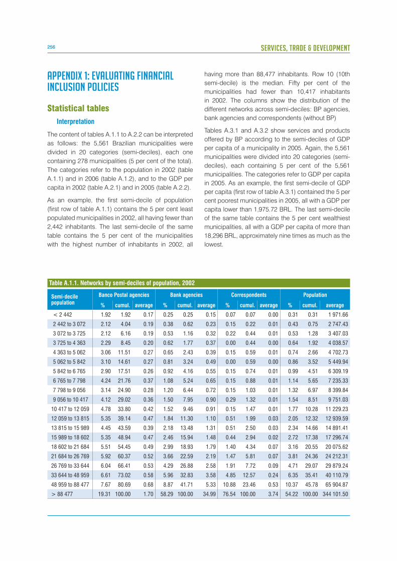
256 SERVICES, TRADE & DEVELOPMENT
APPENDIX 1: EVALUATING FINANCIAL INCLUSION POLICIES
Statistical tables
Interpretation
The content of tables A.1.1 to A.2.2 can be interpreted
as follows: the 5,561 Brazilian municipalities were
divided in 20 categories (semi-deciles), each one
containing 278 municipalities (5 per cent of the total).
The categories refer to the population in 2002 (table
A.1.1) and in 2006 (table A.1.2), and to the GDP per
capita in 2002 (table A.2.1) and in 2005 (table A.2.2).
As an example, the first semi-decile of population
(first row of table A.1.1) contains the 5 per cent least
populated municipalities in 2002, all having fewer than
2,442 inhabitants. The last semi-decile of the same
table contains the 5 per cent of the municipalities
with the highest number of inhabitants in 2002, all
having more than 88,477 inhabitants. Row 10 (10th
semi-decile) is the median. Fifty per cent of the
municipalities had fewer than 10,417 inhabitants
in 2002. The columns show the distribution of the
different networks across semi-deciles: BP agencies,
bank agencies and correspondents (without BP)
Tables A.3.1 and A.3.2 show services and products
offered by BP according to the semi-deciles of GDP
per capita of a municipality in 2005. Again, the 5,561
municipalities were divided into 20 categories (semi-
deciles), each containing 5 per cent of the 5,561
municipalities. The categories refer to GDP per capita
in 2005. As an example, the first semi-decile of GDP
per capita (first row of table A.3.1) contained the 5 per
cent poorest municipalities in 2005, all with a GDP per
capita lower than 1,975.72 BRL. The last semi-decile
of the same table contains the 5 per cent wealthiest
municipalities, all with a GDP per capita of more than
18,296 BRL, approximately nine times as much as the
lowest.
Semi-decile population
Banco Postal agencies Bank agencies Correspondents Population
% cumul. average % cumul. average % cumul. average % cumul. average
< 2 442 1.92 1.92 0.17 0.25 0.25 0.15 0.07 0.07 0.00 0.31 0.31 1 971.66
2 442 to 3 072 2.12 4.04 0.19 0.38 0.62 0.23 0.15 0.22 0.01 0.43 0.75 2 747.43
3 072 to 3 725 2.12 6.16 0.19 0.53 1.16 0.32 0.22 0.44 0.01 0.53 1.28 3 407.03
3 725 to 4 363 2.29 8.45 0.20 0.62 1.77 0.37 0.00 0.44 0.00 0.64 1.92 4 038.57
4 363 to 5 062 3.06 11.51 0.27 0.65 2.43 0.39 0.15 0.59 0.01 0.74 2.66 4 702.73
5 062 to 5 842 3.10 14.61 0.27 0.81 3.24 0.49 0.00 0.59 0.00 0.86 3.52 5 449.94
5 842 to 6 765 2.90 17.51 0.26 0.92 4.16 0.55 0.15 0.74 0.01 0.99 4.51 6 309.19
6 765 to 7 798 4.24 21.76 0.37 1.08 5.24 0.65 0.15 0.88 0.01 1.14 5.65 7 235.33
7 798 to 9 056 3.14 24.90 0.28 1.20 6.44 0.72 0.15 1.03 0.01 1.32 6.97 8 399.84
9 056 to 10 417 4.12 29.02 0.36 1.50 7.95 0.90 0.29 1.32 0.01 1.54 8.51 9 751.03
10 417 to 12 059 4.78 33.80 0.42 1.52 9.46 0.91 0.15 1.47 0.01 1.77 10.28 11 229.23
12 059 to 13 815 5.35 39.14 0.47 1.84 11.30 1.10 0.51 1.99 0.03 2.05 12.32 12 939.59
13 815 to 15 989 4.45 43.59 0.39 2.18 13.48 1.31 0.51 2.50 0.03 2.34 14.66 14 891.41
15 989 to 18 602 5.35 48.94 0.47 2.46 15.94 1.48 0.44 2.94 0.02 2.72 17.38 17 296.74
18 602 to 21 684 5.51 54.45 0.49 2.99 18.93 1.79 1.40 4.34 0.07 3.16 20.55 20 075.62
21 684 to 26 769 5.92 60.37 0.52 3.66 22.59 2.19 1.47 5.81 0.07 3.81 24.36 24 212.31
26 769 to 33 644 6.04 66.41 0.53 4.29 26.88 2.58 1.91 7.72 0.09 4.71 29.07 29 879.24
33 644 to 48 959 6.61 73.02 0.58 5.96 32.83 3.58 4.85 12.57 0.24 6.35 35.41 40 110.79
48 959 to 88 477 7.67 80.69 0.68 8.87 41.71 5.33 10.88 23.46 0.53 10.37 45.78 65 904.87
> 88 477 19.31 100.00 1.70 58.29 100.00 34.99 76.54 100.00 3.74 54.22 100.00 344 101.50
Table A.1.1. Networks by semi-deciles of population, 2002

257CHAPTER X: BRAZIL: POSTAL SERVICES FOR FINANCIAL INCLUSION AND TRADE
Semi-decile population
Banco Postal agencies Bank agencies Correspondents Population
% cumul. average % cumul. average % cumul. average % cumul. average
< 2 416 2.91 2.91 0.58 0.23 0.23 0.15 0.19 0.19 0.27 0.29 0.29 1 942.93
2 416 to 3 031 3.16 6.07 0.63 0.35 0.58 0.22 0.23 0.42 0.33 0.41 0.70 2 735.92
3 031 to 3 752 3.66 9.74 0.73 0.47 1.05 0.30 0.33 0.75 0.46 0.51 1.21 3 403.01
3 752 to 4 367 3.68 13.42 0.74 0.58 1.63 0.37 0.28 1.03 0.40 0.60 1.81 4 061.14
4 367 to 5 096 3.65 17.06 0.73 0.58 2.22 0.37 0.37 1.40 0.52 0.70 2.51 4 702.17
5 096 to 5 890 4.22 21.29 0.85 0.97 3.19 0.62 0.55 1.95 0.78 0.81 3.32 5 471.71
5 890 to 6 794 4.08 25.36 0.82 0.89 4.08 0.56 0.62 2.57 0.87 0.95 4.27 6 369.80
6 794 to 7 937 4.24 29.60 0.85 1.19 5.27 0.76 0.63 3.19 0.89 1.09 5.36 7 322.66
7 937 to 9 237 4.44 34.04 0.89 1.38 6.65 0.88 0.95 4.14 1.35 1.27 6.64 8 561.76
9 237 to 10 690 4.60 38.64 0.92 1.54 8.19 0.98 1.03 5.17 1.45 1.48 8.12 9 936.30
10 690 to 12 463 4.80 43.43 0.96 1.57 9.76 1.00 1.18 6.35 1.68 1.72 9.83 11 519.18
12 463 to 14 294 4.81 48.25 0.96 1.83 11.59 1.17 1.45 7.80 2.05 1.99 11.82 13 380.74
14 294 to 16 672 4.87 53.12 0.97 2.31 13.91 1.47 1.69 9.48 2.39 2.30 14.12 15 422.97
16 672 to 19 279 4.90 58.02 0.98 2.41 16.32 1.54 1.96 11.45 2.78 2.68 16.80 17 991.08
19 279 to 22 815 4.96 62.98 0.99 3.10 19.42 1.97 2.58 14.03 3.66 3.12 19.92 20 940.03
22 815 to 28 164 4.96 67.94 0.99 3.58 23.00 2.28 3.04 17.07 4.31 3.77 23.69 25 349.42
28 164 to 35 612 5.05 72.98 1.01 4.48 27.48 2.85 4.19 21.27 5.95 4.70 28.39 31 562.55
35 612 to 52 082 4.96 77.94 0.99 5.67 33.15 3.60 5.67 26.93 8.03 6.35 34.74 42 639.92
52 082 to 96 515 5.42 83.37 1.09 8.62 41.77 5.48 11.13 38.07 15.78 10.49 45.23 70 452.58
> 96 515 16.63 100.00 3.33 58.23 100.00 37.04 61.93 100.00 87.79 54.79 100.00 367 978.00
Table A.1.2. Networks by semi-deciles of population, 2006
Semi-decile GDP p.cBanco Postal agencies Bank agencies Correspondents Population
% cumul. average % cumul. average % cumul. average % cumul. average
< 1 405.38 4.21 4.21 0.37 0.42 0.42 0.25 0.00 0.00 0.00 2.28 2.28 14 517.2
1 405.38 to 1 603.11 3.84 8.04 0.34 0.59 1.01 0.35 0.00 0.00 0.00 2.57 4.85 16 253.0
1 603.11 to 1 764.94 4.21 12.25 0.37 0.81 1.82 0.49 0.00 0.00 0.00 2.59 7.44 16 411.7
1 764.94 to 1 950.89 4.53 16.78 0.40 0.95 2.77 0.57 0.37 0.37 0.02 2.80 10.24 17 846.1
1 950.89 to 2 147.21 5.72 22.50 0.50 1.15 3.92 0.69 0.51 0.88 0.03 2.80 13.04 17 685.2
2 147.21 to 2 362.36 4.49 26.99 0.40 1.19 5.11 0.72 0.88 1.76 0.04 2.65 15.69 16 867.3
2 362.36 to 2 681.4 4.08 31.07 0.36 1.51 6.62 0.90 1.03 2.79 0.05 2.82 18.51 17 829.4
2 681.4 to 3 096.2 4.98 36.06 0.44 1.95 8.58 1.17 2.87 5.66 0.14 3.63 22.13 23 005.3
3 096.2 to 3 560.51 4.00 40.06 0.35 1.79 10.36 1.08 1.84 7.50 0.09 2.81 24.95 17 906.4
3 560.51 to 4 024.535 4.29 44.34 0.38 2.18 12.54 1.31 3.01 10.51 0.15 3.29 28.24 20 870.1
4 024.535 to 4 479.83 4.25 48.59 0.38 2.63 15.17 1.58 2.21 12.72 0.11 3.32 31.56 21 145.3
4 479.83 to 4 940.06 4.33 52.92 0.38 3.18 18.35 1.91 4.19 16.91 0.21 4.15 35.71 26 351.2
4 940.06 to 5 426.75 4.70 57.62 0.41 3.27 21.62 1.95 3.01 19.93 0.15 3.64 39.35 23 033.4
5 426.75 to 5 951.28 4.65 62.27 0.41 4.50 26.11 2.70 4.85 24.78 0.24 5.09 44.44 32 282.9
5 951.28 to 6 519.49 5.80 68.07 0.51 7.15 33.27 4.31 7.79 32.57 0.38 7.43 51.87 47 183.2
6 519.49 to 7 254.7 4.25 72.32 0.37 5.08 38.35 3.05 3.90 36.47 0.19 4.30 56.17 27 266.6
7 254.7 to 8 285.03 4.45 76.77 0.39 5.60 43.95 3.36 4.71 41.18 0.23 4.60 60.76 29 168.7
8 285.03 to 9 741.27 6.61 83.38 0.58 11.36 55.31 6.79 15.96 57.13 0.78 8.33 69.10 52 851.7
9 741.27 to 13 244 6.49 89.87 0.57 13.56 68.87 8.14 15.96 73.09 0.78 11.11 80.21 70 456.3
> 13 244 10.13 100.00 0.90 31.13 100.00 18.75 26.91 100.00 1.32 19.79 100.00 12 6087
Table A.2.1. Networks by semi-deciles of GDP per capita (current values, BRL), year 2002
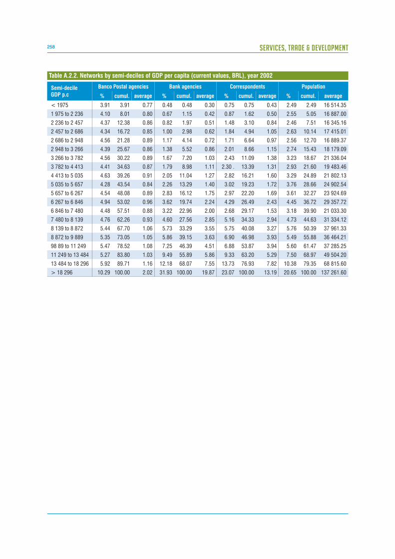
258 SERVICES, TRADE & DEVELOPMENT
Semi-decile GDP p.c
Banco Postal agencies Bank agencies Correspondents Population
% cumul. average % cumul. average % cumul. average % cumul. average
< 1975 3.91 3.91 0.77 0.48 0.48 0.30 0.75 0.75 0.43 2.49 2.49 16 514.35
1 975 to 2 236 4.10 8.01 0.80 0.67 1.15 0.42 0.87 1.62 0.50 2.55 5.05 16 887.00
2 236 to 2 457 4.37 12.38 0.86 0.82 1.97 0.51 1.48 3.10 0.84 2.46 7.51 16 345.16
2 457 to 2 686 4.34 16.72 0.85 1.00 2.98 0.62 1.84 4.94 1.05 2.63 10.14 17 415.01
2 686 to 2 948 4.56 21.28 0.89 1.17 4.14 0.72 1.71 6.64 0.97 2.56 12.70 16 889.37
2 948 to 3 266 4.39 25.67 0.86 1.38 5.52 0.86 2.01 8.66 1.15 2.74 15.43 18 179.09
3 266 to 3 782 4.56 30.22 0.89 1.67 7.20 1.03 2.43 11.09 1.38 3.23 18.67 21 336.04
3 782 to 4 413 4.41 34.63 0.87 1.79 8.98 1.11 2.30 . 13.39 1.31 2.93 21.60 19 483.46
4 413 to 5 035 4.63 39.26 0.91 2.05 11.04 1.27 2.82 16.21 1.60 3.29 24.89 21 802.13
5 035 to 5 657 4.28 43.54 0.84 2.26 13.29 1.40 3.02 19.23 1.72 3.76 28.66 24 902.54
5 657 to 6 267 4.54 48.08 0.89 2.83 16.12 1.75 2.97 22.20 1.69 3.61 32.27 23 924.69
6 267 to 6 846 4.94 53.02 0.96 3.62 19.74 2.24 4.29 26.49 2.43 4.45 36.72 29 357.72
6 846 to 7 480 4.48 57.51 0.88 3.22 22.96 2.00 2.68 29.17 1.53 3.18 39.90 21 033.30
7 480 to 8 139 4.76 62.26 0.93 4.60 27.56 2.85 5.16 34.33 2.94 4.73 44.63 31 334.12
8 139 to 8 872 5.44 67.70 1.06 5.73 33.29 3.55 5.75 40.08 3.27 5.76 50.39 37 961.33
8 872 to 9 889 5.35 73.05 1.05 5.86 39.15 3.63 6.90 46.98 3.93 5.49 55.88 36 464.21
98 89 to 11 249 5.47 78.52 1.08 7.25 46.39 4.51 6.88 53.87 3.94 5.60 61.47 37 285.25
11 249 to 13 484 5.27 83.80 1.03 9.49 55.89 5.86 9.33 63.20 5.29 7.50 68.97 49 504.20
13 484 to 18 296 5.92 89.71 1.16 12.18 68.07 7.55 13.73 76.93 7.82 10.38 79.35 68 815.60
> 18 296 10.29 100.00 2.02 31.93 100.00 19.87 23.07 100.00 13.19 20.65 100.00 137 261.60
Table A.2.2. Networks by semi-deciles of GDP per capita (current values, BRL), year 2002

259
CH
AP
TE
R X
: BR
AZ
IL: P
OS
TA
L S
ER
VIC
ES
FO
R F
INA
NC
IAL IN
CLU
SIO
N A
ND
TR
AD
E
Population Current deposits (#) Savings deposits (#) Accounts (#) Tributes (#)
Semi-decile GDP p.c % cumul. % cumul. average % cumul. average % cumul. average % cumul. average
<1 975.72 2.49 2.49 3.86 3.86 2 860.16 4.42 4.42 717.81 4.53 4.53 926.6655 2.10 2.10 1.62
1 975.72 to 2 236.23 2.55 5.05 3.92 7.78 2 899.11 4.36 8.78 708.88 4.29 8.82 876.7842 2.33 4.43 1.79
2 236.23 to 2 457.8 2.46 7.51 4.58 12.36 3 399.01 4.67 13.45 761.77 4.50 13.33 919.9424 2.66 7.09 2.05
2 457.8 to 2 686.05 2.63 10.14 4.19 16.55 3 103.75 4.82 18.27 782.28 4.26 17.59 871.2122 2.51 9.61 1.93
2 686.05 to 2 948.25 2.56 12.70 4.49 21.04 3 315.10 5.04 23.31 816.01 4.03 21.62 823.7158 1.06 10.66 0.81
2 948.25 to 3 266.09 2.74 15.43 4.58 25.62 3 400.66 5.58 28.88 909.06 4.13 25.75 844.0576 5.06 15.72 3.90
3 266.09 to 3 782.46 3.23 18.67 5.55 31.17 4 091.52 5.55 34.44 898.60 4.80 30.55 981.1223 1.42 17.14 1.09
3 782.46 to 4 413.16 2.93 21.60 4.90 36.07 3 640.27 5.20 39.63 847.15 4.08 34.63 833.5396 30.15 47.28 23.25
4 413.16 to 5 035.39 3.29 24.89 5.07 41.14 3 753.36 5.70 45.33 926.22 4.29 38.91 875.7878 0.24 47.52 0.18
5 035.39 to 5 657.74 3.76 28.66 4.78 45.92 3 539.01 4.58 49.91 743.81 3.89 42.80 794.5504 0.83 48.35 0.64
5 657.74 to 6 267.37 3.61 32.27 4.47 50.39 3 308.72 3.66 53.57' 594.17 3.45 46.25 705.1763 2.66 51.02 2.05
6 267.37 to 6 846.34 4.45 36.72 4.78 55.17 3 526.43 4.17 57.74 675.80 3.48 49.73 711.6151 5.18 56.20 3.97
6 846.34 to 7 480.5 3.18 39.90 4.22 59.39 3 124.63 3.68 61.42 597.68 3.50 53.24 716.036 3.45 59.65 2.65
7 480.5 to 8 139.71 4.73 44.63 4.55 63.94 3 368.68 3.77 65.19 612.41 4.30 57.54 879.3058 5.46 65.11 4.19
8 139.71 to 8 872.64 5.76 50.39 5.22 69.16 3 865.38 4.92 70.11 799.08 4.79 62.32 977.9388 5.20 70.31 4.00
8 872.64 to 9 889.17 5.49 55.88 5.65 74.81 4 179.59 4.83 74.94 785.21 5.84 68.16 1 192.9339 4.08 74.39 3.13
9 889.17 to 11 249.74 5.60 61.47 4.59 79.40 3 409.12 3.95 78.90 644.87 5.03 73.19 1 028.594 6.66 81.05 5.14
11 249.74 to 13 484.76 7.50 68.97 5.14 84.54 3 794.47 4.23 83.12 684.34 5.79 78.98 1 183.076 4.15 85.20 3.18
13 484.76 to 18 296.01 10.38 79.35 5.53 90.07 4 095.35 5.26 88.38 854.49 8.33 87.31 1 701.871 4.70 89.90 3.61
> 18 296.01 20.65 100.00 9.93 100.00 7 374.00 11.62 100.00 1 894.05 12.69 100.00 2 602.924 10.10 100.00 7.79
Table A.3.1. Banco Postal services and products by semi-deciles of GDP per capita (current values, BRL), 2005

Semi-decile GDP p.c
PopulationSocial security payments (#)
Social security paymentss (BRL)
Domestic remittances (#)
Nodomestic remittances (#)
Microcredits (#) E-loans (#) Loans (#)
% cumul. % cumul. average % cumul. average % cumul. average % cumul. average % cumul. average % cumul. average % cumul. average
< 1975.72 2.49 2.49 4.46 4.46 691.946 4.07 4.07 201 988 0.82 0.82 11.60 0.00 0.00 0.00 3.94 3.94 15.73 4.34 4.34 17.51 6.93 6.93 153.55
1 975.72 to 2 236.23 2.55 5.05 3.11 7.57 482.626 2.83 6.90 140 214 1.26 2.07 17.87 0.00 0.00 0.00 4.01 7.94 16.01 4.14 8.48 16.71 5.72 12.65 126.65
2 236.23 to 2 457.8 2.46 7.51 3.31 10.88 515.509 3.07 9.97 152 841 1.34 3.41 19.08 0.00 0.00 0.00 7.38 15.32 29.60 3.98 1Z46 16.12 6.62 19.27 147.05
2. 457.8 to 2 686.05 2.63 10.14 3.62 14.50 561.032 3.37 13.34 167 231 1.62 5.03 23.07 0.02 0.02 0.00 4.30 19.62 17.17 4.81 17.26 19.40 6.15 25.42 136.12
2 686.05 to 2 948.25 2.56 12.70 3.56 18.05 549.756 3.27 16.61 161 586 2.18 7.21 30.85 0.10 0.12 0.01 4.14 23.76 16.47 4.28 21.54 17.20 6.19 31.61 136.53
2 948.25 to 3 266.09 2.74 15.43 3.41 21.46 530.783 3.18 19.78 158 021 3.76 10.97 53.68 0.02 0.15 0.00 6.09 29.84 24.40 5.63 27.17 22.82 5.89 37.50 130.90
3 266.09 to 3 782.46 3.23 18.67 4.78 26.24 738.821 4.47 24.25 220 762 6.05 17.02 85.76 0.00 0.15 0.00 5.28 35.12 21.01 5.96 33.13 23.96 5.91 43.41 130.41
3 782.46 to 4 413.16 2.93 21.60 4.17 30.41 648.921 3.95 28.20 196 798 2.80 19.82 39.90 0.27 0.41 0.04 5.05 40.17 20.25 7.17 40.30 29.05 4.77 48.17 105.92
4 413.16 to 5 035.39 3.29 24.89 4.65 35.06 721.975 4.51 32.71 223 666 2.51 22.33 35.69 0.24 0.66 0.04 5.09 45.26 20.33 7.49 47.78 30.22 5.87 54.04 130.01
5 035.39 to 5 657.74 3.76 28.66 4.84 39.90 750.115 4.77 37.48 236 801 2.65 24.98 37.66 1.19 1.84 0.18 5.71 50.97 22.82 6.24 54.03 25.21 4.53 58.57 100.27
5 657.74 to 6 267.37 3.61 32.27 4.66 44.56 723.46 4.58 42.06 227 227 3.27 28.24 46.48 1.46 3.30 0.22 4.79 55.76 19.13 5.16 59.18 20.81 4.05 62.62 89.73
6 267.37 to 6 846.34 4.45 36.72 5.02 49.59 776.599 5.09 47.15 251 472 3.83 32.07 54.23 1.99 5.29 0.29 3.73 59.48 14.84 4.92 64.10 19.77 3.94 66.57 87.00
6 846.34 to 7 480.5 3.18 39.90 4.76 54.34 738.061 4.80 51.95 238 252 3.80 35.87 54.08 1.38 6.67 0.21 2.80 62.29 11.20 4.96 69.06 20.03 4.16 70.72 92.08
7 480.5 to 8 139.71 4.73 44.63 5.44 59.78 843.842 5.52 57.46 273 802 3.92 39.80 55.77 4.42 11.09 0.65 4.46 66.75 17.83 4.77 73.83 19.25 4.30 75.03 95.30
8 139.71 to 8 872.64 5.76 50.39 5.20 64.98 806.482 5.22 62.68 258 823 5.85 45.65 83.22 6.21 17.31 0.92 5.58 72.33 22.29 4.14 77.97 16.73 4.29 79.31 94.90
8 872.64 to 9 889.17 5.49 55.88 8.51 73.49 1320.4 8.55 71.24 423 541 5.13 50.77 72.92 3.18 20.49 0.47 4.97 77.30 19.86 4.48 82.46 18.10 4.66 83.97 103.10
9 889.17 to 11 249.74 5.60 61.47 6.24 79.73 971.329 6.63 77.86 330 131 4.63 55.40 66.08 8.96 29.44 1.33 4.59 81.88 18.39 3.82 86.28 15.48 3.80 87.77 84.44
11 249.74 to 13 484.76 7.50 68.97 7.78 87.51 1 202.61 8.34 86.20 411 420 5.91 61.32 83.81 8.40 37.84 1.24 5.35 87.24 21.32 4.36 90.64 17.54 3.45 91.22 76.16
13 484.76 to 18 296.01 10.38 79.35 6.98 94.49 1 082.15 7.76 93.95 384 254 7.15 68.47 101.73 12.14 49.98 1.80 6.64 93.87 26.51 4.44 95.08 17.93 449 95.71 99.42
> 18 296.01 20.65 100.00 5.51 100.00 858.664 6.05 100.00 301 153 31.53 100.00 449.95 50.02 100.00 7.44 6.13 100.00 24.57 4.92 100.00 19.94 4.29 100.00 95.33
Table A.3.2. Banco Postal services and products by semi-deciles of GDP per capita (current values, BRL), year 2005260
SER
VIC
ES, TRA
DE &
DEV
ELOP
MEN
T
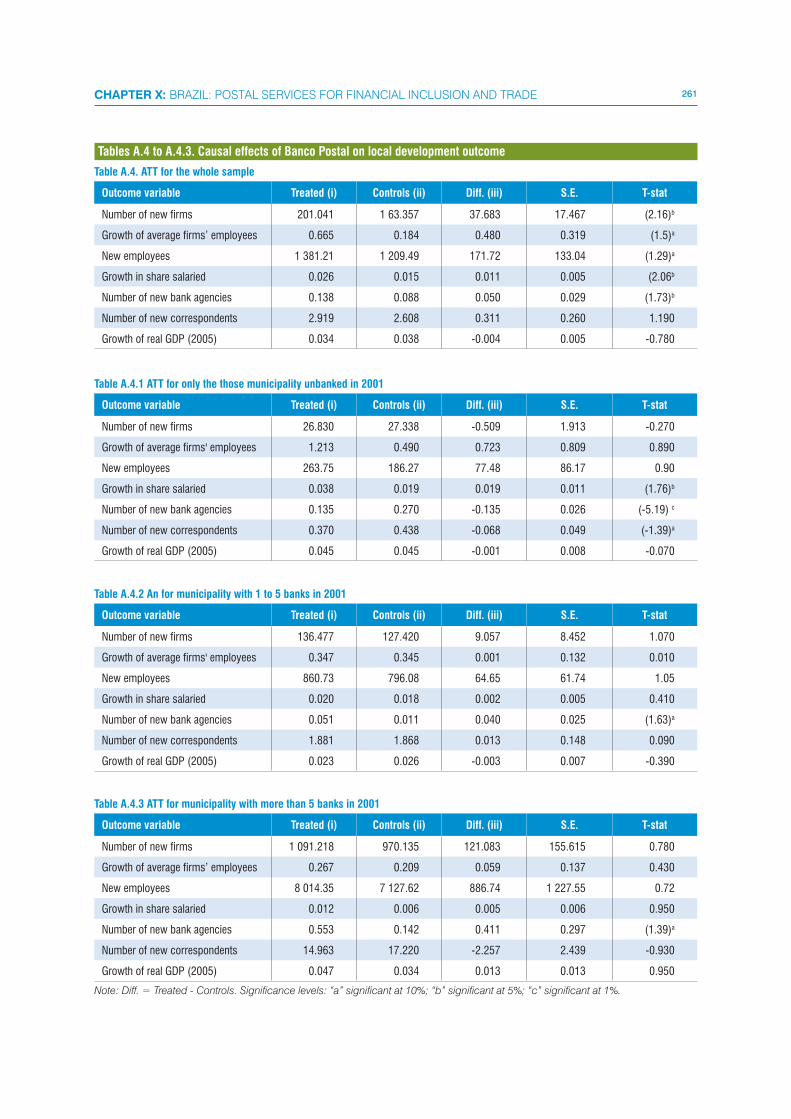
Table A.4. ATT for the whole sample
Outcome variable Treated (i) Controls (ii) Diff. (iii) S.E. T-stat
Number of new firms 201.041 1 63.357 37.683 17.467 (2.16)b
Growth of average firms’ employees 0.665 0.184 0.480 0.319 (1.5)a
New employees 1 381.21 1 209.49 171.72 133.04 (1.29)a
Growth in share salaried 0.026 0.015 0.011 0.005 (2.06b
Number of new bank agencies 0.138 0.088 0.050 0.029 (1.73)b
Number of new correspondents 2.919 2.608 0.311 0.260 1.190
Growth of real GDP (2005) 0.034 0.038 -0.004 0.005 -0.780
Table A.4.1 ATT for only the those municipality unbanked in 2001
Outcome variable Treated (i) Controls (ii) Diff. (iii) S.E. T-stat
Number of new firms 26.830 27.338 -0.509 1.913 -0.270
Growth of average firms' employees 1.213 0.490 0.723 0.809 0.890
New employees 263.75 186.27 77.48 86.17 0.90
Growth in share salaried 0.038 0.019 0.019 0.011 (1.76)b
Number of new bank agencies 0.135 0.270 -0.135 0.026 (-5.19) c
Number of new correspondents 0.370 0.438 -0.068 0.049 (-1.39)a
Growth of real GDP (2005) 0.045 0.045 -0.001 0.008 -0.070
Table A.4.2 An for municipality with 1 to 5 banks in 2001
Outcome variable Treated (i) Controls (ii) Diff. (iii) S.E. T-stat
Number of new firms 136.477 127.420 9.057 8.452 1.070
Growth of average firms' employees 0.347 0.345 0.001 0.132 0.010
New employees 860.73 796.08 64.65 61.74 1.05
Growth in share salaried 0.020 0.018 0.002 0.005 0.410
Number of new bank agencies 0.051 0.011 0.040 0.025 (1.63)a
Number of new correspondents 1.881 1.868 0.013 0.148 0.090
Growth of real GDP (2005) 0.023 0.026 -0.003 0.007 -0.390
Table A.4.3 ATT for municipality with more than 5 banks in 2001
Outcome variable Treated (i) Controls (ii) Diff. (iii) S.E. T-stat
Number of new firms 1 091.218 970.135 121.083 155.615 0.780
Growth of average firms’ employees 0.267 0.209 0.059 0.137 0.430
New employees 8 014.35 7 127.62 886.74 1 227.55 0.72
Growth in share salaried 0.012 0.006 0.005 0.006 0.950
Number of new bank agencies 0.553 0.142 0.411 0.297 (1.39)a
Number of new correspondents 14.963 17.220 -2.257 2.439 -0.930
Growth of real GDP (2005) 0.047 0.034 0.013 0.013 0.950
Note: Diff. = Treated - Controls. Significance levels: “a” significant at 10%; “b” significant at 5%; “c” significant at 1%.
Tables A.4 to A.4.3. Causal effects of Banco Postal on local development outcome
261CHAPTER X: BRAZIL: POSTAL SERVICES FOR FINANCIAL INCLUSION AND TRADE

262 SERVICES, TRADE & DEVELOPMENT
Table A.5. ATT for the whole sample
Outcome variable Treated (i) Controls (ii) Diff. (iii) S.E. T-stat
Number of new firms 199.758 170.527 29.231 19.158 (1.53)a
Growth of average firms’ employees 0.664 0.358 0.306 0.324 0.940
New employees 1 341.31 1 296.51 44.80 128.72 0.35
Growth in share salaried 0.664 0.358 0.306 0.324 0.940
Number of new bank agencies 0.026 0.024 0.001 0.005 0.250
Number of new correspondents 2.684 2.494 0.190 0.235 0.810
Growth of real GDP (2005) 0.034 0.031 0.003 0.005 0.640
Table A.5.1 ATT for only the those municipality unbanked in 2001
Outcome variable Treated (i) Controls (ii) Diff. (iii) S.E. T-stat
Number of new firms 26.886 29.345 -2.459 2.138 -1.150
Growth in average firms' employees 1.204 0.484 0.720 0.796 0.900
New employees 263.69 209.40 54.29 86.23 0.63
Growth in share salaried 0.038 0.035 0.002 0.011 0.220
Number of new bank agencies 0.136 0.248 -0.112 0.026 (-4.28)b
Number of new correspondents 0.371 0.337 0.034 0.046 0.730
Growth of real GDP (2005) 0.045 0.036 0.009 0.008 1.170
Table A.5.2 An for municipality with 1 to 5 banks in 2001
Outcome variable Treated (i) Controls (ii) Diff. (iii) S.E. T-stat
Number of new firms 136.477 116.386 20.091 7.979 (2.52)c
Growth of average firms' employees 0.347 0.276 0.071 0.133 0.53
New employees 860.73 720.84 139.89 66.77 (2.1)b
Growth in share salaried 0.020 0.014 0.005 0.005 1.12
Number of new bank agencies 0.050 0.025 0.025 0.023 1.11
Number of new correspondents 1.881 2.100 -0.219 0.151 -1.45
Growth of real GDP (2005) 0.023 0.030 -0.007 0.007 -1.04
Table A.5.3 ATT for municipality with more than 5 banks in 2001
Outcome variable Treated (i) Controls (ii) Diff. (iii) S.E. T-stat
Number of new firms 1 072.453 1 327.475 -255.022 205.140 -1.240
Growth of average firms’ employees 0.243 0.055 0.188 0.133 (1.42)a
New employees 8 041.67 9 226.28 -1 184.61 1 599.91 -0.74
Growth in share salaried 0.010 0.011 -0.001 0.005 -0.310
Number of new bank agencies 0.453 0.569 -0.116 0.337 -0.340
Number of new correspondents 16.373 17.254 -0.881 2.714 -0.320
Growth of real GDP (2005) 0.053. 0.036 0.016 0.014 1.180
Note: 1. Diff. = Treated - Controls. 2. Significance Levels : asignificant at 10%; bsignificant at 5%; csignificant at 1%.
Tables A.5 to A.5.3. Causal effects of Banco Postal on outcome regional specification
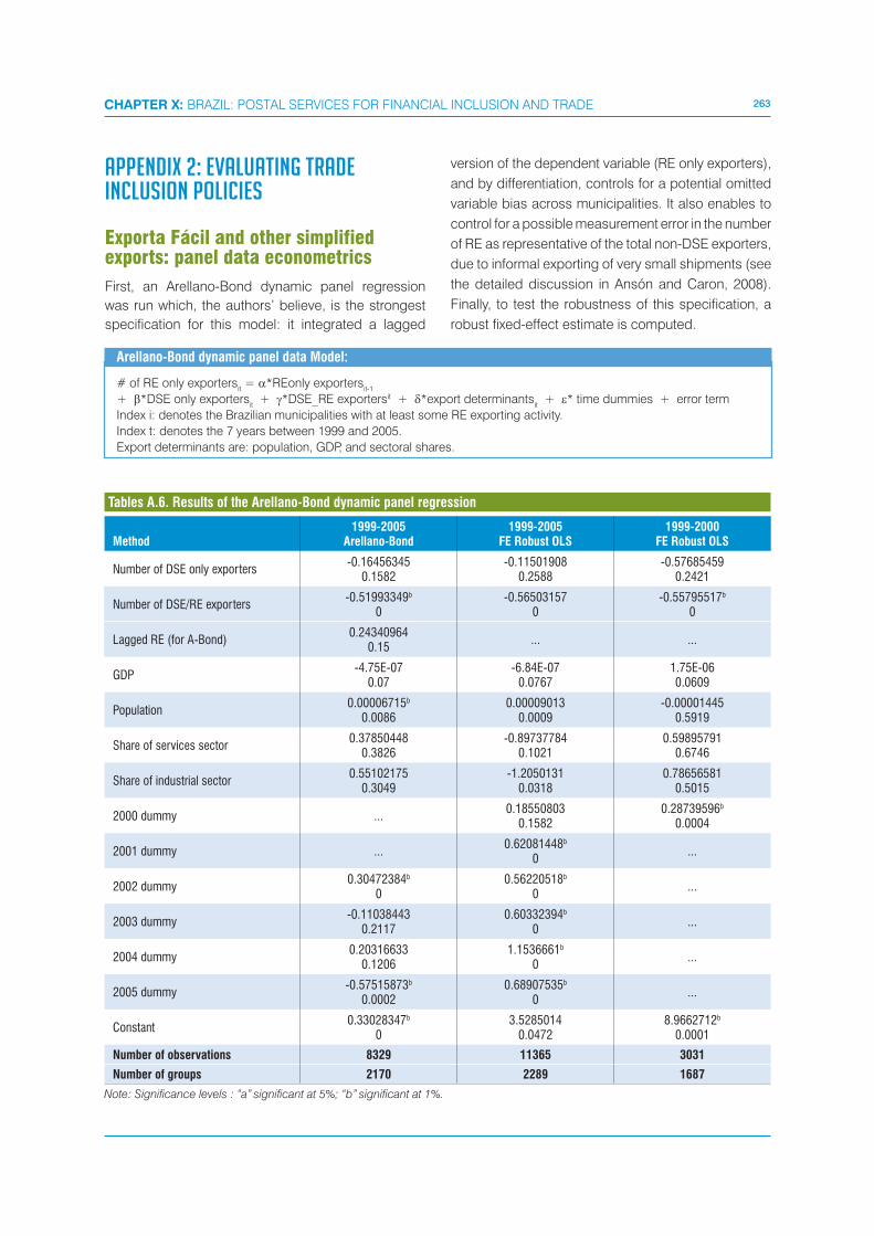
263CHAPTER X: BRAZIL: POSTAL SERVICES FOR FINANCIAL INCLUSION AND TRADE
APPENDIX 2: EVALUATING TRADE INCLUSION POLICIES
Exporta Fácil and other simplified exports: panel data econometrics
First, an Arellano-Bond dynamic panel regression
was run which, the authors’ believe, is the strongest
specification for this model: it integrated a lagged
version of the dependent variable (RE only exporters),
and by differentiation, controls for a potential omitted
variable bias across municipalities. It also enables to
control for a possible measurement error in the number
of RE as representative of the total non-DSE exporters,
due to informal exporting of very small shipments (see
the detailed discussion in Ansón and Caron, 2008).
Finally, to test the robustness of this specification, a
robust fixed-effect estimate is computed.
Arellano-Bond dynamic panel data Model:
# of RE only exportersit = *REonly exporters
it-1
+ �*DSE only exportersit + �*DSE_RE exportersit + *export determinants
it + �* time dummies + error term
Index i: denotes the Brazilian municipalities with at least some RE exporting activity.
Index t: denotes the 7 years between 1999 and 2005.
Export determinants are: population, GDP, and sectoral shares.
Method1999-2005
Arellano-Bond1999-2005
FE Robust OLS1999-2000
FE Robust OLS
Number of DSE only exporters-0.16456345
0.1582-0.11501908
0.2588-0.57685459
0.2421
Number of DSE/RE exporters-0.51993349b
0-0.56503157
0-0.55795517b
0
Lagged RE (for A-Bond)0.24340964
0.15... ...
GDP-4.75E-07
0.07-6.84E-07
0.07671.75E-060.0609
Population0.00006715b
0.00860.00009013
0.0009-0.00001445
0.5919
Share of services sector0.37850448
0.3826-0.89737784
0.10210.59895791
0.6746
Share of industrial sector0.55102175
0.3049-1.2050131
0.03180.78656581
0.5015
2000 dummy ...0.18550803
0.15820.28739596b
0.0004
2001 dummy ...0.62081448b
0...
2002 dummy0.30472384b
00.56220518b
0...
2003 dummy-0.11038443
0.21170.60332394b
0...
2004 dummy0.20316633
0.12061.1536661b
0...
2005 dummy-0.57515873b
0.00020.68907535b
0...
Constant0.33028347b
03.5285014
0.04728.9662712b
0.0001
Number of observations 8329 11365 3031
Number of groups 2170 2289 1687
Note: Significance levels : “a” significant at 5%; “b” significant at 1%.
Tables A.6. Results of the Arellano-Bond dynamic panel regression

264 SERVICES, TRADE & DEVELOPMENT
NOTES1 The terms the Post, postal services, post offices, the postal network and the postal sector are equivalent in this chapter,
except when otherwise indicated.2 http://www.febraban-star.org.br/documentos/pdfs/Banco_Postal.pdf3 Kumar et al.: “Expanding Bank Outreach through Retail Partnerships. World Bank Working Paper No. 85”, 2006; also see
Kumar (2004 and 2005).4 World Bank (2007)5 SEBRAE (2007)6 The legislative act is referred to as the Instrução Normativa SRF no 155, de 22 de dezembro de 1999 http://www.receita.
fazenda.gov.br/Legislacao/Ins/Ant2001/1999/in15599.htm7 World Savings Banks Institute and European Savings Bank Group, Perspectives No. 47 (October 2004).8 Withdrawals refer to shelter withdrawals in BP. However, BP customers can access their savings by other means, mainly
through Bradesco facilities, at ATMs, via Internet and by telephone.9 E-loans are loans for which a BP customer can apply via the Internet.10 Dummies are variables that take the value 1 if the observation corresponds to a specific region, and the value 0 if not.11 The extensive margin means at the « number of » level while the intensive margin means at the « value of » level.12 The possibility of taking into account possible measurement errors is a well-known property of the Arellano-Bond estimation
method.

SERVICES OWNERSHIP AND ACCESS TO SAFE WATER:
WATER NATIONALIZATION IN URUGUAY
It is often argued that privatization results in the delivery of higher
quality goods or services, as profit-driven firms facing stronger market
competition will respond through productivity increases (Chong and
Lopez de Silanes, 2005). On the other hand, critiques of privatization
argue, at least in the case of natural monopolies, such as water
services, this may not be observed. Due to the lack of competition in
the case of natural monopolies, the regulation of privatized firms will be
crucial to ensure an increase in the quality of services. In the absence
of adequate regulation, quality could fall as profit-driven privatized firms
attempt to extract greater profits from consumers. The objective of this
chapter is to explore the impact on the quality of water after Uruguay’s
nationalization of water services in 2004. As a proxy for the quality of
water, this study applies child mortality rates caused by water-related
diseases. An interesting feature of focusing on nationalization rather
than privatization is that it avoids selection bias or cherry-picking by
firms or governments. Nationalization in Uruguay affected all previously
privatized firms. Results suggest that the change in ownership in 2004
led to a decline of water-related child mortality, casting doubts on the
benefits of the earlier privatization of water services in Uruguay.
266 SERVICES, TRADE & DEVELOPMENT
1. INTRODUCTION
In the 1990s privatization of water services was
seen by some as a potential solution to the poor
performance of publicly owned water monopolies that
left more than 1 billion people in developing countries
without access to clean and safe water, exposed to
water shortages, diseases, and trapped in poverty
(Segerfledt, 2005). In the early 1990s many countries
in Eastern Europe and Latin America engaged in the
privatization of water services, with some Asian and
African countries following suit in the mid and late
1990s (Hall et al. 2010). However, the share of public
water companies is still large.1 Moreover, over the last
decade the share has increased due to the backlash
that followed after large foreign multinationals, won
bids for privatized water services, focused on profits
rather than the quality of services. High prices, low
investments and poor performance on leakage were
observed in many cities that privatized their water
services in the 1990s.
Uruguay is a recent example of this reversal. An
amendment to the Constitution of Uruguay passed in
2004 declared water “part of the public state domain”,
making the private provision of water illegal.2 This led to
the nationalization of two water and sewage suppliers
in the Province of Maldonado that were privatized in
1993 and 2000. The private water companies that
operated in the Province of Canelones since the 1940s
also came under the control of the public monopoly.
The apparent reasons for Uruguay’s nationalization
of water companies were no different from the ones
observed in other countries including Bolivia, Argen-
tina, and Brazil – privatization of water services did not
deliver on its promises.3 Private companies became
deeply unpopular due to the low or falling quality of
water they supplied, as well as the high prices they
charged. A series of highly publicized episodes of
low quality water provided by Uragua and Aguas de
la Costa (subsidiaries of Spanish water companies
Aguas de Barcelona and Aquas de Bilbao) led the
Uruguay Minister of Finance to request Uragua leave
the country, in the middle of a financial crisis.
It is of interest to note that two of the largest priva-
tized water companies were foreign owned, and their
nationalization consequently implied the imposition of
a new barrier to trade in services (mode 3 which cap-
tures establishment by foreign companies in GATS’s
terminology). Thus, Uruguay’s water nationalization
project in 2005 fits within the broader objective of
UNCTADs project of assessing the impact of trade
barriers in services. Rather than looking at liberaliza-
tion of trade in services, this chapter considers the
impact of the imposition of new barriers to trade in
services, focusing on social impacts rather than eco-
nomic outcomes.
More specifically, this chapter explores whether, as
expected by the proponents of nationalization of water
services in Uruguay, there has been an improvement
in the access to safe and clean water following the
nationalization of private water providers. As a proxy
for access to safe and clean water, water-related child
mortality rates which are determined not only by the
quality of water, but also sewage access, water tariffs,
and overall rate of growth in household connections
are applied. Arguably, public health issues, and child
mortality in particular, associated with water ownership
are more important goals than low prices or greater
access.4
The existing literature tends to show that water privati-
zation has ambiguous effects on child mortality rates.
One study (across different world cities) found that
government involvement in providing water services,
especially locally, significantly reduced child mortality,
but it also found that private or parastatal provision of
sewage connections was associated with lower child
mortality (Shi 2000). However, problems of selection
bias and endogeneity were difficult to address in a
cross section setup. Still another study, employing
a panel setup, illustrated that in Argentinean munici-
palities where water services were privatized the in-
cidence of child mortality from water-related disease
declined significantly, (whereas the incidence of child
mortality for other reasons remained stagnant) thus
providing indirect evidence of improvements in water
quality and access (Galiani, Gertler and Schargrodsky
2005). Nevertheless, it is noteworthy that the same cri-
tiques as those observed in Uruguay in the late 1990s
and early 2000s were also evident in Argentina’s
press (high prices, highly publicized cases of water
provided by private companies being unfit for human
consumption, or the fact that these private companies
only honoured half of their investment commitments).5
The case of Uruguay is interesting as, contrary to
existing studies, it allows identification of the impact not
through the privatization but rather the nationalization
of water services. If ownership matters, the impact of
reforms should be observed in both directions. This
is interesting since the decision to nationalize could
267CHAPTER XI: SERVICES OWNERSHIP AND ACCESS TO SAFE WATER: WATER NATIONALIZATION IN URUGUAY
be considered as exogenous to each region as it was
taken for the country as a whole, and therefore is not
subject to selection bias. As long as the determinants
of the decision to privatize are not serially correlated it
would comprise a reliable identification strategy.
The empirical methodology that was followed is
similar to the one in Galiani, Gertler, and Schargrodsky
(2005). Using panel data around the nationalization
episode, an attempt is made to identify differences
in water-related child mortality between regions that
privatized their water suppliers (and later nationalized
them) and those that did not, using a difference-in-
difference estimator.
The results across different specifications tend to
weakly suggest that after the nationalization of previ-
ously privatized water companies child mortality rates
declined conditional on district and year specific fixed
effects. Interestingly, the nationalization of water com-
panies had a differential impact on water-related child
mortality and non-water-related child mortality sug-
gesting that the correlation between privatization of
water companies and water-related child mortality is
not spurious. Indeed, once a control for overall child
mortality at the district level was set up, a positive and
statistically significant impact of private water compa-
nies on child mortality was found. Moreover, this sug-
gests that when looking at the impact of privatization
of water companies on child mortality, it is crucial to
observe the causes of death. In the dataset provided
by the Uruguay Ministry of Public Health the precise
types of infectious disease that led to deaths were
identified thus allowing for disentanglement between
water and non-water-related deaths. As shown in the
empirical section, this appears to be very important.
To summarize, it was found that the public sector was
just as competent if not more so in the running and
maintaining of nationalized water companies at the
beginning of the century in Uruguay. This finding is
contrary to existing evidence generally showing pri-
vatization leads to lower levels of child mortality. This
finding could perhaps be due to badly implemented
privatization in Uruguay which was not accompanied
by adequate regulations, or perhaps a public compa-
ny that was more efficient in attaining public health ob-
jectives than those in other countries. Another reason
for this finding may be that the time-span since the
nationalization of the private water companies may
not have been sufficiently long enough to observe
statistically significant impacts. Still, a further reason
could be that this study’s calculation of water-related
child mortality may be more precise than those of pre-
vious studies. Nevertheless, empirical results for the
episode of water nationalization in Uruguay suggest
that privatization is not the silver bullet that can lead
the way toward better access to clean and safe water.
The reminder of the chapter is organized as follows.
Section II describes the functioning of the water
system in Uruguay. Section III provides descriptive
statistics regarding child mortality in Canelones and
Maldonado which are the two regions where privatized
water companies operated. Section IV presents the
empirical methodology. Section V presents the results.
Section VI concludes.
2. THE WATER SYSTEM IN URUGUAY
At the turn of this century water and sewage services
in Uruguay were provided by fifteen private companies
and the publicly-owned company Obras Sanitarias del
Estado (OSE). OSE had the exclusive water provision
monopoly in the capital city – Montevideo and almost
all of the national territory accounting for more than
90 per cent of connections. The private sector was
composed of three big companies (Uragua, Aguas
Corrientes El Pinar and Aguas de la Costa) and
approximately twelve water providers with less than
500 connections each. These small providers were
cooperatives founded by residents to provide water
services in areas that OSE did not reach or reached
with poor quality water.
In 2000, Uragua started to provide water and sewage
services in urban and sub-urban areas of Maldonado.
Maldonado had 150,000 inhabitants out of a total of
3,300,000 in Uruguay. Aragua’s concession was west
of the Maldonado stream with the exception of the
city of Aigua. More specifically, Uragua served the
capital of Maldonado (50,417 inhabitants), San Carlos
(23,878), Pan de Azúcar (6,969), Piriápolis (7,579),
Cerros Azules, Nueva Carrara, Pueblo Gerona, west
of Rivulet Solís, Silver River, Highway 9 North. The
services covered the cities of Maldonado, the interna-
tional well-known Punta del Este (7,298 inhabitants)6
and Piriápolis in the Province of Maldonado.
Uragua was owned by Aguas de Bilbao Vizcaia,
Iberdorla, Kartera 1, a Spanish water provider. In
2004 Uragua was in litigation with OSE due to breach
of contract. Following the 2004 amendment to the
Constitution of Uruguay, Urugua reached an accord
with the Government of Uruguay and had all its assets

268 SERVICES, TRADE & DEVELOPMENT
transferred to OSE in 2005.
Aguas Corrientes El Pinar was a privately, but
nationally-owned company. It was created in 1946
– six years before the creation of OSE – with the
objective of fostering land sales in the El Pinar area
that required connections to water and sewage
services. Up until the 1990s it served less than 1,000
clients, but by the time of the nationalization it served
approximately 5,000 clients due in large part to the
rapid development of the area. Interestingly only 12
persons worked full time in Aguas Corrientes El Pinar.
The connection fee was around $200 and the average
consumption was $10.
Not only did Aguas Corrientes el Pinar provide
services in El Pinar, but also in the adjacent areas
of San Cristóbal, El Palmar, Médanos de Solymar,
Lomas de Solymar, Autodromo, and Colinas de
Solymar in the Province of Canelones. Canelones is
the second largest province with 500,000 inhabitants.
The population in El Pinar and Lomás de Solymar
stood around 33,000. Aguas Corrientes el Pinar was
nationalized in December 2006 and its assets were
transferred to OSE.
The third largest private company in Uruguay was
Aguas de la Costa. Ownership of the company was
shared between S.T.A Ingenerios and Benecio S.A.
(local companies) holding 10 per cent. The remaining
80 per cent belonged to the Spanish company Aguas
de Barcelona, a subsidiary of Suez Lyonaisse des
Eaux. Aguas de la Costa signed the concession in
1993 for twenty-five years and serviced the wealthier
areas of La Barra, Manantiales and José Ignacio next
to Punta del Este in Maldonado, to the east of Maldo-
nado stream. The company had around 3,100 cus-
Figure 1. Map of Maldonado by judicial section
Uragua
OSE
Aguas de la Costa
Aiguá
José Ignacio
ATLANTICOCEAN
LAVALLEJA
CANELONES
ROCHA
4
6
2
35
1
Maldonado
SanCarlosPan de Azúcar
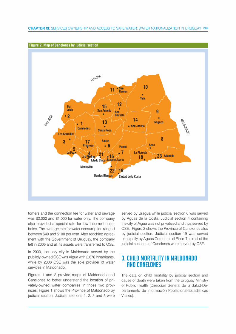
269CHAPTER XI: SERVICES OWNERSHIP AND ACCESS TO SAFE WATER: WATER NATIONALIZATION IN URUGUAY
tomers and the connection fee for water and sewage
was $2,000 and $1,000 for water only. The company
also provided a special rate for low income house-
holds. The average rate for water consumption ranged
between $40 and $100 per year. After reaching agree-
ment with the Government of Uruguay, the company
left in 2005 and all its assets were transferred to OSE.
In 2000, the only city in Maldonado served by the
publicly-owned OSE was Aigua with 2,676 inhabitants,
while by 2006 OSE was the sole provider of water
services in Maldonado.
Figures 1 and 2 provide maps of Maldonado and
Canelones to better understand the location of pri-
vately-owned water companies in those two prov-
inces. Figure 1 shows the Province of Maldonado by
judicial section. Judicial sections 1, 2, 3 and 5 were
served by Uragua while judicial section 6 was served
by Aguas de la Costa. Judicial section 4 containing
the city of Aigua was not privatized and thus served by
OSE. Figure 2 shows the Province of Canelones also
by judicial section. Judicial section 19 was served
principally by Aguas Corrientes el Pinar. The rest of the
judicial sections of Canelones were served by OSE.
3. CHILD MORTALITY IN MALDONADO AND CANELONES
The data on child mortality by judicial section and
cause of death were taken from the Uruguay Ministry
of Public Health (Dirección General de la Salud-De-
partamento de Información Poblacional-Estadísticas
Vitales).
Figure 2. Map of Canelones by judicial section
7
19
2
1
3
54
17
15
21 16
6
13 14
12
18 23
22
FLORIDA
MALD
ON
ADO
SAN
JOSE
1011
8
9
Tala
SanRamon
Migues
Santa Rosa
Montevido
Soca
CanelonesSan Jacinto
Sauce
Los Cermillos
Pandó
La Floresta
Ciudad de la Costa
San Antonio San Bautista
Atlántida
Sta,Lucia
Las PiedrasJoaquín Juarez
Barrios Blancos
Progreso
La Paz
Toledo Chico
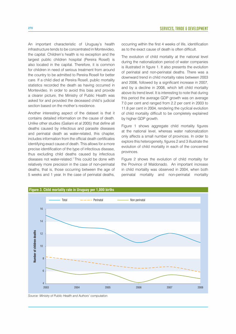
270 SERVICES, TRADE & DEVELOPMENT
An important characteristic of Uruguay’s health
infrastructure tends to be concentrated in Montevideo,
the capital. Children’s health is no exception and the
largest public children hospital (Pereira Rosell) is
also located in the capital. Therefore, it is common
for children in need of serious treatment from around
the country to be admitted to Pereira Rosell for better
care. If a child died at Pereira Rosell, public mortality
statistics recorded the death as having occurred in
Montevideo. In order to avoid this bias and provide
a clearer picture, the Ministry of Public Health was
asked for and provided the deceased child’s judicial
section based on the mother’s residence.
Another interesting aspect of the dataset is that it
contains detailed information on the cause of death.
Unlike other studies (Galiani et al 2005) that define all
deaths caused by infectious and parasite diseases
and perinatal death as water-related, this chapter,
includes information from the official death certificates
identifying exact cause of death. This allows for a more
precise identification of the type of infectious disease,
thus excluding child deaths caused by infectious
diseases not water-related.7 This could be done with
relatively more precision in the case of non-perinatal
deaths, that is, those occurring between the age of
5 weeks and 1 year. In the case of perinatal deaths,
occurring within the first 4 weeks of life, identification
as to the exact cause of death is often difficult.
The evolution of child mortality at the national level
during the nationalization period of water companies
is illustrated in figure 1. It also presents the evolution
of perinatal and non-perinatal deaths. There was a
downward trend in child mortality rates between 2003
and 2006, followed by a significant increase in 2007,
and by a decline in 2008, which left child mortality
above its trend level. It is interesting to note that during
this period the average GDP growth was on average
7.0 per cent and ranged from 2.2 per cent in 2003 to
11.8 per cent in 2004, rendering the cyclical evolution
of child mortality difficult to be completely explained
by higher GDP growth.
Figure 1 shows aggregate child mortality figures
at the national level, whereas water nationalization
only affects a small number of provinces. In order to
explore this heterogeneity, figures 2 and 3 illustrate the
evolution of child mortality in each of the concerned
provinces.
Figure 2 shows the evolution of child mortality for
the Province of Maldonado. An important increase
in child mortality was observed in 2004, when both
perinatal mortality and non-perinatal mortality
Figure 3. Child mortality rate in Uruguay per 1,000 births
Total Perinatal Non perinatal
4
6
8
10
12
14
16
2003 2004 2005 2006 2007 2008
Num
ber
of c
hild
ren
deat
hs
Source: Ministry of Public Health and Authors’ computation.

271CHAPTER XI: SERVICES OWNERSHIP AND ACCESS TO SAFE WATER: WATER NATIONALIZATION IN URUGUAY
increased substantially. Surprisingly this occurred
during a period where GDP was growing fast and
unemployment was falling. However, after this period
and coinciding with the nationalization of water
services, Maldonado experienced a downward trend
in child mortality, albeit with a slight increase above
trend, for non-perinatal deaths in 2007 and perinatal
deaths in 2008.
Figure 3 illustrates the evolution of child mortality in
Canelones, where water companies were nationalized
in 2006. Although a clear pattern is not evident, it can
be inferred that Canelones followed the 2007 peak in
child mortality observed at the national level, with a
slight decline in 2008, but with child mortality rates
above trend levels.
It can be inferred that child mortality followed different
patterns in the two provinces whose water companies
were nationalized and that the evolution in child
mortality also differed from patterns observed at
the national level (figures 1 to 3). Although obvious
province specific factors may explain these results,
this chapter only considers child mortality by
judicial section previously serviced by private water
companies, in order to provide further evidence of the
role nationalization may have played.
Table 1 presents the evolution of child mortality rates
in Maldonado according to the whether the judicial
section was serviced by a private company or by the
public monopoly, OSE, prior to nationalization.8 It is
clear that child mortality rates were higher in regions
with private service providers, both before and after
nationalization. However, although child mortality
rates tend to be lower after nationalization it is believed
these rates followed a time trend.
Table 2 presents similar findings for the Province of
Canelones. Important differences in child mortality
rates are observed for the period 2004 to 2008,
according to the type of water company ownership.
Contrary to Maldonado, child mortality rates were
higher in regions serviced by the public monopoly,
OSE. The nationalization of water in 2006 does
not seem to have had a significant effect on child
mortality rates in those regions once served by private
companies. However, there is an increase in child
mortality rates after nationalization in those judicial
districts that had always been serviced by the public
monopoly. This may suggest that after privatization
the public company in Canelones was spread too thin
across the whole region which led to a reduction in the
quality of water in other areas.
Figure 4. Child mortality rate in Maldonado per 1,000 births
Total Perinatal Non perinatal
2
4
6
8
10
12
14
16
Nationalization
Num
ber
of c
hild
ren
deat
hs
2003 2004 2005 2006 2007 2008
Source: Ministry of Public Health and Authors’ computation.

272 SERVICES, TRADE & DEVELOPMENT
The above figures represent total child mortality rates,
and do not distinguish between deaths caused by
water and non-water-related infectious diseases. In
order to refine the analysis, tables 3 and 4 present
water-related child mortality rates in Maldonado and
Canelones by judicial district depending on whether
the district was serviced by a private or a public
company prior to nationalization.
The two tables seem to indicate a decline in water-
related child deaths in judicial sections serviced by
private companies after nationalization, whereas a
difference was observed in judicial sections that were
always serviced by the public monopoly, even though
child mortality rates were very low in Maldonado
(below 0.04 per 1,000 persons over the 2003 to 2008
period).
One concern from a statistical point of view with the
figures reported in tables 3 and 4 is the small numbers
of water-related deaths. In 2007, there were 12 deaths
in Canelones and 4 deaths in Maldonado. For example,
the increase of the mortality rate in Uragua judicial
section 3, from 0 to 3.4 per 1,000 persons is explained
by a single death (table 3). In order to mitigate this
problem the robustness of the results are checked in
the econometric section by further considering overall
child mortality rates, including deaths lacking verified
causes, and perinatal deaths. If indeed nationalization
of water services was responsible for the change in
water-related child mortality rates, then a similar trend
in overall child mortality or perinatal deaths would not
be observed.
Econometrically the large number of zeros and the
count nature of the data have to be addressed to
provide robust estimates. The econometric analysis
will also allow to control for general trends in child
mortality and other non-observables that could also
affect changes in child mortality rates around the time
of nationalization.
4. METHODOLOGY
The identification strategy follows a similar approach
to that of Galiani et al (2005), with a search for
systematic differences in changes in child mortality
rates between regions that have privatized (or
nationalized) and those that have not changed the
ownership structure of water companies. The control
groups consist of neighbouring judicial districts in
Canelones and Maldonado.9 The analysis consists of
a total of 26 judicial sections for the period 2003 to
2008, resulting in 156 observations.
Figure 5. Child mortality rate in Canelones per 1,000 births
Total Perinatal Non perinatal
2
4
6
8
10
12
14
16
Nationalization
Num
ber
of c
hild
ren
deat
hs
2003 2004 2005 2006 2007 2008
Source: Ministry of Public Health and Authors’ computation.
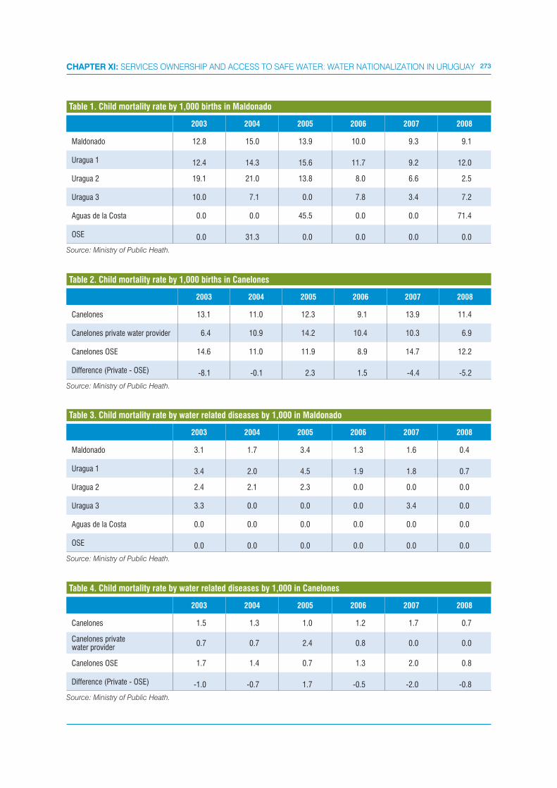
273CHAPTER XI: SERVICES OWNERSHIP AND ACCESS TO SAFE WATER: WATER NATIONALIZATION IN URUGUAY
2003 2004 2005 2006 2007 2008
Maldonado 12.8 15.0 13.9 10.0 9.3 9.1
Uragua 1 12.4 14.3 15.6 11.7 9.2 12.0
Uragua 2 19.1 21.0 13.8 8.0 6.6 2.5
Uragua 3 10.0 7.1 0.0 7.8 3.4 7.2
Aguas de la Costa 0.0 0.0 45.5 0.0 0.0 71.4
OSE 0.0 31.3 0.0 0.0 0.0 0.0
Source: Ministry of Public Heath.
Table 1. Child mortality rate by 1,000 births in Maldonado
2003 2004 2005 2006 2007 2008
Canelones 13.1 11.0 12.3 9.1 13.9 11.4
Canelones private water provider 6.4 10.9 14.2 10.4 10.3 6.9
Canelones OSE 14.6 11.0 11.9 8.9 14.7 12.2
Difference (Private - OSE) -8.1 -0.1 2.3 1.5 -4.4 -5.2
Source: Ministry of Public Heath.
Table 2. Child mortality rate by 1,000 births in Canelones
2003 2004 2005 2006 2007 2008
Maldonado 3.1 1.7 3.4 1.3 1.6 0.4
Uragua 1 3.4 2.0 4.5 1.9 1.8 0.7
Uragua 2 2.4 2.1 2.3 0.0 0.0 0.0
Uragua 3 3.3 0.0 0.0 0.0 3.4 0.0
Aguas de la Costa 0.0 0.0 0.0 0.0 0.0 0.0
OSE 0.0 0.0 0.0 0.0 0.0 0.0
Source: Ministry of Public Heath.
Table 3. Child mortality rate by water related diseases by 1,000 in Maldonado
2003 2004 2005 2006 2007 2008
Canelones 1.5 1.3 1.0 1.2 1.7 0.7
Canelones private water provider
0.7 0.7 2.4 0.8 0.0 0.0
Canelones OSE 1.7 1.4 0.7 1.3 2.0 0.8
Difference (Private - OSE) -1.0 -0.7 1.7 -0.5 -2.0 -0.8
Source: Ministry of Public Heath.
Table 4. Child mortality rate by water related diseases by 1,000 in Canelones
274 SERVICES, TRADE & DEVELOPMENT
As mentioned previously, the fact that nationalization
was undertaken across the board and at different
points in time allows for a better identification strategy,
than for privatization where firms and governments
choose which companies to privatize. In the case of
nationalization, all previously privatized firms were
included thereby mitigating issues of selection from
contaminating the results. In the case of Uruguay’s
nationalization (of water companies during 2005
to 2006), this is particularly comforting, for Aguas
Corrientes el Pinar in Canelones that was founded in
1946, and therefore unlikely that the determinants of
“privatization” at the time could be correlated with the
water nationalization decision.
In Maldonado privatization was more recent. Aguas
de la Costa and Uragua were privatized in 1993 and
2000 respectively. If there was selection in the privati-
zation decision at the time, the endogenous determi-
nants of privatization would also bias the impact of na-
tionalization on child mortality estimates. For example,
if the Government of Uruguay had decided to priva-
tize companies in judicial districts more profitable and
with better prospects, in order to maximize short-term
financial benefits from the privatization. These would
likely be districts in which child mortality was also
low. In such a scenario, child mortality rates would be
lower in regions where water companies were first pri-
vatized and then later nationalized, although there is
no causal impact going from privatization or nationali-
zation to child mortality. This can be explained in two
ways. First, if child mortality rates in Maldonado were
considered prior to and after nationalization it would
seem as though the rates were higher in judicial dis-
tricts where water companies were privatized. It would
thus seem as though judicial districts with the highest
child mortality rates were given to the water compa-
nies. Second, the panel nature of this study’s dataset
allows for control of general trends in child mortality
using year fixed effects.
More precisely, the econometric model is the following
(Equation 1):
Equation 1
where i is the judicial section, t is the year, yit is the child
mortality rate by water-related diseases in province
i in period t (or the number of child deaths when
Poisson or negative binomial estimators are used); Dit
is a dummy variable indicative of whether the water
company in province i in period t is private; i is a
province i specific random or fixed effect depending
on the estimator; !t is a year fixed effect; xit is a vector
of control variables; and uit is a judicial section time-
varying error (distributed independently across judicial
sections and time and hopefully independently of
i and !t). The regression is structured to capture
the effects of aggregate factors and judicial section
specific responses to aggregate factors.
As control variables, in the above equation, average
completed years of education, average household
income per capita and the unemployment rate
at the judicial section level are used. These three
variables were expected to be correlated with child
mortality rates and vary through time and judicial
sections. Higher income and education would be
negatively correlated with child mortality, as this
would help households avoid diseases that could
lead to the death of a child. On the other hand higher
levels of unemployment (conditional on income
and education) would tend to positively affect child
mortality through the additional stress and tension it
caused on the household. These variables are from
the annual Uruguayan National Household Survey,
Encuesta Continua de Hogares (ECH) conducted
by the Instituto Nacional de Estadística (INE). Each
survey wave contained a total of approximately 56,000
persons from about 18,000 households. The ECH was
administered throughout the year with the purpose of
generating an accurate picture of urban employment
along with the socio-economic characteristics of that
population. As data from the ECH for all of the judicial
sections was lacking, the analysis used information
from the closest judicial sections.
The parameter of interest is " which measures the
casual impact of the type of ownership (private versus
public) of the water company on child mortality. A
positive coefficient indicates that in judicial sections
with private companies, child mortality rates are larger
than other areas; conditional on year and judicial
district fixed effects, as well as education, income per
capita and unemployment rates at the judicial section
level.
Because child mortality rates by water-related
diseases are a zero-inflated continuous variable,
due to the important number of judicial sectors that
report zero child mortality, estimating the equation
by ordinary least squares (OLS) would yield biased
and inconsistent estimates of the impact of ownership
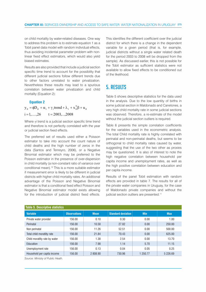
275CHAPTER XI: SERVICES OWNERSHIP AND ACCESS TO SAFE WATER: WATER NATIONALIZATION IN URUGUAY
on child mortality by water-related diseases. One way
to address this problem is to estimate equation 1 as a
Tobit panel data model with random individual effects,
thus avoiding incidental parameter problem with non-
linear fixed effect estimators, which would also yield
biased estimates.
Results are also provided that include a judicial section
specific time trend to account for the possibility that
different judicial sections follow different trends due
to other factors unrelated to water privatization.
Nevertheless these results may lead to a spurious
correlation between water privatization and child
mortality (Equation 2):
Equation 2
Where �i trend is a judicial section specific time trend
and therefore is not perfectly correlated with the year
or judicial section fixed effects.
The preferred set of results used either a Poisson
estimator to take into account the count nature of
child deaths and the high number of zeros in the
data (Santos and Tenreyro, 2006), or a Negative
Binomial estimator which may be preferred to the
Poisson estimator in the presence of over-dispersion
in child mortality (a non-constant ratio of variance over
conditional mean).10 This is a more suitable estimator
if measurement error is likely to be different in judicial
districts with higher child mortality rates. An additional
advantage of the Poisson and Negative Binomial
estimator is that a conditional fixed effect Poisson and
Negative Binomial estimator model exists allowing
for the introduction of judicial district fixed effects.
This identifies the different coefficient over the judicial
district for which there is a change in the dependent
variable for a given period (that is, for example,
judicial districts without a single water related death
for the period 2003 to 2008 will be dropped from the
sample). As discussed earlier, this is not possible for
the Tobit estimator as sufficient statistics were not
available to allow fixed effects to be conditioned out
of the likelihood.
5. RESULTS
Table 5 shows descriptive statistics for the data used
in the analysis. Due to the low quantity of births in
some judicial section in Maldonado and Canelones, a
very high child mortality rate in some judicial sections
was observed. Therefore, a re-estimate of the model
without the judicial section outliers is required.
Table 6 presents the simple correlation coefficients
for the variables used in the econometric analysis.
The total Child mortality rate is highly correlated with
perinatal and non-perinatal deaths, but seems to be
orthogonal to child mortality rates caused by water,
suggesting that the use of the two other as proxies
may be questioned. It is also of interest to note the
high negative correlation between household per
capita income and unemployment rates, as well as
the high positive correlation between education and
per capita income.
Results of the panel Tobit estimation with random
effects are provided in table 7. The results for all of
the private water companies in Uruguay, for the case
of Maldonado private companies and without the
judicial section outliers are presented.11
Variable Observations Mean Standard deviation Min Max
Private water provider 156.00 0.10 0.30 0.00 1.00
Perinatal 156.00 10.58 27.82 0.00 250.00
Non perinatal 156.00 11.26 52.51 0.00 500.00
Total child moratlity rate 156.00 21.84 70.43 0.00 625.00
Child moratlity rate by water 156.00 1.38 2.54 0.00 13.70
Education 156.00 7.98 1.14 5.70 11.15
Unemployment rate 156.00 0.13 0.04 0.05 0.25
Household per capita income 156.00 2 808.90 730.96 1 250.77 5 226.69
Source: Ministry of Public Heath.
Table 5. Descriptive statistics
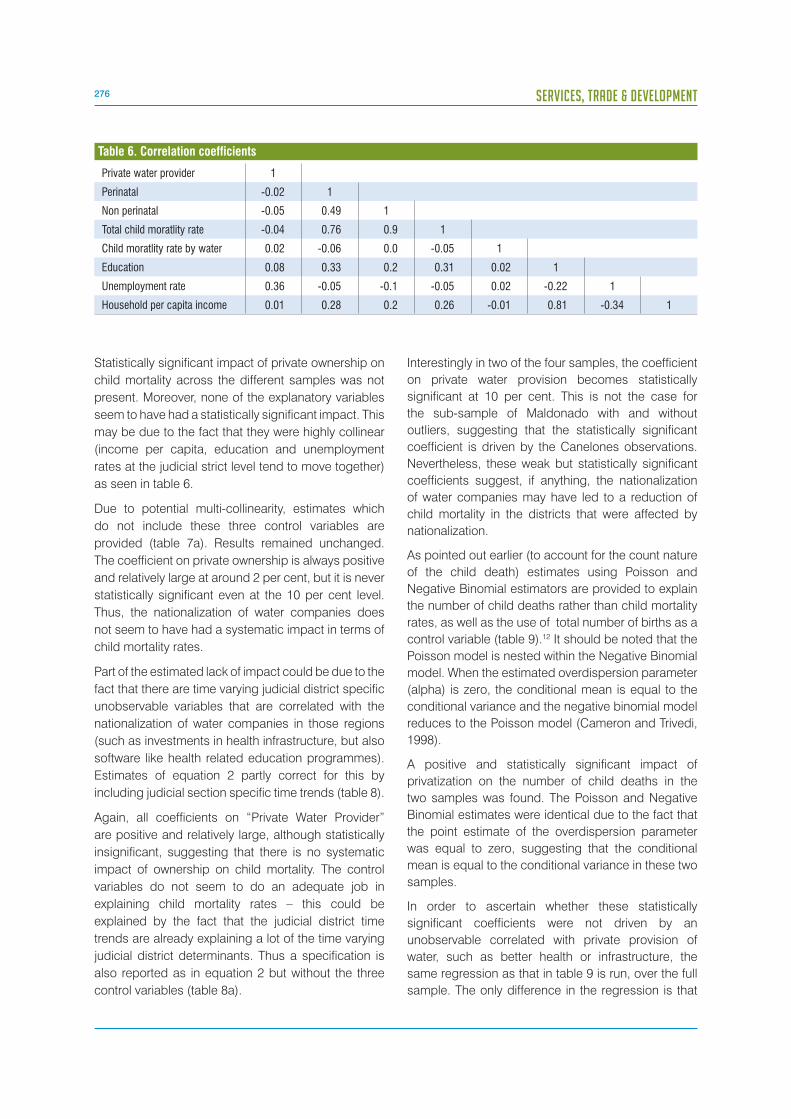
276 SERVICES, TRADE & DEVELOPMENT
Statistically significant impact of private ownership on
child mortality across the different samples was not
present. Moreover, none of the explanatory variables
seem to have had a statistically significant impact. This
may be due to the fact that they were highly collinear
(income per capita, education and unemployment
rates at the judicial strict level tend to move together)
as seen in table 6.
Due to potential multi-collinearity, estimates which
do not include these three control variables are
provided (table 7a). Results remained unchanged.
The coefficient on private ownership is always positive
and relatively large at around 2 per cent, but it is never
statistically significant even at the 10 per cent level.
Thus, the nationalization of water companies does
not seem to have had a systematic impact in terms of
child mortality rates.
Part of the estimated lack of impact could be due to the
fact that there are time varying judicial district specific
unobservable variables that are correlated with the
nationalization of water companies in those regions
(such as investments in health infrastructure, but also
software like health related education programmes).
Estimates of equation 2 partly correct for this by
including judicial section specific time trends (table 8).
Again, all coefficients on “Private Water Provider”
are positive and relatively large, although statistically
insignificant, suggesting that there is no systematic
impact of ownership on child mortality. The control
variables do not seem to do an adequate job in
explaining child mortality rates – this could be
explained by the fact that the judicial district time
trends are already explaining a lot of the time varying
judicial district determinants. Thus a specification is
also reported as in equation 2 but without the three
control variables (table 8a).
Interestingly in two of the four samples, the coefficient
on private water provision becomes statistically
significant at 10 per cent. This is not the case for
the sub-sample of Maldonado with and without
outliers, suggesting that the statistically significant
coefficient is driven by the Canelones observations.
Nevertheless, these weak but statistically significant
coefficients suggest, if anything, the nationalization
of water companies may have led to a reduction of
child mortality in the districts that were affected by
nationalization.
As pointed out earlier (to account for the count nature
of the child death) estimates using Poisson and
Negative Binomial estimators are provided to explain
the number of child deaths rather than child mortality
rates, as well as the use of total number of births as a
control variable (table 9).12 It should be noted that the
Poisson model is nested within the Negative Binomial
model. When the estimated overdispersion parameter
(alpha) is zero, the conditional mean is equal to the
conditional variance and the negative binomial model
reduces to the Poisson model (Cameron and Trivedi,
1998).
A positive and statistically significant impact of
privatization on the number of child deaths in the
two samples was found. The Poisson and Negative
Binomial estimates were identical due to the fact that
the point estimate of the overdispersion parameter
was equal to zero, suggesting that the conditional
mean is equal to the conditional variance in these two
samples.
In order to ascertain whether these statistically
significant coefficients were not driven by an
unobservable correlated with private provision of
water, such as better health or infrastructure, the
same regression as that in table 9 is run, over the full
sample. The only difference in the regression is that
Private water provider 1
Perinatal -0.02 1
Non perinatal -0.05 0.49 1
Total child moratlity rate -0.04 0.76 0.9 1
Child moratlity rate by water 0.02 -0.06 0.0 -0.05 1
Education 0.08 0.33 0.2 0.31 0.02 1
Unemployment rate 0.36 -0.05 -0.1 -0.05 0.02 -0.22 1
Household per capita income 0.01 0.28 0.2 0.26 -0.01 0.81 -0.34 1
Table 6. Correlation coefficients

277CHAPTER XI: SERVICES OWNERSHIP AND ACCESS TO SAFE WATER: WATER NATIONALIZATION IN URUGUAY
Sample
(1) (2) (3) (4)
Variables All All without outliers MaldonadoMaldonado
without outliers
Private water provider2.422
(1.967)1.823
(1.939)1.827
(2.344)1.447
(2.246)
Education0.122
(1.137)0.444
(1.100)0.304
(1.207)0.621
(1.155)
Unemployment rate1.617
(20.11)-2.123
(19.20)1.115
(21.68)-4.789
(20.67)
Household per capita income-9.74e-05(0.00179)
0.000166(0.00173)
-0.000140(0.00197)
0.000410(0.00190)
Constant-3.370
(6.747)-5.296
(6.550)-4.595
(7.194)-6.705
(6.918)
Observations 156.0 152.0 150.0 146.0
Log likelihood -235.1 -233.5 -223.5 -221.8
Table 7. Panel tobit random effects with time effects Dependent variable: Child mortality rate by water-related diseases
Sample
(1) (2) (3) (4)
Variables All All without outliers MaldonadoMaldonado
without outliers
Private water provider2.523
(1.802)2.205
(1.752)1.996
(2.112)1.710
(2.058)
Constant-2.417
(1.371)a
-2.131(1.355)
-2.509(1.457)a
-2.220(1.439)
Observations 156.0 152.0 150.0 146.0
Log likelihood -235.1 -233.8 -223.6 -222.4
Note: Standard errors in parentheses. “a” significant at 10%; “b” significant at 5%, “c” significant at 1%.
Table 7a. Panel tobit random effects with time effects Dependent variable: Child mortality rate by water-related diseases
total child mortality rates and non-water-related child
mortality (including perinatal mortality and deaths
without known causes) were used, instead of water-
related child mortality rates. There was no reason
to expect a systematic impact of the privatization
of water companies on total child mortality or non-
water-related child mortality (again controlling for the
number of births). Table 10 reports the results.
As expected private provision of water services seems
not to have had a statistically significant impact on
total and non-water-related child mortality, (taken as
the difference between total child mortality and water-
related mortality) when using Poisson or a Negative
Binomial estimator.13 This highlights the importance of
correctly measuring water-related child mortality as it
may not move in the same direction as overall child
mortality which will have all sorts of other determinants.
The other determinants may be correlated with the
privatization or nationalization of water services and
therefore lead to spurious conclusions regarding the
impact of privatization on child mortality.
A final robustness check of the results includes non-
water related child deaths as an explanatory variable
to the specification previously reported (table 9).
Indeed, non water related child mortality may be
correlated with other determinants of water-related
child mortality, making it desirable to have it as a
control variable when explaining water-related child
mortality. In this manner the privatization of water
services would not be attributable to what may be a

278 SERVICES, TRADE & DEVELOPMENT
Sample
(1) (2) (3) (4)
Variables All All without outliers MaldonadoMaldonado
without outliers
Private water provider2.788
(2.100)2.788
(2.100)2.582
(2.522)2.582
(2.521)
Education0.264
(1.518)0.264
(1.518)0.512
(1.610)0.513
(1.610)
Unemployment rate-1.823
(24.01)-1.826
(24.01)-0.779
(25.49)-0.782
(25.49)
Household per capita income0.00138
(0.00220)0.00138
(0.00220)0.00174
(0.00250)0.00174
(0.00250)
Constant-5.213
(8.971)-5.215
(8.972)-8.027
(9.558)-8.030
(9.557)
Observations 156.0 152.0 150.0 146.0
Log likelihood -206.8 -206.8 -196.2 -196.2
Table 8. Panel tobit random effects with time effects and judicial section time trend Dependent variable: Child mortality rate by water-related diseases
Sample
(1) (2) (3) (4)
Variables All All without outliers MaldonadoMaldonado
without outliers
Private water provider2.912
(1.673)a
2.912(1.673)a
2.494(1.934)
2.494(1.933)
Constant-0.0997(1.227)
-0.0995(1.227)
-0.0464(1.298)
-0.0462(1.298)
Observations 156.0 152.0 150.0 146.0
Log likelihood -207.5 -207.5 -197.2 -197.2
Note: Standard errors in parentheses. “a” significant at 10%; “b” significant at 5%, “c” significant at 1%.
Table 8a. Panel tobit random effects with time effects and judicial section time trend Dependent variable: Child mortality rate by water-related diseases
Poisson Negative binomial
(1) (2) (3) (4)
Variables All Maldonado All Maldonado
Private water provider1.028
(0.476)b0.897
(0.492)a1.028
(0.476)b0.897
(0.492)a
Observations 120.0 114.0 120.0 114.0
Log likelihood -80.1 -75.5 -80.1 -75.5
Note: Standard errors in parentheses. “a” significant at 10%; “b” significant at 5%, “c” significant at 1%.
Table 9. Poisson and negative binomial fixed effects with time effects Dependent variable: Child mortality by. Water-related diseases

279CHAPTER XI: SERVICES OWNERSHIP AND ACCESS TO SAFE WATER: WATER NATIONALIZATION IN URUGUAY
more general decline in child mortality due to other
factors. If the statistically significant results (table 9)
are robust to the inclusion of non-water related child
mortality as a control variable then evidence that the
nationalization of water services in Uruguay led to
lower rates of child mortality would exist. Results are
reported in table 11.
Again the Poisson and Negative Binomial estimates
are identical indicating that the overdispersion point
estimate (alpha) is equal to zero. Also, results suggest
across all samples and estimators that higher levels
of non-water related child deaths are not correlated
with higher levels of water-related child mortality, as
previously indicated in table 6.14 Thus, there does not
seem to be common determinants of water-related
child mortality and non-water-related child mortality.
More interestingly, the coefficient on private water
provider remains positive in all four specifications.
Moreover, the point estimates are not statistically
different from those reported in table 9, confirming
earlier finding that the nationalization of water services
may have led to a decline in child mortality.
6. CONCLUSIONS
One of the strictest barriers to trade in services
that can be imposed by an importing country is the
imposition of prohibiting foreign companies locating
within its boundaries, especially when the only
mode of delivery of services is through investments
in proximity to the customer (mode 3 delivery in the
jargon of services trade). To all intents and purposes
the Government of Uruguay imposed such prohibition
when it nationalized water companies by amending
the Constitution in 2004. It declared all water sources
belonged in and to the public domain. An important
question from a policy perspective is whether this
reform had a positive or negative impact on the
performance of the service provider and the quality of
the service it provided.
Supporters of trade liberalization in services often argue
that with privatization come more profitable firms and
a better quality of services. Uruguay’s nationalization
of water services provides a natural experiment
to assess the impact of such a reform. Contrary to
most existing literature, it will be possible to identify
Poisson Negative binomial
(1) (2) (3) (4)
Variables Total Non-water-related Total Non-water-related
Private water provider0.199
(0.160)0.078
(0.171)0.228
(0.177)0.119
(0.189)
Observations 155.0 155.0 155.0 155.0
Log likelihood -238.9 -230.6 -233.5 -224.9
Table 10. Poisson and negative binomial fixed effects with time effects Dependent variable: Total child deaths. Total or non-water-related child deaths
Poisson Negative binomial
(1) (2) (3) (4)
Variables Total Maldonado Total Maldonado
Private water provider1.001
(.447)b0.881
(0.493)a1.001
(.447)b0.881
(0.493)a
Non-water related child deaths0.024
(0.027)0.019
(0.028)0.024
(0.027)0.019
(0.028)
Observations 120.0 114.0 120.0 114.0
Log likelihood -79.7 -75.3 -79.7 -75.3
Note: Standard errors in parentheses. “a” significant at 10%; “b” significant at 5%, “c” significant at 1%.
Table 11. Poisson and negative binomial fixed effects with time effects Dependent variable: Child deaths by. Water-related diseases
280 SERVICES, TRADE & DEVELOPMENT
the impact of the reform not through the privatization
of public firms, but rather through the nationalization
of water services. This is an interesting aspect of the
case study because nationalization suffers potentially
less than privatization from selection problems, that
is, governments and private firms select which public
companies should be privatized. In the case of the
nationalization of water services in Uruguay all existing
private companies were nationalized, which facilitates
identifying the impact of the reform on the quality of
the service provided without having to worry whether
the Government and private firms chose the best (or
the worst) firms for privatization.
The focus is on child mortality as a proxy for the
quality of services provided. Although more direct
measures could be applied to gauge the performance
of water companies other than child mortality, such as
water quality, sewage access, water tariffs, and rate of
growth in household connections, they are not always
easier to observe, (even if all were determinants of
child mortality). Thus, by focusing on child mortality,
the impact of the reform in all these variables is taken
into account. Moreover, reductions in child mortality
are arguably a more important objective from a public
policy perspective than water tariffs or sewage access.
Using an estimator that corrects for the large number
of zeros in the dataset, as well as the count data
aspect of child mortality, the nationalization of water
companies in Uruguay was found to lead to a decline
in water-related child mortality. Interestingly, the
nationalization is orthogonal to total child mortality or
non-water-related child mortality, suggesting that the
impact found for water-related child mortality was not
being driven by some spurious correlation.
This result contrasts with existing evidence for
Argentina’s privatization of water services (Galiani et al
2004), which found that privatization of water services
leads to a decline in child mortality. Future research
should try to disentangle the determinants of these
two different outcomes in order to further understand
why privatization did not have the expected impact in
Uruguay.
Potential explanations for these differences may rest
on: any diverse regulations imposed during privati-
zation or nationalization (investment requested, uni-
versal services); different functioning of regulatory
bodies: badly designed contracts and bidding proc-
esses; and so on. A detailed examination of any such
differences could help to understand what works and
what does not work in terms of water privatization.
Furthermore, examining differences in the functioning
of public companies, (external funding, and boards of
directors, amongst others) could help to explain why
in some countries public providers of water services
seem to do better than in other countries.
Finally, the results in this chapter suggest that the
focus on private versus public ownership of natural
monopolies such as water providers may be mislead-
ing. The institutional environment under which the
natural monopoly operates may be much more impor-
tant. In Uruguay, at least, public operators provided a
service of equal, if not better, quality than the previous
private firms.
281CHAPTER XI: SERVICES OWNERSHIP AND ACCESS TO SAFE WATER: WATER NATIONALIZATION IN URUGUAY
NOTES1 According to Hall et al (2010) water services are owned and run by the public sector in 90 per cent of the largest 400 cities
of the world. 2 In the Netherlands water privatization was also made illegal.3 The reason for the failure of privatization is not necessarily inherent to privatization, but may be also explained by poorly
designed contracts (in terms of required investments) or non-adequate regulatory bodies. These are also often associated with problems of corruption (see Chong and Lopez-de-Silanes, 2005).
4 According to the World Bank access to piped sewerage is particularly low in Uruguay at only 53 per cent. This compares badly with other Latin American countries such as Chile, Colombia, Mexico and some comparable States in Brazil.
5 Gamper, Khan and Timmins (2007) and Galdo and Bertha, (2005) also find an import effect of water access on child mortality in Brazil and Ecuador, but these studies do not focus on the impact of ownership on child mortality.
6 Only the national population is used and not the tourist population, which can reach hundreds of thousands during the summer.
7 The following causes of death are included as being water-related: myotonic disorders, bacterial sepsis of newborn, unspecified, necrotizing enterocolitis fetus and necrotizing enterocolitis of the new birth septicemia, unspecified, meningitis, unspecified encephalitis, myelitis and encephalomyelitis, unspecified, bacterial meningitis, unspecified, congenital viral hepatitis, sepsis of new birth by other staphylococcus, and other unspecified, septicemia due to candida.
8 For presentation purposes, judicial section 5 is excluded, which was served by Uragua from the disaggregation because it only includes a few small cities with no child mortality during the period. Nevertheless, this information is obviously used in the econometric exercise later on.
9 More precisely, the judicial sections with private water companies located in Maldonado are judicial sections 1 to 3, 5 and 6, and in Canelones is judicial section 19. As control groups, neighbours judicial sections that did not privatize: judicial section 4 in Maldonado, and judicial sections 1 to 7, 10, 11, 13, 14, 16, 17, 18 and 34 in Canelones are used. Moreover, judicial section 1 is used as a control in Maldonado’s neighbouring Province of Lavalleja and judicial sections 1, 3, 4 and 5 in the Maldonado’s neighbouring Province Rocha.
10 A characteristic of the Poisson distribution is that its mean equals its variance, and as seen later in Table 5 the unconditional variance of child mortality variables is usually more than twice as large as the unconditional mean suggesting that a Negative Binomial estimator may be more appropriate than a Poisson estimator.
11 Outliers are defined as those judicial districts with large child mortality, that is, above 200 per thousand births. 12 The “exposure” is used as an option in stata that conditions the results on the ln (births) with a coefficient set to 1. 13 The Poisson and Negative Binomial estimates are different suggesting that the point estimate of the overdispersion
parameter (alpha) is not equal to zero, that is, the conditional mean is not equal to the conditional variance when explaining either total or non-water related child deaths.
14 The same results are obtained if non-water related child mortality as a control is used. Therefore, this result is not due to the fact that by construction water related child mortality is part of total child mortality.
ROAD INFRASTRUCTURE AND AGRICULTURAL CONTRACTING SERVICES
IMPACT ON RURAL PRODUCTION IN ARGENTINA
The main objective of this Chapter is to understand whether the
construction or maintenance of roads improves productivity by way
of enabling farmer access to agricultural services. To facilitate such an
understanding the links between the provision of road infrastructure
and contracting services on productivity in Argentina’s agricultural
sector are examined. The findings lead to the conclusion that both
road infrastructure and contracting services have a positive, large and
statistically significant effect on agricultural productivity. Specifically,
those farmers affected by the road investment are 17 per cent more
productive in expected value than those farmers unaffected by such
investment. Moreover, farmers who hire agricultural services have
productivity 12 per cent higher than those who do not hire agricultural
services. However, the results do not support the existence of
complementarities between them as each has a direct and differential
impact on the rural sector in Argentina.
284 SERVICES, TRADE & DEVELOPMENT
1. INTRODUCTION
Since 1995, the Argentine farming sector has made
significant progress. The volume of agricultural
production (wheat, maize, soybean and sunflower)
doubled between 1990 and 2005, increasing from 35
million tons to 70 million tons. Although the cultivated
land area was augmented by only 40 per cent, most of
the expansion of the sector is attributed to increases in
productivity. Agricultural exports grew by a staggering
150 per cent during this same period.
Agriculture is a major economic sector, particularly
when the whole supply chain is taken into account.
Increases in farming productivity are associated
with aggregate welfare gains and overall poverty
reduction. Thus, expansion and productivity gains
in the agricultural sector are typically associated
with spillovers to the rest of the economy and, in
consequence, the welfare gains and poverty impacts
can be significantly boosted.
Recent literature1 has considered the following set
of factors to explain the evolution of the agricultural
sector: technology adoption at the farm level including
transgenic seed, direct drilling systems,2 application
of agrochemicals and fertilizers, amongst others;
as well as organizational changes such as double
cropping,3and agricultural contracting services
(outsourcing agriculture).
This chapter focuses on the latter. Recent studies have
highlighted a new form of organization for farms. Many
farms in the Province of Buenos Aires have adopted
new organizational changes that are characterized
by an ownership separation of two of the main
productive factors – land and capital. In these new
organizational arrangements, the contractor or capital
owner provides machinery and agricultural services to
the farmer or land owner. Agricultural services include
land ploughing, disking, sowing, crop protection,
and harvesting.4 The contracting of agricultural
services enables the farmer or land owner to avoid
acquiring capital goods that may end up representing
a significant portion of production costs. This implies
that it is important to have both, good market access
for produced farm goods (grains, meat), as well as
the means to reach the contractors and through them
access to capital (machinery).
Argentina’s adoption of these new types of
arrangements has generated an increase in the capital
intensity of the farming sector. Between 2002 and
2005, there was a significant increase of agricultural
machinery imports – a 280 per cent increase in
value, and a 153 per cent increase in physical units.
Furthermore, 61 per cent of this increase was due to
machinery imports. This fact uncovers a role for trade
as imports of capital goods complement the adoption
of modern production arrangements, allowing for
small landowners to achieve the optimum scale of
production without large capital outlays on fixed
assets. Therefore, agricultural services contractors, in
addition to allowing the incorporation of technology
in the farming sector, also had an important role in
one of the determinants of domestic investment –
imported machinery.
Much less attention has been given to the role carried
out by investment in road infrastructure. The sparse
literature recognizes that road investment generates
a positive impact on economic growth and reduces
poverty. Investment in road infrastructure may reduce
production and transaction costs, promoting trade
and facilitating labour division and specialization
– key elements for a sustained economic growth
(Gannon and Liu 1997). The positive effect of the road
construction is directly linked with better access of
producers to reach goods markets.
The main objective of this chapter is to explore the
links between the provision of road infrastructure
and contracting services on productivity in
Argentina’s agricultural sector. Of particularly
interest is understanding whether road construction
or maintenance improves productivity by enabling
farmers to access agricultural services. To this end,
data panel methods are utilized. The data is derived
from the national agricultural survey (Encuesta
Nacional Agropecuaria – ENA). This survey provides
panel data on approximately 1,800 farming and
livestock holdings (explotaciones agropecuarias –
EAPs), for the period 1993 to 2003.
It should be noted that the analysis in this chapter is
not at the household level but rather at the farm level
– as such the data utilized is composed of a survey of
firms that produce agricultural goods. The structure
of farming suggests that an increase in farm income
can have a direct impact on household income. For
example according to the National Agricultural Census
2002 only 5 per cent of farms were incorporated under
the corporate form (joint stock company or limited
liability company), while the rest were managed by
individuals.

285CHAPTER XII: ROAD INFRASTRUCTURE AND AGRICULTURAL CONTRACTING SERVICES IMPACT ON RURAL PRODUCTION IN ARGENTINA
It was found that both road infrastructure and
contracting services have a positive, large and
statistically significant effect on agricultural
productivity. Specifically, those farmers affected by
the road investment are 17 per cent more productive
in expected value than those unaffected farmers.
Moreover, those farmers hiring agricultural services
have productivity 12 per cent higher than farmers
not hiring. However, the results do not support the
existence of complementarities between them as
each has a direct and differential impact on the rural
sector in Argentina
The chapter is organized as follows. Section 2 presents
a brief literature review. Section 3, describes how the
variables used to evaluate the impact were constructed
and performs a data analysis of road construction and
improvement in the Province of Buenos Aires. Section
4 presents the main econometric analysis and results.
Section 5 concludes.
2. LITERATURE REVIEW
The analytical literature on the effects of different
infrastructure projects on economic and social
variables is diverse, not only with respect to type of
approach (macroeconomic versus microeconomic)
but also with respect to analytical method (cost-benefit
studies versus regressions with control groups).
Investment in infrastructure5 is a very important factor
in a country’s development because of the impact
it has on the remaining economic activities. These
effects include the reduction of production costs
and the increment of productivity, and access to
new markets and better life conditions (Fiel, 1998).
Moreover, investment in road infrastructure allows for
the reduction of transaction costs, promoting trade
and facilitating labour division and specialization – all
key elements for a sustained economic development
(Gannon and Liu, 1997).
Regarding the relation between infrastructure and
development at the macroeconomic level, the more
direct mechanism by which investment affects growth
is by allowing the development of different productive
activities. Indirectly, investment can boost labour and
capital productivity, by way of increments in market
competition or access to new technologies. However,
the specialized literature also states that growth can
generate greater investment in infrastructure. Thus,
the causality relation between these two economic
variables is important. Empirical evidence shows
results supporting both directions.
One study holds that investment in infrastructure
determines private investment and growth (Aschaeur,
1989 – a pioneer in measuring the impact of investment
on growth at a national aggregate level).6 Another study
(Ford and Poret, 1991) holds – after adopting the same
data as Aschaeur, but re-estimating it for a longer time
series – that although results can be confirmed for the
initial time span they certainly could not be confirmed
for a larger time span.7 Still another study identifies
several links between infrastructure investment and
growth that could occur simultaneously (Binswanger
et.al., 1993). It is also possible that a crowding-out
effect of public investment on private investment takes
place. Nevertheless, studies show that this effect is
very improbable in rural areas (Blejer and Kan, 1984;
Creightney, 1983; and Jalan and Ravallion, 1997) due
to the high complementary degree between both
types of investment.
Considering only investment in road infrastructure,
Queiroz and Gautam (1992) find evidence of
investment preceding economic growth. Binswanger
et al. (1993) reach a similar conclusion, identifying
that the lack of roads is a significant constraint on the
supply response of agriculture.
The studies on the effects of infrastructure investment
from a microeconomic point of view are very varied.
Concerning the agricultural sector, Fosu et al. (1995)
analyse the effects of public infrastructure on rural
poverty and development, distinguishing between
direct and indirect effects. The former refers to the
fact that increments in infrastructure raise output,
displacing production possibilities and marginal cost
curve, increasing rate of return of private investment in
rural activities. The indirect effect is related to changes
in the structure of relative price of goods and inputs,
reducing transaction costs faced by producers, and
affecting allocation of resources within the agricultural
activities.
Recently, Khandker et al. (2006) studied the impact
of projects for rural road construction, using panel
data for households in Bangladesh. They found
evidence that investment in rural roads significantly
reduces poverty, due to higher agricultural output
and wages lower transport and input costs as well as
higher prices for the goods produced by the farms.
Similar results were found by Ahmed and Hossain
(1990). Levy (1996), compares the situation before
286 SERVICES, TRADE & DEVELOPMENT
and after the rehabilitation of roads in Morocco with
the situation in areas where roads were not subject
to improvement, finding that road rehabilitation
generated significant increases in agricultural output
and important changes in its composition and in the
employment of inputs, among other relevant results.8
The advantage of these works is to control
systematically for the most important covariates,
in order to isolate the impact of improvements in
rural infrastructure, basically by comparing the
results obtained by the respective group after the
implementation of the improvement versus realised
results by the control group (those who were not
benefited by the improvement).
Cuánto (2000) presents several indicators of the
benefits of rural road rehabilitation and maintenance
for Peru, based on data for households originated in
surveys aimed to evaluate the rural roads programme
(Programa de Caminos Rurales) between 1996 and
1999. This compares beneficiaries located in regions
with rehabilitated roads against other beneficiaries
located in areas with similar roads but not having
undergone rehabilitation.
Specifically, the analysis considers the impact of
road construction on: i) infrastructure and transport
services; ii) access to public services; iii) productive
activities; iv) employment, migration and poverty; and
v) the environment. The results indicate significant
reductions in transportation costs, resulting from
reductions in travel times and lower freight rates.
Investment in roads also leads to improvements
in access to health services, although no sizeable
positive impact on education is recorded. The impacts
on agricultural variables are mixed – productivity
increases are recorded in some crops but not in
others. Finally, the study does not find significant
impacts on poverty reduction.9
Escobal and Ponce (2003), using the same dataset
and making use of potential controls to evaluate the
impact of road rehabilitation on households subject
to intervention, observe increases in income after the
implementation of the improvements. They find that
non-agricultural wages are the main source explaining
the impact of the improvement in the short run.
Conversely, Lockshin and Yemtsov (2003) evaluate
the effect of various community level infrastructure
rehabilitation projects undertaken in rural Georgia,
combining household and community surveys in a
panel data structure. They find that road improvements
do generate welfare gains for the poor.
The channels through which infrastructure investment
can reduce poverty had been extensively studied. In
addition to the previously cited works from Gannon
and Liu (1997), Khandker et al. (2006), and Lockshin
and Yemtsov (2003), the Escobal and Torero (2004)
study considers the impact of different infrastructure
services on households of rural areas of Peru. They
find that the greater the access to infrastructure
facilitates the development of productive activities,
thus raising a household’s income, by one of the
following ways: more worked hours; higher activity
diversification; or changes in the yields of these
activities. The rise in income stimulates poverty
reduction and, consequently, a welfare increase in
rural areas.
Two additional studies by Verner (2006) and Lopez and
Anríquez (2002) are also of interest. The Verner study
utilizes the rural household survey of Argentina and
finds that the incomes of agricultural producers are
positively related by access to paved roads. Similarly,
the López and Anríquez study assess the impact of
agricultural growth on poverty in Chile and finds a
positive relationship between agricultural production
and poverty reduction.
Another study (Lódola 2008) found that the recent
growth of grain production in Argentina resulted from
a new form of organization, where the agricultural
services providers play an important role in enabling
cattle farmers to diversify risks by also producing
agricultural goods, thus transforming into mixed
farms. The study also finds that the emergence of rural
contractors in the countryside has facilitated double
cropping, expanded the agricultural frontier, and
fundamentally improved land use efficiency through
technological change. The same study shows that the
probability of renting agriculture services increases as
the size of farms increase, indicating this may be a
way of acquiring the optimal range of production.
The relationship between farmers and rural contractors
began in the early twentieth century, resulting from an
influx of immigrants to Argentina leasing agricultural
land, leading to the creation of landless capital
holders. Thus, short term contracts coupled with the
field rotation was the outstanding feature of the period
(Llovet 1988).
Therefore, this long association linking agricultural
producers to agriculture service contractors has
strengthened the agricultural sector in Argentina.
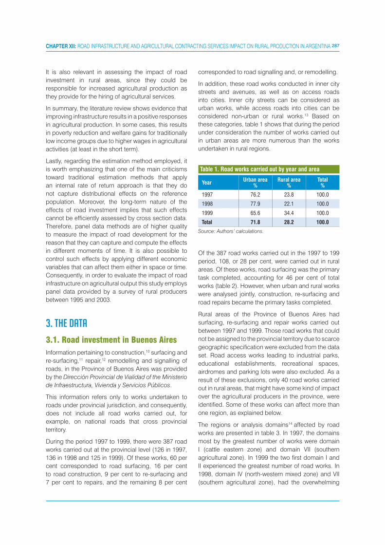
287CHAPTER XII: ROAD INFRASTRUCTURE AND AGRICULTURAL CONTRACTING SERVICES IMPACT ON RURAL PRODUCTION IN ARGENTINA
It is also relevant in assessing the impact of road
investment in rural areas, since they could be
responsible for increased agricultural production as
they provide for the hiring of agricultural services.
In summary, the literature review shows evidence that
improving infrastructure results in a positive responses
in agricultural production. In some cases, this results
in poverty reduction and welfare gains for traditionally
low income groups due to higher wages in agricultural
activities (at least in the short term).
Lastly, regarding the estimation method employed, it
is worth emphasizing that one of the main criticisms
toward traditional estimation methods that apply
an internal rate of return approach is that they do
not capture distributional effects on the reference
population. Moreover, the long-term nature of the
effects of road investment implies that such effects
cannot be efficiently assessed by cross section data.
Therefore, panel data methods are of higher quality
to measure the impact of road development for the
reason that they can capture and compute the effects
in different moments of time. It is also possible to
control such effects by applying different economic
variables that can affect them either in space or time.
Consequently, in order to evaluate the impact of road
infrastructure on agricultural output this study employs
panel data provided by a survey of rural producers
between 1995 and 2003.
3. THE DATA
3.1. Road investment in Buenos Aires
Information pertaining to construction,10 surfacing and
re-surfacing,11 repair,12 remodelling and signalling of
roads, in the Province of Buenos Aires was provided
by the Dirección Provincial de Vialidad of the Ministerio
de Infraestructura, Vivienda y Servicios Públicos.
This information refers only to works undertaken to
roads under provincial jurisdiction, and consequently,
does not include all road works carried out, for
example, on national roads that cross provincial
territory.
During the period 1997 to 1999, there were 387 road
works carried out at the provincial level (126 in 1997,
136 in 1998 and 125 in 1999). Of these works, 60 per
cent corresponded to road surfacing, 16 per cent
to road construction, 9 per cent to re-surfacing and
7 per cent to repairs, and the remaining 8 per cent
corresponded to road signalling and, or remodelling.
In addition, these road works conducted in inner city
streets and avenues, as well as on access roads
into cities. Inner city streets can be considered as
urban works, while access roads into cities can be
considered non-urban or rural works.13 Based on
these categories, table 1 shows that during the period
under consideration the number of works carried out
in urban areas are more numerous than the works
undertaken in rural regions.
YearUrban area
%Rural area
%Total
%
1997 76.2 23.8 100.0
1998 77.9 22.1 100.0
1999 65.6 34.4 100.0
Total 71.8 28.2 100.0
Source: Authors’ calculations.
Table 1. Road works carried out by year and area
Of the 387 road works carried out in the 1997 to 199
period, 108, or 28 per cent, were carried out in rural
areas. Of these works, road surfacing was the primary
task completed, accounting for 46 per cent of total
works (table 2). However, when urban and rural works
were analysed jointly, construction, re-surfacing and
road repairs became the primary tasks completed.
Rural areas of the Province of Buenos Aires had
surfacing, re-surfacing and repair works carried out
between 1997 and 1999. Those road works that could
not be assigned to the provincial territory due to scarce
geographic specification were excluded from the data
set. Road access works leading to industrial parks,
educational establishments, recreational spaces,
airdromes and parking lots were also excluded. As a
result of these exclusions, only 40 road works carried
out in rural areas, that might have some kind of impact
over the agricultural producers in the province, were
identified. Some of these works can affect more than
one region, as explained below.
The regions or analysis domains14 affected by road
works are presented in table 3. In 1997, the domains
most by the greatest number of works were domain
I (cattle eastern zone) and domain VII (southern
agricultural zone). In 1999 the two first domain I and
II experienced the greatest number of road works. In
1998, domain IV (north-western mixed zone) and VII
(southern agricultural zone), had the overwhelming

288 SERVICES, TRADE & DEVELOPMENT
majority of with 86 per cent of total road works.
Considering the four years jointly, the cattle eastern
and the southern agricultural zones account for 49 per
cent of total rural road works.
3.2. The National Agricultural Survey
The ENA survey, carried out by the Argentine Statistical
Office (INDEC), has national coverage and annual
periodicity that gathers data on, among other variables,
livestock, agricultural production and forages as well
as cultural practices. Data also contains information
on size of the agricultural holdings, land tenure regime
and use of land (area used to grow crops, harvested
surface and production by type of crop). Since 2000
ENA collected data, albeit intermittently, on other
activities such as agricultural contracting service and
cultural practices, but not continuously
The reference unit is the farm (explotación
agropecuaria), defined as a unit of organization for
production whose area is not less than 500 square
metres, located within provincial limits, producing
agricultural goods, livestock and forestry goods
supplied through the market. The EAP is defined
independently of the non-contiguous number of
parcels that compounds it.
In order to build a sample for ENA15, a certain number
of segments are randomly extracted within each
stratum. All farms, wholly or partially included in a
selected segment, are interviewed. The segment is a
perfectly delimitated area in the geographic space
Nevertheless, as there are several producers in each
segment, it becomes a statistical unit that is exempt
from the action of individual production strategies.
Moreover, it also presents certain advantages due
to the mobility of farmers, whose consequent land
division or concentration has gradual impact over
time.16
Given all these considerations, and the fact that the
identification of a given agricultural holding, in time,
is complex due to changes in yearly codification,
adequate evaluation of policy impacts was
problematic. To offset this problem “segment” is used
as the unit of measurement to gauge impacts from
investment in road infrastructure, or the provision of
services in agriculture.
3.3. The construction of key variables
This section, focuses on the definition of the different
interest variables employed in this chapter in order to:
a) explain variables related with the quantification of
agricultural production of the analysis unit (segment),
and the improvement of access to inputs and services
Year
Domain
I. Eastern cattle
%
II. North eastern cattle
%
III. Northen agricultural
%
IV. North central mixed
%
V. North central mixed
%
VI. South central mixed
%
VII. Southern agricultural
%
Total%
1997 20.8 12.5 4.2 0.0 20.8 8.3 33.3 100.0
1998 0.0 0.0 14.3 42.9 0.0 0.0 42.9 100.0
1999 34.6 34.6 7.7 7.7 7.7 0.0 7.7 100.0
Total 22.5 15.0 6.3 11.3 12.5 6.3 26.3 100.0
Source: Authors’ calculations.
Table 3. Distribution of the identified road works in rural areas, by year and domain
YearConstruction
%Surfacing
%Re-surfacing
%Repairs
%Others
%Total
%
1997 3.3 50.0 23.3 3.3 20.0 100.0
1998 20.0 46.7 13.3 10.0 10.0 100.0
1999 11.6 46.5 18.6 18.6 4.7 100.0
Total 11.0 45.7 15.0 11.8 16.5 100.0
Source: Authors’ calculations.
Table 2. Distribution of road works carried out in non-urban areas, by year and type
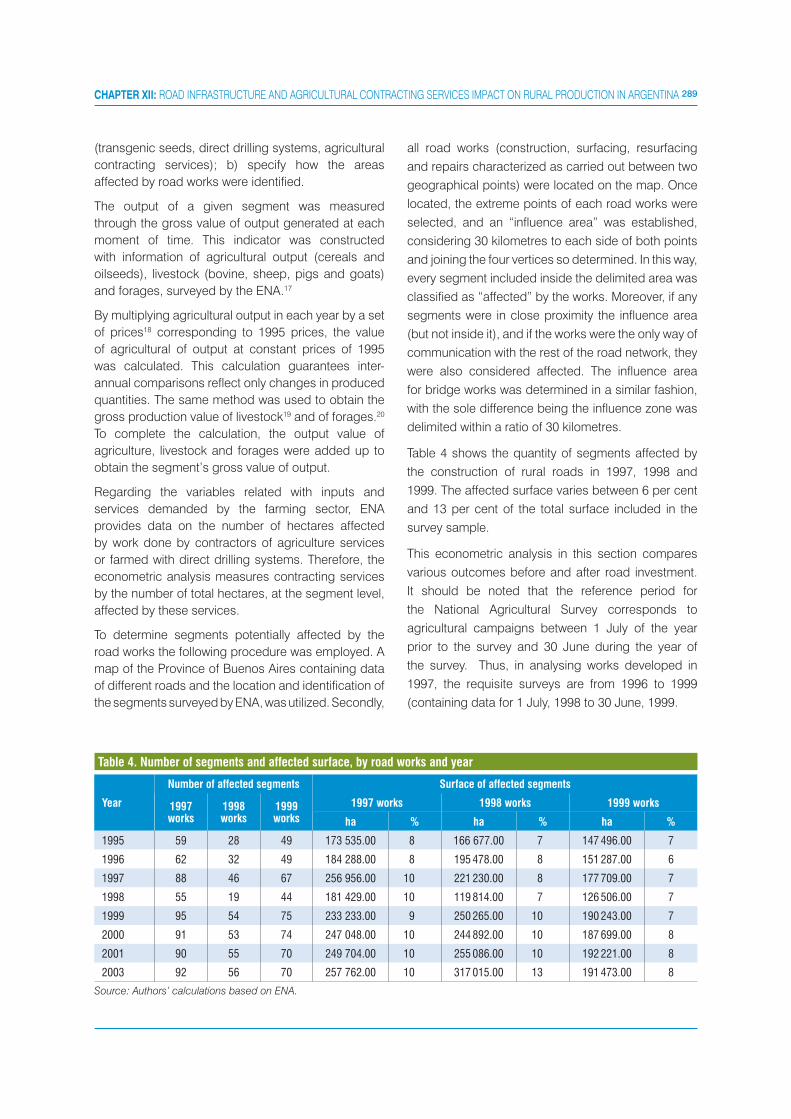
289CHAPTER XII: ROAD INFRASTRUCTURE AND AGRICULTURAL CONTRACTING SERVICES IMPACT ON RURAL PRODUCTION IN ARGENTINA
(transgenic seeds, direct drilling systems, agricultural
contracting services); b) specify how the areas
affected by road works were identified.
The output of a given segment was measured
through the gross value of output generated at each
moment of time. This indicator was constructed
with information of agricultural output (cereals and
oilseeds), livestock (bovine, sheep, pigs and goats)
and forages, surveyed by the ENA.17
By multiplying agricultural output in each year by a set
of prices18 corresponding to 1995 prices, the value
of agricultural of output at constant prices of 1995
was calculated. This calculation guarantees inter-
annual comparisons reflect only changes in produced
quantities. The same method was used to obtain the
gross production value of livestock19 and of forages.20
To complete the calculation, the output value of
agriculture, livestock and forages were added up to
obtain the segment’s gross value of output.
Regarding the variables related with inputs and
services demanded by the farming sector, ENA
provides data on the number of hectares affected
by work done by contractors of agriculture services
or farmed with direct drilling systems. Therefore, the
econometric analysis measures contracting services
by the number of total hectares, at the segment level,
affected by these services.
To determine segments potentially affected by the
road works the following procedure was employed. A
map of the Province of Buenos Aires containing data
of different roads and the location and identification of
the segments surveyed by ENA, was utilized. Secondly,
all road works (construction, surfacing, resurfacing
and repairs characterized as carried out between two
geographical points) were located on the map. Once
located, the extreme points of each road works were
selected, and an “influence area” was established,
considering 30 kilometres to each side of both points
and joining the four vertices so determined. In this way,
every segment included inside the delimited area was
classified as “affected” by the works. Moreover, if any
segments were in close proximity the influence area
(but not inside it), and if the works were the only way of
communication with the rest of the road network, they
were also considered affected. The influence area
for bridge works was determined in a similar fashion,
with the sole difference being the influence zone was
delimited within a ratio of 30 kilometres.
Table 4 shows the quantity of segments affected by
the construction of rural roads in 1997, 1998 and
1999. The affected surface varies between 6 per cent
and 13 per cent of the total surface included in the
survey sample.
This econometric analysis in this section compares
various outcomes before and after road investment.
It should be noted that the reference period for
the National Agricultural Survey corresponds to
agricultural campaigns between 1 July of the year
prior to the survey and 30 June during the year of
the survey. Thus, in analysing works developed in
1997, the requisite surveys are from 1996 to 1999
(containing data for 1 July, 1998 to 30 June, 1999.
Year
Number of affected segments Surface of affected segments
1997works
1998works
1999works
1997 works 1998 works 1999 works
ha % ha % ha %
1995 59 28 49 173 535.00 8 166 677.00 7 147 496.00 7
1996 62 32 49 184 288.00 8 195 478.00 8 151 287.00 6
1997 88 46 67 256 956.00 10 221 230.00 8 177 709.00 7
1998 55 19 44 181 429.00 10 119 814.00 7 126 506.00 7
1999 95 54 75 233 233.00 9 250 265.00 10 190 243.00 7
2000 91 53 74 247 048.00 10 244 892.00 10 187 699.00 8
2001 90 55 70 249 704.00 10 255 086.00 10 192 221.00 8
2003 92 56 70 257 762.00 10 317 015.00 13 191 473.00 8
Source: Authors’ calculations based on ENA.
Table 4. Number of segments and affected surface, by road works and year

290 SERVICES, TRADE & DEVELOPMENT
4. ROAD INFRASTRUCTURE, CONTRACTING SERVICES AND AGRICULTURAL OUTPUT
This section presents econometric analysis of the
impact of roads and agricultural contracting services,
as well as their interaction on agricultural productivity.
The hypothesis is based on the basic claim of this
chapter: that road infrastructure affect productivity
in agriculture. This claim is intuitive and quantitative
evidence is provided to support. Given such evidence,
some of the mechanisms behind this impact are
explored, particularly the belief that one of those
mechanisms is the facilitation of agricultural services.
To support this, consideration is directed toward
whether the use of those services affects agricultural
productivity and then analyse if this is in part due
to road construction. Finally, complementarities
between road construction and agricultural services
are explored to examine if the impacts on agricultural
productivity are greater in those farms having
benefitted by the presence of both road services and
agricultural services.
The analysis evaluates the impact of road works
carried out between 1997 and 1999, requiring a
comparison of data from the 1995 and 1996 ENA
surveys and from the 2001 and 2003 ENA surveys.
4.1. The effect of road on output
By conducting an econometric analysis of the
hypothesis a test of the impact of road constructions
on the agricultural output and productivity is possible.
The first regression model is equation 1:
Equation 1
Where the dependent variable is the logarithm of
the gross value of output (and the log of gross
value per hectare) for each segment i in the year t.
x’it is a vector of controls that includes the following
variables: lTotSurf, that denotes the logarithm of the
total area of the segment, measured in hectares;
AgrProp indicates the proportion of hectares used for
agriculture; and seven regional dummy variables that
represent regions composed by a group of contiguous
municipal jurisdictions that have a similar behaviour on
the main agricultural variables as well as the weather;
dom1 (eastern cattle zone), dom2 (north-eastern
cattle zone), dom3 (northern agricultural zone), dom4
(north-western mixed zone), dom5 (north-central
mixed zone), dom6 (south-central mixed zone), dom7
(southern agricultural zone). These dummy variables
also capture the productive specialization of each
zone (agricultural, cattle or mixed). The variable dom8
(south-western mixed zone) was used to compare
the results of the rest of the dummy variables. As
the south-western mixed zone region is one of
lowest productive performers it is expected that the
coefficients for all the other regional dummy variables
have a positive sign. When fixed-effects model are
estimated, these regional dummies are replaced by
segment dummies. The error term is denoted by �it.
The variable Roadi is a dummy variable equal to 1
when the segment i is affected by the construction or
improvement of rural roads in any of the years of the
period under study (1996 to 1999), and 0 otherwise.
The variable Pt equals 0 if the data corresponds to
the moment before the construction of roads, and 1
if it corresponds to surveys after the road services.
The coefficient of interest is ��, the inraction effect
(Roadi * Pt). In the table results that follow, this is
referred to as “effect” and measures the impact of
road investments on the dependent variable (in this
case, agricultural output) of the segments affected
by provincial road works carried out, in relation to
what may have happened if these segments had not
benefited by the policy.
This regression is applied on a panel of segments
for the years 1995, 1996, 2001 and 2003, taking into
account all road works undertaken during the period
1997 to 1999.
Obtained results for the impact of both components
of the agricultural investment (road investment and
contracting services) on agricultural output (measured
by gross value of output) are presented in table 5.
Table 5 presents model results. The first model
including all works (construction and improvement).
The second model only analyses the effect of
construction works (the variable road is activated
only when rural road construction and surfacing take
place). In the third model, this variable takes a value
of 1 when the works consists of re-surfacing or repairs
of a previously existent road. This differentiation
undertakes to capture with greater precision the effect
of the construction of new roads, that is, the direct
impact of a strong quality improvement in terms of
access to farm holdings.21

291CHAPTER XII: ROAD INFRASTRUCTURE AND AGRICULTURAL CONTRACTING SERVICES IMPACT ON RURAL PRODUCTION IN ARGENTINA
The results for the model considering all kinds of
works (first two columns in Table 5) show that the
coefficient of the variable effect has the expected
sign. Therefore, estimates suggest that road works
generally have a positive effect on agricultural output
of affected segments. According to this model the
benefited segments produced almost 45 per cent
more in expected value22 than segments not affected
by the works.
The controls variables such as segment size and
the proportion of hectares dedicated to agricultural
activities affect positively the gross value of output.
Also the coefficients of the regional variables
correspond to the productive conditions of each
Variable
All works Only construction works Only repair works
Gross value output (in log)
Productivity(in log)
Gross value output (in log)
Productivity(in log)
Gross value output (in log)
Productivity(in log)
Random effects Random effects Random effects
Road-0.417b
(0.19)-0.193b
(0.10)-0.550a
(0.21)-0.299a
(0.11)0,0966(0.29)
0.124(0.15)
P-0.136(0.11)
-0.0161(0.05)
-0.0733(0.10)
0.00207(0.04)
-0.0234(0.10)
0.0367(0.04)
Effect0.375b
(0.18)0.153c
(0.08)0.371c
(0.21)0.186b
(0.09)0.183(0.24)
0.0331(0.10)
ITotSurf 1.086a
(0.07)0.0588c
(0.03)1.086a
(0.07)0.0572c
(0.03)1.103a
(0.07)0.0677b
(0.03)
AgrProp 1.978a
(0.28)1.464a
(0.14)1.965a
(0.28)1.463a
(0.14)1.960a
(0.28)1.454a
(0.14)
dom1 1.863a
(0.43)1.457a
(0.23)1.824a
(0.42)1.441a
(0.22)1.702a
(0.43)1,362a
(0.23)
dom2 1.965a
(0.50)1.630a
(0.26)1.762a
(0.48)1.523a
(0.25)1.649a
(0.53)1.432a
(0.28)
dom3 1.919a
(0.53)1.722a
(0.28)1.929a
(0.53)1.728a
(0.28)1.845a
(0.53)1.680a
(0.28)
dom4 1.852a
(0.43)1.630a
(0.22)1.903a
(0.43)1.659a
(0.22)1.809a
(0.43)1.609a
(0.22)
dom5 1.591a
(0.43)1.417a
(0.23)1.604a
(0.43)1.423a
(0.23)1.575a
(0.44)1.408a
(0.23)
dom6 1.621a
(0.45)1.381a
(0.24)1.633a
(0.45)1.385a
(0.24)1.629a
(0.45)1.385a
(0.24)
dom7 1.649a
(0.46)1.387a
(0.24)1.658a
(0.45)1.393a
(0.24)1.562a
(0.46)1.338a
(0.24)
Constant 2.577a
(0.77)3.166a
(0.39)2.555a
(0.76)3.173a
(0.39)2.353a
(0.76)3.051a
(0.39)
Observations 756.0000 756.0000 756.0000 756.0000 756.0000 756.0000
Number of nsegmento
189.0000 189.0000 189.0000 189.0000 189.0000 189.0000
R-sq: within 0.1300 0.0900 0.1252 0.0900 0.1214 0.0800
between 0.6563 0.5125 0.6606 0.5202 0.6533 0.5098
overall 0.4852 0.3804 0.4874 0.3859 0.4814 0.3768
Source: Authors’ calculations.
Note: Standard errors in parentheses “a” p<0.01, “b” p<0.05, “c” p<0.1.
Table 5. Impact of rural road investment on output
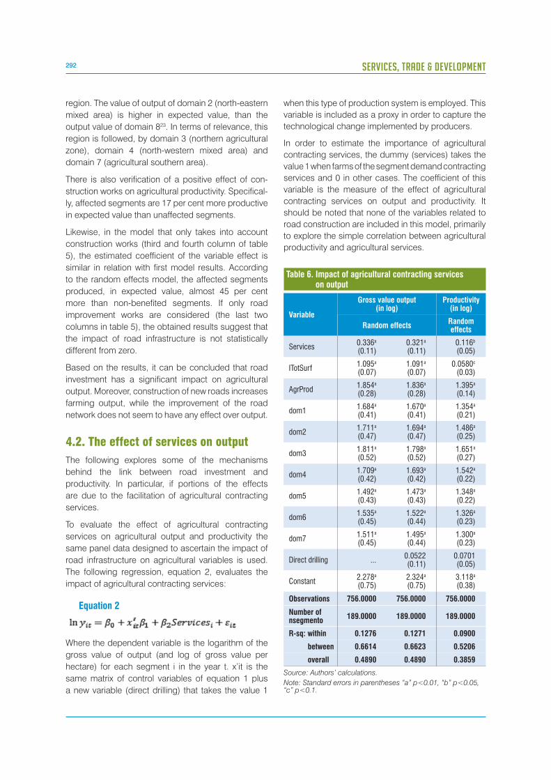
292 SERVICES, TRADE & DEVELOPMENT
region. The value of output of domain 2 (north-eastern
mixed area) is higher in expected value, than the
output value of domain 823. In terms of relevance, this
region is followed, by domain 3 (northern agricultural
zone), domain 4 (north-western mixed area) and
domain 7 (agricultural southern area).
There is also verification of a positive effect of con-
struction works on agricultural productivity. Specifical-
ly, affected segments are 17 per cent more productive
in expected value than unaffected segments.
Likewise, in the model that only takes into account
construction works (third and fourth column of table
5), the estimated coefficient of the variable effect is
similar in relation with first model results. According
to the random effects model, the affected segments
produced, in expected value, almost 45 per cent
more than non-benefited segments. If only road
improvement works are considered (the last two
columns in table 5), the obtained results suggest that
the impact of road infrastructure is not statistically
different from zero.
Based on the results, it can be concluded that road
investment has a significant impact on agricultural
output. Moreover, construction of new roads increases
farming output, while the improvement of the road
network does not seem to have any effect over output.
4.2. The effect of services on output
The following explores some of the mechanisms
behind the link between road investment and
productivity. In particular, if portions of the effects
are due to the facilitation of agricultural contracting
services.
To evaluate the effect of agricultural contracting
services on agricultural output and productivity the
same panel data designed to ascertain the impact of
road infrastructure on agricultural variables is used.
The following regression, equation 2, evaluates the
impact of agricultural contracting services:
Equation 2
Where the dependent variable is the logarithm of the
gross value of output (and log of gross value per
hectare) for each segment i in the year t. x’it is the
same matrix of control variables of equation 1 plus
a new variable (direct drilling) that takes the value 1
when this type of production system is employed. This
variable is included as a proxy in order to capture the
technological change implemented by producers.
In order to estimate the importance of agricultural
contracting services, the dummy (services) takes the
value 1 when farms of the segment demand contracting
services and 0 in other cases. The coefficient of this
variable is the measure of the effect of agricultural
contracting services on output and productivity. It
should be noted that none of the variables related to
road construction are included in this model, primarily
to explore the simple correlation between agricultural
productivity and agricultural services.
Variable
Gross value output(in log)
Productivity(in log)
Random effectsRandom effects
Services0.336a
(0.11)0.321a
(0.11)0.116b
(0.05)
ITotSurf1.095a
(0.07)1.091a
(0.07)0.0580c
(0.03)
AgrProd1.854a
(0.28)1.836a
(0.28)1.395a
(0.14)
dom11.684a
(0.41)1.670a
(0.41)1.354a
(0.21)
dom21.711a
(0.47)1.694a
(0.47)1.486a
(0.25)
dom31.811a
(0.52)1.798a
(0.52)1.651a
(0.27)
dom41.709a
(0.42)1.693a
(0.42)1.542a
(0.22)
dom51.492a
(0.43)1.473a
(0.43)1.348a
(0.22)
dom61.535a
(0.45)1.522a
(0.44)1.326a
(0.23)
dom71.511a
(0.45)1.495a
(0.44)1.300a
(0.23)
Direct drilling ...0.0522(0.11)
0.0701(0.05)
Constant2.278a
(0.75)2.324a
(0.75)3.118a
(0.38)
Observations 756.0000 756.0000 756.0000
Number of nsegmento
189.0000 189.0000 189.0000
R-sq: within 0.1276 0.1271 0.0900
between 0.6614 0.6623 0.5206
overall 0.4890 0.4890 0.3859
Source: Authors’ calculations.
Note: Standard errors in parentheses “a” p<0.01, “b” p<0.05, “c” p<0.1.
Table 6. Impact of agricultural contracting services on output
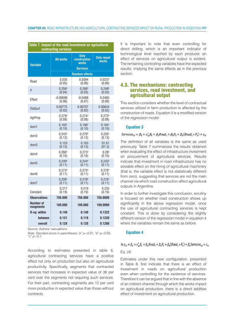
293CHAPTER XII: ROAD INFRASTRUCTURE AND AGRICULTURAL CONTRACTING SERVICES IMPACT ON RURAL PRODUCTION IN ARGENTINA
It is important to note that even controlling for
direct drilling, which is an important indicator of
technological level reached by each producer, an
effect of services on agricultural output is evident.
The remaining controlling variables have the expected
results, implying the same effects as in the previous
section.
4.3. The mechanisms: contracting services, road investment, and agricultural output
This section considers whether the level of contractual
services utilized in farm production is affected by the
construction of roads. Equation 3 is a modified version
of the regression model:
Equation 3
The definition of all variables is the same as used
previously. Table 7 summarizes the results obtained
when evaluating the effect of infrastructure investment
on procurement of agricultural services. Results
indicate that investment in road infrastructure has no
sizeable effect on the hiring of agricultural machinery
(that is, the variable effect is not statistically different
from zero), suggesting that services are not the main
channel via which road construction affect agricultural
outputs in Argentina.
In order to further investigate this conclusion, scrutiny
is focused on whether road construction shows up
significantly in the above regression model, once
the use of agricultural contracting services is kept
constant. This is done by considering the slightly
different version of the regression model in equation 4
where the variables remain the same as before.
Equation 4
Eq. (4)
Estimates under this new configuration, presented
in Table 8, first indicate that there is an effect of
investment in roads on agricultural production
even when controlling for the existence of services.
Therefore it can be argued that in line with the absence
of an indirect channel through which the works impact
on agricultural production, there is a direct additive
effect of investment on agricultural production.
Variable
All worksOnly
construction works
Only repair works
Services
Random effects
Road0.035(0.05)
0.0394(0.06)
0.0237(0.08)
P0.258a
(0.04)0.266b
(0.03)0.248b
(0.03)
Effect-0.00698
(0.06)-0.0488
(0.07)0.0485(0.08)
ITotSurf0.00775
(0.02)0.00707
(0.02)0.00644
(0.02)
AgrProp0.279a
(0.08)0.274a
(0.08)0.272b
(0.08)
dom10.183c
(0.10)0.196c
(0.10)0.184c
(0.10)
dom20.243b
(0.12)0.270b
(0.12)0.226c
(0.13)
dom30.153(0.13)
0.163(0.13)
01.61(01.3)
dom40.266b
(0.10)0.273a
(0.10)0.28a
(0.10)
dom50.240b
(0.11)0.244b
(0.11)0.243b
(0.11)
dom60.273b
(0.11)0.275b
(0.11)0.276b
(0.11)
dom70.209c
(0.11)0.218b
(0.11)0.216c
(0.11)
Constant0.217(0.19)
0.219(0.19)
0.235(0.19)
Observations 756.000 756.000 756.0000
Number of nsegmento
189.000 189.000 189.0000
R-sq: within 0.140 0.140 0.1322
between 0.121 0.119 0.1220
overall 0.128 0.128 0.1280
Source: Authors’ calculations.
Note: Standard errors in parentheses “a” p<0.01, “b” p<0.05, “c” p<0.1.
Table 7. Impact of the road investment on agricultural contracting services
According to estimates presented in table 6,
agricultural contracting services have a positive
effect not only on production but also on agricultural
productivity. Specifically, segments that contracted
services had increases in expected value of 38 per
cent over the segments not requiring such services.
For their part, contracting segments are 12 per cent
more productive in expected value than those without
contracts.

294 SERVICES, TRADE & DEVELOPMENT
It is also worth mentioning that in quantitative terms
the impact of works on rural roads is very similar in this
model to those presented above, which reinforced the
Variable
All worksOnly
construction works
Only repair works
Gross value output(in log)
Random effects
Road-0.436b
(0,18)-0.562a
(0,20)0,0676(0,28)
P-0.373b
(0,15)-0.276b
(0,14)-0.272b
(0,14)
Effect0,0618(0,34)
-0,252(0,41)
0,338(0,50)
Services0.308b
(0,12)0.308a
(0,12)0.352a
(0,12)
ITotSurf1.065a
(0,07)1.067a
(0,07)1.080a
(0,07)
AgrProp1.754a
(0,29)1.746a
(0,28)1.747a
(0,29)
doml1.729a
(0,41)1.696a
(0,40)1.550a
(0,42)
dom21.780a
(0,48)1.607a
(0,46)1.474a
(0,52)
dom31.816a
(0,52)1.828a
(0,51)1.714a
(0,52)
dom41.681a
(0,42)1.748a
(0,41)1.614a
(0,42)
dom51.432a
(0,42)1.478a
(0,42)1.384a
(0,43)
dom61.462a
(0,44)1.491a
(0,43)1.448a
(0,45)
dom71.496a
(0,44)1.519a
(0,44)1.399a
(0,45)
Direct drilling0,246(0,15)
0,199(0,16)
0.254c
(0,15)
Joint0,394(0,33)
0.769c
(0,42)-0,16
(0,51)
Constant2.786a
(0,76)2.712a
(0,74)2.560a
(0,76)
Observations 756.0000 756.0000 756.0000
Number of nsegmento
189.0000 189.0000 189.0000
R-sq: within 0.1400 0.1400 0.1300
between 0.6748 0.6826 0.6679
overall 0.5004 0.5048 0.4940
Source: Authors’ calculations.
Note: Standard errors in parentheses “a” p<0.01, “b” p<0.05, “c” p<0.1.
Table 8. Impact of both channels of investment on agricultural output
fact of the existence of a direct channel as a means
of transmission. In addition services are also being
relevant to explain the agricultural production in those
sectors affected by the works.
Specifically, the results founded for the model of
equation 4, show that segments affected by the
works produced in expected value by 49% rather than
unaffected.
Finally, note that the results from models that exploit
the differentiation by type of work (construction or
repair) are the same as above. That is, the construction
of new roads has a much higher impact than the road
repairs.
Having found evidence of the impact of infrastructure
and agricultural contracting services on agricultural
production in the province, which take place
independently, one additional issue to study is
whether there are complementary effects between the
two forms of production improvements. The purpose
of this analysis is to determine whether a joint effect
between the services and works that will generate
increases in agricultural production. To do this, we
add a dummy (JOINT) that takes the value 1 when
both SERVICES and EFFECT are equal to one. The
model is:
Equation 5
As we show in table 9, the results do not support
the existence of a joint effect, or complementarities,
between investment in roads and contracting services.
5. CONCLUSION
The main objective of this chapter aimed to quantify
the impact of construction and improvement of rural
roads in the Province of Buenos Aires on agricultural
productivity. Evidence supported that road
construction has a positive, large, and statistically
significant impact on agricultural outcomes in
Argentina. Specifically, the affected segments are 17
per cent more productive in expected value than the
unaffected segments.
The analysis attempted to distinguish some of
the mechanisms through which this relationship
functions. In particular, focus was directed on
whether the provision of road infrastructure affected
agricultural productivity by way of facilitating of

295CHAPTER XII: ROAD INFRASTRUCTURE AND AGRICULTURAL CONTRACTING SERVICES IMPACT ON RURAL PRODUCTION IN ARGENTINA
agricultural services, including access to credit,
capital, and technology. Evidence illustrated that
this is not the case and that the type of agricultural
services just described had a positive impact on
agriculture (those who hire agricultural services have
productivity 12 per cent greater than those who do
not hire agricultural services); the availability of those
services is not strongly affected by the construction
of roads. This is somewhat surprising, because, in
principle, the improvement and construction of roads
should facilitate access of machines and should
facilitate interaction between services providers and
farm producers. However, evidence to support this
argument was unable to be generated. It seems
Variable
All works Only construction works Only repair works
Gross value output (in log)
Productivity(in log)
Gross value output (in log)
Productivity(in log)
Gross value output (in log)
Productivity(in log)
Random effects Random effects Random effects
Road-0.432b
(0.18)-0.442b
(0.18)-0.567a
(0.20)-0.567a
(0.20)0.0876(0.28)
0.0705(0.28)
P-0.232b
(0.11)-0.400a
(0.15)-0.174c
(0.10)-0.321b
(0.14)-0.114(0.10)
-0.271b
(0.14)
Effect0.377b
(0.18)0.399b
(0.18)0.389c
(0.21)0.391c
(0.21)0.166(0.24)
0.199(0.24)
Services0.376a
(0.11)0.353a
(0.11)0.380a
(0.11)0.359a
(0.11)0.366a
(0.11)0.345a
(0.11)
lTotSurf1.080a
(0.07)1.062a
(0.07)1.079a
(0.07)1.063a
(0.07)1.097a
(0.07)1.080a
(0.07)
AgrProp1.853a
(0.28)1.756a
(0.29)1.841a
(0.28)1.749a
(0.29)1.842a
(0.28)1.747a
(0.29)
doml1.788a
(0.42)1.708a
(0.42)1.743a
(0.41)1.670a
(0.41)1.628a
(0.42)1.552a
(0.42)
dom21.867a
(0.49)1.772a
(0.49)1.652a
(0.47)1.565a
(0.47)1.558a
(0.52)1.469a
(0.52)
dom31.865a
(0.53)1.791a
(0.52)1.871a
(0.52)1.803a
(0.52)1.789a
(0.53)1.719a
(0.52)
dom41.751a
(0.42)1.656a
(0.42)1.798a
(0.42)1.712a
(0.42)1.706a
(0.42)1.616a
(0.42)
dom51.496a
(0.43)1.395a
(0.43)1.506a
(0.43)1.414a
(0.42)1.481a
(0.43)1.386a
(0.43)
dom61.521a
(0.45)1.436a
(0.44)1.530a
(0.44)1.453a
(0.44)1.530a
(0.45)1.450a
(0.44)
dom71.574a
(0.45)1.483a
(0.44)1.578a
(0.45)1.494a
(0.44)1.486a
(0.45)1.399a
(0.45)
Direct drilling ...0.268c
(0.15)...
0.248(0.15)
...0.256c
(0.15)
Constant2.536a
(0.75)2.806a
(0.76)2.513a
(0.75)2.757a
(0.75)2.306a
(0.75)2.562a
(0.76)
Observations 756.0000 756.0000 756.0000 756.0000 756.0000 756.0000
Number of nsegmento
189.0000 189.0000 189.0000 189.0000 189.0000 189.0000
R-sq: within 0.1400 0.1400 0.1300 0.13000 0.13000 0.1295
between 0.6660 0.6700 0.6700 0.6753 0.6626 0.6677
overall 0.4948 0.4980 0.4900 0.5000 0.4905 0.4938
Source: Authors’ calculations.
Note: Standard errors in parentheses “a” p<0.01, “b” p<0.05, “c” p<0.1.
Table 9. Impact of rural road investment and contracting services on output

296 SERVICES, TRADE & DEVELOPMENT
that, in Argentina, roads and agricultural contractual
services work well in terms of boosting agricultural
production, but work independently. This result
suggests that infrastructure functions much along the
direct lines highlighted in other papers, namely by way
of reductions in transport costs, reduced travel times
and lower freight rates.
Moreover, even though both variables have a
statistically significant impact on agricultural
production and productivity, the evidence indicates
that road construction increases agricultural
productivity more than it fosters the procurement of
agricultural services. This is observed in the case
where both variables are analysed together (table 9)
as well as when they are included separately (tables 5
and 8).
Thus, arguably, policies aimed at improving agricul-
tural production and the income (or well-being) in
rural areas could be successful by targeting road
infrastructure and the provision of agricultural services.
Investment in road construction and improvement of
roads is thus a natural policy-option, as is facilitating
access to agricultural services by smaller producers,
either by means of tax policies or strong and equitable
rules of law.
APPENDIX: ANALYSIS DOMAINS
In the case of the Province of Buenos Aires the
analysis domains for which the Agricultural National
Survey provides representative estimations are the
following:
Eastern cattle zone (1): Ayacucho, Castelli,
Chascomús, Dolores, General Belgrano, General
Guido, General Madariaga, General Lavalle, La
Costa, Las Flores, Magdalena, Maipú, Mar Chiquita,
Pila, Pinamar, Rauch, Tordillo y Villa Gesell.
North-eastern cattle zone (2): Berisso, Brandsen,
Campana, Cañuelas, Escobar, Exaltación de la Cruz,
General Las Heras, General Paz, General Rodriguez,
La Plata, Lobos, Luján, Marcos Paz, Mercedes,
Monte, Navarro, Pilar, San Andrés de Giles, San
Vicente, Suipacha y Zárate.
Northern agricultural zone (3): Arrecifes, Baradero,
Capitán Sarmiento, Carmen de Areco, Colón,
Chacabuco, General Arenales, Junín, Pergamino,
Ramallo, Rojas, Salto, San Antonio de Areco, San
Nicolás y San Pedro.
North-western mixed zone (4): Adolfo Alsina, Carlos
Tejedor, Florentino Ameghino, General Pinto, General
Villegas, Guaminí, Leandro N. Alem, Lincoln, Pehuajó,
Pellegrini, Rivadavia, Salliqueló, Trenque Lauquén y
Tres Lomas.
North central mixed zone (5): Alberti, Bolívar, Bragado,
Carlos Casares, Chivilcoy, Daireaux, General Alvear,
General Viamonte, Hipólito Yrigoyen, Nueve de Julio,
Roque Perez, Saladillo, Tapalqué y Venticinco de
Mayo.
South central mixed zone (6): Azul, Benito Juárez,
General Lamadrid, Laprida, Olavarría y Tandil.
Southern agricultural zone (7): Adolfo Gonzales
Chaves, Bahía Blanca, Balcarce, Coronel Rosales,
Coronel Dorrego, Coronel Pringles, Coronel Suárez,
General Alvarado, General Pueyrredón, Lobería,
Monte Hermoso, Necochea, Saavedra, San Cayetano,
Tornquist y Tres Arroyos.
South-western mixed zone (8): Patagones, Puán y
Villarino.

297CHAPTER XII: ROAD INFRASTRUCTURE AND AGRICULTURAL CONTRACTING SERVICES IMPACT ON RURAL PRODUCTION IN ARGENTINA
NOTES1 For example Bisang, R. (2008)2 Production technology is characterized mainly by the absence of tillage and the presence of a plant residue cover on
the ground. The same can be produced with minimal impact on decreasing soil erosion risks. This technology allows for production without degrading soil, and in many cases improving the physical, chemical and biological characteristics of it.
3 Planting two species in the same field in the same year; for example, wheat is sown between May and October and soybeans between November and April.
4 Agricultural services in this work include what the UN Central Product Classification labels services incidental to agriculture: these ``are services rendered on a fee or contract basis, mostly performed at the site where the agricultural production is done, e.g. services providing agricultural machinery with drivers and crew; harvesting and related services; services of farm labour contractors.’’
5 It is worth noting that the term infrastructure investment includes not only new works, but also repairs, maintenance and widening of existing ones.
6 They obtain product elasticity with respect to infrastructure investment of 0.39.7 Munell (1992), Tatom (1993) and Gramlich (1994), among others, had criticized Aschaeur’s estimates, due to endogeneity
problems derived of the reciprocal effects between the development of infrastructure and the growth of the economy’s aggregate product. While investment in infrastructure can contribute to the increment of an economy’s output, economic growth provokes a growing demand of transport and infrastructure services that, through a rise in the rates of return, leads to an expansion of capital stock.
8 The data used in the work is based in surveys of rural producers and regional and local governments. 9 Further work done by the same agency in 2004 confirmed these findings and established that the impacts of road
improvements are straightforward on transportation conditions and access to basic services, while they are smaller on productive, employment levels and reducing poverty.
10 The term construction includes roads or accesses that join two or more geographic points in the province, and other road works such as bridges or pluvial drainages.
11 Surfacing and re-surfacing works consist of the asphalt of roads, highways, streets, and avenues. 12 Repairs include the improvement of roads, asphalted surfaces, among other types of road rehabilitation. 13 This term will be employed to make reference to those works that are the object of study. However, it should be clear that this
category does not only include the works carried out in rural areas, but also works undertaken in boundary zones between urban and rural areas.
14 The definition of the geographic space included by each domain can be consulted in the appendix.15 Sample selection is based on the stratification of the reference units, according to the use of the land. Thus, the ENA
reports representative estimations for each zone or analysis domain. Each domain is composed by a group of contiguous municipal jurisdictions that have a similar behaviour regarding the principal variables (crops and livestock). The analysis domains corresponding to the Province of Buenos Aires are detailed in the appendix.
16 For example, in the hypothetical case that a agricultural holding is subdivided between one year and the following, maintaining constant its global output, the segments’ production would not show any activity changes, while the analysis of the EAPs could exhibit modifications, depending on which holding is selected as reference point.
17 The survey collects information in tons of each crop produced in all the agricultural campaigns. 18 The prices of the different crops were obtained from the Secretaría de Agricultura, Ganadería, Pesca y Alimentación and
from the Bolsa de Cereales de Buenos Aires. 19 In the particular case of bovine and sheep, the ENA presents decomposition by age and gender, allowing a precise
valuation of output. However, this decomposition is not available for pigs and goats. Thus, the value of output for these two species was estimated by an average price for 1995.
20 The source of information used to valuate output was the publication Márgenes Agropecuarios.21 The results of the regressions for the three models indicate that the estimated coefficients are jointly significant at a 1 per
cent significance level. Moreover, in all the models the null hypothesis of absence of fixed effects is rejected at the usual significance levels, suggesting that non-observable heterogeneity is a statistical relevant factor. The results of the Hausman test confirm the validity of the random effects estimates. Thus, both fixed and random effects estimates are consistent. Lastly, null of absence of random effects is rejected in the Breusch-Pagan test.
22 T his value (0.45) comes from the correct interpretation of the regression coefficient in a log-in (0,375), which must be transformed as follows: ex-1 (e0,375-1 =0.45)
23 This result is logical since the area corresponding to the region known as “domain 2” is one that has the best land for agricultural production in the country, while in contrast the region used for the comparison base is the one with lower agricultural skills. This in turn is reflected in land value for domain 2, the average price per hectare in 2002 was $1,100 against $487 that land in domain 8 fetched.

CHILD LABOUR AND SERVICES FDI:EVIDENCE FROM VIET NAM
The objective of this chapter is to examine the impact of services
foreign direct investment (FDI) on child labour in Viet Nam. Starting
with the reforms in the late 1980s, Viet Nam experienced an economic
boom which led to an important decline in poverty and child labour.
Over the past decade, Viet Nam has witnessed a drastic acceleration of
the structural transition away from agriculture and into manufacturing
and services. This chapter merges repeated household surveys and
enterprise surveys to explore and gauge the contribution of foreign
firms in services and manufacturing in relation to the decline in child
labour. It was found that while higher demand for labour by domestic
firms tends to increase child labour, the entry of FDI in both the
manufacturing and services sectors have contributed to reduce the
labour supply of children. A foreign firm’s marginal impact of entry in
the service sector on child labour supply is larger than the marginal
impact of foreign entry in the manufacturing sector. However, the
overall impact of FDI services on child labour has so far been smaller
than the impact of manufacturing FDI. This is partly due to the fact that
FDI in services has been much smaller than in manufacturing, but the
growing importance of the former suggests that the impact of FDI on
the reduction of child labour supply is becoming larger.

300 SERVICES, TRADE & DEVELOPMENT
1. INTRODUCTION
Critics of globalization argue that openness often
comes with the exploitation of workers in developing
countries where worker protection is weaker. As mul-
tinational firms relocate to markets with less robust
labour standards, governments may be tempted to
diminish their labour standards through legislation
in order to attract more FDI. This chapter considers
whether FDI may create incentive for children to en-
ter or increase their participation in the workplace.
Well publicized cases, in the 1990s, of children being
exploited by multinational companies in developing
countries fuelled this view.1 There is however evidence
that FDI firms tend to pay higher wages than domestic
firms (Lipsey et al., 2007). FDI firms tend also to pro-
duce more complex goods, usually demanding more
specialized, adult labour. Finally, foreign firms serving
international markets are more exposed to media than
domestic firms. As such foreign firm, whose bottom
line may be adversely affected by bad publicity steer
away from hiring children.
Services trade liberalization can generate impor-
tant employment and efficiency gains in developing
countries, and thus represent an important driver of
economic growth. Economic growth, in turn, is a ma-
jor determinant of poverty reduction. However, many
observers argue that the poor are less likely to ben-
efit from such openness as are the non-poor. Such
distributional outcomes might hamper the poverty
reducing impacts of liberalization (Nicita, 2006). The
effects of integration into the world economy on pov-
erty reduction depend crucially on the extent to which
the poor benefit from new employment opportunities
as a result of FDI and increased export activities. If
the poor are marginalized, either because they live
far from the most dynamic areas or they lack relevant
skills, then the overall effects of trade liberalization on
the poor can be small. There can even be negative ef-
fects in the short to medium term if liberalization puts
pressure on the poor households’ production system,
introducing sudden variations on both prices and
availability of inputs.
This chapter analyses the effects of a particular out-
come of services trade liberalization, that is, FDI in
services, on a crucial indicator of households’ welfare
– work and education choices of children. Viet Nam
is the target country of this analysis as it has an ex-
tremely rapid transition from a very closed to a very
open economy, through industrial policies strongly
focussed on the attraction of FDI. The activities of for-
eign companies are a primary component of services
trade liberalization. They alone account for approxi-
mately 50 per cent of all transactions falling under the
GATS (WTO, International Trade Statistics, Geneva:
WTO, 2005 p. 8.). Labour supply and education in-
vestments of children and teenagers are a relevant
indicator of households’ living standards and expo-
sure to external shocks, reflecting different adjustment
capacities of poor and non-poor households. Study-
ing the effects of FDI on the labour supply of children
can also help with understanding the dynamic effects
of openness, as long term impact on growth clearly
depends on how human capital investments adjust.
The empirical work relies on three waves of household
data surveys and enterprise data surveys data for the
period 2002 to 2006. The two datasets are matched
at the level of the 64 Vietnamese provinces. House-
hold data surveys are nationally representative and
detailed. Enterprise data surveys provide accurate
information on the distribution and composition of
wage earning opportunities throughout Viet Nam, as
they cover all the business entities keeping business
accounts and registered under Vietnamese Law. The
correlation between changes in the number of foreign
owned firms in local labour markets and child em-
ployment are identified due primarily to the large het-
erogeneity in exposure to foreign investment across
provinces and over time.
These data revealed that higher rates of FDI entries
in the provinces are associated with a reduction in
children’s labour supply (10 to 14 year olds). The
composition of FDI investments is also important. The
marginal effect of entry by foreign firms in the services
sector is larger than in the manufacturing sector,
suggesting that the move toward more services FDI will
be associated with a stronger reduction in child labour
supply. However, to date, FDI on manufacturing has
had a greater effect than on services, due to higher
levels of FDI on mining and on low-skill manufacturing
(textile and food processing) in provinces with higher
rates of child labour.
While it is difficult to conclude that higher FDI’s have a
strong causal effect on child labour, the findings sup-
port the view that FDI are on average “high quality”
employers in rapidly industrializing environments. This
finding is important as child labour seems to increase
in those provinces that are industrializing at a faster
rate. In this second phase of the Vietnamese transi-
tion, a rapid reallocation of family labour across activi-
301CHAPTER XIII: CHILD LABOUR AND SERVICES FDI: EVIDENCE FROM VIET NAM
ties was observed, with family members substituting
household production for labour supply outside the
household. Given the still modest absorption capaci-
ties of the new firms and the consequent rise in un-
employment, this substitution amounts to trading-off
a low-earning, relatively secure source of income –
household farming – with a higher earning, but more
uncertain, income source – wage labour. Even if all
family members leaving agriculture manage to be
hired in new firms, more pressure will be placed on
children to take up the slack from the resulting scarcity
of the labour available for household production. This
household adjustment in the labour supply is more
pronounced among poor families, who lack resources
to hire outside labour for household production.
On the other hand, as previously pointed out, when
new economic opportunities become available
through FDI, child labour supply seems to decline.
This could be explained by a relative decline in
the relative wage offered to children in provinces
where FDI is prominent (due perhaps to a stronger
reluctance by foreign firms to hire child labour).
Moreover, the income effect associated with higher
wages paid to adults allows them move beyond their
minimum income needs, (such as in Basu, K. and H.
Zarghamee, 2009) thus reducing the reliance on child
labour income.
Another finding, uncovered by the analysis, is that the
greater number foreign firms into services increases
school enrolment rates of 6 to 19 year olds. This
increase in school enrolment is linked to the higher
skill production outputs of FDI firms. As FDI in the
services sector tends to require more educated labour,
the current liberalization process and the consequent
increase in the weight of FDI in services could have
an impact on expected returns to higher education
discouraging education drop-outs in the future.2
The remainder of the chapter is organized along
4 further sections. The next section – section 2 –
reviews the literature on FDI, within household labour
supply and child labour. Section 3 presents the firm-
level and household data used in the chapter, and
discusses the large heterogeneities in education and
working choices of children across income groups
and Vietnamese provinces. Section 4 examines the
methodology and the empirical results. Section 5
concludes.
2. FDI AND CHILD LABOUR: A REVIEW OF THE EVIDENCE
While the enforcement of child labour laws may not
be as strong as in other parts of the world, Viet Nam
experienced a rapid decline in child labour in the
1990s (Edmonds and Turk, 2002). This decrease in
labour market participation of the young has been
mainly attributed to Viet Nam’s rapid economic growth
(which is also consistent with the dominant view
among economists). Indeed, there is now consensus
in economic literature that the main cause of child
labour is poverty (see Edmonds, 2008 or Basu, Das
and Dutta, 2009).
In Becker’s view of time allocation within households,
putting children to work is seen as a rational
household decision (Becker, 1981), as poverty and
lack of opportunities push children into the labour
force. This view makes economists very sceptical of
regulations that impose the elimination of child labour.
According to economic historians (see Nardinelli
1990) the elimination of child labour in Europe and
in the United States of America in the nineteenth
and early twentieth century had as much to do with
child labour legislation as technological progress and
growth making it possible for households not to send
their children to work. Thus, when considering policies
aimed at eliminating child labour it is necessary to
focus on policies that eliminate the dependency of
poor households on children’s income – the reason
why children are working. This requires policies
that would lead to an increase in income for poor
households. Conditional cash transfers, such as
Progresa in Mexico, seem to be an effective tool.3
But policies simply forbidding the utilization of child
labour such as consumer boycotts or trade sanctions
may be counterproductive. Indeed, they may result
in a displacement of child labour from companies
hit by boycotts or sanctions to other firms, where
employment can actually be more dangerous. They
can also increase child labour in other firms, as lower
wages for child labour associated with these polices
(as demand declines) may actually result in a stronger
need for sending children to the workplace. In other
words, lower wages for child labour may imply that
more children are sent to work in order to meet the
minimum income needs of the family (see Basu and
Zarghamee, 2009).4
The rapid increase in FDI experienced by Viet Nam
in the 1990s is in principle an engine of growth which
302 SERVICES, TRADE & DEVELOPMENT
contributed in improving poor households’ income
(see UNCTAD, 2008). This income effect could also
facilitate in reducing child labour. Moreover, consumer
activism and government legislation in OECD coun-
tries has left multinational firms reluctant of hiring
child labour.5 This reluctance may also lead to further
reducing child labour.
However, as previously pointed out, these types of
decisions may backfire and lead to more, not less
child labour, as a reduction in child labour demand
may actually lead to an increase in child labour in
equilibrium in order to match the income needs of
poor families. Therefore, FDI will generally lead to a
reduction in child labour as it progresses economic
opportunities for local workers. Paradoxically FDI
may also inadvertently lead to an increase in child
labour if accompanied by measures that prevent
child employment by multinationals, as child workers
reallocate into other sectors or are forced to enter the
labour market.
A second channel by which FDI might affect child
labour is the induced change in employment choices
of the adults. In fact, for a given level of household
income, children of the self-employed have higher
labour market participation rates than children of the
salaried workers (see Parick and Sadoulet, 2006). In
developing countries, owners of micro-enterprises rely
heavily on labour inputs from their families, as family
workers are not only cheaper but also more flexible.
If FDI increases mobility from self-employment to
salaried work, a negative relationship between FDI
and child labour could be reinforced. However, if adult
workers hired by multinationals are replaced at their
home enterprise by their spouses and children, FDI
may again inadvertently increase child labour through
this channel.
As child labour tends to come primarily from poor
and relatively uneducated families, it is important to
consider the effect of FDI on wage inequality in host
countries. Foreign direct investment and outsourcing
by multinational firms can raise relative demand for
skilled labour, increasing wage inequality. Feenstra
and Hanson (1997) found that capital transfer by
American firms accounted for the bulk of the increase
in the skilled labour share of the total wage bill that
occurred in Mexico in the late 1980s. If the incomes
of the wealthy and skilled increases while the incomes
of the poor remains stagnant, rising prices in the
consumption basket might affect the purchasing
power of those at higher risk of poverty, potentially
increasing child labour.6 On the other hand, even
though wage inequality increases an increase in the
absolute wage of unskilled workers may be observed
suggesting that FDI leads to a decline in child labour
through the impact of FDI on absolute wages. In order
to check whether this is an important mechanism in
the empirical analysis results with and without controls
for wages are reported.
An important consideration of the survey of existing
literature is that whether rapid increase in FDI leads
to a reduction or an increase in child labour is an
empirical question. Cross country evidence provided
by Newmayer and Soysa (2005) in a sample of 145
countries suggests that FDI categorically leads to a
reduction in child labour. However, there could be quite
significant (observed and unobserved) heterogeneity
in the relationship between FDI and child labour. For
example, FDI from non-OECD countries may have
a different impact than FDI from OECD countries,
simply because the latter is more likely to be subject
to consumer activism, or because host countries vary
in their enforcement of child labour laws.
Moreover, Newmayer and Soysa (2005) do not ad-
dress the endogeneity problem, which could poten-
tially lead to significant biases. For example, FDI may
be attracted to countries with higher skill endowments
(see Blonigen et al, 2007), and countries with high-
er skill endowments tend to be richer and have less
child labour for reasons that have little to do with FDI.
Davies and Voy (2009) address this issue in a cross-
country setup and show that the negative relationship
between FDI and child labour disappears once they
instrument and control for GDP per capita, suggesting
that the main channel through which FDI affects child
labour is through its impact on GDP per capita. This
confirms the micro-economic view that what affects
the rates of child labour is level of household income.
It also raises the question of whether the decision of
multinationals not to employ children has any impact
on the child labour employment by other firms. Their
results suggest that the decision would only lead to a
reallocation effect from foreign to domestic firms (in
the non tradable sector). But their aggregate cross
country approach does not allow them to disentangle
the mechanism. In order to deepen understanding of
the complex links between FDI and child labour, a dif-
ferent identification strategy based on merged micro-
data for enterprises and families over multiple years
is put forth. The possible simultaneity between FDI in-
flows and labour supply choices is significantly mini-

303CHAPTER XIII: CHILD LABOUR AND SERVICES FDI: EVIDENCE FROM VIET NAM
mized given that a large number of location and family
characteristics, such as the prevalence of agricultural
activities in the regions, the household income and
education, are controlled for. By using fixed effects
at the level of provinces, the relationship between
changes in labour supply of children and changes in
FDI are focussed on. Thus, time-invariant, province-
level unobservable characteristics are controlled for
that might affect both the extent of child-labour and
the attractiveness of the place where the household
is located. Regarding reverse causality concerns, it
should be noted that the concerned time period is
characterized by large increases in FDI inflows, (as a
consequence of, amongst other things, drastic liber-
alization of FDI entry in the country) and large redis-
tribution of the foreign investments within the country
(through industrial park and special economic zone
policies). In this context, it is unlikely that changes in
household behaviour are a significant determinant of
location choices by foreign firms.
3. FDI, STRUCTURAL CHANGES AND LABOUR SUPPLY IN VIET NAM: DESCRIPTIVE EVIDENCE
This section provides descriptive information on the
industrialization process and labour market choices of
families in Viet Nam from 2000 to 2006.
Data
Two complementary sources of data are used. The first
source is the annual enterprise survey of the General
Statistical Office of Viet Nam, of all establishments.
The enterprise data are collected annually for all
sectors and industries registered under Vietnamese
law. Accordingly, the coverage of the survey includes
almost all enterprises in 29 sectors and industries
in three industrial groups (4 sectors in mining and
quarrying, 23 in manufacturing, and 2 in electricity,
gas and water supply), providing a wide range of
information on the property structure of enterprises,
output, capital stock, investment, employment,
location, wages, sales, and so forth. Three waves of
the surveys that collect information on enterprises’
ownership, productive factors (labour, capital, assets)
and business results in 2002, 2004 and 2006 are
used. Information on the number, ownership and
characteristics of enterprises which started their
activity between 2001 and 2006 is derived from the
data. This information is used to construct the main
explanatory variables in the models.
The second source of data consists of repeated
household and community surveys for 2002, 2004
and 2006, called the Vietnam Household Living
Standard Surveys (VHLSS). The data are represen-
tative at the national and provincial level, including
detailed community level questionnaires only for the
communes in rural areas. The household survey con-
tains information on the number of household mem-
bers, age, income, employment, school attendance,
level of education of the household head, overall
household expenditure and income, as well as the
locality where the household lives. The number of
sampled households in VHLSS 2002, 2004 and 2006
was 29,533, 9,188, and 9,189, respectively. Around
4,000 thousand families are observed longitudinally
for two waves, while a more limited sample of around
1,900 households is observed over all the three waves.
The situation of foreign and domestic enterprises
The Doi Moi (renovation) policies in Viet Nam brought
about remarkable results in terms of economic growth
and poverty reduction. Over two decades (1986-
2006), GDP growth hovers around 7.5 per cent per
year on average and export growth nearly 20 per cent.
The strong growth posted by the Vietnamese economy
has sent poverty rates tumbling since the 1990s. The
poverty headcount has been slashed from 58 per cent
in 1993 to 16 per cent in 2006. The number of people
below the food poverty line also declined from 25 per
cent to 7 per cent during this period (Nguyen, 2009).
There is extensive literature describing the Vietnamese
transition in the 1990s. This section supplements the
literature by describing the rapid evolution of Viet Nam
in the first years of 2000. This second phase of the
Vietnamese transition was marked by a pronounced
industrialization, in part sustained by a new surge of
FDI after the trough between 1997 and 1999. The re-
gion that experienced the greatest decrease in child
labour was the Red River Delta – the economic centre
of northern Viet Nam. As noted by Mai (2004), most
of the FDI in the River Delta region was channelled
toward services.7
Although manufacturing has traditionally attracted
an important share of FDI, recent reforms associated
with Viet Nam’s WTO accession have significantly
increased the share of services FDI. This started
with accession negotiations in 1995 and culminated
304 SERVICES, TRADE & DEVELOPMENT
with the adoption of the Law on Investment in 2005.
Hurdles for services FDI are still relatively important
(most of the 14 sectors subject to conditional approval
are services sectors: see Law on Investment 59-
2005-QH11). However, according to Doanh (2002),
services FDI (hotels, restaurants, transportation and
communication and other service industries such as
insurance) account for 22 per cent of the total projects
and 40 per cent of the total committed capital in 2002.
A large share of FDI comes from non-OECD sources,
implying that legal restrictions in source countries
regarding employment in the host country, common
for OECD countries, may not be such a binding
constraint in Viet Nam.
The most compelling indicator of the structural change
in Viet Nam is the decreasing share of employment in
agriculture. In 2006, 73 per cent of the total population
of 83 million people lived in rural areas (UNFPA, 2008).
The number of rural households in Viet Nam was 9.74
million, a decrease of 950,000 households (8.9 per
cent) compared with 2001. This reduction results from
continuous population growth, (1.21 per cent in 2006)
associated with low productivity growth of agriculture
and progressive conversion of land for the develop-
ment of industrial zones. According to MONRE figures,
162 industrial zones were approved by the Govern-
ment of Viet Nam in 2004, of which 68 were already
in operation and 44 were in the process of establish-
ment (Viet Hung, 2007). A high proportion of industrial
zone land was converted from agricultural use (76 per
cent) and large numbers of rural households were ef-
fected (408,698 individuals according to MONRE fig-
ures quoted in Ngo Viet Hung, 2007). While many rural
households are diversifying their income sources by
engaging in wage earning, they still keep their farmland
as a stable income source (Thinh, 2009).
The maps in figure 1 show the evolution of the share
of FDI employees over total enterprise’s employees
in 2002, 2004 and 2006. As can be seen, the number
of provinces with no FDI employment (in white)
diminishes during this period, suggesting that FDI
investments are spreading outside the most dynamic
areas of the Red River Delta (the Hanoi region in
the north) and of the Mekong Delta and south-east
regions (where Ho Chi Minh city is located). The
tendency for new investments has been to locate
more in neighbouring areas due to increasing costs
of operating in the two major cities. It is interesting
to observe that Hai Duong Province, in the Red
River Delta most affected by agricultural land loss
to the development of industrial parks, also had the
largest increases in FDI employment. In Hai Duong,
the proportion of employees in FDI firms was 7.6 per
cent in the enterprise survey of 2002, 16.1 per cent in
the survey of 2004, and 28.1 per cent in the survey of
2006 (Enterprise Survey data, 2002/2004/2006).
Table 1 provides descriptive statistics on the firms
surveyed by the three enterprise surveys. For each
year, the first column refers to province-level averages
for each and every formal enterprise, while the
second column refers to average values for those
enterprises located in the two major cities of Hanoi
and Ho Chi Minh. A relatively conservative definition
of the services sector was adopted that does not
include those enterprises whose primary activity is
construction, wholesale and retail sales.8
As expected, the overall number of firms and the number
of FDI firms is much larger in the two cities. However,
the increase over time in industrial presence is very
similar in both the full and city sample, suggesting no
increase in concentration around the main metropolis.
The number of FDI firms in the services sector is
very modest, even if the FDI presence in this sector
increased more rapidly than average. The situation
is similar if only foreign firms entering the market in
the two years preceding the survey are considered.
The entry of FDI enterprises in the service sector is
proportionally greater between 2004 and 2006, with
an approximate four-fold increase. Foreign firms in the
service sectors are smaller, (lower turnover and less
employees) and tend to pay higher wages.9
The introduction of the New Law on Enterprises in
1999 and the introduction of the first Competition Law
of Viet Nam in 2005 gave a drastic acceleration to the
privatization process (equitisation). There is a trend
toward privatization of all small and medium State
Owned Enterprises, with the largest and strategic
firms remaining 100 per cent public. WTO accession
in 2007 further accelerated the equitisation process,
even if most sources agree that the objective of full
public disengagement by 2010 will not be met.10
The average enterprise size (indicated by turnover and
employees per firm) based outside large cities in 2002
was greater. Recently, the trend is toward a marked
decrease in firm size, in particular outside large cities.
This trend may reflect both the elevated dynamism
of the private sector under new regulations and the
increased level of formalization of small businesses
(increasingly captured in enterprise surveys).

305CHAPTER XIII: CHILD LABOUR AND SERVICES FDI: EVIDENCE FROM VIET NAM
Real wages at 2000 prices are consistently higher in
FDI firms than in national firms. Even if wages across
all enterprises continue to increase faster than in the
FDI firms, employees in FDI firms seem to enjoy higher
salaries (premiums), especially in the cities of Hanoi
and Ho Chi Minh. It is difficult to gauge whether this
premium is simply due to the fact that foreign-owned
firms tend to be larger, better endowed with capital,
operate in the most productive sectors or located
in the richer provinces. Table 2 shows that FDI firms
tend to pay more, even after controlling for observable
differences in size, capital endowments, sector and
location.
In table 2, column 1 presents a linear regression of the
logarithm of average logarithm of the average wage
(at 2000 prices) of the firm in 2006 on the logarithm of
the number of employees, the logarithm of the capital
value, 25 sector dummies,11 province of location
dummies, and two dummies for public and for foreign
ownerships. Publicly owned firms seem to pay higher
wages than privately owned firms, except when firms
are foreign owned. Thus, the results of column 1
confirm that FDI firms tend to pay higher wages.
In order to assess the evolution of wage growth
between domestic and foreign firms, column 2 (table
2) provides a first-difference regression estimated
on the panel of firms present both in the 2004 and
in the 2006 enterprise surveys. Confirming the earlier
observation in the descriptive statistics – the wage
growth between 2004 and 2006 was (slightly) lower
Figure 1. Proportion of employees in foreign owned firms for the 2002, 2004 and 2006 surveys
0
0,1 - 8
8,1 - 16
16,1 - 22
22,1 - 61
0
0,1 - 8
8,1 - 16
16,1 - 22
22,1 - 57
Percentage employed in FDI (2002)
Percentage employed in FDI (2004)
Percentage employed in FDI (2006)
0
0,1 - 8
8,1 - 16
16,1 - 22
22,1- 48
Hai DuongHai DuongHai Duong
Note: The Vietnamese provinces are assigned darker colors as the ratio of employees in FDI firms over the total number of employees in the surveyed firms increases. Authors’ elaboration using the Viet Nam enterprise surveys of 2002, 2004 and 2006.
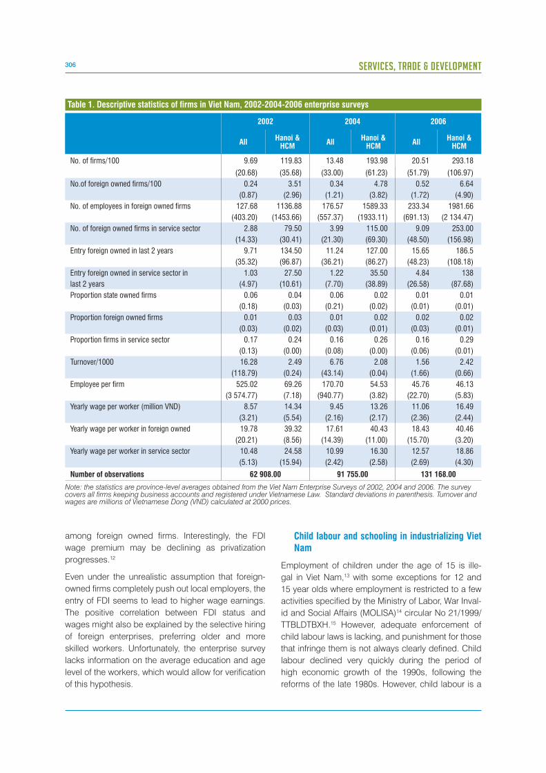
306 SERVICES, TRADE & DEVELOPMENT
among foreign owned firms. Interestingly, the FDI
wage premium may be declining as privatization
progresses.12
Even under the unrealistic assumption that foreign-
owned firms completely push out local employers, the
entry of FDI seems to lead to higher wage earnings.
The positive correlation between FDI status and
wages might also be explained by the selective hiring
of foreign enterprises, preferring older and more
skilled workers. Unfortunately, the enterprise survey
lacks information on the average education and age
level of the workers, which would allow for verification
of this hypothesis.
Child labour and schooling in industrializing Viet Nam
Employment of children under the age of 15 is ille-
gal in Viet Nam,13 with some exceptions for 12 and
15 year olds where employment is restricted to a few
activities specified by the Ministry of Labor, War Inval-
id and Social Affairs (MOLISA)14 circular No 21/1999/
TTBLDTBXH.15 However, adequate enforcement of
child labour laws is lacking, and punishment for those
that infringe them is not always clearly defined. Child
labour declined very quickly during the period of
high economic growth of the 1990s, following the
reforms of the late 1980s. However, child labour is a
2002 2004 2006
AllHanoi &
HCMAll
Hanoi & HCM
AllHanoi &
HCM
No. of firms/100 9.69 119.83 13.48 193.98 20.51 293.18
(20.68) (35.68) (33.00) (61.23) (51.79) (106.97)
No.of foreign owned firms/100 0.24 3.51 0.34 4.78 0.52 6.64
(0.87) (2.96) (1.21) (3.82) (1.72) (4.90)
No. of employees in foreign owned firms 127.68 1136.88 176.57 1589.33 233.34 1981.66
(403.20) (1453.66) (557.37) (1933.11) (691.13) (2 134.47)
No. of foreign owned firms in service sector 2.88 79.50 3.99 115.00 9.09 253.00
(14.33) (30.41) (21.30) (69.30) (48.50) (156.98)
Entry foreign owned in last 2 years 9.71 134.50 11.24 127.00 15.65 186.5
(35.32) (96.87) (36.21) (86.27) (48.23) (108.18)
Entry foreign owned in service sector in
last 2 years
1.03
(4.97)
27.50
(10.61)
1.22
(7.70)
35.50
(38.89)
4.84
(26.58)
138
(87.68)
Proportion state owned firms 0.06 0.04 0.06 0.02 0.01 0.01
(0.18) (0.03) (0.21) (0.02) (0.01) (0.01)
Proportion foreign owned firms 0.01 0.03 0.01 0.02 0.02 0.02
(0.03) (0.02) (0.03) (0.01) (0.03) (0.01)
Proportion firms in service sector 0.17 0.24 0.16 0.26 0.16 0.29
(0.13) (0.00) (0.08) (0.00) (0.06) (0.01)
Turnover/1000 16.28 2.49 6.76 2.08 1.56 2.42
(118.79) (0.24) (43.14) (0.04) (1.66) (0.66)
Employee per firm 525.02 69.26 170.70 54.53 45.76 46.13
(3 574.77) (7.18) (940.77) (3.82) (22.70) (5.83)
Yearly wage per worker (million VND) 8.57 14.34 9.45 13.26 11.06 16.49
(3.21) (5.54) (2.16) (2.17) (2.36) (2.44)
Yearly wage per worker in foreign owned 19.78 39.32 17.61 40.43 18.43 40.46
(20.21) (8.56) (14.39) (11.00) (15.70) (3.20)
Yearly wage per worker in service sector 10.48 24.58 10.99 16.30 12.57 18.86
(5.13) (15.94) (2.42) (2.58) (2.69) (4.30)
Number of observations 62 908.00 91 755.00 131 168.00
Note: the statistics are province-level averages obtained from the Viet Nam Enterprise Surveys of 2002, 2004 and 2006. The survey covers all firms keeping business accounts and registered under Vietnamese Law. Standard deviations in parenthesis. Turnover and wages are millions of Vietnamese Dong (VND) calculated at 2000 prices.
Table 1. Descriptive statistics of firms in Viet Nam, 2002-2004-2006 enterprise surveys
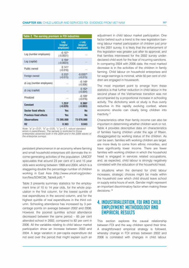
307CHAPTER XIII: CHILD LABOUR AND SERVICES FDI: EVIDENCE FROM VIET NAM
persistent phenomenon in an economy where farming
and small household enterprises still dominate the in-
come-generating activities of the population. UNICEF
speculates that around 23 per cent of 5 and 15 year
olds were working between 1999 and 2004, which is a
staggering double the percentage number of children
working in East Asia (http://www.unicef.org/protec-
tion/files/SOWC06_Table9.pdf).16
Table 3 presents summary statistics for the employ-
ment time of 10 to 14 year olds, for the whole pop-
ulation in the first column, for the lowest quintile of
real expenditures in the second column, and for the
highest quintile of real expenditures in the third col-
umn. Schooling attendance has increased by 3 per-
centage points on average between 2002 and 2006.
However, the poorest quintiles school attendance
decreased between the same period – 85 per cent
attended school in 2002, compared to 82 per cent in
2006. All the variables relating to child labour market
participation show an increase between 2002 and
2004. A large variation in per-capita expenditure did
not exist over the period that might explain such an
Log (wages/
employee)
��Log (wages/
employee)
Log (number employees)-0.107a
(-0.0031)...
Log (capital)0.194a
(-0.0023)...
Public owned0.141a
(-0.016)...
Foreign owned0.332a
(-0.015)-0.0307b
(-0.015)
���������� ���������� ...-0.148a
(-0.006)
��������������� ...0.162a
(-0.004)
Privatized ...-0.109a
(-0.016)
Constant1.253a
(-0.029)0.360a
(-0.003)
Sector fixed effects Yes No
Province fixed effects Yes No
Observations 73 295.000 73 076.000
R2 0.363 0.043
Note: “a” p<0.01, “b” p<0.05, “c” p<0.1, robust standard errors in parentheses. The sample is restricted to those enterprises observed both in the 2004 and in the 2006 waves of the enterprise surveys.
Table 2. The earning premium in FDI industries adjustment in child labour market participation. One
factor behind such a trend is the new legislation ban-
ning labour market participation of children just prior
to the 2001 survey. It is likely that the enforcement of
this legislation was greater just after its approval, and
that families interviewed for the 2002 survey under-
declared child work for the fear of incurring sanctions.
In comparing 2004 with 2006 data, the most marked
decrease is in the activities of the children in family
farming. Child labour on household enterprises and
for wage earnings is minimal, while 50 per cent of chil-
dren are engaged in housework.
The most important point to emerge from these
statistics is that further reduction in child labour in the
second phase of the Vietnamese transition was not
accompanied by a proportional increase in schooling
activity. The dichotomy work or study is thus overly
reductive in this rapidly evolving context, where
economic shocks can clearly bring children into
inactivity.17
Characteristics other than family income can also be
important in determining whether children work or not.
Table 4 provides descriptive data on characteristics
of families having children under the age of fifteen,
disaggregated by working status of the children. As
can be seen, families with working children are larger,
are more likely to come from ethnic minorities, and
have significantly lower income. There are fewer
families with working children in which the household
head is engaged in services related occupations,
and, as expected, child labour is strongly negatively
correlated with the education of the household head.
In situations when the demand for child labour
increases, strategic choices might be made within
the household over which child should leave school
or supply extra hours of work. Gender might represent
an important discriminatory factor when making these
decisions. 18
4. INDUSTRIALIZATION, FDI AND CHILD EMPLOYMENT: METHODOLOGY AND EMPIRICAL RESULTS
This section explores the causal relationship
between FDI and the way children spend their time.
A straightforward empirical strategy is followed,
whereby change in FDI entries between 2002 and
2006 is correlated with changes in child labour.
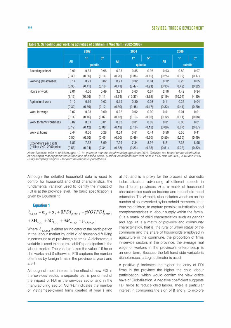
308 SERVICES, TRADE & DEVELOPMENT
Although the detailed household data is used to
control for household and child characteristics, the
fundamental variation used to identify the impact of
FDI is at the province level. The basic specification is
given by Equation 1:
Equation 1
Where t,m,h,c� is either an indicator of the participation
in the labour market by child c of household h living
in commune m of province p at time t. A dichotomous
variable is used to capture a child’s participation in the
labour market. The variable takes the value 1 if he or
she works and 0 otherwise. FDI captures the number
of entries by foreign firms in the province at year t and
at t-1.
Although of most interest is the effect of new FDI in
the services sector, a separate test is performed of
the impact of FDI in the services sector and in the
manufacturing sector. NOTFDI indicates the number
of Vietnamese-owned firms created at year t and
at t-1, and is a proxy for the process of domestic
industrialization, advancing at different speeds in
the different provinces. H is a matrix of household
characteristics such as income and household head
education. The H matrix also includes variables on the
number of hours worked by household members other
than the children, to capture possible substitution and
complementarities in labour supply within the family.
C is a matrix of child characteristics such as gender
and age. M is a matrix of province and community
characteristics, that is, the rural or urban status of the
commune and the share of households employed in
agriculture in the commune, the proportion of firms
in service sectors in the province, the average real
wage of workers in the province’s enterprises.� is
an error term. Because the left-hand-side variable is
dichotomous, a Logit estimator is used.
A positive � indicates the higher the entry of FDI
firms in the province the higher the child labour
participation, which would confirm the view critics
have of Globalization. A negative coefficient suggests
FDI helps to reduce child labour. There is particular
interest in comparing the sign of � and �, to explore
2002 2004 2006
All1st 5th
All1st 5th
All1st 5th
quintile quintile quintile
Attending school 0.90 0.85 0.98 0.93 0.85 0.97 0.93 0.82 0.97
(0.30) (0.36) (0.14) (0.26) (0.36) (0.16) (0.25) (0.39) (0.17)
Working (all activities) 0.14 0.21 0.02 0.21 0.32 0.04 0.12 0.23 0.05
(0.35) (0.41) (0.16) (0.41) (0.47) (0.21) (0.33) (0.42) (0.22)
Hours of work 3.01 4.50 0.49 3.51 5.63 0.67 2.16 4.42 0.94
(9.12) (10.56) (4.11) (8.74) (10.37) (3.92) (7.19) (10.04) (4.80)
Agricultural work 0.12 0.19 0.02 0.19 0.30 0.03 0.11 0.22 0.04
(0.32) (0.39) (0.12) (0.39) (0.46) (0.17) (0.32) (0.41) (0.20)
Work for wage 0.02 0.03 0.00 0.02 0.02 0.00 0.01 0.01 0.01
(0.14) (0.16) (0.07) (0.13) (0.13) (0.03) (0.12) (0.11) (0.08)
Work for family business 0.02 0.01 0.01 0.02 0.01 0.02 0.01 0.00 0.01
(0.12) (0.12) (0.08) (0.13) (0.10) (0.13) (0.09) (0.07) (0.07)
Work at home 0.44 0.50 0.28 0.54 0.61 0.44 0.50 0.55 0.41
0.50) (0.50) (0.45) (0.50) (0.49) (0.50) (0.50) (0.50) (0.49)
Expenditure per capita (million VND, 2000 price)
7.83 7.32 8.99 7.99 7.34 8.97 8.21 7.38 8.95
(0.53) (0.24) (0.34) (0.53) (0.23) (0.35) (0.51) (0.22) (0.32)
Note: Statistics refer to children ages 10-14, younger than the legal working age since 2001. Quintiles are based on the distribution of per-capita real expenditures in food and non-food items. Authors’ calculation from Viet Nam VHLSS data for 2002, 2004 and 2006, using sampling weights. Standard deviations in parenthesis.
Table 3. Schooling and working activities of children in Viet Nam (2002-2006)

309CHAPTER XIII: CHILD LABOUR AND SERVICES FDI: EVIDENCE FROM VIET NAM
No working child Having working child Total
Household size 4.82 5.51 4.87
Fraction of children under 16 year olds 0.36 0.42 0.36
Fraction of people older 60 year olds 0.06 0.04 0.06
Age of head 45.56 44.21 45.46
Ethnic minorities (yes=1) 0.13 0.40 0.15
Living in urban (yes=1) 0.26 0.07 0.25
Income per capita (million VND) 7.83 4.68 76.12
Expenditure per capita (thousand VND) 5.604 3.33 5.44
Head occupation
Leaders/managers 2.44 1.74 2.39
Professionals/technicians 4.97 0.39 4.65
Clerks/service worker 3.69 2.17 3.58
Agriculture/forestry 45.31 70.63 47.06
Skilled workers/machinery 14.31 8.86 13.93
Unskilled workers 18.15 10.61 17.63
Not working 11.13 5.6 10.75
Education of head
< Primary 24.43 42.79 25.7
Primary 26.23 24.62 26.11
Lower-secondary 26.74 25.22 26.63
Upper-secondary 8.49 3.99 8.18
Technical degree 9.43 3.38 9.01
Post-secondary 4.69 0.00 4.36
Number of observations 5 109.00 443.00 5 552.00
Note: Authors’ calculation with VHLSS 2006 data, using sampling weights.
Table 4. Child labor and household characteristics (2006)
whether the demand for labour by foreign owned firms
has different effects other than domestic firms on the
way children spend their time.
Consideration is also given to whether different types
of FDI may lead to different outcomes, for example
to determine whether FDI in manufacturing have
different impacts on child labour from FDI in services.
The impact of FDI on child labour may also depend
on whether domestic firms are in the manufacturing
or services sectors, as this may affect the scope for
displacement, in particular if manufacturing firms
are exporting to OECD countries where consumer
activism may hurt them if they employ child labour. 19
Results are displayed in tables 5, 5a and 6. In the
first column of table 5, individual data from 2002,
2004 and 2006 is pooled and regressed with the
binary variable on child labour (“Working”) on the
number of new FDI firms in service in the province,
as well as the individual, family and community
characteristics explained above. In this pooled
regression without province fixed effects, child labour
and the number of services FDI firms in the province
are positively correlated. As expected, child labour
is more prevalent in communities with a larger share
of households engaged in agricultural activities. The
children from richer and more educated families have
a significantly lower participation rate in the labour
market. There is a significant gender bias, with female
children supplying more labour. Interestingly, while
larger families tend to have more children working,
the propensity of children decreases with the number
of teenagers in the household. This might indicate that
child labour is a last-resort for families experiencing
310 SERVICES, TRADE & DEVELOPMENT
increases in the demand for labour. Families first
expand the supply of labour of the young and only
if further labour-constrained decide to engage
children below the legal working age. Controlling for
real expenditures per-capita, child labour decreases
with higher labour participation of adult household
members (hours worked by 21 to 65 year olds), but
increases with teenager hours worked. The latter
result might reinforce the intuition of complex within-
household interactions in labour supply, with families
resorting to child labour when they have exhausted
the availability of labour supply of older children.
The positive correlation between FDI in services and
child labour in column 1 of table 6 may be spurious
due to excluded province characteristics, most
notably the province’s degree of industrialization.
As already pointed out, rapid industrialization may
result in a high number of family members moving
from farms and home workshops into factory work,
thus increasing the demand for child labour for family
farming and other household activities. In column 2
of table 6, a variable has been added to proxy the
intensity of industrialization in a province, that is, the
number of new enterprises created at t and t-1. It can
be seen that the proxy for the entry of services FDI
firms change signs, becoming negatively correlated
with child labour, even if the variable is statistically
significant only at the 15 per cent level. Interestingly,
the entry of non-FDI firms is positively correlated with
child labour and strongly statistically significant.
Other observed and unobserved province characteris-
tics might also affect the correlation between FDI and
child labour. The estimation results reported in column
2 of table 5 will thus be biased if there is selection
into provinces by FDI firms which may select locations
with characteristics correlated with child labour (good
quality infrastructure or population density). Another
source of selection bias might be regional develop-
ment policies which may drive location of foreign firms
into particular regions.
The availability of data over multiple years allows for the
addition of province fixed-effects that capture observed
and unobserved heterogeneity among provinces.
As long as these unobservable determinants of firm
location, correlated with child labour, are invariant
during the 2002 to 2006 period, the inclusion of
province fixed effects reduces the possible bias due
the endogenous sorting of enterprises. In column 3
of table 5, we report results of a model with province
fixed effects the entry of FDI firms in the services sector
reduces the likelihood of child labour. The coefficient
is greater in size and statistically significant at the
1 per cent level, suggesting that unobservable
province characteristics bias the effect downwards
in the specifications reported in columns 1 and 2. In
column 3 of table 5 we also include the number of FDI
entries in non-service sectors (mostly manufacturing
and mining). This type of foreign investment tends to
reduce the likelihood of child labour. At the margin, the
effect of the entry of an additional foreign-owned firm
in the service sector is greater than the effect of the
entry of a foreign firm in the manufacturing sector. In
fact, the predicted probability of working for children in
the specification in column 3 of table 5 declines from
1 percentage point (from 9 per cent to 8 per cent) as
the number of entries of foreign manufacturing firms
increases from 1 to 12. An increase in the number
of foreign owned firms in the services sector from 1
to 7 is enough to reduce the predicted probability of
working of 1 percentage point (from 8.5 per cent to
7.5 per cent).
However, there are 5 times less foreign-owned firms
in the services sector. This means that the effect
of FDI in manufacturing on child labour is overall
greater than the impact of FDI in services on child
labour. This finding might be explained by the fact
that provinces with higher incidence of child labour
were less successful in attracting the relatively skill-
intensive services sector FDI. As was seen previously,
there has been an equal provincial distribution of
more traditional FDI (textile, mining, food processing)
throughout Viet Nam, as such including those
provinces with larger and more rapidly decreasing
rates of child labour. However, the province and the
year fixed effects should, at least partly, control for
these province-specific trends in child labour.
In the regression with province fixed effects, there is a
general finding that increases in the overall proportion
of firms (both FDI and domestic) in the services
sector lead to a lower incidence of child labour. This
finding can be explained by the relative skill intensity
of services industries with respect to the mining,
agricultural processing and manufacturing industries
in Viet Nam. In column 4 of table 5 the average wage in
each province is added as an additional regressor, in
orders to check whether the main channel driving the
negative correlation between FDI and child labour is
the “earning effect”, described in the previous section.
Interestingly, the wage variable is not significant when
included together with the FDI variable. This suggests
311CHAPTER XIII: CHILD LABOUR AND SERVICES FDI: EVIDENCE FROM VIET NAM
that other channels might be more important in
explaining the main finding – most likely the fact that
FDI industries increase the demand for skilled labour
and provide more secure, high-quality jobs. The
positive link between a rapid domestic industrialization
process (proxied by the increase in non-FDI firm
creation) and child labour deserves further reflection.
Given that child labour is concentrated in agriculture
and household activities, it could be deduced that
a rapid diversification out of agriculture into wage
labour would decrease the frequency of labour
market participation of children. Things might work
differently if labour market imperfections generated
a positive association between industry creation and
unemployment. As the expected earnings in industry
are much greater than the earnings in agriculture,
labour market incumbents (the young in particular)
might be ready to leave agricultural work even at high
risk of transitory unemployment. Teenager transition
out of agriculture is highly relevant in the data (10 per
cent decrease in agricultural participation of the 14-
19 years old between 2004 and 2006), which is in all
likelihood much higher than the absorption capacity
of the new firms.
Shocks associated to transitory unemployment, and
the parallel higher demand for child work due to teens
leaving the household farm, might be particularly
relevant for poor households. In fact, after more
than 15 years of sustained growth, child labour
seems mainly to persist in poor households exposed
to negative income fluctuations. To explore this
hypothesis, the number of new, non-FDI enterprises
with the logarithm of real per capita expenditure of the
household is interacted (column 5). The interaction
term is negative and strongly statistically significant,
indicating that the industrial transition is more likely
to induce increased rates of child labour in poorer
households. Interestingly, the interaction between
expenditures and FDI entries is not statistically
significant (result not shown). Successful attraction
of FDI seems to partially compensate possible
adjustment effects of rapid industrialization on child
labour. A subsample of the families is followed over
the three waves of the surveys, permitting to test
whether the main result on child labour holds when
controlling for household fixed effects (table 5, column
6). The advantage of including the fixed-effect at the
household level is that some crucial unobservable
characteristics, such as family-specific degree of
aversion to child labour or exposure to risk, can be
controlled. However, there are notable problems with
the household fixed effect model. The major problem
being that there is much less variation in child labour
participation within the household, as many families
might not have children in the relevant age range (10 to-
14 year olds) in the three waves. One consequence is
that the overall fit of the model is much worse and few
variables are significant. Another important problem
of the household-fixed effect specification is that
attrition is likely to be non-random, those households
disappearing from the panel being more likely to
have moved to provinces with better living or earning
conditions. As can be seen in table 5 (column 6), the
signs on Service FDI and Non-FDI firms confirm the
results previously discussed, but are not statistically
significant as most of the other variables.
Table 5a tests the robustness of the results using
different measures of child labour. A Tobit model on
the number of hours worked per week by the children
is estimated resulting once again in a significant
negative correlation with the entry of foreign firms in
the services sector (column 1) Binary variables equal
to 1 are regressed (column 2, 3 and 4) if the child is
respectively engaged in agricultural work, domestic
work, and work for a household enterprise. If a child is
not engaged in such types of work, binary levels are
equal to 0. These results have been confirmed.
A relevant objection to the above results is that they
show child labour tends to decrease with higher FDI
entries, and do not imply that children substitute work-
ing with higher schooling. In fact, children might simply
stop working, and spend more time in the playground.
Table 7 inspects whether FDI entry in the service sec-
tor is also accompanied with higher schooling, and
thus life-time improvements in capabilities of the
young. The dependent variable is equal to 1 if those in
schooling age – 6 to 19 year olds are currently attend-
ing school – otherwise the dependent variable is 0.
Table 7 shows that schooling rates increase with the
entry of FDI firms in the services sector, and decrease
with the entry of Vietnamese enterprises (column 1).
Column 2 presents the positive effect of FDI in servic-
es decreasing with the age of the young, most likely
because some older teenagers are likely to search
for employment in FDI enterprises. In column 3, the
interaction between services FDI entry and log expen-
diture is not statistically significant. The positive effect
of FDI entry is greater on female enrolment in school
(column 4).

312 SERVICES, TRADE & DEVELOPMENT
Table 5. Entry of FDI firms in the service sector and working status of the children
Dependent variable: working
1 2 3 4 5 6
Logit OLS
FDI service 0.0072a
(0.002)-0.0062(0.006)
-0.0259a
(0.01)-0.0176c
(0.009)-0.0155
(0.01)-0.0005(0.001)
Domestics firms ...0.0002a
(0.00001)0.0007b
(0.00001)0.0006b
(0.00001)0.0019a
(0.001).00003
(.00004)
FDI manufacturing ... ...-0.0116b
(0.005)... ...
-0.0001(0.001)
Wage per worker ... ... ...-0.002
(0.048)-0.0012(0.048)
-0.0094(0.009)
Domesticc log expenditures ... ... ... ...-0.0002b
(0.00001)...
Proportion in agriculture5.2732a
(0.241)5.2857a
(0.246)4.7769a
(0.268)4.7866a
(0.268)4.7914a
(0.268)0.6495a
(0.078)
Urban0.1681(0.108)
0.159(0.108)
0.0741(0.109)
0.0842(0.107)
0.0877(0.107)
...
Male-0.1406a
(0.049)-0.1488a
(0.049)-0.1440a
(0.051)-0.1414a
(0.051)-0.1416a
(0.051)-0.0186(0.013)
Hours worked by teens0.0214a
(0.002)0.0213a
(0.002)0.0218a
(0.002)0.0218a
(0.002)0.0218a
(0.002)0.0009c
(0.001)
Hours worked by adult-0.0028a
(0.001)-0.0029a
(0.001)-0.0024b
(0.001)-0.0024b
(0.001)-0.0025b
(0.001)-0.0003
(0)
Number of children0.1812a
(0.041)0.1634a
(0.042)0.1375a
(0.043)0.1378a
(0.043)0.1364a
(0.043)0.0242c
(0.013)
Number of teens-0.5239a
(0.056)-0.5178a
(0.057)-0.5275a
(0.058)-0.5260a
(0.058)-0.5265a
(0.058)0.0128(0.017)
Age0.5197a
(0.02)0.5213a
(0.02)0.5484a
(0.02)0.5477a
(0.02)0.5475a
(0.02)0.0599a
(0.004)
Household size0.0415c
(0.024)0.0443c
(0.024)0.0455c
(0.026)0.0447c
(0.026)0.0464c
(0.026)-0.0069(0.012)
Education of the head-0.0527a
(0.01)-0.0543a
(0.01-0.0862a
(0.01)-0.0861a
(0.01)-0.0866a
(0.01)...
Proportion of firms in service
0.1508(0.514)
-0.045(0.529)
-1.6223(1.593)
-1.6272(1.58)
-1.4489(1.587)
0.0158(0.275)
Log Expenditure-0.3613a
(0.075)-0.3549a
(0.076)-0.4162a
(0.08)-0.4178a
(0.08)-0.3613a
(0.084)0.033
(0.027)
20040.5989a
(0.074)0.5968a
(0.075)0.6084a
(0.08)0.5879a
(0.099)0.5817a
(0.099)0.0537a
(0.019)
20060.2661a
(0.091)0.2641a
(0.091)0.1564(0.105)
0.1333(0.178)
0.1101(0.178)
-0.02(0.037)
Constant-7.9947a
(0.675)-8.0509a
(0.681)-8.8021a
(1.665)-9.1830a
(1.775)-10.0083a
(1.832)-1.0289a
(0.255)
Province fixed effects Yes Yes Yes Yes Yes Yes
Household fixed effects No No No No No Yes
Observations 36 295.00 35 923.00 35 923.00 35 923.00 35 923.00 15 875.00
(Pseudo R-squared) 0.22 0.21 0.25 0.25 0.25 0.12
Note: Robust standard errors in parentheses, corrected for within-cluster correlation at the family level. “a” p<0.01, “b” p<0.05, “c” p<0.1. Number of household fixed effects: 4 438. The sample is made of pooled data for 2002, 2004, 2006 on all the children aged 10-14. FDI service, Domestic Firms are counts of enterprises starting operation in the province at “t” and “t-1”.

313CHAPTER XIII: CHILD LABOUR AND SERVICES FDI: EVIDENCE FROM VIET NAM
Table 5a. Entry of FDI firms in the service sector and type of working activity of the children
Hours workedWork in family
agricultureWork for wage
Work for family business
1 2 3 4
Tobit Logit
FDI service-0.2155b
(0.089)-0.0161c
(0.0083)-0.0076b
(0.0032)-0.0238c
(0.014)
Domestic Firms0.0072a
(0.002)0.0006a
(0.0002)0.0003a
(0.0001)0.0010b
(0.0004)
Wage per worker0.1294(0.374)
-0.0487c
(0.0276)-0.0428b
(0.0178)0.1049
(0.0903)
Proportion in agriculture57.3150a
(1.934)5.9448a
(0.1593)0.5872a
(0.0913)-1.7990a
(0.3376)
Urban0.831(0.84)
0.0947(0.0662)
-0.1392a
(0.0354)-0.2122
(0.1511)
Male-1.8745a
(0.482)-0.0662c
(0.0368)-0.5502a
(0.0234)-0.5793a
(0.0962)
Hours worked by teens0.3864a
(0.017)0.0174a
(0.0011)0.0024a
(0.0008)0.0181a
(0.0024)
Hours worked by adult-0.0015(0.008)
-0.0042a
(0.0006)-0.0013a
(0.0004)0.0043a
(0.0016)
Number of children2.0847a
(0.383)0.1019a
(0.0287)0.0788a
(0.0192)0.2960a
(0.082)
Number of teens-8.9568a
(0.549)-0.4666a
(0.0387)-0.2111a
(0.024)-0.0928
(0.0998)
Age8.2376a
(0.194)0.5130a
(0.0143)0.3790a
(0.0086)0.4754a
(0.0362)
Household size0.2379(0.225)
0.0881a
(0.0175)-0.0928a
(0.0113)-0.2080a
(0.0539)
Education of the head-1.3432a
(0.085)-0.0803a
(0.0066)-0.0138a
(0.0041)-0.0723a
(0.0148)
Proportion of firms in service
-23.1078c
(11.818)0.1771
(0.9064)-1.9300a
(0.5323)-4.8302b
(2.4407)
Log expenditure-7.0218a
(0.695)-0.3599a
(0.0519)-0.3100a
(0.0306)-0.0975(0.126)
20046.4840a
(0.817)0.7171a
(0.0611)0.3996a
(0.0402)-0.0508
(0.1575)
2006-0.2292(1.384)
0.4420a
(0.1022)0.3531a
(0.065)-1.3767a
(0.3079)
Constant-120.2514a
(14.225)-9.8100a
(1.2106)-1.4915a
(0.5722)-14.2584a
(3.0974)
Province fixed effects Yes Yes Yes Yes
Observations 35 923.0000 35 923.000 35 923.000 32 131.000
Pseudo R-squared 0.0996 0.278 0.125 0.142
Note: Robust standard errors in parentheses, corrected for within-cluster correlation at the family level. “a” p<0.01, “b” p<0.05, “c” p<0.1. Number of household fixed effects: 4 438. The sample is made of pooled data for 2002, 2004, 2006 on all the children aged 10-14. FDI service, Domestic Firms are counts of enterprises starting operation in the province at “t” and “t-1”.

314 SERVICES, TRADE & DEVELOPMENT
Table 6. Entry of FDI firms in the service sector and schooling enrollments
Dependent variable: Attending school
1 2 3 4
Logit
FDI service0.0084c
(0.005)0.0238b
(0.01)0.0257(0.017)
0.0108b
(0.005)
Domestic firms-0.0003a
(0.0001)-0.0003a
(0.0001)-0.0003a
(0.0001)-0.0003a
(0.0001)
FDI servicec age ...-0.0010c
(0.001)... ...
FDI servicec expenditures ... ...-0.0019(0.002)
...
FD servicec male ... ... ...-0.0043b
(0.002)
Domestic firmsc expenditures ... ... ... ...
Wages-0.0972a
(0.027)-0.0971a
(0.027)-0.0973a
(0.027)-0.0973a
(0.027)
Proportion agriculture-1.1532a
(0.142)-1.1517a
(0.142)-1.1506a
(0.142)-1.1527a
(0.142)
Urban-0.0423(0.061)
-0.0421(0.061)
-0.0409(0.061)
-0.0424(0.061)
Male0.1563a
(0.034)0.1561a
(0.034)0.1563a
(0.0340.1632a
(0.034)
Hours worked by adults-0.0029a
(0.0001)-0.0030a
(0.0001)-0.0030a
(0.0001)-0.0030a
(0.0001)
Number of children-0.1298a
(0.026)-0.1300a
(0.026)-0.1297a
(0.026)-0.1298a
(0.026)
Number of teens-0.1217a
(0.027)-0.1224a
(0.027)-0.1219a
(0.027)-0.1218a
(0.027)
Age-0.5658a
(0.009)-0.5644a
(0.009)-0.5658a
(0.009)-0.5659a
(0.009)
Household size0.0662a
(0.016)0.0664a
(0.016)0.0664a
(0.016)0.0665a
(0.016)
Education of the head0.1352a
(0.006)0.1353a
(0.006)0.1352a
(0.006)0.1352a
(0.006)
Proportion of service0.4013(0.97)
0.4046(0.97)
0.4121(0.97)
0.4004(0.97)
Expenditures1.2337a
(0.051)1.2338a
(0.051)1.2386a
(0.052)1.2345a
(0.051)
2004-0.0671(0.058)
-0.0671(0.058)
-0.0679(0.058)
-0.0672(0.058)
2006-0.1783c
(0.099)-0.1783c
(0.099)-0.1810c
(0.099)-0.1786c
(0.099)
Constant1.5634c
(0.847)1.5613c
(0.849)1.4717c
(0.855)1.5404c
(0.847)
Province fixed effects Yes Yes Yes Yes
Observations 79 459.000 79 459.000 79 459.000 79 459.000
Pseudo R-squared 0.342 0.342 0.342 0.342
Note: Robust standard errors in parentheses, corrected for within-cluster correlation at the family level. “a” p<0.01, “b” p<0.05, “c” p<0.1. The sample is made of pooled data for 2002, 2004, 2006 on all the individuals aged 6 to 19 years old. FDI service, Domestic Firms are counts of enterprises starting operation in the province at “t” and “t-1”.

315CHAPTER XIII: CHILD LABOUR AND SERVICES FDI: EVIDENCE FROM VIET NAM
5. CONCLUSIONS
This chapter explored the impact of services FDI
on child labour. Evidence was found that the entry
of foreign owned firms is associated with a lower
propensity of child labour, and associated with
increased school enrolment rates. Contrary to the
view held by critics of globalization, FDI seems to
improve working conditions in a rapidly industrializing
economy such as Viet Nam, and more importantly
results in greater investment in the human capital
of children. FDI in services has a stronger marginal
effect on the reduction of child labour than FDI into
manufacturing. However, because manufacturing FDI
is much larger, the overall impact of manufacturing
FDI is stronger than the impact of services FDI.
This finding is particularly relevant given that
the industrialization process leads to dramatic
adjustments in labour market participation and in
the activities of Vietnamese households. While the
persistence of child labour in Viet Nam deserves
further monitoring, the current acceleration of trade
liberalization in services seems to be contributing
toward the improvement of the livelihood of the
youngest in poor families, and therefore to the future
growth of Viet Nam.
NOTES1 See for example the debate around the 1994 football world cup in the United States, where it was found that most footballs
produced in the world were undertaken by foreign companies’ subsidiaries that employed child labour. As an example, See Sydney Shanberg, “Six Cents an Hour: On the Playgrounds of America, Every Kids’ Goal Is To Score. In Pakistan, Where Children Stitch Soccer Balls for Six Cents An Hour, The Goal is To Survive,” Life, June, 1996, p. 38. The article’s lead photograph showed 12-year-old Tariq surrounded by Nike soccer ball which he would spend most of a day stitching together for the grand sum of 60 cents. In a matter of weeks, activists all across Canada and the United States were standing in front of Nike outlets, holding up Tariq’s photo.
2 It cannot completely be ruled out that services FDI is more likely to occur in provinces with a more skilled labour force with higher income and therefore less child labour. Province fixed effects are controlled for, thus partly controlling for education of household head as well as its income.
3 Progresa is the acronym for the Programa de Educación, Salud y Alimentación (the Education, Health, and Nutrition Program), introduced in 1997 by the Government of Mexico to develop the human capital of poor households. Progresa targets its benefits directly to the population in extreme poverty in rural areas, through cash transfers to the mothers of households.
4 The income effect could be considered as dominating the substitution effect in child labour supply function, implying that at very low wages, child labour supply slopes downwards.
5 For example the football scandal in Sialkot (Pakistan) led to the Atlanta Agreement in 1997, where the United States’ Sporting Goods Manufacturers Association and the Sialkot Chamber of Commerce and Industry pledged to eliminate child labour from the stitching and production of soccer balls.
6 In Viet Nam, overall CPI increased by approximately 23 per cent during the first 9 months of 2008. During this time, food and non-food CPIs increased by 36 per cent and 13 per cent, respectively (Nguyen, 2009). High inflation can have ambiguous impacts on the poor. The real consumption of the poor can be reduced by inflation. On the other hand, the poor are also producers who can experience increases in income due to inflation. Depending on the reason of inflation and the structure of the economy, the effect of price increases on poverty may be negative and positive.
7 Haiphong, Viet Nam’s main port, lies on a branch of the Delta. A major highway crosses the Delta and the coastal strip beyond, an important transportation route linking China and Viet Nam.
8 In particular, firms considered as belonging to the services sector are those whose primary activity is in: transport, post, tourism, media, finance, professional, cleaning and support services, real-estate and renting services, education, health and social services.
9 Moreover, FDI firms in services are more capital-intensive (higher asset value/number of employees’ ratio). Interestingly, both services and non-services FDI firms tend to employ more women, but the proportion of female employees is higher in non-services foreign establishments.
10 Viet Nam joined WTO in 2007 becoming its 150th member. This accession is something of an endorsement of a long process of trade reform and international integration, which started more than two decades before in 1986 with the launch of Doi Moi (Renovation).

316 SERVICES, TRADE & DEVELOPMENT
11 The 5-digit industry code of the enterprise survey were summarized under the following sector categories: agriculture, aquaculture, mining, food processing, textile, wood, manufacture, power, waste, construction, wholesale, retail, wholesale of textile and food, whole sale of minerals, transport, post, tourism, media, finance, professional service, renting, education, cleaning and low skill services, government, health, reparations, social services, water and sewer.
12 A firm is considered to be privatized if it was under ownership of the central or of the local Government in 2004 and in a different ownership status (including joint public-private ownership) in 2006.
13 Viet Nam was the first Asian country to sign the International Convention on the Rights of the Child in 1990 (ILO Convention 182 that replaced and strengthened ILO Convention 138 of 1973).
14 MOLISA stands for the Ministry of Labour, War Invalid and Social Affairs. 15 These are: acting performance, crafts and fine arts occupations (embroidering and wood carving), pottery glazing and
painting, shell sawing, lacquer painting, and gifted athletes.16 According to UNICEF a child is considered to be involved in child labour activities when: (a) children 5 to 11 years of age
did at least one hour of economic activity or at least 28 hours of domestic work during the week preceding the survey, and (b) children 12 to 14 years of age that during the week preceding the survey did at least 14 hours of economic activity or at least 42 hours of economic activity and domestic work combined.
17 Since children tend to supply labour for family activities, important complementarities or substitution effects can link the work of children with the work of teenagers within the household. It is thus important to give a comparative look at the employment time of teenagers aged 15 (the minimum legal age for working) to 19, the age at which most young tend to start leaving their parent’s household. School attendance for children in the poorest quintile never exceeded 40 per cent while attendance for children in the richest quintile was twice as high in 2002.
18 There are significant differences in the schooling behaviours of boys and girls if the focus is on observation on the poor. There are large discontinuities in enrollment among families in the poorest quintile, with many boys from poor families leaving school at the age of 14, and many girls at the age of 15. Interestingly, enrolment seems to increase again for girls at the age of 16, probably indicating that there are many transitions into and out of school as the young adjust to income shocks or to changes in local labour markets.
19 For example, the United States Trade and Development Act of 2000 restricts eligibility of GSP benefits to countries that the Secretary of Labor certifies as showing progress to eliminate the worst forms of child labor.