A Theory of Marriage, Labor and Divorce. Out of print ...
386
Munich Personal RePEc Archive On the Economics of Marriage - A Theory of Marriage, Labor and Divorce. Out of print. Published originally by Westview Press in 1993 under name Grossbard-Shechtman Grossbard, Shoshana San Diego State University 1993 Online at https://mpra.ub.uni-muenchen.de/81059/ MPRA Paper No. 81059, posted 03 Sep 2017 08:16 UTC
-
Upload
khangminh22 -
Category
Documents
-
view
0 -
download
0
Transcript of A Theory of Marriage, Labor and Divorce. Out of print ...

Munich Personal RePEc Archive
On the Economics of Marriage - A
Theory of Marriage, Labor and Divorce.
Out of print. Published originally by
Westview Press in 1993 under name
Grossbard-Shechtman
Grossbard, Shoshana
San Diego State University
1993
Online at https://mpra.ub.uni-muenchen.de/81059/
MPRA Paper No. 81059, posted 03 Sep 2017 08:16 UTC
ON THE ECONOMICS OF MARRIAGE
A THEORY OF MARRIAGE, LABOR, AND DIVORCE
Second Edition Shoshana Grossbard
Springer Publishing

In memory of my parents, Chaim Yehoshua and Chana
Grossbard, who had the courage to have children after their
mothers--Shoshana Propper and Esther Grossbard--perished
in Auschwitz.

vii
Contents
List of Tables and Figures ix
Preface xiii
Acknowledgments xvii
INTRODUCTION 1
PART ONE
The Economics of Marriage in Perspective 5
1 The Economics of Marriage and Other
Social Sciences 7
2 The Economics of Marriage and Belief Systems 17
PART TWO
A General Theory of Marriage 23
3 A Theory of Allocation of Time in Markets
for Labor and Marriage 25
4 Theoretical Implications for Marriage 54
PART THREE
Sex Ratio Effects 85
5 Sex Ratios and Marriage, Cohabitation,
Labor Supply, and Divorce: Time Trends 87
6 Sex Ratios and Married Women's Labor

viii Contents
Supply--Cross-City Comparisons 104
PART FOUR
Compensating Differentials in Marriage 131
7 Compensating Differentials in Marriage and
Married Women's Labor Supply, with
Shoshana Neuman 133
8 Compensating Differentials and Intermarriage 142
PART FIVE
Cohabitation, Divorce, and Polygamy 159
9 A Theory of Cohabitation and Marriage Formality 161
10 A Theory of Divorce and Labor Supply, with
Michael C. Keeley 182
11 A Theory of Polygamy 214
PART SIX
Marriage, Productivity, and Earnings 241
12 Investments in Spouse's Productivity at Work 243
13 A Market Theory of Virtue as General Human Capital 257
14 A Study of Spousal Help Among Israeli Managers,
with Dafna N. Izraeli and Shoshana Neuman 272
15 Religiosity and Investments in Spousal Productivity,
with Shoshana Neuman 290
CONCLUSION 303
References 307
About the Book and Author 335
Index 337

x
Tables and Figures
Tables
3.1 Traditional labor supply theory vs. general theory of
marriage 36
4.1 Aspects of marriage--hypothesis numbers 59
6.1 Means and standard deviations--white women ages 25-34,
U.S. cities in 1930 114
6.2 Regressions of labor force participation--married
women ages 25-34, U.S. cities in 1930 117
6.3 Regressions of net labor force participation--married
women ages 25-34, U.S. cities in 1930 118
6.4 Definitions, means and standard deviations for various
samples, U.S. cities in 1980 121
6.5 Regressions of participation in the labor force--all
women and foreign-born women, U.S. cities in 1980 124
6.6 Regressions of participation in the labor force--
married white women with low education, ages 25-28,
U.S. cities, 1980 125
7.1 Means and definitions of the variables, Israeli
couples, 1974 137
7.2 Regressions of wife's labor force participation,
Israeli couples, 1974 139
8.1 Definitions, means and standard deviations,
National Jewish Population Survey, 1972 148
8.2 Regressions of likelihood of Jewish man marrying
exogamously by knowledge of Hebrew 150
9.1 Ratio of informally married to formally married
women, North America, 1974 162
9.2 Means and standard deviations of socioeconomic
indicators, 6 Guatemalan villages, 1974 170
9.3 Simple correlations with marriage type and female
schooling 172
9.4 Regressions of marriage formality for subsample 1 174
Tables and Figures xi
9.5 Regressions of marriage formality, first marriages 176
9.6 Regressions of marriage formality, salaried males 177
10.1 Means and labor supply responses--reduced forms, NIT experiments, Denver-Seattl
10.2 Labor supply response as a function of predicted
marital status and eligibility for treatment,
Denver-Seattle, 1970-78 205
10.3 Variables in the control set 212
10.4 Variables related to eligibility 213
11.1 Means and standard deviations in two sets of data
on Maiduguri, Nigeria, 1973 225
11.2 Regressions of number of wives for two samples,
Maiduguri, 1973 228
11.3 Probit regressions of "divorce", Maiduguri, Cohen data, 1973 232
14.1 Predictors of spousal help by theoretical perspective 275
14.2 Sample characteristics: means and standard deviations,
Israeli managers, 1987 280
14.3 Pearson correlations between perceived spousal support
and type of assistance, by gender 281
14.4 Linear regressions of spousal help, by gender,
Israeli managers, 1987 284
14.5 Logit regressions of spousal help, by gender,
Israeli managers, 1987 286
15.1 Israeli men's religious practices, means and
variances, 1968 299
15.2 Regressions of Israeli men's religious practices, 1968 300
Figures
3.1 Individual supplies of household labor and labor 31
3.2 Markets for female spousal labor, male spousal labor,
female labor, and male labor 34
3.3 Labor supply elasticity for two groups of women 44
3.4 Income effects on spousal labor 47
5.1 Sex ratio: unmarried men 20 to 29, to unmarried
women 18 to 29 94
5.2 Percent never married, women 25 to 29 94
5.3 Women's median age at marriage 94
5.4 Unmarried couples living together 95
5.5 Percent women employed, ages 25 to 34 95
5.6 Divorces per 1,000 married women, ages 25 to 34 95
8.1 Markets for spousal labor by women from groups A and B 144
9.1 A woman's indifference curves 165
xii Tables and Figures
9.2 Women's opportunities for income from spousal labor 166
9.3 Optimal match 167
9.4 Life-time productivity of wife and husband, and life-time
profile in compensation for wife's spousal labor 180
10.1 Income effects on spousal labor 185
10.2 A Negative Income Tax program with positive tax
reimbursement 211
13.1 Market for virtuous workers 261

Tables and Figures xiii
xiv
Preface
Marriage is an institution that plays a central role in most societies. As it
affects decisions regarding labor supply, consumption, reproduction, and other
important decisions, marriage receives considerable attention in academic
circles. Much research has been done about marriage, principally by
sociologists, psychologists, and anthropologists.
While recognizing its importance, most economists have let marriage play a
small role in their research. Economic theory ignores marriage almost
completely. In their empirical studies, economists pay little attention to
marriage, even where the evidence indicates that marital status is strongly
related to the topic of research. If they include any reference to marriage,
economists usually reduce marital status to the role of an exogenous control
variable. So far, the economics of marriage, defined as the application of
economic analysis to the study of marriage, has generated very limited interest.
One of the reasons for this limited interest may lie in the lack of available
books focusing on the economics of marriage.
As of the time of this writing, only three books on the economics of
marriage have been published. Gary Becker's (1981) Treatise on the Family,
published in the United States, stands out in the rigor of its mathematical
presentation. Ivy Papps' (1980) On Love and Money, published in England,
focusses on a limited number of applications of the economic analysis of
marriage. The most comprehensive and readable book published on this topic
in the past is Bertrand Lemennicier's (1988) Le Marche du Mariage et de la
Famille. If it has not generated much interest in the economics of marriage in
the United States or the United Kingdom, it is probably because it has not been
translated into English. My major goals in the present book are to show that
economics can be useful and relevant to the study of many aspects of marriage,
and to fill some of the vacuum existing in this area.
Central to the book is the general theory of marriage presented in Part Two.
The idea for that theory occurred to me during the beginning stages of my
doctoral thesis in 1974-75. It was then that I first developed a market for

Preface xv
spousal labor and called it a "market for wife-services" (Grossbard 1976). At
that time I also started writing on the interrelation between labor markets and
spousal labor markets, but I did not have the opportunity to develop that idea
until 1980, when I spent a year as a fellow at Stanford's Center for Advanced
Study in the Behavioral Sciences.
In an attempt to create better communication between the disciplines
engaged in research on marriage and thereby facilitate cross-fertilization, this
book emphasizes materials that are most likely to interest social scientists. The
book deals mostly with issues and data of contemporary relevance to two
industrialized countries, namely the United States and Israel. Of the two
chapters reporting data analysis from developing countries, the chapter
analyzing cohabitation is very relevant to contemporary social policy in
industrialized countries today, given the rapid increase in the incidence of
cohabitation in the West.
Furthermore, this book emphasizes themes that are of interest to
mainstream economists and sociologists. One of the central ideas of the book--
the impact of sex ratios on many aspects of behavior including labor supply--is
an idea I started writing about in 1978 and which has become very popular in
recent years. Another theme emphasized in the book, compensating
differentials in marriage, will hopefully appeal to researchers in both labor
studies and family studies.
Some of the themes covered in the book reflect my own research
opportunities. I have researched polygamy in great part because Theodore W.
Schultz and Gary Becker encouraged me to do so while I was a student at the
University of Chicago. A summer job at Rand in 1976 offered the opportunity
to work with William Butz studying Guatemalan data. As Guatemala is
characterized by very high rates of cohabitation, I started to do research on
cohabitation. An invitation to spend a year at Stanford in 1980 led to
cooperation with Michael Keeley, who was concluding his analysis of the
effects of Negative Income Tax experiments on divorce and labor supply.
Much about this book is new. Five of the fifteen chapters have never been
published in English. Eleven chapters (Chapters 2, 3, 5, 7, 8, 9, 11, 12, 13, and
15) are based on articles that have previously appeared in Hebrew, in an
anthropology journal, in books and in economics journals of varying
accessibility. Most of these chapters have been substantially expanded,
rewritten, or translated.
Most chapters can be read without a strong background in economics or
mathematics. Those chapters that contain some mathematical or economic
analysis (Chapters 3, 7, 10, and 13) are preceded by introductions aiming at
making the economics of marriage more accessible and appealing to readers
without previous knowledge in economics. Even so, some readers may want to

xvi Preface
skip Chapter 3, or at least the portions of that chapter that are formulated in
mathematical terms. The introductions to each part and to each chapter also
facilitate the integration of the various chapters into one book, and often also
create bridges to existing literature.
This book presents a long list of hypotheses. Some chapters are mostly
theoretical (in particular, Chapters 3, 4, 12, and 13), and the other chapters are
mostly empirical. Even though more pages are devoted to testing hypotheses
than to developing them, most hypotheses presented here remain either
untested or inadequately tested. I have attempted to execute many of these tests
on my own or in conjunction with colleagues, but providing adequate scientific
tests for all these hypotheses has not been possible. Many of my results should
be considered tentative, and I am sure they will be improved through the use of
better data and methodologies. If a better understanding of marriage follows
and as a result of such better understanding the economics of marriage can help
us design better social policies or perhaps help us make wiser personal
decisions regarding marriage, I will be very pleased.
Shoshana Grossbard-Shechtman

Preface xvii
xviii
Acknowledgments
I have been blessed with opportunities to learn from some extraordinary
teachers. My economics professors at the University of Chicago inspired me to
practice theory with applications, what Milton Friedman has called "positive
economics." It was at Chicago that Gary Becker introduced me to the
economics of marriage. Friedman, Becker, and others at the University of
Chicago--in particular, the late H. Gregg Lewis, Jacob Mincer, T.W. Schultz,
and the late George Stigler--built on a foundation acquired at the Hebrew
University of Jerusalem, where I learned economics from excellent teachers
such as the late Yoram Ben-Porath, the late Simon Kuznets, Nissan Leviathan,
Gur Ofer, and Don Patinkin. These two outstanding institutions, the Hebrew
University and the University of Chicago, also allowed me to gain familiarity
with the other disciplines that have shaped this book. A double major in
economics and sociology at the Hebrew University has encouraged me to
continue to combine my interests in both disciplines. At the University of
Chicago I had the opportunity to study for a minor degree in anthropology and
to take Judaism courses with Moshe Meiselman, a distinguished rabbi and
mathematician.
Other institutions I would like to acknowledge are the University of
Southern California for giving me the opportunity to learn about sex ratios
from the late Bill Hodge and to work with demographers Kingsley Davis and
David Heer; the Center for Advanced Study in the Behavioral Sciences at
Stanford for creating ideal conditions for writing the basis of this book; San
Diego State University for giving me time to write, opportunities to test my
ideas on students, and help with manuscript preparation; the Sapir Institute at
Tel-Aviv University for giving me my first research grant; and Bar-Ilan
University for giving me time to write and creating conditions for cooperation
with Shoshana Neuman.
I thank Shoshana for letting me use three of our joint papers for this book
and for giving me helpful comments on the entire manuscript. Deborah
Blackwell also read a substantial portion of the book and made very useful
suggestions. The present printing includes a number of corrections based on the

Preface xix
alertness of my students, including Shannon Bathrick and Jesus Garcia. Others
who made valuable comments are acknowledged throughout the book. I also
wish to thank Dafna Izraeli for letting me use a joint paper based on her data;
Michael Keeley for letting me use a joint paper; and William Butz, Ronald
Cohen, Linda Ewanyck, Elyce Rotella, and Jean Steckle for letting me use data
under their control. Many more people helped make my research easier, more
pleasant, more accurate, and more meaningful. I apologize to people whose
contributions I may have forgotten.
I am grateful for typing help provided by Marie Butler, Maureen
McDonnell, Marcelle Samakosky, and Susan Shapiro; and assistance with
word-processing techniques offered by James Edwards, John Hutchins, and
Rachael Litonjua-Witt.
This book is not a purely academic endeavor. In writing on work in
marriage, what I call "spousal labor," I have benefitted immensely from my
own experience. I am very grateful to my late parents, children, friends, and
community, who helped shape that experience. As this book goes to press, my
children, Michal, Zev, Chaim and Esther, are relatively more aware of the
short-run opportunity costs the preparation of this book has generated than of
the benefits that I believe they will derive from my professional expertise.
Most importantly, I thank my husband, Amos, for being a good marriage
partner. As the marriages described in my theory, our marriage involves more
spousal labor on my part than on his, and I am getting materially compensated
for my work as a wife and mother. I am grateful for this opportunity to learn
and grow together. I also appreciate a more prosaic way by which our marriage
has facilitated my writing. By supporting my spousal labor, Amos indirectly
increased the amount of time and money I was able to devote to the preparation
of this book.


Introduction This book deals with marriage from various perspectives. From the
perspective of the different disciplines, this book deals with the economics of
marriage to the extent that most hypotheses developed and tested are based on
economic theory. It can also be classified as economics in the sense that it
touches on many topics traditionally analyzed by economists, such as labor
supply, labor productivity and earnings. This book can be classified as
sociology, demography, or anthropology to the extent that it deals with topics
such as marriage rates, consensual unions, polygamy, and the distribution of
power in marriage, which have traditionally been considered part of the domain
of these disciplines.
While this book contains a lot of facts and empirical findings, and touches
on policy issues, the book's main contribution to the existing literature lies in
the theoretical perspective it offers. The central part of the book is Part Two,
which presents a general equilibrium theory of marriage. Years of experience
have taught me that most people lack the motivation to read this kind of
theoretical material on marriage. Common reasons why people shy away from
such theory are the notions that (1) economics does not have much to add to the
existing literature on marriage, and (2) an economic analysis of marriage leads
to undesirable practical implications, such as denial of love and glorification of
selfishness. Since such notions are so widespread, Part One of this book
attempts to dispel them.
Addressing the first notion, the materials in Part One aim at showing that
other disciplines do not offer close substitutes to an economic analysis of
marriage. Chapter 1 compares the economics of marriage with some of the
related literature found in anthropology and sociology. These disciplines
provide a wealth of studies about marriage, including some theoretical material.
However, sociological and anthropological theories of marriage have some
drawbacks in comparison to economic theories of marriage.
Part One also addresses the second notion that discourages many people
from reading an economic analysis of marriage, namely, the notion that an
economic approach to the analysis of marriage leads to the denial of emotions
and social or spiritual concerns. Most people, including most social scientists,
think about marriage either in romantic terms, or in ethical-religious terms. To
some extent, romanticism contradicts the economic approach. Romantics
typically rely on feelings in making decisions, not on rational comparisons of
costs and benefits. The romantic mentality stresses individual uniqueness, and

2 Introduction
stands in sharp contrast to the economic approach in which markets play a
central role. Chapter 2 attempts to dispel the notion that by applying economics
to the study of marriage one suppresses basic human tendencies for love and
intimacy.
Some readers may want to start directly with Part Two, which presents the
general equilibrium theory of labor and marriage that served as inspiration to
most of the other papers in this volume. Previous analyses of marriage, whether
they were written by sociologists or by economists, have not integrated
marriage markets with labor markets. This theory uses a general equilibrium
framework to integrate labor and marriage markets. Predictions are derived
regarding the effects of particular factors, such as individual resources and
market size, on individual and market labor supply and marital choices. The
two chapters in Part Two complement each other. Chapter 3 emphasizes theory
and applications to labor supply, whereas Chapter 4 emphasizes implications
for the study of marriage and divorce. Readers who lack a background in
economic analysis may want to skip the first part of Chapter 3.
Parts Three and Four deal with implications of the theory: sex ratio effects
and compensating differentials in marriage. A major implication of this general
equilibrium theory integrating marriage markets with labor markets, is that the
sex ratio of marriageable men to marriageable women may influence labor
supply as well as marriage. Part Three consists of two chapters dealing with sex
ratio effects.
The first chapter on sex ratio effects, Chapter 5, was written for a mixed
audience of sociologists and economists, and avoids the technical jargon and
statistical techniques familiar to economists. Chapter 6 is addressed to readers
trained in economics or statistics and includes regression results. The two
chapters also vary in the generality of their subject matter. Whereas Chapter 6
focuses on only one effect of sex ratio variations, namely, its effect on the
participation of married women in the labor force, Chapter 5 looks at the effect
of sex ratio variations on a number of social and economic aspects of life.
The two papers included in Part Four both deal with compensating
differentials in marriage. Chapter 7 is a study of married women's labor supply
and shows how differences between husband's and wife's characteristics,
associated with compensating differentials in marriage, add to our degree of
understanding of women's labor force participation. The paper was written for
an audience of economists.
Chapter 8 attempts to explain an aspect of similarity between husband's and
wife's characteristics, what sociologists call homogamy. The degree of
homogamy in one dimension, such as religion, is related to the similarity of
husband's and wife's characteristics in other areas, such as education, age, and
divorced status. It is assumed that compensating differentials in marriage exist.
Hypotheses regarding the likelihood of intermarriage between members of
different groups are derived and estimated, using the example of Jewish men in
Introduction 3
the United States.
The general equilibrium theory of marriage and labor can be applied in
many different ways to the study of marriage, as suggested in Chapter 4. Part
Five presents further applications of the theory to selected aspects of marriage.
Chapter 9 deals with marriage formality and cohabitation, Chapter 10 with
divorce and labor supply, and Chapter 11 with polygamy. These chapters test a
number of hypotheses regarding the effect of aggregate characteristics--such as
sex ratios--and individual characteristics--such as education and income--on
these aspects of marriage.
The theory of marriage presented in Part Two views individuals as suppliers
of spousal labor, and defines spousal labor as any service benefiting a spouse.
Such spousal labor is not simply about washing dishes and taking care of the
garden, but also about investing in a spouse's human capital. People invest in
their spouse's human capital to the extent that household labor boosts the
spouse's earning capacity or other aspects of the spouse's productive capacity
(including the capacity to produce at home). The papers in Part Six of the
volume all deal with aspects of spousal help that increase a person's human
capital.
Chapters 12 to 14 deal with spousal help aimed at increasing a worker's
earning capacity, whereas Chapter 15 focuses on the contribution of a spouse to
an individual's religious practice, which can be considered as a particular
aspect of home production. The last two chapters are of an empirical nature.
They both analyze Israeli data and were written with Shoshana Neuman. Dafna
Izraeli also collaborated on Chapter 14.

4 Introduction
5
PART ONE
The Economics of Marriagee
in Perspective Most people--including most social scientists--tend to have misconceptions
about the economic analysis of marriage. The first two chapters address some of
these misconceptions. The first misconception, addressed in Chapter 1, is that
the study of marriage does not belong in economics. Chapter 1 compares the
contribution of economics to the study of marriage with some of the research on
marriage produced by other disciplines, principally sociology and anthropology.
A second misconception is that an economic approach to marriage precludes
emotions and morality. In addressing this misconception, Chapter 2 compares
the economic perspective to other perspectives commonly used by people
making decisions about marriage: a romantic perspective and an ethical-
religious perspective. Readers who find it natural to apply economic theory to
marriage may want to read this part later, or skip it, and move on to Part Two.

6 Introduction
6
7
1 The Economics of Marriage and
Other Social Sciences The public at large often views economics as belonging to the domain of
business and government policy directly related to the functioning of "the
economy." Economics, however, can in reality be applied to any decision
making process. Economists interpret the term "economics" as a conceptual
framework that can be helpful any time a choice is made, be it the choice of a
good, a service, an action, or a resource. The application of neo-classical
economics to home-related subjects such as marriage, fertility, and
consumption is referred to as New Home Economics. The New Home
Economics approach was developed by Mincer (1962), Becker (1965), and
Lancaster (1966), when they all taught at Columbia University. Their models
were the first to incorporate household characteristics into formal models of
labor force participation, consumption, or transportation. Because of Becker's
central contribution and his move to the University of Chicago in the early
seventies, the New Home Economics is part of what some people call the
Columbia-Chicago School of Economics.
In its more than twenty-five years of existence, the New Home Economics
has had a substantial impact on research dealing with areas such as the study of
consumption and transportation. In addition, the New Home Economics has
had a limited impact on fields previously considered outside of economics. For
instance, it has become widely accepted that economics can be applied to the
study of fertility. This acceptance explains why economists now present
approximately twenty-five percent of all the papers included in the annual
meetings of the Population Association of America, and fill key positions in
this professional organization. With the exception of the application of game
theory (Manser and Brown 1980 and McElroy and Horney 1981) to the study of
marriage, there have not been many other economic theories related to the
study of marriage since Becker (1973, 1974a) published his first two articles on
the economics of marriage. Of the few economists who have written on the
economics of marriage, most have moved to other areas of research or have
dropped out of academics altogether. The purpose of this book is to encourage

8 Economics and Other Social Sciences
and promote the application of economics to the study of marriage.
The rest of this chapter focuses on previous applications of neo-classical
economics to marriage, and on how economics and some of the other
disciplines converge and diverge with respect to the study of marriage.
Neo-Classical Economic Analysis of Marriage Whenever a decision regarding the optimal use of time, energy, or money
needs to be made, cost-benefit analysis, one of the basic tools of economics, can
be helpful. This applies not only to the firm determining its level of operation,
but also to the individual or the family making decisions regarding
childbearing, consumption levels, or extent of participation in the labor force.
Economics in the sense of a conceptual framework dealing with optimal
allocation of resources is in fact applied mathematics.
The neo-classical economic approach assumes rationality. This rational
approach to decision-making can be contrasted with other approaches
commonly found among intellectuals, such as the Marxist approach which
emphasizes material determinism, and the Freudian approach which
emphasizes the power of instincts over man's behavior.
The two major tools used in general applications of neo-classical economics
are cost-benefit analysis and market analysis:
l. Cost-Benefit Analysis divides the elements related to a particular decision
into two groups: benefits and costs. The optimum point is reached when
marginal benefit equals marginal cost. For instance, a person will spend
money on margarine up to the amount at which the benefit derived from
a pack of margarine equals its price. In this case the price is the marginal
cost. If a good is not sold in the market, but is produced in the home, the
marginal benefit needs to equal the marginal cost, which is also
determined in the home, e.g., as a function of the value of alternative
uses of time and money.
2. Market Analysis. If a good or service is not destined solely to one
"consumer," or is not produced solely by one producer, a market exists,
whether or not it is physically observable. There are markets for goods,

Economics and Other Social Sciences 9
services, and different types of work, such as engineering, teaching, etc.
These two tools, cost-benefit analysis and market analysis, can be applied to
the study of marriage. According to this economic approach, people marry
when a (conscious or unconscious) comparison of costs and benefits makes
marriage look profitable. Benefits can be material, social or spiritual. Costs are
not simply financial or material. They depend on the value a person
attaches to alternative uses of time, and can include, for instance, the value of
the hours a person is unable to devote to studying the Bible because of
marriage.
The other tool borrowed from economics is market analysis. Becker and
before him sociologists and demographers have used the term "marriage
market." According to the version of the economics of marriage presented in
this book, marriage markets consist of markets for spousal labor supplied by
wives and husbands. Individuals participating in these markets act according to
cost-benefit analysis and try to maximize their own utility, which can also
include social and spiritual aspirations. Individuals make decisions about their
willingness to (1) supply services that can be of use to a spouse, (2) supply labor
services in the regular meaning of the term, and (3) acquire goods and services,
including services from spouses. More on this theory is found in Part Two.
The nonmonetary essence of marriage makes measurement difficult and leads
the economist to focus on less central but measurable aspects of marriage. The
first empirical studies of marriage by economists focused on the contemporary
United States, looking at the causes for differences in percentage of married
women per state, individual age at marriage, and probability of divorce.
Examples of early findings are
(1) the inverse relation between the percentage of women married and
percent Catholic across U.S. states (Freiden 1974). Freiden's
explanation relies on the expected costs of divorce: Catholic marriages
are less profitable because of higher expected costs of divorce.
(2) positive income effect on marriage in the sense that ceteris paribus
higher income was found to be associated with earlier marriage
(Keeley 1979).
(3) Becker, Landes, and Michael's (1977) finding of a positive income
effect on marriage in the sense that Americans with higher income
were found to be less likely to divorce. However, the same study also

10 Economics and Other Social Sciences
found that if wealth exceeded the level expected at time of marriage
the chances of dissolution were higher than if wealth was as high as
expected. This finding was explained in terms of a theory where
divorce depends on risk and uncertainty.
Other topics related to marriage which economists have analyzed more
recently, besides the topics covered in this book, include studies of the
allocation of time in household activities (e.g., Carlin 1985), of newspaper ads
related to marriage (e.g., Lemmenicier 1988), and child support payments (e.g.,
Beller and Graham 1986).
Economics and Sociology
The rich sociological literature on marriage does not appear to offer a
comprehensive theory of marriage, if we accept Homans' definition of theory:
"Not until one has properties, and propositions stating the relations between
them, and the propositions form a deductive system--not until one has all three
does one have a theory" (Homans 1964).
Following this definition of theory, only a small fraction of the sociological
literature on the family that claims to be theoretical actually qualifies for that
term. While very useful as inspiration and direction for empirical testing, the
various propositional inventories (e.g. Goode 1959, Hill, Katz, and Simpson
1957, or Nye and Berardo 1966), cannot be called theories. As to Parsons'
(1942) grand "theory" of society, even within sociology it is considered as a
conceptual framework rather than a theory (Hill and Hansen 1960).
Homans' (1961) theory and other versions of social exchange theory have
been applied to marriage. Social exchange theory can be viewed as an
application of price theory, as it is also based on rational choice and market

Economics and Other Social Sciences 11
analysis. Two major pioneers of social exchange theory, Homans and Blau
(1964), explicitly acknowledge their debt to economics.
Sociologists and social psychologists have applied social exchange theory to
the study of separate aspects of marriage, such as intrafamilial distribution of
power, marital stability, and dating, thereby preceding economists in the
application of price theory to marriage. One of the earliest sociological studies
of marriage based on the concept of bargaining is Waller (1937). Some other
early applications include Thibaut and Kelley (1959), Blau (1964), and theories
of intrafamilial power by Blood and Wolf (1960) and Heer (1963). Heer's
theory is a significant improvement over Blood and Wolf's (1960) theory on
that subject, in the sense that Blood and Wolf relied on the concepts of choice
and maximization, but did not recognize how market principles affect the
relative power of husband and wife. In contrast, Heer recognizes the
importance of market factors. Another topic that has been analyzed in terms of
social exchange theory is divorce, e.g., in Levinger's (1965) theory of marital
stability.
Sociologists have also preceded economists in the application of market
analysis to the study of marriage. Sociologists, as well as demographers, have
focused their attention on sex ratios, a particular aspect of marriage markets
presented here, before economists dealt with the topic.1 Demographers have
been mostly interested in studying the effects of sex ratios on marriage. For
instance, Glick, Beresford, and Heer 1963, Henry 1975, Goldman 1977, Smith
1980, Schoen 1983, and Goldman, Westoff and Hammerslough 1984 have
studied the effects of sex ratio on marriage rates. There have also been
numerous sociological and demographic studies of sex ratio effects on
intermarriage between various racial, religious or ethnic groups including Heer
1962, Rosenthal 1970, Della Pergola 1976, and Fisher 1980. Less common are
sociological studies relating sex ratios to divorce and mating patterns other
than intermarriage (e.g. Spanier and Glick 1980, Guttentag and Secord 1983),
suicide (Guttentag and Secord 1983, South and Trent 1989), and crime
(Guttentag and Secord 1983, Trent and South 1988).
In addition, sociologists have also developed theories of marriage pertaining
to timing and selection patterns (e.g., Rockwell 1976, Oppenheimer 1982,
Marini 1984, DiMaggio and Mohr 1985, Wilson 1987, Oppenheimer 1988,
Bennett, Bloom and Craig 1989, Mare 1991, Kalmijn 1991, and Blackwell
1992).
Most of the sociological literature on marriage applies to separate aspects of
marriage or typically considers one causal factor. Where sociologists of
marriage are comprehensive they do not really deal with theory. Where they
take a theoretical perspective, they do not typically take a comprehensive view.
Even in the more comprehensive applications of social exchange theory to
12 Economics and Other Social Sciences
marriage, such as Guttentag and Secord's (1983) Too Many Women - The Sex
Ratio Question--which studies a wide range of socio-economic consequences of
sex ratios--the theory is narrow in that it ignores aspects of marriage markets
other than sex ratios.2 In contrast, economic theories tend to be more general in
the sense that they encompass a range of applications and a range of causal
factors. Another difference is that the sociological theories of marriage which
incorporate the operation of marriage markets do not analyze marriage markets
in a general equilibrium framework, as is done in Part Two of this book.
The type of empirical research sociologists and economists perform often
differs as well. Until recently most economists analyzing marriage empirically
have used more sophisticated statistical techniques than sociologists. Many of
the sociological theories of intermarriage, intrafamily distribution of power, or
divorce were tested using simple techniques such as two-by-two tables. When
regression techniques were used, they were generally less sophisticated than the
techniques used by economists testing the economics of marriage.
However, economics and sociology are converging from the perspective of
applied research on marriage. Many recent studies of marriage by sociologists
have applied statistical tools as sophisticated as those found in similar studies
by economists (e.g., Lichter et al. 1991, South 1988). One finds more and more
economists and sociologists cooperating on joint empirical research. Some
sociologists have taken a lead in applying new statistical techniques to the study
of marriage. As in other areas of empirical research, academic affiliation is
becoming increasingly irrelevant. This book will hopefully also contribute to a
convergence of economics and sociology at the level of marriage theories.
Economics and Anthropology Economics has traditionally explored the more quantifiable sectors of
society with increasingly sophisticated theoretical and empirical tools.3 If we
conceive social reality as a series of fields, economists generally worked on the
scientifically most reachable ones at the intensive margin. Anthropologists, on
the other hand, worked at the extensive margin of social science. Attempting to
study entire cultures and venturing into the most remote communities, they
have accumulated comprehensive insights. Given the scarcity of academic
resources, researchers have had to make trade-offs
between an intensive and an extensive emphasis. While economists gave up
breadth of knowledge, anthropologists have typically collected their
information without much scientific methodology.
Recently, both economics and anthropology are extending their traditional
boundaries: anthropology has become more concerned with the quantitative
Economics and Other Social Sciences 13
intensive margin, while economists have become more interested in the
qualitative extensive margin of inquiry. Since ethnographies have been
collected from most existing cultures, anthropologists have become more
involved in cultural comparisons and theoretical generalizations.
Anthropologist Cohen (1973), who introduced a major methodological
handbook by remarking that "the discipline as a whole does not have a
systematic and cumulative tradition of methodological endeavor," expressed a
"desire to see anthropology become a progressively more rigorous and scientific
branch of the social sciences," "our primary goal...being theory-construction".
In the same volume he also proposed a "restructuring of the social sciences
[which] calls for methodological openness and a lack of concern for
disciplinary boundaries." Along these lines, anthropologist Douglas (1973)
specifically proposed that "economic analysis...be established at the center of
anthropology itself." She saw "the need for a cost-benefit analysis that would
apply across the board to both monetary and non-monetary transactions."
While more and more anthropologists concentrate less upon field work and
more on theory and methods of analysis, economic investigation has expanded
into the traditional specialities of other social sciences. For example, economic
research has penetrated into the domain of the family (see, for instance,
Theodore W. Schultz 1974) and social interactions (see Becker 1974b) and is
creating a link with sociobiology (see Hirshleifer 1978, Becker 1976).
While penetrating into new fields of study, most economists have
maintained their allegiance to the traditional tools of analysis they have used in
their more conventional work: cost-benefit analysis and market analysis. In
making implicit or explicit cost-benefit analyses of marriage and divorce,
economists realize that individuals are guided by preferences which in turn
depend on both culture and nature. They circumvent the questions about these
preferences by studying differences among people who live in the same culture
and who are assumed to have adopted similar values, i.e. they are viewed as
having the same utility functions. However, a social science of marriage needs
to know more about the meaning of marital behavior, that is, it needs to explore
the content of utility functions. It is not sufficient to recognize that cultural
factors such as religion or education have an impact on percentage married or
marital dissolution. It is especially important to study cultural factors when
making cross-cultural generalizations, and even more so when comparing
cultures which are far apart. Such studies of the deeper reasons for marriage
have been a major preoccupation of anthropologists.
In addition to gathering huge numbers of facts about marriage around the
world, anthropologists have analyzed marriage theoretically. Two major
schools of anthropologists have analyzed reasons for marriage: the
functionalists and the structuralists. Rather like sociobiologists, functionalists

14 Economics and Other Social Sciences
view marriage as a means to satisfy functions like reproduction, socialization,
and transmission. Some functionalists stress the function of marriage in
meeting the needs of other parts of the social system while others emphasize
physical needs like sexual gratification. This predominantly British approach,
which leads to institutional determinism and encourages ethnocentrism,
reached a peak in popularity before England lost its colonial empire.
Structuralists disagree with the emphasis on nature and society as determinants
of marriage; they think that cultural factors like relative reliance on the
capacity to reason generate variations in the meaning (utility) individuals
attribute to identical activities. Their analysis draws increasingly on linguistics,
since language can be considered as a major expression of collective meaning
(see Boon and Schneider 1974). Structuralism shares at least one assumption
with economics: the binary oppositions, which according to Levi-Strauss (1969)
are built in the structure of the human mind and create universal components of
culture, appear consistent with the economist's concept of cost vs. benefit.
Besides these two major schools, there are evolutionary theories, ecological
analyses illustrating the importance of the physical environment on the
structure of marriage and descent, and Marxist analyses stressing the important
effect of means of production. While the theoretical focus of functionalists and
structuralists centers on meaning and utility, ecological and Marxist theories
emphasize the importance of constraints in the real world affecting individual
and community choice and are compatible with economic theory.
Furthermore, some of the concepts found in the economic analysis of
marriage have been used in earlier studies by anthropologists. For instance, the
concept of marriage market can be found in the work of e.g., anthropologists
Schneider (1964) and Goldschmidt (1974).
Towards a General Theory
Historically, there have been clear lines of demarcation between economics
and anthropology. Douglas (1973) asserts that centripetal forces attract
resources towards the center of a discipline and discourage turbulence at the
boundaries of a subject out of fear of losing autonomy. If she is correct, then the
present division of the social sciences may not be more than a historical
accident, another instance of institutional self-perpetuation.
These centripetal forces did not discourage Douglas. She communicated her
interest in economic analysis of marriage and other human behavior to
University of Chicago economist T.W. Schultz, and subsequently to
participants in an applied economics seminar at the University of Chicago.4
These centripetal forces also work very potently within the economics
Economics and Other Social Sciences 15
profession.5
This book was in part inspired by Douglas' declaration of intellectual
turbulence. Building on existing trends to stretch disciplinary boundaries, it
proposes that economics and anthropology, together with sociology, work
jointly towards a general study of marriage.
Economics can provide an umbrella theory compatible with the
anthropology or sociology of marriage. An important message from economics
is that the content of utility functions often does not matter in comparisons of
culturally homogeneous units. This could help integrate fascinating
ethnographic material in cases where there are differences of opinion between
anthropologists interpreting the same findings according to diverging insights
into entire societies. Pragmatically, one could accept parts of an
anthropologist's empirical findings and generalizations, while disagreeing
about other parts of the analysis.
An important contribution by anthropologists and sociologists is their expert
knowledge of into the cultural, legal, and political constraints that bind
individual choices. For instance, they can point out the extent to which a
marriage market model is possibly applicable in a particular case.6 Jointly,
anthropologists and economists could
(1) focus their talents on the most difficult questions (understanding the
meaning of utility, for instance), by taking advantage of their
respective skills,
(2) give new significance to previous ethnographic findings, and
(3) collect better data. Cooperation between economists and
anthropologists can lead to new conclusions regarding the type of data
which should be gathered. For instance, in my attempt to explain the
number of wives present in Maiduguri households, I found that
traditional Muslim education--i.e., Koranic education--had an impact
on the number of wives in a household. More precisely, male Koranic
education tended to increase the number of wives, while the same
Koranic education obtained by females reduced the number of co-
wives in a household. This statistical finding, based on data collected
in the Nigerian city of Maiduguri, is consistent with an economic

16 Economics and Other Social Sciences
theory of polygyny (see Chapter 11). When this finding was shown to
anthropologist Cohen, who had spent many years doing field work in
Maiduguri, it led him to regret not having included religious schooling
in his own questionnaire.7
The present state of the general theory of marriage is definitely
unsatisfactory. Most economists who promote it have been limited to the
American experience. Economists have not sufficiently questioned the rationale
behind institutional constraints. Economists can learn from anthropologists
when studying factors which lead to the existence of institutions like polygamy,
the levirate, patrilineality, and dowry. They also have much to learn from
sociologists who have addressed many comparable questions such as the roles
of men and women within the legal, social and political contexts of modern
societies.
Marriage can serve as a good illustration of what social science stands to
gain if the various disciplines join forces. All disciplines can be viewed as
potential partners in a marriage market, a market for marriage among the
disciplines. If it is true that a combination of extensive and intensive
perspectives enriches social science, disciplines with the largest variation in
intensive vs. extensive productivity have the most to gain from an
interdisciplinary marriage. Since anthropology and economics lie respectively
at the extensive and intensive ends of the spectrum, their gains from such
marriage are particularly high.
The creation of a common language and method between disciplines is
necessary to extend the intensive and intensify the extensive, thus building a
science that combines the robustness of theories and empirical work with broad
cultural perspectives.
This unified view on marriage represents only one possible direction of such
an interdisciplinary marriage. It is a good starting point, not only for its
symbolism, but also because cooperation between economics and anthropology
has long been hindered by the lack of applicability of economics to small scale
traditional societies or the perception of this lack of applicability. Economics is
now changing by involving itself with marriage and other more human and less
monetary transactions. This book is an illustration of what a general approach
to marriage, based on economic analysis can accomplish.
Notes
1. Part of my inspiration for writing a general theory of marriage came from my
exposure to sociological studies of the impact of sex ratios while working at the

Economics and Other Social Sciences 17
Population Research Laboratory at USC in 1978-1980. In particular, a seminar
presented by the late William Hodge led me to delve more deeply into the study of sex
ratio effects.
2. When writing the early versions of my theory of marriage I was completely
unaware of the work by Guttentag and Secord. It was first called to my attention by
Noreen Goldman in Stanford in 1981.
3. Adapted from Grossbard (1978a).
4. T.W. Schultz, for whom I worked as a research assistant at that time (1973-
1974) encouraged me to attend Douglas' seminar, even though I was only in my second
year of studies and did not regularly attend seminars at that time. Douglas was a
tremendous source of inspiration.
5. The cost of engaging in interdisciplinary research is very high in economics,
based on my own experience and that of other economists who have dared to enter an
area of study not typically considered as part of economics. While I was still in graduate
school some of my professors warned me of the price I will have to pay in terms of
foregone job opportunities.
6. For instance, the assumption of substitutability may be untenable in a society
with prescribed marriages.
7. Related in a personal communication.
18
2 The Economics of Marriage
and Belief Systems An economic approach to marriage often turns people off. They perceive the
economic approach as contradicting the lofty ideals of love in which they
believe. In our society two belief systems which promote the ideal of love in
marriage are romanticism and religion. These approaches are now contrasted
with an economic approach to marriage. It is shown that these three approaches
do not necessarily contradict each other.
Economics and Romanticism
To some extent, romanticism contradicts the economic approach. Romantics
typically rely on feelings in making decisions, not on the rational comparison of
costs and benefits. The romantic mentality stresses individual uniqueness and
stands in contrast to the economic approach in which markets play a central
role. The existence of a market is based on the assumption of limits to
individual uniqueness.
An economic approach does not deny individual differences. Each person,
each situation, can be unique in a certain sense. An economic approach takes
account of the limits to such uniqueness and recognizes the existence of
substitutes. In that sense, a market perspective is justified even in a sensitive
area such as marriage.
The romantic belief in the existence of a unique life companion is
commonly found among both secularized Westerners and people adhering to
religious belief systems. The belief that marriages are made in heaven, and
Adapted from Dinei Israel, An Annual of Jewish Law: Past and Present, Vol. 12,

Economics and Belief Systems 19
pp. 93-102, 1984-85 (in Hebrew).
that people are destined to meet their very special soul mate, does not preclude
an economic approach to marriage. We live in a world of uncertainty. Even
those people who wait for signs from heaven indicating that they have met their
Romeo or Juliet may have a hard time interpreting such signs. Meanwhile, they
may want to do their best with the limited means at their disposal, and engage
in an efficient search for the ideal partner in life. It is this kind of reasoning
that lies behind the continued reliance on marriage brokers or newspaper ads in
many parts of the world, including in some communities integrated within
Western society, such as strictly observant Jewish communities or immigrants
from India to the U.S. The following section shows a number of ways in which
the economic analysis of marriage is compatible with a religious perspective,
using the example of some Jewish laws and practices concerning marriage.
Economics and Judaism
The subject of marriage takes on great importance in traditional religions,
including Judaism. In contrast, most scholars and intellectuals--who tend to be
loose about observing religious precepts in their own life--consider the study of
marriage of marginal importance. This lack of prominence of marriage as a
topic of scientific research stands out in comparison to other research topics
such as politics and finance. Perhaps indicative of general lack of academic
interest in marriage, interest in the economics of marriage has been very
limited. Far from contradicting a religious perspective to marriage, this novel
research perspective is linked in a number of ways to the perspective of Jewish
law.
According to an economic perspective on marriage, individuals, and
perhaps their parents or other guardians, participate in marriage markets. The
economic model views people as willing to provide a particular form of labor to
a spouse and as having a demand for such labor from a spouse (to be presented
in Part Two). These views are compatible with traditional Jewish law regarding
marriage and divorce, which is based on obligations spouses have towards each
other. What is called labor in such economic models include a wide variety of
activities benefitting a spouse, such as contributions to household work and
children's education. Such spousal tasks often coincide with what Jewish law
20 Economics and Belief Systems
views as obligations of husband and wife, obligations (mitzvot) which deal with
much more than ritual observances. Jewish law views it as an obligation of both
husband and wife to be nice to each other. Husbands are obliged to provide for
their wife's sustenance and material well-being, and wives are obliged to be
primary care-takers of the home (Meiselman 1978). Many commandments deal
with sexual life, including the commandment of ona, which commands a
husband to satisfy his wife's sexual desire (it can be viewed as a service
demanded by the wife and supplied by the husband).1
In every human society laws influence the equilibrium conditions in
marriage markets. Many of these laws define potential justifications for divorce.
Religious laws, such as laws prohibiting polygamy or marriages outside the
faith, also influence marriage markets.2 A large number of rules which Jewish
law has established concerning the obligations of husband and wife, such as the
commandment of ona, can be viewed as expressions of wives' working
conditions in the marriage and as means to regulate spousal labor (work within
the marriage) and/or the compensation for such labor.
The usefulness of an economic approach to marriage is now illustrated with
a number of examples related to the Jewish religion.
Dowries Among Jews
When marriage markets are encouraged to function it is likely that
payments will be made at the time of marriage. As explained in more detail in
Chapter 3, marriage markets are viewed here as markets for spousal labor. For
simplicity, consider a market for women's spousal labor, in which women are
willing to work in marriage-related tasks, and husbands are willing to
compensate their wives for their labor. Dowries are likely to be established
when (1) equilibrium conditions in the market for women's spousal labor are
such that--had market conditions prevailed--women would be paid low
compensations for spousal labor, i.e. work in marriage, and (2) a society sets a
minimum level of compensation for women's spousal labor after marriage.3
These two conditions imply that women are being compensated above their
equilibrium compensation levels, which is expected to cause an excess supply
of women wanting to marry. Dowries help eliminate such excess supply. The
minimum level of compensation for wives may be set by laws, such as Jewish
laws specifying how a wife needs to be treated.
Dowries are often paid at the time tradition-oriented Jews get married.
Dowry payments prior to marriage are most likely to be found where market
conditions for brides are particularly bad. This is the case for brides wanting to
marry grooms who are especially talented scholars of Jewish law. Most
religious Jewish communities only have a small number of such outstanding

Economics and Belief Systems 21
scholars. However, the number of women and their families wanting to marry
these grooms is large, for in accordance with traditional Jewish values, a
woman's ultimate goal is to send her husband and children to study Jewish law.
As a result, the supply of spousal labor by women wanting to marry these
scholars is large in comparison to the demand for spousal labor by this limited
number of scholars, which leads to an excess supply of women's spousal labor if
compensation levels for such labor are not permitted to go down. Dowries then
spring up as a means of dealing with such excess supply. Accordingly, in
today's wealthy religious Jewish communities such dowries are often paid. In
some cases, they can reach more than half a million dollars. Restating this in
terms of the theory presented in Chapter 4, the presence of dowries in certain
religious jewish communities reflects a marriage squeeze for women in the
market for marriage to Talmudic scholars.
Another possible reflection of the unfavorable market conditions faced by
women who want to marry a scholar in Jewish law is the need for such women
to work. Women in strictly observant Jewish communities often work to acquire
the privilege of being married to a scholar, even though they usually have large
families and would otherwise prefer to stay out of the labor force. Participation
of married women in the labor force is more common in traditional Jewish
communities with a low standard of living because it is hard to accumulate
large dowries. It is often the case in Israel, where the high price of housing
increases the need for earnings (even where a dowry was paid), and scholars
are often supported by their wife's earnings from outside labor. It was also
common in Eastern European Jewish communities for a wife or a father-in-law
to support a scholar after marriage. If the supply of scholarly grooms
rises in relation to the supply of brides due, for instance, to selective migration
of unmarried scholars without a similar increase in the number of brides, there
will be an improvement in the marriage conditions of local (for instance,
Israeli) brides, i.e. a marriage squeeze for women will be less acute. This may
not be reflected much in the level of compensation women get for their spousal
labor after marriage (which in turn affects the quality of the marital
relationship and is fixed by religious law). Instead, it may be reflected in a
lower need for the bride to bring a dowry or to support the family. If there
exists such selective migration of scholars to Israel, this would imply that
scholars would receive lower dowries in Israel than in their country of origin.
Indeed, it appears that the families of Belgian scholars of Jewish law are
expected to contribute substantially larger amounts of money towards their
son's marriage if he marries an Israeli bride than if he marries a European or
American bride.4

22 Economics and Belief Systems
Marriage Brokers It follows from an economic perspective on marriage that reliance on
brokers should not be avoided. Brokers can facilitate transactions in many
areas, including family formation. That marriage brokers are less popular in the
West, including that part of Jewish Israeli society influenced more by modern
Western values than by Jewish tradition, reflects the common emphasis on
"marriage out of love." Contemporary Western society understates the
importance of rational and business-like considerations when dealing with
marriage. Both the traditional Jewish approach to marriage and the economic
approach to marriage object to the excessive importance of feelings as criteria
for basic decision-making regarding marriage.
It is interesting to notice that Jews observant of Jewish law are not the only
modern people who rely on marriage brokers. In the Far East modern nations
also look down at Western romanticism as a criterion for decision-making in
the area of marriage. In this respect Japan which learned so much from the
West, is an interesting example. After World War II Americans tried to weaken
the strongholds of traditional power in Japan by passing a new constitution
reducing the influence of extended family units. Accordingly, it was stated that
a couple should not marry because of family considerations, but out of "love."
Most Japanese still do not take this part of the constitution seriously. Parents
often help in the search for an appropriate bride or groom (Hendry 1985).
Marriage brokers are widely used. Employers also often help in the search
process. Many large companies have their own computerized matchmaking
service intended to help single employees. (See Chapters 12 and 13).
Marriage Contracts Another area where Jewish law and the economics of marriage are
compatible is the area of marriage contracts. In view of the facts that women
perform most services in a marriage and that marriage markets are typically
competitive, women may want to obtain legal guarantees from their husbands.5
According to Jewish law, husbands are obligated to give their wives a
marriage contract at the time of marriage.6 Such a marriage contract also serves
as a sort of insurance policy benefitting the wife (Liebermann l983). If we
consider the use of marriage contracts as an indicator of a rational rather than
emotional approach, it seems that the rational approach has recently been
gaining momentum in the United States. In part as the result of the high
divorce rate, more and more couples who are getting married are writing
marriage contracts or prenuptial agreements (Weitzman l983).

Economics and Belief Systems 23
Conclusions
This chapter addressed two common misconceptions regarding the
application of economics to the study of marriage. Accepting the validity of an
economic approach does not imply a view of people as robots solely concerned
with the calculation of personal benefits. Marriage market analysis is relevant
to the extent that people are not totally unique and there is a degree to which
they can be substituted for each other. Nor does an economic approach
necessarily deny the relevance of religious beliefs to marriage. In fact, it was
shown that an economic approach to marriage overlaps with Jewish laws
regarding marriage on a number of issues. It is clearly the case that the gap
between these two approaches is smaller than that between the values presently
popular in the West and traditional Jewish values.
It is apparent from this chapter that an economic analysis of marriage is
also very relevant to laws regarding marriage and divorce in any judicial
system. Some American law scholars interested in marriage and divorce are
now benefitting from this type of economic analysis (see, for instance, Ellman
1989). Likewise, religious organizations dealing with marriage and divorce law
may learn something from the economic approach to marriage.
There does not seem to be anything intrinsic about the subject of marriage
that precludes the application of economic analysis. A critical look at the belief
systems influencing our perceptions about marriage lead to the conclusion that
economics is as relevant to the study of marriage as it is to other areas
commonly recognized as legitimate applications of economics. Notes
1. Jewish law does not impose a parallel commandment on wives (Meiselman
1978).
2. Polygamy was prohibited in Christianity ever since Christianity was born.
Most Jews accepted such prohibition following Rabbi Gershon's edict in the 11th
24 Economics and Belief Systems
Century. For Jews from Arab countries, the prohibition only dates from their recent
forced migration to Israel and other countries prohibiting polygamy.
3. See Becker (1981) and Chapter 4 in this volume.
4. According to information I obtained informally.
5. A theoretical analysis on this subject can be found Becker (1981). The subject
of marriage contracts is also addressed in Chapters 4 and 9.
6. In Hebrew such contract is called a "Ketuba."

25
PART TWO
A General Theory of Marriage The general theory of marriage presented in the following two chapters
serves as basis for the other chapters in this volume. It is a general theory in
that it covers many causal factors and is applicable to many aspects of
marriage, including interactions between marriage and labor supply decisions.
Chapter 3 emphasizes the interaction between marriage and labor supply and
derives predictions regarding labor supply based on the interaction between
labor and marriage markets. The theory presented in Chapter 3 is also a general
theory of labor and marriage to the extent that it analyzes labor and marriage
in a general equilibrium framework. While Chapter 3 focuses on labor supply
and marriage, the chapters in Part Six examine how marriage affects labor
productivity, a major aspect of the demand for labor. Chapter 4 presents
applications to marriage, divorce, cohabitation, conjugal power, polygamy,
bridewealth and dowry.
As Chapter 3 uses mathematical and graphical tools, some readers may
want to skip it and move to Chapter 4.

26
26
3 A Theory of Allocation of Time in
Markets for Labor and Marriage
This chapter was adapted from "A Theory of Allocation of Time in Markets
for Labor and Marriage," Economic Journal, Vol. 94, pp. 863-882, December
1984 (hence Grossbard 1984). Grossbard (1984) was mostly written while I was
a fellow at the Center for Advanced Study in the Behavioral Sciences at
Stanford, in 1980-81. The bargaining theories of marriage of Manser and
Brown (1980) and McElroy and Horney (1981) appeared after this article was
mostly written and I had not read them before this article went to press. Since
then many more bargaining models of marriage have been published and
consensual household models such as Chiappori (1988, 1992) and Apps and
Reed (1997) have appeared too (see Chapter x). Collective models of marriage
first appeared in Chiappori (1992). While Grossbard (1984) covers much of the
same ground as some of these later models, it is unique in its general
equilibrium analysis of markets for labor and marriage.
Economists have long recognized that the nature of the household plays a
role in determining the supply of factors of production and the demand for
goods and services. However, it was not until the "New Home Economics"
(NHE) developed by Mincer (1962), Becker (1965), and Lancaster (1966), that
household structure was given a significant role in economic theory (for more
on the NHE see Chapter x). In the early 1980s, when this article was written,
labor economists regularly wrote about the value of married women's time,1 and
marital status entered economic analyses of consumption.2 However, in most
economic models of labor supply or consumption available at that time couple
formation was not part of the model--single persons did not marry and married
couples did not divorce—and the markets affecting a couple or an individual
Markets for Labor and Marriage 27
were markets for goods, factors or assets, not marriage markets. Marriage
markets continued to be omitted and the assumption of a predetermined marital
status continued to be accepted despite the existence of an abundant
sociological on marriage markets (see Chapter 1) and the introduction of the
economics of marriage by Becker (1973). Grossbard (1984) was the first model
offering a theory analyzing the interdependence between labor and marriage
markets and setting the ground for simultaneous estimations of labor supply
and marriage.
In this chapter it is argued that marriage market conditions influence the
value of time in the home. For instance, the value of the time of a married
woman varies according to the number of single men and women surrounding
the household. Ceteris paribus, she is better off in a town with numerous single
men than in a city disproportionately inhabited by single women. Generally,
marriage-related market mechanisms create a mutual dependence between men
and women who want to work, buy, or reproduce.
This chapter has three sections: a theoretical exposition, implications for
labor supply, and other implications. The theoretical part follows traditional
micro-economic analysis in that it first analyzes individual decision-making
assuming that a market equilibrium exists. This leads to the derivation of (1) an
individual supply of homemaking work, generally a positive function of the
compensation that can be obtained for such labor and a negative function of
wages in regular labor markets and income from sources other than work
(which may include welfare payments);1 (2) an individual supply of (regular)
labor likely to decrease if the wage for homemaking work increases; and (3)
an individual demand for the spouse’s homemaking work likely to be a
negative function of the price of such labor (the quasi-wage w*). Some readers
may want to skip the calculus and move directly to equations 3.7 through 3.9
and Figure 3.1.
The theory then leads to the derivation of equilibrium wages in labor
markets and equilibrium compensations in markets for homemaking. In a
general equilibrium, labor markets and spousal labor markets are
interdependent: conditions in one type of market influence conditions in all
other markets.
This general theory of labor and marriage can be useful even though (1)
quasi-wages for spousal labor cannot be measured directly, and (2) some of the
assumptions behind a competitive market equilibrium do not always hold. All
the usual caveats associated with neo-classical economics are applicable here.
In addition, marriage markets function under the additional constraint of
1 In Grossbard (1984) ‘homemaking work’ was called ‘’spousal labor’; in Grossbard (1999) it was called xx.
28 Markets for Labor and Marriage
monogamy. It is also recognized here that individual marriages may reflect
some degree of bilateral monopoly. This would leave room for bargaining
between spouses, each trying to bring the quasi-wage for spousal labor closer to
their best interest. However, as long as divorce and remarriage are possible, the
degree of monopoly power spouses have over each other is limited, and the
market theory presented here is applicable.
The next two parts of this chapter discuss implications of this theory,
principally to labor supply. The two principal applications are marriage squeeze
effects on labor supply, the subject of Part Three, and compensating
differentials, the subject of Part Four.
This section also sheds some new light on the meaning of differences in
labor supply across various groups, such as ethnic or racial groups. It is
hypothesized that if a group has low correlations between the wage of women
in the labor market and their quasi-wage in the marriage market, these
women's labor supply may be more elastic than that of women belonging to a
group with high correlations between wage and quasi-wage for spousal labor.
This idea could explain differences in the elasticity of substitution between
black and white working wives in the United States, as well as differences in
the elasticity of labor supply between Israeli Jewish women of European-
American descent and those of Asian-African descent.
A general equilibrium theory of labor and marriage markets can further our
understanding of income and wage effects on the labor supply of married
workers in other ways as well. The theory predicts, for instance, that income
changes influence wives' labor supply more than they do husbands', and that
women's labor supply is more backward bending than men's. Also, income or
wage changes may lead spouses to adjust their labor supply in ways differing
from adjustments by single workers, as they may take the implications of their
behavior on expected marital stability into account. This leads to a
simultaneous theoretical analysis of labor supply and divorce, a subject pursued
further in Chapter 10.
The last section briefly mentions implications of this theory for subjects
other than labor supply. Here the reader can find a critique of Willis's (1974)
influential conclusions regarding the effect of male income on the fertility of
families with working and non-working wives. Other subjects briefly discussed
in this section are consumption, divorce settlements, and some of the subjects
covered more in depth in Chapter 4.
Theory To stress the mutual dependence between labor and marriage, marriage is
analyzed within the theoretical framework of neo-classical labor economics.

Markets for Labor and Marriage 29
), x ,h ,s ,h ,l( U = U ijiiiii (3.1)
Marriages are viewed as exchanges of spousal labor,3 i.e., labor which benefits
one's (actual or potential) spouse. Examples of spousal labor are cooking, child
care, counselling, or gardening. What transforms a household task into spousal
labor, is that the task is performed for a longer time than one would spend on
such a task if living alone.4 Women demand male spousal labor, and supply
female spousal labor as well as labor in the ordinary sense of the word
(henceforth simply labor), and similarly for men. In all, transactions take place
in four interrelated labor markets, markets for male and female spousal labor,
and markets for male and female labor. First, individual supply and demand
schedules are derived. It is initially assumed that equilibrium prices have been
established in product and factor markets. Subsequently, individual demands
and supplies are aggregated and market equilibria are established.
Individual Supplies and Demands
It is assumed that each individual makes a separate decision according to
the same general principles of optimization. Decisions are made ex ante for
different equilibrium market prices. The planning horizon consists of one
period.
Individuals devote their time to three kinds of activity: labor, spousal labor,
and leisure (self-oriented time). While benefitting others, both categories of
labor can also benefit the worker. If so, labor and spousal labor contribute
positively to individual utility. Alternatively, labor and spousal labor may
reduce an individual's utility, if they do not enjoy working. In sum, all three
categories of time-use enter an individual utility function. Furthermore
individuals derive utility from goods and services they purchase: services they
obtain from a spouse (spousal labor supplied by j) and all other goods and
services. Individuals accordingly have utility functions:
where i,j = f, m (m = male, f = female, i j), l denotes time allocated to labor,
h is spousal labor, s is self-oriented time,5 and x denotes commercial goods.
Assuming monogamy is legally imposed, labor can be obtained only from one
spouse and hence only a single hj appears in the utility function. The marginal
utility of the two kinds of labor can be positive or negative. Although labor is
often unpleasant, people may derive satisfaction from contributing to others'
well-being. It is assumed that both labor and spousal labor generally have a
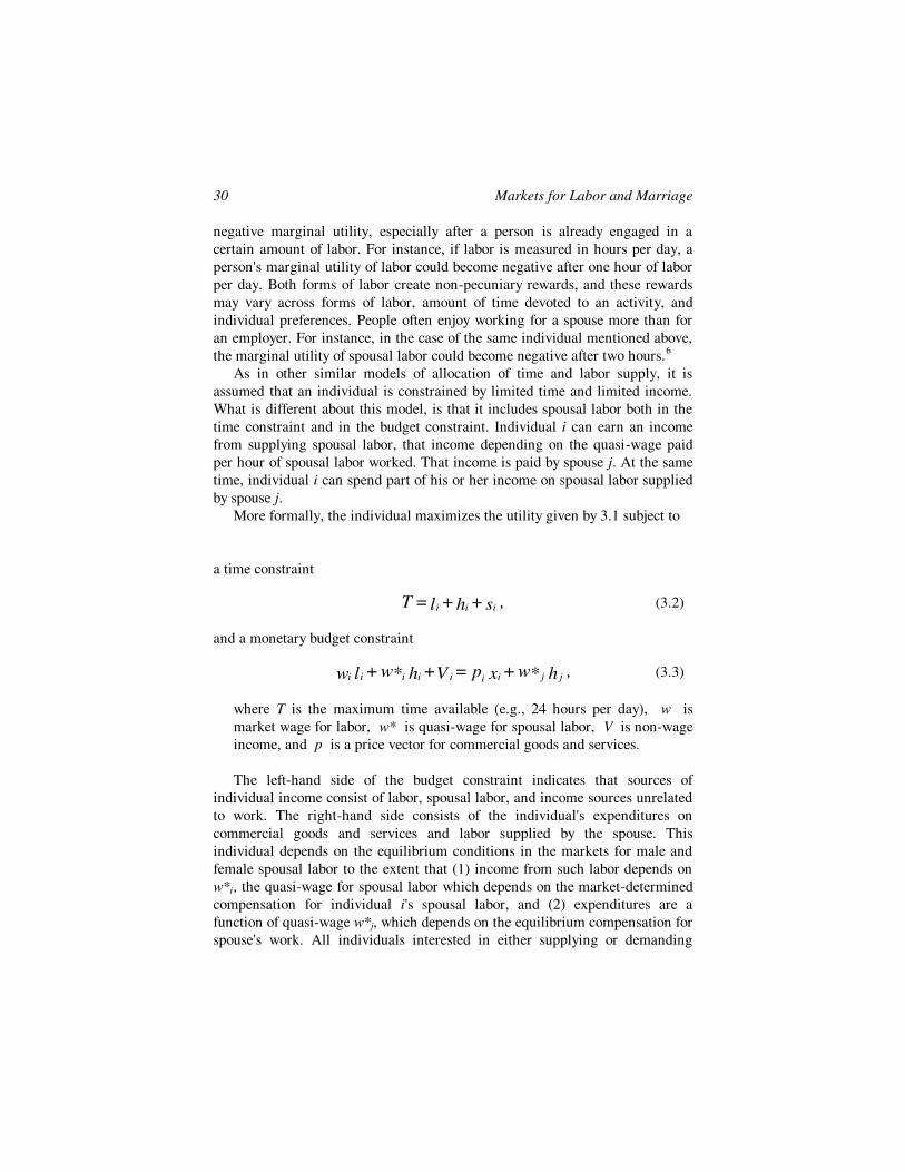
30 Markets for Labor and Marriage
negative marginal utility, especially after a person is already engaged in a
certain amount of labor. For instance, if labor is measured in hours per day, a
person's marginal utility of labor could become negative after one hour of labor
per day. Both forms of labor create non-pecuniary rewards, and these rewards
may vary across forms of labor, amount of time devoted to an activity, and
individual preferences. People often enjoy working for a spouse more than for
an employer. For instance, in the case of the same individual mentioned above,
the marginal utility of spousal labor could become negative after two hours.6
As in other similar models of allocation of time and labor supply, it is
assumed that an individual is constrained by limited time and limited income.
What is different about this model, is that it includes spousal labor both in the
time constraint and in the budget constraint. Individual i can earn an income
from supplying spousal labor, that income depending on the quasi-wage paid
per hour of spousal labor worked. That income is paid by spouse j. At the same
time, individual i can spend part of his or her income on spousal labor supplied
by spouse j.
More formally, the individual maximizes the utility given by 3.1 subject to
a time constraint
and a monetary budget constraint
where T is the maximum time available (e.g., 24 hours per day), w is
market wage for labor, w* is quasi-wage for spousal labor, V is non-wage
income, and p is a price vector for commercial goods and services.
The left-hand side of the budget constraint indicates that sources of
individual income consist of labor, spousal labor, and income sources unrelated
to work. The right-hand side consists of the individual's expenditures on
commercial goods and services and labor supplied by the spouse. This
individual depends on the equilibrium conditions in the markets for male and
female spousal labor to the extent that (1) income from such labor depends on
w*i, the quasi-wage for spousal labor which depends on the market-determined
compensation for individual i's spousal labor, and (2) expenditures are a
function of quasi-wage w*j, which depends on the equilibrium compensation for
spouse's work. All individuals interested in either supplying or demanding
,s + h + l = T iii (3.2)
,h * w+ x p = V + h * w+ l w jjiiiiiii (3.3)

Markets for Labor and Marriage 31
spousal labor affect the market wages for such labor (as shown in the next
subsection). This includes married people who can possibly divorce and
remarry.7
The compensation for spousal labor is not as readily observable as that for
labor. In the case of a housewife married to a working husband, the husband
transfers part of his income to the wife as a compensation for her spousal labor.
She thus earns quasi-earnings from spousal labor and uses these earnings to
purchase goods and services she enjoys, including food, lodging, or clothing. (It
does not matter if this describes the transaction accurately. The exchange of
work for income in the labor market can also take different forms, but nobody
denies that there is work for pay). If both husband and wife supply labor to each
other, barter will occur. The net income transfers may then possibly cancel out.
Maximizing the utility function 3.1 subject to constraints 3.2 and 3.3 yields
supplies of labor and own spousal labor, as well as derived demands for self-
oriented time, other's spousal labor, and commercial goods. From the first-order
conditions, and assuming p = 1, we have:
which indicates that in equilibrium the real wage per hour of work is equal to
the sum of the monetary equivalent of the value of that hour in self-oriented
activities and of the absolute (monetary) value of the disutility of work, and
which has the same meaning as equation 3.4, but relates spousal labor to time
for self. Combining 3.4 and 3.5 yields equation 3.6, which expresses the trade-
off conditions between the two types of work. Expression 3.6 indicates that time
is allocated between two occupations so that the wage in one occupation equals
the wage in the other occupation, plus the monetary equivalent of the difference
in marginal utility produced by these occupations.8
We are now ready to derive an individual supply of spousal labor (equation
3.7) and labor (equation 3.8), as well as a demand for other's spousal labor
(3.4)
(3.5)
(3.6)

32 Markets for Labor and Marriage
(equation 3.9). In reduced form, these variables are solely dependent on
exogenously determined parameters, including the quasi-wages w*'s, which are
based on quasi-wages established in marriage markets, as is shown in the next
subsection.
A graphical representation of these supply functions is found in Figure 3.1.
Panels a and b in Figure 3.1 describe examples of individual supplies of both
kinds of labor. Panel a describes a relationship between spousal labor and its
compensation, w*, whereas panel b presents a relationship between work and
its compensation w. It is assumed that initial hours of work produce positive
utility, thereby causing the supply curves to start at negative
wage levels. The individual whose labor supplies are depicted in Figure 3.1
enjoys the first hours of spousal labor more than the first hours of labor.
Both supply functions are assumed to have the characteristics giving rise to
the standard backward-bending form, i.e., the substitution effect caused by an
increase in the real wage (w*i in panel a and wi in panel b) initially dominates
the income effect, but eventually the income effect comes to dominate the
substitution effect. The equivalent of non-leisure in conventional models is here
the sum of labor and spousal labor. Although this latter sum is predicted to
decrease when income rises, this does not
necessarily mean that both labor and spousal labor decrease with higher
income.
Given that labor and spousal labor are alternative occupations, it follows
that wi is inversely related to the supply of spousal labor h, and that w*i is
inversely related to the supply of labor l. A substitution effect is likely to be
reinforced by an income effect. Non-wage income V is expected to discourage
both kinds of labor supply. After the derivation of market equilibria the reader
will find a comparison between this model and traditional labor theory in terms
of their implications for labor supply and the imputation of value of time in the
home.
The demand for hj is expected to be a downward sloping function of real
wage w*j for the usual reasons determining the slope of derived demands.
) V ,*w ,*w ,w( h = h ijiiii
(3.7)
) V ,*w ,*w ,w( l = l ijiiii (3.8)
) V ,*w ,*w ,w( h = h ijiijj (3.9)
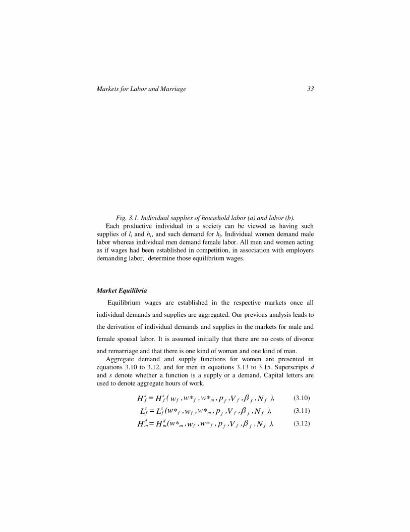
Markets for Labor and Marriage 33
Fig. 3.1. Individual supplies of household labor (a) and labor (b).
Each productive individual in a society can be viewed as having such
supplies of li and hi, and such demand for hj. Individual women demand male
labor whereas individual men demand female labor. All men and women acting
as if wages had been established in competition, in association with employers
demanding labor, determine those equilibrium wages.
Market Equilibria
Equilibrium wages are established in the respective markets once all
individual demands and supplies are aggregated. Our previous analysis leads to
the derivation of individual demands and supplies in the markets for male and
female spousal labor. It is assumed initially that there are no costs of divorce
and remarriage and that there is one kind of woman and one kind of man.
Aggregate demand and supply functions for women are presented in
equations 3.10 to 3.12, and for men in equations 3.13 to 3.15. Superscripts d
and s denote whether a function is a supply or a demand. Capital letters are
used to denote aggregate hours of work.
), N , ,V ,p ,*w ,*w ,w(H = H ffffmffsf
sf (3.10)
), N , ,V ,p ,*w ,w ,*(wL = L ffffmffsf
sf (3.11)
), N , ,V ,p ,*w ,w ,*(wH = H ffffffmdm
dm (3.12)
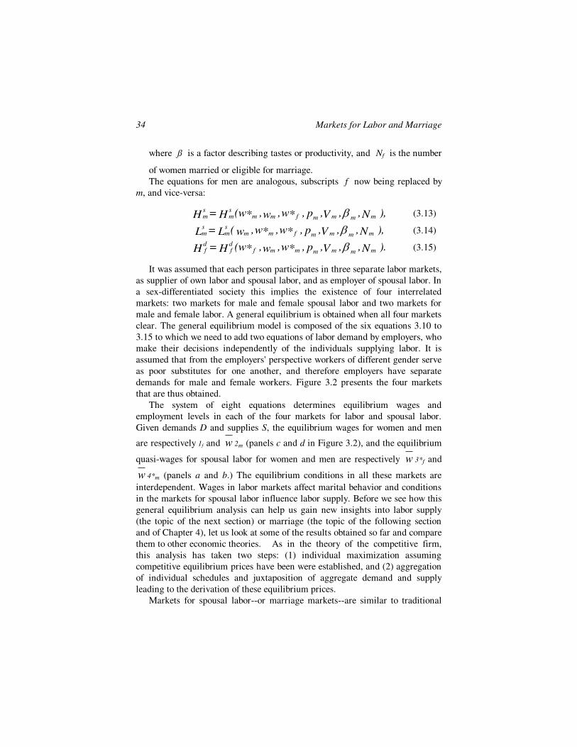
34 Markets for Labor and Marriage
where ß is a factor describing tastes or productivity, and Nf is the number
of women married or eligible for marriage.
The equations for men are analogous, subscripts f now being replaced by
m, and vice-versa:
It was assumed that each person participates in three separate labor markets,
as supplier of own labor and spousal labor, and as employer of spousal labor. In
a sex-differentiated society this implies the existence of four interrelated
markets: two markets for male and female spousal labor and two markets for
male and female labor. A general equilibrium is obtained when all four markets
clear. The general equilibrium model is composed of the six equations 3.10 to
3.15 to which we need to add two equations of labor demand by employers, who
make their decisions independently of the individuals supplying labor. It is
assumed that from the employers' perspective workers of different gender serve
as poor substitutes for one another, and therefore employers have separate
demands for male and female workers. Figure 3.2 presents the four markets
that are thus obtained.
The system of eight equations determines equilibrium wages and
employment levels in each of the four markets for labor and spousal labor.
Given demands D and supplies S, the equilibrium wages for women and men
are respectively 1f and w 2m (panels c and d in Figure 3.2), and the equilibrium
quasi-wages for spousal labor for women and men are respectively w 3*f and
w 4*m (panels a and b.) The equilibrium conditions in all these markets are
interdependent. Wages in labor markets affect marital behavior and conditions
in the markets for spousal labor influence labor supply. Before we see how this
general equilibrium analysis can help us gain new insights into labor supply
(the topic of the next section) or marriage (the topic of the following section
and of Chapter 4), let us look at some of the results obtained so far and compare
them to other economic theories. As in the theory of the competitive firm,
this analysis has taken two steps: (1) individual maximization assuming
competitive equilibrium prices have been were established, and (2) aggregation
of individual schedules and juxtaposition of aggregate demand and supply
leading to the derivation of these equilibrium prices.
Markets for spousal labor--or marriage markets--are similar to traditional
), N , ,V ,p ,*w ,w ,*(wH = H mmmmfmmsm
sm (3.13)
), N , ,V ,p ,*w ,*w ,w(L = L mmmmfmmsm
sm (3.14)
). N , ,V ,p ,*w ,w ,*(wH = H mmmmmmfdf
df (3.15)
Markets for Labor and Marriage 35
labor markets. In all labor markets, market forces are relatively difficult to
identify because of the absence of physically visible institutions, rigidities in
compensation levels and hours of work, limitations on the relative proportion of
pecuniary to non-pecuniary compensation, etc. Such restrictions may be
particularly relevant in the case of spousal labor markets. Participants in
markets for spousal labor face an additional restriction that prohibits polygamy,
thereby forcing one-to-one matches. 9 However, in other labor markets there
exist similar restrictions on the demand side, as we tend to get matches between
one employer and a few employees.
This market model of marriage is based on the assumption that choices are
available, which means that actual or potential spouses are substitutable. This is
especially likely to be the case in densely populated areas. It is assumed that
people have some freedom in deciding whether to become, or remain, married,
and in establishing--often implicit--reciprocal spousal

36 Markets for Labor and Marriage
Fig. 3.2. Markets for (a) Female spousal labor; (b) Male spousal labor;
(c) Female labor; and (d) Male labor.
employment contracts. It is assumed that single persons interested in marriage
(or their representatives) respond to market forces and decide accordingly
whether to marry and how much spousal labor to contribute and employ.
Married people are also viewed as responsive to markets for spousal labor, their
response being a function of the degree of substitutability between one's current
spouse and alternative spouses. In turn, this depends on whether recontracting
into new marriages is costly or not.
In a monogamous society marriage tends to occur when at the equilibrium
w 5*f and w 6*m a man demands the amount of spousal labor a woman wants to
supply and that woman demands the amount of labor supplied by the man. A
married couple in equilibrium experiences no excess demand for, or supply of,
spousal labor at the relevant w*'s. Exchanges of such labor are egalitarian if the
market value of her services w*f hf is identical to w*m hm, the market value of his
services. To the extent that w*f hf exceeds w*m hm, the husband transfers goods
(or means to purchase goods) to the wife. Net transfers from the wife to the
husband are also possible.
This view of marriage may sound strange. As a description of attitudes it is
probably not much more controversial than what economists write about
decision making by firms. However, our goal is not to describe, but rather to
derive testable hypotheses. Feelings are not necessarily absent from this theory.
Personal liking can formally be incorporated in the form of a higher demand
curve for the spousal labor of a particular person (or a shift to the right in the
supply of such labor to that person).
This view of marital relations differs from previous economic analyses of
marriage in its emphasis on the time spouses devote to each other's service.
Changing outside factors can lead not only to changes in income redistribution
between the spouses or to marital break-up (as in Becker 1973, 1981), but also
to new marital labor relations. Thus a married woman's sudden realization that
attractive labor market opportunities are open to her could possibly lead to a
new spousal employment contract, the wife reducing her burden of spousal
labor and using some of her additional wage income to obtain substitutes for
her spousal labor, including perhaps her husband's spousal labor.
So far it has been assumed that men and women are respectively
homogeneous. In the real world, populations are heterogeneous. People of
certain classes, races, or religions may be forbidden to intermarry. In such
cases, separate markets could be considered, one for each group of substitutable
potential spouses.10 In that sense, again, spousal labor markets are not
intrinsically different from other labor markets.
Markets for Labor and Marriage 37
The competitive market model may not always be applicable. Monopolistic
elements enter into an existing marital relationship to the extent that divorce
and marriage are costly (e.g., due to search costs). In that case one could find
divergence between the market w* and the particular w* prevailing in a
particular couple. Bilateral monopoly could often operate. Partners
experiencing higher divorce and remarriage costs are likely to absorb more
consequences of monopolistic exploitation (see Chapter 10).
The remainder of this paper deals primarily with this theory's implications
for labor supply. It is shown that labor economics can be enriched by taking
account of conditions in spousal labor markets, even though w*f or w*m cannot
be directly measured. New insights are offered regarding (1) new variables that
may affect labor supply and are not typically incorporated into labor theory, and
(2) reinterpretations of the effect of variables included in traditional labor
theory.
Implications for Labor Supply The model presented here--a general theory of labor and marriage or GTM--
differs in a number of ways from traditional models of labor supply. Some of
these differences are summarized in Table 3.1. In both models the decision to
enter the labor force is based on a comparison of the attractiveness of work,
measured as the wage (possibly minus the monetary equivalent of the disutility
of work) and the attractiveness of staying at home, which is typically denoted as
the reservation wage w*. Traditional theory of labor supply and the theory
presented here differ first and foremost in the way they derive w*, the value of
time in the home.
Value of Time, w*. Traditionally, w* is derived assuming a predetermined
marital status. Households are either single persons or husband-wife teams with
no options to marry or divorce. The assumptions common to the traditional
literature translate into an individual supply of time for home production in the
form of a transposed L, horizontal at the wage level the individual would
receive if working in the market sector and vertical as soon as the time
constraint is reached. As it is difficult to measure value of time, previous
researchers have included variables which influence such value of time in their
estimations of labor supply. For instance, it has been found that indicators of
women's value of time in the home, such as number and age of children and
husband's income, are inversely related to married women's labor supply (for an
early example, see Mincer 1962).
In the traditional model, the value of a person's time depends only on

38 Markets for Labor and Marriage
household characteristics. There exists no market for spousal labor. Households
are interdependent only to the extent that they supply work to
the same markets or that they buy goods from the same sellers. By using
households as their decision-making units and by assuming that men and
women are permanently bound into families, economists have lost sight of
some important determinants of labor supply, especially the labor supply of
married women. The realization that the supply of labor can shift following
changes in a market-determined wage for spousal labor or quasi-wage w*,
opens new directions for research in labor economics and in particular, for
studies of female labor supply.
Whereas according to traditional theory w* is entirely established in the
household, according to GTM, value of time in the home is partially established
in a market for marriage. Both traditional theory and GTM recognize that the
value of time contains a non-pecuniary or psychic component based on how
much one values activities other than work-for-pay, including activities
performed in the framework of marriage. Where the theories diverge is in that
GTM recognizes that value of time w*--in particular, married women's value of
time--may have a pecuniary (but not necessarily monetary) component as well.
In most societies, including our own, most husbands offer their wives some
form of material or pecuniary compensation for work married women perform
in the framework of marriage, usually in the home. According to GTM this
pecuniary component of the value of time varies positively with value in one's
marriage market (the market for one's spousal labor). In particular, the better
women's marriage market, the higher the pecuniary compensation they can get
as wives and the higher their value of time. A number of reasons why a
woman's value in the marriage market may vary are discussed in the remainder

Markets for Labor and Marriage 39
of this chapter and in the next chapter.
Individual w*'s may diverge from the equilibrium w* established in one's
marriage market to the extent that there are costs of divorce and remarriage (in
short, costs of divorce.)
The more it is costly to divorce and remarry, the more the actual w* of a
married person is likely to diverge from the w* established in the corresponding
marriage market. For instance, a married woman to whom divorce and
remarriage would be costly will be willing to accept a w* below the market-
determined value of time. This is analyzed in more detail in Chapter 10.
Furthermore, an individual w* may diverge from the market-determined w*
due to the presence of non-pecuniary benefits from work and spousal labor.
Even if divorce costs are zero, an individual asking w* based on equation 3.5
may diverge from the equilibrium w* established in the market for spousal
labor. Some people may collect an economic rent from supplying spousal labor
to the extent that their individual asking w* is lower than the w* in the market.
Further individual variations in w* could also be attributed to individual
differences in spousal labor productivity.
According to traditional theory, the value of time in the home always
depends on the individual's work status. If the individual works, the value of
time w* is equal to the wage, and if she does not work, w* exceeds the wage.
According to GTM the value of time depends on work status to the extent that
indivisibilities in hours of work play a role. For both working and non-working
married individuals, value of time is equal to a w* based on a market-
determined pecuniary component, divorce costs, and a non-pecuniary
component. Assume that an individual's market w* is the one found on the left-
hand side of equation 3.6. That w* is then equal to the right-hand side of
equation 3.6, i.e. the wage plus the difference in utility between the two
occupations. If divorce and remarriage are costless and hours of work outside
the home and in the household are easily divisible, the value of time equals the
same w* established in the marriage market whether the individual works or
not. If hours of work are not so easily divisible, the individual may have to
spend either too much or too little time at work, in comparison to a situation of
perfect divisibility. For instance, if there are fixed costs of going to work, a
solution of spending 7 hours in h and 1 hour in l is not feasible. Instead the
individual may not work outside at all, i.e. h will be 8 and l will be zero. This
implies that the value of time w* will be higher than the left-hand side of
equation 3.6, the market-determined w*. If the individual spends "too much"
time at work in comparison to an optimal allocation of time, then the actual w*
will be lower than the market-determined one.
The Decision to Work. Following these basic differences in the way the two
theories define value of time at home w* the two theories also lead to different
40 Markets for Labor and Marriage
hypotheses regarding labor supply. According to both theories the decision to
work is based on a comparison of w and w*. Traditional theory estimates w*
based on the utility of leisure. Such estimates are based on the characteristics of
the individual or the household. The decision to work can also take account of
the (dis)utility of labor, as is assumed in the last column of Table 3.1.
According to GTM, the decision to work is also based on a comparison
between w and w*. However, GTM views w* as depending on more factors than
those taken into consideration by traditional theory. According to GTM, w* is
composed of a pecuniary and a non-pecuniary component. In turn, the
pecuniary component depends on
(1) the equilibrium value of the quasi-wage for spousal labor, established
in a market for such spousal labor, and
(2) costs of divorce and remarriage.
The non-pecuniary component of w* depends on the difference in the value of
marginal utilities of work and spousal labor h.
The higher the value of time--both pecuniary and non-pecuniary--the less a
person is likely to participate in the labor force. If women prefer to perform
household tasks at home instead of working for pay outside the home, the wage
needs to exceed the pecuniary compensation for work in the home.
The introduction of a component of w* established in a market for spousal
labor (or marriage market) leads to a number of theoretical implications which
are derived next. New variables are introduced into the analysis of labor supply:
namely sex ratios and group differences in marriage opportunities. I also
discuss new interpretations of income and wage effects, and of the backward-
bending supply of labor.
The sexual differentiation assumed in the rest of this discussion follows
observed patterns of division of labor, women being generally responsible for
most household production. It is also assumed that both men and women differ
in productivity, tastes, and income.
Marriage Squeeze Effects
Demographers have defined sex ratios as the number of males divided by
the number of females. A marriage squeeze for men occurs when the sex ratio
exceeds 1, and a marriage suqeeze for women when the sex ratio is less than 1.

Markets for Labor and Marriage 41
Sex ratios and female labor force participation are connected to the extent that
marriage squeezes and sex ratios influence the market-determined value of time
w*, and in turn that value of time is related to the decision to participate in the
labor force.
It follows from the general equilibrium equations (3.10 to 3.15 plus two
labor demand equations) that the number of women Nf and the number of men
Nm are parameters which can potentially influence the equilibrium value of all
wages w and w*. Given that the sex ratio is the ratio Nm/Nf , it follows that the
sex ratio is also a determinant of wages and quasi-wages w*. In particular,
given the importance of spousal labor as an alternative form of employment for
married women, married women's value of time w* may be a function of sex
ratio.
In order to derive hypotheses regarding the effect of marriage squeeze and
sex ratio on the value of time w* and the labor supply of married women, we
start by decomposing the sex ratio into its two components. Consider the simple
case of an increase in Nm, the number of males, for instance due to a wave of
all-male immigration. Such increase in Nm affects the system of equations 3.13-
3.15: men's aggregate supplies of labor and demand for wife labor all shift to
the right. In order to predict the net effect of such increase in the number of
men on female labor supply we divide the analysis into three stages: (1) initial
effects on w*f (2) secondary effects on w*f and (3) effect of w*f on the amount of
labor supplied by women.11
1. Initial Effects. According to function 3.15, an increase in Nm causes an
increase in the aggregate demand for female spousal labor. In
graphical terms, this implies a shift to the right from D to D' in panel
a of Figure 3.2, thereby leading to an increase in the market-
established w 7*f. Also, decreases in male equilibrium wages w 8*m
and w 9m originate from shifts in supply in panels b and d (downward
rigidity in wages may impede adjustment in both labor markets).
2. Secondary Effects. These wage changes in turn cause more changes.
Lower male income due to reductions in both male wages tends to
push the aggregate demand for female spousal labor, Hf , back down.12
Moreover, a lower male household wage wm also tends to lead to a
reduction in demand for Hf due to a substitution effect in home
production and consumption (assuming male and female spousal labor
42 Markets for Labor and Marriage
are substitutes). This factor will be minor if men don't engage much in
spousal labor, as is the case in many societies. If it is assumed that
such leftward shift in the demand for Hf from D' to D" is smaller than
the original rightward shift from D to D', the equilibrium wage w*f
ends up increasing in comparison to its pre-immigration level, for
instance to post-immigration wage for wife labor w 10*f'' in Figure 3.2
(panel a).
3. Labor Supply. In turn, the rise in wage in one occupation, spousal labor,
causes a decrease in the supply curve to the other occupation. This
follows from equation 3.8, according to which the supply of labor is
inversely related to w*f due to a substitution and income effect.
Accordingly, women's supply of labor is expected to shift leftwards to
S' in panel c.13 In addition, lower wages for male workers induce
employers to substitute male workers for female workers, leading to a
downward shift in D, the demand for female workers, in panel c.
This combination of a reduction in demand and in supply of female labor
unambiguously leads to a reduction in total female employment. We have thus
seen that an increase in the number of men--which brings a marriage squeeze
for men--is predicted to cause an increase in women's value of time w* and
therefore a decrease in total female employment. In general,
Hypothesis 1
A marriage squeeze for men is expected to be associated with less female
labor supply than a marriage squeeze for women.
The aggregate employment levels in Figure 3.2 do not determine the
division between total number of workers and hours of work per worker. The
effect of a marriage squeeze for men is likely to act on both these dimensions: it
will (1) reduce the proportion of women who participate in the labor force, and
(2) decrease the number of hours individual women work outside the home.
While the predictions regarding the effect of a marriage squeeze for men on
employment levels are unambiguous, the prediction regarding its effect on
wages is ambiguous. Female wages could go up or down, depending on whether
demand or supply shifts more in the market for women's work.14
Hypothesis 1 holds for all women participating in marriage markets affected
by an increase in the number of men. If we distinguish between married women
and single women, and both groups participate in marriage markets, we expect
the hypothesis to hold separately for married women and for single women.
Given that single women do not face divorce costs, their w* is likely to vary
Markets for Labor and Marriage 43
more with market conditions than the w* of married women. However, it is
expected that Hypothesis 1 is more applicable to married women than to single
women given that an occupational choice between work and spousal labor is
likely to be less relevant to single women than to married women. Although it
may have been more common in the past, few single women today reduce their
participation in the labor force in order to prepare for marriage. A correlate of
Hypothesis 1 is therefore that
Hypothesis 1'
A marriage squeeze for men is expected to be associated with less labor
force participation by married women than a marriage squeeze for women.
Related hypotheses are developed in Chapter 6, which also reports tests for
some of the hypotheses linking marriage squeezes and labor supply. Recent
trends in the sex ratio of those eligible for marriage and in female labor force
participation tend to support Hypothesis 1, which states that marriage squeezes
are related to female labor supply. As pointed out in Glick et al. (1963),
marriage squeezes and sex ratios vary over time because (1) on average, women
marry men who are generally somewhat older, and (2) the number of births
fluctuates from year to year. In the early 1950s there were more men than
women in most western countries as a result of declining numbers of births
during the late 1920s and early 1930s. Conversely, in the mid-sixties, when the
baby-boom generation started to reach marriageable age, women in the United
States and other countries with similar demographic trends, began to
experience a shortage of men. Heer (1978) and Heer and Grossbard-Shechtman
(1981) show that this was true in the United States by 1964.15 Since the U.S.
birth rate started a renewed downward trend from 1961, young men have been
finding relatively few marriageable women in the 1980s.
Consistent with Hypotheses 1 and 1' is the dramatic upsurge in the
employment of U.S. women--married women in particular--that occurred in the
late sixties and during the seventies, a period of marriage squeeze for women.
This increase persisted "despite a significant slowing of the growth in real
wages and dramatic acceleration of the rate of inflation. In fact, between 1973
and 1975, real wages fell in two successive years, yet women's labor force
participation continued to grow" (Niemi and Lloyd 1980). Increased
participation despite stagnant wages supports Hypothesis 1, whereby a
reduction in sex ratio pushes the supply of labor rightwards, whereas wages
may go down to the extent that an increase in women's supply of labor
dominates an increase in employers' demand for female labor following a
decrease in male manpower. A popular alternative explanation for the growth
in female labor supply, namely an increase in the demand for female workers,
implies an unambiguous increase in wages.16 Since 1990, for the first time in
44 Markets for Labor and Marriage
almost thirty years, there has been a decrease in women's labor force
participation. This could be related to the marriage squeeze for men of the
baby-bust generation that followed the baby-boom (see Chapter 5).
Additional evidence for the theory is provided by comparisons between
blacks and whites in the United States. Black women have generally been found
to have higher rates of participation in the labor force than white women (for
instance, in a study of labor force attachment soon after pregnancy by Mott and
Shapiro 1978), even after statistical control for income, education, marital
status, and other important variables. This can be explained by the marriage
squeeze hypothesis stated here, for among U.S. blacks the sex ratio of those
eligible for marriage is significantly lower than among whites, due to lower sex
ratio at birth, higher mortality, and higher rates of imprisonment. Moreover,
black males show a much higher tendency to intermarry with whites than do
black females, which adds to the shortage of men experienced by black women
(see Spanier and Glick 1980).
Effects of Individual or Group Differences in Marriage Opportunities
As can be seen from equation 3.6 variation in labor force participation can
be a consequence of variation either in wages or in the value of time in the
home. In their empirical studies economists have looked solely at household
characteristics (such as number and age of children or number of adults) as
determinants of the value of women's time and those of labor supply. (See, for
instance, Gronau 1973, Heckman 1974).17 It follows from this theory that
individual or group differences in marriage opportunities are also related to the
value of time in the home, and therefore labor supply.
The following hypothesis can possibly be tested using a variety of factors
influencing value of time w*.
Hypothesis 2
The higher a woman's value in the marriage market, the higher her value of
time and the lower her labor supply.
Value in the marriage market is not always easy to establish. As mentioned
Markets for Labor and Marriage 45
above, education and income of family of origin could possibly influence value
in the marriage market. A woman's ability to marry into a wealthier family
(judging from a comparison of wealth or income in the bride's and the groom's
family), or her relative number of previous marriages, might also serve as
indicators of her w* (holding other characteristics constant).18
Furthermore, the pecuniary component of a particular woman's value of
time depends not only on her own characteristics and overall value in the
marriage market. In the case of married women, the pecuniary component of
w* also depends on the husband's characteristics. Compensating differentials
may exist, whereby husbands who offer relatively low non-pecuniary benefits to
their wife make up for such shortcoming by providing their wife with more
generous pecuniary benefits than do husbands offering relatively high non-
pecuniary benefits. In other words, husbands can make up for an undesirable
trait, such as old age or poor health, by sharing a higher proportion of their
wealth with their wife. Given that the supply of labor depends on alternative
ways of obtaining pecuniary benefits, it follows that
Hypothesis 3
Compensating differentials leading to pecuniary compensations by
husbands to wives have a discouraging effect on wives' labor supply.
This hypothesis holds for a given income level of husbands, as it is assumed
that husbands do not automatically share a fixed proportion of income with
their wife. Hypothesis 3 will be tested in Chapter 7.
More hypotheses relating marriage-market factors to labor supply could be
elaborated, but I prefer to limit this theoretical discussion to hypotheses that
build towards the more empirical chapters found later in this book.
Furthermore, GTM, the theory presented here, can also shed new light on
traditional topics in labor supply theory, such as wage and income effects.
Marriage and Wage Racial or ethnic origin can not only shift the constant term in labor supply
regressions, but it can also influence the slope of a labor supply. Wage effects
often differ by characteristics such as racial or ethnic origin.
Such differences in slope have been explained in the past in terms of cultural
differences or discrimination. Traditional labor supply theory does not
recognize that marriage market conditions can influence the elasticity of labor
supply. It is hypothesized here that differences in marriage market conditions
can also account for some racial or ethnic differences in wage effects.
In order to see how marriage market conditions can have an effect on the

46 Markets for Labor and Marriage
elasticity of labor supply consider the example of two ethnic or racial groups.
Figure 3.3 represents the supply of two women, one from each group, with
identical opportunities w0 and w*0 in the two relevant labor markets.
Originally, their supply coincides at supply S. We then compare these two
women with women who are offered a higher wage, w1. The observed elasticity
of labor supply, based on a cross-section of each group, could differ across
groups due to varying correlations between w and w*. If there is no link
between w and w*, the observed elasticity is also the true elasticity However, if
w and w* are positively correlated, for instance, because the same unmeasured
characteristics--such as ability--raise opportunities in both the labor market and
the spousal labor (or marriage) market, an increase in wages from w0 to w1
leads simultaneously to both a movement along the supply curve and a leftward
shift of the supply curve (due to a substitution effect and an income effect away
from work). The observed elasticity then differs from the true elasticity. More
specifically,
Fig. 3.3. Labor supply elasticity for two groups of women.
Hypothesis 4
The more positively w* and w are correlated in a cross-section of women,
the lower the observed elasticity of labor supply.
Markets for Labor and Marriage 47
A case in point is the finding by Gronau (1981) that in Israel the labor force
participation of women of Asian-African origin is more sensitive to changes in
wage (actual or potential) than that of European-American women. Gronau's
explanation for the higher observed elasticity of labor supply among Asian-
African women is that the former women react more to pecuniary rewards. The
present theory leads to an alternative explanation based on ethnic differences in
the prevalence of marriage. Marriage seems to be more prevalent among Asian-
African Jews than among European-American Jews, as indicated for instance
by the lower percent of the population at marriageable age who is unmarried
among Asian-African Jews. This is probably related to stricter adherence to
traditional spouse roles among Asian-African Jews (documented for instance by
Yogev and Ayalon 1982). As a result of these differences in marriage patterns,
it is more likely that talented Asian-African women will specialize in spousal
labor and not work at all outside the home, which implies a lower correlation
between w and w* than for women of European-American origin. In turn, a
lower observed correlation between w and w* among Asian-African women
than among European-American women implies that the observed elasticity
and the true elasticity are more likely to coincide in the case of Asian-African
women than for European women. In the case of European-American women
the supply schedule is more likely to shift leftwards to Se, implying a lower
observed elasticity of labor supply for European-American women than for
Asian-African women.
Available evidence suggests that whereas all Israeli women succeeding more
in marriage are less likely to work, this is more so among women of Asian-
African origin. For instance, Matras and Selby (1981) found that all women
who married men whose father had a higher occupation than their own father
(an indicator of higher w*f) were less likely to participate in the labor force, but
that a high w*f had a much more discouraging effect on the labor-force
participation of Asian-African women. This could indicate that wf and w*f are
correlated less positively in that group than among European-American Jews.
This alternative explanation of group differences in the elasticity of labor
supply thus seems to be applicable to Israel.19
Hypothesis 4 could also be applied to Black-White differences in the
elasticity of labor supply in the United States. Hall (1973) found a positive
elasticity of substitution for U.S. women as a whole, while he found a negative
elasticity of substitution for a sample of U.S. black wives. Hall's finding can be
explained in terms of black-white differences in marriage and family patterns.
For whatever reasons (possibly a more imbalanced sex ratio among blacks),
marriage and specialization in spousal labor are found less frequently among
blacks than among whites. Some talented white women, who could possibly
obtain both a high w and a high w* may end up having either a high w or a

48 Markets for Labor and Marriage
high w*, as many of them have the option of specializing in spousal labor. That
option being very rare for talented black women, one expects more of a positive
correlation between the w and w* of various women among blacks than among
whites. In turn, a higher correlation between w and w* among black women
than among white women implies less of a negative elasticity of substitution in
black women's labor supply among black women than among white women,
which is consistent with Hypothesis 4. It is hoped that this interpretation of
Hall's finding will be tested more directly, as it has important policy
implications.
A general theory of labor and marriage can also be used to derive predictions
regarding male and female differences in elasticity of labor supply. Individual
supply of labor outside the home can be substituted for both spousal labor and
self-oriented time. The (compensated) supply of (outside) labor by married
women will be more elastic than that of married men in view of the larger
possibilities of substitution between the two types of work available to women
in comparison to men. This conclusion can also be found in traditional labor
theory. When we analyze uncompensated wage effects which also include
income effects, the analysis according to GTM becomes more complicated.
Before considering such uncompensated wage effects, we look at income
effects.
Marriage, Divorce and Income
The present theory also leads to new insights regarding income effects on
Markets for Labor and Marriage 49
labor supply and divorce. Income effects on labor supply are examined here,
and income effects on divorce are analyzed briefly in Chapter 4, and in more
detail in Chapter 10. It follows from this theory that income effects on labor
supply are likely to be different for men and women. Furthermore, income
effects on the labor supply of married workers are closely related to income
effects on divorce. We start by considering changes in income originating from
sources other than own labor, i.e. non-wage income. It is assumed that these
changes were not expected at the time of marriage.
Consider independent increases in the non-wage income of a couple initially
in equilibrium at the market wages for spousal labor w 11*f and w 12*m (see
Figure 3.4). Assuming that spouse's labor is positively related to own income in
utility function 3.1, higher incomes lead to rightward shifts in each spouse's
demand for the other's labor (both husband and wife have a demand for spousal
labor such as function 3.9 where the partial effect of non-wage income, V, is
positive). If the shifts are proportional to the existing amount of spousal labor
supplied, in most cases the shift in husband's demand for the wife's labor will
be larger than the corresponding shift in wife's demand for the husband's labor.
At the same time, the willingness to supply one's own labor is most likely to
decrease as a result of higher income V. This follows from negative partial
effects of V on h and l according to equations 3.7 and 3.8. Graphically, this
implies that S shifts leftwards in both panels of Figure 3.4, and probably by a
larger absolute amount in the case of female spousal labor than in that of male
spousal labor.
Assuming market wages for spousal labor have not changed (e.g., because
few people are facing a similar increase in income), this couple now
experiences excess demands for spousal labor. Given wives' specialization in
spousal labor, excess demand for the wife's labor is expected to be larger than
excess demand for the husband's labor.
The effects of such excess demands for spousal labor depend on whether
divorce and remarriage are costly. With zero divorce costs, the couple who was
previously in equilibrium in Figure 3.4 will opt for a divorce and remarriage to
new partners with whom they do not experience excess demand for spousal
labor.
If divorce is costly and the couple chooses to remain married, they can do
two possible things: (1) let the material component of w* they give each other
increase beyond the market level w 13*f and w 14*m, or (2) find ways to reduce
excess demands for spousal labor. One way to reduce such excess demand is by
50 Markets for Labor and Marriage
an increase in the supply of spousal labor at the expense of
Fig. 3.4. Income effects on spousal labor.
labor outside the home. To the extent that there existed an initial division
of labor associated with larger amounts of the wife's spousal labor, this
adjustment will require a larger reduction in the wife's labor supply than in her
husband's. To the extent that internal adjustments in w* are limited, it follows
that
Hypothesis 5
If a husband and wife who are married to each other experience
independent equal increases in income, the wife's labor supply is likely to
decrease more than the husband's.
This rejoins Mincer's (1962) conclusion that changes in household income
are likely to reduce the wife's labor supply more than the husband's. What the
present analysis adds is that it points out to some of the correlates of this
asymmetric effect of income on husband's and wife's labor supply. It will be
shown in Chapter 10 that the effect of income on husband's and wife's labor
supply is likely to be more asymmetric the higher the divorce costs, the higher
the divorce costs of the wife relatively to those of the husband, the more the
wife's income is affected relatively to the husband's income, the fewer the
substitutes for spousal labor, and the more women are willing to substitute
between labor and spousal labor.
Part of this discussion of marriage, divorce and income effects is also
applicable to the study of wage effects. An uncompensated wage (w) increase

Markets for Labor and Marriage 51
includes (1) a positive income effect leading people to work less in general, and
most likely also less outside the home, and (2) a positive compensated wage
effect leading to substitution of outside labor for spousal labor and time for self.
It follows from the theory that both these effects will have a stronger
discouraging influence on the labor supply of wives than of husbands, if
couples stay married. Wives will increase their spousal labor in order to bridge
the gap between demanded and supplied spousal labor that originates from a
wage increase experienced by both wife and husband.
Hypothesis 5 was tested using results from a Negative Income Tax (NIT)
program, which transferred income as a function of earnings, and therefore
included both a positive income effect and a negative compensated wage effect.
These results, presented in Chapter 10, support Hypothesis 5.
The analysis leading to Hypothesis 5 also implies that unexpected changes
in income will cause divorce. This is discussed in more detail in Chapters 4 and
10.
The Backward-Bending Supply of Labor
The traditional explanation for a backward-bending supply of labor is that
the supply has a negative slope when a negative income effect dominates a
positive substitution effect. The reasoning behind ethnic or racial differences in
the elasticity of labor supply can also provide an additional rationale for a
backward-bending supply curves. The backward-bending supply of labor could
result from a positive correlation between w and w*, a situation relevant to
women more than to men. Higher wage levels could cause leftward shifts in the
supply of labor if w* and w are positively correlated (e.g., due to lack of control
for ability). If the ensuing shift in supply is large enough, the observed supply
schedule could have a negative slope. In order to see that, one can visualize a
supply of labor such as the one presented in Figure 3.3, which lies to the left of
Se, sufficiently so in order for the observed amount of labor supplied by women
obtaining a wage w1 to be less than the amount supplied by women obtaining a
wage w0.
It follows from this explanation that a backward-bending supply curve is
more likely to be observed among women than among men. It should not come
as a surprise, therefore, that one of the few cross-sectional studies finding a
backward-bending supply of labor used a sample of nurses (Link and Settle
1981).20
Other Implications
52 Markets for Labor and Marriage
This section briefly mentions some additional implications of this theory of
allocation of time in markets for labor and marriage regarding consumption,
fertility and marriage. Many of the implications for marriage are developed in
more detail in Chapter 4.
Consumption. As has been mentioned by Becker (1973,1981), the relative
position of husbands and wives in their respective marriage markets is
predicted to influence their consumption patterns. In terms used here, the
higher w*f relatively to w*m, the higher the wife's well-being compared to the
husband's. One of the means by which this could be expressed is through a
large share of household expenditures benefitting the wife rather than the
husband. Variation in relative compensations for spousal labor could also
explain related trends in gender differences in health, longevity, or time spent
on recreational activities.
Fertility. The study of fertility is another area that could benefit from this
theory. It follows from the theory presented above that there will be no strong
contrast between male income effects on the fertility of married women who are
not employed outside the home and those effects on married women working
outside the home. In contrast, according to Willis (1974) and others following
his approach, an increase in husband's income will not affect the time cost of
children of a married woman employed in the labor force, unless she is induced
to stop working outside the home, whereas such increase in husband's income
is expected to lead to an increase in the value of time of a housewife. From
Willis' point of view, so long as a woman is working outside the home, the
value of her time equals her wage and is unaffected by changes in male income.
But if male income rises and the wife is not working outside, the demand for
spousal labor shifts upwards, her value of time in the home and cost of children
rise, which attenuates the impact of an income effect. This leads Willis to
predict that the absolute value of a male income effect on fertility will be larger
if the wife works outside the home than if she does not.
In contrast, it follows from this model that a woman's value of time in the
home is determined in a market for spousal labor. A rise in the demand for
women's spousal labor resulting from an increase in male income may be
associated with an increase in the value of time in the home (w*), even for
women working outside the home. For instance, in the case of time series,
increases in aggregate male incomes are expected to cause a rightward shift in

Markets for Labor and Marriage 53
demand for women's spousal labor, and therefore an increase in w*, the value
of women's time. However, it remains true that a shift in demand at a point
where the supply is closer to vertical will cause a larger increase in w* than an
upward shift in demand at a point where the supply curve is more elastic, and
that supply is less likely to be elastic when women do not work outside the
home. Also, as pointed out earlier, income effects on value of time depend on
divorce costs. But according to the present approach, it does not necessary
follow that the male income effect on fertility will be stronger if labor force
participation by married women is more widespread, an implication stated in
Willis (1974). It is therefore not surprising that Ermisch's (1979) analysis of
British time series of fertility and Butz and Ward's (1979) analysis of such
series for the United States did not show that male income had a stronger
positive effect if women participated in the labor force. Whatever one's source
of interest it is important to appreciate that, according to equation 3.6, the value
of someone's time in the home does not need to be equal to their wage in the
labor market (assuming they work). People who are much more productive in
the labor market than in the marriage market, which would be reflected in a w*
much lower than w, will probably devote small amounts of time to spousal
labor. For example, the successful executive with an average market w* may
spend few but very enjoyable hours working in spousal labor (including time
devoted to children beyond the amount of time that the executive would
contribute as a single parent).
Alimony. The implications of this theory for value of time in the home are
also relevant for the determination of alimony or life insurance benefits. One
can use some of the ideas presented here in determining optimal methods for
property and income distribution at divorce. The emphasis on household
employment and market-established values of spousal labor implies (1) less
emphasis on the number of hours a person works outside the home than is
presently the case: wives (or husbands) who work outside the home should not
necessarily be deprived of a compensation at the time of divorce, nor should
full-time housewives necessarily receive a large compensation; (2) less
emphasis on income unrelated to spousal labor; (3) a return to the more
individualized divorce settlements which many jurisdictions have recently
replaced by simplified procedures. Marriages involve a great variety of (often
implicit) reciprocal employment contracts, and at dissolution each case needs to
be studied separately.
Finally this theory has many insights to offer regarding our understanding
of variations in marriage and divorce rates, preference for cohabitation versus
formal marriage, acceptance of polygamy, intermarriage, or age at marriage.
These are pursued further in the rest of this book.
54 Markets for Labor and Marriage
Summary and Conclusions
This chapter has presented a theory of interrelated labor and marriage
markets. Demand and supply schedules for labor and spousal labor were
derived based on a theory of allocation of time and on the assumption that
individuals can enter and discontinue marriage contracts. Particular emphasis
was given to the theory's implications for the study of labor supply. Among the
major insights derived from the model are the hypotheses that labor force
participation of married women varies with the extent of marriage squeezes,
that income changes influence wives' labor supply more than husbands', that
group differences in patterns of division of spousal labor influence the elasticity
of female labor supply, and that a positive correlation between achievement in
markets for labor and spousal labor can provide an additional explanation for
the backward-bending supply of labor. The theory also offers interesting
insights regarding consumption, fertility, and marriage.
Further research ought to refine the theoretical apparatus presented here,
test it against further empirical evidence, and explore its implications for public
policy. Numerous laws and government programs affect women's labor force
participation, marriage, fertility, and divorce, as well as the relative welfare of
men and women, whether married or not. This theory will hopefully add to our
understanding of the consequences of public policy for production,
reproduction, and the distribution of wealth.
Notes
1. The derivation of value of time in the home, also called the shadow wage,
follows the economic theory of allocation of time.
2. Marital status obviously counts in economic analyses of fertility (see Becker

Markets for Labor and Marriage 55
1960, for instance).
3. For the purpose of this discussion, no distinction is made between formalized
marriage and living together arrangements. It is assumed that spouses are heterosexual.
4. A similar distinction between work at home and leisure is made in Gronau
(1977).
5. The same activity could be either work or self-oriented time, depending on the
circumstances or the person. Because no distinction is made between consumption and
production, the time single persons devote to activities such as cooking or cleaning
generates positive utility.
6. A person supplying either kind of labor in the range of negative or zero wages,
is performing volunteer work.
7. If costs of such recontracting are positive, this could make divorce
prohibitively costly and lead to a discrepancy between a married person's actual w* and
the w*i that person could receive on the market. Likewise, "on-the-job" training
occurring during marriage could cause such discrepancy.
8. The original Economic Journal article also contained an adaptation of
Becker's (1965) concept of full income incorporating market-determined w*'s.
9. Even in societies allowing polygamy, specific rules limit the kinds and
numbers of marriages. For an economic analysis of polygamy see Becker (1973) and
Chapter 11 here.
10. Such separation is done in the analysis of intermarriage found in Chapter 8.
11. It is assumed that the influx of men does not affect the aggregate demand for
total labor and the level of non-wage income. The following hypotheses 1 and 1' are
about the effect of the number of men, allowing the total population to change. If one
were to analyze the effect of sex ratios keeping the size of the total population constant,
it would follow that an increase in sex ratio would be accompanied by both an increase
in the number of men and a decrease in the number of women. In that case an additional
initial effect would be a leftward shift in women's supply of labor, which would cause
the wages of female workers to increase, a factor encouraging women's labor force
participation. This effect will be stronger if male and female workers are poor
substitutes in the labor market.
12. This will be true as long as the goods and services produced with the help of
women's spousal labor have a positive income elasticity. Note that part of the reduction
in demand comes from men who were already married.
13. Women with higher income will generally choose to work less, implying in
most cases a smaller propensity to supply spousal labor (see the next section on income
effects). The supply of female labor is also expected to shift to the left if the number of
women decreases as the number of men increases, leaving the total population size
unchanged. Consequently, a given woman might not necessarily be less likely to work
when the sex ratio increases. She will be more willing to work to the extent that her
wage increases, and less willing to work to the extent that her quasi-wage for spousal

56 Markets for Labor and Marriage
labor increases.
14. In addition, there could also be shifts in women's demand for male spousal
labor and supply of own spousal labor as a result of changes in income and in w*m,
leading to further ripple effects. These and other presumably small ripple effects are
ignored.
15. Heer and Grossbard-Shechtman (1981) compared the number of unmarried
males aged 20-29 to unmarried females aged 18-29. The dividing line between the two
kinds of marriage squeeze was set at 1.00 (see Chapter 5).
16. An additional explanation for a possible rightward shift in the supply of
female labor has been attributed to changes in female ideology following the surge of
the feminist movement. Such explanation is hard to differentiate from the marriage
squeeze explanation given the data available. However, Heer and Grossbard-Shechtman
(1981) view the feminist movement in part as another consequence of the female
marriage squeeze.
17. Household characteristics such as household size and labor force participation
have been analyzed as jointly determined, for instance, by Cain and Dooley (1976) and
Carliner et al. (1981).
18. As argued in Chapter 9, in certain societies formalization of marriage can also
indicate a woman's higher w*. In ladino villages in Guatemala, women with more
schooling and coming from better homes were found more likely to be married formally
rather than to be living consensually. This can be connected with DaVanzo's (1972)
finding that in Chile, women cohabiting without a formal marriage are more likely to
participate in the labor force than women married formally. Since DaVanzo analyzed
labor supply, marriage type and wages simultaneously, an alternative explanation--that
working women prefer cohabitation--is not so likely.
19. Another explanation views women from the two ethnic groups on the same
supply schedule, but at different points corresponding to different wage levels.
20. Relying on data from time series, some have viewed secular declines in hours
of work as evidence for a backward-bending supply curve (e.g., Cain and Watts 1973).
However, these studies did not isolate factors other than wages and incomes such as
technological change.
57
4 Theoretical Implications
for Marriage The general theory of marriage based on price theory that was presented in
Chapter 3 can be applied to the study of a variety of aspects of marriage. This
chapter develops some hypotheses regarding incidence of marriage and divorce,
consensual unions, distribution of power in the household, and incidence of
dowry and bridewealth. It also summarizes other hypotheses regarding divorce,
intermarriage and polygamy that are developed elsewhere in the book.
This chapter starts by summarizing the theoretical framework found in the
previous chapter. The theory is then extended in ways amenable to the study of
various aspects of marriage. The compensation for spousal labor, the quasi-
wage w*, is decomposed into components capturing various aspects of
marriage. In the discussion found at the end of this chapter one can find a
partial comparison between this theory of marriage and two alternative theories
widely used by social scientists who engage in the study of marriage: resource
theory and sociobiological theory.
This market theory of marriage is an expansion of labor economics. It views
wives and husbands as performing a variety of labor-services for each other in
the framework of marriage or sexual cohabitation (we temporarily
ignore formal and ceremonial distinctions). The term spousal labor is used to
include any task people perform for the benefit of a spouse or partner
Adapted from "A Market Theory of Marriage and Spouse Selection," a paper
presented (in absentia) at the Meetings of the Population Association of America,
Washington, DC, March 1981. I would like to thank Deborah Blackwell, Nancy
Chodorow, Kingsley Davis, David Heer, Adam Kuper, and Yohanan Peres for their
comments; and the National Science Foundation for their financial support (#BNS 76
22943 to the Center for Advanced Study in the Behavioral Sciences).
58 Theoretical Implications for Marriage
and beyond their own needs. Examples of such tasks include child-bearing,
child-rearing, household chores, or spouse counseling.
The exact composition of spousal labor varies from marriage to marriage
and from culture to culture. Parenting services are an important component, but
they are by no means essential to marriage.1 People with no intention to bear
children marry in many societies. Some spousal labor is performed exclusively
by women (childbearing, for example), and in most societies many other
services are performed principally by women.
Most people are ready to perform spousal labor. The amount of time they
are willing to devote to such activity depends on the hourly compensation
involved. The relationship between readiness to work as a spouse and
compensation level for such work can be depicted as a supply of spousal labor.
A supply of spousal labor depicted in panel a of Figure 3.4 indicates how
individual i is willing to supply more hours of spousal labor at a higher
compensation level w*.
Most people are interested in obtaining spousal labor. For instance, a man's
demand curve indicates how much female spousal labor he wants to obtain at
different levels of compensation. Most women are also interested in obtaining
spousal labor from men. A woman's demand curve indicates how much male
spousal labor she wants to obtain at different levels of compensation. Generally,
the cheaper a service, the more its users will rely on it, and therefore demands
for spousal labor are downward-sloping.
Men and women involved or interested in marriage are interrelated via
markets for spousal labor. Markets for spousal labor (or marriage markets) are
obtained when aggregate demand for spousal labor and supply of spousal labor
are juxtaposed. In the marriage market for women, the demand for spousal
labor is by men and the supply of spousal labor by women, while in the
marriage market for men the demand for spousal labor is by women and the
supply of spousal labor is by men.
A market equilibrium is obtained at the intersection of demand and supply.
In the markets for men's and women's spousal labor depicted in panels a and b
of Figure 3.4, the equilibrium w*m and w*f stand respectively for the average
compensation that men are willing to offer women and that women are willing
to offer men in order to have a spouse work for them.2 Marriage tends to occur
between individual men and women who satisfy each other's demand for
spousal labor at the equilibrium w* levels. A net transfer occurs if the value of
one spouse's labor, as valued in the relevant marriage market, exceeds the value
of the other spouse's labor. As women typically engage in more spousal labor
than men, such net transfer is typically "paid" by the husband to the wife. This
transfer is termed the compensation for women's spousal labor or women's
spousal income.3

Theoretical Implications for Marriage 59
The word "paid" has to be interpreted in a general way, for unlike
compensations for other types of labor, the compensation for women's spousal
labor is mainly non-monetary. In most societies, this compensation can be
decomposed into the following elements: a material component consisting of
goods and services consumed by the wife (including food and shelter), and a
non-material component consisting e.g. of household services performed by the
husband for the wife's benefit, expected stability of the relationship, or relative
power of the wife in the home.
Market forces establish an equilibrium value of quasi-wage w*, but do not
specify the form compensations for spousal labor may take. Cultures vary
widely in the rules, guidelines, and customs by which they regulate total
compensation for spousal labor and its components. In societies where marriage
is basically the only honorable way by which women can make a living, the
material compensation for spousal labor takes on more relative importance than
in societies where women have other ways to support themselves materially.
Laws can affect the size and composition of compensations for spousal labor,
e.g., by determining how a husband's property passes to his wife, by requiring
that certain powers be given or be taken away from women, or by punishing
husbands who abuse their wives.4
Certain forms of compensation for spousal labor are found only within a
particular cultural context, while other forms are found in many cultures.
Trade-offs tend to occur between the different components. The following
aspects of marriage may be components of the compensation for spousal labor.
Marriage Formality. Most cultures make distinctions between formal
unions called marriage and informal unions or cohabitation. Even though one
notices many moves to equalize the rights of common-law and legal wives
(Bruch 1981), it still remains true that under most circumstances legal wives
are entitled to more protection in case of separation or husband's death. As a
result, formal marriages tend to be more stable than cohabitating unions. The
higher expected stability associated with marriage formality can be viewed as a
component of the compensation for spousal labor, to the extent that people
prefer a commitment from their mate.
It may be assumed that women have a higher desire for commitment than
men due to the higher costs they may anticipate from an unexpected marital
disruption, especially if children are involved. Consequently, given that net
transfers of compensations for spousal labor tend to go from husband to wife

60 Theoretical Implications for Marriage
rather than vice-versa, women may obtain part of their net compensation for
spousal labor in the form of a promise of increased stability.
Power. To the extent that people generally prefer to be more in control of
their lives, they prefer to make decisions related to their relationship with their
spouse and the spousal labor they perform. Power is used in the sense of
orchestration power and is defined following Safilios-Rothschild (1976) as "the
power to make not only the important and frequent decisions that do not
infringe upon their time but that determine the family life style and the major
characteristics and features of their family." The higher her total compensation
for spousal labor, the more a married woman is likely to have power in
household decision-making.5 Factors associated with high compensations for
women's spousal labor are therefore likely to increase these women's power. A
few such factors are analyzed in this chapter, leading to a number of
hypotheses.
Dowry and Bridewealth. Another aspect of marriage also relates to w*, but
is of a different nature. In certain cultural contexts, bridewealth or dowry
payments are negotiated prior to marriage. Bridewealth and dowry are very
different from each other. Bridewealth is usually paid to the wife's relatives
prior to marriage, with the wife rarely benefiting from that payment. Dowry is
usually paid by the wife's relatives to the couple getting married.
Such transfer payments at marriage originate from rigid rules regarding
compensation levels for spousal labor after marriage. If elements of women's
compensations for spousal labor are fixed by law or tradition, individual
variations in spousal compensations after marriage will be limited.
Consequently, one may find transfers negotiated prior to marriage which
capture some of the positive or negative differences between the net
compensation for women's spousal labor set by law and the value of such
compensation, had market-clearing w* been allowed to operate.6 For instance,
if women's equilibrium w* is very low, and the w* set by law exceeds the
equilibrium w* (which is especially likely when a substantial portion of the
compensation for women's spousal labor consists of in-kind and indivisible
goods such as housing), one may find a compensatory dowry payment made
prior to marriage. Such payment is a transfer from the wife's family to the
groom (or his family). In contrast, if the equilibrium w* in the market for
women's spousal labor is substantial relative to a society's standard of living,
but laws and customs prevent women from receiving compensations for spousal
labor corresponding to their market value after marriage, then one tends to find
transfer payments called bridewealth, which are paid by the groom and his
family to the relatives of the bride who control her marriage decision.
Polygamy. Within a different cultural context, that of a polygynous society,
Theoretical Implications for Marriage 61
the number of co-wives in a household can be viewed as a component of the
value of spousal labor.7 One expects that in a polygynous household at least
one category of spousal labor that husbands supply to wives will on average be
inferior to what it would be in a monogamous situation, namely spousal labor
necessitating the husband's physical availability and readiness.8 In a
polygynous society, women with low w* are less likely to obtain monogamous
privileges than women with high w*.9 Hypotheses regarding polygamy are
derived in Chapter 11.
Overview of Hypotheses
This book offers hypotheses covering a wide range of dependent variables
related to marriage: incidence and timing of marriage, cohabitation and
marriage formality, conjugal power, bridewealth and dowry, intermarriage,
divorce and polygamy. These hypotheses are summarized in Table 4.1, which
lists dependent variables in columns 1 to 8, and explanatory variables in rows 1
to 12.10 The numbers in the boxes indicate the hypothesis number used
throughout this book. The hypotheses are numbered sequentially according to
their order of appearance in Parts Two to Four. (Another set of hypotheses
regarding productivity at work and earnings is found in Part Six). Footnotes at
the end of the table refer readers to the chapter in which the hypothesis is
presented. Where no chapter is mentioned, the hypothesis is presented later in
this chapter.
Given gender asymmetry in marriage, hypotheses are specified by gender.
For simplicity, each aspect of marriage will be studied mostly from the
perspective of one gender, generally women's.
In explaining these various aspects of marriage, we use explanatory
variables at both the micro-individual level and the macro-aggregate level.
Macro level explanatory variables include characteristics of nations, cultures,
and marriage markets. They influence individual marital behavior by
influencing things such as the importance of children, the existence and costs
of substitutes for spousal labor, the relative number of men and women in a
marriage market, the size of a marriage market, inequality among men,
inequality among women, and the prohibition of polygamy. The micro

62 Theoretical Implications for Marriage
explanatory variables included here are female wage, female income, female
spousal productivity, male income, male spousal productivity, and previous
divorce. Examples of indicators of spousal productivity, i.e. productivity in
spousal labor, are education (assuming other effects of education have been
controlled for) and age. Variables such as physical appearance and basic
personality characteristics are also very important in influencing marital
behavior. However, relative to the variables covered here, they are relatively
more difficult to measure and are not as likely to produce macro-level changes
or differentials in marriage.
The hypotheses all deal with partial effects, i.e. when looking at the effect of
a particular variable, it is assumed that all other variables are held constant.
These hypotheses deal with comparative statics in the sense that
we compare two situations differing in terms of one element, and the dynamic
process of change is overlooked.

Theoretical Implications for Marriage 63
64 Theoretical Implications for Marriage
In this chapter little evidence is reported regarding the validity of these
hypotheses. Some of the hypotheses are tested in later chapters. The hypotheses
can be tested using (1) cross-cultural comparisons. For instance, does a
particular society have certain laws or customs, such as dowry or bridewealth,
polygamy, or consensual union, (2) individual variations in such aspects of
marriage within a given society, or (3) time series.
The rest of this chapter explains many of the hypotheses. The following
discussion is organized by dependent variable, i.e. by column in Table 4.1. At
the end of the chapter, there is a brief discussion by row--i.e. by explanatory
factor--as well. Table 4.1 starts by summarizing the five hypotheses dealing
with women's labor supply that were derived in the previous chapter. Column
1, labelled "woman in the labor force," also includes additional hypotheses that
will be presented in later chapters. The next column contains hypotheses
regarding incidence of marriage, to which we turn now.
Incidence of Marriage and Divorce Incidence of marriage can be measured in many different ways, such as
percentage of the population married by a certain age, likelihood that a
particular individual or group is married, or average age at marriage. High
incidence of marriage also tends to be associated with low divorce rates. Any
factor causing an increase in the supply or demand of spousal labor is expected
to increase the incidence of marriage.11 A systematic inquiry into factors that
can possibly explain increases in demand and supply of spousal labor leads to a
series of hypotheses. Many of these hypotheses regarding the incidence of
marriage are similar to hypotheses that have previously been developed in the
sociological and economic literature. The discussion starts with three macro
level factors: demand for children, cost of substitutes for spousal labor, and
numbers of men and women (sex ratio).
Macro Level
Demand for Children. The demand for spousal labor is a positive function
of the demand for children. The individual demands for spousal labor by both
men and women depend on the value of children. In all societies, given the
scarcity of substitutes for a wife's childbearing capacity, the value to men of

Theoretical Implications for Marriage 65
motherhood services is an important component of the value they place on a
unit of spousal labor.12 Men to whom children are very important may also be
willing to supply more spousal labor to their wives than men who do not care
much about children.
Women's demand for men's spousal labor and their supply of spousal labor
also depends on the demand for children. Women placing importance on
having children within wedlock and wanting more such children have a higher
demand for spousal labor by men than women who do not. The importance of
legitimate children to women can also be seen as a factor leading to a large
supply of spousal labor by women.13
The higher the demand for women's spousal labor, and the higher the
supply of women's spousal labor, the higher the incidence of marriage.
Likewise, the higher the demand for men's spousal labor, and the higher the
supply of men's spousal labor, the higher the incidence of marriage. At this
stage marriage stands for any monogamous relationship between men and
women, and variations in marriage formality are ignored. Given that an
increase in the demand for children causes an increase in all demands and
supplies of spousal labor, it follows that
Hypothesis 6
The more important children--in particular, legitimate children--are in a
society, the higher the incidence of marriage and the lower the incidence of
divorce.
This implies that where children are more important, and where it is more
important to have children within wedlock, one expects to find a higher
percentage of the population who will have married at least one time before
they reach the end of their reproductive career. One also expects to find an
inverse relationship between number of children per marriage (typically a
function of importance of children) and divorce, as the same reasons who lead
people to marry will lead them to stay married.
There is plenty of empirical evidence showing that marriage is related to the
demand for children, and particularly legitimate children. For instance, the
incidence of marriage is considerably higher in countries where fertility rates
are high than in countries where fertility rates are low. It has also been found
that children often act as a deterrent to divorce.
Cost of Household Help. The demand for spousal labor is a positive
function of the cost of other services that could substitute for spousal labor.
Both the individual demands for spousal labor by men and by women depend
66 Theoretical Implications for Marriage
on the cost of these alternatives. For instance, if men do not like to cook, or are
not allowed to cook as is the case in some cultures, they are more likely to
desire spousal labor. Also, the harder it is for women to find substitutes for
husband's spousal labor and the more costly such substitutes, the higher
women's demand for spousal labor. Where women have restricted property
rights, for instance, wealthy women have a high demand for husbands as
managers of their property.
At the same time, if it assumed that spousal labor complements activities
people perform for their own satisfaction, the higher the costs of substitutes to
spousal labor, the more individual men and women will be willing to supply
such labor.14
Given that an increase in the cost of substitutes to spousal labor is expected
to cause increases in all demands and supplies of spousal labor, it follows that
Hypothesis 7
The more costly substitutes to spousal labor, the higher the incidence of
marriage and the lower the incidence of divorce.
An example of evidence supporting Hypothesis 7 can be found in the effect
of the AIDS epidemic on monogamous relationships. Casual sexual
relationships are a substitute for monogamous sexual relationships, one aspect
of the exchange of spousal labor. Even though we are not witnessing significant
increases in the incidence of marriage since the epidemic became a serious
problem (many other factors affect changes in incidence of marriage over time),
monogamous relationships--often taking the form of cohabitation--may be on
the rise (Cooper 1992). Another example can be found among the Kanuri, a
people living in Eastern Nigeria. Kanuri custom prohibits men from cooking
and grown sons often do not have the option of eating at their mother's home.
This increases their demand for spousal labor and helps explain why the
percent of women who are married is very high among the Kanuri (Cohen
1971).
Marriage Squeezes. Marriage squeezes for men tend to occur when the sex
ratio--the number of men divided by the number of women--exceeds 1, and the
opposite is true of marriage squeezes for women. As was shown in Chapter 3,
the larger the number of men (or the smaller the number of women) in a

Theoretical Implications for Marriage 67
society, the higher the aggregate demand for women's spousal labor, and the
larger the total amount of spousal labor performed by women (assuming the
number of women is constant.) Furthermore, increasing numbers of men in the
market results in a higher aggregate supply of spousal labor by men, which
does not mean a higher incidence of marriage among men.15 Such increase in
the relative number of men can cause a marriage squeeze for men. In
interpreting the following hypotheses it is important to remember that, so far,
marriage has been defined as a monogamous union, whether formalized or not.
Hypothesis 8.1
Marriage squeezes for men in a society are expected to be associated with a
higher incidence of marriage among women than marriage squeezes for
women.
If the number of women increases, and monogamy is legally imposed as the
only legal form of sexual union,16 a symmetric argument implies that
Hypothesis 8.2
Marriage squeezes for women in a society are expected to be associated
with a higher incidence of marriage among men than marriage squeezes for
women.
A higher incidence of marriage tends to be associated with a lower
incidence of divorce. Therefore, Hypothesis 8.1 is related to Hypothesis 8.3:
Hypothesis 8.3
Marriage squeezes for men in a society are expected to be associated with a
lower incidence of divorce among women than marriage squeezes for
women.
Likewise, the number of men, the number of women, sex ratios and
marriage squeezes are also expected to be associated with variations in divorce
among men. Let us now turn to the effect of some individual (micro)
differences within a population--the effect of income, education and age--on the
incidence of marriage.
Micro Level
Here it is worth noticing that these variables are likely to have a different
impact on various measures of the incidence of marriage. In particular a

68 Theoretical Implications for Marriage
distinction needs to be made between effects on likelihood of marriage and
likelihood of divorce. A distinction also needs to be made between variations
over time experienced by particular individuals, and variability across
individuals.
Income. Consider overall increases in income over time, or a comparison
between low-income and high-income societies. Consider income which
originates from sources other than labor and assume wages are constant.
Income changes can affect marriage due to shifts in both demand for spousal
labor and supply of spousal labor. Let us look at the demand side first. The
higher their income, the more people tend to desire most goods and services,
including spousal labor. Goods whose demand increases with income are called
normal goods in economics. It is assumed that goods produced by spouses are
normal from the perspective of both men's and women's demand for the spousal
labor needed to produce such goods. For instance, as people's income increases,
they may demand more spousal labor in the form of feedback through
communication, intimacy, gourmet meal preparation, entertainment, etc. It
implies that (everything else being constant) demand for spousal labor is likely
to increase as income increases. We now turn to the supply side.
Men and women are generally less willing to work as their income
increases, and this includes reduced willingness to supply spousal labor. This is
where the so-called independence effect comes in. If they can afford it, many
individuals prefer to work less in general, which includes less work in spousal
labor. Consequently, one expects lower supplies of spousal labor as income
increases. Increases in income are thus expected to be associated with lower
supply and higher demand for spousal labor by both men and women. In other
words, within a market for women's spousal labor for instance, an increase in
income causes shifts in demand and supply going in opposite directions. As
pointed out in Chapter 3, in equilibrium a market for spousal labor establishes a
quantity--the amount of spousal labor supplied, which corresponds to certain
levels of incidence and timing of marriage--and a quasi-wage w* for spousal
labor. Figure 3.4 shows such shifts in demand and supply due to income
increases.
The net effect of these four shifts caused by an increase in income--two left-
ward shifts in supply and two right-ward shifts in demand in two different
markets--is ambiguous in terms of their impact on quantity of spousal labor
supplied. Within each market--spousal labor by men and women--it is not clear
whether shifts in demand will dominate shifts in supply or vice-versa.17 If a
right-ward shift (increase) in demand exceeds a leftward shift (decrease) in
supply we expect an increase in quantity of spousal labor supplied,
Theoretical Implications for Marriage 69
corresponding to an increase in incidence of marriage. However, if a left-ward
shift in supply exceeds a right-ward shift in demand, we expect a decrease in
the incidence of marriage. People will marry more and divorce less if the
income effect on demand for spousal labor dominates the income effect on
supply of spousal labor.
It follows that when all individuals in a marriage market experience
changes in income,
Hypothesis 9
There is no clear prediction regarding the effect of income on incidence of
marriage. An income effect on marriage will be positive if the effect of
income on demand for spousal labor dominates its effect on the supply of
spousal labor.
Previous studies analyzing income effects on marriage and divorce have
often overlooked one or the other of these two sides. For instance, in analyzing
such income effects Becker (1973) has basically ignored the supply of spousal
labor. He assumed income affects gain from marriage, and his concept of gain
from marriage corresponds to the sum of the consumer surpluses under the
demand for spousal labor by men and women. Consequently, his theory leads to
the prediction of positive effects of permanent expected income (see below) on
the likelihood of marriage. Other studies have overlooked the demand side,
focussing on the independence effect related to supply.
The effect of income on marriage and divorce depends also on whether an
income change is expected to be permanent or transitory. A transitory increase
in income is expected to last over a short period and is likely to have a limited
effect on behavior. In contrast, increases in permanent income--expected to last
over a long future period--are likely to have a substantial impact on demand
and supply of spousal labor. The effect of income on marriage and divorce is
also a function of how many people experience similar changes in income. If
expected changes in income are limited to selected individuals in a marriage
market, this may induce such individuals to prefer a strategy of sequential
marriage and divorce, the partner chosen to suit individual needs at a particular
stage in the life-cycle. If a significant proportion of the individual men or
women in a marriage market experience similar changes in income, income
changes are not expected to have much of an impact on marriage and divorce
(see Chapter 10).
70 Theoretical Implications for Marriage
A further determinant of income effects on marriage and divorce is the
extent to which income changes are expected or unexpected at the time of
marriage. Unexpected changes can lead to changes in demand and supply of
spousal labor. To the extent that conditions in marriage markets and quasi-
wages for spousal labor based on market conditions do not change, such
unexpected changes can cause excess demand or excess supply of spousal labor,
and therefore may cause divorce.
Hypothesis 9'
Unexpected changes in income lead to divorce.
Expected changes may not affect the demand or supply of spousal labor as
much as unexpected changes, and therefore are less likely to cause divorce.
Empirically, whether we compare countries or individuals within a given
society, there does not seem to be a clear association between income and
incidence of marriage. More on income effects on divorce, including an
empirical analysis, is found in Chapter 10.
Wages. When analyzing the effects of changes in wages that can be
obtained in the labor market, we need to make a distinction between own wage
effects--i.e. the effect of changes in a person's own wage--and spouse's wage
effects. Let us start with own wage effects. People who can earn higher wages
in the labor market are likely to experience a decrease in their supply of spousal
labor. This follows from the choice people often have between earning income
by working in a regular job or by working as a spouse in the context of
marriage, a choice available to women more than men. So on the supply side,
increases in wage clearly cause left-ward shifts in supply, what could be called
independence effects. More precisely, this follows from both an income effect
and a substitution effect (substitution between two kinds of labor). Again,
demand and supply of spousal labor are expected to be affected in opposite
directions. Even if an increase in wage is compensated by a corresponding
reduction in income, i.e. we have a compensated wage effect, such increase in
wage is likely to cause an increase in the demand for spousal labor. This
follows from the possible substitution between own time and spouse's time in
the household. The higher the wage, the more an individual will seek to replace
his or her own time in the household for others' time, including labor by a
spouse.18
When spouse's wages increase, people are expected to demand less spousal
labor. They substitute other services and commercial goods for spousal labor.
They may also replace spousal labor with their own labor, which implies that
they supply more spousal labor themselves. When all wages change, we thus
have a complex case of demand- and supply-driven shifts in markets for male
Theoretical Implications for Marriage 71
and female spousal labor. Consider a specific example, the case of an increase
in female wages, which can be interpreted as an own wage effect for women,
and as a spouse's wage effect for men.
When female wages increase, both the demand for female spousal labor by
men and the supply of female spousal labor by women decrease, which clearly
implies less marriage among women. However, the demand for male spousal
labor by women and the supply of male spousal labor by men is expected to
increase, which implies more marriage among men. To the extent that the
effects of an increase in female wages on female spousal labor dominate the
effects of an increase in female wages on male spousal labor, it is predicted that
Hypothesis 10
Higher female wages are expected to be associated with a lower incidence
of marriage, especially so, the more women's spousal labor is important in
comparison to men's spousal labor.
This implies that women earning higher wages are less likely to be married
and more likely to divorce. Empirical evidence in support of this hypothesis is
mixed (see Oppenheimer 1992). The absence of conclusive evidence in support
of Hypothesis 10 and the apparent association between a time trend towards
higher female wages and lower participation of men in the labor force suggests
that we can not ignore male spousal labor when analyzing the effect of female
wages on the incidence of marriage.
When male wages increase we expect both the supply of spousal labor by
men and women's demand for men's spousal labor to decrease. At the same
time, the supply of women's spousal labor and men's demand for women's
spousal labor are expected to increase. To the extent that changes in the market
for women's spousal labor dominate changes in the market for men's spousal
labor, it is predicted that
Hypothesis 11
Higher male wages are expected to be associated with a higher incidence of
marriage, especially so, the more women's spousal labor is important in
comparison to men's spousal labor.
This explains why many studies have found male income and proportions of
men employed to be positively associated with incidence of marriage, whereas
male unemployment is negatively associated with incidence of marriage (e.g.,
Oppenheimer 1992; Lichter, McLaughlin, Kephart and Landry 1992).

72 Theoretical Implications for Marriage
When all wages rise, the total predicted effect on marriage is not clear.
Assuming male spousal labor does not matter and combining hypotheses 10
and 11 leads to a prediction found in Becker (1973), namely that the lower the
relative wage of women in comparison to that of men, the higher the incidence
of marriage. Many researchers, including Becker (1973) and Cigno (1991),
have explained drops in the incidence of marriage over time as a function of a
historical increase in the relative wages of women. Other studies indicate no
clear effect of relative female wage on marriage timing, (Oppenheimer 1992)
which is consistent with this analysis, assuming men's spousal labor matter, i.e.
men's work in marriage varies and is an important aspect of any analysis of
incidence of marriage or marriage timing.
Education and Productivity in Household Labor. The analysis of the effect
of education on the incidence of marriage is somewhat more complex.
Education can affect the markets for marriage in at least four ways. It can affect
(1) income, (2) preferences, (3) wages in the labor market, and (4) productivity
in spousal labor. (Even if we control for income and wage, education can affect
future incomes and wages).
(1) We saw that the predicted effect of changes in income on the incidence
of marriage is ambiguous.
(2) Education is very likely to affect peoples' expectations of marriage in
terms of what marriage means to them (the concept of preferences),
but it is not clear a priori in what direction.
(3) To the extent that more education implies higher wages in the labor
market, we expect that increased levels of female education will be
associated with a lower incidence of marriage, primarily for women,
whereas higher levels of male education are expected to increase the
incidence of marriage.
(4) However, to the extent that more educated women are more productive
workers in the household, it follows that higher education is expected
to raise the incidence of marriage.19
In general, if we consider productivity in spousal labor, whether it originates
from better or more education or from other sources,
Hypothesis 12
A higher incidence of marriage is expected among people with higher
productivity in spousal labor.
Theoretical Implications for Marriage 73
To the extent that education is an indicator of productivity in spousal labor,
more educated people are more likely to be married.
This hypothesis is relevant for women more than men, to the extent that
they engage more in spousal labor. Whether education contributes to
productivity in the household is an empirical question that will be partially
addressed in Chapters 9 and 11 and in Part Six. Another possible variable
influencing productivity in spousal labor is age. The more an individual is close
to what is considered an optimal age for marriage in a given society, the more
this person is likely to be married. Empirical findings confirming this
prediction are also found in Chapters 9 and 11.
The next column in Table 4.1 presents hypotheses dealing with the
probability of divorce. In general, a prediction of increased incidence of
marriage corresponds to a prediction of reduced probability of divorce. Some
more specific hypotheses about divorce, which will be developed in Chapter 10,
are also summarized in this table.
Next we turn to hypotheses relating the same factors to another aspect of
marriage, namely marriage formality.
Marriage Formality and Cohabitation As mentioned above, one of the aspects of marriage that can possibly be
interpreted as a compensation for spousal labor is marriage formality. It was
assumed that women value the commitment inherent in a formal marriage
more than men do, and that they will therefore opt to translate part of their
compensation for spousal labor into marriage formality. In this section a
number of hypotheses are formulated regarding the effect of the same factors
discussed in the previous section, this time in terms of their effect on marriage
formality. The theory of marriage formality presented here takes three steps: (1)
effect of a factor on shifts in demand and supply of male and female spousal
labor, (2) effect of such shifts on market w*'s and on amount of spousal labor
supplied, and (3) implications for female spousal income, of which expected
stability in the form of marriage formality is one component (as explained
earlier in this chapter.) The explanatory variables are in the same order as they
appeared above in the discussion of incidence and timing of marriage. Macro-
level factors are followed by micro level factors.
Macro Level
Demand for children. The demand for children is the willingness to incur

74 Theoretical Implications for Marriage
the cost of children and depends on both the value of children and the cost of
children. Here it is critical to distinguish between demand for children in
general, and demand for legitimate children. Let us consider the value of
children irrespectively of their legal status. The demand for spousal labor by
both men and women is a positive function of the demand for children. Women
and men who demand more children--perhaps because children are more
important to them--are also willing to supply more spousal labor than people
who have less demand for children.
The higher the aggregate demand for spousal labor, and the larger the
aggregate supply of spousal labor, the larger the total amount of time people
spend working as spouses. As we saw earlier, this implies a higher incidence of
marriage. Likewise, it may also mean that married individuals are spending
more time working in marriage as suppliers of spousal labor.
Given that a higher importance placed on children causes both demand and
supply to shift to the right in the markets for male and female spousal labor, it
is not clear what that will do to the equilibrium (hourly) quasi-wages w*'s
established in these markets. Even if we assume that these quasi-wages do not
change as a result of the increased demand for children, the net result of
increased time spent working as a spouse (h) and unchanged w* is an increase
in women's spousal income, which implies that 20
Hypothesis 13
The more importance attached to children, the higher the incidence of
marriage formality and the lower the incidence of cohabitation.
Evidence for this hypothesis can possibly be found in time trends, cross-
country comparisons, and cross-sectional data within a given society. Time
trends indicate that recent increases in the popularity of cohabitation in the
West coincide with a decrease in the demand for children. As for individual
comparisons within one culture, people who are formally married typically
have more children than people who cohabit.
Instead of looking at the importance of children in general, we may want to
consider the importance of legitimate children. Given that such children are
typically born and raised by formally married parents, it is obvious that when
legitimate children are more important, marriage formality is more likely to be
found.
Cost of Household Help. The analysis regarding demand for children can
also be applied to the effect of the cost of household help (by others than a
spouse.) The higher the cost of household help, the larger the demands for
spousal labor and the supplies of spousal labor. This tends to cause an increase
in women's net income from spousal labor, and therefore in the expected
Theoretical Implications for Marriage 75
stability component of that income. Therefore,
Hypothesis 14
The more costly are substitutes to spousal labor, the higher the percentage
of the adult population that is formally married and the lower the incidence
of cohabitation.
Marriage Squeezes. The more men in a marriage market, the higher the
aggregate demand for female spousal labor, the higher the supply of male
spousal labor, which may cause a marriage squeeze for men. In such
circumstances the value of female spousal labor may be high, and therefore
Hypothesis 15
A marriage squeeze for men is expected to be associated with a higher
incidence of marriage formality and a lower incidence of cohabitation
among women, than a marriage squeeze for women.
This is true if we limit ourselves to a sample of women who either cohabit
or are formally married (i.e. single status is ruled out). Chapter 5 explores this
in further detail. If the number of women increases relatively to that of men,
causing a marriage squeeze for women, and men only have a choice between
marriage and cohabitation it follows that a marriage squeeze for women is
expected to be associated with a lower incidence of marriage formality and a
higher incidence of cohabitation among men than a marriage for women.
Given these gender differences in preference for cohabitation, it follows that
if a distinction is introduced between marriage and cohabitation, marriage
squeezes will not have the exact opposite effect on incidence of marriage
among women (Hypothesis 8.1) and on incidence of marriage among men
(Hypothesis 8.2). This follows from a stronger preference for cohabitation
among men than among women. When cohabitation is a third alternative,
marriage squeezes have a larger impact on incidence of marriage among
women than on incidence of marriage among men. For instance, a marriage
squeeze for men implies that more women enter relationships, be they marriage
or cohabitation. At the same time, a marriage squeeze for men implies a higher
ratio of marriage to cohabitation. Therefore, women marry more in a situation
of marriage squeeze for men for two reasons: they enter more relationships and
they are more likely to convince men that these relationships should be
marriages. In contrast, when there is a marriage squeeze for men, men are less
likely to enter relationships, but these relationships are more likely to be
marriages than other unions. Thus, for women two forces work in the same
direction, whereas for men these same two forces work in opposite directions.
This can be stated as

76 Theoretical Implications for Marriage
Hypothesis 8.4
Variations in marriage squeeze are expected to be associated with more
variation in the proportion of married women than in the proportion of
married men.
Let us now turn to the effect of individual differences within a population--
for instance, the effect of income, education and age--on the formality of
marriage and the incidence of cohabitation.
Micro level Given that the hypotheses depend on the assumption of women's relative
preference for expected stability, we need to analyze the effects of male and
female characteristics separately. As this theory is developed in more detail in
Chapter 9, the following hypotheses are stated briefly here.
Female Income. Women who have access to income which does not
originate from working either as a spouse or on a job, are likely to have a
higher demand for spousal labor than women unable to rely on such non-work
income (see above). The demand for their spousal labor on the part of men is
likely to be high, for men hope to benefit from some of that income.21 Rich
women are likely to supply less spousal labor 22, so that it is not clear what will
be the effect of female income on the amount of spousal labor actually supplied
by women. However, it is clear that income is likely to raise a woman's w*. The
net spousal income of rich women is likely to exceed that of poor women,
implying more marriage formality if the proportion of spousal income going to
expected stability and material benefits remain constant. Furthermore, it is
possible that rich women value material benefits received from a husband less
than poor women do, and rich women may get a higher proportion of their
spousal income in the form of expected stability. It follows that
Hypothesis 16

Theoretical Implications for Marriage 77
Women with higher incomes are more likely to be formally married and less
likely to cohabit than women with lower incomes.
Evidence for this hypothesis is presented in Chapter 9.
Female Wage. Women who can earn higher wages in the labor market are
likely to experience a decrease in their supply of spousal labor, as explained
earlier. An increase in female wages is also likely to cause an increase in
women's demand for spousal labor and a decrease in men's demand for spousal
labor (due to substitution between alternative factors of production within the
household)n This implies that the total amount of time women with high wages
spend in spousal labor is likely to be less than the time women with low wages
spend, and there is no clear prediction regarding the market w*f. In addition,
the demand for male spousal labor by women and the supply of male spousal
labor is expected to increase, which implies more w*mhm. This implies that the
net spousal income of women is likely to decrease when their wages increase.
From that perspective, we expect less expected stability and more cohabitation.
However, if women have incomes from sources other than spousal labor, they
are likely to prefer a mix of spousal income including fewer material benefits
and more expected stability, so the total effect of female wage on marriage
formality is ambiguous.
Female Education. Assuming that education reflects productivity in spousal
labor, it follows that
Hypothesis 17
To the extent that education is an indicator of productivity in spousal labor,
more educated women are more likely to be formally married and less likely
to cohabit.
This is tested in Chapter 9. Any other correlate of women's productivity in
spousal labor is likely to be negatively associated with cohabitation. Another
measurable aspect of productivity is age. The closer women are to an optimal
age for marriage, the less they are likely to cohabit.
Male Income. As explained in Chapter 9, higher male income is likely to
imply a higher material component in women's spousal income. Given that a
trade-off is expected between the two components of female spousal income,
material benefits and expected stability of the relationship, men with higher
incomes are more likely to cohabit than men with lower incomes. On the other
hand, men with higher incomes are expected to have a higher demand for
spousal labor. This implies higher expected stability in the relationship and
lower likelihood of cohabitation. It follows that

78 Theoretical Implications for Marriage
Hypothesis 18
Men with higher incomes may be less likely to be formally married and
more likely to cohabit than men with lower incomes, especially if men's
demand for spousal labor is not income elastic.
This hypothesis is tested in Chapter 9. To the extent that men do not engage
in much spousal labor, the analysis of the effect of higher male wages is similar
to the analysis of the effect of higher male income. Likewise, if male education
is viewed principally in terms of its income-enhancing role, the same analysis
applies.
One could also add a hypothesis about other compensating differentials in
marriage and marriage formality. Following the analysis of compensating
differentials presented in Chapter 3 (see also Part Four) it is expected that men
with less desirable characteristics--desirable as defined in marriage markets--
are likely to transfer a higher total compensation for spousal labor to their wife
(excluding the value of men's spousal labor). If the material component of that
compensation is kept constant, it is predicted that men with less desirable
characteristics are more likely to marry formally and less likely to cohabitate
than men with more desirable characteristics. However, it could be--as in the
case of income--that some of these desirable characteristics are also associated
with higher demand for spousal labor, and therefore a higher likelihood of
formal marriage. Assuming demand for spousal labor is constant,
Hypothesis 18'
Men with less desirable characteristics are more likely to be formally
married than men with more desirable characteristics.
As was mentioned earlier, spousal income can take many forms, including
material benefits, expected stability in the form of marriage formality, and
power in decision-making, as defined above. The same reasoning which was
used to derive hypotheses regarding marriage formality can also be used to
explain the distribution of power in the household.
Power in the Household Husbands would prefer more power to themselves while giving less power to
their wives, whereas the opposite is true of wives. The higher a woman's (net)
spousal income, the more influential she is expected to be in household
decision-making relatively to her spouse. The hypotheses related to marital
power are very similar to Hypotheses 13-18' dealing with cohabitation, and are
summarized in column 4 of Table 4.1. The discussion here is brief, and follows

Theoretical Implications for Marriage 79
the same reasoning as that of the previous section.
19. The more value attached to children, the more power women are likely
to have in the household.
This is true from the perspective of women's total value as suppliers of
spousal labor. However, as mentioned above, a society may determine rules,
laws and customs, which take away women's power and set women's value
below the market equilibrium w*.
20. The more costly substitutes to spousal labor, the more power women are
expected to have power in the home.
21. Marriage squeezes for men are expected to be associated with more
power of women in the home than marriage squeezes for women.
Hypotheses 19 and 20 are parallel to Hypotheses 13 and 14. Hypotheses
regarding the relative power of women need to be tested within a given culture.
The maximum and minimum amount of power available to women tends to be
prescribed culturally. In certain cultures, such as traditional Muslim societies,
women's power tends to be very restricted. It could still be true that within such
society women with characteristics that are highly valued in the marriage
market may get higher total compensation and therefore have relatively more
power in comparison to women without such characteristics.
A separate question of great interest--why certain societies grant more
power to women than others--may not lend itself well to the economic analysis
presented here. Cross-cultural variations in women's relative power may need
to be explained in terms of political economy, as argued by Guttentag and
Secord (1983). According to such analysis, men have more of an incentive to
forcefully take power away from women when women are more valuable in
marriage. This implies that the higher the value of the net compensation for
spousal labor which men have to pay women according to market-determined
w*'s, the more it is likely that they will use political means to force women's
quasi-wage w* at a level below the market-clearing w*.
The following two hypotheses look at the effect of women's characteristics
on power in the marriage and are the equivalent of Hypotheses 16 and 17.
22. Women with higher incomes are likely to have more power in the home,
relative to women with lower incomes.
23. To the extent that education is an indicator of productivity of spousal
labor, more educated women are likely to have more power in the home.
relative to less educated women.
Evidence has been reported for Hypothesis 23. Various empirical studies
80 Theoretical Implications for Marriage
suggest a direct relationship between a wife's education and her relative power
in the marriage. Controlling for husband's education, Blood and Wolfe (1960)
found this to be true for an American sample and Michel (1967) for a French
sample. Although no empirical analysis has plotted a quadratic function of age
in an equation predicting the relative power of wives, it has been reported that
wives have less power when they are either very young or relatively old (Blood
and Wolfe 1960).
The following hypothesis is the equivalent of Hypothesis 18:
24. Men with higher incomes may be likely to have more power in the home
than men with lower incomes, especially if their demand for spousal labor
is not income elastic.
The prediction here is not clear, as men's income sometimes automatically
increases the material component of women's income from spousal labor,
thereby causing compensatory decreases in other possible components of
women's spousal income, such as power in marriage. But if the demand for
spousal labor is income elastic, one expects women married to men with higher
incomes to have more power than women married to men with lower incomes.
This may explain the contradictory findings of numerous studies of conjugal
power regarding the effect of male income on conjugal power (for a summary,
see Scanzoni 1979).
I now present hypotheses relating the same factors to the level or the
incidence of dowry or bridewealth, the subject of column 6.
Dowry and Bridewealth
Dowry and bridewealth are two types of transfer payments at marriage.
They originate from rigid rules regarding the compensation for spousal labor
after marriage. As argued above, dowry is likely to be associated with a w* for
women set by custom or law at a level above its market equilibrium level. This
is likely to occur when the equilibrium w* is low in the first place. If laws and
customs set w* at an artificially low level which prevents women from
receiving spousal income corresponding to their market value, one tends to find
transfer payments called bridewealth paid by the groom and his family to the
relatives of the bride controlling her marriage decision.

Theoretical Implications for Marriage 81
We now return to the same factors considered in previous hypotheses. Any
factor likely to raise women's net spousal income, based on the market w*, is
likely to increase the likelihood of a bridewealth system, reduce the likelihood
of a dowry system, increase the amount of bridewealth or decrease the amount
of dowry. The hypotheses are formulated in terms of levels of dowry or
bridewealth, rather than in terms of one transfer payment or another.
25. The more value attached to children, the lower the expected dowry and
the higher the expected bridewealth.
26. The more costly substitutes to spousal labor, the lower the expected
dowry and the higher the expected bridewealth.
27. Marriage squeezes for men (relative to women) are expected to result in
lower dowries or higher bridewealth payments than marriage squeezes for
women.
28. To the extent that education is an indicator of the productivity in
spousal labor, more educated women are likely to pay a lower dowry or to
receive more bridewealth.
29. Men with higher incomes are likely to receive a higher dowry or to pay
a lower bridewealth (especially if men's demand for spousal labor is not
income elastic and all other characteristics are held constant.)
Evidence for Hypothesis 27 has been reported by Goldschmidt (1974), who
found that at times of better overall economic performance in their region, the
Seibei of sub-Saharan Africa experienced higher bridewealth payments.
This hypothesis can also be used to explain why men with scarce and
desirable characteristics receive higher dowries or pay lower bridewealth
payments. This follows from their desirable position in spousal labor (or
marriage markets). When women with given characteristics are relatively
scarce, the dowries paid are likely to be low or bridewealth payments are likely
to be high. Circumstantial evidence for such views was mentioned in Chapter
2. If it is true that religious Jewish brides from Israel bring lower dowry
payments to marriage than comparable brides from other countries, it could
partially be explained by the existence of a marriage squeeze for men among
religious Jews in Israel and a marriage squeeze for women outside of Israel
(alternatively, lower dowries could be the result of lower incomes of Israelis in
comparison to American or Western European Jews).
Marriage squeezes in particular marriage markets depend on the rules for
intermarriage between men and women with certain characteristics. Interpreted
82 Theoretical Implications for Marriage
in this context, such rules explain why women from higher classes in
traditional societies (such as India today or France in the 17th Century)
generally bring high dowries to a marriage. These societies often prohibit
higher class women from marrying men from lower classes, while higher class
men are allowed to marry women from lower classes. Such gender asymmetry
created a marriage squeeze for higher class women. The relatively high demand
for low class women and the relatively low demand for high class women could
explain the coexistence of bridewealth (among the poor) and dowry (among the
rich) in India. This puzzling fact had been noticed by Bronfenbrenner (1971),
who explained it in terms of variations in women's willingness to supply hard
physical labor.
Dowries and bridewealth are thus one result of gender asymmetric rules
regarding class intermarriage. A possible response to the problems created by
marriage squeezes for women in the higher classes of hierarchical societies
(such as India) consists of allowing consanguinity. By permitting marriage
among blood relatives (usually cousins or uncle-niece marriages), a group
increases the number of men and women available for marriage by an equal
number, which increases the balance in sex ratio and reduces the occurrence of
marriage squeezes. Consequently, it would not be surprising that--controlling
for caste and religion--in areas of India where consanguinity is permitted one
finds reduced levels of dowry or bridewealth payable in comparison to areas
where consanguinity is prohibited (Bittles et al. 1992).
Marriage squeezes for men are also likely to be associated with a
bridewealth system rather than with a dowry system. In contrast, one expects a
dowry system where there is a marriage squeeze for women. Consistent with
this hypothesis, the countries of Europe which still have a widespread dowry
system--Greece and Ireland--also have relatively low sex ratios. Some of these
marriage squeeze effects are tested in Part Three of this book.
Evidence can also be found in support of a variation of Hypothesis 28.
Given that spousal labor includes a variety of activities benefiting a spouse,
aristocratic descent can be viewed as an alternative indicator of woman's
productivity. Kuper (1981) reports that women of aristocratic descent receive
higher bridewealth payments among the Swazi and the Zulu of Southern
Africa.
The next aspect of marriage covered in Table 4.1 is intermarriage (col. 7).
Intermarriage The subject of intermarriage is addressed in Chapter 8, where Hypotheses
30 to 32 are generated and tested using the example of a particular type of

Theoretical Implications for Marriage 83
religious intermarriage. That chapter also presents additional hypotheses
regarding religious intermarriage.
The question of who marries whom is a much broader one. One can study
individual behavior regarding choice of a partner who is like us (homogamy),
which includes marriage with a member of one's group, as opposed to marriage
with somebody who is different (heterogamy), possibly because he or she
belongs to a different group (intermarriage). Furthermore, if homogamy relates
to marriage with one's relatives, it is called consanguinity.
One can also study why societies differ in the kinds of laws, rules, and
traditions they enforce regarding such forms of homogamy or heterogamy. It is
left to the reader to fill the empty boxes in Table 4.1 under the column
"intermarriage." The last aspect of marriage covered in this book is polygamy.
Polygamy
Polygamy, more specifically polygyny, is analyzed in Chapter 11. There it is
hypothesized that the number of wives in a household also varies with the same
factors used to explain the aspects of marriage discussed above. Hypotheses 34
to 46 (col. 8 in Table 4.1) are some of the hypotheses developed in Chapter 11.
What Explains Marriage?
So far, hypotheses have been presented according to the aspect of marriage
serving as dependent variable. In terms of Table 4.1, the hypotheses have been
discussed by column. We can also read the table by row, and examine which
explanatory variables matter. In fact, causality can often run in both directions.
In most cases, I focus only on one direction of causality. In a few cases, a
variable appears as both dependent and independent variable, i.e. as a row and
as a column. The first three rows deal with macro-level explanatory variables,
and so do the last four rows. Rows 4 through 9 deal with the effect of variables
that are mostly interpreted here at the micro-level (although they can also
possibly apply at the macro-level).
The first two rows deal with the demand for children by men and the cost of
other services that could substitute for women's spousal labor, two factors
expected to cause increases in the demand for spousal labor. As hypothesized
earlier, the higher the demand for spousal labor, the more women are likely to
be married and the higher w*. Everything else constant (including the legal and
political system), this implies lower participation of women in the labor force,

84 Theoretical Implications for Marriage
higher marriage formality, more power to women, and higher bridewealth.
Predictions regarding a wife's probability of living in a polygynous household
are ambiguous. As pointed out in Chapter 11, in societies with a higher demand
for wives, polygyny is more likely to be permitted or encouraged. At the same
time, however, if women do not wish to share their husband, their good
position in the marriage market may help them avoid polygynous situations.
Row 3 summarizes hypotheses about effects of marriage squeezes on various
aspects of marriage. It is hypothesized that when there are a relatively large
number of men, casuing a marriage squeeze for men, women (and married
women in particular) are less likely to work (col. 1) and women are more likely
to be married (col. 2) and less likely to divorce (col. 3) than if there is a
marriage squeeze for women. Within the context of a choice between formal
and consensual unions, the higher equilibrium w* may allow more women to
obtain formal reinforcements toward marriage stability (col. 4). It is also
hypothesized that when w* is higher, that other aspect of w*--the wife's
orchestrative power in the household--is expected to be higher (col.5). Also the
presence of more men relative to women may lead to higher bridewealth
payments, if bridewealth is the norm (col. 6), and is likely to affect the
probability of intermarriage (col. 7). Within the context of a polygynous
society, a higher w* is expected to be translated in terms of fewer women
sharing a husband (col. 8).
Rows 4 to 6 contain hypotheses linking factors characterizing women--
female wage, income, and productivity in spousal labor--to the various aspects
of marriage reported in the columns. None of the signs of these effects on
marriage are unambiguously positive or negative, for reasons discussed above.
In the case of the hypotheses regarding the effects of higher female productivity
in spousal labor (row 6), where productivity is interpreted in terms of a more
desirable age or education, it is predicted that these women are more likely to
be married and to spend time outside the labor force after marriage. (We are
ignoring the effects of age and education on labor market opportunities).
If higher compensation for women's spousal labor can be translated into a
higher probability of obtaining a formal union, one expects formal marriages to
be more common among more educated women and women at the most
desirable ages. It is also hypothesized that more productive women are expected
to have more power in the marriage. Furthermore, higher bridewealth payments
are expected to be paid for women of higher quality, and such women may be
less likely to have co-wives if their society is polygynous, a prediction that
appeared to be true in Maiduguri, Nigeria (see Chapter 11).
In assessing the effect of a woman's quality, it is important to control for her
potential wage in other kinds of labor. Clearly, education may raise the
potential wage, which would have very different effects on women's spousal
Theoretical Implications for Marriage 85
income.
No clear-cut predictions can be inferred when male characteristics are used
as explanatory variables. In the case of male income effects, this is due to the
existence of two effects of men's real income. First, there is a straightforward
income effect that may lead higher-income men to demand more women's
spousal labor, meaning better conditions in the market for women's spousal
labor as a whole. Therefore in cross-cultural comparisons and historical studies,
one expects to find increases in male income (or indicators of their real income)
associated with more women getting married, less female labor force
participation (outside the household), more marriage formality, higher
bridewealth, and more conjugal power to the wife. This factor may also be
partially at work in cross-sectional studies. Second, one also expects a trade-off
between different components of women's spousal income, especially in cross-
sectional studies. If material benefits are a fixed proportion of husband's
earnings because of some institutional rigidity, then that portion of women's
compensation for spousal labor will rise with husband's earning power
irrespective of the wife's characteristics and performance. Compensatory
reductions in other components benefitting the wife may therefore occur. For
instance, marriage formality may be hard to obtain, more co-wives may be
present (or mistresses in some cultures), or the wife may have to surrender
some of her power.
The net predicted effect of male income (or education, one commonly used
indicator of permanent income) is expected to be ambiguous. Some evidence in
that direction was mentioned above and is discussed in later chapters.
The row indicating "divorced status" only reports hypotheses related to
female labor force participation developed in Chapters 3 and 10. Chapter 8 also
includes a (unnumbered) hypothesis relating divorced status to intermarriage.
One could easily fill the rest of the columns, assuming divorced status is an
undesirable characteristic in the marriage markets.
The table concludes with four rows relating more macro-level variables to
selected aspects of marriage. The size of the market is an important variable
likely to influence all aspects of marriage discussed here. In this book I only
discuss its effect on labor force participation, divorce, and intermarriage.
Another interesting direction to go, is to study further implications of the
degree of inequality between men and women on patterns of marriage. This
idea is pursued in this book only with respect to the impact of inequality among
men and inequality among women on polygamy. Similar reasoning would show
that an unequal distribution of resources among men and women also
influences other aspects of marriage.
The final row offers an example of a hypothesis relating a type of law to
various aspects of marriage. A prohibition on polygamy in a society is likely to
86 Theoretical Implications for Marriage
affect the incidence of marriage and divorce. It may also affect the other aspects
of marriage discussed here. Furthermore, other laws, regulations, and customs
are expected to affect marriage. For instance, the existence of a legal minimum
age at marriage will affect the aspects of marriage under discussion.
Conclusion: Gains from a Market Model of Marriage This discussion has been limited to selected aspects of marriage and to a
partial range of explanatory factors. It was also limited in its theoretical depth.
Any theory has to be evaluated in light of its ability to lead to testable
implications and to provide acceptable interpretations of existing findings. At
this point, it is somewhat premature to assess the value of this theory in
comparison to that of alternative models and theories. The reader could
compare the theory presented here, based on economic analysis, with resource
theory and sociobiological theory.
Resource theory is a spin-off of social exchange theory, which in turn was
influenced by price theory (see Chapter 1). Although social exchange theory
has had a major influence on sociological theory, its applications to the study of
marriage have sometimes contradicted market principles. Resource theory is
somewhat similar to price theory, but the analytical tools developed by
economists for other purposes can help clarify issues that have not been
emphasized by resource theory. This book hopefully offers a few examples of
the contribution of economic theory to the study of marriage.
Sociobiological theory, another theory that has recently become popular
with some social scientists, is based on the assumption that men and women
engage in mating and reproduction in accordance with a calculus of fitness.
With respect to a comparison with the sociobiological model, the market
theory's advantage for our purposes lies in the relative generality of its
assumptions. The two approaches are related in that they are both based on
calculus. But whereas sociobiologists and their followers in anthropology and
sociology (for instance, Hiatt 1980; and van den Berge 1979) limit the objective
of that calculus to reproductive fitness, economists do not generally impose a
specific content on the objective of the calculus. This makes it possible for their
analysis to be more sensitive to the cultural context of a given society or group
of societies that can be assumed to share similar objectives. The generality of
the economists' market approach carries a distinct advantage over the
restrictive biological focus of this alternative.
An advantage of the economic theory of marriage presented here, relatively
to alternatives, lies in its generality. A wide variety of hypotheses has been
derived, and more could be derived. This theoretical framework is general in
Theoretical Implications for Marriage 87
that it can be adapted to any given cultural setting. How useful these hypotheses
really are depends on whether they can be verified empirically.
This chapter has reported a few findings confirming some of the hypotheses.
Many hypotheses mentioned in this chapter are tested in later chapters. We will
return to an overall assessment of the theory after reporting tests of some of the
hypotheses regarding labor supply (Chapters 5, 6, and 7), divorce (Chapters 5
and 10), intermarriage (Chapter 8), consensual unions (Chapters 5 and 9), and
polygamy (Chapter 11).
This market theory focusses our attention on many of the factors that should
be considered simultaneously when studying a particular aspect of marriage. No
two variables can be viewed in isolation, which rules out simple correlations or
cross-tabulations. It is not even enough to control for supply factors when
studying the effect of a demand factor. Ideally, other determinants of demand
should also be taken into account, and when the dependent variable relates to a
particular component of spousal income, some of the other relevant and
measurable components in a particular society should be covered as well.
Controlling for other factors may be very difficult, especially when
performing cross-cultural comparisons. For instance, it may be difficult to
control for variations in type of women's spousal labor and composition of
spousal income. There can be problems in cross-sectional studies within a given
society as well. For instance, in an empirical study of the effect of male income
on the formality of a union, it is crucial to control for wife quality. This is
especially so in view of the tendency for assortative mating. Higher-status
males tend to marry higher-status females, and the latter are more likely to
marry formally. If controls are not introduced, a positive relationship between
male income and marriage formality may reflect the effect of female, rather
than male, status. In regression analysis of the probability of formal marriage it
was indeed found that when female quality was uncontrolled for, the
relationship between male income and formality was not different from zero.
But after the introduction of female education, age, and wealth in the
regression, male income appeared to be negatively associated with formality
(see Chapter 9).
The same points hold for a study of polygyny or the wife's relative conjugal
power. As Scanzoni (1979) recognized in the case of conjugal power, there has
been--at least until recently-- a lack of multivariate analyses of conjugal power.
Consider the example of the relative love of one spouse for the other, a variable
developed by Safilios-Rothschild (1976). Unless one controls for all measurable
aspects of quality of husband and wife simultaneously (which was not done in
her own empirical study of a Greek sample), the theory is not tested adequately.
Not only do the tools of demand and supply point to the need for using
correct methods of estimation after a survey has been completed, but they can

88 Theoretical Implications for Marriage
also point to the need for including certain variables in a survey. For instance,
it would be useful to collect information pertaining to productivity in spousal
labor. A further assessment of the theory of marriage found in this book is
found in the concluding comments at the end of the book.
Notes
1. The danger of an unwanted pregnancy leads most unmarried women to engage
in sexual relationships more reluctantly than men. The fact that outside of marriage (or
cohabitation) men pay women for the privilege of sexual intercourse much more often
than women pay men supports the view of sex as a net flow of women's spousal labor
(see Heer 1978).
2. Chapter 3 discusses some of the limitations of such market analysis. These
limitations do not appear more of a problem in the case at hand than in the case of other
labor markets.
3. The net transfer of spousal compensation from the husband to the wife can be
called the wife's compensation or wife's spousal income and amounts to w*fhf - w*mhm.
4. Examples of laws affecting the aggregate demand for women's spousal labor
are laws prohibiting polygyny, which reduce the aggregate demand for women's spousal
labor, or laws requiring a minimum age at marriage, which can shift both demand and
supply. Any factor which shifts demand for women's spousal labor more than their
supply leads to higher w*, and is likely to lead to higher compensations for women's
spousal labor.
5. It is assumed that both wives and husbands would prefer to have more power,
although it may be argued by some that this assumption does not capture situations in
which women prefer to abdicate all responsibility for their own actions. My own
interpretation of such abdications would be that they result from resigned acceptance of
unfavorable conditions and not from intrinsic preferences.
6. This idea is adapted from Becker's (1981) theory of marriage. According to
Becker, a rigid division of household income explains marriage transfers. If the portion
of household output going to the wife is fixed by law or tradition, a transfer at marriage
in the form of dowry will help the total gains from marriage to wife and husband (the
wife's income and husband's profit) reach their market equilibrium level.
7. Polygyny is the accurate name for marriage between one husband and more
than one wife. Polygamy refers to all varieties of plural spouses.
8. The cost of having a co-wife varies across polygynous cultures. For instance,
that cost will be higher if a woman cannot easily meet with lovers, and it will be lower
if food technology is such that a senior wife may want additional wives to work for her
(see Chapter 11.)
9. The lower w*fhf is likely to be spent on smaller amounts of this particular
component of w*mhm.
Theoretical Implications for Marriage 89
10. The original paper from which this chapter is adapted focussed around such
summary table.
11. This can be seen graphically in Figure 3.4 by looking at the effect of an
increase in demand or supply on the amount of spousal labor.
12. This is especially true in patrilineal societies, i.e. societies where inheritance
rights pass from father to son.
13. In terms of the model presented in Chapter 3, higher value of children implies
higher betas and therefore increases in supplies 3.10 and 3.13, as well as in demands
3.12 and 3.15.
14. For instance, assume I like a clean house, whether I am married or not. In
terms of the model presented in the previous chapter, cleaning for my own sake is a
self-oriented activity which is complementary to cleaning as a job for a spouse's benefit
(cleaning house is a job to the extent that I clean more than I would for my own sake.)
The more cleaning help is expensive, the more I will be willing to clean for my own
sake and therefore the more I will supply cleaning time to a spouse. Substitution effects
in the household lead to increases in supplies 3.10 and 3.13, as well as in demands 3.12
and 3.15. Higher prices also imply that real income will decrease, causing both supplies
to increase and both demand to decrease. This last decrease in demand is not likely to
turn the entire effects around.
15. Total Hm has to be divided over more men. Also, the larger supply of men
implies lower wages wm and w*m. If men's income decreases, their demand for women's
spousal labor will decrease. It is assumed that such decrease does not cancel the primary
effect of an increase in number of men (see Chapter 3.)
16. This is not necessarily the case. This assumption is relaxed in the discussion
on polygamy found in Chapter 11.
17. In terms of the model presented in Chapter 3, higher income V implies an
increase in supplies 3.10 and 3.13, as well as in demands 3.12 and 3.15.
18. In terms of the model presented in Chapter 3, higher own wage wi implies a
decrease in supplies 3.10 and 3.13, and an increase in demands 3.12 and 3.15. Higher
spouses' wages wj are expected to cause substitution effects (decrease in demands and
increase in supplies) and income effects in the same directions.
19. Same analysis as in footnote 13.
20. When spousal compensations w*f hf and w*mhm both increase, the difference
between the two, the wife's compensation or wife's spousal income w*f hf - w*mhm, is
most likely to increase. For simplicity, let us assume that this spousal income is
composed of two types of benefits, material benefits and expected stability. If the
increased spousal labor associated with a higher value of children affects both male and
female spousal labor in the same proportion, women's net income from spousal labor is
likely to increase. If both components of spousal income--material benefits and expected
stability--increase in the same proportion, this implies what is stated in Hypothesis 13.
This conclusion is more likely to hold if higher value of children affects female spousal

90 Theoretical Implications for Marriage
labor more than male spousal labor, a likely assumption given women's comparative
advantage in this area.
21. This is especially likely to be the case if property laws benefit husbands.
22. Women's income may not have such a discouraging effect on the supply of
spousal labor if there are substantial amounts of joint production between husband and
wife.

Theoretical Implications for Marriage 91


PART THREE
Marriage Squeeze Effects The term marriage squeeze has been coined by Paul Glick to describe a
situation where members of one sex are faced with a relatively small pool of
marriage eligibles (Glick, Beresford, and Heer 1963). It was stated in Part Two
that marriage squeezes for men or women--based on the relative number of
men and women interacting in a marriage market or sex ratio--can have an
impact on labor supply (Hypothesis 1), and on various aspects of marriage
(Hypotheses 8, 15, 21, 27, 32 and 40). In this part, some of these hypotheses are
restated, expanded, and tested.
The two chapters on marriage squeeze effects vary in their level of
technicality. The first chapter, Chapter 5, was written for a mixed audience of
sociologists and economists, and avoids technical jargon and statistical
techniques familiar to economists. Chapter 6 contains a few equations and a
statistical analysis. The chapters also vary in the generality of their subject
matter: whereas Chapter 5 looks at the effect of marriage squeezes on a number
of social and economic aspects of life, Chapter 6 focuses on a single effect of
sex ratio variations, namely, its effect on the participation of married women in
the labor force. Finally, the chapters vary in the type of data they use. Chapter 5
studies variations over time, while Chapter 6 tests for the effects of marriage
squeezes on the participation of married women in the labor force using data
for U.S. cities in 1930 and 1980.
Other chapters in this volume also touch on the subject of marriage squeeze
effects: Chapter 2 mentioned marriage squeeze effects on dowry levels, Chapter
8 develops a hypothesis on the effect of marriage squeezes on the probability of
religious intermarriage, and Chapter 11 explains the hypothesis dealing with
the effect of marriage squeezes on the likelihood that a society outlaws
polygamy.

94 Theoretical Implications for Marriage

Theoretical Implications for Marriage 95

97
5 Marriage Squeezes and Marriage, Cohabitation, Labor Supply,
and Divorce: Time Trends This chapter first adds some hypotheses to the marriage squeeze effects
predicted in Part Two. Measures of marriage squeeze based on sex ratios--the
relative number of men to women--are used to explain marriage rates divorce,
and sorting patterns, cohabitation, married women's labor force participation,
divorce rates and feminism. Additional evidence is also discussed. In particular,
the chapter offers a reinterpretation of black-white differences in marriage,
divorce, and women's participation in the labor force.
Hypotheses and Literature Review Part Two presented a number of hypotheses relating the number of men and
women participating in marriage markets to labor supply and various aspects of
marriage. It was hypothesized that marriage squeezes for men are associated
with lower female labor force participation than marriage squeezes for women
(Hypothesis 1 or H1), with a higher likelihood that women are in any kind of
marriage or union (H8), and with a higher likelihood that a
This chapter was revised in June, 1993 in preparation for the third printing of this
book. Adapted from "Marriage Squeezes and the Marriage Market," in Kingsley Davis
in association with A. Grossbard-Shechtman, eds. Contemporary Marriage:
Comparative Perspectives on a Changing Institution. New York: Russell Sage
Publications, 1985. I would like to thank Muriel Bell, Deborah Blackwell, Nancy
Chodorow, Kingsley Davis, David Heer, Adam Kuper, Yohanan Peres, Alan Stone, and
Myra Stroeber for helpful comments.
woman is formally married (H15) than marriage squeezes for women. These

98 Sex Ratio: Time Trends
hypotheses can also be stated in terms of the relative number of men and
women. Following the convention accepted amongst most demographers, sex
ratios are defined as the number of men divided by the number of women. High
sex ratios (above 1.00) imply a marriage squeeze for men, whereas low sex
ratios (below 1.00) imply a marriage squeeze for women.
Hypothesis 1 stated that marriage squeezes for men are less likely to be
associated with participation of women in the labor force than marriage
squeezes for women. Some of these hypotheses have corollaries that will also be
evaluated empirically. As mentioned in Chapter 3, a corollary of Hypothesis 1
is that a marriage squeeze for men is expected to be associated with lower
participation of married women in the labor force than a marriage squeeze for
women(Hypothesis 1' or H1').
Hypothesis 8.1 stated that a marriage squeeze for men is expected to be
associated with a higher incidence of marriage among women than a marriage
squeeze for women. The effect of variations in marriage squeeze on men's
likelihood to marry, divorce or cohabit is not the mirror image of these effects
on women. Gender asymmetry is caused--at least in part--by differential
tendencies for men and women to select marriage versus its alternatives,
cohabitation and singlehood.1 It was hypothesized in Chapter 4 that women are
more likely than men to prefer a formal marriage over cohabitation. As a result,
as stated in Hypothesis 15, marriage squeezes for men are likely to be
associated with a higher proportion of unions taking the form of formalized
marriage than marriage squeezes for women. It was therefore hypothesized in
Chapter 4 that marriage squeeze variations are expected to have larger effects
on the proportion of married women than on the proportion of married men
(Hypothesis 8.4).
If a marriage squeeze for men occurs--for instance because the number of
marriageable men increases--women are affected as follows: (1) more women
get married and cohabit while fewer women stay single, and (2) of those who
enter a steady relationship, more marry and fewer cohabit. This leads to an
unambiguous prediction regarding a higher likelihood of marriage and lower
likelihood of being single. However, the net effect on the proportion of all
women who cohabit is not clear. Defining the proportion unmarried as the
proportion either never-married or cohabiting, it follows that a marriage
squeeze for men is expected to cause a decrease in the proportion of unmarried
women.
At the same time, an increase in the number of marriageable men causes (1)
a decrease in the proportion of men who get married or cohabit and an increase
in the proportion single, and (2) among men who enter a steady relationship,
an increase in the proportion who marry and a decrease in the proportion who
cohabit. This leads to an unambiguous prediction regarding a lower likelihood

Sex Ratio: Time Trends 99
of cohabitation and higher likelihood of being single. However, the net effect
on the proportion of married men, or the proportion of unmarried men defined
as the sum of men who never marry or who cohabit, is not clear. A marriage
squeeze for men is likely to reduce the percentage of all unmarried individuals,
male or female. However, the percentage of unmarried women is expected to
decrease faster than the percentage of unmarried men.
A marriage squeeze for women leads to increased proportions of unmarried
women for two reasons. First, fewer women are likely to be involved in any
type of heterosexual relationship. Second, women's lower bargaining power
encourages an increase in the ratio of cohabiting to married couples. The
percentage of unmarried men is expected to rise less than the percentage of
unmarried women as a result of a marriage squeeze for women. On the one
hand, more cohabitation occurs at the expense of legal marriages (which leads
to an increase in the proportion of men who are unmarried), but on the other
hand, some men who want to marry find a wife more easily (which leads to a
decrease in the proportion of unmarried men). Likewise, one can look at the
percentage of men and women who marry, keeping in mind that there are three
choices: married, cohabitating, and unmarried.
This chapter also provides evidence for Hypothesis 8.3, which stated that:
Marriage squeezes for men in a society are expected to be associated with a
lower incidence of divorce among women than marriage squeezes for
women.
Chapter 4 considered a number of aspects of marriage related to the
compensation for women's spousal labor w* and women's net spousal income,
including the aspects mentioned in Hypotheses 1 and 15. Aspects of marriage
related to such compensation that were not discussed in Chapter 4 include
desirable qualities of husbands, the ratio of family expenditures benefiting the
wife in relation to the husband, the value of alimony payments, and the
willingness of women to have more children than they would, had they
followed their own inclination.2 It also follows from the market theory of
marriage presented in Part Two that marriage squeezes for men will be
associated with more desirable qualities found in the average husband in
comparison to marriage squeezes for women.
In a marriage squeeze for men women of given quality are able to be more
selective in their mating choices and will marry men with more desirable
qualities than the men they would have married under less favorable market
conditions. It is therefore hypothesized that
Relative to a marriage squeeze for women, in a situation of marriage
squeeze for men one will find fewer matches between women who are young
100 Sex Ratio: Time Trends
and single and men who are substantially older, divorced, unattractive,
poor, or of a background that women prefer to avoid for some reason.3
More generally, one expects age differences in marriage to adjust to
marriage squeezes. It also follows from the theory that in comparison to low sex
ratios, high sex ratios are expected to be associated with relatively more
expenditures benefitting the wife, higher alimony payments, and marital
fertility closer to the wife's preference (if that preference diverges from the
husband's).4
Feminism may also be related to sex ratios and marriage squeezes. A
marriage squeeze for women causes a worsening of market conditions for
women in both marriage markets and labor markets. According to both a union
(or economic) theory of feminism and a frustration (or psychological) theory of
feminism, a worsening of women's market conditions is likely to encourage
feminism. A union theory of feminism suggests that the feminist movement is a
type of labor union protecting women who participate in markets for labor and
marriage. According to this view, women can bargain collectively for better
working conditions. Worsened conditions propel women to organize and to
attempt to raise their compensations above the market level. As in other types
of labor unions, the mechanism that makes bargaining for higher wages
possible involves restrictions on entry into that market. Many feminists have
committed themselves to singlehood, which could reflect their willingness to
trade higher wages (quasi-wages w*) for higher employment levels in markets
for female spousal labor.
Alternatively, we can use a frustration (or psychological) theory of
feminism, which views movements as outlets for personal frustration. People
whose position has worsened relative to that of others often coalesce and form a
group for protest, especially if group awareness develops easily.5 According to
both theories, a women's movement or feminist revolution is more likely to
occur when there is a worsening in women's position in the market for spousal
labor, for instance as the result of a marriage squeeze for women.
The hypotheses mentioned so far in this chapter are now compared to
similar hypotheses found in the literature. Demographers have long been
concerned with sex ratios, the number of available men relative to the number
of women of marriageable age. Demographic theories regarding the effects of
sex ratios tend to be limited to effects on the incidence of marriage or marriage
rates. Many studies have shown that women faced with low sex ratios were less
likely to be married than women faced with high sex ratios (e.g., Glick,
Beresford & Heer 1963, Henry 1975, Smith 1980, Schoen 1983, Goldman
1977, Heer and Grossbard-Shechtman 1981, Lichter et al. 1991).
A more general theoretical perspective on sex ratio effects can be found in
Guttentag and Secord's (1983) Too Many Women--The Sex Ratio Question,

Sex Ratio: Time Trends 101
which was developed independently from the theory presented in Chapters 3
and 4 based on Grossbard-Shechtman (1981, 1984). Guttentag and Secord also
derived hypotheses regarding the potential impact of sex ratios on divorce,
cohabitation, sorting patterns, and labor supply (see Chapter 1).
For instance, an equivalent to Hypothesis 1 can be found in Guttentag and
Secord (1983), who hypothesized that women (both married and unmarried)
are more likely to work when sex ratios are low. However, Guttentag and
Secord never formulated an equivalent to Hypothesis 1', which relates solely to
married women. It is more interesting to test for sex ratio effects on labor force
participation separately for married and unmarried women than to consider all
women together, regardless of marital status. If lower rates of participation for
married and unmarried women combined, are associated with a higher sex
ratio, this could simply follow from the fact that (a) higher sex ratios imply
higher marriage rates for women, and (b) married women typically work less
than unmarried women.
Guttentag and Secord (1983) brought evidence in support of their
hypotheses regarding marriage, divorce, sexual ideology, etc. based on data
from classical Greece, medieval Europe, Russian Jews in the nineteenth
Century, frontier America, and the contemporary United States. Trent and
South (1989) tested the hypothesis of an inverse relationship between sex ratios
and divorce using a cross-societal comparison. Guttentag and Secord's
equivalent of Hypothesis 1 was validated with cross-country data by Ward and
Pampel (1985), Ferber and Berg (1991), and South (1988), who all looked at
overall female labor force participation (combining married and unmarried
women).
The marriage squeeze effects hypothesized in this book are first tested using
data on recent time trends in the United States.
Testing the Effects of Marriage Squeezes over Time
In estimating the effects of changes in marriage squeezes over time one
faces conceptual problems deriving from the life-cycle nature of marriage
decisions. It is not simply the existence of marriage squeezes that affects
decisions, but also the subjective awareness that such marriage squeezes exist
or will occur in the future. Marriage squeezes vary substantially over the life
cycle (Davis and Van den Oever 1982). If people were to take expected
variations in marriage squeeze into account before making a decision, they
102 Sex Ratio: Time Trends
would assess conditions in the market for spousal labor both in the present and
in the future. For instance, the worse the marriage squeeze is expected to be at a
later stage in life, the lower the bargaining position now. In rational decision-
making, while the present would demand more consideration than the future,
both existing and expected marriage squeezes could play an important role.
Another conceptual problem has to do with separating the effects of a
marriage squeeze from other effects. A good test of the theory would require
control for other time-related variables influencing marriage patterns. These
other factors may be categorized as financial (often termed "economic"),
demographic (for instance, number of people born in a particular year), cultural
(for instance, the emphasis on decision making without parental influence), or
political (for instance, the onset of the Vietnam war). The findings reported in
the next section do not attempt to control for such factors, and therefore must
be interpreted very cautiously.
In the United States at various times each sex has experienced a marriage
squeeze. Variations in marriage squeeze occur because, on the average, women
marry men who are generally somewhat older and because the number of births
fluctuates from year to year (Glick, Beresford, and Heer 1963). In the early
1950s men faced a shortage of women. This marriage squeeze for men resulted
from a decline in the absolute number of births each year during the late l920s
and early 1930s. A man born in 1930 seeking a wife born in 1932, for example,
would be at a disadvantage. In the mid-1960s, when the baby-boom generation
started to reach marriageable age, the United States began to experience a
marriage squeeze for women. A woman born in 1946, for example, would be
most likely to marry a man born in 1944. During the post-World War II baby
boom, many more children were born in 1946 than in 1944, so that women
belonging to the 1946 cohort were facing a marriage squeeze. A marriage
squeeze variable defined as the ratio of men between ages 20 and 29 to women
between ages 18 and 29 and pictured in Figure 5.1 for the period 1951-1980
reflects this transition from a marriage squeeze for men to a marriage squeeze
for women around the mid-1960s. Since the early 1980s, we have reentered a
marriage squeeze for men. The sex ratio rose above 1.00 in 1980, and has
continued to rise in the 1980s. This follows from a decline in fertility which
began in the early 1960s and from a continuous--although varying--difference
between the average male and female age at marriage.
For simplicity, I will focus on simple measures of marriage squeeze:
national averages for selected years and cohorts. In accordance with the
theoretical discussion, data on marriage squeezes will be compared to measures
of nuptiality and age at marriage, cohabitation, labor force participation of
Sex Ratio: Time Trends 103
married women, and divorce.
Variations in Marriage Squeeze over Time. As can be seen from Figure 5.1
the generations entering adulthood in the 1950s experienced a marriage
squeeze for men. During that period, the number of unmarried men aged 20-29
exceeded the number of unmarried women aged 18 to 29. This marriage
squeeze for men reached a peak in 1953, after which the sex ratio declined
continuously until the late 1960s. The 1.00 benchmark was crossed in 1965.
Based on this operational definition, it follows that a marriage squeeze for
women started in 1965. In that year, 18 and 19 year old women belonged to the
huge baby-boom generation, while no baby-boom men had reached age 20.
Since 1978 the sex ratio facing young unmarried people has tended to climb,
passing the 1.00 mark briefly in 1980. By 1980, the first generations born after
the baby-boom (the cohorts born in 1961 and 1962) had entered this marriage
market. If one looks at sex ratios defined as the ratio of the total number of men
ages 20-29 divided by the total number of women ages 18-29, one sees the
onset of a new marriage squeeze for men in the 1980s.6
These trends in sex ratio and marriage squeeze are now compared to trends
in marriage, cohabitation, divorce, and labor supply.
Marriage. In the mid-1960s the sex ratio of young unmarried men to young
unmarried women reached a level lower than 1.00, and a marriage squeeze for
women occurred. Simultaneously, the downward trend in women's age at first
marriage reversed and women's chances of being married decreased. Figure 5.2
shows that the onset of a marriage squeeze for women roughly coincided with
the onset of an increase in the percentage of women aged 25-29 who have never
married. The period of marriage squeeze for women also corresponds to an
increase in the median age at first marriage for women from about 20 to 22, as
shown in Figure 5.3. This same period of marriage squeeze for women also
witnessed a growth in the percentage of never-married men. However, as
104 Sex Ratio: Time Trends
predicted from the theory, this increase proceeded at a slower rate than the
increase in the proportion of never-married women. For instance, between 1970
and 1980 the percentage of never-married women aged 25-29 grew at an
average yearly rate of 9.9 percent, whereas the percentage of never-married
men in the same age group grew by only 7.6 percent per year on average (see
sources for Figure 5.2). These facts support Hypotheses 8.1 and 8.2.
The transition from a marriage squeeze for women to a marriage squeeze
for men has not led to a complete reversal of these trends in median age at
marriage and percentage of women who are unmarried. By 1980 a slowdown
had occurred in the increase in women's median age at first marriage and in the
percent never-married, some of which is shown in Figures 5.2 and 5.3. First,
we look at recent trends in percent-never married among white women. In the
1980s the average annual growth rate in the proportion of never-married
women between the ages of 25 and 29 (5.5 percent in the period 1980-1988)
was lower than the annual growth rate of 9.9 percent that characterized the
1970s. This slowdown occurred as women aged 25-29 born during the baby-
boom and experiencing marriage squeezes for women were being replaced by
women aged 25-29 born after the baby-boom, a period of marriage squeezes for
men.

Sex Ratio: Time Trends 105

106 Sex Ratio: Time Trends

Sex Ratio: Time Trends 107
The slowdown in the growth of the proportion of women who never married
is even more dramatic for women between the ages of 20 and 24. In the 1970s,
the proportion of never-married women in that age group grew at an annual
rate of 3.6 percent a year. Between 1980 and 1988, this age group consisted
mostly of post-baby-boomers, and the percent never-married grew only by 3
percent a year. In contrast, the percent never-married among women age 30 to
34 grew at a faster annual rate during the 1980s than during the 1970s (7.6
percent versus 4.7 percent). By 1988 the youngest women in this age group
were still baby-boomers. As for women age 35 to 39, who were pre-baby-
boomers in the 1970s and baby-boomers in the 1980s, the proportion never-
married amongst them grew from 1.3 percent a year to 5.5 percent a year
(Saluter 1989).
Trends in percent never-married for blacks parallel those for whites during
these periods. The rate of growth in proportion of never-married black women
age 20 to 24 slowed down from 5.8 percent during the 1970s to 1.2 percent for
1980-1988. A slowdown also occurred in this rate of growth for women age 25
to 29 (from 9.8 percent to 4.2 percent). In contrast, among black women born
during the baby-boom the proportion never-married grew from a yearly rate of
7.6 percent in the 1970s to 11.8 percent in the 1980s (women age 30-34) and
from a yearly rate of less than 1 percent in the 1970s to 7.8 percent in the 1980s
(women 35-39).
Since 1985, a slowdown has also occurred in the rate of growth of the
median age at first marriage. While women's median age at first marriage grew
at a yearly rate of 5.9 percent in the years 1980 to 1985, it has grown at a
significantly slower yearly rate of 1.3 percent in the period 1985-1988. (Saluter
1989).
Juxtaposition with parallel time-series for men shows no trend reversal for
most age-race groups. During the 1970s the percentage of never-married
women age 25 to 29 rose faster than the percentage of never-married men the
same age (9.9 percent a year for white women versus 7.6 percent a year for
white men). This is consistent with Hypothesis 8.4. However, from 1980 to
1988 the percentage of never-married women in that group also grew faster
than that for men (5.5 percent versus 3.9 percent), even though sex ratios where
higher than in the 1970s. Partial evidence supporting Hypothesis 8.4 can be
found among blacks age 20 to 24. Here one finds that the growth in proportion
never-married slowed down more for women (from 5.8 percent in the 1970s to
108 Sex Ratio: Time Trends
1.2 percent in the 1980s), than for men (from 4.1 percent to 1.2 percent over
the same period).
Cohabitation. Figure 5.4 illustrates the number of unmarried couples living
together in the United States.7 It appears that a dramatic increase in
cohabitation took place in the l970s. From 1970 to 1980, the number of
cohabiting couples grew at an annual rate of 20.4 percent (Saluter 1989).
Unfortunately, no data are available for the late 1960s, so that it is impossible
to determine the exact timing of the jump in the popularity of cohabitation. It
could well be that the upward trend in cohabitation significantly changed in the
mid-1960s and not in 19708, thus coinciding with the shrinking popularity of
marriage, apparent in Figures 5.1 and 5.2, and with the onset of a marriage
squeeze for women. This seems to confirm Hypothesis 15, which predicted that
cohabitation is more likely when there is a small number of men in comparison
to the number of women in a marriage market.
As predicted from Hypothesis 15, the onset of a marriage squeeze for men
in the 1980s may have caused a substantial slowdown in this trend. The yearly
rate of growth in cohabitation went down from 20.4 percent in the 1970s to 7.9
percent in the period 1980-1988. Among couples without children under 15
years, who are mostly young (in 1988 68 percent of all cohabiting couples were
under 34 years old), the yearly rate of growth in cohabitation went down from
25.4 percent in the 1970s to 6.8 percent in the 1980s.
So far, then, the data on young women during the 1960s and 1970s
demonstrate a correspondence between three trends: the onset of a marriage
squeeze for women, a decrease in the tendency for young women to get
married, and (with a possible lag) a dramatic increase in the popularity of
cohabitation. Furthermore, data for the late 1980s indicate that the onset of a
marriage squeeze for men has caused a slowdown in the rise in age at first
marriage, the percent of young people who never marry (both black and white),
and particularly in the rise in cohabitation.
This correspondence does not prove that there was an impact of marriage
squeezes. Other factors influencing marriage and cohabitation need to be
controlled.9 Skeptics may point to the possible lag between the onset of a
marriage squeeze for women and the rapid rise in cohabitation. Such
skepticism can be dealt with by emphasizing the time it takes people to accept
social norms about new lifestyles. Such lags in the adjustment of social norms
can also account for the apparent divergence between the squeeze trend and
that in marriage and cohabitation in the late 1970s. It appears from Figure 5.1
that while the marriage squeeze for women aged 18-29 remained more or less
constant after 1965, trends in marriage and cohabitation changed dramatically
throughout the late 1960s and the 1970s. Such divergence could be the result of

Sex Ratio: Time Trends 109
lags in the spread of new social norms. (It could also be due to the insufficiency
of the marriage squeeze measure used here. A more accurate empirical measure
of the marriage squeeze variable would have to take account of variations over
time for a given cohort.)
It would also be worthwhile to consider how the experience of adjacent
cohorts affects a particular age group experiencing a marriage squeeze. In the
early 1970s, the effect of a marriage squeeze for women aged 18-29 in a
particular year became cumulative. Women entering the market for spousal
labor in 1970 had to cope not only with a relative scarcity of men aged 20-29 in
1965 but also with competition by unmarried women in their thirties. Thus, 28-
year-old women in 1970 faced a more unfavorable market of spousal labor in
objective terms than their older sisters faced in 1965. Their perceptions and
beliefs may also have been influenced by the unpleasant experience of cohorts
immediately preceding them.
Employment. The marriage squeeze also relates to female employment,
divorce and feminist ideology. From Figure 5.5 it is apparent that a dramatic
upsurge in female employment started in 1963, about the time the sex ratio fell
below 1.0.10 Again, it appears that female employment grew rapidly throughout
the 1970s. In contrast, the marriage squeeze for men has been associated with a
dramatic turn-around in women's labor force participation. By the late 1980s
young women's participation in the labor force has grown at a slower pace than
was the case in the 1970s (Grossbard-Shechtman 1992).
Divorce. The divorce rate shows a similar pattern: a takeoff in 1967 for
women aged 25-29, and in 1969 for women aged 30-34 (Carlson 1979), and
steady growth throughout the 1970s and early 1980s (Figure 5.6). By the late
1980s a turnaround had occurred in divorce as well. The latest statistics
available in 1992 indicate a significant decrease in divorce rates after 1985
(Norton and Miller 1991). This is consistent with Hypothesis 8.3.
Feminism. Women's liberation, whose major protagonists had also been
developing and presenting their ideas for more than a decade, became popular
in the mid-1960s. The simultaneous occurrence of a market squeeze for women
and this social response suggests a relationship between objective market
factors and subjectively perceived ideologies such as the women's liberation
movement. Alternatively, worsening market conditions could have propelled
110 Sex Ratio: Time Trends
women into organizing in a union-like manner. The tremendous rise in
popularity of feminist ideas was in part a reflection of the growing frustration
among women who were having a difficult time achieving the standard of
living their mothers and older sisters had reached in the past, and in part a
framework for collective action to improve market conditions.
It seems that the basic pattern of women's liberation followed closely that of
the trends in marriage and cohabitation: a dramatic increase in the mid-1960s,
when the concept of women's liberation reached the headlines, and a
continuous growth throughout the l970s. For instance, the magazine MS. for
career-oriented women first appeared in 1972 and experienced a rapid growth
in its readership. The feminist influence on higher education provides another
indicator of the impact of the feminist revolution, among young women in
particular. Women's studies first appeared in the last half of the 1960s. In 1970
the first integrated women's studies program was officially established at San
Diego State University. "Between 1970 and 1975, 150 new women's studies
programs were founded, a feat that was repeated between 1975 and 1980"
(Boxer 1982).
The growth of the feminist movement not only coincided with the marriage
squeeze and the movement away from marriage but probably also fueled a
stronger reaction to the marriage squeeze. The feminist revolution may have
shortened the lag between cause and actual behavior by making young women
of the 1970s more aware of alternatives to traditional marriages, thereby
encouraging a more widespread response to the unfavorable conditions in the
market for spousal labor.
While a rise in feminism characterized the 1970s, the late 1980s and the
beginning of the 1990s have witnessed the growth of social trends which could
be expected in a period of marriage squeeze for men. By 1992, big weddings
have become more popular and Bride Magazine is thicker than ever (Bratt
1992). This is consistent with a transition from marriage squeeze for women to
marriage squeeze for men. Also, the more recent period has witnessed the
growth of men's movements, which is compatible with increasing levels of
dissatisfaction among men, possibly the result of worsening marriage market
conditions.11
Sex Ratio Effects Over Time - Summary. The evidence presented in this
section suggests that marriage squeezes in the US affect marriage patterns in

Sex Ratio: Time Trends 111
the direction predicted by this theory. The evidence presented here is
impressive in that many different dimensions move in the predicted direction.
More sophisticated statistical analyses which control for other relevant factors
such as income, wages, contraceptive technology, preference for various types
of work, and discrimination, are desirable for establishing the importance of
marriage squeezes on firmer grounds. Additional preliminary evidence
regarding the effects of marriage squeezes is based on comparisons across
different groups (as shown in the next section) or areas (as shown in the next
chapter).
Variations Across States and by Race
State data. Using data for the various states of the Union, Freiden showed
that in states with a lower sex ratio--that is, with more of a marriage squeeze
for women--a lower percentage of women married (Freiden 1974). In the same
vein, Keeley (1979) found that marriage squeezes delay women's expected age
at first marriage.
Blacks vs. Whites. An interesting question is how marriage squeeze
variations explain racial differences. It appears from U.S. data that racial
variations in marriage squeeze relate to a variety of indicators of women's
status. For example, Spanier and Glick (1980) have noted that the sex ratio of
marriage eligibles is considerably lower among blacks than whites, which
causes more acute marriage squeezes for African American women than for
women of European descent. This lower sex ratio is in part a function of
differences in the sex ratio at birth (Willerman 1979) and in part a result of
higher mortality rates for blacks than whites, and for men than women. In
addition, for the years 1967-1970 more than three times as many marriages
between black men and white women occurred as between white men and black
women.12 All these factors depress the equilibrium conditions for black women
in the market for spousal labor. The marriage squeeze theory probably provides
one important reason why in 1970 the percentage of women aged 25-34 who
ever married was 83.3 percent among blacks, as contrasted to 91.0 percent
among whites (U.S. Bureau of the Census 1973).
Black-white comparisons also lend support to the hypothesis that relates

112 Sex Ratio: Time Trends
marriage squeezes to sorting patterns. Spanier and Glick (1980) found that a
large proportion of black women marry men who are significantly older than
the typical age at marriage for the population as a whole. They also discovered
that black women are significantly more likely than white women to marry
either men at lower educational levels than themselves or men who had been
married previously.
In addition, the theory of marriage presented here offers a new explanation
for the fact that black married women have a greater tendency to participate in
the labor force than white married women (Cain 1966). The adverse marriage
conditions that stem from a more severe marriage squeeze for black women
result in their weak bargaining position in gaining compensation for work in
spousal labor. Consequently, many more black women, even those who are
married, are employed outside the home relative to white women.
Furthermore, racial differences in sex ratios may also explain differences in
cohabitation and divorce rates. The black-white differentials in cohabitation are
substantial. In 1976 twice as many black adults as white adults maintained
living quarters without being married (Glick and Norton 1979). A black-white
comparison shows that black women are more likely to be divorced. In 1970,
3.7 percent of all white women were divorced, whereas that proportion stood at
5.1 percent for black women.13
Uneven sex ratios may also have an impact on the incidence of
homosexuality. Evidence to such effect is the prevalence of homosexual
behavior in prisons. It also seems to be the case that black women--who are
faced with substantially worse marriage squeezes than white women--are more
likely to be homosexual than white women. A survey of people who had voted
in the 1992 Presidential election indicates that 13% of the gay women surveyed
were black, in contrast to 9% of all women surveyed being black. The same
survey showed no overrepresentation of blacks among gay men (Cronin 1993).
Conclusion
Since the mid-1960s the United States has experienced a downward trend in
the popularity of marriage, as reflected in later age at marriage, lower
percentages of married men and women, and higher cohabitation and divorce
rates. All these trends were interpreted here as resulting from the onset of a
marriage squeeze for women, which started when baby-boomers reached
adulthood around 1965. In addition, this marriage squeeze for women was
related to the rapid growth in women's labor force participation and feminism
which also occurred in the late 1960s and 1970s.
A marriage squeeze for men began when the post-baby-boom generation

Sex Ratio: Time Trends 113
entered marriage and labor markets in the 1980s. With varying lags, we
observe all the changes we expect based on sex ratio hypotheses derived from
this theory: a slowdown in the movement away from marriage, a slowdown in
the movement towards cohabitation, a turnaround in divorce and female labor
force participation. All these changes are particularly noticeable for the younger
age groups who now are members of the baby-bust generations born after 1960.
Thus, this chapter provides evidence for sex ratio hypotheses 1, 8.1, 8.3, 8.4
and 15.
Marriage squeezes thus seem to affect marriage, cohabitation, divorce,
female labor force participation, and social activities. The existence of such
effects implies that marriage markets exist and have important social and
psychological, as well as economic, ramifications. As unappealing as such
unromantic notions may sound, markets affect even the most intimate aspects
of our lives.
Most readers with a Western cultural background will probably experience
difficulty in accepting these views. However, in countries such as Japan and
India marriage market awareness is a fact of life. These countries use a variety
of means to promote market clearance, such as go-betweens, newspaper
advertising, and local marriage bureaus.14 Awareness of marriage squeezes, and
of marriage market forces in general, may encourage Westerners to move
further away from the sixties and seventies, in a direction toward more lasting
marriages and a more practical approach to marriage, as is the case in the Far
East.
Notes
1. This recognizes that women are more interested in legal protection in case a
separation occurs. Women's preference for tying their husbands to familial obligations,
particularly after dissolution, and men's relative emphasis on avoiding limitations to
their freedom (including the freedom from responsibility to their children) is strongly
rooted in biological differences between the sexes. In Chapter 9, I discuss how women's
stronger desire for legal protection in marriage can be derived from gender differences
in productivity levels (reproductive productivity in particular) and in life-cycle
variations in two major kinds of productivity (reproductive and earnings-generating).
Other biologically rooted gender differences have been related to the asymmetric desire
for legal protection at dissolution. This includes differences in morbidity, mortality, and
sources of sexual satisfaction (see Davis and Van den 0ever 1982). It should also be
kept in mind that women's relative preference for legal protection through marriage is
not universal. For instance, women oriented toward a career outside the home and not
toward childbearing may be less interested in stability and legal protection through
marriage.
114 Sex Ratio: Time Trends
2. In Heer and Grossbard-Shechtman (1981) marriage squeezes are related to
marital fertility, assuming wives are more willing to have children than husbands.
3. 0thers have hypothesized this relation between marriage squeeze and sorting
patterns, among them Lebergott (1965) and Spanier and Glick (1980).
4. Similar hypotheses regarding these additional aspects of marriage could be
derived regarding the effects of other factors, such as those found in the first rows of
Table 4.1.
5. The first explanation was suggested by Yochanan Peres. The second is also
found in Heer and Grossbard-Shechtman (1981).
6. The 1980s witnessed a rapid rise in age at marriage. Consequently, the
number of unmarried 18 and 19 year old women grew faster than the number of
unmarried men in their twenties, even though the total number of women in the relevant
age categories was not growing as fast as the total number of men in the relevant age
categories.(The decreased popularity of marriage among young women in the 1980s
indicates that there is more at stake than variations in sex ratio.)
7. Before 1977, no data were published on the number of unmarried couples
aged 25-34. Therefore I could not present a figure using age groups comparable to the
measure of marriage squeeze.
8. According to the U.S. Bureau of the Census (1981), the ratio of cohabitation
in 1980 compared to that in 1970 was 9.46 for households where the householder was
under 45 and 1.24 for households where the householder was 45 and over. That same
ratio comparing 1980 to 1977 was 1.68 and 1.17 respectively.
9. There are, however, serious statistical problems in testing a theory with
annual data for such a short period.
10. For more empirical evidence on the relationship between marriage squeeze
and female labor force participation, see Chapters 6 and 7.
11. I owe this point to Deborah Blackwell.
12. But total racial exogamy is limited in the United States. "In 1975, about 4.4
percent of married black men and about 2.4 percent of married black women had
partners of a different race, almost always white" (Spanier and Glick 1980, p. 724).
This low exogamy justifies viewing markets for services by black and white wives as
separate.
13. Guttentag and Secord (1983) similarly argue that lower sex ratios among
American blacks than whites account for the former's higher divorce and cohabitation
rates.
14. This happened, for example, on the Japanese island of Hokkaido, where men
who had been experiencing a shortage of brides organized an agency to bring potential
wives from the mainland (New York Times, January 3, 1978).
6 Marriage Squeezes and Married Women's Labor Supply:
Cross-City Comparisons Studies of women's labor force participation that are set in a family context
have generally taken marital status as given. In contrast, it is assumed here that
marriage markets and labor markets are interconnected. This chapter focuses
on one particular application of such interrelationship between the two markets:
the labor force participation effects of imbalances in marriage markets due to
unequal numbers of men and women. A marriage squeeze for women occurs
when a marriage market contains substantially more women than men.
According to Hypothesis 1' derived in Chapter 3, a marriage squeeze for men is
expected to be associated with lower participation of married women in the
labor force than a marriage squeeze for women. This chapter also derives and
tests correlaries of Hypothesis 1' regarding factors influencing the effects of
marriage squeezes on women's labor supply. Analyses of data for U.S. cities in
1930 and 1980 offer some evidence for Hypothesis 1' and its correlaries. It
seems to be the
This chapter was substantially revised in June 1993, in preparation for the third
printing of this book. A paper presenting the 1930 results was presented at the meetings
of the Population Association of America in San Francisco in 1985, and a paper
presenting the 1980 results was presented at the meetings of the Population Association
of America in Denver in 1992. I would like to thank Elyce Rotella for making the 1930
data available to me, The Sapir Center for Development in Israel for partial funding,
Susan Archer and Dan Steinberg for programming assistance, Joel Guttman, Larry
Kenny, J. William Leasure, and anonymous referees for helpful comments, and Xao-
Ping Wang, Kristina File, Jason Kundroth, Paul Lee, Christine Meissner and David
Rosenbaum for their assistance.
case that married women are less likely to participate in the labor force in cities

116 Sex Ratios: Cross-City Comparisons
where there is a marriage squeeze for men, i.e. women are relatively scarce,
than in cities where men are relatively scarce.This is especially likely to be the
case for women with no more than a high school education.
Previous Literature Demographers have long been concerned with marriage squeezes, which are
often defined as a function of sex ratios. Sex ratios are defined as the number of
available men relatively to the number of women of marriageable age.
Demographers analyzing sex ratios have primarily been interested in the effects
of sex ratios on marriage rates. General theories of sex ratio and marriage
squeeze effects that were developed independently by Marcia Guttentag and
Paul Secord (1983) and this writer (Grossbard-Shechtman 1981,1984) lead to
the derivation of additional hypotheses regarding effects of sex ratios on
divorce, cohabitation, sorting patterns, and on labor supply (see Chapters 3, 4
and 5). This chapter focuses on the impact of marriage squeezes and sex ratios
on the labor supply of married women.
Previous research which has related sex ratios to women's labor supply has
not focussed solely on married women. For instance, Guttentag and Secord
(1983) and Wilson (1987) hypothesized that women (both married and
unmarried) are more likely to work when sex ratios are low. This hypothesis
was tested with cross-country data by Ward and Pampel (1985), Ferber and
Berg (1991), and South (1988), who all looked at overall female labor force
participation.
Likewise, the tests reported in the previous chapter--based on time trends
and black-white comparisons--related sex ratios to women's labor force
participation, regardless of marital status.
The fact that the rate of labor force participation of both married and
unmarried women was lower where the sex ratio was higher could simply
follow from the fact that (1) higher sex ratios imply higher marriage rates for
women, and (2) married women typically work less than unmarried women. In
contrast, the analysis presented here tests how sex ratios and marriage squeezes
influence the labor supply of married women.
Previous studies of sex ratio and marriage have pointed out to the need for
analyzing various educational, ethnic, linguistic, racial, or religious groups
separately. For instance, Goldman (1977) constructed separate availability

Sex Ratios: Cross-City Comparisons 117
measures for women differing in educational level and race. Marriage patterns
have also been analyzed separately for blacks and whites by Schoen and
Kluegel (1988), and Lichter, LeClere and McLaughlin (1991), in part due to
the tendency for marriage within a race (racial endogamy). People also prefer to
marry a spouse of similar origin or speaking the same language (e.g., Schoen
and Cohen 1980, Stevens and Schoen 1988.) Whenever possible, the analysis
presented here also separates women by educational level and ethnicity.
Theory
The analysis in Chapter 3 lead to Hypothesis 1, the hypothesis on which the
present chapter focuses: Hypothesis 1 stated that:
A marriage squeeze for men is expected to be associated with lower female
labor force participation than a marriage squeeze for women.
A marriage squeeze of men occurs when there is a relative surplus of men in
a marriage market, whereas a marriage squeeze for women occurs when there
is a relative surplus of women. If sex ratios are defined as the number of
marriageable men divided by the number of marriageable women, it follows
that marriage squeezes for men tend to occur when sex ratios are larger than 1,
and marriage squeezes for women when sex ratios are smaller than 1. One
possible measure of marriage squeeze is the sex ratio in a marriage market. As
argued in Chapter 3, higher sex ratios are associated with a higher aggregate
demand for women's spousal labor (given the supply by women), and
consequently with a higher marriage-market related component of women's
value of time. The basic idea is that the scarcer women are, the more men may
make women feel desirable, and the more attractive dating options for never-
married and divorced women become. This leads to a higher value of time for
women, including married women. Given that value of time and labor force
participation are inversely related, it follows that sex ratios and women's labor
force participation will be inversely related, and that a marriage squeeze for
men may discourage women from participating in the labor force.

118 Sex Ratios: Cross-City Comparisons
This hypothesis applies separately to unmarried and to married women, to
the extent that some women's labor supply decisions are influenced by marriage
market conditions both before and after marriage. To the extent that marriage
market conditions affect married women more than unmarried women, it
follows that:
A marriage squeeze for men is expected to be associated with lower female
labor force participation than a marriage squeeze for women (Hypothesis 1').
Two alternative explanations also lead to Hypothesis 1, the first based on
migration theory and the second on the theory of discrimination in labor
markets. First, an alternative interpretation for a negative association between
sex ratios and women's labor force participation across geographical areas can
be based on job-related migration. If people migrate in order to improve their
employment conditions, high sex ratios could be caused by migration of men to
areas where men have better job opportunities or by migration of women to
areas where women have better job opportunities. In turn, job opportunities are
positively related to labor force participation, and sex ratios are related to
marriage squeezes. A second alternative interpretation for a negative
association between sex ratio and female labor force participation is based on
the existence of discrimination in the job market. This theory assumes that
employers prefer to employ men rather than women. If men are in relatively
short supply (for instance, due to a low sex ratio), employers reluctantly will
hire more women.
It does not follow from a migration interpretation or a discrimination
interpretation that marriage squeeze and sex ratio effects on labor supply are
likely to be more relevant to married women than to unmarried women.
Unmarried female workers are more likely to migrate and to be substituted for
male workers than are married female workers. Therefore, according to these
theories one expects marriage squeezes and sex ratios to be more related to
labor supply among unmarried women than among married women. In
contrast, given the fact that married women are more likely to switch between
supplying labor and spousal labor, and given the fact that most unmarried
women work regardless of marriage market conditions, it follows from a
market theory of marriage that conditions in the market for spousal labor are
more relevant to the decision to work of married women than to the decision to
work of unmarried women. Consequently,
Hypothesis 1.1
Marriage squeeze effects on the labor supply of married women are
expected to be stronger than marriage squeeze effects on the labor supply
Sex Ratios: Cross-City Comparisons 119
of unmarried women.
As explained in Chapter 3, a major premise behind Hypothesis 1 is that for
women work in the labor market and spousal labor are substitute sources of
income. The presence and intensity of marriage squeeze effects is expected to
vary with the importance of work as a source of income.
Marriage squeezes for men are expected to be associated with a higher
pecuniary component of women's value of time in marriage than marriage
squeezes for women. Women who work outside the home primarily for
pecuniary reasons are more likely to use their increased compensation within
marriage in order to avoid work than women who work to a large extent due to
non-pecuniary rewards obtained on the job. Three variables which possibly
reflect the relative importance of pecuniary rewards are education, full-time
work status, and wage. This leads to Hypotheses 1.2 through 1.4.
Marriage Squeeze and Education Women with higher education tend to find work outside the home more
rewarding than do women with low education. The lower their level of
education, the more married women are likely to use their marriage market
position as a means to avoid work outside the home. It follows that
Hypothesis 1.2
The lower women's level of education, the more one is likely to find a
negative association between marriage squeezes for men and women's rate
of participation in the labor force.
Migration theory does not lead to Hypothesis 1.2. According to migration
theory more educated women are expected to migrate more as a function of job
opportunities, which leads to a stronger (negative) association between sex ratio
and labor force participation for more educated women. In other words, high
participation rates of women in the labor force and marriage squeezes for
women are expected to be associated more positively among highly educated
women than among women with low education. Likewise, as men tend to be
more educated workers than women, according to discrimination theory one
expects a stronger association between marriage squeezes and labor force
participation among educated women than among uneducated women.
Marriage Squeeze and Full-Time Work In light of the marriage market analysis presented here, it follows that the
decision to work full-time is more likely to be linked to marriage market
conditions women face than is the decision to work part-time. Part-time
120 Sex Ratios: Cross-City Comparisons
workers are more likely to enjoy work, and not as likely to translate increased
pecuniary compensations in marriage due to marriage squeezes for men (or any
other reason) into the luxury of avoiding work. It follows that
Hypothesis 1.3
Marriage squeeze effects on women's labor force participation are more
likely to be found for full-time workers than for part-time workers.
Another variable related to the relative importance of pecuniary
compensation at work is the wage.
Marriage Squeeze and Wage
The wage a woman can earn in the labor market is going to be related to the
way marriage squeezes affect women's labor force participation for at least two
reasons. First, higher wages may indicate that a job is more satisfying (unless
the wage is higher in order to compensate for unpleasant job characteristics).
From this perspective, marriage squeeze effects are likely to be stronger for
women with low wages who presumably do not enjoy work much than for
women with high wages. Second, where marriage squeezes for men prevail and
women are relatively scarce, that scarcity may affect not only marriage
markets--as discussed so far--but also labor markets. If male and female
workers are poor substitutes this implies that where female workers are scarce,
demand for their work is higher, which may cause both higher wages and more
participation in the labor force. Where marriage squeezes for men are not
associated with higher wages for women, one may infer that there is not much
of a labor market effect of marriage squeeze on female labor force participation
and a negative association between marriage squeeze for men and female labor
force participation is more likely to be observed. For both of these reasons we
expect that
Hypothesis 1.4
The negative effect of a marriage squeeze for men on women's labor force
Sex Ratios: Cross-City Comparisons 121
participation is more likely to be found where women's wages are low.
Given possible substitution between work and spousal labor as sources of
income, the intensity of marriage squeeze effects is also expected to be a
positive function of the importance of the market-determined component of the
value of time. In turn, the impact of marriage markets on individual value of
time is a negative function of duration of marriage.
Marriage Squeeze and Duration of Marriage
Value of time is likely to vary more with marriage market conditions around
time of marriage than either considerably before or after the wedding. The
longer a couple is married, the more they may have made marriage-specific
investments and the higher the costs of divorce. In turn, the higher the costs of
divorce and remarriage, the less important the market-determined component
of w* is expected to be, and the less marriage squeeze effects on the labor
supply of married women are likely to be observed. It follows that
Hypothesis 1.5
The longer the duration of marriage, the less one is likely to find a negative
association between marriage squeezes for men and the rate of
participation of married women in the labor force.
In turn, duration of marriage may be approximated by age at marriage or
age at interview. Therefore, a variation of Hypothesis 1.5 states that Hypothesis
1 is more likely to hold the closer women are to the average age at marriage.
Furthermore, marriage squeeze effects on women's labor supply are expected to
vary with the proportion of women who are married.
Percent Married
The effect of variations in marriage squeeze on female labor force
participation depends on the size of the various curve shifts and on the
elasticities of demand and supply in the relevant markets for spousal labor. To
understand this, one needs to go back the technical analysis of Chapter 3.
Consider a marriage squeeze for men caused by an increase in the number of
122 Sex Ratios: Cross-City Comparisons
men, which was caused by a rightward shift in demand for women's spousal
labor as depicted in Figure 3.2. The more elastic the supply of female spousal
labor at the initial intersection between demand and supply, the smaller the
impact of such rightward shift in demand on the equilibrium w*, and therefore
the smaller the effect of a marriage squeeze for men on women's supply of labor
outside the home. In contrast, the more inelastic the supply of female spousal
labor at the initial intersection of demand and supply, the larger the predicted
impact on the equilibrium w*, the larger the predicted impact on value of time,
and the more women's labor supply will be affected.
In turn, the elasticity of supply of female spousal labor depends on the
proportion of women who are married. The larger the proportion of women
who are married, the less elastic the supply of spousal labor. When most
women are married, further increases in w* will generate little entry of
additional women interested in marriage or increases in the number of hours
married women are willing to work in spousal labor. Under such circumstances
a rightward shift in men's demand for women's spousal labor, caused e.g., by an
increase in the number of men, is likely to cause a large rise in w*, and
consequently a large decrease in labor supply.1 This implies that
Hypothesis 1.6
The higher the percent of women who are married, the more marriage
squeezes for men are likely to be negatively associated with (married)
women's labor force participation.
In other words, the higher the percent of women who are married, the more
Hypothesis 1 (or Hypothesis 1') is applicable.
Accordingly, the elasticity of supply of women's spousal labor is expected to
vary across various groups of women as a function of the percent of women
who are married in that group. For instance, if a higher proportion of high-
class women are married than is the case for low-class women, it follows that a
marriage squeeze for men will have more of a discouraging effect on the labor
force participation of high-class women than on the labor force participation of
low-class women. It also follows that if the percentage of blacks who are
married is lower than that percentage among whites, it is expected that
marriage squeeze effects on black women's labor force participation will be
weaker than marriage squeeze effects on white women's labor force
Sex Ratios: Cross-City Comparisons 123
participation.
Hypothesis 1.6 does not follow from migration theory. Where a higher
proportion of women are married, female migration is expected to be less
sensitive to differences in job opportunities for women. Likewise, Hypothesis
1.6 does not follow from discrimination theory.
The percent of women who are married is expected to affect women's labor
force participation not only via marriage squeezes, but also directly. Where a
higher percentage of women are married this may capture favorable marriage
market conditions for women (for reasons other than a high sex ratio).
Accordingly, one expects percent married and participation of married women
in the labor force to be negatively related. Causality is not so clear. Favorable
marriage market conditions may simultaneously cause more marriage and less
participation of married women in the labor force.
The degree to which marriage squeezes have an impact on women's labor
force participation is also expected to depend on the elasticity of demand for
spousal labor, female labor in particular. If a marriage squeeze for men is
interpreted as a smaller supply of women's spousal labor, it follows that value
of time will be affected more by marriage squeezes the less elastic the demand.
In turn, such elasticity is a function of cost and availability of substitutes.
In interpreting empirical tests of these marriage squeeze effects based on a
comparison of geographical areas one also needs to realize that migration could
occur as a result of better marriage opportunities in another city, possibly the
result of sex ratio variations across cities. Such migration could reduce
variation in sex ratios and thereby weaken marriage squeeze effects on value of
time, and consequently, on labor force participation of married women. If
variations in sex ratio persist over time, it implies that migration motivated by
marriage market factors is limited.
An empirical study of the labor supply of married women also needs to take
account of other variables which belong in a theory of labor supply and are
known to influence labor supply.
Wage and Income Effects Employment levels and wages can be related to labor supply in a number of
ways. Wages enter both the demand and the supply of labor and are eventually
established where demand and supply intersect. The supply of labor is expected
to depend on wage opportunities (positively, to the extent that a substitution
effect dominates, and negatively, to the extent that an income effect prevails).
The demand for labor is a negative function of wages. While there exists
widespread evidence of a positive relation between women's wages and labor
force participation (see for instance, Mincer 1962, Rotella 1981 using earlier
data, Goldin 1983, and Smith and Ward 1985) that evidence is mostly based on

124 Sex Ratios: Cross-City Comparisons
microdata sets or inter-regional comparisons based on historical data.
Income from sources other than own wage is expected to raise a married
woman's value of time, and consequently to discourage her labor force
participation (Mincer 1962). Husband's income from work and income from
other sources are all expected to have such negative effect on the participation
of married women in the labor force.
There is a wealth of evidence which has accumulated regarding wage and
income effects on labor supply (including the labor supply of married women),
some of which has been summarized e.g., by Keeley (1981) and Killingsworth
(1983). As the following empirical work is based on cross-city comparisons, it
is worth reviewing some relevant findings based on similar comparisons
performed in the past. For instance, Bowen and Finegan (1969) and Fields
(1976) estimated models of labor force participation of married women using
cross-city comparisons for 1940, 1950, 1960, and 1970. They found women's
own expected wage was positively related to married women's labor force
participation rates, whereas family (nonemployment) income was negatively
related to such rates. Bowen and Finegan also found that husbands' earnings
were negatively related to the labor force participation of married women.
Fertility and Education Many studies of married women's labor force participation have controlled
for number of children and found a negative relationship between fertility and
such labor force participation. However, causality is hard to establish, as
fertility and labor supply tend to be simultaneously selected. It is also well-
documented that education is positively related to labor supply. Again, causality
is difficult to establish as women are likely to select their educational level and
their level of participation in the labor force simultaneously.
Testing the Marriage Squeeze Hypotheses The marriage squeeze hypotheses stated above were tested using data for
American cities in 1930 and 1980.2 There are two major advantages of using
data at two points in time: (1) it possibly increases the robustness of the results,
and (2) it enables us to make comparisons over time. One expects stronger
effects of marriage squeezes on women's labor force participation in 1930 than
in 1980 for the following reasons:
1. In 1930, there were higher proportions of married women (e.g., because
cohabitation without marriage was less of an option then than it is now),
which implies higher potential effects on value of time based on marriage
market conditions (Hypothesis 1.6).
Sex Ratios: Cross-City Comparisons 125
2. In 1930, there were fewer substitutes for women's spousal labor, and
therefore a less elastic demand by men for women's spousal labor,
which implies stronger effects of sex ratios on quasi-wage w*,
women's value of time and women's labor force participation.
3. In 1930 there was more of a tendency for women to work at arduous jobs
offering little intrinsic rewards. In 1930 women were mostly employed
in manufacturing and domestic service, whereas today most women
are employed in white-collar jobs. Consequently, in 1930 a higher
proportion of women were likely to work for monetary rewards. This
favors the sex ratio hypothesis, which compares monetary returns to
work with the returns to homemaking and does not take non-monetary
benefits from paid employment into account.
In testing the marriage squeeze hypotheses stated above, it is important to
separate foreign-born from natives. Numerous studies have observed
pronounced in-group tendencies for marriage with respect to race, religion, and
national origin (see for instance Blau, Blum, and Schwartz 1982 for a partial
survey of the literature). To the extent that people tend to marry according to
ethnic or religious boundaries, it is preferable to run regressions of the labor
supply of women of a particular origin using ethnic or religion-specific
marriage squeeze estimator(s). People born in the same foreign country tend to
belong to the same ethnic-religious groups and to marry each other. They also
tend to concentrate in a relatively small number of cities when they migrate. It
can be assumed that sex ratios for all foreign-born in a given city are positively
correlated with each other. Marriage squeeze effects on the labor force
participation of foreign-born women may be stronger than such marriage
squeeze effects for native women to the extent that there is more variance in sex
ratio among the foreign-born population or that the foreign-born population is
characterized by some of the factors which are expected to reinforce marriage
squeeze effects on female labor supply, such as high emphasis on work for
pecuniary rewards and high marriage rates for women.
The inclusion of foreign-born gives a further advantage to the 1930 data. In
1930 there was a larger number of cities with a substantial proportion of its
population born abroad than in 19803. In 1980 only a small number of cities
had a number of foreign-born large enough for the calculation of sex ratios and
labor force participation rates for women in their twenties.
In view of the low rate of intermarriage between blacks and whites, and
given the small numbers of blacks in many of the cities, the analysis was
restricted to white women, most Hispanics defining themselves as white.
Empirical tests were limited to young women, for their value of time may be
most related to marriage market opportunities (see Hypothesis 1.5). Marriage
squeezes are expected to have a larger effect on recently married couples, who

126 Sex Ratios: Cross-City Comparisons
are most likely to be aware of marriage market conditions, than on couples
married for a longer time. The longer a couple has been married, the more it is
likely that transactions within a marriage become influenced by factors
unrelated to marriage market conditions, such as affection and the power of
habit. Ideally, I would have liked a sample of recently married young women.
Instead, as age at marriage was not available, I used data on women around the
average age at marriage in the U.S.
It also follows from the theory (Hypotheses 1.2 and 1.3) that one would
want to focus on full-time workers and on uneducated women. In the case of
the 1980 data it was possible to extract data by education and full-time work
status. The available 1930 data did not enable calculation of sex ratios or
participation rates by education or full-time work status.
The model that was estimated included participation of married women in
the labor force on the left-hand side and measures of marriage squeeze on the
right-hand side. In addition, other variables that are possibly related to married
women's labor force participation were included in the equation: proxies for the
demand for women's and men's labor, female wage level, and regional
dummies.
Given the simultaneous relationship between labor force participation and
fertility, reduced forms of labor force participation were estimated.
I first report the analysis of the 1930 data, and then proceed with the 1980
data.
U.S. Cities, 1930
Hypotheses relating marriage squeezes to women's labor supply were first
tested with data on 67 U.S. cities in 1930. The cities included in both samples
were the largest cities for which information was available.
The sample was restricted to women between ages 25 to 34. This age group
seemed an appropriate age group for our test: a majority of women aged 25 to
34 (73 percent) were married, and given their age, they were relatively recently
married.
The following independent variables were included:
Sex Ratio (SR). In this study, the indicator of marriage squeeze was the sex
ratio defined as a continuous variable. Even though younger women tend to
marry men older than themselves, in the computation of sex ratios I was not
able to add men older than 34.4 It is possible to define sex ratios as the total
number of men divided by the total number of women, or alternatively, as the
number of unmarried men divided by the number of unmarried women
(demographers have always put women in the denominator). As can be seen

Sex Ratios: Cross-City Comparisons 127
from Table 6.1, which presents means and standard deviations for all the
variables included in the model, I tried both definitions of sex ratio.
TABLE 6.1 Means and Standard Deviations (in parentheses)--
White Women Ages 25-34, U.S. Cities in 1930 (N=67)
The advantage of the measure including all men and women is that it gives a
more accurate picture of the real marriage opportunities before marriages
actually occur. But people may not become aware of such opportunities if they
do not look at the statistics. They are more likely to become aware of the ratio
of unmarried men to unmarried women, especially after the market has already
been cleared of a lot of participants. In view of men's older age at first
marriage, it appears from Table 6.1 that the overall sex ratios are considerably
lower than the sex ratios among the unmarried, and that sex ratios among the
foreign-born were substantially higher than sex ratios among natives.
Demand for Labor. The variable VALUE was included as an indicator for

128 Sex Ratios: Cross-City Comparisons
the demand for labor typically performed by women. VALUE is the value added
by the five industries that employ most women (food processing, clothing,
paper, leather and tobacco). This variable, constructed by Rotella, was found to
be a significant determinant of employment levels in Rotella (1980, 1981).
It can also be argued, as did Haines (1979), that women's employment
opportunities are negatively related to men's employment opportunities in
mining and heavy industry. Such a negative relationship could result from sex
segregation in the occupational and industrial structure, so that there was little
substitution between male and female workers, or could be caused by men's
higher earnings inducing women to stay home. Haines found women's
employment to be significantly lower in areas with high proportions of men
employed in mining and heavy industry. Accordingly, I constructed a MINING
variable as the percentage of men aged 25 to 34 employed in mining and heavy
industry, and included it in the regressions of female labor force participation.5
Wages. (Wf) actually stands for women's earnings (wages and hours of work
could not be easily separated).
Region. Regional dummies were also included as possible proxies for the
demand for labor. Dummies were included for two regions of the United States:
West and South.
Means and standard deviations can be found in Table 6.1.
Model. The first equation that was estimated is
where MFLFP is the percentage of married women in the labor force.6
Following Hypothesis 1', it is expected that ß1 is negative. It is also expected
that ß2 and ß4 are positive, and that ß3 is negative.7
Even though equation 6.1 contains a measure of employment opportunities
for women (VALUE) and of employment opportunities for men (MINING), as
well as a measure of women's earnings WAGEF, employment opportunities are
far from being perfectly controlled for, so that it is possible that poor
employment opportunities for women, reflected in a low participation of
married women in the labor force (MFLFP), attracted few women through
migration, thereby causing a low sex ratio. Moreover, high sex ratios may be
caused by migration of men to areas where they have better opportunities and
incomes relatively to that of women (Wrigley 1961; Haines 1979). It is also
possible that discrimination in the labor market causes a negative relationship
between sex ratios and female labor force participation. Equation 6.1 thus
SOUTH + W
+ MINING + VALUE + SR + = MFLFP
5f4
3210
(6.1)

Sex Ratios: Cross-City Comparisons 129
cannot distinguish between such alternative explanations.
As an additional test for the sex ratio hypothesis, a second equation, which
includes the labor force participation among unmarried women, UFLFP, was
estimated:
According to the sex ratio hypothesis, the sex ratio is expected to influence
MFLFP more than UFLFP (Hypothesis 1.1) and, consequently, one predicts a
negative coefficient of Sex Ratio (SR) when unmarried women's LFP (UFLFP)
is included in the regression of married women's labor force participation
(MFLFP). According to the alternative explanations based on migration and
discrimination at work, once UFLFP is controlled for, one does not expect that
the coefficient of sex ratio will be statistically significant in a regression of
MFLFP. If the coefficient of sex ratio is significantly negative after control for
UFLFP one can consider this as evidence for the sex ratio hypothesis.8
Logarithmic transformations were made of all variables, excluding the
regional dummies. All regressions were estimated with Ordinary Least Squares.
Results, 1930 All regressions were estimated for three groups of white women: foreign-
born, native, and all white women. As mentioned above, given observed
tendencies for group endogamy, marriage markets differ by national origin.
Table 6.2 reports regression results following the first model (equation 6.1)
which does not include labor force participation rates among unmarried women
(UFLFP). Table 6.3 presents results based on the second model (equation 6.2),
which includes UFLFP as one of the variables explaining MFLFP.
Most regressions show that as predicted, the higher the sex ratio, the less
married women participate in the labor force. The sex ratio takes a negative
sign in most regressions. All regressions estimated on the basis of intercity
variations in foreign born labor force participation and sex ratios indicate a
significant sex ratio effect, whether sex ratios were computed for the total
population age 25 to 34 (col. 2) or were limited to the ratio of unmarried men
to unmarried women in that age range (col. 1), and whether or not UFLFP is
included (Table 6.2 or Table 6.3). While sex ratio effects on the labor force
participation of married women appeared strong for foreign-born women, sex
ratios did not seem to have much effect on the labor force participation of
native married women: regression 3 in Table 6.2 indicates a negative
UFLFP + SOUTH + W
+ MINING + VALUE + SR + = MFLFP
65f4
3210
(6.2)

130 Sex Ratios: Cross-City Comparisons
coefficient which is statistically significant at the 90 percent level.
TABLE 6.2 Regressions of Labor Force Participation--
Married Women Ages 25-34, U.S. Cities in 1930
Once UFLFP is controlled for, the labor force participation of native married
women does not seem to be affected by sex ratio variations (Table 6.3).
When all white women are combined, Table 6.2 indicates a sex ratio effect
that is statistically significant (at the 95 percent level) if sex ratios are
computed for the unmarried population. This coefficient of sex ratio remains
negative in Table 6.3, after control for UFLFP, but only at the 90 percent level.
It appears, therefore, that sex ratio effects on women's labor supply were
stronger amongst the foreign-born than amongst the native white U.S.
population. This may be related to the greater variance in sex ratio found
among the foreign born, the higher percentage of foreign born who were
married 9 (stronger effect on w* as postulated in Hypothesis 1.6), a higher
demand for marriage by more tradition-bound foreign born men, a more
inelastic supply of marriage by more tradition-bound women, or language or
Sex Ratios: Cross-City Comparisons 131
cultural barriers affecting foreigners' job opportunities. Also, as mentioned
above, Hypothesis 1' depends on the assumption that women work not for
TABLE 6.3 Regressions of Net Labor Force Participation--
Married Women Ages 25-34, U.S. Cities in 1930
pleasure, but out of financial necessity. Their culture of origin may discourage
foreign-born women from wanting to leave the home, and they may be more
likely to work out of financial necessity than native women. Interestingly, in
unreported regressions, it was found that a sex ratio defined for natives had no
effect on the participation of the foreign born, and vice versa. A comparison of
Tables 6.2 and 6.3 indicates that the inclusion of unmarried women's LFP had
a small impact on the sex ratio coefficients in the regressions of foreign born
married women's LFP, but that this is not so for native women. In Table 6.3,
which controls for unmarried women's LFP, the size of the sex ratio coefficients
132 Sex Ratios: Cross-City Comparisons
in columns 1 and 2 are almost identical to those found in Table 6.2, where
unmarried women's LFP was not included amongst the explanatory variables.
This suggests a sex ratio effect on foreign-born married women's labor force
participation which is unrelated to job-motivated migration or discrimination
against women. The same is not true for native women. In columns 3 and 4 of
Table 6.3, sex ratio coefficients do not differ significantly from zero, whereas
unmarried and married women's labor force participation are strongly related.
Also, the hypothesis that job-motivated migration simultaneously creates
high sex ratios and low female labor force participation rates leads one to
predict significantly negative sex ratio coefficients in regressions of unmarried
women's LFP, possibly more so than in regressions of married women's LFP
(unmarried women are more likely to migrate as a function of job opportunities
than are married women). In separate regressions of the participation rate of
unmarried women, UFLFP, it was found that the coefficient of sex ratio was
not significantly different from zero, in contrast to the significantly negative
coefficient of sex ratio in the LFP regressions for married women.10
Other noteworthy results include the strong positive effect of the demand for
labor (VALUE) on married women's LFP and the negative coefficient of
MINING.11 The latter result suggests that in cities with more job opportunities
for men in mining and heavy industry, (1) there were possibly fewer job
opportunities for women, or (2) men's higher income made it less necessary for
women to go to work. These two variables indicating demand for labor are
significant in both Tables 6.2 and 6.3. In contrast, the effect of female wage
(Wf) is insignificant in all regressions, possibly because it is the result of both
demand and supply differences across cities.12 Regional patterns appear to
matter. In comparison to married women in the northeast, married women
elsewhere in the country were more likely to participate in the labor force. This
became even more so after inclusion of UFLFP in the regressions.
U.S. Cities, 1980
Most data for this study were extracted from a 1 percent sample of the 1980
Census for most large U.S. cities defined as Standard Metropolitan Statistical
Areas (SMSAs).13 For the main variables used in this study, city averages were
calculated from micro-level data. Given the considerations mentioned earlier,
data were extracted for young women close to the average age at marriage. Sex
ratios and labor force participation rates were calculated for married white
Sex Ratios: Cross-City Comparisons 133
women between the ages of 25 and 28, and income data for men and women
between the ages of 30 and 31. Separate data were extracted for married white
women in this age group who did not complete more than a high school
education. As stated in Hypothesis 1.2, the lower women's educational level the
more one is likely to find a marriage squeeze effect on the participation of
married women in the labor force.14 The dependent variable used in this study
was full-time labor force participation of married women.
Full-time Labor Force Participation. In line with Hypothesis 1 it is more
likely to find marriage squeeze effects on full-time labor force participation of
married women than on part-time participation. Average full-time labor force
participation rates were computed for married women age 25 to 28 in each city,
the alternative being either no work at all or part-time work.
The independent variables were calculated as follows:
Marriage Squeeze. The construction of a marriage squeeze index was based
on two steps: calculation of sex ratios and creation of an "Excess males"
variable. First, sex ratios were calculated as the number of men between the
ages of 27 to 30 divided by the number of women between the ages of 25 to 28.
A two year difference in age at marriage was chosen, in line with the average
age difference at first marriage in the United States in 1980.15 Sex ratios could
also be defined as the number of unmarried men divided by the number of
unmarried women in these age groups. The advantage of the measure including
all men and women is that it gives a more accurate picture of marriage
opportunities before marriages actually occur. Second, a
variable called "Excess males" was constructed. This variable was equal to the
difference between the number of men and the number of women participating
in the same marriage market, relatively to the number of women, provided that
the sex ratio exceeded the mean sex ratio by 1 standard deviation or more (the
operational definition of a marriage squeeze for men).
For each city I calculated marriage squeeze measures (based on sex ratios)
and married women's labor force participation rates for all women and for
women with low education. Low education was defined as a high school degree
or less. In calculating sex ratios for women with high-school education or less,
I used the number of men with three years of college or less, given the tendency
for husbands' educational level to exceed that of their wives.
Table 6.4 shows the calculated rates of full-time labor force participation for

134 Sex Ratios: Cross-City Comparisons
white married women between the ages of 25 and 28 in the two groups selected
for this study: all women and women with low education. It can be seen that
women with lower education tended to work less than women with more than a
high school degree.
The second row in Table 6.4 shows average sex ratios for the selected
groups of women. By design, sex ratios for women with a high school diploma
are expected to exceed 1, as men with higher educational achievements are also
included. The mean value of the marriage squeeze index, EXCESSM, is low,
especially when calculated for people of all educational levels. For many cities--
cities without a marriage squeeze for males--this variable took the value 0, and
for the cities with such marriage squeeze the amount of excess men was divided
by the number of women.
TABLE 6.4 Definitions, Means and Standard Deviations (in parentheses)
for Various Samples, U.S. Cities in 1980

Sex Ratios: Cross-City Comparisons 135
Income. Expected income was computed based on the income of full-time
workers between the ages of 30 and 31: FINCM in the case of women, and
MINCM for men.16 As expected, it can be seen from Table 6.4 that the mean
income of individuals with low education is lower than the mean income of all
individuals.
Wage. (WAGEM) For each city, I also obtained data on the average hourly
wage paid to production workers in manufacturing, directly from the Bureau of
Labor Statistics. Given that most such blue-collar workers are men, this
variable is a proxy for husband's wage, especially in the case of women with
low education.
Regional dummies were also included.
Model. The equations that were estimated have the same format as equation
6.1 mentioned above, the differences lying in the definitions of the variables.
The model was estimated separately for women of all educational levels and for
women of low education.
Following the theory presented above, it is hypothesized that ß1 is negative
(Hypothesis 1'), and more so in the case of women with low education than in
the case of more educated women (Hypothesis 1.2). To the extent that FINCM
is a proxy for expected female wage, and the substitution effect dominates the
income effect, ß2 is expected to be positive. According to Hypothesis 1.4 the
negative effect of a marriage squeeze for men on the participation of married
women in the labor force is likely to depend on the wage these women earn.
Among women with higher wages we expect less of a negative effect of
EXCESSM, i.e. the coefficient ß4 is expected to be positive. To the extent that
MINCM and WAGEM are proxies for husbands' income, ß3 and ß5 are expected
to be negative.
A model aimed at testing Hypothesis 1.6 was also estimated with the 1980
data. Such model adds two variables to the model in equation 6.3: the percent
of women who are married and an interaction term between percent married
and excess male. Based on Hypothesis 1.6, it is expected that this interaction
term will be negative.
The equations were estimated for the two education groups (high-school or
SOUTH + WAGEM + NCMEXCESSM.FI
+ MINCM + FINCM + EXCESSM + = MFLFP
654
3210
(6.3)

136 Sex Ratios: Cross-City Comparisons
less and all levels of education). In each regression, the marriage squeeze index
and the income variables were adapted to the relevant group of women. Given
that the data are city averages, the dependent variable varies continuously
between 0 and 1, and the regressions were estimated using Ordinary Least
Squares.
Results, 1980
Tables 6.5 and 6.6 summarize the results based on a cross-city comparison
for 1980. Table 6.5 presents regression results for women of all educational
levels. It can be seen that the coefficient of EXCESSM (excess males) is
negative, as predicted, but that result is significant only at the 90% level. This
result confirms Hypothesis 1'. Evidence is also found for Hypothesis 1.4, as the
interaction of EXCESSM and FEMALE INCOME (FINCM) has a positive sign
and is also significant at the 90% level. As expected own wages encourage
women to be in the labor force and male wages discourage the participation of
married women.
Table 6.6 presents regression results for women with low education. Here
the excess males index is computed based on sex ratios defined for women with
low education (see definition in Table 6.4). The difference between the two
regressions in Table 6.6 is that equation 2 also includes the percent married
and an interaction between excess males and percent married.
Hypothesis 1' was confirmed in both regressions of Table 6.6. The effect of a
marriage squeeze for males (measured by EXCESSM) is significant in both
regressions (at the 95% level in equation 1). In both regressions the interaction
between EXCESSM and FINCM is positive, as predicted, and significant at the
95% level. That the effect of a marriage squeeze for men is more significant in
the case of women with low education (Table 6.6) than in the case of women at
all educational levels (Table 6.5), is evidence in support of Hypothesis 1.2. In
general, the results in Table 6.6 indicate that the model utilized fits women
with lower education better than women at all educational levels (Table 6.5).
This can be seen, for instance, from a comparison of the R-square coefficients.
Table 6.6 also indicates that the negative effect of a marriage squeeze for

Sex Ratios: Cross-City Comparisons 137
men is stronger in the West than in other regions of the country (other than the
South). Furthermore, it was found that in cities where a larger proportion of all
women had a low educational level the rate of participation of married women
in the labor force was lower, which can be interpreted as additional evidence of
an own wage effect. The interaction between the proportion of women with a
low education and EXCESSM was found to be positive, which implies that the
effect of a marriage squeeze for males is weaker where there are fewer people
with a college education. The availability of fewer men with a college
education seems to depress the marriage opportunities of women with low
education, thereby encouraging them to work (other possible interpretations of
such interaction term--which would possibly reinforce the negative effect of
EXCESSM--seem to matter less).17
TABLE 6.5 Regression of Participation in the Labor Force--
Married Women, Ages 25-28, U.S. Cities in 1980

138 Sex Ratios: Cross-City Comparisons
The coefficient of proportion married was found to be negative (regression 2
in Table 6.6). This indicates that where women are more likely to be married
they are also less likely to work while married, i.e. the amount of spousal labor
and the value of spousal labor are positively related. However, no evidence was
found for Hypothesis 1.6: the effect of EXCESSM did not depend on the percent
of women who are married.
In both regressions in Table 6.6 the coefficients of women's earnings
FINCM were not significant and the sign of MINCM was negative and
significantly so. Wages of production workers in manufacturing, which was
TABLE 6.6 Regressions of Participation in the Labor Force--
Married Women with Low Education, Ages 25-28,
U.S. Cities, 1980

Sex Ratios: Cross-City Comparisons 139
predicted to be negatively related as well, was not found to have a significant
effect in these regressions. So it appears that in each table at least one indicator
of men's earning power has a significantly negative coefficient. Similarly,
Bowen and Finegan's (1969) analysis of earlier Census data had found
husband's income and family income to be negatively related to the
participation of married women in the labor force. Fields' (1976) analysis of the
1970 Census found a significantly negative effect of family income, but not of
husbands' income.18 Southern residence does not have a significant impact on
the labor force participation of married women of all origins. This may indicate
that North-South differences in cultural tradition within the
native (mostly culturally homogeneous) population are minimal.19
Table 6.6 also indicates that in larger cities, with more women in the age
group and educational category studied here, married women are less likely to
participate in the labor force. This could indicate more opportunities for women
in the larger cities, possibly due in part to more (non-work) assets spent by
husbands on their wives.
Conclusions
It was found that both in 1930 and in 1980 young white married women
were less likely to participate in the labor force in cities with more
advantageous marriage market conditions. In the 1930 study, better marriage
140 Sex Ratios: Cross-City Comparisons
market conditions were measured in terms of higher sex ratios. In the 1980
study, the indicator used was a measure of the relative excess number of men,
given that there is a high sex ratio. In cities where marriage markets are more
advantageous to women, married women are less likely to participate in the
labor force. Significant sex ratio and marriage squeeze effects on labor force
participation were found for white married women in their late twenties. The
1930 study found such effects for both foreign-born women and men of all
origins. the 1980 study found marriage squeeze effects for both women with
less than a college education and women at all educational levels. The various
tests using different data sets, definitions, and models, thus point to the possible
validity of Hypothesis 1'.
Marriage squeezes and sex ratios are generally overlooked in studies of
labor supply. No previous studies of labor force participation by married women
had included sex ratios or indicators of marriage squeeze among their
explanatory variables. Previous cross-city comparisons of married women's
labor force participation by Bowen and Finegan (1969) and Fields (1976) did
not include sex ratios, but included the number of women (the denominator of
the sex ratio). Bowen and Finegan (1969) found that in cities with more women
compared to men (ages 14 and over), fewer married women were working. In
Field's (1976) analysis of the 1970 Census the number of women was found to
be insignificant. In contrast, I found that in 1930, where there were more men
compared to women, which is associated with a higher sex ratio, fewer married
women were working. In 1980, where there was more of a relative excess of
males, fewer married women were working full-time. The discrepancy between
previous studies based on data from 1940, 1950, 1960, and 1970 and the
present study based on data from 1930 and 1980 can be explained by the fact
that previous analyses (1) pooled women of all ages together and (2) did not
include sex ratios or an index of marriage squeeze. In contrast, I concentrate
on women between the ages of 25 and 34 (in the 1930 study) and between the
ages of 25 and 28 (in the 1980 study) and look at the effect of either sex ratios
or an index of marriage squeeze.
Some models attempted to separate between the explanation offered here
and alternative explanations for a negative relationship between sex ratios and
married women's labor force participation. The results for 1930 included labor
force participation among unmarried women in regressions of married women's
labor force participation. The fact that in some cases sex ratios still explain

Sex Ratios: Cross-City Comparisons 141
variation in the labor force participation of married women after inclusion of
unmarried women's labor force participation support the marriage market story
told in this book.
Also supportive of the marriage market story are the findings based on 1980
data that excess male effects on married women's labor force participation seem
to be more likely to be found for women with low education (Hypothesis 1.2)
than for women at all educational levels, and the finding that excess male
effects on married women's labor force participation were stronger where
women had lower wages (Hypothesis 1.4).
Also, as predicted from the theory, results seem to be stronger for 1930 than
for 1980. This would not follow from a migration hypothesis, as one expects
migration costs to be lower in 1980 than in 1930, and therefore more migration
to occur as a function of job opportunities in 1980 than in 1930. The stronger
findings for foreign-born than for natives (or total population) in 1930 are also
consistent with the theory of marriage presented in this book.
These results make sense in light of a market theory of labor and marriage.
Alternative explanations of a negative association between sex ratios and
married women's labor force participation do not seem to explain all the
findings reported here. The findings also indicate that in analyzing the effects
of marriage squeezes, it is important to separate educational levels and to take
account of cultural background. These results indicate that marriage squeeze
and sex ratios matter not only when it comes to explain marriage rates, but also
when explaining labor supply. It is hoped that further tests with better and more
kinds of data and based on improved methods of estimation will shed more
light on the validity of the hypotheses presented here.
Notes
1. High sex ratios can also lead to higher rates of marriage among women. Here I
focus on other underlying factors that could cause variations in percent married. It may
be desirable to use a simultaneous model to estimate percent married and labor supply.
2. The choice of 1930 data was prompted by Elyce Rotella's generous offer to let
me use the data she collected. At the time I started working with the 1980 data, these
were the latest census data available.
3. According to the sample of cities included here, the percent foreign-born was
23 percent in 1930. There were more than 67 cities in which the foreign-born made up
at least one percent of the white population.
4. In fact, the age difference at marriage is itself to some extent a function of the
sex ratio.
5. Using the tables published by the U.S Bureau of Census (1930), Volume IV
(Occupations by States), Table 12, the total number of men aged 25 to 34 employed in
142 Sex Ratios: Cross-City Comparisons
extraction of minerals, machinists, and operatives and laborers in iron and steel,
machinery, and vehicle industries was divided by the total number of employed men
aged 25 to 34 for the same city.
6. For the purpose of this discussion, a distinction is made between formalized
marriage and living-together arrangements, and "married" means "formally married."
7. Education was not included in the final regressions. A variable measuring the
percent of women aged 16-17 enrolled in school was consistently insignificant. Such
result can also be explained by selective migration of educated women to cities with
better job opportunities for women. Earlier versions also included men's earnings; the
latter variable was dropped due to its consistently insignificant effect.
8. An alternative to running Regression 2 would be to run regressions of the
same type as model (1) for unmarried women. According to the Migration Hypothesis
SR should have a negative sign in such regression, and its coefficient should be at least
as large as the coefficient of SR in a regression of MFLFP (for married women).
According to the Sex Ratio Hypothesis sex ratios should have stronger effects on
married women than on unmarried women.
9. The proportion of women who were married was 73 percent.
10. The results of such regressions are available upon request.
11. The elasticity of VALUE in the regressions for all women is half or less of that
in the regressions for foreign-born women. This is probably due to the fact that VALUE
does not include white collar jobs. Probably 50 percent of the native women were
employed in white collar jobs.
12. Men's wages consistently appeared insignificant in all regressions. This
suggests that men's migration caused men's supply of labor to follow variations in the
demand for men's labor. Men's migration may cause sex ratio variations more than
women's migration.
13. My goal was to include all 100 largest SMSAs in 1980. Technical constraints
brought the sample down to 85 cities.
14. I also extracted data for foreign-born. As none of the regressions for the
foreign-born were significant, these results are not reported. In a previous version of this
chapter I reported results for foreign-born women based on erroneous computations
from the 1 percent sample of the 1980 Census.
15. In fact, difference in age at marriage is endogenously determined. Where sex
ratios are higher, and men find it relatively harder to marry, larger or smaller age
differences may occur, depending on which age groups are more represented in a
particular city. Such adjustments are definitely occurring when sex ratios vary over
time, but they may also be found where sex ratios vary across cities (Bergstrom and
Lam 1989.)
16. The variable is a composite of both wage income and income from other
sources. At this age most income is derived from work, and the income of full-time
workers is a good proxy for wage. It should be noted, however, that even where income
Sex Ratios: Cross-City Comparisons 143
from work is available, there exists a combination of an income and a substitution
effect.
17. This alternative interpretations implying a negative sign for the interaction
between EXCESSM and proportion with low education are (1) that where a higher
proportion of women have low education, female wages are lower and the negative
effect of EXCESSM is expected to be stronger, and (2) that where a higher proportion of
women have low education there is less potential competition from college graduates in
the marriage market for women with less education, and the negative effect of
EXCESSM (as defined here) is expected to be stronger.
18. The results presented here may differ from previous cross-city comparisons
based on Census data due to the difference in the age of the population studied (women
age 25-28 here, in contrast to all women older than 14 in Bowen and Finegan and all
women older than 16 in Fields), to the difference in definitions of income, or to actual
changes in the effect of men's income on the supply of married women to the labor
force.
19. Another recent study of women's labor force participation which indicates the
absence of South vs. non-South difference is Ono (1991).

144 Sex Ratios: Cross-City Comparisons
145
PART FOUR
Compensating Differentials
in Marriage The two papers included in this part deal with compensating differentials
in marriage. It follows from a general equilibrium theory of marriage that
differences between husbands' and wives' characteristics, associated with
compensating differentials in marriage, add to our degree of understanding of
womens labor force participation and intermarriage. Concepts similar to
compensating differentials in marriage have been found in the sociological
literature for many decades. However, the concept has not been previously
applied to the study of married women's labor supply, the subject of Chapter 7.
Chapter 8 focuses on an aspect of marriage that has previously been connected
to the concept of compensating differentials, namely the question of whether
people marry husbands or wives with similar characteristics, what sociologists
call homogamy. The example used here is that of homogamy amongst Jews in
the United States. The theory is also applicable to our understanding of the
determinants of any kind of homogamy or assortative mating, be it by religion,
ethnicity, education, age, or income.
The economic analysis of intermarriage goes beyond the sociological
concept of reciprocal compensatory exchange. Examples are given of what the
market model adds to the previous literature on homogamy. This aspect of the
general equilibrium theory of marriage can also be applied to topics other than
labor supply and assortative mating, such as financial settlements at divorce or
consumption in marriage. For example, compensating differentials in marriage
could explain why marriages differ in the degree women spend family income
on the satisfaction of their individual needs, holding other relevant
characteristics constant.

146 Sex Ratios: Cross-City Comparisons
146

147
7 Compensating Differentials in Marriage and Married Women's Labor Supply
(with Shoshana Neuman) Models of labor force participation have long recognized that the value of
time in the home is one of the factors affecting individual labor supply. Most
models concentrate on marital status and presence of children as factors
influencing value of time and, therefore, labor force participation. According to
a general equilibrium theory of marriage, the value of time in the home
includes as one of its components a quasi-wage w*, the material compensation
associated with being a spouse which is influenced by marriage market
conditions. As w* is a variable proportion of the income of the other spouse (let
us say the husband), the proportion of husband's income enjoyed by the wife
depends on the individual traits of husband and wife, and on conditions in the
marriage market. Individual traits influence value of time in the home in part
through the mechanism of compensating differentials.
It is hypothesized that a husband with traits that are relatively undesirable
in comparison with his wife's traits has to compensate her materially by letting
her have a larger proportion of his income. When such compensating
differentials in marriage occur, married women are less likely to need work
as a source of income and, therefore, less likely to participate in the labor
______________________________________
Adapted from "Women's Labor Supply and Marital Choice," Journal of Political
Economy, Vol. 96 (December 1988), pp. 1294-1302. We would like to thank the Sapir
Institute for Research in Development, Israel, for its financial support; John Conlisk,
Nathaniel Leff, Cathy Leue, Jacob Mincer, Christopher Robinson, Larry Smith, Dan
Steinberg, participants at the labor workshop at Columbia University, and anonymous
referees for helpful comments; and David Rosenbaum for research assistance.
148 Compensating Differentials and Labor Supply
force. It is also hypothesized that women with traits that are valuable in the
marriage market are less likely to participate in the labor force.
Evidence for these hypotheses is found on the basis of regressions of labor
force participation for a sample of Israeli married women. Women with traits
valued in the marriage market are less likely to participate in the labor force,
and marital sorting patterns that may capture compensating differentials in
marriage are associated with lower participation of the wife in the labor force.
Regressions of married women's labor force participation that include
marriage-related variables have better explanatory power than the standard
regressions estimated in this case.
Theoretical Background The decision to participate in the labor force varies directly with wage
opportunities expected in the labor market and inversely with the value of time
in the home. In a general way the decision to enter the labor force can thus be
modeled as a function g(w, w*), where w is the expected wage and w* is the
value of time in the home. The value of time is usually considered a function of
household characteristics such as marital status and presence of young children
(see, e.g., Mincer 1962, Becker 1965, Heckman 1974). This chapter pursues an
idea stated earlier in this book--in Chapter 3--namely that value of time can
vary with circumstances specific to a marriage or a marriage market. As argued
in Chapter 3, any trait of the wife or husband associated with a higher wife's
share of household income also implies a higher value of time and therefore a
lower likelihood that she participates in the labor force for material reasons.
Formally, w* is viewed as a function w* = k . I, where w* is the value of
time of a spouse, I is a vector of household income sources other than that
spouse's income from work, and k is the proportion of such income that spouse
obtains for her own benefit. We are assuming that spouses' well-being depends
on the extent to which they control the household's income. In turn, this implies
that spouses purchase at least some private (as opposed to public) goods and
that they do not get as much utility out of their spouse's consumption as they
get out of their own. If husbands transfer part of their income to their wives,
this also implies that wives provide more valuable services to husbands than
vice-versa. In the terms used in Chapter 3, it is assumed that the value of
women's spousal labor exceeds that of men's spousal labor.
Proportion k of the household's income obtained by one spouse is established
as a result of marriage market forces and internal bargaining between husband
and wife (see Chapter 3). This is represented as k = k(Vif, Vim), where V are
vectors of traits, and subscript i stands for individual traits such as age or
education, f for wife and m for husband. As stated here, function k is very

Compensating Differentials and Labor Supply 149
general. It could possibly include multiplicative terms such as the product of
wife's and husband's age or ethnicity or differences between wife's and
husband's age. In any case, it is hypothesized that the relative traits of a wife in
comparison with those of her husband influence the strength of her bargaining
power k. For example, if she is relatively well endowed in a trait lacked by her
husband, the value of k would be raised and therefore the value of her time will
go up.
Chapter 3 presented Hypothesis 3, which stated that compensating
differentials leading to pecuniary compensations by husbands to wives have a
discouraging effect on wives' labor supply. (hence called the "compensating
differentials hypothesis"). In other words, a husband with traits that are
relatively undesirable in comparison with his wife's traits has to compensate her
materially by letting her have a larger proportion k of his income or of some
joint income. When such compensating differentials in marriage occur, wives'
material needs are more likely to be satisfied by marriage and married women
are less likely to enter the labor force.
The extent to which a trait is likely to affect proportion k and, therefore, a
woman's value of time depends not only on the tastes of this household but also
on preferences in the marriage market in general. If a trait i is generally
considered as attractive, the holder of such a trait is more likely to translate this
into bargaining power k than if such a trait is specific to the marriage and
therefore attractive only to the spouses. Duration of marriage may be a factor
influencing k since it is positively related to marriage specificity and might
reduce the (general) market value of a person's traits.
In our empirical tests we control for ethnicity: European-American
(Western) versus Asian-African (non-Western) in the context of Israeli Jews.
Being Western is presumably an asset in both the marriage market and the
labor market, so the wife's ethnicity is expected to raise both w and w* and
therefore has an ambiguous impact on labor force participation. We can expect
compensating differentials on the part of non-Western husbands married to
Western wives and therefore lower participation in the labor force on the part of
intermarried Western wives (see Chapter 8 for more on intermarriage and
compensating differentials). However, a trait such as ethnicity is problematic
since it might mean different things to different people and, therefore, the k
function may show discontinuities. For instance, Western Jews might
discriminate against marriage to non-Western men and women, while
simultaneously non-Western Jews might discriminate against Western Jews.
Consequently, we do not have clear predictions regarding ethnicity but include
the ethnic variables for control purposes.
In the following empirical section we report an empirical test of the
compensating differentials hypothesis using a number of traits of husband and
150 Compensating Differentials and Labor Supply
wife. We test for a higher participation rate for women with lower k and,
consequently, lower w*. Lower values of time could result from a woman's
deprived social background or recent arrival to Israel. We also test for lower
participation rates for women married to men considerably older than
themselves. Such men are expected to give their wives compensating
differentials and, consequently, k is expected to be high and labor force
participation low.
The predictions derived from the compensating differentials hypothesis
differ from those one could infer from an alternative theory based on the
relationship between mismatches and divorce probabilities. According to such a
theory the more a couple is mismatched, for example, because the husband is
much older than the wife, the higher the probability of divorce and the more the
wife is likely to enter the labor force.
Empirical Study This theory of labor supply and marital choice was tested using data from
the mobility survey conducted by Israel's Bureau of the Census in 1974, the
only version of the annual labor force survey that includes information on the
fathers of husbands and wives that were interviewed. The hypotheses stated
above assume that the more income derived from marriage, the less married
women choose to work. That would be true only if financial considerations play
a major role in women's decision to work. Women who enjoy working outside
the home on the basis of work's intrinsic rewards tend to be more educated and
often do not work full-time. Therefore, to capture women driven primarily by
work's financial rewards, our study was restricted to women who had not
graduated from high school, and we defined our dependent variable as full-time
participation in the labor force. As is apparent from Table 7.1, 12.8 percent of
all married women in the sample worked full-time. The independent variables
defined in Table 7.1 include variables that have been included in previous
empirical estimations of labor supply--wife's age, earning potential, years of
schooling, husband's schooling and income, number of children, and years of
residence--and innovative independent variables such as father's occupation,

Compensating Differentials and Labor Supply 151
husband-wife ethnicity combinations, and husband-wife age combinations
(husband older).
Models of full-time labor force participation were estimated using the logit
method of estimation. The first model we estimated (regression 1 in Table 7.2)
is one commonly found in the literature.1 It can be seen that once the effect of
education on potential earnings is captured, years of schooling has no impact
on full-time labor supply. This could reflect a nonlinear effect of schooling on
individual success in the marriage market.2 It was found that women who have
resided more years in Israel are less likely to work outside the home.3 In light of
the present theory, years of residence could ben's marriage opportunities,
thereby raising her w* and reducing her need for income from outside work.
This effect does not seem related to earning

152 Compensating Differentials and Labor Supply
Compensating Differentials and Labor Supply 153
potential and discrimination by employers since residence was used as a
determinant of potential wife's earnings.
Regression 2 in Table 7.2 includes variables that are not commonly included
in studies of labor supply: a dummy capturing the wife's father's low
occupational status and a variety of combinations of husband's and wife's
characteristics. Such variables reflecting marital choices appear to improve the
model's productive power. A log likelihood test comparing regressions 1 and 2
shows that the inclusion of these additional variables significantly improves the
model's predictive power (chi-squared significant at the 0.5 percent level).
Some of the signs of the coefficients in regression 2 also seem to confirm our
hypotheses. The dummy reflecting the wife's relatively deprived background
(her father was employed in an occupation of low-prestige and generally low
income), which can be viewed as a nondesirable trait in the marriage market, is
found to be significantly positive.4
It also appears from regression 2 that if a woman is married to a man at
least 3 years older than she is, the older he is the less likely she is to work full-
time. This is consistent with the compensating differentials hypothesis. Older
men are relatively penalized in the marriage market and have to "buy"
themselves the services of a wife by offering high pecuniary w* and thus
making it unnecessary for women to work full-time.5
Interestingly, this negative relation between older husband and labor supply
varies with ethnicity.6 Asian-African Jewish women are less likely to receive
compensating differentials from husbands much older than they are. By using
the approximation rule bp(l - p), where b is the regression coefficient and p the
probability of participation (see Pindyck and Rubinfeld 1981), we found that for
European-American women each additional year of the husband (beyond a 3-
year difference) reduces full-time labor force participation of the wife by 1
percent; that is, for that group older husbands seem to "pay" compensating
differentials. In contrast, the net effect of older husband among Asian-African
women married within their own ethnic group is zero, which may reflect the
fact that the average age difference at first marriage tends to be much higher
than 3 years (the Israeli average) among Jews of Asian-African origin. Asian-
African Jewish women appear to be willing to marry older European-American
men without asking for any pecuniary compensation at all. In fact, the net
effect of older husband on the labor supply of Asian-African wives married to
European-American husbands is to raise their participation rate 1 percent above
that of European-American women married within their own group.
It is difficult to find alternative explanations for this older husband effect. It
has been argued in a Belgian economic study of married women's labor supply
that older husbands have higher incomes and can therefore afford a housewife
(DeWachter 1982). But husband's schooling and income are included in the

154 Compensating Differentials and Labor Supply
regressions. Also, our income measure is current income (an

Compensating Differentials and Labor Supply 155
TABLE 7.2 Regressions of Wife's Labor Force Participation,
Israeli Couples, 1974 (N=635)
156 Compensating Differentials and Labor Supply
imperfect measure of permanent income) which would strengthen our
argument. If permanent income matters more than current income and men are
generally in the upward-sloping part of their lifetime earnings profile, older
men earning the same income as younger men would have a lower permanent
income, and their wives would be more likely to work full-time! Also, it was
not the age of the husband that was found to matter, but a particular function of
the age difference between husband and wife. A culturally oriented alternative
explanation is that older husbands want their wives to fit the stereotype of the
traditional housewife, who stays home and does not work. Such cultural
explanation would not account for the higher participation rates among Asian-
African wives of older European husbands relatively to European wives of older
European husbands. One expects traditional stereotypes to be stronger in the
case of older European husbands married to Asian-African wives than in the
case of such husbands married to European wives.
Inclusion of variables reflecting marital choice also modifies the coefficients
of regressors included in traditional models of female labor force participation.
Some coefficients that were insignificant become significant after the inclusion
of marital choice variables. For example, in regression 2, children are found to
deter mother's labor force participation not only if the children are 4 or younger
but also if they are between ages 5 and 13.7
Summary and Conclusions Husband's characteristics valued in the marriage market are positively
related to wife's labor supply through a mechanism of compensating
differentials. Women with qualities valued in the marriage market are less
likely to work outside the home. Biases in the effect of husband's or wife's
characteristics on wife's labor supply may be caused by insufficient control for
other characteristics and marital sorting patterns. This suggests that female
labor supply studies should include determinants of success in marriage
markets in addition to the variables that are usually included.
Notes
1. Most previous studies, including Gronau's (1981) study using Israeli data,
include number and age of children in regressions of married women's labor force
participation. We followed most previous literature in ignoring the fact that fertility and
labor force participation may be simultaneously determined.
2. See Part Five for discussions of the effect of schooling on indicators of w*.
3. Gronau (1981) also found lower participation rates for women having resided
Compensating Differentials and Labor Supply 157
longer in Israel, but he had no explanation for it.
4. The positive sign of wife's father in low occupation can also be interpreted as
a negative income effect, as we do not have a good measure of nonwage income. The
father low occupation variable is based on a ranking by social status as well as income.
It is likely that women whose fathers had been employed in low-status occupations
might also have lower nonwage income at the time of the survey.
5. Separate regressions in which "husband older" was measured as the ratio of
the age difference between husband and wife to the wife's age showed that it is not the
absolute difference in age that matters, but that difference in proportion to the wife's
age.
6. The statistical significance of the interaction terms with ethnicity can be
questioned. Large samples are needed in order to assume asymptotic normality and
consistency. We only had small numbers of couples in which one spouse is Western and
the other is not, but we had large numbers of people married to spouses of their own
ethnicity.
7. We experimented more with variables related to fertility. The introduction of
interactive terms between the presence of a young child and some traits of husbands and
wives did not add predictive power. In other regressions not presented here, we found
that when the number of children was excluded, most coefficients retained the same
degree of significance they had when children were included.
158
8 Compensating Differentials
and Intermarriage This chapter applies the theory of compensating differentials in marriage, to
the case of marriage between members of two groups. The degree of
homogamy--i.e. assortative mating--in one area, such as religion, is related to
the similarity of husband's and wife's characteristics in other areas, such as
education, age, and divorced status. Despite some similarities, this theory
differs from the theory of compensatory reciprocal exchange developed by
sociologists (see Part One). Analysis within a comprehensive economic theory
of marriage leads to some insights that do not follow from the earlier
sociological literature. This theory also differs from other economic theories of
religious intermarriage, which have been based on the premise that religious
homogamy is always a positive marital trait (Becker 1974, Becker et al. 1977,
Chiswick and Lehrer 1992 and Lehrer and Chiswick 1992). It has
long been clear to scholars from a variety of disciplines that conditions in
markets for husbands and wives influence observed marriage patterns.
Sociologists, demographers, and economists have often related observed
religious or ethnic homogamy to: (1) a group's size (e.g., Heer
Adapted from a paper presented (in absentia) at the Demographic Sessions held at
the 8th World Congress of Jewish Studies in August 1981. The theoretical part was
published as "A Market Approach to Intermarriage," in U.O. Schmelz, P. Glikson, and
S. DellaPergola (eds.) Papers in Jewish Demography 1981, Jerusalem: Institute of
Contemporary Jewry, 1983. I am thankful to the Center for Advanced Study in the
Behavioral Sciences, Stanford, for its support, Lynn Gale for her computorial assistance,
to Fred Massarick and Ron Watts for providing me with the data, and to Evelyn Lehrer
Compensating Differentials and Intermarriage 159
for helpful comments.
1962, Rosenthal 1970, DellaPergola 1976, and Fisher 1980); (2) its sex ratio
and geographic concentration (e.g., DellaPergola 1976 and Fisher 1980); and
(3) personal characteristics of group members, such as age and previous marital
status (e.g., Rosenthal 1970, DellaPergola 1976, Heer 1980, and Becker 1981).
The theory of compensating differentials, embedded in a general theory of
marriage, could also lead to hypotheses predicting correlates of these
compensations, given a certain pattern of inter-group marriage. An interesting
application of this theory regards the use of alimony and child support
payments at divorce. It follows that under the assumptions used for the
derivation of Hypothesis 30, Jewish men marrying non-Jewish women are
likely to pay their wives higher alimony and child support payments at time of
divorce than similar non-Jewish men marrying similar non-Jewish women (this
would include controls for income and education.) Similarly, one expects that
black men marrying white women are likely to pay their white ex-wives higher
alimony and child support payments than would white men of similar
characteristics marrying similar white women. They would also pay higher
alimony and child support to a white ex-wife than to a black ex-wife.
The four hypotheses derived here all deal with the predicted effect of
individual and group characteristics on the probability of intermarriage. The
theory is then tested using a sample of American Jewish men.
Hypotheses The following analysis of intermarriage will be presented in terms of groups
A and B, which could for instance be interpreted as Jews and Christians.
Following the analysis found in Chapter 3, marriage markets are presented as
markets for spousal labor. For simplicity, I will focus on markets for female
spousal labor. I introduce two markets, one for each group of women. It is
assumed that men discriminate between two types of women and that women
from groups A and B cannot be easily substituted for each other. Figure 8.1
presents two markets for spousal labor: panel a is a market for women of type A
and panel b is a market for women of type B.
Similarly to men, women also discriminate between men of types A and B.
Consequently, in each market one has to draw separate supply curves to men A
and to men B. The first case we analyze is a situation where A women
generally prefer homogamy, i.e. A women would rather marry A men. This
case is similar to the case found in Merton (1941) based on the theory of
compensatory reciprocal exchange. The supply of spousal labor by A women to
A men lies below their supply to B men. As a result, as can be seen from panel
a in Figure 8.1, the market establishes a compensation for

160 Compensating Differentials and Intermarriage
Fig. 8.1 Markets for spousal labor (hf) by women from groups A and B.
women of type A who marry B men, wAB*, which exceeds the compensation A
women get when they marry homogamously (wAA*). Were these same women
heterogamous in their preference, their supply to A men would lie above their
supply to B men, and wAB* would be lower than wAA*.
There are many ways by which market conditions, personal characteristics,
and preferences regarding homogamy interact.1 To illustrate the fruitfulness of
a market theory of intermarriage, two assumptions will be made regarding
preferences for homogamy. To make the discussion more concrete, groups A
and B are taken to be Jews and Christians with particular views on
intermarriage.2 In both cases it is assumed that Christians prefer to marry other
Christians, possibly due to discrimination against Jews. In Case 1, Jews prefer
to marry Christians, whereas in Case 2, Jews prefer to marry homogamously.
Case 1. The Discriminating Christian and the Assimilationist Jew. It is
assumed that the person belonging to one group prefers homogamy, whereas
the potential spouse prefers heterogamy. Let us assume that Christian women A
prefer homogamy, for instance because of antisemitism. According to this
analysis, such woman A requires a higher compensation for her spousal labor if
the husband is from Group B than if he is from Group A. Stated differently, if
her husband is also from A part of her compensation consists of the satisfaction
of fulfilling some cultural expectations that she has absorbed. In the context of
Christian-Jewish marriage, the above mentioned assumptions imply that a

Compensating Differentials and Intermarriage 161
Jewish man who prefers to marry a Christian woman, possibly due to his desire
to assimilate into mainstream America, needs to make up for his religious
origin by compensating her with qualities exceeding those she can expect from
a fellow Christian under given market conditions. The same would be true if
marriages were arranged by parents. The guardians of a woman from Group A
would attempt to extract an extra compensation if the groom belonged to Group
B.
An example of what the explicit market theory presented here adds to the
existing theory of compensatory reciprocal exchange is that even if a particular
woman does not discriminate personally between the two types of men, but if
she aims at getting the best possible deal for herself in the marriage market, she
is likely to require a higher compensation when marrying a B man than when
marrying homogamously. She would then take advantage of the fact that other
Christian women tend to discriminate and require extra compensations when
marrying Jews.
The following hypothesis is formulated using Jewish-Christian marriage
from a male perspective as an example, but can be generalized to other groups
and to a female perspective. Homogamy could be measured in terms of income,
education, age or previous marriages.
Hypothesis 30
If Jews prefer assimilation and Christians prefer homogamy, Jewish men
marrying Christian women are expected to have desirable characteristics
relative to their wife's characteristics and to the characteristics of Jewish
men marrying homogamously.
Characteristics of men considered desirable in the marriage market include
income and determinants of spousal productivity such as health and vitality.
Past a certain age, additional years of age is likely to be a liability in the
marriage market, for instance.
How about Jewish women marrying either Jewish or Christian men when
the same assumptions still hold? If they seek assimilation, their supply of
spousal labor to men from their own group will lie to the left of their supply to
men from the other group. Given a downward-sloping demand for that labor,
the equilibrium compensation to men from Group A is lower than that
compensation to men from their own group. In other words, such Jewish
women will provide spousal labor to Christian men at a cheaper rate than to
Jewish men, which implies expecting less productive talent from Christian men
for a given amount of talent the women have.
Given the melting-pot mentality, it is realistic to assume that many Jews
prefer to assimilate. However, there are also many cases of Jews who prefer
homogamy. This brings us to Case 2.

162 Compensating Differentials and Intermarriage
Case 2. Discriminating Jew and Christian. This is a case where both
groups prefer homogamy. It can be shown that for there to be any incidence of
people marrying outside their group when two groups prefer homogamy, it is
necessary to assume either that (1) the equilibrium compensation for a wife
from the same group exceeds the compensation determined in the market for
spousal labor by women from the other group by an amount higher than the
premium a man is willing to pay in order to marry homogamously, or that (2)
search costs for finding a spouse from one's own group are higher than the cost
of finding a spouse from outside the group.
A differential in the compensation for a wife from inside versus that for a
wife from outside the group will occur if the demand and supply curves in each
market are sufficiently different. This could be the case for a number of
reasons, such as imbalances in numbers, differential preferences for
characteristics other than group identity, or differential attitudes towards
marriage and work. Whatever the origin of the differential in equilibrium
compensations, if such differential is the cause of observed heterogamy, the
Jewish men who marry outside their faith will tend to be the ones who were
unable to afford a Jewish wife. In turn, this inability to marry homogamously in
the face of a preference for homogamy is likely to be due to possession of
undesirable characteristics (such as low income, low general education, or
previous marriages).
Therefore, assuming that search costs for spouses from inside the group are
equal to or lower than search costs for spouses from outside the group, we
obtain
Hypothesis 30'
If both Jews and Christians prefer homogamy, it is predicted that Jewish
men marrying Jewish women will have desirable characteristics relatively
to the characteristics of Jewish men marrying Christian women.
It is noteworthy that Hypotheses 30 and 30' lead to opposite predictions. If
Jews prefer assimilation and heterogamy, the ones who marry Christians are
likely to have more desirable characteristics than their counterparts marrying
homogamously. The opposite is true if Jews prefer homogamy. Given the
possible importance of search costs in Case 2, Hypothesis 30' may depend on
variables affecting search costs.
Differences in search costs lead us back to the well-known theoretical
insight stating that the smaller the size and density of the Jewish community,
the higher the likelihood of heterogamy. No interaction terms between size of
Jewish community and personal characteristics is expected if search costs are
uniformly higher for finding Jewish spouses than for finding Christian spouses.
However, search costs for finding a Jewish spouse could be considerably higher

Compensating Differentials and Intermarriage 163
than the costs of finding a Christian spouse if one also searches for relatively
rare characteristics. If search costs are higher for Jewish spouses with given
desirable characteristics than they are for Christian spouses with similar
characteristics, Hypothesis 30' could possibly be blurred.
Moreover, one expects an interaction between effect of size of the Jewish
community and personal characteristics for another important reason. The last
hypothesis was derived on the assumption that search costs are not at the origin
of observed intermarriage. The larger the Jewish community in comparison to
the population on a whole, the more it is likely that different search costs are
not causing intermarriage. This leads to:
Hypothesis 31
Hypothesis 30' is more likely to hold where there is a dense Jewish
population.
If it is relatively easy to find a Jewish mate, actual heterogamy in the face of
preferences for homogamy is not as often associated with differential search
costs as it is with factors related to imbalance in numbers and other factors
causing different compensations for the two types of wives.
Given our assumption about Christian preferences for homogamy,
characteristics of Jews marrying inside and outside their faith depend on Jewish
preferences for homogamy. They also depend on market opportunities. Market
opportunities faced by men and women vary not only as a function of the size of
the pool of marriage eligibles in a given area, but also with changes in the sex
ratio over time. As explained in Chapter 5, marriage squeezes (imbalanced sex
ratios) change over time because (1) on average, women marry men generally
somewhat older; and (2) the number of births fluctuates from year to year. As
pointed out by DellaPergola (1976) the post World War II baby boom has
caused a marriage squeeze for females. It follows that
Hypothesis 32
It will be more likely that a Jewish man will marry the wife of his first
choice (homogamy or heterogamy) if the woman was born during the baby
boom--and faces a marriage squeeze for women--than if the woman was
born prior or after the baby boom.
These hypotheses were tested based on a subsample of married men.
Data and Methods The theory was tested using a subsample of Jewish men interviewed for the

164 Compensating Differentials and Intermarriage
1970-71 National Jewish Population Survey sponsored and financed by the
Council of Jewish Federations and Welfare Funds, the first attempt to conduct a
nationwide survey of U.S. Jews.3 After selection of the men married at the time
of the interview and born Jewish more than 2,200 cases were left.4 Next, the
sample was subdivided according to presumed preference for homogamy or
heterogamy, as measured by exposure to and intensity of Jewish education,
given the well known link between Jewish education and adoption of a
preference for homogamy. Two alternative indicators of Jewish education were
used: knowledge of Hebrew and enrollment in relatively intensive programs of
Jewish education (denoted as medium or high level of Jewish education).5 It is
assumed that the men who learned more about Judaism have a preference for
homogamy, while other
men prefer heterogamy or have neutral preferences.
As can be seem from Table 8.1, 11.4 percent of the Jewish men who do not
know Hebrew married a Christian-born wife, whereas only 5.6 percent of the
men who know Hebrew did so. Of those who had little Jewish edu-
TABLE 8.1 Definitions, Means and Standard Deviations (by Subsample)a,
National Jewish Population Survey, 1972
Compensating Differentials and Intermarriage 165
cation, 10.7 percent intermarried, whereas 7 percent of those with a medium or
high Jewish education did so.
Table 8.1 also defines the variables used to explain the likelihood that a
particular man intermarried. Information on the wife's and husband's (general)
education, age and marital status before their current marriage were included as
characteristics reflecting relative desirability. More general education
presumably increases desirability, e.g., by raising earning potential and
expected children's intelligence.6 Age is likely to reflect attitudes towards
homogamy and other cohort-related effects. Persons who had been divorced
prior to their current marriage are likely to have less desirable characteristics
(especially given that the average age of the respondents was approximately 44
for men and 41 for women and that divorce carried more of a stigma earlier in
the century). An important reason why previously married individuals tend to
be less desirable marital partners is that they often have children from their
previous unions. Such children have been found to have a significant
destabilizing effect on the new marriage (Lehrer 1992). Also included is
information on whether a person was born during the baby-boom following
World War II.7
As a rough indication of the opportunities for Jewish homogamy, a
distinction was made between five regions of the United States: New York City,
the Northeast, the South, the West and the Midwest.8 It appears that among the
men with more Jewish education, 30 percent lived in New York.
In order to test the hypotheses derived above it is necessary to
simultaneously take account of wife and husband characteristics and to control
for region of residence, a goal that can be achieved by means of regression
analysis. Ordinary least squares regressions were estimated, the dependent

166 Compensating Differentials and Intermarriage
variable being marriage to a Christian (non-Jewish) woman.9
Findings Separate repressions were estimated for men presumably preferring
homogamy and for men presumably preferring heterogamy. Table 8.2
approximates preference for homogamy according to knowledge of Hebrew.
Table 8.2 presents regression results for the subsamples of 1,298 men who
know Hebrew and the 911 who do not. For each subsample the table presents
one regression with personal characteristics and location and the other identical
to the first, but also including interaction terms differentiating between the
effect of personal characteristics inside and outside of New York City. The
discussion focuses on coefficients that were statistically significant.
As predicted in Hypothesis 30', it is found that controlling for wife's
characteristics, among those who do not know Hebrew (and presumably

Compensating Differentials and Intermarriage 167
168 Compensating Differentials and Intermarriage
prefer heterogamy) the Jewish husband has relatively more desirable
characteristics if there had been a mixed marriage than in the case of
homogamy. It was found that a Jewish man who does not know Hebrew and
marries heterogamously tends to have more years of (general) schooling than
such Jewish man who marries homogamously. This indicates the presence of
"compensating differentials" if there is a preference for heterogamy. In
contrast, if the husband knows Hebrew and presumably prefers homogamy,
years of schooling and likelihood of intermarriage are not related (significant
positive coefficient of male education in regressions 1 and 2 in Table 8.2).
In support of Hypothesis 30, it was found that an indicator of negative
husband characteristics, previous divorce, is positively associated with
likelihood of intermarriage only if the husband knows Hebrew.10 If the husband
does not know Hebrew, and presumably prefers intermarriage, intermarriage
and male divorce are not related. This result was found only if a couple lives in
the New York metropolitan area and also supports Hypothesis 31, which stated
that where Jews are endogamously oriented and search costs for Jewish spouses
are relatively low one is more likely to find undesirable characteristics to be
associated with heterogamous marriage. In other words, among Jewish men
who are assumed to prefer homogamy and have low costs of finding partners
from their own group, those who marry heterogamously are more likely to have
been divorced prior to the current marriage. In other words, men who marry
homogamously and prefer to do so (and presumably the Jewish women they
marry have the same preferences), have to compensate their wives by showing
good past behavior. Being divorced is a drawback and lessens the likelihood of
homogamy.
The results also show that the likelihood of exogamous marriage is highest
among the youngest and the oldest respondents who do not know Hebrew.
Based on this linear formulation, it would appear that among men who do not
know Hebrew the probability of intermarriage decreases with age, until around
age 68, when that probability increases. The negative relationship with age is
probably due to the secular trend towards more intermarriage, while the
surprising turn in the age-intermarriage function may be due to the small
number of Jews living in the United States prior to 1900 (people who were 68
years old in 1971 were born in 1903) and the high proportion of German Jews
among early Jewish immigrants to the United States. Among men who know
Hebrew this U-shaped curve of intermarriage as a function of age is expressed
in the positive coefficient of age and the positive coefficient of baby-boom
(regression 4 in Table 8.2). From column 4 it appears that throughout the
country men born during the baby boom are more likely to marry
heterogamously, but that this is not true in New York City. The coefficients of
the variables "baby boom" and "age" are difficult to interpret without data on
Compensating Differentials and Intermarriage 169
marriage squeezes faced by American Jews. The fact that younger men born
during the baby boom and living in New York are not more likely to intermarry
than their older counterparts can be explained in two ways. First, Jewish men
who are homogamously oriented and have opportunities to find Jewish women
are more likely to be influenced by the relative over-supply of Jewish women
than by the over-supply of non-Jewish women. Plenty of Jewish baby-boom
women were available in New York for interested baby-boom men. Second,
Jewish babyboomers in New York are more likely to be first or second
generation Americans, many of them children of orthodox holocaust survivors;
their counterparts in other parts of the country are more likely to be Americans
for three or more generations, and therefore less interested in homogamy.
This suggests that in the earlier part of this century the upward trend in
intermarriage was concentrated among Jews with no knowledge of Hebrew and
presumably little preference for endogamy. Given the relatively small number
of Jews who lived in the U.S. when these older respondents got married, age
could also be correlated with high costs of finding a Jewish wife. It would be
very worthwhile to check whether these results are sensitive to method of
estimation.
Location, as defined here, does not appear to have a significant direct effect
on likelihood of intermarriage. However, it has indirect effects via divorce and
baby-boom. The indirect effect of location regarding endogamously oriented
Jews that was formulated in Hypothesis 31 receives some confirmation in
regression 4 that includes interaction between divorce and birth in New York
City. The baby-boom effect found for New York can be viewed as possible
evidence of Hypothesis 32. That the baby-boom effect for the rest of the country
goes in the opposite direction does not necessarily contradict Hypothesis 32, for
changes in the location and position of Jewish communities outside of New
York after World War II could dampen any pure baby-boom effects.
Finally, it appears from Table 8.2 that irrespectively of whether the husband
knows Hebrew or not, non-Jewish (mostly Christian) wives who marry Jews are
more likely to have been previously divorced than Jewish wives. This supports
the assumption that Christians prefer endogamy to marriage with Jews. It is
also interesting that in the regressions for husbands who do not know Hebrew,
the coefficients of divorced are larger in magnitude for women than for men,
and only significant in the case of women. This is consistent with the
interpretation of divorced status as an indication of the presence of children
from a previous marriage. As women retain custody of children more often than
men do, divorced status is more of a negative trait for women than for men.11
Additional tests of the theory were performed by dividing the sample
according to level of Jewish education. It was assumed that people with a low
level of Jewish education have a preference for marrying outside the faith,

170 Compensating Differentials and Intermarriage
while the opposite is true for people with high levels of Jewish education.12
These regressions also showed that men's secular education is associated
positively with heterogamous marriage among Jews with low exposure to
Jewish education, but not among Jews who presumably prefer homogamy. An
interesting finding that also confirms Hypothesis 30' is that where a preference
for homogamy can be assumed the non-Jewish wives are likely to have a better
education (controlling for husband's general education) than do the Jewish
wives. Such finding was not found when husbands presumably prefer
intermarriage to endogamy. The regressions using level of Jewish education as
criterion for endogamous preference also showed evidence for a direct effect of
location, in the expected direction. In New York City homogamously-oriented
previously divorced men were more likely to marry heterogamously than were
similar men who had not been married previously.
Summary and Suggestions for Further Research The market approach to intermarriage presented here lead to the hypotheses
that if non-Jews prefer homogamy, (1) Jews who do not prefer homogamy and
marry a non-Jew have better qualities than their counterparts marrying Jews
(Hypothesis 30), whereas (2) among Jews who prefer homogamy, those
marrying a non-Jew have undesirable characteristics relatively to those of their
counterparts marrying Jews (Hypothesis 30'). Moreover, (3) in locations where
the market for Jewish spouses is large relatively to that for non-Jewish spouses,
the findings of Hypothesis 30' will come out more strongly (Hypothesis 31).
Finally, it was hypothesized that (4) the cohorts born during the post-World
War II baby boom experience a marriage squeeze for females which will make
it easier for Jewish men to marry the wife of their first choice (Hypothesis 32).
These hypotheses were tested by applying regression analysis to subsamples
of Jewish men whose background varied in terms of the intensity of their
exposure to Jewish culture, as measured by knowledge of Hebrew and years of
Jewish education. It was assumed that preferences for homogamy develop as a
result of intensive Jewish education. As predicted, it was found that in the
subsamples likely to have low or no preference for homogamy, Jewish men who
married heterogamously had more desirable characteristics (measured in terms
of general education, and previous marriages) relatively to men who married
homogamously. The opposite was true for Jewish men likely to have a strong
preference for homogamy.
It was found that in New York--and not elsewhere--divorced men who know
Hebrew were more likely to marry heterogamously. This confirms Hypothesis
31, for a previous divorce is generally considered to be an undesirable
Compensating Differentials and Intermarriage 171
characteristic and New York offers a relatively large market for Jewish spouses.
The effects of marriage squeeze were difficult to estimate given that the
variables age and baby-boom contain both period effects and cohort effects.
These results stress the usefulness of the market theory of intermarriage
presented here.13 Further research could add to the value of this study in a
number of ways. First, the empirical study of Jewish-non-Jewish marriage
could be improved by using more appropriate methods of estimation (such as
logit), better explanatory variables, more recent data, and an extension to
heterogamy among Jewish women.14 Second, other empirical studies of
homogamy--whether religious, ethnic, or class--could provide tests for the
theory. Third, the theory of homogamy could benefit from more elaboration.
It is believed that the market theory at hand can not only help us understand
intermarriage between Jews and Christians, but also other cases of
intermarriage. Moreover, insights gained from studying assortative mating
could also contribute to our understanding of the allocation of employees in the
job market.
Postscript
Results from a recent study of intermarriage between U.S. Jews and
Christians indicate the possible existence of compensating differentials of the
kind that were discussed here. Medding, Tobin, Fishman, and Rimor (1992)
distinguish between inmarrying and outmarrying Jews based on data collected
from close to 7,000 households in eight Jewish communities between 1985 and
1988. The tables they report don't include information on spouses, so that it is
not possible to establish whether outmarrying Jews have more desirable
characteristics in comparison to their spouse than do inmarrying Jews. What
Medding et al. do report are comparisons between inmarrying and outmarrying
Jews in terms of educational level, occupation, and income. The authors report
significant differences between respondents older than 45 and younger than 45.
Among older respondents, outmarrying Jews tend to have a higher socio-
economic status than inmarrying Jews. The opposite is the case among
younger respondents. For instance, 4% of Jews above age 55 with a high school
degree married outside their religion (marriages involving a conversion are

172 Compensating Differentials and Intermarriage
categorized as inmarriages for the purpose of this discussion). In contrast, more
than 9% of older Jews with a graduate degree married outside their religion.
Whereas in the past more educated Jews had a higher likelihood to marry out
than less educated Jews, the opposite is the case among Jews younger than 45.
For instance, 41% of Jews age 18-34 with a high school degree married outside
their religion, which is more than double the percentage of outmarriage for
Jews in this age category with a graduate degree (19% of outmarriage).
Similarly, Jews age 18 to 34 in professional or technical occupations had an
outmarriage rate of 20%, less than half the outmarriage rate for their
counterparts working in blue collar occupations or in the service industry
(45%). In contrast, among older Jews, there was no relationship between
outmarriage and occupation. Also, income does not seem to be related to
outmarriage among Jews above age 45. But among Jews under age 45 the
percentage marrying out is 37% among respondents earning less than $30,000
and only 21% among respondents earning more than $75,000 a year.
Medding et al. attribute this difference between older and younger Jews to
the fact that most younger Jews and few older Jews are educated. Consequently,
younger Jews who are not educated can not easily find a Jewish mate. Their
explanation assumes a preference for inmarriage among Jews. Elsewhere, they
report that 33% of the marriages that occurred between 1980 and 1989 (of
which a high proportion presumably involved a respondent age 18-34) were
outmarriages. This stands in contrast to 5% outmarriages among respondents
who married prior to 1960, and 12% outmarriages among respondents who
married between 1960 and 1969. The assumption of a preference for
inmarriage among Jews is compatible with increased rates of outmarriage to the
extent that the driving force behind such increased outmarriage is a reduction
in the degree of antisemitism in the U.S.
Medding et al. also report a clear association between outmarriage and
years of Jewish education and increasing levels of Jewish education over time.
In light of the theory presented here, there is a connection between these
associations between outmarriage and socio-economic status on the one hand,
and outmarriage and Jewish education on the other hand. The theory presented
here predicted that among Jews with low levels of Jewish education, and
presumably a preference for outmarriage, outmarrying Jews would have more
desirable characteristics than inmarrying Jews (which includes higher
education or income). In contrast, among Jews with high levels of Jewish
education, and presumably a preference for inmarriage, outmarrying Jews
would have less desirable characteristics than inmarrying Jews. In theory, the
generational differences in socio-economic characteristics of outmarrying and
inmarrying Jews could possibly be the result of a switch from a population
dominated by a preference for outmarriage to a population dominated by a
Compensating Differentials and Intermarriage 173
preference to inmarriage, a switch which may be related to increased levels of
Jewish education. Such switch could have possibly occurred at the same time
that the percent of outmarriages increased if substantial reductions in
antisemitism occurred as well.
These changes over time thus suggest a substantial reduction in
discrimination against Jews in U.S. marriage markets. If that is the case, the
theory presented here implies that there must have been a substantial reduction
in compensating differentials in marriage. One expects a reduction in the
positive gap between the desirable traits of the Jewish spouse and the non-
Jewish spouse. It is hypothesized that the less antisemitism is prevalent, the less
it is necessary for a Jewish spouse to compensate a non-Jewish spouse for being
Jewish.
A multivariate analysis of the kind presented here could be performed with
recent data, such as the data used by Medding et al. and the 1990 National
Jewish Population Survey, thereby allowing tests of the hypotheses mentioned
in this chapter, including the hypothesis mentioned in this postscript.
Notes
1. Various theories from disciplines other than economics have dealt with the
determinants of preferences for religious homogamy. Such theories have considered the
following factors as influential: the relationship with one's parents along the lines of
psychoanalytical theory (for references, see Berman 1968), the provision of social
controls by parents and religious organizations (see for instance Heiss l960), and the
tendency to avoid the frustration of being part of a minority (DellaPergola l976). Most
relevant to the perspective presented here, Rosenthal (1963) has shown that an
individual's religious education during childhood is a determinant of the propensity to
intermarry.
2. The entire discussion could also be read in terms of marriage between Blacks
and Whites, for instance.
3. For details about this sample and discussion of how representative it is of U.S.
Jews, see Lazerwitz (l973, l974). When the original version of this chapter was written,
this was the only national survey of Jews available.
4. Jewish men, and not women, were selected because (l) there were relatively few
intermarriages between Jewish women and non-Jewish men, and (2) so far the theory
has been simplified by focusing on men's likelihood to intermarry. Information on
whether a wife who was not born Jewish converted or not, was not used here. The
sample was limited to men who were born Jewish and did not convert. Ideally, one
would have preferred a sample including men who have been previously married. By
restricting the sample to men who were married at the time of interview, one excludes
marriages which ended in dissolution, possibly in part due to religious differences.
174 Compensating Differentials and Intermarriage
5. Low level Jewish education was defined as no education at all or attendance
of Sunday school only.
6. However, general education could also reflect different attitudes towards
homogamy, or imbalances in particular categories of education. As Chiswick and Lehrer
(1992) have pointed out, high levels of education also imply wider intellectual horizons,
and additional dimensions of compatibility which may be more beneficial than the
possible cost of religious differences (in cases where homogamy is preferred).
7. The response rate on the question regarding monetary income was so low that
this information was not used in the regressions.
8. Region was defined according to place of birth. It would have been preferable
to include region of residence prior to marriage, but that information was not available.
9. Due to the dichotomous nature of the dependent variable--the likelihood that a
Jewish man be married to a Christian--methods such as logit regressions would be
appropriate. However, given the often similar results obtained with linear regression
models, the method of Ordinary Least Squares was utilized.
10. It is especially appropriate to assume that previous divorce is an undesirable
characteristic in a subsample where the average husband's age at interview was 44
years.
11. I owe this point to Evelyn Lehrer.
12. Some results are available upon request.
13. If Jewish education indeed makes as much difference in explaining
heterogamy as is implied from this study, it would also be interesting to explore in
detail what particular aspects of Jewish education have the most impact on heterogamy
and correlates of heterogamy.
14. Unfortunately, I have not found the time or resources to do any of these things
myself.


176
PART FIVE
Cohabitation, Divorce, and
Polygamy This part of the book addresses four aspects of marriage: cohabitation, labor
supply, divorce, and polygamy. Based on the theory of labor and marriage
presented in Chapter 3, Chapter 4 introduced a few hypotheses regarding
cohabitation and divorce. More hypotheses are presented here-- in particular,
hypotheses relating divorce and labor supply, and a theory of polygamy. All the
chapters presented here also contain an empirical section testing a substantial
fraction of the hypotheses regarding the topics covered in this part of the book.

Compensating Differentials and Intermarriage 177
177

179
9 A Theory of Cohabitation and Marriage Formality
As mentioned in the theory of marriage presented earlier in this book
(Chapter 4), marriage formality is viewed as an indication of commitment and
loyalty. The fact that a particular man and woman are bound by a formal
marriage, instead of living together informally, could indicate that the woman
has a higher value on the marriage market. This chapter expands the
hypotheses regarding cohabitation and marriage formality that were presented
in Chapter 4. Most of the hypotheses are then tested with data from Guatemala
(the 1974 Rand-INCAP survey). This chapter contributes to our understanding
of formality and loyalty in marriage. It could possibly also be useful for studies
of moral hazard and loyalty in the labor market.1
Introduction During most of its history the Western world has overwhelmingly adhered
to formal marriage. Recently there have been signs of a weakening of the
traditional marital institutions, e.g., in Scandinavia and the United States.
Adapted from "A Theory of Marriage Formality: The Case of Guatemala," Economic
Development and Cultural Change. Vol. 30, pp. 813-830, July 1982, University of
Chicago Press. This research was funded by a grant obtained from the Rockerfeller
Foundation to the Labor and Population Studies Department of the Rand Corporation. I
thank William Butz and Finis Welch for enabling me to do this research; Yoram Ben-
Porath, Deborah Blackwell, William Butz, Julie DaVanzo, Kingsley Davis, Arthur
Goldberger, John Stein, Dan Sumner, Robert Willis, and an anonymous referee for
helpful comments; Iva Maclennan for outstanding programming; and Gabriel Sidhom
180 Cohabitation
for his assistance.
For instance, it appears from census data that the number of cohabitating
couples in the U.S. in 1970 was eight times higher than that number in 1960.
This trend has continued throughout the seventies and the eighties, although at
a decreasing pace. For instance, between 1974 and 1980 the ratio of cohabiting
to married couples in the U.S. increased from about .023 to .032. (Glick 1975,
Glick and Norton 1977, Saluter 1989). It is still the case that most couples in
the U.S. are formally married.
In contrast, in most other North American countries the proportion of
couples who are formally married has long been relatively small. As shown in
Table 9.1, the percentage living informally relative to the number of those who
are formally married has been particularly high in Spanish-speaking North and
Central America. Likewise, most South American countries have very high
informality ratios. The phenomenon of informal unions reaches its most
spectacular proportions in Honduras and Guatemala, where people tend to
cohabit rather than marry formally.
There are also wide cross-cultural variations in the degree to which formal
marriages differ from informal unions and in the extent to which they convey
loyalty or commitment. Among the countries where cohabitation resembles
formal marriage more closely one can count Sweden and Guatemala. Legally,
no or very small penalties are imposed on those united informally in
Guatemala.2 The main apparent difference between the two types of union
seems to be the ceremonial acts of celebration in front of people important to
the spouses (relatives, neighbors, state employees, or church functionaries).
Such public recognition reinforces a mutual commitment, thus lowering the
chances of separation. The more elaborate

Cohabitation 181
and public the ceremony, and the more that formal marriage raises divorce
costs, the more marriage formality is expected to encourage stability. In
Guatemala and other Latin American countries, village fiestas follow after a
formal marriage, but not when cohabitation starts, probably as a way for the
community to stress the commitment formal marriage involves. Guatemala was
chosen as the testing ground for the theory of marriage formality developed in
this book, in part because a study of marriage formality in Guatemala allows us
to isolate the element of commitment involved in such formality from legal
differences which are relatively minor in Guatemala.
Theory
This theory of cohabitation and marriage formality is based on the general
theory of marriage presented in Chapters 3 and 4. Chapter 4 developed a
number of hypotheses regarding marriage formality versus cohabitation. The
theory and testable hypotheses are now briefly restated. Other hypotheses are
expanded or added.
According to this theory people are viewed as suppliers of spousal labor. In
most cultures such spousal labor includes parenthood services, food preparation
and homemaking. Additional forms of spousal labor vary widely from one
culture to the next. Spousal labor is supplied in return for a compensation,
called quasi-wage or w*. Quasi-wages for spousal labor are partially determined
by conditions in markets for spousal labor. In turn, the market-determined
component of the quasi-wage for women's spousal labor is determined at the
intersection of the aggregate demand and supply in the market for women's
spousal labor. Likewise, men supply spousal labor and get compensated for it.
A net income transfer is expected to occur from the husband to the wife to the
extent that the value of her spousal labor exceeds the value of his spousal labor.
The form in which wives are compensated for their labor also differs cross-
culturally. In most cultures, it includes a material component, often taking the
form of provision of shelter and basic goods by the husband for the wife's
benefit.
This analysis is based on the assumption that marriage formality indicates
higher expected mating stability than cohabitation. Marriage formality can be
viewed as an expression of loyalty to the institution of marriage in general and
to one's spouse in particular. A second assumption is that women value
commitment and loyalty from a spouse more than men do. A partial

182 Cohabitation
explanation for such gender differences is found in Appendix 9.A.
Consequently, expected stability associated with marriage formality is viewed
as a component of the compensation for women's spousal labor.
Women's Resources
Women's Income. According to this analysis, women cohabit, in part, as a
result of low spousal income, which in turn varies with quasi-wage levels.
Various characteristics of women associated with low value in the market for
women's spousal labor will therefore be positively associated with the
likelihood that a woman will cohabit and not formally marry. Given their
position in the marriage market, such women can not obtain a formal marriage.
The following factors may be associated with low female spousal income.
Education. Education is a characteristic which we assume raises a woman's
value in the market for spousal labor. Female schooling is often a measure of
very basic skills. Knowing how to read and count can clearly add to
productivity at many household tasks. Thus we obtain Hypothesis 16: To the
extent that education is an indicator of productivity in spousal labor, more
educated women are more likely to be married formally and less likely to
cohabit. This hypothesis is clearly applicable within the context of a Less
Developed Country (LDC) such as Guatemala where a year of schooling may
add much to the productivity of spousal labor.3
Hypothesis 16 may not be as applicable in a more developed country, where
it is not as clear than an additional year of schooling contributes to spousal
productivity. For instance, if post-graduate years of schooling don't contribute
to productivity in spousal labor, it is not predicted that women with post-
graduate education are less likely to cohabit than college graduates.
Family Background. Likewise, one can derive hypotheses associating the
likelihood of cohabitation with other characteristics of women which relate to
the market value of their spousal labor, such as family background or fecundity
(the ability to procreate). It is expected that women will be more likely to
formally marry and less likely to cohabit when they come from a family with
above average income rather than from a lower-income family. Likewise,
women at an age considered optimal for marriage in the society in which they
live can use that resource to obtain a formal marriage. In contrast, if having
children from a previous union is a liability in the marriage market, women
who have children are less likely to formally marry and more likely to cohabit.
Cohabitation 183
Men's Resources
The theoretical basis for a prediction regarding the effect of men's resources
on the likelihood of cohabitation is more complex. We start with the effect of
men's income. There are two ways men's income can influence marriage
formality. First, there can be a trade-off between marriage formality and the
material benefits a woman receives in return for providing spousal labor to a
man, in a manner similar to the trade-off between monetary returns and job
stability found in the labor market. Second, men with higher income may
demand more spousal labor. We start with the first point: a trade-off between
material benefits and expected stability.
In the job market, the risk of dissolution implies the risk of unemployment.
It appears that workers are risk averse, for they require a monetary
compensation to engage in occupations with a high risk of unemployment.
Different combinations of risk and wages can coexist, reflecting preferences of
workers and employers, as well as job characteristics.4 A similar trade-off
between low risk and material compensation is expected in the case of
male/female relationships.
As mentioned in earlier chapters, there may be some divisibility problems
creating rigidity in the determination of a quasi-wage. For instance, the wife's
income in marriage may be a constant proportion of the total income of both
spouses 5, implying that she is getting a constant proportion of her husband's
earnings. It follows that the wife's compensation for spousal labor depends not
only on her productivity in marriage and on marriage market conditions, but
also on her husband's income. Alternatively, the proportion of the husband's
income which the wife gets in return for her spousal labor may vary, but it may
not vary enough to reflect actual variations in compensation for spousal labor
applying to men and women with different characteristics. This rigidity in the
determination of the wife's income from

184 Cohabitation
Fig. 9.1 A woman's indifference curves
spousal labor can cause variations in marriage formality.
A woman's preferences for higher material benefits and lower risk of
dissolution imply indifference curves as drawn in Figure 9.1. She is better-off
as she moves toward the southeast. As a result of her preference for risk
aversion, a woman will value deterrents to dissolution, be they socially
sanctioned ceremonies or legal stipulations, and will be willing to give up some
material benefits from her union in order to obtain such deterrents. Also, she
would require higher material benefits if she were to provide spousal labor
without any formal marriage. A woman's actual choice depends not only on her
preferences but also on her opportunities.
Her opportunities are determined by her own productivity as a wife and by
her potential husband's preferences. Figure 9.2 depicts the marriage-
opportunity curve facing a woman of given productivity. She can either marry a
man offering total loyalty (no expected dissolution) with low material benefits
or enter a higher-risk union involving higher benefits. The choice is limited to
these possibilities to the extent that a man values marriage risk positively: he
would rather avoid entering a formal marriage restricting future options of
dissolution. Consequently, he would be willing to pay higher quasi-wage
payments in order to avoid marriage formality. At

Cohabitation 185
Fig. 9.2 Women's opportunities for income from spousal labor.
the extreme, a man would pay the highest material benefits to a woman if she
agrees to provide him with the equivalent of spousal labor without becoming
his wife (formal or informal), implying no obligations whatsoever on his part.
If we assume rigid determination of material benefits for wife's spousal
labor out of the husband's income, men have little choice in moving along a
marriage-opportunity curve. A given income leads to a given level of marriage
benefits which can be illustrated by a vertical line (male income line in Figure
9.2). Consequently a man of income-level 1 will only get involved with a
woman f1 of productivity 1 in a union involving a level or risk r1. Such a union
may never occur, if at that point the indifference curve of that particular woman
is not tangent to the marriage-opportunity curve. Men of income-level 1 may
end up living with a woman f2 of productivity 2 in a union of type r2, if at that
point one of her indifference curves is tangent to the appropriate marriage
opportunity curve (m.o.c.). Figure 9.3 illustrates such marriage patterns under
the assumption that both women f1 and f2 have the same indifference curves.
Similarly, there will be a point of tangency to the first woman's marriage-
opportunity curve that will be associated with a higher risk of dissolution and a
lower-income husband offering lower marriage benefits. As there is only one
point of tangency between a mar-

186 Cohabitation
Fig. 9.3 Optimal match
riage-opportunity curve and an indifference curve, some matches may not be
feasible.
If the proportion of a husband's income going to payments for his wife's
spousal labor is variable, but that variability is limited by rigidities, it is still
likely that a husband with high income will offer a wife low expected stability,
given that he is obliged to provide her with material benefits exceeding the
level such benefits would reach if there were no rigidities and all quasi-wages
were determined in markets for spousal labor.
If it is true that the benefits a husband provides to his wife are a function of
his income (status), one expects higher-status males to enter unions with higher
risk of dissolution. A woman of a given quality and wealth will be indifferent
between living with a man of higher status who provides her with higher
benefits and lower stability or a man of lower income providing her with lower
benefits and higher stability. Consequently, if wife quality is constant, higher-
status men are less likely to formally marry. According to Figure 9.3, shifts of
the male income line along a given marriage-opportunity curve imply higher
risk of dissolution.
At the same time, higher-status men may demand more spousal labor,
thereby raising the total spousal income their potential wives would get. This
could lead to a higher likelihood of marriage formality. This effect is expected
to be strong if the demand for spousal labor is income elastic. Combining these
two effects of male income on the likelihood of cohabitation versus formal
marriage, we obtained Hypothesis 17, which stated that men with higher
income may be less likely to be formally married and more likely to cohabit
than men with lower income, especially if men's demand for spousal labor is
not income elastic.
In contrast to the theoretical analysis presented here, some researchers on
Latin America have reached an opposite conclusion regarding the male-income
(status) effect on marriage formality. While the marriage ceremony--civil or
religious--is usually free, the fiesta accompanying it generates major

Cohabitation 187
expenditures. Judging from Panamanian rural data from 1974, the groom is
responsible for fiesta costs which amounted to around $150-$200 (Gudeman
1976). Some researchers (Adams 1970, for instance) believe that the main
reason that many, especially Indians, avoid formal marriage is that they can not
afford to marry. In other words, they have a "poor Indian" theory of marriage
formality. However, both Gudeman (1976) for Panama, and Kreiselman (1958)
for Martinique estimated that most persons who can afford to live together also
can afford a marriage celebration. The empirical part of this paper will test the
effect of male income on marriage formality: A positive sign would confirm
Adams' interpretation, while a negative sign may confirm my view of marriage
formality as an indication of commitment to marriage.
One could also add hypotheses about other compensating differentials in
marriage and marriage formality. Following the analysis of compensating
differentials presented in Parts Two and Four it is expected that men with fewer
desirable characteristics--desirable as defined in marriage markets--are likely to
give their wives a higher total compensation for spousal labor in other forms. If
the material component of that compensation is kept constant, it is predicted
that men with less desirable characteristics are more likely to formally marry
and less likely to cohabit than men with more desirable characteristics. This
was stated as Hypothesis 17': men with less desirable characteristics are more
likely to be formally married than men with more desirable characteristics.
However, it could be--as in the case of income--that some of these desirable
characteristics are also associated with higher demand for women's spousal
labor, and therefore a higher likelihood of formal marriage. For instance, high-
income men are more likely to marry women willing and able to make heavy
human capital investments in the marriage's children.
Some evidence for this hypothesis was found in the Caribbean, where light
coloring was considered a desirable characteristic in marriage. In the 1950s,
many black families there would rather have their daughter live informally with
a white or brown man than have her formally marry a black man (Henriques
1953).
It follows from this view of marriage formality that lower expected
dissolution is likely to be associated with a lower actual rate of dissolution.
Furthermore, if a union is expected to be unstable, fewer investments specific to
the marriage will be made. Considering that children are such investments,
fertility should be lower among those living together informally than among
those who are formally married (Becker, Landes and Michael 1977).
Empirical Results

188 Cohabitation
Sample As mentioned earlier, formal marriages are not the norm in Guatemala, but
rather the exception. This situation holds in our sample drawn from six villages
that had been studied by Rand and INCAP in 1974. As reported in Table 9.2,
only 35 percent of women's first marriages involved a formal ceremony.
Informal unions are common largely because of the small legal difference
between the two types of union. Under Guatemalan law, formal marriages can
end in divorce, and for children to be legitimate it suffices that parents
recognize them. The only legal differences consist in the easier
inheritance procedures facilitated by formal marriage, and in the Catholic
church's prohibition against divorce, in case a formal marriage was celebrated
Cohabitation 189
in the church.
This small normative contrast between formal and informal unions dates
back to the times of colonization. The insulari, the colonizers from Iberia,
found it convenient to have a way of establishing legal cohabitation with
indigenous women without compromising their chances of marrying (or staying
married to) a fellow Iberian within the rites of the Catholic church. This
became a particularly attractive option as they were often sent to America
without a family for extended periods of time. This historical view of the
institution of marriage in Central and South America appears to agree with
some of the theoretical discussion from the previous section.6 The two forms of
marriage may have evolved side by side, in part, because many lower-class
indigenous women were indifferent between "marrying" high-status insulari
with the low expected stability typical of informal unions, and marrying men of
their own class promising them a stable formal marriage.
The six communities studied in this survey by Rand and INCAP in 1974
were Ladino, meaning that they are mainly composed of descendants from
Indians acculturized to Spanish culture. Four are rural villages northeast of
Guatemala City, the other two lie within a short commuting distance from the
capital. Poverty is common: not all villages have electricity or drinking water,
schooling among adults is very low (see Table 9.2), and housing quality is poor.
Table 9.2 presents means and standard deviations for two selected subsamples
of mothers whose first relationship with a man started as a formal or informal
marriage: (1) women reporting on their first relationship whether their mate
could be interviewed or not, (their mate could be a formal or informal husband,
currently living with them or not) and (2) that section of subsample 1 whose
husbands were also interviewed. Differences between these two subsamples are
noticeable: subsample 2 is mainly restricted to the rural villages (because few
husbands were interviewed in the modernizing villages) and has more stable
marriages (if the first husband is available for interviewing it is less likely that
the marriage ended in separation).
Method First, simple correlations were computed. Then, regression analysis was
used. The dependent variable in the regression--formal marriage as opposed to
informal union--is dichotomous and, therefore, linear ordinary least squares
(OLS) may not be the appropriate regression method. Specially designed for
such cases is the probit method. Some of the regressions (for instance, cols. 1
and 2 in Table 9.4) were estimated by both OLS and probit. Given the
similarity of the results in terms of both coefficients and asymptotic t-statistics
190 Cohabitation
and given technical constraints, most regressions presented here are based
solely on OLS.7
Findings
In order to test income effects on marriage type, one can first infer some
information from the simple correlations presented in Table 9.3. Subsample 1
(cols. 1 and 2) only had information on husband's job. It appears that among
those active in agriculture, independent farmers are more likely to be formally
married than agricultural laborers. Farmers who own their land were excluded
in order to separate ownership from expected income. A different table (not
shown) shows that farmers owning their own land are les
s likely to be formally married than farmers not owning their own land. The
occupations in Table 9.3 are ranked in increasing order of income and pres-

Cohabitation 191

192 Cohabitation
tige. Table 9.3 indicates that well-paid employees (employees were the highest
income category) are slightly more likely to be formally than informally
married, but less so than in the case of farmers (nonowners). Since the latter
are considered to be poorer than employees,8 this may be a first indication that
the male income effect on marriage formality is negative. Similarly, both the
husband's schooling--often considered an indicator of permanent income--and
salaried income have a slightly negative impact on marriage formality.
However, these negative bivariate correlation coefficients may differ from the
true relationships, because some critical variables have not been kept constant.
The table also shows that higher-income men marry women with additional
schooling, and that there exists a positive correlation between female schooling
and formal marriage, the latter result being consistent with the theory.
To estimate the effect of male income on formal marriage when female
schooling is kept constant, one can turn to the regression analyses presented in
Tables 9.4-9.6. These tables also give an indication of the female income effect,
as measured by family ownership of the house where a woman lived prior to
marriage (the bivariate correlation coefficient between this measure of her
family's income and marriage formality is positive).9
Table 9.4 applies to subsample 1, based on female interviews only. Table
9.5 applies to subsample 2, composed of matched female and male interviews,
and Table 9.6 relates to first marriages where all males are salaried workers.
Hypothesis 16 was confirmed in regressions of marriage formality on
selected female characteristics using both the probit method and OLS. As
predicted, it can be seen from Table 9.4 that women with more human or
material assets appear more likely to be married formally. Each year of
schooling increases the likelihood that a woman is formally married.
Women whose family of origin owned a house are more likely to be
formally married. Columns 1 and 2 confirm the prediction that higher-status
women can obtain better marriage conditions in terms of either more stability
or higher material benefits. Thus, if material benefits are held constant because
husband's income is included in the regression, women of higher status are
more likely to formally marry.10 Both indicators of wife quality--schooling and
house-owning family--have a positive coefficient in Table 9.4, but only the
former is significantly positive in Table 9.5.
The regressions in Tables 9.4-9.6 indicate that male income has a negative
impact on marriage formality when female characteristics are kept constant. In
light of Hypothesis 17, it appears that the trade-off between material benefits in
marriage and stability is a more important factor in these Guatemalan
marriages than a positive income effect. Regressions 3 and 4 in Table 9.4, and
1 and 2 in Table 9.5, all including both male and female characteristics,
indicate a negative male income effect principally due to

Cohabitation 193

194 Cohabitation

Cohabitation 195
fewer formal marriages on the part of employees. This effect becomes
insignificant when female characteristics are not held constant, principally
because higher-income men marry women with more education and income,
which in turn leads to more marriage formality (see the coefficient of years of
schooling and family-owned house). Moreover, Table 9.6 indicates that for a

196 Cohabitation
subsample of salaried males, men making more salaried income are less likely
to be married formally (significant only at the 90 percent level).
These findings are consistent with the theoretical prediction of a trade-off
between marriage stability deriving from a formal ceremony, and the material
benefits a woman gets out of marriage. They contradict the "poor Indian"
theory of marriage formality, for the poorest men do not appear to formally
marry less often in Guatemala. It is possible, however, that in a different
cultural context, where legal differences between the two types of union are
larger, a positive male income effect would overpower this negative male
income effect.
Other male attributes did not appear statistically significant: male schooling
mainly succeeded in taking away from the explanatory power of salaried
Cohabitation 197
income (Table 9.5 col. 2). Amount of land planted, for a subsample of farmers,
did not affect marriage formality; neither did male age.
Village residence appeared to be a major determinant of marriage formality.
From the simple correlations in Table 9.3, it already appeared that the villages
differed as to the percentage of residents formally married; given that
occupation was controlled for, this may have reflected differences in religious
activities. The two villages which consistently showed a lower likelihood of
formal marriage (villages 2 and 3) happened to be the only two villages without
a church. While the other villages all had at least one church, they varied in
terms of Catholic and Protestant (evangelical) activism. One expects that the
evangelicals, relatively new on the Guatemalan scene, precisely chose to focus
on villages where religious commitment was low, implying little use of
Catholic marriage rites. Not surprisingly, village 1, where formal marriages
were more frequent, counted many active Catholics (including the priest) and
no active Protestants. The two transitional villages (5 and 6) did not
significantly differ from each other, for they were exposed to the same social
control. Other reasons may have accounted for the observed village differences
in the form of marriages, such as variations in work opportunities for men and
women not captured by the available measures of such opportunities, and sex
ratio variations.
A comparison of columns 3 and 4 in Table 9.4 shows the effect of
controlling for village of residence. When no control is made for village, the
effect of husband's employee status loses in significance and that of house
ownership by the woman's family drops from .15 to .12. This probably reflects
the fact that the villages with low marriage formality are less modernized
compared with the village of reference and, therefore, have more instances of
house ownership (few migrants coming in) and a relatively small proportion of
employees.
Conclusions This chapter presented evidence in support of two hypotheses regarding
marriage formality, which were originally presented in Chapter 4. As predicted
from the theory, women with more human and physical assets and men with
fewer such assets are more likely to marry formally than to live together
informally. The finding regarding male income effects on marriage formality
appears to be culture-specific. In the Guatemalan context, marriage formality
does not carry major legal differences. It would be very interesting to test
whether these hypotheses would also hold for other countries.
This work has implications not only for the study of marriage, but also for
198 Cohabitation
labor economics. It appears that an apparently purely symbolic act undertaken
voluntarily by two people--a marriage ceremony--does have tangible
consequences in terms of material benefits a woman can obtain through
marriage and matching of potential spouses.
The symbolic act of formalizing a marriage may not transform the situation
but instead contain information regarding individual motivations and
expectations. If this is a correct interpretation of marriage formality, acts of
symbolic value in other areas of behavior could also be used as valuable sources
of information. Since the closest analogy to marriage is labor, those interested
in job turnover, wage determination, and job-specific investments should
include these kinds of symbolic cues in their explanatory models. They are
important expressions of differences in taste. To generalize comparisons in job
loyalty between the United States and Japan, for example, one could add cross-
sectional data measuring job loyalty in separate firms by using indicators
reminiscent of the concept of marriage formality (for instance, extent of public
recognition of a labor contract).
Marriage formality does make a difference, and so does probably any formal
symbolic act that a society has bothered to design. Social research should pay
more attention to such formalities.
Postscript
Since this paper was written in the late 1970s other studies have found that
women with more resources are less likely to cohabit. For instance, Bumpass,
Sweet and Cherlin (1991) found that the trend toward cohabitation in the U.S.
has been led by the least educated segment of the population.11 In a similar
vein, Parnell, Swicegood and Stevens (1989) found that U.S. women who had
completed high school or had some post-secondary education were more likely
to legitimate a first birth than high school dropouts. Studies of cohabitation in
Canada (Rao 1989) and Brazil (Greene and Rao 1992) also indicate a negative
relationship between women's education and the likelihood of cohabitation.
Appendix 9.A. Why women prefer stability and husbands tend to be older
than their wives.
It is usually agreed that a woman's peak productivity as a mother, one of the main
components of wife productivity, precedes a man's peak earning productivity. Biology
seems to account for the quasi-universal observation that female fecundity peaks in the

Cohabitation 199
early twenties. (Based on Chapter 11, peak fertility among Maiduguri, Nigeria, women
seems to occur around age 22). But men rarely reach peak productivity in their
occupation before age thirty. Generally, the more male productivity depends on physical
power, the sooner the peak in earnings. Even among uneducated migrant workers in
Liberia, the peak in starting salaries was found to occur at ages 40-42 (Lave and
Mueller 1975). If it is true that, due to rigidity, the wife's compensation for spousal
labor varies with the husband's income at least to some extent, it follows that the peak
in wife compensation for spousal labor comes after the peak in wife productivity.
If the same basic profile occurs for most men and women, and wife's compensation's
dependence on male earnings is universal, it follows that (1) an age differential between
husband and wife would be optimal and (2) to the extent that the
wife's peak productivity precedes that of the husband, he will have an incentive to take
Fig. 9.4 Life-time productivity of wife and husband, and life-time profile in
compensation for wife's spousal labor.
advantage of his wife's productivity as she is producing more than he compensates her
for, but after his compensation based on a fixed proportion of his income exceeds her
productivity (time to in Figure 9.4) he will have an incentive to quit.
An additional reason why men would be more likely to desire dissolution is that

200 Cohabitation
their search costs are lower. Men meet more women while they work and travel,
especially if women do not participate in the labor force (which is generally the case
after childbirth in Guatemala and in most other countries).
Notes
1. The importance of job commitment and loyalty in determining wages,
turnover, and productivity has been recognized, but few models including measures for
such commitment have been developed and applied. Freeman's concept of the voice of
unions and Kuratani's comparison of Japanese and American workers' loyalty closely
relate to such an exogenous commitment factor. (Freeman 1977, Kuratani 1972).
2. According to a personal communication from Charles Teller, INCAP, the only
legal difference between the two types of marriage is that inheritance rights come more
immediately to a formal widow than to an informal one.
3. Another example of the important effect of schooling on marriage can be
found in Chapter 11.
4. See the literature on hedonic wage, for instance Lucas (1977).
5. As argued in Becker (1981), Ch. 4.
6. I owe this point to Kingsley Davis.
7. In order to compare the coefficients obtained by both methods, the partial
derivatives were calculated at the means of the probit function. For the three significant
coefficients in column 1, these derivatives are .04 for schooling, .008 for age at
marriage, and .12 for family-owned house. These values are very close to those obtained
with OLS (col. 2). This empirical research was performed in 1976. I don't have the
resources to reestimate the regressions.
8. Following my own understanding of the male income data collected through
the same INCAP project as well as that of John Stein as communicated to me, the
occupational ranking in Table 9.3 approximates a rising income scale. As Dan Sumner
pointed out to me, farmers often have off-farm jobs, which complicates the income
equivalence of occupations.
9. The fact that prior to marriage a woman lived in a house that her family--
probably her parents--owned, may not only reflect their and her income, but also the
stability of their marriage, which may in turn influence their daughter in getting married
formally.
10. The coefficients of female schooling and family-owned house remained almost
identical when male-occupation dummies were excluded from the regressions.
11. They do not make a distinction between male and female education.

201
10 A Theory of Divorce and Labor Supply
(with Michael C. Keeley)
Abstract
The theory of allocation of time in markets for labor and marriage presented in Part
Two of this book also leads to a theoretical analysis of labor supply and divorce. The
theory presented here focusses on income effects on labor supply and divorce. It gives
some reasons why it is important to estimate income effects on labor supply and divorce
simultaneously. Results are then reported for such joint estimation. This chapter also
offers new interpretations of results from simultaneous empirical analyses of divorce
and labor supply other than the ones presented here, and contributes to the
methodological debate regarding the usefulness of experimental data.
Introduction
The existing literature analyzes income effects on divorce with one set of
tools and its effect on labor supply with a different set of tools. The basic
__________________________________________
Adapted from "Labor Supply and Marriage: A New Model and Evidence from an
Income Maintenance Experiment," working paper, Stanford, 1981. Michael Keeley is
solely (and only) responsible for the empirical part of this chapter. We would like to

202 Divorce and Labor Supply
thank the National Science Foundation (Grant No. BNS 76 11943 to the Center for
Advanced Study) and the Department of Health, Education and Welfare (Contracts
HEW-100-78-0005 and the HEW-100-78-004 to the States of Washington and
Colorado) for their financial support; anonymous referees, Aimee Dechter, Gary Becker,
Raford Boddy, Cathy Leue, Jacob Mincer, Dan Steinberg, Yiannis Venieris, and Yoram
Weiss for their comments; and John Peterson for his useful programming assistance.
framework used by economists for analyzing income effects on labor supply is
the income-leisure trade-off. This framework takes household structure as
given, and has no room for incorporating marriage or divorce. Typically, this
framework is of a static nature, and income changes are conceived of as
unexpected changes in current income, which does not originate from work.
It has been postulated on theoretical grounds and shown empirically that
income and labor supply are negatively related. Economic literature offers
ample evidence that wives' labor supply is more income elastic than that of
husbands. Following Mincer (1962) this has been explained in terms of
women's larger involvement with household work and the existence of
relatively good substitutes for women's time in the home.
The economic analysis of divorce is based on Becker's (1973,1981) theory
of marriage (see also Becker, Landes and Michael 1977). Income effects are
assumed to be unexpected at the time of marriage. Given a higher income,
individuals can obtain a better match than with the spouse they are currently
married to. The sociological literature has also considered the choices between
marriage, singlehood, and remarriage in a cost-benefit framework, and has
focussed on the possible independence from marriage that can be obtained with
added income from outside the marriage (e.g., Hannan, Tuma and Groeneveld
1977, Oppenheimer 1988).
These two separate bodies of theories lead to separate hypotheses of negative
effects of income on labor supply, and positive effects of income on divorce. In
other words, the existing literature does not provide a single explanation
accounting simultaneously for income effects on divorce and on the labor
supply of husbands and wives.
In contrast to the separate theories regarding the determinants of labor
supply and divorce found in the literature, the analytical framework presented
in Part Two allows us to integrate the analysis of labor supply and divorce.
Specifically, in the case of income effects, the same analysis leads to the
hypothesis of larger income effects on wives' labor supply than on husbands'
(Hypothesis 5 in Chapter 3), and to the hypothesis that unexpected changes in
income will be positively related to divorce (Hypothesis 9' in Chapter 4). This
theory of labor supply and divorce can also be useful in offering new
interpretations of results from more recent simultaneous empirical analyses of
labor supply and divorce.1
Divorce and Labor Supply 203
In this chapter, it is shown how income effects on labor supply and divorce
depend on the same intervening factors, including divorce costs and
substitutability in the supply of spousal labor. It is also shown how the
magnitude of income effects on a particular couple depends on the number of
other people in the environment experiencing similar income effects. If large
numbers of people participating in the same marriage market obtain additional
income, for instance, the conditions in the marriage market will vary in
directions similar to the changes occurring to each individual eligible couple.
As a result, divorce will be less likely and labor supply will change less than if
few other people experience an income change.
The possible implications from such analysis are important for policy
purposes. Through programs such as Aid for Families With Dependent
Children (AFDC) the government is presently transferring income, thereby
causing effects on labor supply, divorce and remarriage. In the past, the
government has run Negative Income Tax (NIT) experiments, which have
created unique opportunities for researchers to study unexpected income effects
on labor supply and divorce. It is important to assess correctly the extent to
which any income transfers have an impact on labor supply and family
structure.
Many studies have shown that income transfers such as AFDC and NIT
discourage labor supply and marriage, while they tend to encourage female
headship and divorce. With respect to the welfare system, Moffitt (1992)
reports a number of econometric studies showing that labor supply is reduced
by welfare programs such as AFDC and Food Stamps. Hoffman and Duncan
(1988) have shown that women who were divorced or separated were less likely
to remarry when they could benefit more from AFDC. As to Negative Income
Tax, which at one point was seriously considered as an alternative to traditional
welfare programs, two major reasons for its demise were the findings that NIT
leads to (1) reductions in work time (Rees 1974; Robins and West 1980; and
Robins, Tuma and Yaeger 1980) and (2) increases in divorce or separation
among families receiving support (Hannan, Tuma, and Groeneveld 1977; and
Groeneveld, Tuma, and Hannan 1980, Keeley 1987).2
A major drawback of most studies on the effect of income transfers in
general--and of NIT programs in particular--is that they have not accounted
simultaneously for the effect of income transfers on labor supply and divorce.
Estimating these effects separately leads to biased estimations.
The advantages of a simultaneous estimation are (1) unbiased estimation of
any effects (including income effects) on labor supply or divorce, and (2) given
a simultaneous theoretical analysis of divorce and labor supply, a better
understanding of how income and other factors influence behavior. In
particular, this theory enables us to assess the direction of a possible bias due to

204 Divorce and Labor Supply
the experimental nature of the data.
This chapter first summarizes the theory regarding labor supply and divorce
presented in Chapters 3 and 4, and then expands that theory. This is then
followed by an empirical analysis based on Two-Stage Least Squares. The
chapter's conclusion includes policy implications.
Theory
The general theory of labor and marriage presented in Part Two allows us to
integrate the analysis of labor supply and divorce. The decisions to marry, stay
married or divorce are viewed as closely interrelated with labor supply
decisions in the following ways.
An individual's decision to supply labor is conceived of as a choice between
leisure and two occupations, labor in the conventional sense and spousal labor,
defined as any task performed for the benefit of one's spouse. Marriage is
viewed as the institutional framework within which the exchange of spousal
labor takes place. Given possible substitution between many potential spouses,
markets for spousal labor establish equilibrium quasi-wages for spousal labor
for men and women, the quasi-wage being one material component of the value
of spousal labor.
In a monogamous society marriage tends to occur when at the equilibrium
w 15*f and w 16*m a man demands the amount of spousal labor a woman wants
to supply and that woman demands the amount of labor supplied by the man. A
married couple in equilibrium experiences no excess demand for, or supply of,
spousal labor at the relevant w*'s. For instance, in Figure 3.4, reproduced in
Figure 10.1, a couple is in equilibrium when its demands for spousal labor are
D, its supplies of spousal labor are S, and the equilibrium quasi-wages are
w 17*f1 and w 18*m1.
Based on this analysis, we get predictions regarding both labor supply and
divorce. With respect to labor supply, it was shown in Chapter 3 that given the
existence of marriage markets (markets for spousal labor), the conventional
comparison between w and w*--the basis for individual decisions to work--
involves more than what is usually analyzed in the literature on labor supply.
One component of the value of time w* is the

Divorce and Labor Supply 205
Fig. 10.1 Income effects on spousal labor
quasi-wage established in the marriage market. In addition, w* also has a
material component dependent on marriage-specific and individual factors, and
a non-material (or psychic) component. The material compensation an
individual receives for providing spousal labor thus depends on general
conditions in the market--affecting all individuals somewhat related to the same
market--and on conditions specific to the couple. For instance, a wife is more
likely to gain access to her husband's credit cards if the quasi-wage established
in her marriage market is high, and/or if her husband is attached
specifically to her, and therefore possibly willing to treat her better materially
than the prevailing market-established compensation level.
The same theory can help us analyze divorce decisions as well. Any excess
demand and supply of spousal labor at the equilibrium w* levels can be a
ground for divorce. The benefits of divorce and recontracting into new
marriages are a better match between what a man and a woman want in terms
of demand and supply of spousal labor. However, there are costs of divorce as
well, including costs of search for a new partner, losses from investments in
match-specific capital, and losses due to indivisibilities in marital assets.3 In
addition, divorce may involve direct monetary outlays. Given such divorce
costs, markets for spousal labor are not spot markets. A couple may decide to
stay married even if there are excess demands or supplies of spousal labor at the
market w*s.4
Divorce costs faced by each partner in a marriage and total divorce costs
affect both partners' hours of work and the couple's probability of divorce.
Assume a couple initially in equilibrium at the market level w 19*f1 and
w 20*m1, as depicted in Figure 10.1. Given excess demands or supplies of
spousal labor caused by any exogenous change, husband and wife can either (1)
let the material component of w* they give each other differ from the market
206 Divorce and Labor Supply
level w 21*f and w 22*m, or (2) find other ways to reduce excess demands or
supplies for spousal labor.
When a couple lets a marriage-specific quasi-wage w* differ from the
market equilibrium level w 23*f and w 24*m, the mechanism is as follows. A
wife or husband who demands spousal labor and is faced with positive costs of
divorce experiences utility from spousal labor beyond the utility that would be
provided by potential substitutes.5 In other words, this person's demand for this
particular spouse exceeds his or her demand for spousal labor provided by
others. With higher demand, the marriage-specific w* rises. In turn, this will
also raise the costs of divorce to the partner, who will prefer the higher w*
received from this spouse over the w* available in the market. For instance, if a
husband is in love with his wife, but this love is not reciprocated, he translates
his emotional costs of divorce into a w* exceeding market-level. This shifts part
of the costs of divorce to the wife, who will now find it difficult to obtain as
much income from spousal labor if she marries somebody else. Individuals who
supply spousal labor and who find divorce costly get a higher utility from
working for their present spouse than from working for a potential substitute.
The larger supply that this person is willing to supply to this particular spouse
will cause the marriage-specific w* to be lower than the market equilibrium
w 25*f or w 26*m. (It may be helpful to think of these divorce costs as the value
of match-specific capital either to the worker or to the spouse enjoying the
work.6 Divorce costs thus cause the marriage-specific demands and supplies of
spousal labor to shift in a way that (a) reduces any excess demand or supply for
spousal labor, and (b) creates a gap between market equilibrium w 27*f or
w 28*m and marriage-specific w*.7
If there are limits to fluctuations in marriage-specific w*'s, there is a need to
reduce the excess demands or supplies of spousal labor by other means such as
friendly negotiations between the spouses or use of violence and threat of
violence.
Divorce is linked to labor supply, in the sense that the principal way to
reduce any excess demand or supply of spousal labor is by adjustments in the
amount of labor supplied outside the home.
Higher divorce costs are likely to discourage divorce. They are also likely to
cause more divergences between the labor supply of a married person and that
of a comparable single person. In the case of women, who tend to supply more
spousal labor than men, one expects the difference between the labor supply of
a married woman and that of a single woman to be larger, the higher the costs
of divorce.
Divorce and Labor Supply 207
The Effect of Predicted Divorce on Labor Supply
Predicted divorce is expected to affect labor supply. A lower likelihood of
divorce is likely to be associated with more differences between the labor supply
of married people and that of single people. More specifically,
Hypothesis 33
The labor supply of married women with a high likelihood of divorce will be
larger than the labor supply of women with a low likelihood of divorce.
The likelihood of divorce may vary across individuals, for instance as a
result of differences in divorce costs. Furthermore, the likelihood of divorce
may change over time if divorce becomes more (or less) common. As to men's
labor supply, married men with a high likelihood of divorce are likely to be
more similar to unmarried men than married men with a low likelihood of
divorce. Married men typically work more than unmarried men, but this is less
likely to be the case with married men with high likelihood of divorce.
The effect of costs of divorce and predicted divorce on labor supply
decisions may vary with other factors related to the decisions to work and to
marry. One of these factors is spouse's income.
Effect of Spouse's Income. Labor supply during marriage and after divorce
is a function of the value of time at each of these two points in time. Women
married to higher income husbands are more likely to receive some income
from their spouse after a divorce (in the form of alimony, child support or a
property settlement, for instance). They may also have personal characteristics
that are attractive in marriage markets and it may be relatively easy for these
women to replace their spousal income lost through divorce by remarrying.
Consequently, a predicted divorce does not lower their future value of time as
much as that of similar women married to men earning a lower income. Given
that labor supply responds to changes in predicted value of time in the future,
there is less need for such women to go to work prior to the divorce.
Availability of spousal income after divorce thus lowers the costs of divorce and
therefore reduces the need for a married woman to supply labor as if she were

208 Divorce and Labor Supply
single.
In other words,
Hypothesis 33.1
The effect of predicted divorce on the labor supply of married women will
be stronger the lower the likelihood of post-divorce spousal income such as
alimony or child support.
However, being married to a high-income husband is no guarantee of post-
divorce spousal income. It could be that the wife is not attractive and expects to
do poorly in the marriage market, or that she is being abused by her husband.
In fact, Dechter (1992) has found that relative income losses due to divorce for
wives with high-income husbands tend to exceed such losses for wives with
low-income husbands. This would imply that wives of high-income husbands
experience higher divorce costs than wives of low-income husbands.
Combining these two correlates of high-income husbands (more post-divorce
income and larger income losses), it is not clear whether wives of high-income
husbands are more or less likely to enter the labor force as a result of a
predicted divorce. The effect of predicted divorce on the labor supply of married
women will be stronger for women married to low-income husbands to the
extent that they do not expect post-divorce settlements. However, that effect
will be weaker for women married to low-income husbands to the extent that
they are likely to experience less of an income loss as a result of divorce.
Expected post-divorce spousal income varies positively with husband's
income and with husband's education, a good proxy for his permanent income.
Education may also be related to husband's willingness to agree to a fair
divorce settlement.
An alternative interpretation of weaker effects of predicted divorce on the
labor supply of women married to husbands with higher incomes, is that these
women have more desirable characteristics which are valued in the marriage
market relatively to women married to low-income husbands, the idea behind
Hypothesis 33.2.
Women's Characteristics. Another factor which is likely to affect the
difference in the value of time of a married woman prior to and after divorce is
the level of market-determined w* relevant to women with certain
characteristics. Any factor such as race or age which affects market w* is likely
to also affect actual w* in a marriage, and therefore the potential drop in
income a woman could experience. Black women tend to have a worse
marriage market than white women (see Chapter 5), so Hypothesis 33.2 applies
to them. The hypothesis also applies to women who have passed what most
people consider as the age of peak productivity in spousal labor. In most
Divorce and Labor Supply 209
cultures, that age is associated with youth and fecundity.
Hypothesis 33.2
The effect of predicted divorce on the labor supply of married women will
be larger for women in a better marriage market position, such as white
women in comparison to black women, and women at peak ages in
comparison to older women.
Predicted divorce affects labor supply via its effect on present and future
compensation for spousal labor. The larger the drop in income a woman
expects to experience after divorce, the more she is likely to enter the labor
force prior to divorce. Even though white women's average interval between
divorce and remarriage is shorter than that for black women, it is still the case
that divorced white women do not remarry right away and generally are worse
off after divorce than prior to divorce. Black married women may expect less of
a drop in income from spousal labor as a result of divorce than white women,
given the lower w* they seem to receive while married (judging from
indicators such as black-white differences in female labor supply level and
alimony). Consequently, black married women do not expect divorce to affect
them as much as what white married women expect to experience. Black-white
differences in the effect of predicted divorce on women's labor supply would be
particularly pronounced among women with low chances of remarriage, e.g., a
function of number of children.
More generally, Hypothesis 33.2 applies to any factor which affects market
w*, which includes sex ratio variations.
Men's Spousal Productivity. There may also be trade-offs between various
characteristics of the husband and the material support he gives his wife both
during and after a divorce, as discussed earlier in Parts Two and Four. For
instance, a husband who is much older than his wife--let us say Johnny Carson
and his third wife--may be compensating her generously for this drawback,
both before and after a divorce. Consequently, such a wife would not rush into
the labor force if she predicts a divorce. This leads to the following hypothesis:
Hypothesis 33.3
The effect of predicted divorce on the labor supply of married women will
be weaker in the case of women married to men with relatively undesirable
characteristics, as valued in the marriage market.
Children. It is well known that the presence of young children deters

210 Divorce and Labor Supply
divorce. Children are likely to be associated with higher marriage-specific
benefits and therefore higher loss from divorce to both husband and wife. It was
found by Dechter (1992) that expected economic losses following divorce are
important deterrents to divorce for couples with dependent children. One may
therefore want to estimate whether the effect of predicted divorce on labor
supply of married women varies with husband's income conditional on number
of young children.
There are more factors influencing labor supply and divorce. One factor
influencing labor supply and divorce which is of particular interest in this study
is income.
Income Effects
If both husband and wife experience unanticipated increases in their non-
wage income (Vf and Vm in terms of the notation used in Chapter 3) their
individual demands for normal goods and services, including leisure si, is
expected to increase. To the extent that we are in the range of hf where spousal
labor generates disutility, the wife's higher income, Vf, makes her less interested
in working, including working as a spouse. Similarly, the husband will be less
interested in working outside and inside the household. At the same time,
husband's demand for wife's hf increases as a result of his higher income, Vm,
and wife's demand for husband's spousal labor increases as well. In terms of
Figure 10.1 the supplies S shift leftwards to S' and the demands D shift
rightwards to D'.
Divorce and Labor Supply 211
If it is assumed that the marriage market component of w* is unaffected,
such income changes affecting an individual couple will cause a disequilibrium
for that couple in terms of the amount of spousal labor they supply to each other
and demand from each other. The right-ward shifts in demand for spousal labor
and left-ward shifts in supply of spousal labor cause excess demands for spousal
labor at the unchanged market determined w*'s.
These excess demands for spousal labor at the market-established quasi-
wages are grounds for divorce. If costs of divorce are nonexistent, the couple
will separate. The wife will try to find a new husband who at the market quasi-
wage wants to consume the reduced quantity of spousal labor she supplies,
whereas the husband will look for a new wife wanting to supply him with
higher spousal labor, and similarly with respect to husband's spousal labor. In
other words, if costs of divorce are zero for everybody, markets for spousal
labor are like spot markets.
Assuming husband and wife have the same preference for work compared to
leisure, and assuming there are no divorce costs, there is no reason to expect a
change in own non-wage income V to cause more of a proportional reduction in
the wife's labor supply outside the home than in the husband's labor supply.
Given that divorce is costly, the excess demands for spousal labor caused by
increases in unexpected income can be bridged by either (1) increases in the
material component of w* to bring it above the market level w 29*f1 or w 30*m1,
for instance, to the levels w 31*f2 or w 32*m2 in Figure 10.1, or (2) negotiations
or violent ways to cause reductions in excess demand for spousal labor.
Income and Labor Supply. If excess demand for spousal labor is obtained
through increases in w* we expect an increase in the amount of spousal labor
supplied, and therefore a parallel decrease in the amount of labor supplied
(outside of marriage). If there are limits to fluctuations in marriage-specific
w*'s, and excess demands for spousal labor are reduced through negotiations or
threats, it is also likely that increases in spousal labor supplied will occur. In
either case, an increase in income is expected to cause decreases in labor
supplied outside of marriage.
As was hypothesized in Chapter 3 under Hypothesis 5, to the extent that
there existed an initial division of labor whereby the wife was supplying more
spousal labor than the husband, if a husband and wife who are married to each
other experience independent and equal increases in income, the wife's labor
supply is likely to decrease more than the husband's.
212 Divorce and Labor Supply
It is now shown that the effect of income on husband's and wife's labor
supply is likely to be more asymmetric the higher the divorce costs, the higher
the divorce costs of the wife relative to those of the husband, the more the wife's
income is affected relative to the husband's income, the fewer the substitutes for
spousal labor, and the more women are willing to substitute between labor and
spousal labor.
Divorce Costs. Hypothesis 5 is based on the assumption that costs of divorce
are such that the couple experiencing income increases chooses not to divorce.
If husband and wife opt for divorce, this reflects a situation of zero or low
divorce costs, which implies that the income effects on their labor supply are
likely to be the same. Hypothesis 5 is more likely to hold the higher the costs of
divorce and the less the couple is likely to divorce. It can also be shown that
asymmetry in husband's and wife's divorce costs is related to asymmetry in
income effects on labor supply. To demonstrate that, let us consider two
extreme cases: that where only the wife finds divorce costly, and that where
only the husband finds divorce costly.
If the wife experiences costs of divorce but the husband does not (for
instance, because she expects to be taking care of their children after divorce,
which makes her search for a new partner more difficult than his), the wife will
be willing to let the husband's w*m go up above its market equilibrium level, but
the husband may not be willing to let the wife's w*f increase above its market
equilibrium level. Let us assume flexible w*, and excess demand for husband's
spousal labor disappears. Consequently, even if the original excess demand for
spousal labor was the same for husband and wife (at the market level quasi-
wages), after internal adjustments in quasi-wage an excess demand will be left
in the case of the wife's spousal labor but not in the case of the husband's
spousal labor. Given her costs of divorce, friendly negotiations or threat of
violence will then bring the wife to increase her spousal labor supply and
thereby decrease her labor supply more than the husband will. This effect may
be reinforced by an income effect, as the wife's quasi-wage for spousal labor
does not rise, while that of the husband does. The wife's real income
consequently drops in comparison to the husband's real income.
Also, it is possible that the wife would reduce her demand for husband's
spousal labor, which would also increase the asymmetry between an income
effect on husband's labor supply and wife's labor supply.
If the husband finds divorce costly but the wife does not, the wife will not be
Divorce and Labor Supply 213
willing to let the husband's w*m go up above its market equilibrium level
whereas the husband will be willing to let the wife's w*f increase above its
market equilibrium level. Consequently, even if the original excess demand for
spousal labor was the same for husband and wife (at the market level quasi-
wages), after internal adjustments in quasi-wage an excess demand will be left
in the case of the husband's spousal labor but not in the case of the wife's
spousal labor, thereby generating a smaller decrease in the wife's labor supply
than in the husband's. This will be reinforced by real income effects, as the
wife's real income increases relative to that of the husband.
It follows that Hypothesis 5 is more likely to hold when women's divorce
costs are high compared to men's divorce costs. Divorce costs are expected to be
higher for women than for men due to (1) women's tendency to retain custody
over the children, which reduces the likelihood and speed of remarriage
(Chiswick and Lehrer 1990), and (2) women's tendency to specialize in home
production, which implies their skills are less valuable after divorce than those
of men specializing in the labor market. More generally, the larger women's
relative costs of divorce, the larger the effect of unanticipated income changes
on women's labor supply.
Hypothesis 5.1
The lower the likelihood that women will divorce (e.g. due to women's high
divorce costs), the more an increase in income is likely to reduce the
participation of married women in the labor force.
It is noteworthy to compare Hypotheses 33 and 5.1. Hypothesis 33 deals
with the impact of divorce costs on the level of women's labor supply, whereas
Hypothesis 5.1 deals with the way changes in income cause changes in that
labor supply.
Threat or Violence. If the threat of violence or actual violence is used to
eliminate any excess demand in spousal labor, and it is more likely to be used
by men, and given positive costs of divorce, an unexpected change in income is
more likely to cause an increase in spousal labor supplied by women (or
decrease in spousal labor demanded by women) than a change in men's demand
or supply of spousal labor. Consequently, an unexpected change in income is
more likely to affect women's labor supply than men's.
Source of Income Change. In deriving Hypothesis 5 we assumed that
husband and wife experience equal income changes. It follows from the theory
of marriage presented above that income effects on husband's labor supply will
be larger (compared to income effects on wife's labor supply), the larger the

214 Divorce and Labor Supply
increases experienced by the husband in comparison to the increases
experienced by the wife. Looking at it the other way, Hypothesis 5 is more
likely to hold when women's income increases more than men's.
Substitutes for Spousal Labor. This is a factor that Mincer used in order to
explain what is being predicted in Hypothesis 5. In terms of this theory, the
poorer the substitutes for spousal labor, the more additional income will be
translated into increased demand for spousal labor, the larger the excess
demands for spousal labor, and the more labor supply is likely to decrease as a
result of an income transfer.9 In other words,
Hypothesis 5.2
The poorer the substitutes for spousal labor, the more an income effect on
labor supply is likely to be negative.
If wives' spousal labor is harder to replace than husband's, it follows that
income increases may generate larger excess demands for women's spousal
labor than for men's, and therefore Hypothesis 5 holds. It follows that
Hypothesis 5 is less likely to hold in situations where good substitutes for
spousal labor are easily available or cheap. Note that even if husbands can very
easily find substitutes for their wives' time, no gender asymmetry is expected if
divorce is costless. It is only if divorce is costly that the husband's ability to find
substitutes for his wife's time is likely to affect the wife's labor supply, and
similarly for husband's labor supply.
Substitutability Between Labor and Spousal Labor. A person's ability to
substitute one job for another--spousal labor for labor--determines the extent to
which an unexpected income increase is likely to reduce labor supply. The
elasticity of supply of spousal labor reflects inter alia substitutability between
the two kinds of labor. The larger the resemblance between tasks involved in
spousal labor and outside labor, the more elastic the supply of each kind of
labor. Furthermore, income changes are more likely to cause shifts in the
supply of spousal labor that has low substitution with other forms of labor than
of spousal labor that is easily substitutable.10 For example, a nurse is likely to
find her spousal labor relatively more similar to her work outside the home
than a computer analyst, and her supply of labor will be more elastic. The more
elastic S, the more marriages are likely to survive unexpected changes in
income.
Even though occupational segregation by gender has decreased in recent
years, it remains true that women work in jobs which resemble household work
more often than men do. Therefore, wife's labor supply is likely to drop more
than husband's when each experiences an increase in income. This can be seen,
for instance, by considering the extreme case of a wife with a perfectly elastic
Divorce and Labor Supply 215
supply of hf replacing the supply in panel b of Figure 10.1. When the husband's
income rises and he demands more of her spousal labor, she can accommodate
this change costlessly. A trade-off between reduction in labor supplied and
divorce will not even be at issue. Furthermore, an increase in income is not
likely to cause as large a left-ward shift in spousal labor supply if the two forms
of labor are highly substitutable than if the two forms of labor are very
different, especially if the psychic benefits of spousal labor are less income
elastic than the psychic benefits of a career outside the home.
The higher women's elasticity of substitution between labor and spousal
labor in comparison to men's, and the less women's spousal labor supply is
inelastic in comparison to that of men, the more Hypothesis 5 is likely to hold.
Income and Divorce. There is an incentive for divorce when an individual
couple experiences excess demand or supply of male or female spousal labor at
the relevant w* levels. When husband's and wife's income increase
independently, a gap is created between spousal labor supplied and spousal
labor demanded, which in turn generates an incentive for divorce and
remarriage. Divorce is expected to occur when the benefits of individual
recontracting into marriages with no excess demand or supply of spousal labor
exceed the costs of divorce (including direct and opportunity costs of search for
a new partner). The analysis presented above also leads to predictions
regarding income effects on divorce.
As stated in Hypothesis 9' in Chapter 4, unexpected changes in income
lead to divorce. If divorce were costless, any such excess demand for spousal
labor would cause divorce. Given that divorce is costly, the likelihood of
divorce is a function of both the costs and the benefits of divorce.
Costs and Benefits of Divorce. Hypothesis 9' is more likely to hold if
divorce costs are lower. To the extent that friendly negotiations are happening,
it does not matter who owns the divorce costs, as has been explained in Becker
(1981). If threat of violence is used, then the distribution of divorce costs
matters. The threat of violence is only capable of discouraging divorce if the
abused partner has costs of divorce. Hypothesis 9' is also more likely to
hold when the benefits from divorce are higher. In turn, these benefits depend
on (1) the amount by which both husband's and wife's demand for spousal labor
exceeds the quantity supplied at the market quasi-wages (i.e. the size of the
initial excess demands for spousal labor), (2) the degree to which such excess
216 Divorce and Labor Supply
demands are eliminated through adjustments in match-specific quasi-wage, and
(3) the degree to which such excess demands are eliminated through
negotiations or threats of violence.
Income Elasticity of Demand for Spousal Labor. Unexpected changes in
income are more likely to cause divorce if the demands for spousal labor are
more income-elastic. This follows from the fact that the more income-elastic
such demands, the more one expects a gap between quantity demanded and
supplied at the equilibrium quasi-wages. The larger such a gap, the larger the
possible benefits from divorce and recontracting with a new spouse.
Income Elasticity of Supply of Spousal Labor. Hypothesis 9' is more likely
to hold if the supply of spousal labor responds more to income changes. In such
case, there will be more of a decrease in spousal labor supplied, and therefore
more of an excess demand and more likelihood that this excess demand cannot
be bridged.
Rigidity in Quasi-Wage. Hypothesis 9' is more likely to hold if increases in
marriage-specific quasi-wage are limited by institutional, technical, or legal
constraints. If quasi-wages cannot be changed much, divorce is more likely to
result from excess demands for spousal labor. This rigidity is more of a problem
if supply of spousal labor is inelastic and use of threats is unavailable, and
increases in demand for spousal labor thereby cause large increases in w*.
Implications for Recent Trends in Divorce. This analysis suggests a
number of new explanations for recent trends in divorce. It is possible that
changes in the occupational characteristics of working women, following the
dramatic increase in women's labor force participation in the U.S. since 1965,
combined with decreased use of violence by husbands against wives, have
caused increases in divorce. To the extent that married women have entered an
increasing number of careers involving tasks that are very different from the
tasks typically performed in spousal labor, their supply of spousal labor has
become more inelastic. In contrast, in the past a vast majority of married
women were employed in occupations such as nursing or teaching, which
resemble aspects of spousal labor, and are therefore likely to be associated with
an elastic supply of spousal labor. For many women today, possible switches
between spousal labor and labor have therefore become more costly in terms of

Divorce and Labor Supply 217
career opportunities and satisfaction, than was the case for women in the past.
What probably has not changed, are the pressures for women to make such
adjustments following income fluctuations or other fluctuations over the course
of married life.
It follows from this analysis, that as women's supply of spousal labor has
become less elastic, a given increase in demand for wife's spousal labor due to
increased male income is therefore likely to cause a large increase in w* for a
marriage to continue. If there are rigidities in w* and the use of violence is
limited, larger changes in quasi-wage resulting from given fluctuations in
income are more likely to cause a divorce than was the case when women's
supply of spousal labor was more elastic. In the past, high elasticity of
substitution between the two forms of labor may have implied less of a need for
adjustment in quasi-wage for the marriage to continue to function, and divorce
may have been less likely to follow a given exogeneous change experienced by
a given married couple. Another point following from this analysis, which is of
a more trivial nature, is that the use of violence within marriage and divorce
are alternative ways to coping with the effects of fluctuations in income or other
changes faced by a married couple.
Wage is another factor which is likely to affect labor supply and divorce
simultaneously.
Wage Effects As mentioned in Chapter 3, an individual uncompensated wage (w) increase
includes (1) an income effect leading people to work less in general, and
generally also less outside the home, and (2) a positive compensated wage
effect leading to substitution of outside labor for spousal labor and time for self.
These two effects can therefore cancel each other.
Furthermore, if both partners in a marriage get higher wages, the income
effects are as discussed above. Substitution effects exacerbate the problem of a
decrease in the supply of spousal labor, causing a further gap between spousal
labor demanded and supplied at the equilibrium w*. It follows from the theory
that both these effects will have a stronger discouraging influence on the labor
supply of wives than of husbands, if couples stay married.
A wage effect on divorce also includes a positive income effect encouraging
divorce, and a positive compensated wage effect leading to a decrease in the
supply of spousal labor. In turn, this may lead to divorce.
Next we examine a determinant of labor supply and divorce that has not
218 Divorce and Labor Supply
previously been considered in the literature, and carries potentially important
policy implications.
Number of People Affected by a Change An additional determinant of the effect of unanticipated income changes on
labor supply and divorce is the proportion of people in a given society who
experience such income change. In the discussion above w*, the compensation
established in the market for spousal labor, was assumed to remain unchanged.
This is likely to be the case if most individuals participating in a given market
for spousal labor have demands and supplies that are unaffected by an income
change.
However, the market equilibrium quasi-wage may increase if a considerable
proportion of the men and women interacting in the same markets for spousal
labor receive extra income. This is likely to reduce the need for readjustment
through divorce or changes in labor supply. It follows that
Hypothesis 5.3
A change in income will have a stronger effect on the supply of labor when
fewer people in a marriage market are experiencing a similar change, and
Hypothesis 9'.1
A change in income will have a stronger effect on divorce when fewer
people in a marriage market are experiencing a similar change.
This can be illustrated with the help of Figure 10.1. The two markets for
spousal labor originally have aggregate supplies S and aggregate demands D.
The equilibrium compensations are then w 33*f1 and w 34*m1. If a substantial
amount of participants in these markets get unanticipated increases in income,
and the market demands increase to D' and the market supplies decrease to S',
the market compensation will increase, possibly to w 35*f2 and w 36*m2. If the
same graph also represents an individual couple experiencing unanticipated
income effects and therefore shifts in D and S similar to the shifts occurring in
the markets, at the new equilibrium w 37*f2 and w 38*m2 this couple will have
no reason to divorce. In other words, Hypothesis 9' is not likely to hold if all

Divorce and Labor Supply 219
participants in the same marriage markets are experiencing the same income
changes, and reacting similarly to such changes.
If the new equilibrium corresponds to the same level of hf, there will be no
reason for men and women to adjust their labor supply differently, and
therefore Hypothesis 5 is not likely to hold. Had this couple been the only one
to experience unanticipated changes, they would have experienced an excess
demand for spousal labor, and divorce and adjustment in labor supply may have
occurred. When many people experience unanticipated increases in income,
fewer changes will occur in both labor supply and divorce, even in the case
where divorce costs exist (although aggregation becomes more complicated).
Likewise, the effect of any change in individual characteristics affecting
marriage and labor supply will depend on the extent to which this change is
limited in scope. The more widespread the change, and the more others
surrounding the individual react similarly to that individual, the more marriage
market conditions are likely to move in unison with individual changes, and the
less one expects changes in individual marriage and labor supply.
We are now ready to analyze the effects of a NIT program on labor supply
and divorce.
The Effect of a NIT Program
The entire discussion so far is relevant to the analysis of the effects of a
Negative Income Tax program on labor supply and divorce. A Negative Income
Tax program that transfers income as a function of earnings includes both a
positive income effect and a negative compensated wage effect. (See Keeley et
al. 1978, and Keeley 1981.)
Participation in NIT was generally unanticipated at the time of marriage,
and the income effect involved with NIT is therefore expected to have a positive
impact on divorce. This impact depends on the excess demands for spousal
labor, rigidity in w*, costs of divorce, etc., as discussed above. For the same
reason, we also expect a decrease in labor supply, especially in the case of
wives.
The increase in spousal labor resulting from the negative wage effect will
help the couple in bridging the gap between demanded and supplied spousal
labor that originated from the income transfer to both wife and husband.
Following the discussion above, to the extent that the positive income effect
dominates the negative compensated wage effect, it is predicted that both
married women and married men will work less after they become eligible for
NIT, but that married women's labor supply will respond more to eligibility to

220 Divorce and Labor Supply
treatment than married men's labor supply.
Furthermore, it follows from this analysis that the larger the percentage of
NIT beneficiaries in a marriage market, the fewer the expected divorces and the
less gender asymmetry will be found in NIT's effect on labor supply. This
follows from the fact that market determined w*s will rise if a NIT program
affects a large fraction of the people who would possibly marry each other.
As this book goes to press, new research has appeared regarding the
effective of NIT experiments on divorce (e.g., Cain and Wissoker 1990). The
debate regarding the use of experimental approaches vs. non-experimental
econometric techniques is still unresolved. The analysis presented here does
not invalidate the use of experimental data. It points out to a "small scale bias"
which needs to be corrected if one wants to generalize conclusions based on a
small sample of experimental participants.
To the extent that marriage markets (markets for spousal labor) are
segregated by ethnicity or race,11 it follows that when a larger proportion of an
ethnic group in a particular city participates in a NIT experiment, the smaller
the expected effect on divorce and the less the expected gender asymmetry in
labor effects.
This could explain why NIT experiments have caused more divorce (e.g.,
Groeneveld, Tuma, and Hannan 1980, Keeley 1987) and discouraged female
labor supply more (e.g., Rees 1974, Stephenson and McDonald 1979) among
white participants in an experiment (who typically constitute a minute fraction
of the white population in a city) than among blacks or Chicanos. The NIT
experiments in Denver and Seattle were specifically designed to cover primarily
black areas of Seattle and primarily Chicano areas of Denver. Black and
Chicano experimental subjects constituted a larger fraction of their respective
marriage markets than did white experimental subjects in the same cities. Even
though only a fraction of Denver's Chicanos and of Seattle's blacks participated
in the experiments, the proportion of blacks and Chicanos participating in the
experiments could have been sufficiently higher to cause increases in
equilibrium quasi-wages for spousal labor of a magnitude that would
discourage both divorce and dramatic changes in labor supply, especially in
women's labor supply.
Interestingly, Keeley (1987) found that for Chicanos NIT treatment only
had a positive effect on divorce if they were above the breakeven level. It is
possible that higher income Chicanos intermarry with the non-Chicano
population (mostly of Denver) to a greater extent than lower income Chicanos,
and therefore only Chicanos with lower income experienced an increase in
market w* as a result of the NIT experiment. This would decrease the benefits
of divorce and recontracting for lower income Chicanos but not for higher
income Chicanos.

Divorce and Labor Supply 221
It also follows from the analysis that the divorce response is closely related
to the labor supply response to income changes such as the advent of NIT. It is
therefore necessary to estimate labor supply and divorce simultaneously, as is
done in the empirical work reported below.
Empirical Analysis The joint estimation of income effects on labor supply and divorce was
performed with data from the Negative Income Tax (NIT) experiment
performed in Denver and Seattle during the period 1970-1978.
Sample
Eleven different experimental programs were tested in the Seattle and
Denver Income Maintenance Experiments. The programs differed in support
levels, tax systems, and duration (3, 5, or 20 years). Support levels ranged
from $3,800 to $5,600 in 1971 prices and tax rates ranged from .50 to .80. In
all programs, the support level varied positively with family size. About 60
percent of the sample families were enrolled in one of the 11 NIT programs and
the remainder served as controls. When a divorce occurs, both of the former
spouses are eligible for the NIT plan to which they were originally assigned,
but the new support level depends on who gets custody of the children.
A complex criterion for sample selection was imposed. First, husbands and
wives with pre-enrollment normalized income greater than $11,000 were
excluded. The reason for this exclusion is that the Seattle and Denver
experiments assigned all families with normal income greater than these
bounds into the control group and, therefore, these families cannot be suitably
compared with families on financial treatment. Second, we excluded families
that had pre-enrollment incomes below the breakeven level but greater than 1.3
times the grant breakeven level.12 Third, families who were assigned to the 20-
year program were also excluded because of the extremely nonrandom
procedure used to assign these families to treatment (see Robins and Stieger
1980). Finally, we deleted individuals for whom data are missing for more
than 90 days in any half-year in their employment history or in the pre-
experimental years.13 More on these experiments and procedures can be found

222 Divorce and Labor Supply
e.g., in Keeley 1981.
Methodology
Two models of the effect of NIT on labor supply are estimated. The first looks
simultaneously at labor supply and divorce, whereas the second only looks at
labor supply.
The simultaneous model consists of equations 10.1 and 10.2.
and
where
pd = a dummy variable that equals 1 if the person divorces.
Xp = a vector of pre-experimentally determined
control variables. (See Appendix 10.B)
Zp = a vector of pre-experimental variables including all variables in Xp and
in addition variables measuring eligibility to NIT. Eligibility variables
are parameterizations of the changes in the pre-NIT budget constraints
caused by the particular NIT program to which the family was
assigned. Eligibility variables are described in Appendix 10.C.
l = hours of work (outside the household) in the second experimental year.
T = an eligibility dummy
Both sets of explanatory variables include all possible indirect measures of
divorce costs available. Equation 10.1 enables us to predict the probability that
a person divorces as a result of NIT eligibility. Equation 10.2 predicts hours of
work as a function of background variables Xp, exposure to NIT (T), and
estimated probability of divorce.
The probability of divorce is in part a negative function of divorce costs. As
was seen above, the higher the costs of divorce, the larger the expected
difference between the wife's reduction in labor supply as a result of T and the
reduction in husband's labor supply. It is therefore predicted that expected
probability of divorce will have a stronger positive effect on wife's labor supply
than on husband's.
bZ = p zpd (10.1)
a)Tp-(1 + aTp + ap + bX = l 3d2d1dlp (10.2)
Divorce and Labor Supply 223
The effect of eligibility to NIT on labor supply is given by the difference in
hours with eligibility, denoted as l (T=1) and hours in the absence of eligibility,
denoted as l (T=0). This difference is given by:
Thus, a1 provides an estimate of the indirect effect of eligibility through its
effect on marital status, a2 represents the average response of persons who are
expected to divorce after becoming eligible and a3 is an estimate of average
response of persons who are expected to remain married after becoming
eligible.
Parameters a2 and a3 are predicted to differ in magnitude and perhaps even
in direction in the case of women, but not necessarily in the case of men. If
divorce is predicted to occur, women will probably not shift their supply of
spousal labor to the right at the expense of l, labor outside the household, and
a2 could even be positive. In contrast, if divorce is not predicted to occur,
married women are likely to reduce their labor supply substantially, i.e., a3 is
predicted to be strongly negative. The higher the costs of divorce and the lower
the probability of divorce, the larger the discouraging effect of NIT on married
women's labor supply.
The structural model consisting of equations 10.1 and 10.2 is estimated
using two-stage-least squares (2SLS). This model will be compared to a simple
non-structural model which has been discussed extensively in Keeley and Wai
(1980), and Robins, West, and Stieger (1980)14. The simple model can be
described as
where c1 is likely to lie between a2 and a3. This results from the fact that
married women are predicted to differ in their labor supply response to NIT
experiments not only depending on whether they actually got divorced during
the experiment, but also depending on divorce costs and likelihood of getting
divorced. The negative income effect of a NIT experiment on female labor
supply will be stronger if women are predicted to stay married (e.g., because of
high costs of divorce) than if they are observed to be married without
knowledge about their chances of divorce (a3>c1), and weaker for women
predicted to get divorced than for women observed as married (a2<c1). If
information on divorce costs were available, predicted divorce probabilities
would not be as necessary to obtain good predictions of NIT's effect on labor
supply.
]1)=(T p - 1[a +
1)=(T pa +] 0)=(T p - 1)=(T p[ a = 0)=(T l - 1)=(T l
d3
d2dd1(10.3)
cT + cX = l 1pp (10.4)
224 Divorce and Labor Supply
Estimates from that non-structural model applied to the complete sample
are reduced-form estimates of labor supply response, conditional on initial
marital status. The non-structural model was also applied to separate samples
of husbands and wives who do not change marital status during the first two
years, and husbands and wives who change marital status, i.e., they divorce.
Because of possible selectivity bias, the average response of those with
unchanged marital status cannot be interpreted as the response conditional on
unchanged marital status and there is a similar problem with the results for
those who change marital status.
Variables
The dependent variable measuring labor supply is annual hours of work
during the second year of the experiment with zeros for nonworkers. The
dependent variable measuring marital status is a dichotomous variable that
takes on the value of one if the person divorced at any time during the first two
years of the experiment. Labor supply is measured during the second year
because it is believed that (at least for persons on the 3-year program)
adjustment to either the start-out or end of the experiment will be at a
minimum. In addition, most previous estimates of labor supply response have
used the second year (see Keeley et al. 1978, Robins and West 1980, and
Robins, West and Stieger 1979). Since labor supply is measured during the
second year, marital status change is measured as a change occurring any time
during the first two years. (Persons with changed marital status have been in
their new marital status for varying periods of time.)
The independent variables that were used are described in Appendix Tables
10.B and 10.C. Mean hours of work for various samples of husbands and wives
are found in Table 10.1.
Results
Table 10.1 presents results from the simple model which does not take
Divorce and Labor Supply 225
simultaneity into account. These results confirm our prediction (Hypothesis 5)
that among couples who remain married, eligibility for treatment results in a
larger (negative) labor supply response on the part of wives than on the part of
husbands (a reduction of 172 hours versus a reduction of 144 hours). Similarly,
using different sample and variable specifications Robins and West (1980)
found that participation in the experiment reduced hours worked by husbands
by 129 hours, and by wives by 166 hours. Also consistent with these results is
the finding reported by Robins, Tuma and Yaeger (1980) that wives eligible for
treatment in this NIT experiment showed a decrease in the rate of entering
employment of 30 percent, while such decrease was only 10 percent among
husbands.
These results are consistent with results from other NIT experiments. Labor
market hours decreased by 30.6 percent for white wives enrolled in the New
Jersey-Pennsylvania Income Maintenance experiments, whereas the
corresponding decrease for white husbands was 5.6 percent (Rees, 1974).
Another result is that NIT treatment reduces the hours of work of women
who stay married substantially more than the hours of work of women who
divorce. Table 10.1 also indicates a substantially larger response for husbands
who divorce after the start of the experiment (a significant difference according
to an F-test). However, all these results should be regarded with skepticism
because of possible selectivity bias. In order to obtain unbiased estimates of
response as a function of marital status change, we now turn to the
simultaneous model specified above.

226 Divorce and Labor Supply

Divorce and Labor Supply 227
In Table 10.2 presents estimates of the simultaneous model, which includes
predicted divorce as one of the explanatory variables. Here the difference
between the labor supply response of men and women who remained married is
much larger than was apparent from the reduced-form estimates (170 hours for
husbands versus 279 hours for wives). The contrast between women predicted
to stay married and predicted to divorce during the first 2 years of the
experiment is also much larger than that between women actually staying
married and divorcing according to Table 10.1. Married women eligible for
treatment who divorced during the experiment appear to have increased their
labor supply rather than having reduced it, and the difference in response
between women who stay married and women who divorced (a3 - a2) is
significant at the 1 percent level. Women predicted to stay married worked 766
hours less as a result of the experiment than women predicted to divorce. This
confirms Hypothesis 5.1. In contrast, the simultaneous model indicates no
significant differences in labor supply response between men who are predicted
to divorce and those who are predicted to remain married. (a3 - a2 = -180
hours). The difference between a reduction of 180 hours for men and a
reduction of 766 hours for women is large, and to the extent that it is
statistically significant, this possibly supports Hypothesis 5.2.
The results in Table 10.2 also suggest that the effect of divorce per se
(coefficient a1 in equation 10.3) is to increase hours of work for both husbands
and wives. The effects, however, are relatively small and statistically
insignificant.
It was thus found that the labor supply response of women depends on
whether they are predicted to stay married or not, but that predicted divorce
does not affect the labor supply response of men. That finding confirms the
theoretical analysis presented here. To the extent that predicted divorce is
related to divorce costs, it was hypothesized that with higher divorce costs (i.e.
lower predicted divorce) there would be more of a difference in husbands' and
wives' labor supply response to a change in income. It was found that if divorce
is predicted (e.g., because divorce costs are low) men and women respond in
similar ways to NIT. If it is predicted that divorce does not occur (e.g., because
of high divorce costs) men and women are found to respond very differently to

228 Divorce and Labor Supply
NIT, namely women expected to remain married reduce their labor supply
much more than men expected to remain married.
From the differences in results between the reduced-form and simultaneous
models it appears that selectivity bias may be an important factor affecting the
estimates reported in Table 10.1. This selectivity bias may very well originate
from the absence of adequate information on divorce costs, which affects both
divorce probability and labor supply. Two of the factors one would expect to be
positively related to divorce costs, the number of children aged 4 or less and the
number of family members, were included as independent variables in both the
labor supply and the divorce equation. There are, however, many more
correlates of divorce costs which were not controlled for.
Other Evidence
The theory presented here can also be applied to other joint estimations of
labor supply and divorce. Since the empirical work discussed above was
performed, other studies have also analyzed labor supply and predicted divorce.
Greene and Quester (1982) and Johnson and Skinner (1986), also found that
generally married women's labor supply increases when a divorce is
anticipated, evidence for Hypothesis 33.
Greene and Quester (1982) and Johnson and Skinner (1986) also found that
predicted divorce had more of an impact on the labor supply of white women
than on that of black women. They offer no satisfactory explanations for such
finding, which can be interpreted as evidence for Hypothesis 33.2. Black
married women may expect less of a drop in income from spousal labor as a
result of divorce than white women, and are therefore less likely to change their
labor supply when expecting a divorce.
Johnson and Skinner (1986) also found that the interaction of husband's
income and predicted divorce and of husband's education and predicted divorce
had a negative sign in regression of wives' labor supply. This offers support for
Hypothesis 33.1, according to which women married to higher income
husbands are more likely to receive some income from their spouse after a
divorce, and are therefore less likely to go to work prior to a divorce. The same
explanation holds for the interaction of husband's education and predicted
divorce.
Divorce and Labor Supply 229
Conclusions and Policy Implications
This theory of divorce and labor supply is an attempt at joint modelling of
these two important aspects of behavior. The theoretical part of the paper
explains some of the reasons why a joint theoretical analysis is important, and
why estimates from a simultaneous model of labor supply and divorce would
differ from reduced form estimates of either labor supply or divorce. Some
hypotheses were derived, mostly regarding income and wage effects, the topic
of the empirical analysis.
This chapter adds to Mincer's theory of why women's labor supply responds
more to income changes than men's. It was shown that the difference in the
way married men and women's labor supply respond to income changes
depends on the chances that a divorce will occur, possibly a function of divorce
costs. Furthermore the theory presented here can help explain results from
other simultaneous estimations of labor supply and divorce that have been
published after most of this chapter was written. The theory presented here thus
provides a framework that can potentially be more useful than what was shown
in this paper.
Our simultaneous estimation of the effect of eligibility to a Negative
Income Tax experiment on wives' and husbands' labor supply and on divorce
has shown that single equation models of labor supply taking marital status as
given generate a selectivity bias. The existence of such bias is consistent with
our theory of individual allocation of time from which both labor supply and
divorce decisions are derived simultaneously. Some of the hypotheses derived
in the theoretical section were confirmed.
We found that income transfers reduced wives' labor supply more than
husbands', which is consistent with our theory. Although other theories have
led to the same insight, the advantage of this theory is that the same theory also
explains why some families divorced and others did not, and that it points out
to variables such as divorce costs which intervene in the effect of income
transfers (or other factors) on labor supply.
This chapter also carries policy implications. The results reported here
confirm those of previous studies of Negative Income Tax experiments. As in
other studies, NIT was found to have a significantly negative effect on labor
supply of both husbands and wives, much more so for wives than for husbands.
It was also confirmed that NIT has a positive impact on divorce probability.
To a large extent, talks of replacing the welfare system with NIT have
230 Divorce and Labor Supply
stopped as a result of these strong effects on labor supply and divorce. The
theory presented here suggests that maybe NIT has been shelved away too soon.
According to this, one reason why NIT levels and tax rates were found to have
such strong impact at an experimental level is that relatively few people
participated in these experiments. The theory suggests that under most
assumptions, the more people are experiencing unexpected changes, the less an
individual is likely to be affected by such change. This implies that had NIT
moved out of its experimental stage and become policy, many of the
undesirable effects on labor supply and divorce would not have occurred.
This insight holds for any unexpected change, and not for only NITs. This
chapter is also relevant to the huge literature on the effects of welfare benefits
such as AFDC.
There is clearly much room for further work in this area. The theory could
be derived in a more systematic way and made to include more relevant
variables. It would also be desirable to generalize the theoretical framework by
developing dynamic models. Likewise, there is plenty of room to improve on
the empirical work by using better and more recent data sets and better
methods.
Labor supply, divorce and income transfer programs are all areas of great
policy relevance, and therefore a theory which improves on the state of the arts
in the analysis of these issues can be very valuable.
Notes
1. Most of this chapter was written before models such as Johnson and Skinner
(1986). The empirical estimations by Michael Keeley presented here were performed
prior to 1980.
2. In the Gary experiment no such rise in divorce was observed, but then people
opting for divorce and not receiving custody of their children disqualified from the
experiment, whereas this was not the case in Denver or Seattle (Wolf 1979).
3. Both the costs of search and the benefits from searching for an appropriate
mate are likely to be high in comparison to search for other services or forms of
employment. The costs of search are also a function of the complexity of the vector of
personal characteristics relevant to the choice of a mate. Marriage-specific capital and
costs of search are also found in Becker's theory of divorce (see Becker 1973, and
Becker, Landes and Michael 1977). The latter article emphasizes children as
particularly specific to a marriage, which is consistent with viewing children as a
couple's collective good (see Weiss and Willis 1985). The term "match-specific" capital
has been used with respect to worker-employer relations, e.g., by Rosen (1985). The
terms "match-specific" and "marriage-specific" have all been inspired by the concept of
job skills specific to a firm developed by Becker (1964). These terms have been used
Divorce and Labor Supply 231
independently in an analysis of divorce by Lehrer (1992).
4. The existence of divorce costs also causes aggregation problems. Part of
spousal labor now becomes non-homogeneous, and not fully substitutable. This implies
that market equilibria in hf are most influenced by the demands and supplies obtained
assuming no divorce costs, which applies first of all to the population of marriage
eligibles who are not currently married. Aggregate demand and supply will also include
that part of the demand and supply of married people which is not match-specific. It
still remains true that numbers of men and women (the sex ratio) will affect labor
supply.
5. If a husband finding divorce costly is married to a wife with no divorce costs,
and we focus on women's spousal labor, the situation can be compared to that of a firm
who has invested in a worker's firm-specific human capital, without similar investments
on the worker's part. She may have been paid a higher w* than that available in the
market for women's spousal labor. The husband gets more utility from his present wife's
spousal labor than he would from potential substitutes. The husband is consequently
willing to subsidize his current wife's spousal labor. He will be willing to pay her
according to the compensation for her spousal labor established by the market plus the
costs of divorce he saves by staying married.
6. If the wife finds divorce costly, but the husband does not, she may have been
supplying her spousal labor at a w* lower than the market quasi-wage (prior to the
unexpected income change). This is like a situation where the worker has acquired firm-
specific capital valued by the worker but not by the firm. This implies that the wife is
willing to subsidize her own work to her husband. She may have agreed to have her
compensation for spousal labor lowered, possibly by the entire amount of her divorce
costs.
7. When both spouses find divorce costly, the difference between market
equilibrium quasi-wages and actual quasi-wages for spousal labor can be either positive
or negative. The maximum value of the difference between the two quasi-wages is the
amount of divorce costs faced by the husband. Its minimum value is minus the amount
of divorce costs faced by the wife. In comparison to Becker's (1974a, 1981) theory of
marriage and divorce, the gain from marriage is separated into a producer surplus
enjoyed by the spouse working in the household and a consumer surplus enjoyed by the
employer of such spousal labor. Some of those surpluses are general in the sense that
they could be enjoyed with another spouse, and some are specific in the sense that they
can only be enjoyed with the current spouse. One of the major insights contributed by
Becker's theory of marriage and divorce is that if marriage partners can bargain it is the
total gain from marriage which matters, and not its initial distribution among the
spouses. The present analysis leads to the same conclusion as that version of Becker's
theory which takes account of opportunities for remarriage. It is the sum of the marriage
- specific consumer and producer surpluses that the decision to divorce, since the spouse
experiencing fewer or no divorce costs can be "bribed" into staying married.
232 Divorce and Labor Supply
8. The distinction between husband's income and wife's income also plays an
important role in the bargaining theory of marriage developed by Manser and Brown
(1980).
9. Substitutes for spousal labor are generally imperfect, as is indicated in the
assumption of a downward sloping demand for such labor.
10. This may help explain why it is customary at many workplaces to have women
do tasks such as serving coffee, which are similar to tasks most women perform as
spousal labor. It may be easier for women to perform such tasks on the job than for men,
given past experience in the home. It may also be in the best interest of men as a group
to encourage such customs in order to make women's supply of spousal labor more
elastic.
11. Intermarriage among the various racial-ethnic groups is generally low in the
United States. In 1975, for example, only about 2.4 percent of black women had a
partner of a different race, almost always white (Spanier and Glick 1980).
12. Grant breakeven level is the level of income at which NIT grant becomes zero.
Families in this earning region were erroneously given an experimental tax rate that
may have exceeded 100 percent.
13. Attrition is by far the most important factor causing a reduction in sample
size. However, during the first two years, the period during which response is measured,
sample size was reduced by only 15 percent for husbands and 12 percent for wives, due
to attrition.
14. Using OLS to estimate the probability equation does result in heteroscedastic
errors and a loss in efficiency. Practically the use of probit or logit instead of OLS made
very little difference in other divorce equations we ran. For reasons of costs and
convenience we used OLS and included the squares of many of the variables in Zp in
order to minimize possible specification bias. See also Olsen (1980) for a comparison of
linear and nonlinear estimation procedures.

Divorce and Labor Supply 233
Appendix 10.A
How a NIT Functions
Figure 10.2 shows how an experimental NIT program functions. Gross income
appears on the horizontal axis and disposable income (i.e., income after taxes and with
transfer payments) appears on the vertical axis. If gross income is zero, the NIT grant is
equal to the support level. Without the NIT, a family with gross income A' would have
disposable income A after paying positive income taxes; with the NIT payments, the
family would have disposable income A''. The NIT payment has two components: a grant
and a reimbursement of positive income taxes. At gross income level G', the NIT grant
has declined to zero, but the family still benefits from the program by receiving
reimbursement for its positive income taxes. Positive income taxes are reimbursed
under the NIT program to eliminate taxes other than those imposed by the NIT.
Between the gross income levels G' and B', the family still benefits from the NIT
program by receiving partial reimbursement of its positive income taxes. Families with
incomes above the tax breakeven level, B', do not receive any benefits from the NIT
program. (For further details on the functioning of NIT programs, see Keeley et el.
1978.)
Fig. 10.2. A Negative Income Tax program with positive tax

234 Divorce and Labor Supply
reimbursement

Divorce and Labor Supply 235
Appendix 10.B
TABLE 10.3 Variables in the Control Set Xp

236 Divorce and Labor Supply
Appendix 10.C
TABLE 10.4 Variables in the Control Set

237
11
A Theory
of Polygamy This chapter could more accurately be called a theory of "polygyny," which
is Greek for "marriage to many wives." It presents an analysis of polygamy
which is "economic" in that it considers marriage as a situation of constrained
choice. In contrast, most anthropological studies of polygyny have used
"economic" in a more restricted sense. Murdock (1949), who stresses the "basic
importance of economic factors" in explaining the incidence of polygyny in a
society, includes in his concept of "economic" labor in agriculture, trades, and
crafts, preparation of food, and political and religious functions. While
Murdock excludes certain domestic activities, Boserup (1974) leaves them all
out. It is the same restricted concept of "economic" that Goody (1974) has in
mind when he criticizes Boserup, maintaining that the "reasons behind
polygyny are sexual and reproductive rather than economic and productive."
"Economic" as I have defined it invalidates Goody's dichotomy: the economic
analysis of polygyny treats both its productive and its reproductive aspects.
This chapter explains the theoretical propositions regarding polygamy that
were mentioned in Chapter 4. First, hypotheses are developed at the micro-
level, with the purpose of explaining who lives in a polygamous household
within a polygamous society. Second, hypotheses are developed at the macro-
level. The effects of legalizing polygamy are shown, and hypotheses are deri-
Adapted from "An Economic Analysis of Polygyny: The Case of Maiduguri,"
Current Anthropology 17: 701-707, December, 1976; and "The Economics of
Polygamy," in Research in Population Economics, Vol. 2, ed. by J. DaVanzo and J.
Simon, Greenwich, CT: JAI Press, 1980, p. 321-350; and my Ph.D. dissertation. I thank
T.W. Schultz for giving me the idea for this study, and for his advice. The help of my
thesis chairman, Gary S. Becker, was very appreciated. The data I owe to the kindness
of Jean Steckle, Linda Ewanyk, and Ronald Cohen. The latter, as well as Julie
DaVanzo, Jack Hirshleifer, Edward Lazear, and others at the University of Chicago and
the Rand Corporation also contributed helpful advice.

238 Polygamy
ved regarding the likelihood that a society legalizes polygamy. Both types of
hypotheses are tested. The testable hypotheses which relate male and female
characteristics to the incidence of polygamy within a polygamous society were
tested using data collected in the Nigerian city of Maiduguri. The hypotheses
regarding the likelihood that a society allows polygamy were evaluated based
on cross-cultural evidence.
Theory This theoretical section addresses two questions. First, within the context of
a polygamous society, who are the individuals more likely to live in a
polygamous household? Second, which societies are more likely to prohibit
polygamy? Based on the theoretical framework of Part Two, I derive a number
of hypotheses regarding these two questions. As the other type of polygamy--
polyandry, multiple husbands--is almost non-existent, the discussion alternates
between the use of polygamy and polygyny (multiple wives).
Who Lives in a Polygamous Household? The theory presented in Part Two had been applied to a number of aspects
of marriage. Chapter 4 offered an analysis leading to many of the hypotheses
summarized in Table 4.1. The same theory can be applied to derive predictions
regarding the likelihood that a particular individual lives in a polygynous
household within a polygynous society.
As in the rest of this book, marriage is considered as a framework for
domestic production and reproduction valued by the members of a society who
follow rules of optimization. Individuals determine the extent of their
participation in a polygynous household according to endowed and acquired
attributes.
Male Income and Education. It was hypothesized in Part Two that if
spousal labor is a normal input, men with more income demand more spousal
labor. Within the context of a polygamous society a man can obtain more
spousal labor by marrying more women. Therefore, the likelihood that a
woman is part of a polygamous household varies directly with husband's
income and education, an indicator of permanent income.
Hypothesis 34
Polygyny is a positive function of male income and education.
This was based on the following reasoning. The higher a man's income, the

Polygamy 239
more spousal labor he will demand. (Graphically, a higher income shifts the
demand schedule upwards.) Within the context of a polygamous society a
higher quantity of spousal labor demanded may translate into a larger number
of wives. Education increases one's resources, in terms of both income and the
ingenuity with which time is utilized; thus a man's education may also generate
an upward shift in his demand for spousal labor, and is likely to increase the
likelihood of polygamy.
Male Age. To the extent that income is not measured well and can not be
controlled for adequately, a further approximation for income can be found in a
man's age. If a man is limited in his ability to borrow funds when young, and if
his income grows over time until it peaks, his demand for spousal labor will
increase with age until a certain point of maximum productivity. As polygyny
is a function of the demand for spousal labor, it follows that
Hypothesis 35
Polygyny varies over a man's life-cycle; a man is most likely to be
polygynous when he attains peak productivity.
Empirically, Hypothesis 35 implies a curvilinear relationship between
husband age and polygyny. This can be estimated by specifying a quadratic
function of number of wives as a function of age. In contrast, other studies have
posited a positive linear effect of age on polygyny.1
Next, let us look at the effects of variations in female attributes on the
number of wives in the household. Hypotheses relating female attributes to
likelihood of living in a polygamous household can be derived on two
theoretical grounds. First, as argued in Chapter 4, whether a woman shares her
husband or not is an aspect of her compensation for spousal labor, the quasi-
wage w*. The higher her w* the more she is likely to translate that into the
privilege of monogamy. Second, differences among women are partially
reflected in their productivity as wives. More productive wives are less likely to
have to share a husband as they can possibly provide the equivalent of more
spousal labor (see Grossbard 1976).
Female Education. A factor which is possibly related to women's
productivity in spousal labor, and therefore to the likelihood of polygyny, is
education. Education is a resource which can possibly affect a wife's
productivity positively. More educated women are probably more efficient in
running a household and are capable of providing better education for their
children. As a result, despite the possible countereffect of complementarity,
240 Polygamy
educated women are expected to have fewer co-wives if they are more
productive (see Grossbard 1976, 1980). Furthermore, if their market value is
higher, probably reflecting their higher productivity, their w* is higher and they
are more likely to express that in the non-monetary benefit of not having to
share their husband. It is thus predicted that
Hypothesis 36
Female education relates inversely to polygyny.
Fecundity. Another factor related to productivity of wives is fecundity.
Certain women are more fecund, partially as a function of age. The productivity
of a woman in marriage helps explain the number of co-wives that she will
have. As explained in Grossbard 1976, women differing in fecundity vary in (1)
their supply of spousal labor and (2) their demand for marriage (spousal labor).
There is no reason to expect complementarity between women of varying
fertility. Therefore, if, given his resources, a man aims for a specific number of
children, the possibility of polygyny widens the range of substitute routes
towards that target. A given number of offspring can be obtained with one
unusually fertile wife or with a number of wives of lower expected fertility,
where expected fertility is related to fecundity. There may exist a timing factor:
if after a few years it becomes apparent that the first wife is not able to bear the
desired number of children, the husband may start to look for a second wife.
A woman of higher fertility may also use that asset to acquire more
privileges for herself. This, in turn, may persuade her to choose a husband with
fewer wives. Combining these two considerations brings us to another
hypothesis:
Hypothesis 36'
Women of higher fertility have fewer co-wives.
A direct way to test this will be to assess the relationship between completed
fertility per wife and number of wives. Alternatively, an element of expected
fertility, the age of a woman, may be examined and tested to generate another
hypothesis:
Hypothesis 36''
Women at an age of peak fecundity have fewer co-wives.
Rules on Intermarriage. So far, I have discussed the differential impact of

Polygamy 241
individual male and female characteristics on membership in a polygynous
household. Clearly, people live within a culture imposing constraints on their
individual choices. If this culture effectively prohibits polygyny, men will be
limited to choosing one wife at a time. Observers have noticed that, on a
worldwide scale, cultural background and religion considerably affect the legal
status of polygyny (see Murdock 1949).
The absence of an absolute prohibition on intermarriage implies that all
men and all women belong to the same markets for spousal labor. Were there
an acute shortage of men in one ethnic group, some of the women belonging to
that group would marry men from other groups. This suggests a sixth
hypothesis:
Hypothesis 37
Where all coexisting ethnic groups allow polygyny and intermarriage, there
will be no major effect of ethnic group on the number of wives.
Even though most people in Maiduguri usually marry within their own
group (Steckle and Ewanyk 1973), the Kanuri dominate the Shuwa Arabs
politically, one result of which is an asymmetric intermarriage rule: Kanuri
men may marry Shuwa women, but Shuwa men and Kanuri women are not
allowed to marry (Cohen and Middleton 1970). The ensuing marriage squeeze
for Shuwa men may lead to a lower degree of polygyny among the Shuwa in
comparison to the Kanuri.
Like all the preceding hypotheses, Hypothesis 37 states a partial effect:
tribes generally do not differ in polygyny, once other attributes of men and
women are taken into account. In groups with more wealth and education,
however, men may have more wives.
Divorce. According to sociological theory, the strength of a marital
relationship is a direct function of the attraction within the marriage (Levinger
1965). In terms of an economic theory, fewer returns from marriage increase
the likelihood of divorce (Becker, Landes, and Michael 1977). To the extent
that polygyny reduces the gains of marriage between a polygynist and each of
his wives, in view of the existence of diminishing returns and the selectivity of
women entering polygynous marriage, it follows that
Hypothesis 38
Polygyny leads to more divorce.
Cohen (1971) derived the same prediction by using "simple logic."

242 Polygamy
Hypothesis 38 is applicable to individual cross-sectional data within a given
culture. If one expands its applicability to a cross-cultural context, more factors
could influence the association between divorce and polygamy. If one considers
women's preference for stable relationships, the existence of polygyny can
either encourage or discourage divorce. It encourages divorce to the extent that
women's marriage market is more favorable (see Hypothesis 39) and that
women know it will be easy to remarry. However, it could discourage divorce if
women want to translate their higher w* into more stable relationships.
Tests for Hypotheses 34 to 38 explaining polygyny and for Hypothesis 39
regarding the effect of polygyny on divorce are reported in the section
analyzing data from Maiduguri, Nigeria. Before turning to such empirical
analysis, let us look at hypotheses analyzing polygamy from a macro
perspective.
A Macro Analysis of Polygamy
It follows from an economic analysis of marriage markets that women are
likely to benefit from the legitimation of polygyny. This was shown by Becker
(1973) and also follows from the theory presented in Chapters 3 and 4.
Consider a market for women's spousal labor. A prohibition on polygamy or
legal imposition of monogamy can be viewed as an interference in the marriage
market curtailing men's aggregate demand for spousal labor, whatever that
means within the specific culture. Consequently, assuming the supply of
spousal labor by women has not changed, the new equilibrium quasi-wage w*
will be lower than if polygamy is allowed and demand for spousal labor is
higher. Societies that impose monogamy therefore cause the equilibrium
market-determined compensation for spousal labor to go down due to reduced
competition for spousal labor by potential husbands.
Hypothesis 39
Women are better off when polygyny is permitted (Becker 1973).
A higher w* is expected to be translated into advantages for women, as was
stated in Becker (1973) and Grossbard-Shechtman (1980). However, as
suggested by Guttentag and Secord (1983), men may be tempted to impose
more restrictions on women if they stand to gain more from such restrictions. If
women would get very high benefits according to free marriage market
conditions, it is likely that men will organize politically to prevent such free
market conditions from being established. Polygamy is therefore often
accompanied with men's use of violence to impose compensation levels for
women--including women's rights--which lie below market equilibrium
Polygamy 243
conditions. We are now ready to derive a number of hypotheses regarding the
likelihood that a society will impose monogamy.
Wherever monogamy is imposed, this causes a loss of consumer surplus and
producer surplus in the market for women's spousal labor. The larger the
benefits from allowing polygamy (polygyny), the more polygyny is likely to
occur. Such benefits depend on the existence of marriage squeezes.
Marriage Squeezes. Let us assume that there is a marriage squeeze for
women, i.e., the number of women exceeds the number of men. As shown in
Part Two, this implies that the demand for spousal labor is low compared to
such demand under conditions of a marriage squeeze for men. That causes the
w* in an unrestricted market for spousal labor to be lower if there is a marriage
squeeze for women than if there is a marriage squeeze for men. In a marriage
squeeze for women, when w* is relatively low, the imposition of monogamy can
be even more harmful to women's conditions in the market for spousal labor
than in a marriage squeeze for men. In fact, one can look at a marriage squeeze
for women as a factor pushing down the demand for spousal labor, while
legalization of polygamy is a factor pushing the demand for spousal labor up.
In a marriage squeeze for women, women and society in general benefit more
from the legalization of polygyny than in a marriage squeeze for men.
Therefore,
Hypothesis 40
In a marriage squeeze for women, polygyny is more likely to occur than in a
marriage squeeze for men.
This assumes no political interference with market-determined w*s. As shown
in Grossbard-Shechtman (1980), where equal numbers of men and women
enter the marriage market, equilibrium under imposed monogamy could
possibly have been the same as under a system allowing polygyny. When the
number of women exceeds that of men, women's equilibrium conditions in
marriage are always higher in polygyny than in monogamy, which is likely to
benefit women. Society as a whole is likely to be better off as well. By allowing
polygyny, society enables previously unmarried women to add to the total

244 Polygamy
production in marriage. With more women than men, it is more advantageous
for society to allow polygynous marriage. In such circumstances polygyny is
also more likely to be observed.
Any factor raising the productivity of spousal labor in marriage will affect
the demand for spousal labor performed by men and women. With the total
unrestricted demand for spousal labor being higher, there is more to lose from a
restriction on that demand taking the form of a prohibition on polygamy. This
is especially clear in a marriage squeeze for women. Each additional marriage,
possible only when polygyny is instituted, then yields a larger gain, and society
as a whole benefits more from the legalization of polygyny. The larger the gain
from marriage--i.e. the surplus from consuming and producing spousal labor--
the more a society is likely to experience polygyny. In graphical terms, a larger
gain from marriage is reflected in an upward shift of the derived demand for
spousal labor or a rightward shift in the supply of spousal labor (see Chapters 3
and 4). Next, we look at two factors shifting the demand for spousal labor.
Children. The surplus(es) generated by marriage depends on
complementarity between husband and wife, an important component of which
is complementarity in procreation and childrearing.
Hypothesis 41
The more children are important, the more a society is likely to experience
polygyny.
Substitutes. The availability of substitutes for spousal labor is another factor
influencing the demand for spousal labor. The more other services can be
substituted for women's spousal labor (for instance, in cleaning, food
preparation, or sexual activities), the larger the demand for women's spousal
labor.
Hypothesis 42
The more costly substitutes to women's spousal labor, the more a society is
likely to experience polygyny.
Women's Earnings. The higher women's earnings from work in the labor
market, the lower the demand for their spousal labor by men and the more their
own supply of spousal labor shifts to the left. Consequently,
Hypothesis 43
The lower women's earnings, the more a society is likely to experience
polygyny.

Polygamy 245
Diminishing Marginal Productivity. As shown in Grossbard-Shechtman
(1980) all previous implications can be derived with the simplest conceivable
assumptions, one of which is constant marginal productivity of wives. This
assumption implies that men's demand for women's spousal labor does not
depend on the number of wives. However, there are two main reasons to expect
decreasing marginal productivity of additional wives. First, conflicts may arise
among co-wives married to the same man. Second, the constraint of a fixed
amount of male spousal labor leads to decreasing marginal productivity of
additional female spousal labor. If there is only one man in the marriage,
increasing the number of wives increases the supply of wife-time relative to that
of the fixed factor, husband-time, which leads to diminishing marginal
productivity.
In addition, men's demand for wives is determined by the value of marginal
productivity, and there may be decreasing marginal utility from the products of
marriage. Only one man is enjoying the benefits from marrying a number of
wives, and his capacity to appreciate services such as child services is limited.
For instance, depending on the target number of children he aims at and on the
fertility of each wife, the second wife may have little to contribute.
If the sex ratio equals one, and all men are equal, monogamy will occur
even if polygyny is permitted. No man will be able to offer more to a second
wife than what an identical man offers her if she were his first wife. But, as
shown in Grossbard-Shechtman (1980), it still follows that allowing for
polygyny tends to improve the equilibrium position of women in the marriage
market. The likelihood that a society will impose monogamy depends on the
degree to which each consecutive wife exhibits diminishing marginal
productivity in spousal labor.
Hypothesis 44
The more rapid the decrease in the value of the marginal productivity of
each additional wife the less polygyny is likely to occur.
This is also shown in Grossbard-Shechtman (1980). The effect of decreasing
marginal productivity of wives on the prevalence of polygyny has its equivalent
in zoology. According to Orians (1969), the larger the difference in mean
reproductive success of females in monogamous and bigamous matings in
equivalent environments, the smaller the likelihood that polygyny will evolve.2
Factors influencing reproductive success under conditions of monogamy and
polygyny, i.e., the extent of diminishing marginal productivity of female mates

246 Polygamy
are (1) the extent of male parental care, (2) the possibility for successive
females of a male to be staggered in their breeding so that the periods of
dependence of their offspring overlap little or not at all, and (3) the nature of
food resources controlled by males (p. 594). Factor 1 parallels the reasoning for
diminishing marginal productivity due to fixed husband-time (however, the
present analysis is not exclusively restricted to productivity in childrearing).
Factor (3) could be related to fixed physical resources owned by the husband.
Male Inequality. The above analysis assumed that all men are
homogeneous, and all women are homogeneous. If the assumption of
homogeneity is relaxed, we can derive the following hypotheses. First assume
that males differ in attributes, while women remain identical. It can be shown
that
Hypothesis 45
The more unequal the distribution of productivity-augmenting traits among
men in a society, the more one is likely to find polygyny.
Similar statements are found in Becker's theory of marriage (1974). Some of
the analyses by biologists are also relevant here. For instance, in his theory of
mating systems in the animal world Orians has used the expression "equality in
the quality of the territories of the males of a species" (1969).
It is shown in Grossbard-Shechtman (1980) that by prohibiting polygyny,
the society with more male inequality stands to lose more, since the more
productive men would all marry twice while only a fraction of the other men
would marry, so that total additional surplus after polygyny is larger in the
society with unequal distribution of productivity. The more unequal the
distribution of productivity in marriage, the more the gain from a second
marriage by a high-productivity man is likely to exceed the gain from a first
marriage by a low-productivity man, so that polygyny is more advantageous
even under more general assumptions concerning the marriage market.
Female Inequality. Until now, women were assumed to be identical.
Relaxing this assumption yields the following
Hypothesis 46
Because of positive sorting, female inequality in productivity-augmenting
traits is likely to dampen the positive effect of male inequality on the
incidence of polygyny.
In other words, male inequality has a positive effect on the incidence of

Polygamy 247
polygyny, whereas female inequality is likely to be associated with less
polygyny and more monogamy. This statement has applications regarding the
degree of positive sorting that will be observed in a society.
Polygamy and Positive Sorting. As pointed out in Becker (1974a), positive
sorting is a prediction from economic theory that has received ample support
from empirical evidence, e.g., men marry women of similar income, height,
and education. Likewise, sociologists have hypothesized that people tend to sort
each other positively due to the desire to share values and norms.
Allowing for polygyny is expected to weaken the tendency for positive
sorting. Given polygyny, it may be optimal for a very productive man to marry
two women of low productivity, who would have each married a man with
traits similar to theirs had monogamy been imposed. Since polygyny and
positive sorting are two alternative strategies by which husbands can obtain
more spousal labor, it follows that
Hypothesis 46'
Societies prohibiting polygyny are expected to have more positive sorting.
A demonstration of this hypothesis can be found in Grossbard-Shechtman
(1980).
Later in this chapter, cross-cultural evidence will be brought to bear on
some of these macro-level hypotheses regarding the effects of polygyny on
women and the incidence of legal polygyny. But first, I present a test of the first
micro-level hypotheses based on data from the Nigerian city of Maiduguri.
Maiduguri, Nigeria
Maiduguri was selected for a study of polygyny on two fundamental
grounds. First, approximately at the same time three separate informative
surveys were carried out in that predominantly Kanuri city. In 1969, Ronald
Cohen conducted interviews for his study of divorce among the Kanuri (Cohen
1971). In 1973, Jean Steckle and Linda Ewanyk surveyed the city for their
study of consumer preferences in grain utilization. That same year Margaret
Hardiman undertook a household survey requested by city planners. The
opportunity to use the raw data collected by Cohen and by Steckle and Ewanyk
and to refer to Hardiman's survey partially compensated for the lack of personal
fieldwork. Second, polygyny is common in Maiduguri. In the surveys of Cohen
and Steckle and Ewanyk, the average number of wives exceeds 1.5 (Table

248 Polygamy
11.1).
Maiduguri, the capital of Nigeria's Northeastern State, also functions as the
center of the Bornu-Emirate, homeland of the Kanuri people. Despite a recent
influx of animist and Christian migrants from the south and the west, the
majority of the 165,000 inhabitants adhere to Islam. According to Hardiman's
survey, Maiduguri is 52 percent Kanuri (a Muslim tribe), while other Muslims-
-Hausa, Fulanyi, and Shuwa Arabs--account for another 25 percent of the
population.
One of the principles of Islam limits the number of wives to four, a
regulation strictly respected by Muslims and even non-Muslims: none of the
households surveyed by Steckle and Ewanyk and Cohen had more than four
wives.
According to Cohen (1967,1971), Islam pervades all aspects of Kanuri life.
Women lead a separate social existence and take no part in public life. They are
considered inferior and sexually untrustworthy, which results in ideas of
seclusion and the "code of modesty." Table 11.1 suggests that well over half the
wives of urban Kanuri men are secluded. A woman's sexual activities, her
reproductive power, and some stipulated parts of her economic potential are
transferable to her husband at marriage. The children belong to the father, and
when divorce occurs they remain with him, unless they are not yet weaned.
Divorce is extremely widespread and occurs more often than in the United
States (Cohen 1971). As Table 11.1 shows, 69 percent of all marriages of the
45 men in Cohen's sample had ended in divorce, and the average duration of a
marriage (including extant marriages!) was 7.7 years. From a comparison of
the average numbers of wives and marriages it follows that the latter figure is
high (5.1 marriages per man), in part as a function of the high divorce rate.
This partially reflects the simplicity of divorce; it occurs automatically if a
husband tells his wife "I divorce you" three times. Cohen's total sample
reported approximately 450 divorces, only 3 percent of which involved recourse
to the courts.
Maiduguri's economy relies on an old tradition of commerce with the East
(Steckle and Ewanyk report that 33.6 percent of all men were traders and
businessmen) and on a large sector of public services (12.1 percent were civil
servants, 7.3 percent Koranic teachers, and 3.4 percent teachers and
professionals). Only a small proportion of the population owned a grain farm
(16 percent), and even fewer were farmers and fishermen (5.4 percent).
TABLE 11.1 Means and Standard Deviations
in Two Sets of Data on Maiduguri, 1973
Polygamy 249
Table 11.1 notes (cont.)
With so many teachers in the city, it is not surprising that a large segment
of the population had received some schooling. According to Steckle and
Ewanyk (1973), two-thirds of the men and one-third of the women had
undergone formal schooling, most of it Koranic. Although few Koranic schools
are recognized by the Ministry of Education, the skills they provide--including
reading and writing ability--make them a worthwhile investment. In
economists' language, schooling seems to raise individual productivity in terms
of earning capacity and/or ability to produce goods in the home. For instance, a
woman with Koranic education may be more skilled as a hostess or mother
than a woman who did not go to school.
Most families (75 percent) lived in their own homes, usually part of a
compound. Most compounds did not have a waterstandpipe. Water had to be
carried, which was done by women, children or paid carriers.
Women married very young. By the age of 15 they had most likely been
married at least once. In contrast, most men did not marry before age 20
(Cohen 1971).
Women were most likely to bear children between the ages of 19 and 25
(Hardiman 1973, Steckle and Ewanyk 1973). Hardiman (1973: Table 12)
estimated the average fertility rate for women over 35 to be 3.2. The average
number of children living in a man's household was reported by Steckle and
Ewanyk as 2.5; Cohen found the average number born to a man before and
during a particular marriage to be 2.3.
While on the decline, child mortality was very high. Hardiman estimated
the mortality rate of newborns at 212 per 1,000 live births. Deaths of women at
childbirth did not appear to be very common, since only 2.3 percent of 265
urban Kanuri men's marriages ended with the death of the wife (from all
causes).
After age 34 a woman had a high probability of becoming a divorcee or a
widow. In contrast, men older than 34 were more likely to be married. The
survival of divorcees and widows depends on relatives, usually children. It
appears from Hardiman's survey that many urban divorcees did not receive any
support and died prematurely, especially if they were childless.
Limited labor-force participation increases woman's reliance on husband
250 Polygamy
and children. Of the senior wives in the Steckle and Ewanyk sample, 87
percent were full-time housewives.
When testing for the effect of male and female attributes on the number of
wives in the household, the characteristics of the mate(s) have to be kept
constant. For example, if a man is indifferent between marrying two average
women or one gifted one, given their relative wages and productivity, little can
be inferred about his number of wives by simply comparing his endowments
with other men's endowments. The following hypothesis is more informative:
given that a man has one average wife his attributes lead us to predict that he
will have more than one wife. Consequently, the regressions simultaneously
include male and female attributes. Table 11.2 presents the results obtained
with the two data-sets. The method of estimation was Ordinary Least Squares.
The positive income effect predicted in Hypothesis 34 is verified in all
regressions. Regression 1 estimates income through occupation and ownership
of a waterstandpipe, a grain farm, and a house. All coefficients are positive
and significant.3 Regressions 2 and 3 reflect the same effect with occupation as
the measure of income. Regression 3 also indicates a wealth effect.
A positive income effect on polygyny is well documented, as already
reported by Becker (1974a). Also, Clignet (1975) found that in Yaounde,
Cameroun, 84 percent of the household heads working as manual laborers in
the private sector and having three wives or more owned their house in 1972,
whereas only 76 percent of those with two wives and 57 percent of those with
one wife did so. In three Nigerian towns, it was found that men with the
highest incomes had the largest households and more wives, irrespective of
occupation (Ware 1974). Even in the polyandrous society studied by Majumdar
(1962), where women can marry more than one man and men can marry more
than one woman, men of the higher castes had more wives: 40 percent of the
members of the higher castes were polygynandrous (i.e., a number of brothers
were jointly polygynous), while a much lower fraction of the lower caste
husbands had more than one wife.
Earnings vary over the lifetime and in the absence of reliable information on
income, age can serve as a proxy for earnings. Cross-tabulations (Clignet 1970)
have indicated a positive linear relationship between husband's age and number
of wives (with a slight downturn at later ages when income may fall because of
reduced productivity).
It was also predicted that education of the husband raises the number of
wives, which is confirmed by Regression 1. Given the poor quality of the proxy
for income, however, education may affect the demand for wives through its
effect on earnings.
Similarly, Clignet (1970) has found that men with some primary education
tended to be more polygynous than illiterates, and those going beyond primary

Polygamy 251
schooling more than men who completed their primary education. However,
Clignet also found that those who completed primary schooling

252 Polygamy
Polygamy 253
were less polygynous than those with some primary education. In Clignet's
opinion, as well as in Goode's (1963), education modifies the traditional values
of polygyny among the educated population. But Goode also quotes a Liberian
study (Goode 1963) that found that over one-half of the literate husbands were
polygynously married. In order to detect an effect of education which is
separate from an income effect, a partial analysis is necessary. Such analysis is
offered in this study, but not by Clignet or Goode. It is also desirable to specify
how education modifies "values," if it does. For instance, it may encourage
more demand for child quality (in the United States, father's education is
known to increase child's education), thus discouraging fertility and
consequently polygyny.
It was also hypothesized that at the age of peak productivity a man is likely
to be married to more wives. In all regressions, older men appear to have more
wives. Regression 3, which includes variables "age of husband at last marriage"
and "age of husband at last marriage, square," shows that peak polygyny occurs
when men are between ages 43 and 46,4 which seems consistent with a lifetime
earnings profile.
Another male attribute included in regression 2 is the husband's age at the
time of the interview. The number of wives is probably a positive function of
the length of time since marriage. We expect the number of wives of a man
who is 70 years old at the time of interview and was 25 at the time of marriage
to exceed the number of wives married to a man who is 25 at marriage and time
of interview. The first base for that hypothesis is the health component. If a
man living in Maiduguri has lived 70 years, he is probably healthier than
average. That is an endowment leading to more marital output and more wives.
Secondly, there may be a cohort effect. If there has been some modernization in
Maiduguri, polygyny may be decreasing over time. This hypothesis is verified:
the age of husband at the time of the interview is significantly positive in both
regressions.
Table 11.2 also shows the effect of female attributes on the number of wives
in the household. Regression 1 confirms Hypothesis 36: the more educated the
senior wife, the smaller the number of co-wives. This suggests that some men
substitute marriage to one highly educated wife for marriage to a number of
uneducated wives. Alternatively, this result may be interpreted as evidence of a
higher quasi-wage w* for educated women.
Other studies have also shown evidence for this hypothesis. Simple
tabulations show that 11 percent of Aboure women who were monogamously
married had completed some primary studies or more, while the corresponding
percentages were 8.4 percent and 9.8 percent for senior and junior co-wives.
Among the Bete, these numbers were respectively 7.6 percent, 3.8 percent and
3.0 percent (Clignet 1970, Table 16). In the Yoruba sample, 25 percent of the
254 Polygamy
monogamous wives were completely illiterate, as compared to 39 percent and
47 percent of the women living in households with respectively two or three (or
more) wives (Yoruba Social Structure 1976). The evidence provided here is
more convincing, given that it is based on multivariate analysis.
The finding of a negative relationship between wife's education and number
of wives in the household suggests that educated women are more productive in
spousal labor than uneducated women. If education simply affects women's
preferences for monogamy, without any productivity gain in spousal labor, it is
hard to grasp how educated women would have the opportunity to marry more
monogamously. What they want has to be matched with available
opportunities. In Chapter 9, one also finds indirect evidence of a positive effect
of education on women's productivity in spousal labor. Part Six addresses the
link between education and spousal productivity more directly.
Regression 3 shows that young and old women have more co-wives than
women around an age of peak productivity. As is predicted in Hypothesis 36',
women at their age of peak productivity have fewer co-wives. That peak age, as
computed from the regressions, was between 21 to 23 years, which is consistent
with the description of fertility patterns in Maiduguri.5
The negative relation between fertility per wife and polygyny predicted in
Hypothesis 36'' is confirmed in all regressions.6 In Regression 1 fertility per
wife is measured as an average for the household. Regression 2 includes the
number of children born to a particular marriage between one man and one
woman, while Regression 3 includes this last variable as well as an estimate of
the fertility of previous wives. All three estimates of fertility per wife show a
negative sign. This result does not invalidate the interpretation of age in terms
of fertility, since a woman's potential as a mother is a function of her age and
differs from her actual number of children. A problem with the variable
"average fertility" is the spurious correlation, since the number of wives appears
on both sides of the equation. It is worth noticing that the two sets of data give
similar results despite the difference in the definition of children.
The variable "seclusion," reported by Cohen, differentiates between women
who are secluded and women who are not. Women who agree to marry a
husband who will seclude them are giving up the right to leave the home except
on special occasions, thereby reflecting either a lower productivity or a smaller
demand for satisfaction inside and outside of marriage. The significantly
positive sign may therefore be another evidence of substitution between more
women of lower quality and fewer women of higher quality. Seclusion could
also be an additional proxy for husband wealth or a factor reflecting more taste
for marriage on the part of the husband. The positive sign found in Table 11.2
is consistent with any of these interpretations.7
Ethnic-group membership appears to have little effect on the degree of

Polygamy 255
polygyny. As expected in Hypothesis 37, Regression 1 shows that members of
most tribes did not have a number of wives significantly different from the
Kanuri. While Hausa are Muslim, the other tribes are mostly animist or
Christian; compared to the Kanuri they are equally polygynous. One exception,
however, is that Shuwa Arabs, subject to disfavorable marriage rules imposed
by the Kanuri, have fewer wives.
To conclude this section, I have viewed people as determining their needs
for marriage in terms of their personal values and resources and the costs
involved in marriage. I have considered women as suppliers of spousal labor
and men as demanding these services. Men were expected to marry more wives
when their income, education, and age led them to demand more spousal labor.
A productivity and a demand effect on the supply of spousal labor generated the
prediction of an inverse relationship between polygyny and female education
and between polygyny and fertility. Ethnic-group membership was not
expected to affect polygyny significantly. Finally, it was hypothesized that
polygyny engenders divorce. All of these predictions were tested and most of
them confirmed.
The novelty of this study lies not in the discovery of an income effect on
polygyny, but in the hypotheses generated by considering housewives as
producers. The predictions of a life-cycle effect and of minor tribal effect on
polygyny are also indicative of the fruitfulness of an economic approach. The
results depend crucially on simultaneous consideration of male and female
attributes affecting the demand and supply of women's spousal labor.
Methodologically, regression techniques of Ordinary Least Squares and Probit
proved as useful in explaining polygyny and divorce as they have been in
accounting for paradigms of market economics. The low coefficients of
determination (R2), however, reflect the limitations of an economic analysis.
More knowledge of the culture and more culturally meaningful data are
necessary to improve the results. Further studies may also try applying
regression techniques specifically designed for polychotomous variables such as
number of wives, a variable that was truncated at 4 in this sample.
With respect to Hypothesis 38 relating polygyny to divorce, Cohen (1971)
has shown a positive relation between divorce and polygyny. Using the method
of cross-tabulation, he found that polygynous marriages were more likely to end
in divorce than monogamous unions. Within polygynous families, Cohen
showed that in families with two wives the probability of divorce of the younger
wife was relatively high, while in families with three wives the probability of
divorce of the senior wife was relatively high. Among urban males, Cohen also
found a partial effect of polygyny on divorce. A dichotomous variable of
monogamy accounted for a sizeable fraction of the variation in divorces. In his
multivariate analysis of the probability that a marriage will end in divorce,
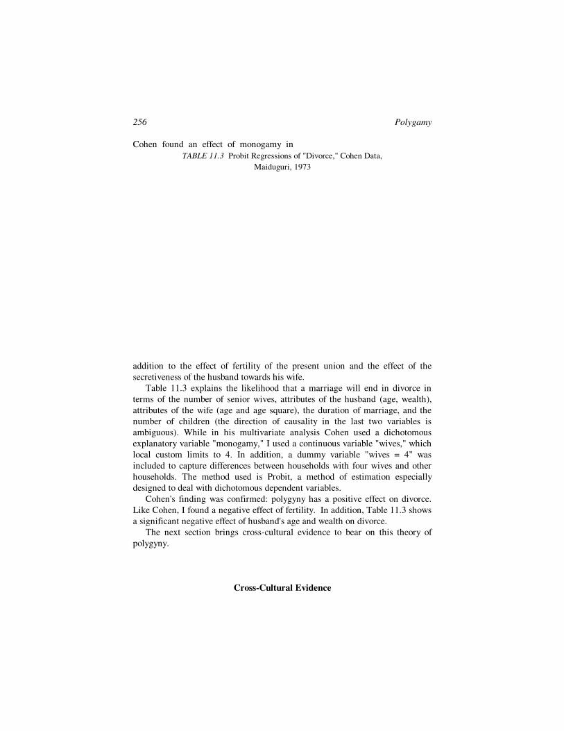
256 Polygamy
Cohen found an effect of monogamy in
TABLE 11.3 Probit Regressions of "Divorce," Cohen Data,
Maiduguri, 1973
addition to the effect of fertility of the present union and the effect of the
secretiveness of the husband towards his wife.
Table 11.3 explains the likelihood that a marriage will end in divorce in
terms of the number of senior wives, attributes of the husband (age, wealth),
attributes of the wife (age and age square), the duration of marriage, and the
number of children (the direction of causality in the last two variables is
ambiguous). While in his multivariate analysis Cohen used a dichotomous
explanatory variable "monogamy," I used a continuous variable "wives," which
local custom limits to 4. In addition, a dummy variable "wives = 4" was
included to capture differences between households with four wives and other
households. The method used is Probit, a method of estimation especially
designed to deal with dichotomous dependent variables.
Cohen's finding was confirmed: polygyny has a positive effect on divorce.
Like Cohen, I found a negative effect of fertility. In addition, Table 11.3 shows
a significant negative effect of husband's age and wealth on divorce.
The next section brings cross-cultural evidence to bear on this theory of
polygyny.
Cross-Cultural Evidence

Polygamy 257
Findings of previous researchers are one possible source of evidence for the
theory of polygyny outlined above. Three kinds of evidence can be brought to
bear on Hypothesis 39, namely that women are better off when polygyny is
permitted (also see Grossbard 1978a and Chapter 1 here).
1[a]. Nobody has yet given a complete explanation on why bridewealth is
paid by husbands in some societies, while elsewhere the bride's family provides
a dowry. Whenever such general theory will evolve, it will have to incorporate
polygyny among the explanatory factors. According to anthropologist Goody
(1973), "dowry is strongly linked with monogamous (and polyandrous),
marriage." Similarly, sociologist Clignet (1970) writes that "the institution of
brideprice is more often found in polygynous than in monogamous African
societies."
These findings make sense if bridewealth versus dowry is seen as an
indication of women's share of marital income. Bride payments can be
considered as lump sum transfers through which men compete for wives when
the equilibrium incomes of married women exceed the income they actually
receive after marriage.8 Conversely, women or their families would pay dowries
prior to marriage in order to obtain a husband when the income they actually
receive exceeds the equilibrium income they would get in a free marriage
market. If the discrepancy between actual and equilibrium share of women in
marital income were greater the larger their equilibrium incomes (as suggested
by Becker 1977) "the frequency and magnitude of brideprices would be
greater...when poly[gyny] is more common." Conversely. when the equilibrium
share of women in marital income is low, their actual income may be higher,
especially if inflexible shares derive from the indivisibility of commodities like
children (Becker 1977). In turn, it was shown above that a prohibition on
polygyny reduces women's equilibrium conditions in the marriage market. It is
clear that the presence of polyandry detriments women's bargaining position
even more, for once men can pool their resources to marry a common wife, the
demand for wives is even lower than in monogamy, and consequently the
equilibrium income of married women even less favorable. The concept of a
marriage market therefore illuminates these observations by Goody and
Clignet.
Economist Bronfenbrenner (1971) has reached a similar conclusion based
on his analysis of Indian marriage markets. He observed that in India, "while
monogamy and dowries prevailed, there were certain subcastes, such as the
laundrymen of Calcutta, in which the master married his labor force. Under
these circumstances, not only polygamy but brideprices were found" (see also
Tambiah 1973). He therefore thinks that "the probability of a positive
brideprice (or negative dowry) will be greater when inter alia the number of
258 Polygamy
wives per husband exceeds unity."9
Not only does it seem that the probability of finding bridewealth versus
dowry varies directly with the presence of polygyny, but evidence also suggests
that bridewealth payments are higher in more polygynous societies. Comparing
two Sebei communities in Eastern Uganda, anthropologist Goldschmidt (1974)
found that the bridewealth was considerably higher in the more polygynous
community. Goldschmidt also cross-tabulated thirteen separate societies in East
Africa by polygyny ("over 150 wives/husbands" and "150 wives/husbands and
under") and brideprice (high and low) and found that only three out of thirteen
societies were not in the "high polygyny-high brideprice" or "low polygyny-low
brideprice" categories.
1[b]. Age at marriage can also indicate benefits from marriage. The more
one stands to gain, the younger one is likely to enter marriage. Hypothesis 39,
therefore, leads us to expect that women will marry younger in polygynous
societies. Since women gain relative to men, a larger sex differential in age at
marriage should be found where more polygyny occurs. Simple comparisons
provide evidence for the theory: women marry younger in countries allowing
for polygyny. For instance, women's average age at marriage is 13 or 14 among
the Hausa and the Kanuri of Eastern Nigeria, societies with widespread
polygyny. (Among the Hausa, 36 percent of all men of marriageable age were
polygynous; see Mair 1953). The Tallensi, another West-African tribe, are
slightly less polygynous (30 percent of marriageable men had more than one
wife; see Mair 1953) and their daughters marry somewhat later: here the
average female age at marriage is 16 and 17. On the whole, women marry
considerably earlier in polygynous areas like Africa and the Muslim world than
in monogamous Europe and America. In addition, while in the United States
the husband is on average two years older than the wife, that difference rises to
seven years in the Arab world and to ten years in some heavily polygynous
African societies like the Kanuri.
Using data from sixteen districts of Congo, Brass et al. (1968) found a
simple correlation of .8 between an index of polygyny (number of married
women per 100 married men) and the difference in mean husband's and wife's
age at marriage, evidence for a positive correlation between degree of polygyny
and difference in age at marriage. Moreover, the South African government's
efforts to limit polygyny (e.g., by imposing taxes on each wife) led to a later
female age at marriage (Mair 1953). Recently many Muslim countries have
simultaneously restricted polygyny and age at marriage. One explanation for
this joint treatment is that, once polygyny is limited, the age at marriage will
rise anyway, so that the second restriction becomes less costly.

Polygamy 259
1[c]. Not only will polygyny encourage women to marry earlier, but it will
lead a larger proportion of women to marry at all ages. Comparing two ethnic
groups in Abidjan (Ivory Coast) and its hinterland, Clignet (1970) found 42
percent unmarried Aboure females as opposed to 30 percent unmarried Bete
females. Not surprisingly, the Aboure are less polygynous: in Abidjan married
men were 91 percent monogamous, while that percentage was 81 percent
among the Bete. Likewise, better marital income opportunities open to women
lead widows to accept being "inherited" by relatives of their husband, as is
specified in the institution of "levirate." In South Africa the restrictions on
polygyny also led widows to "refuse much more often than in the past to be
'inherited' by relatives of their husband" (Mair 1953), which can be interpreted
as the result of a smaller differential between married and widowed income.
The same sixteen districts of the Congo also showed a negative correlation of -
.45 between polygyny and the proportion of married women 15 to 45 years old
(Brass et al. 1968).
Hypothesis 40 predicted that polygyny is more likely in a marriage squeeze
for women. One of the most dramatic demonstrations of such marriage squeeze
effect on polygyny occurred in Paraguay in the nineteenth century. After a
major war against neighboring countries, the shortage of marriageable males
was so drastic (males were only 13 percent of the total population of Paraguay),
that for a limited period Paraguay overruled the prohibition against polygyny
(Becker 1974a). Equally convincing is the case of the South Fore, a New
Guinean tribe, where an increase in the male/female ratio due to the sexual
selectivity of a neurological disorder led to drastic reductions in the male
marriage rate and the rate of polygyny (Glasse and Meggitt 1969). Wagner
(1972) finds a positive relationship between availability ratio (wives per
marriageable men)10 and polygyny ratio (wives per married men) in a study of
twenty-three units of settlement among the Daribi of New Guinea.
If polygyny may result from a marriage squeeze for women, does it follow
that a marriage squeeze for males leads to polyandry? While polygyny is very
widespread, polyandry is extremely rare (perhaps because, as Becker 1974a
suggests, men like to maximize the likelihood of fathering their own genetic
products). In both cases of polyandry on which I obtained documentation, the
sex ratio exceeded one, i.e. there was a marriage squeeze for males. Among the
Todas of India (Murdock 1949), scarcity of females resulted from female
infanticide. In 1951, the polyandrists of Jaunsar-Bawar (Himalaya) had 20
percent more men than women, also related to female infanticide (Majumdar
1962). These mountaineers also had a custom of declaring certain women as
witches, whereafter they were often killed, another reason why men
experienced marriage squeezes.
260 Polygamy
While marriage squeezes affect the presence of polygyny, they account for a
small fraction of variations found in actual polygyny rates. In the most
polygynous area of the world, sub-Saharan Africa, the number of females per
hundred males varies between 95.9 and 136 for different countries and periods
(Dorjahn 1959), i.e. many of these polynous societies experienced marriage
squeezes for women. As pointed out by Dorjahn, the effective sex ratio can be
affected by sex differences in age at marriage. Earlier I emphasized that
differences in age at marriage may result from polygyny. But the observed
correlations may also be interpreted in the opposite direction, and with the
evidence presented here, there is no way to differentiate between the two
interpretations. Viewing age at marriage as a determinant of the effective
degree of marriage squeeze the Muslim governments' restrictions on age at
marriage may act as a means to reduce polygyny.
With regard to the positive relation between the importance of children and
polygyny hypothesized in Hypothesis 41, it can be noted that in continents
where more children are demanded, polygyny is more prevalent.
With respect to Hypothesis 42, a broad world overview also shows that the
continent of highest polygyny, Africa, has limited markets for consumer goods
and servant services 11 and that household production uses a higher ratio of
own time to market goods than is the case in monogamous regions like ours.
Reduced demand for women's spousal labor may be one explanation for the
decline in polygyny in the Middle East (Daghestani 1953).
Smaller markets for consumer goods may also be a cause of restricted job
opportunities for women outside the home. In monogamous societies, many
jobs performed by women in the labor market substitute for women's spousal
labor (for instance, waitresses, seamstresses, salespersons in supermarkets).
This supports Hypothesis 43. In Africa, women have fewer possibilities to be
independent, and therefore the gains from marriage (and polygyny) are larger.
Actual correlations between female labor force participation and polygyny are
hard to interpret, for the low demand for wives in more monogamous societies
may force women to enter the labor market. Keeping this in mind, the finding
that among the more polygynous of two Ivory Coast tribes women participated
less in the labor force, is not necessarily a proof of this proposition (Clignet
1970). To Goode (1953), one of the reasons for the "reduction in the proportion
of the adult population living under concubinage or some form of polygamy" is
that "the female ...now...has alternative modes of employment."
Hypothesis 44 related the prevalence of polygyny to marginal returns from
an additional wife. The possibility of sharply decreasing marginal returns from

Polygamy 261
wives because of frictions between co-wives endangers polygyny to such an
extent that all polygynous societies have taken active measures to minimize
these intramarital conflicts. Four types of arrangements are used to reduce
frictions in polygynous households: (1) separate dwellings for each wife, (2)
supervisory authority in the hands of the senior wife, (3) customs requiring that
the husband cohabitates with each wife in regular rotation, and (4) sororal
polygyny, whereby sisters share a husband. The latter custom was reported in
70 out of 193 polygynous societies surveyed by Murdock (1949). Methods (1)
and (4) appear to serve somewhat as substitutes. In 18 out of 21 societies with
exclusively sororal polygyny, co-wives live in the same house, while in 28 out
of 55 societies with non-sororal polygyny, wives live in separate dwellings.
Clignet and Sween (1974) found that one way urban dwellers in Cameroun
practice polygyny is by having one wife in the city and one in their village of
origin. Higher residential costs in African cities tend to discourage polygyny,
because it becomes harder for husbands to keep wives in separate dwellings.
In practice, there is evidence of both frictions and widespread cooperation
among co-wives. For instance, co-wives cooperate in childrearing. Out of a
sample of 759 co-wives interviewed in the Ivory Coast, only 25.2 percent
exerted authority on their children separately from their co-wives, while three-
quarters raised children under some form of shared or accepted authority
(Clignet 1970).
Reliable cross-cultural data to substantiate Hypotheses 45 and 46, dealing
with inequality among men and women, is hard to obtain. Hypothesis 46,
relating positive sorting and polygyny, is not testable in its original form, but its
corollary, Hypothesis 46', can be tested. Polygyny and positive sorting being
two alternative strategies by which husbands can obtain more spousal labor,
societies prohibiting polygyny should have more positive sorting. In Maiduguri,
I found a simple correlation between married male and female schooling of
+.37. In contrast, holding age and wage rates constant, the correlation between
husband's and wife's years of schooling was +.53 and +.56 for American whites
and blacks respectively (Becker 1974a). The lower correlation in Maiduguri
may be due in part to a possible choice between polygyny and positive sorting.
If there is indeed substitution between positive sorting and polygyny, a
prohibition of polygyny would benefit educated women, for it will raise the
demand for their spousal labor as a replacement for the spousal labor than
could be provided by a larger number of noneducated women. Consequently,
educated women in Africa and Egypt have often been active in political efforts
to prohibit polygyny. Also, West African female students (Omari 1960) were
vocal against polygyny (but favored brideprice), while their male classmates
favored polygyny (but were hostile to brideprice). However, as expected,

262 Polygamy
uneducated women did not seem opposed to polygyny. While 12 percent of
educated Yoruba women would not let their husband take a new wife under any
circumstance, only 0.8 percent of the uneducated women said so (Yoruba Social
Structure 1976).
The evidence presented in this section consisted, for the most part, of cross-
cultural comparisons by level of polygyny and one other variable, ignoring the
many other factors that could intervene and transform an apparently causal
relation into a spurious one. Differences in polygyny between Africa and the
rest of the world, and among selected tribes in Africa, were used repetitively for
different purposes, and it may very well be that in a more careful cross-cultural
investigation some of the correlations would disappear.
Conclusions
A general theoretical approach to the study of polygyny enhances our
understanding of the reasons for cross-cultural variation in the prevalence of
polygyny. It also throws some light on the factors related to the incidence of
polygyny within a particular society. This study is another example of how
economic theory benefits the study of marriage.
This study also shows some of the advantages of interdisciplinary
cooperation. An economic analysis vitally depends on the thorough cultural
understanding anthropologists develop through fieldwork. Without the
information on Maiduguri generously transmitted by Ronald Cohen and the
insights on polygyny previously published by other social scientists, this study
would have been very limited in scope.
The economics of polygyny can potentially be useful in leading to a better
understanding of the mechanisms behind fertility and female labor force
participation in countries allowing polygyny. The study of polygamy comprises
an integral part of the study of marriage institutions, a field where theoretically
grounded research is still the exception. It is hoped that the theory and
empirical research presented here can contribute to the study of marriage in
general.
Notes
1. Clignet's (1970) is one study in which elders are viewed as the traditionally
privileged segment entitled to polygyny. He makes no mention of a maximum seniority

Polygamy 263
beyond which a man becomes less polygynous.
2. He finds evidence for his hypotheses on the basis of comparisons between
different kinds of living creatures, birds in particular. I am indebted to Jack Hirshleifer
for this reference.
3. However, the effect of each of these three dummy variables on the number of
wives has an alternative interpretation. First, waterstandpipes and houses may be
components of the wife's income from spousal labor. This income is principally
nonpecuniary, for it consists of provision for room, board, convenience, etc. The more
wives a man has, the more he needs room to provide for them--especially since in
Maiduguri each wife lives in separate quarters--and the more he is likely to purchase a
house. Similarly, the more wives, the more profitable to compensate all wives by saving
them the trouble of fetching water or purchasing it from water-carriers. (This assumes
increasing returns to scale in waterstandpipe installations.) Owners of grain farms may
be wealthier, but they also need wives as farm labor in addition to the other needs
shared by all men. Unfortunately, there is no way to differentiate between the different
interpretations of these variables. Small simple correlations between possible wealth
proxies emphasize that problem. The correlations between waterstandpipe on the one
hand, and grain farm, house ownership, and occupation on the other hand are
respectively -.07, .15 and .20. The low correlations between house ownership and
occupation (.11) and waterstandpipe (.15) partially derive from the recent inflow of
migrants who do not own houses but are wealthy enough to rent comfortable housing.
4. In mathematical terms, a peak is a maximum. Let us call the variable "wives"
Y and the variable "age of husband" X and abstract from other variables. The regression
equation can then be written as Y = aX + bX2. The first order condition for a maximum
or a minimum is that the first derivative of this equation equal zero, i.e. a + 2bX = 0.
This implies that X = -a/2b. Based on the coefficients of age and age, squared estimated
from regression 2 (.25 and -.0029) we calculate the maximum age as 43.
5. To calculate a minimum value, we follow the same procedure described in
note 4. The values for (woman's) age and age, squared in regression 2 are -.12 and
.0029. Using the formula X = -a/2b, we obtain a minimum age of 21.
6. For a more extensive empirical discussion of the relationship between
polygyny and fertility see Grossbard (1986b).
7. However, here too the causality could be inverse: polygyny could facilitate
seclusion by adding more variety and companionship to the isolated wife's life. From a
separate table (Table II in Grossbard-Shechtman 1980) it appears that the effect of
seclusion varies with duration of marriage. In the sample of all marriages, it is
significantly positive at the 90 percent level, mainly a result of the strongly positive
relation for marriages of intermediate duration.
8. In many societies, the income a married woman actually receives differs from
what would be her income based on market-clearing quasi-wages for spousal labor due
to regulations enforced through law and custom.
264 Polygamy
9. Other factors he considers are productive, skilled and/or arduous work
expected of a wife; few or no legitimate extracurricular substitutes for wives as sexual
partners; high sex ratio of men to women in the population of nubile age; and
prospective husband's old age subsistence depending on numerous healthy sons.
10. Apparently, practically all marriageable women do get married in this society.
11. The question of substitution between wives and servants is particularly
complex since a society's propensity to rely on servants simultaneously affects a
woman's productivity in spousal labor and in outside labor. The institutionalization of
reliance on female servants is in itself an economic question, perhaps related to the
gains from household specialization among women differing in skills.


267
PART SIX
Marriage, Productivity,
and Earnings The theory of marriage presented in Part Two viewed individuals as
suppliers of spousal labor, and defined spousal labor as any service benefiting a
spouse. Such spousal labor is not simply about washing dishes and taking care
of the garden, but also about helping a spouse to earn more at work,
encouraging a wife to live a healthier life, or enabling a husband to find more
peace of mind. People invest in their spouse's human capital to the extent that
spousal labor boosts the spouse's earning capacity or other aspects of the
spouse's productive capacity (including the capacity to produce happiness).
The chapters in this part of the volume all deal with aspects of spousal help that
increase a person's human capital. Chapters 12 to 14 deal with spousal help
aimed at increasing a worker's earning capacity, whereas Chapter 15 focusses
on the contribution of a spouse to an individual's religious practice.
Of the three chapters which deal with the effect of marriage on worker's
productivity, the first two are principally of a theoretical nature, whereas the
last one is mostly an empirical contribution. Of the two theoretical chapters,
Chapter 12 is a relatively accessible introduction to the analysis of spousal help
to workers. Chapter 13 deals with one particular valuable quality which can
enhance individual success at work, in politics, or in marriage, namely one's
virtue or trustworthiness. This chapter presents a concept of general human
capital which goes beyond the usual sense of that expression. In labor
economics, general human capital has been defined as skills which can be
productive to different employers (Becker 1964). Here the notion is introduced
that certain skills can be valuable both to employers and to spouses. Thereby,
skills obtained in marriage could benefit success at work, and skills obtained at
work could benefit success in marriage. Chapter 13 presents the framework for
a market model of virtue or loyalty based on the concept of general human
capital.
Chapter 14 is an attempt to test for the determinants of spousal help as

268 Marriage, Productivity, and Earnings
reported by the workers, a sample of Israeli managers. Hypotheses were
generated based on two theoretical approaches: a human capital approach and a
cultural approach. Results of linear and logit regressions, run separately by
gender, with education, earnings, age, children, religiosity, and ethnic origin as
independent variables, revealed that spousal support is better explained for
women than for men and husbands help more when it is most productive to do
so. However, both theories contribute to explaining spousal support.
The final chapter, Chapter 15, focusses on religiosity as a form of human
capital, and more specifically, on spouses helping investments in such human
capital. The chapter presents an empirical study of the relationship between
wives' religiosity on Jewish husbands' time spent on religious observance. By
exploring factors affecting the association between spouse's religiosity and
individual behavior we find possible evidence of a post-marital learning
process. We also find that the men whose religious observance is strongly
correlated to wife's religiosity tend to have higher levels of secular education,
which possibly reflects the effect of education on the process of in-marriage-
learning.
All the hypotheses related to marriage and productivity at work found in
Part Six are numbered sequentially. These hypotheses were labeled K1 through
K24 in order to separate them from the hypotheses discussed in Parts Two
through Five.
Much more research needs to be done in this area, both at a theoretical and
an empirical level. A general equilibrium theory of marriage can lead to many
further hypotheses regarding the effect of marriage on earnings, consumption,
or other aspects of behavior. Theoretical developments may lead to innovative
ways of testing for effects of marriage on behavior. Meanwhile, it is also
important to have more empirical studies relating marriage and spouses' traits
to individual behavior at work or in the home. More tests of the hypotheses we
tested in Chapters 14 and 15 would also be useful, especially if they are based
on other data sets and statistical techniques.

269
12 Investments in Spouse's
Productivity at Work
Introduction This chapter was written for the first Handbook of Behavioral Economics,
an attempt to bring economists and other behavioral scientists closer together in
a variety of research areas. The subject of the contribution of marriage to
workers' productivity is a good example of how research can benefit from
communication between economics and sociology. While this chapter deals
most with wives' contributions to their husband's career, it is also relevant to
the contribution of husbands to their wife's career.
The chapter first reviews both economic and sociological theories that have
been used to explain marital status differentials in productivity, a possible
source of marital status differentials in earnings. Then, hypotheses are derived
regarding the effect of occupational characteristics on expected marital
differentials in workers' success, hypotheses that were inspired by some of the
sociological literature on the subject. The chapter also mentions hypotheses that
fit well within a general equilibrium theory of marriage and labor. Marital
differentials in earnings are hypothesized to vary with spouse's characteristics,
divorce probability, and divorce laws.
Married people experience economic activities differently than do singles.
Married men work and earn more than single men, married women work and
earn less than unmarried women, and people in married households do
not consume the same bundles of goods and services purchased by singles.
Adapted from "Marriage and Productivity: an Interdisciplinary Analysis" in
Handbook of Behavioral Economics ed. by Ben Gilad and Stanley Kaish. Greenwich,
Conn.: JAI Press, 1986. I would like to thank Shelly Chandler, Roger Frantz, Ben Gilad,

270 Spouse's Productivity at Work
Stanley Kaish, and Ivy Papps for their helpful comments and suggestions.
In the United States, married men earn between 8 and 30 percent more than
single men, after other factors are accounted for (see Kenny 1983), whereas
married women earn some 3 percent less than single women (Becker 1981).
Similarly, in England, married men earned between 10 and 14 percent more
than single men, whereas married women earned 3 percent less than single
women (Greenhalgh 1980). A positive marital differential was also found in
Sweden by Duncan and Holmlund (1983).
The reasons for these differentials have not been studied adequately by
members of the various disciplines to whom this issue is of interest. While
offering relatively well-developed empirical estimations of these marital
differentials, economists explain them using theories of limited scope.
Sociologists and sociopsychologists bring a wider range of explanations, but
their approach is generally nonquantitative. The most valuable contributions by
noneconomists have been made at the micro level--the study of the organization
(family or firm)--namely by microsociologists (a term coined by Turner 1970)
and social psychologists. This makes generalization difficult.
The underdeveloped state of this area of study derives from the
fragmentation of the hehavioral sciences. Academic border treaties have
assigned one part of the problem--production and productivity--principally to
economics and business and the other--marriage--primarily to other behavioral
sciences such as psychology, sociology, and anthropology. Within the present
incentive structure, academic border crossing rarely pays off. As a result, the
effect of marital status on productivity has received insufficient scholarly
attention, and large gains from trade can be reaped through intellectual cross-
fertilization (See Chapter 1).
This chapter discusses some of the relevant sociological and
sociopsychological literature and compares it to research economists have
performed in this area. Its emphasis is on developing testable hypotheses and
suggesting directions for further research. The entire discussion focuses on
men's benefits from being married, even though it could have been stated in
terms of husbands' contribution to the earnings of working women. It makes the
reading somewhat easier to have wives and husbands consistently in one
position.
The chapter first reviews economic theories dealing with marital
differentials, and then summarizes some of the sociological theories on the
same subject. The theoretical section concentrates on one particular theory that
has been mentioned in both the economic and the sociological literature,
namely, wives' investments in their husbands' careers. This section
distinguishes different forms such investments can take. The theory of marital

Spouse's Productivity at Work 271
differentials in productivity that is presented focuses on occupational
characteristics.
Previous Literature
Economic Theories
Economists have explained the observed marital differentials in earnings on
the basis of five different theories. The most commonly referred to is what can
be called the specialization theory (see Mincer 1962; Becker 1965). According
to this theory, men and women specialize in the production of different goods
and services, as a result of differences in endowments, utility, or both. Because
of their comparative advantage in household production, married women work
less and therefore earn less outside the home than do single women, whereas
the opposite is true for married men. For a man, marriage implies engaging in
an exchange of earned income for household income. Married men therefore
specialize in work outside the home more than single men and earn more, even
during the same number of working hours. Married men are more productive
because of their richer work experience and their stronger need to maintain
their earning power in the future (Kenny 1983; Bartlett and Callahan 1984).
While this first theory relates earnings differentials to productivity
differentials, other economists have also presented the "perceived-need"
hypothesis, wherein employers pay married workers more because such workers
need to support a family. Pay scales often reflect such policy, especially in
Europe (Bartlett and Callahan 1984).
A third theory mentioned in the economic literature is that of statistical
discrimination (Siebert and Sloane 1981). According to this theory, employers
discriminate against single men and married women because of past statistics
relating average productivity and marital status.
Fourth, economists have used the human capital investment theory to
provide an alternative explanation for observed marital-status differentials in
productivity and earnings. According to this theory, such differentials originate
from wives' investments in their husband's human capital (see Benham 1974).
In a similar vein, Marxist economists have written about domestic labor
(principally the wife's) as "the care, maintenance and continued socialization of
human beings" (Himmelweit and Mohun 1977).
This last theory is closely related to the first one, for the same activities--
such as cooking or nurturing--in which women specialize often lead to
272 Spouse's Productivity at Work
improvements in human capital; for instance, through better nutrition and
physical or mental health. Indirect evidence for such an investment process has
been found in the effect of wife's schooling on husband's earnings (Benham
1974), health (Grossman 1976), and religious practice (Grossbard-Shechtman
and Neuman 1986). Interestingly, the wife's investment theory has not been
mentioned in much of the economic literature on this subject.
Finally, economists have theorized that causality does not necessarily
proceed from marital status to earnings, but rather from earnings to marital
status. Men earning higher wages are more likely to get married either because
higher income encourages people to marry (see Becker 1981, Grossbard-
Shechtman 1984) or because the same desirable and unmeasured characteristics
that lead to higher earnings also increase the probability of a worker being
married (Kenny 1983).
Theories by Other Behavioral Scientists Specialization theory also takes a major place among the explanations
sociologists and psychologists have offered for the observed marital status
differentials. Sociologists generally call it role specialization (e.g., Parsons
1942).
Social scientists attempting to explain the origin of such specialization are
divided regarding the relative influence of nature and nurture. Psychologists
who specialize in the study of gender differences can be found on both sides of
the controversy (e.g., Maccoby and Jacklyn 1974). Anthropologists and
sociologists tend to be particularly interested in demonstrating the dominance
of cultural influences (e.g., Mead 1949), although a few have recently come to
emphasize biological factors, basing themselves on the work of biologists.
According to the so-called sociobiologists (e.g., Wilson 1975), biological
differences in reproduction technology and in the ability to provide for
dependents determine gender role specialization observed among all species,
including the human race.1 Most researchers view existing human role
specialization as the result of both biologically and culturally determined
gender differences.
Sociologists were writing on the wife's contribution to her husband's success
at work before economists got interested in the subject (e.g., Whyte 1956,
Moore 1962). Sociologists differentiate between the wife's indirect
contribution--her specialization in household tasks, which freed her husband
from such responsibilities--and her direct contribution.
To designate the wife's direct assistance to her husband's success at work,

Spouse's Productivity at Work 273
sociologist Papanek (1973) coined the term two-person career. The term
implies that both members of a married couple are actually working, although
only one of them is officially employed.
Sociologists and social psychologists studying wives' contributions to their
husbands' success at work generally take a micro perspective in the sense that
they focus on one occupation or one organization, mostly the corporation. Their
insights often originate from careful observation of workers on the job. In
contrast, economists writing on this subject have not paid attention to
occupational differences in wives' contributions to husbands' success. Similarly,
economists do not study the effect of husbands' occupation on wives' labor
supply outside the home, a related subject of research.2
The following theoretical section starts with an inventory of possible
investments wives make in their husbands' careers, derived from both the
economic and the sociological literature. The focus is on direct contributions as
defined above.
Theory
Types of Wives' Contributions to their Husbands' Work Performance
The following discussion distinguishes between wives' direct contribution to
their husbands' work performance by means of (1) assistance in central tasks,
(2) investment in husbands' human capital, and (3) contributions to husbands'
peripheral tasks and to the communication of information.
According to Weinstock (1963), a job often includes central and peripheral
task specifications. Central tasks are technical requirements of the occupation
directly related to performance. Peripheral tasks refer to the "nontechnical,
institutionally required social aspects of the job." This distinction is helpful
when discussing the two-person career (see Mortimer, Hall, and Hill 1978), as
are the concepts of human capital (Becker 1964) and organizational capital
(Tomer 1986).
Contributions to Husbands' Central Tasks. Wives sometimes help their
husbands by doing the work that could be done by a paid employee. For
instance, a saleman's wife may promote sales, or a writer's wife may type his
manuscript. According to Kanter (1977a), the winners of one company's award
for exceptional salesmanship all had wives without outside jobs who reported
spending a considerable amount of time helping their husbands with sales
work. Wives may also aid their husbands' success by acting as "sounding
boards," thus helping their husbands think through technical work problems, or
by giving concrete advice that will enhance productivity. The latter form of
274 Spouse's Productivity at Work
direct help may be more relevant to more complex, generally professional,
white-collar occupations.
Investment in Human Capital. This is the only direct contribution
economists have related to (e.g., Benham 1974). The sociological literature
mentions wives' contributions to workers' good nutrition and good physical and
mental health. Parsons' (1942) mention of wives' expressive role relates to their
help as a sounding board and mental health counselor. Likewise, Lasch's
(1977) view of the family as a "haven in a heartless world" centers on the
stress-relieving functions of the wife.
In addition, wives can help develop their husbands' motivation to work and
organizational capital. The motivation argument restates in part the "marriage-
as-need-for-income" argument also mentioned in the economic literature. Using
the sociologists' distinction between instrumental (or extrinsic) and intrinsic
rewards of work, we see that marriage tends to increase the need for work as an
instrument (means) to acquire goods. This is what economists generally mean
when presenting this argument.
Sociologists also write of marriage as a means of promoting the intrinsic
motivation to work--what economists call the nonpecuniary benefits of work.
Turner (1970), for instance, mentions people's need to identify with their job as
a major intrinsic, nonpecuniary reward of work. If a husband can get his wife to
identify with his work, his own commitment to the job will rise; so will his
motivation to work and, consequently, actual productivity.
Whereas workers have intrinsic needs for identity and commitment,
organizations also have an interest in promoting such commitment. If the
commitment is specific to a firm, it is often called loyalty. Such loyalty can be
viewed as organizational human capital, a type of human capital that should be
distinguished from technical human capital in that it enhances productivity
through better work relations within the organization (see Tomer 1986).
Loyalty contributes to productivity in two possible ways: by decreasing the
likelihood that a worker will quit and by increasing his or her work effort.
The value of loyalty as insurance against a worker quitting follows from
conditions of uncertainty and from the relative importance of specific on-the-
job training (see Becker, 1964). The value of loyalty as motivation to work hard
derives in part from the absence of well-defined property rights. Once a worker
has been hired in a team situation, his or her individual extra work effort is a
public good. Therefore, individual workers may have an incentive to be free-
riders (Leibenstein 1982) with respect to their team or to the firm as a whole.
Loyalty reduces free-riding tendencies by fellow workers or employees and
therefore increases workers' productivity3.
Wives can contribute to their husbands' loyalty in marriage. I am assuming
Spouse's Productivity at Work 275
here that the propensity for loyalty is an acquired trait, which needs to be
learned within an organization. Since it is a general skill, individual firms have
limited incentive to teach their workers how to be loyal (See Chapter 13). The
family being such a pervasive organization, it can serve as a teaching ground
for loyalty. In turn, the institution of marriage reinforces the loyalty elements in
family relations, and women do so more actively than men (see Grossbard-
Shechtman 1982 and Chapter 9). In other words, marriage can produce loyalty.
A similar argument has been stated by Marxist economists Himmelweit and
Mohun (1977) when they consider the family as a producer of a disciplined
working class.
In principle, corporate loyalty and family loyalty can compete with each
other. One reason corporations frequently move their employees may be to
subordinate family loyalty to corporate loyalty. Moreover, firms may engage in
activities aimed at reducing the possible competition between loyalty to the firm
and loyalty to the family. For instance, Pahl and Pahl (1971) hypothesize that
the company's sponsorship of social events for their employees increases wives'
willingness to support their husbands' commitment.
Contributions to Husbands' Peripheral Tasks and to the Communication
of Information. Workers get involved in activities that do not seem central to
their job and are often unrelated at first sight. Examples of such activities are
entertaining and participation at public events. A closer look may reveal,
however, that such activities often promote a worker's success on the job. Such
peripheral tasks often serve to communicate valuable information, and here a
spouse can play an important role.
Parties, which can serve as an efficient means of promoting the circulation
of information within the organization, are often catered by wives. Other
peripheral activities enable the employee to communicate personal information
of value to the firm that otherwise is hard to gather.
As mentioned earlier, the firm is interested in workers' loyalty in the hope
that this will increase the worker's motivation to contribute to joint work
efforts, but information on the basic character of a worker is hard to obtain. The
wife's behavior often serves as a testimony and a clue to the character of her
husband.
First, a wife makes it possible for her husband to advertise his propensity for
loyalty by simply remaining married. Men often tend to advertize their family
loyalty at the workplace. Kanter (1977a) reports that in the large corporation
she studied, pictures of wives and children adorned men's offices so commonly
that they seemed almost mandatory. Such photographs may play the role of
advertizing loyalty to the family, possibly implying a willingness to be loyal to
the firm as well.
Next, husbands working for corporations benefit from their wives'

276 Spouse's Productivity at Work
involvement in charitable and community service. Similarly, wives of
independent businessmen can help generate business by promoting a favorable
public image via their volunteer work. In this case the wives' activities serve the
same function as does the funding of a National Geographic TV special by an
oil company. Companies and managers benefit from advertising goodwill and
concern for the community, which can generate direct income for the
independent businessman and promotion for the executive contributing to his
corporation's sales.
Hypotheses Relating Marital Differentials to Occupational Characteristics Given the types of contributions wives can make to their husbands' success
at work, it follows that occupations differ in the degree to which they allow for
potential contributions by wives. The following hypotheses were derived from
the theoretical considerations discussed in the previous section.
Hypothesis K1
Marital differentials will be larger in occupations with potentially steeper
earnings profiles.
The more a man can possibly earn on his job, the larger the potential
differences in earnings, and therefore the larger the potential contribution a
wife can make by whatever means are available: indirect assistance by allowing
the husband to specialize at work, as well as direct assistance applicable to the
work situation. If the husband is an employee, there probably will be more
pressure on the wife to contribute to her husband's career the higher the career
"ceiling" and the more steps in the ladder (Tausky and Dubin 1965, Hall 1975,
Mortimer, Hall, and Hill 1978).
The steepness of earnings profiles is partially a function of educational
level. Educated workers typically experience steeper increases in earnings over
the life-cycle than uneducated workers. It is therefore a corollary of Hypothesis
K1 that marital differentials in earnings will be larger the more educated the
workers.
This is one reason executives tend to benefit more from being married than
do workers in general, and therefore why executives are more often married
than other workers (Whyte 1956). For instance, in 1969, 93.19 percent of the
male managers earning 15,000 a year or more were married, 72.25 percent to
women not in the paid labor force. As income and status go up, even fewer of
Spouse's Productivity at Work 277
the wives hold paid jobs, and even more of the men are married (Kanter
1977a).
Self-employed men with large potential earnings are also likely to gain large
benefits from being married. Independent businessmen or farmers with large
growth potential, for example, may experience higher marital differentials in
earnings than do people of similar background in career tracks without growth
potential. Evidence for this hypothesis can be found in a study of resettled farm
families given land with growth potential in the Columbia Basin project. The
farmers who were most successful were more likely to have wives who
conceived of their roles in traditional terms (Strauss 1958).
Although these occupational differences in marital differentials have not
been tested rigorously, their frequent appearance should lead us to consider this
hypothesis seriously. However, the same findings could possibly be explained
with the help of additional hypotheses.
When careers have a large growth potential, generally only a small
proportion of aspiring ladder climbers ever achieve the highest echelons. This
often creates fierce competition and therefore stress, resulting from intensive
efforts to move up the ladder. Kanter (1977b) calls such careers "absorptive," in
the sense that they absorb a large fraction of a person's time and energy. The
career-minded husband and his family experience stress in two ways: pressure
on the husband's health and pressure on the wife and children, who must put up
with many irregular and unpredictable demands of the husbands' job (Turner
1970). This leads us to another hypothesis.
Hypothesis K2
The more stressful an occupation, the larger the potential marital
differentials in earnings.
The wife of a husband whose occupation generates a high level of stress has
more potential to contribute to her husband in the sense that there is more need
for her to accommodate her husband's work demands: this constitutes an
indirect contribution. There also is more room for direct contributions, such as
direct assistance in central tasks and assistance in maintaining husband's
physical and mental health. Although careers with high growth potential often
tend to be stressful, the two hypotheses are separable to the extent that job stress
and adsorptiveness are measurable. Tests can be designed to ascertain how
stress level influences marital differentials, given a certain pattern of potential
278 Spouse's Productivity at Work
growth in earnings. Moreover, in performing such tests one should control for
additional aspects of a job that are also likely to affect marital differentials.
Hypothesis K3
Marital differentials are likely to be higher in occupations involving more
peripheral tasks.
As was shown in the previous section, one means by which a wife can
promote her husband's career is by helping in peripheral tasks such as
entertainment and community service. The more such tasks are potentially
relevant to an occupation, the more a wife can contribute. Such tasks are more
commonly found in high-prestige occupations (Mortimer, Hall, and Hill 1978),
in occupations involving extensive personal contacts (Weinstock 1963), or in
occupations highly dependent on the maintenance of a stable clientele (Moore
1962). Therefore, we expect higher marital differentials among managers than
among engineers of similar ability, and among owners or managers of firms
that depend more on their public image because of the type of product they sell.
This hypothesis helps explain the apparently high marital differentials
among corporate managers and independent businessmen. It also explains why
wives of university presidents (Clodius and Magrath 1984), politicians
(MacPherson 1975), officers in the military (Goldman 1973), and ministers
(Taylor and Hartley 1975) can make important contributions to their husbands'
careers.
Hypothesis K4
The more complex and potentially substitutable the central tasks of a
husband's occupation, the larger the potential marital differentials in
productivity and earnings.
Blue collar workers rarely are in a position to delegate any of their central
tasks to their wives. In contrast, business managers and writers can have their
wives do secretarial work, clergymen's wives can run the Sunday school, and
wives of storekeepers can tend the store. Wives assisting in central tasks are not
necessarily unpaid. Epstein (1971) found in her study of married lawyer teams
that the wives did much of the paper work contributing to the husband's success
in court or with clients.
Hypothesis K5
The more loyalty contributes to workers' productivity--for example, because
of the profitability of investments in human capital--the larger marital
differentials in earnings.
Spouse's Productivity at Work 279
As mentioned in the previous section, one of the ways in which wives can
potentially contribute to their husbands' careers is by increasing the husbands'
propensity to be loyal to the firm. Moreover, the fact that a man is married
signals his potential for loyalty.
The potential need for workers' loyalty varies by occupation and by
industrial system. Firms need loyal workers more if they consider investing in
the workers' firm-specific skills. An industrial system such as Japan sets a
particularly high value on loyalty to the firm (Clark 1975). It is therefore not
surprising that employers' discrimination in terms of slower advancement of
unmarried workers is more common in Japan than in the United States. In
Japan, marriage also serves as a declaration of the willingness to curb
individualistic aspirations and to contribute to organizations and to society at
large (Hendry 1986).
Other Hypotheses about Marital Differentials in Earnings The degree to which husbands benefit from their wives' contributions is
expected to vary not only with occupational characteristics, but also with wives'
personal traits and the terms of marriage. Similarly, husbands' personal traits
are expected to influence wives' earnings.
Spouse's Characteristics. The larger the potential for marital differentials,
the more men are likely to marry women who are particularly adept at
contributing in the areas of most importance to their job. Women can possibly
invest in their capacity to boost their husband's earnings.
Wives' characteristics that are most likely to contribute effectively to the
tasks discussed earlier are a higher education and time spent in the home. As
hypothesized by Benham (1975)
Hypothesis K6
The more educated the wife, the higher the husband's earnings.
Benham's finding that the husband's income increases with the wife's
schooling, even when the husband's own education and years of work are
controlled, supports this hypothesis. Interestingly, he found that the positive
contribution of the wife's schooling stops at the point of graduate education,
possibly because of the substantially higher percentage of women with graduate
degrees who work outside the home.
Similarly, one expects more educated husbands to contribute more to the
earnings of their wife than uneducated husbands.
Time spent in the home could be related to the wife's labor force status. As
280 Spouse's Productivity at Work
a result, it is possible that
Hypothesis K7
Husband's earnings are positively related to wife's time spent at home.
Evidence of the advantage of a nonworking wife from the husband's point of
view has been offered in a study of male engineers and accountants (Burke and
Weir 1976). Husbands of working wives reported more job pressures, expressed
more dissatisfaction with their jobs, marriages, and other aspects of their lives,
and manifested more symptoms of stress than the husbands of homemakers.
Terms of Marriage. The same husband--with a given occupation
employing him--and wife--with a given occupation, education, etc.--are likely
to have different relationships depending on the terms of their marriage. In
part, these terms depend on the legal environment. Under laws making divorce
easy, most women do not want to invest in their husbands' careers as much as
they would have invested if there is good protection against divorce. When
divorce is easy, it may be necessary for husbands to give their wives more direct
incentives to help them professionally than at times when divorce is difficult.
Unilateral divorce may be a particularly strong factor discouraging investments
by wives in their husbands' careers, as wives faced with husbands asking for a
divorce have very few bargaining tools helping them in retrieving their
investments in their husbands' careers. It follows that
Hypothesis K8
When divorce laws are unilateral, wives will invest less in their husbands'
careers than when divorce laws are not unilateral (for instance when they
are based on mutual agreement.)
This hypothesis could be tested by following marital differentials in
husbands' earnings over time across states and comparing these trends with the
adoption of no-fault divorce laws. More generally, predicted divorce is
expected to have a negative effect on spousal investments in workers'
productivity, and therefore to reduce marital differentials in earnings.
Similarly, expectations about traditional roles of men and women in
marriage will affect the amount of investment by the wife in her husband's
career. The more women accept traditional marital roles, implying few personal
returns for their investments, the more they are likely to support their husbands'
careers. Lopata (1971) found that wives of successful men were more likely to
accept traditional marital roles. The more prestigious the husband's occupation,
the more likely the wife was to turn the enjoyment of her husband's success into
part of her reward (Mortimer, Hall, and Hill 1978). Some women may, in fact,
be caught in a bind, not happy about the compensation they receive for their

Spouse's Productivity at Work 281
contribution and unable to find better opportunities through divorce and
remarriage. Many corporate wives suffer from marital problems, according to
Kanter (1977a). It is not clear, however, if women investing more in their
husband's work have worse marriages than women who invest less in their
husband's work.
The presence of marital status differentials in earnings may affect the
likelihood of divorce.
Hypothesis K9
Divorce may be less common and remarriage more rapid when men engage
in occupations with high marital-status differentials.
Divorce may be less common and remarriage more rapid when men engage
in occupations with high marital differentials. The decisions to marry and
divorce are likely to affect earnings. Bartlett and Callahan (1984) found that
men who were divorced or widowed and who had remarried experienced
particularly rapid growth in wages.4 If marriage really contributes to earnings
as is claimed here, the upward trend in divorce that has characterized recent
decades may be one explanation for the downward trend in productivity left
unexplained by conventional methods of study. In turn, the upward trend in
divorce may be caused in part by legal changes which have lowered the
protection wives receive if they invest in their husbands' careers.
Summary and Conclusions This chapter looked at possible effects of spouses on the other spouse's
career. For simplicity, the entire discussion was stated in terms of wife's effect
on husband's career. In theory, the arguments presented here could also be
applied to the effect of husbands on their wives' career. As shown in Chapter
14, there seems to be evidence that husbands help their wives at work.5 It has
been argued here that marital differentials in earnings are expected to vary with
occupational characteristics (including growth potential, stress and
adsorptiveness, amount of peripheral and central tasks involved, and need for
loyalty), with characteristics of the spouse, and with institutional factors such as
type of divorce laws. Preliminary evidence based on the sociological literature
was offered in partial support of these hypotheses.
The above-mentioned hypotheses all have corollaries, which are derived
from the process by which people select marital status, spouses, occupations,
and employers. Positions with larger marital differentials are more likely to be
filled by married men, the result of voluntary selection and possibly
encouragement by the employer.
282 Spouse's Productivity at Work
This theory also has implications for employers' policies. First, they may
discriminate against unmarried workers. Second, they may select two persons
to fill a position that tends to be a two-person career. Employers in fact often
interview wives of prospective employees as well as the applicants themselves
(Kanter 1977a). Employers may also organize activities that encourage wives to
contribute to their husbands' careers, such as family recreation.
It is hoped that further research will do more to establish the direction of
causality so that we get a better understanding of the relationship between
marriage and productivity at work.
Notes
1. Economists writing on gender differentiation as it affects labor supply have
either ignored the nature-nurture controversy or emphasized biological influences (for
instance Becker 1981). Becker's position on this issue is consistent with his general
view of social, legal, and political institutions as promoting long-run individual well-
being. According to this view, commonly espoused by economists, social behavior (such
as nurturing methods) which is not based on real factor prices and endowments, is not
socially optimal and would therefore disappear over time. This assumes competition in
the broadest sense and the absence of exploitation of one group by another.
2. A critique of the economic literature on female labor supply along these lines
can he found in Mortimer, Hall, and Hill (1978).
3. A related discussion of loyalty can be found in Akerloff (1983).
4. This could also possible reflect a causality whereby higher income facilitates
remarriage.
5. The fact that there are no regular marital differentials in earnings for women
does not mean that husbands do not help working wives.

283
13 A Market Theory of Virtue
as General Human Capital In the long run, the public interest depends on private virtue.
--James A. Wilson
Abstract
This paper deals with one particular valuable quality which can enhance individual
success at work, in politics, or in marriage, namely virtue or trustworthiness. The
theory derives a demand for virtue by employers, a supply of virtue by workers, and
integrates demand and supply in a market for seemingly virtuous workers. Special
attention is devoted to marriage as seemingly virtuous behavior, and more hypotheses
are derived regarding marital differentials in earnings. Among the major insights of this
market model of virtue are a new interpretation of the value of age, individual
investment in virtue, and the value of making virtue general rather than specific.
Introduction The public interest depends on private virtue. So do private interests. Firms
benefit from virtuous workers to the extent that workers committed to their
284 General Human Capital
employer display a smaller tendency to quit and are less likely to destroy their
firm's equipment. Virtue or loyalty is a means of preventing moral hazard. As
was pointed out by Arrow (l975), "every commercial transaction has within
itself an element of trust." Trust, a component of vir-
This is a revised version of "Virtue, Work, and Marriage," published in Applied
Behavioral Economics, edited by Shlomo Maital, Wheatsheaf and N.Y.U. Press, New
York, l988. I am indebted to Joel Guttman for stimulating my interest in this topic, and
to Jack Hirshleifer, Michael Naughton, Harinder Singh and participants at the Second
Annual Conference of the Society for the Advancement of Behavioral Economics and at
a Seminar at Bar-Ilan University for helpful comments.
tue, facilitates productivity not only within a firm, but also in transactions of all
kinds.
People and firms will therefore prefer to associate with virtuous,
trustworthy, people. But information on other people's virtue is extremely
difficult to obtain. This explains in part why firms often rely on costly devices
to gather such information, such as extensive interviews, polygraphs or
graphological tests. Another way for firms to get information on a job
candidate's virtue is to consider their candidates' past behavior in other areas
which may indicate an underlying tendency for virtue. Such behavior I call
"seemingly virtuous behavior." Following Becker's (l964) distinction between
general and specific human capital, it is assumed that seemingly virtuous
behavior is of a general nature. Virtue displayed in one area of life is valuable
to another area of life. Any human relation can serve as evidence of virtue
valuable in the same area of life, or in a different area. Employers may
investigate whether a person is known as a good worker, a good son or
daughter, a good husband or wife, a good soldier, a good tenant, or a good
citizen. Similarly, wives, husbands, or citizens may want to check on the virtue
credentials of candidates for marriage or for public office.
If seemingly virtuous behavior is rewarded, individuals may invest in such
behavior as a means of increasing their success in the future. Given the general
nature of virtuous behavior, one obtains markets for seemingly virtuous
individuals.
In the following analysis, I pursue two examples of activities in which
people engage, at least in part, in order to invest in their virtue capital:
marriage and military service.
Marriage as Seemingly Virtuous Behavior. A candidate's observed family
behavior often serves as an indication of possible virtue, and therefore plays an
General Human Capital 285
important role in hiring and promotion. Employers may investigate marital
status, duration of marriage, marital fidelity, or number of children.
Employer's preference for virtue and married men's potentially higher virtue
relative to unmarried men is one possible explanation for the higher wages
married workers have been observed to receive, keeping standard wage
determinants constant.1 Some of the alternative explanations for such marital
differentials in men's earnings are (1) that married men acquire more human
capital and (2) that the relation between marital status and earnings is spurious:
according to the "economics of marriage," men with higher incomes are more
likely to be married.
The "economics of marriage" explanation can also account for the fact that
marital differentials are generally found for men, and not for women, in view of
the hypothesis that women earning more are less likely to be married. That
marital differentials for men exceed marital differentials for women can also be
explained using a "seemingly virtuous" explanation: exemplary and stable
marital behavior is more likely to indicate true virtue in the case of men than in
the case of women. This follows from biologically or culturally given
differences which lead women to benefit from marital stability more than men.
Men who stay married despite the basic forces driving them in the opposite
direction are more likely to be virtuous than women who more often prefer to
stay married, an argument that was pursued in Chapters 4 and 9. The latter
chapter documents gender asymmetry in individual preferences for
commitment in marriage.
People have an incentive to advertise their seemingly virtuous family
behavior. Accordingly, Kanter (l977a) reports that in a large corporation
pictures of wives and children adorned men's offices so commonly that they
seemed almost mandatory.
Heroism as Seemingly Virtuous. Firms also appear to value seemingly
virtuous behavior in the form of service to the community. Heroism
demonstrated at war often serves as a wage booster in countries with a recent
history of war. For instance, when they leave the army, Israeli officers with a
heroic war record obtain jobs that are better than jobs offered to people with
otherwise comparable credentials and experience. It is expected that even at
peace time ceteris paribus people who volunteer to more dangerous military
positions are likely to reap some benefits from it when applying for positions
for which a tendency for virtue is particularly appreciated.

286 General Human Capital
A piece of Japanese economic history can also reinforce this viewpoint. An
often mentioned partial explanation for l9th century Japan's economic
revolution is the availability of a samurai class who had been trained both as
warriors and as bureaucrats espousing the Confucian principle of public virtue.
These same samurai later became the captains of a modern factory system (see
for instance, Clark l975, Morishima l982). Their Confucian ideology stressing
virtue benefited their own advancement as well as that of Japanese industry.
Next, a market model is applied to analyze seemingly virtuous behavior
such as marriage and heroism.
Theory
Virtue is conceived of as a form of human capital in which people invest in
order to increase their future success at work, in marriage, or in other areas
where virtue may be valuable. I start with analyzing the demand for virtue, and
then consider the supply and the market where demand and supply are
juxtaposed.
The Demand for Virtue
Virtue, called V, cannot be observed. What is observable is behavior v,
termed "seemingly virtuous behavior." The observer does not know, however,
whether v is behavior out of true virtue or faked virtue. It is assumed that v =
v(V), where the first derivative is assumed to be positive. In other words, based
on past experience, seemingly virtuous behavior is interpreted as a signal
reflecting real virtue. I am now analyzing the demand for an individual's
seemingly virtuous behavior by another party. First, I consider the demand for
virtue by employers.
Demand by Employers. V increases a worker's i productivity, as reflected in
the production function Qi = f(ti, Ki, Vi), where Q is output by worker i, t time
worker i spends at work, and K physical capital the individual uses at work.
The cross-derivatives of Q by t and V and of Q by V and K are positive, i.e. V

General Human Capital 287
reinforces the productivity of labor and capital.
V's positive effect on productivity may be due to V's discouraging effect on
the probability to quit, which in turn leads to higher levels of specific training.
Workers' virtue also reduces shirking and could save the firm monitoring costs.
The worker is less likely to misuse capital. If one also adds time of other
workers to the production function, an additional source of shirking lies in the
absence of well-defined property rights. Once a worker operates with a team his
individual extra work effort is a public good. Therefore, individual workers
have an incentive to shirk and be free-riders (Leibenstein l982) with respect to
their team or the firm as a whole. Virtue reduces free-riding tendencies by
employees, and therefore increases workers' productivity. Virtue in this context
is similar to loyalty or discipline. The statements above bring some previous
literature to mind. Marxist economists, for instance, wrote about the value
employers derive from a well-disciplined work force (Himmelweit and Mohun
l977, Bowles l985). Also, Maital and Maital (l984) considered cooperative
workers as a benefit to firms, and Ouchi (l98l) found that loyalty enhances
productivity in Japanese firms and Z-organizations in the U.S.
A firm's demand for seemingly virtuous behavior v is downward-sloping if
the marginal productivity of V is diminishing. The aggregate demand for v by
employers, the sum of individual demands, will also be downward-sloping. The
demand for workers who have displayed virtuous behavior v in the past is also
downward-sloping, as depicted, in Figure 13.1. Employers will demand more
seemingly virtuous behavior the larger V's contribution to productivity and the
more v is associated with V.
To the aggregate demand for virtue and virtuous behavior by firms one can
add the demand by government and the demand by potential spouses. It is
assumed that the same virtue capital is valuable in all these different spheres of
life.
Demand by Government. Public employers--eventually, the voters--value
virtuous employees for the same reasons that they are valued by private firms.
This explains why the entire personal history of politicians running for office
undergoes thorough examination. Candidates can lose an election as a result of
the disclosure of an extra-marital affair or an embarrassing military episode.
Demand for Virtue in Marriage. Spouses can also be viewed as each other's
employers. Marriage markets of the kind analyzed by Becker (l974) and in
Chapters 3 and 4 establish wages for spousal labor in ways similar to these
observed in more conventional labor markets. It is therefore predicted that
people displaying seemingly virtuous behavior outside their marriage will
288 General Human Capital
receive higher quasi-wages in marriage. Although measurement problems
make quantitative applications of this theory to the family harder to come by,
the importance of virtue to families may make this theory even more relevant to
the family than to the firm or the government (see Maital and Maital l984).
Even though this theory is relevant to demand for spouses and politicians as
well as to the demand for workers, for simplicity we will focus on workers.
We now look at some of the determinants of the aggregate demand for
seemingly virtuous workers, i.e. workers who seem to have behaved virtuously
in the past. Hypotheses are formulated in terms of one possible indicator of
virtuous behavior: married status. The demand for seemingly virtuous workers,
such as married workers, depends in part on the demand for (true) virtue.
Fig. 13.1 Market for virtuous workers
Determinants of the Demand for V, Actual Virtue. Workers' virtue is more
likely to be valuable to employers in the following circumstances:
More capital-intensive jobs. Capital and labor generally complement each
other, and worker's productivity is higher when workers use more capital.
Consequently, the value of virtue and of seemingly virtuous behavior such as a
reputable marital history are higher in jobs with higher capital intensity. It
follows that

General Human Capital 289
Hypothesis K10
The more a job is capital-intensive, the more one expects marital
differentials in earnings.
Hourly or monthly contract. When type of contract makes shirking more
likely, virtue is more valuable to the employer. For instance, if workers are paid
by the hour shirking is more likely than if workers are paid by piece-rate. It
follows that
Hypothesis K11
Higher marital differentials in earnings are expected in salaried jobs than
in piece-rate jobs.
Bureaucracy. In large corporations or bureaucracies, where it is easier for a
worker to act as a free rider at the expense of fellow workers, virtue can be
more valuable than in small organizations. The more bureaucratic an
organization the more shirking is potentially beneficial and the harder it is to
monitor work efforts. It is consequently not surprising that the ultimate
employers in a democracy, the taxpayers, seem to pay a lot of attention to
seemingly virtuous behavior when voting for politicians. Voters seem to look
for leaders capable of transcending self-interested motivations (Hirshleifer
l987). They often value any superficial indication of such motivation as
expressed by the apparently virtuous attitudes of politicians towards wife,
children, and even grandchildren. Heroism in war (and peace) seems to be
rewarded in politics too. Politicians can generally improve their public image
by ostentatiously attending church services.
In non-democratic regimes aspiring public servants can also reap benefits
from displaying seemingly virtuous behavior and from openly espousing
benevolent ideologies. Perhaps even more so than in democracies, as the
potential losses the public stands to lose from shirking by its "servants" are so
large. The traditional Chinese and Japanese tested their bureaucrats for their
knowledge of Confucian principles. Candidates for leadership in the Catholic
church and Marxist regimes need (needed) to appear as staunch defendants of

290 General Human Capital
the loftier parts of the official doctrines.
Given the value of virtue in bureaucracies, it follows that
Hypothesis K12
The more bureaucratic an organization, the more one expects marital
differentials in earnings.
Longer tenure. Virtue is more valuable in cases where quits are more costly,
in part a matter of industrial structure. In Japan, for example, expected job
tenure is higher than in the United States. Consequently,
Hypothesis K13
Higher marital differentials in earnings are expected in jobs with long
expected tenure than in jobs with high quit and lay-off rates.
Accordingly, marital differentials in earnings are expected to be larger in a
country like Japan, where workers hold longer tenure at their jobs, than in the
United States. For instance, while in the United States some doors close to
unmarried candidates in the corporate and political world, that is even more so
in Japan, where firms also act as marriage-brokers (Browning l985).
Type of task. Virtue is more valuable where a worker is employed in a task
more amenable to shirking. For example, it is easier to shirk for a worker
employed in marketing than for a worker producing a physical object (see
Barzel 1987). We thus obtain the following hypothesis:
Hypothesis K14
The more tasks are amenable to shirking, the more the workers performing
these tasks are expected to experience marital differentials in earnings.
Creativity. To the extent that emphasis on loyalty hinders creativity, virtue
is going to be more in demand in less creative tasks (see Maital and Maital
1984 on innovation and corporate culture).
Hypothesis K15
The less tasks are creative, the more the workers performing these tasks are
expected to experience marital differentials in earnings.

General Human Capital 291
Certain professions are likely to experience marital differentials in earnings
for a number of reasons related to hypotheses 10 to 15 presented here and to
many of the hypotheses presented in the previous chapter. For instance,
corporate executives hold capital-intensive positions, corporations tend to be
bureaucratic institutions, more responsibility and a higher place in the
corporate ladder opens more opportunities for shirking, earnings profiles of
executives are steep, and executives can expect long tenure. Accordingly, the
positive differential between the earnings of married and unmarried men is
expected to be larger in the case of corporate executives than among other
workers with similar characteristics.
The following are suggestive facts. In 1969, 93.1 percent of the male
managers earning $l5,000 or more (nearly all managers) were married. That
percentage rose as salaries increased. Senior executives also seem to be much
more likely to stay married to the same wife than men in the same age bracket.
For instance, according to a recent survey of children (between l4 and 22 years
old) of senior executives in U.S. corporations with sales of $70 million or more,
only a surprisingly low 8 percent had parents who had ever been separated or
divorced (Crossen l985). In contrast, the father of an average child in that age
group who would on the average be forty years old in l980 had approximately a
30 percent probability of having been divorced (Schoen and Kluegel 1985). An
alternative interpretation seems unconvincing. In principle, causality could run
the other way: the high income earned by executives could increase the
likelihood of marriage and reduce the likelihood of divorce. But men earning
higher incomes might have a higher tendency to divorce than men with average
incomes. In particular, Becker, Landes, and Michael (l977) have shown that
men earning more than would be expected at time of marriage (possibly the
case of many successful corporation managers) are more likely to get divorced
than men earning similar incomes in jobs where virtue is less valuable.
Other Determinants of the Demand for v, Seemingly Virtuous Behavior.
The demand for v is also larger the more v is likely to vary positively with V.
This is more likely the more v is of a general nature.
The generality of virtue is an important element of the demand for
seemingly virtuous behavior. If a good husband is also a good worker, his
virtue is of a general nature. If what makes a soldier or a worker good is of use
292 General Human Capital
to others, his virtue is general and not specific to the context in which he
operated. The more virtue is of a general nature, the more seemingly virtuous
behavior expressed in one sphere of behavior is applicable to other spheres, and
the higher the demand for seemingly virtuous behavior.
We now turn to an analysis of the supply of workers who have displayed
seemingly virtuous behavior.
The Supply of Virtuous Behavior
Short Run Supply. At any given time t, an individual can engage in j kinds
of seemingly virtuous activities. Each activity vtj produces utility. For example,
a two-period utility function is presented as
where xt are market goods. Activity v11 is work in period 1. Other activities
could be various forms of leisure or work performed for a spouse, as discussed
in Chapter 3. It is assumed that no activities are joint. The individual vtj's are
generally positively related to (the stock of) V. The individual maximizes this
utility function subject to a time constraint
and a budget constraint
where r is a discount rate.
In period 1, the first activity v11 is assumed to be the only one generating
income. The individual knows that his wage in period 2, w2, varies positively
with the experience the individual accumulates in period 1, including past
seemingly virtuous behavior. Some activities may be consciously chosen in
period one in order to advertise one's potential for virtue. In other words, the
individual might invest in some activities vtj with the purpose of increasing
future wages, or may engage in more such activity than would otherwise be the
case.
Consider the example of workers. Workers may get married in period 1 and
)]x (V),v(V),..,v (V),v(U ),x (V),v(V),...,v ,(V)v(UU[ = U 22N2221211N12111
,v = T tjt
,r) + (1
xp + xp =
r) + (1
v )v,...,v(w + v w
2211
211N112111

General Human Capital 293
display exemplary devotion to their family, thereby increasing their wage in
period 2. Likewise, volunteers to the marines or other relatively dangerous
assignments may have such investment in mind. In that sense, volunteer
activities generate information as a beneficial side effect.
The supply of a seemingly virtuous activity vj is upward sloping if the
marginal disutility of engaging in such activity vj increases with vj. By
definition, virtue implies that an individual gives up some personal utility for
the benefit of others. The disutility of vj can be expressed in terms of the
foregone utility of another vj producing more utility at the margin (follows from
the first-order conditions of optimization). The higher the return to vj in terms
of higher wages in the next period, the more a person is willing to engage in vj
and to move along his supply curve. The better the substitutes to vj available to
the individual, the more elastic the supply.
More virtuous people, i.e. people with higher stocks of V, will have a supply
that lies to the right of that of people who are less virtuous. It is also expected
that for many activities vtj virtuous people will supply a positive number of
hours at zero wage. The supply of some activities may be more wage elastic
than that of others, depending on various institutional and technical
constraints.
The individual faking virtue is giving up much less when engaging in a
given form of vj than the individual who really attempts to serve others' needs.
Consequently, fakers may supply more of a given type of vj than genuinely
virtuous people.2
The aggregate supply of seemingly virtuous activity is obtained by
aggregating individual supplies.
Long Run Supply. The model above assumed the stock of virtue V as given.
The model could be expanded to include investment in V. Virtue may be
learned from experience. In that case the stock of V in period 2 would increase
when the person engages in seemingly virtuous activities during period l.4
Individuals could also invest in their stock of V by consciously altering the
"internal locus of control," governing their behavior. (If they solely fake virtue
they are influenced by an "external locus of control" such as the firm that will
reward them or the concerned father analyzed by Becker in the Rotten Kid
theorem).5
Virtue can be acquired in various ways, using the intellect, feelings, actions,
or a combination of these. An analysis of the mechanisms for such acquisition
is beyond this chapter's scope. Deliberate exposure to virtuous people is one
possible strategy which involves some learning-by-doing, i.e. virtue is acquired
through action.
294 General Human Capital
This type of voluntary reinforcement of one's virtuous tendencies is a case of
deliberate character planning, and relates to the idea of pre-commitment which
has previously been discussed by economists. Akerlof and Dickens (1982), for
instance, report that when given freedom in job selection, workers tend to show
signs of cognitive dissonance. They tend to ignore information which does not
suit them. For instance, they build beliefs whereby they perceive their work as
safer than it actually is. Van Raaij (l984) mentions that people may take ski or
piano lessons in order to learn to appreciate skiing or music, an example more
directly related to the learning-by-doing of virtue. Similarly individuals may
seek the company of virtuous people in marriage, friendship, religious groups,
or at work.
Precommitment to virtuous groups reminds of Thaler and Shefrin's (1981)
Christmas clubs. People give up some interest earnings in order to commit part
of their income for use during a particular season. Also, Schelling's (1978)
discussion of self-management deals with steps people can take to improve
themselves. Exposed to short run benefits obvious to the doer part of their
personality (immediate spending) and long run benefits their planner is aware
of (Christmas shopping), people may decide to join Christmas clubs where they
receive lower interest on their savings but a guarantee that money will be
available right before Christmas. Likewise, people may join Alcoholics
Anonymous or Weight Watchers or, more relevant here, a group emphasizing
virtue.
Here are some of the factors affecting the supply of workers who have
engaged in seemingly virtuous behavior in the past:
1. The cost of engaging in seemingly virtuous behavior. That cost could be
low if faking virtue is easy, in part because of little social control. For
instance, a man can pretend he is a good husband, and nobody may
check on whether that is true or not. In turn, social controls may be a
function of size of the community, for example.
2. The amount of (true) virtue the person has accumulated in the past, i.e.
virtue capital. The more V, the less seemingly virtuous behavior is costly.
The teaching of virtue may be subsidized by government or religious
organizations. The more such subsidies, the larger the supply of virtuous
behavior.
3. The degree of generality of V, virtue capital. Experience in different areas
of life can then contribute more to the total stock of V a person has
accumulated. The more V, the lower the cost of virtuous behavior.
All these factors lead to a larger supply of virtuous workers, which will be

General Human Capital 295
reflected in a shift to the right in Figure 13.1.
Markets for Virtuous Behavior
A market for seemingly virtuous workers is generated when demand and
supply are juxtaposed. In period 2, employers have a demand for workers who
displayed seemingly virtuous behavior in period l. On the horizontal axis in
Figure 13.1 is the total number of hours of work by workers who displayed
virtue in period 1. The supply by workers in period 2 is based on actions in
period 1 and responds to rewards in period 2.
This market is defined for a given level of average faking by workers. If
faking is common, seemingly virtuous behavior is easy to engage in, and the
market will be flooded with a lot of seemingly virtuous workers. Also, demand
for seemingly virtuous workers will be low. Consequently, employers end up
paying little extra for such workers. Likewise, employers will pay little for past
seemingly virtuous behavior if there is a large supply of workers with such
experience due to social subsidies for the teaching of virtue. In contrast, where
virtue is scarce, i.e. the supply of seemingly virtuous behavior is small,
employers will pay a large bonus for workers who seem to be virtuous.
These insights can be applied to the subject of marital differentials in
earnings, as marital experience is one kind of seemingly virtuous behavior
which tends to be rewarded by employers. The lower the reward for seemingly
virtuous workers, the lower marital differentials in earnings.
Hypothesis K16
Higher marital differentials in earnings are expected in societies where
faking virtue is uncommon.
This implies that if faking virtue becomes less acceptable over time, the
bonus to virtuous workers would increase.
Hypothesis K17
The more virtue is a widespread characteristic in a society, the less one
expects marital differentials in earnings.

296 General Human Capital
This implies that if people become less virtuous over time, the bonus to
virtuous workers would increase.
It is possible for example, as suggested by Phelps (1991), that the aggregate
supply of seemingly virtuous behavior shifted to the left between l957 and l976.
Veroff's measure of power motivation in situations where men and women
interact, the measure used by Phelps that could be interpreted as inversely
related to virtue, increased during those years. This would imply that the pay-
off to workers exhibiting marital stability would also have increased during
those years.
At the same time, however, the upward trend in divorce that occurred
during that period, may decrease the demand by employers for workers who
have exhibited marital stability. When divorce is so common, actual marital
stability may indicate many things besides qualities of virtue in the worker.
One can construct separate markets for different kinds of workers. In the
market for vj by executives, one expects a high demand for vj, as virtue is very
important to the employer. The more executives are willing to engage in
virtuous activities, i.e. the more the supply shifts to the right, the lower the
actual reward for engaging in vj. Employers clearly benefit from a virtuous
population.
The state benefits from a virtuous population in its capacity of employer.
Moreover, it is in a nation's best interest to have a virtuous population to the
extent that this will increase productivity in all activities, private or public. The
more virtuous the population, the more there will be volunteering and other
activities furthering the public good (Weisbrod l977, Hirshleifer l987, Maital
and Maital l984, and Guttman l985).
Policy Implication: General Standards for Virtue
In a market for (seemingly) virtuous behavior, employers (and others)
demand such behavior, and workers supply such behavior. The pay-off for
having exhibited virtuous behavior in the past is a function of factors
influencing both demand and supply of virtuous behavior.
Given virtue's contribution to productivity, it is in a nation's interest to
promote it. One of the ways states have attempted to raise the amount of virtue
capital in a population is by playing a direct role in educating and regulating
the public.
This paper suggests a novel way by which a nation can encourage individual
General Human Capital 297
investments in virtue: it can emphasize the generality of individual virtuous
tendencies. By promoting the general acceptance of well-established standards
of virtue and seemingly virtuous behavior, the state increases the benefits
individuals can derive from behaving virtuously, and therefore encourages the
acquisition of virtue.
For instance, let us assume a given stock of virtue in the population, with a
considerable part of that virtue oriented towards specific groups such as
families, neighborhoods, firms, tribes, or religious groups. If virtue capital
accumulated from experience with one group lacks generality, i.e. it is specific
to that group, the potential benefits individuals can reap from acting virtuously
are limited. Therefore individuals will not be very motivated to learn how to be
virtuous.
More specifically, if a society is divided by race, and virtue exhibited with
one race in the form of seemingly virtuous behavior is not valued later by an
employer from the other race, individuals are less likely to learn how to be
virtuous. Their expected benefits from investing in virtue capital are lowered by
the existence of racism which lowers the generality of their virtue capital.
If the state intervenes and encourages substitution of more universal virtue
for the virtue existing within groups, individuals can gain more from being
virtuous; consequently more investment in virtue will occur, the total stock of
virtue will rise, and average productivity will rise. In other words
Hypothesis K18
The more general the standards of virtue in a society, the higher average
worker's productivity.
States have played a major role in increasing the generality of virtue. One
strategy often used towards that goal is for the state to adopt an official religion,
such as Anglicanism in England, Confucianism in China, or Lutheranism in
Sweden. National standardization of virtuous tendencies can also be achieved
through a variety of national symbols and standards such as royalty, presidency,
or a Constitution. Nationalism is thus valuable as a means of generalizing
virtue capital.
Some of the most dramatic jumps in economic growth observed in the past
can be used as suggestive evidence for the hypothesis advanced here. For
instance, Europe's transformation from separate feudal fiefs into national
boundaries helped its economic expansion because it reduced the amount of
internal malevolence (violence) inside a country, as is commonly argued by

298 General Human Capital
economic historians.
Given the contribution of private virtue to the public interest and the other
benefits of virtue mentioned above, one may view the emergence of modern
economic growth in Europe as the result not only of the neutralization of inter-
tribal and other internal malevolence, but also as the result of the inculcation of
national standards of virtue. The same perspective can also be used to integrate
the often-noted fact that England and Japan, two of the most noteworthy
pioneers in modern economic growth, are islands in which a distinctive
national character had developed more than was the case on the adjacent
mainland. This encouraged more individual investments in virtue, and
consequently more economic growth. As to the United States' economic
success, it may be in part attributed to the general standards for individual
virtue promoted by the American Constitution and other institutions central to
the United States.
Nationalism, while promoting general standards of virtue within a nation,
has a cost if it involves lowering the value of other nations, thereby creating
potential international conflicts. At the present, when economic growth occurs
within a global context, societies promoting the more general standards for
virtue at an international level are likely to create more incentives for their
workforce to invest in virtue, and thereby giving that society a comparative
advantage in workers' productivity. The more general standard for virtue
promoted in the United States in comparison to most other countries may
explain part of the dominating role the United States is playing in today's
global economy.
Summary Employers appreciate virtue in workers and are therefore willing to pay
seemingly virtuous workers a bonus and to speed up their promotion. Workers
are willing to act as if they were virtuous or to actually be virtuous, in part as a
result of the incentives employers give them. Among the insights the market
model presented here has generated one can count (l) the value of general
virtue versus virtue specifically good for a particular group, (2) the idea of
investment in virtue, (3) a list of the determinants of seemingly virtuous
behavior, (4) more hypotheses regarding the determinants of marital
differentials in earnings, and (5) implications for public policy.
An implication for public policy that was emphasized is the importance of
general standards for virtuous behavior as a means of contributing to economic
growth.

General Human Capital 299
Notes
1. For more on the relation between marriage and productivity at work, see
Chapter 10.
2. To these hypocrites one can apply the statement by Pope "Hypocrisy is the
tribute that vice pays to virtue" (citation contributed by Jack Hirshleifer).
3. This is a major justification rabbis have given for the biblical commandments
that men get married and be nice to their wife during the first year of marriage. Jewish
law does not impose parallel commandments on women.
4. These kinds of locus of control have been introduced by Rotter (l966).
Becker's (l976) concerned father displays what I call seemingly virtuous behavior to his
children. It is not clear if he is truly virtuous when he gives goods to his children, see
also Phelps (l988).
300
14 A Study of Spousal Help Among Israeli Managers
(with Dafna N. Izraeli and Shoshana Neuman)
Abstract
This study examines the factors that contribute to a manager's receiving spousal
support for his/her career. Two theoretical approaches--human capital and cultural
norms - generate hypotheses tested on a sample of 869 men and women managers in
Israel. Results of linear and logit regressions, run separately by gender, with education,
earnings, age, children, religiosity and ethnic origin as independent variables, revealed
that spousal support is better explained for women than for men, and that husbands help
more when it is most productive to do so. Cultural norms also contribute to explaining
spousal support.
Introduction
There is evidence that a person's success at work is based, in part, on
benefits received from others. The transmission of human capital is more likely
to take place in marriage than in other nonmarket associations, as there are
greater incentives to share acquired abilities and for each mate to enhance the
productivity of the other within the household (Benham 1974).
Furthermore, the transaction costs within marriage are lower than in other
settings because of physical proximity and ease of communication.
Most theorizing on the subject of spousal help has focussed on the auxiliary
functions provided by a wife to her husband (See Chapter 12). More recently
there is growing interest in the husband's contribution to family work,
including child care and domestic labor (Coverman 1985, Pleck
Spousal Help 301
Adapted from "When Do Spouses Support a Career? A Human Capital Analysis of
Israeli Managers and their Spouses," working paper, 1991.
1985). A spouse can contribute to his or her mate's effective stock of human
capital in many ways. Spousal help is of an indirect nature if the spouse enables
the person to spend more time at work for example, by freeing the worker from
chores associated with the household and other non-work obligations or by
providing encouragement and moral support needed to sustain a person at work
(Moore 1962, Mincer 1962, Becker 1965). Spouses can also provide direct
assistance such as entertainment of colleagues and clients, clerical help, and
access to information through personal contacts and other means. Where the
expectation of direct spousal assistance is an institutionalized characteristic of
the work role--as in the case of doctors, (Gerber 1983, Lorber 1984) diplomats
and the clergy (Railings and Pratto 1984)--we have a "two-person single
career" (Papanek 1973). In such arrangements women are generally the unpaid
partners who provide support to their husbands' occupational role.
Men's greater access to spousal help is often mentioned as an explanation
for the substantially higher earnings of married men in comparison to
unmarried men (Grossbard-Shechtman 1986). According to this view, marriage
not only provides additional incentives for human capital accumulation, but
also facilitates such accumulation either through wife's help in financing
(Kenny 1983) or more direct help. An alternative explanation for the higher
earnings of married men, however, argues that men who earn more are more
likely to be married (Adler and Izraeli 1988).
Human capital theory has also been used to explain why married women do
not earn more than their unmarried counterparts. This difference between men
and women with regard to the benefits of marriage seems to indicate that wives
help their husbands' careers more than husbands help their wives' careers
(Hochschild 1989). Such a conclusion is also shared by observers of particular
workplaces such as the university (Doenias 1988, Hochschild 1989). Observing
the greater benefits accrued to men from marriage than to women led
sociologist Jessie Bernard (1972) to distinguish between "his marriage" and
"her marriage."
Most economic and sociological studies have tended to treat spousal help
primarily as an independent variable with important consequences for
husbands' earnings and wives' decisions regarding labor market participation
(Mortimer 1980). Much less is known about spousal help as a dependent
variable. Until recently, its determinants have hardly been explored, an
exception being Coverman (1985).
This study, a joint enterprise between a sociologist and two economists,
draws on theoretical contributions from both disciplines. It addresses the
question - when is a worker more likely to receive spousal assistance? Spousal
assistance is here defined in both general and subjective terms as what the
respondent perceives to be assistance. This strategy avoids presumptions about
302 Spousal Help
how persons define assistance and the problem of gender asymmetries in the
significance attributed to specific kinds of assistance. For example, women may
view husbands' investments in child care as spousal assistance to their careers
while men may not regard identical behavior on the part of their wives in
similar terms. Our purpose is to identify the factors that influence spousal help
and to examine gender differences in the extent of help received. The
hypotheses are tested on a sample of Israeli managers.
Theoretical Framework We analyze the determinants of spousal help within two theoretical
frameworks: human capital theory and cultural norms, as summarized in Table
14.1. We start by using human capital theory in order to explain the presence of
spousal help. Human capital is defined as any skill people have which enhances
their success or productivity in performing valuable activities. There are two
ways in which spousal help can contribute to a person's human capital: it can
enhance (1) performance at work and (2) performance in the home. To the
extent that a spouse helps a worker's performance at work, this is considered
direct help. To the extent that a spouse helps a worker's performance at home,
it is considered indirect help.
The actual degree to which a spouse helps a worker's productivity at work is
determined by the supply of help by the spouse and by the demand for spousal
help by the worker. The more human capital the spouse possesses, the more
productive spousal help can be, and the greater the demand for spousal help,
both direct and indirect. Also, the demand for spousal help will be greater the
more opportunities there are for the spouse to help both at work and at home.
For instance, if the worker and spouse have a large household, there are more
opportunities for the spouse to provide indirect help that will enable the worker
to devote more time to a career. Any factor that increases the supply of spousal
help or that increases the demand for spousal help is likely to be associated
with more actual spousal help.
Given overall gender differences in responsibilities towards work and home,
we expect employed men to benefit more from spousal help than employed
women to the extent that men tend to spend more hours in paid work than
women. Therefore, any given spousal investment in a man's career is likely to
generate more added earnings than a similar investment by a spouse in a
woman's career. However, from the perspective of work at home, a spouse is
more likely to benefit a female worker than a male worker given social norms
that women be more active in the home. Under such conditions, there are more
ways men can help their wives in home-related tasks than vice-versa, and
Spousal Help 303
therefore, from this perspective, female workers are more likely to demand
spousal help than are male workers. Such gender asymmetry is especially likely
to occur where young children are involved.
It thus appears that from a perspective of potential for direct help, male
workers are likely to demand more spousal help than female workers. However,
from a perspective of indirect help, female workers are likely to demand more
spousal help than male workers. Combining the two perspectives does not
generate clear predictions regarding gender differences in demand for spousal
help. From the perspective of supply of spousal help, there are no a-priori
reasons to expect gender differences.
We now look at a number of factors that can influence either the supply of
spousal help or the demand for spousal help. Most of the hypotheses based on
Human Capital theory are consequences of the hypotheses presented in Chapter
12. Whereas the hypotheses presented so far dealt with marital earnings
differentials, the hypotheses summarized in the first column of Table 14.1 deal
with spousal help.
First, as mentioned in the corollary to Hypothesis K1, the more educated the
304 Spousal Help
worker, the more a spouse can (and, therefore, probably will) contribute to the
worker's success directly or indirectly (by freeing the worker from household
tasks). The tasks of more educated managers are also likely to be more complex
and to offer more opportunities for direct help by a spouse (see Hypothesis K4).
It therefore follows that
Hypothesis K19
The more educated the worker, the more spousal help is expected.
Second, as hypothesized in Hypothesis K6, the productivity of spousal help
is likely to increase with the spouse's education. Education enhances the
productivity of both direct and indirect help provided by the spouse. Analyses
based on male workers in the United States (Benham 1974), Iran (Scully 1979),
Hong Kong (Wong 1986) and Israel (Grossbard-Shechtman and Neuman,
1991) have all shown that the more educated the wife, the more the husband
earns, which can be interpreted in terms of a human capital investment by the
wife in her husband's earnings potential. Also, when both spouses are educated,
communication between spouses seems to be enhanced (as argued in Chapter
15) which could cause the spouse's contribution to worker's productivity at
work to increase.
It is therefore predicted that
Hypothesis K20
The more educated the spouse, the more spousal help is expected.
Third, relative earnings will have an impact on spousal help. The
specialization hypothesis (Becker 1965, Mincer 1962) suggests that the more a
person earns relative to his or her spouse, the more a person will specialize in
the workplace and consequently the more the other spouse will engage in
household tasks providing indirect help towards the success of the spouse
earning more. Therefore, when a person's earnings are significantly greater
than those of his/her spouse, making the spouse's time less valuable than the
person in question, the spouse is more likely to assist than when the person
earns significantly less than his/her spouse. In the case of two spouses working
outside the home, specialization implies that the worker earning more has a
higher demand for total time spent by the spouse in indirect help. This
hypothesis is related to Hypothesis K7.
At the same time, workers earning less and specializing in the home also
have a demand for spousal help. Due to such workers' large scope of activities
and high productivity in the home (as in the case of most working mothers) the
potential productivity of spousal help is higher. This will be translated in
higher demand for spousal help by workers who are active in the home than by
Spousal Help 305
workers who are not very active at home. In sum,
Hypothesis K21
There is no clear prediction regarding the effect of relative earnings on
spousal help.
Fourth, age of the worker is predicted to affect spousal help. Careers have
been conceptualized (Hall 1976, Rosenbaum 1984, Schein 1979) as moving
through sequential stages beginning with rapid advancement, followed by
increasingly slower advancement and a mid-life plateau and then declining into
retirement. Spousal assistance is more effective and consequently expected to be
greatest, at the beginning of a person's career when the opportunities for
advancement are greatest. Again, this relates to Hypothesis K1. One would also
expect younger spouses of workers to find it more profitable to invest as they
may have a lifetime of joint benefits from these investments.
The demand for spousal help is also likely to vary with age to the extent that
younger workers are more active in the home than older workers, mostly due to
the presence of young children. Furthermore, the more health problems a
worker has, the more a spouse can potentially help in the home providing
health care. This is more likely to be the case with older workers, especially if
one also views the prevention of health problems as an aspect of spousal
investments in human capital. A combination of all these considerations related
to age leads us to predict a non-linear relationship between age and spousal
help, a spouse being more likely to help at the beginning and at the end of the
life-cycle. This implies that
Hypothesis K22
The relationship between spousal help and worker's age is U-shaped. The
predicted effect of age is negative and that of age squared is positive.
It also follows that the younger a worker's children, the larger the demand
for spousal indirect help, and the more spousal help may be reported. This is
especially likely to be the case with female workers.
An alternative theoretical perspective, a normative one, argues that spousal
help is closely related to one's values and beliefs and these are shaped by the
culture and role models available in one's significant environment. Social
norms determine both the kind and the amount of help that one spouse gives to
another. Hypotheses based on this normative view are summarized in Column 2

306 Spousal Help
of Table 14.1. The fact that societal norms generally define the woman's role as
that of helpmate to her husband leads us to expect that men receive more help
than do women. This is especially the case when one or both of the partners
have more traditional attitudes toward gender roles in marriage. For this reason
we hypothesize that religiosity and ethnic origin, culture rich identities, have an
impact on spousal help. Among managers who are more religiously orthodox or
those who originate from more religiously orthodox families, as well as among
managers originating from the more traditional Moslem countries of the
Middle-East and North Africa (Eastern origin) and married to spouses of
Eastern origin, men will receive more and women less spousal help than among
managers who are non-religious or who originate from Europe or America
(Western origin).
Similarly, older people are likely to be more influenced by traditional
stereotypes about gender roles so that from the perspective of social norms we
expect older men to receive more and older women to receive less spousal help.
There is research evidence of a relationship between husbands's education
and egalitarian division of labor in the family (Katz and Peres 1988). More
educated husbands tend to have more egalitarian attitudes and therefore, we
expect, would be more supportive of the wives' careers than less educated
husbands. On the other hand, social norms generally require that women earn
less than their husbands (for a review see Hertz 1992). When women's earnings
are equal to or greater than those of their husbands, husbands may be less
supportive of their careers (Hochschild 1989) than when women comply with
social norms and remain the proverbial "two steps behind" (Bernard 1974).
As can be seen from Table 14.1, the predictions from human capital theory
and from cultural theory do not always coincide. Our tests will help us
distinguish between the two theories.
The predictions derived from the different theoretical perspectives were
tested on data collected from a sample of married male and female Israeli
managers and their spouses. Women managers in Israel, differ from those in
the United States and many countries of Europe in that a higher proportion are
married and have children, and they constitute a small proportion of total
managers: 15 percent compared to 37 percent in the U.S. (For a review of the
cross cultural literature on women in management, see Adler and Izraeli 1988,
Antal and Izraeli in press). Childcare services in Israel are more highly
developed than in the United States but less so than in France and the
Scandinavian countries. But the similarities between managers across
countries, especially between the U.S. and Israel, are greater than the
differences. In Israel professional training is based on the American model and
major texts in almost all fields are from the U.S. In all countries women
managers are concentrated in the lower ranks of the hierarchy and are found
Spousal Help 307
more in staff than in line positions. They earn less than men and less than their
husbands and have primary responsibility for childcare and domestic work.
The generalizability of the findings, however, depends less on the
representativeness of the sample than on the validity of the theoretical model. It
is likely that the effects of the specific variables that contribute to the extent of
spousal help that a worker receives will differ somewhat across cultures.
However, we expect that our results, based on an Israeli sample, will be
indicative of the direction of effects of similar variables on spousal help in other
cultures.
Methodology
The Sample
The data, part of Izraeli's larger study of family-work relations were
collected in 1984 from 869 Israeli managers (416 women and 453 men)
employed in a variety of firms, including industrial, retailing, financial services
and public services organizations. The sample is unique in that the men and
women are matched for organization, managerial level and field of managerial
specialization, allowing for a more valid gender comparison than is usually
possible. Matching was accomplished by the following process: within each
firm all the women managers (defined as those responsible for the work of
others and having significant discretion in carrying out their job) were
identified and included in the sample. A comparable sample of male managers
were added. Wherever it was not possible to match for type of job and job level
or grade, a close approximation was selected. The personnel manager in each
firm distributed the questionnaires which were then returned anonymously by
respondents directly to the researcher in self-addressed envelopes. The response
rate was 58 percent. Only married managers were included in the present
analysis. Of the original sample 90 percent of the men and 81.3 percent of the
women were married, approximately 94 percent of each for the first time.
Table 14.2 documents some of the characteristics of the subsample of
married managers we selected. We observe that the women were slightly
younger and slightly more educated than the men. Fewer of them were
religious. Only 20 percent of the women compared to almost 30 percent of the
men described themselves as religiously orthodox or traditional. One third of
the women and almost half of the men came from homes where their parents
were religiously orthodox or traditional. The gender gap may be explained in
terms of expectations that religious and traditional families have regarding the
role of women in society. For example, religiosity in Israel is an important
predictor of work attitudes (Hartman 1978). Traditional families do not
encourage women to select careers such as management where it is difficult to
308 Spousal Help
combine work and family life.
We also observe a gender gap in ethnic origin 2: 28 percent of the men but
only 17 percent of the women were of Asian-African origin. The difference,
here too, reflects not only the more traditional attitudes of Asian and African
families but also the ethnic difference in educational achievement. Education is
an especially important resource for women's access to managerial positions
(Izraeli 1988).
And finally, we observe (Table 14.2), that women contributed significantly
less to the total household income than did the men (47 percent compared
to 72 percent). Data on managers' absolute income were not available. This
gender gap in contribution to family income reflects both women's lower
TABLE 14.2 Sample Characteristics: Means and Standard Deviations,
Israeli Managers, 1987.

Spousal Help 309
earnings (Efroni 1988) and the fact that spouses of female managers earn more
than do the spouses of male managers. In part, this is due to differences in labor
force participation. For example, in our sample 55 percent of the men but only
5 percent of the women were married to a spouse who was either unemployed
or worked part-time.
Table 14.2 also presents the means and standard deviations for spousal help.
Men and women gave almost identical evaluations of spousal help. On a scale
from 1 to 5, all managers ranked their spouses' help on average at 3.9. Also, 69
percent of the women and 65 percent of the men claimed that their careers were
enhanced by spousal assistance. The standard deviations were also similar.
Significant gender differences, however, are noticeable in type of help received.
More women than men reported receiving some or much professional advice
from their spouse (43 percent compared to 18 percent) while more men than
women reported being helped with social connections (36 percent compared to
27 percent). Approximately 80 percent of both men and women reported
receiving some or a great deal of moral support. Very few respondents
benefitted from direct clerical assistance from their spouses. The time spent in
child care, domestic work and in family errands by the wives of the men was
significantly greater than that spent by the husbands of the women in the
sample: 3.32 (sd=2.0), 2.86 (sd=1.54), and 1.16 (sd=0.80) hours per day
respectively compared to 1.59 (sd=1.32), 0.79 (sd=0.78), and 1.12 (sd=0.94),
hours per day respectively.
The correlations between types of assistance and perceived spousal support
(Table 14.3) suggest both similarities and differences in variables men and
women consider in their respective calculations of spousal support. The
relationships between moral support, assists with social connections,
professional advice and spousal support are significant for both but somewhat
stronger for men. The greatest gender difference, however, is in time spent in
housework which is associated with perceived spousal support for women but
not for men. This implies that men tend not to view the daily hours that their
wives invest in housework as making a contribution to their careers.
TABLE 14.3 Pearson Correlations between Perceived Spousal
Support and Type of Assistance, by Gender
310 Spousal Help
The Measures
The dependent variable is a general subjective assessment of spousal help.
The literature suggests that it is the perceived support that an individual
receives which affects his/her behavior (Mortimer et al. 1978, Orthner and
Pittman 1986, Pittman and Orthner 1988). Spousal help was measured by a
direct question which asked the respondent: "all in all, how would you evaluate
your spouse's contribution to your career?" Response possibilities were ranked
from 1 to 5, where 5 (the highest level of help) was "contributed a great deal"; 4
"contributed some- what"; 3 "didn't contribute but didn't disturb"; 2 "disturbed
somewhat" and 1 (the lowest level) "disturbed a great deal." Spousal help, the
dependent variable, was treated once as a continuous variable, and Ordinary
Least Squares regressions were estimated, and once as a dichotomous variable.
In the latter case, the dependent variable was equal to 1 if the spouse helped,
and 0 if the spouse did not help. In the latter case regressions were estimated by
the logit method.
It is not obvious which of these two regression methods is more appropriate
for our purpose of estimating the effects of the explanatory variables on spousal
help. The linear regression has the advantage of utilizing all levels of possible
help (1-5) but has also the drawback of treating help levels as a quantitative
continuous variable with the assumption that the distance between various

Spousal Help 311
answers are all equal. This assumption of identical distances affects the size of
the coefficients but probably not the sign and significance, which are our main
concern. This is supported by our experiments giving other weights to the five
possible answers to the question of whether the respondent's spouse helps,
assuming that the distance between one answer and the next is not necessarily
the same (for instance, "helps a lot" = 12, "helps" = 10, "does not help and does
not disturb" = 7, "disturbs" = 2 and "disturbs a lot" = 0). Alternatively, we
experimented with transforming the dependent variable using two alternative
types of transformation: the logarithmic one (assuming decreasing distances
between the 5 values) and the quadratic one (assuming increasing distances
between the five values). As the results were not very different (in terms of sign
and significance) we preferred to use the original scale.
On the other hand, while the logit regression is free of the assumptions of
continuity of the dependent variable, it generates a loss of information, as we
are referring to only two possibilities: helped or did not help. This lack of more
detailed information could result in insignificant coefficients for some of the
explanatory variables. The use of both estimation techniques contributes to the
robustness of the results and the theory.
In addition, respondents were asked about specific types of spousal help
including professional advice, establishing social connections, clerical services,
moral support, time spent in child care and in domestic work (including family
errands). These specific types of assistance are not included in the measure of
the dependent variable but are presented to enrich our understanding of what
respondents have in mind when they evaluate their spouses' contribution to
their careers.
In both types of regressions the independent variables were: age, years of
own schooling and of spouse schooling, age of youngest child, the share of
family income earned by the respondent, religiosity and religiosity of family of
origin (a dummy variable equal to 1 if the person or the family is traditional or
orthodox), ethnicity of the respondent (a dummy variable equal to 1 when the
respondent was born in Asia or Africa or when the respondent was Israeli-born
whose father was born in Asia or Africa), and spouse's ethnicity (a dummy
variable equal to 1 when the spouse was born in Asia or Africa).
In addition, we included the square value of age, to take into account
non-linearities in the effect of age on spousal help, as well as the interaction of
the respondent's education and the spouse's education, to test for possible
complementarity between the effect of the worker's education and that of the
spouse. Complementarity would produce a positive interaction term.
Alternatively, if such interaction term were found to be negative, it might
indicate that spouse's education substitutes for the worker's education (see
Grossbard-Shechtman and Neuman 1991).
312 Spousal Help
In the linear regressions each coefficient measures a marginal contribution,
i.e., the extent to which the dependent variable--a ranking of spousal help-
-responds when an explanatory variable changes by one unit. In the logistic
regressions, the reported coefficients are the coefficients of an equation
ln(p/(1-p)) = a + bx, where p is the probability that the dichotomous variable
equals 1 (Becker 1965).
Findings Table 14.4 presents the results of linear regressions where spousal help is
defined as a continuous variable with a range between 1 and 5. Table 14.5
reports logit regression results. Both tables present results for male and female
managers separately. The results of both types of regression are similar. The
linear regression results, however, are statistically more significant. This is
probably because the use of dichotomous variables in the logit regressions
results in a loss of information: only two possibilities are considered, compared
to five in the linear regressions. Most of the following discussion relates to the
results based on the continuous variables (Table 14.4).
The more educated the female manager, the more she benefits from her
husband's help (Table 14.4). Each additional year of schooling raises the
TABLE 14.4 Linear Regressions of Spousal Help, by Gender,
Israeli Managers, 1987
Spousal Help 313
degree of help by 0.2 points. This result supports the prediction derived from
human capital theory (Hypothesis K19), however only in the case of women. We
had predicted an education effect for both men and women.
Another prediction derived from human capital theory is that workers
married to more educated spouses would also receive more spousal help
(Hypothesis K20). Again, the regression (Table 14.4) confirms this prediction
for women but not for men, the coefficient of women's spouse's schooling being
positive and significant. The fact that the more educated the husband, the
greater his contribution to his wife's career is also in keeping with the
prediction derived from culture theory and social norms. The logistic
regressions of Table 14.4 show the same sign for own schooling and spouse's
schooling, but the coefficients are insignificant. Despite the strong correlation
between husband and wife education (r = .514 for the female sample and r =
.524 for the male sample) the coefficients for both the women and their spouses'
education were significant in Table 14.4.
When we tested whether own schooling and spouse's schooling are
complements or substitutes by including the interaction of both schooling levels
(see Grossbard-Shechtman and Neuman 1991), we found that in the regression
for female managers such interaction term took a negative sign. This can be
interpreted as indicating that for a female manager her education and her
husband's education are substitutes: the more educated one of the spouses, the
smaller the contribution of the other's education to the manager's career. To
calculate the net effect of both her schooling and spouse's schooling on help
received by a female manager, we deducted the interaction term multiplied by
the spouse's schooling from the direct effect of her schooling. Considering that
both the managers and their spouses had an average of 15 years of schooling,
the full effect of a year of own schooling on a female manager's spousal help is
0.026, (0.191 - 0.011 x 15). Likewise, the full effect of a year of spouse's
schooling is 0.030, (0.195 - 0.011 x 15).
The hypothesis based on a human capital perspective which predicted a U-
curve relationship between age and spousal help (Hypothesis K22) was also
confirmed. This can be seen in the coefficients of age and age squared. Age
takes on a negative coefficient in the regressions in Tables 14.4 and 14.5.
However, only in the regressions for female managers (both the linear
regression in Table 14.4 and the logit regression in Table 14.5) are these
coefficients statistically significant. We also find that the coefficient of "age
square" is positive in regressions for female managers in Tables 14.4 and 14.5,
indicating that the effect of age is not linear. The amount of help a husband

314 Spousal Help
gives his wife decreases until she reaches 50 (48 years according to Table 14.4),
after which it increases. This non-linear pattern is predicted by the human
capital theory discussed above. The social norms perspective explains the
negative sign of age, but not the non-linearity we found.
The magnitude of the effects of education and age appear different for men
and women. To test for the significance of the difference, we ran a pooled
regression of both male and female managers and included interaction terms
between gender and all the other explanatory variables. We found that the
above-mentioned differences between male and female managers were
statistically significant.
Human capital theory did not lead to a clear prediction regarding the effect
of the worker's relative earnings on spousal help (Hypothesis K21), whereas
from culture theory we derived a hypothesis that relative earnings and spousal
help are negatively related. We found an insignificant coefficient for relative
income in all regressions (Benham 1974).
A perspective of human capital investments in the home also led us to
predict that women with younger children would receive more help from their
spouses. As can be seen from Tables 14.4 and 14.5 the coefficient of age of the
youngest child is negative. This confirms our prediction: the younger the child
the more the female manager benefits from her husband's
help. Results from our pooled regression showed that taken in absolute value
the coefficient of "age of youngest child" had a significantly stronger effect for
female managers than for male managers. Of the predictions derived from the
culture theory, religiosity contributes to explaining the variation in spousal
help, but only in the case of men. Men who define
TABLE 14.5 Logit a Regressions of Spousal Help, by Gender,
Israeli Managers, 1987
Spousal Help 315
themselves as religiously orthodox or traditional are more likely to benefit from
spousal help.
In contrast to our prediction, however, women who define themselves as
religious or traditional do not receive less help from their spouses than other
women. Religiosity is one of the few coefficients which is insignificant in the
regression for female managers (see Table 14.4).
We predicted that the effect of a traditional or religious family would be
similar to that of a self-evaluation as traditional or religious. To our surprise,
we found that when both variables are included in a regression of spousal help,
they have opposite signs. In both Tables 14.4 and 14.5 and for both male and
female managers we found that respondents who had grown up in religious or
traditional families reported less spousal help. While this confirms our
predictions for female workers, this result surprises us for male workers.
As predicted, women married to husbands of Eastern origin receive less
spousal help than do women married to men of Western origin. Contrary to our
prediction, however, the ethnic origin of the wife did not affect the amount of
help reportedly received by male managers. We did not predict the higher
reported level of help received by female managers of Eastern origin.
Discussion The major purpose of this study was to identify the factors that influence the
amount of support or assistance for their careers that managers get from their
spouses. The effect of variables derived from a human capital perspective, in
addition to the effects of cultural norms, were examined separately by gender. It
appears from our findings that about two-thirds of the married Israeli managers
in our study acknowledged that their spouses helped promote their career. Such
a finding supports explanations of the observed higher earnings of married
male workers in terms of human capital theory. If a majority of the married
men in our sample reported that their spouses contributed to their success at
316 Spousal Help
work, then it should not come as a surprise that married men earn more than
unmarried men. We also found that a majority of the married women in our
sample reported being helped by their spouses.
Our study suggests ways in which such help might attenuate earnings
differentials between unmarried and married women. The fact that working
women receive substantial help from their spouses could explain why most
studies do not find that married women earn less than unmarried women.
Existing patterns of specialization in the home lead us to expect that the
married woman who works full-time outside the home is in a disadvantageous
situation: she typically has time-consuming responsibilities in the home, which
she has to combine with a full-time paid job. This may be particularly difficult
for a married woman working as a manager.
What this chapter brings out, is that husbands tend to help their employed
wives when it is most productive to do so. That help can be more productive,
either because the wife is more educated, or because she spends more time at
home. For instance, managers with young children receive more spousal help
than managers with older children. If husbands help more when their wives
find it most difficult to handle a full-time paid job in terms of possible time
conflicts, the major source of income variance due to a woman's marital status
is neutralized, and one expects relatively small differences in earnings between
married and unmarried working women.
The fact that husbands substitute for some of their wives' responsibilities
also explains why the interaction of wife's and husband's education had a
negative sign in our regression of spousal help received by female managers.
We also found that younger women receive more help from their husbands,
which can be interpreted in three ways: the husband's help may be more
productive because there are more young children, his help may be more
productive because she has a longer career ahead of her, or his values may be
less traditional. This relationship with age was found to be curvilinear; older
women may have more health problems and need for help.
A point generally overlooked in the literature on this subject, is the impact
of expected returns on investment. In a period of easy divorce and opportunities
for independent careers, people are less likely to invest in a spouse's career if
their chances of personally benefiting from this investment are slim (see
Chapter 12). The willingness of a spouse to invest in a worker's career,
therefore, depends both on the probability of divorce and on the profitability of
the investment. For instance, if young age simultaneously increases the
profitability of spousal investments and the probability of divorce, its net effect
on spousal help may be insignificant. The longer the marriage, the more it is
likely to continue, and the more a spouse has reason to invest in the worker's
earnings potential, even though this potential may have declined over time. We

Spousal Help 317
assume, however, that these considerations are not important in Israel where
the divorce rate is relatively low (approximately 20 percent) and divorce is
equally as likely during the first five years as after 20 years of marriage. It
would follow that more spousal help would be reported in Israel than in a
country with a higher divorce rate, such as the United States.
Few of the variables explaining the degree of spousal help reported by
female managers also explained the degree of spousal help reported by male
managers. This is not surprising, given the asymmetry in the division of labor
typical of most households, including Israeli households. Working men do not
have the same needs for spousal help as do working women. They do not
experience time conflicts when their children are young in the same way
women experience such conflicts. This may explain why none of the hypotheses
derived from the perspective of investments in productivity of spousal labor are
corroborated in the regressions we estimated for male managers.
We can also speculate why the hypotheses based on an analysis of
productivity at work did not hold for men. One possible explanation is that our
dependent variable, spousal help, as a subjective assessment is influenced by
the respondent's willingness to acknowledge receiving such help. Possibly, for
men, more than for women, the variance in the dependent variable may be
explained by factors that affect men's willingness to acknowledge receiving
career assistance from their spouses. Furthermore, the very notion of the
supportive wife who achieves vicariously through her husband and is a
helpmate to him is at the heart of the relationship in a traditional marriage.
Among less traditional or more modern couples there is likely to be greater
competition, and demand for equality and reciprocity.
In conclusion, this study throws new light on the relationship between
marriage and success in the workplace. The fact that both men and women
recognize that their success at work benefits from spousal help, suggests that
the often found correlations between earnings and marital status are not simply
the result of a selection process whereby people earning more find it easier to
get married or stay married. Our evidence shows that there are real transfers of
time and resources behind the comparative success of married workers.
In the case of women managers, the possible benefits from spousal help are
relatively easy to define. We show that spousal help is most likely to be reported
where such help is most productive. We hope that this study will encourage
further explorations of the determinants of spousal help, and of the link
between such help and differentials in earnings between married and unmarried
workers.
Notes

318 Spousal Help
1. Empirically, it is difficult to separate the explanation of earnings as a function
of marital status from the explanation of marital status as a function of earnings (see
Conlisk 1988).
2. The major ethnic cleavage in Israel among Jews is between those from the
Moslem dominated cultures of the Middle East and North Africa, locally known as
Easterners and those from the cultures of Europe, North and South America, locally
known as Westerners. The former tend to be more religious, less educated and generally
more traditional.
3. In order to calculate the marginal contribution of an explanatory variable on p,
we can use the approximation bp(1-p), where b is the coefficient of the logistic
regression and p the probability estimated through the regression (generally at the mean
value of all the explanatory variables).
4. We are only reporting the separate regressions for male and female managers,
for they are easier to read. The results of the pooled regressions are available upon
request.
5. Similarly, spouse's occupational status (defined according to the Kraus scale
which takes values from 1 to 10) did not have a significant effect on spousal help,
neither by itself nor in interaction with schooling (Kraus et al. 1978). However, when
we ran regressions where the dependent variable was spousal help operationalized as
professional advice, the husband's occupational status had a positive and significant
effect on spousal help received by female managers. In contrast, the wife's occupational
status did not affect the amount of professional advice a husband reported receiving.
319
15 Religiosity and Investments in Spousal Productivity
(with Shoshana Neuman) Religiosity, defined as a set of personal attributes, skills, and preferences
inspired or emphasized by religious ideology,1 is expressed in the form of (1)
religious activities such as church attendance or observance of religious codes
of behavior, and (2) purchase of religious goods and services. These religious
activities and goods--hence defined as religion--can be analyzed as either
consumption or investment. Religiosity is human capital to the extent that
religion can be considered as an investment. For instance, religion can provide
peace of mind and, consequently, lead to improved health, which in turn may
lead to higher labor productivity on the job or in marriage (i.e. in labor and
spousal labor, as defined in Chapter 3). Furthermore, religion can also be
viewed as investment to the extent that engaging in religious activities today
can improve individual satisfaction from such activities in the future.
If religion is consumption, religiosity has no impact on future productivity
at home, outside the home, or in leisure defined as time for self. While
recognizing the other aspects of religiosity, in this chapter we focus on
religiosity as a form of human capital, and more specifically, on spouses
helping investments in such human capital.
Spousal labor is similar to labor in many ways. One aspect of such similarity
is that people can invest in their human capital raising their pro-
Adapted from "Economic Behavior, Marriage and Religiosity," Journal of
Behavioral Economics 15 (Spring/Summer 1986): 71-83. We are indebted to Yehuda
Ben-Meir and Peri Kedem for letting us use the data they collected, to John Conlisk,
Roger Frantz, Jacques Silber and Adrian Ziderman for helpful comments. Support from
the Economics Research Institute, Bar-Ilan University, is gratefully acknowledged.
ductivity both at work (labor productivity) and in marriage (productivity in

320 Religiosity and Productivity
spousal labor). Some of these human capital investments occur in the process of
working, in which case we have on-the-job-training at the workplace and in-
marriage-learning in the case of marriage. Individuals learn skills on the job or
in a marriage through experience and exposure to co-workers or spouses. One
can possibly invest in religiosity as human capital by learning from a spouse's
practice of religion. If such investments take place, one expects a positive
correlation between individual and spouse's religiosity. As others did before us,
we find that when both spouses have a similar religious orientation the husband
participates more intensively in religious activities (see Azzi and Ehrenberg
1975, Long and Settle 1977, Ehrenberg 1977, Neuman 1982, Ulbrich and
Wallace 1983). While such positive correlation between spouses' religiosity can
be interpreted in terms of investment in correlation human capital, it also
makes sense as the reflection of compatible preferences in consumption. The
advantage of looking at this question from the perspective of investments in
spousal productivity is that it helps us derive hypotheses regarding factors
influencing the positive correlation between husband's and wife's religiosity.
These hypotheses are then tested using a sample of Israeli Jewish couples.
In view of a general lack of adequate measures of religiosity, especially in
studies of economic behavior, our empirical work is restricted to an estimation
of the impact of wives' religiosity on Jewish husbands' time spent on religious
observance. By further exploring the association between spouse's religiosity
and individual behavior we possibly find evidence of a post-marital learning
process. We also find that the men whose religious observance is strongly
correlated to wife's religiosity tend to have higher levels of secular education,
which possibly reflects the effect of education on the process of in-marriage-
learning.
It is by now well established that economic behavior, such as work and
consumption, is affected by family considerations. Ever since Mincer's (1962)
pathbreaking work on female labor supply in a family context, wives' labor
supply, and very often husbands' labor supply as well, has been modeled as a
family decision. Triggered in part by Becker's (1965) and Lancaster's (1966)
theory of household allocation of time, economists have been studying an
increasing range of economic behavior within a household context. The
perspective taken in this book is a variation on that theme. Instead of families
jointly allocating their resources, individual decision-making is conceived of as
constrained by spousal availability and characteristics. A number of existing
findings can be interpreted either in terms of joint household decision-making
or individual decision-making taking account of marriage markets.
(1) Wives' added worker effect (Mincer 1962) describing an observed
tendency for married women to enter the labor force when their
husbands are unemployed.
Religiosity and Productivity 321
(2) Some aspects of husbands' labor supply have been shown to vary with
wives' labor related characteristics such as her wages or potential
wages (Lundberg 1985).
(3) Benham's (1974) finding that husbands of more educated wives earn
higher wages has in part been interpreted as evidence for wives'
contribution towards their husband's productivity at work (see Chapter
12). Likewise, one could potentially interpret large observed positive
differentials in wages between married and unmarried men as an
indication of wives' contribution to their husbands' productivity.
Substantiation for such claims found in the sociological literature and
alternative interpretations of marital status differentials in earnings are
discussed in earlier chapters. Marital differentials in men's earnings
are also expected to be related to individual characteristics of both
husband and wife, and the type of matching between such
characteristics. Marital differentials in men's earnings, men's marital
status, and type of matching are probably jointly determined. The
economic literature which considers households as given cannot
incorporate such simultaneity. In contrast, all these variables can be
incorporated simultaneously on the base of the theoretical framework
presented in this book, which examines the joint determination of
selection of wife's and husband's characteristics and wife's labor
supply.
(4) Economic behavior and marriage are also related in the sense that
factors influencing the marriage market, such as the ratio of male to
female marriage eligibles, affects female labor supply (see Part Three).
(5) Economists working in the household economics tradition have also
studied spouses' effects on aspects of behavior not considered as
"economic" in a strict sense. For instance, health economist Grossman
1976) has found that wives' schooling has a positive impact on
husband's health.
Economists have thus established that spouses' characteristics such as labor
force participation, wages and education, affect the economic as well as non-
economic behavior of married men and women. One effect on individual
behavior that has been neglected is the effect of own and spouse's religiosity.
The lack of attention economists pay to religiosity as a factor influencing
economic behavior results in part from a view pervading Western thought
which separates religious from worldly matters. Such separation is reflected
even in journals such as The Journal of Political Economy, which has been
associated with the new household economics for many years. The articles it
has published which deal with religion have studied religious activities such as
church attendance or contributions to charities as dependent variables (Azzi

322 Religiosity and Productivity
and Ehrenberg 1975, Long and Settle 1977, and Ehrenberg 1977). When
economists study the relation between economic behavior and religion, they
generally use poor indicators of type and level of religiosity, such as current
religious affiliation, or Jewish background (e.g., Friedman 1972, Solomon
1980, Tomes, 1983). Economists have rarely used variables indicating degree
or nature of religiosity in terms of depth or type of beliefs or level of skills and
attributes taught or emphasized by a religion. Exceptions are Medoff's (1984)
study of female relative success at work as a function of religiosity defined as
percentage of the population in fundamentalist Christian denominations,
Medoff and Skov's (1992) study relating the same measure of religiosity to
marriage, divorce, and other demographic variables, Tomes' (1984) research on
earnings and religion in which an individual was raised, and Lerner and
Chiswick's (1992) study on religion and divorce. Some sociologists, especially
those working in the Weberian tradition, have looked more at the content of
religiosity as it relates to economic behavior but their contributions also have
serious shortcomings (e.g., Greeley 1963).
The following theory analyzes the effect of own religiosity and spouse's
characteristics, including religiosity, on economic behavior.
Theory
Within a framework of allocation of time by utility-maximizing individuals,
labor supply and consumption are a function of time spent by spouse on various
activities as well as of characteristics of self and spouse. The same explanatory
factors also affect the amount of time allocated to other dimensions of behavior,
often called leisure.
The following model is in the tradition of previous theories of allocation of
time such as Becker's (1965). It is different in that it treats individual members
of a household as separate maximizers. Although spouse's influence on own
behavior has been analyzed in past economic research, it has been done within
the theoretical framework of household utility maximization, which assumes
the existence and composition of a couple as given. In contrast, in the theory of
labor and marriage presented in this book the decision to marry or to stay
married is integrated with other choices, such as labor supply or consumption.
This model also differs from previous theories of allocation of time to religious
activities (e.g., Azzi and Ehrenberg 1975) in that it considers religiosity as a set
of attitudes and skills.
Assume an individual i can allocate time to two types of activities, work and
spousal labor.2 A utility function is defined directly in terms of inputs:

Religiosity and Productivity 323
), x ,h ,h ,l( U = U ijiiii (15.1)
where i,j = f, m (m = male, f = female, i j); l denotes time allocated to labor;
h is home-time; and x denotes commercial goods.
Home-time is defined as any time not spent at work (it includes both spousal
labor and time for self, in terms of the model presented in Chapter 3). Own
labor may generate disutility, i.e. the first derivative of U by l is assumed to be
negative whereas the first derivatives of U by the other inputs are generally
positive. One of the inputs is time the spouse contributes to the home hj.
Marriage is viewed as an exchange of spousal labor, defined as an activity an
individual engages in for his or her spouse's benefit. In terms of equation 15.1,
some hi could be conceived of as spousal labor, the rest being pure leisure or
time for self. (The model defines hj, spouse's home time, purely as labor
benefiting the spouse). All men and women interested in marriage participate
in marriage markets, specifically defined as markets for wives' and husbands'
spousal labor (see Chapter 3). Equilibrium values of the quasi-wage for spousal
labor, w*, are established in such markets. Individual marriages occur when at
market w*'s the quantity of spousal labor supplied by one spouse equals that
quantity demanded by the other spouse. Costs of divorce may keep some
marriages alive even if there are potentially preferable matches available in the
market. Individual skills and attributes which increase productivity and the
utility of both kinds of time enter both the utility function and the following
budget constraint:3
where w is market wage for labor; w* is market wage for spousal labor; V is
non-wage income; p is the price vector for commercial goods, A are skills and
attributes improving productivity at work, and G are skills and attributes
improving home-time productivity (of both individual i and spouse j). Higher
levels of A and G affect individual utility not only directly via productivity in l
and h, but can also modify preferences, thus entering directly into equation
15.1.
By solving 15.1 subject to 15.2 and a time constraint, T = li + hi, one
obtains supplies of time to work and home-time and demands for goods and
services. All these individual supplies and demands are functions of the skills
and attributes affecting productivity at work and in the home and utility from
the various activities, goods and services. Moreover, due to the interdependence
of all three functions, spouse's skills and attributes affecting the utility of his
time at home also have an impact on all allocative decisions. Any personal
,h )G( * w+ x p = V + l )A( w jjjiiiiii (15.2)

324 Religiosity and Productivity
attribute influencing own productivity in spousal labor, Gi, or in labor, Ai, or in
spouse's productivity Gj which could cause a shift in demand or supply of
spousal labor, will influence the decision to marry and marital choice. Both
spouses' productivity in spousal labor, Gi, and Gj, are elements by which
marriage partners select each other. If higher levels of a particular type of G
shift husband's and wife's demand and supply of spousal labor to the right,
selection of partners with highly correlated levels of G will be observed. This is
called homogamy in the sociological literature, and positive sorting in Becker's
(1974a,1981) theory of marriage.
Skills and attributes which increase spousal productivity are generally
expected to lead to homogamy. First, because they simultaneously increase
demand and supply of spousal labor. Second, after marriage occurs, an
individual may become more productive in spousal labor because he or she
benefits from a spouse's skills. Formally, this implies that in utility function
15.1 Gj enters as an independent term, not only as an influence on hj's
productivity. Spouse j could also have a direct impact on i's activity levels and
on i's productivity (see Chapter 12).
Any productivity-enhancing trait of a spouse, such as education, health, or
religiosity, can be related to an individual's performance at work or in
consumption due to a sorting mechanism or via a post-marriage effect, whereby
spouse's j attributes Gj influence individual i's productivity (in-marriage-
learning) or behavior.
It is desirable to differentiate between selectivity in marriage and active
contributions by spouses, in view of the many potential implications involved.
For instance, if wives with given attributes actively encourage their husband's
careers, that would add to the benefits men derive from marriage. Marriage
would be viewed more in terms of an investment than as consumption, as it is
generally viewed by economists.
In an attempt to disentangle selectivity from direct contributions by spouses,
one can take account of marital duration and changes in individual behavior
over time. This has been attempted by Kenny (1983) in the case of the
association between marital status and earnings. As mentioned by Kenny
(1983), this is no proof of the existence of investments in marriage.
Religiosity
The economics of human resources principally emphasizes two kinds of
human capital A and G: education and investment in health. (As pointed out by
Grossman (1976), investments in health and education are interrelated).
People's mental attitudes can also influence utility and productivity at work
and in the home, as has been pointed out by behavioral scientists and
economists such as Leibenstein (1981). Religiosity as defined here is part of
Religiosity and Productivity 325
these mental attitudes and can also be viewed as a component of human capital
A and G. For instance, belief in the puritan ethic can drive somebody to be a
good worker on the job or at home. Consequently, own and spouse's religiosity
could shift supplies of labor and demand for goods.
Moreover, one expects interactions between various types of skills
individuals acquire, such as skills obtained through education, health and
religiosity. For instance, religiosity and health could reinforce each other (a
healthy soul in a healthy body), and education could weaken religiosity if
values acquired through education stand in contradiction with religious tenets.
The effect of a particular element of human capital on a particular activity or
good need not necessarily be positive. The sign and impact of religiosity will
depend on the values embodied in a religion (for instance, whether it
encourages work effort), individual characteristics, and possible interaction
effects between those two.
Religiosity is expected to influence work and consumption. It certainly is
expected to influence time individuals spend "in the home," in the general
sense of time not spent at work. In particular, people with more religious
attitudes will generally spend more time on religious activities, a component of
h. The time intensity involved with the implementation of a particular brand of
religiosity may vary widely. For instance, Jewish religiosity, which we will
study in the empirical section, implies many time-consuming activities,
especially from men.
Next, this perspective is used to derive a number of predictions regarding
the relationship between spouse's religiosity and individual time devoted to
religious activities. This human capital perspective is valuable as a basis for
interpreting the empirical results regarding the effect of wife's religiosity on
husband's religious activities which are presented in the next section. The
following empirical analysis attempts to separate between these two kinds of
causality in the case of the well-known positive association between a husband's
and a wife's religiosity. This positive association between a husband's and a
wife's religiosity, which has been observed in the literature, could possibly
result from the two kinds of causality mentioned above. First, there may exist a
tendency for positive sorting, i.e., homogamy. Religious partners may select
each other to avoid potential conflicts over values or to increase the household's
productivity in the production of services of a religious nature, including
intergenerational (utility) transfers from grown-up children pursuing their
parents' lifestyle. Such an approach is consistent with that of Ulbrich and
Wallace (1983) who regard a situation where both spouses are of the same
denomination "as enhancing the consumption benefits (joint consumption) or
reducing the costs (marital discord)." Similarly, Azzi and Ehrenberg (1975)
argue that "The social value of religious activity is probably higher for families
326 Religiosity and Productivity
in which both spouses are of the same religion."
Alternatively, a person could influence his or her spouse's level of religiosity
through a process of investment in the partner, i.e. in-marriage-learning. Such
investment could be direct through formal or informal religious teachings, or
indirect in the form of encouragement, making time available for religious
practice, or exposure to a role-model. This alternative explanation would
reinforce the hypothesis that wives can influence their husband's productivity in
the labor market and in health production.
We now look at religious activity, spouse's religiosity, marital duration and
(secular) education.
Religiosity and Marital Duration. As mentioned above, if changes in
individual behavior occur during the duration of a marriage, this could possibly
mean that investments occur in marriage (although this is no proof). We
consider religious activities as a component of hi and religiosity of i and j as
components of Gi and Gj. If there are no direct effects of Gj on hi, but solely a
selectivity effect, then at time 0, when the marriage starts
where the selection of Gj reflects selectivity by homogamy. Similarly, at a later
time T in the course of the marriage
The effect of Gj on hio is not expected to differ from its effects on hiT. But, if Gj
has a direct effect on hi it is predicted to grow over time with marital duration.
Consequently, under such a scenario the effect of Gj on hiT would be larger than
that on hio.
In light of this discussion, and the gender differentiation inherent in
Judaism, the following hypothesis will be tested.4
Hypothesis K23
The husband's religious activities are likely to be positively related to
marital duration and wife's religiosity.
If this hypothesis is confirmed that could possibly mean that the longer a
marriage survives, i.e., the larger T, the more Gj, spouse's religiosity, has an
opportunity to influence hiT, observed religious activities at time T. This would
be evidence of a direct investment by spouses in their partner's skills and
preferences. Alternatively, confirmation of the hypothesis could also reflect the
longer duration of marriage between partners who selected each other for their
),G ,G( 0h = 0h jiii (15.3)
).G ,G( h = h jiiTiT (15.4)

Religiosity and Productivity 327
similar characteristics.
Religiosity and Education. Another potential way to check whether spouse's
G has a direct effect on individual behavior is to consider interactions between
different types of G, in particular, education and religiosity. From a perspective
of religiosity as human capital, it is expected that (1) own secular education
could weaken own religiosity if it develops an alternative set of secular values,
and (2) education of both spouses can enhance communication between spouses
and consequently facilitate any direct spousal influence and in-marriage-
learning. Effects (1) and (2) go in opposite directions. Effect (2) relates to the
interaction between the two spouses' education and one spouse's religiosity, and
is more likely to occur at high levels of both spouses' education, if
communication on ideological matters requires a certain level of intellectual
sophistication. If that is the case,
Hypothesis K24
The relation between husband's observance and wife's religiosity is
expected to be strongest amongst educated people.
Given effects (1) and (2), the relation posited in Hypothesis K24 may not be
linear.
Data Analysis The data for the present study were obtained from an unpublished survey of
some 700 Jewish workers in Israel carried out by "Israel-Public Opinion
Research Ltd." in June 1968. Respondents answered a battery of questions
related to various areas of every day life, with an emphasis on religious
activities. Information was also obtained regarding the socio-economic
background of respondents, including age, number of children, schooling,
family income, continent of birth and period of immigration.
For reasons mentioned above, we restricted our sample to men. In addition,
we selected men defining themselves as either secular or traditional in order to
increase the potential range of wive's influence on husband's religiosity.
The dependent variable is "time allocated to religious activity." This was
measured by summing the estimated number of yearly hours devoted by
respondents to each of a series of religious activities (see Neuman 1982, 1986).
Means and variances are given in Table 15.1.
The independent variables include a dummy for wife being defined as
religious (as opposed to secular or traditional), dummies concerning length of
residence in Israel, and continent of origin.

328 Religiosity and Productivity
Two independent variables are of particular interest to this study: duration
of marriage and schooling. Duration of marriage and age were
TABLE 15.1 Israeli Men's Religious Practices,
Means and Variances, 1968
strongly correlated so we could not include them both simultaneously.5
Information on schooling was available only for the husband, but from other
studies we know that wife's and husband's schooling are strong correlated (see
Becker, 1981, for instance). The lack of information on spouse's education
makes it even more likely that at higher levels of education the positive
interaction between education and spouse's religiosity will tend to dominate the
negative correlation between own education and own religiosity as reflected in
the selection of a religious spouse. The more educated the husband, the more it
is likely that the wife has the minimum level of education required for value
communication, the basis of an in-marriage-learning effect.
Table 15.2 presents regressions of husband's religious practice. From
column 1 it can be seen that when the wife is defined as religious the husband
Religiosity and Productivity 329
spends significantly more hours practicing Judaism. The next three columns
explore this relationship between wife's and husband's religiosity in an attempt
to test Hypotheses K23 and K24.
Columns 2 and 3 illustrate how a wife's religiosity possibly affects her
husband's hours of practice as a function of the duration of marriage.
Regression 2 shows that the entire effect of wife's religiosity depends on the

330 Religiosity and Productivity
TABLE 15.2 Regressions of Israeli Men's Religious Practices, 1968 (N=357)

Religiosity and Productivity 331
Notes: t-statistics are in parentheses; * Significant at the 95% level; ** Significant at the 90% level.

332 Religiosity and Productivity
duration of marriage: an interaction term of wife's religiosity and duration of marriage is highly
significant, leaving wife's religiosity as a separate term without any explanatory power. The coefficient
of duration of marriage is significantly positive, reflecting mainly the influence of age on religiosity.6
Regression 3 tells us more about the relationship between wife's and husband's religiosity and
duration of marriage. Here we constructed three categories of marital duration. It can be seen that if a
couple is married ten years or less the wife's religiosity is not significantly related to husband's religious
practice. If the couple has been married for between eleven and twenty years a religious wife adds close
to 80 annual hours to the husband's religious practice, the coefficient being statistically significant. (This
is a large amount considering that the sample's average annual hours of religious practice stands at 121.)
Even more impressive is the addition of 214 annual hours of practice if the wife is religious and the
couple has been married over twenty years. This effect is considerably stronger than the separate effect
of age. The findings in regressions 2 and 3 possibly confirm Hypothesis K23. It does not necessarily
prove that the investment-encouragement explanation is more applicable then the selectivity hypothesis,
however, for reasons discussed above.
The results presented in regression 4 strengthen the in-marriage-learning explanation. Here we
separate the effect of wife's religiosity by husband's (secular) education. It is found that the men whose
religious observance is strongly correlated to marriage to a religious wife all belong to the more
educated group with thirteen years of schooling or more. It is also possible that it is the wife who did the
in-marriage-learning, and that her definition as "religious" results from being married to an observant
Jew.
This finding stands out in light of the generally negative effect of own schooling on husband's
religiosity. In all regressions the coefficient of schooling is strongly negative. As pointed out by Neuman
(1982) this can be the consequence of higher time costs since education and income are positively
correlated and we did not have any information on income. Moreover, the negative coefficient of
schooling could reflect secular-scientific views of the world which may conflict with a religious outlook.
However, it can be seen from regression 4 that men married to a religious wife and having over 13
years of schooling spent more time practicing Jewish commandments than people with four years of
schooling.
The presence of a religious wife thus overrides the negative impact of schooling. A possible
explanation for this may be the readier means of communication between educated spouses--assuming
the wife's education is strongly correlated to the husband's, as is usually the case--thus enabling
influence on a spouse's religious practice.
Due to limited sample size, it was not practicable to create further interaction terms, taking account
simultaneously of wife's religiosity, duration of marriage and husband's years of schooling.
Conclusions
This paper first addresses in general terms the relationship between individual behavior (including
economic behavior), marriage, and religiosity. Traditional economics insufficiently explores the
possible impact of marriage and marriage markets on individual behavior. Such deficiency results in

Religiosity and Productivity 333
part from ignoring processes of in-marriage-learning, the equivalent of On-the-Job-Training at the
workplace. Another weakness of traditional economics lies in the insufficient attention it pays to
attitudinal variables such as religiosity. This paper focuses on identifying possible evidence of in-
marriage-learning of religiosity.
An analysis of Israeli Jewish couples indicates that spouses may teach each other some religiosity
during marriage. There seems to be a long run process of religiosity formation, whereby a spouse trains
or encourages a partner with limited initial skills, and more so, the more educated the couple. More
research is necessary in order to disentangle this investment in human capital explanation presented here
from an alternative explanation based on associative matching.
The significance of these results extends beyond the scope of religious studies, as similar processes
on in-marriage-learning could teach spouses a variety of skills and attitudes, including ones that are
more directly relevant to economic behavior.
Notes
1. This view of religiosity corresponds partially to Tomes' (1985) concept of
religiosity as religious capital (see also Iannaccone 1990).
2. This model is simpler than the model presented in Chapter 3, in which a
person chooses between three uses of time: work l, work in the home h, and time for
self s, where work in the home benefits a spouse. Here hi and si are aggregated.
3. Such skills and attributes are assumed to be at least in part of a "general"
nature, which is why they can raise a person's wage or marital compensation (see
Chapter 13).
4. Jewish men are commanded to observe many more time-consuming laws, such
as prayer in the synagogue, phylacteries, etc. than are Jewish women.
5. This strong correlation is due to the classification of age at marriage into a
small number of categories and the concentration of most respondents into the category
of age at marriage in the early twenties.
6. Neuman (1982, 1986) discusses the effect of age on religious practice both at
a theoretical and empirical level.

334 Religiosity and Productivity
334
Conclusion
It is not up to you to complete the work yet you are not free
to desist from it.
--Ethics of the Fathers, Talmud
This book has presented the major insights I have gained from eighteen
years of research on marriage. As suggested from the subtitle, the major
emphasis has been theoretical, although a number of chapters have also
presented empirical results. An attempt was made to add to the existing
literature on marriage by presenting:
1. New ways of organizing existing hypotheses, including connections
between previously unrelated hypotheses. For instance, previously
developed hypotheses regarding the effect of marriage squeezes on the
likelihood of marriage inside a group (in-marriage) were connected to
other marriage squeeze hypotheses and to other hypotheses regarding in-
marriage (see Chapters 3 and 8).
2. New hypotheses, such as the hypotheses regarding the effect of marriage
squeezes on the participation of married women in the labor force. Some
new hypotheses are extensions of existing hypotheses regarding the
relationship between two variables. For instance, it has been
hypothesized in the past that unexpected changes in income are
positively related to the likelihood of divorce. New hypotheses were
presented here regarding third variables which are expected to intervene
in the relationship between the first two variables (see Chapters 3 and
Conclusion 335
10). Many of the new hypotheses that were presented regarded the
predicted relationship between three variables, a type of hypothesis rarely
found in the existing literature on marriage.
3. A few tests of the hypotheses, especially of some of the new hypotheses.
In addressing a subject matter as broad and multi-faceted as marriage, an
attempt was made to take a multi-cultural perspective. Applications were
presented in the context of a modern industrialized nation such as the
contemporary U.S., nations in transition such as the U.S. in 1930 and Israel in
the 1970s, and freshly industrializing nations such as Guatemala or Nigeria in
the 1970s. While the perspective was broad in one sense, it was narrow in the
sense conveyed in the title of this book. The reliance on economics found in
this book was expressed as follows:
1. Focus on aspects of behavior such as labor supply, earnings and
productivity, which are commonly considered legitimate applications of
economics.
2. Use of demand and supply analysis. Many chapters are based on the
concept of markets for spousal labor, as explained in Chapter 3.
3. Use of general equilibrium theory, which combines the analysis of
markets for spousal labor and for labor in general.
4. Use of wage and income as explanatory variable (Chapters 3 to 11) or
dependent variable (Part VI).
There are many ways in which the work presented here is incomplete and
could benefit from further research. Here are some directions for future
research:
1. More empirical tests of previously tested hypotheses, using better data
and statistical techniques.
2. Tests of previously untested hypotheses.
3. More emphasis on policy-relevant issues. For instance, more could be
said on the impact on income-maintenance programs and the welfare
system, starting with some of the analysis found in Chapter 10.
4. Development of more legal implications. Some legal scholars have
already become interested in this line of work (for instance, Ellman
(1989) in his recent work on alimony). At the present time, more
connections could easily been drawn to issues of legal concern such as
divorce laws, spousal support, marriage contracts, and rights of
cohabitating couples. Further cooperation between lawyers and scholars
adopting the approach presented here could be very fruitful.
5. Refinements and extensions of the theory.
If this book will inspire at least a few capable people to expand their

336 Conclusion
research agenda in some of these directions, I will have the satisfaction of
knowing that I did not waste my time.
I will feel equally happy if this book helps some individuals in reaching
their goals with respect to marriage, labor or divorce. The analysis presented
here can clarify the choices and constraints faced by individuals, and thereby
help them make wiser decisions in their personal life. Informal counseling
seems to have become a by-product of the classes in which I teach about this
material. In one particular instance, a student who had become heavily involved
in my work (in part, because he had gone to graduate school in economics at
the University of Chicago...) credited my course for saving his third marriage. I
hope that in the future, my work will help others save their second or first
marriages as well, perhaps in part by helping them think rationally about their
decision to marry and the circumstances surrounding that decision. Of course, I
realize that the book is far from being written in the style of a self-help book,
and that very few will delve deep enough in the abstract analyses to make
connections to their personal life. Maybe one day I will write another book,
which will make it easier for readers to reach such practical insights.
Finally, I allow myself to hope that some of the ideas presented here will
also help policymakers. If this book can contribute in any way to the
improvement of laws and administrative procedures related to marriage, labor
and divorce, I will feel very honored.


338
References Adams, Richard (1970), Crucifixion by Power. Austin: University of Texas
Press.
Adler, N. and Dafna N. Izraeli, eds. (1988), Women in Management
Worldwide. New York: M.E. Sharpe.
Akerloff, George A. (1983), "Loyalty Filter." American Economic Review
73:54-63.
Akerloff, George A. and William T. Dickens (l982), "The Economic
Consequences of Cognitive Dissonance." American Economic Review 72:307-
3l9.
Antal, Ariane B. and Dafna N. Izraeli (1992), "A Global Comparison of
Women in Management: Women Managers in Their Homelands and as
Expatriates." In Women in Management: Trends, Perspectives and Challenges,
edited by Ellen Fagenson. Newbury Park, California: Sage.
Arrow, Kenneth J. (1975), "Gifts and Exchanges." In Altruism, Morality, and
Economic Theory, edited by E. Phelps. New York: Russell Sage Foundation.
Azzi, Corry and Ronald G. Ehrenberg (1975), "Household Allocation of Time
and Church Attendance." Journal of Political Economy 83:27-56.
Bartlett, Robin L. and C. Callahan, III (1984), "Wage Determination and
Marital Status: Another Look." Industrial Relations 23:90-96.
Barzel, Yoram (1987), "The Entrepreneur's Reward for Self-Policing,"
Economic Inquiry 25:103-116.
Becker, Gary S. (1960), "An Economic Analysis of Fertility." In Demographic
References 339
and Economic Change in Developed Countries, a Conference of the
Universities--National Bureau Committee for Economic Research. Princeton,
N.J.: Princeton University Press.
_____. (1964), Human Capital. New York: Columbia University Press.
_____. (1965), "A Theory of the Allocation of Time." Economic Journal 75:
493-515.
_____. (1973), "A Theory of Marriage: Part I." Journal of Political Economy
81:813-846.
_____. (1974a), "A Theory of Marriage: Part II." Journal of Political Economy
82:511-26.
_____. (1974b), "A Theory of Social Interactions." Journal of Political
Economy 70:1-13.
_____. (l976), "Altruism, Egoism, and Genetic Fitness: Economics and
Sociobiology." Journal of Economic Literature l4:8l7-26.
_____. (1977). Economics of the Family, mimeographed, University of
Chicago.
_____. (1981), A Treatise on the Family. Cambridge: Harvard University Press.
Becker, Gary S., Elizabeth Landes, and Robert Michael (1977), "An Economic
Analysis of Marital Instability." Journal of Political Economy 85: 1141-88.
Beller, Andrea and John Graham (1986), "The Determinants of Child Support
Income." Social Science Quarterly 67:353-64.
Benham, Lee (1974), "Benefits of Women's Education within Marriage." In
Economics of the Family, edited by T.W. Schultz. Chicago: Chicago University
Press.
_____. (1975), "Non-Market Returns to Women's Investment in Education." In
Sex, Discrimination and the Division of Labor, edited by Cynthia B. Lloyd.
New York: Columbia University Press.
Bennett, Neil G., David G. Bloom, and Patricia H. Craig (1989), "The
340 References
Divergence of Black and White Marriage Patterns." American Journal of
Sociology 95:692-722
Bergstrom, Theodore and David Lam (1989), "The Two-Sex Problem and the
Marriage Squeeze in an Equilibrium Model of Marriage Markets." Paper
Presented at the Population Association of America, Baltimore.
Berman, Louis A. (1968), Jews and Intermarriage. New York.
Bernard, Jessie (1974), The Future of Motherhood. New York: Penguin.
Bittles, Alan H., W.M. Mason, D. Natasha Singarayer, Sudha Shreeniwa, and
M. Spinar (1992), "Sex Ratio Determinants in Indian Populations: Studies at
National, State and District Levels." In Urban Ecology and Health in the Third
World, edited by L. Schell, M.T. Smith and A. Bilsborough. Cambridge:
Cambridge University Press.
Blackwell, Deborah (1992), "Education and Age at First Marriage among
American Women: A Cultural Capital Approach." Paper Presented at the
Population Association of America, Denver.
Blau, P.M. (1964), Exchange and Power in Social Life. New York : Wiley.
Blau, P.M., T.C. Blum, and Schwartz, J.E. (1982), "Heterogeneity and
Intermarriage." American Sociological Review 47:45-62.
Blood, R.O. and Wolfe, D.M. (1960), Husbands and Wives. New York: Free
Press.
Boon, J.A. and David M. Schneider (1974), "Kinship Vis-a-Vis Myth:
Contrasts in Levi-Strauss' Approach to Cross-Cultural Comparison." American
Anthropologist 76:799-817.
Boserup, Esther (1974), Women's Role in Economic Development. London: St.
Martin's Press.
Bowen, William G. and T. Aldridge Finegan (1969), The Economics of Labor
Force Participation. Princeton, N.J.: Princeton University Press.
Bowles, Samuel (l985), "The Production Process in a Competitive Economy."
American Economic Review 75:l6-36.

References 341
Boxer, Marilyn J. (1982), "For Women and About Women: The Theory and
Practice of Women's Studies in the United States." Signs 7:661-695.
Brass, William et al. (1968), The Demography of Tropical Africa. Princeton:
Princeton University Press.
Bratt, L. Erik (1992), "Wedding-day Dreams Seem Recession-Proof," The San
Diego Union-Tribune June 1, C-1.
Bronfenbrenner, Martin (1971), "A Note on the Economics of the Marriage
Market." Journal of Political Economy 79:1424-25.
Browning, E.S. (1985), "Japan Inc. Becomes a Marriage Broker." Wall Street
Journal, January 3.
Bruch, Carol S. (1981),"Non-marital Cohabitation in the Common Law
Countries: a Study in Judicial-Legislative Interaction." American Journal of
Comparative Law 29:Spring.
Bumpass, Larry L., James A. Sweet and Andrew Cherlin (1991), "The Role of
Cohabitation in Declining Rates of Marriage." Journal of Marriage and the
Family 53:913-27.
Bureau of Labor Statistics (1982), "Occupational Employment in
Manufacturing Industries." Washington, DC.
Burke, R.J. and T. Weir (1976), "Relationship of Wives' Employment Status to
Husband, Wife, and Pair Satisfaction and Performance." Journal of Marriage
and the Family 38:279-287.
Butz, William P. and Ward, Michael P. (1979), "The Emergency of
Countercyclical U.S. Fertility." American Economic Review 69:318-28.
Cain, Glen C. (1966), Married Women in the Labor Force. Chicago: University
of Chicago Press.
Cain, Glen C. and Dooley, Martin D. (1976), "Estimation of a Model of Labor
Supply, Fertility and Wages of Married Women." Journal of Political Economy
84:179-200.

342 References
Cain, Glen C. and Watts, Harold, eds. (1973), Income Maintenance and Labor
Supply: Econometric Studies. Chicago: Markham.
Cain, Glen C. and Douglas Wissoker (1990), " A Reanalysis of Marital
Stability in the Seattle-Denver Income-Maintenance Experiment." American
Journal of Sociology 95:1235-69.
Carlin, Paul S. (1985), "The Importance of Bargaining Phenomena in the
Economics of Marriage and Household Decision-Making." Ph.D. Dissertation,
University of Pittsburgh.
Carliner, G., Robinson, Chris and Tomes, Nigel (1980), "Female Labor Supply
and Fertility in Canada." Canadian Journal of Economics 13:46-64.
Carlson, Ellwood (1979), "Divorce Rate Fluctuations as a Cohort
Phenomenon." Population Studies 33:523-536.
Chiswick, Carmel U. and Evelyn L. Lehrer (1990), "On Marriage-Specific
Human Capital--Its Role as a Determinant of Remarriage." Journal of
Population Economics 3:193-213.
_____. (1992), "Religious Intermarriage: an Economic Perspective."
Contemporary Jewry (forthcoming).
Cigno, Alessandro (1991), Economics of the Family. Oxford: Clarendon Press.
Clark, R. (l975), The Japanese Company. New Haven: Yale University Press.
Clignet, Remi (1970), Many Wives, Many Powers. Evanston: Northwestern
University Press.
_____. (1975), "Distribution et fonctions de la polygamie en milieu africain:
ses effets sur les roles familiaux." Psychopathologie Africaine 11:157-77.
Clignet, Remi and Joyce Sween (1974), "Urbanization, Plural Marriage, and
Family Size in Two African Cities." American Ethnologist 1:221-41.
Clodius, J.E. and D.S. Magrath, eds. (1984), The President's Spouse: Volunteer
or Volunteered. Washington, D.C.: National Association of State Universities
and Land-Grant Colleges.
References 343
Cohen, Ronald (1967), The Kanuri of Bornu. New York: Holt, Rinehart, and
Winston.
_____. (1971), Dominance and Defiance. Washington: American
Anthropological Association.
_____. (1973), "Preface" and "Generalizations in Ethnology." In A Handbook
of Method in Cultural Anthropology, edited by R. Naroll and R. Cohen, New
York.
Cohen, Ronald and J. Middleton (1970), From Tribe to Nation in Africa.
Scranton: Chandler.
Conlisk, John (1988), "Can we Tell Whether Marriage Really Makes Men
More Productive?" Paper Presented at the Society for the Advancement of
Behavioral Economics, San Diego.
Cooper, Susan E. (1992), "Survey Indicates Increase in Monogamy." The Daily
Aztec, February 25.
Coverman, Shelley (1985), "Explaining Husband's Participation in Domestic
Labor." Sociological Quarterly 26:81-97.
Cronin, Anne (1993), "Two Viewfinders, Two Pictures of Gay America." New
York Times Sunday, June 27.
Crossen, C. (l985), "Kids of Top Executives Are Crazy About Dad." Wall
Street Journal (March 19).
Daghestani, K. (1953), "Evolution of the Moslem Family in the Middle Eastern
Countries." UNESCO International Social Science Bulletin 4:684.
DaVanzo, Julie (1972), "The Determinants of Family Formation in Chile,
1960." R-830, AID. Santa Monica: Rand (August).
Davis, Kingsley and Van den Oever, Pietronella (1982), "Demographic
Foundations of New Sex Roles." Population and Development Review 495-512.
Dechter, Aimee (1992), "The Effect of Women's Economic Independence on
Marital Dissolution." Paper Presented at the Population Association of
America, Denver.

344 References
DellaPergola, Sergio (1976), "Demographic Perspectives of Mixed Marriage."
Encyclopedia Judaica Yearbook, 1975-1976, Jerusalem, 198-210.
DeWachter, Marcia (1982), "Arbeidsaanbod en Gezin." Ph.D. Dissertation,
Universiteit Faculteiten St. Ignatius, Antwerp, Belgium.
DiMaggio, Paul and John Mohr (1985), "Cultural Capital, Educational
Attainment, and Marital Selection." American Journal of Sociology 90:1231-
61.
Doenias, Iris (1988), "The Decision to go on Sabbatical in Academia Among
Dual Career Couples," MA Thesis, Tel Aviv University, Faculty of
Management, (Hebrew).
Dorjahn, Vernon (1959), "The Factor of Polygyny in African Demography" in
Continuity and Change in African Cultures, edited by W.R. Bascom and
Melville J. Herskovitz, Chicago: University of Chicago Press.
Douglas, Mary (1973), "The Exclusion of Economics." Times Literary
Supplement, July 6, 781-2.
Duncan, Greg J. and B. Holmlund (1983), "Was Adam Smith Right After All?
Another Test of the Theory of Compensating Wage Differentials." Journal of
Labor Economics 1:366-79.
Ehrenberg, Ronald G. (1977), "Household Allocation of Time and Religiosity:
Replication and Extension." Journal of Political Economy 85:415-423.
Ellman, Ira M. (1989), "The Theory of Alimony." California Law Review 77:3-
81.
Efroni, Linda (1988), "Women in the Civil Service 1978-1988." In Women in
the World of Work. Office of the Advisor to the Prime Minister on the Status of
Women, 21 November, 171-18 (Hebrew).
Epstein, C.F. (1971), "Law Partners and Marital Partners." Human Relations
24:549-64.
Ermisch, John (1979), "The Relevance of the Easterlin Hypothesis and the New
Home Economics To Fertility Movements in Great Britain." Population Studies

References 345
33:39-57.
Ferber, Marianne A. and Berg, Helen M. (1991), "Labor Force Participation of
Women and the Sex Ratio: a Cross-Country Analysis." Review of Social
Economics 49:1-14.
Fields, Judith M. (1976), "A Comparison of Intercity Differences in the Labor
Force Participation Rates of Married Women in 1970 with 1940, 1950, and
1960." Journal of Human Resources 11:568-577.
Fisher, Wesley A. (1980), The Soviet Marriage Market. New York: Praeger.
Freeman, Richard (1977), "The Exit-Voice Trade-off in the Labor Market:
Unionism, Quits and Job Tenure." Mimeographed. Cambridge. Mass.: Harvard
University, January.
Freiden, Alan (1974), "The U.S. Marriage Market." In Economics of the
Family, edited by T.W. Schultz. Chicago: University of Chicago Press.
Friedman, Milton (1972), "Capitalism and the Jews" Mont Pelerin Lecture,
Montreux.
Gerber, L.A. (1983), Married to Their Careers: Career and Family Dilemmas
in Doctors' Lives. New York: Tavistock Publications.
Glasse, R.M. and M.J. Meggitt, eds. (1969), Pigs, Pearlshells, and Women.
Englewood Cliffs: Prentice-Hall.
Glick, Paul C. (1975), "A Demographer Looks at American Families." Journal
of Marriage and the Family 37:15-26.
Glick, Paul C. and Norton, Arthur J. (1979), "Marrying, Divorcing, and Living
Together in the U.S. Today." Population Bulletin, no. 32. Washington, D.C.:
Population Reference Bureau (revised).
Glick, Paul C., Beresford, John C., and Heer, David M. (1963), "Family
Formation and Family Composition: Trends and Prospects." In Sourcebook In
Marriage and the Family, edited by Marvin B. Sussman. Boston: Houghton
Mifflin.
Goldin, Claudia (1983), "The Changing Economic Role of Women." Journal of

346 References
Interdisciplinary History 13:707-33.
Goldman, N. (1973), "Women in the Armed Forces." American Journal of
Sociology 78:892-911.
Goldman, Noreen (1977), "The Marriage Market: Supply and Demand of
Potential Spouses in the United States." Cambridge, Mass.: Harvard University,
Center for Population Studies.
Goldman, Noreen, Charles Westoff and C. Hammerslough (1984),
"Demography of the Marriage Market in the United States." Population Index
50:5-25.
Goldschmidt, William (1974), "The Economics of Brideprice among the Sebei
and in East Africa." Ethnology 13:311-31.
Goode, William J. (1963), World Revolution and Family Patterns. New York:
Free Press.
Goody, Jack (1973), "Bridewealth and Dowry in Africa and Eurasia." In
Bridewealth and Dowry, edited by J. Goody and S.J. Tambiah. Cambridge:
Cambridge University Press.
_____. (1974), "Polygyny, Economy and the Role of Women." In The
Character of Kinship, edited by Jack Goody. Cambridge: Cambridge University
Press.
Greeley, Andrew M. (1963), Religion and Career: A Study of College
Graduates. Sheed and Wards.
Greene, Margaret E. and Vijayendra Rao (1992),"The Marriage Squeeze and
the Rise of Informal Marriage in Brazil." Ms, Population Research Center,
University of Chicago, April.
Greene, W.H. and A.O. Quester (1982), "Divorce Risk and Wives' Labor
Supply Behavior." Social Science Quarterly 63:16-27.
Greenhalgh, C. (1980), "Male-Female Wage Differentials in Great Britain: Is
Marriage an Equal Opportunity?" Economic Journal 90:751-775.
Groeneveld, Lyle P., Nancy Brandon Tuma, and Michael T. Hannan (1980),

References 347
"The Effect of Negative Income Tax Programs on Marital Dissolution."
Journal of Human Resources 15:654-674.
Gronau, Reuben (1973), "The Intrafamily Allocation of Time: The Value of
Housewives' Time." American Economic Review 63:643-51.
_____. (1977), "Leisure, Home Production, and Work--The Theory of the
Allocation of Time Revisited." Journal of Political Economy. 85:1099-124.
_____. (1981), "Wives' Labor Force Participation, Wage Differentials, and
Family Income Inequality: The Israeli Experience." Working Paper 668.
Cambridge, Mass.: NBER.
Grossbard, Amyra (1976), "An Economic Analysis of Polygamy: The Case of
Maiduguri." Current Anthropology 17:701-7.
_____. (1978a), "Towards a Marriage Between Economics and Anthropology
and a General Theory of Marriage." American Economic Review 68:33-37.
_____. (1978b), "The Economics of Polygamy." Unpublished Ph.D.
Dissertation, University of Chicago.
Grossbard-Shechtman, Amyra (1980), "The Economics of Polygamy." In
Research in Population Economics, Vol. 2, edited by Julian L. Simon and Julie
DaVanzo. Greenwich, Conn.: JAI Press.
_____. (1981), "A Market Theory of Marriage and Spouse Selection." Paper
Presented at the Population Association of America.
_____. (1982), "A Theory of Marriage Formality: The Case of Guatemala."
Economic Development and Cultural Change 30:813-30.
_____. (1983), "A Market Approach to Intermarriage." In Papers in Jewish
Demography, 1981 edited by U. O. Schmelz, P. Gerson, and Sergio Della
Pergola. Jerusalem: Hebrew University Institute Contemporary Jewry.
_____. (1984a), "A Theory of Allocation of Time in Markets for Labor and
Marriage." Economic Journal 94:863-82.
_____. (1984b), "Review of Guttentag and Secord's Too Many Women."
Sociology and Social Research 68:390-391.
348 References
_____. (1985a), "Sex Ratios, Marriage Markets and Female Labor Force
Participation." Paper Presented at the Population Association of America, San
Francisco.
_____. (1985b), "Marriage Squeezes and the Marriage Market." In
Contemporary Marriage: Comparative Perspectives on a Changing Institution,
edited by Kingsley Davis in association with A. Grossbard-Shechtman. New
York: Russell Sage Publications.
_____. (1986a), "Marriage and Productivity: An Interdisciplinary Analysis." In
Handbook of Behavioral Economics, edited by B. Gilad and S. Kaish, Vol. 4.
Greenwich: JAI Press.
_____. (1986b), "Economic Behavior, Marriage and Fertility--Two Lessons
from Polygyny." Journal of Economic Behavior and Organization 7:415-24.
_____. (1992a), "Sex Ratio Variations and Labor Force Participation of
Married Women: A Cross-City Comparison, U.S. 1980." Paper Presented at the
Population Association of America, Denver.
_____. (1992b), "Why Did the Growth in Female Labor Force Participation
Stop? Baby-boom and Baby-bust." Ms., San Diego State University.
Grossbard-Shechtman, Amyra and Keeley, Michael C. (1981), "Labor Supply
and Marriage--New Theory and Evidence From an Income Maintenance
Experiment." Ms.
Grossbard-Shechtman, Shoshana A. and Shoshana Neuman (1986),
"Economic Behavior, Marriage and Religiosity." Journal of Behavioral
Economics, Spring/Summer.
_____. (1988), "Labor Supply and Marital Choice." Journal of Political
Economy 96:1294-1302.
_____. (1991), "Cross Productivity Effects of Education and Origin on
Earnings: Are They Really Reflecting Productivity?" in Handbook of
Behavioral Economics, Vol. 2A, edited by R. Frantz H. Singh and J. Gerber,
125-145. Greenwich, CN: JAI Press.
Grossman, Michael (1976), "The Correlation between Health and Schooling."
References 349
In Household Production and Consumption, edited by N. Terleckyj. New York:
Columbia University Press, for the National Bureau of Economic Research.
Gudeman, Stephen (1976), Relations, Residence and the Individual.
Minneapolis: University of Minnesota Press.
Guttentag, Marcia and Secord, Paul F. (1983), Too Many Women: The Sex
Ratio Question. Beverly Hills: Sage Publications.
Guttman, Joel M. (l985), "On Welfare Comparisons of Taste-Regimes." Ms.
Bar-Ilan University.
Haines, Michael (1979), Fertility and Occupation - Population Patterns In
Industrialization. New York: Academic Press.
Hall, Douglas T. (1976), Careers in Organizations. CA: Goodyear Publishing
Co.
Hall, R. (1975), Occupations and the Social Structure. Englewood Cliffs:
Prentice Hall.
Hall, R.D. (1973), "Wages, Income and Hours of Work in the U.S. Labor
Force." In Income Maintenance and Labor Supply: Econometric Studies, edited
by Glen Cain and Harold Watts. Chicago: Markham.
Hannan, Michael T., Tuma, Nancy B. and Groeneveld, L.P. (1977), "Income
and Marital Events: Evidence From an Income-Maintenance Experiment."
American Journal of Sociology 82:1186-211.
Hardiman, M. (1973), Maiduguri 1973 - Report on the Household Survey.
Nigeria: Max Lock Group.
Hartman, Moshe (1978), Roles in the Economy and the Family of Jewish
Married Women in Israel. Research Report, Institute for Social Labor Research,
Tel Aviv University.
Heckman, James J. (1974), "Shadow Prices, Market Wages, and Labor Supply."
Econometrica 42:679-94.
_____. (1979), "Sample Selection Bias as a Specification Error." Econometrica
47:153-161.

350 References
Heer, David M. (1962), "The Trend of Interfaith Marriages in Canada: 1922-
1957." American Sociological Review 27:245-50.
_____. (1963), "The Measurement and Bases of Family Power: An Overview."
Journal of Marriage and the Family 25:133-29.
_____. (1978), "Sex Roles in the United States, 1960 to 1975: a Demographic
Analysis." Ms.: University of Southern California.
_____. (1980), "Intermarriage." In Harvard Encyclopedia of American Ethnic
Groups, edited by S. Thernstrom. Cambridge (Mass.): Harvard University
Press.
Heer, David M. and Grossbard-Shechtman, A. (1978), "The Wife Market, the
Marriage Squeeze and Fertility." Paper presented at the Population Association
of America, April.
_____. (1981), "The Impact of the Female Marriage Squeeze and the
Contraceptive Revolution on Sex Roles and the Women's Liberation Movement
in the United States, 1960 to 1975." Journal of Marriage and the Family
43:49-65.
Heiss, Jerold S. (1960), "Premarital Characteristics of the Religiously
Intermarried in an Urban Area." American Sociological Review 25:47-55.
Hendry, Joy (1985), "Marriage in a Recently Industrialized Society: Japan." In
Contemporary Marriage: Comparative Perspectives on a Changing Institution
edited by Kingsley Davis in association with A. Grossbard-Shechtman. New
York: Russell Sage Publications.
Henriques, F.M. (1953), Family and Color in Jamaica. London: Eyre &
Spottiswoode Printers.
Henry, Louis (1975), "Schema d'Evolution des Marriages apres de Grandes
Variations des Naissances." Population 30:759-779.
Hertz, Rosanna (1992), "Financial Affairs: Money and Authority in Marriage."
In Dual Earner Families: International Perspectives, edited by S. Lewis, D.N.
Izraeli and H. Hootsmans. London: Sage.

References 351
Hiatt, L.R. (1980), "Polyandry in Sri Lanka: A Test Case for Parental
Investment Theory." Man 15:583-602.
Hill, Reuben and D.A. Hansen (1960), "The Identification of Conceptual
Frameworks Utilized in Family Study." Marriage and Family Living
22:299:311.
Hill, Euben, A.M. Katz, and R.L. Simpson (1957), "An Inventory of Research
in Marriage and Family Behavior." Marriage and Family Living
19:89-92.
Himmelweit, S. and Mohun, S. (l977), "Domestic Labor and Capital."
Cambridge Journal of Economics l:l5-3l.
Hirshleifer, Jack (1977), "Economics from a Biological Viewpoint." Journal of
Law and Economics 20:1-52.
_____. (l987), "On the Emotions as Guarantors of Threats and Promises." In
The Latest on the Best: Essays on Evolution and Optimality, edited by J. Dupre.
Cambridge, Mass: M.I.T. Press.
Hochschild, Arlie (1989), The Second Shift. New York: Viking Press.
Hoffman, Saul and Greg Duncan (1988), "A Comparison of Choice-Based
Multinomial and Nested Logit Models: the Family Structure and Welfare Use
Decisions of Divorced or Separated Women." Journal of Human Resources
23:550-62.
Homans, George C. (1961), Social Behavior: Its Elementary Forms. New York:
Harcourt, Brace & World.
_____. (1964), "Bringing Men Back In." American Sociological Review
29:809-818.
Hutchens, Robert M. (1978), "Welfare, Remarriage, and Marital Search."
American Economic Review 69:369-379.
Iannaccone, Laurence R. (1990), "Religious Practice: a Human Capital
Approach." Journal for the Scientific Study of Religion 29:297-314.
Izraeli, Dafna N. (1988),"Women's Movement into Management in Israel." In
352 References
Women in Management Worldwide, edited by N. Adler and D.N. Izraeli. New
York: M.E. Sharpe, 186-212.
Johnson, W.R. and J. Skinner (1986), "Labor Supply and Marital Separation."
American Economic Review 76:455-469.
Kalmijn, Matthijs (1991). "Status Homogamy in the United States." American
Journal of Sociology 97:496-523.
Kanter, RoseBeth M. (1977a), Men and Women of the Corporation. New York:
Basic Books.
_____. (1977b), Work and Family in the United States: A Critical Review and
Agenda for Research and Policy. New York: Russel Sage.
Katz, Ruth and Yochanan Peres (1988), "Is Resource Theory Equally
Applicable to Wives and Husbands?" Journal of Comparative Family Studies
16:1-10.
Keeley, Michael C. (1974), "A Model of Marital Information: The
Determinants of the Optimal Age at First Marriage and Differences in Age At
Marriage." Ph.D. Dissertation, University of Chicago.
_____. (1979), "An Analysis of the Age Pattern of First Marriage."
International Economic Review 20:527-44.
_____. (1980), "A Simultaneous Model of Marital Stability and Labor Supply
Response to an NIT." Ms. Stanford Research Institute International.
_____. (1981), Labor Supply and Public Policy: A Critical Review. New York:
Academic Press.
_____. (1987), "The Effects of Experimental Negative Income Tax Programs
on Marital Dissolution: Evidence from the Seattle and Denver Income
Maintenance Experiments." International Economic Review 28:241-57.
Keeley, Michael C., P.K. Robins, R.G. Spiegelman, and R.W. West (1978),
"The Estimation of Labor-Supply Models Using Experimental Data." American
Economic Review 68:73-87.
Keeley, Michael C. and Hoi S. Wai (1980), "Labor Supply Response to a

References 353
Permanent Negative Income Tax Program." SRI International Research
Memorandum.
Kenny, Lawrence (1983), "The Accumulation of Human Capital During
Marriage by Males." Economic Inquiry 21:233-231.
Killingsworth, Mark R. (1983), Labor Supply. Cambridge: Cambridge
University Press.
Kraus, Vered, R. William Hodge and Oser Schild (1978), "Occupational
Prestige in the Collective Consciousness." Social Forces 56:900-918.
Kreiselman, Miriam (1958), "The Caribbean Family: A Case Study in
Martinique." Ph.D. Dissertation, Columbia University.
Kuper, Adam (1981), Cattle Beget Children. London: Routledge & Kegan
Paul.
Kuratani, M. (1972), "Earnings Distribution and Specific Training: The Case
of Japan." Mimeographed, University of Chicago.
Lancaster, Kelvin J. (1966), "A New Approach to Consumer Theory." Journal
of Political Economy 74:132-57.
Lasch, Christopher (1977), Haven in a Heartless World. New York: Basic
Books.
Lave, Charles A. and James V. Mueller (1975), "The Economic Success of
Tribal Migrants in Liberia." In Formal Methods in Economic Anthropology.
Washington, D.C.: American Anthropological Association.
Lazerwitz, Bernard (1973), "The Sample Design of the National Jewish
Population Survey." Ms: Council of Jewish Federations and Welfare Funds,
New York.
_____. (1974), "Sampling Errors and Statistical Inference from the National
Jewish Population Survey." MS: Council of Jewish Federations and Welfare.
Lebergott, Stanley (1965), "The Labor Force and Marriage as Endogenous
Factors." In The Brookings Quarterly Econometric Model of the United States,
edited by James S. Duesenberry, Gary Fromm, Lawrence R. Klein and Edwin

354 References
Kuh. Chicago: Rand-McNally.
Lehrer, Evelyn L. (1992), "The Role of Marriage-Specific Human Capital as a
Determinant of the Stability of First and Higher Order Marriages." Research in
Population Economics (forthcoming).
Lehrer, Evelyn L. Carmel U. Chiswick (1992), "The Impact of Religious
Intermarriage on Marital Stability." Paper Presented at the Population
Association of America, Denver.
Leibenstein, Harvey (1981), Beyond Economic Man. Cambridge, MA: Harvard
University Press.
_____. (1982), "The Prisoner's Dilemma in the Invisible Hand: an Analysis of
Intrafirm Productivity." American Economic Review 72:92-97.
Lemennicier, Bertrand (1988), Le Marche du Mariage et de la Famille. Paris:
Presses Universitaires de France.
Levi-Strauss, Claude (1969), The Raw and the Cooked, Vol. 1. New York:
Harper and Row.
Levinger, George (1965), "Marital Cohesiveness and Dissolution: An
Integrative Review." Journal of Marriage and the Family 27:19-28.
Lichter, Daniel T., Felicia B. LeClere and Diane K. McLaughlin (1991), "Local
Marriage Markets and the Marital Behavior of Black and White Women."
American Journal of Sociology 96:843-67.
Lichter, Daniel T., Diane K. McLaughlin, George Kephart and David J. Landry
(1992), "Race, Local Mate Availability, and Transitions to First Marriage
Among Young Women." Paper Presented at the Population Association of
America, Denver.
Liebermann, Yehoshua (1983), "The Economics of Ketubah Valuation."
History of Political Economy, 15:519-28.
Link, C.R. and Settle, Russell F. (1981), "Wage Incentives and Married
Professional Nurses: A Case of Backward-Bending Supply." Economic Inquiry
19:144-56.

References 355
Long, Stephen H. And Settle, Russell F. (1977), "Household Allocation of Time
and Church Attendance: Some Additional Evidence." Journal of Political
Economy 85:407-413.
Lopata, Helen (1971), Occupation: Housewife. London: Oxford University
Press.
Lorber, Judith (1984), Women Physicians: Careers, Status and Power. New
York: Tavistock Publications.
Lucas, R.E.B. (1977), "Hedonic Wage Equations and Psychic Wages in the
Returns to Schooling." American Economic Review 67:549-58.
Lundberg, Shelly (1985), "The Added Worker Effect." Journal of Labor
Economics 3:11-37.
Maccoby, E. and C.N. Jacklyn (1974), The Psychology of Sex Differences.
Stanford, CA.: Stanford University Press.
MacPherson, M. (1975), The Power Lovers: An Intimate Look at Politicians
and Their Marriages. New York. Putnam.
Mair, Lucy P. (1953), "African Marriage and Social Change." In Survey of
African Marriage and Family Life, edited by A Phillips. London: Oxford
University Press.
Maital, Shlomo and Maital, Sharon L. (1984), Economic Games People Play.
New York: Basic Books.
Majumdar, D.N. (1962), Himalayan Polyandry. Bombay: Asia Publishing
House.
Manser, Marilyn and M. Brown (1980), "Marriage and Household Decision
Making: a Bargaining Analysis." International Economic Review 21:31-44.
Mare, R. (1991), "Five Decades of Educational Assortative Mating." American
Sociological Review 56:15-32.
Marini, M. (1984), "Women's Educational Attainment and the Timing of Entry
into Parenthood." American Sociological Review 49:491-511.

356 References
Matras, J. and Selbee, K. (1981), "Mate-selection, Labor Force Participation,
and Fertility of Israeli Jewish Women." Ms. (March).
McElroy, Marjorie (1985). "The Joint Determination of Household Membership
and Market Work--The Case of Young Men." Journal of Labor Economics
3:293-316.
McElroy, Marjorie B. and M.J. Horney (1981). "Nash Bargained Household
Decisions: Toward a Generalization of the Theory of Demand." International
Economic Review 22:333-49.
Mead, Margaret (1949), Male and Female. New York: Dell Publishing
Company.
Medding, Peter Y., Gary A. Tobin, Sylvia Barack Fishman, and Mordechai
Rimor (1992), "Jewish Identity in Conversionary and Mixed Marriages." In
American Jewish Year Book, edited by David Singer. New York: American
Jewish Committee.
Medoff, Marshall H. (1984), "Christian Politics and the Economic Status of
Women." Journal of Behavioral Economics 13:23-40.
Medoff, Marshall H. and I. Lee Skov (1992). "Religion and Behavior: an
Empirical Analysis." Journal of Socio-Economics 21:143-151.
Meiselman, Moshe (1978), Jewish Woman in Jewish Law. New York: Yeshiva
University Press.
Merton, Robert K. (1941), "Intermarriage and the Social Structure: Fact and
Theory." Psychiatry 4:361-374.
Michel, Andree (1967), "Comparative Data Concerning Marital Interaction in
French and American Families." Journal of Marriage and the Family 29:337-
44.
Mincer, Jacob (1962), "Labor Force Participation of Married Women: a Study
of Labor Supply." In Aspects of Labor Economics edited by H. Gregg Lewis.
Princeton, N.J.: Princeton University Press.
Moffitt, Robert (1992), "Incentive Effects of the U.S. Welfare System: A
Review." Journal of Economic Literature 30:1-61.

References 357
Moore, W.E. (1962), Conduct of the Corporation. New York: Random House.
Morishima, M. (l982), Why Has Japan `Succeeded'? Western Technology and
the Japanese Ethos. Cambridge: Cambridge University Press.
Mortimer, Jeylan T. (1980), "Family Contributions to Work Commitment."
Journal of Marriage and the Family 48:573-581.
Mortimer, Jeylan T, R. Hall and R. Hill (1978), "Husband's Occupational
Attributes as Constraints on Wife's Employment." Sociology of Work and
Occupations 5:285-313.
Mott, Frank L. and Shapiro, David (1978), "Pregnancy, Motherhood and Work
Activity." In Women, Work and the Family, edited by F.L. Mott. Lexington,
Mass: Lexington Books.
Murdock, G.P. (1949), Social Structure. New York: Macmillan.
_____. (1967), Ethnographic Atlas, Pittsburgh: University of Pittsburgh Press.
Neuman, Shoshana (1982), "Cost of Time Devoted to Religious Activities."
Ph.D. Dissertation, Bar-Ilan University.
_____. (1986), "Religious Observance within a Human Capital Framework:
Theory and Applications." Applied Economics 18:1193-1202.
Niemi, Beth T. and Lloyd, B. Cynthia (1980), "Money Illusion or Price
Illusion: The Effects of Inflation on Female Labor Force Participation." Paper
Presented at the 89th Brooklyn College Conference on Society in Change.
Norton, Arthur J. and Louisa F. Miller (1992), Marriage, Divorce, and
Remarriage in the 1990s. U.S. Bureau of the Census, Current Population
Reports, Series P-25. Washington, D.C.: Government Printing Office.
Nye, F.I. (1978), "Is Choice and Exchange Theory the Key?" Journal of
Marriage and the Family 40:219-232.
Nye, F.I. and F. Berardo (1966), Emerging Conceptual Frameworks in Family
Analysis. New York: Macmillan.
358 References
Olsen, Randall J. (1980), "A Least Squares Correction for Selectivity Bias."
Econometrica 48:1815-1820.
Omari, T.P. (1969), "Changing Attitudes of Students in West African Society
Towards Marriage and Family Relationships." British Journal of Sociology
11:197.
Ono, H. (1991), "Is There a South vs. Non-South Difference in Women's Labor
Force Participation Pattern?" Paper Presented at the Population Association of
America, Washington D.C.
Oppenheimer, Valerie (1982), Work and the Family: A Study in Social
Demography. New York: Academic Press.
_____. (1988), "A Theory of Marriage Timing." American Journal of
Sociology 94:563-91.
_____. (1992), "American Marital Formation in the Eighties: How Important
Was Women's Economic Independence?" Paper Presented at the Population
Association of America, Denver.
Orians, G.H. (1969), "On the Evolution of Mating Systems in Birds and
Mammals." American Naturalist 103:589-603.
Orthner, Dennis K. and Joe F. Pittman (1986), "Family Contributions to Work
Commitment." Journal of Marriage and the Family 50:335-348.
Ouchi, W.C. (1981), Theory Z: How American Business Can Meet the
Japanese Challenge. Reading, Mass.
Pahl, J.M. and R.E. Pahl (1971), Managers and Their Wives. London.
Papanek, Hannah (1973), "Men, Women, and Work: Reflections on the
Two-Person Career." American Journal of Sociology 78:852-72.
Papps, Ivy (1980), For Love or Money: A Preliminary Economic Analysis of
Marriage and the Family. Hobart Paper 86, London: Institute of Economic
Affairs.
Parnell, Allan M., Gray Swicegood and Gillian Stevens (1989), "Nonmarital
Pregnancy and Marriage Behavior in the United States." Paper Presented at the

References 359
Population Association of America, Baltimore.
Parsons, Talcott (1942), "Age and Sex in the Social Structure of the United
States." American Sociological Review 7:606-616.
Perry, G.L. (1977), "Potential Output and Productivity." Brooking Papers on
Economic Activity 1:11-47.
Phelps, Charlotte D. (1991), "The Disappearance of Polarized Altruism."
Journal of Economic Behavior and Organization 15:91-113.
Pindyck, Robert S. and Rubinfeld Daniel L. (1981), Econometric Models and
Economic Forecasts, 2d ed. New York: McGraw-Hill.
Pittman, Joe F. and Dennis K. Orthner (1988), " Predictors of Spousal Support
for the Work Commitments of Husbands." Journal of Marriage and the Family
50:335-348.
Pleck, Joseph (1985), Working Wives/Working Husbands. Beverly Hills, CA:
Sage.
Poloma, M.M. (1972), "Role Conflict and the Married Professional Women."
In Toward a Sociology of Women, edited by C. Safilios-Rothschild. Lexington,
MA: Xerox College, 187-198.
Railings, E.M. and D.J. Pratto (1984), Two-Clergy Marriages- A Special Case
of Dual Careers. New York: University Press of America.
Rao, K. Vaninadha (1989), "What is Happening to Cohabitation in Canada?"
Paper Presented at the Population Association of America, Baltimore.
Rees, Albert (1974), "An Overview of the Labor Supply Results." Journal of
Human Resources 9:158-80.
Robbins, Lionel (1930), "On The Elasticity of Demand For Income in Terms of
Efforts." Economica 10:123-29.
Robins, Philip K., and Gary Stieger (1980), "Analysis of the Labor Supply
Response of Twenty-Year Families in the Denver Income Maintenance
Experiment." Unpublished SRI Research Memorandum.
360 References
Robins, Philip K., Nancy Brandon Tuma, and K. E. Yaeger (1980), "Effects of
SIME/DIME on Changes in Employment Status." The Journal of Human
Resources 15:545-573.
Robins, Philip K. and Richard W. West (1980), "Program Participation and
Labor-Supply Response." The Journal of Human Resources 15:499-523.
Robins, Philip K., Richard W. West, and Gary Stieger (1979), "Breakeven
Status and the Labor Supply Response to an NIT Program: Evidence from the
Seattle and Denver Income Maintenance Experiments." Unpublished SRI
Research Memorandum.
Rockwell, Richard C. (1976), "Historical Trends and Variations in Educational
Homogamy." Journal of Marriage and the Family 38:83-104.
Rosen, Sherwin (1985), "Implicit Contracts--a Survey." Journal of Economic
Literature 23:1144-75.
Rosenbaum, James E. (1984), Career Mobility in a Corporate Hierarchy. New
York: Academic Press.
Rosenthal, Erich (1963), "Studies of Jewish Intermarriage in the United
States." American Jewish Yearbook 64:3-53.
_____. (1970), "Divorce and Religious Intermarriage: The Effect of Previous
Marital Status Upon Subsequent Marital Behavior." Journal of Marriage and
the Family 32:435-440.
Rotella, Elyce (1980), "Women's Labor Force Participation and the Decline of
the Family Economy in the United States." Explorations In Economic History
17:95-117.
_____. (1981), From Home To Office - U.S. Women At Work, 1870-1930. Ann
Arbor: UMI Press.
Rotter, J. B. (1966), "Generalized Expectancies for Internal versus External
Control of Reinforcement." Psychological Monographs, 80(l).
Safilios-Rothschild, C. (1976), "A Macro- and Micro-Examination of Family
Power and Love: An Exchange Model." Journal of Marriage and the Family
38:355-362.
References 361
Saluter, Arlene F. (1989), "Singleness in America." In Studies in Marriage and
the Family, Current Population Reports, Special Studies, P-23, No. 162.
Washington: Government Printing Office.
Sandefur, Gary and Marta Tienda (1988), Divided Opportunities: Minorities,
Poverty, and Social Policy. New York: Plenum Press.
Scanzoni, John (1979), "Social Processes and Power in Families." In
Contemporary Theories about the Family, Vol. I, edited by Burr, et al. New
York: Free Press.
Schein, Edgar (1979), Career Dynamics: Matching Individual and
Organizational Needs. Reading, MA: Addison-Wesley.
Schelling, T. C. (1978), "Egonomics, or the Art of Self-Management."
American Economic Review 68:290-294.
Schneider, Harold (1964), "A Model of African Indigenous Economy and
Society." Comparative Studies in Society and History 7:37-55.
Schoen, Robert (1983), "Measuring The Tightness of a Marriage Squeeze."
Demography 20:61-78.
Schoen, Robert and L. Cohen (1980), "Ethnic Endogamy among Mexican
American Grooms: A Reanalysis of Generational and Occupational Effects."
American Journal of Sociology 86:359-366.
Schoen, Robert and J. R. Kluegel (1988), "The Widening Gap in Black and
White Marriage Rates: The Impact of Population Composition and Differential
Marriage Propensities." American Sociological Review 53:895-907.
Schultz, Theodore W. (1974), Economics of the Family. Chicago: University of
Chicago Press.
Scully, Gerald W. (1979), "Mullahs, Muslims and Marital Sorting." Journal of
Political Economy 87:1139-1143.
Siebert, W.S. and P.J. Sloane (1981), "The Measurement of Sex and Marital
Status Discrimination at the Work Place." Economica 3:125-141.
Silver, Morris (1965), "Births, Marriages, and Business Cycles in the United

362 References
States." Journal of Political Economy 73:237-55.
Smith, J.E. and Kunz, P.R. (1976), "Polygyny and Fertility in Nineteenth
Century America." Population Studies 30:465-80.
Smith, James P. and Ward, Michael P. (1985), "Time-Series Growth in the
Female Labor Force." Journal of Labor Economics 3:S59-S90.
Smith, Peter C. (1980), "Asian Marriage Patterns in Transition." Journal of
Family History 5:58-96.
Solomon, Lewis C. (1980), "New Findings on the Links Between College
Education and Work," Ms. Graduate School of Education, UCLA.
South, Scott J. (1988), "Sex Ratios, Economic Power, and Women's Roles: a
Theoretical Extension and Empirical Test." Journal of Marriage and the
Family 50:19-31.
South, Scott J. and Kathrine Trent (1988), "Sex Ratios and Women's Roles: a
Cross-National Analysis." American Journal of Sociology 93:1096-1115.
Spanier, Graham B. and Glick, Paul C. (1980), "Mate Selection Differentials
Between Whites and Blacks in the United States." Social Forces 58:707-25.
Steckle, Jean and Linda Ewanyk (1973), "A Consumer Preference Study in
Grain Utilization." Preliminary Report, Ministry of National Resources, North
Eastern State, Nigeria.
Stephenson, Stanley P. Jr., and John F. McDonald (1979), "Disaggregation of
Income Maintenance Impacts on Family Earnings." The Review of Economics
and Statistics 61:354-60.
Stevens, Gillian and Robert Schoen (1988), "Linguistic Intermarriage in the
United States." Journal of Marriage and the Family 50:267-279.
Strauss, M.A. (1958), "The Role of the Wife in the Settlement of the Columbia
Basin Project." Marriage and Family Living 20:59-64.
Tambiah, S.J. (1973), "Dowry and Bridewealth and Property Rights of Women
in South Asia." In Bridewealth and Dowry, edited by J. Goody and S.J.
Tambiah. Cambridge: Cambridge University Press.
References 363
Tausky, D. and R. Dubin (1965), "Career Anchorage: Managerial Mobility
Aspirations." American Sociological Review 30:725-35.
Taylor, M.G. and S.F. Hartley (1975), "The Two-Person Career: A Classic
Example." Sociology of Work and Occupation 2:354-72.
Thaler, R. H. and H. M. Shefrin (1981), "An Economic Theory of Self-
Control." Journal of Political Economy 89:392-406.
Thibaut, J.W. and Kelley, H.H. (1959), The Social Psychology of Groups. New
York: Wiley.
Tomer, John F. (1986), "Productivity and Organizational Behavior." In
Handbook of Behavioral Economics, edited by Benjamin Gilad and Stanley
Kaish. Greenwich, CN.: JAI Press.
Tomes, Nigel (1983), "Religion and the Rate of Return on Human Capital:
Evidence from Canada." Canadian Journal of Economics 16:122-138.
_____. (1984), "The Effects of Religion and Denomination on Earnings and the
Returns to Human Capital." Journal of Human Resources 19:472-488.
_____. (1985), "Religion and the Earnings Function." American Economic
Review 75:245-250.
Trent, Katherine and Scott J. South (1989), "Structural Determinants of the
Divorce Rate: A Cross-Societal Analysis." Journal of Marriage and the Family
51:391-404.
Turner, R.H. (1970), Family Interaction. New York: Wiley.
Tyree, Andrea (1981), "Socio-Economic Occupational Status in Israeli
Society." Megamoth 27:7-21 (in Hebrew).
Ulbrich, Holly and Myles Wallace (1983), "Church Attendance, Age and Belief
in the Afterlife: Some Additional Evidence." Atlantic Economic Journal 11:44-
51.
U.S. Bureau of the Census, 1920 Census Abstract.
364 References
U.S. Bureau of the Census, 1930 Census Abstract.
U.S. Bureau of the Census (1973), 1970 Census of Population: General
Population Characteristics. Census Report PC (2)-3A. Washington, D.C.:
Government Printing Office.
U.S. Bureau of the Census (1981), Current Population Reports, Series P-20, No
365, Marital Status and Living Arrangements: March 1980. Washington D.C.:
U.S. Government Printing Office.
Van den Berghe, Pierre L. (1979), Human Family Systems -- An Evolutionary
View. New York: Elsevier.
Van Raaij, R.W. (1984), "Attribution of Causality to Economic Actions and
Events." Papers on Economic Psychology, Erasmus Universiteit, Amsterdam,
No. 30.
Wagner, R. (1972), "Mathematical Prediction of Polygyny Rates Among the
Daribi of Karimui Patrol Post, Territory of Papua and New Guinea." Oceania,
42:205-20.
Waller, Willard (1927), "The Rating-Dating Complex." American Sociological
Review 2:727-34.
Ward, Kathryn B. and Pampel, Fred C. (1985), "Structural Determinants of
Female Labor Force Participation in Developed Nations, 1955-75." Social
Science Quarterly 66:654-667.
Ware, Helen (1974), "The Changing African Family--West Africa."
Mimeographed. Canberra: Australian National University.
Weinstock, S.A. (1963), "Role Elements: A Link Between Accumulation and
Occupational Status." British Journal of Sociology 64:144-49.
Weisbrod, B.A. (1977), "Comparing Utility Functions in Efficiency Terms, or
What Kind of Utility Functions Do We Want." American Economic Review
67:99l-995.
Weiss, Yoram, and Robert T. Willis (1985), "Children as Collective Goods and
Divorce Settlements." Journal of Labor Economics 3:268-292.
References 365
Weitzman, Leonore (1983), The Marriage Contract. New York: Basic Books.
Whyte, W.F. Jr. (1956), The Organization Man. New York: Simon & Schuster.
Willerman, Lee (1979), The Psychology of Individual and Group Differences.
San Francisco: W.H. Freeman.
Willis, Robert J. (1974), "A New Approach to the Economic Theory of Fertility
Behavior." In Economics of the Family, edited by T. W. Schultz. Chicago:
University of Chicago Press.
Wilson, E.O. (1975), Sociobiology. Cambridge: Harvard University Press.
Wilson, James Q. (1985), "The Rediscovery of Character, Private Virtue and
Public Policy." Public Interest 81:3-16.
Wilson, W. J. (1987), The Truly Disadvantaged. Chicago: University of
Chicago Press.
Wolf, Douglas (1979), "Income Maintenance and Marital Stability: Evidence
from the Gary Income Maintenance Experiment." Unpublished Ms.,
Department of Health, Education, and Welfare.
Wong, Yue-Chim (1986), "Entrepreneurship, Marriage and Earnings." Review
of Economics and Statistics 68:693-699.
Wrigley, E. A. (1961), Industrial Growth and Population. Cambridge:
Cambridge University Press.
Yogev, A. and Ayalon, H. (1982), "Sex and Ethnic Variations in Educational
Plans: A Cross-Cultural Perspective." International Review of Modern
Sociology 12:1-19.
Yoruba Social Structure (1976), mimeographed, Australian National
University, Canberra.

366 References
366

367
About the Book and Author Dr. Grossbard-Shechtman develops a theory of marriage in the tradition of
Nobel-prize-winning economist Gary Becker. By incorporating the concept of
spousal labor into her theory, the author derives many new hypotheses
regarding various aspects of marriage, divorce, and cohabitation, thereby
improving our understanding of the institution of marriage. Her analysis is also
an improvement over conventional theories of labor force participation and
labor productivity. She provides empirical evidence for sex ratio effects on the
status of women in society, sex ratio effects on women's labor force
participation, and compensating differentials in marriage. Although her studies
of cohabitation, divorce, intermarriage, polygamy, labor force participation,
spousal help, and religiosity put emphasis on the effects of wage, income, and
education, she also considers cultural and social influences on behavior.
Shoshana Grossbard-Shechtman is professor of economics at San Diego
State University. She has also taught in the economics or sociology department
at Bar-Ilan University, the Claremont Colleges, Occidental College, Tel-Aviv
University, and the University of California in San Diego. While a fellow at
Stanford's Center for Advanced Study in the Behavioral Sciences, she co-
organized an interdisciplinary group studying marriage, which led to a joint
book with Kingsley Davis, Contemporary Marriage--Comparative Perspectives
on a Changing Institution. The economics of marriage has contributed to her
success at combining an academic career with the career of wife and mother of
four.