machines

Review

A Systematic Literature Review of Cutting Tool WearMonitoring in Turning by Using ArtificialIntelligence Techniques

Lorenzo Colantonio * , Lucas Equeter , Pierre Dehombreux and François Ducobu

�����������������

Citation: Colantonio, L.; Equeter, L.;

Dehombreux, P.; Ducobu, F. A

Systematic Literature Review of

Cutting Tool Wear Monitoring in

Turning by Using Artificial

Intelligence Techniques. Machines

2021, 9, 351. https://doi.org/

10.3390/machines9120351

Academic Editor: Ibrahim Nur Tansel

Received: 10 November 2021

Accepted: 6 December 2021

Published: 10 December 2021

Publisher’s Note: MDPI stays neutral

with regard to jurisdictional claims in

published maps and institutional affil-

iations.

Copyright: © 2021 by the authors.

Licensee MDPI, Basel, Switzerland.

This article is an open access article

distributed under the terms and

conditions of the Creative Commons

Attribution (CC BY) license (https://

creativecommons.org/licenses/by/

4.0/).

Machine Design and Production Engineering Lab, University of Mons, 7000 Mons, Belgium;lucas.equeter@umons.ac.be (L.E.); pierre.dehombreux@umons.ac.be (P.D.); francois.ducobu@umons.ac.be (F.D.)* Correspondence: lorenzo.colantonio@umons.ac.be

Abstract: In turning operations, the wear of cutting tools is inevitable. As workpieces producedwith worn tools may fail to meet specifications, the machining industries focus on replacementpolicies that mitigate the risk of losses due to scrap. Several strategies, from empiric laws to moreadvanced statistical models, have been proposed in the literature. More recently, many monitoringsystems based on Artificial Intelligence (AI) techniques have been developed. Due to the scope ofdifferent artificial intelligence approaches, having a holistic view of the state of the art on this subjectis complex, in part due to a lack of recent comprehensive reviews. This literature review thereforepresents 20 years of literature on this subject obtained following a Systematic Literature Review (SLR)methodology. This SLR aims to answer the following research question: “How is the AI used in theframework of monitoring/predicting the condition of tools in stable turning condition?” To answerthis research question, the “Scopus” database was consulted in order to gather relevant publicationspublished between 1 January 2000 and 1 January 2021. The systematic approach yielded 8426 articlesamong which 102 correspond to the inclusion and exclusion criteria which limit the application ofAI to stable turning operation and online prediction. A bibliometric analysis performed on thesearticles highlighted the growing interest of this subject in the recent years. A more in-depth analysisof the articles is also presented, mainly focusing on six AI techniques that are highly representedin the literature: Artificial Neural Network (ANN), fuzzy logic, Support Vector Machine (SVM),Self-Organizing Map (SOM), Hidden Markov Model (HMM), and Convolutional Neural Network(CNN). For each technique, the trends in the inputs, pre-processing techniques, and outputs ofthe AI are presented. The trends highlight the early and continuous importance of ANN, and theemerging interest of CNN for tool condition monitoring. The lack of common benchmark databasefor evaluating models performance does not allow clear comparisons of technique performance.

Keywords: artificial intelligence; turning; cutting tools; condition monitoring; wear; systematicliterature review

1. Introduction

Cutting tools endure mechanical, thermal, and chemical conditions that induce wear,most importantly located on their flank face (flank wear) under nominal machining condi-tions. The workpieces produced with worn tools may exhibit poor quality, consisting ofdimensional discrepancies, poor surface roughness and residual stresses that fall out ofspecifications. In order to limit downtime and risks for the machine and for the productionquality, the cutting tools must be replaced in a timely manner [1]. Due to several wearmechanisms occurring simultaneously [2], the evolution of tool degradation is extremelyvariable even at steady cutting parameters, inducing the need for detection or prediction ofwear. The continuous nature of the machining process does not allow direct measurementof the tool wear degradation. Furthermore, the evolution of different condition monitoringparameters with wear differs highly depending on the measured variable, which makes

Machines 2021, 9, 351. https://doi.org/10.3390/machines9120351 https://www.mdpi.com/journal/machines

Machines 2021, 9, 351 2 of 54

tool wear estimate extremely complex [3]. In consequence, it is estimated that only 50%to 80% of numerical control machining tool life is rationally used [4], hence importantwaste and losses. The industrial practice occasionally contributes to this trend, by usinglower cutting parameter values in order to slow the wear process and replace the tool intime [5]. Therefore, the tool life estimate is a recurring research in machining, and severalapproaches have been attempted, from early empiric laws [6] to stochastic modeling [7],to more advanced statistical models such as the Proportional Hazards model [8], and inrecent years, Artificial Intelligence (AI) methods.

With the rise of industry 4.0, the amount of monitoring data available for analysisincreases, along with the capability of automation for industrial processes, includingmachining [9]. An increasing number of sensors are included in machine tools, accountingfor the rise in data available, but also to the variety of variables being monitored. In thiscontext, AI can be used in order to predict the state of tool wear based on sensors data inorder to replace the cutting insert before adverse effects on production are met. Contraryto previous methods, AI also provides the capability of taking into account large data setsand continuous measurements of several sensors allows updated condition monitoring.

In a 2002 review of Artificial Neural Networks (ANN) used in tool wear monitor-ing in turning, Bernhard Sick covered the research of the previous decade [10]. Its longconclusions summarize the state of the art at the time, but remain specific to ANN, fewapplications of other techniques to tool wear monitoring existing at that time. Indeed,the AI techniques evolve rapidly and the last twenty years provided a large array ofmodels with various input and output variables, which raised numerous methodolog-ical questions. In 2010, Abellan-Nebot and Romero Subirón [11] highlighted the lackof common methodologies for the development of AI in this framework and proposedguidelines for future experiments, regardless of the machining process, using Taguchi’sorthogonal arrays [11]. In a major review of 2013, Siddhpura and Paurobally [12] compre-hensively reviewed the available variables for condition monitoring and the AI techniquesfor decision-making in turning [12]. More recently, taking into account the recent develop-ments in deep learning techniques, Serin et al. [13] reviewed specifically the applications ofdeep learning to tool wear monitoring in machining [13]. In parallel, and specifically formilling, Mohanraj et al. [14] produced a short review on the tool condition monitoring tech-niques in milling, highlighting the main condition monitoring variables and summarizingthe AI techniques used in decision-making relative to this process, highlighting the varietyof techniques available and importance of feature extraction [14]. However, despite thesereviews, which are either outdated or specific to a restricted portion of AI techniques, thereis a lack of hindsight on the current variety of AI techniques applied to tool life estimate inturning, their inputs, pre-processing, and outputs.

In this paper, a brief overview of the background of tool wear in turning and AItechniques is presented in Section 2. Then, in Section 3, the standardized methodologyof the systematic literature review is presented and applied to the current review [15].For this analysis, research questions are identified, then the search process is described. InSection 4, a first bibliometric analysis is performed, then an in-depth analysis of the identi-fied literature entries is proposed in Section 5. The results are discussed in Section 6 andformal answers to the research questions are formulated in Section 7. Finally, conclusionson each aspect of the review and perspectives on future research objectives are identifiedin Section 8.

2. Background in Turning Process and Artificial Intelligence

This section defines some important concepts that are used through this systematicliterature review. First, the concept of tool wear in turning is presented, followed by theintroduction of machine learning. This section does not constitute an exhaustive descriptionof the subjects that it describes, but rather constitutes a comprehensive introduction to thespecificities of tool wear and the AI techniques discussed in the following sections. A short

Machines 2021, 9, 351 3 of 54

introduction to some of the most used AI techniques used in this systematic literaturereview is presented in the appendices of this article (Appendices B.1–B.6).

2.1. Tool Wear in Single Point Turning

Any machining operation induces tool wear. The causes of degradation of the tool canbe numerous and of very varied origins. Among them, the main causes of degradation areadhesion, abrasion, tribochemical reactions and surface disruption [16]. The word “wear”groups together the surface interactions leading to all of these degradation mechanisms.The predominance of one mechanism over another depends on the cutting conditions andmaterials. In nominal cutting conditions, the main mechanism of wear is abrasive wearresulting in the degradation of the flank face. This type of wear is favoured by the toolmanufacturers, as it is considered as the steadiest and most predictable [17,18]. Prominenceof other kinds of wear generally comes from poor cutting parameters choice [8]. In turning,the main cutting parameters are: cutting speed, feed rate, and depth of cut. The workpiecematerial and the choice of cutting parameters each have an effect on the tool life.

In the case of flank wear, the evolution of wear depends on the cutting condition andis constituted of three phrases (Figure 1):

1. An initial wear zone. In this phase, the new insert starts to wear quickly. This periodis generally short in regard of the cutting life;

2. A steady-state region. In this region, the wear slowly gradually increases. The toolspends most of its life in this phase;

3. Accelerated wear. This is the end-of-life of the cutting tool, the wear rate starts toincrease significantly until the tool is worn. When the tool end-of-life criterion isreached, the tool is replaced by a new one.

Defining an end-of-life criterion for a tool can be complex. Wear is generally accompa-nied by a degradation in the quality of the machined surface and compliance with requiredtolerances. The end-of-life criterion is thus variable, depending on the objective of themachining process. The ISO 3685 standard defines the value of VBB as the end-of-lifecriterion for flank wear in the framework of single point turning tool life testing [19]. VBBis defined as presented in Figure 2, and a tool is considered worn if the value of VBB reaches0.3 mm or VBBmax is above 0.6 mm. In industrial applications, this criterion may varydepending on the machining purpose. The value of VBB is obtained by directly measuringthe wear land width on the flank face (Figure 2).

Fla

nk

wea

r V

BB [

mm

]

Initial

wear Steady-state wearAccelerated

wearTime [s]

0.3 Limit wear

Figure 1. Tool life for a given cutting speed.

Machines 2021, 9, 351 4 of 54

Figure 2. Tool wear standardized measurement [19]. Image from Jozic et al. [20] under Creative Commons AttributionLicense [20].

2.2. Artificial Intelligence

In the framework of this paper, the words “artificial intelligence” are often be used tobe as general as possible. It regroups “machine learning” and “deep learning” approaches.

The AI paradigm finds its origin during the 1950s [21] and can be defined as: “an areaof study concerned with making computers copy intelligent human behaviour” [22]. The word“intelligence” should be taken in the broad sense. Indeed, while the task of recognizing acat from a dog is not considered as a marker of high intelligence in humans, achieving thistask is considered as AI for machines. A definition for intelligence in this framework canbe proposed as: “the computational part of the ability to achieve goals in the world” [23].

Machine learning (ML) algorithms can achieve different tasks without the interventionof human beings in the process; they therefore belong to a part of the AI paradigm. Theyare soft computing techniques in the way that they can adapt their architecture in order toachieve the desired task without having explicitly been programmed to do so. The processof adapting the architecture is called “learning”. A model learns through experience,in such a way that the model is influenced by the input data and the desired output.The interest of these techniques is that they are not only able to learn from the data but alsoto generalize the results for previously unseen data [24]. ML can therefore be defined as:“The use and development of computer systems that are able to learn and adapt without followingexplicit instructions, by using algorithms and statistical models to analyse and draw inferencesfrom patterns in data” [22].

In the context of this Systematic Literature Review (SLR), AI methods can be appliedto: detecting the failure of the tool, diagnosing the state of the tool or making a prognosison the future state of the tool, this can be achieved in different ways. There are fourAI families depending on whether it performs: regression, classification, clustering orpattern recognition.

A wide variety of AI techniques exists, varying by their architectures, the way theylearn, their objectives, . . . In the following, six AI approaches are presented: ArtificialNeural Network (ANN), Support Vector Machine (SVM), Hidden Markov Model (HMM),Convolutional Neural Network (CNN), Self-Organizing Map (SOM) and Fuzzy InferenceSystem (FIS). The choice to present these techniques comes from their interest in theliterature of this SLR. These techniques therefore do not represent all aspects of AI butregroup all the approaches that are presented in this SLR.

As part of this SLR and for comparison purposes, it was chosen to structure the use ofa AI method into six steps:

1. Data collection. The first step of using an AI approach is to collect informationfrom the different sensors. In turning, numerous types of sensors are used, and the

Machines 2021, 9, 351 5 of 54

fundamental variables to which they relate have been extensively reviewed in thepast [12]: accelerometers, strain gauges, microphones, etc.

2. Features extraction. As the data come from different types of sensors, extractingthe useful information of the signal is not always feasible without applying a pre-processing technique. These techniques make it possible to extract the useful informa-tion (or features) from the raw signal.

3. Features selection. As all the features extracted from the previous step are notalways useful, a selection of the best features is made. This is generally accomplishedby a correlation analysis such as ANalysis Of VAriance (ANOVA) [25], Pearson’sanalysis [26], etc. or through expert judgment.

4. Input of the selected features into the AI. The number of inputs may vary dependingon the approach.

5. Inference. This is the output of the selected AI approach. Based on the modelarchitecture and the input data, the AI produces an inference of the output.

6. Accuracy. To discuss whether the outputs of the AI technique have a good perfor-mance, some indicators are computed.

These steps allow comparison of the different techniques, and they are discussed inSection 5.

3. Review Protocol

This SLR was conducted following the review protocol suggested by Kitchenhamet al. [15,27]. The definition of a review protocol is a critical step because it ensures therepeatability of this review and reduces the researcher bias in the presented results. Thisprotocol is composed of six stages with the objective of defining the framework of this SLR:

1. Research questions. This step consists of defining the research questions that areaddressed in this SLR.

2. Search process. In this step, the methodology to obtain relevant literature entriesis described.

3. Inclusion and Exclusion criteria. The literature obtained from the previous stepneeds to be sorted in order to obtain only the literature entries that answer theresearch question. Therefore, in this step, paper selection criteria are defined in orderto best answer the research question based on the title and abstract of the articles.

4. Quality assessment. In this step, the content of the selected papers is analysed, and qual-ity criteria are applied to reject papers that do not answer the research question.

5. Data collection. In this step, the researchers extract the useful information from theselected studies.

6. Data analysis. Finally, this step allows the presentation of the results in a relevantand comparable way.

All six stages of this protocol are exposed in the remainder of Section 3. Figure 3presents a summary of the research protocol with the corresponding results.

3.1. Research Questions

As presented in the introduction, the interest of AI techniques applied in manufac-turing is a constantly growing subject. This subject is in fact too broad to be treated in,a single review. In consequence, the main research question of this review is intentionallylimited to the use of AI techniques to monitor the tool wear in stable turning operations.The research question is expressed as:

RQ1 How is the AI used in the framework of monitoring/predicting the condition of toolsin a stable turning condition?

The formulation of this research question aims to precisely define the framework ofthis paper. The concepts of AI and ML have been described in Section 2.2. The words“monitoring/predicting” are used to encompass all monitoring cases, i.e., in real time orwith a prediction of the future state of the tool. As many indicators can be used to monitor

Machines 2021, 9, 351 6 of 54

the tool, the word “condition” is used to encompass them all. The formulation “stableturning condition” aims to reject all papers that discuss chatter or tool breakage detection.As this research question mainly focuses on AI methods applied to the health of the tool,quality-oriented approaches which focus on workpieces are not considered in this review.

Scopus160 search queries

62,832 articles

Remove duplicateBased on DOI

8426 articles

Title and abstractInclusion/Exclusion criteria

475 articles

TurningMilling Other

261 articles 65 articles149 articles

Content analysisQuality criteria

Retained

102 articles

Rejected

47 articles

Figure 3. Methodology pursued to identify the 102 articles.

Machines 2021, 9, 351 7 of 54

The research question is voluntarily broad, such that some sub-questions can be ad-dressed:

RQ2 What are the most used AI techniques used in this context?RQ3 What is the forecasting horizon of each of the identified AI techniques in this context?RQ4 What are the most common inputs used with the different identified AI techniques in

this context?RQ5 What are the most used feature extraction techniques used in this context?

These research questions are answered throughout the SLR analysis process, and theyare explicitly answered in Section 7.

3.2. Search Process3.2.1. Database

To answer the research question, adequate databases should be consulted. The databasemust be as large as possible and related to the subject to have a representative panel ofarticles constituting the current state of the art. In this review, it was chosen to use the Scopusdatabase as it regroups a large number of relevant journals from various publishers [28].Due to the evolution of AI techniques and computing power, it was considered that articlesdating from before 2000 were not representative of the current state of the art in the frameof this SLR. Thus, it was chosen to limit the search process over a 20-year period fromJanuary 2000 to December 2020. Furthermore, other studies also stated that before 2000 thevast majority of AI techniques used was ANN [29]. A literature review made in 2002 [10]already addresses this part of the literature [10].

3.2.2. Keywords

The search terms must be chosen to be the most general in the framework of theresearch question. It ensures that the research addresses the topic without introducingbias. The keywords used to perform the search in the Scopus database are listed in Table 1.A semantic approach was chosen such that each search query is constructed with oneelement of each semantic part. It was chosen to compose the search query with four parts:

1. the tool part;2. the aims part;3. the method part;4. the indicator part.

For the “tool part” in Table 1, the word cutting tool uses the wildcard character(*), which is used to include these different forms of the “tool” word: “tool”, “tools”,and “tooling”. A total of 160 research queries is constructed with this method, creatingall possible combinations with the desired composition. The keywords used to buildthe search query are voluntarily broad and include all machining processes. The mainadvantage of this approach is that it allows for going through all the possible combinations,but it creates a significant amount of “duplicate” results which must be removed. This laststep can easily be realized automatically.

As mentioned previously, the research was done in the Scopus database, each combi-nation of keywords is entered individually, and the results are obtained with the “searchwithin all fields” option. For the results of each piece of research, Scopus provided the fol-lowing informations: Title, authors, year, DOI, abstract, document type, publisher, numberof citation, . . .

From the 160 search queries, 62,832 articles were obtained. The duplicates wereremoved based on their DOI. This lead to 8426 unique articles. On average, every searchmade with this approach yielded 393 results. The most successful search query yielded3180 results and was

• “machining” AND “prediction” AND “artificial intelligence” AND “data”

With only two results, the least successful search was

Machines 2021, 9, 351 8 of 54

• “cutting tool*” AND “prognosis” AND “intelligent data analysis” AND “data”

From the 160 combinations of keywords, 19 combinations gave more than 1000 results.From these 19 combinations, it is possible to generalize a search query that would yieldmost results into this form:

• “machining” AND (“prediction” OR “monitoring”) AND (“artificial intelligence” OR“machine learning”) AND (“condition” OR “data” OR “wear”)

Table 1. List of keywords. Wildcard character (*) includes these different forms of the “tool” word:“tool”, “tools”, and “tooling”

Tool Part Aims Method Indicator

Cutting tool * Prediction Artificial intelligence WearMachining Monitoring Machine learning Remaining useful life

Reliability Intelligent data analysis ConditionPrognosis 4.0 Data

Assessment

3.3. Inclusion and Exclusion Criteria

From the previous step in the procedure, 8426 articles are identified. Not all thesearticles are relevant to answer the research question. To assess the eligibility of each article,it has to be compared with some inclusion and exclusion criteria. These criteria are chosenin accordance with the perspectives of this review and try to be inclusive enough to find allthe articles of interest while clearly delineating the research question. These criteria arelisted below.Inclusion Criteria:

IC1 The paper describes the application of an AI method applied to cutting tools.IC2 The paper is about turning operation. This information must be clearly stated in the

title or the abstract.IC3 The paper is written in English.IC4 The AI must provide information on the tool condition.IC5 The paper has been published between January 2000 and December 2020.

Exclusion Criteria:

EC1 The paper must not include instabilities/chatter in the machining process.EC2 The paper must not be a review.

Based on titles and abstract of the identified articles, the inclusion and exclusioncriteria were applied to obtain 475 results. At this stage, the inclusion criteria IC2 was notapplied to obtain an overview of the application of AI techniques in different machiningprocesses. From the 475 results, 149 articles are in turning, 261 are in milling, and 65 in othermachining processes (Figure 3). These relevant articles are spread across all search queries;in other words, they are distributed uniformly over the 8426 articles identified. It confirmsthat the semantic approach used to build the search terms was successful. In the followingsteps, the criteria IC2 is applied such that only articles about turning are analysed.

Due to the large number of articles and the risk to introduce some bias in the sort-ing previously described, this stage was performed in parallel simultaneously by tworesearchers. After the independent rating phase, in case of disagreement, a discussion tookplace to make a final decision for these articles as proposed by Kitchenham [15]. As it isa manual sorting step, it can introduce some bias into the choice of the selected articledepending on the appreciation of the researchers. To measure the inter-rater reliability,the Cohen’s kappa statistic (κ) was used [30]. This indicator measures the agreement amongraters and is computed as:

κ =Po − Pe

1 − Pe(1)

with Po (observed value: 0.93) the observed agreement and Pe (observed value: 0.64) theprobability of random agreement. After sorting, the obtained κ value was 0.8, which

Machines 2021, 9, 351 9 of 54

indicates that the raters were in “almost perfect agreement” [30]. This means that thedefined criteria were applied in the same way by both researchers. This ensures that thevast majority of relevant articles dealing with the subject of this SLR have been identifiedand provides quality assessment of the sorting process.

3.4. Article Quality Assessment

The previous steps identify 149 articles about turning (Figure 3). These articles wereselected based on their title and abstract, but their contents may still not correspond to theresearch question of this SLR. The quality of the content of the 149 articles is comparedwith quality criteria that helps to answer the research questions. The quality assessmentis often used to assess differences in the execution of studies [15]. In this SLR, this list ofquality indicator is proposed:

QA1 The paper correspond to the inclusion criteria.QA2 The paper presents a clear data input description.QA3 The origin of the data are clearly defined.QA4 The paper clearly describes its methodology.QA5 The pre-processing on the data are explicitly mentioned (if any).QA6 The paper presents an indicator for the quality of their results.

If two or more of these criteria are not met, the paper is rejected. Based on thequality indicators, the rejected articles are articles that do not contribute to answering theresearch question or do not provide enough information to be fairly compared with others.The analysis of content and the application of these criteria results in 102 articles retainedand 47 articles rejected (Figure 3).

3.5. Data Collection and Data Analysis

By following the procedure previously described, 102 articles are selected to be pre-sented in the SLR (Figure 3). In what follows, two types of analyses are performed:

1. A descriptive analysis (Section 4). This part discusses the trends in the literature andshows the state of the art on the research question. Bibliometric information such asyear of publication, authors, number of citations are discussed. A text mapping isalso presented.

2. An in-depth analysis of the AI techniques used (Section 5). A detailed analysis ofthe content of the articles is carried out and presented in the form of tables. Eachcategory of AI is discussed individually and relevant information in each categoryare presented. Criteria such as input data, pre-processing, and output are discussed.

4. Bibliometrics Analysis

From the 102 articles identified with the procedure described above (Section 3), a bib-liometric analysis is performed. The aim of this analysis is to present the trend in theliterature and give a meaningful picture of the state of the art. As described above, thisanalysis focuses on the 102 previously identified articles from the last 20 years in the contextof AI applied to cutting tools in turning operation.

4.1. Distribution in Time

The distribution of the number of publications per year allows for finding if a subjectis of interest among researchers. This makes it possible to show trends over the years andreflects the research interest in a subject. Knowledge of these trends allows researchers toalign their efforts in particular topics to solve current technological challenges.

The distribution of publications between 2000 and 2020 is presented in Figure 4. Itcan be observed that there is a steady growth in the number of articles which reflects thegrowing interest in the use of AI in the industrial sector. This may be related with theevolution of AI techniques and also the amount of data generated by machine tools inthe framework of industry 4.0. From Figure 4, it is possible to divide the timeline into

Machines 2021, 9, 351 10 of 54

three identical periods of seven years: from the period of 2000 to 2006, there is an averageof 2.85 articles per year, from the period of 2007 to 2013, there is an average of 4.14 articlesper year and from the period of 2013 to 2020, there is an average of 7.57 articles per year. Itis observed that the year 2020 was particularly rich in the number of publications whichmay indicate the rise of a hot topic in the literature.

����

����

����

����

����

����

����

����

����

����

����

����

����

����

����

����

����

����

����

����

����

�

�

�

�

�

��

��

��

��

��

��

��

�����

�� ��

����

����

��

�

�

��

� �

��

��

��

�

��

�� �

��

�������

Figure 4. Number of publications per year in turning.

4.2. Repartition of AI Type

From the content analysis of the selected papers, seven “types” of AI stand out.The categorization is the reflection of the occurrence of these techniques in the literature:

1. Artificial Neural Network (ANN) (Appendix B.1).2. Fuzzy approach (FIS and ANFIS models) (Appendix B.2).3. Support Vector Machine (SVM) (Appendix B.3).4. Self Organizing Map (SOM) (Appendix B.4).5. Hidden Markov Model (HMM) (Appendix B.5).6. Convolutional Neural Network (CNN) (Appendix B.6).7. Other. This category regroups techniques that individually are not sufficiently repre-

sented to have their own category. It includes AI techniques such as: decisions trees,K-nearest neighbour classifier, etc.

These different techniques are the subject of an in-depth analysis in Section 5, includingtables summarizing the review results. To be exhaustive and take into account articles thatin addition to the AI approach addressed a non-AI approach, the category “other (not AI)”has been added.

The repartition of the type of AI used to monitor the tool wear is presented in Figure 5.From this figure, it is observed that the majority of articles focuses on the following AItechniques: ANN, Fuzzy and SVM. These three techniques represent about 60% of all

Machines 2021, 9, 351 11 of 54

articles. The other techniques, i.e., SOM, HMM, CNN and “other” together represent theremaining 40% of the literature.

0 20 % 40 % 60 % 80 % 100 %

35.8 %

21.1 %

17.9 %

14.6 %

5.7 %

2.4 %

2.4 %

ANN Fuzzy Other SVM SOM HMM CNN

Figure 5. Global repartition by type of AI.

The repartition of the type of AI by year is presented in Figure 6. It should be notedthat some articles discuss several independent AI techniques, which explains why thenumbers are not consistent with the repartition by year in Figure 4. This figure allowsobserving some trends in the literature:

• The interest for the ANN approach occupies an almost constant proportion of theliterature through the years.

• The SVM approach has seen a growing interest in the last five years.• The fuzzy logic approach aroused great interest up to 2011, but it seems less repre-

sented in recent years.• Techniques such as HMM and SOM are not sufficiently represented to observe

any tendencies.• The CNN approach was first observed in 2020. Therefore, no conclusion can be drawn

as to its use. It will be necessary to monitor its use in future years to observe if this isa hot topic of ongoing research.

• The other AI techniques have a growing interest too. This may indicate an interest totest new approaches.

The choice to carry out an analysis of the literature over the last 20 years thereforemakes it possible to observe the evolution in interest of each of the AI techniques. Thisallows for identifying all the approaches that have been tried and which approaches areraising the most interest for future trends.

4.3. Citations Analysis

Analysing the number of citations helps to identify the most influential papers in asubject. In this SLR, seven types of AI have been identified, and the top 3 of the most citedarticles in each technique is presented in Table 2. The number of citations comes from theScopus database and reports this value as of 1 January 2021. In Table 2, as the HMM andCNN approaches include only three articles, all articles are listed, resulting in a citationnumber of 0 for 3 articles.

Hereafter, the top 3 of the most cited articles in all categories of AI are presented (inboldfacetype in Table 2):

1. The most cited article is [31] (Salgado and Alonso, 2007) and concerns the uses of SVMwith easily accessible signals such as sound, motor current and cutting parameters tomake a real-time estimation of VBB.

2. The second paper that receives the most attention is [32] (Wang et al., 2002). It uses anHMM approach using a pre-processed vibration signal to classify the state of the tool(“new tool” or “worn tool”).

Machines 2021, 9, 351 12 of 54

3. The third most cited paper is [33] (Balazinski et al., 2002) and concerns the use of ANNand Artificial Neural Network Based Fuzzy Inference System (ANNBFIS) with thefeed rate, cutting force and feed force as input signals to estimate the tool wear (VBB).

2000 2001 2002 2003 2004 2005 2006 2007 2008 2009 2010 2011 2012 2013 2014 2015 2016 2017 2018 2019 20200123456789

10111213141516171819202122232425

Num

ber of

pub

licat

ions

2 31

3 2 1 13

1 1 2 24

2 24 4

61

4

1 2

31

3

3

2

1

1

1 1

1

1

2

11

1

1 2

2 3

7

1

11

2

3 2

2

6

1

1

11

1

1

1

1

1

1

3

ANN Fuzzy Other SVM SOM HMM CNN

Figure 6. Chronological repartition of the type of AI—Note that some articles present several AI techniques.

On average, all identified articles are cited 18 times. Even if the HMM approach is notstrongly represented in the literature (Section 4.1), it appears that that publication [32] hasbeen cited a significant number of times. However, this citation analysis may present somebias. Indeed, for a paper to accumulate citations, it has to be published for a sufficient timeto be read and cited. It is therefore normal to observe a majority of papers published before2015 in this analysis. Note that the number of citations was not always available for all102 articles.

Table 2. Top 3 most cited articles by AI techniques, three globally most cited articles in boldface type.

Technique No. Citation Article

ANN

94 [33] “Tool condition monitoring using artificial intelligence methods” Balazinski et al., 200290 [34] “Online metal cutting tool condition monitoring” Dimla and Lister 200083 [35] “Prediction of flank wear by using back propagation neural network modelling when cutting

hardened H-13 steel with chamfered and honed CBN tools” Özel and Nadgir 2002

Fuzzy

94 [33] “Tool condition monitoring using artificial intelligence methods” Balazinski et al., 200263 [36] “Tool wear monitoring using neuro-fuzzy techniques: a comparative study in a turning process”

Gajate et al., 201261 [37] “Online tool wear prediction system in the turning process using an adaptive neuro-fuzzy

inference system” Rizal et al., 2013

Machines 2021, 9, 351 13 of 54

Table 2. Cont.

Technique No. Citation Article

SVM

135 [31] “ An approach based on current and sound signals for in-process tool wear monitoring” Sal-gado and Alonso 2007

45 [38] “On machine tool prediction of flank wear from machined surface images using texture analysesand support vector regression” Dutta et al., 2016

33 [39] “Identification of features set for effective tool condition monitoring by acoustic emission sensing”Sun et al., 2004

SOM

94 [40] “Wear monitoring in turning operation using vibration and strain measurements” Scheffer andHeyns 2001

17 [41] “ Tool wear monitoring—an intelligent approach” Rao and Srikant 200410 [42] “Condition monitoring of the cutting process using a self organized spiking neural network map”

Silva 2010

Other

69 [43] “ Tool condition monitoring based on numerous signal features” Jemielniak et al., 201215 [44] “Fusion of hard and soft computing techniques in indirect online tool wear monitoring” Sick 200212 [45] “Metacognitive learning approach for online tool condition monitoring” Pratama et al., 2019

HMM

125 [32] “ Hidden Markov Model-based tool wear monitoring in turning” Wang et al., 200220 [46] “ A comparative evaluation of neural networks and hidden Markov models for monitoring

turning tool wear” Scheffer et al., 20050 [47] “Tool wear intelligence measure in cutting process based on HMM” Kang and Guan 2011

CNN

1 [9] “ A qualitative tool condition monitoring framework using convolution neural network andtransfer learning” Mamledesai et al., 2020

0 [48] “Indirect cutting tool wear classification using deep learning and chip colour analysis” Paganiet al., 2020

0 [49] “A U-net-based approach for tool wear area detection and identification” Miao et al., 2021

4.4. Journal Analysis

The 102 identified articles appear in 61 journals from 23 publishers. The most influen-tial journals with more than three articles cited in this SLR are identified:

• The International Journal of Advanced Manufacturing Technology is the most representedjournal with 10 articles;

• Journal of Intelligent Manufacturing is the second most represented journal with eight ar-ticles;

• Proceedings of the Institution of Mechanical Engineers, Part B: Journal of EngineeringManufacture with five articles;

• International Journal of Machine Tools and Manufacture with four articles.

The other articles come from either journals or conference proceedings that generallyhave only a single article taken into account in the framework of this SLR.

4.5. Authors

The identified articles were written by 280 different authors. Among those, only13 authors have published more than three articles on this subject.

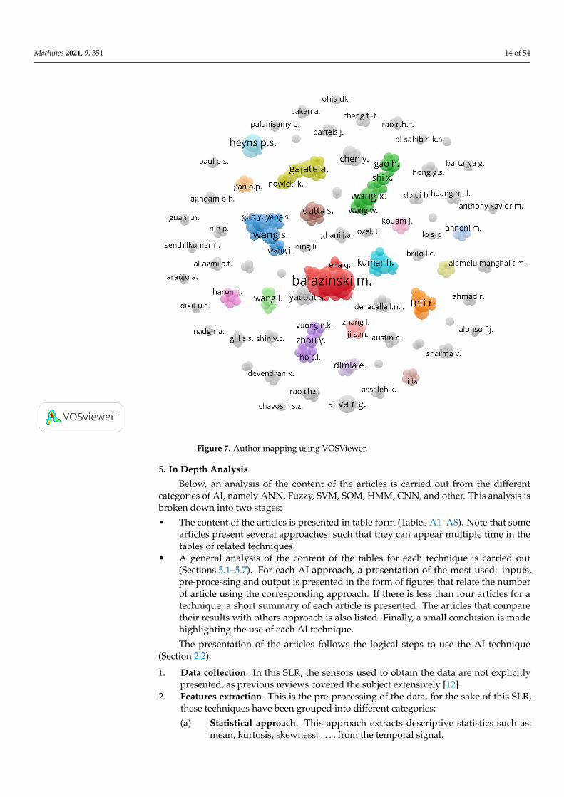
A co-authorship analysis is performed using VOSViewer (a tool for creating, visualiz-ing and exploring meaningful map of items of interest [50]). A mapping of the differentauthors is presented in Figure 7. The size of each item (authors name and associated circles)indicates the occurrence of the authors in the literature. A larger circle means that thecorresponding author appeared more in this SLR. Each cluster represents an author group,i.e., usual co-authors. The larger a cluster, the more authors there are in it. It is observedthat there are some clusters which are larger and bigger than the others. This is generally aspecific lab that works on the subject of this SLR. It is observed that most of the clustersare isolated, and there is no link between them. This does not mean that the authors donot cite each other, but it does indicate that there is very little inter-lab collaboration in theredaction of articles beyond usual co-authors.

Machines 2021, 9, 351 14 of 54

Figure 7. Author mapping using VOSViewer.

5. In Depth Analysis

Below, an analysis of the content of the articles is carried out from the differentcategories of AI, namely ANN, Fuzzy, SVM, SOM, HMM, CNN, and other. This analysis isbroken down into two stages:

• The content of the articles is presented in table form (Tables A1–A8). Note that somearticles present several approaches, such that they can appear multiple time in thetables of related techniques.

• A general analysis of the content of the tables for each technique is carried out(Sections 5.1–5.7). For each AI approach, a presentation of the most used: inputs,pre-processing and output is presented in the form of figures that relate the numberof article using the corresponding approach. If there is less than four articles for atechnique, a short summary of each article is presented. The articles that comparetheir results with others approach is also listed. Finally, a small conclusion is madehighlighting the use of each AI technique.

The presentation of the articles follows the logical steps to use the AI technique(Section 2.2):

1. Data collection. In this SLR, the sensors used to obtain the data are not explicitlypresented, as previous reviews covered the subject extensively [12].

2. Features extraction. This is the pre-processing of the data, for the sake of this SLR,these techniques have been grouped into different categories:

(a) Statistical approach. This approach extracts descriptive statistics such as:mean, kurtosis, skewness, . . . , from the temporal signal.

Machines 2021, 9, 351 15 of 54

(b) Frequency approach. This approach extracts information from the frequencydomain. In this SLR, this is commonly achieved by a Fast Fourier Trans-form (FFT).

(c) Time-frequency approach. This approach extracts information from the time-frequency domain. In this SLR, this is generally done with a Wavelet Packagedecomposition.

(d) Normalization. It consists of scaling the variables between 0 to 1. This allowsthe AI to learn in a more stable and faster way.

(e) Others. This regroups specific approaches. In this SLR, the “others” categorygenerally refers to features extracted from images.

(f) None. An article which does not explicitly describe any pre-processing tech-niques is found in this category. Note that some sort of pre-processing isalways needed.

More detailed descriptions of these approaches exist in the literature [40,51,52].3. Features selection. To avoid any confusion, this part is not systematically presented

in this SLR. Indeed, the articles rarely present the feature selection extensively and,in many cases, the selection is made by the authors. Since little and incompleteinformation is available in the articles, it is therefore not relevant to compare thearticles on this point.

4. Input In this review, a categorization of the input data is realized, and the input iscategorized as: cutting speed, feed rate, depth of cut, cutting time, spindle informa-tion, cutting forces, Acoustic Emission (AE), vibration, surface roughness, images,temperature, and others. The first three inputs listed above are data characterizingthe cutting conditions of the turning operation. These data are not correlated withthe health of the tool but are usually used to give context to the other measured data.In this study, these data are presented in the “input” column in the different tables ofresults and figures related to the approach.

5. Inference In this SLR, the output is categorized in: classification, estimation of VBB,prediction of VBB, remaining useful life (RUL) and others. The difference between“estimation” and “prediction” aims at disambiguating the word “prediction” usedby authors indistinctly for “estimation” (i.e., “monitoring of the current state of thetool”) and “prediction” (i.e., “prediction of the future state of the tool”). This nuanceis discussed in Section 6.

6. Accuracy Comparing the accuracy of different AI techniques is complex, as differentauthors use different indicators (Root Mean Squared Error, Mean Absolute Error,accuracy term, . . . ) to evaluate their approach. Categorizing the results would be toosubjective as it would be necessary to define precision intervals. As all the approachesare very different and use various datasets, it was chosen to refer to each articleauthors’ assessment to judge the accuracy of the approach. All articles cited in thisSLR have obtained a “good” performance. Objectively, the average accuracy of allclassification methods is around 90%. As it is discussed in the following sections,the majority of authors that performed a comparison of an AI approach against astandard statistical approach have shown that the AI approach performed better thanthe statistical approach.

This approach allows for identifying the different trends in the literature for each AIselected techniques. It also allows for highlighting the difficulties and opportunities offeredby each approach.

5.1. ANN

As presented in the bibliometric analysis (Section 4), the artificial neural network is themost popular decision-making method used to monitor the tool life. An explanation of thisapproach is presented in Appendix B.1, and Table A1 presents the 44 articles about ANN.

Machines 2021, 9, 351 16 of 54

5.1.1. General Architecture of the Neural Network

The architecture of a neural network is often defined by trial and error and can have amajor influence on the quality of the results. From the 44 papers about ANN, 17 proposean architecture with one hidden layer [33,41,46,52–65], two propose an architecture withtwo hidden layers [66,67] and the rest does not give any information about the networkarchitecture. From these papers, the most common architecture of the neural network tomonitor the tool wear is presented in Figure 8. This architecture is composed of threelayers: one input layer, one hidden layer and one output layer. The number of neuronsin the input layer depends on the data used as inputs. In the hidden layer, the number ofneurons is around 3 to 5. Finally, the output layer is generally composed of one neuronthat gives information about VBB (Figure 8). This architecture therefore appears to bethe most efficient to resolve the subject of this SLR. Apart from the network architecture,other considerations exist. An exhaustive comparison of different types of NN is presentedin [68]. The influence of the optimizer is studying in [69,70]. A comparison betweendifferent architectures and activation functions is made in [55]. It is also worth notingthat [71] proposes an approach based on a recurrent neural network.

X

inputs1 Hidden layer

3-5 neurons

1 output

VBB

VBB

Figure 8. General form of an ANN used for tool condition monitoring.

5.1.2. Input

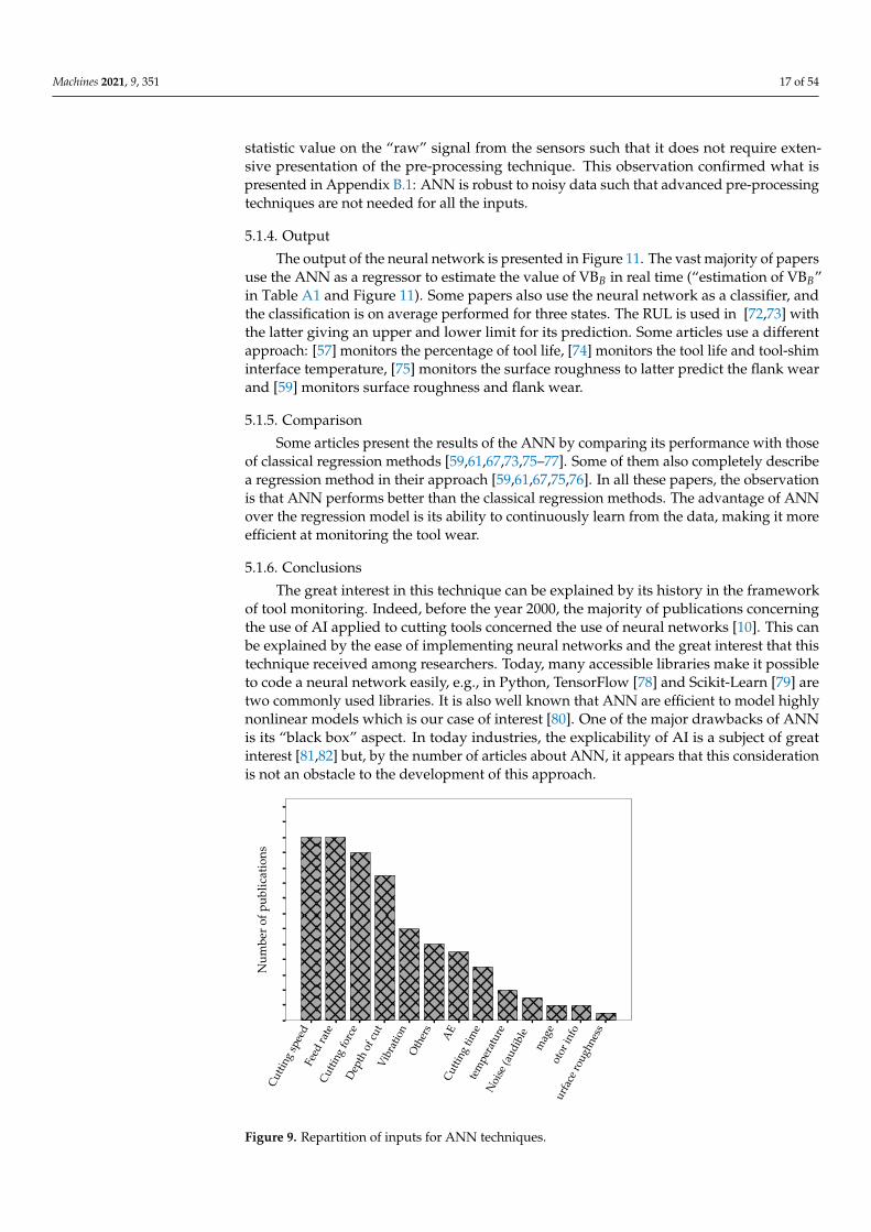
The different features used as input of the neural network, based on the 44 articleson the subject, are presented in Figure 9. The six most used features are: cutting speed,cutting forces, feed, depth of cut, vibration and acoustic emission (AE). In these data, onlythree are dependent on the state of the tool: cutting forces, vibration and AE. The threeothers are cutting parameters that are necessary to help the neural network to identify thecutting conditions.

5.1.3. Pre-Processing

To extract useful information about these signals, pre-processing techniques are em-ployed. Figure 10 shows the pre-processing techniques used in this context. As the twomost used pre-processing techniques are: None and Statistic, it appears that, for ANN,complex techniques are not always required. When a pre-processing is applied, it is a verysimple one that consists of computing the skewness, kurtosis, etc. Note that the category“None” refers to articles that do not present the pre-processing technique used. As somesort of pre-processing is always needed, it indicates that these articles only compute simple

Machines 2021, 9, 351 17 of 54

statistic value on the “raw” signal from the sensors such that it does not require exten-sive presentation of the pre-processing technique. This observation confirmed what ispresented in Appendix B.1: ANN is robust to noisy data such that advanced pre-processingtechniques are not needed for all the inputs.

5.1.4. Output

The output of the neural network is presented in Figure 11. The vast majority of papersuse the ANN as a regressor to estimate the value of VBB in real time (“estimation of VBB”in Table A1 and Figure 11). Some papers also use the neural network as a classifier, andthe classification is on average performed for three states. The RUL is used in [72,73] withthe latter giving an upper and lower limit for its prediction. Some articles use a differentapproach: [57] monitors the percentage of tool life, [74] monitors the tool life and tool-shiminterface temperature, [75] monitors the surface roughness to latter predict the flank wearand [59] monitors surface roughness and flank wear.

5.1.5. Comparison

Some articles present the results of the ANN by comparing its performance with thoseof classical regression methods [59,61,67,73,75–77]. Some of them also completely describea regression method in their approach [59,61,67,75,76]. In all these papers, the observationis that ANN performs better than the classical regression methods. The advantage of ANNover the regression model is its ability to continuously learn from the data, making it moreefficient at monitoring the tool wear.

5.1.6. Conclusions

The great interest in this technique can be explained by its history in the frameworkof tool monitoring. Indeed, before the year 2000, the majority of publications concerningthe use of AI applied to cutting tools concerned the use of neural networks [10]. This canbe explained by the ease of implementing neural networks and the great interest that thistechnique received among researchers. Today, many accessible libraries make it possibleto code a neural network easily, e.g., in Python, TensorFlow [78] and Scikit-Learn [79] aretwo commonly used libraries. It is also well known that ANN are efficient to model highlynonlinear models which is our case of interest [80]. One of the major drawbacks of ANNis its “black box” aspect. In today industries, the explicability of AI is a subject of greatinterest [81,82] but, by the number of articles about ANN, it appears that this considerationis not an obstacle to the development of this approach.

�������(��

���

����(����

�������(��� �

(�����(��( ��

��������

������

��

�������(����

�����������

�����(&���

����'

�����

�����(����

����

�(��

����

����

�!"$

�����!�"�$�����!�"�$

���

���(�

�(���

�� ������

�! �!��

�%

����

%#

!

� ��

Figure 9. Repartition of inputs for ANN techniques.

Machines 2021, 9, 351 18 of 54

���

���������

�������"��

����

����� �������

���!�

�����"���

���

����

�

�

�

�

��

��

��

��

�

��

���

��"�

"���

�������� ��

��

��

� �

Figure 10. Repartition of pre-processing for ANN techniques.

��� �

�� ������VB B

����� � �

� ��

����

���

�����

������������������������������

���

����

�����

� �� ���

��

� ��

Figure 11. Repartition of outputs for ANN techniques.

5.2. Fuzzy Inference System and ANFIS

This section presents the results for the ANFIS and FIS approaches. It was chosen togroup these two approaches because the observations made in the following are identicalfor both. The 26 articles are presented in Table A2 for the FIS and Table A3 for theneuro-fuzzy approach.

5.2.1. Presentation of the Articles

There are 8 articles about FIS: [33,76,83–88] and 18 articles for the neuro-fuzzy ap-proach: [33,36,37,41,58,89–101]. For the inference system, it is important to note that, outof the 8 articles, five articles have the author Balazinski Marek (and Baron Luc for four ofthese articles) in the author list which explains the similarity in the approaches presentedin these articles ([33,84,86–88]).

Machines 2021, 9, 351 19 of 54

5.2.2. Input

The inputs used for the fuzzy models are presented in Figure 12. It is observed thatthe most used input is the cutting forces followed by the AE and feed rate signals. With17 out of 26 articles using it, the cutting force is the most used input signal. A particularapproach using temperature as well as the power and voltage of the machine as inputsignal is presented in [93].

5.2.3. Pre-Processing

The pre-processing technique use is presented in Figure 13. The most used pre-processing techniques are: None and Statistic. It indicates that the fuzzy logic approachesdo not require elaborated pre-processing technique to obtain a good accuracy.

5.2.4. Output

The output of the fuzzy models is presented in Figure 14. The vast majority of articlesuse the fuzzy logic to monitor the flank wear VBB.

5.2.5. Comparison

For the FIS, the papers [86,87] perform a comparison of their approach that uses aTagaki–Sugeno–Kang Fuzzy Approach Based on Subtractive Clustering Method with aneural network, neuro-fuzzy and Mamdani fuzzy logic. The approaches proposed in thesepapers have a lower root mean squared error on the prediction of VBB.

5.2.6. Conclusions

The fuzzy approaches occupied a large amount of the literature around the 2010s;today, they are much less represented in the literature. There is nothing that explain thisdecline in interest. It seems that the interest by the researcher has evolved such that theseapproaches have been replaced. The interest of fuzzy approaches lies mainly in theirexplicable aspect. Unlike neural networks, a fuzzy approach is not a black box. This isa great feature, especially in shop floor applications where the fuzzy approach can be ofinterest by providing more information than a simple prediction. In [41], the low processortime is also cited as a key feature of the fuzzy approach compared with neural networks.

�������%�����

��

��� %���

�������

�������%��

��

�������%����

%�����%��%���

������

�����%����

����

����������

�

�

!

#

��

��

�

�!

�#

��

���

���%�

�%���

��������

�"

$ $

!

� �

� �� �

Figure 12. Repartition of inputs for fuzzy techniques.

Machines 2021, 9, 351 20 of 54

���

����

�����

���

�

���

��

����

���

���

�

���

��!�

����

���

��

���!

���

���

�

�

�

�

�

��

��

��

��

���

��!�

!���

����

���� ��

�

� ��

�

Figure 13. Repartition of pre-processing for fuzzy techniques.

����

���������VB B

���

������

����

�����

������������������

��

�����

�� ��

����

����

��

�

Figure 14. Repartition of outputs for fuzzy techniques.

5.3. SVM

As mentioned in Section 4.2, SVM received great interest over the past five years andis one of the most used techniques to monitor the tool wear with 18 articles. A presentationof these articles is provided in Table A4.

5.3.1. Input

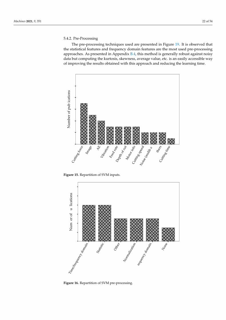
The input features used for the SVM approach are presented in Figure 15. It isobserved that the most used input is the cutting force. It also appears that the use of

Machines 2021, 9, 351 21 of 54

images to generate features is more commonly used in this AI technique than with otherapproaches (except CNN).

5.3.2. Pre-Processing

Due to the sensibility of SVM to noise and outliers, it appears that this approachrequires more pre-processing on the data than ANN. Indeed as Figure 16 shows, the vastmajority of the approaches show the use of a pre-processing technique. This pre-processingis performed in the time-frequency domain and some statistical features are computed.

5.3.3. Output

The output of the SVM is presented in Figure 17. As described, SVM was initially onlyused in classification purpose. Here, the number of articles that use SVM for regressionand classification are almost the same.

5.3.4. Comparison and Particular Approaches

In a particular article [102], the authors use the SVM approach to make a short-termprediction of VBB at time t and also at time t + 1 (“prediction of VBB”). This approach usesSVM coupled with a genetic algorithm to perform this task. A comparison is realized withan AutoRegressive Integrated Moving Average (ARIMA) model and the SVM approachdeveloped in that paper. The authors demonstrate that the SVM approach performs betterthan the ARIMA model.

In another instance, it is proposed to use the cutting forces to classify the state ofthe tool into three states (“initial”, “normal” and “severe” wear) [103]. The cutting forcesare pre-processed with several techniques: normalization, statistical features and time-frequency domain. This is followed by a correlation analysis to find the best features. Thesefeatures are used as input of a Gravitational Search Algorithm–Least Square Support VectorMachine model (GSA-LSSVM). In this entry, the authors compare the results obtained withthis technique with other related methods such as: K-Nearest Neighbour(k-NN), FeedForward Neural Network (FFNN), Classification And Regression Tree (CART) and LinearDiscriminant Analysis (LDA). The classification obtained with the GSA-LSSVM modeloutperforms the others. However, most other authors using SVM in this context compareSVM with ANN, and they show that SVM is more accurate (in classification and regression)than ANN [31,104–106]. Some authors also compare the results obtained with SVM andother AI techniques: [31,103–106].

5.3.5. Conclusions

Applications of SVM appeared later in the literature and remain a relatively modernapproach. As this method is more dependent on the quality of the input data, some featureextraction is required to improve the quality of the inference. Fitting the correct parameterin the SVM approach is a complex task, but it appears that the quality of the inference madewith this approach is at least at the same level as with an ANN approach. In practice, thismethod may be more difficult to implement in the industrial sector due to its sensibility tonoisy data, and it needs a pre-processing approach. However, SVM has the advantage of agood generalization performance which could make this approach particularly interestingin the future.

5.4. SOM

Only 7 articles described this approach and are presented in Table A5.

5.4.1. Input

The inputs of the SOM are presented in Figure 18. Due to the nature of this approach,only inputs that are highly correlated with the tool wear are used. Indeed, the cuttingparameters such as cutting speed, depth of cut, feed rate, etc. are not used as input of theSOM contrary to other approaches.

Machines 2021, 9, 351 22 of 54

5.4.2. Pre-Processing

The pre-processing techniques used are presented in Figure 19. It is observed thatthe statistical features and frequency domain features are the most used pre-processingapproaches. As presented in Appendix B.4, this method is generally robust against noisydata but computing the kurtosis, skewness, average value, etc. is an easily accessible wayof improving the results obtained with this approach and reducing the learning time.

�������'�����

����

��

�������

��� '���

'�����'��'���

�����'����

�������'��

��

�����'%�

����&

������

�������'����

�

�

"

$

��

���

���'�

�'���

��������

#

!

� � � �

� � �

�

Figure 15. Repartition of SVM inputs.

���!�

�����"���

���

���������

����

����� �������

�������"��

����

���

�

�

�

�

��

��

���

��"�

"���

��������

� � �

�

Figure 16. Repartition of SVM pre-processing.

Machines 2021, 9, 351 23 of 54

����

��� ���VB B

���������

������� ���VB B

�

�

�

�

�

��

��

��

���

�����

����

����� � ��

�

�

Figure 17. Repartition of SVM outputs.

5.4.3. Output

This approach is only able to perform classification as observed in Figure 20.

5.4.4. Comparison

Some articles present the SOM with another method. In [2], a comparison betweenSOM, SVM and k-nearest neighbour approach is realized. In [41], the use of SOM, neuro-fuzzy and ANN is discussed and software is presented for shop-floor application. In gen-eral, the SOM approach does not outperform the others but proposes a simple and ac-cessible classification solution. However, the lack of generalization capabilities of thisapproach requires training under all cutting conditions, which is not always necessary withother methods.

5.4.5. Conclusions

The SOM approach is quite different from the others by its unsupervised learningaspect. Some authors use this aspect to try to select the best features independently ofclassical correlation approaches [107]. Other uses this aspect to work with imbalanceddata and uni-sensor approach [2]. In an industrial application, imbalanced data oftenconstitute the only available data, and this technique can therefore be used in this context.The advantage of low computation time is also highlighted [41].

5.5. HMM

The HMM approach is not strongly represented in the literature with only 3 articles: [32,46,47].These articles are presented in Table A6. They are all used to perform a classification on thetool state.

5.5.1. Presentation of the Articles

In Ref. [32], a discrete hidden model uses the wavelet transformation on the vibrationsignal in the feed direction to classify the tool state within two states (“sharp” or “worn”tool). This approach achieves a hit rate up to 97%. The authors try this approach underdifferent training conditions (e.g., length of training data and variation of observationsequence length), and the HMM performs well in all conditions.

Machines 2021, 9, 351 24 of 54

In Ref. [47], a Discrete Hidden Markov Model (DHMM) is used in combination withan SOM. They use the cutting force and the acceleration to monitor the state of the tooland these features are pre-processed with a FFT and coded with a SOM. Their approachperformed well, and a processing time of around 0.2 s is reported, which makes thisapproach usable in online applications.

In Ref. [46], the use of ANN is compared to an HMM to monitor the tool wear. The cut-ting force signal is used as input, pre-processed with multiple techniques: statistical (mean,skewness, etc.), frequency (FFT, PSD) and time-frequency (wavelet and spectrogram).The best features are chosen by the researcher following a correlation analysis. It is con-cluded that both approaches perform well with the advantage of HMM to be extremelyeasy to train but limited to a certain amount of output values (classification).

����

����

���

����

!���

��

����

!���

���� ��

�����

� !��

��

���

!����

���

��!��

���

�

�

�

�

��

���

���!�

�!���

����

����

�

�

�

� � � �

Figure 18. Repartition of SOM inputs.

����

�����

���

���

�!��

���

���

�

���

���

!���

���

���

���

��

����

���

���

�

�

�

�

�

�

��

���

��!�

!���

����

����

��

�� �

�

Figure 19. Repartition of SOM pre-processing.

Machines 2021, 9, 351 25 of 54

�������������

�

�

�

�

�

��

��

�� ���������������

�

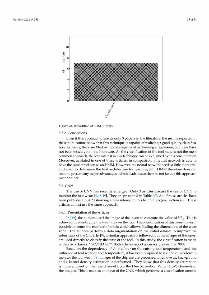
Figure 20. Repartition of SOM outputs.

5.5.2. Conclusions

Even if this approach presents only 3 papers in the literature, the results reported inthese publications show that this technique is capable of realizing a good quality classifica-tion. In theory, there are Markov models capable of performing a regression, but these havenot been tested yet in the literature. As the classification of the tool state is not the mostcommon approach, the low interest in this technique can be explained by this consideration.Moreover, as stated in one of these articles, in comparison, a neural network is able tohave the same precision as an HMM. However, the neural network needs a little more trialand error to determine the best architecture for learning [46]. HMM therefore does notseem to present any major advantages, which leads researchers to not favour this approachover another.

5.6. CNN

The use of CNN has recently emerged. Only 3 articles discuss the use of CNN tomonitor the tool wear: [9,48,49]. They are presented in Table A7. All of these articles havebeen published in 2020 showing a new interest in this techniques (see Section 4.2). Thesearticles almost use the same approach.

5.6.1. Presentation of the Articles

In [49], the authors used the image of the insert to compute the value of VBB. This isachieved by identifying the wear area on the tool. The identification of this zone makes itpossible to count the number of pixels which allows finding the dimensions of the wearzone. The authors perform a data augmentation on the initial dataset to improve therobustness of the CNN. In [9], a similar approach is followed, but the images of the insertare used directly to classify the state of the tool. In this study, the classification is madewithin two classes: “GO/NO GO”. Both articles report accuracy greater than 90%.

Based on the dependency of chip colour on the cutting tool temperature, and theinfluence of tool wear on tool temperature, it has been proposed to use the chip colour tomonitor the tool wear [48]. Images of the chip are pre-processed to remove the backgroundand a kernel density estimation is performed. They show that this density estimationis more efficient on the hue channel from the Hue Saturation Value (HSV) channels ofthe images. This is used as an input of the CNN which performs a classification around

Machines 2021, 9, 351 26 of 54

three classes depending on the class of the wear: “New”, “Medium” and “High”. Theyachieve accuracy of above 90%. A comparison is made with a functional data analysis(FDA) classifier, and it fails to beat the CNN.

5.6.2. Conclusions

The late interest in this technique can be explained by the complexity to obtain asignificant number of images for the datasets. Indeed, this technique uses images ofthe tool which can be impractical to obtain in industrial applications. These approacheswork greatly in laboratory conditions but still require human intervention to achievethem. Comparing this approach with the others presented in this paper, automating thisapproach seems more difficult. In addition, in real production applications, turning isoften performed with cutting fluids which can further complicate image capture. Indeed,the conditions for taking images must be consistent and the light must be controlled so asnot to influence the neural networks [48]. Today, to our knowledge, there is no automatedmachine allowing the introduction of a capture system of this type which may explainthe low interest raised by this technique. This lack of interest can also be explained bythe false belief that CNN is more difficult to implement than ANN [108]. Furthermore,this approach requires stopping the machining process to allow the picture to be takenwhich removes all the interest of monitoring in real time. However, the advantage of thisapproach is that it makes it possible to directly measure the wear on the tool rather thangoing through correlated indicators such as the cutting forces, for example. Automatingthis approach would be equivalent to automating the measurement of VBB, which wouldprovide important data for other forecasting techniques. By using the chip colour instead, itcould then be possible to carry out the measurement without interrupting the process [48].

5.7. Other

This section covers all approaches that are not related to the other categories. The ar-ticles are presented in Table A8. It can be noted that, among these methods, there is amajority of decision trees and classifiers. These approaches are generally compared in pairswith others, hence they do not have a dedicated section in this SLR.

5.8. General Conclusions

Table 3 summarizes the top 3 inputs, pre-processing, and outputs for each AI tech-niques. From this table, the different methods are compared.

For ANN, 2 of the 3 most used inputs are cutting parameters: cutting speed and feedrate. This extensive use of cutting parameters as input signal appears to be specific to ANNas this characteristic is not observed for other methods. All AI techniques extensively usethe cutting force as input signal as it is present in the top 3 of each AI technique (exceptCNN). Vibration and AE signal are also commonly used. It is worth noting that, except forCNN, SVM is the second method that uses features extracted from images as input.

ANN and ANFIS/FIS techniques do not appear to require elaborate pre-processingas most of the articles do not specify the pre-processing techniques employed (“None” inTable 3). SVM, SOM, HMM and CNN all require special attention to the feature extractiontechniques, especially SVM and HMM, which benefit from more advanced pre-processingtechniques in the time-frequency domain. For the majority of methods, the computation ofsimple statistic characteristic on the signal is commonly used. By its nature, CNN does notrequire the same kind of pre-processing technique as it mainly uses images as input.

Two outputs are predominant in the use of AI techniques: estimation of VBB andclassification. In the analysis of AI technique by year (Section 4.1), it was shown that ANN,fuzzy and SVM techniques are predominant in the literature. It is observed that thesethree techniques are the only ones with “Estimation of VBB” as the most represented output.Indeed, approaches such as SOM, HMM and CNN are mainly focused on classification.It is therefore observed that techniques monitoring the value of VBB are favoured over asimple classification purpose.

Machines 2021, 9, 351 27 of 54

Table 3. Comparison of the three most used: input, pre-processing and output for each approaches.

ANN ANFIS & FIS SVM SOM HMM CNN

Nb of articles 44 18 & 8 18 7 3 3

InputCutting Speed (24) Cutting Force (17) Cutting Force (7) Vibration (6) Cutting Force (2) Image(3)Feed rate (24) AE (9) Image (5) Cutting force (5) Vibration (2) /Cutting force (22) Feed rate (9) AE (4) Noise (2) / /

Pre-processingNone (16) None (12) Time-frequency (8) Statistic (6) Time-frequency (2) Image processing (3)Statistic (12) Statistic (6) Statistic (8) Frequency domain (5) Frequency (2) /Frequency domain (7) Other (3) Other (5) Time-frequency (2) Normalization (1) /

Output Estimation of VBB (34) Estimation of VBB (23) Estimation of VBB (10) Classification (7) Classification (3) Classification (2)Classification (7) Classification (5) Classification (9) / Estimation of VBB (1) Estimation of VBB (1)Other (6) / Prediction of VBB (1) / / /

Machines 2021, 9, 351 28 of 54

As it is discussed in Section 6, comparing AI methods on the results they are ableto achieve is not possible. Since each approach is carried out on a different dataset,with different indicators, with different inputs, etc. comparing these results would notprovide a clear and unbiased analysis of the literature. Despite this fact, it is described inthe previous sections that articles that compare the AI techniques with classical methodssuch as statistical model, show that the AI techniques outperform the classical models.

6. Discussion

As indicated by the various authors of the identified publications, all approachespresented in this SLR were able to obtain good results in monitoring the cutting tool health,some authors were even able to obtain more than 90% accuracy. The majority of theseapproaches have the common point to monitor the value of VBB to assess the tool state.Unfortunately, there are few other approaches that try to evaluate the tool health differently.Some papers try to monitor the tool wear with other indicators such as its percentage ofelapsed tool life, and others try to predict the RUL. This lack of other approaches may comefrom the difficulty to define a clear end-of-life criterion to cutting tools. In the ISO 3685standard [19], the maximum value for VBB is set to 0.3 mm as the end-of-life criterion, but,in real application, this value may not represent the cutting tool end-of-life, dependingon the industrial applications and its tolerances. As this end-of-life can be very variable,having approaches based on the RUL or other time indicator can be very difficult toadopt for industrial applications. It is therefore understandable why researchers are moreinterested in the value of VBB rather than trying to define a precise end-of-life criterion. Itis up to the AI user to define the criteria corresponding to its application. By proposing anapproach that monitors VBB, the researchers ensure that their method can be applicable inreal applications.

Knowing the current condition of a tool is obviously of great interest in conditionmonitoring. However, as the industry evolves, predictive monitoring tends to be thepreferred approach. The current state of the art shows that there is too little researchdone to meet the future needs of industries in predictive maintenance, i.e., to predict thecoming evolution of the tool condition. In recent years, advanced statistical models tendto answer this problem but still require a lot of tuning to obtain results. The use of AIcould perhaps meet these needs of industries while guaranteeing models robust enoughto be implemented on shop-floor applications. At this stage, it is not possible to assesswhether this lack of interest in predictive maintenance is due to a lack of interest fromthe researchers or if it comes from a publication bias. Indeed, in this SLR are only listedarticles that present relatively good results, and this may either be due to the fact that alltechniques were always able to perform well, or that the publications which do not getgood results are not published or not submitted for publication. It is therefore possiblethat, currently, research in predictive maintenance is not published due to a possible lackof results.

Due to the different nature of the AI techniques, it is not possible to make a compar-ison between each of them. Many articles compare their approach with other methods.In this SLR, these articles are listed and their results presented, although they are oftencontradictory. Indeed, an approach presented in any of the selected articles is often pre-sented to be the most effective compared with others. Given these contradictions, it isimpossible to identify the best approach, if one exists. This may come from two reasons:(i) the publication bias previously discussed (the papers are not submitted or published iftheir approach is not better than another one), (ii) there is no best approach. Moreover, outof 102 articles, 98 performed a test campaign to obtain their dataset. As these data havebeen collected with different cutting conditions, materials, tools, . . . it is not relevant tocompare the results of these approaches. In turning, there is no benchmark dataset allowingfor fairly comparing all the approaches, whereas benchmarks exist for other categories ofmachining. In milling, for example, some datasets are available on the NASA website [109],on the PHM website [110], . . . This lack of unified benchmarking in turning does not allow

Machines 2021, 9, 351 29 of 54

a clear view of the performance and is a clear limitation of the comparison of performancesin all these articles, which can therefore only be analysed objectively on the bases of theirmethodology instead of their results. The results obtained are therefore highly dependenton the quality of the data recovered during the tests and some data may be more fittedto certain approaches than others. Consequently, the pooling of various test data wouldallow the establishment of benchmarks. These benchmarks should aim to be the mostrepresentative of industrial reality. This lack of unified dataset can also be in relationwith the co-authorship analysis performed in Section 4.5: as there is little inter-laboratorycollaboration in the topic of this SLR, no data are shared between researchers.

It is also observed that the title of the articles could be confusing. Indeed, many articlesincorrectly used the word “prediction” to talk about “monitoring”. As a matter of fact, outof the 102 identified articles, 34 wrongly use the word “prediction” in their title and 62 intheir title or abstract. The word prediction, in the English language, normally evokes thefuture state as defined in the Oxford dictionary: “Prediction is a statement that says what youthink will happen” [22]. As shown in this SLR, the majority of articles actually use the AItechnique as a monitoring system (i.e., to produce an estimate in real time). There is noforecasting of the future state. This abuse of language likely leads to confusion given theprevious remark on the emergence of predictive maintenance.

7. Answers to the Research Questions

This section presents an answer to the research questions identified in Section 3.1.The answers to these questions are distributed through this SLR, but the main results aresummarized here.

RQ1 How is AI used in the framework of monitoring/predicting the condition of tools instable turning condition?

This question is answered throughout this SLR and RQ2 to RQ5. Several approacheshave been mentioned and there is not one that stands out from the others (mainly dueto the lack of unified benchmark). Each approach can find its place depending on themeans and equipment made available to the monitoring system. However, as discussedin Section 6, it appears that, in the current state of the art, too few papers concern theevolution of VBB, as they rather monitor the current state of the tool, which could be aproblem in the framework of predictive maintenance in industry 4.0.

RQ2 What are the most used AI techniques used in this context?

In Section 5 of this SLR, all the AI methods were presented. Among them, there doesnot appear to be a more efficient approach than another. Each approach has its advantagesand disadvantages. However, it appears in Section 4.2 that approaches from neural net-works, fuzzy logic and support vector machines are particularly present in the literature.They all have the ability to be integrated into workshops. Neural network approaches havethe advantage of having been widely studied but have a “black box” aspect which couldcause reluctance in practice. Fuzzy logic seems to no longer be considered even thoughthey had the advantage of presenting the results in an easily understandable way. Inaddition, finally, SVM approaches seem to perform as good as ANN and fuzzy approachesbut require special attention to data pre-processing and the choice of parameters.

RQ3 What is the forecasting horizon of each of the identified AI techniques in this context?

Figure 21 presents the outputs of all the AI techniques presented in this article. Itappears that the majority of articles use AI to monitor the current state of tool wear(estimation of VBB). A classification purpose is also realised to detect the actual state ofthe tool. Some papers also present other kinds of output such as the percentage of tool life.Only five articles propose an approach that consist of a prediction of the future state. Thisis achieved by computing the remaining useful life (RUL) or a prediction of VBB at a futuretime (generally called “t + 1”). As discussed in Section 6, there is a lack of application inpredictive maintenance and the actual state of the art is limited to the actual monitoring ofthe tool.

Machines 2021, 9, 351 30 of 54

RQ4 What are the most common inputs used with the different identified AI techniques inthis context?

As AI techniques are data-driven, the most common features have a high correlationwith the cutting tool state. The repartition of all input data for all techniques is presented inFigure 22. The cutting force is the main input as it appears in 54 of the 102 articles. Featuresthat correspond to the cutting conditions such as: feed rate, cutting speed, and depth ofcut are also used a lot. These features are generally constant through the cutting processbut are important to give context to the correlated data such as the cutting force, vibrationsignal, . . . These cutting parameters thus have a significant impact in the ability of the AItechnique to perform the monitoring of the tool.

RQ5 What are the most used features extraction techniques in this context?

The features extraction technique for each AI approach is presented in Section 5.Figure 23 presents the repartition of all pre-processing techniques in this SLR. It is importantto note that, depending on the approach, the pre-processing technique can be different.For example, it is observed that using ANN does not need much pre-processing while, forSVM, the pre-processing technique is necessary.

�����

����

� �

VB B

����

�� ��

����

���

��

���

����

����

� �

VB B

��

������������������������

���

�� �

��

����

����

��

��

��

��

Figure 21. Output variables of all the approaches.

�������(��� �

����(����

��������

�������(��

���

(�����(��( �� ��

������

�������(����

�����

�����(����

�����(&���

����'

�����������

����

�(��

����

����

"

��

�"

��

�"

�

"

!�

!"

"�

""

���

���(�

�(���

�� ������

"!

" �

�%

�! �

�! � ��

$ #"

�

Figure 22. Input variables of all the approaches.

Machines 2021, 9, 351 31 of 54

���������

���

���!�

�����"���

���

�������"��

����

����

����� �������

�

�

��

��

��

��

��

��

���

��"�

"���

��������

��

��

�� �� �

��

Figure 23. Feature extraction techniques of all the approaches.

8. Conclusions

This paper presents a systematic literature review covering the use of AI techniquesin the monitoring of cutting tool health in stable turning condition. The review protocolallowed for identifying 8426 articles in which 102 articles are corresponding to criteriaof interest (Section 3). The review protocol followed the procedure recommended byKitchenham [15]. During the definition of the research procedure, a new approach thataims to improve the quality of it was proposed. Some conclusions can be made about them:

• In the research procedure for this SLR, the choice to use a semantic approach to buildthe keywords was successful. It was chosen to construct each search query with acombination of four keywords so that each correspond to one part of the semanticapproach (Section 3.2.2). The results show that this approach allows for browsingall of the literature on the subject of interest. However, it needs some additionalsorting steps such as removing the “duplicated” items. Due to the number of articlesidentified, this last step cannot be performed manually. This approach is particularlyinteresting in the context of a systematic literature review.

• In the research procedure, to evaluate the inter-rater reliability, the Cohen’s kappa [30]was used to evaluate the agreement among raters (Section 3.3). This gives an unbiasedjudgement of the quality of the sorting which ensures that the research was carriedout in an unbiased manner.

The bibliometric analysis of the 102 articles was performed in Section 4 and shows thetrends in the literature over the last 20 years. Several aspects were discussed including thedistribution of the number of articles per year (Section 4.1), the number of article citations(Section 4.3), the identification of reference journals (Section 4.4), and a discussion on theauthors (Section 4.5). Some general conclusions can be drawn:

• There is a growing interest in the use of AI techniques to monitor the tool wear inturning operation. This is observed by the increasing number of publications by yearin this domain (Section 4.1).

• Approaches using neural networks are predominant in the subject of this SLR with44 articles (Section 4.2). This may be linked to the ease of implementation of thistype of technique and to its robustness to handle noisy data. Fuzzy logic and SVMapproaches are also often used by the researchers with 26 and 18 articles, respectively.

An in-depth analysis of the six AI approaches identified in this SLR was carried outand presented in the form of Tables A1–A8. A discussion for each approach was performedin Section 5. Some general comments can be provided:

Machines 2021, 9, 351 32 of 54

• Some articles compare the AI techniques and the classical statistical approach. Itappears that the AI techniques outperform the classical approach. The main advantageof the AI technique over the classical approaches is that the AI are able to easily adaptto multiple cutting conditions without any further researcher expertise. This makesAI an interesting approach in the industrial context.

• Almost all the articles presented in this systematic literature review perform a dedi-cated test campaign to obtain their own data. This makes it difficult to determine thebest approach. An establishment of a benchmark dataset would allow for comparingthe different approaches on the same data allowing the researchers to have a clearview of the best approach.

• There is a vast variety of approaches to monitor the tool wear, but the accuracy isusually above 90%. It indicates that, no matter the approach, AI techniques can be usedto monitor the tool health. Due to the wide variety of approaches and the differencesin the AI techniques employed, producing an effective horizontal comparison betweenthe methods is not feasible.

• The forecasting horizon is actually limited to the real-time monitoring with only a fewapplications corresponding to predictive maintenance.

To conclude this SLR, some future scopes that need to be addressed in the use of AI tomonitor the tool wear are highlighted:

• The implementation of a common benchmark dataset is needed to allow an objectivecomparison of the performance of proposed approaches.

• Since all the approaches mainly focus on real-time monitoring of the tool state, the pre-dictive maintenance aspects need to be considered a priority.

Author Contributions: Conceptualization, L.C., L.E., P.D. and F.D.; Methodology, L.C. and L.E.;Software, L.C.; Validation, L.C., L.E., P.D. and F.D.; Formal Analysis, L.C.; Investigation, L.C. and L.E.;Data Curation, L.C.; Writing—Original Draft Preparation, L.C. and L.E.; Writing—Review & Editing,L.C., L.E., P.D. and F.D.; Visualization, L.C.; Supervision, L.E., P.D. and F.D.; Project Administration,L.E., P.D. and F.D. All authors have read and agreed to the published version of the manuscript.

Funding: This research received no external funding.

Conflicts of Interest: The authors declare that they have no conflict of interest.

Machines 2021, 9, 351 33 of 54

Appendix A

Table A1. General summary of ANN-related publications.

Article Method Material Input Output Pre-Processing Comments

[53] ANN Inconel 718Cutting forces

AEVibration

Estimation of VB Time/frequency 3 layers: 3 to 7 neurons in thehidden layer

[71] Recurrent neural network (RNN) mild steelCutting forces

VibrationAcoustic (audible)

Estimation of VB Statistic Best performance with 6 to 9 neuronsin hidden layers

[54] ANN steel EN8

Cutting speedCutting forces

FeedDepth of cut

Estimation of VB None 3 layers: 5 inputs ; 1hidden (5 to10 neurons); 1 output

[55] ANN hardened bearing steel(61HRC)

Cutting forcesVibration Estimation of VB Statistic Multi layer perceptron

[111] Regression neural networks high manganese caststeel

Cutting speedCutting forces

VibrationFeed

Depth of cutTemperature

Estimation of VB Normalization

[70] Generalized regression neural networkwith improved fruit fly optimzation

high manganese caststeel

Cutting speedFeed

Depth of cutEstimation of VB Normalization 93% accuracy

[52] Back Propagation NN aluminum alloy 7050 VibrationAcoustic (audible) Classification Time/frequency 3 layers: 8-11-3; 3 states classification

up to 92.5% accuracy

[72] ANN steel Other RUL None

[56] ANN Ti6Al4V AEVibration Estimation of VB Statistic Best results with 3-3-1 and 3-6-1

[76] ANN, fuzzy logic and regression(not AI) AISI 4140

Cutting speedFeed

Depth of cutEstimation of VB None

[66] ANN AISI 4140

Cutting speedCutting forces

VibrationFeed

Depth of cut

Estimation of VB None shape: 5-14-6-1-1

Machines 2021, 9, 351 34 of 54

Table A1. Cont.

Article Method Material Input Output Pre-Processing Comments

[57] ANN AISI 316Cutting forces

AEVibration

Other Time/frequencyStatistic

3 layers: 6-x-1. Output: percentage oftool life

[74] ANN and case based reasoning steel AISI 304; AISI D2;AISI 52100

Cutting speedFeed

Depth of cutOther

RUL Other Output: Tool life and tool-shiminterface temperature

[112] ANN steel (AISI 4340)Cutting speed

FeedDepth of cut

[75] ANN and regression model (not AI) 3 different steel

Cutting speedFeed

Depth of cutOther

Estimation of VB Other NoneComparison with multiple linear

regression model. Output: surfaceroughness and flank wear

[68] ANN and SVM steel (AISI 4340 AND52100 hardenend) Surface texture Estimation of VB None

Reflectiveness of the surface; 28 ANN:6 Multi Layer Perceptron (MLP), 3MLP with Principal Component

Analysis (MLPPCA), 3 GeneralizedFeedForward (GFF), 3 Radial Basis

Function, 3 Time Delay NeuralNetwork, 3 time-lag recurrent network(TLRN), 3 Recurrent Network, 2 linearregression (LR), 1 probabilistic neural

network (PNN) and 1 SVM models

[67] ANN and regression (not AI) steel (AISI 4340)

Cutting speedCutting forces

FeedDepth of cut

OtherTemperature

Estimation of VB Other Architecture: 6-4-5-4-1. Comparisonwith regression

[58] ANN and CANFIS 7075 alloyCutting speed

FeedDepth of cut

Estimation of VB None Co-Active Neuro Fuzzy InferenceSystem (CANFIS)

[113] ANN grey cast iron

Cutting speedCutting time

FeedDepth of cut

Other None Output: Cutting forces (estimation offlank wear)

Machines 2021, 9, 351 35 of 54

Table A1. Cont.

Article Method Material Input Output Pre-Processing Comments

[114] ANN and polynomial classifiers mild steel

Cutting speedCutting forces

AECutting time

Feed

Estimation of VB OtherStatistic ANN 90% accuracy and classifier 85%

[115] ANN AISI 52100 bearing steel

Cutting speedCutting time

FeedDepth of cut

Other

Estimation of VB Normalization 3 layers: 5-7-1

[59] ANN and regression model (not AI) steel AISI H13Cutting speed

FeedDepth of cut

Estimation of VB Other None3 layers and 5 neurons in the hidden

layer. Output: Flank wear and surfaceroughness

[60] ANN EN-8 steel

Cutting speedCutting time

FeedDepth of cut

OtherTemperature

None

3 layers and 5 neurons in the hiddenlayers. There is a mathematical

relationship to predict the tool wear.The AI does not predict directly

the wear

[35] ANN hardened (55HRC) H-13steel tube

Cutting speedCutting forcesCutting time

Other

Estimation of VB Other

[77] Neural networks Experiment AISI1045 steels

Cutting speedFeed

Depth of cutMotor info

Estimation of VB OtherMachine learning process optimal

linear associative memory(MLP OLAM)

[116]Random Forest; gradient boosting

regression, neural network and Supportvector regression

hardened steel (58 HRC)

Cutting speedCutting forces

AEVibration

FeedDepth of cut

Other

Estimation of VBTime/frequency

StatisticFrequency domain

Machines 2021, 9, 351 36 of 54

Table A1. Cont.

Article Method Material Input Output Pre-Processing Comments

[104]

Classifier: Decision tree, K-neighbour,Random forest; Regressor: MLP,

Random Forest, SVM, Naive Bayes,gradient boosting

Generation on Python(turning case)

Cutting forcesMotor info

ClassificationEstimation of VB None 2 states classification

[61] ANN and Response SurfaceMethodology (RSM) (Not AI) /

Cutting speedFeed

Depth of cutEstimation of VB None

3 layers: 5 neurons in the hidden layer;Activation function: “tansig”; Better

results with the AI approach

[117] MLP ANN Die steel Vibration Classification Frequency domain 2 states classification; 87% accuracy

[62] ANN Ti6Al4V Cutting forcesAE Estimation of VB Statistic 3 layers with 9, 18 or 27 neurons in the

hidden layer

[118] ANN (MLFFNN) steel EN 24 AE Estimation of VB Frequency domain

[41] SOM, neuro-fuzzy,ANN EN-8 Steel Cutting forces ClassificationEstimation of VB None ANN: 3 layers: 2-3-1; SOM:

classification

[63] ANN / Acoustic (audible)Surface texture Estimation of VB Other

Frequency domain 3 layers: 3-4-1

[85] Hybrid: ANN and fuzzy modellingSAE 6150

chromim-vanadiumalloy steel

Cutting forcesAE

VibrationEstimation of VB Statistic

Frequency domain

[34] ANN EN24 steel Cutting forcesVibration Classification Normalization 3 layers MLP: 7-20-1; 7 States

classification

[64] ANN steel aisi 1040

Cutting forcesCutting time

Surface roughnessOther

Temperature

Estimation of VB Normalization 3 layers: 3 neurons in the hidden layer

[119] ANN 100Cr-6 and 54CrV4

Cutting speedCutting forces

AEFeed

Estimation of VB StatisticFrequency domain SOM for correlation analysis

[46] ANN and HMM From another study Cutting forces ClassificationEstimation of VB

Time/frequencyStatistic

Frequency domain

Comparison between thetwo approaches: similar results

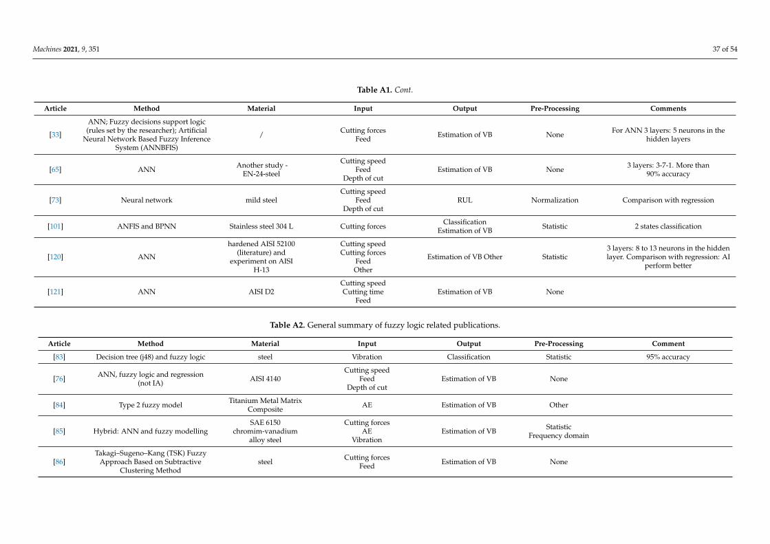
Machines 2021, 9, 351 37 of 54

Table A1. Cont.

Article Method Material Input Output Pre-Processing Comments

[33]

ANN; Fuzzy decisions support logic(rules set by the researcher); Artificial

Neural Network Based Fuzzy InferenceSystem (ANNBFIS)

/ Cutting forcesFeed Estimation of VB None For ANN 3 layers: 5 neurons in the

hidden layers

[65] ANN Another study -EN-24-steel

Cutting speedFeed

Depth of cutEstimation of VB None 3 layers: 3-7-1. More than

90% accuracy

[73] Neural network mild steelCutting speed

FeedDepth of cut

RUL Normalization Comparison with regression

[101] ANFIS and BPNN Stainless steel 304 L Cutting forces ClassificationEstimation of VB Statistic 2 states classification

[120] ANN

hardened AISI 52100(literature) and

experiment on AISIH-13

Cutting speedCutting forces

FeedOther

Estimation of VB Other Statistic3 layers: 8 to 13 neurons in the hiddenlayer. Comparison with regression: AI

perform better

[121] ANN AISI D2Cutting speedCutting time

FeedEstimation of VB None

Table A2. General summary of fuzzy logic related publications.

Article Method Material Input Output Pre-Processing Comment

[83] Decision tree (j48) and fuzzy logic steel Vibration Classification Statistic 95% accuracy

[76] ANN, fuzzy logic and regression(not IA) AISI 4140

Cutting speedFeed

Depth of cutEstimation of VB None

[84] Type 2 fuzzy model Titanium Metal MatrixComposite AE Estimation of VB Other

[85] Hybrid: ANN and fuzzy modellingSAE 6150

chromim-vanadiumalloy steel

Cutting forcesAE

VibrationEstimation of VB Statistic

Frequency domain

[86]Takagi–Sugeno–Kang (TSK) Fuzzy

Approach Based on SubtractiveClustering Method

steel Cutting forcesFeed Estimation of VB None

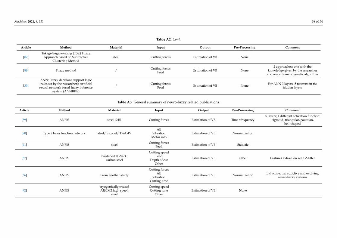
Machines 2021, 9, 351 38 of 54

Table A2. Cont.

Article Method Material Input Output Pre-Processing Comment

[87]Takagi–Sugeno–Kang (TSK) Fuzzy

Approach Based on SubtractiveClustering Method

steel Cutting forces Estimation of VB None

[88] Fuzzy method / Cutting forcesFeed Estimation of VB None

2 approaches: one with theknwoledge given by the researcher

and one automatic genetic algorithm

[33]

ANN; Fuzzy decisions support logic(rules set by the researcher); Artificialneural network based fuzzy inference

system (ANNBFIS)

/ Cutting forcesFeed Estimation of VB None For ANN 3 layers: 5 neurons in the

hidden layers

Table A3. General summary of neuro-fuzzy related publications.

Article Method Material Input Output Pre-Processing Comment

[89] ANFIS steel 1215. Cutting forces Estimation of VB Time/frequency5 layers; 4 different activation function:

sigmoid, triangular, gaussian,bell-shaped

[90] Type 2 basis function network steel/ inconel/ Ti6Al4VAE

VibrationMotor info

Estimation of VB Normalization

[91] ANFIS steel Cutting forcesFeed Estimation of VB Statistic

[37] ANFIS hardened JIS S45Ccarbon steel

Cutting speedFeed

Depth of cutOther

Estimation of VB Other Features extraction with Z-filter

[36] ANFIS From another study

Cutting forcesAE

VibrationCutting time

Estimation of VB Normalization Inductive, transductive and evolvingneuro-fuzzy systems

[92] ANFIScryogenically treatedAISI M2 high speed

steel

Cutting speedCutting time

OtherEstimation of VB None

Machines 2021, 9, 351 39 of 54

Table A3. Cont.

Article Method Material Input Output Pre-Processing Comment

[93] ANFIS D2 X115Cr VMo121steel

Surface textureTemperatureMotor info

Estimation of VB None Accuracy up to 98%

[94] Fuzzy with a new Takagi–Sugeno–Kang(TSK) modelling steel Cutting forces

Feed Estimation of VB None

[58] ANN and CANFIS 7075 alloyCutting speed

FeedDepth of cut

Estimation of VB None Co-Active Neuro FuzzyInference System

[95] Transductive-Weighted Neuro-FuzzyInference System (TWNFIS) From another study

Cutting forcesAE

VibrationEstimation of VB None More than 90% accuracy

[96] ANFIS compared with Hybrid approach steel EN 24 and FG15

Cutting forcesAE

VibrationCutting time

Estimation of VB Normalization

comparison between TransductiveWeighted Neuro-Fuzzy Inference

System (TWNFIS), ANFIS and HybridIncremental Modeling (HIM). HIM

outperform the other

[41] SOM, neuro-fuzzy, ANN EN-8 Steel Cutting forces ClassificationEstimation of VB None ANN: 3 layers: 2-3-1;

SOM: classification

[97] Evolving extended Takagi–Sugeno basedneuro-fuzzy algorithm Inconel 718 Cutting forces

AE Estimation of VB Statistic

[98] Localized fuzzy neural network (LFNN) 45 middle carbide steelworkpiece

Cutting forcesAE Classification Time/frequency

[33]

ANN; Fuzzy decisions support logic(rules set by the researcher); Artificialneural network based fuzzy inference

system (ANNBFIS)

/ Cutting forcesFeed Estimation of VB None For ANN 3 layers: 5 neurons in the

hidden layers

[99] ANFIS steel Cutting forcesAE Classification Statistic Best with triangular and bell function

[100] ANFIS FG15 cast iron

Cutting forcesAE

VibrationCutting time

Estimation of VB Other Around 82% accuracy

[101] ANFIS and Back Propagation NN Stainless steel 304 L Cutting forces ClassificationEstimation of VB Statistic 2 states classification

Machines 2021, 9, 351 40 of 54

Table A4. General summary of SVM-related publications.

Article Method Material Input Output Pre-Processing Comment

[51] SVM high strength steel(45CrNiMoVA)

Cutting forcesVibration

Surface textureEstimation of VB

Time/frequencyStatistic

Frequency domain

Grid search-SVR, Genetic algorithmSVR, Particle swarm optimizer-SVR

and Grid-search SVR

[103]Gravitational search algorithm coupled

with least square support vectormachine model

steel Cutting forces ClassificationTime/frequencyNormalization

Statistic3 states classification

[2] SOM; SVM; k-nearest neighbour steel AISI D6 Vibration ClassificationNormalization

StatisticFrequency domain

Accuracy up to 92%; 2 statesclassification

[102] SVR modified / Other Prediction of Vb Normalization Forecasting at t + 1

[122] SVM and decision tree steel (1.4542) Motor info ClassificationTime/frequencyNormalization

Frequency domain

2 states classification; above 90%accuracy

[123] SVM ZMn13 high manganesecast steel

Cutting speedCutting time

FeedDepth of cut

Estimation of VB None

Nelder–Mead Leave One Out-Leastsquares Support Vector Machines

(NM-LOO-LSSVM), Particle SwarmOptimization-LSSVM (PSO-LSSVM)and LSSVM. Best performances with

NM-LOO-LSSVM

[124] SVM superalloy

AEAcoustic (audible)

FeedDepth of cutMotor info

ClassificationEstimation of VB

Time/frequencyOther Optimization with genetic alogrithms

[68] ANN and SVM steel (AISI 4340 AND52100 hardened) Surface texture Estimation of VB None

Reflectiveness of the surface; 28 ANN:6 Multi Layer Perceptron (MLP),

3 MLP with Principal ComponentAnalysis (MLPPCA), 3 GeneralizedFeedForward (GFF), 3 Radial Basis

Function, 3 Time Delay NeuralNetwork, 3 time-lag recurrent network(TLRN), 3 Recurrent Network, 2 linearregression (LR), 1 probabilistic neural

network (PNN) and 1 SVM models

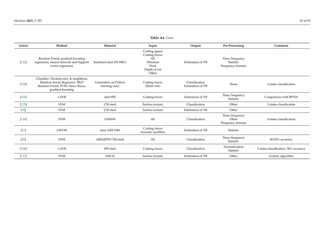
Machines 2021, 9, 351 41 of 54

Table A4. Cont.

Article Method Material Input Output Pre-Processing Comment

[116]Random Forest; gradient boosting

regression, neural network and Supportvector regression

hardened steel (58 HRC)

Cutting speedCutting forces

AEVibration

FeedDepth of cut

Other

Estimation of VBTime/frequency

StatisticFrequency domain

[104]

Classifier: Decision tree, K-neighbour,Random forest; Regressor: MLP,

Random Forest, SVM, Naive Bayes,gradient boosting

Generation on Python(turning case)

Cutting forcesMotor info

ClassificationEstimation of VB None 2 states classification

[105] v-SVR steel #50 Cutting forces Estimation of VB Time/frequencyStatistic Comparison with BPNN

[125] SVM C50 steel Surface texture Classification Other 3 states classification

[38] SVM C50 steel Surface texture Estimation of VB Other

[126] SVM GH4169 AE ClassificationTime/frequency

OtherFrequency domain

4 states classification

[31] LSSVM steel AISI 1040 Cutting forcesAcoustic (audible) Estimation of VB Statistic

[39] SVM ASSAB705/760 steel AE Classification Time/frequencyStatistic 80-85% accuracy

[106] v-SVR #50 steel Cutting forces Classification NormalizationStatistic 2 states classification. 96% accuracy

[127] SVM AISI 01 Surface texture Estimation of VB Other Genetic algorithm

Machines 2021, 9, 351 42 of 54

Table A5. General summary of SOM-related publications.

Article Method Material Input Output Pre-Processing Comment

[2] SOM; SVM; k-nearest neighbour steel AISI D6 Vibration ClassificationNormalization

StatisticFrequency domain

Accuracy up to 92%;2 states classification

[107] SOM steel EN1A1

Cutting forcesVibration

Acoustic (audible)Feed

Motor info

Classification StatisticFrequency domain

[128] SOM mild steelAE

VibrationCutting time

Classification Statistic

[42] Self organizing spiking neuralnetwork map mild steel

Cutting forcesVibration

Acoustic (audible)Classification Statistic

Frequency domain

[41] SOM, neuro-fuzzy,ANN EN-8 Steel Cutting forces ClassificationEstimation of VB None ANN: 3 layers: 2-3-1;

SOM: classification

[40] SOMIndustrial in South

Africa (pistonmanufacturer)

Cutting forcesVibration Classification

Time/frequencyStatistic

Frequency domain3 × 3 output

[129] Self organizing map (SOM) cast iron Cutting forcesVibration Classification

Time/frequencyStatistic

Frequency domain

Table A6. General summary of HMM-related publications.

Article Method Material Input Output Pre-Processing Comment

[47] HMM 45# steel Cutting forcesVibration Classification

OtherNormalization

Frequency domain

[46] ANN and HMM From another study Cutting forces ClassificationEstimation of VB

Time/frequencyStatistic

Frequency domain

Comparison between the 2 approaches:similar results

[32] Discrete Hidden MarkovModel (DHMM) AISI 8620 steel Vibration Classification Time/frequency 2 states classification; more than

97% accuracy

Machines 2021, 9, 351 43 of 54

Table A7. General summary of CNN-related publications.

Article Method Material Input Output Pre-Processing Comment

[49] convolutional neural network (U-Net) 45# steel Surface texture Estimation of VB Other

[48] CNN and functional data analysis low carbon steel(25CrMo4) Surface texture Classification Other 3 states classification; around

90% accuracy;

[9] CNN steel Surface texture Classification Other 2 states classification

Table A8. General summary of publications related to various other methods.

Article Method Material Input Output Pre-Processing Comment

[130]Logical Analysis of data (AI classifier);

Logical analysis of survivalcurves (LASC)

titanium metalmatrix composite Cutting forces Remaining Useful

Life (RUL) None Non AI outperform AI

[2] SOM; SVM; k-nearest neighbour steel AISI D6 Vibration ClassificationNormalization

StatisticFrequency domain

Accuracy up to 92%;2 states classification

[131]Nearest-Neighbour-like algorithm using

non-nested GeneralizedExemplar (NNGE)

steel Vibration Classification Statistic 4 states classification up to100% accuracy

[83] Decision tree (j48) and fuzzy logic steel Vibration Classification Statistic 95% accuracy

[122] SVM and decision tree steel (1.4542) Motor info ClassificationTime/frequencyNormalization

Frequency domain

2 states classification; above90% accuracy

[132]

linear regression, decision trees, randomforests, k-nearest neighbours, adaptive

boosting, bootstrap aggregating andgradient boosting

inconel 718 Cutting forces Estimation of VB Statistic

[133] Hybrid dynamic neuralnetwork (HDNN) steel (different alloy) Motor info Estimation of VB Statistic

[134] Logical analysis of data (LAD) steel (AISI 1045) Cutting forcesFeed Classification None

[74] ANN and case based reasoning steel AISI 304; AISI D2;AISI 52100

Cutting speedFeed

Depth of cutOther

RULOther

Output: Tool life and tool-shiminterface temperature

Machines 2021, 9, 351 44 of 54

Table A8. Cont.

Article Method Material Input Output Pre-Processing Comment

[135] Novelty detection steel Cutting forces Estimation of VB StatisticFrequency domain Up to 100% accuracy

[114] ANN and polynomial classifiers mild steel

Cutting speedCutting forces

AECutting time

Feed

Estimation of VB OtherStatistic

ANN 90% accuracy andclassifier 85%

[136] Hybrid neural network AISI 52100 bearing steel

Cutting speedCutting time

FeedDepth of cut

Other

Estimation of VB Other OtherTraining with an extended Kalmanfilter. Activation function: Sigmoid

and optimization of the network

[44] Hybrid approach / Cutting forces Estimation of VB Other Physical model use to convertthe features

[48] CNN and functional data analysis low carbon steel(25CrMo4) Surface texture Classification Other 3 states classification; around

90% accuracy;

[137] Naive Bayes classifier Oil hardened Nickelsteel

Cutting forcesVibration Classification Time/frequency

4 states classification. 96% accuracywith the cutting forces and 70% with

the vibration signal

[138] Random forest; Gradient boostingmethod (GBM); regression model steel Cutting forces

Vibration Estimation of VB Other Frequency domain Output: tool wear andsurface roughness

[116]Random Forest; gradient boosting

regression, neural network and Supportvector regression

hardened steel (58 HRC)

Cutting speedCutting forces

AEVibration

FeedDepth of cut

Other

Estimation of VBTime/frequency

StatisticFrequency domain

[104]

Classifier: Decision tree, K-neighbour,Random forest; Regressor: MLP,

Random Forest, SVM, Naive Bayes,gradient boosting

Generation on Python(turning case)

Cutting forcesMotor info

ClassificationEstimation of VB None 2 states classification

[139]Functional Series Time dependentAutoRegressive Moving Average

(FS-TARMA)AISI 1045 steels Vibration Other Output: Vibration signal

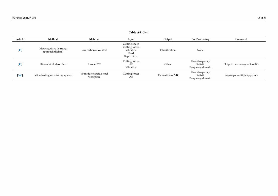
Machines 2021, 9, 351 45 of 54

Table A8. Cont.

Article Method Material Input Output Pre-Processing Comment

[45] Metacognitive learningapproach (Rclass) low carbon alloy steel

Cutting speedCutting forces

VibrationFeed

Depth of cut

Classification None

[43] Hierarchical algorithm Inconel 625Cutting forces

AEVibration

OtherTime/frequency

StatisticFrequency domain

Output: percentage of tool life

[140] Self adjusting monitoring system 45 middle carbide steelworkpiece

Cutting forcesAE Estimation of VB

Time/frequencyStatistic

Frequency domainRegroups multiple approach

Machines 2021, 9, 351 46 of 54

Appendix B

This section presents an introduction to the most used AI techniques presented inthis SLR. The descriptions of the method are not exhaustive but allows a comprehensiveintroduction to some of the concepts that are used in this article.

Appendix B.1. Artificial Neural Network—ANN

The Artificial Neural Network (ANN) is one of the most popular AI techniques.Inspired by the human brain, the architecture of an ANN is composed of at least threelayers: an input layer, some hidden layers and one output layer (Figure A1) [141]. Each layeris composed of neurons which are interconnected with the neurons in the following layer.Each neuron has an associated activation function and the weights of the interconnectionsare updated in the training phase to obtain the desired relationship between the inputand the output. The advantages of ANN are their ability to reproduce highly nonlinearinput-output characteristics, their ease of software implementation and their robustness tonoisy data. It is suggested that ANN can achieve similar performance to any other methodsgiven enough resources [80]. The main downside of ANN is their need for a large amountof data and processing power to learn from the dataset, the trial and error process to choosetheir parameters and the fact that they are to be considered as black boxes [29]. ANN canbe used to achieve regression or classification.

Input 1

Input 2

Input n

Output

Output j

Input layer Hidden layers Output layer

Figure A1. Architecture of an ANN.

Appendix B.2. Fuzzy and Adaptative Neuro-Fuzzy Inference System—FIS & ANFIS

In the framework of this paper, two fuzzy approaches are considered: Fuzzy InferenceSystem (FIS) and Adaptative Neuro-Fuzzy Inference System (ANFIS). Both are based onthe fuzzy logic originally proposed by Zadeh in [142].

An FIS is generally composed of five elements: (i) a set of “if-then” rules; (ii) a databasefor the membership function; (iii) an inference operation system; (iv) a fuzzification inter-face; and (v) a defuzzification interface [143] (Figure A2). Different types of fuzzy reasoningexist (types 1, 2 and 3). In this SLR, the vast majority of FIS are based on approaches that tryto generate the fuzzy rule based on the input–output dataset rather than with the researcherknowledge [144].

ANFIS is the integration of a network that optimizes a FIS. This optimization isachieved by associating and optimizing a series of fuzzy “if-then” rules with the appropriatemembership function [145]. This approach was first proposed in [143] and combines thecapability of adaptation of neural networks while being comprehensible with its set offuzzy rules [143,145].

Machines 2021, 9, 351 47 of 54

Both approaches have the advantages of fuzzy logic: robustness and being easilyunderstandable, and hence a natural implementation. However, the learning capabilitiescan be limited.

Fuzzy inference system

Fuzzi�cation

Inference

Knowledge base

Data base Rule base

Defuzzi�cationInput Output

Figure A2. General layout of FIS.

Appendix B.3. Support Vector Machine—SVM

Support Vector Machine (SVM) is based on statistical learning. This supervised tech-nique was originally developed for classification (Support Vector Classifier, SVC) purposes,but it was later adapted as a regressor (Support Vector Regressor, SVR). The aim of SVC isto find an optimal hyperplane that best separates the data classes by minimizing a loss func-tion. In nonlinear problems, the input can be mapped into a higher-dimensional Hilbertspaces through a kernel function such that the nonlinear approach is transformed into alinear approach in the higher-dimensional space [146] (Figure A3). A similar approach isused for SVR. In this approach, the continuous output is the hyperplane that minimizesthe loss function [147]. SVM has the advantages of being efficient on small datasets andproviding a great generalization, but the training time can be high on bigger datasets, theyare sensitive to datasets with noise and outliers, and fitting the correct parameters can bedifficult (Kernel function).

Kernel function

Input space Output space

Figure A3. SVM principle.

Appendix B.4. Self-Organizing Map—SOM

This unsupervised learning method is a kind of neural network sometimes referredto as a Kohonen map [141]. The neural structure is made to represent the high dimensioninput into a typically two-dimensional map. In other terms, this is a nonlinear transfor-mation from a higher dimensions space to a one- or two-dimensional map (Figure A4).An interesting feature of the SOM is that they preserve their neighbourhood such that,if the data are in the same region in the input space, they are also in a similar region in the

Machines 2021, 9, 351 48 of 54

map [148]. These maps are generally used to perform classification. The main advantageof SOM is its ability to process incomplete data, its ease of interpretation, and its learningspeed. The main disadvantage is that it requires a large number of parameters and mayrequire optimization to perform well.

Weigth

Map

Input 1 Input 2 Input n

Figure A4. SOM principle.

Appendix B.5. Hidden Markov Model—HMM

Hidden Markov Model (HMM) is based on Markov chains. Markov chains describea system by a finite number of states. In a Markov chain, the history of the system isirrelevant and only the current state influences the future state. Two categories of modelsexist: the continuous and discrete models. In continuous model, the changes of the systemcan occur at any time, while, in discrete model, the change can only occur at given timesteps [149]. The particularity of HMM is that the Markov model underlying the data areunknown such that the data are the observation of this model [150]. In other terms: Thismodel is a doubly embedded stochastic process with an underlying stochastic process that is notobservable, but can only be observed through another set of stochastic processes that produce thesequence of observations [150]. HMM are a well-studied probabilistic model but cannot modeldependencies between hidden states.

Appendix B.6. Convolutional Neural Network—CNN

Convolutional Neural Networks (CNN) have seen a growing interest in the past sev-eral years for tool monitoring applications. The architecture of a CNN is an extension of anANN. The main difference comes from the presence of a convolutional and a pooling layerwhich allows for extracting relevant features before the fully connected layers which per-form as classical ANN. The convolutional layer aims to apply filters to the input while thepooling layers gradually reduce the dimensionality of the representation [108] (Figure A5).These two extra layers make CNN a deep learning approach (i.e., the features of interestare extracted autonomously by the model). The dimensionality of the input is generallyhigher than a classical ANN such that these types of networks are much more complex andneed more computing power than classical ANN [151]. In general, CNN also primarilyfocuses on images and pattern recognition.

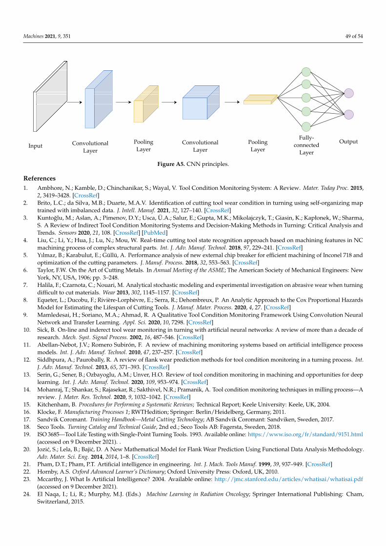
Machines 2021, 9, 351 49 of 54

Input Convolutional

Layer

Convolutional

Layer

Pooling

Layer

Pooling

Layer

Fully-

connected

Layer

Output

Figure A5. CNN principles.

References1. Ambhore, N.; Kamble, D.; Chinchanikar, S.; Wayal, V. Tool Condition Monitoring System: A Review. Mater. Today Proc. 2015,

2, 3419–3428. [CrossRef]2. Brito, L.C.; da Silva, M.B.; Duarte, M.A.V. Identification of cutting tool wear condition in turning using self-organizing map

trained with imbalanced data. J. Intell. Manuf. 2021, 32, 127–140. [CrossRef]3. Kuntoglu, M.; Aslan, A.; Pimenov, D.Y.; Usca, Ü.A.; Salur, E.; Gupta, M.K.; Mikolajczyk, T.; Giasin, K.; Kapłonek, W.; Sharma,

S. A Review of Indirect Tool Condition Monitoring Systems and Decision-Making Methods in Turning: Critical Analysis andTrends. Sensors 2020, 21, 108. [CrossRef] [PubMed]

4. Liu, C.; Li, Y.; Hua, J.; Lu, N.; Mou, W. Real-time cutting tool state recognition approach based on machining features in NCmachining process of complex structural parts. Int. J. Adv. Manuf. Technol. 2018, 97, 229–241. [CrossRef]

5. Yılmaz, B.; Karabulut, E.; Güllü, A. Performance analysis of new external chip breaker for efficient machining of Inconel 718 andoptimization of the cutting parameters. J. Manuf. Process. 2018, 32, 553–563. [CrossRef]

6. Taylor, F.W. On the Art of Cutting Metals. In Annual Meeting of the ASME; The American Society of Mechanical Engineers: NewYork, NY, USA, 1906; pp. 3–248.

7. Halila, F.; Czarnota, C.; Nouari, M. Analytical stochastic modeling and experimental investigation on abrasive wear when turningdifficult to cut materials. Wear 2013, 302, 1145–1157. [CrossRef]

8. Equeter, L.; Ducobu, F.; Rivière-Lorphèvre, E.; Serra, R.; Dehombreux, P. An Analytic Approach to the Cox Proportional HazardsModel for Estimating the Lifespan of Cutting Tools. J. Manuf. Mater. Process. 2020, 4, 27. [CrossRef]

9. Mamledesai, H.; Soriano, M.A.; Ahmad, R. A Qualitative Tool Condition Monitoring Framework Using Convolution NeuralNetwork and Transfer Learning. Appl. Sci. 2020, 10, 7298. [CrossRef]

10. Sick, B. On-line and inderect tool wear monitoring in turning with artificial neural networks: A review of more than a decade ofresearch. Mech. Syst. Signal Process. 2002, 16, 487–546. [CrossRef]

11. Abellan-Nebot, J.V.; Romero Subirón, F. A review of machining monitoring systems based on artificial intelligence processmodels. Int. J. Adv. Manuf. Technol. 2010, 47, 237–257. [CrossRef]

12. Siddhpura, A.; Paurobally, R. A review of flank wear prediction methods for tool condition monitoring in a turning process. Int.J. Adv. Manuf. Technol. 2013, 65, 371–393. [CrossRef]

13. Serin, G.; Sener, B.; Ozbayoglu, A.M.; Unver, H.O. Review of tool condition monitoring in machining and opportunities for deeplearning. Int. J. Adv. Manuf. Technol. 2020, 109, 953–974. [CrossRef]

14. Mohanraj, T.; Shankar, S.; Rajasekar, R.; Sakthivel, N.R.; Pramanik, A. Tool condition monitoring techniques in milling process—Areview. J. Mater. Res. Technol. 2020, 9, 1032–1042. [CrossRef]

15. Kitchenham, B. Procedures for Performing a Systematic Reviews; Technical Report; Keele University: Keele, UK, 2004.16. Klocke, F. Manufacturing Processes 1; RWTHedition; Springer: Berlin/Heidelberg, Germany, 2011.17. Sandvik Coromant. Training Handbook—Metal Cutting Technology; AB Sandvik Coromant: Sandviken, Sweden, 2017.18. Seco Tools. Turning Catalog and Technical Guide, 2nd ed.; Seco Tools AB: Fagersta, Sweden, 2018.19. ISO 3685—Tool Life Testing with Single-Point Turning Tools. 1993. Available online: https://www.iso.org/fr/standard/9151.html

(accessed on 9 December 2021). .20. Jozic, S.; Lela, B.; Bajic, D. A New Mathematical Model for Flank Wear Prediction Using Functional Data Analysis Methodology.

Adv. Mater. Sci. Eng. 2014, 2014, 1–8. [CrossRef]21. Pham, D.T.; Pham, P.T. Artificial intelligence in engineering. Int. J. Mach. Tools Manuf. 1999, 39, 937–949. [CrossRef]22. Hornby, A.S. Oxford Advanced Learner’s Dictionary; Oxford University Press: Oxford, UK, 2010.23. Mccarthy, J. What Is Artificial Intelligence? 2004. Available online: http://jmc.stanford.edu/articles/whatisai/whatisai.pdf

(accessed on 9 December 2021).24. El Naqa, I.; Li, R.; Murphy, M.J. (Eds.) Machine Learning in Radiation Oncology; Springer International Publishing: Cham,

Switzerland, 2015.

Machines 2021, 9, 351 50 of 54

25. Sthåle, L.; Wold, S. Analysis of variance (ANOVA). Chemom. Intell. Lab. Syst. 1989, 6, 259–272. [CrossRef]26. Schober, P.; Boer, C.; Schwarte, L.A. Correlation Coefficients. Anesth. Analg. 2018, 126, 1763–1768. [CrossRef]27. Kitchenham, B.; Pearl Brereton, O.; Budgen, D.; Turner, M.; Bailey, J.; Linkman, S. Systematic literature reviews in software

engineering—A systematic literature review. Inf. Softw. Technol. 2009, 51, 7–15. [CrossRef]28. Burnham, J.F. Scopus Database: A Review. Biomed. Digit. Libr. 2006, 3, 1–8. [CrossRef] [PubMed]29. Wen, J.; Li, S.; Lin, Z.; Hu, Y.; Huang, C. Systematic literature review of machine learning based software development effort

estimation models. Inf. Softw. Technol. 2012, 54, 41–59. [CrossRef]30. Landis, J.R.; Koch, G.G. The Measurement of Observer Agreement for Categorical Data. Biometrics 1977, 33, 159. [CrossRef]31. Salgado, D.; Alonso, F. An approach based on current and sound signals for in-process tool wear monitoring. Int. J. Mach. Tools

Manuf. 2007, 47, 2140–2152. [CrossRef]32. Wang, L.; Mehrabi, M.G.; Kannatey-Asibu, E. Hidden Markov Model-based Tool Wear Monitoring in Turning. J. Manuf. Sci. Eng.

2002, 124, 651–658. [CrossRef]33. Balazinski, M.; Czogala, E.; Jemielniak, K.; Leski, J. Tool condition monitoring using artificial intelligence methods. Eng. Appl.

Artif. Intell. 2002, 15, 73–80. [CrossRef]34. Dimla, D.; Lister, P. On-line metal cutting tool condition monitoring. Int. J. Mach. Tools Manuf. 2000, 40, 769–781. [CrossRef]35. Özel, T.; Nadgir, A. Prediction of flank wear by using back propagation neural network modeling when cutting hardened H-13

steel with chamfered and honed CBN tools. Int. J. Mach. Tools Manuf. 2002, 42, 287–297. [CrossRef]36. Gajate, A.; Haber, R.; del Toro, R.; Vega, P.; Bustillo, A. Tool wear monitoring using neuro-fuzzy techniques: A comparative study

in a turning process. J. Intell. Manuf. 2012, 23, 869–882. [CrossRef]37. Rizal, M.; Ghani, J.A.; Nuawi, M.Z.; Haron, C.H.C. Online tool wear prediction system in the turning process using an adaptive

neuro-fuzzy inference system. Appl. Soft Comput. 2013, 13, 1960–1968. [CrossRef]38. Dutta, S.; Pal, S.K.; Sen, R. On-machine tool prediction of flank wear from machined surface images using texture analyses and

support vector regression. Precis. Eng. 2016, 43, 34–42. [CrossRef]39. Sun, J.; Hong, G.S.; Rahman, M.; Wong, Y.S. Identification of feature set for effective tool condition monitoring by acoustic

emission sensing. Int. J. Prod. Res. 2004, 42, 901–918. [CrossRef]40. Scheffer, C.; Heyns, P. Wear monitoring in turning operations using vibration and strain measurements. Mech. Syst. Signal Process.

2001, 15, 1185–1202. [CrossRef]41. Rao, C.S.; Srikant, R.R. Tool wear monitoring—An intelligent approach. Proc. Inst. Mech. Eng. Part B J. Eng. Manuf. 2004,

218, 905–912. [CrossRef]42. Silva, R.G. Condition monitoring of the cutting process using a self-organizing spiking neural network map. J. Intell. Manuf.

2010, 21, 823–829. [CrossRef]43. Jemielniak, K.; Urbanski, T.; Kossakowska, J.; Bombinski, S. Tool condition monitoring based on numerous signal features. Int. J.

Adv. Manuf. Technol. 2012, 59, 73–81. [CrossRef]44. Sick, B. Fusion of hard and soft computing techniques in indirect, online tool wear monitoring. IEEE Trans. Syst. Man Cybern.

Part C (Appl. Rev.) 2002, 32, 80–91. [CrossRef]45. Pratama, M.; Dimla, E.; Lai, C.Y.; Lughofer, E. Metacognitive learning approach for online tool condition monitoring. J. Intell.

Manuf. 2019, 30, 1717–1737. [CrossRef]46. Scheffer, C.; Engelbrecht, H.; Heyns, P.S. A comparative evaluation of neural networks and hidden Markov models for monitoring

turning tool wear. Neural Comput. Appl. 2005, 14, 325–336. [CrossRef]47. Kang, J.; Guan, L.N. Tool Wear Intelligence Measure in Cutting Process Based on HMM. Appl. Mech. Mater. 2011, 52–54, 482–487.

[CrossRef]48. Pagani, L.; Parenti, P.; Cataldo, S.; Scott, P.J.; Annoni, M. Indirect cutting tool wear classification using deep learning and chip

colour analysis. Int. J. Adv. Manuf. Technol. 2020, 111, 1099–1114. [CrossRef]49. Miao, H.; Zhao, Z.; Sun, C.; Li, B.; Yan, R. A U-Net-Based Approach for Tool Wear Area Detection and Identification. IEEE Trans.

Instrum. Meas. 2021, 70, 1–10. [CrossRef]50. Van Eck, N.J.; Waltman, L. VOSviewer Manual Version 1.6.16. 2020. Available online: https://www.vosviewer.com/

documentation/Manual_VOSviewer_1.6.16.pdf (accessed on 9 December 2021).51. Cheng, M.; Jiao, L.; Shi, X.; Wang, X.; Yan, P.; Li, Y. An intelligent prediction model of the tool wear based on machine learning in

turning high strength steel. Proc. Inst. Mech. Eng. Part B J. Eng. Manuf. 2020, 234, 1580–1597. [CrossRef]52. Du, M.; Wang, P.; Wang, J.; Cheng, Z.; Wang, S. Intelligent Turning Tool Monitoring with Neural Network Adaptive Learning.

Complexity 2019, 2019, 8431784. [CrossRef]53. Segreto, T.; D’Addona, D.; Teti, R. Tool wear estimation in turning of Inconel 718 based on wavelet sensor signal analysis and

machine learning paradigms. Prod. Eng. 2020, 14, 693–705. [CrossRef]54. SK, T.; Shankar, S. Tool wear prediction in hard turning of EN8 steel using cutting force and surface roughness with artificial

neural network. Proc. Inst. Mech. Eng. Part C J. Mech. Eng. Sci. 2020, 234, 329–342. [CrossRef]55. Twardowski, P.; Wiciak-Pikuła, M. Prediction of Tool Wear Using Artificial Neural Networks during Turning of Hardened Steel.

Materials 2019, 12, 3091. [CrossRef] [PubMed]56. Caggiano, A. Tool Wear Prediction in Ti-6Al-4V Machining through Multiple Sensor Monitoring and PCA Features Pattern

Recognition. Sensors 2018, 18, 823. [CrossRef]

Machines 2021, 9, 351 51 of 54

57. Karam, S.; Centobelli, P.; D’Addona, D.M.; Teti, R. Online Prediction of Cutting Tool Life in Turning via Cognitive DecisionMaking. Procedia CIRP 2016, 41, 927–932. [CrossRef]

58. Zare Chavoshi, S. Tool flank wear prediction in CNC turning of 7075 AL alloy SiC composite. Prod. Eng. 2011, 5, 37–47. [CrossRef]59. Palanisamy, P.; Shanmugasundaram, S. Modelling of tool wear and surface roughness in hard turning using regression and

artificial neural network. Int. J. Mach. Mach. Mater. 2008, 4, 76. [CrossRef]60. Rao, C.H.S.; Rao, D.N.; Rao, R.N.S. Online prediction of diffusion wear on the flank through tool tip temperature in turning

using artificial neural networks. Proc. Inst. Mech. Eng. Part B J. Eng. Manuf. 2006, 220, 2069–2076. [CrossRef]61. Tamang, S.; Chandrasekaran, M. Modeling and optimization of parameters for minimizing surface roughness and tool wear in

turning Al/SiCp MMC, using conventional and soft computing techniques. Adv. Prod. Eng. Manag. 2015, 10, 59–72. [CrossRef]62. Caggiano, A.; Napolitano, F.; Teti, R. Dry Turning of Ti6Al4V: Tool Wear Curve Reconstruction Based on Cognitive Sensor

Monitoring. Procedia CIRP 2017, 62, 209–214. [CrossRef]63. Ji, S.M.; Zhang, L.; Wan, Y.; Zhang, X.; Yuan, J.L.; Zhang, L. Research of Intelligent Tool Condition Monitoring Technology Based

on Multi-Information Fusion. Mater. Sci. Forum 2004, 471–472, 187–191. [CrossRef]64. Srikant, R.R.; Krishna, P.V.; Rao, N.D. Online tool wear prediction in wet machining using modified back propagation neural

network. Proc. Inst. Mech. Eng. Part B J. Eng. Manuf. 2011, 225, 1009–1018. [CrossRef]65. Choudhury, S.; Bartarya, G. Role of temperature and surface finish in predicting tool wear using neural network and design of

experiments. Int. J. Mach. Tools Manuf. 2003, 43, 747–753. [CrossRef]66. Salimi Asl, A.; Erdem, A.; Rafighi, M. Applying a multi sensor system to predict and simulate the tool wear using of artificial

neural networks. Sci. Iran. 2017, 24, 2864–2874. [CrossRef]67. Paul, P.S.; Varadarajan, A. ANN assisted sensor fusion model to predict tool wear during hard turning with minimal fluid

application. Int. J. Mach. Mach. Mater. 2013, 13, 398. [CrossRef]68. Cakan, A.; Evrendilek, F.; Ozkaner, V. Data-driven simulations of flank wear of coated cutting tools in hard turning. Mechanika

2016, 21, 486–492. [CrossRef]69. Chang, W.Y.; Wu, S.J.; Hsu, J.W. Investigated iterative convergences of neural network for prediction turning tool wear. Int. J.

Adv. Manuf. Technol. 2020, 106, 2939–2948. [CrossRef]70. Kang, L.; Xiong, X.; Yi, L.; Guo, Y. A Study of Cutting Tool Wear Prediction Utilizing Generalized Regression Neural Network

with Improved Fruit Fly Optimization. In Proceedings of the 2018 Prognostics and System Health Management Conference(PHM-Chongqing), Chongqing, China, 26–28 October 2018; pp. 1–7.

71. Silva, R.; Araújo, A. A Novel Approach to Condition Monitoring of the Cutting Process Using Recurrent Neural Networks.Sensors 2020, 20, 4493. [CrossRef]

72. Mikołajczyk, T.; Nowicki, K.; Bustillo, A.; Yu Pimenov, D. Predicting tool life in turning operations using neural networks andimage processing. Mech. Syst. Signal Process. 2018, 104, 503–513. [CrossRef]

73. Ojha, D.; Dixit, U. An economic and reliable tool life estimation procedure for turning. Int. J. Adv. Manuf. Technol. 2005,26, 726–732. [CrossRef]

74. Xavior, M.A.; Anouncia, S.M. Artificial neural networks and case-based reasoning models for predicting tool life and tool-shiminterface temperature. Int. J. Serv. Oper. Manag. 2016, 24, 379. [CrossRef]

75. Senthilkumar, N.; Tamizharasan, T. Flank wear and surface roughness prediction in hard turning via artificial neural networkand multiple regressions. Aust. J. Mech. Eng. 2015, 13, 31–45. [CrossRef]

76. Rajeev, D.; Dinakaran, D.; Kanthavelkumaran, N.; Austin, N. Predictions of Tool Wear in Hard Turning of AISI4140 Steel throughArtificial Neural Network, Fuzzy Logic and Regression Models. Int. J. Eng. 2018, 31, 32–37.

77. de Farias, A.; de Almeida, S.L.R.; Delijaicov, S.; Seriacopi, V.; Bordinassi, E.C. Simple machine learning allied with data-drivenmethods for monitoring tool wear in machining processes. Int. J. Adv. Manuf. Technol. 2020, 109, 2491–2501. [CrossRef]

78. Abadi, M.; Barham, P.; Chen, J.; Chen, Z.; Davis, A.; Dean, J.; Devin, M.; Ghemawat, S.; Irving, G.; Isard, M.; et al. Tensorflow: ASystem for Large-Scale Machine Learning. In Proceedings of the 12th USENIX Symposium on Operating Systems Design andImplementation (OSDI ’16), Savannah, GA, USA, 2–4 November 2016; pp. 1–20.

79. Pedregosa, F.; Varoquaux, G.; Gramfort, A.; Michel, V.; Thirion, B.; Grisel, O.; Blondel, M.; Prettenhofer, P.; Weiss, R.; Dubourg, V.;et al. Scikit-learn: Machine Learning in Python. J. Mach. Learn. Res. 2011, 12, 2825–2830

80. Fiesler, E.; Beale, R. Handbook of Neural Computation; IOP Publishing and Oxford University Press: Bristol, UK; Philadelphia, PA,USA; New York, NY, USA, 1996.

81. Adler, P.; Falk, C.; Friedler, S.A.; Nix, T.; Rybeck, G.; Scheidegger, C.; Smith, B.; Venkatasubramanian, S. Auditing black-boxmodels for indirect influence. Knowl. Inf. Syst. 2018, 54, 95–122. [CrossRef]

82. Ras, G.; van Gerven, M.; Haselager, P. Explanation Methods in Deep Learning: Users, Values, Concerns and Challenges. InExplainable and Interpretable Models in Computer Vision and Machine Learning; Springer: Cham, Switzerland, 2018

83. Shantisagar, K.; Jegadeeshwaran, R.; Sakthivel, G.; Alamelu Manghai, T.M. Vibration Based Tool Insert Health Monitoring UsingDecision Tree and Fuzzy Logic. Struct. Durab. Health Monit. 2019, 13, 303–316. [CrossRef]

84. Ren, Q.; Baron, L.; Balazinski, M.; Botez, R.; Bigras, P. Tool wear assessment based on type-2 fuzzy uncertainty estimation onacoustic emission. Appl. Soft Comput. 2015, 31, 14–24. [CrossRef]

85. Kuo, R. Multi-sensor integration for online tool wear estimation through artificial neural networks and fuzzy neural network.Eng. Appl. Artif. Intell. 2000, 13, 249–261. [CrossRef]

Machines 2021, 9, 351 52 of 54

86. Ren, Q.; Balazinski, M.; Baron, L. Uncertainty prediction for tool wear condition using type-2 tsk fuzzy approach. In Proceedingsof the 2009 IEEE International Conference on Systems, Man and Cybernetics, San Antonio, TX, USA, 11–14 October 2009;pp. 660–665.

87. Ren, Q.; Balazinski, M.; Baron, L.; Jemielniak, K. Tool condition monitoring using the TSK fuzzy approach based on subtractiveclustering method. In New Frontiers in Applied Artificial Intelligence; Nguyen, N.T., Borzemski, L., Grzech, A., Ali, M., Eds.;Springer: Berlin/Heidelberg, Germany, 2008; Volume LNAI 5027, pp. 1–10.

88. Achiche, S.; Balazinski, M.; Baron, L.; Jemielniak, K. Tool wear monitoring using genetically-generated fuzzy knowledge bases.Eng. Appl. Artif. Intell. 2002, 15, 303–314. [CrossRef]

89. Marani, M.; Zeinali, M.; Kouam, J.; Songmene, V.; Mechefske, C.K. Prediction of cutting tool wear during a turning process usingartificial intelligence techniques. Int. J. Adv. Manuf. Technol. 2020, 111, 505–515. [CrossRef]

90. Zhang, B.; Katinas, C.; Shin, Y.C. Robust Tool Wear Monitoring Using Systematic Feature Selection in Turning Processes withConsideration of Uncertainties. J. Manuf. Sci. Eng. 2018, 140, 081010. [CrossRef]

91. Ren, Q.; Achiche, S.; Jemielniak, K.; Bigras, P. An enhanced adaptive neural fuzzy tool condition monitoring for turning process.In Proceedings of the 2016 IEEE International Conference on Fuzzy Systems (FUZZ-IEEE), Vancouver, BC, Canada, 24–29 July2016; pp. 1976–1982.

92. Gill, S.S.; Singh, R.; Singh, J.; Singh, H. Adaptive neuro-fuzzy inference system modeling of cryogenically treated AISI M2 HSSturning tool for estimation of flank wear. Expert Syst. Appl. 2012, 39, 4171–4180. [CrossRef]

93. Basari, A.; Jaya, A.; Muhamad, M.; Rahman, M.; Hashim, S.; Haron, H. Application of ANFIS in Predicting TiAlN CoatingsFlank Wear. In Proceedings of the 2011 Third International Conference on Computational Intelligence, Modelling & Simulation,Langkawi, Malaysia, 20–22 September 2011; pp. 57–62.

94. Ren, Q.; Balazinski, M.; Baron, L.; Jemielniak, K. TSK fuzzy modeling for tool wear condition in turning processes: Anexperimental study. Eng. Appl. Artif. Intell. 2011, 24, 260–265. [CrossRef]

95. Gajate, A.; Haber, R.E.; Alique, J.R.; Vega, P.I. Transductive-Weighted Neuro-Fuzzy Inference System for Tool Wear Prediction ina Turning Process. In Lecture Notes in Computer Science (Including Subseries Lecture Notes in Artificial Intelligence and Lecture Notes inBioinformatics); Corchado, E., Wu, X., Oja, E., Herrero, Á., Baruque, B., Eds.; Springer: Berlin/Heidelberg, Germany, 2009; VolumeLNAI 5572, pp. 113–120.

96. Penedo, F.; Haber, R.E.; Gajate, A.; del Toro, R.M. Hybrid Incremental Modeling Based on Least Squares and Fuzzy K-NN forMonitoring Tool Wear in Turning Processes. IEEE Trans. Ind. Inform. 2012, 8, 811–818. [CrossRef]

97. Massol, O.; Li, X.; Gouriveau, R.; Zhou, J.H.; Gan, O.P. An exTS based neuro-fuzzy algorithm for prognostics and tool conditionmonitoring. In Proceedings of the 2010 11th International Conference on Control Automation Robotics & Vision, Singapore, 7–10December 2010; pp. 1329–1334.

98. Gao, H.; Xu, M.; Shi, X.; Huang, H. Tool Wear Monitoring Based on Localized Fuzzy Neural Networks for Turning Operation.In Proceedings of the 2009 Sixth International Conference on Fuzzy Systems and Knowledge Discovery, Tianjin, China, 14–16August 2009; Volume 4, pp. 417–420.

99. Lo, S.P. The Application of an ANFIS and Grey System Method in Turning Tool-Failure Detection. Int. J. Adv. Manuf. Technol.2002, 19, 564–572. [CrossRef]

100. Sharma, V.S.; Sharma, S.K.; Sharma, A.K. Cutting tool wear estimation for turning. J. Intell. Manuf. 2008, 19, 99–108. [CrossRef]101. Liu, T.I.; Song, S.D.; Liu, G.; Wu, Z. Online monitoring and measurements of tool wear for precision turning of stainless steel

parts. Int. J. Adv. Manuf. Technol. 2013, 65, 1397–1407. [CrossRef]102. Huang, M.L.; Yang, J.S.; Wu, J.Y.; Chang, S.H. Wear value prediction of CNC turning tools based on ν-GSVR with a new hybrid

evolutionary algorithm. J. Appl. Sci. Eng. 2020, 23, 369–378.103. Kong, D.; Chen, Y.; Li, N. Monitoring tool wear using wavelet package decomposition and a novel gravitational search

algorithm–least square support vector machine model. Proc. Inst. Mech. Eng. Part C J. Mech. Eng. Sci. 2020, 234, 822–836.[CrossRef]

104. Vikash Kumar, K.; Sivasankara Raju, R. Statistical Modeling and Optimization of Al-MMCs Reinforced with Coconut Shell AshParticulates. In Lecture Notes in Mechanical Engineering; Deepak, B., Parhi, D., Jena, P.C., Eds.; Springer Nature: Singapore, 2020;pp. 703–712.

105. Kong, D.; Chen, Y.; Li, N.; Tan, S. Tool wear monitoring based on kernel principal component analysis and v-support vectorregression. Int. J. Adv. Manuf. Technol. 2017, 89, 175–190. [CrossRef]

106. Li, N.; Chen, Y.; Kong, D.; Tan, S. Force-based tool condition monitoring for turning process using v-support vector regression.Int. J. Adv. Manuf. Technol. 2017, 91, 351–361. [CrossRef]

107. Silva, R.G.; Wilcox, S.J. Feature evaluation and selection for condition monitoring using a self-organizing map and spatialstatistics. Artif. Intell. Eng. Des. Anal. Manuf. 2019, 33, 1–10. [CrossRef]

108. O’Shea, K.; Nash, R. An Introduction to Convolutional Neural Networks. pp. 1–11. 2015. Available online: http://xxx.lanl.gov/abs/1511.08458 (accessed on 10 November 2021).

109. Agogino, A.; Goebel, K. Milling Data Set. BEST Lab, UC Berkeley, NASA Ames Prognostics Data Repository. Available online:https://ti.arc.nasa.gov/tech/dash/groups/pcoe/prognostic-data-repository/ (accessed on 9 December 2021).

110. Prognostics, T.; Society, H.M. 2010 PHM Society Conference Data Challenge. Available online: https://phmsociety.org/phm_competition/2010-phm-society-conference-data-challenge/ (accessed on 9 December 2021).

Machines 2021, 9, 351 53 of 54

111. Kang, L.; Wang, S.; Wang, S.; Ma, C.; Yi, L.; Zou, H. Tool wear monitoring using generalized regression neural network. Adv.Mech. Eng. 2019, 11, 1–10. [CrossRef]

112. Mandal, N.; Mondal, B.; Doloi, B. Application of Back Propagation Neural Network Model for Predicting Flank Wear of YttriaBased Zirconia Toughened Alumina (ZTA) Ceramic Inserts. Trans. Indian Inst. Met. 2015, 68, 783–789. [CrossRef]

113. Sarma, D.K.; Dixit, U.S. Neural network modelling of forces and indirect prediction of tool wear in turning of grey cast iron withceramic tool. Int. J. Mach. Mach. Mater. 2010, 8, 55–75. [CrossRef]

114. Deiab, I.; Assaleh, K.; Hammad, F. Application of sensor fusion and polynomial classifiers to tool wear monitoring. In Proceedingsof the 2008 5th International Symposium on Mechatronics and Its Applications, Amman, Jordan, 27–29 May 2008; pp. 1–6.

115. Wang, X.; Wang, W.; Huang, Y.; Nguyen, N.; Krishnakumar, K. Design of neural network-based estimator for tool wear modelingin hard turning. J. Intell. Manuf. 2008, 19, 383–396. [CrossRef]

116. Shen, Y.; Yang, F.; Habibullah, M.S.; Ahmed, J.; Das, A.K.; Zhou, Y.; Ho, C.L. Predicting tool wear size across multi-cuttingconditions using advanced machine learning techniques. J. Intell. Manuf. 2020, 32, 1753–1766. [CrossRef]

117. Gangadhar, N.; Kumar, H.; Narendranath, S.; Sugumaran, V. Condition Monitoring of Single Point Cutting Tools Based onMachine Learning Approach. Int. J. Acoust. Vib. 2018, 23, 131–137. [CrossRef]

118. Srinidhi, R.; Sharma, V.; Sukumar, M.; Venkatesha, C.S. Correlative Flank Wear Analysis of Single Point Turning Inserts UsingAcoustic Emission and Artificial Intelligence Techniques. In Proceedings of the ASME 2008 International Mechanical EngineeringCongress and Exposition, Volume 7: Emerging Technologies, Recent Advances in Engineering, Boston, MA, USA, 31 October–6November 2008; pp. 143–149.

119. Scheffer, C.; Kratz, H.; Heyns, P.; Klocke, F. Development of a tool wear-monitoring system for hard turning. Int. J. Mach. ToolsManuf. 2003, 43, 973–985. [CrossRef]

120. Özel, T.; Karpat, Y. Predictive modeling of surface roughness and tool wear in hard turning using regression and neural networks.Int. J. Mach. Tools Manuf. 2005, 45, 467–479. [CrossRef]

121. Quiza, R.; Figueira, L.; Paulo Davim, J. Comparing statistical models and artificial neural networks on predicting the tool wear inhard machining D2 AISI steel. Int. J. Adv. Manuf. Technol. 2008, 37, 641–648. [CrossRef]

122. Neef, B.; Bartels, J.; Thiede, S. Tool Wear and Surface Quality Monitoring Using High Frequency CNC Machine Tool CurrentSignature. In Proceedings of the 2018 IEEE 16th International Conference on Industrial Informatics (INDIN), Porto, Portugal,18–20 July 2018; pp. 1045–1050.

123. Yang, S.; Wang, S.; Yi, L.; Xue, H.; Cao, Y.; Sun, S. A novel monitoring method for turning tool wear based on support vectormachines. Proc. Inst. Mech. Eng. Part B J. Eng. Manuf. 2016, 230, 1359–1371. [CrossRef]

124. Zhang, K.F.; Yuan, H.Q.; Nie, P. A method for tool condition monitoring based on sensor fusion. J. Intell. Manuf. 2015,26, 1011–1026. [CrossRef]

125. Bhat, N.N.; Dutta, S.; Vashisth, T.; Pal, S.; Pal, S.K.; Sen, R. Tool condition monitoring by SVM classification of machined surfaceimages in turning. Int. J. Adv. Manuf. Technol. 2016, 83, 1487–1502. [CrossRef]

126. Tao, R.; Zhang, Y.; Wang, L.; Zhao, X. Research of Tool State Recognition Based on CEEMD-WPT; Springer International Publishing:Cham, Switzerland, 2018; Volume 11064, pp. 59–70.

127. Qian, Y.; Tian, J.; Liu, L.; Zhang, Y.; Chen, Y. A tool wear predictive model based on SVM. In Proceedings of the 2010 ChineseControl and Decision Conference, Xuzhou, China, 26–28 May 2010; pp. 1213–1217.

128. Silva, R.G.; Reis, R. Adaptive self-organizing map applied to lathe tool condition monitoring. In Proceedings of the 2017 22ndIEEE International Conference on Emerging Technologies and Factory Automation (ETFA), Limassol, Cyprus, 12–15 September2017; pp. 1–6.

129. Al-Sahib, N.K.A.; Bachaa, A.M. Tool Wear Monitoring in Turning Operation Using Vibration and Strain Measurement with NeuralNetwork. In Proceedings of the ASME 2005 International Mechanical Engineering Congress and Exposition, ManufacturingEngineering and Materials Handling, Parts A and B, Orlando, FL, USA, 5–11 November 2005; pp. 783–792.

130. Elsheikh, A.; Yacout, S.; Ouali, M.S.; Shaban, Y. Failure time prediction using adaptive logical analysis of survival curves andmultiple machining signals. J. Intell. Manuf. 2020, 31, 403–415. [CrossRef]

131. Saran, J.; Elangovan, M.; Sugumaran, V. Tool wear monitoring using NNGE algorithm. Int. J. Mech. Prod. Eng. Res. Dev. 2019,9, 53–62.

132. Murua, M.; Suárez, A.; de Lacalle, L.N.L.; Santana, R.; Wretland, A. Feature extraction-based prediction of tool wear of Inconel718 in face turning. Insight-Non-Destr. Test. Cond. Monit. 2018, 60, 443–450. [CrossRef]

133. Yang, H.C.; Li, Y.Y.; Hung, M.H.; Cheng, F.T. A cyber-physical scheme for predicting tool wear based on a hybrid dynamic neuralnetwork. J. Chin. Inst. Eng. 2017, 40, 614–625. [CrossRef]

134. Shaban, Y.; Yacout, S.; Balazinski, M.; Jemielniak, K. Cutting tool wear detection using multiclass logical analysis of data. Mach.Sci. Technol. 2017, 21, 526–541. [CrossRef]

135. Azmi, A.F.A.; Habaibeh, A.A.; Redgate, J. Rapid design of tool-wear condition monitoring systems for turning processes usingnovelty detection. Int. J. Manuf. Technol. Manag. 2009, 17, 232. [CrossRef]

136. Wang, X.; Huang, Y.; Nguyen, N.; Krishnakumar, K. CBN tool flank wear modelling using Hybrid Neural Network. Int. J.Mechatron. Manuf. Syst. 2008, 1, 83. [CrossRef]

Machines 2021, 9, 351 54 of 54

137. Aralikatti, S.S.; Ravikumar, K.N.; Kumar, H.; Nayaka, H.S.; Sugumaran, V. Comparative Study on Tool Fault Diagnosis MethodsUsing Vibration Signals and Cutting Force Signals by Machine Learning Technique. Struct. Durab. Health Monit. 2020, 14, 127–145.[CrossRef]

138. Vuong, N.K.; Xue, Y.; Liu, S.; Zhou, Y.; Wu, M. Predicting Surface Roughness and Flank Wear in Turning Processes. In Proceedingsof the 2020 IEEE International Conference on Prognostics and Health Management (ICPHM), Detroit, MI, USA, 8–10 June 2020;Volume 2020, pp. 1–6.

139. Aghdam, B.H.; Cigeroglu, E.; Sadeghi, M.H. Output Only Functional Series Time Dependent AutoRegressive Moving Average(FS-TARMA) Modelling of Tool Acceleration Signals for Wear Estimation. In Structural Health Monitoring and Damage Detection,Volume 7; Niezrecki, C., Ed.; Springer International Publishing: Cham, Switzerland, 2015; pp. 111–122.

140. Gao, H.; Gao, H.; Chen, C.; Su, Y.; Xu, M. The Investigation of A Self-adjusting Tool Wear Monitoring System. In Proceedings ofthe 2006 International Conference on Mechatronics and Automation, Luoyang, China, 25–28 June 2006; pp. 1690–1694.

141. Abraham, A. Artificial Neural Networks. In Handbook of Measuring System Design; John Wiley & Sons, Ltd.: Chichester, UK, 2005.142. Zadeh, L.A. Fuzzy Set. In Fuzzy Sets, FUZZY Logic, and Fuzzy SYSTEMS; World Scientific: Singapore, 1996; pp. 394–432.143. Jang, J.S. ANFIS: Adaptive-network-based fuzzy inference system. IEEE Trans. Syst. Man Cybern. 1993, 23, 665–685. [CrossRef]144. Castillo, O.; Melin, P.; Kacprzyk, J.; Pedrycz, W. Type-2 Fuzzy Logic: Theory and Applications. In Proceedings of the 2007 IEEE

International Conference on Granular Computing (GRC 2007), Fremont, CA, USA, 2–4 November 2007; p. 145.145. Lei, Y. Individual Intelligent Method-Based Fault Diagnosis. In Intelligent Fault Diagnosis and Remaining Useful Life Prediction of

Rotating Machinery; Butterworth-Heinemann: Oxford, UK, 2017; pp. 67–174.146. Steinwart, I.; Christmann, A. Support Vector Machines; Information Science and Statistics; Springer: New York, NY, USA, 2008;

Volume 14.147. Rozenberg, G.; Back, T.; Kok, J.N. Handbook of Natural Computing; Springer: Berlin/Heidelberg, Germany, 2012; Volume 1–4,

pp. 1–2051.148. Cai, Q.; He, H.; Man, H. Imbalanced evolving self-organizing learning. Neurocomputing 2014, 133, 258–270. [CrossRef]149. Ching, W.K.; Huang, X.; Ng, M.K.; Siu, T.K. Markov Chains; International Series in Operations Research & Management Science;

Springer: Boston, MA, USA, 2013; Volume 189.150. Rabiner, L. A tutorial on hidden Markov models and selected applications in speech recognition. Proc. IEEE 1989, 77, 257–286.

[CrossRef]151. Aghdam, H.H.; Heravi, E.J. Guide to Convolutional Neural Networks: A Practical Application to Traffic-Sign Detection and Classification;

Springer International Publishing: Cham, Switzerland, 2017.