Autonomous Robots 13, 87–104, 2002c© 2002 Kluwer Academic Publishers. Manufactured in The Netherlands.

A System for Semi-Autonomous Tractor Operations

ANTHONY STENTZ, CRISTIAN DIMA, CARL WELLINGTON, HERMAN HERMAN, DAVID STAGERRobotics Institute, Carnegie Mellon University, Pittsburgh, PA 15213, USA

Abstract. Tractors are the workhorses of the modern farm. By automating these machines, we can increasethe productivity, improve safety, and reduce costs for many agricultural operations. Many researchers have testedcomputer-controlled machines for farming, but few have investigated the larger issues such as how humans cansupervise machines and work amongst them. In this paper, we present a system for tractor automation. A humanprograms a task by driving the relevant routes. The task is divided into subtasks and assigned to a fleet of tractorsthat drive portions of the routes. Each tractor uses on-board sensors to detect people, animals, and other vehicles inthe path of the machine, stopping for such obstacles until it receives advice from a supervisor over a wireless link.A first version of the system was implemented on a single tractor. Several features of the system were validated,including accurate path tracking, the detection of obstacles based on both geometric and non-geometric properties,and self-monitoring to determine when human intervention is required. Additionally, the complete system was testedin a Florida orange grove, where it autonomously drove seven kilometers.

Keywords: agricultural robots, position estimation, path tracking, sensor fusion, obstacle detection

1. Introduction

Tractors are used for a variety of agricultural oper-ations. When equipped with the proper implements,these mobile machines can till, plant, weed, fertil-ize, spray, haul, mow, and harvest. Such versatilitymakes tractors prime targets for automation. Automa-tion promises to improve productivity by enabling themachines to drive at a higher average speed, improvesafety by separating the human from the machine andminimizing the risk of accident, and reduce operationalcosts by minimizing the labor and maintenance neededfor each machine.

Many researchers have investigated the automationof mobile equipment in agriculture. There are two basicapproaches. In the first approach, the vehicle drives aroute based on an absolute reference frame. The routeis planned by calculating a geometric coverage patternover the field or by manually teaching the machine.The route is driven by using absolute positioning sen-sors, such as a global positioning system (GPS), mag-netic compass, or visual markers. The planned route isdriven as programmed or taught, without modification.This approach is technically simpler, but it suffers from

an inability to respond to unexpected changes in thefield.

Using this approach, O’Conner et al. (1996) demon-strated an autonomous tractor using a carrier phase GPSwith four antennae to provide both position and headingin the field. The system was capable of positional accu-racy on the order of centimeters at straight-line speedsover 3 km/hour. Noguchi and Terao (1997) used a pairof static cameras in the field to track a visual markeron a tractor and triangulate its position. Additionally,the tractor was equipped with a geomagnetic directionsensor. The system was able to measure the tractor’sposition to an average error of 40 cm for fields up to100 meters long. Erbach et al. (1991) used a pair ofradio beacons to triangulate position in the field witherrors of approximately 50 cm.

In the second approach, the vehicle drives a routebased on a relative frame of reference. The route isplanned by calculating a coverage pattern triggered bylocal reference cues, such as individual plants, a cropline, or the end of a row. The route is driven by usingrelative positioning sensors, such as a camera to detectcrop rows or dead-reckoning sensors like odometry,accelerometers, and gyroscopes. The route is driven

88 Stentz et al.

as topologically planned, with exact position deter-mined by the relative cues. This approach enables amachine to tailor its operation to individual plants asthey change over time (e.g., applying more pesticideson larger trees), but it is technically more difficult.

Using this approach, Billingsley and Schoenfisch(1995) demonstrated an autonomous tractor driving instraight rows of cotton. The system used a camera withsoftware for detecting the crop rows. It was able to driveon straight segments at 25 km/hour with a few centime-ters of error. Gerrish et al. (1997) also used a camerato guide a tractor along straight rows. They reportedresults of 12 cm accuracy at speeds of 13 km/hour.Southall et al. (1999) used a camera to detect individualplants, exploiting the known planting geometry. Thesemeasurements were combined with odometry and iner-tial sensors. The system was used to guide an outdoormobile robot for a short distance at a speed of about2 km/hour.

More recently, researchers have investigated com-bining the two approaches. Ollis and Stentz (1996,1997) and Pilarski et al. (1999) demonstrated an au-tonomous windrowing machine. The system used twomodes of navigation: (1) a camera with crop line de-tection software; (2) a differential GPS integrated withodometry and a heading gyro. The windrower cut hun-dreds of acres of alfalfa fully autonomously at aver-age speeds of 7 km/hour. The machine was able to cutswaths of crop and execute a spin turn at the end of therow. The system was steered by only one navigationmode at a time, with the other serving as a trigger orconsistency check. Zhang et al. (1999) also used abso-lute and relative sensors, namely a camera, GPS, andheading gyro, to guide an autonomous tractor. The sys-tem used a rule-based method to process the sensor dataand steer the machine. The system was able to drive thetractor at speeds of 13 km/hour with less than 15 cm oferror.

Although full autonomy is the ultimate goal forrobotics, it may be a long time coming. Fortunately,partial autonomy can add value to the machine longbefore full autonomy is achieved. For many tasks, theproverbial 80/20 rule applies. According to this rule,roughly 80% of a task is easy to perform and 20% isdifficult. For the 80% that is easy, it may be possiblefor a computer to perform the task faster or more ac-curately (on average) than a human, because humansfatigue over the course of a work shift. The human canremain on the machine to handle the 20% of the taskthat is difficult. We call this type of semi-automation

an operator assist. If the cost of the semi-automationis low enough and its performance high enough, it canbe cost effective.

If the percentage of required human intervention islow enough, it may be possible for a single human tosupervise many machines. We call this type of semi-automation force multiplication. Since the human can-not be resident on all machines at once, he/she mustinteract with the fleet over a wireless link.

The force multiplication scenario raises some chal-lenging questions. How should operations be dividedbetween human and machine? What is the best wayfor the human to interact with the machine? How canthe machine be made productive and reliable for thetasks it is given? These are questions that address au-tomation at a system level, that is, a system of peopleand computer-controlled machines working together.To date, the research literature has focussed primar-ily on achieving full autonomy, steadily improving thespeed and reliability metrics, but without addressingthe larger, system-level questions.

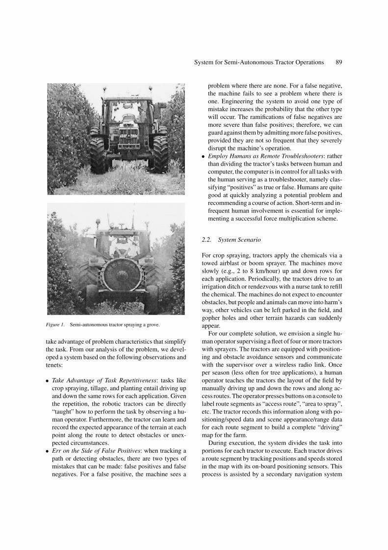
This paper explores these questions in the contextof a semi-autonomous system for agricultural spray-ing operations in groves, orchards, and row crops. Thisapplication is well motivated, since spraying is per-formed frequently and is hazardous to both the vehicleoperator and other workers in the field. We developed acomputer-controlled John Deere 6410 tractor equippedwith a GPS-based teach/playback system and camera-based obstacle detection. In April, 2000, we transportedour tractor to an orange grove in Florida to collect dataand test the autonomous navigation system. For one ofthe tests, the system was taught to drive a 7 kilometerpath through the grove. It was then put in autonomousmode and drove the path at speeds ranging from 5 to8 km/hour, spraying water enroute (see Fig. 1).

In this paper, we present an overview of the systemand approach, and then we detail the user interface, nav-igation, and obstacle detection components. Finally, wesummarize results and draw conclusions.

2. System Overview

2.1. Problem Characteristics and Tenets

In order to field semi-autonomous tractors in a forcemultiplication scenario, the machines must be produc-tive, reliable, safe, and manageable by a human su-pervisor. In general, this is a very difficult problem tosolve. Fortunately, for many tractor operations, we can

System for Semi-Autonomous Tractor Operations 89

Figure 1. Semi-autonomous tractor spraying a grove.

take advantage of problem characteristics that simplifythe task. From our analysis of the problem, we devel-oped a system based on the following observations andtenets:

• Take Advantage of Task Repetitiveness: tasks likecrop spraying, tillage, and planting entail driving upand down the same rows for each application. Giventhe repetition, the robotic tractors can be directly“taught” how to perform the task by observing a hu-man operator. Furthermore, the tractor can learn andrecord the expected appearance of the terrain at eachpoint along the route to detect obstacles or unex-pected circumstances.

• Err on the Side of False Positives: when tracking apath or detecting obstacles, there are two types ofmistakes that can be made: false positives and falsenegatives. For a false positive, the machine sees a

problem where there are none. For a false negative,the machine fails to see a problem where there isone. Engineering the system to avoid one type ofmistake increases the probability that the other typewill occur. The ramifications of false negatives aremore severe than false positives; therefore, we canguard against them by admitting more false positives,provided they are not so frequent that they severelydisrupt the machine’s operation.

• Employ Humans as Remote Troubleshooters: ratherthan dividing the tractor’s tasks between human andcomputer, the computer is in control for all tasks withthe human serving as a troubleshooter, namely clas-sifying “positives” as true or false. Humans are quitegood at quickly analyzing a potential problem andrecommending a course of action. Short-term and in-frequent human involvement is essential for imple-menting a successful force multiplication scheme.

2.2. System Scenario

For crop spraying, tractors apply the chemicals via atowed airblast or boom sprayer. The machines moveslowly (e.g., 2 to 8 km/hour) up and down rows foreach application. Periodically, the tractors drive to anirrigation ditch or rendezvous with a nurse tank to refillthe chemical. The machines do not expect to encounterobstacles, but people and animals can move into harm’sway, other vehicles can be left parked in the field, andgopher holes and other terrain hazards can suddenlyappear.

For our complete solution, we envision a single hu-man operator supervising a fleet of four or more tractorswith sprayers. The tractors are equipped with position-ing and obstacle avoidance sensors and communicatewith the supervisor over a wireless radio link. Onceper season (less often for tree applications), a humanoperator teaches the tractors the layout of the field bymanually driving up and down the rows and along ac-cess routes. The operator presses buttons on a console tolabel route segments as “access route”, “area to spray”,etc. The tractor records this information along with po-sitioning/speed data and scene appearance/range datafor each route segment to build a complete “driving”map for the farm.

During execution, the system divides the task intoportions for each tractor to execute. Each tractor drivesa route segment by tracking positions and speeds storedin the map with its on-board positioning sensors. Thisprocess is assisted by a secondary navigation system

90 Stentz et al.

Figure 2. Human interface to fleet of tractors.

based on the tractor’s visual sensors. While driving,each tractor sweeps the terrain in front with its sensorsto check for obstacles. This process is guided by the ap-pearance/range data stored in the route segment. Whena tractor detects an obstacle in its path, it stops andtransmits an image of the scene to the human operator(see Fig. 2). If the operator disagrees about the pres-ence of an obstacle, or if the obstacle has moved outof the way, the operator signals the tractor to resume;otherwise, the operator travels to the stopped machineto rectify the problem. Periodically, the tractors depletetheir chemical tanks and signal the operator. The oper-ator meets the tractor at a rendezvous point, the tank isre-filled, and semi-autonomous operation is resumed.

We expect that this system will increase the pro-ductivity of each worker by at least a factor of four.Additionally, the tractors will be able to sense the treesand spray chemicals only where they are needed, thusreducing operational costs and minimizing negative en-vironmental impact.

2.3. Experimental Test Bed

We have implemented many components of the full sys-tem described in the previous section. For our tests, weare using a computer-controlled, 90-horsepower DeereModel 6410 tractor (see Fig. 1). The tractor is equippedwith a pair of stereo cameras for range and appearancedata; a differential GPS unit, fiber optic heading gyro,doppler radar unit, and four-wheel odometry for posi-tioning data; a pair of 350-Mz Pentium III processors

running Linux for on-board processing, and a 1 Mbpswireless ethernet link for communication with the hu-man operator. These sensors are described in more de-tail in the following sections.

Our approach is to develop the components neces-sary for a single tractor first, then replicate and integratethe components to produce a multi-vehicle system.Section 3 describes the operator console for trainingand supervising a semi-autonomous tractor. Section 4describes the position-based navigation system fordriving route segments. Section 5 describes the on-board obstacle detection and safeguarding. Section 6describes conclusions.

3. Operator Console

In our scenario, the human operator interacts with thesystem during both the training phase and the oper-ational phase. During training, the operator drives toa section of field and uses a teach interface to collectdatapoints while manually driving a desired path. Theinterface shows the path as it is being recorded and dis-plays the current status of the system. The system onlyallows paths to be recorded when it has a good posi-tion estimate. The operator also presses buttons duringthe teaching phase to label various parts of the path as“access route”, “area to spray”, etc. While teaching thepath, the operator can pause, resume, and change partsof the path.

During full system operation, a single operator over-sees a fleet of four tractors using a remote operator in-terface. This interface includes status information andlive video from all four tractors, and it shows the trac-tors traveling down their paths on a common map. If anytractor has a problem, such as running out of chemical,encountering an obstacle, or experiencing a hardwarefailure, the interface displays a warning to the opera-tor, shows pertinent information, and then he/she cantake appropriate action to solve the problem. In thecase of an obstacle, the system shows what part of theimage was classified as an obstacle, and the operatordecides whether it is safe for the tractor to proceed.To help determine if the path is clear, the tractor has aremotely-operated pan-tilt-zoom camera. If it is safe forthe tractor to continue, the operator can simply click ona “resume” button and the tractor will continue its job.

We have implemented two interfaces that performmany of the capabilities described above. Figure 3shows a simple teach interface that can record a pathand display status information.

System for Semi-Autonomous Tractor Operations 91

Figure 3. Teach interface. Operator interface showing the path thatis being recorded and the status of the system while the system isbeing taught a path.

Figure 4 shows the remote interface. The goal of thisinterface is to allow both a simple global view of allthe tractors during normal operation as well as a fo-cused view that clearly shows all relevant informationfrom a single tractor when there is a problem. Althoughonly one tractor is currently operational, the interfaceis designed for four. In Fig. 4, the bottom left panelshows live video coming from the tractor’s pan-tilt-zoom camera. The space to the right is reserved forvideo from the other tractors. This way, the operatorwill be able to see at a glance what all of the vehiclesare doing. The upper half of the interface is switchablebetween focused views of each tractor and an overallmap that shows all of the tractors together. Figure 4

Figure 4. Remote operator interface. Operator interface showingfocused view of a single tractor during playback, including video,status, and location on the map. A global map view and focusedviews for the other tractors are also available.

shows the focused view of the single operational trac-tor. It contains a larger video image, a compass displayshowing the vehicle heading, status information, andcontrols for the pan-tilt-zoom camera. The map on theright gives the location of the tractor, the previouslytaught path, and the actual path the tractor has drivenautonomously so far. To give the operator context whileusing the pan-tilt-zoom camera, the camera’s approx-imate field of view is drawn on the map. Using ourwireless link, we also have the capability to remotelystart, stop, and resume after an obstacle is detected.

4. Position-Based Navigation

In our application, we are concerned with the absoluterepeatability of the tractor’s position as it drives overa pre-taught path. Therefore, the path representation,position estimation, and navigation are all performedin a consistent world frame based on GPS. The controlpoint of our vehicle is located at the center of its rearaxle directly beneath the GPS antenna mounted on itsroof. This point is near the hitch of the tractor, so towedimplements follow a path similar to the results we showfor the tractor. We currently do not have the capabilityto directly measure the position of a towed implement.

Position errors for a large vehicle such as a tractorcan potentially cause damage to the vehicle as well asthe surrounding environment. This dictates the use of ahighly reliable position estimation and control systemthat is robust to sensor failures and can alert the opera-tor if there is a problem that requires intervention. Thefollowing sections describe how the position estima-tion and path tracking algorithms used on our tractorachieve this goal.

4.1. Position Estimation

As described in the introduction, other researchershave automated agricultural vehicles. However, someof these systems rely on a single sensor such as camera-based visual tracking (Billingsley and Schoenfisch,1999; Gerrish et al., 1997), or differential GPS (DGPS)(O’Conner et al., 1996). With only a single sensor usedfor localization, these systems must stop when a sensorfailure occurs, or else the vehicle could cause damagebecause it does not know its correct position. Further-more, without redundant sensors it becomes more diffi-cult to detect when a sensor fails. Camera-based visualtracking can fail because of many problems, includ-ing changing lighting conditions, crop variation, and

92 Stentz et al.

adverse weather (Gerrish et al., 1997). DGPS also hasproblems because it relies on radio signals that can losesignal strength, become occluded, or suffer from mul-tipath problems (Kerr, 1997; Neumann et al., 1996).We have experienced these problems with DGPS, es-pecially while testing in a Florida orange grove that hadtrees taller than the antenna on our tractor.

To avoid the above problems, other researchers haveused combinations of complementary sensors, such asDGPS, odometry, and visual tracking. These sensorshave been combined using a voting strategy (Pilarskiet al., 1999) or a rule based fusion module that looksat information availability from the different sensors(Zhang et al., 1999). While these methods can handlea sensor failure for a short period of time, they do notmaintain a confidence estimate in their position esti-mate, and therefore cannot make decisions about whenit is safe to continue. One solution to help ensure the ve-hicle’s safety is to stop operation whenever it does nothave a good DGPS signal (Pilarski et al., 1999), but thiscould result in extended downtime if the loss of DGPSsignal is due to the geometry of the environment.

Our tractor uses a redundant set of sensors that com-plement each other. This redundancy allows the tractorto detect sensor failures and combine multiple mea-surements into a higher quality estimate. The primarynavigation sensor is a Novatel RT2 dual frequency real-time kinematic carrier phase differential GPS receivercapable of better than 2 cm standard deviation absoluteaccuracy. This receiver uses an internal Kalman fil-ter to output the uncertainty estimates on the measure-ments (Neumann et al., 1996). The tractor also has aKVH ECore 2000 fiber-optic gyroscope that preciselymeasures the heading rate changes of the vehicle (stan-dard deviation 0.0001 rad/sec), custom wheel encodersthat give a distance measurement that can be convertedinto a forward velocity (standard deviation 0.47 m/sec)and give a secondary measure of heading changes, anda doppler radar unit that is commonly used on farmequipment to measure forward speed (standard devia-tion 0.13 m/sec) even with wheel slip. These sensorsare reliable and provide accurate differential informa-tion but suffer from drift over time. By combining thereliability of the encoders, gyro, and radar unit with theabsolute reference of the DGPS system, the tractor canmaintain an accurate position estimate that is robust toperiodic DGPS dropout.

We use an Extended Kalman Filter (EKF) to com-bine the information from the different sensors de-scribed above into a single position estimate while also

providing the uncertainty in that estimate. This uncer-tainty is used to make decisions about whether the vehi-cle can safely continue or if it needs assistance. Doingthis allows the tractor to continue operating during aDGPS failure for as long as possible, given the positionaccuracy requirements of the particular application.

Under the assumptions of white Gaussian noise cor-rupted measurements and a linear system model, theKalman filter provides the optimal estimate (Maybeck,1982). The EKF is an extension of the Kalman filter tohandle nonlinear system models by linearizing aroundthe current state estimate. The EKF utilizes a model ofthe system to predict the next state of the vehicle. Thisallows the filter to compare sensor measurements withthe expected state of the vehicle and reject sensor mea-surements that are not consistent based on a likelihoodratio test.

We chose to start with a simple 2D tractor modeland it has given us sufficient performance. The modelmakes two important assumptions. It assumes that thevehicle has the non-holonomic constraint that it canonly move forward, not sideways. It also makes a low-dynamics assumption that the forward and angular ac-celerations of the vehicle are essentially constant overa single time step. Making these assumptions explicitin the model allows the filter to reject measurementsthat do not follow these assumptions.

The state vector in our model includes global po-sition x , y, forward velocity v, global heading θ , andheading rate θ̇ . The non-linear system model used inthe EKF that obeys the above constraints is given by

d

dt

x

y

v

θ

θ̇

=

v cos(θ )

v sin(θ )

0

θ̇

0

+ w (1)

where w is a vector of white Gaussian noise represent-ing the uncertainty in the model. The measurementsare given as linear combinations of the states as shownbelow

xgps

ygps

vradar

vencoder

θ̇encoder

θ̇gyro

=

1 0 0 0 0

0 1 0 0 0

0 0 1 0 0

0 0 1 0 0

0 0 0 0 1

0 0 0 0 1

x

y

v

θ

θ̇

+ v (2)

System for Semi-Autonomous Tractor Operations 93

wherev is a vector of white Gaussian noise representingthe uncertainty in the measurements. As mentioned ear-lier, the DGPS receiver gives continuous estimates ofthe uncertainty in its measurements, so these values areused for the first two entries in v. The remaining entriesare constants found from static tests of the other sen-sors. Equation (2) shows that the DGPS, radar, and gyrogive direct measurements of state variables. The rearencoders on our vehicle measure wheel angular dis-placements�αL and�αR but can be converted into for-ward and angular yaw velocities using (Crowley, 1989)

vencoder = R(�αL + �αR)

2�T(3)

θ̇encoder = R(�αL − �αR)

B�T(4)

where R is the rear wheel radius, B is the track(distance between the rear wheels), and �T is the timeinterval. While these conversions can introduce noiseinto the measurements, they allow easy integrationinto the filter structure.

Using the noise estimates and models from Eqs. (1)and (2), the EKF prediction and correction equations(Maybeck, 1982) are run using whichever measure-ments are available at a given time step. This is possi-ble because the measurement errors in v are assumedto be uncorrelated between sensors. At each time step,the filter outputs an estimate of the state of the systemand its associated covariance.

Figures 5 and 6 show the behavior of our positionestimator for three different types of sensor problems:outliers, dropout, and degradation. Figure 5 shows anoverhead view of a path driven by the tractor. Vari-ous sensor problems were simulated during this run.These problems are similar to actual problems we haveexperienced with our DGPS unit, but simulating themallows a comparison of the filter output to the actual po-sition of the tractor as given by the DGPS. The dashedline shows the DGPS baseline position measurement,while the solid line gives the output of the filter. Thex’s are the DGPS measurements that were presented tothe filter. Every five meters along the path, an ellipserepresenting the 1-sigma uncertainty in the positionmeasurement is plotted. Figure 6 shows the same in-formation in a different format. The center line is thedifference between the position estimate and the DGPSbaseline as a function of distance along the path. Theupper and lower symmetric lines give the 1-sigma un-certainty in the position estimate along the direction ofmaximum uncertainty.

Figure 5. Position estimation. Overhead view of position estimateduring outliers, dropout, and sensor degradation. The dashed path isthe DGPS baseline, the x’s are the measurements presented to thefilter, the solid line is the filter output, and the ellipses give the 1-σuncertainty in the estimate.

Figure 6. Position estimation error. Center line is the differencebetween the position estimate and the DGPS baseline. Surround-ing lines give the 1-σ uncertainty in the position estimate along thedirection of maximum uncertainty.

Near the beginning of the run, two incorrect DGPSmeasurements were given to the filter. However, sincethe filter uses its internal uncertainty estimate to test theprobability of measurement validity, the filter was ableto reject these measurements as outliers. Measurementsare classified as outliers if they are beyond 3-sigmafrom the current estimate. Figure 6 shows that neitherthe estimate nor the uncertainty suffered from thesefalse measurements. Other false measurements such

94 Stentz et al.

as excessive wheel spin causing misleading encodermeasurements are similarly filtered out. Prolonged out-liers have the same effect as sensor dropout, which isdescribed next.

During the first turn, the filter stopped receivingDGPS measurements. The estimate was then basedon dead-reckoning alone using the gyro, encoders, andradar. The uncertainty ellipses in Fig. 5 and the uncer-tainty lines in Fig. 6 show that the uncertainty of theestimate integrates with distance (the uncertainty doesnot grow linearly because of the curve in the path andthe nonlinear filter update). The uncertainty ellipses be-come wider transverse to the path. This reflects the factthat a small error in the heading becomes large after itis integrated over a long distance. Using these uncer-tainty estimates, the tractor can find the probability thatthe vehicle has deviated beyond an application-specificthreshold, and stop the tractor if necessary. The remoteoperator would be alerted to the problem and couldcorrect the situation. However, because DGPS dropoutis often caused by occlusion, the vehicle may be ableto reacquire DGPS if it can keep moving to a new lo-cation. Figures 5 and 6 show this case. The tractor wasable to run on dead-reckoning long enough for DGPSto return, at which point the estimate and uncertaintycollapsed to their previous levels before DGPS droppedout.

After the second turn, the filter was given less pre-cise DGPS measurements. Since our DGPS unit out-puts estimates of the variance of its measurements,the filter was able to incorporate the noisy measure-ments correctly, and effectively low-pass filter themwhen it combined the DGPS measurements with mea-surements from the other sensors. Figure 5 shows thatthe position estimate remained smooth and close to thebaseline despite the noisy measurements. As shownin Fig. 6, the noisy DGPS measurements caused anincrease in the position uncertainty, but it remainedbounded because of the availability of absolute (noisy)position measurements. Our DGPS receiver occasion-ally gives measurements with increased noise such asthis when it has fewer satellites, it temporarily losesdifferential correction signals, or during multipath sit-uations. We have observed standard deviation estimatesup to 30 cm from the receiver, and our tests have shownthat the actual measurements normally have a some-what smaller standard deviation than the receiver’s es-timate of its uncertainty. The simulated measurementsshown in Figures 5 and 6 have a standard deviation of30 cm.

Because the filter was designed to handle sensordropouts, our system degrades gracefully and willcontinue to perform well using only DGPS measure-ments to estimate the entire state vector. Without thehigh bandwidth of the gyro, the heading estimate willlag somewhat, but more importantly, a DGPS dropoutin this scenario would cause the tractor to stop immedi-ately because there would be no other measurements toprovide backup information. If the dropout was causedby the geometry of the environment, and the tractorwas forced to stop, there would be no chance of DGPSrecovery and human intervention would be required.

This section illustrates two important points. First,using redundant sensors is advantageous because theirmeasurements can be combined to form a better posi-tion estimate, and their measurements can be comparedto determine if a sensor is malfunctioning. Second, us-ing a filter that determines the uncertainty in its estimateallows the vehicle to continue driving autonomouslyas long as it has determined it is safe to do so. As de-scribed in Section 2.1, there is a trade-off between falsepositives and false negatives. By setting the thresholdsconservatively, the filter is able to err on the side offalse positives, thereby gaining safety at the expenseof a few more interventions by the human operator tocheck whether the tractor is off course or in a dangeroussituation.

Figures 5 and 6 show that despite the use of en-coders, radar, and a gyro, the uncertainty in the posi-tion estimate grows when DGPS measurements are notavailable. This is because DGPS is the only absolutemeasurement that does not suffer from drift. Also, themajority of the uncertainty is due to errors in the ve-hicle heading that are integrated over time. We planto improve this somewhat by incorporating data fromthe other sensors on our vehicle: front-wheel encoders,steering angle potentiometer, and a roll-pitch sensor(this would eliminate many of the spikes in Fig. 6 thatwere caused when the DGPS antenna on the roof ofthe vehicle swung more than 10 cm to the side as thevehicle rolled while driving through a rut) and experi-menting with a more accurate vehicle model. However,because none of these measurements are absolute, theywould still not bound the uncertainty to allow extendedruns without DGPS. To help solve this problem, weplan to incorporate measurements of absolute head-ing from camera images of the crop rows themselves.These measurements will be incorporated into the filterusing outlier detection so that errors in the vision sys-tem don’t corrupt the state estimate. We will also look

System for Semi-Autonomous Tractor Operations 95

into more advanced methods of fault detection and faulthandling.

4.2. Path Tracking

Given the nonlinear nature of an Ackerman steered ve-hicle with an electrohydraulic steering system such asa tractor, the control problem is not trivial. However,simple controllers can give good results. One approachis to use a proportional controller on a point ahead ofthe vehicle (Billingsley and Schoenfisch, 1995; Gerrishet al., 1997; Pilarski et al., 1999; Wallace et al., 1985).Another approach is to linearize about the path, andthen use a PI controller (Noguchi and Terao, 1997),a Linear Quadratic Regulator (O’Conner et al., 1996),or a Feedforward PID controller (Zhang et al., 1999).All of these approaches have given satisfactory per-formance for the relatively low speeds that farm vehi-cles normally travel. We have chosen to track a pointahead on the path because it is simple to implement andtune, and it has given good performance in a variety ofcircumstances.

Because of the variety of maneuvers that a tractoror other vehicle may need to execute, a general pathtracker was developed that can follow arbitrary pathsmade up of points [x, y, θ ] assuming that the spacingof the points is small relative to the length of the vehicleand the curvature of the path is never greater than themaximum curvature of the vehicle. The set of pointsthat make up the path are stored in a position basedhash table to allow fast retrieval of nearby points inlarge paths. The vehicle can start anywhere on the pathas long as its position and orientation from the path arewithin thresholds set for the application. The trackeruses the position estimate from the Extended KalmanFilter described in the previous section. For safety, thetractor will not operate autonomously unless the posi-tion estimate uncertainty is within thresholds.

The inputs to the vehicle are desired speed and cur-vature, and our tractor has a low-level controller thatsets and maintains these two quantities. We placed theorigin of the tractor body frame at the center of therear axle, as shown in Fig. 7. This has the effect of de-coupling the steering and propulsion because vehiclecurvature becomes determined by the steering angleφ alone (Shin et al., 1991). The desired speed of thevehicle can then be set by the application. The trackertakes the desired path and the current state of the vehi-cle and computes the curvature required to stay on thepath. A simple kinematic model that gives the change in

Figure 7. Pure pursuit. Diagram showing vehicle pursuing the goalpoint on the path one lookahead distance away.

position [x, y, θ ] of the vehicle for a given velocity v

and curvature κ is

d

dt

x

y

θ

=

v cos(θ )

v sin(θ )

vκ

(5)

The tracker uses a modified form of the Pure Pursuitalgorithm (Amidi, 1990). The basic algorithm calcu-lates a goal point on the path ahead of the vehicle, andthe tracker then pursues this point, much like a humandriver steers towards a point ahead on the road. Thisgoal point is located a distance one lookahead l awayfrom the vehicle. Figure 7 shows how the algorithmworks. The tracker finds the closest path point and thenwalks up the path, interpolating to find the goal pointone lookahead distance away. The goal point is thentransformed into the vehicle’s coordinate frame to findthe y-offset d. It is shown (Amidi, 1990) that the cir-cular arc that connects the vehicle to the goal point hasa curvature given by

κ = 2d

l2(6)

Equation (6) shows that Pure Pursuit is simply pro-portional control with the error signal computed onelookahead in front of the vehicle. The recorded pathhas heading information as well as position informa-tion. We have found empirically that for the type ofpaths that we are tracking, adding an error term between

96 Stentz et al.

the current vehicle heading θ and the recorded headingon the path θpath both increases controller stability dur-ing path acquisition and reduces the error during pathtracking. This change is given in the following equationfor the curvature

κ = 2d + K (θpath − θ )

l2(7)

where K is a tunable constant.The kinematic model Eq. (5) shows that the state

variables integrate with distance traveled. This meansthat when the vehicle has a high forward velocity, asmall change in curvature will result in large changesin [x, y, θ ]. The curvature Eqs. (6) and (7) show thatincreasing the lookahead distance l reduces the gain ofthe tracker. These observations suggest that when thevehicle has a higher forward velocity, a larger looka-head distance should be used. Making the lookahead afunction of velocity provides a single path tracker thatworks for the entire range of operational speeds.

Despite the simplicity of the tractor model and thePure Pursuit algorithm, the tracker has performed wellover a variety of speeds and through rough terrain.Figure 8 shows a taught path recorded using the Teachinterface. Overlaid on the desired path is the actual paththat the tractor drove under control of the path trackerat a speed of 5 km/hour. The error profile for this runin Fig. 9 shows that the tracking error is the same forstraight segments and curved segments. The results foran 8 km/hour run are similar but have errors of largermagnitude. The Pure Pursuit algorithm does not take

Figure 8. Path tracking. Overhead view showing a taught path andthe autonomously driven path on top (the paths are only centimetersapart, so they appear indistinguishable).

Figure 9. Path tracking error. Error between vehicle’s position es-timate and recorded path using DGPS baseline. The lines represent1-σ bounds for the error.

vehicle dynamics into account, and assumes that steer-ing changes on the vehicle occur instantaneously. Asthe speed of the vehicle increases, the vehicle dynamicsplay a greater role, and the error of this algorithm in-creases. However, for the operating speed ranges thatwe are interested in, the errors have all been withinacceptable tolerances.

Table 1 gives a comparison of the errors at differ-ent speeds. The errors were calculated by comparingthe vehicle’s perceived position to the recorded pathpositions. Therefore, these numbers more accuratelyreflect the error of the tracking algorithm than the trueerror of the system. Since the overall repeatability ofthe entire system is really what matters, we performeda test to judge absolute repeatability. While teachingthe path in Fig. 8, we used a spray paint can mountedon the bottom of the center rear axle of the tractor tomark a line on the ground. Then, while the tractor au-tonomously drove the path, a small camera mountednext to the spray can recorded video of the line as thetractor passed over it. From this video, we took 200 ran-dom samples for each speed and computed the actualerror between the original path and the autonomouslydriven path. This gives an indication of the total errorin the system because it includes errors in the positionestimate as well as errors in the path tracker. This testwas performed on a relatively flat grassy surface thatcontained bumps and tire ruts from repeated driving ofthe tractor.

The results of this analysis are shown in Table 2.The similarity between the results in Tables 1 and 2

System for Semi-Autonomous Tractor Operations 97

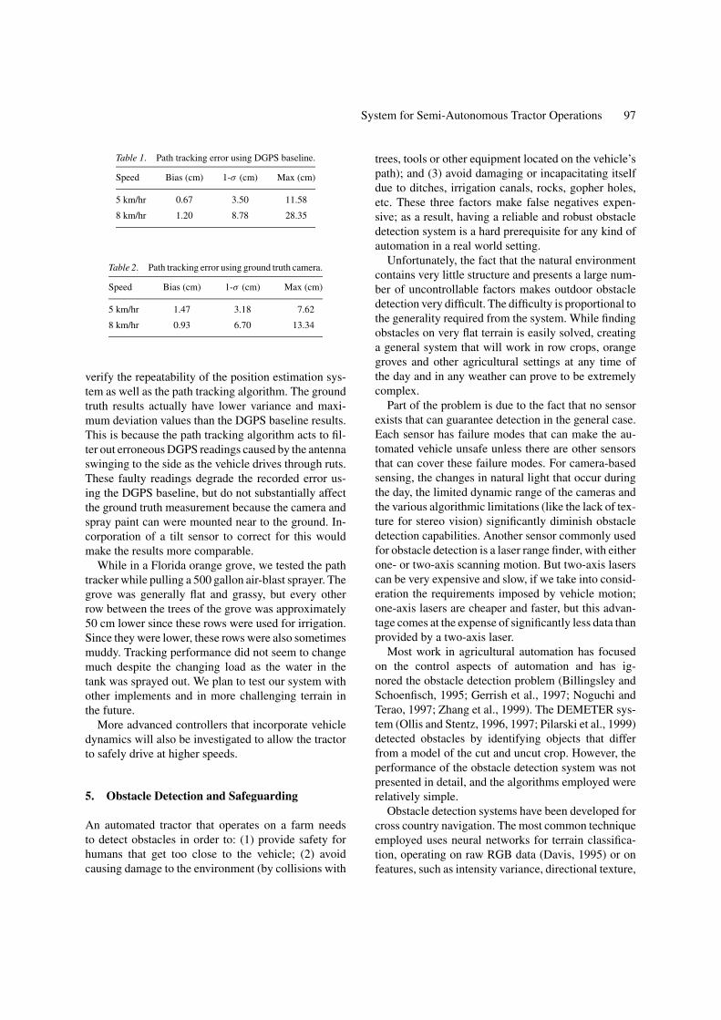
Table 1. Path tracking error using DGPS baseline.

Speed Bias (cm) 1-σ (cm) Max (cm)

5 km/hr 0.67 3.50 11.58

8 km/hr 1.20 8.78 28.35

Table 2. Path tracking error using ground truth camera.

Speed Bias (cm) 1-σ (cm) Max (cm)

5 km/hr 1.47 3.18 7.62

8 km/hr 0.93 6.70 13.34

verify the repeatability of the position estimation sys-tem as well as the path tracking algorithm. The groundtruth results actually have lower variance and maxi-mum deviation values than the DGPS baseline results.This is because the path tracking algorithm acts to fil-ter out erroneous DGPS readings caused by the antennaswinging to the side as the vehicle drives through ruts.These faulty readings degrade the recorded error us-ing the DGPS baseline, but do not substantially affectthe ground truth measurement because the camera andspray paint can were mounted near to the ground. In-corporation of a tilt sensor to correct for this wouldmake the results more comparable.

While in a Florida orange grove, we tested the pathtracker while pulling a 500 gallon air-blast sprayer. Thegrove was generally flat and grassy, but every otherrow between the trees of the grove was approximately50 cm lower since these rows were used for irrigation.Since they were lower, these rows were also sometimesmuddy. Tracking performance did not seem to changemuch despite the changing load as the water in thetank was sprayed out. We plan to test our system withother implements and in more challenging terrain inthe future.

More advanced controllers that incorporate vehicledynamics will also be investigated to allow the tractorto safely drive at higher speeds.

5. Obstacle Detection and Safeguarding

An automated tractor that operates on a farm needsto detect obstacles in order to: (1) provide safety forhumans that get too close to the vehicle; (2) avoidcausing damage to the environment (by collisions with

trees, tools or other equipment located on the vehicle’spath); and (3) avoid damaging or incapacitating itselfdue to ditches, irrigation canals, rocks, gopher holes,etc. These three factors make false negatives expen-sive; as a result, having a reliable and robust obstacledetection system is a hard prerequisite for any kind ofautomation in a real world setting.

Unfortunately, the fact that the natural environmentcontains very little structure and presents a large num-ber of uncontrollable factors makes outdoor obstacledetection very difficult. The difficulty is proportional tothe generality required from the system. While findingobstacles on very flat terrain is easily solved, creatinga general system that will work in row crops, orangegroves and other agricultural settings at any time ofthe day and in any weather can prove to be extremelycomplex.

Part of the problem is due to the fact that no sensorexists that can guarantee detection in the general case.Each sensor has failure modes that can make the au-tomated vehicle unsafe unless there are other sensorsthat can cover these failure modes. For camera-basedsensing, the changes in natural light that occur duringthe day, the limited dynamic range of the cameras andthe various algorithmic limitations (like the lack of tex-ture for stereo vision) significantly diminish obstacledetection capabilities. Another sensor commonly usedfor obstacle detection is a laser range finder, with eitherone- or two-axis scanning motion. But two-axis laserscan be very expensive and slow, if we take into consid-eration the requirements imposed by vehicle motion;one-axis lasers are cheaper and faster, but this advan-tage comes at the expense of significantly less data thanprovided by a two-axis laser.

Most work in agricultural automation has focusedon the control aspects of automation and has ig-nored the obstacle detection problem (Billingsley andSchoenfisch, 1995; Gerrish et al., 1997; Noguchi andTerao, 1997; Zhang et al., 1999). The DEMETER sys-tem (Ollis and Stentz, 1996, 1997; Pilarski et al., 1999)detected obstacles by identifying objects that differfrom a model of the cut and uncut crop. However, theperformance of the obstacle detection system was notpresented in detail, and the algorithms employed wererelatively simple.

Obstacle detection systems have been developed forcross country navigation. The most common techniqueemployed uses neural networks for terrain classifica-tion, operating on raw RGB data (Davis, 1995) or onfeatures, such as intensity variance, directional texture,

98 Stentz et al.

height in the image, and statistics about each color band(Marra et al., 1988). The MAMMOTH system (Davis,1995, 1996) drove an off-road vehicle. MAMMOTHused two neural networks (with one hidden layer each)to analyze separately visual and laser rangefinder data.Each neural network output a steering command. A“task neural network” took as inputs the outputs of thehidden layers in the two networks and fused the in-formation into a steering command. The JPL system(Belluta et al., 2000) detected obstacles in an off-roadenvironment by combining geometric information ob-tained by stereo triangulation with terrain classificationbased on color. The terrain classification was performedusing a Bayes classifier that used mixtures of Gaussiansto model class likelihoods. The parameters of the mix-ture model were estimated from training data throughthe EM algorithm. All of these systems have met withsome success in addressing a very difficult problem.The main difference between our work and the priorwork is that the agricultural application domain allowsus to impose simplifying constraints on the problem toour advantage.

5.1. Technical Approach

At the high level, we have identified three ways to re-duce the difficult problem of general obstacle detectionto a more solvable one:

• Extract as many cues as possible from multi-modalobstacle detection sensors and use sensor fusiontechniques to produce the most reliable result.

• Take advantage of the repeatability of the task bylearning what to expect at a given location on theterrain.

• Since the system can call for human intervention,take a conservative approach to obstacle detectionand allow a few false positive detections in orderto drastically reduce the likelihood of false negativedetections.

Our current sensor suite is shown in Fig. 10. It con-sists of two color CCD cameras used for obstacle de-tection and a Sony D30 pan-tilt color camera used forremote monitoring. The two Sony EVI-370DG cam-eras have a maximum resolution of 640 × 480 anda field of view that can vary from 48.8 to 4.3 de-grees horizontally and 37 to 3 degrees vertically. Weused a zoom setting that corresponds to approximately30 degrees horizontally. The two color CCD cameras

Figure 10. The sensor rack mounted inside the tractor cab. Thetwo cameras used for stereo can slide sideways to vary the baseline.The pitch angle can be adjusted in order to change the look-aheaddistance in front of the tractor. The pan-tilt color camera is used forthe remote operator interface.

Figure 11. ODS architecture. Solid boxes correspond to modulesfor which we present results. Dotted ones represent modules thatconstitute future work.

provide color and geometric cues about the scene. Inthe future we will also use them to extract texture cues.

The current architecture of the obstacle detectionsystem (ODS) is shown in Fig. 11. The ODS currentlyuses just the stereo range data and color data from theCCD cameras. The appearance and range data are sep-arately classified and the results are integrated in thefusion module, which sends obstacle detection confi-dences to the vehicle controller (central module). Thecentral module stops the tractor when the confidenceexceeds a preset threshold.

The color module uses a three-layer artificial neu-ral network trained with back propagation to segment

System for Semi-Autonomous Tractor Operations 99

incoming images into classes defined by the operatorduring the training process. In the orange grove sce-nario, such classes are “grass”, “tree”, “sky”, “obsta-cle”, etc. The “obstacle” class corresponds to colorsthat are not characteristic of any other class. A humanoperator provides the training data by manually clas-sifying portions of recorded images. This training canbe accomplished in minutes due to a graphical user in-terface that simplifies the process. In the future we areplanning to use unsupervised clustering techniques thatwill expedite the training process even more.

At run time, the 320 × 240 pixel images are split intopatches of 4 × 4 pixels, and each pixel is representedin the HSI color space. The intensity component is dis-carded for less sensitivity to brightness, and the hueis expressed by two numbers (sin(H) and cos(H)) toeliminate discontinuities. Thus, the input layer of theneural network has 4 × 4 × 3 inputs. We selected aninput patch of 4 × 4 pixels because it is good compro-mise between a small patch, which is sensitive to noise,and a large one, which permits only a coarse-scaleclassification.

The output layer contains as many output units asclasses used in the training data. In order to label aninput patch as belonging to class C, the output unitcorresponding to class C should have a value close to“ON” and the other units should have values close to“OFF”. If a patch does not fit well into any other class,it is labeled as an obstacle patch. Thus, even thoughan obstacle class is defined for training purposes, thesystem can still correctly classify obstacles that werenot represented in the training set.

In our test scenario we only used the color seg-mentation for obstacle detection, so we defined twoclasses (obstacle/non-obstacle) in order to avoid un-necessary complexity in the neural network’s decisionsurface.

To determine the optimal number of units in the hid-den layer, we started with a large number (allowingthe network to overfit the data) and gradually reducedthem until the total classification error on a standardtest began to rise. We arrived at three hidden units,which was the smallest number that did not degradethe performance of the network on the test set.

The stereo module is currently based on a 3-D “safetybox” representing a navigation zone in front of the trac-tor. The module creates a disparity map and signals thepresence and the location of any objects within this box.While this is certainly a minimalistic approach to ob-stacle detection with stereo vision, the module provides

very fast and reliable results for obstacles that protrudesignificantly upward from the terrain.

For the fusion module, we have the choice ofperforming sensor-level or central-level fusion. Thesensor-level fusion consists of computing a measureof confidence at each separate sensor, and then sum-ming over all the individual sensors to obtain the globalconfidence. In central-level fusion, the sensor data isminimally processed before combination and the com-puted confidence is a more complex function of themulti-modal data.

In general, data can be used more efficiently throughcentral-level fusion than through the sensor-levelparadigm (Klein, 1993). However, this approach hasseveral disadvantages: (1) it does not distribute thecomputational load, (2) it requires precise calibrationof the sensors and registration of the data; and (3) it isdifficult to incrementally add new sensors. In our ap-proach, we opted to investigate sensor modalities oneat a time, understand their individual contributions, andfuse their data at the sensor level using simple strate-gies. Once we have identified the best sensors and datamodalities, we will explore more sophisticated fusionstrategies at the central level to improve the perfor-mance of the system.

5.2. Experimental Results

We performed two kinds of experiments, meant totest two of our claims: (1) that redundancy in sensorsand the use of multi-modal data reduce overall fail-ure modes; and (2) that increasing the locality of thetraining data improves the overall performance.

5.2.1. Multi-Modal Data. To test the effectivenessof using multi-modal data, we measured system per-formance on data that represented failure modes forthe individual modality types: appearance (color) andrange (stereo).

For the first test, we used the scene depicted inFig. 12, which shows a human in a green suit againsta green background. Since the neural network wastrained to consider the green grass a non-obstacle, theresponse of the color module to the human obstaclewas not very strong, as shown in Fig. 13. However,since the stereo module uses only geometric informa-tion, it is unaffected by the similarity in color betweenthe obstacle and the background, and it gives a strongresponse indicating the presence of an obstacle. As aresult, even a simple fusion strategy consisting of the

100 Stentz et al.

Figure 12. Failure mode for color-based ODS: A human with agreen suit against green background.

Figure 13. ODS responses for the obstacle in Fig. 12, as the trac-tor approaches the obstacle. The small peak produced by the colormodule arises from the skin color; when the human is very close, thearea in the image occupied by skin becomes large enough to exceedthe obstacle threshold.

sum of the responses of the two modules (color andstereo) results in reliable detection.

The symmetric case is depicted in Fig. 14: a tarpplaced in the path of the tractor is invisible to the stereomodule. However, as shown in Fig. 15, the color mod-ule is able to detect it, and the ODS reports an obstaclewith high confidence.

We have presented the extreme cases here, but thebenefit of multiple sensors and data modalities becomeseven more significant when class differences are sub-tle. When the individual response from each sensor isnot much higher than the noise level, the correlation

Figure 14. Failure mode for stereo-based ODS: A tarp on theground.

Figure 15. ODS responses for the obstacle in Fig. 14, as the tractorapproaches the obstacle.

between these responses can still produce a cumulativeeffect that trips the threshold and stops the vehicle.

More recent experiments in natural scenes (seeFig. 16) confirm the fact that combining different cuesfor obstacle detection results in more reliable obstacledetection.

5.2.2. Data Locality. Agricultural operations are veryrepetitive. In general, a vehicle drives a given routemany times; therefore, it is possible to learn the appear-ance of terrain at a given location (and time) and use thisinformation for obstacle detection purposes when driv-ing autonomously. This amounts to obtaining traininginformation from all the parts of the route that have dif-ferent appearances. In our case, for the stereo module,

System for Semi-Autonomous Tractor Operations 101

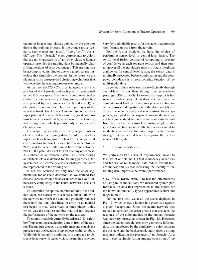
Figure 16. Results of a more recent version of our ODS system ona natural scene. Top: the raw image presenting rocks in front of thevehicle. Bottom: the same image, segmented using color and texturefeatures. The light-gray area represents the obstacle-free region, thedark gray represents obstacles.

this could consist of storing the average height of thegrass for each row in the orange grove, with the resultthat the “safety box” defined by the module is adjustedautomatically depending on the location. For the colormodule, information about the current time of the daycould be used in order to perform more effective colorconstancy or to use different versions of the neural net-work trained with labeled data collected at similar timesof the day.

However, two factors affect the appearance of the ter-rain at a given location and time of day. First, ambientlight and weather conditions vary in both predictableand unpredictable ways. To some extent, this effectcan be cancelled using color constancy techniques. Weused a gray calibration target mounted on the tractorin a place visible to the cameras. As the tractor drove,we repeatedly measured the color shift due to ambi-ent light and corrected the input images accordingly.This approach did not solve the problem completelybut greatly improved the color segmentation.

Second, the terrain at each location changes slowlyover the course of a season. The crop, grass, andweeds grow. The plants change in appearance as well.These effects preclude a purely rote learning strat-egy (based on location and time of day) and require

some generalization. We envision an obstacle detectionsystem which learns not only how to classify terrainbut how to predict changes over time. For example, thegrowing rate of the grass and the appearance changesof the vegetation could be learned and predicted.

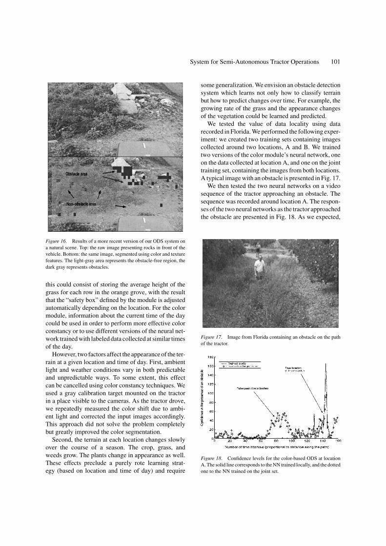
We tested the value of data locality using datarecorded in Florida. We performed the following exper-iment: we created two training sets containing imagescollected around two locations, A and B. We trainedtwo versions of the color module’s neural network, oneon the data collected at location A, and one on the jointtraining set, containing the images from both locations.A typical image with an obstacle is presented in Fig. 17.

We then tested the two neural networks on a videosequence of the tractor approaching an obstacle. Thesequence was recorded around location A. The respon-ses of the two neural networks as the tractor approachedthe obstacle are presented in Fig. 18. As we expected,

Figure 17. Image from Florida containing an obstacle on the pathof the tractor.

Figure 18. Confidence levels for the color-based ODS at locationA. The solid line corresponds to the NN trained locally, and the dottedone to the NN trained on the joint set.

102 Stentz et al.

the neural network that was trained locally performedbetter. In the case presented, the network trained onthe joint set generated a false obstacle peak due tosome bushes that were correctly classified as vegeta-tion by the locally trained network. Other experimentsin Florida and Pittsburgh confirmed the intuition thatthe quality of the color segmentation is related to thelocality of the training data.

The importance of local training data means that inthe future we should focus on methods that are ap-propriate for recording the location and time of theday. Neural networks might not be the best learningalgorithm for this, since the amount of training datarequired would be extremely large. We believe thatmemory-based learning together with automatic clus-tering techniques could be a better approach for ourproblem. In the memory-based paradigm, the systemwould periodically record data and perform automatedclustering of the color data obtained from each image(or from images within some neighborhood). We wouldthen model the data distribution at each location witha Gaussian mixture model. At runtime, we would useany classification algorithm to perform image segmen-tation, based on the distance from the clusters describedby the Gaussian mixture model.

Other areas of future work include: (1) using infor-mation coming from a laser range finder as an addi-tional cue; and (2) switching from the current sensor-level fusion paradigm to central-level fusion.

6. Conclusions

In addition to the component results for position esti-mation, path tracking, obstacle detection, and humanintervention, the tractor was tested as a system in an or-ange grove in Florida. Figure 19 shows a plan view ofthe total path taken during autonomous runs in Florida.Overall, the system performed quite well, navigatingaccurately up and down the rows, even in the presenceof hazards such as irrigation ditches. With commercialGPS units steadily improving in accuracy and drop-ping in cost, position-based navigation will becomethe method of choice for agricultural operations. Theremaining problems include navigating in difficult ter-rain, such as on slopes, over bumps, and in mud; andnavigating during dropout, including in areas with GPSocclusion.

But the real challenge for agricultural operations issafeguarding the people, the environment, and the ma-chines. Until this problem is solved, we cannot field

Figure 19. Overhead view of paths used during autonomous testingin a Florida orange grove. The turning radius of the tractor-sprayercombination requires the machine to travel down every other row.

unmanned vehicles. The outlook is promising, how-ever. By developing cautious systems, involving hu-mans remotely, and capitalizing on the repetitive natureof the task, we can make substantial headway in solvinga problem that is, in the general case, very difficult.

Acknowledgments

The authors would like to thank the entire AutonomousSpraying Project group, past and present, includingChris Fromme, Frank Campagne, Jim Ketterer, BobMcCall, and Mark Ollis. Support was provided byNASA under grant number NCC5-223 and by Deere& Company via a tractor donation.

References

Amidi, O. 1990. Integrated mobile robot control. Masters Thesis,Dept. of Electrical and Computer Engineering, Carnegie MellonUniversity, Pittsburgh, PA.

Belluta, P., Manduchi, R., Matthies, L., Owens, K., and Rankin,A. 2000. Terrain perception for DEMO III. Intelligent VehicleSymposium.

System for Semi-Autonomous Tractor Operations 103

Billingsley, J. and Schoenfisch, M. 1995. Vision guidance of agri-cultural vehicles. Autonomous Robots, 2.

Crowley, J.L. 1989. Control of translation and rotation in a robotvehicle. In Proceedings of the IEEE Conference on Robotics andAutomation.

Davis, I.L. 1995. Neural networks for real-time terrain typing. TheRobotics Institute, Carnegie Mellon University, Pittsburgh, PA,Technical Report CMU-RI-TR-95-06.

Davis, I.L. 1995. Sensor fusion for autonomous outdoor naviga-tion using neural networks. The Robotics Institute, Carnegie Mel-lon University, Pittsburgh, PA, Technical Report CMU-RI-TR-95-05.

Davis, I.L. 1996. A modular neural network approach to autonomousnavigation. The Robotics Institute, Carnegie Mellon University,Pittsburgh, PA, Technical Report CMU-RI-TR-96-35.

Erbach, D.C., Choi, C.H., and Noh, K. 1991. Automated guidance foragricultural tractors. Automated Agriculture for the 21st Century,ASAE.

Gerrish, J.B., Fehr, B.W., Van Ee, G.R., and Welch, D.P. 1997. Self-steering tractor guided by computer vision. Applied Engineeringin Agriculture, 13(5).

Kerr, T.H. 1997. A critical perspective on some aspects of GPS de-velopment and use. In 16th Digital Avionics Systems Conference,AIAA/IEEE, Vol. 2.

Klein, L.A. 1993. Sensor and Data Fusion Concepts and Applica-tions. SPIE Optical Engineering Press: Bellingham, WA.

Marra, M., Dunlay, R.T., and Mathis, D. 1988. Terrain classifi-cation using texture for the ALV. In Mobile Robots III, SPIE,Vol. 1007.

Neumann, J.B., Manz, A., Ford, T.J., and Mulyk, O. 1996. Test resultsfrom a new 2 cm real time kinematic GPS positioning system. InProc. of ION GPS-96, Kansas City.

Noguchi, N.K. and Terao, H. 1997. Development of an agriculturalmobile robot using a geomagnetic direction sensor and image sen-sors. Journal of Agricultural Engineering Research, 67.

O’Connor, M., Bell, T., Elkaim, G., and Parkinson, B. 1996. Auto-matic steering of farm vehicles using GPS. In Proc. of the 3rd Int.Conf. on Precision Agriculture.

Ollis, M. and Stentz, A. 1996. First results in vision-based crop linetracking. In Proc. of the IEEE Int. Conf. on Robotics and Automa-tion.

Ollis, M. and Stentz, A. 1997. Vision-based perception for an au-tonomous harvester. In Proc. of the IEEE/RSJ Int. Conf. on Intel-ligent Robotic Systems.

Maybeck, P. 1982. Stochastic Models, Estimation, and Control,Academic Press: New York.

Pilarski, T., Happold, M., Pangels, H., Ollis, M., Fitzpatrick, K.,and Stentz, A. 1999. The DEMETER system for autonomous har-vesting. In Proc. of the 8th Int. Topical Meeting on Robotics andRemote Systems.

Shin, D.H., Singh, S., and Shi, W. 1991. A partitioned control schemefor mobil robot path tracking. In Proc. IEEE Int. Conf. on SystemsEngineering.

Southall, B., Hague, T., Marchant, J.A., and Buxton, B.F. 1999.Vision-aided outdoor navigation of an autonomous horticulturalvehicle. In Proc. 1st. Int. Conf. on Vision Systems.

Tillet, N.D. 1991. Automatic guidance for agricultural field ma-chines: A review. Journal of Agricultural Engineering Research,50.

Wallace, R., Stentz, A., Thorpe, C., Moravec, H., Whittaker, W., and

Kanade, T. 1985. First results in robot road-following. In Proc. ofthe Int. Joint Conf. on Artif. Intell.

Will, J., Stombaugh, T.S., Benson, E., Noguchi, N., and Reid, J.F.1998. Development of a flexible platform for agricultural auto-matic guidance research. ASAE Paper 983202.

Yukumoto, O. and Matsuo, Y. 1995. Research on autonomous landvehicle for agriculture. In Proc. of the Int. Sym. on Automationand Robotics in Bio-production and Processing, Vol. 1.

Zhang, Q., Reid, J.F., and Noguchi, N. 1999. Agricultural vehiclenavigation using multiple guidance sensors. In Proc. of the Int.Conf. on Field and Service Robotics.

Anthony Stentz is a Senior Research Scientist at the Robotics Insti-tute, Carnegie Mellon University. His research expertise includesmobile robots, path planning, computer vision, system architec-ture, and artificial intelligence in the context of fieldworthy roboticsystems.

Dr. Stentz has led a number of successful research efforts to auto-mate navigation and coal cutting operations for a continuous miningmachine, cross-country navigation for an unmanned ground vehicle,nuclear inspection tasks for a manipulator arm, autonomous landingfor an unmanned air vehicle, crop row tracking for an autonomousharvesting machine, and digging operations for a robotic excavator.

Dr. Stentz received his Ph.D. in computer science from Carnegie-Mellon University in 1989. He received his M.S. in computer sciencefrom CMU in 1984 and his B.S. in physics from Xavier Universityof Ohio in 1982.

Cristian S. Dima is pursuing a Ph.D. degree in robotics at theRobotics Institute, Carnegie Mellon University. He received his B.A.in mathematics and computer science from Middlebury College in1999.

His research focuses on computer vision and multisensor fusionapplied to obstacle detection for autonomous outdoor robots.

104 Stentz et al.

Carl Wellington is pursuing a Ph.D. in robotics at the RoboticsInstitute, Carnegie Mellon University. He received his B.S. in engi-neering from Swarthmore College in 1999.

His research interests are in position estimation and control foroutdoor autonomous robots. Currently he is focusing on the use oflearning algorithms for the safe control of off-road vehicles.

Herman Herman is a Commercialization Specialist at the NationalRobotics Engineering Consortium. He has worked in the field of

robotics and computer vision for the last 12 years. His present andpast works include the automation of an underground mining vehi-cle, a real-time tracking system, a 6-D optical input device and 3-Dimage processing. His area of expertise includes image processing,automation and system engineering.

Dr. Herman received his Ph.D. in Robotics from Carnegie MellonUniversity in 1996 and B.S. in Computer Science from Universityof Illinois at Urbana Champaign in 1989.

David Stager is a Design Engineer at the National RoboticsEngineering Consortium of Carnegie Mellon University. He receivedhis B.S. in Electrical & Computer Engineering and Math & ComputerScience from Carnegie Mellon University in 1995.

While at the NREC, he has helped design and build several fullyautonomous robotic vehicles including forklifts, tuggers, a tractor,and various ATV’s for commercial and military use.