To link to this article: DOI:10.1016/j.energy.2009.10.032

http://dx.doi.org/10.1016/j.energy.2009.10.032

This is an author-deposited version published in: http://oatao.univ-toulouse.fr/

Eprints ID: 4988

To cite this version:

Agha, Mujtaba and Thery, Raphaële and Hétreux, Gilles and Haït, Alain and Le

Lann, Jean Marc Integrated production and utility system approach for

optimizing industrial unit operations. (2010) Energy, vol. 35 (n° 2). pp 611-627 .

ISSN 0360-5442

Open Archive Toulouse Archive Ouverte (OATAO) OATAO is an open access repository that collects the work of Toulouse researchers and

makes it freely available over the web where possible.

Any correspondence concerning this service should be sent to the repository

administrator: staff-oatao@inp-toulouse.fr

Integrated production and utility system approach for optimizing industrialunit operations

Mujtaba H. Agha a, Raphaele Thery a, Gilles Hetreux a,*, Alain Hait b, Jean Marc Le Lann a

aUniversite de Toulouse, Laboratoire de Genie Chimique (ENSIACET-INPT), 4 allee Emile Monso, BP 44362, 31432 Toulouse Cedex 4, FrancebUniversite de Toulouse, Institut Superieur de l’Aeronautique et de l’Espace, 10 av. E. Belin, 31055 Toulouse Cedex 4, France

Keywords:

Scheduling

CHP plant

Utility management

MILP

Energy cost

a b s t r a c t

To meet utility demands some industrial units use onsite utility system. Traditionally, the management of

such type of industrial units is carried out in three sequential steps: scheduling of the manufacturing unit

by minimizing inventory, estimating the utility needs of manufacturing unit and finally operation

planning of the utility system. This article demonstrates the value of an integrated approach which

couples the scheduling of manufacturing unit with operational planning of the utility system. A discrete-

time mixed integer linear programming (MILP) model is developed to compare traditional and integrated

approaches. Results indicate that the integrated approach leads to significant reduction in energy costs

and at the same time decreases the emissions of harmful gases.

1. Introduction

The industrialization in developing countries and especially thatof China and India will increase the global energy demand. Indeveloping countries, the proportion of global energy consumptionis projected to increase from 46 to 58 percent between 2004 and2030, at an average annual growth rate of 3 percent. During thesame period, industrialized nations will witness an annual growthin the demand for energy of 0.9 percent [1].

The industrial sector accounts for one third of global energyconsumption. Although processes used in the industrial sector arehighly diverse, a common feature to all is their reliance on fossilfuels as the primary source of energy. A large part of the energyconsumption of the industrial unit is focused on the production ofutilities. A utility is defined as any quantity which has high energyand can be useful to an industrial unit in manufacturing thefinished product. The utility can be in the form of electricity, steam(at various pressure levels), hot/cold water or hot air.

The reliance on fossil fuels as the primary source of energy hasa huge negative impact on the environment and eco-system of ourplanet. The studies of the Intergovernmental Panel for ClimateChange (IPCC) have acknowledged that the main cause for thephenomenon of global warming is the emission of greenhouse

gases, which are released into the atmosphere during burning offossil fuel. Global warming is considered to be the biggest imped-iment in carrying out sustainable development.

Consequently, there is a concentrated effort in the scientificworldto find alternative sources of energy. Current emphasis is on renew-able energies such aswind, solar, hydrogen, etc. However, evenby themost optimistic assessments, all these alternatives are long-termsolutions. The projections of the Energy Information Administration(EIA), a statistical agencyof theAmericandepartmentof energy, showthat fossil fuels will remain as primary sources of energy in theimmediate future. Thus, along with finding alternative energy sour-ces, an effortmust bemade to look forways of conserving energy thatwill minimize the damage caused by the use of fossil fuels [2].Initiatives like cleaner production [3] and zero-emissions [4] areimportant approaches in this regard. However a short-term solution,which has been identified by the IPCC, is to improve energyefficiencyin industrial processes [5]. This can be achieved by two possiblemeans; firstly, advancements in energy generation technology andsecondly, the use of methodologies such as ‘process integration’.

Combined heat and power (CHP) is an important energy produc-tion technology as it improves the overall energy efficiency of theprocess while simultaneously reducing greenhouse gas emissions,especially that of CO2 [6]. CHP, also known as the ‘cogenerationprocess’, relies on the simultaneous generation of electricity andotherformsofuseful thermal energy (steamorhotwater) formanufacturingprocesses or central heating systems. The energy savings and

* Corresponding author. Tel.: þ33 534323660; fax: þ33 534323399.

E-mail address: gilles.hetreux@ensiacet.fr (G. Hetreux).

doi:10.1016/j.energy.2009.10.032

environmental benefits offered by CHPmake it an ideal candidate foruse in the building sector (district heating) [7] and in industrial units[8]. Both the United Nations [9] and the European Union [10] see CHPas one of the very few technologies that can offer a short or medium-term solution for pollution control by increasing energy efficiency.

CHP is a popular choice for several onsite industrial utilitysystems, which are a feature of many chemical and petrochemicalplants. However, in themajority of these industrial sites ‘‘productionis the king’’ and utility systems are regarded mainly as a supportfunctionwhose objective is to provide service to the manufacturingunit. Due to this biased outlook the utility systems fail to attain theirfull energy efficiency potential. Technological advancement andbreakthroughs in the development of more energy efficient plantmachinery is an ongoing process. However, an industrial process isconstrained by thermodynamic, kinetic and transport limitations.Thus, in addition to technological advancements inplantmachinery,one also needs to address the concept of process integration [11]. Inthe past, process integration was synonymous with the thermody-namic technique of ‘pinch and energy analysis’. Nowadays, process

integration techniques cover four major areas. Firstly, the efficientuse of raw materials, secondly, emission reduction, thirdly, processoperations and of course energy efficiency [12]. Process integrationhas evolved over the years and now makes significant use ofmathematical methods and optimization models.

The objective of this article is to develop an approach where theproduction process and the utility system will be integrated. Theremainder of the paper is organized as follows. Section two outlinesthe problem statement. A mathematical model indicative of thetraditional (sequential) approach and the new (integrated)approach is presented in section three. Section four compares thetwo approaches by applying the model to three different industrialunits. Finally, on the basis of all the data, the conclusions and futureoutlook are presented in section five.

2. Problem statement

Traditionally the industrial sector has been reliant on utility

suppliers for the supply of electricity while it generates other utilities

Nomenclature

Indices

i fuelsj units (processing equipments /boilers/turbines)k tasksq piecewise segment of efficiency curves statest time periodv utility

Sets

BOIL set of boilers in CHP plantFUEL set of fuels in CHP plantJ set of processing equipments in manufacturing unitK set of tasksKconss set of task k which consume state s

Kprods set of task k which produce state s

S set of statesTURB set of turbines in CHP plantUTILITY set of utilities provided by CHP plants; {LP, MP, HP,

electricity}

Parameters

aj consumption coefficient for MP steam redirectedtowards boiler

bj consumption coefficient for electricity required tocarry out boiler operation

cci calorific value of fuel (MJ/kg)cfi cost of fuel (V/ton)CEL electricity purchase cost (V/MWh)CGHG cost incurred for emissions of GHG (V/ton)Copv,k utility v consumed for task k (ton/hr of steam or MW/

hr of electricity required per ton of material processed)CSOX cost incurred for emissions of SOx (V/ton)cpti capacity of storage repository for fuel i (tons)ghgi coefficient of GHG released from boiler due to fuel iehsti exhaust steam parameter for turbine j (defined as

a fraction of TXHPt,j)h enthalpy values based on steam temperature and

pressure (MJ/kg)

Imaxj,i quantity of fuel i that is required to attain maximumsteam level in boiler j

Iminj,i quantity of fuel i that is required to attain minimumsteam level in boiler j

Iq;j;i fuel threshold of the piecewise efficiency curvesegment q

ls inventory coefficient for state s that is used to obtainthe tardiness starting date

pk time duration for executing task k in the unit jQ total number of piecewise segmentsSIdemj,i quantity of fuel i that is used during starting-up phase

of boiler jsoxi coefficient of SOx released from boiler due to fuel issfi safety stock parameter for fuel i (defined as a fraction

of cpti)T time horizonTXHPmaxt,j maximum amount of steam that can enter turbine j

in time period t

TXHPmint,j minimum amount of steam that can enter turbine j

in time period t

XHPmaxj maximum amount of steam that can be produced byboiler j

XHPminj minimum amount of steam that can be produced byboiler j

XHPq;j;i steam threshold of the piecewise efficiency curvesegment q

hj,i efficiency of boiler j with fuel ihj efficiency of the turbine j

Cs;Cmaxs storage capacity and the maximum storage capacity of

state s (tons)Vmink;j ;Vmax

k;j minimum and maximum size of processingequipment j when processing task k (tons)

rconsk;s ; r

prodk;s

proportion of state s consumed or produced by task k

Binary variables

Aq,t,j,I to determine the boiler efficiency as a function of boilerload factor

Wk,j,t to determinewhether task k is being carried out in unitj in time period t

SBt,j,i to determine whether boiler j is operational duringtime period t using fuel i

FSBt,j,i to determine whether boiler j is being restarted duringtime period t using fuel i

on its own (see Fig. 1). Plant machinery, such as boilers, condensers,compressors etc, is used for this purpose. However, there isa growing tendency for high-energy intensive industries to producetheir own electricity. The terminology used for such industrialprocesses is auto-production. This refers to electricity, heat or steamproduced by an industrial facility for its own consumption or in orderto sell to other consumers or to the electricity grid.

It can be assumed that an industrial unit using auto-productioncomprises of two units, a utility system that uses fuels to generateutilities and amanufacturing unit, which consumes these utilities toproduce the finished product. Utilities generated in the utilitysystem have a direct correlation with the activity level in the

manufacturing unit. This relationship between the manufacturingunit and utility system can be established by using mathematicaloptimization, which cannot only help in design and retrofit aspectsbut it can also aid in solving the daily operational problems. Thescope of this studywill be limited to the operational aspect, with nostructural modifications in the industrial unit.

The traditional approach to auto-producer scheduling is depen-dent on the sequential resolution of three sub-problems (Fig. 2):

- First of all ‘task scheduling’ is carried out in the manufacturingunit, which, based on the production recipes, allocates limitedresources (processing equipments) to produce the final

Primary Energy Sources

Fossil fuels Nuclear Bio Fuel Others

Coal

Oil

Gas

Non-renewable sources Renewable sources

Hydral

Solar

Wind

Sea

Hot Water / Steam

GenerationBuilding Sector

Transmission &

Distribution

Electricity Generation Transmission Distribution

Industrial Sector

Commercial Residential

Primary Energy Sources

Fossil fuels Nuclear Bio Fuel Others

Coal

Oil

Gas

Non-renewable sources Renewable sources

Hydral

Solar

Wind

Sea

Primary Energy Sources

Fossil fuels Nuclear Bio Fuel Others

Coal

Oil

Gas

Non-renewable sources Renewable sources

Hydral

Solar

Wind

Sea

Primary Energy Sources

Fossil fuels Nuclear Bio Fuel Others

Coal

Oil

Gas

Non-renewable sources Renewable sources

Hydral

Solar

Wind

Sea

Fig. 1. Utility supply structure.

Simultaneously determine the

production schedule and energy

planning

Globally taking into account the

constraints of production and the

constraints of cogeneration

Criterion :

Weighted sum of the quantity of stock and

energy costs

Establishing scheduling plan

Takes into account only the

constraints of production

Estimating energy demands

Calculations made for utility demands

for each period

Energy planning

Les demandes étant données, calculer

les flux dans la centrales de cogénération

Production

model

Cogeneration

model

Global

model

APPROACH 1 : Approach SequentialAPPROACH 1 : Approach Sequential APPROACH 2 : Approach IntegratedAPPROACH 2 : Approach Integrated

Simultaneously determine the

production schedule and operational

planning of utility system

Globally taking into account the

constraints of production and the

constraints of utility generation

:

Establish a scheduling plan

Takes into account only the

production constraints in manufacturing unit

Estimate energy demands

Calculations made for utility demands

for each period in the scheduling horizon

Utility sytem planning

Operational planning of the utility system ,

Production

model

Utility system

model

Integrated

model

APPROACH 1 : Approach SequentialSequential Approach APPROACH 2 : Approach IntegratedIntegrated Approach

to fulfill the utility demands

Simultaneously determine the

production schedule and energy

planning

Globally taking into account the

constraints of production and the

constraints of cogeneration

Criterion :

Weighted sum of the quantity of stock and

energy costs

Establishing scheduling plan

Takes into account only the

constraints of production

Estimating energy demands

Calculations made for utility demands

for each period

Energy planning

Les demandes étant données, calculer

les flux dans la centrales de cogénération

Production

model

Cogeneration

model

Global

model

APPROACH 1 : Approach SequentialAPPROACH 1 : Approach Sequential APPROACH 2 : Approach IntegratedAPPROACH 2 : Approach Integrated

Simultaneously determine the

production schedule and operational

planning of utility system

Globally taking into account the

constraints of production and the

constraints of utility generation

:

Establish a scheduling plan

Takes into account only the

production constraints in manufacturing unit

Estimate energy demands

Calculations made for utility demands

for each period in the scheduling horizon

Utility sytem planning

Operational planning of the utility system ,

Production

model

Utility system

model

Integrated

model

APPROACH 1 : Approach SequentialSequential Approach APPROACH 2 : Approach IntegratedIntegrated Approach

to fulfill the utility demands

Fig. 2. Comparison between sequential and integrated approach.

product(s). Task scheduling determines the number of tasks, thetiming of these tasks and the batch size of each task to be per-formed in the manufacturing unit. The objective is to minimizethe make-span or inventory.

- Subsequently, on the basis of the task scheduling, the overallutility demands for the manufacturing unit are estimated. Inthese calculations the concept of energy integration [13] andespecially that of pinch analysis [14] can be used to develop a heatexchange network that minimizes the utility demands in themanufacturing unit.

- Finally, knowing the utility demands, the final step is the oper-ational planning of the utility system. The objective in this step isto operate the utility system in such a manner that it not onlymeets the utility demands of the manufacturing unit but alsominimizes the energy costs [15].

In the sequential approach the relationship between themanufacturing unit and the utility system is that of ‘master andslave’. As pointed out by Adonyi et al. [16], the utility demands arestrongly dependent on the first step of the manufacturing unit, taskscheduling. As a consequence, the operational planning of theutility system and the subsequent energy costs are heavily relianton the outcome of the task scheduling. In spite of this directcorrelation, task scheduling does not take into account the opera-tional planning of the utility system. This lukewarm approachtowards not taking into account the utility system in the overallconsiderations can perhaps be explained by the low price of fossilfuels. However, over the last few years increased fuel costs havemeant that considering the utility system as a subsidiary function isno longer feasible. On the other hand, if the operational planning ofthe utility system is carried out first then it generally leads toinfeasibilities at the task scheduling level of the manufacturingunit. Hence, the traditional sequential approach inevitably leads toa non-optimized energy cost.

The task scheduling aspect of the manufacturing unit has beensubject to extensive research. However, few scheduling modelshave been proposed in which the management of utilities isexplicitly taken into account. For example, Kondili et al. [17]developed a model to determine a plan for minimizingmanufacturing costs. The cost of energywas assumed to vary duringthe day and energy consumption was dependent on the nature ofthe product manufactured and the equipment used. The impact ofenergy costs was catered by positioning energy costs in the objec-tive function. This model was further enhanced [18] to developa short-term batch scheduling algorithm which incorporated thelimited availability of the utilities as a scheduling resource constraint.

It should be noted that unlike the resources classicallyconsidered in the scheduling problems (machinery or workforce), utilities have special characteristics which must be takeninto account. Utilities are a more versatile resource and arepresent in various forms (steam at different pressures, electricity,hot water, etc). Utilities are also resources that are difficult tostore in their ultimate form. Some recent studies have taken intoconsideration these peculiarities of utilities. Behdani et al. [19]developed a continuous-time scheduling model, which includedthe constraints related to the production, availability andconsumption of different types of utilities (water cooling, elec-tricity and steam). Hait et al. [20] presented an approach designedto minimize the energy costs of a foundry, subject to the specificprovisions relating to the power pricing and market-basedstrategies for load shedding. However, in all these approaches,the focus is primarily on the manufacturing unit while the utilitysystem is modeled in an aggregated manner. Moreover, theoperational planning aspect of the utility system is not consid-ered in these models.

Conversely, research on the utility system has concentratedexclusively on setting up boilers, turbines and steam distributionnetwork. The process user, that is, the manufacturing unit, is nottaken into consideration. A thermodynamic based heuristic methodwas used by Nisho et al. [21] to design a steam power plant.Grossman and Santibanez [22] presented a mathematical modelingbased approach using Mixed Integer Linear Programming (MILP)for process synthesis. The design of a utility plant using the conceptof ‘superstructure’ was developed by Papoulias and Grossmann[23] using MILP. Subsequent research in this area resulted in morecomplex and multi-period MILP models [24–26].

The objective of all these models was to design a utility systemthat satisfies specific power and steam demands. Similarly, themodels dealing with the operational planning of utility systemsconcentrate uniquely on reducing the energy costs withoutconsidering the task scheduling of the manufacturing unit. Forexample, Marik et al. [27] used a combination of forecasting andoptimization methods to devise an effective decision-making toolfor the management of utility systems. The forecasting methodsdetermine the most probable demands based on the historical dataand optimization methods seek a more efficient operationalregime. De et al. [28] developed an artificial neural network (ANN)model to monitor the performance of the CHP based utility system.Soylu et al. [15] developed a multi-period MILP model for collab-oration between CHP plants located at different industrial sites. Theobjective of the model was to fulfill the utility demands in a multi-site environment. However, the utility demands during each timeinterval were assumed to be given a priori. In each of the abovementioned models no provision is made for sudden changes inconsumer demands, which might alter with varying activity levelsin a manufacturing unit. Therefore, for efficient operations ofindustrial units there is a need to correlate the short-term sched-uling of manufacturing unit with the operational planning of utilitysystem.

Even though this aspect has largely been ignored over the years,some recent research has focused on developing models andmethods that try to incorporate aspects of task scheduling andoperational planning of utility system. Puigjaner [29] presenteda detailed framework for heat and power integration into batch andsemi-continuous processes. Moita et al. [30] developed a dynamicmodel, combining a salt crystallization processing unit anda cogeneration unit. Zhang and Hua [31] developed a model fordetermining the MILP optimum operating points of a refinerycoupled with a cogeneration unit.

In this study an integrated approach is presented, which like itscounterpart sequential approach, gives paramount importance tomeeting the product demands. However, the integrated approachdirectly incorporates the aspect of operational planning of the siteutility system into the task scheduling problem of themanufacturing unit. This results in better synchronization betweenthe manufacturing unit and site utility system, thereby maximizingthe energy efficiency of the whole industrial unit.

3. Mathematical model

The constraints of the mathematical model are provided byapplying production and capacity constraints along with mass andenergy balances to all the components of the industrial unit.Simplifying assumptions make it possible to use linear equationsand binary variables tomodel the behavior of themain componentsof an industrial unit. A discrete time-based MILP model is devel-oped to formulate the problem. The model is divided into T

(t¼ 1.T) one-hour periods representing multi-period operationsof the industrial unit. The nomenclature given at the end providesthe definition of each parameter and variable used in the model.

3.1. Manufacturing unit model

The manufacturing unit employs production recipes via pro-cessing equipments to turn the rawmaterials into intermediate andfinished products. The manufacturing unit is characterized by theResource Task Network (RTN) representation [32,33], a bipartitegraph comprising of two types of nodes: resources (denoted bya circle) and tasks (denoted by a square). The concept of ‘resource’ isentirely general and includes all entities that are involved in theprocess steps, such as materials (raw materials, intermediates andproducts), processing and storage equipment (tanks, reactors, etc.)and utilities (operators, steam, etc.). A ‘task’ is defined as an oper-ation that transforms a certain set of resources into another set.

To simplify the graphical representation, the resource node issub-divided into a state node and an equipment node (Fig. 3). Thestate node (the circle) is used for depicting materials and theequipment node (the oval) is used to portray processing equip-ment. It is assumed that the state nodes also act as storage areas forthe material. The operating times of each task are supposed asknown and independent of the batch size. The constraints of themodel are as follows:

3.1.1. Allocation constraints

At a given time t, processing equipment j can, at the most, initiateone operation. In addition, if an operation (task) k is launched inperiod t (Wk,j,t¼ 1) then this processing equipment j shall no longerbe available (Wk,j,t’¼ 0) during the periods t’¼ t– pkþ 1 till t’¼ t þ pk–1 (i.e. duration of the task). This is expressed by Eq. (1):

X

k˛Kj

X

t

t0 ¼ t ÿ pk þ 1t > 0

Wk;j;t0 � 1 cj˛J;ct ¼ 1; ::; T (1)

3.1.2. Material balance

Eq. (2) shows that the amount of material in state s duringperiod t is the difference between the quantity of the materialproduced and that consumed. The initial stocks S0s are supposedknown and no task k is launched before period t> pk.

Ss;t ¼ Ss;tÿ1 þX

k˛Kprods

rprodk;s

X

j˛Jkt > pk

Bk;j;tÿpkÿX

k˛Kconss

rconsk;s

X

j˛Jk

Bk;j;t0

ÿDs;t cs˛S;ct ¼ 1; ::; T (2)

Ss;0 ¼ S0s cs˛S (3)

3.1.3. Capacity constraint

Eqs. (4) and (5) represent the production capacity and storagelimitation constraints of the processing equipment j.

Wk;j;tVmink;j � Bk;j;t � Wk;j;tV

maxk;j ck˛K;cj˛J;ct ¼ 1; ::; T (4)

0 � Ss;t � Cmaxs cs˛S;ct ¼ 1; ::; T (5)

3.2. Utility system model

A typical CHP based utility system comprises of fuel storagetanks, boilers for high pressure steam production, steam turbinesfor electricity generation, valves for reducing pressure and mixingequipment for mixing likewise material (Fig. 4).

3.2.1. Fuel storage model

The amount of fuel i entering the boiler j and producing HPsteam in the period t is represented by It,j,i. Each fuel repository hasa certain capacity and initial amount of fuel ORF0,i stored in it isassumed as known. To simplify the fuel storage model in this studyit is assumed that the fuel inventory is sufficient to meet utilityrequirements and no fuel purchase is required. It is further assumedthat there are no holding costs incurred for the fuel storage.

ORFt;i ¼ ORFtÿ1;i ÿX

j˛BOIL

ÿ

It;j;i þ SIt;j;i�

ci˛FUEL;ct ¼ 1; ::; T

(6)

cpti � ORFt;i � ssfi$cpti ci˛FUEL;ct ¼ 1; ::; T (7)

S1T1

(1)S1 T1

(task duration)

J1

S2S1T1

(1)S1 T1

(task duration)

J1

S2

Fig. 3. Basic RTN representation.

Fig. 4. Typical CHP based Utility System.

The Eq. (6) models the fuel tank mass balance. Fuel leaving therepository depends on the demands of the boiler. However, asenforced by Eq. (7), the quantity of fuel in the repository can neitherfall below the safety stock limit nor exceed the maximum capacity.

3.2.2. Boiler model

It is assumed that boiler j has an uninterrupted supply of air andwater. The fuel type i is supplied to the boiler where it is burnt togenerate high pressure (HP) steam. The boiler requires a certainamount of medium pressure steam (to pre-heat water) and elec-tricity to carry out its operations. Although multi-fuel fired boileroperation is considered, during time period t only one type of fuel isused in the boiler. The boiler equations can be subdivided into fourbroad categories.

i. Associating fuel consumption with steam production

Eq. (8) models the fuel consumption in boiler j as a function ofthe amount of high pressure (HP) steam produced, calorific value offuel, boiler efficiency and the enthalpy difference between super-heated steam and feed-water heaters. This is essentially a non-linear equation but simplifying assumptions are used to developa representative linear equation. It is assumed that steam pressuresand temperatures are fixed at the boiler inlet and exit, thus turningthe enthalpy difference into a parameter. However, there are stilltwo variables in the equation, boiler efficiency hj,i and fuelconsumption Iq;j;i.

Iq;j;i ¼

�

hb ÿ hfw

�

$XHPq;j;i

cci$hq;j;icq˛Q ;cj˛BOIL;ci˛FUEL (8)

Soylu et al. [15] solved this problem by using the assumptionthat boiler efficiency remained constant irrespective of load factor.However, boiler efficiency is significantly less when it operates atpart load, i.e. operating at less than design capacity. In order toinclude the effect of the efficiency variation with the varying loadfactor and at the same time guarding the condition of linearity,piecewise linear approximation is used (Fig. 5). For this study threelinear pieces are considered (Q¼ 3), where:

XHP 0;j;i ¼ XHPminj; XHP1;j;i ¼ 0:5,XHPmaxj;

XHP2;j;i ¼ 0:75,XHPmaxj and XHP3;j;i ¼ XHPmaxj

Eqs. (9)–(11) develop this piecewise linear approximation curve,quantifying fuel consumption with the varying load factor. XHPminjis the minimum amount of steam that can be produced by the boiler.Below this steam level, it is not economically viable to operate theboiler and hence, it is shutdown. Eq. (9) determines the amount ofHP steam being generated in the boiler. It joins q linear equations byuse of binary variables Aq,t,j,i and continuous variables xq,t,j,i. TheXHPt,j,i amount of steam produced in the boiler is determined by thenumerical value of these binary and continuous variables.

XHPt;j;i¼X

Q

q¼1

Aq;t;j;iXHPqÿ1;j;iþxq;t;j;iÿ

XHPq;j;iÿXHPqÿ1;j;i

�

ct

¼1;::;T ;cj˛BOIL;ci˛FUEL (9)

Eq. (10) models the amount of fuel type i consumed in the boiler togenerate XHPt,j,i amount of steam.

It;j;i ¼X

Q

q¼1

Aq;t;j;iIqÿ1;j;i þ xq;t;j;iÿ

Iq;j;i ÿ Iqÿ1;j;i

�

ct

¼ 1; ::; T ;cj˛BOIL;ci˛FUEL (10)

Eq. (11) enforces that, at maximum, only one binary variable Aq,t,j,i

will have the value ‘‘1’’, while Eq. (12) limits the value of continuousvariable xq,t,j,i between 0 and 1. Eq. (13) imposes a further restrictionwhereby during a particular time period, only one type of fuel canbe burnt in the boiler.

X

Q

q¼1

Aq;t;j;i � 1 ct ¼ 1; ::; T ;cj˛BOIL;ci˛FUEL (11)

0�xq;t;j;i�Aq;t;j;i cq˛Q ;ct¼1;::;T;cj˛BOIL;ci˛FUEL (12)

X

i˛FUEL

Aq;t;j;i � 1 cq˛Q ;ct ¼ 1; ::; T;cj˛BOIL (13)

0 XHP3

HP steam

noit

pm

us

no

c le

uF

0

1

2

3

XHP2XHP1

I0

I2

I1

I3

Boiler shutdown

A1, x1

A2, x2 A3, x3

Aq : binary variables

xq : continuous variables such that :

0 xq 1

Only one couple (Bq,xq) can have non-

zero value

XHP

I

Example:

XHP = A2 XHP1

+ x2 (XHP2 - XHP1)

I = A2 I1 + x2 (I2 – I1)

For a given t, j and i we have

XHP0XHP0

Fig. 5. Fuel consumption as a function of HP steam generated in boiler.

ii. Boiler shutdown and restart constraints

Boiler operations are not instantaneous and it is assumed thatthe boiler takes one hour (equivalent to one time period) to shut-down and also, one hour to restart. Thus, once the boiler is shut-down, it will require a minimum of two hours before it can startgenerating steam again. During the restart phase, the boiler usesSIdemt,j,i amount of fuel without producing any steam.

Eq. (14) confines the amount of HP steam that can be producedby the boiler during its operational phase (i.e. when SBt,j,i¼ 1) andmakes it zero when the boiler is in the shutdown state (whenSBt,j,i¼ 0).

XHPminj,SBt;j;i � XHPt;j;i � XHPmaxj,SBt;j;i ct

¼ 1; ::; T ;cj˛BOIL;ci˛FUEL (14)

Eq. (15) determines that boiler being operational in the futuretime period depends on the current state of the boiler as well as thestate of boiler in the previous time interval (cf. Table 1).

SBtþ1;j;i � SBt;j;i þÿ

1ÿ SBtÿ1;j;i

�

ct

¼ 2; ::; T ÿ 1;cj˛BOIL;ci˛FUEL (15)

Eqs. (16) and (17) establish that ‘boiler restart’ in a given timeinterval will occur only if it is operational in the future period and itis not operational in the current time interval. (cf. Table 2)

FSBtþ1;j;i � SBtþ1;j;i ct ¼ 1; ::; T ÿ 1;cj˛BOIL;ci˛FUEL (16)

FSBtþ1;j;i � SBtþ1;j;i ÿ SBt;j;i ct

¼ 1; ::; T ÿ 1;cj˛BOIL;ci˛FUEL (17)

Fuel consumed during the restart phase without producingsteam is represented by Eq. (18). It is important to note that thepresence of SIt,j,i in the objective function (Crit. 2) makes itmandatory for boiler restart to occur only when it is absolutelynecessary, i.e. preferably FSBt,j,i¼ 0.

SIt;j;i ¼ FSBt;j;i,SIdemj;i ct ¼ 1; ::; T ;cj˛BOIL;ci˛FUEL (18)

Eqs. (19) and (20) are limiting constraints, enforcing that onlyone fuel can be used to restart the boiler and similarly, only one fuelcan be used during the operation of the boiler.

X

i˛FUEL

FSBt;j;i � 1 ct ¼ 1; ::; T ;cj˛BOIL (19)

X

i˛FUEL

SBt;j;i � 1 ct ¼ 1; ::; T;cj˛BOIL (20)

iii. Emission constraints

Eqs (21) and (22) model the amount of SOx and greenhouse gas(GHG) emissions from the boiler.

XSOXt;j¼X

i˛FUEL

soxi$ÿ

It;j;iþSIt;j;i�

ct¼1;::;T ;cj˛BOIL (21)

XGHGt;j¼X

i˛FUEL

ghgi,ÿ

It;j;iþSIt;j;i�

ct¼1;::;T ;cj˛BOIL (22)

iv. Boiler electricity and steam return constraints

The amount of medium pressure heat redirected back to pre-heat water and electricity used by the feed water pump to injectwater into the boiler are modeled by Eqs. (23) and (24).

RETt;j ¼ aj$X

i˛FUEL

XHPt;j;i ct ¼ 1; ::; T ;cj˛BOIL (23)

BELt;j ¼ bj$X

i˛FUEL

XHPt;j;i ct ¼ 1; ::; T ;cj˛BOIL (24)

3.2.3. Turbine model

In this study, it is assumed that multi-stage back pressure steamturbines are used for the purpose of electricity generation. Thewhole functioning of the multi-stage steam turbine is presented inFig. 6. The high pressure steam comes into the first stage of theturbinewhere it expands and ultimately leaves asmedium pressuresteam. This medium pressure steam then enters the second turbinestage and leaves as low pressure steam. Finally the low pressure

steam enters the third stage of the turbine and exits at a very lowpressure. This ‘exhaust steam’ is above the saturated steam levelbut it is not fit to meet the process requirements of themanufacturing unit.

After each stage, some quantities of medium pressure (MP) andlow pressure (LP) steam are extracted from the turbine to meet thesteam demands of the manufacturing unit. Another source formeeting MP and LP steam demands is by expanding the steamthrough pressure release valves (PRVs).

Eq. (25) models the turbine mass balance.

TXHPt;j ¼XMPt;jþXLPt;jþXEHSTt;j ct¼ 1;::;T ;cj˛TURB (25)

Table 1

Boiler Shutdown.

SBtL1 SBt SBtD1

0 0 �1

0 1 �1

1 0 0

1 1 �1

0 0 �1

Table 2

Boiler Startup.

SBtL1 SBtD1 FSBt

0 0 0

0 1 1

1 0 0

1 1 � 1

/ 0 by criteria

0 0 0

TXHP

XMP

hm

hb

h lhe

XLP

TXHP – XMP

XEL

TXHP – XMP – XLP

XEHST

STAGE 2STAGE 1 STAGE 3

he

Fig. 6. Functioning of a multistage turbine.

Eq. (26) places limiting constraint on quantity of steam that canbe extracted from the turbine.

XEHSTt;j � ehstj$TXHPt;j ct ¼ 1; ::; T;cj˛TURB (26)

Eq. (27) is also a limiting constraint which quantifies the amountof steam entering the turbine.

TXHPmint;j�TXHPt;j�TXHPmaxt;j ct¼ 1;::;T ;cj˛TURB (27)

Eq. (28) furnishes the turbine energy balance which quantifiesthe electricity generated by the turbine. To obtain Eq. (28), it isassumed that the kinetic and potential energy effects are negligiblein the turbine and that the turbine operates adiabatically. It isfurther assumed that the steam pressure and temperatures at eachstage of the turbine are known and finally that the turbine effi-ciency hj remains constant.

XELt;j¼hj$�

TXHPt;j$ðhbÿhmÞþÿ

TXHPt;jÿXMPt;j�

$ðhmÿhlÞ

þÿ

TXHPt;jÿXMPt;jÿXLPt;j�

$ðhlÿheÞ�

ct

¼1;::;T ;j˛TURB (28)

3.2.4. Mixer model

Mixers are hypothetical devices and are only used to achieve thematerial balance of HP,MP and LP steam. Eqs. (29)–(31) provide themass balance of the HP, MP and LP steam respectively.

X

i˛FUEL

X

j˛BOIL

XHPt;j;iÿLXHPtÿX

j˛TURB

TXHPt;j�DemHPt ct ¼ 1;::;T

(29)

LXHPtþX

j˛TURB

XMPt;jÿLXMPtÿX

j˛BOIL

RETt;j�DemMPt ct¼1;::;T

(30)

LXMPt þX

j˛TURB

XLPt;j � DemLPt ct ¼ 1; ::; T (31)

Eq. (32) models the amount of electricity generated onsite and theelectricity purchased from an external source:

X

j˛TURB

XELt;j þ ELPt � DemELt þX

j˛BOIL

BELt;j ct ¼ 1; ::; T (32)

3.3. Coupling manufacturing unit and utility system

Each task that is performed in the manufacturing unit requiresa certain amount of energy, which is provided by one or more typesof utilities. The flow of utilities from the utility system to themanufacturing unit provides the link between the two units. Theoverall utility consumption can be calculated using the Eqs. (33)and (34). The variable TBatchk,t represents the total batch size oftask k in period t and CGlobv,t represents the overall utility.

TBatchk;t ¼X

j˛Jk

X

t

t0 ¼ tÿpkþ1t>0

Bk;j;t0 ck˛K;ct¼ 1;::;T (33)

CGlobv;t ¼X

k˛K

Copv;kTBatchk;t cv˛UTILITY ;ct¼ 1;::;T (34)

3.4. Comparison of sequential and integrated approaches

3.4.1. Sequential approach

The sequence of steps followed in this approach is as follows:

a) Establishing a manufacturing schedule by taking into accountonly the production requirements, (Eqs. (1)–(5)). The criterionused for this purpose is tardiness, i.e. minimization of theinventory level.

Cstock ¼X

T

t¼1

X

s˛S

ls$Ss;t (Crit. 1)

b) On the basis of the manufacturing plan Eqs. (33) and (34) areused to estimate utility requirements. The utility requirementsare classified as steam and electricity demands according tofollowing equations:

Demv;t ¼ CGlobv;t cv˛UTILITY ;ct ¼ 1; ::; T (35)

c) Finally, on accountof the estimatedutility demands, theplanningfor the CHP plant is carried out (Eqs. (6)–(32)). The criterion usedfor the CHP planning is the minimization of operational costscomprising of fuel cost, electricity purchase cost and penalty costincurred due to the emission of harmful gases.

COST ¼X

T

t

X

j˛BOIL

X

i˛FUEL

cfi$ÿ

It;j;i þ SIt;j;i�

þX

T

t

ELPt$CEL

X

T

t

X

j˛BOIL

XSOXt;j$CSOX þX

T

t

X

j˛BOIL

XGHGt;j$CGHG

(Crit.2)

3.4.2. Integrated approach

The integrated approach tries to overcome the drawbacks in thesequential approach. Rather than considering the manufacturingunit and utility system as separate entities, the integrated approachregards them as a single unit by concurrently solving Eqs. (1)–(35).The optimization criteria taken into account is the minimization ofoperational energy costs, which is the same as represented in Eq.(Crit. 2). Thus, while evaluating task scheduling the integratedapproach incorporates and cross checks for the availability of utili-ties. In that way, it simultaneously carries out both the task sched-uling of the manufacturing unit and the operational planning of theutility system. This ends the master-slave relationship between thetwo units and leads to more optimum production scheduling.

4. Results

4.1. Methodology

The MILP modeling is done using the software XPRESS-MPrelease 2008A [34]. An Intel(R) Core(TM)2 Duo CPU @ 2.00 GHz and1.00 GB of RAM was used for the resolution of the MILP model. Forthe sequential approach two computer programs SEQ.mos andCHP.mos were developed. SEQ.mos uses Eqs. (1)–(5) and Eq. (Crit. 1)to determine task scheduling (step 1 of sequential approach). ThenEqs. (33) and (34) are used to evaluate the utility requirements(step 2 of the sequential approach). Eq. (35) represents the steamand electricity demands of the manufacturing unit. On the basis ofthe utility requirements the computer program CHP.mos uses theEqs. (6)–(32) and the Eq. (Crit. 2) to determine the operationalplanning of the CHP plant (step 3 of the sequential approach).

In the integrated approach one computer program, INTEG.mos, isused to simultaneously carry out task scheduling and operationalplanning of the CHP plant by concurrently solving Eqs. (1)–(35) andEq. (Crit. 2). The planning horizon of 80 hours is divided in to 10cycles (8 hour duration each). The manufacturing unit must fulfilla certain demand of final products at the end of each cycle.

4.2. Comparison criteria

The two approaches will be judged on the following threecriteria:

i. Energy costs:

The primary criterion for the comparison is the Eq. (Crit. 2) i.e.energy costs. To gauge the environmental effect, SOx and GHGemissions are also compared.

ii. Utility flow ratios:

The whole objective of the integrated approach is to maximizethe use of turbines and minimize the use of PRVs. Four flow ratiosare therefore used to compare the two approaches (Table 3).

iii. Convergence history:

The important aspects in this regard are convergence time andthe gap between the optimal solution and the bounded solution.The total iteration time for the sequential approach is calculated bycombining the iteration times for the XPRESS application, SEQ.mos

and CHP.mos. To judge against the integrated approach thiscombined iteration time is compared to the iteration time forINTEG.mos. As a rule, all the simulations, which had not completelyconverged after thirty minutes, were stopped, except for thosewhose gap was more than 10%. In these cases the simulations wereallowed to run until they achieved a gap of less than 10%.

4.3. Examples

To compare the integrated and sequential approaches threedifferent manufacturing units are considered. For the purpose ofclarity, example 1 (multi-product flow shop) will be presented indetail while the results of other manufacturing units will be brieflysummarized in the subsequent section. To further simplify theanalysis, the same CHP plant parameters are considered for allthree examples. The input parameters for each example, includingthe utility consumption matrix (Copv,k) and the CHP plant, areprovided in the appendix III.

Table 3

Description of utility flow ratios.

Flow ratio Equations Description

Turbine Ratio

PTt¼ 1

P

j˛TURB

TXHPt;j

PTt¼ 1

P

j˛BOIL

P

i˛FUEL

XHPt;j;i ÿPT

t¼1 DemHPt

!

� 100

Ratio of HP steam entering turbine to net steam available after fulfilling the HP steam demands.

Electricity Ratio

1ÿ

PTt¼ 1 ELPt

PTt¼ 1 DemELt

!

� 100The net percentage of electricity produced by the turbines of CHP plant.

HPRV Ratio

PTt¼1 LXHPt;j

PTt¼ 1

P

j˛BOIL

P

i˛FUEL

XHPt;j;i ÿPT

t¼1 DemHPt

!

� 100Ratio of HP steam passing through high pressure relief valves to net steam available after

fulfilling the HP steam demands.

LPRV Ratio

PTt¼1 LXMPt

PTt¼ 1 LXMPt þ

PTt¼1

P

j˛TURB

XLPt;j

!

� 100Ratio of LP steam passing trough low pressure relief valve to the total LP steam generated

to meet the low pressure demands.

S4 S5 S6 S11

T6

(3)

T7

(3)

T8

(2)

T9

(3)

T10

(3)

J5

J3 J4

J2

J1

S1 S2 S3 S10

T1

(2)

T2

(2)

T3

(2)

T4

(3)

T5

(3)

S7 S8 S9 S12

T11

(1)

T12

(1)

T13

(3)

T14

(2)

T15

(2)

S4 S5 S6 S11

T6

(3)

T7

(3)

T8

(2)

T9

(3)

T10

(3)

J5

J3 J4

J2

J1

S1 S2 S3 S10

T1

(2)

T2

(2)

T3

(2)

T4

(3)

T5

(3)

S7 S8 S9 S12

T11

(1)

T12

(1)

T13

(3)

T14

(2)

T15

(2)

Fig. 7. RTN representation of example 1.

4.3.1. Example 1

The production recipe of the multi-product flow shop (Fig. 7)uses five different processing equipments to convert three rawmaterials S1, S4 & S7 into three finished products S10, S11 & S12.The maximum production capacity is established using Eqs. (1)–(5)and the criteria of production maximization.

Cstock ¼X

s˛products

Ds;t ct ¼ 1; ::; T (Crit. 3)

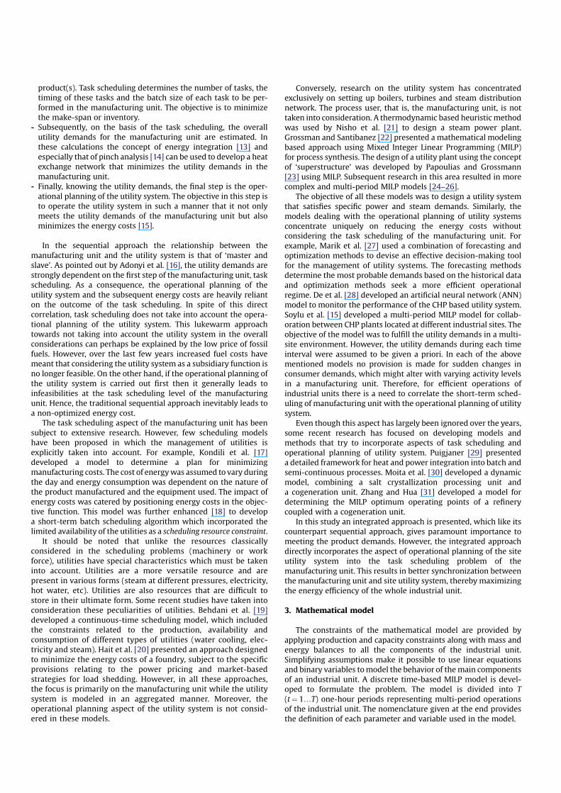
Based on this maximum production capacity, five scenarios aredeveloped inwhich themanufacturing unit respectively operates atcapacities of 50%, 60%, 80%, 90% and 100%. The sequential andintegrated approaches are then compared based on energy costs,flow ratios and convergence history for each of these five scenarios.

The integrated approach leads to significant energy cost savingsand reductions in emissions of SOx and GHG (Table 4). However,these cost savings decrease when the manufacturing unit operates

Table 4

Overall energy costs for example 1, 2 & 3.

Capacity 50% 60% 80% 90% 100%

Sequential Integrated Sequential Integrated Sequential Integrated Sequential Integrated Sequential Integrated

Example 1 Fuel Cost (V) 40,750.3 29,422 45,690 35,985.7 56,281.9 47,696.4 61,432.6 55,942.4 67,823.6 61,064.6

Electricity

Cost (V)

4,536.56 2,201.74 5,453.7 2,268.84 7,793.19 3,392 8,579.78 2,759.84 8,940.47 3,585.07

SOx Emission

Cost (V)

242.281 244.945 292.491 235.237 359.834 299.944 420.924 427.55 455.937 467.267

Total Cost (V) 45,529.1 31,868.7 51,436.2 38,489.8 64,434.9 51,388.4 70,433.3 59,129.8 77,220 65,116.9

GHG Emissions

(tons)

2,009.80 1,514.75 2,272.38 1,794.17 2,798.74 2,367.27 3,080.48 2,845.41 3,392.97 3,106.45

SOx Emission

(tons)

10.53 10.65 12.72 10.23 15.64 13.04 18.30 18.59 19.82 20.32

Example 2 Fuel Cost (V) 66,788.1 61,429.7 77,875 74,166.3 103,878 101,758 119,179 114,006 127,514 125,486

Electricity

Cost (V)

8,189.77 3,340.29 9,090.18 3,838.37 11,261.8 5,986.99 12,540.5 6,797.93 14,551.6 8,684.12

SOx Emission

Cost (V)

397.09 424.65 463.01 531.92 617.61 653.72 830.50 750.15 898.79 770.77

Total Cost (V) 75,374.9 65,194.7 87,248.2 78,536.6 115,758.0 108,339.0 132,550.0 121,554.0 142,066.0 134,941.0

GHG Emissions

(tons)

3,293.99 3,083.74 3,840.80 3,740.59 5,123.27 5,063.01 5,988.76 5,688.53 6,416.89 6,211.41

SOx Emission

(tons)

17.26 18.46 20.13 23.13 26.85 28.42 36.11 32.62 39.08 33.51

Example 3 Fuel Cost (V) 52,450.8 29,592 55,940.2 38,776.3 70,070.2 54,749 77,284.4 63,616.8 84,085.3 72,260.5

Electricity

Cost (V)

4,021.5 1,096.94 6,529.7 1,181.21 9,480.86 2,152.73 11,361 2,509.3 12,560.3 2,697.25

SOx Emission

Cost (V)

372.49 196.338 352.96 283.413 416.6 346.621 459.494 471.539 521.64 505.741

Total Cost (V) 56,844.8 30,885.3 62822.9 40240.9 79967.6 57248.4 89104.9 66597.7 97167.8 75463.5

GHG Emissions

(tons)

2,642.01 1,478.03 2,777.49 1,950.52 3,455.86 2,719.42 3,811.67 3,222.42 4,166.83 3,633.10

SOx Emission

(tons)

16.20 8.54 15.36 12.32 18.11 15.07 19.98 20.50 22.68 21.99

yticapac %06 ta hcaorppAlaitneuqeS

yticapac %06 ta hcaorppAdetargetnI

11T 11T 11T 1T1T 6T6T 11T 11T 6T6T 6T6T 1T1T 1T11T 11T 6T6T 6T6T 11T 11T

21T 21T

6T6T

7T7T 7T7T

31T 31T 31T 31T 31T 31T 31T 31T31T 31T31T 31T3T3T 3T3T 3T3T 3T3T 8T8T 3T3T 8T8T 3T3T 8T8T 3T3T 3T3T 8T8T 8T8T 8T8T 8T8T 8T8T 3T3T3T3T 3T3T3T3T

41T 41T

51T 51T 51T 51T

41T 41T

51T 51T 51T 51T

9T9T 9T9T

01T 01T 01T 01T 01T 01T

9T9T

maets PL gnimusnoc ksaT imusnoc ksaTmaets PM gnimusnoc ksaT c ksaTmaets PM gn yticirtcelE gnimusno

maets PL gnimusnoc ksaT

yticirtcelE dna maets PM gnimusnoc ksaT

yticirtcelE dna

4T4T 4T4T 4T4T 4T4T 4T4T4T4T

5T5T

11T 11T 11T 11T 6T6T 11T 11T 11T 11T

1T

2T 2T 2T

1T 1T

2T2T 2T

1T1T 1T1T 1T1T 1T1T 1T1T 6T6T1T1T6T6T

21T 21T 2T 2T 7T7T 7T7T 7T7T 7T7T 7T7T

31T 31T 3T3T 3T3T 3T3T 31T 31T 8T8T 3T3T 3T3T 31T 31T 3T3T 3T3T 8T8T 3T3T 3T3T 8T8T 8T8T 31T 31T 3T3T 3T3T 3T3T 8T8T 3T3T 3T3T8T8T 8T8T 31T 31T 8T8T 31T 31T 8T8T

41T 41T 4T4T 41T 41T 4T4T 41T 41T 4T4T 4T4T 41T 41T 9T9T 9T9T 9T9T

01T 01T 01T 01T01T 01T01T 01T01T 01T

4T4T 4T4T 4T4T 9T9T

21T 21T 2T

4T4T4T4T

21T 21T 2T 21T 21T 2T 21T 21T

51T 51T 51T 51T

5T5T5T5T

5T5T 5T5T5T5T5T5T5T5T5T5T

Fig. 8. Task scheduling of manufacturing unit operating at 60 % capacity.

at or near its maximum (100%) capacity. This is due to the fact that,while operating near the peak capacity, the manufacturing unit hasa comparatively lesser degree of freedom in shifting and rear-ranging the tasks. Hence, relatively smaller gains in energy cost andemission savings are achieved.

A task scheduling Gantt diagram at 60% capacity illustrates thedifference between the sequential and integrated approaches(Fig. 8). It is clear that in the case of the integrated approach the tasksin the manufacturing unit are arranged in such a manner that theirutility requirements are synchronized with the utility generation inthe CHP plant. This not only minimizes thewastage of utilities but italso means that instead of using pressure reducing valves, steamturbines are used to meet the low and medium pressure steamdemands. Table 5 demonstrates that the integrated approachmaximizes the use of turbine operation and limits the use of pres-sure reducing valves leading to more onsite electricity generationand reduced dependence on external electricity suppliers.

In terms of convergence criteria the sequential approach issuperior to the integrated approach (Table 6). The sequentialapproach is not only much faster, but it almost contains noconvergence gap, the only exception being the manufacturing unitoperating at 90% capacity where the gap was of less than 1%. On theother hand, the average convergence gap in the integratedapproach turns out to be 7.98%. This might appear to be a drawbackbut it is important to note that, despite this convergence gap, theintegrated approach leads to energy cost savings of between 15 and30% and GHG emission reductions of between 7 and 24%.

4.3.2. Example 2

Fig. 9 shows the production recipe of example 2. The overallbenefits (Table 4) in this case are less than those attained inexample 1. The energy cost saving of 13% is achieved by themanufacturing unit operating at a 50% capacity while these savingsreduce to 5% when the manufacturing unit operates at a 100%capacity. The reason for this diminished gain is also partly due tothe slow convergence and gap between the solutions achieved andthe best bounded solution. The convergence history (Table 6)shows that the convergence of example 2 is considerably slowerthan that of example 1. Even the sequential approach takes moretime to converge and in certain cases complete convergence is notachieved. The average gap in the sequential approach simulationsturns out to be 1.8 % while in the integrated approach it is 7.4%. Forthe scenarios in which the manufacturing unit operated at capac-ities of 80, 90 and 100% the gap is greater than 8%. In the case of100% capacity the convergence is extremely slow and no solution isreached during the first 30 minutes. It can be inferred that if thesimulations are allowed to run for a longer duration then this gapmight reduce and subsequently a greater gain in overall energysavings may be achieved.

Table 5 reveals some interesting details about example 2. Theaverage turbine ratio using the sequential approach was 68% inexample 1 while it was a healthy 81% in example 2. This means thatthe structure of the manufacturing unit and the problem parame-ters in example 2 are such that there is less potential for overallenergy cost savings. The analysis of the RTN diagram shows that

Table 5

Utility flow ratios for example 1, 2 & 3.

Capacity 50% 60% 80% 90% 100% Average

Seq. Integ. Seq. Integ. Seq. Integ. Seq. Integ. Seq. Integ. Seq. Integ.

Example 1 Turbine ratio (%) 65.74 89.36 66.33 92.14 62.63 89.93 61.22 96.74 65.17 93.81 64.22 92.40

Electricity ratio (%) 50.57 76.02 50.49 79.41 46.92 76.91 48.06 83.30 51.29 80.47 49.47 79.22

HPRV ratio (%) 34.26 10.64 33.67 7.86 37.37 10.08 38.78 3.26 34.83 6.18 35.78 7.60

LPRV ratio (%) 26.78 10.74 22.45 6.50 43.22 6.32 37.05 2.92 41.19 3.78 34.14 6.05

Example 2 Turbine ratio (%) 65.74 89.36 78.34 96.14 81.72 96.07 83.08 96.91 81.01 92.20 77.98 94.14

Electricity ratio (%) 50.57 76.02 67.96 85.72 70.74 84.45 71.23 84.41 70.12 82.02 66.12 82.52

HPRV ratio (%) 34.26 10.64 21.66 3.86 18.28 3.93 16.92 3.09 18.99 7.80 22.02 5.86

LPRV ratio (%) 26.78 10.74 20.33 1.19 14.56 1.25 13.09 1.74 13.13 2.45 17.58 3.48

Example 3 Turbine ratio (%) 67.89 94.52 68.49 99.88 63.21 98.88 61.64 98.36 62.59 98.64 64.76 98.06

Electricity ratio (%) 62.53 89.76 53.79 91.62 54.69 89.70 53.28 89.66 54.68 90.26 55.79 90.20

HPRV ratio (%) 32.11 5.48 31.51 0.12 36.79 1.12 38.36 1.64 37.41 1.36 35.24 1.94

LPRV ratio (%) 44.46 0.32 43.08 0.00 44.55 0.00 39.28 0.40 33.50 0.00 40.98 0.14

Table 6

Convergence history for example 1, 2 & 3.

Capacity 50% 60% 80% 90% 100%

Sequential Integrated Sequential Integrated Sequential Integrated Sequential Integrated Sequential Integrated

Example

1

Best Solution 45,529.1 31,868.7 51,436.2 38,182.3 64,434.9 51,388.4 70,433.3 59,129.8 77,220.0 65,116.9

Gap (%) 0.0 6.83 0.0 7.15 0.0 7.57 0.89 9.60 0.0 8.75

Best Solution Time 2 min

48.6 s

22 min

23.5 s

20 min

26.8 s

30 min 4 s 5 min 55.9 s 22 min 8.9 s 25 min 8.0 s 20 min

47.3 s

30 min

30.5 s

8 hr 17 min

Total Iteration

Time

3 min

26.9 s

30 min 1 s 22 min

26.8 s

30 min 7.2 s 5 min 55.9 s 30 min 4.3 s 32 min

16.4 s

30 min 5.2 s 30 min

30.5 s

8 hr 33 min

Example

2

Best Solution 75,374.9 65,194.7 87,428.2 78,004.6 115,758 108,399 132,55 121,554 142,066 134,941

Gap (%) 0.0 5.79 0.0 6.0 1.45 8.7 2.51 8.02 1.89 8.36

Best Solution Time 18.7 s 14 min 4.2 s 38 min

22.2 s

27 min 5.1 s 25 min

12.1 s

4 min 42.6 s 55 min 43 s 9 min 40.5 s 2 hr 12 min 15 hr

14 min

Total Iteration

Time

42.5 s 30 min 7.1 s 49 min

12.8 s

30 min 2.8 s 1 hr 1 min 30 min 0.8 s 1 hr 3 min 8 hr 06 min 4 hr 38 min 24 hr

Example

3

Best Solution 56,844.8 30,885.3 62,822.9 40,240.9 70,967.6 57,248.4 89,104.9 66,597.7 97,167.8 75,463.5

Gap (%) 1.93 6.32 0.0 7.88 0.0 6.78 0.0 7.38 0.84 6.12

Best Solution Time 8 min 1.4 s 33 min 1.4 s 3 min 11.6 4 min 38.6 s 12 min

24.8 s

21 min 4.6 s 23 min

17.5 s

24 min

48.8 s

16 min

22.8 s

1 hr 8 min

Total Iteration

Time

30 min 43 s 35 min 2 s 3 min 26.1 s 30 min

16.8 s

14 min

16.6 s

30 min

37.6 s

32 min

09.7 s

30 min 2 s 37 min

31.3 s

4 hr 35 min

example 2 is more constrained with both fewer resources andtasks. This shows that the reductions in overall energy costs and inemissions are dependent on the production recipes and the pro-cessing equipment resources.

4.3.3. Example 3

Fig. 10 shows the production recipe of example 3, which has thegreatest number of resources among all the examples considered.This provides the integrated approach with more latitude tosynchronize the manufacturing unit and the utility system. Asa result, greater savings in the overall energy costs, ranging from22% to 45%, are obtained (Table 4). Similarly the GHG emissionreductions between 12 and 44% are also achieved. The convergencein example 3 is faster than example 2 but a little slower than that inexample 1 (Table 5). Complete convergence is achieved in all casesof the sequential approach while in the integrated approach theconvergence gap is 6% on average.

4.4. Result analysis

On the basis of the above three examples it can be concluded thatthere are significant energy cost savings and emission reductionadvantages in coupling the operational planning of the utility systemwith the task scheduling of manufacturing. Moreover, the use of theintegrated approach enables an industrial unit to achieve higher

productivity levels as it can handle scheduling regimes thatwould beunattainable using the sequential approach (as demonstrated inappendix I). Hence, rather than using the traditional sequentialapproach industrial units should adopt the integrated approach.

However, the use of the integrated approach evokes someinteresting issues. Firstly, significant computation time may berequired to resolve the integrated model. Even though this is a veryrestrictive constraint it is not critical because:

� This tool is used offline which can allow a response time ofseveral hours.

� A ‘‘good’’ solution (that is to say, better than the sequentialapproach) may often be obtained with a reduced computa-tional effort.

However, this computation time problem should not be over-looked, especially if the integrated approach is going to be appliedto an industrial size problem or if it is integrated into a tool fordecision support for which the time response must be muchshorter (in order of minutes). In this context, several alternativescan be envisaged. For example, meta-heuristics (genetic algorithm,neighborhoodmethods) could be used to control the combinatorialaspect of the problem. Another alternative is to use the solutionprovided by the sequential approach (usually obtained withina shorter time) as the first solution of the integrated approach. This

S1T1(1)

T4(2)

J1

S4T5(2)

S2

T2(2)

T3(2)

S6

S5

S8

S3

T6(1)

T7(1)

S7

T8(2)

S9

J2

J3

J4

0.4

0.6

0.5

0.5

0.4

0.6

0.8

0.2

0.9

0.1

S1T1(1)

T4(2)

J1

S4T5(2)

S2

T2(2)

T3(2)

S6

S5

S8

S3

T6(1)

T7(1)

S7

T8(2)

S9

J2

J3

J4

0.4

0.6

0.5

0.5

0.4

0.6

0.8

0.2

0.9

0.1

Fig. 9. RTN representation of example 2.

S1 T1

(1)

J1

S3

T4

(1)

T5

(1)

S2

T2

(2)

T3

(2)

S5

S6

T10

(2)

T11

(2)

S7T7

(3)

S13

J2

J3

S4

S12

T6

(2) S9

S8

T8

(2)

T9

(2)

S10

S11J4

J5

J6

0.5

0.5

0.1

0.4

0.5

0.25

0.75

0.2

0.4

0.4

0.4

0.6

Fig. 10. RTN representation of example 3.

will reduce the research space for the solver and will reduce theiteration time for the integrated approach. Moreover, distributedcomputing can also be used to reduce the computing time.

Secondly, the multi-objective function used in this study iscomposed of energy costs (fuel and electricity) and penalty costs foremissions of harmful gases. As a result, all the emphasis is placed onadapting the task scheduling of the manufacturing unit to meet themost cost efficient operational planning of the utility system.However, in the industry, the reliability of the production process isof overriding importance and normally a reserve margin is set incase of a delay or breakdown in the utility system. This reservemargin could be incorporated using a weighted sum of inventorylevels (of raw materials, intermediate and finished products) andoperational costs (fuel, electricity, penalty costs, etc.) of the utilitysystem as the objective function. Moreover, by varying the weightsof the coefficients, a number of task schedules can be developed,which include all the foreseeable scenarios such as the breakdownof machinery in the utility system.

Another possibility of including a reserve margin in the inte-grated approach is the use of multi-criteria optimization. Thiswould present the management of an industrial unit with multiplesolutions (based on the chosen criteria) and allow them to selectthe most beneficial solution.

Finally, for this study, the emission penalty costs were signifi-cantly underplayed. However, the multi-objective function (Eq.(Crit.2)) can be used to analyze and develop future scenarios when,and if, the proposed taxes on carbon emissions and other harmfulgases come into effect. It should be emphasized that care must betaken while considering the associated emission penalty costs asthey have a profound impact on the overall costs (as demonstratedin appendix II).

5. Conclusion

The energy issue is a crucial problem and will become increas-ingly important in the coming decades. Greater energy costs andprogressively stringent environmental laws are forcing the indus-trial sector to streamline their energy consumption. CHP basedonsite utility systems can make a useful contribution in this regardespecially in the case of industrial units which have high energyneeds. However, to maximize the potential of the CHP based onsiteutility systems, it is imperative to manage the utilities better.Contrary to the traditional reasoning of placing the emphasis solely

on production (manufacturing unit) and treating the utility systemas a subsidiary unit, it is vital to develop an integrated approachwhich simultaneously carries out the task scheduling ofmanufacturing unit and the operational planning of utility system.

The results demonstrate that the integrated approach leads tobetter coordination between themanufacturing unit and site utilitysystem, which in turn leads to significant reductions in energy costsand emissions of harmful gases. However, implementation of theintegrated approach in a real industrial environment would dependupon two factors: (a) extensive use of computer aided tools and (b)enhanced cross functional communication between the manage-ment of respective manufacturing unit and utility system. Theintegrated approach would be difficult to implement in industrialunits with rigid centralized organizational structures.

In the future, a continuous-time MILP model will be developedthat will incorporate additional constraints such as equipmentcleaning, variation of task duration with batch size and the use ofdifferent utilities during the successive phases of the same task (forexample, a reaction that requires preheating at the start and coolingat the end). Inevitably, this will add to the complexity of the inte-grated model and probably aggravate the existing dilemma ofproblem resolution time. This could eventually require the develop-ment of an intermediary approach, which combines the advantagesof both the faster resolution time of the sequential approachwith thegreater operational profitability offered by the integrated approach.

Acknowledgements

This study is a part of project ‘‘Gestion Integree Multi site del’Energie et de la production (Integrated management of energyand production at multi-sites), acronymGIMEP. The project is beingfunded by Centre Nationale de la Recherche Scientifique (CNRS) aspart of its multidisciplinary energy project. The project is beingcarried out conjointly at the research organizations of Laboratoired’Architecture et d’Analyse des Systemes (LAAS) and Laboratoire deGenie Chimique Toulouse (LGCT).

Appendix I. – higher productivity potential of integrated

approach

Consider a utility consumption matrix (Copv,k) and its corre-sponding energy costs demonstrated in Tables 7 and 8 respectively.

Table 7

Utility Consumption Matrix (Copv,k).

Tasks 1 2 3 4 5 6 7 8 9 10 11 12 13 14 15

LP steam 0 0 0 0 0 0 0 0 4 4 3 3 0 2 2

MP Steam 0 0 0 4 4 3 3 0 0 0 0 0 0 0 0

HP Steam 6 6 0 0 0 0 0 0 0 0 0 0 0 0 0

Electricity 0 0 0.2 0.1 0.1 0 0 0.2 0.1 0.1 0 0 0.2 0.1 0.1

Table 8

Overall energy costs.

Capacity Approach Total Cost (V) Fuel Cost

(V)

Electricity Cost

(V)

SOx Cost

(V)

GHG Emissions

(tons)

SOx Emissions

(tons)

100 % Sequential not feasible not feasible not feasible not feasible not feasible not feasible

Integrated 128,068.7 116,457.0 10,898.0 713.7 5,763.0 31.0

90 % Sequential not feasible not feasible not feasible not feasible not feasible not feasible

Integrated 116,522.6 104,958.0 10,916.8 647.8 5,198.1 28.2

80 % Sequential 116,210.5 96,450.5 19,095.9 664.1 4,839.4 28.9

Integrated 102,416.5 91,850.7 9,998.4 567.4 4,549.4 24.7

60 % Sequential 89,553.0 75,357.7 13,656.1 539.2 3,799.5 23.4

Integrated 76,707.2 69,291.5 6,971.9 443.8 3,446.4 19.3

50 % Sequential 75,759.0 63,206.9 12,136.3 415.8 3,153.8 18.1

Integrated 63,222.5 57,356.3 5,525.2 341.0 2,828.8 14.8

Tons/hr

Maximum generation capacity = 750 tons/hr

Net XHP needed = 767 tons/hr

hr0

100

200

300

400

500

600

700

800

0 10 20 30 40 50 60 70 80

maets PL gnimusnoc ksaT yticirtcelE gnimusnoc ksaTmaets PM gnimusnoc ksaTmaets PM gnimusnoc ksaT

maets PL gnimusnoc ksaT

yticirtcelE dna maets PM gnimusnoc ksaT

yticirtcelE dna

11T 11T 11T 11T 11T 11T 11T 11T

21T 21T

1T1T 1T1T 1T1T 1T1T 1T1T 1T1T 1T1T 1T1T 1T1T 1T1T

2T2T2T2T

1T1T

2T2T2T2T 2T2T

6T6T6T6T 6T6T 6T6T 6T6T 6T6T 6T6T11T 11T

7T7T21T 21T7T7T7T7T

31T 31T 31T 31T 31T 31T 31T 31T 31T 31T 31T 31T3T3T 3T3T 3T3T 3T3T 3T3T 3T3T 8T8T31T 31T8T8T 3T3T 3T3T 8T8T 8T8T 3T3T 3T3T 8T8T 3T3T 8T8T 3T3T 8T8T 8T8T 3T3T 3T3T 8T8T 8T8T 8T8T 3T3T

4T4T

5T5T

41T 41T

51T 51T

4T4T

5T5T

41T 41T

01T 01T 5T5T01T 01T

9T9T 4T4T4T4T41T 41T

01T 01T 5T5T 01T 01T 5T5T 01T 01T 51T 51T5T5T

4T4T 9T9T 9T9T 4T4T41T 41T 41T 41T

Fig. 11. Sequential approach task scheduling Gantt diagram and steam load curves of utility system.

0

100

200

300

400

500

600

700

800

0 10 20 30 40 50 60 70 80

Maximum generation capacity = 750 tons/hr

Tons/hr

hr

maets PL gnimusnoc ksaT yticirtcelE gnimusnoc ksaTmaets PM gnimusnoc ksaTmaets PM gnimusnoc ksaT

maets PL gnimusnoc ksaT

yticirtcelE dna maets PM gnimusnoc ksaT

yticirtcelE dna

1T1T11T 11T 1T1T

21T 21T

1T1T

2T2T2T2T

2T2T

2T2T21T 21T 2T2T21T 21T

11T 11T 11T 11T

21T 21T 2T2T 21T 21T

1T1T 1T1T 11T 11T

7T7T

6T6T 6T6T

7T7T

6T6T

7T7T 7T7T 7T7T

31T 31T 3T3T 3T3T 3T3T 31T 31T 8T8T 31T 31T 3T3T 3T3T3T3T 3T3T 8T8T 3T3T 3T3T 8T8T 8T8T 31T 31T 3T3T 3T3T 3T3T 8T8T 3T3T 8T8T 3T3T 8T8T 8T8T 31T 31T31T 31T 8T8T

01T 01T

4T4T41T 41T

5T5T 5T5T

4T4T41T 41T

5T5T 5T5T

4T4T41T 41T 4T4T

01T 01T

4T4T

01T 01T 5T5T 5T5T

41T 41T 9T9T 9T9T

01T 01T 01T 01T

4T4T 4T4T 9T9T

51T 51T

9T9T

51T 51T

Fig. 12. Integrated approach task scheduling Gantt diagram and steam load curves of utility system.

The Table 8 shows that integrated approach not only results inreduction in energy costs but it also leads to feasible solution for allfive scenarios. On the other hand the sequential approach givesinfeasible solutions in scenarios where manufacturing unit oper-ates at 90% and 100% capacity.

For the scenario in which manufacturing unit operates at 90%capacity Figs. 11 and 12 presents the task scheduling Gantt

diagrams and operational planning of utility system (depicted bysteam load curves). The sequential approach calculates taskscheduling without considering operational constraints of the CHPplant. As a result not only there are huge variations in the steamload curves but during period t¼ 15 the steam demands of themanufacturing unit exceed the generation capacity of the CHPplant. This resulted in sequential approach rendering infeasiblesolution. On the other hand in the integrated approach the tasks areshifted and rearranged in such a manner that the utility require-ments never exceed the CHP plant capacity. From this an inferencecan be drawn that the integrated approach enables an industrial

Table 9

Incorporating full emission externality cost for example 3 functioning at 60% capacity.

Emission externality

cost V/ton

Total Cost

(V)

Fuel Cost

(V)

Electricity Cost

(V)

GHG Cost

(V)

SOx Cost

(V)

GHG Emissions

(tons)

SOx Emissions

(tons)

GHG SOx

115.65 3640.54 293,795 36,015.5 14,935.1 206,834 36,011 1788.45 9.89

0 23 40,40.9 38,776.3 1,181.21 0 283,4 1968.52 12.32

Table 10

Utility consumption matrix (Copv,k) for example 1.

Tasks 1 2 3 4 5 6 7 8 9 10 11 12 13 14 15

LP steam 0 0 0 0 0 0 0 0 2 2 1.5 1.5 0 1 1

MP Steam 0 0 0 2 2 1.5 1.5 0 0 0 0 0 0 0 0

HP Steam 3 3 0 0 0 0 0 0 0 0 0 0 0 0 0

Electricity 0 0 0.1 .05 .05 0 0 .05 .05 .05 0 0 0.1 .05 .05

Table 11

Parameters for manufacturing unit example 1.

Vmink;j Vmax

k;j

Unit 1 10 100

Unit 2 10 80

Unit 3 10 50

Unit 4 10 80

Unit 5 10 80

ls Cmaxs Co

s

State 1 0 100,000 5,000

State 2 1 200 0

State 3 1 250 0

State 4 0 100,000 5,000

State 5 1 200 0

State 6 1 250 0

State 7 0 100,000 5,000

State 8 1 200 0

State 9 1 250 0

State 10 2 10,000 0

State 11 2 10,000 0

State 12 2 10,000 0

Maximum (100 %)

production

capacity

Product A¼ State

10

Product B¼ State

11

Product C¼ State

12

Cycle 1 0 0 50

Cycle 2 130 0 0

Cycle 3 170 0 50

Cycle 4 0 50 50

Cycle 5 50 0 0

Cycle 6 160 150 0

Cycle 7 170 0 20

Cycle 8 70 130 0

Cycle 9 50 130 0

Cycle 10 50 50 170

Table 12

Utility consumption matrix (Copv,k) for example 2.

Tasks 1 2 3 4 5 6 7 8

LP steam 0 0 0 2 2 0 0 1

MP Steam 0 2 2 0 0 0 0 0

HP Steam 4 0 0 0 0 0 0 0

Electricity 0 0.1 0.1 0.1 0.1 0.1 0.1 0

Table 13

Parameters for manufacturing unit example 2.

Vmink;j Vmax

k;j

Unit 1 10 100

Unit 2 10 80

Unit 3 10 50

Unit 4 10 100

ls Cmaxs Co

s

State 1 0 10,000 5,000

State 2 0 10,000 5,000

State 3 0 10,000 5,000

State 4 1 100 5,000

State 5 1 200 0

State 6 1 150 0

State 7 1 100 0

State 8 2 10,000 0

State 9 2 10,000 0

Maximum (100 %)

production capacity

Product A¼ State 8 Product B¼ State 9

Cycle 1 0 0

Cycle 2 0 233

Cycle 3 0 0

Cycle 4 0 133

Cycle 5 0 0

Cycle 6 0 258

Cycle 7 258 258

Cycle 8 258 258

Cycle 9 258 258

Cycle 10 258 158

unit to achieve higher productivity as it can handle schedulingregimes that would be unattainable using the sequential approach.

Appendix II – impact of emission externalities on overall

problem

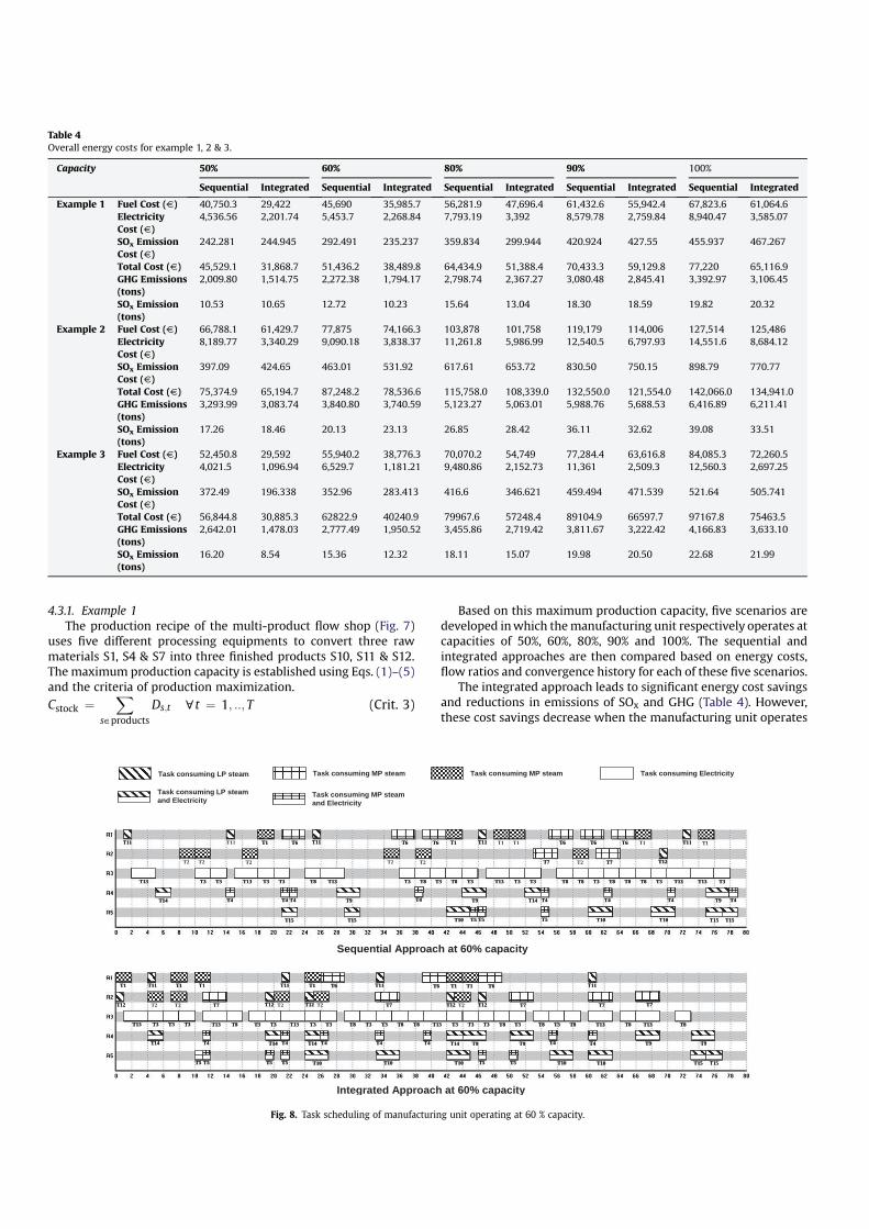
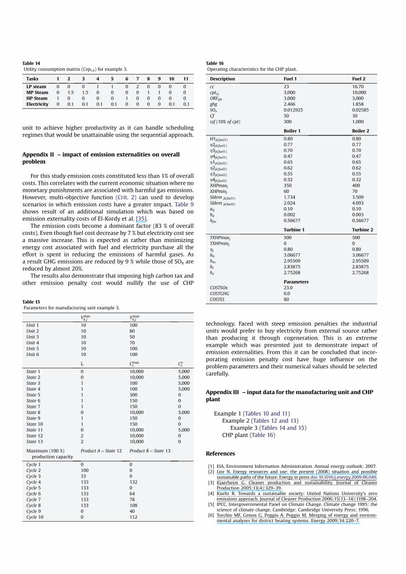
For this study emission costs constituted less than 1% of overallcosts. This correlates with the current economic situationwhere nomonetary punishments are associated with harmful gas emissions.However, multi-objective function (Crit. 2) can used to developscenarios in which emission costs have a greater impact. Table 9shows result of an additional simulation which was based onemission externality costs of El-Kordy et al. [35].

The emission costs become a dominant factor (83 % of overallcosts). Even though fuel cost decrease by 7 % but electricity cost seea massive increase. This is expected as rather than minimizingenergy cost associated with fuel and electricity purchase all theeffort is spent in reducing the emissions of harmful gases. Asa result GHG emissions are reduced by 9 % while those of SOx arereduced by almost 20%.

The results also demonstrate that imposing high carbon tax andother emission penalty cost would nullify the use of CHP

technology. Faced with steep emission penalties the industrialunits would prefer to buy electricity from external source ratherthan producing it through cogeneration. This is an extremeexample which was presented just to demonstrate impact ofemission externalities. From this it can be concluded that incor-porating emission penalty cost have huge influence on theproblem parameters and their numerical values should be selectedcarefully.

Appendix III – input data for the manufacturing unit and CHP

plant

Example 1 (Tables 10 and 11)Example 2 (Tables 12 and 13)

Example 3 (Tables 14 and 15)CHP plant (Table 16)

References

[1] EIA, Environment Information Administration. Annual energy outlook; 2007.[2] Lior N. Energy resources and use: the present (2008) situation and possible

sustainable paths of the future. Energy in press doi:10.1016/j.energy.2009.06.049.[3] Kjaerheim G. Cleaner production and sustainability. Journal of Cleaner

Production 2005;13(4):329–39.[4] Kuehr R. Towards a sustainable society: United Nations University’s zero

emissions approach. Journal of Cleaner Production 2006;15(13–14):1198–204.[5] IPCC, Intergovernmental Panel on Climate Change. Climate change 1995: the

science of climate change. Cambridge: Cambridge University Press; 1996.[6] Torchio MF, Genon G, Poggio A, Poggio M. Merging of energy and environ-

mental analyses for district heating systems. Energy 2009;34:220–7.

Table 14

Utility consumption matrix (Copv,k) for example 3.

Tasks 1 2 3 4 5 6 7 8 9 10 11

LP steam 0 0 0 1 1 0 2 0 0 0 0

MP Steam 0 1.5 1.5 0 0 0 0 1 1 0 0

HP Steam 1 0 0 0 0 1 0 0 0 0 0

Electricity 0 0.1 0.1 0.1 0.1 0 0 0 0 0.1 0.1

Table 15

Parameters for manufacturing unit example 3.

Vmink;j Vmax

k;j

Unit 1 10 100

Unit 2 10 80

Unit 3 10 50

Unit 4 10 70

Unit 5 10 100

Unit 6 10 100

ls Cmaxs Co

s

State 1 0 10,000 5,000

State 2 0 10,000 5,000

State 3 1 100 5,000

State 4 1 100 5,000

State 5 1 300 0

State 6 1 150 0

State 7 1 150 0

State 8 0 10,000 5,000

State 9 1 150 0

State 10 1 150 0

State 11 0 10,000 5,000

State 12 2 10,000 0

State 13 2 10,000 0

Maximum (100 %)

production capacity

Product A¼ State 12 Product B¼ State 13

Cycle 1 0 0

Cycle 2 100 0

Cycle 3 33 0

Cycle 4 133 132

Cycle 5 133 0

Cycle 6 133 64

Cycle 7 133 78

Cycle 8 133 108

Cycle 9 0 40

Cycle 10 0 112

Table 16

Operating characteristics for the CHP plant.

Description Fuel 1 Fuel 2

cc 23 16.70

cpti,j 3,000 10,000

ORFij0 3,000 3,000

ghg 2.466 1.858

SOx 0.012925 0.02585

Cf 50 30

ssf (10% of cpt) 300 1,000

Boiler 1 Boiler 2

H1ji(fuel1) 0.80 0.80

h2ji(fuel1) 0.77 0.77

h3ji(fuel1) 0.70 0.70

h4ji(fuel1) 0.47 0.47

h1ji(fuel2) 0.65 0.65

h2ji(fuel2) 0.62 0.62

h3ji(fuel2) 0.55 0.55

h4ji(fuel2) 0.32 0.32

XHPmaxj 350 400

XHPminj 60 70

SIdem ji(fuel1) 1.734 3.509

SIdem ji(fuel2) 2.024 4.093

aij 0.10 0.10

bij 0.002 0.003

hfw 0.56677 0.56677

Turbine 1 Turbine 2

TXHPmaxj 500 500

TXHPminj 0 0

hj 0.80 0.80

hb 3.06677 3.06677

hm 2.95509 2.95509

hl 2.83875 2.83875

he 2.75268 2.75268

Parameters

COSTSOx 23.0

COSTGHG 0.0

COSTEL 80

[7] Panno D, Messineo A, Dispenza A. Cogeneration plant in a pasta factory:energy saving and environment benefit. Energy 2007;34:746–54.

[8] Lemar Jr PL. The potential impact of policies to promote combined heat andpower in US industry. Energy Policy 2001;29(14):1243–54.

[9] UNESCAP, United Nations Economic and Social Commission for Asia and thePacific. Promotion of cogeneration technology as a means of pollution controland increase in energy efficiency in industrial and commercial sectors, www.unescap.org/esd/publications/energy/co-gen/contents.htm.

[10] European Commission. A community strategy to promote combined heat andpower (CHP) and dismantle the barriers to its development. Brussels, www.cogeneracion.org/archivo/200001.pdf; 1997.

[11] Gundersen T. Process integration PRIMER, SINTEF. Energy Research May 2000.[12] Smith R. State of the art in process integration. Applied Thermal Engineering

2000;20(15–16):1337–45.[13] Corominas J, Espuna A, Puigjaner L. Method to incorporate energy integration

considerations in multiproduct batch processes. Computers & ChemicalEngineering 1994;18(11–12):1043–55.

[14] Linnhoff B. Use of pinch analysis to knock down capital cost and emission.Chemical Engineering Progress 1994;90(8):32–57.

[15] Soylu A, Oruc C, Turkay M, Fujita K, Asakura T. Synergy analysis of collabo-rative supply chain management in energy systems using multi-period MILP.European Journal of Operational Research 2006;174(1):387–403.

[16] Adonyi R, Romero J, Puigjaner L, Friedler F. Incorporating heat integration inbatch process scheduling. Applied Thermal Engineering 2003;23(14):1743–62.

[17] Kondili E, Shah N, Pantelides CC. Production planning for the rational use ofenergy in multiproduct continuous plant. Computers & Chemical Engineering1993;17(Suppl.1):123–8.

[18] Kondili E, Pantelids CC, Sargent WH. A general algorithm for short-termscheduling of batch operations – I. MILP formulation. Computers & ChemicalEngineering 1993;17(2):211–27.

[19] Behdani B, Pishvaie MR, Rashtchian D. Optimal scheduling of mixed batch andcontinuous processes incorporating utility aspects. Chemical Engineering andProcessing 2007;46(4):271–81.

[20] Hait A, Artigues C, Trepanier M, Baptiste P. Ordonnancement sous contraintesd’energie et de ressources humaines. In: 11eme Congres de la Societe Fra-nçaise de Genie des Procedes. Saint-Etienne (France); 2007.

[21] Nisho M, Itoh J, Shiroko K, Umeda T. A thermodynamic approach to steam-power system design. Industrial Engineering Chemistry Process & Develop-ment 1980;19(2):306–12.

[22] Grossmann IE, Santibanez J. Applications of mixed-integer linear program-ming in process synthesis. Computers & Chemical Engineering 1980;4(4):205–14.

[23] Papoulias SA, Grossmann IE. Structural optimization approach in processsynthesis - I. Utility systems. Computers & Chemical Engineering1983;7(6):695–706.

[24] Marechal F, Kalitventzeff B. Process integration: selection of the optimal utilitysystem. Computers & Chemical Engineering 1998;22:S149–56.Supplementary.

[25] Iyer RR, Grossmann IE. Synthesis and operational planning of utility systemsfor multi-period operations. Computers & Chemical Engineering 1998;22(7–8):979–93.

[26] Bojic M, Stojanovic B. MILP optimization of a CHP energy system. EnergyConversion Management 1998;39(7):637–42.

[27] Marik K, Schindler Z, Stluka P. Decision support tools for advanced energymanagement. Energy 2008;33:858–73.

[28] De S, Kaiadi M, Fast M, Assadi M. Development of an artificial neural networkmodel for the steam process of a coal biomass confirmed combined heat andpower (CHP) plant in Sweden. Energy 2007;32:2009–109.

[29] Puigjaner L. Extended modeling framework for heat and power integration inbatch and semi-continuous processes. Chemical Product and ProcessModeling 2007;2(3). Article 3.

[30] Moita RD, Matos HA, Fernandes C, Nunes CP, Prior JM. Dynamic modelling andsimulation of a cogeneration system integrated with a salt recrystallizationprocess. Computers & Chemical Engineering 2005;29(6):1491–505.

[31] Zhang BJ, Hua B. Effective MILP model for oil refinery-wide production plan-ning and better energy utilization. Journal of Cleaner Production2005;15:439–48.

[32] Pantelides CC. Unified frameworks for the optimal process planning andscheduling. In: Proceedings on the second conference on foundations ofcomputer aided operations. CAChE Publications; 1994. p. 253–74.

[33] Castro PM, Barbosa-Povoa AP, Matos HA. Optimal periodic scheduling of batchplants using RTN-based discrete and continuous-time formulations: a case studyapproach. Industrial & Engineering Chemistry Research 2003;42(14):3346–60.

[34] Dash optimization, Xpress-optimizer version 19.00.00 Ó 2008 Fair IsaacCorporation. All rights reserved.www.dashoptimization.com

[35] El-Kordy MN, Badr MA, Abed KA, Ibrahim SMA. Economical evaluation ofelectricity generation considering externalities. Renewable Energy2002;25(2):317–28.