A Survey on Data Processing Protocols in Wireless Sensor Network

[Tripathi, 3(9): September, 2014] ISSN: 2277-9655

Scientific Journal Impact Factor: 3.449

(ISRA), Impact Factor: 2.114

http: // www.ijesrt.com (C)International Journal of Engineering Sciences & Research Technology

[476]

IJESRT INTERNATIONAL JOURNAL OF ENGINEERING SCIENCES & RESEARCH

TECHNOLOGY A Survey on Data Processing Protocols in Wireless Sensor Network

Brisheket Suman Tripathi , Mohit Srivastava

Department of Electronics and Communication Engineering, Maharana Pratap Engineering Collage, India

[email protected]

Abstract Wireless sensor networks consist of small nodes with sensing, computation, and wireless communications

capabilities. Many routing, power management, and data dissemination protocols have been specifically designed

for WSNs where energy awareness is an essential design issue. Routing protocols in WSNs might differ depending

on the application and network architecture.

In this article a survey of state-of-the-art routing techniques in WSNs has presented. We first outline the

design challenges for routing protocols in WSNs followed by a comprehensive survey of routing techniques.

Overall, the routing techniques are classified into three categories based on the underlying network structure: flit,

hierarchical, and location-based routing. Furthermore, these protocols can be classified into multipath-based, query-

based, negotiation-based, QoS-based, and coherent based depending on the protocol operation. We study the design

trade-offs between energy and communication overhead savings in every routing paradigm. We also highlight the

advantages and performance issues of each routing technique. The article concludes with possible future research

areas.

Keywords: Wireless Sensor Networks, Routing Protocol, Quality of service (QoS), Data Processing.

Introduction Due to recent technological advances, the

manufacturing of small and low-cost sensors has

become technically and economically feasible. These

sensors measure ambient conditions in the

environment surrounding them and then transform

these measurements into signals that can be

processed to reveal some characteristics about

phenomena located in the area around these sensors.

A large number of these sensors can be networked in

many applications that require unattended operations,

hence producing a wireless sensor network (WSN).

In fact, the applications of WSNs are quite numerous.

For example, WSNs have profound effects

on military and civil applications such as target field

imaging, intrusion detection, weather monitoring,

security and tactical surveillance, distributed

computing, detecting ambient conditions such as

temperature, movement, sound, light, or the presence

of certain objects, inventory control, and disaster

management.

Deployment of a sensor network in these

applications can be in random fashion (e.g., dropped

from an airplane in a disaster management

application) or manual (e.g., fire alarm sensors in a

facility or sensors planted underground for precision

agriculture). Creating a network of these sensors can

assist rescue operations by locating survivors,

identifying risky areas, and making the rescue team

more aware of the overall situation in a disaster area.

Requirement of Protocols for WSN

Typically, WSNs contain hundreds or

thousands of these sensor nodes, and these sensors

have the ability to communicate either among each

other or directly to an external base station (BS). A

greater number of sensors allows for sensing over

larger geographical regions with greater accuracy.

Figure 1 shows a schematic diagram of sensor node

components. Basically, each sensor node comprises

sensing, processing, transmission, mobilizer, position

finding system, and power units (some of these

components are optional, like the mobilizer). The

same figure shows the communication architecture of

a WSN. Sensor nodes are usually scattered in a

sensor field, which is an area where the sensor nodes

are deployed. Sensor nodes coordinate among

themselves to produce high-quality information about

the physical environment. Each sensor node bases its

decisions on its mission, the information it currently

has, and its knowledge of its computing,

communication, and energy resources. Each of these

scattered sensor nodes has the capability to collect

http://www.ijesrt.com/

mailto:[email protected]





[477]

and route data either to other sensors or back to an

external BS(s).

Figure 1: Component of Sensor Network

A Base Station (BS) may be a fixed or

mobile node capable of connecting the sensor

network to an existing communications infrastructure

or to the Internet where a user can have access to the

reported data. In the past few years, intensive

research that addresses the potential of collaboration

among sensors in data gathering and processing, and

coordination and management of the sensing activity

was conducted. In most applications, sensor nodes

are constrained in energy supply and communication

bandwidth. Thus, innovative techniques to eliminate

energy inefficiencies that shorten the lifetime of the

network and efficient use of the limited bandwidth

are highly required. Such constraints combined with

a typical deployment of large number of sensor nodes

pose many challenges to the design and management

of WSNs and necessitate energy-awareness at all

layers of the networking protocol stack. For example,

at the network layer, it is highly desirable to find

methods for energy-efficient route discovery and

relaying of data from the sensor nodes to the BS so

that the lifetime of the network is maximized.

Routing in WSNs is very challenging due to the

inherent characteristics that distinguish these

networks from other wireless networks like mobile ad

hoc networks or cellular networks.

First, due to the relatively large number of

sensor nodes, it is not possible to build a global

addressing scheme for the deployment of a large

number of sensor nodes as the overhead of ID

maintenance is high. Thus, traditional IP-based

protocols may not be applied to WSNs. Furthermore,

sensor nodes that are deployed in an ad hoc manner

need to be self-organizing as the ad hoc deployment

of these nodes requires the system to form

connections and cope with the resultant nodal

distribution, especially as the operation of sensor

networks is unattended. In WSNs, sometimes getting

the data is more important than knowing the IDs of

which nodes sent the data.

Second, in contrast to typical

communication networks, almost all applications of

sensor networks require the fbw of sensed data from

multiple sources to a particular BS. This, however,

does not prevent the flow of data to be in other forms

(e.g., multicast or peer to peer).

Third, sensor nodes are tightly constrained

in terms of energy, processing, and storage

capacities. Thus, they require careful resource

management.

Fourth, in most application scenarios, nodes

in WSNs are generally stationary after deployment

except for maybe a few mobile nodes. Nodes in other

traditional wireless networks are free to move, which

results in unpredictable and frequent topological

changes. However, in some applications, some sensor

nodes may be allowed to move and change their

location (although with very low mobility).

Fifth, sensor networks are application-

specific (i.e., design requirements of a sensor

network change with application). For example, the

challenging problem of low-latency precision tactical

surveillance is different from that of a periodic

weather monitoring task.

Sixth, position awareness of sensor nodes is

important since data collection is normally based on

the location. Currently, it is not feasible to use Global

Positioning System (GPS) hardware for this purpose.

Methods based on triangulation [1], for example,

allow sensor nodes to approximate their position

using radio strength from a few known points. It is

found in [1] that algorithms based on triangulation or

multilateration can work quite well under conditions

where only very few nodes know their positions a

priori (e.g., using GPS hardware). Still, it is favorable

to have GPS-free solutions [2] for the location

problem in WSNs.

Finally, data collected by many sensors in

WSNs is typically based on common phenomena, so

there is a high probability that this data has some

redundancy. Such redundancy needs to be exploited

by the routing protocols to improve energy and

bandwidth utilization. Usually, WSNs are data-

centric networks in the sense that data is requested

based on certain attributes (i.e., attribute-based

addressing). An attribute-based address is composed

of a set of attribute-value pair query. For example, if

the query is something like [temperature > 60°F],

sensor nodes that sense temperature > 60°F only need

to respond and report their readings. Due to such

differences, many new algorithms have been






[478]

proposed for the routing problem in WSNs. These

routing mechanisms have taken into consideration the

inherent features of WSNs along with the application

and architecture requirements. The task of finding

and maintaining routes in WSNs is nontrivial since

energy restrictions and sudden changes in node status

(e.g., failure) cause frequent and unpredictable

topological changes.

To minimize energy consumption, routing

techniques proposed in the literature for WSNs

employ some well-known routing tactics as well as

tactics special to WSNs, such as data aggregation and

in-network processing, clustering, different node role

assignment, and data-centric methods. Almost all of

the routing protocols can be classified according to

the network structure as flit, hierarchical, or location-

based. Furthermore, these protocols can be classified

into multipath-based, query-based, negotiation-based,

quality of service (QoS)-based, and coherent-based

depending on the protocol operation. In flat networks

all nodes play the same role, while hierarchical

protocols aim to cluster the nodes so that cluster

heads can do some aggregation and reduction of data

in order to save energy. Location-based protocols

utilize position information to relay the data to the

desired regions rather than the whole network. The

last category includes routing approaches based on

protocol operation, which vary according to the

approach used in the protocol. In this article these

routing techniques in WSNs are explored that have

been developed in recent years and develop a

classification for these protocols. Then each of the

routing protocols is discuss under this classification.

Our objective is to provide deeper understanding of

the current routing protocols in WSNs and identify

some open research issues that can be further

pursued. Although there are some previous efforts on

surveying the characteristics, applications, and

communication protocols in WSNs [3, 4], the scope

of the survey presented in this article is distinguished

from these surveys in many aspects. The surveys in

[3, 4] addressed several design issues and techniques

for WSNs describing the physical constraints on

sensor nodes, applications, architectural attributes,

and the protocols proposed in all layers of the

network stack. However, these surveys were not

devoted to routing only. Due to the importance of

routing in WSNs and the availability of a significant

body of literature on this topic, a detailed survey

becomes necessary and useful at this stage. Our

work is a dedicated study of the network layer,

describing and categorizing the different approaches

to data routing. In addition, routing challenges are

summarized and design issues that may affect the

performance of routing protocols in WSNs.

The rest part of this article is organized as

follows. We discuss routing challenges and design

issues in WSNs. A classification and comprehensive

survey of routing techniques in WSNs is presented. A

summary of future research directions on routing in

WSNs is discussed.

Routing challenges & design issues in WSNs Despite the innumerable applications of

WSNs, these networks have several restrictions, such

as limited energy supply, limited computing power,

and limited bandwidth of the wireless links

connecting sensor nodes. One of the main design

goals of WSNs is to carry out data communication

while trying to prolong the lifetime of the network

and prevent connectivity degradation by employing

aggressive energy management techniques. The

design of routing protocols in WSNs is influenced by

many challenging factors. These factors must be

overcome before efficient communication can be

achieved in WSNs. In the following, some of the

routing challenges and design issues that affect the

routing process in WSNs have summarized.

Node Deployment

Node deployment in WSNs is application-

dependent and can be either manual (deterministic) or

randomized. In manual deployment, the sensors are

manually placed and data is routed through

predetermined paths. However, in random node

deployment, the sensor nodes are scattered randomly,

creating an ad hoc routing infrastructure.

If the resultant distribution of nodes is not

uniform, optimal clustering becomes necessary to

allow connectivity and enable energy-efficient

network operation. Inter sensor communication is

normally within short transmission ranges due to

energy and bandwidth limitations. Therefore, it is

most likely that a route will consist of multiple

wireless hops.

Energy Consumption Without Losing Accuracy

Sensor nodes can use up their limited supply

of energy performing computations and transmitting

information in a wireless environment. As such,

energy-conserving forms of communication and

computation are essential. Sensor node lifetime

shows a strong dependence on battery lifetime [5]. In

a multihop WSN, each node plays a dual role as data

sender and data router. The malfunctioning of some

sensor nodes due to power failure can cause

significant topological changes, and might require






[479]

rerouting of packets and reorganization of the

network.

Data Reporting Method

Data reporting in WSNs is application-

dependent and also depends on the time criticality of

the data. Data reporting can be categorized as either

time-driven, event driven, query-driven, or a hybrid

of all these methods. The time-driven delivery

method is suitable for applications that require

periodic data monitoring. As such, sensor nodes will

periodically switch on their sensors and transmitters,

sense the environment, and transmit the data of

interest at constant periodic time intervals. In event-

driven and query-driven methods, sensor nodes react

immediately to sudden and drastic changes in the

value of a sensed attribute due to the occurrence of a

certain event, or respond to a query generated by the

BS or another node in the network. As such, these are

well suited to time-critical applications. A

combination of the previous methods is also possible.

The routing protocol is highly influenced by the data

reporting method in terms of energy consumption and

route calculations.

Node/link Heterogeneity

In many studies, all sensor nodes were

assumed to be homogeneous (i.e., have equal

capacity in terms of computation, communication,

and power). However, depending on the application a

sensor node can have a different role or capability.

The existence of a heterogeneous set of sensors raises

many technical issues related to data routing. For

example, some applications might require a diverse

mixture of sensors for monitoring temperature,

pressure, and humidity of the surrounding

environment, detecting motion via acoustic

signatures, and capturing images or video tracking of

moving objects. Either these special sensors can be

deployed independently or the different

functionalities can be included in the same sensor

nodes. Even data reading and reporting can be

generated from these sensors at different rates,

subject to diverse QoS constraints, and can follow

multiple data reporting models. For example,

hierarchical protocols designate a cluster head node

different from the normal sensors. These cluster

heads can be chosen from the deployed sensors or be

more powerful than other sensor nodes in terms of

energy, bandwidth, and memory. Hence, the burden

of transmission to the BS is handled by the set of

cluster heads.

Fault Tolerance

Some sensor nodes may fail or be blocked

due to lack of power, physical damage, or

environmental interference. The failure of sensor

nodes should not affect the overall task of the sensor

network. If many nodes fail, medium access control

(MAC) and routing protocols must accommodate

formation of new links and routes to the data

collection Base Stations. This may require actively

adjusting transmit powers and signaling rates on the

existing links to reduce energy consumption, or

rerouting packets through regions of the network

where more energy is available. Therefore, multiple

levels of redundancy may be needed in a fault-

tolerant sensor network.

Scalability

The number of sensor nodes deployed in the

sensing area may be on the order of hundreds or

thousands, or more. Any routing scheme must be able

to work with this huge number of sensor nodes. In

addition, sensor network routing protocols should be

scalable enough to respond to events in the

environment. Until an event occurs, most sensors can

remain in the sleep state, with data from the few

remaining sensors providing coarse quality.

Network Dynamics

In many studies, sensor nodes are assumed

fixed. However, in many applications both the BS or

sensor nodes can be mobile [6]. As such, routing

messages from or to moving nodes is more

challenging since route and topology stability

become important issues, in addition to energy,

bandwidth, and so forth. Moreover, the phenomenon

can be mobile (e.g., a target detection/ tracking

application). On the other hand, sensing fixed events

allows the network to work in a reactive mode (i.e.,

generating traffic when reporting), while dynamic

events in most applications require periodic reporting

to the BS.

Transmission Media

In a multihop sensor network,

communicating nodes are linked by a wireless

medium. The traditional problems associated with a

wireless channel (e.g., fading, high error rate) may

also affect the operation of the sensor network. In

general, the required bandwidth of sensor data will be

low, on the order of 1–100 kb/s. Related to the

transmission media is the design of MAC. One

approach to MAC design for sensor networks is to

use time-division multiple access (TDMA)-based

protocols that conserve more energy than contention-






[480]

based protocols like carrier sense multiple access

(CSMA) (e.g., IEEE 802.11). Bluetooth technology

[7] can also be used.

Connectivity

High node density in sensor networks

precludes them from being completely isolated from

each other. Therefore, sensor nodes are expected to

be highly connected. This, however, may not prevent

the network topology from being variable and the

network size from shrinking due to sensor node

failures. In addition, connectivity depends on the

possibly random distribution of nodes.

Coverage

In WSNs, each sensor node obtains a certain

view of the environment. A given sensor’s view of

the environment is limited in both range and

accuracy; it can only cover a limited physical area of

the environment. Hence, area coverage is also an

important design parameter in WSNs.

Data Aggregation

Since sensor nodes may generate significant

redundant data, similar packets from multiple nodes

can be aggregated to reduce the number of

transmissions. Data aggregation is the combination of

data from different sources according to a certain

aggregation function (e.g., duplicate suppression,

minima, maxima, and average). This technique has

been used to achieve energy efficiency and data

transfer optimization in a number of routing

protocols. Signal processing methods can also be

used for data aggregation. In this case, it is referred to

as data fusion where a node is capable of producing a

more accurate output signal by using some

techniques such as beam forming to combine the

incoming signals and reducing the noise in these

signals.

Quality of Service

In some applications, data should be

delivered within a certain period of time from the

moment it is sensed, or it will be useless. Therefore,

bounded latency for data delivery is another

condition for time-constrained applications.

However, in many applications, conservation of

energy, which is directly related to network lifetime,

is considered relatively more important than the

quality of data sent. As energy is depleted, the

network may be required to reduce the quality of

results in order to reduce energy dissipation in the

nodes and hence lengthen the total network lifetime.

Hence, energy-aware routing protocols are required

to capture this requirement.

Figure 2: Classification of Protocols

Routing protocols in WSNs In this section the state-of-the-art routing

protocols for WSNs is surveyed. In general, routing

in WSNs can be divided into flat-based routing,

hierarchical-based routing, and location-based

routing depending on the network structure. In flat-

based routing, all nodes are typically assigned equal

roles or functionality. In hierarchical-based routing,

nodes will play different roles in the network. In

location-based routing, sensor nodes’ positions are

exploited to route data in the network. A routing

protocol is considered adaptive if certain system

parameters can be controlled in order to adapt to

current network conditions and available energy

levels. Furthermore, these protocols can be classified

into multipath-based, query-based, and negotiation-

based, QoS-based, or coherent-based routing

techniques depending on the protocol operation. In

addition to the above, routing protocols can be

classified into three categories, proactive, reactive,

and hybrid, depending on how the source finds a

route to the destination. In proactive protocols, all

routes are computed before they are really needed,

while in reactive protocols, routes are computed on

demand. Hybrid protocols use a combination of these

two ideas. When sensor nodes are static, it is

preferable to have table-driven routing protocols

rather than reactive protocols. A significant amount

of energy is used in route discovery and setup of

reactive protocols. Another class of routing protocols

is called cooperative. In cooperative routing, nodes

send data to a central node where data can be

aggregated and may be subject to further processing,

hence reducing route cost in terms of energy use.

Many other protocols rely on timing and position

information. We also shed some light on these types

of protocols in this article. In order to streamline this






[481]

survey, we use a classification according to the

network structure and protocol operation (routing

criteria). The classification is shown in Fig. 2 where

numbers in the future indicate the references. In the

rest of this section we present a detailed overview of

the main routing paradigms in WSNs. We start with

network-structure-based protocols.

Network-structure-based protocols The underlying network structure can play a

significant role in the operation of the routing

protocol in WSNs. In this section we survey in detail

most of the protocols that fall into this category.

Flat Routing:-

The first category of routing protocols is the

multihop flat routing protocols. In flat networks, each

node typically plays the same role and sensor nodes

collaborate to perform the sensing task. Due to the

large number of such nodes, it is not feasible to

assign a global identifier to each node. This

consideration has led to data-centric routing, where

the BS sends queries to certain regions and waits for

data from the sensors located in the selected regions.

Since data is being requested through queries,

attribute-based naming is necessary to specify the

properties of data. Early work on data centric routing

(e.g., SPIN and directed diffusion [8]) was shown to

save energy through data negotiation and elimination

of redundant data. These two protocols motivated the

design of many other protocols that follow a similar

concept. In the rest of this subsection, we summarize

these protocols, and highlight their advantages and

performance issues.

Sensor Protocols for Information via Negotiation:-

Heinzelman et al. in [9, 10] proposed a

family of adaptive protocols called Sensor Protocols

for Information via Negotiation (SPIN) that

disseminate all the information at each node to every

node in the network assuming that all nodes in the

network are potential BSs. This enables a user to

query any node and get the required information

immediately. These protocols make use of the

property that nodes in close proximity have similar

data, and hence there is a need to only distribute the

data other nodes do not posses. The SPIN family of

protocols uses data negotiation and resource-adaptive

algorithms. Nodes running SPIN assign a high-level

name to completely describe their collected data

(called meta-data) and perform metadata negotiations

before any data is transmitted. This ensures that there

is no redundant data sent throughout the network.

The semantics of the meta-data format is application-

specific and not specified in SPIN. For example,

sensors might use their unique IDs to report meta-

data if they cover a certain known region. In addition,

SPIN has access to the current energy level of the

node and adapts the protocol it is running based on

how much energy is remaining. These protocols work

in a time-driven fashion and distribute the

information all over the network, even when a user

does not request any data. The SPIN family is

designed to address the deficiencies of classic

flooding by negotiation and resource adaptation.

The SPIN family of protocols is designed

based on two basic ideas:

1) Sensor nodes operate more efficiently and

conserve energy by sending data that describe the

sensor data instead of sending all the data; for

example, image and sensor nodes must monitor the

changes in their energy resources.

2) Conventional protocols like flooding or gossiping-

based routing protocols [11] waste energy and

bandwidth when sending extra and unnecessary

copies of data by sensors covering overlapping areas.

The drawbacks of flooding include implosion, which

is caused by duplicate messages sent to the same

node, overlap when two nodes sensing the same

region send similar packets to the same neighbor, and

resource blindness in consuming large amounts of

energy without consideration for energy constraints.

Gossiping avoids the problem of implosion by just

selecting a random node to which to send the packet

rather than broadcasting the packet blindly.

However, this causes delays in propagation

of data through the nodes. SPIN’s meta-data

negotiation solves the classic problems of flooding,

thus achieving a lot of energy efficiency. SPIN is a

three-stage protocol as sensor nodes use three types

of messages, ADV, REQ, and DATA, to

communicate. ADV is used to advertise new data,

REQ to request data, and DATA is the actual

message itself. The protocol starts when a SPIN node

obtains new data it is willing to share. It does so by

broadcasting an ADV message containing meta data.

If a neighbor is interested in the data, it sends a REQ

message for the DATA and the DATA is sent to this

neighbor node. The neighbor sensor node then

repeats this process with its neighbors. As a result,

the entire sensor area will receive a copy of the data.

The SPIN family of protocols includes many

protocols. The main two are called SPIN-1 and SPIN-

2; they incorporate negotiation before transmitting

data in order to ensure that only useful information

will be transferred. Also, each node has its own

resource manager that keeps track of resource

consumption and is polled by the nodes before data






[482]

transmission. The SPIN-1 protocol is a three-stage

protocol, as described above. An extension to SPIN-1

is SPIN-2, which incorporates a threshold-based

resource awareness mechanism in addition to

negotiation. When energy in the nodes is abundant,

SPIN-2 communicates using the three-stage protocol

of SPIN1. However, when the energy in a node starts

approaching a low threshold, it reduces its

participation in the protocol; that is, it participates

only when it believes it can complete all the other

stages of the protocol without going below the low

energy threshold. In conclusion, SPIN-1 and SPIN-2

are simple protocols that efficiently disseminate data

while maintaining no per-neighbor state. These

protocols are well suited to an environment where the

sensors are mobile because they base their

forwarding decisions on local neighborhood

information. Other protocols of the SPIN family are

(please refer to [3, 7] for more details):

• SPIN-BC: This protocol is designed for broadcast

channels.

• SPIN-PP: This protocol is designed for point to

point communication (i.e., hop-by-hop routing).

• SPIN-EC: This protocol works similar to SPIN-PP,

but with an energy heuristic added to it.

• SPIN-RL: When a channel is lossy, a protocol

called SPIN-RL is used where adjustments are

added to the SPIN-PP protocol to account for the

lossy channel.

One of the advantages of SPIN is that

topological changes are localized since each node

need know only its single-hop neighbors. SPIN

provides more energy savings than flooding, and

metadata negotiation almost halves the redundant

data. However, SPIN’s data advertisement

mechanism cannot guarantee delivery of data. To see

this, consider the application of intrusion detection

where data should be reliably reported over periodic

intervals, and assume that nodes interested in the data

are located far away from the source node, and the

nodes between source and destination nodes are not

interested in that data; such data will not be delivered

to the destination at all.

Directed Diffusion:-

In [12], C. Intanagonwiwat et al. proposed a

popular dataaggregation paradigm for WSNs called

directed diffusion. Directed diffusion is a data-centric

(DC) and application-aware paradigm in the sense

that all data generated by sensor nodes is named by

attribute-value pairs. The main idea of the DC

paradigm is to combine the data coming from

different sources en route (in-network aggregation)

by eliminating redundancy, minimizing the number

of transmissions, thus saving network energy and

prolonging its lifetime. Unlike traditional end-to-end

routing, DC routing finds routes from multiple

sources to a single destination that allows in-network

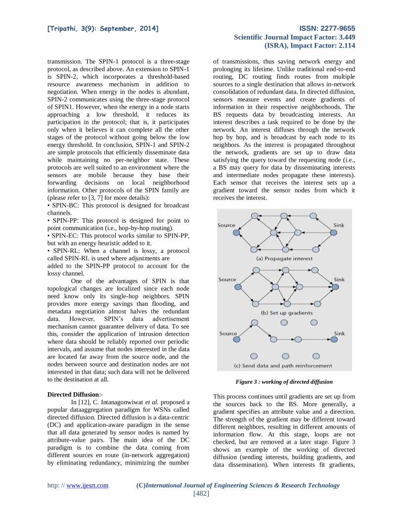
consolidation of redundant data. In directed diffusion,

sensors measure events and create gradients of

information in their respective neighborhoods. The

BS requests data by broadcasting interests. An

interest describes a task required to be done by the

network. An interest diffuses through the network

hop by hop, and is broadcast by each node to its

neighbors. As the interest is propagated throughout

the network, gradients are set up to draw data

satisfying the query toward the requesting node (i.e.,

a BS may query for data by disseminating interests

and intermediate nodes propagate these interests).

Each sensor that receives the interest sets up a

gradient toward the sensor nodes from which it

receives the interest.

Figure 3 : working of directed diffusion

This process continues until gradients are set up from

the sources back to the BS. More generally, a

gradient specifies an attribute value and a direction.

The strength of the gradient may be different toward

different neighbors, resulting in different amounts of

information flow. At this stage, loops are not

checked, but are removed at a later stage. Figure 3

shows an example of the working of directed

diffusion (sending interests, building gradients, and

data dissemination). When interests fit gradients,






[483]

paths of information flow are formed from multiple

paths, and then the best paths are reinforced to

prevent further flooding according to a local rule. In

order to reduce communication costs, data is

aggregated on the way. The goal is to find a good

aggregation tree that gets the data from source nodes

to the BS. The BS periodically refreshes and resends

the interest when it starts to receive data from the

source(s). This is necessary because interests are not

reliably transmitted throughout the network.

All sensor nodes in a directed-diffusion-

based network are application-aware, which enables

diffusion to achieve energy savings by selecting

empirically good paths, and by caching and

processing data in the network. Caching can increase

the efficiency, robustness, and scalability of

coordination between sensor nodes, which is the

essence of the data diffusion paradigm. Other usage

of directed diffusion is to spontaneously propagate an

important event to some sections of the sensor

network. Such a type of information retrieval is well

suited only to persistent queries where requesting

nodes are not expecting data that satisfy a query for

duration of time. This makes it unsuitable for one-

time queries, as it is not worth setting up gradients for

queries that use the path only once.

The performance of data aggregation

methods used in the directed diffusion paradigm is

affected by a number of factors, including the

positions of the source nodes in the network, the

number of sources, and the communication network

topology. In order to investigate these factors, two

models of source placement (shown in Fig. 4) were

studied in [12]. These models are called the event

radius (ER) model and the random sources (RS)

model. In the ER model, a single point in the network

area is defined as the location of an event. This may

correspond to a vehicle or some other phenomenon

being tracked by the sensor nodes. All nodes within a

distance S (called the sensing range) of this event that

are not BSs are considered to be data sources. The

average number of sources is approximately pS2n in

a unit area network with n sensor nodes. In the RS

model, k of the nodes that are not BSs are randomly

selected to be sources. Unlike the ER model, the

sources are not necessarily clustered near each other.

In both models of source placement, for a given

energy budget, a greater number of sources can be

connected to the BS. However, each one performs

better in terms of energy consumption depending on

the application. In conclusion, the energy savings

with aggregation used in directed diffusion can be

transformed to provide a greater degree of robustness

with respect to dynamics in the sensed phenomena.

Directed diffusion differs from SPIN in two aspects.

First, directed diffusion issues data queries on

demand as the BS sends queries to the sensor nodes

by flooding some tasks.

In SPIN, however, sensors advertise the

availability of data, allowing interested nodes to

query that data. Second, all communication in

directed diffusion is neighbor to neighbor with each

node having the capability to perform data

aggregation and caching. Unlike SPIN, there is no

need to maintain global network topology in directed

diffusion. However, directed diffusion may not be

applied to applications (e.g., environmental

monitoring) that require continuous data delivery to

the BS. This is because the query-driven on-demand

data model may not help in this regard. Moreover,

matching data to queries might require some extra

overhead at the sensor nodes.

Rumor Routing:-

Rumor routing [13] is a variation of directed

diffusion and is mainly intended for applications

where geographic routing is not feasible. In general,

directed diffusion uses flooding to inject the query to

the entire network when there is no geographic

criterion to diffuse tasks. However, in some cases

there is only a small amount of data requested fro the

nodes; thus, the use of flooding is unnecessary. An

alternative approach is to flood the events if the

number of events is small and the number of queries

is large. The key idea is to route the queries to the

nodes that have observed a particular event rather

than flooding the entire network to retrieve

information about the occurring events. In order to

flood events through the network, the rumor routing

algorithm employs long-lived packets called agents.

When a node detects an event, it adds the event to its

local table, called an events table, and generates an

agent. Agents travel the network in order to

propagate information about local events to distant

nodes. When a node generates a query for an event,

the nodes that know the route may respond to the

query by inspecting its event table. Hence, there is no

need to flood the whole network, which reduces the

communication cost. On the other hand, rumor

routing maintains only one path between source and

destination as opposed to directed diffusion where

data can be routed through multiple paths at low

rates. Simulation results showed that rumor routing

can achieve significant energy savings compared to

event flooding and can also handle a node’s failure.

However, rumor routing performs well only when the

number of events is small. For a large number of

events, the cost of maintaining agents and event






[484]

tables in each node becomes infeasible if there is not

enough interest in these events from the BS.

Moreover, the overhead associated with rumor

routing is controlled by different parameters used in

the algorithm such as time to live (TTL) pertaining to

queries and agents. Since the nodes become aware of

events through the event agents, the heuristic for

defining the route of an event agent highly affects the

performance of next-hop selection in rumor routing.

Minimum Cost Forwarding Algorithm:

The Minimum Cost Forwarding Algorithm

(MCFA) [8] exploits the fact that the direction of

routing is always known (i.e., toward the fixed

external BS). Hence, a sensor node need not have a

unique ID nor maintain a routing table. Instead, each

node maintains the least cost estimate from itself to

the BS. Each message to be forwarded by the sensor

node is broadcast to its neighbors. When a node

receives the message, it checks if it is on the least

cost path between the source sensor node and the BS.

If this is the case, it rebroadcasts the message to its

neighbors. This process repeats until the BS is

reached. In MCFA, each node should know the least

cost path estimate from itself to the BS. This is

obtained as follows. The BS broadcasts a message

with the cost set to zero, while every node initially

sets its least cost to the BS to infinity. Each node,

upon receiving the broadcast message originated at

the BS, checks to see if the estimate in the message

plus the link on which it is received is less than the

current estimate. If yes, the current estimate and the

estimate in the broadcast message are updated. If the

received broadcast message is updated, it is resent;

otherwise, it is purged and nothing further is done.

However, the previous procedure may result in some

nodes having multiple updates, and those nodes far

away from the BS will get more updates from those

closer to the BS. To avoid this, MCFA was modified

to run a backoff algorithm at the setup phase. The

backoff algorithm dictates that a node will not send

the updated message until a * lc time units have

elapsed from the time at which the message is

updated, where a is a constant and lc is the link cost

at which the message was received.

Gradient-based routing:

Schurgers et al. [14] proposed another

variant of directed diffusion, called gradient-based

routing (GBR). The key idea in GBR is to memorize

the number of hops when the interest is diffused

through the whole network. As such, each node can

calculate a parameter called the height of the node,

which is the minimum number of hops to reach the

BS.The difference between a node’s height and that

of its neighbor is considered the gradient on that link.

A packet is forwarded on a link with the largest

gradient.

GBR uses some auxiliary techniques such as

data aggregation and traffic spreading in order to

uniformly divide the traffic over the network. When

multiple paths pass through a node, which acts as a

relay node, that relay node may combine data

according to a certain function. In GBR, three

different data dissemination techniques have been

discussed:

• A stochastic scheme, where a node picks one

gradient at random when there are two or more next

hops that have the same gradient

• An energy-based scheme, where a node increases its

height when its energy drops below a certain

threshold so that other sensors are discouraged from

sending data to that node

• A stream-based scheme, where new streams are not

routed through nodes that are currently part of the

path of other streams

The main objective of these schemes is to

obtain balanced distribution of the traffic in the

network, thus increasing the network lifetime.

Simulation results of GBR showed that GBR

outperforms directed diffusion in terms of total

communication energy.

Information-driven sensor querying and

constrained anisotropic diffusion routing

Two routing techniques, information-driven

sensor querying (IDSQ) and constrained anisotropic

diffusion routing (CADR), were proposed in [15].

CADR aims to be a general form of directed

diffusion. The key idea is to query sensors and route

data in the network such that information gain is

maximized while latency and bandwidth are

minimized. CADR diffuses queries by using a set of

information criteria to select which sensors can get

the data.

This is achieved by activating only the

sensors that are close to a particular event and

dynamically adjusting data routes. The main

difference from directed diffusion is the

consideration of information gain in addition to

communication cost. In CADR, each node evaluates

an information/cost objective and routes data based

on the local information/cost gradient and end-user

requirements. Estimation theory was used to model

information utility.

In IDSQ, the querying node can determine

which node can provide the most useful information

with the additional advantage of balancing the energy






[485]

cost. However, IDSQ does not specifically define

how the query and information are routed between

sensors and the BS. Therefore, IDSQ can be seen as a

complementary optimization procedure. Simulation

results showed that these approaches are more

energy-efficient than directed diffusion where queries

are diffused in an isotropic fashion and reach nearest

neighbors first.

COUGAR:

Another data-centric protocol called

COUGAR [16] views the network as a huge

distributed database system. The key idea is to use

declarative queries in order to abstract query

processing from the network layer functions such as

selection of relevant sensors and so on. COUGAR

utilizes in-network data aggregation to obtain more

energy savings. The abstraction is supported through

an additional query layer that lies between the

network and application layers.

COUGAR incorporates an architecture for

the sensor database system where sensor nodes select

a leader node to perform aggregation and transmit the

data to the BS. The BS is responsible for generating a

query plan that specifies the necessary information

about the data flow and in-network computation for

the incoming query, and sends it to the relevant

nodes. The query plan also describes how to select a

leader for the query.

The architecture provides in-network

computation ability that can provide energy

efficiency in situations when the generated data is

huge. COUGAR provides a network-layer-

independent method for data query. However,

COUGAR has some drawbacks. First, the addition of

a query layer on each sensor node may add extra

overhead in terms of energy consumption and

memory storage. Second, to obtain successful in-

network data computation, synchronization among

nodes is required (not all data are received at the

same time from incoming sources) before sending the

data to the leader node. Third, the leader nodes

should be dynamically maintained to prevent them

from being hotspots (failure-prone).

ACQUIRE:

In [17], Sadagopan et al. proposed a

technique for querying sensor networks called Active

Query Forwarding in Sensor Networks (ACQUIRE).

Similar to COUGAR, ACQUIRE views the network

as a distributed database where complex queries can

be further divided into several subqueries. The

operation of ACQUIRE can be described as follows.

The BS node sends a query, which is then forwarded

by each node receiving the query. During this, each

node tries to respond to the query partially by using

its precached information and then forwards it to

another sensor node. If the precached information is

not up-to-date, the nodes gather information from

their neighbors within a lookahead of d hops. Once

the query is resolved completely, it is sent back

through either the reverse or shortest path to the BS.

Hence, ACQUIRE can deal with complex

queries by allowing many nodes to send responses.

Note that directed diffusion may not be used for

complex queries due to energy considerations as

directed diffusion also uses a flooding-based query

mechanism for continuous and aggregate queries. On

the other hand, ACQUIRE can provide efficient

querying by adjusting the value of the lookahead

parameter d. When d is equal to network diameter,

ACQUIRE behaves similar to flooding. However, the

query has to travel more hops if d is too small. A

mathematical modeling was used to find an optimal

value of the parameter d for a grid of sensors where

each node has four immediate neighbors.

However, there is no validation of results

through simulation. To select the next node for

forwarding the query, ACQUIRE either picks it

randomly or the selection is based on maximum

potential query satisfaction. Recall that either

selection of the next node is based on information

gain (CADR and IDSQ) or the query is forwarded to

a node that knows the path to the searched event

(rumor routing).

Energy-Aware Routing:

The objective of the Energy-Aware Routing

protocol [18], a destination- initiated reactive

protocol, is to increase the network lifetime.

Although this protocol is similar to directed

diffusion, it differs in the sense that it maintains a set

of paths instead of maintaining or enforcing one

optimal path at higher rates. These paths are

maintained and chosen by means of a certain

probability.

The value of this probability depends on

how low the energy consumption is that each path

can achieve. By having paths chosen at different

times, the energy of any single path will not deplete

quickly. This can achieve longer network lifetime as

energy is dissipated more equally among all nodes.

Network survivability is the main metric of this

protocol. The protocol assumes that each node is

addressable through class-based addressing that

includes the locations and types of the nodes. The

protocol initiates a connection through localized

flooding, which is used to discover all routes between






[486]

a source/ destination pair and their costs, thus

building up the routing tables. High cost paths are

discarded, and a forwarding table is built by choosing

neighboring nodes in a manner that is proportional to

their cost.

Then forwarding tables are used to send data

to the destination with a probability inversely

proportional to the node cost. Localized flooding is

performed by the destination node to keep the paths

alive. Compared to directed diffusion, this protocol

provides an overall improvement of 21.5 percent

energy saving and a 44 percent increase in network

lifetime. However, the approach requires gathering

location information and setting up the addressing

mechanism for the nodes, which complicate route

setup compared to directed diffusion.

Routing protocols with random walks The objective of the random-walks-based

routing technique [19] is to achieve load balancing in

a statistical sense by making use of multipath routing

in WSNs. This technique considers only large-scale

networks where nodes have very limited mobility. In

this protocol, it is assumed that sensor nodes can be

turned on or off at random times. Furthermore, each

node has a unique identifier but no location

information is needed. Nodes were arranged such that

each node falls exactly on one crossing point of a

regular grid on a plane, but the topology can be

irregular. To find a route from a source to its

destination, the location information or lattice

coordination is obtained by computing distances

between nodes using the distributed asynchronous

version of the well-known Bellman-Ford algorithm.

An intermediate node would select as the next hop

the neighboring node that is closer to the destination

according to a computed probability. By carefully

manipulating this probability, some kind of load

balancing can be obtained in the network. The

routing algorithm is simple as nodes are required to

maintain little state information. Moreover, different

routes are chosen at different times even for the same

pair of source and destination nodes. However, the

main concern about this protocol is that the topology

of the network may not be practical.

Hierarchical Routing :- Hierarchical or cluster based routing

methods, originally proposed in wire line networks,

are well-known techniques with special advantages

related to scalability and efficient communication. As

such, the concept of hierarchical routing is also

utilized to perform energy efficient routing in WSNs.

In a hierarchical architecture, higher-energy nodes

can be used to process and send the information,

while low-energy nodes can be used to perform the

sensing in the proximity of the target.

The creation of clusters and assigning

special tasks to cluster heads can greatly contribute to

overall system scalability, lifetime, and energy

efficiency. Hierarchical routing is an efficient way to

lower energy consumption within a cluster,

performing data aggregation and fusion in order to

decrease the number of transmitted messages to the

BS. Hierarchical routing is mainly two-layer routing

where one layer is used to select cluster heads and the

other for routing.

However, most techniques in this category

are not about routing, but rather “who and when to

send or process/ aggregate” the information, channel

allocation, and so on, which can be orthogonal to the

multihop routing function.

LEACH protocol:

Heinzelman, et al. [5] introduced a

hierarchical clustering algorithm for sensor networks,

called Low Energy Adaptive Clustering Hierarchy

(LEACH). LEACH is a cluster-based protocol, which

includes distributed cluster formation. LEACH

randomly selects a few sensor nodes as cluster heads

(CHs) and rotates this role to evenly distribute the

energy load among the sensors in the network.

In LEACH, the CH nodes compress data

arriving from nodes that belong to the respective

cluster, and send an aggregated packet to the BS in

order to reduce the amount of information that must

be transmitted to the BS. LEACH uses a

TDMA/code-division multiple access (CDMA) MAC

to reduce intercluster and intracluster collisions.

However, data collection is centralized and

performed periodically. Therefore, this protocol is

most appropriate when there is a need for constant

monitoring by the sensor network. A user may not

need all the data immediately.

Hence, periodic data transmissions are

unnecessary, and may drain the limited energy of the

sensor nodes. After a given interval of time,

randomized rotation of the role of CH is conducted so

that uniform energy dissipation in the sensor network

is obtained. The authors found, based on their

simulation model that only 5 percent of the nodes

need to act as CHs. The operation of LEACH is

separated into two phases, the setup phase and the

steady state phase. In the setup phase, the clusters are

organized and CHs are selected. In the steady state

phase, the actual data transfer to the BS takes place.

The duration of the steady state phase is longer than

the duration of the setup phase in order to minimize






[487]

overhead. During the setup phase, a predetermined

fraction of nodes, p, elect themselves as CHs as

follows. A sensor node chooses a random number, r,

between 0 and 1. If this random number is less than a

threshold value, T(n), the node becomes a CH for the

current round. The threshold value is calculated

based on an equation that incorporates the desired

percentage to become a CH, the current round, and

the set of nodes that have not been selected as a CH

in the last (1/P) rounds, denoted G. It is given by

𝑇(𝑛) =𝑝

1 − 𝑝 (𝑟 𝑚𝑜𝑑 (1

𝑝))

𝑖𝑓 𝑛 Є 𝑮

Where G is the set of nodes that are

involved in the CH election. All elected CHs

broadcast an advertisement message to the rest of the

nodes in the network that they are the new CHs. All

the non-CH nodes, after receiving this advertisement,

decide on the cluster to which they want to belong.

This decision is based on the signal strength of the

advertisement. The non-CH nodes inform the

appropriate CHs that they will be a member of the

cluster. After receiving all the messages from the

nodes that would like to be included in the cluster

and based on the number of nodes in the cluster, the

CH node creates a TDMA schedule and assigns each

node a time slot when it can transmit.

This schedule is broadcast to all the nodes in

the cluster. During the steady state phase, the sensor

nodes can begin sensing and transmitting data to the

CHs. The CH node, after receiving all the data,

aggregates it before sending it to the BS. After a

certain time, which is determined a priori, the

network goes back into the setup phase again and

enters another round of selecting new CHs. Each

cluster communicates using different CDMA codes

to reduce interference from nodes belonging to other

clusters. Although LEACH is able to increase the

network lifetime, there are still a number of issues

about the assumptions used in this protocol.

LEACH assumes that all nodes can transmit

with enough power to reach the BS if needed and that

each node has computational power to support

different MAC protocols. Therefore, it is not

applicable to networks deployed in large regions. It

also assumes that nodes always have data to send,

and nodes located close to each other have correlated

data. It is not obvious how the number of

predetermined CHs (p) is going to be uniformly

distributed through the network. Therefore, there is

the possibility that the elected CHs will be

concentrated in one part of the network; hence, some

nodes will not have any CHs in their vicinity.

Furthermore, the idea of dynamic clustering brings

extra overhead (head changes, advertisements, etc.),

which may diminish the gain in energy consumption.

Finally, the protocol assumes that all nodes begin

with the same amount of energy capacity in each

election round, assuming that being a CH consumes

approximately the same amount of energy for each

node. The protocol should be extended to account for

non-uniform energy nodes (i.e., use an energy-based

threshold). An extension to LEACH, LEACH with

negotiation, was proposed in [5].

The main theme of the proposed extension is

to precede data transfers with high level negotiation

using meta-data descriptors as in the SPIN protocol

discussed earlier. This ensures that only data that

provides new information is transmitted to the CHs

before being transmitted to the BS. Table 1 compares

SPIN, LEACH, and directed diffusion according to

different parameters.

Table 1: Comparison between SPIN, LEACH and

Directed diffusion

SPIN LEACH Directed

Diffusion

Optimal

Route No No Yes

Network

Lifetime Good

Very

Good Good

Resource

Awareness Yes Yes Yes

Use of

meta-data Yes No Yes

It is noted from the table that directed

diffusion shows a promising approach for energy

efficient routing in WSNs due to the use of in-

network processing.

Power-Efficient Gathering in Sensor Information

Systems:

In [20], an enhancement over the LEACH

protocol was proposed. The protocol, called Power-

Efficient Gathering in Sensor Information Systems

(PEGASIS), is a near optimal chain-based protocol.

The basic idea of the protocol is that in order to

extend network lifetime, nodes need only

communicate with their closest neighbors, and they

take turns in communicating with the BS. When the

round of all nodes communicating with the BS ends,

a new round starts, and so on. This reduces the power

required to transmit data per round as the power






[488]

draining is spread uniformly over all nodes. Hence,

PEGASIS has two main objectives.

First, increase the lifetime of each node by

using collaborative techniques. Second, allow only

local coordination between nodes that are close

together so that the bandwidth consumed in

communication is reduced. Unlike LEACH,

PEGASIS avoids cluster formation and uses only one

node in a chain to transmit to the BS instead of

multiple nodes. To locate the closest neighbor node

in PEGASIS, each node uses the signal strength to

measure the distance to all neighboring nodes and

then adjusts the signal strength so that only one node

can be heard. The chain in PEGASIS will consist of

those nodes that are closest to each other and form a

path to the BS.

The aggregated form of the data will be sent

to the BS by any node in the chain, and the nodes in

the chain will take turns sending to the BS. The chain

construction is performed in a greedy fashion.

Simulation results showed that PEGASIS is able to

increase the lifetime of the network to twice that

under the LEACH protocol. Such performance gain

is achieved through the elimination of the overhead

caused by dynamic cluster formation in LEACH, and

decreasing the number of transmissions and reception

by using data aggregation. Although the clustering

overhead is avoided, PEGASIS still requires dynamic

topology adjustment since a sensor node needs to

know about the energy status of its neighbors in order

to know where to route its data. Such topology

adjustment can introduce significant overhead,

especially for highly utilized networks.

Moreover, PEGASIS assumes that each

sensor node is able to communicate with the BS

directly. In practical cases, sensor nodes use multihop

communication to reach the BS. Also, PEGASIS

assumes that all nodes maintain a complete database

of the location of all other nodes in the network. The

method by which the node locations are obtained is

not outlined. In addition, PEGASIS assumes that all

sensor nodes have the same level of energy and are

likely to die at the same time.

Note also that PEGASIS introduces

excessive delay for distant nodes on the chain. In

addition, the single leader can become a bottleneck.

Finally, although in most scenarios sensors will be

fixed or immobile as assumed in PEGASIS, some

sensors may be allowed to move and hence affect the

protocol functionality. An extension to PEGASIS,

called Hierarchical PEGASIS, was introduced in [2]

with the objective of decreasing the delay incurred

for packets during transmission to the BS. For this

purpose, simultaneous transmissions of data are

studied in order to avoid collisions through

approaches that incorporate signal coding and spatial

transmissions. In the latter, only spatially separated

nodes are allowed to transmit at the same time. The

chain-based protocol with CDMA-capable nodes

constructs a chain of nodes that forms a tree-like

hierarchy, and each selected node at a particular level

transmits data to a node in the upper level of the

hierarchy.

This method ensures data transmitting in

parallel and reduces delay significantly. Such a

hierarchical extension has been shown to perform

better than the regular PEGASIS scheme by a factor

of about 60.

Threshold-Sensitive Energy Efficient Protocols:

Two hierarchical routing protocols called

Threshold-Sensitive Energy Efficient Sensor

Network Protocol (TEEN) and Adaptive Periodic

TEEN (APTEEN) are proposed in [21, 22]. These

protocols were proposed for time-critical

applications. In TEEN, sensor nodes sense the

medium continuously, but data transmission is done

less frequently. A CH sensor sends its members a

hard threshold, which is the threshold value of the

sensed attribute, and a soft threshold, which is a small

change in the value of the sensed attribute that

triggers the node to switch on its transmitter and

transmit. Thus, the hard threshold tries to reduce the

number of transmissions by allowing the nodes to

transmit only when the sensed attribute is in the range

of interest.

The soft threshold further reduces the

number of transmissions that might otherwise occur

when there is little or no change in the sensed

attribute. A smaller value of the soft threshold gives a

more accurate picture of the network, at the expense

of increased energy consumption. Thus, the user can

control the tradeoff between energy efficiency and

data accuracy.

When CHs are to change (Fig. 4a), new

values for the above parameters are broadcast. The

main drawback of this scheme is that if the thresholds

are not received, the nodes will never communicate,

and the user will not get any data from the network at

all. The nodes sense their environment continuously.

The first time a parameter from the attribute set

reaches its hard threshold value, the node switches its

transmitter on and sends the sensed data.






[489]

Figure 4 : Time line for the operation of a) TEEN and b)

APTEEN.

The sensed value is stored in an internal

variable called sensed value (SV). The nodes will

transmit data in the current cluster period only when

the following conditions are true:

• The current value of the sensed attribute is greater

than the hard threshold.

• The current value of the sensed attribute differs

from SV by an amount equal to or greater than the

soft threshold.

Important features of TEEN include its

suitability for time-critical sensing applications. Also,

since message transmission consumes more energy

than data sensing, the energy consumption in this

scheme is less than in proactive networks. The soft

threshold can be varied. At every cluster change time,

fresh parameters are broadcast, so the user can

change them as required. APTEEN, on the other

hand, is a hybrid protocol that changes the periodicity

or threshold values used in the TEEN protocol

according to user needs and the application type.

In APTEEN, the CHs broadcast the

following parameters (Fig. 4b):

• Attributes (A): a set of physical parameters about

which the user is interested in obtaining information

• Thresholds: consists of the hard threshold (HT) and

soft threshold (ST)

• Schedule: a TDMA schedule, assigning a slot to

each node

• Count time (CT): the maximum time period

between two successive reports sent by a node

The node senses the environment

continuously, and only those nodes that sense a data

value at or beyond HT transmit. Once a node senses a

value beyond HT, it transmits data only when the

value of that attribute changes by an amount equal to

or greater than ST. If a node does not send data for a

time period equal to CT, it is forced to sense and

retransmit the data. A TDMA schedule is used, and

each node in the cluster is assigned a transmission

slot. Hence, APTEEN uses a modified TDMA

schedule to implement the hybrid network. The main

features of the APTEEN scheme include the

following. It combines both proactive and reactive

policies. It offers a lot of flexibility by allowing the

user to set the CT interval, and the threshold values

for energy consumption can be controlled by

changing the CT as well as the threshold values. The

main drawback of the scheme is the additional

complexity required to implement the threshold

functions and CT. Simulation of TEEN and APTEEN

has shown that these two protocols outperform

LEACH. The experiments have demonstrated that

APTEEN’s performance is somewhere between

LEACH and TEEN in terms of energy dissipation

and network lifetime. TEEN gives the best

performance since it decreases the number of

transmissions. The main drawbacks of the two

approaches are the overhead and complexity

associated with forming clusters at multiple levels,

the method of implementing threshold-based

functions, and how to deal with attribute-based

naming of queries.

Small minimum energy communication network

(MECN):

In [23], a protocol is proposed that computes

an energy-efficient sub-network, the minimum

energy communication network (MECN), for a

certain sensor network utilizing low power GPS.

MECN identifies a relay region for every node. The

relay region consists of nodes in a surrounding area

where transmitting through those nodes is more

energy-efficient than direct transmission. The

enclosure of a node i is created by taking the union of

all relay regions node i can reach. The main idea of

MECN is to find a sub-network that will have fewer

nodes and require less power for transmission

between any two particular nodes. In this way, global

minimum power paths are found without considering

all the nodes in the network. This is performed using

a localized search for each node considering its relay

region. MECN is self-reconfiguring and thus can

dynamically adapt to node failure or the deployment

of new sensors. The small MECN (SMECN) [24] is

an extension to MECN. In MECN, it is assumed that

every node can transmit to every other node, which is

not possible every time. In SMECN possible

obstacles between any pair of nodes are considered.






[490]

However, the network is still assumed to be fully

connected as in the case of MECN. The sub-network

constructed by SMECN for minimum energy

relaying is provably smaller (in terms of number of

edges) than the one constructed in MECN. Hence, the

sub-network (i.e., subgraph G) constructed by

SMECN is smaller than the one constructed by

MECN if the broadcast region is circular around the

broadcasting node for a given power setting. Sub

graph G’ of graph G, which represents the sensor

network, minimizes the energy usage satisfying the

following conditions:

• The number of edges in G’ is less than in G while

containing all nodes in G.

• The energy required to transmit data from a node to

all its neighbors in sub graph G’ is less than the

energy required to transmit to all its neighbors in

graph G.

Assume that r = (u, u1, …, v) is a path

between u and v that spans k –1 intermediate nodes

u1, … uk–1. The total power consumption of one

path like r is given by

where u = u0 and v = uk, and the power required to

transmit data under this protocol is

p(u,v) = t.d(u,v)n

for some appropriate constant t, n is the path loss

exponent of outdoor radio propagation models n ≥2,

and d(u,v) is the distance between u and v. It is

assumed that a reception at the receiver takes a

constant amount of power denoted c. The sub-

network computed by SMECN helps in sending

messages on minimum energy paths. However, the

proposed algorithm is local in the sense that it does

not actually find the minimum-energy path, it just

constructs a sub-network in which it is guaranteed to

exist. Moreover, the sub-network constructed by

SMECN makes it more likely that the path used is

one that requires less energy consumption. In

addition, finding a sub-network with a smaller

number of edges introduces more overhead in the

algorithm.

Self-organizing protocol:

Subramanian et al. [25] describes a self-

organizing protocol (SOP) and an application

taxonomy that was used to build architecture to

support heterogeneous sensors. Furthermore, these

sensors can be mobile or stationary. Some sensors

probe the environment and forward the data to a

designated set of nodes that act as routers. Router

nodes are stationary and form the backbone for

communication. Collected data are forwarded

through the routers to the more powerful BS nodes.

Each sensing node should be able to reach a router in

order to be part of the network. A routing architecture

that requires addressing of each sensor node has been

proposed. Sensing nodes are identifiable through the

address of the router node to which they are

connected. The routing architecture is hierarchical

where groups of nodes are formed and merge when

needed. The Local Markov Loops (LML) algorithm,

which performs a random walk on spanning trees of a

graph, was used to support fault tolerance and as a

means of broadcasting. Such an approach is similar to

the idea of a virtual grid used in some other protocols

discussed later under location-based routing

protocols. In this approach, sensor nodes can be

addressed individually in the routing architecture;

hence, it is suitable for applications where

communication to a particular node is required.

Furthermore, this algorithm incurs a small cost for

maintaining routing tables and keeping a balanced

routing hierarchy. It was also found that the energy

consumed for broadcasting a message is less than that

consumed in the SPIN protocol. This protocol,

however, is not an on demand protocol, especially in

the organization phase of the algorithm, and thus

introduces extra overhead. Another issue is related to

the formation of a hierarchy. It could happen that

there are many cuts in the network, and hence the

probability of applying reorganization phase

increases, which is an expensive operation.

Sensor aggregates routing:

In [26], a set of algorithms for constructing

and maintaining sensor aggregates were proposed.

The objective is to collectively monitor target activity

in a certain environment (target tracking

applications). A sensor aggregate comprises those

nodes in a network that satisfy a grouping predicate

for a collaborative processing task. The parameters of

the predicate depend on the task and its resource

requirements. The formation of appropriate sensor

aggregates were discussed in [26] in terms of

allocating resources to sensing and communication

tasks. Sensors in a sensor field are divided into

clusters according to their sensed signal strength, so

there is only one peak per cluster. Then local cluster

leaders are elected. One peak may represent one

target, multiple targets, or no target if the peak is

generated by noise sources. To elect a leader,

information exchanges between neighboring sensors

are necessary. If a sensor, after exchanging packets

with all its one hop neighbors, finds that it is higher

than all its one-hop neighbors on the signal field






[491]

landscape, it declares itself a leader. This leader-

based tracking algorithm assumes that the unique

leader knows the geographical region of the

collaboration.

Three algorithms were proposed in [26].

First was a lightweight protocol, Distributed

Aggregate Management (DAM), for forming sensor

aggregates for a target monitoring task. The protocol

comprises a decision predicate P for each node to

decide if it should participate in an aggregate and a

message exchange scheme M about how the grouping

predicate is applied to nodes. A node determines if it

belongs to an aggregate based on the result of

applying the predicate to the data of the node as well

as information from other nodes. Aggregates are

formed when the process eventually converges.

Second, Energy-Based Activity Monitoring

(EBAM) estimates the energy level at each node by

computing the signal impact area, combining a

weighted form of the detected target energy at each

impacted sensor, assuming that each target sensor has

equal or constant energy level.

The third algorithm, Expectation-

Maximization Like Activity Monitoring (EMLAM),

removes the constant and equal target energy level

assumption. EMLAM estimates the target positions

and signal energy using received signals, and uses the

resulting estimates to predict how signals from the

targets may be mixed at each sensor. This process is

iterated until the estimate is sufficiently good.

The distributed track initiation management

scheme, combined with the leader-based tracking

algorithm described in [26], forms a scalable system.

The system works well in tracking multiple targets

when the targets are not interfering, and it can

recover from inter target interference once the targets

move apart.

Virtual grid architecture routing:

An energy efficient routing paradigm is

proposed in [27] that utilize data aggregation and in-

network processing to maximize the network

lifetime. Due to the node stationarity and extremely

low mobility in many applications in WSNs, a

reasonable approach is to arrange nodes in a fixed

topology, as briefly mentioned in [28]. A GPS free

approach [2] is used to build clusters that are fixed,

equal, adjacent, and non-overlapping with symmetric

shapes. In [27], square clusters were used to obtain a

fixed rectilinear virtual topology. Inside each zone, a

node is optimally selected to act as CH. Data

aggregation is performed at two levels: local and then

global. The set of CHs, also called local aggregators

(LAs), perform local aggregation, while a subset of

these LAs are used to perform global aggregation.

Figure 5: Regular shape tessellation applied to network

area.

However, the determination of an optimal

selection of global aggregation points, called master

aggregators (MAs), is NP-hard. Figure 5 illustrates an

example of fixed zoning and the resulting virtual grid

architecture (VGA) used to perform two-level data

aggregation. Note that the location of the BS is not

necessarily at the extreme corner of the grid; it can be

located at any arbitrary place. Two solution strategies

for the routing with data aggregation problem are

presented in [27]: an exact algorithm using an integer

linear program (ILP) formulation, and some near-

optimal but simple and efficient approximate

algorithms: a genetics-algorithm-based heuristic, a k-

means heuristic, and a greedy-based heuristic. In

[29], another efficient heuristic, the Clustering-Based

Aggregation Heuristic (CBAH), was also proposed to

minimize energy consumption in the network and

hence prolong the network lifetime. The objective of

all algorithms is to select a number of MAs out of the

LAs that maximize network lifetime. For a realistic

scenario, it is assumed in [27] that LA nodes form

possibly overlapping groups. Members of each group

sensie the same phenomenon; hence, their readings

are correlated. However, each LA node that exists in

the overlapping region will send data to its associated

MA for each of the groups to which it belongs. It was

noted in [29] that the problem of assigning MAs to

LAs in CBAH is similar to the classical bin packing

problem, a major difference being that neither the

identities nor the amount of power each MA will be

using for different LAs are known. In CBAH, the set

of MAs are selected based on incremental filing of

some bins with capacities. Besides being fast and






[492]

scalable to large sensor networks, the approximate

algorithms in [27, 29] produce results not far from

the optimal solution.

Hierarchical power-aware routing:

In [30], hierarchical power-aware routing

was proposed. The protocol divides the network into

groups of sensors. Each group of sensors in

geographic proximity are clustered together as a

zone, and each zone is treated as an entity. To

perform routing, each zone is allowed to decide how

it will route a message hierarchically across the other

zones such that the battery lives of the nodes in the

system are maximized. Message are routed along the

path that has the maximum over all the minimum of

the remaining power, called the max-min path. The

motivation is that using nodes with high residual

power may be more expensive than the path with the

minimal power consumption. An approximation

algorithm, called the max-min zPmin algorithm, was

proposed in [30].

The crux of the algorithm is based on the

trade-off between minimizing the total power

consumption and maximizing the minimal residual

power of the network. Hence, the algorithm tries to

enhance a max-min path by limiting its power

consumption as follows. First, the algorithm finds the

path with the least power consumption (Pmin) by

using the Dijkstra algorithm. Second, the algorithm

finds a path that maximizes the minimal residual

power in the network.

The proposed algorithm tries to optimize

both solution criteria. This is achieved by relaxing the

minimal power consumption for the message to be

equal to zPmin with parameter z≥1 to restrict the

power consumption for sending one message to

zPmin. The algorithm consumes at most zPmin while

maximizing the minimal residual power fraction.

Another algorithm that relies on max-min zPmin,

called zone-based routing, is also proposed in [30].

Zone-base routing is a hierarchical approach where

the area covered by the (sensor) To send a message

across the entire area, a global path from zone to zone

is found. The sensors in a zone autonomously direct

local routing and participate in estimating the zone

power level.

Each message is routed across the zones

using information about the zone power estimates. A

global controller for message routing is assigned the

role of managing the zones. This may be the node

with the highest power. If the network can be divided

into a relatively small number of zones, the scale for

the global routing algorithm is reduced. The global

information required to send each message across is

summarized by the power level estimate of each

zone. A zone graph was used to represent connected

neighboring zone vertices if the current zone can go

to the next neighboring zone in that direction. Each

zone vertex has a power level of 1. Each zone

direction vertex is labeled by its estimated power

level computed by a procedure, which is a modified

Bellman-Ford algorithm. Moreover, two algorithms

were outlined for local and global path selection

using the zone graph.

Two-Tier Data Dissemination:

An approach in [6], called Two-Tier Data

Dissemination (TTDD), provides data delivery to

multiple mobile BS. In TTDD, each data source

proactively builds a grid structure that is used to

disseminate data to the mobile sinks by assuming that

sensor nodes are stationary and location aware. In

TTDD, sensor nodes are stationary and location-

aware, whereas sinks may change their locations

dynamically. Once an event occurs, sensors

surrounding it process the signal, and one of them

becomes the source to generate data reports. Sensor

nodes are aware of their mission, which will not

change frequently.

To build the grid structure, a data source

chooses itself as the start crossing point of the grid,

and sends a data announcement message to each of

its four adjacent crossing points using simple greedy

geographical forwarding. When the message reaches

the node closest to the crossing point (specified in the

message), it will stop. During this process, each

intermediate node stores the source information and

further forwards the message to its adjacent crossing

points except the one from which the message comes.

This process continues until the message stops at the

border of the network.

The nodes that store the source information

are chosen as dissemination points. After this

process, the grid structure is obtained. Using the grid,

a BS can flood a query, which will be forwarded to

the nearest dissemination point in the local cell to

receive data. Then the query is forwarded along other

dissemination points upstream to the source. The

requested data then flows down in the reverse path to

the sink. Trajectory forwarding is employed as the

BS moves in the sensor field. Although TTDD is an

efficient routing approach, there are some concerns

about how the algorithm obtains location

information, which is required to set up the grid

structure. The length of a forwarding path in TTDD

is larger than the length of the shortest path. The

authors of TTDD believe that the sub-optimality in

the path length is worth the gain in scalability.






[493]

Finally, how TTDD would perform if mobile sensor

nodes are allowed to move in the network is still an

open question. Comparison results between TTDD

and directed diffusion showed that TTDD can

achieve longer lifetimes and shorter data delivery

delays. However, the overhead associated with

maintaining and recalculating the grid as network

topology changes may be high.

Furthermore, TTDD assumed the

availability of a very accurate positioning system that

is not yet available for WSNs. The above mentioned

flat and hierarchical protocols are different in many

aspects. At this point, we compare the different

routing approaches for flat and HR hierarchical

sensor networks as shown in Table 2.

Table 2: Comparision Hierarchical Routing and Flat

Routing

Location-Based Routing Protocols :-

In this kind of routing, sensor nodes are

addressed by means of their locations. The distance

between neighboring nodes can be estimated on the

basis of incoming signal strengths. Relative

coordinates of neighboring nodes can be obtained by

exchanging such information between neighbors [1,

2, 31]. Alternatively, the location of nodes may be

available directly by communicating with a satellite

using GPS if nodes are equipped with a small low-

power GPS receiver [28].

To save energy, some location-based schemes

demand that nodes should go to sleep if there is no

activity. More energy savings can be obtained by

having as many sleeping nodes in the network as

possible. The problem of designing sleep period

schedules for each node in a localized manner was

addressed in [32, 27, 28]. In the rest of this

section, we review most of the location or geographic

based routing protocols.

Geographic Adaptive Fidelity:

GAF [28] is an energy-aware location-based

routing algorithm designed primarily for mobile ad

hoc networks, but may be applicable to sensor

networks as well. The network area is first divided

into fixed zones and form a virtual grid. Inside each

zone, nodes collaborate with each other to play

different roles.

For example, nodes will elect one sensor

node to stay awake for a certain period of time, and

then the rest go to sleep. This node is responsible for

monitoring and reporting data to the BS on behalf of

the nodes in the zone. Hence, GAF conserves energy

by turning off unnecessary nodes in the network

without affecting the level of routing fidelity.

Each node uses its GPS-indicated location to

associate itself with a point in the virtual grid. Nodes

associated with the same point on the grid are

considered equivalent in terms of the cost of packet

routing. Such equivalence is exploited in keeping

some nodes located in a particular grid area in

sleeping state in order to save energy.

Thus, GAF can substantially increase the

network lifetime as the number of nodes increases.

There are three states defined in GAF: discovery, for

determining the neighbors in the grid; active,

reflecting participation in routing; and sleep, when

the radio is turned off. In order to handle mobility,

each node in the grid estimates its time of leaving the

grid and sends this to its neighbors.

The sleeping neighbors adjust their sleeping

time accordingly in order to keep routing fidelity.

Before the leaving time of the active node expires,

sleeping nodes wake up and one of them becomes






[494]

active. GAF is implemented both for non-mobility

(GAF-basic) and mobility (GAF-mobility adaptation)

of nodes.

Fixed zoning that can be used in sensor

networks similar to that proposed in [28]. The fixed

clusters in [28] are selected to be equal and square.

The selection of the square size is dependent on the

required transmitting power and communication

direction. Vertical and horizontal communication is

guaranteed to happen if the signal travels a distance

of a = r/2Ö2, chosen such that any two sensor nodes

in adjacent vertical or horizontal clusters can

communicate directly.

For diagonal communication to happen, the

signal has to span a distance of b = r/2Ö2. The issue

is how to schedule roles for the nodes to act as CHs.

A CH can ask the sensor nodes in its cluster to switch

on and start gathering data if it senses an object. Then

the CH is responsible for receiving raw data from

other nodes in its cluster and forwarding it to the BS.

The authors in [28] assumed that sensor nodes can

know their locations using GPS cards, which is

inconceivable with current technology.

GAF strives to keep the network connected

by keeping a representative node always in active

mode for each region on its virtual grid. Simulation

results show that GAF performs at least as well as a

normal ad hoc routing protocol in terms of latency

and packet loss, and increases the lifetime of the

network by saving energy. Although GAF is a

location-based protocol, it may also be considered a

hierarchical protocol, where the clusters are based on

geographic location. For each particular grid area, a

representative node acts as the leader to transmit the

data to other nodes. The leader node, however, does

not do any aggregation or fusion as in the case of

other hierarchical protocols discussed earlier.

Geographic and Energy Aware Routing:

Yu et al. [33] discussed the use of

geographic information while disseminating queries

to appropriate regions since data queries often

include geographic attributes. The protocol,

Geographic and Energy Aware Routing (GEAR),

uses energy aware and geographically informed

neighbor selection heuristics to route a packet toward

the destination region. The key idea is to restrict the

number of interests in directed diffusion by only

considering a certain region rather than sending the

interests to the whole network.

By doing this, GEAR can conserve more

energy than directed diffusion. Each node in GEAR

keeps an estimated cost and a learning cost of

reaching the destination through its neighbors. The

estimated cost is a combination of residual energy

and distance to destination. The learned cost is a

refinement of the estimated cost that accounts for

routing around holes in the network. A hole occurs

when a node does not have any closer neighbor to the

target region than itself. If there are no holes, the

estimated cost is equal to the learned cost. The

learned cost is propagated one hop back every time a

packet reaches the destination so that route setup for

the next packet will be adjusted. There are two

phases in the algorithm:

• Forwarding packets toward the target region: Upon

receiving a packet, a node checks its neighbors to see

if there is one neighbor that is closer to the target

region than itself. If there are more than one, the

nearest neighbor to the target region is selected as the

next hop. If they are all further than the node itself,

this means there is a hole. In this case, one of the

neighbors is picked to forward the packet based on

the learning cost function. This choice can then be

updated according to the convergence of the learned

cost during the delivery of packets.

• Forwarding the packets within the region: If the

packet has reached the region, it can be diffused in

that region by either recursive geographic forwarding

or restricted flooding. Restricted flooding is good

when the sensors are not densely deployed. In high-

density networks, recursive geographic forwarding is

more energy-efficient than restricted flooding. In that

case, the region is divided into four regions and four

copies of the packet are created. This splitting and

forwarding process continues until regions with only

one node are left. In [33], GEAR was compared to a

similar non-energy-aware routing protocol, GPSR

[34], which is one of the earlier methods in

geographic routing and uses planar graphs to solve

the problem of holes. In GPSR, the packets follow

the perimeter of the planar graph to find their route.

Although the GPSR approach reduces the number of

states a node should keep, it was designed for general

mobile ad hoc networks, and requires a location

service to map locations and node identifiers. GEAR

not only reduces energy consumption for route setup,

but also performs better than GPSR in terms of

packet delivery. The simulation results show that for

uneven traffic distribution, GEAR delivers 70–80

percent more packets than GPSR. For uniform traffic

pairs GEAR delivers 25–35 percent more packets

than GPSR.

MFR, DIR, and GEDIR:

Stojmenovic and Lin [35] described and

discussed basic localized routing algorithms. These

protocols deal with basic distance, progress, and






[495]

direction-based methods. The key issues are forward

and backward directions. A source node or any

intermediate node will select one of its neighbors

according to a certain criterion.

The routing methods that belong to this

category are Most Forward within Radius (MFR),

Geographic Distance Routing (GEDIR) that is a

variant of greedy algorithms, the two-hop greedy

method, alternate greedy method, and DIR (a

compass routing method).

GEDIR is a greedy algorithm that always

moves the packet to the neighbor of the current

vertex whose distance to the destination is

minimized. The algorithm fails when the packet

crosses the same edge twice in succession. In most

cases, the MFR and greedy methods have the same

path to the destination.

In the DIR method, the best neighbor has the

closest direction (i.e., angle) toward the destination.

That is, the neighbor with the minimum angular

distance from the imaginary line joining the current

node and the destination is selected. In MFR, the best

neighbor A will minimize the dot product DA” .DS”,

where S, D are the source and destination nodes,

respectively, and SD” represents the Euclidian

distance between the two nodes S, D. Alternatively,

one can maximize the dot product SD” .SA”. Each

method stops forwarding the message at a node for

which the best choice is to return the message back to

a previous node. GEDIR and MFRs are loop-free,

while DIR may create loops unless past traffic is

memorized or a timestamp is enforced [35].

A comparison study [35] between these

algorithms showed that the three basic algorithms had

comparable performance in terms of delivery rate and

average dilation. Moreover, simulations revealed that

the nodes in MFR and greedy methods select the

same forwarding neighbor in more than 99 percent of

cases, and the entire selected paths were identical in

most cases.

The Greedy Other Adaptive Face Routing:

In [36], a geometric ad hoc routing

algorithm combining greedy and face routing was

proposed. We will now briefly review the key points

of Greedy Other Adaptive Face Routing (GOAFR).

The greedy algorithm of GOAFR always picks the

neighbor closest to a node to be next for routing.

However, it can easily be stuck at some local

minimum (i.e., no neighbor is closer to a node than

the current node).

Other Face Routing (OFR) is a variant of

Face Routing (FR). The FR algorithm [35] is the first

that guarantees success if the source and destination

are connected. However, the worst case cost of FR is

proportional to the size of the network in terms of

number of nodes. The first algorithm that can

compete with the best route in the worst case is

Adaptive Face Routing (AFR).

Moreover, by a lower bound argument, AFR

is shown to be asymptotically worst-case optimal.

But AFR is not average-case efficient. OFR utilizes

the face structure of planar graphs such that the

message is routed from node s to node t by traversing

a series of face boundaries. The aim is to find the best

node on the boundary (i.e., the closest node to the

destination t) by using geometric planes.

When finished, the algorithm returns to s the

best node on the boundary. The simple greedy

algorithm behaves well in dense networks, but fails

for very simple configurations, as was shown in [36].

It was shown that GOAFR can achieve both worst-

case optimality and average-case efficiency. Based

on the simulation results of GOAFR, there are several

ways to further improve the average-case

performance. It was also shown that GOAFR

outperforms other prominent algorithms, such as

GPSR and AFR.

SPAN:

Another position-based algorithm called

SPAN [32] selects some nodes as coordinators based

on their positions. The coordinators form a network

backbone used to forward messages. A node should

become a coordinator if two neighbors of a non-

coordinator node cannot reach each other directly or

via one or two coordinators (three-hop reachability).

New and existing coordinators are not necessarily

neighbors in [32], which in effect makes the design

less energy-efficient because of the need to maintain

the positions of two or three-hop neighbors in the

complicated SPAN algorithm.

Routing protocols based on protocol

operation In this section we review routing protocols

with different routing functionality. It should be

noted that some of these protocols may fall under one

or more of the above routing categories.

Multipath Routing Protocols:- In this subsection the study of routing

protocols that use multiple paths rather than a single

path in order to enhance network performance. The

fault tolerance (resilience) of a protocol is measured

by the likelihood that an alternate path exists between

a source and a destination when the primary path

fails. This can be increased by maintaining multiple






[496]

paths between the source and destination at the

expense of increased energy consumption and traffic

generation. These alternate paths are kept alive by

sending periodic messages.

Hence, network reliability can be increased

at the expense of increased overhead in maintaining

the alternate paths. The authors in [37] proposed an

algorithm that routes data through a path whose

nodes have the largest residual energy.

The path is changed whenever a better path

is discovered. The primary path will be used until its

energy falls below the energy of the backup path, at

which time the backup path is used. Using this

approach, the nodes in the primary path will not

deplete their energy resources through continual use

of the same route, hence achieving longer life.

However, the path switching cost was not

quantified in the article. The authors of [38] proposed

the use of a set of suboptimal paths occasionally to

increase the lifetime of the network. These paths are

chosen by means of a probability that depends on

how low the energy consumption of each path is. The

path with the largest residual energy when used to

route data in a network may be very energy-

expensive too, so there is a tradeoff between

minimizing the total power consumed and the

residual energy of the network.

The authors in [30] proposed an algorithm in

which the residual energy of the route is relaxed a bit

in order to select a more energy efficient path. In

[39], multipath routing was used to enhance the

reliability of WSNs. The proposed scheme is useful

for delivering data in unreliable environments.

It is known that network reliability can be

increased by providing several paths from source to

destination and sending the same packet on each

path. However, using this technique, traffic will

increase significantly. Hence, there is a trade-off

between the amount of traffic and the reliability of

the network. This tradeoff is studied in [39] using a

redundancy function that is dependent on the

multipath degree and failing probabilities of the

available paths.

The idea is to split the original data packet

into subpackets and then send each subpacket

through one of the available multipaths. It has been

found that even if some of these subpackets are lost,

the original message can still be reconstructed.

According to their algorithm, it has also been found

that for a given maximum node failure probability,

using a higher multipath degree than a certain

optimal value will increase the total probability of

failure.

Directed diffusion [12] is a good candidate

for robust multipath routing and delivery. Based on

the directed diffusion paradigm, a multipath routing

scheme that finds several partially disjoint paths is

studied in [40] (alternate routes are not node disjoint,

i.e., routes are partially overlapped). It has been

found that the use of multipath routing provides a

viable alternative for energy-efficient recovery from

failures in WSNs. The motivation for using these

braided paths is to keep the cost of maintaining the

multipaths low. The costs of alternate paths are

comparable to the primary path because they tend to

be much closer to the primary path.

Query-Based Routing:-

In this kind of routing, the destination nodes

propagate a query for data (sensing task) from a node

through the network, and a node with this data sends

the data that matches the query back to the node that

initiated the query. Usually these queries are

described in natural language or high-level query

languages. For example, client C1 may submit a

query to node N1 and ask: Are there moving vehicles

in battle space region 1? All the nodes have tables

consisting of the sensing task queries they receive,

and send data that matches these tasks when they

receive it. Directed diffusion [12] described earlier is

an example of this type of routing.

In directed diffusion, the BS node sends out

interest messages to sensors. As the interest is

propagated throughout the sensor network, the

gradients from the source back to the BS are set up.

When the source has data for the interest, the source

sends the data along the interest’s gradient path. To

lower energy consumption, data aggregation (e.g.,

duplicate suppression) is performed en rute. The

rumor routing protocol [41] uses a set of long-lived

agents to create paths that are directed toward the

events they encounter.

Whenever an agent crosses a path leading to

an event it has not encountered yet, it creates a path

state that leads to the event. When agents come

across shorter paths or more efficient paths, they

optimize the paths in routing tables accordingly. Each

node maintains a list of its neighbors and an events

table that is updated whenever new events are

encountered. Each node can also generate an agent in

a probabilistic fashion. Each agent contains an events

table that is synchronized with every node it visits.

The agent has a lifetime of a certain number of hops,

after which it dies.

A node will not generate a query unless it

learns a route to the required event. If there is no

route available, the node transmits a query in a






[497]

random direction. Then the node waits to know if the

query reached the destination for a certain amount of

time, after which the node floods the network if no

response is received from the destination.

Negotiation-Based Routing Protocols:- These protocols use high-level data

descriptors in order to eliminate redundant data

transmissions through negotiation. Communication

decisions are also made based on the resources

available to them. The SPIN family protocols [9]

discussed earlier and the protocols in [10] are

examples of negotiation- based routing protocols.

The motivation is that the use of flooding to

disseminate data will produce implosion and overlap

between the sent data, so nodes will receive duplicate

copies of the same data.

This operation consumes more energy and

processing by sending the same data by different

sensors. The SPIN protocols are designed to

disseminate the data of one sensor to all other

sensors, assuming these sensors are potential BSs.

Hence, the main idea of negotiation-based routing in

WSNs is to suppress duplicate information and

prevent redundant data from being sent to the next

sensor or the BS by conducting a series of negotiation

messages before the real data transmission begins.

QoS-based Routing:-

In QoS-based routing protocols, the network

has to balance between energy consumption and data

quality. In particular, the network has to satisfy

certain QoS metrics (delay, energy, bandwidth, etc.)

when delivering data to the BS. Sequential

Assignment Routing (SAR) proposed in [42] is one

of the first routing protocols for WSNs to introduce

the notion of QoS into routing decisions. A routing

decision in SAR is dependent on three factors: energy

resources, QoS on each path, and the priority level of

each packet.

To avoid single route failure, a multipath

approach and localized path restoration schemes are

used. To create multiple paths from a source node, a

tree rooted at the source node to the destination nodes

(i.e., the set of BSs) is built. The paths of the tree are

built while avoiding nodes with low energy or QoS

guarantees. At the end of this process, each sensor

node will be part of a multipath tree. As such, SAR is

a table-driven multipath protocol that aims to achieve

energy efficiency and fault tolerance. In essence,

SAR calculates a weighted QoS metric as the product

of the additive QoS metric and a weight coefficient

associated with the priority level of the packet. The

objective of SAR is to minimize the average

weighted QoS metric throughout the lifetime of the

network.

If topology changes due to node failures,

path recomputation is needed. As a preventive

measure, a periodic recomputation of paths is

triggered by the BS to account for any changes in

topology. A handshake procedure based on a local

path restoration scheme between neighboring nodes

is used to recover from a failure. Failure recovery is

done by enforcing routing table consistency between

upstream and downstream nodes on each path.

Simulation results showed that SAR offers less power

consumption than the minimum energy metric

algorithm, which focuses only the energy

consumption of each packet without considering its

priority.

SAR maintains multiple paths from nodes to

BS. Although this ensures fault tolerance and easy

recovery, the protocol suffers from the overhead of

maintaining the tables and states at each sensor node,

especially when the number of nodes is huge.

Another QoS routing protocol for WSNs that

provides soft real-time end-to-end guarantees was

introduced in [43].

The protocol requires each node to maintain

information about its neighbors and uses geographic

forwarding to find the paths. In addition, SPEED

strives to ensure a certain speed for each packet in the

network so that each application can estimate the

end-to-end delay for the packets by dividing the

distance to the BS by the speed of the packet before

making an admission decision. Moreover, SPEED

can provide congestion avoidance when the network

is congested.

The routing module in SPEED is called

Stateless Geographic Nondeterministic Forwarding

(SNFG) and works with four other modules at the

network layer. Delay estimation at each node is

basically made by calculating the elapsed time before

an ACK is received from a neighbor as a response to

a transmitted data packet. By looking at the delay

values, SNGF selects the node that meets the speed

requirement.

If it fails, the relay ratio of the node is

checked, calculated by looking at the miss ratios of

the neighbors of a node (the nodes that could not

provide the desired speed) and is fed to the SNGF

module. When compared to DSR and AOVD,

SPEED performs better in terms of end-to-end delay

and miss ratio. Moreover, the total transmission

energy is less due to the simplicity of the routing

algorithm; control packet overhead is less. However,

SPEED does not consider any further energy metric

in its routing protocol. Therefore, for more realistic






[498]

understanding of SPEED’s energy consumption,

there is a need to compare it to a routing protocol that

is energy-aware.

Coherent and Noncoherent Processing:-

Data processing is a major component in the

operation of wireless sensor networks. Hence, routing

techniques employ different data processing

techniques. In general, sensor nodes will cooperate

with each other in processing different data flooded

in the network area. Two examples of data processing

techniques proposed in WSNs are coherent and

noncoherent data-processing based routing [42]. In

noncoherent data processing routing, nodes will

locally process the raw data before it is sent to other

nodes for further processing. The nodes that perform

further processing are called aggregators. In coherent

routing, the data is forwarded to aggregators after

minimum processing.

The minimum processing typically includes

tasks like time stamping and duplicate suppressio. To

perform energy-efficient routing, coherent processing

is normally selected. Noncoherent functions have

fairly low data traffic loading.

On the other hand, since coherent processing

generates long data streams, energy efficiency must

be achieved by path optimality. In noncoherent

processing, data processing incurs three phases:

• Target detection, data collection, and preprocessing

• Membership declaration

• Central node election

During phase 1, a target is detected, its data

collected and preprocessed. When a node decides to

participate in a cooperative function, it will enter

phase 2 and declare this intention to all neighbors.

This should be done as soon as possible so that each

sensor has a local understanding of the network

topology. Phase 3 is the election of the central node.

Since the central node is selected to perform more

sophisticated information processing, it must have

sufficient energy reserves and computational

capability.

In [42], single and multiple winner

algorithms were proposed for noncoherent and

coherent processing, respectively. In the single

winner algorithm (SWE), a single aggregator node is

elected for complex processing. The election of a

node is based on the energy reserves and

computational capability of that node.

By the end of the SWE process, a minimum-

hop spanning tree will completely cover the network.

In the multiple winner algorithm (MWE), a simple

extension to SWE is proposed. When all nodes are

sources and send their data to the central aggregator

node, a large amount of energy will be consumed;

hence, this process has a high cost. One way to lower

the energy cost is to limit the number of sources that

can send data to the central aggregator node. Instead

of keeping a record of only the best candidate node

(master aggregator node), each node will keep a

record of up to n nodes of those candidates. At the

end of the MWE process, each sensor in the network

has a set of minimum-energy paths to each source

node (SN). After that, SWE is used to find the node

that yields the minimum energy consumption.

This node can then serve as the central node

for coherent processing. In general, the MWE process

has longer delay, higher overhead, and lower

scalability than that for noncoherent processing

networks.

Results and discussion We observed that there are some hybrid

protocols that fit under more than one category. We

summarize recent results on data routing in WSNs in

Table 3.

The table shows how different routing

protocols ft under different categories and also

compares different routing techniques according to

many metrics.

Routing in sensor networks is a new area of

research, with a limited but rapidly growing set of

research results.

Conclusion In this article we present a comprehensive

survey of routing techniques in wireless sensor

networks that have been presented in the literature.

They have the common objective of trying to extend

the lifetime of the sensor network while not

compromising data delivery. Overall, the routing

techniques are classified based on the network

structure into three categories: flat, hierarchical, and

location-based routing protocols.

Furthermore, these protocols are classified

into multipath-based, query-based, negotiation-based,

and QoS-based routing techniques depending on

protocol operation. We also highlight the design

trade-offs between energy and communication

overhead savings in some of the routing paradigm, as

well as the advantages and disadvantages of each

routing technique.

Although many of these routing techniques

look promising, there are still many challenges that

need to be solved in sensor networks. We highlight

those challenges and pinpoint future research

directions in this regard.






[499]

Table 3. Comparison table

Classifi

cation

Mobility Power

Uses

Data

Aggre

gation

Locali

zation

QoS Scalabili

ty

Multi-

path

Quaribased

SPIN Flat Possib. Ltd. Yes No No Limited Yes Yes

Direct

Diffusion

Flat Limited Ltd. Yes Yes No Limited Yes Yes

GBR Flat Limited N/A Yes No No Limited No Yes

MCFA Flat No N/A No No No Good No No

CADR Flat No Ltd. Yes No No Limited No No

COUGAR Flat No Ltd. Yes No No Limited No Yes

ACQUIRE Flat Limited N/A Yes No No Limited No Yes

EAR Flat Limited N/A No N/A No Limited No Yes

LEACH Hiera. Low Max. Yes Yes No Good No No

TEEN Hiera. Low Max. Yes Yes No Good No No

PEGASIS Hiera. low Max. No Yes No Good No No

MECN Hiera. No Max. No No No Low No No

OP Hiera. No N/A No No No Low No No

HPAR Hiera. No N/A No No No Good No No

VGA Hiera. No N/A Yes Yes No Good Yes No

TTDD Hiera. yes Ltd. No No No Low Poss. Poss.

GAF Loca. Limited Ltd. No No No Good No No

GEAR Loca. Limited Ltd. No No No Limited No No

SPAN Loca. Limited N/A No No No Limited No No

MFR Loca. No N/A No No No Limited No No

GOAFR Loca. No N/A No No Low No No N/A

SAR Loca. No N/A Yes No Yes Limited No Yes

SPEED QoS No N/A No No Yes Limited No Yes






[500]

References 1. N. Bulusu, J. Heidemann, and D. Estrin,

“GPS-less Low Cost Out Door Localization

for Very Small Devices,” Tech. rep. 00729,

Comp. Sci. Dept., USC, Apr. 2000.

2. A. Savvides, C.-C. Han, and M. Srivastava,

“Dynamic Fine-Grained Localization in Ad-

Hoc Networks of Sensors,” Proc. 7th ACM

MobiCom, July 2001, pp. 166–79.

3. I. Akyildiz et al., “A Survey on Sensor

Networks,” IEEE Commun. Mag., vol. 40,

no. 8, Aug. 2002, pp. 102–14.

4. S. Tilak, N. Abu-Ghazaleh, W. Heinzelman,

“A Taxonomy of Wireless Micro-sensor

Network Models,” ACM SIGMOBILE

Mobile Comp. Commun. Rev., vol. 6, no. 2,

Apr. 2002, pp. 28–36.

5. W. Heinzelman, A. Chandrakasan and H.

Balakrishnan,“Energy-Efficient Commun-

ication Protocol for Wireless Microsensor

Networks,” Proc. 33rd Hawaii Int’l. Conf.

Sys. Sci., Jan.2000.

6. F. Ye et al., “A Two-Tier Data

Dissemination Model for Large-Scale

Wireless Sensor Networks,” Proc.

ACM/IEEE MOBICOM, 2002.

7. http://www.ieee802.org/15/ 8. F. Ye et al., “A Scalable Solution to

Minimum Cost Forwarding in Large Sensor

Networks,” Proc. 10th Int’l. Conf. Comp.

Commun. and Networks, 2001, pp. 304–09.

9. W. Heinzelman, J. Kulik, and H.

Balakrishnan, “Adaptive Protocols for

Information Dissemination in Wireless

Sensor Networks,” Proc. 5th ACM/IEEE

Mobicom, Seattle, WA, Aug. 1999. pp. 174–

85.

10. J. Kulik, W. R. Heinzelman, and H.

Balakrishnan, “Negotiation-Based

Protocols for Disseminating Information in

Wireless Sensor Networks,” Wireless

Networks, vol. 8, 2002.

11. S. Hedetniemi and A. Liestman, “A Survey

of Gossiping and brocadcasting in

Communication Networks,” IEEE Network,

vol. 18, no. 4, 1988, pp. 319–49.

12. C. Intanagonwiwat, R. Govindan, and D.

Estrin, “Directed Diffusion: a Scalable and

Robust Communication Paradigm for

Sensor Networks,” Proc. ACM MobiCom

2000, Boston, MA, 2000

13. D. Braginsky and D. Estrin, “Rumor

Routing Algorithm for Sensor Networks,”

Proc. 1st Wksp. Sensor Networks and Apps.,

Atlanta, GA, Oct. 2002.

14. C. Schurgers and M.B. Srivastava, “Energy

Efficient Routing in Wireless Sensor

Networks,” MILCOM Proc. Commun. for

Network-Centric Ops.: Creating the Info.

Force, McLean, VA, 2001.

15. M. Chu, H. Haussecker, and F. Zhao,

“Scalable Information Driven Sensor

Querying and Routing for Ad Hoc

Heterogeneous Sensor Networks,” Int’l. J.

High Perf. Comp. Apps., vol. 16, no. 3, Aug.

2002.

16. Y. Yao and J. Gehrke, “The Cougar

Approach to Innetwork Query Processing in

Sensor Networks,” SIGMOD Record, Sept.

2002.

17. N. Sadagopan et al., “The ACQUIRE

Mechanism for Efficient Querying in Sensor

Networks,” Proc. 1st Int’l. Wksp. Sensor

Network Protocol and Apps,. Anchorage,

May 2003.

18. R. C. Shah and J. Rabaey, “Energy Aware

Routing for Low Energy Ad Hoc Sensor

Networks,” IEEE WCNC, Orlando, FL,

Mar. 17–21, 2002.

19. S. Servetto and G. Barrenechea,

“Constrained Random Walks on Random

Graphs: Routing Algorithms for Large Scale

Wireless Sensor Networks,” Proc. 1st ACM

Int’l. Wksp. Wireless Sensor Networks and

Apps., Atlanta, GA, 2002.

20. S. Lindsey and C. Raghavendra, “PEGASIS:

Power-Efficient Gathering in Sensor

Information Systems,” IEEE Aerospace

Conf. Proc., 2002, vol. 3, 9–16, pp. 1125–

30.

21. A. Manjeshwar and D. P. Agarwal, “TEEN:

a Routing Protocol for Enhanced Efficiency

in Wireless Sensor Networks,” 1st Int’l.

Wksp. on Parallel and Distrib. Comp. Issues

in Wireless Networks and Mobile Comp.,

April 2001.

22. A. Manjeshwar and D. P. Agarwal,

“APTEEN: A Hybrid Protocol for Efficient

Routing and Comprehensive Information

Retrieval in Wireless Sensor Networks,”

Proc. Int’l. Parallel and Distrib. Proc.

Symp., pp. 195–202.

23. V. Rodoplu and T. H. Meng, “Minimum

Energy Mobile Wireless Networks,” IEEE

JSAC, vol. 17, no. 8, Aug. 1999, pp. 1333–

44.


http://www.ieee802.org/15/





[501]

24. L. Li, and J. Y. Halpern, “Minimum-Energy

Mobile Wireless Networks Revisited,” IEEE

ICC 2001, vol. 1, pp. 278–83.

25. L. Subramanian and R. H. Katz, “An

Architecture for Building Self Configurable

Systems,” Proc. IEEE/ACM Wksp. Mobile

Ad Hoc Net. and Comp., Boston, MA, Aug.

2000.

26. Q. Fang, F. Zhao, and L. Guibas,

“Lightweight Sensing and Communication

Protocols for Target Enumeration and

Aggregation,” Proc. 4th ACM MOBIHOC,

2003, pp. 165–76.

27. J. N. Al-Karaki et al., “Data Aggregation in

Wireless Sensor Networks Exact and

Approximate Algorithms,” Proc. IEEE

Wksp. High Perf. Switching and Routing

2004, Phoenix, AZ, Apr. 18–21, 2004.

28. Y. Xu, J. Heidemann, and D. Estrin,

“Geographyinformed Energy Conservation

for Ad-hoc Routing,” Proc. 7th Annual

ACM/IEEE Int’l. Conf. Mobile Comp. and

Net., 2001, pp. 70–84.

29. J. N. Al-Karaki, and A. E. Kamal, “On the

Correlated Data Gathering Problem in

Wireless Sensor Networks,” to appear in the

Proc. 9th IEEE Symp. Comp. and Commun.,

Alexandria, Egypt, July 2004.

30. Q. Li, J. Aslam and D. Rus, “Hierarchical

Power-Aware Routing in Sensor Networks,”

Proc. DIMACS Wksp. Pervasive Net., May,

2001.

31. S. Capkun, M. Hamdi, and J. Hubaux,

“GPS-free Positioning in Mobile Ad-hoc

Networks,” Proc. 34th Annual Hawaii Int’l.

Conf. Sys. Sci., 2001 pp. 3481–90.

32. B. Chen et al., “SPAN: an Energy-efficient

Coordination Algorithm for Topology

Maintenance in Ad Hoc Wireless

Networks,” Wireless Networks, vol. 8, no. 5,

Sept.2002.

33. Y. Yu, D. Estrin, and R. Govindan,

“Geographical and Energy-Aware Routing:

A Recursive Data Dissemination Protocol

for Wireless Sensor Networks,” UCLA

Comp. Sci. Dept. tech. rep., UCLA-CSD TR-

010023, May 2001.

34. B. Karp and H. T. Kung, “GPSR: Greedy

Perimeter Stateless Routing for Wireless

Sensor Networks,” Proc. MobiCom 2000,

Boston, MA, Aug. 2000.

35. I. Stojmenovic and X. Lin, “GEDIR: Loop-

Free Location Based Routing in Wireless

Networks,” Int’l. Conf. Parallel and Distrib.

Comp. and Sys., Boston, MA, Nov. 3–6,

1999.

36. F. Kuhn, R. Wattenhofer, and A. Zollinger,

“Worst-Case Optimal and Average-Case

Efficient Geometric Ad Hoc Routing,” Proc.

4th ACM Int’l. Conf. Mobile Comp. and

Net., 2003, pp. 267–78.

37. J.-H. Chang and L. Tassiulas, “Maximum

Lifetime Routing in Wireless Sensor

Networks,” Proc. Adv. Telecommun. and

Info. Distrib. Research Prog., College Park,

MD, Mar. 2000.

38. C. Rahul and J. Rabaey, “Energy Aware

Routing for Low Energy Ad Hoc Sensor

Networks,” IEEE WCNC, vol. 1, Mar. 17–

21, 2002, Orlando, FL, pp. 350–55.

39. S. Dulman et al., “Trade-Off between

Traffic Overhead and Reliability in

Multipath Routing for Wireless Sensor

Networks,” WCNC Wksp., New Orleans,

LA, Mar. 2003.

40. D. Ganesan et al., “Highly Resilient,

Energy-Efficient Multipath Routing in

Wireless Sensor Networks,” ACM

SIGMOBILE Mobile Comp. Commun. Rev.,

vol. 5, no. 4, 2001, pp. 11–25.

41. D. Braginsky and D. Estrin, “Rumor

Routing Algorithm For Sensor Networks,”

Int’l. Conf. Distrib. Comp. Sys., Nov. 2001.

42. K. Sohrabi and J. Pottie, “Protocols for

Self-Organization of a Wireless Sensor

Network,” IEEE Pers. Commun., vol. 7, no.

5, 2000, pp. 16–27.

43. T. He et al., “SPEED: A Stateless Protocol

for Real-time Communication in Sensor

Networks,” Proc. Int’l. Conf. Distrib. Comp.

Sys., Providence, RI, May 2003.






[502]

Author Biblography

Brisheket Suman Tripathi

M.Tech Scholar Department

of Electronics Engineering in

Maharana Pratap Engineering

College, Kanpur. He is also

member of International

Association of Engineers. His

research interest include

Wireless Sensor Network. He

is Student member of IEEE.

Email: [email protected]

Mohit Srivastava

received his M.Tech degree

from HBTI, Kanpur. He has

an experience of 15 years on

various Communication

fields. He is currently a

Professor in the Department

of ECE and Head of

Department, Maharana Pratap

Engineering College Kanpur

(India). His research/ teaching

interest include WSN, DSP,

Image Processing, RADARs

and Soft Computing.

Email:

[email protected]


A Survey on Data Processing Protocols in Wireless Sensor Network

Documents

Transcript of A Survey on Data Processing Protocols in Wireless Sensor Network