A supply chain performance analysis of a pull inspired supply strategy faced to demand uncertainties

J Intell Manuf (2012) 23:91–108DOI 10.1007/s10845-009-0337-z

A supply chain performance analysis of a pull inspiredsupply strategy faced to demand uncertainties

G. Marquès · J. Lamothe · C. Thierry · D. Gourc

Received: 15 December 2008 / Accepted: 7 October 2009 / Published online: 24 October 2009© Springer Science+Business Media, LLC 2009

Abstract Vendor Managed Inventory (VMI) is currentlyseen as a short-term replenishment pull system. Moreover,VMI is usually synonymous with a distribution context andstable demand. However, industrial partners are faced withuncertainty in the context of a B to B relationship. Thus, anadaptation of the actors’ planning processes is needed and thequestion is posed of the interest of VMI in a context of uncer-tain demand. The purpose of this paper is firstly to analyze thelink between VMI and pull logic. Secondly, we explore theextension of VMI notions to the relationship between indus-trial partners and we confront VMI with uncertain demand interms of trend, vision of the trend and variability in order toverify the usual stable demand assumption. We also presentan integration of VMI into a simulation tool called LogiRiskthat we have developed for the evaluation of risks of in supplychain collaboration policies, and a small case study.

Keywords Vendor Managed Inventory · Pull · Simulation ·Risk · Uncertainty

G. Marquès (B) · J. Lamothe · D. GourcUniversité de Toulouse, Mines Albi, Centre Génie Industriel,Campus Jarlard, route de Teillet, 81013 Albi CT Cedex 09, Francee-mail: [email protected]

G. Marquès · C. ThierryUniversité de Toulouse, IRIT, 5 allées Antonio Machado,31058 Toulouse, Francee-mail: [email protected]

J. Lamothee-mail: [email protected]

D. Gource-mail: [email protected]

Introduction

During the past decade the industrial context has changed.The production economic has trended from a market whereconsumers buy standard products offered by manufactur-ers to a market characterized by the personalization and theuncertainty concerning the demand and its forecast. There-fore, using supply chain collaboration more strategically hasbecome crucial. It enables the creation of new revenue oppor-tunities, efficiencies and customer loyalty (Ireland and Crum2005). Among these supply chain collaborations, VendorManaged Inventory (VMI) is today used in industry and hasinspired a large number of academic works.

However, in terms of implementation it clearly appearsthat VMI is limited to particular situations. For example, VMIis today almost exclusively synonymous with a distributioncontext. So the focus must be on ways to extend Distribution-VMI notions to the relationship between industrial partners.Furthermore, many authors agree with the idea that the VMIhas to be set against stable demand.

We can project this stability of demand on different plan-ning horizons. In a strategic horizon, a forecast could be rep-resented by a demand trend. It would be qualified as stableif the trend stays the same all over. Conversely, a change inthe trend, such as an increase or a decrease, leads to instabil-ity. In a shorter horizon, the term stability characterizes realdemand. For example, the stability of this real demand couldbe measured thanks to a standard deviation around a mean:a small standard deviation for stable demand and a large onefor an unstable demand. In this paper, we focus on the stra-tegic aspect in order to analyze the impact of this instabilityon the supply chain performance.

We use a discrete events simulation tool called LogiRiskin order to simulate the strategic choices, exchanges and deci-sions in a given supply chain (Lamothe et al. 2007). This tool

123

92 J Intell Manuf (2012) 23:91–108

enables risk evaluation of different collaboration policies. Acollaboration policy being the gathering of:

• the collaboration protocol that defines decisional pro-cesses between the partners. Here, the protocol is definedby two main aspects: the type of forecast (internal basedon historical forecasts or external transmitted by the part-ner) and the type of supply (push, pull or VMI);

• and the union of the partners’ decisional behaviours dur-ing their decisional activities. Here, we focus on the strat-egy of inventory security level (expressed in weeks).

The purpose of this paper is twofold: on one hand, iden-tifying the pull aspects of the VMI throughout the definitionof its objectives and decision levers. On the other hand, weaim to study the impact of a changing market demand trendon these objectives and the decision levers from a risk anal-ysis process point of view. Consequently, a literature reviewallows VMI objectives and decision levers to be defined. Thisfirst part particularly underlines the shared aspects and dif-ferences with classic push and pull systems. In a second part,we present the elements of our model. In a third part, we dis-cuss the simulation results of a case study. Finally, we giveseveral conclusions and present future research works.

Literature review

Many articles deal with VMI. But what VMI actually is andhow can it be concretely implemented in the supply chain isnot obvious. In this part we aim to emphasize the link betweenVMI and pull logic, through the analysis of its objectives anddecision levers.

VMI systems

The Supply Chain Council (2008) defines VMI as “a con-cept for planning and control of inventory, in which thesupplier has access to the customer’s inventory data and isresponsible for maintaining the inventory level required bythe customer. Re-supply is performed by the vendor throughregularly scheduled reviews of the on-site inventory”.

The traditional VMI implementation success story is thepartnership between Wal-Mart and Procter & Gamble. Othersectors have been explored ever since: house hold electricalappliances (De Toni and Zamolo 2005), automobile (Grön-ing and Holma 2007), grocery (Clark and Hammond 1997;Kaipia et al. 2002; Deakins et al. 2008), others (Tyan andWee 2002; Henningsson and Lindén 2005; Kauremaa et al.2007; Claassen et al. 2008; Gronalt and Rauch 2008).

These case study papers underline the fact that VMI ismore than an operational replenishment system. First, VMI ispart of a larger collaboration partnership that includes tactical

and strategic exchanges between partners. Secondly, theseexchanges imply information technology changes (Holm-ström 1998; Achabal et al. 2000; Vigtil 2007; Vigtil andDreyer 2008).

The main objectives of VMI have been widely studied.According to Tang (2006), the customer’s target is to ensurehigher consumer service levels with lower inventory costs.The supplier’s target is to reduce production, inventory andtransportation costs. Some authors identify common sub-objectives which permit the building of a better collabora-tion between partners, thereby reaching the main objectives.These authors claim that VMI also aims at speeding up thesupply chain (Holweg et al. 2005) and so at reducing the bull-whip effect (Disney and Towill 2003; Holweg et al. 2005;Achabal et al. 2000; Cetinkaya and Lee 2000).

VMI concepts have been defined (Marques et al. 2008) asfollows:

• a replenishment pull inspired system;• where the supplier is responsible for the customer’s inven-

tory replenishment;• within a collaborative pre-established medium- or long-

term scope.

Moreover, VMI introduces information sharing and com-mon decision-making processes. The integration of VMIinto partners’ planning and scheduling processes results ina new collaboration protocol. Three levels in this protocolhave been highlighted. The partnering agreement specifiesthe integration of the planning processes of the partnersinto a “VMI replenishment planning process”. The Logis-tical agreement fixes the parameters, which regulate themanagement of each article (minimum maximum inventorylevel, minimum delivery quantity, transport schedule, etc.)(Gröning and Holma 2007). The Production and dispatchprocess monitors short-term pull decisions such as produc-tion dispatch and transport.

Why is VMI pull inspired?

The comparison between push and pull systems has beenoften studied in the literature (Benton and Shin 1998; Spear-man and Zazanis 1992; Ho and Chang 2001). Benton andShin (1998) define three ways to distinguish the nature ofpush and pull systems:

• order release: removing an end item in pull and anticipat-ing future demand in push. In other terms, the question:“What is the triggering event of the process?” is asked;

• structure of the information flow: local and decentralizedin pull, global and centralized in push. In other terms, thequestion: “What is the information we have to make thedecision?” is asked;

123

J Intell Manuf (2012) 23:91–108 93

• Work In Progress (WIP) management: open queuing net-work with infinite queue space in push and closed queu-ing network in pull. In other terms, the question: “Whichcontrol of the WIP?” is asked.

The first objective of this paper is then to study in which wayVMI inherits pull philosophy. Thus, we first subject VMI tothese three questions.

An order release based on the demand

Lack of demand visibility has been identified as an importantchallenge for supply chain management, resulting in ineffi-cient capacity utilization, poor product availability and highstock levels for each partner (Smaros et al. 2003). Accordingto this, increasing the demand visibility for production andinventory control was a first step to improving this collab-oration between members of the supply chain. In this view,Quick Response (QR) was born in the early 80s in orderto reduce the delay needed to serve customers in the tex-tile industry. The supplier receives point of sale data fromthe customer and uses this information to synchronize pro-duction. In the early 90s, Continuous Replenishment Policy(CRP) was developed: based on consumer demand, the CRPpull system, based on real product consumption rate (Ip et al.2007) replaces historical push systems based on demand fore-cast. Between traditional supply, QR and CRP, suppliers’decisional sphere gradually grew until VMI, which trans-fers responsibility for the totality of the customer’s inventoryreplenishment decisions to the supplier (Tyan and Wee 2002).VMI inherits this pull logic and ODETTE (2004) clearlyunderline this link:

• a replenishment signal is sent after the product consump-tion;

• delivery quantities and times are predefined based on con-sumed quantity (supplier reacts);

• forecast/planned consumption is not taken into accountto make the dispatch decision (but it is taken into accountin the min and max calculation).

A transfer of information for a transfer of a decision

Whatever the type of classic protocol, push or pull, thedemand received by the supplier is composed of two maindimensions:

• the real requirements (or net requirement) related to themarket demand requirements (through the productionrequirements): gross requirement less inventory level;

• the indirect requirements related to the risk management(demand, supply or internal risks): safety stock (in pieces

or in days). They are added to the real requirements whenthe supply decision is made.

In push or pull systems, the supplier can not differentiatethese two types of requirements but simply has to meet theorder. Regarding a customer characterized by a limited riskaversion, the security inventory level could be very large andthe supplier could have some difficulties to respect all theorders. This is one of the primary interests of VMI. WithVMI, the customer delegates ordering and replenishmentplanning decisions to the supplier (Tang 2006). As Disneyand Towill (2003) argue, moving to VMI alters the funda-mental structure of supply chain ordering. If the order releaseremains the customer’s demand, the principle of VMI restson a transfer of responsibility for the customer’s inventoryreplenishment decision. Most authors agree on the interestof transferring the customer’s inventory responsibility fromcustomer to supplier (Dong et al. 2007; Holweg et al. 2005;Kaipia and Tanskanen 2003; Tang 2006; Kuk 2004).

Holweg et al. (2005) explain that the supplier has to basereplenishment decisions on the same information that the cus-tomer previously used to make its purchase decisions. WhenVMI is implemented, the supplier has a better vision of thecustomer’s demand (Kaipia and Tanskanen 2003). Thanksto this improved visibility, the supplier is able to smooththe peaks and the valleys in the flow of goods (Kaipia andTanskanen 2003). In other terms, it could reduce the bullwhipeffect. Disney and Towill (2003) have demonstrated that VMIcan reduce this effect by 50%, mainly thanks to the visibilityof the demand through the in-transit and customer’s inven-tory levels. Yao and Dresner (2007) show that informationsharing reduces the supplier safety stock, thereby reducingthe average inventory level.

Even if it is one of the main causes of VMI failure(Tyan and Wee 2002), this information sharing is the keyaspect of VMI. Being cognizant of a better structure of thedemand could have great consequences on dispatch deci-sions, and therefore on supply performance. These conse-quences should be explored more deeply.

A min/max to control the WIP

In pull systems, strategies as kanban or conwip aim at limit-ing inventory level, respectively, at each stage of a productionprocess or at the whole production line (Gaury et al. 2000).With VMI, the supplier has to maintain the customer’s inven-tory level within certain pre-specified limits (Tang 2006)based on a minimum and maximum range (ODETTE 2004).These bounds allow the quantity sent to the customer to belimited and controlled. That is why, even if there are no kan-ban-style stickers, the supplier monitors in-transit and inven-tory quantities. The supplier must keep sufficient inventoryat the customer’s site so that the customer’s service level

123

94 J Intell Manuf (2012) 23:91–108

Table 1 Push/pull VMI inspiration comparison

Order release Structure of the information flow Work in progress

Push Forecast (future demand) Global middle long term customer information Infinite queuing

Pull Real product consumption rate (removing an end item) Local short term customer information Fixed quantity

VMI Real product consumption rate (end item stock level) Local short middle term customer and supplier information Limited interval

is unchanged (Yao and Dresner 2007). ODETTE (2004)emphasize the fact that min/max inventory levels have tobe agreed mutually by the partners. They give an example ofthis calculation:

• Average Planned Daily Usage (ADU) = (Forecast total/(actual number of weeks with > zero planned usage))/5

• Min calculation = Days of safety stock * ADU• Max calculation = Min + (5/Weekly ship freq.*ADU) +

(Transit days * ADU)

In addition to the decrease of inventory levels, this min-imum and maximum quantity of components constraint inthe customer’s inventory implies more small quantities andhigher delivery frequencies. Implementing VMI leads tohigher replenishment frequencies with smaller replenish-ment quantities (Yao et al. 2007; Dong et al. 2007) and soto greater inventory cost savings (Cetinkaya and Lee 2000).With VMI, the supplier obtains a new degree of liberty. Ithas the liberty of making decisions on quantity and timingof replenishment (Rusdiansyah and Tsao 2005).

Synthesis

Table 1, below summarizes points underlined in the threelast parts. The three columns represent the three previouslyidentified questions: What is the triggering event of the pro-cess? What is the information we have to make the decision?Which control of the WIP?

VMI clearly appears as a pull inspired strategy. The maindifference of this supply strategy when compared to a pullstrategy is the transfer of replenishment decision responsi-bility that modifies the structure of the information flow. Wecan add the fact that with VMI removing an end item does notimply obligatory an order as with pull. A degree of freedom isgiven to the new decision maker: the supplier. Consequently,even if the WIP is not fixed by a real quantity as in pull, it iscontrolled through a limited interval defined by the partners.

Simulation model and approach

We have established a direct relation between pull and VMIand extracted a VMI process. In order to test some common

assumptions about VMI, we have implemented this VMI pro-cess inside a simulation tool. This section is dedicated to theglobal approach and a description of the simulation models.

A simulation and risk oriented approach

In this study, we seek to help managers with strategic deci-sion-making in order to define a collaboration strategy. Thiscollaboration strategy is built up from both a specified col-laboration protocol (or process) and the different partners’local planning behaviors. According to this idea, we proposea simulation approach that helps the decision-maker to fixhis/her choice on a collaboration strategy enabling the eval-uation of the risks of different protocols and behaviors.

After defining the structure of the supply chain, we iden-tify possible decisions and events that can impact the perfor-mance of the chain. We distinguish three types of element:demand market scenario, collaboration protocols and actors’local planning behaviors. This defines an experimental planthat is processed using a simulation. Each experiment in theplan is processed by a simulation tool and defined by severalparameters. Two types of parameters are distinguished:

• Structural parameters: These parameters are shared by allthe experiments. They define the structure of the supplychain under study and its different products. Furthermore,they could define elements of the demand market.

• Simulation parameters: Each simulation parameter has agiven set of values for each experiment. They are definedaccording to the questions the manager formulates. Wedifferentiate parameters that are decisions of actors orgroup of actors and the events that occur during the sim-ulation.

The global performance of the supply chain and perfor-mance of each actor are evaluated. Managers base their deci-sion-making on these evaluations. When all the experimentsare performed, the target is to analyze the impact of eachsimulation parameter on the performance.

A simulation tool: LogiRisk

Our approach is based on an extension of a simulationtool dedicated to risk evaluation of supply chain planning

123

J Intell Manuf (2012) 23:91–108 95

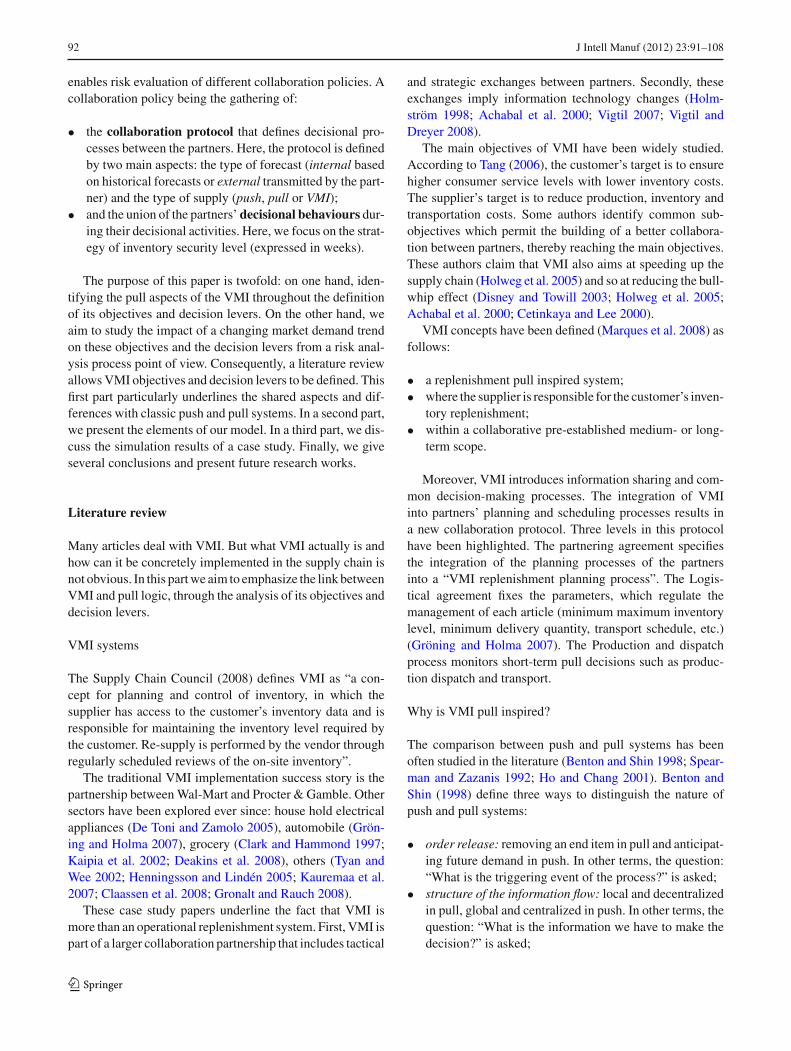
Fig. 1 The generic LogiRiskrepresentation of the supplychain actor’s planning processes

processes. In this part, we first give a general description ofthe macro processes of the tool that have been the subjectof detailed presentations in previous articles (Lamothe et al.2007; Mahmoudi 2006). Then, as VMI processes have beenimplemented in the existing models, we study the impact ofVMI implementation on these in greater detail.

Actor’s planning processes

Lamothe et al. (2007) propose a simulation tool called Logi-Risk developed in Perl language. This simulator is based ona discrete event simulation modeling approach. They haveestablished a generic representation of the different plan-ning processes (SOP, MTP, STP and L&IM) for each supplychain actor. These four planning levels could be seen accord-ing to two points of view: internal (production SOP, produc-tion MTP, …) that expresses one’s own production decisions,and external that expresses the material requirement sent tothe supplier (supply MTP, supply STP, …) or the deliverydecisions (dispatch L&IM). The Fig. 1, below summarizesthese planning processes. Dotted lines separating the differ-ent horizons illustrate the aggregation/desegregation trans-formations which are currently made in LogiRisk.

The actor’s model is centred on the strategic (SOP) and,to a lesser extent, the tactical processes (MTP). LogiRiskdoes not simulate the short-term but only makes a weeklyflow assessment in order to know, for each week, what theactors wanted to produce (STP) and what they actually pro-duced (L&IM). In the Table 2 below, we have cited the mainmodels that define each process (columns 1 and 2). Then, foreach model, we particularly underline parameters associatedto the actors’ behavior. Finally, we give main equations thattake into account these parameters. For further explanations,

we refer to Lamothe et al. (2007). In column 1, we see thatSOP and MTP use the same models. In fact, if the modelsare the same, the input data taken into account are different(granularity, originated process).

The Sales and Operations Planning (SOP) processesdetail the various decisions taken throughout long-term plan-ning. The most important outputs of these processes are theproduction capacities (production SOP) and long-term fore-cast of supply requirement (supply SOP) (see Fig. 1). Thismodel includes the products sale forecasting model. If nodemand forecast is transmitted, the production SOP processinternally computes its forecasts using simple, double, tripleor Holt and Winters Smoothing algorithm (Eq. (1) Table 2).In other cases, it sums up the forecasts transmitted by cus-tomers (Eq. (1’)). According to the demand forecasts, theworkload is computed and smoothed over several time peri-ods (Eq. (2)) in the infinite capacity net requirement model.The resulting workload defines a capacity plan that must bevalidated by the SOP manager (Eq. (3)). This latter has a spe-cific planning behavior: s/he compares the proposed capacityplan to the one validated in the previous SOP process, andaccepts a given percentage of capacity variation. From thiscapacity plan, a planned production is calculated that allowsa long term raw material procurement plan to be computed(Eqs. (4)–(8)).

The Medium-Term Planning (MTP) processes computethe estimated production release of final products, as wellas the required raw materials to order from the suppliers, orinventory levels (Eqs. (2), (4)–(8)) in function of the actor’sbehavior in term of production type (push or pull). As inthe SOP processes, the demand forecasts are either updatedinternally or aggregated from the demand forecast informa-tion received from the customers (Eqs. (1) or (1′)).

123

96 J Intell Manuf (2012) 23:91–108

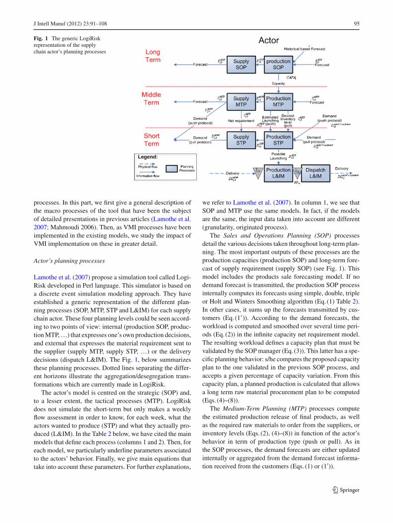
Table 2 Details of actor’s planning processes (inspired from Lamothe et al. 2007)

Processes Process models

Models Actors’ behaviorsparameters

Main equations

P. SOP,P.MTP

Products saleforecasting

Internal forecasting(and type offorecasting: F)

F pi,t = F (Historic demand f or i) (1)

with a function F: Holt and Winters algorithm, simple,double or triple smoothing

External forecasting F pi,t = ∑

Forecasts transmitted f or i (1′)P. SOP P.

MTPInfinite capacity net

requirementProducts Safety

Inventory level(SSi,t )

NRpi,t = F p

i,t+li− R Pi,t+li − I p

i,t+li −1 + SSi,t+li (2)

P. SOP Production capacitiesplan defining

Capacity variationacceptation (δ),Algorithm smooth_1

CAPAt = δ × smooth_1

({N RSOP

i,t

}i)

+(1 − δ) × previousC AP At )

(3)

P. SOP, P.MTP

Production and productsinventory levelsplanning

Production smoothingalgorithm Smooth_2

X pi,t = smooth_2

({N R p

i,t

}i, C AP At

)

(4)

I pi,t = I p

i,t−1 − F pi,t + R Pi,t + X p

i,t−li(5)

G R pj,t = X p

i,t × BO Mi, j (6)

S. SOP, S.MTP

Supply requirement andcomponent inventorylevel planning

Component SafetyStock (SS j,t )

Y pi,t = G R p

j,t+l j− R Pj,t+l j − I p

j,t+l j −1 + SS j,t (7)

I pj,t = I p

j,t−1 − G R pj,t + R Pj,t (8)

P. STP Desired productioncomputing

Push production X Di,t = X MT Pi,t (9)

Pull production X Di,t = I MT Pi,t − I i,t + Di,t (9′)

Admissible productioncomputing

X ST Pi,t = min

(X Di,t ; X Di,t∑

i X Di,t× C AP Ai,t × βi,t

)(10)

G RST Pj,t = X ST P

i,t × BO Mi, j (11)

S. STP Procurement ordercomputing

D j,t ={

Y MT Pj,t if protocol is push

G RST Pj,t + I MT P

j,t − I j,t if protocol is pull(12)

P. L&IM Effective productionlaunching

X L&I Mi,t = min

(

X ST Pi,t ; DL j,t−l j +I j,t

BO Mi, j

)

(13)

Planned receipt planning RPi,t+li = X L&I Mi,t (14)

D. L&IM Deliveries computing DLtoti,t = min

(Di,t +I −

i,t ; R Pi,t +I i,t

)

Di,t +I −i,t

(15)

DLCi,t = DL tot

i,t ×(

DCi,t + I −,C

i,t

)(16)

The Short-Term Planning (STP) and the Launch & Inven-tory Management (L&IM) processes both detail the variousshort-term decisions. The Short-Term Planning process takesinto account the calculation of the desired production release(desired production computing model), the actor’s own con-straints (i.e. breakdowns in admissible production computingmodel) and the demand sent to the suppliers (procurementorder computing model) (Eqs. (9)–(12)).

The Launch & Inventory Management process is respon-sible for taking into account the other actors’ constraints(i.e. insufficient delivery, etc.) and the products invento-ries update. It deduces the real production release andfinally the quantities to be dispatched to each customer(Eqs. (13)–(16)).

Hypothesis applied to express the models in Table 2:

– Each actor manages a single resource: the bottleneck. Pro-duction lot sizes equal to 1

– Products are considered as families as seen from the SOPprocess point of view. Each item of each actor is com-posed of one unique component.

– For a given process, all the actors use the same horizon,granularity, and replanning period. When disaggregatingplans, quantities are equitably distributed over the timebuckets of each planning period.

Notations used in the Table 2:

– i: product i.– j: component j (component of product i).

123

J Intell Manuf (2012) 23:91–108 97

– C: customer of the actor– li : production lead time of the product i (resp. component

j).– Fi : Sales Forecasted of the product i (resp. component j).– N R p

i,t : infinite capacity net requirement of product i at t,by the Process p (∈[SOP;MTP]).

–{

N R pi,t

}i: set for all products i of associated net require-

ment.– C AP At : Capacity decided for period t.– X p

i,t : Planned Production of product i (resp. componentj), for period t, by the Process p (∈[SOP;MTP;STP;L&IM]).

– R Pi,t : Planned Receipt of product i (resp. component j),for period t.

– I pi,t : Inventory level of product i (resp. component j)

planned for the end of period t, by the Processp (∈[SOP;MTP;STP;L&IM]).

– SSi,t : Safety Stock expressed in days of stock of producti (resp. component j) for period t.

– G R pi,t : Gross Requirement of product i (resp. compo-

nent j) for period t, by the Process p (∈[SOP;MTP;STP;L&IM]).

– B O Mi, j : Bill of Material link between the product i andits component j

– Y pi,t : Planned supply requirement of product i (resp. com-

ponent j) for period t, by the Process p (∈[SOP;MTP;STP;L&IM]).

– Ipi,t : Actual inventory position of product i (resp. compo-

nent j).– Di,t : Total orders of product i (resp. component j) received

by the actor for the time t.– DC

i,t : Total orders of product i (resp. component j) receivedby the actor from the customer C for the time t.

– βi,t : Availability rate of the capacity affected to the prod-uct i (resp. component j) at time t. Capacity less break-downs.

– DL toti,t : Total deliveries of product i (resp. component j)

at time t decided by the actor.– DLC

i,t : Total deliveries of product i (resp. component j)at time t decided by the actor for customer C.

– I −i,t : Total of inventory shortage of product i (resp. com-

ponent j) at time t.– I −,C

i,t : Inventory shortage of product i (resp. componentj) at time t toward customer C.

Specific notations for VMI processes (part 3.2.2.)

– VMI_min j,t VMI_ max j,t : targeted inventory min/maxfixed by a customer.

– α: supplier’s behaviour towards the interval [ min;max].– α_VMI j,t : Targeted inventory fixed by the supplier for

its SOP and MTP processes.

– Dreali,t , Dmin

i,t , Dmaxi,t : Total real/min/max requirement seen

by the supplier.– Dreal,C

i,t , Dmin,Ci,t , Dmax,C

i,t : Customer’s C real/ min/maxrequirement received by the supplier.

Collaboration processes

In this part we describe the collaboration process modelsthat are simulated by the tool. In this study three differentcollaboration protocols are implemented:

• Push: modelled by a medium-term component orders.• Pull: inspired from kanban method: short-term orders

with kanban quantity revision associated to STP process-ing.

• VMI: modelled with a medium-/ long-term agreement(LA) and a supply STP decision transfer from the cus-tomer to the supplier.

The Figs. 2–4, below, illustrate the different collaborationprocesses considered in this study. Simulation processingorder is as defined by the numbers (1 to 16 or 17).

In the next part we detail the models of processes thatare impacted by VMI implementation (shown in red in theFig. 4).

VMI impact on the strategic horizon: the min/maxcalculation

On the strategic horizon, partners have to collaborate in orderto fix the customer’s minimum and maximum inventory levelin the LA. However, in reality VMI implementation is mostof time originated by a powerful customer. In this case, thereis no effective negotiation. A true negotiated LA is not real-ized. The min/max inventory levels only include customers’constraints. The supplier has to choose a strategy between themin and the max in order to fix targeted inventory for his ownproduction SOP and MTP processes. The model integratesthis vision. In the model, for a time t, the min/max calcu-lation is only based on the customer’s long-term forecastedgross requirement for components (j), expressed as G RSOP

j,t .

This G RSOPj,t results from the customer’s production SOP

planning process. We introduce two parameters: cover_ min j

and cover_ max j . They are two coefficients applied to theG RSOP

j,t in order to obtain two levels of customer’s targetedinventory min/max.

VMI_ minj,t

=t=cover_ min j∑

t=0

G RSOPj,t couv_ min

j∈ �+ (17)

VMI_ maxj,t

=t=cover_ max j∑

t=0

G RSOPj,t couv_ max

j∈ �+ (18)

123

98 J Intell Manuf (2012) 23:91–108

Fig. 2 Push collaboration process

Fig. 3 Kanban collaboration process

Then the supplier has to express his behavior toward thismin/max level. In consequence, we introduce a parameter,expressed as α, that translates the supplier’s behavior towardsthe interval [ min;max] that it receives. This variable definesthe planned level of replenishment that the supplier wants toachieve.

α_VMI j,t = (1 − α) × VMI_ minj,t

+ α × VMI_ maxj,t

(19)

This planned level of replenishment is taken into accountin the customer’s supply SOP and MTP. It replaces the SafetyStock level in the equations (2):

SS j,t = α_VMI j,t (20)

Impact of VMI on the operational horizon: supplyand dispatch decisions

LogiRisk distinguishes three protocols

• Push: The production MTP process defines planned pro-duction under capacity constraints expressed by the pro-duction SOP process. This planned production of item i attime t is expressed as XMTP

i,t . Then, the customer’s supply

123

J Intell Manuf (2012) 23:91–108 99

Fig. 4 VMI collaboration process

MTP calculates the firm orders of component j at timet, expressed as D j,t . The Bill Of Material link between iand j is expressed as B O Mi, j . In the push protocol, D j,t

is a direct expression of supply requirement planned attime t for component j defined by the customer’s supplyMTP and expressed as Y MTP

j,t .

D j,t = Y MTPj,t (12)

Y MTPj,t integrates both real requirements related to the

market demand requirements and indirect requirementsrelated to the risk management, as referred to in part 2.2.2.

• Kanban: In kanban supply, D j,t is built thanks to theplanned inventory level of j at time t defined by the cus-tomer’s MTP (I MTP

j,t ), the customer’s actual inventory

level (I j,t ) and the production requirements transmittedby the customer’s production STP (XSTP

i,t ).

D j,t = I MTPj,t − I j , t + B O Mi, j × XSTP

i,t (12)

I MTPj,t represents the indirect requirements related to risk

management. The rest of the expression is real require-ments related to market demand.

• VMI: In VMI supply, the customer’s supply STP isreplaced by a supplier’s dispatch STP (transfer of respon-sibility). Consequently, with VMI, customers’ require-ment is not a quantity but an interval in which the supplier

can express its new degree of freedom: the delivery quan-tity. In this case, customers’ requirements comprise threevalues:

Drealj,t = B O Mi, j × XSTP

i,t − I j,t

Dminj,t = VMI_ min j,t

Dmaxj,t = VMI_ max j , t

As in kanban, we find the expression of the custom-ers’ real requirements related to market demand (Dreal

j,t ).However, indirect requirements related to risk manage-ment are not expressed by I MTP

j,t but by the results ofmin/max calculation (VMI_ min j,t and VMI_ max j,t ).In the interval characterized by the triplet (Dreal

i,t , Dmini,t ,

Dmaxi,t ) the supplier’s dispatch STP process fixes a targeted

dispatch level in order to organize the production. Thus,the Eq. (12) is replaced by the following equation:

D j,t = Drealj,t + (1 − α) × Dmin

j,t

+α × Dmaxj,t with α ∈ [0; 1] (12′)

The output of the suppliers dispatch L&IM process is adelivery quantity of i (a supplier’s item i is a customer’scomponent j) sent to the customer C at time t, expressedas DLC

i,t . The structure of the demand transmitted to thesupplier has an impact on this process:

• Push/kanban: in the initial dispatch model, the suppliercompares its actual end products inventory level and the

123

100 J Intell Manuf (2012) 23:91–108

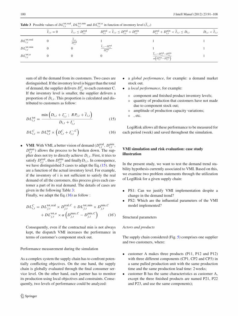
Table 3 Possible values of DL tot,reali,t , DL tot,min

i,t and DL tot,αi,t in function of inventory level (I i,t )

I i,t = 0 I i,t ≤ Dreali,t Dreal

i,t < I i,t ≤ Dreali,t + Dmin

i,t Dreali,t + Dmin

i,t < I i,t ≤ Di,t Di,t < I i,t

DL tot,reali,t 0 I i,t

Dreali,t

1 1 1

DL tot,mini,t 0 0

I i,t −Dreali,t

Dmini,t

1 1

DL tot,αi,t 0 0 0

I i,t −Dreali,t −Dmin

i,t

α(

Dmaxi,t −Dmin

i,t

) 1

sum of all the demand from its customers. Two cases aredistinguished. If the inventory level is bigger than the totalof demand, the supplier delivers DC

i,t to each customer C.If the inventory level is smaller, the supplier delivers aproportion of Di,t . This proportion is calculated and dis-tributed to customers as follow:

DL toti,t =

min(

Di,t + I −i,t ; R Pi,t + I i,t

)

Di,t + I −i,t

(15)

DLCi,t = DL tot

i,t ×(

DCi,t + I −,C

i,t

)(16)

• VMI: With VMI, a better vision of demand (Dreali,t , Dmin

i,t ,

Dmaxi,t ) allows the process to be broken down. The sup-

plier does not try to directly achieve Di,t . First, it tries tosatisfy Dreal

i,t , then Dmini,t and finallyDi,t . In consequence,

we have distinguished 5 cases to adapt the Eq. (15). theyare a function of the actual inventory level. For example,if the inventory of i is not sufficient to satisfy the realdemand of all the customers, this process gives each cus-tomer a part of its real demand. The details of cases aregiven in the following Table 3:Finally, we adapt the Eq. (16) as follow :

DLCi,t = DL tot,real

j,t × Dreal,Cj,t + DL tot,min

j,t × Dmin,Cj,t

+ DL tot,αj,t × α

(Dmax,C

j,t − Dmin,Cj,t

)(16′)

Consequently, even if the contractual min is not alwayskept, the dispatch VMI increases the performance interms of customer’s component stock out.

Performance measurement during the simulation

As a complex system the supply chain has to confront poten-tially conflicting objectives. On the one hand, the supplychain is globally evaluated through the final consumer ser-vice level. On the other hand, each partner has to monitorits production using local objectives and constraints. Conse-quently, two levels of performance could be analyzed:

• a global performance, for example: a demand marketstock out.

• a local performance, for example:

◦ component and finished product inventory levels;◦ quantity of production that customers have not made

due to component stock out;◦ amplitude of production capacity variations;◦ , etc.

LogiRisk allows all these performance to be measured foreach period (week) and saved throughout the simulation.

VMI simulation and risk evaluation: case studyillustration

In the present study, we want to test the demand trend sta-bility hypothesis currently associated to VMI. Based on this,we examine two problem statements through the utilizationof LogiRisk for a given supply chain:

• PS1: Can we justify VMI implementation despite achange in the demand trend?

• PS2: Which are the influential parameters of the VMImodel implemented?

Structural parameters

Actors and products

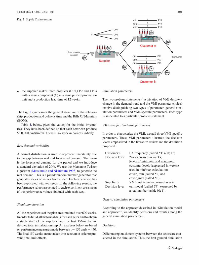
The supply chain considered (Fig. 5) comprises one supplierand two customers, where:

• customer A makes three products (P11, P12 and P12)with three different components (CP1, CP2 and CP3) ina same pulled production unit with the same productiontime and the same production lead time: 2 weeks;

• customer B has the same characteristics as customer A,except the three finished products are named P21, P22and P23, and use the same components);

123

J Intell Manuf (2012) 23:91–108 101

Fig. 5 Supply Chain structure

• the supplier makes three products (CP1,CP2 and CP3)with a same component (C) in a same pushed productionunit and a production lead time of 12 weeks.

The Fig. 5 synthesizes the general structure of the relation-ship, production and delivery time and the Bills Of Materials(BOM).

Table 4, below, gives the values for the initial invento-ries. They have been defined so that each actor can produce5,00,000 units/week. There is no work in process initially.

Real demand variability

A normal distribution is used to represent uncertainty dueto the gap between real and forecasted demand. The meanis the forecasted demand for the period and we introducea standard deviation of 20%. We use the Mersenne Twisteralgorithm (Matsumoto and Nishimura 1998) to generate thereal demand. This is a pseudorandom number generator thatgenerates series of values from a seed. Each experiment hasbeen replicated with ten seeds. In the following results, theperformance values associated to each experiment are a meanof the performance values obtained with each seed.

Simulation duration

All the experiments of the plan are simulated over 600 weeks.In order to build all historical data for each actor and to obtaina stable state of the supply chain, the first 156 weeks aredevoted to an initialization step. All analyses below are basedon performance measures made between t = 156 and t = 450.The final 150 weeks are not taken into account in order to pre-vent time limit effects.

Simulation parameters

The two problem statements (justification of VMI despite achange in the demand trend and the VMI parameter choice)involve distinguishing two types of parameter: general sim-ulation parameters and VMI-specific parameters. Each typeis associated to a particular problem statement.

VMI-specific simulation parameters

In order to characterize the VMI, we add three VMI-specificparameters. These VMI parameters illustrate the decisionlevers emphasized in the literature review and the definitionproposed:

Customer’sDecision lever

LA frequency (called S1: 4; 8; 12;24), expressed in weeks;levels of minimum and maximumcustomer levels (expressed in weeks)used in min/max calculation:cover_ min (called S2) andcover_max (called S3).

Supplier’sDecision lever

VMI coefficient expressed as α inour model (called S4), expressed bya real number inside [0; 1].

General simulation parameters

According to the approach described in “Simulation modeland approach”, we identify decisions and events among thegeneral simulation parameters.

Decisions

Different replenishment systems between the actors are con-sidered in the simulation. Thus the first general simulation

123

102 J Intell Manuf (2012) 23:91–108

Table 4 Initial inventory levelsActor Product Id Type Initial inventory

Supplier CP1 P 2,000,000



Customer A CP1 RM 84,000

Customer B CP1 RM 84,000





Customer A P11 P 334,000

Customer B P21 P 334,000





parameter is the type of supply (supply_type called G1: push;kanban; VMI).

In terms of actors’ local planning behaviors, we intro-duce a general parameter: SS_coef. It allows different safetystock levels to be simulated (expressed in weeks). We dif-ferentiate two SS_coef: for the supplier’s finished productinventory, called SS_coef_FP_S (G2: 0, 3; 0, 4) and for thecustomer’s component inventory, called SS_coef_Cpt_C(G3: 0, 2; 0, 3).

Events

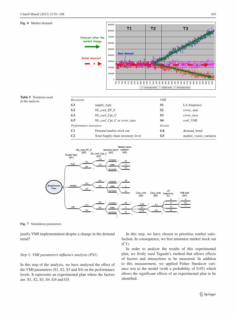
Whatever the type of replenishment, the demand market trendis always stable during a first period (t = 312). However, att = 312, we simulate three different trends (demand_trendcalled G4): increased, stable and decreased. Figure 6, below,shows the demand we have simulated and the different peri-ods we have distinguished for the analysis (T1 = [156; 291],T2 = [292; 364], T3 = [365; 450]).

We also take into account the vision of this market change:when do the actors know the market trend has changed andmodify their forecasts? In order to translate this potentiallag, we introduce a third simulation parameter expressed inweeks: the market_vision_variation (called G5: −20w; 0w;10w). It is negative if the actors know the variation before itsappearance, and positive otherwise.

The Table 5, below, summarizes the notations used:Figure 7 summarizes the experimental plan carried out. It

generates 2664 simulations.

Performance indicators

In terms of performance measurement, in this study we adoptthe supply chain point of view. The whole analysis is basedon two indicators:

• demand market stock out (called C1): for each week, wesum the quantity of orders customers have not respected(all customers and products taken into account);

• total inventory level in the chain (called C2): for eachweek, the sum of suppliers’ and customers’ componentand finished product inventories (all products and com-ponents taken into account).

Depending on the dimension of the manipulated figuresand the granularity level of our model, we round up all resultsto the nearest thousand.

Results and discussion

We have broken down the problem analysis into two mainsteps. First, we have analysed the influence of VMI param-eters faced with the two types of events in addition to realdemand variability: the trend (increased, decreased or sta-ble) and the vision of the trend change (−20, 0, 10 weeks).From this analysis, we have identified which VMI param-eters were influential, in order to make the comparisonto pull and push supply processes. This is the secondstep of the study in which we answer PS2, i.e. can we

123

J Intell Manuf (2012) 23:91–108 103

Fig. 6 Market demand

Table 5 Notations usedin the analysis Decisions VMI

G1 supply_type S1 LA frequency

G2 SS_coef_FP_S S2 cover_ min

G3 SS_coef_Cpt_C S3 cover_max

G3′ SS_coef_Cpt_C or cover_max S4 coef_VMI

Performance measures Events

C1 Demand market stock out G4 demand_trend

C2 Total Supply chain inventory level G5 market_vision_variation

Fig. 7 Simulation parameters

justify VMI implementation despite a change in the demandtrend?

Step 1: VMI parameters influence analysis (PS1)

In this step of the analysis, we have analysed the effect ofthe VMI parameters (S1, S2, S3 and S4) on the performancelevels. It represents an experimental plan where the factorsare: S1, S2, S3, S4, G4 and G5.

In this step, we have chosen to prioritise market satis-faction. In consequence, we first minimize market stock out(C1).

In order to analyze the results of this experimentalplan, we firstly used Tagushi’s method that allows effectsof factors and interactions to be measured. In additionto this measurement, we applied Fisher Snedecor vari-ance test to the model (with a probability of 0.05) whichallows the significant effects of an experimental plan to beidentified.

123

104 J Intell Manuf (2012) 23:91–108

Table 6 Results of the VMI experimental plan during T2 for G4 = increased

G5

S4 S3 S2 C1 C2

−20 0 10 −20 0 10

0 0, 2 0, 05 12,000 18,000 117,000 401,000 351,000 261,000

0, 1 11,000 16,000 110,000 430,000 378,000 283,000

0, 15 10,000 15,000 103,000 460,000 406,000 306,000

0, 3 0, 05 12,000 18,000 117,000 401,000 351,000 261,000

0, 1 11,000 16,000 110,000 430,000 378,000 283,000

0, 15 10,000 15,000 103,000 460,000 406,000 306,000

0, 5 0, 2 0, 05 11,000 15,000 107,000 445,000 392,000 294,000

0, 1 10,000 15,000 103,000 460,000 406,000 306,000

0, 15 10,000 14,000 100,000 474,000 419,000 318,000

0, 3 0, 05 10,000 14,000 100,000 474,000 419,000 318,000

0, 1 10,000 13,000 98,000 489,000 433,000 329,000

0, 15 10,000 13,000 95,000 504,000 447,000 341,000

1 0, 2 0, 05 10,000 13,000 98,000 489,000 433,000 329,000

0, 1 10,000 13,000 98,000 489,000 433,000 329,000

0, 15 10,000 13,000 98,000 489,000 433,000 329,000

0, 3 0, 05 9,000 11,000 87,000 547,000 489,000 377,000

Table 7 Results at T1G1 G2 G3′ C1 C2

Kanban 0, 3 0, 2 16,000 470,000

0, 3 14,000 519,000

0, 4 0, 2 14,000 519,000

0, 3 12,000 568,000

VMI 0, 3 0, 2 16,000 476,000

0, 3 14,000 519,000

0, 4 0, 2 14,000 525,000

0, 3 12,000 568,000

Push 0, 3 0, 2 19,000 472,000

0, 3 15,000 520,000

0, 4 0, 2 17,000 520,000

0, 3 13,000 569,000

Conclusion 1 the Fisher Snedecor variance test shows thatthe LA_frequency has no significant effect on the two perfor-mance measurements.

This result is proved by the current LA model. In themodel, the min/max calculation is imposed by the power-ful customer. No negotiation is done.

Tables 6–10 below, summarizes the results obtained forthe different experiments at T1, T2 and T3. We have ana-lysed the results for each time period: T1, T2 and T3 for

each trend. All the following conclusions are the same foreach time period and each trend.

Conclusion 2 the minimum of market stock out is obtainedfor α = 1(S4 = 1).

α (S4) translates the replenishment level chosen by thesupplier. When α is equal to 1, the supplier targets are allover maximum. Larger is the customer’s component inven-tory level; lower is level of market stock out. In consequence,we fix α = 1 in step 2.

123

J Intell Manuf (2012) 23:91–108 105

Table 8 Results at T2 for C1 (market stock out)

×1000 G5

−20 0 10

G4 G4 G4

G1 G2 G3′ Decreased Stable Increased Decreased Stable Increased Decreased Stable Increased

Kanban 0, 3 0, 2 18 15 10 17 15 15 17 15 82

0, 3 15 13 9 15 13 12 14 13 70

0, 4 0, 2 15 13 9 15 13 12 14 13 70

0, 3 13 11 8 13 11 10 13 11 61

VMI 0, 3 0, 2 18 15 10 17 15 15 17 15 82

0, 3 15 13 9 15 13 12 14 13 71

0, 4 0, 2 15 13 9 15 13 12 14 13 71

0, 3 13 11 8 13 11 10 13 11 61

Push 0, 3 0, 2 22 18 13 21 18 17 21 18 86

0, 3 17 14 10 17 14 13 16 14 73

0, 4 0, 2 19 16 11 19 16 14 18 16 74

0, 3 15 13 9 15 13 12 15 13 63

Table 9 Results at T2 for C2 (total chain inventory)

×1000 G5

−20 0 10

G4 G4 G4

G1 G2 G3′ Decreased Stable Increased Decreased Stable Increased Decreased Stable Increased

Kanban 0, 3 0, 2 417 437 519 436 437 467 489 437 335

0, 3 461 485 578 481 485 524 535 485 384

0, 4 0, 2 461 485 577 481 485 524 535 485 384

0, 3 506 535 636 527 535 582 582 535 436

VMI 0, 3 0, 2 417 437 519 437 437 466 490 437 335

0, 3 461 486 578 482 486 522 536 486 384

0, 4 0, 2 461 486 578 482 486 523 536 486 384

0, 3 506 535 636 528 535 580 583 535 436

Push 0, 3 0, 2 421 439 520 439 439 469 492 439 338

0, 3 463 486 578 483 486 525 536 486 387

0, 4 0, 2 465 487 578 484 487 526 538 487 388

0, 3 508 536 636 528 536 582 583 536 438

Conclusion 3 results C1 and C2 show that, when α = 1, theminimum target level has no effect (S2).

According to the model and the role of α in the choicemade between minimum and maximum, when α = 1 is cho-sen, any minimum target could be fixed. In consequence, wefix the minimum to 0.1 in step 2.

Conclusion 4 the effect of the maximum target (S3) is too sig-nificant to be ignored in step 2. It will be a variable of step 2.

Step 2: collaboration processes comparison (PS2)

In this stage of the analysis we seek to test the demand stabil-ity hypothesis. We therefore analysed the experimental plancomprising: G1, G2, G3, G4, G5 and S3. G3 and S3 play thesame role in the LogiRisk model: the first when G1 is pushor kanban, the second when G1 is VMI. So, in the rest of theanalysis we consider a parameter called G3’ that brings themtogether.

123

106 J Intell Manuf (2012) 23:91–108

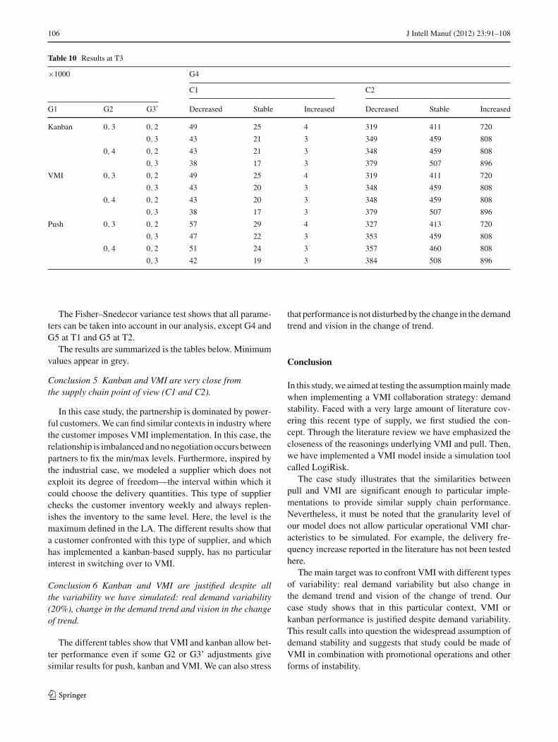
Table 10 Results at T3

×1000 G4

C1 C2

G1 G2 G3′ Decreased Stable Increased Decreased Stable Increased

Kanban 0, 3 0, 2 49 25 4 319 411 720

0, 3 43 21 3 349 459 808

0, 4 0, 2 43 21 3 348 459 808

0, 3 38 17 3 379 507 896

VMI 0, 3 0, 2 49 25 4 319 411 720

0, 3 43 20 3 348 459 808

0, 4 0, 2 43 20 3 348 459 808

0, 3 38 17 3 379 507 896

Push 0, 3 0, 2 57 29 4 327 413 720

0, 3 47 22 3 353 459 808

0, 4 0, 2 51 24 3 357 460 808

0, 3 42 19 3 384 508 896

The Fisher–Snedecor variance test shows that all parame-ters can be taken into account in our analysis, except G4 andG5 at T1 and G5 at T2.

The results are summarized is the tables below. Minimumvalues appear in grey.

Conclusion 5 Kanban and VMI are very close fromthe supply chain point of view (C1 and C2).

In this case study, the partnership is dominated by power-ful customers. We can find similar contexts in industry wherethe customer imposes VMI implementation. In this case, therelationship is imbalanced and no negotiation occurs betweenpartners to fix the min/max levels. Furthermore, inspired bythe industrial case, we modeled a supplier which does notexploit its degree of freedom—the interval within which itcould choose the delivery quantities. This type of supplierchecks the customer inventory weekly and always replen-ishes the inventory to the same level. Here, the level is themaximum defined in the LA. The different results show thata customer confronted with this type of supplier, and whichhas implemented a kanban-based supply, has no particularinterest in switching over to VMI.

Conclusion 6 Kanban and VMI are justified despite allthe variability we have simulated: real demand variability(20%), change in the demand trend and vision in the changeof trend.

The different tables show that VMI and kanban allow bet-ter performance even if some G2 or G3’ adjustments givesimilar results for push, kanban and VMI. We can also stress

that performance is not disturbed by the change in the demandtrend and vision in the change of trend.

Conclusion

In this study, we aimed at testing the assumption mainly madewhen implementing a VMI collaboration strategy: demandstability. Faced with a very large amount of literature cov-ering this recent type of supply, we first studied the con-cept. Through the literature review we have emphasized thecloseness of the reasonings underlying VMI and pull. Then,we have implemented a VMI model inside a simulation toolcalled LogiRisk.

The case study illustrates that the similarities betweenpull and VMI are significant enough to particular imple-mentations to provide similar supply chain performance.Nevertheless, it must be noted that the granularity level ofour model does not allow particular operational VMI char-acteristics to be simulated. For example, the delivery fre-quency increase reported in the literature has not been testedhere.

The main target was to confront VMI with different typesof variability: real demand variability but also change inthe demand trend and vision of the change of trend. Ourcase study shows that in this particular context, VMI orkanban performance is justified despite demand variability.This result calls into question the widespread assumption ofdemand stability and suggests that study could be made ofVMI in combination with promotional operations and otherforms of instability.

123

J Intell Manuf (2012) 23:91–108 107

However, in order to obtain more general conclusionsabout VMI we have to explore other research axes. On theone hand, in term of modeling improvement:

• model negotiation in the LA. The actors have to organizea shared and common planning which is used to parame-terize the customer’s inventory min/max level. This com-mon plan is built around exchanges between the partners.The customer expresses its component requirement plan.The supplier gives a delivery plan. Each actor includesits constraints in its plan. The modelling of this commonplan could rest on the collaboration planning proposed byDudek and Stadtler (2005) based on an exchange processthat help to achieve convergence between each actors’point of view.

• model utilization of the supplier’s degree of freedom interms of delivery quantities. In other terms, authorize avariation of α over time.

These improvements could help us to analyze another VMIaspect: backing up of stocks from the customer to the supplierwarehouse, as reported by Blatherwick (1998).

On the other hand we need to confront VMI with othersources of variability. Thus we also plan to:

• simulate different real demand variability;• study the cumulative effects of increase and decrease

instead of simple increase or decrease;• analyse the effects of actors’ internal constraints: break-

down, quality level, etc.• analyse the effects of external events as strikes, disasters,

etc.

References

Achabal, D., McIntyre, S., Smith, S., & Kalyanam, K. (2000). Adecision support system for Vendor Managed Inventory. Journalof Retailing, 76(4), 430–454.

Benton, W., & Shin, H. (1998). Manufacturing planning and control:The evolution of MRP and JIT integration. European Journal ofOperational Research, 110(3), 411–440.

Blatherwick, A. (1998). Vendor Managed Inventory fashion fad impor-tant supply chain strategy. Supply Chain an International Jour-nal, 3(1), 10–11.

Cetinkaya, S., & Lee, C. (2000). Stock replenishment and shipmentscheduling for Vendor Managed Inventory systems. ManagementScience, 46(2), 217–232.

Claassen, M. J. T., Van Weele, A. J., & Van Raaij, E. M. (2008). Per-formance outcomes and success factors of Vendor ManagedInventory (VMI). Supply Chain Management: An InternationalJournal, 13(6), 406–414.

Clark, T. H., & Hammond, J. H. (1997). Reengineering channel reor-dering processes to improve total supply-chain performance. Pro-duction and Operations Management, 6(3), 248–265.

De Toni, A. F., & Zamolo, E. (2005). From a traditional replenishmentsystem to vendor-managed inventory: A case study from thehousehold electrical appliances sector. International Journal ofProduction Economics, 96(1), 63–79.

Deakins, E., Dorling, K., & Scott, J. (2008). Determinants of successfulVendor Managed Inventory practice in oligopoly industries. Inter-national Journal of Integrated Supply Management, 4(3/4), 355–377.

Disney, S. M., & Towill, D. R. (2003). The effect of VendorManaged Inventory (VMI) dynamics on the Bullwhip Effectin supply chains. International Journal of Production Econom-ics, 85(2), 199–215.

Dong, Y., Xu, K., & Dresner, M. (2007). Environmental determi-nants of VMI adoption: An exploratory analysis. TransportationResearch Part E, 43, 355–369.

Dudek, G., & Stadtler, H. (2005). Negotiation based collaborativeplanning between supply chains partners. European Journal ofOperational Research, 163, 668–687.

Gaury, E. G. A., Pierreval, H., & Kleinjnen, J. P. C. (2000). An evolu-tionary approach to select a pull system among Kanban, Conwipand Hybrid. Journal of Intelligent Manufacturing, 11(2), 157–167.

Gronalt, M., & Rauch, P. (2008). Vendor Managed Inventory in woodprocessing industries—a case study. Silva Fennica, 42(1), 101–114.

Gröning, A., & Holma, H. (2007). Vendor Managed Inventory, prep-aration for an implementation of a pilot project guidance for anupcoming evaluation at Volvo. Master’s thesis. Lulea Universityof technology.

Henningsson, E., & Lindén, T. (2005). Vendor Managed Inventory:Enlightening benefits and negative effects of VMI for Ikea andits suppliers. Master’s Thesis. Lulea University of Technology.

Ho, J. C., & Chang, Y. L. (2001). An integrated MRP andJIT framework. Computers and Industrial Engineering, 41(2),173–185.

Holmström, J. (1998). Business process innovation in the sup-ply chain—a case study of implementing Vendor ManagedInventory. European Journal of Purchasing and Supply Manage-ment, 4(2–3), 127–131.

Holweg, M., Disney, S., Holmström, J., & Smarös, J. (2005). Sup-ply chain collaboration: Making sense of the strategy contin-uum. European Management Journal, 23(2), 170–181.

Ireland, R.K., & Crum, C. (2005). Supply chain collaboration, how toimplement CPFR and other best collaborative practices. J. Rosspublishing and APICS (p. 206).

Ip, W. H., Huang, M., Yung, K. L., Wang, D., & Wang, X. (2007). CON-WIP based control of a lamp assembly production line. Journalof Intelligent Manufacturing, 18(2), 261–271.

Kaipia, R., Holmström, J., & Tanskanen, K. (2002). VMI What areyou losing if you let your customer place orders?. ProductionPlanning and Control, 13(1), 17–25.

Kaipia, R., & Tanskanen, K. (2003). Vendor managed categorymanagement—an outsourcing solution in retailing. Journal ofPurchasing and Supply Management, 9, 165–175.

Kauremaa, J., Småros, J., & Holmström, J. (2007). Empirical evalua-tion of VMI: Two ways to benefit. In Proceedings of NOFOMA2007.

Kuk, G. (2004). Effectiveness of Vendor Managed Inventory in theelectronics industry: Determinants and outcomes. Informationand Management, 41, 645–654.

Lamothe, J., Mahmoudi, J., & Thierry, C. (2007). Cooperation toreduce risk in a telecom supply chain, special issue managingsupply chain risk. Supply Chain Forum: An International Jour-nal, 8(2), 36–53.

Mahmoudi, J. (2006). Simulation et gestion des risques en planificationdistribuée de chaînes logistiques: Application au secteur del’électronique et des télécommunications. PhD. Ecole NationaleSupérieure de l’Aéronautique et de l’Espace.

Marques, G., Lamothe, J., Thierry, C., & Gourc, D. (2008). VendorManaged Inventory, from concept to processes, for a supply chaincollaborative approach. International Conference on Information

123

108 J Intell Manuf (2012) 23:91–108

Systems, Logistics and Supply Chain, Madison, United-States,May 2008.

Matsumoto, M., & Nishimura, T. (1998). Mersenne twister: A 623-dimensionally equidistributed uniform pseudorandom numbergenerator. ACM Transactions on Modeling and Computer Simu-lation, 8(1), 3–30.

ODETTE. (2004). Vendor Managed Inventory (VMI) (version 1.0).Rusdiansyah, A., & Tsao, D. (2005). Coordinating deliveries and

inventories for supply chain under Vendor Managed Inventorysystem. JSME International Journal, 48(2), 85–90.

Smaros, J., Lethonen, J. M., Appelqvist, P., & Holmstrom,J. (2003). The impact increasing demand visibility productioninventory control efficiency. International Journal of PhysicalDistribution and Logistics Management, 33(4), 336–354.

Spearman, M. L., & Zazanis, M. A. (1992). Push and pullproduction systems: Issues and comparisons. OperationsResearch, 40(3), 521–532.

Tang, C. (2006). Perspectives in supply chain risk management. Inter-national Journal of Production Economics, 103, 451–488.

Tyan, J., & Wee, H. (2002). Vendor Managed Inventory: A surveyof the Taiwanese grocery industry. Journal of Purchasing andSupply Management, 9(1), 11–18.

Vigtil, A. (2007). Information exchange in Vendor Managed Inven-tory. International Journal of Physical Distribution and LogisticsManagement, 37(2), 131–147.

Vigtil, A., & Dreyer, H. (2008). Critical aspects of information andcommunication technology in Vendor Managed Inventory. Leanbusiness systems and beyond, 257 (pp. 443–451). Berlin: IFIPInternational Federation for Information Processing, Springer.

Yao, Y., & Dresner, M. (2007). The inventory value of informa-tion sharing, continuous replenishment, and vendor-managedinventory. Transportation Research Part E: Logistics and Trans-portation Reviews. (in press, corrected proof, available online 9April 2007).

Yao, Y., Evers, P., & Dresner, M. (2007). Supply chain inte-gration in vendor-managed inventory. Decision Support Sys-tems, 43(2), 663–674.

123

A supply chain performance analysis of a pull inspired supply strategy faced to demand uncertainties

Documents

Transcript of A supply chain performance analysis of a pull inspired supply strategy faced to demand uncertainties