A substructured FE-shell/XFE-3D method for crack analysis in thin-walled structures

INTERNATIONAL JOURNAL FOR NUMERICAL METHODS IN ENGINEERINGInt. J. Numer. Meth. Engng 2007; 72:757–779Published online 14 March 2007 in Wiley InterScience (www.interscience.wiley.com). DOI: 10.1002/nme.2029

A substructured FE-shell/XFE-3D method for crackanalysis in thin-walled structures

E. Wyart1,∗,†, D. Coulon1, M. Duflot1, T. Pardoen2, J.-F. Remacle3 and F. Lani1

1CENAERO, Avenue J. Mermoz 30, Gosselies B-6041, Belgium2Department of Materials and Processes Sciences, Universite catholique de Louvain,

Louvain-la-Neuve B-1348, Belgium3Department of Civil Engineering, Universite catholique de Louvain, Louvain-la-Neuve B-1348, Belgium

SUMMARY

Stress intensity factors in thin-walled cracked structures are computed using a mixed-dimensional finiteelement (FE) shell/extended finite element (XFE) 3D formulation. The present approach belongs to thefamily of ‘substructuring’ methods. The domain is decomposed into cracked and safe subdomains whichare solved by the XFE-code and the FE-software, respectively. The XFE-3D domain may contain cracksthat do not necessarily join the top and bottom faces of the plate. The interface problem is solved usingthe finite element tearing and interconnecting method. Several validations are provided. Copyright q 2007John Wiley & Sons, Ltd.

Received 6 November 2006; Revised 25 January 2007; Accepted 5 February 2007

KEY WORDS: X-FEM; FETI; domain decomposition; crack analysis; mixed dimensional; thin-walledstructure

1. INTRODUCTION

Various shell and plate formulations are currently used to simulate the response of large thin-walled structures (e.g. outer skin of fuselage, leading edge, etc.) [1] in the frame of the finiteelement method (FEM). Compared with complete 3D simulations, a shell-type formulation limitsthe number of degrees of freedom in an elegant manner, leading to a reasonable computational cost,while keeping a good accuracy. However, most shell formulations prevent incorporating defectssuch as cracks, except for particular plane configurations.

∗Correspondence to: E. Wyart, CENAERO, Avenue J. Mermoz 30, Gosselies B-6041, Belgium.†E-mail: [email protected]

Contract/grant sponsor: Walloon Region and FEDER European funds; contract/grant number: EP1A122030000102

Copyright q 2007 John Wiley & Sons, Ltd.

758 E. WYART ET AL.

In thin-walled structures, out-of-plane effects frequently require the use of a 3D model androbust dedicated methods in order to properly capture the details of the 3D crack-tip conditions[2]. Recently, complex 3D crack analyses have been made possible, thanks to significant progressachieved in the field of computational fracture mechanics. Recent industrial benchmarking analyseshave involved the computation of stress intensity factors and the prediction of crack paths usingadvanced numerical methods such as the mesh-less or mesh-free methods [3], the eXtended FiniteElement Method (XFEM) [4], the Generalized Finite Element Method [5]. These methods havebeen developed to solve singularity and/or discontinuity problems without the need of buildinga conforming mesh. Among them, the XFEM [4] is particularly suited for fracture mechanicsproblems, even for complex 3D cracked configurations [6–8], and is probably the closest tointegration in industrial procedures of crack analysis.

Though a generally admitted trend suggests to treat the cracked regions as 3D models, severalinteresting attempts aiming at incorporating the crack in particular plate and shell formulations usingthe partition of unity method (PUM) are worth being mentioned. Dolbow and co-workers [9] firstintroduced an enriched Reissner–Mindlin plate element. In a recent paper, Areias and Belytschko[10] presented a new XFE-shell formulation also valid for non-linear problems. Nevertheless,

• the 3D effects of the crack cannot be accounted for,• these XFE-shell formulations are restricted to through-the-thickness cracks which are normalto the mid-surface,

• each FE-shell requires the development of the corresponding XFE formulation.

For the study of delamination in hybrid laminates, Remmers et al. discretized the whole structurewith solid-like shell [11] elements that incorporate cracks at material interfaces by means of thePUM.

Coupling XFE- and FE-domains using a substructuring method was first proposed by Bordas andMoran [12]. In this method, the FE-domain is treated as a super-element. The degrees of freedomand the right-hand side of the FE-domain are reduced on the boundary of the XFE-domain. Thebottleneck of the method concerns the generation of the reduced stiffness matrix of the super-element. Moreover, the computed Schur complement is a dense matrix whose size is, in somecircumstances, not negligible and can make the resolution of the total system more difficult. Besidethis, the super-element is reserved to parts that remain in the linear elastic regime. Nevertheless,super-element can be used in materially non-linear analysis as long as the super-element doesnot contain material that yields plastically. Though not rigorous, the use of super-element ingeometrically non-linear analyses is possible in most commercial FE-software, thanks to simpleworkarounds. Note that Bordas and co-workers focused on a complex fully 3D structure but didnot extend the approach to a problem with mixed dimensions.

Another strategy for managing FE- and XFE-domains consists in introducing the X-FEM at thelocal scale following a multiscale strategy. The method is called the multiscale eXtended finiteelement method (MS-XFEM) [13, 14]. In this method, the global domain is decomposed into twooverlapping subdomains and two levels of computation are involved: the macroscopic and themicroscopic levels. In the first subdomain, the mesh is sufficiently refined for capturing the localeffect due to the crack (this is the micro-scale), while in the second subdomain, the mesh remainsunchanged (this is the macro-scale). The multiscale problem is solved using an homogenizationtechnique [15] where a projection operator is used to transfer the solution from the micro- to themacro-level. This method allows for non-conforming interfaces and has been validated for 2Dproblems.

Copyright q 2007 John Wiley & Sons, Ltd. Int. J. Numer. Meth. Engng 2007; 72:757–779DOI: 10.1002/nme

A SUBSTRUCTURED FE-SHELL/XFE-3D METHOD FOR CRACK ANALYSIS 759

In this work, a substructured FE-shell/XFE-3D formulation is proposed. The FE-domain isdiscretized with shell elements while the XFE-domain is modelled with 3D solid elements. Themixed-dimensional formulation is more convenient than a full XFE-3D formulation because itreduces the computational cost. The compatibility of the displacement through the interface isensured using the Reissner–Mindlin formalism.

This method is based on the substructured finite element/eXtended finite element (S-FE/XFE)method [16] which has been proposed for 3D crack analysis. The S-FE/XFE method consists indecomposing the geometry into safe FE-domains and cracked XFE-domains. The interface problemis solved by the finite element tearing and interconnecting (FETI) method [17]. The S-FE/XFEmethod permits to recover most of the tools developed in the FE-software (particular boundarycondition, material law, formulation, etc.). Complex cracked configurations can be treated using alimited number of assumptions about the XFE-domain.

Section 2 provides the basis of the X-FEM and of the level set method. The S-FE/XFE method isexplained in Section 3. The S-FE/XFE introducing shells in the domain treated by the FE-softwareis described in Section 4. Details on the constraint equations used to ensure the compatibilitybetween the FE-shell and the XFE-3D domains are given in Section 4.3. The numerical validationis given in Section 5.

2. THEORETICAL BACKGROUND

2.1. The eXtended finite element method (X-FEM)

The X-FEM [4] is based on the PUM [18]. The X-FEM allows for introducing a priori knowledgeof the solution into the FE-formulation. As a consequence of the PUM, conforming meshes arenot required. Considering fracture mechanics problems where a crack must be incorporated intothe formulation, the XFE approximation of the displacement writes

uh(x)= ∑i∈I

ui�i (x) + ∑j∈J

b j� j (x)H(x) + ∑k∈K

�k(x)4∑

l=1clk F

l(x) (1)

where

• �i is the shape function associated to node i ,• I is the set of all nodes of the domain,• J is the set of nodes whose the shape function support is cut by a crack,• K is the set of nodes whose the shape function support contains the crack front,• ui are the classical degrees of freedom (i.e. displacement) for node i ,• b j account for the jump in the displacement field across the crack at node j . If the crack isaligned with the mesh, b j represent the opening of the crack,

• H(x) is the Heaviside function,• clk are the additional degrees of freedom associated with the crack-tip enrichment functions

Fl ,• Fl is an enrichment which corresponds to the four asymptotic functions in the developmentexpansion of the crack-tip displacement field in a linear elastic solid [19].

An appropriate choice of the set of nodes to be enriched with the terms coming from the LEFMcan lead, in some circumstances, to an increase of the convergence rate [20, 21].


760 E. WYART ET AL.

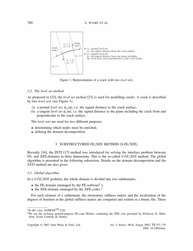
Figure 1. Representation of a crack with two level sets.

2.2. The level set method

As proposed in [22], the level set method [23] is used for modelling cracks. A crack is describedby two level sets (see Figure 1):

(i) a normal level set, �n(x), i.e. the signed distance to the crack surface;(ii) a tangent level set �t (x), i.e. the signed distance to the plane including the crack front and

perpendicular to the crack surface.

The level sets are used for two different purposes:

• determining which nodes must be enriched;• defining the domain decomposition.

3. SUBSTRUCTURED FE/XFE METHOD (S-FE/XFE)

Recently [16], the FETI [17] method was introduced for solving the interface problem betweenFE- and XFE-domains in three dimensions. This is the so-called S-FE/XFE method. The globalalgorithm is presented in the following subsection. Details on the domain decomposition and theFETI method are also given.

3.1. Global algorithm

In a S-FE/XFE problem, the whole domain is divided into two subdomains:

• the FE-domain (managed by the FE-software‡ );• the XFE-domain (managed by the XFE-code).§

For each element of a subdomain, the elementary stiffness matrix and the localization of thedegrees of freedom in the global stiffness matrix are computed and written in a binary file. These

‡In this case, SAMCEFTM [24].§We use the in-house general-purpose FE-code Morfeo containing the XFE core provided by Professor N. Moesfrom ‘Ecole Centrale de Nantes.’



Figure 2. Communications between the FETI solver, the host FE-code and the S-FE/XFE library for thesolution of the global boundary value problem.

information are read by the FETI-code which assembles the local stiffness matrices and solvesthe global interface system. Finally, the solution is transferred back to the S-FE/XFE library thatcomputes the stress intensity factors by the equivalent domain integral method (EDI) [25]. TheEDI method is based on the interaction integral method [26].

The global resolution algorithm is summarized in Figure 2.

3.2. Domain decomposition

The decomposition is based on the level set values stored at the nodes of the mesh. The size ofthe XFE-domain is such that the domain used for the computation of the J-integral belongs to theXFE-domain. The interface of the subdomain must not include enriched degrees of freedom. Thiscondition ensures the compatibility between the FE- and the XFE-domains as the FE-softwarecannot deal with enriched degrees for freedom. This type of decomposition minimizes the compu-tational time associated with the sequential generation of the stiffness matrix of the XFE-domain.

Consequently, the computational load is not properly balanced between the processor assignedto the FE-domain and the processor assigned to the XFE-domain. Properly balanced loads areachieved by the decomposition of the FE- and the XFE-domains into smaller subdomains.

3.3. Solution of the interface problem

In this subsection, the basic concepts of the FETI method described in [27] are recalled.The FETI method has been developed to handle and solve large-scale problems. FETI allows

both parallel and sequential computation schemes. According to [28], computational time andmemory requirements are, respectively, one to two orders of magnitude lower than those of adirect solver. The whole domain is divided into several substructures. The problem is reduced toan interface problem.


762 E. WYART ET AL.

Let us consider a domain �. The condition of static equilibrium writes

Ku= f (2)

where K is the stiffness matrix (symmetric semi-definite positive) on the domain �,u is the nodaldisplacement vector and f is the force vector. The domain � is divided into Ns non-overlappingsubdomains �s . The FETI method consists in replacing Equation (2) by

K(s)u(s) = f (s) − B(s)Tk with s = 1, . . . , Ns (3)

� =Ns∑s=1

B(s)u(s) = 0 (4)

where K(s) and f (s) are the contributions from the subdomain �(s) to K and f, respectively, kis a vector of Lagrange multipliers, and B(s) is a signed boolean matrix which accounts for thelocalization of the degrees of freedom on the interface.

Lagrange multipliers are introduced to enforce continuity of the displacements on the boundary�(s) of the subdomain (i.e. �= 0 on �(s)). Generally, a mesh partition can contain N f �Ns floatingsubstructures (i.e. substructures with an insufficient number of essential boundary conditions toavoid kinematic modes in the matrix K(s)).

The general solution for a floating subdomain is given by

u(s) =K(s)+(f (s) − B(s)Tk) + R(s)a(s) (5)

where K(s)+ is a generalized inverse of K(s), R(s) =Ker(K(s)) is the kernel of K(s) (the rigid bodymodes) and a is a vector containing the intensity of the rigid body modes of K(s). Equation (3)admits a solution if and only if the right-hand side is orthogonal to Ker(K(s)). This statementmeans that the forces cannot excite the rigid modes of the subdomain.

These considerations lead to the interface problem⎡⎣ FI −GI

−GTI 0

⎤⎦

[k

a

]=

[d

−e

](6)

where

FI =Ns∑s=1

B(s)K(s)+B(s)T

GI = [B(1)R(1) . . . B(N f )R(N f )]aT = [a(1)T . . . a(N f )T]T

d=Ns∑s=1

B(s)K(s)+f (s)

eT = [R(1)f (1)T . . . R(N f )f (N f )T]T

(7)

The global interface problem is solved by a projected conjugate gradient (PCG) method [29].



4. SUBSTRUCTURED SHELL-3D FINITE ELEMENT MODEL

The novelty in the present works is to combine the solution of a 3D fracture mechanics problem onthe XFE-domain coupled with a FE-domain modelled with shells. The method consists in generatinga 3D tetrahedral mesh for the XFE-domain. The interface compatibility must be ensured in orderto obtain accurate displacement and stress fields in both subdomains. In the next subsections, the3D mesh generation and the compatibility equations between the FE-shell and the 3D domain arepresented.

4.1. Generation of the 3D mesh on the XFE-domain

The 3D mesh is created on the basis of the 2D-shell discretization as follows:

(i) the 2D shell mesh is extruded, in such a way as to provide a 3D mesh of hexahedra;(ii) the hexahedra are divided into tetrahedra (this step is called simplexation);(iii) the 3D mesh is refined around the crack front. Since the element size being controlled by

the initial 2D shell mesh, the extruded and simplexed 3D meshes could be too coarse toaccurately resolve the fracture mechanics problem.

The mesh utilities are based on the open-source library AOMD [30].

4.1.1. Extrusion of the hexahedron-based mesh. The first key point of the extrusion process is thecomputation of an average normal at each vertex of the original 2D shell mesh. At this point, theaverage normal ni at node i is computed as

ni =∑

e∈E ne�e∑e �e

(8)

where E is the support of the node i, ne is the normal attached to the shell element e and �e isthe area of the shell element e.

The original 2D shell mesh constitutes the mid-surface of the future 3D mesh so that theextrusion must be performed on both sides in order to provide the upper and lower fibres. Otherassumptions could be made in order to account for the eccentricity of the original shell elements.

The extruded mesh is composed of several layers of hexahedra. The second key point of thisextrusion process is the determination of the number of layers. Indeed, the thickness of the layersmust be related to the characteristic length of the original shell elements in order to ensure areasonable aspect ratio.

The mesh refinement (see below) executed after the simplexation step can improve the qualityof the mesh. Figure 3 shows the extruded mesh (from the mid-surface to the upper fibre).

4.1.2. Simplexation of the generated hexahedra into tetrahedra. The current version of our XFE-code and of its crack-analysis package are based on linear tetrahedral elements. Hexahedra mustbe divided into tetrahedra.

Though it is possible to divide a hexahedron without creating new vertices, it usually leads tothe occurrence of spurious stress at the interface between the subdomains due to mesh orientationeffects. In order to minimize these effects, new vertices are created (one at the centre of each faceof the hexahedron, one at the centre of the hexahedron) so that each hexahedron is divided into24 tetrahedra. Figure 4 shows the simplexed mesh.


764 E. WYART ET AL.

Figure 3. Extrusion of the hexahedron mesh from original 2D shell mesh as the mid-surface.

Figure 4. Simplexation of a hexahedron into tetrahedra.

The tetrahedral mesh generated by simplexation suffers from minor mesh orientation effectsonly. These effects are reduced by further mesh refinement operations.

4.1.3. Mesh refinement. The element size being controlled by the initial 2D shell mesh, theextruded and simplexed 3D meshes could be too coarse to accurately resolve the fracture mechanicsproblem. Further mesh refinement is thus needed. Mesh refinement operations answer the followingconditions and requirements:

(i) in order to preserve matching interfaces, the element face on the lateral boundary of theXFE-3D subdomain remain unaffected;

(ii) the elements at the crack front must be small enough in order to accurately capture thestress field and to enable proper computation of the stress intensity factors;

(iii) poorly conditioned elements (in terms of aspect ratio) must be avoided.

4.2. Interface compatibility

Several techniques have been developed in order to handle models using elements ofdifferent dimensions. These techniques differ in mathematical complexity, constraining effect,



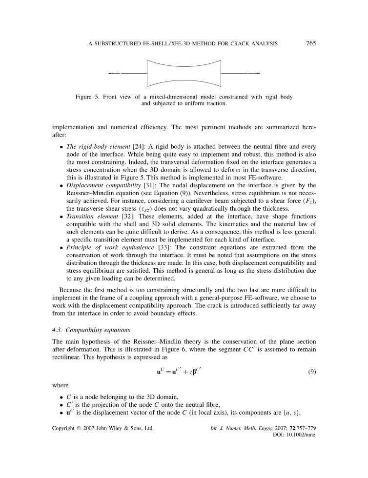
Figure 5. Front view of a mixed-dimensional model constrained with rigid bodyand subjected to uniform traction.

implementation and numerical efficiency. The most pertinent methods are summarized here-after:

• The rigid-body element [24]: A rigid body is attached between the neutral fibre and everynode of the interface. While being quite easy to implement and robust, this method is alsothe most constraining. Indeed, the transversal deformation fixed on the interface generates astress concentration when the 3D domain is allowed to deform in the transverse direction,this is illustrated in Figure 5. This method is implemented in most FE-software.

• Displacement compatibility [31]: The nodal displacement on the interface is given by theReissner–Mindlin equation (see Equation (9)). Nevertheless, stress equilibrium is not neces-sarily achieved. For instance, considering a cantilever beam subjected to a shear force (Fz),the transverse shear stress (�xz) does not vary quadratically through the thickness.

• Transition element [32]: These elements, added at the interface, have shape functionscompatible with the shell and 3D solid elements. The kinematics and the material law ofsuch elements can be quite difficult to derive. As a consequence, this method is less general:a specific transition element must be implemented for each kind of interface.

• Principle of work equivalence [33]: The constraint equations are extracted from theconservation of work through the interface. It must be noted that assumptions on the stressdistribution through the thickness are made. In this case, both displacement compatibility andstress equilibrium are satisfied. This method is general as long as the stress distribution dueto any given loading can be determined.

Because the first method is too constraining structurally and the two last are more difficult toimplement in the frame of a coupling approach with a general-purpose FE-software, we choose towork with the displacement compatibility approach. The crack is introduced sufficiently far awayfrom the interface in order to avoid boundary effects.

4.3. Compatibility equations

The main hypothesis of the Reissner–Mindlin theory is the conservation of the plane sectionafter deformation. This is illustrated in Figure 6, where the segment CC ′ is assumed to remainrectilinear. This hypothesis is expressed as

uC =uC′ + zbC

′(9)

where

• C is a node belonging to the 3D domain,• C ′ is the projection of the node C onto the neutral fibre,• uC is the displacement vector of the node C (in local axis), its components are {u, v},


766 E. WYART ET AL.

Figure 6. Displacement of a node in the Reissner–Mindlin theory.

Figure 7. Relation between the shear angle b and the real rotation h.

• z represents the distance between the node C and the neutral fibre. For a thick shell, theposition of the neutral fibre depends on the curvature of the shell. As a consequence, theneutral fibre must be offset from the mid-surface (see Section 4.3.1),

• bC ′is the shear angle of the section (in local axis). The relationship between bC

′and the real

rotations write

�C′

x = �C′

y

�C′

y = −�C′

x

(10)

as depicted in Figure 7.

Equations (9) and (10) lead to

uC = uC′ + z�C

′y

vC = uC′ − z�C

′x

(11)

In the following subsections, details are given about the neutral fibre offset and the constraintequations.



Figure 8. For a curved section, the neutral fibre does not correspond to the mid-surface.

4.3.1. Neutral fibre offset. For a thick shell, the position of the neutral fibre depends on thecurvature of the shell. The neutral fibre does not correspond to the mid-surface from which the3D mesh has been extruded (Figure 8).

The position of the neutral fibre coincides with the centre of gravity of the section:

xG =∫� xM d�∫

� d�(12)

where xG is the position of the centre of gravity, xM is the position of a given point and � is thevolume. Considering n layers of element, Equation (12) becomes

xG =∑n

i=0

∫�i

xM d�i∑ni=0

∫�i

d�i(13)

The determination of the correct position of the centre of gravity in non-planar extruded meshesdepends on the mesh refinement level: for instance, in the case of a cylinder, a coarse mesh couldlead to a poor estimate of the position of the centre of gravity because the curvature is not wellcaptured.

4.3.2. Constraint equations. The interface constraint equations link the solid degrees of freedom(three translation degrees of freedom) to the shell degrees of freedom (three translation and tworotation degrees of freedom). The starting point of these constraint equations is the compatibilityequation (11) which is valid in the local co-ordinates system attached to each shell element (smallletters). To be consistent with the global equilibrium equations, Equation (11) must be re-writtenin the global co-ordinates system (capital letters), common to the FE- and the XFE-codes, for eachshell element at the interface. So the degrees of freedom uC , vC , �

C ′x and �C

′y in Equation (11) are

replaced by the expressions formulated in the global co-ordinates system given by the followingequations:

uC = cos(x, X)UC + cos(x,Y )VC + cos(x, Z)WC

vC = cos(y, X)UC + cos(y,Y )VC + cos(y, Z)WC(14)


768 E. WYART ET AL.

Figure 9. Interface shell–solid. The node C ′ represent the projection of the node C on theedge A–B. The displacement of the node C is given by the interpolations of the displacement

and the shear angle of the nodes A and B in C ′.

uC′ = cos(x, X)UC ′ + cos(x,Y )VC ′ + cos(x, Z)WC ′

vC′ = cos(y, X)UC ′ + cos(y,Y )VC ′ + cos(y, Z)WC ′ (15)

�C′

x = cos(x, X)�C ′X + cos(x,Y )�C ′

Y + cos(x, Z)�C ′Z

�C′

y = cos(y, X)�C ′X + cos(y,Y )�C ′

Y + cos(y, Z)�C ′Z

(16)

This leads to a first set of constraint equations for the interfaces nodes of which the projectionon the mid-surface coincides with nodes of the shell mesh. The degrees of freedom of a node Cof which the projection C ′ does not coincide with a node of the 2D shell mesh (see Figure 9) areinterpolated as follows:

uC′ = NA(C ′)uA + NB(C ′)uB (17)

hC′ = NA(C ′)hA + NB(C ′)hB (18)

where A and B are the nodes of the edge on which C ′ is projected.The constraint equations for all the nodes of the interface are assembled in a matrix L. The

stiffness matrix associated to the XFE-domain can be written as⎡⎢⎢⎣KXX KXI 0

KIX KII L

0 L 0

⎤⎥⎥⎦

⎡⎢⎢⎣

uX

uI

kXFE3D

⎤⎥⎥⎦ =

⎡⎢⎢⎣fX

fI

0

⎤⎥⎥⎦ (19)



where

• KXX is the stiffness matrix associated with the internal degrees of freedom of the XFE-domain,• KIX and KXI are the stiffness matrices linking the interfacial and internal (XFE-domain)degrees of freedom,

• KII is the stiffness matrix associated with the interfacial degrees of freedom,• L are the coefficients of the constraint equations,• uX are the degrees of freedom associated with the XFE-domain,• uI are the boundary degrees of freedom composed of UC , uC , UC ′

, uC′, HC ′

, hC′,

• kXFE3D are the Lagrange multipliers related to the constraint equations,• fX are the forces associated with the XFE-domain,• fI are the boundary forces.

System (19) is poorly conditioned. Indeed, the values of the components of the matrix L arerelatively small compared to those of the matrix K. In order to ensure a better conditioning of theglobal matrix, the matrix L should be multiplied by a scaling factor, e.g. defined as the product ofYoung’s modulus and the average volume of the element contained in the XFE-domain.

4.4. Fixation of the local �z

The usual local degrees of freedom for a shell formulation are {u, v, w, �x , �y}. The local �z isnot used and no stiffness is associated with this degree of freedom. In Equation (16), �x and �yare related to the three global rotations �X , �Y and �Z . One rotation is then in excess. As aconsequence, each constraint equation involving the rotation degrees of freedom induces a nullpivot in the local matrix of the XFE-domain.

For a large interface, the number of null pivots increases and the problem becomes unsolvable.Indeed, for each null pivot, a projection direction is computed for the projected conjugate gradient(PCG) algorithm. This increases dramatically the computation time by slowing down convergence.

Even if the size of the interface is small, it is more judicious to fix the local �z of each interfacenode. The computational time is minimized owing to improved convergence of the PCG. A newequation expressing �z as a function of �X , �Y and �Z must thus be added to the set of constraintequations for each node of the interface:

�z = cos(z, X)�X + cos(z, Y )�Y + cos(z, Z)�Z = 0 (20)

This equation allows fixing �z along the interface.

4.5. Consistency of the transition between the 2D shell and 3D domains

Particular attention must be paid to the transition between the 2D shell domain and the 3D domainwhen using the FETI method. First, the numbering of the degrees of freedom must be consistent:the translation degrees of freedom of the 3D domain are numbered in such a way as to includedummy rotational degrees of freedom. These dummy degrees of freedom are not assembled in theglobal stiffness matrix. Second, the present implementation of the S-FE/XFE method does notallow for the introduction of constraint equations accounting for non-conforming meshes at theinterface, as already proposed in [34, 35]. In the context of the present implementation, the 3Dmesh is designed so that the nodes of the mid-surface at the interface coincide with those of the2D shell mesh.


770 E. WYART ET AL.

5. NUMERICAL VALIDATIONS

The first validation case consists of a plane shell mesh containing an inclined traversing cracksubjected to uniform traction. The second validation case involves a hollow cylinder containing acircumferential crack subjected to various loading conditions. The third validation case concernsa plane shell with a non-traversing edge crack subjected to a four points bending test. The fourthvalidation case involved the bending of a square plate containing a semi-circular crack. Analyticalsolutions exist for the first three configurations [36] while the fourth case is compared with areference solution [37].5.1. Plane shell mesh containing an inclined traversing crack

The configuration of the crack is given in Figure 10. The characteristics of the geometry and ofthe loading are given in Table I.

The computed normalized and thickness averaged modes I and II stress intensity factors(FI and FII) are compared with the corresponding analytical solutions given by [36]

FI = f( a

W

)cos2(�), FII = f

( a

W

)cos(�) sin(�) (21)

Figure 10. Problem of an inclined crack in a plane subjected to uniform traction.

Table I. Parameters of the shell structure containingan inclined crack.

H 500mmW 200mmt 2.5mma 20mm� From 0 to 90◦E 210GPa� 0.3



Figure 11. Normalized stress intensity factors for an inclined crack in a plane shellsubjected to uniform traction.

with

f( a

W

)= 1.0 + 0.128

( a

W

)− 0.288

( a

W

)2 + 1.525( a

W

)3(22)

As the size of the sample is quite small, the results are compared with those provided by fullXFE-3D computations.

Figure 11 shows the numerical (S-FE shell/XFE-3D and full XFE-3D) and the analyticalmodes I and II stress intensity factors. The average stress intensity factors obtained with the S-FEshell/XFE-3D and full XFE-3D computations are equivalent.

The computed mode I stress intensity factors are slightly higher than the analytical one. Thisis due to 3D effects which are not accounted for by the analytical solution. Indeed, the stresscomponents are not constant along the transverse direction. Therefore, when the Poisson ratio isset equal to zero (see Figure 12), the numerical stress intensity factors correspond to the referencevalues. This behaviour agrees with the results obtained by Kwon and Sun [38] who propose thefollowing relationship between the 2D (K2D) and the 3D (K3D) stress intensity factors:

K3D = K2D

√1 − �2 (23)

According to Kwon, this relationship provides a value for K3D with an average accuracy equal to3% for t<a and even less than 1% otherwise. In our case, differences of about 4% between thenumerical and the analytical values are observed, which again agrees very well with the resultsof Kwon.


772 E. WYART ET AL.

Figure 12. Normalized stress intensity factors for an inclined crack in a plane shell subjected to uniformtraction with a null Poisson ratio.

Figure 13. Geometry of the cracked cylinder to be subjected to various load cases.

5.2. Thin-walled cylinder under various loading conditions

Let us consider a cylinder with a circumferential crack subjected to various load cases. Thegeometry of the sample (see Figure 13) is described by

• cylinder radius= 20mm (at the neutral fibre),• wall thickness= 2mm,



• crack opening angles: � = 15 and 20◦,• cylinder height= 100mm.

Three load cases are investigated: pure tension; bending and inner pressure. For the last loadingcondition, the cylinder bottom and top are closed in order to induce axial stress. The pressure onthe XFE-domain is corrected as follows:

Fc3D =F3D

Se2dS f 3d

(24)

where Fc3D is the corrected force vector, F3D is the vector of forces associated with the element

face, S f 3d is the area of the element face.Tables II and III compare the computed average values of the stress intensity factors and

the corresponding constant analytical value [36] for the three test cases with � = 15 and 20◦,respectively.

Though the agreement is conspicuous, the numerical predictions are slightly higher than theanalytical solutions. This is again due to the 3D effects which are not accounted for by the analyticalmodels except for the pure bending test where the stress states are identical in both the numericaland the analytical solutions. For a cylinder subjected to inner pressure, the error is more important.This could be related to the variation of the radial stress through the thickness. This variationaffects the mode I stress intensity factors along the crack front as shown in Figure 14. Again, inthis case, the radial stress modifies the stress state in the 3D domain which is clearly differentfrom a plane stress or plane strain state.

In Figure 14, a small oscillation of the stress intensity factors can also be observed, which isdue to the tetrahedral mesh discretization as referred in [39].

Table II. Hollow cylinder—mode I stress intensityfactors, �= 15◦.

KI (MPa√m) Pure tension Bending Pressure

Analytical 2.344 1.839 2.240Numerical 2.423 1.853 2.437

Error (%) 3.4 0.76 8.8

Table III. Hollow cylinder—mode I stress intensityfactors, �= 20◦.

KI (MPa√m) Pure tension Bending Pressure

Analytical 2.883 2.246 2.753Numerical 3.097 2.255 3.071

Error (%) 7.4 0.40 11.5


774 E. WYART ET AL.

Figure 14. Mode I stress intensity factor for an hollow cylinder subjected to pressurefrom inner to outer radius for �= 15◦.

Figure 15. Four points bending test.

5.3. Four points bending test

A plane shell with an edge crack is considered (see Figure 15). The shell is subjected to a fourpoints bending test. The mode I stress intensity factor for the S-FE shell/XFE-3D method iscompared with an analytical solution [36] and a XFE-2D plane strain solution (see Table V). Thegeometrical and material characteristics are given in Table IV.

Two unitary forces (P) are imposed at L/4 and 3L/4, respectively.As the zone included between the two forces is undergoing pure bending, an analytical solution

exists for validation. First, the bending moment is given by

M = PL

4(25)



Table IV. Geometrical and material characteristics of aplate containing a non-traversing crack and subjected to

a four points bending test.

L 100mmW 1mmt 2mma 1mmE 210GPa� 0.3

Table V. Four points bending test—mode I stress intensity factors.

KI (MPa√m) Difference from the analytical (%)

XFE-2D 102.08 2.76S-FE shell/XFE-3D 101.90 2.58

Analytical 99.34

the maximum stress can be deduced:

� = 6M

(W )2(26)

The stress intensity factor is equal to

KI = �√

�aFI( a

W

)(27)

with

FI( a

W

)= 1.122 − 1.40

a

W+ 7.33

( a

W

)2 − 13.08( a

W

)3 + 14.0( a

W

)4(28)

Table V shows that the mode I stress intensity factor computed with the S-FE shell/XFE-3Dmethod is very close to the analytical solution and to the value computed using the 2D configuration.Indeed, in the zone located between the two forces, the structure undergoes a pure bending mode.As a consequence, the stress field along the crack front is constant.

5.4. Square plate containing a semi-circular crack subjected to a bending moment

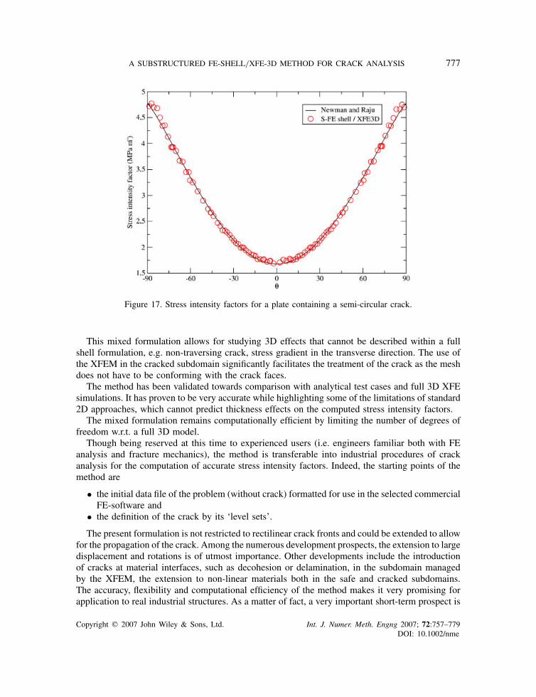
A square plate containing a semi-circular crack is considered, as depicted in Figure 16. The plateis subjected to a unit bending moment. The mode I stress intensity factor computed along the frontusing the S-FE shell/XFE-3D method is compared to the solution built by Newman and Raju [37]based on a parametrized fit of a set of 3D FE simulations. The geometrical and material parametersare given in Table VI.


776 E. WYART ET AL.

Table VI. Geometrical and material parameters ofa plate containing a semi-circular crack and subjected to

a bending moment.

W 20mmL 20mmt 1mma 0.5mmE 210GPa� 0.3

Figure 16. Square plate containing a semi-circular crack subjected to a bending moment. 3D view (top)and view of the crack plane (bottom).

Figure 17 shows the stress intensity factor along the crack front. As the crack is in a symmetryplane, only mode I is observed. The variation of the stress intensity factor along a crack front is,as expected, with the highest values at the free surface where the bending stress is maximum. Theresults obtained with the S-FE shell/XFE-3D method coincide with those obtained by Newmanand Raju.

6. CONCLUSIONS

The S-FE/XFE method has been proposed in order to cope with 3D cracking problems in thin-walled samples initially meshed with shell elements. In this method, the original shell mesh in thedamaged zone (the cracked subdomain) is replaced by a 3D mesh incorporating the crack. Thecrack itself is represented by level sets. The cracked domain is handled by an in-house code usingthe XFEM while the remaining part of the original shell mesh (the safe domain) is handled by aclassical FE-software. The interface problem is solved by the FETI method.



Figure 17. Stress intensity factors for a plate containing a semi-circular crack.

This mixed formulation allows for studying 3D effects that cannot be described within a fullshell formulation, e.g. non-traversing crack, stress gradient in the transverse direction. The use ofthe XFEM in the cracked subdomain significantly facilitates the treatment of the crack as the meshdoes not have to be conforming with the crack faces.

The method has been validated towards comparison with analytical test cases and full 3D XFEsimulations. It has proven to be very accurate while highlighting some of the limitations of standard2D approaches, which cannot predict thickness effects on the computed stress intensity factors.

The mixed formulation remains computationally efficient by limiting the number of degrees offreedom w.r.t. a full 3D model.

Though being reserved at this time to experienced users (i.e. engineers familiar both with FEanalysis and fracture mechanics), the method is transferable into industrial procedures of crackanalysis for the computation of accurate stress intensity factors. Indeed, the starting points of themethod are

• the initial data file of the problem (without crack) formatted for use in the selected commercialFE-software and

• the definition of the crack by its ‘level sets’.

The present formulation is not restricted to rectilinear crack fronts and could be extended to allowfor the propagation of the crack. Among the numerous development prospects, the extension to largedisplacement and rotations is of utmost importance. Other developments include the introductionof cracks at material interfaces, such as decohesion or delamination, in the subdomain managedby the XFEM, the extension to non-linear materials both in the safe and cracked subdomains.The accuracy, flexibility and computational efficiency of the method makes it very promising forapplication to real industrial structures. As a matter of fact, a very important short-term prospect is


778 E. WYART ET AL.

the application to industrial benchmarks involving complex geometries (e.g. stiffened panel with atwo-bay crack), loading (coming from the load spectrum), boundary conditions (e.g. contact, bodyforces) and crack configurations (crack deviations, multiple cracks).

ACKNOWLEDGEMENTS

The authors are grateful to Nicolas Moes for providing his XFEM code. The FETI-code has beendeveloped by Francois-Xavier Roux from the ONERA. It is used in the frame of a collaboration withSAMTECH. This research was funded by the Walloon Region and FEDER European funds under contractNr EP1A122030000102.

REFERENCES

1. Yang H, Saigal S, Masud A, Kapania R. A survey of recent shell finite elements. International Journal forNumerical Methods in Engineering 2000; 47:101–127.

2. Pardoen T, Hachez F, Marchioni B, Blyth PH, Atkins AG. Mode I fracture of sheet metal. Journal of theMechanics and Physics of Solids 2004; 52:423–452.

3. Belytschko T, Lu YY, Gu L. Element-free Galerkin methods. International Journal for Numerical Methods inEngineering 1994; 37:229–256.

4. Moes N, Dolbow J, Belytschko T. A finite element method for crack growth without remeshing. InternationalJournal for Numerical Methods in Engineering 1999; 46:131–150.

5. Melenk JM. On generalized finite element methods. Ph.D. Thesis, University of Maryland, 1995.6. Sukumar N, Moes N, Moran B, Belytschko T. Extended finite element method for three-dimensional crack

modelling. International Journal for Numerical Methods in Engineering 2000; 48:1549–1570.7. Moes N, Gravouil A, Belytschko T. Non-planar 3D crack growth by the extended finite element and level sets—

Part I: mechanical model. International Journal for Numerical Methods in Engineering 2002; 53:2549–2568.8. Gravouil A, Moes N, Belytschko T. Non-planar 3D crack growth by the extended finite element and level

sets—Part II: level set update. International Journal for Numerical Methods in Engineering 2002; 53:2569–2586.9. Dolbow J, Moes N, Belytschko T. Modeling fracture in Mindlin–Reissner plates with the extended finite element

method. International Journal of Solids and Structures 2000; 37:7161–7183.10. Areias PMA, Belytschko T. Non-linear analysis of shells with arbitrary evolving cracks using X-FEM. International

Journal for Numerical Methods in Engineering 2005; 62:384–415.11. Parisch H. A continuum-based shell theory for non-linear applications. International Journal for Numerical

Methods in Engineering 1995; 38:1855–1883.12. Bordas S, Moran B. Enriched finite elements and level sets for damage tolerance assessment of complex structures.

Engineering Fracture Mechanics 2006; 73:1176–1201.13. Guidault P-A, Allix O, Champaney L, Navarro J-P. Une approche micro–macro pour le suivi de fissure avec

enrichissement local. 7eme Colloque National en Calcul des Structures, France, 2005.14. Allix O, Guidault P-A, Champaney L. MS-XFEM: an extended micro–macro approach for crack propagation.

Challenges in Computational Mechanics, France, 2006.15. Ladeveze P, Loiseau O, Dureisseix D. A micro–macro and parallel computational strategy for highly heterogeneous

structures. International Journal for Numerical Methods in Engineering 2001; 52:121–138.16. Wyart E, Duflot M, Coulon D, Martiny P, Pardoen T, Remacle J-F, Lani F. Substructuring FE–XFE approaches

applied to three-dimensional crack propagation. Journal of Computational and Applied Mathematics 2007,in press.

17. Farhat C, Roux FX. A method of finite element tearing and interconnecting and its parallel solution algorithm.International Journal for Numerical Methods in Engineering 1991; 32:1205–1227.

18. Melenk JM, Babuska I. The partition of unity finite element method: basic theory and applications. ComputerMethods in Applied Mechanics and Engineering 1996; 139:289–314.

19. Moes N, Dolbow J, Belytschko T. A finite element method for crack growth without remeshing. InternationalJournal for Numerical Methods in Engineering 1999; 46:131–150.

20. Bechet E, Minnebo H, Moes N, Burgardt B. Improved implementation and robustness study of the X-FEM forstress analysis around cracks. International Journal for Numerical Methods in Engineering 2005; 64:1033–1056.



21. Laborde P, Pommier J, Renard Y, Salaun M. High-order extended finite element method for cracked domains.International Journal for Numerical Methods in Engineering 2005; 64:354–381.

22. Stolarska M, Chopp DL, Moes N, Belytschko T. Modelling crack growth by level sets in the extended finiteelement method. International Journal for Numerical Methods in Engineering 2001; 51:943–960.

23. Sethian JA. Level Set Methods and Fast Marching Methods: Evolving Interfaces in Computational Geometry,Fluid Mechanics, Computer Vision, and Material Science. Cambridge University Press: Cambridge, 1996.

24. SAMCEF. General purpose finite element analysis package, 2006.25. Moran B, Shih CF. Crack tip and associated domain integrals from momentum and energy balance. Engineering

Fracture Mechanics 1987; 27(6):615–641.26. Yau JF, Wang SS, Corten HT. A mixed-mode crack analysis of isotropic solids using conservation laws of

elasticity. Journal of Applied Mechanics 1980; 47:335–341.27. Farhat C, Roux FX. Implicit parallel processing in structural mechanics. Computational Mechanical Advance

1994; 2(1):1–124.28. Lesoinne M, Pierson K. An efficient FETI implementation on distributed shared memory machine with independent

numbers of subdomains and processors. Contemporary Mathematics 1998; 218.29. Saad Y. Iterative Methods for Sparse Linear Systems (2nd edn). SIAM: Philadelphia, PA, 2000.30. Remacle J-F, Shephard M. An algorithm oriented mesh database. International Journal for Numerical Methods

in Engineering 2003; 58:349–374.31. Schiermeier JE, Kansakar RK, Ransom JB, Stroud WJ. Interface elements in global/local analysis—Part 3:

shell-to-solid transition. The 1999 MSC Worldwide Aerospace Conference, Long Beach, U.S.A., 1999.32. Kim J, Varadan VV, Varadan VK. Finite element modeling of structures including piezoelectric active devices.

International Journal for Numerical Methods in Engineering 1997; 40:817–832.33. McCune RW, Armstrong CG, Robinson DJ. Mixed-dimensional coupling in finite models. International Journal

for Numerical Methods in Engineering 2000; 49:725–750.34. Lacour C. Non-conforming domain decomposition method for plate and shell problem. Contemporary Mathematics

1998; 218:304–310.35. Farhat C, Lacour C, Rixen D. Incorporation of linear multipoint constraints in substructure based iterative solvers.

Part I: a numerically scalable algorithm. International Journal for Numerical Methods in Engineering 1998;43:997–1016.

36. Tada H, Paris P, Irwin G. The Stress Analysis of Cracks Handbook (3rd edn). ASME: New York, 2000.37. Newman JC, Raju IS. Analyses of surface cracks in finite plates under tension or bending loads. Technical Report

No. 1578, NASA, 1979.38. Kwon SW, Sun CT. Characteristics of three-dimensional stress fields in plates with a through-the-thickness crack.

International Journal of Fracture 2000; 104:291–315.39. Rajaram H, Socrate S, Parks DM. Application of domain integral method using tetrahedral element to the

determination of stress intensity factors. Engineering Fracture Mechanics 2000; 66:455–482.


A substructured FE-shell/XFE-3D method for crack analysis in thin-walled structures

Documents

Transcript of A substructured FE-shell/XFE-3D method for crack analysis in thin-walled structures