A study on the valuing of biodiversity: the case of three endangered species in Brazil

METHODS

A study on the valuing of biodiversity: the case of threeendangered species in Brazil

Mario Jorge Cardoso de Mendonca a,*, Adolfo Sachsida b,Paulo R.A. Loureiro b

a Instituto de Pesquisa Economica Aplicada (IPEA), Avenida Presidente Antonio Carlos 51, r.1501, Centro, Rio de Janeiro, RJ 20020-

010, Brazilb Universidade Catolica de Brasılia, SGAN 916-Modulo B-Asa Norte, Brasılia, Brazil

Received 17 September 2002; received in revised form 28 February 2003; accepted 17 March 2003

Abstract

Using the analysis developed by Montgomery et al. (J. Environ. Econ. Manage., 1999) as a starting point, this study

establishes the bounds limits to the management price for the conservation of biodiversity. This means, how much the

household would be willing to pay to finance a conservation program for three endangered species in Brazil. This

program must be restricted to the change in habitat with regard to public benefits associated with biodiversity. Here,

this increment in habitat means the marginal benefit derived from the increase in the size of the population. An

important point of this paper is that we work with the robust instrument called the Population Viability Analysis (PVA)

that estimates the survival probability of the species in the future given a current exogenous disturbance. We show that

the results are very sensitive to the parameters of the model, mainly the population’s current size and the degree of

diversity. We also show that the total amount spent on conservation in Brazil is below the socially optimal level,

considering only the three species analyzed in this study.

# 2003 Elsevier Science B.V. All rights reserved.

Keywords: Biodiversity; Management price; Willingness to pay; Population viability analysis

JEL classification: H53; D61

1. Introduction

The value of conserving biodiversity is a recur-

ring issue in environmental economics. However,

what is supposedly being conserved, and what the

relevant trade-off is, are aspects that are not

always clear. The lack of a robust framework

that considers the theoretical and operational

aspects of conservation still plagues biodiversity

valuation. If biodiversity cannot be measured,

then there is no way to make rational decisions

as to what needs to be preserved. In spite of the

fact that the valuing of biodiversity would be

* Corresponding author. Tel.: �/55-21-2240-1920; fax: �/55-

21-3804-8059.

E-mail address: [email protected] (M.J. Cardoso de

Mendonca).

Ecological Economics 46 (2003) 9�/18

www.elsevier.com/locate/ecolecon

0921-8009/03/$ - see front matter # 2003 Elsevier Science B.V. All rights reserved.

doi:10.1016/S0921-8009(03)00080-6

mailto:[email protected]

considered as a stage prior to its measuring, thereis an overriding need for the valuing of said

resource, since a proper analysis of ecological

conservation measures would be hindered if this

were not done, considering that each of these bears

the expected gains and immediate losses for the

well-being of society.

With regard to the utility of biodiversity, as

pointed out by Loomis and White (1996), gains areobtained from several types of benefits, and may

be grouped into the following categories. There are

gains that are obtained from the simple pleasure of

being able to observe a certain species. It is

sometimes said that a certain species must be

preserved because of its beauty, or for having a

certain physical characteristic that makes it unique

in a given habitat. These are derived from its valueof use. There are also those produced by the

probable use of genetic information by the phar-

maceutical industry when developing new pro-

ducts. The pharmaceutical industry has been able

to synthesize chemical substances that are impor-

tant for medicine from the study of components

related to the genetics of certain species (DiMasi et

al., 1991). The value of existence is related to thesatisfaction derived simply from knowing that the

preservation of a species is assured in a sustainable

manner. Lastly, we could mention the inheritance

that will be left for future generations.

Starting from the model appearing in Mon-

tgomery et al. (1999), the aim of this paper is to

determine the management price for the preserva-

tion of three endangered Brazilian species. It mustbe kept in mind that this measure does not

represent the value of biodiversity itself, consider-

ing all the aspects that are inherent in such an

issue, but only the value that must be paid by

household in order to bring about a marginal

change in habitat required to increase the survival

capacity of a species. In this study, this change is

characterized by a change in habitat that producesa variation in the current size of the population.

In a market economy, the main goal in deter-

mining a price for any good is the incorporation of

relevant economic information by decision makers

regarding relative values of inputs and outputs.

The analysis developed by Montgomery et al.

(1999), demonstrates how the ‘management price’

may be used to summarize information regardingbiodiversity through the sequence of relations that

connect land use to biodiversity. These involve

relations between the characteristics of the habi-

tats and the individual species’ populations, the

species and its probability of survival, this prob-

ability and the benefits associated with the biolo-

gical diversity and lastly, the benefits and value

they have for society.Basically, this study attempts to establish the

upper and lower limits for the value that society

would be willing to pay, by way of a ‘lump sum’

tax, to support a preservation program for certain

species. It must be pointed out that there are many

issues that need to be addressed here. The pro-

gram’s feasibility or degree of success, the level of

diversity, and the value of use of each species aresome of the factors the play a role in the forming

of prices for species.

This research paper is divided as follows. In

Section 2, a biodiversity pricing model is outlined

in general terms, and at the end of the section we

indicate information that is required so that said

methodology may be applied empirically. In Sec-

tion 3, we further develop the analysis presented inthe previous section, with the aim of finding a way

in which the several concepts comprising the

model may be dealt with empirically. In the

following section, a case study for three Brazilian

endangered species is outlined, based on the

methodology developed in the previous sections.

Lastly, in Section 5, the main conclusions of this

paper are presented.

2. Theoretical model for the valuing of biodiversity

The consumption efficiency for two goods

requires a marginal rate of substitution, defined

as the ratio of the two marginal utilities of said

goods, which is equal to the price ratio. Assuming

that given a certain natural habitat, the utility ofthe agent is derived from two goods, E (D ) and Y ,

where E (D ) is the expected value for biodiversity,

and Y is the aggregate for the other types of

services that may be obtained from said habitat.

Thus, we have that the utility function of the agent

is defined as U�/U (E (D ), Y ). Related to this we

M.J. Cardoso de Mendonca et al. / Ecological Economics 46 (2003) 9�/1810

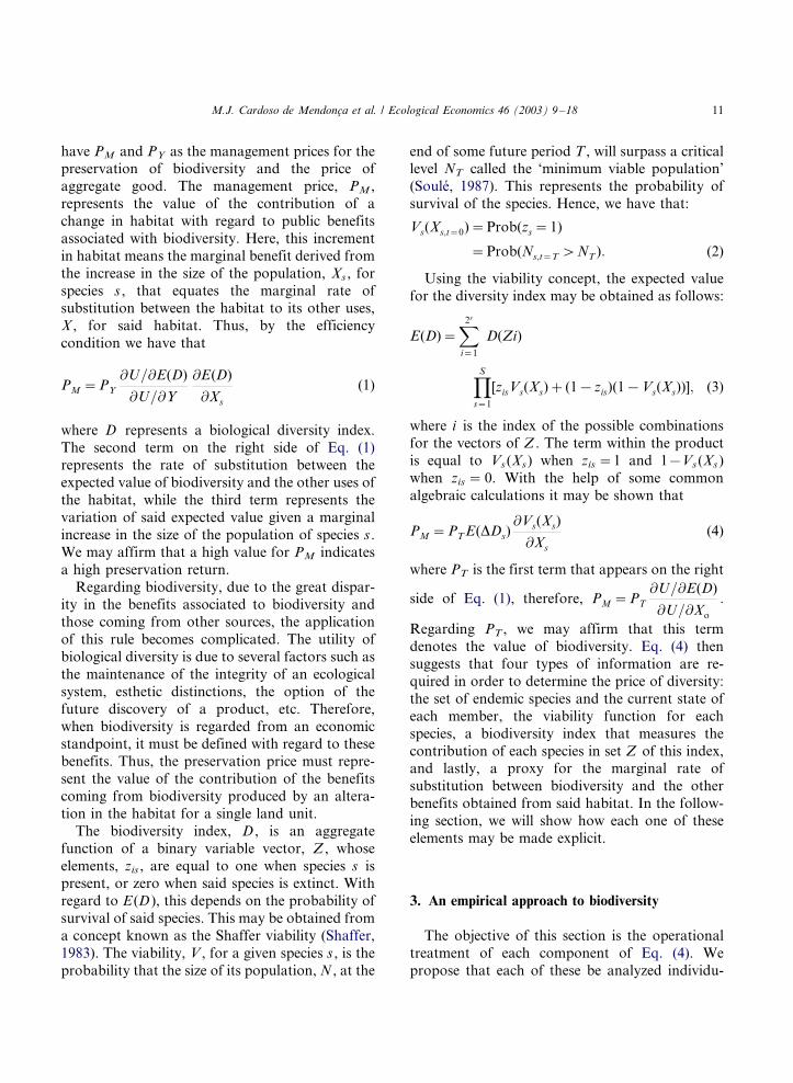
have PM and PY as the management prices for thepreservation of biodiversity and the price of

aggregate good. The management price, PM ,

represents the value of the contribution of a

change in habitat with regard to public benefits

associated with biodiversity. Here, this increment

in habitat means the marginal benefit derived from

the increase in the size of the population, Xs , for

species s , that equates the marginal rate ofsubstitution between the habitat to its other uses,

X , for said habitat. Thus, by the efficiency

condition we have that

PM �PY

@U=@E(D)

@U=@Y

@E(D)

@Xs

(1)

where D represents a biological diversity index.

The second term on the right side of Eq. (1)represents the rate of substitution between the

expected value of biodiversity and the other uses of

the habitat, while the third term represents the

variation of said expected value given a marginal

increase in the size of the population of species s .

We may affirm that a high value for PM indicates

a high preservation return.

Regarding biodiversity, due to the great dispar-ity in the benefits associated to biodiversity and

those coming from other sources, the application

of this rule becomes complicated. The utility of

biological diversity is due to several factors such as

the maintenance of the integrity of an ecological

system, esthetic distinctions, the option of the

future discovery of a product, etc. Therefore,

when biodiversity is regarded from an economicstandpoint, it must be defined with regard to these

benefits. Thus, the preservation price must repre-

sent the value of the contribution of the benefits

coming from biodiversity produced by an altera-

tion in the habitat for a single land unit.

The biodiversity index, D , is an aggregate

function of a binary variable vector, Z , whose

elements, zis , are equal to one when species s ispresent, or zero when said species is extinct. With

regard to E (D ), this depends on the probability of

survival of said species. This may be obtained from

a concept known as the Shaffer viability (Shaffer,

1983). The viability, V , for a given species s , is the

probability that the size of its population, N , at the

end of some future period T , will surpass a criticallevel NT called the ‘minimum viable population’

(Soule, 1987). This represents the probability of

survival of the species. Hence, we have that:

Vs(Xs;t�0)�Prob(zs�1)

�Prob(Ns;t�T �NT ): (2)

Using the viability concept, the expected value

for the diversity index may be obtained as follows:

E(D)�X2s

i�1

D(Zi)

�YS

s�1

[zisVs(Xs)�(1�zis)(1�Vs(Xs))]; (3)

where i is the index of the possible combinations

for the vectors of Z . The term within the product

is equal to Vs (Xs) when zis �/1 and 1�/Vs(Xs )

when zis �/ 0. With the help of some common

algebraic calculations it may be shown that

PM �PT E(DDs)@Vs(Xs)

@Xs

(4)

where PT is the first term that appears on the right

side of Eq. (1), therefore, PM �PT

@U=@E(D)

@U=@Xo

:

Regarding PT , we may affirm that this term

denotes the value of biodiversity. Eq. (4) then

suggests that four types of information are re-

quired in order to determine the price of diversity:

the set of endemic species and the current state of

each member, the viability function for each

species, a biodiversity index that measures the

contribution of each species in set Z of this index,and lastly, a proxy for the marginal rate of

substitution between biodiversity and the other

benefits obtained from said habitat. In the follow-

ing section, we will show how each one of these

elements may be made explicit.

3. An empirical approach to biodiversity

The objective of this section is the operational

treatment of each component of Eq. (4). We

propose that each of these be analyzed individu-

M.J. Cardoso de Mendonca et al. / Ecological Economics 46 (2003) 9�/18 11

ally, as follows. However, before this is done, it isnecessary to establish appropriate definitions with

regard to the species set, S , object of this analysis,

as well as consider its current state, Xs .

According to internationally recognized criteria

for a survival diagnosis of the species (SSD)

(Master, 1991), the risk of extinction is rated as

follows: 1�/critically endangered species; 2�/en-

dangered species; 3�/vulnerable species; 4�/abun-dant species; although endangered in the long run;

and 5�/the species is safe, given current condi-

tions. The definition of each of these depends on

several factors, such as the estimated number of

elements, threats, fragility, population growth

trends, quality of the habitat, etc. For example,

in a study appearing in Montgomery et al. (1999)

conducted for a set of 147 species of birds, apopulation of less than 50 has a SSD rate of 1;

between 50 and 250, the SSF is 2; between 250 and

1000, the SSD is 3; and for a population over 1000,

the SSD was either four or five.

Regarding viability, a biological preservation

technique called a Population Viability Analysis

(PVA) is commonly used (Lamberson et al., 1992).

It is quite sophisticated, and with it, it is possibleto obtain quantitative estimates regarding the

probability of extinction over a period of time in

the future, say, the next 100 years. These estimates

are based on modeling, and in order to ensure

reliability, since extinction is an extremely complex

and probabilistic phenomenon, they require an

immense quantity of detailed demographic and

genetic data on the species (or population) beingstudied, such as survival and reproduction rates at

different ages, age of the first reproduction, sex

ratio, maximum life span, etc. (Brito and Ferna-

dez, 2000b). Since there are several parameters in

the PVA, we can simulate several interesting

situations by changing these parameters. Thus, if

we want to observe the impact on the probability

of the future condition of a species resulting, forexample, from a substantial reduction in the

number of individuals of the species, this may be

done by altering the parameter regarding the

initial size of the population.

In Brazil, PVA studies are only available for a

very few number of species. In the US and

Australia, estimates are available for hundreds of

species. In Brazil, however, studies adopting thePVA method have been conducted for three

species; the mico-leao-dourado (golden lion ta-

marin), the mico-leao-preto (black lion tamarin),

and a type of cuıca , called Micoureus demerarae.

Some studies have obtained an approximate

estimate based on a logistic viability function.

The reason for this is that the logistical form may

detect the evolution of many biological phenom-ena reasonably well (Bevers et al., 1995).

Let us now take a look at how the literature

deals with the biodiversity measurement issue.

When a species becomes extinct there is a loss in

diversity. This loss may be total, in those cases in

which the family of the species has only one

member, or partial, when the family of said species

also includes other species, as is frequently the casewith birds. Intuitively, it is easy to perceive that the

greatest risk of diversity loss is when the extinct

species does not have a strong relationship with

the surviving members of another related species,

as opposed to those cases in which the extinct

species has a high degree of kinship with the living

related species. The challenge then lies in utilizing

this rationale in a practical manner.A plausible measurement of biological diversity

appears in Krajewsky (1989) and was elaborated

by measuring the genetic distance between any

pair of species for a given set of species. Based on

this methodology, Weitzman (1993) constructs

diversity indexes that present desirable economic

properties. We must keep in mind, however, that

the information required for these indexes is costlyand is not always available.

Some researchers use simpler biodiversity mea-

surements that may be obtained from readily

available information, as is the case of Montgom-

ery et al. (1999). This study presents a biodiversity

measurement based on an index proposed by

Vane-Wright et al. (1991), in which weights for

biodiversity are calculated based on taxonomy.The taxonomy system is constructed according to

perceived similarities among species, and though

far from being perfect, it may be considered a good

substitute indicator for the degree of biodiversity.

In order to construct the weights for each species,

it is only necessary to compute the number of

species that are grouped on each level of classifica-


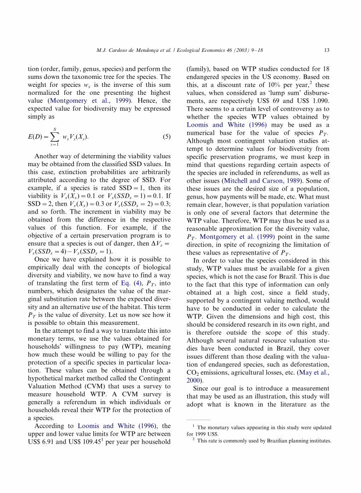
tion (order, family, genus, species) and perform thesums down the taxonomic tree for the species. The

weight for species ws is the inverse of this sum

normalized for the one presenting the highest

value (Montgomery et al., 1999). Hence, the

expected value for biodiversity may be expressed

simply as

E(D)�XS

s�1

wsVs(Xs): (5)

Another way of determining the viability values

may be obtained from the classified SSD values. In

this case, extinction probabilities are arbitrarily

attributed according to the degree of SSD. For

example, if a species is rated SSD�/1, then its

viability is Vs(Xs)�/0.1 or Vs (SSDs �/1)�/0.1. If

SSD�/2, then Vs(Xs )�/0.3 or Vs(SSDs �/ 2)�/0.3;and so forth. The increment in viability may be

obtained from the difference in the respective

values of this function. For example, if the

objective of a certain preservation program is to

ensure that a species is out of danger, then DVs �/

Vs(SSDs �/4)�/Vs(SSDs �/1).

Once we have explained how it is possible to

empirically deal with the concepts of biologicaldiversity and viability, we now have to find a way

of translating the first term of Eq. (4), PT , into

numbers, which designates the value of the mar-

ginal substitution rate between the expected diver-

sity and an alternative use of the habitat. This term

PT is the value of diversity. Let us now see how it

is possible to obtain this measurement.

In the attempt to find a way to translate this intomonetary terms, we use the values obtained for

households’ willingness to pay (WTP), meaning

how much these would be willing to pay for the

protection of a specific species in particular loca-

tion. These values can be obtained through a

hypothetical market method called the Contingent

Valuation Method (CVM) that uses a survey to

measure household WTP. A CVM survey isgenerally a referendum in which individuals or

households reveal their WTP for the protection of

a species.

According to Loomis and White (1996), the

upper and lower value limits for WTP are between

US$ 6.91 and US$ 109.451 per year per household

(family), based on WTP studies conducted for 18

endangered species in the US economy. Based on

this, at a discount rate of 10% per year,2 these

values, when considered as ‘lump sum’ disburse-

ments, are respectively US$ 69 and US$ 1.090.

There seems to a certain level of controversy as to

whether the species WTP values obtained by

Loomis and White (1996) may be used as a

numerical base for the value of species PT.

Although most contingent valuation studies at-

tempt to determine values for biodiversity from

specific preservation programs, we must keep in

mind that questions regarding certain aspects of

the species are included in referendums, as well as

other issues (Mitchell and Carson, 1989). Some of

these issues are the desired size of a population,

genus, how payments will be made, etc. What must

remain clear, however, is that population variation

is only one of several factors that determine the

WTP value. Therefore, WTP may thus be used as a

reasonable approximation for the diversity value,

PT . Montgomery et al. (1999) point in the same

direction, in spite of recognizing the limitation of

these values as representative of PT .

In order to value the species considered in this

study, WTP values must be available for a given

species, which is not the case for Brazil. This is due

to the fact that this type of information can only

obtained at a high cost, since a field study,

supported by a contingent valuing method, would

have to be conducted in order to calculate the

WTP. Given the dimensions and high cost, this

should be considered research in its own right, and

is therefore outside the scope of this study.

Although several natural resource valuation stu-

dies have been conducted in Brazil, they cover

issues different than those dealing with the valua-

tion of endangered species, such as deforestation,

CO2 emissions, agricultural losses, etc. (May et al.,

2000).

Since our goal is to introduce a measurement

that may be used as an illustration, this study will

adopt what is known in the literature as the

1 The monetary values appearing in this study were updated

for 1999 US$.2 This rate is commonly used by Brazilian planning institutes.


benefits transfer function (Markandya, 1998). Thisfunction is based on the per capita income

differential adjusted by the purchasing power

parity and weighted by the income elasticity of

demand. In this case, the benefits transfer function

assumes the following form:

WTPbr�WTPeua�(PPPbr=PPPeua)e; (6)

where: PPPbr is the per capita income in Brazil

adjusted by the purchasing power parity of theReal (Brazilian currency); PPCeuais the per capita

income in the US adjusted by the purchasing

power parity of the US Dollar; e is the income

elasticity of demand.

4. Case study: application for three Brazilian

endangered species

Considering the methodology laid out in this

study, the objective at this point is to value three

endangered Brazilian species, namely the mico-

leao-preto (black lion tamarin) (Leontopithecus

chrisophygus ), the mico-leao-dourado (golden lion

tamarin) (Leontopithecus rosalia ), and a type of

cuıca (Micoureus demerarae ). These three specieswere specifically chosen, as mentioned earlier,

because they are the only ones for which Popula-

tion Viability Analyses (PVA) have been prepared

for Brazil, and thus their extinction probability

estimates may be more reliably used.

Fragmentation and loss of habitat are a serious

threat to biodiversity. This process, occurring on a

global scale, is probably the main threat faced bythe rich fauna of the Brazilian Atlantic Forest, the

so-called Mata Atlantica , the region along the

southeastern coast of Brazil, covering about a

million hectares. This is currently one of the most

endangered ecosystems on the planet, with only

about 5% of its original reserve still remaining

untouched, fragmented into smaller stretches of

land. Distinct types of marsupials and rodents maybe found in these areas, some surviving in isolated

areas, while others have grouped into metapopula-

tions. A metapopulation is defined here as a

population of a certain species that is restricted

to a specific area, as opposed to the population as

a whole. Although most species dealt with are not

endangered from a global perspective, frequentlythe loss of a population found in some segment of

forest may lead to an ecological extinction bring-

ing about considerable changes in the structure

and functioning of local communities.

However, as mentioned in the literature, a local

extinction is also a global one since observations

from islands would suggest that reductions in

continuous areas and isolation of habitats wouldincrease the rate of extinction. For this reason,

knowledge derived from the study of local popula-

tion extinction is likely to be useful in under-

standing the process of global extinction of a

species (Brito and Fernadez, 2000b). One of the

most endangered species in the Mata Atlantica

region is the Micoureus demerarae , which is a

small marsupial found in South America. Thisspecies can be found from Colombia to north-

eastern Argentina. In specific terms, the popula-

tion viability results presented in this study refer to

the study conducted for a metapopulation found

in a sub-region of the Mata Atlantica (Fernandez,

2000). Regarding the scenario upon which it was

based, the results show that this species is highly

endangered. The data show that the probability ofthis species becoming extinct over the next 100

years is approximately 45%. The worst case

scenario indicates that it is almost certain that

the species will become totally extinct.

Regarding the mico-leao-dourado , the PVA

research was conducted based on the metapopula-

tions located at the Poco das Antas reserve. For

the mico-leao-preto , the studies were based on themetapopulations found at the Caitetus and Morro

do Diabo Ecological Stations. With regard to the

research conducted at the Poco das Antas reserve

for the mico-leao-dourado metapopulation, the

results indicate that the probability of this meta-

population becoming extinct over the next 100

years is 15%, while the probability of the mico-

leao-preto metapopulation becoming extinct overthe next 10 years is 78%, indicating that this

species is highly endangered. The results for the

other regions were not conclusive (Seal et al.,

1990).

However, considering the objective of this study,

the determining of the viability function of a

certain species in not enough. According to Eq.


(4), it is necessary to determine the increment in

probability resulting from a variation in the size of

a species. In order to overcome this obstacle, said

variations shall be obtained from the variability

results obtained for different scenarios that may be

related either to situations of higher or lower

degrees of pessimism, as well as to endogenous

or exogenous aspects of the natural habitat, since

our objective here is to determine the preservation

management price from a variation in DSs in

relation to the current size of the species popula-

tion in the habitat. The variation in viability will

be obtained from the difference between the

viability values obtained for a more optimistic

scenario and those obtained for a scenario estab-

lished as a base. The idea here is that a more

optimistic scenario may be associated with some

positive effect regarding the size of the population

(Seal et al., 1990), considering that population size

is one of many PVA parameters. It is also possible

to determine the viability values produced by a

pessimistic scenario. In this case, the values are

derived from a negative shock upon the size of the

population. Table 1 presents the viability values

for three distinct scenarios.

The above results reveal that viability is very

sensitive to the hypotheses assumed for each

scenario. This may be observed in the sharp

difference in the results, especially when the

extremes of the intervals are considered. Also

regarding Table 1, the results indicate that for

any scenario, the probability of the mico-leao-

preto becoming extinct 100 years from now is

almost 100%.It must be pointed out that for the cuıca and the

mico-leao-preto , viability suffers a proportionally

larger impact in the pessimistic scenario than in

the optimistic one, while in the case of the mico-

leao-dourado the situation is not so imbalanced.

However, this may be easily explained. Note that

for the first two species, the PVA in the base

scenario is quite low, which is quite probably

related to the fact the current size of these two

populations is at a critical level. In this case, a

negative shock on the population has a strong

effect on viability, producing an important reduc-

tion in its value since the size of the population is

now at a level below critical. Lastly, the variation

in viability is arrived at from the difference

between the values obtained for the optimistic

and base scenarios.

Once the determining of the viability values, or

their variation, has been defined, the final task is

then to determine the WTP values, and the

diversity measurement for the species. Once these

values have been determined, we are now able to

determine the price for the species under study. As

was pointed out earlier, the WTP values to be used

in this study were derived from Loomis and White

(1996). In their study, the lower and upper WTP

values ranged between US$ 69 and US$ 1090, in

the case of a ‘lump sum’-type disbursement. The

use of ‘lump sum’ tax means that the funds

obtained from society would be immediately put

to use to implement the preservation program. In

other words, the resources obtained must be

allocated towards the execution of a specific

program. This is one way of increasing society’s

willingness to participate in such initiatives.

In Table 2, we shall present the adjusted values

according to the expression appearing in Eq. (6),

adjusted for Brazil. The WTP values are based on

Table 1

Viability scenario for endangered species

Common name of species (1) Pessimistic scenario (2) Base scenario (3) Optimistic scenario (4) Variation in viability DV (5)

Cuicaa 0.01 0.55 0.70 0.15

Mico-leao-preto b 0.05 0.50 0.70 0.20

Mico-leao-dourado c 0.84 0.88 0.96 0.08

The time frame for the mico-leao-preto is 50 years; for the two other species the time frame is 100 years.a Source: Brito and Fernadez (2000a).b Source: Seal et al. (1990).c Source: Kieruff (1993).


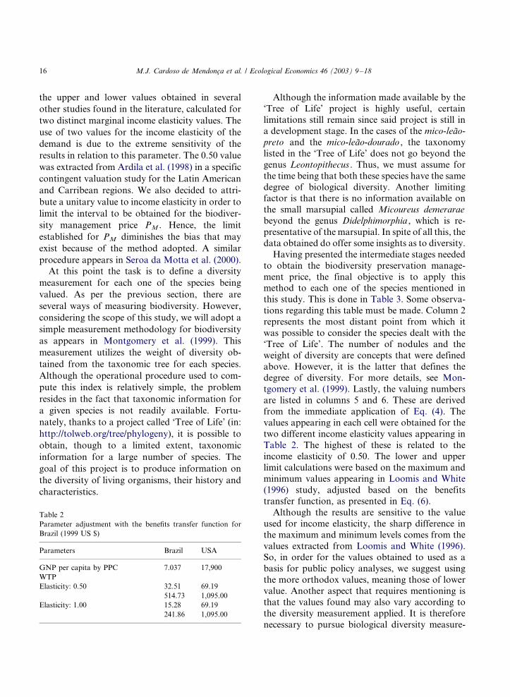
the upper and lower values obtained in several

other studies found in the literature, calculated for

two distinct marginal income elasticity values. The

use of two values for the income elasticity of the

demand is due to the extreme sensitivity of the

results in relation to this parameter. The 0.50 value

was extracted from Ardila et al. (1998) in a specific

contingent valuation study for the Latin American

and Carribean regions. We also decided to attri-

bute a unitary value to income elasticity in order to

limit the interval to be obtained for the biodiver-

sity management price PM . Hence, the limit

established for PM diminishes the bias that may

exist because of the method adopted. A similar

procedure appears in Seroa da Motta et al. (2000).

At this point the task is to define a diversity

measurement for each one of the species being

valued. As per the previous section, there are

several ways of measuring biodiversity. However,

considering the scope of this study, we will adopt a

simple measurement methodology for biodiversity

as appears in Montgomery et al. (1999). This

measurement utilizes the weight of diversity ob-

tained from the taxonomic tree for each species.

Although the operational procedure used to com-

pute this index is relatively simple, the problem

resides in the fact that taxonomic information for

a given species is not readily available. Fortu-

nately, thanks to a project called ‘Tree of Life’ (in:

http://tolweb.org/tree/phylogeny), it is possible to

obtain, though to a limited extent, taxonomic

information for a large number of species. The

goal of this project is to produce information on

the diversity of living organisms, their history and

characteristics.

Although the information made available by the‘Tree of Life’ project is highly useful, certain

limitations still remain since said project is still in

a development stage. In the cases of the mico-leao-

preto and the mico-leao-dourado , the taxonomy

listed in the ‘Tree of Life’ does not go beyond the

genus Leontopithecus . Thus, we must assume for

the time being that both these species have the same

degree of biological diversity. Another limitingfactor is that there is no information available on

the small marsupial called Micoureus demerarae

beyond the genus Didelphimorphia , which is re-

presentative of the marsupial. In spite of all this, the

data obtained do offer some insights as to diversity.

Having presented the intermediate stages needed

to obtain the biodiversity preservation manage-

ment price, the final objective is to apply thismethod to each one of the species mentioned in

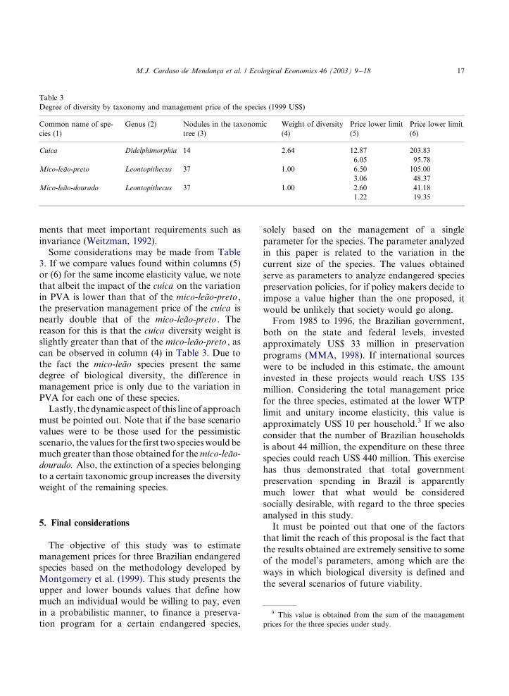
this study. This is done in Table 3. Some observa-

tions regarding this table must be made. Column 2

represents the most distant point from which it

was possible to consider the species dealt with the

‘Tree of Life’. The number of nodules and the

weight of diversity are concepts that were defined

above. However, it is the latter that defines thedegree of diversity. For more details, see Mon-

tgomery et al. (1999). Lastly, the valuing numbers

are listed in columns 5 and 6. These are derived

from the immediate application of Eq. (4). The

values appearing in each cell were obtained for the

two different income elasticity values appearing in

Table 2. The highest of these is related to the

income elasticity of 0.50. The lower and upperlimit calculations were based on the maximum and

minimum values appearing in Loomis and White

(1996) study, adjusted based on the benefits

transfer function, as presented in Eq. (6).

Although the results are sensitive to the value

used for income elasticity, the sharp difference in

the maximum and minimum levels comes from the

values extracted from Loomis and White (1996).So, in order for the values obtained to used as a

basis for public policy analyses, we suggest using

the more orthodox values, meaning those of lower

value. Another aspect that requires mentioning is

that the values found may also vary according to

the diversity measurement applied. It is therefore

necessary to pursue biological diversity measure-

Table 2

Parameter adjustment with the benefits transfer function for

Brazil (1999 US $)

Parameters Brazil USA

GNP per capita by PPC 7.037 17,900

WTP

Elasticity: 0.50 32.51 69.19

514.73 1,095.00

Elasticity: 1.00 15.28 69.19

241.86 1,095.00


http://tolweb.org/tree/phylogeny

ments that meet important requirements such as

invariance (Weitzman, 1992).

Some considerations may be made from Table

3. If we compare values found within columns (5)or (6) for the same income elasticity value, we note

that albeit the impact of the cuıca on the variation

in PVA is lower than that of the mico-leao-preto ,

the preservation management price of the cuıca is

nearly double that of the mico-leao-preto . The

reason for this is that the cuıca diversity weight is

slightly greater than that of the mico-leao-preto , as

can be observed in column (4) in Table 3. Due tothe fact the mico-leao species present the same

degree of biological diversity, the difference in

management price is only due to the variation in

PVA for each one of these species.

Lastly, the dynamic aspect of this line of approach

must be pointed out. Note that if the base scenario

values were to be those used for the pessimistic

scenario, the values for the first two species would bemuch greater than those obtained for the mico-leao-

dourado. Also, the extinction of a species belonging

to a certain taxonomic group increases the diversity

weight of the remaining species.

5. Final considerations

The objective of this study was to estimate

management prices for three Brazilian endangeredspecies based on the methodology developed by

Montgomery et al. (1999). This study presents the

upper and lower bounds values that define how

much an individual would be willing to pay, even

in a probabilistic manner, to finance a preserva-

tion program for a certain endangered species,

solely based on the management of a single

parameter for the species. The parameter analyzed

in this paper is related to the variation in the

current size of the species. The values obtained

serve as parameters to analyze endangered species

preservation policies, for if policy makers decide to

impose a value higher than the one proposed, it

would be unlikely that society would go along.

From 1985 to 1996, the Brazilian government,

both on the state and federal levels, invested

approximately US$ 33 million in preservation

programs (MMA, 1998). If international sources

were to be included in this estimate, the amount

invested in these projects would reach US$ 135

million. Considering the total management price

for the three species, estimated at the lower WTP

limit and unitary income elasticity, this value is

approximately US$ 10 per household.3 If we also

consider that the number of Brazilian households

is about 44 million, the expenditure on these three

species could reach US$ 440 million. This exercise

has thus demonstrated that total government

preservation spending in Brazil is apparently

much lower that what would be considered

socially desirable, with regard to the three species

analysed in this study.

It must be pointed out that one of the factors

that limit the reach of this proposal is the fact that

the results obtained are extremely sensitive to some

of the model’s parameters, among which are the

ways in which biological diversity is defined and

the several scenarios of future viability.

3 This value is obtained from the sum of the management

prices for the three species under study.

Table 3

Degree of diversity by taxonomy and management price of the species (1999 US$)

Common name of spe-

cies (1)

Genus (2) Nodules in the taxonomic

tree (3)

Weight of diversity

(4)

Price lower limit

(5)

Price lower limit

(6)

Cuıca Didelphimorphia 14 2.64 12.87 203.83

6.05 95.78

Mico-leao-preto Leontopithecus 37 1.00 6.50 105.00

3.06 48.37

Mico-leao-dourado Leontopithecus 37 1.00 2.60 41.18

1.22 19.35


Together with the type of individual speciesprotection study conducted here, there is also

another type of study that deals with overall

biome protection. Some of these studies share the

viewpoint that would be the more consistent way

of dealing with the biological preservation pro-

blem. However, several aspects must be analyzed.

It could be argued that there is not necessarily a

trade-off between the two, since by preserving aspecies, the habitat is also being preserved. An-

other important issue is that the cost involved in

protecting the biome is, by definition, greater than

the cost of protecting a species. Thus, the adoption

of specific programs for species is a much more

viable alternative in economic terms. Frequently,

the pressure exerted upon the habitat is exogenous

in nature, and thus more difficult to control,stimulating specifically oriented actions. Lastly, it

is important to keep in mind that the logic behind

environmental protection is not immune to pre-

servation cost/benefit analyses. It is then possible

that costs involved in the complete preservation of

a biome may end up supplanting, from a social

perspective, the current benefits, making it all the

more difficult to sell the preservation proposal tosociety. Considering these issues, it is reasonable to

affirm that the determining of an endangered

species management or protection price is fully

supported within environmental economics.

References

Ardila, S., Queiroga, R. e Vaugham, W.J., 1998. A Review of

the Use of Contingent Valuation Methods in Project

Analysis at the Inter-American Developing Bank. Report

of Vanderbilt University, Nashville.

Bevers, M., Hof, J., Kent, B., Raphael, M.G., 1995. Sustainable

forest management for optimizing multispecies wildlife

habitat. Natural Resource Modeling 9 (1), 1�/24.

Brito, D., Fernadez, F., 2000a. Metapopulation viability of the

marsupial micoureus demerarae in small atlantic forest

fragments in south-eastern Brazil. Animal Conservation 3,

201�/209.

Brito, D., Fernadez, F., 2000b. Dealing with extinction is

forever: understanding the risks faced by small populations.

Ciencia e Cultura 52 (3), 161�/170.

DiMasi, J.A., Hansen, R.W., Grabowsky, H.G., Lasagna, L.,

1991. Cost of innovation in pharmaceutical industry.

Journal Health Economy 10, 107�/142.

Krajewsky, C., 1989. Phylogenetic relationships among cranes

(Gruiformes: gruidae) based on DNA hybridization. The

Auk, CVI, 603�/618.

Lamberson, R.H., McKelvei, R., Noon, B., Voss, C., 1992. A

dynamic analysis of spotted owl in a fragment forest.

Conservation Biological 6, 505�/512.

Loomis, J.B., White, D.S., 1996. Economic benefits of rare and

endangered species: summary and meta-analysis. Ecological

Economics 18 (3), 197�/206.

Kieruff, M.C.M., 1993. Avaliacao das Populacoes Selvagens de

Mico-leao-dourado Leontopithecus rosalia e Proposta de

Estrategia de Conservacao. MSc Thesis, Universidade

Federal de Minas Gerais, Belo Horizonte, MG.

Markandya, 1998. The valuation of health impacts in developing

countries. Planejamento e Polıticas Publicas v. 18, 119�/143.

Master, L., 1991. Assessing threats and setting priorities for

conservation. Conserving Biology 5, 559�/563.

May, P.H., Veiga Neto, F.C., Pozo, O.V.C., 2000. Valoracao

Economica da Biodiversidade: estudo de casos. In: http://

www.mma.gov.br..

MMA-Ministerio do Meio Ambiente, dos Recursos Hıdricos e

da Amazonia Legal. Primeiro Relatorio Nacional para

Convencao sobre Diversidade Biologica. 1998

Mitchell, R., Carson, R., 1989. Using surveys to value public

goods. Resourses for the Future, Washington, DC.

Montgomery, C.A., Pollack, R.A., Freemarck, K., White, D.,

1999. Pricing biodiversity. Journal of Environmental Eco-

nomics and Management 38, 1�/19.

Seal, U.S., Ballou, J.D., Claudio Valladares-Padua., 1990.

Populations extinction model of lion tamarins in currently

protected areas. Leontopithecus, Population Viability Ana-

lysis, Workshop Report, Captive Breeding Specialist Group,

Belo Horizonte, Brasil.

Seroa da Motta, R., Ortiz, R.A., Ferreira, S.F., 2000. Health

and economic values for mortality cases associated with air

pollution in Brazil. Expert Workshop on Assessing The

Ancillary Benefits and Costs of Greenhouse Gas Mitigation

Strategies, Washington, DC, 27�/29, March.

Shaffer, M.L., 1983. Minimal population sizes for species

conservation. Bioscience 31, 131�/134.

Soule, M.E. (Ed.), Viable Populations for Conservation. Cam-

bridge University Press 1987.

Vane-Wright, R.K., Humphries, C.J., Williams, P.H., 1991.

What to protect? systematic and the agony choice. Con-

servation Biological 55, 235�/254.

Weitzman, M., 1993. What to preserve? an application of

diversity theory to crane conservation. The Quarterly

Journal of Economics, 108, 157�/183.

Weitzman, M., 1992. On diversity. The Quarterly Journal of

Economics, 107, 363�/406.


http://www.mma.gov.br.

http://www.mma.gov.br.

A study on the valuing of biodiversity: the case of three endangered species in Brazil

Documents

Transcript of A study on the valuing of biodiversity: the case of three endangered species in Brazil