
A study on optimal utilization of electric heating for buildings
128
Camilla Hengebøl A study on optimal utilization of electric heating for buildings NTNU Norwegian University of Science and Technology Faculty of Information Technology and Electrical Engineering Department of Electric Power Engineering Master’s thesis Camilla Hengebøl A study on optimal utilization of electric heating for buildings Master’s thesis in Energy Use and Energy Planning Supervisor: Karen Byskov Lindberg February 2020
-
Upload
khangminh22 -
Category
Documents
-
view
1 -
download
0
Transcript of A study on optimal utilization of electric heating for buildings
Camilla H
engebøl A study on optim
al utilization of electric heating for buildings
NTN
UN
orw
egia
n U
nive
rsity
of S
cien
ce a
nd T
echn
olog
yFa
culty
of I
nfor
mat
ion
Tech
nolo
gy a
nd E
lect
rical
Engi
neer
ing
Dep
artm
ent o
f Ele
ctric
Pow
er E
ngin
eerin
g
Mas
ter’s
thes
is
Camilla Hengebøl
A study on optimal utilization of electricheating for buildings
Master’s thesis in Energy Use and Energy Planning
Supervisor: Karen Byskov Lindberg
February 2020

Camilla Hengebøl
A study on optimal utilization ofelectric heating for buildings
Master’s thesis in Energy Use and Energy PlanningSupervisor: Karen Byskov LindbergFebruary 2020
Norwegian University of Science and TechnologyFaculty of Information Technology and Electrical EngineeringDepartment of Electric Power Engineering

Abstract
From January 2020, heating systems based on oil or gas are not allowed in Norway. In
addition, stricter building regulations in order to meet the goals set for reduced
CO2-emissions is expected. This enforces new solutions for optimal use of electricity and
heating in buildings.
This master thesis is a further development of an existing model developed in a master thesis
from 2018 [1], and further developed in a master thesis from 2019 [2]. The model is a Mixed
Integer Linear Program (MILP) implemented in the programming language Python, with the
modelling extension library Pyomo. The use of the model has been limited to an
energy-efficient Single Family House (SFH)
The objective of this thesis is to use the already existing model in order to decide whether a
point-source or a waterborne heating system is the favorable option in regard to heating. This
is investigated for a SFH, an apartment block and an office building. In addition to the heating
system itself, all three buildings have been investigated for two different building standards.
The objective was to see if the insulation of the building had an impact on which heating system
that was the favorable option. For this purpose, an implementation of new building types with
associated heating loads has been done. In addition to this, a review of input values for the
model has been done, and new investment costs for larger building has been found.
In order to compare the results, four different cases has been decided. Whereas the base case
PS is a point-source system where the building standard implies an old badly insulated
building, an upgrade including post-insulation of the building can be done. This upgrade
results in the second case for the point-source system, PS_R2.
The two other cases have both updated from point-source system to a waterborne heating
system which results in different applicable technologies for the heating. These two cases are
also divided in one case where the building standard is the same as in the base case WB, and
one case where the building standard is upgraded by post-insulating WB_R2.
Throughout the work of this thesis, the complexity of the choice of heating system has become
clear. It can be stated that an upgrade of heating system from point-source to waterborne
system will reduce energy system costs. Nevertheless, the results show that the reduction of
costs for the energy system is not high enough in order to earn the cost of the renovation. At
the same time, changes in electricity price and stricter restrictions of CO2 emissions will favor
the waterborne solution when seeing the problem in a long-time perspective.
i

ii

Sammendrag
Fra januar 2020 er oppvarming i bygninger basert på olje og gass ulovlig i Norge. I tillegg
forventes det et strengere lovverk for bygninger fremover, for å kunne møte målene som er satt
med tanke på reduksjon av CO2-utslipp. Dette påtvinger nye løsninger for optimal bruk av
elektrisitet og varme i bygninger.
Denne masteroppgaven er en videreutvikling av en allerede eksisterende modell som er
utviklet gjennom en masteroppgave skrevet i 2018 [1], og videreutviklet i en masteroppgave
skrevet i 2019 [2]. Modellen er et MILP implementert i programmeringsspråket Python, med
modellbyggingsbiblioteket Pyomo. Bruken av denne modellen har tidligere vært begrenset til
en energieffektiv enebolig.
Målet med denne masteroppgaven er å bruke den allerede eksisterende modellen til å
bestemme om punktkilde-varme eller vannbåren varme er den beste løsningen for
oppvarming. Dette blir testet for en enebolig, et leilighetskompleks og et kontorbygg. I tillegg
til å teste selve varmesystemet, blir alle tre bygnings-typene testet for to forskjellige
bygnings-standarder. Dette er for å se om isoleringen av ytterveggene på boligen har
innflytelse på hvilket system som er foretrukket. På bakgrunn av dette er nye bygnings-typer
med tilhørende lastprofiler implementert i modellen. I tillegg er det gjennomført en
gjennomgang av de eksisterende input-verdiene for modellen, og nye investeringskostander
for større systemer er innhentet.
For å sammenligne resultatene har det blitt laget fire forskjellige løsninger for utforming av
systemet som sammenlignes med hverandre. Den enkleste løsningen er et punktvarme-system
i en bygning med eldre bygnings-standard som innebærer dårlig isolerte yttervegger. Denne
løsningen er kalt PS. En etter-isolering av denne bygningen kan gjøres, som resulterer i den
andre løsningen, PS_R2.
De to siste løsningene som testes har oppgradert fra punktvarme til et vannbårent
varmesystem. Dette resulterer i andre typer teknologier som kan brukes til å varme opp
bygningen. Disse to løsningene testes også for en eldre dårlig isolert bygning, WB og en
etter-isolert bygning WB_R2.
Gjennom arbeidet med denne masteroppgaven har kompleksiteten i valget av varmesystem
for en bygning blitt tydelig. Fra resultatene kan det ses at en oppgradering fra punkt-varme til
vannbårent system resulterer i reduserte kostnader for selve energisystemet og energibruken.
Likevel viser de totale kostnadene for energisystemet og renoveringene at reduksjonen i
energikostnadene ikke er store nok til å veie opp for renovasjonskostnadene. Samtidig vil
endringer i strømprisene og strengere krav for CO2-utslipp favorisere det vannbårne systemet
på lengre sikt.
iii

iv

Preface
This thesis marks the end of the two-year Master degree in Energy use and energy planning
with specialisation within energy supply. It has been carried out during the autumn of 2019.
I would like to thank my supervisor during this master thesis, Karen Byskov Lindberg, for
valuable sharing of her knowledge in addition to her great willingness of sharing her time
whenever I have needed. Thanks to Marius Bagle at SINTEF Community for his abilities in
coding and the model used in this thesis, and for sharing all of this with me. Also a great
thanks to the others working in SINTEF Community for being open and motivating towards
me at my visits and for letting me use an office at their workplace in Oslo when I have been
visiting.
Finally I must thank all friends and family that have supported me and motivated me through
this work. A special thanks to my study companions who have been working with me and
sharing their valuable input and experiences with me.
Trondheim, February 2020
Camilla Hengebøl
v
Contents
List of Figures ix
List of Tables x
Abbreviations xi
1 Introduction 1
1.1 Thesis Motivation . . . . . . . . . . . . . . . . . . . . . . . . . . . . . . . . . . . . . 1
1.2 Problem Description . . . . . . . . . . . . . . . . . . . . . . . . . . . . . . . . . . . 1
1.3 Approach and Limitations . . . . . . . . . . . . . . . . . . . . . . . . . . . . . . . . 2
1.4 Structure . . . . . . . . . . . . . . . . . . . . . . . . . . . . . . . . . . . . . . . . . . 2
2 Theory and Research 5
2.1 Zero Emission Buildings . . . . . . . . . . . . . . . . . . . . . . . . . . . . . . . . . 5
2.2 Technologies . . . . . . . . . . . . . . . . . . . . . . . . . . . . . . . . . . . . . . . . 6
2.2.1 Heat Pumps . . . . . . . . . . . . . . . . . . . . . . . . . . . . . . . . . . . . 6
2.2.2 Photovoltaic Systems . . . . . . . . . . . . . . . . . . . . . . . . . . . . . . . 8
2.2.3 Electric Boiler . . . . . . . . . . . . . . . . . . . . . . . . . . . . . . . . . . . 10
2.2.4 Biomass Boiler . . . . . . . . . . . . . . . . . . . . . . . . . . . . . . . . . . 11
2.2.5 Electric Battery . . . . . . . . . . . . . . . . . . . . . . . . . . . . . . . . . . 11
2.2.6 Hot Water Accumulator . . . . . . . . . . . . . . . . . . . . . . . . . . . . . 12
2.3 Electricity Pricing . . . . . . . . . . . . . . . . . . . . . . . . . . . . . . . . . . . . . 12
2.4 Grid Tariffs . . . . . . . . . . . . . . . . . . . . . . . . . . . . . . . . . . . . . . . . . 13
2.4.1 Energy Pricing . . . . . . . . . . . . . . . . . . . . . . . . . . . . . . . . . . . 13
2.4.2 Power Subscription Pricing . . . . . . . . . . . . . . . . . . . . . . . . . . . 14
2.4.3 Peak Power Pricing . . . . . . . . . . . . . . . . . . . . . . . . . . . . . . . . 14
2.5 Demand Side Flexibility . . . . . . . . . . . . . . . . . . . . . . . . . . . . . . . . . . 14
3 Methodology 17
3.1 Introduction to Model and Cases . . . . . . . . . . . . . . . . . . . . . . . . . . . . 17
3.2 Electricity and Heat Loads . . . . . . . . . . . . . . . . . . . . . . . . . . . . . . . . 19
3.3 Technology Performance . . . . . . . . . . . . . . . . . . . . . . . . . . . . . . . . . 21
3.4 Weighing factors . . . . . . . . . . . . . . . . . . . . . . . . . . . . . . . . . . . . . . 24
3.5 Investment Costs . . . . . . . . . . . . . . . . . . . . . . . . . . . . . . . . . . . . . . 24
3.5.1 Technology Investment Costs . . . . . . . . . . . . . . . . . . . . . . . . . . 24
3.5.2 Investment Costs for the Waterborne Heating System . . . . . . . . . . . 26
3.5.3 Investment Costs for the Insulation of Buildings . . . . . . . . . . . . . . . 26
3.6 Price for Electricity . . . . . . . . . . . . . . . . . . . . . . . . . . . . . . . . . . . . . 27
3.6.1 Spot Price . . . . . . . . . . . . . . . . . . . . . . . . . . . . . . . . . . . . . 27
3.6.2 Grid Tariffs . . . . . . . . . . . . . . . . . . . . . . . . . . . . . . . . . . . . . 27
vi
3.6.3 Bio fuel price . . . . . . . . . . . . . . . . . . . . . . . . . . . . . . . . . . . 29
3.7 Simulations in PVsyst . . . . . . . . . . . . . . . . . . . . . . . . . . . . . . . . . . . 29
3.7.1 Input Data for PVsyst Simulations . . . . . . . . . . . . . . . . . . . . . . . 29
3.7.2 Results . . . . . . . . . . . . . . . . . . . . . . . . . . . . . . . . . . . . . . . 30
4 Model 33
4.1 Notation . . . . . . . . . . . . . . . . . . . . . . . . . . . . . . . . . . . . . . . . . . . 34
4.2 Objective Function . . . . . . . . . . . . . . . . . . . . . . . . . . . . . . . . . . . . 38
4.3 Constraints . . . . . . . . . . . . . . . . . . . . . . . . . . . . . . . . . . . . . . . . . 39
4.3.1 Capacity Constraints . . . . . . . . . . . . . . . . . . . . . . . . . . . . . . . 39
4.3.2 ZEB-constraint . . . . . . . . . . . . . . . . . . . . . . . . . . . . . . . . . . 39
4.3.3 Technology Constraints . . . . . . . . . . . . . . . . . . . . . . . . . . . . . 39
4.3.4 Storage Constraints . . . . . . . . . . . . . . . . . . . . . . . . . . . . . . . . 41
4.3.5 Grid Interaction Constraints . . . . . . . . . . . . . . . . . . . . . . . . . . 42
4.3.6 Load Constraints . . . . . . . . . . . . . . . . . . . . . . . . . . . . . . . . . 43
5 Results 45
5.1 Main Results . . . . . . . . . . . . . . . . . . . . . . . . . . . . . . . . . . . . . . . . 45
5.2 Single Family House . . . . . . . . . . . . . . . . . . . . . . . . . . . . . . . . . . . . 46
5.3 Apartment Block . . . . . . . . . . . . . . . . . . . . . . . . . . . . . . . . . . . . . . 47
5.4 Office . . . . . . . . . . . . . . . . . . . . . . . . . . . . . . . . . . . . . . . . . . . . 48
5.5 Effect of Post-insulation (R2) . . . . . . . . . . . . . . . . . . . . . . . . . . . . . . . 49
5.6 Effect of Waterborne Heating System (R1) . . . . . . . . . . . . . . . . . . . . . . . 50
6 Sensitivity Analysis 51
6.1 Power Subscription . . . . . . . . . . . . . . . . . . . . . . . . . . . . . . . . . . . . 51
6.2 Electricity Price . . . . . . . . . . . . . . . . . . . . . . . . . . . . . . . . . . . . . . . 55
6.3 Cost of PV Panels . . . . . . . . . . . . . . . . . . . . . . . . . . . . . . . . . . . . . . 58
7 Discussion 61
8 Conclusion 63
9 Further Work 65
References 66
Appendix A Point-source Model 69
Appendix B Waterborne Model 88
Appendix C Load Profiles 109
C.1 Regular building SFH . . . . . . . . . . . . . . . . . . . . . . . . . . . . . . . . . . . 109
vii

C.2 Post-insulated building SFH . . . . . . . . . . . . . . . . . . . . . . . . . . . . . . . 109
C.3 Regular building Apartment Block . . . . . . . . . . . . . . . . . . . . . . . . . . . 110
C.4 Post-insulated building Apartment Block . . . . . . . . . . . . . . . . . . . . . . . 110
C.5 Regular building Office . . . . . . . . . . . . . . . . . . . . . . . . . . . . . . . . . . 111
C.6 Post-insulated building Office . . . . . . . . . . . . . . . . . . . . . . . . . . . . . . 112
viii
List of Figures
2.1 Illustration of ZEB definition [3] . . . . . . . . . . . . . . . . . . . . . . . . . . . . . 5
2.2 Graphically representation of net ZEB balance [4] . . . . . . . . . . . . . . . . . . 6
2.3 Connection between temperature and COP for a2a heat pump . . . . . . . . . . 8
2.4 Cross-section of a solar cell . . . . . . . . . . . . . . . . . . . . . . . . . . . . . . . . 9
2.5 PV system connected to grid [5] . . . . . . . . . . . . . . . . . . . . . . . . . . . . . 9
2.6 Azimuth and tilt angle for PV-panel [6] . . . . . . . . . . . . . . . . . . . . . . . . . 10
2.7 Lithium-ion battery operation [7] . . . . . . . . . . . . . . . . . . . . . . . . . . . . 11
2.8 The outlook in the spot price from 2019-2040 [8] . . . . . . . . . . . . . . . . . . . 13
2.9 Illustration of different load flexibility classes [9] . . . . . . . . . . . . . . . . . . . 15
3.1 System design of point-source system. Adapted from [1] . . . . . . . . . . . . . . 17
3.2 System design of waterborne system. Adapted from [1] . . . . . . . . . . . . . . . 18
3.3 Overview of the different cases investigated in this thesis . . . . . . . . . . . . . . 19
3.4 Heat Demand for Regular SFH . . . . . . . . . . . . . . . . . . . . . . . . . . . . . . 20
3.5 Heat Demand for Post-insulated SFH . . . . . . . . . . . . . . . . . . . . . . . . . . 20
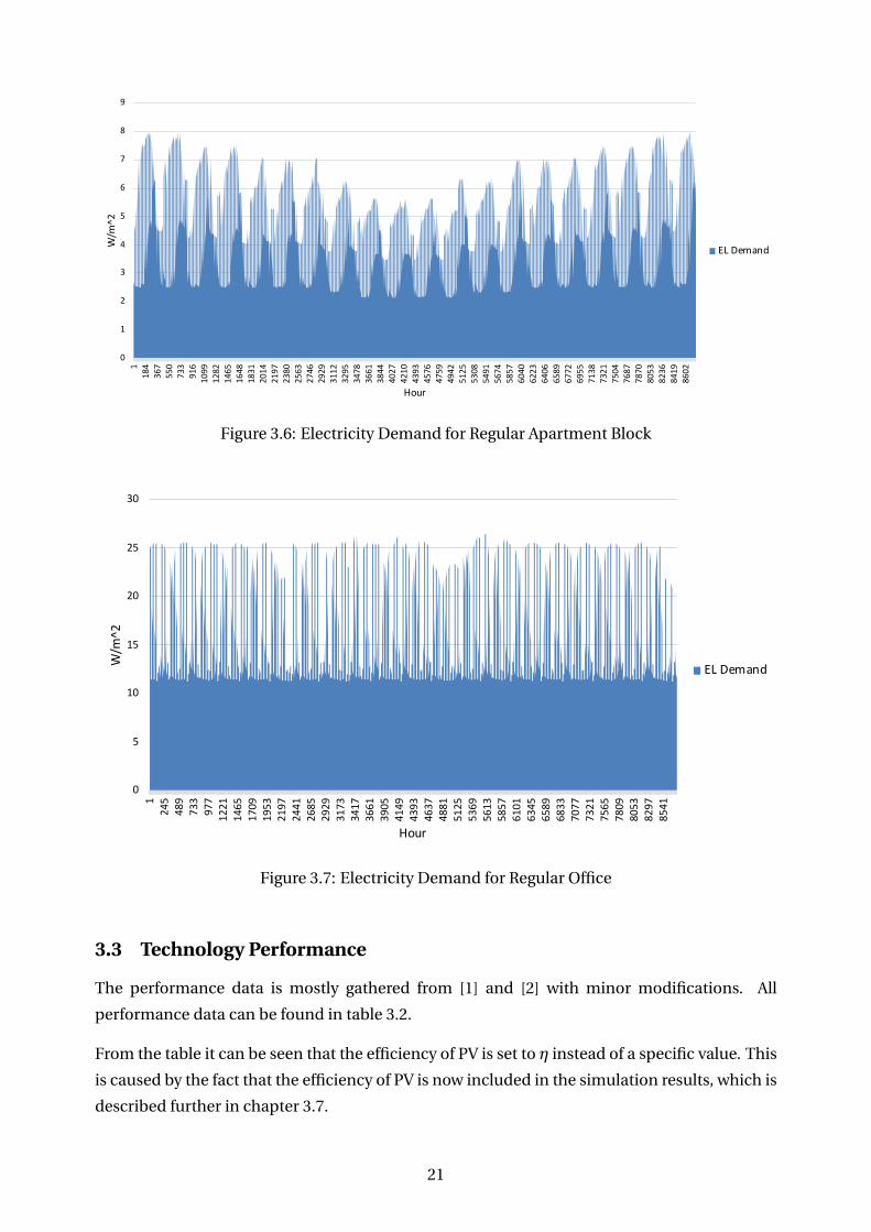
3.6 Electricity Demand for Regular Apartment Block . . . . . . . . . . . . . . . . . . . 21
3.7 Electricity Demand for Regular Office . . . . . . . . . . . . . . . . . . . . . . . . . 21
3.8 Supply temperature as a function of ambient air temperature . . . . . . . . . . . 23
3.9 COPs for passive building vs. Temperature . . . . . . . . . . . . . . . . . . . . . . 23
3.10 COPs for regular building vs. Temperature . . . . . . . . . . . . . . . . . . . . . . . 24
3.11 Spot price Oslo . . . . . . . . . . . . . . . . . . . . . . . . . . . . . . . . . . . . . . . 27
3.12 Specific production . . . . . . . . . . . . . . . . . . . . . . . . . . . . . . . . . . . . 31
4.1 Energy flow of the waterborne system . . . . . . . . . . . . . . . . . . . . . . . . . 33
4.2 Energy flow of the point-source system . . . . . . . . . . . . . . . . . . . . . . . . 34
5.1 Main Results . . . . . . . . . . . . . . . . . . . . . . . . . . . . . . . . . . . . . . . . 45
6.1 Effect of C pl t on total energy system cost for Apartment block, noZEB . . . . . . 52
6.2 Installed capacity per technology for Point-source system Apartment block, noZEB 52
6.3 Installed capacity per technology for Waterborne system for Apartment block,
noZEB . . . . . . . . . . . . . . . . . . . . . . . . . . . . . . . . . . . . . . . . . . . . 53
6.4 Use of technologies for SH on week in January for penalty charge = 0.099,
Apartment block . . . . . . . . . . . . . . . . . . . . . . . . . . . . . . . . . . . . . . 54
6.5 Use of technologies for SH on week in January for penalty charge = 0.6,
Apartment block . . . . . . . . . . . . . . . . . . . . . . . . . . . . . . . . . . . . . . 55
6.6 Effect of spot price on total energy system cost, SFH noZEB . . . . . . . . . . . . 56
6.7 Installed capacity per technology for waterborne system in SFH, noZEB . . . . . 56
6.8 Installed capacity per technology for point-source system in SFH, noZEB . . . . 57
6.9 Operation of technologies for SH-load for one week in January in SFH . . . . . . 57
6.10 Operation of technologies for DHW-load for one week in January in SFH . . . . 58
6.11 Installed capacities for decreasing PV costs, point-source system Apartment block 59
ix
6.12 Installed capacities for decreasing PV costs, waterborne system Apartment block 59
C.1 Electricity Demand for Regular SFH . . . . . . . . . . . . . . . . . . . . . . . . . . 109
C.2 Electricity Demand for Post-insulated SFH . . . . . . . . . . . . . . . . . . . . . . 109
C.3 Heat Demand for Regular Apartment Block . . . . . . . . . . . . . . . . . . . . . . 110
C.4 Electricity Demand for Post-insulated Apartment Block . . . . . . . . . . . . . . . 110
C.5 Heat Demand for Post-insulated Apartment . . . . . . . . . . . . . . . . . . . . . . 111
C.6 Heat Demand for Regular Office . . . . . . . . . . . . . . . . . . . . . . . . . . . . . 111
C.7 Electricity Demand for Post-insulated Office . . . . . . . . . . . . . . . . . . . . . 112
C.8 Heat Demand for Post-insulated Office . . . . . . . . . . . . . . . . . . . . . . . . . 112
List of Tables
3.1 Building types . . . . . . . . . . . . . . . . . . . . . . . . . . . . . . . . . . . . . . . 19
3.2 Technology performance data . . . . . . . . . . . . . . . . . . . . . . . . . . . . . . 22
3.3 Coefficient values for calculating COPs . . . . . . . . . . . . . . . . . . . . . . . . . 22
3.4 Values for calculating supply temperature . . . . . . . . . . . . . . . . . . . . . . . 23
3.5 Weighing factors . . . . . . . . . . . . . . . . . . . . . . . . . . . . . . . . . . . . . . 24
3.6 Investment costs used in calculations . . . . . . . . . . . . . . . . . . . . . . . . . 25
3.7 Investment costs for waterborne heating system inkl. MVA for different building
types [10] . . . . . . . . . . . . . . . . . . . . . . . . . . . . . . . . . . . . . . . . . . 26
3.8 Additional renovation costs for waterborne heating system . . . . . . . . . . . . . 26
3.9 Insulation cost . . . . . . . . . . . . . . . . . . . . . . . . . . . . . . . . . . . . . . . 27
3.10 Investigated grid tariffs . . . . . . . . . . . . . . . . . . . . . . . . . . . . . . . . . . 28
3.11 Subscribed power for apartment block, noZEB . . . . . . . . . . . . . . . . . . . . 28
3.12 Bio fuel prices . . . . . . . . . . . . . . . . . . . . . . . . . . . . . . . . . . . . . . . 29
3.13 Input data for the project applicable for all variations . . . . . . . . . . . . . . . . 29
3.14 Soiling loss [%] . . . . . . . . . . . . . . . . . . . . . . . . . . . . . . . . . . . . . . . 30
3.15 Production of simulation variants . . . . . . . . . . . . . . . . . . . . . . . . . . . . 30
4.1 Sets and indices for the model . . . . . . . . . . . . . . . . . . . . . . . . . . . . . . 34
4.2 Parameters for the model . . . . . . . . . . . . . . . . . . . . . . . . . . . . . . . . . 35
4.3 Continuation of parameters for the model . . . . . . . . . . . . . . . . . . . . . . . 36
4.4 Variables for the model . . . . . . . . . . . . . . . . . . . . . . . . . . . . . . . . . . 37
5.1 Results from all cases with building type Single family house . . . . . . . . . . . . 46
5.2 Results from all cases with building type Apartment block . . . . . . . . . . . . . 48
5.3 Results from all cases with building type Office . . . . . . . . . . . . . . . . . . . . 49
6.1 Results from Power Subscription tariff, Apartment block noZEB . . . . . . . . . . 51
6.2 Total installed capacity for all technologies [kW], Apartment block noZEB . . . . 55
x
Abbreviations
A2A Air-to-Air
AMS Advanced Measuring System
ASHP Air Source Heat Pump
BA Battery
BB Bio Boiler
COP Coefficient of Power
DER Distributed Energy Resources
DHW Domestic Hot Water
DR Demand Response
EB Electric Boiler
FP Fireplace
GSHP Ground Source Heat Pump
HS Heat Storage
HWT Hot Water Tank
MILP Mixed Integer Linear Program
noZEB no Zero Emission Building
PO Panel oven
PV Photovoltaic
SFH Single Family House
SH Space Heating
ZEB Zero Emission Building
xi
1 Introduction
1.1 Thesis Motivation
The importance of energy efficient and environmental friendly solutions for heating and
electricity in buildings are severly increased the past years for both industrial and residential
buildings. New regulations and laws are implemented so that each and everyone fulfills their
duty in regards to their homes, to reduce CO2-emissions.
"Regulations on technical requirements for construction works - TEK 17" is the minimum
requirements a building must hold, in order to be legally built [11]. Throughout the years, this
regulation has been more focused on energy efficiency and flexible energy resources. For this
assignment, section 14-4; Requirements for energy supply solutions, is highly relevant. Firstly,
the section states that installation of fossil fuel heating installations is not permitted. In other
words, no new buildings in Norway is built with a fossil fuel heating system. Secondly,
buildings with a heated gross internal area of more than 1000 m2 shall:
a) have multi-source heating systems
b) be adapted for use of low-temperature heating solutions.
For offices and large apartment buildings for instance, this regulation can have an impact on
how to design energy resources for domestic tap water and space heating.
The concept of heating flexibility in regards to buildings gives an understanding of how to
implement different technologies so that the building can be heated with different methods.
This is important for both the security of supply in addition to efficiency of costs and the
environment.
In additon to "TEK-17", the Ministry of Petroleum and Energy in cooperation with the
Ministry of Climate and Environment decided to adopt a law concerning the use of mineral oil
for heating of buildings. This law prohibits the use of mineral oil and fossil fuel, effective from
01.01.2020. This has resulted in a change of heating system for both Single Family Houses and
larger buildings [12].
1.2 Problem Description
The purpose of this thesis is to determine the best solution for covering the heating demand of
residential buildings, apartment blocks and office buildings.
Energy use in buildings is responsible for 40 % of global greenhouse gas emissions. One way of
reducing these emissions is to heat buildings with electricity rather than oil and gas. Norway
has a vast experience in electric heating, and may be seen as a laboratory for the future
renewable energy system. However, we need more knowledge on how to utilise electricity in
the most cost-effective way. Is it water-based heat pumps that require costly waterborne
1

heating systems inside the buildings, or electric radiators that have far lower efficiency, but are
cheap and easy to install, that will be the future?
How to cover the electricity demand is also a challenge with prospects of an increase in the
electricity price. A solution could therefore be on-site production of Photovoltaic (PV), which is
a technology with increased popularity in Norway the past years. This solution is to be explored
throughout this thesis.
Relevant background for this thesis is the current technical regulations of buildings (TEK 17),
and the optimisation model developed in earlier master thesis for studying design of energy
technologies within buildings.
1.3 Approach and Limitations
The model used in this thesis is developed through earlier work [1], [2] and is a deterministic
MILP. Through this work, a new grid tariff has been implemented in the model, in addition
to gathering of new input data with the objective of expanding the model to larger buildings,
hence larger capacities for the technologies. The new gird tariff is also implemented with the
objective of a more realistic approach to commercial buildings, as they have other regulations
in regard to electricity pricing.
The work approach in this thesis has been gathering of data, processing and implementing this
in the model. Because of the fact that the model has been further developed in the time from
my project thesis to the start of my master thesis, familiarizing myself with the improved model
was quite time consuming in the start and has been a large part of the workload in this thesis
work.
The fact that the Zero Emission Building (ZEB)-constrictions in this model only count for the
operation phase in the building lifetime is one of the main limitations of the model. The level
of ZEB included in this model is called ZEB-O EQ [13] and concerns the operation phase, but
excludes the emissions of the equipment of the technologies.
1.4 Structure
The structure of the thesis is as follows:
• Chapter 2: In this chapter, the theory of the most important aspects in order to
understand the model and the results, are explained. This includes the concept of ZEB
and the technologies which are included in the model. An introduction of electricity
pricing is also included in this chapter, in addition to an introduction in the concept of
demand side flexibility.
• Chapter 3: After the theory, a chapter which introduces the different cases follows. This
2

is also where all input data for the model is introduced for the reader, in addition to an
explanation of how the input data was gathered.
• Chapter 4: A review of the mathematical aspects of the model, and a more thoroughly
explanation of variables and parameters are shown in this chapter. This is where the
reader is able to get an insight of how the model is able to calculate the optimal solution.
• Chapter 5: A presentation of the main results are given at first, followed by discussion
with regards to different approaches of the results. In addition to main results, sensitivity
analysis of the most important aspects of the thesis which are the energy prices and PV
prices are presented and discussed.
• Chapter 6: The final conclusion is presented, in addition to suggestions for further work.
• Appendices: Includes both the waterborne model and point-source model which are
used for the optimization problem. Load profiles for different buildings that are not
presented in chapter three are also included.
3

4
2 Theory and Research
2.1 Zero Emission Buildings
ZEB is a concept of measuring emissions throughout the lifespan of a building. More
regulations on especially commercial buildings requires an interpretation of the concept
which can be widely utilized and easily understood.
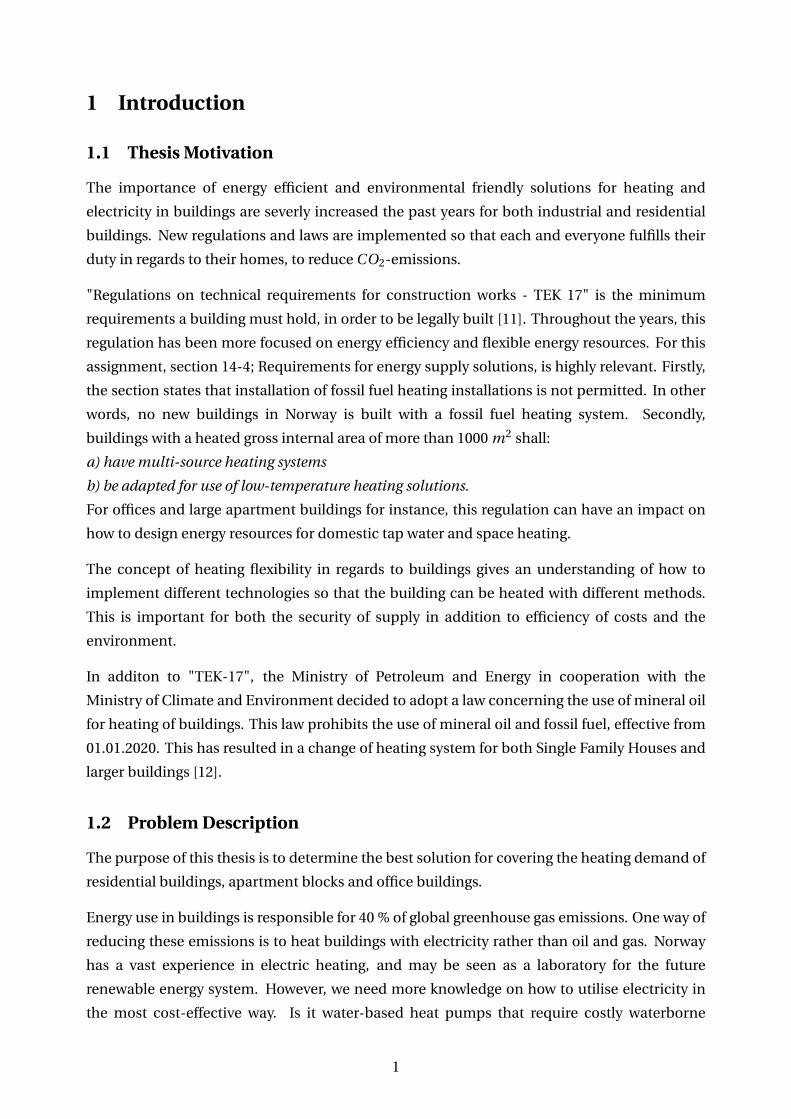
Figure 2.1: Illustration of ZEB definition [3]
In figure 2.1 an illustration of the concept can be seen. The four elements, materials,
construction, use and end of life are the phases of the lifetime of a building which can be
counted for in a ZEB. The more phases counted for, the more strict is the level of ZEB, hence
more difficult to reach. For the strictest ZEB-level, ZEB-COMPLETE, the green circle
compensates for energy use from all phases of the life of the building. It is also possible to
reach a degree of ZEB if for some reason, the achievement of the strictest level is an unrealistic
accomplishment. For instance, a common ZEB-level is to compensate for the energy use,
called ZEB-O. As seen from the figure, reaching a level of ZEB requires on-site production of
energy as Payback CO2 in addition to low emissions from energy use.
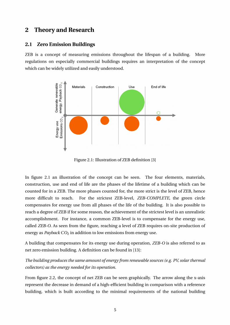
A building that compensates for its energy use during operation, ZEB-O is also referred to as
net zero emission building. A definition can be found in [13]:
The building produces the same amount of energy from renewable sources (e.g. PV, solar thermal
collectors) as the energy needed for its operation.
From figure 2.2, the concept of net ZEB can be seen graphically. The arrow along the x-axis
represent the decrease in demand of a high-efficient building in comparison with a reference
building, which is built according to the minimal requirements of the national building
5
code.[4]. Along the y-axis the amount of energy supply needed to reach the goal of net ZEB
can be found by the red arrow.
Figure 2.2: Graphically representation of net ZEB balance [4]
From figure 2.2, it can be seen that the approach of reaching net ZEB balance is to either
increase amount of energy supply or decreasing the amount of energy demand. The challenge
of increasing the energy supply can be that most of on-site renewable energy generation is
limited. The limitations are for instance wind, sun or area. Introducing energy-saving
measures in the building is therefore important in order to reach the goal of net ZEB balance.
∑i
i mpor ti × fi −∑
iexpor ti × fi =G ∀i ∈ I (2.1)
From equation 4.8 it can be seen that the sum of all energy carriers imported energy times
its respective weighing factor, subtracted the export of all energy carriers times its respective
weighing factor, equals G. When G = 0, the building fulfills the requirements of net ZEB.
The weighing factor in the case of zero emission is called CO2 factor. This is a factor which tells
how much CO2 is produced per kWh generated electricity. The weighing factors used in this
work are given in table 3.5.
2.2 Technologies
In this chapter, the most important technologies of the model is described.
2.2.1 Heat Pumps
The basic principle of a heat pump is to transport heat from a lower to a higher temperature
level. Electricity is needed to transport the heat, but because of the Coefficient of Power
(COP), a heat pump is still a technology which is used to reduce electricity use. COP is the
6
amount of heat produced relative to effect consumption. Heat pumps are often divided into
two categories based upon from where the heat is extracted. Air-source heat pumps extract
the heat from ambient air, while ground-source heat pumps extract heat from the ground [14].
Air-Source Heat Pump
Air Source Heat Pump (ASHP), also extract heat from ambient air, but for the indoor heating
system it is connected to a water-based heating system. Because of the transfer from air to
water, this system can also be used for the domestic hot water demand. This heat pump is
very common because of low investment costs. At the same type it has a lower yearly COP and
shorter lifetime than other variants. This is caused by the difference in outdoor temperature
and heat demand. When heat demand is at its highest, the temperature is at its lowest. This
makes it very hard for the heat pump to produce domestic hot water on the days with coldest
temperatures [15].
Ground-Source Heat Pump
Ground Source Heat Pump (GSHP) are also connected to a water-based indoor heating system
so that the system cover both the space heating demand, and domestic hot water demand.
GSHP can be divided into two different system designs, indirect and direct, but the indirect
design is more commonly used and will therefore be the design focused on in this thesis. The
indirect design uses an anti-freeze fluid which circulates in a closed loop, taking advantage of
the temperature 80-200 meters below ground. Because of the deep borehole, this technology
has higher investment cost than ASHP, but working on a more even temperature throughout
the year, it can achieve a high COP and longer lifetime than other technologies.
To calculate COP for heat pumps with waterborne system, equation 2.2 is suggested [16]:
COPashp,g shp = k0 −k1 ·∆T −k2(∆T )2 (2.2)
where the k-values are retrieved from manufacturers data, and ∆T is the difference between
supply and source temperature as seen in equation 2.3
∆T = Tsuppl y −Tsour ce (2.3)
The supply temperature is given by equation 2.4
Tsuppl y = AT 2amb +BTamb +C (2.4)
where the coefficients are given by the building standard. All k-values and coefficients used in
calculations are given in table 3.3 and 3.4.
7
Air-to-Air Heat Pump
Air-to-Air (A2A) heat pumps have one outdoor unit which extracts heat from the ambient air,
and one or several indoor units for space heating. An A2A heat pump can be used both for
heating and cooling, which can be a great advantage in times with higher temperatures. At
the same time, a disadvantage with this system is that it can not cover the domestic hot water
demand [17].
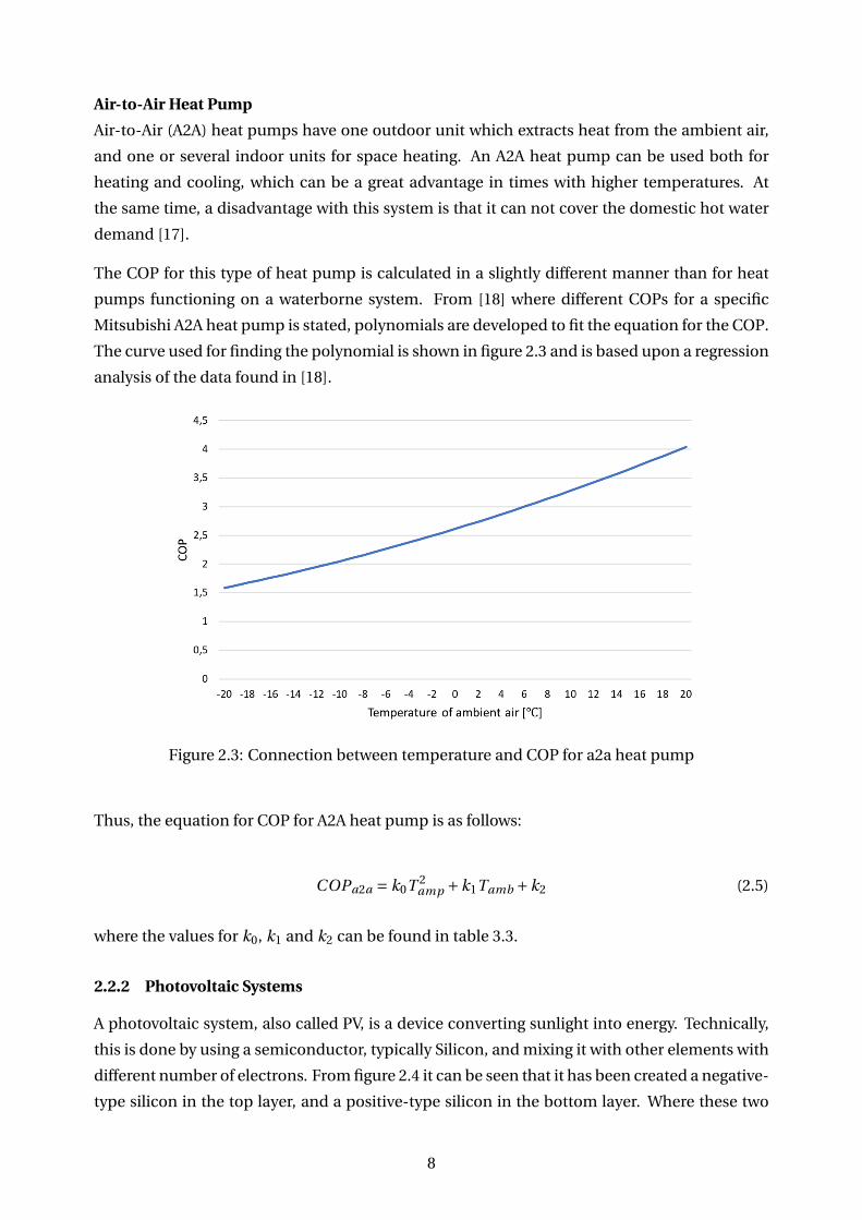
The COP for this type of heat pump is calculated in a slightly different manner than for heat
pumps functioning on a waterborne system. From [18] where different COPs for a specific
Mitsubishi A2A heat pump is stated, polynomials are developed to fit the equation for the COP.
The curve used for finding the polynomial is shown in figure 2.3 and is based upon a regression
analysis of the data found in [18].
Figure 2.3: Connection between temperature and COP for a2a heat pump
Thus, the equation for COP for A2A heat pump is as follows:
COPa2a = k0T 2amp +k1Tamb +k2 (2.5)
where the values for k0, k1 and k2 can be found in table 3.3.
2.2.2 Photovoltaic Systems
A photovoltaic system, also called PV, is a device converting sunlight into energy. Technically,
this is done by using a semiconductor, typically Silicon, and mixing it with other elements with
different number of electrons. From figure 2.4 it can be seen that it has been created a negative-
type silicon in the top layer, and a positive-type silicon in the bottom layer. Where these two
8
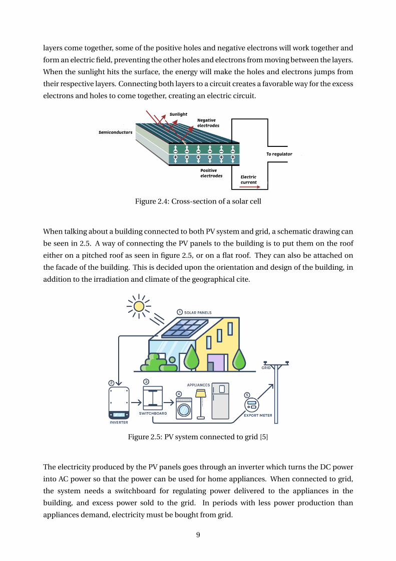
layers come together, some of the positive holes and negative electrons will work together and
form an electric field, preventing the other holes and electrons from moving between the layers.
When the sunlight hits the surface, the energy will make the holes and electrons jumps from
their respective layers. Connecting both layers to a circuit creates a favorable way for the excess
electrons and holes to come together, creating an electric circuit.
Figure 2.4: Cross-section of a solar cell
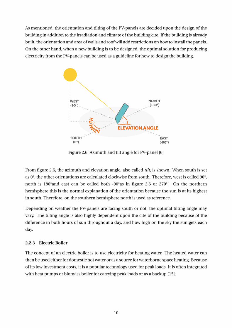
When talking about a building connected to both PV system and grid, a schematic drawing can
be seen in 2.5. A way of connecting the PV panels to the building is to put them on the roof
either on a pitched roof as seen in figure 2.5, or on a flat roof. They can also be attached on
the facade of the building. This is decided upon the orientation and design of the building, in
addition to the irradiation and climate of the geographical cite.
Figure 2.5: PV system connected to grid [5]
The electricity produced by the PV panels goes through an inverter which turns the DC power
into AC power so that the power can be used for home appliances. When connected to grid,
the system needs a switchboard for regulating power delivered to the appliances in the
building, and excess power sold to the grid. In periods with less power production than
appliances demand, electricity must be bought from grid.
9
As mentioned, the orientation and tilting of the PV-panels are decided upon the design of the
building in addition to the irradiation and climate of the building cite. If the building is already
built, the orientation and area of walls and roof will add restrictions on how to install the panels.
On the other hand, when a new building is to be designed, the optimal solution for producing
electricity from the PV-panels can be used as a guideline for how to design the building.
Figure 2.6: Azimuth and tilt angle for PV-panel [6]
From figure 2.6, the azimuth and elevation angle, also called tilt, is shown. When south is set
as 0°, the other orientations are calculated clockwise from south. Therefore, west is called 90°,
north is 180°and east can be called both -90°as in figure 2.6 or 270°. On the northern
hemisphere this is the normal explanation of the orientation because the sun is at its highest
in south. Therefore, on the southern hemisphere north is used as reference.
Depending on weather the PV-panels are facing south or not, the optimal tilting angle may
vary. The tilting angle is also highly dependent upon the cite of the building because of the
difference in both hours of sun throughout a day, and how high on the sky the sun gets each
day.
2.2.3 Electric Boiler
The concept of an electric boiler is to use electricity for heating water. The heated water can
then be used either for domestic hot water or as a source for waterborne space heating. Because
of its low investment costs, it is a popular technology used for peak loads. It is often integrated
with heat pumps or biomass boiler for carrying peak loads or as a backup [15].
10
2.2.4 Biomass Boiler
Bio Boiler (BB) is a technology which uses biomass as fuel for heating water. The water can be
used for domestic hot water and waterborne space heating in the waterborne model. In this
thesis, the fuel for the BB is wood-pellets. Wood-pellets are energy-efficient, hence the BB is
often used as an alternative when the objective is to reduce CO2-emissions.
2.2.5 Electric Battery
The introduction of weather dependent technologies introduces the need for storage on the
building cite. For electricity, a possibility that has been introduced the last years, is to sell
energy to the grid. But as the price for batteries decreases, storing the energy for later use
instead of selling is an alternative.
An electric battery can be seen as a power bank which is able to store energy. The technology
can be profitable in cases where the income of selling energy is low. As the consumers are able
to manage more of their energy use with Smart-meters, the need and desire for battery are also
increasing.
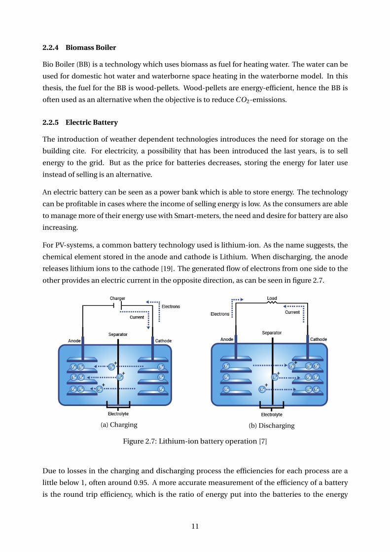
For PV-systems, a common battery technology used is lithium-ion. As the name suggests, the
chemical element stored in the anode and cathode is Lithium. When discharging, the anode
releases lithium ions to the cathode [19]. The generated flow of electrons from one side to the
other provides an electric current in the opposite direction, as can be seen in figure 2.7.
(a) Charging (b) Discharging
Figure 2.7: Lithium-ion battery operation [7]
Due to losses in the charging and discharging process the efficiencies for each process are a
little below 1, often around 0.95. A more accurate measurement of the efficiency of a battery
is the round trip efficiency, which is the ratio of energy put into the batteries to the energy
11
retrieved from the battery. This can also be understood as one charging and discharging cycle.
The round trip efficiency can be found by equation 2.6.
ηr t = ηch ·ηdch (2.6)
2.2.6 Hot Water Accumulator
A hot water accumulator is a storing opportunity for managing the heating demand. For a
waterborne system, the heating demand consists of both domestic hot water and space
heating. Otherwise, for point-source systems, the heating demand covered by the hot water
accumulator is the domestic hot water.
2.3 Electricity Pricing
The electricity price is dependent upon both the grid tariff, see chapter 2.4, and the spot price.
The total cost for electricity can be seen in equation 2.7, adapted from [1].
Total electricity price = Power price+Grid tariff+VAT (2.7)
The spot price varies throughout the entire year because of weather conditions as rainfall and
wind. Especially in Norway where most energy is produced by hydropower, rainfall is an
important factor. In addition to the weather, the spot price is also dependent upon the
situation and spot price in the rest of Europe. Since the seventies, Norway has been connected
to Europe through power cables which allows an exchange of power between Norway and the
rest of Europe [20].
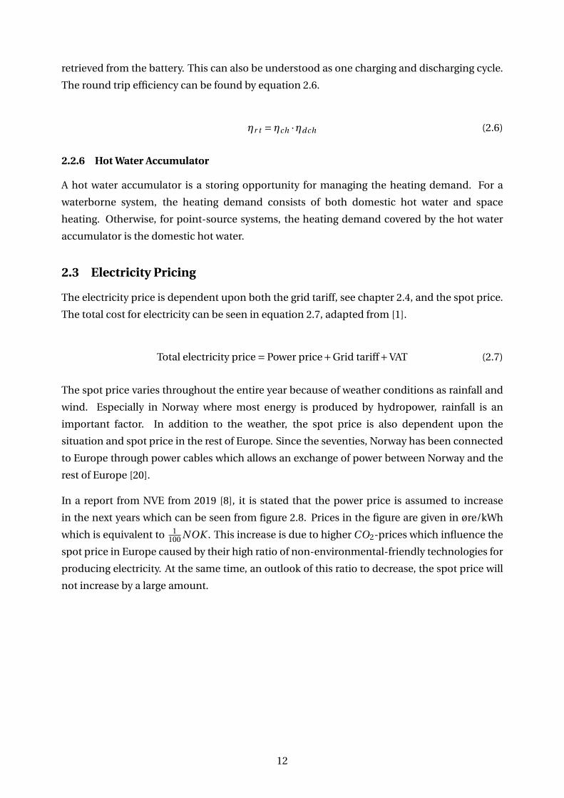
In a report from NVE from 2019 [8], it is stated that the power price is assumed to increase
in the next years which can be seen from figure 2.8. Prices in the figure are given in øre/kWh
which is equivalent to 1100 NOK . This increase is due to higher CO2-prices which influence the
spot price in Europe caused by their high ratio of non-environmental-friendly technologies for
producing electricity. At the same time, an outlook of this ratio to decrease, the spot price will
not increase by a large amount.
12
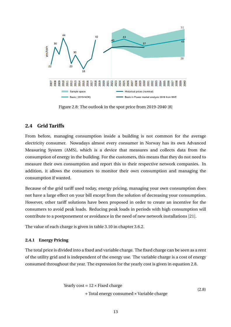
Figure 2.8: The outlook in the spot price from 2019-2040 [8]
2.4 Grid Tariffs
From before, managing consumption inside a building is not common for the average
electricity consumer. Nowadays almost every consumer in Norway has its own Advanced
Measuring System (AMS), which is a device that measures and collects data from the
consumption of energy in the building. For the customers, this means that they do not need to
measure their own consumption and report this to their respective network companies. In
addition, it allows the consumers to monitor their own consumption and managing the
consumption if wanted.
Because of the grid tariff used today, energy pricing, managing your own consumption does
not have a large effect on your bill except from the solution of decreasing your consumption.
However, other tariff solutions have been proposed in order to create an incentive for the
consumers to avoid peak loads. Reducing peak loads in periods with high consumption will
contribute to a postponement or avoidance in the need of new network installations [21].
The value of each charge is given in table 3.10 in chapter 3.6.2.
2.4.1 Energy Pricing
The total price is divided into a fixed and variable charge. The fixed charge can be seen as a rent
of the utility grid and is independent of the energy use. The variable charge is a cost of energy
consumed throughout the year. The expression for the yearly cost is given in equation 2.8.
Yearly cost = 12×Fixed charge
+Total energy consumed×Variable charge(2.8)
13
2.4.2 Power Subscription Pricing
This model is proposed by NVE and taken into use by a few grid companies as trial projects.
This model benefit those who are able to avoid high peaks in their consumption. As consumer,
you subscribe to a certain amount of effect that can be used at one point of time. If this amount
of effect is exceeded, a penalty charge is to be paid.
Yearly cost = 12× (Fixed charge + Subscription charge×Subscription)
+Variable charge×Total energy consumed
+Penalty charge×Penalty volume
(2.9)
2.4.3 Peak Power Pricing
For companies, a different pricing is given. This pricing requires time measurement of the
power consumed and is higher in the winter months than for the summer. The purpose of the
difference in pricing is to reflect the fact that the cost of building the energy grid is dependent
upon the power peaks in the winter months. In addition to the fixed and variable charge, the
power pricing has an effect charge which is dependent upon the highest measured power peak
each month.
Yearly cost = 12×Fixed charge
+Variable charge×Total energy consumed
+12×Effect charge×Peak effect
(2.10)
2.5 Demand Side Flexibility
This chapter is adapted from my own specialisation project, carried out in autumn 2018.
In order to meet the regulations given by the government in regard to energy efficient
buildings and more management of each customers electricity use, demand side flexibility is
of great value. Flexibility of the end-user, in the distribution grid, is called demand side
flexibility. Demand side flexibility can be denoted into two parts, Demand response and
Distributed storage. Demand response means that you change the electricity-usage from their
normal patterns [9] while distributed storage are batteries or larger storage systems. It is also a
known fact that high levels of Distributed Energy Resources (DER) affects grid stability. Hence,
using flexibility services as Demand Response (DR) will contribute to keeping the frequency of
the grid within allowable limits.
14
Figure 2.9: Illustration of different load flexibility classes [9]
From figure 2.9, the two most common ways of Demand response is shown, which are shifting
the loads in time or curtailing loads. The easiest method for the end-user, which is most
common nowadays, is curtailing loads. This method is divided into two classes; reducible and
disconnectable loads. Many Single Family Houses already use this method when they turn off
lights or reduces/turn off heat in rooms which are not used. This results in reducing the
electricity-load at that exact time.
Shifting the loads needs a bit more planning, but is used to avoid having a large load in times
with high electricity prices. In addition, avoiding peak loads will decrease the need for high
installation capacities of the technology which results in a decrease in the investment cost. It
is possible to change both the profile of the and the volume of the load, as shown in figure 2.9.
Both for the corporate market which operates with peak power pricing, and the private market
if power subscription pricing becomes a reality, shifting the loads is an effective method for
saving operational costs.
15

16
3 Methodology
3.1 Introduction to Model and Cases
The model used in this master thesis is based on two previous master thesis at NTNU, first
created by Ingrid Andersen [1] and then further developed by Marius Bagle [2]. Additions to
the model from this thesis, are new investment costs especially developed for larger systems
than used before. Also new heating loads have been implemented for choosing between
different building types. In stead of calculating the PV generation as it has been done earlier,
the PV production in this thesis has been simulated using PVsyst. PVsyst is a simulation
software which is used for studying, sizing and data analysis for PV systems. The simulated PV
generation is implemented in the model with the objective of giving a more accurate
calculation of the size of the PV system needed in the optimal solution. This is further
explained in chapter 3.7.
In this thesis the objective is to compare the waterborne system with the point-source system,
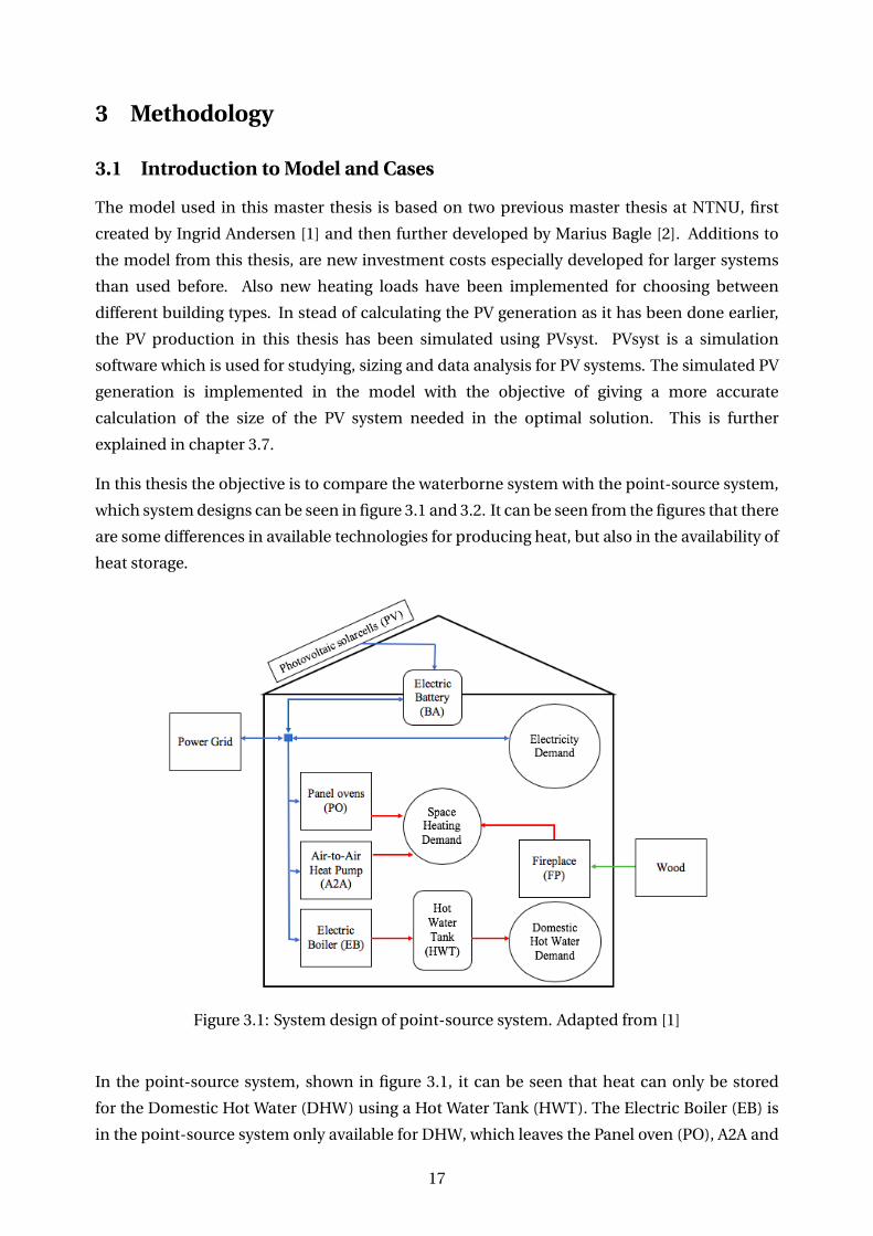
which system designs can be seen in figure 3.1 and 3.2. It can be seen from the figures that there
are some differences in available technologies for producing heat, but also in the availability of
heat storage.
Figure 3.1: System design of point-source system. Adapted from [1]
In the point-source system, shown in figure 3.1, it can be seen that heat can only be stored
for the Domestic Hot Water (DHW) using a Hot Water Tank (HWT). The Electric Boiler (EB) is
in the point-source system only available for DHW, which leaves the Panel oven (PO), A2A and
17
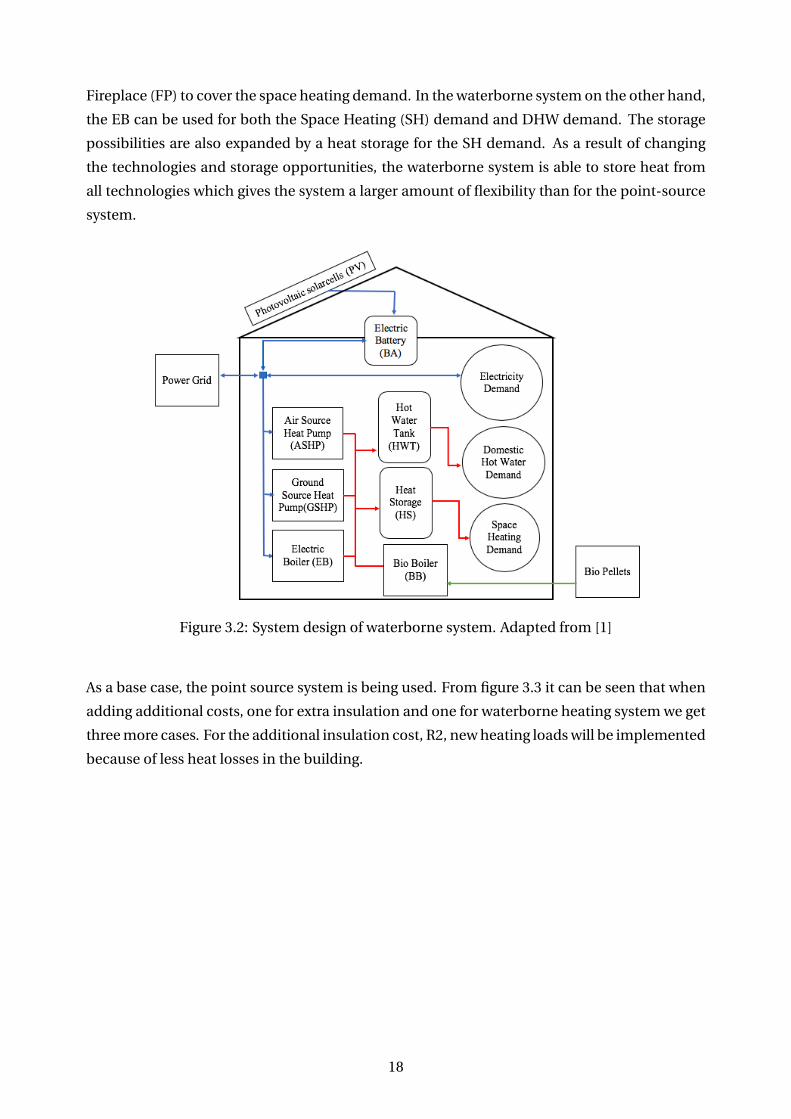
Fireplace (FP) to cover the space heating demand. In the waterborne system on the other hand,
the EB can be used for both the Space Heating (SH) demand and DHW demand. The storage
possibilities are also expanded by a heat storage for the SH demand. As a result of changing
the technologies and storage opportunities, the waterborne system is able to store heat from
all technologies which gives the system a larger amount of flexibility than for the point-source
system.
Figure 3.2: System design of waterborne system. Adapted from [1]
As a base case, the point source system is being used. From figure 3.3 it can be seen that when
adding additional costs, one for extra insulation and one for waterborne heating system we get
three more cases. For the additional insulation cost, R2, new heating loads will be implemented
because of less heat losses in the building.
18
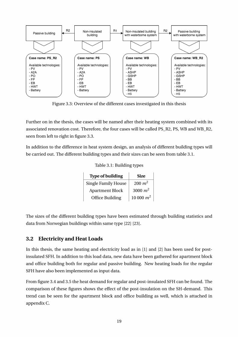
Figure 3.3: Overview of the different cases investigated in this thesis
Further on in the thesis, the cases will be named after their heating system combined with its
associated renovation cost. Therefore, the four cases will be called PS_R2, PS, WB and WB_R2,
seen from left to right in figure 3.3.
In addition to the difference in heat system design, an analysis of different building types will
be carried out. The different building types and their sizes can be seen from table 3.1.
Table 3.1: Building types
Type of building Size
Single Family House 200 m2
Apartment Block 3000 m2
Office Building 10 000 m2
The sizes of the different building types have been estimated through building statistics and
data from Norwegian buildings within same type [22] [23].
3.2 Electricity and Heat Loads
In this thesis, the same heating and electricity load as in [1] and [2] has been used for post-
insulated SFH. In addition to this load data, new data have been gathered for apartment block
and office building both for regular and passive building. New heating loads for the regular
SFH have also been implemented as input data.
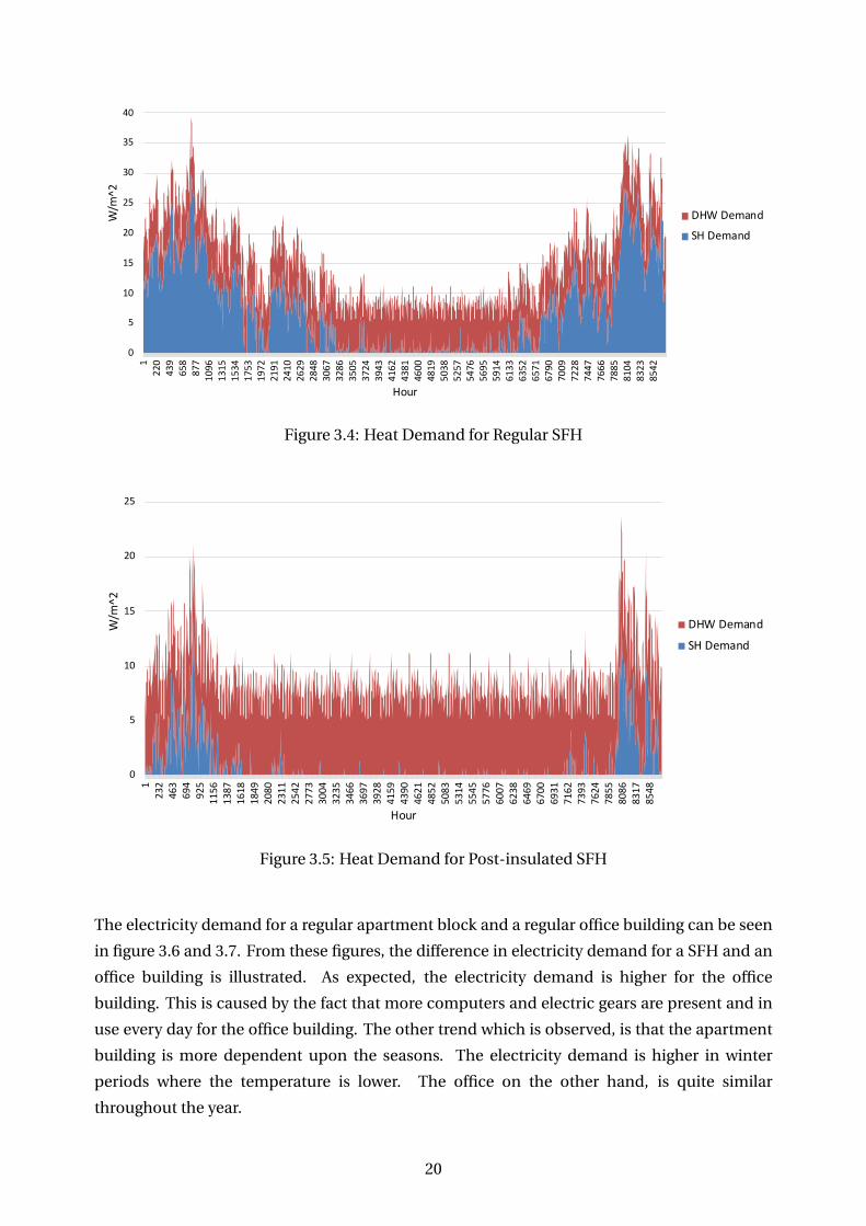
From figure 3.4 and 3.5 the heat demand for regular and post-insulated SFH can be found. The
comparison of these figures shows the effect of the post-insulation on the SH-demand. This
trend can be seen for the apartment block and office building as well, which is attached in
appendix C.
19
0
5
10
15
20
25
30
35
40
45
50
122
043
965
887
710
9613
1515
3417
5319
7221
9124
1026
2928
4830
6732
8635
0537
2439
4341
6243
8146
0048
1950
3852
5754
7656
9559
1461
3363
5265
7167
9070
0972
2874
4776
6678
8581
0483
2385
42
W/m
^2
Hour
DHW Demand
SH Demand
Figure 3.4: Heat Demand for Regular SFH
0
5
10
15
20
25
30
123
246
369
492
511
5613
8716
1818
4920
8023
1125
4227
7330
0432
3534
6636
9739
2841
5943
9046
2148
5250
8353
1455
4557
7660
0762
3864
6967
0069
3171
6273
9376
2478
5580
8683
1785
48
W/m
^2
Hour
DHW Demand
SH Demand
Figure 3.5: Heat Demand for Post-insulated SFH
The electricity demand for a regular apartment block and a regular office building can be seen
in figure 3.6 and 3.7. From these figures, the difference in electricity demand for a SFH and an
office building is illustrated. As expected, the electricity demand is higher for the office
building. This is caused by the fact that more computers and electric gears are present and in
use every day for the office building. The other trend which is observed, is that the apartment
building is more dependent upon the seasons. The electricity demand is higher in winter
periods where the temperature is lower. The office on the other hand, is quite similar
throughout the year.
20
0
1
2
3
4
5
6
7
8
9
118
436
755
073
391
610
9912
8214
6516
4818
3120
1421
9723
8025
6327
4629
2931
1232
9534
7836
6138
4440
2742
1043
9345
7647
5949
4251
2553
0854
9156
7458
5760
4062
2364
0665
8967
7269
5571
3873
2175
0476
8778
7080
5382
3684
1986
02
W/m
^2
Hour
EL Demand
Figure 3.6: Electricity Demand for Regular Apartment Block
0
5
10
15
20
25
30
124
548
973
397
712
2114
6517
0919
5321
9724
4126
8529
2931
7334
1736
6139
0541
4943
9346
3748
8151
2553
6956
1358
5761
0163
4565
8968
3370
7773
2175
6578
0980
5382
9785
41
W/m
^2
Hour
EL Demand
Figure 3.7: Electricity Demand for Regular Office
3.3 Technology Performance
The performance data is mostly gathered from [1] and [2] with minor modifications. All
performance data can be found in table 3.2.
From the table it can be seen that the efficiency of PV is set to η instead of a specific value. This
is caused by the fact that the efficiency of PV is now included in the simulation results, which is
described further in chapter 3.7.
21
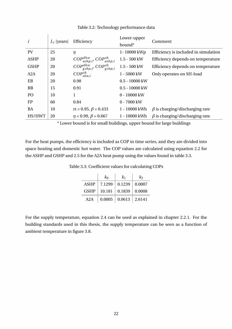
Table 3.2: Technology performance data
i Li [years] EfficiencyLower-upper
bound*Comment
PV 25 η 1- 10000 kWp Efficiency is included in simulation
ASHP 20 COP dhwashp,t , COP sh
ashp,t 1.5 - 500 kW Efficiency depends on temperature
GSHP 20 COP dhwg shp,t , COP sh
g shp,t 1.5 - 500 kW Efficiency depends on temperature
A2A 20 COP sha2a,t 1 - 5000 kW Only operates on SH-load
EB 20 0.98 0.5 - 10000 kW
BB 15 0.91 0.5 - 10000 kW
PO 10 1 0 - 10000 kW
FP 60 0.84 0 - 7000 kW
BA 10 rt = 0.95, β = 0.433 1 - 10000 kWh β is charging/discharging rate
HS/HWT 20 η = 0.99, β = 0.667 1 - 10000 kWh β is charging/discharging rate
* Lower bound is for small buildings, upper bound for large buildings
For the heat pumps, the efficiency is included as COP in time series, and they are divided into
space heating and domestic hot water. The COP values are calculated using equation 2.2 for
the ASHP and GSHP and 2.5 for the A2A heat pump using the values found in table 3.3.
Table 3.3: Coefficient values for calculating COPs
k0 k1 k2
ASHP 7.1299 0.1239 0.0007
GSHP 10.181 0.1839 0.0008
A2A 0.0005 0.0613 2.6141
For the supply temperature, equation 2.4 can be used as explained in chapter 2.2.1. For the
building standards used in this thesis, the supply temperature can be seen as a function of
ambient temperature in figure 3.8.
22
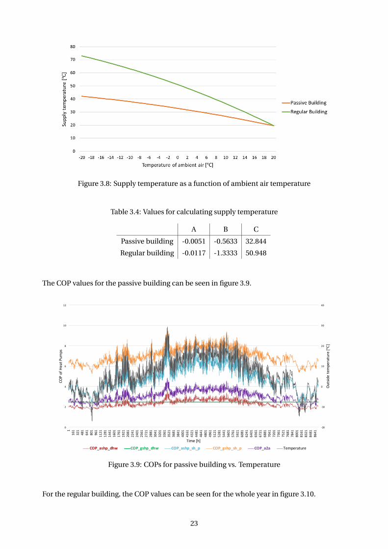
Figure 3.8: Supply temperature as a function of ambient air temperature
Table 3.4: Values for calculating supply temperature
A B C
Passive building -0.0051 -0.5633 32.844
Regular building -0.0117 -1.3333 50.948
The COP values for the passive building can be seen in figure 3.9.
-20
-10
0
10
20
30
40
0
2
4
6
8
10
12
116
132
148
164
180
196
111
2112
8114
4116
0117
6119
2120
8122
4124
0125
6127
2128
8130
4132
0133
6135
2136
8138
4140
0141
6143
2144
8146
4148
0149
6151
2152
8154
4156
0157
6159
2160
8162
4164
0165
6167
2168
8170
4172
0173
6175
2176
8178
4180
0181
6183
2184
8186
41
Outs
ide
tem
pera
ture
[℃]
COP
of H
eat P
umps
Time [h]
COP_ashp_dhw COP_gshp_dhw COP_ashp_sh_p COP_gshp_sh_p COP_a2a Temperature
Figure 3.9: COPs for passive building vs. Temperature
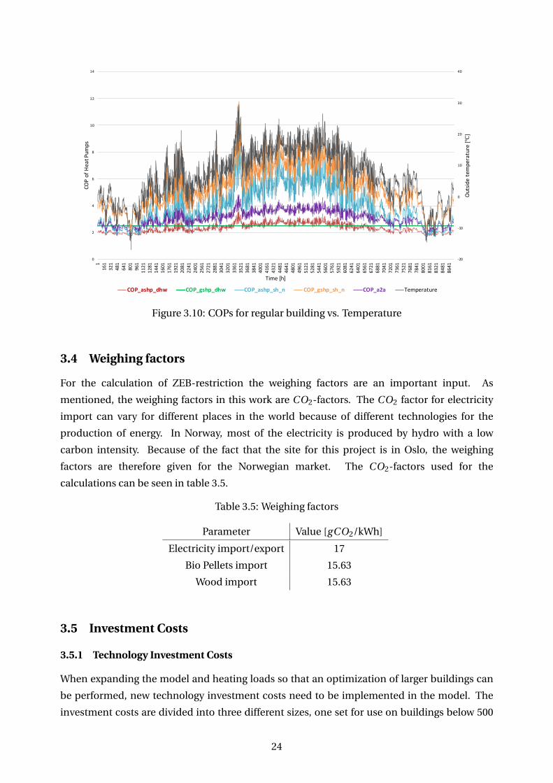
For the regular building, the COP values can be seen for the whole year in figure 3.10.
23
-20
-10
0
10
20
30
40
0
2
4
6
8
10
12
14
116
132
148
164
180
196
111
2112
8114
4116
0117
6119
2120
8122
4124
0125
6127
2128
8130
4132
0133
6135
2136
8138
4140
0141
6143
2144
8146
4148
0149
6151
2152
8154
4156
0157
6159
2160
8162
4164
0165
6167
2168
8170
4172
0173
6175
2176
8178
4180
0181
6183
2184
8186
41
Outs
ide
tem
pera
ture
[℃]
COP
of H
eat P
umps
Time [h]
COP_ashp_dhw COP_gshp_dhw COP_ashp_sh_n COP_gshp_sh_n COP_a2a Temperature
Figure 3.10: COPs for regular building vs. Temperature
3.4 Weighing factors
For the calculation of ZEB-restriction the weighing factors are an important input. As
mentioned, the weighing factors in this work are CO2-factors. The CO2 factor for electricity
import can vary for different places in the world because of different technologies for the
production of energy. In Norway, most of the electricity is produced by hydro with a low
carbon intensity. Because of the fact that the site for this project is in Oslo, the weighing
factors are therefore given for the Norwegian market. The CO2-factors used for the
calculations can be seen in table 3.5.
Table 3.5: Weighing factors
Parameter Value [gCO2/kWh]
Electricity import/export 17
Bio Pellets import 15.63
Wood import 15.63
3.5 Investment Costs
3.5.1 Technology Investment Costs
When expanding the model and heating loads so that an optimization of larger buildings can
be performed, new technology investment costs need to be implemented in the model. The
investment costs are divided into three different sizes, one set for use on buildings below 500
24
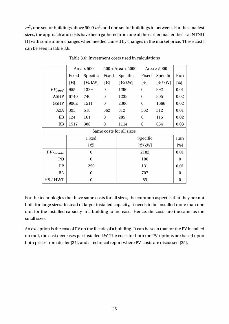
m2, one set for buildings above 5000 m2, and one set for buildings in between. For the smallest
sizes, the approach and costs have been gathered from one of the earlier master thesis at NTNU
[1] with some minor changes when needed caused by changes in the market price. These costs
can be seen in table 3.6.
Table 3.6: Investment costs used in calculations
Area < 500 500 < Area < 5000 Area > 5000
Fixed Specific Fixed Specific Fixed Specific Run
[AC] [AC/kW] [AC] [AC/kW] [AC] [AC/kW] [%]
PVr oo f 955 1329 0 1290 0 992 0.01
ASHP 6740 740 0 1238 0 805 0.02
GSHP 9902 1511 0 2306 0 1666 0.02
A2A 393 518 562 312 562 312 0.01
EB 124 161 0 285 0 115 0.02
BB 1517 386 0 1114 0 854 0.03
Same costs for all sizes
Fixed Specific Run
[AC] [AC/kW] [%]
PV f acade 0 2182 0.01
PO 0 180 0
FP 250 131 0.01
BA 0 707 0
HS / HWT 0 83 0
For the technologies that have same costs for all sizes, the common aspect is that they are not
built for large sizes. Instead of larger installed capacity, it needs to be installed more than one
unit for the installed capacity in a building to increase. Hence, the costs are the same as the
small sizes.
An exception is the cost of PV on the facade of a building. It can be seen that for the PV installed
on roof, the cost decreases per installed kW. The costs for both the PV-options are based upon
both prices from dealer [24], and a technical report where PV-costs are discussed [25].
25
3.5.2 Investment Costs for the Waterborne Heating System
Table 3.7: Investment costs for waterborne heating system inkl. MVA for different buildingtypes [10]
Source Building type Size [m2] Cost [NOK/m2]
COWI Single family house 127 618
COWI Apartment Block 3091 396
COWI Kindergarten 303 645
COWI Office 3613 386
COWI Office 7241 313
Using the costs from COWI and the sizes for the different building types found in 3.1, we can
find the costs of installing waterborne heating system.
Table 3.8: Additional renovation costs for waterborne heating system
Building type Size [m2] Cost [NOK] Cost [EUR]
Single family house 200 123 500 12 243
Apartment Block 3000 1 118 750 110 902
Office 10 000 3 125 000 309 781
3.5.3 Investment Costs for the Insulation of Buildings
The price for insulating the building in order to minimize heat losses, is dependent upon the
size of external walls. Since the buildings in this thesis are fictional, the calculation of such a
cost can be hard to define. Nevertheless, from a database made by Byggstart [26], it can be
found that most of the projects taken into consideration had a price-range of 168-297
EU R/m2 of wall area. It is also stated that insulating the building in connection with other
exterior renovations will reduce the cost. For insulation on exterior walls, 198 EU R/m2
appears to be a common pricing.
As a method for finding exterior wall area of a 200 m2 SFH, imaging a two floors cube where
each wall has a length of 10 meters. If each floor is 2.5 meters high, the total exterior area is 200
m2.
The apartment block can be seen as a 6 floors cube with two walls with length of 25 meters, and
two walls with length 20 meters. With a height of each floor of 2.5 meters, the total exterior wall
area is 1350 m2.
For the office building, imaging a 10 floors cube with two walls as 25 meters and the other two
with a length of 40 meters. If each floor is 2.5 meters high i has a total height of 25 meters. This
equals a total exterior wall area of 3250 m2.
26
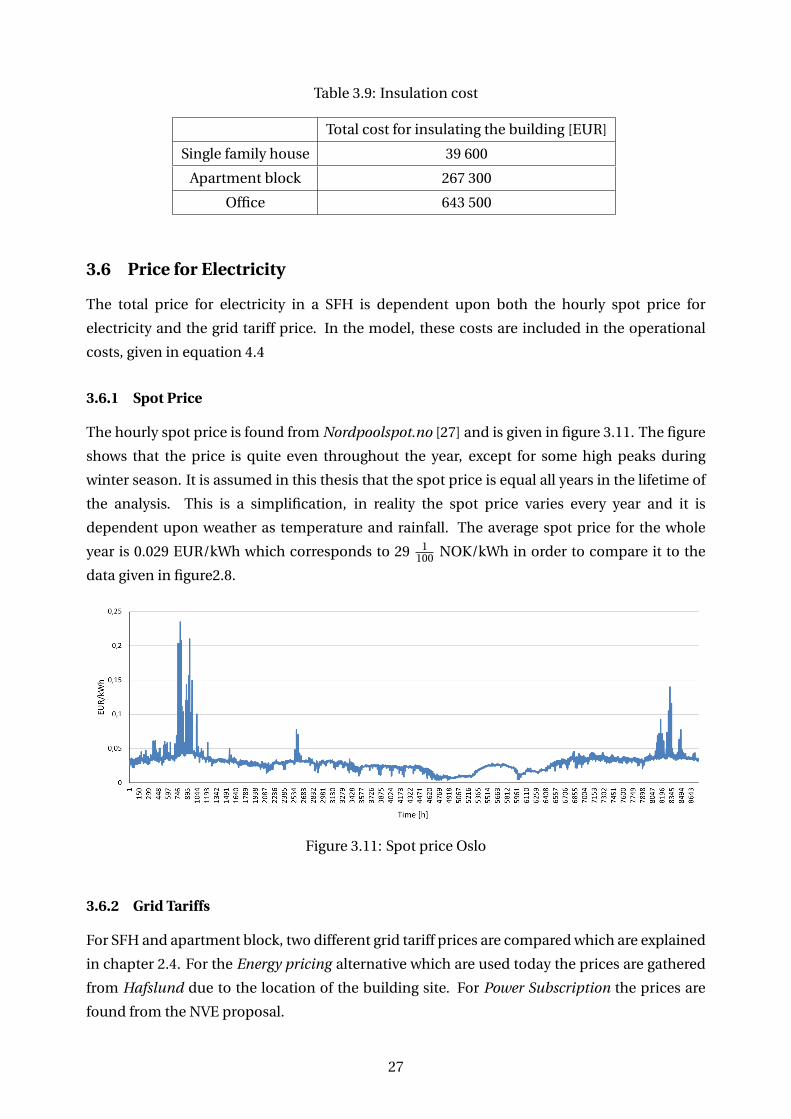
Table 3.9: Insulation cost
Total cost for insulating the building [EUR]
Single family house 39 600
Apartment block 267 300
Office 643 500
3.6 Price for Electricity
The total price for electricity in a SFH is dependent upon both the hourly spot price for
electricity and the grid tariff price. In the model, these costs are included in the operational
costs, given in equation 4.4
3.6.1 Spot Price
The hourly spot price is found from Nordpoolspot.no [27] and is given in figure 3.11. The figure
shows that the price is quite even throughout the year, except for some high peaks during
winter season. It is assumed in this thesis that the spot price is equal all years in the lifetime of
the analysis. This is a simplification, in reality the spot price varies every year and it is
dependent upon weather as temperature and rainfall. The average spot price for the whole
year is 0.029 EUR/kWh which corresponds to 29 1100 NOK/kWh in order to compare it to the
data given in figure2.8.
Figure 3.11: Spot price Oslo
3.6.2 Grid Tariffs
For SFH and apartment block, two different grid tariff prices are compared which are explained
in chapter 2.4. For the Energy pricing alternative which are used today the prices are gathered
from Hafslund due to the location of the building site. For Power Subscription the prices are
found from the NVE proposal.
27
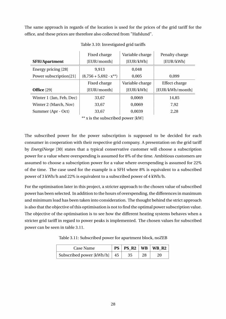
The same approach in regards of the location is used for the prices of the grid tariff for the
office, and these prices are therefore also collected from "Hafslund".
Table 3.10: Investigated grid tariffs
Fixed charge Variable charge Penalty charge
SFH/Apartment [EUR/month] [EUR/kWh] [EUR/kWh]
Energy pricing [28] 9,913 0,048
Power subscription[21] (8,756 + 5,692 · x**) 0,005 0,099
Fixed charge Variable charge Effect charge
Office [29] [EUR/month] [EUR/kWh] [EUR/kWh/month]
Winter 1 (Jan, Feb, Dec) 33,67 0,0069 14,85
Winter 2 (March, Nov) 33,67 0,0069 7,92
Summer (Apr - Oct) 33,67 0,0039 2,28
** x is the subscribed power [kW]
The subscribed power for the power subscription is supposed to be decided for each
consumer in cooperation with their respective grid company. A presentation on the grid tariff
by EnergiNorge [30] states that a typical conservative customer will choose a subscription
power for a value where overspending is assumed for 8% of the time. Ambitious customers are
assumed to choose a subscription power for a value where overspending is assumed for 22%
of the time. The case used for the example is a SFH where 8% is equivalent to a subscribed
power of 3 kWh/h and 22% is equivalent to a subscribed power of 4 kWh/h.
For the optimisation later in this project, a stricter approach to the chosen value of subscribed
power has been selected. In addition to the hours of overspending, the differences in maximum
and minimum load has been taken into consideration. The thought behind the strict approach
is also that the objective of this optimisation is not to find the optimal power subscription value.
The objective of the optimisation is to see how the different heating systems behaves when a
stricter grid tariff in regard to power peaks is implemented. The chosen values for subscribed
power can be seen in table 3.11.
Table 3.11: Subscribed power for apartment block, noZEB
Case Name PS PS_R2 WB WB_R2
Subscribed power [kWh/h] 45 35 28 20
28
3.6.3 Bio fuel price
For the technologies which are not electricity driven, a different pricing is valid. The prices
used in the calculation are obtained from dealers and can be seen in table 3.12.
Table 3.12: Bio fuel prices
Price [EUR/kWh]
Bio Pellets 0.058
Wood 0.088
3.7 Simulations in PVsyst
PVsyst is a simulation software which is used for studying, sizing and data analysis of PV
systems [31]. Both specific and generic systems can be simulated, depending on the accuracy
and amount of input data. It also contains a large Meteonorm database which can be used to
customize the data to fit your location. If even more specific weather data is required for your
project, it is possible to import personal data into the model.
3.7.1 Input Data for PVsyst Simulations
The input data applicable for all of the variants in the project can be found in table 3.13. The
location for this simulation is set to Slemdal in Oslo. For this location, the albedo values can
be set to 0.2 for all months without snow. In winter months, it is assumed that there will be
some snow laying in the location which will result in a higher reflection of sun. Therefore, the
albedo values are set to 0.4 throughout these months. The weather data is from the Meteonorm
database.
Table 3.13: Input data for the project applicable for all variations
Location Latitude 59.95°N, Longitude 10.70°E, Altitude 142m
Monthly albedo values Dec, Jan, Feb, Mar, Apr: 0.4, May, Jun, Jul, Aug, Sep, Oct, Nov: 0.2
PV Module Si-Poly, 295 Wp (REC295TP2), 1.670m2
Inverter 3kWac inverter(generic)
From Technic spesification SN/TS 3031:2016 - Energy performance of buildings, Calculation of
energy needs and energy supply [32] the values for soiling loss were found. These losses take
into account coverage of the PV modules caused by snow, leaves, dust etc. The values used in
the simulation is found in table 3.14 for their respective tilting solutions.
29
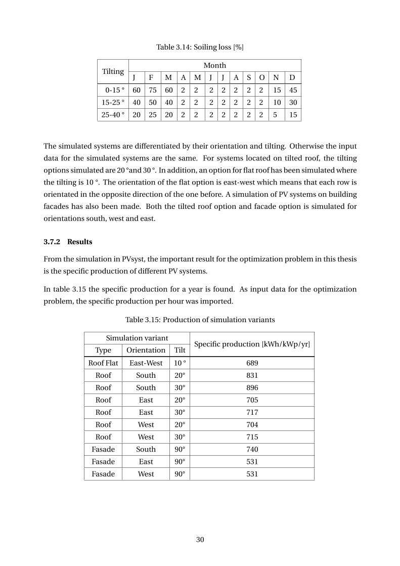
Table 3.14: Soiling loss [%]
TiltingMonth
J F M A M J J A S O N D
0-15 ° 60 75 60 2 2 2 2 2 2 2 15 45
15-25 ° 40 50 40 2 2 2 2 2 2 2 10 30
25-40 ° 20 25 20 2 2 2 2 2 2 2 5 15
The simulated systems are differentiated by their orientation and tilting. Otherwise the input
data for the simulated systems are the same. For systems located on tilted roof, the tilting
options simulated are 20 °and 30 °. In addition, an option for flat roof has been simulated where
the tilting is 10 °. The orientation of the flat option is east-west which means that each row is
orientated in the opposite direction of the one before. A simulation of PV systems on building
facades has also been made. Both the tilted roof option and facade option is simulated for
orientations south, west and east.
3.7.2 Results
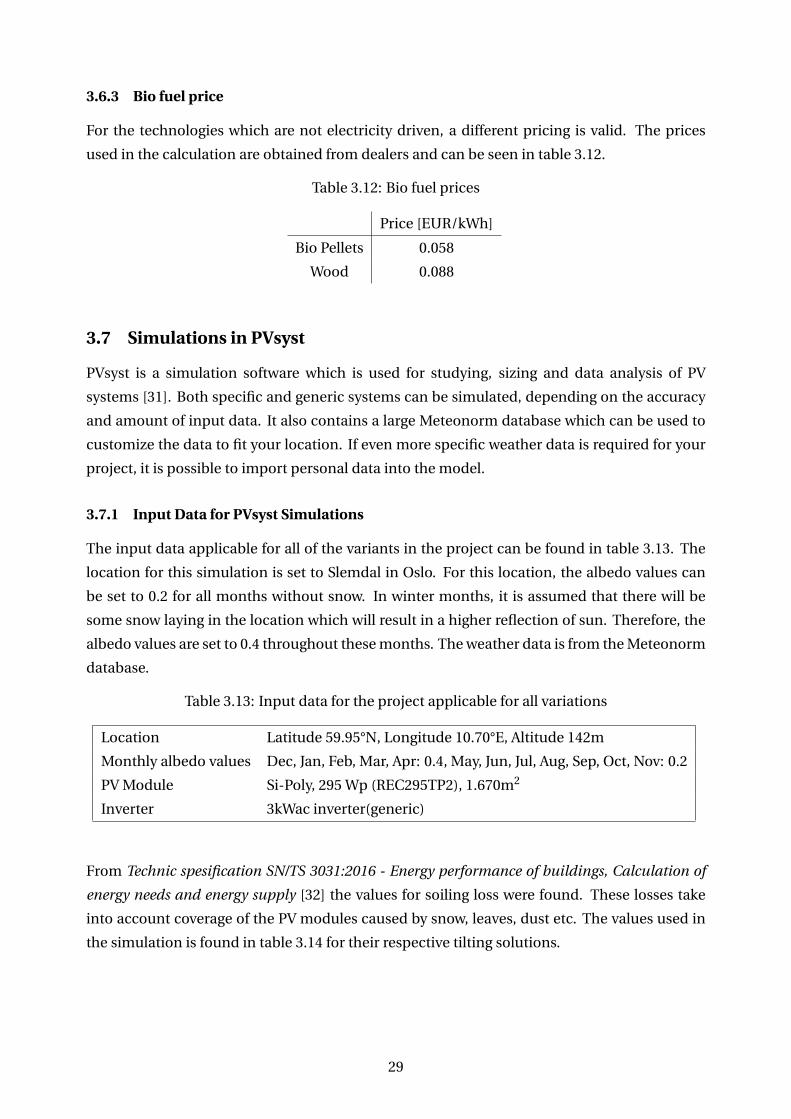
From the simulation in PVsyst, the important result for the optimization problem in this thesis
is the specific production of different PV systems.
In table 3.15 the specific production for a year is found. As input data for the optimization
problem, the specific production per hour was imported.
Table 3.15: Production of simulation variants
Simulation variantSpecific production [kWh/kWp/yr]
Type Orientation Tilt
Roof Flat East-West 10 ° 689
Roof South 20° 831
Roof South 30° 896
Roof East 20° 705
Roof East 30° 717
Roof West 20° 704
Roof West 30° 715
Fasade South 90° 740
Fasade East 90° 531
Fasade West 90° 531
30
In figure 3.12 an example of how the specific production is distributed throughout a year can be
seen. As it can be seen from the figure, most of the production is made in the summer months.
This figure is the specific production of a PV-system on tilted roof with 30°tilting facing south.
0
0,1
0,2
0,3
0,4
0,5
0,6
0,7
0,8
0,9
11
173
345
517
689
861
1033
1205
1377
1549
1721
1893
2065
2237
2409
2581
2753
2925
3097
3269
3441
3613
3785
3957
4129
4301
4473
4645
4817
4989
5161
5333
5505
5677
5849
6021
6193
6365
6537
6709
6881
7053
7225
7397
7569
7741
7913
8085
8257
8429
8601
Spec
ific p
rodu
ctio
n [k
W/k
Wp]
Hour
Figure 3.12: Specific production
31

32
4 Model
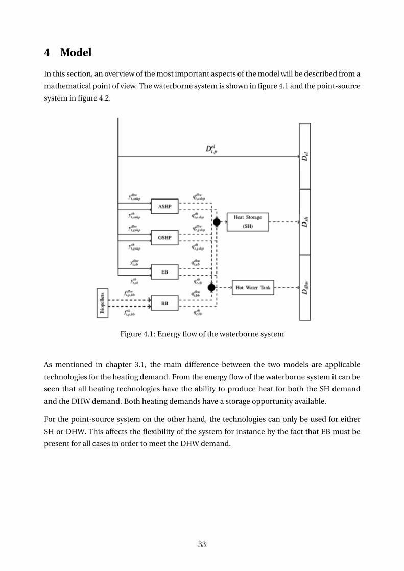
In this section, an overview of the most important aspects of the model will be described from a
mathematical point of view. The waterborne system is shown in figure 4.1 and the point-source
system in figure 4.2.
Figure 4.1: Energy flow of the waterborne system
As mentioned in chapter 3.1, the main difference between the two models are applicable
technologies for the heating demand. From the energy flow of the waterborne system it can be
seen that all heating technologies have the ability to produce heat for both the SH demand
and the DHW demand. Both heating demands have a storage opportunity available.
For the point-source system on the other hand, the technologies can only be used for either
SH or DHW. This affects the flexibility of the system for instance by the fact that EB must be
present for all cases in order to meet the DHW demand.
33
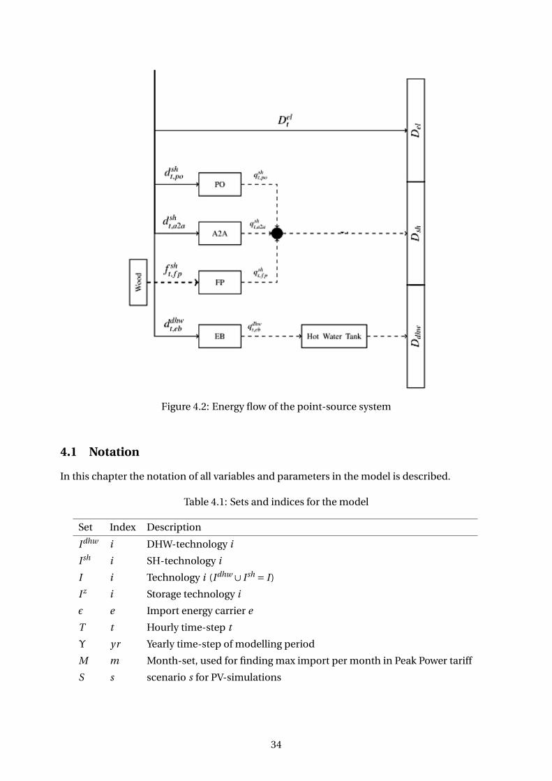
Figure 4.2: Energy flow of the point-source system
4.1 Notation
In this chapter the notation of all variables and parameters in the model is described.
Table 4.1: Sets and indices for the model
Set Index Description
Idhw i DHW-technology i
Ish i SH-technology i
I i Technology i (Idhw ∪ Ish = I)
Iz i Storage technology i
ε e Import energy carrier e
T t Hourly time-step t
Υ yr Yearly time-step of modelling period
M m Month-set, used for finding max import per month in Peak Power tariff
S s scenario s for PV-simulations
34
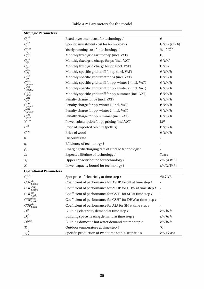
Table 4.2: Parameters for the model
Strategic Parameters
Cfxdi Fixed investment cost for technology i AC
Cspei Specific investment cost for technology i AC/kW (kW h)
Cruni Yearly running cost for technology i % of Cspe
i
Cfxdep Monthly fixed grid tariff for ep (incl. VAT) AC)
Cfxdps Monthly fixed grid charge for ps (incl. VAT) AC/kW
Cfxdpp Monthly fixed grid charge for pp (incl. VAT) AC/kW
Cspeep Monthly specific grid tariff for ep (incl. VAT) AC/kW h
Cspeps Monthly specific grid tariff for ps (incl. VAT) AC/kW h
Cspepp,w1 Monthly specific grid tariff for pp, winter 1 (incl. VAT) AC/kW h
Cspepp,w2 Monthly specific grid tariff for pp, winter 2 (incl. VAT) AC/kW h
Cspepp,s Monthly specific grid tariff for pp, summer (incl. VAT) AC/kW h
Cptyps Penalty charge for ps (incl. VAT) AC/kW h
Cptypp,w1 Penalty charge for pp, winter 1 (incl. VAT) AC/kW h
Cptypp,w2 Penalty charge for pp, winter 2 (incl. VAT) AC/kW h
Cptypp,s Penalty charge for pp, summer (incl. VAT) AC/kW h
Y sub Power subscription for ps pricing (incl.VAT) kW
Cbf Price of imported bio fuel (pellets) AC/kW h
Cwo Price of wood AC/kW h
R Discount rate -
ηi Efficiency of technology i -
βi Charging/discharging rate of storage technology i -
Li Expected lifetime of technology i Years
Xi Upper capacity bound for technology i kW (K W h)
Xi Lower capacity bound for technology i kW (K W h)
Operational Parameters
Cspott Spot price of electricity at time step t AC/kWh
COPsht,ashp Coefficient of performance for ASHP for SH at time step t -
COPdhwt,ashp Coefficient of performance for ASHP for DHW at time step t -
COPsht,gshp Coefficient of performance for GSHP for SH at time step t -
COPdhwt,ashp Coefficient of performance for GSHP for DHW at time step t -
COPsht,a2a Coefficient of performance for A2A for SH at time step t -
Delt Building electricity demand at time step t kW h/h
Dsht Building space heating demand at time step t kW h/h
Ddhwt Building domestic hot water demand at time step t kW h/h
Tt Outdoor temperature at time step t °C
Y pvt,s Specific production of PV at time step t , scenario s kW /kW h
35
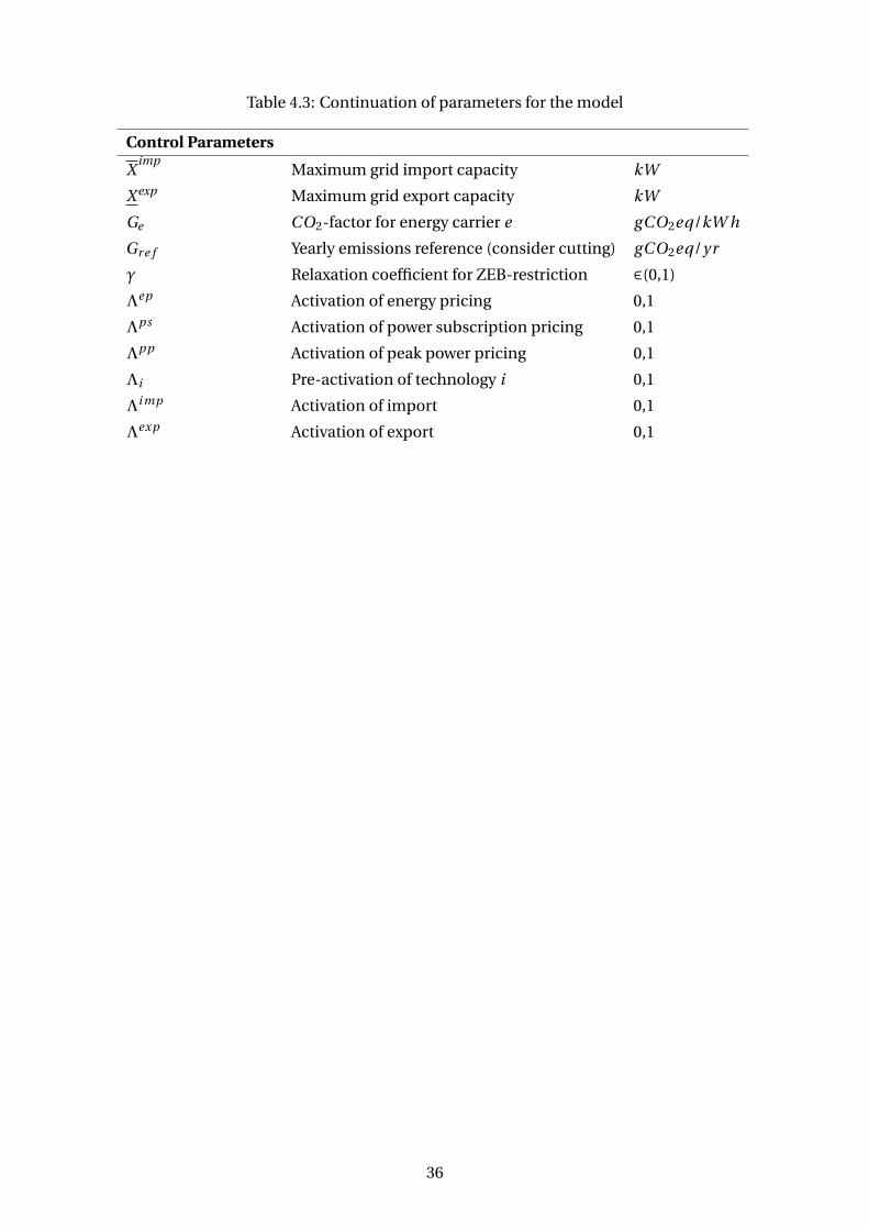
Table 4.3: Continuation of parameters for the model
Control Parameters
Ximp
Maximum grid import capacity kW
X exp Maximum grid export capacity kW
Ge CO2-factor for energy carrier e gCO2eq/kW h
Gr e f Yearly emissions reference (consider cutting) gCO2eq/yr
γ Relaxation coefficient for ZEB-restriction ∈(0,1)
Λep Activation of energy pricing 0,1
Λps Activation of power subscription pricing 0,1
Λpp Activation of peak power pricing 0,1
Λi Pre-activation of technology i 0,1
Λi mp Activation of import 0,1
Λexp Activation of export 0,1
36
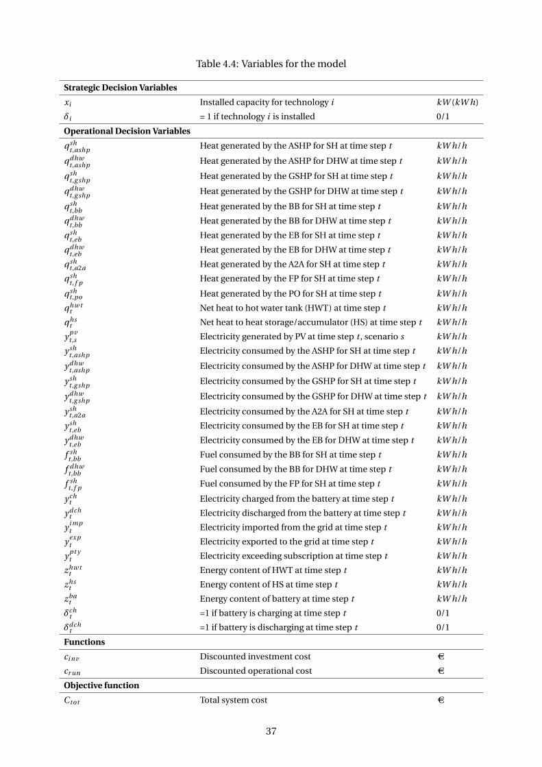
Table 4.4: Variables for the model
Strategic Decision Variables
xi Installed capacity for technology i kW (kW h)
δi = 1 if technology i is installed 0/1
Operational Decision Variables
q sht ,ashp Heat generated by the ASHP for SH at time step t kW h/h
qdhwt ,ashp Heat generated by the ASHP for DHW at time step t kW h/h
q sht ,g shp Heat generated by the GSHP for SH at time step t kW h/h
qdhwt ,g shp Heat generated by the GSHP for DHW at time step t kW h/h
q sht ,bb Heat generated by the BB for SH at time step t kW h/h
qdhwt ,bb Heat generated by the BB for DHW at time step t kW h/h
q sht ,eb Heat generated by the EB for SH at time step t kW h/h
qdhwt ,eb Heat generated by the EB for DHW at time step t kW h/h
q sht ,a2a Heat generated by the A2A for SH at time step t kW h/h
q sht , f p Heat generated by the FP for SH at time step t kW h/h
q sht ,po Heat generated by the PO for SH at time step t kW h/h
qhw tt Net heat to hot water tank (HWT) at time step t kW h/h
qhst Net heat to heat storage/accumulator (HS) at time step t kW h/h
y pvt ,s Electricity generated by PV at time step t , scenario s kW h/h
y sht ,ashp Electricity consumed by the ASHP for SH at time step t kW h/h
ydhwt ,ashp Electricity consumed by the ASHP for DHW at time step t kW h/h
y sht ,g shp Electricity consumed by the GSHP for SH at time step t kW h/h
ydhwt ,g shp Electricity consumed by the GSHP for DHW at time step t kW h/h
y sht ,a2a Electricity consumed by the A2A for SH at time step t kW h/h
y sht ,eb Electricity consumed by the EB for SH at time step t kW h/h
ydhwt ,eb Electricity consumed by the EB for DHW at time step t kW h/h
f sht ,bb Fuel consumed by the BB for SH at time step t kW h/h
f dhwt ,bb Fuel consumed by the BB for DHW at time step t kW h/h
f sht , f p Fuel consumed by the FP for SH at time step t kW h/h
ycht Electricity charged from the battery at time step t kW h/h
ydcht Electricity discharged from the battery at time step t kW h/h
y i mpt Electricity imported from the grid at time step t kW h/h
yexpt Electricity exported to the grid at time step t kW h/h
y pt yt Electricity exceeding subscription at time step t kW h/h
zhw tt Energy content of HWT at time step t kW h/h
zhst Energy content of HS at time step t kW h/h
zbat Energy content of battery at time step t kW h/h
δcht =1 if battery is charging at time step t 0/1
δdcht =1 if battery is discharging at time step t 0/1
Functions
ci nv Discounted investment cost AC
cr un Discounted operational cost AC
Objective function
Ctot Total system cost AC
37
4.2 Objective Function
The objective function of the optimisation problem is the total cost of all technology
investment and operational costs throughout the analysis period, as seen in equation 4.1.
ctot = mi n(ci nv + cr un) (4.1)
Where ci nv is the investment cost function given by equation 4.2 and cr un is the operational
cost function given by equation 4.4.
ci nv = ∑i∈I
(C spei xi +C f xd
i δi ) ·αi (R,Li ,Υn) (4.2)
The final discounting factor αi , is given in equation 4.3.This factor takes into account the
lifetime of each technology, and as a result of that lifetime compared with the time of the
analysis, the forced reinvestments.
αi (R,Li ,Υn) = 1− (1+R)−(Yn−Li K )
1− (1+R)−Li· 1
(1+R)K Li+
K−1∑k=0
1
(1+R)kLi(4.3)
The operational cost is the sum of operation and maintenance cost for each technology, cost
of bio fuel, electricity cost and the grid charge. There are three different grid charge options in
this thesis, where the activation of each option is based on the binary variables Λep , Λps and
Λpp . Only one of the variables can be activated at the same time.
cr un =(∑
i∈IC r un
i C spei xi +
∑t∈T
y i mpt C spot
t ·1.25− yexpt C spot
t + f i mpt C f ·1.25
+ (12 ·C f xdep + ∑
t∈Ty i mp
t )Λep
+ (12 · (C f xdps +C sub
ps ·Ysub)+C speps
∑y i mp
t +C pt yps
∑t∈T
y pt yt )Λps
+ (C f xdpp +C spe
pp
∑t∈M
y i mpt +C pt y
pp · y i mp,maxm )Λpp
)·λ(Υn ,R)
(4.4)
The total capitalization factor λ is given in equation 4.5. This factor is used to obtain a present
value of all yearly running costs throughout the time of analysis.
λ(Υn ,R) = 1− (1+R)−Υn
R· 1
(1+R)1(4.5)
38
4.3 Constraints
To ensure that all variables in the optimal solution calculated by the model are within specified
limits, constraints must be implemented in the model. Some of the constraints are based upon
limits in order to make the solution as close to real life as possible. Others are important in
order to ensure that demands are met. Hence, some of the constraints are operated by ≤ or ≥,
while the ones who are to ensure the meeting of demands are operated by = .
4.3.1 Capacity Constraints
The following constraints are important in order to ensure that the installed capacity for each
technology are within realistic limits. In addition, the constraints are a part of limiting the
amount of possible solutions for the model.
The installed capacity of each technology i must be less than M, which is a large number called
big M in operations research:
xi ≤ δi M ∀i ∈ I (4.6)
The lower and upper limits of each technology are stated in table 3.2, which sets limitations for
the installed capacity in addition to big M :
Xiδi ≤ xi ≤ XiΛi (4.7)
4.3.2 ZEB-constraint
As explained in chapter 2.1, the restriction in order to meet the ZEB-goal for the operational
phase of the building is to import the same amount of energy as exported throughout a year of
operation. How this is coded in the model can be seen from equation 4.8 where the relaxation
coefficient γ decides whether the requirement equals ZEB or no Zero Emission Building
(noZEB). For γ = 0 gives noZEB and γ = 1 signifying ZEB.
γ∑t∈T
(y i mp
t Gel + f i mpt G f
)≤ ∑
t∈Tyexp
t Gel (4.8)
4.3.3 Technology Constraints
All energy production on-site is limited by the capacity of their respective technologies. For
heat technologies, producing both for SH and DHW the following must hold:
q sht ,i +qdhw
t ,i ≤ xi ∀t ∈ T , i ∈ I (4.9)
39
For the PV production the following prerequisites must be present:
y pvt ,s = xpv
s Y pvt ,s Λpv ∀t ∈ T , s ∈ S (4.10)
where all scenarios that have been simulated is taken into consideration for the optimal
solution. Y pvt ,s is the simulated specific PV-production for each scenario, shown in table 3.15.
For the heat pumps, the generated heat is limited by the COP of each heat pump technology
and heat load:
q sht ,ashp = y sh
t ,ashpCOP sht ,ashpΛashp ∀t ∈ T (4.11)
qdhwt ,ashp = ydhw
t ,ashpCOP dhwt ,ashpΛashp ∀t ∈ T (4.12)
q sht ,g shp = y sh
t ,g shpCOP sht ,g shpΛg shp ∀t ∈ T (4.13)
qdhwt ,g shp = ydhw
t ,g shpCOP dhwt ,g shpΛg shp ∀t ∈ T (4.14)
where the COP can be seen as a hourly time series in figure 3.9 and 3.10 in chapter 3.3 where
the performance of each technology is discussed.
For the A2A heat pump, the difference between building types is not taken into consideration
when calculating the heat pump. In addition to this, the A2A heat pump is only operating on
the SH-load. Hence, only one constraint concerns the heat generated by this technology:
q sht ,a2a = y sh
t ,a2aCOPt ,a2aΛa2a ∀t ∈ T (4.15)
In addition to this constraint concerning the A2A heat pump, it is assumed that the technology
has a limited ability to transport heat between rooms:
q sht ,a2a ≤ 0.5 ·D sh
t ∀t ∈ T (4.16)
where D sht is the total space heating load for each time-step. In addition to the heat pumps, the
EB and PO are also dependent upon the electricity consumption. For the point-source system
the EB can only operate on the SH load. The constraints for the two technologies are therefore
as follows for the point-source system:
40
q sht ,po = y sh
t ,poηpoΛpo ∀t ∈ T (4.17)
q sht ,eb = y sh
t ,ebηebΛeb ∀t ∈ T (4.18)
On the other hand, for the waterborne system the EB has the ability to operate on both SH and
DHW load. Therefore the additional constraint for the waterborne model is as follows:
qdhwt ,eb = ydhw
t ,eb ηebΛeb ∀t ∈ T (4.19)
For the technologies which are dependent upon the amount of fuel imported, the waterborne
system has the BB and the point-source system have the FP. The BB can be operated on both
SH and DHW load:
q sht ,bb = f sh
t ,bbηbbλbb ∀t ∈ T (4.20)
qdhwt ,bb = f dhw
t ,bb ηbbλbb ∀t ∈ T (4.21)
The fireplace on the other hand, ca only be operated on SH load. It is also restricted to only
being able to operate between 16:00 and 24:00. The constraints concerning the fireplace are
therefore as follows:
q sht ′, f p = f sh
t ′, f pη f pλ f p ∀t ′ ∈ T ′ (4.22)
q sht ′, f p = 0 ∀t ′ ∉ T ′ (4.23)
where t ′ = t − f loor ( 124 ) ·24 and T ′ = {16,17, ...,24}
4.3.4 Storage Constraints
For the energy storage technologies, the HWT and Heat Storage (HS) is modeled in the same
way as they both are applicable for the heat load. The generated heat for those technologies
are dependent upon the amount of energy stored:
qhw t ,hst = zhw t ,hs
t−1 − zhw t ,hst ∀t ∈ T (4.24)
41
where the charging rate of the storage can be seen from:
|qhw t ,hst | ≤ xhw t ,hsβhw t ,hs ∀t ∈ T (4.25)
The battery is modeled in a slightly different manner:
zbat = zba
t−1 + ycht ηc h − ydch
t1
ηdch∀t ∈ T (4.26)
where the charging and discharging are constrained as well:
ycht ≤ (xba − zba
t−1)1
ηchλba ∀t ∈ T (4.27)
ydcht ≤ zba
t−1ηdchΛba ∀t ∈ T (4.28)
Within one timestep, it is only allowed for the battery to either charge or discharge. This is
ensured using following constraints:
ycht ≤ δch M ∀t ∈ T (4.29)
ydcht ≤ δdch M ∀t ∈ T (4.30)
δcht +δdch
t ≤ 1 ∀t ∈ T (4.31)
The charging and discharging rate within one hour is restricted with following constraint:
ych,dcht ≤ xbaβba ∀t ∈ T (4.32)
4.3.5 Grid Interaction Constraints
In the same way that the technologies have a maximum limit, the grid interaction is limited for
both the import and export of energy:
y i mpt ≤ X
i mpδ
i mpt ∀t ∈ T (4.33)
42
yexpt ≤ X
expδ
expt ∀t ∈ T (4.34)
Power Subscription Pricing
For the power subscription pricing, the penalty volume is decided upon following equations:
y i mpt −Y sub ≤ y pt y
t (4.35)
0 ≤ y pt yt (4.36)
Peak Power Pricing
For the peak power pricing, the maximum value of imported electricity for each month must
be found. For this purpose it is created a month-set, M, which holds all months for the entire
year. Each month in the month-set holds every hour for that specific month. When counting
through the time-steps of that specific month, the max value is updated if the value for that
time-step fulfill the restriction:
y i mp,maxm ≥ y i mp
t (4.37)
When counted through the entire month, the updated value for the maximum imported
electricity is the value used in the calculation for the grid tariff.
4.3.6 Load Constraints
In chapter 3.1 where the model is introduced, it can be seen that there are three different load
demands which must be met, Electric, Space Heating and Domestic Hot Water. In order to
ensure the fulfillment of these demands, balances for each demand have been defined:
Delt = y i mp
t + y pvt + ydch
t − ycht − ∑
i∈I dhw
y it −
∑i∈I sh
y it ∀t ∈ T (4.38)
Ddhwt = zhw t
t−1 − zhw tt + ∑
i∈I dhw
q it ∀t ∈ T (4.39)
D sht = zhs
t−1 − zhst + ∑
i∈I sh
q it ∀t ∈ T (4.40)
For the space heating balance, the heat storage is only available for the waterborne system.
43

44
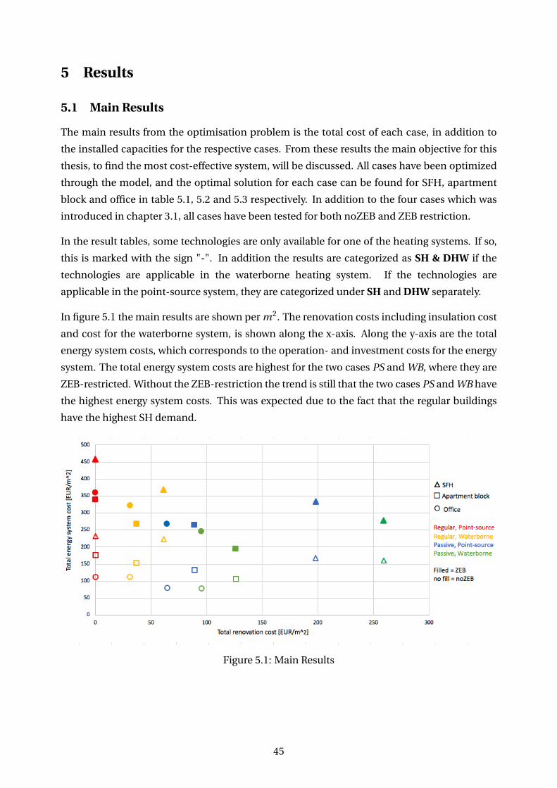
5 Results
5.1 Main Results
The main results from the optimisation problem is the total cost of each case, in addition to
the installed capacities for the respective cases. From these results the main objective for this
thesis, to find the most cost-effective system, will be discussed. All cases have been optimized
through the model, and the optimal solution for each case can be found for SFH, apartment
block and office in table 5.1, 5.2 and 5.3 respectively. In addition to the four cases which was
introduced in chapter 3.1, all cases have been tested for both noZEB and ZEB restriction.
In the result tables, some technologies are only available for one of the heating systems. If so,
this is marked with the sign "-". In addition the results are categorized as SH & DHW if the
technologies are applicable in the waterborne heating system. If the technologies are
applicable in the point-source system, they are categorized under SH and DHW separately.
In figure 5.1 the main results are shown per m2. The renovation costs including insulation cost
and cost for the waterborne system, is shown along the x-axis. Along the y-axis are the total
energy system costs, which corresponds to the operation- and investment costs for the energy
system. The total energy system costs are highest for the two cases PS and WB, where they are
ZEB-restricted. Without the ZEB-restriction the trend is still that the two cases PS and WB have
the highest energy system costs. This was expected due to the fact that the regular buildings
have the highest SH demand.
Figure 5.1: Main Results
45
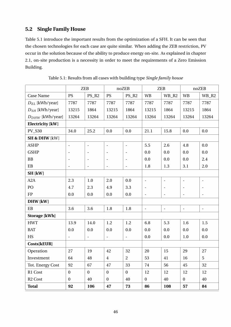
5.2 Single Family House
Table 5.1 introduce the important results from the optimization of a SFH. It can be seen that
the chosen technologies for each case are quite similar. When adding the ZEB restriction, PV
occur in the solution because of the ability to produce energy on-site. As explained in chapter
2.1, on-site production is a necessity in order to meet the requirements of a Zero Emission
Building.
Table 5.1: Results from all cases with building type Single family house
ZEB noZEB ZEB noZEB
Case Name PS PS_R2 PS PS_R2 WB WB_R2 WB WB_R2
DEL [kWh/year] 7787 7787 7787 7787 7787 7787 7787 7787
DSH [kWh/year] 13215 1864 13215 1864 13215 1864 13215 1864
DD HW [kWh/year] 13264 13264 13264 13264 13264 13264 13264 13264
Electricity [kW]
PV_S30 34.0 25.2 0.0 0.0 21.1 15.8 0.0 0.0
SH & DHW [kW]
ASHP - - - - 5.5 2.6 4.8 0.0
GSHP - - - - 0.0 0.0 0.0 0.0
BB - - - - 0.0 0.0 0.0 2.4
EB - - - - 1.8 1.3 3.1 2.0
SH [kW]
A2A 2.3 1.0 2.0 0.0 - - - -
PO 4.7 2.3 4.9 3.3 - - - -
FP 0.0 0.0 0.0 0.0 - - - -
DHW [kW]
EB 3.6 3.6 1.8 1.8 - - - -
Storage [kWh]
HWT 13.9 14.0 1.2 1.2 6.8 5.3 1.6 1.5
BAT 0.0 0.0 0.0 0.0 0.0 0.0 0.0 0.0
HS - - - - 0.0 0.0 1.0 0.0
Costs[kEUR]
Operation 27 19 42 32 20 15 29 27
Investment 64 48 4 2 53 41 16 5
Tot. Energy Cost 92 67 47 33 74 56 45 32
R1 Cost 0 0 0 0 12 12 12 12
R2 Cost 0 40 0 40 0 40 0 40
Total 92 106 47 73 86 108 57 84
46
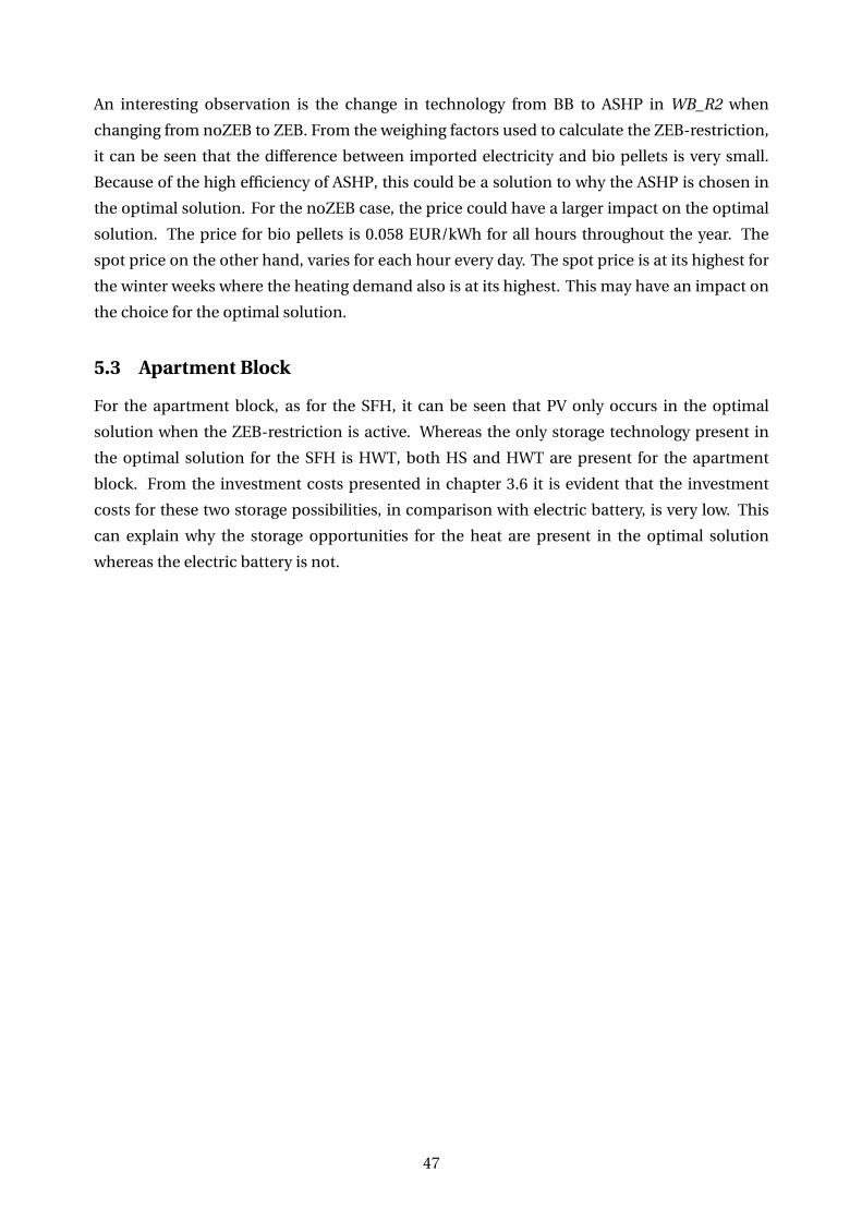
An interesting observation is the change in technology from BB to ASHP in WB_R2 when
changing from noZEB to ZEB. From the weighing factors used to calculate the ZEB-restriction,
it can be seen that the difference between imported electricity and bio pellets is very small.
Because of the high efficiency of ASHP, this could be a solution to why the ASHP is chosen in
the optimal solution. For the noZEB case, the price could have a larger impact on the optimal
solution. The price for bio pellets is 0.058 EUR/kWh for all hours throughout the year. The
spot price on the other hand, varies for each hour every day. The spot price is at its highest for
the winter weeks where the heating demand also is at its highest. This may have an impact on
the choice for the optimal solution.
5.3 Apartment Block
For the apartment block, as for the SFH, it can be seen that PV only occurs in the optimal
solution when the ZEB-restriction is active. Whereas the only storage technology present in
the optimal solution for the SFH is HWT, both HS and HWT are present for the apartment
block. From the investment costs presented in chapter 3.6 it is evident that the investment
costs for these two storage possibilities, in comparison with electric battery, is very low. This
can explain why the storage opportunities for the heat are present in the optimal solution
whereas the electric battery is not.
47
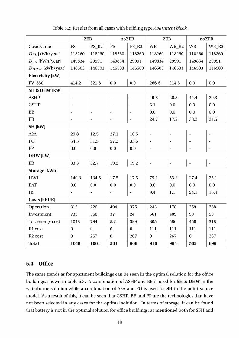
Table 5.2: Results from all cases with building type Apartment block
ZEB noZEB ZEB noZEB
Case Name PS PS_R2 PS PS_R2 WB WB_R2 WB WB_R2
DEL [kWh/year] 118260 118260 118260 118260 118260 118260 118260 118260
DSH [kWh/year] 149834 29991 149834 29991 149834 29991 149834 29991
DD HW [kWh/year] 146503 146503 146503 146503 146503 146503 146503 146503
Electricity [kW]
PV_S30 414.2 321.6 0.0 0.0 266.6 214.3 0.0 0.0
SH & DHW [kW]
ASHP - - - - 49.8 26.3 44.4 20.3
GSHP - - - - 6.1 0.0 0.0 0.0
BB - - - - 0.0 0.0 0.0 0.0
EB - - - - 24.7 17.2 38.2 24.5
SH [kW]
A2A 29.8 12.5 27.1 10.5 - - - -
PO 54.5 31.5 57.2 33.5 - - - -
FP 0.0 0.0 0.0 0.0 - - - -
DHW [kW]
EB 33.3 32.7 19.2 19.2 - - - -
Storage [kWh]
HWT 140.3 134.5 17.5 17.5 75.1 53.2 27.4 25.1
BAT 0.0 0.0 0.0 0.0 0.0 0.0 0.0 0.0
HS - - - - 9.4 1.1 24.1 16.4
Costs [kEUR]
Operation 315 226 494 375 243 178 359 268
Investment 733 568 37 24 561 409 99 50
Tot. energy cost 1048 794 531 399 805 586 458 318
R1 cost 0 0 0 0 111 111 111 111
R2 cost 0 267 0 267 0 267 0 267
Total 1048 1061 531 666 916 964 569 696
5.4 Office
The same trends as for apartment buildings can be seen in the optimal solution for the office
buildings, shown in table 5.3. A combination of ASHP and EB is used for SH & DHW in the
waterborne solution while a combination of A2A and PO is used for SH in the point-source
model. As a result of this, it can be seen that GSHP, BB and FP are the technologies that have
not been selected in any cases for the optimal solution. In terms of storage, it can be found
that battery is not in the optimal solution for office buildings, as mentioned both for SFH and
48
apartment block as well.
Table 5.3: Results from all cases with building type Office
ZEB noZEB ZEB noZEB
Case Name PS PS_R2 PS PS_R2 WB WB_R2 WB WB_R2
DEL [kWh/year] 1404989 1279917 1404989 1279917 1404989 1279917 1404989 1279917
DSH [kWh/year] 656579 210330 656579 210330 656579 210330 656579 210330
DD HW [kWh/year] 153261 153261 153261 153261 153261 153261 153261 153261
Electricity [kW]
PV_S30 2247.5 1763.8 0.0 0.0 1952.4 1576.4 0.0 0.0
SH & DHW [kW]
ASHP - - - - 171.3 78.6 98.3 45.9
GSHP - - - - 0.0 0.0 0.0 0.0
BB - - - - 0.0 0.0 0.0 0.0
EB - - - - 187.8 73.4 286.3 116.0
SH [kW]
A2A 131.7 48.5 104.7 38.8 - - - -
PO 257.1 115.9 284.1 125.5 - - - -
FP 0.0 0.0 0.0 0.0 - - - -
DHW [kW]
EB 21.8 21.8 21.8 21.8 - - - -
Storage [kWh]
HWT 1.1 1.1 1.1 1.1 7.8 36.2 7.4 17.4
BAT 0.0 0.0 0.0 0.0 0.0 0.0 0.0 0.0
HS - - - - 170.8 28.9 43.3 8.1
Costs [kEUR]
Operation 556 406 999 752 521 375 953 705
Investment 2946 2267 123 53 2694 2086 164 74
Tot. Energy cost 3502 2673 1121 806 3215 2460 1117 779
R1 cost 0 0 0 0 310 310 310 310
R2 cost 0 644 0 644 0 644 0 644
Total 3502 3316 1121 1449 3525 3414 1427 1732
5.5 Effect of Post-insulation (R2)
From all three result tables it can be seen that SH demand is lower for the pot-insulated
buildings. For the office building, the electric demand is also lower for the post-insulated
building. This results in a lower installed capacity for all technologies except EB and HWT who
are dependent upon the DHW demand.
49
Because of the lower installed capacities, the investment costs are lower in the post-insulated
buildings than for the regular buildings. In addition, the operating costs are lower for the post-
insulated buildings as a result of lower total energy demand. Overall, this result in a lower total
energy cost for the post-insulated buildings.
At the same time it must be kept in mind that the post-insulation comes with an additional
cost, R2. Comparing the regular and post-insulated buildings it can be seen that for both SFH
and Apartment Block, the total cost of the regular building is lower than for the post-insulated
building. This holds for the Office building as well in regards of the noZEB cases. For the cases
with ZEB-restriction on the other hand, the regular buildings have the highest costs.
As mentioned in chapter 3.5.3, the cost for post-insulation can vary within a wide range, which
must be kept in mind when reading the results. The most important observation in regards of
the post-insulation is therefore that the total energy cost decreases when meeting the demands
of a post-insulated building. It must be remembered that an additional cost will occur, but
this cost should be more precisely calculated if using this optimisation method for a specific
building case.
5.6 Effect of Waterborne Heating System (R1)
The same trends as for the post-insulation can be seen for the effect of waterborne heating
system. For all cases, the total energy cost is lower for the waterborne system than for the point-
source system. It can be seen that when ZEB-restriction is active, the difference between the
costs are the highest. When adding the additional renovation cost for the waterborne system
on the other hand, the total price is lower for the point-source system in 9 out of 12 cases.
At the same time, it must be mentioned that the renovation cost for the waterborne system
can vary. When comparing the cases with point-source system to the cases with waterborne
system, the difference in total price is quite low. As for the post-insulation it is important to
differ between the total energy cost and the renovation costs as the renovation costs are more
dependent upon each and every specific building case.
50
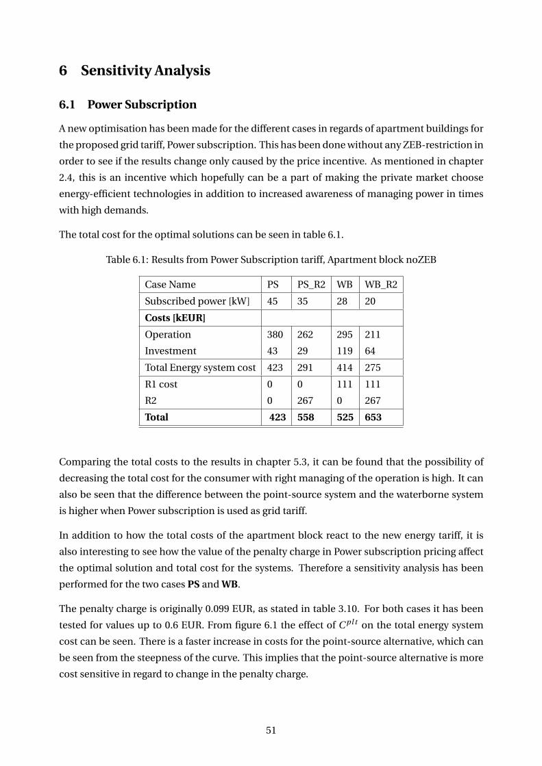
6 Sensitivity Analysis
6.1 Power Subscription
A new optimisation has been made for the different cases in regards of apartment buildings for
the proposed grid tariff, Power subscription. This has been done without any ZEB-restriction in
order to see if the results change only caused by the price incentive. As mentioned in chapter
2.4, this is an incentive which hopefully can be a part of making the private market choose
energy-efficient technologies in addition to increased awareness of managing power in times
with high demands.
The total cost for the optimal solutions can be seen in table 6.1.
Table 6.1: Results from Power Subscription tariff, Apartment block noZEB
Case Name PS PS_R2 WB WB_R2
Subscribed power [kW] 45 35 28 20
Costs [kEUR]
Operation 380 262 295 211
Investment 43 29 119 64
Total Energy system cost 423 291 414 275
R1 cost 0 0 111 111
R2 0 267 0 267
Total 423 558 525 653
Comparing the total costs to the results in chapter 5.3, it can be found that the possibility of
decreasing the total cost for the consumer with right managing of the operation is high. It can
also be seen that the difference between the point-source system and the waterborne system
is higher when Power subscription is used as grid tariff.
In addition to how the total costs of the apartment block react to the new energy tariff, it is
also interesting to see how the value of the penalty charge in Power subscription pricing affect
the optimal solution and total cost for the systems. Therefore a sensitivity analysis has been
performed for the two cases PS and WB.
The penalty charge is originally 0.099 EUR, as stated in table 3.10. For both cases it has been
tested for values up to 0.6 EUR. From figure 6.1 the effect of C pl t on the total energy system
cost can be seen. There is a faster increase in costs for the point-source alternative, which can
be seen from the steepness of the curve. This implies that the point-source alternative is more
cost sensitive in regard to change in the penalty charge.
51

0
100000
200000
300000
400000
500000
600000
0,099 0,2 0,3 0,4 0,5 0,6
Tota
l ene
rgy s
yste
m co
st [E
UR]
Value of penalty charge c_plt [EUR/kWh]
Point-Source
Waterborne
Waterborne incl.WB cost
Figure 6.1: Effect of C pl t on total energy system cost for Apartment block, noZEB
At the same time, it can be seen from the figure that when adding the cost of the whole system,
not only the technologies, the point-source system has the lowest costs even though it is the
most cost sensitive. The penalty charge has to increase by 6 times originally value in order to
change the results of point-source alternative being the one with the lowest cost.
A solution to why the point-source heating system is more sensitive in regard to higher costs,
could be the fact that the technologies available in the point-source system are more
dependent upon electricity in order to meet the demand. Figure 6.2 shows the results of the
sensitivity analysis of the penalty charge in regard to installed capacity. As expected, the
installed capacity of the point-source system increases with installed capacity.
0
10
20
30
40
50
60
70
80
90
100
0,099 0,2 0,3 0,4 0,5 0,6
Inst
alle
d ca
pacit
y [kW
(kW
h)]
Value of penalty charge [EUR/kWh]
HWT
EB
FP
PO
A2A
Figure 6.2: Installed capacity per technology for Point-source system Apartment block, noZEB
The two technologies that vary the most are the HWT and FP, which have both increased with
more than double of their originally installed capacity. The HWT is used as storage for domestic
hot water, and the increase of this technology results in more flexibility in order to managing
52

peak loads. Because of the fact that the EB is only used for domestic hot water in the point-
source system, extracting hot water from storage instead of EB in periods where the electricity
price is high, will reduce costs.
The FP is used for the space heating demand, and the technology reduces the use of electricity
because of the fact that wood is used as fuel instead of electricity. Increasing the use of FP
results in a reduction in the use of PO, which can be seen from figure 6.2.
From table 3.2 in chapter 3.3 it can be seen that the efficiency for PO is 1, while the efficiency for
FP is 0.84. A result of this is that it needs to be installed higher capacity for FP in order to meet
the same demand as the PO was able to meet. Therefore, even though the share of installed
capacity by technologies that are not dependent upon electricity is increased, the total cost
still increases.
The waterborne system on the other hand, was able to keep the total costs of the energy system
more stable even though the penalty charge was increased. The installed capacities for each
technology can be seen in figure 6.3.
0
5
10
15
20
25
30
35
40
45
50
0,099 0,2 0,3 0,4 0,5 0,6
Inst
alle
d ca
pacit
y [kW
(kW
h]
Value of penalty charge [EUR/kWh]
HWT
EB
BB
ASHP
HS
Figure 6.3: Installed capacity per technology for Waterborne system for Apartment block,noZEB
Figure 6.3 shows that the installed capacity of the BB increases with almost three times its
original value. The BB can supply both the SH and DHW demand, and the result of the
increase of that technology is a decrease in installed capacity for both ASHP and EB. How this
affects the use of each technology can be seen in figure 6.4 and 6.5. These figures shows how
the technologies in cooperation covers the SH-demand.
53
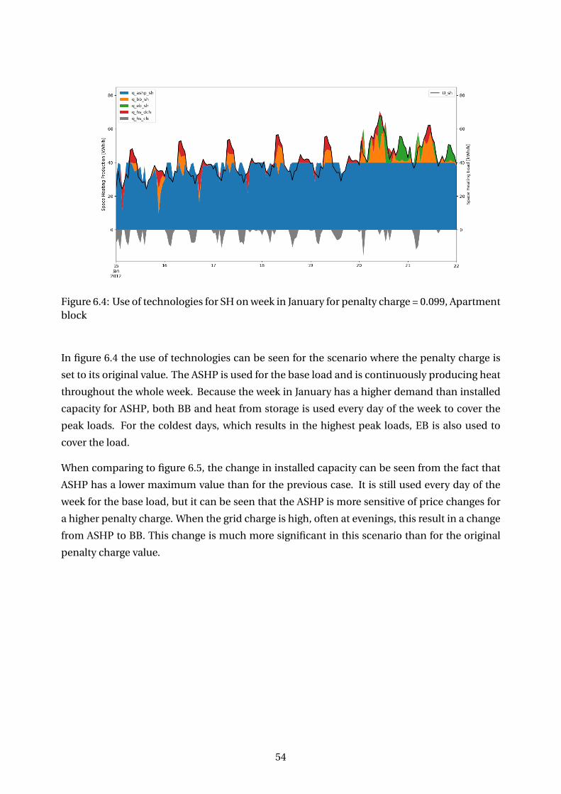
Figure 6.4: Use of technologies for SH on week in January for penalty charge = 0.099, Apartmentblock
In figure 6.4 the use of technologies can be seen for the scenario where the penalty charge is
set to its original value. The ASHP is used for the base load and is continuously producing heat
throughout the whole week. Because the week in January has a higher demand than installed
capacity for ASHP, both BB and heat from storage is used every day of the week to cover the
peak loads. For the coldest days, which results in the highest peak loads, EB is also used to
cover the load.
When comparing to figure 6.5, the change in installed capacity can be seen from the fact that
ASHP has a lower maximum value than for the previous case. It is still used every day of the
week for the base load, but it can be seen that the ASHP is more sensitive of price changes for
a higher penalty charge. When the grid charge is high, often at evenings, this result in a change
from ASHP to BB. This change is much more significant in this scenario than for the original
penalty charge value.
54
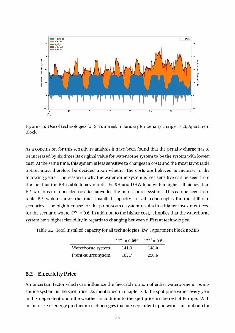
Figure 6.5: Use of technologies for SH on week in January for penalty charge = 0.6, Apartmentblock
As a conclusion for this sensitivity analysis it have been found that the penalty charge has to
be increased by six times its original value for waterborne system to be the system with lowest
cost. At the same time, this system is less sensitive to changes in costs and the most favourable
option must therefore be decided upon whether the costs are believed to increase in the
following years. The reason to why the waterborne system is less sensitive can be seen from
the fact that the BB is able to cover both the SH and DHW load with a higher efficiency than
FP, which is the non-electric alternative for the point-source system. This can be seen from
table 6.2 which shows the total installed capacity for all technologies for the different
scenarios. The high increase for the point-source system results in a higher investment cost
for the scenario where C pl t = 0.6. In addition to the higher cost, it implies that the waterborne
system have higher flexibility in regards to changing between different technologies.
Table 6.2: Total installed capacity for all technologies [kW], Apartment block noZEB
C pl t = 0.099 C pl t = 0.6
Waterborne system 141.9 148.0
Point-source sysem 162.7 256.6
6.2 Electricity Price
An uncertain factor which can influence the favorable option of either waterborne or point-
source system, is the spot price. As mentioned in chapter 2.3, the spot price varies every year
and is dependent upon the weather in addition to the spot price in the rest of Europe. With
an increase of energy production technologies that are dependent upon wind, sun and rain for
55
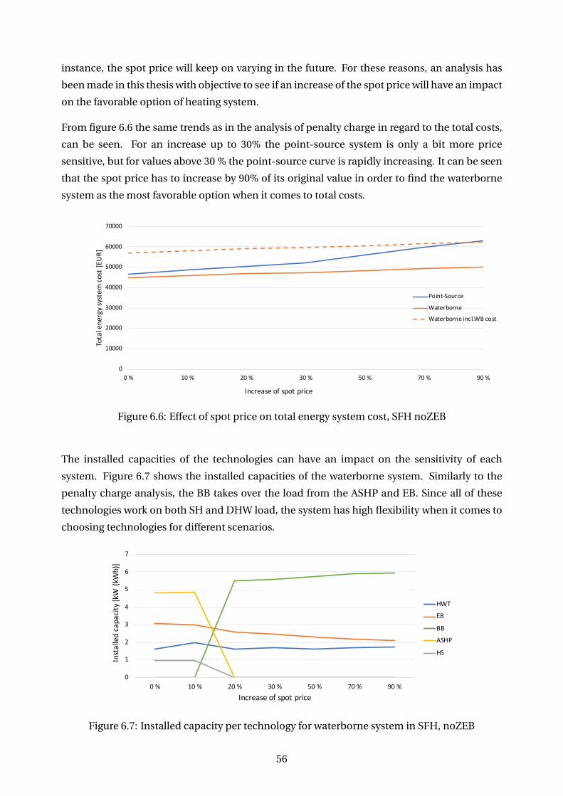
instance, the spot price will keep on varying in the future. For these reasons, an analysis has
been made in this thesis with objective to see if an increase of the spot price will have an impact
on the favorable option of heating system.
From figure 6.6 the same trends as in the analysis of penalty charge in regard to the total costs,
can be seen. For an increase up to 30% the point-source system is only a bit more price
sensitive, but for values above 30 % the point-source curve is rapidly increasing. It can be seen
that the spot price has to increase by 90% of its original value in order to find the waterborne
system as the most favorable option when it comes to total costs.
0
10000
20000
30000
40000
50000
60000
70000
0 % 10 % 20 % 30 % 50 % 70 % 90 %
Tota
l ene
rgy s
yste
m co
st [E
UR]
Increase of spot price
Point-Source
Waterborne
Waterborne incl.WB cost
Figure 6.6: Effect of spot price on total energy system cost, SFH noZEB
The installed capacities of the technologies can have an impact on the sensitivity of each
system. Figure 6.7 shows the installed capacities of the waterborne system. Similarly to the
penalty charge analysis, the BB takes over the load from the ASHP and EB. Since all of these
technologies work on both SH and DHW load, the system has high flexibility when it comes to
choosing technologies for different scenarios.
0
1
2
3
4
5
6
7
0 % 10 % 20 % 30 % 50 % 70 % 90 %
Inst
alle
d ca
pacit
y [kW
(kW
h)]
Increase of spot price
HWT
EB
BB
ASHP
HS
Figure 6.7: Installed capacity per technology for waterborne system in SFH, noZEB
56
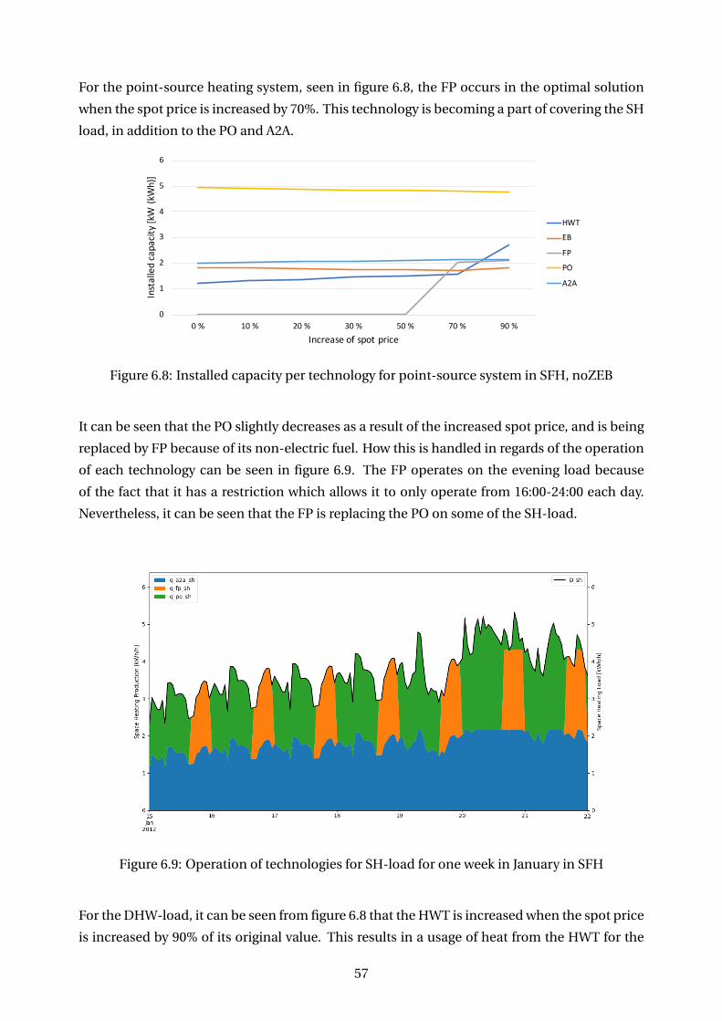
For the point-source heating system, seen in figure 6.8, the FP occurs in the optimal solution
when the spot price is increased by 70%. This technology is becoming a part of covering the SH
load, in addition to the PO and A2A.
0
1
2
3
4
5
6
0 % 10 % 20 % 30 % 50 % 70 % 90 %
Inst
alle
d ca
pacit
y [kW
(kW
h)]
Increase of spot price
HWT
EB
FP
PO
A2A
Figure 6.8: Installed capacity per technology for point-source system in SFH, noZEB
It can be seen that the PO slightly decreases as a result of the increased spot price, and is being
replaced by FP because of its non-electric fuel. How this is handled in regards of the operation
of each technology can be seen in figure 6.9. The FP operates on the evening load because
of the fact that it has a restriction which allows it to only operate from 16:00-24:00 each day.
Nevertheless, it can be seen that the FP is replacing the PO on some of the SH-load.
Figure 6.9: Operation of technologies for SH-load for one week in January in SFH
For the DHW-load, it can be seen from figure 6.8 that the HWT is increased when the spot price
is increased by 90% of its original value. This results in a usage of heat from the HWT for the
57
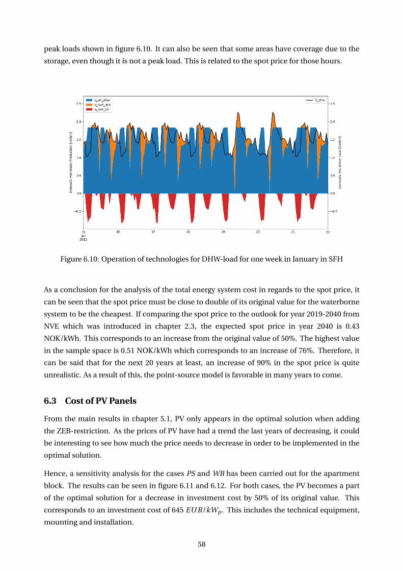
peak loads shown in figure 6.10. It can also be seen that some areas have coverage due to the
storage, even though it is not a peak load. This is related to the spot price for those hours.
Figure 6.10: Operation of technologies for DHW-load for one week in January in SFH
As a conclusion for the analysis of the total energy system cost in regards to the spot price, it
can be seen that the spot price must be close to double of its original value for the waterborne
system to be the cheapest. If comparing the spot price to the outlook for year 2019-2040 from
NVE which was introduced in chapter 2.3, the expected spot price in year 2040 is 0.43
NOK/kWh. This corresponds to an increase from the original value of 50%. The highest value
in the sample space is 0.51 NOK/kWh which corresponds to an increase of 76%. Therefore, it
can be said that for the next 20 years at least, an increase of 90% in the spot price is quite
unrealistic. As a result of this, the point-source model is favorable in many years to come.
6.3 Cost of PV Panels
From the main results in chapter 5.1, PV only appears in the optimal solution when adding
the ZEB-restriction. As the prices of PV have had a trend the last years of decreasing, it could
be interesting to see how much the price needs to decrease in order to be implemented in the
optimal solution.
Hence, a sensitivity analysis for the cases PS and WB has been carried out for the apartment
block. The results can be seen in figure 6.11 and 6.12. For both cases, the PV becomes a part
of the optimal solution for a decrease in investment cost by 50% of its original value. This
corresponds to an investment cost of 645 EU R/kWp . This includes the technical equipment,
mounting and installation.
58
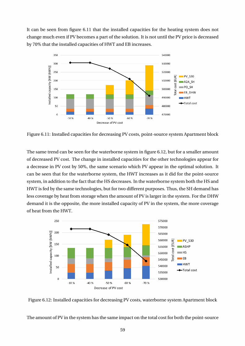
It can be seen from figure 6.11 that the installed capacities for the heating system does not
change much even if PV becomes a part of the solution. It is not until the PV price is decreased
by 70% that the installed capacities of HWT and EB increases.
Figure 6.11: Installed capacities for decreasing PV costs, point-source system Apartment block
The same trend can be seen for the waterborne system in figure 6.12, but for a smaller amount
of decreased PV cost. The change in installed capacities for the other technologies appear for
a decrease in PV cost by 50%, the same scenario which PV appear in the optimal solution. It
can be seen that for the waterborne system, the HWT increases as it did for the point-source
system, in addition to the fact that the HS decreases. In the waterborne system both the HS and
HWT is fed by the same technologies, but for two different purposes. Thus, the SH demand has
less coverage by heat from storage when the amount of PV is larger in the system. For the DHW
demand it is the opposite, the more installed capacity of PV in the system, the more coverage
of heat from the HWT.
Figure 6.12: Installed capacities for decreasing PV costs, waterborne system Apartment block
The amount of PV in the system has the same impact on the total cost for both the point-source
59

and the waterborne system. Total amount of installed capacity increases, but because of the
export of PV the total cost of the system decreases. In other words, the increase of investment
cost by installing a larger amount of technology in the building is less than the decrease in
operation cost by selling electricity produced by the installed PV.
From this result, it is important to remember that the cite in this thesis is Oslo. In addition to
the cite, the panels are also oriented directly towards south, and with a tilting that is close to
optimal for this cite. Therefore, PV-production is quite high and favorable, in comparison with
the usage of batteries to decrease the electricity import. When using this optimisation model
as a decision tool for design of new buildings, the method works very well. But if the model
should be used for already built buildings, with a fixed orientation and tilting on the roof that
is not optimal, this is important to take into consideration.
60
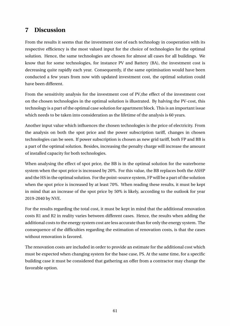
7 Discussion
From the results it seems that the investment cost of each technology in cooperation with its
respective efficiency is the most valued input for the choice of technologies for the optimal
solution. Hence, the same technologies are chosen for almost all cases for all buildings. We
know that for some technologies, for instance PV and Battery (BA), the investment cost is
decreasing quite rapidly each year. Consequently, if the same optimisation would have been
conducted a few years from now with updated investment cost, the optimal solution could
have been different.
From the sensitivity analysis for the investment cost of PV,the effect of the investment cost
on the chosen technologies in the optimal solution is illustrated. By halving the PV-cost, this
technology is a part of the optimal case solution for apartment block. This is an important issue
which needs to be taken into consideration as the lifetime of the analysis is 60 years.
Another input value which influences the chosen technologies is the price of electricity. From
the analysis on both the spot price and the power subscription tariff, changes in chosen
technologies can be seen. If power subscription is chosen as new grid tariff, both FP and BB is
a part of the optimal solution. Besides, increasing the penalty charge will increase the amount
of installed capacity for both technologies.
When analysing the effect of spot price, the BB is in the optimal solution for the waterborne
system when the spot price is increased by 20%. For this value, the BB replaces both the ASHP
and the HS in the optimal solution. For the point-source system, FP will be a part of the solution
when the spot price is increased by at least 70%. When reading these results, it must be kept
in mind that an increase of the spot price by 50% is likely, according to the outlook for year
2019-2040 by NVE.
For the results regarding the total cost, it must be kept in mind that the additional renovation
costs R1 and R2 in reality varies between different cases. Hence, the results when adding the
additional costs to the energy system cost are less accurate than for only the energy system. The
consequence of the difficulties regarding the estimation of renovation costs, is that the cases
without renovation is favored.
The renovation costs are included in order to provide an estimate for the additional cost which
must be expected when changing system for the base case, PS. At the same time, for a specific
building case it must be considered that gathering an offer from a contractor may change the
favorable option.
61

62
8 Conclusion
Throughout the work with this thesis, an implementation of new building types with associated
heating loads has been done. In addition, a review of input values for the model has been done,
and new investment costs for larger building has been found. This resulted in three different
buildings types in which all four cases have been optimised with respect to the total cost of the
energy system.
Whereas the base case PS is a point-source system where the building standard implies an old
badly insulated building, an upgrade including post-insulation of the building can be done.
This upgrade results in the second case for the point-source system, PS_R2.
The two other cases have both updated from a point-source system to a waterborne heating
system which results in different applicable technologies for heating. These two cases are also
divided in one case where the building standard is the same as in the base case WB, and one
case where the building standard is upgraded by post-insulating WB_R2.
For SFH the total cost was the lowest for the base case, PS. Comparing the total energy costs for
all cases it can be seen that the difference between the base case and WB_R2 is 15 kEUR. The
additional renovation cost is 52 kEUR. This implies that the renovation costs for this building
type are high compared to the energy system costs. Hence, a renovation of the building is not
favorable.
When adding the ZEB-restriction for this building type on the other hand, WB becomes the
most favorable solution. This is related to the higher flexibility for storage and heating
technologies in the waterborne system. Thus, the waterborne system reacts better to stricter
restrictions and higher costs than the point-source system.
As of this time, there is no outlook of restrictions for private residents in regard to ZEB. Hence
the most favorable option for this building type remains PS.
For apartment block, the exact same trends can be seen as for the SFH. At the same time it
can be seen from figure 5.1 that the renovation costs are much lower per m2 than for the SFH.
Hence, an upgrade of the heating system from point-source to waterborne system is more likely
to pay off for the apartment block than for the SFH.
When adding the ZEB-restriction, the favorable option for the apartment block is WB, with
WB_R2 as the second best option. The probability of a ZEB-restriction for apartment-buildings
are more likely to happen than for the SFH. Hence, an upgrade from point-source system to
waterborne could be the favorable option for the apartment building if thinking a few years
ahead.
For the office building, a ZEB-restriction is more relevant than for the other building types.
When ZEB-restriction is active, PS_R2 is the most favorable solution. The second best option
63

is WB_R2. Hence, the low renovation-costs per m2 have a large impact on the solution for this
case.
For all cases it can be seen that the point-source system is the most favorable option. At the
same time, seen from the sensitivity analysis and when adding the ZEB-restriction, the
waterborne system has a better reaction to higher costs and stricter restrictions. Choosing
between a point-source system or a waterborne system must therefore be decided upon
whether the investment is seen in a short-time or a long-time perspective. The longer
perspective, the more favorable the waterborne system becomes. The additional cost for
post-insulation must be decided in the same manner, but it must be kept in mind that the
additional cost is more favorable for larger buildings.
64
9 Further Work
• Include technology cost as a function of time
From the sensitivity analysis, we were able to see how the change in investment cost
may change the optimal solution regarding both costs and installed technologies. If the
technologies were modeled as a function of time instead of constant, this would be taken
into account when calculating the optimal solution.
• Include more than the operational phase of the building in regard to ZEB.
As mentioned, this model is limited to the operational phase of the building in regard
to ZEB. An estimate could be calculated for the emissions in other phases for different
building types and standards. The emissions of the equipment for the technologies could
also be included.
• Expand the model to include more than one building.
The model is used for one building at the time. Now that different building types are
included, it could be interesting to see if a neighbourhood of different buildings would
give another solution to the optimisation problem.
• Restrict the PV-solutions for each building type
In the optimal solution for this thesis, the available area for PV-production is not limited
for each building type. For generic buildings, it is hard to know the available area. At the
same time, the model should have an option for restriction if wanted. This will make the
model more useful in optimisation of real-life cases.
• Investigate the optimal value for subscribed power
For the analysis of the proposed grid tariff, power subscription, an optimal value of
subscribed power is not investigated. In order to improve the results to be more close to
reality, this value should be optimised for the different building types and building
standards.
65
References
[1] Ingrid Marie Andersen. Stochastic Optimization of Zero Emission Buildings. Master’s
thesis, Norwegian University of Science and Technology - NTNU, 7 2018.
[2] Marius Bagle. Investigation into the impact of thermal energy flexibility on cost optimal
design and operation of Zero Emission Buildings. Master’s thesis, Norwegian University of
Science and Technology - NTNU, 7 2019.
[3] The Research Centre on Zero Emission Buildings. Zeb definitions. http://www.zeb.no/
index.php/en/about-zeb/zeb-definitions, 2019. Last checked: 08.01.2020.
[4] K.Voss I.Sartori, A.Napolitano. Net zero energy buildings:a consistant definition
framework. Energy and buildings, 48:220–232, 2012.
[5] My Solar Quotes. How a grid-connected solar power system
works. https://mysolarquotes.co.nz/about-solar-power/residential/
how-grid-connect-solar-power-systems-work/, 2019. Last checked: 28.10.2019.
[6] Phil Taylor-Parker. Tilt & azimuth angle: Finding the optimal angle to mount your solar
panels. https://www.wholesalesolar.com/blog/solar-panel-azimuth-angle/, 11 2018.
Last checked: 13.01.2020.
[7] Enevate Corporation. Hd-energy technology. http://www.enevate.com/technology/,
2019. Last checked: 04.12.2019.
[8] Langsiktig kraftmarkedanalyse 2019-2040. Technical report, NVE, 10 2019.
[9] Stig Ødegaard Ottesen. Techno-economic models in Smart Grids. PhD thesis, Norwegian
University of Science and Technology - NTNU, 2017.
[10] Enova SF. Faktastudie - kostnader for elektrisk og vassboren oppvarming. Technical
report, COWI, 12 2012.
[11] Direktoratet for byggkvalitet. Byggteknisk forskrift (tek17) med veiledning. https://dibk.
no/byggereglene/byggteknisk-forskrift-tek17/14/14-4/, 2017. Last checked: 17.10.2019.
[12] Miljø- og energidorektoratet. Forskrift om forbud mot bruk av mineralolje til oppvarming
av bygninger. https://lovdata.no/dokument/LTI/forskrift/2018-06-28-1060, 6 2018. Last
checked: 17.10.2019.
[13] K.Sørnes et al. F. Selamawit, R. Schlanbudch. A norwegian zeb definition guideline.
Technical report, The Research centre on Zero Emission Buildings, 2016.
[14] Nigel Brandon Adam Hawkes Iain Staffell, Dan Brett. A review of domestic heat pumps.
Energy and Environmental Science, 5:9291–9306, 2012.
66
https://mysolarquotes.co.nz/about-solar-power/residential/how-grid-connect-solar-power-systems-work/
[15] David Zijdeman. Vannbaserte oppvarmings- og kjølesystemer. Skarland Press AS, 2014.
[16] D.Fischer et al. K.Lindberg, G.Doorman. Methodology for optimal energy system design
of zero energy buildings using mixed-integer linear programming. Energy and Buildings,
127:194–205, 2016.
[17] Jørn Stene. Economical heating and cooling systems for low-energy houses. Technical
report, SINTEF Energiforskning AS, 4 2017.
[18] Encore Geothermal. Mitsubishi zuba cold climate air source heat pumps. https://web.
archive.org/web/20141021195035/http:/encore-geothermal.ca/sustainable-solutions/
air-source-heat-pumps/, 2013. Last checked: 10.01.2020.
[19] Office of Energy Efficiency & Renewable Energy. How does a lithium-ion battery work?
https://www.energy.gov/eere/articles/how-does-lithium-ion-battery-work, 09 2017. Last
checked: 04.12.2019.
[20] Petter Winther. Nve spår høye strømpriser fremover - karbonkvoter og kraftkabler
får skylden. https://www.dn.no/makrookonomi/strompris/nve/strom/nve-spar-hoye-
strompriser-fremover-karbonkvoter-og-kraftkabler-far-skylden/2-1-528774, 2019. Last
checked 25.01.2020.
[21] Forslag til endring i forskrift om kontroll av nettvirksomhet. Technical report, Norges
vassdrags- og energidirektorat, 5 2017.
[22] Analyse av energibruk i yrkesbygg. Technical report, Norges vassdrags- og
energidirektorat, 2 2016.
[23] Enova SF. Enovas byggstatistikk 2017. Technical report.
[24] Sivilingeniør Carl Christian Strømberg AS. Nøkkelferdige solcelleanlegg
med montering. https://solcellespesialisten.no/solcelleanlegg/
nokkelferdige-solcelleanlegg-med-montering.html, 2019. Last checked: 2.12.2019.
[25] Rapport: Solcellesystemer og sol i systemet. Technical report, Solenergiklyngen, 3 2018.
[26] Byggstart. Etterisolering: Hva koster det? (2019-pris). https://www.byggstart.no/pris/
etterisolering, 2020. Last checked: 08.01.2020.
[27] Nordpoolspot. Historical market data. https://www.nordpoolgroup.com/historical-
market-data, 2020. Last checked 20.01.2020.
[28] Hafslund Nett. Priser på nettleie for privatkunder. https://www.hafslundnett.no/artikkel/
Priser-pa-nettleie-for-privatkunder, 1 2019. Last checked: 8.11.2019.
[29] Hafslund Nett. Nettleiepriser for bedriftskunder. https://www.hafslundnett.no/artikkel/
Nettleiepriser-for-bedriftskunder, 1 2019. Last checked: 21.11.2019.
67

[30] EnergiNorge. Abonnert effekt - vanskelig å forstå for kunden?
https://www.energinorge.no/contentassets/de16563d50a4475f950ecb4a3c08397e/abonnert-
effekt-vanskelig-a-kommunisere—husholdningskunder-og-naringskunde.pdf, 3 2018.
[31] PVsyst. General description of the pvsyst software. https://www.pvsyst.com/help/
general_descr.htm, 2019. Last checked: 04.12.2019.
[32] Sn/ts 3031:2016 - bygningers energiytelse, beregning av energibehov og energiforsyning.
Technical report, Standard Norge, 2016.
68
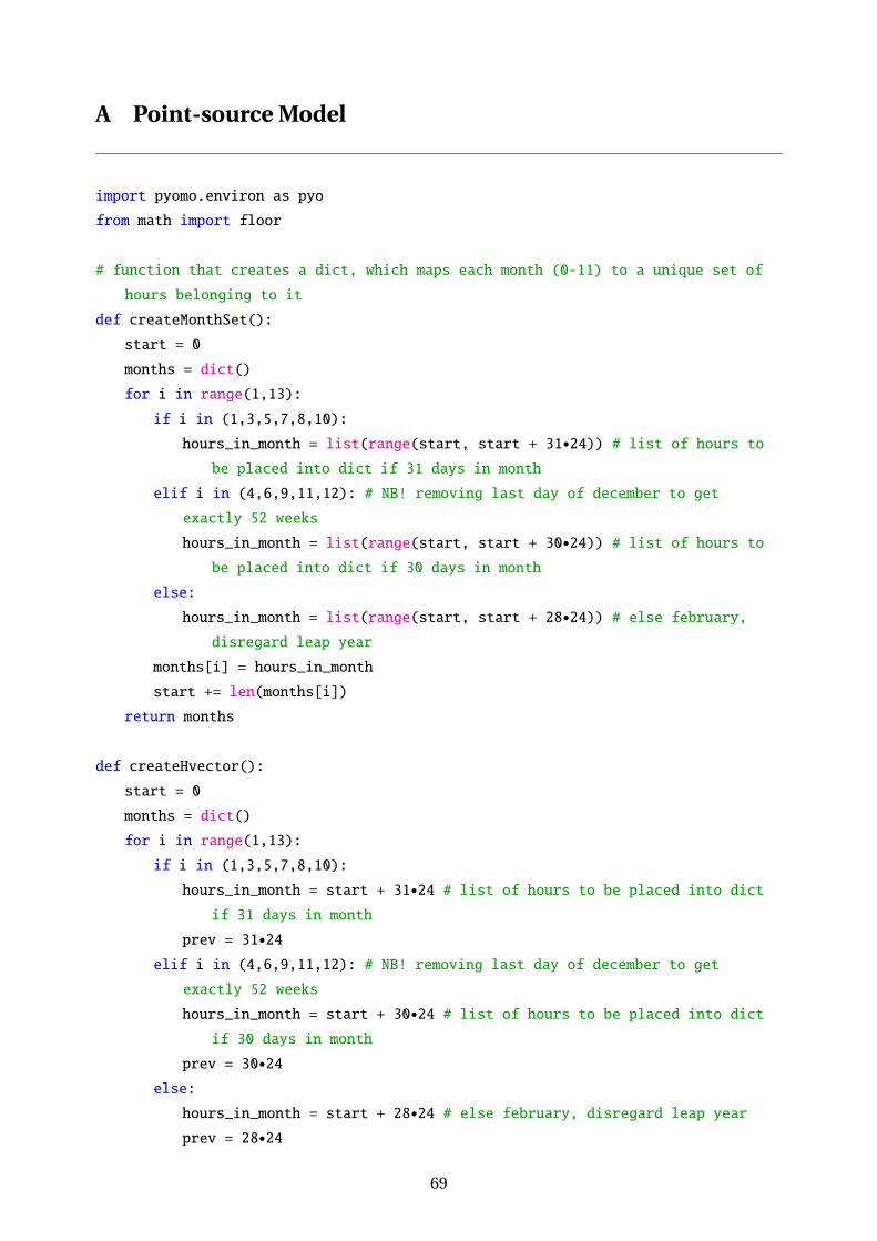
A Point-source Model
import pyomo.environ as pyo
from math import floor
# function that creates a dict, which maps each month (0-11) to a unique set of
hours belonging to it
def createMonthSet():
start = 0
months = dict()
for i in range(1,13):
if i in (1,3,5,7,8,10):
hours_in_month = list(range(start, start + 31•24)) # list of hours tobe placed into dict if 31 days in month
elif i in (4,6,9,11,12): # NB! removing last day of december to get
exactly 52 weeks
hours_in_month = list(range(start, start + 30•24)) # list of hours tobe placed into dict if 30 days in month
else:
hours_in_month = list(range(start, start + 28•24)) # else february,disregard leap year
months[i] = hours_in_month
start += len(months[i])
return months
def createHvector():
start = 0
months = dict()
for i in range(1,13):
if i in (1,3,5,7,8,10):
hours_in_month = start + 31•24 # list of hours to be placed into dictif 31 days in month
prev = 31•24elif i in (4,6,9,11,12): # NB! removing last day of december to get
exactly 52 weeks
hours_in_month = start + 30•24 # list of hours to be placed into dictif 30 days in month
prev = 30•24else:
hours_in_month = start + 28•24 # else february, disregard leap yearprev = 28•24
69
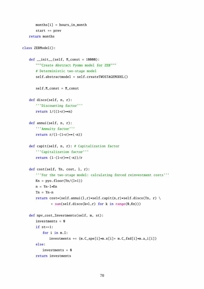
months[i] = hours_in_month
start += prev
return months
class ZEBModel():
def __init__(self, M_const = 10000):
"""Create Abstract Pyomo model for ZEB"""
# Deterministic two-stage model
self.abstractmodel = self.createTWOSTAGEMODEL()
self.M_const = M_const
def disco(self, n, r):
’’’Discounting factor’’’
return 1/((1+r)••n)
def annui(self, n, r):
’’’Annuity factor’’’
return r/(1-(1+r)••(-n))
def capit(self, n, r): # Capitalization factor
’’’Capitalization factor’’’
return (1-(1+r)••(-n))/r
def cost(self, Yn, cost, l, r):
’’’For the two-stage model: calculating forced reinvestment costs’’’
Kn = pyo.floor(Yn/(l•1))n = Yn-l•KnTn = Yn-n
return cost•(self.annui(l,r)•self.capit(n,r)•self.disco(Tn, r) \+ sum(self.disco(k•l,r) for k in range(0,Kn)))
def npv_cost_Investments(self, m, st):
investments = 0
if st==1:
for i in m.I:
investments += (m.C_spe[i]•m.x[i]+ m.C_fxd[i]•m.a_i[i])else:
investments = 0
return investments
70

def npv_cost_Operations(self, m, st):
’’’Operational costs for two-stage/deterministic
Summation of yearly costs for all years in YRN’’’
techrun = 0
runcosts = 0
gridtariff = 0
operations = 0
if m.lastT == 4367:
f = 2
elif m.lastT == 23:
f = 8736/24
elif m.lastT == 95:
f = 8736/96
elif m.lastT == 287:
f = 8736/288
elif m.lastT == 671:
’’’multiplicationfactor will be 13 if reduced model’’’
f = 13
elif m.lastT == 727:
f = 12
elif m.lastT == 8735:
f = 1
if st == 2:
for i in m.I:
techrun += m.C_run[i]•m.C_spe_0[i]•m.x[i]if m.A_ps + m.A_ep + m.A_pp > 1 or m.A_ps + m.A_ep + m.A_pp < 1:
raise ValueError("Please select ONE AND ONLY ONE grid tariff
type.")
if m.A_ep: #Grid tariff model (includes VAT): Energy pricing
’’’ (inkluderer enova-avgift samt moms)’’’
gridtariff = 12•m.C_fxd_ep + m.C_spe_ep•sum(f•m.y_imp[t] for t inm.T)
VAT = 1.25
runcosts = sum(m.f_fp[t]•m.C_wo + VAT•m.y_imp[t]•m.P_spot[t] -m.y_exp[t]•m.P_spot[t]•m.A_exp for t in m.T)
elif m.A_ps == 1: #Grid tariff model(includes VAT): Power subscription
VAT = 1.25
gridtariff = VAT•(12•(m.C_fxd_ps+(5.69•m.Y_max)) +m.C_pty_ps•sum(f•m.y_pty[t] for t in m.T) +m.C_spe_ps•sum(f•m.y_imp[t] for t in m.T))
runcosts = sum(m.f_fp[t]•m.C_wo + VAT•m.y_imp[t]•m.P_spot[t] -
71
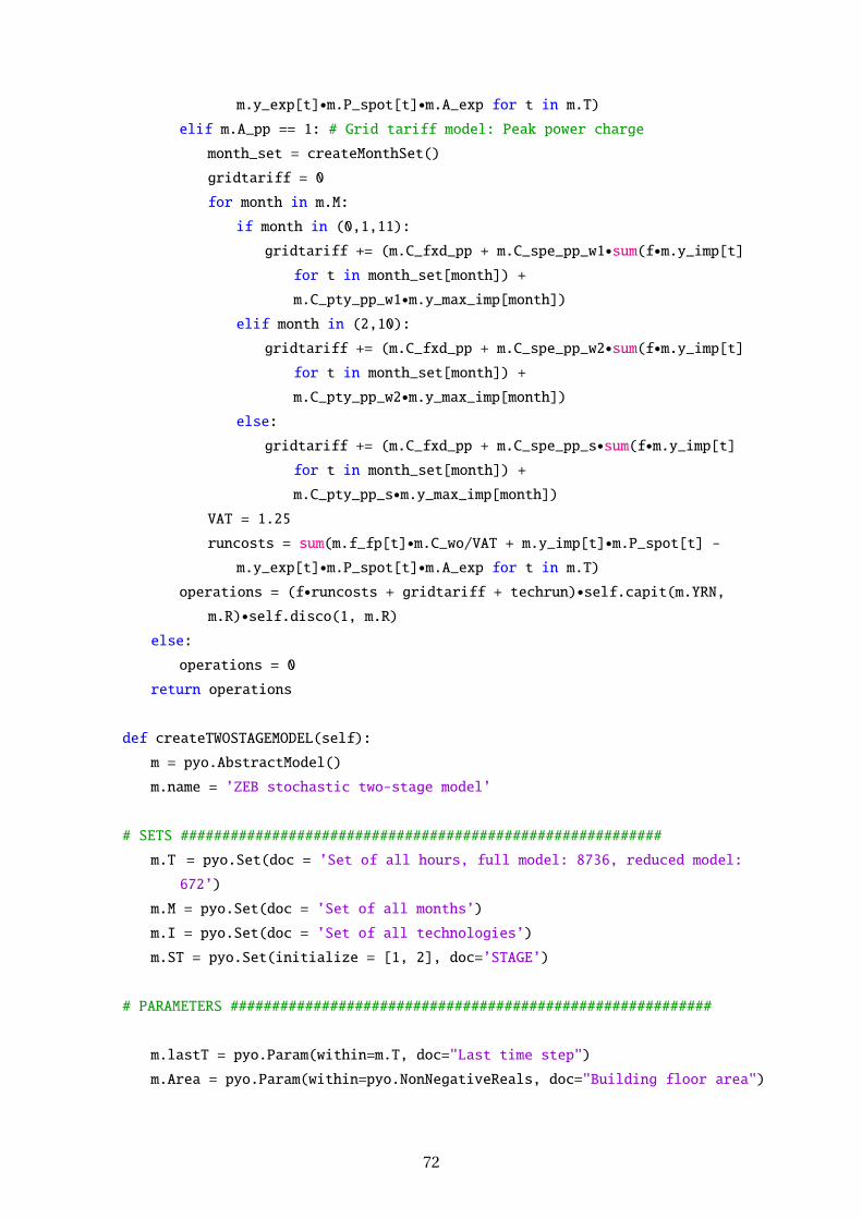
m.y_exp[t]•m.P_spot[t]•m.A_exp for t in m.T)elif m.A_pp == 1: # Grid tariff model: Peak power charge
month_set = createMonthSet()
gridtariff = 0
for month in m.M:
if month in (0,1,11):
gridtariff += (m.C_fxd_pp + m.C_spe_pp_w1•sum(f•m.y_imp[t]for t in month_set[month]) +
m.C_pty_pp_w1•m.y_max_imp[month])elif month in (2,10):
gridtariff += (m.C_fxd_pp + m.C_spe_pp_w2•sum(f•m.y_imp[t]for t in month_set[month]) +
m.C_pty_pp_w2•m.y_max_imp[month])else:
gridtariff += (m.C_fxd_pp + m.C_spe_pp_s•sum(f•m.y_imp[t]for t in month_set[month]) +
m.C_pty_pp_s•m.y_max_imp[month])VAT = 1.25
runcosts = sum(m.f_fp[t]•m.C_wo/VAT + m.y_imp[t]•m.P_spot[t] -m.y_exp[t]•m.P_spot[t]•m.A_exp for t in m.T)
operations = (f•runcosts + gridtariff + techrun)•self.capit(m.YRN,m.R)•self.disco(1, m.R)
else:
operations = 0
return operations
def createTWOSTAGEMODEL(self):
m = pyo.AbstractModel()
m.name = ’ZEB stochastic two-stage model’
# SETS ##########################################################
m.T = pyo.Set(doc = ’Set of all hours, full model: 8736, reduced model:
672’)
m.M = pyo.Set(doc = ’Set of all months’)
m.I = pyo.Set(doc = ’Set of all technologies’)
m.ST = pyo.Set(initialize = [1, 2], doc=’STAGE’)
# PARAMETERS ##########################################################
m.lastT = pyo.Param(within=m.T, doc="Last time step")
m.Area = pyo.Param(within=pyo.NonNegativeReals, doc="Building floor area")
72
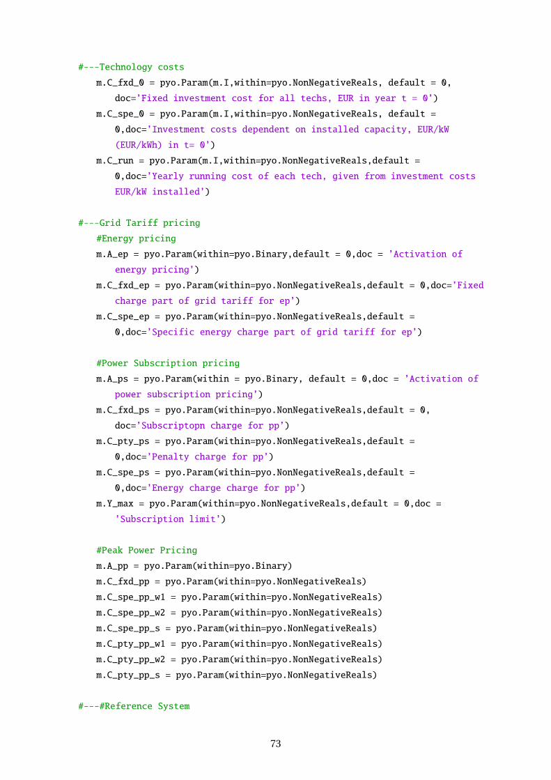
#---Technology costs
m.C_fxd_0 = pyo.Param(m.I,within=pyo.NonNegativeReals, default = 0,
doc=’Fixed investment cost for all techs, EUR in year t = 0’)
m.C_spe_0 = pyo.Param(m.I,within=pyo.NonNegativeReals, default =
0,doc=’Investment costs dependent on installed capacity, EUR/kW
(EUR/kWh) in t= 0’)
m.C_run = pyo.Param(m.I,within=pyo.NonNegativeReals,default =
0,doc=’Yearly running cost of each tech, given from investment costs
EUR/kW installed’)
#---Grid Tariff pricing
#Energy pricing
m.A_ep = pyo.Param(within=pyo.Binary,default = 0,doc = ’Activation of
energy pricing’)
m.C_fxd_ep = pyo.Param(within=pyo.NonNegativeReals,default = 0,doc=’Fixed
charge part of grid tariff for ep’)
m.C_spe_ep = pyo.Param(within=pyo.NonNegativeReals,default =
0,doc=’Specific energy charge part of grid tariff for ep’)
#Power Subscription pricing
m.A_ps = pyo.Param(within = pyo.Binary, default = 0,doc = ’Activation of
power subscription pricing’)
m.C_fxd_ps = pyo.Param(within=pyo.NonNegativeReals,default = 0,
doc=’Subscriptopn charge for pp’)
m.C_pty_ps = pyo.Param(within=pyo.NonNegativeReals,default =
0,doc=’Penalty charge for pp’)
m.C_spe_ps = pyo.Param(within=pyo.NonNegativeReals,default =
0,doc=’Energy charge charge for pp’)
m.Y_max = pyo.Param(within=pyo.NonNegativeReals,default = 0,doc =
’Subscription limit’)
#Peak Power Pricing
m.A_pp = pyo.Param(within=pyo.Binary)
m.C_fxd_pp = pyo.Param(within=pyo.NonNegativeReals)
m.C_spe_pp_w1 = pyo.Param(within=pyo.NonNegativeReals)
m.C_spe_pp_w2 = pyo.Param(within=pyo.NonNegativeReals)
m.C_spe_pp_s = pyo.Param(within=pyo.NonNegativeReals)
m.C_pty_pp_w1 = pyo.Param(within=pyo.NonNegativeReals)
m.C_pty_pp_w2 = pyo.Param(within=pyo.NonNegativeReals)
m.C_pty_pp_s = pyo.Param(within=pyo.NonNegativeReals)
#---#Reference System
73
#CO2-Factors
m.A_co2 = pyo.Param(within=pyo.Binary,doc = ’Activation of co2 crediting
system’)
m.G_ref = pyo.Param(within=pyo.NonNegativeReals,doc=’CO2 reference
emissions’)
m.G_el_imp = pyo.Param(within=pyo.NonNegativeReals,doc=’gCO2 eq. per kWh
imported/exported’)
m.G_el = pyo.Param(within=pyo.NonNegativeReals,doc=’gCO2 eq. per kWh
imported/exported’)
m.G_bf = pyo.Param(within=pyo.NonNegativeReals,doc=’gCO2 eq. per kWh for
technology i, i.e BB’)
m.G_wo = pyo.Param(within=pyo.NonNegativeReals,doc=’gCO2 eq. per kWh for
wood technology’)
m.G_tot = pyo.Param(within=pyo.NonNegativeReals,doc=’gCO2 total for
noZEB’)
#Primary Energy Factors
m.A_pe = pyo.Param(within=pyo.Binary,doc = ’Activation of primary energy
crediting system’)
m.PE_ref = pyo.Param(within=pyo.NonNegativeReals,doc=’CO2 reference
emissions’)
m.PE_imp = pyo.Param(within=pyo.NonNegativeReals,doc=’PE per kWh imported
electricity’)
m.PE_exp = pyo.Param(within=pyo.NonNegativeReals,doc=’PE per kWh exported
electricity’)
m.PE_bf = pyo.Param(within=pyo.NonNegativeReals,doc=’PE per kWh for
technology i, i.e BB’)
#---Technologies
m.A_i = pyo.Param(m.I, within=pyo.Binary,doc=’Pre-activation of each
tech’)
m.Eff = pyo.Param(m.I,within=pyo.NonNegativeReals, doc=’Technology
efficiency’)
m.Eff_ba_ch = pyo.Param(within=pyo.NonNegativeReals,doc=’Battery charging
efficiency’)
m.Eff_ba_dch = pyo.Param(initialize = 1, doc=’Battery discharge
efficiency’)
m.Beta_ba =
pyo.Param(within=pyo.NonNegativeReals,doc=’Charging/discharging rate’)
m.Beta_hs = pyo.Param(within=pyo.NonNegativeReals, doc=’identical
74

charging rate for heat storage’)
m.L = pyo.Param(m.I, within=pyo.NonNegativeIntegers, doc=’Lifetime of
technology i’)
m.X_min = pyo.Param(m.I, within=pyo.NonNegativeReals, doc=’Max possible
installed capacity of technology ’)
m.X_max = pyo.Param(m.I, within=pyo.NonNegativeReals, doc=’Min possible
installed capacity of technology ’)
m.Temp = pyo.Param(m.T, within=pyo.Reals, doc=’Ambient temperature of
certain hour’)
m.Y_pv_f10 = pyo.Param(m.T, within=pyo.NonNegativeReals,doc=’Possible PV
output at time t’)
m.Y_pv_S20 = pyo.Param(m.T, within=pyo.NonNegativeReals,doc=’Possible PV
output at time t’)
m.Y_pv_S30 = pyo.Param(m.T, within=pyo.NonNegativeReals,doc=’Possible PV
output at time t’)
m.Y_pv_E20 = pyo.Param(m.T, within=pyo.NonNegativeReals,doc=’Possible PV
output at time t’)
m.Y_pv_E30 = pyo.Param(m.T, within=pyo.NonNegativeReals,doc=’Possible PV
output at time t’)
m.Y_pv_W20 = pyo.Param(m.T, within=pyo.NonNegativeReals,doc=’Possible PV
output at time t’)
m.Y_pv_W30 = pyo.Param(m.T, within=pyo.NonNegativeReals,doc=’Possible PV
output at time t’)
m.Y_pv_S90 = pyo.Param(m.T, within=pyo.NonNegativeReals,doc=’Possible PV
output at time t’)
m.Y_pv_E90 = pyo.Param(m.T, within=pyo.NonNegativeReals,doc=’Possible PV
output at time t’)
m.Y_pv_W90 = pyo.Param(m.T, within=pyo.NonNegativeReals,doc=’Possible PV
output at time t’)
m.COP_a2a = pyo.Param(m.T, within=pyo.NonNegativeReals, doc=’Air-to-air
heat pump performance at time t w/r SH’)
#BITES-params
m.SS_cap = pyo.Param(within=pyo.NonNegativeReals, doc=’Shallow storage
capacity of house, fully determined by area, thus a parameter instead
of a variable’)
m.DS_cap = pyo.Param(within=pyo.NonNegativeReals, doc=’Deep storage
capacity of house, ---=---’)
m.K_shallow = pyo.Param(doc=’loss factor for BITES, shallow part’)
75
m.K_deep = pyo.Param(doc=’loss factor for BITES, deep part’)
m.K_flow = pyo.Param(doc=’flow factor for BITES, cross-node flow’)
#---Energy Demand
m.D_el = pyo.Param(m.T, within=pyo.NonNegativeReals, doc=’Hourly building
electricity demand’)
m.D_sh = pyo.Param(m.T, within=pyo.NonNegativeReals, doc=’Hourly building
space heating demand’)
m.D_dhw = pyo.Param(m.T, within=pyo.NonNegativeReals, doc=’Hourly
building domestic hot water demand’)
#---Grid
m.P_spot = pyo.Param(m.T, within=pyo.NonNegativeReals, doc=’Hourly price
of imported electricity EUR/kWh including certificates’)
m.X_max_imp = pyo.Param(within=pyo.NonNegativeReals, doc=’Maximum grid
import’)
m.X_max_exp = pyo.Param( within=pyo.NonNegativeReals,doc=’Maximum grid
export’)
m.A_imp = pyo.Param( within=pyo.Binary, doc=’Binary: Import is activated,
1/0’)
m.A_exp = pyo.Param( within=pyo.Binary,doc=’Binary: Export is activated,
1/0’)
m.C_bf = pyo.Param(within=pyo.NonNegativeReals, doc=’Constant price of
biofuel’)
m.C_wo = pyo.Param(within=pyo.NonNegativeReals, doc=’Constant price of
wood’)
#---Control
m.gamma = pyo.Param( within=pyo.NonNegativeReals, doc=’=0 for strictly
ZEB’)
m.R = pyo.Param(within=pyo.NonNegativeReals, doc=’Chosen discount Rate’)
m.YRN = pyo.Param( within=pyo.NonNegativeIntegers, doc=’Total years in
modelling period’)
def npv_inv_spe(m, i):
return self.cost(m.YRN, m.C_spe_0[i], m.L[i], m.R)
m.C_spe = pyo.Param(m.I, rule = npv_inv_spe)
def npv_inv_fxd(m, i):
return self.cost(m.YRN, m.C_fxd_0[i], m.L[i], m.R)
m.C_fxd = pyo.Param(m.I, rule = npv_inv_fxd)
76
#VARIABLES ##########################################################
# 1 STAGE : STRATEGIC VARIABLES
m.x = pyo.Var(m.I,within = pyo.NonNegativeReals,
doc=’Optimal installed capacity (storage size), semi-continous, kW
(kWh)’)
m.a_i = pyo.Var(m.I, within = pyo.Binary,
doc=’Activation binary decision for technology i, 1/0’)
#2 STAGE : OPERATIONAL VARIABLES
m.q_hwt = pyo.Var(m.T, domain = pyo.Reals,
doc=’Keeping track of HWT discharge’)
m.q_eb_dhw = pyo.Var(m.T,domain = pyo.NonNegativeReals,
doc=’Net heat supplied from (DHW) electric boiler at time t, kWh/h’)
m.q_po_sh = pyo.Var(m.T,domain = pyo.NonNegativeReals,
doc=’Net heat supplied from (SH) paneloven at time t, kWh/h’)
m.q_a2a_sh = pyo.Var(m.T, domain= pyo.NonNegativeReals,
doc=’Net heat supplied from air-to-air heat pump at time t, kWh/h’)
m.q_fp_sh = pyo.Var(m.T, domain=pyo.NonNegativeReals,
doc=’Net heat supplied from bio boiler at time t, kWh/h’)
m.f_fp = pyo.Var(m.T, domain= pyo.NonNegativeReals,
doc=’Wood input to the fireplace at time t kWh/h’)
m.z_hwt = pyo.Var(m.T, domain = pyo.NonNegativeReals,
doc=’Content in hot water tank (HWT) at the end of time t, kWh’)
m.z_ss = pyo.Var(m.T, domain = pyo.NonNegativeReals,
doc=’Content in shallow BITES at the end of time t, kWh’)
m.z_ds = pyo.Var(m.T, domain = pyo.NonNegativeReals,
doc=’Content in deep BITES at the end of time t, kWh’)
m.z_ba = pyo.Var(m.T, domain = pyo.NonNegativeReals,
doc=’Content of battery at the end of time t, kWh’)
#charging variables for BITES, shallow part
m.q_ss = pyo.Var(m.T, domain = pyo.Reals, doc=’Energy
released from shallow BITES at the end of time t, kWh’)
m.Flow = pyo.Var(m.T, domain = pyo.Reals,
doc=’Cross-node flow of two-node BITES model at time t, kWh’)
m.y_imp = pyo.Var(m.T, domain = pyo.NonNegativeReals,
doc=’Electricity imported from grid at time t, kWh’)
m.y_exp = pyo.Var(m.T, domain = pyo.NonNegativeReals,
77
doc=’Electricity exported to grid at time t, kWh’)
m.y_pv_f10 = pyo.Var(m.T, domain = pyo.NonNegativeReals,
doc=’PV production at time t, kWh/h’)
m.y_pv_S20 = pyo.Var(m.T, domain = pyo.NonNegativeReals,
doc=’PV production at time t, kWh/h’)
m.y_pv_S30 = pyo.Var(m.T, domain = pyo.NonNegativeReals,
doc=’PV production at time t, kWh/h’)
m.y_pv_E20 = pyo.Var(m.T, domain = pyo.NonNegativeReals,
doc=’PV production at time t, kWh/h’)
m.y_pv_E30 = pyo.Var(m.T, domain = pyo.NonNegativeReals,
doc=’PV production at time t, kWh/h’)
m.y_pv_W20 = pyo.Var(m.T, domain = pyo.NonNegativeReals,
doc=’PV production at time t, kWh/h’)
m.y_pv_W30 = pyo.Var(m.T, domain = pyo.NonNegativeReals,
doc=’PV production at time t, kWh/h’)
m.y_pv_S90 = pyo.Var(m.T, domain = pyo.NonNegativeReals,
doc=’PV production at time t, kWh/h’)
m.y_pv_E90 = pyo.Var(m.T, domain = pyo.NonNegativeReals,
doc=’PV production at time t, kWh/h’)
m.y_pv_W90 = pyo.Var(m.T, domain = pyo.NonNegativeReals,
doc=’PV production at time t, kWh/h’)
m.y_eb_dhw = pyo.Var(m.T, domain = pyo.NonNegativeReals,
doc=’Electricity drawn from (DHW) electric boiler at time t, kWh/h’)
m.y_po_sh = pyo.Var(m.T, domain = pyo.NonNegativeReals,
doc=’Electricity drawn for (SH) paneloven at time t, kWh/h’)
m.y_a2a_sh = pyo.Var(m.T, domain=pyo.NonNegativeReals,
doc=’Electricity drawn for air-to-air heat pump at time t, kWh/h’)
m.y_ch = pyo.Var(m.T, domain = pyo.NonNegativeReals,
doc=’Amount of electricity to battery (charging) at time t, kWh/h’)
m.y_dch = pyo.Var(m.T, domain = pyo.NonNegativeReals,
doc=’Amount of electricity discharge from battery at time t, kWh/h’)
m.y_pty = pyo.Var(m.T, domain = pyo.Reals, doc =
’Penalty volume’)
m.y_max_imp = pyo.Var(m.T, domain = pyo.Reals, doc =
’Max import of every month, stored in list-like container (one value
for each month)’)
m.y_max = pyo.Var(m.M, domain = pyo.NonNegativeReals, doc=’max
power for every month’)
m.a_ch = pyo.Var(m.T, domain = pyo.Binary, doc =
’Charging activation inward time t, 1 = activated’)
78
m.a_dch = pyo.Var(m.T, domain = pyo.Binary, doc =
’Discharging activation inward time t, 1 = activated’)
# CONSTRAINTS ##########################################################
# 1 STAGE : INVESTMENTS
#---Activation and boundary constraints
def Tech_active(m, i, st):
return m.x[i] <= m.a_i[i]•self.M_constm.Tech_active = pyo.Constraint(m.I, m.ST, rule = Tech_active)
def Tech_Min(m, i, st):
return m.X_min[i]•m.a_i[i] <= m.x[i]m.Tech_Min = pyo.Constraint(m.I, m.ST, rule= Tech_Min)
def Tech_Max(m, i, st):
return m.x[i] <= m.X_max[i]•m.A_i[i]m.Tech_Max = pyo.Constraint(m.I, m.ST, rule= Tech_Max)
#2 STAGE : OPERATIONS
#---Balacing constraints
def El_Balance(m, t, st):
return m.D_el[t] == m.y_imp[t] + m.y_pv_f10[t] +m.y_pv_S20[t]
+m.y_pv_S30[t] +m.y_pv_E20[t] +m.y_pv_E30[t] +m.y_pv_W20[t]
+m.y_pv_W30[t] +m.y_pv_S90[t] +m.y_pv_E90[t] +m.y_pv_W90[t] -
m.y_exp[t] + m.y_dch[t] - m.y_ch[t] - m.y_a2a_sh[t] - m.y_po_sh[t]
- m.y_eb_dhw[t]
m.El_Balance = pyo.Constraint(m.T, m.ST, rule = El_Balance)
def SH_balance(m, t, st):
return m.D_sh[t] == m.q_ss[t] + m.q_po_sh[t] + m.q_a2a_sh[t] +
m.q_fp_sh[t]
m.SH_balance = pyo.Constraint(m.T, m.ST, rule = SH_balance)
def DHW_balance(m, t, st):
if t == 0:
return m.D_dhw[t] + m.z_hwt[t] == m.z_hwt[m.lastT]•m.Eff[’HWT’] +m.q_eb_dhw[t]
else:
return m.D_dhw[t] + m.z_hwt[t] == m.z_hwt[t-1]•m.Eff[’HWT’] +
79
m.q_eb_dhw[t]
m.DHW_balance = pyo.Constraint(m.T, m.ST, rule = DHW_balance)
#---Capacity
def PO_SH_Restriction(m,t, st):
return m.q_po_sh[t] <= m.x[’PO_SH’]
m.PO_SH_Restriction = pyo.Constraint(m.T, m.ST, rule = PO_SH_Restriction)
def FP_SH_Restriction(m,t, st):
i = t - floor(t/24)•24if i >= 16 and i <= 24:
return m.q_fp_sh[t] <= m.x[’FP_SH’]
else:
return m.q_fp_sh[t] == 0
m.FP_SH_Restriction = pyo.Constraint(m.T, m.ST, rule = FP_SH_Restriction)
def A2A_SH_Restriction(m,t, st):
return m.q_a2a_sh[t] <= m.x[’A2A_SH’]
m.A2A_SH_Restriction = pyo.Constraint(m.T, m.ST, rule =
A2A_SH_Restriction)
def A2A_SH_Restriction_1(m,t, st):
return m.q_a2a_sh[t] <= 0.5•m.D_sh[t]m.A2A_SH_Restriction_1 = pyo.Constraint(m.T, m.ST, rule =
A2A_SH_Restriction_1)
def EB_DHW_Restriction(m,t, st):
return m.q_eb_dhw[t] <= m.x[’EB_DHW’]
m.EB_DHW_Restriction = pyo.Constraint(m.T, m.ST, rule =
EB_DHW_Restriction)
#---Grid equations
def Grid_Import(m,t, st):
return m.y_imp[t] <= m.X_max_imp
m.Grid_Import = pyo.Constraint(m.T, m.ST, rule=Grid_Import)
def Grid_Export(m,t, st):
return m.y_exp[t] <= m.X_max_exp
m.Grid_Export = pyo.Constraint(m.T, m.ST, rule=Grid_Export)
#---Storage equations
80
def HWT_Restriction(m, t, st):
return m.z_hwt[t] <= m.x[’HWT’]
m.HWT_Restriction = pyo.Constraint(m.T, m.ST, rule=HWT_Restriction)
def SS_Restriction(m, t, st):
return m.z_ss[t] <= m.x[’SS’]•m.A_i[’SS’]m.SS_Restriction = pyo.Constraint(m.T, m.ST, rule=SS_Restriction)
def DS_Restriction(m, t, st):
return m.z_ss[t] <= m.x[’DS’]•m.A_i[’DS’]m.DS_Restriction = pyo.Constraint(m.T, m.ST, rule=DS_Restriction)
def SS_charge_active(m,t, st):
return m.q_ss[t] <= m.z_ss[t]
m.SS_charge_active = pyo.Constraint(m.T, m.ST, rule=SS_charge_active)
def SS_discharge_active(m,t, st):
return - m.z_ss[t] <= m.q_ss[t]
m.SS_discharge_active = pyo.Constraint(m.T, m.ST,
rule=SS_discharge_active)
def HWT_charge_active(m,t, st):
return m.q_hwt[t] <= m.z_hwt[t]
m.HWT_charge_active = pyo.Constraint(m.T, m.ST, rule=HWT_charge_active)
def HWT_discharge_active(m,t, st):
return - m.z_hwt[t] <= m.q_hwt[t]
m.HWT_discharge_active = pyo.Constraint(m.T, m.ST,
rule=HWT_discharge_active)
def HWT_Balance_ch(m,t,st):
if t == 0:
return m.q_hwt[t] == m.z_hwt[m.lastT] - m.z_hwt[t]
else:
return m.q_hwt[t] == m.z_hwt[t-1] - m.z_hwt[t]
m.HWT_Balance_ch = pyo.Constraint(m.T, m.ST, rule = HWT_Balance_ch)
def Flow_Constraint(m,t,st):
return m.Flow[t] == m.K_flow•((m.z_ss[t]/m.SS_cap) -(m.z_ds[t]/m.DS_cap))
m.Flow_Constraint = pyo.Constraint(m.T, m.ST, rule = Flow_Constraint)
81
def SS_balance_ch(m, t, st):
if t == 0:
return m.q_ss[t] == m.z_ss[m.lastT] - m.z_ss[t] - m.Flow[t] -
m.z_ss[t]•(1 - m.K_shallow)else:
return m.q_ss[t] == m.z_ss[t-1] - m.z_ss[t] - m.Flow[t] -
m.z_ss[t]•(1 - m.K_shallow)m.SS_balance_ch = pyo.Constraint(m.T, m.ST, rule = SS_balance_ch)
def DS_balance_ch(m, t, st):
if t == 0:
return m.z_ds[t] == m.z_ds[m.lastT] + m.Flow[t] - m.z_ds[t]•(1 -m.K_deep)
else:
return m.z_ds[t] == m.z_ds[t-1] + m.Flow[t] - m.z_ds[t]•(1 -m.K_deep)
m.DS_balance_ch = pyo.Constraint(m.T, m.ST, rule = DS_balance_ch)
def HWT_discharge_rate_min(m,t, st):
return -m.x[’HWT’]•m.Beta_hs <= m.q_hwt[t]m.HS_discharge_rate_min = pyo.Constraint(m.T, m.ST,
rule=HWT_discharge_rate_min)
def HWT_discharge_rate_max(m,t, s):
return m.q_hwt[t] <= m.x[’HWT’]•m.Beta_hsm.HWT_discharge_rate_max = pyo.Constraint(m.T, m.ST,
rule=HWT_discharge_rate_max)
def BA_Restriction(m,t, st):
return m.z_ba[t] <= m.x[’BA’]
m.BA_restriction = pyo.Constraint(m.T, m.ST, rule=BA_Restriction)
def BA_Balance(m,t, st):
if t == 0:
return m.z_ba[t] == m.z_ba[m.lastT] - m.y_dch[t]•(1/m.Eff_ba_dch)+ m.y_ch[t]•m.Eff_ba_ch
else:
return m.z_ba[t] == m.z_ba[t-1] - m.y_dch[t]•(1/m.Eff_ba_dch) +m.y_ch[t]•m.Eff_ba_ch
m.BA_Balance = pyo.Constraint(m.T, m.ST, rule=BA_Balance)
def BA_Charge_Balance(m, t, st):
82
if t == 0:
return m.y_ch[t] <= (m.x[’BA’] -
m.z_ba[m.lastT])•m.A_i[’BA’]•(1/m.Eff_ba_ch)else:
return m.y_ch[t] <= (m.x[’BA’] -
m.z_ba[t-1])•m.A_i[’BA’]•(1/m.Eff_ba_ch)m.BA_Charge_Balance = pyo.Constraint(m.T, m.ST, rule=BA_Charge_Balance)
def BA_Discharge_Balance(m,t, st):
if t == 0:
return m.y_dch[t] <= m.z_ba[m.lastT]•m.A_i[’BA’]•m.Eff_ba_dchelse:
return m.y_dch[t] <= m.z_ba[t-1]•m.A_i[’BA’]•m.Eff_ba_dchm.BA_Discharge_Balance = pyo.Constraint(m.T, m.ST,
rule=BA_Discharge_Balance)
def BA_charge_active(m,t, st):
return m.y_ch[t] <= m.X_max_imp
m.BA_charge_active = pyo.Constraint(m.T, m.ST, rule=BA_charge_active)
def BA_discharge_active(m,t, st):
return m.y_dch[t] <= m.X_max_imp
m.BA_discharge_active = pyo.Constraint(m.T, m.ST,
rule=BA_discharge_active)
def BA_charge_rate(m,t, st):
return m.y_ch[t] <= m.x[’BA’]•m.Beta_bam.BA_charge_rate = pyo.Constraint(m.T, m.ST, rule=BA_charge_rate)
def BA_discharge_rate(m,t, st):
return m.y_dch[t] <= m.x[’BA’]•m.Beta_bam.BA_discharge_rate = pyo.Constraint(m.T, m.ST, rule=BA_discharge_rate)
#---Production constraints for generating technologies
def PV_f10_Balance(m,t, st):
return m.y_pv_f10[t] == m.x[’PV_f10’]•m.Y_pv_f10[t]m.PV_f10_Balance = pyo.Constraint(m.T, m.ST, rule=PV_f10_Balance)
def PV_S20_Balance(m,t, st):
return m.y_pv_S20[t] == m.x[’PV_S20’]•m.Y_pv_S20[t]m.PV_S20_Balance = pyo.Constraint(m.T, m.ST, rule=PV_S20_Balance)
83
def PV_S30_Balance(m,t, st):
return m.y_pv_S30[t] == m.x[’PV_S30’]•m.Y_pv_S30[t]m.PV_S30_Balance = pyo.Constraint(m.T, m.ST, rule=PV_S30_Balance)
def PV_E20_Balance(m,t, st):
return m.y_pv_E20[t] == m.x[’PV_E20’]•m.Y_pv_E20[t]m.PV_E20_Balance = pyo.Constraint(m.T, m.ST, rule=PV_E20_Balance)
def PV_E30_Balance(m,t, st):
return m.y_pv_E30[t] == m.x[’PV_E30’]•m.Y_pv_E30[t]m.PV_E30_Balance = pyo.Constraint(m.T, m.ST, rule=PV_E30_Balance)
def PV_W20_Balance(m,t, st):
return m.y_pv_W20[t] == m.x[’PV_W20’]•m.Y_pv_W20[t]m.PV_W20_Balance = pyo.Constraint(m.T, m.ST, rule=PV_W20_Balance)
def PV_W30_Balance(m,t, st):
return m.y_pv_W30[t] == m.x[’PV_W30’]•m.Y_pv_W30[t]m.PV_W30_Balance = pyo.Constraint(m.T, m.ST, rule=PV_W30_Balance)
def PV_S90_Balance(m,t, st):
return m.y_pv_S90[t] == m.x[’PV_S90’]•m.Y_pv_S90[t]m.PV_S90_Balance = pyo.Constraint(m.T, m.ST, rule=PV_S90_Balance)
def PV_E90_Balance(m,t, st):
return m.y_pv_E90[t] == m.x[’PV_E90’]•m.Y_pv_E90[t]m.PV_E90_Balance = pyo.Constraint(m.T, m.ST, rule=PV_E90_Balance)
def PV_W90_Balance(m,t, st):
return m.y_pv_W90[t] == m.x[’PV_W90’]•m.Y_pv_W90[t]m.PV_W90_Balance = pyo.Constraint(m.T, m.ST, rule=PV_W90_Balance)
def A2A_SH_Balance(m,t, st):
return m.q_a2a_sh[t] == m.y_a2a_sh[t]•m.COP_a2a[t]m.A2A_SH_Balance = pyo.Constraint(m.T, m.ST, rule = A2A_SH_Balance)
def PO_SH_Balance(m,t, st):
return m.q_po_sh[t] == m.y_po_sh[t]•m.Eff[’PO_SH’]m.PO_SH_Balance = pyo.Constraint(m.T, m.ST, rule = PO_SH_Balance)
def FP_SH_Balance(m,t, st):
84
return m.q_fp_sh[t] == m.f_fp[t]•m.Eff[’FP_SH’]•m.A_i[’FP_SH’]m.FP_SH_Balance = pyo.Constraint(m.T, m.ST, rule = FP_SH_Balance)
def EB_DHW_Balance(m,t, st):
return m.q_eb_dhw[t] == m.y_eb_dhw[t]•m.Eff[’EB_DHW’]m.EB_DHW_Balance = pyo.Constraint(m.T, m.ST, rule = EB_DHW_Balance)
#---Zero emission/energy constraints
def ZE_Balance(m):
if m.A_co2==1:
print(’ACTIVE ZEB-carbon RESTRICTION’)
if m.lastT == 8735:
return sum(m.y_imp[t]•m.G_el_imp + m.f_fp[t]•m.G_wo for t inm.T) <= sum(m.y_exp[t]•m.G_el for t in m.T)
if m.lastT == 4367:
return 2•sum(m.y_imp[t]•m.G_el - m.y_exp[t]•m.G_el +m.bf[t]•m.G_bf for t in m.T) <= m.G_ref•m.gamma
elif m.lastT == 727:
return 12•sum(m.y_imp[t]•m.G_el - m.y_exp[t]•m.G_el +m.bf[t]•m.G_bf for t in m.T) <= m.G_ref•m.gamma
elif m.lastT == 671:
return sum(m.y_imp[t]•m.G_el_imp + m.f_fp[t]•m.G_wo for t inm.T) <= sum(m.y_exp[t]•m.G_el for t in m.T)
elif m.lastT == 287:
return (8736/288)•sum(m.y_imp[t]•m.G_el - m.y_exp[t]•m.G_el +m.bf[t]•m.G_bf for t in m.T) <= m.G_ref•m.gamma
elif m.lastT == 95:
return sum(m.y_imp[t]•m.G_el - m.y_exp[t]•m.G_el +m.bf_sh[t]•m.G_bf + m.bf_dhw[t]•m.G_bf for t in m.T) <=sum(m.y_exp[t]•m.G_el for t in m.T)
elif m.lastT == 23:
return (8736/24)•sum(m.y_imp[t]•m.G_el - m.y_exp[t]•m.G_el +m.bf[t]•m.G_bf for t in m.T) <= m.G_ref•m.gamma
elif m.A_pe == 1:
print(’ACTIVE ZEB-pef RESTRICTION’)
if m.lastT == 8735:
return sum(m.y_imp[t]•m.PE_imp - m.y_exp[t]•m.PE_exp +m.bf[t]•m.PE_bf for t in m.T) <= m.PE_ref•m.gamma
elif m.lastT == 671:
return 13•sum(m.y_imp[t]•m.PE_imp - m.y_exp[t]•m.PE_exp +m.bf[t]•m.PE_bf for t in m.T) <= m.PE_ref•m.gamma
else:
85
print(’NO ZEB RESTRICTION’)
return pyo.Constraint.Skip
m.ZE_Balance = pyo.Constraint(rule=ZE_Balance)
#Subscription power pricing Constraint
def pty_volume(m, t): #counting all power within one hour exceeding max
limit
if m.A_ps == 1:
return m.y_imp[t] - m.Y_max <= m.y_pty[t]
else:
return m.y_pty[t] == 0
m.pty_volume = pyo.Constraint(m.T, rule = pty_volume)
def pty_volume2(m, t):
return 0 <= m.y_pty[t]
m.pty_volume2 = pyo.Constraint(m.T, rule = pty_volume2)
# Peak power restriction
def peak_power(m, t):
H = createHvector()
for key in H.keys():
if t <= H[key]:
month = key
break
if t <= H[month]:
return m.y_max_imp[month] >= m.y_imp[t]
else:
return pyo.Constraint.Skip
m.peak_power = pyo.Constraint(m.T, rule = peak_power)
# OBJECTIVE FUNCTION #################################################
def cost_Investments_rule(m, st):
expr = self.npv_cost_Investments(m, st)
return expr
m.cost_Investments = pyo.Expression(m.ST, rule = cost_Investments_rule)
def cost_Operation_rule(m, st):
expr = self.npv_cost_Operations(m, st)
return expr
m.cost_Operations= pyo.Expression(m.ST, rule = cost_Operation_rule)
86

def objective_TotalCost(m):
expr = pyo.summation(m.cost_Investments) +
pyo.summation(m.cost_Operations)
return expr
m.objective_TotalCosts = pyo.Objective(rule = objective_TotalCost, sense
= pyo.minimize)
return m
def createConcreteModeltwoStage(self, data):
’’’Function creating instance from input data’’’
concretemodel = self.abstractmodel.create_instance(data = {
’mymodel’:data}, namespace = ’mymodel’)
return concretemodel
87
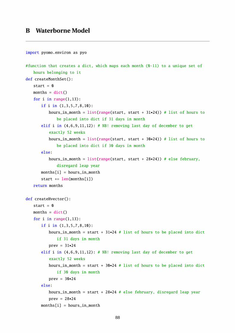
B Waterborne Model
import pyomo.environ as pyo
#function that creates a dict, which maps each month (0-11) to a unique set of
hours belonging to it
def createMonthSet():
start = 0
months = dict()
for i in range(1,13):
if i in (1,3,5,7,8,10):
hours_in_month = list(range(start, start + 31•24)) # list of hours tobe placed into dict if 31 days in month
elif i in (4,6,9,11,12): # NB! removing last day of december to get
exactly 52 weeks
hours_in_month = list(range(start, start + 30•24)) # list of hours tobe placed into dict if 30 days in month
else:
hours_in_month = list(range(start, start + 28•24)) # else february,disregard leap year
months[i] = hours_in_month
start += len(months[i])
return months
def createHvector():
start = 0
months = dict()
for i in range(1,13):
if i in (1,3,5,7,8,10):
hours_in_month = start + 31•24 # list of hours to be placed into dictif 31 days in month
prev = 31•24elif i in (4,6,9,11,12): # NB! removing last day of december to get
exactly 52 weeks
hours_in_month = start + 30•24 # list of hours to be placed into dictif 30 days in month
prev = 30•24else:
hours_in_month = start + 28•24 # else february, disregard leap yearprev = 28•24
months[i] = hours_in_month
88
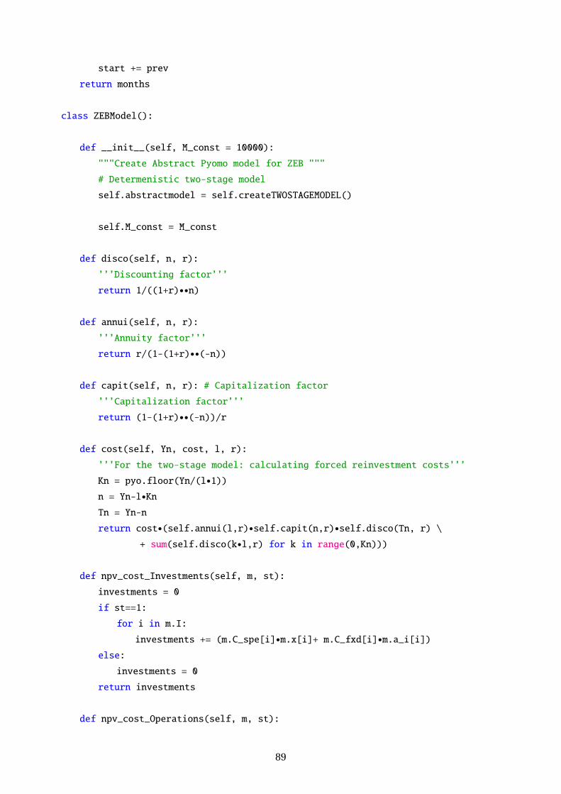
start += prev
return months
class ZEBModel():
def __init__(self, M_const = 10000):
"""Create Abstract Pyomo model for ZEB """
# Determenistic two-stage model
self.abstractmodel = self.createTWOSTAGEMODEL()
self.M_const = M_const
def disco(self, n, r):
’’’Discounting factor’’’
return 1/((1+r)••n)
def annui(self, n, r):
’’’Annuity factor’’’
return r/(1-(1+r)••(-n))
def capit(self, n, r): # Capitalization factor
’’’Capitalization factor’’’
return (1-(1+r)••(-n))/r
def cost(self, Yn, cost, l, r):
’’’For the two-stage model: calculating forced reinvestment costs’’’
Kn = pyo.floor(Yn/(l•1))n = Yn-l•KnTn = Yn-n
return cost•(self.annui(l,r)•self.capit(n,r)•self.disco(Tn, r) \+ sum(self.disco(k•l,r) for k in range(0,Kn)))
def npv_cost_Investments(self, m, st):
investments = 0
if st==1:
for i in m.I:
investments += (m.C_spe[i]•m.x[i]+ m.C_fxd[i]•m.a_i[i])else:
investments = 0
return investments
def npv_cost_Operations(self, m, st):
89
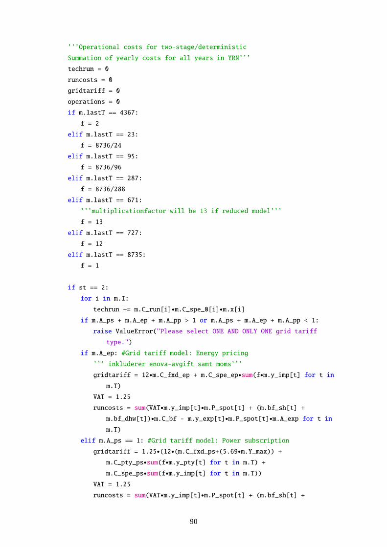
’’’Operational costs for two-stage/deterministic
Summation of yearly costs for all years in YRN’’’
techrun = 0
runcosts = 0
gridtariff = 0
operations = 0
if m.lastT == 4367:
f = 2
elif m.lastT == 23:
f = 8736/24
elif m.lastT == 95:
f = 8736/96
elif m.lastT == 287:
f = 8736/288
elif m.lastT == 671:
’’’multiplicationfactor will be 13 if reduced model’’’
f = 13
elif m.lastT == 727:
f = 12
elif m.lastT == 8735:
f = 1
if st == 2:
for i in m.I:
techrun += m.C_run[i]•m.C_spe_0[i]•m.x[i]if m.A_ps + m.A_ep + m.A_pp > 1 or m.A_ps + m.A_ep + m.A_pp < 1:
raise ValueError("Please select ONE AND ONLY ONE grid tariff
type.")
if m.A_ep: #Grid tariff model: Energy pricing
’’’ inkluderer enova-avgift samt moms’’’
gridtariff = 12•m.C_fxd_ep + m.C_spe_ep•sum(f•m.y_imp[t] for t inm.T)
VAT = 1.25
runcosts = sum(VAT•m.y_imp[t]•m.P_spot[t] + (m.bf_sh[t] +m.bf_dhw[t])•m.C_bf - m.y_exp[t]•m.P_spot[t]•m.A_exp for t inm.T)
elif m.A_ps == 1: #Grid tariff model: Power subscription
gridtariff = 1.25•(12•(m.C_fxd_ps+(5.69•m.Y_max)) +m.C_pty_ps•sum(f•m.y_pty[t] for t in m.T) +m.C_spe_ps•sum(f•m.y_imp[t] for t in m.T))
VAT = 1.25
runcosts = sum(VAT•m.y_imp[t]•m.P_spot[t] + (m.bf_sh[t] +
90
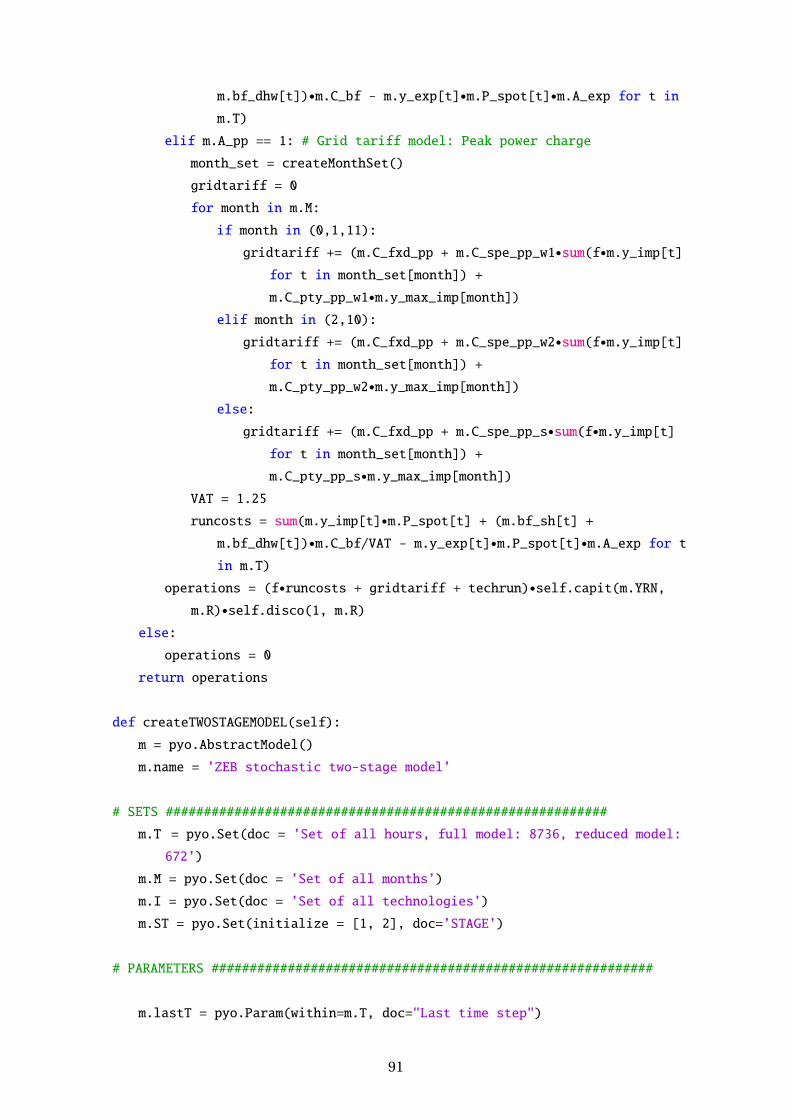
m.bf_dhw[t])•m.C_bf - m.y_exp[t]•m.P_spot[t]•m.A_exp for t inm.T)
elif m.A_pp == 1: # Grid tariff model: Peak power charge
month_set = createMonthSet()
gridtariff = 0
for month in m.M:
if month in (0,1,11):
gridtariff += (m.C_fxd_pp + m.C_spe_pp_w1•sum(f•m.y_imp[t]for t in month_set[month]) +
m.C_pty_pp_w1•m.y_max_imp[month])elif month in (2,10):
gridtariff += (m.C_fxd_pp + m.C_spe_pp_w2•sum(f•m.y_imp[t]for t in month_set[month]) +
m.C_pty_pp_w2•m.y_max_imp[month])else:
gridtariff += (m.C_fxd_pp + m.C_spe_pp_s•sum(f•m.y_imp[t]for t in month_set[month]) +
m.C_pty_pp_s•m.y_max_imp[month])VAT = 1.25
runcosts = sum(m.y_imp[t]•m.P_spot[t] + (m.bf_sh[t] +m.bf_dhw[t])•m.C_bf/VAT - m.y_exp[t]•m.P_spot[t]•m.A_exp for tin m.T)
operations = (f•runcosts + gridtariff + techrun)•self.capit(m.YRN,m.R)•self.disco(1, m.R)
else:
operations = 0
return operations
def createTWOSTAGEMODEL(self):
m = pyo.AbstractModel()
m.name = ’ZEB stochastic two-stage model’
# SETS ##########################################################
m.T = pyo.Set(doc = ’Set of all hours, full model: 8736, reduced model:
672’)
m.M = pyo.Set(doc = ’Set of all months’)
m.I = pyo.Set(doc = ’Set of all technologies’)
m.ST = pyo.Set(initialize = [1, 2], doc=’STAGE’)
# PARAMETERS ##########################################################
m.lastT = pyo.Param(within=m.T, doc="Last time step")
91
m.Area = pyo.Param(within=pyo.NonNegativeReals, doc="Building floor area")
#---Technology costs
m.C_fxd_0 = pyo.Param(m.I,within=pyo.NonNegativeReals, default = 0,
doc=’Fixed investment cost for all techs, EUR in year t = 0’)
m.C_spe_0 = pyo.Param(m.I,within=pyo.NonNegativeReals, default =
0,doc=’Investment costs dependent on installed capacity, EUR/kW
(EUR/kWh) in t= 0’)
m.C_run = pyo.Param(m.I,within=pyo.NonNegativeReals,default =
0,doc=’Yearly running cost of each tech, given from investment costs
EUR/kW installed’)
#---Grid Tariff pricing
#Energy pricing
m.A_ep = pyo.Param(within=pyo.Binary,default = 0,doc = ’Activation of
energy pricing’)
m.C_fxd_ep = pyo.Param(within=pyo.NonNegativeReals,default = 0,doc=’Fixed
charge part of grid tariff for ep’)
m.C_spe_ep = pyo.Param(within=pyo.NonNegativeReals,default =
0,doc=’Specific energy charge part of grid tariff for ep’)
#Power Subscription pricing
m.A_ps = pyo.Param(within = pyo.Binary, default = 0,doc = ’Activation of
power subscription pricing’)
m.C_fxd_ps = pyo.Param(within=pyo.NonNegativeReals,default = 0,
doc=’Subscriptopn charge for pp’)
m.C_pty_ps = pyo.Param(within=pyo.NonNegativeReals,default =
0,doc=’Penalty charge for pp’)
m.C_spe_ps = pyo.Param(within=pyo.NonNegativeReals,default =
0,doc=’Energy charge charge for pp’)
m.Y_max = pyo.Param(within=pyo.NonNegativeReals,default = 0,doc =
’Subscription limit’)
#Peak Power Pricing
m.A_pp = pyo.Param(within=pyo.Binary)
m.C_fxd_pp = pyo.Param(within=pyo.NonNegativeReals)
m.C_spe_pp_w1 = pyo.Param(within=pyo.NonNegativeReals)
m.C_spe_pp_w2 = pyo.Param(within=pyo.NonNegativeReals)
m.C_spe_pp_s = pyo.Param(within=pyo.NonNegativeReals)
m.C_pty_pp_w1 = pyo.Param(within=pyo.NonNegativeReals)
m.C_pty_pp_w2 = pyo.Param(within=pyo.NonNegativeReals)
m.C_pty_pp_s = pyo.Param(within=pyo.NonNegativeReals)
92

#---#Reference System
#CO2-Factors
m.A_co2 = pyo.Param(within=pyo.Binary,doc = ’Activation of co2 crediting
system’)
m.G_ref = pyo.Param(within=pyo.NonNegativeReals,doc=’CO2 reference
emissions’)
m.G_el = pyo.Param(within=pyo.NonNegativeReals,doc=’gCO2 eq. per kWh
imported/exported’)
m.G_bf = pyo.Param(within=pyo.NonNegativeReals,doc=’gCO2 eq. per kWh for
technology i, i.e BB’)
#Primary Energy Factors
m.A_pe = pyo.Param(within=pyo.Binary,doc = ’Activation of primary energy
crediting system’)
m.PE_ref = pyo.Param(within=pyo.NonNegativeReals,doc=’CO2 reference
emissions’)
m.PE_imp = pyo.Param(within=pyo.NonNegativeReals,doc=’PE per kWh imported
electricity’)
m.PE_exp = pyo.Param(within=pyo.NonNegativeReals,doc=’PE per kWh exported
electricity’)
m.PE_bf = pyo.Param(within=pyo.NonNegativeReals,doc=’PE per kWh for
technology i, i.e BB’)
#---Technologies
m.A_i = pyo.Param(m.I, within=pyo.Binary,doc=’Pre-activation of each
tech’)
m.Eff = pyo.Param(m.I,within=pyo.NonNegativeReals, doc=’Technology
efficiency’)
m.Eff_ba_ch = pyo.Param(within=pyo.NonNegativeReals,doc=’Battery charging
efficiency’)
m.Eff_ba_dch = pyo.Param(initialize = 1, doc=’Battery discharge
efficiency’)
m.Beta_ba =
pyo.Param(within=pyo.NonNegativeReals,doc=’Charging/discharging rate’)
m.Beta_hs = pyo.Param(within=pyo.NonNegativeReals, doc=’identical
charging rate for heat storage’)
m.L = pyo.Param(m.I, within=pyo.NonNegativeIntegers, doc=’Lifetime of
technology i’)
93

m.X_min = pyo.Param(m.I, within=pyo.NonNegativeReals, doc=’Max possible
installed capacity of technology ’)
m.X_max = pyo.Param(m.I, within=pyo.NonNegativeReals, doc=’Min possible
installed capacity of technology ’)
m.Temp = pyo.Param(m.T, within=pyo.Reals, doc=’Ambient temperature of
certain hour’)
m.Y_pv_f10 = pyo.Param(m.T, within=pyo.NonNegativeReals,doc=’Possible PV
output at time t’)
m.Y_pv_S20 = pyo.Param(m.T, within=pyo.NonNegativeReals,doc=’Possible PV
output at time t’)
m.Y_pv_S30 = pyo.Param(m.T, within=pyo.NonNegativeReals,doc=’Possible PV
output at time t’)
m.Y_pv_E20 = pyo.Param(m.T, within=pyo.NonNegativeReals,doc=’Possible PV
output at time t’)
m.Y_pv_E30 = pyo.Param(m.T, within=pyo.NonNegativeReals,doc=’Possible PV
output at time t’)
m.Y_pv_W20 = pyo.Param(m.T, within=pyo.NonNegativeReals,doc=’Possible PV
output at time t’)
m.Y_pv_W30 = pyo.Param(m.T, within=pyo.NonNegativeReals,doc=’Possible PV
output at time t’)
m.Y_pv_S90 = pyo.Param(m.T, within=pyo.NonNegativeReals,doc=’Possible PV
output at time t’)
m.Y_pv_E90 = pyo.Param(m.T, within=pyo.NonNegativeReals,doc=’Possible PV
output at time t’)
m.Y_pv_W90 = pyo.Param(m.T, within=pyo.NonNegativeReals,doc=’Possible PV
output at time t’)
m.COP_ashp_dhw = pyo.Param(m.T, within=pyo.NonNegativeReals, doc=’Heat
pump performance at time t w/r DHW’)
m.COP_gshp_dhw = pyo.Param(m.T, within=pyo.NonNegativeReals, doc=’Heat
pump performance at time t w/r DHW’)
m.COP_ashp_sh = pyo.Param(m.T, within=pyo.NonNegativeReals, doc=’Heat
pump performance at time t w/r SH’)
m.COP_gshp_sh = pyo.Param(m.T, within=pyo.NonNegativeReals, doc=’Heat
pump performance at time t w/r SH’)
#BITES-params
m.SS_cap = pyo.Param(within=pyo.NonNegativeReals, doc=’Shallow storage
capacity of house, fully determined by area, thus a parameter instead
of a variable’)
m.DS_cap = pyo.Param(within=pyo.NonNegativeReals, doc=’Deep storage
capacity of house, ---=---’)
94
m.K_shallow = pyo.Param(doc=’loss factor for BITES, shallow part’)
m.K_deep = pyo.Param(doc=’loss factor for BITES, deep part’)
m.K_flow = pyo.Param(doc=’flow factor for BITES, cross-node flow’)
#---Energy Demand
m.D_el = pyo.Param(m.T, within=pyo.NonNegativeReals, doc=’Hourly building
electricity demand’)
m.D_sh = pyo.Param(m.T, within=pyo.NonNegativeReals, doc=’Hourly building
space heating demand’)
m.D_dhw = pyo.Param(m.T, within=pyo.NonNegativeReals, doc=’Hourly
building domestic hot water demand’)
#---Grid
m.P_spot = pyo.Param(m.T, within=pyo.NonNegativeReals, doc=’Hourly price
of imported electricity EUR/kWh including certificates’)
m.X_max_imp = pyo.Param(within=pyo.NonNegativeReals, doc=’Maximum grid
import’)
m.X_max_exp = pyo.Param( within=pyo.NonNegativeReals,doc=’Maximum grid
export’)
m.A_imp = pyo.Param( within=pyo.Binary, doc=’Binary: Import is activated,
1/0’)
m.A_exp = pyo.Param( within=pyo.Binary,doc=’Binary: Export is activated,
1/0’)
m.C_bf = pyo.Param(within=pyo.NonNegativeReals, doc=’Constant price of
biofuel’)
#---Control
m.gamma = pyo.Param( within=pyo.NonNegativeReals, doc=’=0 for strictly
ZEB’)
m.R = pyo.Param(within=pyo.NonNegativeReals, doc=’Chosen discount Rate’)
m.YRN = pyo.Param( within=pyo.NonNegativeIntegers, doc=’Total years in
modelling period’)
def npv_inv_spe(m, i):
return self.cost(m.YRN, m.C_spe_0[i], m.L[i], m.R)
m.C_spe = pyo.Param(m.I, rule = npv_inv_spe)
def npv_inv_fxd(m, i):
return self.cost(m.YRN, m.C_fxd_0[i], m.L[i], m.R)
m.C_fxd = pyo.Param(m.I, rule = npv_inv_fxd)
#VARIABLES ##########################################################
95
# 1 STAGE : STRATEGIC VARIABLES
m.x = pyo.Var(m.I,within = pyo.NonNegativeReals,
doc=’Optimal installed capacity (storage size), semi-continous, kW
(kWh)’)
m.a_i = pyo.Var(m.I, within = pyo.Binary,
doc=’Activation binary decision for technology i, 1/0’)
#2 STAGE : OPERATIONAL VARIABLES
m.q_hs = pyo.Var(m.T, domain = pyo.Reals,
doc=’Keeping track of HS discharge’)
m.q_eb_sh = pyo.Var(m.T,domain = pyo.NonNegativeReals,
doc=’Net heat supplied from (SH) electric boiler at time t, kWh/h’)
m.q_eb_dhw = pyo.Var(m.T,domain = pyo.NonNegativeReals,
doc=’Net heat supplied from (DHW) electric boiler at time t, kWh/h’)
m.q_bb_sh = pyo.Var(m.T,domain = pyo.NonNegativeReals,
doc=’Net heat supplied from (SH) bio boiler at time t, kWh/h’)
m.q_bb_dhw = pyo.Var(m.T,domain = pyo.NonNegativeReals,
doc=’Net heat supplied from (DHW) bio boiler at time t, kWh/h’)
m.bf_sh = pyo.Var(m.T, domain= pyo.NonNegativeReals,
doc=’Biofuel input to bio boiler at time t for SH kWh/h’)
m.bf_dhw = pyo.Var(m.T, domain= pyo.NonNegativeReals,
doc=’Biofuel input to bio boiler at time t for DHW kWh/h’)
m.q_ashp_sh = pyo.Var(m.T,domain=pyo.NonNegativeReals,
doc=’Net heat supplied from air source heat pump (SH) at time t,
kWh/h’)
m.q_gshp_sh = pyo.Var(m.T,domain=pyo.NonNegativeReals,
doc=’Net heat supplied from ground source heat pump (SH) at time t,
kWh/h’)
m.q_ashp_dhw = pyo.Var(m.T,domain=pyo.NonNegativeReals,
doc=’Net heat supplied from air source heat pump (DHW) at time t,
kWh/h’)
m.q_gshp_dhw = pyo.Var(m.T,domain=pyo.NonNegativeReals,
doc=’Net heat supplied from ground source heat pump (DHW) at time t,
kWh/h’)
m.q_ashp_eff = pyo.Var(m.T,domain=pyo.NonNegativeReals,
doc=’Net effective heat supplied from air source heat pump at time t,
adjusted for source temperature, kWh/h’)
m.q_ashp = pyo.Var(m.T,domain=pyo.NonNegativeReals, doc=’Net
effective heat supplied from air source heat pump at time t, kWh/h’)
96
m.z_hs = pyo.Var(m.T, domain = pyo.NonNegativeReals,
doc=’Content in heat storage (HS) at the end of time t, kWh’)
m.z_hwt = pyo.Var(m.T, domain = pyo.NonNegativeReals,
doc=’Content in hot water tank (HWT) at the end of time t, kWh’)
m.z_ss = pyo.Var(m.T, domain = pyo.NonNegativeReals,
doc=’Content in shallow BITES at the end of time t, kWh’)
m.z_ds = pyo.Var(m.T, domain = pyo.NonNegativeReals,
doc=’Content in deep BITES at the end of time t, kWh’)
m.z_ba = pyo.Var(m.T, domain = pyo.NonNegativeReals,
doc=’Content of battery at the end of time t, kWh’)
m.Flow = pyo.Var(m.T, domain = pyo.Reals,
doc=’Cross-node flow of two-node BITES model at time t, kWh’)
#charging variables for BITES, shallow part
m.q_ss = pyo.Var(m.T, domain = pyo.Reals, doc=’Energy
released from shallow BITES at the end of time t, kWh’)
m.q_hwt = pyo.Var(m.T, domain = pyo.Reals, doc=’Energy
released from HWT at the end of time t, kWh’)
m.y_imp = pyo.Var(m.T, domain = pyo.NonNegativeReals,
doc=’Electricity imported from grid at time t, kWh’)
m.y_exp = pyo.Var(m.T, domain = pyo.NonNegativeReals,
doc=’Electricity exported to grid at time t, kWh’)
m.y_pv_f10 = pyo.Var(m.T, domain = pyo.NonNegativeReals,
doc=’PV production at time t, kWh/h’)
m.y_pv_S20 = pyo.Var(m.T, domain = pyo.NonNegativeReals,
doc=’PV production at time t, kWh/h’)
m.y_pv_S30 = pyo.Var(m.T, domain = pyo.NonNegativeReals,
doc=’PV production at time t, kWh/h’)
m.y_pv_E20 = pyo.Var(m.T, domain = pyo.NonNegativeReals,
doc=’PV production at time t, kWh/h’)
m.y_pv_E30 = pyo.Var(m.T, domain = pyo.NonNegativeReals,
doc=’PV production at time t, kWh/h’)
m.y_pv_W20 = pyo.Var(m.T, domain = pyo.NonNegativeReals,
doc=’PV production at time t, kWh/h’)
m.y_pv_W30 = pyo.Var(m.T, domain = pyo.NonNegativeReals,
doc=’PV production at time t, kWh/h’)
m.y_pv_S90 = pyo.Var(m.T, domain = pyo.NonNegativeReals,
doc=’PV production at time t, kWh/h’)
m.y_pv_E90 = pyo.Var(m.T, domain = pyo.NonNegativeReals,
doc=’PV production at time t, kWh/h’)
m.y_pv_W90 = pyo.Var(m.T, domain = pyo.NonNegativeReals,
97
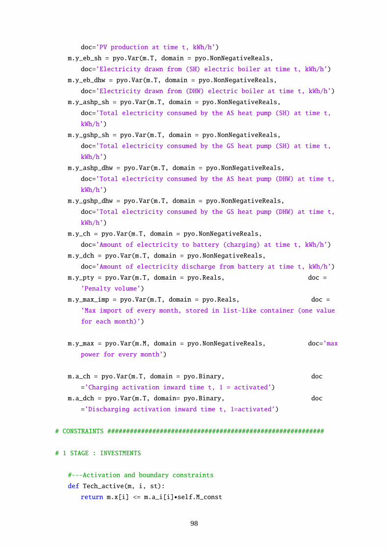
doc=’PV production at time t, kWh/h’)
m.y_eb_sh = pyo.Var(m.T, domain = pyo.NonNegativeReals,
doc=’Electricity drawn from (SH) electric boiler at time t, kWh/h’)
m.y_eb_dhw = pyo.Var(m.T, domain = pyo.NonNegativeReals,
doc=’Electricity drawn from (DHW) electric boiler at time t, kWh/h’)
m.y_ashp_sh = pyo.Var(m.T, domain = pyo.NonNegativeReals,
doc=’Total electricity consumed by the AS heat pump (SH) at time t,
kWh/h’)
m.y_gshp_sh = pyo.Var(m.T, domain = pyo.NonNegativeReals,
doc=’Total electricity consumed by the GS heat pump (SH) at time t,
kWh/h’)
m.y_ashp_dhw = pyo.Var(m.T, domain = pyo.NonNegativeReals,
doc=’Total electricity consumed by the AS heat pump (DHW) at time t,
kWh/h’)
m.y_gshp_dhw = pyo.Var(m.T, domain = pyo.NonNegativeReals,
doc=’Total electricity consumed by the GS heat pump (DHW) at time t,
kWh/h’)
m.y_ch = pyo.Var(m.T, domain = pyo.NonNegativeReals,
doc=’Amount of electricity to battery (charging) at time t, kWh/h’)
m.y_dch = pyo.Var(m.T, domain = pyo.NonNegativeReals,
doc=’Amount of electricity discharge from battery at time t, kWh/h’)
m.y_pty = pyo.Var(m.T, domain = pyo.Reals, doc =
’Penalty volume’)
m.y_max_imp = pyo.Var(m.T, domain = pyo.Reals, doc =
’Max import of every month, stored in list-like container (one value
for each month)’)
m.y_max = pyo.Var(m.M, domain = pyo.NonNegativeReals, doc=’max
power for every month’)
m.a_ch = pyo.Var(m.T, domain = pyo.Binary, doc
=’Charging activation inward time t, 1 = activated’)
m.a_dch = pyo.Var(m.T, domain= pyo.Binary, doc
=’Discharging activation inward time t, 1=activated’)
# CONSTRAINTS ##########################################################
# 1 STAGE : INVESTMENTS
#---Activation and boundary constraints
def Tech_active(m, i, st):
return m.x[i] <= m.a_i[i]•self.M_const
98
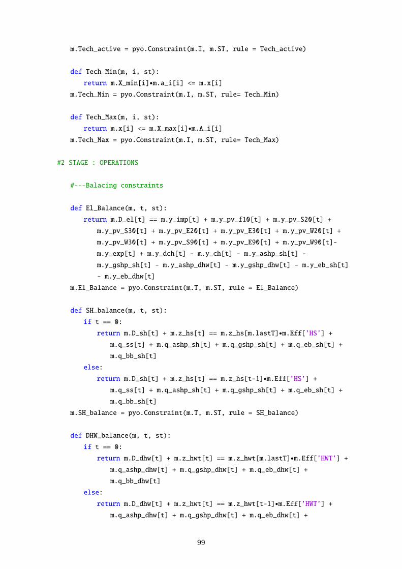
m.Tech_active = pyo.Constraint(m.I, m.ST, rule = Tech_active)
def Tech_Min(m, i, st):
return m.X_min[i]•m.a_i[i] <= m.x[i]m.Tech_Min = pyo.Constraint(m.I, m.ST, rule= Tech_Min)
def Tech_Max(m, i, st):
return m.x[i] <= m.X_max[i]•m.A_i[i]m.Tech_Max = pyo.Constraint(m.I, m.ST, rule= Tech_Max)
#2 STAGE : OPERATIONS
#---Balacing constraints
def El_Balance(m, t, st):
return m.D_el[t] == m.y_imp[t] + m.y_pv_f10[t] + m.y_pv_S20[t] +
m.y_pv_S30[t] + m.y_pv_E20[t] + m.y_pv_E30[t] + m.y_pv_W20[t] +
m.y_pv_W30[t] + m.y_pv_S90[t] + m.y_pv_E90[t] + m.y_pv_W90[t]-
m.y_exp[t] + m.y_dch[t] - m.y_ch[t] - m.y_ashp_sh[t] -
m.y_gshp_sh[t] - m.y_ashp_dhw[t] - m.y_gshp_dhw[t] - m.y_eb_sh[t]
- m.y_eb_dhw[t]
m.El_Balance = pyo.Constraint(m.T, m.ST, rule = El_Balance)
def SH_balance(m, t, st):
if t == 0:
return m.D_sh[t] + m.z_hs[t] == m.z_hs[m.lastT]•m.Eff[’HS’] +m.q_ss[t] + m.q_ashp_sh[t] + m.q_gshp_sh[t] + m.q_eb_sh[t] +
m.q_bb_sh[t]
else:
return m.D_sh[t] + m.z_hs[t] == m.z_hs[t-1]•m.Eff[’HS’] +m.q_ss[t] + m.q_ashp_sh[t] + m.q_gshp_sh[t] + m.q_eb_sh[t] +
m.q_bb_sh[t]
m.SH_balance = pyo.Constraint(m.T, m.ST, rule = SH_balance)
def DHW_balance(m, t, st):
if t == 0:
return m.D_dhw[t] + m.z_hwt[t] == m.z_hwt[m.lastT]•m.Eff[’HWT’] +m.q_ashp_dhw[t] + m.q_gshp_dhw[t] + m.q_eb_dhw[t] +
m.q_bb_dhw[t]
else:
return m.D_dhw[t] + m.z_hwt[t] == m.z_hwt[t-1]•m.Eff[’HWT’] +m.q_ashp_dhw[t] + m.q_gshp_dhw[t] + m.q_eb_dhw[t] +
99
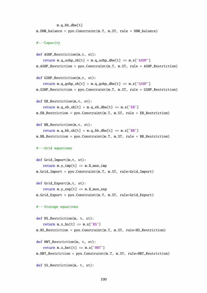
m.q_bb_dhw[t]
m.DHW_balance = pyo.Constraint(m.T, m.ST, rule = DHW_balance)
#---Capacity
def ASHP_Restriction(m,t, st):
return m.q_ashp_sh[t] + m.q_ashp_dhw[t] <= m.x[’ASHP’]
m.ASHP_Restriction = pyo.Constraint(m.T, m.ST, rule = ASHP_Restriction)
def GSHP_Restriction(m,t, st):
return m.q_gshp_sh[t] + m.q_gshp_dhw[t] <= m.x[’GSHP’]
m.GSHP_Restriction = pyo.Constraint(m.T, m.ST, rule = GSHP_Restriction)
def EB_Restriction(m,t, st):
return m.q_eb_sh[t] + m.q_eb_dhw[t] <= m.x[’EB’]
m.EB_Restriction = pyo.Constraint(m.T, m.ST, rule = EB_Restriction)
def BB_Restriction(m,t, st):
return m.q_bb_sh[t] + m.q_bb_dhw[t] <= m.x[’BB’]
m.BB_Restriction = pyo.Constraint(m.T, m.ST, rule = BB_Restriction)
#---Grid equations
def Grid_Import(m,t, st):
return m.y_imp[t] <= m.X_max_imp
m.Grid_Import = pyo.Constraint(m.T, m.ST, rule=Grid_Import)
def Grid_Export(m,t, st):
return m.y_exp[t] <= m.X_max_exp
m.Grid_Export = pyo.Constraint(m.T, m.ST, rule=Grid_Export)
#---Storage equations
def HS_Restriction(m, t, st):
return m.z_hs[t] <= m.x[’HS’]
m.HS_Restriction = pyo.Constraint(m.T, m.ST, rule=HS_Restriction)
def HWT_Restriction(m, t, st):
return m.z_hwt[t] <= m.x[’HWT’]
m.HWT_Restriction = pyo.Constraint(m.T, m.ST, rule=HWT_Restriction)
def SS_Restriction(m, t, st):
100
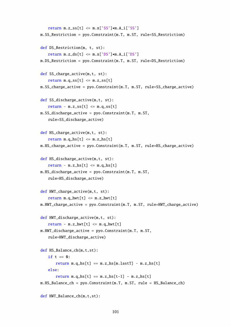
return m.z_ss[t] <= m.x[’SS’]•m.A_i[’SS’]m.SS_Restriction = pyo.Constraint(m.T, m.ST, rule=SS_Restriction)
def DS_Restriction(m, t, st):
return m.z_ds[t] <= m.x[’DS’]•m.A_i[’DS’]m.DS_Restriction = pyo.Constraint(m.T, m.ST, rule=DS_Restriction)
def SS_charge_active(m,t, st):
return m.q_ss[t] <= m.z_ss[t]
m.SS_charge_active = pyo.Constraint(m.T, m.ST, rule=SS_charge_active)
def SS_discharge_active(m,t, st):
return - m.z_ss[t] <= m.q_ss[t]
m.SS_discharge_active = pyo.Constraint(m.T, m.ST,
rule=SS_discharge_active)
def HS_charge_active(m,t, st):
return m.q_hs[t] <= m.z_hs[t]
m.HS_charge_active = pyo.Constraint(m.T, m.ST, rule=HS_charge_active)
def HS_discharge_active(m,t, st):
return - m.z_hs[t] <= m.q_hs[t]
m.HS_discharge_active = pyo.Constraint(m.T, m.ST,
rule=HS_discharge_active)
def HWT_charge_active(m,t, st):
return m.q_hwt[t] <= m.z_hwt[t]
m.HWT_charge_active = pyo.Constraint(m.T, m.ST, rule=HWT_charge_active)
def HWT_discharge_active(m,t, st):
return - m.z_hwt[t] <= m.q_hwt[t]
m.HWT_discharge_active = pyo.Constraint(m.T, m.ST,
rule=HWT_discharge_active)
def HS_Balance_ch(m,t,st):
if t == 0:
return m.q_hs[t] == m.z_hs[m.lastT] - m.z_hs[t]
else:
return m.q_hs[t] == m.z_hs[t-1] - m.z_hs[t]
m.HS_Balance_ch = pyo.Constraint(m.T, m.ST, rule = HS_Balance_ch)
def HWT_Balance_ch(m,t,st):
101

if t == 0:
return m.q_hwt[t] == m.z_hwt[m.lastT] - m.z_hwt[t]
else:
return m.q_hwt[t] == m.z_hwt[t-1] - m.z_hwt[t]
m.HWT_Balance_ch = pyo.Constraint(m.T, m.ST, rule = HWT_Balance_ch)
def Flow_Constraint(m,t,st):
return m.Flow[t] == m.K_flow•((m.z_ss[t]/m.SS_cap) -(m.z_ds[t]/m.DS_cap))
m.Flow_Constraint = pyo.Constraint(m.T, m.ST, rule = Flow_Constraint)
def SS_balance_ch(m, t, st):
if t == 0:
return m.q_ss[t] == m.z_ss[m.lastT] - m.z_ss[t] - m.Flow[t] -
m.z_ss[t]•(1 - m.K_shallow)else:
return m.q_ss[t] == m.z_ss[t-1] - m.z_ss[t] - m.Flow[t] -
m.z_ss[t]•(1 - m.K_shallow)m.SS_balance_ch = pyo.Constraint(m.T, m.ST, rule = SS_balance_ch)
def DS_balance_ch(m, t, st):
if t == 0:
return m.z_ds[t] == m.z_ds[m.lastT] + m.Flow[t] - m.z_ds[t]•(1 -m.K_deep)
else:
return m.z_ds[t] == m.z_ds[t-1] + m.Flow[t] - m.z_ds[t]•(1 -m.K_deep)
m.DS_balance_ch = pyo.Constraint(m.T, m.ST, rule = DS_balance_ch)
def HS_discharge_rate_min(m,t, st):
return -m.x[’HS’]•m.Beta_hs <= m.q_hs[t]m.HS_discharge_rate_min = pyo.Constraint(m.T, m.ST,
rule=HS_discharge_rate_min)
def HS_discharge_rate_max(m,t, s):
return m.q_hs[t] <= m.x[’HS’]•m.Beta_hsm.HS_discharge_rate_max = pyo.Constraint(m.T, m.ST,
rule=HS_discharge_rate_max)
def HWT_discharge_rate_min(m,t, st):
return -m.x[’HWT’]•m.Beta_hs <= m.q_hwt[t]m.HWT_discharge_rate_min = pyo.Constraint(m.T, m.ST,
102
rule=HWT_discharge_rate_min)
def HWT_discharge_rate_max(m,t, s):
return m.q_hwt[t] <= m.x[’HWT’]•m.Beta_hsm.HWT_discharge_rate_max = pyo.Constraint(m.T, m.ST,
rule=HWT_discharge_rate_max)
def BA_Restriction(m,t, st):
return m.z_ba[t] <= m.x[’BA’]
m.BA_restriction = pyo.Constraint(m.T, m.ST, rule=BA_Restriction)
def BA_Balance(m,t, st):
if t == 0:
return m.z_ba[t] == m.z_ba[m.lastT] - m.y_dch[t]•(1/m.Eff_ba_dch)+ m.y_ch[t]•m.Eff_ba_ch
else:
return m.z_ba[t] == m.z_ba[t-1] - m.y_dch[t]•(1/m.Eff_ba_dch) +m.y_ch[t]•m.Eff_ba_ch
m.BA_Balance = pyo.Constraint(m.T, m.ST, rule=BA_Balance)
def BA_Charge_Balance(m, t, st):
if t == 0:
return m.y_ch[t] <= (m.x[’BA’] -
m.z_ba[m.lastT])•m.A_i[’BA’]•(1/m.Eff_ba_ch)else:
return m.y_ch[t] <= (m.x[’BA’] -
m.z_ba[t-1])•m.A_i[’BA’]•(1/m.Eff_ba_ch)m.BA_Charge_Balance = pyo.Constraint(m.T, m.ST, rule=BA_Charge_Balance)
def BA_Discharge_Balance(m,t, st):
if t == 0:
return m.y_dch[t] <= m.z_ba[m.lastT]•m.A_i[’BA’]•m.Eff_ba_dchelse:
return m.y_dch[t] <= m.z_ba[t-1]•m.A_i[’BA’]•m.Eff_ba_dchm.BA_Discharge_Balance = pyo.Constraint(m.T, m.ST,
rule=BA_Discharge_Balance)
def BA_charge_active(m,t, st):
return m.y_ch[t] <= m.X_max_imp•m.a_ch[t]m.BA_charge_active = pyo.Constraint(m.T, m.ST, rule=BA_charge_active)
def BA_discharge_active(m,t, st):
103
return m.y_dch[t] <= m.X_max_imp•m.a_dch[t]m.BA_discharge_active = pyo.Constraint(m.T, m.ST,
rule=BA_discharge_active)
def Battery_Balance(m,t, st):
return m.a_ch[t] + m.a_dch[t] <= 1
m.Battery_Balance = pyo.Constraint(m.T, m.ST, rule=Battery_Balance)
def BA_charge_rate(m,t, st):
return m.y_ch[t] <= m.x[’BA’]•m.Beta_bam.BA_charge_rate = pyo.Constraint(m.T, m.ST, rule=BA_charge_rate)
def BA_discharge_rate(m,t, st):
return m.y_dch[t] <= m.x[’BA’]•m.Beta_bam.BA_discharge_rate = pyo.Constraint(m.T, m.ST, rule=BA_discharge_rate)
#---Production constraints for generating technologies
def PV_f10_Balance(m,t, st):
return m.y_pv_f10[t] == m.x[’PV_f10’]•m.Y_pv_f10[t]m.PV_f10_Balance = pyo.Constraint(m.T, m.ST, rule=PV_f10_Balance)
def PV_S20_Balance(m,t, st):
return m.y_pv_S20[t] == m.x[’PV_S20’]•m.Y_pv_S20[t]m.PV_S20_Balance = pyo.Constraint(m.T, m.ST, rule=PV_S20_Balance)
def PV_S30_Balance(m,t, st):
return m.y_pv_S30[t] == m.x[’PV_S30’]•m.Y_pv_S30[t]m.PV_S30_Balance = pyo.Constraint(m.T, m.ST, rule=PV_S30_Balance)
def PV_E20_Balance(m,t, st):
return m.y_pv_E20[t] == m.x[’PV_E20’]•m.Y_pv_E20[t]m.PV_E20_Balance = pyo.Constraint(m.T, m.ST, rule=PV_E20_Balance)
def PV_E30_Balance(m,t, st):
return m.y_pv_E30[t] == m.x[’PV_E30’]•m.Y_pv_E30[t]m.PV_E30_Balance = pyo.Constraint(m.T, m.ST, rule=PV_E30_Balance)
def PV_W20_Balance(m,t, st):
return m.y_pv_W20[t] == m.x[’PV_W20’]•m.Y_pv_W20[t]m.PV_W20_Balance = pyo.Constraint(m.T, m.ST, rule=PV_W20_Balance)
104
def PV_W30_Balance(m,t, st):
return m.y_pv_W30[t] == m.x[’PV_W30’]•m.Y_pv_W30[t]m.PV_W30_Balance = pyo.Constraint(m.T, m.ST, rule=PV_W30_Balance)
def PV_S90_Balance(m,t, st):
return m.y_pv_S90[t] == m.x[’PV_S90’]•m.Y_pv_S90[t]m.PV_S90_Balance = pyo.Constraint(m.T, m.ST, rule=PV_S90_Balance)
def PV_E90_Balance(m,t, st):
return m.y_pv_E90[t] == m.x[’PV_E90’]•m.Y_pv_E90[t]m.PV_E90_Balance = pyo.Constraint(m.T, m.ST, rule=PV_E90_Balance)
def PV_W90_Balance(m,t, st):
return m.y_pv_W90[t] == m.x[’PV_W90’]•m.Y_pv_W90[t]m.PV_W90_Balance = pyo.Constraint(m.T, m.ST, rule=PV_W90_Balance)
def ASHP_SH_Balance(m,t, st):
return m.q_ashp_sh[t] == m.y_ashp_sh[t]•m.COP_ashp_sh[t]m.ASHP_SH_Balance = pyo.Constraint(m.T, m.ST, rule = ASHP_SH_Balance)
def ASHP_DHW_Balance(m,t, st):
return m.q_ashp_dhw[t] == m.y_ashp_dhw[t]•m.COP_ashp_dhw[t]m.ASHP_DHW_Balance = pyo.Constraint(m.T, m.ST, rule = ASHP_DHW_Balance)
def GSHP_SH_Balance(m,t, st):
return m.q_gshp_sh[t] == m.y_gshp_sh[t]•m.COP_gshp_sh[t]m.GSHP_SH_Balance = pyo.Constraint(m.T, m.ST, rule = GSHP_SH_Balance)
def GSHP_DHW_Balance(m,t, st):
return m.q_gshp_dhw[t] == m.y_gshp_dhw[t]•m.COP_gshp_dhw[t]m.GSHP_DHW_Balance = pyo.Constraint(m.T, m.ST, rule = GSHP_DHW_Balance)
def EB_SH_Balance(m,t, st):
return m.q_eb_sh[t] == m.y_eb_sh[t]•m.Eff[’EB’]m.EB_SH_Balance = pyo.Constraint(m.T, m.ST, rule = EB_SH_Balance)
def EB_DHW_Balance(m,t, st):
return m.q_eb_dhw[t] == m.y_eb_dhw[t]•m.Eff[’EB’]m.EB_DHW_Balance = pyo.Constraint(m.T, m.ST, rule = EB_DHW_Balance)
def BB_SH_Balance(m,t, st):
return m.q_bb_sh[t] == m.bf_sh[t]•m.A_i[’BB’]•m.Eff[’BB’]
105
m.BB_SH_Balance = pyo.Constraint(m.T, m.ST, rule=BB_SH_Balance)
def BB_DHW_Balance(m,t, st):
return m.q_bb_dhw[t] == m.bf_dhw[t]•m.A_i[’BB’]•m.Eff[’BB’]m.BB_DHW_Balance = pyo.Constraint(m.T, m.ST, rule=BB_DHW_Balance)
#---Zero emission/energy constraints
def ZE_Balance(m):
if m.A_co2==1:
print(’ACTIVE ZEB-carbon RESTRICTION’)
if m.lastT == 8735:
return sum(m.y_imp[t]•m.G_el + m.bf_sh[t]•m.G_bf +m.bf_dhw[t]•m.G_bf for t in m.T) <= sum(m.y_exp[t]•m.G_elfor t in m.T)
if m.lastT == 4367:
return 2•sum(m.y_imp[t]•m.G_el - m.y_exp[t]•m.G_el +m.bf[t]•m.G_bf for t in m.T) <= m.G_ref•m.gamma
elif m.lastT == 727:
return 12•sum(m.y_imp[t]•m.G_el - m.y_exp[t]•m.G_el +m.bf[t]•m.G_bf for t in m.T) <= m.G_ref•m.gamma
elif m.lastT == 671:
return sum(m.y_imp[t]•m.G_el + m.bf_sh[t]•m.G_bf +m.bf_dhw[t]•m.G_bf for t in m.T) <= sum(m.y_exp[t]•m.G_elfor t in m.T)
elif m.lastT == 287:
return (8736/288)•sum(m.y_imp[t]•m.G_el - m.y_exp[t]•m.G_el +m.bf[t]•m.G_bf for t in m.T) <= m.G_ref•m.gamma
elif m.lastT == 95:
return sum(m.y_imp[t]•m.G_el - m.y_exp[t]•m.G_el +m.bf_sh[t]•m.G_bf + m.bf_dhw[t]•m.G_bf for t in m.T) <=sum(m.y_exp[t]•m.G_el for t in m.T)
elif m.lastT == 23:
return (8736/24)•sum(m.y_imp[t]•m.G_el - m.y_exp[t]•m.G_el +m.bf[t]•m.G_bf for t in m.T) <= m.G_ref•m.gamma
elif m.A_pe == 1:
print(’ACTIVE ZEB-pef RESTRICTION’)
if m.lastT == 8735:
return sum(m.y_imp[t]•m.PE_imp - m.y_exp[t]•m.PE_exp +m.bf[t]•m.PE_bf for t in m.T) <= m.PE_ref•m.gamma
elif m.lastT == 671:
return 13•sum(m.y_imp[t]•m.PE_imp - m.y_exp[t]•m.PE_exp +m.bf[t]•m.PE_bf for t in m.T) <= m.PE_ref•m.gamma
106
else:
print(’NO ZEB RESTRICTION’)
return pyo.Constraint.Skip
m.ZE_Balance = pyo.Constraint(rule=ZE_Balance)
#Subscription power pricing Constraint
def pty_volume(m, t): #counting all power within one hour exceeding max
limit
if m.A_ps == 1:
return m.y_imp[t] - m.Y_max <= m.y_pty[t]
else:
return m.y_pty[t] ==0
m.pty_volume = pyo.Constraint(m.T, rule = pty_volume)
def pty_volume2(m, t):
return 0 <= m.y_pty[t]
m.pty_volume2 = pyo.Constraint(m.T, rule = pty_volume2)
# Peak power restriction
def peak_power(m, t):
H = createHvector()
for key in H.keys():
if t <= H[key]:
month = key
break
if t <= H[month]:
return m.y_max_imp[month] >= m.y_imp[t]
else:
return pyo.Constraint.Skip
m.peak_power = pyo.Constraint(m.T, rule = peak_power)
# OBJECTIVE FUNCTION #################################################
def cost_Investments_rule(m, st):
expr = self.npv_cost_Investments(m, st)
return expr
m.cost_Investments = pyo.Expression(m.ST, rule = cost_Investments_rule)
def cost_Operation_rule(m, st):
expr = self.npv_cost_Operations(m, st)
return expr
m.cost_Operations= pyo.Expression(m.ST, rule = cost_Operation_rule)
107

def objective_TotalCost(m):
expr = pyo.summation(m.cost_Investments) +
pyo.summation(m.cost_Operations)
return expr
m.objective_TotalCosts = pyo.Objective(rule = objective_TotalCost, sense
= pyo.minimize)
return m
def createConcreteModeltwoStage(self, data):
’’’Function creating instance from input data’’’
concretemodel = self.abstractmodel.create_instance(data = {
’mymodel’:data}, namespace = ’mymodel’)
return concretemodel
108
C Load Profiles
C.1 Regular building SFH
0
1
2
3
4
5
6
7
8
9
121
542
964
385
710
7112
8514
9917
1319
2721
4123
5525
6927
8329
9732
1134
2536
3938
5340
6742
8144
9547
0949
2351
3753
5155
6557
7959
9362
0764
2166
3568
4970
6372
7774
9177
0579
1981
3383
4785
61
W/m
^2
Hour
EL Demand
Figure C.1: Electricity Demand for Regular SFH
C.2 Post-insulated building SFH
0
1
2
3
4
5
6
7
8
9
127
554
982
310
9713
7116
4519
1921
9324
6727
4130
1532
8935
6338
3741
1143
8546
5949
3352
0754
8157
5560
2963
0365
7768
5171
2573
9976
7379
4782
2184
95
W/m
^2
Hour
EL Demand
Figure C.2: Electricity Demand for Post-insulated SFH
109
C.3 Regular building Apartment Block
0
5
10
15
20
25
30
35
117
033
950
867
784
610
1511
8413
5315
2216
9118
6020
2921
9823
6725
3627
0528
7430
4332
1233
8135
5037
1938
8840
5742
2643
9545
6447
3349
0250
7152
4054
0955
7857
4759
1660
8562
5464
2365
9267
6169
3070
9972
6874
3776
0677
7579
4481
1382
8284
5186
20
W/m
^2
Hour
DHW Demand
SH Demand
Figure C.3: Heat Demand for Regular Apartment Block
C.4 Post-insulated building Apartment Block
0
1
2
3
4
5
6
7
8
9
113
827
541
254
968
682
396
010
9712
3413
7115
0816
4517
8219
1920
5621
9323
3024
6726
0427
4128
7830
1531
5232
8934
2635
6337
0038
3739
7441
1142
4843
8545
2246
5947
9649
3350
7052
0753
4454
8156
1857
5558
9260
2961
6663
0364
4065
7767
1468
5169
8871
2572
6273
9975
3676
7378
1079
4780
8482
2183
5884
9586
32
W/m
^2
Hour
EL Demand
Figure C.4: Electricity Demand for Post-insulated Apartment Block
110
0
2
4
6
8
10
12
14
16
18
20
115
029
944
859
774
689
510
4411
9313
4214
9116
4017
8919
3820
8722
3623
8525
3426
8328
3229
8131
3032
7934
2835
7737
2638
7540
2441
7343
2244
7146
2047
6949
1850
6752
1653
6555
1456
6358
1259
6161
1062
5964
0865
5767
0668
5570
0471
5373
0274
5176
0077
4978
9880
4781
9683
4584
9486
43
W/m
^2
Hour
DHW Demand
SH Demand
Figure C.5: Heat Demand for Post-insulated Apartment
C.5 Regular building Office
0
5
10
15
20
25
30
35
40
45
122
645
167
690
111
2613
5115
7618
0120
2622
5124
7627
0129
2631
5133
7636
0138
2640
5142
7645
0147
2649
5151
7654
0156
2658
5160
7663
0165
2667
5169
7672
0174
2676
5178
7681
0183
2685
51
W/m
^2
Hour
DHW Demand
SH Demand
Figure C.6: Heat Demand for Regular Office
111
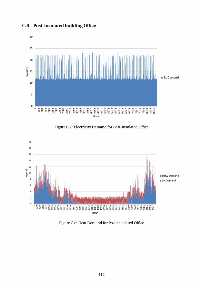
C.6 Post-insulated building Office
0
5
10
15
20
25
301
252
503
754
1005
1256
1507
1758
2009
2260
2511
2762
3013
3264
3515
3766
4017
4268
4519
4770
5021
5272
5523
5774
6025
6276
6527
6778
7029
7280
7531
7782
8033
8284
8535
W/m
^2
Hour
EL Demand
Figure C.7: Electricity Demand for Post-insulated Office
0
2
4
6
8
10
12
14
16
18
20
122
043
965
887
710
9613
1515
3417
5319
7221
9124
1026
2928
4830
6732
8635
0537
2439
4341
6243
8146
0048
1950
3852
5754
7656
9559
1461
3363
5265
7167
9070
0972
2874
4776
6678
8581
0483
2385
42
W/m
^2
Hour
DHW Demand
SH Demand
Figure C.8: Heat Demand for Post-insulated Office
112

Camilla H
engebøl A study on optim
al utilization of electric heating for buildings
NTN
UN
orw
egia
n U
nive
rsity
of S
cien
ce a
nd T
echn
olog
yFa
culty
of I
nfor
mat
ion
Tech
nolo
gy a
nd E
lect
rical
Engi
neer
ing
Dep
artm
ent o
f Ele
ctric
Pow
er E
ngin
eerin
g
Mas
ter’s
thes
is
Camilla Hengebøl
A study on optimal utilization of electricheating for buildings
Master’s thesis in Energy Use and Energy Planning
Supervisor: Karen Byskov Lindberg
February 2020