A Study on External Memory Scan-basedSkyline Algorithms

Nikos Bikakis1,2, Dimitris Sacharidis2, and Timos Sellis3

1 National Technical University of Athens, Greece2 IMIS, “Athena” R.C., Greece3 RMIT University, Australia

Abstract. Skyline queries return the set of non-dominated tuples, wherea tuple is dominated if there exists another with better values on all at-tributes. In the past few years the problem has been studied extensively,and a great number of external memory algorithms have been proposed.We thoroughly study the most important scan-based methods, whichperform a number of passes over the database in order to extract theskyline. Although these algorithms are specifically designed to operatein external memory, there are many implementation details which are ne-glected, as well as several design choices resulting in different flavors forthese basic methods. We perform an extensive experimental evaluationusing real and synthetic data. We conclude that specific design choicescan have a significant impact on performance. We also demonstrate that,contrary to common belief, simpler skyline algorithm can be much fasterthan methods based on pre-processing.

Keywords: Experimental evaluation, experimental survey, disk-based algorithm.

1 Introduction

The skyline query, or skyline operator as it was introduced in [3], has in the pastfew years received great attention in the data management community. Given adatabase of objects, the skyline query returns those objects which are not dom-inated. An object dominates another, if it has better values on all attributes,and strictly better value on at least one. Finding the skyline is also known asthe Pareto-optimal set, or maximal vectors problem in multi-objective optimiza-tion research, where it has been studied extensively in the past, but only forin-memory computations. For example the well-known divide and conquer algo-rithm of [7] has complexity O(N logd−2 N), for d ≥ 2, where N is the number ofobjects, and d their dimensionality; the algorithm is optimal for d = 3.

The interest in external memory algorithms has sparked after the seminalwork in [3]. The most efficient method in terms of worst-case Input/Output(I/O) operations is the algorithm in [15], which requires in the worst case

O(

(N/B) logd−2M/B(N/B)

)I/Os, where M is the memory size and B the block

(minimum unit of transfer in an I/O operation) size in terms of objects. However,

in practice, other external-memory algorithms proposed over the past years canbe faster.

This work studies in detail an important class of practical algorithms, thescan-based skyline algorithms. An algorithm of this class performs multiple passesover an input file, where the input file in the first pass is the database, and in asubsequent pass it is the output of the previous pass. The algorithm terminateswhen the output file remains empty after a pass concludes. Generally speaking,during each pass, the algorithm maintains in main memory a small window ofincomparable objects, which it uses to remove dominated objects from the inputfile. Any object not dominated is written to the output file.

Although the studied algorithms are specifically designed to operate in exter-nal memory, little attention has been given to important implementation detailsregarding memory management. For example, all algorithms assume that theunit of transfer during an I/O operation is the object, whereas in a real systemis the block, i.e., a set of objects. Our work addresses such shortcomings by in-troducing a more realistic I/O model that better captures performance in a realsystem. Furthermore, by thoroughly studying the core computational challengein these algorithms, which is the management of the objects within the window,we introduce several novel potentially interesting policies.

Summarizing, the contributions of our study are the following:

− Based on a standard external memory model [1], we appropriately adapt fourpopular scan-based algorithms, addressing in detail neglected implementa-tion details regarding memory management.

− We focus on the core processing of scan-based algorithms, the managementof objects maintained in the in-memory window. In particular, we introducevarious policies for two tasks: traversing the window and evicting objectsfrom the window. Both tasks can have significant consequences in the numberof required I/Os and in the CPU time.

− We experimentally evaluate concrete disk-based implementations, rather thansimulations, of all studied algorithms and derive useful conclusions for syn-thetic and real datasets. In particular, we demonstrate that, in many casesand contrary to common belief, algorithms that pre-process (typically, sort)the database are not faster.

− We perform an extensive study of our proposed policies, and reach the con-clusion that in some settings (dimensionality and dataset distribution) thesepolicies can reduce the number of dominance checks by more than 50%.

2 Preliminaries

2.1 Definitions

Let O be a set of d-dimensional objects. Each object o ∈ O is represented byits attributes o = (o1, o2, . . . , od). The domain of each attribute, is the positivereal numbers set R+. Without loss of generality, we assume that an object o1is better than another object o2 on an attribute j, iff oj1 < oj2. An object o1

dominates another object o2, denoted by o1 � o2, iff (1) ∀i ∈ [1, d], oi1 6 oi2 and(2) ∃j ∈ [1, d], oj1 < oj2. The skyline of an object set O, denoted as SL(O), is theset of objects in O that are not dominated by any other object of O. Formally,SL(O) = {oi ∈ O | @ok ∈ O : ok � oi}.

2.2 External Memory I/O Model

This section describes an external memory model, similar to that of [1]. Theunit of transfer between the main memory and the external memory (i.e., thedisk) is a single block.4 Any external memory algorithm, like the skyline methods,read/write blocks from/to disk files. We assume that files are stored contiguouslyon disk, and therefore a new block is written always at the end of a file.

We denote as N = |O| the size of the database, i.e., N is the total number ofobjects to be processed. We measure the fixed size B of a block in terms of objects(tuples). Similarly, main memory can fit M objects, with the requirements thatM < N (and often much smaller) to justify the need for external memoryalgorithms, and M > 2B to support basic in-memory operations.

We next discuss Input/Output (I/O) operations. We assume no input oroutput buffers, so that blocks from the disk are transferred directly to (resp.from) the disk from (resp. to) the main memory. Equivalently, the input/outputbuffers share the same memory of size M with the algorithm.

We categorize I/O operations in two ways. Naturally, a read transfers datafrom the disk, whereas a write transfers data to the disk. The second catego-rization is based on the number of blocks that are transferred. Note that a read(resp. write) operation transfers at least one block and at most bMB c blocks intomain memory (resp. disk). We also remark that in disks, the seek time, i.e., thetime it takes for the head to reach the exact position on the ever spinning diskwhere data is to be read or written, is a crucial parameter in disk performance.Reading or writing k consecutive blocks on the disk is much faster than read-ing or writing k blocks in arbitrary positions on the disk. The reason is thatonly one seek is required in the first case, compared to the k seeks for the sec-ond. Therefore, we distinguish between sequential and random I/Os. A randomI/O incorporates the seek time, whereas a sequential I/O does not. For example,when a procedure reads k blocks sequentially from the disk, we say that it incurs1 random read and k − 1 sequential reads.

3 A Model for Scan-based Skyline Algorithms

3.1 Design Choices

All skyline algorithms maintain a set of objects, termed window, which consistsof possible skyline objects, actual skyline objects, or some arbitrary objects ingeneral. A common procedure found in all algorithms is the following. Givensome candidate object not in the window, traverse the window and determine if

4 [1] assumes that P blocks can be transferred concurrently; in this work we set P = 1

the candidate object is dominated by a window object, and, if not, additionallydetermine the window objects that it dominates. Upon completion of the traver-sal and if the candidate is not dominated, the skyline algorithm may choose toinsert it into the window, possible evicting some window objects.

In the aforementioned general procedure, we identify and focus on two dis-tinct design choices. The first is the traversal policy that determines the orderin which window objects are considered and thus dominance checks are made.This design choice directly affects the number of dominance checks performedand thus the running time of the algorithm. An ideal (but unrealistic) traversalpolicy would require only one dominance check in the case that the candidate isdominated, i.e., visit only a dominating window object, and/or visit only thosewindow objects which the candidate dominates.

The second design choice is the eviction policy that determines which windowobject(s) to remove so as to make room for the candidate object. This choiceessentially determines the dominance power of the window, and can thus indi-rectly influence both the number of future dominance checks and the number offuture I/O operations.

We define four window traversal policies. The sequential traversal policy(sqT ), where window objects are traversed sequentially, i.e., in the order theyare stored. This policy is the one adopted by all existing algorithms. The randomtraversal policy (rdT ), where window objects are traversed in random order. Thispolicy is used to gauge the effect of others. The entropy-based traversal policy(enT ), where window objects are traversed in ascending order of their entropy

(i.e.,∑d

i=1 ln(oi + 1)) values. Intuitively, an object with a low entropy value hasgreater dominance potential as it dominates a large volume of the space.

In addition to these traversal policies, we define various ranking schemes forobjects, which will be discussed later. These schemes attempt to capture thedominance potential of an object, with higher ranks suggesting greater poten-tial. Particularly, we consider the following traversal policies. The ranked-basedtraversal policy (rkT ), where window objects are traversed in descending orderbased on their rank values. Moreover, we consider three hybrid random-, rank-based traversal policies. The highest-random traversal policy (hgRdT ), where thek objects with the highest rank are traversed first, in descending order of theirrank; then, the random traversal policy is adopted. The lowest-random traversalpolicy (lwRdT ), where the k objects with the lowest rank are compared first,before continuing with a random traversal. Finally, the recent-random traver-sal policy (rcRdT ), where the k most recently read objects are compared first,before continuing with a random traversal.

Moreover, we define three eviction policies. The append eviction policy (apE ),where the last inserted object is removed. This is the policy adopted by themajority of existing algorithms. The entropy-based eviction policy (enE ), wherethe object with the highest entropy value is removed. Finally, the ranked-basedeviction policy (rkE ), where the object with the lowest rank value is removed.In case of ties in entropy or rank values, the most recent object is evicted.

We next discuss ranking schemes used in the ranked-based traversal and evic-tion policies. Each window object is assigned a rank value, initially set to zero.Intuitively, the rank serves to identify “promising” objects with high dominancepower, i.e., objects that dominate a great number of other objects. Then, the sky-line algorithm can exploit this information in order to reduce the required dom-inance checks by starting the window traversal from promising objects, and/orevict non-promising objects.

We define three ranking schemes. r0R: the rank of an object o at a timeinstance t, is equal to the number of objects that have been dominated by o untilt. In other words, this ranking scheme counts the number of objects dominatedby o. r1R: this ranking is similar to r0R. However, it also considers the number ofobjects that have been dominated by the objects that o dominates. Let rank(o)denote the rank of an object o. Assume that object o1 dominates o2, Then, therank of o1 after dominating o2 is equal to rank(o1) + rank(o2) + 1. r2R: thisranking assigns two values for each object o, its r1R value, as well as the numberof times o is compared with another object and none of them is dominated (i.e.,the number of incomparable dominance checks). The r1R value is primarilyconsidered to rank window objects, while the number of incomparable check isonly considered to solve ties; the more incomparable checks an object has, thelower its rank.

3.2 Algorithm Adaptations for the I/O Model

BNL. The Block Nested Loop (BNL) [3] algorithm is one of the first externalmemory algorithms for skyline computation. All computations in BNL occurduring the window traversal. Therefore, BNL uses a window as big as the memoryallows. In particular, let W denote the number of objects stored in the window,and let Ob denote the number of objects scheduled for writing to disk (i.e., inthe output buffer). The remaining memory of size Ib = M −W − Ob serves asthe input buffer, to retrieve objects from the disk. Note that the size of the I/Obuffers Ib and Ob vary during the execution of BNL, subject to the restrictionthat the size of the input buffer is always at least one disk block, i.e, Ib ≥ B,and that the output buffer never exceeds a disk block, i.e., Ob ≤ B; we discusslater how BNL enforces this requirements.

We next describe memory management in the BNL algorithm. BNL performsa number of passes, where in each an input file is read. For the first pass, theinput file is the database, whereas the input file in subsequent passes is createdat the previous pass. BNL terminates when the input file is empty. During apass, the input file is read in chunks, i.e., sets of blocks. In particular, each readoperation transfers into main memory exactly b IbB c blocks from disk, incurring

thus 1 random and b IbB c − 1 sequential I/Os. On the other hand, whenever theoutput buffer fills, i.e., Ob = B, a write operation transfers into disk exactly 1block and incurs 1 random I/O.

We now discuss what happens when a chunk of objects is transfered intothe input buffer within the main memory. For each object o in the input buffer,

BNL traverses the window, adopting the sequential traversal policy (sqT ). Then,BNL performs a two-way dominance check between o and a window object w.If o is dominated by w, o is discarded and the traversal stops. Otherwise, if odominates w, object w is simply removed from the window.

At the end of the traversal, if o has not been discarded, it is appended in thewindow. If W becomes greater than M −Ob−B, BNL needs to move an objectfrom the window to the output buffer to make sure that enough space exists forthe input buffer. In particular, BNL applies the append eviction policy (apE ),and selects the last inserted object, which is o, to move into the output buffer.If after this eviction, the output buffer contains Ob = B objects, its contents arewritten to the file, which will become the input file of the next pass.

A final issue is how BNL identifies an object o to be a skyline object, BNLmust make sure that o is dominance checked with all surviving objects in theinput file. When this can be guaranteed, o is removed from the window and re-turned as a result. This process is implemented through a timestamp mechanism;details can be found in [3].

SFS. The Sort Filter Skyline (SFS) [4] algorithm is similar to BNL with onesignificant exception: the database is first sorted by an external sort procedureaccording to a monotonic scoring function. SFS can use any function defined inSection 3.1.

Similar to BNL, the SFS algorithm employs the sequential window traversalpolicy (sqT ) and the append eviction policy (apE ). There exist, however, twodifferences with respect to BNL. Due to the sorting, dominance checks duringwindow traversal are one-way. That is an object o is only checked for dominanceby a window object w. In addition, the skyline identification in SFS is simplerthan BNL. At the end of each pass, all window objects are guaranteed to beresults and are thus removed and returned.

LESS. The Linear Elimination Sort for Skyline (LESS) [5] algorithm improveson the basic idea of SFS, by performing dominance checks during the externalsort procedure. Recall that standard external sort performs a number of passesover the input data. The so-called zero pass (or sort pass) brings into mainmemory M objects, sorts them in-memory and writes them to disk. Then, thek-th (merge) pass of external sort, reads into main memory blocks from up tobM/Bc − 1 files created in the previous pass, merges the objects and writes theresult to disk.

LESS changes the external sort procedure in two ways. First, during the zeropass, LESS maintains a window of size W0 objects as an elimination filter toprune objects during sorting. Thus the remaining memory M −W0 is used forthe in-memory sorting. The window is initially populated after reading the firstM − W0 objects by selecting those with the lowest entropy scores. Then foreach object o read from the disk and before sorting them in-memory, LESS per-forms a window traversal. In particular, LESS employs the sequential traversalpolicy (sqT ) performing a one-way dominance check, i.e., it only checks if o isdominated. Upon comparing all input objects with the window, the object with

the lowest entropy oh is identified. Then, another sequential window traversal(sqT ) begins, this time checking if oh dominates the objects in the window. Ifoh survives, it is appended in the window, evicting the object with the highestentropy score, i.e., the entropy-based eviction policy (enE ) is enforced.

The second change in the external sort procedure is during its last pass,where LESS maintains a window of size W objects. In this pass, as well asany subsequent skyline processing passes, LESS operates exactly like SFS. Thatis the sequential traversal policy (sqT ) is used, one-way dominance checks aremade, and window objects are removed according to the append eviction policy(epE ).

RAND. In the Randomized multi-pass streaming (RAND) algorithm [13], eachpass in RAND consists of three phases, where each scans the input file of theprevious pass. Therefore, each pass essentially corresponds to three reads of theinput file. In the first phase, the input file is read and a window of maximum sizeW = M −B is populated with randomly sampled input objects (using reservoirsampling).

In the second phase, the input file is again read one block at a time, while thewindow of W objects remain in memory. For each input object o, the algorithmtraverses the window in sequential order (sqT ), performing one-way dominancechecks. If a window object w is dominated by o, w is replaced by o. Note that,at the end of this phase, all window objects are skyline objects, and can bereturned. However, they are not removed from memory.

In the third phase, for each input object o, RAND performs another se-quential traversal of the window (sqT ), this time performing an inverse one-waydominance check. If o is dominated by a window object w, or if o and w corre-spond to the same object, RAND discards o. Otherwise it is written on a file onthe disk, serving as the input file for the next pass. At the end of this phase, thememory is cleaned.

4 Related Work

External memory skyline algorithms can be classified into three categories: (1)scan-based, (2) index-based, and (3) partitioning-based algorithms.

The scan-based approaches perform multiple passes over the dataset and usea small window of candidate objects, which is used to prune dominated objects.The algorithms of this category can be further classified into two approaches:with and without pre-processing. Algorithms of the first category, directly pro-cess the set of objects, in the order in which they are stored, or produced (e.g.,in the case of pipelining multiple operators). The BNL [3] and RAND [13] algo-rithms, detailed in Section 3.1, lie in this category. On the other hand, methodsin the second category perform an external sort of the objects before, or par-allel to the skyline computation. The SFS [4] and LESS [5], also detailed inSection 3.1, belong to this category. Other algorithm, include Sort and LimitSkyline algorithm (SaLSa) [2], which is similar to SFS and additionally intro-duces a condition for early terminating the input file scan, and Skyline Operator

on Anti- correlated Distributions (SOAD) [14], which is also similar to SFS butuses different sorting functions for different sets of attributes.

In index-based approaches, various types of indices are used to guide thesearch for skyline points and prune large parts of the space. The most well-known and efficient method is the Branch and Bound Skyline (BBS) [12] algo-rithm. BBS employs an R-tree, and is shown to be I/O optimal with respectto this index. Similarly, the Nearest Neighbor algorithm (NN) [6] also uses anR-tree performing multiple nearest neighbor searches to identify skyline objects.A bitmap structure is used by Bitmap [16] algorithm to encode the input data.In the Index [16] algorithm, several B-trees are used to index the data, oneper dimension. Other methods, e.g., [9,10], employ a space-filling curve, such asthe Z-order curve, and use a single-dimensional index. The Lattice Skyline (LS)algorithm [11] builds a specialized data structure for low-cardinality domains.

In the partitioning-based approaches, algorithms divide the initial space intoseveral partitions. The first algorithm in this category, D&C [3] computes theskyline objects adopting the divide-and-conquer paradigm. A similar approachwith stronger theoretical guarantees is presented in [15]. Recently, partitioning-based skyline algorithms which also consider the notion of incomparability areproposed in [17,8]. OSP [17] attempts to reduce the number of checks betweenincomparable points by recursively partition the skyline points. BSkyTree [8]enhances [17] by considering both the notions of dominance and incomparabilitywhile partitioning the space.

5 Experimental Analysis

5.1 Setting

Datasets. Our experimental evaluation involves both synthetic and real datasets.To construct synthetic datasets, we consider the three standard distributiontypes broadly used in the skyline literature. In particular, the distributions are:anti-correlated (ANT), correlated (CORR), and independent (IND). The syn-thetic datasets are created using the generator developed by the authors of [3].

We also perform experiments on three real datasets. NBA dataset consistsof 17,264 objects, containing statistics of basketball players. For each playerwe consider 5 statistics (i.e., points, rebound, assist, steal blocks). House is6-dimensional dataset consists of 127,931 objects. Each object, represents themoney spent in one year by an American family for six different types of ex-penditures (e.g., gas, electricity, water, heating, etc.). Finally, Colour is a 9-dimensional dataset, which contains 68,040 objects, representing the first threemoments of the RGB color distribution of an image.

Implementation. All algorithms, described in Section 3.1, were written inC++, compiled with gcc, and experiments were performed on a 2.6GHz CPU. Inorder to accurately convey the effect of I/O operations, we disable the operatingsystem caching, and perform direct and synchronous I/O’s.

The size of each object is set equal to 100 bytes, as was the case in theexperimental evaluation of the works that introduced the algorithms under in-vestigation. Finally, the size of block is set to 2048 bytes; hence each blockcontains 20 object.

Metrics. To gauge efficiency of all algorithms, we measure: (1) the number ofdisk I/O operations, which are distinguished into four categories, read, writeoperations, performed during the pre-processing phase (i.e., sorting) if any, andread, write operations performed during the main computational phase; (2) thenumber of dominance checks; (3) the time spent solely on CPU processing de-noted as CPU Time and measured in seconds; (4) the total execution time,denoted as Total Time and measured in seconds; In all cases the reported timevalues are the averages of 5 executions.

5.2 Algorithms Comparison

Table 1. ParametersDescription Parameter Values

Number of Objects N 50k, 100K, 500K, 1M, 5MNumber of Attributes d 3, 5, 7, 9, 15Memory Size M/N(%) 0.15%, 0.5% 1%, 5%, 10%

Table 1 lists the parame-ters and the range of val-ues examined. In each ex-periment, we vary a singleparameter and set the re-maining to their default (bold) values. SFS and LESS sort according to theentropy function. During pass zero in LESS, the window is set to one block.

Varying the number of objects. In this experiment, we vary the number ofobjects from 50K up to 5M and measure the total time, number of I/O’s anddominance checks, and CPU time, in Figures 1–4.

The important conclusions from Figure 1 are two. First, RAND and BNLoutperform the other methods in anti-correlated datasets. This is explained asfollows. Note that the CPU time mainly captures the time spent for the followingtask: dominance checks, data sorting in case of LESS/SFS, and skyline identifi-cation, in case of BNL. From Figure 4 we can conclude that BNL spends a lotof CPU time in skyline identification. BNL requires the same or more CPU timethan RAND, while BNL performs fewer dominance checks than RAND. Thisis more clear in the case of independent and correlated datasets where the costfor dominance checks is lower compared to the anti-correlated dataset. In thesedatasets, the BNL CPU time increased sharply as the cardinality increases.

The second conclusion is that, in independent and correlated datasets, theperformance of BNL quickly degrades as the cardinality increases. This is due tothe increase of the window size, which in turn makes window maintenance andskyline identification more difficult.

Figure 2 shows the I/O operations performed by the algorithms. We observethat BNL outperforms the other methods in almost all settings. Particularly, inthe correlated dataset, LESS is very close to BNL. Also, we can observe that, ingeneral, the percentage of write operations in LESS and SFS is much higher thanin BNL and RAND. We should remark that, the write operations are generallymore expensive compared to the read operations. Finally, for LESS and SFS, we

can observe that the larger amount of I/O operations are performed during thesorting phase.

101

102

103

104

50k 100k 500k 1M 5M

Tot

al T

ime

(sec

)

# Objects

LESSSFS

RANDBNL

(a) Anti-correlated

10-1

100

101

102

103

104

50k 100k 500k 1M 5M

Tot

al T

ime

(sec

)# Objects

LESSSFS

RANDBNL

(b) Independent

10-1

100

101

102

103

104

50k 100k 500k 1M 5M

Tot

al T

ime

(sec

)

# Objects

LESSSFS

RANDBNL

(c) Correlated

Fig. 1. Total Time: Varying Number of Objects

10^0

10^1

10^2

10^3

10^4

10^5

10^6

10^7

50k 100k 500k 1M 5M

# I/O

# Objects

LES

SS

FS

RA

ND

BN

L

(a) Anti-correlated

10^0

10^1

10^2

10^3

10^4

10^5

10^6

10^7

50k 100k 500k 1M 5M

# I/O

# Objects

LES

SS

FS

RA

ND

BN

L

(b) Independent

10^0

10^1

10^2

10^3

10^4

10^5

10^6

10^7

50k 100k 500k 1M 5M

# I/O

# Objects

LES

SS

FS

RA

ND

BN

L

Computation Write

Computation Read

Sorting Write

Sorting Read

(c) Correlated

Fig. 2. I/O Operations: Varying Number of Objects

107

108

109

1010

1011

50k 100k 500k 1M 5M

# D

omin

ance

Che

cks

# Objects

LESSSFS

RANDBNL

(a) Anti-correlated

105

106

107

108

109

1010

50k 100k 500k 1M 5M

# D

omin

ance

Che

cks

# Objects

LESSSFS

RANDBNL

(b) Independent

104

105

106

107

108

50k 100k 500k 1M 5M

# D

omin

ance

Che

cks

# Objects

LESSSFS

RANDBNL

(c) Correlated

Fig. 3. Dominance Checks: Varying Number of Objects

100

101

102

103

104

50k 100k 500k 1M 5M

CP

U T

ime

(sec

)

# Objects

LESSSFS

RANDBNL

(a) Anti-correlated

10-2

10-1

100

101

102

103

50k 100k 500k 1M 5M

CP

U T

ime

(sec

)

# Objects

LESSSFS

RANDBNL

(b) Independent

10-2

10-1

100

101

102

103

50k 100k 500k 1M 5M

CP

U T

ime

(sec

)

# Objects

LESSSFS

RANDBNL

(c) Correlated

Fig. 4. CPU Time: Varying Number of Objects

100

101

102

103

104

3 5 7 9 15

Tot

al T

ime

(sec

)

# Dimensions

LESSSFS

RANDBNL

(a) Anti-correlated

100

101

102

103

104

3 5 7 9 15

Tot

al T

ime

(sec

)

# Dimensions

LESSSFS

RANDBNL

(b) Independent

100

101

102

103

3 5 7 9 15

Tot

al T

ime

(sec

)

# Dimensions

LESSSFS

RANDBNL

(c) Correlated

Fig. 5. Total Time: Varying Number of Attributes

10^0

10^1

10^2

10^3

10^4

10^5

10^6

10^7

3 5 7 9 15

# I/O

# Dimensions

LES

SS

FS

RA

ND

BN

L

(a) Anti-correlated

10^0

10^1

10^2

10^3

10^4

10^5

10^6

10^7

3 5 7 9 15

# I/O

# Dimensions

LES

SS

FS

RA

ND

BN

L

(b) Independent

10^0

10^1

10^2

10^3

10^4

10^5

10^6

3 5 7 9 15

# I/O

# Dimensions

LES

SS

FS

RA

ND

BN

L

Computation Write

Computation Read

Sorting Write

Sorting Read

(c) Correlated

Fig. 6. I/O Operations: Varying Number of Attributes

106

107

108

109

1010

1011

1012

3 5 7 9 15

# D

omin

ance

Che

cks

# Dimensions

LESSSFS

RANDBNL

(a) Anti-correlated

105

106

107

108

109

1010

1011

3 5 7 9 15

# D

omin

ance

Che

cks

# Dimensions

LESSSFS

RANDBNL

(b) Independent

105

106

107

108

109

3 5 7 9 15

# D

omin

ance

Che

cks

# Dimensions

LESSSFS

RANDBNL

(c) Correlated

Fig. 7. Dominance Checks: Varying Number of Attributes

100

101

102

103

104

3 5 7 9 15

CP

U T

ime

(sec

)

# Dimensions

LESSSFS

RANDBNL

(a) Anti-correlated

10-1

100

101

102

103

104

3 5 7 9 15

CP

U T

ime

(sec

)

# Dimensions

LESSSFS

RANDBNL

(b) Independent

10-1

100

101

102

103

3 5 7 9 15

CP

U T

ime

(sec

)

# Dimensions

LESSSFS

RANDBNL

(c) Correlated

Fig. 8. CPU Time: Varying Number of Attributes

Regarding the number of dominance checks, shown in Figure 3, LESS andSFS perform the fewest, while RAND the most, in all cases. Figure 4 shows the

0

200

400

600

800

1000

1% 5% 10%

Tot

al T

ime

(sec

)

Memory Size

LESSSFS

RANDBNL

(a) Anti-correlated

0

200

400

600

800

1% 5% 10%

Tot

al T

ime

(sec

)

Memory Size

LESSSFS

RANDBNL

(b) Independent

0

200

400

600

800

1% 5% 10%

Tot

al T

ime

(sec

)

Memory Size

LESSSFS

RANDBNL

(c) Correlated

Fig. 9. Total Time: Varying Memory Size

CPU time spent by the methods. SFS spends more CPU time than LESS eventhough they perform similar number of dominance checks; this is because SFSsorts a larger number of object than LESS. Finally, as previously mentioned,BNL spends considerable CPU time for skyline identification.

Varying the number of dimensions. In this experiment we investigate theperformance as we vary the number of dimensions from 3 up to 15. In Figure 5where the total time is depicted, the performance of all methods become almostthe same for anti-correlated and independent datasets, as the dimensionalityincreases. In the correlated dataset, the skyline can fit in main memory, henceBNL and RAND require only a few passes, while SFS and LESS waste timesorting the data.

Regarding I/O’s (Figure 6), BNL outperforms all other methods in all cases,while LESS is the second best method. Similarly, as in Figure 2, LESS and SFSperforms noticeable more write operations compared to BNL and RAND. Fig-ure 7 shows that LESS and SFS outperforms the other method, performing thesame number of dominance checks. Finally, CPU time is presented in Figure 8,where once again the cost for skyline identification is noticeable for BNL.

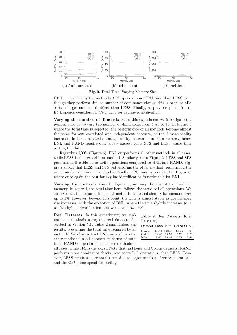
Varying the memory size. In Figure 9, we vary the size of the availablememory. In general, the total time here, follows the trend of I/O operations. Weobserve that the required time of all methods decreased sharply for memory sizesup to 1%. However, beyond this point, the time is almost stable as the memorysize increases, with the exception of BNL, where the time slightly increases (dueto the skyline identification cost w.r.t. window size).

Table 2. Real Datasets: TotalTime (sec)

Dataset LESS SFS RAND BNL

House 30.11 178.21 15.25 4.98Colour 14.43 90.73 3.70 1.28NBA 9.45 26.68 0.71 0.41

Real Datasets. In this experiment, we eval-uate our methods using the real datasets de-scribed in Section 5.1. Table 2 summarizes theresults, presenting the total time required by allmethods. We observe that BNL outperforms theother methods in all datasets in terms of totaltime. RAND outperforms the other methods inall cases, while SFS is the worst. Note that, in House and Colour datasets, RANDperforms more dominance checks, and more I/O operations, than LESS. How-ever, LESS requires more total time, due to larger number of write operations,and the CPU time spend for sorting.

5.3 Policies Evaluation

In this experiment, we study the effect of different window policies in scan-based skyline algorithms. Particularly, we use BNL and SFS algorithms and weemploy several traversal and eviction and policies, in conjunction with differentranking schemes. The effect of policies in LESS are similar to those in SFS andare not shown. Regarding RAND, only the window traversal policy affects itsperformance; its effect is not dramatic and hence it is also not shown.

All results are presented w.r.t. the original algorithms. That is, let m be ameasurement for the original algorithm, and m′ be the corresponding measure-ment for an examined variation. In this case, the measurement presented for thevariation is 1 + (m′ −m)/m.

BNL. We first study the performance of BNL under the 10 most importantpolicy and ranking scheme combinations. Figure 10 shows the I/O operationsperformed by the BNL flavors. As we can see, none of the examined variationsperforms significant better than the original algorithm. In almost all cases, theI/O performance of most variations is very close to the original. The reason isthat the append eviction policy (apE), adopted by the original BNL alreadyperforms very well for two reasons. First, the apE policy always removes objectsthat have not dominated any other object. This way, the policy indirectly im-plements a dominance-oriented criterion. Second, the apE policy always removesthe most recently read object, which is important for BNL. A just read object,requires the most time (compared to other objects in the window) in order tobe identified as a skyline, thus propagated to the results and freeing memory.Hence, by keeping “older” objects we increase the probability of freeing memoryin the near future. Still it is possible to marginally decrease the number of I/Os.

Figure 11 shows the number of dominance checks performed. We can observethat, in several cases, the variants that adopt rank-based traversal, perform sig-nificant fewer dominance checks than the original. Particularly, the rkT/rkE/r1Rand rkT/rkE/r2R variants outperform the others in almost all cases, in inde-pendent and correlated datasets, by up to 50%. Similar results also hold forlow dimensionalities in the anti-correlated dataset. However, this does not holdin more dimensions, due to the explosion of skyline objects in anti-correlateddatasets.

SFS. Here, as in the previous experiment, we examine the performance of SFSalgorithm adopting several policies. Similar to BNL, none of SFS variants per-form noticeable fewer I/O operations (Figure 12). Regarding the dominancechecks (Figure 13), in anti-correlated and independent datasets, most of vari-ants have similar performance to the original algorithm. Only for correlateddatasets, ranked-based policies exhibit significant performance gains.

5.4 Discussion

In an I/O-sensitive setting, i.e., when I/O operations cost significantly more thanCPU cycles, BNL seems to be the ideal choice, as it performs less I/O operations

0.84 0.86 0.88 0.9

0.92 0.94 0.96 0.98

1

0 5 10 15 20 25 30

Spea

rman

’s f

ootr

ule

sqT/rkE/r0RsqT/rkE/r1R

enT/apErkT/rkE/r1R

rkT/rkE/r2RrdT/rkE/r1R

rdT/rkE/r2RmnRdT/rkE/r1R

mxRdT/rkE/r1RrcRdT/rkE/r1R

0.95

1

1.05

1.1

1.15

1.2

1.25

1.3

3 5 7 9 15

# I/O

(vs

. BN

L)

# Dimensions

0.99 1

1.01 1.02 1.03 1.04 1.05 1.06 1.07 1.08 1.09

3 5 7 9 15

# I/O

(vs

. BN

L)

# Dimensions

0.99

0.995

1

1.005

1.01

3 5 7 9 15

# I/O

(vs

. BN

L)

# Dimensions

(a) Anti-correlated (b) Independent (c) Correlated

Fig. 10. BNL Policies (I/O Operations): Varying Number of Attributes

0.4

0.6

0.8

1

1.2

1.4

1.6

3 5 7 9 15# D

omin

ance

Che

cks

(vs.

BN

L)

# Dimensions

(a) Anti-correlated

0.4

0.6

0.8

1

1.2

1.4

1.6

3 5 7 9 15# D

omin

ance

Che

cks

(vs.

BN

L)

# Dimensions

(b) Independent

0.4

0.6

0.8

1

1.2

1.4

1.6

3 5 7 9 15# D

omin

ance

Che

cks

(vs.

BN

L)

# Dimensions

(c) Correlated

Fig. 11. BNL Policies (Dominance Checks): Varying Number of Attributes

0.98 1

1.02 1.04 1.06 1.08 1.1

1.12 1.14 1.16

3 5 7 9 15

# I/O

(vs

. SF

S)

# Dimensions

(a) Anti-correlated

1 1.005 1.01

1.015 1.02

1.025 1.03

1.035 1.04

3 5 7 9 15

# I/O

(vs

. SF

S)

# Dimensions

(b) Independent

0.99

0.995

1

1.005

1.01

3 5 7 9 15

# I/O

(vs

. SF

S)

# Dimensions

(c) Correlated

Fig. 12. SFS Policies (I/O Operations): Varying Number of Attributes

0.2 0.4 0.6 0.8

1 1.2 1.4 1.6 1.8

2 2.2

3 5 7 9 15# D

omin

ance

Che

cks

(vs.

SF

S)

# Dimensions

(a) Anti-correlated

0.6 0.8

1 1.2 1.4 1.6 1.8

2 2.2

3 5 7 9 15# D

omin

ance

Che

cks

(vs.

SF

S)

# Dimensions

(b) Independent

0

0.5

1

1.5

2

3 5 7 9 15# D

omin

ance

Che

cks

(vs.

SF

S)

# Dimensions

(c) Correlated

Fig. 13. SFS Policies (Dominance Checks): Varying Number of Attributes

than all other methods in almost all settings. Additionally, BNL and RANDperform less write operation than the other methods. On the other hand, in aCPU-sensitive setting, LESS and RAND seem to be good choices. LESS performsthe fewest dominance checks, while RAND doesn’t spend time for sorting the

data, or for skyline identification. Finally, regarding the policies tested, the rank-based ones show significant gains but only in CPU-sensitive settings.

Acknowledgements

This research has been co-financed by the European Union (European SocialFund – ESF) and Greek national funds through the Operational Program “Ed-ucation and Lifelong Learning” of the National Strategic Reference Framework(NSRF) – Research Funding Program: Thales. Investing in knowledge societythrough the European Social Fund.

References

1. Aggarwal, A., Vitter, J.S.: The input/output complexity of sorting and relatedproblems. Commun. ACM 31(9) (1988)

2. Bartolini, I., Ciaccia, P., Patella, M.: Efficient sort-based skyline evaluation. TODS33(4) (2008)

3. Borzsonyi, S., Kossmann, D., Stocker, K.: The skyline operator. In: ICDE (2001)4. Chomicki, J., Godfrey, P., Gryz, J., Liang, D.: Skyline with presorting. In: ICDE

(2003)5. Godfrey, P., Shipley, R., Gryz, J.: Algorithms and analyses for maximal vector

computation. VLDBJ 16(1) (2007)6. Kossmann, D., Ramsak, F., Rost, S.: Shooting stars in the sky: An online algorithm

for skyline queries. In: VLDB (2002)7. Kung, H.T., Luccio, F., Preparata, F.P.: On finding the maxima of a set of vectors.

Journal of the ACM 22(4) (1975)8. Lee, J., Hwang, S.w.: Bskytree: scalable skyline computation using a balanced pivot

selection. In: EDBT (2010)9. Lee, K.C.K., Zheng, B., Li, H., Lee, W.C.: Approaching the skyline in z order. In:

VLDB (2007)10. Liu, B., Chan, C.Y.: Zinc: Efficient indexing for skyline computation. VLDB 4(3)

(2010)11. Morse, M.D., Patel, J.M., Jagadish, H.V.: Efficient skyline computation over low-

cardinality domains. In: VLDB (2007)12. Papadias, D., Tao, Y., Fu, G., Seeger, B.: Progressive skyline computation in

database systems. TODS 30(1) (2005)13. Sarma, A.D., Lall, A., Nanongkai, D., Xu, J.: Randomized multi-pass streaming

skyline algorithms. VLDB 2(1) (2009)14. Shang, H., Kitsuregawa, M.: Skyline operator on anti-correlated distributions.

vol. 6 (2013)15. Sheng, C., Tao, Y.: Worst-case i/o-efficient skyline algorithms. TODS 37(4) (2012)16. Tan, K.L., Eng, P.K., Ooi, B.C.: Efficient progressive skyline computation. In:

VLDB (2001)17. Zhang, S., Mamoulis, N., Cheung, D.W.: Scalable skyline computation using

object-based space partitioning. In: SIGMOD (2009)