A STUDY OF OBLIQUE CUTTING

Thesis presented for the degree of

Doctor of Philosophy

of the

University of Edinburgh

by

Ching Y. CHOI, BSc M.Sc.

July, 1968.

(ii)

ACKNOWLEDGMENTS

The author gratefully acknowledges the financial

support of Rolls Royce Limited to pursue this investigation,

the advice and help of Professor L.G. Jaeger and

Professor T.D. Patten at the early stages of this.project,

the provision of research facilities by Professor T.B.Worth

of the University of Aston and the supervision by Dr. A.D.S. Barr

and Professor T.C. Hsu,

CON T E N TS (iii)

PAGE

CHAPTER 1 Introduction.

1.1 General Review, 1

1,1.1 Orthogonal Cutting. 1

1,1,2 Oblique Cutting. 10

1,2 Scope of the Investigation. 15

Figs. 1 1 to 1- 5

CHAPTER 2 - Shear Plane Theoy

2,1 Theories and Analysis, 16

2,1,1 Basis Assumption of Mei.'obant's Theory. 16

2,1,2 Velocity Relationships. 17

2,1,3 Force Relationships, 18

2,1,4 Balance of Euergy0 21

22 Experimental Techniques, 21

2,2,1 Measurement of Deformation, 21

2,2,2 Measurement of Cutting Force, 23

(1) Three dimensional cutting force dynamometer. 23

(2) Electrical circuit. 24

(3) Calibration. 25

22,3 Cutting Tool and Bluntness Control, 28

23 Direct observations. 30

2,3,1 Testing Conditions. 30

23,2 Cutting Ratio. 31

233 Chip Flow Angle, 32

2030k Deformation due to oblique cutting. 32

2,3,5 Cutting Force0 33

236 Friction Force, 37

2,3,7 Shear Angle and Stresses on the Shear Plane. 38

23,8 Energy, 39 i

(iv)

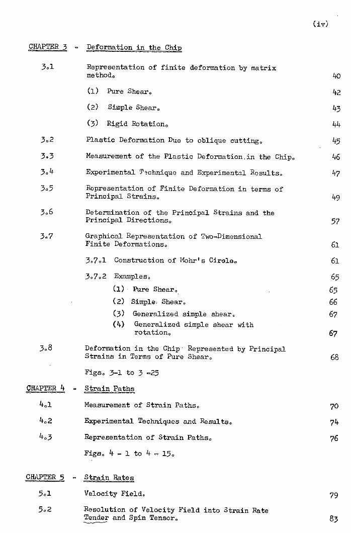
CH!PTE Deformation in the Chi

31 Representation of finite deformation by matrix method0 LiO

(i) Pure Shear. 1+2

Simple Shear. 1+3

Rigid Rotation. 44

32 Plastic Deformation Due to oblique cutting 0 1+5

33 Measurement of the Plastic Deformation in the Chip. 1+6

31+ Experimental Technique and Experimental Results, 1+7

305 Representation of Finite Deformation in terms of Principal Strains. 1+9

36 Determination of the Principal Strains and the Principal Directions. 57

37 Graphical Representation of Two-Dimensional Finite Deformations. 61

3 .7 . 1 Construction of MohrVs Cirole, 61

3 . 7 . 2 Examples. 65

Pure Shear..

Simple Shear. 66

(3) Generalized simple shear. 67 (If) Generalized simple shear with

rotation. 67

38 Deformation in the Chip Represented by Principal Strains in Terms of Pure Shear. 68

Figs. 3-1 to 3 -25

9HAPTERk - Strain Paths

ki Measurement of Strain Paths. 70

4.2 Experimental Techniques and Results. 71+

4-3 Representation of Strain Paths. 76

Figs. 1+ - 1 to 1 - 15

CH,t'.' Strain Rates

51 Velocity Field. 79

52 Resolution of Velocity Field into Strain Rate Tender and Spin Tensor. 83

(v) 5.3 Determination of Velocity Field and Strain

Rates from the Deformed Grid Pattern. 89 5k Exrerimenta]. Recu1ts, 95

Figs, 5 1 to 5 40

CHAPTER 6 Discussion and Conclusion

61 Method of Analysis of Finite Plastic Deformation in Three Dimensions. 96

62 Actual Plastic Deformation due to Oblique Cutting,, 99

63 Shortcomings of the S.mplo Shear Plane Theory,, 100

6+ Cutting forces. 102

6.5 Desirable Future Investigations0 103

Appendix References. 107

QVT\TCDQT q

Merchant's single shear plane theory is attractive

both in its simplicity and in the many possible deductions.

However, it is not supported by experimental results, because

the assumed deformation mechanism is fictitious.

An investigation into the actual deformation due

to oblique cutting has been carried out. Plastic deformations

in oblique cutting processes are so large that the conventional

theories of infinitesmal deformations used in linear elaoticity

no longer hold. Therefore a method of finite deformation

analysis was introduced. Critical comparison shows that

Merchant's theory does not produce the actual deformation,

nor can modified Merchant's theory, such as that based on a

different shear plane, produce it.

Because the properties of a pre-strained material

depend not only on the total strain but on the strain history

as well, an investigation of the strain path and strain rate

also has been performed. Analysis and direct observations revea

that

Deformation is, in general, three dimensional, and

can not be represented by a two dimensional simple

shear such as Merchant suggested;

Deformation occurs not on a single shear plane, but

in a plastic zone of finite dimensions;

(vi)

(vii)

Because the deformation is non-coaxial and very large,

the conventional method of strain analysis does not

hold and the strain rate can not be obtained by simply

differentiating the strain path

With the use of the stress-strain rate relationships

and the equilibrium equations, it is thaoretically

possible to obtain a complete stress field.

Since the oblique cutting process is very complicated,

in order to obtain a complete solutimi for the mechanics of

oblique cutting, much more detailed research work isiequired.

Therefore, attention has also been paid to the experimental

determination of cutting force and a set of empirical

equations have been suggested.

Though this investigation was solely devoted to

oblique cutting, it was thought that the method of analysis

and experimental techniques might be used for the studies

of some other types of metal forming processes.

CHAPTER 1

INTRODUCTION

101 General Review

10101

Orthogonal Cutting

The cutting of metals is one of the most common and

the most economical methods of producing components in

engineering. Billions of pounds are spent yearly for this

purpose. An understanding of the mechanics of the metal

cutting process is therefore very important, because on the

process of chip formation depend the cutting forces, the

power consumption and amount of heat generated, the accuracy

of the machined components and the quality of its surface,

the operating conditions of the machine tool, the tools, etc.

Research into metal cutting process can be traced

as far back as the seventeenth centure, though most work has

been done only during the past three or four decades. It is

impossible to review the whole historical development of this

research, and the purpose of this chapter is merely to outline

breifly some important and influential work.

The process of chip formation is very complicated.

During the cutting process there exist many different phenomena,

such as plastic and other deformations, external friction,

thermal phenomena, abrasive, diffusion and chemical wear,

strain hardening, phase transitions, etc. All these phenomena

influence each other and are in turn determined by the cutting

conditions.

1

2

However, the plastic deformation is predominantly the most

important aspect of all the phenomena above mentioned because

most of the phenomena are its various consequences.

Merchant (1) (2) proposed that the basic mechanism

of metal-cutting process is that of deformation of metal

lying ahead the cutting edge by a process of simple shear.

Figure (1-1) illustrates the mechanism for the simplest case. 9

that of a continuous chip without BUE during orthogonal cutting.

In this case, metal is deformed by simple shear in a narrow

zone extending from the cutting edge to the work surface.

This zone of shear may, for purposes of mathematical analysis,

be treated, according to Merchant, as a single plane commonly

known as the "shear plane". In Figure (1-1), the shear plane

is indicated by the line which makes an angle with the

direction of tool motion. As the metal lying ahead of the

tool reaches this plane, it is displaced by a simple shear

to form the chip, which then slides up the rake face of the tool,

In the case of the continuous chip without SUE,

the simple shear occurs without fracture of the metal and so

a continuous chip is formed. In the case of discontinuous

chip, however, the metal is not able to undergo the required

amount of shear without fracture, and thus fracture occurs

intermittently along the shear plane, breaking the chip up

into segments. In the case of chip with BIJE, the metal

undergoes simple shear without fracture, but the resistance

to the sliding of the chip up the rake face produces

additional deformations in the chip; and the portion

of the chip metal adjacent to the rake face leaves the

body of the chip and remains behind as the built-up edge.

Based on Merchant's single shear plane model, the

force system acting on an orthogonal cutting tool can be

represented by a schematic diagram shown in Fig. (1-2).

From the geometry of Figures (1-1) and (1-2) equations can

be derived from which various geometrical and mechanical

quantities can be calculated

Shear angle Cos 0( = tan a ti.

t1/t2 ., (i-i)

Shear strain E = cot 0 + tan (d a) ,, (1-2)

Velocity of shear V5 V Cos C( (1-3) C a) Cos

Velocity of chip flow = Vc S1flCos a ) ,. (1-4)

R +R tana Coefficient of friction = .. (1-5)

Friction force R = RtcosO + .. (1-6)

COSq) Rtsin Mean shear strength S = R c Sifl()

S A0

Specific work done in shearW = SE 7,, (1-8) S Q

Specific work done in W = A overcoming friction o .. (1-9)

3

Total specific work dome in W = Fc

cutting A0 (i-b)

Ytj Cutting ratio

Oc Rake angle

VC Cutting Speed

R = (F 2 + Resultant cutting force

A0 Cross-sectional area of chip before removal

from workpiece

RC Cutting force; force component acting

in direction of motion of tool relative to

workpiece.

Thrust force; force component acting in directi

perpendicular to R0 and machined surface.

Equations (i-i) to (1-10) show that the shear angle

is of great importance, since these equations are useful only

if the value of the shear angle 0 is known. Metal cutting process, however, is an unconstrained process and it will be

seen from Figure (i-i) that the shear angle (or chip thickness)

has no obvious value as, for example, the exit thickness in

rolling.

In order to formulate a satisfactory criterion for

the shear angle, Ernst and Merchant assumed

the work done in cutting is minimum;

the friction angle ? is constant and

independent of the shear angle.

4

5

On the other hand, from the geometry of Figure (1-2),

the following relations can also be obtained ,.

BS

f 2 + R 2) ( ( + ), a ) ( 1-11) n

kt and B = sine

where R The normal force acting on the rake face

Shear force acting on the shear plane

A Friction angle

k 0 The plane strain yield shear stress of

the material.

Hence, (R 2 + B 2 ) .

-

kt1 0 (1-13)

sin cos + )

Bearing in mind, that the cutting force R is the horizontal

component of the resultant cutting force we have

R = (B2 + R2)' cos C A a

= kt3- Cos (AO( ) 1-1 sine cos ( + a ) 00

Ernst and Merchant's first assumption implies that

the shear plane takes up such a value of 0 which makes B

a minimum. For B to be a minimum, sin() cos +'A a ) requires to be a maximum. This yields the equation

2 =n + ce'. -

oo (1-15)

However, most orhtogonal cutting tests, including

Merchant's own experiments, were not in agreement with

expression (1-15) Since then many attempts based on various

assumptions have been made to formulate the criterion for the (4) (5)

shear angle. Some of them are shown as follows

Merchant 2 + A - cc = TV2 o R 2Q

Stabler t 00V2 = I/4

Lee and Shaffer + X—oc = 4 OR 45°+

Huchs + t2

a 4 OR Q

= 4-

= 54.70

= tt_ 2 tan

Sata and Mizuno = a OR 15 0

Oxley ot

Shaw

Weisz

Co lding cot 2Q J

tan= O.5It 2q) + cos 2(_)sjfl2A)J tan A

Zoreb 2+X — a = 9d'-

COS-3 KL Sata and Yashikawa cot = cot.3 + ( cc)

where Shear angle

A Friction angle

Rake angle

Angle between shear plane and direction of

maximum principal stress

Angle determining the size of build up edge

Angle between shear plane and direction of

maximum shear stress

friction coefficient

Parameter of anisotropy of work material

Angle between shear plane and direction of

cutting force

Angle between free surface of shear deformed

zone and cutting direction

K Ratio of shear stress on shear plane to that

on rake face

L Ratio of tool chip contact length to depth of cut

While many researchers were devoting themselves to

formulating the criterion for the orientation of the shear

plane, others started questioning the truth of Merchant's

single shear plane model. 6

When Kobayashi and Thomsen measured the direction

of the most elongated grains (major axis of the ellipse) in the

chip of steel SAE 1112, they found that it does not coincide

with Merchant's theory.

7

Li]

(7) Cook and Shaw established by photographic

studies of the cutting process that there is no unique shear

plane and that the chip formation zone takes the form of a

wedge whose apex adjoints the cutting edge. Works by Llbrecht (8) (9)

, Zoreb and others also confirmed this.

In 1959, Palmer and Oxley (10) (11) studied the

trajectories and speeds of several crystals through the zone of

deformation. By using these data, they established

experimentally a slip-line field. Then they applied the

modified Hencky equation for stress

Ci + 2kl1J+ d = constant along ana-line

( + 2 k14 d constant along an p_line

to the slip-line field. Many of the points which can not

be answered by the simple shear theory can thus be explained.

In 1966, a matrix method for the analysis of large (12)

deformations has been developed by Hsu Through the

analysis of the large plastic deformation in the chip due to

cutting, he established that two variables are required to

represent the deformation (I 3)

Iccording to Merchant's theory, metal is deformed

in a narrow region which may be idealized into a shear plane

making a shear angle with the direction of the movement of

the tool. It is assumed that metal undergoes simple shear

in the shear plane so that a unique square on the upstream

side of it becomes a parallelogram on the downstream.

Bearing in mind that the shear plane can always be located

by extending the free surfaces of the chip and the workpiece

to meet each other, therefore shear angle is a function of

the cutting ratio t 2t1 and the rake angle:

Cos ( - cx' - sin - i

and that the magnitude of the simple shear assumed by Merchant

is also fixed by the magnitudes of a and t/t1 ; thus for a

given tool (fixed a ), there is only one variable (or t2/t1 for representing the deformation in the chip. In other

words, Merchant allows only one degree of freedom in

orthogonal cutting, where there should be two.

The problem of the metal cutting process is

basically a problem of plastic flow. Therefore attempts to

apply the slip line field theory to the metal cutting problem

have been made by many researchers, e.g. Lee and Shaffer etc.

However, the application of the slip line theory

to the metal cutting problem also encounters many difficulties

such as:

in practice most of the materials machined are

not ideally plastic;

large plastic deformations due to metal cutting

are noncoaxial strain (or a strain path in which

not all the incremental strains have the same

principal axis with respect to the material);

10

(3) due to the popularity and simplicity of Merchant's

theory, most researchers were, perhaps unconsciously,

led to devoting themselves to the modification

of Merchant's theory.

Therefore, it is not surprising that none of the

existing theories is able to provide a complete satisfactory

solution over the entire range of practice, 10e0 for high

and low cutting speeds, large positive and negative rake

angles, variety of work material etc.

1.1.2 Oblique Cutting

The orthogonal cutting process is the simplest

form of the metal cutting processes. In practice, the

cutting process is rarely of the orthogonal type, although

some (e0g0 parting off tools) may approximate to it. Most

practical cutting processes are oblique, i.e. the motion of

the tool relative to the workpiece is not perpendicular to

the cutting edge, but makes an angle with it.

The idea that oblique cutting involved certain

additional factors not present in orthogonal cutting was first

revealed by Sellergren in 1896, but since then relatively

little further attention has been given to it.

In 1944, basing on his single shear plane model

(cf010101) Merchant (2) proposed a generalized single shear

plane model for the oblique cutting process (a more detailed

introductiOn will be presented in Chapter 3)

.s in the case of orthogonal cutting, he assumed that the

deformation due to oblique cutting takes place in an idealized

shear plane which makes an angle ( n with the machined surface.

However the direction of chip flow up the rake face is in

general no longer perpendicular to the cutting edge, but

makes an angle fc with such a perpendicular. This genera1ize

model suggested by Merchant and the corresponding force

system are as shown in Figures (1-3) (1-4) and (1-5).

From the geometry of Figures (1-3) (1_4) and (1-5)

it is not difficult to obtain

t1/t2 cos O n normal shear angle tan 1(l t1/t2

angle of shear f8 = - tan f sing) ±.7.. (1-17)

eQs

shear strain Es - cot O p+ tan4 cos f

. Xnl (1-18) -

•0

$

velocityof shear V6 = V cos cos ,Q cos cos p-a)

velocity of chip flow Vf C = V cos 13 sin

cos ±' cos C

.. (i-ig

00 (1-20)

-1 R = tan -1 (1-21) angle fS R cos + Rtsin . )

coefficient of friction .t = tan (

. ( 1-22) Jc

11

12

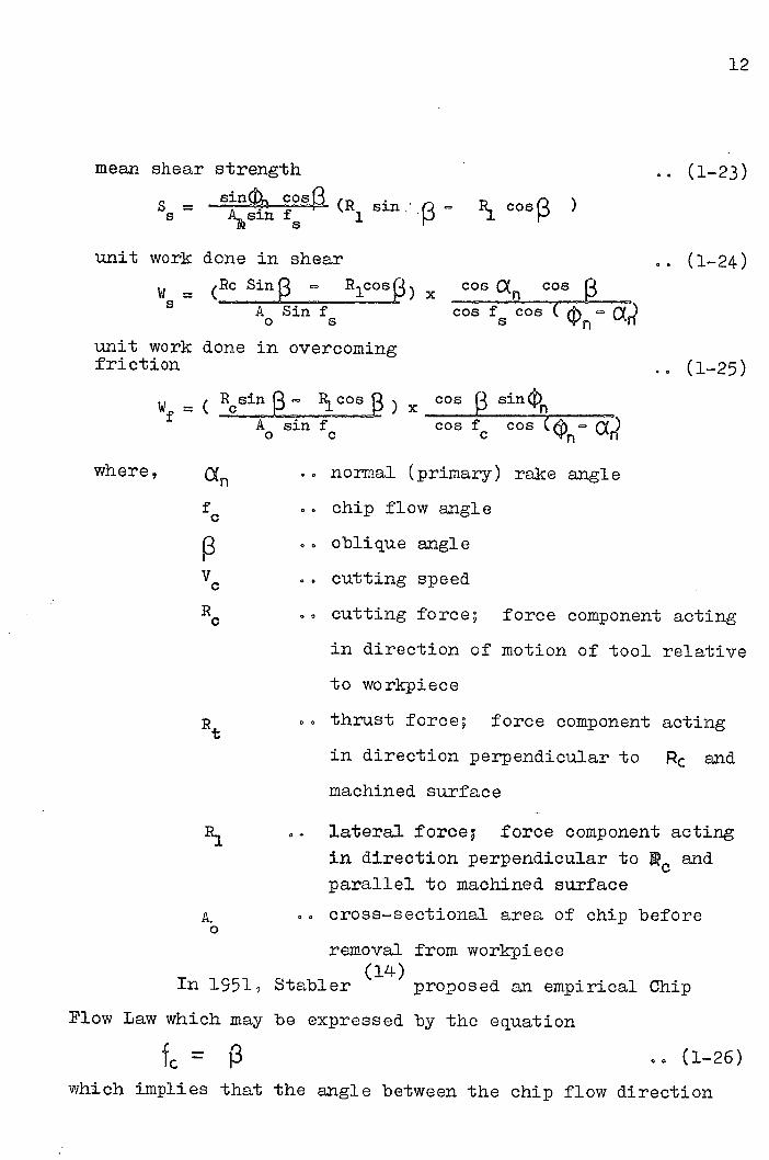
mean shear strength . (1-23)

S = cosg (R sin.' p P1 cos3 )

unit work done in shear . (1-24) = Bc Sin 13 R1COS ) X Cos LX n cos 13

A o s S

Sin f cos f cos C

unit work done in overcoming friction (1-25)

= Rsin 13 P, COS 13) x COS I

sin On _______ A sin f cos £ cos oc,. o c C

where, normal (primary) rake angle

chip flow angle

P oblique angle

V0 cutting speed

cutting force; force component acting

in direction of motion of tool relative

to workpiece

thrust force; force component acting

in direction perpendicular to R C and

machined surface

P1 - lateral forced force component acting

in direction perpendicular to R and parallel to machined surface

cross-sectional area of chip before 0

removal from workpiece

In 1951, Stabler (14)

proposed an empirical Chip

Plow Law which may be expressed by the equation

(1-26)

which implies that the angle between the chip flow direction

and the perpendicular of the cutting edge in the plane of

the tool face is equal to the oblique angle. The chip flow

direction is supposed to be independent of cutting speed,

tool material, work materials etc.

The mechanics of oblique cutting becomes very simple

if Merchant's theory and Stabler's Chip Flow Law are both true.

Unfortunately, further researches revealed that not all

experimental results are in agreement with Merchant's theory

and/or Stabler's Chip Flow Law.

i.ccording to the single shear plane theory, the

orthogonal cutting process is solely governed by the shear

angle (P . With some additional assumptions of non-geometrical

nature, such as those suggested by Ernst and Merchant, shear

angle () can be determined by solving an angle relationship

of the type

== - nX+P0!

where, shear angle

A friction angle

rake angle

q, fl p constants.

... (1-27)

Equation (1-27) shows that the tool rake angle a

is a very important parameter, which governs the shear angle(s)

and consequently affects the whole cutting process.

ill order to generalize the results for orthogonal

cutting process to oblique cutting process, one of the main

problems is the selection of the rake angle corresponding to

13

14

the unique rake angle in orthogonal cutting. It is obvious

that this angle should be measured from the tool rake face to

the line perpendicular to the cutting velocity. However

various alternative planes may be employed, e.g.

a plane normal to the cutting edge, giving the

normal (primary) rake angle O

a plane parallel to the cutting velocity vector

and perpendicular to the machined surface, giving

the velocity rake angle,

a plane containing the cutting velocity vector and

the chip flow vector, giving the effective rake

angle a ( From the geometrical relationship, we have

tan tan a n cosç3

(1-28)

sinO= sin f sin + Cos j' Cos P (1-29) C n

This argument has attracted many researchers because

it was thought that a suitably selected definition of the

rake angle might bring the experimental results in agreement

with the single shear plane theory.

15

1.2 Scope of the Invest igation

Although numerous investigations into the mechanics

of metal cutting have been performed in the past and many

theories have been proposed, it is still not possible to find

a theory which checks well with experimental results.

The work by Christopherson, Oxley and Palmer (ii)

was a considerable contribution to the understanding of the

orthogonal cutting process. Their approach relies on the

experimental determination of streamlines. Hencky's

equations, adapted to allow for work-hardening, are then

applied to the slip-line field obtained experimentally.

The usual correlation of theory and experiment was by this

method vastly improved, though many problems remain unsolved.

Study of oblique cutting process is rare compared

with that of orthogonal cutting. Most researchers still

content Merchant's single shear

plane theory. It is therefore decided that this investigation

should be devoted to the following topics (not in order):

Method of three dimensional finite strain

analysis;

Determination of finite strains, strain paths

and strains due to oblique cutting;

Critical comparison of Merchant's theory and

experimental results;

Measurement and representation of cutting force

due to oblique cutting.

L 4L WORK PIECE

/

FIG. I-I GEOMETRY OF ORTHOGONAL CUTTING

SUG(ESTEh BY MERCHANT

CHIP

NZI A, TOOL

"R /Rf I

/

WORK PIECE

FIG. 1-2 FORCE DIAGRAM

- f

71 T r4I

worpice

L -

FIG. -3 GEOMETRY OF CBLJE cJTT:N

SUGGESTED BY MERHANT

z

an

Jc

FIG. 1-4 G ECM ET R'-AL kELATICNSHPS

SUS,ESTED BY MERCHANT

FIG. I-S FORCE DIAGRAM

CHAPTER 2

SINGLE SHEAR PLANE THEORY

21 Theories andialysis

211 Basis Assumptions of Merchant's Theory

s in the case of orthogonal cutting, Merchant

assumed that the chip is formed by a process of simple shear

on a plane which makes an angle with the surface generated (2)

Thus the geometry involved in oblique cuttings, as Merchant

suggested, can be represented by a model such as shown in

Figs. (l-.) and (l-Lj) In Fig.('-3) the primary rake angle

(normal rake angle) is designated by and the normal shear

angle is represented by On . The thickness of the chip is

denoted byt 2 and the thickness of the chip before removal is

designated by t 1 Knowing t1 , t and an , () can be

determined from the following equation which can be readily

derived from the geometry of Fig0(1_3)0

tanc = /t2 COS0_

WHO lo ti72sin . (2-1)

In Pig 0 (1-4) the direction of motion of tool

relative to work is indicated by vector L 19 which makes an

angle 13 with X axis (i.e. the cutting edge). Plane OBC

is an extension of the shear plane, while plane iCBx is

parallel to the tool face and passes through the terminal

point L of vector 11.If the cutting tool advances along

the work piece a distance L 1 , then a point which was

ME

originally at 0 on the chip will have advanced up the tool

face a distance L 2 in the direction of chip flow as given

by f ' and will have advanced relative to the workpiece a

distance L 3 in the plane of shear, thus bringing it to point D.

Therefore L 3 represents the direction of shear of the metal

on the shear plane. It is obvious that L 3 does not, in general,

coincide with OB, which is lying on the tool face and

perpendicular to the cutting edge. The angle between L 3 and

OB is designated by f5 and called shear flow angle. From

the geometry of Fig. (l_Ll) ,it is possible to derive the

following relation between f 5 and f 0.

tan ±' cos - a) - tan f sin . (2-2)

cos The shear strain in the chip is therefore determined by

Ex

or = Cot - OD + tan ( , .. (2- 3) cot f

S

2.1.2 Velocity relationsps

It is obvious that the above mentioned vectors L1,

L2 and L3 are proportional to the velocities of cutting,

of chip flow, and of shear, thus,

V V

c _;f=

L 1 L 2

17

WQ

Therefore, from Fig. (1-4) the following velocity relationships

can be obtained these equations:

V = S C

V coJ3 COsOr (2-5) COS -Y cos

S

cos 13 Si n V =V

f c cof cos a) (2-6) C

where, V Velocity of cutting (cutting speed) C

V S

0 Velocity of shear

V 00 Velocity of chip flow

2.1.3 Force relationships

For the convenience of nieasuremert, the cutting

force (resultant cutting force) acting on the workpiece are

generally resolved in three components R , and R such

as shown in Fig. (2-1)0

The resultant cutting force R can be resolved with

reference to some other co-ordinate systems rather than the

co-ordinate system XYZ, such as system , 2 ,0 Axis

of the new co-ordinate system is perpendicular to the rake

face and the component of the resultant force R along this

direction is usually called the normal force component.

L.xis 2 of the new co-ordinate system is parallel to the

cutting edge and axis is perpendicular to the cutting edge

and parallel to the rake face. The geometrical sum of the

componenets along and E39

which is ohiiously lying on the

rake face, is generally called the friction force component.

Since the co-ordinate system , , can be obtained

from system x , y , 2 by rotating it successively about

axes yand f ( Z" is in the new direction of 2 after the first rotation) by angles -113 and - G.respectively The relation between the force systems mentioned above can be

represented by matrix equation

RE Fcos C(n sin o cosp o

sinp Rd

%= sin cos o 0 1 o R.

o 0 i ±n I3 1 co B 00 (2-7)

where,

normal force component acting in the

direction perpendicular to the rake face.

0 shear force component acting in the

direction perpendicular to the cutting edge

and parallel to the rake face

.. shear force component acting in the S3

direction parallel to the rake face said

perpendicular to the cutting edge.

Consequently we have,

0= (

2 2 r2 00 (2-8)

= ton (-b- C 00 (2-9)

where, R 00 the resultant friction force acting on the

chip

19

the angle which represents the direct of R

2nother reference co-ordinate system 3

with one of its axis perpendicular to the shear plane, one

along the cutting edge and that perpendicular to the cutting

edge and parallel to the shear plane is also of great

importance in the theory of single shear plane.

Relation between co-ordinate systems c2'

and

X, y / 2 can be represented by a rotation matrix

cosc sind o cos o sin

sin n cos4: o 1 =

iJ sinr3 ° co3j (2-10)

T cosØn c0813 sine cos 1. si

I sinn cos cos 0 sin sir L sin [3 o cosf3 .J

Hence it follows that

r1 r R 1

LR siriOn cos cos sin(Dn sinp ntj

R I1 0 cos(3 (2-11)

P1

where R shear force component acting on the shear plane

in the direction perpendicular to the cutting edge.

.. normal force component acting on the shear plane

R 0 0 shear force component acting on the shear plane

in the direction along the cutting edge.

Consequently we obtain

R = (R + S

= tan '(-4- ) . (2-12)

00 (2-13)

20

21

Rs Ps -ES= =

ç sin cos 13 (2-14)

= S cos

R = R . (2-15)

where R

resultant shear force acting on the shear plane

direction of the resultant shear force Rs

* shear stress on the shear plane

normal stress on the shear plane

area of the shear plane.

2.1.4 Balance of Energy

There are three fundamental types of specific energy

involved in oblique cutting, namely;-

The friction energy per unit volume

Iff R cos(f -Tb) V H

= C C bt V = -cos(f -Tic)

1 c .hoc c (2-16)

where A is. the cross-sectional area of the chip.

The deformation energy per unit volume

- H cos(f -Ti ) V

ljt 1 VC S-

Ti sTi s (2-17)

The total energy per unit volume

W = W. +

(2-18)

22 Experimental Techniques

2.2.1 Measurement of Deformation

According to Merchant's theory, the deformation in

the chip due to oblique cutting is a function of the shear

angle (or the cutting ratiot2/t 1)and the chip flow angle f only.

The chip flow angle f C

can be determined by

various methods, (2) (15) (16), e.g.

measured directly with a protractor as the chip

flows across the tool face;

calculated from measurement of the ratio of

chip width to width of cut;

by staining the tool rake face with "mark-out"

dye, the chip flow angle is determined from the

chip flow line left in the dye;

by measuring the direction of the friction force

acting on the tool rake face.

However, researchers' experiences showed that

none of these methods could produce an accurate measurement.

To overcome the difficulty of measuring angles when cutting

takes place, in 1964 Stabler used a high speed camera to

record the cutting process and then measured the results

in leisure (17)

In this investigation, the tests were carried out

on a heavy duty shaper. The main specification of the shapex

used is as follows:

Type GSP600

Manufacturer llinanc e de Constnict eurs

Length of stroke (max) 600 nun.

Cutting speed (max) 64 IT/min-

Power 5 1.

22

Strips of the work material, - in. wide and ifr in0

long, were held in the cylinder L of the quick stopping

mechanism (Fig, 2-2). The mechanism was in turn clamped

on the shaper table. During the cutting process, i is

prevented from sliding through B by a ring C, held in place

by shear pins. After the tool had cut about in. through

the specimen, the tongue D hit the end of A and the pins

sheared. Thus the cutting action was arrested abruptly.

The specimen was then taken down for measurement of t 2/t1

and f on the MU214B Universal Measuring Machine.

2.2.2 Measurement of Cutting Force

(1) Three dimensional cuttin g force eyamoineter

The dynamometer mainly contains two plates and four

octagonal rings located as shown in Fig, (2-3a). The octagonal

rings carrying the top plate are fixed to the base plate,

which is in turn clamped to the shaper table. The workpiece

is held on the top plate and cutting force is transmitted to

the shaper table through the dynamometer. 0 Therefore, the

components of a three dimensional cutting force applied to the

workpiece can be deduced from the supporting force acting on

the four octagonal rings.

To measure the force components eight strain gauges

are mounted on each octagonal ring as shown in Fig0(2-3b).

From these eight strain gauges we have two Wheatstone Bridges

circuits with four active arms in each for measuring

23

two mutually perpendicular and simultaneously acting forces

applied on the ring.

By suitably locating the octagonal rings, the

cutting force components acting on the workpiece then can be

deduced from the output signals of the eight Wheatstone

Bridges.

The principles of design for this type of dynamometr

can be found in references (18) (19) (20) and they will not be

repeated. here. For the particular dynamometer used, the main

specification of the octagonal rings is chosen such as

Material Mild steel

Mean diameter 2.12 in.

Thickness of ring 0.32 in.

Width of ring 1. 5 in,

The horizontal and vertical deflections per unit load

thus are 6.06 x 10 in. per lb. The natural frequency of

the dynamometer is about 450 cps., the exact frequency

depending on the particular workpiece holder used.

(2) Electrical circuit

Type

Nominal resistance

Gauge factor

Grid type

Dimension of grid

Max, operation temp.

Max, current

PR9812 (wire gauge)

Wrap-around

6x8mm2

2O0C

20 Mk

24

Considering the possible interference of the

reactions due to the horizontal components of the cutting

force with the true vertical component and the fact that a

complete cancellation of this interference can be achieved

only if the sensitivity of the Wheatstone Bridge circuits

are identical, the strain gauges mounted on the rings are

connected to a Type MR703 Strain Gauge Balance system which

provides

eight independently controlled stabilized

D.C. power supplies (0-30V).-

independent balance of each bridge.

In order to increase the sensitivity of the

balancing circuit, a fine balancing circui is also added

to the Type MB.703 Strain Gauge Ballace System.

The suitably combined electrical signals from the

bridges are then connected to the UV recorder or the

galvanometer through a D.C. amplifier.

The complete electrical circuit is shown in Fig. (2-4)

(3) Calibration

The dynamometer was calibrated on a Mohr & Federhaff

50T hydraulic universal Testing Machine. A general arrange-

ment of the calibration set-up is shown in Fig. (2-5)0

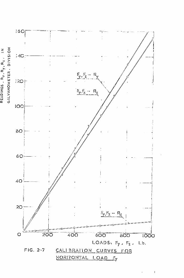
Examples of calibration curves under the following

conditions - bridge D.C. supply 12 volts gain of D.C. amplifier 100, gain of scalamp galvanometer 1000

are shown in Figs. (2-6) to (2-8).

25

It can be seen that the relation between the applied load

and the electrical output from the strain gauge bridge is

linear. Therefore, the relation can be conveniently

represented by the matrix equation

rai1 a12 a131

F - a21 a22 a23 R

F a a a I IR Lz 31 32 33J

z

where, FX 'Z 00 force components, lb.

.. (2-19)

R, R9 R z readings from galvanometer, div.

constants, lb/div. 1 J

According to Pig (2-6) R x = 3.5 div 9 R= 4.0 div9 R= 120.3 div.

when Fx= F= 0 and F z = 800 lb. Substituting these values

in equation (2-19) and expanding it, we have :

0 = 3a5 all + 4. 12 + 120-3 a13 (220)

0 = 3.5a+ 4.Oa22 + 120o3a •. (2-21)23

800 3o5a31 + 4°° a32 + 120.3a33 .. (222)

Similarly, from Pigs. (2-7) and (2-8) and equation (2-19)

we obtain

0 = 5-7a + 133.8a12 + 124.2 a13

800 = 5.7a + 133.8 a22 + 124.2a 23

800 = 5.7a31 + 133.8 a32 + 124.2a33

-800 = -13 , 2a 1 + 1.6a12 + 123 ° 5 a13

0 =-133. 2 a + 1.6a + 123. 5a2321

800 = -133.2a 31 + 1.6a 32+ 123.5a 33

•, (2-23)

.. (2-24)

.. (2-25)

.. (2-26)

.. (2-27)

.. (2-28)

1122

Combination of equations (2-20) to (2-28) yields :

all = 5.850 a12 = 0.094 a 3 = -0.167

a 21 = 00 111 a22 = 6.171 a23 = -0. 203

a31 -0.159 a32 = -0.203 a33 = 6.652

Therefore, equation (2-19) representing the sensitivity of

the dynamometer becomes

ri r56850 0.094 -0.1671 [RX I = -0.111 6.171 -0.203 R (2-29)

LZJ E00159 -00203 6.65J LRZ j The outputs from the UV recorder were calculated in the same

way and the relation between the outputs (deflections) and

the force components are represented by a similar matrix

equation:

Fx i xxl

0 I j RO YY

(2-30) p I = -0.111 6.171-0.203

850 -0.094 0.l67 r RV

I 1 y I I I. P I -0-159 -0.203 6.652 J R J LZJ LZZJ

where R R, R 00 reading from the UV recorder, division

ixg j, J .. constants

The values of the constants J, 1 and J are dependent on

he sensitivity of the galvanometers of the UV recorder used

and the gain of the D.C. amplifier chosen. In practice,

the value of J, J and J can be calibrated with the

Scalamp Galvanometer.

At the first glance, equations (2-29) and (2-30)

seem to be a little cumbersome. However, they provide us

with a relatively easy way of taking the cross interferences

27

into account.

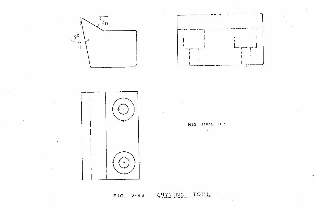
22.3Cutting Tool and Bluntness Control

The cutting tool used consists of two parts,

the tool tip and the tool holder (Fig. 2-9). The tool

tip was made of high speed steel (Speedicut Maximum 18)

its composition said heat treatment condition being:

composition: C

75

heat treatment:

Cr V W

425 1010 1800

Preheating for hardening 0 0 0 0 8000/8500 C.

Hardening in Oil 0 0 0 0 00 12800/1320°C.

Tempering (Double) 5500/580'

The rake face of the tool tip was first ground

to the required normal rake angle of 300 and clearance

face was ground to a clearance angle of 70 The base

face of the tool holders was machined to various oblique

angles. The tool tip was then fastened on the tool holder

with two bolts. Thus the normal rake angle and the

clearance angle measured on a plane perpendicular to the

cutting edge can be kept constant for tests with various

oblique angles.

It used to be assumed that there was no force

acting on the cutting edge if the tool used is very sharp.

It has been found that though a tool with a very sharp

cutting edge (e0g0 with a maximum crumbling at the edge

less than 000001 in.) can be produced by special polishing (21)

techniques, the radius at the edge increased very fast 0

Wo

In order to demonstrate the blunting progress of

the cutting tool, some preliminary tests have been carried

out with carefully sharpened tools under the following

29

conditions:

Machine

Cutting speed

Variation of cutting speed

Material of cutting tool

Rake angle

Oblique angle

Clearance angle

Material of workpiece

Width of workpiece

Length of workpiece

Depth of cut.

GSP shaper

120 fpm.

less than 0.50

HSS Speedicut Maximum 18.

30 0

0°

7 °

Aluminium alloy HE-9--WP

0.25 in.

1.5 in.

0.015 in.

Direct measurement of the radius of the cutting

edge is difficult, therefore an indirect method for the (22)

measurement suggested by Hsu was adopted here.

For this purpose, two soft aluminium alloy strips, each

with one face polished, were pressed together and held in

the cylinder of the quick stopping mechanism. Then the

strips were cut half-way through the cutting action was

arrested abruptly and the form of the tool edge was imprinted

at the root of the chip. The radius of the cutting edge

was then measured on the Vickers Projection Microscope.

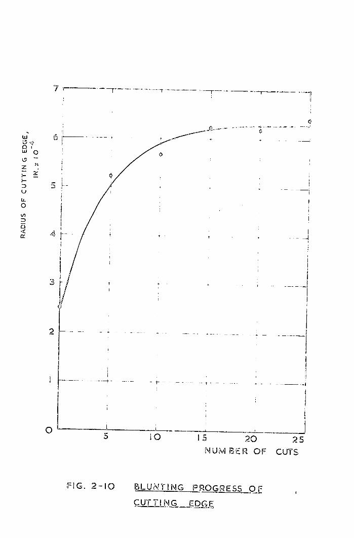
Example of experimental results were shown in

Fig (2-10). It can be seen that the blunting progress

curve can be divided into two parts:

at the first stage, the radius of the cutting

edge increased rapidly with the number of cuts.

For the example shown in Fig (2-l0), the radius

of the cutting edge increased from 0.00025 to

0.00053 after only five cuts;

at the second stage, the blunting progress

became very slow. After a further 15 cuts,

the radius of the cutting edge only increased

by 0.0001 in.

Therefore it can be concluded that though the

cutting tool with very sharp edge can be produced, it is

not practical to use them for testing purposes due to the

difficulties in maintenance and control. Throughout the

investigation, the radius of the cutting edge of the tools

used were controlled within the range 0.00055 to 0.00065 in0

and the mean radius, r = 0.0006 in., was used for analysis.

23 Direct Observations

2.3.1 Testing Conditions

Experimental results presented in this chapter

were obtained under the following conditions:

30

Machine

Cutting speed.

Variation of cutting speed

Material of cutting tool

Normal rake angle

Oblique angle

Clearance angle

Material of specimen

Width of specimen

Length of specimen

Depth of cut

GSP shaper

120 fpm.

less than 0.5%

HSS Speedicut Maximum 18

300

Various

70

Aluminium alloy HE-9--WP

0.25 in.

105 in.

Various

31

2. 3. 2 Cutting Ratio

The cutting ratio t2/t1 obtained experimentally were

plotted against the depth of cut t 1 for various oblique

angle in Fig 0 (2-11) 9 while Fig. (2-12) shows the relation

between the cutting ratio t2/t, and the oblique angle for

various depth of cut

It can be seen that the cutting ratio depends

considerably on the oblique angle 0 As the oblique angle

is increased from 00 to 40 0 , the cutting ratio yt1

for 0.02 in0 decreased from 2.85 to 2.3, i.e. nearly

by 20%.

It can also be noticed from Figs 0 (2-11) and (2-12)

that the cutting ratio t 2/t1 is slightly influenced by the

depth of cut t1.

2.3.3 Chip Flow Angle

In Pig (2-13) the curves in solid line are shown

of the relation between the chip flow angle f and the oblique

angle 13 For the purpose of comparison, the Stabler's

Chip Flow Law, i.e. 13 = f is also shown in Fig (2-13) in broken line. It is evident that experimental results are

not in agreement with Stabler's Chip Flow Law.

In 1964, using the experimental results obtained

by the use of high speed photographic method, Stabler

reported that on some occasions, the chip flow angle might

not be equal to the oblique angle due to some unknown factors.

But he insisted that the relation between the chip flow

angle f and the oblique angle 13 remaine6 linear and independent of other parameters, such as the cutting speed,

depth of cut, etc.

However, it can be seen from Fig. (2-13) that

the relation between the chip flow angle f 0

and oblique angle P is non-linear;

the relation between the chip flow angle

and oblique angle 0 may be affected by the

depth of cut t 2 , even though the effect is

small in this particular case.

2.3.4 Deformation due to Oblique CUtt

Lccording to Merchant's theory, the deformation

in the chip due to oblique cutting can be represented by

32

091

a simple shear of the following magnitude:

= cot tan S cosf

S

which occurs on the shear plane along a direction

characterized by :

f = tan1 tan P cos C CC) - tan f sin On S

cos an

(2-32)

Using equations (2-31) and (2-32), values of and f. for

0015 in were calculated from the experimentally

obtained values of and f0 shown in Figs (2-12) and

(2-13) These values of and f 5 were plotted against

oblique angle in Figs (2-14) and (2-15) It can be

seen that:

the deformation in the chip due to oblique

cutting decreased with the increase in oblique

angle;

the value of angle f 9 , which represents the

direction of the simple shear, increases when the

oblique angle is increased.

2.3.5 Cutting force

In the past, it was usually assumed that the

force acting on the edge of the cutting tool, i.e. the

ploughing force, is negligible. In 1960, Albrecht (23)'

using tools of controlled bluntness, first separated the

ploughing force from the resultant cuting force in

34

orthogonal cutting Experimental results obtained by

Albrecht revealed that the force-depth of cut curve

consists of two parts. The first part, the curved position,

indicated that the ploughing force component undergoes a

development in the lower range of tr In other words, the

ploughing force P depends on the depth of cut t 1 . When a

certain value of t or a certain value of the ratio of the

radius of the cutting edge r to the depth of cut t 1 is

reached, the force-depth of cut curve becomes practically

a straight line. This implies that

the resultant cutting force R can be resolved

into two components, cornppnent Q acting on

the rake face and the ploughing force P acting

on the cutting edge;

after a certain value of t 1 is reached the force Q

is proportional to the uncut chip thickness,

the ploughing force P remains constant with

varying t1 and the friction angle is also

independent of

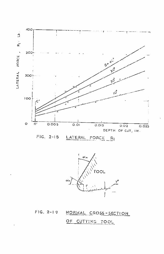
Figs. (2-16) to (2-18) show the cutting force due

to oblique cutting obtained experimentally. It can be seen

that all three force components, RC Rt and R , are linear

with respect to undeformed chip thickness t 1 0 Therefore,

it is reasonable to assume that the ploughing force

components remain constant no matter how deep the cut may be

35

and that the force components, Q C 9 Qt

and Q are proportional

to the depth of cut..

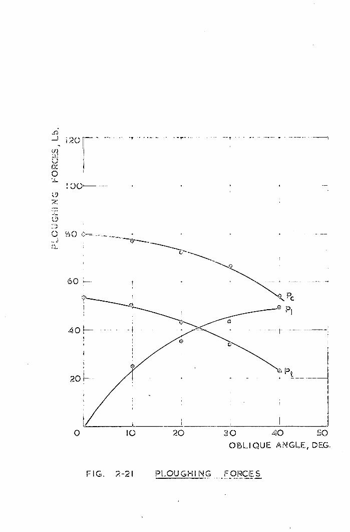
From Figs. (2-lto (2-18), it can also be noticed

that both the cutting force component Q and ploughing force

component P depend on the oblique angle For a specified

oblique angle the resultant cutting force acting on the tool

can be represented by:

rR0l rQJ

Rt I t + I

R ' QLJ L1J L1 (2-33)

Values of P, Pt, and P1 can be readily obtained

by the use of backward extrapolation. It was at one time

thought the values of P 0 , P and P1 may be taken as the

intercepts on the force axes 24 16

However, a little

reflection will show that when the thickness of undeformed

chip is reduced to zero, there is nothing left to cut or

plough.

Fig..(2-19) shows part of the cross-section of

the cutting tool perpendicular to the cutting edge.. It

can be seen that the depth of the work material ploughed

by the rounded edge is r(l+sin, where r is the radius

at the edge measured on a plane perpendicular to the

cutting edge and an is the normal (primary) rake angle..

In order to determine the ploughing force components,

ordinates O'A', O'B I and 0' C I are drawn in Figs (2-16),

(2-17) and (2-18) at a distance r(1+sin oW from the R , Rt

and R axes 9 and the force-depth of out curves are extended

to cut O'11.' , 0B 9 and 00 1 respectively. Since it has been

assumed that the ploughing force remains constant when the

force-depth of cut curve appears linear, it may be concluded

that the corresponding intercepts are the ploughing force

components P, P and P1 respectively.

Bearing in mind that the cutting force component Q

will be equal to zero if the depth of cut is equal to or less

than r(l+sin an) the cutting force components Qc I Qt and Q

can be determined from

EQ1 EB I C 1 1 C

Qt Bt te

:LeJ LB1

where te = t - r(1+sin a) B , Bt9 B1

(2-34)

effective depth of cute

slopes of the correspond-

ing force-depth of cut

curves

Let

We have

1 b

QC Qt =

Li.

rBcl

LJ = rbl b-

Lbii

b

Lb i

bt e

.0(2- 35)

(2-36)

36

37

r and RI lb P ci ic C

R [ = b bte + 4b t (2-37)

Lb1 P ij

where b , bt9 b 1 . specific cutting force components

per unit width of cut

b width of cut0

Examples of the effect of oblique angle P on specific

cutting force and ploughing force are shown in Figs-(2-20)

and (2-21)

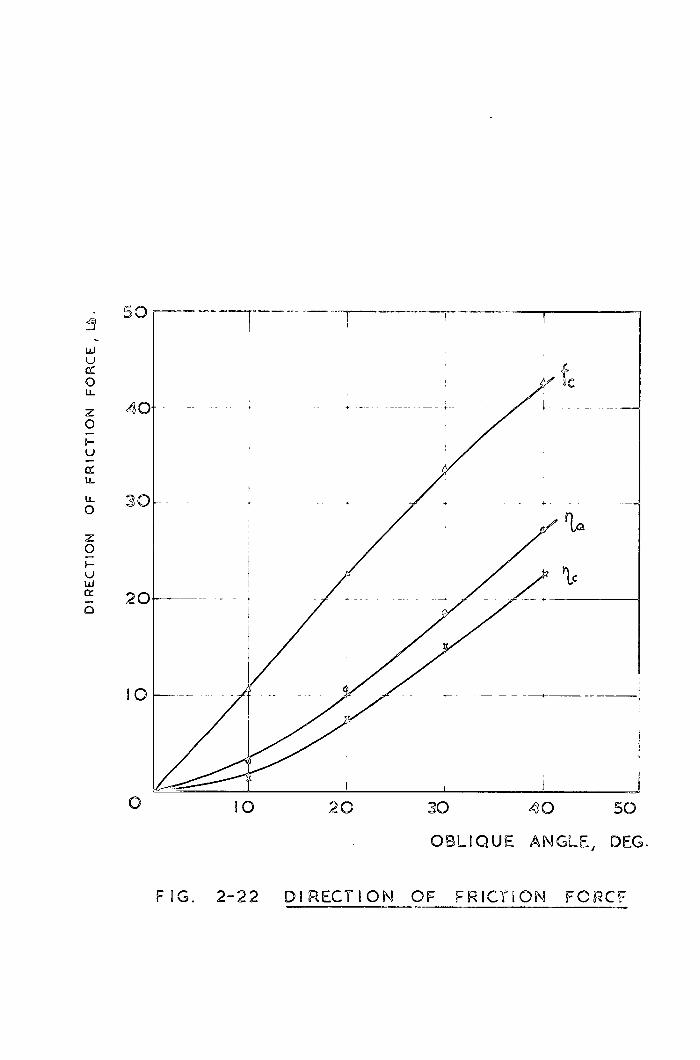
2.3.6 Friction force

Since the resultant cutting force can be resolved

on the

P I

Pt:: + 62

P S3 sin;

cosa

0

into a force acting

ie [L1 = [

coso(n cos 3

inc cos13

- sin3

rake face and the ploughing force,

QE I =

LQ

C0S(r, sin rP C rJ

sin ri cos f3 C P . + ) o.(238)

cos3 P1

The friction force can also be resolved two parts, namely

Q., the friction force acting on the rake face

= (Q+ Q) (2-3g)

Psg the friction force acting on the cutting edge

= (P2 + (2-40)

The directions of the resultant friction force R and the

friction force acting on the rake face Q.are determined

respectively by

= tan-1 ( = tan-1 +

= tani ( -44 Qjz

(2-42)

Values of and% obtained experimentally for

the depth of cut of 0.015 were plotted against the oblique

angles in Fig (2-22). For the purpose of comparison, the

chip flow angle was also shown in Fig. (2-22). It was

surprising to find that neither one of the - curves

coincided with the f 0— P curve,

2.3.7 Shear L.ngle and Stresses on the Shear Plane

Values of the normal shear angle found from the

chip thickness measurement are shown in Fig,(2-23) for

tool with 30 ° normal rake angle. It can be seen that the

magnitude of the shear angle depends on the oblique angle.

Pigs. (2-24) and 2-15) show the effect of oblique

angle on the normal and shear stresses and the direction of

the shear stress on the shear plane. It is of interest to

note that

(1) all the values of G ,Ts and are functions

of the oblique angle P.

39

(2) the direction of shear stress does not coincide

with the direction of the shear strain (Fig 0 2-15)

2.3.8

In Pig 0 (2-25) the curves are shown of the change in

the specific energy required for oblique cutting and its

components W and W as a function of oblique angle

Values of R and R obtained experimentally at a depth of

cut of t1 = 0015 and equations (2-16) to (2-17) were used

to construct the curves in Fig. (2-25).

The same data were used to plot the diagram in

Fig 0 (2-26) which shows the change in balance of the specific

energy required for oblique cutting when oblique angle is

increased. From this diagram it follows that the percentage

content of energy required for deforming the chip decreases

continuously with increase in oblique angle, while the

percentage content of energy for overcoming friction rises

continuously when the oblique angle is increased.

7

-=---.

COMPONENTS

Sh

0

A

if

1FG. 22 QUICK STOPPNG MECHANSM

-

0

.fLoO

I 6.000"

3.000"

- - - +

000T .00 0- 1

if f

4t i L JL'v 1

tE

I

F 1G. 2-3a THREE DIMENSIONAL

- ' i- j H I

Jr

I

L.

---4------

-- 1-----

- '/I6r/

011

3/16 rod,

L i- J~ -

LJ

1.500"

FIG. 23

OCTAGONAL R I NG

'0

11

0

or

VETAL HCRIZCNTAL SELECTC

ELEc.T'RS

A

i: KA - I

KfI

,------------ _-----__-_-_--_. .----

/ • I

- / - - - --- -- ---

/ -- -- -- - -

/

A-_-- -i- ----- - - --

/ r -- r

10 K fl

R i NG 3 - - --------------------- I

__ -----

/

RIN ' t1 Z E7

4 1

5 1 Kft 10 KR

RiNG

/ - 12M ¶! 51K11 H Tf7 GALVANOMETER

TO U.V. REtRDER

--------- -- --- ----- --

NAOTER

- ----------- - ----- ----

C\i SThAN GAi AANC AN) cALA1CN

SYSTEA

--

-

HNE BALANCE

C RCUIT

M. 1266

D.C. AMPLI FIE1

PYE 79C4/T

SCA LAMP FIG. 2- 4 ELECTRiCAL CCUT

GALVANCMETER

---- —J

MH300

J.V. RECCRDER

LCA1

/•/////// 7

CIrcn o

LJ criLJ

FG. 25 ALATON_ARANGEENT

ISO l y

FIG. 2-6 CALIBRATION CURVES FOR

VERTICAL LOAD

z 0

z2

LU

w Z

i I L

140

'2C

40

20

[SI 200 400 600 800 1000 LOAD, Fz , Lb.

FG. 27 CAL RRAT I ON CURVES FO R PR!ZON1AL LOADF

-

LOADS F . , Lb.

I I

/ I if

LU

- 120--

in I

c > UI

° ff7

60

20J

ED 400 600 zoo 1000

LOADS, F.F1 Lb.

CAL IBRATIQ F0R H0RZON1A L LO AD F

- On-

-" L1

r

H •S.S TOOL TIP

FIG. 2-9

cLTJ TgS2J.

-Q IT-

ii

-

FIG. 2- 9b CUTTING TOOL

Ui

Ui0

D 5 U

U- 0

D U

Ki

+ + -

- H

+ ---

S

10

20j5 NUMBER OF CUTS

FIG. 2-10 BLUNTING PROGRESS OF

crr Lg

- - - 1 4

S

0

3 • 5 H - 0

1-

U 3---

2.5

2

1.5

nice 0.005 0.01 0.05 0.02 0.025 0.03

DEPTH OF CUT, IN.

FIG. 2-I RELATION BETWEEN CUTTING -BA=

AND DEPTH OF CUT FOR VARIOUS

OBLIQUE ANGLE

0

z

U

3

2.5

2

•

o O 20 30 40 O BL: QUE ANGLE, deg.

FIG. 2I2 ELA1I0N BETWEEN CUTTING

RAT I O AND OBLIQUE ANGLE

E.QJ. _VAflOUS DEPTH OF

Ii

7O X -t, 0.02 in.

= 0.015

0OI

StABLER'S LAW

o /

I 40L - -

/

10 20 30 40 50

OBLIQUE ANGLE, DEG.

FIG. 2-3 CHIP FLOW ANGLE

3

--

Lu 2 + +

:1)

Lu I J)

0 10 20 30 40 50

OBLIQUE ANGLE, DEG.

FIG. 2-14 DEFORMATION DUE TO OBLIQUE CUTTING

AJ

cuJ

z ,,

Ld

I-

z

0

U,

30

20 b-

10

I STRAIN

tO 20 30 40 50 OBLIQUE ANGLE,DEG.

FIG. 2-I5 DIRECTION OF SHEAR STRAIN AND

STRESS

z

0

400

200

1400

-J

U ix

Ui

200

C U-

0 0.005 0.01 0.015 0.02 0.025

DEPTH OF CUT, IN.

FIG. 2-16 CUTTING FORCE P.

-J

w L)

0 LL

I H

r

I.I.]

300

200

iW

0 Of 0.005

C.CI5 G32 0.025

DEPTH OF CUT, IN.

HG. 2'=17

THRUST FORCE Rt

2CC

100

400r-

3 C(

0.015 0.02 0.025

DEPTH OF CUT, IN.

FG. 2-IS LATERAL FORC

-J

TOOL

70

FIG.. 2-19

NORMAL _CROSS - SECTION

OF CUII:NG TOOL

-J

Ui 1

C

-j

Ui

-J

20'

i lot

-

16 U

22

T

F

10 20 30 40 50 OBLIQUE ANGLE, DEG.

FIG. 2-20

SPECFIC_CUllING FORCES

2O[

z

o

60

40

20

0 10 20 30 40 50

OBLIQUE ANGLE, DEG.

FIG. 2-21 PLOUGHING FORCES

Ui U

0 LL

z 4

U

cc LL

LL a 0

z 0 H U w

2

10 20 30 40 50

OBLIQUE ANGLE, DEG.

HG. 2-22 DIRECTION OF FRICTION FCRC

+ - + - --- --

-- -- ------- t --- -_ -

io 20

30 405

OBLIQUE ANGLE, DEG.

- t-

sor - -T

554

•

20

KIN

5

Al

FIG. 2-23 NORMAL SHEAR ANGLE

. 6 T r

I (çc

5

j)

#' QI JL

w

0

3 ±

2--- --

00 20

- 4 - -------------

--

30 40 50 OLQUE ANGLE, DEG.

HG. 224 EFFECT OF OBL I QUE ANGLE

ON NORMAL AND SHEAR STRESSES

600 JIlL 1:: -

T

LJ

u 2CC-

- - -- --..- --- -

J JO 20 30 40

OBLIQUE ANGLE, DEG.

FIG. 2-25 ENERGY

> 100

17 w z

LL

U

3Q 0 U

N z w60 U

U

20

JO 20 30 40 OBLIQUE ANGLE, DEG.

HG. 2-26 BALANCE OF ENERGY

Eel

CHAPTER 3

DEFORMATION IN THE CHIP

3.1 Representation of finite-deformation by matrix method

The mathematical properties of finite deformations

are very different from those of in±'initesmal ones.

Infinitesmal deformations are usually represented by two

types of strains, or strain components, the direct and

the shear strain, and strain at a point, or state of strain,

can be graphically represented by Mohr's circles. Two

infinitesmal strains can be superposed by means of the

Mohr's circle. For finite deformations, two strains not

of the same principal axis can not, in general, be easily

superposed. Finite strains, in general, can only be

adequately represented by an affine transformation, thus,

4 = all x + a12 x2 + a13 x3

a 1 X1 + a22 x2 + a23 x3 (31)

= a31 x + a32 x2 + a33 x3

or, in matrix language,

r X1 a11 a12 a13

a 1 a x2

2 22 a23

-) a31 a32 a33 X

3

E -

aX2 -- oX31

I

I ax' ôX 2 2 X2

I ax1 '3 X2 ox31

Io _oxl La xi Ox2 ox.d

40

where, x1 , x and x3 are the Cartesian co-ordinates of a

point before deformation 4 , 4 and x are corresponding co-ordinates after deformation referred to the same axes and

Q• (i0e ) are constants, 3 X.

Any three-by--three matrix represents a three

dimensional deformation and any homogeneous three dimensional

deformation can be represented by a matrix. However, for

incompressibility of the material, the determinant of the

co-ordinates transformation matrix must be equ1 to unit, i.e.

i aii a12

det a a21

La 31 a32

L. transfo

a1 a11 a12

a13

a23 a a22 a23 = 00(33)

a33J a31 a32 a33

rmation represented by equation (3-1),

followed byanother transformation, such as

X = b11x + b12x + b13x

xtI =b 1x + b22x + b23x

x =b3 x + b32x + b33x

is equivalent to an overall transformation

X =c x + Cj2X2 + 13 3

= c21x1 + c22x2 + c23x3

X3 = 031X1 + C 32 x + C33X3

By the use of the matrix language, equations (3-1), (3-4) and

(3-5) become

rx re11 C12 rxil = I 2 c 21 022 023 X2

xJ L031 032

c33J Lx 3]

41

42

ra a a 1 where c11 C12 n b12 b13 11 12 13 I 021 022 0 23 b21 b22 a a a I

LC31 032 c33J 31 b32 b3 3j a31 a

al 32

23 21 22 23 I

(3-7)

Here it should be noted that, while for infinitesimal

deformations the result does not depend on the order in which

the deformations occur, finite deformations do not obey the

commutative law. Likewise, the matrices in a matrix multi-

plication may not, in general, be interchanged.

For the purpose of illustration we cite here three

fundamental af±'ine transformations in three dimensions

(1) Pure shear

n example of the direct stretching along the

reference axes (pure shear) is shown in Pig. (3-1), where the

unit cube in solid lines is understood to be the undeformed

body and the rhmbus in broken lines the deformed body.

The value of the nine components1 can be found by

substituting the co-ordinates of points Pk into equation (3-1).

Thus, the transformation of this type of deformation can be

written as

xi e r 0 0 lxi

0 eE2 ., 1x 2 ..(3-8) I £31

Lx3 00 e...L 3

where E, £2 , and E 3 are the corresponding natural strains

of the line elements lying along the reference axes, and e is

base of natural logarithms.

43

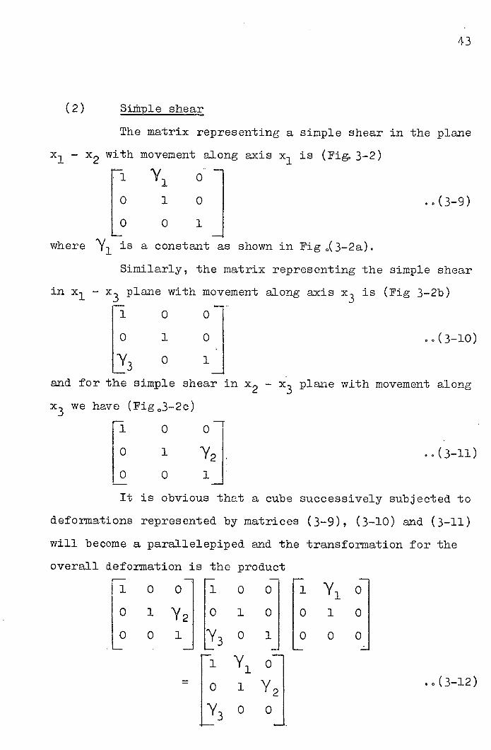
(2) Sithple shear

The matrix representing a simple shear in the plane

- x with movement along axis x 1 is (Fig. 3-2)

Yi

t o i 0 .0(3-9)

Lo o

where 'V1 is a constant as shown in Fig .(3-2a). Similarly, the matrix representing the simple shear

in x1 - x3 plane with movement along axis x 3 is (Fig 3-2b)

0 0

0 1 0 ..(3-10)

•L'V3 0 1_I

and for the simple shear in x 2 - x3 plane with movement along

x3 we have (F1g 03-2c)

0 01

0 1 Y2

0 ij

It is obvious that a cube successively subjected to

deformations represented by matrices (3-9), (3-10) and (3-11)

will become a parallelepiped and the transformation for the

overall deformation is the product

r1 0 olri 0 0

0 1 V20 1 0

.L0 0 1JN3 0 1

r1i

f o 1 ji/30 0J

Yi 01 to i 01

L°°°i

(3) RiLd rotation

Since there is no deformation involved, the rotation

of rigid body can be described by the relative position of two

co-ordinate systems shown in Fig-(3 - 3), where x1 , x2 and x' 3

represent the original position and Xj x2 and x the final

positions iccording to the analytical geometry, the relative

position of two rectangular co-ordinate systems can be

represented by nine direction cosines. However, the use of

three Eulerian angles may often considerably simplify the

problem. If we denote the Eulerian angles by- 1 ,-J2 and- 3

(Fig 0 3-3), the rotation matrix is written as

rR11 R12 R1

R22 R231

LR31 R32 R 3

- S111

3 °1 f 1 0 0 Cosa,--sin Sir cos 3 0 0 cos- _sin -'3i cos 1 0

L 0 0 'J L° silka2 cos° J 0 L -CO Ssin.l SjflSjA2

-sircos.32sin

sin.3cos3j -sin. 3 sin3 -cos 3sin 2 + cos53 cos3-V2 + cos 3 cos .J-2 cos -1

siir 2 sin' 1 sin 2 cos cos 2

(3-13)

32 Plastic Deformation Due to Oblique Cutting

ctua1ly the deformation due to oblique cutting is

three-dimensional though it is subjected to several restrictions

due to symmetry and the streamlined flow (which produces

the continuous chip), and hence is less complicated than

the general three-dimensional deformation.

Hsu ' suggested that the deformation due to oblique

cutting may be divided into five steps (Fig. .3-4) - (a) a pure

shear in the x 1 x 2 plane, (b) a simple shear in the x1x3 plane,

(c) a simple shear in the x 1 x 2 plane (d) a simple shear in

the x 2 x 3 plane, and (e) a relation about the x3 axis though

an angle equal to (90 °-O(,- (not shown, in Fig-3-4). Each of

the first four steps is represented in Fig0(3-4) as a

deformation of a unit cube (dotted). Each step may be

represented by a matrix and the overall deformation is the

produce of the five matrices, as follows

rcos (900 O) sin (90 a) ol Ji o o

sin (900 an ) COS (900 - 1 Jo 1

L ° ° iL0121

r1 y, 0 j 0 1 0 Jo 1 0 Jo t2/t1 o =

-° 0 '_ L3 o 3.1 L o 0 1

1 ..(3-14)

_f2 ti sina sin cos o

1 cosO '2 ( '1 cos Q,, + sin p ) 0

t2 'Cl

1; ly

t2 2

3 t1 2

45

where 192 and 3 are as defined in Fig. (3-4) and

is the primary rake angle (normal rake angle).

303 Measurement of the Plastic Deformation in the chip

As can be seen in equation (3-14) for a given tool

(fixed C) four quantities (Y] Y 2 9Y ) are

required to represent the deformation in the chip.

The ratio t/t1 can be easily measured, since the

chip thickness t.2 can be measured with a micrometer.

To determine the simple shear 3 , let us first

consider a unit cube of the undeformed material with one of

its edges lying on the cutting edge. After deformation it

becomes a parallelepiped in the chip, which is shown in its

three orthogonal projections in Fig-(3-5b), that in the tool

face (top left), that in the plane normal to the cutting

edge (top right) and that in the plane through the cutting

edge normal to the tool face. A line element MG which was

originally in the direction of the motion of the tool and on

the top the unit cube (Fig 0 3-5a) will become MG at the

deformed parallelepiped (Fig-3-5b). Some reflection will

show that the angle f is generally defined as the chip flow

angle. From the geometry of Fig0(3-5), we have

-Y 3- tan - tan f . , (3-15) c

Therefore, the simple shear 3 can be determined by the

cutting ratio t 2/t1 and the chip flow angle

The measurement of the simple shearsV 1 andy 2

is more difficult than those of the t2/t1 and 3 , because

the location of the line element OH at the deformed

parallelepiped is required Suppose the position of OH is

known and is represented by the co-ordinates of points 0 and

H (x01 , x029 x03 and XH19 XH2 and XH3) then simple shears

Yi and/ 2 can be determined by

-Yl = XH2 - X02 - tan a n t2 cos n

= (XH - x02)/t2 (3-17)

304 Experimental Tecbnis and Experimental Results

The cutting tests were made on a heavy-duty

shaping machine (GSP)0 The variation of the speed of the

ram along the stroke during actual cutting was found to be

less than 05%

The cutting tools used were of high speed steel

(Speedicut Maximum 18) Specimens were made of an aluminium

alloy H.-9-WP (B0S0501476) and tested under the following

conditions:

primary rake (normal rake) 3Q0

clearance angle measured on a plane perpendicular to the cutting edge 7 cutting speed 160 fpm.

depth of cut 0015 in.

width of cut 025 in.

47

In order to measure the simple shears 1 and ' 2 ,

a small hole was drilled on the specimen such as shown in

Fig0(3-6a), then a copper wire was-fitted in the hole.

During the cutting process, part of the copper wire was also

deformed and became part of the chip (Fig.3-6b). By the use

of the quick stopping mechanism, the cutting action was

arrested abruptly. The specimen was then taken down for

taking measurement on the IVIU214B Universal Measuring Machine.

For the convenience of measurement, the positions

of points 0 and H were measured with reference to co-ordinate

system Y 1 Y 2 Y 3 such as shown in Fig 0 (3-6a). Consequently,

equations (3-16) and (317) for determining the simple shears

Yi and 'Y2 were modified and became

H202 tan =t2osa .,(3-l8)

_ =

_ - (sina - cos (3-19) t2 coa l3

The experimental results obtained are shown in

Figs,(3.-7) to (3-10). It can be seen that

(i) the chip flow angle f 0 obtained experimentally

is not in agreement with Stabler's Chip Flow Law;

and deviation of f from f3 is not linear;

(2) the cutting ratio and the shear angle

decrease with increase in oblique angle

4;

(3) the value of"j 2 , the chip flow angle f and

consequently the simple shear 3 increase when

the oblique angle f3 is increased.

305 Representation of Finite Deformation in

i finite deformation, for the convenience of

investigation can be resolved into several steps in different

ways. For example, Hsu suggested that the plastic deformatior

due to oblique cutting can be represented by the product of

a pure shear (t2/t1), three simple shears (y19Y29 and'/3)

and a rotation (9Q0_ ) (13)

However, for the purpose

of comparing two different finite deformations, it is desirable

to represent them by principal strains in terms of pure shears,

because it is known that simple shear occurs along a

noncoaxial strain path, or a strain path in which not all

the incremental strains have the same principal axis with

respect to the material (12) (25) It is, therefore,

desirable to introduce briefly the analysis of finite

deformation (26) (27)

The position of a material point P in the undeformed

body is denoted by a rectangular co-ordinate system X 1 , X, X3 0

After deformation the position of the corresponding spatial

point p is designated by a new co-ordinate system x 1 , x2 , X* 3*

By employing co-ordinate systems X1 , X2 X3 and x1 , x2 , x.3 (Fig-3-11)

X11 ID11 D12 D131' Ix1 f fd11

X2 , = J D D22 D23 21 x =

L x3j L' D32 D3 x d 31

lxii

a 012 x2 ox 2

Iaxl ox1 a x.11

X2

I ax

d12 d 1 3 x1

d 22 d23 x2 =

d32 d33 x3

00(3-23)

the motion,whichrries various material points through

various spatial points, can be represented by

X1 (x1 ,x293 )

= X2 (x19 x29 x3 )

L X3 X3(x1,x2,x3

or X rxi(xi,x29x3) X2 = x2(X1 ,X29X3 )

Lx 3_ L3i,x29x3

..(3-20)

1. homogeneous deformation can be represented by the affine

transformation.

50

-- Txi FDll

= 1D21

LX 3_ LD31

0 x3

I

La x1 For continuous media the

D12 D1] -ii

D22 D 2 3 X2

D32 D 3 3 X3

E;k Oxil 0X2 ã ox2 ox2 x2

OX3 0X3 x 02 8X3

inverse transformation of (3-22)

exists and can be expressed by

On the other hand, through equations (3-20) and

51

(3-21) we have

r- x11 dx2 =

L dx3 and rax

dX = L3:

rD11 D12 D13 { [dx1

D21 D22 D23 ax2

LD31 D32 D33 Lax3

r aii a12 d3j r1 d21 a22 d23

La31 d32 d33 LJ

(3-24)

(3-25)

The square of the length of the infinitesmal line

elements in the u.ndeformed and deformed bodies may be expressed

respectively as

as2 = [dXlg ax2 ax3j H11 1ax2 1 Lax 3J

ds2 = x1 , dx, dx rax 2I

dx3j

Substituting equations (3-24) (3-25) and

rdx: 1 , 2' dx3J = [ax19 ax29 X 1' D11 D12 D131

1D21 D22 D23

L31 D32 3D33

[dX19 ax 29 ax3J = Ldxi , dx2, dxd d 11 d12

d21 d22 d 2 3

[31 a32 a33J

(3-26)

(3-27)

(3-28)

(3-29)

into equations (3-26) said (3-27) yields

dS2 =[dxl , dx 2 , dx cil 12 013 r1 c21 c22 C 23 dx2

L°31 C 32 CJ

L3i 00 (3

and ds2 =.I:dXl,dX2 qdX 3j 1 011 012 Ci ri1 021 022 0231 I dX 2 0 (3-31)

[31 032 C33J LJ where Ec11 012 Cl rd 11 d21 d3 Jd11 d12 d1

021 022 c23 = 1d12 d22 d32 d21 d22 d23

[31 032 C 3 j d 13 d23 d3 J d d32 d3331

.(3-32)

said [ill 012 a1 JD11 D 2 1 D3 D D12 D13

021 022 C23 = ID12 D D 22 32 D 21 D22 D23 J C3l 032 033j LD

13 D23 3i D32 D331

which are called respectively Cauchys deformation tensor

and Green's deformation tensor. Both are symmetrical, i.e.

cj = c1j. and Cjj = C' i ig and both are positive and positive-

definite.

The ratio of the lengths of line elements dx

and dX is a function of the direction of either dX 1 or dx

and is called the stretch and denoted by N() Q n d

respectively.

52

53

By the use of equations (3-30) and (3-31) we have

92 dX3] 11 012 C

13 ri 2

N)

1 021 022 023J I2 I L031 032 c33j LJ - (3-34)

n) dS= ds ( C-dx 1 gdx2, dx [dii c12 c [ã.Xi1) 021 022 C23J I2 I ti 032 c33j Lx3J

(3-35)

Let N1 dX = i and ni= equations (3-34) and (3-35) become dS ds

N) = [Nj9N 2 9N 31 rii 012 C13 Nl1) 2

CJ C 023 J N22

La31 '32 03j LN3J =( C1N1N )2

(3-36)

1

and ?fl) =

fli 9291[ {ii c 12 C 1, 1 —n 1-

1 021 022 0231 I n2 [31 032 C3j L3

= Cijij "(3-37)

Ln infinitesimaispheroid at point P(X 19X29X3 )

swept by a vector [dx19dx29dxij r 1 2 2 .dX 2 dS = K

L 3

Through the motion (3-20), the material points of this

spheroid are carried into a ellipsoid at the spatial point

p(x19 x2 ,x3 ) of the deformed body, i.e.

/jx1,dx2,dx3] [cll 012 0131 fix 11 c21 022 023 dx2 = dS2 =

[_c31 032 033 LdX3J - "(3-39)

This ellipsoid is called the material strain ellipsoid.

Ii!

Similarly, by inverse mapping,

[ [x1 [

(dx2

LXL

the infinitesimal spheroid

= ds2 =

(3-40)

at p(x1 ,x29 x3 ) is cariied into an ellipsoid at P(X 1 ,X2 ,X3 )

r'ax J r11 C12 CJ. 31 rdx1l = ds2 = k2

021 C22 C23dX 2 I

L031 032 33

dX LJ called the spatial strain ellipsoid.

Now let dX '2 dXj. and P-d-Xi,dXdXJ be two orthogonal vectors at P(X 19X2 ,X3 ), i.e.

[dX,,dX 29dX3] [ax1 = 9

LJ

55

L.ccording to (3-26) and (3-30) equation (3-42) becomes

dx L1'2'3i rOil 012 0131 r'i = 0

C21 022 023 dx

031 032 C3 LJ (-43)

This indicates that perpendicular diameters of an infinitesmal

spheroid at P(X19 X2 ,X3 ) are deformed into conjugate diaantbers

of the material strain ellipsoid at p(x1g x2 ,x3 )

An ellipsoid has three diameters which are each

perpendicular to its conjugate diametersActually these

axes are the mappings of a set of orthogonal axes of the

spheroid at P(X19 X29 X3 ). Therefore, we may conclude that at

a point P(11 ,X2 ,X3 ) of the undeforned body tnere extists at

least three orthogonal diameters which remain orthogonal after

deformation and constitute the principal axes of the material

strain ellipsoid at p(x 1 ,x2 ,x3 ) (Fig. 3-12a)0

It is obvious that what is said in the last paragraph

applies to the inverse deformation, i.e0 at the point

p(x1 ,x2 ,x3 ) of the deformed body there exist at least three

orthogonal diameters which remain orthogonal after the

inverse deformation takes place, and constitute the principal

axes of the spatial strain ellipsoid at P(X19 X29 X3 ) (Fig.3-12b).

It little reflection will show that, owing to the fact

that the materials in question are continuous media and if

it is further assumed that the state of strain is neither

spherical nor cylindrical, the principal axes of the strain

ellipsoid must coincide with the corresponding diameters of

the undeformed spheroid (Pig3.-12).

This leads to the following COflCiUSOflS

(1) J. homogeneous finite deformation can be resolved

as follows:

Ln infinitesimaispheroid with its centre at

P(X19X2 ,x3 ) is stretched along the principal

axes of the spatial strain ellipsoid.

The ellipsoid (i0e, the deformed spheroid)

is rapidly translated in parallel transport

to p(x19 x29 x3 )e

The deformed ellipsoid is then rigidly

rotated until its principal axes coincide

with those of the material strain ellipsoid.

However, it should be noted that the deformation

in question can actually be resolved in many other

ways

(2) In order to describe a homogeneous finite deformation

in terms of principal stretches (or principal

strains), it is necessary and sufficient to obtain

the following data:

The principal stretches (or principal strains).

The principal directions of the material strain

ellipsoid.

The principal directions of the spatial strain

ellipsoid.

W.

57

(3) The difference between the principal directions

of the material strain ellipsoid and those of

the spatial strain ellipsoid represents the

rotation of the principal axes

3.6 Determination of the Prinpl Strains and the Principal Directions

Since the stretches 'N) along the three orthogonal

diameters, which are carried into the principal axes of an

ellipsoid at p(x19 x29 x3 ) take extreraum values, the analytical

determination of these three directions may thus be affected

by minimizing 2

1N) C1N1N

with respect toLN19 N29 N3 J subject to the condition that

E19N 2 9 N 3

1 is a unit vector, i.e.

1 0(3-45)

Lagrange's method of multipliers may be used for this purpose.

Thus,

aNkN) k [CIJNINJ C(ÔIJNINJ— I )] = a ..(3-46)

where C is an unknown Lagrange multiplier. This gives three

linear homogeneous equations for

- c61 ) N = 0 .0(3-47)

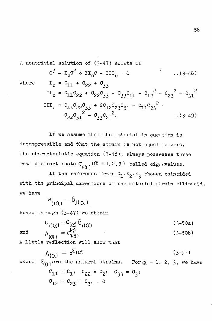
L. nontrivial solution of (3-47) exists if

- I CC2 + iic - iii = o (3-48)

where I C =11 + 022 + 033

Iic= 011022 + 022033 + 033011 - 012 2 - 023 2 - 0312

Mc = 011022033 + 2012023031 - 011023 -

0220312 - 033021 0 (3-49)

If we assume that the material in question is

incompressible and that the strain is not equal to zero,

the characteristic equation (3-48), always possesses three

real distinct roots (CX I,2,3) called eigenvalues

If the reference frame X1 ,X29X3 chosen coincided

with the principal directions of the material strain ellipsoid,

we have N

i(a) Hence through (3-47) we obtain

Cica) = C()ö.(a) (3-50a)

and A( = d ) ( 3-50b) i little reflection will show that

A() =- eE(c) (3-51)

where Ea )are the natural strains. For = 1, 2, 3, we have

011 = 0 022 = 02; 033 = 03 ;

012 = 023 = 031 = 0

59

This indicates that the eigenvalues are the normal components

of the deformation tensor in the principal axes, and the

shear components in this frame of reference are zero.

The square roots of the eigenvalues are the principal

stretches.

Therefore the spatial strain ellipsoid with reference

to the principal axes becomes

ds 2 = XddXj rl 0 0 1xNl1 0 020 HN2l

L0 0 O3JLdXN3J (3-52)

Now 0119022 and 033 are positive, hence 0

Thus (3-52) is an ellipsoid having semi-axis lengths equal

to and the directions of the principal axes of the

spatial strain ellipsoid can be obtained by diagonalizing the

Green's deformation tensor.

It is obvious that the same arguments apply to the

inverse deformation. Thus, the determination of the

directions of the principal axes of the material and spatial

strain ellipsoids and the determination of the principal

stretches (or principal strains) are simply equivalent to

the diagoniization of the Cauchy's deformation tensor and

the Green's deformation tensor.

Consequently, the procedure of determining the

finite deformation in terms of principal strains can be

summarized as follows:

(1) Determination of the co-ordinate transformation matri:ces

D12 B13

LD11

D21 D22 D23 (353)

B31 D32 D331

and d12 d13 1 rD11 D12 D1 -i [dii

a21 a22 a23 = [ D21 D22 D23

a31 d32 d3 LD31

D32 D3 -54)

Determination of the Green's deformation tensor and

the 'Cauchys deformation tensor by using the

following equations

C11 012 C 1 3 D11 D21 D311 D 11 D12 D1

C21 022 C23 = D12 D22 D32 D21 D22 D23

031 032 C33 13 D23 D3D 31 D32 D 3

00 (3- 55)

C11 012 0131 [ill d 21 d 31 dil d12 d131

°21 022 °23 =d 12 d 22 d32 d21 d22 d23 (3-56)

L c 31 032 c33J [113 d 23 d3j d31 d32 CL

Diagonalizat ion of the G

deformation tensor 321d

TIR

the CaucIr's deformation tensor.

61

307 pca1pesentation 0: Pwo-Dimensio:

3.7.1 Construction of Mohr's Circle

The diagonalization of a symmetrical tensor can be

affected by rotating its axes. For the Green's deformation

tEnsor, the transformation is characterized by the equation

i rCO.P r11 c121

Lsi10 [ c L' co Lc21 c22J 00 (357)

where is defined as shown in Fig0(3-13), i.e. it is

measured from the x1 axis in the anti-clockwise direction.

Solving from equation (3_57) for C, 02 and

we have

11 22= _ + (c1l_22) 2 + 012] 00 (3-58)

02 = C 1 + 0 -

2

sin24 = 2012

l 2

E C11-C22 2!J 2 .(3-59)

0 0(3-60)

Equations (3_57) to (3-60) can be represented graphically

by a Mohr's circle. For this purpose, we take a Cartesian

co-ordinate system with origin at 0 and the positive directions

of the axes as shown in Fig-0-14). Let the axes represent

the normal and shear components of the Green's deformation

tensor respectively. Points Cii(C,o), 022( 022, 0 )9 D1 (0119 C12 ) and D2 (C229 -012 ) are then constructed as shown

62

in Fig. (3-14). The line D 1 D 2 crosses the abscissa at a

point F. Using F as the centre and PD1 (or as radius,

we draw a circle. It can be shown that

= + = ~ uE2

+ C122C1' .(3-6l)

= JL 22 2 22

) + C122j (3- 62)

Sin LAFD1 = Sin 21-ABD = ii = 2 G2 6

FD1 I''2

, .(3- 3)

To determine the major (tension) principal stretch

A O.L.

A 1 (or ), we use point (--o) as the centre said -

O

- as

the radius to draw a half circle such as sown in Fig,, (3-14)

Then a perpendicular line is constructed from point (1.0)

and cut the half circle at H.

we have 1 H - OA

or = c 2 =A1

From triangles OJH and ORB

.. (3-6i)

..(3-65)

TherGfore, if a Green's deformation tensor in its general form

is given, the corresponding diagonalized tensor can be

determined by the use of Mohr's circle. In the Mohr's circle

(Fig-3-14) BD1 and BD represent the minor and major principal

components of the Green's deformation tensor respectively,

OH or OH' represents the major (tension) principal stretch

and BD the major principal material direction.

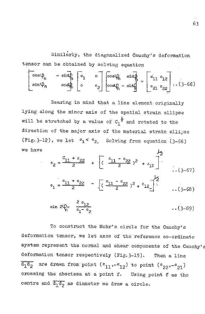
Similarly, the diagonalized Cauchy's deformation

tensor can be obtained by solving equation

oscp si4 [

o

c2

J Fosii r11 c12J

J L c c22J (3-66)

Bearing in mind that a line element originally

lying along the minor axis of the spatial strain ellipse

will be stretched by a value of C1 2 and rotated to the

direction of the major axis of the material strain ellij.se

(Fig03.-12), we let C1 < C2 Solving from equation (3-66)

we have

C11 + C22 r C11 C22 2

2 + 2 12

(3-67)

CC

11 22 - 11 22 2 1 = 2 L - + 12J (3-68)

2c12 sin 2(4=

1_C 2 (3-69)

To construct the Mohr's circle for the Cauchy's

deformation tensor, we let axes of the reference co-ordinate

system represent the normal and shear components of the Cauchy's

deformation tensor respectively (Fig03-15) , Then a line

are drawn from point (0119_c12) to point (c 22 9_c21 )

crossing the abscissa at a point f. Using point 1' as the

centre and as diameter we draw a circle.

63

It can be seen that

C +c c -C 1122 11 22c 2 7a 7f = 2 2

+ 12 =2

(3-7o)

C

=

C22 - L 2 22 + c122 = 1 (3-71)

sin LafcL, = sin 2 L d

dbd.. 1 c 211 C12

S±fl 2 1

C1'C2 n (3-72)

Therefore, bd in Fig0(3-15) represents the

direction of the major axis of the material strain ellipse.

Since the Cauchy's deformation tensor represents

the inverse deformation, a little reflection shows that

02

• C 2 =

Hence, we obtain

•(3-73) 01+02 -

00f 2 2

= Cl_02 c 2-c1 "(3-74)

Equations (3-73) and (3-74) imply that the Mohr's

circles for the Green's and Cauchy's deformation tensors

possess identical centre and diameter with reference to their

own co-ordinate system. We can therefore express these two

tensors by a single modified Mohr's circle (Pig3-16).

In Fig(3-16) bd1 and BD represent the directions

of the major axis of the material strain ellipse and the

5101

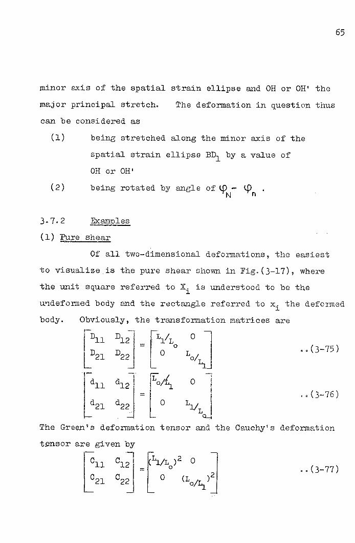
minor axis of the spatial strain ellipse and OH or OH' the

major principal stretch. The deformation in question thus

can be considered as

being stretched along the minor axis of the

spatial strain ellipse BD1 by a value of

OH or OH'

being rotated by angle of (.p- (.P fl

3.7.2 Examples

(1) Pure shear

Of all two-dimensional deformations, the easiest

to visualize is the pure shear shown in Fig. (3-17), where

the unit square referred to X is understood to be the

undeforined body and the rectangle referred to x the deformed

body. Obviously, the transformation matrices are

rD11 D121 rLl/L

LD21 D22J I 0 L0/ j

[ 11 d 12 0/4 0

I = ..( 3-76)

Ld21 d22J L 0 L1/ J The Greens deformation tensor and the Cauchy's deformation

t.nsor are given by

65

1011 C 1 k1/L 1

L021 L )2

1 ) (L .0(3-77)

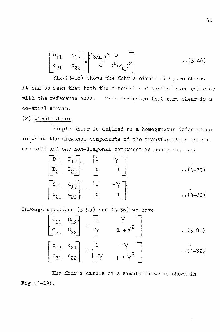
W.

12 0 ~11

(3-48 L 21 c 22 o

Fig. (3-18) shows the Mohr' s circle for pure shear.

It can be seen that both the material and spatial axcs coincide

with the reference axes. This indicates that pure shear is a

co-axial strain.

(2) Simple Shear

Simple shear is defined as a homogeneous deformation

in which the diagonal components of the transformation matrix

are unit and one non-diagonal component is non-zero, i.e.

TD 11 Dl21 LD21 D22

- LO iJ .0(3-79)

rdll d12J = -vi Ld2i d22j L° lt ..(3-80)

Through equations (3-55) and (3-56) we have

rc11 cJ V 1 L021 022JY 1

rd l2 c 21 = -v Lc 21 C22J +_'Y/2 j

The Mohr' a circle of a simple shear is shown in

Fig (3-19).

Generalized simple shear

4i. more general case of deformation is shown in

Fig-(3-20). This deformation can be considered as the result

of a pure shear and a simple shear, i.e. a pure shear

followed by a simple shear.

transformation matrix is

D11 B12 I '( j .'/. .'-'o 0

21 D2 2J iJ L L/j

The overall co-ordinate

- rLl/L YL1

- L 0 L/Lj ..(3-83)

d11dL 12 0/11.:y o/L

21 d2 L ° L1 J Through equations (3-55) and (3-56), we obtain

Fli C12 1 f(Ll/L ) 2

L021 c22JL ,y CLO/L1)2 (1 . . ( 3-85)

1l c1 L (L/L)2 - ( /L) 2

2l c22JL&ol)2y (L /) 2 + ( 3-86)

Figure (3-21) shows the Mohr's circle for the

generalized simple shear.

Generalized simple shear with rotation

Obviously, the most general case of deformation in

two dimensions can be considered as a generalized simple

shear followed by a rotation such as shown in Fig-0-22).

67

L'II]

When the reference co-ordinate

x 1 x 2 are chosen such as shown in Pig (3-,

matrices, the Green's deformation tensor tensor

deforma-tionare identical with those for

simple shear.

systems X1X2 and

22), the transformation

and the Cauchy 's

the generalized

Mohr's circle for the generalized simple shear with

rotation is shown in Fig(3-23). In this circle, line BDL

which is obtained by rotating Bb by an angle (.J) represents the actual major axis of the material strain

ellipse. This generalized simple shear with rotation thus

can be considered as the result of

a principal stretching along the direction of

I (i0e0 n 2 ) by OH.l;

a rotation of +

38 Deformation in the Chip - ReEresentedjby Principal Strains in Terms of Pure Shears

Example of plastic deformation due to oblique

cutting represented by principal strains in terms of pure

shears are shown in Figs.( 3-24) and (3-25) The reference

frame is shown in Fig (3-24a) In Figures (3-24b) and

(3-25b), an tndeformed unit cube is illustrated by chain

lines and its edges are originally parallel to the spatial

principal axes Hl , H 2 and 43 respectively, During the

cutting process, the cube is first rotated rigidly to the

direction of the material principal axes A,, -R2, and 13O

Then it is stretched along arid fl3 by

and finally becomes a parallelepiped such as shown in

Figs (3-24b) and (3-25b).

Here it should be noted that, during the cutting

process, the unit cube is rotated and stretched simultaneously.

In order to have a better understanding of the cutting

process it is also necessary to investigate the history

of deformation, e.g. the strain path and strain rate.

This will be introduced in the next chapter.

For the purpose of evaluating Merchant's single

shear plane model 9 corresponding results obtained from

equations (2-1), (2-2) and (2-3) are shown in Figs. (3-24c)

and (3-25c).

Comparison of Figs. (3-24b) and (3-25b) with

(3-24c) and (3-25c) reveals that Merchant's model does

not and can not produce the actual deformation. Deformation

due to oblique cutting proposed by Merchant differs from the

actual one in the magnitude of the principal strains as

well as in the directions of the material and spatial

principal axes.

69

x3

x

FIG.3 S1E1CHG ALONG E'ERENCE

AXES

'I

x2 I

0

F G. 3-2c SHEAR - PLANE 2

WTH MOVEMENT ALONG AXIS

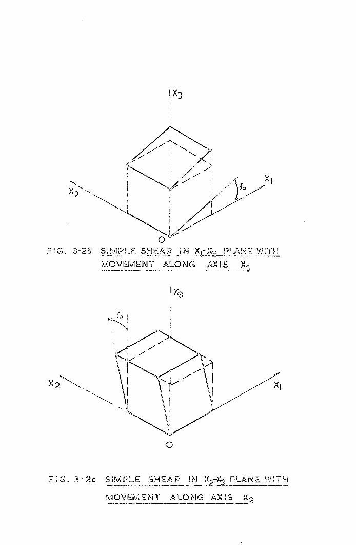
U

F G. 32 L4LE SHEAR. J3ANg!)1 MOVEMENT ALONG AXIS

XI

F G. 3-2c 5MFLE SHEAR iN)X3 PLA NE W TH

OVN?_ALONG

I

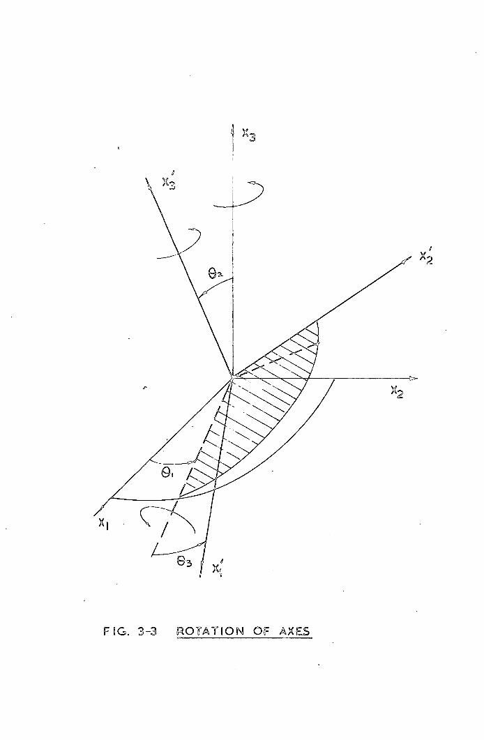
93

FG. 3-3 ROTATION OF AXES

X

x 2

11

2

I -

, -

(b)

U

c)

(d)

HG. 3-4 DEFORMATION DUE TO

OBLiQUE T , N

G

M L

TZ

Qn i

0]

C. op vi; of

4

t 2 1

L

t

2

10-1

b. Dfowd prIppd

FIG. 3 5 &S1EEN J OF PI-ASTIC

DEFORMATION N THE CHIP

J 03,

/ r1 /

-

A

(a

c)

F I G. 3-6 MEASUREMENT OF PLASTIC

DEFORMATION IN THE CHIP

3 5

' 3.0 0

• 2.5

¼)

2.0

im

4

L

0r

0 ao 20 30 40 angle,Oblique

1G. 3..7

CU1TNCI RAT 10

50, T

0

0

20 U

EEó

107,

4C

-Q

761 3C

tO 20 30 40

Oblique angle, dzg, experimental results

Stab1r'Chip Flow Law

FIG, 3-8 CHP FLOW ANGLE

-- 1

- 0• -:

c- 4

0 11 020 30 40 0bqu dg.

HG. 3 -9 SHEAR ANGLE tn

C

IN

C

'J)

WN

Kwj

cc

20 3C' 40

ObHqu iny1, dg. I ""1. i-i

SHEAR AN,LEtan

! '¼

IN

1° \ x2 \JJ

0

F .. :FENc cccRDNAi-:

cg

4D Ural ellipsoid

xv g h

b) ptia! Uipo

FG. 3H2 STRAIN LLPSOiD5

N2

iN

F! G. 3-13 ROTATION OF AXES

2' c 2I

2

A1

FIG. 3-14 MOHRS CIRCLE FOR GREEN'S

DEFCRMATION TENSOR

C2

C 2

FIG. 3-15

MCHR'S CIRCLE

FOR CA!JCHY'S

DEFCRMAT: CC TEN S C, R

2 C12

19 2

Al

FIG. 3-16 MCDF lED MOHR'S CIRCLE

9 2

Lo

0' 9 1 0 I

FIG. 3-17 PURE SHEAR

C 12 , C12

A l

C!

FIG. 3-16 MOHR'S CIRCLE FOR

PURE SHEAR

Al

Cl -

X 2 N2

Ian r

FIG. 3-19 MOHR'S CIRCLE F('R SIMPLE SH.AR

/

x

Li

FIG. 3-20 GENERALIZED SIMPLE SHEAR

C 12 cl

-

F C 11 Tc 1 II / 22

Al

Cl

FIG. 3-21 MOHS CIRCLE FOR GENERALIZED

SIMPLE SHEAR

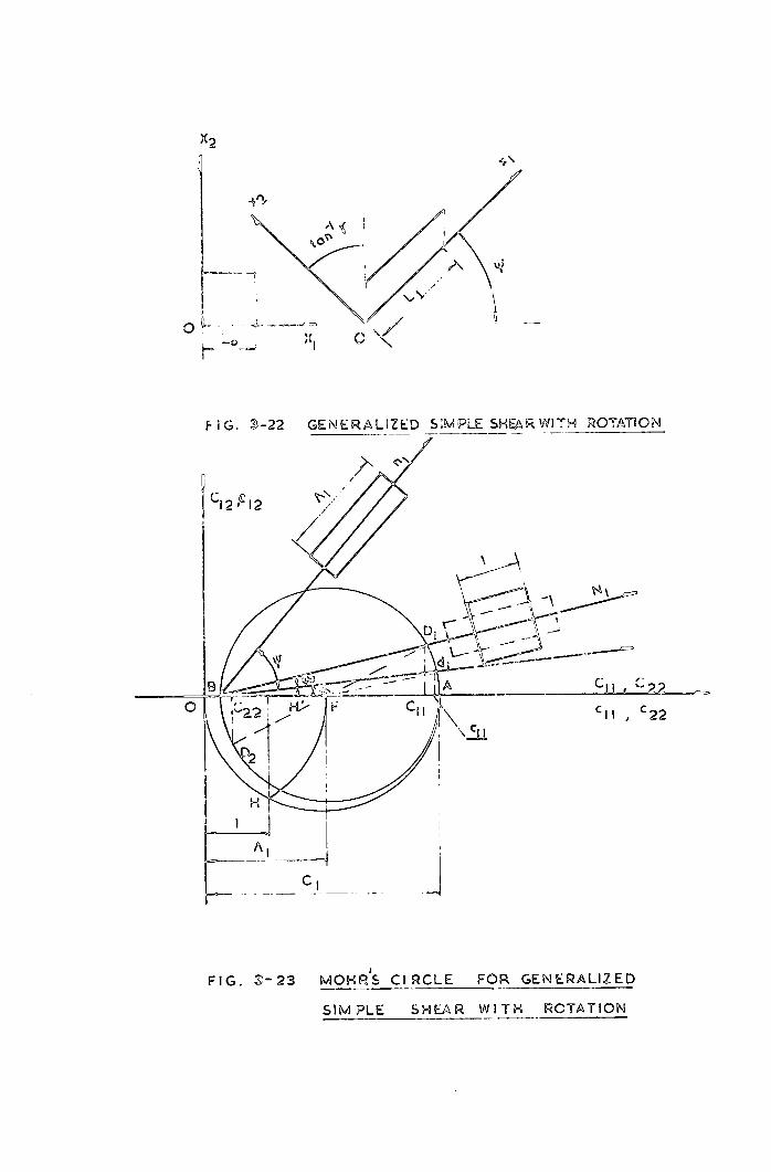
X2

FIG. -22 GENERALIZED SMPLE SHEAR. WITH ROTATION

FIG. 3-23 MOHRS CIRCLE FOR GENERALIZED

SIMPLE SHEAR WITH RçTATION

2

REFERENCE FRAME

cc

H

X2

A = 2.725 /

//•

A2 LO4

X 3 A3 -0353

actual d1orjon

HG. 3-24b DEFORMATION DUE TO

OBLIQUE CJTTiNc

&

X2

/

/

dor mat on sugt'd

by Merchant

FIG. 3-2C DEFORMATION DUE TO

OBLIQUE CUTTING

x

nr 41,

N

X2

,

A l = 2.452

A2= 1.095

AS =0.3B5

actuI d'gorton

FIG. 3-25 h DEFORMATION DUE TO

0BLQUE CUTTtN

/

N2

/x 3

d 1orriation by Mrchnt

FIG. 3-2C

s uggt'd

\fl3

A l =2.66

=

A3 =0.376

DEFORMATION DUE TO

OBLIQUE CUTTNG

7 / / 71 13

x 2

CHPTR 4

STRAIN PATHS

4.1 Measurement of strain paths

The plastic deformation in the chip due to oblique

cutting, as explained previously, can be represented by four

parameters, e0g0t2/t1 Yj 9 Y2and Y3 , The co-ordihates

transformation neglecting the translation is then expressed

70

by

xf fcos(9o °- c)

= sin(90 0- ()

xf L0

1 ° L o

sinUn

I COS

L'c

where, xl ,x29 x3

Xi ,X 9 X

-sin(9Q°- CW 0 fl 0 oJ

cos (90 °- c) 0 0 1 0 0 1 y2 iJ

1

[E EJ j:]

LXJ (4-1)

co-ordinates of a certain point in the undefomed workpiece.

00 co-ordinates of this point in the chip.

0 I I 0 ii

- cos) 0 1 rxi

r(icosn + sin) 0 1x2

normal rake angle t It ' 1 cutting ratio

It is obvious that a finite time interval must be

taken for performing the deformation. In other words, during

the cutting process, a unit cube of undeformed material

is gradually and simultaneously subjected to

pure shear along

simple shear in the plane x 1-x3 with movement

along axis

simple shear in the plane x 1-x3 with movement

along axis xi

simple shear in the plane xk_x3 with movement

along axis

rigid rotation about axis x 3 .,

Therefore, in order to determine the strain path

it is necessary to measure the instantaneous values of

rc, "1 ,'y'2 , Y3 and , If we denote the instantaneous values of r , 'y and by , and sL

equation (4-1) becomes

= sin r(Y1 1 sina - cos ') 0 xi

x f

2 r( 'Y coso + sinOt) 0 x2

1 x3 (4-2)

With reference to a new co-ordinate system

y19y29y3 (Fig 03-6a), which is obtained by rotating

co-ordinate system x19 x29 x3 about axis x3 by an angle

The co-ordinates transformation matrix becomes

71

72

cos3 0 Sisir

I

ii, , rd (Y sin cosa) 1 L 0 1 0 cosa r ( 'cos+ sin) 0

sinj3 0 coL'r lj r cos13 0 sin([ Ea11 a12

0 1 0 a 2

a 22 a 231

.0(4-3) 0 c013 La31

a32 a 3

where, a11 = Il sin cos213 - s93( V3 r cos13 -sin ). 0 (4-3a) C C

a12 = I!' I

Y, sin-cos) cos C sin 3 0 (4-3b)

'13 3-

= ;'; sina' sin 5 cos 3r sin

(4-3c)

1 + 008

a = FT Cos C( 0 0(4-3d)

a22 (YC0S + sin ) 0 0 (4-3e)

a23 f

C

COS (X " 5.11 13 00 (-3)

1 a31 = sin csinf3 cos 13 + cos i3r cosI3 00 (4-39) c -osin13)

I r 2 a32 = C (sinoo. cosç) sinf3 ~ 'Y c cos4 .0(4-3h)

a33 = sina1 sin2p + Slfl sin 13+ COS1-1

1i line element OB which originally lies on axis yj

with one end 0 at the origin of the co-ordinate system

becomes OBI (Fig 4-l) Since the rigid translation

does not affect the deformation, the original line element

OB and the deformed line element OBI can be represented by

co-ordinates ooJ and[(Yl)B9 2B' ..4

The relation between OB and OBI thus can be expressed by

(Y1)B all a12 - (Y) 3 101

2B = a a22 a23 021-

(y ) a31 a32 a33 J 0 -

pning (4_4 ) yields

cr sinc(,cos3 - $ini3(Y3 cos3 sinr3(Y(5)

= ( ._4. cos cos !3 ) (4-6)

1 3B = sinsinf3 cosI3 + COS 1

(.-r cos13. sin)7 o (4-7)

Similarly, for a line element originally lying on axis

(Fig4-2), we have

11 a12 a13 0

2A = a2 a22 a23 : (4-8)

L 3A L.a31 a32 a33J L °

and ( YsinOt cos) cosf3 _Y9 sinl3Y 2)0

2B = C ( 'cosç + sina 27 20

3B z; (Y11 sinoç' cos) sin r3~ Y21 cos3J (Y2)0 (4-11)

By rearrangements, we have from equations (4-5) to (4-11)

3B 1B

tan1[ yy- sin +

cos 0 -7

73

(Y ) ri cosa;1 13

Y3r

Sin ) sin 13 cos 13 =- 0 C

1 2 rr COS

C

(1) 1

(YT2A

FT -tana' YI = C

(4-14)

74

T,2 , C

( 'y'sin cc - cos tan 13

(Y )

sina'. rv cosa') cosj3 CY r I sin

C

4.2 Experimental Teclmiauesand Results

(4-17)

The specimen used for the investigation of the history

of deformation due to oblique cutting is split in the middle

and a photographic chequer-board pattern is printed in the

surfaces which are to be pressed together (Fig-4-2).

The photographic chequer-board pattern was first

suggested and developed by Hsu in the Department of Mechanical

Engineering of the University of Edinburgh. By comparison

with the conventional rectangular grid pattern like that of

a graph paper, the principal advantage of the method lies in

its ability to produce a very fine grid pattern.

L.fter the surfaces of the specimen, on which the

chequer-board pattern is to be printed, are carefully machined,

polished and cleaned, a thin layer of filtered Kodak Photo Resist

used for sensitizing is coated evenly on the specimen.

The sensitized specimen is then exposed through a master

negative. The exposed specimen is then developed in the

Kodak Photo Resist developer which contains a dye.

By the use of the quick stopping mechanism, the

cutting action is suddenly stopped and the specimen is

taken down for taking measurement on the MtJ214B Universal

Measuring Machine.

Fig. (4-3) shows the deformed grid pattenn obtained

under the following cutting conditions

75

Machine

Cutting speed

Variation of cutting speed

Tool material

Normal rake angle

Clearance angle

Oblique angle

Workpiece material

Width of cut

GSP Shaper

160 fpm.

less than 005%

HSS Speedicut Max 18

300

70

20

HE-30-WP

0.25 in.

Depth of cut 0.025 in.

Values o±t/t1, Y , , and obtained from

the experimental result (Fig-4-3) through equations (4-12)

to (4-17) are shown in Figs. (4-4) to (4-8).

M-4

43 Representation of Strain Paths

L state of strain in three dimensions may be

represented by three principal natural strains E , £2

and €3 If it is assumed that the material in question

is incompressible, i. e.

I 1 E2+ E3 0 .,(4-18)

any set of values forE1 E. andEs which satisfies equation

(4-18) may be plotted in the triangular co-ordinates Fi(4-9)

A. point P in Fig. (4-9) represents three principal strains

whose sum is zero, because in Fig (4-9)

El = E: Cos £2= £COS(-. -126)

£3— £ COS(- _2400)

where £ is represented by the length of OP and

(cos .+ cos (-a- 1200 ) + cos(-- 240 0 )) vanishes identically.

Solving from equations (4-19) we have

rF2 q+(F F 3

oo(420)

It is obvious from Fig. (4-9) and equations (4-19) that the

value of E represents the intensity of the strain and the

angle the ratio between the principal strains. If let 6

(4-21)

the ratio E £2 00 E3 may be represented by a single number

ranging from 0 to 12, instead of a number from 0 to 2

or 0 to 3600. Subsequently the number is called the

characteristic index. Some reflection will show that all

odd numbers represent pure shear, numbers 2, 6 and 10

represent compression and numbers 4, 8 and 12 tension (Fig.4-10)

Fig, (4-11) showB the strain intensity of four

particles along the stream lines. The same data were used

for plotting the distribution of the strain intensity in

the y1-y2 plane (Fig.4-12). The characteristic index

of strain for a particle travelling along stream line 3

is plotted against time in Fig.(4-13).

In two non-coaxial strain increments, the relation

between the two sets of principal axes can be expressed in

terms of three angles, because three angles are required to

locate one set of Cartesian axes with respect to another.

The change of the directions of the principal axes for a

particle along stream line 3 is shown in Fig,(4-14).

In Fig, (4-14), - - and are three eulerian angles

used for locating the directions of the principal axes

with respect -b the reference co-ordinate system Y19 Y29 Y3 0

From Figs,(4-11) to (4-14) it can be seen that

the plastic deformation due to oblique cutting is in

general three dimensional and non-coaxial. Therefore,

five quantities, i.e. the intensity of strain, the strain

characteristic index and three angles, are required to

77

im

show a complete picture of the strain paths of the deformation

due to oblique cutting.

Fig 0(4-15) illustrates an example of the strain

path for a particle along stream line 3. In Figure 4-14) 9

the instantaneous state of strain of the particle in question

is represented by a deformed cube in solid lines. The

magnitude of the principal strains and the direction of the

principal axes are represented by the length of the sides of

the cube.

/

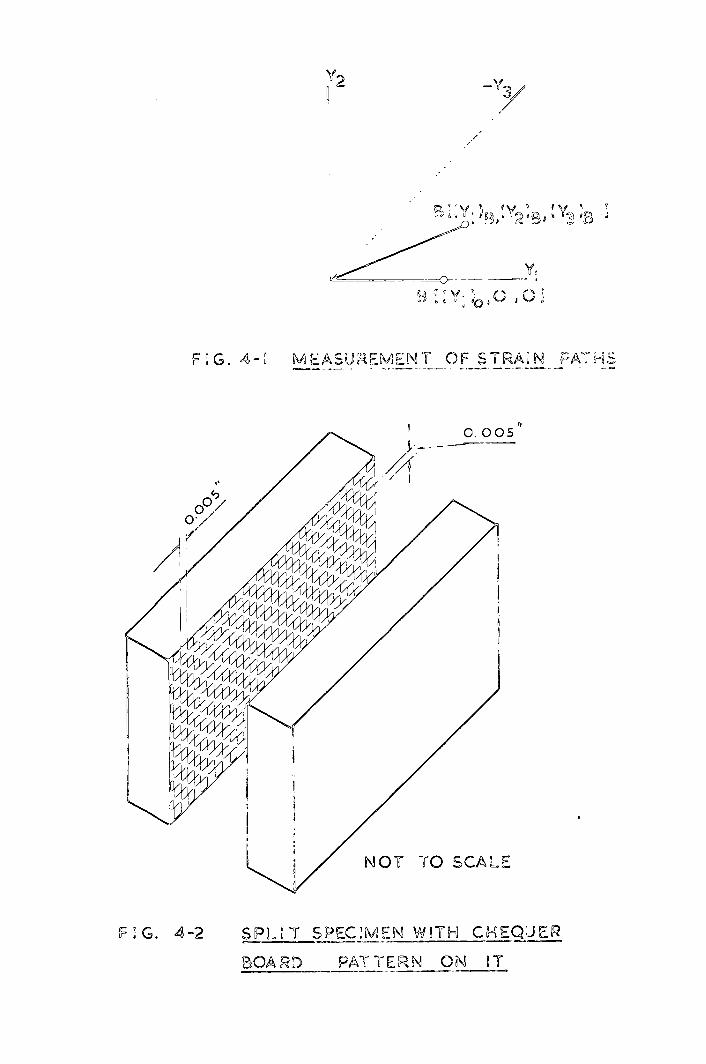
i1 iy Y~~ '0 ~3 , ty B

Y; ,O

FG. 4- EASUvENT OF STRAN PATE

It

NOT TO SCALE

HG. 42 SPLMSPECMEN WTH CHEQUE R

OAD PATTERN ON IT

I'

A \ /•

N \• \•

I I

:ItItTtI 1 it I •t ....1 EJ I !

L

'UJJJ±JJ

0 I

/2\ /

4 \/, A

/

(

S:A.E

\V \ \

F 43 [7. f7lR!:) PATN

C

1.6

U L4

ST REAM .i NES

SYMBOL NO. 0

2

3

+ 4

1.2

b C d

j - p MARR

FIG. 4-4 CUTTING LATO

1 STREAMLINES

SYMC)L NO. 0

o 2 3

+ + 4

- 0.8 ---- 1 LLB

0.6

w

0.2 H

oh-

---. b C I

h i j

p

FIG. 4-5 SIMPLE iHEAR

Ui I U)

Ui -J

NO

- 0.02

h i

JA<ER SIMPLE SHEAR (WITH REFERENCETOcccRDtNATE

SYSTEM

o.

-0j

-0.11 11

cu D C

FIG. 4-6

O.O6

ES

NO.

2

3

4

STREAM LINES

SYMBOL NC.

o I

O 2 -. 3

+ 4

0

w I tri-004

Ui —j Ol

-0i2

-0.16

-O.2L a b

FIG. 4.7

c d I h

SiMPLE SHEAR (WrkFEkN.

CCCRDINATE SYSTEM X )fX3 1

- 0 p

STREAMLINES

SYMBOL NC.

0 w

-ac

Ui

0 z 6(

El

2

14 a b c d g h

j k Im n o p

TDME MARKER

4-6 ANCLEct

L

: I

J .

- - 4 -

- - -J -- -

)---- - --- -h-' /\

.----- -\--)

/

44

FIG. 4-9 TRIANGULAR COORDINATES FOR

PLASTC STRA!NS

2

\.

I

I \\ /

\

TI ci: - TENSION /

COMPRESSION 7/

PURE SHEAR 6

FG. 4-10 LINES OF PURETENSON PURE COMPRESSION

AND PURE SHEAR

I- 'I,

U. 0.8

>-

'I,

z w I- z - Q6

NO

0.2

2 4 6 8 10 12 14

Iu -4

TIME X IC SEC.

FIG. 4-I1 INTENSITY OF STRAIN ALONG STEAMLNE

FIG. 4-12 DISTRIBUTION OF STRAIN INTEN:TY IN Y,-v,., LAN

L&j 3 z

MA

H 'I)

lx w U

I U

H

2

MW

2

1122. 6

8 10 12 14 20 ME,O

FIG. 4-13 STAN_CHARACTERSTC iN-:x

A PART:cLE ALONG STEAMLN. :i

HG. 4-I4 DIRECT!ONS OF PRINCIPAL STRAINS RETD Y

THREE EULERIAN ANGLES

w 0

90 U,

z <

70

OW

50

2 4 6 8 10 12 20

U

n

C ,

/

- 0 - C

(g) MO)

- - - I

TIME •\\A. ' XI

X3

R'It- '

A \

fl 3\\

/c

0 C)

M)

0 0 C

CS) C 6) (7)

CJJPTEIR 5

STRL.IN RtTES

51 Velocity Field

is it was mentioned in Chapter Z a finite

homogeneous deformation can be represented by an affine

transformation

E x1l rD11 D12 D13 1x1 J = D D22 21 D23 X (5-i)

X3]

r--1 LD31 D32 D33J LX 3J lxi Oxi oT1E

or xl! J ( ixil

2 X2 c) x2

X2

X3 13 31 Ix2 Li jX1 oX2

where x the spatial co-ordinates

the material co-ordinates

For incompressible materials

I D h1 Dl2 Dl3( I Oxi OX1 oxi I i10x20X3

D21 D22 D23 =

1' 0 x2

1. 0 x2 0 x2

=1

I D3l D32 D34 ,

X I IbX2 3!

From the assumption that the material is a continuous medium,

there exists an inverse transformation

79

r x11 rd 11 d12 a13 1 rx1 = d21 d22 d23 J X

2 (5-4)

L x3j Ld31 a32 a33j

.-- x 3-

where rd 11 d12 d 113 C) X1 oX1 aX1 1 r-1

D12 D 1 3 -

I I 1X2 r) X2 d21 a22 a23 = = D21 D D2322

31 a32 a33

L 2 L3' D32

eo(55)

said d11 a12 a1. rDfl D12 Di 3 a21 a2 d3 ID 21 D22 D23 = 1

Ld31 a32 d3 LD31 D32 D 3 J

For the purpose of investigating the strain rates,

the positiOn of a material point at time :b = 0 is represented

by material co-ordinates At time t, this material point

is carried to a spatial point designated by spatial co-ordinates

x. The relation between these two sets of co-ordinates

MCI MWA

can be expressed by transformation. -

()x1 (xjt) ôxi(xt) oxi ( t ) 1 x1 (X.,t) X1 X 2 OX 3

X2 ( Xi t ) Ox2(xjt)

x2 (Xi ,t) OX1 OX2 OX x

0x3(x1 9 t) 0x3(xj 9 t) t) 0x3(x1 9 x3(X,t) Ox1 OX2

x3

(5-7)

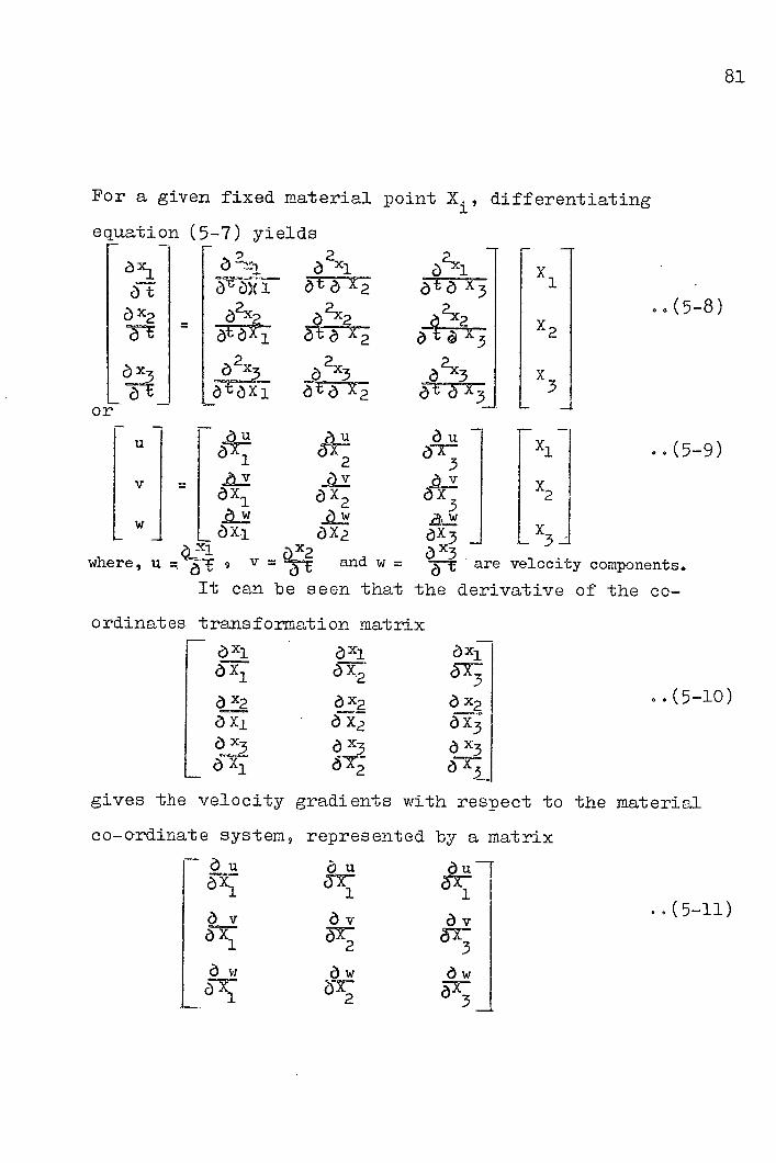
C)

0

0

'1

jcF

0/C

, C

', 010

CD

co

CD

H

1J

<4

FP

<V

Fj

CD

0,

Fd

Fj

rul.ci

H1

co

CD

CD

0••

AOv

'i H

1

c+

F

j

in H

H

Uq

0

CD

Cl)

CD

CD

______

Cl)

0

C'!

C/C

IQ/

0'c

C)

HjiE

—

HH

CD

H

) 0

p

p

Pi

P.

ka,

Ci,

><:<

rr\r)

'J,H

cf

p

co

1.

0/i

0/0/0/0o,

CD

1X

<k

\J

e

Id

CD

C) cf

0

Cl-

CD

p

CD

\jfl

H

0

iji

CD

CD

•1

ii

C,

C'

p

CD

0lI C

)

co

CD

CD

r

tj

rIri

£

cl-

Il Ic

Q,

cJ

4J4

k\J

Pi

1-1

CD

H

CD

1 H

- C

)

CD

I-i-

c-I.

0c.

Fb()

0

CD

C)

CD

I Oct D) G

0

CD

F1

1

IN

C

l- 1-

¼jJ

ctH

H

0

II

C,

c4c, C

O3

o,l

i'

I1

H

H H

H

CD

Pi

'o

C,

lQv

G. 0

'

l\)

H

0

p

CD

Ft k

CD

Pi

CD

p

H

0

k

H-

F-b

F-b

CD

11

CD

c-F

H-

H-

For changing the reference co-ordinate system in

equation (5-8), we substitute equation (5-4) and the

following relation

Ou ouJ r r X1 a X1 OX 1 ôX 3 OX 0x2 OX 1 OX2 1) x3

o 3 Ov'= I ày a 0X2 0X2 6 x2 OXOX2 OX3I T,OT

Ow Ow Owl Ow Owl I 0X3 OX3 (

[2 3J L0 X1 x 0x31 L0 r1

into equations (5-10), (5-11) and obtain

roxi 1 2 J __ 2 Oxi

2 T

2

2 I I 02 2 2 2

[xii

I = f 3x Ct 0 I

3J 0X3

LJ 2 ___ 2

0X3 2 ox_

or [u Ou r d u

l O X2 On t [ xii

V 1

x1 o Z2

ày I Ow

XFLI—xi O•i

2 jL73 J In the language of matrix algebra, the left-

hand side of equations (5-13) and (5-14) is a velocity

vector and the right-hand side is the product of a three-by-

three square matrix and a position vector.

The velocity field at a point in a deforming body

is the velocity field in an infinitesmal volume around that

point. In an incompressible medium, unless there are

velocity discontinuities such as opening cracks, the

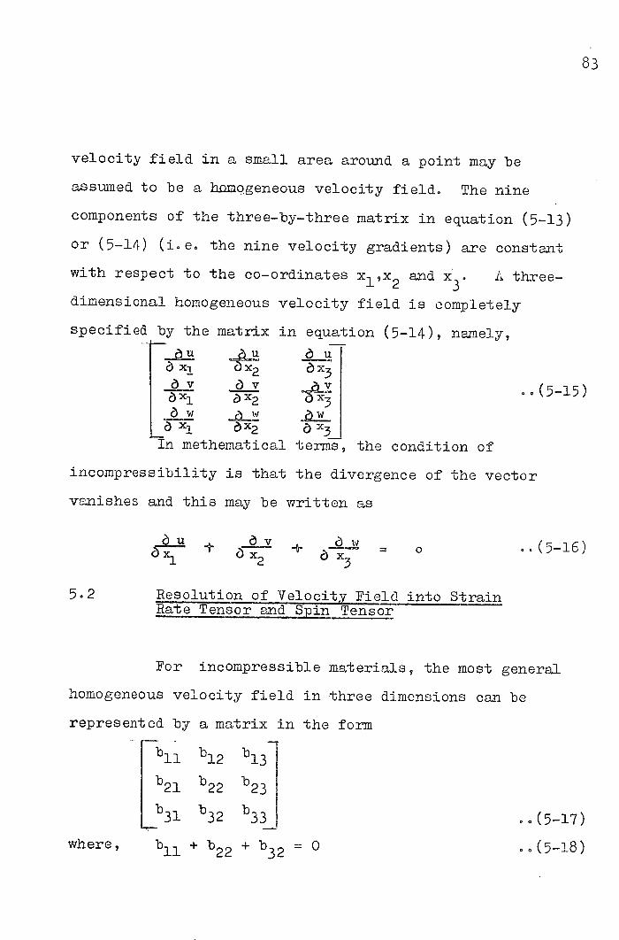
velocity field in a small area around a point may be

assumed to be a homogeneous velocity field. The nine

components of the three-by-three matrix in equation (5-13)

or (5-14) (i.e. the nine velocity gradients) are constant

with respect to the co-ordinates x19 x2 and x3 . L. three-

dimensional homogeneous velocity field is completely

specified by the matrix in equation (5-14), namely,

ô xl c) x3 a x c) x2 ox3

o xl OX2 0X3

In methematical terms, the condition of

incompressibility is that the divergence of the vector

vanishes and this may be written as

1- + (5-16)

X2 Ox3

52 Resolution of Velocity Field into Strain Rate Tensor and Spin Tensor

For incompressible materials, the most general

homogeneous velocity field in three dimensions can be

represented by a matrix in the form

rbll b 12 b 13 b21 b22

Lb 31 b 32 b33 (5-17)

where, b11 + b22 + b32 = 0 .(5-18)

Such a matrix may be considered to be the sum of two

matrices

b 1 b12 b13 21. b22 b23

= b21+b12

Lb 31 b32 b 33 223 bj3

b-b 21 b 13-b 31

+ b21-b12 b23-b32

b3- 32-b 0

]

In other words, a general homogeneous velocity field may be

considered as the sum of two velocity fields, one represented

by a synunetrical matrix and the other a skew--symmetrical matrix.

It is obvious that the skew-symmetrical matrix

in equation (5-19) represents a velocity field of rigid

rotation and is generally called the spin tensor.

To understand the physical significance of the

symmetrical matrix in equation (5-19), let us first consider

one of the simplest velocity fields, in which —au is a

function of x1 only, is a function of x 2 only and

is one of x 3 only. This implies that line elements

originally coinciding with the reference co-ordinate axes

do not change their directions. Therefore we have

C) X-1 =1t

]2

5-2O)

Ow ='fl

and

where , are functions of t, having single finite value

for any particular value of t. Since it has been assumed

that u is a function of x only, v is a function of x 2 only 1

and w is one of x3 only, it follows that

-- x - Ox2 - ox3 - Ox1 - "3Ox, Ox2

Hence, the particular velocity field can be represented by

11I a

(5-22) a )13J

Example of this type o± deformation is illustrated.

in Pig (3-i..), where an undeformed unit cube in solid lines

becomes a rectangular prism of equal volume (dotted lines) r t

after deformation. It can be shown that 1hdt

1t t Jo

01 2

dt and so )l 3 dt are, respectively, the natural strains of line elements along reference axes in Fig.(-J. ).

Substituting equations (5-20) and (5-21) in equation (5-14)

and expanding it we have

M

ln =

dt + C1

1flX2 = 'fl 2 dt + C2 (5-23)

:I.nx3 = 5113dt + C3

where, C19 C2 and Q3 are constants of integration

When t = 0, the values of x1 ,x2 and x3 are those of the

original co-ordinates before deformation, say, X 19 X2 and X3

respectively. Hence

Ct exp( \ 'fldb

Jo

X2 rt dt ex Jo 2

(5-24)

x Ct = exp(

çt çt rt In other words, \ fl dt , \ 1 dt and\ Thdt are, respectively,

J0 I ° 2 the natural strains of the line elements originally lying

along the reference axes. The rates of increase (or

decrease) in the strains in the line elements lying along

the reference axes are thereforeli 1' 29 andl)

L. more general velocity field can be represented

by a deformation shown in Pig (5-1 ), in which the unit

cube in solid lines with its sides parallel to x 19 x2 and

is stretched and compressed along axes y 1 ,y2 and y3 of

another co-ordinate system. Since the relation between

co-ordinate systems x and y1 can be represented by

E00M

- y1 . R11 R12 R13 [x1

= R21 R22 R23 x2 (5-25)

3J LR31.R32 R33 LX3

where the three-by- -three matrix is a rotation matrix, it

follows that 1 ôx1 I oY'1 r R11 R12 R13l --

I C)2 R21R22R fl 23 ITI

Lo t i L R31 R32 R3 3J I ô X ..(5-26) LTht I

On the other hand, the velocity vector with reference to

co-ordinate system y and be determined by

r -T1 0 0

I 0 'fl 0 Y2 (5-27) = '2 00

L 0 0

Combination of equations (5-25) to (5-27) yields

r - - xçj- I U I - t R11 R12 R1 m 0 01 ji f n 11 R12 R131 xl

fl I M=I. 2 = i iiri I I

R 21 R22 R2 [o 2 0 R21 R22 R I

L J LOtJ R R 31 32 L R 0 0

33 L31 R32 R:J :J 00(528)

Bearing in mind that product of two or more

symmetrical matrices is still a symmetrical matrix, equation

(5-28) may be represented by

RE [SI.]

I B11 B12 B13

V == B21 B22 B23 x2 0(5-29) C)t

w] -LB31 B

32 B33

where B12 = B21

B13 = B31

B23 = B32

Equation (5-29) indicates that the velocity field of the

deformation shown in Fig (5-16) can be represented by a

symmetrical matrix, which is usually defined as the strain

rate t ens or0

According to the above discussion, it can be

concluded that

the change of deformation contains two parts,

±0 e. the rotation of the principal axes and

the strain rate;

the rate of change of deformation can be

determined by measuring the velocity field;

the rotation of the principal axes is characterized

by the rotation velocity field represented by

a skew-symmetrical matrix called spin tensor;

the strain rate is characterized by the strain

rate tensor represented by a symmetrical matrix

LOOR

(5) the principal strains rate and the direction

of the principal strain rates can be determined

by diagonalizing the strain rate tensor.

53 Determination of Velocity and Strain Rates from the Deformed GridPa.tte

The deformed grid pattern shown in Fig0(4-3) can

also be used for determining the velocity field.

Because the plastic flow due to oblique cutting

in this investigation is under steady conditions, one set

of the grid lines (solid lines in Fig 4-3) are the stream

lines. It is obvious that the other set of the grid lines

(broken lines in Fig04-3) are the time inarker, because when

a particle in the undeformed material moves through one pitch

(like dLe4) in Fig 4-3) each broken line replaces the one in

front of it. The velocity of point j 3 is therefore

proportional to the length of line element j 3 k 3 and in the

direction of j 3k3 0 The velocity components U, V and w

in the direction of the reference axes are proportional to

the projections of the line element on the corresponding

reference axee0

Since the deformation due to oblique cutting is

three dimensional, the velocity components u, v and ware

functions of the reference co-ordinates.

90

Thus we have du - Ou

z -. ãa dz1 + ôz2 d +

2 1•3 dz3 (5-30)

dv = dz + ôz1 1

dw = ôz dz

1 +

&x dz2 + dz3 z2 oz

O—W 'dz + - dz

3z 2 à 3 3 (5-32)

where di 9 dv and dw are the incremental velocity components

corresponding to a small increase in co-ordinates z 1 , z2 and

z3

Some reflection shows that

(1) When the pointzl)iAr,(z2)j,(z3)jJis moved

to PointC(z1) 4 9(z 2 ) 4 (z 3 ) 4 Jthe velocity

components will be increased by

(Zl). - ( z ). (du) i4 1 i4

(533)

?2j4 2i4 (dv)4 = t "(5-34)

(z3)4 - ( Z)j4 (dw) = t

where (z1)4 - (z 1)d4

= v (5-36)

and v0 is the cutting speed.

The increase in co-ordinates can be determined by

(dz1 ) 4 = (z1 ) - (z1 ) 14

(dz2 ) 14 = (z2) - (z2)4 .(5-38)

(dz3 ) = (z3 ) 4 - (z3)4

91

If the point Pl ). 49 (z2 ). 4 (z3 ).,j is moved

to 2 i39

, the incremental

velocity components are

(du)14 =

(z1 ) 13 - 1) ill t •.(5-40)

(z2)3 - (z1 ) 14 (dy) 14 = •.(5-41)

(dw) 4 = 3 i4 ,(542)

The increase in co-ordinates are represented by

(dz1 ) 14 = ( z1)3 - (z1), (54)

(dz 2 ) 1A = ( z2)3 - (z2)14 •o(544)

(dz 3 ) 14 = (z3)3 - (z3)14 .0(5-45)

By the assumption that there is no side flow of

material in the direction of the cutting edge, the

velocity of points lying on a line parallel to the

cutting edge will be identical. Therefore, if the

increase in co-ordinates ar6 chosen such as

(dz1 ). 4 = tan ..(546)

(dz2)±E =

(dz3 ) 4 = 1 ..(5-48)

then all three inremental velocity components are equal to

zero i0 e.

(du) i4 = 0 .0(5-49)

(dv) 1 = 0 .,(5-50)

(d.w). 4 = 0 ..(5-51)

Substituting equations (5-33) to (5-39) into

(5-3J to (5-32) we have

r(z1 ). (z1)jk7+ (( Z2). (z2) .)7 t a.z1

..(552) 4.= (z))7 Z3

ir2iv =ÔY - (z).J +- / ( z2 ) .k - ( z2)/ t ô.z1 2

+ /73)4 .'i-7

(zl)1kJ+ z2)j4 (z2)1J

+3Z3)jLf (z3 ) i4-7

Similarly, substitution of equations (5-40) to (5-51)

into equations (5-30) to (5-32) yields (z) /z ) (zi)

__+ 'z2)13 (z2)j47

+ pu Z3 Z3)j3 -

(z3 ) i4-7 • (5-55)

!2 ?i3 _22 Z)j3 - (zl)±kJ ôz2

/r 2) 3 (z2)j4J t c)z1

+ av Z3)j3 (z3442 Z3

(z3)j3 (z3 ) i4 = a v Jz1 ) j3 - (z1)iJz2

/TZ2)3 (z2)1 .J t

+Q L(z) ( z3) i4-7 Z3 "(5-57)

a - c = tan 3+ & -

àz3 ..(5-58)

0 = tan( ~ (5-59) z1 z3

0 = ;\ - tan( + c.w .(5-60 ) az1 N' ôz3

92

(5-56)

93

By rearranging and solving equations (5-52) to (5-60) we

obtain

1f (Zl ) jk ( z2)J (z2)14 (z3 ) (z 34 x de A

t j3

[

() () (z) (z 2)j(z3 j3 ) (z3 ) ± I(5_6l) t I 0

r(z1 ) 4 (z) (z2)4

0

(z2) i4 (z3)4

1 - (Z3 )j

ô-u = 1 x d. (zl)lk (z2)i3 (z2)j4 (z3)3 Z2

tan 0 .!.(5-62)

U144 - (z) (z2)j4 (z2)14 (z3 ) jk (z3)iz'

1 =xdet A C z1 ) j3 ( zl ) . k ( z2 ) 13 (z2 ) 1

t (Z3 ) 3

(z )i4 I ô.Z3

t I tans 0 0

(5-63) (z) ( z2 ) j ( z2) . ( z3 ) .k (z3 )

t

Sz, = x det A ( z2 13 ) ( z2 ) j ( z2 j3 ) - (z2)jk (z3 ) 3 (z3 ) 4 t

- 0 0 (5-64)

(z 1 ) i4 ( Z2 ) .4 (z2).k (Z3). (z3). 4

t v

Oz 1 = xdet A

(Z.).3 (zl ) .k (z2).3 (z2)i4(z2). (Z3).3 (z3).k 2 t

• tan 0 5-65) L (z 1)i4 (z 2)j4 (z 2 ) i4 (z2).4 ( z2 ) j

t ày 1 = x det (Z) 3 (z)

( z2 ) j3 - ( z2 ) . ( z2 ) 13 ( z2 ) l4 t

- tan 0 0 ..(5-66)

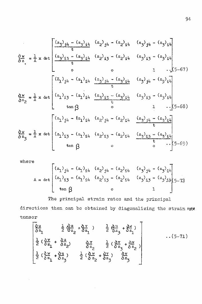
• (Z(Z3). (z2) .4 - ( z2).4 (z3)jk (z3)jk t

= x det (23)3 ( z3)Ik ( z2 ) 13 (z2)jk (z3)3 (z3)jk

(Z 1)j4 (z 1)i4 (z7 ).4

- (Z3).Lf ( z3).k - t

= x de (zl)i3 (z 1)i4 (Z3).7 _5•4

(Z3).3 (z3).k

- tans o 1 .(5-68)

(z 1)i4 (z2).k -

ow - x det (z ) ( z ) k (z)3 2 .k ( z ) 1.i3 l . 2 .

tan ç3 o

where

(z 1)j4 (z,<).k (z2)jk - (z2)jk

A=det I 13 (z )

i

- (Z).4 (z ) - (z ) 2 i3 21k

tan 13

t 3 3-41

( z 3 ) 13

00k5-69)

(z 3 ' C

(Z3 ). 3

1

The principal strain rates and the principal

directions then can be obtained by diagonalizing the strain rate

txmnsor

1U 2 ) 2

1U )

2 Z3

Z

z1 + 1 (

àZ2 2 oz3 az2 1 W

+) - + a Z3 2 a Z2 .Z3

5 , 4 Experimental Results

From the assumption that the material in question

is incompressible, the principal strain rates)] ,)] '11 satisfy equation

T1 1 '0 2 3 + r ..(5-72)

Hence, the principal strain rates can be plotted in a

triangular co-ordinates, similar to that for the finite

strains, and represented by

the intensity of strain rate

= 2 "(5-73)

the characteristic index of strain rate

6 ___Cos

1-c 1 .0(5-74)

Fig-(5-2) shows the intensity of strain rate of

four particles along the stream lines. The same data were

used for plotting the distribution of the intensity of strain

rate in the Y J Y 2 plane (Fig.5-3).

The direction of the fastest stretching and fastest

shrinking fibres is shown in Fig,(5-4). For the purpose of

comparison, the direction of principal strain rates for the

particle travelling along stream line 3 is also shown in

Fig. (4-15) in broken lines. It can be seen that the direction

of the principal strains does not in general coincide with that

of the principal strain rates.

95

-

\

\

/ \\ \

x

/ X2

FIG. 5-0 STRETCHING ALONG AXES

WHICH DO NOT 'COINCIDE

WITH THF REFFPENE AXS

N

1EAMLNE I

L 2J U

c)

0

U

z

"7

0 >-

z w

0.5

- 0 2 4

IC

2

14 —4

x IC SEC.

35

1

0 0.5 i2

L. \--

/ /

/

/

UNIT:- 10 j I SEC.

HG. 5-3 DSTR!B'JTION OF STRAIN RATE INTENSfiTY V_V 01

/ /

x 2

/ \ N

\

/

0

\

-' -

NC 'Az N

rftVW RM

CHJPTER 6

DISCUSSION AND CONCLUSION

6.1 Method of alysis of Finite Plastic Deformation in Three Dimensions

Plastic deformations in metal cutting processes are

so large that the conventional theories of infinitesimal

deformations used in linear elasticity no longer hold.

However, a finite deformation can be represented by an

affine transformation. By the use of matrix algebra, the

three-dimensional large finite deformation, i.e. the end

product of the strain history, can be represented by a

three-by-three square matrix.

For the purpose of measurement, the large finite

plastic deformation can be resolved into several steps.

For example, the plastic deformation in oblique cutting,

as Hsu suggested, may be considered as the product of a

pure shear t2/t1 , three simple shears'\' 9Y2 and

and a rigid rotation.

Since a finite deformation can be resolved in

different ways and only pure shear occurs along a coaxial

strain path, that is a strain path in which all the.

incremental strains have the same principal axes with

respect to the material, it is desirable to express the

deformation by principal strains in terms of pure shear.

In terms of principal strains, a most generalized

finite deformation can be considered as the result of

a principal stretching along the principal

spatial axes by a value of

a rigid rotation carrying the principal spatial

axes to the directions of the principal material

axes;

a rigid translation..

A finite deformation, therefore, can and should be

represented by three sets of quantities as follows:

the magnitude of the principal strains;

the direction of the principal spatial axes;

the direction of the principal material axes..

The magnitude oi the principal strains and the

direction of the principal spatial and material axes can be

easily obtained by diagonalizing the Green's and the Cauchy's

deformation tensors..

Because the properties of a pre-strained material

depend not only on the total strain but on the strain history

as well, in the research on processes involving plastic

deformation it is often necessary to determine the strain

path and strain rate of the material.

In three dimensions, five quantities, the intensity

of strain, the strain characteristic index and three angles,

OA

are required to represent the strain path.. Method for large

98

finite deformation analysis can also be used for determining

the strain path

L. strain path is defined as non-coaxial 9 if not

all the incremental strains have the same principal axes

For non-coaxial strains, the strain rate can not be obtained by

differentiating the strain path

The strain rate of a non-coaxial strain can be

obtained Only from the study of the velocity field. A

homogeneous velocity field (or a velocity field at a point)

is completely specified by the matrix

rb1l b10 b21 - o X1 (X

- 22 b29 b 2 3

X_ 0 oW - b31 b32 b33

which may be considered as the sum of

(1) the strain rate tensor

b 11

b12-b21 b

2. 2

b 21-b 12 b b23--b32

22 2

b31-b13 b -b32

2 2 33

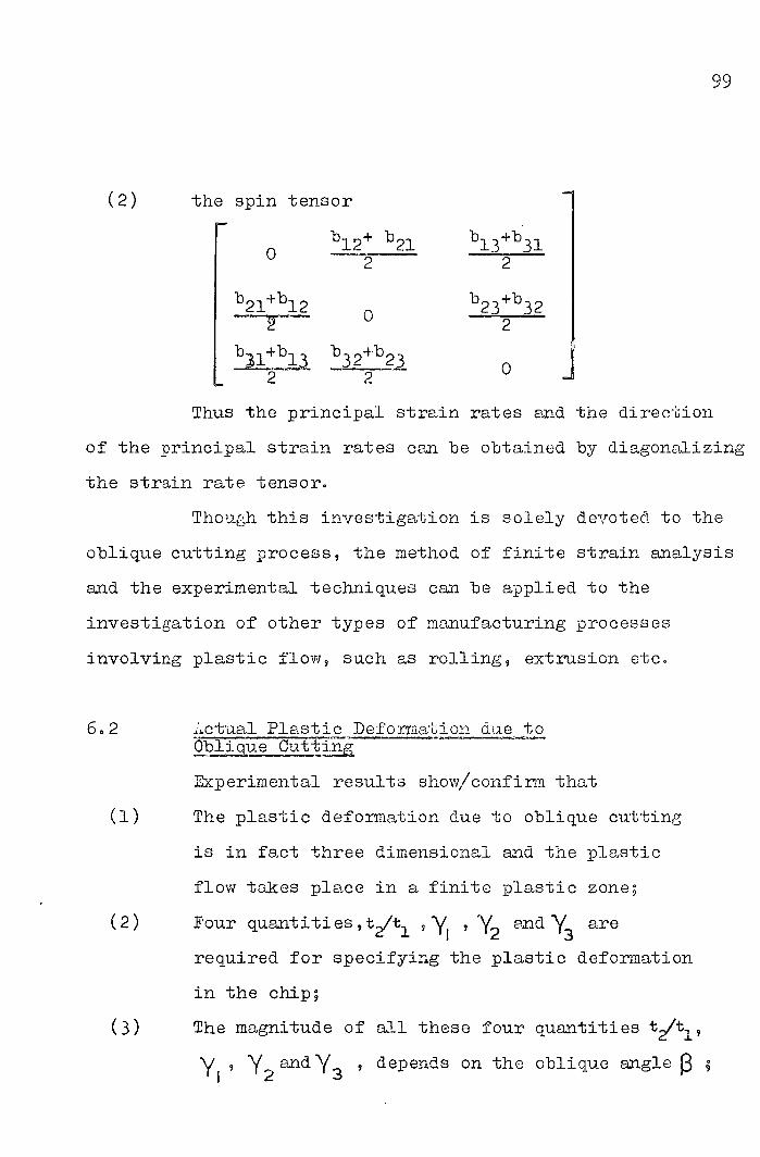
(2) the spin tensor 1 b12+ b21 b13+b31

2 I

[b2l+bl2 o b23+b32

I 2

31b +b b'.

b 32-b23 0 J L 2 2

Thus the principal strain rates and the direction

of the principal strain rates can be obtained by diagonalizing

the strain rate tensor.

Though this investigation is solely devoted to the

oblique cutting process, the method of finite strain analysis

and the experimental techniques can be applied to the

investigation of other types of manufacturing processes

involving plastic flow, such as rolling, extrusion etc.

6.2 ictual Plastic Defomiation due to Oblique Cutting

Experimental results show,/confirn that

The plastic deformation due to oblique cutting

is in fact three dimensional and the plastic

flow takes place in a finite plastic zone;

Four quantities,t/t1 , y1 , "p2 and Y3 are

required for specifying the plastic deformation

in the chip;

The magnitude of all these four quantities t 2/t1 ,

depends on the oblique angle

The strain path of material in oblique cutting

is three dimensional. i.e.the strain characteristic

index is not exactly equal to an odd integer

(although it is sometimes very nearly so);

The strain -oath of material in oblique cutting

is non-coaxial, ie the incremental strains do

not have the same principal axes with respect

to the material;

The strain rates are also three-dimensional

and non-coaxial;

While the directions of the fastest stretching

and fastest shrinking fibres in orthogonal

cutting lie in a plane (28)

those in oblique

cutting lie on a curve surface;

The principal axes of finite strains and strain

rates do not have the same directions.

6.3 Short congs of the Single Shear Plane Theory

This investigation reveals that experimental

results are not in agreement with Merchant's single shear

plane theory. The main diaagreements can be summarized

as follows:

(1) The normal shear angle O n chip flow angle f 9

shear stress on the shear plane and specific

energy etc0 are functions of oblique angle 3

101L

The direction of chip flow does not coincide

with the direction of the friction force on

the rake face;

The direction of the shear stress on the shear

plane differs from that of the shear strain.

Since the normal shear angle O n , chip flow

angle f c' shear stress on the shear plane and the specific

energy depend on the oblique angle the application of

the single shear plane theory becomes questionable.

That the direction of the shear stress on the

shear plane differs from that of the shear strain is not

surprising, because comparison of the actual deformations

in oblique cutting with those suggested by Merchant shows

that Merchant's model does not and can not produce the

actual deformations.

Investigation into the normal and shear stresses

(22 'p9) on the orthogonal cutting tool ' revealed that the

chip does not slide over the tool rake face in the whole

contact areas L.ctually the contact area can be divided

into two regions, the sliding and the sticking regions.

In the sliding region, the friction force and its direction

obey Coulomb's law of friction. However, as the normal

stress increases to a certain value, the junction grows to

such a size that the chip practically sticks to the tool

rake face and the friction force and its direction

102

(in the sticking region) is governed by the plastic flow

accurring between the chip-tool interface.

While plastic flow in orthogonal cutting occurs

in a plane perpendicular to the cutting edge, our experimental

result shows that the plastic flow in oblique cutting is

three dimensional and non-coaxial. Therefore the direction

of the resultant friction force in oblique cutting does not,

in general, coincide with that of the chip flow.

Thus it can be concluded that-

The main shortcomiigs of Merchant's theory are

attributed to his inappropriate assumption that

the deformation in oblique cutting can be

represented by a two dimensional simple shear

on a single plane;

(2) It is most unlikely that a modified definition

of the rake angle or shear angle might bring the

experimental results into agreement with the

single shear plane theory.

6.4 Cutting Forces

By the use of Albrecht's method, the cutting force

due to oblique cutting can also be separated into two parts,

the cutting force acting at the tool rake face and the

ploughing force acting at the tool edge. Experimental

103

results show that, as in the case of orthogonal cutting,

the ploughing force poss asses a constant value for a cutting

tool with a fixed radius of the cutting edge and the cutting

force acting at the rake face is proportional to the depth

of cut. Therefore, the cutting force due to oblique cutting

can be represented by an empirical matrix equation

P. P b C C C

4b P.t + bt b

Hi

where b= width of workpiece, in.

te effective depth of cut.

PC= _0.0162713 - 0.025(3+ 80

Pt _0.015(3 - 0.150 + 53

P1 = -0.02625(32 + 2 . 27 513 b=.-0.001375(32 - 0.475(3+ 15.7

b t = _0.001 0.035(3 + 4.6

b= -0.002375(32 + 0.2075(3

oblique angle, dog.

6.5 Desirable Future Invest igations

Merchant's theory is attractive both in its

simplicity and in the many possible deductions. By assuming

a very narrow plastic zone and idealizing it into a plane,

a problem of plastic deformation is simplified into one of

rigid 'bodies. Normally, observation and experimental data

104

effect theory, in this case an attractive theory produces

a reverse effect on observation and data. Thus, many people

are led to believe that the chip slides over the tool

according to the laws of kinetic friction, that the type of

deformation is simple shear and that there is maximum shear

stress on the shear plane.

is is well known, Merchant's theory for orthogonal

cutting is not supported by experimental results. Many other

metal cutting theories have been proposed, some by eetorig

Merchant's -theory, some by injecting theories of plasticity

into it and some by using semi-empirical assumptions. Of

the different ways of doctoring Merchant's theory may be

mentioned the assumption of a curved shear plane, that of

pre-flow and after flow said of single shear taking place

along a plane inclined to the shear plane. Of the many

theories proposed special mention should be made here of (30)

Lee and Shaffer's Theory , because it is based on an

entirely new theoretical foundation, namely, the slip-line

theory. However, application of the slip-line -theory to

the mechanics of metal cutting also encounters many difficul-

ties and the theory proposed by Lee and Shaffer does not

check with experimental results.

This investigation shows that Merchant's theory

for oblique cutting is no more in agreement with experimental

results than that for orthogonal cutting.

Critical comparison of the deformation in oblique cutting

proposed by Merchant and the actual deformation shows that

Simply doctoring Merchant's theory, such as

changing the definitions of the rake angle and

the shear plane, can not bring the single shear

plane theory into agreement with experiment;

i..s in the case of orthogonal cutting, the

application of slip-line theory is difficult,

if at all possible.

Recent developments in the research on metal forming

show that the visioplasticity method, such as that employed (10) (ii) by Christopherson, Oxley and Palmer is a considerable

contribution to the understanding of the metal forming

mechanics (31)

The finite strains and strain rates are

calculated from the velocity field obtained experimentally.

Then with the use of the stress-strain rate relationships

and the equilibrium equations it is possible to obtain a

complete stress field.

It is obvious that the visioplasticity method

relies on the experimental determination of the velocity

field and consequently can not be used for prediction

since the experiment must first be performed. However,

the experimental results from such investigations can lead,

through generalization, to valid theories. Once a theory

is formed, the prediction of the distributions of finite

105

strains, strain rate and stresses follow.

Though method of finite strain analysis and

experimental techniques for determining the velocity field,

finite strains and strain rates have been thoroughly

explored, to provide a complete solution to the oblique

cutting mechanics much more detailed research work must

be done.

According to the discussion above, it may be

suggested that the future research should be directed towards

the following topics:

Effect of cutting conditions on stream lines;

Effect of strain rate and strain on yield stress;

Method of determining stress field in three

dimensions;

Improvement of experimental techniques.

MGM

APPENDIX

References

M. E. MCHLNT

Mechanics of Metal Cutting Process Journal of i.pplied Physics, 1945, Vol.16, P.267.

M E. MERCHANT

Basic Mechanics of the Metal-cutting Process Journal of Lpplied Mechanics, Trans. ASME, 1944, Vol.66, P.L-168,

H. ERNST JND M. E. MERCHANT

Chip Formation, Friction and High-Quality Machined Surfaces. Trans. J.S.IvI. 9 1941, Vol.29 9 P.299.

T. SJTJ

Recent Developments concerning Cutting Mechanics. International Research in Production Engineering, LSME, 19639 P.1.

B.P. von TURKOVICH

Mechanics of Cutting International Research in Production Engineering, .LBME, 1963. P.26.

H. KOBL.YASHI LND THOMSEN

Ln ipp1ication of Plastic Plow Lnalysis to Orthogonal Metal Cutting. University of California, Institute of Engineering Research, Contract No. DL.-11-070-508-ORD-605, Final Report No.2, Series No.117, May 1959.

COOK LND M. C. SHAW

L. Visual Metal Cutting Study Mechanical Engineering, 1951, Vol.73, No.11.

107

A.B. L.LBRECHT

Chip Studies Reveal What Happens The Machinist, 1953, Vol.97, No.26.

N.N. Z0R17

Metal Cutting Mechanics Pergamon Press, Oxford, 1966.

W.B. PIJAVH. LID P.L.B. OXJIEY

Mechanics of Orthogonal Machining. Proc.Instn. Mech. Engineers. 1960 9 Vol-173, P.623.

D.G. CHRISTOPHERSON, P.L:B. OJCLEY AND W.B. PLJIER

Orthogonal Cutting of a Work-hardening Material. Engineering, 1956, Vol.186, P.113.

T.C. HSU

411 Study of Large Deformations by Matrix lgebra Journal of Strain Analysis, 1966. Vol.1 No.4. P.313.

T. C. HSU

Ln .Lnalysis of the Plastic Defamation due to Orthogonal and Oblique Cutting. Journal of Strain Jna1ysis, 1966, Vol.1, No.5, P.375 ,

G. V. STJ.BLER

The Fundamental Geometry of Cutting Tools. Proc.Instn. Mech.Ergineers. 1951. Vo1.15 , P.14.

M. C. SHL.W, N.H. COOK I.ND P. L.. SMITH

The Mechanics of Three Dimensional Cutting Operation. Trans. i.S,M.E., 1954, Vol.74, P.1055.

R. H. BROWN IND E. J. L., iBMEGE

Oblique Cutting with a Single Edge. International Journal of Machine Tool Design and Research. 1964, Vol.4. P.9.

Wool

G.V. ST.LBLER

The Chip Flow Law and its Consequence. Proceedings of the 7th International ivI.T,D.R, Conference, 1966 9 P.243 ,

N.H. COOK LITD E. G. LOEWEN

Metal Cutting Measurements and their Interpretation. Proc.1n.Soc.E:p. 9 Stress Lnalysis. 1956 9 V01.139 No.2. 9 P.57-52,

F. KOENIGSBEIRGER, K.D. LLRWLHJ LND .J.P. S.BBEFXTILL,

Design and Performance of Two Milling Force Dynamometers. Journal of the Institution of Production Engineers, Dec. 1958.

. J. P.BBERWIJJ.

Improved Three Dimension Dynamometer Engineering, 1960, Vol-189, P.401.

i. .1. J. CHISHOLM AND T. C. HSLJ

!.Microtechniquo of Studying the Wear of Cemented Carbide Cutting Tools. Report MF/MS 60, Mechanical Engineering Research Laboratory, 195 2.

T. C. HSU

L. Study of the Normal said Shear Stress on a Cutting Tool. Journal of Engineering for Industry, Trans. ASME, Series B, Vol.88, No.1, 1966, P.51.

P. LLBRECHT

New Developments in the Theory of the Metal-Cutting Process. Part 1, The Ploughing Process in Metal Cutting. Journal of Engineering for Industry, Trans. L.SME, Series B, 1958, Vol.80, P.1089.

P. V1. ViL.LLACE AND G. BOOTBROYD

Tool Forces and Tool-chip Friction in Orthogonal Machining. Journal of Mechanical Engineering Science, 1964, Vol6, No.1, P.74.

T. C. HSU

The Characteristics of Coaxial and Non-coaxial Strain Paths. Journal of Strain Lnalysis, 1966, Vol.1. N0.3. P.216.

C. TRUESDL .AND R. TPIN

The Classical Field Theories. "Handbuch der Physik", 1960. Vol. Ill/i., Springer-Verlag 9 Berlin.

L. C. ERINGEEL

Nonlinear Theory of Continuous Media, McGraw-Hill Book Co., New York, 1962.

T..C. HSTJ

Velocity Field and Strain Rates in Plastic Deformation, Journal of Strain Lnalysis, 1967, Vol.2, N0.3 P.195.

N.N.ZOREV

Interrelationship between Shear Processes Occurring Iaong Tool Face and on Shear Plane in Metal Cutting. International Research in Production igineering, IJ.SME 9 1963, P.42.

E.H. LEE fiND B.W. SHIi.FFER

The Theory of Plasticity Lpplied to a Problem of Machining. Journal of Ipplied Mechanics, Trans. ASME, 1951, Vol. 73, P.405.

E. G. THOMSEN AND S. KOBAYASHI

Indicated Directions of Materials - Forming Research Proceedings of the 5th International MTDR Conference, 1964, P.211.

32 A.K. PILL fiND F. KOENIGSBERGER

Some Lspects of the Oblique Cutting Process Int.J.Mach.Tool Des.Res. 1958, Vol-8. P.45.

110

11 J_J_ -

33. G.L. BL.RLl.YLL, J. PiEKER L11J j.77- PLOWETT

Mechanical and. Photographic Processes for Producing a Grid of Lines. Int.J,Mech.Sci. , 1963, Vol-5, P.365.

34 M.0. SILO, P-11. SMITH IiND N. H. COOK

The Rotary Cutting Tool. Trans. LSME, 1954- Vol.74.

£L. NLDL.I

The Flow of Metals under Various Stress Conditions Proc.Instn. Mech. Engineers., 1947, Vol. 157, P.121.

L.C. ERINGEN

Mechanics of Continua Joirn Wiley & Son, Inc. 1967.

L.I. SEDOV

Foundations of the Non-Linear Mechanics of Continua. Pergarnon Press, 1966.

V.V. ITOVOZHILOV

Foundations of the Nonlinear Theory of Elasticity. Graylock Press, 1953.