A Study Of Non-Linear Servomechanisms

DissertationPresented in Partial Fulfillment of the Requirements

for the Degree Doctor of Philosophy in the Graduate School of the Ohio State

UniversityBy

Chih-Chi Hsui)B.S.S.E., Chiao-Tung University, I9J4.5 M.S.E., University of Michigan , 19)4.9

1951

Approved by:

Adviser

-i-

Acknowledgement

Acknowledgement is gratefully made to Professor P. G. Weimer under whose supervision and advice this paper was written ; and also to Professor H* S. Kirsch baum for his constant encouragement .

-ii-

SC2521

Table Of ContentsChapter I

Introduction ------------------------------------------ 1Chapter II

Servo System With Amplitude Dependent Non-Linear E l e m e n t ---------------------------------------------1. A brief summary of the amplitude locus method.2. A study of a special non-linear servomechanism.3. Further study of the special non-llrear servo.

Case 1 : f(x) = k, x1'*’ , k,>0Case 2 : f(x) * k, x*' , k,<.0Case 3 : f (x) «•£ kimx **

Chapter IIIServo System With Frequency Dependent Non-Linear E l e m e n t ----------------------------------------------- 5-’1. Difference between the non-linear element N

whose output to input ratio is a function of Input frequency only and a linear element.

2. Non-linear treatment for linear servomechanisms.3. Non-linear element whose describing function

locus is a function of frequency only.4. Two Locus method to determine the absolute

stability.

- H i

5. Some discussion In finding the characteristic point pairs like (a,b) which helps to determine the stability.

Chapter IVServo System V/ith Non-Linear Element In G e n e r a l jc

1. The Introductory cases:(a). On-off servo system with a proportional

gain device connected In parallel with the on-off non-llnear gain device.

(b). On-off servo system with a derivative control gain device connected In parallel with the on-off non-llnear gain device.

2. System of describing function loci which can be reduced to a single amplitude locus, with a single modified final frequency locus.

3. System of describing function loci which cannot be reduced to a single amplitude locus with a single modified final frequency locus.

4. System stability discussion for the on-off servosystem with a pure derivative controller connect­ing in parallel with the on-off contactor device.

5. The amount of derivative control required tostabilize the on-off servo system with a deriva­tive controller In parallel with the on-off con­tactor device.

Chapter VExperimentation----------------------------------- 1611. Description of the laboratory set-up.2. Data and Results.3. fneoretical check-up of the experimental results.(I). The describing function of the non-linear

element.(II). The Inverse transfer function of the analo­

gous circuit of the motor, and the time delay element.

(ill). The transfer function of the parallel loop.(lv). The combined describing function loci of the

non-llnear element and the parallel loop.(v). Prediction of the results from the describ­

ing function and the Inverse transfer function.a. V/ithout the parallel loop.b. With the parallel loop.

4. Some qualitative oscilloscope records when the characteristic of the non-linear element is cnanged.

5. Conclusions.R e f e r e n c e ----------------- — 2 2 5

-v-

Chapter I IntroductionThe art of analysis and synthesis of linear

servomechanisms has been developed to a satisfactory degree. This may be credited to those researchers who have attacked the problem directly but most of all we have to credit the success to other scientists and mathematicians who have given the necessary and power­ful analytical tools to solve the linear system problems.

As far as the non-linear problem is concerned, no perfect method of attack has yet been developed.People have tried to attack the non-linear problem by1,2,3several methods, both graphically and analytically. But trey all have shortcomings. Among the graphical methods, the topological method seems very powerful, however It is limited by the number of degrees of freedom. ho stan­dard exact method to solve non-linear problem analytically has been given yet, except for few special cases. The analytical method, no matter whether it is the method of perturbation or the method of iteration or some other method of approximation, usually Involves much monotonous computing and equation-writing. The accuracy of the result after laboring a long time on substitution and equation- writing, sometimes may still not be satisfactory. The approximation can usually be Improved by further substitu­tion and equation-writing, which is known as high order

1+approximation. This of course means more work.

-1-

When people encounter non-linearity in linear servo-system design, they either try to avoid it or to minimize it. However in the problem of contactor servo- analysis and synthesis, the degree of non-linearity in­volved cannot be neglected. Different methods have beendeveloped to study that special problem: by the direct

5 6 differential equation method, by the phase plane rre thod,7by the Laplace transform series method^ and the most recent

one, by the frequency response method.The advantage of the frequency response me thod

will not be repeated here. However, it was shown only how the problem can be handled when the describing func­tion locus is only a single amplitude locus. The effect of the compensating networks in series with the on-off servo system can be studied beautifuJly because we stil] have a single amplitude locus. but wnen the compensating network is connected in parallel with the contactor de­vice, things are a little different. If we consider the compensating network and the contactor device in parallel as a single non-linear element, the describing function locus which was a single amplitude locus before, may turn out to be a system of loci which depends not only upon the amplitude but also upon the frequency.

We do not wish to avoid and minimize the non- linearity. We shall now try to study the non-linearity in the light that we may be able to take some advantage of

-2-

the non-linear elements. Hence we are not most likely to meet the non-linear elements whose describing function is a function of amplitude only, we may meet some non-linear elements whose describing function is a function of fre­quency only, or in general, the describing function locus is not a single locus but a group of loci which depends not only on the amplitude but also on the frequency. How to deal with such cases, expecially their absolute stability, is the main purpose of this paper.

Chapter II introduces the frequency response meth­od with a brief summary. Ihen it will be followed by a study of a special servo-system and an attempt to show that In some cases a non-linearity can help the servo perfoimanoe.

Chapter I±± deals with servo system with fre­quency dependent non-linear elements. We then take the linear element as a special case of the non-linear elements and treat it non-linearly to help to develop the two-locusme thod•

Chapter IV deals with the servo system with a non­linear element in general. The on-off servo system with compensating networks in parallel with the on-off gain de­vice is studied.

Finally in Chapter V, an experiment is carried out on an on-off servo with a compensating network in parallel with the contactor device. The results are verified with the theory.

-5-

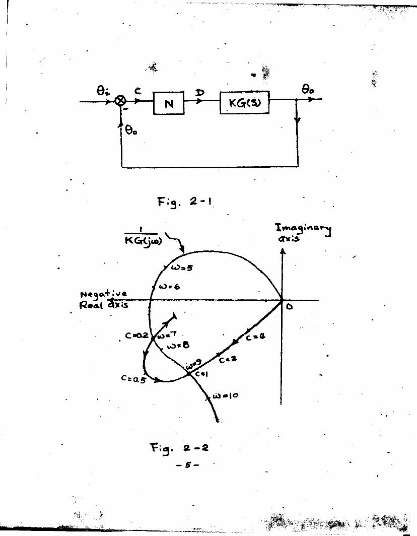
Chapter II Servo System with Amplitude DependentNon - Linear Element.

In this chapter, a servo system as shown in Fig. 2-1 will be studied. Ihe non-linear element N, is supposed to have its non-linear output response in such a way that the ratio of the output response to input does not depend on the input frequency. In other words, it de­pends upon the input magnitude only. Ihe basic techniqueto treat such a system has been developed by Dr. Kochenbur^r

6in connection with contactor servomechanism. Only a brief summary will be given In this chapter. Ihe rest of the chapter will be devoted to a study of a special non-linear servomechanism of this type, to illustrate the method and the possible advantage of introducing non-linearity.1. A brief summary of the amplitude locus method.

Ihe non-linear element is usually an harmonic generator. Input of one frequency at one end will give an output at the other end consisting of several other fre­quencies beside the input frequency. If we disregard the harmonics and consider its fundamental only, we can derive the output and input relation as we usually do with a linear element, and call it the transfer function. But in the non-linear case, the ratio between the fundamental of the output and the input Is not necessarily a constant.In the case of a contactor device, It depends upon the in­put amplitude only. Hence for one Input amplitude, we have

-4-

0 i c

' ©€

N t>K 6K$>

6 o — ►

§

F.9. 2-1

c»cx2 yC>*'7A,c«i

- 5 -

one value for the ratio of output to input, for another amplitude we get another value for that ratio. In order to distinguish this ratio from the ordinary transfer function, we call It the Describing Function" of that non­linear element.

The sytem will now be a quasi-linear one. For a certain amplitude input c to the non-linear element, It acts as if it were linear with an output to input ratioN ( c ) the describing function. This approximationmakes the ordinary frequency response method applicable to the non-linear servo.

Die determination of stability by the famous Nyquist plot for the linear system is based upon the fact that the equation,

1 t K G (S) = 0 (2-1),should have no roots in the right half of the s-plane. Die critical condition, I.e. the boundary condition between stable and unstable operation occurs when

1 + K G( j# ) - 0 (2-2)For the non-linear system as shown by Fig. 2-1,

that boundary condition will give a self-sustained oscilla­tion and it will occur when

1 + N(c)Ka( .)•») = 0 (2-3)or

- N(C) = 1 (2-1*.)

-6-

1 *V» .

Wi’Hi Co**\pe^5<v^on N « + W Of-K

XlW.

-7

It should be noticed that N(c) la also a vector quantity. The values of w and c at which eq. (2-lj.) is satisfied cor­respond to the pissible self-sustained oscillation frequen­cies and magnitudes respectively. Since both sides of eq. (2-14.) are usually very complicated, the easiest way to get the solution is by plotting both sides on the sane sheet of paper and with same scale. The intersecting points will automatically come out to be the possible self- sustained oscillation states. We notice that the right side ofeq. (2-li) Is the inverse transfer function of the rest of the system excluding the non-linear element. There­fore if we plot the left side of eq. (2-I4.) on the inverse

plottransfer function polarAof the rest of the system,we can determine the self-sustained oscillation point very easily. The plot of -N(c) which depends upon magnitude only in this case gives what we called the Amplitude locus. Fig. 2-2 gives a general Idea about those loci.

For any given amplitude c , we get a correspond­ing point on the amplitude locus. The system at that value of amplitude will be stable if that point on the amplitude locus is on one side of the 1 locus and will be un-stable if on the other side. The point on the amplitude locus Is just like the critical point - 1 in the ordinary linear servo theory. Hence in Fig. 2-2, the system will be stable when c= 2, c = I4. and in fact It is stable for all values c > l . On the other hand, the system is unstable

-8-

when 0.2<c<l. Hie system beoomes stable again when c<0.2. When o»0.2 and c-1, self-sustained oscillations occur, with #•7 and respectively. When the system is stable theamplitude c decreases as times goes on; when the system is unstable, the amplitude c becomes larger and larger. Ihe change of the position of the critical point along the amp­litude locus is shown by arrows on Fig. 2-2. It is very obvious that the oscillation state c*0 .2 , tf=7> is very un­stable, while the self-sustained oscillation state at c*l, *»-9 is very stable. Any little amplitude deviation from the point c=l, w*r9 will automatically come back to that point•

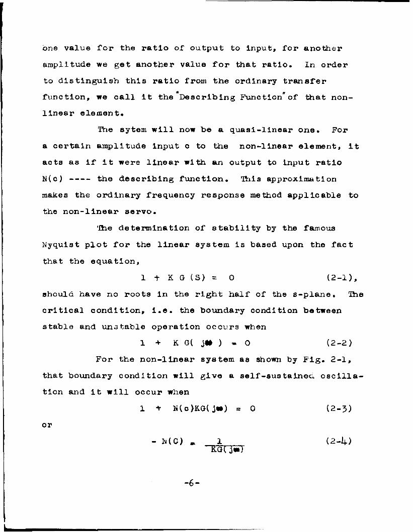
servo system. Hence it Is sometimes necessary to have compensation networks to be connected In cascade with the

no intersecting point between the two loci, i.e. there will be no possibility for the existence of the self-sustained oscillations. Fig 2-5 shows the situation.

pressed as the peak value of the output to input ratio. For the open loop, when the error is C, with an amplitude of c, then

Self-sustained oscillations are not desired In a

servo loop to reshape the so that there Is

The relative stability of such a sys tern Is ex

output (2-5)C

and we know that:Input = output + C (2-6)

-9 “

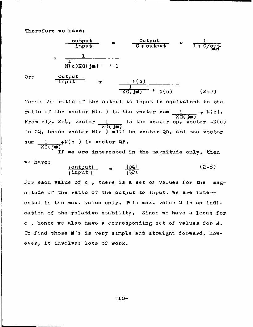
Therefore we have:output _ Output _ 1input C -t output i t C/ou£•

m c W G ( T * T 4 lOr: Output

Input =■ M( c )1tfoT j*J 4 N(c) (2-7)

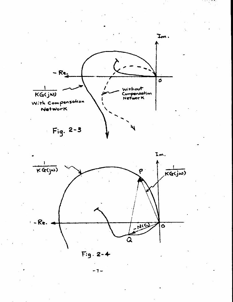
th? ratio or the output to input is equivalent to theratio of the vector N(c ) to the vector sum 1 N(c).

. KG( jw)Prom Fig. 2 - I f , vector 1 is the vector op, vector -N(c)ItCKj«)

is OQ, hence vector N(c ) will be vector QO, and tne vector sum 1 +N(c ) is vector QP.

rtoi Jew)If we are interested in the magnitude only, thenwe have:

toutputl |0Q,1 (2-8)|input | lQP\

For each value of c , there is a set of values for the mag­nitude of the ratio of the output to input. We are inter­ested in the max. value only. This max. value M is an indi­cation of the relative stability. Since we have a locus for c , hence we also have a corresponding set of values for M. To find those M ’s is very simple and straight forward, how­ever, it Involves lots of work.

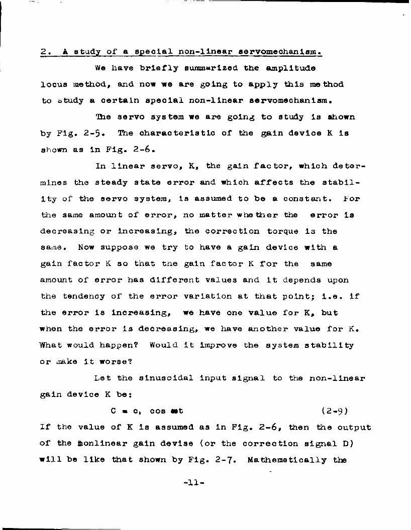
2. A study of a special non-linear servomechanism.We have briefly summarized, the amplitude

locus method, and now we are going to apply this method to study a certain special non-llnear servomechanism.

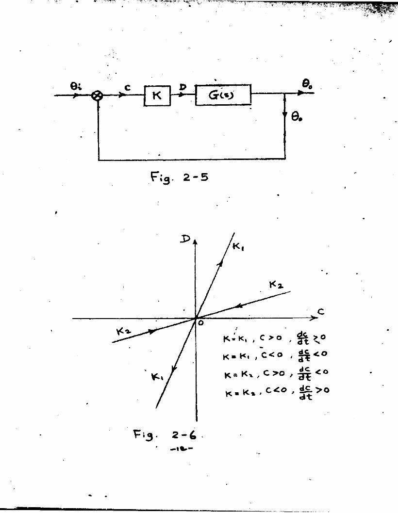
The servo system we are going to study is shown by Fig. 2-5• The characteristic of the gain device K is shown as in Fig. 2-6.

In linear servo, K, the gain factor, which deter­mines the steady state error and which affects the stabil­ity of the servo system, Is assumed to be a constant. For the same amount of error, no matter whether the error is decreasing or increasing, the correction torque is the same. Now suppose we try to have a gain device with a gain factor K so that the gain factor K for the same amount of error has different values and it depends upon the tendency of the error variation at that point; I.e. If the error is increasing, we have one value for K, but when the error is decreasing, we have another value for K. What would happen? Would it improve the system stability or make It worse?

Let the sinusoidal Input signal to the non-linear gain device K be:

C » c, cos set (2-9)If the value of K is assumed as in Fig. 2-6, then the output of the Nonlinear gain devise (or the correction signal D) will be like that shown by Fig. 2-7. Mathematically the

-11-

F . 3 . 2 - 6

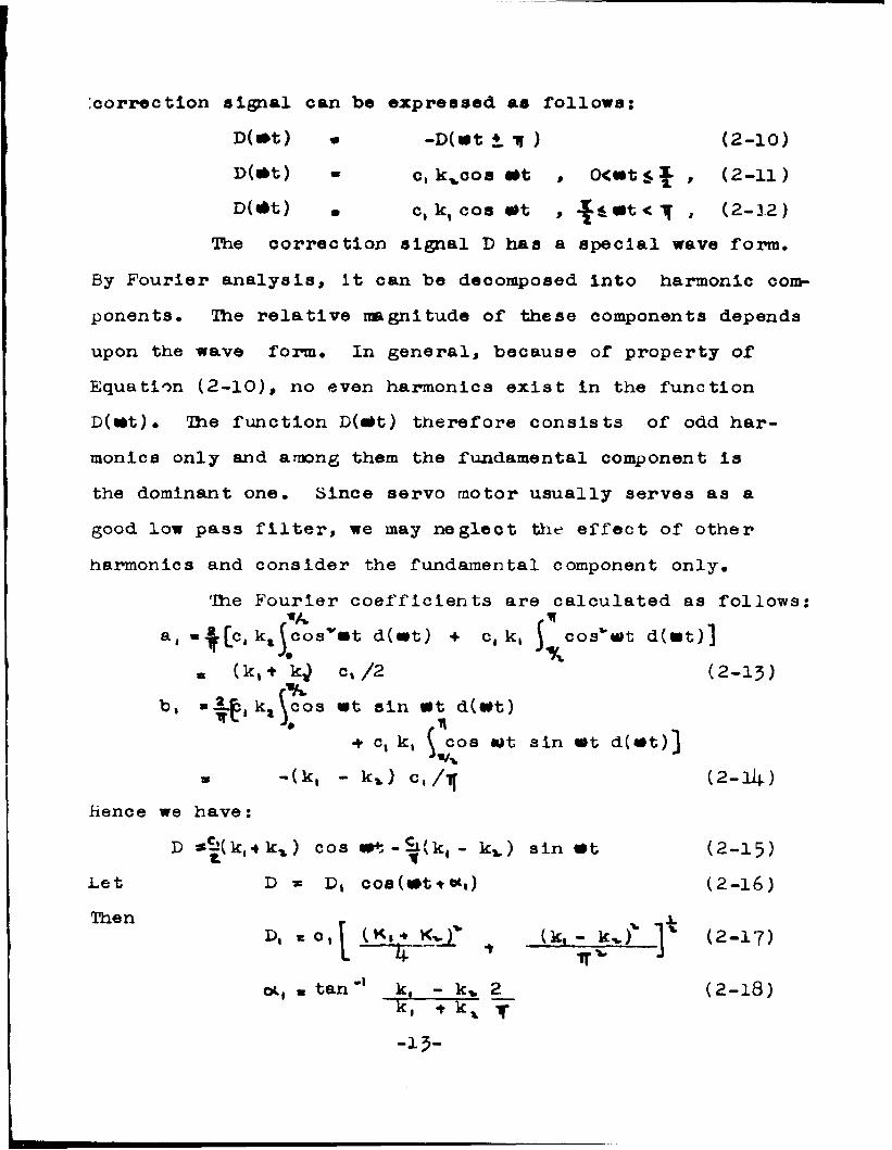
Correction signal can be expressed as follows:D(*t) • -D(#t ♦ ff ) (2-10)D(*t) - c, kvcos «St , 0<«*t$^ , (2-11)D(#t) m c, k, cos s>t , Sit < , (2-32)

(2-10)

The correction signal D has a special wave form.By Fourier analysis, it can be decomposed into harmonic com­ponents. Ihe relative magnitude of these components depends upon the wave form. In general, because of property of Equation (2-10), no even harmonics exist in the function D(*t). Ihe function D(«*t) therefore consists of odd har­monics only and among them the fundamental component is the dominant one. Since servo motor usually serves as a good low pass filter, we may neglect the effect of other harmonics and consider the fundamental component only.

'Ihe Fourier coefficients are calculated as follows

* (k | + k^ c i /2 (2-13)

-(k, - k*) c,/if (2-34)Hence we have:

LetD * £ ( k , k * ) cos tat -^(k, - kv ) sin mt

D * D, cos(*t + *i)(2-15)(2-16)

ThenD, ■tot, « t a n k , - kv 2

k . ♦ T-13-

(2-18)

Q — Controld Xnpot to ti>e non-l»n«*r 9«»n device )

jp ___ Correction! signet j\ Oootpat *rKe non-l^eor- ^ device J

F i 3 - 2 - 7— *M> -

v

If k, > kx , ot, Is positive. Attention is called to the fact that W, is independent of the value c, • The describ­ing function of the non-linear gain device is defined as follow:

N = D/C (2-19)In our case, we have:

N r D,/c, ISLiT (k, ♦ kv)' (k, - k-w)'* 1* * J^tlsL+ t~]LSL (2-20)

.v XWhere T (k, * kj (k, - k„) i_rv, * l— V + — v ^ j (2- 2i)

and it is also independent of the value of c, •Since both and ot, are independent of c, , the

vectorN is therefore a fixed one, once the gain factors are specified. In other words, the amplitude locus is a point.

With k, a k x ,»0, we then have /V = X , L °which is exactly the linear case.

If k, k v, we have to study the system from the Inverse transfer function plot, Wtih k,-^ k v, o<,will be negative, the position of the amplitude locus, wnich is now a point, will be now as shown by Fig. 2-8. With k,> k^

will be positive and the position of the amplitude locus will now be as shown by Fig. 2-9. For the inverse transfer function locus (the frequency locus) as shown Inthe two cases, it is obvious that when k^< k x, the stabil­ity is impaired, but when k, > k x, the stability isimproved. What 0<tdoes Is to shift the position of the "Criterion axis"

-15-

(the negative real axis) with respect to the transfer locus. The effect of the angle 0(, is somewhat equivalent to a phase shift network, *hlch shifts the angle lead or lag the same amount regardless of the frequency.

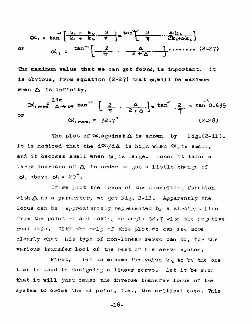
But even when o^,ls positive, It does not necess­arily benefit the system. It may impair the stability too. Ihis is because the magni tude changes rapidly with <, •In order to find the relation between the values ofk, , k x, ot, and , we assume k, > k,,, and k^is fixed to meetthe steady state error requirement.Let

k, - k v - h-kv (2-22)

thenk, ♦ k x = 2 k x + Kv- A (2- 23)

From equation (2-21):a T (2k ^ A - k „ ) V + £*' k Z (2-21+)

J < . A ' ] * (2-25)where

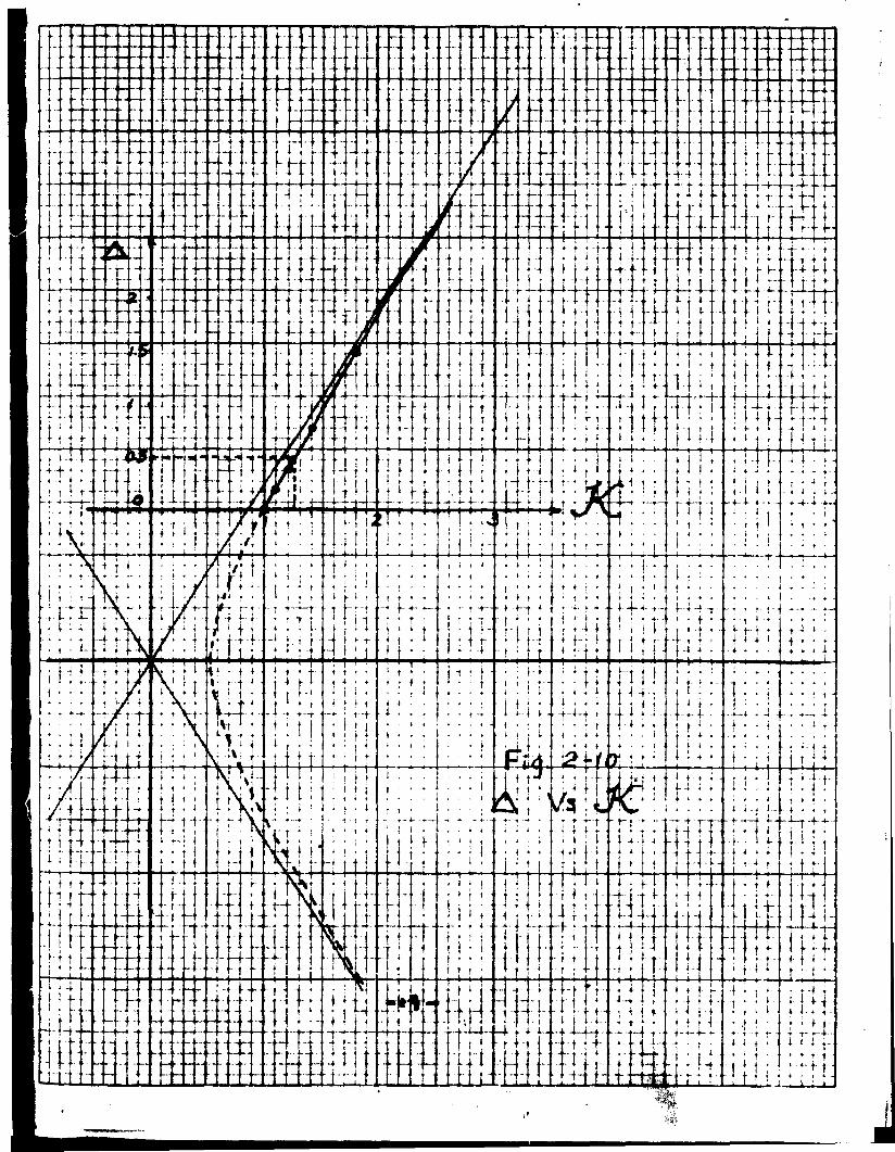
Hence after reduction, we have:2.86 j C . - ( 1 .^3)**' * 0.82 ...... (2-26)

If we plot against JC we will have a section of a hyper­bola as shown by Fig. 2-10. It Is obvious: since K can not be less than 1, the rate of increasing th £ is approx­imately a constant.

The variation of the angle oi.x with & can be seen from equation (2-l8):

-16-

In*.,»*SV

O , Is n e 9^+;ve

Fi3 . 2-8

axisc*

o(, is positive.

- o -

-* r k, - k v 2 i tari‘*T 2_______ a*k^. 1OC, a tan L k, ♦ TT J® t T 3

or , tan*' \ 2 & *1......... (2-27)<*< = l- T - ‘ “ "S+'A J

The maximum value that we can get foroi, ia important. Itia obvious, from equation (2-27) that o*,will be maximumwhen A is Infinity.

_ Lim -i r _ -ltan I 2. . - tan 2 = tan O .655

L T T T 5 j torC><,^. » 52.7 (2-28)

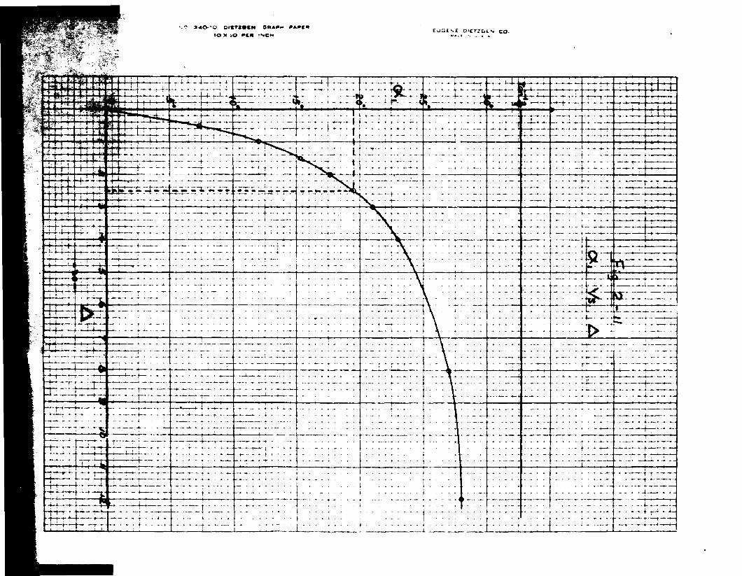
The plot of Of, against A is snown by Fig.(2-11). It is noticed that the d^i/dA is high when <1 is small,and it becomes small when c , is large. hence it takes alarge Increase of In order to get a little change of©I, above * 20*.

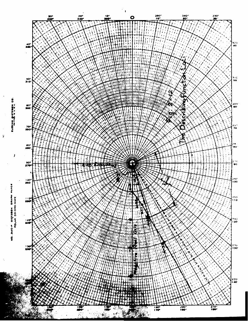
If we plot the locus of the describing functionwith as a parameter, we get Fig. 2-12. Apparently the locus can be approximately represented by a straight line from the point -1 and making an angle 32.7 with the negative real axis. 7<Ith the help of this plot we can see more clearly what his type of non-linear servo can do, for the various transfer loci of tne rest of the servo system.

First, let us assume the value to be the one tliat is used In designing a linear servo. Let it be such that it will just cause the inverse transfer locus of the system to cross the -1 point, i.e., the critical case. This

-18-

ut

rJ , i

■ i— l

+-r-

>■«»

3 * 0 - ’ 0 DICTSSCM 5«APh PAPER to X to PER INCHcuuts£ oicrjGtN co-

$Ft.r:Trr

40”K X \ \ >

, \

50"JIO

•O"»oo

*70*

1 0 0MO

90* 20°IM * 940*

\ v\\\ • \* ■" V\V.M\

>0°r * r -

■\Vv \ ‘ -

T ?

350"10*

\VVVC'.A,i* V^ > v

: » \ V

x\Xv -A ■ -

* t!

tii

<>V

• \>' v„/*' >■ a ;, a\vVX.V*"V'iVuvU'*U+

\W . tvmT

y A ,

'X/SX,x - ; .

v / / ,

v k -;.

" X L

•J-M

f >0*

120*940*

7 7

■ m w J h u L !

TH "T*7-

340 *90"' '77;/-/

i j 7,7 7/7 ' */ W

f/r.7 • /. ■i j

. / / ’

/ / ■' j i,

V.

- r ^ W ■/.' 7 a,

/ . &

m m k w '

™ !!m «, , , , , , /A /M /';

. / - s / X - // ■

• X.

V , ■

■ v

Lil: x

‘ In*<■ / /"' AUthr-t-’ > . L W f W W v H- v.: ' % •. V

■.-a

A£x x -

>

444-

vv;

x

>• V S ' V '>k

X \

vV >•- V J

•MLu'V, A ‘hi*

■ N S M Z & ' M W r L * '

X - Zffl'fcffiWMWti\ 7

X

'/■/,>

•Ufi+ii

o<w/m u.

*y7///St i/•7i f •

’! - !, MW

tLLm

f ;r-;

-f

: -X S I

-U .

' w '

m m ., j ..:■>■ ■] i I f : ♦ ;f ?+L ill

y . m

. V -VV . - y '■■' \ ' V

^ .

. a a i W

■ 7 y.M< . . / n

..<■

\WW\w

r \ \

X . M

' V v

X \ A '

</ • -• / •• •

7j

v ;X '

ill'

v \ \ v ' 7 > -L \ ' ’

< V \ > \ y S o . * , X * V• v u - V A . \ v ' iL^¥l> W \ V * _»\ Ju \ * V s i vV * \ i ‘ \ y v . > \ x X v A' * \ * \ \ * V V v

V '

-'.v>t - \

■ •' • W*A> ' • • V

M m - ' ; V * V '

\ \ \ \ *.' > r ' *

' / ,

/ A ,

190®

- VV\‘ \■r.AA.v»<* ■

200 ' '

» 0 O '

> ‘ - *3 v' X^ \ y.

y . ' X X ' X '

12 0 40

1 t C 50

JOO• o

2fyO70

?«■ ■ 8 0 '

2 ■’ O 9 0

2*>nt o o

? ? 0 1 1 0 ‘

2 4 0 1 2 0

2 10 190'

220 '1 4 0

210"

&

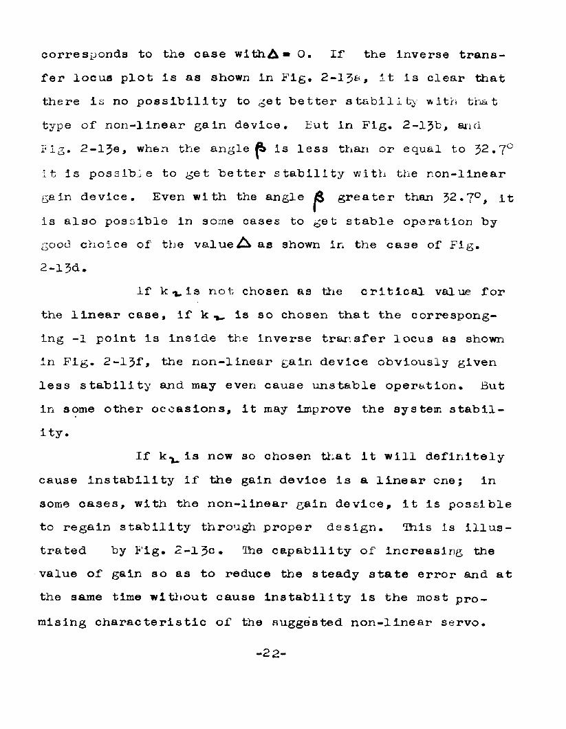
corresponds to the case w i t h & » 0. If the Inverse trans­fer locus plot is as shown in Fig. 2 - It is clear that there is no possibility to get better stability with that type of non-linear gain device. But in Fig. 2-lJb, and Fig. 2-lJe, when the angle is less than or equal to 32.7° it is possible to get better stability with the non-linear gain device. Even with the angle ^ greater then 32.7°, it is also possible in some cases to get stable operation by good choice of the value A as shown In the case of Fig. 2-l3d.

If k v is not chosen as the critical value for the linear case, if k v is so chosen that the correspong- ing -1 point Is Inside the inverse transfer locus as shown in Fig. 2-13f, the non-linear gain device obviously given less stability and may even cause unstable operation. But in some other occasions, It may improve the system stabil­ity.

If is now so chosen that It will definitelycause Instability if the gain device is a linear one; In some cases, with the non-linear gain device, it is possible to regain stability through proper design. This is Illus­trated by Fig. 2 - 1 3c. Ihe capability of increasing the value of gain so as to reduce the steady state error and at the same time without cause instability Is the most pro­mising characteristic of the suggested non-linear servo.

-22-

C O Cd)

F;3. 2-13 - » 1-

The design technique of such a non-linear servo is therefore very simple. Of course, the first step is to determine whether or not the system considered is suit­able for such a non-linear gain device. There are certain types of servo systems which are definitely unsuitable for this kind of non-linear gain device, such as the case of Fig. 2 - 1 So we draw the inverse transfer locus first. Through the cross over point on the negative real axis draw a line making an angle of 32.7° with the negative real axis. From the relative positions of the inverse transfer function locus and the 32.7° line we can easily see whether the system can have its performance improved by such a non-linear gain device or not.

The second step is to determine what is the max­imum possible k ^ which is allowed without causing instabil­ity. This can be done by shifting the 32.7° line along the negative real axis so that it is tangent to the inverse transfer function locus (in the third quadrant only). The position of the end point of this 32.7° line on the neg­ative real axis gives an approximate value for the upper limit of the value of k .and also the minimum possible value of the steady state error.

The actual position of the operating point on the 32.7° line depends upon the degree of relative stabil­ity. The U criterion can be applied here too. So shift the 32.7 degree line along the negative real axis first to

—2i_p—

a position to meet the steady state error requirement and then try along this 32.7 degree line to find the point which gives the largest circle that tangent to the Inverse transfer function locus. The relative stability of the system can be recognized from the size of that circle.

From the study of this special non-linear servo system, we can get the following conclusions:

&• It is possible to have the performance of a linear servo Improved by introducing a non-linear element into the system.

b. The introducing of a non-linear element Into a linear servo may be suitable for one system but harmful for another.

c. T e special non-linear gain device used In the above study acts as a phase advancing network but it shifts the same angle for all frequencies.

d. One bad point about the above non-linear gain device as far as operation is concerned Is that the phase advance Is limited to less than 52•7 degrees.

3, Furtiier study of the special non-linear servo*The non-linear ^ain device we used before has

two different gains k, and , both are constants. Vi/e shall now try to modify the non-linear gain device a little bit. We o till assume k^, to be a constant, but not k ( • The gain k, is now assumed to be proportional to the some power of the magnitude of the input to the non-linear gain device.

Let the input to the non-linear gain device (the control signal) be:

and assume the corresponding output of the non-linear gain device (the correction signal) to be:

C • c , cos •» t (2-29)

= f(C) 9 y z < tit < TT 0 < «*t <. ^/2

The Fourier coefficients are:

2 . A (2-31)

^ ( f(c, cos s»t) sin wt d(«*t)}

(2-32)- 2 6 -

Hie correction effort will besD * D, cos(«t*d) ...........................(2- 33)

where 0 * arc tan • (-b/a) • arc tan . (-B/A) .......(2-3 4-)Prom the previous study, we know that we want

Ck to be positive in order that the non-linear gain device shall have the same effect as a phase advancing network. Therefore B rnvjist be negative. Since k xc,/2 is positive, from equation (2 - 32), f(c, cos #t) sin w t d(*t) must be n e g ­ative. But we know that sin #t is positive in the interval ( V , if ), hence f (c, cos <#t) should be negative in the in­terval ( T ,tj ).

Case 1: f(x) is in the form k, • x"" (k,>0)In this case k,* c,m cos’*' wt must be negative in

the interval ( ^ ). But cos wt is negative in thatinterval, hence m must be an odd number.

We can then assume that:f(x) * k, c, cos «*t ................. (2- 33)

If m < 0 , then •when cos #t Is zero, f(x) has to be Infinite, which make it impossible to realize such a device in preactice. Therefore we can disregard those cases.

If in> 0, the general Fourier coefficients will be as follows:

a s | L k v 008 m t <*(**) J

b « 3L k ^ c , /2 k , j c ^ c o £ " W sin *t d(#t)3

(2.37)If the describing function is;

N « D/C - (D. /cj Z£ii * j ( tlSL>. (2-58)then

-» . -«tanOC, * tan (-=£)r K.C,'*' K-w2W *2 " ---_p. ir c»«**

l - I T + 1

(2-59)tW .V

* . • - I - [ lE* £ - * i - c" >

. , *,0?"* - K^ n ^. ( 2 - 4o )+ (2m 4 2- tT'J

When m » 0:r*L a arc tan. (k» - k-w) (2) (2-4l)' (F,“ " Tc'J ’ Hp

^ (k, + k v / + (kt JV. ..(2-142)

which is exactly the case we have studied before.If m > 0, from equations (2-59)> (2-4.0) we can

see that for any fixed value of m, when c approaches zero;OL, — . tan’1 -k-wA> >- (-2.) — *• - 52.7°

IT A T(2-45)

<j C , * (1/4-t-i/ir^ k^.= 0 .- - ......................................... _ 595k^ 0.6 k. (2-44)

Hence for all positive valhes of m, the amplitude

-28-

locus will end at an angle Ok, s - 32.7°, which is equiv­alent to a phase lag instead of a lead. But one interest­ing point is that the value of^£(is only 60;£ of •

We are not satisfied to look at that partic­ular pair of values for^^and ©<( only. Let us find thegeneral tendency of the variation of ^(ando<t as c, varies.

Set d^fydc, * 0, we have:

■x ( KiC,^ Ky \ ***K, _ )v XVM4X x / Cl > * ° (2-1+5)

hence c*"" *» 0, or c, * 0 (2-1+6)also after reduction and simplification:

\ _ »•*••• (>""»»)_ Kv he-vi ~ x q.U -- _____________

1 Vi t I- »*£••• \v (2—1+7)C » , 0 ■* T [ a-lf... )

Consider the numerator — 1-— - -* "— c*-— *0 we noticea a..u. ...that it will always he negative for all positive values ofm. In other words, no real value of c, can be found tosatisfy the equation (2-1+7). Hence the minimum value forJ C . is when ct = 0 , w i t h ^ ^ s 60% k t , and the value of K ,

increases and goes to infinity when c ( is increased fromzero to infinity.

From equation 2-39* set d(-b/a) /dc, s 0, wehave; ___K|>w» c

1__________KVX.„ „ i» C l (KvX + k , V »L-: JU - 1 c*")a \ 4* t 2« ••• *v)

(2-1+8)-29-

After simplification we find that the only possible solu­tion Is at:

|. ........ ( Vi) —K, |. ....... V T I * ^ Q

2* ^ x ' * 0O .......... (2 -14-9 )

i.e. when c, * (2 -50)nence the Min. o*., is at c, * 0 , and ^,*£-32*7 degrees. The Max. Ot, is at c,*oo and depends upon the valueof m:

.r«£ 1 !

For

m*l

0 ,

. 2.14-.6...... (2mv2 ) . . (2-51)

(2-52)

_ i i.= tan -y

Oi ■= t®** ^ If, *»**.■» tan -p*

0 <. * tan 4rv , «***. — r if*. tan*1 xlfe. ±.

515e tc.

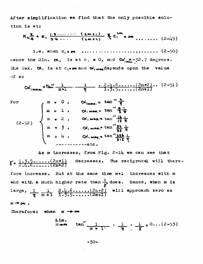
As m increases, from Fig. 2 -1I4. we can see that.5*5...... (2m+l) decreases. The reciprocal will there'Zk-.b ...... (2m+2 )

fore increase. But at the same time m+1 increases with mand with a much higher rate t h a n d o e s . Hence, when m is0large, 1

■q rn

m 00 .Therefore: when m -

Lim.

1 2 .li-.6.......(2klt2 ) w+ 1 I.5.5...... (2m-r 1 )

111 approach zero as

tanm 1 * 1 ,0...(2-53)

X

- 50-

m *

"Ptg. 2.-15

Th.e value of J C at whichot.sO la also of Interest. The angle o<(* 0, when (from eq. 2-39)

- (m+1 ).k v / k ............................. (2-5I1)From which we know that when:

m » 0 , the amplitude locus willnever cross the axis

m ^ 0 , then:

^ ' (at“'*0) = [ i ♦........ (2-55)

Hence, for:m * 1 r ^ x.■» - 2 , J C , . i i k % . k ^

m * 5 * >C, * -ft*!. = (,S/i«-) k„ e tc .

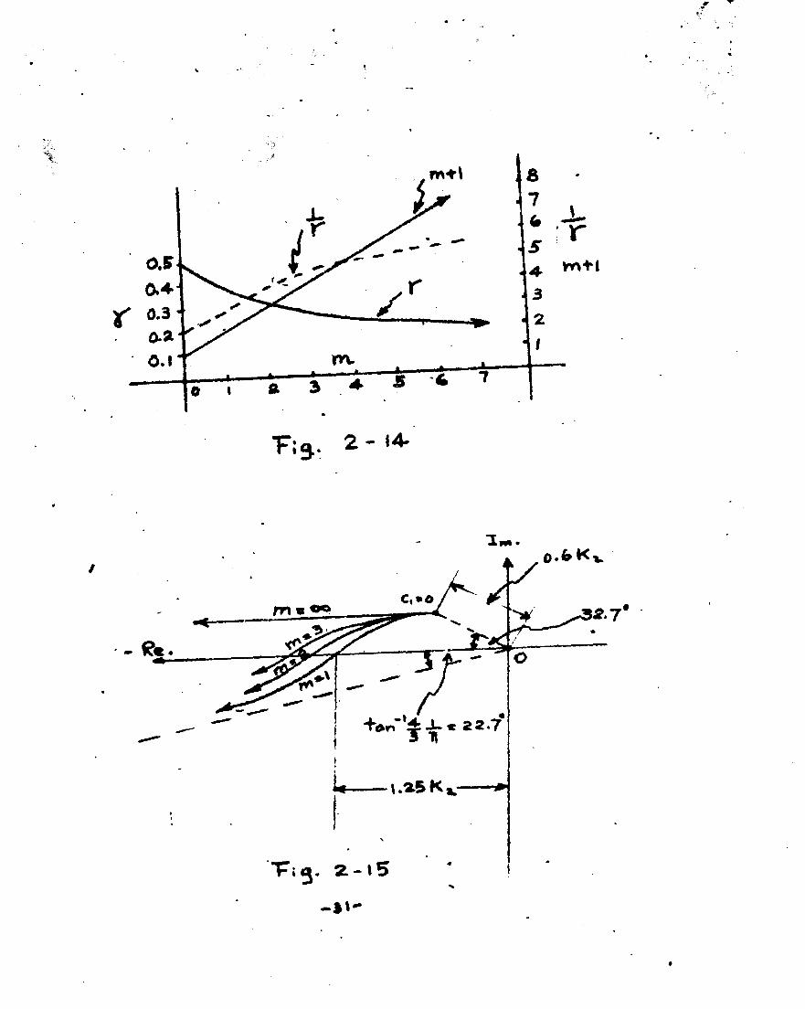
' m s 00 , 1 « 00Therefore the amplitude locus will cross the axis with a magnitude greater or equal to 5icv/ 4-» which is of course greater than k v.

If we draw a rough sketch for the possible ampli­tude loci we have something like those in Fig. 2-15.

From Fig. 2-15# it Is very clear that if f(x) be of the form k, x , wlth.k, > 0, the phase shift will beeither lead or lag, depending upon the value of m and the amplitude c( • As far as maximum equivalent phase advance is concerned, the case with m * 0, i-.e. the special case we

-32-

*' ' * -, ■-

* * •.* . -S'5"

x~*.

F ; 3 . Z - i L

w -

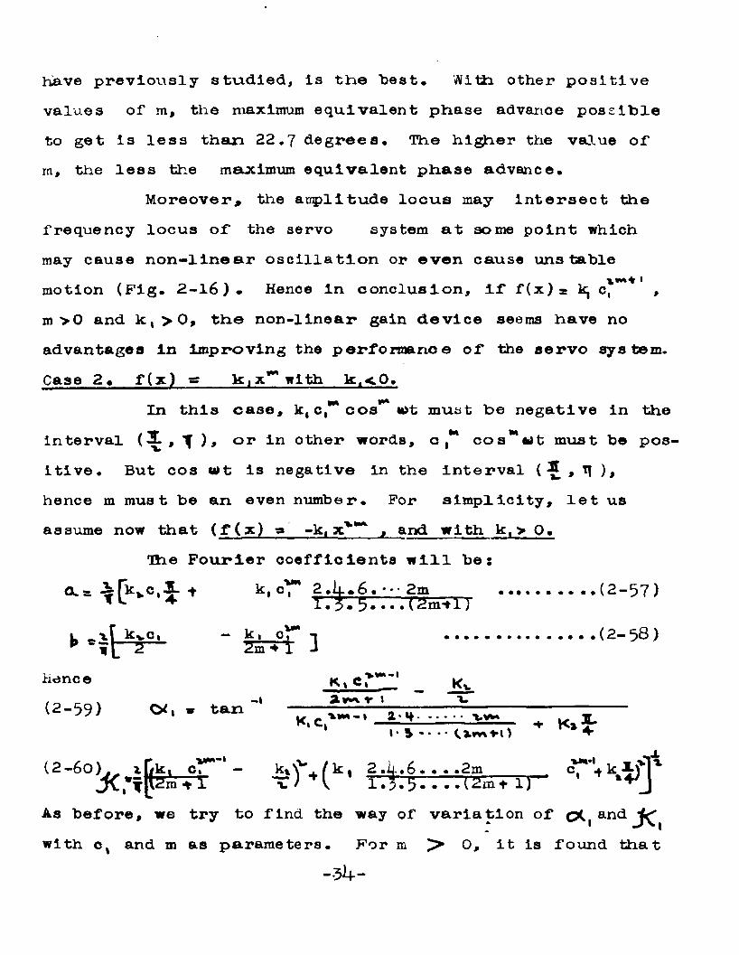
have previously studied, is the best* With other positive values of m, the maximum equivalent phase advance possible to get is less than 22.7 degrees* The higher the value of m, the less the maximum equivalent phase advance.

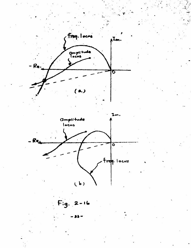
Moreover, the amplitude locus may intersect the frequency locus of the servo system at some point which may cause non-linear oscillation or even cause unstable motion (Fig. 2-16) - Hence in conclusion, if f(x) s kj c, , m >0 and k, > 0 , the non-linear gain device seems have no advantages in improving the performance of the servo system. Case 2* f(x) ■& lCiX^wlth k.<0.

In this case, k, c, cos a>t must be negative in the , f ), o r in other words, c, cos st must be pos­

itive. But cos ist is negative in the interval ( , tj ), hence m must be an even number* For simplicity, let us assume now that (f (x ) g -k, x v>~ , and with k , > 0 .

The Fourier coefficients w ill be s♦ m : ...........

‘ ] ( 2 - 5 8 )

HenC® K * C » __ Ky(2-59) CX( - t a n “' f . . 7 " ^ --------- ^----

(2-60). x |/3<ca Cr ' - /k. 2 .if.,6 ... *2m c ^ k l f l 'iC.'fjfem'-rr i . 3 .5 - • • M s m T T j " 1

As before, we try to find the way of variation of CX, and with c, and m as parameters. For m > 0, It is found that

-5k-

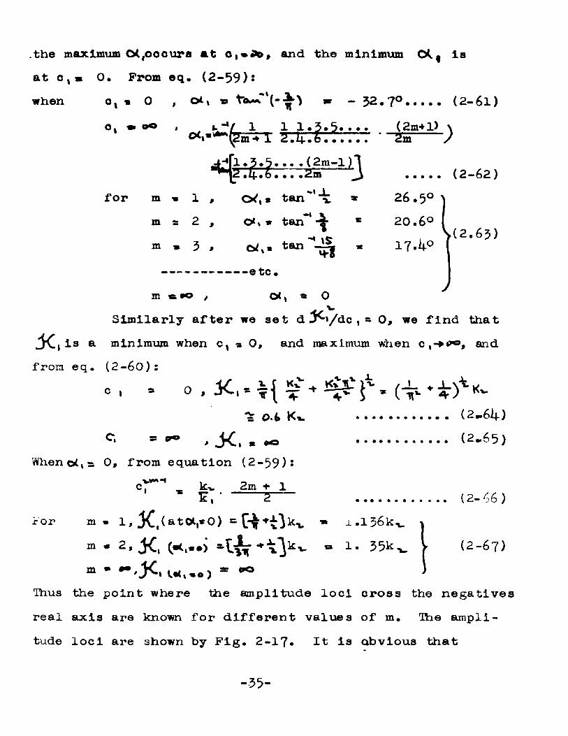
.the maximum <Xfocours at c , • Ao , and the minimum 0 .| is at c,* 0. From eq. (2-59)*when °t * 0 , o i x 9 td** ,(--3|*') v e - 32.7° ..... (2- 6l)

# *."*/ 1 11.3 * 5 . . * . (2m+l) \<*.— ( S S T T S.b.t . . _____ ‘ SS )

A - h *3•5••- •(2m - l )1 2m J ..... (2-62)

for m m 1 , o^, * tan '* \ * 2 6 *5°m s 2 , O** * tan”* * 20 .6°

. S(2.63)m » 3 * crft« tan * 17.4°------------ etc.

m c. 90 , &L, 9 0Similarly after we set d 3^'/dc , » 0, we find that

4 C , is a minimum when c , » 0, and maximum when andfrom eq. (2-60):

c, - 0 . ( V * ) * " * -■= O.t K<. ................. (2.6)4.)

= o** > X . - — ................. (2'6 5 >Whenot,s 0, from equation (2-59)*

c y *"1 _ k-w 2m + 1E, ' .... 2... (2-46 )

For m • 1 , X , ( a t « > *0 ) “ C Hhil kx * i.l36k x. \®> » 2 » J C « * • > “ 1 - 55^,. I (2 -67)m - -.jK. » «° '

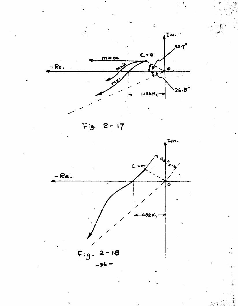
Thus the point where the amplitude loci cross the negatives real axis are known for different values of m. The ampli­tude loci are shown by Fig. 2-17* It Is obvious that

- 35-

tr • ■*

V : 3 . 2 - 1 71

Re.

2-18- l i -

Fig. 2-17 is similar to Fig. 2-15; hence the same conclu­sion can he applied.

So far we have considered only m > o, for m * 0, the case will be different from others. Hie Fourier co­efficients ares

a = k v * C '^ * k '^ (2 -68)• c./x. ~ k » \ .......................... (2-69)

C * , ■= tan k i - k v.c , /2 (2- 70)k i ■+ k jc , ■n/4-. y

J C (= - ItJFpr.................. (2-71)when c, « 0 , $ C % « wo (2 -72)

C* , = tan'1 a 1+5°....................(2- 73)

ot,- tan-’c- = -32.7°..................... (2-75)Wnen 0(,s 0 , from equation (2 -70) and (2- 71):

c, -s 2k ,/kw (2 -76)

j c . = 1^ 4 - 1 • k - & , - 0,82 l2' 77>Whenf^»kfc, o, » 1.31 k, /kv .................... (2-78)and o*, « 9-7° (2-79)

The amplitude locus with m s 0 is shown as in Fig. 2-l8. It is interesting to note that the maximum equivalent phase advance reaches 1+5 degrees.Case 3:_____f (x) ~ k,^xT

Hie study of the non-linear gain device with f(x) as a linear combination of k ||Wx*** may be grouped into following types:

- 37 -

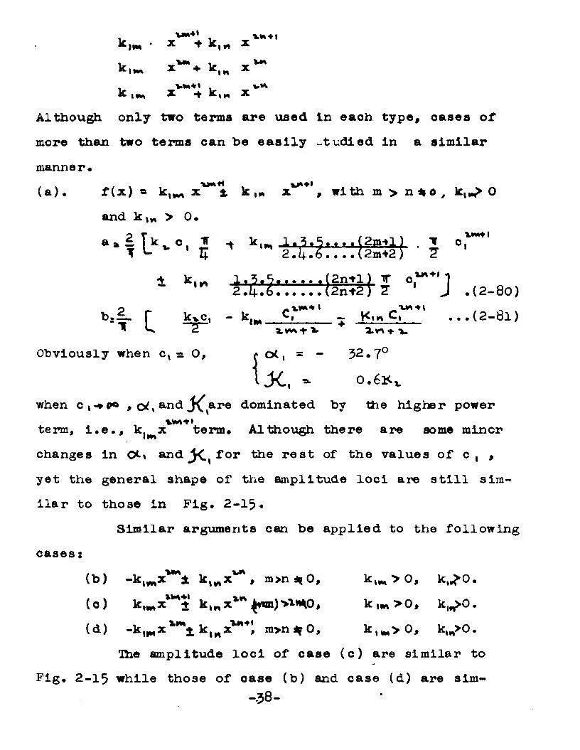
Although only two terms are used In eaoh type, oases or more than two terms can be easily studded in a similar manner*(a). f (x) » k,^ x'** ± k ,* x***' , with m > n * o , k t > 0

and k tM > 0 *c,

- K m ... (2-8l)I n •* *u

a » | T k v o, J ^ k,„ , IT u 5 2 *l+.6 ....(2m +2 5 2

— • • • (2 n t l ) T o r '1 02*4.6......(2n+2 ) 2 J *(2-8o)o . /* i

f £i°. - * , m — £i____

Obviously when cv =. O, n oC , = - 52.7°

\ jK., » o.6k vwhen c , p© » Oiy and X, are dominated by the higher power term, i.e., term. Although there are some minerchanges in G*-\ and for the rest of the values of c , , yet the general shape of the amplitude loci are still sim­ilar to those in Pig* 2-15*

Similar arguments can be applied to the followingcases:

(b) Vm , vn _-klmx ± kt*x , m > n * 0,(o) k^x**? k * * x*n un) >1*40, IM 0 # kln>°.(d) ~)£xmx Xm± k|Hx'l,,*l m > n ^ 0 , k,*,>0 , k,n>0 .

Ihe amplitude loci of case (c) are similar to Fig. 2-15 while those of case (b) and case (d) are sim-

ilar to Fig. 2-17.Although the amplitude loci of the above Tour

cases have no appreciable changes from Fig. 2-13 and Fig* 21-7, when we consider the following special oases, we will find something different* They arej

(e)

(e) lc,x t x 1 m > 0 9 K > 0 , k >0in.

(f) k, x - VW m > 0 9 k, > 0 , k ,>0(6 ) ~k, -*• k x^ 1K i w x * m > 0 9 k t> 0 , KJt 0(h) -k 1 - m > 0 9 k t> 0 , ^ > 0(i) -k * «* K m * » k ,>0 9 k,> 0 .f (x) «. kx ♦ k im.* . -1 m >0 f k,>0

1 r , * 1, , U * ***** tt a * tt * c- J(2-82) J b s «2u J" Kxti _ KiCi _ -i1 H L ■*- '■*

K. - . K ivm C,*~= 1a*ne - J t K . + K v ) -* \ »’ > ‘• • •<*»?♦*>+ ^ 2-M-- •

W - A [ ( ISiiJSv * VIf L v »■ /, ir(Ki*>Kv) _ it i> i*V- C»"**0 + ( 3r ^ K,m vtf; cw%v) ^ JWhen c, » 0 , o <., ® tan"1 JL K.-K-*. ...... (2-8 3 )1 IT lCTt<LWhich is exactly the same as the case we have studied p r e ­viously. As long as k^»k>0 , CX,>0.

When G 00 , the tenn k,^x dominates and ,will depend upon the value of m. From equation (2-52)

O C , will never exceed 32.7 degrees.The variation of CX, and can be predicated by

/

the same treatment as before. Ihe amplitude locus depends upon the relative magnitude of m, k, and k x • Fig. (2-19) shows the different cases. Fig. (2-l9c) is for the case

-39-

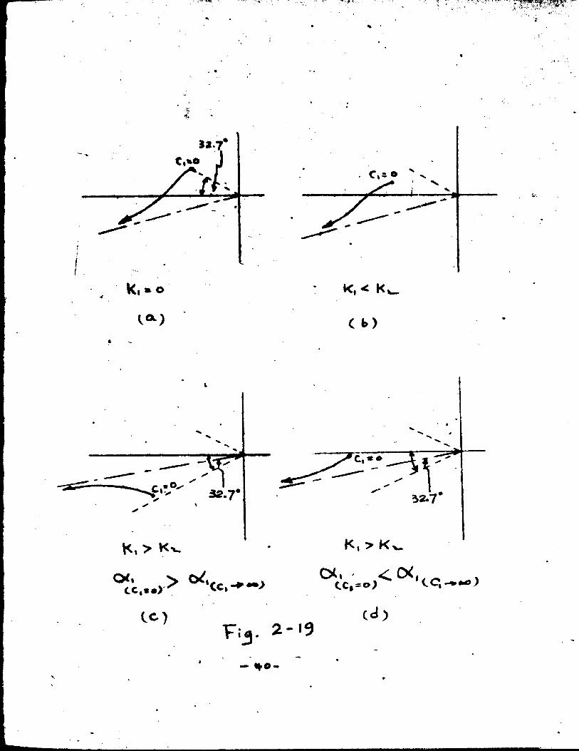
V'- -TTi * r.-:

Ki» o

V

( b)

K, > K

cc,,o,< 0 <:,C c ; ^ - >

tc-)Fij- 2 - ' 9

- «*o-

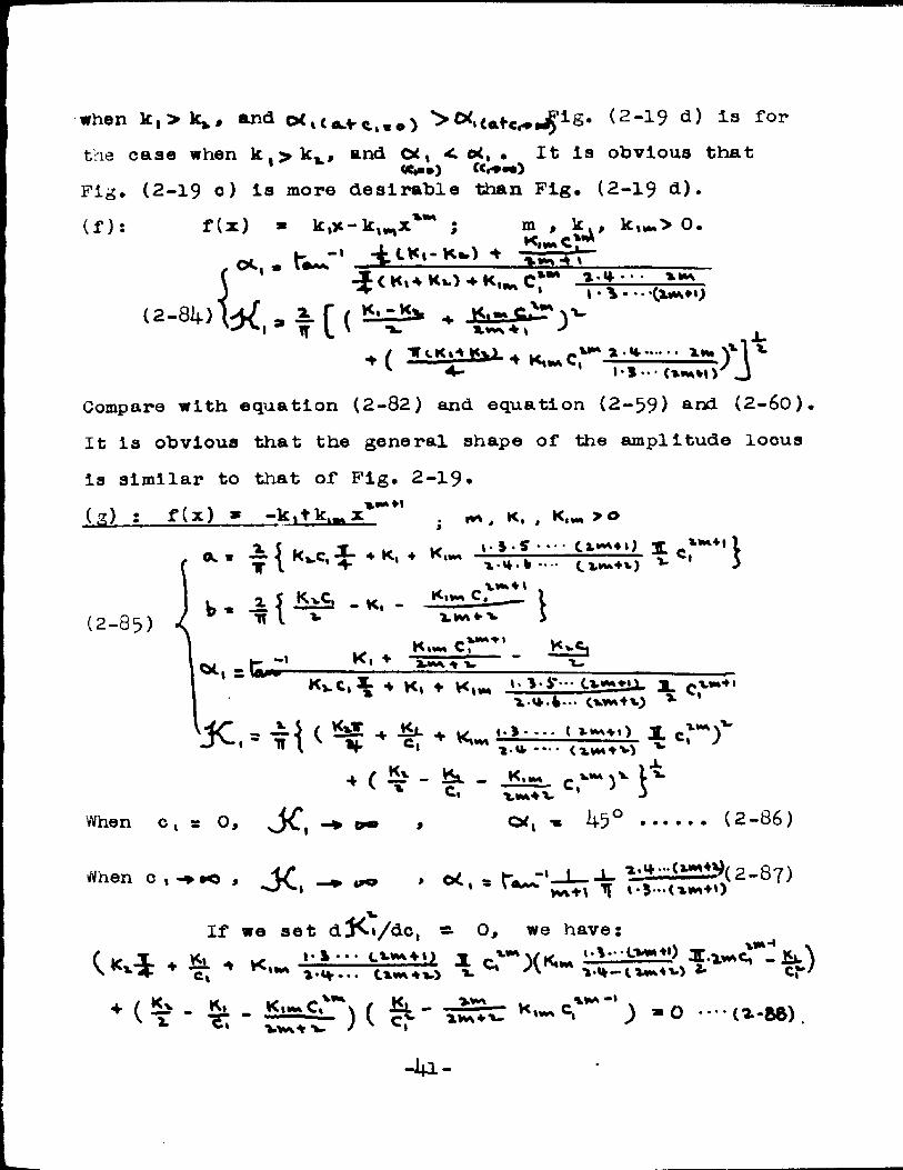
when k,> k ,, and t,**) ^ (^“^9 ^) isthe case when k . > k . , and 04, 4 o<, • It is obvious that1 <*.•) C<r»«0Fig, (2-19 o) is more desirable than Fig, (2-19 <*)•(f): f(x) * k^-k^x'** ; m , k^, k,**> 0 .

<*, . ti~" + “ " » » > * t £ $ T___________< « M K * ) * ^ e r r-V.-hp S ,

(2-8i+) W , » f ( + n,-c£r )■>-'-'v*i IT L ' **- J ^

+ ( + k , „ c r ? * x~ T \ *■4- I*S •• •(****») JCompare with equation (2-82) and equation (2-59) snd (2-60), It is obvious that the general shape of the amplitude loous is similar to that of Fig. 2-19,(g) : f(x) * - k ^ k ^ x *"**1 . im, k, , KIWI >©

x < _ -r . - u, i* S S Cx****) It „****• ITf i k-C* 4 * K* + v C* J. .

L , l j JSiS - K, - K>~_£j i(2-85) •( Tt I v x**A*»v >

K>»- c r > * _ V<vC._ |~l______ **» ♦ 1 * ^ ■» x. ______ t-* ~ KV C,1 ♦ Kt t K,« >• VS*- • cxi»*»X<*-fc»> (mfv) x

W C . = i M ( •* 4*- -► «-•■»•••• (**»♦'> i e D vM *1- c« i.a-... <xv**v> ^ ' y+ ( % . & . . j < ^ c -~)- ^

When c* s O, sj £ | -* c~ * CX, 14-5° ...... (2-86)

flhen o , - . o , J C , — - ’ «*. » r ^ S ) U '87)

If we set dj^-i/dc, =• 0, we have:u a ♦ % - * — * £ : : & *

+ ( t» - £ - ) ( |t - - ^ T C ) * 0 •••• (»-88) .*■ '*• vv**v. / *

-la-

.This equation is very complicated. It depends upon the arameters k, , , k,*, , and m. If we assume m *1,

we have :

V K "~ + “ "ip) KvXi~C,<>

+ C f c v ♦ £ > * » * - « * ■ + c-t- - i.k ,'-

= O (2-89)Equation (2-89) is a tenth order equation, the solution is of course very tedious. But the existence of positive real root for C| is assured by the sign of these terms in the equation. If we rewrite the equation Into the following form.

A|0 C * o - 0 -»> 0 * c ? t o . c ? -v C, •* A * c,s o c * ♦ o • c,' ♦ o- c N A , c , - A0- O ( 2- 90 )

we can see that there is a variation of sign between the terms, which according to the Descartes1 rule in the theory of equations, assures the existence of one positive root. This positive root of c^will give the corresponding mini­mum vaiue of 4 4 •

Similary the variation of the angle O*, in this case Is also very complicated. However we can sketch out the general shape of the amplitude locus If we know when the angle 0 (*» o.

Prom equation (2-85)* we know that of,* 0,WHM + lwhen ^ K.m g. _ K«-Ci ^ q (2-91)^ **“Ihis is again an high order equation. Ihe existence of the

-1*2 -

OZ-Z ‘C.'J,

_ 5 _ =CT'3’M• V O " q o ' X > Q ' **vj |

+ Z +'o ^'x14-wur d

I

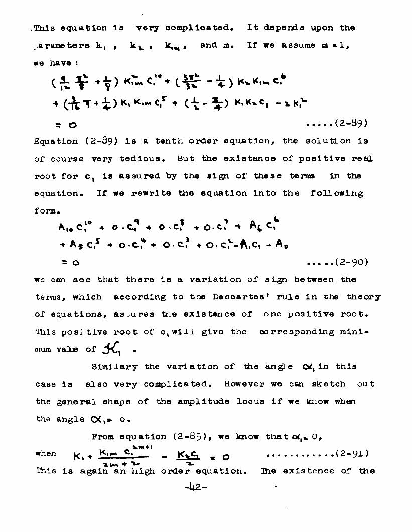
solution can be treated as follows*Refer to Fig. 2-*20; the curve^represents

the equations

3 *c »______ + K,a ^ + v

(2- 92 )

and the lines oa, ob, oc represent the equations:II a ^ Vy — ... 12-9 5 )

with k uas a parameter. It Is obvious from the figurethere are three possible cases. When the value of k v ^is such that the line just toucnes the curve p, tnere is only one value of c ( which will makeOtj* 0. Hence the amplitude locus Is tangent to the negative real axis at a single point.

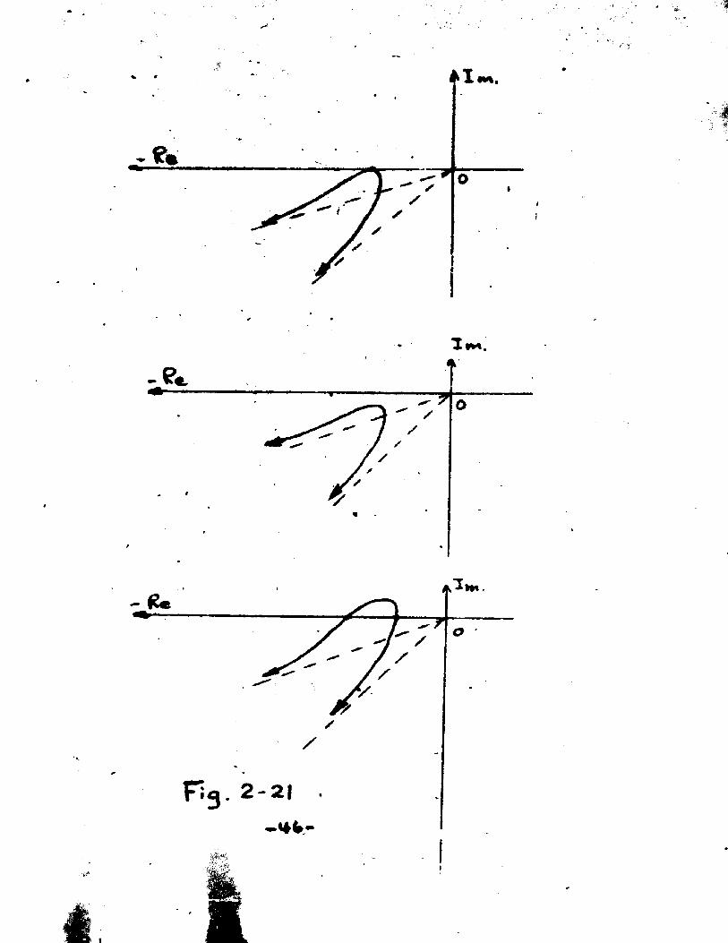
If k x is less than that value, there will be no solution; that means the amplitude locus will never cross the negative real axis. On the other hand, if islarger than that, there will be two positive real roots; that is: the amplitude locus will cross the negativereal axis twice. The amplitude locus corresponding to these cases are are shown by Fig. 2-21.

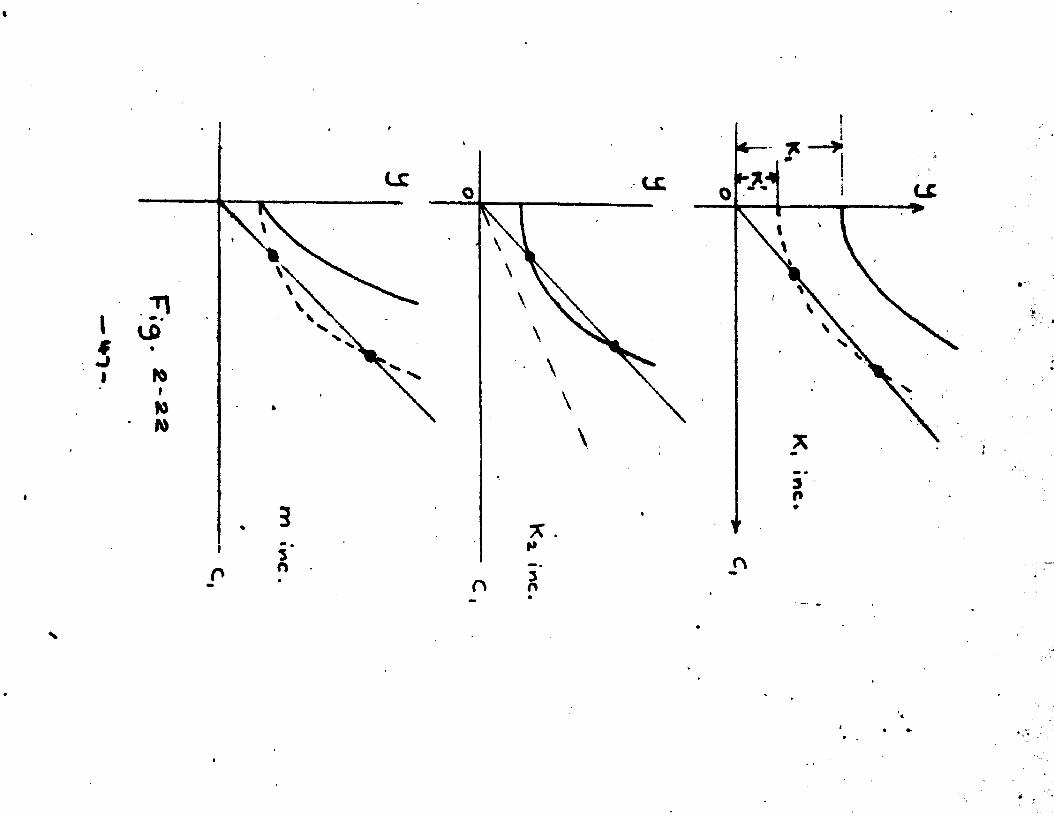
Prom Fig. 2-20, we can also study the effect of changing parameters upon the amplitude locus. If k ( is lnoreased, the curve p will move away frum the line y m kv^ c, , thus moving the peak of the amplitude locus down. If kt.is increased, it moves the peak of the amplitude locus upward. If m is increased, the curve p will move away from the line y^k^Ci /2 , thus moving the peak of the amplitude locus downward. All those cases shown by Pig. 2-22.

*■

%

LC

Km* C(h) s f(x) » -Kr'if’

W K, ■* K w C . \ K w C * * * (2-9k)».»..•(iiwf i>......... ^

" v C, 1 !• !••■ ■ C i m * i ) /n q c »+ tJ ^ . _ K w + K.~ c.— W ^ ............. (2-95)

c ' 1IM «♦ \ 7 >wKet* Ct • O , 0*%* 4 S # , (2-96a)

V/ hen c (*09, 0 <** ‘ * '*•' * * « + 1) • ?£■! T.r. .. (2 -96U)Anen ol,» 0 , ^ + K.t _ c «.** m ................ ........... (2 -9 7 )

1 v w t i 1Compare equations (2-94), (2-95), (2-96), (2-97) with e q u a ­tions (2 -8 5 ), (2-86, (2 -87 ) and (2 -9 1 ); we can easily see that the amplitude locus must be similar to that of case(g) as shown by Fig, 2-21.(1) ; f(x) » -k. •*• k.«x; K,, K >0 .

C, t K i l

- <jaSi - k ,311 .............(2- 98 )ot( _ K, + -fc. C K „ - Kv) c^

+ C.K.,. t Kv) c,

X , - f 1 ( 4 : * *<•*■•- K O ] V 1 t % + tK,.+ K O ^ ] V^

When c ( « 0 , ot,« 45° ,

When c , * 00 f o<, « +du^ *»• ~

1

(2-99)

K|# t K v(2-100)

- 4 8 -

_ •

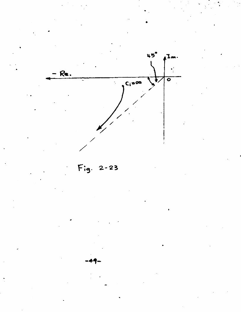
- 1?«. . \>

«

o) /

• / /■ / /

/ v/ /

* / '/

/

F ; ^ . 2.-23

I

- ♦ V

When ot,« 0,

( 2 i o i )

If k |#>l^p there is no solution for real pos tive c,for equation (2 -101); i.e. the amplitude locus nevercrosses the negative real axis and that is what we desired.however, the benefit of more equivalent phase advance ( T/ii-)is completely spoiled by the rela tionjJ{^*#®when c, * 0 .

The amplitude locus with k ^ k x is shown byFig. 2-25.Chapter III Servo system with frequency dependent

non-linear element.In this chapter the non-linear element N shown

in Fig. 3-1 is assumed to have such a property that the ratio of the output response to the input depends upon the input frequency only. It Is al so assumed that it Is Inde- pendent of the input magnitude as those cases we have dealt with in Chapter II.

For example; if the input to the non-linear ele­ment N Is:

C * c # cos iftt ...................... (3-1)and if the output D is related to the input by a n o n ­linear relation as follows: J)« 4 -1 1 ................. (3-2 )then we h a v e :

D _ C - C . v f C n lotCC.tourt^"*'

-BC-

or D x C . u i ^ C M « o t ........(J J )

Hence D 9 (3-4)d

which is entirely independent of the input magnitude, and which is a function of frequency only. The physical real­ization of suah a non-linear element which has a charac­teristic as represented hy equation (3-2 ) is not easy if indeed possible, but that is another problem. We are not going to prove or disprove the existence of such a non­linear element. The point we are interested in here is to determine the stability of the servo system if such a type of non-linear element exists.

If we consider a linear element as a special kind of non-linear element, then it also has a ratio of output to input which depends upon the Input frequency only.1 • Differnece between the non-linear element N whose

output to input ratio :ls a function of the input frequency only and a linear element.

Suppose we have such a non-linear element N as defined by the equations: (3-1 )* (3-2 ), (3- 3 ) and (3-4 )* the output to input ratio according to equation (3-4 ) is :

..................If at this time we have a linear element whose output to

- 31-

c .1— 1

F i g . 3 — 1

FIg. 3-2.#

* 5 1 -

input relation is:

D m T t * ..............then obviously when a signal C m c, cos o>t is fed. into theelement, the output will be:

||Dr- C, H0 cos o>t (3-6)and the output to input ratio will be:

..................(5-7)wlhch is exactly the sa ne as equation (3-4 ) •

This means that the non-linear element N and the linear element with characteristics specified by equation (3-5) have the same output to Input ratio when a sinu­soidal si^ial is fed in.

Hie difference between these two elements can be seen immediately if we consider the signal fed in as:

C * c, cos *a, t + cv sin *frxt ........ (3-8)For the linear element we have:

D s c, cos t + c v«e^sin «rtut ......... (3-9 )But for the non-linear element we have:

D s c'"-' C <*tv) i- v»\or D s (c, cos W, t * cvsin ^ vt )

x (c,<dTcos t + c,t^sin s»>,t )....(3-io)

Equation (3-9) «-nd equation (3-10) cannot be the same u n ­less «ti» *»v . This can be seen from the case itien n » 1. From equation (3-9) we have:

- 33 -

D * o , ^ cos «>(t c t«\ainFrom equation (5-10) we have:

(3-11)

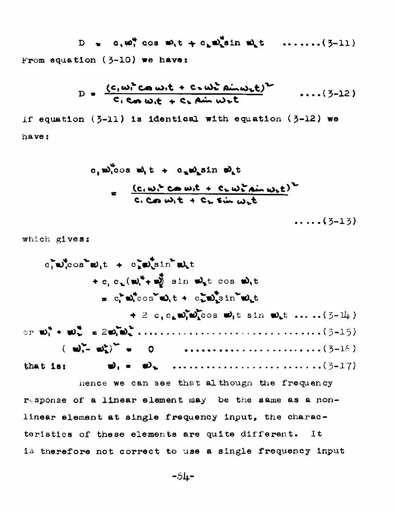
_ tc «u>.v c-o uO.t ♦ Cvuiv /, , *D * " " ” ” . • • e * \ 5“12 )C| CO it 4* Cv u)vtIf equation ( 3 - H ) Is identical with equation (5-12) we h a v e :

c t«£tcos w\ t + o ^ s i n w>ktCc, iOiV C e u>it ♦ Cv, u>y“/w> tOyt)**"Ct C n w)it 4 C v f ««» u)vt

(3-13)which gives:

v 4 v . . v . v .c,t),cos o)tt + c fctOvsin sd^t♦ c, sin w\t cos wO,ta W)I*C oa^wl, t + c^«>*s in^il^t

+ 2 c, cfcw)7« cos sin ....(3-l4)or w>r + B 2*Va>^.................................... (5-15)

( m fr- a 0 ........................ (3-16 )that is: «>, ■ #>•*. (3-17)

iience we can see that al thougn the frequency response of a linear element may be the same as a non­linear element at single frequency input, the charac­teristics of these elements are quite different. It is therefore not correct to use a single frequency input

-b\\r

signal to determine whether the element is linear or not. But as Tar as stability of the servo system Is concerned, as long as the output to input ratio depends upon the input frequency only when a single frequency signal is fed in, there is no difference whetner the element is linear or not. For this reason, the re­mainder of this chapter will actually deal with the non-linear treatment of a linear servo system.2. Non-Linear treatment for linear servomechanisms.

The ordinary linear aerVo system is merely a special case of the general non-linear servo system. The art of linear servo may or may not be applicable to a non-linear servo system. It Is therefore fruit­ful to see what happens when the non-linear method is applied to a linear servo system, whose solution we already know.

(a). Proportional error contro1. xf the n o n ­linear element h In Fig. 3“1 is QJa ordinary linear amplifier with gain k, the describing function is a constant. The amplitude locus will degenerate Intoa single point on the negative real axis of the inverse transfer function plot. This agrees exactly with the linear treatment.

(b). Derivative control. Refer to Fig 5-2; If

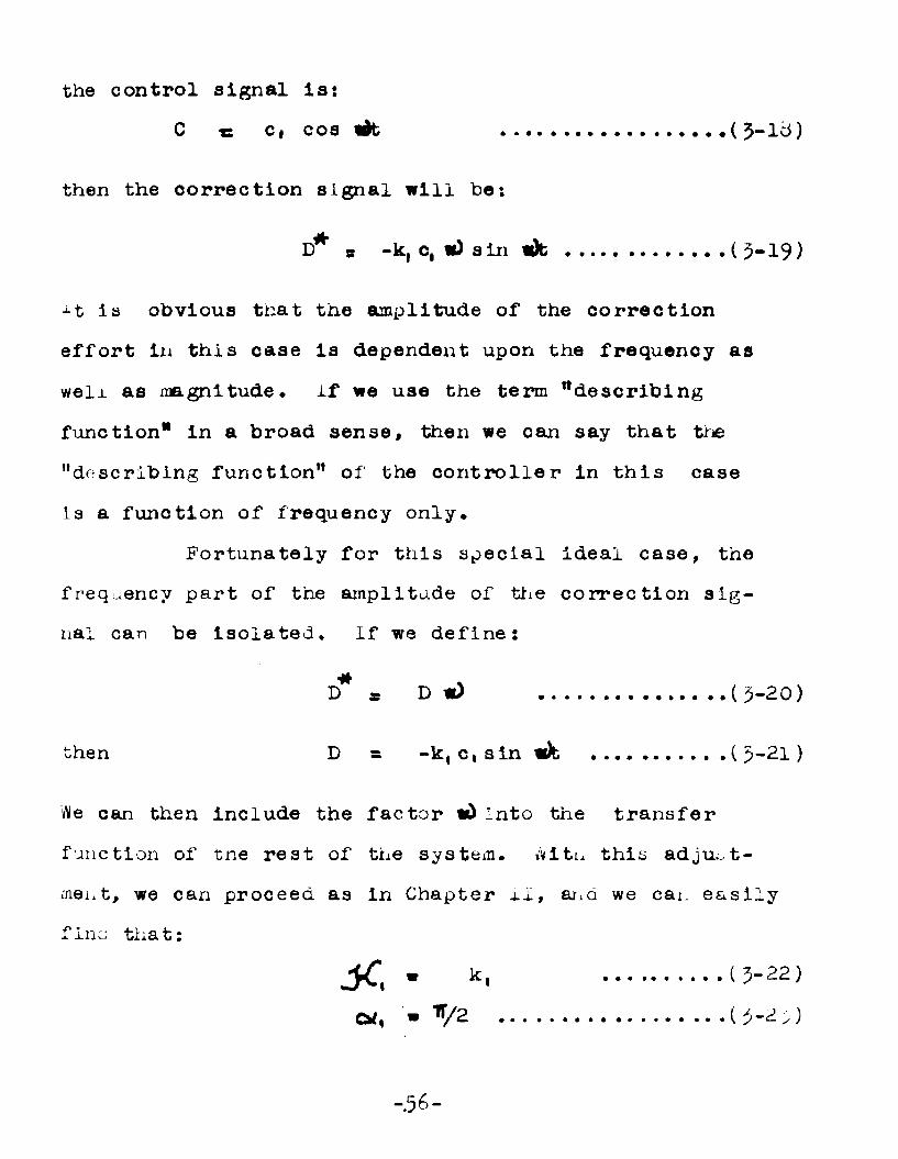
the control signal Is:C « C| cos ..................... (5-lb)

then the correction signal will be:

D* 8 -k, c, «)sin w)t ............... (5-19)

is obvious tnat the amplitude of the correction effort in this case is dependent upon the frequency as wel± as magnitude. if we use the term "describing function11 in a broad sense, then we can say that the "describing function" of the controller in this case is a function of frequency only.

Fortunately for this special ideal case, the frequency part of the amplitude of the correction sig­nal can be isolated. If we define:

D* s D tt) (5-20)

then D =■ -k, c, sin ............ ( 5-21 )

fle can then include the factor into the transfer function of tne rest of the system. «vitn this adjust­ment, we can proceed as in Chapter 11, ana we can easily fine that:

( 3- 2 2 )

» V 2 .....................( 5-21)

-.56 -

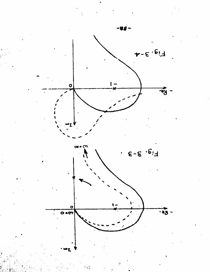
Ihat Is: the frequency locus keeps its position liiilethe critical point -1 on the negative real axis is rotated 90 degrees oounter-clock-wise In the inverse transfer function plane, After we correct the frequency for the extra factor wDisolated from the controller's "describing function,,, we will get the final locus as shown by Fig. 5-3* Fig. 3-k- represents the inverse transfer function locus before and after the deriva­tive control is introduced into the servo system by ordinary linear servo theory. If we compare Fig. 3-5 with Fig. 3~k-> we find that the position of the dotted locus In Fig. 3-3 with respect to the imagin­ary axis is Identical with the position of the dotted locus in Fig. 3-^ with respect to the negative real axis.

( c ). Integral control. The non-linear elementU in Fig. 3-1 Is now assumed to be a linear integral controller. If the Input to h Is C*c# cos lit, the output of N will be:

D* « C/ k, /m)j) sin «>t ........... (3-21*.)

The "describing function" here is again a function of frequency only. With a similar adjustment as in (b),

- 57 -

-si-

✓X

o#« C*

Ml-

by includjng the factor 1/td Into the rest of the system we have i

D * . D/mi (3-25)D « c, k, sin «dt ...............(3-26)

and we find: K, ....................... (3-27)<*, « -T/2 ....................... (3-26)

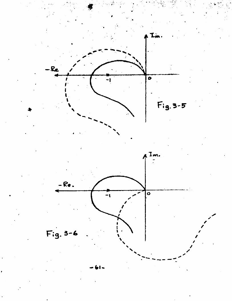
in tnls case the frequency locus keeps its pos­ition while the critical point -1 on the negative real axis is rotatea 90 degrees clockwise in the inverse transfer function plane* The final locus after the fre­quency correction for the extra factor l/t& is shown as the dotted locus in fig. 3-5 • if we compare this with the dot~cd locus in rib. 3-6 which is obtained by the ordin­

ary servo theory, we can find that the relative position of the dotted locus in Fig. 3-3 with respect to the imaginary axis is the same as the relative position of the dotted locus in Fig. 3-6 with respect to the nega­tive real axis*

(d), Combined proportional and derivative control*We have seen tnat in both the derivative

control system and the in-tegral control system, the "describing function" of the controller is a function of frequency. But the frequency part of the correction

- 59 -

effort I?*can be isolated anc; included into the transferfunction of the rest of the servo-cystem, and then it can be treated as a pure proportional error control sys­tem. how we are going to study the servo system wi th a combined proportional and derivative controller, of which the "describing function" of the controller is also a function of ii put frequency only, but it is difficult (although it is still possible) to isolate the frequency part of the correction effort D. If the Input signal to the controller is:

C * c, cos «)t (5-29)

D * k, c, cos ti>t - kxc,*)sin idt(5-30)

• c j £ ^ 5 1 ^ cos (tfc+tX,) (5-31)

* fc/k| ........................ (i>-32 )

D » k, c ,/ T T T f T k j r cos (^t-wsg(3-55)

Ot* = tan 1 ( cO ) ............ ( 5-5U )

JC, * k . J 1 + ( ***4 )'...........(5-53)

Both ©4, and are functions of frequency only. For a particular frequency we have a particular value of Ot, a n d ^ £ t . The locus of 04, and JCt » with as a

-60-

then

If

then

r.ence

s4

/\ x

I

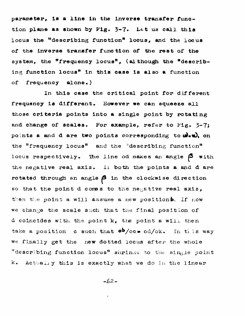
parameter, is a line In the inverse transfer f u n c ­tion plane as shown by Fig. 3-7» Let us call this locus the Mdescribing function" locus, and the locus of the inverse transfer function of the rest of the system, the "frequency locus", (al though the "describ­ing function locus" in this case is also a function of frequency alone.)

In this case the critical point for different frequency Is different. However we can squeeze all those criteria points into a single point by rotating and change of scales. For example, refer to Fig. 3“ 7; points a and d are two points corresponding to onthe "frequency locus" and the 'describing function" locus respectively. The line od makes an angle £5 with the negative real axis. II both the points a and d are rotated through an angle ^ in the clockwise direction so that the point d comes to the negative real axis, then the point a will assume a new posltlonb. If now we change the scale such that the final position of a coincides with the point k, the point a wilj. then take a position c such that o^/oc* od/ok. In tils way we finally get the new dotted locus after the whole "describing function locus" shrinks to the single point k. Actiiaij y this is exactly what we do in the linear

- 6 2 -

1 m

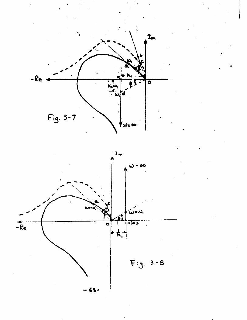
servo theory about a compensating network. We multiply the transfer function of the compensating network withthe transfer function of the rest of the system. Graph­ically we draw the two inverse transfer function loci and then shift and change the positions of the points of one locus according to the corresponding points on tne oth^r- locus as shown by Fig. 5-8*3. lion-linear element whose "describing function locus11

is a function of frequency only.So far we have discussed the linear cases. We

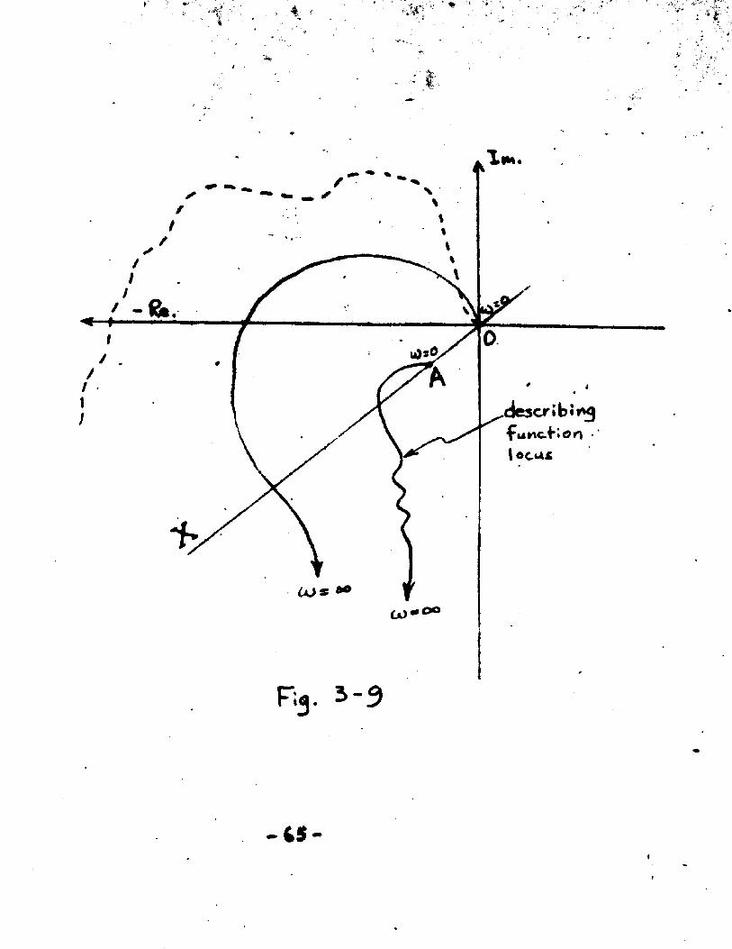
observed that as long as the describing function ofthe element is a funotion of frequency only, it isalways possible to squeeze the describing function locus to a single point and have the "frequency locus" modified. Then we can apply the stability criterion easily. For example, in Fig. 3-9> the describing func­tion locus is a very arbitrary one, whose mathematical expression may be even not known. Still we can squeeze it into a single point. It is also noticed that the final critical point is not necessarily a point on the negative real axis. It can be chosen at other points. Fig. 3-9 shows the situation when the new critical point is point A. The dotted locus is obtained after modification with line oX as new negative real axis.

CO

«

4 5

hence we oonolude here that all elements whose describ­ing function is a function of frequency only can al­ways be squeezed to a single point with the "frequency locus" modified and be treated as in a linear servo system.

Ifro-locus method to determine the absolute stability.We have learned that all elements whose des­

cribing function is a function of frequency only, can always be squeezed to a single point and be treated as in a linear servo system. In doing so, we have at least to rotate the original locus, and change the scales, point by point, to get the final locus. It is obvious that it involves some work, although the work may be very simple. Would it be possible to get the informations directly from the two loci instead of after combine them into one? Since the combined locus is uniquely defined if its original component loci are defined, it is therefore logical to conclude that it is possible to obtain such informations directly from the two component loci. It may be possible that information obtained this way may involve more work; however, as far as absolute stability is con­cerned, in most non-linear cases it is more convenient. We shall try the investigation first on those linear

- 66-

cases•(a). Derivative control (when the two lool do not Intersect),

We have studied the derivative control by iso­lating the frequency part of tre amplitude of the correc-

<*•tion effort D. Here, we are going to study it without isolation, ftie two loci will be as shown by Fig. 5-10.

9inoe the describing function locus is a straight line through the origin and there is no intersecting point between the "describing function locus" and the frequency locus" except the origin, the system has no chance for self-sustained oscillations, Ihe system can only be stable or unstable. Since all points on the "frequency locus" are in the second and in the third quadrants and they all are subjected to be rotated 90° clockwisely, according to ordinary Nyquist's criterion, the sytem is therefore stable.(b.) Integral control (when the two loci do not intersect).

The two loci in this case will be as shown by Fig 3-11. Again, the describing function locu3 is a straight line through the origin, and there is nootner intersecting point between the two loci. Since all the points on the "frequency locus" are in the second and

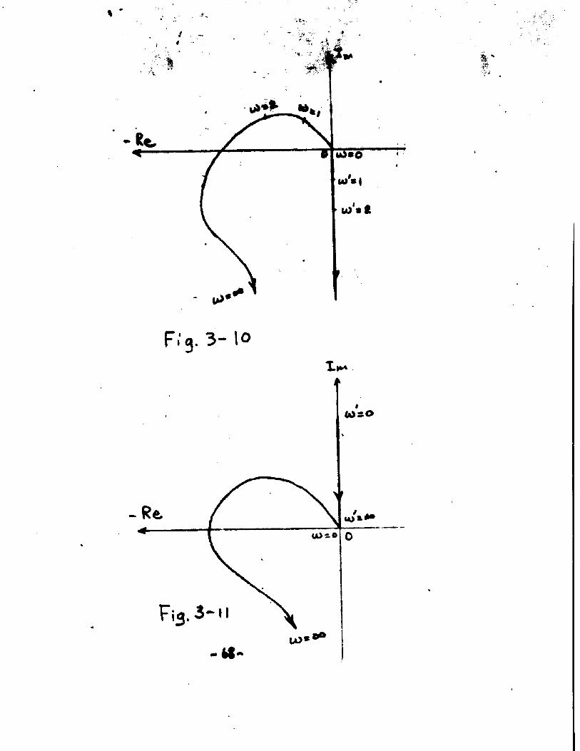
u>«|

Fi'g. 3- lo

the third quadrant and they are subjected to be rotated 90° counterclockwisely in the inverse transfer function plane, the system is therefore unstable.(c). Derivative control (when the two loci intersect).

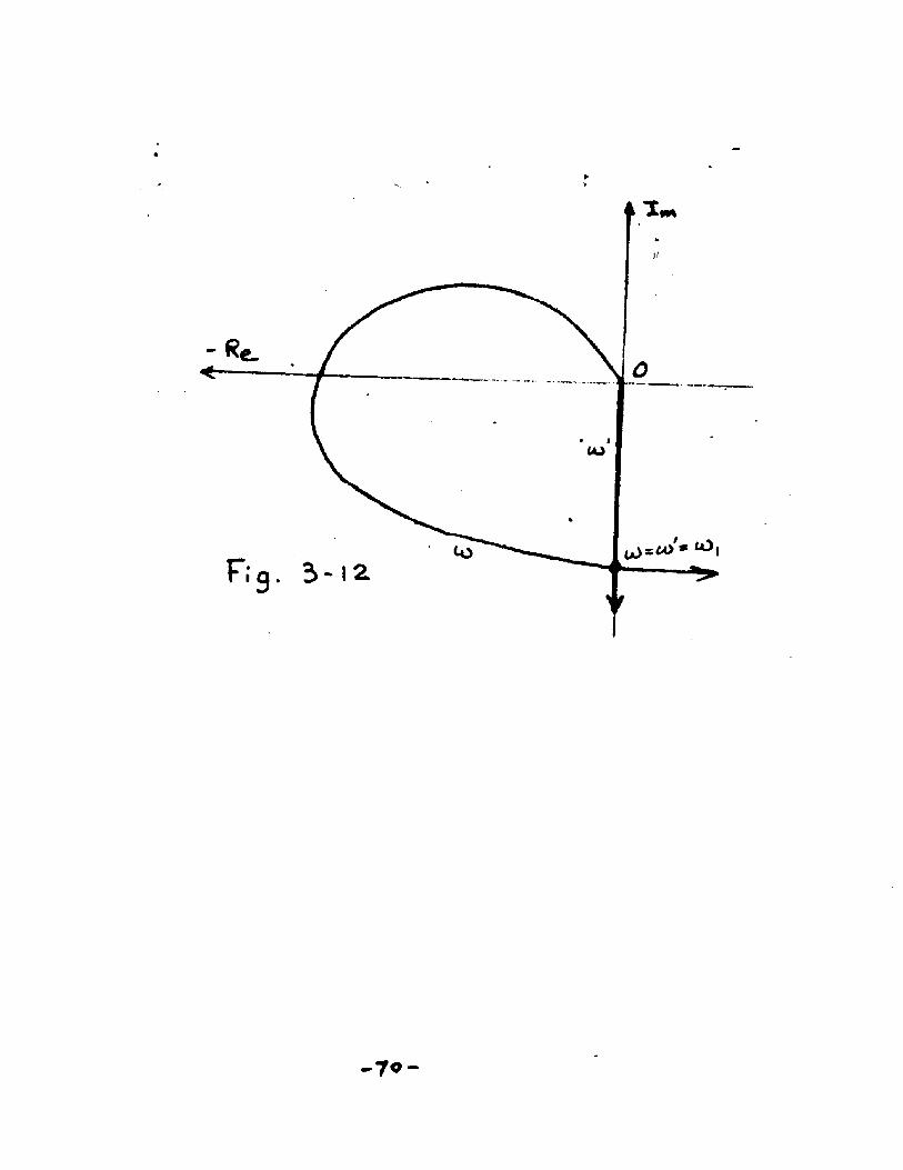
When the frequency locus and the describing function locus intersect at some point with same fre­quency value read from both loci as shewn byFig. 3-12, the system will give a self-sustained os­cillation of frequency and the system is there­fore unstable.

However, if the two loci intersect with eachother, but the frequency read from one locus at theintersecting point is different from the frequency value read from the other locus, then there will be no self- sustained oscillations. Hie stability depends upon the relative magnitude of the two frequency values at the intersecting point.

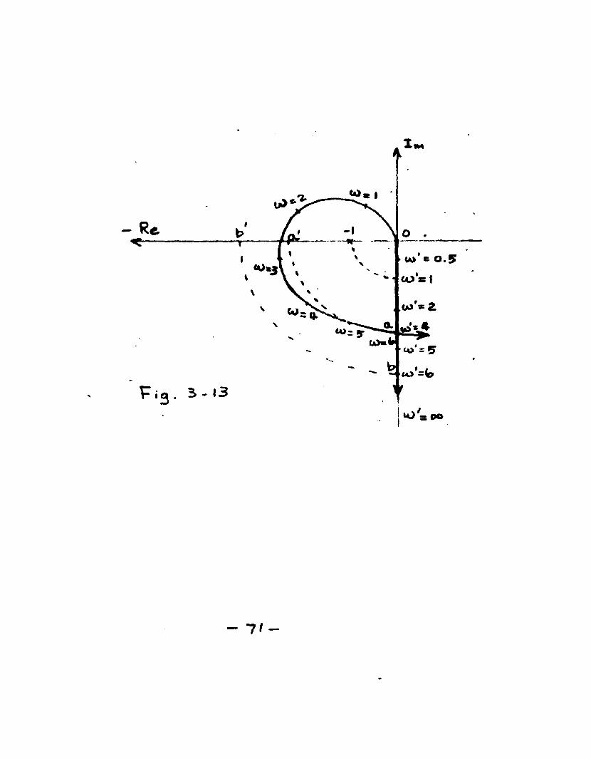
Let us first take the case as shown byFig. 3-13* Bie intersecting point "a" reads ip onthe describing function locus and and on the fre­quency locus. The point on the describing functionlocus is the point b, and ob>oa. When the point a and

-§9-

CO

70-

Re

- 71-

the point b are both rotated through an angle of 90 degrees clockwise, the two points will come to the two new positions a'and b' respectively, (with oa1» oa

and ob'« ob) • Since oa' o b ', and since both oa' and o b ' are subjected to the same scale change, when the point b' comes to coincide with the -1 point on the negative real axis; the point a' must locate to the right of the -1 point* Therefore the system is unstable •

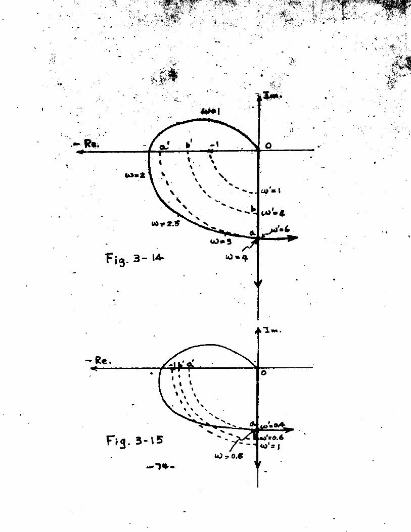
On the other hand, if the intersecting point a reads iD»J+ from the frequency locus and 1^*6 from the describing function locus as shown by Fig* 3-1I4., then ob < ca. That means ob'<oa', therefore when the point b' shrinks to the -1 point, the point a' must come to a new position to the left of the -1 point. The system is therefore stable .

Other cases arise when the intersecting point has a frequency value < 1 read from the describing function locus. Take the case as shown by Fig. 3-15«T h e intersecting point a reads s O.ii and t O » 0.6.It is obvious that after rotating and scale changing

- 72-

when the point to* expands to the point -1 , the new position or a* will toe located to the rigjit of It and the system is therefore unstable.

If the case is changed to one such that the intersecting point a reads « o.l+. and cd* » 0.6 as shown toy Fig. 2-l6, it is not difficult to conclude that this case is stable•

So far we have seen all the cases with a derivative control servo system. We can summar­ize our results as follows:

1. When the two loci do not Intersect (except at the origin) the system is stable.

2. If the two loci intersect at a point, if #* is the frequency value read from the describing function locus and If# Is the frequency value fead from the frequency locus, then if a> « «•*««!,, the system will give a self-sustained oscillation, with a frequency •

3. If the two loci intersect and if a* > «•*, the system is unstable.

!(.. If the two loci Intersect and «e<tf*, the system will be 3table•

- 7 3 -

Aiv-r . ^ :.'-rP! =K

* '■ S•f’V

u> * I

00*2.5

FiJ. 3- t5 CO s I(O 3 0*0

** - >«•> * |

»

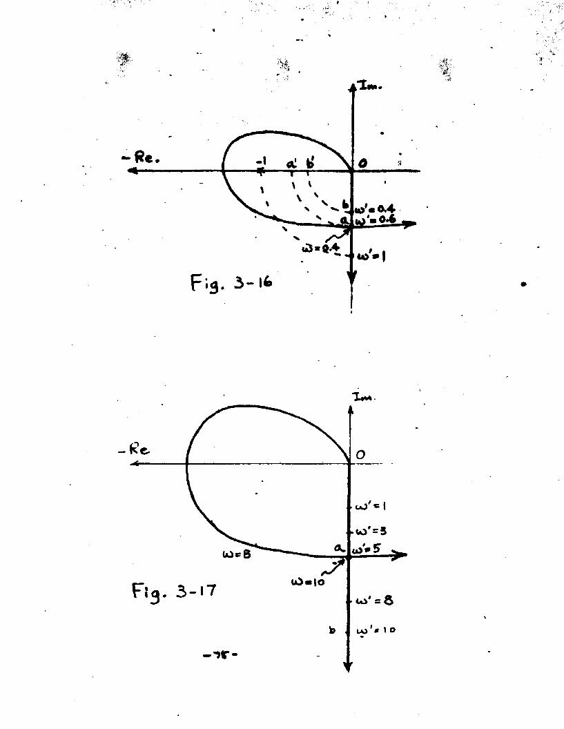
uj' = I

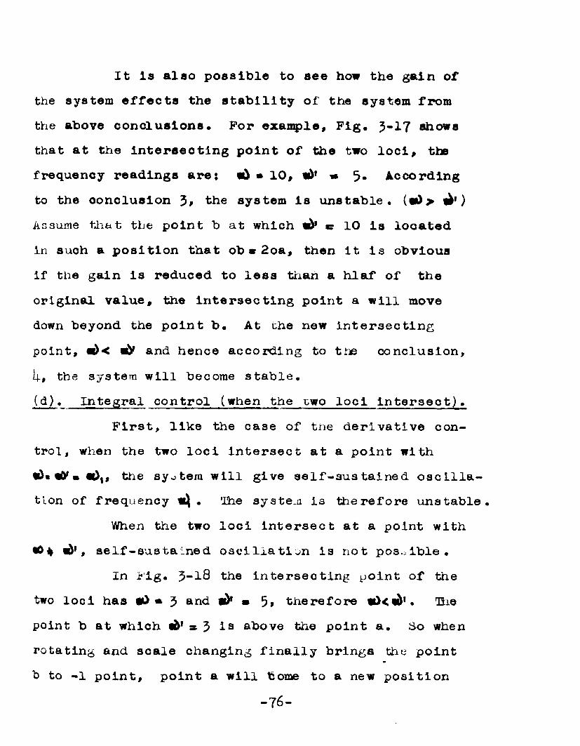
It Is also possible to see how the gain of the system effects the stability of the system from the above conclusions. For example, Fig, 3*17 shows that at the intersecting point of the two loci, the frequency readings ares • 10, & w 5. According to the conclusion 3* the system is unstable. («t)> )Assume that the point b at which ^ e 10 is located in such a position that o b * 2oa, then it is obvious if the gain is reduced to less than a hlaf of the original value, the intersecting point a will move down beyond the point b. At uhe new intersecting point, *d< «2y and hence according to the conclusion,

the system will become stable.(d). Integral control (when the two loci intersect).

First, like the case of the derivative con­trol, when the two loci intersect at a point with

the ayotera will give self-sus tained oscilla­tion of frequency w!} • The system Is therefore unstable.

When the two loci intersect at a point with•0* , self-sustained oscillation Is not possible.

In Fig, 3-18 the intersecting point of thetwo loci has «0 * 3 and » 5> therefore . Hiepoint b at which •&' s 3 I s above the point a. So whenrotating and scale changing finally brings the point b to -1 point, point a will borne to a new position

-76-

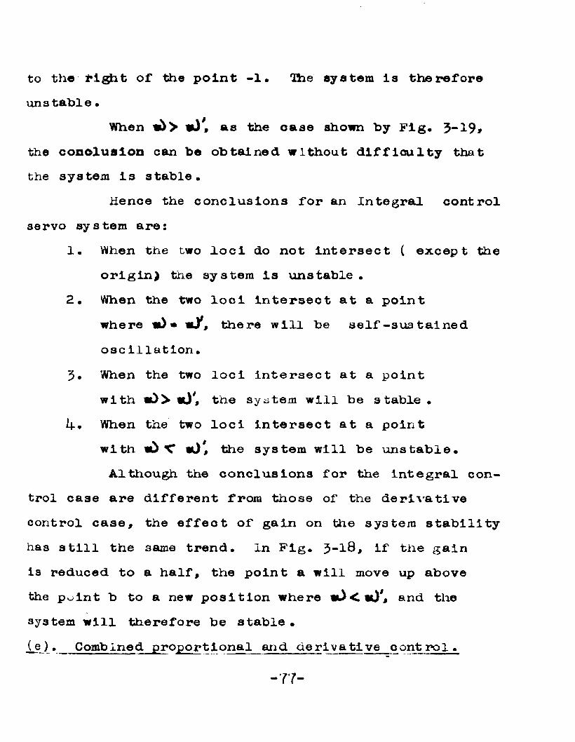
to the l*lght of the p oint -1 * The system is therefore unstable•

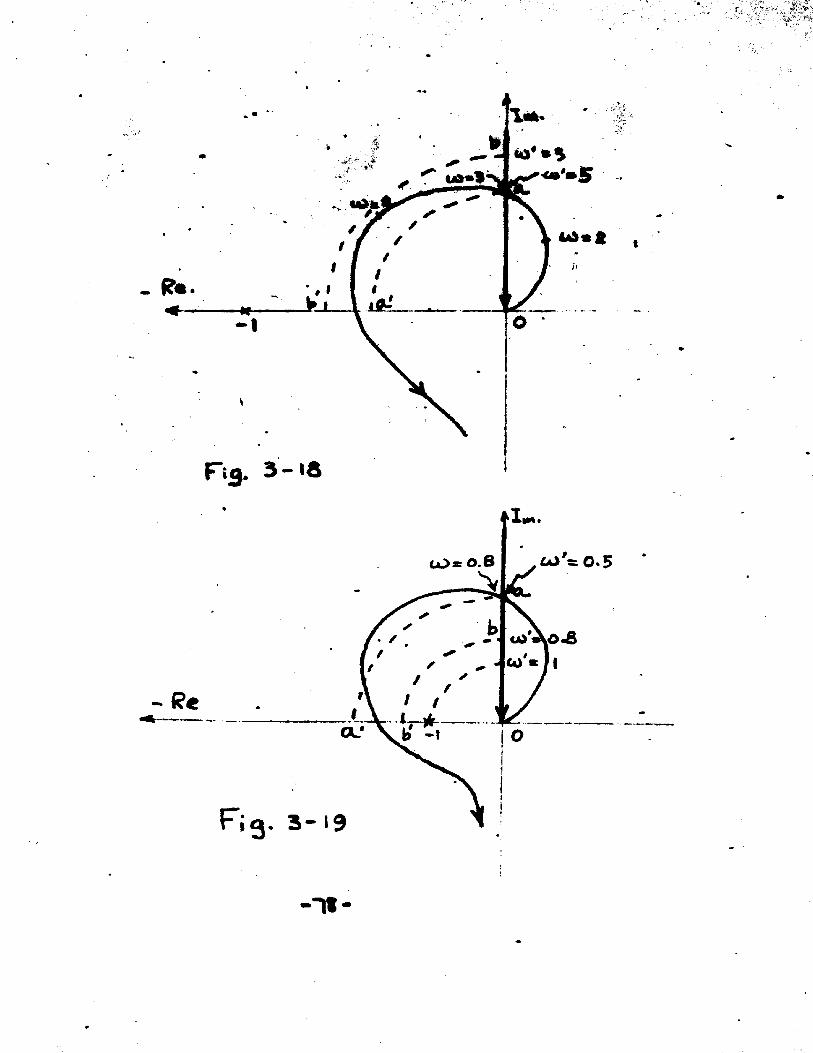
W hen «*> «y. as the oase shown by Fig. 3-19,

the conolusion can be obtained without difficulty that the system is stable.

Hence the conclusions for an Integral control servo system are:

1. When the two loci do not intersect ( except the origin) the system is unstable •

2. When the two loci Intersect at a pointwhere m) • m)1, there will be self-sustained osc illation.

5* When the two loci intersect at a pointw i t h the system will be stable •

!(-• W hen the two loci Intersect at a pointw i t h <0 K i0 * the system will be unstable.Although the conclusions for the integral con­

trol case are different from those of the derivative control case, the effect of gain on the system stability has still the same trend. In Fig. 3-1&, if the gain is reduced to a half, the point a will move up above the point b to a new position where and thesystem will therefore be stable •(e). Combined proportional and derivative control.

- 7 7 -

CL*

Fig. 3

-1«-

We have taken up two ideal cases; the deriva­tive control and the integral control. Both have a describing function locus as a straight line through the origin. Now we are going to take up the case of com­bined proportional and derivative control. In our new case the describing function locus is again a straight line, but it is no longer a straight line through the origin.-as those cases before. Hence the conclusions we got for the above two cases cannot be applied, 2 Actually this is a more general case, the above two cases can be considered as two special cases of this case,

(i). If the two loci intersect at a point, and if the frequency value read from the describing function locus at that point is the same as the fre­quency value read from the frequency locus, i.e."*0 = lO7, we can conclude Immediately that the system will give self-sustained oscillation and therefore Is unstable.

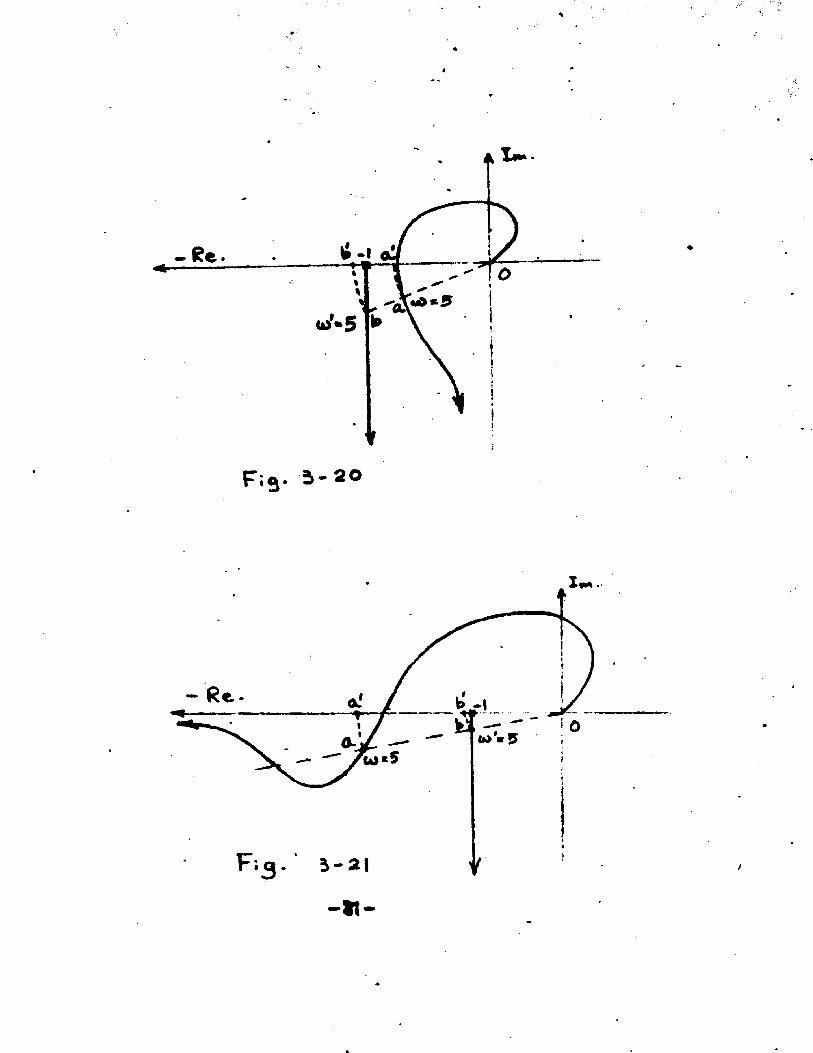
(ii). Consider the case when the two loci do not intersect. First, take up the case as shown by Fig. 3-20. If in Fig, 3-20 we can find a point a on the frequency locus and a point b on the describing function locus with the same frequency value and the line connect­ing these two points passing through the origin, then

-79-

the 3e two point a will give ua the Inf orma tlon about the system stability. Refer to Pig. 3-20# since both, point a and point b are of same frequency value and o a and ob make the same angle w i t h the negative real axis, when p o i n t a is rotated to the n e w position a* on the negative real axis, point b will take the position b'. A f t e r the soale changing, point b* shrinks to the position of the -1 point, point a 1 will also assume a new position w h i c h in this case will be to the right o f the -1 point. According to the ordinary Nyquistfs criterion the system w i l l be unstable.

Ihe case shown in Fig. 3-21 also gives no intersecting point. In this case, we assume that we still c a n find two points a and b on the frequency locus a n d the describing function locus respectively, so that the line ab passing through the origin and both points have the same frequency reading. We notice that oa > ob, therefore after rotating and. scale ehang- ing, w h e n point b assumes the position -1 point, point a will be at a new position to the left of the -1 point.Ihe system is therefore stable.

(ill). When the two loci intersect but with different frequency:

^ 8* 3 —22 shows that the two loci intersect but at- 80-

4

*

h> >

It

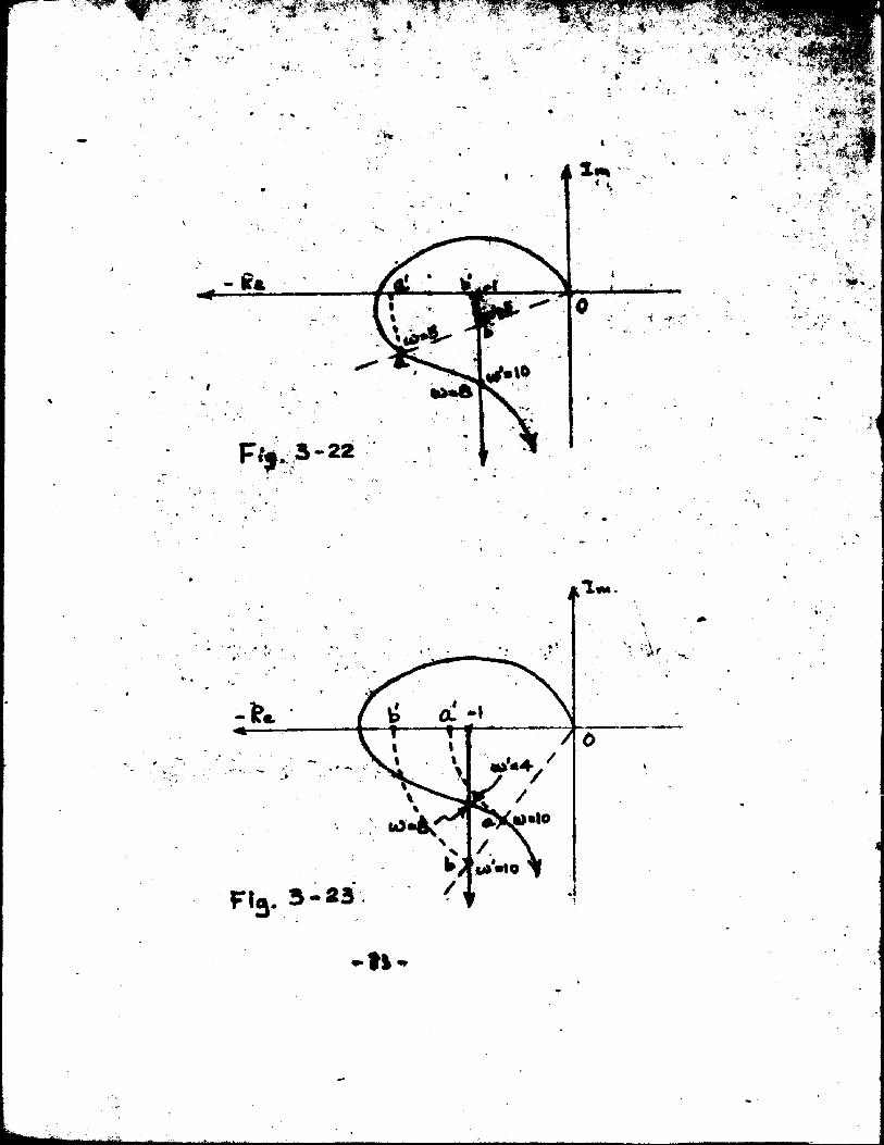
different frequency value. Hie only conclusion we can have off hand is that there will be no self-sustalned oscillations. Whether the system is statle or not has to be determined. Assume that we also find a point a on the frequency locus and a point b on the descrlf- in^ function locus so that the line ab passing through the origin and both points have the same frequency value as shown in the figure. It is obvious that since o a > o b , after rotating and changing of scale, when point b assumes the position of the -1 point, point a will assume a new position to the left of the -1 point. The system is^therefore stable.

Fig. 3-23 shows the case that oa< ob, it is obvious that the system will be unstable.

(iv). When the two loci intersect, and there are several pairs of points like (a,b):

So fhr we have considered oases that we can find a pair of points a and b on the frequency locus and the des­cribing function locus respectively, with same fre­quency value and the line ab passing through the origin.

-82-

3f' 'y

g,.

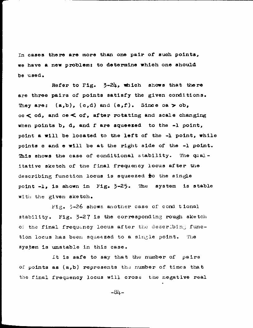
In cases there are more than one pair of such points, we have a new problem: to determine which one should be used*

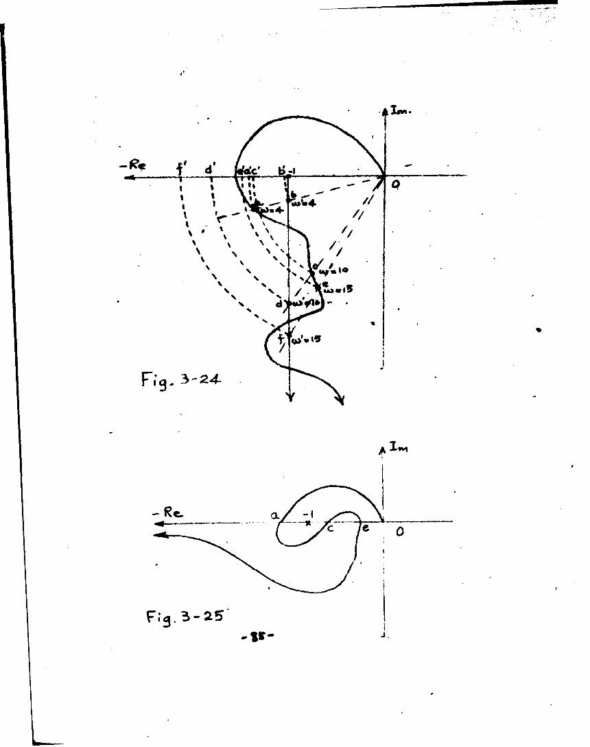
Refer to Fig* 5-214., which shows that there are three pairs of points satisfy the given conditions* They are: (a,b), (c,d) and (e,f)* Since oa > ob,oc < od, and oe <. of, after rotating and scale changing when points b, d, and f are squeezed to the -1 point, point a will be located to the left of the -1 point, while points o and e will be at the right side of the -1 point. This shows the case of conditional stability. The qual­itative sketch of the final frequency locus after the describing function locus is squeezed to the single point -1, is shown in Fig* 5-25* 'I*le system is stable with the given sketch.

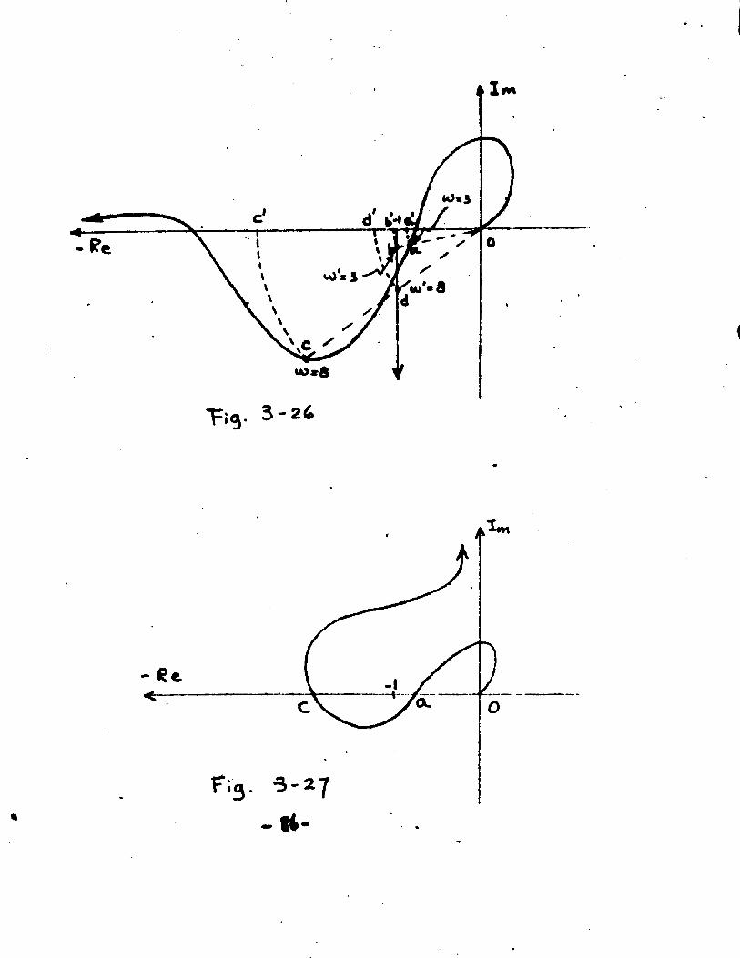
Fig. 5-26 shows another case of cond tional stability. Fig. 5-2 7 is the corresponding rou^i sketch oi the final frequency locus after the describing func­tion locus has been squeezed to a single point. The system Is unstable in this case.

It Is safe to say that the number of pairs of points as (a,b) represents the number of times that the final frequency locus will cross the negative real

- 81|—

-< L X»*»»

»4*

V

At

4 X m

OL

«

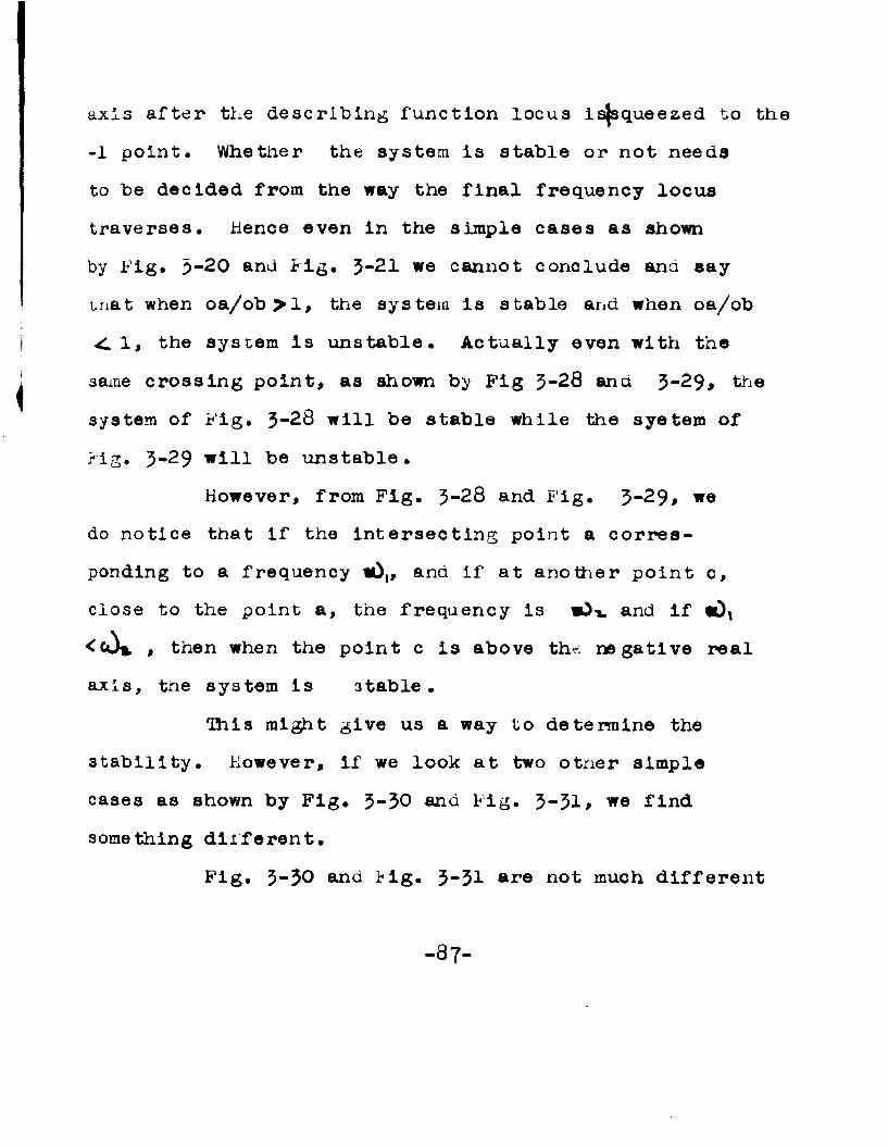
axis after the describing function locus is^squeezed to the -1 point. Whether the system is stable or not needs to be decided from the way the final frequency locus traverses. Hence even in the simple cases as shown by Fig. 3-20 and Fig. 3-21 we cannot conclude ana say tnat when oa/ob>l, the system is stable and when oa/ob < 1 , the system is unstable. Actually even with the same crossing point, as shown by Fig 3-28 and 3-29, the system of Fig. 3-28 will be stable while the syetem of Fig. 3-29 will be unstable.

However, from Fig. 3-28 and Fig. 3-29* w© do notice that if the intersecting point a corres­ponding to a frequency lO,, and if at another point c, close to the point a, the frequency is »)•*. and if cD*

, then when the point c is above the negative real axis, the system is 3table.

Hiis might give us a way to determine the stability. However, if we look at two otner simple cases as shown by Fig. 3-30 and Fig. 3-31# w© find something different.

Fig. 3-30 and Fig. 3“31 ©re not much different

- 87-

/S.

T.0.3-Z9

t

COCOi

Fiq. 3- 30 F.o. 3-31- It-

I

from the Fig* 3-28 and Fig. 3-29• The big difference Is that the crossing point a Is now on the other side of the -1 point* If and «)t&re defined as the frequency values of points a and o respectively and If «Ov ls close to but less than «d(, then when the point c is above the real axis* Hie system Is stable; when c Is below the real axis, the system is unstable*

We notice that even in these s i.mple cases, we have to use it^for Fig. 3-20# Fig. 3-29 and forFig. 3-30 and Fig* 3-31* This is very inconvenient. But if certain assumptions are made we can find a better rule.

If we consider Infinity as a virtual crossing point, then we can formulate a rule as follows:

If the closest crossing point to the left of the -1 point has a frequency , then If any point w i t h a frequency value mj, , les*> than but close enou^i to the frequency value iDc, is above the real axis, the system is stable. If It is below the real axis, the system is unstable.

Apply this rule to Fig. 3-28 and Pig. 3-29; the frequency value «\ls infinity. When this rule is applied to Fig. 3-30 and Fig. 3-31# t*10 frequency value lsc£|.

- 8 9 -

All four cases are workable with this rule.(f ). General rule to determine the stability by two-

locus method. :The rule wc obtained above can easily be applied

to the cases of Fig. 3-25> Fig. 3-27 ana some other more complicated cases. However, the rule is written in terms of the final frequency locus. A translation and rewording of the rule are necessary in order to form a rule which can be applied to the two loci directly without bothering the final frequency locusi

( i ). The rule :If we have several pairs of points on the two

loci like (a,b.) such that each pair has the same frequency value and the line joining each pair of these characteris­tic points passes through the origin, the stability can be determined as follows:

1. Find the pair of points which has the least ratio oa/Ob ;> 1. The frequency value of this pair of characteristic points will be «0 . In case such points do not exist, take wt>c»«o.

2. Pick up a point in the vicinity of that fre­quency value, which has a frequency value less than but close enough to , say w^on the frequency locus. Draw a line passing througih

-90-

this point and the origin. Assume this line makes an angle oC with the negative real axis,

3 . Fiok up the corresponding point on the describ­ing function locus which has the same frequency value u>i , Draw a line passing through this point and the origin. Assume this line makes an angle |3 with the negative real axis.

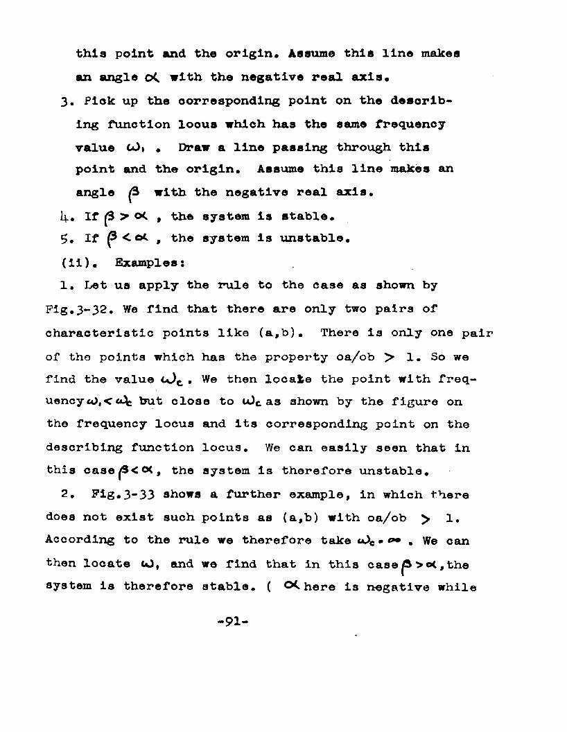
L|_. If (3 > , the system is stable,5. If p < ot. , the system is unstable,(il). Examples:1, Let us apply the rule to the case as shown by

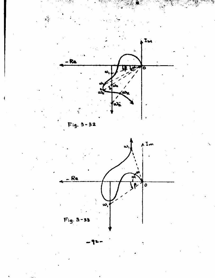
Fig,3-32, We find that there are only two pairs of characteristic points like (a,b). There is only one pair of the points which has the property oa/ob > 1. So we find the value Cc)c • We then locate the point with freq- uency«0,<a^. but close to u)t as shown by the figure on the frequency locus and its corresponding point on the describing function locus. We can easily seen that in this case|8 <o<, the system is therefore unstable,

2. Fig,3-33 shows a further example, in which there does not exist such points as (a,b) with oa/ob > 1 .According to the rule we therefore take <Oe • , We canthen locate (O, and we find that in this case ,thesystem is therefore stable, ( OC here is negative while

- 91-

-H-\i*X‘•?

I

ot.

M>,

\

- I 1*"

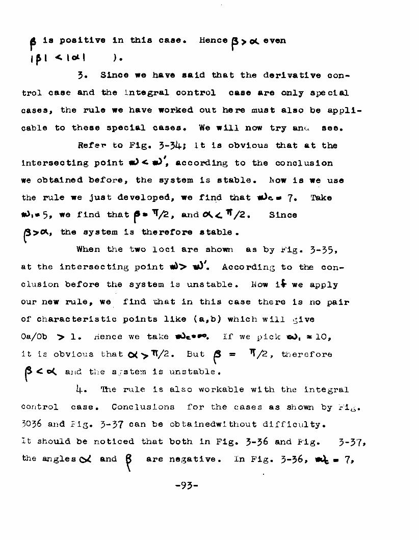
f is positive in this case. Hence p > oC evenIf I < loll ).

3. Since we have said that the derivative con­trol case and the integral control case are only special cases, the rule we have worked out here must also be appli­cable to these special cases. We will now try ana see.

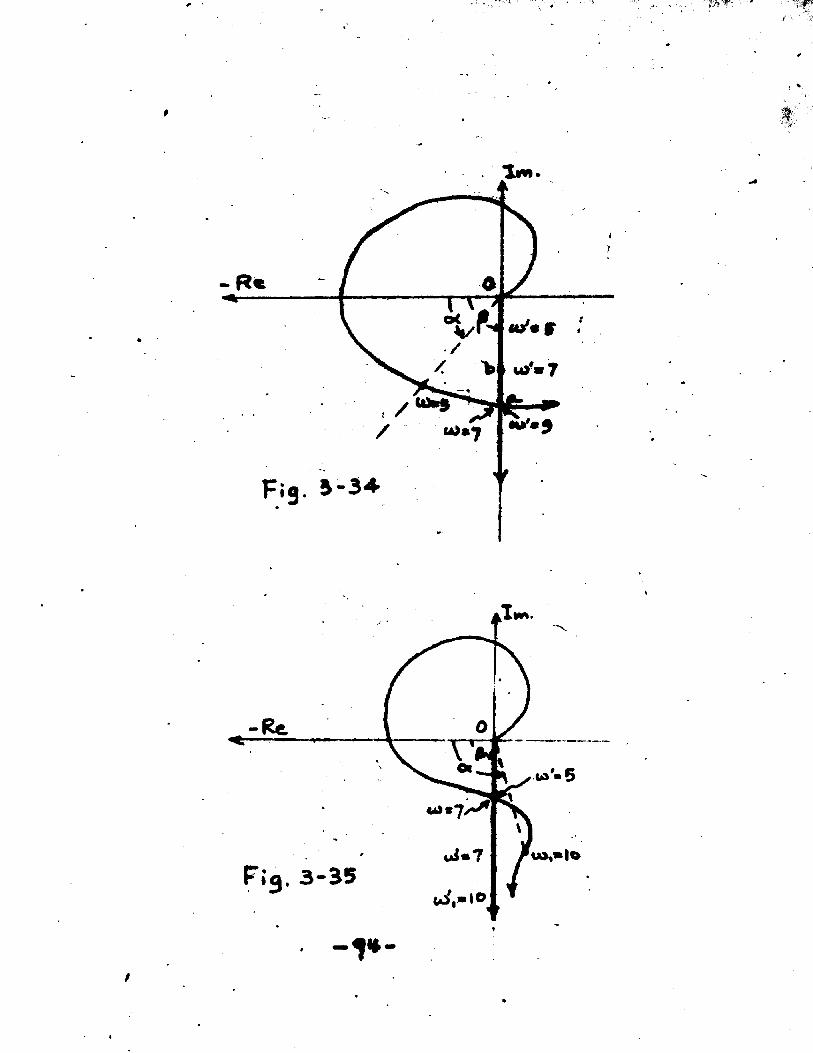
Refer to Fig. 3-54* it is obvious that at the intersecting point m) <■ t0 #, according to the conclusion we obtained before, the system is stable, how is we usethe rule we just developed, we find that Wk)e. ■ 7. Take1O 1* we find that p * /2, a n d O ^ ^ . ^ /2 . Since ^ > 01, the system is therefore stable •

When the two loci are shown as by Fig. 3“35* at the intersecting point w&> 1 According to the con­clusion before the system is unstable. Wow it we apply our new rule, we find -chat in this case there is no pair of characteristic points like (a,b) which will give Oa/Ob > 1. Hence we take w0«.**°. If we pick «0, *10, it is obvious that 0< > *H/2. But ^ /2 , therefore

< ©C. and the s./stem Is unstable.Ip. The rule is also workable with the integral

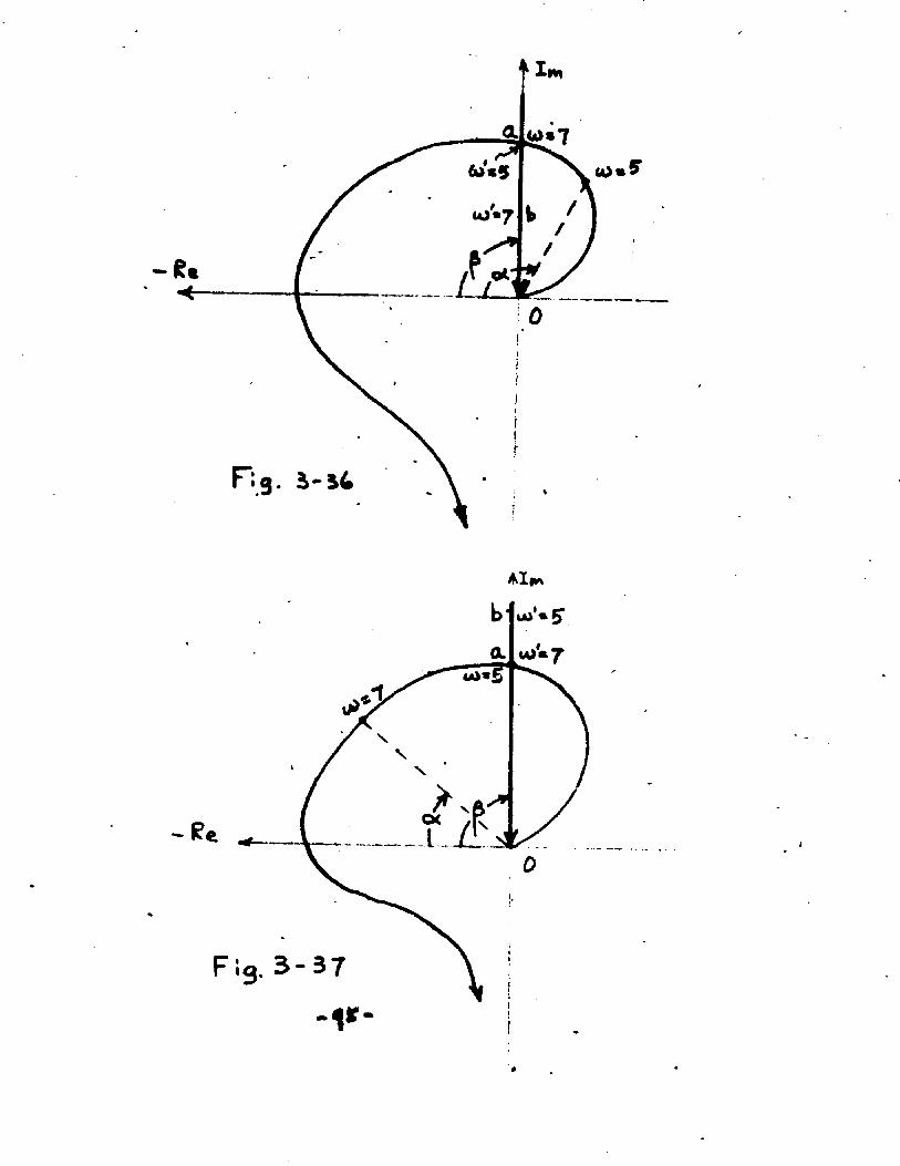
control case. Conclusions for the cases as shown by rig. 3036 and Pig. 3-37 can be obtainedwithout difficulty.It should be noticed that both in Fig. 3-36 and Pig* 3~37>the a n g l e s ^ and ^ are negative. In Fig. 3-36, ■ 1*

-93-

l m .

Re

Fig. S-3*

Re

3-S5- j * -

u>.*

In Fig* 3-37 there is no such characteristic point pairs like (a,b) which will give oa/ob > 1, therefore we take

hence we have:

(g). Application of the stability rule to two loci in general.

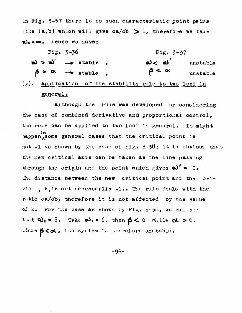
the case of combined derivative and proportional control, the rule can be applied to two loci in general. It might happenAsome general cases that the critical point is not -1 as shown by the case of Fig. $-3 8 ; it is obvious that the new critical axis can be taken as the line passing through the origin and the point which gives •J7 » 0.The distance between the new critical point and the ori­gin t k,is not necessarily -1 .. Hie rule deals with the ratio oa/ob, therefore it is not affected by the value of k. For the case as shown by Fig. 3-3^> we can see that 8 . Take » 6, then <. 0 while ©L > 0.■^ince & < o C , tne system is therefore unstable.

Fig. 3-36 «0 > « y — ► stable ,

stable ,• ) < tik)' uns tabler ^ unstable

Fig. 3-37

Although the rule was developed by considering

- 96 -

I

R e

F.

3• Some discussion In finding the characteristic pointpairs like (a,b) which helps to determine the stability

We may think that the determination of such char­acteristic point pairs like (a,b) is not so easy. The fol­lowing discussion may offer a little help.

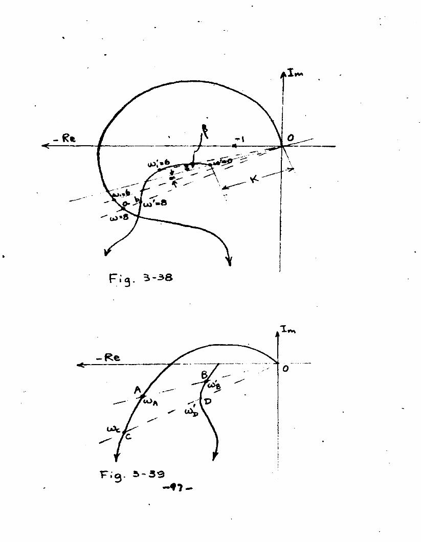
Refer to Fig. 3- 39 # two arbitray lines through the origin are drawn and intersect the two loci at points A, B, C and D as shown. If the frequency values for points A,B,C and X> are a)^ , and respectivelyand if wdA > wJ§* , lOb < myj , or «0A < ;then in between these two lines there I s at least one pair of points which have the same frequency value and the line joining them passing through the origin.

The region can further be narrowed down if atnird line is drawn between the two lines. We will find that at least one sub-region will contain such a pair of characteristic points provided the third line does not pass through such a pair of points.

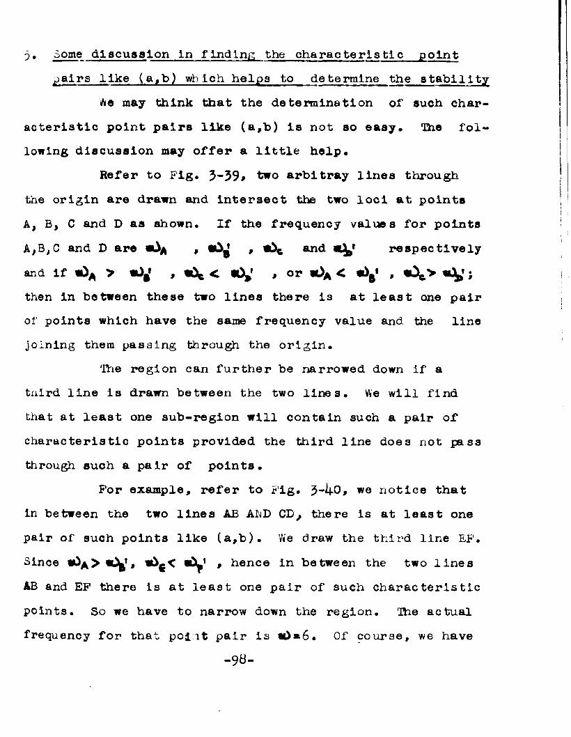
For example, refer to Fig. 3~4o# we notice that in between the two lines AB AhD CD, there is at least one pair of such points like (a,b). We draw the third line EF. Since «0A > , # hence in between the two linesAB and EF there is at least one pair of such characteristic points. So we have to narrow down the region. The actual frequency for that poiit pair is Of course, we have

-98-

-Hr*\ + - i ’S'i

or-c -B; j

to assume that both loci are continous functions of fre­quency, although they may be any shape or even be a brokenline •

Usually we can use the negative real axis as one of the auxiliary i:nes.

Several other points might save the time to de ­termine the stability:

1. We are interested in finding that pair of char­acteristic points which gives the minimum value of oa/ob. > 1 . So we can disregard those pairs which gives oa/ob K 1 .

2. If the two loci after a certain frequency showsa tendency that when a line is drawn through the origin, the frequency value of the intereecting point of one locus with that line is always larger than the frequency value of the intersecting point of the other locus with that line, and if the line rotates toward increasing frequency about the origin and If we find that the frequency value of the lar­ger one is increasing faster than that of the smaller one, we can make a guess and say that after that frequency value there are no such character­istic points as (a,b).

3. The shape of the two loci will give us some idea when there are several possible pairs of such

- 100-

characteristic points like (a,b) with oa/ob > 1. We can approximately deolde which one will be the one gives the minimum oa/ob ratio.

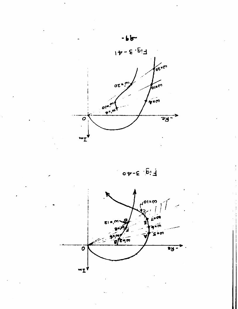
Refer to Fig. 3*41; we have three pairs of suoh characteristic point pairs like (a,b). From the shape of the two lool we can Immedi­ately tell that the ratio oa/ob of the pointpair (20,20) Is the least one.

. *c4. The Interushing point between two loci usually serves as a good guide for the characteristic pairs of points we are looking for. It is al­ways true that on one side of the intersecting point the ratio oa/ob < 1, on the other side of the Intersecting point oa/ob > 1 , if such points as (a,b) exist.

Refer to Fig. 3-42; the shaded area above the point B to A will give a ratio oa/ob < 1, if such points as (a,b) exist in this region. So we do not bother with It.

The tangent line oD shows that after a}1 * 8, there Is no possibility to find suchpairs of points as (a,b).

101

Iwi

< -

-102

The only possibility that such points may exist Is between point B and point C. If the Intersecting point B In this case has a fre­quency value u) > Q, then there are no such points as (avb) at all which will give oa/ob > 1* If point B has Cl) < 8, there might be such a pair of points aB (a,b).

Fig. 3-4-3 serves another example. It Is obvious that we need not to bother with the shaded region since the ratio oa/ob < 1 even If such points pairs as (a,b) exist In those regions.

5. Care should be taken when • It Is veryeasy to make false conclusions In such cases.

For an example, when the rule Is applied to a servo system with combined proportional and derivative control as shown by Fig. 3-44, we notloe that the frequency locus at high frequency gets farther and farther from the origin at a very high rate while the describ­ing funotlon loous goes In a much slower rate. It Is easy to assume from the figure that p < °< If , and therefore get a wrong con-

-103-

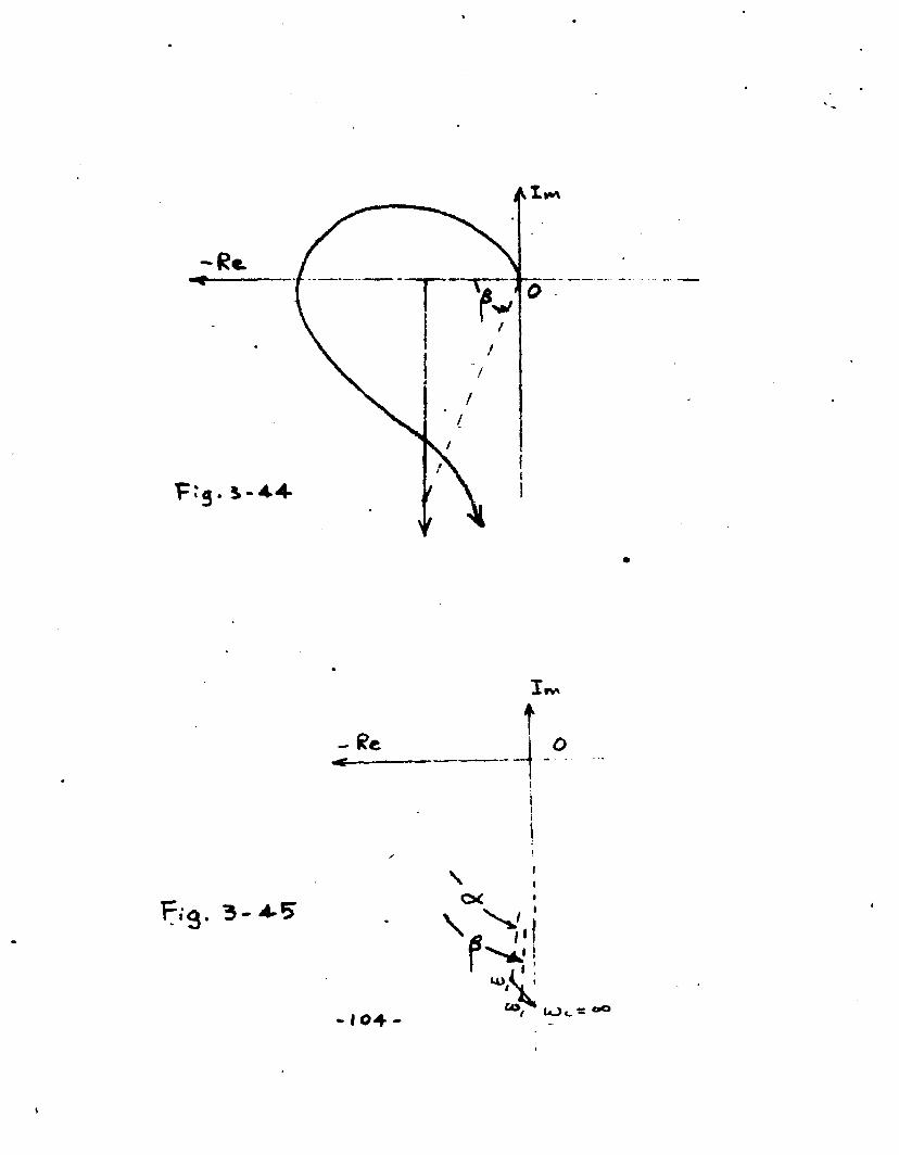
- Re

P r ’ O . 3 ' < 4 * 5

- 104 -

\cx\

f u>

iI*

$ lOc *

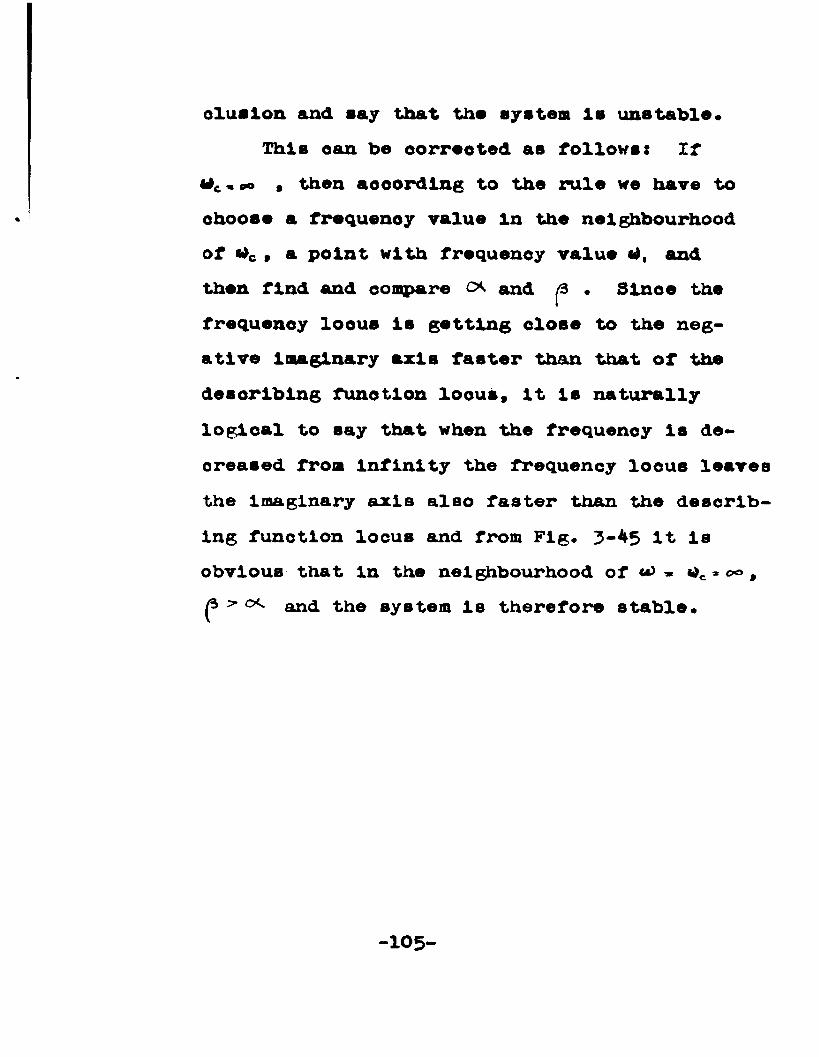
oluslon and say that the system Is unstable*This ean be eorreeted as follows: If

«4C. 0 0 9 then according to the rule we have toohoose a frequency value in the neighbourhood of *>c » a point with frequency value and then find and compare O- and • Since the frequency loous Is getting close to the neg­ative Imaginary axis faster than that of the describing function locus, it Is naturally logioal to say that when the frequency Is de­creased from infinity the frequency locus leaves the imaginary axis also faster than the describ­ing function locus and from Fig* 3-45 it Is obvious that in the neighbourhood of a) » * ©o 9p and the system Is therefore stable*

-105-

Chapter IV Servo system with non-linear elementin general.

In this chapter the non-linear element shown In Fig. 4-1 will be assumed to have a general non-linear property, that is; when a sinusoidal al&ial Is fed Into the element, the ratio of the output re­sponse to the Input Is not only a function of the In­put frequency but also a function of the Input magni­tude. Sometimes several non-linear elements may be conneoted In series and parallel combinations, in­cluding one or two linear elements. We may treat the entire group as a big non-linear element In general.The chapter begins with an Introductory case Intending to improve the performance of an on-off servo with linear element connected In parallel with the contactor device.

In order to Improve the performance of an on-off servo, networks oonneoted in series with the elements of the on-off servo have been used and treated. As introductory cases for this chapter, we are going to investigate the oases when networks are connected in parallel with the contactor device of the on-off servo.

-106-

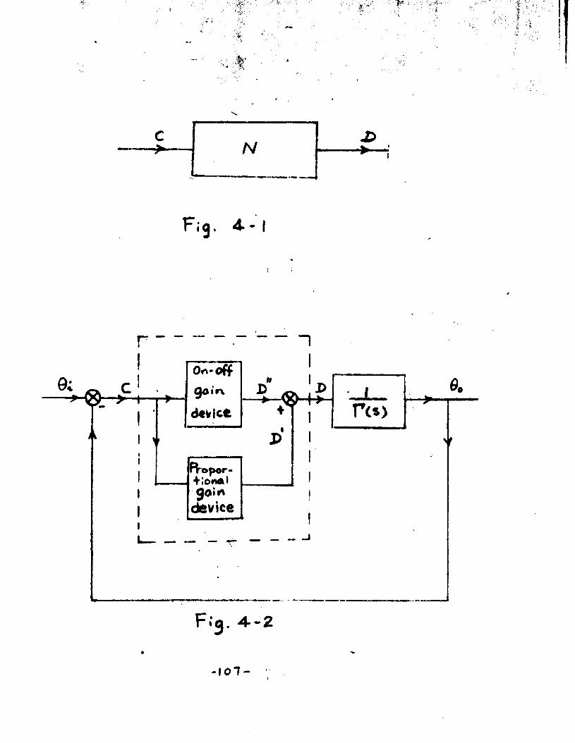
■'S'

Fig. 4.-I

rc 1

!

n

_ t

Fig. 4- -2

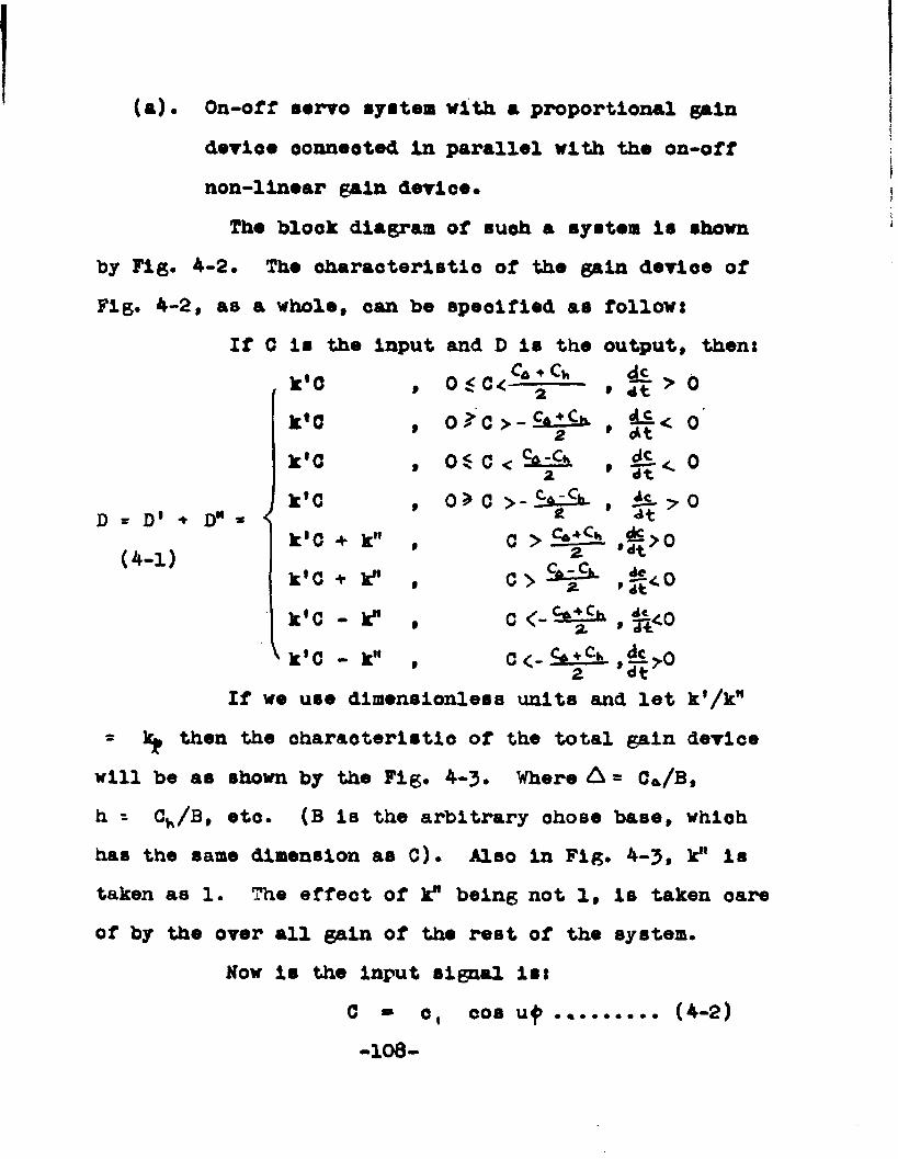
(a). On-off servo system with a proportional gaindevloe connected in parallel with the on-offnon-linear gain device*

The block diagram of such a system is shown by Fig. 4-2* The characteristic of the gain devloe of Fig. 4-2, as a whole, can be specified as follow:

If G is the input and D is the output, then:

- Up then the characteristic of the total gain device will be as shown by the Fig* 4-3* Where A = Ca/B,h - Ch/B, eto* (B is the arbitrary chose base, whichhas the same dimension as C)* Also in Fig* 4-3, k" is taken as 1. The effect of k" being not 1, is taken oareof by the over all gain of the rest of the system.

D - D' * D" * S

k'Gk,0k'G

k'C + k" C > S+*SlL ,$>02 *dt(4-1)k'C + k" k'C - k"

V k » c -If we use dimenslonless units and let k'/k"

Now is the input signal is:C ® o, cos - 108-

(4-2)

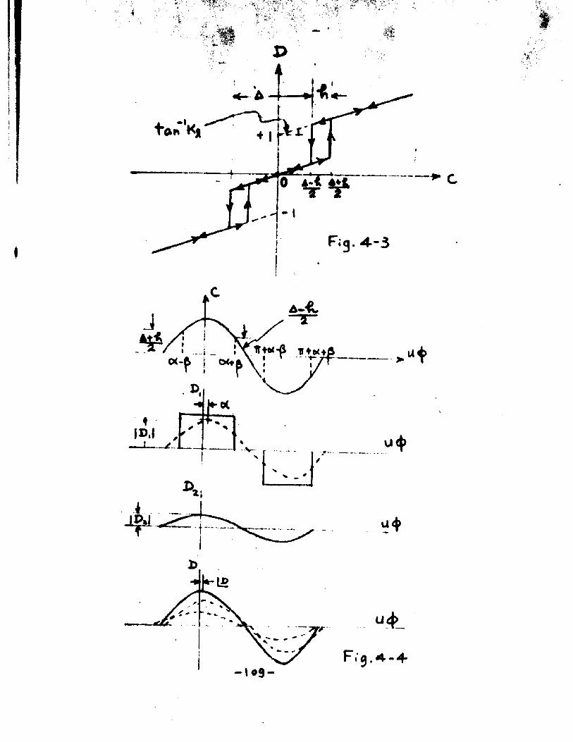
tftn K|

C

- >

■ V -

p*l

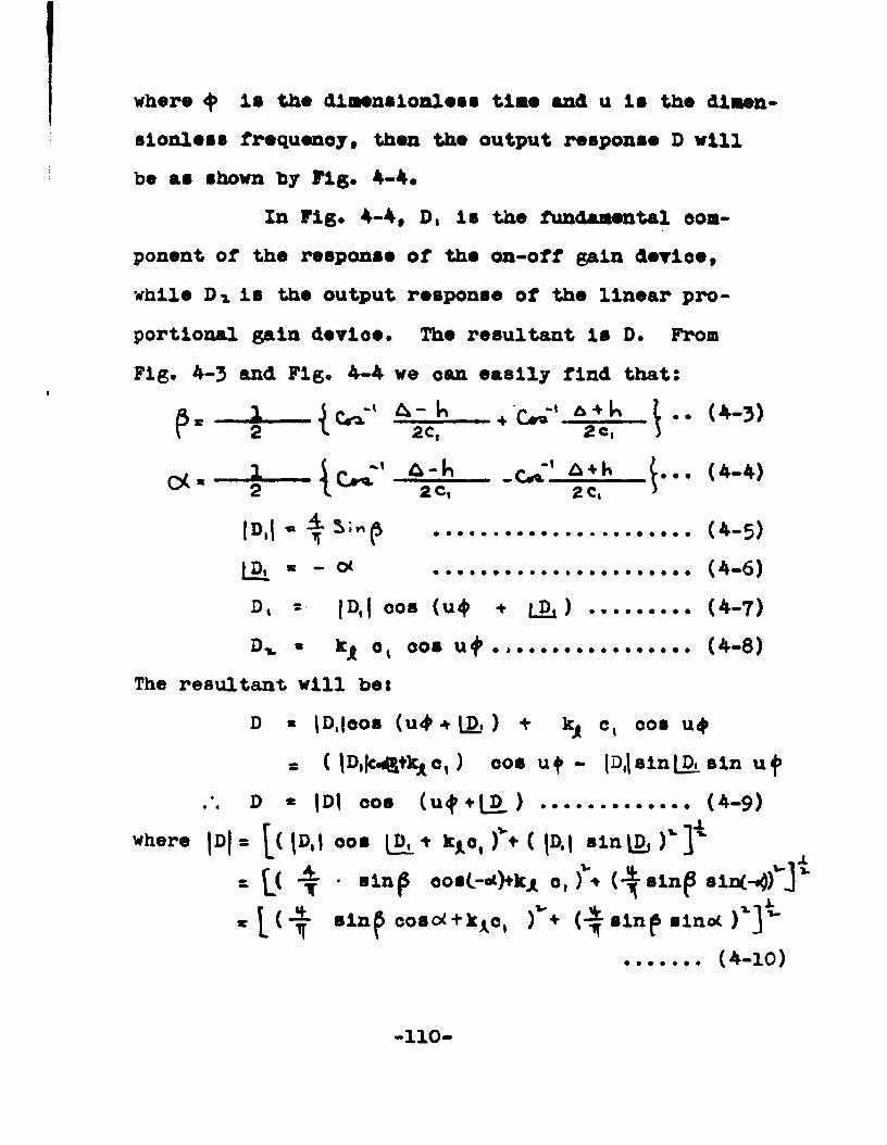
where <$> is the dlmsnslonless time and u is the dimen* slonless frequeney, then the output response D will be as shown by Fig* 4-4*

In Fig* 4-4, D| is the Fundamental com­ponent of the response of the on-off gain device, while Di is the output response of the linear pro­portional gain devioe. The resultant is D. From Fig. 4-3 and Fig. 4-4 we oan easily find that:

fir - 1 i <VaT' & - ^ 6 + 1 .1 .. (4-3)r s 2 \ 2Ct 2 c, ]

i Cra A -_h r-«"' A + h (4-4)O * 2 I 2 C, 2 C,

l».l . A Sin LD, « — cx ---- (4-6)D, r . |D,| cos (u4> ♦ ) •-•••Dv « kjj c, oos U^ ...... ---- (4-8)

The resultant will be:D * jDJoos (u^ + LD, ) y k| c, cos u^

s ( |D,|c^tkA c, ) cos uf - (DjainlDi. sin ufD « |D| cos (u^^LD.) ............. (4-9)

where |D| = [( |D,| cos i- k^c, )% ( |D,| sin ID, )v ]'“ \S *t’ oosC- Hk* o,)e (“»sln6 sln(- ) Jv« ^ sinp costf + k^c, )V+ sinp sinot )XJ 1'

...... (4-10)

-110

-* J L -and Lfi- * "t&n T ■•IttP_________ H a 2 < ___A aln p oo»o< t kfto , ... (4-11)The describing function*

N(c , li ) » D / e ,oos u<|>, IDI | D .... (4-12)Expand Equation (4-10)s^ x\D| «|^sin^ + 2 ^ s i n p kj cosfirfc, + kjo*].*?.. -. (4-13)

Hence ^ .iDi/c, (4-M>

Rewrite Equation (4-11):, 4 Al d « - C o f - ^ slaP,ggy* + fa g,1— IZT^in^rainir ... (4-15)

But sin cx eln^, 1 cos (o».-jS ) - 1 cos (<xtp) (4-16)and

c o b ( oi - p ) * ( a * k ) / 2 ............ (4-17)c o b (oc i p ) * ( n - h ) / 2 ............ (4-18)

^ slnp s i n o « « | [ ( ) - (A-hj* 2i^ * 2h/j (4-19)[D_ - -cot '... cot<x+i|k^ c, /2h ] ............. (4-20)

Equation (4-14) and equation (4-20) determines the des­cribing function locus. As for the pure on-off servo, we find that in this oase the describing funotlon is also a function of amplitude only. Hence the describ­ing function locus will be an amplitude locus. As for the pure on-off servo we oan compute and draw the am­plitude locus with different assigned values for

-111

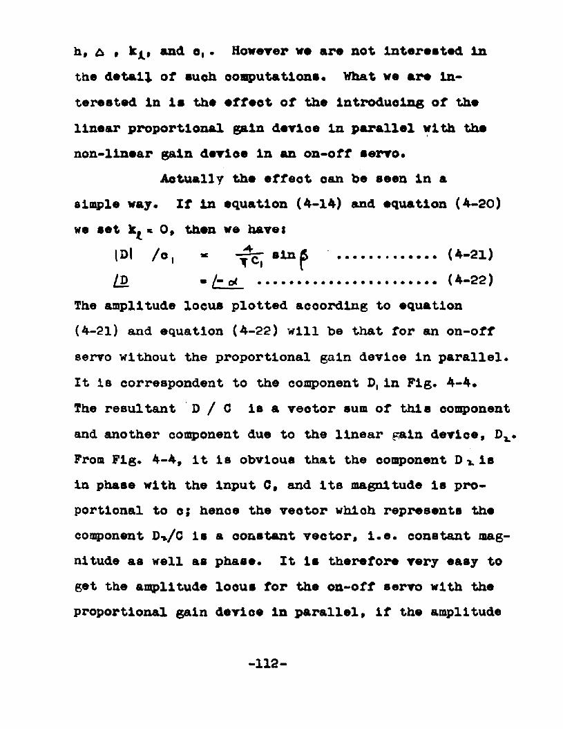
h, a , k^» and e, • However we are not Interested in the detail of auoh computations • What we are in­terested in is the effeet of the introducing of the linear proportional gain device in parallel with the non-linear gain device in an on-off servo*

simple way* If in equation (4-14) and equation (4-20) we set * 0, then we haves

The amplitude locus plotted according to equation (4-21) auid equation (4-22) will be that for an on-off servo without the proportional gain devloe in parallel. It Is correspondent to the component D, in Fig. 4-4*The resultant D / 0 is a veotor sum of this oomponent and another component due to the linear gain device, D^* From Fig. 4-4, it is obvious that the component D * is in phase with the input C, and its magnitude is pro­portional to o; hence the veotor whloh represents the component Da/C is a constant vector, i.e. constant mag­nitude as well as phase. It is therefore very easy to get the amplitude locus for the on-off servo with the proportional gain device in parallel, if the amplitude

Actually the effeot can be seen in a

iDl , l n (*-21)(*-22)

-112

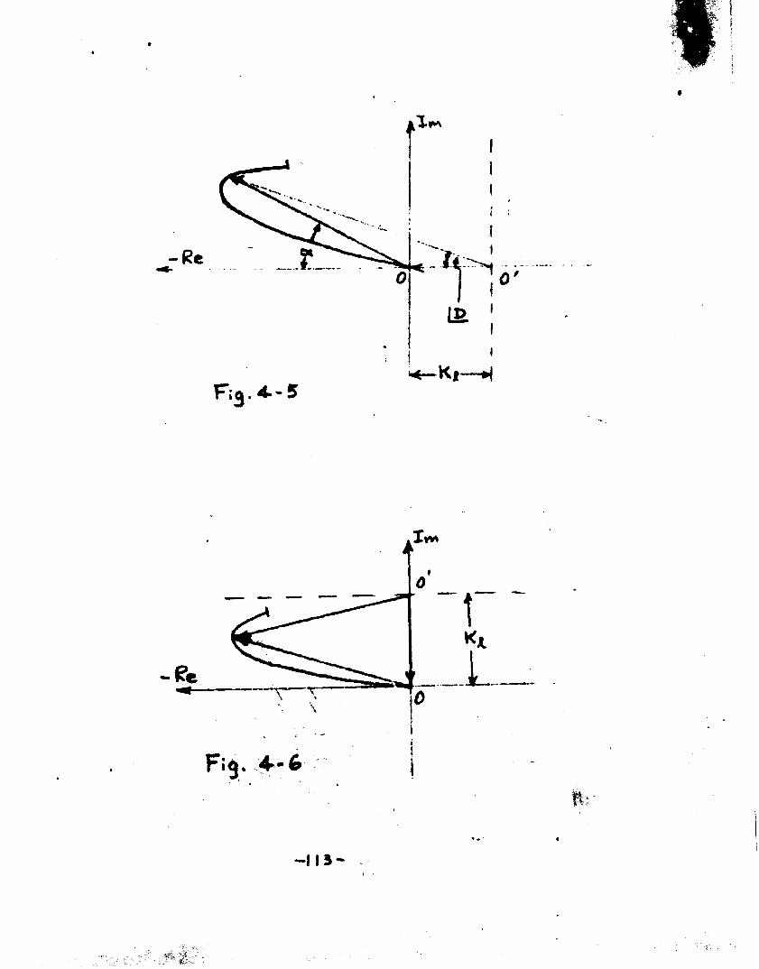
Ht-— Kjf '■

loeus for the on-off servo alone is given. This la Illustrated in Fig* 4-5*

From Fig. 4-5, we oan see that the net effeot of lntroduolng the proportional gain device in parallel with the on-off gain device In an on-off servo Is to shift the amplitude loeus toward the left* As far as stability Is concerned, the larger the value of

, the lesB the stability* However when k^ Is small, the net effect on stability can be made negligible.The sacrifice of stability in this case is of course compensated by the less steady state error* Theoreti­cally with kj > 0, however small, the servo system will give no steady state error when the servo is used as a position servo*

(b). On-off servo system with a derivative con­trol gain device connected in parallel with the on-off non-linear gain device*From the study of case (a), we learned that

the presence of a proportional gain devloe In parallel with the on-off gain devloe In an on-off servo system is equivalent to shift the amplitude locus towards left In the Inverse transfer function plane* Therefore it decreases the stability* This Immediately gives us a hint, that the amplitude locus can be shifted one

-114-

way or the other by connecting & different gain device In parallel with the on-off gain devloe. One way to do ltv which cornea to mind immediately la to uae a linear gain devloe, whoae output la proportional to the derivative of the Input signal, In parallel with the on- off gain devloe.

Before we go further on, we ahall try to study a special oaae first. Let us assume that a linear gain devloe la connected to the on-off gain device of the on-off servo aystem. We also assume that; that linear gain devloe has such a property that It gives an output with lta magnitude proportion to the Input but It also gives a phase shift of 90 degrees lrrespect to the frequency. That la; if the input Is:

C * o ( Cos kit D v » -kjj c t sin kit

The analysis of this ease la similar to the case before. The result oan be best understood by re­ferring to Fig. 4-6.

It Is obvloua from Fig. 4-6, that the effect of such an arrangement la to shift the amplitude looua downward, whloh to a certain degree, usually helps to improve stability.

-115-

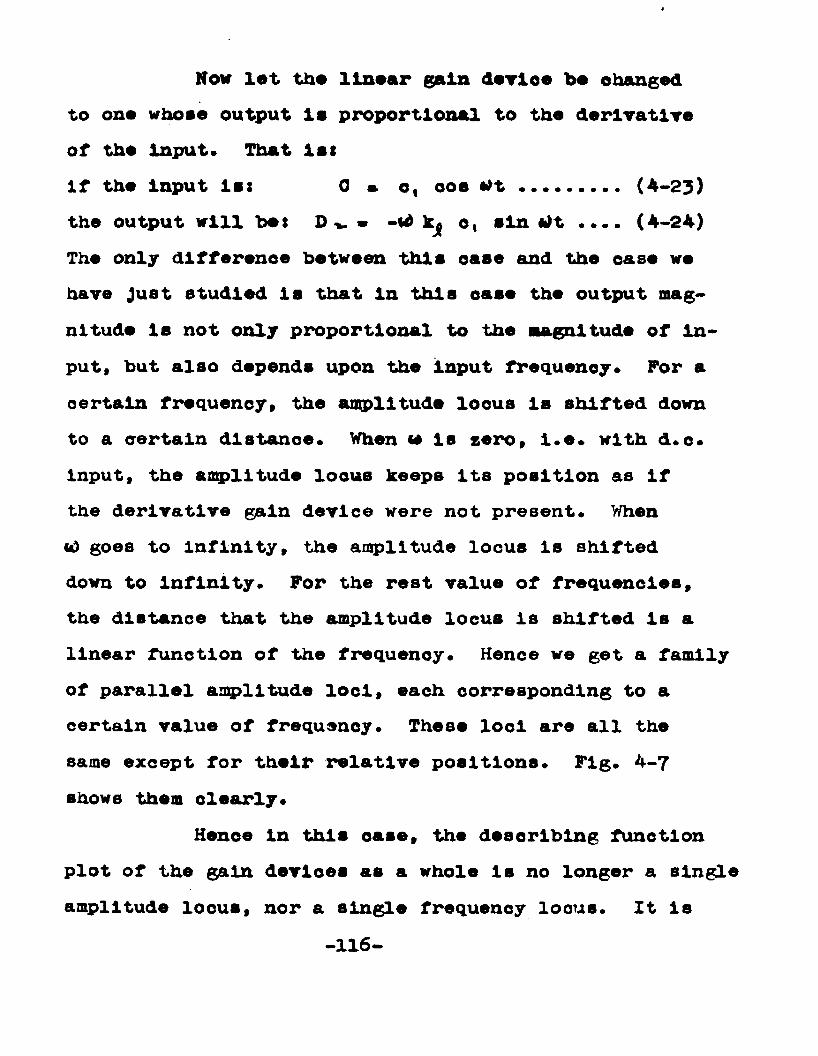
Now let the linear gain devloe be ohanged to one whose output is proportional to the derivative of the Input. That 1stif the Input Is: 0 » o, cos *>t......... (4-23)the output will bet D °» 11111 ll>t •••• (4-24)The only difference between this oase and the ease we have Just studied Is that In this oase the output mag­nitude Is not only proportional to the magnitude of In­put, but also depends upon the input frequency. For a certain frequency, the amplitude locus Is shifted down to a certain distance. When «* Is zero, i.e. with d.e. input, the amplitude locus keeps Its position as If the derivative gain device were not present. When <0 goes to Infinity, the amplitude locus is shifted down to infinity. For the rest value of frequencies, the distance that the amplitude locus is shifted Is a linear function of the frequency. Hence we get a family of parallel amplitude loci, each corresponding to a certain value of frequency. These loci are all the same except for their relative positions. Fig. 4-7 shows them clearly.

Hence In this oase, the describing function plot of the gain devices as a whole Is no longer a single amplitude locus, nor a single frequency locus. It Is

-116-

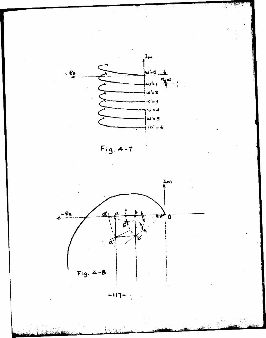
a system of lool which depends upon the frequency as well as the amplitude of the input. How we are going to deal with suoh a case with the describing function not only a function of frequency but also a function of amplitude is the main purpose of this chapter*£* fuagftlaa Iggl wblofr.aaa-frt

reduoed to a single amplitude locus* with asingle modified final frequency locue*

Not necessarily all systems of describing funotion loci whioh depend upon both the input magni­tude and the input frequency can be reduoed to a single loous which depends either on frequency only or on mag­nitude only, with a single modified final frequency locus. If it is possible to reduce such a system of loci to a single amplitude locus or a single locus whioh depends upon frequency only and still with a single modified final frequency locus, then we can apply the two loci method as in chapter II and chapter III. The stability criterion of suoh oases would be of no diffi­culty. But unfortunately this is not true. For ex­ample, the case as shown by Fig. 4-7» we Just cannot do it*But in some cases it is possible to reduce suoh a

-118-

ay stem of describing funetlon lool Into a single amp­litude looua and still with a single modified final frequeney locus. Let us find out now when such, cases are possible.

We first take a simple ease as shown by Fig. 4-8. The describing function loci in this case are only four pointst a, b for a certain frequency range, and a', b* for the rest of the frequency range. For sim­plicity we assume that points a, a 1 cover the same range of amplitude and points b, b* cover the rest of the amp­litude range. It is obvious that even in such a simple case when a' is rotating to the position an on the neg­ative real axis, point b* is rotated to a new position b" which is not on the negative real axis. Hence it is impossible to get point b' to the position b when the point a' assumes the position a through further scale changing.

However if the points are originally lo­cated as shown by Fig. 4-9, then when the point a r is rotated to the position a", the point b ’ will also be rotated to the negative real axis. Moreover, since tri­angle aa'o and triangle bb'o are similar, hence

2ft = — g&* , .2*"ob o b ^ Ob*1 ........ (4-25)

-119-

Therefore when -the point a' aasunea the position a, the point b' will assume the position b. In this case, it is therefore possible to reduce the describing func­tion looi to one set of points a and b.

Of oourse we can extend our result to the case where the two describing function loci are two lines ab and a'b'*

What would happen if we hare a broken line as shown by Fig. 4-10? In Fig. 4-10 the triangle oab and the triangle oa'b* are similar, while the triangle oaMb,t is not* Since rotation and scale changing do not change the form of the triangle, a right triangle will still be a right triangle and a non-right-triangle cannot become a right triangle* Hence the broken line oa'b' cam finally assume the position oab while the broken line oa"b" cannot*

Similarly for any curve segments as shown by Fig* 4-11, if we draw two lineB through the origin to the terminating points of the curves, if the geometri­cal configuration of ^he resultant regions are similar (as shown by the shaded areas), then these loci may be squeezed into one locus by rotating and soale changing and still with one final modified frequenoy locus*

-121

a.i-

Pi q. 4*- 11

l»n.

For example, suppose ve have a non-llnear devloe and a linear element connected In oasoade beside the rest of the servo system. If we oonslder the combi­nation of the linear element and the non-linear element in cascade as a single new non-llnear element, then the describing funotlon loci of this non-llnear element will be very complicatein general. If however the original non-llnear element gives a describing function locus de­pending upon the amplitude only, as the case of an on- off servo, and if the linear element that we include in­to the new non-linear element is an ideal combined pro­portional and derivative control compensating network, the system of the describing function loci will be as shown by Fig. 4-12.

We notice that the shaded areas are all similar, hence such system can be analyzed by squeezing all those describing function loci into a single ampli­tude locus.

It is not necessary that those shaded areas must increase or decrease in a certain order. As long as they are similar and the system of the describing funotlon loci are continuous funotlon of frequency, we can always squeeze them into a single loous. For ex-

-123-

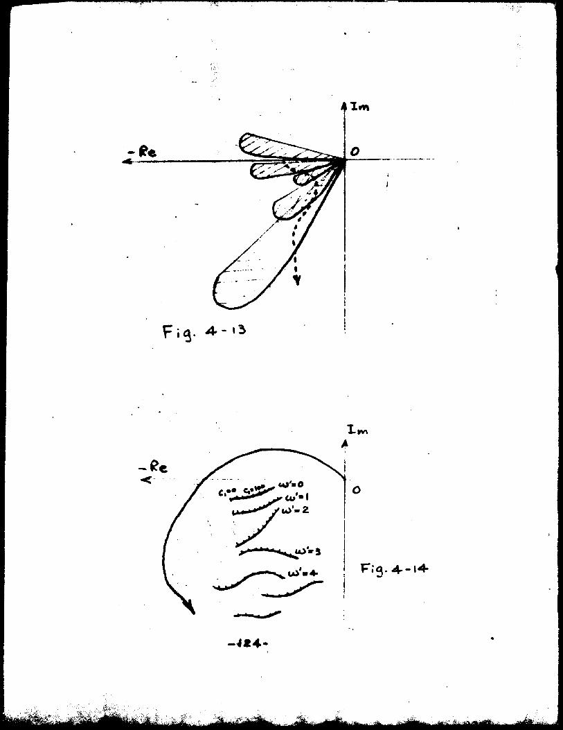
4 1 m

Fi$*

F;g.4.-i4-

- 4* 4 -

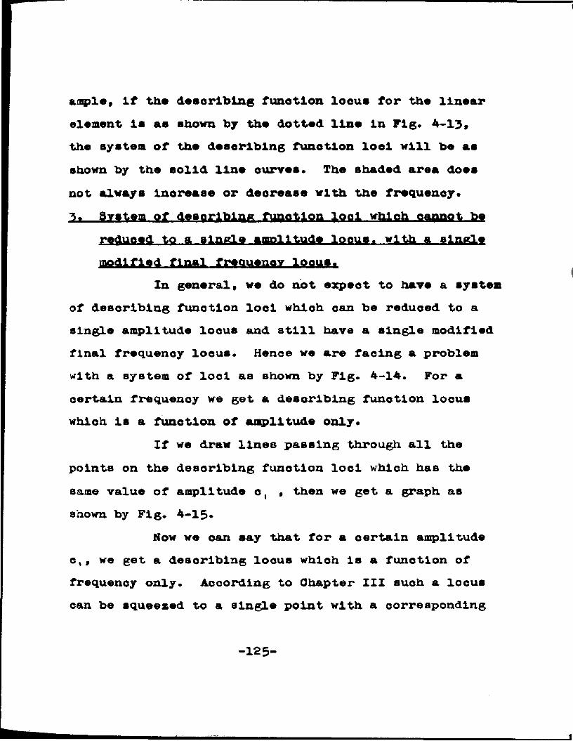
ample, if the describing funotion locus for the linear element is as shown by the dotted line in Fig* 4-13> the system of the describing funotion loci will be as shown by the solid line curves. The shaded area does not always lnorease or decrease with the frequency*3* System of describing function lool which oannot be

reduced to a single amplitude locus, with a singlet l m l fr«qvwMz.lQflMLi*

In general, we do not expect to have a system of describing funotion loci which can be reduced to a single amplitude locus and still have a single modified final frequenoy locus. Hence we are facing a problem with a system of loci as shown by Fig. 4-14. For a certain frequency we get a describing funotlon locus which is a function of amplitude only*

If we draw llneB passing through all the points on the describing funotlon loci which has the same value of amplitude o, , then we get a graph as shown by Fig. 4-15*

Now we can say that for a certain amplitude c,, we get a describing locus which Is a funotlon of frequenoy only. According to Chapter III such a locus can be squeezed to a single point with a corresponding

-125

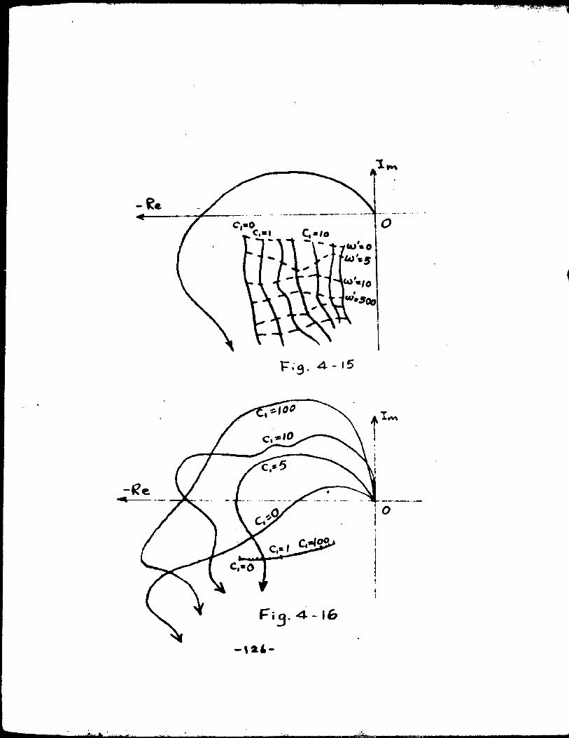
c,«l

reshaped final frequenoy locus. In -this way it is therefore possible for us to squeese all the describing funotion loci into a single one, however, not with a single final frequenoy loous but with a group of the modified final freqpenoy loci as shown by Fig. 4-16.

In Fig. 4-16, each amplitude o, has its own final frequenoy loous. The stability criterion will depend on the relative position of that point and its associated modified final loous. Henoe we have to try all these points one by one. It is possible to get the solution, but it really needs lots of time to get the new set of the modified final frequenoy loci. To save the time, the two-locus method discussed in Chap­ter III will offer a great help.

Take an example, say the case of on-off servo with a derivative control gain device in parallel with the on-off devioe, i.e. the case we have discussed in the beginning of this chapter as an introductory case. If we assume the dlmenslonless characteristic of the contactor devioe of the on-off servo as represented by Fig. 4-17, then the desoribing funotlon locus of the contactor device alone can be calculated by equation (4-21) and equation (4-22).

-127-

The describing funotlon of the oomblnatlon of tho two gain device In parrallei as a whole oan be calcu­lated by equation (4-14) and equation (4-20); or In this oaee It la easier by shifting the describing funotlon loous of the oontaotor device alone along the negative real axis. If we aasume that*

A * 0.1V\ « 0.02

and the transfer funotlon of the rest of the servo system3 CJU ’ * ja'u*ju)'

and also assume that the parallel loop of the oontaotordevice has a transfer funotion: kjg Ju , then the systemof the describing funotion loci will be as shown by Fig.4-18. It is really not difficult to draw those loci ifwe know one of them. We Just make a templet and shiftA the negative imaginary axis.

We can now apply the two-locus method to dis­cuss the system stability.As frfr* 9Br9££_S3rig

system with a pure derivative controller connecting in parallel with the on-off contactor device*

The system stability oan be discussed asfollows:

-128

♦*<

ifH .

ih

W

-»

p » Q . 4-* I?

ic

•*r !

■J-i? A-Jlt

(a)* Without the derivative device connected in par­allel with the contactor device, the eyetea is unstable. It will give a self-sustained oscillation.(b). With the parallel loop (the derivative controller) the possibility to have a self-sustained oscillation occurs only at those polnta where the frequency locus intersects the describing function loci. This would happen between the belt region, as shown by Fig. 4-19,if there were such oscillations.(c). If there were no suoh points correepondlng to self-sustained oscillations, then we proceed to determine whether the system Is stable or not. We try to find the

chapter.(i). Let us assume that we find such a value

We assume A reads u = uc on the frequency locus and has a describing function locus with u f « u^passlng through it. We also assume the point B is the inter­secting point between the frequenoy locus and the des­cribing funotion loous with u 1 « u t(cuj. If the

value of ue, then compare and

of u t at point A with 0 <. u c u#on the portion of the frequency locus EG within the belt region as shown by Fig. 4-20.

-131-

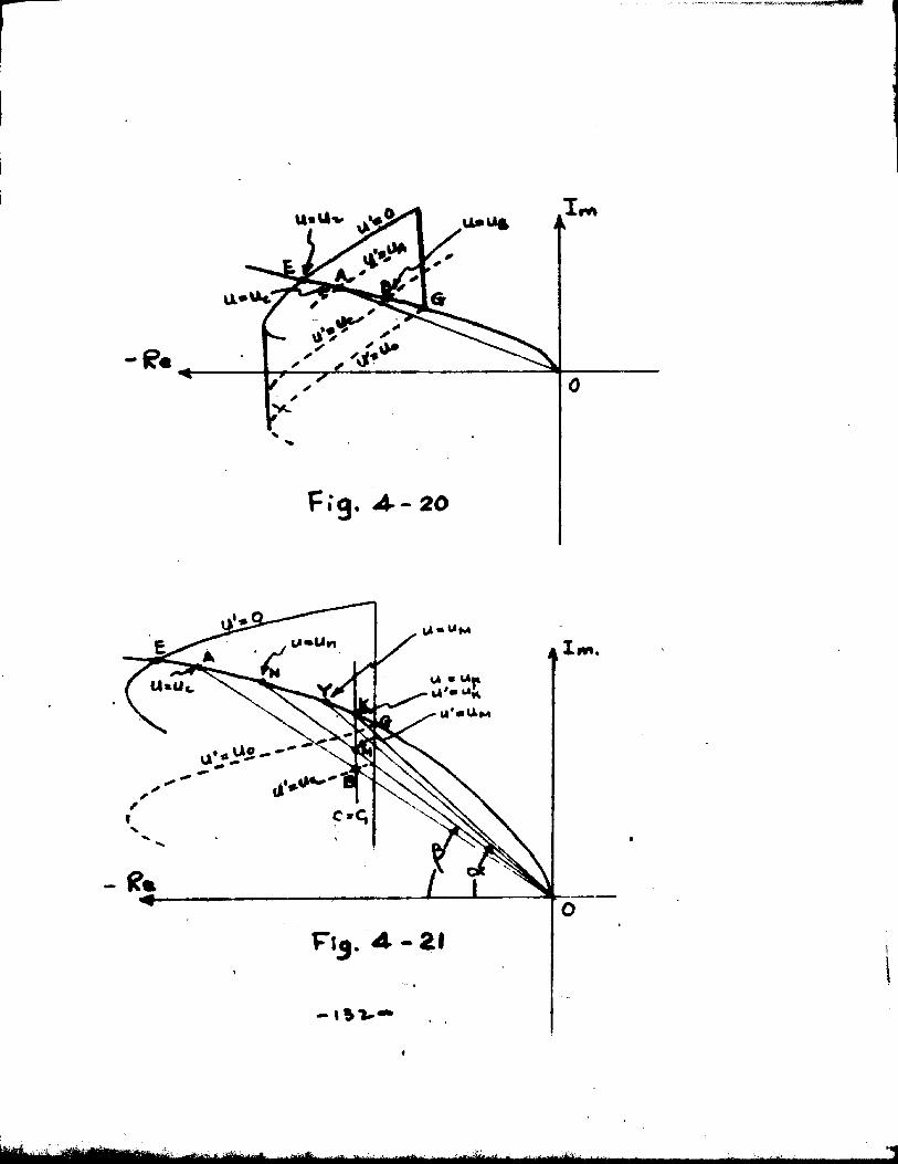
llVI

X

«

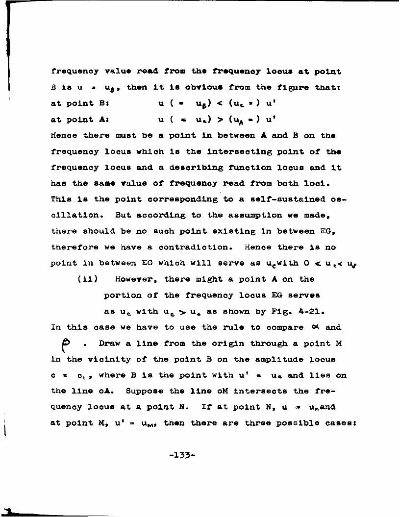
frequenoy value read from the frequenoy loous at point B is u a Uj, then it is obvious from the figure that;at point Bx u ( ■ u^) < (ut *) u'at point As u ( * u«.) > (uA » ) u*Hence there must be a point in between A and B on thefrequency loous which is the intersecting point of the frequency locus and a describing funotion loous and it has the same value of frequency read from both lool.This is the point corresponding to a self-sustained os­cillation. But according to the assumption we made, there should be no such point existing in between EG, therefore we have a contradiction. Hence there is no point in between EG which will serve as uewith 0 < u e<

(li) However, there might a point A on the portion of the frequency locus EG serves as u t with u t > u 0 as shown by Fig. 4-21.

In this case we have to use the rule to compare and • Draw a line from the origin through a point M

in the vicinity of the point B on the amplitude locus c * c, , where B is the point with u' * u a and lies on the line oA. Suppose the line oM Intersects the fre­quency locus at a point N. If at point N, u <• u„and at point M, u* =» uM , then there are three possible cases:

-133-

(1). »(2). <(3). > u*4

We assume that u* Is the frequenoy value which gives the minimum Oa/Ob > 1. Since the closer the point Aapproaches to the point k (the intersecting point of the frequency locus and the amplitude locus with o a c) , the samller the ratio Oa/Ob if there were more than one pair of such characteristic points like (a,b). Case (1) will give an contradiction if it exists, hence it is automatically ruled out.

Consider the case (2), we find that at point k, it is necessary that: u ( * uK) > (u* » ) u'while at points M and N: u ( - ur) < ( u M « ) u 'Therefore in between N and K there must be a point cor­responding to another pair of characteristic points like (a,b). But if such points exist, it will give a ratio Oa/Ob less than that of the point A, which we have assumed to have the minimum ratio Oa/Ob > 1.Therefore case (2) is also ruled out.

The only possible case exists is the case (3)* where we have u n > uM. The point on the frequenoy loous whioh has the same value of frequency as u M must lie below the point N or in the portion ON of the

-134-

frequenoy loous. Let us assume that point ¥ be such a point with u * uM as shown by Fig. 4-21, then it is obvious that: \ot 1 >\£>1Since both ot and ft are negative in this oase, hence:

(5 > * *the system will be stable.

(ill). In oase we can't find the frequency u c onthe portion of the frequency locus QE, we might find such point above the point E and below sm­other point Q with u •» u^, where u^ is thefrequency value at which the describing func­tion locus Just comes completely under the negative real axis as shown by Fig. 4-22.

Assume that A is the point with u » uc. At point B u' x u*and OAB is a straight line. Then as before we draw the line OM intersecting the frequency loous at point N, where point M is the point on the amplitude loous with o = c ( and passing through the point B. Point M also has a frequenoy value which is lower than but very close to the frequency value of point B. With the assumption that point A is the point which gives the minimum Oa/Ob > 1 ratio in that region, then the same arguments oan be applied to here as in (ii). The

-135-

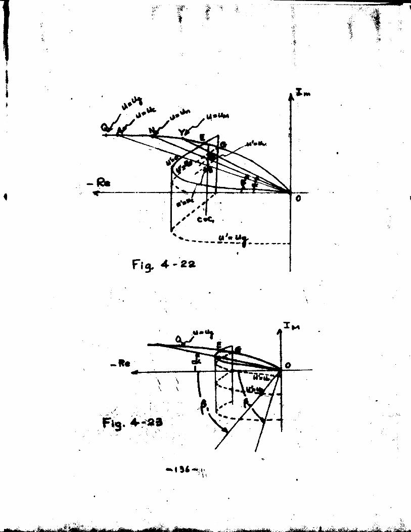
W»

a*'*'

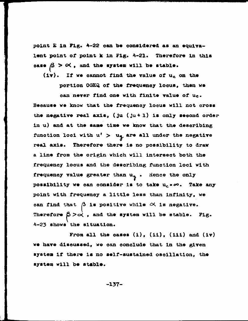
point E In Fig* 4-22 oan bo oonaldorod as an equlva- lont point of point k in Fig. 4-21. Therefore in this ease 3 > o< , and the system will be stable*

(It )* If we eannot find the value of ut on theportion OGEQ, of the frequency loous, then we oan never find one with finite value of Uc*

Because we know that the frequenoy locus will not cross the negative real axis, (Ju (ju+l) is only second order in u) and at the same time we know that the describing function loci with u* > u . are all under the negative real axis* Therefore there is no possibility to draw a line from the origin which will intersect both the frequency loous and the describing function loci with frequency value greater than u^ • Hence the only possibility we oan oonsider is to take uc»cx>. Take any point with frequenoy a little less than infinity, we can find that p is positive while is negative* Therefore p >c< , and the system will be stable. Fig* 4-23 shows the situation*

From all the oases (i), (11), (ill) and (iv) we have dlsoussed, we can conclude that in the given system if there is no self-sustained osolllation, the system will be stable*

-137-

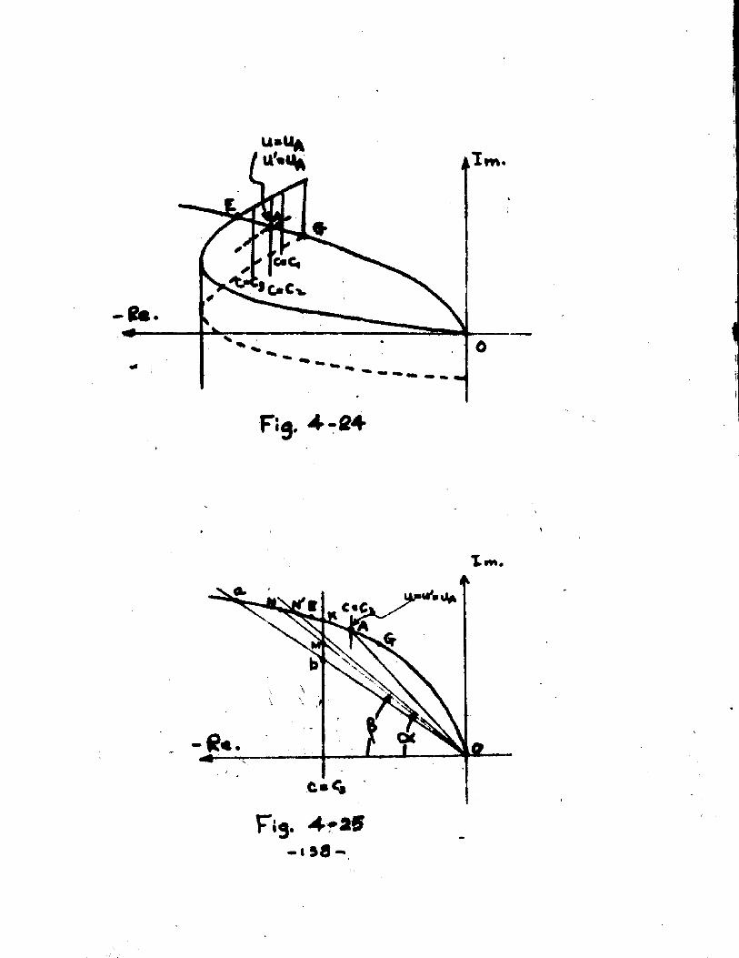
c-c,Fig. 4* 2 5

- » s a -

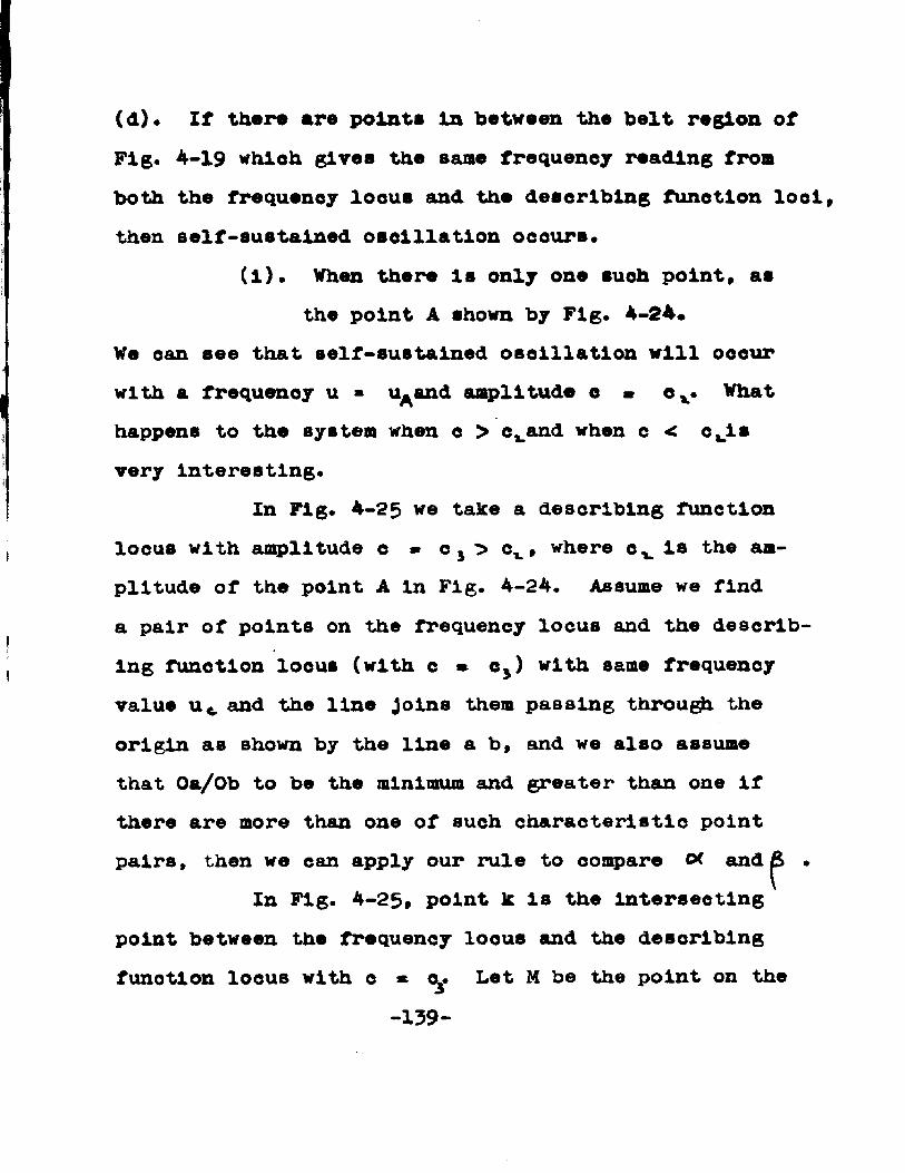
(d). If there ere point* in between the belt region of Fig* 4-19 which gives the same frequency reading from both the frequenoy locus and the describing funotion loci, then self-sustained oscillation ocours*

(i). When there is only one such point, as the point A shown by Fig* 4-24.

We oan see that self-sustained oscillation will occur with a frequency u » u^and amplitude e - c x. What happens to the system when e > e^and when c < cuis very interesting*

In Fig* 4-25 we take a describing function locus with amplitude c * c 5 > cx , where cv is the am­plitude of the point A in Fig. 4-24. Assume we find a pair of points on the frequency locus and the describ­ing funotion locus (with c * e3) with same frequencyvalue u c and the line Joins them passing through the origin as shown by the line a b, and we also assume that Oa/Ob to be the minimum and greater than one if there are more than one of such characteristic point pairs, then we can apply our rule to compere o< and^ •

In Fig. 4-25, point k is the intersectingpoint between the frequency loous and the describing funotion locus with c * cy Let M be the point on the

-139-

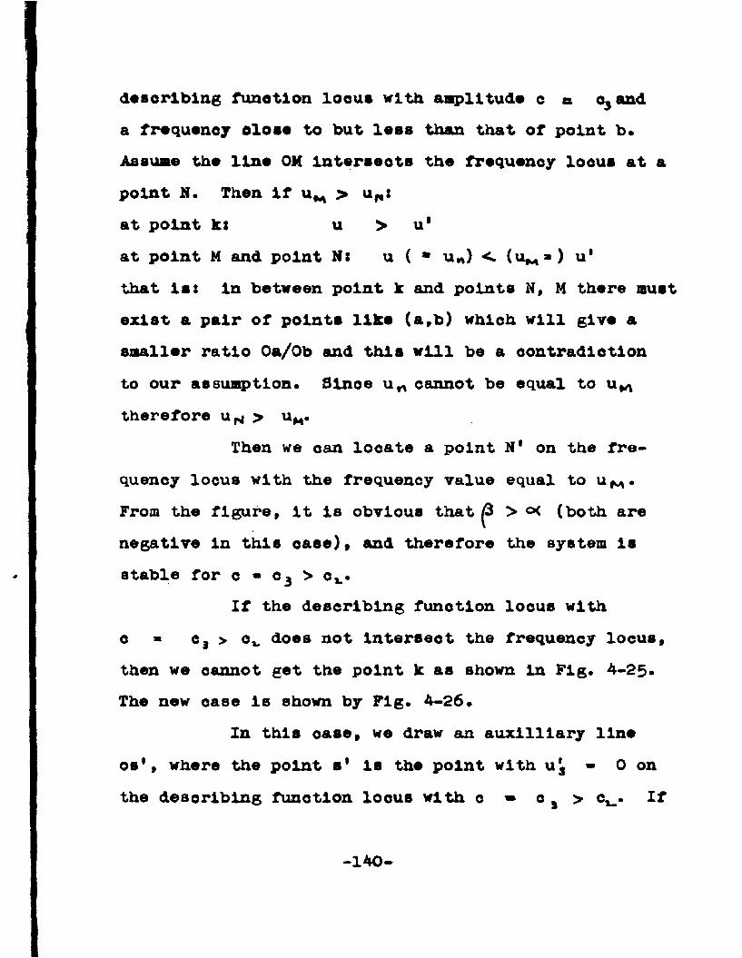
describing funotlon loous with amplitude c e o3anda frequency close to but less than that of point b.Assume the line OM Intersects the frequenoy loous at apoint N. Then If u M > u^tat point let u > u'at point M and point Nt u ( * u n) < (u^,*) u*that is: in between point k and points N, M there mustexist a pair of points like (a,b) which will give asmaller ratio Oa/Ob and this will be a contradictionto our assumption. Slnoe u n cannot be equal to u Mtherefore u i > uM.

Then we oan locate a point N' on the fre­quency locus with the frequency value equal to u M .From the figure, It la obvious that p > <=* (both arenegative in this oase)v and therefore the system isstable for c * c3 > ct.

If the describing funotlon locus with o * c3 > Cj_ does not Intersect the frequency locus, then we cannot get the point k as shown In Fig. 4-25. The new oase is shown by Fig. 4-26.

In this oase, we draw an auxilliary line os', where the point s' is the point with u 3 - 0 onthe describing funotion locus with c » c s > c*_. If

-140

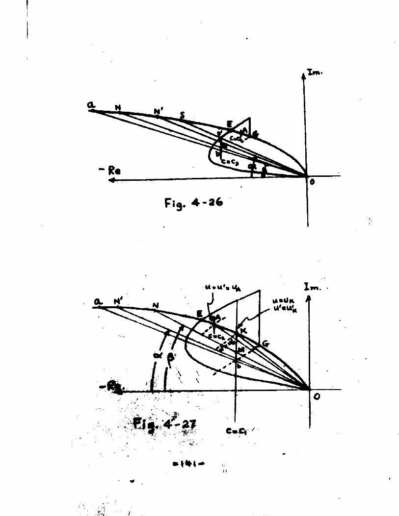
ia»Uku'cul

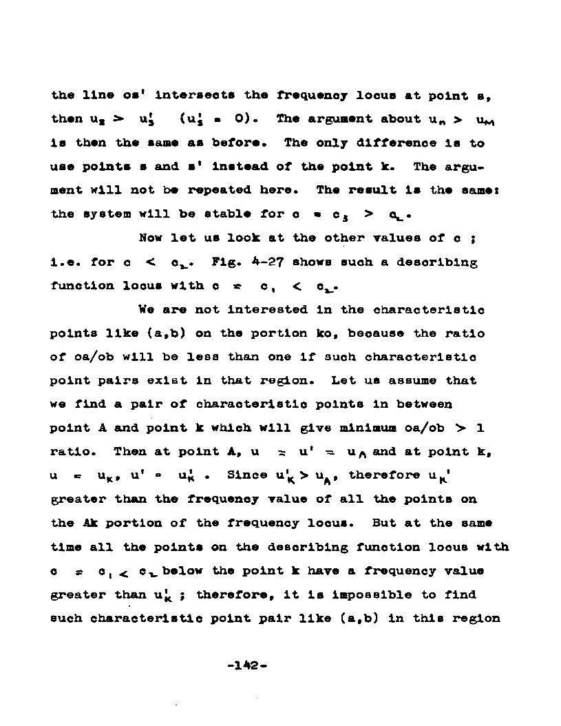
the line os' Intersects the frequenoy locus at point a* then us >■ uj (uj ■ 0). The argument about u n > u^la then the same aa before. The only difference la to uae points a and a' inate&d of the point k. The argu­ment will not be repeated here. The result la the same* the system will be stable for o ■ c s > •

Now let ua look at the other values of c ; i.e. for c < c^. Fig. 4-27 ahowa such a describing function loous with c «■ c , < c _.

We are not interested In the characteristic points like (a,b) on the portion ko, beoause the ratio of oa/ob will be less than one If such characteristic point pairs exist in that region. Let ua assume that we find a pair of characteristic points in between point A and point k which will give minimum oa/ob > 1 ratio. Then at point A v u - u* ■=. u and at point k 9 u uK* u* » u* • Since u'^ > u^f therefore u^'greater than the frequency value of all the points on the Ak portion of the frequency locus. But at the same time all the points on the describing function loous with o » o , < c -v below the point k have a frequency value greater than u^ ; therefore, it is Impossible to find such characteristic point pair like (a,b) in this region

-142-

too. The onlj possible region to have suoh character­istic point pairs oust exist above the point A on the frequency loous If there Is any*

Let us assume suoh a point pair exists as the points a and b In Fig. 4-27* The line OMN Is drawn in the same manner as the previous oases. If u n > u M then In between the point N and A we oan find another point pair like (a,b), which Is oontradlotory to our assumption that the given one Is the characteristic point pair with minimum oa/ob > 1 ratio. Therefore u N < u Mand we oan looate a point N' on the frequency locus with u = u v^B shown In the figure. It is ob­vious from the figure that in this case ot > • Hence the conclusion will bet The system will be unstable for c * c , < e v.

The foregoing discussion gives us the infor­mation about the system motion, that: when the magnitudeo Is greater than ex, the system is stable, the magni­tude of c will therefore decrease toward c » ev .When the magnitude c Is less than oL, the system is un­stable, the magnitude of c will therefore Increase toward c v cv. Therefore no matter what the Initial condi­tion Is, if the motion once started, it will come to that

-143-

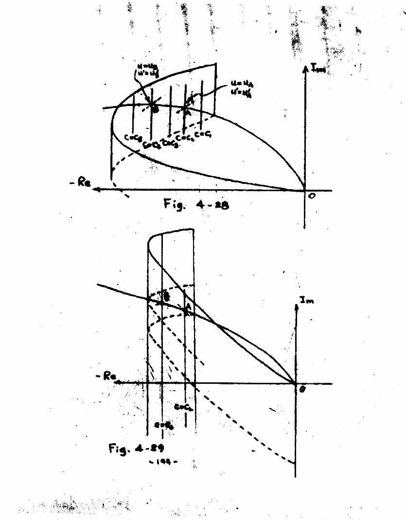
-e«

f

#.

Fij. 4 - * «

I «'* %

V J

0

Fif . * - * *

- $ST. '’• * . , ■ .«S‘

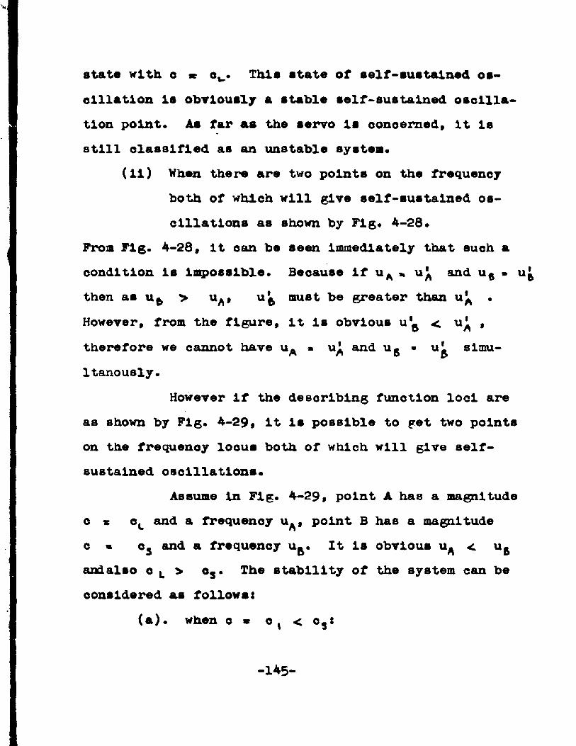
state with e *• cv. This state of self-sustained os­cillation Is obviously a stable self-sustained oscilla­tion point* As far as the servo is concerned, it is still classified as an unstable system*

(11) When there are two points on the frequency both of which will give self-sustained os­cillations as shown by Fig* 4-28*

From Fig. 4-28, it can be seen Immediately that such a condition is impossible. Because if u A « u A and u 6 > u£ then as u^ > uA, u^ must be greater than u A • However, from the figure, it is obvious u'g < uA , therefore we cannot have uA » uA and Ug ■ Ug simu- ltanously.

However if the describing funotion loci are as shown by Fig. 4-29, it is possible to get two points on the frequency loous both of which will give self- sustained oscillations*

Assume in Fig* 4-29* point A has a magnitude o s oL and a frequenoy u^, point B has a magnitude o » c5 and a frequency Ug. It is obvious u^ < Ug andalso c L > es* The stability of the system can be considered as follows:

(a), when c ■ c ( < c?:

-145-

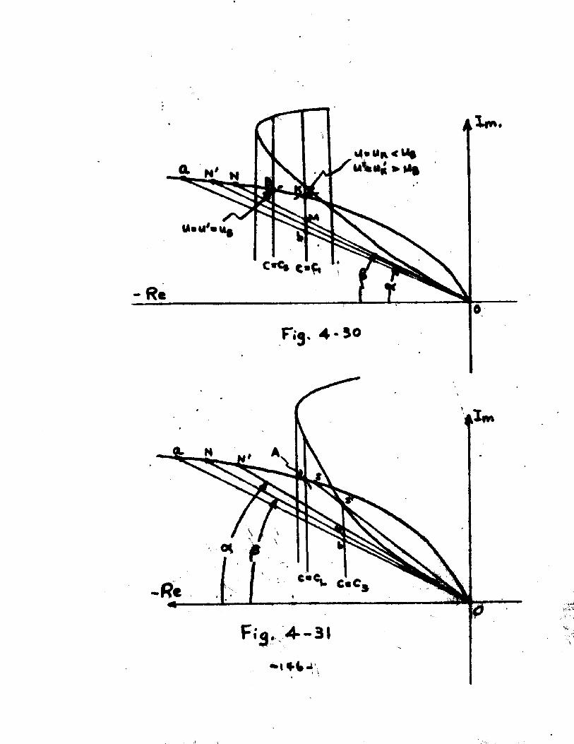
I •

-Re

c-cu c«c

Fiq, 4--3I

Refer to Pig. 4-30; let the deaerlbiag function loeue with o • o , < os Intersect the fre­quency loous at point k. We then try again the rule to compare o<> and ^ . Let the characteristicpoint pair be (a,b) as shown in the figure. Draw the line oM to interseot the frequency locus at point N. Point M is a point with a frequency do s e to but less than that of point b on the describing function locus with c * c, < c s. Since at point k:

u s U K < u5u* » U*K. > U Su*K > U K

therefore the frequency value of point M, u M iust also greater than the frequency value of point N, u n . We can then locate the point M' on the frequency locus with frequenoy value u M . 0( and ^ are then compared. Fromthe figure, it is obvious that > p . The Bystem istherefore unstable with c ■=• c x < e$ •

(b). When c * c 3 > cxtRefer to Fig. 4-31, there will be no inter­

secting point between the frequency locus and the describ ing function locus with c * c5 > oL* Let the charac­teristic point pairs be (a,b) as shown in the figure.

-147-

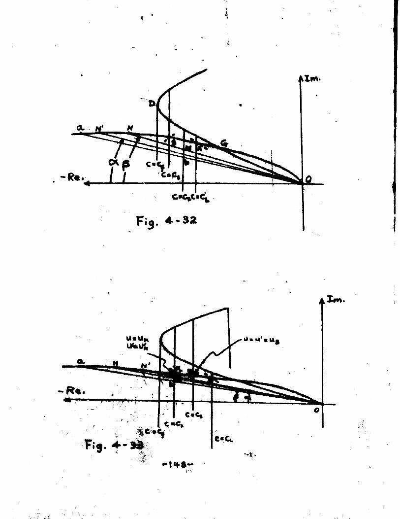
Aim*

D

C>C|C«C^

Fi3 . 4.-32

I#n

> R %

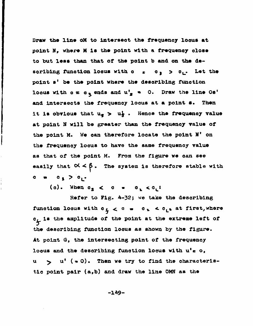
Draw the line oM to Interseat the frequency looue at point N, where M Is the point with a frequency close to but less than that of the point b and on the de­scribing funotlon locus with o « Cj > oL. Let the point s' be the point where the describing function locus with o s c ends and u't « 0. Draw the line Os'and Intersects the frequency locus at a point s* Then it Is obvious that uf > uj- . Hence the frequency value at point N will be greater than the frequency value of the point M. We oan therefore locate the point N' on the frequency locus to have the same frequency value as that of the point M. From the figure we oan see easily that Oi < . The system is therefore stable with c m o | > cL»

(c). When cs < c • o x < cL*Refer to Fig. 4-32; we take the describing

function locus with e ^ < c « c x < cL* at first, where is the amplitude of the point at the extreme left of

the describing function locus as shown by the figure.At point G, the intersecting point of the frequency locus and the describing funotlon locus with u'e o, u y u' (» 0). Then we try to find the characteris­tic point pair (a,b) and draw the line OMN as the

-149-

previous oases. Since point N is on the other side of the point A( and at point Oj u > u' ; therefore at points H and N 9 > u h. We oan then looate the pointNf on the frequenoy loous which has a frequency value u*,. It is easily seen from the figure that & • The systemis therefore unstable with c^< c » e < cL»

Now we take the describing function locus with cs < e » e^_< as shown by Pig. 4-33• Let k bethe point of Intersection between the frequency locus and the describing funotlon locus with os< c » cx<cc^. Then:at point B : u (c u^) - (u6 » ) u'at point k : u^( > u p) > u'K (<. u^)If we find the characteristic point pair (a,b) as shown in the figure and draw the line OMN as before, we will find u ^ > u . Because point N and point k are on the same side of the point B. It is easily seen from the figure after we have located the position of the point N* on the frequency locus with frequency value u^t that

>cX. • The system is therefore stable with c, < c a c x < c^.

Now if we summarize the result of (A), (B)

-150-

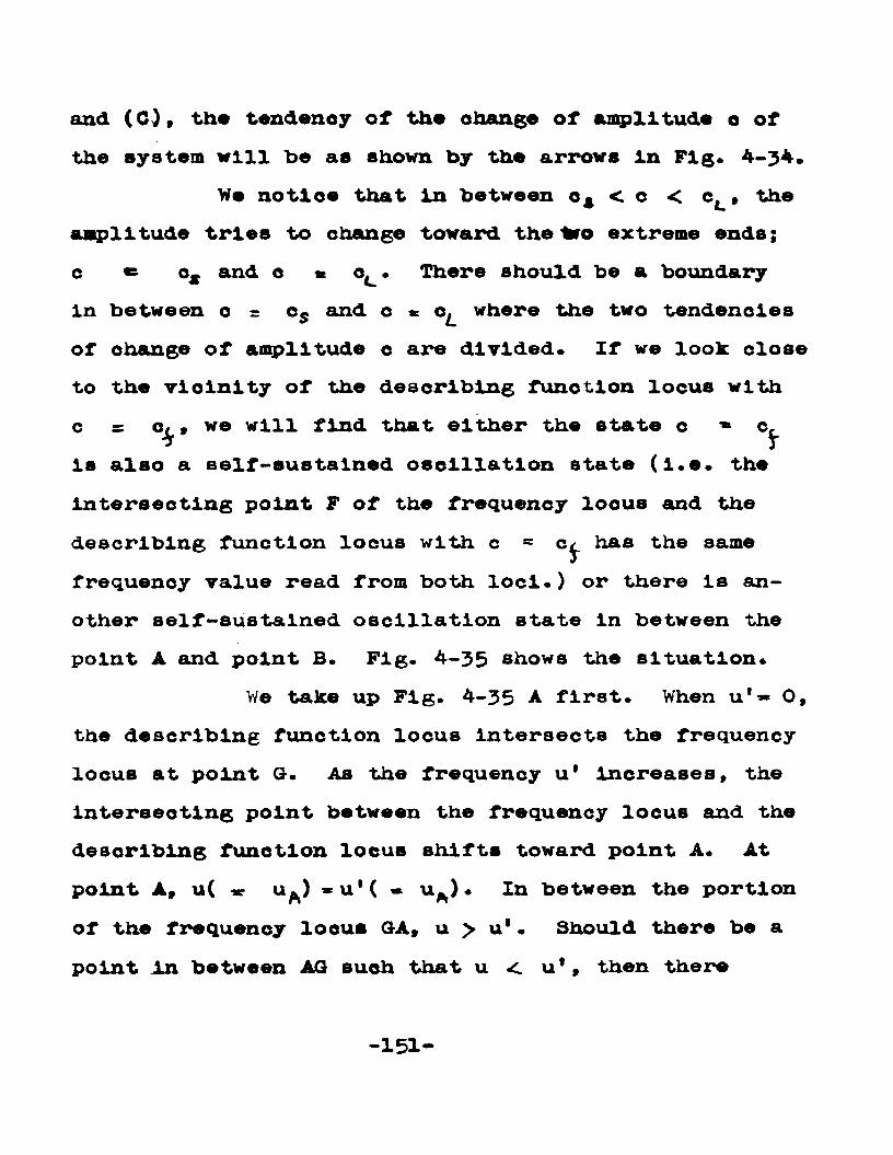
and (0), the tendency or the change of amplitude o of the system will he as shown by the arrows In Fig. 4-34.

We notice that In between os < o < cL , theamplitude tries to change toward the %ro extreme ends;c « os and e * ec * There should be a boundaryin between c = cs and c * where the two tendenciesof change of aiqplltude c are divided. If we look closeto the vicinity of the describing function locus withc s Ot , we will find that either the state c » ct

* Iis also a self-sustained oscillation state (I.e. theintersecting point F of the frequency locus and the describing function locus with c = has the same frequenoy value read from both loci.) or there is an­other self-sustained oscillation state in between the point A and point B. Fig. 4-35 shows the situation.

We take up Fig. 4-35 A first. When u'» 0, the describing function locus intersects the frequency locus at point G. As the frequency u' increases, the intersecting point between the frequency locus and the describing funotlon locus shifts toward point A. At point A, u( uft) -u'( «- u A ). In between the portion of the frequency locus G A , u > u'• Should there be a point In between AG such that u < u', then there

-151

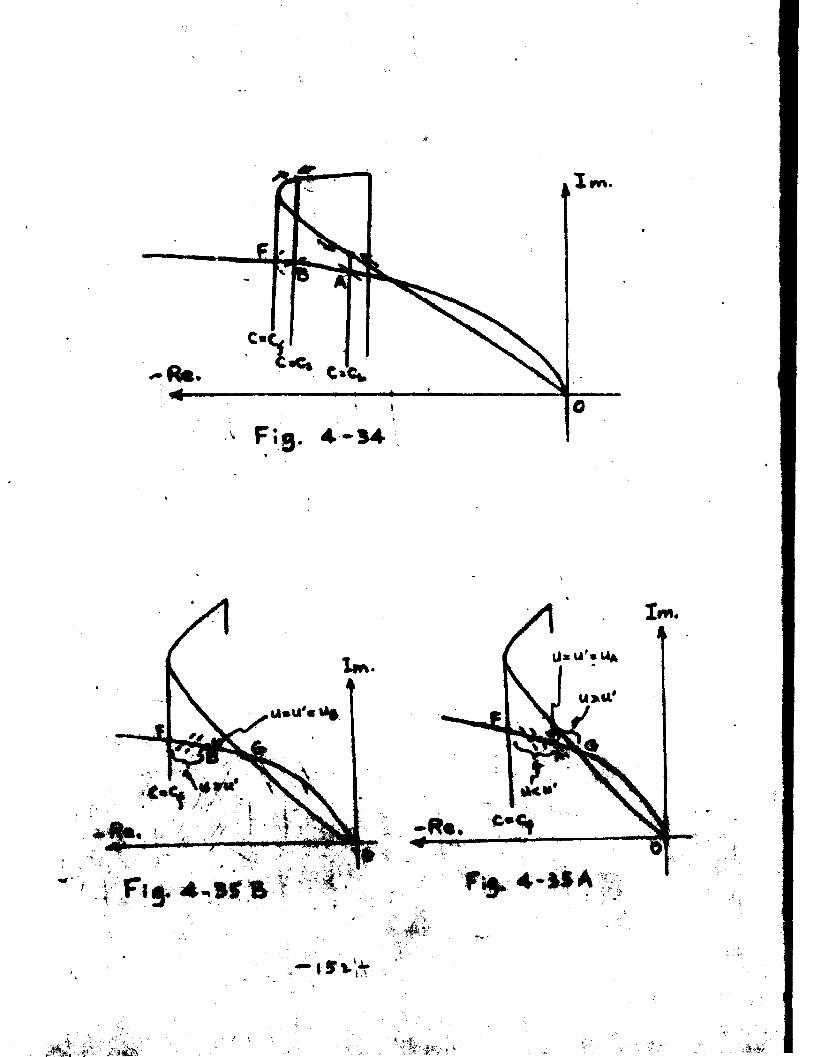
C*

Z 1

Irw.4

U»U'mUA

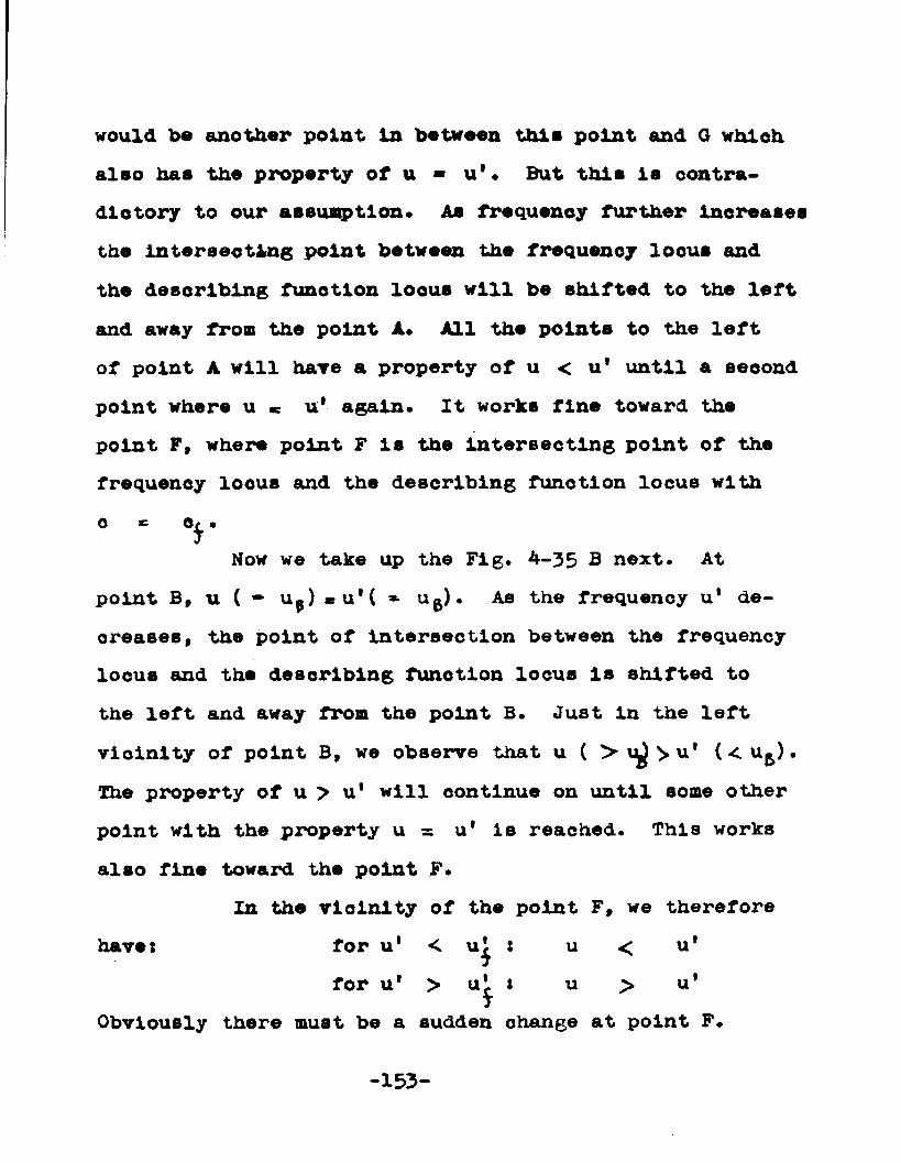
would bo another point in between this point and G whieh also has the property of u * u'. But this is contra­dictory to our assumption. As frequenoy further increases the intersecting point between the frequency locus and the describing function locus will be shifted to the left and away from the point A. All the points to the left of point A will have a property of u < u* until a second point where u « u* again. It works fine toward the point F, where point F is the intersecting point of the frequency locus and the describing function locus with o - Oj.

Now we take up the Fig. 4-35 B next. At point B, u ( • Up) *u'( *■ up)« As the frequency u' de­creases, the point of intersection between the frequency locus and the describing funotlon locus is shifted to the left and away from the point B. Just in the left vicinity of point B, we observe that u ( >i^J>u' (<u^). The property of u > u' will continue on until some other point with the property u s u' is reached. This works also fine toward the point F.

In the vicinity of the point F , we therefore have: for u 1 < u^ : u < u*

for u* > u^ i u > u'Obviously there must be a sudden change at point F.

-153-

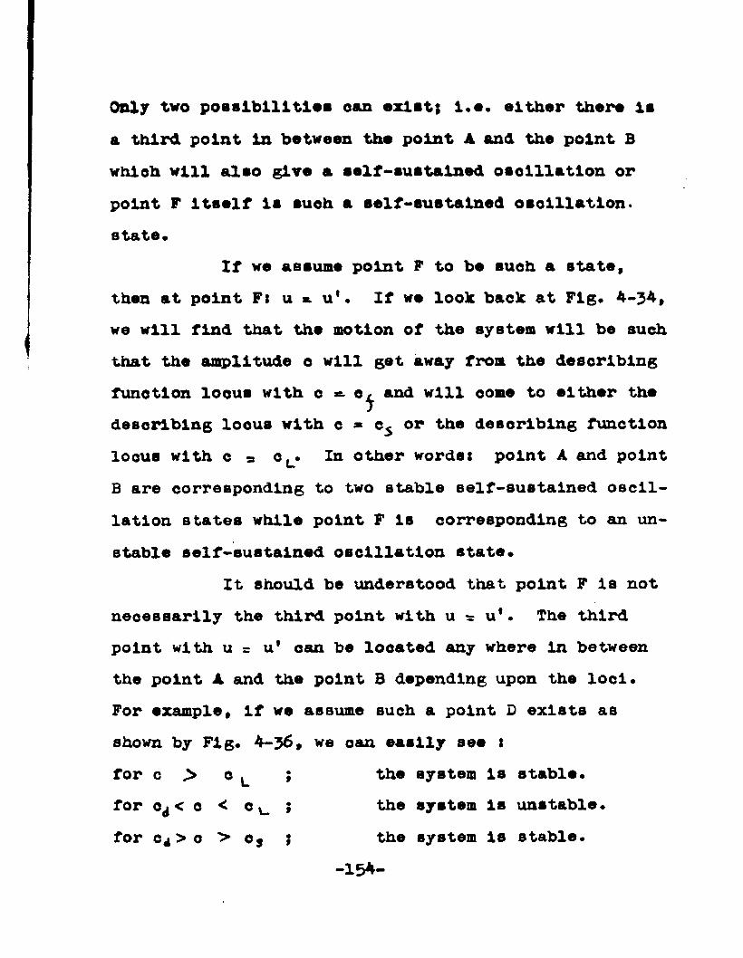
Only two possibilities oan exist; i.e. either there la a third point in between the point A and the point B which will alao give a self-sustained oscillation or point P Itself ia aueh a self-sustained oscillation, state.

If we assume point F to be aueh a state, then at point Fs u *. u*. If we look back at Fig. 4-34, we will find that the motion of the system will be such that the amplitude c will get away from the describing function locus with c ■. c^ and will oome to either the describing locus with c * c5 or the describing function locus with c = oL. In other words: point A and pointB are corresponding to two stable self-sustained oscil­lation states while point F is corresponding to an un­stable self-sustained oscillation state.

It should be understood that point F ia not necessarily the third point with u ^ u*• The third point with u = u' oan be located any where in between the point A and the point B depending upon the loci.For example, if we assume such a point D exists as shown by Fig. 4-36, we oan easily see :

the system is stable, the system is unstable, the system is stable.

-154-

for c > c L for o^ < o < o u for c4 > o > cs

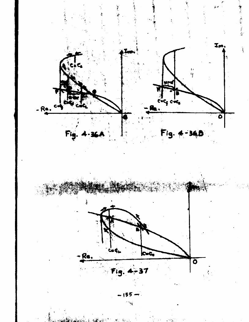
ii.

igX

:■

'f»■

$

F«j. 4 - a t * r.

f^g.

THA£■*■

f

for o < c, ; the ay stem is unstable.Therefore point A and point B are corresponding to two stable self-sustained oscillation states, while the point D is corresponding to an unstable self-sustained oscil­lation state.

This example oan also be considered as an in­formal illustration that: in between two stable self-sustained oscillation states, there must be always an unstable self-sustained oscillation state.

Although we have proved that in Pig. 4-28, that to find two points on the frequency locus both of which will give self-sustained oscillation is impossible for that particular oase, also in the case of Fig. 4-29 we have finally proved that there are actually three points on the frequenoy locus all of which will give self-sustained oscillation; yet that does not mean we oannot find two points on the frequenoy Io c u b both of which will give self-sustained oscillations in other cases. For example, Fig. 4-37 shows a oase where there are two points A and B on the frequency locus both of which will give self-sustained oscillation. It is not difficult to prove that the tendency of changing of e is shown by the arrows. Therefore in this case point A corresponds to a stable self-sustained oscillation state while point B

-156-

corresponds to an unstable self-sustained oscillation state.5* Tttt W Q W b Qt flermUTg. QQBtrql -cggvOrafl-. ta .Stabi­

lize the on-off servo system with derivative con­troller In parallel with the on-off contactor device.

We have discussed the stability In our ex­ample already. Now we are going to determine the amount of the derivative control required for our special example to stabilize the system.

We cannot consider a system to be stable when there is self-sustained oscillation. In our discussion of stability for our special example we have concluded that the system will be stable If there is no self-sus­tained oscillation. Hence the derivative control added in parallel must try to eliminate those self-sustained oscillation conditions, or In other words there should be no point on the frequency locus which at the same time Is the point on a describing function locus with the same value of frequency read from both lool. Since we have also proved that such points oan only occur In the EG portion of the frequenoy locus as shown by Fig. 4-38, we therefore concentrate our attention to that region.

First we learn from Fig. 4-28 that for our

-157-

» !. • *.\/ •

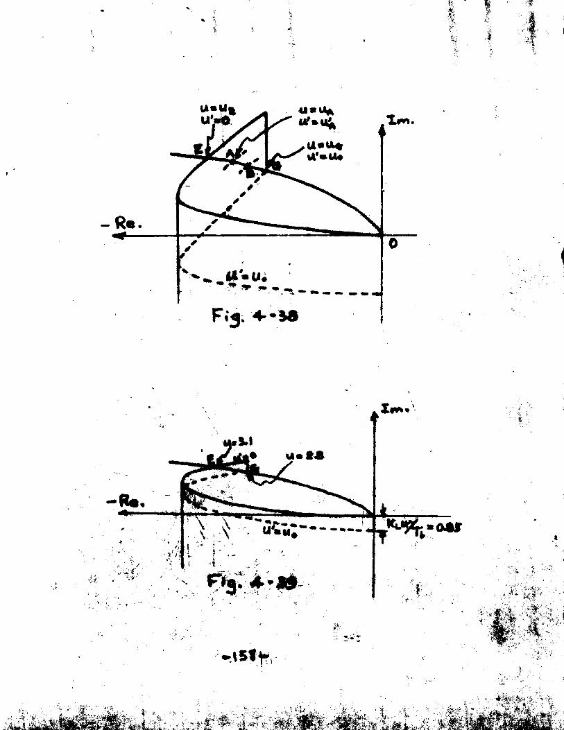
to.' -• ■ &•••.

*-4> * \ ’V:j •'; i- ■_

‘r’ j t

X**<

f

*. \‘ *

special oase, it Is impossible to have two points in between the portion EG of the frequenoy locus such that u * u*• Then It is not difficult to extend the result to more than two points* Hence for our special example we oan conclude that: there is either one point in be­tween the portion EG of the frequency locus which hasthe property u a* u* or there is none. We notice that;at point Es u' » 0, therefore u > u'Now is at point G; u* > u t then in between the portion EG of the frequency I o c u b there must be a point which has the property of u = u' and which is the point corresponding to a self-sustained oscillation state. However, if at point Gs u > u'then there would be no point in between the portion EG of the frequency locus which has the property u * u 1. This can be proved as follows; Refer to Fig. 4-38, assume that at point G; u (» > u 1 (» u.)If at the same time we assume that point A to be the point in betwwen EG such that: u ( » ) * u'~ )»then since to the left side of the point A, u > u ', there must exist a point B to the right of point A whloh has the property u < u*• But at point G, u > u', therefore in between the point B and point G there must be another point which has the property u =- u* • But

-159-

we have proved that there oan at moat only one point exist In between the portion EG of the frequency locus which has the property u « u* , hence we have a contra­diction. Therefore If at point G, u > u 1, there will be no point In between the portion EG which has the pro­perty u = u' and accordingly the system will be stable.

to find the value of kj (refer to Fig. 4-18) such that It will free the system from self-sustained oscillations. Fig. 4-39 is a reproduce of part of Fig. 4-18.

The critical case Is when at the point G: u s u* , i.e.

> 0.304Tb .where Is the time base used for the dlmensionless

Now let us put the numerical value In and try

From Fig. 4-39» we know that at point E:

At point G:

2.8 » T w 0.85/k*k ^ * T w 0.85/2.8

- 0.304TkWhen k ^ < o*304 , at point G s u < u*.7/hen k > 0.304 , at point G s u > u * .Therefore to stabilize the system, we must have:

system -160-

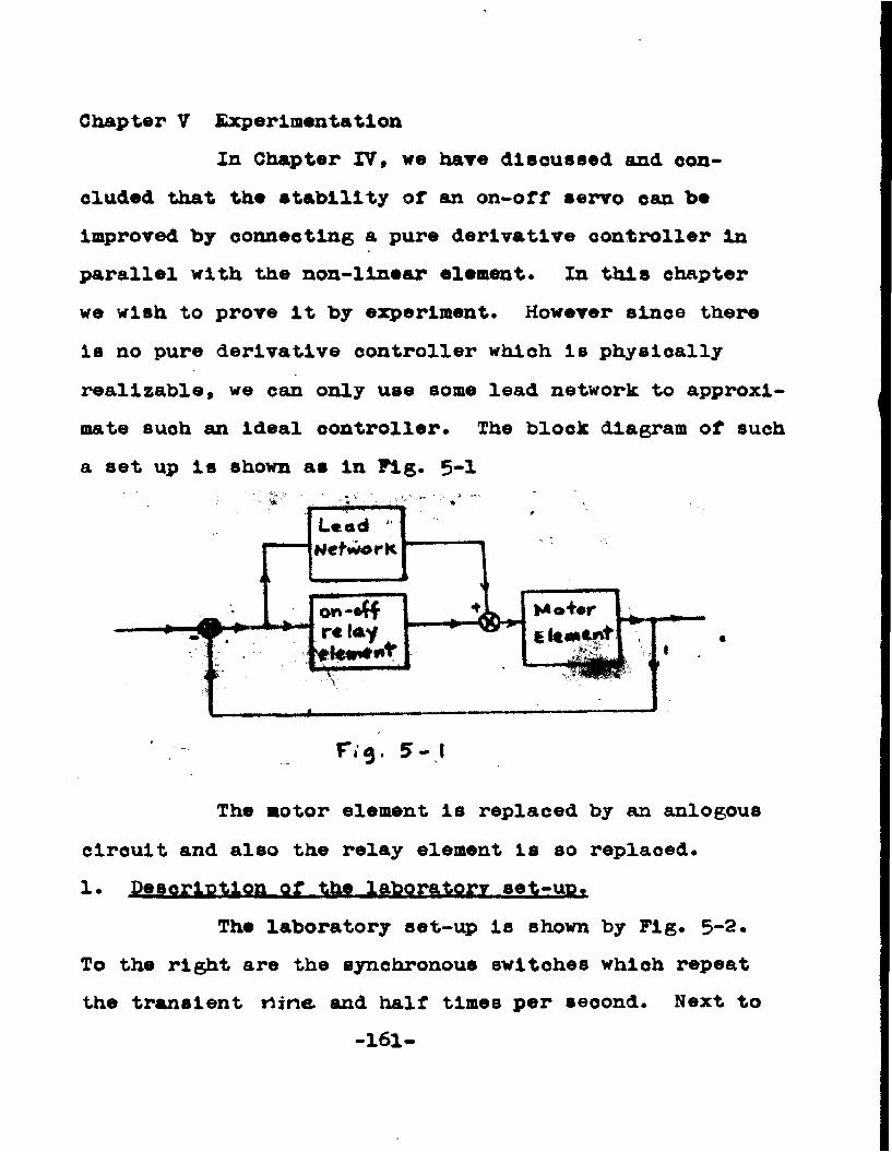
Chapter V ExperimentationIn Chapter IV, we have discussed and con­

cluded that the stability of an on-off servo can be Improved by connecting a pure derivative controller in parallel with the non-linear element. In this chapter we wish to prove it by experiment. However since there is no pure derivative controller which is physically realizable, we can only use some lead network to approxi­mate such an ideal controller. The blook diagram of such a set up is shown as in Tig. 5*1

F, 5- I

The motor element is replaced by an anlogous circuit and also the relay element is so replaced.1. Description of the laboratory set-uo.

The laboratory set-up is shown by Pig. 5-2. To the right are the synchronous switches which repeat the transient nine and half times per second. Next to

- 161-

the switches Is the oscilloscope which is set to reoord the error. Beside the oscilloscope is a regulated D.C. power supply. Next to that power supply is the main unit, the analogous circuit of the servomechanism under in­vestigation. To the left are 1wo other regulated D.C. power supplies. The large groups of B-batteries, here and there, are for the D.C. amplifiers.

Fig- 5-3 is the circuit diagram for the ana­logous circuit of the servomechanism under investigation. Fig. 5-4 is the blook diagram for this circuit to show all the elements in the system.

The non-linear element, or the relay element (which will be reproduced In Fig. 5-23 for further dis­cussion) contains four 6AL5 twin-diode tubes. Each tube Is used as a single diode by connecting the two units In parallel. Those 400 Ohms resistors in series with each tube are in an attempt to equllize the dif­ferent internal resistance of the four tubes.

-162-

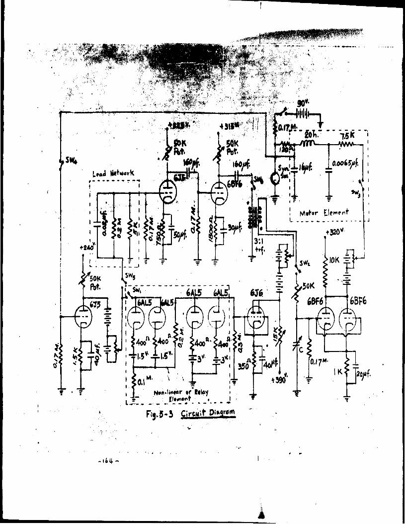
90*IfM M M i

-ww—

svliV*Lwui Ht»«w*x

nl0K ?Jp

6A15 6AL5in

© f> EbAL5

a* >4oo >4«o. <•)

N -U ar ir Mty

FIJ.5-J CircuiF P‘» y ™

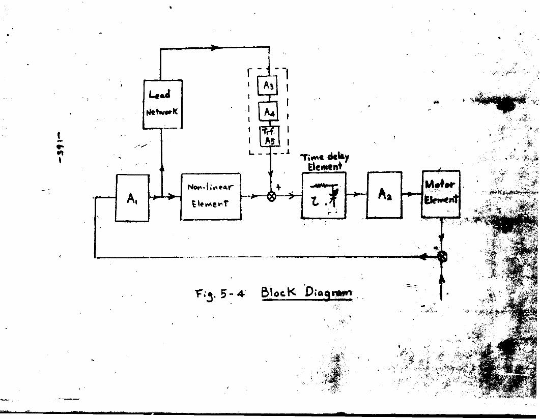
31»

tte+werK

Nor»-(io*^r

_ _ i

rTi*»« dtky Ekwtt^ ■■ . . . - .

M«ftr

>

B lo c K Diaqrawn|'« ■ ■■1 1 mmrnm*0Lmmmmm

£s Pata and ResultsThe amplifier gains are measured: C +. F; . 5 -4 -)

A, 11Av. 6.8A} x A* 36A r 1/3

The non-linear element has an output and input response follows:

* The sign due to phase rever­sing of the am­plifier is eom- bined to and taken care of by the amplifier A..

Input Output30*

22.5 3016.5 3010.5 259 226 194.5 143 81.5 0

- 1.5 - 0- 3 - 13- 4.5 - 20- 6 - 30- 9 - 46- 10.5

-166-- 52

Input - 16*5

Output - 70

- 22.5 - 45

- 72- 74

The plot of the non-linear element charac­teristic is shown by Fig. 5-5*

The time delay element is adjusted to the following values during the experimentation: *£ « 0 sec.,

The error recorded by the oscillograph when a step velocity input is applied to the servomechanism shows the transient response of the system very clearly. The oscillograph records are presented from Fig. 5-6A through Fig. 5” ®** Error .)

0.27x105sec., 0*72x109 sec., and 2.52x10*9 sec*.

-167

4-

m: j o ': w 50

T h e Chanxtiflrisfic Qf T h e Non-Linear Element

ia. 5 - 5

_ .l"T I:

-bl' -

V 9 - S 'Ssim+.'m o « 3.

■£, ■ 0.27 * I O' 5«C. YV<tkouf- par*We,\ 100 pCo rr&c,bon

1

X / = 0 - 2 7 x 1 o ~ * S € C , W i t h f a r a t l e . 1 l o o p C o r r e c t o ' 1

F;^. 5 - ^ 6- '7o-

"£, * 0.2-Y * f O ~ * Sec. Wi'Hi Paraltm.1 loop( ~fhe lead ne4i\>ork Cor^fc^ier increased \^ *h> 0.25 * /©"‘ fd.

F ig . 5 - 6 C

- n i

0 *7 2 x W ith o u t P a r a l le l loof>

< h r M fM v^ A " M ' M r ‘, v V ; v V V V » l •,' *

*£, * 0-72 * *0~3 s«°* Wi*H» paro.net loopF*9. 5>-6> D

-(72-

t * 2.92 x 1 o ‘% 3«c. WtHiouf f-hrail1.1 [oo^>

* I ' ./v

I * . 1«

2.J2 I |e‘* » « . W.tV loopFifl. 5-6 E

3* Theoretical check-up of the experimental result.The experimental results are now compared

with the theoretically predicted values* From the results of Fig. 5-6, we notloed that the parallel loop does help to stabilise the system. Although sustained oscillations may still exist In some cases, they are of less magnitude. The frequency of those self-sustained oscillations are also very Interesting. We first find the describing function of the non-linear element from the characteristic curve. Then we compute the transfer functions for the motor unit and the parallel loop. Flnhlly we put them together and study the whole system. The describing funotlon of the non-llnear element*

In order to simplify the calculation, the characteristic of the non-llnear element as shown by Fig. 5-5 Is approximated by straight line segments as shown by Fig. 5-7. The mathematical expression for suoh a characteristic Is as follows:

D « 0 , \o \ < 1.5D «= 5.7 (e - 1.5) • 1.5 £ o < 6.8

(5-1) S D =, 30 , o ^ 6.8D = 5.7 (o + 1.5), -1.5 £ o ^ -14.3D « -73 , o < -14.3

With sinusoidal Input, the output will be as follows:-174-

Inputs 0 * e sin aitoutputs t D » 0 * (c mlmdt \ ^ 1.5

D » 5*7(o alnw>t - 1.5)* 1.5$ o alncdt^ 6.8(5-2) < D - 30 , o flnu)t > 6.8

D * 5*7(o slntdt ♦ 1.5) , -1.5 cslnw>t^ -14.3D a -73 , e sin *6 -14.3

If we defineso Bin o*. a 1.5 >e sin JS =• 6.8 V (5-3)e Bln y a 14.3 )

Then the Fourier Coefficients for the fundamental of the output will bes

a, .-J-lftx) cos x dx (5-4)'o£

or ij- a, » ( 5-7(0 sin o)t- 1.5) cob tdt d(u*t)°* . ft-?♦ \ 30 008 «■>t d(«?t)

• 7(c Bln «*»t - 1*5) cob odt d(u>t)♦ [5.1 - V ppt+ir* I 5.7(o Bln a)t + 1.5) oob cet d(c*t)■'n ♦ ck vt-r(-73) OOB «)t d(«tt)+rxt- A

( 5.7(o sin o>t ♦ 1.5) oob odt d(a»t)M 'r (5-5)

5.

-175-

0 19

The Approximate Characteristic Of The Non -Linear

• Element.

50:

SlnoeJ

Similarly:

Also:

Therefore

or

\ 5*7 (c sin elt - 1 .5 ) 0 0 s «t d(*>t)-Jf

r \5»7[o sin (eiti-TJ ) - I.5J cos(«t + w ) d(u>t*J[)

1* \5»7 [o sin ( T[ -«st) - l.*f)cos(if -«*t) d( ij- -«lt)!= \ 5-7 [0 - 1.53 eos e>t d(eit)

Jf

- J^»7 I? 8ln *** “ 0 0 8 ^ d(e»t)

f ^ r15*7 tc sin «*t-t-1.53 008 ^ d(elt).x -ot

-7 (c sin «t+1.5) cos wt d(cat)\ 5.7K v - rrn-pV 30 cos cot d(«dt) » 0p\ (-73) cos o>t d(cdt) s 0

a 1 * 0

* 0 (5-6)

-177-

b,

or if

But

s

a

Similarly

Also

* ~if \ f(x) *in * dx (5-7)9

>i*\ 5-7 (c sin at - 1.5) sin at d(at)Y ' p■f \ 30 sin at d(at) f £ +-»■ \5-7 (o sin *)t - 1.5) sin at d(at) f i*r

♦ \ 5*7 (o sin at ■* 1.5) sin at d(at)rvn ^- I 73 * m at d(at)n ♦ if"

*xt- «L♦ (5«7 (c sin at +1.5) sin at d(at) (5-8)J, w _ *p - *

\ 5-7 (c sin cut - 1.5) sin wt d(at)' J- Y 5-7 (c sin at - 1.5) sin wt d(at)

^ 5 - 7 (o sin at - 1.5) sin at d(at) (5-9)'Ok

,v*-*5*7 (c sinat+1.5) sin at d(o)t)i

\ 5-7 (c sin at + 1.5) slnoJt d(«it) (5-10)

s'30 Sin at d(at) m j 30 Sin at d(«*t)f + I 30 sin at d(cit)

-178-

Therefore

Similarly

Therefore

Therefore

ft*

5 0 sin d(eit) = 2 \ 3 0 sin *»t d(e»t)^ (5-11)

(-73) Bin *>t d(oit)

2 \ (-73) Bln «t d(«#t) (5-12)

\ b, * \5*7 (c Bln a)t - 1.5) sin «*t d(tit)*

\ 30 Bln «t d(*t)

L4- \ 5*7 (o eln «it + 1 .5 ) sin «*t d(«at)

-v \(- 7 3 ) Bln elt d(oit) ......... (5-13)

i b , . 5.70 t-|s- - s t y <w )|^

,P ,Vv♦ 5.7 X 1.5 008 <k)t I - 30 COB «t

T + t+ 5.7 o (-3ft- -

I j + r5 . 7 X 1 . 5 COB 6>tI H ♦ <*

73 cob «t k ............. (5-1*)t if-179-

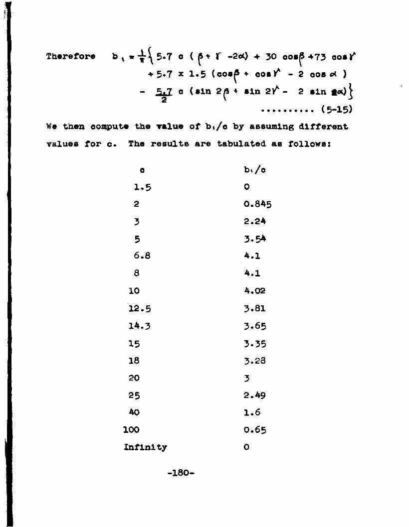
Therefore t x * - ^ 5 . 7 0 ( p * T -2cO + 30 ooa^ 4 . 7 3 coa^♦ 5*7 x 1.5 (eoa^ + cos/ - 2 oob c* )

- c (ain 2p 4 aln 2/ - 2 aln *<x).......... (5-15)

We than compute the value of b</o by assuming different values for c. The results are tabulated as follows:

0 b» /e1.5 02 0.8453 2.245 3.546.8 4.18 4.110 4.0212.5 3.8114.3 3.6515 3.3518 3*2320 325 2.4940 1.6

100 O .65Infinity 0

-180-

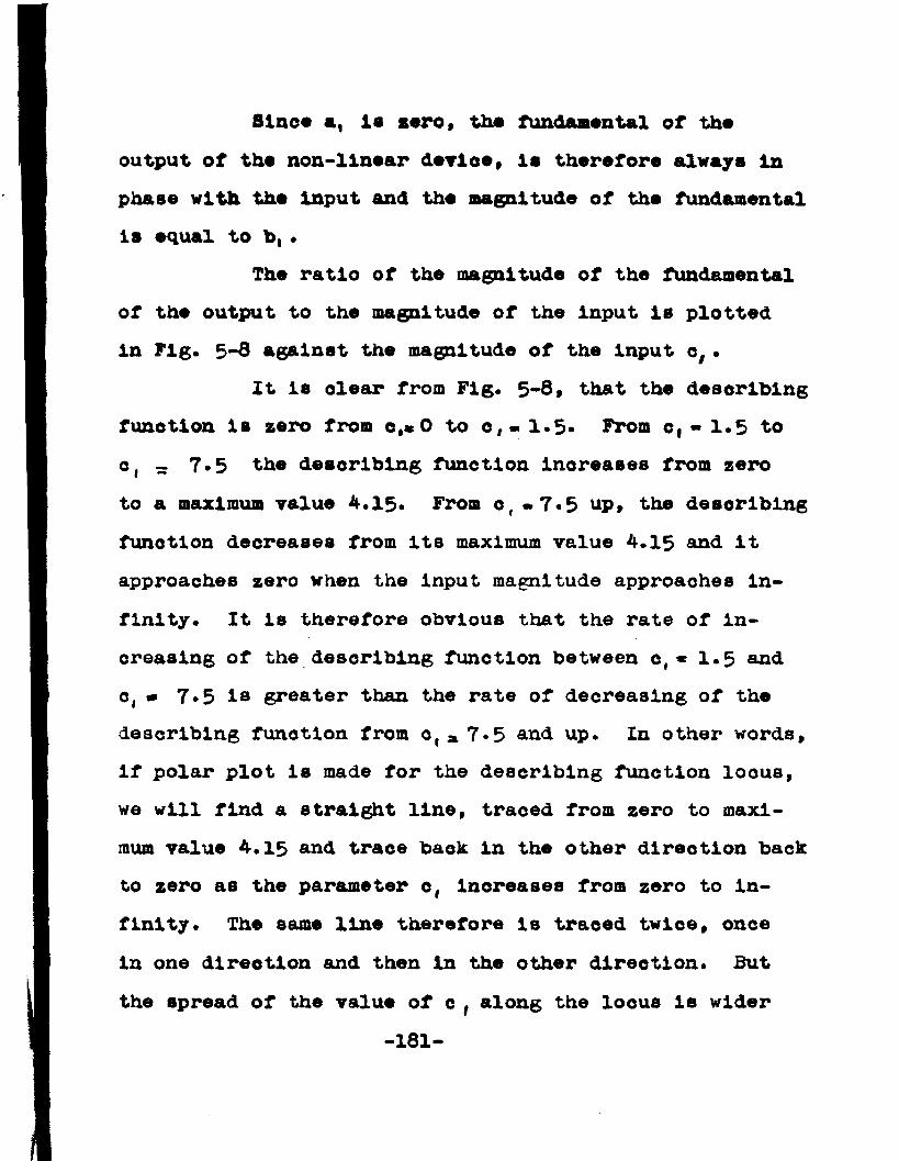
Sine* a, is zero, the fundamental of the output of the non-llnear device, Is therefore always In phase with the input and the magnitude of the fundamental is equal to b, .

The ratio of the magnitude of the fundamental of the output to the magnitude of the input is plotted in Fig. 5-8 against the magnitude of the input c, •

It is ole&r from Fig. 5*8* that the describing function is zero from c,«0 to c,- 1.5» From c, - 1.5 to c, - 7*5 the describing function increases from zero to a maximum value 4.15. From e r -7.5 up, the describing function decreases from its maximum value 4.15 and it approaches zero when the input magnitude approaches in­finity. It is therefore obvious that the rate of in­creasing of the describing function between e( * 1.5 and c( - 7.5 is greater than the rate of decreasing of the describing function from o(ai7*5 and up. In other words, if polar plot is made for the describing function locus, we will find a straight line, traced from zero to maxi­mum value 4.15 and trace back in the other direction back to zero as the parameter c, increases from zero to in­finity. The same line therefore is traced twice, once in one direction and then in the other direction. But the spread of the value of c , along the locus is wider

- 181-

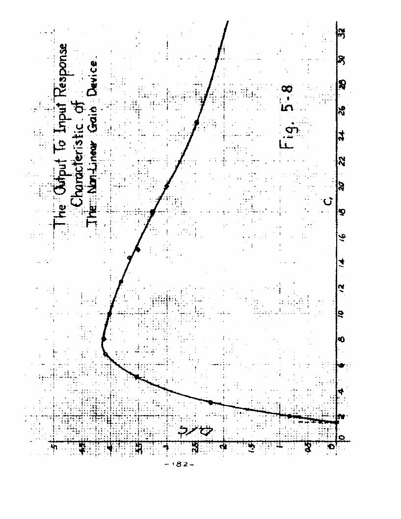
r ^ £

I

■ • r;;(i;:ii.L.;;i.;L. a

.. .,k ;. ..i'.. L: i:.:

- ' 8 2 -

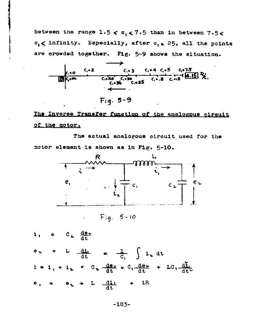
between the range 1.5 < c,<7.5 than in between 7.5< c, < Infinity. Especially, after c, «. 25, all the points are crowded together. Fig. 5-9 shows the situation.

*c,*o C,*2 C,a3 C,*4 C,*5 C,»7.S

c(*4e c;»te ’ c,*,8 c,*<2c,*a5

Ihft Inverse Transfer function of the analogous circuit of the motor.

The actual analogous circuit used for the motor element is shown as in Fig. 5-10.

TR

-AAAAA-L

. i ~ c.tx

F l a . 5-10

t

i , = c,' *■ dt

e t. + L dl.dt

i • i . ♦ i, - CT T S

4gr v O.-SLS: dt ' dt

iv dt* LC, Adtv

♦ 1Rdt

- 183 -

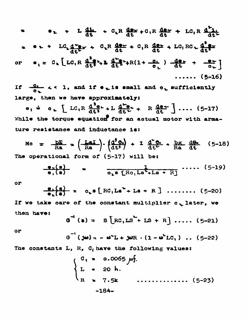
♦ L 2^- * °-R i t * + LC'R

* e V ♦ LCLd^p-* 4. 0XR 4 * ^ + C.R Aft* * LO,dt dt dt*

OP . , = o » L L O . R ^ V i - ^ t ,- + R < i + - ^ > -it* ♦ - £ ]

...... (5*-l6)If —£*— <. < 1, and If • v Ia small and e. sufficientlyc vlarge, then we hare approximately!

°t * c »- L L C ‘R dt?*- 4,L d t ^ + R d t ^ 1 ---- (5-17)While the torque equatlox? for an actual motor with arma­ture resistance and induotanoe is:

He =• -bg - 9 (—h & i - i .8n) 4- 1 9*- 4 J&fiL. (5-18)Ra V Ra / ydt»7 dt~ Ra dtThe operational form of (5-17) will be:

(5-19)oxs (JRc,Ls ♦Ls 4 RJ or

* o,8 L R C tL8% Ls 4 r J ........ (5-20)If we take oare of the constant multiplier c x later, we then have:

a"* (s) = S R C , ! ^ * LS + R j (5-21)or -tG ( >>) 4 >)R • (1 - aVLC, ) .. (5-22)The constants L, R, C, have the following values:

G x * o • OO65 jj§.L • 20 k.R » 7.5k (5-23)

-184-

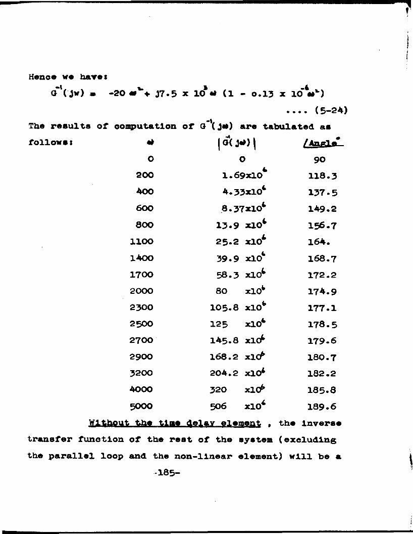
Hence we haresoYjw) * -20 < w % J7.5 x 10* «* (1 - 0.13 x id’4##*')

-v. (5-24)

The results or computation of a~'( J#) are tabulated as follows s | <»( J*> | /Anp-1 m

o 0 90200 1.69xl04 118.3400 4.33x10* 137-5600 8.37x10* 149.2800 13.9 xlO* 156.7

llOO 25-2 xlO* 164.1400 39-9 xlO* 168.71700 58.3 xlO* 172.22000 80 xlO* 174.92300 105.8 xlO* 177.12500 125 xlO* 178.52700 145.8 xicf 179.62900 168.2 xlC^ 180. 73200 204.2 xlO* 182.24000 320 xlC^ 185.85000 506 xlO* 189.6

Without the time .dsl&x-gltas&S • the Inversetransfer function of the rest of the system (excluding the parallel loop and the non-llnear element) will be a

185-

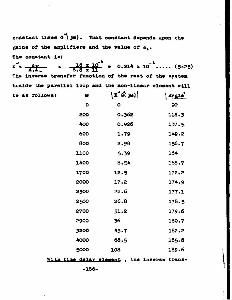
•I. .constant tines a (Jai) • That constant depends upon the gains of the anpllflers and the value of ox.The constant 1st

* sxt i If * °-21* x 10~*......(5-25)The inverse transfer funotion of the rest of the system beside the parallel loop and the non-linear element will be as follows: •ft \iV( j»)| ^ArgaV

0 0 90200 0*362 118*3400 0*926 137.5600 1.79 149*2800 2.98 156-7

1100 5.39 1641400 8.54 168.71700 12.5 172.22000 17*2 174.92300 22.6 177.12500 26.8 178.52700 31*2 179.62900 36 180.73200 43.7 182.24000 68.5 185.83000 108 189.6

With time delay element , the inverse trans- -186-

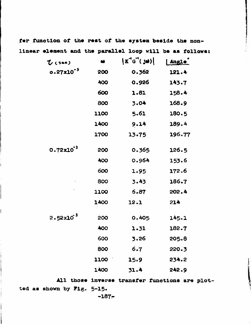
fer function of the rest of the system beside the non- llnear element and the parallel loop will he as follows*

X /

o.27xlO*5

0.72 x 10~3

2. 52 xlO* 3

*1 \k V ( J*)| 1 Angle*200 0.362 121.4400 0.926 143.7600 1.81 158.4800 3.04 168.9

1100 5.61 180.51400 9.14 189.41700 13.75 196.77

200 0.365 126.5400 0.964 153.6600 1.95 172.6800 3.43 186.7

1100 6.87 202.41400 12.1 214

200 0.405 145.1400 1.31 182.7600 3.26 205.8800 6.7 220.3

1100 15.9 234.21400 31.4 242.9

All those lnrerse transfer funotlons are plot­ted as shown by Pig, 5-15*

-187-

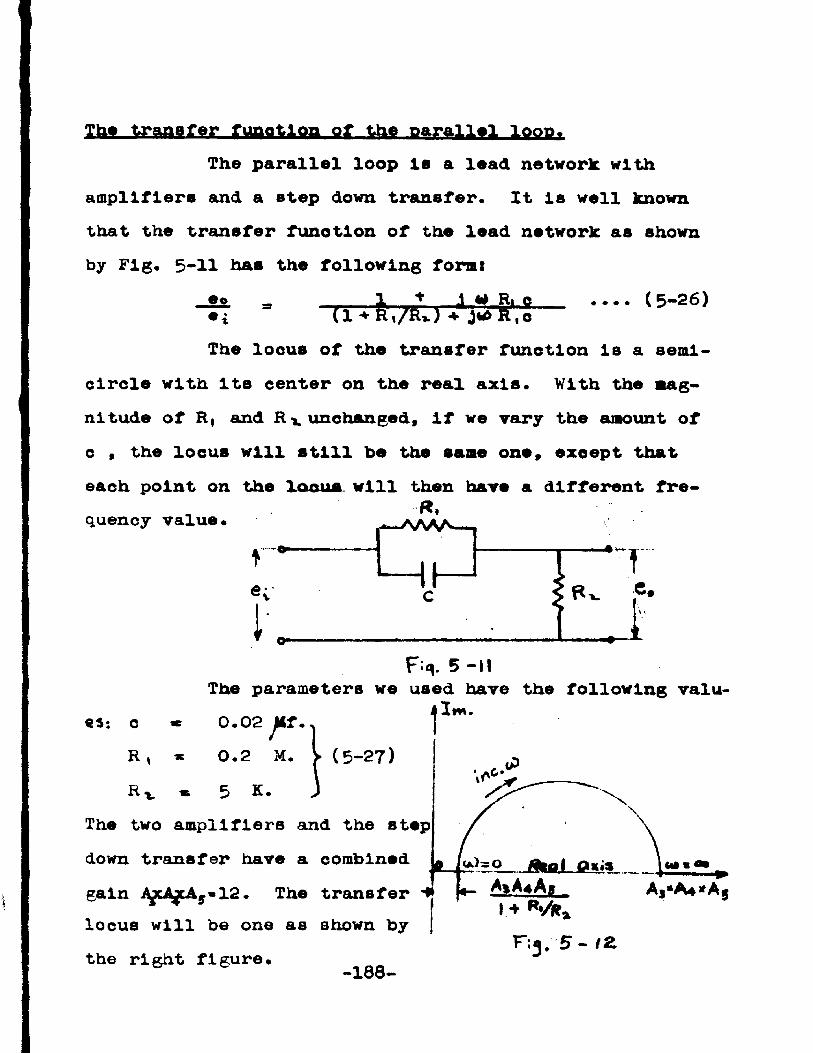
The transfer function of the parallel loop.The parallel loop le a lead network with

amplifiers and a step down transfer. It is well known that the transfer function of the lead network as shown by Fig. 5-11 has the following form:

So .... (5-26)

The locus of the transfer function is a semi­circle with its center on the real axis. With the mag­nitude of R, and R x unchanged, if we wary the amount of c , the locus will still be the same one, except thateach point on the 1noua will then have a different f re­

ft.

CH,

F;q. 5 -MThe parameters we used have the following valu> 0.02 lf.

(5-27)* 0.2 M.R v * 5 K.

The two amplifiers and the step down transfer have a combined gain A£cAgcAff«12. The transfer ^ locus will be one as shown by the right figure. -188—

g. 1 ^ = 9 f lif ljL f liil.B

I♦r.j. 5 - t&

[to» mAj*A4*Aj

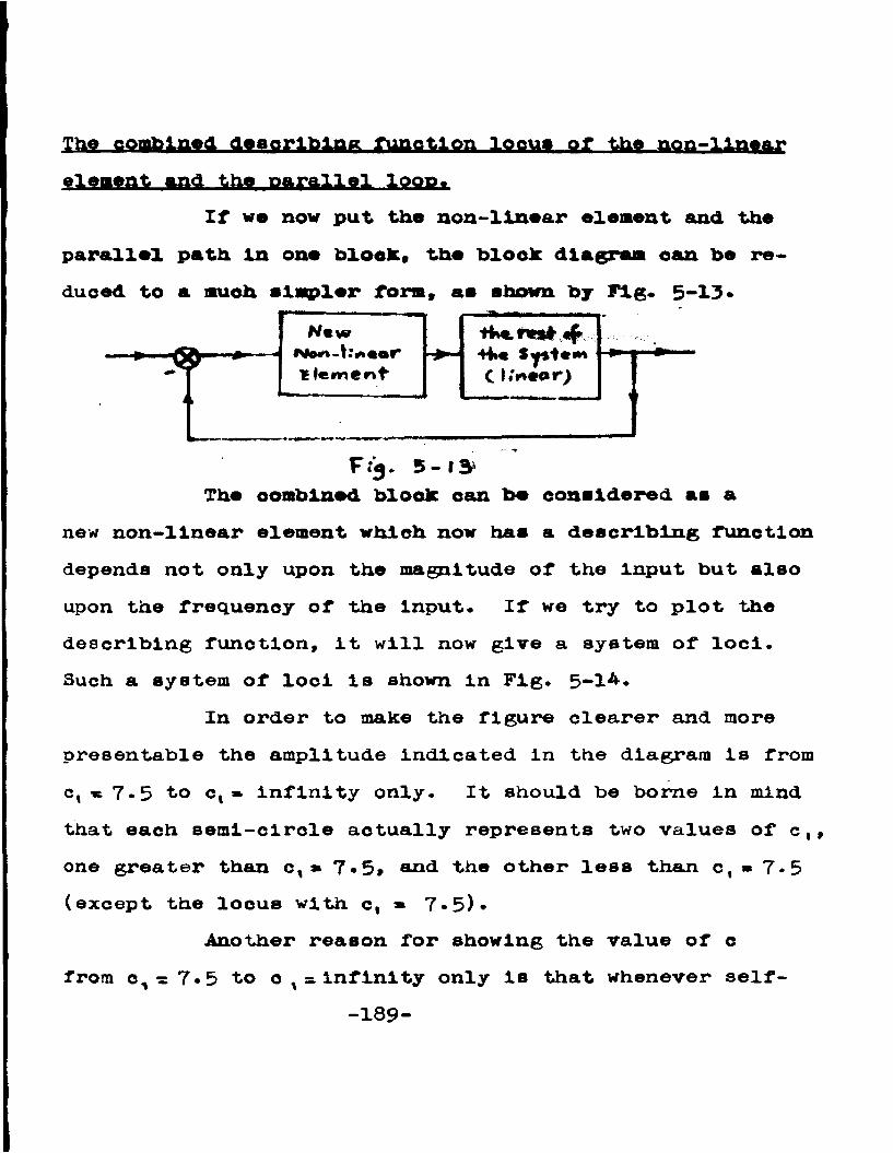
The combined dssorlbinR function locus of the non-lln»ar element and the parallel loop.

If we now put the non-llnear element and the parallel path In one blook, the block diagram can be re­duced to a much simpler form, as shown by Fig. 5-13*

H*.rss*v«fI lernent C t.V%sor;

Ff$. 5 - 13*The combined block can be considered as a

new non-llnear element which now has a describing function depends not only upon the magnitude of the input but also upon the frequency of the input. If we try to plot the describing function, it will now give a system of loci.Such a system of loci Is shown In Fig. 5-14.

In order to make the figure clearer and more presentable the amplitude indicated in the diagram is from c, * 7*5 to ct» infinity only. It should be borne In mind that each semi-clrole actually represents two values of c,, one greater than c, * 7*5# and the other less than c, * 7*5 (except the locus with c, * 7-5)*

Another reason for showing the value of c from c,l= 7 . 5 to c t s. inflnlty only ls that whenever self-

-189-

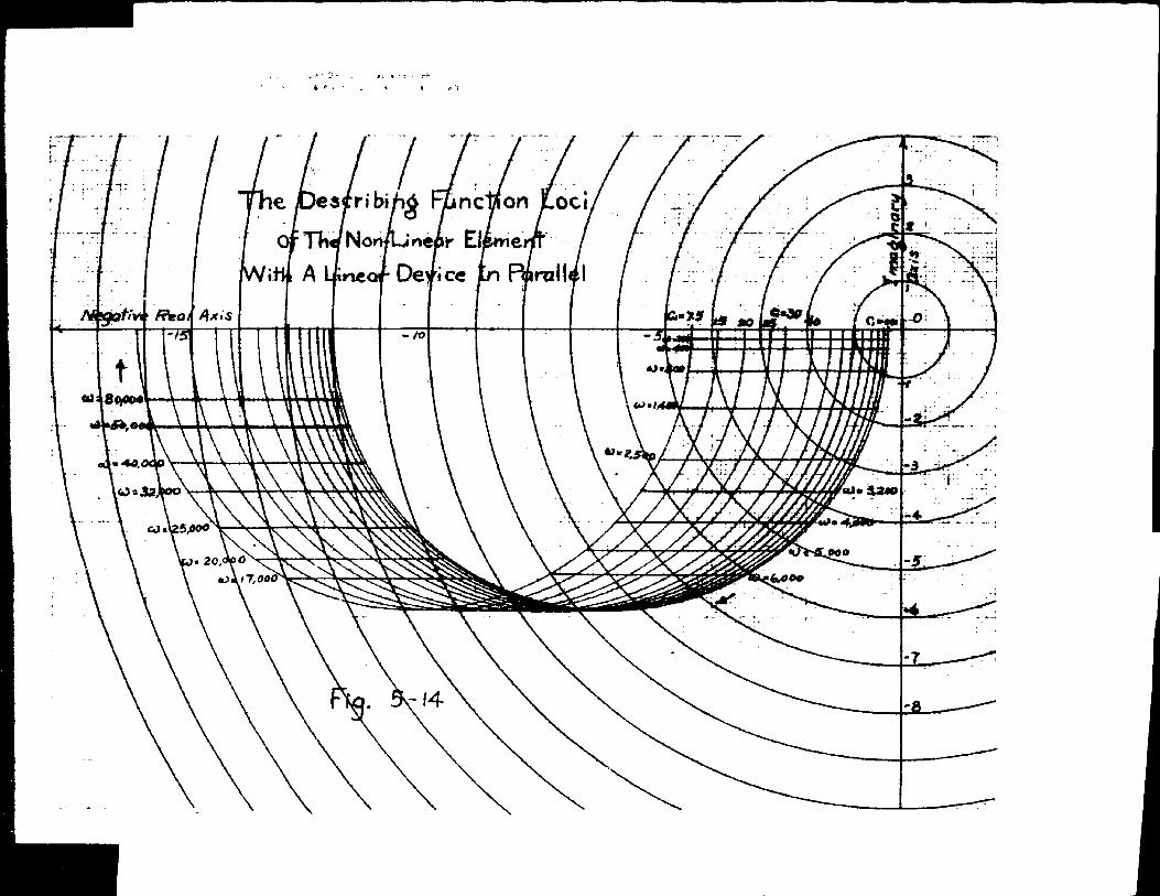
nc w o n LociNoi nebr I

W itU A Lftneof D e v ic e ra lle l

rti'tf • Real Axis ao■ ■ a m .mm i»tito

NO* 20.

sustained oscillation ooours, the magnitude corresponding to o ( < 7*5 Is a point of unstable equilibrium while that corresponding to c* 7*5 a point of stable equilibrium. Prediction of results from the describing function and the Inverse transfer functions, a. Without the parallel loon*

non-llnear element and the inverse function of the rest of the system are plotted In Fig. 5-15* There are four Inverse transfer function loci: A, B, D and E; eachhas a time delay element with a time delay constants^* 0,

From the figure, we can easily see that loci A and B do not Intersect the describing function locus, while loci C and D do intersect the describing function loous. The system will therefore have the following characteristics:

The negative of the describing function of the

A 7 * 0 secB £r 0.27x10 sec.D Z r 0.72xicf3s e c

The system ls stable.The system ls stable.The system will have a self- sustained oscillation with a magnitude corresponding to o ( * 24, and a frequency of about s 700 rad./sec.

-191-

i

—3X £,* 2*52x10 seo* The system will have *self-sustained osollla- tlon with a magnitude corresponding to o,* 48, and a frequency of about & ■* 400 rad*/eeo*

Now ls we look at the aotual oscillograph records we have obtained from our experiment, we can easily verify those predicted results. Hie top ploture of Fig. 5-6A and the top ploture of Fig. 5-6B, which

_ - 5correspond to the cases with £ = O and •£, = 0.27x10 sec. respectively, show clearly that the transient oscilla­tions died away. The system ls therefore stable. The top picture of Fig. 5-6D and the top picture of Fig.5-6E, which correspond to the cases with Z = 0.72x10

-iand t * 2.52x10 sec., however, indicate a different story. They both give self-sustained oscillations. The frequencies of these oscillations can be roughly calcu­lated from the number of oscillations of the transient in the picture and the speed of the synchronous switch.

The synchronous switoh we used has a motor with a speed of 1725 r.p.m. and a 3 to 1 gear train which reduce the speed to 573 r.p.m. If we convert this value

-192-

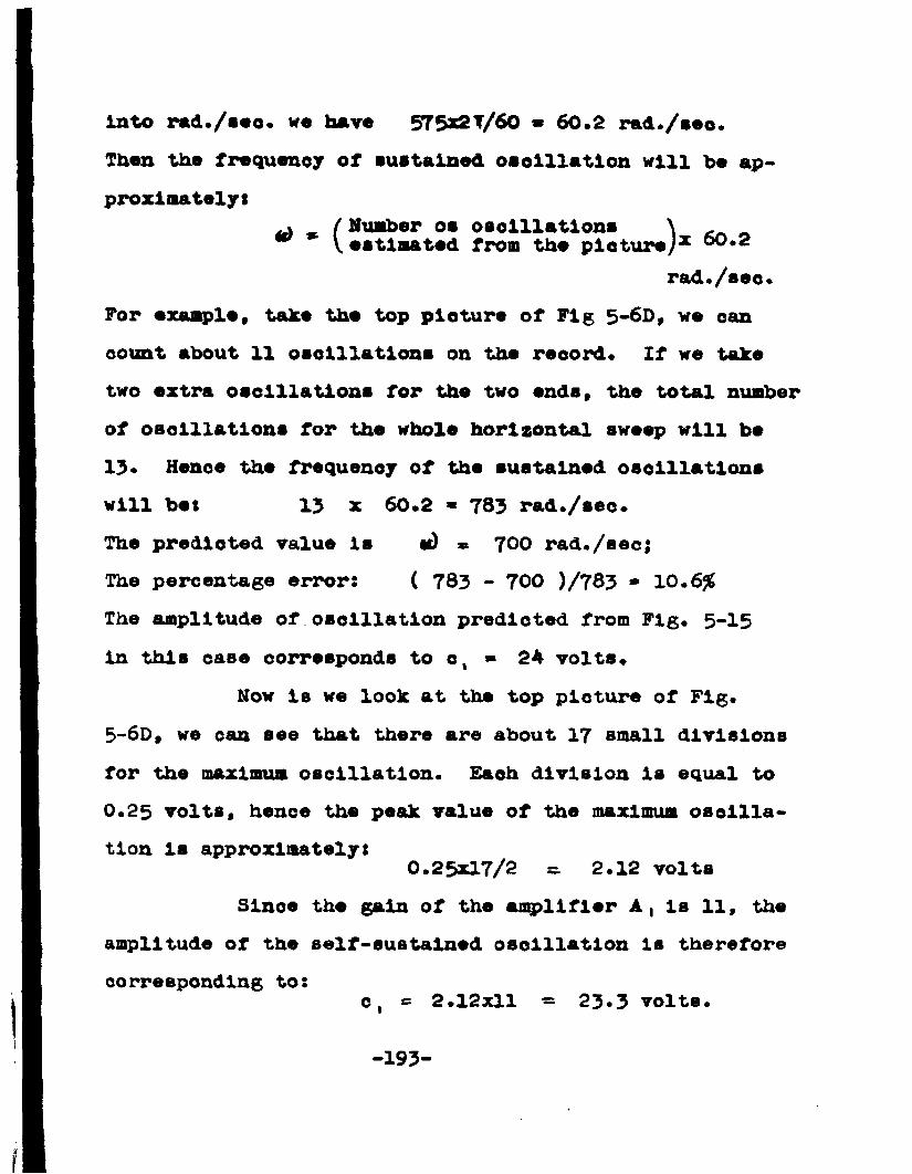
Into r«d./i«o. we have 575x2T/60 * 60.2 rad./eeo.Then the frequency of sustained oscillation will be ap­proximately*

^ _ /Number os osolllatlons \V estimated from the picture/* «0.2

rad./see.For example, take the top picture of Fig 5-6D, we can count about 11 oscillations on the record. If we take two extra oscillations for the two ends, the total number of oscillations for the whole horizontal sweep will be 13* Henoe the frequency of the sustained oscillations will bet 13 x 60.2 * 783 rad./seo.The predicted value is a) * 700 rad./sec;The percentage errors ( 783 - 700 )/783 * 10*6%The amplitude of oscillation predicted from Fig. 3-15 in this caBe corresponds to c, » 24 volts.

Now is we look at the top picture of Fig.5-6D, we can see that there are about 17 small divisions for the maximum oscillation. Each division ls equal to O.25 volts, hence the peak value of the maximum oscilla­tion ls approximately* 0.25x17/2 a 2.12 volts

Slnoe the gain of the amplifier ▲, ls 11, the amplitude of the self-sustained oscillation is therefore corresponding to:

c ( *= 2.12x11 ® 23.3 volts.

-193-

The percentage error in magnitude of the self-sustained oscillation is therefore:

( 24 - 23.3 )/23-3 - 3*Slnll*rly for th. .... of X. » 2.'52xlO~ «««..

the predioted values obtained from Fig. 5-15 for the self-sustained oscillations are:

The frequency: » 400 rad-/sec.The anqplltude: o , - 50 volte

How from the top picture of Fig. 5-6E, we can see that there are about 34 small divisions for the maxi­mum swing. Hence the amplitude of the sustained oscilla­tion ls: c,*ll x 0.25 x 34/2 » 46.8 volts

Also we can see that there are approximately eight oscillations for the entire horizontal sweep. Hence the frequeney of the self-sustained osolllatlon wll be:

- 8 x 60.2 « 481 rad./sec.The percentage errors for this case will there­

fore be:for frequency: ( 481 - 400 )/48l*l6.8j6 for amplitude: ( 50 - 46.8)/46.8 » 6.95*

-194-

MO. 3-40 *» OICTZOCH 8NAPH P*PC«

POLAR OO-ORO'NATCEUDCMt OICTZOCN CO-

Tio. 5-15 T h e Frequency Loci And

T h e Describing Function Locus(Wt'fitour Lm tur Device I-n Hj*"allel

W iW iT h e Non -L i< ita r Ele<ncn1")

...\ • ’r-•'Y - V ,-Dv .• %• ■ /. -\ .< v - *

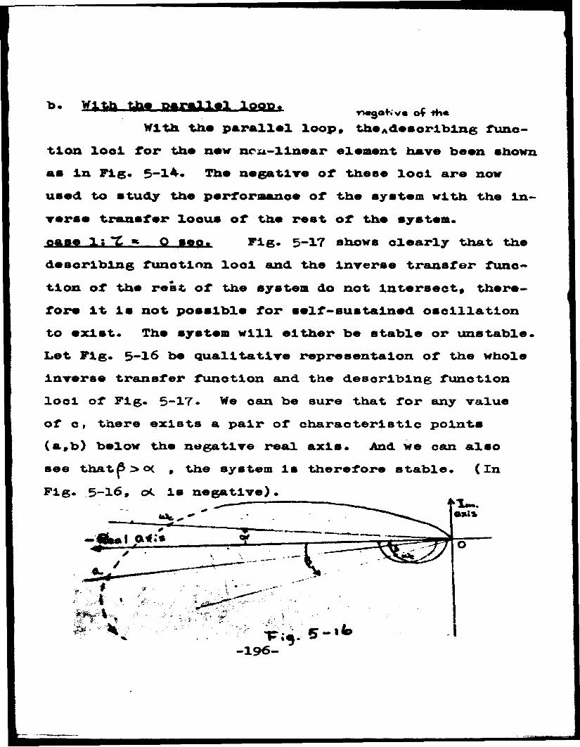
to. Wl ftfc. tteff .b« m u l i+i ig q p t r^ o K v . of *»•With th# parallel loop* th«Ad«8orltolng func­

tion lool Tor tht now nru-llnear element have been shown as In Fig. 5-14. Ttoo negative of ’those lool are now used, to study the performance of the system with the In­verse transfer loous of the rest of the system. case 1; X * Q aeo. Fig. 5-17 shows clearly that the describing function lool and the inverse transfer func­tion of the rest of the system do not Intersect* there­fore It Is not possible for self-sustained oscillation to exist. The system will either be stable or unstable. Let Fig. 5-16 be qualitative repreaentalon of the whole Inverse transfer function and the describing function loci of Fig. 5-17. We can be sure that for any value of Ci there exists a pair of characteristic points (a,b) below the negative real axis. And we can also see thatp>o( , the system Is therefore stable. (In Fig. 5-16, oC Is negative).

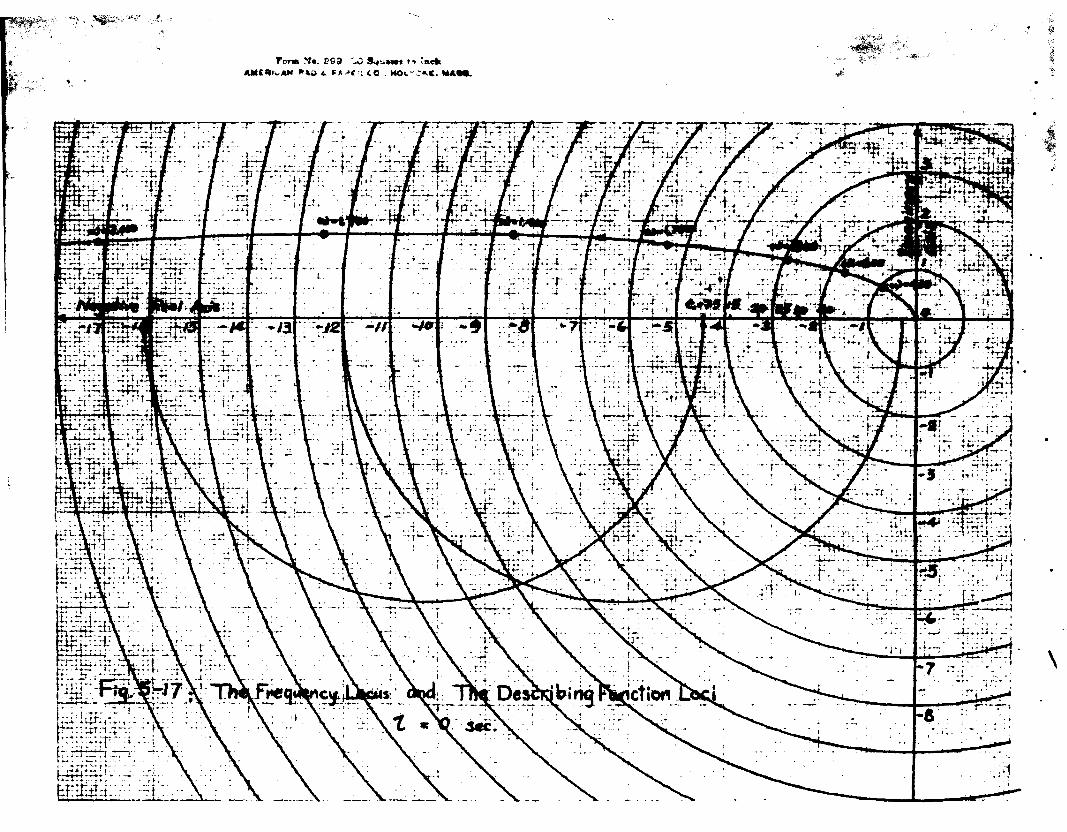
’•tow

f

v-f.Form M«. £S9 -0 »t> 'nett

AMC^l^AN P\o 4. **>€ =; CO . MOc :».C. *

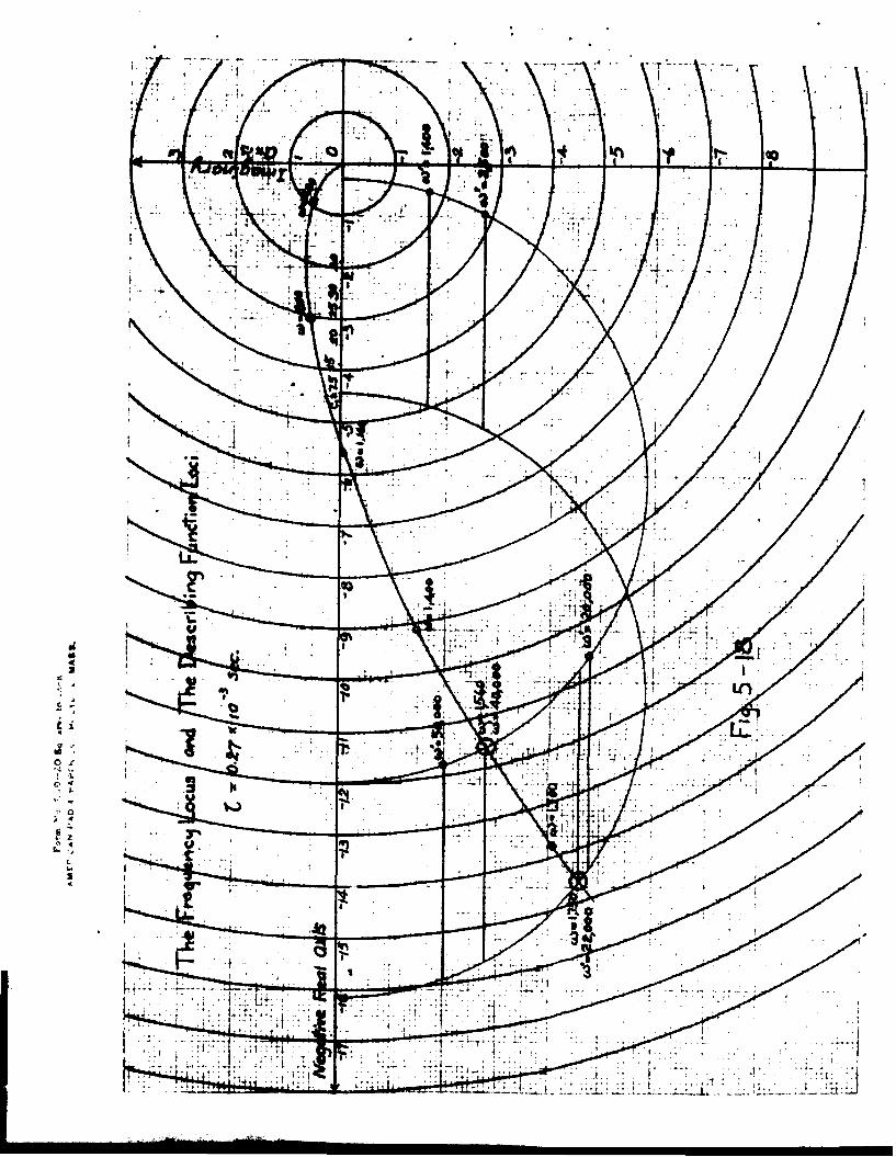
case 2 1 I • Q *27x10 m o *The negative of the describing function of

tne non-linear element loci and the Inverse transfer function locus are plotted as shown by Fig* 5-18. It Is different from case 1 In that the Inverse transfer function locus does Intersect the describing function loci* However, there Is still no posslbllty for a self-sustained oscillation to exist* If there were such posslbllty, then the frequency would be In the range from m> = 1560 to m) - 1750* However, upon looking at Fig* 5*18, the frequency on the describing function loci at that looatlon is from td* * 22,000 to uP = 40,000* The system therefore can only be either stable or un­stable* With similar reason to that given In the case 1, the system Is therefore also stable*

From the bottom picture of Fig. 5-6A and Fig. 5-6B we can see both case 1 and case 2 checks with the experimental results* case. 5 ;%, * Q*72xl0~5 sec*

The plot of the describing function and the inverse transfer function of the rest of the system are shown by Fig. 5-19* With only a few steps we can see easily that there does exist a self-sustained oscilla­tion with a frequency,approximately corresponds to

-199-

<4 s 900 rad./sec. and an amplitude of c,« 10 volts.From the bottom picture of Fig. 5-6D, we

notloe that there are about 16 oscillations throughout the entire horizontal sweep. The frequency of the experi­mental result Is therefore!

e) - 16 x 60*2 * 964 rad./sec.We also notloe that the maximum swing has about

eight small divisions. The amplitude of the self sus­tained oscillation therefore has a magnitude correspondingto: g.

o x =■ 11 x 0.25 x ® / 2 = 11 volts.The percentage errors are:

for frequency: ( 964 - 900 )/964 * 6.6%for amplitude: ( 1 1 - 1 0 )/ 11 s* 9-1*Case * 2 « 5 2 x 10 * seo.

The plot of the describing function loci and the inverse transfer function locus are shown by Fig. 5-20. With only a few steps we can easily locate the frequency and the magnitude of the self-sustained oscillation. The predicted values are:

o, • 38 voltsft) % 500 rad ./sec.

Now if we look at the bottom picture of Fig.5-6E, we can easily see that there are about ten oscll-

-200

latlons. throughout the entire horizontal sweep. The frequency of the self-sustained oscillation from the experimental result Is therefore!

i/d » 10 x 60.2 m 602 rad./seo.We also notloe that the maximum swing has

about 28 small divisions, the amplitude of the self- sustained oscillation therefore has a magnitude corresponding to: * o,• 11 x 0.25 x 28/2 » 38*5 volts. The percentage errors are:for frequenoy: ( 602 - 500 )/500 » 20.4%for amplitude: ( 38.5 - 38 )/38.5 * 1*3%

201

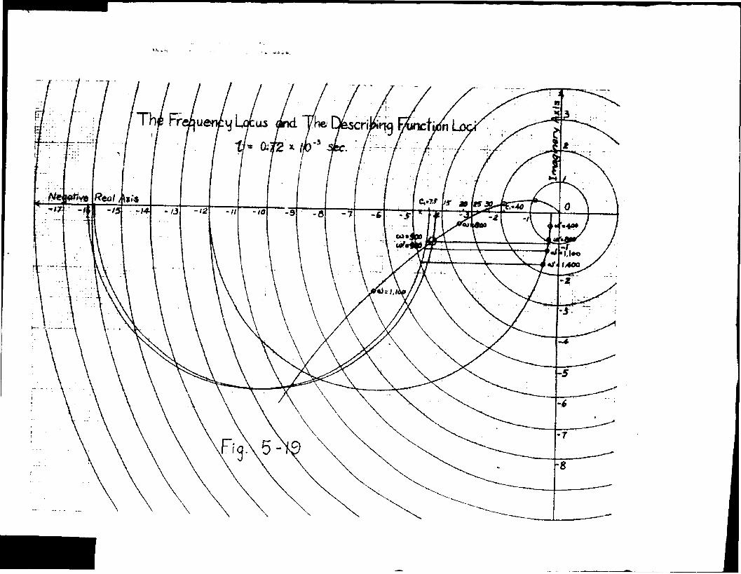
M >M*oI>400

y Locus e Deicnbi.52 X//0

*4

2 ©4

-

S u m m a r y of Results:*£, in see. Without parallel loop

Predicted ExperimentalA. 0 The system is The system is

stable. stable.

B. 0 . 2 7 x 1 0-i

D. 0.72x10-3

The system is stable.

The system will have sustained oseillations id x 700 c.24

The system is 8table.

The system will have sustained oscillationsa). 783 c = 23.3

With p a r a l l e l loo p Predicted E x p e r i m e n t a lThe system is stable.

The systemis stable.

The system will hare sustained

Th e s y s t e m is s t a b l e w i t h l e s s t r a n s i e n t os d i l a t i o n s . T h e s y s t e m 1 j stable, w i t h l e s s t r a n s i e n t o s c i l l a t i o n s . T h e s y s t e m w i l l b a w e s u s t a i n e d

o s c i l l a t i o n s o s e i l l a t i o n sid • 900c - 10

id » 9 6 4c * 11

%OZ

K. 2.52x10**

I

\

Tha system The system The system The systemwill hare will hare will hare will haveself-sus­ self-sus­ self-bus- self-sus­tained tained « \ained tainedoscillations oscillations oscillations oscillationswith: with: with: with:u) * 400 u> , *81 *>• 500 y)« 602o * 48 c « 46.8 c * 38 e * 38*5

g i u 5i Qt27 x 10, .gfttt . teat ttw Itftfl ntfrfpgfc,QondmiT in the parallel loop has btn lnoreased to 0t£5 Bft,

So far we have diaouseed all the pictures of Fig. 5-6, exoept the picture of Fig. 5-60. This is the actual oscilloscope record when the condenser In the lead network of the parallel loop has been inoreased from0.02 Jtf. to 0.25 lf/ As we have mentioned before that if the resistances in the lead network are remained un­changed, the change of the value of condenser does not affect the shape of the transfer function plot of the parallel loop. The plot of the transfer function of the parallel loop will still have the same locus, except that each point on the locus will have a new frequency value. For our case, the new frequency value for the same point on the locus will be 0.02/0.25 or eight tenths of the old frequency value. For example, the point which marked u) * 1400 in Fig. 5-18, will now have a new fre­quency value * 1400 x 0.8 » 1120 rad./sec.. The de­scribing function of the combined element of the parallel loop and the non-linear element will therefore also have the same loci exoept for the frequency value. This is shown by Fig. 5-21 with the inverse transfer function plot of the rest of the system.

-206-

If we compare rig. 5-21 with Fig. 5-18, we oan that they are almost tha samm, axeapt the fre­quency Yalue of tha daaorlblng funotion lool. Tha In­verse transfer funotion looua doaa Intersect the desorlb- lng funotion lool as before but this tine it doaa give a self-sustained oscillation of frequenoy:

it) m 1735 rad./see. and an amplitude corresponding to:

o, • 10 vbltsFrom Fig. 5-6C, we can sea that there are

about 2 5 oscillations throughout tha entire horizontal sweep. Henee the frequency of the self-sustained oscil­lation will be: so * 25 * 60.2 * 1500 rad./sec.

Also from Fig. 5-6C, we notice that there are about five small. divisions for tha maximum swing. Hence tha amplitude of tha self-sustained oscillation will have a magnitude corresponding to:

c, * 11 x 0 . 2 5 x 5 / 2 « 7 voltsThe percentage errors are:

for frequency: (1735 “ 1500)/1500 * 16%

for amplitude: ( 1 0 - 7 )/7 * *3%

The large percentage error for amplitude In this case may be due to a little variation in the

-207-

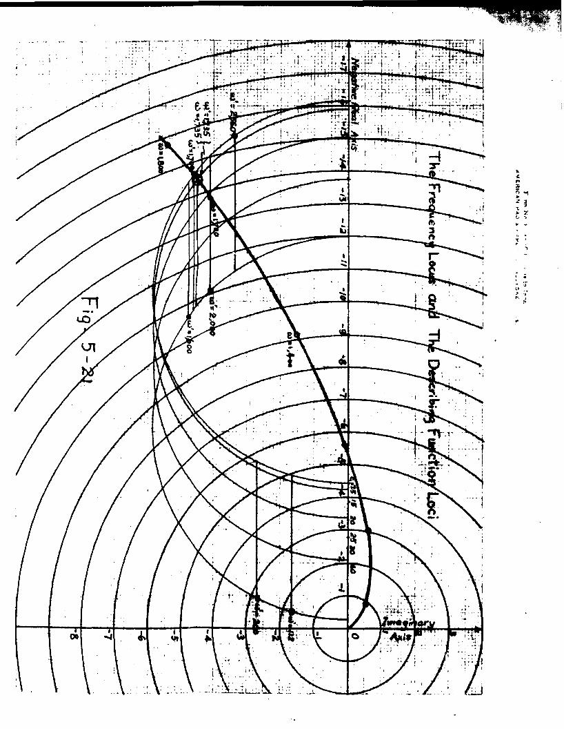
rOQ

I

■ * i."

• t , •

;’ere * > ir.r

f t

vnu'.i

*

V

/

g

“T«»

r f

i • t:

vrn*’ Tr. ’ff'ywi '"TT*^ j||rr

. ... w . . , . |T ||_ '•4)4'U ' "

iOf

amplifier gain of osolllosoope and the circuit. If the maximum swing of the ploture were 6 instead of 5, then we would have:

o, a 11 x 0.25 x 6/2 « 8.25 voltsand the percentage error will he reduced to:

( 10 - 8.25 )/8.25 ** 21.2*s •

which would be considered as satisfactory.At the first look it may sound strange that

the system performance becomes worse when the condenser in the lead network of the parallel loop is increased too much. However if we examine the transfer locus of the lead network, we can easily see that when the condenser is increased too much, the low frequency range of the transfer function locus is extended and the network is no longer a good approximation of an ideal lead network. On the contrary, when the condenser is Increased too much, the performance becomes worse.

Fig. 5-22 gives a series of qualitative pic­tures when the lead network condenser is Increased. The top ploture of Fig. 5-22 A, shows the performance without the parallel loop correction. The bottom picture shows the system performance with the parallel loop correction. It is obvious there is a definite Improvement of the system performance with the parallel loop correction.

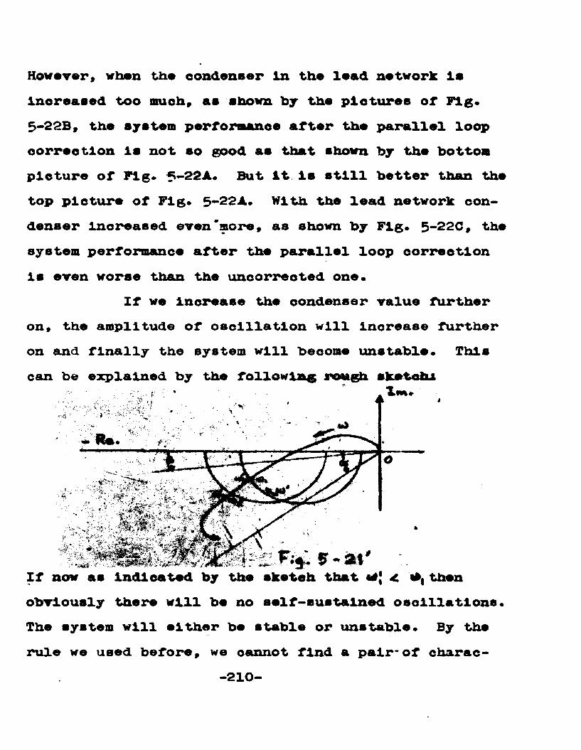
However, when the condenser In the lead network is increased too nuoh, as shown by the pietures or Fig* 5-22B, the system performance after the parallel loop oorreotion is not so good as that shown by the bottom pieture of Pig* 5-22A* But it is still better than the top picture of Fig* 5-22A. With the lead network con­denser increased even'more, as shown by Fig* 5-22C, the system performance after the parallel loop correction is even worse than the uncorrected one*

If we increase the condenser value further on, the amplitude of oscillation will increase further on and finally the system will become unstable* Thiscan be explained by the following rough sketch!

. t: ■ *' • Tm«

f> - at*If now as indicated by the sketeh that «** 4. then obviously there will be no self-sustained oscillations The system will either be stable or unstable* By the rule we used before, we cannot find a pair'of charac-

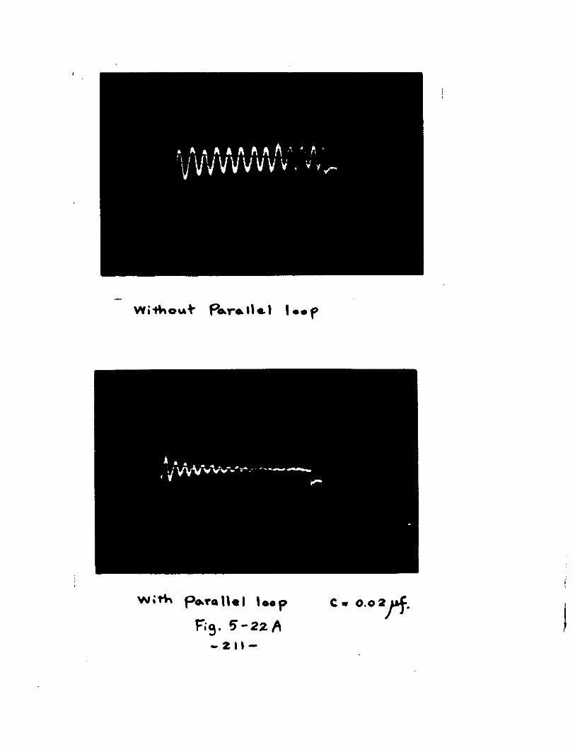
. A « A » A A A A 'y y y v v v m

Wii out Paral)«.) I •• p

l . , ., 1 V V V v W v

W.H* p<KroU«l i M p C » 0.02jrff.F;3 . * - 2 z A

- 2 I» -

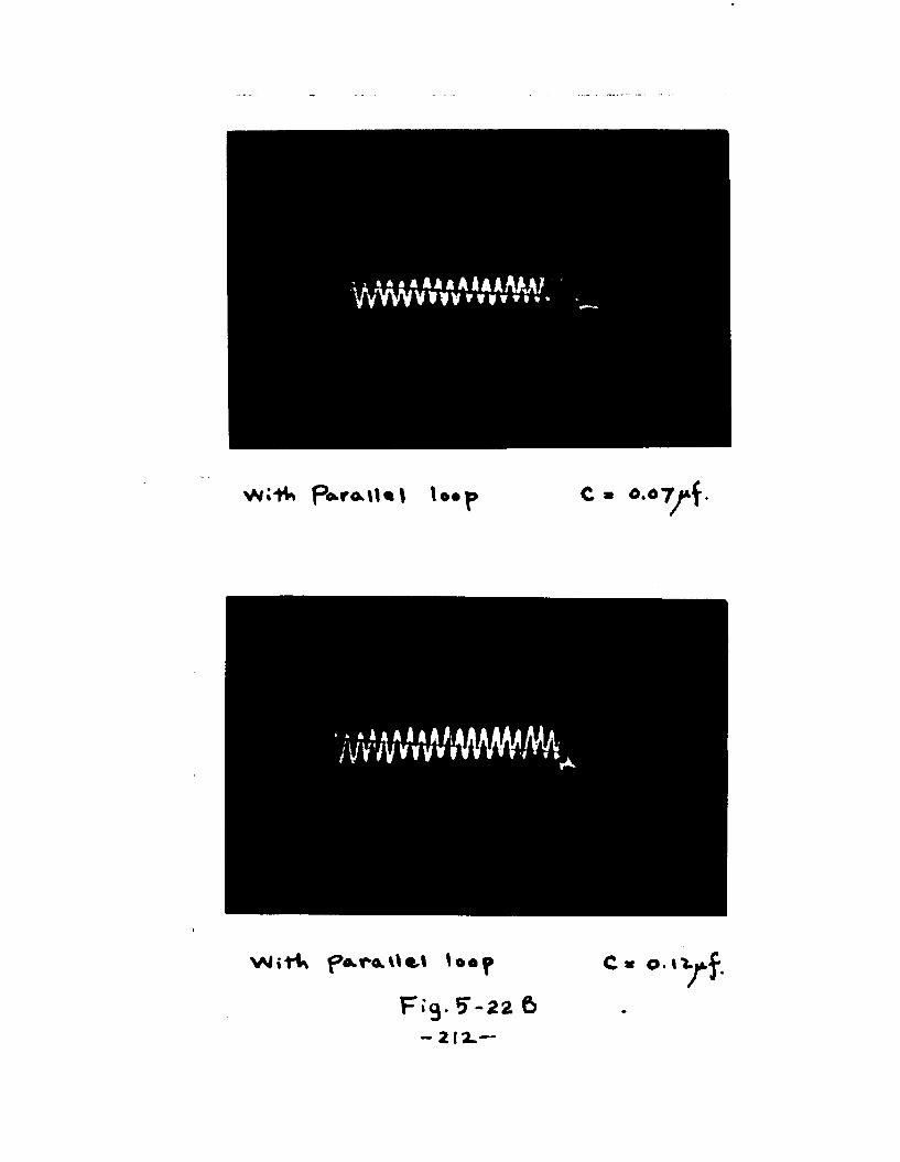
V v m V A W A m

I'tVi P»r&U«l C » o.«7/f

/VVVvAVvV

F » 3 - 5 - 2 2 6- 2 I3 L —

C * © • > y f.

P a r o c U e t > « « f C •=■ l .o ay*^ :

F i g . 5 - 2 2 C .

- av 3 -

terlstic points (a,b). Hence we take the point Infinity* And we can easily see that In this oase9 oA Is always greater than £3 , the system Is therefore unstable.(Compare the result with Fig. 5-16).

4. Some qualitative oscilloscope records when thecharacteristic of the non-linear element Is changed.

The relay element of the syatem is composed of rectifier elements and batteries. The schematic diagram is shown here again as Fig. 5-23*

F.g. 5 - 2 3 In the experiment, we have used 1.5 volts

for battery A and A'; 3 volts for battery B and B'.The experimental results have been checked with pre­dicted values with satisfactory agreement.

If we change the voltages of A, A*, B and B * 9 some other results should come out. Since we do not

-214-

want to repeat the routine numerioal check up work, a set of qualitative oscilloscope records would be enough for our interest.

We first reduce the voltage A and A' to zero; i.e. short circuit the batteries A and A'. This would give less stability. The pictures of Fig. 5-24 shows the situation clearly. (Compare with Fig. 5-6)*

Now if we also reduce the voltage of battery B and B* to one half; i.e. 1*5 volts, the system per­formance should be better than before. This is illus­trated by the pictures of Fig. 5-25*

All the pictures of Fig. 5-24 and Fig. 5-25 show a definite Improvement of system performance by the parallel loop correction.

-215-

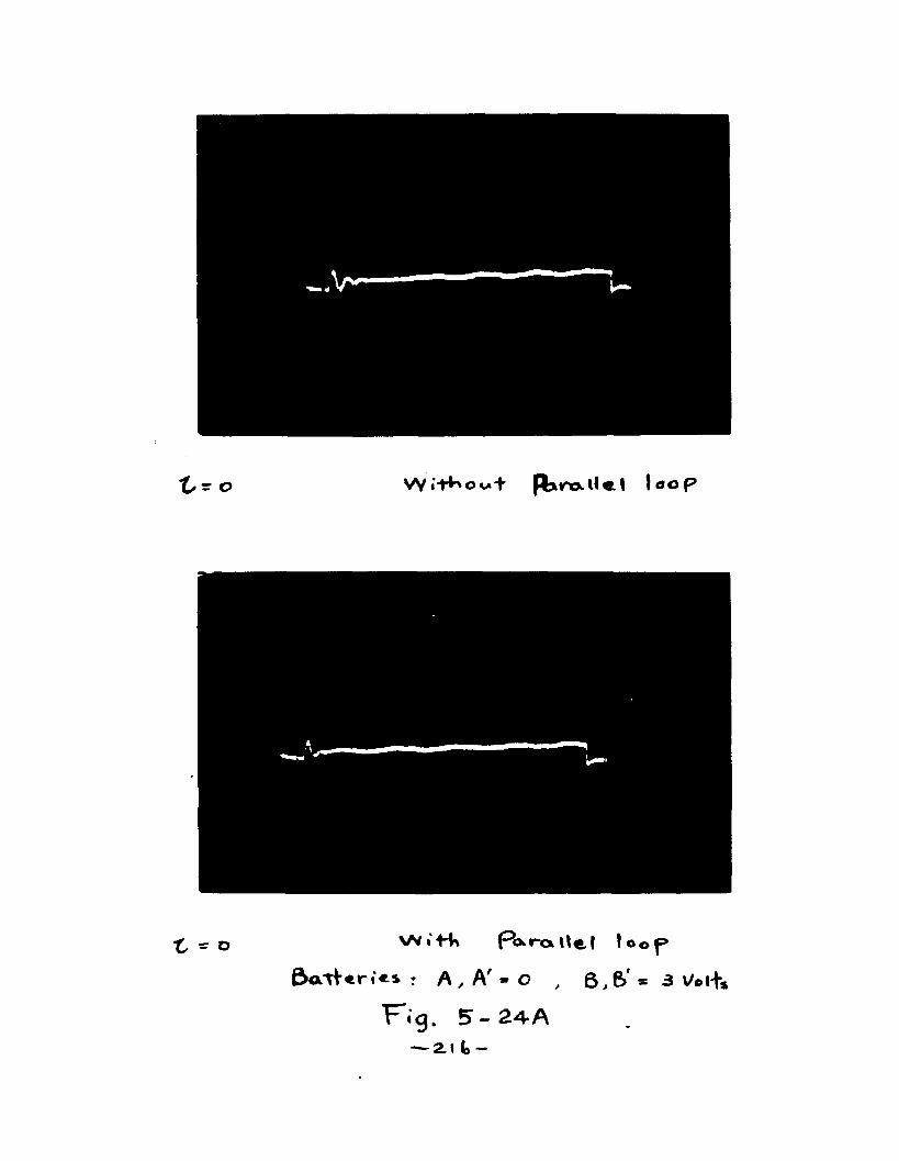
W i1 + 'o w + I o o p

c o NA/i-H* P<xr-o Uel lo0 p&atV«ri'es : A, A ' • o , 6,6'= 3 v/oi+*

F ig . 5-24-A— 2.1 (> -

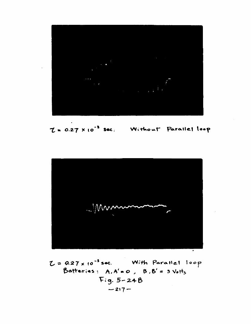
*£ « 0.27 * *° * Sec- W«H*ow-t" P«xr<K»le.< le*7

^ s: C.27 x fO~*S«C. Wi'fVt Poralle.! t 0 0 p»g><*1teri** : /\,A'*© , & , 6'= 3 V«l45

V . g . 5 -2 .-4 - 6

' 2 < 7 —

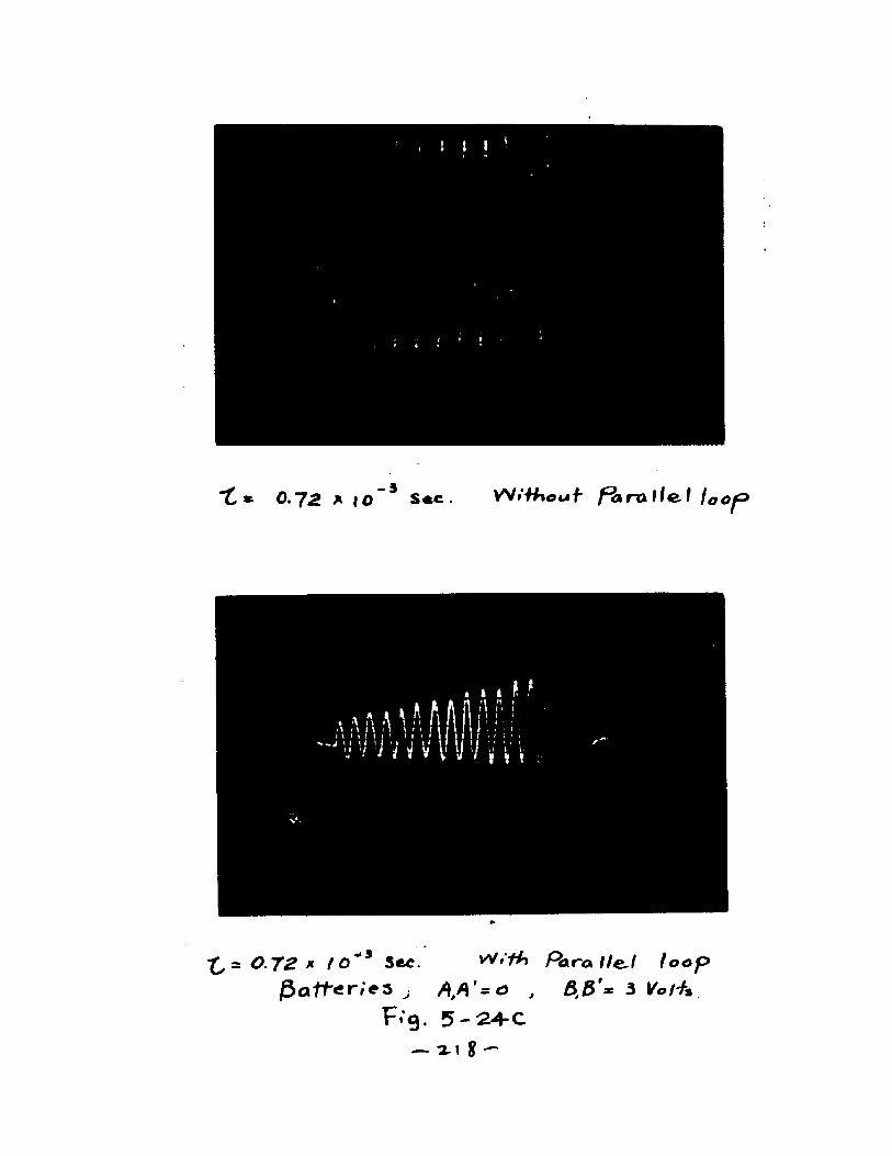
*. 0.72 * lO-5 S*c . WrWicuf fitmlle.1 loop*

, * A A H ft ft1 1 I \ M M I * * f l t

t i i J \ i \ i I I I #* ■> i * ¥

1 1i i;::iti

• ^ * 0 . 7 2 * t o * 9 Sec. vV«7*> Paralle.1 loop f$a1terie3 , 6,5'* 3 lfc/*V

F«*g. 5-24-C

»

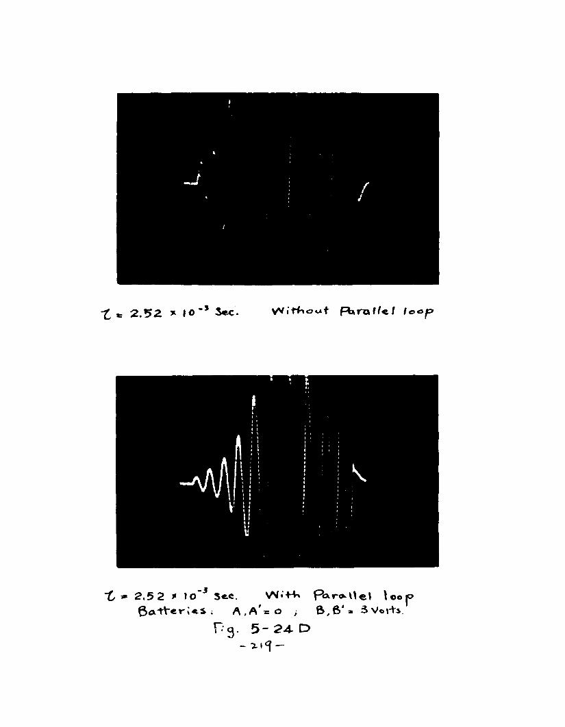
* tA

— r

*£ c 2 . 5 2 * IO '5 Sec. VVitf«o**t pbra I /e f loop

■ A

l

"£, » 2,5 2 * lO~J Sec. Pc\r<*Wel \ oo jo; A , A ' = o ; 6,6' » 3Vol+SHg. 5-24-D

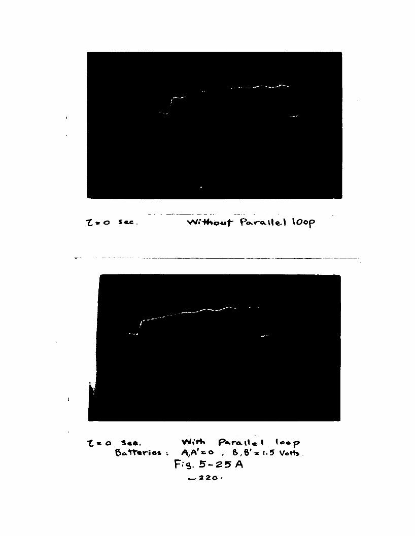
x» o Sec . Po-ravlel \Oop

*£ * o So«. W»tfc P^rcv it« .

C>ott*ri«s •. ^ A r*.o , 6 ,8'*F-’S- 5 - 2 5 A

— 220 -

i too pt.5 Vort*

— I -Cl -9 S S - 5

^•l\ £*t -,9'9 ' °~,V'V<io®l r»\\ x»ax^3 ^;rA **»S

: S»*Jk«44«3.0 1 * Z«*o » 3-

4'r*°'1+.,/SA a»S 0 1 * LZ'O *3-

O '7X > l O " 5 S*C. fVr<xlle1 loop

* 0«7l * io'*S«e. WiH» ParcxOel loopS<xTt«.ries : y%A'» o , &,$'= 1.5 V-

F:6 . 5 - 2 5 C— I l l —

\

V/

A/

•J* 2.52 x t o ' 3 See. w«'Hiouf ^krAlfcl /«op

£ * 2.52 * /<>“* Sec. W.'rfi Parallel U»f>6«f+«r#e* , 6,&'=t.a> V.

5 - 25 £>

5. fioaglMglttngiTh« conclusions of tills chapter are as

follows:1* Parallel loop correction can be used to Im­

prove the system performance of a non-linear servo*

2. The treatment of the non-linear element which depends n o t only on amplitude but also on the frequency as suggested by previous chapters to predict the system stability has been checked fairly closely with the experimental result* The close agreement between the p r e ­dicted values and the experimental results encourages us to apply the same technique to other non-linear problems in general*

-224

SttXqrgflgqq1. Kryloff, N. and Bogolluboff, N. in^rg^VQtlon To

Non-Linear* Meqhflntna , Kief (Russia), 1937*(English revision by Lefschetz, S . , Princeton University, 19^9*)

2. Andronow, A* A. and Chaikin, C. E. Theory ofOscillations , Moscow , 1937* (English revision by Lefschetz, S., Princeton University, 1949.)

3. Minor sky, N. Introduction to Non-Linear Mechanics , Ann Arbor, Michigan, Edwords Brothers, 1947.

4. Kryloff, N. and Bogolluboff, N. Introduction ToNon-Linear Mecnanics , English revision by LefBchetz,S. Princeton, 1949, pp.40-55*

5a. Hazen, H. L. Theory of Servomechanisms , J. F r ^ ^ ; n

Institute , Vol. 218, No. 3, PP* 279-330.5b. Oldenbourg, R. C. and Sartorlus, H. Dysamlk Selb-

sttatlger Recrelungen , Munchen and Berlin , 1944. (English revision under the name The Dynamics of Auto matlc controls by Mason, H. L . , New ¥ork, A.S.M.E., 1948.)

6a. MacColl, L.A. Fundamental Theory of Servomechanisms D. Van Nostrand, New York, 1945. pp. 107-125.

6b. Weiss, H. K. Analysis of Relay Servomechanisms ,J. Aero. Science Vol. 13 No. 7» July 1946, pp. 364.

- 225 ' -

7 . Kahn, D. A. " An Analysis or Relay Servomechanisms 1! A.I.E,Et Trans. 68 (19U 9) , p p .1 0 7 9 -6 7 .

8 . Kochenburger, R.J. , M A Frequency-Response Method For Analyzing and Synthesizing Contactor Servo­mechanisms ", A.I,E.E. Trans, 69 (1950) ,PP*270-83.

9. McCann, G-. D. , Herwald, S. W. and Kirschbaum, 3. , " -Ilsctrical Analogy Methods Applied to Servo­mechanism pr o b l e m s ”, A.I.E.E, T rans. (1914.6 ), pp.91-96.

2 2 6 -

Autobiography I, Chlh-Chl Hsu, was b o m in Shanghai, China,

June 30, 1923. I received my primary and seoondary school education in China. My undergraduate training was obtained at the Chiao-Tung University, which is also in China, and from which I received the degree Bachelor or Science in Electrical Engineering in 1945* After my graduation I worked at Tsingtao Power Company as a Junior engineer. In the spring of 1948, I came to this country and enrolled in the University of Michigan. The next year I received my degree of Master in Engineering from the University of Michigan. In September 1949, I received an appointment as University Scholar in The Ohio State University. I was specified in the field of Servomechanisms. In June 1950, I was appointed as a graduate assistant in the Department of Electrical Engineering. I held this position for one and half years while completing the requirements for the degree Doctor of Philosophy.

2 2 7 -