University of WindsorScholarship at UWindsor

Electronic Theses and Dissertations

2012

A structural investigation to develop guidelines forthe finite element analysis of the Mini-Baja vehicleBabak Shahabi

Follow this and additional works at: http://scholar.uwindsor.ca/etd

This online database contains the full-text of PhD dissertations and Masters’ theses of University of Windsor students from 1954 forward. Thesedocuments are made available for personal study and research purposes only, in accordance with the Canadian Copyright Act and the CreativeCommons license—CC BY-NC-ND (Attribution, Non-Commercial, No Derivative Works). Under this license, works must always be attributed to thecopyright holder (original author), cannot be used for any commercial purposes, and may not be altered. Any other use would require the permission ofthe copyright holder. Students may inquire about withdrawing their dissertation and/or thesis from this database. For additional inquiries, pleasecontact the repository administrator via email (scholarship@uwindsor.ca) or by telephone at 519-253-3000ext. 3208.

Recommended CitationShahabi, Babak, "A structural investigation to develop guidelines for the finite element analysis of the Mini-Baja vehicle" (2012).Electronic Theses and Dissertations. Paper 5342.

A STRUCTURAL INVESTIGATION TO DEVELOP GUIDELINES

FOR THE FINITE ELEMENT ANALYSIS OF THE MINI-BAJA

VEHICLE

By

Babak Shahabi

A Thesis

Submitted to the Faculty of Graduate Studies

through the Department of Mechanical, Automotive and Materials Engineering

in Partial Fulfillment of the Requirements for

the Degree of Master of Applied Science at the

University of Windsor

Windsor, Ontario, Canada

2011

© 2011 Babak Shahabi

A structural investigation to develop guidelines for the finite element analysis of the

Mini-Baja vehicle

by

Babak Shahabi

APPROVED BY:

______________________________________________

Dr. S. Das (Outside Program Reader)

Department of Civil & Environmental Engineering

_____________________________________________

Dr. R. Barron (Program Reader)

Department of Mechanical, Automotive and Materials Engineering

______________________________________________

Dr. N. Zamani (Advisor)

Department of Mechanical, Automotive and Materials Engineering

______________________________________________

Dr. S. Erfani (Co-advisor)

Department of Electrical & Computer Engineering

______________________________________________

Dr. B. Zhou (Chair of Defence)

Department of Mechanical, Automotive and Materials Engineering

December 16, 2011

III

AUTHOR’S DECLARATION OF ORIGINALITY

I hereby certify that I am the sole author of this thesis and that no part of this

thesis has been published or submitted for publication.

I certify that, to the best of my knowledge, my thesis does not infringe upon anyone‟s

copyright nor violate any proprietary rights and that any ideas, techniques, quotations, or

any other material from the work of other people included in my thesis, published or

otherwise, are fully acknowledged in accordance with the standard referencing practices.

Furthermore, to the extent that I have included copyrighted material that surpasses the

bounds of fair dealing within the meaning of the Canada Copyright Act, I certify that I

have obtained a written permission from the copyright owner(s) to include such

material(s) in my thesis and have included copies of such copyright clearances to my

appendix.

I declare that this is a true copy of my thesis, including any final revisions, as

approved by my thesis committee and the Graduate Studies office, and that this thesis has

not been submitted for a higher degree to any other University or Institution.

IV

ABSTRACT

Mini-Baja is a special type of vehicle used for recreational and exploration

purposes. In many aspects it is similar to an All-Terrain Vehicle (ATV) except that it is

much smaller in size. An international competition is organized by the Society of

Automotive Engineers (SAE) for universities throughout the world to design and

fabricate their vehicles and then compete against each other.

The objective of the present research was to carry out finite element analysis and

crash simulations for a Mini-Baja chassis structure. The aim of this task was to write a

comprehensive finite element guide for a Mini-Baja SAE vehicle that had already been

built by students at the University of Windsor for the year 2010 Baja competition in

Rochester New York.

Initially, an example of a Z-frame is explained and evaluated by simple hand

calculations. Subsequently, the preliminary design of the Mini-Baja roll cage was

generated using CAD data. To study the effects of stress and deformation on the frame

members, linear static analysis followed by transient modal superposition analysis was

carried out as the first steps toward this project. The static analysis in this thesis was used

to arrive at an acceptable mesh size for the Mini-Baja roll cage dynamic analysis.

Additionally, the more realistic frontal impact analysis was performed on the

Mini-Baja vehicle at a cruise velocity of 48 km/h (30 mph). Different FEA commercial

packages were used throughout the project and results obtained from Abaqus/CAE and

LS-DYNA were compared with one another.

Furthermore, crash test simulations for side impact and vehicle-to-vehicle crash scenarios

were also performed for the Mini-Baja frame to evaluate the structural rigidity and

vehicle behaviour due to crash.

V

DEDICATION

Dedicated to my parents and my brother,

for their endless support, love and encouragement

VI

ACKNOWLEDGEMENTS

I would like to express my most sincere gratitude and profound appreciation to

Dr. Nader Zamani for his supervision, guidance and support. His knowledge and

expertise has been of immeasurable assistance throughout my graduate studies and

research. This work could not have been achieved without his help and support.

I owe my deepest gratitude to Dr. William Altenhof for his guidance and

encouragement. I appreciate all his contributions to make my experience productive and

stimulating at the University of Windsor. The joy and enthusiasm he has for his research

was contagious and motivational for me throughout my graduate degree.

I would like to take this opportunity to also thank my co-advisor Dr. S. Erfani,

and my committee members Dr. S. Das and Dr. R. Barron for helping me throughout this

thesis.

Lastly, I offer my regards and blessings to my friends, colleagues, and all of those

who supported me in any respect during the completion of this thesis.

Babak Shahabi

VII

TABLE OF CONTENTS

AUTHOR’S DECLARATION OF ORIGINALITY ----------------------------------------------- III

ABSTRACT ----------------------------------------------------------------------------------------------- IV

DEDICATION --------------------------------------------------------------------------------------------- V

ACKNOWLEDGEMENTS ----------------------------------------------------------------------------- VI

LIST OF TABLES --------------------------------------------------------------------------------------- XI

LIST OF FIGURES ------------------------------------------------------------------------------------- XII

LIST OF APPENDICES ------------------------------------------------------------------------------ XXI

NOMENCLATURE ----------------------------------------------------------------------------------- XXII

CHAPTER І ------------------------------------------------------------------------------------------------- 1

1. INTRODUCTION ---------------------------------------------------------------------------------- 1

1.1 Scope and objective of the project ----------------------------------------------------------------- 1

1.2 About the SAE Mini-Baja --------------------------------------------------------------------------- 2

1.3 The CAD model of the Mini-Baja frame and chassis ----------------------------------------- 3

1.4 The role of non-linearities in the analysis of Mini-Baja--------------------------------------- 7

1.5 Literature review ------------------------------------------------------------------------------------ 12

1.5.1 Literature review of “SAE Mini-Baja” capstone reports ----------------------------- 12

1.5.2 Literature review of “Vehicle Crash Impact Analysis” papers --------------------- 23

CHAPTER ІІ ----------------------------------------------------------------------------------------------- 37

2. FINITE ELEMENT THEORY WITH NUMERICAL EXAMPLE ----------------------------- 37

2.1 Objectives and overview of Chapter ІІ --------------------------------------------------------- 37

2.2 A brief history of finite element method ------------------------------------------------------- 37

VIII

2.3 Finite element analysis fundamentals ----------------------------------------------------------- 38

2.4 Finite element form of the assumed solution -------------------------------------------------- 39

2.5 Finite element library ------------------------------------------------------------------------------ 42

2.6 Z-frame example ------------------------------------------------------------------------------------ 43

2.6.1 Computer implementation (Matlab) for the Z-frame --------------------------------- 47

2.6.2 Computer simulation (Catia) for the Z-frame ------------------------------------------ 52

2.6.3 Z-frame modified ---------------------------------------------------------------------------- 54

CHAPTER ІІІ ---------------------------------------------------------------------------------------------- 61

3. APPLICATION OF BEAM, SHELL, AND SOLID ELEMENTS FOR THE MINI-BAJA

FRAME (LINEAR STATIC AND DYNAMIC ANALYSIS) ------------------------------------------- 61

3.1 Objectives and overview of Chapter ІІІ -------------------------------------------------------- 61

3.2 Mini-Baja modeling methodology -------------------------------------------------------------- 61

3.2.1 Material properties --------------------------------------------------------------------------- 65

3.2.2 Section property ------------------------------------------------------------------------------ 68

3.2.3 Loading condition---------------------------------------------------------------------------- 68

3.2.4 Connections ----------------------------------------------------------------------------------- 70

3.3 Static results ----------------------------------------------------------------------------------------- 71

3.4 Transient dynamic analysis ----------------------------------------------------------------------- 76

3.4.1 Damping effect ------------------------------------------------------------------------------- 78

3.4.2 Dynamic force -------------------------------------------------------------------------------- 79

3.4.3 Transient dynamic simulation ------------------------------------------------------------- 80

3.5 Mesh convergence study -------------------------------------------------------------------------- 87

CHAPTER ІV ---------------------------------------------------------------------------------------------- 92

4. NON-LINEAR DYNAMIC ANALYSIS OF THE MINI-BAJA FRAME IN FRONTAL

CRASH (LS-DYNA) -------------------------------------------------------------------------------------- 92

4.1 Objectives and overview of Chapter ІV -------------------------------------------------------- 92

4.2 Key parameters of a non-linear explicit vehicle simulation -------------------------------- 93

4.2.1 Implicit vs. explicit time integration methodologies ---------------------------------- 93

4.2.2 Viscoplastic material model --------------------------------------------------------------- 95

4.2.3 Shell elements and B-L-T element ------------------------------------------------------- 98

IX

4.2.4 Hourglass energy modes ------------------------------------------------------------------- 101

4.2.5 Time step and mass scaling --------------------------------------------------------------- 102

4.2.6 Contact and friction modeling ------------------------------------------------------------ 103

4.3 Simulation of the front portion of the frame (LS-DYNA) --------------------------------- 107

4.4 Frontal impact simulation of the Mini-Baja frame structure (LS-DYNA) ------------- 112

4.4.1 Energy balance ------------------------------------------------------------------------------ 118

CHAPTER V --------------------------------------------------------------------------------------------- 121

5. EVALUATION OF THE FRONTAL CRASH OF THE MINI-BAJA VEHICLE BY

(ABAQUS/CAE) ---------------------------------------------------------------------------------------- 121

5.1 Objectives and overview of Chapter V -------------------------------------------------------- 121

5.2 Simulation of the front portion of the frame (Abaqus/CAE) ------------------------------ 122

5.3 Frontal impact simulation of the Mini-Baja frame chassis (Abaqus/CAE)------------- 130

5.4 Further comparison of LS-DYNA and Abaqus/CAE results ------------------------------ 134

CHAPTER VІ -------------------------------------------------------------------------------------------- 139

6. A MORE COMPLETE MODEL OF THE MINI-BAJA VEHICLE FOR CRASH ANALYSIS

(LS-DYNA) ---------------------------------------------------------------------------------------------- 139

6.1 Objectives and overview of Chapter VІ ------------------------------------------------------- 139

6.2 Modeling of the tires ------------------------------------------------------------------------------ 139

6.3 Simulation of the complete Mini-Baja vehicle ----------------------------------------------- 143

6.3.1 The frontal crash of the Mini-Baja vehicle -------------------------------------------- 147

6.3.2 The side crash of the Mini-Baja vehicle ------------------------------------------------ 153

6.3.3 Head-on collision of two Mini-Baja vehicles at 30 degree impact angle -------- 157

CHAPTER VІІ ------------------------------------------------------------------------------------------- 161

7. CONCLUSIONS AND RECOMMENDATIONS FOR FUTURE WORK ----------------- 161

7.1 Conclusions ----------------------------------------------------------------------------------------- 161

7.2 Recommendations for future work ------------------------------------------------------------- 163

REFERENCES ------------------------------------------------------------------------------------------- 166

X

APPENDICES -------------------------------------------------------------------------------------------- 171

APPENDIX A -------------------------------------------------------------------------------------------- 172

A. SEAM WELD CONNECTION ----------------------------------------------------------------- 172

APPENDIX B -------------------------------------------------------------------------------------------- 173

B. WIREFRAME LINE CONNECTION ISSUE ------------------------------------------------- 173

APPENDIX C -------------------------------------------------------------------------------------------- 174

C. TRANSIENT DYNAMIC ANALYSIS ---------------------------------------------------------- 174

VITA AUCTORIS --------------------------------------------------------------------------------------- 175

XI

LIST OF TABLES

Table 2.1 Nodal displacement of the Z-frame -------------------------------------------------------------- 54

Table 2.2 Nodal rotations of the Z-frame -------------------------------------------------------------------- 54

Table 2.3 Frequency analysis of the Z-frame ( , ----------------- 57

Table 2.4 von Mises stress for Z-frame ( , ------------------------ 60

Table 3.1 Alloy composition of 4130 chromoly (by weight) [35] -------------------------------------- 66

Table 3.2 Mechanical properties of 4130 steel [35] ------------------------------------------------------- 66

Table 3.3 Structural property of 4130 chromoly used in static simulation ---------------------------- 67

Table 3.4 Number of modes and corresponding natural frequencies ----------------------------------- 82

Table 3.5 Variation of maximum displacement and stress due to change in shell element size -- 87

Table 3.6 Displacement and stress at selected points in the frame -------------------------------------- 90

Table 4.1 Effect of different hourglass control techniques on accuracy and computational time ----

-----------------------------------------------------------------------------------------------------------------108

Table 4.2 Effect of adaptive method on zero energy modes -------------------------------------------- 109

Table 6.1 Aluminum 6061 material properties ------------------------------------------------------------ 144

XII

LIST OF FIGURES

Figure 1.1 University of Windsor Mini-Baja vehicle, 2010 ------------------------------------------------ 2

Figure 1.2 University of Windsor Mini-Baja vehicle, 2010 ------------------------------------------------ 3

Figure 1.3 Preliminary design of the chassis from SAE rule guide [1] ---------------------------------- 5

Figure 1.4 Preliminary design of the chassis from SAE rule guide [1] ---------------------------------- 5

Figure 1.5 CAD model of the Mini-Baja vehicle ------------------------------------------------------------- 6

Figure 1.6 CAD model of the Mini-Baja chassis ------------------------------------------------------------- 6

Figure 1.7 Behaviour of transverse beam sections in (a) slender beams and (b) thick beams [8] -- 9

Figure 1.8 Large deflection of a cantilever beam [8] -------------------------------------------------------- 9

Figure 1.9 Non-linear load-displacement curve [8] -------------------------------------------------------- 10

Figure 1.10 Front impact – loading point of application [14] -------------------------------------------- 13

Figure 1.11 Full meshed model in Ansys [15] -------------------------------------------------------------- 14

Figure 1.12 Front impact scenario in Visual Nastran [16] ------------------------------------------------ 18

Figure 1.13 Rollover impact scenario in Visual Nastran [16] ------------------------------------------- 19

Figure 1.14 Left: finite element mesh with masses and rigid-walls; Right: optimized design of the

chassis [17] -------------------------------------------------------------------------------------------------------- 21

Figure 1.15 Deformation of the chassis at 0.030 sec [17] ------------------------------------------------ 22

Figure 1.16 Energy plot for frontal impact [17] ------------------------------------------------------------ 22

Figure 1.17 The chassis frame [18] --------------------------------------------------------------------------- 23

Figure 1.18 Idealization with 58 and 22 nodes [18] ------------------------------------------------------- 24

Figure 1.19 Digitization arm being used on underside of hood [20] ----------------------------------- 26

XIII

Figure 1.20 Flow chart of the project with digitization [20] --------------------------------------------- 27

Figure 1.21 Consumer information label for a vehicle with at least one NCAP star rating [22] -- 28

Figure 1.22 Crush depth location and comparison [21] --------------------------------------------------- 29

Figure 1.23 Crash output results at different stages of the simulation [21] --------------------------- 30

Figure 1.24 FE model of the 2006 Ford F250 [23] -------------------------------------------------------- 31

Figure 1.25 Left: comparison of the global deformation for NCAP test and simulation; Right:

simulation data for energy balance [23] ---------------------------------------------------------------------- 32

Figure 1.26 Simulation and impact test comparison [25] ------------------------------------------------- 33

Figure 1.27 Finite element model of the C2500 pickup truck [26] ------------------------------------- 34

Figure 1.28 Comparison of pendulum test 02025 and simulation [26] -------------------------------- 35

Figure 1.29 Comparison of pendulum test 02027 and simulation [26] -------------------------------- 35

Figure 2.1 Element generation --------------------------------------------------------------------------------- 40

Figure 2.2 Beam element with uniform cross-section ----------------------------------------------------- 41

Figure 2.3 Element library of LS-DYNA [30] -------------------------------------------------------------- 42

Figure 2.4 Z-frame setup ---------------------------------------------------------------------------------------- 44

Figure 2.5 An arbitrary oriented frame element ------------------------------------------------------------ 45

Figure 2.6 Three-element model for the Z-frame ---------------------------------------------------------- 46

Figure 2.7 FE model of the Z-frame -------------------------------------------------------------------------- 52

Figure 2.8 Nodal displacement of the Z-frame ------------------------------------------------------------- 53

Figure 2.9 FE model of the Z-frame with beam, shell and solid elements ---------------------------- 56

Figure 2.10 Displacement vector; beam, shell and solid -------------------------------------------------- 57

XIV

Figure 2.11 Vertical vibration behaviour of beam, shell and solid models --------------------------- 58

Figure 2.12 Horizontal vibration behaviour of beam, shell and solid models ------------------------ 59

Figure 2.13 Out of plane mode of vibration of beam, shell and solid models ------------------------ 59

Figure 2.14 von-Mises stress contour; shell and solid ----------------------------------------------------- 60

Figure 3.1 Linear tetrahedron solid element [34] ---------------------------------------------------------- 62

Figure 3.2 Solid idealization of the Mini-Baja structure -------------------------------------------------- 63

Figure 3.3 Linear triangular shell element [34] ------------------------------------------------------------- 64

Figure 3.4 Shell idealization of the Mini-Baja structure -------------------------------------------------- 64

Figure 3.5 Beam idealization of the Mini-Baja structure ------------------------------------------------- 65

Figure 3.6 Stress-strain curves of different grades of steel [35] ----------------------------------------- 67

Figure 3.7 Sectional property of beam and shell models ------------------------------------------------- 68

Figure 3.8 Linear impulse and momentum applied on Mini-Baja frontal collision ----------------- 69

Figure 3.9 Seam welded connection CATIA V5 ----------------------------------------------------------- 70

Figure 3.10 Weld-connection for the beam model CATIA V5 ------------------------------------------ 71

Figure 3.11 Deformation shape for the beam model ------------------------------------------------------- 72

Figure 3.12 Deformation shape for the shell model ------------------------------------------------------- 73

Figure 3.13 Deformation shape for the solid model ------------------------------------------------------- 74

Figure 3.14 von Mises stress distribution for the shell model ------------------------------------------- 75

Figure 3.15 von Mises stress distribution for the solid model ------------------------------------------- 75

Figure 3.16 Left: static response for a slowly varying load; Right: dynamic response for a fast

varying load [31] -------------------------------------------------------------------------------------------------- 76

XV

Figure 3.17 Structure response for different types of damping [37] ------------------------------------ 78

Figure 3.18 Schematic diagram of a vehicle model over a bump --------------------------------------- 79

Figure 3.19 Constraint condition for dynamic analysis --------------------------------------------------- 80

Figure 3.20 Constraint condition for dynamic analysis --------------------------------------------------- 81

Figure 3.21 Deformation shape in static analysis ---------------------------------------------------------- 81

Figure 3.22 Stress contours in static analysis --------------------------------------------------------------- 82

Figure 3.23 Time modulation of the dynamic applied load ---------------------------------------------- 83

Figure 3.24 Maximum displacement of the frame at 0.0135 sec in dynamic analysis -------------- 84

Figure 3.25 Node for displacement graphs ------------------------------------------------------------------ 84

Figure 3.26 Three components of the displacement response of the selected point for the time

duration of 0.9 sec ------------------------------------------------------------------------------------------------ 85

Figure 3.27 Three components of the velocity response of the selected point for the time duration

of 0.9 sec ----------------------------------------------------------------------------------------------------------- 85

Figure 3.28 Distribution of von Mises stress through the cage in time -------------------------------- 86

Figure 3.29 Mesh convergence study for maximum displacement ------------------------------------- 88

Figure 3.30 Mesh convergence study for maximum stress ----------------------------------------------- 88

Figure 3.31 Selection of points for the mesh convergence study --------------------------------------- 89

Figure 3.32 Mesh convergence study for displacement at selected points ---------------------------- 90

Figure 3.33 Mesh convergence study for stress at selected points -------------------------------------- 91

Figure 4.1 Cost versus model size in explicit and implicit methodologies [8] ----------------------- 94

Figure 4.2 Determination of effective plastic strain ------------------------------------------------------- 95

Figure 4.3 4130 chromoly plastic behaviour ---------------------------------------------------------------- 96

XVI

Figure 4.4 Stress-strain response of a viscoplastic material at different strain rates [39] ---------- 97

Figure 4.5 Yield stress vs. effective plastic strain at different strain rates [30] ---------------------- 98

Figure 4.6 A representation of membrane forces on a membrane element and bending moments

on a plate element [40] ------------------------------------------------------------------------------------------ 99

Figure 4.7 LS-DYNA shell elements, node numbering for normal direction [30] ------------------- 99

Figure 4.8 Representation of warped shell elements [42] ----------------------------------------------- 100

Figure 4.9 a) A fully integrated element to the left and a under integrated element to the right; b)

Two hourglass modes for the under integrated element [41] ------------------------------------------- 101

Figure 4.10 Penalty contact algorithm in LS-DYNA [37] ----------------------------------------------- 104

Figure 4.11 Tied contact between tubes --------------------------------------------------------------------- 105

Figure 4.12 Front portion of the vehicle -------------------------------------------------------------------- 107

Figure 4.13 von Mises stress at different speeds for the front portion of the vehicle -------------- 107

Figure 4.14 Adaptive method applied on the frame ------------------------------------------------------ 108

Figure 4.15 Hourglass energy vs. hourglass control models -------------------------------------------- 109

Figure 4.16 Deformation shape of models with different adaptive refinements (in terms of the

threshold angle) -------------------------------------------------------------------------------------------------- 110

Figure 4.17 Deformation vector of 4 different models --------------------------------------------------- 111

Figure 4.18 Energy balance for front portion at 150 km/h (model 1) --------------------------------- 111

Figure 4.19 Mini-Baja frame structure ---------------------------------------------------------------------- 112

Figure 4.20 von Mises stress at 0.013 sec ------------------------------------------------------------------ 113

Figure 4.21 Maximum von Mises stress at 0.015 sec ---------------------------------------------------- 113

Figure 4.22 Maximum plastic strain at 0.045 sec --------------------------------------------------------- 114

XVII

Figure 4.23 Strain rate of 0.08/s at 0.006 sec -------------------------------------------------------------- 114

Figure 4.24 Strain rate of 80/s at 0.0109 sec --------------------------------------------------------------- 115

Figure 4.25 Highest Strain rate of 132/s at 0.014 sec ----------------------------------------------------- 115

Figure 4.26 Strain rate of 5/s at 0.038 sec ------------------------------------------------------------------ 115

Figure 4.27 Velocity contour in y-direction at 0.0109 sec----------------------------------------------- 116

Figure 4.28 Selected joints for contact force --------------------------------------------------------------- 116

Figure 4.29 Highest contact forces at the joints ----------------------------------------------------------- 117

Figure 4.30 Rigid wall normal force ------------------------------------------------------------------------- 117

Figure 4.31 Percentage of mass increase -------------------------------------------------------------------- 118

Figure 4.32 Energy balance for the complete mock-up at 48 km/h ------------------------------------ 120

Figure 4.33 Energy ratio of the simulation at 48 km/h --------------------------------------------------- 120

Figure 5.1 Front portion of the frame in frontal impact setup (Abaqus/CAE) ----------------------- 122

Figure 5.2 Tie contact (Abaqus/CAE) ----------------------------------------------------------------------- 123

Figure 5.3 Energy balance for front portion at 60 km/h (Abaqus/CAE) ------------------------------ 124

Figure 5.4 Energy balance for front portion at 60 km/h modified (Abaqus/CAE)------------------ 125

Figure 5.5 Energy balance for front portion at 60 km/h (LS-DYNA) --------------------------------- 125

Figure 5.6 The ratio of artificial strain energy over elastic strain energy ----------------------------- 126

Figure 5.7 von Mises stress distribution of the front portion at 60 km/h (LS-DYNA) ------------ 127

Figure 5.8 von Mises stress distribution of the front portion at 60 km/h (Abaqus/CAE) --------- 127

Figure 5.9 von Mises stress distribution of the front portion at 150 km/h (Abaqus/CAE) -------- 128

Figure 5.10 von Mises stress distribution of the front portion at 150 km/h (LS-DYNA) --------- 128

XVIII

Figure 5.11 Comparison of energy balance of the front portion at 150 km/h ------------------------ 129

Figure 5.12 Frontal impact scenario of the Mini-Baja vehicle (Abaqus/CAE) ---------------------- 130

Figure 5.13 Example of a wrong material direction ------------------------------------------------------ 131

Figure 5.14 Energy balance of the frontal impact at 48 km/h (Abaqus/CAE) ----------------------- 132

Figure 5.15 von Mises stress distribution at 0.013 sec (Abaqus/CAE) ------------------------------- 132

Figure 5.16 Maximum von Mises stress at 0.016 sec (Abaqus/CAE) --------------------------------- 133

Figure 5.17 Maximum plastic strain at the end of the simulation 0.045 sec (Abaqus/CAE) ----- 133

Figure 5.18 Maximum plastic strain at the end of the simulation 0.045 sec ------------------------- 134

Figure 5.19 Energy balance of the full Mini-Baja mock-up at 48 km/h ------------------------------ 135

Figure 5.20 Selected point for side displacement --------------------------------------------------------- 135

Figure 5.21 Side displacement of point (P) ----------------------------------------------------------------- 136

Figure 5.22 Selected roof point (Q) -------------------------------------------------------------------------- 136

Figure 5.23 Vertical displacement of the roof point (Q) ------------------------------------------------- 137

Figure 5.24 Wall reaction force ------------------------------------------------------------------------------- 138

Figure 5.25 Reaction wall force versus resultant displacement (stiffness) --------------------------- 138

Figure 6.1 Actual tires and suspension assembly --------------------------------------------------------- 140

Figure 6.2 CAD model of the tire ---------------------------------------------------------------------------- 140

Figure 6.3 FE model of the tire assembly displaying the sectional thicknesses --------------------- 141

Figure 6.4 Deformation of the tires at 90mm displacement of the wall------------------------------- 142

Figure 6.5 Deformation of the tires at 0.04 sec for the rear tires and at 0.032 sec for front tires -----

-----------------------------------------------------------------------------------------------------------------142

XIX

Figure 6.6 FE model of the completed Mini-Baja vehicle ----------------------------------------------- 143

Figure 6.7 Body panels and nodal rigid body constrained ----------------------------------------------- 144

Figure 6.8 Body panels, rear suspension, and shocks ---------------------------------------------------- 145

Figure 6.9 Behaviour of the low density foam [30] ------------------------------------------------------- 145

Figure 6.10 Stress-strain curve for the low density foam cushion ------------------------------------- 146

Figure 6.11 Revolute joint and angular velocity of the tires -------------------------------------------- 146

Figure 6.12 Test setup for equilibrium check -------------------------------------------------------------- 148

Figure 6.13 Reaction force of the rigid ground ------------------------------------------------------------ 148

Figure 6.14 Isometric view of the detailed model simulation of the Mini-Baja vehicle into the

rigid wall at 48 km/h -------------------------------------------------------------------------------------------- 149

Figure 6.15 Left: the maximum von Mises stress at 0.011 sec; Right: effective plastic strain at the

end of the simulation -------------------------------------------------------------------------------------------- 149

Figure 6.16 Side, top and front views of the deformation at t = 0.014 sec --------------------------- 150

Figure 6.17 Side, top and front views of the deformation at t = 0.025 sec --------------------------- 150

Figure 6.18 Side, top and front views of the deformation at t = 0.036 sec --------------------------- 150

Figure 6.19 Traced nodes on the rear tire at t = 0.04 sec ------------------------------------------------ 151

Figure 6.20 Energy balance for frontal crash at 48 km/h ------------------------------------------------ 151

Figure 6.21 Energy balance for frontal crash at 48 km/h (low density tire)-------------------------- 152

Figure 6.22 Kinetic energy based on density of tires at 48 km/h --------------------------------------- 152

Figure 6.23 Side impact setup --------------------------------------------------------------------------------- 153

Figure 6.24 Sequential views of the side impact scenario 1 at initial position ---------------------- 154

Figure 6.25 Sequential views of the side impact scenario 1 at t = 0.033 sec------------------------- 154

XX

Figure 6.26 Sequential views of the side impact scenario 1 at the end of the simulation --------- 154

Figure 6.27 Energy balance of the side crash scenario 1 at 48 km/h ---------------------------------- 155

Figure 6.28 Sequential views of the side impact scenario 2 at initial position ---------------------- 155

Figure 6.29 Sequential views of the side impact scenario 2 at t = 0.016 sec------------------------- 156

Figure 6.30 Sequential views of the side impact scenario 2 at t = 0.025 sec------------------------- 156

Figure 6.31 Sequential views of the side impact scenario 2 at the end of the simulation --------- 156

Figure 6.32 Energy balance of the side crash scenario 2 at 48 km/h ---------------------------------- 157

Figure 6.33 Configuration of the vehicle-to-vehicle crash at 30 degree impact angle ------------- 158

Figure 6.34 Sequential views of the vehicle-to-vehicle crash at initial position -------------------- 158

Figure 6.35 Sequential views of the vehicle-to-vehicle crash at t = 0.017 sec ---------------------- 159

Figure 6.36 Sequential views of the vehicle-to-vehicle crash at t = 0.036 sec ---------------------- 159

Figure 6.37 Sequential views of the vehicle-to-vehicle crash at t = 0.07 sec ------------------------ 159

Figure 6.38 Energy balance of the vehicle-to-vehicle crash at 48 km/h ------------------------------ 160

Figure 6.39 Maximum von Mises stress for vehicle-to-vehicle crash at t = 0.02 sec -------------- 160

Figure 7.1 Hybrid III occupant dummy --------------------------------------------------------------------- 164

Figure 7.2 Two Mini-Baja‟s impact scenario at 30 degree impact angle ----------------------------- 165

Figure A.1 Seam weld connection tutorial ----------------------------------------------------------------- 172

Figure B.1 Line connection issue tutorial ------------------------------------------------------------------- 173

Figure C.1 Transient dynamic analysis tutorial ------------------------------------------------------------ 174

XXI

LIST OF APPENDICES

APPENDICES -------------------------------------------------------------------------------------------- 171

APPENDIX A -------------------------------------------------------------------------------------------- 172

A. SEAM WELD CONNECTION -------------------------------------------------------------------- 172

APPENDIX B -------------------------------------------------------------------------------------------- 173

B. WIREFRAME LINE CONNECTION ISSUE -------------------------------------------------- 173

APPENDIX C -------------------------------------------------------------------------------------------- 174

C. TRANSIENT DYNAMIC ANALYSIS ---------------------------------------------------------- 174

XXII

NOMENCLATURE

Transverse shear strains

Linear stiffness matrix

Incremental matrix

Initial stress matrix

Degree of freedom

Stiffness matrix

Mass matrix

Damping matrix

Natural frequency of harmonic motion

Shape function

Distributed loads

Point loads and moments

Plastic strain

Elastic strain

Strain rate

Initial yield stress

Static stress

Membrane forces

Characteristic length

c Sound speed

Bulk modulus

Penetration distance

1

CHAPTER І

1. INTRODUCTION

1.1 Scope and objective of the project

In this thesis, considerable effort has been dedicated to the use of different

commercial finite element analysis packages available at the University of Windsor. The

intended objective of this thesis is to present some of the findings and challenges with

regard of the finite element modeling of a Mini-Baja vehicle. It is anticipated that this

research will assist undergraduate and graduate students or other readers who have

limited experience in computational methods in using FEA tools for design purposes.

An introduction to the Mini-Baja vehicle, basic fundamentals of simulation, and

the assumptions made for the non-linear dynamic analysis of the vehicle are discussed in

Chapter 1. The finite element method and its application for a simple Z-frame is

discussed in Chapter 2. There, the numerical results of a linear finite element analysis are

compared with theoretical solution using a Matlab program.

In Chapter 3, the application of shell, beam and solid elements for a Mini-Baja

frame are discussed for a linear static analysis. Later in this chapter, dynamic loads

transmitted to the frame are simulated for a case where the vehicle goes over a bump.

Chapter 4 provides an explicit non-linear dynamic simulation for a frontal crash of the

frame into a rigid wall at 48 km/h (30mph). The results from this simulation are validated

by another FEA package in Chapter 5.

In Chapter 6, the model in refined by including body panels and other components

such as suspension arms, wheels and steering wheel for a more realistic vehicle analysis.

Validation by experimental crash test on this vehicle is beyond the scope of the project.

2

1.2 About the SAE Mini-Baja

The Society of Automotive Engineers (SAE) organizes an inter-collegiate

competition in which various universities from all around the world build a Mini-Baja

vehicle to compete against one another. The automotive society has laid down a set of

guidelines and rules [1] that every vehicle should follow. These guidelines are based on

recommendations and tests conducted by design professionals and engineers.

Being a competition, every university has to develop its own design without any

professional assistance or knowledge sharing. Baja SAE consists of three regional

competitions that simulate real-world engineering design projects and their related

challenges. Engineering students are tasked to design and build an off-road vehicle that

will survive the severity of rough terrain and sometimes even water.

Figure 1.1 University of Windsor Mini-Baja vehicle, 2010

All vehicles are powered by a ten-horsepower Intek Model 20 engine donated by

Briggs & Stratton Corporation. Figures 1.1 and 1.2 show snapshots of the University of

Windsor‟s 2010 vehicle and gives the reader an idea of the terrain during the competition.

3

The mechanical engineering capstone project is an attempt to design a Mini-Baja from

scratch, based on the guidelines provided by SAE. Certain practices by the industry in

off-road vehicles and the concepts of mechanical engineering are employed to develop

and design a chassis which is safe, ergonomic and has the minimum possible weight.

Competitiveness of the vehicle in terms of sustainability and manoeuvrability should also

be kept as a design goal.

Figure 1.2 University of Windsor Mini-Baja vehicle, 2010

The rules [1] are set in order to comprise a number of limitations on the vehicle‟s

configuration, vehicle maximum size, all terrain capability of the vehicle as well as

vehicle ergonomic capacity. As far as safety issues are concerned, there are several

regulations concerning the electrical systems, battery location and orientation, kill

switches and brake specifications.

1.3 The CAD model of the Mini-Baja frame and chassis

The Mini-Baja vehicle is designed and fabricated as a capstone project at the

University of Windsor every year. Although the capstone team is divided into different

sections, it is understood that the design and fabrication of the chassis is one of the main

4

challenges of the project. Each year students attempt to deliver a better design by

analyzing the frame with the aid of computer modeling and simulation. The Mini-Baja

vehicle for the academic year 2010 was available at the university and therefore, it was

selected for the finite element analysis and discussion in this thesis. The reader should

keep in mind that the impetus of this thesis is to analyze a pre-existing design to identify

its important aspects and deficiencies.

The Society of Automotive Engineers has laid down a set of required

specifications for the design and manufacturing of the roll cage. The cage must be

designed to prevent any structural failure. It must be a space frame made up entirely of

tubular steel components. Several members are mandatory in the design of the cage,

which are shown in figures 1.3 and 1.4, the dimensions of these members; member‟s

length, thicknesses and orientations are given in detail in the SAE guideline.

Some preliminary design data was available from previous reports and files on the

2010 Mini-Baja vehicle; nevertheless the CAD modeling of the frame and other

components for this thesis were done again through reverse engineering of the vehicle

leading to new CAD data, figures 1.5 and 1.6.

Several assumptions were made on the finite element modeling of the vehicle.

Suspension arms, slender members such as A-arms and the frame‟s back axle were

modeled with simple beam elements. The engine has been replaced by the equivalent of

structural distributed mass over appropriate members. The spring and dampers were

modeled with acceptable discrete elements to incorporate their effects on the vehicle‟s

kinematics, whereas the models of the shocks themselves were excluded.

5

Figure 1.3 Preliminary design of the chassis from SAE rule guide [1]

Figure 1.4 Preliminary design of the chassis from SAE rule guide [1]

6

In vehicle‟s structural analysis, four common crash scenarios are considered.

These are; Front crash, Rear crash, Side crash and Rollover crash. It is understood that,

among these crash scenarios, frontal impact crash is at the highest of importance.

According to vehicle safety standards [2], for both fatally and seriously injured

occupants, frontal impacts are the most important crash type followed by side impacts.

Therefore, this thesis focuses mainly on frontal crash analysis.

Figure 1.5 CAD model of the Mini-Baja vehicle

Figure 1.6 CAD model of the Mini-Baja chassis

7

1.4 The role of non-linearities in the analysis of Mini-Baja

The preponderance of finite element analyses in engineering design today is still

linear FEM. In stress analysis, linear FEM is applicable only if the material behaviour is

linear elastic, strains are infinitesimal and no contact is present. These assumptions are

discussed in more detail later in the thesis. For most operational loads, linear analysis is

adequate as it is usually undesirable to have excessive loads that can lead to non-linear

material behaviour or large strains [3]. This however is not the case where large

deformations exist such as impact engineering or vehicle crash problems.

There are three sources of non-linearities in the analysis of solid continua [4]:

Material non-linearity, in which material properties are functions of the state of

stress or strain. Examples include non-linear elasticity, plasticity and creep.

Contact non-linearity, in which a gap between adjacent parts may open or close,

the contact area between parts changes as the contact force changes, or there is

sliding contact with frictional forces.

Geometrical non-linearity, in which deformation is large enough that equilibrium

equations must be written with respect to the deformed structural geometry. Also,

loads may change direction as they increase. A typical example is the excessive

bending of a fishing rod.

Material non-linearity occurs when the stress-strain behaviour given by the

constitutive relation is non-linear (e.g. viscoplasticity), whereas geometric non-linearity is

important when changes in geometry have a significant effect on the load-deformation

behaviour. Material non-linearity can be considered to encompass contact friction,

whereas geometric non-linearity includes deformation-dependent boundary conditions

and loading [5].

Non-linear finite element analysis is an essential component of computer-aided

design. Testing of prototypes is increasingly being replaced by simulation using non-

linear finite elements. This provides a more rapid and economical way of evaluating

design concepts and design details. For example, in the field of automotive design,

8

simulation of crash is replacing full scale tests, both for the evaluation of early design

concepts and details of the final design. In many fields of manufacturing, simulation is

speeding the design process by allowing simulation of processes such as sheet-metal

forming, extrusion of parts and casting. For both users and developers of non-linear finite

element programs, an understanding of the fundamental concepts of non-linear finite

element analysis is essential. Without an understanding of the fundamentals, a user must

treat the finite element program as a black box that is not desirable [6].

Yang and Lianis [7] developed one of the very first finite element displacement

formulations and solution procedures for the analysis of large displacement problems of

viscoelastic beams and frames. Because of the complexity involved in the non-linear

integral-differential equation for viscoelastic beams, solution was only obtained by

numerical approximations.

The term “large strain” problem is used repeatedly in this thesis and it is highly

recommended that FEA users have some basic understanding of the non-linear finite

element theory of solid mechanics to better interpret computer simulation results.

In the context of beam analysis, geometric non-linearity arises when deformations

are large enough to alter the distribution or orientation of applied loads, or the orientation

of internal resisting forces and moments [4]. In small deflection theory, the slope of the

beam is assumed to be small and therefore its contribution is neglected in the curvature

equation. The classical Euler-Bernoulli‟s beam theory no longer holds when the beam is

under large strains.

If the beam‟s cross-sectional plane does not remain normal to the beam‟s axis and

undistorted under deformations, beam theory is not adequate to model the deformation; in

general this is the limit of the applicability of the Euler-Bernoulli‟s beam theory, (figure

1.7). Problems with geometrical non-linearity cannot be analysed with classical Euler-

Bernoulli beam elements, since the shear deformation will govern the distribution of the

internal forces and stresses rather than pure bending as assumed in classical beams. In

such a case, beam elements (Timoshenko beams) are formulated such that their cross-

9

sectional area can change as a function of the axial deformation, an effect that is

considered only in geometrically non-linear simulations [8].

Figure 1.7 illustrates the transverse shear behaviour of beams: in (a), beam‟s axis

that is initially normal to the beam surface remain straight and normal to the deflected

mid-surface throughout the deformation. Hence, transverse shear strains are neglected

( ). On the other hand in (b): beam axis that is initially normal to the beam mid-

surface does not necessarily remain normal to the surface throughout the deformation,

thus transverse shear flexibility has a nonzero value, ( ).

Figure 1.7 Behaviour of transverse beam sections in (a) slender beams and (b) thick beams [8]

Figure 1.8 Large deflection of a cantilever beam [8]

For example, consider a cantilever beam loaded vertically at the tip, as shown in

figure 1.8. If the tip deflection is small, the analysis can be considered as being

approximately linear. However, if the tip deflection is large, the shape of the structure

10

and hence its stiffness changes and the load-deflection curve is non-linear as in figure 1.9.

In other words, as the tip load increases, beam's stiffness changes non-linearly [8].

Figure 1.9 Non-linear load-displacement curve [8]

One would expect large strains to have a significant effect on the way that

structures carry loads. However, strains do not necessarily have to be large for geometric

non-linearity to be important [8], other situations such as large displacement of

viscoelastic materials may happen when large strain theory is needed as well. Elongation

of a fishing rod is a more tangible example of such a case.

It appears that a very simple yet highly effective way to treat the large deflection

problem using finite elements is that developed by Yang [9]. The solution procedure

includes the conventional stiffness formulation for small deflection where the effect of

axial force is then taken into account by adding an incremental stiffness matrix or initial

stress matrix to the original stiffness equation [10]:

(1-1)

where is the axial force, is the linear stiffness matrix and is the incremental

matrix associated with the effect of axial force on bending deflection. Because

contains the load P, it is often referred to as the initial stress matrix . This is a

non-linear equation (i.e. figure 1.9) and a simple way to solve this equation is to use step-

by-step linear incremental procedure. The prediction of this load-displacement path by

linearized midpoint tangent incremental procedure together with coordinate

transformation at every step can be found in [10] and the modified and modern technique

11

used in today‟s software can be found in [8]. Further studies in the vibration of frames

and axial-flexural coupling effect in frame vibration can be found in [11] and [12].

Problems that display geometric non-linearity may simultaneously display contact

non-linearity and plasticity, as for example in vehicle crash analysis. The linear theory

assumes small strains. This approach may lead to inaccurate results or convergence

difficulties in cases where these assumptions are not valid. The large displacement

solution is needed when the acquired deformation alters the stiffness (ability of the

structure to resist loads) significantly [13]. The large strain solution assumes that the

stiffness changes during loading, so it applies the load in steps and updates the stiffness

for each solution step as shown in eq. (1-1).

12

1.5 Literature review

As mentioned before, knowledge sharing is not allowed for SAE Mini-Baja

participating teams. Therefore, it was difficult to collect detailed and specific information

on this topic. Nonetheless, some capstone project reports and theses from other

universities were secured from variety of sources and these are reviewed in section 1.5.1.

In addition, section 1.5.2 contains relevant literature published on the topics of

dynamic analysis of space frame structures, frontal crash impacts, crashworthiness

assessment and validation of automobiles finite element models which are equally

applicable to a Mini-Baja vehicle.

The reader is advised that in some instances the writing of the original authors‟

best expresses the issue and for that reason, the paragraphs were incorporated with major

editing for narrowing down the contribution of the literature on our subject of interest, so

there might be some repetition or minor jump between each part.

1.5.1 Literature review of “SAE Mini-Baja” capstone reports

Although the Mini-Baja project has been developed by many universities

worldwide, the detailed designs are not in the public domain. These projects were to

design and manufacture a Mini-Baja vehicle that participated in the global Mini-Baja

competition organised by SAE annually meeting their specifications.

To design the chassis of the vehicle, most of the universities develop a

preliminary design based on specifications given in the SAE guideline, then the vehicle is

tested using PVC pipes for driver space followed by checking the design using different

finite element packages such as Solidworks, Ideas, Algor, Abaqus/CAE, Ansys, Catia,

Nastran and LS-DYNA. Based on the literature collected on this subject, it is understood

that selecting the appropriate impact forces to apply on the frame is one of the major

challenges during the finite element analysis of the cage. Therefore, an effort has been

made to present a short review on this issue.

In [14], an initial design of the roll cage was done using the Solidworks modeling

package, followed by the analysis of the frame with the Algor finite element package. In

13

this report, it is mentioned that the human body will lose conscientiousness at loads

greater than 9 times the force of gravity, or 9g. Therefore, the value of 10g was selected

for the worst case collision of the frame. Based on other assumptions used by the

automotive industry, an impact force of 5g and 2.5g were chosen for the side impact and

rollover impact respectively.

In the case of frontal collision, an equivalent of 10g (7500 lbf) was applied on a

front most point of the frame as shown in figure 1.10 with a red arrow.

Figure 1.10 Front impact – loading point of application [14]

This procedure was also repeated for the analysis of side and rollover impact

scenarios. Analyzing the outcome resulted in the addition of new structural member‟s

braces to the frame as well as changes in dimensions and thicknesses of critical

components. One of the major deficiencies in this report was that it does not replicate

realistic crash of the vehicle into a rigid wall. Rather, it involves a rough estimation of

impact forces applied at different locations on the frame which cannot be reliably used

for a vehicle collision. Besides, vehicle crash is a dynamic process in which strain

sensitive members are under significant deformation and therefore a linear finite element

14

analysis based on constraining or clamping a specific location of the cage and applying

point loads is not appropriate.

In [15], the work plan was divided into 5 stages; initially, a preliminary design

based on SAE specifications was prepared. This was then tested for driver space by

building a plastic mock-up model using PVC pipes. It was next followed by modeling the

chassis in Pro/E. The design was then checked using finite element analysis in Ansys for

further optimization in terms of weight and safety. A rollover analysis was carried out to

ensure safer rollover capabilities.

Material properties were assumed to be linear elastic and the model was meshed

using just “Beam” elements as shown in figure 1.11. These elements are based on the

Euler-Bernoulli beam theory and have 6 degrees of freedom at each node. In the context

of vehicle crash, beam elements are considered as acceptable for specific members in a

vehicle. A full beam model that was developed for a Mini-Baja is not capable of

simulating a real vehicle crash scenario.

Figure 1.11 Full meshed model in Ansys [15]

15

In the project reported in [15], force estimations were based on perfectly inelastic

collisions which are as follows:

Estimation of front impact force.

(1-2)

where and

are the two colliding masses with velocities

and

respectively. The

masses and were assumed to be equal, and the vehicle is

assumed at rest . The term in eq. (1-2) was derived from the impulse

momentum equation. Using the above assumptions, one gets;

(1-3)

(1-4)

where „ ‟ is the impact time. Therefore

(1-5)

The mass of the vehicle was assumed to be 200 kg, whereas the driver‟s mass was

taken to be 75 kg which resulted in = 200 + 75 = 275 kg. Maximum speed of the

vehicle was assumed 10 meters per seconds with the impact time of 100 milliseconds.

Consequently, the force was derived from eq. (1-5); .

Although the distortion energy in eq. (1-3) seems correct, there was no

explanation for the term in eq. (1-4), which states that the transmitted force to the frame

is equal to the energy divided by the impact time. It is understood that the conservation of

momentum divided by impulse time could be assumed as the force acting on the matter

, but energy divided by time cannot be assumed as the acting force. This is not

even dimensionally correct.

16

Estimation of wheel bump forces. An assumption was made that when the vehicle

goes over a bump, the entire weight of the vehicle is felt as two point loads

transmitted to the chassis, through the suspension.

These two point loads were equated to the weight of the chassis. Hence,

(1-6)

(1-7)

(1-8)

(approx). (1-9)

where safety factor was chosen to be 1.1 in eq. (1-8).

Estimation of loading forces while heaving. For this condition, all the upper

points of the frame were fixed while the four bottom points of the frame where

the suspension is attached were loaded vertically. It was assumed that the entire

weight of the vehicle was transmitted into two points, hence F =1500N similar to

wheel bump forces was chosen.

Forces in case of rollover. In case of rollover, IS 11821 (BUREAU OF INDIAN

STANDARDS) defines a set of tests and acceptance conditions for agricultural

tractors. The same conditions were incorporated for the Mini-Baja finite element

analysis to see if the vehicle fails to meet the acceptance conditions.

According to IS 11821, estimation of rollover force was as follows. The strain

energy absorbed by the structure is equated to the required input energy in joules (Es)

based on the equation below:

(1-10)

17

where Mt is the mass of the vehicle, which in this case is estimated to be 200 kg.

Therefore

(1-11)

For a loading at the front and rear of the structure, the force Ft was taken as

(1-12)

Thus, (1-13)

Estimation of impact forces where based on the collision of the Mini-Baja with

another vehicle rather than a stationary object. While simulating a vehicle crash into a

rigid wall is a highly non-linear plastic problem, simulating a vehicle crash to another

vehicle is even more complex, because of the unpredictability of deformation behaviour

of different components with respect to one another. Certainly, the problem cannot be

analyzed with point loads on an elastic frame.

The main focus of reference [15] was to carry out a design check of the Mini-Baja

chassis under estimated loading conditions and to minimize the weight of the frame

keeping a safety factor of 2. The factor of safety is defined as the ratio of yield strength to

maximum von Mises stress.

Obviously, vehicle impacts are highly dynamic cases where members are under large

deformations. Therefore, by obtaining a maximum stress outputted from a linear code

without plasticity or strain rates considerations, one cannot be confident that the results

would be reasonably accurate. In such situations, the safety factor is not a satisfactory

parameter for minimizing the weight.

In [16], finite element analysis was conducted on the frame of the Mini-Baja to

analyze stresses and deflections present in the frame during a front impact crash as well

as rollover crash scenarios. The purpose of this project was to observe where critical

stresses were present in the frame and whether yielding takes place. First, a replica of the

vehicle frame was modeled in ProEngineer. Then, loading conditions of front impact and

rollover were obtained by simulating both instances in Visual Nastran at 30 mph. Areas

18

of high stress concentrations, such as joints, were captured by using h-adaptivity1 on the

frame.

The front impact was simulated by positioning the frame on a frictionless surface

and colliding it against a rigid wall (figure 1.12). The frame was given a constant

velocity prior to impact and additional mass was added to compensate for the weight of

the driver and the drive train.

Figure 1.12 Front impact scenario in Visual Nastran [16]

Rollover was simulated by placing the vehicle on a frictionless curved path that

would cause the car to rollover due to large centripetal forces and high centre of mass.

The initial 30 mph velocity was slowed down slightly upon reaching the curve since this

is likely to occur in practice (figure 1.13).

1 h-adaptive and r-adaptive are two major mesh optimisation techniques used in today‟s FE commercial

packages. In h-adaptive strategy, the connectivity of the elements as well as the total number of degrees of

freedom may change while the polynomial degree of the shape functions remains the same. (i.e. one

element can be divided into smaller elements in the deformation process)

19

Figure 1.13 Rollover impact scenario in Visual Nastran [16]

From observing the location of the stresses in both the front impact and rollover, it was

concluded that the main reason for such a high stress concentration in members was due

to bending loads in long members. To avoid such loading, modifications such as moving

supports closer to the centre of long members and even adding some supports, were

made. Along with this, modifications were made between the base of the car and the

front end, so that the front end could absorb more of the energy and not produce the

bending loads throughout the cage [16].

In [17], the objective of the project was to perform a linear static analysis as well

as a dynamic crash analysis. A frontal multi-body dynamic analysis using FE package

LS-DYNA was created to determine acceleration response, energy dissipation and

reaction forces of the frame structure.

A CAD model was created using Pro/Engineer Wildfire 4.0 and then the model was

meshed with shell elements using Altair HyperMesh. After setting the parameters, the

simulation was run using OptiStruct solver for static analysis.

According to the Motor Insurance Repair Research Centre, the maximum g-force

that the Baja car will see is 7.9g. Therefore, this value was used as the impact force in the

20

static analysis that is roughly equivalent to the peak dynamic force observed during an

impact. The corresponding force is calculated below:

(1-14)

Analytical calculation of the force was also done for assessing the values used. For a

perfectly inelastic collision, the impact force was estimated using the equations:

(1-15)

(1-16)

Eq. (1-15) states that the change in kinetic energy is equal to the net work done, and the

work needed to stop the car is equal to the force times distance. Therefore, for ;

(1-17)

It is further assumed that the vehicle comes to rest at 0.1 sec after the impact and a

vehicle speed of 17.88 m/s (40 mph) was used. Therefore, the distance traveled after the

impact was 1.79 m. This leads to a force value of

(1-18)

Here, three different types of loads (i.e. 26,698 N (10g force), 21,092 N (7.9g

force) & 24,304 N (analytical value)) were calculated and

was chosen employing a safety factor of 1.25 with respect to the

highest force estimated.

In this reference, a grid sensitivity study was performed to obtain an optimized

mesh size. Both displacement and von Mises stress were used as criteria to perform mesh

21

convergence study for tubes which resulted in 4.24 mm optimum mesh size based on

computational time and accuracy of the static results.

Results from static analysis were analyzed and consequently extra members were

added to the frame. Optimal dimension and thicknesses of frame members were obtained

which resulted in a new design as shown in figure 1.14.

Figure 1.14 Left: finite element mesh with masses and rigid-walls; Right: optimized design of the

chassis [17]

The finite element analysis software program employed for solving the dynamic

impact problem was LS-DYNA. The weights of all the components were evaluated and

equivalent weights were modeled in the form of solid rigid blocks. In order to reduce the

computational time of the simulation, the mass of these rigid components were modeled

as lumped mass elements assigned to nodal points using ELEMENT_MASS. These

element masses are shown in red in figure 1.14. MAT_PLASTIC_KINEMATIC (MAT

number 3 in LS-DYNA material library) card was used to model the plastic behaviour of

the chassis‟s tubes.

To ensure proper interaction between components during a crash event, contacts

between the components were specified using

22

CONTACT_TIED_SURFACE_TO_SURFACE. The analysis was carried out for the

impact velocity of 15mph toward a rigid wall. RIGID_WALL_PLANAR was used as a

simple way of treating contact between the frame‟s deformable members and the

stationary wall. Rigid walls are shown with blue and green surfaces in figure 1.14. Since

the project was limited to chassis crash analysis, the gravitational loads and frictional

forces between the tire and road surface were neglected.

Figure 1.15 Deformation of the chassis at 0.030 sec [17]

Deformation of the roll cage is shown in figure 1.15 at 30 milliseconds toward the

impact. The energy plot outputted for the frontal crash simulation is shown in figure 1.16.

It is noted that the conservation of energy is well balanced and the hourglass energy is

maintained at almost zero level throughout the simulation.

Figure 1.16 Energy plot for frontal impact [17]

23

1.5.2 Literature review of “Vehicle Crash Impact Analysis” papers

In this section, the literature related to analysis of generic frame structures is

reviewed. Besides simple frame structures, some recent NCAC1 publications regarding

crash simulations in terms of modeling and validation are covered.

In reference [18], which is relatively old, it is pointed out that any structural

analysis using finite element technique requires high speed computers. A generic

automobile chassis frame structure, shown in figure 1.17, has been used as a model

structure to be analysed dynamically using the finite element method. Natural resonances

of the frame up to 100 Hz have been examined. The structure is taken as being made up

entirely of beam elements with 58 and 22 nodes idealizations (figure 1.18). Every effort

was made to ensure that the mass of the structure remained unaltered in these

idealizations.

As a part of this study, it was concluded that this project would eventually lead to

the development of computer programs capable of predicting the natural undamped

frequencies and associated mode shapes of structures. Keep in mind that [18] dates back

to 1972. To validate the computational results, the vibration characteristics of this

structure were investigated using these programs and compared with results obtained

from experimental work.

Figure 1.17 The chassis frame [18]

1 The National Crash Analysis Centre

24

Figure 1.18 Idealization with 58 and 22 nodes [18]

Discussion on how a lumped mass idealization is used in place of a distributed

mass idealization and how this choice affects the computer storage area as well as

computer running time both at the assembly stage and in the subsequent eigenvalue

analysis was presented. It is shown that the complications in programming of the

distributed consistent mass approach would not economically justify the improved

accuracy. By using the lumped mass idealization, the size of the structure which can be

assembled within the core of the computer was almost doubled.

Furthermore, preparation of the structural matrices for the eigenvalue extraction

was discussed in detail. In the study it was also assumed that all points on the structure

were vibrating with simple harmonic motion and the effect of damping and non-linearity

were ignored. Structural stiffness and mass matrices for eigenvalue extraction are related

in the dynamic case by;

(1-16)

where the variables are defined below

25

K: Stiffness matrix

M: Mass matrix

: Natural frequency of harmonic motion

: Degree of freedom

For beam structures of the type analysed in [18], the use of a lumped mass

approach, with consequent release of much computer storage space, was fully justified.

Two solution techniques of solving the classic eigenvalue problem of the form

were mentioned. The non-iterative program was faster for structures

having few nodes, but for larger idealization having highly banded dynamic matrices, the

iterative program was a more efficient one.

Although the reviewed paper [18] dates back to 1972, it is very important to note

that from the very beginning of the development of finite element programming and

analysis, researchers working in this field were always looking for different ways to

reduce the computer run time and increasing the accuracy of the results.

References [19] and [20] deal with more recent experiences and difficulties that

may arise during the development of an automobile finite element model. Due to the lack

of blueprints and design data of the vehicles which were selected for crashworthiness

simulations and tests [19], the process of reverse engineering had to be adopted to acquire

geometric data needed for development of FE models.

Creating a fleet of FE “vehicles” is not a simple task of collecting existing models. While

CAD programs and FE programs are standard tools for today‟s manufacturers, they do

not all use the same software nor do they reveal their proprietary models, even to

government agencies. Therefore, the only option is to reverse engineer complete finite

element models (FEMs) from actual vehicles and shop manual drawings. A new vehicle

is disassembled until all relevant components have been measured. The measurements

include mass, centre-of-gravity, and geometry. Coupon samples are also taken for

destructive strength testing to obtain accurate material properties. Having been converted

26

into numerical data, the components of the car are then reassembled into a complete FE

vehicle. The complete reverse engineering process consists of four steps [20]:

Data collection

Finite element model construction

Model validation

Model implementation

The digitization phase of data collection is the process by which a numerical

representation of the vehicle‟s undeformed geometry is obtained for finite element

analysis. The primary tool used for digitization in [20] was a segmented articulating

measuring instrument. This device interfaces with the computer and is capable of

accurately recording the position of a probe at the end of the arm. In [19], FaroArm

digitizing equipment and accompanying software AnthroCAM were the major tools used

to obtain the geometric data of the bus components. It allows for digitizing of points,

scanning curves and construction of polylines for each structural component, (Figure

1.19). The flow chart of the project is shown in figure 1.20.

Figure 1.19 Digitization arm being used on underside of hood [20]

27

Figure 1.20 Flow chart of the project with digitization [20]

The first step toward the digitization process, followed by the determination of

mass, centre of gravity, material properties as well as model validation for each

component individual test and full vehicle tests and implementation of the model is

available in detail in [20].

High cost of actual crash test experiments on one hand and difficulties with

collecting accurate results from actual crash tests on the other hand lead to an increasing

interest in finite element methods and computer simulations rather than actual tests [19].

It was justified in [20] that computer simulation also has its own drawbacks; in order to

get reliable results from crash simulations; one should first find an efficient way to collect

correct geometrical data of the actual model which is both complex and time consuming.

28

In [21], a finite element computer simulation of a New Car Assessment Program

(NCAP) 1 and full scale crash test using LS-DYNA3D is described. The full scale test

selected for this study is a 30mph frontal impact of a 1993 Ford Taurus vehicle into a

rigid wall.

Figure 1.21 Consumer information label for a vehicle with at least one NCAP star rating [22]

The finite element models of the vehicle, a hybrid dummy and a driver side airbag

were used to simulate this test, figure 1.23. The model validation focused on the

comparison of the test and simulations in terms of crush depth in the front of the vehicle

shown in figure 1.22, the acceleration at different locations of the vehicle as well as the

head and chest accelerations and the femur loads of the dummy [21]. Validation of the

individual models can be found in their corresponding references of this paper.

1 In 1979, NHTSA (National Highway Traffic Safety Administration) created the New Car Assessment

Program (NCAP), to encourage manufacturers to build safer vehicles and consumers to buy them. Since

that time, the agency has improved the program by adding rating programs, facilitating access to test

results, and revising the format of the information to make it easier for consumers to understand. The

agency established a frontal impact test protocol based on Federal Motor Vehicle Safety Standard 208

(“Occupant Crash Protection”). According to FMVSS No. 208 the frontal impact for NCAP test is

conducted at 56 km/h (35 mph) [22].

More recently, in an effort to improve the dissemination of NCAP ratings and as a result of the Safe,

Efficient Transportation Act, the agency has issued a Final Rule requiring manufacturers to place NCAP

star ratings on the automobile price sticker, Figure 1.21, [22].

29

Full Scale Test Crush Depth

(mm)

Simulation Crush Depth

(mm)

C1 274 288

C2 320 340

C3 312 381

C4 305 389

C5 310 339

C6 280 308

Figure 1.22 Crush depth location and comparison [21]

The model description like material models, element types, contact difficulties

and summary of modifications in order to incorporate the dummy and the airbag models,

application of injury assessment, experimental validation of the dummy, airbag model

description and computer simulation are discussed in brief in report [21]. Different

techniques and methods of comparison between crash tests and computer simulations as

well as difficulties in recording accurate injury assessments like HIC (Head Injury

Criterion) and CSI (Chest Injury Index) have been discussed. As the computer

technology and code development become more advanced, the use of combined vehicle,

dummy and airbag models that includes detailed mesh, sophisticated material models,

contact algorithms, and parts connectivity for the prediction and assessment of occupant

injury and the vehicle crash performance is within the reach of engineering community

[21].

30

Figure 1.23 Crash output results at different stages of the simulation [21]

In [23], the development of a model for the 2006 Ford F250 pickup truck (figure

1.24) was discussed. Material data and properties for major structural components were

31

obtained through tensile coupon testing 1 from samples taken from vehicle parts.

Appropriate strain rate values were determined and included in the model for analysis of

stress and strain behaviour in the crash simulation. It is worth mentioning that for

accurate results one cannot simply include the stress-strain curves of the used material for

the simulation. The material curves after manufacturing processes are different from that

of the virgin materials.

Different validation graphs, such as acceleration of rear and front seats,

acceleration of engine top and bottom locations, energy balances, total wall force as well

as the vehicle stiffness were studied closely to come up with appropriate validation

metrics which have already been suggested by the Society of Crash Engineering in order

be adopted for the Mini-Baja vehicle. Comparison of the overall deformation of the

vehicle in frontal crash with the conservation of energy toward the impact is shown in

figure 1.25.

Figure 1.24 FE model of the 2006 Ford F250 [23]

1 Stress-strain curves are derived from tests on samples of the material to be characterized (often called

coupons) where a regular sinusoidal stress is applied by a testing machine which also counts the number of

cycles to failure. This process is known as coupon testing or tensile testing [24].

32

Figure 1.25 Left: comparison of the global deformation for NCAP test and simulation; Right:

simulation data for energy balance [23]

In [25], the focus was mainly on a single unit truck impacting a roadside obstacle.

It was noted that the response of any vehicle impacting a PCB (Portable Concrete

Barrier) is primarily governed by the mass and suspension characteristics of the vehicle.

When impacting roadside safety obstacles, the vehicle often experiences stability

problems. The suspension response is particularly important for truck impacts. The

severity of the crash as well as the characteristics of the truck with higher centre of

gravity makes it less stable and more susceptible to rollover than other vehicles.

Therefore, the suspension and the steering system was the major focus in [25].

An important aspect of a bullet-vehicle1 is the ability to simulate its overall

kinematics. For instance in case of a truck, existence of accurate models for mass

distribution and response of wheels and suspension components are very important for

capturing accurate kinematic responses. In the case of low impact angle of a single unit

truck (SUT) into a portable concrete barrier (PCB), the spinning of wheels and

1 Once a finite element vehicle model is validated successfully to represent full scale crash tests, the bullet-

model can be applied to new crash scenarios with varied crash parameters, such as impact angle, vehicle

speed, and even the new design of the roadside barrier.

33

suspension models should capture the truck riding up the barrier. If such capability is

missing, the simulation results will not provide reliable information about the barrier‟s

effect on the trucks kinematics. Using fixed tires in head-on crash is acceptable, but in the

case of barrier impacts, especially when the tire is the first object that comes in contact

with the obstacle, detailed wheel, suspension and steering models are needed. For a

vehicle impacting a roadside hardware, the angular displacements (i.e. yaw, pitch and

roll) of the impacting vehicle is greatly affected by its suspension and steering

characteristics [25]. Hence, these metrics were compared and validated with actual test

results as well as the overall rigid body motion of the truck which is shown in figure 1.26.

In the case of a Mini-Baja vehicle, it can be seen that the response of the vehicle could be

governed by the suspension as it is the first object that comes into contact with the wall.

Figure 1.26 Simulation and impact test comparison [25]

34

In [26], a detailed discussion of the suspension of a pickup truck (figure 1.27) and

its finite element model was described. Over the past years after the initial release of the

model (Chevrolet C2500 pickup1 truck), modifications and additional details have been

incorporated into the finite element model to add capabilities, better represent dynamic

response, and allow the use of the model in different scenarios.

Figure 1.27 Finite element model of the C2500 pickup truck [26]

In this report, the modification made on the rear suspension finite element model

were validated with actual pendulum tests2 conducted at the Federal Highway

Administration Federal Outdoor Impact Laboratory (FOIL) for the dynamic response of

the model.

The characteristics of the pickup truck, including the higher centre of gravity,

higher bumper and greater mass, tend to make it less stable and more susceptible to

rollover, which can result in more severe crashes than for other vehicles. Therefore, the

suspension and steering systems, which have great influence on roadside crashes, were

the focus of several modifications to the finite element models [26].

1 The importance of the pickup truck for roadside safety research was elevated by National Cooperative

Highway Research Program (NCHRP) Report 350, published in 1993. The report contains the

recommended procedures for testing and evaluating roadside safety features. The C2500 was chosen by the

need to have a large test vehicle more representative of the fleet of vehicles operating on US highways,

[26].

2 Simulations for pendulum test 02025 (figure 1.28) and 02027 (figure 1.29) which are the two techniques

in evaluating suspension systems, are discussed in reference [26].

35

Figure 1.28 Comparison of pendulum test 02025 and simulation [26]

Figure 1.29 Comparison of pendulum test 02027 and simulation [26]

36

To validate these changes, pendulum tests that were performed on the pickup

suspension were compared to simulation results. A summary of the validation results

were based on the displacement of the rear axle, accelerations measured at different

positions during test and the visual comparisons of the test film and initial simulation

sequential. (Refer to [26] for more detailed graphs)

It is shown that modification on the suspension will change the overall reaction of

the model to different impact scenarios. In this report, different modifications were made

on the geometry, mesh, connections, constraints, joints and material to better capture the

rigid body motion of the suspension in pendulum tests. It was concluded that in computer

simulations, often is not very easy to model the actual geometry or physics within

different components, so using different keyword commands in order to adequately

resemble the actual model and realistic behaviour toward a crash scenario is very critical

to overcome modeling difficulties.

Many different keyword commands (LS-DYNA) were implemented in these

models for accuracy of the results; “Nodal rigid body constraint”, “Constrained extra

nodes added to rigid body”, “Revolute joints”, “spherical joints”, “Spot-welds”, “Spring

and dampers”, “Rigid-bodies” are some of many commands that have been studied

closely for understanding the application and acceptable assumptions and hypothesis

within vehicle modeling . These reports were very helpful in the process of the finite

element modeling of the Mini-Baja vehicle which is discussed in detail in the following

chapters.

37

CHAPTER ІІ

2. FINITE ELEMENT THEORY WITH NUMERICAL EXAMPLE

2.1 Objectives and overview of Chapter ІІ

In this chapter, a brief history of the finite element method and its practical

application, often known as finite element analysis, is presented. An introduction of the

fundamental concepts of the finite element method is discussed by focusing on classical

beam theory and desired beam elements. Furthermore, a numerical example of a Z-frame

structure is introduced which is solved by numerical implementation in Matlab and

computer simulation in Catia. Results are compared in terms of accuracy and the example

is modified for further discussion and analysis. This comparison validates the use of

different elements employed in the full Mini-Baja model later in the thesis.

2.2 A brief history of finite element method

The rapid development of computing power has completely changed and

revolutionized research and study in every branch of science and engineering. The dream

that every engineering office would have a microcomputer has become a reality.

According to Yang [9], personal computers in the 1980s were as popular as pocket

calculators were in the 1970s and slide rules in the 1960s. Microcomputers have rapidly

evolved to have exceptional memory, speed and correspondingly number crunching

capabilities. Following this trend, analysis and design methods that provide computerized

solutions to scientific and engineering problems have rapidly been used in increasingly

routine fashion [9]. In this thesis the focus is on one such significantly developed

method, the Finite Element Analysis (FEA).

Finite Element Analysis (FEA) was first introduced in 1943 by R. Courant, who

utilized the Ritz method of numerical analysis and minimization of variational calculus to

obtain approximate solutions to vibration systems [27].

38

According to Fish and Belytschko [3], in the 1950s the finite element method was

first developed in the aerospace industry. The major players were Boeing and Bell

Aerospace in the United States and Rolls Royce in the United Kingdom at the time.

Turner et al., published one of the first papers that laid out the major ideas of the method

in 1956; the paper discussed the "stiffness and deflection of complex structures". It

established the procedures of element matrix assembly and element formulations, but did

not use the term „finite elements‟. The second author of this paper, Clough, was a

professor at Berkeley, and was at Boeing at the time. Subsequently, he wrote a paper that

first used the term „finite elements‟ and has been given much credit as one of the

founders of the method. He worked on finite elements only for a few more years, and

then turned to experimental methods, but his work ignited a tremendous effort at

Berkeley, led by the younger professors, primarily Wilson and Taylor and graduate

students such as Hughes, Felippa and Bathe, and Berkeley became the centre of finite

element research for many years. This research coincided with the rapid growth of

computer power, and the method quickly became widely used in the nuclear power,

defence, aerospace and automotive industries [3].

Engineers and scientists worldwide use the FEA to predict the behaviour of

structural, mechanical, thermal, electrical and chemical systems for both design and

analyses. Its popularity can be shown by the fact that over $1 billion is spent annually in

the United States on FEA software and computer time [3]. A 1991 bibliography (Noor,

1991) lists nearly 400 finite element books in English and other languages. A web search

(in 2006) for the phrase „finite element‟ using the Google search engine yielded over 14

million pages of results. Mackerle (http://ohio.ikp.liu.se/fe) lists 578 finite element books

published between 1967 and 2005 [3].

2.3 Finite element analysis fundamentals

The origin of finite element analysis can be traced back to the matrix analysis of

structures where the concept of displacement or stiffness approach was introduced [28].

From a mathematical point of view, the finite element method is a form of the well-

known Galerkin and Rayleigh-Ritz methods for finding approximate solution of

differential equations.

39

In engineering analysis, physical problems can be converted into differential

equations (e.g. equilibrium of forces acting on a loaded bar). Not only an equilibrium of

forces on a bar, but also many other physical principles, such as mass balance and energy

conservation lead to differential equations. In simple cases it is possible to integrate

differential equations to obtain the exact solutions for problems. Over many years,

different methods have been developed for solving various classes of differential

equations. However, in many cases finding analytical solutions to complex problems

become a very difficult and often impossible task. Writing differential equations for

complex geometries with arbitrary 2-D and 3-D regions or satisfying complex boundary

conditions makes it even more important for an alternative solver method.

Finite element method is one of the numerical methods for obtaining approximate

solutions of ordinary or partial differential equations. Other numerical methods such as

finite difference and boundary element methods may be competitive or even superior to

the finite element method in some engineering problems [29], nevertheless the power of

the FEM when dealing with complex geometry or complex boundary conditions has

made it the preferred method of choice over the last few decades for solution of many

practical problems.

There are two major methods used for finding of approximate assumed solution

problems modeled as differential equations. In both methods the differential equation is

first converted to an equivalent integral form and then solved for the assumed solution of

linear or higher order form. In the Rayleigh-Ritz method the integral form is based on

energy consideration, while the Galerkin method uses a residual weighted approach.

2.4 Finite element form of the assumed solution

Since the assumed solution should be defined over the entire solution domain,

often a large number of terms should be included to accurately represent the solution

[29]. In finite element method this problem is resolved by discretizing the solution

domain into smaller subdomains called elements. Elements may have physical properties

such as thickness, density, Young's modulus, shear modulus and Poisson's ratio. The

assumed solution can easily be written for elements. Since they have simpler geometry,

40

usually a low-degree polynomial can be used. Locations where the assumed solution is

defined are called nodal points, and unknown coefficients of the assumed solution are

called nodal degrees of freedom which may include translations, rotations, and for special

applications, higher order derivatives of displacements.

Figure 2.1 Element generation

In figure 2.1, a circular plate is discretized with triangular elements. Nodal points are

shown with red dots and elements are in blue divided from each other with solid lines.

When the nodes displace, they will drag the elements along in a certain manner

dictated by the element equation. In other words, displacements of any points in the

element will be interpolated from the nodal displacements, and this is one of the reasons

for the approximate nature of the solution. Using interpolation functions such as

Lagrange or Hermite formulations, the solution can be written for each element based on

nodal degrees of freedom. Finally, contributions of all elements are assembled together in

a matrix format to solve for the entire solution domain.

For instance, consider a uniform straight beam shown in figure 2.2. The beam

element is assumed to have two degrees of freedom at each nodal point. As shown in

figure 2.2 these degrees of freedom are: a transverse deflection v and an angle of

41

rotation . Corresponding to these two degrees of freedom, v and , a

transverse shear force (F) and a bending moment (M) respectively act at each nodal point.

Figure 2.2 Beam element with uniform cross-section

In order to write an assumed solution over this beam element, four unknowns are

involved, in other words, four degrees of freedom are needed to model the element.

(2-1)

or,

(2-2)

Here is the transverse displacement function and describes the deflection behaviour

of the beam element. , , , and describe the distribution or shape of

the displacement associated with the degrees of freedom over the element.

Note that the beam element considered above is just one simple example of many

other types of elements that can be solved and discussed (i.e. truss, frame, rectangular,

2D triangular elements or 3D hexahedral elements). The same procedure can be adopted

for other variety of elements with different degrees of freedom associated with the finite

element equations.

42

2.5 Finite element library

One of the very first steps toward finite element analysis is to analyze the

geometry of the problem, so as to come up with the best choice of element type suited to

the geometry (beam, shell or solid). In figure 2.3, a complete library of elements available

in most of today‟s FEA packages are shown.

Figure 2.3 Element library of LS-DYNA [30]

The simplest category of elements is straight or curved one-dimensional elements

also known as Beam elements with physical properties such as axial, bending, and

tensional stiffness. This type of element is suitable for modeling cables, braces, trusses,

beams, stiffeners, grids and frames. Straight elements usually have two nodes, one at

each end, and an extra node to include the orientation of the cross-section. According to

[8], for beam theory to produce acceptable results, the cross-section dimensions should be

less than 1/10 of the structure's typical axial dimension. The axial dimension can be the

distance between supports, the distance between gross changes in cross-section, or the

wavelength of the highest vibration mode of interest. Furthermore, if the cross-section

43

dimensions was less than 1/15 of the typical axial dimension of the structure, it can be

assumed that shear deformations are negligible and consequently “slender beams” can be

used (refer to Euler-Bernoulli‟s slender beam; section 1.4).

A two-dimensional element (Shell) is the combination of a membrane element

(only axial, membrane forces) and a plate element (only bending stiffness). There are a

variety of shell elements such as flat or curved triangles, rectangles and quadrilaterals.

Nodes are usually placed at the element corners and, if needed for higher accuracy,

additional nodes can be placed along the element edges or even inside the element. The

elements are positioned at the mid-surface of the actual layer thickness. According to [8],

a structure such as a pressure vessel, whose thickness is less than 1/10 of a typical global

structural dimension, generally can be modeled with shell elements. Furthermore, if this

ratio was less than 1/15, shear deformations are negligible and “thin shells” are used.

The following are examples of typical global dimensions:

The distance between supports

The distance between stiffeners or large changes in section thickness

The radius of curvature

The wavelength of the highest vibration mode of interest.

Three-dimensional solid elements are used for modeling 3D shaped objects such

as machine components. Common element shapes include Tetrahedral or regular and

irregular Hexahedral. Nodes are placed at the vertices, interior, and possibly in the

element faces. In principle, every object is 3-dimesional, and should be modeled with

solid elements, but the required resources make it impractical even with today‟s

computing power [31]. In later chapters more discussion on element type and formulation

on the Mini-Baja FE model is provided.

2.6 Z-frame example

In order to sum up the mathematical background of finite element theory

mentioned above, a numerical example is chosen and modified as a case study. Mini-Baja

vehicle consists of long slender members welded together at their joints making a

44

structure technically known as a space frame. For this reason a Z-frame example is taken

as a benchmark from Bhatti‟s book [29], to investigate displacements and rotations at

each node, and to compare the relative performance of different element types.

In figure 2.4 a 2D rigid-frame structure is shown (referred to as a Z-frame).

Displacements and rotations for each nodal point are to be obtained by using the

following numerical data:

A clockwise moment of is applied over the right end of the frame. The

middle member of the structure is loaded vertically by . Lengths of all the

members are , the area of cross-section is , the second moment of

inertia is , and the frame is made entirely of steel components with the

elastic modulus .

Figure 2.4 Z-frame setup

As a point of information, a rigid plane frame is a series of beam-type elements

rigidly connected to each other. The term rigid implies that the original angles made

between members at their joints remain unchanged after the deformation [32]. It is also

assumed that the axial and flexural bending effects are uncoupled and transverse shear

deformation is neglected according to small deflection theory.

45

Members in a rigid-jointed plane frame are designed to resist axial force, shear

force and bending moments. The two node beam element has two degrees of freedom at

each node, which are the transverse displacement and rotation as mentioned in section

2.4. In the case of an element having an arbitrarily orientation with the horizon (figure

2.5), the theory is slightly more complicated.

Figure 2.5 An arbitrary oriented frame element

Since axial and flexural behaviour of structural finite elements are unaffected by one

another for small deformations, to assemble frame elements, the stiffness matrices of an

axial deformation bar element is combined with a flexural stiffness matrix of a beam

element, to form an element that can be used to analyze rigid-jointed planar frameworks.

This matrix should undergo a coordinate transformation procedure to account for the

arbitrarily orientation . In such a case , where bar refers to the local

coordinate, is the transformation matrix and is the axial-flexural stiffness matrix

in global coordinates system.

In many applications, the coupling between the axial and bending forces can be very

significant. Clearly the treatment presented in this chapter does not take into account such

46

scenarios. For further discussion on how this issue is resolved refer to [9] and [11], where

the coupling effect is discussed in detail for variety of frame structures. Nevertheless the

coupling effect does not have a significant effect on our specific Z-frame example. The

magnitude of axial loading is not large enough for the coupling effect to exist.

The simplest possible model for the Z-frame is to use three beam elements

connected to each other at their joints as shown in figure 2.6 below. Each node has three

degrees of freedom; two displacement components of u and v in the x and y direction,

and an angle of rotation θ.

Figure 2.6 Three-element model for the Z-frame

47

2.6.1 Computer implementation (Matlab) for the Z-frame

The analysis of the planar frame shown in figure 2.4 can be performed by writing

two Matlab functions, one for defining the element stiffness matrix and possible applied

forces and moments, (Plane_Z_Frame.m) and the other, for computing nodal solutions,

(Z_Frame_NodalDOF.m). When the two preliminary functions are inputted as (m files)

into Matlab, a code defining the parameters of the Z-frame can be provided to solve for

nodal unknowns. The two functions described here were implemented with the help of

notes available in reference [29].

Plane_Z_Frame.m:

Function [ke, rq] = Plane_Z_Frame(modulus, inertia, A, qs, qt, coord)

This function generates equations for a plane frame element as a function of

following numerical data:

modulus = modulus of elasticity

inertia = moment of inertia

A = area of cross-section

qs = distributed load along the element axis

qt = distributed load normal to the element axis

coord = coordinates at the element ends

It is known that the element stiffness can be related to nodal unknowns by

(2-3)

In reference to eq. (2-3), is the stiffness matrix of a frame element, is the nodal

unknowns or degrees of freedom associated with the element, and is the matrix

defining possible distributed loads in the axial or transverse direction.

defines the point loads and moments applied on a specific node

of the structure.

48

EI=modulus*inertia; EA = modulus*A;

x1=coord(1,1); y1=coord(1,2);

x2=coord(2,1); y2=coord(2,2);

L=sqrt((x2-x1)^2+(y2-y1)^2);

ls=(x2-x1)/L; ms=(y2-y1)/L;

ls and ms are cosine and sine of the angle between the element and the horizontal axis

respectively (e.g. the angle in figure 2.5). x1 and y1 defines the coordinates of the

nodes and correspondingly the length of the element is obtained with the term L.

In order to write the stiffness equation for an element, first a differential

governing equation is written with respect to equilibrium of forces acting on a differential

element. Then this differential equation can be solved with either Galerkin or Rayleigh-

Ritz finite element methods using an assumed solution and boundary conditions. Both

methods result in stiffness matrices(ke)and load vector(rq)as follows:

ke = [(EA*L^2*ls^2 + 12*EI*ms^2)/L^3, ((-12*EI + EA*L^2)*ls*ms)/L^3,

...

(-6*EI*ms)/L^2, -((EA*L^2*ls^2 + 12*EI*ms^2)/L^3), ...

((12*EI - EA*L^2)*ls*ms)/L^3, (-6*EI*ms)/L^2;

((-12*EI + EA*L^2)*ls*ms)/L^3, (12*EI*ls^2 + EA*L^2*ms^2)/L^3, ...

(6*EI*ls)/L^2, ((12*EI - EA*L^2)*ls*ms)/L^3, ...

-((12*EI*ls^2 + EA*L^2*ms^2)/L^3), (6*EI*ls)/L^2;

(-6*EI*ms)/L^2, (6*EI*ls)/L^2, (4*EI)/L, ...

(6*EI*ms)/L^2, (-6*EI*ls)/L^2,(2*EI)/L;

-((EA*L^2*ls^2 + 12*EI*ms^2)/L^3), ((12*EI -EA*L^2)*ls*ms)/L^3, ...

(6*EI*ms)/L^2, (EA*L^2*ls^2 + 12*EI*ms^2)/L^3, ...

((-12*EI + EA*L^2)*ls*ms)/L^3, (6*EI*ms)/L^2;

((12*EI - EA*L^2)*ls*ms)/L^3, -((12*EI*ls^2 + EA*L^2*ms^2)/L^3),...

(-6*EI*ls)/L^2, ((-12*EI + EA*L^2)*ls*ms)/L^3, ...

(12*EI*ls^2 + EA*L^2*ms^2)/L^3, (-6*EI*ls)/L^2;

(-6*EI*ms)/L^2, (6*EI*ls)/L^2, (2*EI)/L, (6*EI*ms)/L^2, ...

(-6*EI*ls)/L^2, (4*EI)/L];

rq = [(L*(ls*qs - ms*qt))/2; (L*(ms*qs + ls*qt))/2;(L^2*qt)/12;

(L*(ls*qs - ms*qt))/2; (L*(ms*qs + ls*qt))/2; -(L^2*qt)/12];

At this point, the stiffness equation and force matrix for one element can be obtained.

49

Z_Frame_NodalDOF.m:

Function [d, rf] = Z_Frame_NodalDOF (K, R, debc, ebcVals)

This function computes nodal solution and reactions with the following numerical

data:

K = global stiffness matrix

R = global right hand side vector

debc = list of degrees of freedom with specified values

ebcVals = specified values

dof = length(R);

df = setdiff(1:dof, debc);

Kf = K(df, df);

Rf = R(df) - K(df, debc)*ebcVals;

dfVals = Kf\Rf;

d = zeros(dof,1);

d(debc) = ebcVals;

d(df) = dfVals;

rf = K(debc,:)*d - R(debc);

Using these functions, a code was written for the solution of the Z-frame example;

nodes = [0, 0; 1, 0; 1, -1; 2, -1];

conn=[1,2; 2,3; 3,4];

lmm=[1,2,3,4,5,6; 4,5,6,7,8,9; 7,8,9,10,11,12];

R = zeros(12,1); R(5)=-10; R(12)=-20;

K=zeros(12);

The term; nodes, defines the nodal coordinates of the frame. The term conn,

defines the arrangement of each element between nodes. The term lmm and

lm=lmm(i,:)dictate where the contribution of the element matrix is placed in the final

global stiffness matrix. The integer 12 is the number of DOF in the Z-frame, and

therefore, the stiffness matrix is written in the format of a 12 by 12 matrix.

50

for i=1

lm=lmm(i,:);

con=conn(i,:);

[ke,rq] = Plane_Z_Frame(210000000, 0.0004, 0.04, 0, 0, nodes ([1

2],:));

K(lm, lm) = K(lm, lm) + ke;

R(lm) = R(lm) + rq;

End

for i=2

lm=lmm(i,:);

con=conn(i,:);

[ke,rq] = Plane_Z_Frame(210000000, 0.0004, 0.04, 0, 0, nodes ([2

3],:));

K(lm, lm) = K(lm, lm) + ke;

R(lm) = R(lm) + rq;

End

for i=3

lm=lmm(i,:);

con=conn(i,:);

[ke,rq] = Plane_Z_Frame(210000000, 0.0004, 0.04, 0, 0, nodes ([3

4],:));

K(lm, lm) = K(lm, lm) + ke;

R(lm) = R(lm) + rq;

end;

K

R

debc=[1,2,11]; ebcVals=zeros(length(debc),1);

d = Z_Frame_NodalDOF(K, R, debc, ebcVals)

Each loop above will solve the stiffness matrix of each element. The contribution

of the elements in terms of loading and stiffness are assembled in the global matrices

with the use of K(lm, lm) = K(lm, lm) + ke and R(lm) = R(lm) + rq.

Once all the elements are solved for stiffness K and reaction R, the results can be

obtained as shown in the matrix eq. (2-4). Note that matrix eq. (2-4) was derived

intentionally with less decimal values for display purposes.

51

106

8.4

0

0

8.4

0

0

0

0

0

0

0

0

0

1.008

0.504

0

1.008

0.504

0

0

0

0

0

0

0

0.504

0.336

0

0.504

0.168

0

0

0

0

0

0

8.4

0

0

9.408

0

0.504

1.008

0

0.504

0

0

0

0

1.008

0.504

0

9.408

0.504

0

8.4

0

0

0

0

0

0.504

0.168

0.504

0.504

0.672

0.504

0

0.168

0

0

0

0

0

0

1.008

0

0.504

9.408

0

0.504

8.4

0

0

0

0

0

0

8.4

0

0

9.408

0.504

0

1.008

0.504

0

0

0

0.504

0

0.168

0.504

0.504

0.672

0

0.504

0.168

0

0

0

0

0

0

8.4

0

0

8.4

0

0

0

0

0

0

0

0

0

1.008

0.504

0

1.008

0.504

0

0

0

0

0

0

0

0.504

0.168

0

0.504

0.336

u1 0

v1 0

1

u2

v2

2

u3

v3

3

u4

v4 0

4

0

0

0

0

10

0

0

0

0

0

0

20

As shown in eq. (2-4), the degrees of freedom associated with the two ends of the Z-

frame are restrained by the boundary conditions dictating u1 and v1 to be zero, as well as

v4 at the roller support. A force is applied at node number 2 which

corresponds to the vertical degree of freedom v2. A moment applying

rotation on node number 4 corresponds to θ4. Once the equation above is solved, nodal

solutions are obtained as

(2-5)

Note that displacements u and v are in meters and rotation θ is in radians.

(2-4)

0

0

0

0

10

0

0

0

0

0

0

20

52

2.6.2 Computer simulation (Catia) for the Z-frame

In this section, the determination of the nodal solutions which were obtained

analytically in the previous section, are described and compared with the one obtained

from Catia simulations. The major focus here is to validate the FE model created in Catia

for further analysis and discussion.

The geometry of the frame was created in Catia as shown in figure 2.7, which was

meshed with 3 beam elements each 1 meter with other numerical data given in the Matlab

implementation. As shown in figure 2.7, the left end of the frame is free to rotate around

the X-axis, meaning is not zero while u1 and v1 are fixed. Nodes 2 and 3 are free to

move and rotate and are not restrained. The right end is a roller support, denoting that

only the vertical displacement v4 is restrained. A 10 kN force is applied vertically at node

2 and a 20 kN.m counter-clockwise moment is applied at node 4.

Figure 2.7 FE model of the Z-frame

53

The frame can be assembled with just one part and there is no need to define

different parts corresponding to these 3 members. Furthermore, there is no need to define

connections at the joints as it has identical sectional property.

Generative structural analysis toolbar in Catia was used for the analysis of the frame. The

computed nodal displacements are shown in figure 2.8.

Figure 2.8 Nodal displacement of the Z-frame

By creating local displacement and rotation sensors for each nodal point, nodal solutions

were obtained for the Z-frame. Table 2.1 reports nodal displacements in the frame. C2

and C3 are horizontal and vertical deflections corresponding to u and v respectively.

54

Table 2.1 Nodal displacement of the Z-frame

x(m) y(m) z(m) C2(m)=u C3(m)=v

Node1 0 0 0 0 0 Node2 0 1 0 7.14049e-019 6.85516e-005 Node3 0 1 -1 1.89484e-005 7.03373e-005 Node4 0 2 -1 1.89484e-005 0

As you can see in figure 2.8, maximum displacements of the frame occur at node 3 which

was confirmed by table 2.1. Table 2.2 corresponds to nodal rotations. Results reported in

tables 2.1 and 2.2 are identical to those derived from Matlab in eq. 2-5.

Table 2.2 Nodal rotations of the Z-frame

x(m) y(m) z(m) C1(rad)=rotation about x axis

C2&C3(rad)

Node1 0 0 0 7.84722e-005 0 Node2 0 1 0 4.87103e-005 0 Node3 0 1 -1 -1.08135e-005 0 Node4 0 2 -1 -0.0001596230 0

2.6.3 Z-frame modified

In this section, the numerical values of the Z-frame structure are changed in a

fashion that can be solved with different element types. It is intended to present a

preliminary case study on the Z-frame and compare different element types in this

particular structure. This section presents the modified version of the previous Z-frame

modeled with beam, shell and solid elements.

In the earlier Z-frame model, the cross-sectional area and second moment of area were

given as and , respectively.

55

Therefore, assuming a tubular section, the following two equations are valid;

(2-6)

(2-7)

Solving for and gives and . These values

were rounded to and .

All other numerical values are same as before; a clockwise moment of

with a vertical force of is applied on nodes 1 and 4 respectively.

Lengths of all the members are 1 meters each and the frame is made of steel with the

elastic modulus of and poisson ratio .

A static analysis as well as a frequency analysis was employed on the modified Z-

frame to compare the deformation shape of the structure as well as modes and their

corresponding natural frequencies modeled with different element types. Figure 2.9

below shows a representation of the FE mesh for beam, shell and solid elements.

In the case of a solid mesh, it is known that the number of elements through the

thickness plays a critical role in the accuracy of stress distribution. As the number of

elements through the thickness direction is increased, a more accurate response can be

produced. This, however, can be expensive since the smallest dimension of a solid

element will control its run time or in case of dynamic events, its time step.

For the shell and solid FE mesh, a simple linear 0.03 m triangular and tetrahedron

elements were used respectively. In case of beam elements, a 0.027 m mesh size was

used to obtain the same element distribution between the 3 models.

56

Figure 2.9 FE model of the Z-frame with beam, shell and solid elements

The tricky part when using shell and solid elements is how to apply the downward

force P acting on node2. Normally, Catia applies the force on a surface or generally on a

geometric entity such as a point or a line. Therefore, to create a more realistic loading

condition in case of shell and solid models, an extra surface was needed. To do so, a

sphere was created on the top of the frame, and a curved surface was created by

intersecting the sphere and the structure. Then the surface was filled and sewed to the

actual geometry to be able to mesh it as a part of the structure.

Figure 2.10 below, shows the deformation shape of the Z-frame. It is noted that the

amount of deformation for solid and shell elements are almost equal while it is larger in

the case of beam elements. Keep in mind that the intended purpose of this analysis was a

57

general comparison between different element types rather than proposing validation

metrics.

Figure 2.10 Displacement vector; beam, shell and solid

The results for the free vibration of the beam, shell and solid elements are

described in table 2.3. In this table the values designated by “OP” refers to the out of

plane modes of vibration, “V” refers to vertical behaviour modes of vibration and “H”

refers to horizontal behaviour modes of vibration.

Table 2.3 Frequency analysis of the Z-frame ( ,

Frequency (Hz)

mode Beam Shell Solid 1 83.40 (V) 99.50 (H) 111.3 (OP) 2 111.9 (H) 107.3 (OP) 112.7 (H)

3 174.4 (OP) 135.2 (V) 149.1 (V)

58

For better visualization of the mode shapes, the figures below are presented

regarding the frequency analysis of the Z-frame and corresponding mode shapes. A black

solid Z-frame represents the model undeformed state, and the blue deformed mesh is the

mode shape.

As shown in figure 2.11, deformed shapes of the structure which are shown with

blue mesh, follow a vertical vibration behaviour. While this deformation is occurring at

different direction for shell and solid elements, the corresponding natural frequencies are

very close to one another.

Figure 2.11 Vertical vibration behaviour of beam, shell and solid models

Figure 2.12 shows the horizontal vibration behaviour of the structure and figure 2.13 is

the out of plane mode of vibration.

59

Figure 2.12 Horizontal vibration behaviour of beam, shell and solid models

Figure 2.13 Out of plane mode of vibration of beam, shell and solid models

60

The von-Mises stress plots for the Z-frame are shown in figure 2.14. As shown in the

figure, the locations of the maximum and minimum stresses are very close to one another

in shell and solid models. Table 2.4 describes the stress values of the structure.

Table 2.4 von Mises stress for Z-frame ( ,

Range of von Mises stress

Shell Solid Max 8.18E+06 1.55E+07 Min 3.14E+04 3.19E+04

Figure 2.14 von-Mises stress contour; shell and solid

61

CHAPTER ІІІ

3. APPLICATION OF BEAM, SHELL, AND SOLID ELEMENTS FOR THE MINI-

BAJA FRAME (LINEAR STATIC AND DYNAMIC ANALYSIS)

3.1 Objectives and overview of Chapter ІІІ

In this chapter, the modeling of the Mini-Baja frame with beam, shell and solid

elements are implemented. Since this chapter covers a preliminary static analysis of the

vehicle, the complete mock-up of the Mini-Baja frame was not modeled.

Knowing how the design reacts to different loading conditions would allow

designers to make modifications in the FE model. A linear static analysis is a foundation

for dynamic and non-linear finite element analysis. If a design cannot survive a linear

static analysis, it has to be modified before moving on to more complex, time consuming

and expensive dynamic or non-linear analysis. Therefore, a linear static analysis was first

performed on the chassis frame. At the end of the chapter, a transient linear dynamic

analysis is executed to determine the response of dynamic loads transmitted to the

structure.

In [33], some key points on the analysis of frame structures are discussed. The

main focus in [33] is how to design a cage structure rather than analyzing it. A simplified

CAD model of the structure is introduced and discussed by describing two examples;

Formula SAE and Baja SAE. This simplified model is very helpful for those who have

interest in designing the chassis of such structures.

3.2 Mini-Baja modeling methodology

The purpose of this section is to present a fundamental knowledge of the

methodology that was used to model the Mini-Baja structure for static analysis.

A CAD model of the preliminary design was available from the 2010 Baja team.

Therefore, by using the existing CAD files as well as other actual measurements taken

from the developed vehicle, an FE model has been created in Catia V5 for this thesis.

62

The finite element model was created using solid, shell and beam elements as

shown in figures 3.2, 3.4 and 3.5. The solid idealization of the vehicle was meshed with

2.5 mm linear tetrahedron elements as shown in figure 3.1 (i.e. a total of 1,678,000 solid

elements was used in the solid mesh). This element has three translational degrees of

freedom at each node. Linear tetrahedron element has only one Gauss point1, the gravity

centre P1 of the tetrahedron.

Figure 3.1 Linear tetrahedron solid element [34]

The reader should keep in mind that at the initial stage, there was no information

available for the mesh convergence study of the model, and therefore, a relatively fine

mesh was used in the static analysis to have some confidence in the accuracy of the

results.

1 The stresses are usually calculated at Gauss integration points, which is p1 in the case of figure 3.1. The

element formulation and stiffness equations are written at these Gauss points, and correspondingly, stress

and strain are evaluated at integration points. To find stresses at desired nodal point, the values from Gauss

points are extrapolated to element edges and corners.

63

Figure 3.2 Solid idealization of the Mini-Baja structure

A fully parametric model of the structure was created to ensure that future

changes could be made easily. It is worth noting that in modeling with different element

types, a parametric model could be of much help due to major differences between shell,

beam, and solid idealizations, (i.e. while a structure can be modeled with solid elements

from the actual dimensions, shell model should be created with respect to the middle

surface through the thickness. Note that Catia by default divides the shell thickness by

two and applies it on both sides of the middle surface. In the case of a beam model, a

totally different approach, the wireframe of the structure, is used to generate the model

with appropriate sectional properties).

The shell model was meshed with 2.5 mm linear triangular elements as shown in

figure 3.4, (i.e. a total of 555,300 shell elements was generated for the shell model). The

64

element used for shell model has 6 degrees of freedom at each node (3 translations and 3

rotations) with one Gauss point P1. As a point of comparison, note that the parabolic

triangular element has 6 nodes and 3 Gauss points.

Figure 3.3 Linear triangular shell element [34]

Figure 3.4 Shell idealization of the Mini-Baja structure

The beam model was meshed with 1.9 mm beam type elements as shown in figure

3.5, (i.e. a total of 9,300 beam elements was used in the model).

65

Figure 3.5 Beam idealization of the Mini-Baja structure

The next step in the analysis was the selection of different parameters for the

static simulation. The parameters included material properties, section properties, loading

conditions, weld joints and other simulation related considerations.

3.2.1 Material properties

All the tubes in construction of the Mini-Baja are made of 4130 Chromoly. Steel

41xx is considered a family of steel grades, as specified by the Society of Automotive

Engineers (SAE). Alloying elements of 4130 are composed of chromium and

molybdenum and, as a result, are often referred to as chromoly steel or CRMO. They

have an excellent strength to weight ratio. It is easily welded and it is considerably

stronger and harder than standard 1020 steel. Examples of applications for 4130 include

structural tubing, bicycle frames and roll cages.

66

Alloy composition and mechanical property of this material are given in tables 3.1

and 3.2 below. Stress-strain curves given for a couple of steel grades are also displayed in

figure 3.6 for comparison.

Table 3.1 Alloy composition of 4130 chromoly (by weight) [35]

SAE

grade

% Cr % Mo % C % Mn % P

(max)

% S

(max)

% Si

4130 0.8–1.1 0.15–0.25 0.28–0.33 0.4–0.6 0.035 0.04 0.15–0.35

Table 3.2 Mechanical properties of 4130 steel [35]

Material Condition Tensile strength

[psi (MPa)]

Yield strength

[psi (MPa)]

Elongation

in 2" [%]

Hardness

(Rockwell1)

4130 Cold drawn2-

normalized

85,000–110,000

psi (590–760

MPa)

70,000–85,000

psi (480–590

MPa)

20–30 B 90–96

1 The Rockwell scale is a hardness scale based on the hardness of a material. The Rockwell test determines

the hardness by measuring the depth of penetration of an indenter under a large load compared to the

penetration made by a preload.

2 Cold working, also known as work hardening or strain hardening, is the strengthening of a metal by

plastic deformation. This strengthening occurs because of dislocation movements within the crystal

structure of the material. Any material with a reasonably high melting point such as metals and alloys can

be strengthened in this fashion.

67

Figure 3.6 Stress-strain curves of different grades of steel [35]

Structural properties of the 4130 chromoly, inputted for the static simulation in Catia, are

given in table 3.3 below.

Table 3.3 Structural property of 4130 chromoly used in static simulation

Material

4130 Chromoly

Young's modulus 2.050e+011Pa

Poisson's ratio 0.29

Density 7850.00kg_m3

Coefficient of thermal expansion 1.17e-005_Kdeg

Yield strength 4.351e+008Pa

68

3.2.2 Section property

Sectional properties for the solid model are automatically dealt with in Catia

without user interface. The shell model was created using the middle surface of the tubes

with corresponding thicknesses as shown in figure 3.7 (b). Beam model as shown in

figure 3.7 (a) was created with respect to the wire idealization of the structure with

tubular sectional property and corresponding radii. The tubes‟ thicknesses range from

0.049 inch for long members to 0.069 inch in cross members, as shown in figure 3.7.

Figure 3.7 Sectional property of beam and shell models

3.2.3 Loading condition

Frontal impact is a non-linear dynamic event, but to do a preliminary linear elastic

or quasi-static analysis on the frame, first the magnitude of the impact force should be

estimated. Therefore, one needs to compute the force to be used in the static analysis that

is roughly equivalent to the peak dynamic force or average dynamic force observed

during an impact.

To find an appropriate value of impact force transmitted to the frame, the

principle of linear impulse and momentum was applied to the system shown in figure 3.8.

Impulse and momentum is conserved for any isolated collision (i.e. in the current case,

inelastic collision). While conservation of impulse and momentum can be valid for any

69

collision, conservation of kinetic energy is usually not. Kinetic energy can be converted

to thermal energy and internal strain energy due to deformations in collision, and

therefore, kinetic energy is not preserved in an inelastic collision. The conservation of

kinetic energy can be used in analyzing of elastic collisions where no deformation is

happening, (e.g. striking of two billiard balls).

Figure 3.8 Linear impulse and momentum applied on Mini-Baja frontal collision

It was assumed that the initial velocity of the vehicle is 30 mph (or 13 m/s), as this

is the maximum velocity that a Mini-Baja can achieve. Mass of the structure constructed

of chromoly 4130 is 17 kg, and since the impact time of vehicle crash is of the order of

milliseconds, impact time of 0.01 sec was assumed. Furthermore, it was assumed that the

rebound velocity of the vehicle backward after the impact is negligible, i.e. .

Hence,

(3-1)

(3-2)

By calculation of F in eq. (3-2), the impact force is estimated to be F = 22,100 N.

70

3.2.4 Connections

Components of the Mini-Baja vehicle are welded together at their joints (also

known as fish-joints). In regard of the wireframe model, two structural beam elements

properly connected together behave like a fully welded connection (i.e. beam elements

will transmit forces and moments). To make a perfect connection at the joints, all degrees

of freedom should be coupled together, and therefore, all translational and rotational

degrees of freedom can be transmitted through the welded connection.

For the solid and shell model, the connection was modeled using rigid seam weld

in Catia V5. If the mesh is compatible, Catia uses a seam weld to connect a line of nodes

on the first surface directly to a line of nodes on the second surface. If the mesh is

incompatible, a spot weld distributes the connection between the surfaces among several

nodes automatically. Catia uses a curved path at the joint to define the weld between two

tubes as shown in figure 3.9. The mesh quality was ensured for the best possible

idealization of the joints since it has a critical role in the deformation characteristic of the

structure as well as stress distribution through the cage. For seam weld connections, a

step-by-step tutorial is provided in Appendix “A”.

It is necessary to use a fine mesh in the vicinity of the weld since it uses very

small rigid beam connectors between nodes. These connections consequently would

result in coupling of all degrees of freedom between the two corresponding nodes at the

joint.

Figure 3.9 Seam welded connection CATIA V5

71

Figure 3.10 Weld-connection for the beam model CATIA V5

In the beam model, there are two types of connections used to create a fully

welded frame. As shown in figure 3.10, the black dots are those connected rigidly at the

joints with rigid connection property. For those connections where a line is intersecting

another line in the middle, as shown in figure 3.10 by blue dots, first a node should be

created on the mesh at the corresponding joint, and then the two corresponding points are

connected together using a rigid node to node connection property. A step-by-step

tutorial on this connection issue in wireframes is provided in Appendix “B”.

3.3 Static results

After setting the parameters, the simulation was run using Catia V5. To develop a

sense of behaviour in a front crash scenario, the bottom back end of the frame was

clamped to be fixed and the back frame was constrained not to deflect horizontally.

Subsequently, a static analysis was run for the current problem to find out the

deformation contours and von Mises stress distribution. Figures below show the

deformation shape for the beam, shell and solid models.

72

Figure 3.11 Deformation shape for the beam model

Although the deformation contour is almost the same for all three models, the value

differs among them. The maximum deformation occurs in the shell model as shown in

figure 3.12 while the beam model deflects the least.

73

There are many factors that can contribute to the accuracy of the final results.

Mesh sizes and type of mesh is one of those factors that can be very important in the

analysis. It is one of the key factors in characterizing a distribution of displacement or

stress in elements. For the current static analysis, relatively stiff elements triangles and

tetrahedral were chosen for the shell and solid models, respectively.

Figure 3.12 Deformation shape for the shell model

74

Figure 3.13 Deformation shape for the solid model

The von Mises stress distribution is shown for the shell and solid models in

figures 3.14 and 3.15. The analysis determines the intensity and the areas of the highest

von Mises stresses that the frame members are subjected to for the applied load. The

location of the maximum stress is different between the two models. Nevertheless, the

distribution of the stress is reasonably identical and the stress values are almost the same.

Based on the comparison made between the three models, it was concluded that the shell

idealization is the more reasonable option for the finite element analysis of tubular frame

structures. The beam model is very helpful in the preliminary analysis of the structure

since the modeling is much easier and is the most computationally efficient choice.

Furthermore, although the solid model can be characterized as the ideal FE model, in

order to obtain accurate results, a greater number of elements are needed.

75

Figure 3.14 von Mises stress distribution for the shell model

Figure 3.15 von Mises stress distribution for the solid model

76

3.4 Transient dynamic analysis

Since the response of the Mini-Baja vehicles is known to be dynamic, in this

section vertical dynamic loads transmitted through the suspension of the frame are

discussed by using the transient dynamic analysis case in Catia V5. It is assumed that the

vehicle goes over a bump at relatively high speed resulting in a dynamic behaviour.

Transient dynamics analysis, often called “Time-History Analysis”, is a technique

used to determine the dynamic response of a structure under the action of any general

time-dependent loading. This type of analysis is used to determine the time-varying

displacements and stresses as it responds to any combination of transient or harmonic

loadings.

Generally speaking, all loads in nature are transient, (they vary as a function of

time). However, this does not mean that the problem being studied responds dynamically.

In dynamic analysis, the time-scale of loading is such that the inertia and damping effects

are considered to be important. Therefore, the equation of motion from static

events turns into in dynamic events. If the

frequency of loading is much smaller than the natural frequencies of the structure, the

analysis can be solved statically. This assumption is normally applied when the frequency

of loading is less than one third of the lowest natural frequency of the structure [36]. But,

if the input frequency of the loading is too high, a transient analysis taking into account

the inertia effect must be performed. This effect is schematically shown in figure 3.16.

The damping effect is discussed in section 3.4.1.

Figure 3.16 Left: static response for a slowly varying load; Right: dynamic response for a fast

varying load [31]

77

Within Catia, the technique used to analyze transient dynamic problems is modal

superposition. It can be performed only after the frequency extraction procedure since it

is based on the structure's vibration modes of the system. After an eigenfrequency

analysis has been used to find the eigenvalues of a model, the software automatically

calculates the modal participation factor1, the effective mass

2, and the composite modal

damping3 for each mode so that these variables are available for use in subsequent linear

dynamic analysis [8].

As mentioned before in Chapter I, the frequency extraction procedure used in all

FEA packages, calculates the frequencies and the corresponding mode shapes of a

system. This involves the equation for free vibration analysis:

(3-3)

where the variables are: K = Stiffness matrix, M = Mass matrix, = Natural frequency of

harmonic motion, = Degrees of freedom.

Once the classical structural eigenvalue problem in eq. (3-3) is solved for desired

natural frequencies and corresponding mode shapes, eq. (3-4) corresponding to the

dynamic load excitation in a transient dynamic response case is implemented [34]:

(3-4)

where t is the time, is the static load, is the time modulation, and is the scale

factor.

The approximations in this analysis procedure are the linearization of the problem,

meaning that the loadings are assumed to vary piecewise linearly with time, and a finite

number of eigenmodes are used for the representation of the system. It is understood that

1 Participation factor is a variable that indicates how strongly motion in the global x-, y- or z-direction or

rotation about one of these axes is represented in the eigenvector of that mode [8].

2 If the effective masses of the modes used in the analysis add up to a value that is significantly less than

the model's total mass, this suggests that modes that have significant participation in excitation in that

direction have not been extracted correctly [8].

3 Composite modal damping provides an option to define a composite damping factor for each material.

These are assembled into fractions of critical damping values for each mode [8].

78

the number of modes extracted from the frequency analysis must be sufficient to model

the dynamic response of the system adequately.

3.4.1 Damping effect

In dynamic analysis, in addition to the inertia effect, damping is also present in

some form or other within structures. The damping present can be thought of as an

“energy absorber”. The following diagram shows the response of a single degree of

freedom system displaced from the equilibrium position with respect to amount of

damping present.

Figure 3.17 Structure response for different types of damping [37]

If the level of damping is high, then the structure is critically damped and the response

curve shows a steeper variation as shown in figure 3.17.

If there is no damping present (undamped), then the energy is not dissipated in the

structure and the amplitude of the response remains unchanged. Underdamping is the

most frequent form of damping present in most structures [36].

79

3.4.2 Dynamic force

The force transmitted to the frame while the vehicle goes over a bump as shown

schematically in figure 3.18 was modeled using the eq. (3-5). According to [38] the

magnitude of the transmitted force at a critical speed is given by

(3-5)

where is the transmitted force. The data used to estimate the transmitted force is

, , , ,

and as displayed in figure 3.18. Note that this formula

assumes that the vehicle travels at a constant speed. Furthermore, it was assumed that the

deflection of the bump is sinusoidal and that the damping of the vehicle‟s suspension is

light.

Figure 3.18 Schematic diagram of a vehicle model over a bump

By inputting the desired values to eq. (3-5) for the 17 kg model, the calculated

transmitted force is . Keep in mind that the whole mass of the model was

used intentionally instead of a quarter model. This introduces a safety factor of 4 in the

force estimation.

80

3.4.3 Transient dynamic simulation

The procedure of transient dynamic analysis in Catia V5 consists of a

combination of static, frequency and transient dynamic case. As noted in eq. (3-4) first a

static analysis is run by applying the amplitude of the dynamic load at the desired

location, then the frequency analysis is run to obtain the natural frequencies and

corresponding mode shapes. Finally, the transient case is added by selecting the number

of desired frequency extractions. A step-by-step tutorial is provided regarding the

transient dynamic analysis in Appendix “C”.

The Mini-Baja frame was constrained at the top and at the left bottom as shown in

figure 3.19 and 3.20. Pivot restraints in Catia were used at three different locations as

shown to constrain the frame while the right corner goes over the bump. To simulate this

situation, the dynamic load calculated in section 3.4.2 was applied upward at the right

corner.

Figure 3.19 Constraint condition for dynamic analysis

Initially the simulation was run statically by the constant force of

where translational results are shown in figures 3.21 and the von Mises stress is also

displayed in figure 3.22.

81

Figure 3.20 Constraint condition for dynamic analysis

Figure 3.21 Deformation shape in static analysis

82

Figure 3.22 Stress contours in static analysis

It is worth mentioning that the frequency extraction was run using 100

mode shapes which resulted in the range of frequencies shown in table 3.4.

Table 3.4 Number of modes and corresponding natural frequencies

Number of modes Frequency (Hz)

1 37.61

2 50.37

3 56.18

4 67.59

: :

: :

98 939.71

99 951.36

100 953.86

83

Finally, by selecting the frequency analysis as a base for the modal superposition

cases, the transient dynamic analysis was run. Keep in mind for applying the dynamic

load, a time modulation curve is needed to apply the magnitude of the static load with

reference to time. It takes 0.022 seconds for the Mini-Baja frame to pass over the defined

bump based on assumptions discussed in section 3.4.2. The time modulation of the

applied load is shown in figure 3.23.

Figure 3.23 Time modulation of the dynamic applied load

The maximum displacement of the frame occurred at the time 0.0135 seconds as

expected. This time corresponds to a location where the maximum amplitude of the

dynamic load was transmitted to the frame. As shown in figure 3.24, the frame was

displaced almost 60 millimetres in the global coordinate system.

84

Figure 3.24 Maximum displacement of the frame at 0.0135 sec in dynamic analysis

A node exactly under the location of the applied load was chosen to plot the

displacement graphs. The selected point is shown in figure 3.25 with a red dot.

Figure 3.25 Node for displacement graphs

85

Figure 3.26 Three components of the displacement response of the selected point for the time

duration of 0.9 sec

Although the duration of the applied load was 0.022 seconds, in order to get the

full response of the frame, the simulation was run for 0.9 seconds.

Figure 3.27 Three components of the velocity response of the selected point for the time duration

of 0.9 sec

86

Figures 3.26 and 3.27 indicate that the response of the frame to dynamic loading

is being damped due to 1% critical damping applied to all the modes of the system. As

previously shown in figure 3.16, this type of response is very common in transient

dynamic analyses since the inertia effects and damping effects are significant.

The distribution of the von Mises stress through the cage is shown in figure 3.28. It is

noted that the maximum magnitude of the stress corresponds to the time 0.0135 seconds,

exactly after the peak of the load was transmitted.

Figure 3.28 Distribution of von Mises stress through the cage in time

As mentioned earlier in section 3.4, the modal superposition procedure uses the

frequency extraction to solve the dynamic response of structures. The computational effort

involved in obtaining the response by modal superposition method is relatively small,

especially when compared to the cost of direct integration of the governing equations used

for general analyses. The term “direct” means that prior to numerical integration, there is no

transformation of the equations into a different form. On the other hand in modal

superposition, the equations of motion are transformed to the modal coordinates and the

Duhamel integral is used for integration purposes.

87

The central difference method (explicit) and Newmark method (implicit) are two numerical

methods used for direct integration of the equations of motion in time. In following chapters

the application of the central difference method is employed for the non-linear response of

the Mini-Baja vehicle.

3.5 Mesh convergence study

Mesh size has an important role in both convergence and accuracy of the

numerical solution. Generally speaking, a finite element model with a finer mesh

produces more accurate results, but can be computationally expensive. This means that

the numerical simulation with a single run, regardless of the mesh size, provides no

information on the accuracy and correspondingly element size of the model [31]. Hence,

mesh convergence studies were performed to obtain a suitable mesh size.

Based on this method, a sequence of simulations was run for the static analysis of

the shell Mini-Baja model for obtaining an acceptable mesh size. The convergence study

was performed based on both maximum displacements and stresses variation in the cage.

Initially a coarse mesh of 17 mm was used to study the effects of the frontal static loading

on the frame. The mesh size was reduced further to 14 mm, 12 mm, 10 mm, 8 mm, 6

mm, 4 mm, 2.5 mm (the size used in the static analysis; section 3.2), 1.5 mm, and 1 mm.

The results obtained from each mesh size are compared in table 3.5.

Table 3.5 Variation of maximum displacement and stress due to change in shell element size

Number Mesh size (mm)

Number of elements

Max. stress (pa)

Max. disp. (mm)

Computation time

1 1 3,570,600 2.01E+10 112 1.5 hour

2 1.5 1,478,700 1.72E+10 109 50 min

3 2.5 603,200 1.32E+10 108 10 min

4 4 225,079 9.92E+09 105 7 min

5 6 155,000 8.98E+09 104 4 min

6 8 57,800 4.11E+09 78 2 min

7 10 39.631 2.32E+09 66 1 min

8 12 30,712 2.31E+09 62.9 1 min

9 14 26,101 1.72E+09 43.3 5 sec

10 17 17,757 9.47E+08 31.8 5 sec

88

Figure 3.29 Mesh convergence study for maximum displacement

Figure 3.30 Mesh convergence study for maximum stress

Figure 3.30 plots the trend in maximum von Mises stress as the element size

decreases to 1 mm. It is known that displacements converge faster than stresses, which

can be observed by comparing figures 3.29 and 3.30. However the second entity is more

important on this issue and obviously the curve in figure 3.30 has not converged to an

acceptable value. Therefore, a number of selected critical points were chosen in the

model for further mesh convergence study for a more reliable element size based on

stress values.

6 mm

0

20

40

60

80

100

120

024681012141618

Dis

pla

cem

ent

(mm

)

Mesh size (mm)

Disp.

6 mm

0

5E+09

1E+10

1.5E+10

2E+10

2.5E+10

024681012141618

von

Mis

es s

tres

s (P

a)Mesh size (mm)

Stress

89

Figure 3.31 Selection of points for the mesh convergence study

By knowing that the maximum stress is acting on the front member, points A and

B were selected at the front portion of the cage. It was understood that the correct

application of the welds were significantly dependent on the mesh size at the joints.

Therefore, point C was also selected to observe the variation of the stress and

displacement at the upper joint. Keep in mind that if tubes are attached perfectly, joints

should be able to transmit the displacement behaviour throughout the cage and the

correspondingly stress is propagated in members attached by the joints. Upper long

members are under considerable bending stress and therefore point C was selected in

order to examine the function of the upper joint with respect to mesh size. This

examination is presented in table 3.6.

90

Table 3.6 Displacement and stress at selected points in the frame

Displacement(mm) Stress(Pa)

mesh size A B C A B C

1 106 101 2.51 6.04E+09 9.64E+09 2.59E+09

1.5 104 99 2.68 5.93E+09 8.95E+09 2.51E+09

2.5 102 97 2.72 5.47E+09 8.82E+09 2.33E+09

4 99 94.7 2.56 5.39E+09 6.84E+09 2.03E+09

6 98 93 2.19 5.40E+09 6.57E+09 1.66E+09

8 74 68 1.06 3.40E+09 1.00E+09 8.15E+08

10 55.9 50.9 2.2 1.28E+09 5.26E+08 4.98E+08

12 55.3 49 4 2.31E+09 4.67E+08 4.66E+08

14 39.6 27.4 16 1.41E+09 4.11E+08 3.38E+08

17 27.4 5.9 31.2 5.10E+07 8.77E+06 1.97E+08

Figure 3.32 indicates that the curve corresponding to the displacement at point C

follows a different trend compared to the other points. This is due to the fact that joint C

is not capable of simulating the weld connection at large element sizes (more than 12

mm). It is noted that as the elements get finer, the joint is capable of resisting the bending

stress but at coarse elements the weld is not functioning accurately and therefore bending

will consequently deflect the whole structure resulting in unrealistic amount of

displacement at the joint.

Figure 3.32 Mesh convergence study for displacement at selected points

6 mm

-10

10

30

50

70

90

110

130

024681012141618

Dis

pla

cem

ent

(mm

)

Mesh size (mm)

A

B

C

91

Figure 3.33 Mesh convergence study for stress at selected points

In numerical simulation one key criteria that helps selecting the acceptable mesh

size is computational run time versus the mesh size. In figure 3.33 it is noted that when

the element size was decreased to 6 mm, the stress curves started to converge and

therefore, an element size of 6 mm was selected as a compromise between run time and

accuracy. Please note that the computational time given in table 3.5 is only for a static

simulation. Therefore, care should be taken since the mesh is being selected for the more

computationally expensive explicit non-linear simulations.

6 mm

0

2E+09

4E+09

6E+09

8E+09

1E+10

1.2E+10

024681012141618

von

Mis

es s

tres

s (P

a)

Mesh size (mm)

A

B

C

92

CHAPTER ІV

4. NON-LINEAR DYNAMIC ANALYSIS OF THE MINI-BAJA FRAME IN

FRONTAL CRASH (LS-DYNA)

4.1 Objectives and overview of Chapter ІV

In this chapter, first some key parameters that directly affect the non-linear

dynamic analyses and correspondingly the behaviour of a structure to an impact scenario

are discussed briefly. Furthermore, the mock-up of the Mini-Baja frame is completed

with the addition of necessary structural members in the cage. Moreover, some important

aspects and issues that arise in interpreting the results of non-linear explicit finite element

simulations are discussed in detail. The finite element software LS-DYNA was used for

the analysis of the Mini-Baja vehicle in a frontal impact scenario.

The LS-DYNA program was first developed at Lawrence Livermore National

Laboratory by John Hallquist. In 1989, he founded the company Livermore Software and

Technology, which markets the program.

Initially, the program had non-linear explicit dynamic capabilities only, which were used

primarily for crashworthiness, sheet metal forming and prototype simulations such as

drop tests. Hallquist quickly added a large range of capabilities, such as static analysis,

heat transfer, and fluid solid interaction [3].

Some of the key factors in the success of the DYNA codes were the development of

contact-impact interfaces, the degree of vectorization, and the use of one-point quadrature

elements. The latter issue has become somewhat irrelevant with the new generation of

computers, but this combination enabled the simulation with models of substantial size to

make full scale simulation of problems, such as a full scale car crash, feasible [6].

The frame of any structure is the “skeleton” of the vehicle. In the case of Mini-

Baja, the roll cage provides a framework to protect the driver from injuries. In the event

93

of accident and collisions, the roll cage is designed to absorb as much of the inertia as

possible to decrease the impact of the collision to the driver.

It is understood that vehicle crashes are highly non-linear dynamic events and

therefore a great amount of computational time is needed to simulate a real vehicle

accident. Hence, before jumping into modeling the whole frame, first the front portion of

the vehicle was assembled for a frontal crash. A consistent set of units were used for all

the numerical models in this thesis. Calculations are based on mass in kg, time in sec,

length in mm, and the rest of the units will derive from this base units. Therefore, stress

will be in or KPa, force will be in or mN and work will be in

or μJ.

4.2 Key parameters of a non-linear explicit vehicle simulation

Progressively through this thesis, to account the non-linear behaviour of the Mini-

Baja frame, more complexity is being incorporated to the model in terms of material,

contact, and other simulated related parameters. The purpose of this gradual progression

is to develop a more realistic response of the Mini-Baja vehicle in the frontal crash

scenario.

As the starting point on this issue, various technical information and recent

modeling complications were studied closely to better understand the difficulties both in

modeling and simulating of non-linear vehicle‟s finite element models. Therefore, in this

section some general information of important aspects of non-linear vehicle‟s finite

element models are briefly discussed.

4.2.1 Implicit vs. explicit time integration methodologies

For many analyses it is clear whether implicit or explicit schemes should be used.

Implicit is more efficient for solving smooth non-linear problems. On the other hand,

explicit is the clear choice for complex non-linear analyses. There are, however, certain

static or quasi-static problems that can be simulated well with either algorithm. Typically,

these are problems that usually would be solved with implicit schemes but may have

difficulty converging because of contact or material complexities.

94

The explicit integration method solves for the unknown values of displacement,

velocity and acceleration at each new time using the known values at time as

the initial condition. The implicit integration method on the other hand solves for the

unknown values at each new time using data at time and time . For a

multi-degree of freedom system, implicit scheme require more computational time at

each time step compared to explicit scheme [5].

Whereas implicit scheme uses iteration to determine the solution to a non-linear

problem, explicit scheme determines the solution without iterating by explicitly

advancing the kinematic state from the previous increment [5]. Even though a given

analysis may require a large number of time increments using the explicit method, the

analysis can still be more efficient than the implicit scheme, because each iteration in

implicit scheme requires the solution to a large set of linear equations.

Another advantage of explicit algorithm is that it requires much less disk space

and memory than implicit scheme for the same simulation [8]. For problems in which the

computational cost of the two programs may be comparable, the substantial disk space

and memory savings of explicit method makes it the method of choice.

Using the explicit method, the computational cost is proportional to the number of

elements and roughly inversely proportional to the smallest element dimension. The

comparison between the computing cost of implicit and explicit method is given in figure

4.1 [8].

Figure 4.1 Cost versus model size in explicit and implicit methodologies [8]

95

4.2.2 Viscoplastic material model

Material properties of the 4130 chromoly tubes were described for an elastic

condition in section 3.2.1. But, as a vehicle undergoes a plastic deformation process

where structural steel deforms under different strain rates, an appropriate material model

which takes both plasticity and rate effects into account has to be chosen for the

numerical model. Material model 24 from the material library of LS-DYNA which is the

most commonly used strain-rate dependent material model in automotive impact

engineering (MAT_PIECEWISE_LINEAR_PLASTICITY; elasto-plastic material) was

chosen for this numerical simulation.

The curve for plastic behaviour in LS-DYNA plasticity model should be the

residual true strains after unloading elastically. This conversion is schematically shown in

figure 4.2 and the expression is presented in eq. (4-1). It is shown in figure 4.2 that while

the structure has been recovered elastically , the plastic strain remains as a

permanent strain due to the plasticity of the material; .

(4-1)

Figure 4.2 Determination of effective plastic strain

The curve shown in figure 4.3 describes the plastic behaviour of the 4130

chromoly that has been inputted to the software.

96

Figure 4.3 4130 chromoly plastic behaviour

When using MAT_24, one should input a smooth stress-strain curve utilizing a

minimal number of points. Input of noisy non-linear data may cause unstable behaviour.

Full iterative plasticity has been invoked for shells, by setting appropriate commands in

CONTROL_SHELL keyword card.

Viscoplasticity is a theory in continuum mechanics that describes the rate-

dependent inelastic behaviour of solids. In this context “rate-dependence” means that the

deformation of the material depends on the rate at which loads are applied. To display

what is happening in rate-dependant material models, figure 4.4 is provided. To explain

the stress-strain behaviour shown in blue in figure 4.4, the material at first is loaded at a

strain rate of 0.1/s. The strain rate is then instantaneously raised to 100/s and it remains

constant at that value for some time. At the end of that time period the strain rate is

dropped back to 0.1/s and the cycle is continued for fluctuating values of strain. This

behaviour is displayed for the response of the material between just two corresponding

strain rates. To fully define this behaviour, a model with plasticity that has a rate-

dependent stress-strain curve should be incorporated. It is clear that without incorporation

of appropriate strain rate dependency into the material model the stress distribution can

be inaccurate.

97

Figure 4.4 Stress-strain response of a viscoplastic material at different strain rates [39]

Strain rates are accounted by using the Cowper-Symonds strain rate term with

parameters of C and P considered as 40.4 and 5 respectively (these constants can be

functions of temperature and possibly other predefined state variables of a material).

There are three options available to account for the strain rate dependency with material

24. The first option is when the viscoplastic formulation is off and the yield stress is

scaled with term [30]

(4-2)

Here is the yield stress, is the initial yield stress, is the strain rate, c and p are

Cowper-Symonds strain rate parameters. If the viscoplastic option is active then the yield

stress is computed from [30]

(4-3)

where is the dynamic yield stress, is the static stress which is inputted as a curve,

and is the initial yield stress which is multiplied by the Cowper-Symonds rate term.

98

The third option is a more general approach where the rate effects can be accounted for

by defining a table of curves (LCSS) as shown in figure 4.5. Each curve is specified for a

particular strain rate. In this thesis the first option (eq. (4-2)) were used to account for the

strain rates.

Figure 4.5 Yield stress vs. effective plastic strain at different strain rates [30]

4.2.3 Shell elements and B-L-T element

Shell elements can be regarded as plate bending elements combined with plane

membrane elements. That is, a shell carries load both in the plane (membrane forces), and

perpendicular to the surface. Shell problems generally fall into one of two categories: thin

shell problems and thick shell problems. Thick shell counts the effects of transverse shear

deformation whereas thin shell neglect it .

Membrane element by definition cannot have rotational degrees of freedom. It can only

have translational degrees of freedom as needed. Therefore, only in-plane stiffness is

formulated. Very small out-of-plane stiffness will be applied just to provide stability on

the element. Consequently, only in-plane forces (membrane forces) are admissible, refer

to figure 4.6.

99

Plate element does not account for the out-of-plane rotational degree of freedom. The

other rotational degrees of freedom can be applied in the plane of the element. Nodal

forces, nodal moments (except when about an axis normal to the element face) are

supported.

Figure 4.6 A representation of membrane forces on a membrane element and bending moments

on a plate element [40]

Figure 4.7 LS-DYNA shell elements, node numbering for normal direction [30]

100

The stresses are calculated as a superposition of membrane forces and bending moments.

For a linear elastic thin shell the normal forces are independent of z and the bending

stress varies linearly with z;

[41].

Stresses are evaluated at so called integration points within the element. An element

needs 4 integration points to be fully integrated. Elements with less integration points are

called under-integrated. At every integration point a number of integration points through

the thickness can be used to describe the non-linear behaviour of stress variation.

Furthermore, as the number of integration points through the thickness increases, a more

accurate stress can be determined through the thickness. Keep in mind that acceleration,

velocity and displacements are evaluated at nodal points, but stress and strains are

evaluated at integration points.

The most frequently used shell element in impact engineering is the so called

Belytschko-Lin-Tsay (B-L-T) element. It was first implemented in LS-DYNA as a

computationally more efficient element comparing to Hughes elements. It is considerably

more efficient than the other types of shells and this advantage depends on several

mathematical simplifications [42]. However, because of these simplifications, it has some

disadvantages. It loses stiffness considerably when it is warped and it is therefore not

appropriate for analysing warped structures. But yet, has proven to be fairly accurate in

crash worthiness applications [42]. Element formulation 16 in LS-DYNA is the fully

integrated option of it. For warped B-L-T shells, shown in figure 4.8, warping stiffness

has been added to warped elements by setting appropriate command in

CONTROL_SHELL keyword card.

Figure 4.8 Representation of warped shell elements [42]

101

4.2.4 Hourglass energy modes

Since only one integration point in the plane of B-L-T is used, zero energy modes

may occur. Zero energy modes are also known as “hourglass” modes because of their

shapes. Two typical hourglass modes are shown in Figure 4.9 (b).

Figure 4.9 a) A fully integrated element to the left and a under integrated element to the right; b)

Two hourglass modes for the under integrated element [41]

Since the strain is only evaluated in one point, it is possible that no strains occur in that

point as shown in figure 4.9. Therefore, the strain energy of the element is zero even

though the element is considerably deformed which is an unrealistic situation. For a fully

integrated element, the hourglass effect will not be present since it has sufficient number

of integration points in element formulation.

After any FE analysis, it is essential to check the hourglass energy. One way to see if the

model is accurate is to compare the hourglass energy with the internal energy. It is known

that the ratio should be less than 10%; otherwise, the hourglass energy is excessive.

An element formulation of higher degree can affect the critical time step of the analysis

considerably, and therefore fully integrated element formulation is rarely used in an

explicit finite element solver. Therefore, the hour glassing control must be addressed.

102

Next two common approaches to combat zero energy modes (hour glassing) are

mentioned;

An hourglass force can be added to the equation of motion in LS-DYNA to

control the formation of zero energy modes. Forces are applied to nodes to

eliminate hourglass deformation shapes. Depending on the physics of the

problem hourglass forces can be the function of displacement (stiffness form) or

velocity (viscous form).

The other option is to carefully use the fully integrated element formulation in

critical regions. Keep in mind that this approach is more complex since it needs

localized sectional properties.

Application of different methods used to control zero energy modes are compared and

discussed later in this chapter.

4.2.5 Time step and mass scaling

The time step of an explicit finite element analysis is determined as the minimum

stable time step in any deformable element of the mesh. In general, the Courant-

Friedrichs-Lewy (CFL) condition given in eq. (4-4) [20] is a necessary condition for

stability. As a consequence, the time step must be less than a certain value in explicit

computer simulations; otherwise the simulation will produce incorrect results.

(4-4)

Where the characteristic length and c is is the sound speed in the material. This

equation roughly corresponds to the transient time it takes for an acoustic wave to

propagate through an element using the shortest characteristic distance. Physically, this

requires that the numerical time step be smaller than the time needed by the physical

wave to cross the element. The CFL condition thus tells us that we cannot numerically

calculate the effects of a stress wave in locations physically unreachable in the elapsed

time [20].

103

During the solution one loops through the elements to determine a new time step size by

taking the minimum value over all elements [30];

(4-5)

Where n is the number of elements, TSSFAC is a fudge factor for stability reasons

(default in LS-DYNA =0.9)

For beam and truss elements,

and therefore, Time step in beams are evaluated

by;

(4-6)

For other elements refer to [30] for more information on in two and three dimensional

elements.

It can be seen in eq. (4-6) for beam elements, and consequently for shell and solid

elements that the time step of an explicit simulation is a function of density.

LS-DYNA allows increasing the minimum stable time step by adding virtual mass to

those critical elements which decreased the time step. This is called mass scaling and is

routinely used to control the time step and to reduce computational time in crash

simulations. This additional mass may be up to 2-7% without introducing unfavourable

mass effects and can be justified by looking at the energy balance of the system.

4.2.6 Contact and friction modeling

In dynamic finite elements, particularly when used for crash modeling,

deformations are much larger than those typically seen in static analysis. Accurately

modeling the contact within a structure needs describing the inter-part contact between

different parts of the model as well as intra-part contact when a part buckles in upon

itself.

For a complicated model with many parts, such as a full vehicle model, the automatic

contact algorithms are preferred. As the structure collapses, the contact table is

periodically updated at each time step. In the case of a penalty-based contact, when a

104

penetration is found a force proportional to the penetration depth is applied to resist, and

ultimately eliminates the penetration as shown in figure 4.10.

The contact force is calculated as , where k is the stiffness of the spring placed

between the slave and master and is the penetration distance. The stiffness of the spring

for a shell element is given as [37];

(4-7)

Where

is the bulk modulus, A is the face area of the segment being

penetrated, and L is the maximum shell diagonal being penetrated. For shell elements

is the scale factor for the interface stiffness [37].

Figure 4.10 Penalty contact algorithm in LS-DYNA [37]

One consequence of assembling a model from many parts is that some initial

penetrations can occur; this introduces some initial localized stress. The program can

handle small initial penetrations by adjusting the locations of the nodes automatically.

But, large initial penetrations, however, can cause the local stresses to exceed the

materials yield stress. In these cases, the initial node positions have been readjusted

manually.

An automatic SINGLE_SURFACE contact algorithm with an automatic

SURFACE_TO_SURFACE contact which are both a penalty-base algorithms were used

to prevent penetration of different parts into one another. To model the weld connection

105

between tubes a TIED_SHELL_EDGE_TO_SURFACE constraint-base contact

definition was used to connect the tubes together.

In figure 4.11 the tied contact algorithm mentioned above is shown. It uses a node

set to connect the slave nodes of the blue component to the master segment created on the

red component. It will tie both translational and rotational degrees of freedom of the slave

nodes to the segment surface, thus allows moments to be transferred.

Figure 4.11 Tied contact between tubes

Besides the constrain connection defined to connect the tubes, other contact algorithms

mentioned earlier were used to prevent any penetration of parts into each other. For that

reason, frictions were an essential parameter to properly define the contact behaviour

between parts.

In LS-DYNA the frictional force is given by the equation:

(4-8)

Here is the normal force acting on the slave node discussed earlier, and is the

coefficient of friction, which is computed by the relation; [43];

(4-9)

where, is the static friction coefficient, is the dynamic friction coefficient, is the

decay coefficient and v is the relative velocity between the slave node and the master

106

segment. The decay value determines the rate at which the friction coefficient transitions

from to .

It is known that the static coefficient of friction should be larger than the dynamic

coefficient, and experiences in LS-DYNA [43], suggests using a friction coefficient of

about 0.1-0.15. It is also understood that in many crash simulations these values are

inputted equally to avoid creation of additional noise in data. Based on the literature

covered in crash engineering, as well as trials and errors implemented for this issue on the

Mini-Baja crash simulations, values of static and dynamic coefficients were considered as

0.2 and 0.15 respectively. Furthermore, the decay coefficient was also considered as

0.001. For further discussion on friction modeling and friction graphs refer to [43].

The energy associated with the friction forces acting on surfaces in contact is the sliding

energy. The sliding energy is the integral of the frictional forces times displacement and

is commonly used as a validation metric in most impact type problems [43].

107

4.3 Simulation of the front portion of the frame (LS-DYNA)

First, the frontal portion of the vehicle as shown in figure 4.12 was subjected to a

couple of tests to see the overall response of the structure toward impact. In these series

of simulations the speed of the specimen was varied and different techniques were tested

to control the accuracy of results regarding computational efficiency. The main objective

of these tests was to run a preliminary analysis using explicit code.

Figure 4.12 Front portion of the vehicle

In figure 4.13, specimens were subjected to impact a rigid wall at different speeds. The

one traveling at 150 km/h hits the wall earlier and the amount of plastic strain is 0.7

comparing with the other one traveling at 60 km/h resulting in 0.3 plastic strains.

Figure 4.13 von Mises stress at different speeds for the front portion of the vehicle

108

In order to reduce the hourglass energy in the model, the different techniques

which were discussed earlier were applied and the results are presented in table 4.1. The

speed of 150 km/h was chosen for these examinations because a more destructive case

was needed to be fully confident on the controlling techniques.

Table 4.1 Effect of different hourglass control techniques on accuracy and computational time

Type of model Hourglass energy (μJ) Elapsed time

1 Model (under integrated ) 8.50E+06 1 min

2 Model (adaptive_2 deg + hourglass control) 1.60E+06 28 min

3 Model (fully integrated ELFORM 16) 0 14 min

4 Model (localized ELFORM 16) 1.85E+06 8 min

It is noted that the first model with under integrated element formulation has the

highest amount of hourglass energy present. In order to explore the possibility of

reducing this energy, the models 2 through 4 were looked at. First an adaptive mesh

shown in figure 4.14 (i.e. based on an angle change relative to surrounding elements in

each element to be refined), was implemented with the use of hourglass control (stiffness

form) keyword card simultaneously which reduced the hourglass energy to 1.6E+6 μJ in

model two. It was already expected that element formulation 16 results in zero hourglass

energy since it has fully integrated element formulation. Nevertheless a localized

approach of element formulation 16 was also implemented on the forth model that

resulted in much better computational time than in the third model.

Figure 4.14 Adaptive method applied on the frame

109

The adaptive method implemented for the frame is a function of number of parameters

such as angle change between surrounding elements. To see the effect of the threshold

angle, table 4.2 below introduces 4 new models with different angle change varying from

2 to 16 degrees.

Table 4.2 Effect of adaptive method on zero energy modes

Type of model Hourglass energy (μJ) Elapsed time

5 Model with adaptive mesh_2 deg 4.00E+06 28 min

6 Model with adaptive mesh_8 deg 4.30E+06 4 min

7 Model with adaptive mesh_12 deg 5.00E+06 2 min

8 Model with adaptive mesh_16 deg 5.55E+06 2 min

It is noted that as the number of elements generated due to adaptivity increases, the

hourglass energy is decreased. The deformation shapes of the models in table 4.2 are

shown in figure 4.16.

All eight models are schematically shown in a bar graph below with regard of hourglass

energy.

Figure 4.15 Hourglass energy vs. hourglass control models

0.00E+00

1.00E+06

2.00E+06

3.00E+06

4.00E+06

5.00E+06

6.00E+06

7.00E+06

8.00E+06

9.00E+06

1 2 3 4 5 6 7 8

Ho

rgla

ss e

ner

gy (μ

J)

Model

Hourglass control

110

Figure 4.16 Deformation shape of models with different adaptive refinements (in terms of the

threshold angle)

Figure 4.16 shows the deformation shapes of adaptive refinement models; 5 to 8.

It was noted that as the amount of elements are increased due to adaptive refinement, the

amount of stress and correspondingly plastic strain decreases slightly. To address this

change more accurately a new model was proposed and compared to other models in

figure 4.17.

In figure 4.17, the deformation shape for model 1, 5, 3 and a new model with both

fully integrated element formulation 16 and adaptive refinement method is presented. It is

shown that the model with both methods has the lowest amount of deformation among

other models. Model 1 is the under integrated model, model 5 is the 2 degree adaptive

refinement method and 3 corresponds to fully integrated shell (ELORM 16). This model

was proposed to show how these methods of controlling accuracy can misguide the user

by producing more stiffness into the model.

111

Figure 4.17 Deformation vector of 4 different models

Throughout the simulations the total energy was 0.93E+9 μJ and there was effectively no

sliding energy or external work present in the system as shown in figure 4.18. Although

the hourglass energy present was just 1% compared to the internal energy, these

observations were helpful in both modeling and controlling of the full Mini-Baja chassis

analysis. Figure 4.18 shows stable total energy throughout the simulation and reasonable

correlation between the kinetic and internal energy.

Figure 4.18 Energy balance for front portion at 150 km/h (model 1)

112

4.4 Frontal impact simulation of the Mini-Baja frame structure (LS-DYNA)

The complete mock-up of the frame was created in Catia. Then the frame was

meshed with rectangular elements in LS-PrePost 3.1 with 6 mm element size. Figure 4.19

shows the frame with the added structural members.

Figure 4.19 Mini-Baja frame structure

In the real Mini-Baja vehicle, there is a 28 kg engine located in the basket behind

the frame. In order to account the mass of the engine, non-structural1 mass has been

defined over appropriate members. Current mass of the vehicle with the engine mass

added to the structure is 53.6 kg.

Based on literature found from crash agencies, it was understood that the standard

impact velocity for frontal rigid barrier crash is 48 km/h (based on NHTSA and NCAC

publications and FMVSS NO. 208 standards [44]). Although the velocity was varied in

several runs, but in this thesis results are only presented for 48 km/h. Therefore, the frame

was subjected to a 48 km/h (13 m/s) initial velocity. Gravity has been incorporated into

the model for a more realistic impact scenario.

1 Non-structural mass distributes a defined mass over a selected part by an area weighted distribution

method to all nodes of a given part

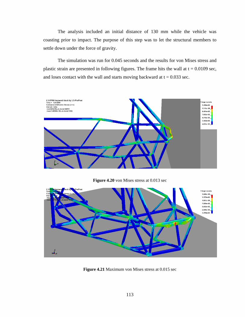
113

The analysis included an initial distance of 130 mm while the vehicle was

coasting prior to impact. The purpose of this step was to let the structural members to

settle down under the force of gravity.

The simulation was run for 0.045 seconds and the results for von Mises stress and

plastic strain are presented in following figures. The frame hits the wall at t = 0.0109 sec,

and loses contact with the wall and starts moving backward at t = 0.033 sec.

Figure 4.20 von Mises stress at 0.013 sec

Figure 4.21 Maximum von Mises stress at 0.015 sec

114

The maximum plastic strain at the end of the simulation is shown in figure 4.22.

Figure 4.22 Maximum plastic strain at 0.045 sec

In order to show the importance of strain rate effect in a vehicle crash scenario,

following figures 4.23 through 4.26 were captured at different instances of the simulation

corresponding to different strain rates. It is shown that how this rate is changing rapidly

with respect to time. It was observed that the strain rate kept fluctuating as the structure is

under deformation where it reaches its highest value of 132/s at 0.014 seconds. After the

frame loses contact with the wall the rate goes down from 30/s at 0.03 sec to 2/s at 0.045

seconds. Please note that these values are recorded by the software at the prescribed

instances.

Figure 4.23 Strain rate of 0.08/s at 0.006 sec

115

Figure 4.24 Strain rate of 80/s at 0.0109 sec

Figure 4.25 Highest Strain rate of 132/s at 0.014 sec

Figure 4.26 Strain rate of 5/s at 0.038 sec

116

Figure 4.27 shows the contours of nodal velocities in y-direction (direction of

impact) at 0.0109 seconds, where the frame first touches the wall. At this instant of time,

the nodes displaying with red have higher velocity than the nodes at the vicinity of the

impact. This indicates that the rigid wall has slowed down the vehicle at the tip of the

structure while the back of the frame is pushing the structure forward resulting in

crushing of the bumper into the wall. The velocity is in mm/s, therefore, red points have

the velocity of 13.7 m/s at this instant (initial velocity was 13 m/s).

Figure 4.27 Velocity contour in y-direction at 0.0109 sec

In order to observe what exactly is happening at the joints, different values of

contact forces were plotted at selected points A to H as shown in figure 4.28.

Figure 4.28 Selected joints for contact force

117

It is shown in figure 4.29 that the reaction force at the joints is fluctuating in time.

The maximum amount of contact force was observed at regions A and B right in front of

the structure as expected. Furthermore, it was observed that points G and H have the

second highest values which are due to the large number of components meeting in the

middle of the chassis. Moreover, interestingly it was noted that points E and F have one

of the lowest reaction forces among all which can be interpreted because of the layout of

the structural components around those joints. All the curves experience their maximum

value exactly where the maximum wall force as shown in figure 4.30 is acting on the

frame.

Figure 4.29 Highest contact forces at the joints

Figure 4.30 Rigid wall normal force

118

The computational time in this simulation was controlled by introducing mass

scaling to the system. The amount of added mass was determined very carefully since the

amount of kinetic energy present in the problem was high. The amount of mass increase

during the simulation as it is shown in figure 4.31 has an increasing behaviour. This

shows that as the frame undergoes deformation, elements get distorted and consequently

more mass is being added to the system to balance the desired time step. With this

amount of scaled mass, the computational time of about 25 hours was decreased to 30

minutes, and correspondingly the time step was increased from 5e-8 to 9.8e-7.

Figure 4.31 Percentage of mass increase

Figure 4.31 is a two phase diagram. It shows that at every instance, how much

mass is being added to the system and correspondingly what is percentage of that added

mass with regard of the total structural mass.

4.4.1 Energy balance

Examining the energy balance of a system can be thought as monitoring the

balance of a system as to improve the reliability of the numerical simulation [45].

Investigation in energy components such as kinetic, potential, dissipated, and etc, during

a simulation can be helpful in identifying the cause of the numerical instabilities of

vehicle responses during an impact.

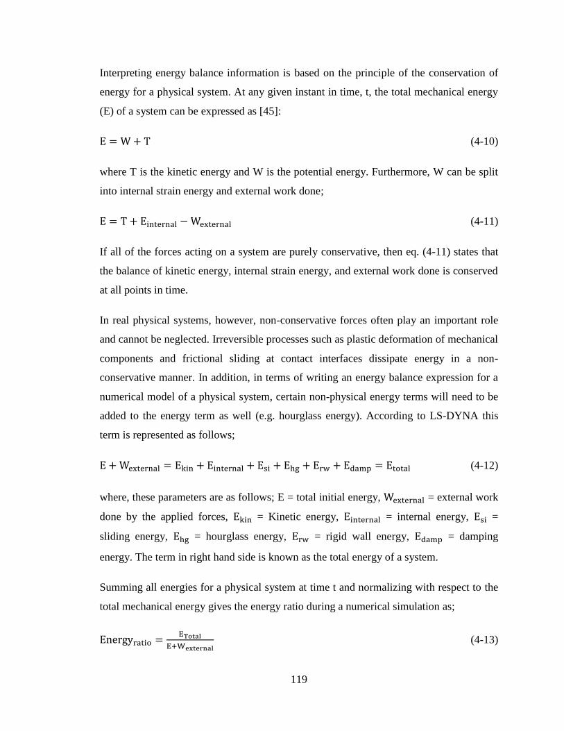
119

Interpreting energy balance information is based on the principle of the conservation of

energy for a physical system. At any given instant in time, t, the total mechanical energy

(E) of a system can be expressed as [45]:

(4-10)

where T is the kinetic energy and W is the potential energy. Furthermore, W can be split

into internal strain energy and external work done;

(4-11)

If all of the forces acting on a system are purely conservative, then eq. (4-11) states that

the balance of kinetic energy, internal strain energy, and external work done is conserved

at all points in time.

In real physical systems, however, non-conservative forces often play an important role

and cannot be neglected. Irreversible processes such as plastic deformation of mechanical

components and frictional sliding at contact interfaces dissipate energy in a non-

conservative manner. In addition, in terms of writing an energy balance expression for a

numerical model of a physical system, certain non-physical energy terms will need to be

added to the energy term as well (e.g. hourglass energy). According to LS-DYNA this

term is represented as follows;

(4-12)

where, these parameters are as follows; E = total initial energy, = external work

done by the applied forces, = Kinetic energy, = internal energy, =

sliding energy, = hourglass energy, = rigid wall energy, = damping

energy. The term in right hand side is known as the total energy of a system.

Summing all energies for a physical system at time t and normalizing with respect to the

total mechanical energy gives the energy ratio during a numerical simulation as;

(4-13)

120

Figure 4.32 Energy balance for the complete mock-up at 48 km/h

Figure 4.32 refers to the energy balance of the Mini-Baja vehicle in the frontal

impact scenario at 48 km/h which correlates with the law of conservation of mechanical

energy. It shows that the total mechanical energy of the system is roughly constant

with respect to time and changes in kinetic energy are balanced by changes in internal

energy. The sliding and hourglass energy are well controlled below the acceptable level

and no external work is done on the system.

Based on eq. 4-13, figure 4.33 is in regard of the energy ratio for the Mini-Baja

frontal crash simulation, which shows a reasonable ratio toward the end. The ratio is kept

between 1.063 and 1.038 during the impact.

Figure 4.33 Energy ratio of the simulation at 48 km/h

121

CHAPTER V

5. EVALUATION OF THE FRONTAL CRASH OF THE MINI-BAJA VEHICLE BY

(ABAQUS/CAE)

5.1 Objectives and overview of Chapter V

In order to create a sense of validation for the frontal impact simulation of the

Mini-Baja vehicle that was discussed in previous chapter, in this chapter the Mini-Baja

frame is modeled once again for validation purposes. The vehicle is implemented in the

same crash scenario with incorporation of same assumptions as before. Furthermore,

some important aspects and factors that can be critical and sometimes even decisive in

finite element simulations are handled differently in this chapter to make sure that the

vehicle response is reliable. The finite element software Abaqus/CAE was selected for

the validation of the Mini-Baja vehicle in a frontal impact scenario in this chapter.

Abaqus is an engineering simulation program based on the finite element method,

which can solve problems ranging from relatively simple linear analysis to challenging

non-linear simulations. Abaqus was developed by a company called HKS, which was

founded in 1978. The program was widely used by researchers because HKS introduced

gateways to the program, so that users could add new material models and elements [3].

Material models include metals, rubber, polymers, composites, reinforced concrete,

crushable and resilient foams, and geotechnical materials (soils and rock).

Abaqus is used in automotive, aerospace, and industrial products industries. The

product is popular with academic and research institutions due to the program's ability to

be customized. Abaqus also provides a good collection of multi-physics capabilities, such

as coupled acoustic-structural, piezoelectric, and structural-thermal capabilities, making it

attractive for production-level simulations where multiple fields need to be coupled.

122

In most simulations, including highly non-linear ones, the user need only provide

the engineering data (structure geometry, material behaviour, boundary conditions, and

applied loads) and Abaqus automatically chooses appropriate load increments and

convergence tolerances and continually adjusts these parameters during the analysis to

ensure accurate solutions.

5.2 Simulation of the front portion of the frame (Abaqus/CAE)

In order to model the frontal impact scenario is Abaqus/CAE, it was necessary to

create the mesh in Abaqus/CAE environment with Abaqus meshing tools.

To be able to compare the results with LS-DYNA simulations, as in the previous chapter,

first the frontal portion of the frame was modeled.

Figure 5.1 Front portion of the frame in frontal impact setup (Abaqus/CAE)

Abaqus/Explicit was used to solve this non-linear impact analysis. The reduced-

integration, small membrane-strain1 quadrilateral shell element (S4RSW) was used with

incorporation of warping and hourglass control for the front portion. The element size

was specified 6 mm as was the case in previous chapter.

1 The small membrane strain elements are effective for explicit dynamics problems involving small

membrane strains and arbitrarily large rotations [8].

123

The material model elastic-plastic was used with inclusion of strain rates

dependency by power law hardening model.

Two types of rate-dependent models are offered for plasticity. The one that has been used

here is based on the rate-dependent yield strength of the material model. This method is

suggested by [8] for relatively high strain rate applications, such as dynamic events. This

type of rate dependency can be introduced by overstress power law in following

equation:

(5-1)

where is the plastic strain rate, D and n are material parameters, and R is the ratio of

the yield stress at nonzero strain rate to the static yield stress (

). Keep in mind that

R at zero plastic strain rates is 1. Parameter of D = 40.4 and n = 5 are identical to C and P

in Cowper-Symonds model discussed in section 4.2.2.

One of the crucial factors in large deformation analyses of vehicle crash is contact

modeling. Within crash, it is a common scenario where contact non-linearity arises and

therefore, structural response is highly dependent by the way those contacts are defined in

the problem.

Figure 5.2 Tie contact (Abaqus/CAE)

124

The weld connections were defied by using constraints methods in Abaqus/CAE. As

shown in figure 5.2 the nodes of the purple member are tied to the surface of the red

member with a node to surface discretization method.

Furthermore, the contact between the structure and the wall as well as different

components with each other were defined with a general explicit contact algorithm with

coefficients of static and dynamic friction as 0.2 and 0.15 respectively and decay

coefficient of 0.001.

The model was run first for 60 km/h and results in term of energy balance are

shown in figure 5.3. Note that ALLAE is the amount of artificial strain energy, ALLWK

is the external work, ALLFD is the frictional dissipation, ALLIE is the internal energy,

ALLKE is the kinetic energy, and ETOTAL is the total energy of the system. In

Abaqus/CAE, artificial strain energy is primarily the energy dissipated to control

hourglass deformation. If the artificial strain energy is too excessive, it means that too

much strain energy is dissipating to control hourglass deformations. A general rule is that

it is desirable to keep the ratio of the ALLAE/ALLSE well below 10% (ALLSE is the

elastic strain energy).

Figure 5.3 Energy balance for front portion at 60 km/h (Abaqus/CAE)

125

As it is observed in figure 5.3 the amount of artificial strain energy dissipated in

the simulation is non-zero. In order to increase the accuracy of the solution the model was

further studied. The linear, finite-membrane-strain, fully integrated, quadrilateral shell

element (S4) was used for greater solution accuracy. For problems prone to membrane

and bending-mode hourglassing, or for problems where in-plane bending is expected the

element type S4 is suggested [8]. As shown in figure 5.4 the amount of artificial strain

energy is well controlled by using fully integrated elements.

Figure 5.4 Energy balance for front portion at 60 km/h modified (Abaqus/CAE)

Figure 5.5 Energy balance for front portion at 60 km/h (LS-DYNA)

126

It is shown in figure 5.6 that the ratio of artificial strain energy to elastic strain

energy resulted below 9% using S4 elements. Furthermore, it was observed that at the

time 0.012 where the frame impacts into the wall is the instant where the maximum

amount of artificial strain is being dissipated due to large number of distorted elements.

Figure 5.6 The ratio of artificial strain energy over elastic strain energy

In the following figures, the von Mises stress distribution over the front frame is

compared between the LS-DYNA model and Abaqus/CAE model. The amount of plastic

strain is 0.241 in LS-DYNA compared to 0.268 in Abaqus/CAE.

127

Figure 5.7 von Mises stress distribution of the front portion at 60 km/h (LS-DYNA)

Figure 5.8 von Mises stress distribution of the front portion at 60 km/h (Abaqus/CAE)

The structure was also run for 150 km/h, and the results are compared with model

1 (LS-DYNA) proposed in section 4.3;

128

Figure 5.9 von Mises stress distribution of the front portion at 150 km/h (Abaqus/CAE)

Figure 5.10 von Mises stress distribution of the front portion at 150 km/h (LS-DYNA)

The amount of plastic strain for the Abaqus/CAE model was 0.44 compared to the

LS-DYNA model which was 0.43 at 150 km/h.

129

Results of the two models at 150 km/h are compared in terms of energy balance in

figure 5.11. In this figure, I.E = Internal energy, E.W = External work done by applied

forces, K.E = Kinetic energy, T.E = Total energy.

Figure 5.11 Comparison of energy balance of the front portion at 150 km/h

0

1E+09

0 0.005 0.01 0.015 0.02

Ener

gy b

alan

ce (

μ J

)

Time (sec)

I.E. ABAQUS

E.W. ABAQUS

K.E. ABAQUS

T.E. ABAQUS

K.E. LS-DYNA

I.E. LS-DYNA

T.E. LS-DYNA

E.W. LS-DYNA

130

5.3 Frontal impact simulation of the Mini-Baja frame chassis (Abaqus/CAE)

The complete mock-up of the frame was modeled in Abaqus/CAE as shown in

figure below. The computational time was controlled in a similar way, except that this

time smaller time increments (7E-7) were used. Instead of using mass scaled solution

based on elements, here a semi-automatic mass scaling on the whole model was used to

obtain a target step time. It was intended to change the step time to see any possible effect

of it on the model.

Figure 5.12 Frontal impact scenario of the Mini-Baja vehicle (Abaqus/CAE)

The linear, finite-membrane-strain, reduced-integration, quadrilateral shell

element (S4R) was used to mesh the complete mock-up of the chassis. Plastic material

model with inclusion of power law strain theory for effect of strain rates as discussed

earlier was used.

Incorrect material orientation can be very costly in crash simulations where stress

is typically very hard to obtain. Most finite element packages automatically resolve the

issue of contact where material direction and normal direction are incorrect. However in

order to get reliable stress distribution, one should be careful about material direction.

Figure 5.13 is an example of an incorrect material direction that will consequently result

in incorrect contact behaviour between the two tubes. Furthermore, the values of stress

131

outputted will be incorrect because the principle directions are mixed up. The

inconsistency is due to the fact that for most elements the dominant stress is the

circumferential stress, but for some elements it is the axial stress (shown in figure 5.13).

Figure 5.13 Example of a wrong material direction

The energy balance of the vehicle is shown in figure 5.14. As shown, the amount

of artificial strain energy and frictional dissipation is rather excessive. Nonetheless the

energy balance is well within the desired limit. Keep in mind that the intention of the

Abaqus/CAE simulations was to develop an overall comparison between the two models

to see if on the whole the response of the structure in frontal crash scenario makes sense.

Therefore, no additional study was performed to decrease the excessive undesired

energies, since there were fully discussed in previous chapter.

132

Figure 5.14 Energy balance of the frontal impact at 48 km/h (Abaqus/CAE)

In following figures, results regarding the stress distributions and plastic strain of

the frame modeled in Abaqus/CAE are shown at instances similar to chapter 4. Results

showed good coloration between the two models.

Figure 5.15 von Mises stress distribution at 0.013 sec (Abaqus/CAE)

133

Figure 5.16 Maximum von Mises stress at 0.016 sec (Abaqus/CAE)

Figure 5.17 Maximum plastic strain at the end of the simulation 0.045 sec (Abaqus/CAE)

134

Figure 5.18 Maximum plastic strain at the end of the simulation 0.045 sec

5.4 Further comparison of LS-DYNA and Abaqus/CAE results

In this section different data curves outputted from each software are compared in

one graph. In figure 5.19 the energy balance of the two models are compared. All the

comparisons were made on the complete mock-up model at 48 km/h.

In these graphs; I.E = Internal energy, E.W = External work done by applied

forces, K.E = Kinetic energy, T.E = Total energy, RF = Reaction wall force, and Disp. =

Displacement.

135

Figure 5.19 Energy balance of the full Mini-Baja mock-up at 48 km/h

In order to create a sense of comparison for the horizontal elongation of the frame

from the sides, point “P” as shown below was selected to show the buckling behaviour of

the frame outward. Results for x-displacement and the resultant displacement of the

selected node are plotted in figure 5.21.

Figure 5.20 Selected point for side displacement

0

500000000

1E+09

1.5E+09

2E+09

2.5E+09

3E+09

3.5E+09

4E+09

4.5E+09

5E+09

0 0.005 0.01 0.015 0.02 0.025 0.03 0.035 0.04 0.045

Ener

gy b

alan

ce (

μ J

)

Time (sec)

I.E ABAQUS

E.W. ABAQUS

K.E. ABAQUS

T.E. ABAQUS

K.E LS-DYNA

I.E. LS-DYNA

T.E. LS-DYNA

E.W. LS-DYNA

136

Figure 5.21 Side displacement of point (P)

It was observed as shown in figure 5.21 that the structure solved by LS-DYNA

resembles a more dynamic behaviour. It can be seen in the x displacement behaviour of

the point P that how the component oscillates back and forth after the impact (green

curve). In LS-DYNA, vibration characteristic of the frame components has been

captured perfectly whereas the curves corresponding to the model solved by

Abaqus/CAE shows differently. To further study the vibration characteristic of

components during the impact, another critical point “Q” was selected on the roof as

shown in figure 5.22.

Figure 5.22 Selected roof point (Q)

0

50

100

150

200

250

300

0 0.005 0.01 0.015 0.02 0.025 0.03 0.035 0.04 0.045

Dis

pla

cem

ent

(mm

)

Time (sec)

x Disp. ABAQUS

Resultant Disp. ABAQUS

x Disp. LS-DYNA

Resultant Disp. LS-DYNA

137

Results based on z-displacement of point “Q” are plotted in figure 5.23. As it is

shown, the magnitude of the vertical oscillation is much higher for the LS-DYNA model.

Furthermore, it is noted that the corresponding direction of excitation are 180 degree out

of phase between the two models.

Figure 5.23 Vertical displacement of the roof point (Q)

In figure 5.24, the reaction of the wall is plotted for comparison. In order to

provide a criterion for evaluation of the generalized stiffness in both models, in figure

5.25, the wall force is plotted versus the resultant displacement of a specific point “S” as

shown in figure 5.20. The displacement of a middle member was selected that could be

representing an overall displacement of the vehicle.

For a point of comparison, the generalized stiffness defined above for the LS-

DYNA model is 437.5 e+3 N/m compared to 375 e+3 N/m (Abaqus/CAE) at 160 mm.

-5

5

15

25

35

45

55

0 0.005 0.01 0.015 0.02 0.025 0.03 0.035 0.04 0.045

Dis

pla

cem

ent

(mm

)

Time (sec)

z Disp. ABAQUS

z Disp. LS-DYNA

138

Figure 5.24 Wall reaction force

Figure 5.25 Reaction wall force versus resultant displacement (stiffness)

-80

-70

-60

-50

-40

-30

-20

-10

0

0 0.005 0.01 0.015 0.02 0.025 0.03 0.035 0.04 0.045 0.05

Rea

ctio

n w

all f

orc

e (m

N)

E+0

6

Time (sec)

RF ABAQUS

RF LS-DYNA

0

10

20

30

40

50

60

70

80

0 50 100 150 200 250

Wal

l fo

rce

(mN

)

E+0

6

Displacement (mm)

Stiffness (ABAQUS)

Stiffness (LS-DYNA)

139

CHAPTER VІ

6. A MORE COMPLETE MODEL OF THE MINI-BAJA VEHICLE FOR CRASH

ANALYSIS (LS-DYNA)

6.1 Objectives and overview of Chapter VІ

In this chapter, a number of extra components such as suspension arms, wheels,

seat, and body parts were added to the Mini-Baja vehicle to create a more realistic model.

The frame of the vehicle is the same one used in chapter 5.

As a first step, the tire assembly was developed and simulated as a sub model

before incorporating it into the Mini-Baja finite element model. Subsequently, the body

panels and suspension shocks are assembled into the previously discussed structure and

simulated for an equilibrium test under the load of gravity. Although gravity is not an

important loading condition in this problem, this step was used to ensure that desired

contact and material models were properly functioning. In the final step, the entire finite

element model of the Mini-Baja vehicle was simulated for crashworthiness assessment in

front, side, and head-on crash scenarios.

6.2 Modeling of the tires

Tires were modeled based on the geometry and approximated shape of the actual

tires used in the Mini-Baja vehicle. In figure 6.1, the front and rear tires used in the actual

Mini-Baja vehicle are shown. The generated CAD representations of the tires are also

shown in figure 6.2.

In this section, the tires undergo a severe deformation for verification and

validation of the correct contact behaviour and checking any possible discontinuity in the

deployment of the tires. The primary objective of this effort was to provide a general

validation and to gain some insights on the performance of the tires. Keep in mind that just

the tires were simulated here and the suspension arms and other additional components

were assembled directly to the Mini-Baja FE model.

140

Figure 6.1 Actual tires and suspension assembly

Figure 6.2 CAD model of the tire

To check the connection defined between different components of the wheel, a

simulation was carried out where, the bottom end nodes of the tires were constrained in

141

all translational directions and a rigid wall were prescribed a downward motion crushing

the tires harshly. It should be mentioned that the tires themselves were constructed from

an appropriate elastic material and the outer rims were made of steel.

The inner rims and wheel hubs were made of rigid material and are connected to

each other using rigid body constraints. All the components in the assembly of the wheels

are modeled with shell elements with elements sizes ranging between 6 to 12 millimetres.

The sectional properties are shown in figure 6.3.

These assumptions used in the modeling of the Mini-Baja‟s tire assembly were

closely studied and taken from the actual FE vehicle models used by the society of crash

engineers (NCAC).

Figure 6.3 FE model of the tire assembly displaying the sectional thicknesses

As shown in figure 6.4 and 6.5 the tires are under a relatively large displacement

of 90 mm due to the downward motion of the rigid wall. The intention was to produce a

highly destructive scenario ensuring the correct functionality of the tires when used in the

Mini-Baja crash simulations.

142

Figure 6.4 Deformation of the tires at 90mm displacement of the wall

Figure 6.5 Deformation of the tires at 0.04 sec for the rear tires and at 0.032 sec for front tires

143

6.3 Simulation of the complete Mini-Baja vehicle

Ultimately a more complete mock-up of the Mini-Baja vehicle was constructed

which includes; suspension arms, seat, and steering wheel. This mock-up is shown in

figure 6.6. Many assumptions were made in order to prepare this FE model for the full

frontal crash simulation. Some additional parts such as suspension arms and the rear axle

were made of ordinary beam elements (Hughes-Liu with cross-section integration rule).

Spring and dampers were constructed with simple discrete elements using spring elastic

material and damper viscous material models respectively.

Figure 6.6 FE model of the completed Mini-Baja vehicle

The body panels are thin sheets of aluminum 6061 with 1 mm thickness. Material

model 18 in the material library of LS-DYNA was chosen to define the body panels. This

is an isotropic plasticity model with rate effects which uses a power law hardening rule.

In this model, the yield stress is a function of plastic strain and obeys [30];

(6-1)

where, is the elastic strain to yield strain and is the effective plastic strain. K is the

strength coefficient and n is the hardening exponent. The strain rate effect was accounted

by using Cowper and Symonds constitutive model. The material properties of the

aluminum 6061 are given in table (6.1) [46].

144

Table 6.1 Aluminum 6061 material properties

Material properties AL-6061

Density kg/m^3 2.71E+03

Elastic modulus (Gpa) 6.89E+10

Poission's ratio 0.33

Yield stress (Mpa) 252

K (thin plate) 4.11E+08

n 6.30E-02

C 6500/25000

P 0.95

The body as it is shown in figures 6.7 and 6.8 is attached to the frame with nodal

rigid bodies (NRB); this is a rigid body which consists of defined nodes each belonging

to a deformable body. The nodal rigid body in the model prevents any motion between

the corresponding constrained nodes.

Figure 6.7 Body panels and nodal rigid body constrained

145

Figure 6.8 Body panels, rear suspension, and shocks

The material model 57 in LS-DYNA which is MAT_LOW_DENSITY_FOAM is

a highly compressible low density foam and its main applications are for seat cushions

and interior of the vehicle. This material model was used to define the Mini-Baja seat

material. Typical loading and unloading stress-strain curves of foams are shown in figure

6.9. The loading curve for the Mini-Baja seat is shown in figure 6.10 and the unloading

behaviour was defined with hysteresis and shape factors of 1 and 5 respectively.

Figure 6.9 Behaviour of the low density foam [30]

146

In references [47] and [48], a detailed discussion on experimental tests and numerical

modeling of the seats and cushions are available. The loading behaviour in the present

model is based on experimental data given in [48].

Figure 6.10 Stress-strain curve for the low density foam cushion

In order to account the rotation of the tiers, a revolute joint was created at each

wheel assembly. The angular velocity of 51.181 rad/s was prescribed based on

considerations shown in figure 6.11.

Figure 6.11 Revolute joint and angular velocity of the tires

0

50

100

150

200

250

300

0 0.1 0.2 0.3 0.4 0.5 0.6 0.7 0.8 0.9 1

Stre

ss (

KP

a)

Strain (%crush)

Foam "seat"

147

6.3.1 The frontal crash of the Mini-Baja vehicle

The vehicle consists of 170,000 elements including; shell, solid, beam, discrete

and lumped mass elements. The CAD files were generated in Catia V5 and then the

components were meshed in Crash (HyperMesh) and LS-PresPost 3.1. These STEP files

were then imported to LS-DYNA for implementation of the crash simulation.

Coefficients of static and dynamic friction were considered as 0.2 and 0.1

respectively. Furthermore the exponential decay coefficient of friction was assumed as

10. The undesirable excessive hourglass energy was controlled with the hourglass control

and higher order element formulation in localized regions. The negative sliding energy

was handled with additional contact modifications and manual master and slave

adjustments.

A range of values for the corresponding constants of spring and damper discrete

elements were available for the Mini-Baja vehicle. In order to verify the suspension

assembly, an equilibrium test was performed on the Mini-Baja to check the functionality

of the suspension as well as spring and damper constants. Consequently the constants of

spring and damper were established as 5E+4 N/m and 800 N.s/m respectively. In these

series of tests, the force displacement response of the discrete springs was optimized so

as the vehicle settles to equilibrium position under gravity loading. To check the

equilibrium position, simulation were performed by dropping the vehicle onto a rigid

ground under the action of gravity. Figure 6.12 shows the setup for this test.

Figure 6.13 shows the reaction force of the rigid ground when the vehicle is

stabilizing. In approximately 0.4 sec the Mini-Baja vehicle reaches equilibrium, and the

measured force is equal to the product of the mass of the Mini-Baja (212 kg for the

complete model) and the acceleration due to gravity (the corresponding force at 0.6 sec is

2.146E+3 N).

A “bw” 20 filter was used to reduce the numerical noise effects in the equilibrium

simulation for the reaction force of the wall shown in figure 6.13.

148

Figure 6.12 Test setup for equilibrium check

Figure 6.13 Reaction force of the rigid ground

Upon getting satisfactory results from the added components, the vehicle was

given an initial velocity of 48 km/h (30 mph) approaching a rigid wall. Figures 6.14 were

recorded at different instances of the simulation for the vehicle colliding into the rigid

wall.

149

Figure 6.14 Isometric view of the detailed model simulation of the Mini-Baja vehicle into the

rigid wall at 48 km/h

The maximum von Mises stress was 1.77E+6 KPa at time t = 0.011 seconds in

frontal crash simulation. The effective plastic strain at the end of the simulation was 0.83

mm/mm (shown in figure 6.15). Figure 6.16 through 6.18 shows the deformation of the

Mini-Baja frame using the side, top, and front views.

Figure 6.15 Left: the maximum von Mises stress at 0.011 sec; Right: effective plastic strain at the

end of the simulation

150

Figure 6.16 Side, top and front views of the deformation at t = 0.014 sec

Figure 6.17 Side, top and front views of the deformation at t = 0.025 sec

Figure 6.18 Side, top and front views of the deformation at t = 0.036 sec

151

Figure 6.19 Traced nodes on the rear tire at t = 0.04 sec

Two corresponding nodes as shown in figure 6.19 on the rear tire were traced

throughout the simulation to show the rotation of the rear tire affecting the deformation of

the vehicle after the impact. It is shown that long after the crash of the vehicle into the

rigid wall; the rear tire is still rotating which finally stops by the friction of the ground. In

figure 6.20 the energy balance for the front impact scenario is given.

Figure 6.20 Energy balance for frontal crash at 48 km/h

It was observed that the front wheels are the first components that crash into the

rigid wall, which tremendously can influence the behaviour of the vehicle in the crash.

For this reason and also to explain the sudden change in the kinetic energy at 0.013 sec as

shown in figure 6.20, the properties of the elastic tires were deliberately changed.

152

In figure 6.21 it is shown that as the tires were made lighter; the kinetic energy of

the vehicle is decreased and therefore the rebound inertia of the tires in particular are less

as well.

Figure 6.21 Energy balance for frontal crash at 48 km/h (low density tire)

In figure 6.22 the kinetic energy for 3 different tire densities is shown. It was

observed that as the tires were lighter, the rotational inertia of front tires is less. In other

words the tires would not tilt backward due to less momentum and are able to act as a

shield in front the vehicle and damp much of the impact force and as a result, experience

much smoother kinetic energy.

Figure 6.22 Kinetic energy based on density of tires at 48 km/h

153

Keep in mind that the discussion above was to clarify the sudden change in the

kinetic energy in figure 6.20. Furthermore, one has to take into account that the correct

material data that was implemented is the high density tires shown in figure 6.22, and the

discussion presented was carried out intentionally for comparison purposes.

6.3.2 The side crash of the Mini-Baja vehicle

In this simulation, another sever scenario for the vehicle is proposed where the

Mini-Baja impacts a rigid column from the side. The setup of the side crash is shown in

figure 6.23.

Besides the severity of the damage to the structure, it can be thought as one of the

worst case scenarios, which the driver inside the vehicle can experience. The base of the

structure; the rectangular frame behind the seat is constructed from heavier and thicker

tubes compared to the rest of the structure. Therefore, to fully observe the response of the

vehicle in the side crash, two major locations of the rigid column are simulated.

In the first case, the column is next to the seat, while in the second case the column is

distanced from the support frame in order to observe the maximum deformation of the

frame at the centre.

Figure 6.23 Side impact setup

The deformation sequence of the side impact simulation (first case where the column is

next to the seat) is shown in figures 6.24 through 6.26 at selected instances in time.

154

Figure 6.24 Sequential views of the side impact scenario 1 at initial position

Figure 6.25 Sequential views of the side impact scenario 1 at t = 0.033 sec

Figure 6.26 Sequential views of the side impact scenario 1 at the end of the simulation

155

The energy balance of the first case is shown in figure 6.27. The maximum von

Mises stress of 2.88E+6 KPa was distributed at time 0.007 seconds; just 3 ms after the

frame impacted the rigid column. The effective plastic strain at the end of the simulation

was 1.13 mm/mm.

Figure 6.27 Energy balance of the side crash scenario 1 at 48 km/h

In the second simulation the rigid column was moved to the centre line of the

vehicle to observe the maximum deformation contour throughout the frame. Figures 6.28

through 6.31 show the sequence of the side impact at selected instances.

Figure 6.28 Sequential views of the side impact scenario 2 at initial position

156

Figure 6.29 Sequential views of the side impact scenario 2 at t = 0.016 sec

Figure 6.30 Sequential views of the side impact scenario 2 at t = 0.025 sec

Figure 6.31 Sequential views of the side impact scenario 2 at the end of the simulation

157

The maximum von Mises stress in the second scenario was 1.43E+6 at time 0.022

seconds. The effective plastic strain at the end of the simulation was 1.28 mm/mm. The

balance of the energy for the side crash second case is shown in figure 6.32.

Figure 6.32 Energy balance of the side crash scenario 2 at 48 km/h

6.3.3 Head-on collision of two Mini-Baja vehicles at 30 degree impact angle

In references [44] and [49] some standard procedures and practices in conducting

a vehicle-to-vehicle crash tests are discussed. It is mentioned that regarding the peak

chest acceleration occurrences in comparison to frontal rigid barrier impacts, the 48 km/h

velocity has been re-established for head-on collisions. Also, an impact angle of 30

degrees was chosen as a standard value for such a crash scenario. In [49] a complete flow

chart representing different crash configuration for various crash modes regulated by

NHTSA are given.

Based on the guidelines [44] and [49], a simulation is described where two Mini-

Baja vehicles are subjected to collision as shown in figure 6.33. An initial velocity of 48

km/h has been set for the vehicles and the angle between the lines of travel of the two

vehicles is 30 degrees.

158

Figure 6.33 Configuration of the vehicle-to-vehicle crash at 30 degree impact angle

The distance between the two vehicles was prescribed in accordance with the

orientation of the tires of the vehicles. The objective was to see the responses of the

vehicles as they crash into each other; therefore, the model was setup in order to avoid

the crash of tires against each other. Figures 6.34 through 6.37 show the sequence of the

head-on collision at selected instances.

Figure 6.34 Sequential views of the vehicle-to-vehicle crash at initial position

159

Figure 6.35 Sequential views of the vehicle-to-vehicle crash at t = 0.017 sec

Figure 6.36 Sequential views of the vehicle-to-vehicle crash at t = 0.036 sec

Figure 6.37 Sequential views of the vehicle-to-vehicle crash at t = 0.07 sec

160

The impact velocity of 60 km/h and 70 km/h was also simulated to ensure the

stability of the model and the tendency to the increase of the plastic deformation and

energies. Despite that, results are given for one particular speed (48 km/h).

The amount of hourglass energy as shown in figure 6.38 is 3.5 % compared to the

internal energy, which is acceptable. Furthermore, it was also noted that the amount of

sliding energy is increased as the vehicles are squashed into each other.

Figure 6.38 Energy balance of the vehicle-to-vehicle crash at 48 km/h

The distribution of von Mises stress is shown in figure 6.39. The amount of

plastic strain for both vehicles is 0.87 mm/mm.

Figure 6.39 Maximum von Mises stress for vehicle-to-vehicle crash at t = 0.02 sec

161

CHAPTER VІІ

7. CONCLUSIONS AND RECOMMENDATIONS FOR FUTURE WORK

7.1 Conclusions

As stated in the introduction chapter, the objective of this thesis was to develop a

general guideline and report the findings for the finite element analysis of tubular-type

structures such as the Mini-Baja all terrain vehicle. In this context, two major approaches

were considered. On one hand the finite element method could be utilized in the process

of design optimization and fabrication of such structures, and on the other hand this tool

can be employed in analyzing an existing structure. The objective of the present research

was to perform a step-by-step study on the finite element analysis of the vehicle rather

than for design purposes.

An attempt was made to distinguish between static, quasi-static, and dynamic

analysis of Mini-Baja due to loading conditions. The research includes the

implementation of finite element analysis for high deformation crash scenarios. In finite

element analysis, the structure is broken up into small elements which are easier to

analyze. It is the only approach that can be adopted for the solution of complicated

structural problems.

In chapters 2 and 3, a comparison between beam, shell, and solid element

idealizations was discussed. It was concluded that due to high computational cost of solid

elements and disadvantages of wireframe idealizations, shell model is the ideal choice for

analysing the Mini-Baja frame. Based on the simulations conducted, it was observed that

in the static or the transient modal superposition analyses, it is important to constrain the

frame as little as possible. Therefore, constraining and releasing the appropriate degrees

of freedom are crucial in obtaining realistic results.

Based on the results presented in chapters 4 and 5; it was concluded that a localized

higher order element formulation implemented simultaneously with hourglass stiffness-

162

form control is best suited for reducing the detrimental effects of the zero energy modes

in deformation of the Mini-Baja structure.

It is clear that while the finite element method offers a powerful tool for analysis

purposes, it requires a profound understanding of the finite element theory, the FEA

software, and the structure being modeled. Generally speaking, the finite element method

provides an approximate solution of a physical model; therefore, in creating a numerical

model careful considerations should be employed to reasonably represent the exact

physics of an event. In chapter 6, it was shown that many assumptions were necessary for

incorporating the additional components into the Mini-Baja finite element model. It was

also concluded that although assumptions were necessary in modeling a detailed vehicle,

it is very important to carefully select appropriate keyword commands to define those

desired assumptions.

Based on the findings in this thesis, some of the important parameters in analyzing Mini-

Baja vehicle are listed below:

Contact non-linearity is one of the most important factors in a crash scenario, and

should be treated carefully to overcome inaccurate results. Automatic single

contact algorithms are preferred in crash applications, but it was observed that

local contact algorithms are more accurate in terms of a Mini-Baja vehicle.

Higher order element formulations produce a more stiff response of the body and

should be employed wisely.

When meshing with shell elements, quadrilateral elements are preferred over

triangular elements. Triangular elements do not have hourglass modes; however,

they can lead to a stiff response. Furthermore, quadrilateral shells that are initially

warped or that become warped due to deformation can lead to significant

inaccuracies.

Assigning meaningful friction coefficients on the rigid-walls are essential for

correct impact characteristic of the vehicle crash.

163

Nodal rigid bodies should be used very carefully since it is turning a deformable

point to a rigid point in a deformable body, and therefore, should be created

between nodes with small distances in assembly applications.

In problems where mass scaling is employed, always the results should be

checked. The kinetic energy for instance should be checked based on the mass

and velocity of the vehicle .

Energy associated with different components should be plotted and interpreted in

order to check if anything is unrealistic or any energy is excessive in one

particular component.

In finite element analysis a very minor error such as nodal numbering (normal

shell directions) can result in erroneous results and therefore, manually checking

the whole input code and keyword commands are essential.

To conclude this section it is worth reminding the reader that; the purpose of a

vehicle chassis is to connect four wheels to a structure. While it should be designed to be

as rigid as possible in bending and torsion it must be capable of absorbing as much of the

inertia without excessive deflections. This is a key point for protecting the driver.

7.2 Recommendations for future work

In this thesis, the frontal impact problem was discussed for the Mini-Baja vehicle

in detail. Furthermore, the side impact condition and a head-on collision was developed

as well. It is highly recommended that future work on this project take the following

bulleted items into considerations;

In order to improve the accuracy in the crash problems, some additional

components can be added to the frame. Among those; frame braces, accurate

representation of the engine, protecting flops about the vehicle, rivets and

fasteners used in the assembly process are of major importance.

It is suggested by the society of crash engineers to conduct a roll-over simulation

which was intentionally left out of this thesis. Looking into this problem is highly

recommended.

164

To study the response of the frame when impacting roadside hardware, a barrier

impact to be implemented. This barrier can be the standard terrain hardware in the

Mini-Baja field competition.

In order to conduct a roll-over and barrier impact simulation on the current Mini-

Baja geometry, more accurate models of the steering wheels and suspension

components are necessary. This is to capturing accurate kinematic response of the

vehicle.

To incorporate appropriate failure criterion for a more accurate response, a failure

criterion has to be defined for welded joints as well as the body panels.

To study the effect of a crash on human body, a Hybrid III1 occupant dummy can

be added to the system as shown in figure 7.1. Occupant dummy is necessary in

design of restrain systems (seatbelt and airbags) for optimum occupant protection.

A crash scenario where two Mini-Baja vehicles are colliding at 30 degree impact

angle with inclusion of occupant dummies could be one of the next steps in

analyzing Mini-Baja crashworthiness response. (Figure 7.2)

Figure 7.1 Hybrid III occupant dummy

1 The Hybrid III dummy is an anthropomorphic test device (ATD) that represents the human body. By

developing the geometry, weight, inertia, joint stiffness, and energy absorption characteristics of a human

body, ATDs are expected to simulate human response when exposed to a crash scenario. Hybrid III

dummies are frequently used for impact scenarios and safety assessments and prediction of established

injury criteria such as HIC and Chest indexes [50].

165

Figure 7.2 Two Mini-Baja‟s impact scenario at 30 degree impact angle

The following two recommendations are primarily addressed to the undergraduate

students who are involved with Mini-Baja capstone-project for using finite elements in

their work.

Providing a criterion for analyzing the vehicle by students at the University of

Windsor. Here, at the university, every year the students are teamed up to build a

new vehicle to compete against each other and other universities. A consistent set

of criteria can be introduced to compare the capstone-projects from year to year.

Vehicle user defined over-all stiffness or pitch, yaw and roll rotations can be

examples of such criterion.

The Mini-Baja vehicle to be heavily instrumented to record the history of loads,

accelerations, displacement, etc for comparison against the finite element

simulations. In this area, certain tests such as speed bump test, gravity equilibrium

check, and slopped terrain tests can be introduced as non-destructive

crashworthiness tests.

166

REFERENCES

[1] 2012 Baja SAE Rules; http://students.sae.org/competitions/bajasae/rules/

[2] Safety Net (2009) Vehicle Safety–web text, The European Commission Directorate-

General Transport and Energy, 2009.

[3] J. Fish and T. Belytschko, “A First Course in Finite Elements”, Chichester,

JohnWiley & Sons Inc., 2007.

[4] R.D. Cook, D.S. Malkus, M.E. Plesha and R.J. Witt, “Concepts and Applications of

Finite Element Analysis”, New York, JohnWiley & Sons Inc., 2002.

[5] J. Bonet and R.D. Wood, “Nonlinear Continuum Mechanics for Finite Element

Analysis”, Cambridge, Cambridge University Press, 1997.

[6] T. Belytschko, W.K. Liu and B. Moran, “Nonlinear Finite Elements for Continua and

Structures”, Chichester, JohnWiley & Sons Inc., 2001.

[7] T.Y. Yang and G. Lianis, “Large displacement analysis of viscoelastic beams and

frames by the finite-element method”, Journal of Applied Mechanics 1974, 74, pp. 635-

640.

[8] Abaqus/CAE 6.9 Documentation;

file:///C:/SIMULIA/Documentation/docs/v6.9/index.html

[9] T.Y. Yang, “Finite Element Structural Analysis”, New Jersey, Prentice-Hall Inc.,

1986.

[10] T.Y. Yang, “Matrix displacement solution to elastic problems of beams and frames”,

International Journal of Solids and Structure 1973, 9, pp. 829-842.

[11] T.Y. Yang and C.T. Sun, “Axial-flexural vibration of frameworks using finite-

element approach”, Journal of Acoustical Society of America 1973, 53(1), pp. 137-146.

167

[12] T.Y. Yang and C.T. Sun, “Finite elements for the vibration of framed shear walls”,

Journal of Sound and Vibration 1973, 27(3), pp. 297-311.

[13] Solidworks Web Help, 1995-2011 Dassault Systèmes, http://help.solidworks.com

[14] J. Hastie, “Mini-Baja Vehicle Design Optimization Technical Report”, College of

Engineering, North-Eastern University 2005.

[15] V. Jain and M. Singh, “Design of a Mini-Baja Chassis for Crashworthiness through

Finite Element Analysis”, Indian Institute of Technology 2005.

[16] C. Martinez Jr., “A finite element analysis of „steel horse‟ frame”, The University of

Texas-Pan American (UTPA), 2003.

[17] N. Noorbhasha, “Computational analysis for improved design of a SAE BAJA frame

structure”, Graduate College, University of Nevada Las Vegas (UNLV), 2010.

[18] D.T. Anderson and B. Mills, “Dynamic analysis of a car chassis frame using the

finite element method”, International Journal of Mechanical Sciences 1972, 14, pp. 799-

808.

[19] L. Kwasniewski, H. Li, R. Nimbalkar and J. Wekezer, “Crashworthiness assessment

of a paratransit bus”, International Journal of Impact Engineering 2006, 32, pp. 883–888.

[20] J.G. Thacker, S.W. Reagan, J.A. Pellettiere, W.D. Pilkey, J.R. Crandall and E.M.

Sieveka, “Experience during development of a dynamic crash response automobile

model”, Journal of Finite Element in Analysis and Design 1998, 30, pp. 279-295.

[21] D. Marzougui, C.D. Kan and N.E. Bedewi, “Development and validation of an

NCAP simulation using LS-DYNA3D”, Fourth International LS-DYNA3D Conference

1996, Minneapolis, September 5-6, pp. 319-332.

[22] National Highway Traffic Safety Administration (NHTSA), http://www.nhtsa.gov/

[23] “Development & Validation of a Finite Element Model for the 2006 Ford F250

Pickup Truck”, Technical Summary, December 2008, NCAC 2008-T-003.

168

[24] H.E. Boyer, “Atlas of Stress-Strain Curves”, ASM International, 2002.

[25] “Validation of a Single Unit Truck Model for Roadside Hardware Impacts”,

Working paper, November 2003, NCAC 2003-W-001.

[26] “Development and Validation of a Pick-Up Truck Suspension Finite Element Model

for Use in Crash Simulation”, Working paper, November 2003, NCAC 2003-W-003.

[27] N.M. Baran, “Finite Element Analysis on Microcomputers”, Oxford, McGraw-Hill

Book Company, 1988.

[28] W. Weaver Jr. and J.M. Gere, “Matrix Analysis of Framed Structures”, 3rd Edition,

Springer-Verlag, 1966.

[29] M.A. Bhatti, “Fundamental Finite Element Analysis and Application”, New Jersey,

John Wiley & Sons Inc., 2005.

[30] J.O. Hallquist, “LS-DYNA Keyword User's Manual” Livermore Software

Technology Corporation, 2001.

[31] N.G. Zamani, “Finite element analysis in solid mechanics; issues and trends”,

Physics in Canada 2008, 64(2), pp. 55-58.

[32] D.L. Logan, “A First Course in the Finite Element Method”, California, Brooks/Cole

Thomson Learning Inc., 2002.

[33] W. Riley, “Design and Analysis of Vehicular Structures”, Master of Engineering

Report, University of Windsor, 2000.

[34] Catia V5 Documentation; “ELFINI finite element reference guide”.

[35] ASM Aerospace Specification Metals Inc., AISI 4130 Steel,

http://www.aerospacemetals.com/contact-aerospace-metals.html

[36] Ansys 13.0 Documentation.

169

[37] J.O. Hallquist, “LS-DYNA Theoretical Manual”, Livermore Software Technology

Corporation, 1998.

[38] W. J. Bottega, “Engineering Vibrations”, Florida, Taylor & Francis Group, 2006.

[39] http://en.wikipedia.org/wiki/Viscoplasticity

[40] O.C. Zienkiewicz and R.L. Taylor, “Finite Element Method - Solid Mechanics”,

Oxford, McGraw-Hill Book Company, 2000.

[41] I. Oskarsson, “A new h-adaptive method for shell elements in LS-DYNA”, Division

of Structural Mechanics, Lund University, 2006.

[42] S. Bala and J. Day, “General Guidelines for Crash Analysis in LS-DYNA”,

Livermore Software Technology Corporation.

[43] J.D. Reid and N.R. Hiser, “Friction modeling between solid elements”, International

Journal of Crashworthiness 2004, 9(1), pp. 65-72.

[44] W.T. Hollowell, H.C. Gabler, S.L. Stucki, S. Summers, and J.R. Hackney, “Updated

Review of Potential Test Procedures for FMVSS NO. 208”, October 1999, NHTSA.

[45] G.R. Consolazio, J.H. Chung and K.R. Gurley, “Impact simulation and full scale

crash testing of a low profile concrete work zone barrier”, The Journal of Computers and

Structures 2003, 81, pp. 1359-1374.

[46] S. Abotula and V. B. Chalivendra, “An experimental and numerical investigation of

the static and dynamic constitutive behaviour of aluminum alloys”, The Journal of Strain

Analysis for Engineering Design 2010, 45(8), pp.555-565.

[47] “Finite element analyses with IMPAXX energy absorbing foams in headliner

applications (Modeling instructions and material models for use in FMVSS201U head

impact simulations)”, Trademark of the Dow Chemical Company.

170

[48] “Methodology for Seat Design and Certification by Analysis”, Report Number;

Agate-WP3.4-034012-079, August 2001, prepared for National Aeronautics and Space

Administration.

[49] S.L. Stucki, W.T. Hollowell and O. Fessahaie, “Determination of frontal offset test

conditions based on crash data”, NASS/USA 1998, Paper Number 98-S1-O-02

[50] A. Noureddine, A. Eskandarian and K. Digges, “Computer modeling and validation

of a Hybrid III dummy for crashworthiness simulation”, Journal of Mathematical and

Computer Modelling 2002, 35, pp. 885-893.

171

APPENDICES

172

APPENDIX A

A. SEAM WELD CONNECTION

In order to provide a comprehensive tutorial for a seam weld connection in “Catia

V5” a video tutorial was created and is attached by a DVD to this thesis.

The description of the seam weld tutorial is as follows; two circular tubes with

diameters of 20 mm and 30mm with arbitrarily lengths are orientated as shown in figure

A.1. The thicknesses of the tubes are 1 mm each. In this tutorial a seam weld connection

is to be created at the joint.

Figure A.1 Seam weld connection tutorial

173

APPENDIX B

B. WIREFRAME LINE CONNECTION ISSUE

In order to provide a comprehensive tutorial for the line connection issue in

wireframe structures, a video tutorial was created and is attached by a DVD to this thesis.

The description of the wireframe line connection tutorial is as follows; two lines

as shown in figure B.1 with tubular cross-sectional properties are connected to each other

at 90 degree angle. The dimensions of the lines are not important and can be assumed as

desired. In this tutorial a rigid connection is to be created at the intersection for a

perfectly rigid joint.

Figure B.1 Line connection issue tutorial

174

APPENDIX C

C. TRANSIENT DYNAMIC ANALYSIS

In order to provide a comprehensive tutorial for the dynamic analysis simulation

in “Catia V5” a video tutorial was created and is attached by a DVD to this thesis.

The description of the transient analysis tutorial is as follows; a beam element as

shown in figure C.1 with tubular cross-sectional property is orientated in y-direction. In

this tutorial transient dynamic loads transmitted to the tip of the beam are analyzed with

transient dynamic response case in Catia. The length of the beam can be arbitrarily

assumed.

Figure C.1 Transient dynamic analysis tutorial

175

VITA AUCTORIS

NAME: Babak Shahabi

PLACE OF BIRTH Tehran, Iran

YEAR OF BIRTH 1986

EDUCATION Saeed High School, Tehran 2000-2004

University of Science & Research Tehran, Iran

2004-2009 B.Sc.

University of Windsor, Windsor, Ontario

2009-2011 M.Sc.