A STOCHASTIC FRONTIER ANALYSIS OF OUTPUT LEVEL

AND GROWTH IN POLAND AND WESTERN ECONOMIES

JACEK OSIEWALSKIACADEMY OF ECONOMICS, KRAKÓW

GARY KOOPDEPARTMENT OF ECONOMICSUNIVERSITY OF EDINBURGH

MARK F.J. STEELCENTER AND DEPARTMENT OF ECONOMETRICS

TILBURG UNIVERSITY

JEL classification: C11, O47

Keywords: Bayesian inference; Efficiency; Gibbs sampling; Productivity analysis; Technicalchange;

ABSTRACT: This paper uses Bayesian stochastic frontier methods to measure theproductivity gap between Poland and Western countries that existed before the beginning ofthe main Polish economic reform. Using data for 20 Western economies, Poland andYugoslavia (1980-1990) we estimate a translog stochastic frontier and make inference aboutindividual efficiencies. Following the methodology proposed in our earlier work, we alsodecompose output growth into technical, efficiency and input changes and examine patternsof growth in the period under consideration.

ACKNOWLEDGEMENTS: The first author was supported by the European Commission’sPhare ACE Programme 1995 and benefitted from the hospitality of the Center for EconomicResearch (Tilburg, The Netherlands).

Corresponding author: Mark F.J. Steel, Department of Econometrics, Tilburg University,P.O. Box 90153, 5000 LE Tilburg, The Netherlands. Phone: +31-13-466 3246; Fax: +31-13-466 3280; E-mail: steel@kub.nl.As of January 1, 1998: Department of Economics, University of Edinburgh, 50 GeorgeSquare, Edinburgh EH8 9JY, U.K. Phone: +44-131-650 8352; Fax: +44-131-650 4514

1. Introduction

Estimating the productivity gap between countries from both sides of the former "iron

curtain", as well as comparing their growth patterns, is one of the important methodological

problems related to the East-West European integration. In this paper we apply the Bayesian

stochastic frontier framework, developed in Koop, Osiewalski and Steel (1997b) [hereafter

KOS] to model output levels and growth rates in 22 countries under the assumption that there

exists a common technology which defines the "world frontier" ("frontier" here meaning the

maximum technically feasible output given inputs). We measure the distance between the

actual output and its projection onto the theoretical world frontier. The latter distance

measures the efficiency gap with respect to the production possibilities. We focus attention

on Poland, but we also include Yugoslavia in our empirical study. The choice of these two

countries, as well as the time period (1980-1990), was determined by the availability of

comparable capital stock data. We use the Penn World Tables (Version 5.6) where the

relevant data for East European countries are very limited.

In this paper, the idea of a production frontier is applied in a macroeconomic context

in which countries are producers of output (e.g. GDP) given inputs (e.g. capital and labor).

Accordingly, countries can be thought of as operating either on or within the frontier; and the

distance from the frontier as reflecting inefficiency. Over time, a country can become less

inefficient and "catch up" to the frontier or the frontier itself can shift over time, indicating

technical progress. In addition, a country can move along the frontier by changing inputs.

Hence, output growth can be thought of in terms of three different components: efficiency

change, technical change and input change. Economists often refer to the first two

components collectively as "productivity change".

Färe, Grosskopf, Norris and Zhang (1994) use Data Envelopment Analysis (DEA) to

construct a frontier model for growth comparisons. DEA is a nonparametric methodology

which assumes that the frontier is piecewise linear and no measurement error exists. In KOS

we developed an alternative technique using a stochastic frontier model. Such models were

pioneered by Meeusen and van den Broeck (1977) and Aigner, Lovell and Schmidt (1977).

In KOS we argued that, at least for small, noisy data sets such as typically exist in the growth

1

literature, stochastic frontier methods have several advantages.1

To estimate the stochastic frontier model considered in this paper we use Bayesian

methods proposed in KOS. A justification for the use of Bayesian methods is given in our

previous work (e.g. van den Broeck, Koop, Osiewalski and Steel (1994)). In particular, the

adoption of a Bayesian stochastic frontier approach enables us to: i) Obtain exact small

sample results in a way that is particularly appropriate for the treatment of this paper’s very

small data set. ii) Focus on any quantity of interest and derive its full posterior distribution;

and in particular, the full posterior distribution of any individual efficiency or any function

of the parameters and the data. iii) Easily integrate out nuisance parameters since each is

assigned a probability distribution. Thus, we can take into account parameter uncertainty, a

characteristic which is bound to be important since the small sample size will tend to prohibit

precise estimation. iv) Easily impose (unlike classical methods) economic regularity conditions

on the production function. Fernández, Osiewalski and Steel (1997) briefly discuss some

aspects of classical estimation procedures.

We use recently developed numerical methods based on Markov chain random

sampling, in particular, the Gibbs sampler (see e.g. Gelfand and Smith (1990)), to conduct the

actual calculations. Note that our models can be easily handled using a personal computer.

The remainder of the paper is organized as follows: Section 2 defines the frontier

model and the basic decomposition of output growth. Section 3 presents our Bayesian model

and inference technique. Our empirical results are discussed in Section 4, and Section 5

concludes.

2. Modeling Output and Decomposing Growth

If we let Yti, Kti and Lti be real output, capital stock and labor in period t (t=1,..,T) in

country i (i=1,..,N), respectively, and assume a common world frontier ft, evolving over time,

then the model we consider takes the form:

1In KOS we used Version 5.5 of the Penn World Tables (and examined 17 OECDcountries over the period 1979-1988) in order to retain full comparability with Färe et al.(1994). Version 5.6, used in this study, is a substantial revision of the previous data set.

2

whereτti is the efficiency (i.e. 0<τti≤1 andτti=1 implies full efficiency) and wti reflects the

(1)Yti f t ( Kti , Lti ) τ ti wti ,

stochastic nature of the frontier itself (due to, e.g., measurement error). Throughout this paper,

we assume a translog production frontier. Under this assumption a loglinear model based on

(1) is obtained:

where uti=-ln(τti) is a nonnegative random variable, vti=ln(wti) and is assigned a symmetric

(2)yti x ti βt v ti uti ,

distribution with mean zero,xti (1 k ti l ti k ti l ti k 2

ti l 2ti ) ,

βt ( βt0 ... βt5 ) ,

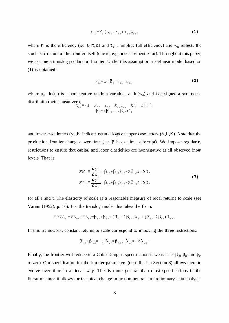
and lower case letters (y,l,k) indicate natural logs of upper case letters (Y,L,K). Note that the

production frontier changes over time (i.e.β has a time subscript). We impose regularity

restrictions to ensure that capital and labor elasticities are nonnegative at all observed input

levels. That is:

for all i and t. The elasticity of scale is a reasonable measure of local returns to scale (see

(3)EKti ≡ ∂yti

∂kti

βt1 βt3 l ti 2βt4 k ti ≥0,

ELti ≡ ∂yti

∂l ti

βt2 βt3 k ti 2βt5 l ti ≥0,

Varian (1992), p. 16). For the translog model this takes the form:

In this framework, constant returns to scale correspond to imposing the three restrictions:

ERTSti EKti ELti βt1 βt2 ( βt3 2βt4 ) k ti ( βt3 2βt5 ) l ti .

Finally, the frontier will reduce to a Cobb-Douglas specification if we restrictβt3, βt4 andβt5

to zero. Our specification for the frontier parameters (described in Section 3) allows them to

evolve over time in a linear way. This is more general than most specifications in the

literature since it allows for technical change to be non-neutral. In preliminary data analysis,

3

more flexible assumptions (e.g. quadratic) did not seem warranted.

Given the world frontiers in periods t and t+1, and the inputs and inefficiencies of

country i in both periods, the expected increase in the log of country i’s GDP is:

where the first term is due to changes in the input use in country i (i.e. changes in allocation

(4)12

( x t 1, i x ti ) ( βt 1 βt )12

( βt 1 βt ) ( x t 1, i x ti ) ( uti ut 1, i ).

and scale), the second term captures the effect of the shift in the frontier (i.e. world technical

progress) on the quantity of maximum attainable output for country i, and the third component

reflects changes in efficiency of country i. Thus, we define the following theoretically

expected annual change in GDP of country i:

which is the product of the annual input change

(5)GCt 1,i ICt 1,i×TCt 1,i×ECt 1,i,

and the annual productivity change

(6)ICt 1,i exp[12

(βt 1 βt) (xt 1,i xti)],

where ECt+1,i=exp(uti-ut+1,i) is the annual efficiency change (i.e.τt+1,i/τt,i) and

(7)PCt 1,i TCt 1,i×ECt 1,i,

measures the annual technical change (see KOS). Note that PCt+1,i is the output-based

(8)TCt 1,i exp[12

(xt 1,i xti) (βt 1 βt)]

Malmquist productivity change index used in Färe et al. (1994).

Average changes: AGCi, AICi, APCi, ATCi, AECi are defined as geometric averages

of annual changes defined above. To facilitate interpretation, we use average percentage

growth rates in our empirical section: AGGi=100x(AGCi-1), AIGi=100x(AICi-1),

APGi=100x(APCi-1), ATGi=100x(ATCi-1), and AEGi=100x(AECi-1).

4

3. Bayesian Inference

Following our previous work (see KOS), we assume that the vti’s in (2) are

independent Normal random variables with mean 0 and varianceσ2 (unknown) and the uti’s

are independent of each other and of the vti’s. The efficiency distribution of uti=-ln(τti) must

be one-sided to ensure thatτti lies between zero and one, and uti here is taken to be

Exponential with meanλ. In order to model the shifts of the frontier in a parsimonious way,

we use the linear trend specification for the J=6 elements ofβt:

Thus model (2) can be written as:

βt β tβ ,

where y=(y1’...yT’)’, y t=(yt1...ytN)’; u=(u1’...uT’)’, u t=(ut1...utN)’; v=(v1’...vT’)’, v t=(vt1...vtN)’;

(9)y X β u v,

β=(β*’ β** ’)’;

and Xt=(xt1...xtN)’. Note thatβ is a 2Jx1 vector (where J=6).

X

X1 X1

. .

Xt tXt

. .

XT TXT

These assumptions suffice to specify the likelihood function which, when combined

with a prior distribution, yields our Bayesian model. Note that we always impose the

regularity conditions given in (3) through the prior. Throughout, we use a Uniform prior for

β, truncated to ensure that these economic regularity conditions hold at all points in the

sample. In order to obtain a well-defined posterior, informative priors must be placed onσ

andλ. The use of the traditional flat prior for ln(σ-2) or ln(λ) precludes the existence of the

posterior distribution as the marginal data density is then notσ-finite (see Fernández,

Osiewalski and Steel (1997)). We elicit the informative prior in such a fashion so as to allow

it to be dominated by the sample.

5

Our Bayesian model is:

where

(10)f TNN (y X β u,σ2ITN)p(β X )p(σ 2)p(λ 1)

T

t 1

N

i 1

fG(uti 1,λ 1),

and p(βX*)=1 if the regularity conditions are satisfied and zero otherwise. In (10), fNM(. a,B)

p(λ 1) fG(λ 1 1, ln(τ )),

p(σ 2) σ2 exps0

2σ2,

denotes the density function of the M-variate Normal distribution with mean a and covariance

matrix B, and fG(. a,b) denotes the Gamma density with shape parameter a and scale

parameter b, the mean being a/b. We choose s0=10-6, which makes the prior density of the

symmetric error precision close to the "usual" flat prior on ln(σ-2) for small to moderately

large values ofσ-2: its main effect is to downweigh excessively large values of the precision.

Although the prior adopted here is improper, it leads to a proper posterior (see Proposition

1 of Fernández, Osiewalski and Steel (1997)). A detailed justification of, and suggestions for,

prior elicitation forλ are given in van den Broeck, Koop, Osiewalski and Steel (1994). It is

sufficient to note here that we choose an Exponential prior, and thatτ* is the prior median

efficiency, which is a natural quantity to elicit in practice. We typically chooseτ*=.75 (which

indicates,a priori, that we expect the median of the efficiency distribution to be .75) but we

also considered other values for our sensitivity analysis. Unless otherwise specified,τ*=.75

throughout the paper.

In order to evaluate posterior properties of the models, we use Gibbs sampling

methods. (See Gelfand and Smith (1990) and Casella and George (1992) for an introduction).

Essentially, Gibbs sampling involves taking sequential random draws from the full conditional

posterior distributions. Under very mild assumptions (see e.g. Tierney (1994)), these draws

then converge to draws from the joint posterior. Once draws from the joint distribution have

been obtained, any posterior feature of interest can be calculated.

Note that the joint posterior density of the parameters and inefficiency terms as well

as all conditional posterior densities are proportional to (10). The Gibbs sampler we use for

marginal posterior inference draws from analytically tractable conditional posterior

6

distributions. Details can be found in KOS. The empirical results are based on a sequential

Gibbs sampler with 50,000 included and 2,000 burn-in passes. That is, for various starting

values, we generated 52,000 passes and discarded the first 2,000 to eliminate possible start-up

effects. The reader is referred to Koop, Steel and Osiewalski (1995) for a discussion of

various implementations of the Gibbs sampler and techniques for assessing convergence in

the context of stochastic frontier models.

4. Empirical Results

We apply our methods to a sample of 22 countries over the period 1980-1990. That

is, we include all the countries which are currently (1997) within the European Union, five

other Western economies (the U.S., Canada, Australia, Switzerland and Norway), and the two

East European countries for which comparable capital stock data were available (Poland and

Yugoslavia). Aggregate output (Y) is measured by real GDP; labor (L), by total employment;

and capital stock (K) is calculated from capital stock per worker.2

The focus of this paper is on the decomposition of the observed output levels into the

frontier and inefficiency terms and on the components of output and productivity growth.

4.1. Model fit, simplifications and robustness

Before going to the economic interpretation and implications of our results, let us

discuss the fit of our model and the plausibility of certain simplifications of the translog

specification.

In terms of GDP growth rates, the fit is quite good in that observed and expected

(AGG) average GDP growth are close for most countries (see Table 5); the difference is

usually less than one posterior standard deviation, with the exception of The Netherlands,

Portugal and Yugoslavia. Note that Portugal and Yugoslavia represent two extreme growth

patterns in the sample (the highest GDP growth and the largest GDP drop, respectively).

Moreover, the fit is now not as good as it was in KOS where we used an earlier version of

2This capital stock measure includes gross investment in producer durables andnonresidential construction but excludes residential construction.

7

the Penn World Tables, a slightly different time period (1979-88) and a smaller group of

countries. With the revised data set the results change a lot. This illustrates the fragility of

inferences based on highly aggregated international data which are subject to comparability

problems and other imperfections.3 However, we shall just use the data that seem the best

available and proceed conditionally on them.

In view of our modeling experience from KOS it seems clear that a more general

model than our translog specification with a linear trend in its parameters would be

overparameterized as we have just 22 countries observed over 11 years. However, we could

consider simplified versions of our basic model. If the marginal posterior ofβ would be

Normal, we could easily construct a Highest Posterior Density test for the more restricted

versions of our model, by using the fact that the standardized inner product should have aχ2

distribution. Of course, this Normality does not really hold, but we shall base an approximate

χ2 test on this idea. That should give us at least a rough idea of the appropriateness of certain

simplifications. If we then test the restriction of constant returns to scale, we obtain the value

118 for this inner product, which should have an approximateχ26 distribution under the null

hypothesis of constant returns to scale, thus strongly corroborating that the simplifying

hypothesis of constant returns to scale is not supported by the data. For the hypothesis that

the linear trend only affects the constant termβt0, we have to compare the value 43.7 with a

χ25 distribution, which again leads to very strong rejection of the null, and for the even

stronger hypothesis that no trend at all should be present in the LT model, we obtain 56.5 to

test for six restrictions. Also, when we test the restrictions leading to the Cobb-Douglas form

of the frontier, we have to compare the value 264 with aχ26 posterior distribution. Thus, none

of these extra restrictions seem to have any data credibility, and our preferred model will

clearly be the full translog model with a linear trend in its parameters.

As discussed earlier, the priors are all quite flat. The key prior hyperparameter is the

prior median efficiency,τ*. We selectτ*=0.75, which implies that the median of the

(relatively noninformative) prior efficiency distribution is 0.75. Since this is an important

dimension in which to investigate prior sensitivity, we also considered the very different

valuesτ*=0.5 andτ*=0.9. The inference on quantities of interest is completely insensitive to

3Note that the Penn World Tables are considered among the best data sets. Yet,comparison of numbers in Version 5.6 and its predecessor reveals that serious changes andcorrections have been made.

8

this prior input.

4.2. Properties of the frontier

The world production frontier shows significant shifts over the relatively short time

period under consideration (1980-90), as is evidenced by the strong rejection of the constancy

of βt. This implies both world technical change, which will be discussed later, and changing

patterns of factor elasticities and returns to scale calculated for different countries on the basis

of this moving frontier.

Table 1 contains the averages over all the periods in the sample, for each country, of

the capital and labor elasticities, denoted by EKti and ELti respectively in (3), as well as the

returns to scale ERTSti (i.e., the sum of the elasticities), for the different countries and years.

It turns out that there is some difference in returns to scale, but most countries indicate

increasing returns, with very small standard errors. The exceptions are: Luxembourg, showing

decreasing returns to scale, and Switzerland and Norway, both with constant returns. Note that

they are all small (in terms of population) and very rich countries. The smallest values of

increasing returns to scale are found for Finland, Ireland and Denmark, and then for Belgium,

Austria and Sweden. The highest increasing returns to scale are obtained for the two East

European economies (i.e., Yugoslavia and Poland) as well as for some large Western

countries (the U.S. and the U.K.) and Portugal (which is much smaller, but relatively quite

poor). The decomposition over the factors shows much more variability. Capital elasticity

ranges from a lowest posterior mean of 0.139 for Switzerland (and 0.155 for Germany) to a

high of 0.878 for Yugoslavia (and 0.827 for Portugal). Labor elasticity ranges from 0.241 for

Yugoslavia and 0.262 for Portugal to 0.861 for the U.S. and 0.909 for Germany.

For Poland, the average posterior means of both returns to scale (1.115) and capital

elasticity (0.702) are the third highest in the sample, and the average posterior mean of labor

elasticity is the third lowest (0.413) and nearly the same as for Ireland (0.420).

The countries with the highest capital-labor ratios (Switzerland, Germany and Norway)

are exactly those with the lowest capital elasticities. Conversely, the highest values for EKi

are found for Yugoslavia, Portugal and Poland, where the capital-labor ratio is lowest.

However, for other (not that extreme) countries this relationship does not hold (e.g.,

Luxembourg, with the fourth highest K/L, has an average capital elasticity). The situation for

labor elasticity is even more complicated. While the lowest values are found for Yugoslavia,

9

Portugal and Poland, the highest are for Germany, U.S., Switzerland, and then France (the

U.S. and France have about average K/L).

Table 2 reports the evolution of the country averages of these quantities over time.

There is a clear tendency for ELt to decrease over time, which is partly offset by an

increasing capital elasticity, but the resulting returns to scale ERTSt is decreasing somewhat

over time. Note, incidentally, that we face the situation that returns to scale is much easier

to determine than its components as the latter have much larger posterior standard deviations

than their sum.

Since returns to scale are not very far from unity, it makes sense to graphically portray

a slice from the three-dimensional surface that defines the frontier. Figure 1 plots the output-

labor ratio (Y/L) against the capital-labor ratio (K/L) using the posterior means of the frontier

parameters, for a labor force of 22.5 million. We have also indicated six countries with labor

forces around that number: Canada, Poland, Italy, France, the U.K. and Germany (ordered

here according to the size of their labor forces). We would expect countries to lie somewhat

below the frontier, although relatively large positive values of the symmetric error component

vti in (2) could lead to the opposite situation4. In addition, the frontier as drawn is subject to

random variation inβt. Note that all countries increase K/L from 1980 to 1990 (although

Poland only marginally), and that Poland is the only country in the graph that suffers a

(small) drop in output per worker over this period.

4.3. Efficiency levels

Table 3 presents year averages of efficiency levels for all countries. The Netherlands

and Canada appear to be most efficient, followed by Belgium, Australia and Luxembourg.

These countries experienced almost no efficiency change over the period 1980-1990 (see

Table 5). For Canada, this situation is graphically depicted in Figure 15. The second group

of highly efficient economies (with average efficiency about 0.93) consists of the U.S., Italy,

Yugoslavia, the U.K. and Sweden. The third group includes Ireland, Switzerland, Portugal,

4However, of the expected squared distance from the frontier, only 5.3% is due to thesymmetric disturbance whereas the rest originates from inefficiency.

5Since Canada has by far the smallest labor force of the countries plotted in the graph andreturns to scale are somewhat increasing (see Subsection 4.2), it will appear slightly lessefficient than it should be. For the other countries, such scale effects should be negligible.

10

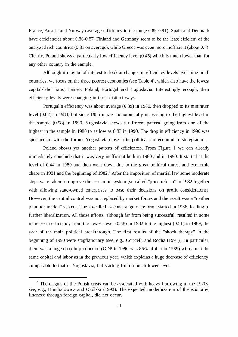
France, Austria and Norway (average efficiency in the range 0.89-0.91). Spain and Denmark

have efficiencies about 0.86-0.87. Finland and Germany seem to be the least efficient of the

analyzed rich countries (0.81 on average), while Greece was even more inefficient (about 0.7).

Clearly, Poland shows a particularly low efficiency level (0.45) which is much lower than for

any other country in the sample.

Although it may be of interest to look at changes in efficiency levels over time in all

countries, we focus on the three poorest economies (see Table 4), which also have the lowest

capital-labor ratio, namely Poland, Portugal and Yugoslavia. Interestingly enough, their

efficiency levels were changing in three distinct ways.

Portugal’s efficiency was about average (0.89) in 1980, then dropped to its minimum

level (0.82) in 1984, but since 1985 it was monotonically increasing to the highest level in

the sample (0.98) in 1990. Yugoslavia shows a different pattern, going from one of the

highest in the sample in 1980 to as low as 0.83 in 1990. The drop in efficiency in 1990 was

spectacular, with the former Yugoslavia close to its political and economic disintegration.

Poland shows yet another pattern of efficiences. From Figure 1 we can already

immediately conclude that it was very inefficient both in 1980 and in 1990. It started at the

level of 0.44 in 1980 and then went down due to the great political unrest and economic

chaos in 1981 and the beginning of 1982.6 After the imposition of martial law some moderate

steps were taken to improve the economic system (so called "price reform" in 1982 together

with allowing state-owned enterprises to base their decisions on profit consideratons).

However, the central control was not replaced by market forces and the result was a "neither

plan nor market" system. The so-called "second stage of reform" started in 1986, leading to

further liberalization. All those efforts, although far from being successful, resulted in some

increase in efficiency from the lowest level (0.38) in 1982 to the highest (0.51) in 1989, the

year of the main political breakthrough. The first results of the "shock therapy" in the

beginning of 1990 were stagflationary (see, e.g., Coricelli and Rocha (1991)). In particular,

there was a huge drop in production (GDP in 1990 was 85% of that in 1989) with about the

same capital and labor as in the previous year, which explains a huge decrease of efficiency,

comparable to that in Yugoslavia, but starting from a much lower level.

6 The origins of the Polish crisis can be associated with heavy borrowing in the 1970s;see, e.g., Kondratowicz and Okólski (1993). The expected modernization of the economy,financed through foreign capital, did not occur.

11

In order to give some explanation of the very low efficiency levels for Poland we may

notice that the average capital-labor ratio was 7588 for Yugoslavia, 9638 for Portugal and

11462 for Poland, but the average output per worker was 11560 in Yugoslavia, 12484 in

Portugal and only 8026 in Poland. Thus, with much more capital per worker Poland produced

much less output per worker than each of the two other countries.

It seems that our estimates of efficiency are in perfect agreement with historical

experience and the data. However, a rather subtle methodological issue arises: do the

estimates for Poland reflect low efficiency or do they just indicate that the country used a

different technology ? Unfortunately, these hypotheses are not testable as we have only one

country operating on a potentially different frontier. Thus, we can only conclude that our

inefficiency estimates for Poland may measure the total productivity (i.e. technological and

efficiency) gap with respect to the world leaders.

4.4. Growth decomposition

We have decomposed expected GDP growth into its three components: input growth,

technical growth and efficiency growth (measured by AIG, ATG and AEG, respectively).

Table 5 presents posterior means and standard deviations of these three measures along with

expected GDP growth (i.e. AGG), which is approximately equal to the sum of AIG and

APG), actual GDP growth, and productivity growth (i.e. APG, which is approximately

ATG+AEG) for the 22 countries under consideration. The standard deviations of most of our

average growth measures are very substantial, and thus, our conclusions contain a

considerable degree of uncertainty. This is not surprising. Indeed, it would be even more

surprising to expect our small and noisy data set to answer the complicated questions about

growth decomposition that we are posing with any high degree of accuracy. Average input

growth (AIG) is the only quantity with small posterior standard deviations.

A general pattern appears to be that input change and, for most countries, technical

change provide the major impetus for growth, and that changes in efficiency play a relatively

minor role. For almost all countries, there was either no efficiency change or it was somewhat

negative. Two countries that suffered severe decreases in efficiency levels are Yugoslavia and

Germany, and the two where efficiency had a positive role to play are Portugal (growing

fastest) and the U.K. (growth above average). The efficiency loss for Germany and the gain

12

for the U.K. can also be inferred directly from Figure 1. For other fast growing countries

(Luxembourg, Ireland, Finland, Spain, Canada, Australia and the U.S.), efficiency gains did

not appear to play any role in economic growth, and most growth seems to be linked to input

changes. The case of Canada is graphically illustrated in Figure 1. Portugal, Spain and the

U.K. achieved fast GDP growth largely through input growth, while Luxembourg, the U.S.,

Finland, Canada, Australia and Ireland relied also on technical change to achieve their fast

growth (again, see Figure 1 for Canada). Conversely, for those relatively rich European

countries that experienced slower than average GDP growth (i.e. Switzerland, Germany,

France, Denmark, The Netherlands, Belgium and Italy), slow growth in inputs would appear

to be the culprit since technical change was above average. Germany and, to a lesser extent,

France, suffered some decline in efficiency which outweighed their very high technical growth

(this can also be seen in Figure 1). In terms of productivity growth, Luxembourg was first,

followed by Finland, Ireland, Norway and the U.S., while Yugoslavia, Poland, and, to much

lesser extent, Portugal experienced constant decrease of productivity, largely due to negative

technical change. As these three countries have the lowest capital-labor ratios, it seems that

their input mix was just incompatible with the directions of world technical progress. Indeed,

Figure 1 shows that countries with K/L smaller than that of the U.K. will suffer technical

regress. Portugal was able to compensate this negative technical change by the huge input

change and considerable efficiency improvement (both highest in the sample) and reached the

fastest growth, clearly underestimated by our model. Hovewer, the East European economies

did very poorly. In Yugoslavia, the second highest input growth was completely unproductive

due to huge negative technical change and a spectacular drop in efficiency. This pattern of

highly negative GDP growth is very difficult to explain through our modeling strategy and

thus the model underestimates the actual GDP losses. On the contrary, Poland’s moderately

negative GDP growth is almost perfectly fitted by our model and it is explained by a poor

performance in all three categories: the lowest input change, a highly negative effect of world

technical progress and no efficiency improvement.

5. Concluding Remarks

The methodology developed in KOS and applied here has enabled us to estimate the

13

"world production frontier" and, in particular, efficiency levels of the Polish economy in the

period 1980-1990. It also accurately modelled GDP growth and yielded its decomposition into

input, technical and efficiency changes. It will be of great interest to apply the same

methodology to the data for the 1990s. It seems that the very low efficiency at the beginning

of Polish reforms, and thus the possibility of increasing output through efficiency change

alone, may explain Poland’s fast growth which has been observed in recent years.

References

Aigner, D., C.A.K. Lovell and P. Schmidt, 1977, Formulation and estimation of stochasticfrontier production function models,Journal of Econometrics, 6, 21-37.

van den Broeck, J., G. Koop, J. Osiewalski and M.F.J. Steel, 1994, Stochastic frontier models:A Bayesian perspective,Journal of Econometrics, 1994, 61, 273-303.

Casella, G. and E. George, Explaining the Gibbs sampler, 1992,The American Statistician,46, 167-174.

Coricelli, F. and R. Rocha, 1991, Stabilisation programs in Eastern Europe. A comparativeanalysis of the Polish and Yugoslav programs of 1990, in: V. Corbo, F. Coricelli and J.Bossak, eds.,Reforming central and eastern European economies: Initial results andchallenges(World Bank, Washington D.C.).

Färe, R., S. Grosskopf, M. Norris and Z. Zhang, 1994, Productivity growth, technicalprogress, and efficiency change in industrialized countries,American Economic Review, 84,66-83.

Fernández, C., J. Osiewalski and M.F.J. Steel, 1997, On the use of panel data in stochasticfrontier models with improper priors,Journal of Econometrics, 79, 169-193.

Gelfand, A.E. and A.F.M. Smith, 1990, Sampling-based approaches to calculating marginaldensities,Journal of the American Statistical Association, 85, 398-409.

Kondratowicz, A. and M. Okólski, 1993, The Polish economy on the eve of the Solidaritytake-over, in: H. Kierzkowski, M. Okólski and S. Wellisz, eds.,Stabilisation and structuraladjustment in Poland(Routledge, New York).

Koop, G., J. Osiewalski and M.F.J. Steel, 1997a, Bayesian efficiency analysis throughindividual effects: Hospital cost frontiers,Journal of Econometrics, 76, 77-105.

Koop, G., J. Osiewalski and M.F.J. Steel, 1997b, The components of output growth: A

14

stochastic frontier analysis." mimeo, CentER, Tilburg University.

Koop, G., M.F.J. Steel and J. Osiewalski, 1995, Posterior analysis of stochastic frontiermodels using Gibbs sampling,Computational Statistics, 10, 353-373.

Meeusen, W. and J. van den Broeck, 1977, Efficiency estimation from Cobb-Douglasproduction functions with composed error,International Economic Review, 8, 435-444.

Tierney, L., 1994, Markov chains for exploring posterior distributions (with discussion),Annals of Statistics, 22, 1701-1762.

Varian, H.R., 1992,Microeconomic analysis, Third Edition (W.W. Norton, New York).

15

Table 1: Year Averages of Factor Elasticities and Returns to Scale

Country EKi ELi ERTSi

Australia 0.338 (0.031) 0.707 (0.030) 1.045 (0.007)

Austria 0.416 (0.027) 0.617 (0.025) 1.033 (0.007)

Belgium 0.369 (0.030) 0.661 (0.029) 1.031 (0.006)

Canada 0.301 (0.037) 0.757 (0.034) 1.058 (0.010)

Denmark 0.426 (0.030) 0.601 (0.028) 1.026 (0.007)

Finland 0.334 (0.036) 0.679 (0.036) 1.013 (0.007)

France 0.307 (0.046) 0.771 (0.042) 1.078 (0.012)

Germany 0.155 (0.063) 0.909 (0.053) 1.063 (0.019)

Greece 0.529 (0.023) 0.519 (0.018) 1.047 (0.011)

Ireland 0.606 (0.044) 0.420 (0.030) 1.026 (0.017)

Italy 0.356 (0.040) 0.724 (0.039) 1.081 (0.011)

Luxembourg 0.418 (0.084) 0.523 (0.081) 0.941 (0.017)

The Netherlands 0.396 (0.026) 0.648 (0.025) 1.045 (0.006)

Norway 0.294 (0.042) 0.708 (0.043) 1.002 (0.008)

Poland 0.702 (0.028) 0.413 (0.042) 1.115 (0.022)

Portugal 0.827 (0.042) 0.262 (0.034) 1.088 (0.029)

Spain 0.466 (0.024) 0.613 (0.028) 1.079 (0.010)

Sweden 0.375 (0.028) 0.659 (0.027) 1.034 (0.006)

Switzerland 0.139 (0.052) 0.858 (0.053) 0.997 (0.016)

U.K. 0.512 (0.033) 0.593 (0.041) 1.105 (0.014)

U.S. 0.257 (0.076) 0.861 (0.070) 1.118 (0.020)

Yugoslavia 0.878 (0.043) 0.241 (0.048) 1.120 (0.032)

average 0.427 (0.040) 0.625 (0.039) 1.052 (0.013)

16

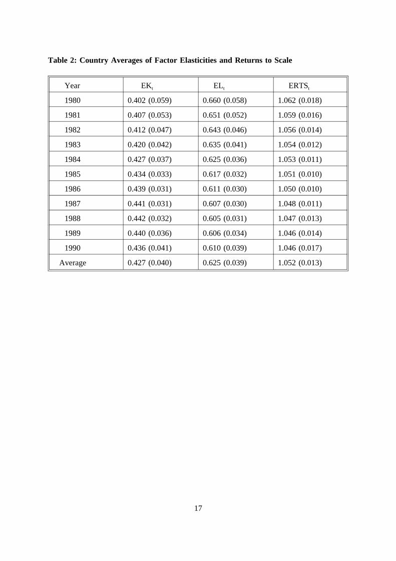
Table 2: Country Averages of Factor Elasticities and Returns to Scale

Year EKt ELt ERTSt

1980 0.402 (0.059) 0.660 (0.058) 1.062 (0.018)

1981 0.407 (0.053) 0.651 (0.052) 1.059 (0.016)

1982 0.412 (0.047) 0.643 (0.046) 1.056 (0.014)

1983 0.420 (0.042) 0.635 (0.041) 1.054 (0.012)

1984 0.427 (0.037) 0.625 (0.036) 1.053 (0.011)

1985 0.434 (0.033) 0.617 (0.032) 1.051 (0.010)

1986 0.439 (0.031) 0.611 (0.030) 1.050 (0.010)

1987 0.441 (0.031) 0.607 (0.030) 1.048 (0.011)

1988 0.442 (0.032) 0.605 (0.031) 1.047 (0.013)

1989 0.440 (0.036) 0.606 (0.034) 1.046 (0.014)

1990 0.436 (0.041) 0.610 (0.039) 1.046 (0.017)

Average 0.427 (0.040) 0.625 (0.039) 1.052 (0.013)

17

Table 3: Year Averages of Efficiency

Country Average efficiency

Australia 0.955 (0.030)

Austria 0.891 (0.042)

Belgium 0.958 (0.029)

Canada 0.970 (0.024)

Denmark 0.862 (0.043)

Finland 0.814 (0.041)

France 0.897 (0.042)

Germany 0.809 (0.046)

Greece 0.694 (0.036)

Ireland 0.908 (0.041)

Italy 0.934 (0.037)

Luxembourg 0.945 (0.036)

The Netherlands 0.975 (0.021)

Norway 0.891 (0.043)

Poland 0.450 (0.025)

Portugal 0.898 (0.040)

Spain 0.873 (0.043)

Sweden 0.928 (0.038)

Switzerland 0.905 (0.045)

U.K. 0.928 (0.036)

U.S. 0.935 (0.041)

Yugoslavia 0.932 (0.036)

average 0.880 (0.037)

18

Table 4: Efficiency Levels for Selected Countries

Year Portugal Poland Yugoslavia

1980 0.890 (0.052) 0.443 (0.027) 0.974 (0.023)

1981 0.875 (0.050) 0.403 (0.024) 0.970 (0.025)

1982 0.871 (0.048) 0.378 (0.021) 0.961 (0.030)

1983 0.842 (0.046) 0.403 (0.022) 0.950 (0.034)

1984 0.822 (0.044) 0.429 (0.023) 0.948 (0.034)

1985 0.847 (0.045) 0.458 (0.025) 0.928 (0.039)

1986 0.890 (0.045) 0.481 (0.026) 0.952 (0.033)

1987 0.938 (0.038) 0.493 (0.027) 0.926 (0.041)

1988 0.955 (0.032) 0.513 (0.028) 0.900 (0.045)

1989 0.968 (0.026) 0.512 (0.029) 0.914 (0.045)

1990 0.980 (0.018) 0.434 (0.025) 0.834 (0.049)

Table 5: Growth Rate Components

Country GDPgrowth

AGG AIG ATG AEG APG

Australia 2.96 3.30(0.51)

2.65(0.06)

0.97(0.23)

-0.33(0.49)

0.63(0.50)

Austria 2.12 2.32(0.60)

2.12(0.08)

0.87(0.24)

-0.68(0.61)

0.20(0.59)

Belgium 1.89 2.05(0.38)

1.13(0.04)

0.96(0.24)

-0.05(0.33)

0.91(0.38)

Canada 2.97 3.34(0.40)

2.40(0.13)

1.05(0.25)

-0.12(0.35)

0.92(0.40)

Denmark 2.10 2.11(0.68)

1.28(0.04)

0.93(0.24)

-0.11(0.71)

0.82(0.67)

Finland 3.06 3.06(0.70)

1.79(0.09)

1.05(0.30)

0.20(0.73)

1.25(0.69)

19

Country GDPgrowth

AGG AIG ATG AEG APG

France 2.22 2.31(0.62)

1.66(0.08)

1.07(0.29)

-0.43(0.64)

0.63(0.61)

Germany 2.14 2.15(0.68)

1.64(0.10)

1.64(0.62)

-1.11(0.86)

0.51(0.68)

Greece 1.87 1.87(0.69)

1.43(0.04)

0.55(0.26)

-0.10(0.73)

0.44(0.68)

Ireland 3.42 3.14(0.52)

2.01(0.10)

0.86(0.47)

0.24(0.51)

1.11(0.50)

Italy 2.14 2.29(0.52)

1.60(0.07)

0.84(0.26)

-0.16(0.51)

0.68(0.51)

Luxembourg 3.66 3.88(0.58)

2.14(0.24)

1.82(0.67)

-0.12(0.47)

1.70(0.62)

TheNetherlands

2.01 2.62(0.33)

1.86(0.02)

0.84(0.22)

-0.10(0.26)

0.74(0.33)

Norway 2.44 2.45(0.67)

1.41(0.06)

1.06(0.37)

-0.04(0.73)

1.02(0.66)

Poland -0.76 -0.76(0.67)

0.88(0.02)

-1.44(0.55)

-0.19(0.86)

-1.63(0.66)

Portugal 4.25 3.25(0.57)

3.57(0.14)

-1.29(0.52)

0.99(0.63)

-0.31(0.58)

Spain 3.06 3.07(0.64)

2.67(0.06)

0.34(0.27)

0.04(0.66)

0.38(0.63)

Sweden 2.01 2.21(0.60)

1.88(0.07)

0.93(0.24)

-0.60(0.60)

0.33(0.59)

Switzerland 2.06 2.14(0.60)

1.32(0.11)

0.97(0.61)

-0.16(0.71)

0.80(0.62)

U.K. 2.85 2.54(0.58)

1.90(0.06)

-0.15(0.45)

0.78(0.65)

0.63(0.58)

U.S. 2.64 2.91(0.61)

1.89(0.15)

1.53(0.72)

-0.51(0.73)

1.00(0.61)

Yugoslavia -1.36 -0.63(0.60)

3.61(0.13)

-2.57(0.52)

-1.56(0.64)

-4.09(0.57)

average 2.26 2.35(0.58)

1.95(0.09)

0.58(0.39)

-0.19(0.61)

0.39(0.57)

20