Frontier analysis and agricultural typologies - AGRODEP

ZEF-Discussion Papers on Development Policy No. 251

Eduardo Maruyama, Máximo Torero, Phoebe Scollard, Maribel Elías, Francis Mulangu, and Abdoulaye Seck

Frontier analysis and agricultural typologies

Bonn, March 2018

The CENTER FOR DEVELOPMENT RESEARCH (ZEF) was established in 1995 as an international,

interdisciplinary research institute at the University of Bonn. Research and teaching at ZEF

address political, economic and ecological development problems. ZEF closely cooperates

with national and international partners in research and development organizations. For

information, see: www.zef.de.

ZEF – Discussion Papers on Development Policy are intended to stimulate discussion among

researchers, practitioners and policy makers on current and emerging development issues.

Each paper has been exposed to an internal discussion within the Center for Development

Research (ZEF) and an external review. The papers mostly reflect work in progress. The

Editorial Committee of the ZEF – DISCUSSION PAPERS ON DEVELOPMENT POLICY includes

Joachim von Braun (Chair), Christian Borgemeister, and Eva Youkhana. Chiara Kofol is the

Managing Editor of the series.

Eduardo Maruyama, Maximo Torero, Phoebe Scollard, Maribel Elías, Francis Mulangu, and

Abdoulaye Seck, Frontier analysis and agricultural typologies, ZEF – Discussion Papers on

Development Policy No. 251, Center for Development Research, Bonn, March 2018, pp. 91.

ISSN: 1436-9931

Published by:

Zentrum für Entwicklungsforschung (ZEF)

Center for Development Research

Genscherallee 3

D – 53113 Bonn

Germany

Phone: +49-228-73-1861

Fax: +49-228-73-1869

E-Mail: [email protected]

www.zef.de

The authors:

Eduardo Maruyama, International Food Policy Research Institute, Contact:

[email protected] (corresponding author)

Máximo Torrero, World Bank Group, [email protected]

Phoebe Scollard, International Food Policy Research Institute. Contact: [email protected]

Maribel Elías, International Food Policy Research Institute. Contact: [email protected]

Francis Mulangu, AGRODEP, Millennium Challenge Corporation. Contact: [email protected]

Abdoulaye Seck, AGRODEP, Cheikh Anta Diop University. Contact: [email protected]

Contents

Acknowledgements ...................................................................................................................vii

Acronyms and abbreviations .................................................................................................... viii

Executive Summary ....................................................................................................................ix

1 Background ......................................................................................................................... 1

2 Literature review ................................................................................................................. 2

3 Conceptual framework ....................................................................................................... 4

4 Methodological approach ................................................................................................... 8

4.1 Model ............................................................................................................................... 8

4.2 Estimation ....................................................................................................................... 10

4.3 GIS data and accessibility model .................................................................................... 13

4.4 Typology construction .................................................................................................... 13

5 Results ............................................................................................................................... 15

5.1 Burkina Faso ................................................................................................................... 15

5.2 Ethiopia ........................................................................................................................... 21

5.3 Ghana ............................................................................................................................. 25

5.4 Kenya .............................................................................................................................. 32

5.5 Malawi ............................................................................................................................ 39

5.6 Nigeria ............................................................................................................................ 48

5.7 Togo ................................................................................................................................ 55

5.8 Zambia ............................................................................................................................ 63

6 Concluding remarks .......................................................................................................... 72

References ................................................................................................................................ 74

Appendix 1: SFA estimation results.......................................................................................... 77

Appendix 2: Accessibility maps ................................................................................................ 84

Tables

Table 1: Typology classification .................................................................................................. 6

Table 2: Typology classes and examples of interventions ......................................................... 7

Table 3: Survey samples constraints ........................................................................................ 12

Table 4: Burkina Faso: Agricultural revenue SFA estimation ................................................... 14

Table 5: Ethiopia: Agricultural revenue SFA estimation results ............................................... 77

Table 6: Ghana: Agricultural revenue SFA estimation results ................................................. 78

Table 7: Kenya: Agricultural revenue SFA estimation results .................................................. 79

Table 8: Malawi: Agricultural revenue SFA estimation results ................................................ 80

Table 9: Nigeria: Agricultural revenue SFA estimation results ................................................ 81

Table 10: Togo: Agricultural revenue SFA estimation results .................................................. 82

Table 11: Zambia: Agricultural revenue SFA estimation results .............................................. 83

Figures

Figure 1: Four key dimensions to characterize the regional heterogeneity of the agricultural

environment ............................................................................................................................... 4

Figure 2. Role of efficiency vs. potential oriented agricultural innovations .............................. 5

Figure 3: Stochastic production frontier in the single-output, single-input case ...................... 9

Figure 4: Burkina Faso: Agricultural potential .......................................................................... 17

Figure 5: Burkina Faso: Annual precipitation (mm), 2013 ....................................................... 18

Figure 6: Burkina Faso: Agricultural efficiency ......................................................................... 18

Figure 7: Burkina Faso: Unrealized agricultural potential ........................................................ 19

Figure 8: Burkina Faso: Maize production (Tons), 2013 .......................................................... 19

Figure 9: Burkina Faso: Rice production (tons), 2013 .............................................................. 20

Figure 10: Burkina Faso: Poverty map ..................................................................................... 20

Figure 11: Burkina Faso: Agricultural typology ........................................................................ 21

Figure 12: Ethiopia: Annual precipitation (mm), 2015 ............................................................. 22

Figure 13: Ethiopia: Poverty map ............................................................................................. 23

Figure 14: Ethiopia: Agricultural potential ............................................................................... 23

Figure 15: Ethiopia: Agricultural efficiency .............................................................................. 24

Figure 16: Ethiopia: Unrealized agricultural potential ............................................................. 24

Figure 17: Ethiopia: Agricultural typology ................................................................................ 25

Figure 18: Ghana: Annual precipitation (mm), 2013 ............................................................... 27

Figure 19: Ghana: Agricultural potential .................................................................................. 28

Figure 20: Ghana: Agricultural efficiency ................................................................................. 29

Figure 21: Ghana: Unrealized agricultural potential ................................................................ 30

Figure 22: Ghana: Poverty map ................................................................................................ 31

Figure 23: Ghana: Agricultural typology .................................................................................. 32

Figure 24: Kenya: Agricultural potential .................................................................................. 34

Figure 25: Kenya: Annual precipitation (mm), 2005 ................................................................ 35

Figure 26: Kenya: Agricultural efficiency .................................................................................. 36

Figure 27: Kenya: Unrealized agricultural potential ................................................................ 37

Figure 28: Kenya: Poverty map ................................................................................................ 38

Figure 29: Kenya: Agricultural typology ................................................................................... 39

Figure 30: Malawi: Agricultural potential ................................................................................ 41

Figure 31: Malawi: Maize production (tons), 2011 .................................................................. 42

Figure 32: Malawi: Tobacco production (tons), 2011 .............................................................. 43

Figure 33: Malawi: Annual precipitation (mm), 2011 .............................................................. 44

Figure 34: Malawi: Agricultural efficiency................................................................................ 45

Figure 35: Malawi: Unrealized agricultural potential .............................................................. 46

Figure 36: Malawi: Poverty map .............................................................................................. 47

Figure 37: Malawi: Agricultural typology ................................................................................. 48

Figure 38: Nigeria: Agricultural potential ................................................................................. 50

Figure 39: Nigeria: Annual precipitation (mm), 2015 .............................................................. 51

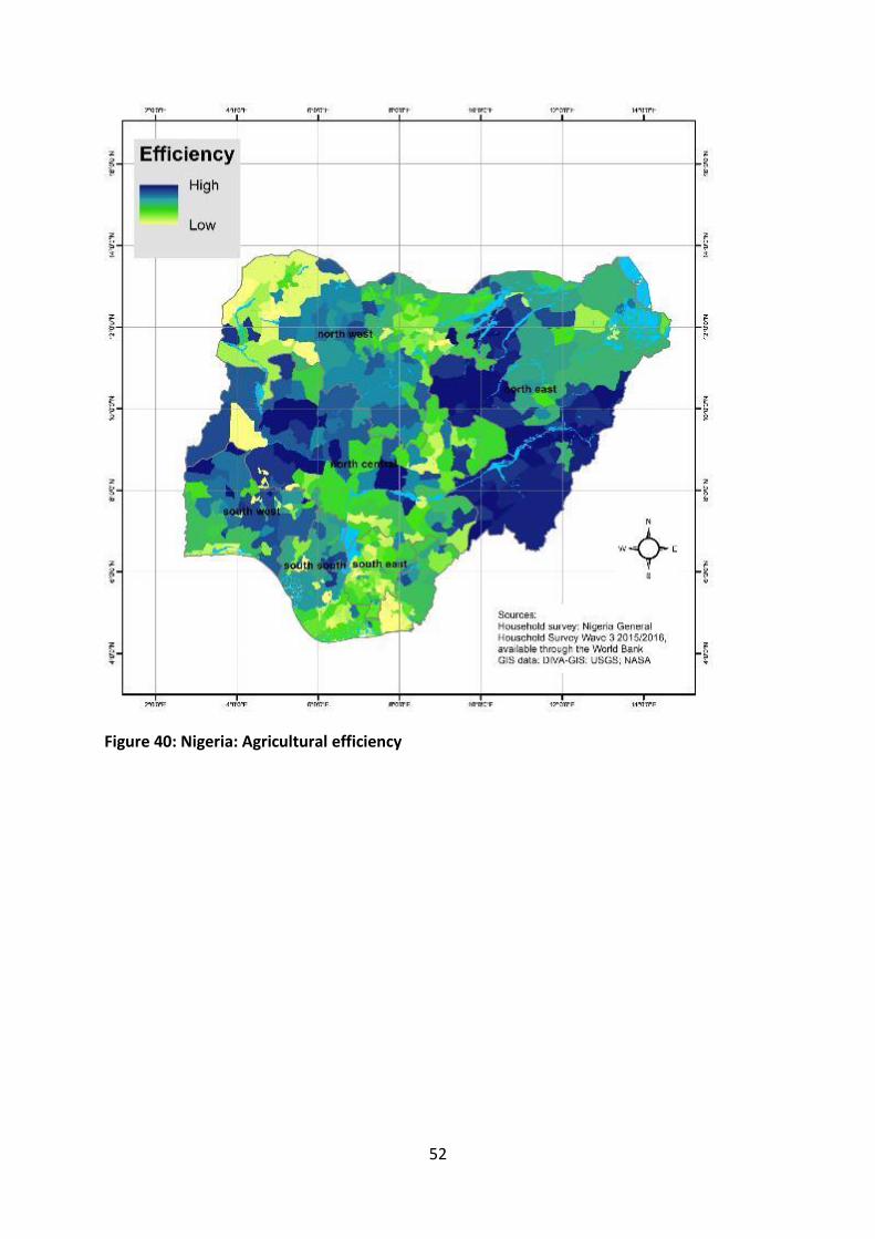
Figure 40: Nigeria: Agricultural efficiency ................................................................................ 52

Figure 41: Nigeria: Unrealized agricultural potential ............................................................... 53

Figure 42: Nigeria: Poverty map ............................................................................................... 54

Figure 43: Nigeria: Agricultural typology ................................................................................. 55

Figure 44: Togo: Agricultural potential .................................................................................... 57

Figure 45: Togo: Annual precipitation (mm), 2011 .................................................................. 58

Figure 46: Togo: Precipitation condition index, 2014 .............................................................. 59

Figure 47: Togo: Agricultural efficiency ................................................................................... 60

Figure 48: Togo: Unrealized agricultural potential .................................................................. 61

Figure 49: Togo: Poverty map .................................................................................................. 62

Figure 50: Togo: Agricultural typology ..................................................................................... 63

Figure 51: Zambia: Agricultural potential ................................................................................ 65

Figure 52: Zambia: Maize production (tons), 2011 .................................................................. 66

Figure 53: Zambia: Annual precipitation (mm), 2010 .............................................................. 67

Figure 54: Zambia: Agricultural efficiency ................................................................................ 68

Figure 55: Zambia: Unrealized agricultural potential .............................................................. 69

Figure 56: Zambia: poverty map .............................................................................................. 70

Figure 57: Zambia: Agricultural typology ................................................................................. 71

Figure 58: Burkina Faso: Accessibility ...................................................................................... 84

Figure 59: Ethiopia: accessibility .............................................................................................. 85

Figure 60: Ghana: Accessibility ................................................................................................. 86

Figure 61: Kenya: Accessiblity .................................................................................................. 87

Figure 62: Malawi: Accessibility ............................................................................................... 88

Figure 63: Nigeria: Accessibility................................................................................................ 89

Figure 64: Togo: Accessibility ................................................................................................... 90

Figure 65: Zambia: Accessibility ............................................................................................... 91

Acknowledgements

This study was conducted under a contract between the Center for Development Research

(ZEF) and the International Food Policy Research Institute (IFPRI) for the Program of

Accompanying Research for Agricultural Innovation (PARI). We are particularly indebted to

Prof. Dr. Joachim Von Braun and Dr. Heike Baumüller for their advice, coordination, and

support at all stages of the study.

We are grateful to the German Federal Ministry for Economic Cooperation and Development

(BMZ) for funding this work through PARI, as part of the One World, No Hunger Initiative

(SEWOH) by the German Government.

We benefitted from helpful and valuable comments from two anonymous reviewers at ZEF.

We also received useful comments from participants at the 2015 and 2016 PARI Annual

Meetings, and the 2016 PARI Ghana and Ethiopia National Policy Roundtables

At IFPRI, we thank the Director for Africa, Dr. Ousmane Badiane, for his guidance and support.

Acronyms and abbreviations

AEZ agroecological zone

AGRODEP African Growth & Development Policy Modeling Consortium

BMZ German Federal Ministry for Economic Cooperation and Development

DEA data envelopment analysis

FAO Food and Agriculture Organization of the United Nations

GIS geographical innovation system

ICT information and communication technology

IFPRI International Food Policy Research Institute

OECD Organization for Economic Co-operation and Development

PARI Program of Accompanying Research for Agricultural Innovation

PCA principal component analysis

R&D research and development

SEWOH One World, No Hunger Initiative

SFA stochastic frontier analysis

ZEF Center for Development Research

Executive Summary

PARI’s main goal is to contribute to sustainable agricultural growth and food security in Africa

and India by supporting the scaling of proven innovations in the agri-food sector in

collaboration with all relevant actors. PARI accompanies specified innovations with ex-ante

impact research and identifies further innovation opportunities, including those expressed by

end users of research in collaboration with the multi-stakeholder innovation platforms. Within

PARI’s work, AGRODEP and IFPRI have the task of assisting in the development of a

methodology and concept for strategic analysis and visioning by providing economic

modelling tools to help understand where the best opportunities for innovation investments

in value chains are. For this purpose, IFPRI has constructed agricultural typologies of micro-

regions for 8 of the 12 African countries in PARI to identify micro-regional level opportunities,

bottlenecks and investment gaps based on the concept of the production possibilities frontier

applied to farm activities, drawing on highly detailed household-level survey and geospatial

data on agroecological conditions, accessibility and poverty.

The stochastic frontier approach allows the econometric exploration of the notion that, given

the fixed local agroecological and economic conditions in a micro-region and the occurrence

of random shocks that affect agricultural production (weather, prices, etc.), the investment,

production decisions and technological innovations a farmer makes translate into higher or

lower production and income. In such a context, inefficiency is defined as the loss incurred in

by operating away from the frontier given the current prices and fixed factors faced by the

household. By estimating where the frontier lies, and how far each producer is from it, the

stochastic frontier approach helps to identify local potential and efficiency levels to construct

the typology.

With this estimation approach estimates are obtained that allow for the prediction and

extrapolation of agricultural income potential and efficiency measures at the regional level,

which can then be grouped and classified into types to construct the typology. The typology

then allows the identification of types of regions with extremely different needs, bottlenecks

and opportunities, which in turn will result in a different set of investment recommendations

for development in each type of region, including decisions regarding investments in

agricultural innovation.

Keywords: Production Efficiency Measures, Agricultural Policy, Rural Development,

Economic Geography.

JEL codes: D24, O13, Q18, R11, R12.

1

1 Background

Africa is increasingly emphasizing the role of innovation in development. Innovation for

sustainable and high agricultural growth forms an important part of the Science, Technology

and Innovation Strategy for Africa 2024 (STI Strategy 2024). The German Government has

acknowledged this innovation potential and wants to support the improvement of food and

nutrition security and sustainable agricultural value chains through Agricultural Innovation

Centers in 12 African countries and in India. ZEF’s Program of Accompanying Research for

Agricultural Innovation (PARI) offers independent scientific advice to support these Innovation

Centers.



collaboration with all relevant actors. PARI accompanies specified innovations with ex-ante

impact research and identifies further innovation opportunities, including those expressed by

end users of research in collaboration with the multi-stakeholder innovation platforms. PARI

also fosters synergies with and links to existing innovation systems in the respective countries.

Within PARI’s work, AGRODEP and IFPRI have the task of assisting in the development of a

methodology and concept for strategic analysis and visioning by providing economic

modelling tools to help understand where the best opportunities for innovation investments

in value chains are. For this purpose, we have constructed agricultural typologies of micro-

regions for 8 of the 12 African countries in the PARI project to identify micro-regional level

opportunities, bottlenecks and investment gaps based on the concept of the production

possibilities frontier applied to farm activities, drawing on highly detailed household-level

survey and geospatial data on agroecological conditions, accessibility and poverty. The rest of

this report is organized as follows. Section 2 presents a brief literature review. Section 0

explains the conceptual framework behind the typology approach and how this work falls

within the larger scope of the modeling work in PARI. Section 0 describes the methodology

developed to construct the typologies. Section 0 presents the main results of this study and

Section 0 concludes.

2

2 Literature review

Agricultural development depends on innovation, widely recognized as a major source of

improved productivity, competitiveness, and economic growth, while also playing an

important role in creating jobs, generating income, alleviating poverty, and driving social

development (OECD, 2009). Agricultural innovation is a process that goes beyond

conventional lineal models of knowledge and technological transfer (from researcher to

extension agent to farmer, or vice versa), and is instead the result of a complex system of

interactions between these and many other actors, practices, rules, that take place in a

complex environment (Spielman et al., 2009; World Bank, 2012). This environment,

characterized by its multidimensional nature (biophysical, technological, sociocultural,

economic, institutional, and political), sets the space in which the interactions between

different levels (international, national, regional, and local), and the restrictions and interests

of different stakeholders (producers, government, researchers, etc.) interact over time to

generate agricultural innovation (Schut et al., 2014; Giller et al., 2008; Funtowicz and Ravetz,

1993).

Poverty maps have been one of the most widely used tools to guide and target rural

development policies by providing a method to measure the spatial location of the poor using

household survey and census data (Lanjouw, 1998; Hentschel et al., 2000; Elbers et al., 2001;

Deichmann, 1999).1 Global maps of agroecological zones (AEZs) (FAO, 1978; Fischer et al.,

2002), land cover and land use (Anderson et al., 1976, Loveland et al., 2000) have also helped

prioritize agricultural investments by identifying the spatial heterogeneity in the conditions

for, and the performance of, agricultural activities in any region of the world. However,

understanding the biophysical and economic dimensions of the environment in which

agriculture and agricultural innovation take place requires an approach that combines

economic, statistical, and spatial analysis tools.

There have been some efforts to guide investments in agriculture and agricultural innovation

through spatial and statistical classifications of regions or farms. Cluster analysis approaches

have been used to identify types of farms and farming systems associated with better

adoption rates of new technologies (Bidogeza et al., 2009; Hardiman et al., 1990). Bryan et al.

(2011) develop a method for calculating a spatial measure of expected profits from

agricultural land to guide landscape planning for natural resource management to increase

the cost-effectiveness of environmental investments through spatial targeting. Byerlee (2000)

makes the case for using mapping tools that combine agroecological and socioeconomic

variables to improve targeting of research investments for poverty alleviation, while Bigman

and Loevinsohn (2003), studying specific cases in Sub-Saharan Africa, point out that the

1 See also Bigman and Fofack (2000) for a comprehensive review of GIS applications for targeting poverty

alleviation programs.

3

effectiveness of these geographical targeting efforts can be significantly increased when

regional disparities are large. Bellon et al. (2005) use small area estimation methods and

spatial analysis to combine, through cluster analysis, poverty maps and georeferenced

biophysical data relevant to maize-based agriculture in Mexico to improve stratifying and crop

breeding efforts to meet the demands of poor farmers.

4

3 Conceptual framework2

Several of the studies mentioned in the previous section have linked agricultural potential and

need-based criteria to target development oriented investments by combining agroecological

and poverty data. However, to fully address the link between agricultural driven growth and

poverty reduction, it is key to include in these assessments the economic components of the

environment in which smallholders operate, such as market prices and the degrees of access

to those markets. For investments in agricultural innovation to be sustainable, farm-level

increases in productivity need to be translated into higher incomes and better livelihoods for

rural households. Our proposed approach attempts to bridge that gap by mapping estimates

of agricultural potential and efficiency under the framework of production theory applied to

agriculture by combining agroecological, poverty, market, and farm-level information (see

Figure 1).3

Figure 1: Four key dimensions to characterize the regional heterogeneity of the agricultural environment

The idea behind the concept of agricultural innovation is to allow agricultural education,

research, and extension to contribute substantially to enhance agricultural production and

reduce rural poverty. Hence, when deciding where to invest and introduce innovations in

agriculture, priority should be given to areas where rural poverty is high and increases in

2 This section explains the rationale for the typology work as a standalone element of the PARI modeling work,

but it should be noted it is also a piece of a larger set of modeling tools that feed into each other: a general equilibrium economic model, crop models, and a visualization tool (eAtlas).

3 The institutional framework is also central to the characterization of the environment in which agricultural innovation takes place, but we do not explicitly include it in this analysis as in most cases it is set at the national level and this study focuses on identifying factors that explain heterogeneity at the sub-national level.

5

agricultural production would be more beneficial. However, high poverty areas can be very

heterogeneous both in terms of what their current agricultural potential is, and how much of

this farmers are able to attain by operating efficiently. For example, poor areas with high

agricultural potential and low efficiency would benefit the most from innovations that help

farmers reduce the specific short-term inefficiencies they face, while poor areas with low

potential would require frontier shifting technological change attainable only through long-

term investments in R&D. This idea is depicted in Figure 2.

Figure 2. Role of efficiency vs. potential oriented agricultural innovations

Since the objective of the typology is to systematize the way in which analytical information

is presented, it is necessary to specify the criteria used to group the estimates for agricultural

potential, agricultural efficiency, and poverty into classes or types. While there are several

ways of choosing such criteria depending on specific user needs, the common idea behind this

typology approach is based on the following building blocks:

1. Priority, which describes a region’s degree of urgency for investments in development,

measured in terms of the wellbeing of the local population and the ultimate target

beneficiaries of agricultural innovation efforts. For the eight countries in this report we

will use poverty rates as the preferred measure of regional welfare, because of their

availability and consistent measurement (although other measures such as

malnutrition (stunting) rates, which would approximate regional food security status,

could also be used.

2. Agricultural (income) potential, which establishes the maximum agricultural income

smallholders in a region can attain if performing at maximum capacity (their own, as

6

well as of the markets, productive infrastructure, and basic services surrounding

them). Agricultural income potential is determined by both the biophysical factors that

condition agricultural production and the economic factors that influence crop prices.

Under perfect conditions, it is the interaction of these two sets of elements that

establishes the maximum income a farmer can earn from agricultural activities. To

increase their agricultural income potential, farmers require long-term investments in

R&D that completely shift the productive paradigm through technological change.

3. Agricultural (income) efficiency, which describes how much of the potential described

above is attained by farmers in a region under current conditions. To increase their

efficiency, farmers need to reduce transaction costs in agricultural production and

marketing through improved infrastructure (such as roads) and services (such as

market information), overcome market failures (access to credit, insurance, land

markets, etc.), and receive better access to basic services (such as education and

extension services).

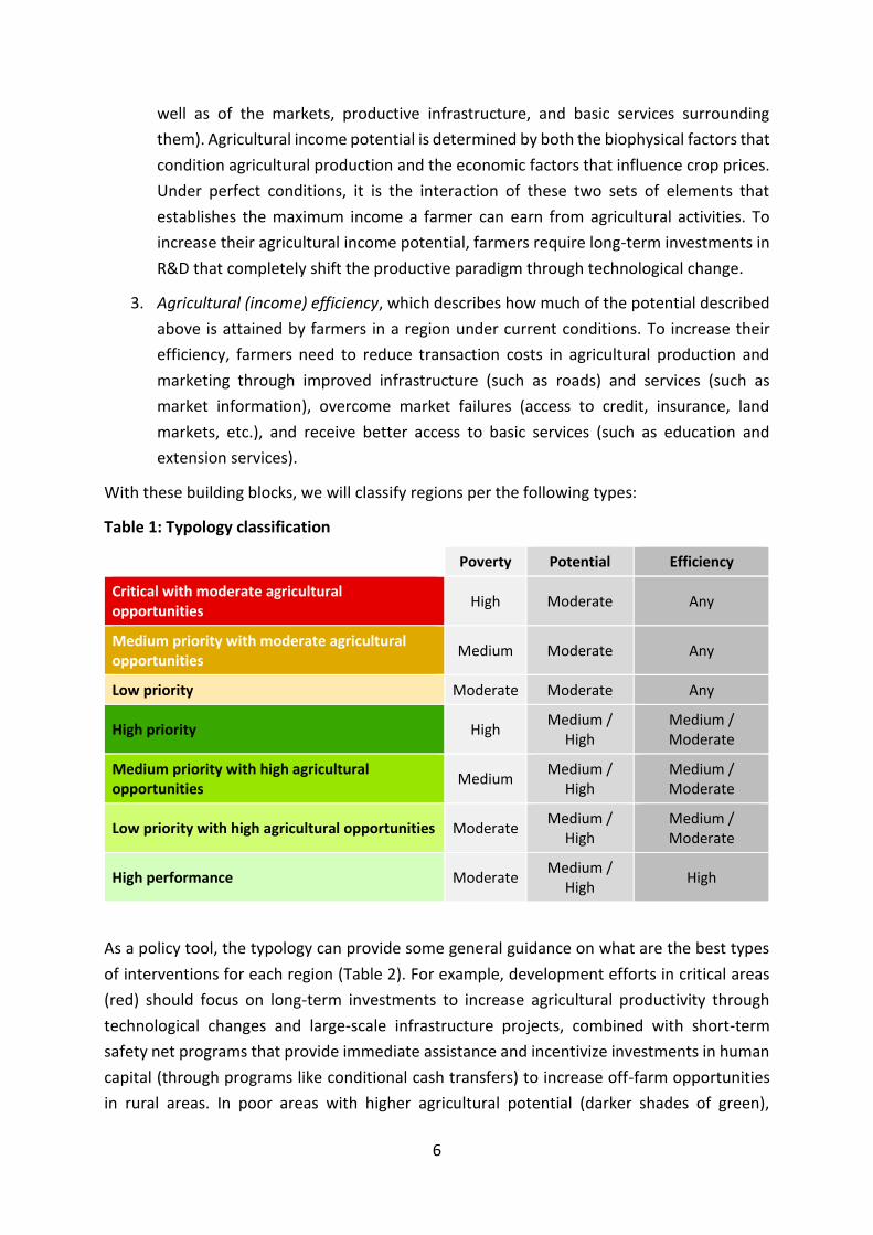
With these building blocks, we will classify regions per the following types:

Table 1: Typology classification

Poverty Potential Efficiency

Critical with moderate agricultural opportunities

High Moderate Any

Medium priority with moderate agricultural opportunities

Medium Moderate Any

Low priority Moderate Moderate Any

High priority High Medium /

High Medium / Moderate

Medium priority with high agricultural opportunities

Medium Medium /


Low priority with high agricultural opportunities Moderate Medium /


High performance Moderate Medium /

High High

As a policy tool, the typology can provide some general guidance on what are the best types

of interventions for each region (Table 2). For example, development efforts in critical areas

(red) should focus on long-term investments to increase agricultural productivity through

technological changes and large-scale infrastructure projects, combined with short-term

safety net programs that provide immediate assistance and incentivize investments in human

capital (through programs like conditional cash transfers) to increase off-farm opportunities

in rural areas. In poor areas with higher agricultural potential (darker shades of green),

7

innovation investments should focus on reducing the inefficiencies that are preventing

farmers in those regions from performing closer to the frontier. While not necessarily a

priority from the poverty reduction perspective, farmers in high performing areas (light green)

should be the focus of analysis as potential drivers for farmer-led innovation, and be the

recipients of institutional innovations (through vertical and horizontal integration) that allow

for better linkages with urban and export markets and obtain higher prices for their output

through improvements in quality and certification processes.

Table 2: Typology classes and examples of interventions

Typology class

Description Examples of recommended innovations

Critical High poverty, moderate potential

Long-term investments in agriculture such as funding R&D activities to generate technological changes and major investments in infrastructure.

Short-term assistance programs such as conditional cash transfers that incentivize human capital investments are recommended.

High priority High poverty, medium/high potential, medium/moderate efficiency

Reduction in market access costs through road improvements and price information systems (ICTs).

Innovations that allow for improved access to inputs and extension services.

Innovative inclusive financial instruments to allow for savings of harvest income towards investments in next season’s production, credit for working capital, and insurance to mitigate risk of adopting new technologies

Strengthening of horizontal and vertical integration institutions that provide better access to markets to smallholders such as farmer groups and contract farming arrangements

Medium and small-scale productive infrastructure investments such as mini-irrigation projects and land management projects.

Medium priority with high agricultural opportunities

Medium poverty, medium/high potential, medium/moderate efficiency

Low priority with high agricultural opportunities

Moderate poverty, medium/high potential, medium/moderate efficiency

High performance

Moderate poverty, medium/high potential, high efficiency

Orientation to high values and export markets.

Certification and organic production to obtain higher premiums from agricultural production.

Increased financial inclusion to allow for higher returns on profit savings, credit to purchase additional land and expand farm and non-farm businesses.

8

4 Methodological approach

4.1 Model

In our setup, we do not only consider as agricultural innovations those paradigm-shifting

technological changes that dramatically increase agricultural potential, but also the smaller

innovations that allow smallholders to catch up to their peers and larger farmers by helping

them overcome the specific challenges they face. Implicit in this setup, is the idea that there

exists a maximum or optimum level farmers can catch up to with the smaller innovations of

their own and their peers (and hence become more efficient), and an upper bound (which we

call potential) that can be increased by larger investments in R&D with the support of

governments, donors, and researchers. Hence, the approach needed to estimate the building

blocks of our typology need to acknowledge this setup.

The two most commonly used methods to estimate the efficiency of production units are data

envelopment analysis (DEA) (Charnes et al., 1978; 1981) and stochastic frontier analysis (SFA)

(Aigner et al., 1977; Meussen and van den Broeck, 1977; Battese and Corra, 1977). DEA is a

non-parametric approach that uses linear programming to identify the efficient frontier, while

SFA is a parametric approach that hypothesizes a functional form and uses the data to

econometrically estimate the parameters of that function.4 Both methods measure efficiency

as the distance between observed and maximum possible (frontier) outcomes, but the key

advantage of SFA for our purposes is that, unlike DEA, it allows to separate random noise in

the error term from the actual efficiency score. This is an important feature when analyzing

agricultural activities, which are constantly exposed and extremely sensitive to (negative and

positive) random shocks such as droughts, variation in international prices, etc. DEA estimates

a deterministic frontier that incorporates the noise as part of the efficiency score, which is

more appropriate when analyzing decision making units such as banks or factories rather than

smallholder farms in developing countries. Hence, we prefer SFA for this study since it allows

us to separate efficiency and random noise.5

The SFA approach allows the econometric exploration of the notion that, given the fixed local

agroecological and economic conditions in a micro-region and the occurrence of random

shocks that affect agricultural production (weather, prices, etc.), the investment, production

decisions and technological innovations a farmer makes translate into higher or lower

production and income. In such a context, inefficiency is defined as the loss incurred by

operating away from the frontier given the current prices and fixed factors faced by the


4 See for example Park and Simar (1994), Kumbhakar and Tsionas (2008), and Martins-Filho and Yao (2015) for

semi-parametric approaches to SFA estimation that relax some of its parametric functional form requirements. 5 The main cost or disadvantage of using SFA is that it requires more detailed data to properly model the

efficiency term and, as in any parametric approach, it relies on making the correct choice of functional form.

9


the typology. A graphical depiction of this concept is shown in Figure 3.

Figure 3: Stochastic production frontier in the single-output, single-input case

Using the basic model proposed by Aigner et al. (1977) and Meeusen & van den Broeck (1977)

depicted in Figure 3, the stochastic frontier production function is defined as:

𝑦𝑖 = 𝑓(𝑥𝑖; 𝛽)exp(𝑣𝑖 − 𝑢𝑖) (1)

where 𝑦𝑖 is the possible production for farmer 𝑖,

𝑓(𝑥𝑖; 𝛽) is an adequate function of inputs 𝑥 and parameters 𝛽,

𝑣𝑖 is a random error with zero mean, associated with random factors that are not under

the farmer’s control, and

𝑢𝑖 is a non-negative random variable associated with factors that prevent farmer 𝑖

from being efficient.

Then the possible production 𝑦𝑖 is bounded by the stochastic quantity 𝑓(𝑥𝑖; 𝛽)exp(𝑣𝑖). It is

assumed that the stochastic errors 𝑣𝑖 are i.i.d. random variables distributed 𝑁(0, 𝜎2), and

independent from 𝑢𝑖. A farmer’s technical efficiency is defined as the fraction of the frontier

production that is achieved by his current production.

10

Given the frontier production of farmer 𝑖 is 𝑦𝑖∗ = 𝑓(𝑥𝑖; 𝛽)exp(𝑣𝑖) then his technical efficiency

can be defined as:

𝑇𝐸𝑖 =𝑦𝑖

𝑦𝑖∗ =

𝑓(𝑥𝑖;𝛽)exp(𝑣𝑖−𝑢𝑖)

𝑓(𝑥𝑖;𝛽)exp(𝑣𝑖)= exp(−𝑢𝑖) (2)

Caudill & Ford (1993) and Caudill et al. (1995) showed that the presence of heteroskedasticity

in 𝑢𝑖 is particularly harmful because it introduces biases in the estimation of 𝛽 and technical

efficiency. This is very likely to occur if there exist sources of inefficiency related to factors

specific fo the producer. In this case the distribution of 𝑢𝑖 will not be the same for all the

observations in the sample and a correction for heteroskedasticity needs to be made by

modelling the variance of 𝑢𝑖:

𝜎𝑢𝑖2 = exp(𝑧𝑖𝛿) (3)

where 𝑧𝑖 are farmer-specific factors affecting his or her technical efficiency.6

4.2 Estimation

To estimate the model expressed by equations (1)-(3) it is necessary to address the fact that

farms are multi-output production units, making it necessary to move from a production

function to a profit function approach.7 The stochastic frontier profit function can be

expressed as (Kumbhakar & Lovell, 2000):

𝜋𝑖 = 𝑓(𝑝𝑖, 𝑤𝑖; 𝛽)exp(𝑣𝑖 − 𝑢𝑖) (4)

where 𝑝𝑖 and 𝑤𝑖 are output and input price vectors, respectively.

In addition to the farm-specific factors affecting the farmer’s technical efficiency, 𝑧𝑖, referred

to in (3), in an agricultural context it is necessary to consider certain production factors that

affect the farm’s potential that cannot be easily modified in the short or medium term, such

as climate and soil quality. For this reason, the farm’s potential or frontier is adjusted using

GIS data on agroecological zones or agricultural land use types. These variables are introduced

as shifters of the deterministic portion of the frontier so (4) becomes:

𝜋𝑖(𝑝, 𝑤, 𝐴𝐸𝑍) = 𝑓(𝑝𝑖, 𝑤𝑖, 𝐴𝐸𝑍𝑖 ; 𝛽)exp(𝑣𝑖 − 𝑢𝑖) (5)

where 𝐴𝐸𝑍 are the agroecological zone variables.

6 One of these farmer-specific factors particularly relevant to (the adoption of) agricultural innovations is risk

aversion. Risk aversion, and the lack of mechanisms for many smallholders to deal with risk exposure (such as loss insurance), has a clear influence on a farmer’s ability to be efficient and adopt new crops, practices, and technologies. Unfortunately, data on risk preferences is not available in the household surveys for most of the countries in this study, although it could be the subject of a country-specific study.

7 In some cases, it will be necessary to move to a revenue frontier (instead of a profit one), since most surveys lack adequate data on smallholder farming costs, particularly input prices.

11

Assuming a Cobb-Douglas production function the normalized profit or revenue frontier

function for the single output case estimated through maximum likelihood is:

ln𝜋

𝑝= 𝛿0 + ∑ 𝛿𝑛 ln

𝑤𝑛

𝑝𝑛 + ∑ 𝛿𝑞𝐴𝐸𝑍𝑞𝑞 + 𝑣𝜋 − 𝑢𝜋 (6)

To estimate equation (6) the typical data requirements are:8

- Household survey data for farm profits, producer level output and input prices, and

farm and household characteristics.

- GIS data for local agroecological characteristics, such as land use, as well as for market

access measures.

For each country, we restrict the survey sample to include only rural households involved in

agriculture that engage in output marketing and report positive revenues. It is important to

note that we do not value and incorporate the households’ own consumption into agricultural

revenues. The main reason for this is that we want our estimation to capture the difficulties

smallholders face in accessing markets. If, for example, farmers are able to sell only a small

amount of their output because they are facing severe efficiency bottlenecks, valorizing the

unsold output and counting it as revenue would completely obscure this problem and make

accessibility problems irrelevant.

Table 3 shows the effect of imposing the market orientation restriction to the survey sample

sizes in each country. While for most countries in the study market-oriented farmers represent

approximately 80% of the total number of farmers in the sample, an important fraction of the

remainder 20% reports to be storing part of the harvest for sale at a future date. For Burkina

Faso, where only 20% of the farmers report having sold any of their harvest, 98.5% of those

who have not sold yet report still having most of their harvest in storage, and 40% of them

have concrete plans to sell it soon. For Malawi, 43% of the farmers have not sold any of their

harvest, but at least half of them reported to be storing part of their production for potential

sales. While this raises concerns about the representativeness of the results based on the

constrained samples, particularly for these two countries, it also indicates that this selection

is partially caused by the timing of the surveys and the way they are rolled out, and not by

inherent differences between farmers who report having sold already and farmers who have

not. Including households that reported no agricultural income in the estimation sample

would also present a few methodological challenges.9 Ultimately, it should be acknowledged

8 In an ideal setup, data from a recent agricultural census would also be used to extrapolate regional estimates

using the survey level parameters and census level regional means. 9 When estimating profit or revenue models, SFA employs semi-flexible functional forms such as the log or

translog functions that facilitate convergence when maximizing the likelihood function (Berger and Mester, 1997). Since it is not possible to take the logarithm of a non-strictly positive value, the most common way to address zeroes or negatives in the dependent variable of a SFA estimation has been to add a positive constant to its unlogged value (Berger and Mester, 1997, Vander Vennet, 2002, Maudos et al., 2002). However, as Bos and Koetter (2011) point out, this manipulation can have undesired effects on the error term structure, which is particularly problematic in SFA, given the outcome of interest is the composition of total error, rather than coefficient estimates or marginal effects.

12

that the route we take in this study (truncating the estimation sample to positive revenue

values) has a minimal effect on the determination of the agricultural revenue potential (which

should be more influenced by the more successful market engaged farmers), but could result

in an overall upward bias in the agricultural efficiency estimates, and biased estimates of the

coefficients in the technical inefficiency heteroskedasticity correction estimation.

Table 3: Survey samples constraints

Households in the full

survey sample

Households engaged in agriculture

Households reporting

agricultural revenue

(3) / (2)

(1) (2) (3) (4)

Burkina Faso 10,441 7,347 1,489 0.203

Ethiopia 4,954 3,592 2,786 0.776

Ghana 16,772 9,100 7,262 0.798

Kenya 13,158 7,548 6,049 0.801

Malawi 12,271 10,165 5,822 0.573

Nigeria 4,582 2,842 2,162 0.761

Togo 5,532 3,521 2,739 0.778

Zambia 19,397 9,870 7,865 0.797

Source: IFPRI

Table 4 illustrates the frontier estimation results for the case of Burkina Faso.10 The

deterministic portion of the agricultural revenue frontier is determined by the prices11 of the

main crops produced by the households in the sample, and the GIS AEZ variables. An increase

in the price of a crop or the area in a specific land use type with a coefficient with a positive

and significant sign is associated with higher agricultural revenue potential. The second half

of the table reports the results of the heteroskedasticity correction of the variance of the

technical inefficiency error term. Because this term is non-negative, a positive value for the

coefficient of any of these variables indicates an increase in value associated with a decrease

in inefficiency (or increase in efficiency). For example, in the case of Burkina Faso an increase

in the landholding of a farmer is linked with decreased inefficiency, which reflects that better

access to land allows farmers to adjust to market conditions (by having more freedom to

choose at what scale to operate) and be more efficient. Under perfect land and credit market

conditions, farmers could adjust their scale by either selling, buying, renting in, or renting out

land and land size would not be a significant factor in determining efficiency.

10 SFA estimations for the other seven countries are included in Appendix 1. 11 For the estimation, we normalize and take the logarithm of all the prices and variables expressed in monetary

term.

13

With the estimation approach described above, parameter estimates are obtained that allow

for the prediction and extrapolation of agricultural income potential and efficiency measures

at the regional level, which can then be grouped and classified into types to construct the

typology. The typology then allows the identification of types of regions with extremely

different needs, bottlenecks and opportunities, which in turn will result in a different set of

investment recommendations for development in each type of region, including decisions

regarding investments in agricultural innovation.

4.3 GIS data and accessibility model

One of the factors 𝑧𝑖 influencing efficiency in Equation (3) is the degree of market accessibility

each region has. For this purpose, IFPRI has estimated an accessibility model for each of the

12 PARI countries to determine what are the time costs of accessing the closest market from

any point in a country’s territory, where “market” is defined as actual markets to trade

agricultural outputs, or as towns or cities of certain size that generate high levels of demand

for those products. To calculate this model, global geographic data on water, roads, railroads,

topography, and natural barriers publicly available from DIVA-GIS is used. GIS land cover type

data from NASA and the USGS is also used as an explanatory variable in the stochastic frontier

estimation.

4.4 Typology construction

It is worth noting that the classification above is one of several ways to classify the different

elements of the typology into types. For this study, we will focus on a method for categorizing

poverty, potential, and efficiency into moderate/medium/high classes known as “natural”

breaks.12 The natural breaks approach uses Jenks Natural Breaks algorithm13, which, similarly

to cluster analysis methods, minimizes differences within classes, and maximizes them across

classes. This approach reduces the arbitrariness in the positioning of the cutoffs between

classes, by finding “natural” breaking points that preserve clusters of “similar” units. Thus, the

category groups generated by the natural breaks approach can be very uneven, and the

resulting typology map can have fewer classes or some classes with very few regions, but it is

a more natural reflection of the underlying data.

12 The tercile breaks approach is an alternative method that splits the distribution (at the lowest tier

administrative level) of the three typology variables (potential, efficiency, and poverty) at the 33rd and 67th percentiles, effectively creating three categories (moderate, medium, and high). Classifications and maps constructed under the tercile breaks approach are available from the authors upon request.

13 See de Smith et al. (2015).

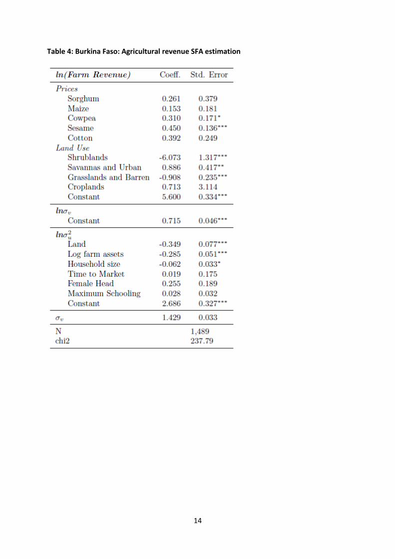
14

Table 4: Burkina Faso: Agricultural revenue SFA estimation

15

5 Results

In this section, we present the results and typology maps for Burkina Faso14, Ethiopia, Ghana,

Kenya, Malawi, Nigeria, Togo, and Zambia, with additional maps on market accessibility for

each country presented in Appendix 2. Auxiliary maps from the eAtlas are also included to

further explain the typology results.15 High resolution versions of the maps (including

shapefiles) are also available for download on the eAtlas (http://eatlas.resakss.org)

5.1 Burkina Faso

The data sources used for the estimations and mapping for Burkina Faso are:

- Household survey: Enquete Multisectorielle Continue 2013/14, publicly available

through the World Bank Microdata Catalog. It has a sample of 10,860 households, out

of which 1,489 are used for the frontier estimation, and is representative at the

national, regional, and urban/rural levels. As mentioned before, the survey does not

include information on livestock and its by-products.

- Poverty data: 2014 UNDP report Carogtaphie de la Pauvrete et des Inegalites au

Burkina Faso.

The agricultural potential map generated by the frontier estimation for Burkina Faso (Figure

4) shows a clear north – south divide. The low agricultural potential in the north of the country

results from unfavorable conditions for agriculture: predominance of shrubs, savanna and

steppe, characterized by rocky soils, and a short wet season that produces an average of 300

– 400 mm of rain per year. In contrast, the south received more than 750 mm of rain in 2013

(Figure 5).

The agricultural efficiency map (Figure 6) shows instead an east – west divide, with higher

efficiency regions appearing more often in the western side of the country. Combining

potential and efficiency into a single map by estimating the unrealized agricultural potential

(Figure 7) helps to illustrate the existing potential yet to be attained in each region (i.e., the

size of the potential or frontier gap). As expected from the patterns in the potential and

efficiency maps, the unrealized potential measure follows closely the north – south pattern of

the potential map, with larger potential gaps being found in the south of Burkina Faso, except

for the southwestern region where the high potential opportunities are offset by the high

efficiency levels. The combination of high agricultural potential in the south and high

14 Because of the questionnaire design of the household survey used for Burkina Faso, revenues from livestock

activities are not included in its frontier analysis and typology maps. 15 The years for the eAtlas maps are chosen to match as best as possible the year of each country’s household

survey used for the analysis.

16

agricultural efficiency in the west is also consistent with the production patterns of major

crops such as maize and rice (Figure 8 and Figure 9).

The poverty map for Burkina Faso (Figure 10) shows a more heterogeneous picture than the

agricultural maps, with a less obvious geographical pattern, but with lower poverty areas

concentrated in the regions of Boucle du Mouhoun, Cascades, and Hauts-Bassins in the west.

It is extremely interesting to note also that the poorest area of the country, the south-eastern

section of the Est region, is also a high (unrealized) potential area which indicates the

opportunity to reduce poverty through efficiency enhancing investments in agriculture in the

region.

Combining the potential, efficiency, and poverty estimates results in the agricultural typology

shown in Figure 11. The predominance of red (critical with moderate agricultural potential)

and orange (medium priority with moderate agricultural opportunities) areas in the north of

the country is consistent with the above average poverty rates and the poorer agroecological

conditions. While animal husbandry plays an important role in providing a source of livelihood

for rural households in this region, livestock activities were not included in the analysis for

Burkina Faso because of data limitations. Moving south to the Sub-Sahelian zone

encompassing the central and north central areas of the country, the map colors shift to light

green indicating better opportunities for agriculture (higher potential). Sorghum and millet

are two of the more important crops in this region, which is damper than the northern parts

of the country. This is also an area of higher population density, with more income generating

opportunities beyond agriculture. Still, the dark green regions in the southern half of the

country reveal pockets of high poverty areas with agricultural potential gaps that can be

targeted to improve living conditions of rural households in these areas.

Following the rationale described in Section 0, we can define two types of innovations:

efficiency enhancing and potential enhancing. Efficiency enhancing innovations help farmers

overcome bottlenecks in agricultural production and marketing in the short term, by affecting

those factors they can control. For example, improved farming and land management

practices, or access to existing technologies and knowledge, are context-specific innovations

that can help close efficiency gaps and let farmers falling behind catch up with those operating

closer to their maximum potential (frontier). Potential enhancing innovations, which are

aimed at shifting the current production frontier, usually tackle inefficiencies in stages of the

production and marketing process beyond the direct control of the farmer, and tend to yield

benefits in the longer term. This would involve R&D investments in new technologies, seeds,

and fertilizers, better adapted to specific contexts, large scale improvements of the

transportation network to reduce transaction costs and prices at the local, regional, and

national levels, etc.

Regions that would be a better target for efficiency enhancing innovations are areas that have

high potential and low efficiency (areas with high unrealized potential such as dark green

17

areas). The large efficiency gaps in these areas make them ideal for the implementation of

agricultural innovations and investments in rural development that help these areas reach

their maximum potential. Areas with low agricultural potential and above average poverty

rates (such as red areas) require instead different investments in rural development, focused

in increasing the overall farming potential of the region before increasing efficiency.

Consistent with our discussion of the typology map results, potential enhancing innovations

are most needed in the north of the country, where conditions for agriculture are less

favorable, while efficiency enhancing innovations would yield greater returns in the center

and south, where the agricultural potential gaps are large.

Figure 4: Burkina Faso: Agricultural potential

18

Figure 5: Burkina Faso: Annual precipitation (mm), 2013

Figure 6: Burkina Faso: Agricultural efficiency

19

Figure 7: Burkina Faso: Unrealized agricultural potential

Figure 8: Burkina Faso: Maize production (Tons), 2013

20

Figure 9: Burkina Faso: Rice production (tons), 2013

Figure 10: Burkina Faso: Poverty map

21

Figure 11: Burkina Faso: Agricultural typology

5.2 Ethiopia

The data sources used for the estimations and mapping for Ethiopia are:

- Household survey: The Ethiopia Socioeconomic Survey Wave Three 2015/16, publicly

available through the World Bank Microdata Catalog. It has a sample of 4,954

households, out of which 2,786 are used for the frontier estimation, and is

representative at the national and urban/rural levels.

- Poverty data: Oxford Poverty and Health Development Initiative.

Ethiopia’s geography is characterized by mountains running from north to south, separated

by the Rift Valley running southwest to northeast, and by the lowlands in the Northeast and

south-western portions of the country. Rainfall is also generally correlated with altitude, with

higher elevations receiving much more precipitation than lowlands. Regions above 1,500

meters receive above 900 mm annually while lower lying areas average receive below 600 mm

(Figure 12). The exception to this is the western most portions of the country where the

lowlands do receive substantial rainfall, which explains the lower poverty rates and higher

agricultural potential in the area (Figure 13 and Figure 14). While not well suited for crop

farming due to limited rainfall, the northern half of the Afar region shows high potential while

some areas in the Somali region show medium potential levels due to the importance of

22

animal husbandry in this part of the country. In both regions, livestock revenue makes up 85%

and 93% of farm revenue respectively, compared to an average of approximately 50% in the

rest of the country.

The regional efficiency levels (Figure 15) combined with the agricultural potential determine

the location of the largest potential gaps (Figure 16). The areas with the highest unrealized

potential levels can be found in Afar and Benishangul-Gumaz.

The typology map (Figure 17) shows that most regions of the country are considered high

priority (dark green) and critical (red) areas. The natural breaks approach finds that the

differences in poverty levels across regions are too small to separate them and classifies most

of the country in the high poverty class, except for Tigray and Gambela. The high priority

regions would benefit the most from efficiency enhancing innovations, due to their high

poverty rates and large potential gaps.

Figure 12: Ethiopia: Annual precipitation (mm), 2015

23

Figure 13: Ethiopia: Poverty map

Figure 14: Ethiopia: Agricultural potential

24

Figure 15: Ethiopia: Agricultural efficiency

Figure 16: Ethiopia: Unrealized agricultural potential

25

Figure 17: Ethiopia: Agricultural typology

5.3 Ghana

The data sources used for the estimations and mapping for Ghana are:

- Household survey: The Ghana Living Standards Survey 6 2012/2013, available through

the Ghana Statistical Service and the World Bank. It has a sample of 16,772 households,

out of which 7,262 are used for the frontier estimation, and is representative at the

national and regional levels.

- Poverty data: Ghana Poverty Mapping Report from the Ghana Statistical Service

(2015).

Agricultural practices in Ghana are largely determined by rainfall patterns (Figure 18), which

increases moving from north to south with the northern regions receiving less than 1,100 mm

annually and the southern portions receiving over 2,000 mm. The exception to this is the

south-eastern coast, which is one of the driest areas of the country receiving on average of

750 mm per year. The agricultural potential map in Figure 19 reflects this pattern well with

the lower potential areas in the north and the high potential areas, with a few exceptions, in

the southwest. The area around the Volta Lake region, while offering an additional water

source in some of the drier portions of the country has generally poor soil quality. However,

the northern region also has abundant grassland which helps explain the cluster of high and

26

medium potential regions scattered through the upper portion of the Volta Lake due to the

potential for livestock production.

The agricultural efficiency map on the left panel of Figure 21 shows pockets of high efficiency

concentrated in the northeast and southwest of the country. A clearer pattern emerges once

this efficiency map is combined with the potential map, as shown on Figure 20. The unrealized

agricultural potential map (Figure 21) shows the current potential yet to be attained in each

region (i.e., inefficiency × agricultural potential, where inefficiency = 1 - efficiency). The high

efficiency areas in the northeast are also low potential regions, and therefore leave little

potential left to be exploited without frontier shifting innovations. Medium to high unrealized

potential opportunities emerge in the central areas of the country due to the combination of

medium agricultural efficiency and potential. And for most of the southern regions of Ghana,

but particularly for the south west, the high levels of agricultural potential make efficiency-

oriented innovation investments attractive regardless of the current levels of efficiency.

The poverty map in Figure 22 reveals a pattern that is the mirror opposite of the agricultural

potential map, with poverty rates increasing from south to north, and particularly towards the

northwest.

The combination of the potential, efficiency, and poverty dimensions results in the agricultural

typology shown in Figure 23. The typology map displays and expands the patterns from the

previous maps, showing most of the better off areas (high performance class in light green) in

the cocoa producing region of the south west, and more pockets of high poverty regions

appearing moving north (shaded in dark green and red depending on the level of unrealized

agricultural potential). Following these patterns, efficiency enhancing innovations are better

suited for the south of the country, while potential enhancing innovations are ideal for the

northwest and the poor soil quality areas around the Volta Lake.

27

Figure 18: Ghana: Annual precipitation (mm), 2013

28

Figure 19: Ghana: Agricultural potential

29

Figure 20: Ghana: Agricultural efficiency

30

Figure 21: Ghana: Unrealized agricultural potential

31

Figure 22: Ghana: Poverty map

32

Figure 23: Ghana: Agricultural typology

5.4 Kenya

The data sources used for the estimations and mapping for Kenya are:

- Household survey: The Kenya Integrated Household Budget Survey 2005/2006,

available through the National Data Archive of the Kenya National Bureau of Statistics.

It has a sample of 13,390 households, out of which 6,049 are used for the frontier

estimation, and is representative at the national, provincial, and district levels.

- Poverty data: Basic Report on Well-Being in Kenya from the Kenya National Bureau of

Statistics.

33

Agricultural potential (Figure 24) in Kenya is driven by rainfall patterns, elevation, and local

vegetation characteristics. Rainfall is higher in the southern half of the country (see Figure 25),

and the combination of high precipitation, better soil quality, higher elevations and cooler

temperatures in areas of the (former) Central province and the south of the Rift Valley

province allow to produce staple crops and cash crops such as coffee and tea. The maize

producing region slightly inland from the coast with the Indian Ocean also has medium to high

agricultural potential. Livestock is a stronger driver for the high potential in the grass areas of

the north east of Kenya, where rainfall is lower and temperatures are higher. The areas around

Lake Victoria are associated with higher population density and more opportunities to

diversify incomes for rural households beyond agriculture which explains their low potential

levels.

Combining the agricultural potential with the agricultural efficiency estimates (Figure 26)

makes it possible to identify where are the areas with the best opportunities for agricultural

growth (Figure 27). Due to a combination of higher potential and lower efficiency, the cash

cropping regions of the Central and Rift Valley provinces, the maize producing region of the

Coast province, and particularly the livestock oriented areas of the North-Eastern province

present the largest gaps in terms of potential which can be attained by making investments

oriented to increase agricultural efficiency.

Combining the agricultural potential and efficiency estimates with poverty figures (Figure 28)

results in the tercile breaks typology shown in Figure 29. The high poverty areas concentrated

in the pastoral lands of the North Eastern and Coast regions also have high unrealized

agricultural potential (darker blue areas in Figure 27) which make then high priority regions

(dark green in Figure 29) for efficiency enhancing innovations in livestock production. Some

smaller areas located in the cereal oriented Eastern and Rift Valley regions (maize, millet,

sorghum) also show considerable potential gaps and should be targeted for efficiency

enhancing innovations. Low potential regions that would benefit from potential enhancing

innovations are more dispersed, but are slightly more concentrated in the maize producing

southern section of the Coast region and the livestock oriented areas around Lake Turkana in

the Rift Valley region.

34

Figure 24: Kenya: Agricultural potential

35

Figure 25: Kenya: Annual precipitation (mm), 2005

36

Figure 26: Kenya: Agricultural efficiency

37

Figure 27: Kenya: Unrealized agricultural potential

38

Figure 28: Kenya: Poverty map

39

Figure 29: Kenya: Agricultural typology

5.5 Malawi

The data sources used for the estimations and mapping for Malawi are:

- Household survey: The Integrated Household Survey 3 2010/2011, publicly available

through the World Bank Microdata Catalog. It has a sample of 12,271 households, out

of which 5,822 are used for the frontier estimation, and is representative at the

national, regional, district, and urban/rural levels.

- Poverty data: The Integrated Household Survey 3 2010/2011.

40

The higher precipitation levels and the agroecological suitability for horticulture in the

Kasungu Lilongwe Plain (central), and the staple crop producing areas in the north (such as

Chipita) explain the high agricultural potential in the northern and central regions of Malawi

(Figure 30). This pattern is consistent with the production data available for several crops in

the eAtlas, such as maize (Figure 31) and tobacco (Figure 32). The southern region suffers from

lower potential due to poorer general weather conditions and lower rainfall levels (Figure 33),

which limit the length of the growing periods (less than 120 days in a year). The districts of

Chikwawa and Nsanje are an exception to this, and show higher potential than the rest of the

southern region due to large scale irrigation projects that create opportunities for growing

cash crops in the area.

The spatial distribution of agricultural efficiency (Figure 34) follows a similar pattern than the

distribution of agricultural potential, with higher levels in the northern half of the country. The

unrealized potential map (Figure 35) shows that despite the high levels of efficiency, potential

in the north is high enough for the remaining gap to be significant, and that the levels of

efficiency in the southern tip of the country are low enough to offer some opportunities for

efficiency enhancing innovations in those areas as well.

Poverty rates in Malawi follow a similar spatial pattern, with higher poverty rates in the south

than in the north of the country (Figure 36). Combining the three typology variables, the result

is a predominance of low and medium priority areas with high agricultural potential in the

north, and critical and high priority areas in the south (Figure 37). Areas in the different shades

of green in the typology (darker shades of green indicate higher poverty levels) are areas

where efficiency enhancing innovations would be suitable, particularly those in which the

levels of unrealized potential are high, including small sections of the districts of Mzimba and

Nkhata Bay in the northern region with high potential for coffee and tea production under

irrigation. Investments in innovations that enhance agricultural potential or expand the

technological frontier should target areas with moderate agricultural potential and medium

to high poverty levels (orange and red), which are more predominant in the southern region.

41

Figure 30: Malawi: Agricultural potential

42

Figure 31: Malawi: Maize production (tons), 2011

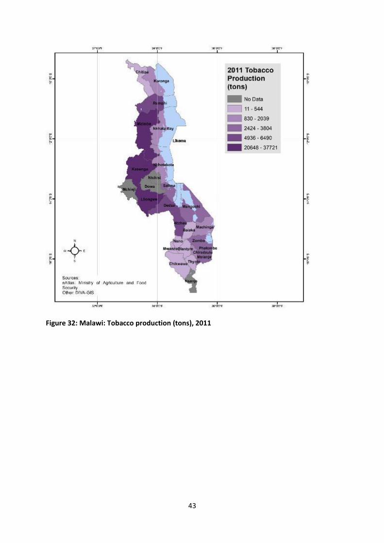
43

Figure 32: Malawi: Tobacco production (tons), 2011

44

Figure 33: Malawi: Annual precipitation (mm), 2011

45

Figure 34: Malawi: Agricultural efficiency

46

Figure 35: Malawi: Unrealized agricultural potential

47

Figure 36: Malawi: Poverty map

48

Figure 37: Malawi: Agricultural typology

5.6 Nigeria

The data sources used for the estimations and mapping for Nigeria are:

- Household survey: The General Household Survey Wave 3 2015/2016, publicly



representative at the national, zonal, and urban/rural levels.

- Poverty data: Nigeria Poverty Profile 2010 from the National Bureau of Statistics.

The agricultural potential map for Nigeria (Figure 38) shows a high concentration of areas with

potential for agricultural activities in the south-western zone, as well as some in the northern

central zone. The high potential in the south-western zone comes from the income generating

opportunities associated with cash crop farming including cocoa and palm oil, and coastal

49

fishing activities from Lagos to Port Harcourt. In the northern central zone, areas in the central

highland and plain regions around Abuja show high potential due to the vast web of rivers and

water sources and a relatively dense zone for irrigation development that can be further

exploited given this area’s ideal location close to large urban markets. The general spatial

pattern show in the agricultural potential map is supported by the annual precipitation

pattern shown in Figure 39.

The agricultural efficiency map and the unrealized potential map are shown in Figure 40 and

Figure 41. The combination of high efficiency levels and low potential in the North-East zone

(particularly the states of Bauchi, Gombe, and Taraba) result in low levels of potential left to

be gained without investing in frontier shifting innovations. Alternatively, high efficiency areas

in the south-western and Northern central zones still have significant unrealized potential

gaps due to the underlying high potential levels. The northern border area limiting with Niger

also displays high levels of unrealized potential due to a combination of medium levels of

potential and low to medium levels of efficiency.

The poverty map (Figure 42) generally follows a similar spatial pattern as the agricultural

potential map, with high potential areas showing lower levels of poverty. Figure 43 shows the

agricultural typology map resulting from combining potential, efficiency, and poverty. In

general, better performing areas are in the south-western zone of the country, and higher

priority and critical regions become more common moving towards the northeast. This

reflects the higher agricultural potential and lower poverty rates of the south-western zone,

as well as the relatively less friendly agricultural environment in the Sahelian region towards

the north and northeast. However, potential enhancing innovations should be considered in

this area due to the local predominance of staple crops such as maize, yam, potatoes,

sorghum, millet, cowpeas, etc. which are key for food security of rural households.

50

Figure 38: Nigeria: Agricultural potential

51

Figure 39: Nigeria: Annual precipitation (mm), 2015

52

Figure 40: Nigeria: Agricultural efficiency

53

Figure 41: Nigeria: Unrealized agricultural potential

54

Figure 42: Nigeria: Poverty map

55

Figure 43: Nigeria: Agricultural typology

5.7 Togo

The data sources used for the estimations and mapping for Togo are:

- Household survey: Questionnaire des Indicateurs de Base de Bien-Être 2011, publicly



representative at the national and subgroup level (Grand Lom Lomé, other towns, rural

south and rural north).

- Poverty data:

http://www.arcgis.com/home/item.html?id=d4b4fe7952014d61879007c83ac374e4

Despite being one of the smallest countries of West Africa, Togo’s territory covers several

bioclimatic regions and this heterogeneity is reflected in the agricultural potential map (Figure

44). Northern Togo is characterized by the seasonal Sudanian climate, with a single rainy

56

season, which is reflected in the annual precipitation map from the eAtlas (Figure 45).

Agriculture is gaining ground to the woodlands and savannas that are predominant in the

north, but this region’s exposure to dry Harmattan winds and proneness to drought (as seen

by the red areas in Figure 46) results in low agricultural potential. The wooded landscapes and

isolated dense tropical forest remnants in the Togo (Atacora) mountain range crossing the

Centre region also results in low potential for agriculture. The southern half of the country

falls into the Guinean climatic region, characterized by two rainy seasons and higher

agricultural potential. The coastal area, however, is part of the Dahomey Gap, a relatively dry

savanna zone receiving an average of only 900 mm of rainfall per year and reduced agricultural

potential.

Combining agricultural potential (Figure 44) with agricultural efficiency (Figure 47) results in

the unrealized potential map (Figure 48). Low potential and high efficiency levels in the north

(Savanes) result in little agricultural potential left to be exploited without investing in frontier

shifting innovations. The highest unrealized potential levels are found under the favorable rain

and agroecological conditions of the Guinean climate in the Plateaux region, especially around

the “cocoa-coffee triangle” formed by Kpalimé , Badou and Atakpamé with naturally rich soils

and humid and warm climate. Figure 49 shows that poverty follows the spatial pattern of the

agricultural potential map, with high potential areas being associated with lower poverty

rates, with the exception of the Maritime region where the proximity to Lomé and other major

urban centers reduces the importance of the role of agriculture as the major source of income.

The agricultural typology map is shown in Figure 50. The high poverty areas in the Savanes

region (north) and the Centre region fall in different classes due to the differences in their

agricultural potential classification, with the north falling in the critical (red) class due to its

moderate potential, and the Centre region falling in the high priority class due to its medium

potential classification. The high potential Plateaux region combines high, medium and low

priority areas (shades of green) which result from how the tercile breaks approach classifies

poverty levels in this region. High performance regions appear in the Plateaux region

consistent with the high productivity and income generating capacity of areas like the cocoa-

coffee triangle.

57

Figure 44: Togo: Agricultural potential

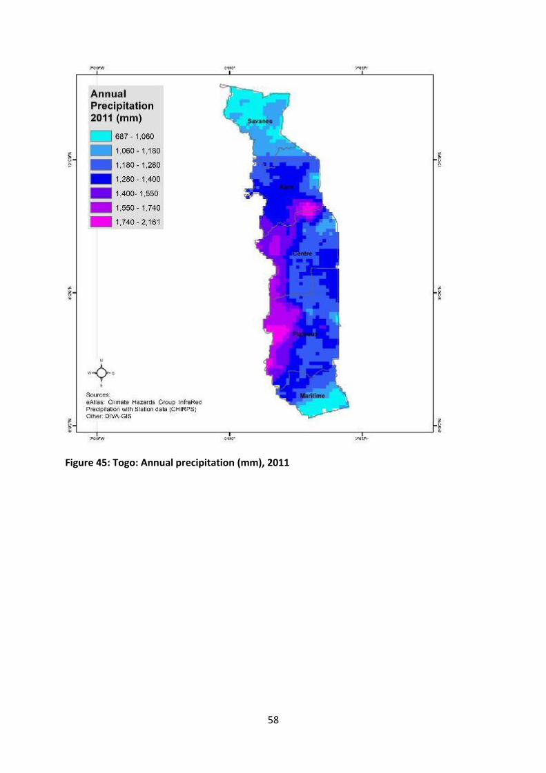
58

Figure 45: Togo: Annual precipitation (mm), 2011

59

Figure 46: Togo: Precipitation condition index, 2014

60

Figure 47: Togo: Agricultural efficiency

61

w

Figure 48: Togo: Unrealized agricultural potential

62

Figure 49: Togo: Poverty map

63

Figure 50: Togo: Agricultural typology

5.8 Zambia

The data sources used for the estimations and mapping for Zambia are:

- Household survey: The Living Conditions Monitoring Survey 2010, available through

the Zambia National Data Archive and the World Bank. It has a sample of 20,000


representative at the national, provincial, and urban/rural levels.

- Poverty data: Mapping Subnational Poverty in Zambia from the Central Statistics Office

(2015).

Figure 51 shows the agricultural potential map for Zambia. The favorable agroecological

conditions for maize and livestock in the Eastern region combined with the good access to

urban markets explain the high agricultural potential of the Eastern region. The Southern

64

region is also a large maize producer (Figure 52), but lower rainfall levels (Figure 53) explain

its mix of medium to low potential. The high potential area covering the Central province

results from a combination of high soil quality and an intermediate amount of rainfall. While

the Northern Province has high rainfall and humidity, problems with soil acidity explain its

overall lower agricultural potential, and the higher presence of areas suitable for potential

enhancing innovations, as in the Western region, which is the driest part of the country.

The combination of potential with efficiency (Figure 54) produces the unrealized potential

map in the central panel of Figure 55. While several regions of the map show areas with limited

unrealized potential gaps, this is particularly problematic in the Western, Luapula, and

Northern provinces where poverty levels are high (Figure 56).

The agricultural typology is shown in Figure 57. High poverty rates and low agricultural

potential explain the areas in the critical (red) class in the Western, Luapula, and Northern

provinces. Located east from both of these critical areas are high priority zones, while also

suffering from high poverty offer large unrealized potential gaps. The central stretch of the

country (Copperbelt, Central, Lusaka, and Southern provinces) fall into the high performance

or low priority classes. In general, a mix of efficiency enhancing and potential enhancing

innovations appear to be necessary in the east and west of the country to tackle their higher

poverty rates.

65

Figure 51: Zambia: Agricultural potential T

66

Figure 52: Zambia: Maize production (tons), 2011

67

Figure 53: Zambia: Annual precipitation (mm), 2010

68

Figure 54: Zambia: Agricultural efficiency

69

Figure 55: Zambia: Unrealized agricultural potential

70

Figure 56: Zambia: poverty map

71

Figure 57: Zambia: Agricultural typology

72

6 Concluding remarks



collaboration with all relevant actors. Agricultural development depends on innovation, which

is the result of a complex system of interactions that takes place in an environment

characterized by its multidimensional nature (biophysical, technological, sociocultural,

economic, institutional, and political). Understanding the biophysical and economic

dimensions of the environment in which agriculture and agricultural innovation take place

requires an approach that combines economic, statistical, and spatial analysis tools.

Several of the studies have linked agricultural potential and need-based criteria to target

development oriented investments by combining agroecological and poverty data, but have

ignored the role markets play in the process of innovation. For investments in agricultural

innovation to be sustainable, farm-level increases in productivity need to be translated into

higher incomes and better livelihoods for rural households. Our proposed approach attempts

to bridge that gap by mapping estimates of agricultural potential and efficiency under the

framework of production theory applied to agriculture by combining agroecological, poverty,

market, and farm-level information.

The idea behind the concept of agricultural innovation is to allow agricultural education,

research, and extension to contribute substantially to enhance agricultural production and

reduce rural poverty. Hence, when deciding where to invest and introduce innovations in

agriculture, priority should be given to areas where rural poverty is high and increases in

agricultural production would be more beneficial. However, high poverty areas can be very

heterogeneous both in terms of what their current agricultural potential is, and how much of

it farmers are able to attain by operating efficiently.

In our setup, we do not only consider as agricultural innovations those paradigm-shifting

technological changes that dramatically increase agricultural potential, but also the smaller

innovations that allow smallholders to catch up to their peers and larger farmers by helping

them overcome the specific challenges they face. Implicit in this setup, is the idea that there

exists a maximum or optimum level farmers can catch up to with smaller innovations of their

own and their peers (and hence become more efficient), and an upper bound (which we call

potential) that can be increased by larger investments in R&D with the support of

governments, donors, and researchers.

The SFA approach allows the econometric exploration of the notion that, given the fixed local

agroecological and economic conditions in a micro-region and the occurrence of random

shocks that affect agricultural production (weather, prices, etc.), the investment, production

decisions and technological innovations a farmer makes translate into higher or lower

production and income. In such a context, inefficiency is defined as the loss incurred in by

73

operating away from the frontier given the current prices and fixed factors faced by the



the typology.

Our series of maps for the eight different countries included in this study (Burkina Faso,

Ethiopia, Ghana, Kenya, Malawi, Nigeria, Togo, and Zambia) highlight the degree of

heterogeneity in the potential and efficiency levels of agriculture across and within countries.

Our analysis recognizes that different types of innovation approaches are necessary for areas

in which farmers are operating close to their maximum potential or far from it, and identifies

areas in which investments are more necessary to alleviate poverty. While the goal for this

report was to create a consistent set of results and maps for all 8 countries, our hope is that

through AGRODEP and the network of country partners in PARI, we can extend and enrich this

work by focusing this methodology to specific countries, regions, and value chains to better

identify efficiency bottlenecks and match them with relevant solutions and innovations.

74

References

Aigner, D. J., Lovell, C. A., & Schmidt, P. (1977). Formulation and Estimation of Stochastic

Frontier Production Function Models. Journal of Econometrics, 6, 21-37.

Anderson, J. R., Hardy, E. E., Roach, J. T., & Witmer, R. E. (1976). A Land Use And Land Cover

Classification System For Use With Remote Sensor Data. Geological Survey Professional

Paper 964, United States Government Printing Office, Washington.

Battese, J. E., and Corra, G. S. (1977). Estimation of a Production Frontier Model: With

Application to the Pastoral Zone of Eastern Australia. Australian Journal of Agricultural

Economics, 21(3), 169-79.

Berger, A. N., & Mester, L. J. (1997). Inside the Black Box: What Explains Differences in the

Efficiencies of Financial Institutions. Journal of Banking & Finance, 21, 895–947.

Bidogeza, J. C., Berentsen, P. B. M., De Graaff, J., & Oude Lansink, A. G. J. M. (2009). A typology

of farm households for the Umutara Province in Rwanda. Food Security, 1, 321-335.

Bigman, D., & Fofack, H. (2000). Geographic Targeting for Poverty Alleviation. Methodology

and Applications. Regional and Sectoral Studies 21089, World Bank, Washington.

Bigman, D., & Loevinsohn, M. (2003). Targeting agricultural research and development for

poverty reduction: general principles and an illustration for sub-Saharan Africa. In:

Mathur, S., Pachico, D. (Eds.), Agricultural Research and Poverty Reduction: Some Issues

and Evidence. Centro Internacional de Agricultura Tropical Publication no. 335, Economics

and Impact Series no. 2, Cali, Colombia.

Bos, J. W. B., & Koetter, M. (2011). Handling losses in translog profit models. Applied

Economics, 43(3), 307-312.

Bryan, B. A., King, D., & Ward, J. R. (2011). Modelling and mapping agricultural opportunity

costs to guide landscape planning for natural resource management. Ecological

Indicators, 11, 199-208.

Byerlee, D. (2000). Targeting poverty alleviation in priority setting for agricultural research.

Food Policy, 25(4), 429-445.

Caudill, S. B., & Ford, J. M. (1993). Biases in Frontier Estimation Due to Heteroskedasticity.

Economic Letters, 41, 17-20.

75

Caudill, S. B., Ford, J. M., & Gropper, D. M. (1995). Frontier Estimation and Firm-Specific

Inefficiency Measures in the Presence of Heteroskedasticity. Journal of Business and

Economic Statistics, 13, 105-111.

Charnes, A., Cooper, W. W., Lewin, A. Y., & Seiford, L. M. (1978). Measuring the Efficiency of

Decision Making Units. European Journal of Operational Research, 2(6), 429-444.

Charnes, A., Cooper, W. W., & Rhodes, E. (1981). Evaluating Program and Managerial

Efficiency: An Application of Data Envelopment Analysis to Program Follow Through.

Management Science, 27(6), 668-697.

de Smith, M., Goodchild, M., & Longley, P. (2015). Geospatial Analysis – A comprehensive

guide. http://www.spatialanalysisonline.com/HTML/index.html.

Deichmann, U. (1999). Geographic aspects of inequality and poverty.

http://www.worldbank.org/poverty/inequal/index.htm.

Elbers, C., Lanjouw, J.O. & Lanjouw, P. (2001). Welfare in villages and towns: micro-level

estimation of poverty and inequality. World Bank.

FAO (1978). Report on Agro-Ecological Zones Project. Vol 1. Methodology and Results for

Africa. World Soil Resources Report #48. FAO: Rome.

Fischer, G., van Velthuizen, H., Shah, M., & Nachtergaele, F. (2002). Global Agro-ecological

Assessment for Agriculture in the 21st Century: Methodology and Results. IIASA: Austria

& FAO: Rome.

Funtowicz, S. O., & Ravetz, J. R. (1993). Science for the post-normal age. Futures, 25, 739-755.

Giller, K. E., Leeuwis, C., Andersson, J. A., Andriesse, W., Brouwer, A., Frost, P., et al. (2008).

Competing claims on natural resources: What role for science? Ecology and Society, 13,

34.

Hardiman, R. T., Lacey, R., & Mu Yi, Y. (1990). Use of Cluster Analysis for Identification and

Classification of Farming Systems in Qingyang County, Central North China. Agricultural

Systems, 33, 115-125.

Hentschel, J., Lanjouw, J.O., Lanjouw, P., & Poggi, J. (2000). Combining census and survey data

to trace the spatial dimensions of poverty: a case study of Ecuador. World Bank Economic

Review, 14, No. 1: 147-165.

Kumbhakar, S. C., & C. A. K. Lovell (2000). Stochastic Frontier Analysis. Cambridge University

Press.

76

Kumbhakar, S. C., & Tsionas, E. G. (2008). Scale and efficiency measurement using a

semiparametric stochastic frontier model: evidence from the U.S. commercial banks.

Empirical Economics, 34(3), 585-602.

Lanjouw, P. (1998). Ecuador’s rural nonfarm sector as a route out of poverty. World Bank,

Policy Research Working Paper No. 1904.

Loveland, T. R., Reed, B. C., Brown, J. F., Ohlen, D. O., Zhu, Z., Yang, L., & Merchant, J. W.

(2000). Development of a global land cover characteristics database and IGBP DISCover

from 1 km AVHRR data. International Journal of Remote Sensing, 21:6-7.

Martins-Filho, C., & Yao, F. (2015). Semiparametric Stochastic Frontier Estimation via Profile

Likelihood. Econometric Reviews, 34(4), 413-451.

Maudos, J., Pastor, J. M., Pérez, F., & Quesada, J. (2002). Cost and Profit Efficiency in European

Banks. Journal of International Financial Markets, Institutions and Money, 12, 33-58.

Meeusen, W., & van den Broeck, J. (1977). Efficiency Estimation from Cobb-Douglas

Production Functions with Composed Error. International Economic Review, 18, 435-444.

OECD (2009). Growing Prosperity. Agriculture, Economic Renewal, and Development. Draft

Outcome Document from the Experts Meeting “Innovating Out of Poverty,” OECD, Paris,

April 6–7.

Park, B. U., & Simar, L. (1994). Efficient Semiparametric Estimation in a Stochastic Frontier

Model. Journal of the American Statistical Association, 89(427), 929-936

Schut, M., van Passen, A., Leeuwis, C., y Klerkx, L. (2014). Towards dynamic research

configurations: A framework for reflection on the contribution of research to policy and

innovation processes. Science and Public Policy 41, 207-218.

Spielman, D. J., Ekboir, J., y Davis, K. (2009). The art and science of innovation systems inquiry:

Applications to Sub-Saharan African agriculture. Technology in Society, 31, 399-405.

Vander Vennet, R. (2002). Cost and Profit Efficiency of Financial Conglomerates and Universal

Banks in Europe. Journal of Money, Credit, and Banking, 34, 254-282.

World Bank (2012). Agricultural innovation systems: An investment sourcebook. The World

Bank, Washington, DC.

77

Appendix 1: SFA estimation results

Table 5: Ethiopia: Agricultural revenue SFA estimation results

78

Table 6: Ghana: Agricultural revenue SFA estimation results

79

Table 7: Kenya: Agricultural revenue SFA estimation results

80

Table 8: Malawi: Agricultural revenue SFA estimation results

81

Table 9: Nigeria: Agricultural revenue SFA estimation results

82

Table 10: Togo: Agricultural revenue SFA estimation results

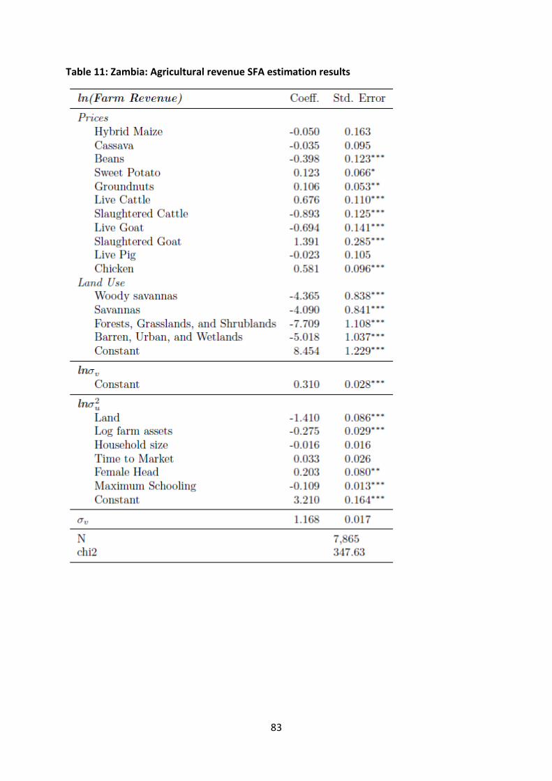
83

Table 11: Zambia: Agricultural revenue SFA estimation results

84

Appendix 2: Accessibility maps

Figure 58: Burkina Faso: Accessibility

85

Figure 59: Ethiopia: Accessibility

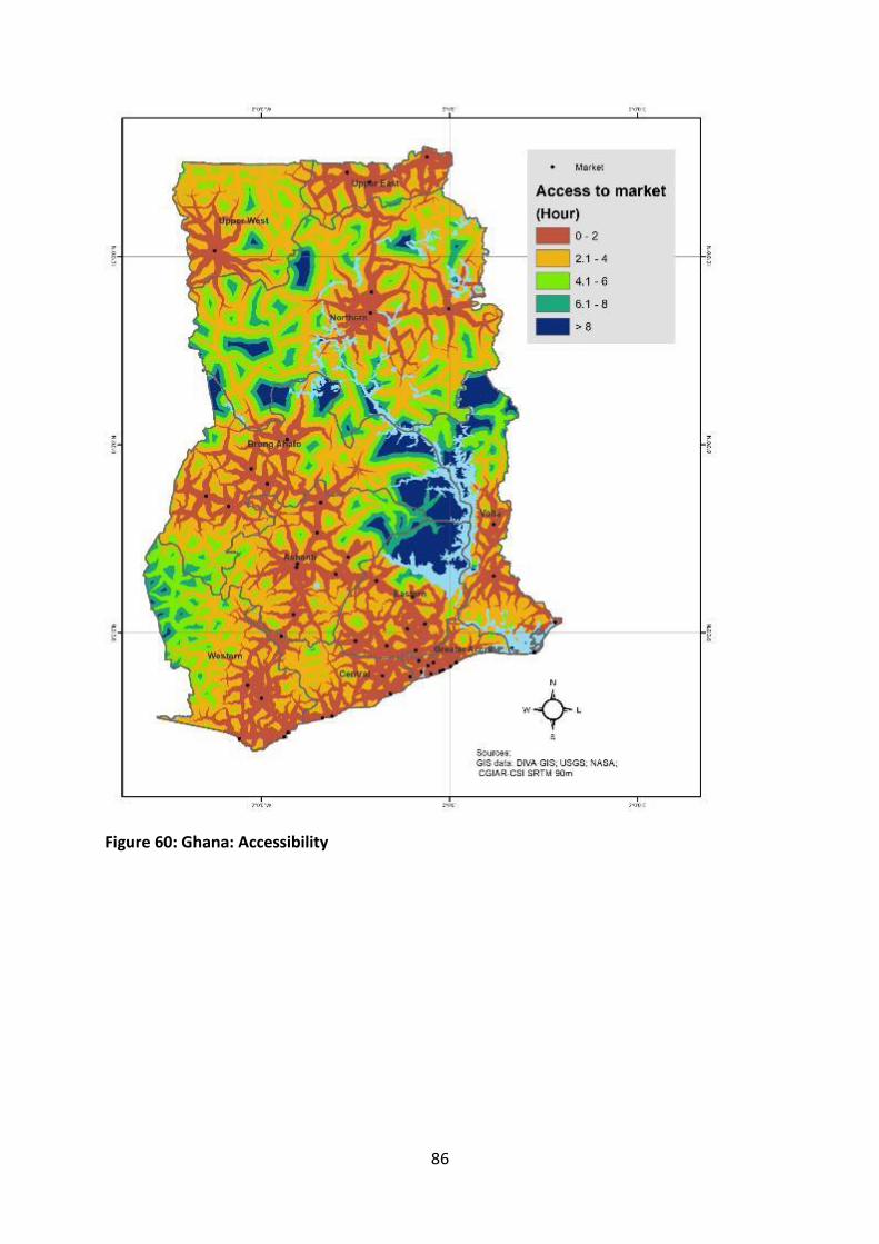
86

Figure 60: Ghana: Accessibility

87

Figure 61: Kenya: Accessibility

88

Figure 62: Malawi: Accessibility

89

Figure 63: Nigeria: Accessibility

90

Figure 64: Togo: Accessibility

91

Figure 65: Zambia: Accessibility

Frontier analysis and agricultural typologies - AGRODEP

Documents

Transcript of Frontier analysis and agricultural typologies - AGRODEP