TRANSPORT SAFETY PERFORMANCE IN THE EU A STATISTICAL OVERVIEW
Upload
khangminh22Category
view
1download
0
A STATISTICAL ANALYSIS OF STUDENT
PERFORMANCE FOR THE 2000-2013 PERIOD
AT THE COPPERBELT UNIVERSITY IN
ZAMBIA
By
Mwanabute Ngoy
Dissertation presented for the degree of Doctor of Philosophy in the
Faculty of Economics and Management Sciences
at
Stellenbosch University
Promoter: Prof. N.J. Le Roux
December 2017

ii
DECLARATION
By submitting this dissertation electronically, I declare that the entirety of the work contained therein
is my own, original work, that I am the sole author thereof (save to the extent explicitly otherwise
stated), that reproduction and publication thereof by Stellenbosch University will not infringe any third
party rights and that I have not previously in its entirety or in part submitted it for obtaining any
qualification.
Date: December 2017.
Copyright 2017 Stellenbosch University
All rights reserved
I declare that an official permission was granted by The Deputy Vice-Chancellor’s Office, the
Registrar’s Office, and the Directorate of Information and Communication Technology from
the CBU, and also from the ECZ Headquarters to obtain and use all data in this thesis.
Additionally, random identification numbers were allocated where needed so as to remove
any direct link between a particular person and his/her data.
Stellenbosch University https://scholar.sun.ac.za

iii
ABSTRACT Education in general, and tertiary education in particular are the engines for sustained development of a
nation. In this line, the Copperbelt University (CBU) plays a vital role in delivering the necessary
knowledge and skills requirements for the development of Zambia and the neighbouring Southern Africa
Region. It is thus important to investigate relationships between school and university results at the CBU.
The first year and the graduate datasets comprising the CBU data for the 2000-2013 period were analysed
using a geometric data analysis approach. The population data of all school results for the whole Zambia
from 2000 to 2003 and from 2006 to 2012 were also used.
The findings of this study show that the changes in the cut-off values for university entrance resulted in the
CBU admitting school leavers with better school results, i.e. most recent intakes of first year students had
higher school results than the older intakes. But the adjustment on the cut-off values did not have a major
effect on the university performance. There was a general tendency for students to achieve higher scores
at school level which could not translate necessarily into higher academic achievement at university.
Additionally, certain school subjects (i.e. school Mathematics, Science, Physics, Chemistry, Additional
Mathematics, Geography, and Principles of Accounts) and the school average for all school subjects were
identified as good indicators of university performance. These variables were also found to be responsible
for the group separation/discrimination among the four groups of the first year students. For graduate
students, the school average was the major determinant of the degree classification. However, most school
variables had limited discrimination power to differentiate between successful and unsuccessful students.
Furthermore, it was found that policies of making school results available as grades rather than actual
percentages can have a marked influence on expected university achievements.
One of the major contributions of this thesis is the use of optimal scores as an alternative imputation method
applicable to interval-valued and categorical data. This study also identified years of study which needed
more focus in order to enhance the performance of students: the first two years of study for business related
programmes, the third year of study for engineering programmes, and the third and fifth year of study for
other programmes. Additionally, the study also identified certain school variables which were good
indicators of university performance and which could be used by the university to admit potential successful
students. It was also found that the first year Mathematics had the worst performance at the first year level
despite the students achieving outstanding results in school Mathematics. It was also found that a clear
demarcation exists between the “clear pass” (CP) students, i.e. those who successfully passed the first year
of study and other first year groups. Also the “distinction” (DIS) group, i.e. those who completed their
undergraduate studies with distinction, was apart from the other groups. These two groups (CP and DIS
groups) mostly achieved outstanding results at school level as compared to other groups.
Stellenbosch University https://scholar.sun.ac.za

iv
OPSOMMING
Opvoeding in die algemeen en tersiêre opvoeding in die besonder is die dryfkrag vir volhoubare
ontwikkeling van ’n volk. In hierdie opsig speel die Copperbelt Universiteit (CBU) ’n deurslaggewende
rol in die verskaffing van die nodige kennis- en vaardigheidsbehoeftes vir die ontwikkeling van Zambië en
die omliggende suider Afrikaanse gebied. Gevolglik is dit belangrik om die verwantskappe tussen skool-
en universiteitsresultate by die CBU te ondersoek. Met hierdie doel voor oë is datastelle bestaande uit
eerstejaarprestasie sowel as die prestasie van graduandi aan die CBU vir die periode 2000-2013 ondersoek
deur ’n geometriese data-analisebenadering te volg. Die data afkomstig van die populasie bestaande uit alle
skoolresultate vir die hele Zambië vir die periodes 2000 tot 2003 asook van 2006 tot 2012 is ook gebruik.
Die bevindings van hierdie studie toon dat die verandering in die afsnypunt vir universiteitstoelating
daartoe gelei het dat die CBU skoolverlaters met beter skoolprestasie toegelaat het, dit wil sê, die mees
resente innames van eertejaarstudente toon beter skoolprestasies as die innames in vorige periodes. Dit is
egter gevind dat hierdie aanpassing in die toelatingsvereistes nie gepaard gegaan het met ’n beduidende
verandering in universiteitsprestasie nie. Daar was ’n algemene tendens dat studente hoër punte op skool
behaal het, maar wat nie noodwendig gelei het tot beter akademiese prestasie op universiteit nie. Verder is
bepaalde skoolvakke (naamlik skool wiskunde, wetenskap, fisika, chemie, addisionele wiskunde, geografie
en beginsels van rekeningkunde) en die skoolgemiddelde van alle skoolvakke ook ge-identifiseer as goeie
indikatore vir universiteitsprestasie. Dit is gevind dat hierdie veranderlikes verantwoordelik is vir die
onderskeiding/diskriminasie tussen vier groepe van eerstejaarstudente. In die geval van graduandi is gevind
dat die skoolgemiddelde die vernaamste determinant vir graadprestasie is. Die meeste skoolvakke het egter
’n beperkte diskriminasievermoë getoon om tussen suksesvolle en onsuksesvolle studente te onderskei.
Verder is gevind dat die beleid om skoolprestasie in die vorm van graderings eerder as werklike
persentasies bekend te maak ’n beduidende invloed het op die verwagte universiteitsprestasie.
Een van die belangrikste bydraes van hierdie tesis is die gebruik van optimale tellings as ’n alternatiewe
imputasie metode vir toepassing op interval- en kategoriese data. Hierdie studie het ook studiejare ge-
identifiseer waarop meer gekonsentreer moet word ten einde studenteprestasie te verbeter: die eerste twee
jaar vir besigheidsverwante programme; die derde studiejaar vir ingenieursprogramme en die derde asook
vyfde jaar van studie vir die ander programme. Verder het die studie ook bepaalde skoolveranderlikes ge-
identifiseer wat goeie indikatore vir universiteitsprestasie is en wat ook kan dien om skoolverlaters met die
potensiaal om suksesvol op universiteit te presteer tot die CBU toe te laat. Dit het geblyk dat prestasie in
eerstejaar wiskunde die swakste was tydens die eerste studiejaar op universiteit ten spyte daarvan dat die
studente uitstekende resultate in skool wiskunde behaal het. Daar is ook ’n duidelike onderskeid gevind
tussen studente wat die eerste studiejaar suksesvol geslaag het ( ‘clear pass’ oftewel CP studente) en die
ander eerstejaarsgroepe. Bowendien kon die groep wat die eerste universiteitsjaar met onderskeiding
geslaag het (‘distinction’ oftewel die DIS groep) heeltemal ge-isoleer word. Hierdie twee groepe (CP en
DIS) het meestal ook oor uitstekende skoolresultate beskik in vergelyking met die ander groepe.
Stellenbosch University https://scholar.sun.ac.za

v
ACKNOWLEDGEMENTS
• First and foremost, I wish to thank the Almighty GOD for granting me the opportunity to further
my education, and for giving me strength, wisdom, and intelligence to complete this study.
• I wish to express my sincere and heartfelt gratitude to Prof. N. J. Le Roux, my promoter, for
his fatherly heart, his patience, invaluable guidance, support, and encouragement throughout
this study. I am also grateful to Prof. Tertius de Wet for his support and encouragement.
• I would like to thank Pastor John Chitalu, Minister of the Gospel John Nkhata, Trustee Mate,
and all the brethren from Kitwe Tabernacle for their support, spriritual guidance, and
encouragement throughout this study. I also wish to thank Pastor Joseph Kamunga, Associate
Pastor Richard Bulungo, sister Fofo, and the brethren from Cape Town Tabernacle for their
help, support, and encouragement.
• I am indebted to my mother Ilunga Theresa, my late father Lenge Ambroise, my young brother
Jean Claude, my young sister Odia Beatrice, and all the brothers and sisters for the financial
supports at my early stage of my education.
• My special gratitude goes to my late elder brother Lenge Samy, my elder brothers Mitonga
Simon and Mwamba Story and their wives Germaine, Feli and Alfonsine for their supports.
• I am also very grateful to my beloved wife Mujinga Moneta Henriet Ngoy, and my daughters
Rebecca Chimanga, and Sharon Rose Ngoy for their ultimate sacrifice, love, encouragement
and spiritual support throughout this study. My earnest gratitude also go to my daughter in Cape
Town, Beauty Jacky Luinyika, and my precious brother and son-in-law Peter Luinyika for their
true love, support, and encouragement.
• I also thank the Deputy Vice-Chancellor’s Office, and the Registrar’s Office for granting me
the permission to get access to all the documents and files pertaining to the student performance.
Additionally, I wish to thank the ECZ Headquarters, the staffs at the Academic office, and the
University Computer Centre, especially Mrs Teza Musakanya, Ms Chellah and Mr Moomba
for their help during the data collection process.
• I also wish to thank the Vice-Chancellor and the Deputy Vice-Chancellor Offices for granting
me a special leave in order to complete this study.
• My sincere gratitude also goes to Prof. Frank Tailoka, Prof. Kweku Taylor, Dr Henry Mulenga,
Dr Roy Chileshe, the late Registrar Mr Ilunga Mulopwe, Mr Golden Kalima, and Mr Jerous
Nguluwe for their advice, support and encouragement.
• Finally, my special thanks go to anyone who contributed, one way or the other, to my academic
career.
“Oh, give thanks to the LORD, for He is good! For His mercy endures forever”. Psalm 136:1
Stellenbosch University https://scholar.sun.ac.za

vi
CONTENTS
Acronyms xii
List of Figures xiv
List of Tables xxv
1. Introduction 1
1.1 Background and problem statement …………………………………………………….1
1.2 Aims of the study………………………………………………………………………..8
1.3 Thesis outline …………………………………………………………………………...9
2. A brief overview of the literature 10
2.1 Introduction …………………………………………………………………………...10
2.2 Admission criteria at universities ……………………………………………………...10
2.2.1 Admission requirements outside the African continent …………………….10
2.2.2 Admission requirements in African Universities ……………………………13
2.2.3 Admission requirements at the Copperbelt University.……………………...18
2.2.4 Summary of the admission requirements ……………………………………18
2.3 Student academic performance studies ………………………………………………..19
2.3.1 Student academic performance and admission/school variables ……………19
2.3.2 Statistical techniques used in student academic performance
studies reviewed …………………………………………………………….21
2.4 Discussion …………………………………………………………………………….26
2.4.1 Variables used ………………………………………………………………26
2.4.2 Comments on the statistical methods used………………………………….. 27
2.4.3 Approach to be followed in this thesis ………………………………………30
2.5 Conclusion …………………………………………………………………………….31
3. Description of the CBU data and a brief overview of the statistical methods for
interval-valued data 32
3.1 Introduction …………………………………………………………………………...32
3.2 Brief history of the Copperbelt University ………………………………………… …32
3.3 The Examinations Council of Zambia ………………………………………………...34
3.4 CBU data ……………………………………………………………………………...35
3.4.1 Different datasets of the CBU data ………………………………………….35
Stellenbosch University https://scholar.sun.ac.za

vii
3.4.2 Sources of information and variables included in the datasets ………………38
3.4.3 School and university averages variables …………………………………...40
3.4.4 Problems encountered when collecting the data……………………………. 41
3.4.5 Limitations and scope of the data ……………………………………………42
3.5 CBU data as symbolic data ……………………………………………………………43
3.5.1 Possible approaches of analysis when viewing the CBU data as interval-
valued data …………………………………………………………………..44
3.5.2 Comments on the statistical methods of the interval-valued data ……………53
3.6 Statistical techniques to be applied to the CBU data …………………………………. 55
4. Univariate analysis of the CBU data using exploratory data analysis techniques 58
4.1 Introduction …………………………………………………………………………...58
4.2 Statistical univariate analysis of the CBU data using notched boxplots ……………….59
4.2.1 Comparison of the overall school performance over the fourteen-year
period based on grades using the first year dataset of the CBU data……….. 60
4.2.2 Comparison of G12AVE and individual school results variables for the
years 2009, and 2011 to 2013 for the first year dataset ………………………63
4.2.3 Comparisons of first year subjects over nine year period (from 2005
to 2013) for the first year dataset …………………………………………….70
4.2.4 Comparisons of average performances from the first year to the final year of
study over five year period (from 2009 to 2013) for the graduate dataset ……77
4.2.5 Comparison of school and first year university performances for the years 2009
and 2011 to 2013 using the first year dataset……………………………….. 81
4.2.6 Comparisons of school and university average performances using the
graduate dataset ……………………………………………………………..87
4.2.7 Comparisons of the CP, PR, PT and EX groups for the first year dataset….. 89
4.2.8 Comparisons of the graduate with the non-graduate groups for the graduate
dataset ………………………………………………………………………96
4.2.9 Comparisons of the groups of graduate students using the graduate dataset .101
4.3 Notched boxplots and line plots for the population data ……………………………...104
4.3.1 Comparison of individual school results variables using the population data
over eleven years …………………………………………………………..104
4.3.2 Comparison of school results variables using both CBU data and population
data………………………………………………………………………... 108
4.4 Density estimation of the distributions of the CBU data…………………………… 109
Stellenbosch University https://scholar.sun.ac.za

viii
4.4.1 Kernel density estimates of school and university results variables for business
related programmes using the first year dataset of the CBU data …………..110
4.4.2 Kernel density estimates of school and university results variables for
engineering related programmes for the first dataset of the CBU data……115
4.4.3 Kernel density estimates of school and university results variables for other
programmes ………………………………………………………………118
4.4.4 Kernel density estimates of the school results variables of the population and
of CBU data……………………………………………………………….. 120
4.4.5 Kernel density estimates of school and university results variables for the
graduate of CBU data………………………………………………………121
4.5 Summary of findings and concluding remarks ……………………………………….123
5. Correspondence analyses of the CBU data 126
5.1 Introduction ………………………………………………………………………….126
5.2 Brief overview of the CA technique.………………………………………………...127
5.2.1 CA computations…………………………………………………………..127
5.2.2 CA biplots …………………………………………………………………130
5.2.3 CA as an optimal scaling technique …………………………………132
5.3 The CA technique and the CBU data………………………………………….133
5.4 CA of square tables …………………….……………………………………………134
5.5 Variables involved in the bivariate analysis based on CA with their associated
categories…………………………………………………………………………….136
5.6 CA of FYAVE with school results variables using the first year dataset ……………136
5.6.1 CA of FYAVE and G12AVE of the first year dataset over four years…….. 136
5.6.2 CA of FYAVE and NDIS of the first year dataset over four years …………153
5.6.3 CA of FYAVE with EPOINT using the first year dataset over four years… 156
5.6.4 CA of FYAVE with DEPOINT over four-year period using the first year
dataset ……………………………………………………………………..161
5.6.5 CA of FYAVE with individual school subjects over the four-year period using
the first year dataset……………………………………………………….. 161
5.6.6 Summary of the findings of the CA of FYAVE with school results
variables …………………………………………………………………...168
5.7 CA of FCCO and school results variables over fourteen-year period ………………...169
5.7.1 FCCO versus NDIS………………………………………………………...169
5.7.2 FCCO versus EPOINT and DEPOINT……………………………………. 172
5.7.3 FCCO versus G12AVE ……………………………………………………174
5.7.4 Summary of the findings of the CA of FCCO with school results
Stellenbosch University https://scholar.sun.ac.za

ix
Variables …………………………………………………………………..177
5.8 School Mathematics vs first year Mathematics……………………………………… 178
5.8.1 School Mathematics vs first year Mathematics using grades……………… 178
5.8.2 School Mathematics vs first year Mathematics using actual marks (in %)…182
5.8.3 School Mathematics versus first year Mathematics with the upper
distinction grade for school Mathematics split into small bins ……...185
5.9 FCCO versus individual school variables when the upper distinction for the school
variable was split into small bins ……………………………………………………..189
5.9.1 FCCO versus school Mathematics and school English …………………….189
5.9.2 FCCO versus other individual results variables…………………………….193
5.10 DECLA versus school results variables ……………………………………………...193
5.10.1 DECLA vs school results variables using actual marks…………………… 194
5.10.2 DECLA vs EPOINT, NDIS and school results variables based on grades….197
5.10.3 Summary of the CA of DECLA with school results variables ……………..198
5.11 UWA versus school results variables ………………………………………………...199
5.11.1 UWA versus G12AVE, school Mathematics and English………………… 199
5.11.2 UWA versus variables EPOINT and NDIS ………………………………..201
5.11.3 Summary of the CA of UWA with school variables ……………………….203
5.12 CA of square tables …………………………………………………………………..203
5.12.1 Differential flows of grades from grade twelve to the first year of study….. 204
5.12.2 Differential flows of grades from school Maths to first year Maths ………. 208
5.12.3 CA of square tables: following the performance of the same cohort of students
from grade twelve level through their academic career……………………. 212
5.13 CA of three- and four-way contingency tables: stacked table analysis ……………….227
5.13.1 Approaches to reduce a multiway table into a two-way table………………227
5.13.2 CA of three-way contingency tables: stacked table analysis involving only the
time factor …………………………………………………………………228
5.13.3 CA of four-way contingency tables: stacked table analysis involving the type
of programme of study and the time factor………………………………...243
5.14 Summary of findings based on the CA technique and conclusive remarks………….. 246
6. Multiple correspondence analyses of the CBU data 250
6.1 Introduction…………………………………………………………………………..250
6.2 The Multiple Correspondence Analysis (MCA) technique…………………………...250
6.2.1 MCA computations based on the indicator matrix………………………… 251
6.2.2 MCA computations based on the Burt matrix………………………………252
6.2.3 Correcting the percentage of inertia for contributions from the diagonal
Stellenbosch University https://scholar.sun.ac.za

x
block submatrices of the Burt matrix………………………………………252
6.2.4 Interpretation of the MCA solution………………………………………... 254
6.2.5 Subset MCA ……………………………………………………………….255
6.3 MCA applied to the CBU data………………………………………………………..255
6.3.1 The MCA technique and the CBU data…………………………………….255
6.3.2 Categorical variables involved in the analysis ……………………………..256
6.3.3 MCA of school and first year results of the first year dataset using grades... 256
6.3.4 MCA of school and first year results variables based on actual marks
(in %) of the first year data set ……………………………………………...261
6.3.5 Subset MCA of variables using actual marks for the first year dataset ……..265
6.3.6 MCA of variable DECLA with school results variables …………………...268
6.3.7 MCA of university averages with school results variables………………... 272
6.3.8 MCA of university variables UWA and DECLA with school
results variables …………………………………………………………...275
6.3.9 MCA of variable GSTATUS with school results variables………………... 277
6.3.10 MCA based on the extended matching coefficient (EMC) ………………...280
6.3.11 Summary and concluding remarks on the MCA technique ………………...288
7. Separating groups in the CBU data 290
7.1 Introduction ………………………………………………………………………….290
7.2 Brief overview of the multivariate statistical techniques used in this chapter………. 290
7.2.1 The biplot methodology……………………………………………………290
7.2.2 PCA and Categorical PCA…………………………………………………291
7.2.3 Canonical Variate Analysis (CVA…………………………………………294
7.2.4 The Canonical Analysis of Distance ……………………………………….295
7.2.5 Categorical Canonical Variate Analysis (CatCVA)……………………….. 298
7.2.6 Test about the group means …………………………………………300
7.3 Application of the multivariate analysis techniques to the CBU data ………………...300
7.4 PCA and Categorical PCA applied to the CBU data………………………………….302
7.4.1 Categorical PCA and PCA for the graduate dataset using actual
marks (in %)………………………………………………………………..303
7.4.2 Categorical PCA for the graduate dataset using grades……………………. 313
7.4.3 PCA and Categorical PCA of the first year dataset using FCCO as the grouping
variable…………………………………………………………………….319
7.4.4 Categorical PCA of the first year dataset using FYEAR as the grouping
variable actual ……………………………………………………………..330
7.5 Analysis of the CBU data by taking into account the group structures in the data…... 334
Stellenbosch University https://scholar.sun.ac.za

xi
7.5.1 CVA and AoD applied to the CBU data……………………………………334
7.5.2 Categorical CVA applied to the CBU data…………………………………342
7.6 Comparison of the optimal scores from CA, MCA and categorical PCA……………..355
7.7 Summary of the findings of PCA, categorical PCA, CatCVA, and AoD techniques..356
7.7.1 Findings of the PCA and the categorical PCA……………………………...356
7.7.2 Findings of the CatCVA and the AoD techniques………………………….358
7.7.3 Optimal score values: an alternative imputation method………………….. 359
8. Conclusion and recommendations. 361
8.1 Introduction ………………………………………………………………………….361
8.2 Summary of the main findings……………………………………………………..... 362
8.3 Recommendations …………………………………………………………………...367
8.4 Areas for further research and concluding remarks …………………………………372
References 373
Appendix
A 388
A.1 Distribution of students in the study per year and per faculty for the datasets
CBUFY and CBUGRA……………………………………………………………..388
A.2 Number of variables and observations in each dataset and each sub dataset………390
A.3 Description of variables of the datasets…………………………………………….392
A.4 Grading schemes…………………………………………………………………....401
B R codes used 402
B.1 R codes for the figures in Chapter 4 ……………………………………………….402
B.2 R codes for the figures in Chapter 5…………………………………………. ……422
B.3 R codes for the figures in Chapter 6 ……………………………………………….441
B.4 R codes for the figures in Chapter 7 ……………………………………………….451
C Results for univariate analyses 460
D Correspondence analyses results 465
E Multiple correspondence analysis results 498
F Categorical PCA results 504
G CVA and AoD results 508
Stellenbosch University https://scholar.sun.ac.za

xii
ACRONYMS
ACSEE Advanced certificate of secondary education examination
ACT American College Test
ACH College entrance examination board achievement tests
AoD Analysis of Distance
APS Admission point score
AQL Academic quantitative literacy
BGCSE Botswana General Certificate of Secondary Education
CA Correspondence analysis
CatCVA Categorical canonical variate analysis
CBU Copperbelt University
CGPA Cumulative grade point average
CVA Canonical variate analysis
DDEOL Directorate of Distance Education and Open Learning
DHIPS Dag Hammarskjöld Institute for Peace Studies
ECZ Examinations Council of Zambia
EMC Extended matching coefficient
ENEM Exame National do Ensino Médio
EPOINT Entry point
GCE General Certificate of Education
GDA Geometric Data Analysis
GPA Grade point average
HESA Higher Education South Africa
HSCR High school class rank
JAB Joint Admissions Board
JAMB Joint Admissions and Matriculation Board
KCSE Kenyan Certificate of Secondary Education
KDE Kernel density estimate or Kernel density estimators
K-S Kolmogorov-Smirnov (test)
MAD Median absolute deviation
MAP Minimum admission points
Stellenbosch University https://scholar.sun.ac.za

xiii
MCA Multiple correspondence analysis
MP Mathematics proficiency
NBT National Benchmark Tests
NSC National School Certificate
OSS Ögrenci Seçme Sinavi
OLS Ordinary least squares
PCA Principal component analysis
PES Private Entry Scheme
PUJAB Public Universities Joint Admissions Board
SAT Scholastic Aptitude Test
SB School of Business
SBE School of the Built Environment
SDA Symbolic data analysis
SMMS School of Mines and Mineral Sciences
SMNS School of Mathematics and Natural Sciences
SNR School of Natural Resources
SE School of Engineering
ST School of Technology
SSSC Senior secondary school certificate
SSSCE Senior secondary school certificate examination
TER Percentile tertiary entrance rank,
TCU Tanzania Commission for Universities
U(a, b) Uniform distribution with parameters a and b.
UCE Ugandan Certificate of Education
UME University matriculation examinations
UNAM University of Namibia
USE Unified state examinations
WASSCE West African senior secondary school certificate examination
Stellenbosch University https://scholar.sun.ac.za

xiv
LIST OF FIGURES
1.1 Pie chart of the average numbers of excluded cases per year in nine CBU degree programmes over the 2004-2009 period……………………………………………………………………….7
4.1 Notched boxplots of NDIS for the first year students admitted in SBE and ST programmes over the 2000-2013 period using the first year dataset of the CBU data……………………………..60
4.2 Notched boxplots of EPOINT for the first year students admitted in the four faculties over the 2000-2013 period for the first year dataset of the CBU data …………………………………..62
4.3 Notched boxplots of school Mathematics and Additional Mathematics for first year students for all four faculties combined in 2009, and 2011 to 2013 for the first year dataset of CBU data....64
4.4 Notched boxplots of school English and English Literature for the first year students for all faculties combined in 2009, 2011 to 2013 for the first year dataset of the CBU data. ………...66
4.5 Notched boxplots of school Physics and Chemistry for the first year students for all four faculties combined in 2009, 2011 to 2013 for the first year dataset of the CBU data. ………...66
4.6 Notched boxplots of school Science and Biology for the first year students for all four faculties combined in 2009, 2011 to 2013 for the first dataset of the CBU data. …………………….....67
4.7 Notched boxplots of school Mathematics for each faculty in 2009, 2011, 2012 and 2013 using the first year dataset of CBU data………………………………………………………………67
4.8 Notched boxplots of school English for each faculty in 2009, 2011, 2012 and 2013 using the first year dataset of CBU data……………………………………………………………….....68
4.9 Notched boxplots of G12AVE for each faculty in 2009, and 2011 to 2013 using the first year dataset of CBU data…………………………………………………………………………….68
4.10 Notched boxplots of first year Mathematics course in SB over the nine-year period using the first year dataset of CBU data……………………………………………………………………….71
4.11 Notched boxplots of first year Mathematics course in SBE over the nine-year period using the first year dataset of CBU data…………………………………………………………………..72
4.12 Notched boxplots of first year Mathematics course in SNR over the nine-year period using the first year dataset of CBU data…………………………………………………………………..72
4.13 Notched boxplots of first year Mathematics course in ST over the nine-year period using the first year dataset of CBU data………………………………………………………………………..73
4.14 Notched boxplots of FYAVE in SB over the nine-year period using the first year dataset…….75
4.15 Notched boxplots of FYAVE in SBE over the nine-year period using the first year dataset of CBU data……………………………………………………………………………………………...76
4.16 Notched boxplots of FYAVE in SNR over the nine-year period using the first year dataset of CBU data………………………………………………………………………………………..76
4.17 Notched boxplots of FYAVE in ST over the nine-year period using the first year dataset……77
Stellenbosch University https://scholar.sun.ac.za
xv
4.18 Notched boxplots of UWAY1 for all programmes combined, and per type of programme for the graduation years 2009 to 2013 using the graduate dataset……………………………………..78
4.19 Notched boxplots of variable UWA for all programmes combined, and per type of programme for the graduation years 2009 to 2013 using the graduate dataset……………………………….78
4.20 Notched boxplots of variables UWAY1 to UWAY4 of CBU students who graduated in four-year programmes in 2010 and 2011 using the graduate dataset………………………………………80
4.21 Notched boxplots of variables UWAY1 to UWAY5 of CBU students who graduated in five-year
programmes in 2012 and 2013 using the graduate dataset……………………………………..80
4.22 Notched boxplots of selected school results variables and FYAVE in SB in 2011 using the first year dataset of CBU data……………………………………………………………………….82
4.23 Notched boxplots of selected school results variables and FYAVE in SB in 2013 using the first year dataset of CBU data……………………………………………………………………….82
4.24 Notched boxplots of school results variables (Mathematics, English, Biology, Science, Physics, Chemistry, and Geography) and FYAVE for SBE in 2013 using the first year dataset………..83
4.25 Notched boxplots of school results variables (History, Religious Education, English Literature, and Drawings) and FYAVE for SBE in 2013 using the first year dataset………………………83
4.26 Notched boxplots of selected school results variables and FYAVE for SNR in 2009 using the first year dataset……………………………………………………………………………………...84
4.27 Notched boxplots of school results variables (Mathematics, English, Biology, Additional Mathematics, Science, Physics and Chemistry) and FYAVE for ST in 2013 using the first year dataset…………………………………………………………………………………………..85
4.28 Notched boxplots of school result variables (Geography, History, Commerce and Drawings) FYAVE for ST in 2013 using the first year dataset……………………………………………...85
4.29 Notched boxplots of G12AVE and FYAVE in the four faculties in 2009 using the first year dataset…………………………………………………………………………………………..86
4.30 Notched boxplots of G12AVE and FYAVE in the four faculties in 2013 using the first year dataset…………………………………………………………………………………………..86
4.31 Notched boxplots of the school average results (G12AVE) and university average variables for graduates who were in their first year of study in 2009 for four-year degree programmes (panel one) and for five-year degree programmes (panel two) using for the graduate dataset………….88
4.32 Notched boxplots of school results variables (Mathematics and English) and university average variables for graduates who were in their first year of study in 2009 for four-year degree programmes (panel one) and for five-year degree programmes (panel two) using for the graduate dataset..........................................................................................................................................88
4.33 Notched boxplots of G12AVE in 2009 and 2011 to 2013 for the CP, PR, PT and EX groups using the first year dataset……………………………………………………………………………..91
4.34 Notched boxplots of NDIS in the years 2002, 2007, 2010 and 2012 for the CP, PR, PT and EX groups using the first year dataset……………………………………………………………….91
Stellenbosch University https://scholar.sun.ac.za

xvi
4.35 Notched boxplots of EPOINT in the years 2003, 2007, 2010 and 2012 for the CP, PR, PT and EX groups using the first year dataset………………………………………………………………92
4.36 Notched boxplots of school Mathematics of CBU first year students in the years 2009 and 2011 to 2013 for the CP, PR, PT and EXC groups using the first year dataset………………………94
4.37 Notched boxplots of school English of CBU first year students in the years 2009 and 2011 to 2013 for the CP, PR, PT and EX groups using the first year dataset………………………….94
4.38 Notched boxplots of school Science of CBU first year students in the years 2009 and 2011 to 2013 for the CP, PRR, PT and EXC groups using the first year dataset……………………….95
4.39 Notched boxplots of school Biology of CBU first year students in the years 2009 and 2011 to 2013 for the CP, PRR, PT and EXC groups using the first year dataset…………………………95
4.40 Notched boxplots of NDIS for the graduate group (GRAD), and the non-graduate group (NOTGRAD) at first year level in 2004, 2005, 2006 and 2008 using the graduate dataset…….97
4.41 Notched boxplots of NDIS for the graduate group (GRAD), and the non-graduate group (NOTGRAD) at second year level in 2000, 2002, 2005 and 2007 using the graduate dataset…97
4.42 Notched boxplots of EPOINT for the graduate group (GRAD), and the non-graduate group (NOTGRAD) at first year level in 2006, 2007, 2008 and 2009 using the graduate dataset……98
4.43 Notched boxplots of EPOINT for the graduate group (GRAD), and the non-graduate group (NOTGRAD) at second year level in 2002, 2005, 2006 and 2007 using the graduate dataset….98
4.44 Notched boxplots of G12AVE, School Mathematics, English and Science for the non-graduate group over the 2011-2013 period using the graduate dataset…………………………………100
4.45 Notched boxplots of EPOINT for the three groups of graduate students (the D&M, CR and PA groups) in the completion years 2005, 2008, 2012 and 2013 using the graduate dataset………101
4.46 Notched boxplots of G12AVE, school Mathematics, English, and Chemistry for the three groups of graduate students (the D&M, CR and PA groups) who were in their first year of study in.2009 using the graduate data………………………………………………………………………...102
4.47 Notched boxplots of EPOINT for the two groups of graduate students (those who graduated within the minimum stipulated number of years and those who needed extra years) for the completion years 2005, 2009, 2011 and 2012 using the graduate dataset…………………….103
4.48 Means plots of school Mathematics, English, Biology, Physics, Chemistry, Science, Additional Mathematics, English Literature, Geography and History over eleven years using the population data…………………………………………………………………………………………….106
4.49 Means plots of school Religious Education, Zambian Language, Metal/Wood works, Agriculture Science, Drawing, Principles of Accounts, Commerce, Food & Nutrition, French and Arts over eleven years using the population data…………………………………………………………..107
4.50 Median absolute deviations plots of school Mathematics, English, Biology, Physics, Chemistry, Science, Additional Mathematics, English Literature, Geography and History over eleven years using the population data………………………………………………………………………107
Stellenbosch University https://scholar.sun.ac.za

xvii
4.51 Medians absolute deviations plots of school Religious Education, Zambian Language, Metal/ Wood works, Agriculture Science, Drawings, Principles of Accounts, Commerce, Food & Nutrition, French and Arts over eleven years using the population data……………………...108
4.52 Notched boxplots of school Mathematics, Science, English, Biology, Additional Mathematics and English Literature in the year 2013 using the CBU data and the population data………..109
4.53 Kernel density estimates of the densities for FYAVE and G12AVE in the years 2009, and 2011 to 2013 for SB using the first year dataset of CBU data……………………………………....111
4.54 Kernel density estimates of the densities for FYAVE, school Mathematics, English and Biology in the years 2009 and 2011 to 2013 for SB using the first year dataset of CBU data………...111
4.55 Kernel density estimates of the densities for FYAVE, Physics and Chemistry in the years 2009
and 2011 to 2013 for SB using the first year dataset of CBU data……………………………113 4.56 Kernel density estimates of the densities for FYAVE and G12AVE in the years 2009 and 2011
and 2013 for ST using the first year data of CBU data………………………………………..115 4.57 Kernel density estimates of the densities for FYAVE, school Mathematics, English and Biology
in the years 2009 and 2011 to 2013 for ST using the first year data of CBU data…………....116 4.58 Kernel density estimates of the densities for FYAVE, school Physics and Chemistry in the years
2009 and 2011 to 2013 for ST using the first year dataset of CBU data……………………...118 4.59 Kernel density estimates of the densities for FYAVE and G12AVE in the years 2009 and 2011
to 2013 for other programmes using the first year dataset of CBU data……………………...119 4.60 Kernel density estimates of the densities for FYAVE, school Mathematics, English and Biology
in the years 2009 and 2011 to 2013 for other programmes of CBU data……………………..119 4.61 Kernel density estimates of the densities for school Mathematics using the CBU data, and
population data in the years 2009 and 2011 to 2013………………………………………….120 4.62 Kernel density estimates of the densities for school English using CBU data, and population data
in the years 2009 and 2011 to 2013……………………………………………………...........120 4.63 Kernel density estimates of the densities for UWA, G12AVE, school Mathematics, English and
Biology for students who entered in the first year of four-year programmes in 2009 and who graduated in 2012……………………………………………………………………………...122
4.64 Kernel density estimates of the densities for UWA, G12AVE, school Mathematics, English and Biology for students who entered in the first year of five-year programmes in 2009 and who graduated in 2013……………………………………………………………………………...122
5.1 Asymmetric maps of variables FYAVE and G12AVE for all programmes combined using the first year dataset for the year 2011………………………………………………………………….141
5.2 Asymmetric maps of variables FYAVE and G12AVE for all programmes combined using the first year dataset for the year 2013………………………………………………………………….142
Stellenbosch University https://scholar.sun.ac.za

xviii
5.3 Graph of attractions between the categories of FYAVE and G12AVE for the year 2011 using the association rate matrix in Table 5.3 (with threshold = 0.15)………………………………….143
5.4 Graph of attractions between the categories of FYAVE and G12AVE for the year 2013 using the association rate matrix in Table 5.3 (with threshold = 0.10)………………………………….143
5.5 CA biplots of FYAVE and G12AVE for all programmes combined using the first year dataset for the year 2011…………………………………………………………………………………..145
5.6 CA biplots of FYAVE and G12AVE for all programmes combined using the first year dataset for the year 2013…………………………………………………………………………………..146
5.7 CA biplot of row profiles, and CA asymmetric map of FYAVE and G12AVE for business related programmes in 2012 using the first year dataset……………………………………................149
5.8 CA biplot of row profiles and CA asymmetric map of FYAVE and G12AVE for engineering related programmes in 2011 using the first year dataset………………………………………150
5.9 Graph of attractions between the categories of FYAVE and G12AVE for the year 2012 in business related programmes (with threshold = 0.15)…………………………………………………...151
5.10 CA biplot of row profiles and CA asymmetric map of FYAVE and NDIS in 2012 for all programmes combined using the first year dataset……………………………………………155
5.11 CA biplot of row profiles and CA asymmetric map of FYAVE and EPOINT for all programmes combined in 2009 using the first year dataset…………………………………………………158
5.12 CA biplot of row profiles and CA asymmetric map of FYAVE and EPOINT for all programmes combined in 2012 using the first year dataset………………………………………………...159
5.13 CA biplot of row profiles and CA asymmetric map of FYAVE and school Mathematics for all programmes in 2011 using the first year dataset………………………………………………163
5.14 CA biplot of row profiles and CA asymmetric map of FYAVE and school English for all
programmes in 2013 using the first year dataset……………………………………………...164
5.15 Graph of attractions with threshold = 0.10, and CA biplot of row profiles of FYAVE and school Biology for all programmes in 2012 using the first year dataset………………………………167
5.16 CA biplot of row profiles and CA asymmetric map of FCCO and NDIS for all programmes in 2009 using the first year dataset………………………………………………………………171
5.17 CA biplot of row profiles and CA asymmetric map of FCCO and EPOINT for all programmes in 2012 using the first year dataset……………………………………………………………….173
5.18 CA biplot of row profiles and CA asymmetric map of FCCO and G12AVE for all programmes in 2012 using the first year dataset…………………………………………………………….175
5.19 CA biplot of row profiles and CA asymmetric map of school Mathematics and first year Mathematics for all programmes in 2010 using the first year dataset…………………………179
5.20 Graph of attractions of categories of first year Mathematics and school Mathematics for the year 2010 using the first year dataset……………………………………………………………….180
Stellenbosch University https://scholar.sun.ac.za

xix
5.21 CA biplot of row profiles and CA asymmetric map of school Mathematics and first year Mathematics for all programmes in 2012 using the first year dataset……………....................184
5.22 CA biplots of row profiles of school Mathematics and first year Mathematics for all programmes combined for 2012 using the first year dataset with the unmodified and modified upper distinction bins…………………………………………………………………………………………….187
5.23 CA biplots of row profiles of school Mathematics and first year Mathematics for all programmes
combined for 2013 using the first year dataset with the unmodified and modified upper distinction bins…………………………………………………………………………………………….188
5.24 CA biplots of row profiles of variables school Mathematics and FCCO for all programmes
combined for 2009 using the first year dataset with the unmodified and modified upper distinction bins…………………………………………………………………………………………….191
5.25 CA biplots of row profiles of school Mathematics and FCCO of all programmes combined for
2013 using the first year dataset with the unmodified and modified upper distinction bin…...192
5.26 CA biplot of row profiles and CA asymmetric map of DECLA and G12AVE for all programmes combined for graduate students who were in their first year of study in 2009………………..195
5.27 CA biplot of row profiles and CA asymmetric map of UWA and G12AVE for all programmes combined for graduate students who were in their first year of study in 2009…………………200
5.28 CA biplot of row profiles and CA asymmetric map of UWA and EPOINT for all programmes combined for graduate students who were in their first year of study in 2009………………..202
5.29 CA maps of the symmetric and skew-symmetric parts of G12AVE and FYAVE for all programmes combined in the year 2013 using the first year dataset………………………….206
5.30 CA maps of the symmetric and the skew-symmetric parts of school Mathematics and first year
Mathematics for all programmes combined in the year 2013 using the first year dataset……..210 5.31 CA maps of the symmetric and skew-symmetric parts of G12AVE and UWAY1 for the 2009
students in engineering related programmes who graduated in 2013…………………………213 5.32 CA maps of the symmetric and skew-symmetric parts of UWAY1 and UWAY2 for the 2009
students in engineering related programmes who graduated in 2013………………………….215 5.33 CA maps of the symmetric and the skew-symmetric parts of UWAY2 and UWAY3 for the 2009
students in engineering related programmes who graduated in 2013…………………………216 5.34 CA maps of the symmetric and skew-symmetric parts of UWAY3 and UWAY4 for the 2009
students in engineering related programmes who graduated in 2013…………………………218 5.35 CA maps of the symmetric and skew-symmetric parts of UWAY4 and UWAY5 for the 2009
students in engineering related programmes who graduated in 2013…………………………219
Stellenbosch University https://scholar.sun.ac.za

xx
5.36 CA maps of the symmetric and skew-symmetric parts of G12AVE and UWAY1 for the 2009 students in business related programmes who graduated in 2012……………………………..221
5.37 CA maps of the symmetric and skew-symmetric parts of UWAY1 and UWAY2 for the 2009
students in business related programmes who graduated in 2012…………………………….223 5.38 CA maps of the symmetric and skew-symmetric parts of UWAY2 and UWAY3 for the 2009
students in business related programmes who graduated in 2012…………………………….224 5.39 CA maps of the symmetric and skew-symmetric parts of UWAY3 and UWAY4 for the 2009
students in business related programmes who graduated in 2012…………………………….225 5.40 CA biplot of row profiles of four stacked contingency tables (stacked using FYEAR) of FYAVE
and G12AVE for all programmes combined using the first year dataset……………………..230
5.41 CA biplot of row profiles of four stacked contingency tables (stacked using FYEAR) of FYAVE and NDIS for all programmes combined using the first year dataset…………………………..232
5.42 CA biplot of row profiles of four stacked contingency tables (stacked using FYEAR) of FYAVE and EPOINT for all programmes combined for the first year dataset…………………………234
5.43 CA biplot of row profiles of four stacked contingency tables (stacked using FYEAR) of FYAVE and school Mathematics for all programmes combined using first year dataset………………235
5.44 CA biplot of row profiles of four stacked contingency tables (stacked using FYEAR) of FYAVE and school English for all programmes combined using the first year dataset………………..237
5.45 CA biplot of row profiles of four stacked contingency tables (stacked using FYEAR) of FCCO and G12AVE for all programmes combined using the first year dataset……………………..239
5.46 CA biplot of row profiles of four stacked contingency tables (stacked using FYEAR) of school Mathematics and first year Mathematics for all programmes combined using the first year dataset…………………………………………………………………………………………242
5.47 CA biplot of row profiles of twelve stacked contingency tables (stacked using FYEAR and TPROG) of FYAVE and G12AVE using the first year dataset………………………………245
6.1 Adjusted MCA map (when Dimensions 1 and 2 are used as scaffolding) of the categorical variables in Table 6.1 of the first year data set without zoom (top). The bottom figure is the zoomed version of the top one…………………………………………………………………258
6.2 Adjusted MCA map (when Dimensions 1 and 3 are used as scaffolding) of the categorical variables in Table 6.1 of the first year data set without zoom (top). The bottom figure is the zoomed version of the top one…………………………………………………………….......259
6.3 Adjusted MCA map, without zoom (top), of the variables in Table 6.1 and the variables G12AVE and FYAVE of the first year data set, with school and first year results categorised using actual marks in %.. The bottom figure is the zoomed version of the top one ……….........................263
6.4 Subset MCA maps, without zoom (top), of the variables in Table 6.4 when considering the two topmost categories of both school and first year results variables. The bottom figure is the zoomed version of the top one …………………………………………………………………………267
Stellenbosch University https://scholar.sun.ac.za
xxi
6.5 Adjusted MCA maps, without zoom (top), of variables in Table 6.6 of the graduate data set, with school results categorised using grades. The bottom figure is the zoomed version of the top one ………………………………………………………………………………………………......270
6.6 Adjusted MCA maps, without zoom (top), of variables in Table 6.8. The bottom figure is the zoomed version of the top one ………………………………………………………………..273
6.7 Adjusted MCA maps, without zoom (top), of university variables DECLA and UWA and school results variables using the graduate dataset with categorical variables created using actual marks (in %). The bottom figure is the zoomed version of the top one ……………………...............276
6.8 Adjusted MCA maps, without zoom (top), of variable GSTATUS (graduation status) and school results variables using the graduate dataset. The bottom figure is the zoomed version of the top one……………………………………………………………………………………………..278
6.9 Biplots with the plotting of the samples suppressed, without zoom (top), based on the EMC of university variables DECLA and UWA and school results variables of the graduate dataset with categorical variables created using actual marks (in %). The quality of the two-dimensional display is 25.1%. The bottom figure is the zoomed version of the top one…………………….281
6.10 Biplots with the samples plotted, without zoom (top), based on the EMC of university variables DECLA and UWA and school results variables of the graduate dataset with categorical variables created using actual marks (in %). The quality of the two-dimensional display is 25.1%. The bottom figure is the zoomed version of the top one……………………………………………282
6.11 MCA biplots, without zoom (top), based on the indicator matrix using university variables DECLA and UWA and school results variables of the graduate dataset with categorical variables created using actual marks (%). The bottom figure is the zoomed version of the top one……………………………………………………………………………………………..285
6.12 MCA biplots, without zoom (top), based on the Burt matrix using university variables DECLA and UWA and school results variables of the graduate dataset with categorical variables created using actual marks (%). The bottom figure is the zoomed version of the top one……………...286
7.1 PCA biplots with 0.95-bags added (with the observations plotted in the top panel, and with the plotting of the observations suppressed in the bottom panel) of variables Ma, En, Ph, Ch, Bi, and GA of the graduate dataset…………………………………………………………………….305
7.2 Transformation plots (final optimal z-scores) of the variables Ma, En, GA, UW, Tp, Dc, Nd, and Ep of the graduate dataset……………………………………………………………………..308
7.3 Categorical PCA biplot with 0.95-bags and shifted axes using the variables Ma, En, GA, UW, Dc, Nd, Ep, and Tp of the graduate dataset………………………………………………………….309
7.4 Categorical PCA biplot with 0.95-bags and shifted axes of variables Ma, En, Ph, Ch, Bi, GA, UW, Dc, Nd, Tp, and Ep of the graduate dataset……………………………………………………..312
7.5 Categorical PCA biplots with 0.95-bags and shifted axes for the year 2001 for the categorical variables in Table 7.9…………………………………………………………………………...315
7.6 Categorical PCA biplots with 0.95-bags and shifted axes for the year 2012 for the categorical variables in Table 7.9……………………………………………………………………………316
Stellenbosch University https://scholar.sun.ac.za

xxii
7.7 PCA biplots with 0.95-bags of the variables Ma, En, and GA of the first year dataset for the years 2009 (top left panel), 2011 (top right panel), 2012 (bottom left panel), and 2013 (bottom right panel)……………………………………………………………………………………………321
7.8 PCA biplots with 0.95-bags of the variables Ma, En, Ph, Ch, Bi, and GA of the first year dataset for the years 2009 (top left panel), 2011 (top right panel), 2012 (bottom left panel), and 2013 (bottom right panel)…………………………………………………………………………….322
7.9 Categorical PCA biplot for the year 2012 using the variable Fc as the grouping variable and the variables Ma, En, GA, Tp, Nd, and Ep of the first year dataset…………………………………325
7.10 Categorical PCA biplot for 2006 using Fc as the grouping variable and the variables Ma, En, Ph, Ch, Bi, Tp, and Nd of the first year dataset (analysis based on grades)………………………329
7.11 Categorical PCA biplot using Fy as the grouping variable and the variables Ma, En, GA, Tp, Fc, and Nd of the first year dataset (analysis based on actual marks)…………………………….332
7.12 Categorical PCA biplot using Fy as the grouping variable and the variables F1, F2, F3, F4, F7, YA, and Tp of the first year dataset (analysis based on actual marks)…………………………333
7.13 Weighted AoD biplot with 0.95 bags (top panel: with the individual observations plotted, bottom panel: with the plotting of the observations suppressed) for the 2009 first year intake using the variables GA, Ma, En, Ph, Ch, and Bi…………………………………………………………338
7.14 Weighted AoD biplot with 0.95 bags (top panel: with the individual observations plotted, bottom panel: with the plotting of the observations suppressed) for the 2013 first year intake using the variables GA, Ma, En, Ph, Ch, and Bi…………………………………………………………339
7.15 Weighted AoD biplot with 0.95 bags (top panel: with the individual observations plotted, bottom panel: with the plotting of the observations suppressed) of the graduate dataset using the variables GA, Ma, En, Ph, Ch, and Bi……………………………………………………………………341
7.16 CatCVA biplot (with the observations for each group plotted in the top panel, and with the plotting of the observations suppressed in the bottom panel) using the variables Ma, En, Nd, Ep, and Fc (grouping variable) of the first year dataset for the year 2000…………………………………344
7.17 CatCVA biplot (with the observations for each group plotted in the top panel, and with the plotting of the observations suppressed in the bottom panel) using the variables Ma, En, Nd, Ep, and Fc (grouping variable) of the first year dataset for the year 2008…………………………………345
7.18 CatCVA biplot (with the observations for each group plotted in the top panel, and with the plotting of the observations suppressed in the bottom panel) using the variables Ma, En, Ph, Ch, Bi, Nd, Ep, and Fc (grouping variable) of the first year dataset for the year 2005. The arrow shows the position of Ch4 outside the edge of the graph…………………………………………………347
7.19 CatCVA biplot (with the observations for each group plotted in the top panel, and with the plotting of the observations suppressed in the bottom panel) using the variables Ma, En, Ph, Ch, Bi, Nd, Ep, and Fc (grouping variable) of the first year dataset for the year 2008. The arrows show the positions of En1 and En2 outside the edges of the graph……………………………………..348
7.20 CatCVA biplot (with the observations for each group plotted in the top panel, and with the plotting of the observations suppressed in the bottom panel) using the variables Ma, En, Nd, Ep, and Dc (grouping variable) of the graduate dataset for the year 2010…………………………………351
Stellenbosch University https://scholar.sun.ac.za

xxiii
7.21 CatCVA biplot (with the observations for each group plotted in the top panel, and with the plotting of the observations suppressed in the bottom panel) using the variables Ma, En, Ph, Ch, Bi, Nd, Ep, and Dc (grouping variable) of the graduate dataset for the year 2010……………………353
C.1 Notched boxplots of school Geography and History for first year students in all four faculties combined in 2009, 2011 to 2013 using the first year dataset of CBU data……………………460
C.2 Notched boxplots of school Principles of Accounts and Commerce for first year students in all four faculties combined in 2009, 2011 to 2013 using the first year dataset of CBU data…….460
C.3 Notched boxplots of school Technical/Mechanical/Geometric Drawings and Metal/Wood Works for first year students in all four faculties combined in 2009, 2011 to 2013 using the first year dataset of CBU data……………………………………………………………………………461
C.4 Notched boxplots of school Religious Education and Agriculture Science for first year students in all four faculties combined in 2009, 2011 to 2013 using the first year dataset of CBU data…………………...................................................................................................................461
C.5 Notched boxplots of school Mathematics and school Additional Mathematics over eleven years using the population data………………………………………………………………………462
C.6 Notched boxplots of school English and English Literature over eleven years using the population data…………………………………………………………………………………………….462
C.7 Notched boxplots of school Science and Physics over eleven years using the population data….463
C.8 Notched boxplots of school Chemistry and Biology over eleven years using the population data……………………………………………………………………………………………...463
C.9 Notched boxplots of school Geography and History over eleven years using the population
data……………………………………………………………………………………………..464
D.1 CA biplot of row profiles and CA asymmetric map of FYAVE and NDIS for all programmes combined in 2009 using the first year dataset………………………………………………...469
D.2 CA biplot of row profiles and CA asymmetric map of FYAVE and NDIS for all programmes combined in 2011 using the first year dataset………………………………………………...470
D.3 CA biplot of row profiles and CA asymmetric map of FYAVE and school Physics for all programmes in 2013 using the first year dataset……………………………………………...475
D.4 CA biplot of row profiles and CA asymmetric map of FYAVE and school Chemistry for all programmes in 2011 using the first year dataset……………………………………………...476
D.5 CA biplot of row profiles and CA asymmetric map of FYAVE and school Science for all programmes in 2009 using the first year dataset……………………………………………...477
D.6 CA biplot of row profiles and CA asymmetric map of FYAVE and school Additional Mathematics for all programmes in 2011 using the first year dataset………………………………………478
D.7 CA biplots of row profiles of FCCO with school Chemistry and Physics for all programmes combined in 2011 using the first year dataset…………………………………………………480
Stellenbosch University https://scholar.sun.ac.za

xxiv
D.8 CA biplots of row profiles of FCCO with school Science in 2012 and school Additional Mathematics in 2013 for all programmes combined using the first year dataset……………...481
D.9 CA biplot of row profiles and CA asymmetric map of DECLA and school Mathematics for all programmes for graduates who were in their first year of study in 2009…………………….. 483
D.10 CA biplot of row profiles and CA asymmetric map of UWA and EPOINT in engineering related programmes for graduates who were in their first year of study in 2007………………………484
D.11 CA map of the symmetric and skew-symmetric part of G12AVE and FYAVE for engineering related programmes in the year 2013 using the first year dataset………………………………486
D.12 CA biplot of row profiles of four stacked contingency tables (stacked using FYEAR) of FCCO and school Mathematics for all programmes combined using the first year dataset…………..494
D.13 CA biplot of row profiles of four stacked contingency tables (stacked using FYEAR) of FCCO and school English for all programmes combined using the first year dataset………………..496
E.1 Adjusted MCA maps without zoom (top) of variables in Table E.1 of the graduate data set, with individual school results in school Maths, English, Science and Biology categorised using grades. The bottom panel is the zoomed version of the top one………………………………………501
E.2 Adjusted MCA maps without zoom (top) of variables in Table E.1, with school results in school Maths, English, Physics, Chemistry and Biology categorised using grades. The categories of school subjects are abbreviated in the top map by using only the first letter. For variable CYEAR, the abbreviation “y” is used. The bottom panel is the zoomed version of the top one………..502
F.1 Transformation plots (final optimal z-scores) of the variables Ma, En, Ph, Ch, Bi, Tp, Dc, and Nd for the year 2001, using the graduate dataset ………………………………………………504
F.2 Transformation plots (final optimal z-scores) of the variables Ma, En, Ph, Ch, Bi, Tp, Dc, and Nd for the year 2012, using the graduate dataset…………………………………………………..505
F.3 Transformation plots (final optimal z-scores) of the variables Ma, En, GA, Tp, Fc, Nd, and Ep for the year 2012, using the first year dataset (analysis based on actual marks).……………...506
F.4 Transformation plots (final optimal z-scores) of the variables Ma, En, Ph, Ch, Bi, Tp, Fc, and Nd for the year 2006, using the first year dataset (analysis based on grades).…………………….507
G.1 Weighted CVA biplot with 0.95 bags (top panel: with the individual observations plotted, bottom panel: with the plotting of the observations suppressed) of the graduate dataset using variables GA, Ma, En, Ph, Ch, and Bi……………………………………………………………………508
G.2 Weighted CVA biplot with 0.95 bags (top panel: with the individual observations plotted, bottom panel: with the plotting of the observations suppressed) for the 2013 first year intake using variables GA, Ma, En, Ph, Ch, and Bi.…………………………………………………………509
G.3 Weighted AoD biplot with 0.95 bags (top panel: with the individual observations plotted, bottom panel: with the plotting of the observations suppressed) for the 2011 first year intake using variables GA, Ma, En, Ph, Ch, and Bi………………………………………………………….510
G.4 Weighted AoD biplot with 0.95 bags (top panel: with the individual observations plotted, bottom panel: with the plotting of the observations suppressed) for the 2012 first year intake using variables GA, Ma, En, Ph, Ch, and Bi……………………………………………………..…..511
Stellenbosch University https://scholar.sun.ac.za
xxv
LIST OF TABLES
3.1 Description of the university weighted marks for the CBUGRA dataset………………………..40
4.1 Means, medians and standard deviations for school subjects in 2009, and 2011 to 2013 for the
first year dataset of CBU data…………………………………………………………………...65
4.2 Means, medians and standard deviations of G12AVE for each faculty over four-year period for the first year dataset of CBU data……………………………………………………………....69
4.3 Means, medians, standard deviations, and median absolute deviations of FYAVE for the four faculties over nine-year period for the first year dataset………………………………………..75
4.4 Means and standard deviations of university weighted averages for the 2009 to 2013 graduates
for all programmes combined using the graduate dataset……………………………………...79 4.5 Summary statistics for school variables (Mathematics, English and school average) and university
averages for students in four-year programmes who graduated in 2012…………......................87 4.6 Summary statistics for school results variables (Mathematics, English and school average) and
university averages for students in five-year programmes who graduated in 2013……………87 4.7 Means, medians, standard deviations (SD) and median absolute deviations (MAD) for school
subjects for the graduate (GRAD) and the non-graduate (NGRAD) students in 2009………..100 4.8 Summary statistics for some school results variables for the 2009 intake of students who graduated
in 2012 for four year programmes and in 2013 for five year programmes by degree classification…………………………………………………………………………………..102
5.1 Variants of CA with their mathematical formulations, their approximations using the inner products and the matrices of the row and column coordinates ……………………………….132
5.2 Principal inertias (values and %), cumulative of the principal inertias (in %) in the first two dimensions, total inertia, chi-squared values and p-values, qualities and contributions of rows and columns in the first two dimensions of the variables FYAVE and G12AVE…………………..137
5.3 Associate rate matrix for the contingency table in Table 5.5 for the year 2011……………….139
5.4 Associate rate matrix for the contingency table in Table 5.5 for the year 2013……………….139
5.5 Two-way contingency tables of FYAVE and G12AVE for 2011 (left) and 2013 (right) for all faculties combined for the first year dataset…………………………………………………...139
5.6 Principal inertias (values and %), cumulative of the principal inertias (in %) in the first two dimensions, total inertia, chi-squared value and p-value of FYAVE and G12AVE per type of programmes over the four year period using the first year dataset……………………………..148
5.7 Principal inertias (values and %), cumulative of the principal inertias (in %) in the first two dimensions, total inertia, chi-squared values and p-values in the first two dimensions of the variables FYAVE and NDIS…………………………………………………………………..154
Stellenbosch University https://scholar.sun.ac.za

xxvi
5.8 Principal inertias (values and %), cumulative of the principal inertias (in %) in the first two dimensions, total inertia, chi-squared value and p-values of FYAVE and EPOINT…………...157
5.9 Two-way contingency tables of FYAVE and EPOINT for 2009, 2011, 2012, and 2013 for all faculties combined using the first year dataset………………………………………………...157
5.10 Two-way contingency tables of FYAVE and school Mathematics for 2009, 2011, 2012, and 2013 for all faculties combined using the first year dataset………………………………………….162
5.11 Principal inertias (values and %), cumulative % in the first two dimensions, total inertia, chi-squared values and p-values of FYAVE and school Mathematics, English and Biology for all programmes combined over the four year period using the first year dataset…………………..162
5.12 Principal inertias (values and %), cumulative % in the first two dimensions, total inertia, chi-squared values and p-values of FCCO and NDIS for all programmes combined over fourteen-year period using the first year dataset…………………………………………………………170
5.13 Original and transformed optimal scale values of the categories of FCCO from the CA of FCCO with NDIS for the year 2009…………………………………………………………………...172
5.14 Principal inertias (values and %), cumulative % in the first two dimensions, total inertia, chi-squared values and p-values of FCCO and EPOINT for all programmes combined over fourteen-year period using the first year dataset…………………………………………………………174
5.15 Two-way contingency tables of FCCO and G12AVE for 2009, 2011, 2012, and 2013 for all faculties combined using the first year dataset………………………………………………..176
5.16 Principal inertias (values and %), cumulative % in the first two dimensions, total inertia, chi-squared values and p-values of FCCO and G12AVE for all programmes combined over the four year period using the first year dataset…………………………………………………………176
5.17 Principal inertias (values and %), cumulative % in the first two dimensions, total inertia, chi-squared values and p-values of school Mathematics and first year Mathematics for all programmes combined over the ten year period using the first year dataset…………………...178
5.18 Two-way contingency table for school Mathematics and first year Mathematics in 2010 for all programmes combined………………………………………………………………………...180
5.19 Optimal scales values and transformed scale values from CA for school mathematics and first year Mathematics for the year 2010……………………………………………………………182
5.20 Principal inertias (values and %), cumulative % in the first two dimensions, total inertia, chi-squared values and p-values of school Mathematics and first year Mathematics for all programmes combined for the years 2009, and 2011 to 2013 using the first year dataset……...183
5.21 Two-way contingency table of school Mathematics and first year Mathematics for the year 2012 for all programmes combined, with the upper distinction grade of school Mathematics partitioned into G12D1 to G12D4 bins…………………………………………………………………….186
5.22 Two-way contingency table of school Mathematics and first year Mathematics for the year 2013 for all programmes combined, with the upper distinction grade of school Mathematics partitioned into G12D1 to G12D5 bins…………………………………………………………………….186
5.23 Original and transformed optimal scale values of the categories of DECLA from the CA of DECLA with G12AVE………………………………………………………………………..196
Stellenbosch University https://scholar.sun.ac.za

xxvii
5.24 Optimal scales values and transformed scale values of the categories of DECLA from the CA of DECLA with school Mathematics and English………………………………………………. 197
5.25 Principal inertias (values and %), cumulative of the principal inertias (in %) in the first two dimensions, total inertia, chi-squared value and p-value of UWA with G12AVE, school Mathematics and English for all programmes combined and per type of programmes for graduates who were in their first year of study in 2009………………………………………...201
5.26 Two-way contingency square table of G12AVE and FYAVE for the year 2013 for all programmes combined………………………………………………………………………………………205
5.27 Principal inertias and their associated percentages, and percentages of the symmetric and the skew-symmetric parts of the variables G12AVE and FYAVE for the year…………………..205
5.28 Two-way contingency square table of school Mathematics and first year Mathematics for the year
2013…………………………………………………………………………………………... 209
5.29 Principal inertias and their associated percentages, and percentages of the symmetric and the skew-symmetric parts of the variables school Mathematics and first year Mathematics for the year 2013…………………………………………………………………………………….. 209
5.30 Four stacked two-way contingency tables of the variables FYAVE and G12AVE, using variable FYEAR for all programmes combined………………………………………………………...229
5.31 Partial CA results of four stacked contingency tables (stacked using variable FYEAR) of variables FYAVE and G12AVE for all programmes combined using the first year dataset……………..229
5.32 Partial CA results of four stacked contingency tables (stacked using variable FYEAR) of variables FYAVE and NDIS for all programmes combined using the first year dataset…………………231
5.33 Four stacked two-way contingency tables of the variables FYAVE and school Mathematics, using variable FYEAR for all programmes combined……………………………………………….236
5.34 Partial CA results of four stacked contingency tables (stacked using variable FYEAR) of variables FYAVE and school Mathematics for all programmes combined……………………………...236
5.35 Four stacked two-way contingency tables of the variables FCCO and G12AVE, using variable FYEAR for all programmes combined………………………………………………………..238
5.36 Partial CA results of four stacked contingency tables (stacked using variable FYEAR) of variables FCCO and G12AVE for all programmes combined using the first year dataset……………….240
5.37 Four stacked two-way contingency tables of school Mathematics and first year Mathematics, using variable FYEAR for all programmes combined………………………………………..241
5.38 Partial CA results of four stacked contingency tables (stacked using variable FYEAR) of first year Mathematics and school Mathematics for all programmes combined using the first year dataset………………………………………………………………………………………....243
5.39 Partial CA results of the stacked table (stacked using variables FYEAR and TPROG) of variables FYAVE and G12AVE using the first year dataset……………………………………………244
6.1 List of categorical variables and their categories based on grades for the first year dataset…..257
6.2 Partial MCA results of the categorical variables in Table 6.1 using the first year dataset…….257
Stellenbosch University https://scholar.sun.ac.za

xxviii
6.3 Partial MCA results of the variables in Table 6.1 with two additional variables (G12AVE and FYAVE) of the first year dataset, with school and first year results categorised using actual marks in %............................................................................................................................................262
6.4 List of categorical variables based on actual marks (%) and the categories retained for the subset
MCA…………………………………………………………………………………………..265
6.5 Partial subset MCA results involving the variables in Table 6.5………………………………...266
6.6 List of categorical variables and their categories based on grades for the graduate dataset……...269
6.7 Partial MCA results of the variables in Table 6.6 for the graduate dataset using grades…………269
6.8 Variables and their categories for the analysis involving university averages and school variables using the graduate dataset……………………………………………………………………...272
6.9 Partial MCA results of the variables in Table 6.8……………………………………………...274
6.10 Partial MCA results based on actual marks (%) of variables DECLA and UWA and school results variables of the graduate dataset for graduates students who were in their first year of study in 2009…………………………………………………………………………………………...275
6.11 Variables and their categories for the analysis involving variable GSTATUS (graduation status) and school variables of the graduate dataset…………………………………………………...279
6.12 Partial MCA results based on actual marks (%) of variable GSTATUS and school results variables of the graduate dataset…………………………………………………………………………279
6.13 Partial MCA results for EMC, the indicator and the Burt versions of MCA, and the adjusted MCA based on actual marks (%) of DECLA and UWA with school results variables of the graduate dataset for students who were in their first year of study in 2009………………………………284
7.1 School subjects selected and the corresponding number of cases…………………………….303
7.2 Mean values of the school subjects of the graduate dataset included in the analysis ………...304
7.3 Overall qualities of Figure 7.1 in each of the six dimensions……………………………..…..304
7.4 Axis predictivities and sample predictivities of the group means of Figure 7.4 in each of the six dimensions ……………………………………………………………………………………306
7.5 Mean values of the school subjects of the graduate dataset included in the analysis involving PCA……………………………………………………………………………………………306
7.6 Final optimal z-scores of the variables in the graduate dataset. Ties are shown in bold ………310
7.7 Optimal score values and their transformations for the categories of school Mathematics ……310
7.8 Final optimal z-scores of the variables in the graduate dataset with more school subjects added. Ties are shown in bold.………………………………………………………………………..313
7.9 Categorical variables (with their categories, and their levels of analysis) of the graduate dataset used in the analysis based on the categorical PCA……………………………………………..314
7.10 Final optimal z-scores for the year 2001 of the variables in Table 7.9.…………………………318
Stellenbosch University https://scholar.sun.ac.za

xxix
7.11 Final optimal z-scores for the year 2012 of the variables in Table 7.9………………………..318
7.12 Two-dimensional axis predictivities of Figure 7.7 of the variables Ma, En and GA for the years
2009, 2011, 2012, and 2013……………………………………………………………………319
7.13 Mean values of the Fc1, Fc2, Fc3, and Fc4 groups for the variables Ma, En and GA of the first
year dataset for the years 2009, 2011, 2012, and 2013………………………………………..320
7.14 Coefficients of the first two principal components (PC) of the variables Ma, En, and GA of the first year dataset for the years 2009, 2011, 2012, and 2013…………………………………..320
7.15 Overall quality (%) and sample predictivity of the group means for the two-dimensional PCA biplots in Figure 7.7……………………………………………………………………………320
7.16 Two-dimensional axis predictivities of Figure 7.8 of the variables Ma, En, Ph, Ch, Bi, and GA for the years 2009, 2011, 2012, and 2013…………………………………………………….323
7.17 Coefficients of the first two principal components (PC) of the variables Ma, En, Ph, Ch, Bi, and GA of the first year dataset for the years 2009, 2011, 2012, and 2013……………………….323
7.18 Overall quality (%) and sample predictivity of the group means for the two-dimensional PCA biplots in Figure 7.8……………………………………………………………………………324
7.19 Final optimal z-scores for the variables Ma, En, GA, Tp, Fc, Nd, and Ep of the first year dataset
for the years 2009, and 2011 to 2013. Ties between categories are in bold………………….326
7.20 Final optimal z-scores of the variables Ma, En, Ph, Ch, Bi, Tp, Fc, and Nd for the year 2006,
using the first year dataset (analysis based on grades). Ties are in bold ………………………328
7.21 The results of the permutation tests and the partitioning of the sums of squares obtained from the AoD using Ma, En, Ph, Ch, Bi, GA, and the grouping variable Fc of the first year dataset for the years 2009, and 2011 to 2013………………………………………………………………….336
7.22 Two-dimensional overall quality (%) associated with the (unweighted and weighted) AoD biplots when using the variables Ma, En, Ph, Ch, Bi, and GA of the first year dataset for the years 2009, and 2011 to 2013………………………………………………………………………………336
7.23 Group mean values for the variables Ma, En, Ph, Ch, Bi, and GA of the first year dataset for the years 2009, and 2011 to 2013…………………………………………………………………337
7.24 Group mean values of each of the variables included in the analysis using six variables of the
graduate dataset for graduates who were in their first year of study in 2009…………………340
7.25 The partitioning of the sums of squares obtained from the CatCVA analysis using the variables Ma, En, Nd, Ep, and Fc (grouping variable) of the first year dataset for the years 2000 to 2008, and 2010 ………………………………………………………………………………………342
7.26 The partitioning of the sums of squares obtained from the CatCVA analysis using the variables
Ma, En, Ph, Ch, Bi, Nd, Ep, and Fc (grouping variable) of the first year dataset for the years 2000
to 2008, and 2010……………………………………………………………………………...349
Stellenbosch University https://scholar.sun.ac.za
xxx
7.27 The partitioning of the sums of squares obtained from the CatCVA analysis using the variables Ma, En, Nd, Ep, and Dc (grouping variable) of the graduate dataset for the years 2000 to 2013………………………………………………………………………………...................352
7.28 The partitioning of the sums of squares obtained from the CatCVA analysis using the variables Ma, En, Ph, Ch, Bi, Nd, Ep, and Dc (grouping variable) of the graduate dataset for the years 2000 to 2013………………………………………………………………………………………...352
7.29 Optimal scores using the CA, MCA, and categorical PCA techniques ………………………356
7.38 Optimal scores using the CA, MCA, and categorical PCA techniques…………………………368
A.1 Distribution of students in the CBUFY dataset per year and per faculty………………………..388
A.2 Distribution of students in the CBUGRA dataset per completion of studies year (or per exclusion
year) and per faculty…………………………………………………………………………...389
A.3 Datasets with their number of observations and column names………………………………390
A.4 Description of variables for the CBUDATA dataset………………………………………….392
A.5 Description of variables for dataset RAS012………………………………………………….400
A.6 Grading scheme for School (Grade 12) subjects………………………………………………401
A.7 Grading scheme of university subjects…………………………………………………………401
D.1 Labels and number of categories for categorical variables used in CA …………………….…465
D.2 Qualities and contributions (permills) of rows and columns to the first two dimensions for FYAVE and G12AVE in business related programmes over the four-year period using the first year dataset…………………………………………………………………………………………466
D.3 Qualities and contributions (permills) of rows and columns to the first two dimensions for FYAVE and G12AVE in engineering related programmes over the four-year period using the first year dataset…………………………………………………………………………………………467
D.4 Qualities and contributions (permills) of rows and columns to the first two dimensions of FYAVE and G12AVE in other programmes over the four-year period using the first year dataset…………………………………………………………………………………………467
D.5 Qualities and contributions (permills) of rows and columns to the first two dimensions for FYAVE and NDIS over the four-year period using the first year dataset……………………………….468
D.6 Qualities and contributions (permills) of rows and columns to the first two dimensions for FYAVE and EPOINT over the four-year period using the first year dataset……………………………471
D.7 Qualities and contributions (permills) of rows and columns to the first two dimensions for FYAVE and school Mathematics for all programmes combined over the four-year period using the first year dataset…………………………………………………………………………...................472
Stellenbosch University https://scholar.sun.ac.za

xxxi
D.8 Qualities and contributions (permills) of rows and columns to the first two dimensions for FYAVE and school English for all programmes over the four-year period using the first year dataset….473
D.9 Qualities and contributions (permills) of rows and columns to the first two dimensions for FYAVE and school Biology for all programmes over the four-year period using the first year dataset…473
D.10 Principal inertias (values and %), cumulative % in the first two dimensions, total inertia, chi-squared values and p-values of FYAVE with school Science, Physics and Chemistry for all programmes combined over the four year period using the first year dataset…………………..474
D.11 Principal inertias (values and %), cumulative % in the first two dimensions, total inertia, chi-
squared values and p-values of FYAVE with school Additional Mathematics, English Literature and Geography for all programmes over the four year period using the first year dataset…………………………………………………………………………………………474
D.12 Grading schemes for school Mathematics for the 2007, and 2009 to 2011 grade twelve examination years……………………………………………………………………………..479
D.13 Categories of school Mathematics used in the analysis of Section 5.8.3 for the 2007, and 2009 to 2011 grade twelve examination years (corresponding to year in the first year of study 2009, and 2011 to 2013)………………………………………………………………………………….479
D.14 Principal inertias (values and %), cumulative of the principal inertias (in %) in the first two dimensions, total inertia, chi-squared value and p-values in the first two dimensions of the variables DECLA and school variables G12AVE, Mathematics and English for all programmes combined for graduates who were in their first year of study in 2009………………………….482
D.15 Principal inertias (values and %), cumulative of the principal inertias (in %) in the first two dimensions, total inertia, chi-squared value and p-values in the first two dimensions of the variables UWA and EPOINT for all programmes combined for graduates who were in their first year of study during the 2006-2010 period…………………………………………………….482
D.16 Two-way contingency square table of G12AVE and FYAVE for the year 2013 in engineering related programmes…………………………………………………………………………...485
D.17 Principal inertias and their associated percentages, and percentages of the symmetric and the skew-symmetric parts of the variables G12AVE versus FYAVE for the year 2013 in engineering related programmes……………………………………………………………………………485
D.18 Two-way contingency square tables of G12AVE and UWAY1, UWAY1 and UWAY2, UWAY2 and UWAY3, UWAY3 and UWAY4, and UWAY4 and UWAY5 for students in engineering related programmes who were in their first year of study in 2009 and who graduated in 2013…………………………………………………………………………………………...487
D.19 Partial CA of the contingency tables in Table B.18: total inertia (Inr), inertia, inertias of the best two dimensions (Inr1 and Inr2), their percentages (Inr1% and Inr2%) and cumulative percentages (Cum %) for the symmetric and skew-symmetric parts………………………………………..489
D.20 Dimensions and best two dimensions for the symmetric part and skew-symmetric parts for contingency tables in Table D.18……………………………………………………………...489
Stellenbosch University https://scholar.sun.ac.za

xxxii
D.21 Two-way contingency square tables of G12AVE and UWAY1, UWAY1 and UWAY2, UWAY2 and UWAY3, and UWAY3 and UWAY4 for the 2009 students in business related programmes who graduated in 2012………………………………………………………………………...490
D.22 Partial CA of the contingency tables in Table D.21: total inertia (Inr), inertia, inertias of the best two dimensions (Inr1 and Inr2), their percentages (Inr1% and Inr2%) and cumulative percentages (Cum %) for the symmetric and skew-symmetric parts………………………………………..491
D.23 Dimensions and best two dimensions for the symmetric part and skew-symmetric parts for contingency tables in Table D.21……………………………………………………………...491
D.24 Four stacked two-way contingency tables of the variables FYAVE and EPOINT, using variable FYEAR for all programmes combined………………………………………………………...492
D.25 Partial CA results of four stacked contingency tables (stacked using variable FYEAR) of variables FYAVE and EPOINT for all programmes combined using the first year dataset…………….492
D.26 Four stacked two-way contingency tables of the variables FCCO and school Mathematics, using variable FYEAR for all programmes combined……………………………………………….493
D.27 Partial CA results of four stacked contingency tables (stacked using variable FYEAR) of variables FCCO and school Mathematics for all programmes combined using the first year dataset…………………………………………………………………………………………493
D.28 Four stacked two-way contingency tables of the variables FCCO and school English, using variable FYEAR for all programmes combined………………………………………………495
D.29 Partial CA results of four stacked contingency tables (stacked using variable FYEAR) of variables FCCO and school English for all programmes using the first year dataset………...................495
D.30 Twelve stacked two-way contingency tables of the variables FYAVE and G12AVE, using variables FYEAR and TPROG………………………………………………………………..497
E.1 Categorical variables used in MCA with their numbers of categories and the labels of categories……………………………………………………………………………………...498
E.2 List of categorical variables and their categories for the graduate dataset based on grades.....500
E.3 Partial MCA results of the variables in Table C.2 for the graduate dataset with individual school results variables categorised based on grades using only school Maths, English, Science and Biology………………………………………………………………………………………..503
E.4 Partial MCA results of the variables in Table C.2 for the graduate dataset with individual school results variables categorised based on grades using only school Maths, English, Physics, Chemistry and Biology………………………………………………………………………..503
Stellenbosch University https://scholar.sun.ac.za

1
CHAPTER 1
INTRODUCTION
1.1 Background and problem statement.
This study assesses the determinants of students’ academic achievement at various degree programmes of
the Copperbelt University (CBU) by critically examining the school results variables and their
relationships with the university academic variables using the geometric data analysis (GDA) approach
(Le Roux & Rouanet, 2004 & 2010; Lebaron, 2012). The main feature of this approach is that it gives rise
to graphical displays which can be used to visualise the data (Nolan & Perrett, 2015), guides the data
exploration and further investigation, serves as aids in communicating, presenting, and interpreting the
results and the findings of the statistical analyses (Sonnad, 2002; Settimi, Knight, Steinbach & White,
2005; Yandell, 2007). The GDA techniques provide efficient statistical tools because of their ability to
represent complicated relationships among variables (i.e., school and university results variables in this
context) using appropriate graphical displays.
The uncovering of the relationships between the school and university results variables is very useful in
coming up with appropriate actions to achieve positive outcomes in the satisfaction of the university, the
government and the students. Additionally, the importance of this study stems from the fact that
admission at the CBU and at all higher learning institutions in Zambia is solely based on the school
results from the national school leaving examinations set by the Examinations Council of Zambia (ECZ)
and taken by learners at the end of the secondary school, that is, at grade twelve level. Selecting good
students who successively complete their studies may have a positive impact on the institution’s
reputation, while admitting poor and unsuccessful students can have a negative effect on the university
and can represent social and economic waste. Hence the need to have a full understanding of the
relationships between the school results variables and the students’ academic performance at the
university level.
As alluded to in the previous paragraph, school results from the grade twelve examinations are used to
admit school leavers at the CBU. In order to gain access into any academic programme, the applicant’s
entry points (EPOINT) must satisfy the programme cut-off points. Normally, after the grade twelve
learners have written the school leaving examinations, the scores (in %) achieved in each school subject
are converted into point-grades ranging from one point or an upper distinction grade to nine points
translating into a failure (i.e., a fail grade). EPOINT is the total number of points obtained by an applicant
in the best five school subjects with Mathematics and English being compulsory subjects. But due to the
Stellenbosch University https://scholar.sun.ac.za
Stellenbosch University https://scholar.sun.ac.za

2
limited capacity in different programmes of study, the lack of financial and material resources at the
institution, most admissible candidates are not selected and are not absorbed into the university system,
resulting in many school leavers being denied an opportunity for higher education. Those who are usually
selected in different degree programmes are those achieving outstanding grade twelve results and having
mostly achieved at least one upper distinction in the grade twelve subjects. They represent the topmost
school leavers in their high schools of origin.
As an illustration of this severe constraint at tertiary institutions, out of the school leavers who
successfully complete the secondary education each year in Zambia, only 6% of them are able to access
tertiary education, and from this figure, only 2% access public universities (Mulenga, 2010). This
situation was caused by the previous governments’ policy that put more emphasis on primary and
secondary education leading to the construction of more primary and secondary schools, but neglecting
tertiary education (De Kemp, Elbers & Gunning, 2008). As a result of this policy, there has been a sharp
increase in the school leavers seeking access into higher education. In an attempt to correct this situation,
the government allowed the establishment of fourteen private universities and one public university
(GRZ, 2011). This led to an increase in the enrolment at tertiary level from 12 774 students in 2005 to 19
086 students in 2009 for the entire Zambia. Despite this increase, the demand for higher education was
still high. There have been efforts and pledges by the government which came into power in 2011 to
improve and increase the access to tertiary education by establishing at least one public higher education
institution in each province. This will result in the creation of at least seven new institutions countrywide
(University World News, Zambia. New law to revamp higher education, 2013).
The problem of imbalance in demand and supply of higher education is not unique to the CBU. It is
inherent to many African universities. Most universities in Africa are not able to support the high demand
for university education. This increasing demand is due to the fact that education in many African
countries is regarded as the key instrument for economic, political and educational development
(Ofoegbu, 2007).
Another factor is the high rate of the population growth in Africa (Stothart, 2007). The population of
Africa has grown from 230 million to 811 million during the second half of the 20th century and with a
high birth rate of five children per woman, it will continue to grow rapidly. This growth increase is due to
its young-age-structure (half the population is less than 20 years) (Deen, 2011).
While Africa continues to enjoy a high population growth and to have a higher demand for tertiary
education, in some parts of the world there is a surplus capacity in higher education (Sharma, 2012). In
Europe, for example, the number of students is falling because of the demographic decline. If this trend
Stellenbosch University https://scholar.sun.ac.za
Stellenbosch University https://scholar.sun.ac.za

3
continues, tertiary institutions will be reduced in numbers and size (Stothart, 2007). In some Asian
countries, the demographic decline is also affecting universities. In China, Singapore and South Korea,
with declining birth rates at 1.6, 1.2, and 1.1 births per woman, respectively, the number of students at
universities is decreasing. Japan, which is having the oldest population in the world, is also facing the
challenge of a fall in the demand for higher education (East West Centre, 2010).
The demographic gain in Africa has resulted in the increase of the number of children demanding for
primary and secondary education. As a corollary to this demand, governments have been compelled to
construct more primary and secondary schools. In turn the increase in these schools has resulted in more
school leavers seeking higher education.
In Zambia, the population growth coupled with its policy aimed at improving access to basic education
(by abolishing school fees) in particular and to the whole education sector in general resulted in a sharp
increase in the number of children enrolled. In 1990, the enrolment level at primary schools was
1.5 million children. In 1999, it slightly increased to 1.6 million, but between 2000 and 2006 it increased
from 1.6 million to 2.7 million for learners in primary schools (grades 1 to 7), and from 1.8 million to 3.0
million for learners in basic education (grades 1 to 9) (De Kemp et al., 2008). In an attempt to cope with
the ever increasing number of children enrolling for primary and secondary education, the Zambian
government embarked on the construction projects of primary and secondary schools countrywide, and on
upgrading many basic schools into full secondary schools. For example in 1999, there were 4 300 schools
offering basic education. In 2000, the number increased to 5 300, and in 2006, there were more than 8 000
schools (De Kemp et al., 2008). This increase in the number of schools has not been followed by the
growth in educational resources at tertiary level and has resulted in excess demand for higher education
and in many candidates being denied the opportunity for higher education. This poses a threat as
education in general, and tertiary education in particular is the engine for sustained economic
development of a nation. In the Southern Africa region, education is one of the priority themes for
sustainable development. Developmental issues and challenges in this region can be eradicated, or at least
reduced by approaches which aim at incorporating them in the core activities (teaching, research and
community services) of higher education institutions (Ketlhoilwe, 2010).
At the CBU, in order to cope with the ever growing demand for higher education, the only action which
has been taken so far is to raise the admission standards by adjusting the programmes’ cut-off points to
the higher side resulting in a limited access of the school leavers into the university system. To satisfy
these requirements, students strive to meet the programmes’ cut-off points. Only applicants with
exceptionally good school results and excellent entry points are selected in different degree programmes.
Stellenbosch University https://scholar.sun.ac.za
Stellenbosch University https://scholar.sun.ac.za

4
It is noteworthy to mention that there is an inverse relationship between the point-grades and the scores
(in %) achieved at the grade twelve level by the grade twelve learners. That is, lower point-grades
characterise good performance, whereas higher point-grades typify poor achievement. This inverse
connection also applies to the variable EPOINT and the programmes’ cut-off points. That is, lower cut-off
points correspond to higher admission standards and similarly a lower EPOINT translates into a higher
school achievement for the school leaver. Another action related to the admission process is the dual cut-
off points system for male and female candidates which was implemented in 2005 in order to allow more
female school leavers with low school results to be admitted in the university.
Although the upward adjustment on the cut-off points was dictated by the limited places at the institution,
with high entry requirements CBU also hoped to select candidates most likely to succeed in their
programmes of studies. However, does the attainment of high scores at the grade twelve level in the
national high school examinations truly measures students’ aptitude for higher education? Are the results
in all grade twelve subjects be equally reliable? Can the admission criteria be adjusted and/or
supplemented to provide more appropriate and efficient selection criteria for CBU students? Do
outstanding results achieved in school subjects correspond to higher grades at university level? Are there
any patterns of associations between the school and university results variables? Are the admission
criteria good indicators of the university performance?
In many studies on students’ academic performance reviewed (see Chapter 2), similar questions were
investigated and examined. In Touron (1987), Ward, Ward, Wilson & Deck (1993), Gist, Goedde & Ward
(1996), Garton, Ball & Dyer (2002), Gallacher (2005), Benford & Gess-Newsome (2006), and Byrne &
Flood (2008) for example, the admission variables were found to positively correlate with the academic
performance and to be related with it. These findings simply imply that good admission criteria translate
into good performance. That is, increasing or raising the admission standards results in an efficient
selection process allowing good students who are capable and apt for higher education to be brought into
the university system. And because of the link between the admission variables and the academic
achievement, the former must provide good indicators and good predictors of the latter. But, as Oyebola
(2006) cautioned, brilliant or potentially good candidates who attended poorly staffed and underequipped
schools in developing countries may obtain low school results which do not reflect their true abilities and
may not be granted admission at universities. On the other hand, students admitted with excellent school
results may not be academically sound, as their good results may be due to excessive tuitions with tutors
in almost every school subject, to the availability and affordability of past examinations papers on the
market. This word of caution must be taken seriously, especially in the CBU context, which is solely
using the results from the school leaving examinations in its selection process.
Stellenbosch University https://scholar.sun.ac.za
Stellenbosch University https://scholar.sun.ac.za

5
The question of all school subjects being equally reliable is about the individual school subjects being
able to contribute equally to the predicting power of the academic achievement. The CBU is using an
unweighted procedure in the computation of EPOINT, where all school subjects are equally treated. Is
this procedure appropriate? On the other hand, Mathematics and English for all programmes are
compulsory subjects. Do these two subjects have more predictive powers than other school subjects in
predicting academic performance? The main reason why English is given a special status is because it is
the medium of instruction at CBU. This is to ensure that, when admitted, students will not have any
problem with learning due to a lack of proficiency in English (Seelen, 2002). In his study, Seelen (2002)
found that the school results in English hardly correlated with the academic achievement. He concluded
that the emphasis on English cannot be justified as it actually works to keep a number of very promising
students outside the university system (students with good results in other subjects, but with poor results
in English, may be denied admission). It is thus important, in this study, to explore the association
between the performance in school English (and also in school Mathematics) and the university academic
performance of students using the CBU data.
As regard to supplemented/adjusted admission criteria resulting in more appropriate selection criteria,
Kale (2004), Salahdeen & Murtala (2005) and Oyebola (2006) reported in their studies that the university
matriculation examinations (UME) used in Nigeria, alone were not good predictors of the academic
performance. By conducting a retrospective study on a cohort of students previously admitted on the basis
of their UME scores only, Afolabi, Mabayoje, Togun & Oyadeyi (2007) demonstrated the efficacy of the
selection criteria consisting of a combination of the UME scores and the school results (by assigning
equal weights to each of these two components). That is, those with good university performance were the
ones with good combined UME and school certificate scores. Also in Sandow, Jones, Peek, Courts &
Watson (2002), it was reported that, by combining two or more admission criteria resulted in a more
reliable way of predicting the academic success at the university level. This, again, needs to be
investigated with the CBU data.
In Thomas, Marr, Thomas, Hume & Walker (1996), Garton et al. (2002), and Vandamme, Meskens &
Superby (2007) indicated in their studies that it was possible to discriminate among groups of students
using the admission variables. Can this be applicable to the CBU? This is a question to be addressed.
Although in other parts of the world the above questions were elicited, so far no attempt has been made at
the CBU to investigate on the admission criteria and their implications on the student academic
achievement. The literature search has not revealed any study relating the school results variables to the
university results variables in other public universities in Zambia. Therefore, it is imperious to carry out a
Stellenbosch University https://scholar.sun.ac.za
Stellenbosch University https://scholar.sun.ac.za

6
major and in-depth statistical investigation on the admission variables and their relations to the academic
performance in order to come up with the determinants of the student success in various degree
programmes.
This study is important because the CBU is a public university and is fully funded by the government,
with most students in degree programmes getting government bursaries in forms of accommodation and
tuition fees, monthly stipends, and book allowances. It is clear that the failure of students will translate
into a waste of government resources. Its importance also resides in its potential to provide more insight
into core grade twelve subjects which have the ability to discriminate between groups of students, and to
determine the factors hindering the performance of students and the determinants of students’ success.
The results of this study will also be useful in making admission decisions and checking the adequacy of
the current admission criteria at the CBU. Furthermore, with the current efforts by the government to
create more universities countrywide, it is anticipated that demands for higher education in the three
existing public universities will be reduced. But at the same time, this is likely to have adverse effects on
the current admission criteria (which consist of selecting the school leavers with only outstanding school
results) as the establishment of these new universities will bring competition among universities. The few
school leavers achieving outstanding results at school level will be redistributed not in three public
universities as is the case now, but in several universities, forcing them to lessen admission standards.
Hence the importance of this study. Although numerous studies have been devoted to the investigation of
the school variables and the admission criteria and their relations with the university academic
achievement in developed countries and other parts of the world, little has been done in developing
countries, especially in the sub-Saharan region. Zambia being a typical country in this region, this study is
the first of its kind to the knowledge of the author and is important in order to elucidate relationships
between the school and university results variables.
Likewise, understanding the factors affecting the grades (classes) of the degrees for graduating students at
the CBU is important for the institution, the employers, and the students. The class of degree obtained by
a student is an important determinant of success in the graduate labour market (Smith & Naylor, 2001;
Urién, 2003; Ali, Jusoff, Ali, & Salamat, 2009). A graduate with a good degree class can be guaranteed a
job offer by employers (Smith & Naylor, 2001). At the CBU for example, the students who graduate with
distinction or merit are likely to be retained at the institution as staff development fellows. Other
employers from the mining sector and from other sectors make offers to the best graduating students.
Additionally, the students who do not complete their studies in the stipulated time face the risk of not
graduating after exhausting the maximum number of years allowed to complete a degree programme (six
years for four-year degree programmes and seven years for five-year degree programmes). Thus the
Stellenbosch University https://scholar.sun.ac.za
Stellenbosch University https://scholar.sun.ac.za

7
knowledge of determinants of the degree completion time is important in order to identify students at risk
and institute measures to correct the situation.
In this study, the data on the first year students and the former graduates from the CBU are used. This is
motivated by the need to investigate if admission or school results variables are able to predict the
academic achievement of students at entry level (first year level) and at exit point (when the students are
graduating and leaving the CBU). The assessment of the students’ academic performance at the first year
level is important because of the high rate of failure recorded in degree programmes as compared to other
years of study (see Figure 1.1 below). In this figure, average numbers of excluded cases (i.e., those who
failed and who were excluded from the university) per year in nine CBU degree programmes (business
administration, accountancy, marketing, architecture, building science, real estate, urban and regional
planning, forestry, computer science, chemical engineering and electrical/electronics engineering) during
the 2004-2009 period are given. As indicated in this figure, an average of 65 students was being excluded
per year in the first year of study of the nine degree programmes during the period 2004-2009 period.
This was followed by the second year of study (44 excluded cases per year). The failure recorded in the
fifth year of study was representing students who exhausted the maximum number of years allowed to
complete five-year degree programmes and who could not graduate. The average number of excluded
cases in the fourth year of study (fifteen cases per year) also includes students who could not graduate in
four-year programmes.
Figure 1.1: Pie chart of the average numbers of excluded cases (those who failed and who were excluded
from the university) per year in nine CBU degree programmes over the 2004-2009 period.
First year
Second year
Third year
Fourth year
Fifth year
65(39.88%)
44(26.99%)
32(19.63%)
15(9.2%)
7(4.29%)
Stellenbosch University https://scholar.sun.ac.za
Stellenbosch University https://scholar.sun.ac.za

8
1.2 Aims of the study.
The aims of the study are the following:
• To determine any pattern changes in the main features (viz. location, spread, skewness) of the
school and the university results variables over time (i.e. over the period of study);
• To explore the relationships between the school and university results variables;
• To investigate the properties and characteristics of the school and the university results variables
with respect to multimodality, variation, tails, and skewness in the CBU data, and to identify the
school results variables whose distributions closely correspond to the university results variables;
• To compare the attributes of the school results variables in the CBU data and the population data
in order to check for similar patterns and trends;
• To investigate the patterns of associations between the school and the university results variables
at first year level, and at the completion of the undergraduate studies by considering two variables
at a time;
• To assess the effects of the widths of the bins associated with the grades of the school results
variables on the university performance;
• To investigate if the attainment of higher achievements at the school level results in improved and
enhanced academic performances at the university level;
• To establish whether the school results variables are good indicators of the students’ university
performance;
• To examine the simultaneous interrelationships between the school and university results
variables at the first year level and at the completion of the undergraduate studies;
• To study the transitional changes occurring in the students’ academic performance through their
academic career (i.e., from the grade twelve level to the first year of study, and from the first year
to the final year of study at the university level);
• To develop composite measures of the school performance which can be used to identify
important school subjects in the admission process;
• To identify the school results variables which could be used to discriminate between the different
groups in the CBU data;
• To investigate for any group differences or similarities in the CBU data.
In order to put these aims into perspective, a literature review on the admission criteria, students’
performance studies done elsewhere in the world and their associated statistical methods employed will
Stellenbosch University https://scholar.sun.ac.za
Stellenbosch University https://scholar.sun.ac.za

9
be undertaken. A brief overview of the literature on the statistical methods for interval-valued data will
also be carried out.
The data will be also collected and analysed using the GDA techniques. As a starting point, the data will
be analysed by means of exploratory data procedures using univariate graphical techniques. This will be
followed by the application of multivariate techniques to the data. Throughout this thesis, the geometric
approach will be followed. This approach consists of communicating the results of the statistical
investigations using graphical displays. Graphical techniques are important and are valuable aids in any
data analysis since they provide some insight about the data, like clusters of data points, patterns of
relationships in the data, early indication of the presence of outliers and the violation of assumptions, and
assist the analyst in interpreting the results.
The data to be used, fully described in Chapter 3, consist of two main datasets. The first main dataset
concerns the CBU data which comprise two datasets (i.e. the first year dataset and the graduate dataset),
and which cover a fourteen-year period (from 2000 to 2013). The second main dataset, on the other hand,
is the population data of the school results (in %) of all the school subjects for the entire country for the
years 2000 to 2003 and 2006 to 2012.
1.3 Thesis outline.
This study will begin with an introduction in Chapter 1.
Chapter 2 will provide a literature review of the students’ performance studies.
Chapter 3 will fully describe the CBU data, present an overview of the statistical methods for interval-
valued data, discuss the imputation methods for symbolic interval-valued data, and establish the statistical
techniques to be applied on the CBU data.
Chapter 4 will perform a univariate exploratory data analysis on the CBU data and the population data for
the entire country.
Chapter 5 will be concerned with bivariate analyses using the correspondence analysis technique of two-
way contingency tables.
Chapter 6 will deal with the multiple correspondence analyses of the CBU data.
Chapter 7 will be concerned with separating groups in the CBU data, while Chapter 8 will wind up the
study by presenting the conclusions, and identifying some areas for further research.
Stellenbosch University https://scholar.sun.ac.za
Stellenbosch University https://scholar.sun.ac.za

10
CHAPTER 2
A BRIEF OVERVIEW OF THE LITERATURE
2.1 Introduction.
In this chapter a brief overview of the literature on student academic performance studies is instituted
in order to put the proposed study into perspective. Apart from reviewing studies on student
performance, admission requirements at universities within Africa and in different parts of the world
are assessed. Moreover, statistical techniques issues, and various variables included in different studies
are also examined.
2.2 Admission criteria at universities.
The increase in the number of applicants has lead universities to abolish free entry policy and to
establish admission criteria in order to select candidates likely to succeed in their studies (Häkkinen,
2004). While the selection criteria vary among universities, most universities use secondary schools
based assessments (high school class rank, high school grade point average (GPA)), externally set
examinations, university aptitude or entrance examinations or a combination of these (Häkkinen, 2004).
By varying or combining the different types of admission requirements, it is hoped that good candidates
can be brought into the university system.
Externally based assessments should foster and support the attainment of sound curriculum objectives;
provide a regular index of performance that allow comparison overtime and comparison between
secondary schools; and provide a basis for selection at various stages within the education system
(Ministry of Education, 1992, p.43). The secondary school-based assessments, on the other hand, put
more emphasis on the school where the learner is enrolled and assume that the learner’s teachers are
well placed to judge his standards, achievements and potential for further education. As regard to
entrance examinations, universities want to make sure that selected candidates have the necessary
backgrounds to tackle university education.
In the next subsections, admission requirements within and outside the African continent are first
discussed before considering the admission criteria at the CBU.
2.2.1 Admission requirements outside the African continent.
In most American Universities, school-board assessments and externally set examinations are combined
to measure the overall assessment of students in the selection process. Some others add their own
assessment of the students in terms of entrance or aptitude examinations. Internally set assessments
include high school GPA, high school class rank, teacher’s recommendation, and participation in
extracurricular activities, while externally set examinations are in the form of Scholastic Aptitude Test
Stellenbosch University https://scholar.sun.ac.za

11
(SAT) and American College Test (ACT). Almost every American University accepts and treats the
ACT and SAT equally (Betts & Morell, 1999; Häkkinen, 2004; Rothstein, 2004)
Because of the principle of federation in USA, there are substantial differences in teaching methods,
curriculum among secondary schools, both in regard to high schools in separate states and between high
schools in the same state. These differences make it difficult for American Universities to compare
prospective students in an effort to identify and admit the most deserving and promising candidates. In
the absence of a national and centralized secondary education school exit examinations such as the
French Baccalaureate, Irish Leaving Certificate, British-A-Levels, Zambian School Certificate
Examinations, ACT and SAT were merely incorporated in the admission criteria as a way of assessing
students coming from secondary schools with different class ranking and grading systems.
While the selection procedures vary among American Universities, admission to universities in Canada
is a straightforward process where students are called to generally rank their choice institutions in order
of preference and submit their school results to the institution or provincial application service for
appraisal (http://www.Canadian-universities.net/campus/Admissions.html)
In European Universities, entry into most universities is granted upon successful completion of
secondary schools, while for some other universities, entrance examination is also required. In Germany
(Braun & Dwenger, 2009), Italy (http://www.unimi.it/ENG/courses/29553.htm), Sweden, Austria,
France, Belgium-French Community, United Kingdoms, Bulgaria, Denmark, Netherlands, Norway
(http://www.euroeducation.net) for example, admission of students into universities is basically done
using secondary school certificates. Additional specific requirements expressed in terms of courses at
secondary school level, secondary school certificate minimum score might also be considered. In other
universities, additional requirement is in the form of university entrance examinations. For example, in
Finland, admission to the university is based on various subject-related entrance examinations and
grades in the national senior secondary school final examination (Häkkinen, 2004). In Portugal, the
final evaluation to get admission into public institutions includes the secondary school average mark
and the scores at the university entrance examinations. In Russia, admission is currently based on scores
obtained at the unified state examinations (USE). However, some universities are using their own
entrance tests in addition to the USE (http://www.euroeducation.net).
In Latin America, requirements for entrance at universities were also examined. In Argentina for
example, admission to undergraduate education frequently requires the candidate to take entrance
examinations. These admission tests are specific to each university; that is, each university has its own
way of administering these examinations (Gallacher, 2005). Admission to a university in Chile is based
on the candidate scores obtained at the entrance university test called Prueba de selection Universitana.
Peruvian Universities admit students solely on the basis of scores obtained in the entrance examination.
Only very few universities use high school grades and personal interviews as criteria for admittance
Stellenbosch University https://scholar.sun.ac.za

12
(http://www.fulbrightperu.info/english/grading.htm). In Brazilian Universities, admission is based on
the scores obtained in a public open examination called Vestibular. This is a week-long examination on
compulsory high school subjects such as Mathematics, Physics, Chemistry, Biology, History,
Geography, Portuguese language and literature, and a foreign language (usually English). Because of
the limited number of places in universities, only the best ranked candidates according to their overall
Vestibular grade are selected for admission. Due to the high number of applicants, some universities
include a preliminary elimination phase in the Vestibular and only candidates meeting the minimum
cut-off score advance to the second part of the Vestibular. With the introduction of the new national
secondary school exam known as ENEM (Exame National do Ensino Médio), admission criteria have
been considerably changed. Some universities are now selecting candidates according to the overall
grade in ENEM, while others use ENEM as part of the final overall grade in the Vestibular. Other
universities continue using the Vestibular by replacing the elimination phase by the ENEM (http://www.
studyabroaduniversities.com/Admission_Procedure_for_study_in_Brazil.aspx).
In other parts of the world, entry requirements at universities are similar to those in countries already
discussed. In Australian Tertiary Institutions for example, admission is determined according to one
index or a combination of indices, such as secondary school results or ranking (overall or in specific
subjects), the score of some form of scholastic aptitude test, school recommendation, and other relevant
experience (Evans, 1999). In Turkey, admission to higher education is through a central examination
known as OSS (Ögrenci Seçme Sinavi) (Çepni, Özsevgeç & Gökdere, 2003) and managed by the
student selection and placement centre. The university entrance examination is given to high school
graduates annually (Dayioğlu & Türüt-Aşik, 2004). In Pakistan, universities have common entrance
tests for undergraduate admissions (Sedgwick, 2005). Malaysia and Singapore have similar admission
requirements. That is, to be admitted into universities, students must pursue one or two years of post-
secondary education after successfully completing the secondary education (Singapore Ministry of
Education, 2006; https://fordhamdataanalysis.wikispaces.com/file/view/singapore+schools.pdf; http://
www: educationmalaysia-gov.my). Entrance into public universities in Indonesia is through the national
public university entrance examinations (Fahmi, 2007). In China, admission to the universities is based
on the national college entrance examination (http://www.cucas.edu.cn/Article/FutureStudents/index
_263.shtml).
The admission requirements of the countries discussed so far include national and externally set
entrance examinations such as SAT and ACT in the USA, OSS in Turkey, Vestibular in Brazil; entrance
examinations set by individual universities; and school results. Some universities use just one category
of admission criteria, others combine two or more different criteria. In the next subsection, admission
requirements in African Universities are discussed at length.
Stellenbosch University https://scholar.sun.ac.za

13
2.2.2 Admission requirements in African Universities.
The African continent was colonised and shared among the Arabs, Portuguese, British, Italian, French
and other European countries and as a result different domains of life in African countries were affected
and were dependent on the colonial countries. Education also was dominated and tailored after
metropolitan models. Higher learning institutions started off as colleges or affiliates of the metropolitan
higher learning institutions (Sawyer, 2002). In the ex-British, ex-French, ex-Belgian and other ex-
colonies, universities were established with a close link with metropolitan institutions.
In Francophone Africa consisting of Benin, Burkina Faso, Cameroun, Central African Republic, Chad,
Congo-Brazaville, Ivory Coast, Gabon, Guinea, Madagascar, Mali, Mauritania, Niger and Togo, higher
education follows the traditional French pattern and is offered at universities and higher institutions.
France in its colonies had a policy to establish institutions in order to integrate the African culture into
its culture (Assefa, 1990). The education system was made uniform in all its colonies. Access to
universities in most ex-French colonies and Francophone Africa is open to baccalaureate (a school
leaving certificate earned by school leavers who score a minimum average of 50% in all the subjects
examined) holders. In some universities the baccalaureate examination plays the role of both a high
school leaving examination and a university entrance examination. Others supplement the baccalaureate
by their own entrance examinations. In Togo for example, every faculty organises its own entrance
examination every year. In Benin, an entrance examination is required in some faculties. The same
applies to Cameroun, Guinea, and Congo-Brazaville, which require both the baccalaureate and the
entrance examinations (http://www.universitylisting.info/2011). In ex-Belgian colonies (Democratic
Republic of Congo (DRC), Burundi and Rwanda), the education system is close to that of the ex-French
colonies. That is, admission to universities is open to candidates in possession of the school leaving
certificate. In DRC, school leaving certificate obtained with a minimum of 60% is required. Those with
scores below 60% in the school leaving examinations are required to write entrance examinations
(http://guide_beta.aau.org/country.php?).
In the Maghreb region including former French colonies Tunisia, Algeria and Morocco, admission
requirement, as in other ex-French colonies, is based on the baccalaureate. Although other ex-French
colonies continued using French as the language of instruction after independence, in the Maghreb
region reforms were undertaken for the Arabization of curricula in schools and universities (Clark,
2006). In Tunisia, the selection process is controlled through the national university orientation. In
Algeria, apart from the baccalaureate, learners must meet other requirements set annually by the
Ministry of Higher Education and Scientific Research. In Morocco, additional requirements (entrance
examinations, minimum grades requirements in the proposed programmes of study for students) have
also been introduced in many faculties because of the inability of universities to meet the growing
Stellenbosch University https://scholar.sun.ac.za

14
demand created by the Moroccan government policy of open access for all baccalaureate holders. In
Sudan, which is another Arab country, admission to higher education is based on the Sudanese
secondary school certificate. Candidates must pass seven subjects of which four must be Arabic,
English, Religion, and Mathematics. The three other subjects are depending on each faculty. In Eritrea,
the admission is reduced to holders of the Eritrean secondary education certificate examinations with
five subjects passes, while in Ethiopia, admission is through the Ethiopian higher education entrance
examinations. In Egypt, admission is based on the general secondary education certificate with a
minimum score of 70%.
In the ex-British and Anglophone Africa, universities, as in other colonies in Africa, followed the same
trend and were modelled based on metropolitan institutions. In contrast to ex-French colonies which
use an aggregate percentage score of all the school subjects, in the Anglophone Africa, the school
leaving certificate records separate grades for each school subject examined and a certain number of
school subjects with specific grades are required for admission at universities.
In Ghana, which is one of the countries in Anglophone Africa in the western part, the minimum
admission requirement is a senior secondary school certificate (SSSC) or a West African senior
secondary school certificate examination (WASSCE). The WASSCE is a type of standardised test in
West-Coast Africa that is administered by The West African Examinations Council and is only offered
to candidates residing in Anglophone West African countries. For the University of Ghana for example,
the general requirements for entry to degree programmes are a SSSCE with four passes in the four core
subjects, namely, English, Mathematics, Integrated Science, and Social Studies and three elective
subjects with an aggregate score of 24 or better in the SSSCE or WASSCE (http://www.ug.edu.gh/
index1.php?linkid=191). As for the University of Cape Coast, the minimum admission requirement for
WASSCE applicants is an aggregate score of 36 while for SSSCE applicants, it is set at 24. Candidates
must obtain passes in six school subjects consisting of English, Mathematics, Integrated Science and
three elective subjects. In addition to these requirements, candidates must also satisfy specific
requirements for each programme (http://www.uccghanaportal.com). For the Central University, the
admission criteria are similar to those of the University of Cape Coast (http://www.CentralUniversity
.org/admission_reg.htm).
In Liberia, Sierra Leone and Gambia, which are other Anglophone West African countries, the selection
process is also based on WASSCE with a minimum of five credit passes (Gambia and Sierra Leone),
a WASSCE with an entrance examination (Liberia) (http://www.lasierra.edu/departments/admission/
ugrad-procedure.html; http://www.ngalauniversity.net/admissionrequirements; http://tusol.org/historical).
Admissions into Nigerian tertiary education systems are handled by the Joint Admissions and
Matriculation Board (JAMB). Before the introduction of JAMB, each tertiary institution carried out its
own admission process by conducting examinations and offering places to the successful candidates in
Stellenbosch University https://scholar.sun.ac.za

15
accordance with defined criteria (Ofoegbu, 2007). JAMB conducts the University Matriculation
Examinations (UME) and acceptance into different programmes is solely based on the UME scores (the
school certificate results are only used to select eligible candidates for the UME). The University of
Ibadan is an exception to the Nigerian selection process. It gives consideration to both school results
and the UME scores by using a weighted selection procedure with 60% allocated to school certificate
results and 40% to the UME scores (Afolabi, Mabayoje, Togun & Oyadeyi, 2007).
Concerning the eastern part of Africa, the situation is not too different from other countries in
Anglophone Africa. In Uganda for example, the minimum qualification for entry into public
universities is two principal passes on the Ugandan Advanced certificate of Education Examination.
The scores obtained in school subjects are weighted according to the requirements of individual
programmes and the top-scoring students who satisfy the programme cut-off points are admitted.
Applicants holding the Ugandan Certificate of Education (UCE) with at least six credit passes obtained
at the same sitting are also considered (http://www.universitylisting.info/2011/10/mbarara-university-
of-science-and-technology-admission-requirements/). The admission process consists of two different
types of applications. Learners wishing to be admitted with a government sponsorship apply through
the Public Universities Joint Admissions Board (PUJAB), while students who cannot be sponsored by
the government can apply through the Private Entry Scheme (PES). These two admission processes are
jointly managed by all public universities.
In Tanzania, although each tertiary institution has its own minimum admission requirements, the
minimum entry requirement set by the Tanzania Commission for Universities (TCU) is to have at least
two principal level passes in the advanced certificate of secondary education examination (ACSEE) and
a subsidiary pass with a total of not less than 4.5 points for non-Science students and 2.5 points for
Science students (TCU, 2010). For example, for degree programmes at the University of Dar-es-
Salaam, the minimum admission points (MAP) from three subjects are three or five points depending
of the programmes of study. Additionally, cut-off points are established for each programme. For other
universities the MAP are either 2.5 or 4.5 points. The basic admission to degree programmes at Kenyan
universities is based on the minimum qualification of the Kenyan Certificate of Secondary Education
(KCSE) mean grade of C+ in some designated school subjects. Applicants with a C grade are admitted
to the foundation course as a prerequisite for university admission. A minimum grade in some specific
subjects is required as additional requirement for some programmes. For example, in the Faculty of
Agriculture, a grade C is required in Biology or Biological Science; Physics and Chemistry or Physical
Sciences; and Mathematics. For Economics and Economics and Statistics, a minimum of C+ in
Mathematics is desired, while for the Faculty of Engineering, a minimum of C+ in Mathematics,
Physics, Chemistry and Biology is required. As for the Ugandan education system, students wishing to
be sponsored by the government are admitted through the Joint Admissions Board (JAB). Students who
Stellenbosch University https://scholar.sun.ac.za

16
obtain a minimum mean grade of C+ at the KCSE but are not selected by the JAB can be admitted
through the privately sponsored students programme (http://www.mu.ac.ke/admissions/index.html).
The southern part of the Anglophone Africa comprises Botswana, Lesotho, Malawi, Mauritius,
Namibia, Swaziland, South Africa, Zambia and Zimbabwe. Other countries in this part of Africa are
Angola and Mozambique which belong to the Lusophone Africa. Access to universities into these
Lusophone African countries is based on the secondary school leaving certificate and a university
entrance examination (http://guide_beta.aau.org/). In Malawi, the minimum entry requirements for
degree programmes are, for ordinary level, six credit passes, including English in the Malawi school
certificate of education or its equivalents. For advanced level, at least a grade C in three subjects
preferred by the faculty in which a candidate is applying (http://lilongwe.usembasy.gov/advising_
services6.html).
The basic requirement for admission to undergraduate programmes at the University of Namibia
(UNAM) is the possession of the Namibian Senior Secondary Certificate or its equivalents with passes
in five subjects (in not more than three examinations sittings). In addition, a candidate should obtain a
minimum of 25 points on the UNAM point evaluation scale) in the best five subjects which must include
English. If a specific subject is a prerequisite for entry to a faculty, it must also be one of the five
subjects counted (http://www.schoolnet.na/ICS?careers/admissionrequirement.html). The Polytechnic
of Namibia has similar requirements and also uses the point evaluation scale. Beside the general
admission requirements, individual programmes have their own additional requirements. In Zimbabwe,
the admission to any undergraduate programme applicants is subject to passing five O-level subjects or
equivalent, including English and Mathematics at grade C or better and passes in relevant subjects at
GCE A-level or equivalent (http://www.Universitylisting.info/2011/12/).
At the University of Botswana, the normal basic entry requirement is the Botswana General Certificate
of Secondary Education (BGCSE) with a grade C or better in English language and specific programme
requirements on the school subjects. Entry into Science programmes, for example, is on the basis of
BGCSE Science and Mathematics aggregate and a grade D or better in English language (htpp://www.
ub.bw/documents/UB_underGrad_cal_2010_2011.pdf). The current minimum requirements for
admission into higher education in South Africa is the National School Certificate (NSC) with at least
four of the seven school subjects falling within the list of designated list of grade twelve subjects. An
achievement rating four (adequate achievement of 50-59%) in these four subjects must be satisfied
(Department of Education, 2008). The NSC replaced the Senior Certificate in 2008. In addition to the
NSC, each institution was granted the right to come up with specific admission requirements to different
programmes. Some universities also require students to write the National Benchmark Tests (NBT).
The NBT were introduced in 2005 by Higher Education South Africa (HESA) as a way of assessing
entry-level academic quantitative literacy (AQL) and Mathematics proficiency (MP) of students, to
Stellenbosch University https://scholar.sun.ac.za

17
measure the relationship between higher education entry level requirements and school-level exit
outcomes; to provide a service to higher education institutions requiring additional information to help
them in placement of students in appropriate curricula and to assist with curriculum development.
Separate scores are given for each component.
As an illustration for specific criteria in individual institutions, the University of Cape Town (UCT),
Rhodes University (RU), University of the Free State (UFS), Monash University-South Africa,
Witwatersrand (Wits) and University of the Western Cape (UWC) were considered. When deciding on
admission in a particular programme at UCT, the percentages achieved in the NSC examinations are
allocated an admission point score (APS) equal to that percentage. The sum of the six subject scores,
excluding Life Orientation, but including English and any other required subjects for that programme
is computed. For the faculties of Commerce, Humanities and Law, and Science, the APS is used in the
admission process, while for the faculties of Health Sciences, Engineering and the Built Environment,
the APS consists of the sum of the NSC total scores out of 600 reduced to 50 and the NBT total score
out of 300 reduced to 50. Bonuses, in some programmes, are added to the APS (htpp://uct.ac.za/apply/
criteria/eligibility).
In order to be admitted in UWC degree programmes, candidates should achieve a minimum of 27 points.
In case when the number of qualified candidates exceeds the number of available places, the selection
will be based on criteria determined by faculty selection committees. In some cases, faculties will use
results achieved in the NBT (htpp://www.uwc.ac.za/usrfiles/1/admission_policy_uwc_2010.pdf).
When admitting a student at the Rhodes University, the percentages achieved in the NSC examinations
are converted into admission point scores (APS). According to the overall APS score (sum of the APS
obtained in the seven school subjects with English receiving a double weight), a student can receive a
firm offer or can be admitted at the discretion of the Dean. In this regard various factors will be
considered. Students can also be considered by the Dean for the extended studies (Rhodes University
handbook 2011-2012). For all faculties, Life Orientation is not allocated any APS but students are
required to obtain at least an achievement level four in this subject for acceptance.
In order to gain access in most UFS degree programmes, a learner must get an overall APS of at least
30 points (there are exceptions where a higher or a lower overall APS is required) and a minimum
achievement level of four in the chosen UFS language of instruction: English or Afrikaans.
Additionally, the learner must pass certain school subjects with a given level of achievement in order
to enrol in a specific module. For example, for BCom in Risk Management and Financial Mathematics,
an achievement level six (70%) is required in Mathematics. For the bachelor of Accountancy, an overall
APS of 30 points and an achievement level five (60%) in Mathematics and Accountancy are desired.
For faculties of Medicine and Allied Health professions, the admission requirements include an overall
APS of at least 36 points, an achievement level five (60%) in the language of instruction, Mathematics,
Stellenbosch University https://scholar.sun.ac.za

18
Physical Sciences and Life Sciences; and the writing of the NBT. Students who fail to gain admission
to the university may follow a university preparatory programme to obtain access. This programme
provides students with a chance to get access at higher education after successfully completing the
bridging year (UFS prospectus, 2012). At Monash South Africa, an overall APS in NSC of at least 32
points is required for entry in most degree programmes. That is, 32 points for Social Science, Business
Science, and Public Health; 33 points for Computer and Information Sciences; and 35 points for Arts
programmes (http://www.monash.ac.za/prospective/admissions/). Students not meeting the requirements
are taken into a foundation programme meant to bridge the gap between the highest education
qualifications and the academic qualifications accepted by Monash South Africa. At Wits, applicants
for degree programmes are based on different procedures including a rating system, questionnaires,
selection tests, interviews, auditions or written assignments (http://www.wits.ac.za/prospective/
undergraduate/admissionrequirements/11639/overviews.html). When computing the overall APS,
Mathematics is compulsory for programmes in Engineering and Built Environment, Commerce,
Science, Law and Management. Mathematics Literacy is accepted by Law, Education and Humanities
programmes.
2.2.3 Admission requirements at the CBU.
The CBU, as other universities in different parts of the world, is faced with the difficult task of selecting
best candidates to be admitted in its academic programmes. Like other universities in Anglophone
Africa in general and the universities in the Anglophone southern region in particular, its admission
criteria are based on the results from the national school leaving certificate examinations set by the ECZ
as alluded to in Chapter 1. These examinations are taken in the fifth year of secondary school, that is,
in grade twelve. The actual marks (in %) achieved in the examinations are converted into point-grades
(one point to nine points) with one point corresponding to an upper distinction grade and nine points
translating into a failure. Entry into the CBU is highly competitive. To be eligible for admission in any
academic programme, a candidate must obtain O-level passes in at least five grade twelve subjects. The
selection criteria are almost similar in all faculties. The grade twelve subjects are organised into three
schedules with schedule A having Mathematics and English as compulsory subjects. For each applicant,
the total number of points or EPOINT obtained in the best five school subjects (the two compulsory
subjects from schedule A and the other three taken from schedule B and schedule C) is compared with
the cut-off points of the programmes applied for. To be admitted into a programme, the applicant’s
EPOINT must satisfy the programme’s cut-off points for that particular programme.
2.2.4 Summary of the admission requirements.
In the last three subsections, university admission requirements in the African continent and in other
parts of the world have been discussed at length. These requirements consist of school results as
reflected in the school leaving certificates, entrance examinations at national level, university level,
Stellenbosch University https://scholar.sun.ac.za

19
even at faculty level. Additional criteria are set to suit the need of a particular university, faculty or
programme of study. There is no recipe for admission, common to all universities in the world. But the
admission requirements can be divided into general university requirements and specific requirements
applicable to particular programmes of study. These specific requirements are a consequence of the
different nature of programmes which are demanding different levels of intellectual effort and
achievement.
In most African countries, the basic minimum requirement is the school leaving certificate. Depending
on which part of Africa the university is located, an overall score (in %) or an overall admission point
score (APS) or entry points in a certain number of school subjects is used for admission purpose. In
Francophone Africa, an aggregate percentage score corresponding to the average score obtained in all
school subjects is used in the admission process without reference to scores obtained in individual
subjects. In Anglophone Africa, the grades obtained in each individual grade twelve subject are
considered separately and an overall APS (EPOINT at the CBU) in a certain specified number of school
subjects is used in the admission decision. Also reference to grades obtained in specific school subjects
is made for entry into a particular programme. Universities in other parts of Africa are falling in one of
the two major parts of Africa (Anglophone and Francophone). The next section establishes a link
between student academic performance and admission variables by reviewing some studies on
academic performance.
2.3 Student academic performance studies.
2.3.1 Student academic performance and admission/school variables.
Many studies have been conducted to analyse the usefulness of admission criteria and school
performance in predicting academic performance in individual courses and in specific years of study.
In individual courses, Economics was found to be related to high school performance in Mathematics,
English and Economics (Bradsfield, Harrison & James, 1993; Anderson, Benjamin & Fuss, 1994). For
Accounting courses, Booker (1991) observed a significant difference in the performance of blacks in
the first intermediate Accounting course across the American College Test (ACT) grouping schemes.
Ward, Ward, Wilson, & Deck (1993) extended Booker’s study and reported a positive relation between
Composite and Mathematics ACT scores and black students’ performance. Gist, Goedde & Ward
(1996) used the variables Scholastic Aptitude Test (SAT), college grade point average (GPA) at the
beginning of the semester grades, in Algebra and Calculus, major area of students and gender in their
study. Of these factors, only GPA, SAT and performance in Calculus were important in explaining the
variation in the Principles of Accounting courses. Byrne & Flood (2008) found admission variables
(grades in the national high school examinations) to be associated with the students’ academic
performance in Accounting at Dublin City University in Ireland. Lynn (2006) assessed the factors
affecting the academic achievement of students in upper Accounting courses at the University of
Stellenbosch University https://scholar.sun.ac.za

20
Baltimore in the USA. He found that GPA, students’ diagnostic examination scores and students’ self-
assessment of course learning objectives were significant in predicting the performance in these courses.
When assessing the possible factors likely to affect the performance in Managerial Accounting, Cost
Accounting and Advanced Managerial Accounting courses using the data from Qassim University in
Saudi Arabia, Al-Twaijry (2010) found that school Accounting was significantly impacting on the
Advanced Managerial Accounting course, while the performance in the Managerial Accounting course
was only affected by school Mathematics.
In their study of predictors of the undergraduate students’ performance, Alfan & Othman (2005)
reported that subjects taken by the students in pre-university level and entry qualification were among
important variables in assisting the students in undertaking the courses in both Business and Accounting
programmes. Benford & Gesse-Newsome (2006) analysed the factors affecting student academic
success in gateway courses at Northern Arizona University; that is, large enrolment, entry-level college
courses that are prerequisite for majors or graduation in Business, Science, and Mathematics subjects.
In their study, they included demographic variables (gender, age, ethnicity), admission variables (ACT
and SAT scores, high school variables: high school name, high school GPA, High School class rank),
university variables (college hours completed, cumulative college GPA, current semester hours
enrolled, current semester GPA, major), instructional style and academic habits (attendance, number of
hours devoted to each course, course preparation time, etc.). Admission variables, among other
variables, were found to be related to academic performance. In their study on the predictors of
academic performance of first year nursing and paramedic students at an Australian university in a
Bioscience subject, Whyte, Madigan & Drinkwater (2011) found the university admission index and
school Biology to be positively associated with the academic success in this course.
When considering the overall performance at the university first year level, Garton et al. (2002)
investigated admission variables (ACT score, high school core GPA, high school class rank) and first
year students’ preferred learning style in the College of Agriculture, Food and Natural Resources at the
University of Missouri as possible predictors for academic performance and retention of the first year
students. They found the best predictors to be a combination of high school core GPA and ACT.
Although learning style preference was exhibiting some changes with the college GPA, it had no
predictive value when other variables were considered. Evans & Farley (1998) explored and indicated
a significant relationship between students’ final year achievement at secondary school and first year
academic performance in both overall and discipline specific in Monash’s Faculty of Business and
Economics in Australia. Touron (1987) assessed the relationship between high school ranks, admission
variables and the performance at the end of the first year of the bachelor degree in medicine in Spain.
High school GPA in Science courses, the global examinations and the admission test were found to be
significantly associated with grades in the first year of study. In their study designed to assess the effect
of combining (by equal weighting) school certificate results and University Matriculation Examinations
Stellenbosch University https://scholar.sun.ac.za

21
scores on the university performance, Afolabi et al. (2007) found a significant impact of the combined
selection procedure in first year GPA, Physiology scores and overall success in the faculty
comprehensive examinations; with those with high scores in this combined admission process achieving
higher scores at university level. Yang, Glick & McClevand (1987) established that it was possible to
identify potentially successful candidates for admission to nursing programmes on the basis of
admission data. Sandow, Jones, Peek, Courts & Watson (2002) concluded that two or more admission
criteria, in combination, provide a more reliable means of predicting academic success at the university.
Olani (2009) in his study to identify the most important predictors of university GPA for first year
students enrolled at Adama University in Ethiopia found school performance to positively impact on
the first year university performance. In the first year undergraduate nursing programme at the
University of Auckland in New Zealand, school GPA was found to be positively associated with first
year overall performance (Shulruf, Wang, Zhao & Baker, 2011). Other studies which dealt with the
prediction of first year academic performance include Rothstein (2004) at the University of California;
Wook, Wahab, Awang, Yahaya, Isa & Seong (2009) at the University of Malaysia; Cela-Ranilla,
Gisbert & Oliviera (2011) at a Spanish University.
Gallacher (2005) concluded that admission tests are a useful tool for predicting the academic
performance for students enrolled in the second, third and fourth years of study and graduating students
in four-year programmes at University del CEMA in Argentina. Häkkinen (2004) found a significant
relationship between academic performance and subject-related entrance examinations and indicators
of past secondary school performance of students in Social Sciences, Sport Science, Education and
Engineering who were followed from admission to graduation at the two Finnish universities, i.e.
University Jyvăskylă and Helsinki University of Technology. Peskun, Detsky & Shandling (2007)
found that admission variables provide the best correlations with final grades in a medical school.
2.3.2 Statistical techniques used in student academic performance studies reviewed.
The statistical procedures employed in most studies reviewed include regression analysis (ordinary least
squares regression and logistic regression) and discriminant analysis. Other statistical techniques are
probit analysis (Mandilaras, 2004; Horn & Jansen, 2008), tobit analysis (Urién, 2003; Horn & Jansen,
2008), ANOVA (Whyte et al., 2011), and simple correlation analysis (Sandow et al., 2002; Peskun et
al., 2007; Sackett, Kuncel, Arneson, Cooper & Waters, 2009; Al-Twaijry, 2010).
Seelen (2002) performed an ordinary least squares (OLS) regression to test if English was a relevant
entry requirement for admission at the National University of Lesotho. The overall weighted mean over
the first year was taken as the dependent variable while the school result in English and the aggregate
score of the school certificate examinations were among the independent variables. Only the aggregate
score was found to be significantly associated with the dependent variable. On the other hand, English
was not a good predictor of the first year performance. In his study, logistic regression was also used
Stellenbosch University https://scholar.sun.ac.za

22
with the first year pass (assuming value 1 if the student passed the first year of study and 0 otherwise)
and the fourth year pass (with value 1 if the student completed the degree programme after a minimum
duration of four years and 0, otherwise) as dependent variables. Similar results to OLS regression were
achieved. The author performed some tests to check the validity of the regression model with respect
to the assumptions and the problem of multicollinearity. The multicollinearity problem was absent from
the model and was found to have no effect on the results.
At the CBU, school English and Mathematics are the two compulsory grade twelve subjects when
computing the students’ overall admission points. The main reason why English is given a special status
is because it is the medium of instruction at the CBU. And as Seelen (2002) pointed out, the special
status given to English is to ensure that, when admitted, students will not have any problem with
learning due to a lack of proficiency in the language of instruction. It is thus important in this study to
investigate on the association between the performance in English (and also Mathematics) and the
university academic performance of students using the CBU data.
In the work of Evans & Farley (1998), a multiple regression analysis was done to explore the
relationship between the first year academic performance (marks in %) in compulsory subjects covering
the discipline areas of Accounting, Economics, Statistics, Management and Marketing at the Monash
University in Australia and the independent variables: secondary school categories, campus settings
and grades in school subjects. Both the overall measure of school performance and the measures of
performance in pre-requisite subjects and associated subjects were used in the model. In their study they
reported that TER (percentile tertiary entrance rank, measuring the overall school performance of
students) was significant in explaining the variation in the university performance in all disciplines
studied and campus settings. But when variables representing the achievements in specific school
subjects were also introduced in the model, the significance of TER (and some specific school variables)
varied according to campus. This variation could be due to the presence of multicollinearity in the
model. TER measuring the overall school performance is expected to be intercorrelated with the
performance in individual school subjects (even the achievements in school schools can have high
correlations among themselves), thus bringing the problem of multicollinearity.
To assess for any gender difference in academic performance, Dayioğlu & Türüt-Aşik (2004) performed
an OLS regression per year of study from first year to fourth year of study at the Middle East Technical
University in Turkey, for male students alone, female students alone, and for both male and female
students using academic achievement as measured by the cumulative grade point average (CGPA) as
the dependent variable and age, high school type, student university entrance score, preference for
department as some of the independent variables. They established that, despite entering the university
with low scores and being under-represented in most departments, female undergraduate students
excelled and outperformed their male counterparts during the college years.
Stellenbosch University https://scholar.sun.ac.za

23
In his paper, Gallacher (2005) used two datasets (one consisting of graduates of four-year undergraduate
programmes in Economics and Business Administration, and the other one comprising students enrolled
in the second, third and fourth year of study) from the Universidad del CEMA in Argentina to predict
academic performance. Two OLS regressions, using the graduating grade point average (GPA) and the
GPA at the end of the first year of study as dependent variables, were done with programme of study
(Economics or Business Administration) and admission test results in verbal and quantitative ability as
independent variables. It was concluded that admission tests were a useful tool when predicting the
academic performance. In this work, the author did some preliminary analyses on the residuals to check
the adequacy of the model. However, in all regression models considered, a low coefficient of
determination was recorded. This may be due to the inadequacy of the model with respect to the linearity
assumption (may be a non-linear relationship in the model could have been appropriate) and to the small
number of regressors used.
Using OLS regression for each field of study (social sciences, sport sciences, education and
engineering) with the number of credits after four years of study as the dependent variable, Häkkinen
(2004) reported that initial entry points based on past performance in schools were good predictors of
graduation from the university and the number of credits in the field of education. In social sciences,
sport and engineering, percentile ranks in entrance examination provided a better prediction for student
academic achievement.
Fox & Bartholomae (1999), in their quest to explore the relationship between student learning style and
academic outcome in a financial management course at Ohio State University, performed an OLS
regression using demographic variables, learning style, academic history, and time-use characteristics
as explanatory variables. Only academic history and time-use variables were found to be significant
predictors of grades in the course. Student learning style had no impact on the academic outcome of the
financial management course.
In Olani’s work (Olani, 2009), ordinary least squares method and stepwise regression were applied to
the data on first year students from Adama University in Ethiopia in the academic year 2007/2008 with
first year GPA scores as dependent variable and the set of two variables: prior academic achievement
measures (school GPA, aptitude tests and university entrance exam scores) and psychological variables
(achievement motivation and academic self-efficacy). Only school GPA was found to be significant in
predicting first year GPA (for both sexes). The author attributed the non-significance of the other two
prior achievement measures in predicting university GPA to the test anxiety, lack of proper test quality
and malpractices during examinations. The reasons given may be valid, but this may also be due to the
effects of multicollinearity in the model since the three prior academic achievement measures were
expected to be intercorrelated.
Stellenbosch University https://scholar.sun.ac.za

24
In their paper, Byrne & Flood (2008) used the ordinary least squares method with students’ overall
performance in first year and performance in financial accounting and management accounting at an
Irish University as dependent variables. Independent variables considered in the three models were prior
academic achievement, prior knowledge of Accounting, gender, motive expectations and preparedness
for higher education. Prior academic achievement, as measured by students’ performance in the national
high school leaving certificate examinations, was the most important variable in explaining first year
academic performance. Byrne and Flood checked the problem of severe multicollinearity in the three
models using the variance inflation inflators. They reported the non-existence of this problem in their
models.
Baron & Norman (1992) employed multiple regression analysis to predict the academic performance
represented by students’ cumulative GPA based on the mean SAT score, mean of three college entrance
examination board achievement tests (ACH) and student’s high school class rank (HSCR). Their results
show that ACH and HSCR were significant in predicting cumulative GPA, whereas SAT was not. When
establishing a prediction equation for GPA at the end of the first term of the first year of study using
ACT and high school percentage rank, Thornell & Reid (1986) reported that school performance was a
better predictor of GPA than the ACT composite. A multiple regression analysis was used in their study.
In Cheesman, Simpson & Wint (2006), several independent variables (including variables like gender,
enrolment status, matriculation status, age, area of residence, etc.) were used in the model with data
from the University of West Indies, but only few were found to be significant in estimating and
predicting the dependent variable (class of degree). And again, this may be due to the effect of
multicollinearity in the model (since no test was performed to check for its presence or not). More
seriously, they used the ordinary least squares method which is not appropriate with a categorical
dependent variable (class of degree) as this attracts the violation of the assumptions of normality and
constant variance of the error terms (see for example, Freund, Wilson & Sa, 2006).
Park & Kerr (1990), when investigating on the determinants of academic performance in a Money and
Banking course at Binghamton University (a public university which is part of the State University of
New York system), considered variables representing absence (number of times the student was absent
from or tardy to class), students’ ranking on a scale from 0 to 4 to the general perceived value of the
course, percentile ranking on ACT and cumulative GPA (CGPA). They used ordered logistic regression
since the grades were given in terms of letter-grades (i.e., grades A, B, C, D and F). They found a strong
relationship among the independent variables suggesting that the problem of multicollinearity was
present in the model. They corrected this problem by substituting the filtered CGPA for the original
CGPA in the model. This technique helped improve the size of the coefficient corresponding to CGPA
and also improved the efficiency of the ACT rank and the variable absence.
Stellenbosch University https://scholar.sun.ac.za

25
Regression analysis was also used by Arnold & Straten (2012) to explain first year study success as
measured by four dependent variables (that is, the number of credits which students were able to obtain
at the end of the first year of study, GPA for all first year courses, a binary variable (PASS) on whether
students passed the first year of study, and a second binary variable (MAX) on whether students were
able to attain the maximum number of credits) incorporating as independent variables in the model
motivational variables derived from factor analysis, school GPA, school Mathematics grades, school
track and gender. Using the data from the first year students in the bachelor programme of Economics
from the Erasmus School of Economics at the Erasmus University in the Netherlands. For MAX and
PASS, a logit model was used, whereas for the number of credits and the first year GPA, ordinary least
squares model was applied. In all four regression models, they found that school GPA, school track and
school Mathematics grades and one of the motivational variables were significantly related to the first
year academic performance. In this study, care was taken to use the appropriate regression model
depending on the nature of the dependent variable. However, the problem of multicollinearity was not
checked for its presence.
In their study to measure the effects of class size on grades (letter-grades ranging from A to F) received
by students in different undergraduate courses at Binghamton University in New York, Kokkelenberg,
Dillon & Christy (2008) used logistic regression and found that class size negatively affects grades.
Other independent variables considered in the model, include gender, marital status, verbal and
Mathematics SAT, advanced placement credit, class mean and student level.
Yousef (2009) used correlation and stepwise multiple regression to examine the factors related to a third
course in Operations Research (OR) course in the College of Business and Economics at the United
Arab Emirates University. Independent variables included in the model were school major, school
score, gender, grades in a first year Statistics, first year and second year Mathematics and GPA
(calculated by removing first year Statistics, first and second year Mathematics). They indicated
significant correlations between OR grades and the independent variables. Results from regression
analysis also showed GPA to be the most significant regressor in estimating and predicting OR grades.
In his study to find out if the degree classification of students in the Economics Department at the
University of Surrey in the United Kingdoms was related to the industrial placement, Mandilaras (2004)
found that the choice to go on professional placement significantly increases the likelihood of higher-
class degree for graduating students. Control variables used include gender, nationality, prior study of
Mathematics and Economics, average mark before going to placement. Both ordered probit
methodology and ordinary least squares regression were used in his works.
For studies involving the discriminant analysis methodology, the studies of Vandamme et al. (2007),
Garton et al. (2002), and Thomas et al. (1996) were reviewed. In their study, Vandamme et al. (2007)
used data from three Belgian Universities to classify the first year students into low risk, medium risk,
Stellenbosch University https://scholar.sun.ac.za

26
and high risk brackets so as to take remedial measures in order to reduce the failure rate. For this
purpose, discriminant analysis, neural networks, random forests, and decision trees were applied with
the dependent variable defined as the risk-of-failure category low risk, medium risk, and high risk for
each student. Nine independent variables which were highly correlated with the dependent variables
were retained in the model. The overall total classification rate for the three methods were 57.35%,
51.88% and 40.63%, respectively. In performing the linear discriminant analysis, they assumed without
further tests, the normality assumption and the equality of covariance matrices.
Garton et al. (2002), apart from using regression analysis, performed a stepwise discriminant analysis
to determine a linear combination of learning style, ACT score, high school class rank, and high school
GPA that could be used to predict the retention of first year students for enrolment in the sophomore
year. Because of the presence of multicollinearity in the model, high school class rank was removed
from the analysis. Further analysis revealed that only the high school GPA had predictive value for
retaining first year students in the College of Agriculture, Food and Natural Resources at the University
of Missouri in the USA for sophomore year.
Thomas et al. (1996) used a linear discriminant analysis to predict the student performance in an
introductory electromagnetism course and to identify students at risk in future sections of the course.
Among the independent variables used in the analysis, only the student overall GPA, grade in the
calculus course and grade in particle dynamics course were successful in predicting student
performance.
2.4 Discussion.
2.4.1 Variables used.
Some of the variables included in the few articles reviewed include school variables and university
variables. The school variables could be classified into two classes, school results variables and school
background variables. School background variables were used to describe high schools attended by the
students. They include school type (whether private or public), school population (small, medium or
large), school gender (all boys, all girls or both boys and girls), school location (urban or rural). School
results variables comprise the performance in individual school subjects as measured by the grade point
averages (GPA) or actual scores (in %) and the high school overall performance as given by the overall
school GPA. Students demographic and background variables identified in the literature include age,
socio-economic and socio-educational status of parents, gender, race, nationality, ethnic group, marital
status, status of students (whether part time or full time, first time or repeat students, on or off campus,
with or without bursaries, etc.). Other variables related to students were prior study of school subjects,
student academic motivation, tutorial/lecture attendance, study skills, student behaviour, entrance
examination/aptitude tests scores, and initial entry points.
Stellenbosch University https://scholar.sun.ac.za

27
For the university variables, variables identified include programme preference, faculty of study, year
of study, degree classification upon graduation, performance in individual university subjects as
measured by the GPA, the grades (letter-grades), the actual scores (in %) or by binary variables (with
value 1 if a student passed the subject of interest and zero otherwise), and overall performance in a
particular year of study as measured by the weighted average (in %) , the cumulative GPA , the number
of credits, or given by binary variables (with value 1 if a student passed a particular year of study and
zero otherwise).
In this study, not all variables listed above will be used. Some are not applicable to this research, while
some others are not obtainable. The variables that will be used in this study include the performance in
individual school subjects as given by the grades (point-grades) and/or actual marks (in %), the overall
school performance as measured by the number of upper distinctions at school level (NDIS), the entry
points (EPOINT), the average school marks (in %) for all grade twelve subjects, the performance in
individual university subjects, the overall performance in particular years of study as measured by
different weighted average marks (in %) and the degree classification at the completion of the
undergraduate studies. Other variables included in the study are fully described in the next chapter.
2.4.2 Comments on the statistical methods used.
From the few articles reviewed, some issues emerged concerning the statistical methods used. While
some researchers took the precaution of conducting preliminary analyses to check the validity of the
statistical methods used with respect to the assumptions attached to them, others ignored this aspect of
the analysis in their studies. It should be recalled that this step of the analysis is very important and
should be performed if one wants the findings and the results to be valid.
In regression analysis for example , one or several assumptions of the regression model such as linearity
of the regression function, normality, homoscedasticity and independence of the error terms may not be
appropriate with the data at hand (Neter, Wasserman & Kutner, 1985; Weisberg, 2005; Hair, Anderson,
Tatham & Black, 1998; Freund et al., 2006). Additionally, if independent variables used in the analysis
are intercorrelated, this creates a problem of multicollinearity. Multicollinearity can have an adverse
effect on the regression coefficients, regression sum of squares, and statistical tests of the regression
coefficients (Neter et al., 1985; Hair et al., 1998). Specifically, when the independent variables in the
model are highly correlated, adding or deleting an independent variable, or altering or deleting an
observation results in large changes of the estimated regression coefficients. The individual tests on the
regression coefficients for important variables may not be statistically significant even though a
statistical relation exists between the dependent variables and the set of independent variables, and the
regression coefficients associated with important independent variables will have wide confidence
intervals. The presence of outliers can also have an adverse effect on the regression analysis.
Stellenbosch University https://scholar.sun.ac.za

28
Another form of regression analysis is logistic regression (Johnson & Wichern, 2007; Weisberg, 2005;
Kleinbaum & Klein, 2002). Logistic regression belongs to a class of models known as generalised linear
models (GLM). Like any GLM, logistic regression can be expressed as a function of the mean response
that is linear in the explanatory (independent) variables. Additionally, it is characterised by a link
function, the logit function, which serves to link the mean response to the linear function of the
explanatory variables. Logistic regression enables the researcher to overcome many of the restrictive
assumptions of OLS regression. That is, it does not assume a linear relationship between the dependent
variable and the independent variables; it does not require normally distributed variables; and it does
not assume homoscedasticity. However, it is affected by the problem of multicollinearity and the
presence of outliers in the data.
Concerning discriminant analysis methods (Huberty & Olejnik, 2006; Rencher, 2002; Johnson &
Wichern, 2007), linear discriminant analysis (LDA) usually assumes that each group follows a
multivariate normal distribution, and that the different groups have identical covariance matrices.
Quadratic discriminant analysis (QDA), on the other hand, can be used as an alternative to LDA if the
covariance matrices are not equal, but it still requires the normality assumption. Another multivariate
technique is multivariate analysis of variance (MANOVA), and also canonical variate analysis (CVA)
which are closely related to discriminant analysis (DA). They also have the assumptions of multivariate
normality and homogeneity of covariance matrices as in DA. If the assumption of homogeneity of
covariance matrices is violated in MANOVA, its impact is minimal if the groups are of approximately
equal size. On the other hand, the heterogeneity of the covariance matrices can negatively affect the
classification process. Like regression analysis, multicollinearity and outliers can have a substantial
impact on both DA and MANOVA.
From the discussion above, it is imperative to check the appropriateness of any statistical technique for
the data at hand before any further analysis can be undertaken. Unfortunately, for some of the studies
on student performance cited, this aspect of the analysis was ignored. Some researchers did not look at
the adequacy and aptness of the statistical techniques with respect to the underlying assumptions.
When the assumptions attached to a statistical technique are not met, the researcher should come up
with alternative procedures to that technique. One approach is to find a suitable transformation to be
applied to the original data such that the transformed data can satisfy the assumptions of the classical
methods. Another route to be followed would be the use of assumptions-free statistical techniques on
the original data. These types of techniques do not depend on one or more assumptions of the traditional
or classical methods. For example, as a methodological alternative to LDA and QDA, operational
research or management science researchers have proposed mathematical programming methods for
solving DA problems (see for example Sueyoshi, 2001, 2004 & 2006; Glen, 2006; Lam & Moy, 2002;
Duarte Silva & Stam, 1994). These methods are viable alternative methods and have a methodological
Stellenbosch University https://scholar.sun.ac.za

29
benefit over the classical LDA and QDA since they are distribution-free and robust to outliers
(Sueyoshi, 2001; Duarte Silva & Stam, 1994).
Other alternative methods come from the computer science discipline where neural network, decision
trees and other computer science methods have been successfully applied to DA. Logistic regression
also is frequently used in place of LDA and QDA methods as it has less stringent requirements; that is,
it does not require normally distributed variables, does not assume the equally in covariance matrices,
is robust and handles categorical as well as continuous variables. However, despite their shortcoming
concerning the underlying assumptions and the methodological strength of mathematical programming
(MP) based methods, LDA, QDA and logistic regression are the most widely used DA methods because
they have well established statistical inferences and tests, which are not available for MP-based and
other methods. And as Hand (2004) argued, more sophisticated approaches tend to be less interpretable,
and any gains in classification performance they may provide are often small in practical applications.
Also before analysing extensions to other methods, Duarte Silva and Brito (2006) suggested that
classical and well established ones should be first investigated. Furthermore, LDA is moderately robust
for small amount of skewness, longer tails symmetric distributions, mixture of normals and for small
differences between covariance matrices (Moreno-Roldán, Munòz-Pichardo & Enguix-Gonzáles, 2007)
Another approach is to use robust statistical methods which consist of robustifying the classical ones.
Robust statistical methods can be used as alternatives when the assumptions underlying classical
statistical methods are not satisfied. Robust methods should be resistant to a sizeable proportion of
outliers or deviation from assumptions. They should also yield reasonable results when the assumptions
are valid (Filzmoser, Serneels, Maroma & Van Espen, 2009). In regression analysis, the least squares
estimates of the coefficients of regression are sensitive to the presence of outliers in the data. In this
case, robust regression has be to run by using robust estimators of the coefficients of regression. Some
of the robust estimators in regression analysis include the M- estimators, M-M estimators, S-estimators,
least median of squares estimators and least trimmed squares estimators (Jurečhová & Picek, 2006). As
in regression analysis, LDA, Fisher LDA and QDA rules can also be affected by outliers and need to
be robustified. This is done by plugging in robust estimators for the group means and covariance
matrices. The same approach can be followed for any multivariate technique built on the multivariate
location and covariance (mean and covariance matrices) when outliers are detected in the data. In this
case these multivariate location and covariance are replaced by their robust versions which include the
MCD (minimum covariance discriminant), the multivariate S-estimators, the M-estimators, the M-M
estimators, the MVE (minimum volume ellipsoid) estimators, and the Stahel-Donoho estimators
(Hubert, Rousseeuw & Van Aelst, 2008; Filzmoser et al., 2009).
As an example of a robust procedure involving variable selection in LDA, Todorov (2007) came up
with a robustified stepwise selection based on a robust version of the Wilks’ lambda statistic, utilizing
Stellenbosch University https://scholar.sun.ac.za

30
the MCD estimators of the multivariate multigroup of location and scatter. Another example of robust
variable selection concerns Krusinska & Liebhart (1989) who devised robust methods by using the
numerical equivalency of LDA with two classes and multiple linear regression. They first transformed
the discrimination problem into the context of regression and then used robust variable selection for
regression. For several classes, multiple or multi-class LDA was shown to be equivalent to multivariate
linear regression with a specific class indicator matrix (Hastie, Tibshirani & Friedman, 2001).
2.4.3 Approach to be followed in this thesis.
In the previous subsection, statistical techniques used in the studies on students’ performance reviewed
were discussed. Most of them rely on assumptions which must first be checked before further analyses
on the data can be undertaken. The use of these statistical methods without checking the validity of the
assumptions underlying them can lead to unreliable results. Alternative approaches to statistical
methods when their assumptions are violated were outlined. These include using the classical statistical
methods with the transformed data; using robust statistical methods which must be resistant to a sizeable
proportion of outliers or deviation from assumptions; and utilising statistical techniques with fewer and
less stringent assumptions.
While these statistical techniques can be applied to the CBU data, they might not be sufficient or
adequate to meet the aims of this study. Some others might not work properly with the CBU data. For
example, from the studies reviewed on students’ performance, the ordinary least squares method was
used in most instances. This method assumes that the independent variables are evenly impacting on
the entire distribution of the dependent variables (O’Garra & Mourato, 2007). However, this assumption
might not be true in this study, because of the admission standards requiring students to have
exceptionally good school results in order to be selected in various degree programmes of the CBU.
Quantile regression methods might work well and can be used to estimate relationships on the range of
quantiles along the conditional distribution.
It is noteworthy to mention that this study is concerned with the school results variables and their
relations with the university performance at first year level, and at the completion of the undergraduate
studies. The patterns in the CBU data, and the relationships between the school and university results
variables can be well unveiled using good graphical displays which can be otherwise difficult to obtain
using any classical statistical methods (Chambers, Cleveland, Kleiner & Tukey, 1983; Everitt, 1994).
In general, graphical techniques are important and vital for analysing and displaying the data and
provide the vehicle for discovering the unexpected (Everitt & Hothorn, 2010). More specifically,
graphical techniques provide the visualisation of the data (Nolan & Perrett, 2015). They help the
researchers to gain insight into datasets in terms of relationship identification, outlier detection,
violation of statistical assumptions, model selection, cues for inference and hypotheses generation
(Anscombe, 1973; Hoaglin, Mosteller & Tukey, 1983; Nolan & Perrett, 2015). They can also guide the
Stellenbosch University https://scholar.sun.ac.za

31
initial exploration of the data, and further investigations (Yandell, 2007). Additionally, graphical
methods can serve as an aid in understanding and interpreting the results from classical statistical
methods (Feder, 1974). Furthermore, they can provide efficient tools for communicating, presenting,
and interpreting important findings of statistical analyses (Sonaad, 2002; Settimi, Knight, Steinbach &
White, 2005).
Thus the geometric approach will be followed to analyse the CBU data in this study. With this approach,
the multivariate datasets are represented as clouds of points in a multidimensional Euclidian space and
the statistical interpretation of the data is based on these clouds (Le Roux & Rouanet, 2004). As in Le
Roux & Rouanet (2004), all statistical procedures that will be employed in this study will culminate in
graphical displays in lower dimensional spaces, especially in two-dimensional spaces. Additionally,
preference in this study will be given to statistical procedures requiring a minimum of assumptions.
2.5 Conclusion.
In this chapter, admission requirements in different universities have been discussed. Additionally, an
overview of the students’ performance studies has also been done. In most studies reviewed, the
admission variables were found to be related and to be significantly impacting on students’ performance
in both individual university subjects and in specific years of study. Pre-university performance was
also found to be a good indicator of university performance. School (grade twelve) performance is
normally included in any student performance study because it is assumed that students who are
efficiently performing at school level will also continue to excel at university level (Al-Twaijry, 2010).
Some of the pre-university variables or school results variables used in previous studies will also be
included in this study. In the next chapter, the data to be used in this study will be fully described. A
complete list of the variables that will be incorporated in different statistical investigations will also be
provided.
After a discussion on the statistical methods used in the previous studies on student performances, the
choice has been on the geometric approach as a way to analyse the CBU data and to put all the aims of
this study into perspective. In the next chapter, the school and university results variables are viewed as
interval-valued data. In this regard, a further overview of the literature on the statistical methods for
interval-valued data will be undertaken. This will be followed by a discussion on the imputation
methods that can be used to transform interval-valued data into single-valued data or quantitative data.
Specific statistical techniques that will be applied to the CBU data will also be considered.
Stellenbosch University https://scholar.sun.ac.za

32
CHAPTER 3
DESCRIPTION OF THE CBU DATA AND A BRIEF OVERVIEW OF THE
STATISTICAL METHODS FOR INTERVAL-VALUED DATA
3.1 Introduction.
The previous chapter gave an overview of the admission requirements of the universities from different
parts of the world. This was followed by a brief overview of the literature on the student academic
performance studies in order to put the study into perspective. In this chapter the necessary data to
achieve the aims of the study are fully described. First a brief history of the CBU is presented. Then
ensues a brief account of the ECZ. Moreover, the difficulties encountered when collecting the data and
their limitations are also outlined. Furthermore, an overview of the imputation methods and some of the
statistical methods for interval-valued data are introduced. Finally, the statistical techniques to be applied
on the CBU data are also defined.
3.2 Brief history of the CBU.
The CBU is currently one of the three old Public Universities in Zambia. It was established in 1987.
Before then, it was one of the three constituent institutions of the University of Zambia Federal System
which comprised the University of Zambia at Lusaka, the University of Zambia at Ndola and the
University of Zambia at Solwezi. In 1987, the Government converted the University of Zambia at Lusaka
into the University of Zambia while the University of Zambia at Ndola became the CBU (Copperbelt
University Calendar, 2010-2012). The CBU started to operate with two faculties, viz. the Faculty or
School of Business (SB) and the Faculty or School of the Built Environment (SBE).
In 1989, the Zambia Institute of Technology was integrated into the CBU to form a third faculty known as
the Faculty or School of Technology (ST). Initially the Faculty of Technology was only running
certificate and diploma programmes inherited from the Zambia Institute of Technology. In 1996, it
introduced three degree programmes, namely; Bachelor of Engineering in Electrical/Electronics
Engineering, Bachelor of Engineering in Chemical Engineering and Bachelor of Science in Computer
Science. These were later followed by the Bachelor of Engineering in Electrical/Mechanical Engineering,
Bachelor of Engineering in Mining Engineering, Bachelor of Engineering in Metallurgical Engineering
and Bachelor of Engineering in Environmental Engineering. In 2009, the CBU Senate approved the
introduction of the eighth degree programme: Bachelor of Information Technology. The CBU Senate also
Stellenbosch University https://scholar.sun.ac.za
Stellenbosch University https://scholar.sun.ac.za

33
approved the establishment of postgraduate programmes in Mining Engineering, Chemical Engineering
and Computer Science. In 2010, the Faculty of Technology was dissolved and split into the Faculty or
School of Engineering (SE) and the Faculty or School of Mines and Mineral Sciences (SMMS). Senate
also made a decision to transfer the civil engineering department from the Faculty of the Built
Environment to the newly established Faculty of Engineering.
The Faculty or School of Forestry and Wood Science was established in 1996 with a single degree
programme: Bachelor of Science in Forestry. Following the introduction of more degree programmes, it
was found necessary to rename this faculty into the Faculty or School of Natural Resources (SNR) in
2001.
In 2008, the CBU Executive of Council approved the establishment of two more faculties, i.e., the
Faculty or School of Mathematics and Natural Sciences (SMNS) and the Faculty or School of Graduate
Studies. Another decision was made to move the computer science department to SMNS. Among other
things, The Faculty of Graduate Studies was established to coordinate all postgraduate academic
programmes in all faculties in the University, to facilitate the research and publication of postgraduate
students and members of staff, and to create research linkages with Faculties of Graduate Studies of other
universities.
In 2011, the CBU Senate approved the resolution to adopt the establishment of the Faculty or School of
Medicine as the eighth School of the CBU. The establishment of this faculty which was sanctioned by the
Government of the Republic of Zambia was a way to mitigate and to address a critical shortage of skilled
health workers in the country.
Apart from the faculties listed above, the CBU has two more academic units, viz. the Directorate of
Distance Education and Open Learning (DDEOL), and the Dag Hammarskjöld Institute for Peace Studies
(DHIPS). The DDEOL, formerly known as the Centre for Life Long Education, was established as a
department under the Institute of Consultancy, Applied Research and Extension Studies in 1990
(Copperbelt University Calendar, 2010-2012). It became an autonomous unit in 2001 and was renamed in
2009 with the main functions of undertaking seminars and workshops and offering academic programmes
through part-time and distance learning programmes as well as through the affiliation of selected colleges.
The DHIPS, on the other hand, was created in 2003 under the name of the Dag Hammarskjöld Chair for
Peace, Human Rights and Conflict Management, but was in 2011 transformed into an institute with
activities aimed, among other things, at conducting community service and education in Peace and
Conflict Studies.
Stellenbosch University https://scholar.sun.ac.za
Stellenbosch University https://scholar.sun.ac.za

34
In the year 2012, the CBU Senate decided to have common admission criteria for all students seeking
admission in the Bachelor of Science and Bachelor of Engineering (BSC/BENG) programmes. These
students have a common courses structure in the first year of study, but are free to join their programmes
of choice in the second year of study.
By the beginning of the year 2014, CBU had eight faculties, a directorate and an institute and was
offering several diploma programmes and over 26 degree programmes at undergraduate level organised
into eight faculties. It also run several evening degree and diploma programmes.
Most of the CBU degree programmes were introduced after 1995 and saw their first graduates in 1999
for four-year programmes and in 2000 for five-year programmes. That is the reason why the year 2000 is
symbolic and is the starting point for this study.
3.3 The ECZ.
The ECZ is the National Assessment Body in Zambia whose main functions, among other things, consists
of conducting examinations, awarding certificates or diplomas of candidates who pass its examinations,
carrying out relevant research on examinations and formulating syllabuses for examinations. As an
examining board, it is in charge of conducting grade seven, grade nine and grade twelve national
examinations (UNESCO-IBE, 2010).
The Grade seven National Examination is conducted at the end of the primary school cycle (i.e., after
seven years of primary education). This examination is composite because the scores obtained in different
subjects are aggregated into a single score. The aggregate scores are then used to select learners into grade
eight of the junior secondary school (ECZ, 2012). The Grade nine National Examination, on the other
hand, is organised at the end of two years of junior secondary school. It forms the basis for selecting
candidates into grade ten at senior secondary school level. Its grading system is based on a fixed cut
scores of 40% for pass, 50% for credit, 60% for merit and 75% for distinction for all the grade nine
subjects.
The Grade twelve Examination or Joint Examination for the School Certificate and the General
Certificate of Education Ordinal Level is conducted at the end of three years of senior secondary school
(i.e., at the end of grade twelve) and provides a basic qualification for higher education and professional
life. While the grade nine grading system is fixed, at grade twelve level, the grading system is variable.
They vary from subject to subject and, within a subject, from year to year. Nine grade boundaries are set
up for each examination session by an awards committee based on the examiners’ recommendations,
background information about the candidates and performance statistics. These boundaries are used to
Stellenbosch University https://scholar.sun.ac.za
Stellenbosch University https://scholar.sun.ac.za

35
convert actual marks (in %) obtained by grade twelve learners in each subject into point-grades, ranging
from one point for the upper distinction boundary, which corresponds to the highest performance
achieved, to nine points associated with the lowest performance. The general grading scheme for all
subjects is reported in Table A.6 in Appendix A.
As mentioned in the previous chapter, admission at the Copperbelt University and at all tertiary
institutions in Zambia is solely based on the school (grade twelve) results from the grade twelve
examination. After grade twelve learners have sat for the grade twelve examination and the results have
been compiled, the grading scheme for each grade twelve subject is determined. These grading schemes
are not constant, they vary from subject to subject and from year to year as mentioned above. These
schemes imply that, on two different years, the same marks (in %) obtained by the students in a particular
grade twelve subject may represent two different point-grades awarded. Similarly, during the same year,
students who obtain the same marks (in %) in two different grade twelve subjects may be awarded two
different point-grades. To be specific, point-grade one in English for the year 2011 was awarded to
students who achieved marks of at least 70%. For the same subject, in 2010, point-grade one was given to
students who obtained marks of at least 62%. Using these schemes, students who obtained 63% in
English, for example, were awarded point-grade one or an upper distinction grade in 2010, whereas those
who obtained the same marks in 2011 were granted point-grade two or a lower distinction grade. These
varying grading schemes may have serious repercussions as far as the admission at the CBU and the
university performance are concerned because of the “floating points” representing different levels of
actual marks (in %) obtained at grade twelve level.
3.4 CBU data.
3.4.1 Different datasets of the CBU data.
The data for this study comprise two main datasets, namely CBUDATA and RAS012. The first main
dataset CBUDATA is a consolidated dataset providing the information on the school and university
performances of the CBU students during the 2000-2013 period, whereas the second dataset RAS012
furnishes the actual marks (in %) of all grade twelve candidates for the entire country in all grade twelve
subjects for the years 2000 to 2003, and the years 2006 to 2012.
The CBUDATA dataset has a total of 7 986 rows (with each row representing the records for each
student) and 186 columns, and comprises three datasets, viz. CBUFY, CBUGRA and CBUMA which
have some records overlapping. Initially, these datasets were taken as different entities with no links
between them. Efforts were made to retrieve identification variables (student computer numbers, first
Stellenbosch University https://scholar.sun.ac.za
Stellenbosch University https://scholar.sun.ac.za

36
names and surnames, and identification numbers, which were deleted when the data were exported into
the R-Environment). These identification variables were then used to consolidate the three datasets into a
single dataset. The first dataset extracted from CBUDATA, denoted by CBUFY, is restricted to fourteen
cohorts of undergraduate students in degree programmes who were in their first year of study during the
2000-2013 period. It has a total of 6 809 rows representing characteristics of first year students considered
in the study. Whereas efforts were made to include all students in their first year of study during the years
2000 to 2013, only students having complete records in terms of school and university results and who
were admitted to the university under normal admission criteria (i.e., school leavers) were incorporated in
the study. Students with missing school results were excluded from the study as the main aim of the
investigation was to assess and explore relationships between school and university results variables.
Additionally, students admitted under alternative admission criteria (non-school leavers) were also
excluded from the study. The distribution of students in the CBUFY dataset per year and per faculty is
reported in Table A.1 in Appendix A.
As alluded to above, The CBU had over 26 undergraduate degree programmes organised into eight
faculties by the beginning of the year 2014, but only fourteen programmes were considered in the study.
These are: business administration (BBA), accountancy (BAC) and marketing (MKT) programmes from
SB; architecture (ARCH), building science/quantity surveying (BUILD/QS), real estate (RE) and urban
and regional planning (URP) programmes from SBE; chemical engineering (CHEM), computer science
(CS), electrical/electronics engineering (EE), metallurgical engineering (MET), electrical/mechanical
engineering (EM), and mining engineering (MIN) programmes from former ST; and forestry (FORE)
programme from SNR. The criteria for selecting degree programmes into this study were based on those
degree programmes which were operational by the year 2000 and which had, within each faculty,
common courses structure in the first year of study. Production management programme from SB was
among the oldest degree programmes at CBU, but was not considered in the study since it has a different
set of first year courses as compared to other old SB programmes. Although ST was dissolved and spilt
into two faculties, namely, the School of Engineering and the School of Mines and Mineral Sciences as
mentioned in Section 3.2, in the remainder part of this thesis reference will be made to ST and not to the
newly formed faculties.
The fourteen programmes in the study were classified by type of programmes (TPROG) and by
programme length (LPROG). In terms of type of programmes, they were categorised into business related
programmes (BBA, BAC and MKT from the School of Business), engineering related programmes
(incorporating ST programmes), and other programmes (comprising SBE programmes and Forestry
programme from SNR). With respect to programme length, the programmes were organised into four-
Stellenbosch University https://scholar.sun.ac.za
Stellenbosch University https://scholar.sun.ac.za

37
year programmes (all SB programmes, forestry programme from SNR and computer science from ST),
and five-year programmes for the remaining programmes.
In order to facilitate the analysis, two subsets (CBUMAGY and CBUMAFY) were extracted from the
CBUFY dataset. CBUMAGY, with a total number of 2 405 observations, gives the actual marks (in %)
and the point-grades of school (grade twelve) and first year results variables for the years 2009, and 2011
to 2013. The second subset CBUMAFY contains the actual marks (in %) and the letter-grades of first year
subjects for the years 2005 to 2013. It will be utilised for an analysis focusing only on first year results
variables. These two subsets are convenient and more manageable than the main dataset when separate
analyses are needed for school results only or for university results only (see Tables A.3 and A.4 in
Appendix A for more details).
The second dataset drawn from the CBUDATA dataset is known as CBUGRA. It has a total of 3 915
observations and consists mainly of 3 154 undergraduate students (representing 80.56% of the total
number of observations in the CBUGRA dataset) who graduated between 2000 and 2013 in the fourteen
degree programmes listed above and contains school (grade twelve) results and university results from the
first year to the final year of study. These degree programmes are old programmes which were producing
graduates by the year 2000. Apart from those who successfully completed their studies at CBU, this
dataset also includes a small proportion (761 out of 3 915, or 19.44% of the total number of observations
in the dataset) of the unsuccessful students. These are students who were not able to complete their
studies either by exhausting the maximum number of years allowable to complete degree programmes
(six years for four-year programmes and seven years for five-year programmes) or by being excluded in
the first three years of study. The students excluded in the first year or the second year of study could not
benefit from the re-admission policy as re-admission was only restricted to higher levels of study. The
current re-admission policy was implemented in 2004. Before then, students excluded in any year of
study, including first and second year of study, were free to come back in the same programme after
staying away for one year. Actual marks (in %) for university subjects were only available for 1496
records, whereas for the remaining 2419 records, only the letter-grades were obtainable. The distribution
of students in the CBUGRA dataset per completion year (or exclusion year) and per faculty is reported in
Table A.2 in Appendix A.
Similar to the CBUFY dataset, two sub datasets, namely CBUGRAMA and CBUGRAMAGE, were also
derived from the CBUGRA dataset. CBUGRAMA with a total of 1 496 observations, provides the
information on actual marks (in %) for university subjects from the first year to the final year of study of
the CBU graduates for the years 2009 to 2013. The second subset CBUGRAMAGE, with a total of 286
Stellenbosch University https://scholar.sun.ac.za
Stellenbosch University https://scholar.sun.ac.za

38
observations, comprises actual marks (%) for both grade twelve and university subjects (from first year to
the final year of study) of students who were in their first year of study in the year 2009 and who
completed their studies in 2012 for four-year programmes, and in 2013 for five-year programmes (see
Tables A.3 and A.4 in Appendix A for more details).
The third dataset, named as CBUMA, was auxiliary and was mainly used to extract actual marks (in %) of
university subjects. Although it had a total of 2 157 records, only 1 496 were complete and had marks (in
%) from first year to final year of study. For the remaining records, actual marks for some university
results were missing.
The second main dataset, named as RAS012, provides the information on the actual marks (in %) in all
school (grade twelve) subjects obtained by all learners for the entire country who sat for the grade twelve
examinations during the period extending from 2000 to 2003, and from 2006 to 2012. It has 1 161 930
rows and 32 columns. Results for 2004 and 2005 were not available. This dataset was considered as the
population data for school results variables as all cohorts of learners who sat for the grade twelve
examinations were all represented (see Tables A.3 and A.5 in Appendix A for all variables included in
this dataset). Because of its huge size, RAS012 was split into eleven small and manageable subsets based
on the years in which the school leavers sat for grade twelve examinations.
The use of these three main datasets and their subsets was necessitated by the need to gather enough
information in order to achieve the aims of the study as discussed in Chapter 1.
3.4.2 Sources of information and variables included in the datasets.
The data used in this thesis were collected from three different sources, viz. the University Academic
Office, the University Computer Centre and the ECZ Headquarters. In order to get access to the data from
these three sources, special permissions were granted by the relevant authorities, i.e. the Registrar’s
Office, the Deputy Vice-Chancellor’s Office, the Director of Information and Communication
Technology (formerly known as Computer Centre) and the ECZ Headquarters. Additionally, all the
information obtained was treated confidentially and the coded identification numbers were used in order
to make it impossible for readers of the thesis to trace any information back to a particular individual.
Information on school variables, personal background and school performance in individual subjects was
extracted from personal students’ files warehoused by the Academic Office in the Registrar’s Office,
while the academic performance in individual university subjects was readily available from both the
students’ personal files at the Academic Office store room and examination results box files at the
Academic Office Examinations’ section. Additional information in electronic format from the University
Stellenbosch University https://scholar.sun.ac.za
Stellenbosch University https://scholar.sun.ac.za

39
Computer Centre was also utilised. The second source of data was used in order to supplement the data
from the first source and more importantly to get the actual marks (in %) of examinations results of
university subjects. This information was neither available in the students’ personal files nor in the
examinations box files. The data available from the Academic Office were the point-grades for school
subjects and the letter-grades for university subjects. The third data source was important in order to
extract the actual marks (in %) of school subjects for students who were part of the study. Unfortunately,
because of the unavailability of the examination numbers to identify students in the dataset RAS012, not
all grade twelve actual marks (in %) of students were retrieved from this dataset. As a consequence, grade
twelve actual marks (in %) were only obtainable for the years 2009, and 2011 to 2013 intakes for which
the examination numbers were available.
For the CBUFY dataset, information was collected on the following variables: year in the first year of
study, faculty, programme of study, type of programme, length of programme, programme cut-off points,
grade twelve entry points, high school name, high school gender, high school classification, high school
location, province, district code, gender, number of upper distinctions at grade twelve level, student status
at the end of the first year regarding the academic achievement (comment code in the first year of study),
overall and individual school performance and university performance in different subjects at first year
level. A detailed account of all variables associated with this dataset can be found in Tables A.3 and A.4
in Appendix A.
As regarding the CBUGRA dataset, most variables from the CBUFY dataset were also applicable for this
dataset (see Table A.3 in Appendix A). Other variables requisitioned, with full details provided in Table
A.4 in Appendix A, were: year in the second year of study, completion or exclusion year, number of
years taken to complete the programme or number of years till exclusion from the university, graduation
status, reason for not graduating, academic attainment measured in terms of degree classification, overall
high school performance as measured by the average marks in all grade twelve subjects taken (for those
who had actual marks available), school performance in individual grade twelve subjects, university
performance as measured by the letter-grades and/or actual marks (in %) obtained in individual subjects
from first year to final year (for those who graduated) or up to the time of exclusion (for those who failed
to graduate), and comment code regarding the academic performance in the second year of study. For a
complete description of all variables in this dataset, see Tables A.3 and A.4 in Appendix A.
Stellenbosch University https://scholar.sun.ac.za
Stellenbosch University https://scholar.sun.ac.za
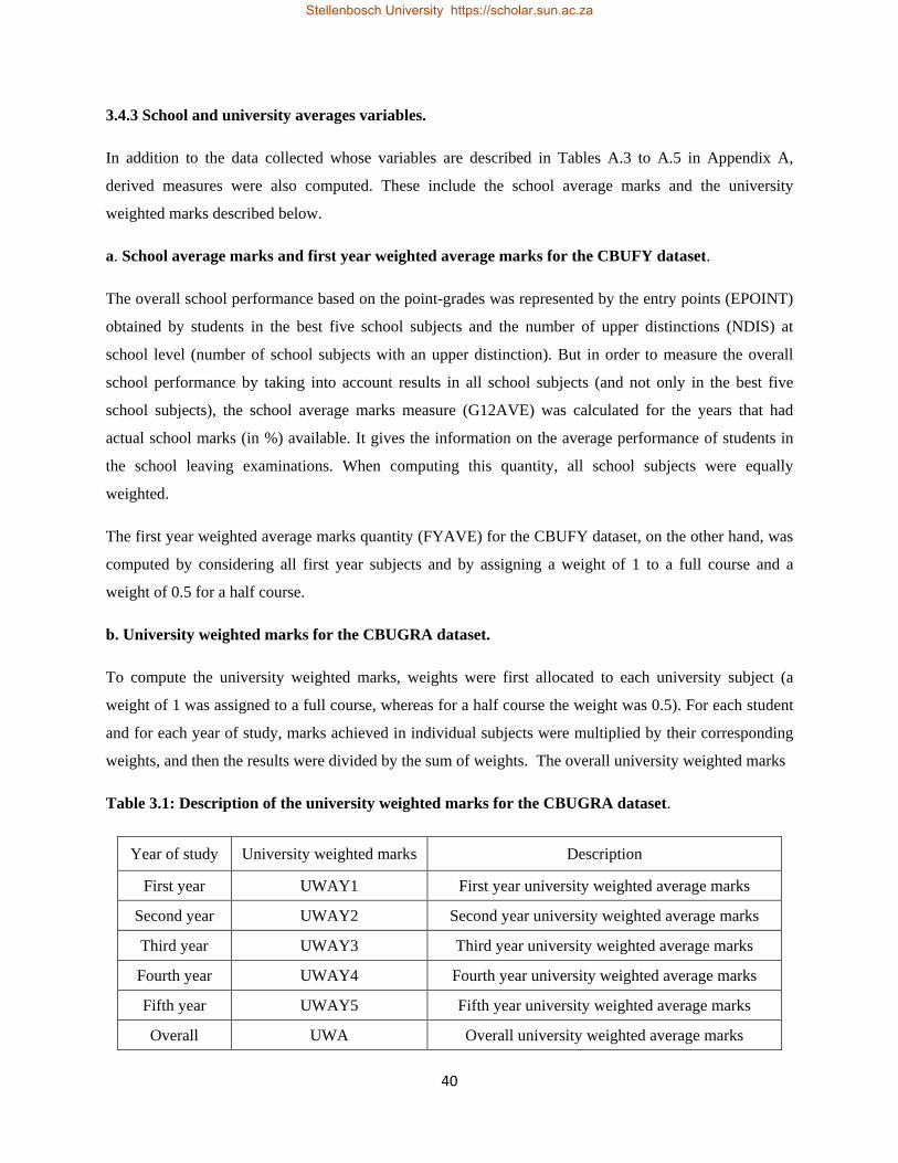
40
3.4.3 School and university averages variables.
In addition to the data collected whose variables are described in Tables A.3 to A.5 in Appendix A,
derived measures were also computed. These include the school average marks and the university
weighted marks described below.
a. School average marks and first year weighted average marks for the CBUFY dataset.
The overall school performance based on the point-grades was represented by the entry points (EPOINT)
obtained by students in the best five school subjects and the number of upper distinctions (NDIS) at
school level (number of school subjects with an upper distinction). But in order to measure the overall
school performance by taking into account results in all school subjects (and not only in the best five
school subjects), the school average marks measure (G12AVE) was calculated for the years that had
actual school marks (in %) available. It gives the information on the average performance of students in
the school leaving examinations. When computing this quantity, all school subjects were equally
weighted.
The first year weighted average marks quantity (FYAVE) for the CBUFY dataset, on the other hand, was
computed by considering all first year subjects and by assigning a weight of 1 to a full course and a
weight of 0.5 for a half course.
b. University weighted marks for the CBUGRA dataset.
To compute the university weighted marks, weights were first allocated to each university subject (a
weight of 1 was assigned to a full course, whereas for a half course the weight was 0.5). For each student
and for each year of study, marks achieved in individual subjects were multiplied by their corresponding
weights, and then the results were divided by the sum of weights. The overall university weighted marks
Table 3.1: Description of the university weighted marks for the CBUGRA dataset.
Year of study University weighted marks Description
First year UWAY1 First year university weighted average marks
Second year UWAY2 Second year university weighted average marks
Third year UWAY3 Third year university weighted average marks
Fourth year UWAY4 Fourth year university weighted average marks
Fifth year UWAY5 Fifth year university weighted average marks
Overall UWA Overall university weighted average marks
Stellenbosch University https://scholar.sun.ac.za
Stellenbosch University https://scholar.sun.ac.za

41
measure, representing the overall university performance from first year to the final year of study, was
calculated as the simple arithmetic mean of the university weighted marks from the first year to the final
year of study. The description of these variables is given in Table 3.1.
3.4.4 Problems encountered when collecting the data.
The data collection stage turned out to be much more demanding than envisaged and took more time than
expected. This was mainly due to the manual filing system for students’ records in the university,
individual students’ files with missing school results and other valuable information. Although getting the
information for students who were still at the CBU and those who successfully graduated from the
university was not a major problem, tracing excluded students and those who failed to graduate was a
very difficult, time consuming and challenging task. Data in electronic format from the University
Computer Centre had some valuable information missing and in formats which needed substantial time
for reformatting before the files could be ready for export into the R environment. Additionally, the
information in electronic format was only available for more recent years (from 2005 and onward for first
year data; and 2009 and 2011 to 2013 for school data).
During the year 2009 and part of 2010, initial data involving just school point-grades and university
letter-grades were gathered. Part of 2011 was also spent in correcting, cleaning and amending the data.
An attempt was made to analyse the data by transforming the point-grades of the school subjects and the
letter-grades of the university subjects into continuous data using the midpoints of the intervals of marks
(in %) representing the grades. The results appeared to be distorted because the university mistakenly
adopted the fixed grading scheme for grade nine examination as the grading scheme for grade twelve
examination. This is what motivated the data collection process to continue in 2012 and 2013 in order to
get data on actual marks (%) in both school and university subjects and secure first-hand information
from the ECZ Headquarters.
It is important to note that the records on admission and examinations results kept at the Academic Office
were not arranged and put in formats that could facilitate further research. They were there just to aid the
university in satisfying its immediate needs, for example student transcripts, enrolment statistics and
examinations results statistics. Normally after the admission process has been completed, the final files
including the lists of selected students with full information on admission or entry points, actual marks (in
%) (obtainable from ECZ) and point-grades of school results in the best five school subjects and in all
school subjects in which students sat for in grade twelve examinations need to be made readily available.
Additionally, after the year had ended, Senate reports have been prepared, examinations results have been
published, appeals on examinations results have been exhausted, the next task could be to arrange the data
Stellenbosch University https://scholar.sun.ac.za
Stellenbosch University https://scholar.sun.ac.za

42
in a way that could permit and facilitate further investigation, by including also the actual marks (in %)
and not only the letter-grades as is currently the case. The status of the data management at CBU needs
urgent attention and action in order to correct the current situation. With the introduction of new
undergraduate and postgraduate programmes, the size of the university is fast growing and as a result, the
manual filing system is becoming cumbersome and the process of getting information from the personal
students’ files is turning out to be a challenging task as older students’ files are now more difficult to
trace.
Notwithstanding the difficulties encountered during the data collection process, it must be acknowledged
the overwhelming and tremendous support offered by the staffs at both the University Computer Centre
and the Academic Office during the data collection stage. They did everything possible to make this
critical stage a success.
3.4.5 Limitations and scope of the data.
This study only includes the degree programmes which were operational by the year 2000 (for the
CBUFY dataset) and which were producing graduates by 2000 (for the CBUGRA dataset). Other degree
programmes were not considered for the sake of having the study covering a longer period.
Notwithstanding this, it is believed that the programmes included in this study are representative of all
CBU degree programmes as they cover all types of programmes. Additionally, all undergraduate faculties
(except the School of Medicine) are represented in the study by at least one degree programme.
The data also were confined to undergraduate degree students. Postgraduate, diploma, and distance
learning students, and students who were brought into the university system using alternative selection
criteria (for example mature age students) were not part of the study as they were non-traditional students,
were self-sponsored, and were facing problems different from the rest of the degree students. Students
holding school leaving certificates obtained from secondary schools outside Zambia were also dropped
from the study. Additionally, the data only provide information on students who were admitted into the
CBU system. Information of admissible candidates and those whose applications were rejected was not
readily available.
Another issue about the data concerns the missing values in school subjects not selected by the school
leavers. Apart from school (grade twelve) Mathematics and English which are compulsory subjects taken
by all grade twelve leaners, other school subjects are optional and are not all offered in secondary schools
because of lack of teachers and teaching resources. For example some secondary schools only offer
Science and not Physics or Chemistry, while others teach only Physics and Chemistry. The same applies
Stellenbosch University https://scholar.sun.ac.za
Stellenbosch University https://scholar.sun.ac.za

43
to other optional subjects. The implication of low candidature in optional subjects and the restricted
number of examination subjects resulted in the data having several missing values corresponding to
school subjects in which students did not sit for examinations.
Another major limitation of the data was the unavailability of the actual marks (in %) of the school and
university subjects for some students and for some years in the study. It is noteworthy to mention that the
actual marks (in %) obtained by the grade twelve learners are not known to the public and are not
published. The information which the ECZ releases and which is recorded on both the examinations slips
and the school certificates are the point-grades in the school (grade twelve) subjects that the school
leavers sat for examinations. The same applies to examination results for the university subjects where
only letter-grades are recorded on the examination results slips given to students and on examination
results box files kept at the Academic Office (see Table A.7 in Appendix A for the university grading
scheme). The inaccessibility of school and university subjects’ actual marks (in %) for some years and for
some students included in the study have serious implications and limitations on the statistical techniques
that will be used to analyse the data.
In the remaining sections, an overview of the statistical methods for interval-valued data is provided. This
is followed by a discussion on the imputation methods used to transform the interval-valued data into
continuous data. Finally, the statistical techniques to be used in this study are listed.
3.5 CBU data as symbolic data.
As mentioned in Section 3.4, the actual marks (true marks) (in %) for school and first year results
variables were only available in 2009 and 2011 to 2013 for the first year dataset. They were also available
for students who were in their first year of study in 2009, and who graduated in 2012 for four-year
programmes, and in 2013 for five-year programmes. These graduates had actual marks (%) available for
school subjects, and for university subjects from the first year to the final year of study. The data for the
remaining years in the CBUFY and CBUGRA datasets were given in terms of point-grades (from one
point to nine points) for school subjects, and in terms of letter-grades (from A+ to D) for university
subjects.
Normally, after all grade twelve learners write the national school leavers examinations, the actual (true)
marks (in %) obtained in each grade twelve subject are converted into point-grades (from one to nine
points, with one point corresponding to the highest achievement or an upper distinction grade, and nine
points representing the lowest achievement or a fail grade). It is this information that is showed on the
Stellenbosch University https://scholar.sun.ac.za
Stellenbosch University https://scholar.sun.ac.za

44
examination results slips and on the school leavers’ certificates. The actual marks are not made available
to the public.
Likewise, the actual marks (in %) obtained by students in different university subjects are converted into
letter-grades (from A+ to D, with A+ representing marks above 85% or an upper distinction grade, and D
corresponding to marks below 40% or a definite fail grade). It is the letter-grades which are recorded on
the examination results slips and the students’ transcripts.
The data on point-grades for school results variables and the letter-grades for university subjects fall
within a class of data called symbolic data, or more specifically symbolic interval-valued data (or just
interval-valued data) since the true marks (%) are not known, only the bins in which these point-grades or
letter-grades fall are known. Other symbolic data include multi-valued and modal-valued data
(Rademacher & Billard, 2011).
3.5.1 Possible approaches of analysis when viewing the CBU data as interval-valued data.
When the CBU data are viewed as symbolic interval-valued data, three approaches can be used to analyse
such data. These include the symbolic data approach, the semi-symbolic approach, and the non-symbolic
approach.
a. Symbolic data analysis approach.
Symbolic data analysis (SDA) seeks to extend and provide alternative methods to classical or traditional
statistical techniques to handle symbolic data (Diday & Esposito, 2003). In order to account for the
internal structure found in symbolic data (which does not exist in classical datasets), the SDA approach is
to be followed.
When using the SDA approach, the data to investigate are interval-valued data and the results from the
analysis are presented in interval format rather than as single-valued entities. Additionally, the graphical
displays associated with the SDA methods must take into account the interval variation of the interval-
valued data. Below, an overview of some symbolic data methods is given.
i. Symbolic principal component analysis (SPCA) methods.
These methods extend traditional principal component analysis in order to deal with interval-valued data.
This is basically done by transforming the interval-valued data matrix into a new matrix and then
performing the classical PCA on the latter matrix. Three methods for SPCA on interval-valued data,
known as centres PCA (C-PCA), vertices PCA (V- PCA), and midpoint-radius PCA (MR-PCA)
Stellenbosch University https://scholar.sun.ac.za
Stellenbosch University https://scholar.sun.ac.za

45
proposed in the literature (see for example Cazes, Chouakria, Diday & Schektman, 1997; Billard &
Diday, 2003; Palumbo & Lauro, 2003; D’Urso & Giordani, 2004; Giordani & Kiers, 2004; and
Zuccolotto, 2007) are briefly described below.
Let X be an n × p interval-valued data matrix where each element x𝑖𝑖𝑖𝑖 = �a𝑖𝑖𝑖𝑖 , b𝑖𝑖𝑖𝑖�, for a𝑖𝑖𝑖𝑖 ≤ b𝑖𝑖𝑖𝑖, 𝑖𝑖 =
1, 2, … ,𝑛𝑛 and p < n:
𝐗𝐗 = �
x11 … x1𝑝𝑝⋮ ⋱ ⋮
x𝑛𝑛1 … x𝑛𝑛𝑝𝑝
� =
⎣⎢⎢⎡[a11 , b11] … �a1𝑝𝑝 , b1𝑝𝑝�
⋮ ⋱ ⋮
[a𝑛𝑛1 , b𝑛𝑛1] … �a𝑛𝑛𝑝𝑝 , b𝑛𝑛𝑝𝑝�⎦⎥⎥⎤ (3.1)
Then (3.1) can be transformed into singled-valued matrices XC, XV, and XR based on the midpoints or
centres, vertices and radii of the elements of matrix X, respectively.
If mij = a𝑖𝑖𝑖𝑖 + b𝑖𝑖𝑖𝑖
2 and rij =
b𝑖𝑖𝑖𝑖 − a𝑖𝑖𝑖𝑖2
are the midpoint or the centre, and the radius or midrange of
the element x𝑖𝑖𝑖𝑖 = �a𝑖𝑖𝑖𝑖 , b𝑖𝑖𝑖𝑖� of X, then the singled-valued matrices XC and XR can respectively be
written as:
XC = �
m11 … m1𝑝𝑝
⋮ ⋱ ⋮
m𝑛𝑛1 … m𝑛𝑛𝑝𝑝
� (3.2)
and XR = �
r11 … r1𝑝𝑝⋮ ⋱ ⋮
r𝑛𝑛1 … r𝑛𝑛𝑝𝑝
� (3.3)
When constructing the singed-valued matrix XV, the n rows of X are transformed into n submatrices of
the form 𝐗𝐗𝑉𝑉𝑖𝑖of order 2p × p with its rows containing the 2p vertices of the hyperrectangle associated with
row i of X, for i =1, 2, ..., n. The matrix XV is formed by stacking below each other the n matrices 𝐗𝐗𝑉𝑉𝑖𝑖
to get an (n × 2p) × p matrix. That is,
Stellenbosch University https://scholar.sun.ac.za
Stellenbosch University https://scholar.sun.ac.za
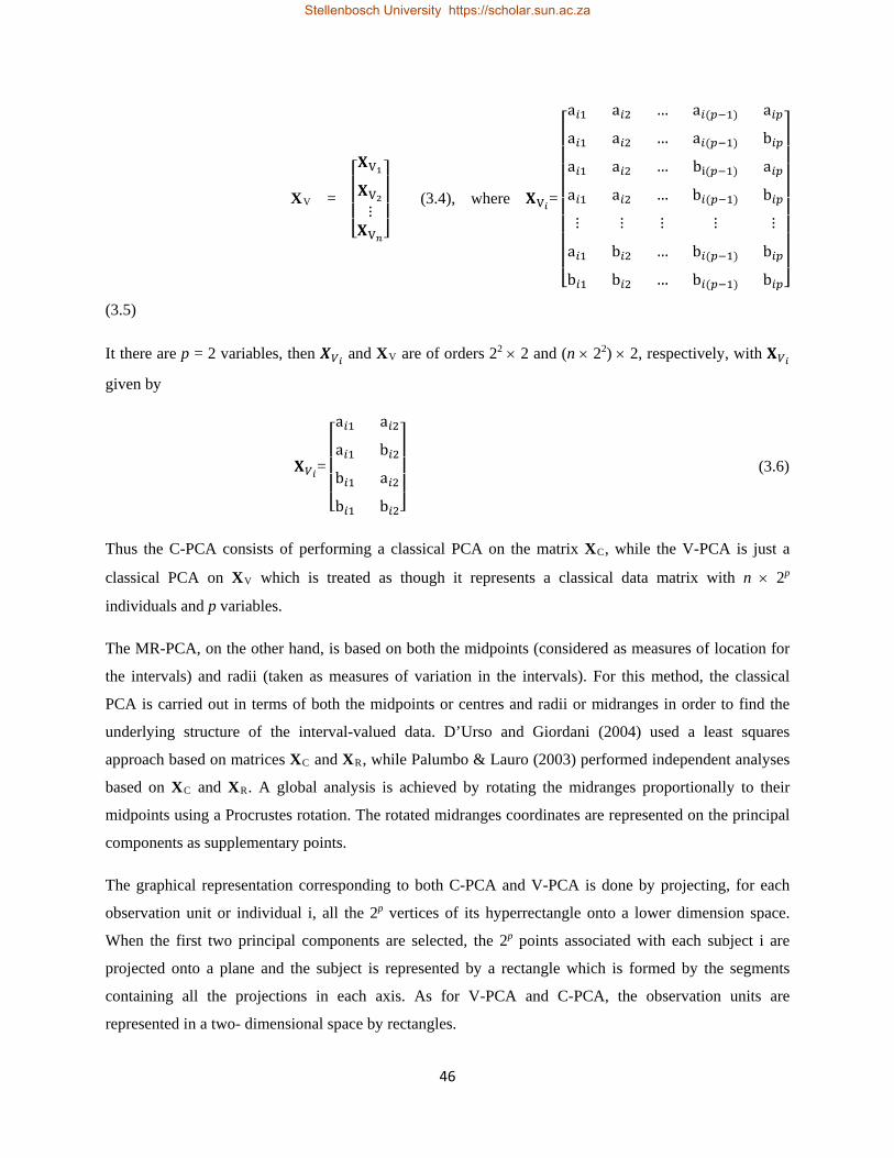
46
XV =
⎣⎢⎢⎢⎡𝐗𝐗V1𝐗𝐗V2⋮
𝐗𝐗V𝑛𝑛⎦⎥⎥⎥⎤ (3.4), where 𝐗𝐗V𝑖𝑖=
⎣⎢⎢⎢⎢⎢⎢⎢⎢⎡a𝑖𝑖1 a𝑖𝑖2 … a𝑖𝑖(𝑝𝑝−1) a𝑖𝑖𝑝𝑝a𝑖𝑖1 a𝑖𝑖2 … a𝑖𝑖(𝑝𝑝−1) b𝑖𝑖𝑝𝑝a𝑖𝑖1 a𝑖𝑖2 … bi(𝑝𝑝−1) a𝑖𝑖𝑝𝑝a𝑖𝑖1 a𝑖𝑖2 … b𝑖𝑖(𝑝𝑝−1) b𝑖𝑖𝑝𝑝⋮ ⋮ ⋮ ⋮ ⋮
a𝑖𝑖1 b𝑖𝑖2 … b𝑖𝑖(𝑝𝑝−1) b𝑖𝑖𝑝𝑝b𝑖𝑖1 b𝑖𝑖2 … b𝑖𝑖(𝑝𝑝−1) b𝑖𝑖𝑝𝑝⎦
⎥⎥⎥⎥⎥⎥⎥⎥⎤
(3.5)
It there are p = 2 variables, then 𝑿𝑿𝑉𝑉𝑖𝑖 and XV are of orders 22 × 2 and (n × 22) × 2, respectively, with 𝐗𝐗𝑉𝑉𝑖𝑖
given by
𝐗𝐗𝑉𝑉𝑖𝑖=
⎣⎢⎢⎢⎡a𝑖𝑖1 a𝑖𝑖2a𝑖𝑖1 b𝑖𝑖2b𝑖𝑖1 a𝑖𝑖2b𝑖𝑖1 b𝑖𝑖2⎦
⎥⎥⎥⎤
(3.6)
Thus the C-PCA consists of performing a classical PCA on the matrix XC, while the V-PCA is just a
classical PCA on XV which is treated as though it represents a classical data matrix with n × 2p
individuals and p variables.
The MR-PCA, on the other hand, is based on both the midpoints (considered as measures of location for
the intervals) and radii (taken as measures of variation in the intervals). For this method, the classical
PCA is carried out in terms of both the midpoints or centres and radii or midranges in order to find the
underlying structure of the interval-valued data. D’Urso and Giordani (2004) used a least squares
approach based on matrices XC and XR, while Palumbo & Lauro (2003) performed independent analyses
based on XC and XR. A global analysis is achieved by rotating the midranges proportionally to their
midpoints using a Procrustes rotation. The rotated midranges coordinates are represented on the principal
components as supplementary points.
The graphical representation corresponding to both C-PCA and V-PCA is done by projecting, for each
observation unit or individual i, all the 2p vertices of its hyperrectangle onto a lower dimension space.
When the first two principal components are selected, the 2p points associated with each subject i are
projected onto a plane and the subject is represented by a rectangle which is formed by the segments
containing all the projections in each axis. As for V-PCA and C-PCA, the observation units are
represented in a two- dimensional space by rectangles.
Stellenbosch University https://scholar.sun.ac.za
Stellenbosch University https://scholar.sun.ac.za

47
Although the V-PCA is easy to perform once the matrix XV has been computed, its drawback is that the
number of vertices tend to be very large as the number of variables increases. Also the analysis is done
with respect to the vertices rather than the observation units as a whole. That is, the vertices in the V-PCA
are treated as simple and independent points losing any relationship among vertices belonging to the same
individual or observation unit.
ii. Symbolic linear discriminant analysis (LDA) methods.
In order to extent the LDA to interval-valued data, Duarte Silva & Brito (2006) considered three
approaches. In the first approach, a uniform distribution for each observed interval was assumed, while
the second approach consisted of performing a classical discriminant analysis using the matrix XV
defined in the previous section. The last approach was based on matrices XC and XR* = 2XR = matrix of
ranges. The details for these three approaches can be found in Duarte Silva & Brito (2006) (see also see
Bertrand & Goupil, 2000; Billard & Diday, 2003). For these approaches, the interval representations of
the observation units similar to the symbolic PCA methods can be displayed in the discriminant space.
iii. Symbolic multidimensional scaling.
Multidimensional scaling (MDS) has also been extended to interval-valued data (see Denoeux & Masson,
2000; Groenen, Winsberg, Rodriguez & Diday, 2006; Terada & Yadohisa, 2010 & 2011).
In classical MDS, each entry of the dissimilarity matrix is a single numerical value and each object is
represented as a point in Rp. But when the dataset for the analysis is an interval-valued dataset consisting
of interval-valued variables, the resulting dissimilarities δij will be an interval of values, i.e., δij =
�a𝑖𝑖𝑖𝑖 , b𝑖𝑖𝑖𝑖� for i, j = 1, 2, ..., n. Apart from the case when interval-valued dissimilarities are resulting from
interval-valued variables, there are situations where it might be appropriate to represent dissimilarities
between pairs of objects by interval-valued dissimilarities: preference of the judge to use ranges of values
rather than single values to indicate differences between pairs of objects, difficulties in quantifying the
proximity of certain pairs of objects by a single value, or a very large number of objects to be rated
(Denoeux & Masson, 2000; Groenen et al., 2006).
Denoeux & Masson (2000) developed two MDS techniques based on interval-valued dissimilarity
matrices, one technique based on the hypersphere model, yielding a representation in which each object
was displayed by a hyphersphere in a lower dimensional space. The second technique used a
hyperrectangle display of the objects. The gradient descent methods were utilised to solve the two
models associated with the two techniques. Groenen et al. (2006) improved the hyperrectangle models of
Stellenbosch University https://scholar.sun.ac.za
Stellenbosch University https://scholar.sun.ac.za
48
Denoeux & Masson by using iterative majorization, while Terada & Yadohisa (2010) proposed the
iterative majorization with the hypersphere models of Denoeux & Masson (2000).
iv. Symbolic regression analysis methods.
Several methods dealing with the regression analysis for interval-valued data (where the dependent and
the independent variables are interval-valued variables) have been proposed in the literature (see for
examples Billard & Diday, 2000, 2002 & 2007; Lima Neto & De Carvalho, 2008 & 2010; Boukezzoula,
Galichet & Bisserier, 2011; Lima Neto, Cordeiro & De Carvalho, 2011; Blanco-Fernández, Colubi &
Gonzáles-Rodríguez, 2012). Like most of the symbolic data methods, most of the symbolic regression
analysis methods perform the classical ordinary least squares linear regression using the transformed
interval-valued data (i.e., midpoints and/or radii of the interval values), and furnish the results in terms of
intervals by reconstructing them from the estimated midpoints and/or radii.
b. Semi-symbolic methods.
The semi-symbolic methods take into account the interval structure of the data (i.e., use as input the
interval-valued format of the data), but express the final results as singled-valued rather than interval-
valued outputs. Examples of these methods include the interval regression (see Stewart, 1983; Cameron
& Huppert, 1989; O’Garra & Mourato, 2007), and the kernel density estimators for interval-valued data
(see Braun, Duchesne & Stafford, 2005).
c. Non-symbolic methods.
The aim of these methods is to apply the classical statistical techniques to interval-valued data by first
transforming them into classical or single-valued data using appropriate imputation methods. The final
results are not expressed as symbolic objects like in symbolic data methods, but are presented in singled-
valued format. The major advantage of this approach is that it releases the researcher of the task to
develop complex methodologies for symbolic data. Instead, already established classical statistical
methods with known properties are used on the transformed data. In order to transform the interval-valued
data into single-valued data or classical data, several imputation methods have been proposed in the
literature. Some are briefly described below.
i. The midpoint method.
The rationale of using this approach stands from the fact that the interval midpoint is considered to be the
estimate of the true mean value of all the values falling within a given interval. That is, the true mean
value of the unknown values falling in a given interval is approximated by the average of the lower and
Stellenbosch University https://scholar.sun.ac.za
Stellenbosch University https://scholar.sun.ac.za

49
upper bounds of the interval. With this approach, all the observations falling in a particular interval are all
replaced by the interval midpoint.
Although this approach is easy to implement, it has many drawbacks. First, the assumption that the
midpoints are reasonable approximations of the means of the intervals might not be valid especially when
the data are skewed, and when intervals are wide and are not closed (Tarsitano, 1988). In case when the n i
items falling in the ith interval [a i , b i] have a uniform distribution with parameters ai and b i, then their
true mean is the same as the midpoint (ai + b i)/2 of the interval. Thus the midpoint imputation works well
when the unknown observations in each interval have uniform distributions.
Second, in some applications, it might not be appropriate and realistic to assume that all observations
falling in a given interval are identical and equal to the midpoint. By doing so will result in biased results.
Additionally, when only fewer intervals with wider widths are available, this may distort the distribution
of the underlying interval-valued data (Von Fintel, 2006). Stewart (1983) reported that the ordinary least
squares regression using midpoints as proxies to the dependent interval-valued variable in the regression
model may yield inconsistent estimates.
Finally, problems may arise when the first interval (or the last interval) does not have the lower bound (or
the upper bound) as in the case of income distributions for example. When dealing with such income data,
some researchers have suggested using the midpoint approach with the Pareto distribution, giving rise to
the midpoint-Pareto approach (see for example Von Fintel, 2006). This approach involves using the
midpoint imputation for narrow intervals and the Pareto imputation for the last interval (which does not
have an upper bound) and for upper intervals which have greater widths. For each concerned interval, a
Pareto mean is estimated and is assigned to each of the observations falling in that interval.
From the discussion above, it transpires that the midpoint imputation may yield passable approximations
of the observations within the intervals if the number of intervals involved is very large. These intervals
must be relatively narrow and must all have both lower and upper bounds.
ii. Conditional mean imputation.
The midpoint approach is a particular case of the conditional mean imputation when the uniform
distribution is assumed. In general, when a distribution is assumed for the interval-valued data at hand,
this approach consists of imputing the unknown observations known to lie in intervals by the conditional
means.
Stellenbosch University https://scholar.sun.ac.za
Stellenbosch University https://scholar.sun.ac.za

50
Case when a parametric distribution is assumed.
Consider a random variable X with probability density function (pdf) f(x,θ) and cumulative density
function (cdf) F(x,θ), where θ is the vector of parameters. If the distribution of X is assumed within a
given interval [a, b], then the expressions of the pdf and the cdf within this interval, denoted by
f(x / a ≤ X ≤ b) and F(x/ a ≤ X ≤ b), are defined as (Nadarajah & Kotz, 2006; Von Fintel, 2006;
Nadarajah, 2009):
𝑓𝑓(𝑥𝑥,𝜽𝜽 ∕ 𝑎𝑎 ≤ 𝑥𝑥 ≤ 𝑏𝑏) =𝑓𝑓(𝑥𝑥,𝜽𝜽)
𝐹𝐹(𝑏𝑏,𝜽𝜽) − 𝐹𝐹(𝑎𝑎,𝜽𝜽) (3.7)
and
𝐹𝐹(𝑥𝑥,𝜽𝜽 ∕ 𝑎𝑎 ≤ 𝑋𝑋 ≤ 𝑏𝑏) =𝐹𝐹(𝑥𝑥,𝜽𝜽) − 𝐹𝐹(𝑎𝑎,𝜽𝜽)𝐹𝐹(𝑏𝑏,𝜽𝜽) − 𝐹𝐹(𝑎𝑎,𝜽𝜽)
, (3.8)
where −∞ < a < b < ∞.
Expressions (3.7) and (3.8) are the conditional pdf and cdf of X corresponding to the interval [a, b] and
are just the pdf and the cdf of the truncated distribution of X within this interval.
The expected value of this truncated distribution, which is the same as the conditional expected value of
X given that a ≤ X≤ b, is given by (see Nadarajah & Kotz, 2006; Von Fintel, 2006; Nadarajah, 2009):
𝐸𝐸(𝑋𝑋,𝜽𝜽|a ≤ 𝑋𝑋 ≤ 𝑏𝑏) = �𝑥𝑥𝑏𝑏
𝑎𝑎
𝑓𝑓(𝑥𝑥,𝜽𝜽|a ≤ 𝑥𝑥 ≤ 𝑏𝑏)
=1
∫ 𝑓𝑓(𝑥𝑥,𝜽𝜽)𝑑𝑑𝑥𝑥𝑏𝑏𝑎𝑎
� 𝑥𝑥𝑓𝑓(𝑥𝑥,𝜽𝜽)𝑑𝑑𝑥𝑥 (3.9𝑎𝑎)𝑏𝑏
𝑎𝑎
=1
𝐹𝐹(𝑏𝑏,𝜽𝜽) − 𝐹𝐹(𝑎𝑎,𝜽𝜽)�𝑥𝑥𝑓𝑓(𝑥𝑥,𝜽𝜽)𝑑𝑑𝑥𝑥 (3.9𝑏𝑏)𝑏𝑏
𝑎𝑎
Using this conditional mean, the unknown observation xi in the ith interval [ai, b i] is approximated by
E(X | a i ≤ X≤ b i), for i = 1, 2, …, n. If this expectation depends on the unknown parameters, then the
parameters must first be estimated. Additionally, numerical methods can be used to find the expectation
in (3.9a or 3.9b) when an analytical form does not exist. |
Von Fintel (2006) obtained the expression of (3.9b) for the normal distribution as
Stellenbosch University https://scholar.sun.ac.za
Stellenbosch University https://scholar.sun.ac.za

51
𝐸𝐸(𝑋𝑋,𝜽𝜽|a ≤ 𝑋𝑋 ≤ 𝑏𝑏) = 𝜇𝜇 − 𝜎𝜎𝜙𝜙 �𝑏𝑏 − 𝜇𝜇
𝜎𝜎 � − 𝜙𝜙 �𝑎𝑎 − 𝜇𝜇𝜎𝜎 �
Φ�𝑏𝑏 − 𝜇𝜇𝜎𝜎 � − Φ�𝑎𝑎 − 𝜇𝜇
𝜎𝜎 � , (3.10)
where φ(.) and Φ(.) are the pdf and the cdf of the standard normal distribution.
To determine the value of (3.10), Von Fintel (2006) proposed to estimate the parameters µ and σ by
performing an interval regression with only a constant.
For the lognormal distribution with parameters µ and σ, Jawitz (2004) found the following expression
𝐸𝐸(𝑋𝑋,𝜽𝜽|a ≤ 𝑋𝑋 ≤ 𝑏𝑏) = 𝑒𝑒𝑥𝑥𝑒𝑒(𝜇𝜇 + 𝜎𝜎2 2⁄ ) �Φ�𝑙𝑙𝑛𝑛𝑏𝑏 − 𝜇𝜇 − 𝜎𝜎2
𝜎𝜎� − Φ�
𝑙𝑙𝑛𝑛𝑎𝑎 − 𝜇𝜇 − 𝜎𝜎2
𝜎𝜎�� (3.11)
When a gamma distribution with parameters 𝜽𝜽 = (α, β) is assumed, (3.9b) can be written as (Zaninetti,
2013)
𝐸𝐸(𝑋𝑋,𝜽𝜽|a ≤ 𝑋𝑋 ≤ 𝑏𝑏) = −𝑘𝑘𝛽𝛽2
[Γ(1 + 𝛼𝛼, 𝑏𝑏𝛽𝛽) − Γ(1 + 𝛼𝛼,𝑎𝑎𝛽𝛽], (3.12)
where
Γ(𝑑𝑑, 𝑧𝑧) = � 𝑡𝑡𝑑𝑑−1𝑒𝑒−𝑡𝑡𝑑𝑑𝑡𝑡 (3.13)∞
𝑧𝑧
is the upper incomplete gamma function and
𝑘𝑘 =𝛼𝛼
1𝛽𝛽 Γ(1 + 𝛼𝛼,𝑎𝑎𝛽𝛽) − 1
𝛽𝛽 Γ(1 + 𝛼𝛼, 𝑏𝑏𝛽𝛽) + 𝑒𝑒−𝑏𝑏𝑏𝑏(1 𝛽𝛽−𝛼𝛼+1⁄ )𝑏𝑏𝛼𝛼 − 𝑒𝑒−𝑎𝑎𝑏𝑏(1 𝛽𝛽−𝛼𝛼+1⁄ )𝑎𝑎𝛼𝛼 (3.14)
Note that to evaluate the expressions (3.10), (3.11) and (3.12), the unknown parameters must first be
estimated.
Case when no assumption is made on the distribution.
When no distributional assumption is made about the interval-valued data of interest, Braun, Duchesne &
Stafford (2005) proposed to replace in (3.9a) f(x,θ) by its kernel density estimate
Stellenbosch University https://scholar.sun.ac.za
Stellenbosch University https://scholar.sun.ac.za

52
𝑓𝑓(𝑥𝑥) =1𝑛𝑛�𝐸𝐸�
1ℎ𝐾𝐾�
𝑥𝑥 − 𝑋𝑋ℎ � |a ≤ 𝑋𝑋 ≤ 𝑏𝑏�
𝑛𝑛
𝑖𝑖=1 (3.15)
The expression (3.15) is just the usual kernel density estimate extended to the interval-valued data, where
X is only known to lie in the interval I = [a, b] (see Braun et al., 2005). Once the density function is
estimated, then expression (3.9a) can be evaluated via numerical methods (see Kim, 2009).
When a distributional form of the data is not assumed, the imputation of the unknown observations falling
in the intervals can also be done by using a nonparametric maximum likelihood estimate of the
distribution of the data (see Hsu, Taylor, Murray & Commenges, 2007; Zhang, Zhang, Chaloner &
Stapleton, 2009).
iii. Random imputation assuming a parametric distribution.
Case when the uniform distribution is assumed.
This approach assumes that the unknown ni observations falling in the ith interval [ai, bi] follow the
uniform distribution (Bertrand & Goupil, 2000; Billard & Diday, 2003; Duarte & Brito, 2006; Hsu et al.,
2007; Rademacher & Billard, 2011; Ahn, Peng, Park & Jeon, 2012). In this case, each unknown
observation is replaced by a randomly selected value xij from the uniform distribution with parameters ai
and bi, for i = 1, 2, .., k and j = 1, 2,…, ni, where k is the number of intervals in the data set. This method
has the merit over the midpoint since all observations in the ith interval are estimated by different uniform
values.
Alternatively if the interval-valued data have n intervals [a1, b1] , [a2, b2] , …, [an, bn] with each interval
representing each of the unknown single-valued observations, then these observations can be imputed by
the n values xi’s randomly drawn from uniform distributions U(ai, bi), for i =1, 2, …, n.
Non-uniform case.
When a non-uniform parametric distribution is assumed for the interval-valued data of size n, then the n
unknown observations falling in the n intervals are approximated by n values randomly selected from the
assumed probability distribution. Similarly, if the data consist of k intervals (case of grouped data), then
the ni observations falling in the ith interval can be replaced by ni randomly drawn values from the
assumed distribution.
Note that for the non-uniform case, a truncated distribution must be assumed within an interval so that the
unknown observations can be replaced by randomly selected values from this distribution. Alternatively,
the imputation can be achieved by randomly selecting values from the complete distribution.
Stellenbosch University https://scholar.sun.ac.za
Stellenbosch University https://scholar.sun.ac.za

53
iv. The random midpoint approach.
This method uses the midpoint of an interval and then randomly distributes the observations falling within
this interval across it. More specifically if k is the number of intervals, ni is the number of observations
falling in the ith interval [ai, bi], mi is the interval midpoint, then the random midpoint imputation of the
jth observation that lies in the interval i, denoted by Xij, is given by:
X𝑖𝑖𝑖𝑖 = m𝑖𝑖 + sign𝑖𝑖𝑖𝑖U𝑖𝑖𝑖𝑖 for 𝑖𝑖 = 1,2, . . , 𝑘𝑘 and 𝑗𝑗 = 1,2, … ,𝑛𝑛𝑖𝑖 (3.16)
where signij is the sign corresponding to observation j in interval i assuming 1 or −1 with probability 1/2,
U ij is a uniform random variable between the lower bound ai and the interval midpoint (see for example
Malherbe, 2007).
The random midpoint has an advantage over the midpoint approach since there is no need to replace all
observations found in the ith interval by the same value. Although the uniform distribution is assumed,
other distributions can also be considered.
v. The resampling approach or the multiple imputation approach (Case when a parametric
distribution is assumed).
This approach was used by Ahn et al. (2012) when performing an interval-valued data regression. In
general, this approach employs the random imputation scheme to randomly select B sets of single-valued
data using the original interval-valued values and then carries out any classical statistical technique. The
final results of the analysis are obtained by combining the results from the B sets of data in a convenient
fashion.
More specifically if [a1, b1], [a2, b2], …, [an, bn] is the original interval-valued dataset, then the B single-
valued datasets �𝑥𝑥1𝑏𝑏 , 𝑥𝑥2𝑏𝑏 , … , 𝑥𝑥𝑛𝑛𝑏𝑏�, for b = 1, 2, …, B, are selected from uniform distributions U(a1, b1),
U(a2, b2),…, U(an, bn) or from non-uniform truncated distributions using the random imputation scheme.
Each single-valued dataset thus obtained provides the input for a classical statistical technique.
Combining the results of the B datasets will yield the final results for the analysis.
3.5.2 Comments on the statistical methods of the interval-valued data.
The SDA approach reviewed in the previous section allows for the interval variations in the interval-
valued data to be preserved by presenting the outputs in interval format. This approach cannot work
properly with the CBU data because of the graphical representation which consists of displaying the
observation units as hyperrectangles or hyperspheres in a lower dimensional space or as rectangles or
Stellenbosch University https://scholar.sun.ac.za
Stellenbosch University https://scholar.sun.ac.za

54
spheres in a two-dimensional space. For PCA for example, the observation units are represented in a two-
dimensional space R2 by rectangles rather than single points. This interval representation is convenient
when the number of individuals or observations to display is very small. But when the number of
observations is large, as is the case of the CBU data, the interval representation of interval-valued data
becomes unreadable and of no use, defeating even the geometric approach that will be followed in this
thesis.
Regarding the non-symbolic approach, this might be a viable way of analysing the CBU data, but the
outcomes of the analyses may be affected by the imputation methods used to convert interval-valued data
into single-valued data or classical data. Additionally, some of the imputation methods might not be
appropriate with the CBU data. For example the midpoint imputation of the unobservable or unknown
marks (in %) might not work, because of the small number of distinct intervals associated with the point-
grades (for school results variables) and letter-grades (for university results variables). Moreover, it might
not be realistic to assume that all students who obtained the same point-grades or the same letter-grades
have identical marks equal to the midpoints. The situation is critical for school results variables which
have the bulk of the individuals concentrated in the upper and lower distinctions bins because of the high
admission standards at the CBU. This will imply that the estimated marks for most students will take only
two distinct values, one value corresponding to the midpoint of the upper distinction interval, and the
other one being the midpoint of the lower distinction interval.
In fact, a preliminary analysis using the midpoint imputation to convert the grades (point-grades and
letter-grades) of the school and university results variables into continuous data produced disastrous
results when constructing boxplots and kernel density plots. That is, the kernel densities showed artificial
multimodalities mainly due to the use of the midpoint imputation. The shapes of the boxplots were also
affected by the use of midpoints.
Furthermore, some imputation methods require distributional assumptions of the variables under
investigation. It might not be appropriate to assume a priori parametric distribution for a particular school
results variable or a university results variable.
Finally, when the CBU data are viewed as symbolic interval-valued data, the statistical methods
developed for such types of data might not work properly because of the geometric approach that is to be
followed throughout this study. Some other methods might not be able to meet the aims of this study. In
the next section the statistical techniques to be used in this study are outlined.
Stellenbosch University https://scholar.sun.ac.za
Stellenbosch University https://scholar.sun.ac.za

55
3.6 Statistical techniques to be applied to the CBU data.
In the quest for the statistical techniques to be applied to the CBU data, statistical procedures used in the
studies on students’ performances were reviewed in the previous chapter. Additionally, statistical
techniques for interval-valued data were also discussed in the previous section. These statistical
procedures might not be adequate to put all the aims of this study into perspective. The statistical
techniques that have been retained to analyse the CBU data fall within the framework of the geometric
data analysis approach and require a minimum of assumptions. These include correspondence analysis
(CA), multiple correspondence analysis (MCA), categorical principal component analysis (categorical
PCA), and categorical canonical variate analysis (CatCVA). These statistical procedures do not depend on
the normality assumptions and have minimal assumptions. Other statistical techniques to be considered in
this study, for the years having actual marks (in %) available, are principal component analysis (PCA),
canonical variate analysis (CVA), and analysis of distance (AoD). For all these methods, the biplot
methodology can be employed in order to allow for several types of visualisations (see for example
Gower, Lubbe & Le Roux, 2011).
It is noteworthy to mention that CA, PCA, and MCA are the three standard methods of what is called
geometric data analysis (GDA) (Le Roux and Rouanet, 2004 & 2010). Le Roux & Rouanet (2004 &
2010) describe GDA as a geometric approach of multivariate statistical analysis which is aimed at
modelling the multivariate data as configurations (or clouds) of points on which to base the interpretation
of the data. Any multivariate statistical method can be considered from the viewpoint of GDA (Le Roux
& Rouanet, 2004). Thus categorical PCA, CVA, CatCVA, and AoD can also be regarded as GDA
methods.
The graphical displays resulting from the statistical procedures listed in the previous paragraphs are not
simple graphs, they are based on special distance measures. For example, the CA and MCA are based on
the Chi-squared distance, while the Pythagorean distance is used for PCA. For CVA, the Mahalanobis
distance is applicable (Gower & Hand, 1996).
In the remaining chapters of this study, the geometric data analysis approach will be followed throughout.
Although time can be spent to educate individuals who are not familiar with the graphical displays that
will be generated by the GDA techniques, these graphics help communicate the statistical findings to a
greater audience, even to non-statisticians.
Thus in Chapter 4, univariate data analysis will be performed on the data using notched boxplots, line
plots, and kernel density plots. More specifically, the notched boxplots will be used to assess for any
Stellenbosch University https://scholar.sun.ac.za
Stellenbosch University https://scholar.sun.ac.za

56
pattern changes in the main features (viz. location, spread, skewness) of the school and university results
variables over the period of study (i.e., from 2000 to 2013). Additionally, the notched boxplots will assist
in exploring the relationship between the school and university results variables; in checking if the
attainment of high scores (in %) at the school level and the raising of the admission standards were being
accompanied by better results at the university level; in examining if school results variables were good
indicators of the university performance; and in investigating if school results variables were able to
discriminate between the different groups in the first year and the graduate datasets.
The line plots, on the other hand, will be used to check if the means, standard deviations, medians, and
median absolute deviations of the school subjects in the population data were following some pattern
changes over time, while the kernel density plots will help in the investigation of the properties and
characteristics of the school and university results variables with respect to multimodality, variation, tails,
and skewness in the data. The kernel density plots will also assist in identifying the school results
variables whose distributions are closely corresponding to the university results variables.
The notched boxplots and the kernel density plots will also be used to compare the attributes of the school
results variables using the CBU data and the population data in order to check for similar patterns and
trends.
The CA technique which will be the subject of Chapter 5, will be applied to the CBU data, to investigate,
among other things, the patterns of associations between the school and university results variables at first
year level, and at the completion of the undergraduate studies by considering two variables at a time.
Additionally, using this technique, the transitional changes occurring in the students’ academic
performance through their academic career (i.e., from the grade twelve level at the secondary schools to
the first year of study, and from the first year to the final year of study at the university level) will be
studied. Moreover, CA will be employ to check the adequacy of the grading system of the school subjects
used to convert the true marks (in %) into the point-grades. More specifically, the effect of the width of
the bins associated with the upper distinction grades of the school results variables on the university
performance will be investigated. Furthermore, CA will assist in assessing whether the attainment of
higher performance at the school level was resulting in improved and enhanced academic achievement at
the university level. Finally, CA will provide the optimal scale values for school and university results
variables when their true marks (in %) are not available.
The CA technique only consider two variables at a time in the analysis. When several variables are
simultaneously incorporated in the analysis, multivariate statistical techniques will be performed on the
CBU data. These include MCA (in Chapter 6), PCA, CVA, AoD, categorical PCA, and CatCVA (in
Stellenbosch University https://scholar.sun.ac.za
Stellenbosch University https://scholar.sun.ac.za

57
Chapter 7). When applying MCA on the data, all variables are considered as nominal categorical
variables. Categorical PCA is also used on the data in order to take into account the ordering nature
present in the school and university results variables of the CBU data. Moreover, AoD and CatCVA are
also utilised in order to take care of the different groupings present in the CBU data. Furthermore, CA,
MCA, and categorical PCA viewed as optimal scaling techniques can provide optimal scale values which
can be used to quantify the CBU data. These optimal scale values can offer an alternative imputation
method that can be used to transform interval-valued data into single-valued or classical data.
MCA will examine the simultaneous interrelationships between the school and university results variables
at the first year level and at the completion of the studies, while categorical PCA will investigate the
simultaneous interrelationships among the variables included in the analysis by taking into account the
ordering nature of the ordinal variables. For the years with actual marks (in %) available for school and
results variables, PCA will be performed on the data to construct a composite measure of the school
performance which can be used to identify school subjects likely to play a pivotal role in the admission
process. Although PCA and categorical PCA are not designed to represent the group structures in the
data, they can at least provide a first indication of the group separation and the amount of overlap between
the groups in the data. AoD, which is specifically designed to represent the group structures, allow for the
visualization of the multivariate variation of these group structures. It optimally separates the different
groups in the data and provide the information about the overlap and the separation between these groups.
AoD, along with PCA and categorical PCA will help identify the school results variables which
discriminate between the different groups in the data. Similar to AoD, the application of catCVA to the
data will also allow for the visualisation of the group structures in the CBU data, and the investigation of
the similarities or dissimilarities between the different groups when the variables are categorical.
The statistical techniques listed in the previous paragraphs will be discussed in more details in the
subsequent chapters where their applications to the CBU data will be explored. For all the statistical
analyses undertaken in this thesis, the statistical programming language R, version 2.15.3 (R Core Team,
2013) will be utilised.
Stellenbosch University https://scholar.sun.ac.za
Stellenbosch University https://scholar.sun.ac.za

58
CHAPTER 4
UNIVARIATE ANALYSIS OF THE CBU DATA USING EXPLORATORY
DATA ANALYSIS TECHNIQUES
4.1 Introduction.
In this chapter exploratory data analysis techniques based on graphical methods are used to analyse the
CBU data by considering a single variable at a time. It should be recalled that this study seeks, among
other things, to check for any pattern change in the school and university results variables; to assess if
raising the admission standards resulted in better university performance; and to explore for any
relationship between the school results variables and the university performance. As a starting point, the
statistical analyses using graphical tools for univariate data are performed on the CBU data and the school
results data for the entire country which will be referred to as the population school results data (or just
the population data) in the remaining part of this chapter.
The univariate analysis explores each variable in a dataset separately. It is performed so as to facilitate
more complicated analyses, i.e. bivariate and multivariate analyses to be performed in the subsequent
chapters. The graphical displays used in this chapter to provide a visual representation of the univariate
distributions of the school and university variables from the CBU data, and the school results variables
from the population data include notched boxplots, line plots and kernel density plots.
As described in the previous chapter, the CBU data comprise two major datasets. The first dataset, known
as the first year dataset, provides the information on both school and first year results variables for the
2000 to 2013 intakes of first year students in degree programmes. The second dataset, referred to as the
graduate dataset, gives details of the school and university results variables from the first year to the final
year of study for the students who successfully completed their undergraduate studies in degree
programmes, or from the first year to the year of study that the students got excluded from their
programmes of study. These two datasets are analysed separately. Although both datasets cover the period
from 2000 to 2013, the actual marks (in %) for the school and university subjects for the first year dataset
were only available in the years 2009, and 2011 to 2013, while for the graduate dataset, they were only
accessible for the students who were admitted in their first year of study in 2009. For other years, only
point-grades (for school subjects) and letter-grades (for university subjects) were obtainable. Thus the
boxplots and the kernel density plots for the school and university results variables will be constructed
only for the years which had actual marks (in %) available. But for the overall school performance
variables EPOINT (total number of points in the best five school subjects) and NDIS (number of school
Stellenbosch University https://scholar.sun.ac.za
Stellenbosch University https://scholar.sun.ac.za

59
subjects with an upper distinction) (see Appendix A for a full description of these variables), the entire
period (i.e. from 2000 to 2013) will be considered.
4.2 Statistical univariate analysis of the CBU data using notched boxplots.
In this section, a variant of a boxplot, known as notched boxplot, is used. Like the standard boxplot, it
presents the five sample statistics consisting of the minimum and maximum values and the first, second
and third quartiles (Hoaglin, Mosteller & Tukey, 1983). The whiskers extend to the minimum and
maximum values if there are no outliers in the dataset. If there are outliers, the whiskers extend to the
smallest and largest values of the data points within the range of 1.5 times the interquartile range IQR.
For this plot, the sides of the box are notched (or narrowed). The median of the distribution is shown as
the centre of the notches, and the lower and upper quartiles are the hinges of the box. The notches
themselves represent an approximate 95% confidence interval about the median of the data (McGill,
Tukey & Larsen, 1978; Velleman & Hoaglin, 2004) and are equivalent to an approximate test for
comparing two or more medians. If this interval goes beyond the lower quartile or the upper quartile then
the notches extend beyond the box.
Side-by-side or parallel notched boxplots assist in comparing the various attributes or characteristics of
two or more datasets and their notches give an indication of the statistical difference between the
medians. That is, if the notches do not overlap, then statistically differences exist between the datasets
with respect to their medians (Velleman & Hoaglin, 2004).
The univariate statistical analyses of the CBU data based on the notched boxplots are motivated by the
need to assess if there were some pattern changes in the main features (viz. location, spread, skewness,
tail length and outlying points) of the school and university results over the fourteen-year period (from
2000 to 2013); to examine the relationship between the school and university results variables in order to
check, among other things, if the attainment of high scores at school level and the raising of the admission
standards (by down adjusting the programmes’ cut-off points) were being accompanied by better
performance at the university level; to examine if the school results variables were good indicators of the
university performance; to investigate if the school variables were able to discriminate between different
groups of the first year and graduate students.
Several notched boxplots were generated using the R source codes with a modified version of the R-
function boxplot ( ) known as boxplot.NJ () from the UBbipl R-package (Le Roux & Lubbe, 2010) . The
means, medians, standard deviations, and median absolute deviations (MAD) were also calculated (see
the R source codes in Appendix B). The notched boxplots associated with both datasets are shown in
Stellenbosch University https://scholar.sun.ac.za
Stellenbosch University https://scholar.sun.ac.za

60
Sections 4.2.1 to 4.2.9, respectively. The line plots of the means, standard deviations, medians and
median absolute deviations were also produced in order to see if the computed statistics were following
some patterns over time.
4.2.1 Comparison of the overall school performance over the fourteen-year period based on grades
using the first year dataset of the CBU data.
In this section, the univariate statistical investigations are concerned with various comparisons of the
overall school performance variables EPOINT and NDIS over the fourteen-year period using the first year
dataset to assess for some pattern changes over the period considered. The corresponding notched
boxplots are shown in Figures 4.1 and 4.2. The variable EPOINT is inversely related to the performance
at grade twelve level. That is, lower EPOINT translates into better school results, whereas high EPOINT
signifies a poor performance at grade twelve level.
Figure 4.1: Notched boxplots of NDIS for the first year students admitted in SBE and ST programmes
over the 2000-2013 period using the first year dataset of the CBU data.
The notched boxplots for ST in Figure 4.1 reveal that NDIS had a median of two for the 2000-2007
period (except in 2003 and 2006 which had a median of one), while for the remaining years it was three.
The shifting in the median from two to three after 2007 was occasioned by a downward adjustment of the
cut-off points for all engineering related programmes and a reduction in the gaps between the male and
female cut-off points which resulted in the raising of the admission standards. In 2011 the cut-off points
for all engineering related programmes were further reduced and were set at eight points for male and ten
points for female students. For the years 2003 and 2006; 2004, 2005 and 2007; and the years 2008 to
2012 notches were overlapping. The appearance of the 2013 boxplot is a consequence of the raising of the
Stellenbosch University https://scholar.sun.ac.za
Stellenbosch University https://scholar.sun.ac.za

61
admission standards which resulted in admitting students in engineering related programmes with at least
two upper distinctions in the school subjects.
For SBE programmes, the notches for the years 2001 to 2004 (group one); 2005, 2006, 2007 and 2009
(group two); and for the years 2010, 2011 and 2013 (group three) were overlapping with a median of one
for group one and two for the other two groups. The notched boxplots for SB (not reported) showed that
the first year students in business related programmes achieved a median of three upper distinctions at
school level, except for the 2001, 2006 and 2013 intakes who had a median of two upper distinctions.
This suggests that, during the fourteen-year period (except in 2001, 2006 and 2013), about 50% of the
first year students selected in business related programmes achieved at most three upper distinctions in
school subjects, while the remaining half got at least three upper distinctions at school level. The shift in
the median from three to two in 2013 was due to the relaxation of the admission standards which saw the
cut-off points for business related programmes increasing from nine to eleven points for male students
and from ten to twelve for female students.
Concerning SNR (notched boxplots also not shown), the median of NDIS was zero in 2000 and 2002 and
one for the remaining years. After 2002, a moderate upward trend in the median (from zero to one), the
first and third quartiles was noticeable and was due to the downward adjustment of cut-off points for the
forestry programme from eighteen points to eleven points in 2003. The effect of the reduction in the cut-
off points for this programme could not be fully felt mainly due to the conflicting effects of the dual cut-
off points system which was introduced in 2005 and which allowed more female candidates with lower
school results to be admitted in this programme.
Figure 4.2 displays the notched boxplots for the variable EPOINT for the first year students in each of the
four faculties over the fourteen-year period. The distributions of EPOINT for the first year students in SB
shows a stable pattern during the 2000-2013 period with a median entry point fluctuating between eight
and nine points. The notches for 2005, 2007 and 2009 to 2012 are overlapping. The shift in the median
from eight to nine points in 2013 is noticeable and is the result of the relaxation of the admission criteria
in business related programmes. That is, for the first time since 2001 the cut-off points for business
related programmes were increased in 2013 from nine points (in 2001) to eleven points for male students,
and twelve points for female students. From the same figure, it is observed a higher variation in EPOINT
for the years 2003, 2006 and 2008 as compared to other years which have similar variations as exhibited
by the sizes of the boxes of the corresponding notched boxplots.
Figure 4.2 also demonstrates that SBE programmes have higher cut-off points (translating into lower
admission standards) as compared to business and some engineering related programmes. From 2000 to
Stellenbosch University https://scholar.sun.ac.za
Stellenbosch University https://scholar.sun.ac.za

62
2012, the notched boxplots for EPOINT in SBE show a decreasing trend in the medians from twelve
points in 2000 to ten points in 2012 (see Figure 4.2). Notches in 2001 and 2002; and in 2008 to 2011 and
2013 are overlapping. The decline in the entry points can be attributed to the downward adjustment of
cut-off points of SBE programmes between 2004 and 2012 and is due to the increasing number of
admissible candidates and the limited places in these programmes. For 2013, an upward adjustment in the
cut-off points is recorded. This resulted in the increase of the median from ten points in 2012 to twelve
points in 2013.
Figure 4.2: Notched boxplots of EPOINT for the first year students admitted in the four faculties over the
2000-2013 period for the first year dataset of the CBU data.
Similar to SBE programmes, the notched boxplots of EPOINT in engineering related programmes exhibit
a decreasing pattern from 2006 to 2013.This again could be attributable to the effect of raising the
admission standards for chemical, electrical/electronics, electrical/mechanical, metallurgical and mining
engineering programmes. The year 2013 has the lowest median of seven points because of the cut-off
Stellenbosch University https://scholar.sun.ac.za
Stellenbosch University https://scholar.sun.ac.za

63
points which were made uniform in all engineering programmes and set at eight points for male students
and ten points for female students. In the forestry programme at SNR, the notched boxplots are
characterised by non-overlapping notches over the fourteen-year period with varying medians.
The findings in this section have shown that, during the fourteen-year period, the school leavers with
outstanding school achievements were admitted into SB and ST programmes because of high demanding
and competitive programmes with low cut-off points in these two faculties, whereas students with
moderate school results went to SBE and SNR. Additionally, the changes of patterns observed over the
fourteen-year period in the overall school performance measures were due to the increase in the
admission standards resulting from the downward adjustment of the programme cut-off points and the
implementation of the dual cut-off points system for male and female students. This system was
introduced in order to allow more female applicants to be selected in degree programmes of the CBU
because of their low school results in the school leaving examinations as compared to their male
counterparts.
While the adjustment process of cut-off points had no marked effect on the variable EPOINT of SB
students, in non-business related programmes the effect was felt. In ST and SNR for example,
programmes were affected by both the upward adjustment of the admission standards and the insertion of
the dual cut-off points system. In SBE, programmes were more affected by the adjustment in the cut-off
points than by the dual admission system.
In the next section, the assessment of individual school results variables and the third overall school
performance measure G12AVE (school average marks of all school subjects) will be carried out in the
years which had actual marks (in %) in individual school subjects available. Whereas EPOINT and
G12AVE are both measures of the overall school performance, the latter is a more comprehensive overall
measure at it takes into account the performance of students in all individual grade twelve subjects.
EPOINT only considers the performance in the best five school subjects.
4.2.2 Comparison of G12AVE and individual school results variables for the years 2009, and 2011
to 2013 for the first year dataset.
Figures 4.3 to 4.10 below show the notched boxplots of grade twelve subjects mostly used by the
university to calculate the entry points (viz. Mathematics, Additional Mathematics, English, English
Literature, Science, Physics, Chemistry, Biology, Geography, History, Principles of Accounts,
Commerce, Technical/Geometric/Mechanical Drawings, Wood/Metal Works, Religious education and
Agriculture Science) for all four faculties combined. The summary statistics (means, standard deviations
Stellenbosch University https://scholar.sun.ac.za
Stellenbosch University https://scholar.sun.ac.za

64
and medians) are also reported in Table 4.1. The median absolute deviations (MAD) were also computed
but are not shown as they were closer and very similar to the standard deviations.
In Figure 4.3 the notched boxplots for school Mathematics in 2009 and 2011 to 2013 have medians
slightly greater than the means. In the years 2011 to 2013, they are showing a slight upward trend in the
means and the medians, with the highest mean of 73.0% and median of 74.0% achieved in 2013 (see
Table 4.1). This is in contrast with Additional Mathematics whose means and medians are more or less
constant over the four years considered. When comparing their variations, Table 4.1 reveals that
Additional Mathematics has greater variation than Mathematics. It is evident from the same table that
Mathematics, Additional Mathematics, English Literature, Principles of Accounts, Commerce, Drawing,
Religious Education and Metal/Wood Works have greater variations as compared to other school
subjects. But for each school subject, the standard deviations are similar, comparable and are not showing
any particular trend over time.
Figure 4.3: Notched boxplots of school Mathematics and Additional Mathematics for first year students
for all four faculties combined in 2009, and 2011 to 2013 for the first year dataset of CBU
data.
From the notched boxplots in Figure 4.4, it transpires that the school results in English Literature have
lower means and medians but greater variations as compared to English with standard deviations ranging
from 10.64% to 13.32% (MADs were between 10.38% and 14.08%). Lower medians and means and
greater variations exhibited by Additional Mathematics and English Literature are due to the way papers
in these subjects are usually set up in the school leaving examinations. The grade twelve learners are more
comfortable with Mathematics and English than with Additional Mathematics and English Literature
which are more demanding.
Stellenbosch University https://scholar.sun.ac.za
Stellenbosch University https://scholar.sun.ac.za

65
Table 4.1: Means, medians, and standard deviations for school variables in 2009, and 2011 to 2013 for
the first year dataset of the CBU data.
Subj. Means Medians Standard deviations
2009 2011 2012 2013 2009 2011 2012 2013 2009 2011 2012 2013
Math 67.91 67.49 70.26 72.99 69.00 68.00 71.00 74.00 12.40 11.76 12.19 12.45
AdM 67.78 66.20 66.18 66.30 68.00 69.00 69.00 67.0 13.56 13.31 16.46 14.09
Eng 63.31 57.95 58.88 66.96 63.00 58.00 59.00 68.00 7.68 6.74 7.52 7.43
EnLi 55.90 57.85 51.86 56.86 57.00 58.00 52.00 57.50 13.32 10.64 11.10 11.08
Scien 60.39 64.35 56.59 58.17 61.00 65.00 57.00 59.00 8.77 9.80 8.49 9.26
Phys 57.93 59.61 59.38 58.23 59.00 60.00 60.00 59.00 7.58 7.40 8.26 10.00
Chem 68.43 59.48 68.81 56.65 69.00 59.00 70.00 57.00 9.02 11.26 9.49 10.59
Biol 52.69 43.06 46.33 49.60 53.00 43.00 46.00 49.00 8.52 8.78 8.26 8.30
Geog 64.36 64.12 66.14 62.52 65.00 65.00 66.00 63.00 9.00 9.02 7.81 7.43
Hist 57.61 58.71 58.50 49.06 59.00 61.00 58.00 48.00 11.25 10.60 10.92 11.71
Acc 60.41 60.03 52.02 60.38 61.00 59.00 53.00 61.00 15.38 13.89 15.43 13.01
Com 51.53 49.75 47.70 46.43 52.50 50.00 48.00 46.00 12.60 13.92 12.28 12.20
Draw 65.35 68.53 74.73 66.67 67.00 71.00 78.00 68.00 12.81 14.61 14.76 13.65
RE 63.54 66.84 62.66 62.71 64.00 68.00 65.00 65.00 16.02 13.20 14.71 14.40
AgSc 35.63 34.68 34.76 39.29 36.00 34.00 35.00 39.00 8.53 8.11 7.88 7.12
Mww 56.63 55.24 64.21 61.96 59.00 56.00 65.00 63.00 13.07 11.44 11.41 11.83
Figures 4.5 and 4.6 provide the notched boxplots for the school results in Science, Physics, Chemistry and
Biology. These four subjects are found in the low variation category with similar and comparable
variations over the four years. School Biology has lower means and medians below 50%, except in 2009
which has slightly higher mean and median of 53% as compared to the other three subjects. Its notched
boxplots show an upward trend between 2011 and 2013 (see Figure 4.6). When comparing Science,
Physics and Chemistry, it is clear that the results in school Physics for the students included in the study
(see Figure 4.5) over the four-year period are more stable than those in Science and Chemistry, with more
or less constant means, medians, standard deviations and MADs (see Table 4.1). Notched boxplots for
Science and Chemistry do not exhibit any particular trend over the four-year period.
Notched boxplots for other school subjects are displayed in Figures C.1 to C.4 in Appendix C. From these
figures, there is no dramatic shift in both the measures of location and variation over the four-year period
except for History, Metal/Wood Works (MWW), and Drawings. History has a sharp decrease in the mean
and the median in 2013 (see Figure C.1 and Table 4.1), whereas MWW in Figure C.3 is characterised by
Stellenbosch University https://scholar.sun.ac.za
Stellenbosch University https://scholar.sun.ac.za

66
high means and high medians in 2012 and 2013. In the same figure, Drawings exhibits an increasing shift
in both the means and the medians from 2009 to 2012 (with means and medians varying between 65.35%
and 74.73% and between 67% and 78%, respectively). But in 2013, both the mean and the median
decrease.
Figure 4.4: Notched boxplots of school English and English Literature for the first year students for all
faculties combined in 2009, 2011 to 2013 for the first year dataset of the CBU data.
Figure 4.5: Notched boxplots of school Physics and Chemistry for the first year students for all four
faculties combined in 2009, 2011 to 2013 for the first year dataset of the CBU data.
Stellenbosch University https://scholar.sun.ac.za
Stellenbosch University https://scholar.sun.ac.za

67
Figure 4.6: Notched boxplots of school Science and Biology for the first year students for all four
faculties combined in 2009, 2011 to 2013 for the first dataset of the CBU data.
Figure 4.7: Notched boxplots of school Mathematics for each faculty in 2009, 2011, 2012 and 2013 for
the first year dataset of CBU data.
In Figure C.2, Commerce presents a decreasing shift in both the means and the medians over the four-
year period. In the same figure, Principles of Accounts also exhibits a downward pattern from 2009 to
2012, but in 2013 an increase in both the mean and the median is recorded. For Religious Education and
Agricultural Science (see Figure C.4), a decreasing trend in the medians and means is observed for the
former from 2011 to 2013, while for the latter, an increasing trend is noticeable during the same period.
Stellenbosch University https://scholar.sun.ac.za
Stellenbosch University https://scholar.sun.ac.za

68
Figure 4.8: Notched boxplots of school English for each faculty in 2009, 2011, 2012 and 2013 for the
first year dataset of CBU data.
Figure 4.9: Notched boxplots of G12AVE for each faculty in 2009, and 2011 to 2013 for the first year
dataset of CBU data.
Figures 4.7 and 4.8 display the notched boxplots of Mathematics and English for individual faculties. A
comparison of these notched boxplots with those for all faculties portrayed in Figures 4.3 and 4.4 reveals
similar trends for boxplots of all faculties combined and for individual faculties. That is, like in Figure
4.3, a slight upward trend is also observed for the notched boxplots of Mathematics for each faculty in
Figure 4.7. Comparable patterns are also observed for English for combined faculties and individual
faculties (see Figures 4.4 and 4.8). Notched boxplots for other school subjects for individual faculties are
Stellenbosch University https://scholar.sun.ac.za
Stellenbosch University https://scholar.sun.ac.za

69
not reported as they showed similar patterns as those for combined faculties in Figures 4.4 to 4.6, and C.1
to C.4 in Appendix C.
Table 4.2: Means, medians and standard deviations of G12AVE for each faculty over four-year period for
the first year dataset of CBU data.
FAC. Means Medians Standard deviations
2009 2011 2012 2009 2011 2012 2009 2011 2012 2009 2011 2012
SB 63.57 59.95 59.62 58.90 63.00 60.00 58.00 59.00 4.86 4.89 6.50 5.62
SBE 57.82 57.42 57.30 57.05 57.00 58.00 58.00 57.00 5.12 4.65 5.56 4.82
SNR 54.41 54.29 53.13 53.80 54.00 54.00 53.00 53.00 4.55 3.56 3.89 4.30
ST 63.45 62.02 61.93 63.33 64.00 63.00 62.00 63.00 5.74 5.57 6.52 5.33
In Figure 4.9 the notched boxplots for the third overall school performance measure G12AVE for the first
year students in the four faculties over four years (2009, and 2011 to 2013) are presented. Summary
statistics (means, medians and standard deviations) are also reported in Table 4.2. The MADs were
similar to the standard deviations and are thus not shown.
Notched boxplots for G12AVE for the four faculties are characterised by similar means and medians and
low variations (between 3.84% and 5.88%), except for the year 2012 for SB and ST which have standard
deviations of 6.50% and 6.52%, respectively. The year 2009 has highest means and highest medians for
SB, SNR and ST as compared to other years. From 2009 to 2012, it is observed a downward trend in both
the means and the medians for SB due probably to the slight relaxation in the admission standards. But in
2013, a moderate increase in the median is recorded (see Table 4.2). For ST, a moderate increasing
pattern is noticeable between 2012 and 2013 due to a greater reduction in the cut-off points in all
engineering programmes for both male and female students (with means shifting from 61.93% to 63.33%
and medians moving from 62% to 63% as can be seen in Table 4.2). For SNR and SBE, there are no
apparent trends in both the means and the medians.
The findings from the above univariate statistical analyses reveal that the students admitted in the first
year of study in business and engineering related programmes achieved higher scores in most grade
twelve subjects as compared to students in other programmes (at SBE and SNR). When comparing
Mathematics to Additional mathematics, English to English Literature, Science to Biology, Physics to
Chemistry, Principles of Accounts to Commerce, and Geography to History, there was a general tendency
in all programmes considered for students to score higher in Mathematics, English, Science, Chemistry,
Stellenbosch University https://scholar.sun.ac.za
Stellenbosch University https://scholar.sun.ac.za

70
Principles of Accounts and Geography than in Additional Mathematics, English Literature, Biology,
Physics, Commerce and History at school level. Students were finding difficult to cope with Additional
Mathematics because of more advanced topics of Mathematics in this course. Also the English Literature
paper was more demanding than the English paper.
From the statistical analysis of the school results variables using notched boxplots, it can be said that
there were no dramatic pattern changes over time in the results of grade twelve subjects of students who
were admitted in the first year of study at the CBU over the fourteen-year period. Changes (in variations,
means, medians, and shapes of boxplots) observed in the grade twelve results over time were mainly due
to the increase in the admission standards, the implementation of the dual cut-off points system, the
heterogeneity of secondary schools supplying the students and the years when students sat for the school
leaving examinations. Some notched boxplots were showing outliers which affected their appearance. For
all years considered, the distributions of most school subjects were characterised by heavy tails and
thinner peaks as demonstrated by their notched boxplots with the length of the whiskers exceeding that of
the boxes. Distributions of school Mathematics, English, Physics, Geography, Science, Biology and
Religious Education exhibited nearly some symmetric patterns, whereas for English Literature,
Additional Mathematics and other school subjects the distributions were asymmetric.
Having compared the school performance in individual school subjects and overall school performance,
the next section deals with the comparison of the university results variables (i.e. first year subjects for the
first year dataset and first year to final year averages for the graduate data) for the years which had actual
marks (in %) for university subjects available.
4.2.3 Comparisons of first year subjects over the nine-year period (from 2005 to 2013) for the first
year dataset.
In this section, the notched boxplots for first year subjects in the four faculties using the first year dataset
are compared over the 2005-2013 period. Other comparisons for university results in the next section
concern the average results from first year to final year of study for students who graduated from CBU
from 2009 to 2013 for the graduate dataset.
The students in the programmes considered have common first year courses within each faculty. The
notched boxplots are used to check for any pattern change in the performance of these courses over time,
and to investigate the effect of the increase in the admission standards on the first year university
performance.
Stellenbosch University https://scholar.sun.ac.za
Stellenbosch University https://scholar.sun.ac.za

71
Results from the notched boxplots (only notched boxplots for the first year Mathematics are shown in
Figures 4.9 to 4.13) reveal that the performance in the first year subjects was relatively low as compared
to school results variables with means and medians below 65 % for most years. First year Mathematics
recorded the worst performance among all first year subjects in SB, SBE and SNR. Other first year
subjects with high standard deviations and low performance include Basic Financial Accounting in SB
and Chemistry in SNR. The remaining subjects had moderate variations comparable to the school
subjects. For all first year subjects in SB, an upward trend was observed in the means and the medians
between 2009 and 2012, with the year 2012 recording the highest means and medians. However, in 2013,
the means and medians decreased, probably due to the relaxation of the admission standards which saw
the cut-off points increased from nine to eleven points for male students and from ten to twelve points for
female students. This pattern was not observed in other faculties.
Figure 4.10: Notched boxplots of first year Mathematics subject in the Faculty of Business (SB) over the
nine-year period using the first year dataset of CBU data.
The notched boxplots of Mathematics in Figures 4.10 to 4.13 exhibit greatest variation as compared to
other first year subjects. In ST, students achieved better performance in first year Mathematics than in the
other three faculties with means and medians exceeding 60% for most years, and first quartiles and third
quartiles above 50% and 70%, respectively (see Figure 4.13). In SB, the situation was worse with
students recording an average score below 50% for all years, except in 2005 and 2012 which had means
of 50% and 53%. Also the medians were below 53%. The means and medians for most years in SNR
were below 55% and 59%, respectively, whereas in SBE, the performance in the first year Mathematics
was fair with means and medians in excess of 50% for all years considered.
Stellenbosch University https://scholar.sun.ac.za
Stellenbosch University https://scholar.sun.ac.za

72
Figure 4.11: Notched boxplots of first year Mathematics course in SBE over the nine-year period for the
first year dataset of CBU data.
Figure 4.12: Notched boxplots of first year Mathematics course in SNR over the nine-year period using
the first year dataset of CBU data.
While the poor performance recorded in SNR first year Mathematics could be attributed to students
admitted with poor school results, at SB the poor performance in Mathematics could not be due to
students with poor school background as they were admitted with outstanding results in school
Mathematics. This situation could be ascribed in part to the nature of the first year Mathematics at SB
which is a blend of pre-calculus and calculus topics with numerous applications. School Mathematics was
not able to prepare students for this first year subject. Additionally, business related programmes being
among the most popular programmes in the CBU usually attract many school leavers every year. As a
result, classes in the School of Business are overcrowded as compared to other faculties. In order to
improve the situation, it was decided in 2011 to introduce the tutorial system. The increase in the mean
Stellenbosch University https://scholar.sun.ac.za
Stellenbosch University https://scholar.sun.ac.za

73
and the median in 2012 in this subject (see Figure 4.10) could be attributable to this remedial measure
which worked well and helped to enhance the performance in this course. Furthermore, the upward trend
in the notched boxplots between 2009 and 2012 was also observed for notched boxplots of other SB first
year subjects.
Figure 4.13: Notched boxplots of first year Mathematics course in ST over the nine-year period using the
first year dataset of CBU data.
The high variation observed in the performance of the first year Mathematics in SBE and ST could be
explained in part by the heterogeneity of students in different programmes with different cut-off points.
Additionally, changes occurring in lecturers had also an impact in the performance of this first year
course in the two faculties. The increase in both the mean and the median in SBE first year Mathematics
in 2011 and 2012 (see Figure 4.11) was due to the raising of the admission standards which resulted in the
reduction of the cut-off points for SBE degree programmes and the reduction of gaps between cut-off
points for male and female students. In 2013, both the mean and median were lower than in 2012 (58.37%
in 2012 and 51.03% in 2013 for the mean; and 61% in 2012 and 53% in 2013 for the median). This could
be due to the relaxation of admission standards which was effected in 2013 in SBE programmes. The
continued reduction in the cut-off points and the narrowing of the differences between males and females’
cut-off points in ST degree programmes resulted in better performance with higher mean and median in
Mathematics over the nine-year period. This trend was observed for other ST first year courses. It is
noteworthy to mention that the downward pattern of the notched boxplots in 2012 and 2013 was mainly
due to the increase of the sizes of all first year classes in Mathematics, and also in other first year subjects,
resulting in poor performance in Mathematics.
Apart from examining the performance of individual first year subjects in the four faculties, the univariate
statistical investigations are extended to the variable FYAVE, which represents the overall average
Stellenbosch University https://scholar.sun.ac.za
Stellenbosch University https://scholar.sun.ac.za

74
performance in the first year of study. Notched boxplots for this variable are displayed in Figures 4.14 to
4.17. The means, medians, standard deviations, and median absolute deviations are also summarised in
Table 4.3. This table shows that the variable FYAVE in SB and SNR has standard deviations which
exhibit an increasing trend between 2005 and 2008. After 2008 variations in these two faculties are higher
but similar and comparable. SBE has low, similar and comparable variations over the nine-year period,
except in 2013 which has a slightly higher variation (standard deviation and median absolute deviation of
7.04% and 7.41%, respectively) as compared to other years. In ST, FYAVE possesses greater standard
deviations and median absolute deviations as compared to the other three faculties with highest variations
attained in 2012 and 2013.
In SB, the notched boxplots of FYAVE (see Figure 4.14) show a decreasing pattern from 2005 to 2008,
while between 2008 and 2012 there is an upward trend. The means and medians for FYAVE in SB are
less than 60% for all years, except for 2012 which has the highest mean and median of 64.07% and 66%,
respectively. In 2013 there is a reduction of 8.67% and 10% in the mean and the median for FYAVE,
respectively. The pattern change observed in the means and medians for FYAVE between 2005 and 2012
is not linked to the increase in the admission standards as the cut-off points for business related
programmes were only adjusted downward by one point during the 2001-2012 period. However, the
reduction in the mean and median experienced in 2013 could be the effect of the relaxation of admission
standards. The means and the medians for FYAVE in SNR are similar and comparable over nine-year
period and are all below 60% (see Table 4.3 and also Figure 4.16).
In SBE and ST, the means and medians are similar and comparable with no major pattern change during
the nine-year period, except for 2011 in ST which has a higher mean and median (of 62.47% and 64%,
respectively). An increase in the mean and the median of FYAVE in SBE is also observed for 2012,
whereas for ST, there is a decrease in 2012 and 2013 in these quantities. The upward shift recorded in the
two faculties is mainly due to the refinement of the admission standards which saw the cut-off points of
their programmes greatly reduced. A reduction in the mean and median recorded for 2012 and 2013 in ST
(see Figure 4.17) is probably due to the lack of remedial measures to deal with large classes ensuing from
the university decision to harmonise the cut-off points for all engineering programmes and organise all
engineering first year students in large classes. From Table 4.3 and also Figure 4.15, a reduction in the
mean and the median in 2013 for SBE is noticeable, this could be the result of an upward adjustment in
the cut-off points of programmes in this faculty.
Stellenbosch University https://scholar.sun.ac.za
Stellenbosch University https://scholar.sun.ac.za

75
Table 4.3: Means, medians (Md), standard deviations (SD) and median absolute deviations (MAD) of
FYAVE for the four faculties over the nine-year period for the first year dataset.
Faculty Statistic Year
2005 2006 2007 2008 2009 2010 2011 2012 2013
SB Mean 56.25 53.34 55.38 50.63 58.61 59.07 59.30 64.07 55.40
Md 56.00 53.00 56.00 51.00 59.00 60.00 60.00 66.00 56.00
SD 5.64 6.71 6.79 8.73 8.06 9.60 8.70 9.38 9.20
MAD 5.93 5.93 8.90 10.38 7.41 8.90 7.41 7.41 8.90
SBE Mean 60.60 59.99 59.37 61.73 58.90 57.98 57.21 58.32 53.94
Md 61.00 61.00 60.00 63.00 60.00 58.00 58.00 59.00 54.00
SD 5.12 6.02 5.16 6.85 4.99 5.38 6.67 5.25 7.04
MAD 4.45 5.93 5.19 5.93 4.45 5.93 5.93 4.45 7.41
SNR Mean 54.56 58.89 58.96 56.83 56.44 56.12 57.97 54.59 57.41
Md 54.50 57.00 59.50 58.00 57.00 55.50 58.00 56.00 57.00
SD 6.69 7.00 7.39 7.80 7.77 8.72 8.32 6.04 7.83
MAD 6.67 5.93 6.67 8.90 5.93 8.90 5.93 4.45 8.15
ST Mean 58.51 60.86 61.13 59.88 61.81 56.64 62.47 56.21 56.68
Md 60.00 62.00 62.00 61.00 61.00 57.00 64.00 57.00 57.00
SD 8.74 10.52 8.74 10.36 8.80 10.28 9.10 11.88 11.54
MAD 7.41 8.90 8.90 10.38 8.90 10.38 8.90 10.38 11.86
Figure 4.14: Notched boxplots of FYAVE in SB over the nine-year period using the first year dataset.
Stellenbosch University https://scholar.sun.ac.za
Stellenbosch University https://scholar.sun.ac.za

76
Figure 4.15: Notched boxplots of FYAVE in SBE over the nine-year period using the first year dataset of
CBU data.
Figure 4.16: Notched boxplots of FYAVE in SNR over the nine-year period using the first year dataset of
CBU data.
The univariate statistical analyses of the university results variables based on the notched boxplots in this
subsection have demonstrated that the performance in individual courses and overall performance in the
first year of study for the four faculties did not exhibit spectacular pattern changes over the nine-year
period and were lower than the performance in school (grade twelve) subjects. The situation was serious
in the first year university Mathematics where students admitted with extremely high scores in school
Mathematics were failing to perform accordingly in first year Mathematics. To some extent, the changes
in the admission standards which occurred as the result of adjusting the programmes’ cut-off points
affected the performance of students at first year level.
Stellenbosch University https://scholar.sun.ac.za
Stellenbosch University https://scholar.sun.ac.za

77
Figure 4.17: Notched boxplots of FYAVE in ST over the nine-year period using the first year dataset.
4.2.4 Comparisons of average performances from the first year to the final year of study over five-
year period (from 2009 to 2013) for the graduate dataset.
Figures 4.18 and 4.19 display the notched boxplots for the variables UWAY1 (first year weighted average
for all first year subjects) and UWA (overall weighted average marks for all university subjects from the
first year to the final year of study) for all programmes combined (panel one of Figures 4.18 and 4.19)
and per type of programmes (panels two to four of Figures 4.18 and 4.19), whereas the notched boxplots
for UWAY1 to UWAY4 (fourth year weighted average) for the four-year programmes and those for
UWAY1 to UWAY5 (fifth year weighted average) for the five-year programmes are represented in
Figures 4.20 and 4.21, respectively. Summary statistics (means and standard deviations only) for all
programmes combined were also computed and are shown in Table 4.4.
Figure 4.18 demonstrates that the notched boxplots for UWAY1 for all programmes combined (panel
one) have means and medians showing a slightly increasing pattern for the 2009 to 2013 graduates (i.e.
those who completed their studies in 2009 to 2013). Those who completed their studies in 2009 were in
their first year of study in 2005 and had lower first year average performance than other graduates. This
was due to the dual admission system which was implemented in 2005 which allowed female students to
be admitted with low school results. For other years, the average performance in the first year of study
improved due probably to the adjustment of admission criteria and the reduction in the gaps between the
cut-off points of male and female students. Some outliers are apparent in Figure 4.18 and correspond to
students with higher first year performance.
Stellenbosch University https://scholar.sun.ac.za
Stellenbosch University https://scholar.sun.ac.za

78
Figure 4.18: Notched boxplots of variable UWAY1 for all programmes combined (panel one) and per
type of programme (panels two to four) for the graduation years 2009 to 2013 using the graduate dataset.
Figure 4.19: Notched boxplots of UWA variable for all programmes combined (panel one) and per type
of programmes (panels two to four) for the graduation years 2009 to 2013 using the graduate dataset.
In business related programmes, an increasing trend is observed in the means and the medians of variable
UWAY1 (see panel two of Figure 4.18). The means and medians of UWAY1 for the 2009 to 2013
graduates in engineering related programmes (see panel three of Figure 4.18) increase from 2009 to 2011
and then slightly decrease in 2012 and 2013, while in other programmes (see panel four of Figure 4.18),
their trend is decreasing. The appearance of the first notched boxplot in panel two of Figure 4.18 is due to
the small number of observations involved in its construction and could not allow a proper interpretation.
Stellenbosch University https://scholar.sun.ac.za
Stellenbosch University https://scholar.sun.ac.za

79
Notched boxplots for other university averages (i.e. UWAY2 to UWAY5) showed patterns similar and
comparable to those in Figure 4.18 and are not reported.
Figure 4.19 displays the notched boxplots of the variable UWA (overall university performance) for the
2009 to 2013 graduates. In this figure, an upward change in the means and medians of UWA from 2009
to 2010 is perceptible. From 2010 to 2013, the means, medians and variations for all programmes
combined (see panel one of Figure 4.19) are similar, comparable and stable. During this period, the
notched boxplots for UWA in business related programmes (see panel two of Figure 4.19) exhibit an
upward trend, while in engineering related programmes (see panel three of Figure 4.19), UWA increases
from 2009 to 2011 and then decreases from 2011 to 2013. In other programmes, a downward pattern is
observed from 2010 to 2013 (see panel four of Figure 4.19)
Table 4.4: Means and standard deviations of university weighted averages for the 2009 to 2013 graduates for all programmes combined using the graduate dataset.
Un. weig.
average
Mean Standard deviation
2009 2010 2011 2012 2013 2009 2010 2011 2012 2013
UWAY1 60.84 63.01 62.55 63.51 62.84 4.86 5.65 4.98 5.90 5.87
UWAY2 60.99 63.09 64.35 63.30 63.11 4.32 5.83 5.59 5.80 5.92
UWAY3 63.01 65.37 63.53 63.44 63.28 4.59 6.65 5.12 5.55 5.53
UWAY4 64.95 64.89 64.55 63.18 64.27 5.02 5.18 5.36 5.19 5.35
UWAY5 67.52 64.74 65.94 64.79 65.52 7.49 5.21 5.23 5.41 5.36
UWA 62.31 64.05 63.61 63.78 63.57 3.60 4.55 3.98 4.49 4.60
An inspection of Table 4.4 shows that the means for all university averages for the 2009 to 2013
graduates are comparable and between 60% and 68%. Additionally, from the first year to the final year of
study the means of the university average variables form an increasing sequence. For example, variables
UWAY1 to UWAY5 have means increasing from 60.84% (mean of first year average) to 67.52% (mean
of fifth year average) for the 2009 graduates. The medians of the university averages (not shown) were
similar and comparable to the means. From Table 4.4, it is also seen that all university average variables
have low and similar variations over the period considered.
The notched boxplots in Figure 4.20 are characterised by low variations, means closer to medians and
increasing patterns for summary statistics (means, medians, first quartile Q1 and third quartile Q3) from
the first year to the final year of study. The notched boxplots for the 2009 and 2012 graduates are not
shown as they exhibited similar behaviour as those displayed in Figure 4.20. Students in the four-year
Stellenbosch University https://scholar.sun.ac.za
Stellenbosch University https://scholar.sun.ac.za

80
programmes who graduated in 2010 had their average performances in the second year of study slightly
lower than those in the first year of study (see panel one of Figure 4.20).
Figure 4.20: Notched boxplots of UWAY1 to UWAY4 variables of CBU students who graduated in four-
year programmes in 2010 and 2011 using the graduate dataset.
Figure 4.21: Notched boxplots of UWAY1 to UWAY5 variables of CBU students who graduated in five-
year programmes in 2012 and 2013 using the graduate dataset. Figure 4.21 shows the notched boxplots of the variables UWAY1 to UWAY5 of the 2012 and 2013
graduates. The average academic achievement of the 2012 graduates (see panel one) increases from the
first year to the second year of study, then decreases from the second year to the fourth year of study. In
the fifth year of study, it increases again. For the 2013 graduates (see panel two of Figure 4.21), the first
year average performance is lower as compared to that for the second year. Similarly, the third year
Stellenbosch University https://scholar.sun.ac.za
Stellenbosch University https://scholar.sun.ac.za

81
average performance is lower than that for the second year. From the third year to the fifth year, the
average performance increases. For the 2009 graduates (boxplots not shown), an increasing pattern was
observed, while the 2011 graduates (boxplots not shown) had average performances from first year to the
fifth year comparable to the 2013 graduates. Students who completed their studies in 2010 (boxplots not
shown) had their average academic performance increased from the first year to the third year of study. In
the fourth year, it slightly dropped and then in the fifth year it again increased.
In this subsection, comparisons of the university average variables for different cohorts of graduates (i.e.
2009 to 2013 graduates) have shown no major changes in these variables over the period considered.
When comparing the average university performances from the first year to the final year of study of the
same cohorts of the graduates, an increasing trend was observed. That is, students who successfully
completed their first year of study achieved higher performance from the second year to the final year of
study).
Sections 4.2.1 to 4.2.4 were concerned with assessing some pattern changes over time in the school and
university results variables separately. In the next two sections school and university results variables are
compared for each year.
4.2.5 Comparison of school and first year university performances for the years 2009 and 2011 to 2013 using the first year dataset.
In this section, the univariate statistical investigations are performed to examine the relationships between
the school results variables and the university overall performance in the first year of study using the first
year dataset. These investigations are also motivated by the need to check if the attainment of higher
scores at school level were being accompanied by better performance at university level.
Figures 4.22 to 4.28 present notched boxplots for the school results variables and the overall first year
performance as measured by FYAVE in the four faculties. Only the notched boxplots for 2011 and 2013
in SB, 2013 in SBE, 2012 in SNR, and 2013 in ST are reported. The other notched boxplots were similar
and comparable to those in Figures 4.22 to 4.28 and are not shown. Notched boxplots of the variables
G12AVE (representing the school average performance) and FYAVE (first year university average
performance) are also presented in Figures 4.29 and 4.30 for the years 2009 and 2013. Notched boxplots
for 2011 and 2012 are not shown. Summary statistics (means, medians, standard deviations and median
absolute deviations) were also computed, but are not reported.
Stellenbosch University https://scholar.sun.ac.za
Stellenbosch University https://scholar.sun.ac.za
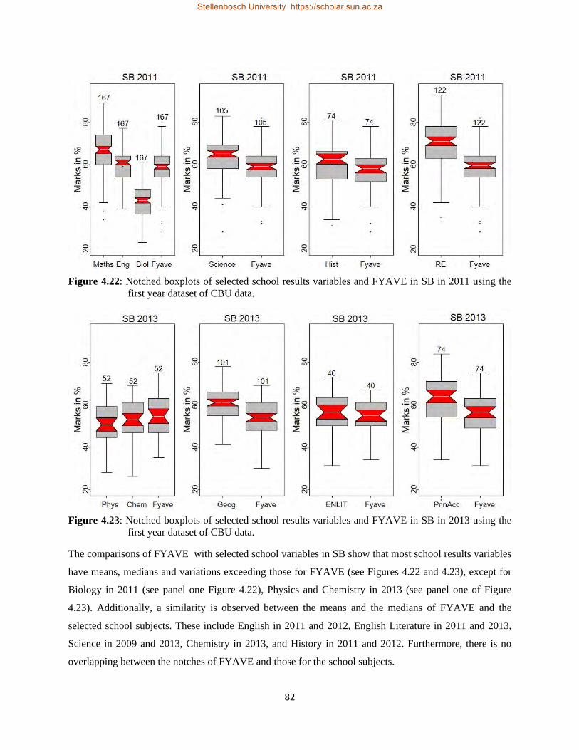
82
Figure 4.22: Notched boxplots of selected school results variables and FYAVE in SB in 2011 using the
first year dataset of CBU data.
Figure 4.23: Notched boxplots of selected school results variables and FYAVE in SB in 2013 using the
first year dataset of CBU data.
The comparisons of FYAVE with selected school variables in SB show that most school results variables
have means, medians and variations exceeding those for FYAVE (see Figures 4.22 and 4.23), except for
Biology in 2011 (see panel one Figure 4.22), Physics and Chemistry in 2013 (see panel one of Figure
4.23). Additionally, a similarity is observed between the means and the medians of FYAVE and the
selected school subjects. These include English in 2011 and 2012, English Literature in 2011 and 2013,
Science in 2009 and 2013, Chemistry in 2013, and History in 2011 and 2012. Furthermore, there is no
overlapping between the notches of FYAVE and those for the school subjects.
Stellenbosch University https://scholar.sun.ac.za
Stellenbosch University https://scholar.sun.ac.za

83
Figure 4.24: Notched boxplots of school results variables (Mathematics, English, Biology, Science,
Physics, Chemistry, and Geography) and FYAVE for SBE in 2013 using the first dataset.
Figure 4.25: Notched boxplots of school results variables (History, Religious Education, English
Literature, and Drawings) and FYAVE for SBE in 2013 using the first dataset.
Figures 4.24 and 4.26 also show that most school subjects in SBE and SNR have higher means and
medians, and greater standard deviations and median absolute deviations as compared to FYAVE, except
in 2013 which has FYAVE in ST with greater variation as compared to Chemistry, Geography, Science
and English (see Figures 4.24 and 4.25). Additionally, there is no overlapping between the notches of
FYVE and the school subjects. This indicates that the medians for each of the school subjects and those of
FYAVE are significantly different at the approximate 5% significance level. In Figures 4.24 to 4.26, some
school subjects (in 2013 for SBE and in 2012 for SNR) have lower means and medians as compared to
FYAVE. But this trend was not detected for other years.
Stellenbosch University https://scholar.sun.ac.za
Stellenbosch University https://scholar.sun.ac.za

84
Figure 4.26: Notched boxplots of selected school results variables and FYAVE for SNR in 2009 using
the first dataset.
The notched boxplots for the school variables and FYAVE for ST programmes in 2013 are displayed in
Figures 4.27 and 4.28. Notched boxplots for other years had similar patterns as in 2013 and are not
shown. In these figures, most school variables are characterised by higher means, medians and variations
as compared to FYAVE over the period considered. Biology (see the first panel of Figure 4.27), History
and Commerce (see Figure 4.28) are among the few school subjects whose means and medians exceed
that of FYAVE. Like in other faculties, there is no overlapping between the notches of FYAVE and the
school results variables.
The notched boxplots of FYAVE and G12AVE variables for the years 2009 and 2013 are displayed in
Figures 4.29 and 4.30 for all four faculties (the boxplots for other years are not shown). Over the four-
year period (2009 and 2011 to 2013), the standard deviations and the median absolute deviations of
G12AVE are lower than those of FYAVE for all faculties. In Figure 4.30, the means and medians for
G12AVE in SB and ST for the year 2009 are higher than those of FYAVE, while in SNR, the opposite is
observed. The same trend is exhibited for these faculties in 2013 (see Figure 4.30) and in other years
(notched boxplots not shown). For SBE, G12AVE has both mean and median exceeding those for
FYAVE for 2013 (see panel two of Figure 4.30), but for other years, the opposite is noted.
This pattern of results was expected in the four faculties since SB and ST usually admit school leavers
with outstanding school results. This is in contrast with SBE and SNR which generally receive students
with moderate school results.
Stellenbosch University https://scholar.sun.ac.za
Stellenbosch University https://scholar.sun.ac.za

85
Figure 4.27: Notched boxplots of school results variables (Mathematics, English, Biology, Additional
Mathematics, Science, Physics and Chemistry) and FYAVE for ST in 2013 using the first dataset.
Figure 4.28: Notched boxplots of school result variables (Geography, History, Commerce and Drawings)
FYAVE for ST in 2013 using the first year dataset. In summary, comparisons of school results variables with FYAVE have demonstrated that students are
usually admitted in different degree programmes of the CBU with exceptionally good results from the
school leaving national examinations, but achieve on the average lower marks in the first year of study.
This situation is more serious in SB and ST. Although no perfect matching between school and university
achievements was identified, as illustrated by non-overlapping notches of FYAVE and school variables,
some few school variables were in close correspondence with FYAVE and exhibited means and medians
Stellenbosch University https://scholar.sun.ac.za
Stellenbosch University https://scholar.sun.ac.za

86
which were closer to that of FYAVE. To fully answer the question on whether the attainment of high
marks at school level was being accompanied by better performance at the university level, further
investigation needs to be instigated in Chapter 5 using the correspondence analysis technique.
Figures 4.29: Notched boxplots of G12AVE and FYAVE in the four faculties in 2009 using the first
dataset.
Figures 4.30: Notched boxplots of G12AVE and FYAVE in the four faculties in 2013 using the first year
dataset.
Stellenbosch University https://scholar.sun.ac.za
Stellenbosch University https://scholar.sun.ac.za

87
4.2.6. Comparisons of school and university average performances using the graduate dataset.
These comparisons involve the graduate students who were in their first year of study in 2009 and who
completed their studies in 2012 for four-year degree programmes and in 2013 for five-year degree
programmes. The school results variables were compared to the university average variables to assess
whether school results variables were corresponding to students’ university performance. The notched
boxplots for the school average, Mathematics, English and university average variables are shown in
Figures 4.31 and 4.32, whereas Tables 4.5 and 4.6 report their summary statistics. The notched boxplots
and the summary statistics for the other school results variables are not reported.
The comparisons of G12AVE (school average performance) with the university average variables from
the first year to the final year of study suggest that the school average performance for students in four-
year programmes was higher than the average performance in the first year to the third year of study, and
the overall average university performance (see panel one of Figure 4.31). In the fourth year of study,
these students attained the highest academic achievement. In five-year degree programmes (see panel
two of Figure 4.31), the average performance at school level was lower than the average university
performances for first year to the fifth year of study which exhibit an increasing trend.
Table 4.5: Summary statistics for school variables (Mathematics, English and school average) and university averages for students in four-year programmes who graduated in 2012.
Statistic MATHS ENG G12AVE UWAY1 UWAY2 UWAY3 UWAY4 UWA
Mean 71.58 66.27 64.69 63.87 62.24 63.49 65.65 64.22
Median 73.00 67.00 64.00 62.58 60.69 62.90 64.84 63.30
SD 10.44 7.06 4.72 5.53 5.86 5.33 5.79 4.62
MAD 10.38 7.41 5.93 5.43 4.69 4.24 5.13 4.17
Table 4.6: Summary statistics for school results variables (Mathematics, English and school average) and university averages for students in five-year programmes who graduated in 2013.
Statistic MATHS ENG G12AVE UWAY1 UWAY2 UWAY3 UWAY4 UWAY5 UWA
Mean 69.76 62.25 61.94 64.03 64.89 64.15 66.10 67.05 65.07
Median 71.00 63.00 61.00 62.70 63.93 63.92 66.00 66.90 64.60
SD 11.93 7.44 6.34 6.47 5.97 5.94 5.51 5.11 4.87
MAD 11.86 5.93 5.93 6.23 5.74 7.07 6.08 5.78 4.77
Stellenbosch University https://scholar.sun.ac.za
Stellenbosch University https://scholar.sun.ac.za

88
Figure 4.31: Notched boxplots of the school average results (G12AVE) and university average variables
for graduates who were in their first year of study in 2009 for four-year degree programmes (panel one) and for five-year degree programmes (panel two) using the graduate dataset.
Figure 4.32: Notched boxplots of school results variables (Mathematics and English) and university average variables for graduates who were in their first year of study in 2009 for four-year degree programmes (panel one) and for five-year degree programmes (panel two) using the graduate dataset.
However, the overall average university performance (as represented by the variable UWA) was slightly
lower than the fourth and the fifth year average university achievements, and higher than the average
school performance.
When comparing the university average performances with the performance in individual school subjects,
it was found that the students who graduated in four-year degree programmes in 2012 (i.e. business
related programmes) achieved higher marks in school Mathematics and school English as compared to the
Stellenbosch University https://scholar.sun.ac.za
Stellenbosch University https://scholar.sun.ac.za

89
average university performances from first year to the fourth year of study (see panel one of Figure 4.32
and also Table 4.5). Similar patterns were discernible for five-year programmes (see panel two of Figure
4.32 and Table 4.6) with the performance in school English being closely in correspondence with the first
year average performance. Notched boxplots for other individual school subjects with the university
average variables and their accompanying summary statistics (not shown) revealed that the performance
in most school subjects was in excess of that for the university from the first year to the final year of study
in four-year degree programmes, whereas for five-year degree programmes, the opposite was observed.
In summary, graduates in business and engineering related programmes were admitted in the university in
2009 with excellent school results as compared to degree programmes in SBE and SNR. While students
in engineering related programmes achieved higher performance at university than at school level,
students in business related programmes had lower university academic achievement than the school
performance. The low average performance recorded at university level (as compared to school
performance) in business related programmes is in part due to the sizes of classes. While the classes of
first year students in engineering related programmes are also large; at second year level, sizes of classes
for engineering students (and also in SBE five-year programmes) are greatly reduced due to the
bifurcation of students into their respective programmes. In business related programmes, the bifurcation
into individual programmes of study occurs in the third year of study.
The next sections continue with the statistical investigations based on the notched boxplots by comparing
the school results variables of different groups of the first year students based on the first year results for
the first year dataset, and on the university results from the first year to the final year of study for the
graduate dataset.
4.2.7 Comparisons of the CP, PR, PT and EX groups for the first year dataset.
Further univariate statistical analyses are instituted in this section to determine whether school results
variables can be used to discriminate between different groups of students. Different groupings of
students considered in this section are based on the first year university performance, the graduation
status, the degree classification and the number of years taken by students to complete their studies. Four
groups are distinguished when considering the performance in the first year of study: the EX, PT, PR and
CP groups (represented by Fc1, Fc2, Fc3, and Fc4 in Chapters 6 and 7). The CP (clear pass) group
comprises students who pass all first year subjects and who unconditionally proceed into the second year
of study. The second group, known as the PR (proceed and repeat) group incorporates students who fail
one or two subjects at first year level and who are allowed to proceed into the second year of study
subject to repeating the failed courses. The PT (part time) students are those who fail three first year
Stellenbosch University https://scholar.sun.ac.za
Stellenbosch University https://scholar.sun.ac.za

90
subjects and who are permitted to repeat on part time basis the failed subjects. The last group, the EX
(exclude) group, concerns students who fail to proceed into the second year of study because of failing
four or more first year subjects and who are thus excluded from their respective programmes of study.
The second grouping is based on the graduation status of students. Two groups are considered: the G-
group and the NG-group. The G-group or the graduate group includes all students who completed their
studies in different degree programmes, whereas the NG-group or the non-graduate group consists of
students who were excluded in the first year, second year and third year of study or who failed to graduate
because of exhausting the maximum number of years allowed to complete a degree programme (six years
for four-year programmes and seven years for five-year programmes). Another classification of students,
associated with the degree classification, involves the D & M group (students who completed their studies
with distinction or merit), the CR group (those who graduated with credit) and the PA group (graduates
who got a degree with a pass). In Chapters 6 and 7, they are represented by Dc4, Dc3, Dc2, and Dc1. The
last grouping is based on the time taken to graduate: students who completed their studies within the
minimum stipulated number of years (four years for four-year programmes and five years for five-year
programmes) and those who took longer to graduate. Comparisons were made between these different
groups based on their school results. In what follows, the CP, PR, PT and EX groups are compared.
Figures 4.33 to 4.35 display the notched boxplots for the school overall performance measures G12AVE,
NDIS and EPOINT of the four groups of the first year students. Other notched boxplots showed similar
patterns as those presented in these figures and are thus not shown. To consolidate the findings from the
boxplots, means, medians, standard deviations and median absolute deviations were also computed, but
are not shown.
Figure 4.33 shows the notched boxplots for G12AVE for the four groups over the four-year period. For
all years considered, there is a close correspondence between the means and medians of G12AVE in each
of the four groups. Additionally, the standard deviations and the median absolute deviations for these
groups are closer and similar in all four years. In all years considered, the CP students have higher school
average marks as compared to other groups and have means and medians exceeding 60%. This is
followed by the PR group, then by the EX and PT groups. It is also observed a non-overlapping of the
notches for the four groups, except in 2013 which has the EX and the PR groups with overlapping notches
and the same means and medians of about 60%. In general, it can be said that G12AVE was, to some
extent, able to discriminate between the four groups of first year students during the period considered.
Stellenbosch University https://scholar.sun.ac.za
Stellenbosch University https://scholar.sun.ac.za

91
The notched boxplots of the variables NDIS and EPOINT for the four groups are displayed in Figures
4.34 and 4.35, respectively. Figure 4.34 demonstrates that NDIS, to some extent, was able to differentiate
the four groups of first year students. In panel one of Figure 3.34 (for the year 2002) for example, there is
a clear distinction between the EX, PR, and CP groups. The CP has greater variation, and higher median
and third quartile (of three and four, respectively) as compared to the PR and EX groups. This is followed
by the PR group with a median of two, and a third quartile of two. This group has a slightly lower spread
than the CP group. The EX group has the lowest median, first and third quartile (of one, zero, and two,
respectively) as compared to the other groups, while The PT group has the same median as the CP group,
Figure 4.33: Notched boxplots of G12AVE in 2009 and 2011 to 2013 for the CP, PR, PT and EX groups
using the first year dataset.
Figure 4.34: Notched boxplots of NDIS in the years 2002, 2007, 2010 and 2012 for the CP, PR, PT and
EX groups using the first year dataset.
Stellenbosch University https://scholar.sun.ac.za
Stellenbosch University https://scholar.sun.ac.za

92
but with lower variation. In panel two (for the year 2007 (see panel two), the CP group is different from
the EX group and has a high first quartile, median, and third quartile, and a greater variation. The PR and
PT groups have similar boxplots with identical medians and third quartiles (of two and three,
respectively) as the CP group, but with a greater variation. The EX group has the lowest variation, median
and third quartile as compared to the other three groups, but has the same first quartile as the PR and PT
groups. In panel three (for the year 2010), the CP has high mean, median, first and third quartile as
compared to the other three groups, while the PR and EX groups are almost similar (with the same
median, first and quartiles of two, one and three, respectively), but with the PR group having a higher
mean. The PT group has also the same median and third quartile as the PR and EX groups, but with a low
variation. In panel four (for the year 2012), The CP and the PR groups have identical notched boxplots
with overlapping notches, identical medians, first and third quartiles (of three, two, and four,
respectively), but with different means (i.e. the CP group has higher means). The EX and PT groups have
both a median of two, but have different variations (i.e. the former has a greater variation).
Figure 4.35: Notched boxplots of EPOINT in the years 2003, 2007, 2010 and 2012 for the CP, PR, PT
and EX groups using the first year dataset.
Figure 4.35 portrays the notched boxplots of EPOINT for the years 2003, 2007, 2010, and 2012. For other
years, the boxplots are not shown. In all years considered, except in 2006, the CP students were admitted
at the CBU with a median of ten points (in 2001, 2003 and 2004) or less (nine points in 2000, 2005,
2007, 2008 and 2011; eight points in 2002, 2009, 2010, 2012 and 2013) in the best five grade twelve
subjects. In 2006, the median of EPOINT for the CP group was eleven points. Notches only overlapped in
2001 for the CP and PR groups and in 2013 for the PR, PT and EX groups.
Stellenbosch University https://scholar.sun.ac.za
Stellenbosch University https://scholar.sun.ac.za

93
In the first three panels of Figure 4.35, the CP group is distinct from the other three groups, with the
lowest median, first and third quartiles, while the EX has the highest median, mean, first and third
quartiles (except in the third panel where it assumes the same median as the PT group). In the fourth
panel, the CP group has the lowest mean, first and third quartiles than the other groups, but has the same
median as the PR group. On the same panel, the EX and PT groups have identical medians, first and third
quartiles, but with different means.
These findings suggest that the CP group had the lowest entry points, while the EX group had the highest
entry points for most years considered. Similarly, the PR group possessed lower entry points as compared
to the PT and EX groups. While most first year students with lower entry points proceeded in the second
year of study, there were also students with lower entry points who were excluded or put on part time. For
example, half of those who were excluded in 2010 and 2012 (see the third and fourth panels of Figure
4.35) had entry points below ten and nine, respectively.
Figures 4.36 to 4.39 show the notched boxplots for school Mathematics, English, Science and Biology for
the four groups of the first year students. The notched boxplots for other school subjects exhibited
patterns similar to those in Figures 4.36 to 4.39 and are not shown.
It is clear from Figure 4.36 that the CP group has higher means and medians in Mathematics as compared
to other groups. This is followed by the PR group. The means for the CP group are ranging from 71.18 %
to 77.43 %, while for the PR group, they are between 64 % and 69.53 %. For the PT and EX groups, they
are varying between 61.00 % and 67.77 %, and between 57.90 % and 67.87 %, respectively. It is noted
higher medians (of 74% and 79%) in the years 2012 and 2013 for the CP group. When comparing the
standard deviations, the median absolute deviations and also the sizes of the boxes of the boxplots of the
four groups in Figure 4.36, the CP group is characterised by more or less constant variation over the four-
year period. Other groups have greater variations.
The notched boxplots in Figure 4.37 show that the four groups are almost similar with respect to school
English over the four-year period considered. The means and the medians for each group are mostly the
same (i.e. for example, the means and medians in 2011 were: 57.75% and 58% for CP; 58.19% and 58%
for PR; 57.3% and 58% for PT; 58.97% and 59% for EX). Additionally, from the notched boxplots of the
years 2009, 2011, and 2012 (see panels one to three of Figure 4.37), it is seen that the CP, PR, and PT
have almost similar and comparable means, medians, and variations, while the EX group has slightly
higher means and medians as compared to the other three groups. In the fourth panel (for the year 2013),
all four groups are almost similar and comparable with respect to the means, medians, and variations.
Stellenbosch University https://scholar.sun.ac.za
Stellenbosch University https://scholar.sun.ac.za

94
Figure 4.36: Notched boxplots of school Mathematics of CBU first year students in the years 2009 and
2011 to 2013 for the CP, PR, PT and EX groups using the first year dataset.
Figure 4.37: Notched boxplots of school English of CBU first year students in the years 2009 and 2011 to
2013 for the CP, PR, PT and EX groups using the first year dataset.
These findings suggest that school English had no ability to discriminate between the four groups of the
first year students over the four-year period considered.
The notched boxplots for school Science in Figure 4.38 are characterised by the means in decreasing
sequence for the CP, PR, PT and EX groups in 2009, 2012 and 2013. For example, in the third panel (for
the year 2012) the means for the CP, PR, PT and EX groups are 57.62%, 56.35%, 54.27% and 53.53%,
respectively. The same trend is also noted for the medians, but in 2009 only. Additionally, within each
Stellenbosch University https://scholar.sun.ac.za
Stellenbosch University https://scholar.sun.ac.za

95
group, there is a closeness between the means and the medians. Apart from the CP group which has the
highest means and medians over the four-year period, some other groups have identical medians (EX and
PT in 2011, EX and PR in 2012, and PR and PT in 2013). In the first panel (for the year 2011), the EX
group has a mean exceeding that of the PT group, whereas in the fourth panel (for the year 2013), the
notches for the PR and PT groups are overlapping implying that, at the 5% significance level, the medians
for these two groups are not significantly different. The notched boxplots for school Physics and
Chemistry had patterns similar to school Science and are not reported.
Figure 4.38: Notched boxplots of school Science of CBU first year students in the years 2009 and 2011
to 2013 for the CP, PR, PT and EX groups using the first year dataset.
Figure 4.39: Notched boxplots of school Biology of CBU first year students in the years 2009 and 2011
to 2013 for the CP, PR, PT and EX groups using the first year dataset.
Stellenbosch University https://scholar.sun.ac.za
Stellenbosch University https://scholar.sun.ac.za

96
Figure 4.39 portrays the notched boxplots for School Biology. It is clear, from Figure 4.39, that the CP
group is different from the other three groups and has slightly higher means and medians. Similarly, the
PR group is different from the PT group (see panels one to three for the years 2009, 2011 and 2012), but
in the fourth panel (for the year 2013) the PT group has slightly higher mean and median. It is also
observed in Figure 4.39, that for all four groups, the means, the medians and the third quartiles for all four
groups are all below 60%.
For school Geography (notched boxplots not shown), the CP group was different from the PR group in
the four years considered, and had higher means and medians than the other three groups. In 2009, 2011
and 2012, the means and medians of the PR group were higher than those of the PT group, but in 2013 the
opposite was observed. Concerning school History, the CP group was closer to the PR group. When
comparing the notched boxplots of school Principles of Accounts and Commerce, the former was
somehow able to discriminate between the four groups, whereas for the latter, only the difference between
the CP and other three groups was clear. School Religious Education had overlapping notches for the CP
and PR groups in 2011, but for the other years the means and the medians for CP were slightly exceeding
those for PR. When analysing school Additional Mathematics and school English Literature, the former
was able, to some degree, to differentiate between the four groups, while for the latter a clear demarcation
was visible only for the CP and the PR groups. For other school subjects there was no clear demarcation
between the four groups.
After carrying out the univariate statistical investigations in order to assess whether individual school
variables were able to discriminate between the four groups of the first year students (i.e. the CP, PR, PT
and EX groups), it is clear that not all school subjects were capable of differentiating the four groups.
School subjects like Mathematics, Science, Biology, Geography, Principles of Accounts, and Additional
Mathematics had somehow the ability to differentiate between the four groups, but their discrimination
power was limited. School English, despite playing a key role in the admission process (it is one of the
compulsory school subjects in the computation of the entry points), was not in a position to discriminate
between the four groups. From the above investigations, it was also clear that the overall school measures
G12AVE, NDIS and EPOINT were able to discriminate between the four groups of first year students.
4.2.8 Comparisons of the graduate with the non-graduate groups for the graduate dataset.
The graduate and the non-graduate groups were compared using the variables NDIS and EPOINT over
the fourteen-year period at the first year and the second year levels. Associated notched boxplots are
displayed in Figures 4.40 and 4.41 for NDIS and Figures 4.42 and 4.43 for EPOINT.
Stellenbosch University https://scholar.sun.ac.za
Stellenbosch University https://scholar.sun.ac.za

97
Figure 4.40: Notched boxplots of NDIS for the graduate group (GRAD) and the non-graduate group
(NOTGRAD) at first year level in 2004, 2005, 2006 and 2008 using the graduate dataset.
Figure 4.41: Notched boxplots of NDIS for the graduate group (GRAD) and the non-graduate group
(NOTGRAD) at second year level in 2000, 2002, 2005 and 2007 using the graduate dataset.
The pattern exhibited by the notched boxplots in 2004 (see Figure 4.40) was identical to that in the years
2000 and 2003 (not shown) with medians of two upper distinctions for the G-group (graduate group) and
one upper distinction for the NG-group (the non-graduate group). In 2004, the two groups had the same
third quartiles (of three upper distinctions). However, in 2000 and 2003, the G-group had higher third
quartiles (of three upper distinctions) than those of the NG-group which were two upper distinctions. For
the years 2002 and 2009, the two groups had identical medians (of three upper distinctions) with the
notched boxplots of the G-group having longer tails than those of the NG-group. But in 2008 (see panel
Stellenbosch University https://scholar.sun.ac.za
Stellenbosch University https://scholar.sun.ac.za

98
four) they had different medians. The students who achieved at least four upper distinctions at school
level were represented as outliers in the notched boxplots for the G-group. The notched boxplots for 2001
and 2006 (see panel three) exhibited similar patterns with the boxplots for the G-group having more
variation, longer right tails, medians of two upper distinctions, and third quartiles of three distinctions. In
2005 and 2007, the G-group was characterised by the notched boxplots having longer right tails with
medians identical to those of the NG-group. For the year 2005 (see panel two), the two groups had
identical medians (of two upper distinctions), first and third quartiles (of one and three upper distinctions,
respectively).
Figure 4.42: Notched boxplots of EPOINT for the graduate group (GRAD) and the non-graduate group
(NOTGRAD) at first year level in 2006, 2007, 2008 and 2009 using the graduate dataset.
Figure 4.43: Notched boxplots of EPOINT for the graduate group (GRAD) and the non-graduate group
(NOTGRAD) at second year level in 2002, 2005, 2006 and 2007 using the graduate dataset.
Stellenbosch University https://scholar.sun.ac.za
Stellenbosch University https://scholar.sun.ac.za

99
To some extent, NDIS was able to discriminate between the non-graduate group (i.e. the students who
were excluded at the first year level) and the graduate group (i.e. the students who passed their first year
of study and who successfully completed their studies) for some years only. Additionally, for all years
considered, the means of NDIS for the G-group were exceeding those of the NG-group. This implies that
the students who are usually admitted in different degree programmes at CBU with more upper
distinctions in school subjects are likely to pass the first year of study and thus complete their studies than
those with fewer upper distinctions at school level.
The notched boxplots reported in Figure 4.41, demonstrates that, at the second year level, it was not
possible to differentiate between the two groups (i.e. the students who passed the second year of study
and who graduated in their programmes of study (the G-group) and those who were excluded in the
second year of study and who could not complete their studies (the NG-group)) on the basis of the
variable NDIS. In the years 2000, 2003, 2005, 2007 and 2008, the two groups had identical medians,
whereas in the years 2001, 2002 and 2004 they were different. For most years, the G-group had greater
variations than the NG-group.
When considering the notched boxplots of the variable EPOINT in Figure 4.42 for the years 2006, 2007,
2008, and 2009 (the notched boxplots for other years are not shown), it is clear that the medians and the
means for the G-group are lower than those for the NG-group (except in 2006 which had identical
medians for both groups). Between 2006 and 2009, it is also noted a decreasing trend in the means and
the medians for both groups. This was probably due to the down adjustment of the programmes’ cut-off
points during this period.
At the second year level, EPOINT was able to demarcate between the two groups. There was a tendency,
for most years for the NG-group to have higher medians than the G-group. Also for most years, the
notched boxplots for NG-group had greater variations and longer tails as compared to the G-group (see
Figure 4.43 for the years 2002, 2005, 2006 and 2007).
Further comparisons of the two groups based on individual school subjects were not made because of the
small number of students in the NG-group. In order to have an idea on any difference between the two
groups using school results, summary statistics were computed and are presented in Table 4.7. The
descriptive numerical measures in this table show that the graduate students (G-group) who were in their
first year of study in 2009 obtained in G12AVE, school Mathematics and Biology higher means and
medians as compared to the non-graduate students. However, the NG-group had a mean and a median in
English slightly in excess to those of the G-group. Additionally, G12AVE for the NG-group had greater
variation than the G-group (see Table 4.7).
Stellenbosch University https://scholar.sun.ac.za
Stellenbosch University https://scholar.sun.ac.za

100
Table 4.7: Means, medians, standard deviations (SD) and median absolute deviations (MAD) for school subjects for the graduate (GRAD) and the non-graduate (NGRAD) students in 2009.
Variable Mean Median SD MAD
GRAD NGRAD GRAD NGRAD GRAD NGRAD GRAD NGRAD
G12AVE 62.17 58.11 62.00 58.00 6.22 7.44 5.93 10.38
MATHS 69.78 55.00 71.00 54.00 11.56 8.80 11.86 8.90
ENGS 62.87 67.67 63.00 70.00 7.79 8.00 8.90 7.41
BIOLS 53.59 49.11 54.00 46.00 8.54 8.54 8.90 7.41
Figure 4.44: Notched boxplots of G12AVE, School Mathematics, English and Science for the non-
graduate group over the 2011-2013 period using the graduate dataset.
A further investigation of the non-graduate students who were in their first year of study in 2011, 2012
and 2013 and who got excluded in the same years (cf. Figure 4.44) revealed that, during the 2011-2013
period, school results for the NG-group followed an increasing sequence for G12AVE, School
Mathematics, English and Science (from 2012 to 2013). The notched boxplots for other school results
(not shown) had similar patterns. This implies that most non-graduate students were admitted with good
results in most recent years. This was mainly due to the raising of the admission standards, specifically in
engineering related programmes where their cut-off points were made uniform and reduced to eight points
for male students and ten points for female students.
In order to rationalise teachings in engineering related programmes, all first year students in these
programmes were organised in large classes. This was a new phenomenon in these programmes. In
business related programmes also the sizes of first year classes increased during this period. As a result,
Stellenbosch University https://scholar.sun.ac.za
Stellenbosch University https://scholar.sun.ac.za

101
students with good school results got excluded at the first year level and could not graduate in their
respective programmes of study.
4.2.9 Comparisons of the groups of graduate students using the graduate dataset.
In order to check if the degree classification (distinction, merit, credit and pass) of students who graduated
over the 2000-2013 period was related to the admission variables, the notched boxplots of EPOINT and
NDIS were constructed for the three groups: D&M (distinction and merit combined), CR (credit) and PA
(pass). The notched boxplots for EPOINT are shown in Figure 4.45 for the completion years 2005, 2008,
2012 and 2013. For other years, the notched boxplots are not reported.
Figure 4.45: Notched boxplots of EPOINT for the three groups of graduate students (the D&M, CR and
PA groups) in the completion years 2005, 2008, 2012 and 2013 using the graduate dataset.
Notched boxplots in Figure 4.45 (and other boxplots not shown) show that the D&M group is distinct
from the other two groups and has the lowest entry points, suggesting that the students in this group were
admitted into the university with good results in the best five school subjects. In 2005 (see panel one),
2012 (see panel three), 2002, and 2004 (boxplots not shown), there was a clear demarcation between the
three groups with the D&M group having lower means, medians, first and third quartiles. This was
followed by the CR group, and then the PA group. In 2005, the PA group had the greatest variation, while
in 2012, the three groups had almost similar variation. In 2008 and 2013 (see panels two and four), the
PA and CR groups had identical medians, but the latter had a greater variation.
Stellenbosch University https://scholar.sun.ac.za
Stellenbosch University https://scholar.sun.ac.za

102
Table 4.8: Summary statistics for some school results variables for the 2009 intake of students who graduated in 2012 for four-year programmes and in 2013 for five-year programmes by degree classification (D&M-Distinction & Merit, CR-Credit, PA-Pass).
Subject Mean Median SD MAD
D&M CR PA D&M CR PA D&M CR PA D&M CR PA
G12AVE 65.66 61.47 60.56 66.00 61.00 61.00 6.26 5.80 5.84 7.41 5.93 5.93
Mathematics 73.55 69.08 67.91 75.00 70.00 68.00 11.18 11.74 11.03 11.86 11.86 11.86
English 64.81 62.65 61.72 64.00 62.00 62.00 7.71 7.76 7.71 7.41 8.90 8.90
Biology 57.68 52.43 52.22 58.00 53.00 53.00 8.41 8.44 7.85 8.15 7.41 7.41
Science 63.32 60.74 61.18 65.00 60.00 60.00 10.05 8.20 7.85 8.90 7.41 8.15
Physics 61.48 58.38 56.31 61.00 59.00 55.00 6.22 7.98 7.50 5.19 8.15 8.15
Chemistry 72.55 69.07 68.58 73.00 69.00 69.00 7.75 8.58 7.26 8.15 11.12 7.41
Geography 67.68 64.78 63.22 70.00 65.00 65.00 9.73 8.90 8.51 8.15 11.86 5.93
Accounts 69.73 61.22 58.93 72.00 60.00 59.00 9.94 14.37 12.93 5.93 11.12 8.90
History 62.35 59.64 57.15 60.00 61.00 58.00 13.54 9.95 11.52 14.83 7.41 10.38
Figure 4.46: Notched boxplots of G12AVE, school Mathematics, English, and Chemistry for the three
groups of graduate students ((the D&M, CR and PA groups) who were in their first year of study in.2009 using the graduate data.
Comparisons of the three groups based on the variable NDIS (notched boxplots not shown) showed a
clear demarcation between the three groups only in 2005 and 2013 with the D&M group having a higher
number of upper distinctions at school level, followed by the CR group, and then the PA group. In 2002,
2004 and 2012, the D&M group was distinct from the other two groups which were almost similar.
Stellenbosch University https://scholar.sun.ac.za
Stellenbosch University https://scholar.sun.ac.za

103
When the same groups were compared using school results variables for students who were in their first
year of study in the year 2009, and who graduated in 2012 for four-year programmes, and in 2013 for
five-year programmes, the D&M group was clearly distinct from the other two groups with an average
achievement at school level of 65.66% (mean) and 66% (median) as compared to 61.47% (mean) and
61%(median) for the CR group, and 60.56% (mean) and 61% (median) for the PA group (see Table 4.8
and panel one of Figure 4.46). It also had higher mean, first and third quartiles as compared to the PA and
CR groups. In individual school subjects, the D&M group also achieved higher marks than the other two
groups (see Table 4.8, and panels two to four of Figure 4.46 for school Mathematics, English and
Chemistry). The CR and PA groups were almost similar with respect to the individual school subjects.
Figure 4.47: Notched boxplots of EPOINT for the two groups of graduate students (those who graduated
within the minimum stipulated number of years and those who needed extra years) for the completion years 2005, 2009, 2011 and 2012 using the graduate dataset.
Figure 4.47 presents the notched boxplots of EPOINT of the two groups of graduates who completed their
studies within the minimum stipulated time (group one) and those who needed extra time to graduate
(group two). Figure 4.47 shows that the entry points for group one were lower than those of the second
group for the 2005 and 2012 graduates (see panels one and four). Similar patterns were observed for the
2000, 2001, 2004, 2008, 2010 and 2013 graduates (boxplots not shown). However, for the 2003, 2006 and
2011 graduates (see panel three of Figure 4.47 for the year 2011), the two groups were almost similar
with respect to the variable EPOINT. When comparisons were made using the variable NDIS, no
difference was detected among the two groups.
In this section, the comparisons of the school results variables of CBU graduates in degree programmes
have suggested that the students admitted with better school results were likely to attain good
performance at the university level, complete their undergraduate studies within the stipulated number of
Stellenbosch University https://scholar.sun.ac.za
Stellenbosch University https://scholar.sun.ac.za

104
years and achieve a higher degree classification. However, school results variables were not the only
factors affecting the degree classification and the completion time. Other factors like the length of the
programmes, the types of programmes, and the number of subjects in the programmes of study were
detrimental in determining the degree classification of graduates.
The univariate statistical investigations based on the boxplots continue in the next section with the analysis of the school results for the population data.
4.3 Notched boxplots and line plots for the population data.
Section 4.2 dealt with the statistical graphical analyses of the school and the university results variables
using the CBU data. In this section, the statistical investigations of the school results variables using the
data for the entire country are carried out. The CBU data in this section will be referred to as the CBU
sample data as they concern only the students admitted at CBU, whereas those for the entire country will
be viewed as the population data. It should be recalled that the admission criteria at the CBU and in all
higher learning institutions in Zambia are solely based on the school (grade twelve) results in different
school subjects. It is thus important to check for pattern changes, over the years, in the school results
using the population data. Additionally, it is also essential to compare the school results variables using
both the CBU data and the population data for the entire country in order to check for similar patterns and
trends. Notched boxplots and line plots (means plots and median absolute deviations plots) were
constructed. The numerical descriptive measures (means, medians, standard deviations and median
absolute deviations) were also computed (but are not shown) to assist with the comparison of the various
characteristics of the school results variables in the population data.
4.3.1 Comparison of individual school results variables using the population data over eleven years.
The notched boxplots for Mathematics, Additional Mathematics, English, English Literature, Science,
Physics, Chemistry, Biology, Geography and History are displayed in Figures C.5 to C.9 in Appendix C.
The means plots and median absolute deviations plots are also reported in Figures 4.48 to 4.51.
Additionally, the minimum and maximum values, means, medians and median absolute deviations of all
school subjects for the entire population were also computed, but are not shown.
When inspecting the notched boxplots (see Figures C.5 to C.9), and the tables of descriptive numerical
values (not reported), the following features were retained:
• Over the eleven-year period, the means and the medians for most school subjects were below
50%, except for some few school subjects (i.e. Additional Mathematics (in 2000 and 2001), Arts
(in all years except in 2000 and 2001), Chemistry (2003 and 2007), Computer studies (2000,
Stellenbosch University https://scholar.sun.ac.za
Stellenbosch University https://scholar.sun.ac.za

105
2001, 2007, and 2012), French (2000, 2001, and 2009), Food and Nutrition (2009), Music (2008),
and Zambian Language (2000, 2001) for the means). These school subjects had also medians
slightly in excess of 50% for some years only.
• From the sizes of the boxes of the notched boxplots (see Figures C.5 to C.9 for Mathematics,
Additional Mathematics, English, English Literature, Science, Physics, Chemistry, Biology,
Geography, and History. For other school subjects, the boxplots are not shown), the values of the
standard deviations, and the median absolute deviations (not shown), it is clear that each school
subject had similar and comparable variations over the eleven-year period.
• The school subjects with the highest variations (with MADs mostly above 20%) comprised
Religious Education and Drawing (see Figures 4.50 and 4.51). Low variations were recorded for
Agriculture Science, Arts, Food & Nutrition and Biology.
• The grade twelve learners who achieved the highest scores in the school leaving examinations
were representing a small percentage of the entire population and were displayed as outliers in the
notched boxplots. These are among the school leavers who managed to get admitted in various
degree programmes of the public universities.
• Mathematics and Agriculture Science recorded the lowest performance in the school leaving
examinations with the means and the medians mostly below 30%. Other school subjects with
poor performance included Science, History, Biology, English Literature, Commerce and
Principles of Accounts.
• On the higher performance brackets were found Additional Mathematics, Chemistry, Physics,
English, Geography, Arts, Food & Nutrition, Computer Studies, Zambian Language, Drawing,
Metal/Wood works, Religious Education and French with means and medians mostly in excess of
45%.
• It was noted in Figure C.5 that school Mathematics had low means and medians (below 30%) as
compared to Additional Mathematics whose means and medians were mostly between 40% and
50%. However, Additional Mathematics showed a greater variation than Mathematics. The
notched boxplots for Mathematics were highly skewed to the right, whereas those for Additional
Mathematics were nearly symmetric. It is important to note that those who sat for Additional
Mathematics only represent 2% (3% in 2000 and 2001, and 2% for other years) of the students
who wrote Mathematics paper. These candidates mostly got a median and average marks above
60% in Mathematics. When comparing English and English Literature, it was observed from
Figure C.6 that English literature had low means and medians, and greater variations as compared
to English. Similarly, Science recorded low means and medians as compared to Physics and
Chemistry. But these three subjects, over the eleven-year period, had similar and comparable
Stellenbosch University https://scholar.sun.ac.za
Stellenbosch University https://scholar.sun.ac.za

106
variations (see Figures C.7 and C.8). Comparisons of Geography and History (see Figure C.9)
and also of Commerce and Principles of Accounts suggest that History had greater variations and
lower means and medians as compared to Geography. Likewise, Principles of Accounts had
higher means and medians than Commerce, but both had similar variations.
The means and the median absolute deviations are graphically displayed in Figures 4.48 to 4.51 (plots for
the medians and the standard deviations are not shown). To some extent, Religious Education and French;
and Commerce and Agriculture Science had similar trends with downward shift in the means over the
eleven-year period. From 2009 to 2012, similar trends were observed in Principles of Accounts, French,
Drawings, Metal/Wood Works and Zambian Language. On the other hand, Food & Nutrition and Arts
had an increasing trend in the means and the medians (see Figure 4.49 for the means plots).
Figure 4.48: Means plots of school Mathematics, English, Biology, Physics, Chemistry, Science,
Additional Mathematics, English Literature, Geography and History over eleven years using the population data.
From Figure 4.48, an upward shift in the means (also in the medians) was noticeable between 2000 and
2002 for Chemistry, English Literature, Geography, Mathematics, History, while for Biology, the shift in
the means was downward. After 2007, the pattern changes and shift in the means were more smooth and
stable. Chemistry, Metal/Wood Works and Drawings had means fluctuating between upward and
downward shifts.
Figure 4.50 demonstrates that Additional Mathematics had the highest variation with smooth shift in the
means between 2001 and 2009. In the same figure, Mathematics and Geography had a decreasing trend in
the variation after 2006. Between 2000 and 2002, Principles of Accounts and Agriculture Science had
similar trends (see Figure 4.51). Also between 2000 and 2007, trends of variation of Metal/Wood Works
and Commerce were the same, but after 2007, a downward shift for Commerce and an upward shift for
Stellenbosch University https://scholar.sun.ac.za
Stellenbosch University https://scholar.sun.ac.za

107
Metal/Wood Works were observed. On the other hand, throughout the eleven-year period, a downward
shift in the variation was recorded for French.
Figure 4.49: Means plots of school Religious Education, Zambian Language, Metal/Wood works,
Agriculture Science, Drawing, Principles of Accounts, Commerce, Food & Nutrition, French and Arts over eleven years using the population data.
Figure 4.50: Median absolute deviations plots of school Mathematics, English, Biology, Physics,
Chemistry, Science, Additional Mathematics, English Literature, Geography and History over eleven years using the population data.
Stellenbosch University https://scholar.sun.ac.za
Stellenbosch University https://scholar.sun.ac.za

108
Figure 4.51: Medians absolute deviations plots of school Religious Education, Zambian Language,
Metal/Wood works, Agriculture Science, Drawings, Principles of Accounts, Commerce, Food & Nutrition, French and Arts over eleven years using the population data.
4.3.2 Comparison of school results variables using both CBU data and population data.
In this section, the univariate statistical investigations using the notched boxplots are performed in order
to compare the attributes of the school results variables for the CBU data and the population data.
Although the notched boxplots were constructed for all four years (i.e. 2009, and 2011 to 2013) and for
all school subjects, only those for school Mathematics, Science, English, Biology, Additional
Mathematics and English Literature for the 2013 first year intake are displayed in Figure 4.52. The
notched boxplots for other years and other school subjects exhibited similar patterns as those shown in
Figure 4.52, and are not shown.
From Figure 4.52, it is evident that the attributes of the school results variables using the CBU data were
completely different from those of the population data. School results variables using the population data
were characterised by the presence of several outliers, greater variations, and lower means and medians
mostly below 50% as compared to those in the CBU data which had means and medians in excess of 60%
for most school subjects. As an illustration, the mean and median for Mathematics using the CBU data
were 72.36% and 73.00%, as compared to 24.52% and 20.00% for the entire country. The distributions
for most school results variables in the population were positively skewed with right long tails indicating
that the majority of the grade twelve learners in the population achieved lower scores. This was in
contrast with the school results variables using the CBU data whose distributions were corresponding to
the upper parts of the distributions in the population. These results were expected, as the CBU only
admits students with outstanding grade twelve results. The students admitted in different degree
programmes were among the top 10% of the best students with respect to the school results. From the first
Stellenbosch University https://scholar.sun.ac.za
Stellenbosch University https://scholar.sun.ac.za
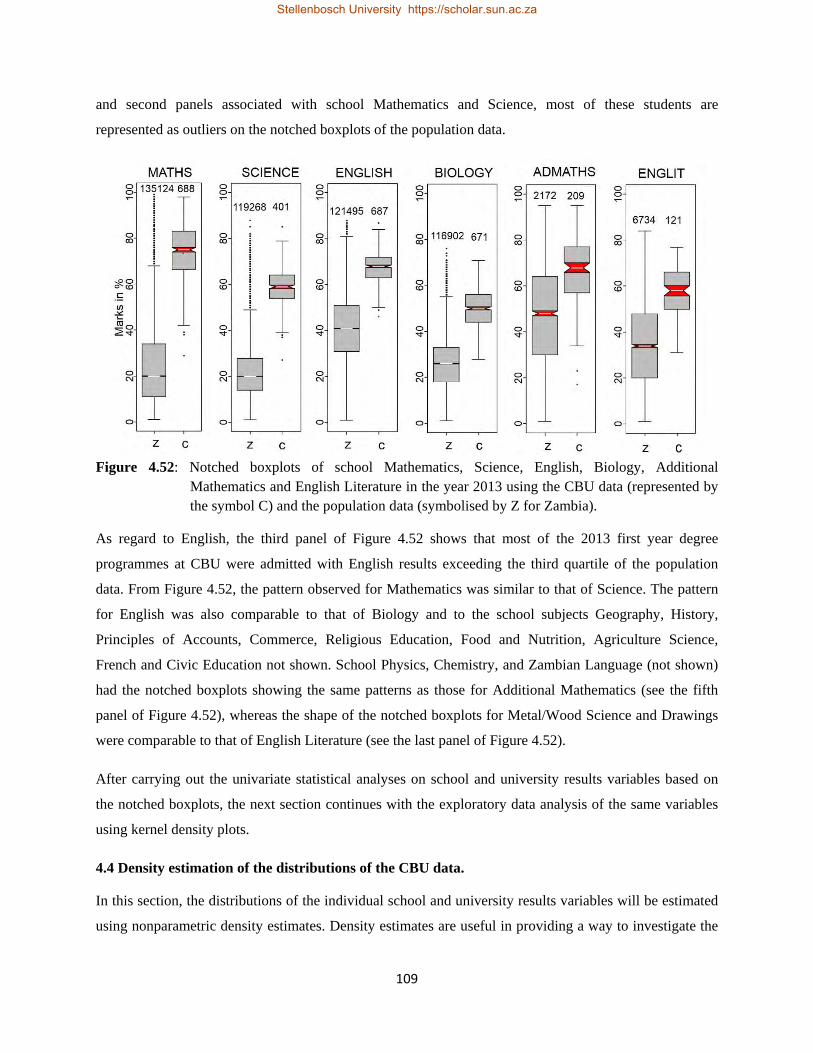
109
and second panels associated with school Mathematics and Science, most of these students are
represented as outliers on the notched boxplots of the population data.
Figure 4.52: Notched boxplots of school Mathematics, Science, English, Biology, Additional
Mathematics and English Literature in the year 2013 using the CBU data (represented by the symbol C) and the population data (symbolised by Z for Zambia).
As regard to English, the third panel of Figure 4.52 shows that most of the 2013 first year degree
programmes at CBU were admitted with English results exceeding the third quartile of the population
data. From Figure 4.52, the pattern observed for Mathematics was similar to that of Science. The pattern
for English was also comparable to that of Biology and to the school subjects Geography, History,
Principles of Accounts, Commerce, Religious Education, Food and Nutrition, Agriculture Science,
French and Civic Education not shown. School Physics, Chemistry, and Zambian Language (not shown)
had the notched boxplots showing the same patterns as those for Additional Mathematics (see the fifth
panel of Figure 4.52), whereas the shape of the notched boxplots for Metal/Wood Science and Drawings
were comparable to that of English Literature (see the last panel of Figure 4.52).
After carrying out the univariate statistical analyses on school and university results variables based on
the notched boxplots, the next section continues with the exploratory data analysis of the same variables
using kernel density plots.
4.4 Density estimation of the distributions of the CBU data.
In this section, the distributions of the individual school and university results variables will be estimated
using nonparametric density estimates. Density estimates are useful in providing a way to investigate the
Stellenbosch University https://scholar.sun.ac.za
Stellenbosch University https://scholar.sun.ac.za

110
properties and characteristics of the variables of the CBU data with respect to multimodality, variation,
tails, and skewness in the data. The knowledge of these density estimates is also vital for comparing
school and university results variables across faculties, programmes and over time. This information is
also important in assessing changes which occurred over time in the school and university results
variables and in checking the suitability of admission criteria by assessing if raising the admission
standards were being accompanied by upward changes in the university performance.
Kernel density estimators (KDE) based on Gaussian kernel functions (see Efron & Tibshirani, 1993;
Härdle & Simar, 2003; Carmona, 2004; and Everitt & Hothorn, 2010) are used to estimate the
distributions of the school and university results variables for the CBU data and the population data. This
analysis concerns only the years which had actual marks (in %) available for both school and university
results variables; that is, in the years 2009, and 2011 to 2013 for the first year dataset. For the graduate
dataset, the actual marks (in %) for the school subjects and university results from the first year to the
final year of study were only accessible for the students who entered the university in 2009. Additionally,
the actual marks (%) for the 2009 to 2013 graduates were also available.
As a starting point for the values of bandwidths to use, Silverman’s rule on values of bandwidths of
h = 0.9𝑛𝑛−1/5min �s, IQR1.349
� with IQR being the interquartile range, n the sample size and s the sample
standard deviation, was adopted (see Silverman, 1986). The R source codes used to generate the density
plots are given in Appendix B.
When comparing the school and the university results variables using their KDEs, the Kolmogorov-
Smirnov (K-S) test will be used to test the null hypothesis of equality of the two distributions associated
with a school results variable and a university results variable. If the two distributions are identical, there
should be a close agreement between them (Daniel, 1990).
4.4.1 Nonparametric density estimation: Kernel density estimates (KDE) of school and university results variables for business related programmes using the first year dataset of the CBU data.
Figures 4.53 to 4.55 display the kernel density estimates (KDEs) of the variables FYAVE, G12AVE and
some selected school results variables for SB. For visibility and readability of the graphs, all school
results could not be represented on the same figure.
Stellenbosch University https://scholar.sun.ac.za
Stellenbosch University https://scholar.sun.ac.za

111
Figure 4.53: Kernel density estimates of the densities for FYAVE and G12AVE in the years 2009, and
2011 to 2013 for SB using the first year dataset of CBU data.
Figure 4.54: Kernel density estimates of the densities for FYAVE, school Mathematics, English and
Biology in the years 2009 and 2011 to 2013 for SB using the first year dataset of CBU data.
In Figure 4.53, the distributions of FYAVE in 2009, 2011and 2012 had modes occurring near 60% and
being close to the means of 60.19%, 59.08% and 59.28% and the medians of 60%, 59% and 60% for the
three years. The closeness between the modes, means and medians suggests that the densities of FYAVE
over the three years could be approximated by the normal distribution. For the year 2013, FYAVE had a
bimodal distribution with minor and major modes located at approximately 50% and 62%, respectively.
This indicates that most of the 2013 first year students (the CP and PR groups) in business related
Stellenbosch University https://scholar.sun.ac.za
Stellenbosch University https://scholar.sun.ac.za

112
programmes achieved average marks between 50% and 62% in the first year of study. When comparing
the minor and major modes with the means and medians of the CP and PR groups, it was discovered that
the minor mode of 50% was corresponding to the PR group which had a mean of 52.44% and a median of
52%, whereas the major mode of 62% was associated with the CP group whose mean and median were
61.69% and 62 %, respectively. The CP and PR groups were only discernible from the density of FYAVE
in 2013 only. For other years, this grouping was not apparent.
When examining the kernel density estimates for G12AVE over the four-year period (see Figure 4.53), it
is observed that this variable had single peaks (i.e. modes) occurring at 65%, 60%, 55% and 60% for the
four years considered. It is important to note that these modes were forming a decreasing sequence in the
years 2009, 2011 and 2012. The same order was observed for the means 63.57%, 59.95% and 59.62% and
the medians 63%, 60% and 58%. But in 2013, the mode and the median increased to 60% and 59%,
respectively, while the mean (of 58.90%) was at its lowest level over the four years considered. This
could be the result of the admission standards which were lowered in 2013 for business related
programmes at SB. From Figure 4.53, it is also seen that the distribution of FYAVE was in close
agreement to that of G12AVE in 2012. This was reinforced by a non-significant Kolmogorov-Smirnov
(K-S) test for equality of the distributions of FYAVE and G12AVE (p-value = 0.2681). In other years, the
distributions of these variables were statistically different (p-values of 0.0005, 0.0018 and 0.0000 in 2009,
2011 and 2013, respectively).
Figure 4.54 presents the kernel density estimates of FYAVE, and school Biology, Mathematics and
English. School Biology had modes near 55%, 42%, 45% and 45% over the four-year period. Over the
same period, the means and the medians for this variable were 53.54%, 42.14%, 45.04% and 47.06%; and
54%, 43%, 45% and 46%, respectively, and were in close connection with the modes, indicating that the
distribution of Biology in the four years could be estimated by a normal distribution.
A comparison of Biology with FYAVE revealed that a greater proportion of students achieved at least
50% in both FYAVE and Biology for the 2009 intake of the first year students in business related
programmes. But for other years, a different pattern was observed with most of the students getting scores
of at least 50% in FYAVE. From these students, only a small proportion achieved scores of at least 50%
in Biology. These results suggest that students were admitted in business related programmes with
relatively low results in Biology in 2011, 2012 and 2013 as compared to the year 2009. The other two
estimated densities presented in Figure 4.54 show that the modes of Mathematics and English were both
attained at 70% in 2009 and 2013. In 2011 and 2012, they were below 70% (near 65% and 62% for
English, and 66% and 68% for Mathematics). Over the four-year period, the majority of students who
Stellenbosch University https://scholar.sun.ac.za
Stellenbosch University https://scholar.sun.ac.za

113
obtained at least 50% in FYAVE, also achieved scores of at least 50% in school Mathematics and
English.
A comparison of all densities in Figure 4.54 indicates that Mathematics had the highest variation over the
four years considered. Other variables had similar and comparable variations. As regarding the shape of
the densities of Mathematics and English, the distribution of the latter exhibited some negative skewness
in 2009, 2011 and 2013. But in 2012, it was fairly symmetric. For Mathematics, the distribution was
negatively skewed with a long tail on the left for all four years. When comparing the distributions of
FYAVE with those of school Mathematics, English and Biology, only English was in a close agreement
with FYAVE in 2011 and 2012, as shown by a non-significant K-S test for equality of the two
distributions (p-values of 0.6923 in 2011 and 0.2607 in 2012).
Figure 4.55: Kernel density estimates of the densities for FYAVE, Physics and Chemistry in the years
2009 and 2011 to 2013 for SB using the first year dataset of the CBU data. In Figure 4.55, the densities of Physics and Chemistry were compared to that of FYAVE. A close
correspondence was noted between FYAVE and Physics in 2011 and 2013, with both variables having
the same modes of 60% in 2011, and 50% in 2013 (coinciding with the minor mode of FYAVE). This
was confirmed by non-significant K-S tests for equality of the distributions of FYAVE and Physics (p-
values of 0.7426 in 2011 and 0.4173 in 2013). However, in 2009 and 2012, the distributions of these two
variables were different with modes of 62% and 60% in 2009; and 65% and 55% in 2012. The situation in
2012 indicates that from the majority of students who obtained at least 60% in FYAVE, only a small
proportion achieved scores of at least 60% in Physics. When comparing FYAVE and Chemistry, it was
found that in 2013 the densities for the two variables almost coincided (K-S p-value = 0.8793) and were
Stellenbosch University https://scholar.sun.ac.za
Stellenbosch University https://scholar.sun.ac.za

114
both bimodal with the same minor modes around 50% and major modes at 65%. During the same year,
the means (of 54.92% for FYAVE and 53.12% for Chemistry) and the medians (of 54.5% for FYAVE
and 53% for Chemistry) were also similar and comparable. However, for the years 2009 and 2012 the
distribution of Chemistry had higher modes (of 75% in 2009 and 2012), as compared to that of FYAVE
which had modes of 62% in 2009 and 65% in 2012. Chemistry also possessed higher means (of 70.09%
and 67.02% as compared to 62.55% and 62.22% for FYAVE) and medians (of 71% and 67.5% as
compared to 62% for FYAVE) in 2009 and 2012. In 2011, Chemistry had lower mode, mean and median
(of 52%, 55.65% and 55%, respectively) than FYAVE implying that the 2011 first year intake of students
in business related programmes scored lower in school Chemistry as compared to FYAVE. When
examining the shapes of the densities estimates in Figure 4.55, it transpired that, for all four years, the
distribution of Physics was nearing a symmetric distribution and could be approximated by the normal
distribution. For FYAVE and Chemistry, distributions were either positively or negatively skewed over
the four years.
Comparisons of FYAVE with the other school results variables revealed a close agreement between
FYAVE with History in 2009 and 2012 ( K-S p-values of 0.1848 and 0.7741), Science in 2009 and 2013
(K-S p-values of 0.2032 and 0.4203), Additional Mathematics in 2009, 2011 and 2013 (K-S p-values of
0.4413, 0.3877 and 0.6208), English Literature in 2011, 2012 and 2013 (K-S p-values of 0.6465, 0.4143
and 0.7591), Commerce in 2009 (K-S p-value of 0.2198), Drawings in 2009, 2011 and 2013 ( K-S p-
values of 0.6272, 0.2997, and 0.2154), Principles of Accounts in 2012 (K-S p-value of 0.454) and
Metal/Wood Works in 2009, 2012 and 2013 (K-S p-values of 0.5412, 0.9048 and 0.1314). Densities for
all other years and other school results were different from those of FYAVE.
When comparing the distributions of Mathematics and Additional Mathematics with those of FYAVE,
and also of English and English Literature with those of FYAVE, it was seen that Mathematics and
English had densities which showed some stability and less variation than the distributions of Additional
Mathematics and English Literature. A bimodality feature was noted in the distribution of English
Literature in 2009 with modes at 70% and at 45% suggesting that this distribution was a mixture of two
densities. The component corresponding to the main peak at 70% was closely associated with a small
percentage (of the CP group) who obtained scores in excess of 70% in both English Literature and
FYAVE. For other years, the behaviour of English Literature was similar to that of English.
Having statistically investigated the distributions of school results variables and FYAVE in SB, it can be
concluded that not all school results variables had densities in close correspondence with that of FYAVE.
Some school variables had densities exhibiting higher means, medians and modes as compared to
Stellenbosch University https://scholar.sun.ac.za
Stellenbosch University https://scholar.sun.ac.za

115
FYAVE. Additionally, bimodality, long tail and skewness features were associated with the densities of
some variables.
The next two sections continue with the univariate statistical analyses based on the kernel density
estimates of the school and university results variables for engineering related programmes and other
programmes. The aim was to unveil the situation prevailing in non-business related programmes and
ascertain whether the trends observed in business related programmes were also prevalent in these
programmes.
4.4.2 Kernel density estimates of school and university results variables for engineering related programmes for the first dataset of the CBU data.
Figures 4.56 to 4.58 provide the kernel density estimates of the school results variables and FYAVE in
engineering related programmes.
Figure 4.56: Kernel density estimates of the densities for FYAVE and G12AVE in the years 2009 and
2011 and 2013 for ST using the first year data of the CBU data. FYAVE in Figure 4.56 had a long tail on the left and was negatively skewed with modes at 65% in 2009
and 2011, 61% in 2012 and 55% in 2013. Small humps were observed on the left of the density of
FYAVE at 45% (in 2009, 2011 and 2012) and at 40% in 2013. This could represent a small group of EX
students who were excluded in each of the ST degree programmes. Small humps were also visible on the
right of the distribution of FYAVE at 75% (in 2009, 2011 and 2013), and at 70% in 2012 probably
representing a small proportion of the CP group who achieved higher marks at both school and first year
levels. Another characteristic of FYAVE concerns its means (of 62.16%, 60.15%, 58.74% and 56.97%)
Stellenbosch University https://scholar.sun.ac.za
Stellenbosch University https://scholar.sun.ac.za

116
and medians (of 63%, 61%, 60% and 57%) which were forming a decreasing sequence over the four-year
period. Moreover, the means and medians were similar and comparable over the four-year period.
Figure 4.57: Kernel density estimates of the densities for FYAVE, school Mathematics, English and
Biology in the years 2009 and 2011 to 2013 for ST using the first year data of the CBU data. G12AVE in the same figure had single peaks at 65% for all four years. Similarly, for the SB programmes,
the means (of 63.45%, 62.02% and 61.93%) and the medians (of 64%, 63% and 62%) of this variable
were in decreasing order for the years 2009, 2011 and 2012. But in 2013, both the mean and the median
slightly increased (from 61.93% to 63.33% for the mean, and from 62% to 63% for the median). This
could be the result of the major raising of the admission standards which saw the cut-off points in ST
programmes greatly reduced and made uniform for all engineering related programmes. During the same
year, FYAVE recorded the lowest mode, mean and median, probably due to the lack of remedial
measures to deal with the introduction of large classes which was a new phenomenon in ST. When
comparing the distributions of G12AVE and FYAVE, a closeness was observed between these two
variables. This was reinforced by the majority of students who achieved at least 60% in 2011 and 2012,
and at least 55% in 2009 and 2013 in both G12AVE and FYAVE. When testing the hypothesis of
equality of the distributions of these two variables, the K-S test was significant in all years, except in
2009 (K-S p-value of 0.0965).
In Figure 4.57, the distributions of Mathematics had higher variation, with means, medians and modes
well in excess of 70% for all four years, suggesting that the students in engineering related programmes
entered the first year of the university with outstanding results in school Mathematics. Although the
majority of students obtained scores in school Mathematics in excess of 70%, only a small proportion of
these students achieved an average score exceeding 70% at first year level, indicating that Mathematics
Stellenbosch University https://scholar.sun.ac.za
Stellenbosch University https://scholar.sun.ac.za

117
had scores not in close correspondence with those of FYAVE. In the same figure, it is seen that the
densities of FYAVE, English and Biology had similar and comparable variation. However, English was
closely corresponding to FYAVE (in 2009, 2011 and 2012), except in 2013 which had mean (of 67.85%),
median (of 68%) and mode (of 70%) higher than those of FYAVE. In 2009, the distributions of FYAVE
and English were coinciding, suggesting an equality of these distributions (K-S p-value of 0.5559). As in
business related programmes, the students in ST programmes obtained relatively low scores in Biology.
While most students achieved more than 55% in FYAVE, only a small proportion of these students
achieved more than 55% in Biology.
Figure 4.58 reveals that the distributions of Physics and Chemistry were different in 2009 and 2012, with
modes attained at 60% for Physics, and around 72% and 75% for Chemistry. However, in 2011 and 2013
they both achieved a peak at 63% in 2011, and at 60% in 2013 suggesting that they were closely matching
in these two years. The density of FYAVE was closely corresponding to that of both Physics and
Chemistry in 2011 (K-S p-values of 0.3788 and 0.4804). But in 2012, FYAVE was only closely matching
with Physics (K-S p-value of 0.2085), whereas in 2013, it was closely connected to Chemistry
(K-S p-value = 0.5538).
The kernel density estimates for FYAVE and Science (not reported) showed that students in the first year
of study in ST scored high marks in Science with modes, means and medians exceeding those of FYAVE,
implying that this school subject was not closely corresponding to FYAVE. When considering the
estimated densities for English Literature, Geography, Additional Mathematics, and History (not shown),
there were some indication of close agreement between English Literature (for all four years with K-S
p-values of 0.8079, 0.3877, 0.2634 and 0.5616) and History (in 2011 and 2012 only with K-S p-values of
0.3034 and 0.4611) with FYAVE. But for Geography and Additional Mathematics, there was a clear
tendency for the students admitted in ST programmes to achieve higher marks (in %) in Geography and
Additional Mathematics at school level than in FYAVE. For example, the distribution of Additional
Mathematics for all four years had greater variation and higher modes (in excess of 75%), means and
medians. The pattern observed in SB programmes concerning Principles of Accounts, Drawings,
Commerce and Religious Education also prevailed in engineering related programmes.
The findings in this section have shown that the students admitted in engineering related programmes
showed a tendency to achieve higher marks in school subjects than in FYAVE. Only a small number of
school results variables had scores comparable to that of FYAVE. The next section discusses the kernel
density estimates for other programmes.
Stellenbosch University https://scholar.sun.ac.za
Stellenbosch University https://scholar.sun.ac.za

118
Figure 4.58: Kernel density estimates of the densities for FYAVE, school Physics and school Chemistry
in the years 2009 and 2011 to 2013 for ST for the first year dataset of CBU data. 4.4.3 Kernel density estimates of school and university results variables for other programmes.
Figure 4.59 presents the kernel density estimates associated with FYAVE and G12AVE over the four-
year period for non-engineering and non-business related programmes. For all four years, G12AVE had
modes of 55% similar and comparable to the means and medians. The distribution of G12AVE was
nearing symmetry suggesting that, over the four-year period, a normal distribution could be used to
approximate the density of G12AVE in non-business and non-engineering programmes. The distribution
of FYAVE had means and medians below 60% and modes at 60% (in 2011 and 2012), major and minor
modes at 60% and 50% (in 2009) and at 50% and 60% (in 2013). Additionally, the distribution for this
variable was negatively skewed in 2011, 2012 and 2013. In 2009, G12AVE and FYAVE were very
closely matching with a non-significant K-S for equality of their distributions (K-S p-value = 0.0975).
The kernel density estimates in Figure 4.60 show that Mathematics had a greater variation as compared to
the other variables. This pattern was also observed in business and engineering related programmes. Its
distributions had single peaks at 70% in 2011 and 2013, and 62% in 2009 and 2012. The densities of
Biology, on the other hand, had modes, means and medians below 50%. Concerning the distributions of
English, peaks were attained at 62% in 2009, 55% in 2011, 59% in 2012, and 70% in 2013. The
comparisons of the distributions of FYAVE to those of English, Biology and Mathematics suggest that
the students in other programmes (in SBE and SNR) were admitted in the first year of study with higher
scores in Mathematics and lower scores in Biology as compared to FYAVE. School English, on the other
hand, was closely corresponding to FYAVE only in 2009 (K-S p-value = 0.0944) and 2012 (K-S p-value
Stellenbosch University https://scholar.sun.ac.za
Stellenbosch University https://scholar.sun.ac.za

119
= 0.1867). The kernel density estimates for the other school variables are not shown. Generally, FYAVE
was not corresponding closely with most school results variables.
Figure 4.59: Kernel density estimates of the densities for FYAVE and G12AVE in the years 2009 and
2011 to 2013 for other programmes of CBU data.
Figure 4.60: Kernel density estimates of the densities for FYAVE, school Mathematics, school English
and school Biology in the years 2009 and 2011 to 2013 for other programmes of CBU data.
Stellenbosch University https://scholar.sun.ac.za
Stellenbosch University https://scholar.sun.ac.za
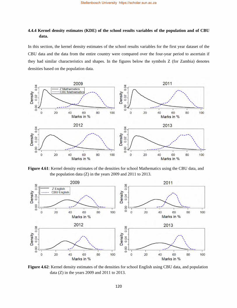
120
4.4.4 Kernel density estimates (KDE) of the school results variables of the population and of CBU data.
In this section, the kernel density estimates of the school results variables for the first year dataset of the
CBU data and the data from the entire country were compared over the four-year period to ascertain if
they had similar characteristics and shapes. In the figures below the symbols Z (for Zambia) denotes
densities based on the population data.
Figure 4.61: Kernel density estimates of the densities for school Mathematics using the CBU data, and
the population data (Z) in the years 2009 and 2011 to 2013.
Figure 4.62: Kernel density estimates of the densities for school English using CBU data, and population
data (Z) in the years 2009 and 2011 to 2013.
Stellenbosch University https://scholar.sun.ac.za
Stellenbosch University https://scholar.sun.ac.za

121
The kernel density estimates for Mathematics and English are shown in Figures 4.61 and 4.62,
respectively. In all four years considered, the distribution of Mathematics was positively skewed in the
population with single peaks around 15%, means and medians below 25% (see Figure 4.61). Using the
CBU data, this variable showed a completely different behaviour with densities being skewed to the left,
and with almost all the students achieving scores in excess of 50%. Additionally, the distribution of
school Mathematics of the first year students was bimodal in 2009 with a major peak near 70% and a
minor peak at 45%. The minor peak was associated with a small proportion of the 2009 first year CBU
students who scored at school (grade twelve) level less than 50% in school Mathematics. In 2011 and
2012, school Mathematics for CBU data had a single mode at 70%, while in 2013, it had two modes at
70% and 82%.
In Figure 4.62, school English exhibited a different behaviour from that of school Mathematics in Figure
4.61. In all four years, the distributions of English had single peaks in both the population data and the
CBU data and were nearing symmetric distributions, suggesting that a normal distribution could be used
to approximate densities of English. In the population, the densities of English had modes around 35%
(except in 2013 which had a mode at 40%), means and medians below 42%. Using the CBU data, the
modes were at 65% (in 2009), 60% (in 2011 and 2012) and 70% (in 2013).
The kernel density estimates for the other school results variables are not shown. Generally, most school
results variables had a tendency to show positive skewness when the data for the entire country were used
and exhibited negative skewness when using the CBU data. Additionally, school results variables in the
population recorded lower means, modes and medians mostly below 50%. These findings were expected
as the students admitted in the different programmes of CBU and other two public universities were
representing the top 10% of all the candidates who wrote the school leaving examinations for a particular
year. However, there were few school variables which had similar skewness in both the population data
and the CBU data. For example, the distribution of Physics was skewed to the left and for Biology it was
positively skewed in both datasets for all four years considered.
4.4.5 Kernel density estimates of school and university results variables for the graduate of CBU data.
As mentioned above, the actual marks (%) for the school results and the university averages from the first
year to the final year of study were only available for the students who entered into the university in 2009
and who successfully completed their studies in 2012 for four-year degree programmes, and in 2013 for
five-year degree programmes. Only the notched boxplots for the overall university average (variable
UWA), school average (G12AVE), school Mathematics, English and Biology are shown (see Figure 4.63
Stellenbosch University https://scholar.sun.ac.za
Stellenbosch University https://scholar.sun.ac.za

122
for four-year programmes and Figure 4.64 for five-year programmes). The notched boxplots for the other
university and school results variables are not reported.
Figure 4.63: Kernel density estimates of the densities for UWA, G12AVE, school Mathematics, English
and Biology for students who entered in the first year of four-year programmes in 2009 and who graduated in 2012.
Figure 4.64: Kernel density estimates of the densities for UWA, G12AVE, school Mathematics, English
and Biology for students who entered in the first year of five-year programmes in 2009 and who graduated in 2013.
Stellenbosch University https://scholar.sun.ac.za
Stellenbosch University https://scholar.sun.ac.za

123
The variable UWA in Figures 4.63 and 4.64 was slightly skewed to the right with small humps (around
78% for four-year degree programmes in Figure 4.63, and 72% for five-year degree programmes in
Figure 4.64) corresponding to a small group of students who achieved higher overall average marks in
excess of 70% at the end of their studies. In four-year programmes (see Figure 4.63), G12AVE and UWA
were in close agreement (K-S p-value = 0.4199) with similar means (of 64.27% for UWA and 64.65% for
G12AVE), medians (of 63.38% for UWA and 64.65% for G12AVE) and comparable variations.
In Figure 4.63, UWA had a mode around 62%, whereas G12AVE was bimodal with major and minor
modes attained at 65% and 71%, respectively. In the same graph, school Mathematics, English and
Biology had single peaks at 75%, 71% and 53 %, respectively. Additionally, school Mathematics and
English were skewed to the left, whereas the density for school Biology was nearing a symmetric
distribution. Furthermore, it is seen in Figure 4.63 that the majority of students in four-year programmes
who attained an overall average score in excess of 60% at the completion of their undergraduate studies
also achieved more than 60% on the average at school level and in most individual school subjects.
In Figure 4.64, UWA had a mode around 62% which was lower than that of school Mathematics and
English (modes of 72% for school Mathematics, and 63% for English). The peaks of G12AVE and
Biology were attained at 62% and 55%, respectively. For five-year programmes, the distribution of
Mathematics was negatively skewed, whereas the distributions for other school variables in the same
graph were nearly symmetric.
The kernel density estimates for UWAY1 to UWAY4 for four-year programmes and for UWAY1 to
UWAY5 for five-year programmes were also constructed but are not shown. They exhibited some
negative skewness as the overall university average UWA and had longer right tails. When the kernel
density estimates of these individual university averages variables were compared to those of the school
variables, they showed behaviours similar and comparable to the kernel density estimates of UWA with
the school variables.
4.5 Summary of findings and concluding remarks.
A lengthy univariate statistical analysis based on the notched boxplots and the kernel density estimates of
the school and university results variables was carried out for the CBU data. The Population data from the
entire country were also utilised for comparison purposes with the CBU data. The aim, when comparing
the CBU data and the population data, was twofold. First, it was important to explore the population data
for the entire country because it is where the school results variables of the CBU data were coming from.
Second, the comparison between the school results variables for the CBU and the entire country was to
Stellenbosch University https://scholar.sun.ac.za
Stellenbosch University https://scholar.sun.ac.za

124
show that the students selected and admitted in different degree programmes at CBU (and in other public
universities in Zambia) were representing the topmost of the school leavers with the best grade twelve
results among all school leavers for the entire country.
It should be recalled that the statistical investigations using the CBU data in this chapter were instituted to
assess for any pattern change over time in the school and university results variables; to examine
relationships between the school and university results variables in order to check if the attainment of
high scores at the school level and the raising of admission standards (by down adjusting the
programmes’ cut-off points) was being accompanied by better performance at the university level; that is,
to examine if the school variables were good indicators of the university performance; to investigate if the
school variables were able to discriminate between the different groups of the first year students and the
graduates.
From all the statistical analyses done, it can be concluded that there were no dramatic pattern changes in
the school and university results variables over the fourteen-year period. The changes observed over time
in the school variables were due to the raising of the admission standards which started in the year 2002,
the implementation of the dual admission criteria system which intervened in the year 2005, and the
variations associated with the high schools of origin attended by the students in the study, and the years in
which they wrote the grade twelve school leaving examinations. To some extent, the changes in the
admission standards which resulted from the adjustment of the cut-off points from time to time affected
the performance at the university level.
There was also a general tendency for the students to be admitted into the university with outstanding and
“inflated” school results but to score lower at the university level. This situation was exacerbated in first
year Mathematics which recorded the worse performance among all first year subjects, despite most
students achieving outstanding results in school Mathematics. This indicates that the attainment of high
scores in school subjects was not always accompanied by higher academic achievement at the university
level. It was also discovered that the school variables had just a limited discrimination power to
differentiate between different groups of the CBU students.
The statistical analyses based on the kernel density estimates assisted in uncovering several important
features and properties of the school and university results variables under investigation. Most school and
university results were unimodal and had skewed distributions. The negative skewness in the densities of
the school variables was due to the higher admission standards implemented at the CBU in the selection
process, which resulted in admitting the school leavers with only outstanding grade twelve results. In
addition, it was found that some few school results variables (in some years only) had scores closely
Stellenbosch University https://scholar.sun.ac.za
Stellenbosch University https://scholar.sun.ac.za

125
corresponding to those of FYAVE at first year level. This was further confirmed by non-significant K-S
tests for equality between the distributions of FYAVE and these school variables.
Before closing this chapter, it is noteworthy to mention that the exploratory data analysis techniques used
in this chapter have been valuable in providing some insight on the school and university results
variables. But this was only based on the univariate analyses which consider a single variable at a time. It
is thus important to consolidate and supplement these analyses by more techniques based on multivariate
analyses in order to gain more insights on the data and to put into perspective all the objectives of the
study. This will be the subject of the subsequent chapters.
Stellenbosch University https://scholar.sun.ac.za
Stellenbosch University https://scholar.sun.ac.za

126
CHAPTER 5
CORRESPONDENCE ANALYSES OF THE CBU DATA
5.1 Introduction.
The previous chapter dealt with the analysis of the data from both the entire country and the CBU using
univariate exploratory data analysis techniques. More specifically, notched boxplots, line plots (i.e.
mean plots, median plots, standard deviation plots and median absolute deviation plots) and kernel
density estimates were utilised to assess, among other things, for pattern changes in both school and
university results variables; to check if the raising of the admission standards resulted in better academic
achievements at the university level; to compare distributions of school results variables of CBU data
with those of the population data for the entire country; and to explore the relationship between school
and university results variables. Univariate analyses alone were not sufficient to put into perspective all
the objectives of the study and did not provide adequate answers to all the research questions.
Additionally, these analyses were only considering variables separately (i.e. one variable at a time). In
this chapter, two variables are simultaneously taken into account in the analysis.
The main purpose of a bivariate analysis is to explore the concept of relationship between variables,
whether there exists an association and the strength of this association. Common forms of a bivariate
analysis involve constructing a scatterplot and the computation of a simple correlation coefficient when
both variables are numeric. In the case of two categorical variables, a chi-squared test can be used to
determine the association between them. The data matrix corresponding to these variables can be
displayed in a contingency table and can be analysed by correspondence analysis (CA). Bivariate
histograms, bivariate boxplots or bagplots, and bivariate kernel densities can also be constructed. As
for a one-dimensional histogram, a bivariate histogram lacks smoothness and can be replaced by a
bivariate density estimate which results in an appropriate estimate of a bivariate density function. A
bagplot which extends the properties of a boxplot to two variables simultaneously portrays the
information on the location, spread, correlation, skewness, and tails of the bivariate data. The
components of a bagplot include a bag containing the inner 50% of the data points, a fence that separates
inliers from outliers, and a loop indicating the points outside the bag but inside the fence (see
Rousseeuw, Ruts & Tukey, 1999).
In this chapter, in line with the goals of geometric data analysis, the analysis mainly focuses on bivariate
analyses using correspondence analysis (CA) (see for example Le Roux & Rouanet, 2004 and
Greenacre, 2007). This technique is motivated by the need to find school results variables which are
closely related to the university results variables. This is done by including in the analysis a single
school subject at a time. This allows more school variables to be investigated. It is noteworthy to point
out that grade twelve learners only sit for about six to eight school subjects in the school leaving
Stellenbosch University https://scholar.sun.ac.za
127
examinations. The list of school subjects selected varies from one learner to the other, and depends on
the high schools attended, on the individual preferences of grade twelve learners, and on the availability
of teachers in particular school subjects. As a result, school subjects in the CBU data which were not
selected by the students at grade twelve level have missing values. Bivariate analyses which consider a
university variable with a single school subject at a time permit capturing as many school variables as
possible. This is in contrast when several school variables are simultaneously included in the analysis.
Although this has the advantage of simultaneously investigating the interrelationships between several
school results variables and the university variables, there is a limitation on the number of school
subjects to be included in the analysis simultaneously because of missing values. In the next chapter, it
will be shown that the number of observations to analyse decreases when more school subjects are
simultaneously included in the analysis. In fact, apart from school Mathematics and English which do
not have missing values on the CBU data, the remaining school subjects have missing values. In what
follows, a brief overview of the CA method is provided. This is followed by its application to the CBU
data.
5.2 Brief overview of the CA technique.
The CA methodology is a bivariate exploratory data analysis technique designed to explore
relationships among two categorical variables (Rencher, 2002; Greenacre & Blasius, 2006; Greenacre,
2007). Its main aim is to transform a two-way table of numerical information into a graphical display
in which the rows and columns of the table are represented by points. In alternative displays, row
categories (column categories) can be represented by calibrated axes and column categories (row
categories) by points; or both entities can be displayed by axes (Gower et al., 2011).
As input, the CA procedure uses a cross tabulation of two categorical variables with p and q categories
respectively. The data are arranged into a p × q contingency table denoted by X ≡ {x ij}. In general, any
rectangular data matrix with nonnegative entries and positive row and column totals can also be treated
as an input for CA.
A common procedure, prior to the CA computations, is to transform the matrix X into a correspondence
matrix P by dividing X by n (grand total of X) (see for example Greenacre, 2007). Alternatively, X can
be directly used in the analysis (Gower et al., 2011).
5.2.1. CA maps.
There are several different approaches to CA (Greenacre, 2007). A popular approach (Greenacre, 2007)
is to start with the matrix of standardised residuals under the independence model assuming that the
row classification of P is independent of its column classification. Denote this matrix of standardised
residuals by S: p × q expressed into its singular value decomposition (SVD) as
Stellenbosch University https://scholar.sun.ac.za

128
𝐒𝐒 = 𝐃𝐃r−1 2⁄ �𝐏𝐏 − 𝐫𝐫𝐜𝐜𝐓𝐓�𝐃𝐃c
−1 2⁄ = 𝐔𝐔𝐃𝐃α𝐕𝐕T , (5.1)
where r: p × 1 and c: q × 1 are column vectors of row sums (row masses) and column sums (column
masses) of P, respectively; Dr and Dc are p × p and q × q diagonal matrices having as diagonal elements
the row and column masses, respectively; Dα is a K × K diagonal matrix with singular values in
descending order: 1 > α1 ≥ α2 ≥ ... ≥ αK > 0, K = rank(S) = min (p − 1, q − 1); U is a p × K column
orthonormal matrix whose columns are the left singular vectors of P; V is a q × K column orthonormal
matrix whose columns are the right singular vectors of P, i.e. UTU = VTV= IK.
Coordinates for constructing CA maps are given by the columns of matrices A, B, F and G calculated
from (5.1) where:
𝐅𝐅 = 𝐃𝐃r−1/2𝐔𝐔𝐃𝐃α (5.2)
𝐆𝐆 = 𝐃𝐃c−1/2𝐕𝐕𝐃𝐃α (5.3)
𝐀𝐀 = 𝐃𝐃r−1/2𝐔𝐔 (5.4)
𝐁𝐁 = 𝐃𝐃c−1 2⁄ 𝐕𝐕 (5.5)
The coordinates given by F and G are called principal coordinates while the columns of A and B are
standard coordinates.
The graphical displays (in the Greenacre context) in which both rows and columns of the contingency
table are represented by points will be referred to as CA maps in the remaining part of this chapter. Row
profiles of P can be regarded as points in a q-dimensional space and similarly, column profiles of P as
points in a p-dimensional space. For an optimal two-dimensional asymmetric CA map of the rows
(columns) the first two columns of F (G) are used as principal coordinates together with the columns
(rows) in standard coordinates obtained from the first two columns of A (B). Chi-squared distances for
the row profiles and the column profiles are optimally represented. This implies that row-to-row and
column-to-column distances can be interpreted, but there are no row-to-column distances interpretation
since they are not defined. In these maps, the closeness of row points (column points) is an indication
of the rows (columns) having similar profiles across the columns (rows). If a row (column) is closer to
the origin, then its profile is closer to the average profile (see for example Johnson and Wichern, 2007).
It follows from the definition of principal coordinates that the points in such coordinates might appear
bunched together in an asymmetric CA map. Therefore, many researchers in practice prefer a symmetric
CA map. In symmetric CA maps, the two separate spaces, one for the row profiles and the other for
the column profiles, are superimposed in a joint display. These CA maps can be convenient and legible
Stellenbosch University https://scholar.sun.ac.za

129
since both row and column points are in principal coordinates. However, since row-to-column distances
are not defined symmetric CA maps are prone to overinterpretation. For this reason symmetric CA
maps will not be used in this study.
As an aid to the interpretation of the asymmetric CA maps, the following quantities, usually provided
in a CA output, can be helpful: the total inertia (a measure of variation between row (column) points),
the inertias associated with each dimension, each row point and each column point (Husson, Lê &
Pagès, 2011; Greenacre, 2007). The total inertia is defined as:
trace (𝐒𝐒𝐒𝐒𝐓𝐓) = trace (𝐒𝐒T𝐒𝐒) = trace(𝐃𝐃α2) = �𝜆𝜆𝑘𝑘 = �𝛼𝛼𝑘𝑘2
𝐾𝐾
𝑘𝑘=1
𝐾𝐾
𝑘𝑘=1
, (5.6)
where 𝜆𝜆𝑘𝑘 is the kth largest eigenvalue of SST or STS. The eigenvalue 𝜆𝜆𝑘𝑘 indicates the variance in the
table explained by the kth principal axis. The amount of inertia accounted for by the first two principal
axes provides a measure of the overall quality of the two-dimensional display. In percentages, it is given
by:
𝜆𝜆1 + 𝜆𝜆2∑ 𝜆𝜆𝑘𝑘 𝐾𝐾𝑘𝑘=1
× 100. (5.7)
The inertia of the ith row (jth column), represents the contribution of the ith row (jth column) point to
the total inertia and is given by:
r𝑖𝑖 � f𝑖𝑖𝑘𝑘2𝐾𝐾
𝑘𝑘=1
for row 𝑖𝑖, and 𝒄𝒄𝒋𝒋� g𝑗𝑗𝑘𝑘2 K
k=1
for column 𝑗𝑗 , (5.8)
where fik and gjk are the elements of matrices F and G, respectively. As a guideline to determine
major row (column) contributors to the total inertia, the quantities in (5.8) for rows (columns)
should be compared to the average row (column) contribution. More specifically, if p and q are
the number of rows, and the number of columns in a contingency table and if the total inertia
permills is 1000, then the average row contribution, and the average column contribution are
given by 1000/p and 1000/q, respectively. A major row (column) contributor to inertia is the
one whose row (column) inertia is exceeding the average row (column) contribution.
The absolute contributions of the ith row and jth column points to the kth dimension are given
respectively by:
Stellenbosch University https://scholar.sun.ac.za

130
r𝑖𝑖f𝑖𝑖𝑘𝑘2
λ𝑘𝑘 for row 𝑖𝑖, and
c𝑗𝑗g𝑗𝑗𝑘𝑘2
λ𝑘𝑘 for column 𝑗𝑗. (5.9)
These quantities measure the importance of each point in determining the direction of the principal
axes and assist in their interpretation. Dominant contributors to dimensions (principal axes) are row
(column) points with large percentages of inertia.
Another measure which assists in the diagnosis of the position of a point on the map is known as the
relative contribution of the kth dimension to the ith row (jth column) point is given by:
f𝑖𝑖𝑘𝑘2
∑ f𝑖𝑖𝑘𝑘2𝐾𝐾𝑘𝑘=1
for row 𝑖𝑖, and g𝑗𝑗𝑘𝑘2
∑ g𝑗𝑗𝑘𝑘2𝐾𝐾𝑘𝑘=1
for column 𝑗𝑗. (5.10)
This quantity determines points which are most explained by the kth dimension (principal axis).
The relative contribution of each point in the first two-dimensional space, which is the sum of
(5.10) for k =1, 2, is called the quality of a point. It measures the quality of a point in the two-
dimensional map, i.e. determines whether a point is well represented in the map, or poorly
represented. When a point is poorly represented on the map, it should be interpreted with
caution (Greenacre, 2007).
Apart from the quantities introduced above, another aid when interpreting the CA results is the graph
of attractions between the row and the columns points. This graph displays the row points which are
most in attraction with column points (see Le Roux & Rouanet, 2004).
5.2.2 CA biplots.
In this chapter, a distinction is made between a CA map, and a CA biplot. The two-dimensional CA
map described in the previous section, is constructed by first converting the two-way table X into a
correspondence matrix P, and then representing both row and column categories by points – one set of
points in principal coordinates and the other one in standard coordinates. Greenacre (2007) also
discusses a closely related visual display viz. the CA biplot. However, in this section CA biplots, as
suggested by Gower et al. (2011), will be used for displaying a two-way table X. In this display, row
categories (column categories) are represented by calibrated axes (called biplot axes) simultaneously
with column categories (row categories) by points. The CA biplot axes must be calibrated, that is tick
marks with values must be placed on these axes in order to indicate a scale for reading off the values of
the variables. Calibration of the axes assist in reading off the values of the observations on the variables
by just projecting perpendicularly the points representing the observations onto the biplot axes
representing these variables. In this chapter only CA biplots will be considered while a discussion of
biplots in general will be deferred until Chapter 7.
Stellenbosch University https://scholar.sun.ac.za
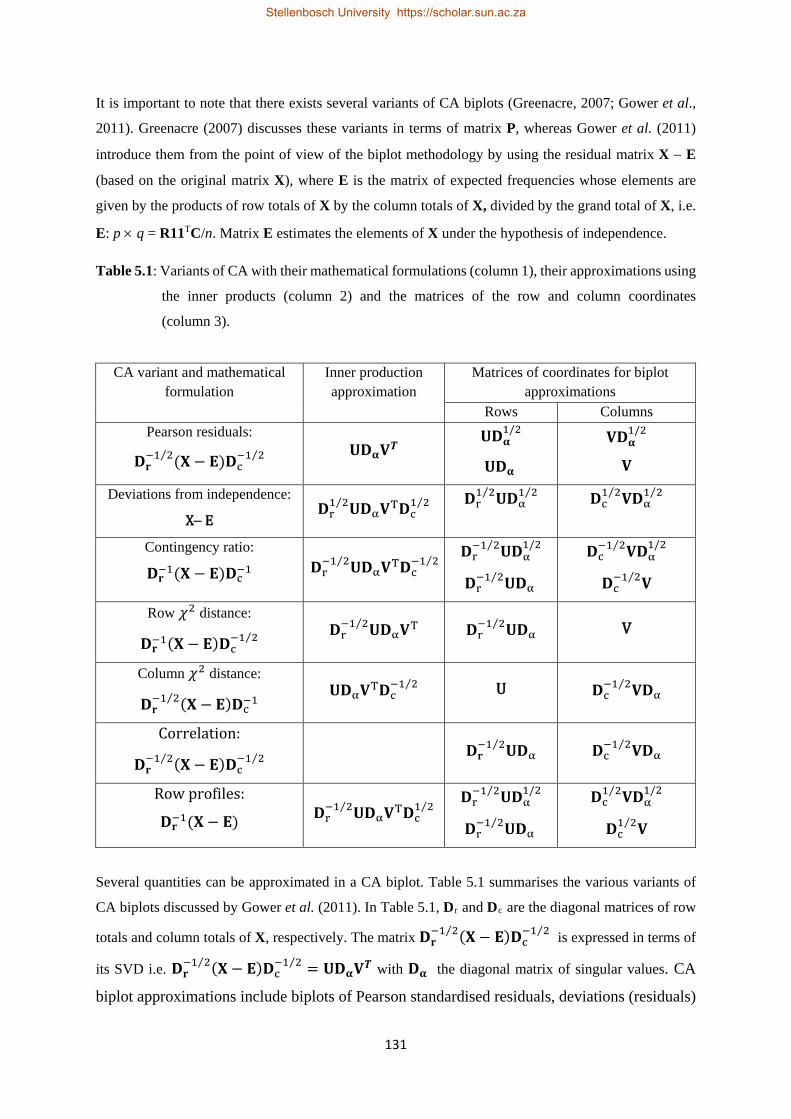
131
It is important to note that there exists several variants of CA biplots (Greenacre, 2007; Gower et al.,
2011). Greenacre (2007) discusses these variants in terms of matrix P, whereas Gower et al. (2011)
introduce them from the point of view of the biplot methodology by using the residual matrix X − E
(based on the original matrix X), where E is the matrix of expected frequencies whose elements are
given by the products of row totals of X by the column totals of X, divided by the grand total of X, i.e.
E: p × q = R11TC/n. Matrix E estimates the elements of X under the hypothesis of independence.
Table 5.1: Variants of CA with their mathematical formulations (column 1), their approximations using
the inner products (column 2) and the matrices of the row and column coordinates
(column 3).
CA variant and mathematical formulation
Inner production approximation
Matrices of coordinates for biplot approximations
Rows Columns Pearson residuals:
𝐃𝐃𝐫𝐫−1 2⁄ (𝐗𝐗 − 𝐄𝐄)𝐃𝐃c
−1 2⁄ 𝐔𝐔𝐃𝐃𝛂𝛂𝐕𝐕𝑻𝑻
𝐔𝐔𝐃𝐃𝛂𝛂1/2
𝐔𝐔𝐃𝐃𝛂𝛂
𝐕𝐕𝐃𝐃𝛂𝛂1/2
𝐕𝐕
Deviations from independence:
X− E 𝐃𝐃r1 2⁄ 𝐔𝐔𝐃𝐃α𝐕𝐕T𝐃𝐃c
1 2⁄ 𝐃𝐃r1 2⁄ 𝐔𝐔𝐃𝐃α
1 2⁄ 𝐃𝐃c1 2⁄ 𝐕𝐕𝐃𝐃α
1 2⁄
Contingency ratio:
𝐃𝐃𝐫𝐫−1(𝐗𝐗 − 𝐄𝐄)𝐃𝐃c
−1 𝐃𝐃r−1 2⁄ 𝐔𝐔𝐃𝐃α𝐕𝐕T𝐃𝐃c
−1 2⁄ 𝐃𝐃r−1 2⁄ 𝐔𝐔𝐃𝐃α
1/2
𝐃𝐃r−1 2⁄ 𝐔𝐔𝐃𝐃α
𝐃𝐃c−1 2⁄ 𝐕𝐕𝐃𝐃α
1/2
𝐃𝐃c−1 2⁄ 𝐕𝐕
Row 𝜒𝜒2 distance:
𝐃𝐃𝐫𝐫−1(𝐗𝐗 − 𝐄𝐄)𝐃𝐃c
−1 2⁄ 𝐃𝐃r−1 2⁄ 𝐔𝐔𝐃𝐃α𝐕𝐕T 𝐃𝐃r
−1 2⁄ 𝐔𝐔𝐃𝐃α V
Column 𝜒𝜒2 distance:
𝐃𝐃𝐫𝐫−1 2⁄ (𝐗𝐗 − 𝐄𝐄)𝐃𝐃c
−1 𝐔𝐔𝐃𝐃α𝐕𝐕T𝐃𝐃c
−1 2⁄ U 𝐃𝐃c−1 2⁄ 𝐕𝐕𝐃𝐃α
Correlation:
𝐃𝐃𝐫𝐫−1 2⁄ (𝐗𝐗 − 𝐄𝐄)𝐃𝐃c
−1 2⁄ 𝐃𝐃𝐫𝐫
−1 2⁄ 𝐔𝐔𝐃𝐃α 𝐃𝐃c−1 2⁄ 𝐕𝐕𝐃𝐃α
Row profiles:
𝐃𝐃𝐫𝐫−1(𝐗𝐗 − 𝐄𝐄) 𝐃𝐃r
−1 2⁄ 𝐔𝐔𝐃𝐃α𝐕𝐕T𝐃𝐃c1 2⁄
𝐃𝐃r−1 2⁄ 𝐔𝐔𝐃𝐃α
1/2
𝐃𝐃r−1 2⁄ 𝐔𝐔𝐃𝐃α
𝐃𝐃c1 2⁄ 𝐕𝐕𝐃𝐃α
1/2
𝐃𝐃c1 2⁄ 𝐕𝐕
Several quantities can be approximated in a CA biplot. Table 5.1 summarises the various variants of
CA biplots discussed by Gower et al. (2011). In Table 5.1, Dr and Dc are the diagonal matrices of row
totals and column totals of X, respectively. The matrix 𝐃𝐃𝐫𝐫−1 2⁄ (𝐗𝐗 − 𝐄𝐄)𝐃𝐃c
−1 2⁄ is expressed in terms of
its SVD i.e. 𝐃𝐃𝐫𝐫−1 2⁄ (𝐗𝐗 − 𝐄𝐄)𝐃𝐃c
−1 2⁄ = 𝐔𝐔𝐃𝐃𝛂𝛂𝐕𝐕𝑻𝑻 with 𝐃𝐃𝛂𝛂 the diagonal matrix of singular values. CA
biplot approximations include biplots of Pearson standardised residuals, deviations (residuals)
Stellenbosch University https://scholar.sun.ac.za

132
from independence, contingency ratios, chi-squared distances between the rows (columns)
correlations and row profiles (column profiles) of X. In this chapter, CA biplots simultaneously
displaying row profiles as points and columns as appropriately calibrated biplot axes are
constructed. The UBbipl R package (Le Roux & Lubbe, 2010) is used when constructing these
biplots. The function calls for producing the different graphs are given in Appendix B.
The problem of bunched points in principal coordinates occurring with asymmetric CA maps
can be remedied using the device of lambda-scaling defined by Gower et al. (2011). This device
uses the fact that the inner product between two vectors is unchanged if the one vector is scaled by a
positive scalar constant λ while simultaneously the other vector is scaled by 1/λ.
5.2.3 CA as an optimal scaling technique.
The optimal scaling process converts qualitative variables into quantitative ones. CA viewed
as an optimal scaling method consists of quantifying the categories of the row (column)
variable of a contingency table so that there is a highest possible discrimination between the
categories of the column (row) variable. If the optimal score values for the row categories are
sought, then the process will consist of maximising the variance associated with the column
categories and vice versa. The optimal score values are given by the standard coordinates of
the row (column) categories on the first CA principal axis, while the maximum variance is the
first principal inertia (inertia associated with the first principal axis).
The optimal scale values of the row (column) categories can also be determined by minimising
the row-to-column distances weighted by the frequencies in the contingency table. The optimal
scale values of the row and column categories can also be found by maximising the correlation
between these two sets of categories. The solution is given by the coordinates of the row and
the column categories, specifically on the first CA principal axis, and the maximum correlation
attained is the square root of the first principal axis and is called the canonical correlation
(between the row and the column categories) (see Greenacre, 2007).
In order to uniquely determine the solution for the optimal scale values, identification
conditions must be added to the maximisation or minimisation problems. Greenacre (2007)
defines these conditions in terms of zero mean and unit variance for row (column) categories.
The advantage of optimal scale values is that they can be linearly transformed into more
convenient values. However, they are not unique and depend on the criterion to optimise, the
Stellenbosch University https://scholar.sun.ac.za

133
identification conditions, and on the data (contingency tables) used (Greenacre, 2007). Optimal
scoring will be discussed in more details in Chapter 7.
5.3 The CA technique and the CBU data.
One of the objectives of this study is to examine relationships between school and university results
variables. As alluded to in chapter three, all higher learning institutions in Zambia are relying on the
school results to admit school leavers in their different programmes of study. It is thus important to
uncover these relationships to help improve the admission criteria in these institutions. Of interest, it is
cardinal to check if the attainment of high scores at school level was being accompanied by better
performance at the university level. In the previous chapter, comparisons of school results variables
between CBU data and the data for the entire country revealed that students selected in different degree
programmes at CBU (and also in other public universities in Zambia) are among the topmost school
leavers who obtained outstanding results at school level. Assuming that their mental ability will
continue to prevail at university level, these students are supposed to also excel in their different
programmes of study. Although chi-squared tests can be used to assess relationships between two
categorical variables, they do not provide any information about individual associations between pairs
of rows and columns of a two-way contingency table. Additionally, they do not divulge how these
associations are constructed. In order to allow an investigation of similar or different categories and to
explore individual response categories of the categorical variables, CA can be utilised. More
specifically, CA is applied to the CBU data to investigate patterns of associations between different
levels of academic achievement at school level with those at university level. That is, to explore the
associations between different levels of the academic achievement at first year level (as measured by
variables FCCO and FYAVE), and at the completion of the studies (as quantified by variables DECLA
and UWA) on one hand, and the different levels of school performance in individual school subjects
and the overall school performance as measured by the variables EPOINT, NDIS and G12AVE on the
other hand (see Appendix A for a description of the variables used in the study).
Furthermore, investigations based on CA are carried out to check the adequacy of the grading system
used by the ECZ which consists of converting the actual marks obtained by school leavers in individual
grade twelve subjects using a nine-point scale (with a grade of one point corresponding to an upper
distinction, which is the topmost achievement at grade twelve level, and a grade of nine points
translating into a fail, which is the lowest achievement). Although an upper distinction grade
corresponds to the highest achievement in a school subject, the corresponding bin is somehow wide.
For example, an upper distinction grade in school Mathematics for candidates who wrote the grade
twelve examinations in 2006 was awarded to those who recorded marks between 66% and 100%. In
2007, it was set at marks between 58% and 100%. The task, using CA, is then to partition the upper
distinction bin into two or more smaller categories and identify the actual level of those who could not
Stellenbosch University https://scholar.sun.ac.za

134
perform well at first year level despite having an upper distinction. In School Mathematics for example,
among the 535 first year degree students for the 2008 first year intake considered in this study (these
are the students who wrote the school leaving examination in 2006), 292 students (representing about
55% the total of 535 students) achieved an upper distinction. However, out of this number, only 5%
(that is, 14 students out of a total of 292) obtained the highest grade of A+ in the first year Mathematics,
while 24% of students (i.e. 70 out of 292 students) failed in first year Mathematics.
In this chapter, the use of optimal scaling values provided by the CA technique to quantify grades of
school results is illustrated. In Chapter 3, several imputation methods that can be used to convert
symbolic interval data into quantitative or continuous data were introduced. The optimal scale values
derived using the CA technique can provide an additional imputation method for symbolic interval data.
In effect, the CBU data have actual marks (in %) available for both school and university subjects only
in the years 2009, and 2011 to 2013 for the first year dataset. For the graduate dataset, actual marks (in
%) for school and university subjects from first year to the final year of study are only available for
students who were in their first year of study in 2009, and who graduated in 2012 for four-year
programmes, and in 2013 for five-year programmes. For other years, only grades (points for school
subjects and letter grades for university subjects) are given. The grades (points) of school subjects
(given as integers from one to nine as mentioned above) cannot be considered as quantitative entities,
and are difficult to justify, as any other set of integer values can be used to represent the grades. One
approach is to quantify them by using optimal scaling values provided by the CA technique. These
values furnish valid quantitative data which can be used with any statistical procedure meant for
continuous data.
Before presenting the CA results on the CBU data, a brief account of the procedure involved when
performing a CA on a square matrix is first given in the next section.
5.4 CA of square tables.
A CA of square tables requires tables with rows and columns having the same labels. The rows and
columns of such tables often refer to the same objects or individuals in two different states or measured
at two different time points (Greenacre, 2000 & 2007; Van Der Heijden, 2005).
A square table can be symmetric or asymmetric. It is asymmetric when the rows and columns of the
table have different meanings, otherwise it is said to be symmetric. Examples of square tables include
transition tables. In such tables, the rows are the category levels of the categorical variable measured at
one time point or one state and the columns are the category levels of the same categorical variable (or
a different categorical variable) at another time point or state. In this study, square tables arise when
considering the performance of the same group of students in consecutive years. The data consist of
transition tables with rows referring to the performance of students in the previous year of study and
the columns to the performance of the same students in the next year of study.
Stellenbosch University https://scholar.sun.ac.za
135
The aim, when analysing square tables, consists of getting an insight into transitions or changes from
one time point or state to the other time point or state (Van Der Heijden, 2005) by focusing on the off-
diagonal entries of the table. These entries represent objects or individuals that have changed from one
category of the row variable to a different category of the column variable. Most often, diagonal
elements in a square table have high values as compared to the off-diagonal entries. If a standard CA is
applied to such tables, the diagonal elements will dominate the analysis and will mask the patterns of
the off-diagonal elements, defeating the main purpose of the analysis. One solution to this problem is
to use the deviations from the quasi-independence, instead of that for the independence model (see Van
Der Heijden, De Vries & Van Hooff, 1990; Van Der Heijden, 2005). Another approach (which is
applied in this study) consists of analysing the symmetric and asymmetric parts of the square table
separately (Greenacre, 2000 & 2007).
More specifically, if X is the original p × p square table, then it can be written as a sum of the symmetric
and skew-symmetric parts; that is,
X = Y + Z, (5.10)
where Y = 12
(𝐗𝐗 + 𝐗𝐗T) and Z = 12
(𝐗𝐗 − 𝐗𝐗T) are the p × p symmetric and skew-symmetric parts of
the square table X. Matrix Y gives the average flow between rows and columns, while Z provides the
differential flow.
The analysis will then proceed by applying a standard CA on the Y and Z tables separately. These two
analyses can be obtained by applying one single standard CA on a 2p × 2p block table X* given by
(Greenacre, 2000 & 2007):
𝐗𝐗∗ = � 𝐗𝐗 𝐗𝐗T𝐗𝐗T 𝐗𝐗
� (5.11)
The results for this single CA will yield 2p – 1 dimensions, of whom p – 1 will correspond to the
symmetric part Y (associated with unique principal inertias) and p to the skew-symmetric part Z. The
CA display of Y can be interpreted as any standard CA graph, whereas the interpretation of the CA map
of Z is given in terms of areas of triangles formed by any two points in the map with the origin
(Greenacre, 2000 & 2007).
The approach of CA for square tables is applied to CBU data in order to uncover patterns of transitions
and changes occurring on the grades of students from one year to the next year of study. With respect
to the first year dataset, the analysis is concerned with investigating the “flow” from grade categories
of school results to that of first year results in order to examine the general tendency of migrations and
changes between grade levels of school performance and first year academic performance. The
investigation using the graduate dataset consists of following the performance of the same cohort of
Stellenbosch University https://scholar.sun.ac.za

136
students from grade twelve level to the first year and through their undergraduate studies and checking
for any pattern changes taking place in their performance throughout their undergraduate studies.
5.5 Variables involved in the bivariate analysis based on CA with their associated categories.
CA is carried out using both grades and actual marks (in %). For the first year dataset, actual marks (in
%) in both school and first year subjects are only accessible in the years 2009, and 2011 to 2013,
whereas for the graduate dataset, only students who were in their first year of study in 2009 have actual
marks (in %) available in school subjects. So, for the years with missing actual marks (in %), grades
are used instead. Table D.1 in Appendix D summarises the different categories of the variables used in
the analysis based on the CA technique.
In order to come up with final categories of the variables in Table D.1 in Appendix D, initial CA were
first carried out on the data. These preliminary analyses resulted in some sparse contingency tables and
in some CA maps having outlying points with low masses (close to zero) which were affecting the CA
solutions. To improve the CA solutions, some adjacent categories of affected variables which showed
some closeness to each other were combined (see Greenacre, 2007, pp. 91-92). The results from
performing the CA on the school and university results variables are presented in the remaining sections.
5.6 CA of FYAVE with school results variables using the first year dataset.
5.6.1 CA of FYAVE and G12AVE of the first year dataset over four years.
In the previous chapter, comparisons of FYAVE with school results variables and G12AVE using
notched boxplots showed that, on the average, students admitted in the first year of study in CBU degree
programmes achieved higher scores (in %) at school level than at first year level. To further the
investigations, CA is performed to study patterns of associations between different categories of
FYAVE and those for school variables. Two-way contingency tables resulting from the cross-tabulation
of FYAVE with G12AVE over the years with actual marks (in %) available for school results variables
(i.e. 2009, and 2011 to 2013) are analysed using CA. The CA results retained for interpretation purpose
include the total inertia (Inr), the principal inertias in the first two dimensions (denoted by Inr1 and
Inr2) with their associated percentages (Inr1% and Inr2%); the cumulative percentages (Cum%); chi-
squared values and their p-values (denoted by Chisq and P-value); the absolute contributions of row
and column points to the first two dimensions (ctr1 and ctr2) in permills; and the relative contribution
or quality (qlt) in permills, also known as sample and axis predictivities (see Gower et al., 2011) of
each row point and column point in the optimal two-dimensional space. Asymmetric CA maps of row
profiles constructed using the Greenacre philosophy and CA biplots of row profiles (case B) are
considered (see Table 5.1).
Stellenbosch University https://scholar.sun.ac.za

137
Table 5.2: Principal inertias (values and %), cumulative of the principal inertias (in %) in the first two dimensions, total inertia, chi-squared values and p-values, qualities and contributions of rows and columns in the first two dimensions of the variables FYAVE and G12AVE.
ITEM YEAR
2009 2011 2012 2013 Inr1 0.293 0.286 0.199 0.327 Inr2 0.034 0.094 0045 0.047 Inr 0.338 0.392 0.251 0.380
Inr1% 86.6 73.0 79.2 85.9 Inr2% 10.2 24.1 17.8 12.5 Cum% 96.8 97.1 97.0 98.3 Chisq 150.12 228.55 159.39 282.49
P-value 0.00 0.00 0.00 0.00
FYAVE
UNM1. qlt 973 974 974 1000 UNM2. qlt 903 940 967 983 UNM3. qlt 891 875 876 536 UNM4. qlt 540 998 709 985 UNM5. qlt 940 843 905 939 UNM6. qlt 999 999 999 1000 UNM1. ctr1 101 161 131 142 UNM2. ctr1 100 79 43 87 UNM3. ctr1 72 54 45 9 UNM4. ctr1 3 1 15 2 UNM5. ctr1 63 25 39 67 UNM6. ctr1 661 679 727 693 UNM1. ctr2 362 505 372 105 UNM2. ctr2 17 3 17 163 UNM3. ctr2 13 8 67 24 UNM4. ctr2 35 105 20 474 UNM5. ctr2 389 206 400 79 UNM6. ctr2 184 174 124 154
G12AVE
G12M1. qlt 991 990 975 989 G12M2. qlt 940 925 843 908 G12M3. qlt 915 996 374 947 G12M4. qlt 991 943 920 983 G12M5. qlt 991 978 999 998
G12M1. ctr1 154 204 157 137 G12M2. ctr1 112 118 87 96 G12M3. ctr1 25 18 0 29 G12M4. ctr1 133 243 25 160 G12M5. ctr1 576 418 732 579
Stellenbosch University https://scholar.sun.ac.za

138
Table 5.2 continued.
ITEM YEAR 2009 2011 2012 2013
G12M1. ctr2 525 492 417 548 G12M2. ctr2 0 26 29 8 G12M3. ctr2 378 238 8 116 G12M4. ctr2 9 0 417 135 G12M5. ctr2 87 244 129 193
The CA results of variables FYAVE and G12AVE over the four-year period are depicted in Table 5.2,
whereas the associated CA maps for 2011 and 2013 are displayed in Figures 5.1 to 5.4. In order to help
in the interpretation of the CA plots, the association rate matrices between the categories of FYAVE
and G12AVE for the years 2011 and 2013 were calculated and are given in Tables 5.3 and 5.4, while
the graphs of attractions for 2011 and 2013 are shown in Figures 5.5 and 5.6. The contingency tables
for the years 2011 and 2013 are presented in Table 5.5. In the asymmetric plots (see Figures 5.1 and
5.2), the plotting characters of the row (column) points are proportional to the frequencies (in the two-
contingency tables in Table 5.5).
From Table 5.2 (rows 6 and 7), it is clear that, over the four-year period, the chi-squared test show a
statistically significant association between the variables FYAVE and G12AVE (p-value < 0.001).
Additionally, the CA solutions for the four years are stable and consistent, and are characterised by total
inertias explained by dimension one exceeding 72%; the first two dimensions accounting for most of
the total inertia (cumulative percentage in excess of 95%) and all the points being well represented in
the two-dimensional maps with their qualities (in permills) being close to 1000, except for categories
UNM3 (in 2013), UNM4 (in 2009) of FYAVE and category G12M3 of G12AVE in 2012. These points
have qualities given, respectively, by 536, 540 and 374 (in permills).
Furthermore, according to the “permills contributions” of rows and columns in Table 5.2, G12AVE
category “G12M5” was the dominant contributor to the first axis over the four-year period (with
percentages of contributions given by 57.6 %, 41.8 %, 73.2 % and 57.9 %), followed by the category
G12M1 (in 2009 and 2012) and the category G12M4 (in 2011 and 2013). For the variable FYAVE, the
two major contributors to the first axis, over the four-year period, are UNM1 and UNM6. These two
points explain more than 75 % of the inertia on the first axis (i.e. 76.6 % in 2009, 75.8% in 2011, 77.0
% in 2012 and 83.5% in 2013). On the second axis, categories UNM1 and UNM5 of the variable
FYAVE are the most important in determining the direction of this axis in 2009, 2011 and 2012 (in
2013, the major contributors are UNM2 and UNM5),whereas for the variable G12AVE, category
G12M1 is the leading contributor.
An inspection of the CA plots of the row (profiles) analysis for the years 2011 and 2013 (see top panels
of Figures 5.1 and 5.2 of asymmetric maps) shows important features of the associations between the
Stellenbosch University https://scholar.sun.ac.za

139
six categories UNM1, UNM2, UNM3, UNM4, UNM5 and UNM6 of FYAVE (corresponding to the
bins, in %, [0, 50), [50, 55), [55, 60), [60, 65), [65, 70), and [70, 100)) and the five categories G12M1,
G12M2, G12M3, G12M4 and G12M5 of G12AVE (representing the intervals [0, 55), [55, 60),
[60, 65), [65, 70) and [70, 100)). In these maps, these categories are plotted in their inherent order
from lowest intervals of marks (in %) on the left side of the first axis, to the highest intervals of marks
(in %) on the right of the first axis. From the sizes of the plotting points representing categories of
FYAVE in the top panel of Figure 5.1 (and also in Figure 5.2), categories UNM3 and UNM4 have high
frequencies (of 132 and 151 out 583, respectively, whereas category UNM1 has the lowest frequency
(of 57 out of 583) (see the left panel of Table 5.5)).
Table 5.3: Associate rate matrix for the contingency table in Table 5.5 for the year 2011.
FYAVE G12AVEG12M1 G12M2 G12M3 G12M4 G12M5
UNM1 2.1471 0.0739 − 0.7322 − 0.6212 − 1.0000UNM2 0.4784 0.3080 − 0.1391 − 0.7232 − 1.0000UNM3 0.1163 0.2588 − 0.0288 − 0.5093 − 0.7792UNM4 − 0.3212 0.0811 0.1522 − 0.0467 − 0.6139UNM5 − 0.7244 − 0.1851 0.3785 0.5479 − 0.6866UNM6 − 0.8220 − 0.7976 − 0.0249 1.5991 5.4778
Table 5.4: Associate rate matrix for the contingency table in Table 5.5 for the year 2013.
FYAVE G12AVEG12M1 G12M2 G12M3 G12M4 G12M5
UNM1 0.6953 0.2304 0.0374 − 0.4806 − 0.9344UNM2 0.8622 0.1173 0.0222 − 0.4751 − 0.8106UNM3 − 0.1835 0.2896 0.0458 − 0.1945 − 0.3219UNM4 − 0.6946 0.0142 0.1600 0.3991 − 0.4564UNM5 − 0.7346 − 0.4285 0.1066 0.5583 0.8890UNM6 − 1.0000 − 0.9448 − 0.6792 1.1681 4.6578
Table 5.5: Two-way contingency tables of FYAVE and G12AVE for 2011 (left) and 2013 (right) for all faculties combined for the first year dataset (categories of G12AVE are represented by numbers 1 to 5).
FYAVE G12AVE FYAVE G12AVE1 2 3 4 5 Total 1 2 3 4 5 Total
UNM1 28 21 5 3 0 57 UNM1 46 62 63 20 1 192UNM2 18 35 22 3 0 78 UNM2 35 39 43 14 2 133UNM3 23 57 42 9 1 132 UNM3 15 44 43 21 7 130UNM4 16 56 57 20 2 151 UNM4 6 37 51 39 6 139UNM5 4 26 42 20 1 93 UNM5 3 12 28 25 12 80UNM6 2 5 23 26 16 72 UNM6 0 1 7 30 31 69Total 91 200 191 81 20 583 Total 105 195 235 149 59 743
Stellenbosch University https://scholar.sun.ac.za

140
From the top panel of Figure 5.1, it is seen that categories G12M5, G12M4, and G12M1 of variable
G12AVE are the three major contributors to the first axis (contributing 41.8%, 24.3%, and 20.4%,
respectively, to the variance of dimension 1 (see Table 5.2)). It is also noted that G12M1 and G12M5
are furthest apart with the former being on the left-hand pole, and the latter on the right-hand pole of
the first axis (this situation also transpired in other years). Additionally, G12M1 and G12M2 are
positioned on the left, while G12M3, G12M4 and G12M5 are on the right of the first axis. For the years
2009, 2012, and 2013, G12M1, G12M2 and G12M3 of G12AVE were lying on the left, while G12M4
and G12M5 were found on the right of the first axis (see the top panel of Figure 5.2 for the year 2013).
Therefore, the first principal axis separates low school performance on the left from high school
performance on the right. This suggests that, for all four years, Dimension 1 can be interpreted as a
dimension of school average performance, with low performance at the left-hand pole, and high
performance at the right-side pole.
On the second axis, categories G12M5 and G12M1 at the upper pole are the leading contributors, while
G12M1 is the single dominant contributor at the lower pole. Categories G12M2 and G12M4 have the
lost contributions to the inertia of Dimension 2. This implies that the direction of the second principal
axis is determined by the categories G12M1, G12M5, and G12M3 (see the top panel of Figure 5.1).
Therefore, Dimension 2 contrasts the highest and lowest school performance (at the upper pole) with
the intermediate school performance (at the lower pole). Similarly, from the top panel of Figure 5.2,
Dimension 2 opposes the highest and lowest school performance (at the lower pole) with the
intermediate performance (at the upper pole). This dimension demonstrates that there were cases of few
students who achieved high school performance (i.e. those who were admitted in the first year of study
with inflated grade twelve results), but who poorly performed in the first year of study, and vice versa.
Using these facts, the relationships between categories of FYAVE and G12AVE can now be defined.
In the top panel of Figure 5.1, categories UNM1 to UNM4 of the variable FYAVE are on the left-hand
pole of axis one, indicating that these four categories have a tendency to be associated with the lower
average school performance (below 60%).
Categories UNM5 and UNM6 are on the higher side of the first axis (right-hand side), suggesting an
association between these categories with higher school performance at school level. The findings are
reinforced by the graph of attraction in Figure 5.3, where categories of FYAVE and G12AVE with large
positive association rates (see the matrix of association rates for the year 2011 in Table 5.3) are joined.
In this graph, two clusters appear, where categories UNM1, UNM2, and UNM3 of FYAVE are in
attractions with G12M1 and G12M3 (cluster 1), and categories UNM4, UNM5, UNM6 which are in
attraction with G12M3, G12M4 and G12M5.
Stellenbosch University https://scholar.sun.ac.za

141
Figure 5.1: Asymmetric maps (top panel: row analysis, bottom panel: column analysis) of FYAVE and
G12AVE for all programmes combined using the first year dataset for the year 2011.
Stellenbosch University https://scholar.sun.ac.za

142
Figure 5.2: Asymmetric maps (top panel: row analysis, bottom panel: column analysis) of FYAVE and
G12AVE for all programmes combined using the first year dataset for the year 2013.
Stellenbosch University https://scholar.sun.ac.za

143
Figure 5.3: Graph of attractions between the categories of FYAVE and G12AVE for the year 2011 using the association rate matrix in Table 5.3 (with threshold = 0.15).
Figure 5.4: Graph of attractions between the categories of FYAVE and G12AVE for the year 2013
using the association rate matrix in Table 5.4 (with threshold = 0.10).
Stellenbosch University https://scholar.sun.ac.za

144
More specifically, the following associations are uncovered: UNM6 is associated, almost exclusively,
with G12M5 (which corresponds to school average performance of at least 70%). It is also associated
with G12M4 (school average performance between 65 % and 69 %), and G12AM3. Category UNM5
is associated with G12M3 and G12M4, and to some extent with G12M2. The cluster of categories
UNM2, UNM3 and UNM4 is associated with G12M2, and to some extent with G12M3, while the last
category UNM1 is related to G12M1, and to some degree with G12M2. Similar patterns of associations
were also observed in 2009 and 2011 (CA asymmetric maps not shown).
The CA asymmetric map for the row analysis in 2013 (see the top panel in Figure 5.2) is slightly
different from those in the years 2009, 2011 and 2012. From this figure, it is clear that the cluster of
categories UNM1 and UNM2 is related to G12M1 and G12M2, whereas the cluster of UNM4, UNM5,
and UNM6 tend to be associated with categories G12M3, G12M4, and G12M5. Category UNM3 tends
to be associated with G12M2 and G12M3. These patterns of associations are also observed in the graph
of association in Figure 5.4 (see the matrix of association rates in Table 5.4).
The patterns of associations between the categories of the variables FYAVE and G12AVE uncovered
by the CA asymmetric maps were also confirmed using the CA biplots of the row profiles (see top
panels of Figures 5.5 and 5.6 for the years 2011 and 2013). In these CA biplots, the plotting of the
column points (categories of G12AVE) are suppressed since they do not have a distance interpretation.
Instead it is the biplot axes which are shown. These axes are calibrated in standardised profile units so
that the values of the row profiles can be read off by projecting the six categories of FYAVE on these
axes.
Thus, from the top panel of Figure 5.5, UNM6 has the highest row profile value (in terms of deviations
from the marginal row profiles) on the biplot axes G12M5 and G12M4, followed by UNM5 (on the
axis G12M4), and UNM4 (on the axis G12M4). Categories UNM1 to UNM3 have the lowest profile
elements on both axes G12M4 and G12M5. On axis G12M3, categories UNM4, UNM5, and UNM6
have high profiles elements as compared to UNM1 to UNM3, while on axis G12M2, the categories
with high profile values are identified as UNM3, UNM4, and UNM2. On axis G12M1, category UNM1
has the highest profile value, then UMM3, and UNM2, with UNM5 and UNM6 having the lowest
profile values. In Figure 5.6 (see top panel), category UNM6 has the highest profile value on the biplot
axis G12M5, followed by UNM5, while on axis G12M4, categories UNM4 to UNM6 have high profile
elements. On axes G12M1 to G12M3, categories UNM1 to UNM4 have high profile values.
The analysis of the column profiles was also performed. The CA plots are at the bottom panels of
Figures 5.1, 5.2, 5.5, and 5.6 for the years 2011 and 2013 (CA plots for other years are not shown).
Graphs of attractions were also constructed, but are not shown. The results from the column analysis
are almost similar to those of the row analysis. That is, in all four years (see the bottom panels of
Figures5.1 and 5.2 for 2011 and 2013), Dimension 1 is interpreted as the first year average performance
Stellenbosch University https://scholar.sun.ac.za

145
Figure 5.5: CA biplots (top panel: row profiles, bottom panel: column profiles) of FYAVE and
G12AVE for all programmes combined using the first year dataset for the year 2011.
Stellenbosch University https://scholar.sun.ac.za

146
Figure 5.6: CA biplots (top panel: row profiles, bottom panel: column profiles) of FYAVE and
G12AVE for all programmes combined using the first year dataset for the year 2013.
Stellenbosch University https://scholar.sun.ac.za

147
dimension high performance side from one pole, and low performance on the other pole. In 2011, the
high first year performance was on the left-hand side pole, while the low first year performance was on
the right- hand side pole. In 2013, the left-to-right direction was tantamount to low-to-high first year
performance. Dimension 2, on the other hand, contrasts the highest and lowest first year performances
with the intermediate first performance.
Additionally, for the year 2011, categories G12M3 to G12M5 were located on the left side and were
associated with UNM5 and UNM6, while the rest of categories of G12AVE were related to UNM1 to
UNM4. In 2013, categories G12M4 and G12M5 were related to UNM4 to UNM6, whereas G12M1 to
G12M4 on the left-hand side of axis one were associated with UNM1 to UNM3. These patterns of
associations were confirmed by the graphs of attractions (not shown). The CA biplots at the bottom
panels of Figures 5.5 and 5.6 also support the findings based on the graphs of attractions and the CA
asymmetric maps, and demonstrates that categories of G12AVE representing high achievement at
school level have with high profile values on the biplot axes associated with high performance at the
first year level. For example, categories G12M4 and G12M5 have highest profile values on the biplot
axis UNM6 on the CA biplots (see bottom panels of Figures 5.5 and 5.6 for the years 2011 and 2013),
while G12M1 and G12M2 have highest profile elements on the biplot axes UNM1 and UNM2.
The statistical investigation on the patterns of associations between the categories of FYAVE and
G12AVE using the CA technique was also extended to each type of programmes over the four-year
period. The CA plots were constructed, but only the CA asymmetric maps and the CA biplots for
business related programmes in 2012, and for engineering related programmes in 2011 are reported (see
Figures 5.7 and 5.8). Partial results for the CA outputs are also summarised in Table 5.6. Other CA
results are shown in Tables D.2 to D.4 in Appendix D.
In Table 5.6, it is seen that, for all three types of programmes and over the four-year period, FYAVE
and G12AVE are highly associated as demonstrated by high chi-squared values and very small p-values,
except in 2012 which have a small chi-squared value and a large p-value of 0.48. The same table shows
that the first two dimensions explain at least 90% of the total inertia in the two-way contingency tables,
except in 2013 in business related programmes, and in 2011 for other programmes which have 88.0 %
and 87.3 %, respectively, of the total inertia associated with the first two dimensions. When referring
to Tables D.2 to D.4 in Appendix D, it is clear, based on the relative contributions of each point to the
first two-dimensional space, that most of the rows and columns are well represented in the two-
dimensional CA maps in business and engineering related programmes, except for categories UNM5
(in 2012) and G12M2 (in 2013) for business related programmes; and UNM4 and UNM5 (in 2009) for
engineering related programmes. In other programmes, the categories with poor fit in two-dimensional
CA maps include G12M2 (in 2009); UNM1, UNM2, UNM3, UNM4, G12M2 and G12M4 (in 2011).
The “qualities” of these points are all below 50% (or 500 permills) (see Tables D.2 to D.4 in Appendix
D). Major contributors of rows and columns to the first two dimensions are not the same over the four-
Stellenbosch University https://scholar.sun.ac.za

148
year period. For example, in other programmes in 2009, UNM5 category was a single row most
important contributor, contributing itself to about 77.9 % of the inertia in the first dimension, whereas
in 2011, UNM6 supplied about 89.9% to the inertia of the first dimension. In 2012 and 2013, single
major contributors were UNM1 and UNM4, respectively (see Table D.4 in Appendix D).
Table 5.6: Principal inertias (values and %), cumulative of the principal inertias (in %) in the first two dimensions, total inertia, chi-squared value and p-value of FYAVE and G12AVE per type of programmes over the four-year period using the first year dataset.
Item Business related programmes Engineering related progs. Other programmes
2009 2011 2012 2013 2009 2011 2012 2013 2009 2011 2012 2013
Inr1 0.273 0.284 0.321 0.271 0.361 0.268 0.231 0.329 0.225 0.270 0.092 0.148
Inr2 0.109 0.101 0.095 0.081 0.094 0.086 0.079 0.036 0.093 0.138 0.032 0.051
Inr 0.417 0.411 0.459 0.400 0.474 0.359 0.322 0.376 0.353 0.522 0.130 0.211
Inr1% 65.5 69.3 69.8 67.7 76.2 74.6 71.8 87.6 63.8 51.8 70.9 7.3
Inr2% 26.1 24.6 20.7 20.3 19.8 23.9 24.6 9.6 26.3 26.5 24.8 24.2
Cum% 91.6 93.9 90.5 88.0 96.1 98.5 96.3 97.1 90.1 78.3 95.7 94.4
Chisq 45.0 71.4 66.1 64.9 90.1 71.8 122.0 164.7 51.6 109.0 14.6 30.2
P-value 0.00 0.00 0.00 0.00 0.00 0.00 0.00 0.00 0.00 0.00 0.48 0.01
An inspection of the CA asymmetric maps not shown (see the bottom panel of Figure 5.7 for 2012 only)
for business related programmes revealed that the positions of points representing the categories of the
variables FYAVE and G12AVE did not change much over the four-year period. In 2009, categories
G12M1, G12M2, and G12M3 were on the left of the first principal axis, whereas in other years, only
G12M1 and G12M2 were positioned on the left, with the rest of G12AVE categories on the right. Since
all five categories of G12AVE were spread out from left to the right of the first axis, according to their
order of magnitudes, then the left-to-right direction was viewed as the low-to-high average performance
at school (grade twelve) level. Thus Dimension 1 was interpreted as the school average performance
axis with low school performance on the left-hand side, and high school performance on the right-hand
side of the first axis. As for all programmes combined, Dimension 2 in business related programmes
was contrasting the highest and lowest school performances with the intermediate school performance.
Additionally, when inspecting the positions of the categories of FYAVE on these maps, it was seen
that the categories UNM1, UNM2, UNM3 in 2009 were located on the left-hand side pole of axis 1 (i.e.
on the lower school performance side), suggesting that students whose average first year marks were
within these categories achieved school average marks in the bins G12M1, G12M2, and G12M3. In
2011 and 2013, UNM3 passed to the right of the first axis, leaving only UNM1 and UNM2 categories
on the left.
Stellenbosch University https://scholar.sun.ac.za

149
Figure 5.7: CA biplot of row profiles (top panel) and CA asymmetric map (bottom panel) of variables
FYAVE and G12AVE for business related programmes in 2012 using the first year dataset.
Stellenbosch University https://scholar.sun.ac.za

150
Figure 5.8: CA biplot of row profiles (top panel) and CA asymmetric map (bottom panel) of FYAVE
and G12AVE for engineering related programmes in 2011 using the first year dataset.
Stellenbosch University https://scholar.sun.ac.za

151
Figure 5.9: Graph of attractions between the categories of FYAVE and G12AVE for the year 2012 in
business related programmes (with threshold = 0.15).
The graph of attractions between the categories of FYAVE and G12AVE for business related
programmes in 2012 in Figure 5.9 clearly shows two different patterns of association, i.e. categories
UNM1 to UNM4 are in attraction (or in association) with G12M1 and G12M2, while categories UNM5
and UNM6 are in attraction with G12M3 to G12M5. This is exactly the patterns of association exhibited
in the CA asymmetric map in Figure 5.7 (see the bottom panel). More specifically, both the graph of
attractions and the CA asymmetric map show the following patterns of associations: UNM6 is
associated, almost exclusively, with G12M5, and also with categories G12M3 and G12M4; UNM5 is
found to be related with G12M3 and G12M4; UNM4 is in attraction with G12M1 and G12M2; UNM3
is linked to G12M2; and UNM1 and UNM2 are associated with G12M1. These findings are
consolidated by the CA biplot at the top panel of Figure 5.7, where category UNM6 has the highest
profile value on the biplot axes G12M3, G12M4, and G12M5, followed by UNM5. Similarly, UNM4
has the highest profile element on both axes G12M1 and G12M2, while category UNM3 is highly
loaded on the biplot axis G12M2. The last two categories UNM1 and UNM2 have both high profile
values on the biplot axis G12M1. Patterns of associations for other years (2009, 2011 and 2013) were
similar and comparable to those for the year 2012 depicted in Figure 5.7.
On the second principal axis, categories G12M1 and G12M2 are the leading contributors to the inertia
of the second dimension with 61.8 + 32.8 = 94.6% of contribution and occupy extreme positions. This
suggests that this axis separates the categories of FYAVE with more frequencies on G12M1 on the
upper pole from the categories of FYAVE with more frequencies on G12M2 on the lower pole. That is,
categories UNM1 and UNM2 (on top) have more students with school performance falling within
Stellenbosch University https://scholar.sun.ac.za

152
category G12M1 as compared to G12M2, while categories UNM3 and UNM4 comprise more students
whose school performance falls in the category G12M2.
In engineering related programmes, categories G12M1, G12M2, and G12M3 were constantly
positioned on the left-hand side pole, while the other two categories G12M4 and G12M5 were found
on the right-hand side pole of the first principal axis for all four years (see the CA asymmetric map for
the year 2011 at the bottom panel of Figure 5.8). As in business related programmes, there were no
major changes in the patterns of associations between the variables G12AVE and FYAVE over the
four-year period. An inspection of the CA plots for the year 2011 in Figure 5.8 and also the graph of
attractions (not shown) demonstrates that UNM6 is associated with G12M5 and G12M4. This indicates
that most of the 2011 first year students in engineering related programmes who achieved first year
average marks in the topmost bin (UNM6), got almost exclusively average school marks in the bins
G12M4 and G12M5. Also categories UNM4 and UNM5 are associated with G12M2, G12M3 and
G12M4, whereas UNM1, UNM2 and UNM3 are related to G12M1 and G12M2.
These results are reinforced by the CA biplot at the top of Figure 5.8. In effect, it is seen that UNM6
has the highest profile values on both G12M4 and G12M5 axes, followed by UNM4 and UNM5 (on
the G12M4 axis only). Additionally, UNM4 and UNM5 have the highest profiles on the biplot axes
G12M2 and G12M3, while categories with high profile elements on the axes G12M1 and G12M2 are
UNM1, UNM2, and UNM3.
The CA solutions for other programmes (i.e. non-business and non-engineering related programmes)
were not stable over the four-year period and exhibited patterns of associations different from those in
business and engineering related programmes (CA plots not shown).
In this section, patterns of associations between the variables G12AVE and FYAVE have been
investigated over the four-year period using the CA technique, for all programmes combined, and for
each type of programme. The findings show that, to some extent, the attainment of higher marks at
school level was being accompanied by higher achievement at the first year level. This is the case, for
example, of UNM6 which was found to be associated with G12M5, implying that students who
achieved average school marks of at least 70%, also obtained similar marks at first year level. There
was also a tendency, for first year students, to achieve higher marks at school level, and to get lower
marks at the end of the first year of study. This is the case, for example, of category UNM1 being
associated with G12M2, indicating that students who obtained average marks (in %) within the bin
[55, 59] at school level, got less than 50% at the first year level. Likewise, an association between
categories UNM2 and G12M2 or G12M3 signifies that students who achieved average marks between
50 % and 54 % at the first year level, obtained school average marks between 55% and 59% or between
60% and 64%. An attraction between categories UNM5 and G12M5 indicates that students with school
average marks of at least 70%, obtained first year average marks between 65 % and 69%., whereas an
Stellenbosch University https://scholar.sun.ac.za

153
association between categories UNM1 and categories G12M1 and G12M2 suggests that students who
got average marks below 60% at school level were at risk of failing at the end of the first year level.
This clearly indicates and confirms the findings from the previous chapter based on the notched boxplots
of a group of students who were admitted in different degree programmes with inflated school results
which were not tallying with their first year academic achievements. To further this investigation,
analyses of square two-way contingency tables are performed in Section 5.12.
5.6.2 CA of FYAVE and NDIS of the first year dataset over four years.
The variable NDIS is another measure of the overall performance at school level, which gives the
number of upper distinctions at school (number of grade twelve subjects with an upper distinction
grade). It has five categories: ND0, ND1, ND2, ND3 and ND4 (represented on the maps by “ND>=4”)
corresponding to zero, one, two, three and at least four upper distinctions in the school (grade twelve)
subjects. The partial CA results are summarised in Tables 5.7 and D.5 in Appendix D, only the CA
asymmetric map, and the CA biplot for the year 2012 are reported in Figure 5.10, other plots are
displayed in Appendix D (see Figures D.1 and D.2).
From Table D.5 in Appendix D (see the columns of the contributions “ctr1”), categories UNM6 and
ND4 are the major single contributors to the inertia of the first principal axis, each explaining more than
43% of the inertia. Additionally, almost all row and column points are well represented in the two-
dimensional space (see the columns of qualities “qlt” in Table D.5), except the categories UNM4 and
ND2 (in 2011); and UNM2 and ND3 (in 2012). The overall qualities of the CA maps were also
satisfactory with over 89 % of the total inertia explained by the first two dimensions (see Table 5.5.).
From the same table, it is noted a significant relationship between the variables FYAVE and NDIS
during the four-year period as attested by large chi-squared values and small p-values.
In Figure 5.10 (bottom panel), the CA asymmetric map for the year 2012 shows that category ND4 of
the variable NDIS, and categories UNM5 and UNM6 of FYAVE are on the right-hand pole of the first
principal axis, while the rest of the categories for both variables are found on the left-hand pole. On the
first principal axis, ND0 and ND4 are extreme points, indicating that the left-to-right direction
corresponds to the low-to-high number of upper distinctions at school level. This suggests that
Dimension 1 is a dimension of school performance measured in terms of the number of upper
distinctions. On the second axis, the principal contributor is ND1 (with contribution 47.3%), followed
by ND2, and then ND3. On this axis, ND2 and ND3 (at the lower pole) almost coincide and are distant
from ND1 (at the upper pole). Thus the second dimension can be interpreted as a dimension which
contrasts students with one upper distinctions with those with two or three distinctions.
Stellenbosch University https://scholar.sun.ac.za

154
Table 5.7: Principal inertias (values and %), cumulative of the principal inertias (in %) in the first two
dimensions, total inertia, chi-squared values and p-values in the first two dimensions of the
variables FYAVE and NDIS.
Item Year 2009 2011 2012 2013
Inr1 0.180 0.122 0.101 0.135 Inr2 0.020 0.017 0.017 0.012 Inr 0.219 0.150 0.131 0.151
Inr1% 82.4 81.9 76.8 89.6 Inr2% 9.0 11.1 13.0 8.3 Cum% 91.4 93.1 89.8 97.9 Chisq 97.3 87.1 83.4 112.2
P-value 0.00 0.00 0.00 0.00
On the first dimension, categories UNM5 and UNM6 are located on the high side of school performance
and tend to be associated with category ND4, and to a lesser extent with the cluster formed by the
categories ND2 and ND3. Also UNM4 is related to ND2 and ND3, while UNM1, UNM2, and UNM3
are associated with NDO, ND1 and UND2.
On the second dimension, UNM3 is the closest to ND1, whereas UNM4 is nearest to ND2 and ND3,
indicating that more students whose first year average marks were in the bin UNM3 (i.e. marks between
55% and 60%) got one upper distinction at school level than students in other first year bins. Similarly,
students more students in the bin UNM4 (i.e. marks between 60% and 65%) obtained two or three upper
distinctions than students in other first year performance bins. Additionally, category ND4 is close to
lower categories of FYAVE (i.e. UNM1, UNM2, and UNM3). This implies that high achievement at
school level is corresponding to lower performance at first year level. This, again, is an indication of a
group of students being admitted in the first year of study with inflated grade twelve results. The
findings for the year 2012 using the CA asymmetric map, are supported by the graph of attraction (not
shown) and the CA biplot at the top panel of Figure 5.10. In this biplot, UNM6 has the highest profile
value on axis ND4, suggesting that most 2012 first year students who achieved first year average marks
in the bin UNM6 (i.e. marks of at least 70%), got four or more upper distinctions at school level.
Categories UNM1, UNM2, and UNM3 have high profile values on the axes NDO, ND1, and ND2,
while category UNM4 has the highest profile elements on axes ND2 and UD3.
For other years (see Figures D.1 and D.2 in Appendix D for the years 2009 and 2011), the CA solutions
do not differ much with those for the year 2012.
Stellenbosch University https://scholar.sun.ac.za

155
Figure 5.10: CA biplot of row profiles (top panel) and CA asymmetric map (bottom panel) of FYAVE
and NDIS in 2012 for all programmes combined using the first year dataset.
Stellenbosch University https://scholar.sun.ac.za

156
Once again, the findings in this section reinforce the results in the previous section. That is, most first
year students with a high number of upper distinctions at school level (i.e. four or more upper
distinctions), achieved the highest performance at the first year level (i.e. marks of at least 70%).
However, there was also a tendency for a group of students to get more upper distinctions at school
level, but to achieve a low performance at the first year level. The next section continues with the
analysis of the patterns of associations between levels of FYAVE and the variables EPOINT and
DEPOINT.
5.6.3 CA of FYAVE with EPOINT using the first year dataset over four years.
In this section, the analysis of the patterns of association of the third overall measure of school
performance, EPOINT, with FYAVE done using again the CA technique. The variable EPOINT has
four categories, namely, “E5-7”,”E8-9”,”E10-11”, and ”E≥12”, representing entry point values between
five and seven points, eight and nine points, ten and eleven points, and at least twelve points. The CA
results are summarised in Table 5.8 and Table D.6 in Appendix D, whereas the two-way contingency
tables for the variables FYAVE and EPOINT for all programmes combined over the four-year period
are found in Table 5.9. The CA displays over the four-year period were almost similar, and only those
for the years 2009 and 2012 are shown in Figures 5.11 and 5.12.
Table 5.8 shows that the chi-squared test of association between FYAVE and EPOINT is highly
significant over the four-year period (p-values < 0.001). Additionally, the first two dimensions explain
at least 93% of the total inertia for all CA maps for the years 2009, and 2011 to 2013. Furthermore,
UNM6 and E5-7 are among the most important contributors to the inertia of the first principal axis (see
Table D.6 in Appendix D). Also from the same table, it is noted that, apart from categories UNM4 (in
2009) and E8-9 (in 2011), all row and columns points are well represented in the two-dimensional
space.
The CA biplot of the variables FYAVE and EPOINT in 2009 (see top of Figure 5.11) shows that
category UNM6 is highly loaded on the biplot axis E5-7, this is followed by the category UNM5. In the
same plot, category UNM5 has the highest profile value on the biplot axis E8-9, this is followed by
UNM3 and UNM4. Categories UNM1 to UNM4 have high profile elements on the axes E10-11 and
E≥12.
From the CA asymmetric map (see bottom of Figure 5.11), it is noted that, along the first dimension,
category UNM6 of FYAVE and category E5-7 of EPOINT are furthest away from the origin (on the
right), demonstrating that the greatest differences in the academic achievement at school and first year
of study are basically between the students in the category UNM6 and those in the rest of other
categories of FYAVE (i.e. UNM1 to UNM5); and between the category E5-7 and the other EPOINT
levels E8-9, E10-11 and E≥12. Since the level E5-6 is on the right side and the other three categories of
Stellenbosch University https://scholar.sun.ac.za

157
EPOINT are on the left of the first principal axis, then the left-to-right difference is tantamount to high
entry points versus low entry points, translating into low admission standards versus high admission
standards. This implies that category UNM6 is associated, exclusively, with category E5-7. This is
confirmed by the CA biplot (see top panel of Figure 5.11) where UNM6 has the highest profile value
on the axis E5-6, and by the graph of attractions (not shown) which shows UNM6 in attraction with
E5-7. Category UNM5 is also on the right side, and is related to E5-7 and E8-9. Likewise, categories
UNM1 to UNM4 (on the left side of the first axis) are related to E10-11 and E≥12, and to a lesser extent
with E5-7 and E8-9.
Table 5.8: Principal inertias (values and %), cumulative of the principal inertias (in %) in the first two
dimensions, total inertia, chi-squared value and p-values of FYAVE and EPOINT.
Item Year 2009 2011 2012 2013
Inr1 0.174 0.108 0.096 0.144 Inr2 0.039 0.012 0.019 0.016 Inr 0.227 0.122 0.115 0.166
Inr1% 76.8 88.6 82.4 86.5 Inr2% 17.1 9.5 16.3 9.7 Cum% 93.9 98.1 98.7 96.2 Chisq 100.6 71.17 73.3 123.6
P-value 0.00 0.00 0.00 0.00
Table 5.9: Two-way contingency tables of FYAVE and EPOINT for 2009 (top left), 2011 (top right), 2012 (bottom left) and 2013 (bottom right) for all faculties combined using the first year dataset.
FYAVE EPOINT FYAVE EPOINT
E5-7 E8-9 E10-11 E≥12 E5-7 E8-9 E10-11 E≥12 UNM1 7 15 9 8 UNM1 3 19 14 21 UNM2 19 20 18 14 UNM2 17 31 11 19 UNM3 25 37 30 14 UNM3 30 46 33 23 UNM4 38 31 33 10 UNM4 35 59 36 21 UNM5 24 30 6 1 UNM5 35 38 14 6 UNM6 47 6 1 1 UNM6 35 26 9 2 FYAVE EPOINT FYAVE EPOINT
E5-7 E8-9 E10-11 E≥12 E5-7 E8-9 E10-11 E≥12 UNM1 23 48 18 22 UNM1 59 72 45 16 UNM2 20 36 18 9 UNM2 33 43 35 22 UNM3 44 45 18 21 UNM3 43 53 20 14 UNM4 49 61 22 6 UNM4 62 49 24 4 UNM5 42 39 11 3 UNM5 46 27 6 1 UNM6 50 25 5 0 UNM6 60 8 1 0
Stellenbosch University https://scholar.sun.ac.za

158
Figure 5.11: CA biplot of row profiles (top panel) and CA asymmetric map (bottom panel) of FYAVE
and EPOINT for all programmes combined in 2009 using the first year dataset.
Stellenbosch University https://scholar.sun.ac.za

159
Figure 5.12: CA biplot of row profiles (top panel) and CA asymmetric map (bottom panel) of FYAVE
and EPOINT for all programmes combined in 2012 using the first year dataset.
Stellenbosch University https://scholar.sun.ac.za

160
On the second axis, levels E8-9 and E≥12 are extreme with respect to their positions. Although
dimension two is associated with a lower percentage of the total inertia (i.e. 17.1 % of the total inertia),
it can be stated that category UNM5 has more students in the category E8-9 than category UNM6.
Similarly, categories UNM1 to UNM4 have more students in categories E10-11 and E≥12 than
categories UNM5 and UNM6. The patterns of associations in 2011 (CA maps not shown), was almost
similar to that of the year 2009.
In the top panel of Figure 5.12, the CA biplot for the year 2012 has categories UNM5 and UNM6 with
high profile values on the biplot axis E5-7, whereas categories UNM4, UNM2, and UNM1 are highly
loaded on the biplots axes E8-9 and E10-11. Categories of FYAVE with high profile values on the
biplot axis E≥12 are UNM1 and UNM3.
An inspection of the CA asymmetric map (see bottom panel of Figure 5.12) and the graph of attractions
(not shown) confirms the findings from the CA biplot. That is, UNM6 is associated, almost exclusively,
with E5-7. The cluster (UNM4, UNM5) is related to E5-7 and E8-9. Similarly, category UNM2 and the
cluster (UNM1, UNM3) are related to E8-9, and to some extent to E5-7 and E10-11.
On the second principal axis, E10-11 and E≥12 are the leading contributors (with contributions 21.5%
and 42.2%, respectively) and are extreme. This suggests that Dimension 2 is contrasting between the
last two categories of the variable EPOINT. On this dimension, UNM1 and UNM3 are nearest to E≥12
at the upper pole, whereas UNM2 and UNM4 are closest to E10-11 at the lower pole. This indicates
that categories UNM1 and UNM3 have more students falling in E5-7 and E≥12 than the rest of the
categories of FYAVE, while UNM4 has more students in the level E8-9 than the other categories of
FYAVE. The CA solution for the year 2013 (CA maps not shown) was almost similar to that of the
year 2012.
The findings in this subsection have shown that most students who obtained first year average marks of
at least 70% (in the bin UNM6) were those who were admitted in CBU with entry points between five
and seven point (in the category E5-7). In this category were also found students who got first year
average marks between 60% and 70% (in the bins UNM4 and UNM5). Additionally, most students who
joined the university with entry point values of at least twelve points, got first year average marks below
60%.
In the next section, the associations between the categories of the variables FYAVE and DEPOINT are
assessed. The variable DEPOINT has three categories, namely, “EP<PC” (if the students’ EPOINT
values are below the programmes’ cut-off points), “EP=PC” (if the EPOINT values and the
programmes’ cut-off are the same) and “EP>PC” (in the case where the EPOINT values are exceeding
the programmes’ cut-off points).
Stellenbosch University https://scholar.sun.ac.za

161
5.6.4 CA of FYAVE with DEPOINT over the four-year period using the first year dataset.
The CA results (not shown) of the variables FYAVE and DEPOINT were characterised by low chi-
squared values and low inertias. Notwithstanding that, correspondences between the levels of these two
variables were instituted. It was found that most students who achieved average scores of at least 70%
at the end of the first year level were those who joined CBU with EPOINT values below the
programmes’ cut-off points. The majority of students who achieved average scores below 69 % at the
first year level, entered the university with EPOINT values below or equal to the programmes’ cut-off
points. Additionally, there was a tendency for students with average first year scores below 50% to be
associated with EPOINT values exceeding the programmes’ cut-off points. There were also students
with EPOINT values below the programmes’ cut-off points, who achieved average scores (at first year
level) below 50%. This was the case, for example, of 72.4 % of 2013 first year students in the UNM1
category (i.e. those with average marks below 50% at the first year level) who were admitted with
EPOINT values below the programmes’ cut-off points, raising again the concern that school results
variables were not good indicators of university academic achievement.
The next section continues with the assessment of associations between the variables FYAVE and
individual school subjects.
5.6.5. CA of FYAVE with individual school subjects over the four-year period using the first year
dataset.
In this section, the CA technique is again carried out to assess the associations between the levels of the
variable FYAVE and those for the individual school subjects to check if higher scores in individual
school subjects were being accompanied by higher achievement at the first year level. Table 5.10
provides two-way contingency tables for the cross-tabulation of the variables FYAVE and school
Mathematics, whereas Table 5.11 summarises partial CA results for the variable FYAVE with school
Mathematics, English and Biology. Other CA results are found in Tables D.7 to D.9.
From table 5.11, it is noted a significant relationship between FYAVE and school Mathematics for all
four years as demonstrated by large chi-squared values and small p-values. Additionally, the first two
dimensions explain more than 93% of the total inertia in the contingency tables, with the first dimension
contributing more than 83% of the total inertia. Furthermore, all points are well represented in the two-
dimensional space, except categories UNM2 and UNM3 of the variable FYAVE in 2012. The two most
important row contributors to the inertia of the first principal axis are UNM1 and UNM6 over the four-
year period, whereas the single column contributor is G12M5 (see Table D.7 in Appendix D).
Figure 5.13 displays the CA maps for the variables FYAVE and school Mathematics for the year 2011.
CA solutions for other years produced CA plots with patterns of associations not departing much from
the 2011 situation and are not shown.
Stellenbosch University https://scholar.sun.ac.za

162
From the CA asymmetric map in Figure 5.13 (see bottom panel), category G12M5 of school
Mathematics is on the right-hand side of the first axis, while all other categories are positioned on the
left-hand side, giving an indication that the greatest differences in the performance of school
Mathematics among the first year students, over the four-year period, is between category G12M5
category (corresponding to scores of at least 70%) and the other four categories of variable G12AVE.
As regard to the categories of FYAVE, it is noted that categories UNM4, UNM5 and UNM6 are on the
right-hand side of the first axis. This trend as also observed in 2009. But in 2012, category UNM4
migrated to the left-hand side, while in 2013, it shifted back to the right-hand side with category UNM3.
Table 5.10: Two-way contingency tables of FYAVE and school Mathematics for 2009 (top left), 2011 (top right), 2012 (bottom left) and 2013 (bottom right) for all faculties combined using the first year dataset.
FYAVE School Mathematics FYAVE School Mathematics
1 2 3 4 5 1 2 3 4 5 UNM1 15 5 5 9 5 UNM1 22 11 9 8 7 UNM2 16 10 14 10 21 UNM2 25 12 15 11 15 UNM3 14 17 17 21 37 UNM3 21 16 28 23 44 UNM4 9 12 17 16 58 UNM4 11 16 16 36 72 UNM5 2 4 3 8 44 UNM5 4 2 11 17 59 UNM6 0 2 0 4 49 UNM6 0 0 2 5 65 FYAVE School Mathematics FYAVE School Mathematics
1 2 3 4 5 1 2 3 4 5 UNM1 26 12 13 28 32 UNM1 32 17 30 26 87 UNM2 10 9 13 8 43 UNM2 19 14 15 24 61 UNM3 15 13 16 18 66 UNM3 7 9 11 21 82 UNM4 13 10 21 28 66 UNM4 5 6 7 17 104 UNM5 5 4 9 11 66 UNM5 2 3 0 7 68 UNM6 5 1 2 2 70 UNM6 1 0 0 1 67
Table 5.11: Principal inertias (values and %), cumulative % in the first two dimensions, total inertia,
chi-squared values and p-values of FYAVE and school Mathematics, English and Biology for all programmes combined over the four-year period using the first year dataset.
Item FYAVE vs school Maths FYAVE vs school English FYAVE vs school Biology
2009 2011 2012 2013 2009 2011 2012 2013 2009 2011 2012 2013 Inr1 0.220 0.264 0.123 0.147 0.035 0.023 0.043 0.019 0.186 0.022 0.083 0.106 Inr2 0.025 0.029 0.014 0.011 0.011 0.015 0.016 0.006 0.037 0.014 0.012 0.013 Inr 0.251 0.304 0.147 0.161 0.053 0.044 0.066 0.029 0.239 0.040 0.098 0.127
Inr1% 87.4 86.8 83.5 91.4 65.6 51.8 66.1 65.8 81.8 55.7 85.1 83.3 Inr2% 9.8 9.4 9.7 7.1 21.3 34.8 24.4 22.6 15.4 34.2 12.9 10.0 Cum% 97.2 96.1 93.2 98.4 86.9 86.6 90.5 88.4 97.2 90.0 98.0 93.3 Chisq 111.6 177.5 93.4 119.8 23.5 25.38 41.9 21.2 98.6 22.3 60.1 92.1
P-value 0.00 0.00 0.00 0.00 0.26 0.19 0.00 0.39 0.00 0.33 0.00 0.00
Stellenbosch University https://scholar.sun.ac.za

163
Figure 5.13: CA biplot of row profiles (top panel) and CA asymmetric map (bottom panel) of variables
FYAVE and school Mathematics for all programmes in 2011 using the first year dataset.
Stellenbosch University https://scholar.sun.ac.za

164
Figure 5.14: CA biplot of row profiles (top panel) and CA asymmetric map (bottom panel) of variables
FYAVE and school English for all programmes in 2013 using the first year dataset.
Stellenbosch University https://scholar.sun.ac.za

165
When examining the patterns of association between these two variables, UNM6 is seen to be ultimately
associated with category G12M5 of school Mathematics, implying that students who score high at the
first year level (i.e. at least 70% on the average), are those who also have high in school Mathematics
(i.e. at least 70%). This trend was also observed in other years. It is also noted in the same map students
with highest achievement in school Mathematics (in the bin G12M5) being linked to lower categories
of FYAVE (i.e. categories UNM4 and UNM5), corresponding to first year average marks between 60%
and 70%. Categories UNM1 to UNM3 are associated with the categories G12M1 to G12M3.
On the second axis, categories UNM1 and UNM2 are closest to G12M5, indicating cases of students
with highest achievement in school Mathematics with low scores at the first year level. Also the former
categories are nearest to G12M1, suggesting that they comprise more students in the bin G12M1 than
any other category of FYAVE. Similarly, categories UNM3 and UNM4 comprise more students in the
categories G12M2, G12M3, and G12M4 than the rest of the categories of FYAVE.
The patterns of associations uncovered using the CA asymmetric at the bottom of Figure 5.13 are
consolidated by the graph of associations (not shown) and the CA biplot at the top panel of Figure 5.13.
In effect, the CA biplot for 2011 (see the top panel of Figure 5.13) shows that category UNM6 has the
highest profile value on the biplot axis G12M5, followed by the categories UNM5 and UNM4.
Similarly, category UNM4 has the highest profile elements on the biplot axis G12M4, while category
UNM3 has higher profile values on the biplot axes G12M1, G12M2 and G12M3. Also categories
UNM1 and UNM2 has highest profile values on the biplot axes G12M1 and G12M2. The CA biplots
for other years (not reported) showed patterns of associations almost similar to those in Figure 5.13.
Figure 5.14 presents the CA maps for the variable FYAVE with school English in 2013. From the CA
asymmetric plot (see bottom panel), it is seen that all points representing the categories of FYAVE are
bunched up in the middle of the map and are very far from the five vertices, indicating that their profiles
are close to their average profiles. The relationship between FYAVE and school English is not
significant for most years as indicated by low chi-squared values and large p-values. Additionally, the
inertia is low (see Table 5.11), causing all profile points to be close to the origin. Although most points
are well represented on the two-dimensional space with the overall qualities of the CA displays
exceeding 86% (see Table 5.11 and also Table D.8 in Appendix D), patterns of associations are not
clearly well-defined. For example, UNM1, UNM5 and UNM6 are seen to be associated with G12M5.
On the second axis, UNM1, UNM2, and UNM3 are closest to G12M5, indicating that the former
categories have more students in the latter category than the remaining categories of FYAVE.
Additionally, UNM1 has the highest profile value on the axis G12M5 (see the top panel of Figure 5.14).
This is confirmed by the graph of attractions (not shown), where UNM1 is the only category of FYAVE
which is in attraction with G12M5. This indicates that more students who achieved the highest marks
in school English, got low marks at the first year level. In fact, the contingency table of FYAVE and
Stellenbosch University https://scholar.sun.ac.za

166
school English (not reported), shows that out of a total of 289 students who attained the highest
achievement in school English (i.e. marks of at least 70%), about 31% got first year average marks
below 50%, while only 10% obtained the highest marks in the first year of study (i.e. marks of at least
70%). Also about 65% whose marks in English were within the bin G12M5, achieved first year average
marks below 60%).
Other categories of FYAVE (i.e. UNM2, UNM3, and UNM4) are associated with G12M1, G12M2,
G12M3, and G12M4. The pattern of associations depicted in the CA plots for year 2013 was also almost
similar in other years. These findings consolidate the results based on the notched boxplots in Chapter
4, that school English is not a good indicator of the performance of students at the first year level of the
university.
The CA results of FYAVE with school Biology in Table 5.11 show that the CA displays for these
variables are satisfactory with the total inertia explained by the first two dimensions exceeding 89%.
Almost all row and column points are well displayed in the two-dimensional space with associated
qualities close to 100% (see Table D.9 in Appendix D). Over the four-year period, the CA of FYAVE
with school Biology was characterised by the CA asymmetric maps (not shown) which had all row
points bunched up in the middle of the origin because of the low total inertia.
Figure 5.15 shows the graph of attractions and the CA biplots of the variables FYAVE and school
Biology for the year 2012. On the graph of attraction, category UNM3 is seen to be in attraction with
G12M1. This is confirmed by the CA biplot which shows UNM3 with the highest profile value on the
axis G12M1, suggesting that most students who got average first year marks between 55% and 60% (in
the bin UNM3), obtained marks between 50% and 55% (in the bin G12M1) in Biology. Categories
UNM4 to UNM6 are also in attraction with G12M2 to G12M5 (see top panel of FIGURE 5.15). The
former categories have high profile values on the axes of G12M2 to G12M6 (see bottom panel of Figure
5.15), implying that most students who achieved at least 55% in school Biology, obtained first year
average marks exceeding 59%.
Apart from the CA of FYAVE and school Mathematics, English and Biology, the patterns of
associations of FYAVE with school Science, Chemistry, Physics, Additional Mathematics, English
Literature and Geography were also investigated (see Tables D.10 and D.11 in Appendix D for partial
CA results). For other school subjects, the CA results are not shown. From Tables D.10 and D.11, it
noted that the CA representations in the two-dimensional space yielded satisfactory displays with at
least 80% of the total inertia in most contingency tables explained by the first two dimensions. Most
row and column points were also well represented in the two-dimensional space. Additionally, there
were significant relationships between FYAVE and the school subjects Science, Chemistry, Physics,
Additional Mathematics and Geography as exhibited by high chi-squared values and small p-values,
except for English Literature (see Table D.10 and D.11 in Appendix D for more details).
Stellenbosch University https://scholar.sun.ac.za

167
Figure 5.15: Graph of attractions with threshold = 0.10 (top panel), and CA biplot of row profiles
(bottom panel) of FYAVE and school Biology for all programmes in 2012 using the first year dataset.
Stellenbosch University https://scholar.sun.ac.za

168
The CA plots of FYAVE with school variables Physics, Chemistry, Science, and Additional
Mathematics (see Figures D.3 to D.6 in Appendix) and the graphs of attractions (not shown) are
characterised by the category UNM6 with the highest profile value in the axis G12M5, followed by
UNM5. Categories UNM5 and UNM6 have also high profile values on the axis G12M4. Likewise,
categories UNM1 to UNM3 are associated with G12M1 to G12M3. This implies that marks obtained
by students in these school subjects were closely corresponding to their first year average marks.
Additionally, the attainment of highest achievement in these school subjects was being accompanied
by highest performance at the first year level. Likewise, low marks in these school subjects were
agreeing with low first year average marks.
Patterns of associations between school English Literature and FYAVE (CA maps not shown) were
similar to those of English and were not following any particular trend. The CA maps of FYAVE with
school Geography, History, Principles of Accounts, Commerce, and Religious Education (not shown)
revealed that all categories of FYAVE were closely corresponding to G12M1 in some years, and in
some other years to both G1M1 and G12M5, and also G12M4 to some extent. These school subjects
are optional subjects. Grade twelve learners writing the school leaving examinations normally tend to
focus more on school Mathematics, English, and Science subjects (i.e. Science, Physics and Chemistry)
to the detriment of optional school subjects resulting in low performance in the optional school subjects.
5.6.6. Summary of the findings of the CA of FYAVE with school results variables.
The previous sections dealt with the assessment of patterns of associations between FYAVE, which
measures the overall university achievement at first year level, with overall school performance
measures (as represented by variables G12AVE, EPOINT and NDIS) and individual school results
variables using the CA technique. The main aim of the CA investigation was to check if the attainment
of higher academic achievement at school level was being accompanied by higher university
performance at first year level. To some degrees, G12AVE, school Mathematics, Science, Physics,
Chemistry, and Additional Mathematics were good indicators of the university performance at first year
level. This was indicated by an association of the two topmost categories of FYAVE with higher
categories of school results variables. English, English Literature, and other school subjects were not
good indicators of the first year university performance.
In general, most students who achieved average marks of at least 65% at the end of the first year of
study were among those who also obtained scores of at least 65% in individual school subjects. It was
also observed that most students in the highest bracket of marks at first year level (i.e. those who
achieved average marks of at least 70%) were among those who entered the university with EPOINT
values (i.e. total number of grade-points in the best five school subjects) between five and seven points;
those whose EPOINT values were below the programmes cut-off points; those who obtained more
upper distinctions in school subjects; those who achieved average school marks and marks in individual
Stellenbosch University https://scholar.sun.ac.za

169
school subjects of at least 65%. There was also another tendency of a group of students who entered the
first year of study with inflated and outstanding school results, but who could not attain higher
achievement at the first year university level, raising again a concern about the adequacy of the current
admission criteria which are solely based on the school results from the school leaving examinations.
To completely exhaust the analysis of FYAVE with school variables, the CA technique will be applied
to square contingency tables to examine the direction of “flows” and patterns of changes between
categories of variables from school level to the university level. This will be done in Section 5.12. In
the meantime, the next section continues the analysis of the variable FCCO with school results variables.
5.7. CA of FCCO and school results variables over fourteen-year period.
5.7.1. FCCO versus NDIS.
The CA partial results of the variables FCCO and NDIS are depicted in Table 5.12. As in previous
analyses, significant relationships are recorded between FCCO and NDIS over the fourteen-year period
as indicated by high chi-squared values and small p-values. Additionally, the CA solutions with two
dimensions are very satisfactory as they explain most of the total inertia in the tables with percentages
ranging from 88.4% to 99.8% over the fourteen-year period. Furthermore, most of the row and column
points are well represented in two-dimensional spaces.
The CA maps of FCCO with NDIS, over the fourteen-year period (i.e. from 2000 to 2013) did not
indicate any major changes in the positions of the row and column points in two-dimensional spaces.
From the inspection of all CA maps, the left-to-right direction was tantamount to low versus high
number of upper distinctions at school level, translating into low to high school performance. Over the
period considered, the CP group was invariably found on the right of the first axis and was associated
with category ND4 of NDIS. In 2009 and 2013, the categories CP of FCCO and ND4 of NDIS were
located on the left, while in 2002, 2006, 2010 and 2011, category ND3 was positioned to the right of
the first axis along with categories CP and ND4, suggesting an association between them. For other
years, the CP category was found on the right with either categories ND1, ND2, ND3 and ND4 or with
ND2, ND3, and ND4. For most years, category PR of FCCO was linked to categories ND2 and ND3,
and occasionally with ND1, whereas categories PT and EX were mostly linked to ND0 and ND1,
although in some years, they had some correspondences with higher categories of the variable NDIS.
Typical CA plots of the variables FCCO and NDIS are displayed in Figure 5.16 for the year 2009. In
the CA asymmetric map (see bottom panel), categories CP and ND4 are on the right-hand pole of the
first axis, while the remaining categories of both variables are found on the left-hand pole. The CP
category has more students in the ND4 category than in any other category of variable NDIS, whereas
the PR group comprises more students with two or three upper distinctions at school level. The
categories PT and EX are associated with categories ND0 and ND1. These results are confirmed by the
Stellenbosch University https://scholar.sun.ac.za

170
CA biplot (see top panel) and also the graph of attractions (not shown), where CP is seen with the
highest profile value on the axis ND4, implying that most students who achieved four or more upper
distinctions at school level, proceeded to the second year of study without conditions. Also PR has the
highest profile values on the axes ND2 and ND3, while PT and EX have high profile elements on the
axes ND0 and ND1.
On the second axis, CP is nearest to ND2 and ND3. This shows students in the CP group who achieved
two, or three upper distinctions at school level. The categories PT and EX are also nearest to ND4,
indicating the few cases of students who got four or more upper distinctions, but who were put on part
time and who were excluded from their respective programmes.
When the CA technique is viewed as an optimal scaling technique, then the optimal scaling values of
the categories of the variable FCCO are provided by the standard coordinates. Along the first dimension,
the principal inertia of 0.0493 can then be interpreted as the canonical correlation between the categories
of the variables FCCO and NDIS. The optimal scaling values obtained are transformed using the scale
from 0 to 100. Table 5.13 shows the original and the transformed values for the categories of FCCO for
the year 2009.
Table 5.12: Principal inertias (values and %), cumulative % in the first two dimensions, total inertia, chi-squared values and p-values of FCCO and NDIS for all programmes combined over fourteen-year period using the first year dataset.
Year Item
Inr1 Inr2 Inr Inr1% Inr2% Cum% Chisq P-value 2000 0.112 0038 0.157 71.5 24.1 95.6 34.0 0.00 2001 0.221 0.024 0.248 89.1 10.0 99.1 49.9 0.00 2002 0.120 0.064 0.208 57.7 30.7 88.4 77.1 0.00 2003 0.079 0.020 0.099 79.5 19.8 99.3 24.4 0.02 2004 0.066 0.046 0.117 56.0 39.0 95.0 31.8 0.00 2005 0.0710 0.029 0.101 70.0 28.4 98.5 37.8 0.00 2006 0.022 0.007 0.032 67.4 22.9 90.3 14.7 0.26 2007 0.049 0.004 0.054 91.1 8.3 99.4 28.2 0.01 2008 0.047 0.014 0.062 76.0 21.8 97.8 33.3 0.00 2009 0.049 0.005 0.056 87.3 9.0 96.3 31.9 0.00 2010 0.065 0.012 0.077 83.2 15.1 98.3 43.7 0.00 2011 0.030 0.007 0.037 80.1 18.3 98.4 23.0 0.03 2012 0.058 0.004 0.062 92.7 6.9 99.6 40.9 0.00 2013 0.042 0.004 0.046 91.7 8.1 99.8 47.7 0.00
Stellenbosch University https://scholar.sun.ac.za

171
Figure 5.16: CA biplot of row profiles (top panel) and CA asymmetric map (bottom panel) of variables
FCCO and NDIS for all programmes in 2009 using the first year dataset.
Stellenbosch University https://scholar.sun.ac.za

172
Table 5.13: Original and transformed optimal scale values of the categories of FCCO from the CA of
FCCO with NDIS for the year 2009.
Category of FCCO Original optimal scale value Transformed optimal scale value CP 0.8163 100.00 PR − 0.9609 36.21 EX − 1.2215 26.90 PT − 1.9697 0.00
As can be seen from Table 5.13, the optimal scale values do not place the four categories of FCCO at
equal distance from each other. There is a big difference between category CP and the rest of the
categories of FCCO, and a small difference between PR and EX.
5.7.2 FCCO versus EPOINT and DEPOINT.
The CA results of the variables FCCO and EPOINT are shown in Table 5.14. Over the fourteen-year
period, strong relationships between these variables were observed. In all CA maps, most of the row
and column points had adequate representations in two-dimensional spaces. The first two dimensions
were retained in the analysis as they accounted for most variance in the tables with percentages ranging
from 88% to 100%. After inspecting the CA maps over the fourteen-year period, patterns of associations
between the variables FCCO and EPOINT emerged. That is, the left-to-right direction in Dimension 1
was equivalent to the low versus high EPOINT values representing the high to low school performance
(as there was an inverse relationship between EPOINT values and school performance). There was a
general tendency for the CP category to be mainly associated with category “E5-7”, although in some
years it was also linked to the categories “E8-9” and “E10-11”. Additionally, categories CP and PR
were more related to low EPOINT values, whereas the EX and PT groups were linked to high EPOINT
values.
Figure 5.17 displays the CA plots of FCCO and EPOINT for the year 2012. On the CA asymmetric
map (see bottom panel), categories CP and E5-7 are on the left-hand side of the first axis, while the rest
of the categories of the two variables are on the right-hand side. An inspection of the two CA plots in
Figure 5.17 suggests that CP has more students in the E5-7 category, and is also related to category
E8-9. Categories PR, PT and EX of FCCO are also associated with categories E8-9, E10-11 and E>=12
of EPOINT. Additionally, the EX, PT groups have high profile values on the axis E8-9, E10-11 and
“E>=12”, followed by PR.
A further investigation was also instituted to examine the correspondence between the categories of
FCCO and the three levels of variable DEPOINT. Over the fourteen-year period, there was a general
tendency for the CP category to be closely related with category “EP<PC” of DEPOINT, indicating that
Stellenbosch University https://scholar.sun.ac.za

173
Figure 5.17: CA biplot of row profiles (top panel) and CA asymmetric map (bottom panel) of variables
FCCO and EPOINT for all programmes in 2012 using the first year dataset.
Stellenbosch University https://scholar.sun.ac.za

174
most students who were admitted with EPOINT values below the programmes’ cut-off points were able
to proceed to the second year of study without conditions. The CA results (not shown) also revealed
that most students who were excluded at the end of the first year of study entered the university with
high EPOINT values (low school results). Additionally, for all years considered, the first dimension
was dominant and explained most of the variation in the contingency tables.
Table 5.14: Principal inertias (values and %), cumulative % in the first two dimensions, total inertia, chi-squared values and p-values of FCCO and EPOINT for all programmes combined over fourteen-year period using the first year dataset.
Year Item Inr1 Inr2 Inr Inr1% Inr2% Cum% Chisq P-value
2000 0.045 0.010 0.057 79.4 17.2 96.6 12.4 0.19 2001 0.141 0.019 0.162 86.9 11.7 98.7 32.5 0.00 2002 0.092 0.025 0.127 72.5 19.9 92.4 47.1 0.00 2003 0.104 0.018 0.122 85.1 14.6 99.7 30.1 0.00 2004 0.053 0.030 0.085 62.6 35.2 97.8 23.1 0.01 2005 0.103 0.021 0.133 77.4 16.0 93.4 49.8 0.00 2006 0.054 0.027 0.092 58.7 29.3 88.0 42.1 0.00 2007 0.037 0.00 0.037 99.2 0.7 99.9 19.5 0.02 2008 0.061 0.003 0.065 94.6 5.0 99.7 35.0 0.00 2009 0.085 0.021 0.106 79.8 19.3 99.1 60.0 0.00 2010 0.069 0.007 0.078 88.2 8.8 97.0 43.8 0.00 2011 0.039 0.004 0.043 91.3 8.6 99.9 26.3 0.00 2012 0.053 0.002 0.545 97.1 2.9 100 35.9 0.00 2013 0.037 0.001 0.038 97.1 0.7 99.8 39.4 0.00
5.7.3 FCCO versus G12AVE.
In this subsection, CA is performed on the variables FCCO and G12AVE in order to investigate the
patterns of associations between the categories of these variables for the years which had actual marks
(in %) available (i.e. 2009 and 2011 to 2013). Two-way contingency tables and partial CA results over
the four years considered are summarised in Tables 5.15 and 5.16, respectively. CA plots were also
constructed and only those for the year 2012 are displayed in Figure 5.18.
In Table 5.16, chi-squared values are large, while p-values are very small indicating a significant
relationship between FCCO and G12AVE. In the same table it is seen that, for all four years, the first
two dimensions account for more than 97% of the total inertia.
Furthermore, all category points have the best fit in the two-dimensional space as indicated by the high
values (mostly above 90%) of the relative contributions for the first two dimensions (not shown).
Stellenbosch University https://scholar.sun.ac.za

175
Figure 5.18: CA biplot of row profiles (top panel) and CA asymmetric map (bottom panel) of FCCO and G12AVE variables for all programmes in 2012 using the first year dataset.
Stellenbosch University https://scholar.sun.ac.za

176
Table 5.15: Two-way contingency tables of FCCO and G12AVE for 2009 (top left), 2011 (top right), 2012 (bottom left) and 2013 (bottom right) for all faculties combined using the first year dataset (categories of G12AVE are represented by numbers 1 to 5).
G12AVE Tot. FCCO G12AVE Tot.
1 2 3 4 5 1 2 3 4 5 CP 21 61 77 67 43 269 CP 30 100 113 58 18 319 EX 3 2 2 2 0 9 EX 12 9 1 1 0 23 PR 30 39 49 16 3 137 PR 43 80 72 19 2 216 PT 12 10 6 0 1 29 PT 6 11 5 3 0 25
Total 66 112 134 85 47 444 Total 91 200 191 81 20 583
FCCO G12AVE Tot. FCCO G12AVE Tot. 1 2 3 4 5 1 2 3 4 5
CP 40 66 79 60 47 292 CP 23 79 111 106 49 368 EX 16 10 11 3 0 40 EX 25 28 28 7 1 89 PR 48 79 65 40 14 246 PR 38 56 57 20 8 179 PT 21 19 11 4 2 57 PT 19 32 39 19 1 110
Total 125 174 166 107 63 635 Total 105 195 235 152 59 746
Table 5.16: Principal inertias (values and %), cumulative % in the first two dimensions, total inertia, chi-squared values and p-values of FCCO and G12AVE for all programmes combined over the four-year period using the first year dataset.
Year Item
Inr1 Inr2 Inr Inr1% Inr2% Cum% Chisq P-value
2009 0.136 0.013 0.152 89.6 8.2 97.8 67.5 0.00
2011 0.091 0.012 0.105 87.4 11.0 98.4 61.0 0.00
2012 0.079 0.010 0.092 86.2 11.2 97.4 58.4 0.00
2013 0.130 0.004 0.135 96.5 3.0 99.5 100.3 0.00
A scrutiny of all CA plots showed that the CP category was consistently located on the right-hand side
of the first axis with either categories G12M4 and G12M5 (in 2009 and 2013), or with categories
G12M3, G12M4 and G12M5 (in 2011 and 2012). Other categories of variables FCCO and G12AVE
were found on the left-hand side. For all four years considered, the left-to-high direction was suggesting
a low versus high average school performance. This suggests that there was an association between
category CP and higher categories of G12AVE. Other categories of FCCO (i.e. PR, PT and EX
categories) were associated with lower categories of G12AVE. More specifically, most students who
successfully completed their first year of study (i.e. the CP group), achieved school average marks
exceeding 59% for the years 2011 and 2012, or exceeding 64% for the years 2009 and 2013. Likewise,
most students who were excluded at the end of the first year of study or who were put on part time
hardly achieved high school average marks. Most of them obtained average school marks in the bin
G12M1 (corresponding to marks below 55%) or in the bin G12M2 (i.e. marks between 55% and 59%).
Stellenbosch University https://scholar.sun.ac.za

177
Most PR students, on the other hand, had their average school marks (in %) falling in the first three
categories of the variable G12AVE, although very few of them achieved average marks between 65%
and 69% and also above 69%.
The CA plots in Figure 5.18 are prototype of all the CA plots for the four years considered. The CA
biplot (see top panel) indicates that category CP has high profile values (in standardised form) on the
biplot axes G12M3, G12M4 and G12M5, while category PR is loading high on the biplot axis G12M2.
The EX and PT categories have high profile elements on the axis G12M1. These findings are
consolidated by the CA asymmetric map (see bottom panel), and the graph of attraction (not shown)
which show an association between CP and categories G12M3, G12M4 and G12M5 of the variable
G12AVE. The PR category is closely related to G12M2, and also to categories G12M1 and G12M3,
whereas categories EX and PT are most associated with the lowest category of G2AVE and also with
the second lowest category G12M2.
CA was also carried out on the variables FCCO and G12AVE for business related programmes,
engineering programmes and other programmes. The results exhibited similar patterns as those for all
programmes combined, and are thus not shown. Additionally, patterns of association between FCCO
and individual school results variables (CA results not shown) were also analysed and followed similar
trends as those of FCCO with G12AVE.
5.7.4 Summary of the findings of the CA of FCCO with school results variables.
The findings in this section suggest that most students with low EPOINT values and high average school
results were among those who cleared all first year courses and proceeded to the second year of study
without condition. An association or an attraction between category CP, on one side, and low EPOINT
values, EPOINT values below the programmes cut-off points, and high categories of G12AVE, on the
other side, implies that students who successfully passed the first year of study were among those who
attained higher academic attainment at school level. Also, students with high EPOINT values and with
school average marks in the two lowest bins of variable G12AVE (corresponding to low average school
performance) were among those who were excluded or who were put on part time at the end of their
first year of study.
Apart from the general trend observed of a direct link between the performance at school level and that
at the first year level, there was also another tendency for a group of students with low EPOINT values
(i.e. good grade twelve results) to perform below expectation in the first year of study, while a small
proportion of students with moderate school results were able to clear all first year courses. The next
section continues with the investigation of the patterns of associations between school Mathematics and
first year Mathematics using the first year dataset.
Stellenbosch University https://scholar.sun.ac.za

178
5.8 School Mathematics vs first year Mathematics.
The statistical investigation based on the notched boxplots in Chapter 4 demonstrated that the worst
performance in the first year of study at CBU was recorded in Mathematics. In order to investigate
patterns of associations between the categories of school Mathematics and that for the first year
Mathematics, CA is again carried out to check if the attainment of higher achievement in school
Mathematics was being followed by better performance in the first year Mathematics. From the years
2000 to 2008 and the year 2010, grades (points) are used in the analysis, whereas for the years 2009,
and 2011 to 2013, actual marks (in %) are utilised.
5.8.1 School Mathematics vs first year Mathematics using grades.
The partial CA results of school Mathematics and first year Mathematics in Table 5.17 show that, over
the ten year period (from 2000 to 2008 and in 2010), the first two dimensions explain most of the total
inertia in the table (accounting for percentages ranging from 90.8% to 99.3%), with the first dimension
accounting for almost all the percentages (ranging from 76.3% to 94.3%) of the total inertia.
Additionally, chi-squared values are very high, while the associated p-values are very small (except in
the year 2000) suggesting a significant relationship between the grades in school Mathematics and first
year Mathematics. Furthermore, row and column points are well represented in the two-dimensional
space (with most quality values, not shown, exceeding 80%).
In Figure 5.19, the CA biplot (top panel) and the CA asymmetric map (bottom panel) for the year 2010
are displayed. Also, the graph of attractions for the year 2010 is shown in Figure 5.20. An inspection of
the CA asymmetric map shows the highest category of school Mathematics (upper distinction UD12)
on the left-hand side pole the first axis with categories DUU (upper distinction), DLU (lower
distinction), MEU (merit), CRU (credit) and PAU (pass) of first year Mathematics.
Table 5.17: Principal inertias (values and %), cumulative % in the first two dimensions, total inertia, chi-squared values and p-values of school Mathematics and first year Mathematics for all programmes combined over the ten year period using the first year dataset.
Year Item
Inr1 Inr2 Inr Inr1% Inr2% Cum% Chisq P-value 2000 0.098 0.027 0.128 76.3 21.2 97.5 27.8 0.11 2001 0.211 0.037 0.266 79.5 14.1 93.6 53.4 0.00 2002 0.0213 0.050 0.272 78.5 18.2 96.7 100.5 0.00 2003 0.195 0.053 0.250 78.0 21.2 99.2 61.8 0.00 2004 0.151 0.028 0.196 76.8 14.0 90.8 53.4 0.00 2005 0.175 0.010 0.187 93.2 5.4 98.6 69.9 0.00 2006 0.109 0.012 0.126 86.6 9.8 96.4 57.4 0.00 2007 0.198 0.015 0.214 92.3 7.0 99.3 112.6 0.00 2008 0.199 0.015 0.218 91.6 6.8 98.4 116.6 0.00 2010 0.242 0.012 0.256 94.3 4.7 99.0 144.3 0.00
Stellenbosch University https://scholar.sun.ac.za

179
Figure 5.19: CA biplot of row profiles (top panel) and CA asymmetric map (bottom panel) of school
Mathematics and first year Mathematics for all programmes in 2010 using the first year dataset.
Stellenbosch University https://scholar.sun.ac.za

180
Figure 5.20: Graph of attractions of categories of first year Mathematics and school Mathematics for the year 2010 using the first year dataset.
Table 5.18: Two-way contingency table for school Mathematics and first year Mathematics in 2010 for all programmes combined.
First year
Maths School Mathematics Total
UD12 LD12 UM12 LM12 CF12 DUU 36 1 0 0 0 37 DLU 56 2 2 0 0 60 MEU 52 9 0 0 0 61 CRU 40 9 7 0 0 56 PAU 105 39 19 4 2 169 FAU 59 48 54 15 4 180 Total 348 108 82 19 6 563
Likewise, the lowest category FAU (fail grade) of first year Mathematics is on the right-hand pole with
the remaining categories of school Mathematics i.e. LD12 (lower distinction), UM12 (upper merit),
LM12 (lower merit), and CF12 (upper credit, lower credit, upper pass, lower pass and fail grades
combined). This suggests that Dimension 1 can be interpreted as a dimension which contrasts the
highest achievement of school Mathematics on the left-hand side with the rest of achievement levels in
school Mathematics. It also differentiates the fail grade in first year Mathematics on the right-hand side
with other grades on the left side. On the same map, it is also noted that Dimension 2 contrasts the
second highest grade (i.e. LD12) and the lowest grade (i.e. CF12) of school Mathematics on the upper
pole with the other three grades (i.e. UD12, UM12, and LM12).
Patterns of associations between the categories of school Mathematics and first year Mathematics are
Stellenbosch University https://scholar.sun.ac.za

181
evident in the three plots (i.e. CA plots in Figure 5.19, and graph of attractions in Figure 5.20). That is,
all categories of first year Mathematics (except the lowest category FAU) are associated with the highest
grade UD12 of school Mathematics. This is seen in the top panel of Figure 5.19, where the two highest
categories DUU and DLU of first year Mathematics had higher profile elements on the UD12 biplot
axis, followed by the categories MEU, CRU, and then PAU. The graph of attractions where the highest
category of school Mathematics is in attractions with most of the categories of the first year
Mathematics. Additionally, the lowest category of first year Mathematics is associated with all
categories of school Mathematics except the highest categories. On the second axis (see bottom panel
of Figure 5.19), category FAU is closest to UD12, indicating that there is a group of students who
achieved the highest grade in school Mathematics, but who failed in the first year Mathematics. The
patterns of associations for other years (CA plots not shown) are similar to those for the year 2010.
These findings imply that most students who obtained at least a pass grade (corresponding to marks of
at least 50%) in the first year Mathematics achieved the highest grade (upper distinction) in school
Mathematics. Additionally, those who got an upper distinction (corresponding to marks of at least 86%),
or a lower distinction (or marks between 76% and 85%) in the first year Mathematics exclusively
achieved the highest grade (upper distinction) in school Mathematics. Most students who obtained an
upper merit or below at school level in school Mathematics failed in the first year Mathematics. These
findings are also evident in the contingency table in Table 5.18.
The results in this subsection consolidate the findings based on the notched boxplots and raise concern
about the ability of school Mathematics to predict the grades in the first year Mathematics. It should be
noted that those who achieved an upper distinction or lower distinction in school Mathematics were
among a very small proportion who obtained these grades in the entire country, and were representing
the “elite” group who excelled in this grade twelve subject and paradoxically most of them were not
able to attain higher achievement in the first year Mathematics.
The analysis in this subsection is based on the grades for both school and first year Mathematics.
Although bins corresponding to grades of university subjects are known and identical for all subjects
(see Table A.7 in Appendix A), the bins for grades of school subjects are not known. Achievement
levels in school subjects are given by integer values from 1 to 9, and are used to identify grades, with 1
representing the upper distinction grade, and 9 corresponding to a fail grade (see Table A.6 in Appendix
A). These integer values cannot be considered as quantifications for the grades and are difficult to
justify, as any other set of integer values can also be used to represent these grades.
Therefore, these grades can be quantified by using the optimal scale values provided by the CA
technique. Optimal scale values are given by the standard coordinates of the categories of school and
first year Mathematics. Table 5.19 shows the optimal score values and their transformed versions for
school Mathematics and first year mathematics. Transformed scale values were calculated by allocating
Stellenbosch University https://scholar.sun.ac.za

182
to the endpoints (i.e. the lower limit and the upper limit of the original optimal scale values) new values
determined using the actual marks (%) for the years 2009, and 2011 to 2013. Thus, for school
Mathematics, the new lower limit and upper limits of the transformed scale values were set to 38% and
77%. The first number is the mean of all individual who achieved the lowest grade, while 89% is the
mean of all students in the study who achieved an upper distinction in school distinction. Similarly, new
lower limit and upper limits for first year Mathematics were set to 32% and 89%.
Table 5.19: Optimal scales values and transformed scale values from CA for school mathematics and
first year Mathematics for the year 2010.
School Mathematics First year Mathematics Category Optimal scale values Category Optimal scale values
Original Transformed (%) Original Transformed (%) UD12 − 0.7538 77 DUU − 1.4489 89 LD12 0.7833 55 DLU − 1.2719 85 UM12 1.5659 45 MEU − 1.0721 81 LM12 2.0566 38 CRU − 0.4411 68 CF12 1.7093 43 PAU − 0.0867 61 FAU 1.3038 32
In Table 5.19, it is evident that the optimal scale does not place the grades of the two subjects at equal
distances from each other. For school Mathematics, for example, there is a big difference between
category UD12 (upper distinction) and the rest of categories. There is also a moderate difference
between categories LD12 (lower distinction) and UM12 (upper merit), but small differences between
categories UM12, LMM12, and CF12. Likewise, there is a big difference because the lowest grade of
first year Mathematics, and the rest of the grades, but small differences between the three highest
categories. There is also a small difference between categories CRU (credit) and PAU (pass), while
between MEU (merit) and CRU, there is quite a distance.
The transformed optimal scale values in Table 5.19 are the quantifications of the grades for school
Mathematics and first year Mathematics and can be used with any statistical method for quantitative
data. Quantification of other subjects can be done in a similar fashion.
5.8.2 School Mathematics vs first year Mathematics using actual marks (in %).
In this subsection, the CA results are based on actual marks (in %) for both school and first year
Mathematics. Similar to the analysis based on grades in the previous subsection, the first two
dimensions are sufficient to explain most of the variation in the tables with percentages of the total
inertia explained by these dimensions in excess of 95% for all four years considered (see Table 5.20).
From Table 5.20, it is evident that all points for the two variables are well represented in the two-
Stellenbosch University https://scholar.sun.ac.za

183
dimensional space. In addition, for all four years, chi-squared values are high, while p-values are very
small. The CA plots for all four years exhibited similar patterns of associations between the categories
of the two variables. Only those for the year 2012 are shown in Figure 5.21.
Table 5.20: Principal inertias (values and %), cumulative % in the first two dimensions, total inertia, chi-squared values and p-values of school Mathematics and first year Mathematics for all programmes combined for the years 2009, and 2011 to 2013 using the first year dataset.
Year Item
Inr1 Inr2 Inr Inr1% Inr2% Cum% Chisq P-value 2009 0.262 0.033 0.304 86.5 10.7 97.2 134.8 0.00 2011 0.358 0.084 0.447 80.1 18.8 99.0 260.6 0.00 2012 0.251 0.034 0.299 83.9 11.3 95.2 189.8 0.00 2013 0.254 0.021 0.282 90.0 7.3 97.3 209.7 0.00
Unlike the CA plots based on the grades in the previous section , the left-to-right direction on the first
axis of the CA maps using actual marks (in %) is tantamount to low-to-high performance at school level
and since the categories G12M1 and G12M5 are extreme points on this axis, then Dimension 1 is
labelled as school Mathematics achievement axis.
From Figure 5.21, categories UNM4, UNM5 and UNM6 of first year Mathematics are clustered with
category G12M5 on the high side of school performance, which implies that they are related to the
highest achievement at school level in Mathematics. Categories UNM1, UNM2 and UNM3 are on the
low school performance side, indicating that these categories tend to be associated with low categories
G12M1, G12M2 and G12M3 (see bottom panel of Figure 5.21). Also, from the top panel plot of Figure
5.22, it is observed that category UNM6 has a high profile value on the G12M5 biplot axis, this is
followed by categories UNM5 and UNM4. Category UNM3 has high loadings on biplot axes G12M4
and G12M3, whereas category UNM1 has high profile elements on G12M1 and G12M2.
These findings indicate that most students who attained the highest achievement (which corresponds to
marks of at least 70%) in the first year, obtained marks within the topmost bin of school Mathematics
(corresponding to marks of at least 70%). Other students who attained the highest achievement in school
Mathematics, were found in the bins UNM5 (corresponding to scores between 65% and 69%) and
UNM4 (or scores between 60% and 64%). Additionally, students who scored low in first year
Mathematics (below 50%), were among those who obtained marks below 60% in school Mathematics.
This indicates that students with low marks in school Mathematics (below 60%) are at risk of failing
first year Mathematics.
When comparing the CA results based on the grades and those based on actual marks (in %), it can be
conjectured that the CA results based on the actual scores, in this section, have produced better solutions
than those based on grades because all categories (except the lowest category) of the first year Mathematics
Stellenbosch University https://scholar.sun.ac.za

184
Figure 5.21: CA biplot of row profiles (top panel) and CA asymmetric map (bottom panel) of school
Mathematics and first year Mathematics for all programmes in 2012 using the first year dataset.
Stellenbosch University https://scholar.sun.ac.za

185
were linked to the highest achievement in school Mathematics when grades were used in the analysis.
This could be mainly due to the wide bin width associated with the upper distinction grade of school
Mathematics. For the year 2010, for example, about 61% (348 students out of a total of 563) of the
students included in the analysis attained the highest achievement in school Mathematics when using
grades. Likewise, about 81% of the students either got a lower distinction or an upper distinction in
school Mathematics (see Table 5.18). The CA results per type of programme did not deviate much from
that of the combined programmes and are not reported.
To investigate on the effect of the width of the bin associated with the upper distinction grade, a
comparison of the two CA solutions for the four years which had actual marks (%) available are made
in the next subsection.
5.8.3 School Mathematics versus first year Mathematics with the upper distinction grade
for school Mathematics split into small bins.
In order to investigate the effect of the large width of the bin representing the upper distinction grade
of school Mathematics on the performance of first year Mathematics, this bin was partitioned into
smaller bins (four categories G12D1 to G12D4 in the years 2009, 20011 and 2012; and five categories
G12D1 to G12D5 in the year 2013) and the CA technique was performed for the years which had actual
marks (in %) available in school Mathematics.
Patterns of associations were almost similar for the 2009, 2011 and 2012, except for some minor
differences. Only the CA biplots and the contingency tables for 2012 and 2013 are shown in Figures
5.22 and 5.23, and in Tables 5.21 and 5.22, respectively. Other CA results are not reported. The intervals
of marks (in %) corresponding to each category of school Mathematics are summarised in Table D.13
in Appendix D.
The CA results of school Mathematics and first year Mathematics for the years 2009, and 2011 to 2013
using the unaltered upper distinction grade for school Mathematics exhibited similar patterns of
association as in section 5.81. That is, all categories (except FAU) of the first year Mathematics were
associated, almost exclusively, with the upper distinction category G12UD of school Mathematics.
In Figures 5.22 and 5.23 (see top panels), category DUU of first year Mathematics has the highest
profile value on axis G12UD, implying that students who attained the highest achievement in the first
year Mathematics exclusively obtained an upper distinction grade in school Mathematics. Categories
LUU, MEU, CRU and PAU have also high profile values on the biplot axis G12UD, suggesting that
these categories are associated with category G12UD of school Mathematics. It is also seen in the same
plots, that FAU has high profile values on biplot axes G12LD, G12UM, G12LM and G12CF, indicating
that students with a lower distinction grade or with a grade below in school Mathematics tend to achieve
the lowest grade (fail grade) in first year Mathematics.
Stellenbosch University https://scholar.sun.ac.za

186
The bottom panels of Figures 5.22 and 5.23 show CA biplots for the years 2012 and 2013 with category
G12UD being partitioned into four and five smaller bins , respectively. It is clear, from the CA biplot
for the year 2012 (and also from the CA biplots for the years 2009 and 2011 not shown), that category
DUU of first year Mathematics has the highest profile value on the smaller bin G12D4 of school
Mathematics (corresponding to marks of at least 80%), followed by category LUU, MEU, and then
CRU. In Figure 5.23 (see bottom panel), categories DUU, LUU, and MEU have high profile elements
on the biplot axes G12D5 (corresponding to scores of at least 87% in school Mathematics) and G12D4,
while CRU has high profile values on the biplot axes G12D4, G12D3, and G12D2.
These results imply that, when the upper limit grade is partitioned in smaller bins, the highest category
DUU of school Mathematics tends to be associated, exclusively, with the smaller bin representing the
highest category G12D4 (for the years 2009, 2011, and 2012) or G12D5 (for the year 2013).
Table 5.21: Two-way contingency table of school Mathematics and first year Mathematics for the year 2012 for all programmes combined, with the upper distinction grade of school Mathematics partitioned into G12D1 to G12D4 bins.
First year Mathematics
School Mathematics Total G12CF G12LM G12UM G12LD G12D1 G12D2 G12D3 G12D4
FAU 2 4 27 47 30 25 11 11 157 PAU 0 1 17 34 42 44 25 32 195 CRU 0 0 4 8 8 13 15 28 76 MEU 0 0 1 5 5 9 16 39 76 LUU 0 0 1 8 3 5 9 29 55 DUU 0 0 0 0 0 1 1 14 16 Total 2 6 50 102 88 97 77 153 575
Table 5.22: Two-way contingency table of school Mathematics and first year Mathematics for the year 2013 for all programmes combined, with the upper distinction grade of school Mathematics partitioned into G12D1 to G12D5 bins.
First year Maths
School Mathematics Total G12CF G12LM G12UM G12LD G12D1 G12D2 G12D3 G12D4 G12D5
FAU 4 3 41 70 52 44 36 24 15 289 PAU 0 2 10 30 33 37 28 23 17 180 CRU 0 0 3 4 6 8 12 18 5 56 MEU 0 0 1 2 5 9 16 17 26 76 LUU 0 0 1 1 5 4 8 15 35 69 DUU 0 0 0 0 0 0 1 7 10 18
Total 4 5 56 107 101 102 101 104 108 688
Stellenbosch University https://scholar.sun.ac.za

187
Figure 5.22: CA biplots of row profiles of school Mathematics and first year Mathematics for all
programmes combined for 2012 using the first year dataset with the unmodified (top panel) and modified upper distinction bins (bottom panel).
Stellenbosch University https://scholar.sun.ac.za

188
Figure 5.23: CA biplots of row profiles of school Mathematics and first year Mathematics for all
programmes combined for 2013 using the first year dataset with the unmodified (top panel) and modified upper distinction bin (bottom panel).
Stellenbosch University https://scholar.sun.ac.za

189
Similarly, the second highest category of first year Mathematics LUU is associated, most exclusively,
with the two smaller bins representing the highest marks for school Mathematics. Categories MEU
(merit) and CRU (credit) of first year Mathematics tend to be associated with lower smaller bins, while
categories PAU (pass) and FAU (fail) are more associated the two lowest smaller bins G12D1 and
G12D2 than with higher small bins.
The above findings show the need to use actual marks (in %) to study patterns of associations between
school Mathematics and first year Mathematics, (or between any school subject with university results
variables) because of the large width of the upper distinction grade of school Mathematics (or any
school subject). Its partitioning has assisted in uncovering more associations between categories of first
year Mathematics with the smaller bins. That is, students who achieved marks of at least 86% in the
first year Mathematics (corresponding to an upper distinction grade or an A+ grade), or marks between
76% and 85% (corresponding to a lower distinction grade or an A grade) were those who scored,
exclusively in the two topmost smaller bins.
When using grades in the analysis, patterns of associations between school Mathematics and first year
Mathematics, are concealed and affected by the wide width of the upper distinction grade of the former
subject, giving the impression that school Mathematics was a worse indicator of first year Mathematics.
For example, in 2013, a total of 171 students with an upper distinction grade (G12DU) in school
Mathematics failed in first year Mathematics. But when the G12DU grade was partitioned into five
smaller bins G12D1 to G12D5, only 39 out of 171 students of those who failed first year Mathematics
(representing about 22.81%) achieved either G12D4 or G12D5 grades (see the contingency table in
Table 5.22). This in contrast with students who achieved the highest grade in first year Mathematics. In
the year 2013 for example (see Table 5.22), out of total of 18 students who obtained an A+ grade in
first year mathematics (corresponding to category DUU or marks exceeding 86%), 17 (or 94.44%) got
grades G12D4 or G12D5 in school Mathematics (corresponding to marks between 82% and 86%, or
marks exceeding 86%). Similar trends were also observed in other years. From these results, it can be
inferred that the highest achievement in school Mathematics was being accompanied by the highest
academic performance in first year Mathematics.
The next section continues the CA of FCCO with individual school subjects with the upper distinction
category being partitioned into smaller bins.
5.9 FCCO versus individual school variables when the upper distinction for the school variable
was split into small bins.
5.9. 1 FCCO versus school Mathematics and school English.
In Section 5.7, patterns of associations between FCCO and various school results variables were
investigated. This subsection continues with the CA of FCCO with the two compulsory school subjects
Stellenbosch University https://scholar.sun.ac.za

190
in the admission process, using both the unmodified upper distinction grade of school subjects, and the
one partitioned into smaller bins (as in Section 5.8.3), for the which had actual marks (%) available (i.e.
in the years 2009, and 2011 to 2013).
The CA biplots for school Mathematics and FCCO for the years 2009 and 2013 are displayed in Figures
5.24 and 5.25, respectively. The CA results for the years 2011 and 2012 exhibited almost similar
patterns of associations comparable to the year 2009 and are not shown.
The CA biplot in Figure 5.24 (see top panel) and also the CA asymmetric map (not shown) indicate
that category CP has the highest profile value on axis G12UD, suggesting that it tends to be associated,
almost exclusively with G12UD. Likewise, category PR is associated with categories G12UD, G12LD
and G12UM, while PT has the highest profile element on axis G12CF, and is also related to categories
G12UM, and G12UD, to a lesser extent. Moreover, category EX has the highest profile values on the
biplot axes G12UM, G12LM, and G12LD.
The CA biplot with category G12UD partitioned into four small bins G12D1 to G12D4 in Figure 5.24
(see bottom panel) shows that category CP is now associated, almost exclusively, with the three highest
smaller bins G12D2 and G12D3, and G12D4, whereas PT is related to G12CF, G12UM, and the lowest
bin G12D1 of category G12UD. Category EX has high profile elements on G12LD, and G12UM, and
is more associated with the two lowest smaller bins G12D1 and G12D2 than with the two topmost
smaller bins G12D3 and G12D4.
The CA asymmetric map for the year 2013 (not shown) showed categories of FCCO bunched up in the
middle of the map, indicating that they had similar profiles and were associated with categories G12UD,
G12LD and G12UM of school Mathematics.
From the CA biplot in Figure 5.25 (see top panel), category CP had more students in the G12UD
category, followed by PR, PT, and EX, while category PT has more students in category G12UM. The
EX category has high profile value on the G12LD biplot axis. After partitioning category G12UD into
five bins (see bottom panel of Figure 5.25), category CP tends to be associated with the three highest
bins G12D3, G12D4 and G12D5, whereas category PR is related to G12D1, and G12D2. Categories
EX and PT, on the other side, have high profile values only on the biplot axis corresponding to the
lowest smaller bin G12D1.
The CA results for school English and FCCO (not reported) exhibited patterns of association different
from those of school Mathematics with FCCO. More specifically, category CP had more students in
lower categories of school English then in the higher partitioned smaller bins.
The findings in this subsection again stress the importance of taking into account the width of the upper
distinction bin of school subjects when applying CA to the data. If this bin is not partitioned into small
intervals, patterns of association will be masked and will be misleading. With the partition of the upper
Stellenbosch University https://scholar.sun.ac.za

191
Figure 5.24: CA biplots of row profiles of variables school Mathematics and FCCO for all programmes
combined for 2009 using the first year dataset with the unmodified (top panel) and modified upper distinction bins (bottom panel).
Stellenbosch University https://scholar.sun.ac.za

192
Figure 5.25: CA biplots of row profiles of school Mathematics and FCCO variables of all programmes
combined for 2013 using the first year dataset with unmodified upper distinction (top panel) and the altered upper distinction (bottom panel).
Stellenbosch University https://scholar.sun.ac.za

193
distinction grade into smaller bins, better insight can be gained into the patterns of associations between
categories of FCCO with the new bins. For example, for the year 2013, after the partitioning, it was
observed that most CP students achieved scores in the highest bins G12D3, G12D4, and G12D5
corresponding to intervals of marks (in %) of 77% to 81%, 82% to 86% and 87% to 100%, respectively.
Also the PR group had more students in the G12D2 category, implying that more PR students obtained
scores between 72% and 76% in school Mathematics. The partitioning of the upper distinction grade of
school English did not have any effect on the patterns of associations, agreeing with findings from the
previous chapter and in Section 5.6 that school English, although being given a special status in the
admission process, is not a good indicator of the performance in the first year of study.
5.9. 2 FCCO versus other individual results variables.
As in Section 5.9.1, the upper distinction grades for school Chemistry, Physics, Science and Additional
Mathematics were partitioned into smaller bins and the CA technique was performed using these bins.
Over the four-year period, similar patterns were observed and only CA biplots for selected years, i.e.
school chemistry and Physics in 2011, school Science in 2012, and Additional Mathematics in 2013 are
shown in see Figures D.7 and D.8 in Appendix D. Other CA maps and results are not shown.
Similar to school Mathematics, category CP tends to be associated with higher categories of school
Chemistry, Physics, Science and Additional Mathematics, and most exclusively with higher smaller
bins (resulting from the partitioning of the original upper distinction grades). Also, category PR, to
some extent, is associated to some of the small bins (see Figures D7 and D8 in Appendix D).
The findings in this section again consolidate and confirm the conclusion reached in Chapter 4 and in
Section 5.6, that science subjects, Additional Mathematics and Mathematics are, to some extent, good
indicators of the academic achievement in the first year of study.
In the next sections, the statistical analysis based on the CA technique is extended to the graduate
dataset.
5.10 DECLA versus school results variables.
In the preview section, the CA technique was used to explore the patterns of associations of the school
results variables and the four groups of first year students (i.e. CP, PR, PT, and EX). In this section, the
CA technique is again performed on the graduate dataset to study the patterns of associations between
the school results variables and the four groups of graduates over the 2000-2013 period. The variable
DECLA (degree classification) has four categories: distinction (DIST), merit (MERI), credit (CRED)
and pass (PASS). Students who successfully complete their studies can be classified in one of these four
groups depending on their overall university performance. Thus the need to check for any
correspondence between school results and the degree classification (DECLA).
Stellenbosch University https://scholar.sun.ac.za

194
The analysis uses the actual marks (in %) of school subjects (which were only available for graduates
who were in their first year of study in 2009) and the grades for other years.
5.10.1 DECLA versus school results variables using actual marks.
Graduates who were in their first year of study in 2009 had actual marks (%) in school subjects and
university subjects from first year to the final year of study. The school results variables were converted
into categorical variables with categories determined by partitioning the actual marks into bins of equal
width (see Table D1 in Appendix D for a complete description of categorical variables with their
categories).
The CA results of DECLA with G12AVE suggest that all points are well represented in the two-
dimensional space and that the first two dimensions account for 91.7% of the total inertia in the
contingency table. The chi-squared value is large and the associated p-value is small (see Table D.14 in
Appendix D).
From the asymmetric CA map (see bottom panel of Figure 5.26), categories MERI and DIST of variable
DECLA are positioned on the right-hand side of the first axis with the two highest bins G12M4 and
G12M5 of variable G12AVE, indicating an association between the former and the latter categories. At
the top right corner of the map, the points representing categories DIST and G12M5 coincide and are
at a distance from the remaining points. This is also seen from the top panel of Figure 5.26 where
category DIST is on the biplot axis G12M5 and has also the highest profile value on it, followed by
category MERI. This is an indication that category DIST is associated, exclusively, with category
G12M5. In other terms, it can be stated that students who were admitted in their first year of study in
2009 and who successfully completed their studies with distinction exclusively attained the highest
school achievement (i.e. school average marks of at least 70%).
Similarly, those whose degrees were classified as merit obtained, quasi-exclusively, school average
marks either between 65% and 69%, or in excess of 69%. The other two categories of DECLA (i.e.
PASS and CRED) are closest, and are positioned on the left-hand side of axis one (see bottom panel of
Figure 5.26) suggesting that they have similar average school performance profiles and are closely
related to categories G12M1, G12M2 and G12M3 of variable G12AVE.
When the CA is viewed as an optimal scoring process, the principal inertia along the first axis of 0.158
can be interpreted as the canonical correlation between the variables DECLA and G12AVE. The
optimal scale values associated with the categories of DECLA, and the transformed scale values on a
scale 0-100 are given in Table 5.23. The transformed optimal scale values of the categories of DECLA
reinforce the findings based on the CA plots in Figure 5.26. In effect, there is a big difference between
categories DIST and MERI, and a small difference between categories CRED and PASS. Category
MERI is also distant from category CRED. The optimal scale values (and their transformed values) in
Stellenbosch University https://scholar.sun.ac.za

195
Figure 5.26: CA biplot of row profiles (top panel) and CA asymmetric map (bottom panel) of DECLA
and G12AVE variables for all programmes combined for graduate students who were in their first year of study in 2009.
Stellenbosch University https://scholar.sun.ac.za

196
Table 5.23: Optimal scale values and transformed scale values of the categories of DECLA from the
CA of DECLA with G12AVE.
Category Optimal scale value Transformed scale value DIST 5.3976 100.00 MERI 1.4432 34.24 CRED − 0.4319 3.06 PASS − 0.6158 0.00
Table 5.23 quantify the categories of the categorical variable DECLA and provide a valid continuous variable which can be used in any statistical technique for quantitative data.
Patterns of associations (CA maps not reported) for business and engineering related programmes were
generally similar to those of all programmes combined, whereas for non-business and non-engineering
programmes, the results were slightly different for categories CRED and PASS. That is, category PASS
was associated, almost exclusively, with category G12M1, while CRED was mostly linked to G12M2
and G12M3. There was no students in non-business and non-engineering programmes who completed
their studies with distinction.
The CA results of DECLA with school Mathematics were slightly different than those of DECLA with
G12AVE and was characterised by Dimension 1 accounting for most of the variation in the contingency
table (with 92.2% attributed to Dimension 1); a low chi-squared value (and large p-value); and a low
inertia of 0.049 (see Table D.14 in Appendix D) suggesting that the profiles corresponding to the
variable DECLA were not dispersed on the two-dimensional space and were lying close to their average
profiles. This is readily seen from the asymmetric CA map at the bottom panel of Figure D.9 (in
Appendix D), where categories CRED, PASS and MERI are close together and also close to the origin.
Similar to the CA of DECLA with G12AVE, categories DIST and G12M5 coincide on the map
indicating that these two categories are exclusively associated. Category MERI is also associated, quasi-
exclusively, with G12M5. The last two categories PASS and CRED of DECLA are on the lower school
Mathematics performance side and are associated with categories G12M1, G12M3, G12M3 and
G12M4.
From the CA biplot (see top panel of Figure D.9 in Appendix D), category CRE has more students in
categories G12M1 and G12M4, while category PASS comprises more students in categories G12M2
and G12M3. Category DIST has the highest profile value on the biplot axis G12M5, followed by MERI.
Category PASS has the lowest profile element on axis G12M5. Optimal scale values and their
transformed values in Table 5.24 confirm the findings based on the CA maps. That is, DIST is distant
from MERI (i.e. there is a big difference between DIST and MERI), and CRED is nearest to PASS.
Also, there is a bigger difference between MERI and CRED than between CRED and PASS.
Stellenbosch University https://scholar.sun.ac.za

197
When investigating the patterns of associations of DECLA with school English, the CA maps (not
shown) demonstrated that categories MERI, CRED, and PASS were close to each other and close to
the origin suggesting that they had similar profiles close to their average profiles. DIST and G12M5
were quite close together and separated from the cluster of MERI, CRE, and PASS. This implies that
DIST was related, almost exclusively, to G12M5. This is seen in Table 5.24, where the optimal scale
values and the transformed scale values of the categories of DECLA resulting from the CA of DECLA
with school English show a big difference of DIST with MERI, and small differences between
categories MERI, CRED, and PASS.
Table 5.24: Optimal scales values and transformed scale values of the categories of DECLA from the
CA of DECLA with school Mathematics and English.
DECLA vs school Mathematics DECLA vs school English Category of
DECLA Optimal
scale value Transformed
scale value (%) Category of
DECLA Optimal
scale value Transformed scale value (%)
DIST 3.8372 100.00 DIST 4.2652 100.00 MERI 1.5696 52.19 MERI 1.2053 44.40 CRED − 0.2672 13.46 CRED 0.1140 24.57 PASS − 0.9054 0.00 PASS − 1.2382 0.00
It is noteworthy to emphasise that optimal scale values associated with the categories of a categorical
variable are not unique. Among other things, they depend on a given cross-tabulation on which they are
based. This is the case of the optimal scale values of the categories of variable DECLA reported in
Tables 5.23 and 5.24 which are different as they result from three different cross-tabulations (of DECLA
with G12AVE in Table 5.23, DECLA with school Mathematics, and DECLA with school English in
Table 5.24). Patterns of associations of DECLA with other school results variables (CA results not
shown) were comparable to that of DECLA with school English.
5.10.2 DECLA versus EPOINT, NDIS and school results variables based on grades.
The CA results (not reported) of DECLA with individual school subjects using grades, were mostly
characterised by low inertias, small chi-squared values, and points representing categories MERI,
CRED, and PASS of variable DECLA being close together and lying close to their average profiles.
Category DIST was separated from the other three categories of DECLA and was associated, almost
exclusively, to category UD12 (representing the upper distinction grade of school subjects), and to some
extent with LD12 (representing the lower distinction grade of school subjects), while in some years
category MERI was related, quasi-exclusively, with category LD12 and to a lesser extent with category
UD12. The CA results also revealed that students who successfully completed their studies during the
2000-2013 period mostly achieved grades of upper merit and above in individual school subjects. There
Stellenbosch University https://scholar.sun.ac.za

198
were very few cases of graduates who achieved grades below the upper merit in individual school
subjects.
When the CA technique was applied to variable DECLA with variables EPOINT and NDIS, results
similar to DECLA with individual school results variables were obtained. That is, for all years
considered (2000-2013 period), there were low associations (between DECLA and EPOINT, and
between DECLA and NDIS), low inertias and small chi-squared values. Category DIST was standing
alone and was associated, almost exclusively, with category “E5-7” of variable EPOINT, and category
“ND4” of variable NDIS. The CA by type of programmes produced results similar to those of all
programmes combined.
5.10.3 Summary of the CA of DECLA with school results variables.
The findings in the last two subsections have indicated that, apart from the overall school performance
as measured by the variable G12AVE, other school results variables had a low canonical correlation
with the variable DECLA (degree classification), over the fourteen-year period (i.e. from the years 2000
to 2013).
In spite of the low association observed between DECLA and school results variables, the CA results
have shown that students who are admitted into the university with average school marks of at least
70% are likely to obtain a bachelor degree with distinction. This translates into getting at least four
upper distinctions in individual school (grade twelve) subjects, and being admitted with entry points
between five and seven points. Students with an upper distinction or lower distinction grade in
individual school subjects, and with school average marks of at least 65% stand a chance to complete
their studies with a merit grade. Those with merit or below in individual school subjects are likely to
graduate with a lower degree classification (pass or credit grade).
It is important to note that the calculation of the grade of the degree depends, to a great extent, on
different factors set by each faculty. That is, the number of university subjects to be used in the
computation, the weighting factors to be allocated to each subject or to a component of the programme,
the years of study taken into account when making the computation (for four-year programmes, results
obtained by the students in the third year and fourth year of study are considered, while for five-year
programmes, results from the third year to the fifth year of study are used), and the type of the
programme of study.
Apart from the factors specific to each faculty and programme, a common procedure is being used in
the computation of the grade of the degree. That is, letter grades (from A+ to C grades) are converted
into scores ranging from five points for A+ to one point for C+ (grade C is allocated zero point) for full
courses. For half courses, these scores are divided by two. Additionally, different weighting factors are
allocated to each component or a subject in the programme of study. The next step consists of computing
Stellenbosch University https://scholar.sun.ac.za

199
the cumulative weighted average, which is partitioned into four different bins corresponding to
distinction, merit, credit and pass grades. The boundaries for the bins vary from faculty to faculty, and
within faculties, from programme to programme.
5.11 UWA versus school results variables.
The variable UWA (overall weighted university average) measures the overall achievement from the
first year to the final year of study of students who successfully completed their degree programmes.
The CA technique is again carried out in order to check if the attainment of higher achievement at
school level was being accompanied by a greater overall performance at the completion of the studies.
It has four categories UNM1 to UNM4 corresponding to the bins (in %) [0, 57), [57, 61), [61, 70), and
[70, 100). The bins of G12AVE and individual school subjects are shown in Table D.1 in Appendix D.
5.11.1 UWA versus G12AVE, school Mathematics and English.
The partial CA results for UWA with G12AVE, school Mathematics and English in Table 5.25 show
that the first two dimensions explain most of the variation in the tables for all programmes combined
and per type of programme, i.e. in business related programmes, engineering related programmes, and
other programmes. Additionally, for G12AVE and school Mathematics (except in business related
programmes), chi-squared values are large, while associated p-values are small. The CA of UWA and
school English has lower inertias as compared to that of UWA with G12AVE and school Mathematics
(except for other programmes). All points are also well represented in a two-dimensional space (quality
values not reported).
An inspection of the CA asymmetric map (for all programmes combined) in the bottom panel of Figure
5.27 shows that category UNM4 is on the higher school performance side, indicating that this category
tends to be associated, exclusively, with the two highest bins of G12AVE (i.e. G12M4 and G12M5).
This is also shown in the CA biplot (see top panel of Figure 5.27), where UNM4 has the highest profile
values on the biplot axes G12M4 and G12M5. Also, categories UNM2 and UNM3 tend to be related to
G12M3 and, to some extent, with G12M2. The last category UNM1 of UWA is associated with G12M2.
Similar patterns of associations were also observed for the analysis involving each type of programme,
except in business related programmes where category UNM4 was associated, almost exclusively, with
G12M5, and in other programmes, where UNM2 was related to G12M1 (CA plots not shown).
When examining the CA plots for UWA and School Mathematics (not shown), it was found that, apart
from category UNM4 which was associated, quasi-exclusively, with the highest level G12M5 of
variable G12AVE (i.e. UNM4 had the highest profile value on the biplot axis G12M5), all other
categories of UWA were close to each other and were lying near the origin, suggesting that their profiles
were similar and identical to their average profiles. Similarly, the CA plots for UWA and school English
Stellenbosch University https://scholar.sun.ac.za

200
Figure 5.27: CA biplot of row profiles (top panel) and CA asymmetric map (bottom panel) of UWA
and G12AVE for all programmes combined for graduate students who were in their first year of study in 2009.
Stellenbosch University https://scholar.sun.ac.za

201
(not shown) were characterised by low inertias and, and by categories of UWA with profiles similar to
their average profiles.
Table 5.25: Principal inertias (values and %), cumulative of the principal inertias (in %) in the first
two dimensions, total inertia, chi-squared value and p-value of UWA with G12AVE, school Mathematics and English for all programmes combined and per type of programmes for graduates who were in their first year of study in 2009.
Item G12AVE School Mathematics School English
All Bus Eng Other All Bus Eng Other All Bus Eng Other
Inr1 0.214 0.183 0.221 0.393 0.096 0.065 0.163 0.133 0.028 0.080 0.045 0.312
Inr2 0.009 0.039 0.009 0.069 0.008 0.039 0.040 0.039 0.007 0.016 0.021 0.064
Inr 0.224 0.241 0.238 0.462 0.107 0.105 0.223 0.172 0.036 0.104 0.069 0.376
Inr1% 95.6 75.9 92.5 85.1 89.5 62.1 73.0 77.4 78.0 76.9 64.7 82.9
Inr2% 4.0 16.2 4.0 14.9 7.7 37.2 18.1 22.6 20.2 16.1 31.1 17.1
Cum% 99.6 92.1 96.5 100 97.2 99.3 91.1 100 98.2 93.0 95.8 100
Chisq 54.3 17.8 27.9 23.5 25.9 7.8 26.1 8.8 8.8 7.7 8.1 19.2
P-value 0.00 0.04 0.01 0.00 0.01 0.80 0.01 0.36 0.72 0.80 0.77 0.01
When examining the CA plots for UWA and School Mathematics (not shown), it was found that, apart
from category UNM4 which was associated, quasi-exclusively, with the highest level G12M5 of
variable G12AVE (i.e. UNM4 had the highest profile value on the biplot axis G12M5), all other
categories of UWA were close to each other and were lying near the origin, suggesting that their profiles
were similar and identical to their average profiles. Similarly, the CA plots for UWA and school English
(not shown) were characterised by low inertias and, and by categories of UWA with profiles similar to
their average profiles.
5.11.2 UWA versus variables EPOINT and NDIS.
The CA results for UWA with EPOINT (see Table D.5 in Appendix D) and NDIS (not shown) for all
programmes combined and for graduates who were in their first year of study during the 2006-2010
period are characterised by low inertias (below 0.2), and by the first two dimensions explaining more
than 90% of the variation in the tables.
In specific programmes (CA results not shown), especially in non-engineering related programmes, the
total inertias in the tables were also low. This was indicative of the profiles of the categories of UWA
which were not scattered very much and which were lying close to their average profiles. In engineering
related programmes, inertias were slightly higher than in business related programmes and in other
programmes.
Stellenbosch University https://scholar.sun.ac.za

202
Figure 5.28: CA biplot of row profiles (top panel) and CA asymmetric map (bottom panel) of UWA
and EPOINT variables for all programmes combined for graduate students who were in their first year of study in 2009 using the graduate dataset.
Stellenbosch University https://scholar.sun.ac.za

203
The CA plots of UWA and EPOINT for the year 2009 for all programmes combined are shown in
Figure 5.28, while those for the same variables for the year 2007 in engineering related programmes
are displayed in Figure D.10 (in Appendix D).
In Figure 5.28, category UNM4 has the highest profile value on axis E5-7 (see top panel), suggesting
that the former is associated, almost exclusively, with the latter (see also bottom panel). Also categories
UNM2 and UNM3 tend to be associated with categories E8-9, E5-7, E10-11, and E>=12, while
UNM1is related, almost exclusively, to E8-9 (i.e. it has the highest profile value of the biplot axis E8-
9 (see top panel)).
The CA biplot of UWA with EPOINT in the engineering programmes for the year 2007 (see top panel
of Figure D.10 in Appendix D) shows that categories have high profile values on the biplot axes E5-7
and E8-9, while UNM2 has the highest profile element on axis E>=12. Category UNM1 has also the
highest profile value on axis E10-11, followed by UNM2. This implies that UNM4 is associated, almost
exclusively, with E5-7 and E8-9. Category UNM3 is also associated with categories E5-7, E8-9, and
also with E10-11. Categories UNM2 and UNM3 tend to be also associated with E>=12, while UNM1
is associated, most exclusively with E10-11. These patterns of associations were almost similar in other
years (CA plots not shown) and in business related programmes.
Concerning the patterns of associations when variable NDIS (CA plots not reported) was involved in
the analysis, category UNM4 was associated, almost exclusively, with ND4, while the cluster formed
by UNM2, and UNM3 was related to ND3 and, to some extent, to ND4 and ND2.
5.11.3 Summary of the CA of UWA with school variables.
The findings from the CA of UWA with school results variables have revealed that, apart from the
variable G12AVE, individual school results variables and overall school performance measures
EPOINT and NDIS had a low association with the variable UWA. This signifies that these school
variables could not be relied upon to give a concise indication of the overall achievement of students at
the completion of study. Notwithstanding this, it could be concluded that students who attained the
highest overall achievement at the end of their studies were among those who attained the highest
achievement at school level. The next section deals with the CA of square tables.
5.12. CA of square tables.
This section is concerned with the analysis of square tables. As stated in Section 5.4, the approach to
take, when analysing such tables, consists of first splitting the square table into two parts: the symmetric
part and the skew-symmetric part. The symmetric component contains the average flow between the
rows and columns of the table, while the skew-symmetric component comprises the differential flows
between pairs of points. The next step consists of applying the CA technique on the two parts separately.
The CA map of the symmetric part is interpreted as a standard CA map and shows the overall
Stellenbosch University https://scholar.sun.ac.za
204
association between points, whereas for the skew-asymmetric map, the interpretation is in terms of areas
of triangles subtended by any pair of points in the map with the origin. A large triangle corresponds to
a strong differential flow between two points, whereas a small triangle shows that there is no differential
flow between the points (see Greenacre, 2007).
5.12.1 Differential flows of grades from grade twelve level to the first year of study.
In Section 5.6, the CA results of variables FYAVE and G12AVE revealed a general tendency of
students achieving higher marks at school level, which were not matching with first year performance.
Only a small proportion of students in the topmost distribution of the school variable G12AVE attained
the highest achievement in the first year of study.
This section continues with the analysis of these two variables. The categories for G12AVE and
FYAVE are denoted by the symbols m1 to m7, and M1 to M7, respectively. Although both categories
represent the same intervals of marks (in %) [0, 50), [50, 55), [55, 60), [60, 65), [65, 70), [70, 75), and
[75, 100), the symbols m1 to m7 refer to the categories of the row variable, while M1 to M7 designate
the categories of the column variable.
The CA results for all programmes combined in all four years (i.e. 2009, and 2011 to 2013) exhibited
somehow similar patterns. Only the partial CA results for the year 2013 are shown in Table 5.27. The
CA maps for 2013 are displayed in Figure 5.29, while the two-way contingency table of G12AVE and
FYAVE for the year 2013 is given in Table 5.26.
An inspection of the CA maps of the symmetric parts over the four-year period showed that categories
m1 to m4 were forming a cluster, suggesting that there was a high level of exchange between m1, m2,
m3 and m4. There was also an average flow between categories m5 to m7. Large differential flows
were seen among categories m1 to m4, while asymmetric flows with small magnitudes were associated
with categories m5 to m7.
A typical situation is depicted in Figure 5.29 for the year 2013, where the CA map of the symmetric
part (top panel) shows a closeness between categories m1 to m4 on the right-hand side of the first axis,
indicating average flows between them, irrespective of the direction of the flows. On the same plot,
categories m5 to m7 are close to each other, with category m5 closer to the cluster of categories m1 to
m4. Dimensions 1 and 4 are the best two dimensions for displaying the symmetric part and explain
0.3417 (0.3189 + 0.0228) of the inertia 0.3691 (of the symmetric part), or 92.6% (sum of the two second
percentages 86.4% and 6.2% of Dimensions 1 and 4) (see top panel of Figure 5.29 and also Table 5.27).
Relative to the total inertia 0.7385 (see Table 5.27), Dimensions 1 and 4 of the symmetric part account
for 46.4 % (sum of the first percentages of 43.2% and 3.1% on the top panel map of Figure 5.29) of the
total inertia. The first pair of dimensions (2 and 3) for the skew-symmetric part, with each dimension
having a principal inertia of 0.1635 (see Table 5.27) and explaining 44.3% + 44.3% = 88.6% of the
Stellenbosch University https://scholar.sun.ac.za

205
inertia of the skew-symmetric part of 0.3693, are the best in visualising the skew-symmetric part. With
respect to the total inertia of 0.7384, the skew-symmetric Dimensions 2 and 3 account for 22.1 % +
22.1% = 44.2%.
Table 5.26: Two-way contingency square table of G12AVE and FYAVE for the year 2013 for all programmes combined.
G12AVE FYAVE Total M1 M2 M3 M4 M5 M6 M7
m1 6 8 4 1 1 0 0 20 m2 40 27 11 5 2 0 0 85 m3 62 39 44 37 12 0 1 195 m4 63 43 43 51 28 5 2 235 m5 20 14 21 39 25 20 10 149 m6 1 2 7 6 8 11 10 45 m7 0 0 0 0 4 4 6 14
Total 192 133 130 139 80 40 29 743
Table 5.27: Principal inertias and their associated percentages, and percentages of the symmetric and
the skew-symmetric parts of the variables G12AVE and FYAVE for the year 2013 (The
numbers in ( ) in the last row, in columns 4 and 5 refer to the total inertias associated with
the symmetric part and the skew-symmetric part, respectively).
Dim Principal inertia % inertia % symmetric part % skew-symmetric part 1 0.3189 43.2 86.4 2 0.1635 22.1 44.3 3 0.1635 22.1 44.3 4 0.0228 3.1 6.2 5 0.0210 2.8 5.7 6 0.0209 2.8 5.7 7 0.0209 2.8 5.7 8 0.0035 0.5 0.9 9 0.0020 0.3 0.5 10 0.0009 0.1 0.3 11 0.0003 0.0 0.0 12 0.0003 0.0 0.0 13 0.0000 0.0 0.0
Total 0.7385 100.0 100.0 (0.3691) 100.0 (0.3693)
The CA map of the skew-symmetric part at the bottom panel of Figure 5.29 gives the directions of the
flows if they are not symmetric. Categories m2, m3 and m4 form large triangles (shown on the map
Stellenbosch University https://scholar.sun.ac.za

206
Figure 5.29: CA map of the symmetric part (top panel) and CA map of the skew-symmetric part
(bottom panel) of G12AVE and FYAVE for all programmes combined in the year 2013, using the first year dataset.
Stellenbosch University https://scholar.sun.ac.za

207
with arrows to m1) with category m1, suggesting strong differential flows between the former
categories with the latter category. By considering the clockwise direction to indicate the direction of
the flows from school (grade twelve) to the first year of study (the clockwise is shown by the curved
down arrow on the map), it is noted that students with average school marks falling in categories m2,
m3 and m4 most frequently migrate to category m1 (M1) of first year average marks. In Table 5.26, the
magnitudes of flow from m2, m3 and m4 to m1 (M1) are 40 (out 85 or 47.1%), 62 (out of 195, or
31.8%) and 63 (out 235, or 26.8%), respectively, whereas the flows in the other direction are 8, 4, and
1, respectively. There is also an asymmetric flow from m5 to m1 (M1), and from category m5 to
category m4 (M4). Moderate asymmetric flows are also detected from categories m3, m4 and m5 to
category m2 (M2), while flows with small magnitudes are observed from categories m4 and m5 to
category m3 (M3). In the same map, categories m5 and m6 make small triangles with category m7
(shown on the map), suggesting that there are small differential flows between m5 and m7 and also
between m6 and m7. That is, categories m5 and m6 of variable G12AVE experience outflows to
category m7 (M7) of variable FYAVE. Similarly, a small triangle is associated with categories m5 and
m6, indicating a flow with a small magnitude from m5 of G12AVE to m6 (M6) of variable FYAVE.
The CA results per type of programmes (i.e. business related programmes, engineering programmes
and other programmes) did not differ much from those of all programmes combined. As an illustration,
the CA maps for engineering related programmes for the year 2013 are shown in Figure D.11. The
corresponding two-way contingency table and the partial CA results are also presented in Tables D.16
and D.17, respectively.
A comparison of CA partial results of Table D.17 with Table 5.27 reveals that, in engineering related
programmes (for the year 2013), the best two dimensions for both the symmetric and skew-symmetric
parts are the same as for all programmes combined (i.e. Dimensions 1 and 4 for the symmetric part and
Dimensions 2 and 3 for the skew-symmetric part). Dimensions 1 and 4 account for 94.9% (80.9% +
14.0%) of the symmetric inertia of 0.3900, whereas for the skew-symmetric part, Dimensions 2 and 3
explain 90.2% (45.1% + 45.1%) of the skew-symmetric inertia of 0.5834 (see Table D.17 in Appendix
D).
Likewise, the CA maps for engineering related programmes in Figure D.11 (in Appendix D) had similar
features and movements of flows comparable to those in Figure 5.29: average flows among the
categories in the cluster formed by m1, m2, m3 and m4; low level of exchange between categories m5,
m6, and m7 (see the symmetric map at the top panel of Figure D.11); large triangle formed by m4, m2
and the origin and large triangles subtended by categories m2, m3, m4, and m5 with category m1 and
the origin, indicating strong differential flows between these categories; small triangles formed by
categories m5,m6, and m7 with the origin suggesting small differential flows between m5 and m6, m5
and m7, and m6 and m7 (see the skew-symmetric map at the bottom panel of Figure D.11). In Figure
Stellenbosch University https://scholar.sun.ac.za

208
D.11, the curved arrow indicates the clockwise direction of flows. Also on the same map, triangles
representing asymmetric flows (from m2, m3, and m4 to m1, from m5 and m6 to m7, and from m6 to
m7) are drawn. On these triangles, arrows point to categories receiving flows.
The results from this section confirm and consolidate the findings from Section 5.6. That is, first year
students in degree programmes are usually admitted at CBU with inflated school results which do not
match with their first year marks (%). This was indicated on the skew-symmetric maps by asymmetric
flows from higher categories of variable G12AVE to lower categories of FYAVE. That is, from
categories m5, m4, m3, m2 to category m1 (M1); from categories m3, m4 and m5 to category m2 (M2);
from m4 and m5 to m3 (M3); and from m5 to m4 (M4). For example, flow from m5 to m1 signifies
that students who achieved average marks between 65% and 69% at school level, obtained, at first year
level, averages marks below 50%. Similarly, flow from m5 to m2 (M2) implies that students with school
average marks between 65% and 69%, managed to get only average marks between 50% and 54% at
first year level.
However, there were also small differential flows between lower categories of G12AVE with higher
categories of FYAVE as indicated by inflows from m5 and m6 experienced by m7 (represented on the
maps in Figures 5.29 and D.11 in Appendix D by small triangles), and also from m5 to m6. This signifies
that there was a small proportion of students with school average scores between 65% and 69%
(category m5), and between 70% and 74% (category m6) who managed to attain higher average scores
of at least 75% (category M7) at the first year level. Also among students who obtained school average
scores between 65% and 69% (category m5), a small proportion of them achieved average scores
between 70% and 74% (category M6) at first year level.
5.12.2 Differential flows of grades from school Mathematics to first year Mathematics.
The patterns of associations between categories of school Mathematics and first year Mathematics were
instituted in Section 5.8. To further the analysis on these two variables, patterns of transitions and
changes taking place in their marks are investigated. As in section 5.12.1, both variables are categorised
using seven levels. The CA technique is applied to both symmetric and skew-symmetric parts of the
transition tables for all four years (in 2009, and in 2011 to 2013), for all programmes combined and per
type of programmes. Similar to the analysis in Section 5.12.1, similar results were observed for all four
years and for all programmes. Only the CA results for the year 2013 are reported (see the two-way
contingency table for the year 2013 in Table 5.28, and the CA partial results in Table 5.29).
For all four years, the two-way contingency tables of the variables school Mathematics and first year
Mathematics are characterised by large values below the main diagonal and small values (mostly 0, 1
and 2) above the main diagonal (see for example the contingency table for the year 2013 in Table 5.28).
Additionally, all CA results are dominated by the skew-symmetric parts which explain most of the
inertias in the tables. For example, for the year 2013, out of the total inertia of 0.8312, the skew-
Stellenbosch University https://scholar.sun.ac.za

209
symmetric inertia was 0.7497 (or 90.2% of the total), while the symmetric inertia was only 0.0815 (or
9.8%) (see Table 5.29).
Table 5.28: Two-way contingency square table of school Mathematics and first year Mathematics for
the year 2013.
School Mathematics
First year Mathematics Total M1 M2 M3 M4 M5 M6 M7
m1 28 7 0 0 1 0 0 36 m2 22 2 2 1 1 0 2 30 m3 31 7 4 2 2 2 1 49 m4 39 17 3 4 0 0 0 63 m5 45 19 13 6 6 2 5 96 m6 57 18 15 12 4 4 6 116 m7 89 27 34 41 42 36 84 353
Total 311 97 71 66 56 44 98 743
Table 5.29: Principal inertias and their associated percentages, and percentages of the symmetric and
the skew-symmetric parts of the variables school Mathematics and first year Mathematics
for the year 2013 (The numbers in ( ) in the last row, in columns 4 and 5 refer to the total
inertias associated with the symmetric part and the skew-symmetric part, respectively).
Dim Principal inertia % inertia % symmetric part % skew-symmetric part 1 0.3693 44.4 49.3 2 0.3693 44.4 49.3 3 0.0529 6.4 65.0 4 0.0126 1.5 15.5 5 0.0071 0.8 8.7 6 0.0046 0.6 0.6 7 0.0046 0.6 0.6 8 0.0043 0.5 5.3 9 0.0036 0.4 4.4 10 0.0010 0.1 0.1 11 0.0010 0.1 0.1 12 0.0009 0.1 1.1 13 0.0000 0.0 0.0
Total 0.8312 100.0 100 (0.0815) 100 (0.7497)
Figure 5.30 displays the CA maps for the symmetric part (top panel) and the skew-symmetric part
(bottom panel). On the skew-asymmetric map (see bottom panel of Figure 5.30), some triangles
representing flows between categories are drawn (other triangles are not constructed to avoid obscuring
Stellenbosch University https://scholar.sun.ac.za

210
Figure 5.30: CA map of the symmetric part (top panel) and CA map of the skew-symmetric part
(bottom panel) of school Mathematics and first year Mathematics for all programmes combined in the year 2013 using the first year dataset.
Stellenbosch University https://scholar.sun.ac.za

211
the map). Dimensions 3 and 4, and Dimensions 1 and 2 are the best dimensions in visualising the
symmetric component and the skew-symmetric part of the table, respectively.
The symmetric dimensions explain about 0.0529 + 0.0126 = 0.0655 or 65% + 15.5% = 80.5% of the
symmetric inertia, whereas for the skew-symmetric component, Dimensions 1 and 2 have each a
principal inertia of 0.3693, accounting for 49.3% + 49.3% = 98.6% of the skew-symmetric component
of 0.74967 (see Table 5.29). The first percentages in brackets on the CA maps of Figure 5.30 represent
the percentages of the inertia with respect to the total inertia of the table of 0.8312.
An inspection of the CA map of the symmetric component (see top panel of Figure 5.30) indicates three
clusters of points along the first axis: points m1 and m2; points m4, m5 and m6; and points m3 and m7.
Along the second axis, all seven points are close to each other. When considering the CA map of the
skew-symmetric component, asymmetric flows from higher categories of school Mathematics to lower
categories of first year Mathematics are observed. That is, flows from m2, m3, m4, m5, m6 and m7 to m1
(M1); from m3, m4, m5, m6, and m7 to m2 (M2); from m4, m5, m6, and m7 to m3 (M3); from m5, m6
and m7 to m4 (M4); from m6 and m7 to m5 (M5); and from m7 to m6 (M6). The direction of positive
flows (clockwise direction) is indicated by the curved arrow. It is also specified by arrows pointing to
entities receiving flows.
Largest triangles (shown on the map) are formed by categories m5, m6 and m7 (of school Mathematics)
with category m1 (M1) of First year Mathematics and the origin, which are interpreted as strong
differential flows between m5 and m1 (M1), m6 and m1 (M1), and between m7 and m1 (M1). This is
readily seen in Table 5.28, where the magnitudes of flows from m5, m6 and m7 to m1 (M1) are 45, 57,
and 89, respectively, whereas the movements of flows are 1, 0, and 0 in the opposite direction. Other
asymmetric flows with large magnitudes are identified from categories m7 (of school Mathematics) to
categories m3 (M3), m4 (M4), m5 (M5) and m6 (M6) (of first year Mathematics); and from categories
m3 and m4 to m1 (M1). An example of a weak differential flow is depicted on the map (see bottom panel
of Figure 5.30) by a small triangle subtended by categories m4 and m3 and the origin.
Patterns of changes between marks of school Mathematics and first year Mathematics in other years (i.e.
in 2009, 2011 and 2012), and per type of programmes (CA results not reported), were similar and
compared to those in 2013.
The findings in this subsection have strengthened the results from Section 5.8 that students entered the
first year of study with inflated marks in school Mathematics, but failed to achieve higher performance
in the first year Mathematics. There is just a small proportion of students who attained the topmost
achievement in both school and first year Mathematics. In the year 2013 for example, out of 353
students who obtained marks in the bin m7 (i.e. marks of at least 75%) in school Mathematics, only 84
students (representing 23.8% of the total) also achieved the same marks in the first year Mathematics.
Stellenbosch University https://scholar.sun.ac.za

212
The remaining students within the m7 bin got marks below 75% in the first year Mathematics (see row
m7 of the contingency table in Table 5.28).
5.12.3 CA of square tables: following the performance of the same cohort of students from grade
twelve level through their academic career.
The CA technique based on square tables is carried out in this subsection to follow the same cohort of
students through their undergraduate studies, starting from grade twelve, in order to check for patterns
of changes occurring in their performance through their academic careers. Four transition tables for
four-year programmes, and five transition tables for five-year programmes (with rows referring to the
performance of students in the previous year of study and columns consisting of the performance of the
same students in the subsequent year of study) are subjected to the CA technique based on square tables.
The data (actual marks in %) depicting the performance of students from grade twelve to the final year
of study were only available for the cohort of students who were in their first year of study in 2009 and
who graduated in 2012 for business related programmes, and in 2013 for engineering related
programmes and programmes in the Faculty or School of the Built Environment (SBE). For the purpose
of the analysis, variables G12AVE and UWAY1 to UWAY5 are partitioned into seven bins
corresponding to the intervals of marks (in %) [0, 57), [57, 60), [60, 63), [63, 66), [66, 69), [69, 72),
and [72,100). These intervals are represented by categories m1, m2, m3, m4, m5, m6, and m7 for the
row variable, and M1, M2, M3, M4, M5, M6, and M7 for the column variable.
In engineering related programmes, the two best dimensions (see Table D.20 in Appendix D for the two
best dimensions of the five transition matrices) for the symmetric components of the five transition
matrices explain 92.4%, 89.6%, 90.1%, 74.6% and 82.3% of the symmetric inertias, whereas for the
skew-symmetric parts, the percentages of the skew-symmetric inertias accounted for by the best two
dimensions are 77.0%, 71.2%, 85.8%, 79.4% and 78.4% (see Table D.19 in Appendix D). This indicates
that points in both symmetric and skew-symmetric components were well represented in the two-
dimensional spaces.
Figure 5.31 displays the CA maps for the symmetric part (top panel) and the skew-symmetric part
(bottom panel) of the transition table of variables G12AVE and UWAY1 (see Table D.18.a in Appendix
D) for students in engineering related programmes. The CA map of the symmetric part shows that m1
and m3; m4 and m5; and m6 and m7 are close to each other. On the first axis, category m2 is closest to
the cluster formed by the categories m1 and m3; while category m5 is closest to category m7. On the
second axis, categories m1, m4, m5, m6 and m7 are close to each other.
The points are well presented in the map with 92.4% of the symmetric inertia displayed. The CA of the
skew-symmetric part (see bottom panel of Figure 5.31) shows that categories m4 and m5 subtend the
Stellenbosch University https://scholar.sun.ac.za

213
Figure 5.31: CA maps of the symmetric part (top panel) and the skew-symmetric part (bottom panel)
of G12AVE and UWAY1 variables for the 2009 students in engineering related programmes who graduated in 2013.
Stellenbosch University https://scholar.sun.ac.za

214
largest triangle with the origin, which is interpreted as a strong differential flow between these
categories. The positive direction of the flow from grade twelve level to the first year of study
corresponds to the clockwise direction (indicated on the map by a curved arrow). Thus, it is deduced
that category m4 experiences the largest outflow to category m5. From Table D.18.a in Appendix D, it
is seen that, from the 25 students who obtained marks (in %) within category m4, corresponding to the
interval [63, 66) in G12AVE, seven students moved to the bin m5 (M5) in UWAY1 (i.e. obtained marks
within the interval [66, 69)), whereas there was zero flow in the opposite direction.
There is also a large asymmetric flow from category m5 (of G12AVE) to category m7 (M7) (of
UWAY1), suggesting that some students who achieved marks (in %) within the bin m5 (corresponding
to the interval of marks [66, 69) in G12AVE, moved to the category m7 and got marks between 69%
and 71% in UWAY1. Other asymmetric flows are from m4 to m6; from m4 to m7; and from m6 to m7.
Categories m1, m2, and m3 are close to the origin of the map, which is an indication of the small
difference between the inflow and outflow among these categories.
In general, when considering the changes taking place from grade twelve to the first year of study, it
can be deduced that the 2009 cohort of students in engineering related programmes, had their average
performance improved in the first year of study when compared to the average performance at grade
twelve (school) level. This is indicated by flows from lower categories of G12AVE to higher categories
of UWAY1.
Figure 5.32 shows the symmetric (top panel) and skew-symmetric CA maps for Table D.18.b in
Appendix D of variables UWAY1 and UWAY2. The symmetric map reveals two clusters of categories
formed by m1, m2, and m3; and by m4, m5 and m6. Additionally, category m7 is close to the cluster
of categories m4, m5 and m6, while m2 is closest to m4. The overall quality of the map is slightly
smaller than that of the variables G12AVE and UWAY1 (i.e. 89.6% as compared to 92.4%). The skew-
symmetric map (see bottom panel of Figure 5.32) shows a better performance in UWAY2 as compared
to UWAY1 and displays completely different patterns of changes from the first year to the second year
of study. That is, the largest asymmetric flow is now observed from category m1 (of UWAY1) to m3
(M3) (of UWAY2) and indicates a strong differential flow between these categories. This is depicted
on the map by a large triangle subtended by m1 and m3 with the origin. Other large asymmetric flows
are recorded from category m2 to category m3, and from category m2 to category m4 (also represented
on the map by large triangles). There are also asymmetric flows with small magnitudes between
categories m5, m6 and m7 (which are close to the origin of the map).
Similar to the first transition table involving G12AVE and UWAY1, flows from UWAY1 to UWAY2
are interpreted in a clockwise direction (shown on the map by a curved arrow). The percentage
explained by the best two dimensions for this map is 71.2%.
Stellenbosch University https://scholar.sun.ac.za

215
Figure 5.32: CA map of the symmetric part (top panel) and CA map of the skew-symmetric part
(bottom panel) of UWAY1 and UWAY2 variables for the 2009 students in engineering related programmes who graduated in 2013.
Stellenbosch University https://scholar.sun.ac.za

216
Figure 5.33: CA map of the symmetric part (top panel) and CA map of the skew-symmetric part
(bottom panel) of UWAY2 and UWAY3 variables for the 2009 students in engineering related programmes who graduated in 2013.
Stellenbosch University https://scholar.sun.ac.za

217
The CA maps for the symmetric and skew-symmetric components of Table D.18.c for the variables
UWAY2 and UWAY3 are depicted in Figure 5.33. The overall qualities (of the best two dimensions)
for the symmetric and skew-symmetric maps were 90.1% and 85.8%, respectively. From the symmetric
map (see top panel of Figure 5.33), two clusters of categories are detected: cluster one with categories
m1, m2 and m3 and cluster two with categories m4, m5, and m6. Category m7 is closest to the second
cluster.
The general patterns of changes from UWAY2 to UWAY3 are observed from higher categories of
UWAY2 to lower categories of UWAY3, suggesting that the average performance in the third year of
study for students in engineering related programmes was lower as compared to that in the second year
of study. More specifically, the CA map of the skew-symmetric component (see bottom panel of Figure
5.33) shows that large asymmetric flows are experienced from category m3 to categories m1 (M1) and
m2 (M2) (represented on the map by large triangles formed by m3, m2 and m1 with the origin). This
implies that, among students in the m3 category of UWAY2 (i.e. those who obtained average marks
between 60% and 62% in the second year of study), some moved to categories m2 (M2) and to m1 (M1)
of UWAY3 (corresponding to marks below 57% and between 57% and 59%, respectively). This is
readily seen in Table D.18.c in Appendix D, which has a total of 23 students in the m3 category of
UWAY2, of whom ten students moved to the m2 (M2) category and six shifted to the m1 (M1) category
of UWAY3. Five students stayed in the m3 (M3) category in the third year of study. Only two students
changed to the m4 (M4) category of UWAY3. The anticlockwise direction (shown by a curved arrow
on the map) indicates the movement of changes taking place from the second year to the third year of
study. Category m2 of UWAY2 also experiences large outflow to the category m1 (M1) of UWAY3.
Other asymmetric flows of small magnitudes are observed from m5 to m4 and from m6 to m5
(represented by a small triangle formed by m6 and m5 with the origin).
The CA maps for the four and fifth transition tables in Tables D.18.d and D.18.e in Appendix D are
displayed in Figures 5.34 and 5.35, respectively. Percentages of the symmetric inertia explained by the
two best dimensions are 74.6% (for the symmetric map at the top panel of Figure 5.34), and 82.3% (for
the symmetric map at the top panel of Figure 5.35). The inspection of the symmetric map for the
transition table involving variables UWAY3 and UWAY4 (see the top panel of Figure 5.35) shows a
cluster of categories m4, m5, and m6 (cluster one). Another cluster (cluster two) is formed by categories
m2 and m3. Category m7 is closest to the first cluster, whereas category m1 is closest to the second
cluster. The symmetric map associated with the variables UWAY4 and UWAY5 also reveals two
clusters formed by categories m2, m3, and m4 (cluster one), and by m6, and m7 (cluster two). Category
m1 is closest to cluster one, while category m5 is closest to cluster two and to category m4.
The general transitional changes in the performance of students from the third year to the fourth year of
study, and from the fourth year to the fifth year of study were occurring from lower categories to higher
Stellenbosch University https://scholar.sun.ac.za

218
Figure 5.34: CA map of the symmetric part (top panel) and CA map of the skew-symmetric part
(bottom panel) of UWAY3 and UWAY4 variables for the 2009 students in engineering related programmes who graduated in 2013.
Stellenbosch University https://scholar.sun.ac.za
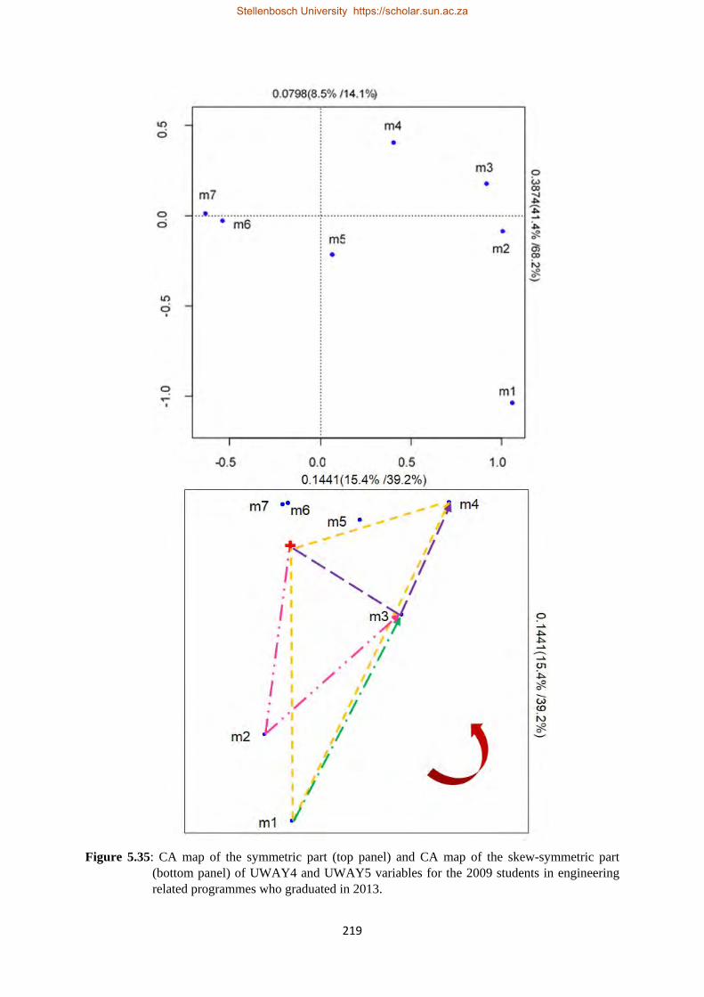
219
Figure 5.35: CA map of the symmetric part (top panel) and CA map of the skew-symmetric part
(bottom panel) of UWAY4 and UWAY5 variables for the 2009 students in engineering related programmes who graduated in 2013.
Stellenbosch University https://scholar.sun.ac.za

220
categories. That is, the average performance in the fourth year of study was better as compared to that
of the third year of study. Similarly, the average performance in the fifth year was enhanced as compared
to that in the fourth year of study. More specifically, a scrutiny of the skew-symmetric map in Figure
5.34 (bottom panel) indicates that category m1 experiences large outflow to category m3 (M3) and also
to category m2 (M2) (as indicated by triangles on the map subtended by categories m1 and m3, and by
categories m1 and m2 with the origin). Similarly, category m2 is losing more students to category m3
(this is represented by a triangle formed by the categories m2 and m3 with the origin), while m3 was
experiencing outflow to category m6. Other asymmetric flows with small magnitudes are from m6 to
m4; from m5 to m6 (as shown by a triangle subtended by m5 and m6 with the origin on the map); and
from m4 to m7. For the skew-symmetric map in Figure 5.35 (bottom panel), category m1 experiences
large outflow to categories m3 and m4 (shown on the map by triangles formed by categories m1 and
m4, and by categories m1 and m3 with the origin). Similarly, m4 experiences large inflow from m3
(indicated on the map by triangle subtended by categories m3 and m4 with the origin). Other asymmetric
flows are detected from m2 to m3 (represented on the map by triangle formed by m2 and m3 with the
origin), from m3 to m5, from m5 to m6, and from m6 to m7.
For both skew-symmetric maps, flows from categories of UWAY3 to categories of UWAY4, and from
categories of UWAY4 to categories of UWAY5 are interpreted in terms of the anticlockwise direction
(indicated by a curved arrow on the maps).
The transitional changes in the performance of students are also investigated for business related
programmes from grade twelve to the fourth year of study. The CA technique adapted to square tables
is performed on the four transition tables (see Table D.21 in Appendix D). The percentages explained
by the best two dimensions of these tables (see Table D.23 in Appendix D for the two best dimensions
of both the symmetric and skew-symmetric parts) are 69.6%, 85.1%, 94.0% and 71.2% for symmetric
parts, while for the skew-symmetric components of the same tables, they are 65.8%, 75.2%, 56.4%, and
87.8% (see Table D.22 in Appendix D). This suggests that all points are satisfactorily represented in
the two-dimensional displays, except for the skew-symmetric map associated with the transition table
of variables UWAY2 and UWAY3 which has a percentage for the best two dimensions below 60% (i.e.
56.4%).
Figure 5.36 portrays the symmetric and skew-symmetric maps of the transition table in Table D.21.a in
Appendix D. The symmetric map (see top panel of Figure 5.36) shows two clusters of categories: cluster
one formed by categories m1 and m2, and cluster two with categories m3, m4, and m5. Additionally,
on the first axis, category m6 is closest to m5, while on the second axis, categories m1 to m5 are close
to each other. The inspection of the skew-symmetric map shows that the largest triangle is subtended
by categories m6 and m7 with the origin of the map. This indicates a strong differential flow from m7
to m6 (M6). There are also asymmetric flows from categories m2, m3 and m4 to category m1 (M1);
Stellenbosch University https://scholar.sun.ac.za
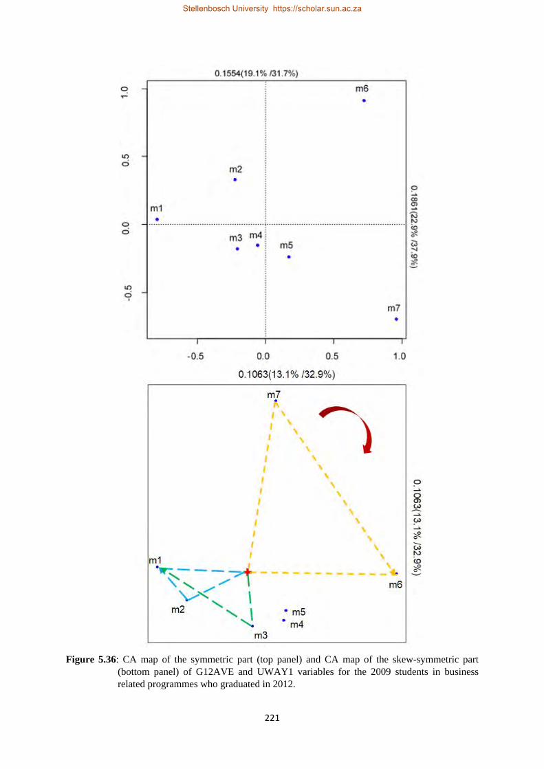
221
Figure 5.36: CA map of the symmetric part (top panel) and CA map of the skew-symmetric part
(bottom panel) of G12AVE and UWAY1 variables for the 2009 students in business related programmes who graduated in 2012.
Stellenbosch University https://scholar.sun.ac.za

222
from m4 to m2 (M2); and from m5 to m3 (M3). On the map (see bottom panel of Figure 5.36), flows
from m2 to m1, and from m3 to m1 are represented by triangles formed by m2 and m1 with the origin,
and by m3 and m1 with the origin, respectively. The flows from the categories of G12AVE to the
categories of UWAY1 are interpreted in terms of the clockwise direction (as indicated on the map by
the curved arrow).
The symmetric map (see top panel of Figure 5.37) associated with the transition from the first year to
the second year of study is a bit different from that from grade twelve to the first year of study. That is,
categories m1 to m6 are close to each other, while m7 is at a distance from the rest of the categories,
but is closest to category m5 on the first axis. Similar to the transition from grade twelve to the first
year of study, flows from categories of UWAY1 to categories of UWAY2 are interpreted in a clockwise
direction (as shown by the curved arrow). From the skew-symmetric map (see bottom panel of Figure
5.37), asymmetric flows are recorded from categories m2, m3 and m4 of UWAY1 to category m1 of
UWAY2 (as in the first transition from G12AVE to UWAY1); from categories m3, m4, m5 to m2; from
categories m4 and m5 to m3; from categories m5 and m6 to m4; and from categories m6 and m7 to m5.
Flows from m3 to m1, from m4 an m2, and from m4 and m6 are represented by triangles on the map
(see bottom panel of Figure 5.37). For legibility of the map, other triangles are not shown.
Figures 5.38 and 5.39 display the symmetric and skew-symmetric maps of the transitions from second
year to third year and from third year to fourth year of study associated with square tables in Tables
D.21.c and D.21.d, respectively. Flows from UWAY2 to UWAY3, and from UWAY3 to UWAY4 are
still interpreted in a clockwise direction (as indicated by the curved arrow on the maps), but with
outflows from lower categories to higher categories.
The symmetric map associated with variables UWAY2 and UWAY3 (see top panel of Figure 5.38)
reveals that categories m1 to m6 are very close to each other on the first axis, whereas category m7 is
at the far right end, separated from the rest of the points. On the second axis, m1, m2, and m3 form a
cluster. Category m3 is close to m6, while m5 is closest to m6. When examining the skew-symmetric
map (see bottom panel of Figure 5.38), it is deduced that there are asymmetric flows from m1 to
categories m2, m3, and m4; from m2 to categories m3, m4, m5 and m6; and from m3 to categories m4
and m6. Flows from m3 to m6, from m2 to m3, and from m1 to m4 are indicated by triangles on the
map (see bottom panel of Figure 5.38).
As regarding the transition from UWAY3 to UWAY4, the symmetric map in Figure 5.39 (top panel)
shows the following positioning of the points: m2, m3, and m4 are close to each other; m1 is nearest to
m3; m4 and m5 are close; m7 is closest to m5 and m4; m2 is closest to m6. An inspection of the skew-
symmetric map in Figure 5.39 (bottom panel) shows asymmetric flows from categories m1 and m2 to
m3; from m2 to categories m4 and m6; from m3 to categories m4, m5, m6 and m7; from m4 to
Stellenbosch University https://scholar.sun.ac.za

223
Figure 5.37: CA map of the symmetric part (top panel) and CA map of the skew-symmetric part
(bottom panel) of UWAY1 and UWAY2 variables for the 2009 students in business related programmes who graduated in 2012.
Stellenbosch University https://scholar.sun.ac.za

224
Figure 5.38: CA map of the symmetric part (top panel) and CA map of the skew-symmetric part
(bottom panel) of UWAY2 and UWAY3 variables for the 2009 students in business related programmes who graduated in 2012.
Stellenbosch University https://scholar.sun.ac.za

225
Figure 5.39: CA map of the symmetric part (top panel) and CA map of the skew-symmetric part
(bottom panel) of UWAY3 and UWAY4 variables for the 2009 students in business related programmes who graduated in 2012.
Stellenbosch University https://scholar.sun.ac.za

226
categories m5 and m7; and from m5 to m7. Flows from m2 to m3, from m2 to m4, and from m4 to m5
are represented by triangles on the map. Other triangles representing flows are not shown.
Patterns of transition and changes occurring in the performance of students from grade twelve to the
first year of study and through their undergraduate studies were also investigated for non-engineering
five-year programmes in the Faculty or School of the Built Environment (SBE). Results are not
reported. Transitional changes taking place from grade twelve to the first year, from first year to the
second year, from third year to the fourth year were similar to those in five-year engineering
programmes. That is, from grade twelve to the first year, lower categories of G12AVE variable were
losing more students toward higher categories of UWAY1 (in the first year of study). The same trend
was observed when considering the transitions from first year to the second year and from third year to
the fourth year of study. However, the transitions from second year to the third year and from fourth
year to the fifth year were different from those in engineering related programmes. In SBE programmes,
lower categories of UWAY2 were experiencing outflows to higher categories of UWAY3, whereas in
engineering related programmes, the opposite was observed. For the transition from fourth year to fifth
year, lower categories of UWAY4 were losing more students to higher categories of UWAY5 in
engineering related programmes, whereas in SBE programmes, it is the higher categories of UWAY4
which were experiencing outflows to lower categories of UWAY5.
The findings in this section are also supported by the statistical investigation based on notched boxplots
in Section 4.2.6 in Chapter 4. That is, the transitional changes occurring in the average performance
from school (grade twelve) level to the first year of study, and from first year to the second year of study
were downward in business related programmes, while in engineering related programmes, they were
upward. The trend observed in the first two years of study in the Faculty or School of Business (SB)
was mainly due to large classes in this faculty. Normally students in business related programmes (i.e.
business administration, accountancy and marketing) are being taught as one group in the first two years
of study. The bifurcation into respective programmes takes place in the third year of study. As a result
of the reduction in class sizes, upward transitional changes from second year to the third year, and from
third year to the fourth year of study are recorded. In engineering programmes, the bifurcation into
individual programmes occurs in the second year of study. Small classes helped to enhance the
performance in the second year of study. In the third year of study, the performance decreased, due to
specialised subjects in individual programmes.
In the previous sections, the CA technique was used on two-way contingency tables of a single school
variable with a single university variable. The CBU data incorporate a time factor as well as a
programme type factor. It was not possible to include the time factor, and the type of programme in the
analysis. Comparisons over time and by type of programme were made by producing several CA plots.
In order to simultaneously include the time factor and the type of programme in a single analysis,
Stellenbosch University https://scholar.sun.ac.za

227
statistical techniques incorporating more than two variables need to be applied to the data. The next
section partially addresses this issue through stacked table analysis. In the next chapter the analysis of
multiway contingency tables will receive full attention by performing multiple correspondence analysis
(MCA) on the CBU data.
5.13 CA of three- and four-way contingency tables: stacked table analysis.
5.13.1 Approaches to reduce a multiway table into a two-way table.
So far, the CA technique has been applied to two-way contingency tables. That is, two variables were
used at a time in the analysis. In order to simultaneously visualise more than two categorical variables,
MCA can be performed on the data. This will the target of the next chapter. An intermediate approach
to MCA would be to reduce the multiway contingency table into a two-way contingency table and then
carry out simple CA (Greenacre, 2007). This can be achieved by interactively coding two or more
variables. The process of interactive coding several variables consists of creating a new variable which
gives all possible combinations of their categories.
In previous sections, CA was applied to the first year dataset of the CBU data by using one single
school variable versus a single university variable for a particular year, and a particular type of
programme. In order to include for example the variables FYEAR (with fourteen categories) and
TPROG (with three categories) in a CA involving variables EPOINT (with four categories) and FCCO
(with four categories), then the variables FYEAR, TPROG, and EPOINT need to be interactively coded.
This results in a new variable with 14 × 3 × 4 = 168 combinations. This new variable can then be cross-
tabulated with variable FCCO to produce a 168 × 4 contingency table to be analysed using the standard
CA technique. Although this method allows for the visualisation of interactions between variables, the
possible combinations of the new variable becomes large when the number of variables to code
increases. As an alternative to interactive coding, the two-way contingency table for the analysis can be
created by stacking several two-way contingency tables row-wise (i.e. one on top of each other),
columnwise (i.e. side-by-side), or both row- and columnwise, and then by applying the regular CA
technique to the two-way table thus formed (Greenacre & Blasius, 2006; Greenacre, 2007).
Within the context of this study, there exists two properties of the CBU data which need to be introduced
in the analysis. These include the factor time, and the variable TPROG (type of programme). These two
variables are important in order to ascertain whether patterns of associations between school and
university results variables are similar within different programmes of study or over time. In previous
sections, this was done by generating separate CA plots for each year and for each type of programme,
and then comparing them. To circumvent this problem and introduce more variables in the analysis,
stacked table analysis is considered.
Stellenbosch University https://scholar.sun.ac.za

228
When the time factor is to be introduced in the analysis as a third variable, the three-way contingency
table can be reduced to a two-way contingency table by stacking tables associated with different years
row-wise. In the case when the variable TPROG (types of programme) is also introduced in the analysis
as a fourth variable, the four-way contingency table can be re-expressed in the form of a two-way
contingency table by stacking row-wise two-way contingency tables associated with different years and
stacking columnwise tables corresponding to different types of programme.
In the subsections below, the CA biplots are retained in the analysis. For legibility purpose and easy
comparison over time and/or by type of programmes, the plotting of column points is suppressed.
5.13.2 CA of three-way contingency tables: stacked table analysis involving only the time factor.
a. CA involving variables FYAVE, G12AVE and FYEAR.
In the CA analyses for all programmes combined involving university results variables and school
results variables in previous sections, the variable FYEAR (year when entering the first year of study)
was added to the analysis. Table 5.30 presents the three-way contingency table involving variables
FYAVE, G12AVE and FYEAR for all programmes combined. Categories UNM1 to UNM6 defined in
Section 5.6.1, are abbreviated as U1 to U6, with the numbers 09, 11, 12, and 13, representing the years
2009, 2011, 2012 and 2013, affixed on them. For example, the symbol “U5.09” corresponds to category
UNM5 for the year 2009. Categories G12M1 to G12M5 (as defined in Section 5.6.1) are also
abbreviated as G1 to G6. The three-way table is stacked using variable FYEAR. The regular CA
technique is performed on the resulting four stacked two-way contingency tables in Table 5.30. The
associated CA partial results are presented in Table 5.31.
The overall quality of the two-dimensional display is acceptable with about 93.5% of the total inertia
of 0.3646 explained by the first two dimensions (see Table 5.31). All points are well represented in the
two-dimensional space (qualities of the points are not shown).
An inspection of the CA asymmetric map (not shown) reveals that categories U6 (for all four years),
U5 (in 2009, 2012, and 2013), and U4 (for the years 2009 and 2013) of variable FYAVE are located on
the right-hand pole of the first axis with categories G4 and G5 of G12AVE. The rest of the categories
of G12AVE (i.e. G1, G2, and G3) and categories U1, U2, and U3 (for all four years), as well as
categories U5 (for the year 2011) and U4 (in 2011 and 2012) of FYAVE are positioned on the left-hand
pole. This implies that, over the four-year period (i.e. in 2009, and in 2011 to 2013), the two highest
categories U5 (except in 2011) and U6 of FYAVE representing the highest achievement at the first year
level tend to be associated with the two highest categories G4 and G5 of G12AVE. The other categories
of FYAVE on the left-hand side of axis one are associated with lower school performance.
The CA biplot in Figure 5.40 shows that, for all four years, category U6 has the highest profile value
(in standardised form) on the biplot axes G5 and G4, this is followed by U5 (in 2009, 2012 and 2013).
Stellenbosch University https://scholar.sun.ac.za

229
This suggests that category U6 of FYAVE is, almost exclusively, associated with the two highest
categories G5 and G4 of G12AVE. That is, most students who attained the highest achievement in the
first year of study (i.e. first year average marks of at least 70%), obtained school average marks of at
least 65%.
Table 5.30: Four stacked two-way contingency tables of the variables FYAVE and G12AVE, using
variable FYEAR for all programmes combined.
FYEAR FYAVE G12AVE G1 G2 G3 G4 G5
2009 U1 14 12 10 3 0 U2 16 24 24 5 2 U3 18 35 33 18 2 U4 16 28 36 24 8 U5 1 10 25 14 11 U6 1 3 6 21 24
2011 U1 28 21 5 3 0 U2 18 35 22 3 0 U3 23 57 42 9 1 U4 16 56 57 20 2 U5 4 26 42 20 1 U6 2 5 23 26 16
2012 U1 41 31 27 9 3 U2 22 24 23 11 3 U3 23 44 36 21 4 U4 26 46 34 23 9 U5 8 21 26 29 11 U6 5 8 20 14 33
2013 U1 46 62 63 20 1 U2 35 39 43 14 2 U3 15 44 43 21 7 U4 6 37 51 39 6 U5 3 12 28 25 12 U6 0 1 7 30 31
Table 5.31: Partial CA results of four stacked contingency tables (stacked using variable FYEAR) of
variables FYAVE and G12AVE for all programmes combined using the first year dataset.
Dim Principal inertia % inertia Cumulative % 1 0.2784 76.4 76.4 2 0.0624 17.1 93.5 3 0.0160 4.4 97.8 4 0.0079 2.2 100.0
Total 0.3647 100.0
Stellenbosch University https://scholar.sun.ac.za

230
Figure 5.40: CA biplot of row profiles of four stacked contingency tables (stacked using variable FYEAR) of variables FYAVE and G12AVE for all programmes combined using the first year dataset.
From the position of the points U6.09, U6.11, U6.12, and U6.13 on the CA biplot in Figure 5.40, it can
be said that the largest number of “G5” students in the U6 bin is recorded in 2013. From 2009 to 2011,
this number decreases. In 2012, it increases but not to its level in 2009. Likewise, for category U5, there
is a diminution of its profile values on the G4 and G5 biplot axes in 2011. For other points (of FYAVE),
there is no much change in their positions on the biplot, which also implies that their associated profiles
do not change much over the four-year period.
Stellenbosch University https://scholar.sun.ac.za

231
These findings concur with the CA results of single two-way contingency tables in Section 5.6.1.
Stacking analysis has the advantage over the analysis based on individual two-way contingency tables,
as it facilitates comparisons over time. But the major drawback is that, when the number of stacked
tables increases, the points to represent on the plot also become numerous, reducing thus its legibility.
b. CA involving variables FYAVE, NDIS and FYEAR.
In Section 5.6.2, individual CA maps (asymmetric plots and CA biplots) were constructed for each year
and comparisons over the years were made. Similar to the analysis in the previous section, the standard
CA is performed on the four stacked two-way contingency tables of variables FYAVE and NDIS using
the variable FYEAR. Only the CA biplot is shown in Figure 5.41. The CA partial results are summarised
in Table 5.32. From this table, it is noted that the first two dimensions account for about 91.3% of the
total inertia of 0.1785 in the contingency table. The two-dimensional qualities for the row and column
points or sample and column predictivities (not shown) for most points (except for categories U1 and
U4 in 2009, U5 in 2011, U2 in 2012, U3 in 2013 and ND3 in 2013) indicate that most points are well
represented in two-dimensional maps.
Table 5.32: Partial CA results of four stacked contingency tables (stacked using variable FYEAR) of
variables FYAVE and NDIS for all programmes combined using the first year dataset.
Dim Principal inertia % inertia Cumulative % 1 0.1440 80.7 80.7 2 0.0190 10.7 91.3 3 0.0117 6.6 97.9 4 0.0038 2.1 100.0
Total 0.1785 100.0
An inspection of the CA asymmetric map (not reported) shows that the left-to-right direction is
analogous to high-to-low school performance with respect to the number of upper distinctions at school
level. For all four years, category U6 of FYAVE is consistently positioned on the left-hand side of axis
one with categories U5 (in 2009, 2012 and 2013), U4 (in 2013 only) and ND4. This indicates that higher
categories of FYAVE are associated with the highest category of variable NDIS. Other categories of
FYAVE are on the right-hand side of the first axis and are linked to categories ND0, ND1, ND2 and
ND3 of variable NDIS.
From Figure 5.41, it is noted for all four years that U6 has the highest profile value on the ND4 biplot
axis, then U5 (in 2009, 2012 and 2013 only), and U4 (in 2013 only). On the ND3 biplot axis, U4 (in
2011 and 2012) has the highest profile element, followed by U5 (in 2011 only), whereas on the ND2
biplot axis, U4 (in 2011) has the highest profile value. In 2009, U3 has the highest profile value on
both ND0 and ND1 biplot axes, while in 2011, it is U1 which has the highest profile element on these
biplot axes.
Stellenbosch University https://scholar.sun.ac.za

232
Figure 5.41: CA biplot of row profiles of four stacked contingency tables (stacked using variable FYEAR) of variables FYAVE and NDIS for all programmes combined using the first year dataset.
The position of U6 for different years in Figure 5.41 indicates a large diminution of the number of
students in the U6 category (i.e. those who obtained average first year marks of at least 70%) who had
at least four upper distinctions at school level (the ND4 group) from 2009 to 2011. From 2011 to 2013,
it is increased. The same trend is observed for students in category U5 who achieved at least four upper
distinctions at school level. An increase is also observed on the number of students in the U4 category
who achieved three upper distinctions at school level (the ND3 group) and two distinctions (the ND2
group) from 2009 to 2011, whereas in 2012 and 2013, this number is reduced. For students in other
categories of FYAVE, some changes are also observed. For example, a reduction in the number of
Stellenbosch University https://scholar.sun.ac.za

233
students in the U3 category with zero or one distinction is observed from 2009 to 2013, whereas during
the same period, the number of students in the U1 bracket with zero or one distinction is increased from
2009 to 2011 and then is decreased in 2012 and 2013. For the U2 group with zero or one distinction, a
small increase is noted from 2009 to 2011, and in 2013. In 2012, a small reduction is recorded.
Although the findings agree, to some extent, with those in Section 5.6.2, the stacked analysis has
facilitated comparisons over time by using a single CA biplot instead of several CA plots.
c. CA involving variables FYAVE, EPOINT and FYEAR.
The four contingency tables of variables FYAVE and EPOINT were also stacked row-wise using
variable FYEAR. The resulting four stacked two-way contingency tables and the partial CA results are
reported in Table D.24 and D.25 in Appendix D, respectively, whereas the CA biplot is displayed in
Figure 5.42. The overall quality of the two-dimensional display in Figure 5.42 is satisfactory with
91.5% of the total inertia in the tables explained by the first two dimensions (see Table D.25).
From the inspection of the CA asymmetric map (not reported), it was noted an association between
category U6 of FYAVE and category E5-7 of EPOINT for all four years considered, indicating that
most students who achieved average scores of at least 70% at the first year level were admitted in the
first year of study with entry points between five and seven points. This is seen in Figure 5.42 where
U6 has the highest profile value on the biplot axis E5-7 for all four years, then U5 and U4 (in 2013
only)
In Figure 5.42, some changes in the profile values of categories of FYAVE on the biplot axes are
observed. For example, from 2009 to 2011, there is a large reduction in the number of students in
category U6 who were admitted in the university with entry points between five and seven points. From
2011 to 2013, a gradual increase is observed. Likewise, the profile values of U5 on the biplot axis E5-
7 show an increasing trend from 2009 to 2013. Some small changes on the profile values of U4 on the
biplot axis E8-9 are also noticeable in Figure 5.42. Category U1 has the largest profile value in 2011 on
the biplot axis E>=12, as compared to other years.
d. CA involving variables FYAVE, individual school variables and FYEAR.
The analysis of stacked tables in this subsection involves variable FYAVE with individual school
variables. The focus is on school Mathematics and English because of their special status in the
admission criteria (i.e. they are compulsory subjects required in the admission process). The four
stacked two-way contingency tables involving FYAVE and school Mathematics are found in Table
5.33, whereas the corresponding partial CA results are summarised in Table 5.34. CA maps were also
constructed. Only the CA biplot is shown (see Figure 5.43).
Stellenbosch University https://scholar.sun.ac.za

234
Figure 5.42: CA biplot of row profiles of four stacked contingency tables (stacked using variable
FYEAR) of variables FYAVE and EPOINT for all programmes combined for the first year dataset.
The CA biplot in Figure 5.43 and the CA asymmetric map (not shown) provide satisfactory fits for the
data as the overall quality is 93.5% (see Table 5.34). Additionally, most categories of the two variables
involved in the analysis are well represented in the two-dimensional displays.
A scrutiny of Figure 5.43 indicates that U6 has the highest profile value on the MA5 biplot axis for all
four years, then U5, U4 (in 2013 only) and U3 (in 2013 only). On the biplot axis MA1, U1 has the
highest profile value for all four years. This is followed by category U2. From the positions of the points
representing the categories of FYAVE in four years, there is evidence of minor changes (small reduction
Stellenbosch University https://scholar.sun.ac.za
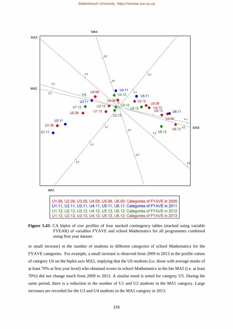
235
Figure 5.43: CA biplot of row profiles of four stacked contingency tables (stacked using variable
FYEAR) of variables FYAVE and school Mathematics for all programmes combined using first year dataset.
or small increase) in the number of students in different categories of school Mathematics for the
FYAVE categories. For example, a small increase is observed from 2009 to 2013 in the profile values
of category U6 on the biplot axis MA5, implying that the U6 students (i.e. those with average marks of
at least 70% at first year level) who obtained scores in school Mathematics in the bin MA5 (i.e. at least
70%) did not change much from 2009 to 2013. A similar trend is noted for category U5. During the
same period, there is a reduction in the number of U1 and U2 students in the MA1 category. Large
increases are recorded for the U3 and U4 students in the MA5 category in 2013.
Stellenbosch University https://scholar.sun.ac.za

236
Table 5.33: Four stacked two-way contingency tables of the variables FYAVE and school
Mathematics, using variable FYEAR for all programmes combined.
FYEAR FYAVE School Mathematics MA1 MA2 MA3 MA4 MA5
2009 U1 15 5 5 9 5 U2 16 10 14 10 21 U3 14 17 17 21 37 U4 9 12 17 16 58 U5 2 4 3 8 44 U6 0 2 0 4 49
2011 U1 22 11 9 8 7 U2 25 12 15 11 15 U3 21 16 28 23 44 U4 11 16 16 36 72 U5 4 2 11 17 59 U6 0 0 2 5 65
2012 U1 26 12 13 28 32 U2 10 9 13 8 43 U3 15 13 16 18 66 U4 13 10 21 28 66 U5 5 4 9 11 66 U6 5 1 2 2 70
2013 U1 32 17 30 26 87 U2 19 14 15 24 61 U3 7 9 11 21 82 U4 5 6 7 17 104 U5 2 3 0 7 68 U6 1 0 0 1 67
Table 5.34: Partial CA results of four stacked contingency tables (stacked using variable FYEAR) of
variables FYAVE and school Mathematics for all programmes combined.
Dim Principal inertia % inertia Cumulative % 1 0.1947 84.0 84.0 2 0.0220 9.5 93.5 3 0.0105 4.5 98.0 4 0.0047 2.0 100.0
Total 0.2319 100.0
The analysis of stacked tables involving FYAVE and school English (see the CA biplot in Figure 5.44)
exhibits somehow different patterns with major changes occurring, over the four-year period, on the
profile values of the categories of FYAVE on the biplot axes. That is, from 2009 to 2011, the numbers
of U1, U2, U5, and U6 students in the EN4 and EN5 categories (i.e. corresponding to marks between
Stellenbosch University https://scholar.sun.ac.za

237
Figure 5.44: CA biplot of row profiles of four stacked contingency tables (stacked using variable
FYEAR) of variables FYAVE and school English for all programmes combined using the first year dataset.
65% and 69%, and at least 70% in school English, respectively) considerably decrease, while from 2011
to 2013, a large increase is recorded. In 2011, the profile values for all categories of FYAVE augment.
Another distinguishing feature of the CA biplot in Figure 5.44 from that in Figure 5.43 is the tendency
of lower categories of FYAVE to be associated with higher categories of school English and vice-versa.
For example, in 2009 and 2013, U1 has the highest profile value on the biplot axes EN4 and EN5, while
in 2011, higher profile elements for U3, U4, U5 and U6 are observed on the biplot axis EN2. These
findings again show that school English, although being given a special status like school Mathematics
in the admission process, is not a good indicator of the university academic performance.
Stellenbosch University https://scholar.sun.ac.za

238
e. CA involving variables FCCO, G12AVE, FYEAR and individual school variables.
The stacked analysis is extended to the variable FCCO with school variables (i.e. G12AVE, school
Mathematics and English). The stacked table of FCCO with G12AVE, stacked over time is reported in
Table 5.35, while that for FCCO with school Mathematics and FCCO with school English are
summarised in Tables D.26 and D.28 in Appendix D, respectively. The associated partial CA results
are presented in Tables 5.36, D.27 and D.29, while the CA biplots are shown in Figures 5.45, D.12 and
D.13 (in Appendix D).
The overall qualities of the CA maps are adequate with percentages of the total inertia explained by the
first two dimensions being 94.9 % (for FCCO and G12AVE), 92.0% (for FCCO and school
Mathematics) and 95.6 % (for FCCO and school English) (see Tables 5.36, D.27 and D.29). In all CA
biplots constructed, almost all points are well represented as indicated by their sample and column
predictivities (not shown).
Table 5.35: Four stacked two-way contingency tables of the variables FCCO and G12AVE, using
variable FYEAR for all programmes combined.
FYEAR FCCO G12AVE G1 G2 G3 G4 G5
2009 CP 21 61 77 67 43 EX 3 2 2 2 0 PR 30 39 49 16 3 PT 12 10 6 0 1
2011 CP 30 100 113 58 18 EX 12 9 1 1 0 PR 43 80 72 19 2 PT 6 11 5 3 0
2012 CP 40 66 79 60 47 EX 16 10 11 3 0 PR 48 79 65 40 14 PT 21 19 11 4 2
2013 CP 23 79 111 106 49 EX 25 28 28 7 1 PR PT
35 56 57 20 8 19 32 39 16 1
Stellenbosch University https://scholar.sun.ac.za

239
Figure 5.45: CA biplot of row profiles of four stacked contingency tables (stacked using variable
FYEAR) of variables FCCO and G12AVE for all programmes combined using the first year dataset.
Figure 5.45 shows that category CP of FCCO has the highest profile value on the biplot axes G4 and
G5 in the years 2009, 2012 and 2013, whereas in 2011, it has the highest profile element on the biplot
axis G3. From the position of category CP on the CA biplot in four years, it is deduced that, in 2011,
there is a large reduction in the number of CP students (i.e. those who clear passed all first year subjects)
in the G4 and G5 categories, and an increase in the CP students in the G3 group. For other categories
of FCCO, an increase in the number of EX students (i.e. those who were excluded at the end of the first
year of study) in the G1 category is observed in 2011. On the biplot axis G2, category PR has the highest
profile element in 2011. This is followed by category PT during the same year. A moderate reduction
in 2012, and then a small increase in 2013 in the number of PR students (i.e. those who proceeded in
Stellenbosch University https://scholar.sun.ac.za

240
the second year of study and who were repeating one or two first year subjects) in the G2 category are
recorded. There is also an augmentation on the number of PT students (i.e. those who were put on part
time) in the G2 category in 2013.
Table 5.36: Partial CA results of four stacked contingency tables (stacked using variable FYEAR) of
variables FCCO and G12AVE for all programmes combined using the first year dataset.
Dim Principal inertia % inertia Cumulative % 1 0.1147 79.4 79.4 2 0.0225 15.5 94.9 3 0.0037 2.6 97.5 4 0.0036 2.5 100.0
Total 0.1445 100.0
Figures D.12 and D.13 in Appendix D display the CA biplots for stacked tables involving FCCO with
school Mathematics, and school English, respectively. In Figure D.12, there is an indication that the
CP group, over the four-year period, has basically a great number of students in the MA5 category of
school Mathematics as evidenced by the highest profile value of CP on biplot axis MA5. This is in
contrast with Figure D.13 where CP is associated with lower categories of school English. For example,
CP has the highest profile value on the EN1 biplot axis in 2011. On the EN4 biplot axis, PR has the
highest profile element in 2009, while during the same year, EX has the highest profile quantity on axis
EN5. These findings consolidate previous analyses in this chapter and in Chapter 4 and indicate that
English is not a good indicator of the university performance. A check of the two-dimensional quality
values of all points (mostly above 90%) (not reported) permits to state that all points are well represented
on the two-dimensional displays.
From the position of category CP on the CA biplot in Figure D.12, little change is observed on the
number of CP students in the MA5 category of school Mathematics from 2009 to 2012. In 2013, an
increase in the profile value of MA5 is noticeable. The positions of other categories of FCCO in Figure
D.12 also indicate some changes in their profile values on the biplot axes. For example, a reduction in
the number of EX students in the MA1 category of school Mathematics from 2009 to 2012 is noted. In
2013, a small increase in the profile values of EX on the biplot axes MA2, MA3 and MA4 is observed.
The increase of the CP students in the MA5 category, and the EX students in the MA2, MA3 and MA4
categories in 2013, was probably be due to the effect of raising the admission standards which were a
consequence of down adjusting the programmes’ cut-off points, and reducing the gap between the
programmes cut-off points of the male and female students. Many students with good school results
who were admitted in 2013, completed successfully their first year of study, while other were excluded
at the end of the year.
Stellenbosch University https://scholar.sun.ac.za

241
f. CA involving school Mathematics, school first year Mathematics and FYEAR.
In this subsection the regular CA technique is applied on the stacked table involving school Mathematics
and first year Mathematics over time (i.e. variable FYEAR) (see Table 5.37). The partial results are
reported in Table 5.38, while the CA biplot is displayed in Figure 5.46. The overall quality of the display
(of 94.6 %) in Figure 5.46 is acceptable (see Table 5.38).
Table 5.37: Four stacked two-way contingency tables of school Mathematics and first year
Mathematics, using variable FYEAR for all programmes combined.
FYEAR First year Mathematics
School Mathematics MA1 MA2 MA3 MA4 MA5
2009 F1 20 16 24 9 4 F2 9 9 11 6 0 F3 11 20 43 37 14 F4 3 11 27 35 14 F5 0 5 9 10 10 F6 1 1 10 42 33
2011 F1 29 32 33 13 2 F2 6 12 19 9 1 F3 17 30 57 43 11 F4 2 9 48 43 10 F5 0 2 20 39 23 F6 0 1 4 29 39
2012 F1 17 34 38 26 6 F2 3 12 22 12 6 F3 10 25 67 62 26 F4 3 14 23 49 F5 1 3 17 53 43 F6 1 0 2 23 30
2013 F1 22 40 62 7 26 F2 6 13 22 65 23 F3 7 15 52 32 41 F4 1 6 16 53 58 F5 0 4 7 41 54 F6 0 1 0 26 47
The CA asymmetric map (not reported) shows that the left-to-right direction corresponds to low-to-
high school Mathematics performance. Categories MA4 and MA5 of school Mathematics are on the
right-hand side, while the other categories are situated on the left-hand side of axis one. For all four
years, categories F5 and F6 of the first year Mathematics are positioned on the right-hand side and are
associated with the two highest categories (i.e. MA4 and MA5) of school Mathematics. Categories F4
(in 2012 and 2013 only), F2 (in 2013) and F3 (in 2013) are also found on the right side, while the
Stellenbosch University https://scholar.sun.ac.za

242
Figure 5.46: CA biplot of row profiles of four stacked contingency tables (stacked using variable FYEAR) of school Mathematics and first year Mathematics for all programmes combined using the first year dataset.
remaining categories of first year Mathematics are located on the lower school performance side.
From the CA biplot in Figure 5.46, it is noted that category F6 of first year Mathematics (for all four
years) has the highest profile value on the biplot axis MA5, followed by F5 and F4 (in 2012 and 2013
only). Categories F1, F2 and F3 have lower profile elements on axis MA5. Over time, changes in the
profile values of categories of first year Mathematics are perceptible in the CA biplot in Figure 5.46.
For example, the profile values of F5 and F6 on the MA5 biplot axis exhibit an increasing trend over
the four-year period, while the profile values for F1 and F2 on the biplot axes MA1 and MA2 show a
reduction over the same period. On the biplot axes MA3 and MA4, profile values of F4 increase from
Stellenbosch University https://scholar.sun.ac.za

243
2009 to 2011. In 2012 and 2013, they decrease. A similar trend is observed for the profile values of F5
on the MA4 biplot axis
Table 5.38: Partial CA results of four stacked contingency tables (stacked using variable FYEAR) of
first year Mathematics and school Mathematics for all programmes combined using the
first year dataset.
Dim Principal inertia % inertia Cumulative % 1 0.2952 77.4 77.4 2 0.0668 17.5 94.9 3 0.0127 3.3 98.3 4 0.0066 1.7 100.0
Total 0.3813 100.0
g. Summary of the stacked table analysis using the time factor.
In this section, the standard CA technique has been performed on the stacked tables of university and
school results variables over time. The time factor has been introduced in the analysis as a third variable.
This has facilitated the comparison of the patterns of associations for different time periods using a
single CA biplot. Changes occurring on the profile values of the categories of the row variables on the
biplots axes have been noted. This has permitted to assess whether students in categories of university
variables falling in the categories of school results variables have increased and decreased over the four-
year period. For example, the stacked table analysis involving variables FYAVE and G12AVE has
shown that the number of students in the highest bin of the first year academic performance who attained
the highest achievement at school level decreased from 2009 to 2011, but increased from 2011 to 2013.
This increase could be attributed to the downward adjustment of cut-off points of degree programmes
and the narrowing of the gap between the programmes’ cut-off points between the male and the female
students. These two actions combined permitted to admit students with good school results.
In the next subsection the fourth variable representing the type of programmes is introduced in the
analysis.
5.13.3 CA of four-way contingency tables: stacked table analysis involving the type of programme
of study and the time factor.
In an attempt to simultaneously analyse several variables, the time factor and the type of programmes are
added to the two variables representing school and university performances. In order to apply the regular
CA to the resulting four-way contingency table, two-way contingency tables were stacked row-wise using
the variable FYEAR, and stacked columnwise using the variable TPROG (types of programmes). As an
illustration of this procedure, twelve stacked two-way contingency tables of variables FYAVE and
G12AVE, using variables FYEAR (with four categories) and TPROG (with three categories) were
Stellenbosch University https://scholar.sun.ac.za
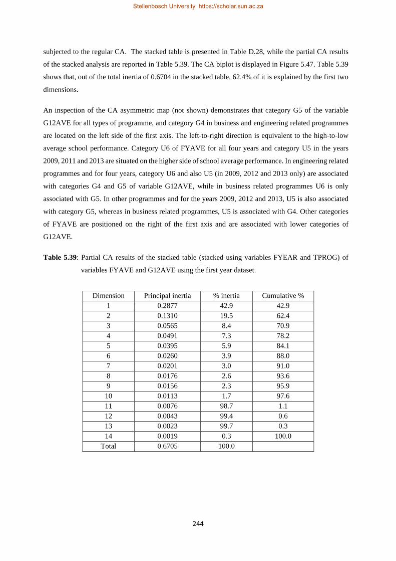
244
subjected to the regular CA. The stacked table is presented in Table D.28, while the partial CA results
of the stacked analysis are reported in Table 5.39. The CA biplot is displayed in Figure 5.47. Table 5.39
shows that, out of the total inertia of 0.6704 in the stacked table, 62.4% of it is explained by the first two
dimensions.
An inspection of the CA asymmetric map (not shown) demonstrates that category G5 of the variable
G12AVE for all types of programme, and category G4 in business and engineering related programmes
are located on the left side of the first axis. The left-to-right direction is equivalent to the high-to-low
average school performance. Category U6 of FYAVE for all four years and category U5 in the years
2009, 2011 and 2013 are situated on the higher side of school average performance. In engineering related
programmes and for four years, category U6 and also U5 (in 2009, 2012 and 2013 only) are associated
with categories G4 and G5 of variable G12AVE, while in business related programmes U6 is only
associated with G5. In other programmes and for the years 2009, 2012 and 2013, U5 is also associated
with category G5, whereas in business related programmes, U5 is associated with G4. Other categories
of FYAVE are positioned on the right of the first axis and are associated with lower categories of
G12AVE.
Table 5.39: Partial CA results of the stacked table (stacked using variables FYEAR and TPROG) of
variables FYAVE and G12AVE using the first year dataset.
Dimension Principal inertia % inertia Cumulative % 1 0.2877 42.9 42.9 2 0.1310 19.5 62.4 3 0.0565 8.4 70.9 4 0.0491 7.3 78.2 5 0.0395 5.9 84.1 6 0.0260 3.9 88.0 7 0.0201 3.0 91.0 8 0.0176 2.6 93.6 9 0.0156 2.3 95.9 10 0.0113 1.7 97.6 11 0.0076 98.7 1.1 12 0.0043 99.4 0.6 13 0.0023 99.7 0.3 14 0.0019 0.3 100.0
Total 0.6705 100.0
Stellenbosch University https://scholar.sun.ac.za

245
Figure 5.47: CA biplot of row profiles of twelve stacked contingency tables (stacked using variables
FYEAR and TPROG) of FYAVE and G12AVE using the first year dataset.
The patterns of associations detected using the CA asymmetric map, are also uncovered using the CA
biplot in Figure 5.47 with the added advantage that the latter is more legible than the former and
facilitates comparisons over time and by type of programme. For both business and engineering related
programmes, category U6 has the highest profile value on the G5 biplot axis for all four years, this is
followed by U5 for the years 2009, 2012 and 2013. In other programmes, it is U5 (in 2009 only) which
has the highest profile element on the G5 axis. On the G4 biplot axis (in business related programmes),
Stellenbosch University https://scholar.sun.ac.za
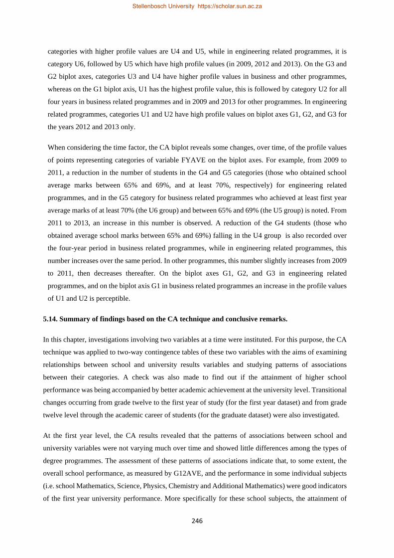
246
categories with higher profile values are U4 and U5, while in engineering related programmes, it is
category U6, followed by U5 which have high profile values (in 2009, 2012 and 2013). On the G3 and
G2 biplot axes, categories U3 and U4 have higher profile values in business and other programmes,
whereas on the G1 biplot axis, U1 has the highest profile value, this is followed by category U2 for all
four years in business related programmes and in 2009 and 2013 for other programmes. In engineering
related programmes, categories U1 and U2 have high profile values on biplot axes G1, G2, and G3 for
the years 2012 and 2013 only.
When considering the time factor, the CA biplot reveals some changes, over time, of the profile values
of points representing categories of variable FYAVE on the biplot axes. For example, from 2009 to
2011, a reduction in the number of students in the G4 and G5 categories (those who obtained school
average marks between 65% and 69%, and at least 70%, respectively) for engineering related
programmes, and in the G5 category for business related programmes who achieved at least first year
average marks of at least 70% (the U6 group) and between 65% and 69% (the U5 group) is noted. From
2011 to 2013, an increase in this number is observed. A reduction of the G4 students (those who
obtained average school marks between 65% and 69%) falling in the U4 group is also recorded over
the four-year period in business related programmes, while in engineering related programmes, this
number increases over the same period. In other programmes, this number slightly increases from 2009
to 2011, then decreases thereafter. On the biplot axes G1, G2, and G3 in engineering related
programmes, and on the biplot axis G1 in business related programmes an increase in the profile values
of U1 and U2 is perceptible.
5.14. Summary of findings based on the CA technique and conclusive remarks.
In this chapter, investigations involving two variables at a time were instituted. For this purpose, the CA
technique was applied to two-way contingence tables of these two variables with the aims of examining
relationships between school and university results variables and studying patterns of associations
between their categories. A check was also made to find out if the attainment of higher school
performance was being accompanied by better academic achievement at the university level. Transitional
changes occurring from grade twelve to the first year of study (for the first year dataset) and from grade
twelve level through the academic career of students (for the graduate dataset) were also investigated.
At the first year level, the CA results revealed that the patterns of associations between school and
university variables were not varying much over time and showed little differences among the types of
degree programmes. The assessment of these patterns of associations indicate that, to some extent, the
overall school performance, as measured by G12AVE, and the performance in some individual subjects
(i.e. school Mathematics, Science, Physics, Chemistry and Additional Mathematics) were good indicators
of the first year university performance. More specifically for these school subjects, the attainment of
Stellenbosch University https://scholar.sun.ac.za

247
high marks at school level was being accompanied by higher achievement at the first year level of study.
Also, students with better academic performance at first year level, were among those who achieved at
least four upper distinctions at school level, those who were admitted in the university with entry points
between five and seven points, and those whose entry points were below the programmes’ cut-off points.
However, this trend was observed for a small proportion of students only. For a large proportion of
students, there was a tendency for students to achieve higher performance at school level, but to attain
low academic achievement at the first year level. This was an indication of students who were admitted
with inflated school results which were not matching with the university performance.
When studying patterns of associations between variable FCCO and school results variables, a close
association between the CP students (i.e. students who successfully completed the first year of study and
who unconditionally proceeded to the second year of study), on one side, and low entry points below the
programmes’ cut-off points, and higher categories of G12AVE, on the other side, was unveiled, implying
that these students were among those who attained higher academic achievement at school level.
Additionally, students with higher entry points and who were found in the last two lower brackets of the
G12AVE variable (corresponding to the lower performance side at grade twelve level) were at risk of
being excluded or being put on part time at the end of their first year of study.
Another investigation of interest was to examine patterns of associations between school and first year
Mathematics. This investigation was important since the first year Mathematics was identified as having
the worst performance among all first year subjects. When using grades for both variables, it was found
that categories DU (upper distinction), and LU (lower distinction) of first year Mathematics were, quasi-
exclusively, associated with category UD12 (upper distinction) of school Mathematics, implying that
students who attained the highest achievement in the first year Mathematics were among those who also
obtained the highest performance in school Mathematics. Other students who got merit, credit or pass in
first year Mathematics were also drawn for the highest performance category of school Mathematics.
Students with a grade of upper merit or below in school Mathematics, were at risk of failing the first year
Mathematics.
The findings, using actual marks (in %) for both school and first year Mathematics, indicate that most
students whose scores were falling in the topmost category (corresponding to scores of at least 70%) of
the first year Mathematics, were among those who were in the top category of school Mathematics (also
corresponding to scores of at least 70%). Other students who attained the highest achievement in school
Mathematics, were found in the bins UNM5 (corresponding to scores between 65% and 69%) and UNM4
(or scores between 60% and 64%). Additionally, students who obtained scores below 60% in school
Mathematics, were at risk of getting scores below 50% in the first year Mathematics. When comparing
the CA results based on the grades and the actual marks (in %), it was established that the investigation
Stellenbosch University https://scholar.sun.ac.za

248
based the latter produced better results than using the former, mainly because of the wide width associated
with the upper distinction grade of most school subjects.
The CA technique, when applied to the graduate dataset using the variable DECLA with the school results
variables, showed that the students who successfully completed their undergraduate studies with
distinction and also with merit, were those who exclusively achieved higher performance at school level;
those with low entry points (mostly between five and seven points). When the CA technique was carried
out on the variable UWA (measuring the overall university performance from the first year to the final
year of study) and the school results variables, a close association was observed between UWA and the
overall school performance, as measured by G12AVE. Other school results variables were not good
indicators of the overall university performance.
The application of the CA technique on square tables involving the school average and the first year
average performances, as measured by G12AVE and FYAVE, respectively, detected asymmetric flows
from higher categories of G12AVE to lower categories of FYAVE. This was indicative of students being
admitted in the first year of study with inflated school results, which were not matching, in most cases,
with first year results. Similar trends were also observed from the analysis of square tables involving
school Mathematics and first year Mathematics.
When following the same cohort of students from grade twelve level through their undergraduate studies,
transitional changes from one year of study to the other were detected. That is, from grade twelve level
to the first year of study in engineering related programmes, differential flows were observed from lower
categories of G12AVE to higher categories of UWAY1 (first year university weighted average mark).
This was an indication that the 2009 cohort of engineering students had their first year academic
performance improved as compared to the school (grade twelve) performance. A better performance in
the second year as compared to the first year of study was also recorded, while the performance in the
third year of study was lower than that in the second year of study. Transitional changes in the
performance of engineering students from the third year to the fourth year, and from the fourth year to
the fifth year of study were upward with differential flows from lower categories to higher categories,
suggesting an enhanced performance in the fourth year and the fifth year of study. In business related
programmes, downward transitional changes were witnessed from grade twelve level to the first year of
study, and from first year to the second year of study, while from second year to the third year of study,
and from third year to fourth year, upward transitional changes in the performance were noted. For other
programmes in the Faculty or School of the Built Environment, transitional changes from grade twelve
to first year, from first year to second year, and from third to fourth year, were similar to that in
engineering related programmes. In the third year of study, the performance was higher than that in the
second year of study, while in the fifth year of study, it was lower as compared to that in the fourth year
of study.
Stellenbosch University https://scholar.sun.ac.za

249
In an attempt to simultaneously analyse more than two variables, an intermediate approach consisted first
of reducing multiway contingency tables into two-way contingency tables by stacking row-wise and/or
columnwise several two-way tables. The next step involved applying the regular CA technique on the
resulting stacked tables. The CA maps resulting from the stacked analysis have the advantage over
separate CA maps as they facilitate comparison over time and by type of programme. When the multiway
data are available, if instead of reducing them to lower dimensional data by stacking two-way contingency
tables, it is desired to respect the multiway design of the data, appropriate statistical methods can be
applied (see Kroonenberg, 2008).
Although patterns of associations have been uncovered using the CA technique, this was involving only
two variables at a time. In order to study the simultaneous interrelationships between several variables,
multivariate statistical techniques must be considered. One of these methods include the MCA technique,
which can be considered as an extension to simple CA to three or more categorical variables.
It is noteworthy to mention that the CA technique considers only the cross-tabulation of two variables at
a time. This is advantageous at it allows to include more school subjects in the analysis. This is in contrast
to MCA which involves several school variables. Because of the missing values in the school subjects
which students did not sat for the school leaving examination at grade twelve level, the number of school
subjects to include in the analysis is limited.
Stellenbosch University https://scholar.sun.ac.za

250
CHAPTER 6
MULTIPLE CORRESPONDENCE ANALYSES OF THE CBU DATA
6.1 Introduction.
In the previous chapter, bivariate analyses based on the CA technique were carried out by considering
two variables at a time. In order to simultaneously analyse several variables and to better understand
the data in high dimensional space, multivariate statistical analyses need to be instituted and applied
to the CBU data.
Multivariate statistical analysis consists of a collection of methods when several variables are
considered simultaneously (Rencher, 2002; Morrison, 2005). The use of multivariate statistical
techniques puts an increasing burden on the researcher to understand, evaluate, and interpret the more
complex results (Hair, Anderson, Tatham & Black, 1998). In order to assist in understanding the basic
characteristics of the underlying data and relationships, multivariate exploratory data analysis
techniques can be carried out. Some of these methods include multiple correspondence analysis
(MCA), multidimensional scaling (MDS) techniques, principal component analysis (PCA),
categorical principal component analysis (categorical PCA), canonical variate analysis (CVA),
canonical analysis of distance (CAoD), and categorical canonical variate analysis (CatCVA), just to
mention few of them (Hair et al., 1998; Rencher, 2002; Härdle & Simar, 2003; Johnson & Wichern,
2007; Gower et al., 2011). All these methods fall within the framework of the geometric approach to
the data analysis pursued throughout this study and will be performed on the CBU data (except the
MDS technique) in this chapter and the next one.
In this chapter, MCA is utilised, while other multivariate techniques will be considered in the next
chapter. In what follows, a brief account of MCA is given. This is followed by its application to the
CBU data.
6.2 The MCA technique.
In Chapter 5, CA was applied to the CBU data using two categorical variables at a time in order to
study patterns of associations between school and university results variables at first year level and at
the completion of the undergraduate studies. An investigation was also made to check if the
attainment of high school performance was being accompanied by better academic achievement in the
university. Furthermore, a study of the transitional changes occurring in the students’ academic
performance through their academic career (i.e. from grade twelve to the first year of study, and from
the first year up to the final year of study in the university) was instigated.
Stellenbosch University https://scholar.sun.ac.za

251
When three or more categorical variables are simultaneously studied, MCA can be used. MCA is
considered as an extension of simple CA to more than two categorical variables and is one of the main
standard methods for geometric data analysis (Le Roux & Rouanet, 2004). It is also closely related to
principal component analysis (PCA); that is, it applies the same principles as PCA, but it uses
categorical variables. It is also known as homogeneity analysis (see for example Gower & Hand,
1996; Greenacre & Blasius, 2006; Greenacre, 2007; Gower et al., 2011), optimal scaling, dual scaling,
scalogram analysis, and quantification method (Michel & Forrest, 1985) and is a multivariate
exploratory data analysis procedure for examining the relationships among a set of more than two
categorical variables.
6.2.1 MCA computations based on the indicator matrix.
MCA viewed as an extension of CA to more than two categorical variables can be performed by
applying the CA on the indicator matrix or the Burt matrix.
Consider a data matrix X giving the responses of n subjects (individuals, objects, etc.) on p categorical
variables. Each categorical variable has Lj categories or category levels (𝑗𝑗 = 1, 2,⋯ ,𝑝𝑝). The total
number of category levels for the p variables is 𝐿𝐿 = 𝐿𝐿1 + 𝐿𝐿2 + ⋯+ 𝐿𝐿𝑝𝑝. If the responses of the n
individuals on each of the p variables can be coded using matrices 𝐆𝐆1,𝐆𝐆2,⋯ ,𝐆𝐆𝑃𝑃, where 𝐆𝐆𝑗𝑗 is an
n × Lj matrix (with elements g𝑗𝑗(𝑖𝑖, 𝑙𝑙) = 1, for i = 1, 2, …, n and l = 1, 2, …, Lj, if individual i belongs
to category l of variable j; and g𝑗𝑗(𝑖𝑖, 𝑙𝑙) = 0 if the individual belongs to another category of variable j),
then the indicator matrix associated with the data matrix X is formed by stacking matrices
𝐆𝐆1,𝐆𝐆2,⋯ ,𝐆𝐆𝑃𝑃 side by side and is written as:
𝐆𝐆 = [𝐆𝐆1,𝐆𝐆2, … ,𝐆𝐆𝑃𝑃]:𝑛𝑛 × 𝐿𝐿 indicator matrix.
A CA performed on the indicator matrix G will provide the coordinates of the row points
(corresponding to the n individuals) and column points (associated with the L categories). These two
sets of points can be plotted separately or can be represented on the same graph (Greenacre & Blasius,
2006; Greenacre, 2007; Husson, Lê & Pagès, 2011).
The total inertia, resulting from the application of the CA on the indicator matrix is given by:
Inertia (𝐆𝐆) =𝐿𝐿 − 𝑝𝑝𝑝𝑝
, (6.1)
where L – p is the number of nonzero singular values of G (see Greenacre, 2007).
As a guideline to decide which dimension should be interpreted, Greenacre (2007) suggests to
consider only dimensions having inertias greater than 1/p.
Stellenbosch University https://scholar.sun.ac.za

252
6.2.2 MCA computations based on the Burt matrix.
The Burt matrix B is a square symmetric block-matrix with L rows and L columns, where each row
and each column correspond to one of the L categories of the p variables. It is given by B = GTG,
𝐁𝐁 = 𝐆𝐆T𝐆𝐆 =
⎣⎢⎢⎡𝐆𝐆1
T𝐆𝐆1 𝐆𝐆1T𝐆𝐆2 ⋯ 𝐆𝐆1T𝐆𝐆𝑃𝑃𝐆𝐆2T𝐆𝐆1 𝐆𝐆2T𝐆𝐆2 ⋯ 𝐆𝐆2T𝐆𝐆𝑃𝑃⋮
𝐆𝐆𝑃𝑃T𝐆𝐆1⋮
𝐆𝐆𝑃𝑃T𝐆𝐆2⋱…
⋮𝐆𝐆𝑃𝑃T𝐆𝐆𝑃𝑃⎦
⎥⎥⎤
The diagonal blocks 𝐆𝐆1T𝐆𝐆1,𝐆𝐆2T𝐆𝐆2,⋯ ,𝐆𝐆𝑃𝑃T𝐆𝐆𝑝𝑝 are diagonal matrices of frequencies of the categorical
variables, whereas the off-diagonal blocks 𝐆𝐆𝑖𝑖T𝐆𝐆𝐽𝐽, for i ≠ j, correspond to all 12𝑝𝑝(𝑝𝑝 − 1) two-way
contingency tables for any two different categorical variables. A CA can again be applied to the
matrix B. The total inertia of B is the average of the inertias of the submatrices 𝐆𝐆iT𝐆𝐆j,
for 𝑖𝑖, 𝑗𝑗 = 1, 2,⋯ , 𝑝𝑝.
The Burt and the indicator versions of the MCA are related and are almost equivalent. That is, they
both yield the same standard coordinates of the category points, and the percentages of inertia which
are artificially low, due to the coding scheme utilised when constructing the indicator matrix. They
also underestimate the percentage of explained inertia in the two-dimensional space. However, the
two variants of the MCA differ with respect to their principal coordinates, principal inertias and their
percentages of explained inertia. The principal inertias of the Burt version are the squares of those for
the indicator version. Additionally, the Burt version has higher percentages of inertia and reduced
scale principal coordinates as compared to the indicator version (Greenacre, 2007).
6.2.3 Correcting the percentage of inertia for contributions from the diagonal block submatrices
of the Burt matrix.
The total inertia of the MCA using the Burt matrix B is artificially inflated by the inertias of the
diagonal submatrices of B which are very high. As a consequence, the percentages of inertias along
the principal axes are very low and are underestimated, giving the impression that the data are poorly
represented (Greenacre, 2007). Since the interest is to visualise the off-diagonal submatrices of B
corresponding to the two-way contingency tables of distinct pairs of variables, an alternative
procedure, known as joint correspondence analysis (JCA) can be utilised. This technique fits only the
off-diagonal submatrices, ignoring the diagonal submatrices 𝐆𝐆𝑖𝑖T𝐆𝐆𝑖𝑖, for 𝑖𝑖 = 1, 2,⋯ ,𝑝𝑝. It proceeds
iteratively by applying the CA to the modified Burt matrix until convergence.
As a starting point, JCA uses the MCA solution to get a modified Burt matrix. This is achieved by
replacing the diagonal submatrices of the Burt matrix with estimates computed from the solution itself,
using the reconstitution formula (see Greenacre, 2007, p. 146)):
Stellenbosch University https://scholar.sun.ac.za

253
�̂�𝑝𝑗𝑗𝑗𝑗′ = 𝑐𝑐𝑗𝑗𝑐𝑐𝑗𝑗′�1 + �𝜆𝜆1𝛾𝛾𝑗𝑗1𝛾𝛾𝑗𝑗′1 + �𝜆𝜆2𝛾𝛾𝑗𝑗2𝛾𝛾𝑗𝑗′2�,
where �̂�𝑝𝑗𝑗𝑗𝑗′ is the estimated value of the relative frequency in the (𝑗𝑗, 𝑗𝑗′)th cell of the Burt matrix; 𝑐𝑐𝑗𝑗
and 𝑐𝑐𝑗𝑗′ are the column masses of columns 𝑗𝑗 and 𝑗𝑗′ of the Burt matrix (which are the same as the row
masses since the Burt matrix is symmetric); 𝜆𝜆1and 𝜆𝜆2 are the first and second principal inertias; 𝛾𝛾𝑗𝑗1,
𝛾𝛾𝑗𝑗′1, 𝛾𝛾𝑗𝑗2 and 𝛾𝛾𝑗𝑗′2 are the standard coordinates for columns 𝑗𝑗 and 𝑗𝑗′ of the Burt matrix. A new solution
is then obtained by applying CA on the modified Burt matrix.
In the next iteration, a new modified Burt matrix is obtained using the solution of the previous
iteration and then CA is performed on the new modified Burt matrix. This new modified version of the
Burt matrix is determined by replacing the values on the diagonal matrices of the modified Burt matrix
(from the solution of the previous iteration) with estimated values calculated using the reconstitution
formula above. This procedure is repeated until convergence (Greenacre, 2007; Nenadic & Greenacre,
2007)
A comparison of the JCA and the Burt version of the MCA solutions shows that the former produces
a solution which is differentiated from the latter by a scale change. Thus, instead of performing JCA,
an intermediate solution, which consists of investigating simple scale changes of the MCA solution,
can be envisaged. It involves using regression analysis to find the best weighted least squares fit to the
off-diagonal submatrices. The squares of the estimated regression coefficients give the optimal values
of the principal inertias (which are close to the JCA solution), while the coefficient of determination
provides the improved percentage of explained inertias (Greenacre, 2007).
Although JCA and the intermediate procedure result in improved measures of the total inertia and the
percentage of explained inertias, they produce solutions which are not nested as in MCA. In order to
get solutions which are nested (but which are sub-optimal) and which keep the properties of the MCA,
an adjusted MCA procedure can be used. This procedure consists of applying some adjustments to the
MCA solution of the Burt matrix. The adjustments proposed by Greenacre (2007) are given by:
λ𝑘𝑘∗ =
⎩⎪⎨
⎪⎧�
𝑝𝑝𝑝𝑝 − 1
�2��λ𝑘𝑘 −
1𝑝𝑝�2
if �λ𝑘𝑘 >1𝑝𝑝
0 if �𝜆𝜆𝑘𝑘 ≤1𝑝𝑝
(6.2)
and
I∗ =𝑝𝑝
𝑝𝑝 − 1 �inertia (𝐁𝐁) −
𝐿𝐿 − 𝑝𝑝𝑝𝑝2 � , (6.3)
Stellenbosch University https://scholar.sun.ac.za

254
where λk is the kth eigenvalue (principal inertia) of the MCA based on the Burt matrix; 𝜆𝜆𝑘𝑘∗ is the
adjusted principal inertia of the Burt matrix; inertia (B) is the sum of the principal inertias of the MCA
based on the Burt matrix; and I* is the adjusted total inertia (average of the off-diagonal inertias).
Using (6.2) and (6.3), the adjusted percentage of the inertia along the kth axis is thus given by λ𝑘𝑘∗ / I*.
In this study, the adjusted MCA technique is applied to the data and the results are generated using the
computer R-codes (in Appendix B) involving the function mjca ( ) in the R-package ca (Nenadic &
Greenacre, 2007). The graphical displays resulting from using this function are referred through this
chapter as MCA maps. In these maps, the principal axes are shown. Other MCA displays constructed
using the R-package UBbipl (Le Roux & Lubbe, 2010), are referred to as MCA biplots since they
display the individual samples together with the variables (not as calibrated axes, but as category level
points (CLPs)). In these biplots, the principal axes are used as scaffoldings and are not shown.
6.2.4 Interpretation of the MCA solution.
As in CA, the first two dimensions are plotted to investigate patterns of associations among the
categories. More insight about these associations can be realised by considering other dimensions.
When interpreting the MCA results in a two-dimensional map, points found in approximately the
same direction from the origin and in approximately the same region of the space should be
considered.
As an aid to interpreting the MCA map, similar quantities to those discussed in Chapter 5 can be used.
These include the absolute contributions of points to the principal inertias and the relative
contributions of dimensions to the point inertias (or squared cosines between the points and the
principal axes). The former quantities help to identify the points which are important for a given
dimension (principal axis), while the latter quantities help to diagnose dimensions (principal axes)
which are important for a given point.
While the sum of the first k percentages of explained inertias gives the (overall) quality of the display,
the sum of the relative contributions of a point in the first k dimensional space provides the quality of a
point. In a two-dimensional display, the overall quality of the display is satisfactory when the sum of the
first two percentages of explained inertias is relatively high (i.e. close to 100%). Similarly, a point is
said to be well represented on the map when its associated quality, given as a percentage, is relatively
high (i.e. close to 100%). The position of a point is interpreted with confidence when its quality value is
high, otherwise, it should be interpreted with caution. Therefore, before interpreting that two categories
are close on the map, their contributions to the principal inertias and their squared cosines (i.e.
contributions of principal axes to the inertias of these categories) should be high (Greenacre, 2007;
Kalayci & Basaran, 2014).
Stellenbosch University https://scholar.sun.ac.za
255
6.2.5 Subset MCA.
When patterns of associations of specific categories in the data are sought, subset MCA can be
performed of the parts of the indicator matrix or the Burt matrix associated with these categories. This
analysis is performed when the interest is to investigate and visualise interrelationships between a
subset of categories. In other cases, subset MCA is desirable for legibility and interpretability
purposes. In fact, the MCA technique produces maps which could be obscured by the many categories
of the data which are simultaneously visualised. To remedy this problem, subset MCA can be carried
out (see Greenacre & Blasius, 2006; Greenacre, 2007). Another alternative consists of zooming into
an interactively selected area of the MCA map.
It is important to note that subset MCA is not merely applying MCA procedures on a subset of data
but it analyses the submatrix selected by keeping the margins of the original complete (indicator or
Burt) table fixed for all calculations of masses and chi-squared distance (Greenacre, 2007).
In this study, subset MCA is used to check if the attainment of outstanding school results was being
accompanied by higher performance at the university level.
6.3 MCA applied to the CBU data.
6.3.1 The MCA technique and the CBU data.
In Chapter 5, patterns of associations between school and university results variables were
investigated using the CA technique by considering two variables at a time. That is, one particular
university variable was being analysed with one single school variable. This only permitted to gauge
the university performance using the school academic achievement of students in a single school
variable. MCA is utilised in order to capture simultaneous interrelations between several variables of
the CBU data. With this technique it is possible to relate the university performance to the school
performance using two or more individual subjects and overall school performance measures. Using
the first year dataset for example, the overall university performance at the first year level, as
measured by the first year average marks (in %) and the status of the students at the end of the first
year of study (i.e. CP, PR, PT and EX cases) can be simultaneously analysed using two or more
school results variables. Similarly, patterns of associations between the overall university performance
(from first year to the final year of study) and two or more school results variables can be achieved in
one single analysis. If CA is to be used, this will require separate pairwise analyses to be performed.
Additionally, when making comparisons over time (by considering different cohorts of first year and
graduate students), and by type of programmes, several CA maps were generated and comparisons
were made. In this chapter, the time factor and the categorical variable representing the type of
programme are incorporated in one single MCA analysis. This will facilitate comparisons over time
and by type of programme.
Stellenbosch University https://scholar.sun.ac.za

256
Although MCA can incorporate several variables in a single analysis, there is a limit on the number of
school results variables to be included. Apart from school Mathematics and English which are
compulsory in grade twelve and taken by all grade twelve learners, other school subjects are elective
and are not all offered in high schools. For example, there are high schools which only offer school
Science and do not have provision for Physics and Chemistry, while some others have both school
Physics and Chemistry available, with no school Science. If the three subjects (i.e. Science, Physics
and Chemistry) are simultaneously included in the analysis based on the MCA technique, there will
be no data to analyse as the data matrix will result in zero cases or observations. In such cases, care
must be exercised when selecting school results variables to be included in the analysis.
6.3.2 Categorical variables involved in the analysis.
Table E.1 in Appendix E gives the categories or category levels of the categorical variables involved
in the MCA of the data. For the years which had actual marks (in %) available, categories were
formed by partitioning the actual marks into bins of equal width, whereas for other years (which only
had grades), categories were provided by grades.
As the MCA maps simultaneously visualise all the categories of the categorical variables, the names
of the variables were abbreviated and categories were replaced by numbers. The labels of the
categories were thus created by affixing the numbers representing the categories to the shortened
names of the categorical variables (see Table E.1 in Appendix E).
6.3.3 MCA of school and first year results of the first year dataset using grades.
In the previous chapter (i.e. Sections 5.6, 5.7, and 5.8), patterns of associations between school and
first year university results variables were investigated. This involved pairwise analyses of single
school variables with single first year university variables based on CA. In this subsection, all these
separate analyses are consolidated in one analysis using MCA. Categorical variables included in the
analysis are displayed in Table 6.1 (see also Table E.1 in Appendix E for more details).
The partial MCA results are summarised in Table 6.2 (only the first three rows and the last row of the
results are shown), while the adjusted MCA map of the categorical variables in Table 6.1 with its
zoomed version, using as scaffolding Dimensions 1 and 2, are displayed in Figure 6.1. The biplots
using as scaffolding Dimensions 1 and 3 are shown in Figure 6.2. The results in Table 6.1 show that
the first two dimensions account for 62.7% of the adjusted total inertia of 0.1562, with the first
dimension alone explaining about 54.0%. If the first and the third dimensions are considered, the
percentage of adjusted total inertia accounted for by these dimensions is 61.1%, which is only slightly
lower than that for the first two dimensions. These results suggest using as scaffolding Dimensions 1
and 2, or Dimensions 1 and 3 since the contributions of the former dimensions are almost the same as
Stellenbosch University https://scholar.sun.ac.za

257
those for the latter dimensions. The qualities (not shown) of most points are in excess of 70.0%,
indicating that these points are satisfactory displayed in the two-dimensional display.
Table 6.1: List of categorical variables and their categories based on grades for the first year dataset.
Variable Abbreviation Labels of categories (CLPs)
School Mathematics Ma Ma1, Ma2, Ma3, Ma4 and Ma5
School English En En1, En2, En3, En4 and En5.
First year Mathematics F7 F71, F72, F73, F74, F75, and F76.
FCCO Fc Fc1, Fc2, Fc3 and Fc4.
TPROG Tp Tp1, Tp2 and Tp3.
FYEAR Fy Fy1, Fy2, Fy3, Fy4, Fy5, Fy6, Fy7, Fy8, Fy9,
Fy10, Fy11, Fy12, Fy13 and Fy14.
NDIS Nd Nd0, Nd1, Nd2, Nd3 and Nd4.
EPOINT Ep Ep1, Ep2, Ep3 and Ep4.
DEPOINT Dp Dp1, Dp2 and Dp3.
Table 6.2: Partial MCA results of the categorical variables in Table 6.1 using the first year dataset.
Dim Principal inertia % inertia Cumulative %
1 0.0844 54.0 54.0
2 0.0136 8.7 62.7
3 0.0110 7.1 69.8
⁞ ⁞ ⁞ ⁞
19 0.0000 0.0 74.6
Total 0.1562
When considering the points found in approximately the same direction from the origin and in the
same region on the maps in Figure 6.1, interrelationships between categories can be revealed. Looking
at the top-right region of Figure 6.1 (top panel), it is noted that categories Ep1, Tp1, Tp2, En5, Dp1
and F76 are associated. This suggests that more students who obtained an upper distinction grade in
the first year Mathematics (corresponding to marks of at least 86%), were admitted in business and
engineering related programmes. They also had entry points between five and seven (the Ep1 group),
below the programmes’ cut-off points, achieved an upper distinction grade in school English and
Mathematics, and got at least four upper distinctions at school level. In the same quadrant, categories
Tp1 and Tp2, and also Fy13 and Fy14 are close on the map, indicating that the profiles of students in
business and engineering related programmes, especially for the years 2012 and 2013, were similar.
Stellenbosch University https://scholar.sun.ac.za

258
Figure 6.1: Adjusted MCA map (when Dimensions 1 and 2 are used as scaffolding) of the categorical variables in Table 6.1 of the first year data set without zoom (top). The bottom figure is the zoomed version of the top one.
Stellenbosch University https://scholar.sun.ac.za

259
Figure 6.2: Adjusted MCA map (when Dimensions 1 and 3 are used as scaffolding) of the categorical variables in Table 6.1 of the first year data set without zoom (top). The bottom figure is the zoomed version of the top one.
Stellenbosch University https://scholar.sun.ac.za

260
The two categories Tp1 and Tp2 of the variable TPROG are away from the third category Tp3 (on the
left). This indicates that more business and engineering students achieved better results at both school
and first year levels than students in other programmes.
Progressing in a clockwise direction in the map in Figure 6.1 (top panel), categories Fy10 to Fy12 are
close, implying that the 2009, 2010 and 2011 intakes of CBU first year students in degree
programmes had similar profiles. In the same quadrant, students who obtained lower distinction, merit
and credit grades in first year Mathematics were admitted in the first year of study with entry points
between five and seven points or between eight and nine points, and achieved an upper distinction
grade in school Mathematics, lower distinction in school English and an overall of three upper
distinctions at school level.
The bottom-left region (of the top panel of Figure 6.1) indicates that category F72 (of first year
Mathematics) is associated with categories En2, En3, Ma4, Ep2, Ep3, Nd2 and Nd1, while in the top-
left quadrant, categories Ma1, Ma2, Ma3, En1, Dp3, Nd0 and Ep4 are also associated. This indicates
that more students who achieved one or two upper distinctions at school level, a lower distinction
grade in school Mathematics and a lower/upper merit in school English, and who were admitted in the
first year of study with entry points between ten and eleven points or more than eleven points, attained
a pass grade in first year Mathematics. Also, more students who failed the first year Mathematics (see
the top-left region of Figure 6.1) are basically those who were admitted in the first year of study with
poor school results (i.e. grades in school Mathematics below the lower distinction grade, entry points
exceeding eleven points and no upper distinction at school level).
Groups of years 2000, 2001, 2004 and 2007 (corresponding to categories Fy1, Fy2, Fy5, and Fy8);
and 2002, 2003, 2005, 2006 and 2008 (associated with categories Fy3, Fy4, Fy6, Fy7, and Fy9) are on
the lower school and lower first year performance side, and have similar profiles. It is important to
note that, after the year 2008, admission criteria in degree programmes were refined (by down
adjusting the programmes’ cut-off points and reducing the gap between the programmes’ cut-off
points for male and female students). This permitted to admit more students with better school results,
which in turn, resulted in improving the performance in the first year Mathematics (as can be seen
from the right side of the horizontal axis). The effect of down adjusting the programmes’ cut-off
points on the first year performance was not readily seen when performing pairwise analyses of
variables using the CA technique in the previous chapter, thus stressing the importance to apply MCA
on the CBU data in order to reveal simultaneous interrelations of several school and university
variables.
Concerning the variable FCCO, it is seen that the first principal axis is separating category Fc4
(representing the CP students) on the right from the rest of categories for this variable, suggesting that
most students who successfully completed their first year of study had outstanding school results (i.e.
Stellenbosch University https://scholar.sun.ac.za

261
three or more upper distinctions at school level; upper distinction grade in Mathematics, English and
probably in other school subjects; entry points between five and seven points, or between eight and
nine points, mostly below the programmes’ cut-off points).
The vertical axis is separating categories Tp1 and Tp2 (above) from category Tp3 (below). This
dimension is also separating categories Ma4 and Ma5 (corresponding to upper and lower distinction
grades in school Mathematics) from the rest of categories (above) of school Mathematics. Categories
of FCCO are also being differentiated by the second axis with category Fc4 below and the rest of
categories above the axis.
When comparing Figure 6.2 to Figure 6.1, it is noted that the positions of some points are altered
when Dimensions 1 and 3 are used as scaffolding. For example, F73 to F75 are now in the top-right
region with F76. Similarly, Ma5 now moves to this region, while En5 joins En4 in the bottom-right
region. Also, Fc4 moves to the top-right region, while Fc1 to Fc3 are now in the bottom-left region.
From Figure 6.2, it is clear that Dimension 3 separates F71 from F72 to F76. It also differentiates Fc4
with Fc1 to Fc3; Dp1 with Dp2 and Dp3; and En1 to En3 with En4 and En5. This suggests that
Dimension 3 discriminates between students who failed first year Mathematics (the F71 group) and
those who passed this subject; between students who successfully passed the first year of study (the
Fc4 or the CP group) and the other three groups; between students who were admitted with entry
points below the programmes’ cut-off points (the Dp1 group) and those whose entry points were
greater than or equal to the programmes’ cut-off points; and between students who achieved an upper
or lower distinction grades in school English and those who obtained grades below the lower
distinction grade.
In this subsection, school and first year results variables of the first year dataset were converted into
categorical variables using grades. The statistical analysis based on MCA covered a fourteen-year
period (from 2000 to 2013). In the next subsection, MCA is again performed on the first year dataset,
but with school and first year results variables converted into categorical variables using actual marks
(in %) for the years 2009 and 2011 to 2013.
6.3.4 MCA of school and first year results variables based on actual marks (in %) of the first
year dataset.
In the previous subsection, school and university results variables were categorised using grades. In
this subsection, MCA is again applied to the first year dataset, but only for the years which had actual
marks (in %) available for both school and first year subjects. As mentioned in Section 6.3.2,
variables to be used in the analysis were first categorised by partitioning the actual marks of the
school and university results variables into bins of equal width.
Stellenbosch University https://scholar.sun.ac.za

262
Apart from the variables in Table 6.1, two more variables were added to the analysis. These are
G12AVE (school average marks) abbreviated as GA with labels of categories GA1, GA2, GA3, GA4
and GA5; and FYAVE (first year weighted average marks) with abbreviation YA and labels of
categories YA1, YA2, YA3, YA4, YA5 and YA6. Additionally, the variable FYEAR now has four
categories Fy1, Fy2, Fy3 and Fy4 corresponding to the years 2009 and 2011 to 2013 which had actual
marks available. The categories of school Mathematics, English, first year Mathematics (in Table
6.1), G12AVE and FYAVE are now representing intervals or bins of marks in % (see Tables E.1 in
Appendix E and also D.1 in Appendix D for more details). Again the adjusted MCA is performed on
the first year dataset. The partial MCA results and the associated map are found in Table 6.3 and
Figure 6.3, respectively
Table 6.3: Partial MCA results of the variables in Table 6.1 with two additional variables (G12AVE
and FYAVE) of the first year dataset, with school and first year results categorised using
actual marks in %.
Dim Principal inertia % inertia Cumulative %
1 0.1029 55.7 55.7
2 0.0248 13.4 69.1
3 0.0144 7.8 76.9
⁞ ⁞ ⁞ ⁞
16 0.0000 0.0 82.5
Total 0.1847
The first two dimensions account for about 69.1% of the adjusted total inertia of 0.1847 (see Table
6.3). The quality values (not shown) associated with each point suggest that most points corrsponding
to the categories of variables are well represented in the two-dimensional display.
An inspection of the adjusted MCA maps in Figure 6.3 demonstrates that the first dimension is
discriminating between students on the basis of school and first year results: the left-to-right direction
is tantamount to low versus high first year and high school performances. In the year 2013 and also in
2009 (represented on the map by Fy4 and Fy1), especially in engineering related programmes (see
top-right quadrant of Figure 6.3), more students entered the first year of study with outstanding school
results.
On both horizontal and vertical axes, category Fc4 (representing the “clear pass” group of first year
students) on the bottom-right quadrant on the map in Figure 6.3 is far apart from the other three
categories Fc1, Fc2, and Fc3 of variable FCCO. These latter categories exhibit a high level of
homogeneity on the first dimension. But on the vertial axis, category Fc3 is apart from Fc1 and Fc2.
Stellenbosch University https://scholar.sun.ac.za

263
Figure 6.3: Adjusted MCA map, without zoom (top) of the variables in Table 6.1 and the variables G12AVE and FYAVE of the first year data set, with school and first year results categorised using actual marks in %. The bottom figure is the zoomed version of the top one.
Stellenbosch University https://scholar.sun.ac.za

264
In other terms, the first two principal axes are discriminanting between the CP group (clear pass
group, represented by Fc4) from the rest of categories of FCCO, while the second axis is responsible
for differentiating the PR group (proceed and repeat group, denoted by Fc3 on the map) and the other
two groups (i.e. part time PT and exclude EX, represented by Fc2 and Fc1, respectively).
The first dimension also separates students on the basis of the performance in school Mathematics and
English with category Ma5 (representing the topmost bin in school Mathematics with marks of at least
70%) and categories En4 and En5 (corresponding to marks between 65 % and 69% and at least 70%
in school English) on the right and the rest of categories of these two school subjects on the left. Also,
on this axis, categories FA1 to FA6 of variable FYAVE are not positioned at equal distances from one
another, whereas on the vertical axis, there is some homogeneity among categories FA2 to FA6. A big
difference is observed between category FA1 and the rest of other categories. Also, there is no big
difference between categories Tp1 and Tp2 (representing business and engineering related
programmes), but Tp3 (representing non-business and non-engineering programmes) is away from the
former categories on the horizontal axis.
A scrutiny of the positions of points representing school and first year results reveals more
interrelationships between the variables observed. That is, categories of school and first year variables
on the right of the map in Figure 6.3 are associated. This implies that most students who achieved
average scores of at least 55% (corresponding to categories GA3 to GA5) at school level; who
obtained at least 70% in school Mathematics (denoted by Ma5) and scores between 65% and 69%
(denoted by En4) or at least 70% (represented by En5) in school English; who were admitted in the
first year of study with entry points between five and seven points (denoted by Ep1), below the
programmes’ cut-off points (represented by Dp1), and who got three or more upper distinctions at
school level, cleared all first year subjects and proceeded without condition to the second year of
study. Additionally, they achieved scores of at least 60% in the first year Mathematics and average
scores of at least 60% in the first year of study.
Category FA6 (corresponding to average scores of at least 70% in the first year of study) has more
students in the category GA5, implying that most students who obtained school average scores of
70% or above, also achieved first year average scores of at least 70%. On the other side (i.e. left side)
of the first axis, categories Fc1 and Fc2 were associated with YA1, F71, and to some extent with
YA2, Ma1, and GA1, indicating that students who were put on part time (the Fc2 group) and those
who were excluded (the Fc1 group) mostly failed in the first year Mathematics and had first year
average scores below 50% (the YA1 group) or between 50% and 54 % (the YA2 group).
Most students in other programmes (Tp3 group in the Faculties of the Built Environment and Natural
Resources) were admitted in the first year of study with low school results (see the bottom-left of the
maps in Figure 6.3).
Stellenbosch University https://scholar.sun.ac.za

265
The results above have again revealed simultaneous patterns of associations between school and
university variables in the four years (i.e. in 2009 and 2011 to 2013) which had actual marks (in %)
available for both school and first year subjects. To some extent, higher performance at school level
was being accompanied by better results in the first year of study, especially in engineering related
programmes. In effect, it is during this period (2009 and 2011 to 2013) that admission criteria for
engineering programmes in the former Faculty or School of Technology were tuned to the higher side
by reducing the engineering programmes’ cut-off points, which culminated in the year 2011 into
common cut-off points for these programmes.
In the next subsection, MCA is performed to study the association between the highest performance
level at both school and first year levels.
6.3.5 Subset MCA of variables using actual marks for the first year dataset.
One of the objectives, when applying the CA technique in the previous chapter, was to check if the
attainment of outstanding results at school level was being translated into better academic
performance at the university level. This was done by considering two variables at a time. In this
subsection, subset MCA (Greenacre & Blasius, 2006; Greenacre, 2007) is carried out to put into
perspective this aim in the context of simultaneous interrelations between variables by selecting the
two topmost categories of both school and first year results variables. Table 6.4 shows the variables
and the categories retained in the analysis.
Table 6.4: List of categorical variables based on actual marks (%) and the categories retained for the
subset MCA.
Variables Abbreviation Categories retained
School Mathematics Ma Ma4 and Ma5
School English En En4 and En5
G12AVE GA GA4 and GA5
First year Mathematics F7 F75 and F76
FYAVE YA YA5 and YA6
FCCO Fc Fc1, Fc2, Fc3 and Fc4
TPROG Tp Tp1, Tp2 and Tp3
FYEAR Fy Fy1, Fy2, Fy3 and Fy4
NDIS Nd Nd0, Nd1, Nd2, Nd3 and Nd4
EPOINT Ep Ep1, Ep2, Ep3 and Ep4
DEPOINT Dp Dp1, Dp2 and Dp3
Stellenbosch University https://scholar.sun.ac.za

266
Table 6.5: Partial subset MCA results involving the variables in Table 6.5.
Dim Principal inertia % inertia Cumulative %
1 0.0956 33.3 33.3
2 0.0293 10.2 43.5
3 0.02317 8.1 51.6
⁞ ⁞ ⁞ ⁞
33 0.0000 0.0 100.0
Total 0.2874 100.0
The partial subset MCA results based on the variables in Table 6.4 and the corresponding map are
found in Table 6.5 and Figure 6.4, respectively.
Like any MCA solution based on the Burt matrix, the percentages of the principal inertias on the axes
are low, i.e. 33.3% and 10.2% for the first two dimensions (see Table 6.5). The solution may be
improved by rescaling it in order to optimise the fit of the off-diagonal subtables (Greenacre, 2007).
Figure 6.4 clearly shows that the topmost categories of school and first year results variables in
engineering related programmes were highly associated, especially in the years 2009 (denoted by
Fy1) and 2013 (Fy4), and to some extent in 2012 (represented by Fy3). This indicates that most
students whose average scores (in %) at first year level were in the topmost bin (i.e. scores of at least
70%), were those who achieved the highest school average performance in the bin GA5
(corresponding to scores of at least 70%), and to some extent, in the bin GA4 (associated with scores
between 65% and 69%). Additionally, these students were basically admitted with entry points
between five and seven points and achieved at least four upper distinctions at school level (see the
top-right of the map without zoom in Figure 6.4).
When considering the performance in the first year Mathematics, it is observed in the map that those
who best performed in this subject (the F76 group with scores of at least 70%), also attained the
highest performance (with marks of at least 70%) in school Mathematics and also in English; had at
least four upper distinctions at school level; got average school marks falling either in the bin GA5 (or
scores of at least 70%) or in the category GA4 (or scores between 65% and 69%); and were admitted
at the CBU with entry points between five and seven points, mostly below the programmes’ cut-off
points.
Category Fc4 is located on the higher performance side of the first axis, indicating that more students
in the Fc4 category (the CP group) attained higher achievement at both school and first year levels.
On the same side of the first axis, students with first year average scores between 65% and 69% (the
Stellenbosch University https://scholar.sun.ac.za

267
Figure 6.4: Subset MCA maps, without zoom (top), of variables in Table 6.4 when considering the
two topmost categories of both school and first year results variables. The bottom figure is the zoomed version of the top one.
Stellenbosch University https://scholar.sun.ac.za

268
YA5 group) also attained school average scores of the same magnitude, but scored at least 70% in
school Mathematics (the Ma5 group) and English (the En5 group) or scores between 65% and 69% in
English (the En4 group). They also had entry points below the programmes’ cut-off points.
On the left of axis one, more students in other programmes (the Tp3 group) were associated with low
school performance. Category Tp1 (representing business related programmes) was also found on that
side, but was at proximity with category Tp2 (denoting engineering related programmes).
In this subsection, more insight in the patterns of associations between highest levels of the
performance at both school and the first year of study has been gained by simultaneously considering
several variables in the analysis. That is, subset MCA has demonstrated that the attainment of higher
performance at school level was also accompanied by higher achievement at the first year level,
especially in engineering related programmes. This was not evidenced in business related programmes
and in other programmes.
In the next section, the statistical investigation based on MCA is also extended to the graduate dataset.
6.3.6 MCA of variable DECLA with school results variables.
a. Using only compulsory individual school subjects.
In Section 5.10 of the previous chapter, patterns of associations were investigated between the
variable DECLA and school results variables using the CA technique. In order to gain more insight in
these patterns of associations, school variables are simultaneously included in the analysis (see Table
6.6 for all variables included in the analysis).
The partial MCA results in Table 6.7 indicate that the total adjusted inertia and the adjusted principal
inertias with their associated percentages for the first two dimensions are 0.1453, 0.0907 (62.4%), and
0.01323 (9.1%), respectively. The map generated by the adjusted MCA is displayed in Figure 6.5.
The first dimension in the map separates categories of the variable TPROG (type of programme): Tp1
and Tp2 are on the right of axis one and are associated with higher school achievement, while Tp3 is
found on the left with moderate to low performance at school level. This indicates that business and
engineering programmes had more students who completed their undergraduate studies with
distinction (Dc4) and merit (Dc3). Students who obtained their undergraduate studies with distinction
were most exclusively those who got four or more upper distinctions at school level (the Nd4 group)
and who were admitted in the first year of study with entry points between five and seven points (the
Ep1 group) below the programmes’ cut-off points (see top-right quadrant of Figure 6.5). On the other
hand, students who graduated with merit (the Dc3 group) and also with credit (the Dc2) also achieved
better school results (i.e. three upper distinctions at school level, entry points between eight and nine
points and to some extent, between five and seven points, below the programmes’ cut-off points. In
Stellenbosch University https://scholar.sun.ac.za

269
other programmes (the Tp3 group), there were more students who graduated with pass (the Dc1
group) and also with credit. They mostly achieved moderate school results.
Table 6.6: List of categorical variables and their categories based on grades for the graduate dataset.
Variables Abbreviation Labels of categories
School Mathematics Ma Ma1, Ma2, Ma3, Ma4 and Ma5
School English En En1, En2, En3, En4 and En5
DECLA Dc Dc1, Dc2, Dc3 and Dc4
TPROG Tp Tp1, Tp2 and Tp3
CYEAR Cy Cy1, Cy2, Cy3, Cy4, Cy5, Cy6, Cy7, Cy8, Cy9, Cy10,
Cy11, Cy12, Cy13 and Cy14
NDIS Nd Nd0, Nd1, Nd2, Nd3 and Nd4
EPOINT Ep Ep1, Ep2, Ep3 and Ep4
DEPOINT Dp Dp1, Dp2 and Dp3
Table 6.7: Partial MCA results of the variables in Table 6.6 for the graduate dataset using grades.
Dim Principal inertia % inertia Cumulative %
1 0.0907 62.4 62.4
2 0.0133 9.1 71.5
3 0.0045 3.1 74.6
⁞ ⁞ ⁞ ⁞
16 0.0000 0.0 79.1
Total 0.1453
The first dimension also differentiates completion years 2007 (denoted by Cy6), 2011 (Cy12), 2012
(Cy13) and 2013 (Cy14) on the right, and the rest of the years on the left. Completion years on the
right were associated with higher achievement at school level and at the completion of undergraduate
studies, whereas those on the left were linked to lower achievements at both school and university
levels.
The top-left quadrant shows the association between the lower degree classification (Dc1 representing
the pass grade) and the lower school performance (i.e. low grade in individual school subjects, entry
points between ten and eleven points or at least twelve points, zero or one upper distinction at school
level).
Stellenbosch University https://scholar.sun.ac.za

270
Figure 6.5: Adjusted MCA maps, without zoom (top), of variables in Table 6.6 of the graduate data
set, with school results categorised using grades. The bottom figure is the zoomed version of the top one.
Stellenbosch University https://scholar.sun.ac.za
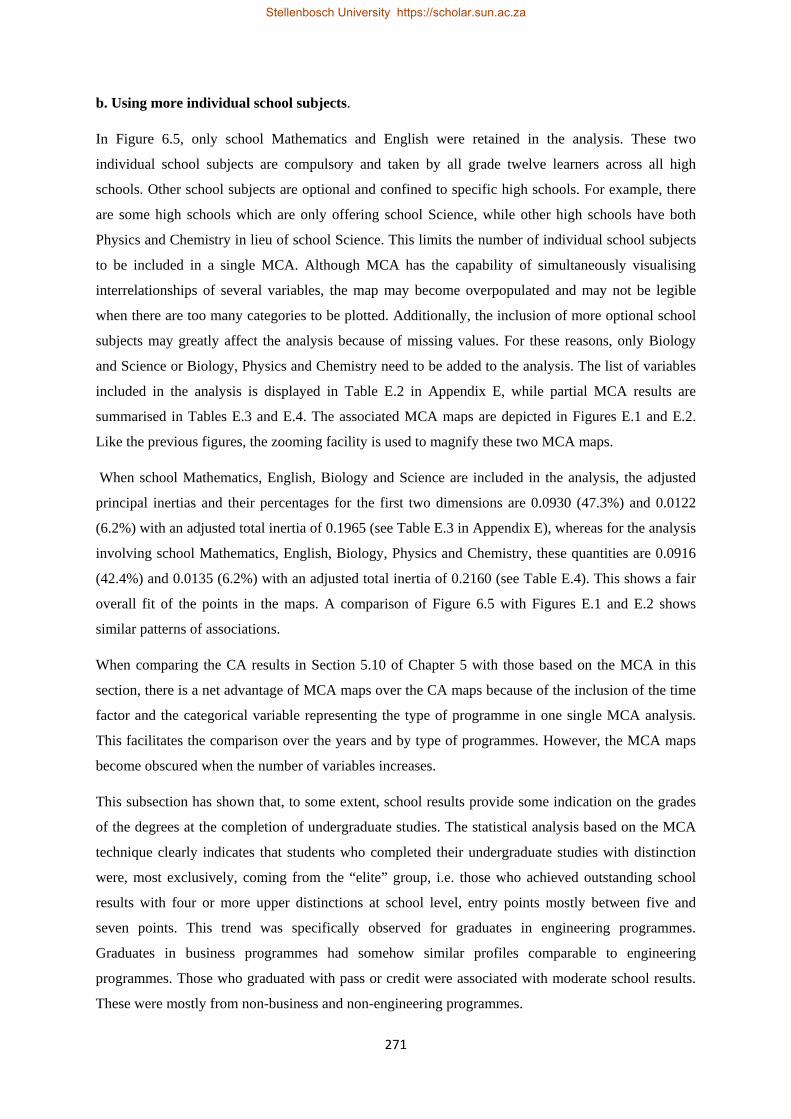
271
b. Using more individual school subjects.
In Figure 6.5, only school Mathematics and English were retained in the analysis. These two
individual school subjects are compulsory and taken by all grade twelve learners across all high
schools. Other school subjects are optional and confined to specific high schools. For example, there
are some high schools which are only offering school Science, while other high schools have both
Physics and Chemistry in lieu of school Science. This limits the number of individual school subjects
to be included in a single MCA. Although MCA has the capability of simultaneously visualising
interrelationships of several variables, the map may become overpopulated and may not be legible
when there are too many categories to be plotted. Additionally, the inclusion of more optional school
subjects may greatly affect the analysis because of missing values. For these reasons, only Biology
and Science or Biology, Physics and Chemistry need to be added to the analysis. The list of variables
included in the analysis is displayed in Table E.2 in Appendix E, while partial MCA results are
summarised in Tables E.3 and E.4. The associated MCA maps are depicted in Figures E.1 and E.2.
Like the previous figures, the zooming facility is used to magnify these two MCA maps.
When school Mathematics, English, Biology and Science are included in the analysis, the adjusted
principal inertias and their percentages for the first two dimensions are 0.0930 (47.3%) and 0.0122
(6.2%) with an adjusted total inertia of 0.1965 (see Table E.3 in Appendix E), whereas for the analysis
involving school Mathematics, English, Biology, Physics and Chemistry, these quantities are 0.0916
(42.4%) and 0.0135 (6.2%) with an adjusted total inertia of 0.2160 (see Table E.4). This shows a fair
overall fit of the points in the maps. A comparison of Figure 6.5 with Figures E.1 and E.2 shows
similar patterns of associations.
When comparing the CA results in Section 5.10 of Chapter 5 with those based on the MCA in this
section, there is a net advantage of MCA maps over the CA maps because of the inclusion of the time
factor and the categorical variable representing the type of programme in one single MCA analysis.
This facilitates the comparison over the years and by type of programmes. However, the MCA maps
become obscured when the number of variables increases.
This subsection has shown that, to some extent, school results provide some indication on the grades
of the degrees at the completion of undergraduate studies. The statistical analysis based on the MCA
technique clearly indicates that students who completed their undergraduate studies with distinction
were, most exclusively, coming from the “elite” group, i.e. those who achieved outstanding school
results with four or more upper distinctions at school level, entry points mostly between five and
seven points. This trend was specifically observed for graduates in engineering programmes.
Graduates in business programmes had somehow similar profiles comparable to engineering
programmes. Those who graduated with pass or credit were associated with moderate school results.
These were mostly from non-business and non-engineering programmes.
Stellenbosch University https://scholar.sun.ac.za

272
It is important to note that students who graduated with distinction were just representing a very small
proportion of the “elite” group mentioned in the previous paragraph. The remaining students from this
group completed their undergraduate studies with a grade below distinction. This again shows that the
achievement of outstanding results at school level does not always correspond to higher academic
performance at the university level. Nevertheless, the findings in this section have at least indicated
that students with outstanding university achievements are to be found in the “elite” group, and those
with poor university results had moderate school results, indicating that, to some extent, the CBU
admission policies helped to bring the right school leavers into the university system. But some other
students were admitted in the university with inflated school results which were not matching with
their university performance.
6.3.7 MCA of university averages with school results variables.
In this subsection, the adjusted MCA technique is again performed on the graduate dataset in order to
simultaneously study interrelationships between university averages and school results variables for
the years which had actual marks (in %) available for university subjects only. Table 6.8 displays the
variables used in the analysis. The partial results for the adjusted MCA are reported in Table 6.9,
while the corresponding MCA maps are displayed in Figure 6.6.
Table 6.8: Variables and their categories for the analysis involving university averages and school
variables using the graduate dataset.
Variables Abbreviation Labels of categories
School Mathematics Ma Ma1, Ma2, Ma3, Ma4 and Ma5 or M1, M2, M3, M4 and M5
School English En En1, En2, En3, En4 and En5 or E1, E2, E3, E4 and E5
TPROG Tp Tp1, Tp2 and Tp3.
CYEAR Cy Cy1, Cy2, Cy3, Cy4 and Cy5 or y1 to y5
NDIS Nd Nd0, Nd1, Nd2, Nd3 and Nd4
EPOINT Ep Ep1, Ep2, Ep3 and Ep4
DEPOINT Dp Dp1, Dp2 and Dp3
UWAY1 U1 U11, U12, U13, U14, U15, U16 and U17
UWAY2 U2 U21, U22, U23, U24, U25, U26 and U27
UWAY3 U3 U31, U32, U33, U34, U35, U36 and U37
UWAY4 U4 U41, U42, U43, U44, U45, U46 and U47
UWA UW UW1, UW2, UW3, UW4, UW5, UW6 and UW7
Stellenbosch University https://scholar.sun.ac.za
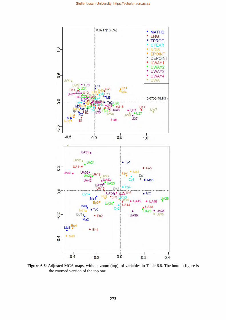
273
Figure 6.6: Adjusted MCA maps, without zoom (top), of variables in Table 6.8. The bottom figure is the zoomed version of the top one.
Stellenbosch University https://scholar.sun.ac.za

274
Table 6.9: Partial MCA results of the variables in Table 6.8.
Dim Principal inertia % inertia Cumulative %
1 0.0735 45.8 45.8
2 0.0217 13.5 59.3
3 0.0125 7.8 67.0
⁞ ⁞ ⁞ ⁞
23 0.0000 0.0 77.6
Total 0.1606
The MCA results in this table indicate that about 59.3% of the total adjusted inertia of 0.1606 is
explained by the first two dimensions, with 45.8% due to the first dimension alone.
A scrutiny of Figure 6.6 shows that the left-to-right direction is tantamount to low performance versus
high performance at both school and university levels, while the top-to-bottom direction is
differentiating categories with respect to the type of programme, entry points and the number of upper
distinctions at school level. At the higher performance side (i.e. top-right and bottom-right quadrants),
categories of university averages representing intervals of marks (in %) [66, 69), [69, 72), and [72,
100) are associated with highest achievement at school level (represented by categories Ep1, Nd4,
M4, E5, Nd3 and Ep2).
Additionally, Tp1 and Tp2, representing business and engineering related programmes, are also
located on this side. That is, engineering and also business students (especially those who completed
their undergraduate studies in 2012 and 2013) who achieved average scores of at least 66% in the first
year to the fourth year of study, and who had also an overall university average of the same
magnitude, exclusively attained higher performance at school level (i.e. three or more upper
distinctions at school level, entry points below the programmes’ cut-off points and between five and
seven points or between eight and nine points, and scores of at least 70% in individual school
subjects). On the left side, categories representing lower performance at university level (i.e. scores
below 66% in university averages) are associated with lower achievement at school level (i.e. entry
points of at least ten points, mostly equal or above the programmes’ cut-off points, scores below 70%
in individual school subjects, fewer upper distinctions at school level). This trend was mostly
observed for students in non-engineering and non-business related programmes (the Tp3 group) and
for those who completed their studies in the years 2009 and 2010.
The second principal axis differentiates students with entry points below the programmes’ cut-off
points from those with entry points equal or above the programmes’ cut-off points; and students with
Stellenbosch University https://scholar.sun.ac.za

275
entry points of nine points or below from those with entry points in excess of nine points. On this
dimension, there is no big difference between those who got three upper distinctions at school level
(denoted by Nd3) and those with four or more distinctions (denoted by Nd4), but big differences are
observed between categories Nd3 and Nd4 and the rest of other categories of variable NDIS.
6.3.8 MCA of university variables UWA and DECLA with school results variables.
In Subsection 6.3.6, patterns of associations were investigated between variable DECLA and school
results variables. Grades were used to convert school results variables into categorical variables. In
this subsection, actual marks (in %), which were available for students who were in their first year of
study in the year 2009, are used to create categorical variables. Then simultaneous interrelationships
of DECLA and UWA, representing both overall university performance measures, with school results
variables are examined.
Most of the variables in Table 6.8 are included in the analysis, except the variables CYEAR and
UWAY1 to UWAY4. The Variable G12AVE, representing the overall school performance, is also
added to the analysis. Table 6.10 reports the partial results of the adjusted MCA, while the MCA
maps are displayed in Figure 6.7.
The adjusted principal inertias and the associated percentages for the first two dimensions are 0.1610
(59.6%) and 0.0312 (11.5%). Altogether, the first two dimensions account for about 71.1% of the
adjusted total inertia of 0.2704, indicating that the two-dimensional MCA solution provides a
satisfactory fit to the data. This implies that by representing the categories of the variables into a two-
dimensional display, the discrepancy between their exact (true) positions (in higher dimensional
space) and their approximations in a two-dimensional space is low (i.e. 100% − 71.1% = 29.1%).
Only 29.1% of the dispersion of the points in higher dimensions is sacrificed.
Table 6.10: Partial MCA results based on actual marks (%) of variables DECLA and UWA and
school results variables of the graduate dataset for graduate students who were in their
first year of study in 2009.
Dim Principal inertia % inertia Cumulative %
1 0.1610 59.6 59.6
2 0.0312 11.5 71.1
3 0.0082 3.0 74.1
⁞ ⁞ ⁞ ⁞
14 0.0000 0.0 80.6
Total 0.2704
Stellenbosch University https://scholar.sun.ac.za

276
Figure 6.7: Adjusted MCA maps, without zoom (top), of university variables DECLA and UWA and school results variables of the graduate dataset with categorical variables created using actual marks (in %). The bottom figure is the zoomed version of the top one.
Stellenbosch University https://scholar.sun.ac.za
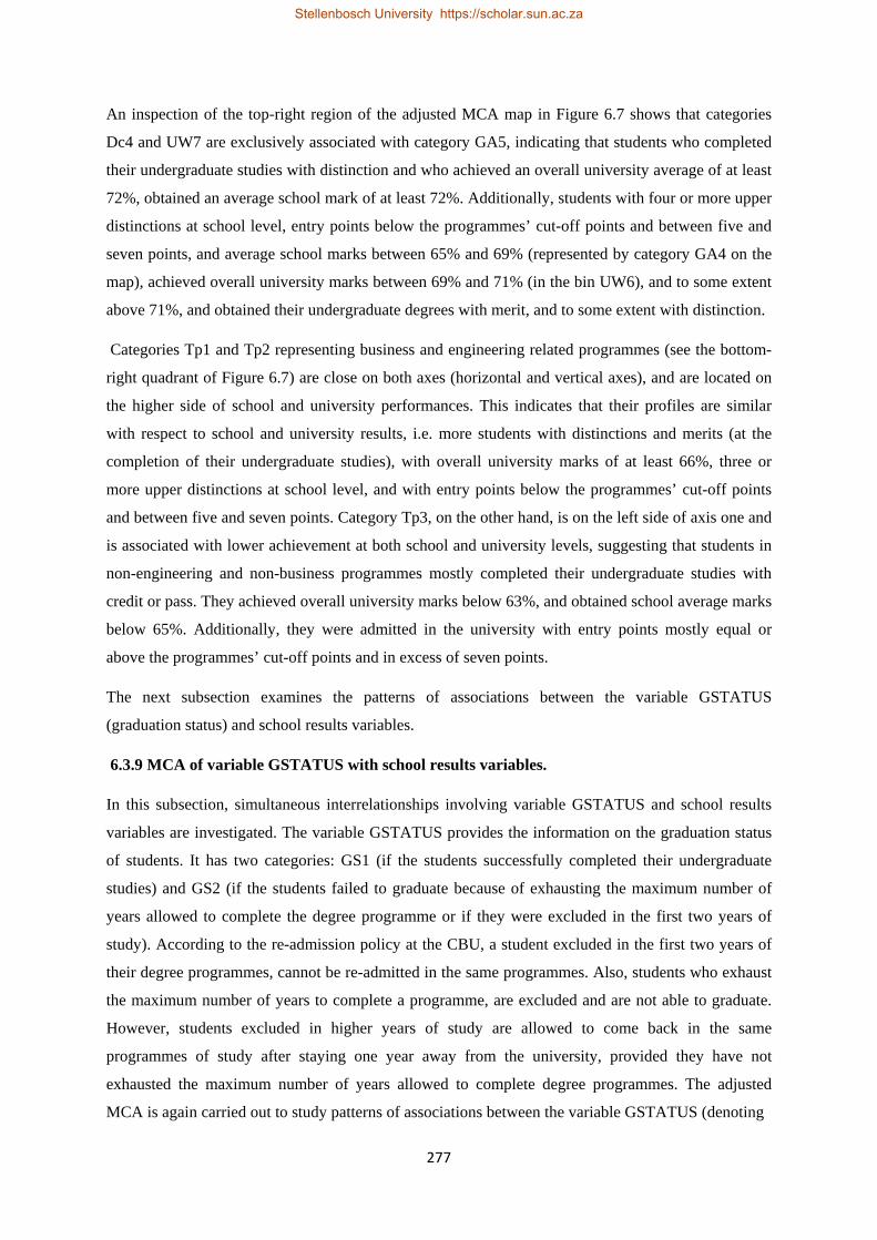
277
An inspection of the top-right region of the adjusted MCA map in Figure 6.7 shows that categories
Dc4 and UW7 are exclusively associated with category GA5, indicating that students who completed
their undergraduate studies with distinction and who achieved an overall university average of at least
72%, obtained an average school mark of at least 72%. Additionally, students with four or more upper
distinctions at school level, entry points below the programmes’ cut-off points and between five and
seven points, and average school marks between 65% and 69% (represented by category GA4 on the
map), achieved overall university marks between 69% and 71% (in the bin UW6), and to some extent
above 71%, and obtained their undergraduate degrees with merit, and to some extent with distinction.
Categories Tp1 and Tp2 representing business and engineering related programmes (see the bottom-
right quadrant of Figure 6.7) are close on both axes (horizontal and vertical axes), and are located on
the higher side of school and university performances. This indicates that their profiles are similar
with respect to school and university results, i.e. more students with distinctions and merits (at the
completion of their undergraduate studies), with overall university marks of at least 66%, three or
more upper distinctions at school level, and with entry points below the programmes’ cut-off points
and between five and seven points. Category Tp3, on the other hand, is on the left side of axis one and
is associated with lower achievement at both school and university levels, suggesting that students in
non-engineering and non-business programmes mostly completed their undergraduate studies with
credit or pass. They achieved overall university marks below 63%, and obtained school average marks
below 65%. Additionally, they were admitted in the university with entry points mostly equal or
above the programmes’ cut-off points and in excess of seven points.
The next subsection examines the patterns of associations between the variable GSTATUS
(graduation status) and school results variables.
6.3.9 MCA of variable GSTATUS with school results variables.
In this subsection, simultaneous interrelationships involving variable GSTATUS and school results
variables are investigated. The variable GSTATUS provides the information on the graduation status
of students. It has two categories: GS1 (if the students successfully completed their undergraduate
studies) and GS2 (if the students failed to graduate because of exhausting the maximum number of
years allowed to complete the degree programme or if they were excluded in the first two years of
study). According to the re-admission policy at the CBU, a student excluded in the first two years of
their degree programmes, cannot be re-admitted in the same programmes. Also, students who exhaust
the maximum number of years to complete a programme, are excluded and are not able to graduate.
However, students excluded in higher years of study are allowed to come back in the same
programmes of study after staying one year away from the university, provided they have not
exhausted the maximum number of years allowed to complete degree programmes. The adjusted
MCA is again carried out to study patterns of associations between the variable GSTATUS (denoting
Stellenbosch University https://scholar.sun.ac.za

278
Figure 6.8: Adjusted MCA maps, without zoom (top), of variable GSTATUS (graduation status) and school results variables of the graduate dataset. The bottom figure is the zoomed version of the top one.
Stellenbosch University https://scholar.sun.ac.za
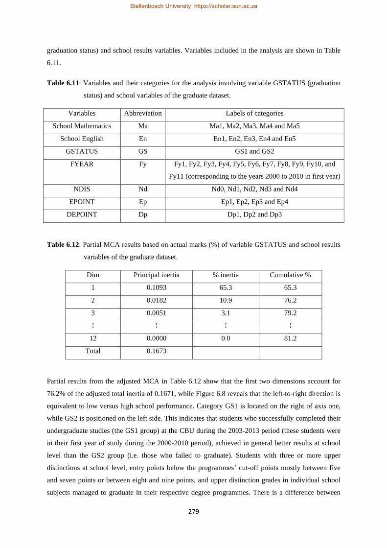
279
graduation status) and school results variables. Variables included in the analysis are shown in Table
6.11.
Table 6.11: Variables and their categories for the analysis involving variable GSTATUS (graduation
status) and school variables of the graduate dataset.
Variables Abbreviation Labels of categories
School Mathematics Ma Ma1, Ma2, Ma3, Ma4 and Ma5
School English En En1, En2, En3, En4 and En5
GSTATUS GS GS1 and GS2
FYEAR Fy Fy1, Fy2, Fy3, Fy4, Fy5, Fy6, Fy7, Fy8, Fy9, Fy10, and
Fy11 (corresponding to the years 2000 to 2010 in first year)
NDIS Nd Nd0, Nd1, Nd2, Nd3 and Nd4
EPOINT Ep Ep1, Ep2, Ep3 and Ep4
DEPOINT Dp Dp1, Dp2 and Dp3
Table 6.12: Partial MCA results based on actual marks (%) of variable GSTATUS and school results
variables of the graduate dataset.
Dim Principal inertia % inertia Cumulative %
1 0.1093 65.3 65.3
2 0.0182 10.9 76.2
3 0.0051 3.1 79.2
⁞ ⁞ ⁞ ⁞
12 0.0000 0.0 81.2
Total 0.1673
Partial results from the adjusted MCA in Table 6.12 show that the first two dimensions account for
76.2% of the adjusted total inertia of 0.1671, while Figure 6.8 reveals that the left-to-right direction is
equivalent to low versus high school performance. Category GS1 is located on the right of axis one,
while GS2 is positioned on the left side. This indicates that students who successfully completed their
undergraduate studies (the GS1 group) at the CBU during the 2003-2013 period (these students were
in their first year of study during the 2000-2010 period), achieved in general better results at school
level than the GS2 group (i.e. those who failed to graduate). Students with three or more upper
distinctions at school level, entry points below the programmes’ cut-off points mostly between five
and seven points or between eight and nine points, and upper distinction grades in individual school
subjects managed to graduate in their respective degree programmes. There is a difference between
Stellenbosch University https://scholar.sun.ac.za

280
the two categories of variable GSTATUS on the horizontal axis, but on the vertical axis, they are
close. Categories Dp1, Dp2 and Dp3 are also distant apart on the first principal axis, but close to each
other on the vertical axis.
The years 2000, 2001, 2002, 2009 and 2010 represented on the map by categories Fy1, Fy2, Fy3,
Fy10 and Fy11 (on the right of the horizontal axis with category GS1) had more students who
graduated than in other years.
6.3.10 MCA based on the extended matching coefficient (EMC).
In Chapter 5, the chi-squared distance was used as a measure of distance between any two rows or any
two columns of a two-way contingency table when performing CA on the data. More specifically, if
𝐗𝐗 ≡ �𝑥𝑥𝑖𝑖𝑗𝑗� ∶ 𝑝𝑝 × 𝑞𝑞 is a two-way contingency table with row totals and column totals given by ri (i = 1,
2, …, p) and cj (j = 1, 2, …, q), respectively, then the (squared) chi-squared distances between rows i
and i’, and between columns j and j’ are given, respectively by (Gower & Hand, 1996; Everitt, 2007;
Greenacre, 2007) :
𝑑𝑑𝑖𝑖𝑖𝑖′2 = �
1𝑐𝑐𝑗𝑗
𝑞𝑞
𝑗𝑗=1
�𝑥𝑥𝑖𝑖𝑗𝑗𝑟𝑟𝑖𝑖−𝑥𝑥𝑖𝑖′𝑗𝑗𝑟𝑟𝑖𝑖′
�2
(6.4)
and
𝑑𝑑𝑗𝑗𝑗𝑗′2 = �
1𝑟𝑟𝑖𝑖
𝑝𝑝
𝑖𝑖=1
�𝑥𝑥𝑖𝑖𝑗𝑗𝑐𝑐𝑗𝑗−𝑥𝑥𝑖𝑖𝑗𝑗′𝑐𝑐𝑗𝑗′
�2
(6.5)
Equations (6.4) and (6.5) are viewed as weighted Euclidean (or Pythagorean) distances with weights
1/𝑐𝑐𝑗𝑗 and 1/𝑟𝑟𝑖𝑖 which make rare categories of row variables or column variables have a greater influence
on the distance than others.
The MCA variants based on the indicator and the Burt matrices, and the adjusted MCA in Greenacre
(2007) are based on chi-squared distance. The same applies to the MCA biplots based on the indicator
and the Burt matrices in Gower et al. (2011). The indicator version of the MCA biplot is based on the
standardised two-way contingency table 𝐃𝐃r−1 2⁄ 𝐗𝐗𝐃𝐃c
−1 2⁄ for CA (where X is the two-way contingency
table, 𝐃𝐃r−1 2⁄ is the diagonal matrix of the row sums and 𝐃𝐃c
−1 2⁄ is the diagonal matrix of the column
sums of X) (see Chapter 5), with X, 𝐃𝐃r−1 2⁄ and 𝐃𝐃c
−1 2⁄ replaced by G, pI and L, respectively (Gower
et al., 2011). This gives 𝑝𝑝−1/2𝐆𝐆𝐋𝐋−𝟏𝟏/𝟐𝟐, whose singular value decomposition is given by (Gower et al.,
2011):
𝑝𝑝−1/2𝐆𝐆𝐋𝐋−𝟏𝟏/𝟐𝟐 = 𝐔𝐔𝐔𝐔𝐕𝐕T (6.6)
Stellenbosch University https://scholar.sun.ac.za

281
Figure 6.9: Biplots with the plotting of the samples suppressed, without zoom (top), based on the EMC of university variables DECLA and UWA and school results variables of the graduate dataset with categorical variables created using actual marks (in %). The quality of the two-dimensional display is 25.1%. The bottom figure is the zoomed version of the top one.
Stellenbosch University https://scholar.sun.ac.za

282
Figure 6.10: Biplots with the samples plotted, without zoom (top), based on the EMC of university
variables DECLA and UWA and school results variables of the graduate dataset with categorical variables created using actual marks (in %). The quality of the two-dimensional display is 25.1%. The bottom figure is the zoomed version of the top one.
Stellenbosch University https://scholar.sun.ac.za

283
After discarding the singular value of unity and the associated first singular vectors, the row chi-
squared MCA biplot (other MCA biplots can also be constructed by considering the different CA
variants in Table 5.1) based on G is constructed by plotting the row points using the first two columns
of 𝐙𝐙0 = 𝐔𝐔𝐔𝐔 and plotting the column points as projected category-level points (CLPs) using the first
two columns of 𝑝𝑝−1/2𝐋𝐋−𝟏𝟏/𝟐𝟐𝐕𝐕. For the Burt version, the normalised Burt matrix is used. It is found by
pre-multiplying the expression on the left side of (6.6) by its transpose to get:
(𝑝𝑝−1/2𝐆𝐆𝐋𝐋−𝟏𝟏/𝟐𝟐)T(𝑝𝑝−1/2𝐆𝐆𝐋𝐋−𝟏𝟏/𝟐𝟐) = 𝑝𝑝−1𝐋𝐋−𝟏𝟏/𝟐𝟐𝐆𝐆T𝐆𝐆𝐋𝐋−𝟏𝟏/𝟐𝟐 (6.7)
The spectral decomposition of (6.7) is given by:
𝑝𝑝−1𝐋𝐋−𝟏𝟏/𝟐𝟐𝐆𝐆T𝐆𝐆𝐋𝐋−𝟏𝟏/𝟐𝟐 = 𝐕𝐕𝐔𝐔𝟐𝟐𝐕𝐕T (6.8)
or
𝐋𝐋−𝟏𝟏/𝟐𝟐𝐆𝐆T𝐆𝐆𝐋𝐋−𝟏𝟏/𝟐𝟐 = 𝑝𝑝𝐕𝐕𝐔𝐔𝟐𝟐𝐕𝐕T (6.9)
The left side of equation (6.9) gives the normalised Burt matrix. The MCA biplot based on this
normalised Burt matrix is thus constructed by plotting the CLPs using the first two columns of
𝐋𝐋−𝟏𝟏/𝟐𝟐𝐕𝐕𝐔𝐔𝟐𝟐 and the observations at the centroids of their category points using the first two columns of
𝐙𝐙0 = 𝐆𝐆𝐙𝐙/𝑝𝑝 (Gower et al., 2011).
The justification of using the chi-squared distance in MCA is based on treating this technique as a CA
of the indicator matrix G (or the Burt matrix B). By doing so, G is treated as a two-way contingency
table. Taking into account that G is a binary matrix with its underlying p-variate structure, Gower &
Hand (1996) proposed another distance measure known as the extended matching coefficient (EMC).
This coefficient counts the proportion of matches among the p variables for any pair of observations.
The extended matching coefficients of all pairs of observations of G are summarised in the EMC
matrix (Gower & Hand, 1996; Gower et al., 2011):
𝐆𝐆𝐆𝐆T/𝑝𝑝 (6.10)
with associated dissimilarity matrix given by:
𝟏𝟏𝟏𝟏𝑇𝑇 − 𝐆𝐆𝐆𝐆T/𝑝𝑝 (6.11)
Expression (6.11) is treated as the (EMC) matrix of squared distances. The biplot based on the EMC
matrix can be constructed by applying the principal coordinate analysis (PCO) of G for the
observations and the unit matrix IL for the CLPs. If UΣVT is the SVD (singular value decomposition)
of (I − 11T/n )G = G −11TL/n , then the coordinates of the n observations and the L CLPs in r
Stellenbosch University https://scholar.sun.ac.za

284
dimensions are given by UΣr = (G −11TL/n )Vr and (I − 11TL/n )Vr, respectively, where Σr and Vr
are formed by the first r columns of Σ and V, respectively (Gower & Hand, 1996; Gower et al., 2011).
Table 6.13: Partial MCA results for EMC, the indicator and the Burt versions of MCA, and the
adjusted MCA based on actual marks (%) of DECLA and UWA with school results
variables of the graduate dataset for students who were in their first year of study in 2009.
An illustration of the biplots based on the EMC (with its zoomed version and with the plotting of
samples suppressed) of the variables UWA and DECLA with school results variables is shown in
Figure 6.9 (see Figure 6.7 in Section 6.35 for the adjusted MCA plot of the same variables).
MCA variant Dim Principal inertia % inertia Cumulative %
Indication matrix 1 0.4678 12.9 12.9
2 0.2680 7.4 20.4
3 0.1915 5.3 25.7
⁞ ⁞ ⁞ ⁞
32 0.0125 0.3 100.0
Total 3.6125 100.0
Burt matrix 1 0.2188 34.4 34.4
2 0.0718 11.3 45.7
3 0.0367 5.8 51.5
⁞ ⁞ ⁞ ⁞
41 0.0002 0.0 100.0
Total 0.6354 100.0
Adjusted MCA 1 0.1610 59.6 59.6
2 0.032 11.5 71.1
3 0.0082 3.0 74.1
⁞ ⁞ ⁞ ⁞
14 0.0000 0.0 80.6
Total 0.2704
EMC 1 284.2427 16.0 16.0
2 162.8642 9.1 25.10
3 135.9679 7.6 32.7
⁞ ⁞ ⁞ ⁞
41 0.0000 0.0 100
Total 1780.766 100.0
Stellenbosch University https://scholar.sun.ac.za

285
Figure 6.11: MCA biplots, without zoom (top), based on the indicator matrix using university
variables DECLA and UWA and school results variables of the graduate dataset with categorical variables created using actual marks (%). The bottom figure is the zoomed version of the top one.
Stellenbosch University https://scholar.sun.ac.za

286
Figure 6.12: MCA biplots, without zoom (top), based on the Burt matrix using university variables DECLA and UWA and school results variables of the graduate dataset with categorical variables created using actual marks (%). The bottom figure is the zoomed version of the top one.
Stellenbosch University https://scholar.sun.ac.za

287
Figure 6.10 reproduces the biplots in Figure 6.9 with the samples plotted. The plotting of the samples
on the biplot has the effect on the CLPs. i.e. the CLPs are bunched up in the middle of the biplots,
while the points representing the samples are spread out (see Figure 6.10). Even after zooming out the
biplot (in the top panel of Figure 6.10), the zoomed version is still not legible (see the bottom panel of
Figure 6.10).
For comparison purpose, MCA biplots of the unadjusted MCA, i.e. based on the indicator and the
Burt matrices were constructed and are displayed in Figures 6.11 and 6.12. The MCA maps based on
the indicator and the Burt matrices were also constructed, but are not shown. The MCA biplots (in
Figures 6.11 and 6.12) and the EMC based biplots (in Figures 6.9 and 6.10) were generated using the
function MCAbipl ( ) in the UBbipl package (Le Roux & Lubbe, 2010), while the MCA maps (not
shown) based on the indicator and the Burt matrices were constructed using the function mjca ( ) in
the ca R-package (Nenadic & Greenacre, 2007).
A comparison of the MCA biplotsca (in Figures 6.11 and 6.12) with the MCA maps (for the adjusted
MCA in Figure 6.7, and for the indicator and the Burt matrices not shown) shows identical patterns of
associations between school and university results variables for all these plots. Additionally, for all
these plots, the configuration of the category level points for most variables involved in the analysis
are plotted in their inherent order with lower categories on the left and higher categories on the right
side and are forming parabolic curves. This particular pattern of the configuration of points is known
as the Guttman effect or the horseshoe effect (Greenacre & Blasius, 2006; Greenacre, 2007; Husson et
al., 2011). For example, the categories of G12AVE representing school average marks are shaped like
a parabola from the lowest category level GA1 on the top left, via the category level GA3 on the
bottom middle to the category level GA5 on the top right. Categories for other variables have similar
trends.
Table 6.13 shows the partial MCA results based on the indicator and the Burt matrices, the adjusted
MCA and the EMC distance. From this table, it is clear that the MCA based on the indicator matrix
has the lowest quality of 20.4% for the two-dimensional display. For the EMC based biplot, the MCA
based on the Burt matrix and the adjusted MCA, the qualities are 25.7%, 45.7% and 71.1%,
respectively. Lower percentages produced by the indicator and the Burt versions of MCA are
artificially low due to the coding scheme used to come up with G (Greenacre, 2007). The percentages
of inertia of the EMC are also low because the computations are based on the indicator matrix
(expressed in deviations from the column means). These results justify the use of the adjusted MCA in
this chapter as the best approach for the CBU data.
Stellenbosch University https://scholar.sun.ac.za

288
6.3.11 Summary and concluding remarks on the MCA technique.
In this chapter, MCA has been successfully applied to the CBU data in order to simultaneously
examine the interrelationships between university and school results variables. This was done by
basically using the adjusted MCA, which gives an improved measure of fit as compared to the
solution based on the Burt matrix or the indicator matrix. The adjusted MCA solution produces the
same standard coordinates as the one based on the Burt matrix, but the principal coordinates are
computed by using the adjusted principal inertias (see Greenacre & Blasius, 2006). This results in an
improved quality of the display. But this solution is not optimal. It is the JCA technique which yields
an optimal solution. The intermediate procedure based on regression analysis also gives a solution
which is close to the JCA solution. Since both the JCA and the intermediate procedure produce
optimal solutions which are not nested, the adjusted MCA was adopted in this chapter as it yields and
keeps the properties of optimality of scale values (Greenacre & Blasius, 2006).
The findings based on the MCA technique have an added advantage over pairwise analyses using the
CA technique since interrelationships of more than two variables have been simultaneously visualised
and examined. This has permitted an easy interpretation and comparison over time, and between
different types of programmes. However, the MCA technique has its limitations. First, it produces
“overpopulated” maps, when the number of categories to be plotted increases. This problem can be
circumvented by using subset MCA, the zooming process and by interactively turning on/off some
selected points. The other issue concerns the number of school results variables to be included in a
single analysis. There is a limitation on the number of individual school results variables to be
included in the analysis because of missing values associated with elective school subjects not
selected by grade twelve learners. In fact, apart from school Mathematics and English which are taken
by all grade twelve learners, the remaining school subjects are not all offered in high schools. For
example, those opting for school Science do not take school Physics and Chemistry. There are also
very few grade twelve learners who select Additional Mathematics or English Literature. The same
applies to other optional school subjects.
It is also important to note that, besides treating MCA as the CA of the indicator matrix or the Burt
matrix, MCA may also be considered as an optimal scores method. In this context, it can be viewed as
a generalisation of the optimal scaling procedure based on the CA technique and is also known as a
homogeneity analysis. Under this approach, the data matrix (indicator matrix) G : n × L is converted
into a numerical matrix, where the nominal category levels are replaced by numerical optimal scores.
That is, if the scores are summarised into an L-vector 𝐳𝐳 = (𝐳𝐳1, 𝐳𝐳2,⋯ , 𝐳𝐳𝑝𝑝), with zj: Lj × 1 giving the
scores corresponding to the Lj category levels of the jth categorical variable, then the approach
consists of replacing G by its quantified version Gz (see Gower & Hand, 1996; Gower et al., 2011).
The vector of scores z is determined by maximising the ratio of the sum of squares between the row
Stellenbosch University https://scholar.sun.ac.za

289
totals Gz with the total sum of squares, i.e. zTGTGz/zTLz subject to zTLz = 1. This leads to the same
solution as the MCA based on the Burt matrix (Gower et al., 2011). These results imply that when all
p variables in the analysis are categorical variables, MCA (of the Burt matrix) can be viewed as a
simple homogeneity analysis.
The MCA technique does not take into account the ordering in the categorical variables. To
incorporate this information in the analysis, categorical principal component analysis (Categorical
PCA), to be presented in the next chapter, will be performed on the data. Like MCA, Categorical PCA
belongs to statistical techniques known as quantification methods or optimal scaling methods which
consist of transforming the data matrix of categorical variables into a quantitative matrix which may
be analysed with statistical techniques meant for quantitative variables. For the years which had actual
marks (in %) available for both school and university results, PCA will be also performed on the data.
In the CBU data, there are group structures which are present. Either MCA or Categorical PCA do not
take into account these group structures. In order to consider the group structures in the data,
categorical canonical variate analysis (CatCVA) (for years which did not have actual marks (in %) for
school and university results available), canonical variate analysis (CVA) and canonical analysis of
distance (CAoD) (for the years which had actual marks available for school and university results)
will be performed on the data in the next chapter.
Stellenbosch University https://scholar.sun.ac.za

290
CHAPTER 7
SEPARATING GROUPS IN THE CBU DATA
7.1 Introduction.
The previous chapter gives a geometric perspective on the CBU data using MCA. Although this
technique incorporated several variables in the analysis and simultaneously studied the
interrelationships between school and university results variables, it treated all categorical variables as
nominal. However, both datasets of the CBU data include several ordinal categorical variables. In order
to take the ordering into account, categorical principal component analysis (categorical PCA) is applied
in this chapter to the CBU data. Principal component analysis (PCA) is also performed on the data for
those years which had actual marks (in %) available for both school and university results variables.
Furthermore, the CBU data consist of samples coming from predefined groups. Information of
externally defined group structure is not taken into account by both MCA and categorical PCA. To
analyse the CBU data as grouped data, statistical methods specifically designed to deal with such data
need to be considered. Specifically, the aim will be to optimally separate the externally defined groups
in the CBU data. Thus, categorical canonical variate analysis (CatCVA), canonical variate analysis
(CVA) and canonical analysis of distance (CAoD) will be performed on the CBU data. In order to allow
for visualisations of these methods, biplot methodology is used.
In Section 7.2, a brief overview of the biplot methodology associated with the multivariate statistical
techniques to be applied to the CBU data in this chapter is provided. This is followed by a detailed
discussion of their applications to the CBU data.
7.2 Brief overview of the multivariate statistical techniques used in this chapter.
7.2.1 The biplot methodology.
In Chapter 4, notched boxplots and KDEs graphically depicted single variables, while the CA maps and
CA biplots in Chapter 5 provided for visualisations of two-way contingency tables. This was followed
in Chapter 6 by MCA that allowed a geometric approach which takes into account the multivariate
nature of the CBU data by visual displays involving more than two categorical variables simultaneously.
What has not yet been addressed, are the ordinal nature of several of the categorical variables, the
presence of continuous variables in some of the datasets and recognising the presence of externally
defined groups in the data. The techniques introduced in this chapter aim to address these issues. In
agreement with the geometric approach followed thus far, biplot-based visualisations will be
extensively used in this chapter. Therefore, a brief introduction to the necessary biplot-based
visualisations will first be given.
Stellenbosch University https://scholar.sun.ac.za

291
The classical biplot was introduced by Gabriel (1971) to represent a data matrix by two sets of vectors,
one set for the rows (the samples or observations) and the other set for the columns (the variables). In a
biplot, all the elements of the matrix are represented by the inner products of the vectors associated with
their rows and columns (Aldrich, Gardner & Le Roux, 2004). The prefix ‘bi’ indicates that both
observations (samples) and measured variables are simultaneously represented. This can be done in any
dimension but it can be visualised only in one, two or three dimensions. This means that a biplot display
is usually an approximation of the full space in one, two or three dimensions.
The traditional biplot as introduced by Gabriel (1971) is interpreted by means of inner products which
are not always readily appreciated by the practitioner (Erasmus, Lambrechts, Gardner & Le Roux,
2001). To provide a graphical display which is readily interpretable, Gower & Hand (1996) proposed
an approach to biplot methodology by presenting it as a multivariate extension of an ordinary
scatterplot. Like scatterplots, biplots as viewed by Gower & Hand (1996) are useful for providing a
visual representation of the multidimensional data in fewer dimensions, usually two dimensions; for
detecting patterns which can lead to formal analyses; and for displaying results found by more formal
statistical methods of analysis.
If the data consisting of n observations and p variables are summarised in a data matrix X : n × p, the n
observations can be considered as points in a p-dimensional space. The n observations and p variables
can be simultaneously represented in the form of a one-, two- or three-dimensional biplot display.
Generally, this display will be an approximation of the full p-dimensional space. In this display, the
multidimensional observations are plotted as points, while continuous variables are represented as
biplot axes. In a scatterplot, the axes representing the two variables are perpendicular, but the biplot
axes associated with the p continuous variables are not perpendicular and are calibrated in convenient
units, e.g. the original scales of measurements (Walters & Le Roux, 2008). The biplot axes in this
chapter are called prediction axes and they are used for reading off values of variables and not for
placement of new samples into the biplot. The latter process is called ‘interpolation’ and will be
programmatically dealt with when needed (see Gower et al., 2011). In the case of categorical variables,
as was seen in Chapters 5 and 6, they are represented not by calibrated axes but by category level points
(Le Roux, Gardner-Lubbe & Gower, 2014; Gower, Le Roux & Gardner-Lubbe, 2016).
7.2.2 PCA and Categorical PCA.
a. Principal Component Analysis (PCA).
PCA is a dimension reduction statistical technique which is concerned with explaining the variance-
covariance structure of a dataset by forming a small number of uncorrelated linear combinations of the
original variables. These linear combinations are called principal components and account for as much
Stellenbosch University https://scholar.sun.ac.za

292
variations in the dataset as the original variables, whereas their values are known as principal component
scores (Sharma, 1996; Johnson & Wichern, 2007).
The magnitudes of the coefficients of the original variables in a given principal component measure the
contributions of these variables to that principal component, while the loadings (simple correlations
between the original variables and the principal components) provide the information of the degree of
influence of the original variables in forming the principal components (Sharma, 1996).
b. PCA biplot.
PCA can be extended with the biplot methodology to provide the PCA biplot (Aldrich et al., 2004; Le
Roux & Gardner, 2005; Gower et al., 2011). To construct this biplot, the data matrix X : n × p with
n ≥ p (X is assumed to be column-centred and if the variables use different measurement units, then
they must be standardised to unit variance or some other preferred standardisation like unit range or
unit sum of squares) is first approximated in r dimensions by minimising �𝐗𝐗 − 𝐗𝐗��2, where 𝐗𝐗� is the
approximation of X in r dimensions (Gower et al., 2011). This is achieved by the singular value
decomposition:
𝐗𝐗 = 𝐔𝐔𝐔𝐔𝐕𝐕T , (7.1)
where U is an n × p orthonormal matrix, 𝐕𝐕 = [𝐯𝐯1, 𝐯𝐯2,⋯ , 𝐯𝐯𝒑𝒑] is a p × p orthogonal matrix, and 𝐔𝐔 is a
p × p diagonal matrix of singular values σ1,σ2,⋯ ,σ𝑝𝑝 (σ1 ≥ σ2 ≥ ⋯ ≥ σ𝑝𝑝 ≥ 0) associated with the
matrix of right singular vectors V.
The columns 𝐯𝐯1, 𝐯𝐯2,⋯ , 𝐯𝐯𝒑𝒑 R of matrix V give the coefficients that are used to form the p principal
components of X, while XV = 𝐔𝐔𝐔𝐔 provides the principal component scores. The approximation of X in
the r-dimensional space is
𝐗𝐗� = 𝐔𝐔𝑟𝑟𝐔𝐔𝑟𝑟𝐕𝐕𝑟𝑟T (7.2)
In equation (7.2), Ur : n × r and Vr : p × r are formed by the first r columns of U and V, respectively,
while 𝐔𝐔𝒓𝒓 : r × r contains the first r largest singular values of 𝐔𝐔. The choice of r = 1, 2 or 3 corresponds
to the dimension of the space in which the PCA biplot is constructed. Mostly, the preferred dimension
of the approximation space is r = 2. In this case, the coordinates of the n observations are given by
XV2 = 𝐔𝐔2𝐔𝐔2 = X[v1, v2], while the p rows of V2 give the directions of the biplot axes which can be
calibrated in terms of any preferred units like the original scales of measurements or standard scores.
The importance of the solution (7.2) is that according to the Eckart-Young theorem it gives the best
approximation by minimising the least squares criterion �𝑿𝑿 − 𝑿𝑿��2 where minimisation is over all
matrices of rank r (Eckart & Young, 1936). The first r = 1, 2 or 3 columns of Vr furnish the r principal
components which are used as scaffolding to plot the n observations in the biplot (Gower & Hand, 1996;
Stellenbosch University https://scholar.sun.ac.za

293
Gower et al., 2011, 2015). Using the first r columns as scaffolding provides the optimal biplot display
in r dimensions. However, any r columns can be used for a biplot display which is not necessarily
optimal but may provide useful information in any preferred dimension(s).
The overall quality of the biplot in r dimensions is given by (Gardner-Lubbe, Le Roux & Gower, 2008;
Gower et al., 2011):
∑ 𝜎𝜎𝑗𝑗2𝑟𝑟𝑗𝑗=1
∑ 𝜎𝜎𝑗𝑗2𝑝𝑝𝑗𝑗=1
(7.3)
Other measures of fit for PCA biplots are available and are found in Gower et al. (2011). These
measures include axis predictivities and sample predictivities for judging how well each of the original
variables and samples (observations) are respectively approximated in the biplot.
c. Categorical Principal Component Analysis (categorical PCA).
PCA assumes that all variables to be analysed are continuous and that the relationships between these
variables are linear. An alternative to PCA when the variables are nominal or ordinal is categorical
PCA. In categorical PCA, similar to MCA, each categorical variable has a total of 𝐿𝐿𝑗𝑗 ( 𝑗𝑗 = 1, 2,⋯ ,𝑝𝑝)
category levels, known as category level points (CLPs), so that for all p variables, there are
𝐿𝐿 = 𝐿𝐿1 + 𝐿𝐿2 + ⋯𝐿𝐿𝑝𝑝 CLPs. In contrast to MCA where the variables are directly analysed, in categorical
PCA, the categories of each variable are first replaced by a set of (continuous) optimal scores. More
specifically, categorical PCA aims at quantifying the data matrix X : n × p by finding numerical scale
values 𝐳𝐳1, 𝐳𝐳2,⋯ , 𝐳𝐳𝑝𝑝 for the category levels of the p categorical variables that yield a best PCA in the rth
specified dimension (Greenacre & Blasius, 2006).
Consider the quantified version of the original data matrix X with p categorical variables, having each
Lj category levels (j =1, 2, …, p), i.e. 𝐘𝐘 = �𝐆𝐆1𝐳𝐳1,𝐆𝐆2𝐳𝐳2,⋯ ,𝐆𝐆𝑝𝑝𝐳𝐳𝑝𝑝� ∶ 𝑛𝑛 × 𝑝𝑝35T, where 𝐆𝐆𝑗𝑗 is the n × Lj
indicator matrix for the jth variable, zj is the Lj-vector of category quantifications (score values) to be
determined to replace the Lj category levels of the jth variable. Then the estimation of category
quantifications and the approximation 𝐘𝐘� of the quantified version Y in r dimensions are accomplished
by a two-step procedure. First, for given quantifications 𝐳𝐳𝑇𝑇 = (𝐳𝐳1T, 𝐳𝐳2T, … , 𝐳𝐳𝑝𝑝T) satisfying the
identification constraints �𝐆𝐆𝒋𝒋𝐳𝐳𝒋𝒋�2 = 1 and 𝟏𝟏𝑛𝑛𝑇𝑇𝐆𝐆𝑗𝑗𝐳𝐳𝑗𝑗 = 0, the least squares criterion �𝐘𝐘 − 𝐘𝐘��2 is
minimised over Y as described for PCA in Section 7.2.2.b. The second step proceeds by using the
solution 𝐘𝐘� to update 𝐳𝐳𝑇𝑇 = (𝐳𝐳1T, 𝐳𝐳2T, … , 𝐳𝐳𝑝𝑝T) using a constraint regression approach. These two steps are
iterated until convergence. When the process converges, the PCA r-dimensional approximation of Y is
given by 𝐘𝐘�. The original data matrix X can then be replaced by its quantified version Y on which PCA
and its associated biplots can be applied (Gower et al., 2011).
Stellenbosch University https://scholar.sun.ac.za

294
In categorical PCA, calibrations are done only for the computed quantifications and are labelled by their
CLPs. Although categorical PCA also displays the simultaneous relationships between several
categorical variables and is an optimal scaling technique as MCA, the latter technique does not take
into account the ordered nature of the categorical variables, i.e. consider all variables at nominal level.
In categorical PCA however, a monotone regression step or splines function can be included to ensure
a required ordering of the optimal scores as prescribed by the original ordinality of a categorical
variable.
7.2.3 Canonical Variate Analysis (CVA).
PCA introduced in the previous section does not consider any possible external group structure in the
data. It is possible to interpolate properties of such groups into a PCA biplot after its construction, i.e.
interpolate group means into the biplot or by using different colours for samples belonging to different
groups. Information about the group structure in the data may also be suggested by enclosing the
samples of each group with an α-bag (which can be viewed as bivariate extensions of the univariate
boxplots) (Walters & Le Roux, 2008) on the PCA biplot. If a graphical display of the group structure
present in the data is specifically desired, canonical variate analysis can be utilised. CVA takes into
account the groupings present in the data and optimally separates the groups of observations (Alkan &
Atakan, 2011; Gower et al., 2015).
The data for a CVA are summarised into an n × p data matrix X consisting of measurements on p
continuous variables for n observations split into K groups of size 𝑛𝑛1,𝑛𝑛2,⋯ ,𝑛𝑛𝐾𝐾 with
𝑛𝑛 = 𝑛𝑛1 + 𝑛𝑛2 + ⋯+ 𝑛𝑛𝐾𝐾, while the group memberships of the observations are given by the 𝑛𝑛 × 𝐾𝐾
matrix 𝐆𝐆 = [𝐠𝐠1,𝐠𝐠2,⋯ , 𝐠𝐠𝐾𝐾], where g𝑖𝑖𝑖𝑖 = 1 (𝑖𝑖 = 1, 2,⋯ ,𝑛𝑛; 𝑘𝑘 = 1, 2,⋯ ,𝐾𝐾) when the ith observation
belongs to the kth group and zero, otherwise. The data matrix 𝐗𝐗 is centred such that 𝟏𝟏T𝐗𝐗 = 𝟎𝟎T.
CVA is closely related to MANOVA and shares with it the assumption of homogeneity of group
covariance matrices for all K groups. Additionally, if inference about the group mean vectors is desired,
then the normality assumption of the observations must also be made (Gower & Krzanowski, 1999).
Gower et al. (2011 & 2015) introduced CVA as a two-step procedure. That is, in Step 1 the data matrix
𝐗𝐗 is transformed into an 𝑛𝑛 × 𝑝𝑝 matrix of canonical variables 𝐘𝐘 = 𝐗𝐗𝐗𝐗. In the second step, a PCA is
carried out on the 𝐾𝐾 × 𝑝𝑝 matrix of the transformed means (i.e. matrix of canonical means) 𝐘𝐘� = 𝐗𝐗�𝐗𝐗 by
performing its SVD. The transformation matrix 𝐗𝐗 ∶ 𝑝𝑝 × 𝑝𝑝 is such that 𝐗𝐗𝐗𝐗𝐓𝐓 = 𝐖𝐖−1 and 𝐗𝐗T𝐗𝐗 = 𝚲𝚲−1,
where 𝚲𝚲 is the 𝑝𝑝 × 𝑝𝑝 diagonal matrix of eigenvalues satisfying the two-sided eigenvalue equation
𝐖𝐖𝐗𝐗 = 𝐗𝐗𝚲𝚲; 𝐖𝐖 = 𝐓𝐓 − 𝐁𝐁 is the 𝑝𝑝 × 𝑝𝑝 within-groups matrix, 𝐓𝐓 = 𝐗𝐗T𝐗𝐗 is the total sum-of-squares
matrix, 𝐁𝐁 = 𝐗𝐗�𝐓𝐓𝐍𝐍𝐗𝐗� is the between-groups matrix, and 𝐗𝐗� = 𝐍𝐍−1𝐆𝐆T𝐗𝐗 is the 𝐾𝐾 × 𝑝𝑝 grouped means matrix
with 𝐍𝐍 = diag (𝑛𝑛1,𝑛𝑛2,⋯ ,𝑛𝑛𝐾𝐾) ∶ 𝐾𝐾 × 𝐾𝐾 diagonal matrix with diagonal elements given by 𝑛𝑛1,𝑛𝑛2,⋯ ,𝑛𝑛𝐾𝐾.
Stellenbosch University https://scholar.sun.ac.za

295
The PCA of 𝐘𝐘� = 𝐗𝐗�𝐗𝐗 can be weighted by the group sizes or not. This will result in a weighted CVA or
an unweighted CVA. If 𝐗𝐗�𝐗𝐗 is written as 𝐂𝐂1 2⁄ 𝐗𝐗�𝐗𝐗, where 𝐂𝐂 is a 𝐾𝐾 × 𝐾𝐾 matrix. The choice of 𝐂𝐂 = 𝐈𝐈 or
𝐂𝐂 = 𝐈𝐈 − 𝐾𝐾−1𝟏𝟏𝟏𝟏T will yield the unweighted CVA, while the choice for C = N will produce the weighted
CVA (Gower et al., 2011). From the PCA of the canonical means (pre-multiplied by C1/2) 𝐂𝐂1 2⁄ 𝐗𝐗�𝐗𝐗, the
coordinates of the points representing the group means in the canonical space of dimension
min (p, K – 1) are determined. These group centroids may be approximated in an r-dimensional space
using as coordinates the rows of 𝐗𝐗�𝐗𝐗𝐕𝐕Rr, where Vr is a p × r matrix formed by the first r columns of V,
and V is the p × p orthogonal matrix of right singular vectors of matrix 𝐂𝐂1 2⁄ 𝐗𝐗�𝐗𝐗, with C defined as
above. All samples can be interpolated into the biplot using as coordinates the rows of XLVr.
As in PCA, the CVA biplot is constructed by adding calibrated biplot axes for representing the p
variables. It follows also that Mahalanobis distances (see Aldrich et al., 2004; Gower et al., 2011 &
2015) between the group means become ordinary Euclidean distances in the canonical space.
By its construction CVA biplots optimally separate group means. The interpolated samples provide a
visual appraisal of within groups variation. A measure of the overlap or separation among the groups
as well as the nature of such overlap or separation between groups is proposed by Gower et al. (2011)
in the form of α-bags for the respective means. Additionally, measures of fit for CVA biplots, similar
to those of the PCA biplots, are available (see Gower et al., 2011).
When inference about the group means vectors is needed, then this can be accomplished using
MANOVA because of its connection with CVA, provided the observations in the different groups are
normally distributed. Furthermore, since CVA uses Mahalanobis distance which assumes the
homogeneity of the within-group covariance matrices, then prior utilising CVA, this assumption must
be verified with the data at hand. The visualisations based on the α-bags or the visualisation of the
individual observations from the different groups can be used to assess if this assumption is violated
(Gower et al., 2015).
7.2.4 The Canonical Analysis of Distance.
The CVA procedure in the previous section requires the within-group covariance matrices for all K
groups satisfy the homogeneity assumption. An additional distributional assumption (i.e. the normality
assumption of the observations) is needed when inference about the group means is to be performed.
When these assumptions do not hold, an alternative technique known as Canonical Analysis of Distance
(CAoD) or just AoD, can be performed on the data (Gower, Le Roux & Gardner-Lubbe, 2014). In the
remaining part of this chapter, CAoD will be designated as AoD.
AoD makes no distributional assumption about the data and does not require the within-group
covariance matrices to be homogeneous. It is suitable even for small group sizes. It assumes only very
mild assumptions mainly that some distance measure be defined between pairs of samples. It is based
Stellenbosch University https://scholar.sun.ac.za

296
on its connection with the analysis of variance established by expressing the sample variance in terms
of pairwise squared distances of the observations (Gower & Krzanowski, 1999).
The procedure for constructing an AoD biplot as developed and discussed in Gower et al. (2014, 2015)
is summarised in the steps below.
Step 1:
Obtain the matrix 𝑫𝑫 ∶ 𝑛𝑛 × 𝑛𝑛 ≡ �− 12𝑑𝑑𝑖𝑖𝑖𝑖′2 � giving the ddistances defined by −1
2𝑑𝑑𝑖𝑖𝑖𝑖′2 for samples i and
i′ for every pair of samples, i.e. rows of the data matrix X : n × p. Let the indicator matrix defining the
groups be given by 𝑮𝑮 ∶ 𝑛𝑛 × 𝐾𝐾 = [𝐠𝐠1, 𝐠𝐠2, … , 𝐠𝐠𝐾𝐾] where 𝐠𝐠𝑖𝑖 denotes an n-vector of zeros except for a
one in position i if sample i belongs to group k. Let 𝐍𝐍 = 𝐆𝐆T𝐆𝐆 denote the diagonal matrix containing the
group sizes and define the K × K matrix 𝐃𝐃� ≡ {𝐷𝐷�𝑖𝑖𝑖𝑖′} = 𝐍𝐍− 1𝐆𝐆T𝐃𝐃𝐆𝐆𝐍𝐍− 1 with the (k, k′)th element
given by 𝐷𝐷�𝑖𝑖𝑖𝑖′ = 1𝑛𝑛𝑘𝑘𝑛𝑛𝑘𝑘′
𝐠𝐠𝑖𝑖𝑇𝑇𝐃𝐃𝐠𝐠𝒌𝒌′ representing the average ddistances between members of the kth
and k′th groups.
Next obtain 𝚫𝚫 ≡ {∆𝑖𝑖𝑖𝑖′} the K × K ddistance matrix with ∆𝑖𝑖𝑖𝑖′= 𝐷𝐷�𝑖𝑖𝑖𝑖 + 𝐷𝐷�𝑖𝑖′𝑖𝑖′ − 2𝐷𝐷�𝑖𝑖𝑖𝑖′ giving the
ddistance between the centroids of groups k and k′. The space of dimension m = K – 1 containing the
group centroids will be called the ∆-space. In order to obtain a biplot approximation in r dimensions, a
principal coordinate analysis (PCO) is performed. This necessitates the spectral decomposition of
matrix of the double-centred matrix Δ (Gower et al., 2014):
𝐘𝐘 �𝐘𝐘 �T = �𝐈𝐈𝑖𝑖 − 𝟏𝟏𝑖𝑖𝟏𝟏𝑖𝑖T/𝐾𝐾�∆�𝐈𝐈𝑖𝑖 − 𝟏𝟏𝑖𝑖𝟏𝟏𝑖𝑖T/𝐾𝐾� = 𝐕𝐕𝚲𝚲𝐕𝐕𝐓𝐓, (7.4)
where 𝐘𝐘� T𝐘𝐘� = 𝚲𝚲 : m × m, is a diagonal matrix of eigenvalues and 𝐘𝐘� = 𝐕𝐕𝚲𝚲1/2: K × m, with m = K – 1.
The coordinates of the group means, as represented by their centroids 𝐺𝐺1,𝐺𝐺2,⋯ ,𝐺𝐺𝐾𝐾 are given by the
respective rows of matrix 𝐘𝐘� = 𝐕𝐕𝚲𝚲1/2. In an r-dimensional display space, the first r columns of
𝐘𝐘� provide the coordinates for approximating the group means.
Step 2:
Interpolate the points representing the n individual observations into the configuration of the group
centroids found in Step 1. Using the results from Step 1, any individual observation, represented by a
point P can be added to the map of the group means by using the squared distances of P from the group
centroids 𝐺𝐺1,𝐺𝐺2,⋯ ,𝐺𝐺𝐾𝐾. That is, if the squared distances from P to the group means are given in a vector
𝛅𝛅 = −12
(𝛿𝛿12, 𝛿𝛿22, … , 𝛿𝛿𝐾𝐾2), with 𝛿𝛿𝑖𝑖2 = 𝐷𝐷�𝑖𝑖𝑖𝑖 −2𝑛𝑛𝑘𝑘𝟏𝟏T𝐝𝐝𝑖𝑖 and d being a vector of size nk giving the squared
distances from P to the observations in the kth group, then point P has coordinates (Gower et al., 2014):
Stellenbosch University https://scholar.sun.ac.za

297
𝐲𝐲𝑃𝑃 = 𝚲𝚲−1𝐘𝐘�T(𝛅𝛅 − 𝚫𝚫𝟏𝟏/𝐾𝐾) (7.5)
Equation (7.5) can be used to interpolate the n observations in the configuration of the group means.
The coordinates of the group centroids and the n observations are given in m = K – 1 dimensions. The
approximation in r dimensions (r ≤ m = K – 1) is achieved by using only the r largest eigenvalues of 𝚲𝚲
and their associated eigenvectors of 𝐕𝐕 in equation (7.4).
Step 3:
In order to obtain a biplot, calibrated prediction axes representing the variables must be added to the
map of group means. This can be done by letting the vector d in Step 2 be chosen for a pseudo sample
for the jth variable to have value μe j and then trace out a nonlinear trajectory for the jth variable by
varying μ. The trajectory may be calibrated for suitably chosen values of μ. When Euclidean distances
are used, this nonlinear trajectory becomes a linear biplot axis (see Gower et al., 2011 & 2014). These
authors show that the co-ordinates for tracing a prediction biplot axis is based on a series of lines with
equation
�𝑑𝑑𝛅𝛅𝑑𝑑𝑑𝑑�
T
⎣⎢⎢⎢⎡
1𝜆𝜆1𝑦𝑦�11
1𝜆𝜆2𝑦𝑦�12
⋮ ⋮1𝜆𝜆1𝑦𝑦�𝐾𝐾1
1𝜆𝜆2𝑦𝑦�𝐾𝐾1⎦
⎥⎥⎥⎤
𝐳𝐳 = −1𝐾𝐾𝟏𝟏T �
𝑑𝑑𝛅𝛅𝑑𝑑𝑑𝑑�
(7.6)
where z denotes the two-dimensional coordinates in a two-dimensional biplot space and ijy is the ijth
element of 𝐘𝐘� ∶ 𝐾𝐾 × 𝑚𝑚 . The ddistances between pseudo sample τ(µ) and the nk samples in the kth
group are given by
𝐝𝐝(𝜏𝜏)𝑖𝑖(𝑑𝑑) =
⎣⎢⎢⎢⎢⎢⎡ −
12�𝑓𝑓𝑗𝑗�𝑥𝑥1𝑗𝑗 , 0� +
12𝑓𝑓𝑡𝑡(𝑥𝑥1𝑡𝑡 , 0) −
12𝑓𝑓𝑡𝑡(𝑥𝑥1𝑡𝑡 , 𝑑𝑑)
𝑝𝑝
𝑗𝑗=1⋮
−12�𝑓𝑓𝑗𝑗�𝑥𝑥𝑛𝑛𝑘𝑘𝑗𝑗 , 0� +
12𝑓𝑓𝑡𝑡�𝑥𝑥𝑛𝑛𝑘𝑘𝑡𝑡, 0� −
12𝑓𝑓𝑡𝑡(𝑥𝑥𝑛𝑛𝑘𝑘𝑡𝑡 ,𝑑𝑑)
𝑝𝑝
𝑗𝑗=1 ⎦⎥⎥⎥⎥⎥⎤
where fj(., .) is a function defining squared distance for variable j.
Therefore, for the kth group and variable t, it follows that
Stellenbosch University https://scholar.sun.ac.za

298
𝑑𝑑𝑑𝑑𝑑𝑑
𝐝𝐝(𝜏𝜏)𝑖𝑖(𝑑𝑑) =
⎣⎢⎢⎢⎡ −
12𝑑𝑑𝑑𝑑𝑑𝑑
𝑓𝑓𝑡𝑡(𝑥𝑥1𝑡𝑡 , 𝑑𝑑)
⋮
−12𝑑𝑑𝑑𝑑𝑑𝑑
𝑓𝑓𝑡𝑡�𝑥𝑥𝑛𝑛𝑘𝑘𝑡𝑡 ,𝑑𝑑�⎦⎥⎥⎥⎤
(7.7)
From Step 2 and (7.7), it follows that
{ } ∑=
=′−=i
ii
n
jjttniniii xf
ddD
dd
dd
1
1)(
22 ),()( µµ
µµ
δµ τd1 and
𝑑𝑑𝛅𝛅𝑑𝑑𝑑𝑑
=
⎣⎢⎢⎢⎢⎢⎢⎢⎢⎢⎡ −
12𝑛𝑛1
𝑑𝑑𝑑𝑑𝑑𝑑
� 𝑓𝑓𝑡𝑡�𝑥𝑥𝑖𝑖1𝑗𝑗 ,𝑑𝑑�𝑛𝑛1
𝑖𝑖1=1
−1
2𝑛𝑛2𝑑𝑑𝑑𝑑𝑑𝑑
� 𝑓𝑓𝑡𝑡�𝑥𝑥𝑖𝑖2𝑗𝑗 , 𝑑𝑑�𝑛𝑛2
𝑖𝑖2=1⋮
−1
2𝑛𝑛𝐾𝐾𝑑𝑑𝑑𝑑𝑑𝑑
� 𝑓𝑓𝑡𝑡�𝑥𝑥𝑖𝑖𝐾𝐾𝑗𝑗 , 𝑑𝑑�𝑛𝑛𝐾𝐾
𝑖𝑖𝐾𝐾=1
⎦⎥⎥⎥⎥⎥⎥⎥⎥⎥⎤
Writing (7.6) as a(µ)Tz = c*(µ) with reparameterisation
)()(/)()( 22
21 µµµµ aaal ii += for i = 1, 2
and )()(/)()( 22
21
* µµµµ aacc +=
the normal projection prediction biplot trajectories are given by
𝝉𝝉(𝑑𝑑) = �𝑙𝑙2(𝑑𝑑)� 𝑙𝑙1(𝑑𝑑) �𝑑𝑑𝑑𝑑𝑑𝑑
�𝑐𝑐(𝑑𝑑)𝑙𝑙2(𝑑𝑑)
��𝜇𝜇
𝜇𝜇0𝑑𝑑𝑑𝑑 𝑙𝑙1(𝑑𝑑)� 𝑙𝑙2(𝑑𝑑) �
𝑑𝑑𝑑𝑑𝑑𝑑
�𝑐𝑐(𝑑𝑑)𝑙𝑙1(𝑑𝑑)
��𝜇𝜇
𝜇𝜇0𝑑𝑑𝑑𝑑�
T
,
where 𝑑𝑑0 is the solution to 𝑐𝑐(𝑑𝑑0) = 0 and the circle projection prediction biplot trajectories are given
by 𝝉𝝉(𝑑𝑑) = [𝑙𝑙1(𝑑𝑑)𝑐𝑐(𝑑𝑑) 𝑙𝑙2(𝑑𝑑)𝑐𝑐(𝑑𝑑) ]T (Gower et al., 2011).
The above three steps have been implemented in the R function AODbiplot of Gower et al. (2014) and
will be used to construct the AoD biplots in this chapter.
The three steps process above refers to the unweighted AoD. If the group sizes are taken into
consideration, the weighted AoD can be performed by replacing equation (7.4) by:
𝐘𝐘�𝟐𝟐𝐘𝐘�2T = (𝐈𝐈𝑛𝑛 − 𝟏𝟏𝑛𝑛𝐧𝐧T/𝑛𝑛)∆(𝐈𝐈𝑛𝑛 − 𝐧𝐧𝟏𝟏𝑛𝑛T/𝑛𝑛) (7.8)
Stellenbosch University https://scholar.sun.ac.za

299
7.2.5 Categorical Canonical Variate Analysis (CatCVA).
In CVA and AoD biplots, variables considered in the analysis are continuous. When some or all
variables are categorical, CatCVA can be performed on the data. This technique extends the
methodology of AoD/CVA and can also be used in the presence of a mixture of continuous and
categorical variables (Le Roux et al., 2014).
As in Step 1 of AoD (in the previous section), the map of the groups means in m = K – 1 dimensional
space (∆-space) is first obtained. This is achieved by performing a PCO on ∆ (Le Roux et al., 2014):
𝐁𝐁∆ = �𝐈𝐈𝑖𝑖 − 𝟏𝟏𝑖𝑖𝟏𝟏𝑖𝑖T/𝐾𝐾�∆�𝐈𝐈𝑖𝑖 − 𝟏𝟏𝑖𝑖𝟏𝟏𝑖𝑖T/𝐾𝐾� = 𝐘𝐘∆𝐘𝐘∆𝐓𝐓 = 𝐕𝐕∆𝚲𝚲∆𝐕𝐕∆𝐓𝐓, (7.9)
where 𝐘𝐘∆𝐓𝐓𝐘𝐘∆ = 𝚲𝚲∆ : m × m is a diagonal matrix of eigenvalues and 𝐘𝐘∆ = 𝐕𝐕Δ𝚲𝚲Δ1/2 : K × m,
with m = K – 1. The coordinates of the group means in the ∆-space, as represented by their centroids
𝐺𝐺1,𝐺𝐺2,⋯ ,𝐺𝐺𝐾𝐾 are given by the rows of matrix 𝐘𝐘∆.
In the next step, the n observations are added to the map of the group means. Le Roux et al. (2014)
furnished the coordinates of the n observations in an m × n matrix Yn:
𝐘𝐘𝑛𝑛 = 𝚲𝚲∆−𝟏𝟏𝐘𝐘∆𝐓𝐓
⎝
⎜⎜⎛
𝐠𝐠1T
𝑛𝑛1⋮𝐠𝐠𝑖𝑖T
𝑛𝑛𝑖𝑖⎠
⎟⎟⎞𝐁𝐁∆ (7.10)
Equation (7.10) gives the coordinates of all observations, relative to the centroid G of all observations.
In an AoD biplot, each continuous variable is represented by a biplot axis, whereas in a CatCVA biplot,
categorical variables are represented by CLPs which form their reference system. Thus, instead of
adding biplot axes to the map, it is the L CLPs of all the p categorical variables which must be projected
onto K – 1 dimensions. The coordinates of the CLPs and the category centroids in K – 1 dimensions
are given, respectively by (Le Roux et al., 2014):
𝐙𝐙𝑗𝑗(Δ)∗ :𝑚𝑚 × 𝑛𝑛 = 𝚲𝚲∆−𝟏𝟏𝐘𝐘∆𝐓𝐓
⎝
⎜⎜⎛
𝐠𝐠1T
𝑛𝑛1⋮𝐠𝐠𝑖𝑖T
𝑛𝑛𝑖𝑖⎠
⎟⎟⎞𝐁𝐁𝒋𝒋, 𝑗𝑗 = 1, 2, … ,𝑝𝑝 (7.11)
and
𝐗𝐗𝑗𝑗−1𝐂𝐂𝑗𝑗T𝐘𝐘, (7.12)
Stellenbosch University https://scholar.sun.ac.za

300
where B j =(𝐈𝐈𝑛𝑛 − 𝟏𝟏𝑛𝑛𝟏𝟏𝑛𝑛T/𝑛𝑛)𝐃𝐃𝒋𝒋(𝐈𝐈𝑖𝑖 − 𝟏𝟏𝑛𝑛𝟏𝟏𝑛𝑛T/𝑛𝑛) : 𝑛𝑛 × 𝑛𝑛, is the double centred matrix associated with
the 𝑛𝑛 × 𝑛𝑛 ddistance matrix D j generated by the n rows and the jth column of the data matrix X, L j is
the Lj × Lj diagonal matrix of the frequencies for each category level of the jth variable, Y is the n × m
matrix of the coordinates of the n observations, and Cj is the n × Lj indicator matrix corresponding to
the jth categorical variable.
The n columns of 𝐙𝐙𝑗𝑗(Δ)∗ give the coordinates of the Lj CLPs (with repetitions) of the jth variable
according to its frequency.
7.2.6 Test about the group means.
Gower & Krzanowski (1999) (see also Gower et al., 2011 & 2014) showed that inference about the
group means can be performed by using a permutation testing procedure. Since a sum of squares can
be expressed as a sum of squared distances, the sum of squared distances (T) can be partitioned into a
within groups component (W) and a between groups component (B), i.e.
𝟏𝟏T𝐃𝐃𝟏𝟏𝑛𝑛
= 𝐧𝐧T𝐃𝐃𝐧𝐧𝑛𝑛
+ �𝐠𝐠𝑖𝑖T𝐃𝐃𝐠𝐠𝑖𝑖𝑛𝑛𝑖𝑖
𝐾𝐾
𝑖𝑖=1
(7.13)
The decomposition (7.13) allows the calculation of a pseudo-F value. The permutation testing
procedure can be considered as a non-parametric test requiring very mild assumptions.
Essentially the only assumption is that a distance between any two observations has to be
defined. It proceeds by getting a large number of random permutations of the observations into
K groups of fixed sizes 𝑛𝑛1,𝑛𝑛2,⋯ ,𝑛𝑛𝐾𝐾 and by calculating the pseudo-F value for each of the
random allocations of the samples into K groups. Let F* denote the pseudo-F value obtained
from (7.13). The achieved significance level (ASL) of the test is the proportion of times F* is
exceeded by the pseudo-F values arising from the random allocations into K groups. The null
hypothesis of equal group means is rejected for small values of the ASL (see for example
Gower & Krzanowski, 1999; Gardner et al., 2005; Gower et al., 2011).
7.3 Application of the multivariate analysis techniques to the CBU data.
Univariate and bivariate analyses were conducted on the CBU data in Chapters 4 and 5. These analyses
were not sufficient to provide answers to all the research questions and to put into perspective all the
aims of this study. Thus the need for the analysis which simultaneously incorporate more than two
variables. Multivariate statistical techniques are motivated by the need to provide more insight into the
relationships between school and university results variables of the CBU data.
Stellenbosch University https://scholar.sun.ac.za

301
The application of multivariate statistical methods to the CBU data will normally generate more
complex results which need to be understood and interpreted. In order to understand and interpret these
results and to make them exposed to a greater audience, even to non-statisticians, they need to be put in
a simplified format using graphical representations. Biplot methodology plays a key role for that
purpose in Chapters 5 and 6. In Chapter 7 the use of biplots is further employed to meet the challenges
discussed in Section 7.2.1. Biplots serve as visualisation devices of multidimensional observations in
a lower dimensional space, mostly in two-dimensions when applied to the CBU data. As such they will
provide a valuable tool to the Admission Officers regarding the variation and the prominent features
present in the school results variables used in the admission process at the CBU.
In the admission process at CBU, entry points (EPOINT) form the basis for selecting students in
different undergraduate degree programmes. These values are calculated by adding the grades (points)
obtained by school leavers in the best five school subjects and represent the overall performance
measure at school level of candidates seeking admission at the CBU. Besides the EPOINT variable, the
variable G12AVE also represents an overall performance measure at school level for school leavers and
was used extensively in univariate and bivariate analyses in previous chapters. The school subjects
involved in the computation of these two overall school measures are equally weighted. But when using
notched boxplots, it was established that some school subjects were able to differentiate between groups
of first year and also graduate students better than others and thus qualify for increased weights. The
relative importance of the school subjects can be assessed and the weights or coefficients assigned to
them accordingly by the Admission Officers, for the respective faculties or departments. They may also
be generated using statistical procedures. PCA can be used for that purpose and can summarise the
information found in the school results variables into few composite indices which can be used in the
admission process. The extension with the biplot methodology provides a graphical representation for
displaying the multidimensional observations corresponding to students in the study together with the
information on the school results variables.
PCA will be performed on the CBU data for the years which had actual marks (in %) available. For
other years with no actual marks (in %), categorical principal component analysis (Categorical PCA),
which is the counterpart to PCA when only categorical variables are accessible, will be carried out on
the CBU data. Apart from studying the simultaneous interrelationships between the variables included
in the analysis when the ordered nature of the ordinal categorical variables is taken into account,
Categorical PCA (and also PCA) provide a first indication on the group separation and amount of
overlap between the group structures in the data. In the first year dataset for example, there are four
groups of students according to their first year performance. For the graduate dataset, many groupings
are also present. These include two groups based on the graduation status, four groups based on the
degree classification and two groups based on the time taken by students to complete their studies.
Stellenbosch University https://scholar.sun.ac.za

302
When performing PCA or categorical PCA, the group structures found in the CBU data are not taken
into account. In order to take into consideration these different groupings, statistical techniques which
optimally separate the groups of students need to be performed on the CBU data.
There were some indications, when using notched boxplots, of some school results variables being able
to differentiate between the groups of students. To complement the univariate analysis based on the
notched boxplots, CVA and AoD can then be used. They have the advantage over the univariate analysis
in that they simultaneously incorporate several variables in the analysis and provide the information on
the variables responsible for the overlapping or separation of the groups of students. This information
is vital for the Admission Officers and will assist them in identifying school subjects which must play
an important role in the admission process. CVA and AoD have also an added advantage over PCA and
categorical PCA since they optimally separate the groups in the data.
CVA and/or AoD will be applied to the CBU data for the years with actual marks (in %) for both school
and university results variables. For other years which had only grades, categorical canonical variate
analysis (CatCVA) will be considered.
In Chapter 5, patterns of association between school and university results variables were investigated
using the CA technique by considering two variables at a time. In order to capture simultaneous
interrelations between several variables of the CBU data and to take into account the ordered nature of
categorical variables, categorical PCA needs to be performed. Similar to MCA, all the variables
involved in categorical PCA must be categorical.
In the remaining part of this chapter, different multivariate statistical techniques briefly described in the
previous section are carried out on both datasets of the CBU data.
7.4 PCA and categorical PCA applied to the CBU data.
As mentioned in Chapter 3, grades for school and university subjects were available for most years,
while actual marks (in %) were only obtainable in the years 2009, and 2011 to 2013 for the first year
dataset. For the graduate dataset, they were only available for students who were admitted in their first
year of study in 2009. The availability for actual marks, albeit only for certain years, allows performing
a PCA for the years which had actual marks (in %). Hence PCA is considered in this section for those
years having actual marks available while categorical PCA is applied to both first year and graduate
datasets for the years which did not have actual marks (in %) available. Like in MCA, it was not possible
to include all the school subjects in the analyses because of missing values in the elective school subjects
which the students did not take in grade twelve. Apart from school Mathematics and English which are
compulsory subjects and taken by all school leavers at grade twelve level, other school subjects
incorporated in the analysis include Biology, Physics and Chemistry.
Stellenbosch University https://scholar.sun.ac.za

303
In what follows, PCA and Categorical PCA are conducted on the data in order to simultaneously display
the relationships between school and university results variables.
7.4.1 PCA and categorical PCA for the graduate dataset using actual marks (in %).
Graduate students who were in their first year of study in 2009 had actual marks (in %) available for
both school and university subjects from first year to the final year of study. As mentioned above, it
was not possible to include all school subjects in the analysis because of missing values in school
subjects not taken by students at grade twelve level. Table 7.1 shows the number of observations
available for different groups of school subjects selected. For example, when only school Mathematics
and English are selected, all observations (i.e. 286 cases) are taken into account. When additional school
subjects (i.e. Physics, Chemistry and Biology) are added to the analysis, the number of observations to
analyse is reduced by more than half. Further reductions are recorded when more school subjects are
considered. Thus, to avoid having very few cases to analyse, only school subjects English (En),
Mathematics (Ma), Physics (Ph), Chemistry (Ch), Biology (Bi) and school average performance (GA)
are retained in the analysis involving PCA. The variable UWA (abbreviated as UW) (overall weighted
university average corresponding to the overall university performance from first year to the final year
of study) and the categorical variables TPROG (type of programme), DECLA (degree classification),
NDIS (number of school subjects with upper distinctions) and EPOINT (total number of points in the
best five school subjects) (abbreviated as Tp, Dc, and Nd) are also considered.
Table 7.1: School subjects selected with the number of observations to be analysed.
School subjects Number of observations
Mathematics and English 286
Mathematics, English, Physics, Chemistry, and Biology 123
Mathematics, English, Physics, Chemistry, Biology, and Geography 69
Mathematics, English, Physics, Chemistry, Biology, Geography, and
Principles of Accounts
12
PCA is first performed on the data. Categorical PCA is also applied to the data by first considering
compulsory school subjects (Mathematics and English), and then adding in the analysis elective school
subjects Physics, Chemistry and Biology. As in the previous chapter, quantitative variables representing
school and university results variables (in %) are categorised prior to using categorical PCA.
The aim of categorical PCA, when applied to the graduate dataset, is to investigate the simultaneous
interrelationships between the variables included in the analysis when the ordering of the categories for
the ordinal variables is taken into account. In order to give a first indication on the separation of the
four groups of graduates (i.e. pass, credit, merit and distinction groups, represented by the symbols Dc1
Stellenbosch University https://scholar.sun.ac.za

304
to Dc4) based on the variable Dc (degree classification), the alpha-bags or convex hulls are
superimposed on the resulting PCA biplots or categorical PCA biplots. Different colours are also used
to identify observations belonging to different groups (Gower et al., 2011). The relationships between
the variables involved in the analysis are deduced from the PCA or categorical PCA biplots. That is,
there is a strong relationship between any two variables if the angle formed by their corresponding
biplot axes is small. A weak relationship exists if the angle subtended by the two biplot axes is large.
Categorical PCA also provides the optimal z-scores for the categories of all variables included in the
analysis. The scores quantify the categories so that the categorical variables can be treated
quantitatively.
a. PCA biplots using the graduate dataset.
PCA is performed on the graduate dataset using school results variables En (English), Ma
(Mathematics), Ph (Physics), Ch (Chemistry), Bi (Biology) and GA (school average performance).
Figure 7.1 displays the resulting PCA biplots. The two PCA biplots in Figure 7.1 demonstrate that the
school results for the four groups of graduates who were admitted in their first year of study in 2009
were different. That is, the students in the Dc4 (distinction) group are positioned to the higher school
performance side as compared to other groups. Although the 0.95-bags show a high level of overlap
between the Dc1 (pass), Dc2 (credit), and Dc3 (merit) groups, the students in the Dc1 group are situated
on the lower school performance side (the left side of the origin). Roughly half of the students in the
Dc2 and Dc3 groups lie towards the higher school performance side. In Figure 7.1, the group means are
represented by solid symbols, while their values are given in Table 7.2. The positions of the points
representing the mean values in the biplots and the values in Table 7.2 show that students who
completed their undergraduate studies with a distinction grade or a merit grade achieved, on the average,
higher results at school level than those who graduated with credit and pass grades.
Table 7.2: Mean values of the school subjects of the graduate dataset included in the analysis.
Dc Ma En Bi Ph Ch GA Dc1 71.92 63.14 54.64 56.31 68.58 62.64 Dc2 75.30 63.07 55.15 58.31 68.80 64.57 Dc3 77.97 65.92 58.94 60.97 72.19 67.22 Dc4 82.00 66.00 69.33 66.00 76.00 71.33
Table 7.3: Overall qualities of Figure 7.1 in each of the six dimensions.
Dimension Dim 1 Dim 2 Dim 3 Dim 4 Dim 5 Dim 6 Overall quality (%) 47.60 64.85 76.92 88.88 96.87 100.00
Other results from PCA (i.e. overall quality, axis predictivities and sample predictivities of the group
means in each of the six dimensions) are summarised in Tables 7.3 and 7.4. The coefficients of the first
Stellenbosch University https://scholar.sun.ac.za

305
Figure 7.1: PCA biplots with 0.95-bags added (with the observations plotted in the top panel, and with
the plotting of the observations suppressed in the bottom panel) of variables Ma, En, Ph, Ch,
Bi, and GA of the graduate dataset.
Stellenbosch University https://scholar.sun.ac.za

306
two principal components are provided in Table 7.5. Axis predictivities and sample predictivities
measure the quality of the representation of individual variables and samples (observations),
respectively. An overall quality of the PCA biplot represents an overall measure for the approximation
of the elements of the data matrix in a reduced r-dimensional space (Gower et al., 2011). For a good
approximation, a high value for the overall quality is desired. When a PCA biplot has a low overall
quality, conclusions drawn from the biplot should be taken with some reservations.
From Table 7.3, it is seen that the first principal component explains 47.6% of the total variance in the
data. Collectively, the first two principal components explain 64.85% of the total variance. This implies
that the overall quality of fit (of 64.85%) of the PCA biplot (in Figure 7.1) is satisfactory. In other terms,
it can be concluded that the variation in the data can be satisfactorily summarised by the first two
principal components and a reduction in the data from six variables to two principal components is
reasonable. If a third dimension is added, the overall quality of fit of the biplot becomes 76.92%.
Table 7.4: Axis predictivities and sample predictivities of the group means of Figure 7.4 in each of the six dimensions.
Dim Axis predictivity Sample predictivity of the group means
Ma En Bi Ph Ch GA Dc1 Dc2 Dc3 Dc4 1 0.5697 0.1886 0.4323 0.2989 0.5069 0.8597 0.9216 0.6247 0.9811 0.8700 2 0.5994 0.7879 0.4810 0.6552 0.5076 0.8597 0.9491 0.7636 0.9829 0.8736 3 0.7897 0.7891 0.7874 0.8050 0.5783 0.8657 0.9496 0.8753 0.9921 0.9714 4 0.8339 0.9480 0.9048 0.9290 0.8460 0.8713 0.9799 0.9378 0.9970 0.9858 5 0.9689 0.9928 0.9950 0.9928 0.9907 0.8721 0.9901 0.9879 0.9990 0.9994 6 1.0000 1.0000 1.0000 1.0000 1.0000 1.0000 1.0000 1.0000 1.0000 1.0000
Table 7.5: Coefficients of the first two principal components of the variables included in the analysis.
A scrutiny of the axis predictivities in Table 7.4 reveals that GA and En have the highest predictivity
values of 0.86 and 0.78, respectively. This indicates that these two variables are well represented in the
biplot. Other variables have axis predictivity values below 0.70. In three dimensions, all variables,
except Chemistry (with axis predictivity value of 0.58), have axis predictivity values above 0.78.
Finally, an inspection of the sample predictivity values of the group means (see the last four columns
of Table 7.4) reveals that all four group means have high sample predictivities (of 0.95, 0.76, 0.98, and
Variable Coefficient of the first PC Coefficient of the second PC
Ma 0.4467 − 0.1696 En 0.2570 0.7601 Bi 0.3890 0.2170 Ph 0.3235 − 0.5868 Ch 0.4213 − 0.0265 GA 0.5486 − 0.0060
Stellenbosch University https://scholar.sun.ac.za

307
0.87 for the Dc1, Dc2, Dc3, and Dc4 groups, respectively). This suggests that the predictions of the six
variables for these group means can be precisely deduced from the PCA biplot in Figure 7.1.
The coefficient of a variable in a principal component measures the contribution of the variable to that
principal component. Its magnitude measures the importance of the variable, irrespective of the other
variables (Johnson & Wichern, 2007). Since all the coefficients for the first component are positive, the
first principal component can be viewed as a composite measure of school performance or as a weighted
average of the six school results variables included in the analysis, while the second principal
component contrasts school Mathematics, Physics, Chemistry, and the school average performance with
school English and Biology. The largest coefficient (of 0.5486) in the first principal component is
associated with G12AVE, followed by the coefficient of Mathematics (0.4466). English has the lowest
contribution to the first principal component (the corresponding coefficient is the smallest, i.e. 0.2570).
This indicates that the school average performance is playing a pivotal role in the composite measure
of the school performance. This confirms the results in Chapter 5 (see Section 5.10), where it was found,
using CA, a high degree of association between variables G12AVE (school average performance) and
Dc. Additionally, individual school variables (especially English) had a low association with Dc.
For comparison purpose, categorical PCA is performed using the same school results variables.
Additional variables are also considered. These include variables UW (overall university weighted
average), Tp (type of programme), Nd (number of upper distinctions at school level), Ep (entry points)
and Dc (degree classification).
b. Categorical PCA using eight variables.
In this subsection, categorical PCA is performed on the graduate dataset using eight variables. These
include four continuous variables (school Mathematics, English, average school performance and
university weighted average abbreviated as Ma, En, GA and UW) categorised using actual marks (see
Chapter 6) and four categorical variables TPROG, NDIS, EPOINT, and DECLA abbreviated as Tp, Nd,
Ep, and Dc.
The final optimal z-scores of the variables in the analysis are summarised in Table 7.6 and are displayed
in Figure 7.2. From the plots in Figure 7.2 (where the original category levels, on the x-axis, are plotted
against the category quantifications), it is noted a nonlinear relationship between the categories of the
variables in the analysis, except for the variables NDIS (Nd) and EPOINT (Ep) whose transformations
are close to linear and whose categories are almost equally spaced. The variables Mathematics (Ma)
and UWA (UW) have transformations which are nonlinear (the associated transformation plots
approximate a convex function). This implies that the lower categories are less distinct than the higher
categories. This is in contrast with variables G12AVE (GA), English (En) and DECLA (Dc), whose
transformation plots show some concavity. This is an indication that the higher categories are less
spaced than the lower ones. Categories Tp1 (representing business related programmes) and Tp2
Stellenbosch University https://scholar.sun.ac.za

308
(representing engineering related programmes) of the variable TPROG (Tp) are close from each other,
and distant from Tp3 (representing non-business and non-engineering programmes). Additionally,
categories En2 and En3 are similar (i.e. they have the same optimal scores).
These findings are consolidated by the final optimal z-scores in Table 7.6. These optimal scores do no
place the categories of the variables at equal distances from each other as the original categories. For
example, when school Mathematics is considered, large differences are observed between categories
Ma3, Ma4 and Ma5, whereas for lower categories Ma1, Ma2 and Ma3, small differences are detected.
Figure 7.2: Transformation plots (final optimal z-scores) of the variables Ma, En, GA, UW, Tp, Dc,
Nd, and Ep of the graduate dataset.
-0.1
50.
05
Ma
a
qua
t
Ma1 Ma2 Ma3 Ma4 Ma5-0
.15
0.05
En
q
En1 En2 En3 En4 En5
-0.1
50.
05
GA
a
qua
t
GA1 GA2 GA3 GA4 GA5
-0.1
50.
05
UW
q
UW1 UW2 UW3 UW4 UW5 UW6 UW7
-0.1
50.
05
Dc
a
qua
tc
Dc1 Dc2 Dc3 Dc4
-0.1
50.
05
Nd
q
Nd1 Nd2 Nd3 Nd4
-0.1
50.
05
Tp
a
qua
t
Tp1 Tp2 Tp3
-0.1
50.
05
Ep
q
Ep1 Ep2 Ep3 Ep4
Stellenbosch University https://scholar.sun.ac.za

309
Figure 7.3: Categorical PCA biplot with 0.95-bags and shifted axes using the variables Ma, En, GA,
UW, Dc, Nd, Ep, and Tp of the graduate dataset.
Stellenbosch University https://scholar.sun.ac.za

310
The optimal z-scores in Table 7.6 may be transformed in a convenient way by assigning some
meaningful values to the endpoints. For example, for the 2009 first year intake of students, the minimum
and the maximum marks (in %) of those who were part of the study were 39% and 94%, respectively.
By setting the optimal value of − 0.1028 to 39% and the value of 0.0504 to 94%, transformed optimal
score values can be obtained (see Table 7.7). Other transformed optimal scores can be calculated in a
similar manner.
Table 7.6: Final optimal z-scores of the variables in the graduate dataset. Ties are shown in bold.
Category Variable Ma En GA UW Dc Nd Tp Ep
1 − 0.1028 − 0.1209 − 0.1379 − 0.1037 − 0.0767 − 0.1153 0.0452 0.0609 2 − 0.0988 − 0.0207 − 0.0515 − 0.0786 − 0.0032 − 0.0622 0.0246 − 0.0218 3 − 0.0732 − 0.0207 − 0.0089 − 0.0351 0.0897 0.0017 − 0.1146 − 0.0956 4 − 0.0236 0.0250 0.0487 0.0030 0.1379 0.0609 − 0.1558 5 0.0504 0.0859 0.0902 0.0479 6 0.0656 7 0.1114
Table 7.7: Optimal score values and their transformations for the categories of school Mathematics.
Category Original optimal scores Transformed optimal scores Ma1 − 0.1030 39.00 Ma2 − 0.0988 40.44 Ma3 − 0.0732 49.63 Ma4 − 0.0236 67.43 Ma5 0.0504 94.00
The transformed optimal scores in Table 7.7 confirm what has been said before about the closeness of
the categories of Mathematics. They demonstrate that the five categories are not equally spaced. That
is, categories Ma1, Ma2 and Ma3 are close to each other, while Ma5 is further apart from Ma4, and
Ma3 is further apart from Ma4.
Figure 7.3 displays the categorical PCA biplots with 0.95-bags and shifted axes for the variables
included in the analysis. Variables Ma, En, GA, UW, Dc, and Nd were analysed at ordinal level, while
the variables Tp and Ep were treated as nominal categorical. The parallel orthogonal transformed axes
help with the interpretation. The width of axes for ordinal variables is increased to delimit their different
category levels with the largest width corresponding to the highest category, and the smallest width
associated with the lowest category. For nominal variables, different colours are used to separate their
category levels. Different colours are also used to indicate the groups to which the observations belong
as shown in the legend in Figure 7.3.
Stellenbosch University https://scholar.sun.ac.za
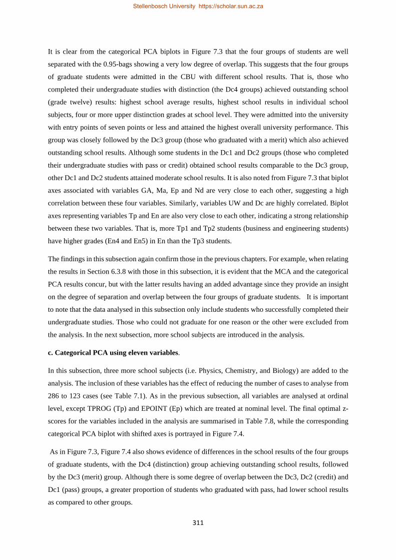
311
It is clear from the categorical PCA biplots in Figure 7.3 that the four groups of students are well
separated with the 0.95-bags showing a very low degree of overlap. This suggests that the four groups
of graduate students were admitted in the CBU with different school results. That is, those who
completed their undergraduate studies with distinction (the Dc4 groups) achieved outstanding school
(grade twelve) results: highest school average results, highest school results in individual school
subjects, four or more upper distinction grades at school level. They were admitted into the university
with entry points of seven points or less and attained the highest overall university performance. This
group was closely followed by the Dc3 group (those who graduated with a merit) which also achieved
outstanding school results. Although some students in the Dc1 and Dc2 groups (those who completed
their undergraduate studies with pass or credit) obtained school results comparable to the Dc3 group,
other Dc1 and Dc2 students attained moderate school results. It is also noted from Figure 7.3 that biplot
axes associated with variables GA, Ma, Ep and Nd are very close to each other, suggesting a high
correlation between these four variables. Similarly, variables UW and Dc are highly correlated. Biplot
axes representing variables Tp and En are also very close to each other, indicating a strong relationship
between these two variables. That is, more Tp1 and Tp2 students (business and engineering students)
have higher grades (En4 and En5) in En than the Tp3 students.
The findings in this subsection again confirm those in the previous chapters. For example, when relating
the results in Section 6.3.8 with those in this subsection, it is evident that the MCA and the categorical
PCA results concur, but with the latter results having an added advantage since they provide an insight
on the degree of separation and overlap between the four groups of graduate students. It is important
to note that the data analysed in this subsection only include students who successfully completed their
undergraduate studies. Those who could not graduate for one reason or the other were excluded from
the analysis. In the next subsection, more school subjects are introduced in the analysis.
c. Categorical PCA using eleven variables.
In this subsection, three more school subjects (i.e. Physics, Chemistry, and Biology) are added to the
analysis. The inclusion of these variables has the effect of reducing the number of cases to analyse from
286 to 123 cases (see Table 7.1). As in the previous subsection, all variables are analysed at ordinal
level, except TPROG (Tp) and EPOINT (Ep) which are treated at nominal level. The final optimal z-
scores for the variables included in the analysis are summarised in Table 7.8, while the corresponding
categorical PCA biplot with shifted axes is portrayed in Figure 7.4.
As in Figure 7.3, Figure 7.4 also shows evidence of differences in the school results of the four groups
of graduate students, with the Dc4 (distinction) group achieving outstanding school results, followed
by the Dc3 (merit) group. Although there is some degree of overlap between the Dc3, Dc2 (credit) and
Dc1 (pass) groups, a greater proportion of students who graduated with pass, had lower school results
as compared to other groups.
Stellenbosch University https://scholar.sun.ac.za

312
Figure 7.4: Categorical PCA biplot with 0.95-bags and shifted axes of variables Ma, En, Ph, Ch, Bi,
GA, UW, Dc, Nd, Tp, and Ep of the graduate dataset.
Stellenbosch University https://scholar.sun.ac.za

313
From Figure 7.4 and the final optimal z-scores in Table 7.8, there is a clear indication that the categories
of some variables are not equally spaced. For example, there is a large difference between category
Ma1 and other categories of Mathematics (Ma). The same applies to categories En1, Ph1, Ch1 and GA1
which are further apart from the remaining categories. For the variable EPOINT (Ep), there is a large
difference between categories Ep3 and Ep4. Additionally, Table 7.8 shows some ties between categories
Ph4 and Ph5 of Physics (Ph), and categories Ch3 and Ch4 of Chemistry (Ch).
Table 7.8: Final optimal z-scores of the variables in the graduate dataset with more school subjects added. Ties are shown in bold.
Category 1 2 3 4 5 6 7 Variable
Ma − 0.4883 − 0.2136 − 0.1057 − 0.0558 0.0391 En − 0.1962 − 0.0468 − 0.0390 0.0565 0.1037 Ph − 0.1496 0.0042 0.0482 0.0923 0.0923 Ch − 0.2276 − 0.1186 − 0.0663 − 0.0663 0.0796 Bi − 0.0967 − 0.0031 0.0903 0.1214 0.1711
GA − 0.4640 − 0.1109 − 0.0603 0.0316 0.1275 UW − 0.1605 − 0.1216 − 0.0700 − 0.0078 0.0357 0.1255 0.1280 Dc − 0.1158 − 0.0161 0.1088 0.2092 Nd − 0.1624 − 0.1005 − 0.0353 0.0940 Tp 0.1357 − 0.0289 − 0.1396 Ep 0.0803 − 0.0635 − 0.1162 − 0.4844
When comparing Figure 7.1 to 7.4 (and also to the categorical PCA biplot involving only variables Ma,
En, Ph, Ch, Bi, GA, and Dc, not shown) , it can be inferred that categorical PCA is more able to show
separation between the four groups of the variable Dc (DECLA) than PCA. There is less overlap
between the 0.95-bags in the categorical PCA biplot than in the PCA biplot. This may be due to the
linear constraints that PCA imposes on the variables to be analysed (i.e. linear relationships are assumed
among the variables). Categorical PCA, on the other hand, assumes a nonlinear relationship between
the variables in the analysis. In fact, the transformation plots in Subsections 7.4.1.a (see Figure 7.2) and
7.4.1.b (not shown) exhibit nonlinear functions, indicating that the relationships among the variables
might be nonlinear. In the next section, categorical PCA is carried out on the graduate dataset using
grades.
7.4.2 Categorical PCA for the graduate dataset using grades.
In the previous section, PCA and categorical PCA have been performed on the graduate dataset using
actual marks (in %). This section continues with the analysis based on categorical PCA for students
who graduated during the 2000-2013 period. During this period, only grades for both school and
university subjects were obtainable (see Tables A.6 and A.7 in Appendix A for the school and university
grading schemes).
Stellenbosch University https://scholar.sun.ac.za

314
The grades of the school subjects were taken as the categories for the corresponding variables. The
lowest category for each school subject was representing all grades below the lower merit grade (i.e.
fail, lower pass, upper pass, lower credit, and upper credit grades). Other grades (upper distinction,
lower distinction, upper merit, and lower merit) were forming the remaining categories. The labels of
these categories were formed by affixing numbers 1 to 5 to the abbreviated names of the variables. For
example, the categories for Mathematics are Ma1, Ma2, Ma3, Ma4, and Ma5. They represent the grades:
upper credit and all grades below, lower merit, upper merit, lower distinction, and upper distinction in
school Mathematics. The two lowest categories of the school subjects were merged prior the analysis,
since for most years, either the lowest category or the second lowest category were empty.
As in the previous section, the variable DECLA (degree classification) is taken as the grouping variable.
Only three categories (i.e. Dc1, Dc2, and Dc3 representing the pass, credit, and merit groups) are
considered. For most years (during the period considered), there were no students who completed their
undergraduate studies with a distinction grade. Table 7.9 shows all the variables included in the analysis
with their categories and their levels of analysis. Using the variables described in Table 7.9, categorical
PCA is again performed in order to investigate the simultaneous interrelationships among the variables.
Table 7.9: Categorical variables (with their categories, and their levels of analysis) of the graduate
dataset used in the analysis based on the categorical PCA.
Variable Abbreviation Labels of the categories Level of the analysis
School Mathematics Ma Ma2, M3, Ma4, and Ma5 Ordinal
School English En En2, En3, En4, and En5 Ordinal
School Physics Ph Ph2, Ph3, Ph4, and Ph5 Ordinal
School Chemistry Ch Ch2, Ch3, Ch4, and Ch5 Ordinal
School Biology Bi Bi2, Bi3, Bi4, and Bi5 Ordinal
Type of programme Tp Tp1, Tp2, and Tp3 Nominal
Degree classification Dc Dc1, Dc2, and Dc3 Ordinal
Number of upper distinctions
Nd Nd0, Nd1, Nd2, Nd3, and Nd4 Ordinal
Figures 7.5 and 7.6 display the categorical PCA biplots for the years 2001 and 2012 with 0.95-bags and
parallel orthogonal translated axes to help with the interpretation. The categorical PCA biplots for other
years are comparable to those in Figures 7.5 and 7.6 and are not shown (i.e. the categorical PCA biplots
for the years 2000, 2002, 2003, and 2007 were quite similar to that for the year 2001, while for the years
2004, 2005, 2006, 2008, 2009, 2010, 2011, and 2013, they were comparable to that for the year 2012).
Stellenbosch University https://scholar.sun.ac.za

315
Figure 7.5: Categorical PCA biplots with 0.95-bags and shifted axes for the year 2001 for the
categorical variables in Table 7.9.
Stellenbosch University https://scholar.sun.ac.za

316
Figure 7.6: Categorical PCA biplots with 0.95-bags and shifted axes for the year 2012 for the
categorical variables in Table 7.9.
Stellenbosch University https://scholar.sun.ac.za

317
A scrutiny of all categorical PCA biplots (those shown in Figures 7.5 and 7.6, and those not shown)
indicates no major changes in the simultaneous interrelationships between the variables included in the
analysis. That is, for the period considered, there was a tendency for Mathematics and Biology;
Mathematics and Physics; Mathematics and Chemistry; Physics and Chemistry to be strongly related
most often. It was also noted a weak relationship between English and other school subjects. More
specifically, the categorical PCA biplot for the year 2001 (see Figure 7.5) shows a strong relationship
between Biology, Physics and Chemistry. For the year 2012 (see Figure 7.6), there is a strong
relationship between Physics and Chemistry.
Figure 7.5 shows that School Mathematics and English distinguish between the three groups with Dc3
having lower grades in Mathematics (in the categories Ma2 and Ma3) and higher grades in English (in
the category En5) as compared to Dc1 and Dc2. It is also clear from Figure 7.5 that Dc1 and Dc2 have
more students in the two topmost categories of Physics, Biology, and Chemistry (in Ph4 and Ph5 for
Physics, Bi4 and Bi5 for Biology, and Ch4 and Ch5 for Chemistry). Additionally, Dc1 and Dc2 have
more students with upper distinctions at school level (in the categories Nd3 and Nd4) than Dc3. These
results indicate that the students who completed their undergraduate studies in 2001 with a merit grade
(the Dc3 group), were admitted in the CBU with lower school results as compared to those who
graduated with a pass and a credit grades (the Dc1 and the Dc2 groups). This trend was also observed
for the years 2000, 2002, 2003, and 2007. In these years, most of the graduates in the Dc 3 group were
from non-business and non-engineering related programmes who entered the university with high entry
points and moderate school results.
The situation in the year 2012 (see Figure 7.6) is quite different from that in 2001 (see Figure 7.5). In
Figure 7.6, all three groups have quite high school Mathematics (in the categories Ma4 and Ma5).
Additionally, school English (En) distinguishes between the three groups with higher En grades for Dc3
and lower En grades for Dc1 and Dc2. In other school subjects, Dc3 has more students with higher
grades in English, Biology, Physics and Mathematics than Dc1 and Dc2. Furthermore, Dc3 has more
students with three or more upper distinctions at school level as compared to Dc1 and Dc2. In contrast
to the year 2001, the majority of the students who completed their undergraduate studies with a merit
(the Dc3 group) in 2012, and also in the years 2004 to 2006, 2008, 2010, 2011, and 2013, were from
business and engineering related programmes and were admitted into the university with better school
results.
The final optimal z-scores for the years 2001 and 2012 are shown in Tables 7.10 and 7.11, while the
corresponding transformation plots are displayed in Figures F.1 and F.2 in Appendix F (for other years
they are not shown). It is noted from Figures F.1 and F.2 (and also from Tables 7.10 and 7.11) that the
variables are nonlinearly related. Additionally, the optimal z-scores do not place the categories of the
variables at equal distances like the original categories.
Stellenbosch University https://scholar.sun.ac.za
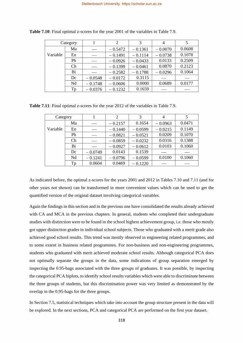
318
Table 7.10: Final optimal z-scores for the year 2001 of the variables in Table 7.9.
Category 1 2 3 4 5 Variable
Ma − 0.5472 − 0.1361 − 0.0070 0.0608 En − 0.1491 − 0.1114 − 0.0738 0.1078 Ph − 0.0926 − 0.0433 0.0133 0.2509 Ch − 0.1399 − 0.0461 0.0870 0.2123 Bi − 0.2582 − 0.1788 − 0.0296 0.1064 Dc − 0.0548 − 0.0172 0.3115 Nd − 0.1748 − 0.0606 0.0000 0.0689 0.0177 Tp − 0.0376 − 0.1232 0.1659
Table 7.11: Final optimal z-scores for the year 2012 of the variables in Table 7.9.
Category 1 2 3 4 5 Variable
Ma − 0.2157 0.1654 − 0.0963 0.0471 En − 0.1440 − 0.0599 − 0.0215 0.1149 Ph − 0.0821 − 0.0521 0.0209 0.1070 Ch − 0.0859 − 0.0232 0.0316 0.1388 Bi − 0.0927 − 0.0612 0.0103 0.1060 Dc − 0.0749 0.0143 0.1539 Nd − 0.1241 − 0.0796 − 0.0599 0.0100 0.1060 Tp 0.0604 0.0469 − 0.1220
As indicated before, the optimal z-scores for the years 2001 and 2012 in Tables 7.10 and 7.11 (and for
other years not shown) can be transformed in more convenient values which can be used to get the
quantified version of the original dataset involving categorical variables.
Again the findings in this section and in the previous one have consolidated the results already achieved
with CA and MCA in the previous chapters. In general, students who completed their undergraduate
studies with distinction were to be found in the school highest achievement group, i.e. those who mostly
got upper distinction grades in individual school subjects. Those who graduated with a merit grade also
achieved good school results. This trend was mostly observed in engineering related programmes, and
to some extent in business related programmes. For non-business and non-engineering programmes,
students who graduated with merit achieved moderate school results. Although categorical PCA does
not optimally separate the groups in the data, some indications of group separation emerged by
inspecting the 0.95-bags associated with the three groups of graduates. It was possible, by inspecting
the categorical PCA biplots, to identify school results variables which were able to discriminate between
the three groups of students, but this discrimination power was very limited as demonstrated by the
overlap in the 0.95-bags for the three groups.
In Section 7.5, statistical techniques which take into account the group structure present in the data will
be explored. In the next sections, PCA and categorical PCA are performed on the first year dataset.
Stellenbosch University https://scholar.sun.ac.za

319
7.4.3 PCA and Categorical PCA of the first year dataset using FCCO as the grouping variable.
In the previous section, PCA and categorical PCA were performed on the graduate dataset. This section
continues with the analysis based on these two techniques using the first year dataset. PCA uses the
actual marks (%), while for categorical PCA, the analysis is performed by first converting the school
results variables into categorical variables using the actual marks (%), with five categories (for school
variables) and six categories (for first year variables) representing the intervals or the bins of marks (in
%) (see Table E.1 in Appendix E and also Table D.1 in Appendix D). In Subsection 7.4.3.c, categorical
PCA is again performed on the first year dataset by converting the school results variables into
categorical variables by using grades (see Section 7.4.2).
In Chapter 5 (see Section 5.8.3), it was shown that the use of the actual marks to categorise school
variables resulted in uncovering more patterns of associations between variables. It is hoped that by
categorising the variables using the actual marks (%) will provide more indication on the group
separation among the first year students. The results of PCA will be compared with those from
categorical PCA.
a. PCA biplots of the variables of the first year dataset.
This subsection deals with PCA performed on the first year dataset using three school results variables
Ma (Mathematics), En (English), and GA (G12AVE)), and then five variables (Ma, En, GA, Ph
(Physics), Ch (Chemistry), and Bi (Biology)). The PCA results are used to come up with a composite
measure of the school performance or school performance index. The results from PCA are also
compared with those from categorical PCA. For each of the four years considered, the PCA biplots are
constructed to reveal the relationships between the points in the configuration and the variables involved
in the analysis. The variable Fc (FCCO) is used as the grouping variable.
The PCA biplots with the 0.95-bags of the four groups Fc1, Fc2, Fc3, and Fc4 for the years 2009, 2011,
2012, and 2013 of the variables Ma, En, and GA are displayed in Figure 7.7. In order not to obstruct
the biplots, the plotting of the observations is suppressed. The other results (i.e. axis predictivities,
means values of the four groups, coefficients of the first two principal components, overall quality (%),
and sample predictivities of the group means) are summarised in Tables 7.12 to 7.15.
Table 7.12: Two-dimensional axis predictivities of Figure 7.7 of the variables Ma, En and GA for the years 2009, 2011, 2012, and 2013.
Variable Axis predictivity 2009 2011 2012 2013
Ma 0.8928 0.8610 0.8713 0.8774 En 0.9809 0.9819 0.9785 0.9838 GA 0.8626 0.8510 0.8508 0.8573
Stellenbosch University https://scholar.sun.ac.za

320
Table 7.13: Mean values of the Fc1, Fc2, Fc3, and Fc4 groups for the variables Ma, En and GA of the first year dataset for the years 2009, 2011, 2012, and 2013.
Group Ma En GA 2009 2011 2012 2013 2009 2011 2012 2013 2009 2011 2012 2013
Fc1 55.00 55.13 61.05 67.87 67.67 57.57 58.08 67.12 58.11 53.30 56.52 58.09 Fc2 56.34 62.48 65.65 67.77 62.52 58.96 58.02 68.67 56.24 56.84 56.53 59.53 Fc3 63.09 64.18 68.76 69.53 63.43 59.18 59.16 66.65 59.20 58.54 59.61 59.22 Fc4 72.03 71.01 73.66 77.43 63.19 57.07 58.91 66.58 63.08 60.94 62.17 63.11
Table 7.14: Coefficients of the first two principal components (PC) of the variables Ma, En, and GA of the first year dataset for the years 2009, 2011, 2012, and 2013.
Variable Coefficient of the first PC Coefficient of the second PC 2009 2011 2012 2013 2009 2011 2012 2013
Ma 0.6231 0.6864 0.6572 0.6534 − 0.4530 0.2736 − 0.3717 − 0.3708 En 0.3708 0.1434 0.2578 0.2847 0.8889 − 0.9593 0.9283 0.9282 GA 0.6887 0.7130 0.7083 0.7015 − 0.0687 − 0.0704 0.0069 − 0.0313
Table 7.15: Overall quality (%) and sample predictivity of the group means for the two-dimensional PCA biplots in Figure 7.7.
Year Overall quality (%) Sample predictivity of the group means Fc1 Fc2 Fc3 Fc4
2009 91.21 0.9893 0.9995 0.9999 0.9999 2011 89.80 0.9976 0.9790 0.9987 0.9999 2012 90.02 0.9832 0.9691 0.9992 0.9993 2013 90.62 0.9821 0.9945 0.9965 0.9982
From Table 7.15 (second column), it is seen that the four PCA biplots in Figure 7.7 have each an overall
quality exceeding 89% (for 2013 for example, the overall quality is 90.62%) when considering the first
two dimensions. This suggests that the total variation in the data can be best summarised by the first
two principal components in a two-dimensional space. For all four years, school English (En) has the
highest axis predictivity values in excess of 0.97. For example, for the year 2013, the axis predictivity
is 0.9838. Mathematics (Ma) and G12AVE (GA) are also well represented in the four biplots in Figure
7.7 (their axis predictivities exceed 0.85). Additionally, the sample predictivities of the mean vectors of
the four groups of first year students interpolated in the biplots are very large and exceed 0.96 (see the
last four columns of Table 7.15), indicating that these group means (see Table 7.13) can be accurately
predicted by using the PCA biplots in Figure 7.7.
An inspection of the PCA biplots in Figure 7.7 shows a very high level of overlap between the 0.95-
bags representing the four groups. Despite this overlap, it is observed that the Fc4 group for each of the
four intakes of first year students has a greater proportion of students who achieved outstanding results
at school level. The solid symbol representing the mean of the Fc4 group is separated from the symbols
Stellenbosch University https://scholar.sun.ac.za
321
Figure 7.7: PCA biplots with 0.95-bags of the variables Ma, En, and GA of the first year dataset for
the years 2009 (top left panel), 2011 (top right panel), 2012 (bottom left panel), and 2013
(bottom right panel).
Stellenbosch University https://scholar.sun.ac.za

322
Figure 7.8: PCA biplots with 0.95-bags of the variables Ma, En, Ph, Ch, Bi, and GA of the first year
dataset for the years 2009 (top left panel), 2011 (top right panel), 2012 (bottom left panel),
and 2013 (bottom right panel).
Stellenbosch University https://scholar.sun.ac.za

323
representing the other groups, implying that the students in the Fc4 group obtained on the average higher
school results than those in the other groups (see also Table 7.13 which shows the group mean values
for all four groups). The Fc3 students also achieved higher marks (in %) in school subjects close to the
Fc4 group. More students in the Fc1 group are positioned on the lower school performance side. For
the year 2009, solid symbols representing the group means are distinct, while for 2011, those associated
with the Fc2 and the FC3 groups are very close to each other. For the year 2012, the Fc2 group is close
to the Fc1 group, and for 2013, the Fc1, Fc2, and Fc3 are almost similar.
When more school subjects are included in the analysis (see Figure 7.8 for the corresponding PCA
biplots), the overall qualities (in %) are lower as compared to those corresponding to the biplots in
Figure 7.7. In effect, the PCA biplots in Figure 7.8 have overall qualities exceeding 60%, but below
68% (see Table 7.18). Although the total variation in the data can be fairly summarised using the first
two components, adding a third dimension would improve the quality of fit of the biplots (the three-
dimensional overall qualities for the four years are 77.24%, 77.90%, 74.92%, and 80.12%,
respectively). Table 7.18 also shows that, for all four years (except for the Fc1 group for the years 2011
to 2013, and the Fc3 group for the year 2012), the group means have predictivities exceeding 0.84,
suggesting that the means for Fc2, Fc3, Fc4 (except for the year 2012), and Fc1 (for the year 2009 only)
can be accurately predicted, for the variables in the analysis, from the two-dimensional PCA biplots in
Figure 7.8. Similarly, the axis predictivities in Table 7.16 are relatively low as compared to those in
Table 7.12. Biology (Bi) has the lowest predictivity, while English (En) and G12AVE (GA) have
predictivities exceeding 0.84.
Table 7.16: Two-dimensional axis predictivities of Figure 7.8 of the variables Ma, En, Ph, Ch, Bi, and GA for the years 2009, 2011, 2012, and 2013.
Variable Axis predictivity 2009 2011 2012 2013
Ma 0.6010 0.5983 0.6791 0.6123 En 0.8738 0.9531 0.8510 0.9415 GA 0.8526 0.8417 0.8816 0.8869 Bi 0.4657 0.2554 0.5103 0.3908 Ph 0.5582 0.5012 0.6008 0.6327 Ch 0.5501 0.5016 0.5791 0.5895
Table 7.17: Coefficients of the first two principal components (PC) of the variables Ma, En, Ph, Ch, Bi, and GA of the first year dataset for the years 2009, 2011, 2012, and 2013.
Variable Coefficient of the first PC Coefficient of the second PC 2009 2011 2012 2013 2009 2011 2012 2013
Ma 0.4468 0.4451 0.4372 0.4512 −0.1683 −0.2872 −0.2972 −0.0688 En 0.1951 0.0168 0.2003 0.0669 0.8583 0.9389 0.8437 0.9310 GA 0.5444 0.5623 0.5345 0.5412 0.0622 0.1632 0.0397 0.1106 Bi 0.3843 0.3132 0.3606 0.3454 0.2031 0.0544 0.3280 −0.1807 Ph 0.3625 0.4398 0.4265 0.4504 −0.4186 0.0607 −0.1996 0.1607 Ch 0.4322 0.4404 0.4137 0.4206 −0.1214 −0.0531 −0.2257 −0.2404
Stellenbosch University https://scholar.sun.ac.za

324
Table 7.18: Overall quality (%) and sample predictivity of the group means for the two-dimensional PCA biplots in Figure 7.8.
Year Overall quality (%) Sample predictivity of the group means Fc1 Fc2 Fc3 Fc4
2009 65.02 0.8707 0.9357 0.9450 0.9900 2011 60.86 0.6598 0.9042 0.8933 0.9287 2012 68.37 0.6112 0.9778 0.6179 0.8763 2013 67.56 0.7737 0.8412 0.9396 0.9587
The PCA biplots in Figure 7.8 have some similarities with those in Figure 7.7. That is, for all four years,
more students in the Fc4 group are concentrated on the higher school performance side than the students
in the other groups. For the years 2009, 2011 and 2012, the Fc3 group is close to the Fc4 group, while
for the year 2013, the Fc1, Fc2, and Fc3 groups are close to each other and have the symbols
representing their means almost coinciding.
When examining the coefficients of the first two principal components in Tables 7.14 and 7.17, it is
clear that the school variables with the highest contribution to the first principal component are
G12AVE and Mathematics, with coefficients exceeding 0.68 and 0.62, respectively, for three variables
case (see Table 7.14), and 0.53 and 0.42, respectively, for six variables case (see Table 7.17). English
seems to play a minor role in the construction of the first principal component (i.e. it has the smallest
coefficients in both cases). The school variables with the third largest coefficient are Chemistry in 2009
and 2011, and Physics in 2012 and 2013 (see Table 7.17).
b. Categorical PCA of the first year dataset using actual marks (in %).
In the previous subsection, PCA was performed on the first year dataset using actual marks (%). In this
subsection, the analysis continues on the same dataset using categorical PCA in order to investigate the
simultaneous interrelationships between the variables included in the analysis and to check if there is a
first indication of the group separation of the four groups of the first year students. As in Subsections
7.4.1.b and 7.4.1.c, school results variables are first categorised using actual marks (in %). The
categories of these variables represent the intervals or bins of marks (in %). The analysis is done over
the four-year period (i.e. 2009, and 2011 to 2013) by first using three school results variables Ma
(Mathematics), En (English), and GA (G12AVE), and then by adding three more school results
variables Ph (Physics), Ch (Chemistry), and Bi (Biology)) in the analysis. In both cases, categorical
variables Fc (FCCO), Tp (TPROG), Nd (NDIS), and Ep (EPOINT) are also included in the analysis.
Figure 7.9 displays the categorical PCA biplot for the year 2012 of the four groups of first year students
when Fc (FCCO) is used as the grouping variable (the categorical PCA biplots for other years are not
shown), while Table 7.19 summarises the final optimal z-scores for the four-year period. The
transformation plots are only shown for the year 2012 (see Figure F.3 in Appendix F).
Stellenbosch University https://scholar.sun.ac.za

325
Figure 7.9: Categorical PCA biplot for the year 2012 using the variable Fc as the grouping variable and
the variables Ma, En, GA, Tp, Nd, and Ep of the first year dataset.
Stellenbosch University https://scholar.sun.ac.za

326
Table 7.19: Final optimal z-scores for the variables Ma, En, GA, Tp, Fc, Nd, and Ep of the first year
dataset for the years 2009, and 2011 to 2013. Ties between categories are in bold.
Category Year Ma En GA Tp Fc Nd Ep
1 2009 −0.0908 −0.0747 −0.0846 0.0493 −0.1760 −0.0904 0.0531
2011 −0.0745 −0.0436 −0.0714 0.0401 −0.0995 −0.0828 0.0542
2012 −0.0710 −0.0503 −0.0587 −0.0044 −0.0810 −0.0916 0.0441
2013 −0.0727 −0.0512 −0.0656 −0.0239 −0.0531 −0.0866 0.0388
2 2009 −0.0377 −0.0324 −0.0265 0.0227 −0.0752 −0.0656 0.0007
2011 −0.0432 −0.0163 −0.0191 0.0221 −0.0507 −0.0576 0.0072
2012 −0.0429 −0.0186 −0.0209 0.0258 −0.0583 −0.0574 −0.0052
2013 −0.0482 −0.0512 −0.0233 0.0290 −0.0531 −0.0574 −0.0080
3 2009 −0.0309 −0.0189 0.0075 −0.0664 −0.0409 −0.0374 −0.0488
2011 −0.0266 0.0271 0.0225 −0.0546 −0.0368 −0.0152 −0.0333
2012 −0.0423 0.0319 0.0138 −0.0815 −0.0198 −0.0250 −0.0422
2013 −0.0482 −0.0344 0.0090 −0.0615 −0.0115 −0.0261 −0.0431
4 2009 −0.0092 0.0303 0.0511 0.0350 0.0138 −0.0815
2011 0.0101 0.0653 0.0550 0.0361 0.0179 −0.0663
2012 −0.0115 0.0489 0.0446 0.0391 0.0074 −0.0796
2013 −0.0242 −0.0073 0.0419 0.0340 0.0050 −0.0710
5 2009 0.0438 0.0674 0.0684 0.0537
2011 0.0374 0.0879 0.0779 0.0592
2012 0.0339 0.0489 0.0633 0.0463
2013 0.0267 0.0422 0.0529 0.0412
An inspection of the categorical PCA biplot in Figure 7.9 for the year 2012 shows that most first year
students in all four groups have actual marks (%) in the bins Ma4 to Ma5 for Ma, En1 to En3 for En,
and GA1 to GA4 for GA. Additionally, they have at least one upper distinction at school level
(categories Nd1 to Nd4 of Nd). However, the Fc4 and Fc3 groups have more students on the higher
school performance side (i.e. in the highest category Ma5 of Ma, the two highest categories En4 and
En5 of En, GA4 and GA5 of GA, and Nd3 and Nd4 of Nd) then the Fc1 and Fc2 groups.
From Figure 7.9, Tp2 is close to Tp1, but is further apart from Tp3. Also, Tp1 and Tp2 are located on
the higher school performance side as compared to Tp3. The analysis by type of programme (categorical
PCA biplots not shown) revealed that more students in the Fc4 groups for Tp1 and Tp2 were in the two
highest categories of the school variables as compared to the Fc4 group for Tp3.
Stellenbosch University https://scholar.sun.ac.za

327
For other years (categorical PCA biplots not shown), the patterns of interrelationships between the
variables involved in the analysis were almost similar to that of the year 2012, except in 2013 where
the Fc1 group had more students in the bins Ma4 and Ma5 of Ma, and the bins En4 and En5 of En as
compared to the Fc1 groups for other years.
For the four years, strong relationships are observed between variables Nd and Ep, and between GA
(G12AVE) and Ma (school Mathematics). En (English), on the other hand, has a weak relationship with
other school variables.
The final optimal z-scores in Table 7.19 and the corresponding transformation plots for 2012 in Figure
F.3 in Appendix F (other transformation plots are not shown) show some tied categories (En4 and En5
in 2012; Ma2 and Ma3, En1 and En2, Fc1 and Fc2 in the year 2013), while some other categories are
almost similar (Ma2 and Ma3 in 2009 and 2012). Additionally, categories are not positioned at equal
distances. For example, small differences are observed between categories Ma2 and Ma3 in 2011; En2
and En3 in 2009; GA4 and GA5, while for the categories Ma1 and Ma2 in 2009; Ma4 and Ma5 in 2009,
2012 and 2013; GA1 and GA2 in 2009, 2011, and 2013; Tp2 and Tp3 in 2009 and 2011; and Tp1 and
Tp3 in 2013, large differences are observed. Furthermore, the transformation plots show nonlinear
relationships between the variables.
When more individual school subjects (i.e. Ph, Ch, and Bi) are included in the analysis (categorical
PCA not shown), the results are almost similar to the situation involving only two school subjects case.
The results from this subsection concur with those based on MCA (see Section 6.3.4). However,
categorical PCA has an added advantage over MCA. In effect, the 0.95-bags superimposed on the
categorical PCA biplots visualise the amount of overall and the amount of separation between the four
groups of first year students.
c. Categorical PCA of the first year dataset using grades.
In this subsection, Categorical PCA is applied to the first year dataset for the years (i.e. 2000 to 2008,
and 2010) which had only grades for school and university subjects. The grades are taken as the
categories of the school results variables, with the highest grade (upper distinction) corresponding to
the highest category, and the upper credit grade or below (i.e. upper credit, lower credit, upper pass,
lower pass, and fail grades combined) representing the lowest category. For example, the categories
Ma1, Ma2, Ma3, Ma4, and Ma5 of Ma (Mathematics) represent the upper credit grade (and all grades
below), the lower merit grade, the upper merit grade, the lower distinction grade, and the upper
distinction grade. All the variables included in the analysis are treated as ordinal categorical variables,
except the variable Tp (TPROG) which is analysed at nominal level.
The final optimal z-scores for each of the eight variables included in the analysis for the year 2006 are
presented in Tables 7.20, whereas Figure F.4 displays the associated transformation plots. The
Stellenbosch University https://scholar.sun.ac.za

328
categorical PCA biplot for the year 2006 is shown in Figure 7.10. The final optimal z-scores, the
transformation plots, and the categorical PCA biplots for other years are not shown.
Table 7.20: Final optimal z-scores of the variables Ma, En, Ph, Ch, Bi, Tp, Fc, and Nd for the year 2006, using the first year dataset (analysis based on grades). Ties are in bold.
Category Variable Ma En Ph Ch Bi Tp Fc Nd
1 − 0.0994 − 0.0422 − 0.0964 − 0.0831 − 0.1094 0.0742 − 0.1499 − 0.1119 2 − 0.0757 − 0.0422 0.0192 0.0063 − 0.0797 − 0.0841 − 0.1169 − 0.0569 3 − 0.0757 − 0.0422 0.0192 0.0069 − 0.0553 0.0257 − 0.0507 − 0.0102 4 − 0.0153 − 0.0422 0.0493 0.0069 − 0.0329 0.0511 0.0453 5 0.0717 0.1108 0.1044 0.1625 0.0758 0.1175
An inspection of the final optimal z-scores in Table 7.20 for 2006 (for other years, they are not given)
and their corresponding transformation plots in Figures F.4 (plots for other years are not shown) reveals
the similarities and ties for some categories of the ordinal categorical variables. This is the case, for
example, of school Mathematics with ties between categories Ma1 and Ma2 (in 2002, 2005, and 2007),
and between Ma2 and Ma3 (in 2006 and 2008). For all years considered (see Figure F.4 for 2006), the
highest category Ma5 was further apart from the other categories of Ma. This trend was also observed
for other variables (i.e. En5 for En, Ph5 for Ph, Ch5 for Ch, Bi5 for Bi, and Nd4 for Nd). For other
ordinal categorical variables, the ties are: En2, En3 and E4 (in 2002 and 2004); En1, En2, En3 and En4
(in 2003 and 2006); En1 and En2 (in 2007 and 2010); Ph1 and Ph2 (in 2002); Ph2 and Ph3 (in 2006
and 2010); Ch2, Ch3 and Ch4 (in 2004); Ch2 and Ch3 (in 2005); Ch3 and Ch4 (in 2006); Ch1 and Ch2
(in 2007); Bi1 and Bi2 (2010), Bi2 and Bi3 (in 2003, 2007 and 2008); Bi3 and Bi4 (in 2004); Bi2, Bi3
and Bi4 (in 2005); Bi4 and Bi5 (in 2007).
In Figure 7.10, the 0.95-bags show a high level of overlap between the four groups of first year students.
This trend was observed for other years. Additionally, there are no ties between the categories of Fc.
Furthermore, most of the students in the four groups have grades in the categories Ma3 to Ma5 of Ma,
En3 to En5 of En, Bi3 to Bi5 of Bi, Ph1 to Ph4 of Ph, Ch1 to Ch4 of Ch, and Nd1 to Nd4 of Nd.
However, the Fc4 has more students in the topmost categories Ma5, En5, Ph5, Ch5, Bi5, and Nd4 of
the variables Ma, En, Ph, Ch, Bi, and Nd as compared to the other three groups. Also, more students in
the Fc3 group have good school results as compared to the Fc2 and Fc1 groups. For other years, a
similar pattern was observed. This suggests that most students who successfully completed their first
year of study (the Fc4 group) were to be found among those who achieved outstanding school results,
i.e. those who obtained three or more upper distinctions at school level, and upper distinction or lower
distinction grades in individual school subjects.
Stellenbosch University https://scholar.sun.ac.za

329
Figure 7.10: Categorical PCA biplot for 2006 using Fc as the grouping variable and the variables Ma,
En, Ph, Ch, Bi, Tp, and Nd of the first year dataset (analysis based on grades).
Stellenbosch University https://scholar.sun.ac.za

330
Ties were also observed between the categories of the grouping variable Fc (i.e. there were ties between
Fc1 and Fc2 for the years 2003 and 2005; Fc2 and Fc3 for the year 2002; Fc1, F2, and Fc3 for the years
2004, 2007 and 2010). The categorical PCA biplots were constructed after merging the tied categories.
For the years 2006 and 2008, there were no ties in the categories of Fc.
The categorical PCA biplot in Figure 7.10 also shows evidence of relationships among the variables.
That is, a strong relationship is observed between Phi and Ch; Ma, Bi, and Nd. For other years
(categorical PCA biplots not shown), Ma was strongly related to Ph and Ch. School English (En) had a
weak relationship with other school subjects, except in 2004 where it was strongly related to Biology
(Bi).
In this section, PCA and categorical PCA have been performed on the first year dataset using Fc as the
grouping variable. PCA used actual marks (in %) in the analysis (see Subsection 7.4.3.a), while
categorical PCA utilised both actual marks and grades to categorise school results variables (see
Subsections 7.4.3.b and 7.4.3.c). A comparison of the PCA biplots with the categorical PCA biplots
(see Subsections 7.4.3.a and 7.4.3.b) suggests that the latter biplots give a better indication of the group
separation than the former biplots. Additionally, categorical PCA has an advantage over PCA because
it does not assume a linear relationship between the variables involved in the analysis. Furthermore,
Subsection 7.4.3.b has again illustrated the advantage of using actual marks (in %) to categorise school
results variables over the use of grades. In fact, the analysis using grades (see Subsection 7.4.3.c)
produced results with more ties in the variables, and in the grouping variable Fc (FCCO), whereas the
analysis in Subsection 7.4.3.b had very few ties in the categories of the variables, with ties in the
grouping variable only in the year 2013 for the categories Fc1 and Fc2. Additionally, there was more
indication of group separation, despite the overlap observed between the 0.95-bags of the four groups.
In the next section, techniques that are designed to optimally separate and take into account the group
structures in the data are applied to both datasets of the CBU data.
7.4.4 Categorical PCA of the first year dataset using Fy (FYEAR) as the grouping variable.
In this section, categorical PCA is performed on both school subjects and first year subjects of the first
year dataset in order to check for any change occurring in the school and first year subjects over the
four years which had actual marks (%) available (i.e. in 2009, 2011, 2012 and 2013). Both school and
first year results variables were categorised using actual marks (%). School subjects included in the
analysis comprise the two compulsory subjects Mathematics (Ma) and English (En), and the school
average G12AVE (GA). For first year subjects, the university weighted average FYAVE (YA) and five
individual subjects F1, F2, F3, F4 and F7 (see Tables A.4, D.1, and E.1 in Appendices A, D, and E,
respectively, for a full description of all first year results variables) are considered in the analysis. The
other variables in the analysis include the categorical variables Tp (TPROG), Fc (FCCO), and Nd
Stellenbosch University https://scholar.sun.ac.za

331
(NDIS). The variable FYEAR is taken as the grouping variable with categories Fy1, Fy2, Fy3 and Fy4
representing the years 2009, and 2011 to 2013
Figures 7.11 and 7.12 display the categorical PCA biplots for the school results variables and the first
results variables, respectively. The 0.95-bags were constructing after merging tied categories Fy1 and
Fy2 of the grouping variable FYEAR. The merged category is denoted by Fy12.
Albeit a high degree of overlap between the three 0.95-bags, there is a tendency for the bags representing
most recent years in Figure 7.11 to move toward the higher school performance side, with the year 2013
(represented by the category Fy4) having more students with outstanding school results as compared to
other years. Additionally, students in engineering related programmes are positioned on the higher
school performance side than those in business and in non-business and non-engineering programmes.
When more school subjects (Ph, Ch, and Bi) are added to the analysis, the number of cases to analyse
is reduced. Additionally, categories Fy1, Fy2 and Fy3 (representing the years 2009, 2011 and 2012) of
the grouping variable FYEAR are tied and merged into category Fy123. The categorical PCA biplot
(not shown) revealed that more 2013 intake of first year students were positioned to the higher school
performance side than the other years.
When considering the categorical PCA biplots involving first year subjects in Figure 7.12, an inverse
trend is observed; that is, there is a tendency for the 0.95-bags representing most recent years (2012 and
2013) to move toward the lower first year performance side. This suggests that most recent years (2012
and 2013) had more students with first year results in the lower categories than in the years 2009 and
2011.
The analysis based on grades during the fourteen-year period, i.e. from 2000 to 2013 (categorical PCA
biplots not shown) yielded similar results as the analysis based on the actual marks (in %). That is, more
recent intakes (especially in 2012 and 2013) of first year students were admitted with better school
results than the older intakes. In 2012 and 2013, business and engineering students had better school
results than the students in non-engineering and non-business related programmes. These findings were
expected because after the year 2010, admission criteria were tuned on the higher side by down
adjusting the programmes’ cut-off points and by narrowing the gaps between the cut-off points for male
and female students. This resulted in admitting the best school leavers in the years 2012 and 2013 with
respect to the school results.
In this subsection and the previous one, the variable FYEAR has been used as the grouping variable.
The categorical PCA biplot involving school subjects have shown a first indication of the group
separation, with most recent years having more students with better school results. This was due to the
double effects of raising the admission standards by down adjusting the programmes’ cut-off points and
by narrowing the gaps between the cut-off points of the male and the female students. In other terms,
Stellenbosch University https://scholar.sun.ac.za

332
Figure 7.11: Categorical PCA biplot using Fy as the grouping variable and the variables Ma, En, GA,
Tp, Fc, and Nd of the first year dataset (analysis based on actual marks).
Stellenbosch University https://scholar.sun.ac.za

333
Figure 7.12: Categorical PCA biplot using Fy as the grouping variable and the variables F1, F2, F3,
F4, F7, YA, and Tp of the first year dataset (analysis based on actual marks).
Stellenbosch University https://scholar.sun.ac.za

334
the raising of admission standards in degree programmes, especially in engineering related programmes,
helped admit school leavers with better results. However, most recent years (which had better school
results) did not necessarily have students with improved first year results.
In the next section, techniques that are designed to optimally separate and take into account the group
structures in the data are applied to both datasets of the CBU data.
7.5 Analysis of the CBU data by taking into account the group structures in the data.
In this section, statistical techniques that take into account the group structures in the data are performed
on the CBU data. These include CVA (canonical variate analysis), AoD (analysis of distance), and
CatCVA (categorical CVA). When the variables included in the analysis are continuous and the within-
group covariance matrices are homogeneous, CVA can be utilised. The assumption of equality of
within-group covariance matrices must be checked with the data at hand prior using CVA. Formal tests
for testing the homogeneity of covariance matrices exist (see for example Tiku & Balakrishnan, 1985;
Aslam & Rocke, 2005). The shapes of the α-bags superimposed on the CVA biplot can provide the
information about the differences in variation of the groups and can also be used to check if the
assumption of equality of covariance matrices is violated. When this assumption is not plausible, an
alternative technique could be to use the analysis of distance (AoD). Both CVA and AoD are only
applicable to continuous variables. When some or all variables included in the analysis are categorical,
categorical CVA (CatCVA) can be utilised. In what follows, CVA and AoD are performed on the data
for the years which had actual grades (in %) available. For the years which had only grades for school
and university results variables, CatCVA is utilised.
7.5.1 CVA and AoD applied to the CBU data.
This section applies the CVA and AoD techniques to the first year and the graduate datasets. While
AoD makes no assumption about the homogeneity of the within-group covariance matrices, CVA is
based on this assumption. In order to check the appropriateness of this assumption, weighted CVA
biplots with the 0.95-bags are used. Figure G.1 in Appendix G shows the weighted CVA biplots for the
graduate dataset using five individual school subjects and the overall school average. For the first year
dataset, only the weighted CVA biplots for the 2013 first year intake are displayed in Figure G.2 for
five individual school subjects and the overall school average. Weighted CVA biplots for other first
year intakes exhibited similar patterns comparable to those displayed in Figure G.2, and are thus not
shown. Similarly, weighted CVA biplots involving only the two compulsory school subjects, i.e.
Mathematics and English showed similar and comparable patterns as those involving six variables and
are not shown. The two variable case was investigated since Mathematics and English are compulsory
school subjects at high schools and are both taken into account in all degree programmes when
computing the entry points. Additionally, when only school Mathematics and English are incorporated
Stellenbosch University https://scholar.sun.ac.za

335
in the analysis, all observations are used. However, the inclusion of more school variables in the analysis
has the effect of reducing the number of observations to analyse.
An inspection of the weighted CVA biplots in Figure G.1 in Appendix G (the unweighted CVA biplots
were similar to the weighted ones and are not displayed), suggests that the assumption of identical
within-group covariance matrices is not valid. In effect, the shapes and sizes of the 0.95-bags for the
four groups are different implying that the variation of the observations within each group is not the
same. The Dc4 (distinction) group has a small variation, while in the Fc2 (credit) group, there is a large
variation. Similarly, the 0.95-bags associated with the four groups of the 2013 intake of the first year
students in Figure G.2 do not have the same shape and give an indication of heterogeneity of within-
group covariance matrices. The CVA biplots for other years (not reported) also showed evidence of
different variations of the observations within each group. In what follows, the AoD technique is applied
to both datasets of the CBU data since the assumption of identical within-group covariance matrices on
which the CVA technique is based is not plausible with the data at hand.
a. AoD applied to the first year dataset for the years 2009, and 2011 to 2013.
In this subsection, AoD is performed on the first year dataset for the years which had actual marks (in
%) for both school and university results variables available. As a preliminary step, the variables were
first normalised to unit variances. Both the unweighted and weighted analyses were carried out on the
data and for this purpose the Pythagorean distance was used. The weighted AoD biplots are shown in
Figures 7.13, 7.14, G3, and G4 (in Appendix G). The unweighted AoD biplots are not displayed as they
were similar to those produced by the weighted analysis. The permutation test of no significant
differences between the group means for the four groups of first year students was also performed for
each of the four years. The results for this test, along with the breakdown of the total AoD sum of
squared distances (into the between and within sums of squared distances) using six variables are
summarised in Table 7.21, respectively. Other results for the AoD procedure are the two-dimensional
overall qualities of the AoD displays in Table 7.22, and the group mean values in Table 7.23.
The overall quality for all unweighted and weighted AoD is exceeding 95% for six variables (see Table
7.22). This indicates that the group means are best represented in two-dimensional AoD biplots and
their values for each variable can be accurately read off from the biplot axes. The mean values inferred
from the biplots are in agreement with those in Table 7.23 (in Appendix G).
The AoD biplot for the year 2009 using six variables in Figure 7.13 shows that the four group means
occupy different positions. The Fc4 group has a greater proportion of the observations (i.e. more than
50% of the observations) with marks in Mathematics exceeding 70%. This is followed by the Fc3 group.
The Fc1 group has all of its observations with marks in Mathematics below 70%, while for the Fc2
group, only a small proportion of observations has marks in this school subject in excess of 70%. The
four groups also differ with respect to Physics, Chemistry, and the variable G12AVE, with the Fc4
Stellenbosch University https://scholar.sun.ac.za

336
group scoring high in these school subjects. This is followed by the Fc3 group. The Fc1 and Fc2 groups
score low in these subjects as compared to the Fc3 and the Fc4 groups and are almost similar with
respect to Physics, but differ with respect to Chemistry, and G12AVE (The Fc2 group has the lowest
marks in these two subjects).
The AoD biplots in Figures G.3 and G.4 for the 2011 and 2012 first year intakes of students using six
variables reveals that the four group means are still lying apart from each other as in Figure 7.13, and
that, for the 2011 intake, the Fc4 group has high marks (%) in Mathematics, as well as in Physics,
Chemistry, and G12AVE, but scores low in English. Similarly, the Fc3 group scores higher in these
subjects than the Fc1 and Fc2 groups. The particularity of the Fc1 group is that it has the lowest marks
in Mathematics, Chemistry, Physics, and G12AVE, but scores high in Biology. The Fc2, Fc3, and Fc4
groups are almost similar with respect to Biology, whereas the Fc1, Fc2, and Fc3 groups are almost
alike with respect to English. The situation prevailing in 2012 is comparable to that in 2011, except that
the Fc3 group is closest to the Fc4 group, and that the Fc1, Fc3, and Fc4 are almost similar with respect
to Chemistry (although the Fc4 has slightly higher marks in this subject than the other groups).
Table 7.21: The results of the permutation tests and the partitioning of the sums of squares obtained
from the AoD using Ma, En, Ph, Ch, Bi, GA, and the grouping variable Fc of the first year
dataset for the years 2009, and 2011 to 2013.
Year Between ss Within ss Total ss Number of permutations ASL (achieved
significance level
2009 73.94 1036.06 1110.00 3000 0.0000
2011 107.78 1278.22 1386.00 3000 0.0000
2012 77.74 1374.26 1452.00 3000 0.0000
2013 145.21 1630.79 1776.00 3000 0.0000
Table 7.22: Two-dimensional overall quality (%) associated with the (unweighted and weighted) AoD
biplots when using the variables Ma, En, Ph, Ch, Bi, and GA of the first year dataset for
the years 2009, and 2011 to 2013.
Year Unweighted AoD Weighted AoD
2009 99.24 99.57
2011 95.61 97.33
2012 99.14 99.45
2013 99.46 99.64
Stellenbosch University https://scholar.sun.ac.za

337
Table 7.23: Group mean values for the variables Ma, En, Ph, Ch, Bi, and GA of the first year dataset
for the years 2009, and 2011 to 2013.
Year Group Ma En Ph Ch Bi GA
2009 Fc1 61.00 68.33 50.67 62.67 56.33 62.00
Fc2 67.38 64.38 51.50 57.00 49.88 59.62
Fc3 69.84 64.76 56.05 66.66 54.82 62.39
Fc4 75.55 63.72 59.07 69.80 56.56 64.87
2011 Fc1 57.71 58.00 51.43 51.14 48.57 56.86
Fc2 68.33 60.78 53.67 53.56 41.78 58.56
Fc3 67.97 60.78 59.38 56.19 43.55 60.53
Fc4 75.08 57.77 60.50 61.92 44.22 62.44
2012 Fc1 65.70 61.60 57.00 69.00 43.70 61.10
Fc2 67.22 59.94 55.39 62.89 46.11 59.11
Fc3 74.74 59.94 59.18 68.08 47.67 63.75
Fc4 77.71 59.73 60.27 70.03 50.80 65.38
2013 Fc1 72.33 68.83 57.50 47.33 49.50 59.56
Fc2 71.74 70.67 53.15 54.56 50.15 61.15
Fc3 74.21 69.41 54.57 53.99 50.28 61.37
Fc4 80.41 67.88 61.29 59.52 52.51 64.81
Figures 7.14 displays the AoD biplot for the 2013 first year intake when six variables are used. The
main feature of the AoD biplot in Figure 7.14 is the closeness of the group means for the Fc2 and Fc3
groups. Additionally, the Fc4 group has still high marks (in %) in Mathematics, as well as in other
subjects, except in English where it has low marks. The Fc1, Fc2, and Fc3 groups, on the other hand,
are almost alike with respect to Mathematics, Physics and English. The Fc1 group scores low marks in
Biology, Chemistry, and G12AVE.
In Figure 7.14, the projections of the 0.95-bags onto the Mathematics axis show that most of the
observations in the Fc4 group score higher than 75%, whereas less than half of the observations in the
other groups score that high. Likewise, the projections of the 0.95-bags onto the G12AVE axis show
that most of the observations in the Fc4 group have marks exceeding 60% in G12AVE, while
approximately half of the observations in the Fc2 and Fc3 groups score marks exceeding 60%. The Fc2
group has a small proportion of its observations in excess of 60% in G12AVE. This tendency is also
observed when the 0.95-bags in Figure 7.16 are projected onto the Physics and Chemistry axes. That
is, at the benchmark of 60%, about half of the observations in the Fc4 group score high, while only a
small proportion of the observations in the other groups have high marks.
Stellenbosch University https://scholar.sun.ac.za

338
Figure 7.13: Weighted AoD biplot with 0.95 bags (top panel: with the individual observations plotted,
bottom panel: with the plotting of the observations suppressed) for the 2009 first year intake using the variables GA, Ma, En, Ph, Ch, and Bi.
Stellenbosch University https://scholar.sun.ac.za

339
Figure 7.14: Weighted AoD biplot with 0.95 bags (top panel: with the individual observations plotted,
bottom panel: with the plotting of the observations suppressed) for the 2013 first year intake using the variables GA, Ma, En, Ph, Ch, and Bi.
Stellenbosch University https://scholar.sun.ac.za

340
In order to consolidate the findings based on the AoD biplots about the differences between the four
groups of first year students, permutation tests for testing the null hypothesis about the equality of the
four group means were performed with 3,000 random permutations, and the achieved significance level
(ASL) for each test was determined. The resulting permutation densities were also constructed, but are
not shown. The results for the permutation tests along with the breakdown of the total AoD sum of
squared distances into its components for the years 2009, and 2011 to 2013 are reported in Table 7.21
for six variables. For all four years, the null hypothesis of no difference between the four group means
was rejected with an ASL of approximately zero (see the last column of Table 7.21).
b. AoD applied to the graduate dataset.
The AoD biplot for the graduate dataset is given in Figure 7.15 for six variables, while the group mean
values are reported in Table 7.24. The overall qualities for both the unweighted and weighted AoD are
99%. This indicates that the group means of the four groups of graduates are accurately represented in
the two-dimensional AoD biplots and can be exactly deduced from these displays. The values of the
group means read off from the AoD biplots for each variable agree exactly with those in Table 7.24.
Table 7.24: Group mean values of each of the variables included in the analysis using six variables of
the graduate dataset for graduates who were in their first year of study in 2009.
Group Ma En Ph Ch Bi GA
Dc1 71.92 63.14 56.31 68.58 54.64 62.64
Dc2 75.30 63.07 58.31 68.80 55.15 64.57
Dc3 77.97 65.92 60.97 72.19 58.94 67.22
Dc4 82.00 66.00 66.00 76.00 69.33 71.33
In Figure 7.15, the four group means are apart from each other. The Dc4 group takes on high marks in
all six subjects as compared to other groups. Similarly, the Dc3 group records higher marks than the
Dc2 and the Dc1 groups which are almost similar with respect to Biology, and which differ on other
school subjects (the Dc2 group has high marks in English, Mathematics, Physics, Chemistry, and
G12AVE as compared to the Dc1). The 0.95-bags and the convex hull for the four groups suggest that
the variation of the observations within each group is not the same. The Dc4 has the lowest within-
group variation.
The formal test of no difference between the group means using the permutation test yielded an ASL
of approximately 0.0000, implying that the null hypothesis of equality of group means was rejected.
The breakdown of the total AoD sum of squared distances T into its components B (between sum of
squared distances) and W (within sum of squared distances) gave: T = 768.00, B = 63.54, and
W = 704.46.
Stellenbosch University https://scholar.sun.ac.za

341
Figure 7.15: Weighted AoD biplot with 0.95 bags (top panel: with the individual observations plotted,
bottom panel: with the plotting of the observations suppressed) of the graduate dataset using the variables GA, Ma, En, Ph, Ch, and Bi.
Stellenbosch University https://scholar.sun.ac.za

342
In the next subsection, CatCVA is performed on both the first year dataset and the graduate dataset for
the years which had only grades available.
7.5.2 Categorical CVA applied to the CBU data.
a. Categorical CVA of the first year dataset using two school subjects.
The first year dataset had only grades available for both school and university subjects for the years
2000 to 2008, and 2010. These grades were used to create categorical variables corresponding to the
school and university results variables (see Section 7.4). When the grouping variable FCCO (Fc) is
considered, four groups of first year students (i.e. the Fc1, Fc2, Fc3, and Fc4 groups) are distinguished.
The main aim of categorical CVA in this subsection is then to visualise this group structure present in
the first year dataset. The data are first analysed by considering only the two compulsory school
subjects, and then more school subjects are included in the analysis. The two variable case is first
investigated as it allows all the available observations to be analysed. The inclusion of more school
variables in the analysis has the effect of reducing the number of observations to analyse.
Table 7.25: The partitioning of the sums of squares obtained from the CatCVA analysis using the
variables Ma, En, Nd, Ep, and Fc (grouping variable) of the first year dataset for the years
2000 to 2008, and 2010.
Year Between ss Within ss Total ss Year Between ss Within ss Total ss
2000 0.0962 3.6538 3.7500 2005 0.1162 3.6338 3.7500
2001 0.1869 3.5631 3.7500 2006 0.0560 3.6940 3.7500
2002 0.1287 3.6213 3.7500 2007 0.0881 3.6619 3.7500
2003 0.1070 3.643 3.7500 2008 0.0717 3.6783 3.7500
2004 0.0968 3.6532 3.7500 2010 0.0744 3.6756 3.7500
Table 7.25 summarises the partitioning of the sums of squares for CatCVA of the first year data when
only two compulsory school subjects are included in the analysis. For the period considered (i.e. from
2000 to 2008, and 2010), the within groups sums of squares are much higher than the between groups
sums of squares. This is an indication that there a great variation within the groups and less variation in
the group means of the four groups.
The CatCVA biplots were constructed for the years 2000 to 2008, and 2010. Since they were almost
similar and comparable, only those for the years 2000 and 2008 are displayed in Figures 7.16 and 7.17,
respectively. When interpreting a CatCVA biplot, the centroid properties and the approximated
distances between the observations and the group centroids, and also between the CLPs and the group
centroids should be considered. More specifically, the CLPs which are closely surrounding a point
Stellenbosch University https://scholar.sun.ac.za

343
representing an observation or a group centroid can be considered as valid category points for that point
or group centroid (Le Roux et al., 2014).
Figure 7.16 displays the CatCVA biplot using the variables Ma (Mathematics), En (English), Nd
(NDIS), Ep (EPOINT), and Fc (FCCO) (grouping variable) of the first year dataset for the year 2000.
In this biplot, the points representing the group centroids of the Fc3 and FC4 groups are very close to
each other and are further apart from the other two groups (i.e. the Fc1 and Fc2 groups). This suggests
that the Fc3 and Fc4 groups are almost similar with respect to the variables involved in the analysis.
When examining the CatCVA biplot in the top panel, it is noted that most points representing the
observations of the Fc4 group are closely surrounded by the CLPs Ma4, Ma5, En3, En4, En5, Nd3,
Nd4, and Ep1, indicating that most first year students in the CP group for the year 2000 were found in
the two top grades of Mathematics (i.e. Ma4 and Ma5), and the three top grades of English (En3, En4
and En5). These students were admitted in the first year of study with entry points between five and
seven points and achieved three or more upper distinctions at school level. The point representing the
group centroid for the Fc1 group in Figure 7.16 has within its surrounding region the CLPs Ep4, Nd0,
and Ma3, implying that this group has more students who were admitted with entry points exceeding
eleven points, no upper distinction at school level, and who obtained an upper merit grade in
Mathematics (Ma3).
In a CatCVA biplot, apart from the group centroids, the CLPs associated with the variables involved in
the analysis are also represented. This permits to examine the simultaneous interrelationships among
the variables. In Figure 7.16, the CLPs Ma5, Nd4, and Ep1 almost coincide on the biplot and are closer
to the point representing the group centroid of the Fc4 group. This suggests that most Fc4 students for
the 2000 first year intake who entered the university with entry points between five and seven points
(Ep1) and who had at least four upper distinctions at school level, also achieved the highest grade in
Mathematics (Ma5) at school level. Similarly, the CLTs En3, En5, and Ma4 are also related, implying
that most Fc4 students for the year 2000 who achieved the second highest grade (i.e. a lower distinction)
in Mathematics (Ma4), either obtained an upper merit grade (En4) or a lower merit grade (En3) in
English. The CatCVA biplots for the years 2001 and 2002, exhibited almost similar and comparable
features as the CatCVA biplot for the year 2000 and are not shown.
The CatCVA biplots for the year 2003 to 2008 and 2010 were also constructed, but only the CatCVA
biplot for the year 2008 is depicted in Figure 7.17. The CatCVA biplots for the years 2003, 2004, 2006,
and 2010 were characterised by the points representing all four group centroids lying close to each other
with the Fc4 group being closest to the Fc3 group. For the CatCVA biplot in the year 2005, the Fc3
group was at the vicinity of the Fc1 group, whereas for the year 2007, the Fc2 and Fc3 groups are the
closest. In Figure 7.17 (for the year 2008), the Fc1, Fc2 and the Fc3 groups are the closest.
Stellenbosch University https://scholar.sun.ac.za

344
Figure 7.16: CatCVA biplot (with the observations for each group plotted in the top panel, and with
the plotting of the observations suppressed in the bottom panel) using the variables Ma,
En, Nd, Ep, and Fc (grouping variable) of the first year dataset for the year 2000.
Stellenbosch University https://scholar.sun.ac.za

345
Figure 7.17: CatCVA biplot (with the observations for each group plotted in the top panel, and with
the plotting of the observations suppressed in the bottom panel) using the variables Ma,
En, Nd, Ep, and Fc (grouping variable) of the first year dataset for the year 2008.
Stellenbosch University https://scholar.sun.ac.za

346
Although the four group centroids are close to each other in Figure 7.17, the Fc4 group is apart from
the cluster formed by the Fc1, Fc2 and the Fc3 groups. This indicates that the latter groups are almost
similar with respect to the variables involved in the analysis. Most points representing the observations
in the Fc4 group are closely bounded by the CLPs En3, Nd2, En4, Ma5, Ep1, Nd4, Ep3, and Nd3,
indicating that most students in the Fc4 group, for the 2008 first year intake, had grades in Mathematics
and English corresponding to Ma5 (upper distinction in Mathematics), En3 (upper merit in English)
and En4 (lower distinction in English), with at least two upper distinctions at school level and entry
points below twelve points. In Figure 7.17, relationships between the variables through their CLPs are
also discernible: Ep1 and Nd4 for the Fc3 and Fc4 groups; Ep1, Nd4 and Ma5 for the Fc4 group; Ep2
and Nd3 for the Fc4 group; En3, Nd2, En4 and Nd1 for the Fc4 group and also for the other three groups
are related. The CatCVA biplots for other years (not reported) showed patterns of relationships almost
similar and comparable to those for the year 2008. For example, the Fc1 group was consistently in the
vicinity of the CLTs Ma3 (in 2004, 2005, 2006 and 2010), Ep4, Nd0, and Nd1, suggesting that most
students in the Fc1 group were admitted with poor school results as demonstrated by their high entry
points exceeding eleven points (Ep4) with one or zero upper distinction at school level.
b. Categorical CVA of the first year dataset using more school subjects.
In the previous subsection, only two school subjects were involved in the analysis. In this subsection,
three more school subjects (i.e. school Physics (Ph), Chemistry (Ch), and Biology (Bi)) are added in
the analysis. Table 7.26 shows the breakdown of the total sum of squares into the between and the
within groups sums of squares. As in the case of two school subjects, the within groups sums of squares
for all years considered are exceedingly high as compared to the between groups sums of squares
indicating a low variation between the group means. Within each group, there is a high variation among
the individual observations.
The CatCVA biplots for the years 2000 to 2008 and 2010 were constructed and only those for the years
2005 and 2008 are displayed in Figures 7.18 and 7.19, respectively. For all years considered, the points
representing the group centroids were separated, but were relatively at a close distance from each other.
The variables responsible for the group separation over the period considered were identified as Ph
(Physics), Ch (Chemistry), and to some extent the variables Nd (NDIS) and Ep (EPOINT). For all years,
the Fc3 group was closest to the Fc4 group, except in the year 2005 (see Figure 7.18) which had the
Fc3 group nearest to the Fc1 group. The proximity of the group centroids of the Fc3 and the Fc4 groups
suggests that these groups are almost similar with respect to some variables included in the analysis,
especially Mathematics, English, and Biology.
When considering the CLTs closely encircling the observations belonging to the Fc4 group, it was
noted, for most years, the presence of the CLTs Ma4, Ma5, En3, En4, En5, Ph4, Ph5, Bi4, Bi5, Nd3,
Nd5, and Ep1. These category levels correspond to the highest achievement at school level and suggest
Stellenbosch University https://scholar.sun.ac.za

347
Figure 7.18: CatCVA biplot (with the observations for each group plotted in the top panel, and with
the plotting of the observations suppressed in the bottom panel) using the variables Ma,
En, Ph, Ch, Bi, Nd, Ep, and Fc (grouping variable) of the first year dataset for the year
2005. The arrow shows the position of Ch4 outside the edge of the graph.
Stellenbosch University https://scholar.sun.ac.za

348
Figure 7.19: CatCVA biplot (with the observations for each group plotted in the top panel, and with
the plotting of the observations suppressed in the bottom panel) using the variables Ma,
En, Ph, Ch, Bi, Nd, Ep, and Fc (grouping variable) of the first year dataset for the year
2008. The arrows show the positions of En1 and En2 outside the edges of the graph.
Stellenbosch University https://scholar.sun.ac.za

349
Table 7.26: The partitioning of the sums of squares obtained from the CatCVA analysis using the
variables Ma, En, Ph, Ch, Bi, Nd, Ep, and Fc (grouping variable) of the first year dataset
for the years 2000 to 2008, and 2010.
Year Between ss Within ss Total ss Year Between ss Within ss Total ss
2000 0.1551 3.7021 3.8571 2005 0.1167 3.5976 3.7143
2001 0.0840 3.7731 3.8571 2006 0.0613 3.7958 3.8571
2002 0.1838 3.6734 3.8571 2007 0.1044 3.7528 3.8571
2003 0.1617 3.6954 3.8571 2008 0.0863 3.7708 3.8571
2004 0.1306 3.5837 3.7143 2010 0.1376 3.5767 3.7143
that most Fc4 students achieved highest grades in school subjects as compared to other groups. This
confirms the findings, using other statistical methods in this chapter and in the previous chapters, that
most Fc4 students were admitted at the CBU with outstanding school results. Some of the CLTs closely
surrounding the Fc1 and Fc2 groups, for most years, include Ph1, Ph2, Ph3, Ch1, Ch2, Ch3, and Ep4
(for the Fc1 group only), suggesting that these two groups had low achievement in Physics and
Chemistry as compared to the Fc4 group.
The CatCVA biplots in Figures 7.18 and 7.19 for the years 2005 and 2008 illustrate and confirm the
general trend observed in other years as regarding the closeness of the group centroids representing the
four groups, the CLTs tightly enclosing the observations in each of the four groups, and the variables
responsible for the group separation. In Figure 7.18, the CLTs in the region of the Fc4 observations
include Ma5, En4, Ch3, Ph3, Ph5, Nd4, Bi4, Bi5, and Ep1, whereas those in the region of the Fc3 group
are Ma3, Ma5, En3, En5, Ph1, Ph3, Ch1, and Ch3. For the Fc1 group, they are basically the same as
those for the Fc3 group, except for En3 and Ma3 which exclusively characterise the latter group and
Ep4 applicable to the former group only. The Fc2 has the CLTs Ma4, En5, Ph1, Ch1, and Bi4 on its
surrounding.
Similarly, the CLTs at proximity to most of the observations belonging to the Fc4 group in Figure 7.19
are almost the same as those in Figure 7.18, with the CLTs Ma4, En5, Ch4, Ch5, Bi3, Ep2, and Nd2
being added to the list. In Figure 7.19, the Fc3 group is almost similar to the Fc4 group with respect to
the variables English, Biology and NDIS. But the two groups differ on Physics and Chemistry, and to
some extent on Mathematics, i.e. the Fc3 group has more students with lower grades (below lower merit
grades) in Physics and Chemistry (represented by Ph1 and Ch1). Similarly, the Fc1 and Fc2 groups
differ from the Fc4 group on these two subjects.
Despite the low between group variations which characterise the CatCVA biplots of the first year dataset
in this subsection and the previous one, there is evidence of group separation, with the Fc4 group being
associated with outstanding school results, and the Fc1 group generally exhibiting low school results.
Stellenbosch University https://scholar.sun.ac.za

350
For the Fc3 and Fc2 groups, the former is comparable to the Fc4 group, while the latter is almost similar
to the Fc1 group, to some extent. This is in contrast with the categorical PCA biplots in Section 7.4.3.b
which showed a high degree of overlap between the 0.95-bags representing the four groups of first year
students and which had some groups being merged as a result of the groups being completely similar.
Although there were some indication of the group separation, this was clear only with respect to the
Fc4 group vis-à-vis the other three groups. The other advantage of CatCVA over categorical PCA is
that it allows for the visualisation of more complex relationships among the variables in the analysis by
considering the CLTs which lie closer to each other. The next subsection continues with CatCVA
applied to the graduate dataset.
c. Categorical CVA of the graduate dataset.
In Section 7.4.2, the categorical PCA was performed on the graduate dataset using grades for students
who successfully completed their studies in degree programmes of the CBU over the 2000-2013 period.
In this subsection, CatCVA is applied to the same dataset by using the variable Dc (DECLA) as the
grouping variable. As this statistical technique is specifically designed to visualise the group structure
present in a dataset, it is hoped that the group separation in the graduate dataset will be more apparent
than using categorical PCA. The partitioning of the sums of squares of CatCVA for the completion
years 2000 to 2013 is shown in Table 7.27 for the analysis involving two school subjects, and in Table
7.28 for five school subjects. The CatCVA biplot for the year 2010, with two school subjects is
displayed in Figure 7.20, and that with five school subjects is depicted in Figure 7.21. The CatCVA
biplots for other years are not shown.
An inspection of Table 7.27 shows that the between sums of squares for all years are lower than the
within sums of squares. Similarly, the between sums of squares when five school subjects are involved,
are lower as compared to the within sums of squares, but slightly higher than those in Table 7.28. This
indicates that, for both cases, the variation between the groups is much smaller as compared to the
variation of the individual observations within each group. This is readily seen in the CatCVA biplot
involving two school subjects in Figure 7.20 where the points representing the group centroids are at
close distances from each other. This trend was observed in other years (CatCVA biplots not shown).
In Figure 7.20, the three group centroids are separated and are at equal distances from each other. This
pattern was also observed in the completion years 2005, 2006, 2008, 2009, and 2011 (CatCVA biplots
not shown). For other years, the group centroid for the Dc1 group was closer to that for the Dc2 group.
It is also observed from Figure 7.20 that the CLTs closely surrounding most of the observations in the
Dc1 group are Ma5, Ep3, En3, Ma4, Nd1, Ep4, Ma3, En5, En4, and Ep2. These CLTs also encircle
most of the observations in the Dc2 group. Other CLTs close to the Dc2 group include En2, Nd4, and
Ep1. Most of the observations in the Dc3 group are characterised by the CLTs Ep3, En3, Ep4, Ma3,
En5, En4, Ep1, Ep2, Nd2, and Ma5.
Stellenbosch University https://scholar.sun.ac.za

351
Figure 7.20: CatCVA biplot (with the observations for each group plotted in the top panel, and with
the plotting of the observations suppressed in the bottom panel) using the variables Ma,
En, Nd, Ep, and Dc (grouping variable) of the graduate dataset for the year 2010.
Stellenbosch University https://scholar.sun.ac.za

352
Table 7.27: The partitioning of the sums of squares obtained from the CatCVA analysis using the
variables Ma, En, Nd, Ep, and Dc (grouping variable) of the graduate dataset for the years
2000 to 2013.
Year Between ss Within ss Total ss Year Between ss Within ss Total ss
2000 0.0353 3.7147 3.7500 2007 0.0568 3.6932 3.7500
2001 0.0954 3.6546 3.7500 2008 0.0436 3.7064 3.7500
2002 0.0484 3.7016 3.7500 2009 0.0298 3.7202 3.7500
2003 0.0257 3.7243 3.7500 2010 0.0329 3.7171 3.7500
2004 0.0901 3.6599 3.7500 2011 0.0162 3.7338 3.7500
2005 0.1203 3.6297 3.7500 2012 0.0657 3.6843 3.7500
2006 0.0401 3.7099 3.7500 2013 0.0584 3.6916 3.7500
Table 7.28: The partitioning of the sums of squares obtained from the CatCVA analysis using the
variables Ma, En, Ph, Ch, Bi, Nd, Ep, and Dc (grouping variable) of the graduate dataset
for the years 2000 to 2013.
Year Between ss Within ss Total ss Year Between ss Within ss Total ss
2000 0.1075 3.6068 3.7143 2007 0.1200 3.3085 3.4286
2001 0.1460 3.5683 3.7143 2008 0.0587 3.5127 3.5714
2002 0.082 3.7751 3.8571 2009 0.0402 3.8169 3.8571
2003 0.060 3.7971 3.8571 2010 0.0604 3.7967 3.8571
2004 0.1370 3.5773 3.7143 2011 0.0344 3.8228 3.8571
2005 0.1385 3.5758 3.7143 2012 0.1088 3.6055 3.7143
2006 0.0654 3.6488 3.7143 2013 0.0894 3.4821 3.5714
In general, for the completion year 2010, most observations in the Dc3 group were found in the category
Ma5 of Mathematics; the categories En3, En4, and En5 of English; Nd2, Nd3 and Nd4 of variable
NDIS; and Ep1, Ep2, and Ep3 of variable EPOINT. In other terms, students who graduated in the year
2010 with at least a merit grade, mostly achieved the highest grade (i.e. upper distinction) in school
Mathematics, at least an upper merit grade in school English, two or more upper distinctions at school
level, and were admitted in the first year of study with entry points below twelve points. Students who
completed their undergraduate studies with a pass or a credit grade (i.e. the Dc1 group or the Dc2 group)
mostly obtained at least an upper merit grade in school Mathematics and English.
Stellenbosch University https://scholar.sun.ac.za

353
Figure 7.21: CatCVA biplot (with the observations for each group plotted in the top panel, and with
the plotting of the observations suppressed in the bottom panel) using the variables Ma,
En, Ph, Ch, Bi, Nd, Ep, and Dc (grouping variable) of the graduate dataset for the year
2010.
Stellenbosch University https://scholar.sun.ac.za

354
The relationships identified between the observations in the three groups and the different CLTs in the
year 2010 (see Figure 7.20) are almost similar to those in the years 2005, 2006, 2008, 2009, and 2011,
except for some few variations. In the year 2005 for example, students in the Dc3 group mostly achieved
an upper distinction in school Mathematics and English, while those in the Dc2 group had more students
in the categories Ma5, En5, Nd4 and Ep1 than the Dc1 students. The Dc1 group, on the other hand, had
more students with no upper distinction at school level. These students were admitted in the first year
of study with entry points exceeding eleven points as compared to the other two groups. In 2006, more
students in the Dc1 group obtained a lower distinction in Mathematics (Ma4) than those in the other
two groups, while in the year 2009, the Dc2 group had more students in the categories Ma5, Ep1, and
Nd4 as compared to other groups.
In the years 2000 to 2004, 2007, 2012 and 2013, the CatCVA biplots (not shown) were characterised
by the closeness of the three group centroids with the Dc1 and Dc2 groups being closest and almost
similar with respect to the variables included in the analysis. More specifically, in the year 2000, the
CLTs tightly encircling the Dc1 and the Dc2 groups include En4, and En5, while those closely
surrounding the MEDI group were Nd1, Nd2, Ep2, and Ep3. The main feature for the remaining years
is that the observations in the three groups were closely surrounded by the CLTs Ma3 to Ma5, and En3
to En5, with most observations in the Dc3 group in the category En5 in 2001; in the categories Ma5,
En4, and En5 in 2002; and Ep1 and Nd4 in 2004.
The CatCVA biplots for the years 2000 to 2013 with five school subjects were also constructed. Only
the CatCVA biplot for the year 2010 is shown in Figure 7.21. As is the case of two school subjects,
there were no major changes in the positions of the group centroids, and in the CLTs being at proximity
to the observations in the three groups for all CatCVA biplots examined. For the years 2000 to 2005,
the points representing the group centroids for the Dc1 and Dc2 groups were the closest, while for other
years the three group centroids on the biplots were at equal distance from each other.
For most years, the three groups were almost similar with respect to the variables in the analysis, except
for some few differences. Additionally, the CLTs representing grades below the upper merit were
further apart from the observations in the three groups, while those closely surrounding the observations
include Ma3 to Ma5, En3 to En5, Ph3 to Ph5, Ch3 to Ch5, and Bi3 to Bi5. For example, the Dc3 group
had most observations closest to the CLT En5 in 2001; the CLTs Ma5, En4, En5, Ph4, Ph5, Bi4, and
Bi5 in the years 2002 to 2005; and the CLT Ma5 in 2011. In the year 2010 (see Figure 7.21), the three
groups are separated but are at close distance from each other with almost the same CLTs closely
surrounding their observations. That is, most observations in the three groups are confined within the
region bounded by the CLTs Ma3 to Ma5 of school Mathematics; En3 to En5 of school English; Ph1,
and Ph3 to Ph5 of school Physics; Ch3 to Ch5 of school Chemistry; Bi3 to Bi5 of school Biology; Nd1
to Nd3 of variable NDIS; and Ep1 to Ep3 of variable EPOINT.
Stellenbosch University https://scholar.sun.ac.za

355
In this subsection, the CatCVA biplots have been constructed using both two and five school subjects.
Albeit a low between groups variation over the 2000-2013 period, the points representing the three
group centroids did not coincide and were well separated. The inclusion of more school variables in the
analysis did not improve the CatCVA results as was the case for the first year dataset. Although the
variables in the analysis could not clearly differentiate the three groups of graduates, there was an
indication, for most years, of the school subjects Mathematics and Physics to help differentiate between
the Dc3 group and the other two groups. That is, students in the Dc3 group mostly achieved an upper
distinction in Mathematics, a lower or upper distinction in Physics. For some years, most students in
the Dc3 group also obtained either an upper distinction or a lower distinction in Chemistry and Biology.
7.6 Comparison of the optimal scores from CA, MCA and categorical PCA.
The CA, MCA, and categorical PCA can be viewed as quantification or optimal scaling techniques
since they all convert the categories of the categorical variables involved in the analysis into numeric
values or optimal score values. In CA, the categories of the two categorical variables classifying the
contingency table are transformed into optimal score values through the quantification process.
Similarly, in MCA and categorical PCA, the categories of the categorical variables in the analysis are
transformed into numerical optimal score values.
While in MCA, all categorical variables are considered as nominal, in categorical PCA, each level of
the analysis for each variable (nominal, ordinal, spline-nominal, or spline-ordinal) is taken into account
when computing the optimal score values (Linting, Meulman, Groenen & van der Kooij, 2007). This
implies that the levels of the analysis of the variables are likely to affect the quantifications of the
categories. For an ordinal categorical variable, categorical PCA allows ties among its categories, while
all optimal scores for CA and MCA are different.
In MCA, the optimal score values of the categories of the variables in the analysis are given by the
standard coordinates of these categories (Greenacre, 2007). Since the standard coordinates provided by
the three variants of the MCA (i.e. MCA based on the indicator matrix, the Burt matrix, and the adjusted
MCA) are the same, then any of these variants can be used to get the quantifications of the categorical
variables.
It is important to note that the optimal score values are not unique, they depend on the statistical
procedures used to generate them, on the criterion of optimisation, the identification conditions, as well
as the data employed in the analysis (Greenacre, 2007). As a guideline, when the analysis involves only
two variables, then CA can be used to get the optimal scores associated with the categories of these
variables. On the other hand, if several variables are to be quantified, then MCA or categorical PCA
can be utilised. Additionally, if all the categorical variables are nominal, then MCA can be performed
on the data. When there are nominal and ordinal categorical variables, categorical PCA can be
employed.
Stellenbosch University https://scholar.sun.ac.za

356
As an illustration, the CA, MCA, and categorical MCA were applied to the first year dataset
CBUMAGY (see Chapter 3 and Appendix A) for the year 2013 with the university variable YA
(FYAVE), the school variables Ma (Mathematics) and En (English), and some background variables.
Table 7.29 presents the optimal scores from the three statistical techniques. An inspection of Table 7.29
reveals that the optimal scores of the same variable from the three methods are different as mentioned
above. While the optimal scores based on MCA and categorical PCA for the three variables were
obtained by a single application of these methods to the data, those for the CA were achieved by
applying the CA on two contingency tables (for FYAVE and Mathematics, and for FYAVE and
English). As expected, the optimal scores of FYAVE from applying the CA on two different
contingency tables are different. For categorical PCA scores, there are ties between categories Ma2 and
Ma3 of Mathematics, and between categories E1 and E2 of English.
Table 7.29: Optimal scores using the CA, MCA, and categorical PCA techniques.
C
at
CA MCA Categorical PCA
YA Ma YA En YA Ma En YA Ma En
1 −1.0833 −1.7231 −1.3035 1.1562 −1.4028 −2.1975 −0.0470 −0.0523 −0.0677 −0.0508
2 −0.9116 −1.1965 0.2478 1.7343 −1.0473 −1.1931 0.3756 −0.0199 −0.0523 −0.0508
3 0.0874 −1.6685 1.1988 0.9024 0.2051 −2.0298 0.2686 0.0165 −0.0523 −0.0320
4 0.6949 −0.7042 1.0338 0.0679 0.9477 −0.7704 0.2839 0.0353 −0.0235 −0.0100
5 1.2397 0.7358 −0.1348 −1.0942 1.4570 0.8661 −0.4080 0.0363 0.0269 0.0429
6 1.7697 −1.0205 1.9510 0.0400
Although the three methods produce different values for the optimal values, they convey the same
information as regarding the distances between the categories of a variable. For example, when
considering the variable FYAVE, all three methods show a big difference between the categories two
and three, and small differences between other categories. However, since categorical PCA takes into
account the ordered nature of the variables YA, Ma, and En, its optimal scores are preferred.
7.7 Summary of the findings of PCA, categorical PCA, CatCVA, and AoD techniques.
7.7.1 Findings of the PCA and the categorical PCA.
In Sections 7.4.1 to 7.4.4, categorical PCA, and also PCA have been successfully applied to the first
year dataset and the graduate dataset of the CBU data. Like the MCA in the previous chapter, categorical
PCA was performed on the CBU data to study the simultaneous interrelationships between the
variables. It has an added advantage over MCA because it takes into account the ordered nature of the
ordinal categorical variables. Additionally, the superimposition of the α-bags on the categorical PCA
biplots provide a first indication on the group separation and the amount of overlap between the groups
Stellenbosch University https://scholar.sun.ac.za

357
in the dataset. Important group structures investigated in the above sections, include the first year groups
of students (EX, PT, PR, and CP groups also denoted by Fc1 to Fc4 groups)) using the variable FCCO
as the grouping variable, and the graduate groups (pass, credit, merit, and distinction groups,
represented by Dc1, Dc2, Dc3, and Dc4) using the variable DECLA as the grouping variable.
Other group structures were based on the grouping variables FYEAR (year when students entered in
the first year of study) associated with the first year dataset, and CYEAR (completion year), when the
graduate dataset is considered. These group structures were also investigated to check for any pattern
change over time in the school results for different intakes of first year students and for different
graduate batches. For years having actual marks (in %) available for both school and university subjects,
PCA was also used in order to summarise the total variation in the data by using few uncorrelated new
variables, called principal components, which are linear combinations of the original variables.
Grouping variables were not used in the construction of the PCA biplots, but were incorporated in them
by using different colours and symbols (plotting characters) to differentiate the observations in the
different groups. Group means vectors were interpolated in the PCA biplots and were represented by
solid symbols (plotting characters).
When the variable FCCO was used as the grouping variable, it was found that the Fc4 group had more
students on the higher school performance side than the other three groups. Despite a high level of
overlap of the 0.95-bags corresponding to each of the four groups, the Fc4 group achieved outstanding
school results, with more upper distinctions at school level. In general, the Fc1 group had more students
which were positioned on the lower performance side and was similar to the Fc2 group, while the Fc3
group was close to the Fc4 group with respect to the school results. The categorical PCA of school
results variables using FYEAR as the grouping variable showed that most recent intakes of first year
students (especially the years 2012 and 2013) had better school results than the older intakes. This,
apparently, was due to the double effects of down adjusting the programmes’ cut-off points and of
narrowing the gaps between the cut-off points of the male and female students. When performing the
categorical PCA of the first year results variables, an inverse trend was observed. That is, most recent
intakes of first year students (who achieved better results as compared to old intakes), had more students
with lower first year results than older intakes. These findings demonstrate that raising the admission
criteria helped the University to admit school leavers with better results, which, in general did not lead
to outstanding academic performance at the first year level.
The categorical PCA and PCA techniques were also performed on the graduate dataset and used the
variable DECLA to provide the group structure in the data. For the year which had actual marks (in %)
accessible for both school and university subjects, it was found that, to some extent, the degree
classification was depending on the school results. That is, students who completed their undergraduate
studies with a distinction grade and also a merit grade obtained outstanding school results, as compared
Stellenbosch University https://scholar.sun.ac.za

358
to graduates in the “credit” and “pass” groups. The superimposition of the 0.95-bags on the categorical
PCA biplot provided the information on the amount of overlap and separation amongst the four groups
of graduates. For completion years which had only grades available, the categorical PCA biplots were
characterised by a high level of overlap of the 0.95-bags representing different groups of graduates,
with some groups coinciding. Additionally, there were no major changes in the school results of the
different groups of graduates over the years.
When comparing results from the categorical PCA technique with the variables in the analysis
converted into categorical variables using the grades and the actual marks (in %), it was found that the
categorical PCA using the actual marks (%) produced more accurate results than that using grades.
Similarly, the results using the categorical PCA were more accurate than those of the PCA. This may
be due to the linear relationship between the variables assumed in PCA. Categorical PCA does not make
this assumption.
Finally, when the total variation in the first year dataset and the graduate data was summarised by few
principal components, it was found that the first principal component had coefficients which were all
positive, and could represent a composite measure of school performance. The greatest contributor of
the first principal component was the variable G12AVE (school average). It had the highest coefficient.
This was followed by Mathematics, and then the Science subjects (Physics/Chemistry). The least
contributor to the first principal component was English.
7.7.2 Findings of the CatCVA and the AoD techniques.
The application of the CatCVA and the AoD techniques in this study was dictated by the need to take
into account the group structures present in the two datasets of the CBU data. CatCVA was applied to
the CBU data for the years which had only grades for both school and university subjects, while AoD
was performed on the data for the years which had actual marks (in %) available for both school and
university results variables. AoD was used as an alternative to CVA. The latter technique depends on
the assumption of homogeneity of the within-group covariance matrices. This assumption was not valid
with the data at hand.
All analyses based on the CatCVA technique were characterised by low between group variations as
compared to the within group variations, indicating a high level of variation of the observations within
each group. The CatCVA biplots associated with the first year dataset showed some evidence of group
separation, with the points representing the group means of the four groups of first year students being
apart from each other. Although the 0.95-bags superimposed on these biplots were overlapping, it was
found that the Fc4 group was associated with better school results as compared to the other three groups,
while the Fc1 group was identified with low school results. For the intermediate groups (i.e. the Fc2
and the Fc3 groups), there was a tendency for the Fc3 group to be close to the Fc4 group and the Fc2 to
be almost similar to the Fc1 group, to some degree.
Stellenbosch University https://scholar.sun.ac.za

359
The CatCVA biplots of the graduate dataset demonstrated that the group centroids of the three groups
of graduate students (i.e. the distinction and the merit combined group, the credit group and the pass
group) were well separated over the period of study considered. Although there was a high level of
overlap between the 0.95 bags added to the biplots (suggesting some similarities between the groups of
graduate students with respect to at least one school variable in the analysis), there were some indication
of the ability of some school variables to differentiate these groups. That is, the three groups differed
mostly with respect to school Mathematics and Physics, and also with respect to Chemistry and Biology
to some extent, with the Dc3 and Dc4 groups mostly achieving better results (i.e. upper or lower
distinction grade) in these subjects as compared to the other groups.
When AoD was performed on the first year dataset, it was found that the group means associated with
the four groups of first year students were apart from each other on the AoD biplots. Additionally, there
were some evidence of the difference between the four groups of first year students with respect to the
school variables. The analysis involving only two school subjects (i.e. Mathematics and English)
indicated that Mathematics was able to discriminate between the four groups than English, with the Fc4
group scoring high in school Mathematics, followed by the Fc3 group. The Fc1 and Fc2 were almost
alike with respect to Mathematics. With the inclusion of more variables in the analysis, the four groups
of first year students differed with respect to Mathematics, Physics, Chemistry, and G12AVE. That is,
the Fc4 group achieved high marks in these subjects. This was followed by the Fc3 group. The Fc1
group, on the other hand, scored low in these subjects. Biology and English had a low ability to
differentiate between the four groups of first year students.
The AoD biplots of the graduate dataset also showed that the group means of the four groups of the
graduate students (i.e. distinction, merit, credit and pass groups) were lying at a distance from each
other. Additionally, the distinction (Dc4) group differed from the other three groups with respect to all
variables included in the analysis (i.e. Mathematics, English, Physics, Chemistry, Biology, and
G12AVE. The distinction (Dc4) group scored high in these subjects. This was followed by the merit
(Dc3) group. In general, the credit (Dc2) group was almost similar to the pass (Dc1) group with respect
to Biology, but scored high in other subjects.
The findings based on the AoD biplots were consolidated by the results from the permutation tests
which rejected the null hypothesis of no difference between the group means of the different groups of
both first year and graduate students.
7.7.3 Optimal score values: an alternative imputation method.
In Chapter 3, different imputation methods of symbolic interval data or interval censored data were
introduced. An additional imputation method that can be used to transform the interval valued data into
continuous or quantitative data is provided by the categorical PCA, MCA and CA. As outlined in
Section 7.6, if only two variables are to be quantified then the CA technique can be used, but if more
Stellenbosch University https://scholar.sun.ac.za

360
than two variables are involved in the analysis, then the MCA and the categorical MCA are appropriate
techniques for quantifying the categories of these variables.
It is noteworthy to mention that the imputation methods discussed in Chapter 3 only apply to interval
valued variables, while the optimal scores can be used to any categorical variables.
Stellenbosch University https://scholar.sun.ac.za

361
CHAPTER 8
CONCLUSIONS AND RECOMMENDATIONS
8.1. Introduction.
The major aim of this thesis was to thoroughly investigate the school results variables and the relations
with the students’ university academic performance at the CBU. This study started with an introductory
chapter. In that chapter, the need and the importance of this study were stressed. A full understanding
of the relationships between the school results variables and the university academic performance is of
great importance for the CBU and for all tertiary institutions in Zambia as they solely rely of the school
(grade twelve) results of the school leavers to admit students in their different programmes of study.
Before starting the statistical analyses, an overview of the literature on the admission criteria, the
students’ performance studies in different universities and their statistical procedures utilised as well as
statistical techniques for interval-valued data was undertaken. It emerged from this literature review
that many statistical techniques used in previous studies were relying on different assumptions which
needed first to be satisfied before carrying out the analyses of the data. Additionally, the symbolic data
analysis approach for the interval-valued data was not deemed to be adequate with the CBU data. Also
the non-symbolic approach, consisting of first transforming the interval-valued data into the single-
valued data before using the classical statistical techniques on the transformed data, was not judged
appropriate because the results of the analyses were supposed to be depending on the imputation
methods utilised to transform the data.
In order to put all the objectives of the study into perspective, a geometric data analysis approach was
chosen. The advantages of the geometric data analysis methods are that they make no distributional
assumptions on the data and rely on minimal assumptions. The main feature of these methods is that
they communicate the results of the analyses using graphical displays which are tools for data
exploration, and for understanding the complex relationships existing in the data. Thus the statistical
analyses based on univariate exploratory methods, correspondence analysis, multiple correspondence
analysis, principal component analysis, analysis of distance, canonical variate analysis, categorical
principal component analysis, and categorical canonical variate analysis were applied to the CBU data.
In what follow, a summary of the main findings, some recommendations, and areas for further
investigation are outlined.
Stellenbosch University https://scholar.sun.ac.za

362
8.2. Summary of the main findings.
8.2.1. Population data versus CBU data.
The attributes of the school results variables using the CBU data were completely different from those
in the population data. School results variables in the population data were characterised by the presence
of several outliers, greater variations, and lower modes, means and medians mostly below 50% as
compared to those in the CBU data which had modes, means and medians in excess of 60%, and lower
variations for most school subjects. Additionally, the distributions for most school results variables
using the population data were positively skewed with right long tails demonstrating that in the
population most of the grade twelve learners achieved low scores. This was in contrast with the school
results variables using the CBU data whose distributions exhibited a negative skewness, and were
corresponding to the upper parts of the distributions in the population. Additionally, the distributions
for most school variables (using the CBU data) were characterised by heavy tails and thinner peaks.
These results were expected since the CBU only admits school leavers with outstanding grade twelve
results. In fact, the students admitted in different degree programmes at the CBU for a particular year,
were among the top 10% of the best grade twelve learners with respect to the school results in the school
leaving examinations.
8.2.2. Patterns of changes over time in the school and the university results variables at the first year level.
The univariate analyses did not detect any dramatic patterns of changes in the school results of the
different intakes of the first year students over the fourteen-year period. Similarly, the first year
performance in individual subjects and the overall first year performance for different intakes of the
first year students did not exhibit any spectacular patterns of changes over time and were found to be
lower as compared to the performance in school subjects.
When the school and the first year results were investigated using multivariate techniques, the patterns
of changes in these quantities over time were detected. That is, over the fourteen-year period, there was
a tendency for more recent intakes of first year students to be admitted with better school results than
the older intakes, especially in the years 2012 and 2013. This was probably due to the double effects of
raising the admission standards by down adjusting the programmes’ cut-off points and by narrowing
the gaps between the cut-off points of the male and the female students. The first year results, on the
other hand, followed an inverse trend over time; that is, most recent years (which had better school
results) did not necessarily have students with improved first year results.
These findings demonstrate that the downward adjustment of the programmes’ cut-off points, and the
reduction of the gaps between the cut-off points of the male and female students, assisted the CBU to
Stellenbosch University https://scholar.sun.ac.za

363
admit school leavers with better results,333 which, in general did not lead to outstanding academic
performance at the first year level.
8.2.3. First year Mathematics performance versus school performance.
When comparing the performance in the first year subjects, the first year Mathematics was identified
as the one having the worst performance in the first year of study. Students who best performed in this
subject (i.e. those who attained the highest achievement), also attained the highest performance in
school Mathematics and also in English; had at least four upper distinctions at school level; got average
school marks falling in the two topmost categories; and were admitted at the CBU with entry points
between five and seven points, mostly below the programmes’ cut-off points.
Students who were admitted in the first year of study with moderate school results (i.e. grades in school
Mathematics below the lower distinction grade, entry points exceeding eleven points and no upper
distinction at school level) failed the first year Mathematics.
Although the first year students who achieved at least a pass grade in the first year Mathematics, were
among those who mostly achieved an upper distinction grade in school Mathematics, a non-negligible
proportion of students with the highest achievement in the latter subject, failed the former subject. This
suggests that school Mathematics alone was not a good indicator of the first year Mathematics. Students
again were admitted in the first year of study with inflated school results in school Mathematics which
could not match with the performance in the first year Mathematics.
8.2.4. Comparison of the four groups of first year students: FCCO versus school performance.
The various statistical analyses performed have demonstrated that most students in the Fc4 group
achieved outstanding school results as compared to the other three groups, i.e. three or more upper
distinctions at school level; upper distinction grades (and also lower distinction grades) in most
individual school subjects; entry points between five and seven points, or between eight and nine points,
mostly below the programmes’ cut-off points. They also achieved better grades in the first year
Mathematics, while the students in the Fc1 and Fc2 groups mostly failed this first year subject. The Fc3
group was closer to the Fc4 group with respect to the school results. Most students in the Fc1 group
were identified with moderate to low school results.
Additionally, it was found that there were low variations between the four groups as compared to the
variations within the groups, indicating that within each group, there was a high level of variation. The
low between group variation and also the high level of overlap between the groups suggest that the
school results variables had a limited power to discriminate between the different groups of first year
students.
A formal test of no difference between the four group means was rejected with an ASL of approximately
zero, suggesting that these four groups were different with respect to at least one school variable.
Stellenbosch University https://scholar.sun.ac.za

364
8.2.5. Transitional changes in the performance of the students from the grade twelve level to the
first year level.
When analysing the differential flows of grades (marks) from the grade twelve level to the first year of
study using the variables G12AVE and FYAVE, asymmetric (differential) flows were observed from
higher categories of the school performance to the lower categories of the first year performances. This
demonstrates that, on the average, school leavers were admitted into different degree programmes of
the university with inflated grade twelve results which could not match, in most cases, with the first
year results.
8.2.6. Transitional changes in the performance of the students from the grade twelve Mathematics to the first year Mathematics.
The investigation of the differential flows from the school (grade twelve) Mathematics to the first year
university Mathematics showed that there were strong differential flows from the higher achievement
of the former to the lower academic performance of the latter. This again suggests that the first year
students were admitted with inflated results in school Mathematics which did not tally with their results
in the first year Mathematics. Only a small fraction of students attained the highest achievement in both
the school and the first year Mathematics.
8.2.7. Great contributors of the school performance.
When summarising the total variation in the first year dataset and the graduate data by using few
principal components, it was found that the first principal component had coefficients which were all
positive, and could represent a composite measure of school performance. The greatest contributor of
the first principal component was the variable G12AVE (school average). It had the highest coefficient.
This was followed by Mathematics, and then the Science subjects (Physics/Chemistry). The least
contributors to the first principal component were English and Biology.
8.2.8. Good indicators of the university performance.
To some extent, the school variable G12AVE, measuring the average school performance, and some
individual school subjects (i.e. school Mathematics, Science, Physics, Chemistry and Additional
Mathematics) were found to be good indicators of the first year university performance. When using
the graduate dataset, it was found that, among all school results variables, the variable G12AVE,
measuring the overall school performance, was a good indicator of the overall university performance,
as measured by the variable UWA.
Stellenbosch University https://scholar.sun.ac.za

365
8.2.9. School results variables responsible for the group separation/ discrimination at the first
year level.
In this study, four groups of the first year students were considered (i.e. CP, PR, PT, and EX groups,
also represented by Fc1, Fc2, Fc3, and Fc4). The univariate analyses identified the individual school
subjects Mathematics, Science, Biology, Geography, Principles of Accounts, and Additional
Mathematics that could be used to differentiate between these four groups. Also, the overall school
measures G12AVE, NDIS and EPOINT were responsible for the group separation, especially the CP
(Fc4) group with respect to the other three groups of the first year students.
The multivariate analyses based on the grades and using the school results variables English,
Mathematics, Chemistry, Physics, Biology, NDIS, and EPOINT, identified school Chemistry, Physics,
and to some extent NDIS, and EPOINT as the variables responsible for the group separation among the
four groups of first students. For most intake years, the PR (Fc3) group was closest to the CP (Fc4)
group. These two groups were almost similar with respect to Mathematics, English, and Biology.
When the actual marks (in %) were used in the multivariate analyses incorporating the school variables
Mathematics, English, Physics, Chemistry, Biology, and G12AVE, it was found that the four groups
differed with respect to Mathematics, Physics, Chemistry, and G12AVE. The variables Biology and
English had a low ability to differentiate between these groups.
8.2.10. Completion years with better school results.
When comparing the different intakes of graduates over the period of study, it was found that most
recent graduates (especially those who completed their studies in the years 2011 to 2013) were
associated with higher achievements at both school level and university level than in other completion
years. This trend was not observed in the first year dataset, where more recent intakes had better school
results, but lower first year results.
8.2.11. Comparison of the four groups of graduate students: DECLA versus school performance.
When considering the four groups of graduates, some evidence of group separation was found. That is,
those who obtained their undergraduate degrees with distinction (the Dc4 group) mostly achieved
outstanding school results: highest school average results, highest school results in individual school
subjects, four or more upper distinction grades at school level. They entered the university with seven
points or less. They also attained the highest overall university performance. This trend was mostly
observed in engineering related programmes.
This group was closely followed by the “merit” (Dc3) group which also achieved good school results.
Most students who graduated with credit and pass grades (the Dc2 and Dc1 groups) achieved lower
school results as compared to the “distinction” and the “merit” groups, although a smaller proportion
obtained school results comparable to those who completed their studies with a merit grade.
Stellenbosch University https://scholar.sun.ac.za

366
A formal test of no difference between the group means of the four groups of graduates yielded an ASL
of approximately 0.0077 when only two school variables were used, and 0.0000 for six variables. These
results indicate that the four groups of the graduates were different with respect to at least one school
variable.
8.2.12. Transitional changes in the performance of the students from grade twelve level to the
first year of study and from the first year to the final year of study.
When considering the changes occurring from the grade twelve level to the first year of study in
engineering related programmes, there were strong differential flows from the lower category of the
school performance to the higher categories of the first performance, indicated an improved
performance from the grade twelve level to the first year of study. Similarly, there were also improved
performances from the first year level to the second year of study, from the third year to the fourth year,
and from the fourth year to the fifth year of study. But there were downward transitional changes in the
performance from the second year to the third year of study.
In business related programmes, downward transitional changes from the grade twelve level to first
year of study, and from the first year to the second year of study were observed. From the second year
to the third year, and from the third year to the fourth year of study, strong differential flows were
observed from the lower categories to the higher categories, suggesting enhanced performances in the
third and in the fourth year of study. For non-business and non-engineering related programmes, the
transitional changes in the performance from the grade twelve level to the first year of study, from the
first year to the second year, and from the third year to the fourth year were upward, while from the
second year to the third year, and from the fourth and the fifth year of study, they were downward.
The lower performance recorded by students in business related programmes when moving from grade
twelve to the first year, and from first year to the second year of study, was probably due to large classes.
In fact, students in business related programmes are all combined during the first two years of their
programmes, the bifurcation into their respective programmes of study takes place in the third year of
study. This is in contrast to non-business related programmes, where students move into their respective
programmes in the second year of study. The lower performance in higher levels of study in non-
business related programmes (for example, in the third year of study for engineering related
programmes) may be due to the specialised subjects associated with specific programmes of study.
8.2.13. School results variables responsible for the group separation/ discrimination among the
four groups of the graduate students.
The investigations based on the actual grades (in %) and incorporating the school variables
Mathematics, English, Physics, Chemistry, Biology, and G12AVE in the analyses, demonstrated that
the distinction (Dc4) group (those who completed their undergraduate studies with a distinction grade)
Stellenbosch University https://scholar.sun.ac.za

367
differed from the other three groups with respect to these variables. The distinction (Dc4) group scored
high in these subjects. This was followed by the merit (Dc3) group. In general, the credit (Dc2) group
was almost similar to the pass (Dc1) group with respect to Biology, but scored high in other subjects.
8.2.14. Grades versus actual marks (%).
In this study, the statistical analyses were performed using both the grades and the actual marks (in %)
for the school and university subjects. As outlined in Chapter 3, only few years had available the school
and university results given in terms of true marks (in %). For other years, only the grades were
obtainable. When comparing the investigations based on the grades and the actual marks (in %), it was
established that the analyses based on the actual marks (%) produced better and more accurate results
than those using the grades. It was found that the widths of bins associated with the upper distinction
grades for most school subjects were wide and were affecting the analyses.
For all university subjects, the bin of the upper distinction grade was narrow and was corresponding to
the interval of marks (in %) [86, 100). For school subjects, the intervals corresponding to the upper
distinction grades were varying from subject to subject and were depending on the examination years.
For example, for the 2008 examination year, the upper distinction grade for school Mathematics was
corresponding to the interval [65, 100). During the same year, it was [62, 100) for school English. When
the bins associated with the upper distinction grades of the school subjects incorporated in the analysis
were partitioned into smaller bins, more accurate results were achieved.
8.2.15. Optimal scores as an alternative imputation method.
In this study an inventory of the imputation methods available in the literature that can be used to
transform the interval-valued data into continuous data was performed. An additional imputation has
been provided by the CA, MCA and categorical PCA. In effect, these methods are optimal scaling
methods that produce the optimal score values that can be used to transform the categories of the
categorical variables into numeric values.
The optimal score values have the advantage over the other imputation methods introduced in Chapter
3 as they do not only pertain to interval-valued variables, but they are applicable to any categorical
variables. For example, the background variables (i.e. gender, type of programme, faculty, programme
of study, etc.) can be converted into numeric values that can be used with any statistical technique
requiring numeric data.
8.3. Recommendations.
In view of the findings of this study and the summary of the findings in the previous section, the
following recommendations are formulated.
Stellenbosch University https://scholar.sun.ac.za

368
8.3.1. Need to make available the actual marks (%), and the grade boundaries for the school
subjects, and to establish common and fixed grade boundaries for all school subjects.
In this study, it was found that the analyses based on the actual marks (%) yielded more appropriate
results than using the grades. As mentioned in Chapter 3, when the school leavers write the grade twelve
examinations, the true or actual marks (in %) obtained by the candidates in different school subjects are
converted into point-grades. The actual marks (in %) and also the boundaries (bins) associated with
each point-grade are not made available to the public. These two pieces of information are of prime
importance and can assist the university in the admission process. When comparing for example the
performances in the school and the first year Mathematics, it was found that many students who
achieved an upper distinction in school Mathematics failed the first year Mathematics. These results
could suggest that the school Mathematics is not a good indicator of the first year Mathematics. But
when the upper distinction grade was partitioned into smaller bins, it was observed that those who failed
the first year Mathematics were mostly associated with the lower smaller bins of the upper distinction
grade. Those who obtained an upper distinction in the first year Mathematics were mostly associated
with the highest smaller bin of the upper distinction grade of the school Mathematics.
Apart from making available to the university the actual marks (in %) and the grade boundaries for the
students selected in different programmes of study, the widths of the bins corresponding to the upper
distinction grades should be narrowed. Additionally, the grade boundaries should be the same for all
school subjects as is the case for the university subjects (see Table A.7 in Appendix A). In other
countries in the Southern African region, they use fixed grade boundaries for all school subjects. For
example, the grade boundaries for all grade twelve subjects in the National School Certificate in South
Africa are the same (i.e. the boundaries corresponding to the achievement levels 1 to 7 are [0, 29),
[30, 39), [40, 49), [50, 69), [60, 69), [70, 79), and [80, 100).
8.3.2. Need for the students to bifurcate in their specific programmes of study at the second year level.
The sizes of the classes in business related programmes were found to be one of the plausible causes of
the lower performance recorded in the first two years of study (as compared to the school performance).
There are studies in the literature that relate the sizes of classes to student performance. For example,
Keil & Partell (1997) investigated the effect of class size on student performance at the Binghamton
University. They found that large classes have a negative effect on student performance, while small
classes result into higher academic achievement. Thus, one way to enhance the academic achievement
of students in business related programmes, at least at the second year level, could be to bifurcate the
students in their respective programmes of study at the second year level. This will have the effect to
reduce the sizes of the classes and help improve student performance.
Stellenbosch University https://scholar.sun.ac.za

369
As regarding the performance in the first year of study, appropriate remedial measures need to be put
in place. For example, the first year students with common course structures can be split into smaller
classes to be taught by different lecturers, instead of a single lecturer concentrating on one big group of
students. The tutorial system needs also to be consolidated, especially in the first year Mathematics.
8.3.3. Need for adjustment of the admission criteria.
It has been demonstrated, when using the CBU and the population data that the students admitted in the
CBU were representing the best school leavers in the country. Additionally, when comparing the
performances of the students at the school level and the first year level, it was established that the down
adjustment of the programmes’ cut-off points only helped to admit students with inflated school (grade
twelve) results who could not perform to the expectation in the first year of study.
The CBU cannot continue indefinitely making downward adjustment in the programmes’ cut-off points
in order to recruit good candidates. First, there is a limit to that action since the school leavers with good
grade twelve results represent only a small fraction of all grade twelve learners who wrote the grade
twelve examinations for a particular examination year. With the advent of more public and private
universities, and the introduction of more programmes of study, it will be difficult for the CBU to fill
the quotas of the candidates in its various degree programmes if its admission criteria are not adjusted.
Second, the continuous down adjustment of the programmes’ cut-off points will not completely enhance
the performance at the university level because it has been shown that this policy only helped to admit
students with inflated school (grade twelve) results who could not perform to the expectation in the first
year of study. In fact, it was demonstrated, that over the period of this study, more recent intakes of first
year students were admitted with outstanding school results than the old intakes. But when analysing
the performance in the first year of study, it was found that the first year performance of the more recent
intakes was lower as compared to that of the old intakes. So, there is no guarantee that when the
admission criteria are raised, this will enhance the performance at the university level.
There has been an outcry in the university community to introduce entrance examinations at the CBU.
In 2015, The CBU Senate appointed a committee to look at the modalities and possibility to introduce
entrance examinations at the CBU (see Mwitwa, Mbale, Taylor, Chileshe, Mwanabute & Chinyanta,
2015). Introducing the university entrance examinations will not bring a magic solution to the problem
of the university performance as nothing will change to the school background of the candidates seeking
admission to the CBU.
One avenue to enhance the performance at the University level could be to adjust the admission criteria.
The current admission criteria are based on the entry points (point-grades in the best five school
subjects) of the candidates. Those whose entry points satisfy the programmes’ cut-off points are selected
in the programmes of study. Although a close association was established between the entry points and
the performance at the first year level, and at the completion of the undergraduate studies (i.e. most
Stellenbosch University https://scholar.sun.ac.za

370
students who achieved higher performance at the university level were to be find in the group of students
who had low entry points), other overall school performance measures were also found to be closely
linked to the university performance. These include number of upper distinctions at the school level
(NDIS), and the school average scores (G12AVE). Additionally, there were individual school subjects
which were found to be related to university performance, i.e. those who scored higher in these school
subjects were likely to achieve higher performance at university level.
Thus, when selecting the school leavers into different programmes of study, the CBU should not only
consider the entry points, which just provide the information in the best five school subjects. Other
school variables, like the variables G12AVE and NDIS should also be taken into consideration. The
performance in individual school subjects (especially in Mathematics, Additional Mathematics,
Science, Physics and Chemistry) should also be taken into account. Similar to the programmes’ cut-off
points, thresholds for each admission variable should be worked out by the University for each
programme of study.
8.3.4. Need to improve the data management at the CBU.
As alluded to in Chapter 3, the data collection stage was challenging and took more time than expected
to complete, because of the way the data are managed at the CBU. Many students were excluded from
this study because of incomplete records and missing information. The inaccessibility of the actual
marks (%) for the school and university subjects had a serious implication with respect to the statistical
techniques used in this study.
One of the main functions of the CBU is research. The availability of good and proper databases
encourages and promotes research. Although the data on the point-grades and letter-grades are available
at the university, they have missing information, and are in formats that do not facilitate and encourage
further investigations. The current records at the Academic Office are arranged and are in formats that
only satisfy the immediate needs of the University in terms of student transcripts, enrolment statistics,
and examination results statistics.
Additionally, the CBU is growing at a fast pace in terms of new undergraduate and postgraduate
programmes being introduced and the size of the students’ populace. As a consequence, the manual
filing system is becoming very difficult to sustain and to rely upon. Tracing older students’ files is now
becoming problematic.
Thus, it is imperative for the CBU to improve the data management system and stores all the students’
records in electronic form. That is, after the completion of the admission process, the records of all
school leavers admitted into the university system should be available in electronic formats, and should
include the entry (admission) points, the point-grades in the best five school subjects used in the
admission process, and in all school subjects on the students’ school certificates. Additionally, the
Stellenbosch University https://scholar.sun.ac.za

371
records should comprise the personal data (age, gender, year of sitting for the grade twelve examination,
etc.), and the background information (name, gender, and location) of the high schools attended by the
school leavers. The university should also make efforts to obtain, from the ECZ, the actual (true) marks
(in %) in all school subjects of the school leavers selected into the university.
Concerning the examinations results, the information on both the letter-grades and the actual (true)
marks (in %) of all the university subjects must be readily available for all students in all programmes.
This could be done after the Senate reports have been prepared, the examinations results have been
published, and the appeals on the examinations results have been completely exhausted. As to permit
further research of the school and university results, the university records of the students in a particular
year of study should be added to their existing records. For example, for first year students, the first
year results should be appended to the already available school results.
8.3.5. Need to have a linkage with the ECZ.
Almost all school leavers (except for some few foreigner students) admitted at the CBU sit for the grade
twelve examination set by ECZ. This implies that this entity has available all the information about the
school leavers. The CBU can save valuable time and can optimise the admission process by liaising
with the ECZ to get the information about the applicants seeking admission. The interrelation between
the ECZ and the CBU can greatly reduce the time spent by the latter to capture all the information of
the applicants. Additional information which the university wants to know about the applicants and
which is not available from the ECZ database can then be added.
8.3.6. Need for the CBU to introduce remedial measures for first year students.
Throughout this thesis, it has been demonstrated that the school leavers admitted each year in the first
year of study enter into the university system with inflated school results which do not provide good
indicators for the performance of the first year students. At secondary schools, the grade twelve learners
are mostly taught, and given ideas and clues on how to pass the grade twelve examination, instead of
extensively teaching them various topics in the school subjects. The availability and the affordability of
the past examinations papers contribute to the inflation of the grade twelve results. As a consequence,
the school leavers are admitted at the CBU with deficient academic backgrounds.
The current policy of combining the first year students from various programmes of study for
Mathematics and other foundation courses in order to optimise the university resources can further
aggravate the already volatile situation and negatively affect the performance of the first year students
if follow up measures are not implemented.
In order to remedy this situation, one venue which the university can explore is to introduce bridging
courses, especially in Mathematics and Science subjects to cushion the school leavers’ poor
Stellenbosch University https://scholar.sun.ac.za

372
backgrounds. The University should also reinforce the tutorial system, especially in the first year
Mathematics. For tutorial purposes, first year classes should be divided into very small classes as to
allow for a one-to-one contact with the tutors.
8.3.7. Need to introduce the R statistical programming language at the CBU.
Mastering the R platform is vital and very important for the researchers using advanced and novel
statistical techniques. This statistical programming is readily available and can be freely downloaded
from the internet. While the statistical packages (SPSS, Minitab, SAS, etc.) are available on the market,
they are not free. The advantage of the R platform is twofold. It is free and then it has several statistical
techniques not implemented in most commercial statistical package. In view of this, the R statistical
programming language can be introduced to senior students and postgraduate students as a tool for
research.
8.4. Areas for further research and concluding remarks.
This study focused only on the programmes of study which were operational by the year 2000.
Additionally, only two dimensions in the data were explored. These are the time factor and the type of
programme. Further research is required in order to analyse the CBU data at the programme of study
level. In fact, the programmes of study are not similar in terms of the number of students excluded,
students failing to graduate, number of courses, and so on. Analysing the data for each programme will
help to uncover the relationships between school results variables and the performance in a programme
of study. This study can be broadened by including all programmes of study and by extending it to other
public universities.
Further research is also required in order to conduct an empirical study to compare different imputation
methods for interval-valued data. In Chapter 3, an overview of the imputation methods used to convert
the interval-valued data into quantitative data was instituted. An additional imputation method, which
resulted from the statistical techniques used in Chapter 7, was also introduced. A comparative study can
be conducted in order to examine the performance of each imputation method
Before ending this study, it is noteworthy to state that the enhancement of the students’ performance is
a very complex issue that should start at the secondary schools. Instead of merely coaching the learners
to pass the grade twelve examination, they should be seriously taught all the topics pertaining to school
subjects. Syllabi of school subjects should be consolidated and improved. Qualified teachers, especially
in Mathematics and Science subjects should be trained and recruited.
Stellenbosch University https://scholar.sun.ac.za

373
REFERENCES
AFOLABI, A. O., MABAYOJE, V. O., TOGUN, V. A. & OYADEYI, A. S., 2007. Selection criteria
for entry into the medical programme at Nigerian University: the efficacy of combining school
certificate results with JAMB scores in the selection of candidates into the Ogbomosho medical school.
African Journal of Biomedical Research, 10: 203-209.
AHN, J., PENG, M., PARK, C. & JEON, Y., 2012. A resampling approach for interval-valued data
regression. ASA Data Science Journal, 5(4): 336-348.
ALKAN, B. & ATAKAN, C., 2011. Use of canonical variate analysis biplot in examination of chlorine
content data of some foods. International Journal of Food Sciences and Nutrition, 62(2): 171- 174.
ALDRICH, C., GARDNER, S. & Le ROUX, N. J., 2004. Monitoring of metallurgical process plants
by using biplots. American Institute of Chemical Engineers Journal, 50 (9): 2167-2186.
ALI, N., JUSOFF, K., ALI, N. M. & SALAMAT, A. S. A., 2009. The factors influencing students’
performance at Universiti Teknologi MARA Kedah, Malaysia. Management Science & Engineering,
3(4): 81-90.
AL-TWAIJRY, A. A., 2010. Student academic performance in undergraduate managerial-accounting course. Journal of Education for Business, 85(6): 311-322.
ALFAN, E. & OTHMAN, M. N., 2005. Undergraduate students’ performance; the case of university
Malaya. Journal of Quality Assurance in Education, 13(4): 329-343.
ANDERSON, G., BENJAMIN, D. & FUSS, M., 1994. The determinants of success in university
introductory economics courses. Journal of Economic Education, 25(2): 99-120.
ANSCOMBE, F. J., 1973. Graphs in statistical analysis. The American Statistician, 27(1): 17-21.
ARNOLD, I. J. M. & STRATEN, J. T., 2012. Motivation and Math Skills as Determinant of First-Year
Performance in Economics. The Journal of Economic Education, 43(1):33-47.
ASLAM, S. & ROCKE, D. M., 2005. A robust testing procedure for the equality of covariance matrices.
Computational Statistics & Data Analysis, 49:863-874
ASSEFA, M., 1990. Profiles of higher education in selected countries of French-Speaking Africa.
World Education Services, Inc. News and Reviews, Spring 1990.
BARON, J. & NORMAN, M. F., 1992. SATs, achievement tests, and high school class rank as
predictors of college performance. Educational and Psychological Measurement, 52: 1047-1055.
Stellenbosch University https://scholar.sun.ac.za

374
BENFORD, R. & GESS-NEWSOME, J. N., 2006. Factors affecting student academic success in
gateway courses at Northern Arizona University. Centre for Science Teaching and Learning, Northern
Arizona University, Arizona. ERIC Document No ED495693.
BERTRAND, P. & GOUPIL, F., 2000. Descriptive statistics for symbolic data in analysis of symbolic
data, eds. Bock, H. H. & Diday, E., Springer-Verlag: Berlin, pp 103-124.
BETTS, J. R. & MORELL, D., 1999. The determinants of undergraduate grade point average: the
relative importance of family background, high school resources, and peer groups effects. The Journal
of Human Resources, 34(2): 268-293.
BILLARD, L. & DIDAY, E., 2000. Regression analysis for interval-valued data. In Kiers, H. A. L.,
Rassoon, J. P., Groenen, P. J. F. & Schader, M., eds., Data Analysis, Classification, and Related
Methods, Springer: Berlin, pp 369–374.
BILLARD, L. & DIDAY, E., 2002. Symbolic regression analysis. In Jajuga, K., Sokołowski, A. &
Bock, H. H., eds., Classification, Clustering, and Data Analysis. Studies in Classification, Data
Analysis, and Knowledge Organization, Springer: Berlin, pp 281–288.
BILLARD, L. & DIDAY, E., 2003. From the statistics of data to the statistics of knowledge: Symbolic
data analysis. Journal of the American Statistical Association, 98(462): 470-487.
BILLARD, L. & DIDAY, E., 2007. Symbolic Data Analysis: Conceptual Statistics and Data Mining.
Wiley: Chichester.
BLANCO-FERNÁNDEZ, A., COLUBI, A. & GONZÁLES-RODRÍGUEZ, G., 2012. Confidence sets
in a linear regression model for interval data. Journal of Statistical Planning and Inference, 142: 1320-
1329.
BOOKER, Q., 1991. A case study of the relationship between undergraduate black accounting majors’
ACT scores and their intermediate accounting performance. Issues in Accounting Education, 6(1): 66-
73.
BOUKEZZOULA, R., GALICHET, S. & BISSERIER, A., 2011. A Midpoint-Radius approach to
regression with interval data. International Journal of Approximate Reasoning, 52: 1257-1271.
BRADSFIELD, D. W., HARRISON, E. E. & JAMES, P. M., 1993. The impact of high school
economics on the college principles of economics course. Research in Economic Education, 99-111.
BRAUN, J., DUCHESNE, T. & STAFFORD, J. E., 2005. Local likelihood density estimation for
interval censored data. The Canadian Journal of Statistics, 33(1): 39-60.
Stellenbosch University https://scholar.sun.ac.za

375
BRAUN, S. & DWENGER, N., 2009. Success in the university admission criteria process in Germany.
Higher Education, 58:71-80.
BYRNE, M & FLOOD, B., 2008. Examining the relationships among background variables and
academic performance of first year accounting students at an Irish University. Journal of Accounting
Education, 26: 202-212.
CAMERON, T. & HUPPERT, D. D., 1989. OLS versus ML estimation of non-market resource values
with payment card interval data. Journal of Environmental Economics and Management, 17: 230-246.
CARMONA, R. A., 2004. Statistical analysis of financial data in S-plus. Springer: New York.
CAZES, P., CHOUAKRIA, D. & SCHEKTMAN, Y., 1997. Extension de l’analyse en composantes
principales à des donneés de type intervalle. Revue de Statistique Appliquée, 45(3): 5-24.
CELA-RANILLA, J. M., GISBERT, M. & DE OLIVIERA, J. M., 2011. Exploring the relationship
among learning patterns, personality traits, and academic performance in freshmen. Educational
Research and Evaluation: An International Journal on Theory and Practice, 17(3): 175-192.
ÇEPNI, S., ÖZSEVGEÇ, T. & GÖKDERE, M., 2003. The comparing questions OSS and entrance high
school exam according to cognitive level and the properties formal operational steps. National
Educational Journal, 157:1-9.
CHAMBERS, J. M., CLEVELAND, S., KLEINER, B. & TUKEY, P. A, 1983. Graphical methods for
data analysis. Wadsworth: Belmont.
CHEESMAN, J., SIMPSON, N. & WINT, A. G., 2006. Determinants of student performance at university: reflections from the Caribbean. Research project of the UWI, Mona Strategic Transformation Team.
CLARK, N., 2006. Education in the Maghreb. World Education News & Reviews, 19(2).
COPPERBELT UNIVERSITY CALENDAR, 2010-2012. Copperbelt University Calendar 2010-2012.
Mission Press: Ndola.
DANIEL, W. W., 1990. Applied nonparametric statistics. 2nd Edition. PWS-KENT: Boston.
DAYIOĞLU, M. & TÜRÜT-AŞIK, S., 2004. Gender differences in academic performance in a large
public university in Turkey. ERC Working Papers in Economics 04/17. METU.
DE KEMP, A., ELBERS, C. & GUNNING, J. W., 2008. Primary education in Zambia. IOB Impact
Evaluation, No. 31, April 2008. Printing OBT: The Hague.
Stellenbosch University https://scholar.sun.ac.za

376
DEEN, T., 2011. Africa faces explosive population growth. Inter Press Service (IPS) - North America,
Inc., 20-06-2011. [Online]. Available from http://www.ipsnews/news.asp?idnews=56153.
DENOEUX, T. & MASSON, M., 2000. Multidimensional scaling of interval-valued dissimilarity data.
Pattern Recognition Letters, 21(1): 83-92
DEPARTMENT OF EDUCATION, 2008. Minimum admission requirements for higher certificate,
diploma and bachelor’s degree programmes. Government gazette, No. 31231, 11 July, 2008, Pretoria,
South Africa.
DIDAY, E. & ESPOSITO, F., 2003. An introduction to symbolic data analysis and the SODAS
software. Intelligent Data Analysis, 7:583-601.
DUARTE SILVA, A. P. & STAM, A., 1994. Second order mathematical programming formulations
for discriminant analysis. European Journal of Operational Research, 72: 4-22.
DUARTE SILVA, A. P. & BRITO, P., 2006. Linear discriminant analysis for interval data.
Computational Statistics, 21: 289-308.
D’URSO, P. & GIORDANI, P., 2004. A least squares approach to principal component analysis for
interval valued data. Chemometrics and Intelligent Laboratory Systems, 70: 179-192.
EAST-WEST CENTER, 2010. Declining birth rates raising concerns in Asia. Available from
http://www.eastwestcenter.org.
ECKART, C. & YOUNG, G., 1936. The approximation of one matrix by another of lower rank.
Psychometrika, 1(3): 211-218.
EXAMINATIONS COUNCIL OF ZAMBIA, 2012. Examinations Performance Review. Lusaka,
Zambia.
EFRON, B. & TIBSHIRANI, R. J., 1993. An introduction to the bootstrap. Chapman & Hall/ CRC:
Boca Raton.
ERASMUS, P. D., LAMBRECHTS, L. J., GARDNER, S. & Le ROUX, N. J., 2001. The use of biplots
to interpret multivariate data measuring capital intensity. Management Dynamics, 10(4): 48-73.
EVANS, M., 1999. School-leavers’ transition to tertiary study: A literature review. Working Paper 3/99.
Department of Econometrics and Business Statistics. Monash University, Australia.
EVANS, M. & FARLEY, A., 1998. Institutional characteristics and the relationship between student’s
first year university and final year secondary school academic performance. Working Paper18/98.
Department of Econometrics and Business Statistics. Monash University, Australia.
Stellenbosch University https://scholar.sun.ac.za

377
EVERITT, B. S., 1994. Exploring multivariate data graphically: a brief review with examples. Journal
of Applied Statistics, 21: 63–93.
EVERITT, B., 2007. An R and S-PLUS companion to multivariate analysis. Springer-Verlag: London.
EVERITT, B. S. & HOTHORN, T., 2010. A Handbook of statistical analyses using R, 2nd Edition.
Chapman & Hall/ CRC: Boca Raton.
FAHMI, M., 2007. Indonesian higher education: The chronicle, recent development and the new legal
entity universities. Working Paper in Economics and Development Studies. Department of Economics,
Padjadjaran University.
FEDER, P. I., 1974. Graphical techniques in statistical data analysis. Technometrics, 16(2): 287-299.
FILZMOSER, P., SERNEELS, S., MAROMA, R. & VAN ESPEN, P. J., 2009. Robust multivariate
methods in chemometrics. Forshungsbericht CS-2007-3. Vienna University of Technology. Austria.
FOX, J. & BATHOLOMAE, S., 1999. Student learning style and education outcomes: evidence from
a family financial management course. Financial Service Review, 8:235 – 251.
FREUND, R. J., WILSON, W. J. & SA, P., 2006. Regression analysis: statistical modelling of a
response variable. 2nd edition. Elsevier Inc: New York.
GABRIEL, K. R., 1971. The biplot graphical display of matrices with application to principal
component analysis. Biometrika, 58:453–467.
GALLACHER, M., 2005. Predicting academic performance. University of CEMA Working Paper 312.
GARDNER-LUBBE, S., Le ROUX, N. J. & GOWER, J. C., 2008. Measures of fit in principal
component and canonical variate analyses. Journal of Applied Statistics, 35(9): 947–965.
GARDNER, S., Le ROUX, N. J., RYPSTRA, T. & SWART, J. P. J., 2005. Extending a scatterplot of
displaying group structure in multivariate data. A case study. ORION, 21(2):111-124.
GARTON, B. L., BALL, A. L. & DYER, J. E., 2002. The academic performance and retention of
college of agriculture students. Journal of Agricultural Education, 43(1): 46-56.
GIORDANI, P. & KIERS, H. A. L., 2004. Three-way component analysis of interval-valued data.
Journal of Chemometrics, 18: 253-264.
Stellenbosch University https://scholar.sun.ac.za

378
GIST, W. E., GOEDDE, H. & WARD, B. H., 1996. The influence of mathematics skills and other
factors on minority student performance in principles of accounting. Issues in Accounting Education,
11(1): 49-60.
GLEN, J. J., 2006. A comparison of standard and two-stage mathematical programming discriminant
analysis methods. European Journal of Operational Research, 171:496-515.
GOWER, J. C. & HAND, D. J., 1996. Biplots. Chapman & Hall: London.
GOWER, J. C. & KRZANOWSKI, W. J., 1999. Analysis of distance for structured multivariate data
and extension to multivariate analysis of variance. Applied Statistics, 48: 505- 519.
GOWER, J. C., LUBBE, S. & Le ROUX, N. J., 2011. Understanding Biplots. John Wiley & Sons: Chichester. GOWER, J. C., Le ROUX, N. J. & GARDNER-LUBBE, S., 2014. The canonical analysis of distance.
Journal of Classification, 31: 107-128.
GOWER, J. C., Le ROUX, N. J & GARDNER-LUBBE, S., 2015. Biplots: quantitative data. WIREs
Computational Statistics, 7: 42- 62.
GOWER, J. C., Le ROUX, N. J. & GARDNER-LUBBE, S., 2016. Biplots: qualitative data. WIREs
Computational Statistics, 8:82-111.
GREENACRE, M. & BLASIUS, J., 2006. Multiple correspondence analysis and related methods.
Chapman & Hall/CRC: Boca Raton.
GREENACRE, M., 2000. Correspondence analysis of squares asymmetric matrices. Journal of the
Royal Statistical Society. Series C (Applied Statistics), 49(3): 297-310.
GREENACRE, M., 2007. Correspondence analysis in practice, 2nd Edition. Chapman & Hall/ CRC:
Boca Raton.
GROENEN, J. F., WINSBERG, S., RODRIGUEZ, O. & DIDAY, E., 2006. I-Scal.: Multidimensional
scaling of interval dissimilarities. Computation Statistics & Data Analysis, 51: 360-378.
GRZ, 2011. Sixth national development plan 2011-2015. Ministry of Finance and National Planning:
Lusaka.
JAWITZ, J. W., 2004. Moments of truncated continuous univariate distributions. Advances in Water
Resources, 27:269-281.
Stellenbosch University https://scholar.sun.ac.za

379
JOHNSON, R. A. & WICHERN, D. W., 2007. Applied multivariate statistical analysis. 6th edition.
Prentice Hall: Upper Saddle River.
JUREČHOVÁ, J. & PICEK, J., 2006. Robust statistical methods with R. Chapman & Hall/CRC: Boca
Raton.
HÄKKINEN, I., 2004. Do university entrance exams predict academic achievement? Working Paper
16. Department of Economics. Uppsala University.
HAIR, J. F., ANDERSON, R. E., TATHAM, R. L. & BLACK, W. C., 1998. Multivariate data analysis.
5th edition. Prentice Hall: Upper Saddle River.
HAND, D. J., 2004. Academic obsessions and classification realities: Ignoring practicalities in
supervised classification. In Banks, D., McMorris, F. R., Arabie, P. & Gaul, W., eds., Classification,
Clustering and Data Mining Applications, Banks, Springer: Berlin, pp 209-232.
HÄRDLE, W. & SIMAR, L., 2003. Applied multivariate statistical analysis. Springer-Verlag: Berlin.
HASTIE, T., TIBSHIRANI, R. & FRIEDMAN, J., 2001. The elements of statistical learning: Data-
Mining, Inference, and Prediction. Springer: New York.
HOAGLIN, D. C., MOSTELLER, F. & TUKEY, J. W., 1983. Understanding robust and exploratory
data analysis. John Wiley & Sons: New York.
HORN, J. & JANSEN, A., 2008. Do tutorial programs influence the performance of economics
students? A case study of the Economics 178 course at Stellenbosch University. Stellenbosch Economic
Working Paper 02/08, Department of Economics, Stellenbosch University.
HSU, C. H., TAYLOR, J. M. G., MURRAY, S. & COMMENGES, D., 2007. Multiple imputation for
interval censored data with auxiliary variables. Statistics in Medicine, 26: 769-781.
HUBERT, M., ROUSSEEUW, P. J. & VAN AELST, S., 2008. High-breakdown robust multivariate
methods. Statistical Science, 23(1): 92-119.
HUBERTY, C. J. & OLEJNIK, S., 2006. Applied MANOVA and discriminant analysis, 2nd edition.
Wiley-Interscience: New Jersey.
HUSSON, F., LÊ, S. & PAGÈS, J., 2011. Exploratory multivariate by example using R. Chapman &
Hall/CRC: Boca Raton.
KALAYCI, N. & BASARAN, M. A., 2014. A combined approach using multiple correspondence
analysis and log-linear models for student perception in quality in higher education. Procedia
Economics and Finance, 17: 55-62.
Stellenbosch University https://scholar.sun.ac.za

380
KALE, O. O., 2004. An educational system in decline, lecture 3 of Nigeria in distress: a trilogy on the
nation’s health status. University lecture, University of Ibadan P. 83 O’dua Printing and Publishing
Company: Ibadan.
KEIL, J. & PARTELL, P. J., 1997. The effect of class size on student performance and retention at
Binghamton University. Office of Budget and institutional research. Binghamton University. New York
KETLHOILWE, M. J., 2010. Education for Sustainable Development in Higher Education Institutions
in Southern Africa. International Journal of Scientific Research in Education, 3(3): 141-150. Retrieved
on July 31, 2014 from http: //www.ijsre.com
KLEINBAUM, D. G. & KLEIN, M., 2002: Logistic regression, 2nd edition. Springer-Verlag: New
York.
KIM, S., 2009. Imputation based on local likelihood density estimation for interval censored survival
data with application to the mortality in British Columbia. MSc dissertation. Simon Fraser University,
Canada.
KOKKELENBERG, E. C., DILLON, M., & CHRISTY, S. M., 2008. The effects of class size on student
grades at a public university. Economics of Education Review, 27: 221-233.
KROONENBERG, P. M., 2008. Applied multiway data analysis. John Wiley & Sons: Hoboken.
KRUSINSKA, E. & LIEBHART, J., 1989. Some further remarks on robust selection of variables in
discriminant analysis. Biometrical Journal, 31: 227-233.
LAM, K. F. & MOY, J. W., 2002. Combining discriminant methods in solving classification problems
in two-group discriminant analysis. European Journal of Operational Research, 138: 294-301.
LEBARON, F., 2012. Geometric data analysis in the study of social spaces. Symposium on statistical
leaning and data science. Centre Universitaire de Recherche sur l’Action Publique et le Politique, Centre
National de la Recherche Scientifique/Université de Picardie J. Verne, UMR 7319.
Le ROUX, N. J. & GARDNER, S., 2005. Analysing your multivariate data as a pictorial: A case for
applying biplot methodology. International Statistical Review, 73(3): 365-387.
Le ROUX, N. J. & LUBBE, S., 2010. UBbipl: Understanding biplots: datasets and functions. R package
version 1.0. Available at http://www.wiley.com/go/biplots
Stellenbosch University https://scholar.sun.ac.za

381
Le ROUX, N. J., GARDNER-LUBBE, S. & GOWER, J. C., 2014. The analysis of distance of grouped
data with categorical canonical variate analysis: categorical canonical variate analysis. Journal of
Multivariate Analysis, 132: 9-24.
Le ROUX, B. & ROUANET, H., 2004. Geometric data analysis: from correspondence analysis to
structured data analysis. Kluwer Academic Publishers: Dordrecht.
Le ROUX, B. & ROUANET, H., 2010. Multiple correspondence analysis. SAGE: Thousand Oaks.
LIMA NETO, E. A. & DE CARVALHO, F. A. T., 2008. Centre and Range methods for fitting a linear
regression model to symbolic interval data. Computational Statistics & Data Analysis, 52: 1500-1515.
LIMA NETO, E. A. & DE CARVALHO, F. A. T., 2010. Constrained linear regression models for
symbolic interval-values variables. Computational Statistics and Data Analysis, 54: 333-347.
LIMA NETO, E. A., CORDEIRO, G. M. & DE CARVALHO, F. A. T., 2011. Bivariate symbolic
regression models for interval-valued variables. Journal of Statistical Computation and Simulation,
81(11): 1727-1744.
LINTING, M., MEULMAN, J. J., GROENEN, P. J. K. & VAN DER KOOIJ, A. J., 2007. Nonlinear
Principal Components Analysis: Introduction and Application. Psychological Methods, 12(3): 336-358.
LYNN, S. A., 2006. Academic success of non-traditional students: factors affecting performance in an
upper-division undergraduate accounting course. Journal of College Teaching & Learning, 3(12): 85-
96.
MALHERBE, J. E., 2007. An analysis of income and poverty. MCom thesis. Stellenbosch University.
Stellenbosch.
MANDILARAS, A., 2004. Industrial placement and degree performance: Evidence from a British
higher institution. International Review of Economics Education, 3(1): 39-51.
MCGILL R., TUKEY J. W. & LARSEN W. A., 1978. Variations of boxplots. The American
Statistician, 32: 12-16.
MICHEL, T., & FORREST, W. Y., 1985. An analysis and synthesis of multiple correspondence
analysis, optimal scaling, dual scaling, homogeneity analysis, and other methods for quantifying
categorical multivariate data. Psychometrika, 50(1): 91-119.
MINISTRY OF EDUCATION, 1992. Focus of learning. Strategies for the development of school
education in Zambia. Report of the team appointed to review investment strategies in education.
Ministry of Education, Lusaka, Zambia.
Stellenbosch University https://scholar.sun.ac.za

382
MORENO-ROLDÁN, D., MUNÕZ-PICHARDO, J. M., & ENGUIX-GONZÁLES, A., 2007.
Influence diagnostics in multiple discriminant analysis. Test Journal 16(1): 172-187
MORRISON, D. F., 2005. Multivariate statistical methods. 4th edition. Brook/Cole Thomson Learning:
Belmont.
MULENGA, A., 2010. Tertiary education in Zambia is a disaster [online]. Available from
http://www.postzambia.com/post-read art.php?articleid=5989
MWITWA, J., MBALE, J., TAYLOR, T. K., CHILESHE, R., MWIYA, B., MWANABUTE, N. &
CHINYANTA, P., 2015. Consideration of possibility to introduce entrance examination for
undergraduates to improve student performance at the Copperbelt University. Feasibility report for
Senate consideration. Copperbelt University, Kitwe, Zambia.
NADARAJAH, S. & KOTZ, S., 2006. R Programs for Computing Truncated Distributions. Journal of
Statistical Software, 16: 1-8.
NADARAJAH, S., 2009. Some truncated distributions. Acta Applicandae Mathematicae, 106: 105-
123.
NENADIC, O. & GREENACRE, M. J., 2007. Correspondence analysis in R with two and three-
dimensional graphics: the ca package. Journal of Statistics Software, 20(3): 1-13.
NETER, J., WASSERMAN, W. & KUTNER, M., 1985. Regression, analysis of variance, and
experimental designs. 2nd edition. Irwin: Homewood.
NOLAN, D. & PERRETT, J., 2015. Teaching and learning data visualization: ideas and assignments.
The American Statistician, 70(3): 260-269.
OFOEGBU, F. I., 2007. Matriculation related wastage in Nigerian Universities. International Studies
in Educational Administration, 35(2): 51-65.
O’GARRA, T. & MOURATO, S., 2007. Public preferences for hydrogen buses: comparing interval
data, OLS and quantile regression approaches. Environmental & Resource Economics, 36: 389-411.
OLANI, A., 2009. Predicting first year university students’ academic success. Electronic Journal of
Research in Educational Psychology, 7(3): 1053-1072.
OYEBOLA, D. D. O., 2006. The importance of ‘O’ level grades in Medical School Admission. The
University of Ado Ekiti experience. African Journal of Biomedical Research, 9: 15-21.
Stellenbosch University https://scholar.sun.ac.za

383
PALUMBO, F. & LAURO, C. N., 2003. A PCA for interval-valued data based on midpoints and radii.
In Yanai, H., Okada, A., Shigemasu, K., Kano, Y. & Meulman J., eds, New Developments in
Psychometrics, Psychometric Society, Springer: Tokyo, pp 641-648.
PARK, K.H. & KEN, P. M., 1990. Determinants of academic performance. Journal of Economic
Education, 21(2): 101-111
PESKUN, C., DETSKY, A. & SHANDLING, M., 2007. Effectiveness of medical school admission
criteria in predicting residency ranking four year later. Medical Education, 41:57-64.
RADEMACHER, J. & BILLARD, L., 2011. Likelihood functions and some maximum likelihood
estimators for symbolic data. Journal of Statistical Planning and Inference, 141: 1593-1602.
R CORE TEAM, 2013. R: A language and environment for statistical computing. R Foundation for
Statistical Computing, Vienna, Austria. ISBN 3-900051-07-0, URL http://www.R-project.org/.
RENCHER, A. C., 2002. Methods of multivariate analyses, 2th edition. Wiley-Interscience: New
Jersey.
RHODES UNIVERSITY, 2011-2012. Student Handbook. Available at http://www.ru.ac.za.
ROTHSTEIN, J. M., 2004. College performance predictions and the SAT. Journal of Econometrics,
121: 297-317.
ROUSSEEUW, P. J., RUTS, I. & TUKEY, J. W., 1999. The bagplot: a bivariate boxplot. The American
Statistician, 53: 382-387.
SACKETT, P. R., KUNCEL, N. R., ARNESON, J. J., COOPER, S. R. & WATERS, S. D., 2009. Does
socioeconomic status explain the relationship between admission tests and post-secondary academic
performance? Psychological Bulletin, 135 (1): 1-22.
SALAHDEEN, H. M. & MURTALA, A. B., 2005. Relationship between admission grades and
performance of students in the first professional examination in a new medical school. Journal of
Biomedical Research, 8 (1): 51-57.
SANDOW, P. L., JONES, A. C., PEEK, C. W., COURTS, F. J. & WATSON, R. E., 2002. Correlation
of admission criteria with school performance and attrition. Journal of Dental Education, 66(3): 385-
392.
SAWYER, A., 2002. Challenges facing African universities. Association of African universities.
Selected issues. African Studies Review, 47(1): 1-59.
Stellenbosch University https://scholar.sun.ac.za

384
SEDGWICK, R., 2005. Private universities in Pakistan. World Education News & Reviews, 18(1).
SEELEN, L. P., 2002. Is performance in English as a second language a relevant criterion for admission
to an English medium university? Higher Education, 44(2): 213-232.
SETTIMI, R., KNIGHT, L. V., STEINBACH, T. A. & WHITE, J. D., 2005. An application of graphical
modelling to the analysis of intranet benefits and applications. Journal of Data Science, 3: 1-17.
SINGAPORE MINISTRY OF EDUCATION, 2006: New ‘A’ level curriculum 2006. Available at
https://www.moe.gov.sg/microsites/cpdd/alevel2006/university/appl.htm.
SHARMA, S., 1996. Applied multivariate techniques. John Wiley & Sons: Hoboken.
SHARMA, Y., 2012. East Asia: Demographic decline hits universities. University World News, 08-01-
2012. [Online]. Available from http://www.universityworldnews.com/article.php?story=2012010616.
SHULRUF, B., WANG, Y.G., ZHAO, Y.J. & BAKER, H., 2011. Rethinking the admission criteria to
nursing school. Nurse Education Today, 31(8): 727- 732.
SILVERMAN, B. W., 1986. Density estimation for Statistics and data analysis. Monographs in
Statistics and Applied Probability 26. Chapman & Hall/CRC: London.
SMITH, J. & NAYLOR, R., 2001. Determinants of degree performance in UK universities: A statistical
analysis of the 1993 student cohort. Oxford Bulletin of Economics and Statistics, 63(1): 29-60.
SONNAD, S. S., 2002. Describing data: Statistical & graphical methods. Radiology, 225(3): 622-628.
STEWART, M. B., 1983. On least squares estimation when the dependent variable is grouped. The
Review of Economic Studies, 50(1): 737-753.
STOTHART, C, 2007. Demographic decline threatens Europe. Times Higher Education (THE), 04-05-
2007. [Online]. Available from http://timeshighereducation.co.uk/Story.asp?code=208825.
SUEYOSHI, T., 2001. Extended DEA-Discriminant analysis. European Journal of Operational
Research, 131:324-651.
SUEYOSHI, T., 2004. Mixed integer programming approach of extended DEA- Discriminant analysis.
European Journal of Operational Research, 152: 45-55.
SUEYOSHI, T., 2006. DEA- Discriminant analysis: Methodological comparison among eight
discriminant analysis approaches. European Journal of Operational Research, 169: 247-272.
Stellenbosch University https://scholar.sun.ac.za

385
TARSITANO, A., 1988. Estimating the income shares of a grouped frequency distribution of incomes.
Rivista Statistica Applicata, 21(3): 307-319.
TERADA, Y. & YADOHISA, H., 2010. Hypersphere model MDS for interval-valued dissimilarity
data. Proceedings of the 27th annual meeting of the Japanese Classification Society, 35-38.
TERADA, Y. & YADOHISA, H., 2011. Multidimensional scaling with the nested hypersphere model
for percentile dissimilarities. Procedia Computer Science, 6: 364-369.
TCU (Tanzania Commission for Universities), 2010. Students’ guidebook for the central admission
system for higher education institutions. Available at http://www.wdmi.ac.tz/docs/Guide%20
Commission%20of”0universities.pdf.
THOMAS, E. W., MARR, M. J., THOMAS, A., HUME, R. M. & WALKER, N., 1996. Using
discriminant analysis to identify students at risk. Frontiers in Education Conference, VI: 185-188.
THORNELL, J. & REID, J., 1986. The college admissions equation. ACT scores versus secondary
school grade performance. Paper presented at the annual meeting of the Mid-South Educational
Research (Memphis, TN, November 19-21, 1986).
TIKU, M. & BALAKRISHNAN, N., 1985. Testing the equality of variance-covariance matrices the
robust way. Communications in Statistics-Theory and Methods, 14:3033-3051.
TODOROV, V., 2007. Robust selection of variables in linear discriminant analysis. Statistical Methods
& Applications, 15: 395-407.
TOURON, J., 1987. High school ranks and admission tests as predictors of first year medical students’
performance. Higher Education, 16: 257-266.
UNESCO-IBE, 2010. World data on Education: Zambia, 7th edition. Available at http://www.
ibe.unesco.org/sits/default/files/zambia.pdf.
UNIVERSITY OF THE FREE STATE, 2012. Prospectus. Available at http://student_portal.ufs.ac.
za/documents/1312/2012/2012_Prospectus_Eng.pdf.
UNIVERSITY WORLD NEWS, Zambia. New law to revamp higher education. No 261, 02 March,
2013.
URIÉN, A.S., 2003. Determinants of academic performance of HEC-Lausanne Graduates. Working
Paper in HEC-Lausanne. Available from http://www.hec.unil./modmacro/recueil/sakho.pdf.
Stellenbosch University https://scholar.sun.ac.za

386
VANDAMME, J. P., MESKENS, N. & SUPERBY, J. F., 2007. Predicting academic performance by
data mining methods. Education Economics, 15(4): 405-419.
VAN DER HEIJDEN, P. G. M., DE VRIES, H. & VAN HOOFF, J. A. R. A. M., 1990. Correspondence
analysis of transition matrices, with special attention to missing entries and asymmetry. Animal
Behaviour, 40: 49-64.
VAN DER HEIJDEN, P. G. M., 2005. Correspondence analysis of longitudinal data. In Encyclopedia
of Biostatistics. P. Armitage and T. Colton, eds. John Wiley & Sons: Chichester.
VELLEMAN, P. F. & HOAGLIN, D. C., 2004. Applications, basics and computing of exploratory data
analysis. Duxbury Press: Boston.
VON FINTEL, D., 2006. Earnings bracket obstacles in household surveys- How sharp are the tools in
the shed. Stellenbosch Economic Working Papers: 08/06. Department of Economics. University of
Stellenbosch, South Africa.
WALTERS, J. S. & Le ROUX, N. J., 2008. Monitoring gender remuneration inequalities in academia
using biplots. ORION, 24(1): 49-73.
WARD, S. P., WARD, O. R., WILSON, T. H. & DECK, A. B., 1993. Further evidence on the
relationship between ACT scores and accounting performance of black students. Issues in Accounting
Education, 8(2): 239-247.
WEISBERG, S., 2005. Applied linear regression, 3rd edition. Wiley-Interscience: New Jersey.
WHYTE, D. G., MADIGAN, V. & DRINKWATER, E. J., 2011. Predictors of academic performance
of nursing and paramedic students in first year bioscience. Nurse Education Today, 31: 849-854.
WOOK, M., WAHAB, N., AWANG, N. F., YAHAYA, Y. H., ISA, M. R. M. & SEONG, H. Y., 2009.
Predicting NDUM student’s academic performance using data mining. Second International
Conference on Computer and Electrical Engineering: 357-361.
YANDELL, B. S., 2007. Graphical data presentation, with emphasis on genetic data. HortScience,
42(5): 1047-1105.
YANG, J. C., GLICK, O. J. & McCLELLAND, E., 1987. Academic correlates of baccalaureate
graduate performance on NC LEX- RN. Journal of Professional Nursing, 3(5): 298-306.
YOUSEF, D.A., 2009. Success in an introductory operations research course. A case study at the United
Arab Emirates University. International Journal of Educational Management, 23(5): 421-430.
Stellenbosch University https://scholar.sun.ac.za

387
ZANINETTI, L., 2013. A right and left truncated gamma distribution with application to the stars.
Advanced Studies in Theoretical Physics, 23: 1139-1147.
ZHANG, W., ZHANG, Y., CHALONER, K. & STAPLETON, J. T., 2009. Imputation methods for
doubly censored HIV data. Journal of Statistical Computation and Simulation, 79(10): 1245-1257.
ZUCCOLOTTO, P., 2007. Principal components of sample estimates: An approach through symbolic
data analysis. Statistical Methods & Applications, 16: 173-192.
Stellenbosch University https://scholar.sun.ac.za

388
APPENDIX A
A.1. Distribution of students in the study per year and per faculty for the datasets CBUFY and
CBUGRA.
Table A.1 displays the distribution of students in the CBUFY dataset according to faculty and year
when entering the university as a first year student, whereas Table A.2 gives the information on the
number of students considered in the CBUGRA dataset, classified according to the completion year or
the exclusion year from the university and the faculty of study.
It is noted in Table A.2 an increase in the number of students who graduated or who were excluded
after 2003. This was due in part to the number of students who were excluded in the first two years of
study and who could not be re-admitted because the 2004 re-admission policy.
Table A.1: Distribution of students in the CBUFY dataset per year and per faculty.
Year when entering the university as a first year
student
Faculty Total
SB SBE SNR ST
2000 89 49 11 68 217 2001 93 61 15 43 212 2002 118 88 33 147 386 2003 80 69 14 100 263 2004 99 82 20 118 319 2005 117 105 42 143 407 2006 119 122 40 199 480 2007 124 114 40 258 536 2008 128 112 57 250 547 2009 125 154 48 238 565 2010 122 166 42 233 563 2011 186 186 35 211 618 2012 150 79 39 390 658 2013 238 152 44 604 1038 Total 1788 1539 480 3002 6809
Stellenbosch University https://scholar.sun.ac.za

389
Table A.2: Distribution of students in the CBUGRA dataset per completion of studies year (or per exclusion year) and per faculty.
Year of completion of
studies or year of exclusion from the university.
Faculty Total
SB SBE SNR ST
2000 47 24 18 49 138 2001 61 30 16 42 149 2002 75 52 19 68 214 2003 81 58 5 77 221 2004 69 47 21 58 195 2005 148 52 30 97 327 2006 114 69 26 79 288 2007 104 62 29 78 273 2008 89 78 16 75 258 2009 87 92 22 45 246 2010 87 75 30 149 341 2011 77 81 34 135 327 2012 90 82 46 187 405 2013 111 124 24 271 530 Total 1240 926 336 1410 3912
Stellenbosch University https://scholar.sun.ac.za

390
A.2. Number of variables and observations in each dataset and each sub dataset.
Table A.3 presents the summary information on the number of observations and the column names for
each dataset.
Table A.3: Datasets with their number of observations and column names.
Dataset or sub
dataset name
Number of
observations
Columns representing different variables in the study
CBUDATA 7 986 Variables common to all three datasets derived from
CBUDATA: ID, GID, DATA1, DATA2, DATA3, DORIG,
FORIG, LAST, FIRST, SIN, GENDER, FYEAR, FAC, FAC1,
PROG1, TPROG, and LPROG.
Variables only applicable to CBUFY: FYMARK, SMAFY,
PROG, FC1S, PFC1, FC2S, PFC2, FC3S, PFC3, FC4S, PFC4,
FC5S, PFC5, FC6S, PFC6, FC7S, and PFC7.
Variables associated only with CBUGRA: UMARK, SYEAR,
SCCO, CYEAR, DECLA, GSTATUS, RNGRAD, NYEAR,
G12AVE, PFC1U, PFC2U, PFC3U, PFC4U, PFC5U, PFC6U,
PFC7U, PSC1, PSC2, PSC3, PSC4, PSC5, PSC6, PSC7, PSC8,
PTC1, PTC2, PTC3, PTC4, PTC5, PTC6, PTC7, PTC8 ,
PFOC1, PFOC2, PFOC3, PFOC4, PFOC5, PFOC6, PFOC7,
PFOC8, PFOC9, PFOC10, PFOC11, PFOC12, PFIC1, PFIC2,
PFIC3, PFIC4, PFIC5, PFIC6, PFIC7 and PFIC8.
Variables valid only for CBUFY and CBUGRA: G12Y,
G12MARK, FCCO, NDIS, EPOINT, PCUPOI, EXANUM,
HSNAME, HSGEND, HSCLAS, HSLOCA, PROCODE,
DISCODE, SCHCODE, PMATH, MATHS, PADMATH,
ADMATHS, PENG, ENGS, PENLIT, ENLITS, PSCIEN,
SCIENS, PPHYS, PHYSS, PCHEM, CHEMS, PBIOL, BIOLS,
PGEOG, GEOGS, PHIST, HISTS, PACC, ACCS, PCOM,
COMS, PDRAW, DRAWS, PAGSC, AGSCS, PRE, RES,
PZAML, ZAMLS, PMWW, MWWS, PCS, CSS, PFOODNUT,
FOODNUTS, PART, ARTS, PFRENCH, FRENCHS, PCIEDU
and CIEDUS.
Stellenbosch University https://scholar.sun.ac.za

391
Table A.3 continued.
Dataset or
subdataset name
Number of
observations
Columns representing different variables in the study
Variables common to CBUGRA and CBUMA only: FC1SU,
FC2SU, FC3SU, FC4SU, FC5SU, FC6SU, FC7SU, SC1S,
SC2S, SC3S, SC4S, SC5S, SC6S, SC7S, SC8S, TC1S, TC2S,
TC3S, TC4S, TC5S, TC6S, TC7S, TC8S , FOC1S, FOC2S,
FOC3S, FOC4S, FOC5S, FOC6S, FOC7S, FOC8S,
FOC9S,FOC10S, FOC11S, FOC12S, FIC1S, FIC2S, FIC3S,
FIC4S, FIC5S, FIC6S, FIC7S and FIC8S.
CBUFY 6 809 See above.
CBUMAGY 2 405 See above. This subdataset has two additional columns
corresponding to the computed variables G12AVE and FYAVE,
where G12AVE represents the average mark (in %) of all grade
twelve subjects and FYAVE denotes the weighted average first
year mark (in %) of all first year subjects.
CBUMAFY 4 965 See above. Additional variables include G12AVE and FYAVE.
CBUGRA 3 912 See above. Additional computed variables include university
weighted averages UWAY1, UWAY2, UWAY3, UWAY4,
UWAY5 and UWA (see chapter three for their descriptions).
CBUGRAMA 1 496 See above.
CBUGRAMAGE 286 See above.
CBUMA 2 157 See above.
RAS012 1 161 930 EXANUM, SCHCODE, GENDER, HSNAME, STATUS,
PROCODE, DISCODE, G12Y, ENGS, ENLITS, CIEDUS,
RES, HISTS, GEOGS, FRENCHS, ZAMLS, MATHS,
ADMATHS, AGSCS, PHYSS, CHEMS, BIOLS, SCIENS,
ARTS, MUSIS, MWWS, FAFAS, FOODNUTS, CSS,
DRAWS, COMS, and ACCS.
Stellenbosch University https://scholar.sun.ac.za

392
A.3. Description of variables of the datasets.
Tables A.4 and A.5 provide a description of the variables for the two main datasets CBUDATA, and
RAS0012.
Table A.4: Description of variables for the CBUDATA dataset.
No Variable Description
1 ID Unique coded identification number corresponding to each student.
2 GID Generalised coded identification number associated with each student. It
has 17 digits which provide the information on students’ background
variables: GENDER (digit 1), DATA1 (digit 2), DATA2 (digit 3), DATA3
(digit 4), FYMARK (digit 5), SMAFY (digit 6), G12MARK (digit 7), FAC
(digit 8), PROG (digits 9 to 11), TPROG (digit 12), LPROG (digit 13) and
ID (digits 14 to 17). For example, a student with GID given by
11111121002143739 corresponds to a female student (digit 1=1) in the
Faculty of Business (digit 8 = 1), admitted in BBA programme (digits 9 to
11 = 002), which is a fourth year programme (digit 13 = 4) classified as a
business related programme (digit 12 =1). This student was found in all the
three datasets CBUFY, CBUGRA and CBUMA (digit 2 = digit 3 = digit 4
= 1) and also in the sub dataset CBUMAFY (digit 6 =1), and had actual
marks (in %) for first year subjects available (digit 5 =1), whereas only
grades (points) for grade 12 subjects were available (digit 7 = 2).
3 SIN University student identification number. For confidentiality reasons, actual
student identification numbers were replaced with coded numbers.
4 &
5
LAST and
FIRST
Surname and first name of the student. For confidentiality reasons, actual
first names and surnames were replaced with dummy names.
6 GENDER Gender of the student with
1 = Female,
2 = Male.
7 DATA1 Binary variable used to select records for CBUFY dataset with value one if
the record belongs to CBUFY and zero if not.
8 DATA2 Binary variable used to select records for CBUGRA dataset with value one
if the record belongs to CBUGRA and zero if not.
9 DATA3 Binary variable used to select records for CBUMA dataset with value one
if the record belongs to CBUMA and zero if not.
Stellenbosch University https://scholar.sun.ac.za

393
Table A.4 continued.
No Variable Description
10 DORIG Data origin or source of data with
1= UAO (University Academic Office),
2 = UCC (University Computer Centre),
3 = UCC/UAO (both UCC and UAO).
11 FORIG File origin with
1 = CBUDATA4 (old CBUGRAB: old file of students who graduated after
the year 2000),
2 = CBUDATA5 (old CBUGRAA: old file of students who graduated in
the year 2000),
3 = CBUDATA2 (file common to CBUFY and CBUMA datasets),
4 = CBUDATA6 (file common to CBUFY and old CBUGRAB datasets),
5 = CBUDATA7 ( file common to CBUFY, CBUMA and old CBUGRAB
datasets),
6 = CBUDATA1 (file associated only with CBUMA dataset),
7 = CBUDATA3 (file corresponding only to CBUFY dataset).
12 FYMARK Variable associated with CBUFY dataset with
0 = No first year results are available,
1 = Actual marks (in %) for first year subjects are available,
2 = Only letter-grades for first year subjects are available.
13 SMAFY Variable used to select records of the sub dataset CBUMAFY of the dataset
CBUFY, with
1 if the record belongs to the sub dataset CBUMAFY and
0 if not.
14 G12MARK Variable indicating whether the school (grade twelve) results are available
or not, with
0 = No school (grade twelve) results are available,
1 = Actual marks (in %) are available for school (grade twelve) subjects,
2 = Only point-grades are available for school (grade twelve) subjects.
15 UMARK Variable indicating whether the university results are available or not, with
0 = No university results are available / university results for some subjects
are missing,
1 = Actual marks (in %) for all university subjects from first year to the
final year of study are available,
2 = Only letter-grades for university subjects are available.
Stellenbosch University https://scholar.sun.ac.za

394
Table A.4 continued.
No Variable Description
16 EXANUM Grade twelve examination number: identification number assigned to
each grade twelve candidate writing grade twelve examination. For
confidentiality reasons, actual numbers were replaced with coded numbers.
17 HSNAME High school name (name of the high school attended by the student).
18 HSGEND High school gender, where
1 = All girls,
2 = All boys,
3 = Both boys and girls.
19 HSCLAS High school classification, where
1 = Grant-aided,
2 = Private,
3 = Public.
20 HSLOCA High school location, where
1= Urban,
2 = Rural.
21 PROCODE Province code with
0 = Muchinga,
1 = Northern,
2 = Luapula,
3 = Southern,
4 = Eastern,
5 = Copperbelt,
6 = Northwestern,
7 = Central,
8 = Western,
9 = Lusaka.
22 DISCODE District code.
23 SCHCODE High school code.
24 G12Y Year when the student wrote grade 12 examination.
25 FYEAR Year when the student entered the university as a first year student.
26 FAC Faculty in which the student was admitted, with
1 = SB (School of Business),
2 = SBE (School of the Built Environment),
Stellenbosch University https://scholar.sun.ac.za

395
Table A.4 continued.
No Variable Description
3 = SNR (School of Natural Resources),
4 = ST (School of Technology).
27 FAC1 New faculty name after the establishment of other faculties with
1 = SB (School of Business),
2 = SBE (School of the Built Environment),
3 = SNR (School of Natural Resources),
4 = ST (School of Technology)
5 = SE (School of Engineering),
6 = SMMS (School of Mines and Mineral Sciences),
7 = SMNS (School of Mathematics and Natural Sciences).
28 PROG Degree programme of study of the student (without reference to the faculty)
with
1 = ARCH (Architecture),
2 = BBA/BAC/MKT (Business Administration/Accountancy/ Marketing),
3 = BSC/ BENG ( Bachelor of Science/ Bachelor of Engineering),
4 = BUILD/QS (Building Science/ Quantity Surveying),
5 = CHEM (Chemical Engineering),
6 = CS (Computer Science),
7 = EE (Electrical/Electronics Engineering),
8 = EM (Electrical/Mechanical Engineering),
9 = FORE (Forestry),
10 = MET (Metallurgical Engineering),
11 = MIN (Mining Engineering),
12 = RE (Real Estate studies),
13 = URP (Urban and Regional Planning).
200 = NK (not known): programme of study not known.
29 PROG1 Degree programme of study of the student (where the first digit corresponds
to the faculty which incorporates the programme) with
10 = BBA/BAC/MKT (Business Administration/Accountancy/ Marketing),
11 = BBA (Business Administration),
12 = MKT (Marketing),
13 = BAC (Accountancy),
Stellenbosch University https://scholar.sun.ac.za

396
Table A.4 continued.
No Variable Description
20 = ARCH (Architecture),
21 = BUILD/QS (Building Science/ Quantity Surveying),
22 = RE (Real Estate studies),
23 = URP (Urban and Regional Planning),
30 = FORE (Forestry),
40 = BSC/ BENG ( Bachelor of Science/ Bachelor of Engineering),
41 = CHEM (Chemical Engineering),
42 = CS (Computer Science).
43 = EE (Electrical/Electronics Engineering),
44 = EM (Electrical/Mechanical Engineering),
45 = MET (Metallurgical Engineering),
46 = MIN (Mining Engineering),
200 = NK (not known): programme of study not known.
30 PCUTPOI Programme cut-off points: maximum number of points that students should
obtain in order to be admitted in a particular programme.
31 TPROG Type of programme with
1 = BUS (Business related programmes),
2 = ENG (Engineering related programmes, including computer science),
3 = OTH (other programmes: programmes from SBE and Forestry from
SNR).
32 LPROG Length of the programme of study (4 or 5 years)
33 FCCO First year comment code: first year results classification with
1 = CP (Clear Pass): if a student cleared all first year courses,
2 = EX (Exclude): if a student was excluded at the end of the first year,
3 = PR (Proceed and Repeat): if a student proceeded to the second year of
study with some first year courses to repeat,
4 = PT (Part Time): if a student was put on part time basis with some
specific courses to clear before proceeding to full time basis.
34 SYEAR Year when the student was in the second year of study.
35 SCCO Second year comment code: second year results classification with
1 = CP (Clear Pass): if a student cleared all the second year courses,
2 = EX (Exclude): if a student was excluded at the end of the second year
of study,
Stellenbosch University https://scholar.sun.ac.za

397
Table A.4 continued.
No Variable Description
3 = PR (Proceed and Repeat): if a student proceeded in the third year with
some second year courses to repeat,
4 = PT (Part Time): if student was put on part time basis with some specific
courses to clear before proceeding to full time basis.
36 CYEAR Year when the student completed his/her studies or when he/ she was
excluded from the university.
37 DECLA Degree classification: overall university results classification with
1 = Distinction: if a student graduated with distinction,
2 = Merit: if a student graduated with merit,
3 = Credit: if a student graduated with credit,
4 = Pass: if a student graduated with pass.
38 GSTATUS Graduation status with
1= Graduated (if a student graduated),
2= Failed to graduate (if a student failed to graduate).
39 RNGRAD Reason for not graduating with
1 = Excluded in the first year of study,
2 = Excluded in the second year of study,
3 = Excluded in the third year of study,
4 = Exhausted the maximum number of years.
40 NYEAR Number of years taken by the student to complete the programme of study
(which includes the number of years where the student was away from the
university because of the exclusion or withdrawal from the university) /
Number of years till exclusion from the university.
41 NDIS Number of school (grade twelve) subjects with upper distinctions.
42 EPOINT Entry points: total number of points obtained by the student in the best five
school (grade twelve) subjects.
43
to
64
PMATH, PADMATH, PENG, PENLIT, PSCIEN, PPHYS, PCHEM,, PBIOL, PGEOG,
PHIST, PACC, PCOM, PDRAW, PAGSC, PRE, PZAML, PMWW, PCS, PFOODNUT,
PFRENCH, PART and PCIEDU: point-grades (as described in Table A.6) obtained in school
(grade 12) subjects , i.e., in Mathematics, Additional Mathematics, English Literature, Science,
Physics, Chemistry, Biology, Geography, History, Principles of Accounts, Commerce,
Geometrical and Mechanical Drawings/Geometrical and Building Drawings, Agriculture
Science, Religious Education/Bible Knowledge, Zambian Language, Metal/Wood Work,
Computer Science, Food and Nutrition, French, Art and Civic Education.
Stellenbosch University https://scholar.sun.ac.za

398
Table A.4 continued.
No Variable Description
65
to
86
MATHS, ADMATHS, ENGS, ENLITS, SCIENS, PHYSS, CHEMS, BIOLS, GEOGS,
HISTS, ACCS, COMS, DRAWS, AGSCS, RES, ZAMLS, MWWS, CSS, FOODNUTS,
FRENCHS, ARTS and CIEDUS: actual marks (in %) obtained in school (grade 12) subjects.
87 FC1S Actual marks (in %) and grades of first year university course 1: Basic
Financial Accounting for SB/ Studio projects for SBE/ Botany for
SNR/Engineering Drawing/ System Analysis I/Biology for ST
88 PFC1
89 FC2S Actual marks (in %) and grades of first year university course 2:
Microeconomics for SB/ Economic Environment for SBE/ Forest
Engineering I for SNR/Physics for ST
90 PFC2
91 FC3S Actual marks (in %) and grades of first year university course 3: Business
Environment for SB/ Built Environment for SBE/Introduction to
Computing for SNR/Introduction to Computing for ST
92 PFC3
93 FC4S Actual marks (in %) and grades of first year university course 4: Principles
of Management for SB/ Physical Environment for SBE/ Chemistry for
SNR/ Chemistry for ST
94 PFC4
95 FC5S Actual marks (in %) and grade of first year university course 5: Business
Law for SB/ Social Environment for SBE/ Forest Ecology for SNR 96 PFC5
97 FC6S Actual marks (in %) and grade of first year university course 6: Business
Communication for SB/ Communication Skills for SBE/ Communication
Skills for SNR / Communication skills for ST
98 PFC6
99 FC7S Actual marks (in %) and grade of first year university course 7:
Mathematical Analysis for SB/ Mathematics for SBE/Mathematics for
SNR/ Mathematics for ST
100 PFC7
101
to
107
PFC1U, PFC2U, PFC3U, PFC4U, PFC5U, PFC6U and PFC7U: Updated grades of first year
subjects of those who proceeded to the second year of study.
108
to
115
SC1, SC2, SC3, SC4, SC5, SC6, SC7 and SC8: grades of second year subjects.
116
to
123
TC1, TC2, TC3, TC4, TC5, TC6, TC7 and TC8: grades of third year subjects.
Stellenbosch University https://scholar.sun.ac.za

399
Table A.4 continued.
No Variable Description
124
to
135
FOC1, FOC2, FOC3, FOC4, FOC5, FOC6, FOC7, FOC8, FOC9, FOC10, FOC11 and
FOC12: grades of fourth year subjects.
136
to
143
FIC1, FIC2, FIC3, FIC4, FIC5, FIC6, FIC7 and FIC8: grades of fifth year subjects.
144
to
186
FC1SU, FC2SU , FC3SU, FC4SU, FC5SU, FC6SU, FC7SU, SC1S, SC2S, SC3S, SC4S,
SC5S, SC6S, SC7S, SC8S, TC1S, TC2S, TC3S, TC4S, TC5S, TC6S, TC7S, TC8S , FOC1S,
FOC2S, FOC3S, FOC4S, FOC5S, FOC6S, FOC7S, FOC8S, FOC9S,FOC10S, FOC11S,
FOC12S, FIC1S, FIC2S, FIC3S, FIC4S, FIC5S, FIC6S, FIC7S, FIC8S: actual marks (in %)
of first year (updated results) to fifth year university subjects.
Stellenbosch University https://scholar.sun.ac.za

400
Table A.5: Description of variables for the dataset RAS012.
No Variable Description
1 EXANUM Grade twelve examination number. For confidentiality reasons, actual
numbers were replaced with coded numbers.
2 SCHCODE High school code.
3 GENDER Gender of the student with
1 = Female
2 = Male
4 HSNAME High school name: Name of the high school attended by the student.
5 STATUS Status of candidate with
I= Internal candidate (candidate in normal secondary schools)
A= External candidate from an APU centre.
E = External candidate from a GCE centre.
6 PROCODE Province code with
0= Muchinga
1= Northern
2= Luapula
3= Southern
4= Eastern
5= Copperbelt
6= Northwestern
7= Central
8= Western
9= Lusaka
7 DISCODE District code
8 G12Y Year when the student wrote the grade 12 examination.
9 to
32
MATHS, ADMATHS, ENGS, ENLITS, SCIENS,PHYSS, CHEMS, BIOLS, GEOGS,
HISTS, ACCS, COMS, DRAWS, AGSCS, RES, ZAMLS, MWWS, CSCS, FOODNUTS,
FRENCHS, ARTS, CIEDUS, MUSIS, FAFAS: Actual marks (in %) of grade 12 subjects.
Stellenbosch University https://scholar.sun.ac.za

401
A.4. Grading schemes.
Tables A.6 and A.7 summarise the school and university grading schemes, respectively. While the
university grading scheme is the same for all years, years of study, and all university subjects, the school
(grade twelve) scheme is not constant and vary from subject to subject and from year to year. This is
why only the points and their corresponding classifications are given in Table A.6.
Table A.6: Grading scheme for school (grade 12) subjects.
Table A.7: Grading scheme of university subjects.
Letter grade Classification Numerical grade
interval (in %)
Code
A+ Upper distinction 86 to 100 1
A Lower distinction 76 to 85 2
B+ Merit 68 to 75 3
B Credit 62 to 67 4
C+ Definite pass 56 to 61 5
C Bare pass 50 to 55 6
D+ Bare fail 40 to 49 7
D Definite fail Below 40 8
Grade (points) Classification
1 Upper distinction
2 Lower distinction
3 Upper merit
4 Lower merit
5 Upper credit
6 Lower credit
7 Upper pass
8 Lower pass
9 Fail
Stellenbosch University https://scholar.sun.ac.za

402
APPENDIX B
R CODES USED This appendix provides the R codes that were used to generate all the graphs in this thesis. For the
figures of the same type, a generic function is provided and the arguments that must be changed to
construct the various figures of the same kinds are specified and described.
B.1 R codes for the figures in Chapter 4.
B.1.1 Function boxp.rncbufy.ndis3.
This function was used to produce the notched boxplots in Figure 4.1 for the variable NDIS. Another
function, similar and comparable to this function was also created (R codes not shown) to produce the
notched boxplots for the variable EPOINT in Figure 4.2. The main function boxplot.NJ()from the
the UBbipl R-package (Le Roux and Lubbe, 2010) was utilised in all functions in this section and in
Sections B.1.1 to B.1.12, and B.1.14 to generate notched boxplots. The R codes are shown below.
function (data=RNCBUFY,k="NDIS",v=2000:2013,ylim=c(0,8),
fac=c("SBE","ST"),ylab="Number of upper distinctions")
{
par(mfrow=c(1,2))
for (i in 1:2)
{
data1<-subset(data,data$FAC==fac[i])
split.out<-split(data1[,k],data1$FYEAR)
split.groupvec<-rep(names(split.out),c(length(split.out[[1]]),
length(split.out[[2]]),length(split.out[[3]]),length(split.out[[4]]),length(split.out[[5]]),length(split.ou
t[[6]]),length(split.out[[7]]),length(split.out[[8]]),length(split.out[[9]]),length(split.out[[10]]),length
(split.out[[11]]),length(split.out[[12]]),length(split.out[[13]]),length(split.out[[14]])))
n<-as.vector(apply(table(data1[,k],data1$FYEAR),2,sum))
boxplot.NJ(data=data.frame(unlist(split.out),split.groupvec),notch=TRUE,means=TRUE,ylim=
ylim, names=v,main=fac[i],ylab=ylab)
text(locator(14),labels=paste("(",n,")"),cex=0.7)
}
}
B.1.2 Function boxp.rnmgy.g12.
The function boxp.rnmagy.g12 generates the side-by-side notched boxplots of a given school
subject over the first year intake years 2009, and 2011 to 2013 for all faculties combined. The changing
Stellenbosch University https://scholar.sun.ac.za

403
arguments are k and m which give the name of the school subject to be selected and the label for the
main title of the notched boxplots. The arguments which remain constant are data (the data for the
analysis = RNMAGY = first year dataset), and v (the first year intake years = c(2009, 2011, 2012,2013).
The R codes for this function are given by
function (data=RNMAGY,k,m,v=c(2009,2011:2013),ylim=c(0,100),ylab="Marks in %")
{
data1<-data
split.out<-split(data1[,k],data1$FYEAR)
split.groupvec<-rep(names(split.out),c(length(split.out[[1]]),
length(split.out[[2]]),length(split.out[[3]]),length(split.out[[4]])))
n<-as.vector(apply(table(data1[,k],data1$FYEAR),2,sum))
boxplot.NJ(data=data.frame(unlist(split.out),split.groupvec),notch=TRUE,means=TRUE,
ylim=ylim, names=v,main=m,ylab=ylab)
text(locator(4),labels=paste("(",n,")"),cex=0.7)
}
These R codes were used to construct Figures 4.3 to 4.6, and C.1 to C.4 (in Appendix C). Other notched
boxplots drawn are not shown.
B.1.3 Function boxp.ras.g12.
This function is similar to that in the previous subsection, but it creates the side-by-side notched
boxplots over the years 2000 to 2003, and to 2006 to 2012 using the population data RA012 (see
Appendix A). The changing arguments are k (the school subject selected) and m (the main title of the
notched boxplots. The R codes are in the box below
function (X=RAS012,k,cyear=RAS012$G12Y,v=c(2000:2003,2006:2012),ylim=c(0,100),m)
{split.out<-split(X[,k],cyear)
split.groupvec<-rep(names(split.out),c(length(split.out[[1]]), length(split.out[[2]]),
length(split.out[[3]]), length(split.out[[4]]), length(split.out[[5]]), length(split.out[[6]]),
length(split.out[[7]]),length(split.out[[8]]),length(split.out[[9]]),length(split.out[[10]]),
length(split.out[[11]])))
n<-as.vector(apply(table(X[,k],X$G12Y),2,sum))
boxplot.NJ(data=data.frame(unlist(split.out),split.groupvec),notch=TRUE,means=TRUE,
ylim=ylim, names=v,main= m,ylab="Marks in %")
text(locator(11),labels=n,cex=0.8)
}
Stellenbosch University https://scholar.sun.ac.za

404
Figures C.5 to C.9 (and other notched boxplots not shown) were created using this function.
B.1.4 Function boxp.rnmagy.g12fac.
In Subsection B.1.2, the notched boxplots are produced by combining all faculties. In this subsection,
the function boxp.rnmagy.g12fac creates the notched boxplots, over the years 2009, and 2011 to
2013, for a given school subject, but for each faculty. The associated R codes are given in the box
below. The varying argument is k which gives the school subject for which the notched boxplots are
constructed. Figures 4.7 to 4.9 were made using this function.
function (data=RNMAGY,k,v=c(2009,2011:2013),ylim=c(0,100),
fac=c("SB","SBE","SNR","ST"), ylab="Marks in %")
{
par(mfrow=c(1,4))
for(i in 1:4)
{
data1<-subset(data,data$FAC==fac[i])
split.out<-split(data1[,k],data1$FYEAR)
split.groupvec<-rep(names(split.out),c(length(split.out[[1]]),
length(split.out[[2]]),length(split.out[[3]]),length(split.out[[4]])))
n<-as.vector(apply(table(data1[,k],data1$FYEAR),2,sum))
boxplot.NJ(data=data.frame(unlist(split.out),split.groupvec),notch=TRUE,means=TRUE,ylim=
ylim,names=v,main=fac[i],ylab=ylab)
text(locator(4),labels=paste("(",n,")"),cex=0.7)
}
}
B.1.5 Function boxp.rnmafy.fyfac.
This function produces the side-by-side notched boxplots for a given first subject over the 2005-2013
period, per faculty. Similar to the previous subsection, the changing arguments are k which furnishes
the first year subject to be analysed, and fac which gives the faculty of interest. Figures 4.10 to 4.17
(and other notched boxplots not shown) were generated using this function. The R codes for this
function are.
> boxp.rnmafy.fyfac
function (data=RNMAFY,k,v=2005:2013,ylim=c(0,100), fac, ylab="Marks in %")
{
data1<-subset(data,data$FAC==fac)
Stellenbosch University https://scholar.sun.ac.za

405
split.out<-split(data1[,k],data1$FYEAR)
split.groupvec<-rep(names(split.out),c(length(split.out[[1]]),
length(split.out[[2]]),length(split.out[[3]]),length(split.out[[4]]),length(split.out[[5]]),length(split.ou
t[[6]]),length(split.out[[7]]),length(split.out[[8]]),length(split.out[[9]])))
n<-as.vector(apply(table(data1[,k],data1$FYEAR),2,sum))
boxplot.NJ(data=data.frame(unlist(split.out),split.groupvec),notch=TRUE,means=TRUE,
ylim=ylim, names=v,ylab=ylab)
text(locator(9),labels=paste("(",n,")"),cex=0.7)
}
B.1.6 Functions for comparing school variables with FYAVE.
Several functions were created to produce the side-by-side notched boxplots to compare the school
results variables with FYAVE (first year weighted average) per faculty and per first year intake year.
They include boxp.rnmagy.fyave0, and boxp.rnmagy.fyave1 to boxp.rnmagy.fyave11
for comparing FYAVE with school Mathematics, English, and Biology; FYAVE with Science; FYAVE
with Physics and Chemistry; FYAVE with Geography; FYAVE with History; FYAVE with Additional
Mathematics; FYAVE with Religious Education; FYAVE with English Literature; FYAVE with
Principles of Accounts; FYAVE with Commerce; and FYAVE with Drawings. Since these functions
have common structures, only the R codes for boxp.rnmagy.fyave0 and boxp.rnmagy.fyave1
are shown in the box below.
The changing arguments for all these functions are k (vector of the variables to be used), v (names
associated with the boxplots), fac (faculty selected: SB, SBE, SNR, or ST), and year (first year intake
year: 2009, 2011, 2012, or 2013) and ylim (limits on the y-axis). The notched boxplots in Figures 4.22
to 4.30 were drawn using these functions.
boxp.rnmagy.fyave0 <-
function(data=RNMAGY,k=c("G12AVE","FYAVE"),v=c("G12ave","Fyave"),fac,year,ylim=c(0,1
00))
{
X1<-subset(data,data$FAC==fac)
X2<-na.omit(X1[,c("FYEAR",k)])
X<-subset(X2,X2$FYEAR==year)
vec1<-c(X[,k[1]],X[,k[2]])
n<-nrow(X)
vec2<-rep(c(1:2),each=n)
Stellenbosch University https://scholar.sun.ac.za

406
split.out<-split(vec1,vec2)
n<-as.vector(apply(table(vec1,vec2),2,sum))
boxplot.NJ(data=data.frame(unlist(split.out),vec2),notch=TRUE,means=TRUE,names=v,ylim=yli
m,ylab="Marks in %" ,main = paste (fac, year, sep =" "))
text(locator(2),labels=paste("(",n,")"),cex=0.8)
}
boxp.rnmagy.fyave1<-
function(data=RNMAGY,k=c("MATHS","ENGS","BIOLS","FYAVE"),v=c("Maths","Eng","Biol"
,"Fyave"),fac,year, ylim=c(0,100))
{
X1<-subset(data,data$FAC==fac)
X2<-na.omit(X1[,c("FYEAR",k)])
X<-subset(X2,X2$FYEAR==year)
vec1<-c(X[,k[1]],X[,k[2]],X[,k[3]],X[,k[4]])
n<-nrow(X)
vec2<-rep(c(1:4),each=n)
split.out<-split(vec1,vec2)
n<-as.vector(apply(table(vec1,vec2),2,sum))
boxplot.NJ(data=data.frame(unlist(split.out),vec2),notch=TRUE,means=TRUE,names=v,ylim=yli
m,ylab="Marks in %", main= paste (fac, year, sep=" "))
text(locator(4),labels=paste("(",n,")"),cex=0.8)
}
B.1.7 Functions for comparing the university weighted averages.
The function boxp.cbugrama.uway creates the side-by-side notched boxplots of a given university
weighted average (UWAY1, UWAY2, UWAY3, UWAY4, UWAY5 or UWAY5), for all programmes
combined over the graduation years 2009 to 2013, while the function boxp.cbugrama.
uway.tprog does the same thing as the former, but per type of programmes. They both use the dataset
CBUGRAMA (see Chapter 3 and Appendix A), and the arguments k (university average selected),
tprog (integer denoting the type of programmes selected: 1 for business related programmes, 2 for
engineering related programmes, and 3 for other programmes), m (label of the type of programmes
selected), v (vector of graduation years, v = c (2009:2013)), and ylim (limits of values on the y-axis).
These functions were used to construct the notched boxplots in Figures 4.18 and 4.19.
The other functions dealing with the university averages are boxp.cbugrama.gralpro4.
uwaperyear and boxp.cbugrama.gralpro5.uwaperyear. The former produces the side-
Stellenbosch University https://scholar.sun.ac.za

407
by-side notched boxplots of the university weighted averages UWAY1 to UWAY4 in four-year
programmes for a given graduation year, while the latter constructs the notched boxplots of the
university weighted averages UWAY1 to UWAY5 in five-year programmes. The notched boxplots in
Figures 4.20 and 4.21 were created using these functions.
The R codes for the four functions are given in the box below
boxp.cbugrama.uway<-
function (data=CBUGRAMA,k,v=2009:2013,ylim=c(45,85),ylab="Marks in %")
{
data1<-data
split.out<-split(data1[,k],data1$CYEAR)
split.groupvec<-rep(names(split.out),c(length(split.out[[1]]),
length(split.out[[2]]),length(split.out[[3]]),length(split.out[[4]]),length(split.out[[5]])))
n<-as.vector(apply(table(data1[,k],data1$CYEAR),2,sum))
boxplot.NJ(data=data.frame(unlist(split.out),split.groupvec),notch=TRUE,means=TRUE,
ylim=ylim, names=v,ylab=ylab, main=paste(k, " for all programmes combined", sep=""),
cex.main=1)
text(locator(5),labels=paste("(",n,")"),cex=0.9)
}
boxp.cbugrama.uway.tprog)<-
function(data=CBUGRAMA,k,v=2009:2013,ylim=c(45,85),m,tprog,ylab= "Marks in %")
{
data3<-subset(data,data$CYEAR>=2009)
data1<-subset(data3,data3$TPROG==tprog)
split.out<-split(data1[,k],data1$CYEAR)
split.groupvec<-rep(names(split.out),c(length(split.out[[1]]),
length(split.out[[2]]),length(split.out[[3]]),length(split.out[[4]]),length(split.out[[5]])))
n<-as.vector(apply(table(data1[,k],data1$CYEAR),2,sum))
boxplot.NJ(data=data.frame(unlist(split.out),split.groupvec),notch=TRUE,means=TRUE,ylim=
ylim,names=v,ylab=ylab,main=paste(k, "for", m,sep=" "),cex.main=1)
text(locator(5),labels=paste("(",n,")"),cex=0.9)
}
boxp.cbugrama.gralpro4.uwaperyear<-
Stellenbosch University https://scholar.sun.ac.za

408
function(data=CBUGRAMA,k=c("UWAY1","UWAY2","UWAY3","UWAY4"),lprog=4,cyear =
2009,ylim=c(50,90),ylab="Marks in %")
{
X1<-subset(data,data$LPROG==lprog)
X2<-X1
X<-subset(X2,X2$CYEAR==cyear)
vec1<-c(X[,k[1]],X[,k[2]],X[,k[3]],X[,k[4]])
n<-nrow(X)
vec2<-rep(c(1:4),each=n)
split.out<-split(vec1,vec2)
n<-as.vector(apply(table(vec1,vec2),2,sum))
boxplot.NJ(data=data.frame(unlist(split.out),vec2),notch=TRUE, means= TRUE, names = k,
ylim=ylim, ylab=ylab,main=cyear)
text(locator(4),labels=paste("(",n,")"),cex=0.8)
}
boxp.cbugrama.gralpro5.uwaperyear<-
function(data = CBUGRAMA, k=c("UWAY1","UWAY2","UWAY3","UWAY4","UWAY5"),
lprog=5, cyear=2009, ylim=c(50,90), ylab="Marks in %")
{
X1<-subset(data,data$LPROG==lprog)
X2<-X1
X<-subset(X2,X2$CYEAR==cyear)
vec1<-c(X[,k[1]],X[,k[2]],X[,k[3]],X[,k[4]],X[,k[5]])
n<-nrow(X)
vec2<-rep(c(1:5),each=n)
split.out<-split(vec1,vec2)
n<-as.vector(apply(table(vec1,vec2),2,sum))
boxplot.NJ(data=data.frame(unlist(split.out),vec2),notch=TRUE,means=TRUE,names=k,
ylim=ylim, ylab=ylab,main=cyear)
text(locator(5),labels=paste("(",n,")"),cex=0.8)
}
Stellenbosch University https://scholar.sun.ac.za

409
B.1.8 Functions for comparing the school results variables with the university weighted averages.
Four functions were used to construct the notched boxplots in Figures 4.31 and 4.32. They include
boxp.cbugramage.lp4.1 (for comparing school Mathematics, and English with the university
averages UWAY1 to UWAY4 and UWA in four-year programmes), boxp.cbugramage.lp5.1
(for comparing school Mathematics, and English with the university averages UWAY1 to UWAY5 and
UWA in five-year programmes), boxp.cbugramage.lp4.2 (for comparing G12AVE with the
university averages in four-year programmes), and boxp.cbugramage.lp5.2 (for comparing
G12AVE with the university averages in five-year programmes). The R codes are given below
boxp.cbugramage.lp4.1<-
function(data=CBUGRAMAGE,k=c("MATHS","ENGS","UWAY1","UWAY2","UWAY3","UW
AY4","UWA"), m=c("MATH","ENG","UWA1","UWA2","UWA3","UWA4" ,"UWA"),
ylim=c(45,95))
{
data<-subset(data,data$LPROG==4 & data$CYEAR==2012)
X<-na.omit(data[,c("CYEAR",k)])
vec1<-c(X[,k[1]],X[,k[2]],X[,k[3]],X[,k[4]],X[,k[5]],X[,k[6]],X[,k[7]])
n<-nrow(X)
vec2<-rep(c(1:7),each=n)
split.out<-split(vec1,vec2)
n<-as.vector(apply(table(vec1,vec2),2,sum))
boxplot.NJ(data=data.frame(unlist(split.out),vec2),notch=TRUE,main= "FOUR-YEAR
PROGRAMMES", means=TRUE,names=m,ylim=ylim,ylab="Marks in %")
text(locator(7),labels=paste("(",n,")"),cex=0.9)
}
boxp.cbugramage.lp5.1<-
function(data = CBUGRAMAGE, k=c("MATHS","ENGS","UWAY1","UWAY2","UWAY3",
"UWAY4","UWAY5", "UWA"), m=c("MATH","ENG","UWA1","UWA2","UWA3","UWA4",
"UWA5","UWA"),ylim=c(40,95))
{
data<-subset(data,data$LPROG==5 & data$CYEAR==2013)
X<-na.omit(data[,c("CYEAR",k)])
vec1<-c(X[,k[1]],X[,k[2]], X[,k[3]],X[,k[4]],X[,k[5]], X[,k[6]],X[, k[7]],X[,k[8]])
n<-nrow(X)
vec2<-rep(c(1:8),each=n)
Stellenbosch University https://scholar.sun.ac.za

410
split.out<-split(vec1,vec2)
n<-as.vector(apply(table(vec1,vec2),2,sum))
boxplot.NJ(data=data.frame(unlist(split.out),vec2),notch=TRUE,main="FIVE-YEAR
PROGRAMMES", means=TRUE,names=m, ylim=ylim, ylab="Marks in %")
text(locator(8),labels=paste("(",n,")"),cex=0.9)
}
boxp.cbugramage.lp4.2<-
function(data=CBUGRAMAGE, k=c("G12AVE","UWAY1","UWAY2","UWAY3", "UWAY4",
"UWA"), m=c("G12AVE","UWA1","UWA2","UWA3","UWA4", "UWA"),ylim=c(50,80))
{
data<-subset(data,data$LPROG==4 & data$CYEAR==2012)
X<-na.omit(data[,c("CYEAR",k)])
vec1<-c(X[,k[1]],X[,k[2]],X[,k[3]],X[,k[4]],X[,k[5]],X[,k[6]])
n<-nrow(X)
vec2<-rep(c(1:6),each=n)
split.out<-split(vec1,vec2)
n<-as.vector(apply(table(vec1,vec2),2,sum))
boxplot.NJ(data=data.frame(unlist(split.out),vec2),notch=TRUE,main="FOUR-YEAR
PROGRAMMES", means=TRUE,names=m, ylim=ylim, ylab= "Marks in %")
text(locator(6),labels=paste("(",n,")"),cex=0.9)
}
> boxp.cbugramage.lp5.2
function(data=CBUGRAMAGE, k=c("G12AVE", "UWAY1", "UWAY2", "UWAY3", "UWAY4",
"UWAY5", "UWA"), m=c("G12AVE", "UWA1", "UWA2", "UWA3",
"UWA4","UWA5","UWA"),ylim=c(42,82))
{
data<-subset(data,data$LPROG==5 & data$CYEAR==2013)
X<-na.omit(data[,c("CYEAR",k)])
vec1<-c(X[,k[1]], X[,k[2]],X[,k[3]], X[,k[4]],X[,k[5]], X[,k[6]], X[, k[7]])
n<-nrow(X)
vec2<-rep(c(1:7),each=n)
split.out<-split(vec1,vec2)
n<-as.vector(apply(table(vec1,vec2),2,sum))
boxplot.NJ(data=data.frame(unlist(split.out),vec2),notch=TRUE,main="FIVE-YEAR
PROGRAMMES", means=TRUE,names=m, ylim=ylim, ylab="Marks in %")
Stellenbosch University https://scholar.sun.ac.za

411
text(locator(7),labels=paste("(",n,")"),cex=0.9)
}
B.1.9 Functions for comparing the four groups of first year students using the school variables.
The functions boxp.fcco.rnmagy and boxp.fcco.rncbufy create the notched boxplots for
the four groups of the first year students (i.e. CP, PR, PT, and EX) using the school results variables.
The former uses the dataset CBUMAGY, while the latter utilises the dataset CBUFY (see Chapter 3
and Appendix A). For both functions, the changing arguments are k (school results variable selected),
ylim, and year (first year intake year). Figures 4.33 to 4.39 were produced using these two functions
whose R codes are in the box below.
boxp.fcco.rnmagy<-
function
(data=RNMAGY,k="G12AVE",year=c(2009,2011,2012,2013),ylim=c(40,80),ylab="Marks in %")
{
par(mfrow=c(1,4))
for (i in 1:4)
{
data1<-subset(data,data$FYEAR==year[i])
X<-na.omit(data1[, c(k,"FYEAR","FCCO")])
fcco<-unclass(X$FCCO)
split.out<-split(X[,k],fcco)
split.groupvec<-rep(names(split.out),c(length(split.out[[1]]),
length(split.out[[2]]),length(split.out[[3]]),length(split.out[[4]])))
n<-as.vector(apply(table(X[,k],fcco),2,sum))
boxplot.NJ(data=data.frame(unlist(split.out),split.groupvec),means =TRUE, notch=TRUE,
ylim=ylim, names=c("CP","EXC","PRR","PT"),main= year[i], ylab=ylab)
text(locator(4),labels=n,cex=0.9)
}
}
boxp.fcco.rncbufy <-
function(data=RNCBUFY,k="NDIS",year=c(2000,2001,2002,2003),ylim=c(-1,8),ylab="number of
upper distinctions")
{
par(mfrow=c(1,4))
Stellenbosch University https://scholar.sun.ac.za

412
for (i in 1:4)
{
data1<-subset(data,data$FYEAR==year[i])
X<-data1
fcco<-unclass(X$FCCO)
split.out<-split(X[,k],fcco)
split.groupvec<-rep(names(split.out),c(length(split.out[[1]]),
length(split.out[[2]]),length(split.out[[3]]),length(split.out[[4]])))
n<-as.vector(apply(table(X[,k],fcco),2,sum))
boxplot.NJ(data=data.frame(unlist(split.out),split.groupvec),means=TRUE,notch=TRUE,ylim=
ylim,names=c("CP","EXC","PRR","PT"),main= year[i], ylab=ylab)
text(locator(4),labels=n,cex=0.9)
}
}
B.1.10 Functions for comparing the two groups in the graduate dataset.
The functions boxp.gstatus.cbugra and boxp.gstatus.syear.cbugra produce the
notched boxplots of the graduate group and the non-graduate groups at first year and second year levels,
using the variables NDIS and EPOINT. Figures 4.40 to 4.43 were created using these functions. The R
codes for the first function are reproduced below. The second function is almost identical to the first
one and its R codes are not shown.
boxp.gstatus.cbugra<-
function(data=CBUGRA,k="NDIS",fyear=c(2000,2001,2002,2003),ylim=c(-1,8),ylab="Number of
upper distinctions")
{
par(mfrow=c(1,4))
for (i in 1:4)
{
data1<-subset(data,data$FYEAR==fyear[i])
X<-data1
gstatus<-unclass(X$GSTATUS)
split.out<-split(X[,k],gstatus)
split.groupvec<-rep(names(split.out),c(length(split.out[[1]]),
length(split.out[[2]])))
n<-as.vector(apply(table(X[,k],gstatus),2,sum))
Stellenbosch University https://scholar.sun.ac.za

413
boxplot.NJ(data=data.frame(unlist(split.out),split.groupvec),means =TRUE, notch=TRUE, ylim=
ylim, names=c("GRAD.","NOTGRAD."),main= fyear[i], ylab=ylab)
text(locator(2),labels=n,cex=0.9)
}
}
B.1.11 Function boxp.gstatus.ngra.g12.1.
This function was used to create the notched boxplots in Figure 4.44 for G12AVE, school Mathematics,
English, and Science only (notched boxplots for other school variables are not shown). It produces the
notched boxplots to compare the performance of the non-graduate group over the years 2011, 2012, and
2013 in school results variables. The associated R codes are given below
boxp.gstatus.ngra.g12.1<-
function (data=CBUGRA,k,m,v=c(2011:2013),ylim=c(0,100),ylab="Marks in %")
{
# k is the grade 12 subject.
data1<-subset(data,data$GSTATUS==2 & data$FYEAR>=2011)
split.out<-split(data1[,k],data1$FYEAR)
split.groupvec<-rep(names(split.out),c(length(split.out[[1]]),
length(split.out[[2]]),length(split.out[[3]])))
n<-as.vector(apply(table(data1[,k],data1$FYEAR),2,sum))
boxplot.NJ(data=data.frame(unlist(split.out),split.groupvec),notch=TRUE,means=TRUE,
ylim=ylim, names=v,main=m,ylab=ylab)
text(locator(3),labels=paste("(",n,")"),cex=0.7)
}
B.1.12 Function boxp.gra.cbugrama.
The function boxp.gra.cbugrama produces the side-by-side notched boxplots for the two groups
of graduates (those who completed their studies within the stipulated time and those who needed extra
time to graduate) using the school variables for different graduation years. Figure 4.47 was
constructedusing this function for the graduation years 2005, 2009, 2011, and 2012 only (notched
boxplots for other school variables and other years are not shown). The R codes are in the box below.
boxp.gra.cbugrama <-
function (data=CBUGRA,k="EPOINT",cyear=c(2000,2001,2002,2003),ylim=c(5,20),ylab="Points
in the best five grade 12 subjects")
Stellenbosch University https://scholar.sun.ac.za

414
{
data<-subset(data,data$GSTATUS==1)
ETIME<-ifelse(data$NYEAR==data$LPROG,1,2)
data<-cbind(data,ETIME)
par(mfrow=c(1,4))
for (i in 1:4)
{
data1<-subset(data,data$CYEAR==cyear[i])
X<-data1
etime<-unclass(X$ETIME)
split.out<-split(X[,k],etime)
split.groupvec<-rep(names(split.out),c(length(split.out[[1]]),length(split.out[[2]])))
n<-as.vector(apply(table(X[,k],etime),2,sum))
boxplot.NJ(data=data.frame(unlist(split.out),split.groupvec),means=TRUE,notch=TRUE,
ylim=ylim, names=c("NO EXTRA YEARS","EXTRA YEARS"),main= cyear[i], ylab=ylab)
text(locator(2),labels=n,cex=0.9)
}
}
B.1.13 Function lineplot.ras.fun.
This function creates the line plots (mean plots, median plots, standard deviation plots, mean absolute
deviation plots, minimum plots, and maximum plots) of the school results variables using the population
data over the period from 2000 to 2003, and from 2006 to 2012. It has the following arguments:
data The data to be used in the analysis. For the line plots in this thesis, the population data RAS012
were used (see Appendix A)
v Vector of the school results variables selected.
t Integer value (assuming values 1 to 6) specifying the type of the line plot to be constructed:
t =1 for mean plot, 2 for median plot, 3 for standard deviation, 4 for mean absolute deviation,
5 for minimum plot, and 6 for maximum plot.
label Vector of years covering the period of the analysis. For the line plots in Figures 4.48 to 4.51,
label=c("2000","2001","2002","2003","2006","2007","2008","2009","2010","2011","2012")
The call to this function is made by changing the arguments v and t. The other arguments remain
unchanged for all calls of the function. The R codes are given by
Stellenbosch University https://scholar.sun.ac.za

415
function (data,v,label,t)
{
if (t==1) mat<-mean.ras.forlines(data=data,v=v)
if (t==2) mat<-median.ras.forlines(data=data,v=v)
if (t==3) mat<-sd.ras.forlines(data=data,v=v)
if (t==4) mat<-mad.ras.forlines(data=data,v=v)
if (t==5) mat<-min.ras.forlines(data=data,v=v)
if (t==6) mat<-max.ras.forlines(data=data,v=v)
mat<-t(mat)
myplot<-function(mat)
{
plot(c(1,length(label)),c(min(mat)-2,max(mat)+2),type="n",xaxt="n",xlab="",ylab="Marks in %")
axis(side=1,at=1:length(label),labels=label)
k<-nrow(mat)
c1<-UBcolours2
c2<-c(c1[1:7],c1[14:15],c1[18],c1[12],c1[16],c1[13],c1[24])
for(j in 1:k)
{
lines(1:length(label),mat[j,],col=c2[j],lwd=2)
points(1:length(label),mat[j,],pch= j,lwd=2,col=c2[j])
legend(locator(1),legend=v[j],col=c2[j],pch=j, lwd=2,cex=1.2)
}
}
myplot(mat)
In the function lineplot.ras.fun, the functions mean.ras.forlines, mad.ras.forlines
(and other similar functions), are used and are specified in the box below.
Mean.ras.forlines<-
function (data,v)
{
data1<-data
year<-data1$G12Y
Stellenbosch University https://scholar.sun.ac.za
416
data2<-data1[,v]
means.dat<-apply(data2,2,function(x)
{mat<-na.omit(cbind(x,year))
tapply(mat[,1],mat[,2],mean)})
means.dat<-round(means.dat)
means.dat
}
Mad.ras.forlines<-
function (data,v)
{
data1<-data
year<-data1$G12Y
data2<-data1[,v]
mad.dat<-apply(data2,2,function(x)
{mat<-na.omit(cbind(x,year))
tapply(mat[,1],mat[,2],mad)})
mad.dat<-round(mad.dat)
mad.dat
}
B.1.14 Function boxp.rnmaggy711.4.
This function constructs, for a particular school subject, two side-by-side notched boxplots using the
population data and the CBU data. Its arguments are: data1 (population data), data2 (CBU first year
data), v (vector of the symbols Z (representing the notched boxplot using the population data) and C
(denoting the CBU data)), k (vector giving the school subjects whose notched boxplots are drawn), and
gyear (grade twelve examination year). For the notched boxplots in Figure 4.52, the changing argument
is k, while the argument gyear is fixed at 2011. The R codes are.
function(data1=RAS791011,data2=RNMAGGY711, k=c("MATHS","MATHS"), v=c("Z","C"),
gyear, ylim=c(0,100))
{
fyear=gyear+2
X1<-subset(data1,data1$G12Y==gyear)
X2<-subset(data2,data2$G12Y==gyear)
vec1<-c(X1[,k[1]],X2[,k[2]])
n1<-nrow(X1)
Stellenbosch University https://scholar.sun.ac.za

417
n2<-nrow(X2)
c<-c(rep(1,each=n1),rep(2,each=n2))
vec2<-sort(c)
split.out<-split(vec1,vec2)
n<-as.vector(apply(table(vec1,vec2),2,sum))
boxplot.NJ(data=data.frame(unlist(split.out),vec2),notch=TRUE,names=v,means=TRUE,
ylim=ylim, ylab="Marks in %",main=k[1])
text(locator(2),labels= n,cex=0.8)
}
B.1.15 Functions to construct the KDEs for FYAVE with school results variables.
The functions dens.rnmagy.d1ks, dens.rnmagy.d3ks, and dens.rnmagy.d4s create the
KDEs for FYAVE with the school results variables over the four-year period (i.e. in 2009, and 2011 to
2013). They all use the same first year dataset CBUMAGY (RNMAGY) and have changing arguments
fac (faculty) (= “SB”, or “ST”), xlim, and ylim. Figures 4.53 to 4.58 were constructed using these
functions. In order to produce Figures 5.59 and 5.60, the functions den.rnmagy.d1ks.oth and
dens.rnmagy.d3ks.oth (these are variants of den.rnmagy.d1ks and dens.rnmagy.d3ks,
with the argument fac replaced by tprog. The R codes are given below.
dens.rnmagy.d1ks<-
function
(data=RNMAGY,fac,xlim=c(10,90),ylim=c(0,0.08),year=c(2009,2011,2012,2013),v=c("FYEAR","
FYAVE","G12AVE"),k=c("FYAVE","G12AVE"))
{
par(mfrow=c(2,2))
data<-subset(data,data$FAC==fac)
data<-na.omit(data[,v])
ks<-c(0,0,0,0)
for(i in 1:4)
{
data1<-subset(data,data$FYEAR==year[i])
ks[i]<-round(ks.test(data1$FYAVE,data1$G12AVE)[[2]],digits=4)
plot(density(na.omit(data1$FYAVE),bw=2),lty=1,xlab="Marks in %", xlim=xlim, ylim=ylim,
main=paste(fac,year[i],"(K.S. p-value=",ks[i],")",sep=" "),lwd=2.4)
lines(density(na.omit(data1$G12AVE),bw=2),lty=2,lwd=2.4,col=2)
legend(locator(1),k,lty=1:2,col=1:2,cex=1,bg="white",lwd=2.5)
Stellenbosch University https://scholar.sun.ac.za

418
}
mns<-apply(data[,-1],2,function(x) tapply(x,data$FYEAR,mean))
mds<-apply(data[,-1],2,function(x) tapply(x,data$FYEAR,median))
sds<-apply(data[,-1],2,function(x) tapply(x,data$FYEAR,sd))
mads<-apply(data[,-1],2,function(x) tapply(x,data$FYEAR,mad))
mns<-t(mns)
mds<-t(mds)
sds<-t(sds)
mads<-t(mads)
mat<-cbind(mns,mds,sds,mads)
mat<-round(mat,digits=2)
mat
}
dens.rnmagy.d3ks <-
function (data=RNMAGY,fac,xlim=c(10,90),ylim=c(0,0.08),year=c(2009,2011,2012,2013))
{
par(mfrow=c(2,2))
data<-subset(data,data$FAC==fac)
data<-na.omit(data[,c("FYEAR","FYAVE","BIOLS","MATHS","ENGS")])
ks1<-c(0,0,0,0)
ks2<-c(0,0,0,0)
ks3<-c(0,0,0,0)
for(i in 1:4)
{
data1<-subset(data,data$FYEAR==year[i])
ks1[i]<-round(ks.test(data1[,2],data1[,3])[[2]],digits=4)
ks2[i]<-round(ks.test(data1[,2],data1[,4])[[2]],digits=4)
ks3[i]<-round(ks.test(data1[,2],data1[,5])[[2]],digits=4)
plot(density(na.omit(data1$FYAVE)),lty=1,xlab="Marks in %",xlim=xlim,ylim=ylim,
main=paste(fac,year[i],"(,K.S.p-values=",ks1[i],",",ks2[i],","," and ",ks3[i],")",sep=" "),lwd=2.6)
lines(density(na.omit(data1$BIOLS)),lty=2,lwd=2.6,col=2)
lines(density(na.omit(data1$MATHS)),lty=3,lwd=2.6,col=4)
lines(density(na.omit(data1$ENGS)),lty=4,lwd=2.6,col=6)
legend(locator(1),c("FYAVE","G12 Biology","G12 Mathematics","G12 English"),
lty=1:4,col=c(1,2,4,6), cex=1,bg="white",lwd=2)
Stellenbosch University https://scholar.sun.ac.za

419
}
mns<-apply(data[,-1],2,function(x) tapply(x,data$FYEAR,mean))
mds<-apply(data[,-1],2,function(x) tapply(x,data$FYEAR,median))
sds<-apply(data[,-1],2,function(x) tapply(x,data$FYEAR,sd))
mads<-apply(data[,-1],2,function(x) tapply(x,data$FYEAR,mad))
mns<-t(mns)
mds<-t(mds)
sds<-t(sds)
mads<-t(mads)
mat<-cbind(mns,mds,sds,mads)
mat<-round(mat,digits=2)
mat
}
dens.rnmagy.d4ks<-
function (data=RNMAGY,fac,xlim=c(10,90),ylim=c(0,0.08),year=c(2009,2011,2012,2013))
{
par(mfrow=c(2,2))
data<-subset(data,data$FAC==fac)
data<-na.omit(data[,c("FYEAR","FYAVE","PHYSS","CHEMS")])
ks1<-c(0,0,0,0)
ks2<-c(0,0,0,0)
for(i in 1:4)
{
data1<-subset(data,data$FYEAR==year[i])
ks1[i]<-round(ks.test(data1[,2],data1[,3])[[2]],digits=4)
ks2[i]<-round(ks.test(data1[,2],data1[,4])[[2]],digits=4)
plot(density(na.omit(data1$FYAVE)),lty=1,xlab="Marks in %",xlim=xlim,ylim=ylim,
main=paste(fac,year[i],"( K.S.p-values=", ks1[i]," and ",ks2[i],")",sep=" "),lwd=2.7)
lines(density(na.omit(data1$PHYSS)),lty=2,lwd=2.7,col=2)
lines(density(na.omit(data1$CHEMS)),lty=3,lwd=2.7,col=4)
legend(locator(1),c("FYAVE","G12 Physics","G12 Chemistry"),
lty=1:3,col=c(1,2,4), cex=1,bg="white",lwd=2.7)
}
mns<-apply(data[,-1],2,function(x) tapply(x,data$FYEAR,mean))
Stellenbosch University https://scholar.sun.ac.za

420
mds<-apply(data[,-1],2,function(x) tapply(x,data$FYEAR,median))
sds<-apply(data[,-1],2,function(x) tapply(x,data$FYEAR,sd))
mads<-apply(data[,-1],2,function(x) tapply(x,data$FYEAR,mad))
mns<-t(mns)
mds<-t(mds)
sds<-t(sds)
mads<-t(mads)
mat<-cbind(mns,mds,sds,mads)
mat<-round(mat,digits=2)
mat
}
>
B.1.16 Function dens.maggy791011.
This function produces the KDEs of a given school subject (argument k) using the population data and
the CBU data for the years 2009, and 2011 to 2013. Several KDEs were generated, but only those for
school Mathematics and English are shown in Figures 4.61 and 4.62. The R codes for this function are
dens.maggy791011<-
function(data1=RAS791011,data2=MAGGY791011,k="MATHS",v=c("Z Mathematics","CBU
Mathematics"), xlim=c(0,100), b,ylim=c(0,0.08),year=c(2007,2009,2010,2011))
{
par(mfrow=c(2,2))
for(i in 1:4)
{
m<-year[i]+2
data3<-subset(data1,data1$G12Y==year[i])
data4<-subset(data2,data2$G12Y==year[i])
plot(density(na.omit(data3[,k]),bw=b),lty=1,xlab="Marks in %",xlim=xlim,ylim=ylim,
main=m,lwd=2)
lines(density(na.omit(data4[,k]),),lty=2,lwd=2,col=4)
legend(locator(1),legend=v,lty=1:2,col=c(1,4), cex=0.8,bg="white",lwd=2)
}
}
Stellenbosch University https://scholar.sun.ac.za

421
B.1.17 Function dens.gramage2.
This function was used to construct the KDEs of UWA with the school results variables G12AVE,
Mathematics, English, and Biology in Figure 4.63 for four-year programmes, and in Figure 4.64 for
five-year programmes. The R codes are in the box below.
function
(data=CBUGRAMAGE,xlim=c(30,95),ylim=c(0,0.1),v=c("UWA","G12AVE","MATHS","ENGS"
,"BIOLS"))
{
data1<-subset(data,data$LPROG==4 & data$CYEAR==2012)
data2<-subset(data,data$LPROG==5& data$CYEAR==2013)
data1<-na.omit(data1[,c("CYEAR",v)])
data2<-na.omit(data2[,c("CYEAR",v)])
ks12<-round(ks.test(data1[,2],data1[,3])[[2]],digits=4)
ks13<-round(ks.test(data1[,2],data1[,4])[[2]],digits=4)
ks14<-round(ks.test(data1[,2],data1[,5])[[2]],digits=4)
ks15<-round(ks.test(data1[,2],data1[,6])[[2]],digits=4)
ks22<-round(ks.test(data2[,2],data2[,3])[[2]],digits=4)
ks23<-round(ks.test(data2[,2],data2[,4])[[2]],digits=4)
ks24<-round(ks.test(data2[,2],data2[,5])[[2]],digits=4)
ks25<-round(ks.test(data2[,2],data2[,6])[[2]],digits=4)
plot(density(na.omit(data1[,2])),lty=1,xlab="Marks in %",xlim=xlim,ylim=ylim,
main=paste("FOUR-YEAR PROGRAMMES","(K.S.p-values=",ks12,",",ks13,",",ks14,", ","and",
ks15,")", sep=" "),lwd=2.9)
lines(density(na.omit(data1[,3])),lty=2,lwd=2.9,col=2)
lines(density(na.omit(data1[,4])),lty=3,lwd=2.9,col=4)
lines(density(na.omit(data1[,5])),lty=4,lwd=2.9,col=6)
lines(density(na.omit(data1[,6])),lty=5,lwd=2.9,col=8)
legend(locator(1),c("UWA","G12AVE","SCHOOL MATHEMATICS","SCHOOL ENGLISH",
"SCHOOL BIOLOGY"),lty=1:5,col=c(1,2,4,6,8), cex=1,bg="white",lwd=2.9)
windows()
plot(density(na.omit(data2[,2])),lty=1,xlab="Marks in %",xlim=xlim,ylim=ylim,
main=paste("FIVE-YEAR PROGRAMMES","(K.S.p-values=", ks22,",",ks23,", ",ks24,"and",
ks25,")", sep=" "),lwd=2.9)
lines(density(na.omit(data2[,3])),lty=2,lwd=2.9,col=2)
Stellenbosch University https://scholar.sun.ac.za

422
lines(density(na.omit(data2[,4])),lty=3,lwd=2.9,col=4)
lines(density(na.omit(data2[,5])),lty=4,lwd=2.9,col=6)
lines(density(na.omit(data2[,6])),lty=5,lwd=2.9,col=8)
legend(locator(1),c("UWA","G12AVE","SCHOOL MATHEMATICS","SCHOOL ENGLISH",
"SCHOOL BIOLOGY"), lty=1:5,col=c(1,2,4,6,8), cex=1,bg="white",lwd=2.9)
mns1<-apply(data1[,-1],2,mean)
mds1<-apply(data1[,-1],2,median)
sds1<-apply(data1[,-1],2,sd)
mads1<-apply(data1[,-1],2,mad)
mns1<-t(mns1)
mds1<-t(mds1)
sds1<-t(sds1)
mads1<-t(mads1)
mat1<-cbind(mns1,mds1,sds1,mads1)
mat1<-round(mat1,digits=2)
mns2<-apply(data2[,-1],2,mean)
mds2<-apply(data2[,-1],2,median)
sds2<-apply(data2[,-1],2,sd)
mads2<-apply(data2[,-1],2,mad)
mns2<-t(mns2)
mds2<-t(mds2)
sds2<-t(sds2)
mads2<-t(mads2)
mat2<-cbind(mns2,mds2,sds2,mads2)
mat2<-round(mat2,digits=2)
list(mat1,mat2)
}
B.2 R codes for the figures in Chapter 5.
The R functions used in Chapter 5 to generate the graphs, the contingency tables and the CA results
include CORANA3B.FUN, CORASTAB.FUN, and CORASTACKED.FUN. The function CORANA3B.FUN
performs a correspondence analysis on a standard contingency table, while for the correspondence
analysis of the square tables, the function CORASTAB.FUN is utilised. For the stacked analysis, the
function CORASTACKED.FUN is employed. These three functions require the R-package ca (Nenadic
& Greenacre, 2007) to generate the CA maps, and the R-package UBbipl (Le Roux & Lubbe, 2010) to
Stellenbosch University https://scholar.sun.ac.za

423
get the CA biplots. There is another function, ASRATE.PLOT.FUN, which was used to create the
graphs of attractions and the matrix of association rates (Le Roux & Rouanet, 2004) between the
categories of two categorical variables.
B.2.1 Function CORANA3B.FUN.
This function performs a correspondence analysis on a standard contingency table of two categorical
variables. It first converts the variables involved in the analysis into categorical variables (this step is
skipped when the variables are categorical) and creates the contingency table for the analysis. The
results generated by this functions are in forms of the CA maps, the CA biplots and the CA outputs.
The R codes for this function are given below
function(data=FCBUMAGY,subyear="FYEAR",leyear,subtprog="TPROG.CAT",letprog,
rvar="FYAVE.CAT", cvar="G12AVE.CAT",rvars="FYAVE",
cvars="G12AVE",subsettingyear=TRUE, pch=c(20,1,17,24),subsettingyeartprog=FALSE,
asymrow=TRUE, asymcol=TRUE, ubbiprowp=TRUE,
ubbipcolp=TRUE,g12.breaks=c(0,55,60,65,70,101),
g12.labels=c("G12M1","G12M2","G12M3","G12M4","G12M5"),uni.breaks=c(0,50,55,60,65,70,1
01),
uni.labels=c("UNM1","UNM2","UNM3","UNM4","UNM5","UNM6"),rvarcat=TRUE,cvarcat=TR
UE, output=FALSE, reflect=FALSE, plot.col.points=FALSE,
lambda=TRUE,ax=TRUE,offset=c(0,0.2,0,0.2),
legend.text=c(": Principal coords",": Standard coords"))
{
par(pty="s")
##################################################################
# This function performs a correspondence analysis on a two-way contingency table formed by the
# row variable rvar and column variable cvar.
# First the categorical variables are formed and then the functions subset.fun and table.fun are called.
# The former generates a subset of the data to be used, whereas the latter produces a two-way
contingency table # for correspondence analysis.
##################################################################
if(rvarcat)
{ data[,rvar]<-cut(data[,rvars],breaks=uni.breaks,labels=uni.labels,include.lowest=F,right=F) }
if(cvarcat)
{ data[,cvar]<-cut(data[,cvars],breaks=g12.breaks,labels=g12.labels,include.lowest=F,right=F)}
if (subsettingyear)
{
Stellenbosch University https://scholar.sun.ac.za

424
subset.data<-SUBYEAR.FUN(data=data, subyear=subyear, leyear)
letprogt<-NULL
}
else subset.data<-data
if (subsettingyeartprog)
{
subset.data<-
SUBYEARTPROG.FUN(data=data,subyear=subyear,leyear,subtprog=subtprog,letprog)
letprogt<-letprog
}
twoway.table<-TABLE.FUN(data=subset.data, rvar,cvar)
r.sum<-apply(twoway.table,1,sum)
c.sum<-apply(twoway.table,2,sum)
t.sum<-sum(twoway.table)
table1<-cbind(twoway.table,r.sum)
t.sum1<-c(c.sum,t.sum)
table2<-rbind(table1,t.sum1)
#After getting the two-way contingency table, in the next step a correspondence analysis is carried
out.
r<-nrow(twoway.table)
c<-ncol(twoway.table)
dfr<-(r-1)*(c-1)
n<-sum(twoway.table)
require(ca)
out<-ca(twoway.table)
outt<-ca(t(twoway.table))
#outt: ca results of t(twoway.table): for column profile
out1<-summary(out)
out1a<-summary(outt)
# Optimal scaling values for ROWS and COLUMNS FOR ROW PROFILES ANALYSIS
rcoord.r<-round(out$rowcoord[,1],4)
ccoord.r<-round(out$colcoord[,1],4)
# Optimal scaling values for ROWS and COLUMNS FOR COLUMN PROFILES ANALYSIS
rcoord.c<-round(outt$rowcoord[,1],4)
ccoord.c<-round(outt$colcoord[,1],4)
Stellenbosch University https://scholar.sun.ac.za
425
prin.inertia<-round(out$sv^2,4)
prin.inertia.perc<-round((out$sv^2)*100/sum(out$sv^2),1)
prin.inertiat<-round(outt$sv^2,4)
prin.inertia.perct<-round((outt$sv^2)*100/sum(outt$sv^2),1)
chisq.value<-round(n*sum(out$sv^2),5)
p.value<-pchisq(chisq.value,df=dfr,lower.tail=FALSE)
a1<-out1[[2]][,c(1,3,7,10)]
a2<-out1[[3]][,c(1,3,7,10)]
a3<-rbind(a1,a2)
aa1<-out1a[[2]][,c(1,3,7,10)]
aa2<-out1a[[3]][,c(1,3,7,10)]
aa3<-rbind(aa1,aa2)
if(asymrow)
{
#Asymmetric map with row profiles in principal coordinates
par(pty="s")
par(mar=c(3,2,1,1))
plot(out,pch=pch,adj=1,map="rowprincipal",mass=c(TRUE,FALSE),cex=1.5)
text(locator(2),labels=c(paste(prin.inertia[1],"(",prin.inertia.perc[1],"%)",sep=""),
paste(prin.inertia[2],"(",prin.inertia.perc[2],"%)",sep="")),cex=0.7)
legend(locator(1),pch=c(20,17),legend=legend.text,col=c("blue","red"),cex=1,pt.cex=1.4)
windows()
plot(1:25,1:25,type="n",ylab="",xlab="",xaxt="n",yaxt="n")
legend("topleft",pch=c(20,17),legend=legend.text,col=c("blue","red"),cex=1,pt.cex=1.4)
windows()
}
if(asymcol)
{
par(pty="s")
par(mar=c(3,2,1,1))
#Asymmetric map with columns profiles in principal coordinates
plot(outt,pch=pch,adj=1,map="rowprincipal",cex=1.5)
text(locator(2),labels=c(paste(prin.inertiat[1],"(",prin.inertia.perct[1],"%)",sep=""),
paste(prin.inertiat[2],"(",prin.inertia.perct[2],"%)",sep="")),cex=0.7)
Stellenbosch University https://scholar.sun.ac.za

426
capred<-ca.predictivities(twoway.table)[c(1,3,4,5)]
if(ubbiprowp)
{
par(pty="s")
cabipl(X = as.matrix(twoway.table), axis.col = UBcolours2[22],ca.variant = "RowProfB", lambda =
lambda,plot.col.points=plot.col.points,ax=ax,pos="Hor", marker.col = "black", offset = offset,
offset.m = rep(-0.2,c), ort.lty = 2, predictions.sample = NULL, reflect = reflect)
}
if(ubbipcolp)
{
t1<-t(twoway.table)
par(pty="s")
cabipl(X=as.matrix(t1),axis.col=UBcolours2[22],ca.variant="RowProfB",lambda=lambda,plot.col.
points= plot. col.points,ax=ax,pos="Hor", marker.col = "black", offset = offset, offset.m = rep(-
0.2,c), ort.lty = 2, predictions.sample = NULL, reflect = reflect)
}
if(output)
{
list(Contingency.table= table2, a3=a3,aa3=aa3, Chi.square.value=chisq.value, p.value= p.value,
out1=out1, out1a=out1a, rcoord.r=rcoord.r, ccoord.r=ccoord.r, rcoord.c=rcoord.c, ccoord.c=
ccoord.c, outcapred=capred)
}
}
When calling the function to generate the CA results, the CA asymmetric maps and/or the CA biplots,
the R code COARANA3B.FUN (data, subyear, leyear, subtprog, letprog, rvar, cvar, rvars, cvars,
subsettingyear, subsettingyeartprog, asymrow, asymcol, ubbiprowp, ubbipcolp, g12.breaks, g12.labels,
uni.breaks, uni.labels, rvarcat, cvarcat, output) is used.
The arguments that need to be changed are:
data The data for the analysis: CBUFYG.CAT (first year dataset) and CBUGRAG.CAT (graduate
dataset) when the school and the university results variables are converted into categorical
variables using grades; and FCBUMAGY, FCBUGRAMA and FCBUGRAMAGE when
the school and university results variables are converted into categorical variables using the
actual marks (in %).
Stellenbosch University https://scholar.sun.ac.za
427
subyear Variable to be used to select the intakes of students to be analysed: “FYEAR” for first year
intakes, “CYEAR” for graduates intakes.
leyear A particular year to be analysed, if subyear= “FYEAR”, then leyear can take values 2000 to
2013 when the grades are used or 2009, and 2011 to 2013 when the actual marks (in %) are
used. If subyear= “CYEAR”, then leyear can assume values 2000 to 2013 if the grades are
used, or 2012 and 2013 when the actual marks are used.
subtprog NULL if all programmes are used or equal to “TPROG.CAT” if the analysis is to be
performed per type of programme.
letprog A particular type of programme selected: “BUS”, “ENG”, or “OTH” if subtprog =
“TPROG.CAT”
rvar, cvar Names of the row variable and column variable that are used to construct the contingency
table.
rvarcat, cvarcat Logical TRUE or FALSE for indicating if the variable named rvars and cvars are to
be converted into categorical variables
rvars, cvars NULL or giving the names of the variables to be converted into categorical variables.
subsettingyear Logical TRUE or FALSE for indicated whether a subset of the data for the year
specified by the argument leyear is to be obtained.
subsettingyeartprog Logical TRUE or FALSE for specifying if a subset of the data for the year given
by the argument leyear, and for the type of programme provided by the argument
letprog, is to be obtained.
asymrow, asymcol, ubbiprowp, ubbipcolp Logical TRUE or FALSE associated with the construction
of the CA asymmetric map for row profiles, the CA asymmetric for column profiles,
the CA biplot for the row profiles and the CA biplot for the column profiles.
g12.breaks, uni.breaks NULL or numerical vector of unique cut points of the grade 12 and the
university categorical variables created.
g12.labels, uni.labels NULL or vectors of labels of the categories for the grade twelve and the
university categorical variables created.
B.2.2 Function CORASTAB.FUN.
This function carries out the analysis of the square tables using the CA technique. This analysis is
important since it helps unveil the transitional changes occurring in the performance of students from
the grade twelve level to the first year level, and from the grade twelve level through their undergraduate
Stellenbosch University https://scholar.sun.ac.za

428
career. Similar to the function in the previous section, the function CORASTAB.FUN first creates the
categorical variables and then constructs the contingency tables for the analysis. Besides the CA outputs
(results), it also constructs the CA map for the symmetric part and the CA map for the skew symmetric
part of a square contingency table. These two CA maps are used to analyse the average flows and the
differential flows between the rows and the columns of the square contingency table. The R codes
follow
function(data=FCBUMAGY,subyear="FYEAR",leyear,subtprog="TPROG.CAT",letprog,
rvar="G12AVE.CAT", cvar="FYAVE.CAT", rvars="G12AVE", cvars="FYAVE", subsettingyear
=TRUE, subsettingyeartprog=FALSE, pch=c(20,1,17,24),breaks=c(0,45,50,60,70,75,101),
g12.labels=c("m1","m2","m3","m4","m5","m6"),uni.labels=c("M1","M2","M3","M4","M5","M6")
, output=T, syindex,skindex,supsym.index,supsksym.index,dimsy, dimsk, camap=F )
{
par(mar=c(3,1,1,1))
par(pty="s")
##################################################################
# This function performs a correspondence analysis for square two-way contingency tables formed
# by the row variable rvar and column variable cvar.
# First the categorical variables are created using the actual marks (in %) and then the functions
#subset.fun and table.fun are called. The former generates a subset of the data to be used, whereas
#the latter produces a two-way contingency table for correspondence analysis.
##################################################################
data[,rvar]<-cut(data[,rvars],breaks=breaks,labels=g12.labels,include.lowest=F,right=F)
data[,cvar]<-cut(data[,cvars],breaks=breaks,labels=uni.labels,include.lowest=F,right=F)
if (subsettingyear)
{
subset.data<-SUBYEAR.FUN(data=data,subyear=subyear,leyear)
letprogt<-NULL
}
else subset.data<-data
if (subsettingyeartprog)
{
subset.data<- -
SUBYEARTPROG.FUN(data=data,subyear=subyear,leyear,subtprog=subtprog,letprog)
letprogt<-letprog
}
Stellenbosch University https://scholar.sun.ac.za

429
twoway.table<-TABLE.FUN(data=subset.data,rvar,cvar)
r.sum<-apply(twoway.table,1,sum)
c.sum<-apply(twoway.table,2,sum)
t.sum<-sum(twoway.table)
table1<-cbind(twoway.table,r.sum)
t.sum1<-c(c.sum,t.sum)
table2<-rbind(table1,t.sum1)
#After getting the two-way contingency table, in the next step a correspondence analysis is carried
#out.
r<-nrow(twoway.table)
c<-ncol(twoway.table)
require(ca)
N<-twoway.table
N<-as.matrix(N)
B<-rbind(cbind(N,t(N)),cbind(t(N),N))
out<-ca(B)
out1<-summary(out)
pinertia<-out$sv^2
pinertia.sym<-pinertia[syindex]
pinertia.sksym<-pinertia[skindex]
pinertia.sym1.perc<-round(pinertia.sym*100/sum(pinertia),1)
pinertia.sym2.perc<-round(pinertia.sym*100/sum(pinertia.sym),1)
pinertia.sym<-round(pinertia.sym,4)
pinertia.sksym1.perc<-round(pinertia.sksym*100/sum(pinertia),1)
pinertia.sksym2.perc<-round(pinertia.sksym*100/sum(pinertia.sksym),1)
pinertia.sksym<-round(pinertia.sksym,4)
nd1<-nrow(B)-1
#supsym.index<-1:c
#supsksym.index<-1:c
if(camap)
{
out2<-summary(ca(B,nd=nd1))
c1<-nrow(B)/2
maxlim<-c1*3-1
Stellenbosch University https://scholar.sun.ac.za

430
loc.coord<-seq(5,maxlim,3)
skcoord<-loc.coord[dimsk]
sycoord<-loc.coord[dimsy]
csk1<-dimsk[1]
csk2<-dimsk[2]
e1<-csk1*3+2
e2<-csk2*3+2
dsy1<-dimsy[1]
dsy2<-dimsy[2]
d1<-dsy1*3+2
d2<-dsy2*3+2
#b12coord<-out2[[2]][1:c,sycoord]/1000
#c12coord<-out2[[2]][1:c1,skcoord]/1000
c1coord<-out2[[2]][1:c1,e1]/1000
c2coord<-out2[[2]][1:c1,e2]/1000
c12coord<-cbind(c1coord,c2coord)
b1coord<-out2[[2]][1:c1,d1]/1000
b2coord<-out2[[2]][1:c1,d2]/1000
b12coord<-cbind(b1coord,b2coord)
bl<-out2[[2]][1:c,1]
par(pty="s")
#### CA MAP OF THE SYMMETRIC PART
plot(b12coord,type="n",ylab="",xlab="",asp=1)
abline(h=0,lty=3)
abline(v=0,lty=3)
points(b12coord,pch=20,col="blue")
text(b12coord,labels=bl,pos=3)
text(locator(2),labels=c(paste(pinertia.sym[1],"(",pinertia.sym1.perc[1],"% /",
pinertia.sym2.perc[1], "%)",sep=""),paste(pinertia.sym[2],"(",pinertia.sym1.perc[2],"% /",
pinertia.sym2.perc[2],"%)",sep="")),cex=0.7)
windows()
#### CA MAP OF THE SKEW SYMMETRIC PART
par(mar=c(1,1,1,1))
par(pty="s")
Stellenbosch University https://scholar.sun.ac.za

431
plot(c12coord,type="n",ylab="",xlab="",xaxt="n",yaxt="n",asp=1)
text(0,0,"+",col="red")
points(c12coord,pch=20,col="blue")
text(c12coord,labels=bl,pos=3)
#text(c12coord,labels=bl)
text(locator(2),labels=c(paste(pinertia.sksym[1],"(",pinertia.sksym1.perc[1],"% /",
pinertia.sksym2.perc[1],"%)",sep=""),paste(pinertia.sksym[2], "(",pinertia.sksym1.perc[2],"% /",
pinertia.sksym2.perc[2],"%)",sep="")),cex=0.7)
windows()
c12coord<--1*c12coord
par(mar=c(1,1,1,1))
par(pty="s")
plot(c12coord,type="n",ylab="",xlab="",xaxt="n",yaxt="n",asp=1)
text(0,0,"+",col="red",lwd=2)
points(c12coord,pch=20,col="blue")
text(c12coord,labels=bl,pos=3)
text(locator(2),labels=c(paste(pinertia.sksym[1],"(",pinertia.sksym1.perc[1],"%
/",pinertia.sksym2.perc[1],"%)",sep=""), (pinertia.sksym[2], "(",pinertia.sksym1.perc[2],"% /",
pinertia.sksym2.perc[2],"%)",sep="")),cex=0.7)
}
if (output) list(Contengency.table=table2,N=N,out1=out1,B12=b12coord,C12=c12coord)
#if (output) list(Contengency.table=table2,out.ca=out1[[1]])
}
The calls for this function involve the R command CORASTAB.FUN (data, subyear, leyear, subtprog,
letprog, rvar, cvar, rvars, cvar, subsettingyear, subsettingyeartprog, breaks, g12.labels, uni.labels,
output =T, syindex, skindex, supsym.index, supsksym.index, dimsy, dimsk, camap=F).
Where
data FCBUGRAMAGE.BUS, FCBUGRAMAGE.ENG, or FCBUGRAMAGE.OTHSBE,
when the transitional changes from the grade twelve through the undergraduate
career for business related programmes, engineering related programmes, and
SBE programmes are investigated. FCBUMAGY, when the transitional changes
from the grade twelve level to the first year level are investigated.
subyear NULL or “FYEAR” when the argument data = FCBUMAGY.
Stellenbosch University https://scholar.sun.ac.za

432
leyear Particular first year intake selected. It can take the values 2009, 2011, 2012 or
2013.
subtprog, letprog Same as above
rvar, cvar Same as above
subsettingyear Same as above
subsettingyeartprog Same as above
rvars, cvars Names of the row and column variables to be converted into categorical variables
breaks Numerical vector of unique cut points for both the grade twelve and the
university categorical variables created.
g12.labels Vectors of labels of the categories for the grade twelve categorical variables created
uni.labels Vectors of labels of the categories for the university categorical variables created
symdex, skindex Dimension indices for the symmetric and skew symmetric matrices.
dimsy, dimsk The best two dimensions for the symmetric matrix, and the first pair of
dimensions for the skew symmetric matrix.
output Logical TRUE OR FALSE if the output of the analysis is to be printed.
camap Logical TRUE or FALSE if the CA MAPS are to be constructed.
B.2.3 Function CORASTACKED.FUN.
This function performs the correspondence analysis of stacked tables created by stacking row-wise four
two-way contingency tables corresponding to the 2009, 2011, 2012 and 2013 first year intakes. It
generates the CA biplots of the row profiles of the stacked tables. The associated R codes are given
below.
function (data=FCBUMAGY, year=c("09","11","12","13"), fyear ="FYEAR", pch=c(20,1,17,24),
rvar="FYAVE.CAT", cvar="G12AVE.CAT",rvars="FYAVE", cvars="G12AVE", g12.breaks=c(0,
55,60,65,70,101), g12.labels=c("G1","G2","G3","G4","G5"), uni.breaks= c(0,50,55, 60, 65, 70,101
), uni.labels=c("U1","U2","U3","U4","U5","U6"), rvarcat=TRUE, cvarcat= TRUE, reflect=FALSE
, plot.col.points=FALSE, lambda=TRUE, output=FALSE, ax=TRUE, legend =TRUE, offset=c(0,0,
0,0), legend.text=c("U1.09, U2.09, U3.09, U4.09, U5.09, U6.09: Categories of FYAVE in 2009",
"U1.11, U2.11, U3.11, U4.11, U5.11, U6.11: Categories of FYAVE in 2011", "U1.12, U2.12,
U3.12, U4.12, U5.12, U612: Categories of FYAVE in 2012","U1.13, U2.13, U3.13, U4.13, U5.13,
U6.13: Categories of FYAVE in 2013"))
Stellenbosch University https://scholar.sun.ac.za

433
{
UBcol=c(UBcolours2[c(1,3,14)], "brown")
par(pty="s")
##################################################################
# This function performs a correspondence analysis on stacked tables formed by stacking one on top
of another table, two-way contingency tables for different first year intakes years.
# rvar: row variable and cvar: column variable.
##################################################################
if(rvarcat)
{
data[,rvar]<-cut(data[,rvars],breaks=uni.breaks,labels=uni.labels,include.lowest=F,right=F)
}
if(cvarcat)
{
data[,cvar]<-cut(data[,cvars],breaks=g12.breaks,labels=g12.labels,include.lowest=F,right=F)
}
### Getting three-way contingency table.
three.table<-table(data[,rvar],data[,cvar],data[,fyear])
table1<-three.table[,,1]
year1<-rep(year[1],times=nrow(table1))
rownames(table1)<-paste(rownames(table1),year1,sep=".")
### Getting stacked tables
stacked.table<-table1
col1<-c(rep(UBcol[1],times=nrow(table1)))
for (i in 2:length(year))
{
table2<-three.table[,,i]
year2<-rep(year[i],times=nrow(table2))
col2<-c(rep(UBcol[i],times=nrow(table2)))
rownames(table2)<-paste(rownames(table2),year2,sep=".")
stacked.table<-rbind(stacked.table,table2)
col1<-c(col1,col2)
}
r.sum<-apply(stacked.table,1,sum)
c.sum<-apply(stacked.table,2,sum)
Stellenbosch University https://scholar.sun.ac.za

434
t.sum<-sum(stacked.table)
table3<-cbind(stacked.table,r.sum)
t.sum1<-c(c.sum,t.sum)
table4<-rbind(table3,t.sum1)
#After getting the two-way contingency table, in the next step a correspondence analysis is carried
#out.
r<-nrow(stacked.table)
c<-ncol(stacked.table)
dfr<-(r-1)*(c-1)
n<-sum(stacked.table)
require(ca)
out<-ca(stacked.table)
out1<-summary(out)
prin.inertia<-round(out$sv^2,4)
prin.inertia.perc<-round((out$sv^2)*100/sum(out$sv^2),1)
chisq.value<-round(n*sum(out$sv^2),5)
p.value<-pchisq(chisq.value,df=dfr,lower.tail=FALSE)
capred=ca.predictivities(stacked.table)[c(1,3,4,5)]
t.stacked.table=t(stacked.table)
par(pty="s")
cabipl(X = as.matrix(stacked.table), axis.col = UBcolours2[22], ca.variant = "RowProfB", lambda
= lambda, marker.col =UBcolours2[24], row.points.size=1, plot.col.points= plot.col.points, row.
points.col =col1, col.points.col="brown", offset = offset, offset.m = rep(-0.2,c), ort.lty = 2,
predictions.sample = NULL, reflect = reflect,ax=ax,pos="Hor")
if(legend)
{
windows()
plot(1:25,1:25,type="n",ylab="",xlab="",xaxt="n",yaxt="n")
legend.col=UBcol
legend("topleft",legend=legend.text,text.col=legend.col,cex=1)
}
if(output)
{
Stellenbosch University https://scholar.sun.ac.za

435
list(Table=stacked.table,TTable=t.stacked.table,Contengency.table=table4,Chi.square.value=chisq.
value,p.value=p.value,out1=out1,capred=capred)
}
}
The function calls are accomplished by using the R command CORASTACKED.FUN (rvar, cvar, rvars,
cvars, g12.breaks, g12.labels, uni.breaks, uni.labels, legend.text), with the arguments rvar, cvar, rvars,
cvars, g12.breaks, g12.labels, uni.breaks and uni.labels as described above. The argument legend.txt
gives the text for the legend. In order to get Figures 5.40 to 5.47, D.12 and D.13, the arguments in the
R command must be changed.
To construct Figure 5.47, the R code CORASTACKED.FYEAR.TPROG() was executed. The function
CORASTACKED.FYEAR.TROG is a modified version of the function CORASTACKED.FYEAR to
accommodate the time factor and the type of programme in the analysis. The stacked contingency table
for the analysis was obtained by stacking row-wise and columnwise twelve two-way contingency tables
using variables FYEAR and TPTOG. The R codes for this modified function (i.e.
CORASTACKED.FYEAR.TPROG) are provided below.
function (data=FCBUMAGY, year=c("09","11","12","13"), prg=c("B","E","O"), fyear="FYEAR",
tprog="TPROG.CAT", pch=c(20,1,17,24), rvar="FYAVE.CAT", cvar="G12AVE.CAT", rvars=
"FYAVE",cvars="G12AVE",g12.breaks=c(0,55,60,65,70,101),g12.labels=c("G1","G2","G3","G4"
,"G5"),legend=TRUE,uni.breaks=c(0,50,55,60,65,70,101),pos="Hor",uni.labels=c("U1","U2","U3"
,"U4","U5","U6"),rvarcat=TRUE,cvarcat=TRUE,reflect=FALSE,plot.col.points=FALSE,lambda=
TRUE,output=FALSE,ax=TRUE,offset=c(0,0,0,0))
{
UBcol=UBcolours2[c(1,3,14,17)]
par(pty="s")
##################################################################
# This function performs a correspondence analysis on stacked tables formed by stacking two-way
#contingency tables using variables FYEAR and TPROG row-wise and columnwise
# rvar: row variable and cvar: column variable.
##################################################################
if(rvarcat)
{
data[,rvar]<-cut(data[,rvars],breaks=uni.breaks,labels=uni.labels,include.lowest=F,right=F)
#data<-cbind(data,rvar)
Stellenbosch University https://scholar.sun.ac.za

436
}
if(cvarcat)
{
data[,cvar]<-cut(data[,cvars],breaks=g12.breaks,labels=g12.labels,include.lowest=F,right=F)
#data<-cbind(data,cvar)
}
### Getting four-way contingency table.
four.table<-table(data[,rvar],data[,cvar],data[,fyear],data[,tprog])
##################################################################
table1<-four.table[,,1,1]
year1<-rep(year[1],times=nrow(table1))
prg1<-rep(prg[1],times=ncol(table1))
ax.name.col<-c(rep(c("brown",UBcolours2[4],"darkorange"),each=ncol(table1)))
axis.col<-c(rep(c("brown",UBcolours2[4],"darkorange"),each=ncol(table1)))
rownames(table1)<-paste(rownames (table1),year1,sep=".")
colnames(table1)<-paste(colnames(table1),prg1,sep=".")
### Getting stacked tables
stacked.year<-table1
col1<-c(rep(UBcol[1],times=nrow(table1)))
for (i in 2:length(year))
{
table2<-four.table[,,i,1]
year2<-rep(year[i],times=nrow(table2))
col2<-c(rep(UBcol[i],times=nrow(table2)))
rownames(table2)<-paste(rownames(table2),year2,sep=".")
stacked.year<-rbind(stacked.year,table2)
col1<-c(col1,col2)
}
stacked.table<-stacked.year
##################################################################
for(j in 2:length(prg))
{
table1<-four.table[,,1,j]
year1<-rep(year[1],times=nrow(table1))
Stellenbosch University https://scholar.sun.ac.za

437
prg1<-rep(prg[j],times=ncol(table1))
rownames(table1)<-paste(rownames(table1),year1,sep=".")
colnames(table1)<-paste(colnames(table1),prg1,sep=".")
### Getting stacked tables
stacked.year<-table1
col1<-c(rep(UBcol[1],times=nrow(table1)))
for (i in 2:length(year))
{
table2<-four.table[,,i,j]
year2<-rep(year[i],times=nrow(table2))
col2<-c(rep(UBcol[i],times=nrow(table2)))
rownames(table2)<-paste(rownames(table2),year2,sep=".")
stacked.year<-rbind(stacked.year,table2)
col1<-c(col1,col2)
}
stacked.table<-cbind(stacked.table,stacked.year)
}
r.sum<-apply(stacked.table,1,sum)
c.sum<-apply(stacked.table,2,sum)
t.sum<-sum(stacked.table)
table3<-cbind(stacked.table,r.sum)
t.sum1<-c(c.sum,t.sum)
table4<-rbind(table3,t.sum1)
#After getting the two-way contingency table, in the next step a correspondence analysis is carried
#out.
r<-nrow(stacked.table)
c<-ncol(stacked.table)
dfr<-(r-1)*(c-1)
n<-sum(stacked.table)
require(ca)
out<-ca(stacked.table)
out1<-summary(out)
Stellenbosch University https://scholar.sun.ac.za

438
prin.inertia<-round(out$sv^2,4)
prin.inertia.perc<-round((out$sv^2)*100/sum(out$sv^2),1)
chisq.value<-round(n*sum(out$sv^2),5)
p.value<-pchisq(chisq.value,df=dfr,lower.tail=FALSE)
capred=ca.predictivities(stacked.table)[c(1,3,4,5)]
t.stacked.table=t(stacked.table)
par(pty="s")
par(mar=c(4,4,4,4))
cabipl(X = as.matrix(stacked.table), axis.col =axis.col, ca.variant = "RowProfB", lambda = lambda,
marker.col =UBcolours2[24], row.points.size=1,plot.col.points=plot.col.points,row.points.col=col1,
col.points.col="brown",offset = offset, offset.m = rep(-0.2,c), ort.lty = 2, predictions.sample =
NULL, pos=pos,reflect = reflect,ax=ax,ax.name.col=ax.name.col,ax.col=ax.col)
#offset=c(2,2,0.5,0.5)
#if(plot.col.points){text(0,0,"+",cex=2)}
if(legend)
{
windows()
plot(1:25,1:25,type="n",ylab="",xlab="",xaxt="n",yaxt="n")
legend.text=c("U1.09,...,U6.09: Categories of FYAVE in 2009",
"U1.11,...,U6.11: Categories of FYAVE in 2011",
"U1.12,...,U612: Categories of FYAVE in 2012",
"U1.13,...,U6.13: Categories of FYAVE in 2013",
"G1.B,..., G5.B: Categories of G12AVE in BUS",
"G1.E,..., G5.E: Categories of G12AVE in ENG",
"G1.O,..., G5.O: Categories of G12AVE in OTH")
legend.col=c(UBcol,"brown",UBcolours2[4],"darkorange")
legend("topleft",legend=legend.text,text.col=legend.col,cex=1)
}
if(output)
{
list(Table=stacked.table,TTable=t.stacked.table,Contengency.table=table4,Chi.square.value=chisq.
value,p.value=p.value,out1=out1,capred=capred)
}
}
Stellenbosch University https://scholar.sun.ac.za

439
B.2.4 The R codes for the function ASRATE.PLOT.FUN.
The R codes for the function ASRATE.PLOT.FUN are given below.
function (data=FCBUMAGY,subyear="FYEAR",leyear,subtprog="TPROG.CAT",letprog,rvar=
"FYAVE.CAT", cvar="G12AVE.CAT",rvars="FYAVE",cvars="G12AVE",subsettingyear=TRUE,
subsettingyeartprog=FALSE, g12.breaks=c(0,55,60,65,70,101),g12.labels= c("G12M1", "G12M2",
"G12M3","G12M4","G12M5"), uni.breaks=c(0,50,55,60,65,70,101),uni.labels =c("UNM1",
"UNM2","UNM3","UNM4","UNM5","UNM6"),rvarcat=TRUE, cvarcat=TRUE, dim1= TRUE ,
threshold=0.15)
{
if(rvarcat)
{
data[,rvar]<-cut(data[,rvars],breaks=uni.breaks,labels=uni.labels,include.lowest=F,right=F)
}
if(cvarcat)
{
data[,cvar]<-cut(data[,cvars],breaks=g12.breaks,labels=g12.labels,include.lowest=F,right=F)
}
if (subsettingyear)
{
subset.data<-SUBYEAR.FUN(data=data,subyear=subyear,leyear)
letprogt<-NULL
}
else subset.data<-data
if (subsettingyeartprog)
{
subset.data<-
SUBYEARTPROG.FUN(data=data,subyear=subyear,leyear,subtprog=subtprog,letprog)
letprogt<-letprog
}
twoway.table<-TABLE.FUN(data=subset.data,rvar,cvar)
require(ca)
assoc.mat.temp <- association.rate.matrix(twoway.table)
plot(0:1, 0:1, type="n", xlab="", ylab="", xaxt="n", yaxt="n")
if (dim1)
Stellenbosch University https://scholar.sun.ac.za

440
{
proj.rows <- ca(twoway.table)$rowcoord[,1]
proj.cols <- ca(twoway.table)$colcoord[,1]
}
else
{
proj.rows <- ca(twoway.table)$rowcoord[,2]
proj.cols <- ca(twoway.table)$colcoord[,2]
}
assoc.mat.ord <- assoc.mat.temp[(order(proj.rows)), (order(proj.cols))]
row.cats <- rownames(assoc.mat.ord)
col.cats <- colnames(assoc.mat.ord)
temp1 <- lapply(list(row.cats, col.cats),length)
temp.list <- lapply(temp1, function(x) seq(from=0.9, to=0.1,len=x)) #Note from big to small
coords.x1 <- rep(0.2, length(row.cats))
coords.x2 <- rep(0.8, length(col.cats))
coords.y1 <- temp.list[[1]]
coords.y2 <- temp.list[[2]]
points(x=coords.x1, y=coords.y1,pch=16, cex=2)
text(x=coords.x1, y=coords.y1, pos=2, labels = row.cats)
points(x=coords.x2, y=coords.y2,pch=16, cex=2)
text(x=coords.x2, y=coords.y2, pos=4, labels = col.cats)
assoc.mat.bin <- assoc.mat.ord > threshold
temp.list <- apply(assoc.mat.bin,1,function(x) which(x==1))
lapply(1:length(temp.list), function(k)
{
if(length(temp.list[[k]]) > 0)
for(i in temp.list[[k]]) lines(x=c(0.2,0.8), y=c(coords.y1[k],coords.y2[i]), lwd=2,col="red")
}
)
round(assoc.mat.temp,4)
}
The arguments of this function, i.e. data, subyear, leyear, subtprog, letprog, rvar, cvar, rvars, cvars,
rvarcat, cvarcat, subsettingyear, subsettingyeartprog, g12.breaks, uni.breaks, g12.labels and uni.labels
Stellenbosch University https://scholar.sun.ac.za

441
are the same as those in the function CORANA3B.FUN. Additionally, the call for the function
ASRATE.PLOT.FUN uses these arguments as in the call for the function CORANA3B.FUN.
B.3 R codes for the figures in Chapter 6.
The main function in this chapter is MCAMAP.FUN which involves the function mjca()in the ca R-
package (Nenadic & Greenacre, 2007). It was used to generate the MCA maps in Figures 6.1 to 6.7,
E.1 and E.2. To produce Figures 6.8 to 6.10, the function MCABipl()in the UBbipl R-package (Le
Roux & Lubbe, 2010) was utilised, while Figure 6.3 was constructed using the function MCAMAPSUB
.FUN. The R codes for these two functions are given in subsection B.3.1 and B.3.2.
B.3.1 R codes for the function MCAMAP.FUN.
The R codes for this function are provided below.
function
(data=CBUFYMCA[,c(2,4,28,36,38,41,42,43,44)],points.col=c(rep("blue",5),rep("brown",5),rep("
darkorange",6),rep("dimgrey",3),rep("navy",4),rep("firebrick2",14), rep("green",5),
rep("darkmagenta",4), rep("deeppink",3)), points.size=1.2, legend.col=c("blue", "brown",
"darkorange", "dimgrey", "navy","firebrick2","green","darkmagenta", "deeppink"), legend.text =
c("MATHS","ENG","FMATHS","TPROG","FCCO","FYEAR","NDIS","EPOINT","DEPOINT"),
legend=TRUE,points.label.size=0.5, MCA.plot=c("xy","xminusy", "minusxy"), expfac=1.2,
text.size=0.8, pch=20, parmar=c(3,3,1,1), legend.cex=0.9, legend.pt.cx = 0.9, plots=TRUE, output=
TRUE, zoomval=NULL, pos=4, legend.x="bottomright")
{
# This function performs a MCA on the data.
require(ca)
out<-mjca(obj=data)
sout<-summary(out)
princ21<-round(sout[[1]][,2][[1]],4)
princ22<-round(sout[[1]][,2][[2]],4)
pprinc21<-round(sout[[1]][,3][[1]],4)
pprinc22<-round(sout[[1]][,3][[2]],4)
if(plots)
{
if(MCA.plot=="xy")
{
Stellenbosch University https://scholar.sun.ac.za

442
par(pty="s",mar=parmar)
coords<-out$colpcoord[,1:2]
minmax<-c(min(coords),max(coords))
plot(coords,type="n", asp=1, xlim=minmax*expfac, ylim=minmax*expfac, xlab="",ylab="")
points(coords,pch=pch,col=points.col,cex=points.size)
text(coords, labels=out$levelnames,col=points.col,cex=text.size,pos=pos)
abline(h=0,lty=4)
abline(v=0,lty=4)
text(locator(2),labels=c(paste(princ21,"(",pprinc21,"%)",sep=""),paste(princ22,"(",pprinc22,"%)",s
ep="")),cex=0.8)
if(legend)
legend(x=legend.x,legend=legend.text,pch=20,cex=legend.cex,pt.cex=legend.pt.cx,text.col=legend.
col,col=legend.col)
if(!is.null(zoomval))
{
zoomval1<-zoom(zoomval)
plot(coords,type="n", asp=1, xlim=zoomval1[1:2], ylim=zoomval1[3:4], xlab="",ylab="")
points(coords,pch=pch,col=points.col,cex=points.size)
text(coords, labels=out$levelnames,col=points.col,cex=text.size,pos=pos)
abline(h=0,lty=4)
abline(v=0,lty=4)
}
}
if(MCA.plot=="xminusy")
{
windows()
par(pty="s",mar=parmar)
coordsb<-out$colpcoord[,1:2]
coordsx<-coordsb[,1]
coordsy<--coordsb[,2]
coords<-cbind(coordsx,coordsy)
minmax<-c(min(coords),max(coords))
plot(coords,type="n", asp=1, xlim=minmax*expfac, ylim=minmax*expfac, xlab="",ylab="")
points(coords,pch=pch,col=points.col,cex=points.size)
text(coords, labels=out$levelnames,col=points.col,cex=text.size,pos=pos)
Stellenbosch University https://scholar.sun.ac.za

443
abline(h=0,lty=4)
abline(v=0,lty=4)
text(locator(2),labels=c(paste(princ21,"(",pprinc21,"%)",sep=""),paste(princ22,"(",pprinc22,"%)",s
ep="")),cex=0.8)
if(legend)
legend(x=legend.x,legend=legend.text,pch=20,text.col=legend.col,cex=legend.cex,pt.cex=legend.pt
.cx,col=legend.col)
if(!is.null(zoomval))
{
zoomval1<-zoom(zoomval)
plot(coords,type="n", asp=1, xlim=zoomval1[1:2], ylim=zoomval1[3:4], xlab="",ylab="")
points(coords,pch=pch,col=points.col,cex=points.size)
text(coords, labels=out$levelnames,col=points.col,cex=text.size,pos=pos)
abline(h=0,lty=4)
abline(v=0,lty=4)}
}
if(MCA.plot=="minusxy")
{
windows()
par(pty="s",mar=parmar)
coordsb<-out$colpcoord[,1:2]
coordsx<--coordsb[,1]
coordsy<-coordsb[,2]
coords<-cbind(coordsx,coordsy)
minmax<-c(min(coords),max(coords))
plot(coords,type="n", asp=1, xlim=minmax*expfac, ylim=minmax*expfac, xlab="",ylab="")
points(coords,pch=pch,col=points.col,cex=points.size)
text(coords, labels=out$levelnames,col=points.col,cex=text.size,pos=pos)
abline(h=0,lty=4)
abline(v=0,lty=4)
text(locator(2),labels=c(paste(princ21,"(",pprinc21,"%)",sep=""),paste(princ22,"(",pprinc22,"%)",s
ep="")),cex=0.8)
Stellenbosch University https://scholar.sun.ac.za

444
if(legend)
legend(x=legend.x,legend=legend.text,pch=20,text.col=legend.col,cex=legend.cex,pt.cex=legend.pt
.cx,col=legend.col)
if(!is.null(zoomval))
{
zoomval1<-zoom(zoomval)
plot(coords,type="n", asp=1, xlim=zoomval1[1:2], ylim=zoomval1[3:4], xlab="",ylab="")
points(coords,pch=pch,col=points.col,cex=points.size)
text(coords, labels=out$levelnames,col=points.col,cex=text.size,pos=pos)
abline(h=0,lty=4)
abline(v=0,lty=4)
}
}
}
if(output)
return(sout=sout)
}
In order to call this function to construct Figures 6.1 to 6.7, E.1, and E.2, the R code MCAMAP.FUN
(data,MCA.plot,points.col,legend.col,legend.text) was used. The argument data
specifies the dataset to be used in the analysis and can be one of the following: CBUFYMCA or
CBUMAGYMCA (first year dataset with all school and university results variables converted into
categorical variables using grades or actual marks in %); CBUGRAMCA, CBUGRAMAMCA,
CBUGRAMAGEMCA, or CBUGRAMCA.GS1 when analysing the graduate dataset. The second
argument which must be changed is MCA.plot which can be “xy” (if the x and y coordinates are used),
“xminusy” (if the y coordinates are multiplied by −1, or “minusxy” if both coordinates are multiplied
by − 1. The arguments points.col (vector of colours for the points associated with the categories of the
variables in the analysis), legend.col and legend.text (vectors of colours to be used for the texts of the
legend found in legend.text) must also be changed.
B.3.2 R codes for the function MCAMAPSUB.FUN.
This function performs the subset MCA of Figure 6.3 using the first year dataset CBUMAGYMCA
which has all school and university results variables converted into categorical variables using the actual
marks (in %). It has the following R codes.
Stellenbosch University https://scholar.sun.ac.za

445
function
(data=CBUMAGYMCA[,c(2,4,22,29,30,38,40,43,44,45,46)],points.col=c(rep("blue",5),rep("brow
n",5), rep("goldenrod",5),rep("darkorange",6), rep("cyan",6), rep("dimgrey",3), rep("navy",4),
rep("firebrick2",4),rep("green",5),rep("darkmagenta",4),rep("deeppink",3)),points.size=1.2,
legend.col=c("blue","brown","goldenrod","darkorange","cyan","dimgrey","navy","firebrick2",
"green","darkmagenta","deeppink"),legend.text=c("MATHS","ENG","G12AVE","FMATHS",
"FYAVE","TPROG","FCCO","FYEAR","NDIS","EPOINT","DEPOINT"),legend=TRUE,points.la
bel.size=0.5,MCA.plot=c("xy","xminusy","minusxy"),expfac=1.2,text.size=0.8,pch=20,
parmar=c(3,3,1,1), points.col.sub=c(rep("blue",2), rep("brown",2), rep("goldenrod",2),
rep("darkorange",2), rep("cyan",2), rep("dimgrey",3), rep("navy",4), rep("firebrick2",4),
rep("green",5),rep("darkmagenta",4),rep("deeppink",3)), plots=FALSE,output=FALSE, zoomval =
NULL,pos=4,subsetmca = TRUE, subind=c(1:3,6:8,11:13,16:19,22:25), all=FALSE, plotsub =
TRUE, outputsub=FALSE, legend.cex=0.9, legend.pt.cx=0.9)
{
# This function performs both MCA and subset MCA.
# If all =TRUE, MCA is performed on the entire dataset.
# If all =FALSE,but subsetmca=TRUE, then subset MCA is carried out on the Burt matrix formed
#by deleting columns and rows using indices in subind.
require(ca)
out<-mjca(obj=data)
if(all)
{
sout<-summary(out)
princ21<-round(sout[[1]][,2][[1]],4)
princ22<-round(sout[[1]][,2][[2]],4)
pprinc21<-round(sout[[1]][,3][[1]],4)
pprinc22<-round(sout[[1]][,3][[2]],4)
if(plots)
{
if(MCA.plot=="xy")
{
par(pty="s",mar=parmar)
coords<-out$colpcoord[,1:2]
minmax<-c(min(coords),max(coords))
plot(coords,type="n", asp=1, xlim=minmax*expfac, ylim=minmax*expfac, xlab="",ylab="")
Stellenbosch University https://scholar.sun.ac.za

446
points(coords,pch=pch,col=points.col,cex=points.size)
text(coords, labels=out$levelnames,col=points.col,cex=text.size,pos=pos)
abline(h=0,lty=4)
abline(v=0,lty=4)
text(locator(2),labels=c(paste(princ21,"(",pprinc21,"%)",sep=""),paste(princ22,"(",pprinc22,"%)",s
ep="")),cex=0.8)
if(legend)
legend("bottomright",legend=legend.text,pch=20,pt.cex=legend.pt.cx,cex=legend.cex,text.col=lege
nd.col,col=legend.col)
if(!is.null(zoomval))
{
zoomval1<-zoom(zoomval)
plot(coords,type="n", asp=1, xlim=zoomval1[1:2], ylim=zoomval1[3:4], xlab="",ylab="")
points(coords,pch=pch,col=points.col,cex=points.size)
text(coords, labels=out$levelnames,col=points.col,cex=text.size,pos=pos)
abline(h=0,lty=4)
abline(v=0,lty=4)
}
}
if(MCA.plot=="xminusy")
{
windows()
par(pty="s",mar=parmar)
coordsb<-out$colpcoord[,1:2]
coordsx<-coordsb[,1]
coordsy<--coordsb[,2]
coords<-cbind(coordsx,coordsy)
minmax<-c(min(coords),max(coords))
plot(coords,type="n", asp=1, xlim=minmax*expfac, ylim=minmax*expfac, xlab="",ylab="")
points(coords,pch=pch,col=points.col,cex=points.size)
text(coords, labels=out$levelnames,col=points.col,cex=text.size,pos=pos)
abline(h=0,lty=4)
abline(v=0,lty=4)
text(locator(2),labels=c(paste(princ21,"(",pprinc21,"%)",sep=""),paste(princ22,"(",pprinc22,"%)",s
ep="")),cex=0.8)
Stellenbosch University https://scholar.sun.ac.za
447
if(legend)
legend("bottomright",legend=legend.text,pch=20,text.col=legend.col,pt.cex=legend.pt.cx,cex=lege
nd.cex,col=legend.col)
if(!is.null(zoomval))
{
zoomval1<-zoom(zoomval)
plot(coords,type="n", asp=1, xlim=zoomval1[1:2], ylim=zoomval1[3:4], xlab="",ylab="")
points(coords,pch=pch,col=points.col,cex=points.size)
text(coords, labels=out$levelnames,col=points.col,cex=text.size,pos=pos)
abline(h=0,lty=4)
abline(v=0,lty=4)}
}
if(MCA.plot=="minusxy")
{
windows()
par(pty="s",mar=parmar)
coordsb<-out$colpcoord[,1:2]
coordsx<--coordsb[,1]
coordsy<-coordsb[,2]
coords<-cbind(coordsx,coordsy)
minmax<-c(min(coords),max(coords))
plot(coords,type="n", asp=1, xlim=minmax*expfac, ylim=minmax*expfac, xlab="",ylab="")
points(coords,pch=pch,col=points.col,cex=points.size)
text(coords, labels=out$levelnames,col=points.col,cex=text.size,pos=pos)
abline(h=0,lty=4)
abline(v=0,lty=4)
text(locator(2),labels=c(paste(princ21,"(",pprinc21,"%)",sep=""),paste(princ22,"(",pprinc22,"%)",s
ep="")),cex=0.8)
if(legend)
legend("bottomright",legend=legend.text,pch=20,pt.cex=legend.pt.cx,cex=legend.cex,text.col=lege
nd.col,col=legend.col)
if(!is.null(zoomval))
{
zoomval1<-zoom(zoomval)
plot(coords,type="n", asp=1, xlim=zoomval1[1:2], ylim=zoomval1[3:4], xlab="",ylab="")
Stellenbosch University https://scholar.sun.ac.za

448
points(coords,pch=pch,col=points.col,cex=points.size)
text(coords, labels=out$levelnames,col=points.col,cex=text.size,pos=pos)
abline(h=0,lty=4)
abline(v=0,lty=4)
}
}
}
if(output)
return(sout=sout)
}
if(subsetmca)
{
Burt.mat<-out$Burt
names<-out$levelnames
colnames(Burt.mat)<-names
rownames(Burt.mat)<-names
subset<-c(1:nrow(Burt.mat))[-subind]
out.ca<-ca(obj=Burt.mat,subsetrow=subset,subsetcol=subset)
princ<-round(out.ca$sv^2,6)
pprinc<-round((out.ca$sv^2)*100/sum(out.ca$sv^2),1)
princ<-round(princ,4)
# Computation of principal coordinates for the column points.
xcolpcoord<-out.ca$colcoord[,1]*out.ca$sv[1]
ycolpcoord<-out.ca$colcoord[,2]*out.ca$sv[2]
pcoords<-cbind(xcolpcoord,ycolpcoord)
princ21<-princ[[1]]
princ22<-princ[[2]]
pprinc21<-pprinc[[1]]
pprinc22<-pprinc[[2]]
if(plotsub)
{
if(MCA.plot=="xy")
{
par(pty="s",mar=parmar)
Stellenbosch University https://scholar.sun.ac.za

449
minmax<-c(min(pcoords),max(pcoords))
plot(pcoords,type="n", asp=1, xlim=minmax*expfac, ylim=minmax*expfac, xlab="",ylab="")
points(pcoords,pch=pch,col=points.col.sub,cex=points.size)
text(pcoords, labels=out.ca$colnames,col=points.col.sub,cex=text.size,pos=pos)
abline(h=0,lty=4)
abline(v=0,lty=4)
text(locator(2),labels=c(paste(princ21,"(",pprinc21,"%)",sep=""),paste(princ22,"(",pprinc22,"%)",s
ep="")),cex=0.8)
if(legend)
legend("bottomright",legend=legend.text,pch=20,text.col=legend.col,pt.cex=legend.pt.cx,cex=lege
nd.cex,col=legend.col)
if(!is.null(zoomval))
{
zoomval1<-zoom(zoomval)
plot(pcoords,type="n", asp=1, xlim=zoomval1[1:2], ylim=zoomval1[3:4], xlab="",ylab="")
points(pcoords,pch=pch,col=points.col.sub,cex=points.size)
text(pcoords, labels=out.ca$colnames,col=points.col.sub,cex=text.size,pos=pos)
abline(h=0,lty=4)
abline(v=0,lty=4)
}
}
if(MCA.plot=="xminusy")
{
windows()
par(pty="s",mar=parmar)
coordsb<-pcoords
coordsx<-coordsb[,1]
coordsy<--coordsb[,2]
pcoords<-cbind(coordsx,coordsy)
minmax<-c(min(pcoords),max(pcoords))
plot(pcoords,type="n", asp=1, xlim=minmax*expfac, ylim=minmax*expfac, xlab="",ylab="")
points(pcoords,pch=pch,col=points.col.sub,cex=points.size)
text(pcoords, labels=out.ca$colnames,col=points.col.sub,cex=text.size,pos=pos)
abline(h=0,lty=4)
abline(v=0,lty=4)
Stellenbosch University https://scholar.sun.ac.za

450
text(locator(2),labels=c(paste(princ21,"(",pprinc21,"%)",sep=""),paste(princ22,"(",pprinc22,"%)",s
ep="")),cex=0.8)
if(legend)
legend("bottomright",legend=legend.text,pch=20,text.col=legend.col,pt.cex=legend.pt.cx,cex=lege
nd.cex,col=legend.col)
if(!is.null(zoomval))
{
zoomval1<-zoom(zoomval)
plot(pcoords,type="n", asp=1, xlim=zoomval1[1:2], ylim=zoomval1[3:4], xlab="",ylab="")
points(pcoords,pch=pch,col=points.col.sub,cex=points.size)
text(pcoords, labels=out.ca$colnames,col=points.col.sub,cex=text.size,pos=pos)
abline(h=0,lty=4)
abline(v=0,lty=4)}
}
if(MCA.plot=="minusxy")
{
windows()
par(pty="s",mar=parmar)
coordsb<-pcoords
coordsx<--coordsb[,1]
coordsy<-coordsb[,2]
pcoords<-cbind(coordsx,coordsy)
minmax<-c(min(pcoords),max(pcoords))
plot(pcoords,type="n", asp=1, xlim=minmax*expfac, ylim=minmax*expfac, xlab="",ylab="")
points(pcoords,pch=pch,col=points.col.sub,cex=points.size)
text(pcoords, labels=out.ca$colnames,col=points.col.sub,cex=text.size,pos=pos)
abline(h=0,lty=4)
abline(v=0,lty=4)
text(locator(2),labels=c(paste(princ21,"(",pprinc21,"%)",sep=""),paste(princ22,"(",pprinc22,"%)",s
ep="")),cex=0.8)
if(legend)
legend("bottomright",legend=legend.text,pch=20,pt.cex=legend.pt.cx,cex=legend.cex,text.col=lege
nd.col,col=legend.col)
if(!is.null(zoomval))
{
zoomval1<-zoom(zoomval)
Stellenbosch University https://scholar.sun.ac.za

451
plot(pcoords,type="n", asp=1, xlim=zoomval1[1:2], ylim=zoomval1[3:4], xlab="",ylab="")
points(pcoords,pch=pch,col=points.col.sub,cex=points.size)
text(pcoords, labels=out.ca$colnames,col=points.col,cex=text.size,pos=pos)
abline(h=0,lty=4)
abline(v=0,lty=4)
}
}
}
if(outputsub)
list(out.ca,princ.inertia=princ,pprinc.inertia=pprinc)
}
}
The function call is achieved by using the R code MCAMAPSUB.FUN().
B.4 R codes for the graphs in Chapter 7.
In Chapter 7, various figures were constructed using basically the functions CVAbipl, AOD.SS,
PCAbipl, CATPCAbipl.2.new (variant of CATPCAbipl) from the R-package UBbipl (Le Roux &
Lubbe, 2010), and AOD.cat (see https://dl.dropboxusercontent.com/u/17860902/JMVA.RData). The
descriptions of all the arguments for these functions can be found in Gower et al. (2011). The short R
codes (incorporating these functions) and their calls are given below.
B.4.1 R codes for the function CVA.FUN.
The function CVA.FUN, given in the box below, involves the main function CVAbipl and was used
to create the CVA biplots in Figures G.1 and G.2 in Appendix G. The function call is done through the
R code CVA.FUN(X, pos.m, offset.m, n.int, specify.classes, v1, v2, year, side.label). The changes in
the arguments to construct the different CVA biplots are defined below.
X The data for the analysis: the first year dataset FCBUMAGYCVA or the graduate
dataset FCBUGRAMAGECVA.
pos.m = rep(4,6) when six variables are used.
offset.m = rep(− 0.1, 6).
n.int = rep(8, 6)
side.label = c(rep("right",6)) if six variables are used.
Stellenbosch University https://scholar.sun.ac.za

452
specify.classes = 1:4 (default values) if the observations for all four groups are drawn in the biplot,
or NULL if the plotting of the observations is suppressed.
v1 Vector specifying all the columns to be selected from the dataset X. it can be c(13,18,
25, 27, 30, 31, 32, 47) when X = FCBUMAGYCVA; c(15, 18, 27, 29), or c(15, 18,
27, 29, 32, 33, 34, 49) when X=FCBUGRAMAGECVA.
v2 Vector specifying the columns to be included in the analysis: c(3:8) if six variables
are used.
year Year selected for the analysis= 2009 if the graduate dataset is used or can be 2009,
2011, 2012 or 2013 if the first dataset is utilised.
For example, to construct Figure G.1, the function CVA.FUN was called twice, i.e. CVA.FUN() and
CVA.FUN(specify.classes = NULL).
function (X=FCBUGRAMAGECVA,v1= c(15, 18, 27, 29, 32, 33, 34, 49), year=2009,
v2=c(3:8),colours =c("green", "brown", "darkorange","blue"),colours.means= c("green", "brown",
"darkorange","blue"), pch.samples = c(0:2,5),line.type = rep(1, 4),n.int = rep(8, 6), pch.means =
c(15,16, 17,18), specify.bags = 1:4,pos.m = rep(4, 6),offset.m = rep(−0.1,6), specify.classes=1:4,
legend.type=c(T,T,T), alpha=0.95,weightedCVA="weighted",side.label = c(rep("right",6)))
{
#
X<-na.omit(X[,v1])
# The first column of X corresponds to the grouping variable, while the second variable is FYEAR.
X<-subset(X, X[,2]==year)
G<-indmat(X[,1])
X<-X[,v2]
CVAbipl(X=X, X.new.samples = NULL,G=G,means.plot =TRUE,colours=colours, pch.samples =
pch.samples,colours.means=colours.means, ,pch.samples.size = 0.9, label = FALSE, pos = "Hor",
line.type=line.type,n.int=n.int , line.width = rep(2, 4), offset = c(-0.2,0.2, 0.1, 0.2), pch.means=
pch.means , pch.means.size = 1.5, side.label = side.label, pos.m=pos.m , specify.bags=specify.bags,
offset.m=offset.m , predictivity.print = FALSE, parplotmar = c(3, 3, 3, 3), alpha = alpha,
legend.type = legend.type, Tukey.median = FALSE, specify.classes= specify.classes,
weightedCVA=weightedCVA)
}
Stellenbosch University https://scholar.sun.ac.za

453
B.4.2. R codes for the function CAD.FUN.
The function CAD.FUN uses the main function AOD.SS (Le Roux & Lubbe, 2010) to construct the
AoD biplots in Figures 7.13, 7.14, 7.15, G.3, and G.4 through the function call CAD.FUN(X,
specify.classes, specify.bags, ax, expand.markervalsR, expand.markervalsL, n.int, v1, v2, year), where
X The data for the analysis: FCBUMAGYCAD for the first year dataset, or
FCBUGRAMAGECAD for the graduate dataset.
expand.markervalsR = rep(1,6) for six variables.
expand.markervalsL = rep(1,6) for six variables.
n.int = rep(10,6)
ax = 1:6
v1 Vector of selected columns from the dataset X. it can be c(13,18, 25, 27, 30,
31, 32, 47) when X = FCBUMAGYCAD or c(15, 18, 27, 29, 32, 33, 34, 49)
when X=FCBUGRAMAGECAD.
The other arguments (i.e. v2 and year) are defined in the previous section.
The R codes for CAD.FUN are given
function(X=FCBUMAGYCAD,zoomval=NULL,quality.prints=TRUE,specify.classes=1:4,specify.
bags=1:4,bg="darkorange",legend.x="bottomleft",legend.fractx=0.01,legend.fracty=0.22,n.int =
rep(10,6),ax=1:6, expand.markervalsR=rep(1,6),expand.markervalsL=rep(1,6), output=FALSE,
weight="weighted", legend.type=c(TRUE, TRUE, TRUE), v1= c(15, 18, 27, 29, 32, 33, 34, 49),
v2= c(3:8), year = 2009)
{
#
X<-na.omit(X[,v1])
# The first column of X corresponds to the grouping variable, while the second variable is FYEAR.
X<-subset(X, X[,2]==year)
class.vec<-X[,1]
X<-X[,v2]
AOD.SS(X=X, class.vec=class.vec, scaled.mat=TRUE, X.new.samples=scale(X), prediction.type =
"circle", label = FALSE, pch.samples.col =c("green","brown","darkorange","blue"), pch.samples =
c(0:2,5), pch.means=c(15:18),line.type=rep(1,4),dist="Pythagoras", means.plot=TRUE,
pch.means.col = c("green","brown","darkorange","blue"), pch.means.size=1.5,expand.markervalsR
Stellenbosch University https://scholar.sun.ac.za

454
= expand.markervalsR, expand.markervalsL=expand.markervalsL, line.width=rep(1.4,4),n.int=n.int
, num.points=100,ax=ax, lwd=2, legend.type=legend.type,legend.x=legend.x, legend.fractx=
legend.fractx, legend.fracty = legend.fracty,zoomval=zoomval,specify.classes=specify.classes,
quality.print=quality.print,specify.bags=specify.bags,output=output,bg=bg,weight=weight)
}
B.4.3 R codes for the function CCVA.FUN.
This function is based on the main function AOD.cat (see https://dl.dropboxusercontent.com/u/
17860902/JMVA.RData). It is used to construct the categorical CVA biplots of the first year dataset,
per first year intake year, and the graduate dataset (for those who graduated only) per graduation year
(only six CatCVA biplots are shown in Figures 7.16 to 7.21). The R command that is performed to call
this function is CCVA.FUN(X, exp.factor, plot.samples, plot.CLPs.pch, plot.CLPs.col, v1, v2, year),
where:
X The data for the analysis: CBUFYCCVA if the first year data is analysis, or
CBUGRACCVA.GS1 if the graduate dataset (for those who graduated) is used.
exp.factor Positive numeric number greater than or equal to 1 used to expand the graph.
plot.samples Logical TRUE or FALSE for drawing or not drawing the observations in the biplot.
plot.CLPs.pch Common plotting character to be used for representing the CLPs (category-level
points) of the variables included in the analysis: rep(17,4) or rep(17,7), if four or
seven variables are used.
plot. CLPs.col vector of colours to be used to represent the CLPs in the biplots: c("darkmagenta",
"brown", "deeppink","goldenrod") for four variables, or c("darkmagenta", "brown",
"deeppink","goldenrod","navy","dimgrey","darkkhaki") for six variables.
v1 Same as defined above: c(38, 41, 2, 4, 42, 43) or c(38, 41, 2, 4, 7, 8, 9, 42, 43) when
X = CBUFYCCVA; c(34, 37, 2, 4, 38, 39), or c(34, 37, 2, 4, 8, 9, 38, 39) when
X=FCBUGRACCVA.GS1.
v2 Same as defined above: c(3:6), or c(3:9) if four or seven variables are used in the
analysis.
year first year intake year (one of the intake years “Fy1” to “Fy14”, representing the years
2000 to 2013), or graduation year (can be one of “Cy1” to “Cy14”, representing the
years 2000 to 2013).
The R codes for the function CCVA.FUN are:
Stellenbosch University https://scholar.sun.ac.za

455
function (exp.factor=1.6,dist.metric="ChiSq",X=CBUFYCCVA,
legend.col=c("red","green","blue","darkorange"),
plot.CLPs.col=c("darkmagenta","brown","deeppink","goldenrod"),plot.CLPs.pch=rep(17,4),legend
.x="bottomright",plot.samples=T,v1=c(38,41,2,4,42,43), v2=c(3:6),year="Fy1")
{
AOD.cat(sample.labels = F, plot.CLPs = 1, CLP.multiplier = 1)
X<-na.omit(X[,v1])
X<-subset(X, X[,2]==year)
group.vec<-X[,1]
group<-levels(group.vec)
X<-X[,v2]
out <-AOD.cat (X= X, group.vec = group.vec, dist.metric=dist.metric, plot.CLPs=1:ncol(X),
CLP.multiplier=ncol(X), exp.factor=exp.factor, plot.CatCent=NULL, pch.group=rep(15,4),
pch.group.col=legend.col,pch.group.cex=1.2,
plot.CLPs.pch=plot.CLPs.pch,
plot.CLPs.col=plot.CLPs.col, plot.CLPs.cex=0.8, plot.CLPs.labels.cex = 0.8,
CatCentroids.pch=rep(24, ncol(X)), CatCentr.group="All",sample.label=F,
sample.labels.cex=0.7, predict.samples = 1:nrow(X),plot.samples=plot.samples)
legend(x =legend.x, legend=group, pch=rep(15,4), col= legend.col,text.col=legend.col, cex=0.9)
#draw.text(string="EX",cex=1)
#draw.text(string="PT",cex=1)
#draw.text(string="PR",cex=1)
#draw.text(string="CP",cex=1)
for(i in 1:length(group)) draw.text(string=group[i],,cex=1,col=legend.col[i])
return(out)
AOD.cat(X= X,dist.metric=dist.metric,
group.vec = group.vec,
plot.CLPs=1,CLP.multiplier=1,
plot.CatCent=1,CatCentroids.col=rep("cyan",ncol(X)),
plot.CLPs.pch=plot.CLPs.pch,plot.CLPs.col= rep("cyan",ncol(X)),
CatCentroids.pch=rep(24,ncol(X)),CatCentr.group="All",
sample.label=F,sample.labels.cex=0.7,plot.samples=plot.samples)
windows()
AOD.cat( X= X,dist.metric=dist.metric, group.vec = group.vec, plot.CLPs=1,CLP.multiplier=1,
Stellenbosch University https://scholar.sun.ac.za

456
plot.CatCent=1,CatCentroids.col=rep("cyan", ncol(X)), plot.CLPs.pch= plot.CLPs.pch,
plot.CLPs.col= rep("cyan", ncol(X)),CatCentroids.pch=rep(24, ncol(X)), CatCentr.group="EX",
sample.label=F,sample.labels.cex=0.7,plot.samples=plot.samples)
windows()
AOD.cat(X= X,dist.metric=dist.metric, group.vec = group.vec, plot.CLPs=1, CLP.multiplier=1,
plot.CatCent=1,CatCentroids.col=rep("cyan",ncol(X)), plot.CLPs.pch= plot.CLPs.pch,
plot.CLPs.col= rep("cyan",ncol(X)), CatCentroids.pch=rep(24,ncol(X)), CatCentr.group="PT",
sample.label=F,sample.labels.cex=0.7,plot.samples=plot.samples)
windows()
AOD.cat(X= X,dist.metric=dist.metric,group.vec = group.vec, plot.CLPs=1,CLP.multiplier=1,
plot.CatCent=1,CatCentroids.col=rep("cyan",ncol(X)), plot.CLPs.pch= plot.CLPs.pch,
plot.CLPs.col= rep("cyan",ncol(X)),CatCentroids.pch=rep(24,ncol(X)),CatCentr.group="PR",
sample.label=F,sample.labels.cex=0.7,plot.samples=plot.samples)
windows()
AOD.cat(X= X,dist.metric=dist.metric, group.vec = group.vec,plot.CLPs=1,CLP.multiplier=1,
plot.CatCent=1,CatCentroids.col=rep("cyan",ncol(X)), plot.CLPs.pch= plot.CLPs.pch,
plot.CLPs.col= rep("cyan",ncol(X)), CatCentroids.pch=rep(24,ncol(X)), CatCentr.group="CP",
sample.label=F,sample.labels.cex=0.7,plot.samples=plot.samples)
}
B.4.4 R codes for the function PCA.FUN.
The function PCA.FUN uses the main function PCAbipl (Le Roux & Lubbe, 2010) to construct the
PCA biplots in Figures 7.1, 7.7, and 7.8. The call of this function is done by performing the R command
PCA.FUN (data, n.int, specify.classes, rotate.degrees, v1, v2, v3, year), where
data The dataset to be used in the analysis: FCUMAGYPCA (first year dataset), or
FCBUGRAMAFEPCA (graduate dataset).
n.int Vector of integer values which controls the number of tickmarks on each biplot axis.
The default is c(5,5,5) (if three variables are used in the analysis) or c(5,5,5,5,5,5) (if
six variables are included in the analysis).
specify.classes Same as in Section B.4.1.
Stellenbosch University https://scholar.sun.ac.za

457
year Same as above: 2009, 2011, 2012, or 2013 if the first dataset is used; 2009 (default) if
the graduate dataset is used.
rotate.degrees Degrees for anti-clockwise rotation (if the value is positive), or clockwise rotation (if the value is negative). The default is 0. The values used in this study were either 0 or 180.
v1 Same as about: c(13,18, 25, 27,47) or c(13,18, 25, 27, 30, 31, 32, 47) when X =
FCBUMAGYPCA; c(15, 18, 27, 29), or c(15, 18, 27, 29, 32, 33, 34, 49) when
X=FCBUGRAMAGEPCA.
v2 Same as in section B.4.1.
v3 levels of the grouping variables: v3 = c("Fc1","Fc2","Fc3","Fc4") if the first year
dataset is used, or v3= c("Dc1","Dc2","Dc3","Dc4") if the graduate dataset is utilised.
The R codes for PCA.FUN are given below.
function
(data=FCBUMAGYPCA,alpha=0.95,predictions.mean=FALSE,means.plot=FALSE,large.scale=
FALSE,n.int=c(5,5,5),specify.bags=1:4,specify.classes=1:4, rotate.degrees=0,
v1=c(13,18,25,27,47), v2=c(3:5), v3=c("Fc1","Fc2","Fc3","Fc4"),year=2009)
{
data<-na.omit(data[,v1])
data<-subset(data, data[,2]==year)
G<-indmat(data[,1])
#data<-data[,-2]
sample.g1<-subset(data,data[,1]==v3[1])
sample.g2<-subset(data,data[,1]==v3[2])
sample.g3<-subset(data,data[,1]==v3[3])
sample.g4<-subset(data,data[,1]==v3[4])
G1.mean<-apply(sample.g1[,c(-1,-2)],2,mean)
G2.mean<-apply(sample.g2[,c(-1,-2)],2,mean)
G3.mean<-apply(sample.g3[,c(-1,-2)],2,mean)
G4.mean<-apply(sample.g4[,c(-1,-2)],2,mean)
newsamples<-as.matrix(rbind(G1.mean,G2.mean,G3.mean,G4.mean))
dimnames(newsamples) <- list(v3, dimnames(data[,c(-1,-2)])[[2]])
Stellenbosch University https://scholar.sun.ac.za

458
PCAbipl(X=data[,v2],X.new.samples = newsamples, G=G, colours=UBcolours[1:4],
pch.samples=c(0:2,5),pch.new = c(15,16,17,18),pch.new.cols=UBcolours[1:4],pch.new.labels=v3,
pch.new.size=1.5,pch.means=c(15,16,17,18),pch.means.size=1.5,pch.samples.size=1.2,label=FAL
SE, scaled.mat=TRUE, colours.means=UBcolours[1:4], legend=c(T,T,T), offset.m=rep(0,6),
means.plot=means.plot,large.scale=large.scale, line.width=rep(2,4), line.type=rep(1,4)
,alpha=alpha,predictions.mean=predictions.mean, offset=rep(0.25,4),
specify.bags=specify.bags,output=c(3,4,5,6,7,8,9),pos="Hor",specify.classes=specify.classes,rotate.
degrees=rotate.degrees)
}
B.4.5 R codes for constructing the categorical PCA biplots in Chapter 7.
The categorical PCA biplots in Chapter 7 were constructed using several R codes which are based on
the main function CATPCAbipl.2.new (variant of CATPCAbipl)(Le Roux & Lubbe, 2010).They
include CPCA.FUN.GRAMAGE for Figures 7.3 and 7.4; CPCA.FUN.GRA for Figures 7.5 and 7.6;
CPCA.FUN.MAGY.FC2 for Figure 7.9, CPCA.FUN.CBUFY1 for Figure 7.10; CPCA.FUN.MAGY2 and
CPCA.FUN.MAGY2. TIES for Figures 7.11 and 7.12.
Depending on the variables included in the analysis, the mode used to categorise the variables (either
using grades or actual marks in %), the grouping variable considered, and the years considered in the
analysis, both datasets of the CBU data and their subsets were used.
The arguments in the R codes that were mostly changing in order to construct various figures include:
data, ax, z.score.graph, plot.samples, exp.factor, z.score.graph.lim, reverse, specified.bags,
orthog.transx, orthog.transy, calibration.label.pos, calibration.label.offset, line.type.bags, and class.pch.
The descriptions of these arguments can be found in Gower et al. (2011). Although several categorical
PCA biplots were created, only the most prominent ones are shown in this thesis.
As an illustration, Figure 7.4 was constructed by the calling the function CPCA.FUN.GRAMAGE with
arguments: orthog.transx=c(0,1.3,0,-0.68,-0.5,0,1.4,0,-0.38,0,0), orthog.transy=c(0.35,0,-0.85,0,0,1.03,
0, 0.52 ,0,-0.7 ,0.8 ), calibration. label.pos =c(4,2,3,1,1,1 ,1,3,3,3,3) , and calibration. label.offset =c(0.4
,0.3, 0.3, 0.2, 0.3,0.3,0.3,0.4,0.2,0.3,0.4), and with other arguments being the same as specified in the
R codes below:
function(data=CBUGRAMAGECPCA.S1,ax= 1:11,alpha=95, legend=TRUE, z.score.graph=c(6,2)
, plot.samples=1:nrow(CBUGRAMAGECPCA.S1),select.origin = FALSE, w.factor = 1.75,
exp.factor=1.9, z.score.graph.ylim = c(-0.49,0.49),reverse=rep(TRUE,11), class.vec=
CBUGRAMAGECPCA.S1[,5],specify.bags=levels(CBUGRAMAGECPCA.S1[,5]),
Stellenbosch University https://scholar.sun.ac.za

459
line.type.bags=rep(2,length(levels(class.vec))),calibration.label.pos = rep(1,11), calibration. label.
offset = rep(0.3,11),orthog.transx=c(0,0,0,0,0,0,0,0,0,0,0), orthog.transy= c(0,0,0,0,0,0,0,0,0,0,0),
factor.type=c(rep("ord",6), "nom","nom","ord","ord","ord"),
drawbagplots=TRUE,class.pch=rep(2,length(levels(class.vec))))
{
levels(data[,6])<-c("Nd1","Nd1","Nd2","Nd3","Nd4")
colours<-c("green","brown","darkorange","blue")
class.cols<-colours[1:4]
samples.dc1 <-data[,5]=="Dc1"
samples.dc2 <-data[,5]=="Dc2"
samples.dc3 <-data[,5]=="Dc3"
samples.dc4 <-data[,5]=="Dc4"
col.vec<-rep(class.cols[1],nrow(data))
col.vec[samples.dc2]<- class.cols[2]
col.vec[samples.dc3]<- class.cols[3]
col.vec[samples.dc4]<- class.cols[4]
if(legend)
{
plot(1:25,1:25,type="n",ylab="",xlab="",xaxt="n",yaxt="n")
legend("topleft",legend=levels(data[,5]),col=colours[1:4],
lwd=2.5,cex=1.0,lty=rep(1,length(levels(data[,5]))),pch=16,merge=FALSE)
windows()
}
CATPCAbipl.2.new(Xcat= data,factor.type=factor.type ,plot.samples = plot.samples, samples.col =
col.vec, samples.size = 0.5, calibration.size = 0.9, calibration.pch = 15, calibration.label.col =
"black" ,calibration.label.size = 0.7, calibration.label.offset = calibration.label.offset, ord.col =
rep("gray40", 12), nom.col = c("red","darkgreen","darkmagenta","purple"), reverse =reverse,
select.origin = select.origin, w.factor = w.factor, pos = "Hor", offset = c(0, 0.3, 0.15, 0), alpha=
alpha,exp.factor=exp.factor,class.vec= class.vec, specify.bags=specify.bags, line.type.bags=
line.type.bags, drawbagplots=drawbagplots,class.pch=class.pch,class.cols=class.cols,ax = ax,
calibration.label.pos = calibration.label.pos, boxtype = "o",z.score.graph= z.score.graph,
z.score.graph. ylim=z.score.graph.ylim, orthog.transx=orthog.transx,orthog.transy=orthog.transy)
}
Stellenbosch University https://scholar.sun.ac.za

460
APPENDIX C
RESULTS FOR UNIVARIATE ANALYSES C.1 Notched boxplots.
Figure C.1: Notched boxplots of school Geography and school History for first year students in all four
faculties combined in 2009, 2011 to 2013 using the first year dataset of CBU data.
Figure C.2: Notched boxplots of school Principles of Accounts and Commerce for first year students
in all four faculties combined in 2009, 2011 to 2013 using the first year dataset of CBU
data.
Stellenbosch University https://scholar.sun.ac.za

461
Figure C.3: Notched boxplots of school Technical/Mechanical/Geometric Drawings and school
Metal/Wood Works for first year students in all four faculties combined in 2009, 2011 to 2013 using the first year dataset of CBU data.
Figure C.4: Notched boxplots of school Religious Education and Agriculture Science for first year
students for all four faculties combined in 2009, 2011 to 2013 for the first year dataset of
CBU data.
Stellenbosch University https://scholar.sun.ac.za

462
Figure C.5: Notched boxplots of school Mathematics and school English over eleven years using the
population data.
Figure C.6: Notched boxplots of school Additional Mathematics and school English Literature over
eleven years using the population data.
Stellenbosch University https://scholar.sun.ac.za

463
Figure C.7: Notched boxplots of school Science and school Biology over eleven years using the
population data.
Figure C.8: Notched boxplots of school Chemistry and school Physics over eleven years using the
population data.
Stellenbosch University https://scholar.sun.ac.za
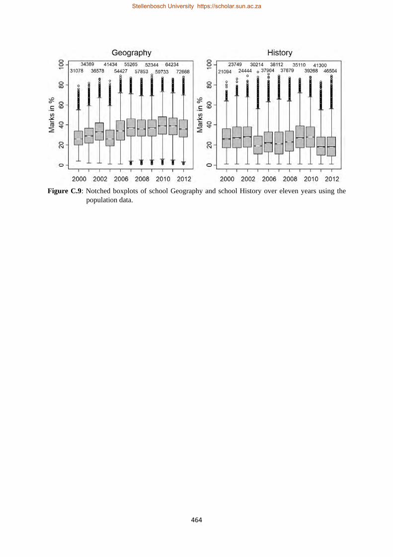
464
Figure C.9: Notched boxplots of school Geography and school History over eleven years using the
population data.
Stellenbosch University https://scholar.sun.ac.za

465
APPENDIX D
CORRESPONDENCE ANALYSIS RESULTS.
D.1. Categorical variables with their categories used in CA.
Table D.1: Labels and number of categories for categorical variables used in CA.
Variable Categories Labels of categories
FCCO 4 EX, PT, PR and CP (in Table E.1, they are represented by Fc1. Fc2,
Fc3 and Fc4, respectively).
NDIS 5 ND0, ND1, ND2, ND3 and ND4 or ND4 (or Nd0 to Nd4 in Table
E.1) corresponding to 0, 1, 2, 3 and at least four upper distinctions
DECLA 4 PASS, CRED, MERI and DIST (pass, credit, merit and distinction)
(in Table E.1, they are represented by Dc1, Dc2, Dc3 and Dc4,
respectively)
EPOINT 4 E5-7, E8-9, E10-11 and E12 (EPOINT between 5 and 7 points;
between 8 and 9 points; between 10 and 11 points; and at least 12
points). In Table E.1, they are represented by Ep1 to Ep4.
DEPOINT 3 E<P, E=P and E>P (or Dp1 to Dp3 in Table E.1) (EPOINT less than,
equal to and greater than the programme cut-off points).
All school
subjects
(grades)
5 UD12 (upper distinction), LD12 (lower distinction), UM12 (upper
merit), LM12 (lower merit) and CF12 (upper and lower credit, upper
and lower pass, and fail grades combined)
All school
subjects
(marks in %)
5 G12M1, G12M2, G12M3, G12M4, and G12M5 corresponding to the
bins of marks (in %): [0, 55), [55, 60), [60, 65), [65, 70), and
[70, 100).
G12AVE 5 Same bins of marks (in %) as for individual school variables.
All university
subjects
(grades)
6 DUU (upper distinction), LUU (lower distinction), MEU (merit),
CRU (credit), PAU (pass) and FAU ( fail)
All university
subjects
(marks in %)
6 UNM1, UNM2, UNM3, UNM4, UNM5 and UNM6 corresponding to
the bins of marks (in %): [0, 50), [50, 55), [55, 60), [60, 65), [65, 70),
and [70, 100).
University
averages
(marks in %)
7 UNM1, UNM2, UNM3, UNM4, UNM5, UNM6 and UNM7
corresponding to the bins of marks (in %): [0, 57), [57, 60), [60, 63),
[63, 66), [66, 69), [69, 72), and [72, 100).
Stellenbosch University https://scholar.sun.ac.za

466
D.2. Quality values and contributions of rows and columns to the first two dimensions of the
variables FYAVE and G12AVE per type of programmes over the four-year period.
Table D.2: Qualities and contributions (permills) of rows and columns to the first two dimensions for
FYAVE and G12AVE in business related programmes over the four-year period using the
first year dataset.
Category Year
2009 2011 2012 2013
Qlt Ctr1 Ctr2 Qlt Ctr1 Ctr2 Qlt Ctr1 Ctr2 Qlt Ctr1 Ctr2
Row
1
814
89
297
966
405
201
932
46
534
902
297
0
2 905 127 119 872 212 1 978 106 182 885 161 1
3 804 81 89 807 1 85 971 54 65 657 17 116
4 849 31 301 888 46 148 914 245 80 984 176 525
5 968 44 23 616 25 18 445 25 99 963 142 352
6 992 628 171 1000 311 547 959 525 40 716 207 6
Column
1 866 48 245 920 339 165 1000 188 618 948 474 35
2 964 23 355 848 186 1 955 175 328 404 25 2
3 837 184 47 941 83 359 799 79 10 743 92 74
4 713 8 371 993 268 220 619 89 2 789 250 91
5 992 738 33 983 123 255 909 470 43 1000 158 798
In column one of Table D.2, the rows numbers one to six and column numbers one to five represent
categories UNM1 to UNM6 of the variable FYAVE with associated interval of marks [0, 50),
[50, 55), [55, 60), [60, 65), [65, 70) and [70, 100) and categories G12M1, G12M2, G12M3, G12M4
and G12M5 of G12AVE corresponding to interval of marks [0, 55), [55, 60), [60, 65), [65, 69) and
[70, 100).
Stellenbosch University https://scholar.sun.ac.za

467
Table D.3: Qualities and contributions (permills) of rows and columns to the first two dimensions for FYAVE
and G12AVE in engineering related programmes over the four-year period using the first year dataset.
Category Year
2009 2011 2012 2013
Qlt Ctr1 Ctr2 Qlt Ctr1 Ctr2 Qlt Ctr1 Ctr2 Qlt Ctr1 Ctr2
Row
1
996
228
564
994
137
405
987
321
278
995
225
444
2 968 151 1 951 106 42 870 44 2 896 34 96
3 910 40 322 981 78 13 888 4 152 737 18 11
4 256 2 10 932 10 171 794 5 63 874 0 196
5 240 4 6 940 10 280 866 94 182 711 25 131
6 993 575 97 1000 659 89 999 532 323 999 698 122
Column
1 996 191 648 999 156 664 952 200 287 949 58 556
2 921 166 124 998 202 31 939 177 4 909 151 40
3 753 77 14 748 2 76 657 2 55 945 110 61
4 970 129 57 924 106 52 933 58 368 971 86 189
5 995 436 157 998 534 176 999 564 287 998 596 154
Table D.4: Qualities and contributions (permills) of rows and columns to the first two dimensions of FYAVE and
G12AVE in other programmes over the four-year period using the first year dataset
Category Year
2009 2011 2012 2013
Qlt Ctr1 Ctr2 Qlt Ctr1 Ctr2 Qlt Ctr1 Ctr2 Qlt Ctr1 Ctr2
Row
1
582
87
6
392
56
161
984
408
343
1000
101
2
2 877 28 204 213 4 7 861 119 50 975 247 95
3 856 78 82 254 8 36 992 267 135 700 12 185
4 771 2 240 109 3 9 987 15 279 957 493 0
5 997 779 81 910 31 711 765 48 103 946 146 308
6 888 25 386 998 899 76 999 143 89 978 1 411
Column
1 851 233 36 514 70 172 995 455 84 959 332 124
2 452 37 26 224 10 67 1000 527 115 653 51 71
3 981 395 51 960 88 464 743 4 270 995 6 732
4 943 0 654 462 0 161 894 14 531 967 610 73
5 935 335 233 993 832 137
Stellenbosch University https://scholar.sun.ac.za

468
In Table D.4, the variable G12AVE only had four categories in 2012 and 2013. The fifth category
corresponding to the interval of marks [70, 100) was empty and was thus deleted from the two-way
contingency tables for 2012 and 2013.
D.3. CA results of the variables FYAVE and NDIS for all programmes combined over the four -
year period using the first year dataset.
Table D.5: Qualities and contributions (permills) of rows and columns to the first two dimensions for
FYAVE and NDIS over the four-year period using the first year dataset.
Category Year
2009 2011 2012 2013
Qlt Ctr1 Ctr2 Qlt Ctr1 Ctr2 Qlt Ctr1 Ctr2 Qlt Ctr1 Ctr2
Row
1
764
52
216
998
269
144
995
240
49
951
118
154
2 920 61 27 945 11 120 387 48 21 998 176 602
3 797 98 228 885 60 22 800 59 245 90 16 25
4 974 24 514 512 6 258 760 0 391 761 23 113
5 703 83 2 695 41 272 999 137 105 974 125 2
6 990 682 13 998 613 185 995 514 189 996 542 103
Column
1 686 5 32 988 90 21 989 141 54 982 96 563
2 859 210 0 962 01 256 997 198 473 963 152 117
3 907 85 509 326 25 5 717 109 195 965 186 161
4 769 36 456 827 2 516 324 3 186 683 7 110
5 993 617 3 999 582 201 995 550 92 999 560 49
In column one of Table D.5 the rows numbers one to six and column numbers one to five represent
categories UNM1 to UNM6 of the variable FYAVE and categories ND0, ND1, ND2, ND3 and ND4 of
the variable NDIS corresponding zero, one, two, three, and at least four upper distinctions in school
subjects.
Stellenbosch University https://scholar.sun.ac.za

469
Figure D.1: CA biplot of row profiles (top panel) and CA asymmetric map (bottom panel) of FYAVE
and NDIS variables for all programmes combined in 2009 using the first year dataset.
Stellenbosch University https://scholar.sun.ac.za

470
Figure D.2: CA biplot of row profiles (top panel) and CA asymmetric map (bottom panel) of FYAVE
and NDIS variables for all programmes combined in 2011 using the first year dataset.
Stellenbosch University https://scholar.sun.ac.za
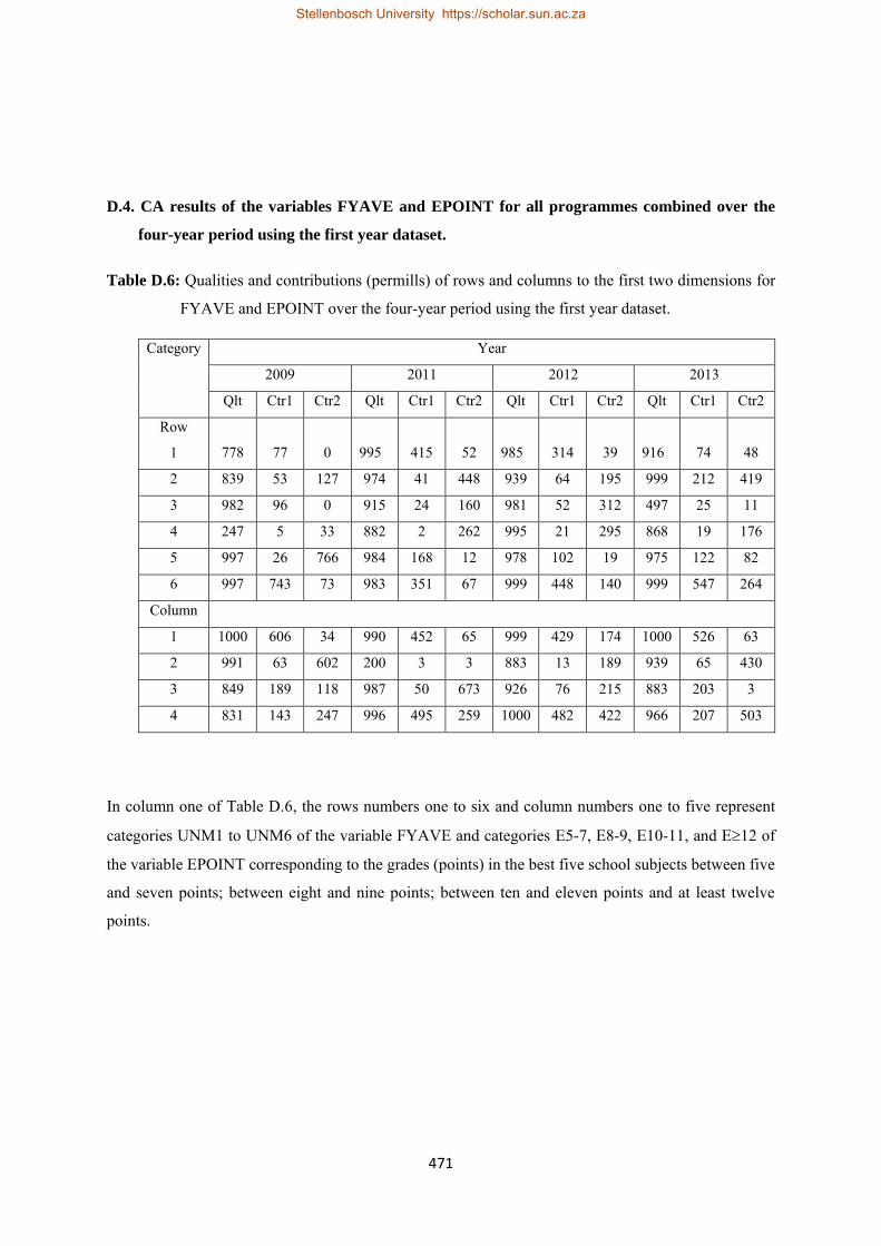
471
D.4. CA results of the variables FYAVE and EPOINT for all programmes combined over the
four-year period using the first year dataset.
Table D.6: Qualities and contributions (permills) of rows and columns to the first two dimensions for
FYAVE and EPOINT over the four-year period using the first year dataset.
Category Year
2009 2011 2012 2013
Qlt Ctr1 Ctr2 Qlt Ctr1 Ctr2 Qlt Ctr1 Ctr2 Qlt Ctr1 Ctr2
Row
1
778
77
0
995
415
52
985
314
39
916
74
48
2 839 53 127 974 41 448 939 64 195 999 212 419
3 982 96 0 915 24 160 981 52 312 497 25 11
4 247 5 33 882 2 262 995 21 295 868 19 176
5 997 26 766 984 168 12 978 102 19 975 122 82
6 997 743 73 983 351 67 999 448 140 999 547 264
Column
1 1000 606 34 990 452 65 999 429 174 1000 526 63
2 991 63 602 200 3 3 883 13 189 939 65 430
3 849 189 118 987 50 673 926 76 215 883 203 3
4 831 143 247 996 495 259 1000 482 422 966 207 503
In column one of Table D.6, the rows numbers one to six and column numbers one to five represent
categories UNM1 to UNM6 of the variable FYAVE and categories E5-7, E8-9, E10-11, and E12 of
the variable EPOINT corresponding to the grades (points) in the best five school subjects between five
and seven points; between eight and nine points; between ten and eleven points and at least twelve
points.
Stellenbosch University https://scholar.sun.ac.za

472
D.5. CA results of the variables FYAVE and individual school subjects for all programmes
combined over the four-year period using the first year dataset.
Table D.7: Qualities and contributions (permills) of rows and columns to the first two dimensions for
FYAVE and school Mathematics for all programmes combined over the four-year period
using the first year dataset.
Category Year
2009 2011 2012 2013
Qlt Ctr1 Ctr2 Qlt Ctr1 Ctr2 Qlt Ctr1 Ctr2 Qlt Ctr1 Ctr2
Row
1
995
275
499
980
259
141
998
410
371
997
303
302
2 902 130 0 997 207 81 187 0 76 958 149 80
3 881 55 189 742 40 75 304 3 16 854 1 272
4 897 11 136 801 22 310 704 23 251 984 90 49
5 989 156 26 945 119 5 941 121 16 976 165 1
6 998 373 150 997 353 389 1000 443 270 1000 291 296
Column
1 996 349 461 996 374 321 769 184 470 985 264 265
2 947 51 134 931 126 21 762 87 30 975 94 76
3 942 96 371 717 61 66 970 54 490 959 236 49
4 696 40 3 896 1 487 839 227 2 999 64 585
5 999 465 30 1000 438 105 1000 448 9 1000 342 26
In Table D.7, the categories of School Mathematics, and also of other school subjects were the same as for the variable G12AVE.
Stellenbosch University https://scholar.sun.ac.za

473
Table D.8: Qualities and contributions (permills) of rows and columns to the first two dimensions for FYAVE
and school English for all programmes over the four-year period using the first year dataset.
Category Year
2009 2011 2012 2013
Qlt Ctr1 Ctr2 Qlt Ctr1 Ctr2 Qlt Ctr1 Ctr2 Qlt Ctr1 Ctr2
Row
1
962
329
240
647
33
1
933
20
473
976
440
35
2 480 20 114 998 676 43 633 84 77 603 11 237
3 832 125 47 248 2 43 723 98 5 895 252 150
4 882 297 10 870 163 0 966 176 225 998 199 340
5 698 28 184 644 125 125 939 106 216 367 2 70
6 958 200 404 989 1 789 990 517 3 867 97 168
Column
1 889 1 475 726 235 28 400 11 47 722 85 129
2 808 161 110 925 7 400 554 13 89 869 304 58
3 892 260 343 831 12 458 784 72 240 670 144 8
4 181 22 3 860 64 113 926 6 618 981 1 678
5 963 556 69 927 682 2 999 898 7 997 466 127
Table D.9: Qualities and contributions (permills) of rows and columns to the first two dimensions for FYAVE
and school Biology for all programmes over the four-year period using the first year dataset.
Category Year
2009 2011 2012 2013
Qlt Ctr1 Ctr2 Qlt Ctr1 Ctr2 Qlt Ctr1 Ctr2 Qlt Ctr1 Ctr2
Row
1
794
31
66
930
144
86
904
97
2
975
54
169
2 832 27 0 969 107 92 980 63 0 869 75 163
3 876 99 46 993 677 0 959 174 28 950 13 355
4 975 57 0 168 9 14 962 4 402 973 15 216
5 1000 64 735 599 3 117 995 66 553 472 36 94
6 1000 722 153 966 61 690 998 595 15 991 807 4
Column
1 999 267 87 997 23 87 998 129 0 999 136 127
2 928 17 399 970 19 796 950 187 25 982 11 572
3 904 123 32 892 426 81 978 349 119 885 307 3
4 989 318 81 911 294 35 996 23 481 954 540 78
5 975 275 401 878 238 0 976 103 375 725 6 220
Stellenbosch University https://scholar.sun.ac.za

474
Table D.10: Principal inertias (values and %), cumulative % in the first two dimensions, total inertia, chi-squared values and p-values of FYAVE with school Science, Physics and Chemistry for all programmes combined over the four-year period using the first year dataset.
Item FYAVE vs School Science FYAVE vs School Physics FYAVE vs School Chemistry
2009 2011 2012 2013 2009 2011 2012 2013 2009 2011 2012 2013
Inr1 0.150 0.156 0.097 0.205 0.202 0.177 0.144 0..286 0.147 0.162 0.067 0.189
Inr2 0.026 0.059 0.031 0.03 0.014 0.05 0.019 0.068 0.043 0.021 0.029 0.03
Inr 0.186 0.231 0.136 0.242 0.223 0.230 0.179 0.370 0.208 0.193 0.103 0.229
Inr1% 80.8 67.3 71.2 84.6 90.5 77.1 80.5 77.5 70.7 83.8 65.6 82.7
Inr2% 14.2 25.5 22.6 12.4 6.2 20.0 10.8 18.5 20.6 11.1 27.8 13.0
Cum% 95.0 92.8 93.8 97.0 96.7 97.2 91.3 96.0 91.4 94.9 93.4 95.8
Chisq 45.5 77.7 51.5 105.7 44.3 56.6 45.2 113.5 41.3 47.5 26.0 70.0
P-value 0.00 0.00 0.00 0.00 0.00 0.00 0.00 0.00 0.00 0.00 0.17 0.00
Table D.11: Principal inertias (values and %), cumulative % in the first two dimensions, total inertia, chi-squared values and p-values of FYAVE with school Additional Mathematics, English Literature and Geography for all programmes over the four-year period using the first year dataset.
Item FYAVE vs School Ad. Maths FYAVE vs School Eng. Liter. FYAVE vs School Geograp.
2009 2011 2012 2013 2009 2011 2012 2013 2009 2011 2012 2013
Inr1 0.266 0.408 0.300 0.392 0.096 0.086 0.246 0.090 0.102 0.067 0.059 0.071
Inr2 0.100 0.065 0.069 0.089 0.084 0.052 0.064 0.057 0.019 0.027 0.019 0.010
Inr 0.397 0.489 0.428 0.511 0.196 0.159 0.356 0.176 0.131 0.100 0.083 0.083
Inr1% 67.1 83.4 70.0 76.6 48.9 54.0 69.1 51.1 78.2 67.2 70.9 86.0
Inr2% 25.1 13.3 16.2 17.4 42.8 32.9 18.1 32.3 14.7 27.1 22.4 13.1
Cum% 92.2 96.7 86.1 94.0 91.7 86.9 87.2 83.4 92.9 94.3 93.3 99.1
Chisq 50.0 70.8 74.9 110.9 13.3 16.8 28.5 22.5 35.7 34.8 32.0 35.1
P-value 0.00 0.00 0.00 0.00 0.862 0.67 0.10 0.31 0.02 0.02 0.04 0.02
Stellenbosch University https://scholar.sun.ac.za

475
Figure D.3: CA biplot of row profiles (top panel) and CA asymmetric map (bottom panel) of FYAVE
and school Physics for all programmes in 2013 using the first year dataset.
Stellenbosch University https://scholar.sun.ac.za

476
Figure D.4: CA biplot of row profiles (top panel) and CA asymmetric map (bottom panel) of FYAVE
and school Chemistry for all programmes in 2011 using the first year dataset.
Stellenbosch University https://scholar.sun.ac.za

477
Figure D.5: CA biplot of row profiles (top panel) and CA asymmetric map (bottom panel) of FYAVE
and school Science for all programmes in 2009 using the first year dataset.
Stellenbosch University https://scholar.sun.ac.za

478
Figure D.6: CA biplot of row profiles (top panel) and CA asymmetric map (bottom panel) of FYAVE
and school Additional Mathematics for all programmes in 2011 using the first year dataset.
Stellenbosch University https://scholar.sun.ac.za

479
D6. Grading schemes for school Mathematics for the 2007, and 2009 to 2011 grade twelve
examination years.
Table D.12 summarises the grades (points) with their association classifications, and numerical interval
grades for school Mathematics for the 2007, and 2009 to 2011 grade twelve examination years.
Numerical interval were estimated by cross-classifying the grades (points) with the actual marks (in %)
provided by the Examinations Council of Zambia (ECZ). The actual grade boundaries corresponding
to the grades were not readily available. Grade boundaries from lower credit to fail were not indicated
as these grades were rarely achieved by degree students.
Table D.12: Grading schemes for school Mathematics for the 2007, and 2009 to 2011 grade twelve examination years.
Grades Numerical interval grades (in %)
Points Classification 2007 2009 2010 2011
1 Upper distinction (UD) 65 to 100 66 to 100 65 to 100 67 to 100
2 Lower distinction (LD) 57 to 64 57 to 65 57 to 64 58 to 66
3 Upper merit (UM) 44 to 56 45 to 56 44 to 56 46 to 57
4 Lower merit (LM) 39 to 43 41 to 44 40 to 43 42 to 45
5 Upper credit (UC) 35 to 38 37 to 40 34 to 39 37 to 41
6 Lower credit (LC)
7 Upper pass (UP)
8 Lower pass (LP)
9 Fail (FA)
Table D.13: Categories of school Mathematics used in the analysis of Section 5.8.3 for the 2007, and 2009 to 2011 grade twelve examination years (corresponding to year in the first year of study 2009, and 2011 to 2013).
Categories Numerical interval grades (in %) Symbols Description 2007 2009 2010 2011 G12D5 Upper distinction 5 87 to 100 G12D4 Upper distinction 4 80 to 100 81 to 100 80 to 100 82 to 86 G12D3 Upper distinction 3 75 to 79 76 to 80 75 to 79 77 to 81 G12D2 Upper distinction 2 70 to 74 71 to 75 70 to 74 72 to 76 G12D1 Upper distinction 1 65 to 69 66 to 70 65 to 69 67 to 71 G12LD Lower distinction 57 to 64 57 to 65 57 to 64 58 to 66 G12UM Upper merit 44 to 56 45 to 56 44 to 56 46 to 57 G12LD Lower merit 39 to 43 41 to 44 40 to 43 42 to 45 G12CF Fail to upper credit combined 0 to 38 0 to 40 34 to 39 37 to 41
Stellenbosch University https://scholar.sun.ac.za

480
D.7. CA biplots of the variable FCCO with individual school subjects for all programmes
combined for selected years over the four-year period using the first year dataset.
Figure D.7: CA biplots of row profiles of FCCO with school Chemistry (top panel) and school Physics
(bottom panel) for all programmes combined in 2011 using the first year dataset.
Stellenbosch University https://scholar.sun.ac.za
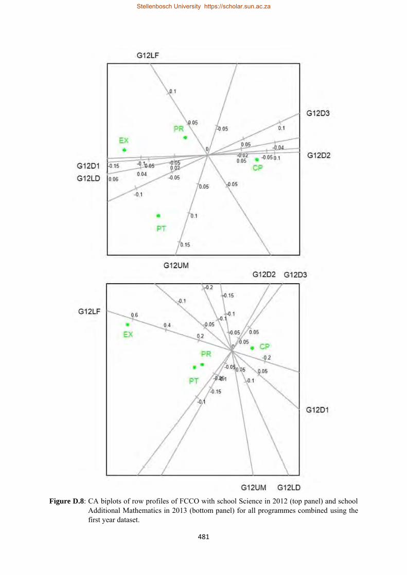
481
Figure D.8: CA biplots of row profiles of FCCO with school Science in 2012 (top panel) and school
Additional Mathematics in 2013 (bottom panel) for all programmes combined using the first year dataset.
Stellenbosch University https://scholar.sun.ac.za

482
D.7. CA results of the variables DECLA and UWA with school results variables for all
programmes combined for the graduate dataset.
Table D.14: Principal inertias (values and %), cumulative of the principal inertias (in %) in the first two
dimensions, total inertia, chi-squared value and p-values in the first two dimensions of the
variables DECLA and school variables G12AVE, Mathematics and English for all
programmes combined for graduates who were in their first year of study in 2009.
Item School variables G12AVE Mathematics English
Inr1 0.158 0.045 0.026 Inr2 0.020 0.002 0.015 Inr 0.194 0.049 0.047
Inr1% 81.4 92.2 56.2 Inr2% 10.3 4.4 33.1 Cum% 91.7 96.6 89.3 Chisq 51.1 13.0 12.3
P-value 0.00 0.37 0.42
Table D.15: Principal inertias (values and %), cumulative of the principal inertias (in %) in the first two
dimensions, total inertia, chi-squared value and p-values in the first two dimensions of the
variables UWA and EPOINT for all programmes combined for graduates who were in their
first year of study during the 2006-2010 period.
Item Year 2006 2007 2008 2009 2010
Inr1 0.067 0.049 0.073 0.134 0.098 Inr2 0.013 0.020 0.012 0.020 0.081 Inr 0.085 0.069 0.086 0.154 0.181
Inr1% 78.7 71.1 84.5 86.4 54.2 Inr2% 15.3 28.8 14.3 13.0 44.9 Cum% 94.0 99.9 98.8 99.4 99.1 Chisq 24.2 23.0 20.8 48.2 16.6
P-value 0.00 0.01 0.01 0.00 0.05
Stellenbosch University https://scholar.sun.ac.za

483
Figure D.9: CA biplot of row profiles (top panel) and CA asymmetric map (bottom panel) of DECLA
and school Mathematics variables for all programmes for graduates who were in their first
year of study in 2009.
Stellenbosch University https://scholar.sun.ac.za

484
Figure D.10: CA biplot of row profiles (top panel) and CA asymmetric map (bottom panel) of UWA
and EPOINT in engineering related programmes for graduates who were in their first
year of study in 2007.
Stellenbosch University https://scholar.sun.ac.za

485
D.8. Results of CA of square tables: G12AVE versus FYAVE.
Table D.16: Two-way contingency square table of G12AVE and FYAVE for the year 2013 in
engineering related programmes.
G12AVE FYAVE Total M1 M2 M3 M4 M5 M6 M7
m1 1 0 0 0 0 0 0 1 m2 11 1 2 1 1 0 0 16 m3 37 16 19 17 5 0 1 95 m4 48 26 23 27 22 2 2 150 m5 17 14 17 27 22 19 8 124 m6 1 2 4 6 6 10 10 39 m7 0 0 0 0 3 4 6 13
Total 115 59 65 78 59 35 27 438
Table D.17: Principal inertias and their associated percentages, and percentages of the symmetric and
the skew-symmetric parts of the variables G12AVE versus FYAVE for the year 2013 in
engineering related programmes (the numbers in ( ) in columns 4 and 5 of the last row refer
to the total inertias associated with the symmetric part and the skew-symmetric part,
respectively).
Dim Principal inertia % inertia % symmetric part % skew-symmetric part
1 0.3156 32.4 80.9
2 0.2633 27.0 45.1
3 0.2633 27.0 45.1
4 0.0546 5.6 14.0
5 0.0276 2.8 4.7
6 0.0276 2.8 4.7
7 0.0111 1.1 2.8
8 0.0063 0.6 1.6
9 0.0021 0.2 0.5
10 0.0010 0.1 0.2
11 0.0010 0.1 0.2
12 0.0004 0.0 0.1
13 0.0000 0.0 0.0
Total 0.9739 100.0 100.0 (0.3901) 100.0 (0.5838)
Stellenbosch University https://scholar.sun.ac.za

486
Figure D.11: CA map of the symmetric part (top panel) and CA map of the skew-symmetric part
(bottom panel) of G12AVE and FYAVE variables for engineering related programmes in the year 2013 using the first year dataset.
Stellenbosch University https://scholar.sun.ac.za

487
D.9. Results of CA of square tables: following the performance of students in engineering and
business related programmes from grade twelve to the fifth year of study.
Table D.18: Two-way contingency square tables of G12AVE and UWAY1 (table a), UWAY1 and
UWAY2 (table b), UWAY2 and UWAY3 (table c), UWAY3 and UWAY4 (table d), and
UWAY4 and UWAY5 (table e) variables for students in engineering related programmes
who were in their first year of study in 2009 and who graduated in 2013.
a.
G12AVE UWAY1 Total M1 M2 M3 M4 M5 M6 M7
m1 3 1 3 2 0 0 1 10 m2 4 7 0 1 3 0 0 15 m3 3 2 4 2 0 1 0 12 m4 1 3 3 4 7 3 4 25 m5 2 2 2 0 2 1 6 15 m6 0 0 0 0 1 3 5 9 m7 0 1 1 0 1 3 7 13
Total 13 16 13 9 14 11 23 99 b.
UWAY1 UWAY2 Total M1 M2 M3 M4 M5 M6 M7
m1 2 3 7 1 0 0 0 13 m2 2 4 4 3 2 1 0 16 m3 1 1 2 4 2 3 0 13 m4 0 0 5 2 1 1 0 9 m5 0 2 3 2 1 2 4 14 m6 0 0 2 1 3 1 4 11 m7 0 0 0 4 5 7 7 23
Total 5 10 23 17 14 15 15 99 c.
UWAY2 UWAY3 Total M1 M2 M3 M4 M5 M6 M7
m1 2 3 0 0 0 0 0 5 m2 5 2 1 2 0 0 0 10 m3 6 10 5 2 0 0 0 23 m4 0 3 4 3 3 3 1 17 m5 0 1 1 4 3 1 4 14 m6 0 0 0 2 5 6 2 15 m7 0 0 0 0 3 2 10 15
Total 13 19 11 13 14 12 17 99
Stellenbosch University https://scholar.sun.ac.za

488
d.
UWAY3 UWAY4 Total M1 M2 M3 M4 M5 M6 M7
m1 0 6 6 0 1 0 0 13 m2 2 4 5 3 3 2 0 19 m3 0 0 1 2 3 5 0 11 m4 0 0 1 5 3 0 4 13 m5 0 1 2 0 2 7 2 14 m6 0 0 0 2 2 2 6 12 m7 0 0 1 1 1 8 6 17
Total 2 11 16 13 15 24 18 99 e.
UWAY4 UWAY5 Total M1 M2 M3 M4 M5 M6 M7
m1 0 0 3 4 0 0 0 7 m2 0 1 2 1 2 0 0 6 m3 1 0 5 4 4 1 1 16 m4 0 0 1 2 3 4 3 13 m5 0 0 0 4 3 5 3 15 m6 0 0 1 1 2 11 9 24 m7 0 0 0 0 3 6 9 18
Total 1 1 12 16 17 27 25 99
Stellenbosch University https://scholar.sun.ac.za

489
Table D.19: Partial CA of the contingency tables in Table B.18: total inertia (Inr), inertia, inertias of
the best two dimensions (Inr1 and Inr2), their percentages (Inr1% and Inr2%) and
cumulative percentages (Cum%) for the symmetric and skew-symmetric parts.
Items G12AVE vs.
UWAY1
UWAY1 vs.
UWAY2
UWAY2 vs.
UWAY3
UWAY3 vs.
UWAY4
UWAY4 vs.
UWAY5
Inertia (symmetric) 0.5344 0.5734 0.9920 0.6837 0.5678
Inertia (skew-sym) 0.2948 0.2327 0.3635 0.5223 0.3676
Total inertia 0.8292 0.8061 1.3555 1.2060 0.9354
Inr1 (symmetric) 0.3729 0.3917 0.6938 0.3666 0.3874
Inr2 (symmetric) 0.1206 0.1221 0.2001 0.1436 0.0798
Inr1% (symmetric) 69.8 68.3 69.9 53.6 68.2
Inr2% (symmetric) 22.6 21.3 20.2 21.0 14.1
Cum% (symmetric) 92.4 89.6 90.1 74.6 82.3
Inr1 (skew-sym.) 0.1136 0.0829 0.1557 0.2071 0.1441
Inr2 (skew-sym.) 0.1136 0.0829 0.1557 0.2071 0.1441
Inr1% (skew-sym.) 38.5 35.6 42.9 39.7 39.2
Inr2% (skew-sym.) 38.5 35.6 42.9 39.7 39.2
Cum% (skew-sym.) 77.0 71.2 85.8 79.4 78.4
Table D.20: Dimensions and best two dimensions for the symmetric part and skew-symmetric parts for
contingency tables in Table D.18.
Variables Dims for
symmetric parts
Dims for skew-
symmetric parts
Best two dims
for symm. part
Best two dims
for skew-sym.
G12AVE vs. UWAY1 1, 2, 7, 8, 9 ,12, 13 3, 4, 5, 6, 10, 11 1, 2 3, 4
UWAY1 vs. UWAY2 1, 2, 7, 8, 9 ,10, 13 3, 4, 5, 6, 11, 12 1, 2 3, 4
UWAY2 vs. UWAY3 1, 2, 5, 6, 9, 12, 13 3, 4, 7, 8, 10, 11 1, 2 3, 4
UWAY3 vs. UWAY4 1, 4, 5, 6, 9 ,12, 13 2, 3, 7, 8, 10, 11 1, 4 2, 3
UWAY4 vs. UWAY5 1, 4, 5, 8, 9 ,12, 13 2, 3, 6, 7, 10, 11 1, 4 2, 3
Stellenbosch University https://scholar.sun.ac.za

490
Table D.21: Two-way contingency square tables of G12AVE and UWAY1 (table a), UWAY1 and
UWAY2 (table b), UWAY2 and UWAY3 (table c), and UWAY3 and UWAY4 (table d)
variables for the 2009 students in business related programmes who graduated in 2012.
a.
G12AVE UWAY1 Total M1 M2 M3 M4 M5 M6 M7
m1 2 0 0 0 0 0 0 2 m2 2 2 6 2 1 0 2 15 m3 2 6 5 4 0 0 0 17 m4 1 7 4 2 3 1 0 18 m5 2 2 2 2 2 2 0 12 m6 0 0 3 2 2 0 1 8 m7 0 0 1 1 1 4 1 8
Total 9 17 21 13 9 7 4 80 b.
UWAY1 UWAY2 Total M1 M2 M3 M4 M5 M6 M7
m1 4 5 0 0 0 0 0 9 m2 8 5 3 1 0 0 0 17 m3 4 10 3 2 1 1 0 21 m4 1 5 4 3 0 0 0 13 m5 0 2 2 2 1 1 1 9 m6 0 1 1 3 2 0 0 7 m7 0 0 0 0 2 0 2 4
Total 17 28 13 11 6 2 3 80
c.
UWAY2 UWAY3 Total M1 M2 M3 M4 M5 M6 M7
m1 2 8 3 4 0 0 0 17 m2 4 9 6 6 1 1 1 28 m3 2 1 5 3 0 2 0 13 m4 0 4 2 4 0 0 1 11 m5 0 0 3 1 2 0 0 6 m6 0 0 0 1 1 0 0 2 m7 0 0 0 0 0 0 3 3
Total 8 22 19 19 4 3 5 80 d.
UWAY3 UWAY4 Total M1 M2 M3 M4 M5 M6 M7
m1 2 1 3 1 1 0 0 8 m2 1 5 5 9 0 2 0 22 m3 0 1 3 9 2 2 2 19 m4 0 1 4 4 5 1 4 19 m5 0 0 0 1 1 0 2 4 m6 0 0 0 0 0 2 1 3 m7 0 0 0 0 1 1 3 5
Total 3 8 15 24 10 8 12 80
Stellenbosch University https://scholar.sun.ac.za
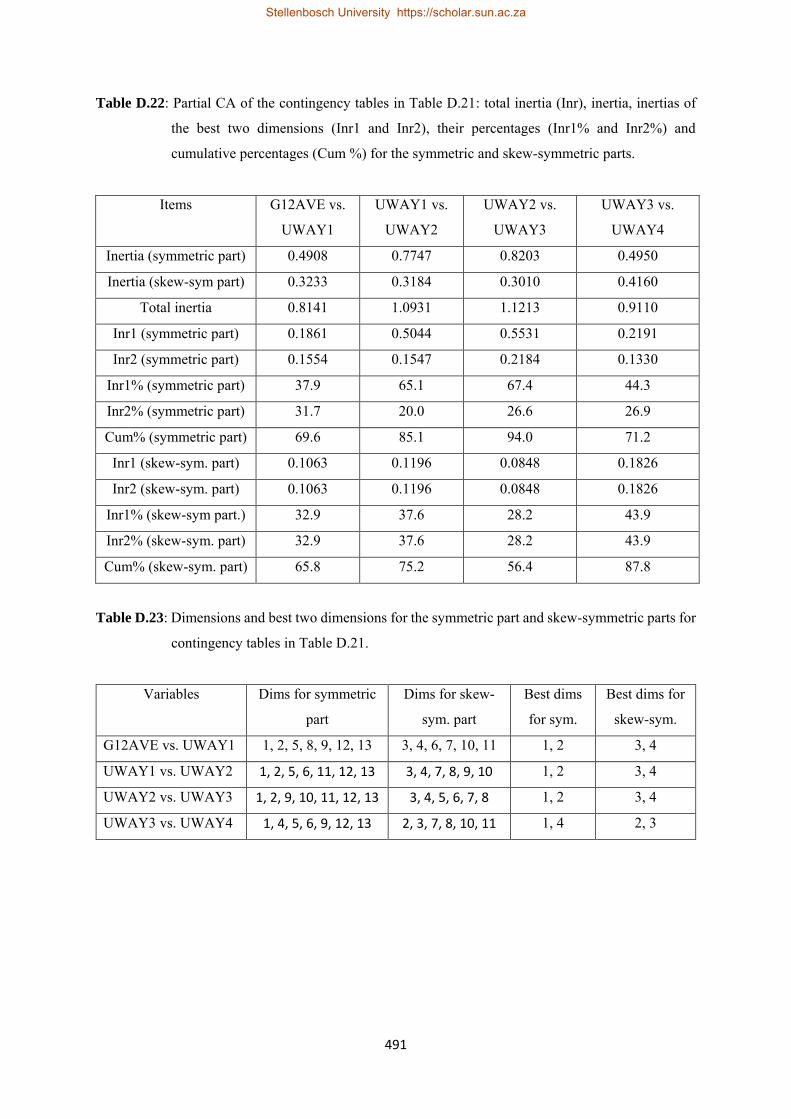
491
Table D.22: Partial CA of the contingency tables in Table D.21: total inertia (Inr), inertia, inertias of
the best two dimensions (Inr1 and Inr2), their percentages (Inr1% and Inr2%) and
cumulative percentages (Cum %) for the symmetric and skew-symmetric parts.
Items G12AVE vs.
UWAY1
UWAY1 vs.
UWAY2
UWAY2 vs.
UWAY3
UWAY3 vs.
UWAY4
Inertia (symmetric part) 0.4908 0.7747 0.8203 0.4950
Inertia (skew-sym part) 0.3233 0.3184 0.3010 0.4160
Total inertia 0.8141 1.0931 1.1213 0.9110
Inr1 (symmetric part) 0.1861 0.5044 0.5531 0.2191
Inr2 (symmetric part) 0.1554 0.1547 0.2184 0.1330
Inr1% (symmetric part) 37.9 65.1 67.4 44.3
Inr2% (symmetric part) 31.7 20.0 26.6 26.9
Cum% (symmetric part) 69.6 85.1 94.0 71.2
Inr1 (skew-sym. part) 0.1063 0.1196 0.0848 0.1826
Inr2 (skew-sym. part) 0.1063 0.1196 0.0848 0.1826
Inr1% (skew-sym part.) 32.9 37.6 28.2 43.9
Inr2% (skew-sym. part) 32.9 37.6 28.2 43.9
Cum% (skew-sym. part) 65.8 75.2 56.4 87.8
Table D.23: Dimensions and best two dimensions for the symmetric part and skew-symmetric parts for
contingency tables in Table D.21.
Variables Dims for symmetric
part
Dims for skew-
sym. part
Best dims
for sym.
Best dims for
skew-sym.
G12AVE vs. UWAY1 1, 2, 5, 8, 9, 12, 13 3, 4, 6, 7, 10, 11 1, 2 3, 4
UWAY1 vs. UWAY2 1, 2, 5, 6, 11, 12, 13 3, 4, 7, 8, 9, 10 1, 2 3, 4
UWAY2 vs. UWAY3 1, 2, 9, 10, 11, 12, 13 3, 4, 5, 6, 7, 8 1, 2 3, 4
UWAY3 vs. UWAY4 1, 4, 5, 6, 9, 12, 13 2, 3, 7, 8, 10, 11 1, 4 2, 3
Stellenbosch University https://scholar.sun.ac.za

492
D.10. CA results of stacked tables of variables FYAVE and EPOINT using variable FYEAR.
Table D.24: Four stacked two-way contingency tables of the variables FYAVE and EPOINT, using
variable FYEAR for all programmes combined.
FYEAR FYAVE EPOINT E5-7 E8-9 E10-11 E>=12
2009 U1 7 15 9 8 U2 19 20 18 14 U3 25 37 30 14 U4 38 31 33 10 U5 24 30 6 1 U6 47 6 1 1
2011 U1 3 19 14 21 U2 17 31 11 19 U3 30 46 33 23 U4 35 59 36 21 U5 35 38 14 6 U6 35 26 9 2
2012 U1 23 48 18 22 U2 20 36 18 9 U3 44 45 18 21 U4 49 61 22 6 U5 42 39 11 3 U6 50 25 5 0
2013 U1 59 72 45 16 U2 33 43 35 22 U3 43 53 20 14 U4 62 49 24 4 U5 46 27 6 1 U6 60 8 1 0
Table D.25: Partial CA results of four stacked contingency tables (stacked using variable FYEAR) of
variables FYAVE and EPOINT for all programmes combined using the first year dataset.
Dim Principal inertia % inertia Cumulative %
1 0.1405 78.0 78.0
2 0.0242 13.5 91.5
3 0.0153 5.5 100.0
Total 0.1800 100.0
Stellenbosch University https://scholar.sun.ac.za

493
D.11. CA results of stacked tables of variables FYAVE with school Mathematics and English
using variable FYEAR.
Table D.26: Four stacked two-way contingency tables of the variables FCCO and school Mathematics,
using variable FYEAR for all programmes combined.
FYEAR FCCO School Mathematics G1 G2 G3 G4 G5
2009 CP 12 25 25 40 167 EX 5 1 2 1 0 PR 26 22 27 20 42 PT 13 2 2 7 5
2011 CP 24 19 37 55 184 EX 11 3 5 1 3 PR 43 30 34 4 69 PT 5 5 5 4 6
2012 CP 17 17 28 41 189 EC 13 4 6 7 10 PR 36 24 32 30 124 PT 8 4 8 17 20
2013 CP 15 19 15 39 280 EX 13 7 17 13 39 PR 19 14 20 26 100 PT 19 9 11 18 50
Table D.27: Partial CA results of four stacked contingency tables (stacked using variable FYEAR) of
variables FCCO and school Mathematics for all programmes combined using the first year
dataset.
Dim Principal inertia % inertia Cumulative %
1 0.1250 82.6 82.6
2 0.0142 9.4 92.0
3 0.0088 5.8 97.8
4 0.0033 2.2 100.0
Total 0.1513 100.0
Stellenbosch University https://scholar.sun.ac.za

494
Figure D.12: CA biplot of row profiles of four stacked contingency tables (stacked using variable
FYEAR) of variables FCCO and school Mathematics for all programmes combined for the first year dataset.
Stellenbosch University https://scholar.sun.ac.za

495
Table D.28: Four stacked two-way contingency tables of the variables FCCO and school English, using
variable FYEAR for all programmes combined.
FYEAR FCCO School English G1 G2 G3 G4 G5
2009 CP 35 55 70 46 62 EX 0 2 1 1 5 PR 19 21 37 33 27 PT 7 3 7 6 6
2011 CP 115 91 74 31 8 EX 8 6 5 4 0 PR 61 47 60 32 16 PT 4 11 6 2 2
2012 CP 86 75 60 42 29 EX 10 13 9 4 4 PR 65 59 63 41 17 PT 15 16 18 5 3
2013 CP 25 38 69 106 129 EX 7 8 11 26 37 PR 12 18 38 44 67 PT 3 11 13 24 56
Table D.29: Partial CA results of four stacked contingency tables (stacked using variable FYEAR) of
variables FCCO and school English for all programmes combined using the first year
dataset.
Dim Principal inertia % inertia Cumulative %
1 0.2211 91.4 91.4
2 0.0104 4.3 95.6
3 0.0081 3.3 9.0
4 0.0025 1.0 100.0
Total 0.2421 100.0
Stellenbosch University https://scholar.sun.ac.za

496
Figure D.13: CA biplot of row profiles of four stacked contingency tables (stacked using variable FYEAR) of variables FCCO and school English for all programmes combined for the first year dataset.
Stellenbosch University https://scholar.sun.ac.za

497
D.12. Stacked table of variables FYAVE and G12AVE, stacked using variables FYEAR and
TPROG.
Table D.30: Twelve stacked two-way contingency tables of the variables FYAVE and G12AVE, using
variables FYEAR and TPROG.
FYEAR FYAVE TPROG
Business related prog. Engineering related prog. Other programmes
G12AVE G12AVE G12AVE
G1 G2 G3 G4 G5 G1 G2 G3 G4 G5 G1 G2 G3 G4 G5
2009 U1 1 5 4 2 0 5 4 5 0 0 8 3 1 1 0
U2 1 6 12 2 1 3 9 9 3 0 12 9 3 0 1
U3 0 4 14 5 1 1 15 12 13 1 17 16 7 0 0
U4 0 2 8 9 4 2 7 13 11 4 14 19 15 4 0
U5 0 3 6 5 4 1 5 11 9 5 0 2 8 0 2
U6 0 2 0 1 6 0 1 4 19 18 1 0 2 1 0
2011 U1 5 10 1 0 0 5 4 3 1 0 18 7 1 2 0
U2 3 17 5 0 0 5 7 10 3 0 10 11 7 0 0
U3 2 14 19 3 1 5 8 10 6 0 16 35 13 0 0
U4 1 12 23 5 1 2 11 20 11 1 13 33 14 4 0
U5 0 14 14 5 1 1 10 15 12 0 3 2 13 3 0
U6 0 3 5 7 3 2 1 16 19 12 0 1 2 0 1
2012 U1 5 1 1 1 0 27 28 25 8 3 9 2 1 0 0
U2 5 4 1 0 0 8 16 18 10 3 9 4 4 1 0
U3 3 9 3 1 0 6 14 27 18 4 14 21 3 2 0
U4 8 21 3 1 0 5 16 25 19 9 13 9 6 3 0
U5 4 14 11 8 3 2 4 14 20 8 2 3 1 1 0
U6 3 6 10 6 12 2 1 10 8 21 0 1 0 0 0
2013 U1 20 14 7 3 0 12 37 48 17 1 14 11 8 0 0
U2 12 9 9 0 0 1 16 26 14 2 22 14 8 0 0
U3 5 11 9 3 3 2 19 23 17 4 8 14 11 1 0
U4 1 10 17 8 0 1 17 27 27 6 4 10 7 4 0
U5 1 3 6 2 3 1 5 22 22 9 1 4 0 1 0
U6 0 0 2 3 1 0 1 4 27 30 0 0 1 0 0
Stellenbosch University https://scholar.sun.ac.za

498
APPENDIX E
MULTIPLE CORRESPONDENCE ANALYSIS RESULTS.
E.1 Categorical variables with their categories used in MCA.
The variables in Table E.1 are fully described in Table A.4 in Appendix A. Additional information is
provided in Table D.1 in Appendix D.
Table E.1. Categorical variables used in MCA with their numbers of categories and the labels of
categories.
Variable Abbreviation Number of
categories
Labels of categories
FCCO Fc 4 Fc1, Fc2, Fc3 and Fc4 representing categories EX,
PT, PR, and CP.
NDIS Nd 5 Nd0, Nd1, Nd2, Nd3 and Nd4 corresponding to zero,
one, two, three and at least four distinctions.
FYEAR Fy 14 or 4 From Fy1 to Fy14 representing the years 2000 to 2013
when the grades are used and from Fy1 to Fy4
corresponding to the years 2009, and 2011 to 2013
when marks (in %) are used.
CYEAR Cy 5 Cy1, Cy2, Cy3, Cy4, and Cy5 representing the years
2009 to 2013.
DECLA Dc 4 Dc1, Dc2, Dc3, and Dc4: Pass, Credit, Merit and
Distinction.
EPOINT Ep 4 Ep1, Ep2, Ep3 and Ep4 representing categories E5-7,
E8-9, E10-11 and E12.
DEPOINT Dp 3 Dp1, Dp2, and Dp3 representing categories E<P,
E=P, and E>P.
All school
subjects
5
School
subjects
Ma (Mathematics), Ad (Additional Mathematics), En (English Literature), Ss
(Science), Ph (Physics), Ch (Chemistry), Bi (Biology), Ge (Geography), Hi
(History), Ac (Principles of Accounts), Co (Commerce), Dr (Geometrical and
Mechanical Drawings/Geometrical and Building Drawings), As (Agriculture
Science), Re (Religious Education/Bible Knowledge), Za (Zambian Language), Mw
Stellenbosch University https://scholar.sun.ac.za

499
Table E1 continued.
Variable Abbreviation Number of
categories
Labels of categories
(Metal/Wood Work), Cs (Computer Science), Fn (Food and Nutrition), and Ce
(Civic Education).
All school
subjects
(grades)
5 CF12, LM12, UM12, LD12, and UD12 coded as 1, 2,
3, 4, and 5. The labels of categories are created by
combining the abbreviations of the variables with the
numbers representing the categories. For example for
Mathematics, the different labels are Ma1, Ma2, Ma3,
Ma4 and Ma5.
All school
subjects
(marks in %)
5 G12M1, G12M2, G12M3, G12M4, and G12M5
corresponding to the bins of marks in %: [0, 55),
[55, 60), [60, 65), [65, 70) and [70, 100) and coded as
1, 2, 3, 4, and 5. Again the labels of categories are
created by combining the abbreviations of the
variables with the numbers representing the
categories. For example for Mathematics, the
different labels are Ma1, Ma2, Ma3, Ma4 and Ma5.
G12AVE GA 5 GA1, GA2, GA3, GA4 and GA5 representing
categories G12M1, G12M2, G12M3, G12M4, and
G12M5.
All first
university
subjects
(grades)
6 FAU, PAU, CRU, MEU, LUU and DUU coded as 1,
2, 3, 4, 5, and 6.
All first
university
subjects
(marks in %)
6 UNM1, UNM2, UNM3, UNM4, UNM5 and UNM6
corresponding to the bins of marks in %: [0, 50),
[50, 55), [55, 60), [60, 65), [65, 70) and [70, 100) and
coded as 1, 2, 3, 4, 5 and 6.
First year
subjects
F1, F2, F3, F4, F5, F6 and F7 with labels of categories created by affixing the
numbers representing the categories to the abbreviations of the first year subjects.
For example for F1, the labels are F11, F12, F13, F14, F15, and F16.
University
averages
UA1 (UWAY1), UA2 (UWAY2), UA3 (UWAY3), UA4 (UWAY4), UA5
(UWAY5), and UW (UWA) with the labels of the categories created by combining
the abbreviations of the variables with the numbers representing the categories.
Stellenbosch University https://scholar.sun.ac.za

500
Table E1 continued
Variable Abbreviation Number of
categories
Labels of categories
For example for variable UWA with abbreviation UW, the labels are UW1, UW2,
UW3, UW4 and UWA5.
University
averages
(marks in %)
7 UNM1, UNM2, UNM3, UNM4, UNM5, UNM6 and
UNM7 corresponding to the bins of marks in %:
[0, 57), [57, 60), [60, 63), [63, 66), [66, 69), [69, 72),
and [72, 100), and coded as 1, 2, 3, 4, 5, 6 and 7.
E.2 MCA results of variable DECLA with more individual school results variables.
Table E.2: List of categorical variables and their categories for the graduate dataset based on grades.
Variable Abbreviation Labels of categories
School Mathematics Ma Ma1, Ma2, Ma3, Ma4 and Ma5 or M1, M2, M3, M4 and
M5
School English En En1, En2, En3, En4 and En5 or E1, E2, E3, E4 and E5
School Science Ss Ss1, Ss2, Ss3, Ss4 and Ss5
School Biology Bi Bi1, Bi2, Bi3, Bi4 and Bi5 or B1, B2, B3, B4 and B5
School Physics Ph Ph1, Ph2, Ph3, Ph4 and Ph5 or P1, P2, P3, P4 and P5
School Chemistry Ch Ch1, Ch2, Ch3, Ch4 and Ch5 or C1, C2, C3, C4 and C5
DECLA Dc Dc1, Dc2, Dc3 and Dc4
TPROG Tp Tp1, Tp2 and Tp3.
CYEAR Cy Cy1, Cy2, Cy3, Cy4, Cy5, Cy6, Cy7, Cy8, Cy9, Cy10,
Cy11, Cy12, Cy13 and Cy14 or y1 to y14
NDIS Nd Nd0, Nd1, Nd2, Nd3 and Nd4
EPOINT Ep Ep1, Ep2, Ep3 and Ep4
DEPOINT Dp Dp1, Dp2 and Dp3
Stellenbosch University https://scholar.sun.ac.za

501
Figure E.1: Adjusted MCA maps (without zoom (top) of variables in Table E.1 of the graduate data
set, with individual school results in school Maths, English, Science and Biology
categorised using grades. The bottom panel is the zoomed version of the top one.
Stellenbosch University https://scholar.sun.ac.za

502
Figure E.2: Adjusted MCA maps (without zoom (top) of variables in Table E.1, with school results in school Maths, English, Physics, Chemistry and Biology categorised using grades. The categories of school subjects are abbreviated in the top map by using only the first letter. For variable CYEAR, the abbreviation “y” is used. The bottom panel is the zoomed version of the top one.
Stellenbosch University https://scholar.sun.ac.za

503
Table E.3: Partial MCA results of the variables in Table E.2 for the graduate dataset with individual
school results variables categorised based on grades using only school Maths, English,
Science and Biology.
Dim Principal inertia % inertia Cumulative %
1 0.0930 47.3 47.3
2 0.0122 6.2 53.5
3 0.0052 2.6 56.2
⁞ ⁞ ⁞ ⁞
24 0.0000 0.0 61.4
Total 0.1965
Table E.4: Partial MCA results of the variables in Table E.2 for the graduate dataset with individual
school results variables categorised based on grades using only school Maths, English,
Physics, Chemistry and Biology.
Dim Principal inertia % inertia Cumulative %
1 0.0916 42.4 42.4
2 0.0135 6.2 48.7
3 0.0053 2.5 51.1
⁞ ⁞ ⁞ ⁞
27 0.0000 0.0 57.4
Total 0.2160
Stellenbosch University https://scholar.sun.ac.za

504
APPENDIX F
CATEGORICAL PCA RESULTS. F.1 Transformation plots for the years 2001 and 2012 of the variables in Table 7.9.
Figure F.1: Transformation plots (final optimal z-scores) of the variables Ma, En, Ph, Ch, Bi, Tp, Dc,
and Nd for the year 2001, using the graduate dataset.
-0.4
0.0
Ma
Fina
l z q
uant
ificat
ion
Ma2 Ma3 Ma4 Ma5
-0.4
0.0
En
Fina
l z q
uant
ificat
ion
En2 En3 En4 En5
-0.4
0.0
Tp
Fina
l z q
uant
ificat
ion
Tp1 Tp2 Tp3
-0.4
0.0
Dc
Fina
l z q
uant
ificat
ion
Dc1 Dc2 Dc3
-0.4
0.0
Nd
Fina
l z q
uant
ificat
ion
Nd0 Nd1 Nd2 Nd3 Nd4
-0.4
0.0
Ph
Fina
l z q
uant
ificat
ion
Ph2 Ph3 Ph4 Ph5
-0.4
0.0
Ch
Fina
l z q
uant
ificat
ion
Ch2 Ch3 Ch4 Ch5
-0.4
0.0
Bi
Fina
l z q
uant
ificat
ion
Bi2 Bi3 Bi4 Bi5
Stellenbosch University https://scholar.sun.ac.za

505
Figure F.2: Transformation plots (final optimal z-scores) of the variables Ma, En, Ph, Ch, Bi, Tp, Dc,
and Nd for the year 2012, using the graduate dataset.
-0.2
0.0
MaFi
nal z
qua
ntific
atio
n
Ma2 Ma3 Ma4 Ma5
-0.2
0.0
En
Fina
l z q
uant
ificat
ion
En2 En3 En4 En5
-0.2
0.0
Tp
Fina
l z q
uant
ificat
ion
Tp1 Tp2 Tp3
-0.2
0.0
Dc
Fina
l z q
uant
ificat
ion
Dc1 Dc2 Dc3
-0.2
0.0
Nd
Fina
l z q
uant
ificat
ion
Nd0 Nd1 Nd2 Nd3 Nd4
-0.2
0.0
PhFi
nal z
qua
ntific
atio
n
Ph2 Ph3 Ph4 Ph5
-0.2
0.0
Ch
Fina
l z q
uant
ificat
ion
Ch2 Ch3 Ch4 Ch5
-0.2
0.0
Bi
Fina
l z q
uant
ificat
ion
Bi2 Bi3 Bi4 Bi5
Stellenbosch University https://scholar.sun.ac.za

506
F.2 Transformation plots based on actual marks (%) for 2012 using the first year dataset.
Figure F.3: Transformation plots (final optimal z-scores) of the variables Ma, En, GA, Tp, Fc, Nd, and
Ep for the year 2012, using the first year dataset (analysis based on actual marks).
-0.0
50.
05
Ma
Fina
l z q
uant
ificat
ion
Ma1 Ma2 Ma3 Ma4 Ma5
-0.0
50.
05
En
Fina
l z q
uant
ificat
ion
En1 En2 En3 En4 En5
-0.0
50.
05
GA
Fina
l z q
uant
ificat
ion
GA1 GA2 GA3 GA4 GA5-0
.05
0.05
Tp
Fina
l z q
uant
ificat
ion
Tp1 Tp2 Tp3
-0.0
50.
05
Fc
Fina
l z q
uant
ificat
ion
Fc1 Fc2 Fc3 Fc4
-0.0
50.
05
Nd
Fina
l z q
uant
ificat
ion
Nd0 Nd1 Nd2 Nd3 Nd4
-0.0
50.
05
Ep
Fina
l z q
uant
ificat
ion
Ep1 Ep2 Ep3 Ep4
Stellenbosch University https://scholar.sun.ac.za

507
F.3 Transformation plots based on grades for the year 2006 using the first year dataset.
Figure F.4: Transformation plots (final optimal z-scores) of the variables Ma, En, Ph, Ch, Bi, Tp, Fc,
and Nd for the year 2006, using the first year dataset (analysis based on grades).
-0.1
50.
05
Ma
Fina
l z q
uant
ificat
ion
Ma1 Ma2 Ma3 Ma4 Ma5
-0.1
50.
05
En
Fina
l z q
uant
ificat
ion
En1 En2 En3 En4 En5
-0.1
50.
05
Ph
Fina
l z q
uant
ificat
ion
Ph1 Ph2 Ph3 Ph4 Ph5-0
.15
0.05
Ch
Fina
l z q
uant
ificat
ion
Ch1 Ch2 Ch3 Ch4 Ch5
-0.1
50.
05
Bi
Fina
l z q
uant
ificat
ion
Bi1 Bi2 Bi3 Bi4 Bi5
-0.1
50.
05
Tp
Fina
l z q
uant
ificat
ion
Tp1 Tp2 Tp3
-0.1
50.
05
Fc
Fina
l z q
uant
ificat
ion
Fc1 Fc2 Fc3 Fc4
-0.1
50.
05
Nd
Fina
l z q
uant
ificat
ion
Nd0 Nd1 Nd2 Nd3 Nd4
Stellenbosch University https://scholar.sun.ac.za

508
APPENDIX G
CVA AND AoD RESULTS.
G.1 CVA biplots for the graduate dataset using variable Dc (DECLA) as the grouping variable.
Figure G.1: Weighted CVA biplot with 0.95 bags (top panel: with the individual observations plotted,
bottom panel: with the plotting of the observations suppressed) of the graduate dataset using variables GA, Ma, En, Ph, Ch, and Bi.
Stellenbosch University https://scholar.sun.ac.za

509
G.2 CVA biplots for the first year dataset using variable Fc (FCCO) as the grouping variable.
Figure G.2: Weighted CVA biplot with 0.95 bags (top panel: with the individual observations plotted,
bottom panel: with the plotting of the observations suppressed) for the 2013 first year intake using variables GA, Ma, En, Ph, Ch, and Bi.
Stellenbosch University https://scholar.sun.ac.za
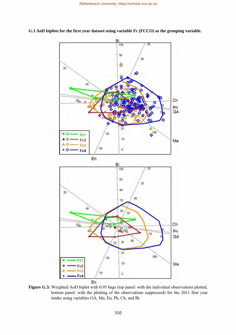
510
G.3 AoD biplots for the first year dataset using variable Fc (FCCO) as the grouping variable.
Figure G.3: Weighted AoD biplot with 0.95 bags (top panel: with the individual observations plotted,
bottom panel: with the plotting of the observations suppressed) for the 2011 first year intake using variables GA, Ma, En, Ph, Ch, and Bi.
Stellenbosch University https://scholar.sun.ac.za

511
Figure G.4: Weighted AoD biplot with 0.95 bags (top panel: with the individual observations plotted,
bottom panel: with the plotting of the observations suppressed) for the 2012 first year intake using variables GA, Ma, En, Ph, Ch, and Bi.
Stellenbosch University https://scholar.sun.ac.za
Copyright © 2022 FDOKUMEN