arX

iv:1

207.

1848

v1 [

phys

ics.

data

-an]

8 J

ul 2

012

A Simple Non-Markovian Computational Model of the Statistics ofSoccer Leagues: Emergence and Scaling effects

Roberto da Silva1, Mendeli Vainstein1, Luis Lamb2, Sandra Prado1

1 - Instituto de FısicaUniversidade Federal do Rio Grande do Sul

Av. Bento Goncalves 9500Caixa Postal 15051 91501-970, Porto Alegre RS, BrazilE-mail:rdasilva,mendeli,sprado@if.ufrgs.br

2 - Instituto de InformaticaUniversidade Federal do Rio Grande do Sul

Av. Bento Goncalves 9500Caixa Postal 15064 91501-970, Porto Alegre, RS, Brazil

E-mail:lamb@inf.ufrgs.br

Abstract

We propose a novel algorithm that outputs the final standingsof a soccer league, based on a simpledynamics that mimics a soccer tournament. In our model, a team is created with a defined poten-tial(ability) which is updated during the tournament according to the results of previous games.The updated potential modifies a teams’ future winning/losing probabilities. We show that thisevolutionary game is able to reproduce the statistical properties of final standings of actual editionsof the Brazilian tournament (Brasileirao). However, other leagues such as the Italian (Calcio) andthe Spanish (La Liga) tournaments have notoriously non-Gaussian traces and cannot be straight-forwardly reproduced by this evolutionary non-Markovian model. A complete understanding ofthese phenomena deserves much more attention, but we suggest a simple explanation based ondata collected in Brazil: Here several teams were crowned champion in previous editions corrob-orating that the champion typically emerges from random fluctuations that partly preserves thegaussian traces during the tournament. On the other hand, inthe Italian and Spanish leagues onlya few teams in recent history have won their league tournaments. These leagues are based on morerobust and hierarchical structures established even before the beginning of the tournament. Forthe sake of completeness, we also elaborate a totally Gaussian model (which equalizes the win-ning, drawing, and losing probabilities) and we show that the scores of the Brazilian tournament“Brasileirao” cannot be reproduced. This shows that the evolutionary aspects are not superfluousin our modeling and have an important role, which must be considered in other alternative models.Finally, we analyse the distortions of our model in situations where a large number of teams isconsidered, showing the existence of a transition from a single to a double peaked histogram ofthe final classification scores. An interesting scaling is presented for different sized tournaments.

Preprint submitted to Elsevier July 10, 2012

1. Introduction

Soccer is an extremely popular and profitable, multi-billion dollar business around the world.

Recently, several aspects regarding the sport and associated businesses have been the subject of

investigation by the scientific community, including physicists who have devoted some work and

time to describe statistics related to soccer. In the literature about soccer models, one can find

applications of complex networks [1] and fits with generalized functions [2]; however, they oft-

times have only one focus: goal distribution (see e.g. [3, 4,5]). Outside the soccer literature,

it is important to mention other interesting studies which do not necessarily focus on the scores

of the games, such as models that investigate properties of patterns emerging from failure/success

processes in sports. In the case of basketball, it has been suggested [6] that the “hot hand” phe-

nomenon (the belief that during a particular period a player’s performance is significantly better

than expected on the basis of a player’s overall record), a definitively a non-random pattern, can be

modeled by a sequence of random independent trials. Returning to soccer, some authors [7] have

devoted attention to the influence of the perceptual-motor bias associated with reading direction in

foul judgment by referees.

However, it is interesting to notice that there is a void in the literature: few studies have been

carried out under the game theoretic approach of considering the outcome of a tournament from

a simple dynamics among the competing teams. In other words,in looking at the statistics that

emerge from this complex system called soccer, one can ask ifthe properties of the distribution

of final tournament classification points can be seen as an emerging property of a soccer tourna-

ment dynamics established by simple rules among the different competing teams, or how these

classification point distributions emerge from a soccer tournament by considering all “combats”

among the teams. Here, we propose a model that combines previous studies concerning goal dis-

tribution [5] and a game theoretic approach to football tournaments that produces realistic final

tournament scores and standings.

In this paper, we explore the statistics of standing points in the end of tournaments disputed

according to the “Double Round Robin System” (DRRS)1 in which the team with the most tour-

nament points at the end of the season is crowned the champion, since many soccer tournament

tables around the world are based on this well-known system.In general, 20 teams take part in the

1http://en.wikipedia.org/wiki/Round-robintournament

2

first tier tournament, such as “Serie A” in Italy, the English“Premier League”, the Spanish “La

Liga” and the Brazilian “Brasileirao” (from 2003 onwards)soccer tournaments. During the course

of a season, each team plays every other team twice: the “home” and “away” games. Moreover

the points awarded in each match follows the 3-1-0 points system: teams receive three points for a

win and one point for a draw; no points are awarded for a loss. The Serie A Italian soccer tourna-

ment, or simply the “Calcio”, has been played since 1898, butonly from 1929 was it disputed in

its current format and system. Their main champions have been Juventus, winner of the league 27

times, and Milan and Internazionale which won the league 18 times each. The Spanish “La Liga”

also started in 1929, and over its history, the tournament has been widely dominated by only two

teams: Real Madrid and Barcelona.

In Brazil, the national tournament, popularly known as “Brasileirao”, was first organized in a

modern format in 1971. In 2010 the Brazilian Soccer Confederation (CBF) recognized as national

champions the winners of smaller national tournaments suchas the “Taca Brasil” (played from

1959 to 1968) and another tournament known as “Roberto GomesPedrosa” (played from 1967

to 1970). However, only in 2003 the Brazilian League startedbeing disputed via the DRRS. In

all past editions of the tournament the league table was based on the method of preliminaries,

typically used in Tennis tournaments, which will not be considered in this paper. In the 10 editions

played under the DRRS, the brazilian tournament has alreadybeen won by 6 different football

clubs: Cruzeiro, Santos, Sao Paulo, Corinthians, Flamengo, and Fluminense.

The statistics as well as the fluctuations associated to the standings and scores of teams in

tournaments with 20 teams playing under the DRRS can be very interesting. Moreover, if we

are able to reproduce such statistics via a simple automatonconsidering the teams as “agents”

which evolve according to definite “rules” based on their previous performances and conditions,

one could use this information when preparing or building upa team before a competition. Thus,

models (e.g. automata) of games in a tournament, whose results are defined by the evolving

characteristics of the teams, could provide important knowledge. Therefore, by exploring the

conditions under which the standing and scores of tournaments can be mimicked by a model, we

propose a simple, but very illustrative, evolutionary non-Markovian process.

It is known that many events can alter the performance of teams during a season besides their

initial strengths, such as the hiring of a new player, renewed motivation due to a change in coach,

key player injuries, trading of players, among others. For the sake of simplicity, we consider that

3

the teams in the model initially have the same chance of winning the games and that the combi-

nation of events that can lead to an improvement of a team willbe modeled solely by increasing

the probability of a team winning future games after a victory. Similarly, a loss should negatively

affect their future winning probabilities.

Our main goal is to verify if the Brazilian Soccer tournamenthas final standing scores with the

same statistical properties that emerge from our simple model, and to check whether the properties

of the Brazilian tournament differ from other leagues and, if so, the reasons for that behavior. In

the first part of the paper we calibrate our model by using constant draw probabilities introduced ad

hoc, based on data from real tournaments. In the second part,we have used draw probabilities that

emerge from the model dynamics, being dependent on the teams“abilities”. Both situations are

able to reproduce real tournament data. The advantage of thesecond approach is the independence

of extra parameters, i.e., the first one uses pre-calculatedrates from previous statistics. In addition,

we analyze distortions of our model under hypotheses of inflated tournaments. Finally, we show

a transition from single to double peaked histograms of finalstanding scores, which occurs when

we analyze a small league and large tournaments. However, itis possible to obtain a scaling for

different tournaments with different sizes.

2. A first Model: ad-hoc draw probabilities

In our model, each team starts with a potentialϕi(0) = ϕ0, wherei = 1, ..,n indexes the teams.

Each team plays once with the othern−1 teams in each half of the tournament; a teamA plays

with B in the first half of the tournament andB plays withA in the second, i.e. the same game

occurs twice in the tournament and there is no distinction between home and away matches (the

“home court advantage” could be inserted in the potential ofthe teams). In a game between team

i and teamj, the probability thati beatsj is given by

Pr(i ≻ j) =ϕi

(ϕi +ϕ j). (1)

The number of games in the tournament isN = n(n−1) and in each half of the tournament,

n− 1 rounds ofn/2 games are played. In each round, a matching is performed over the teams

by a simple algorithm, that considers all circular permutations to generate the games. We give an

illustration forn= 6 teams, starting with the configuration:

4

1 2 34 5 6.

This configuration implies that in the first round, team 1 plays team 4, 2 plays 5 and team 3

plays team 6. To generate the second round, we keep team 1 fixedin its position and we rotate the

other teams clockwise:

1 4 25 6 3

Now, team 1 plays team 5, team 4 plays 6 and team 2 plays 3. Aftern−1 = 5 rounds, the

system arrives at the last distinct configuration and all teams have confronted every other only

once. We repeat the same process to simulate the second half of the tournament.

In our model, the outcome of each match is a draw with probability rdraw and one team will

beat the other with probability(1−rdraw); the winning team is decided by the probabilities defined

by Eq.(1). After each match, we increaseϕi by one unit if teami wins, decreaseϕi by one unit if

teami loses andϕi ≥ 1, and leave it unchanged in the case of a draw. Here, we usedrdraw = 0.26

that is the average draw probability in actual tournaments around the world. Actually, we observe

thatrdraw ranges from 0.24 (Spanish La Liga) to 0.28 (Italian Calcio); see table 1.

Besides this, the team is awarded points according to the 3-1-0 scheme. In each new match, the

updated potentials are considered and the second half of thetournament begins with the conditions

acquired by the teams in the first half. The team evolution dynamics is briefly described by the

following algorithm:

Main Algorithm1 If (rand[0,1]< rdraw) then2 pi = pi +1 andp j = p j +1;3 else4 if (rand[0,1]< ϕi

(ϕi+ϕ j )) then

5 pi = pi +3; ϕi = ϕi +1; ϕ j = ϕ j −1;6 else7 p j = p j +3; ϕi = ϕi −1; ϕ j = ϕ j +1;8 endif9 Endif

Here, it is important to notice that the algorithm works under the constraintϕ j ≥ 1, for every j. It

is important to mention that the arbitrary choice of increments equal to one unit is irrelevant, since

5

it is possible to alter the relative change in potential by assigning it different starting values. For

example, if teamA is matched against teamB in a certain round, we can denote byNA andNB the

difference in number of wins and losses up to that round (NA andNB can be negative or postive

integers) for each team. We can then writeϕA = ϕ0+NA andϕB = ϕ0+NB, so our model works

with unitary increments/decrements, i.e.,∆ϕ = 1. As can be observed, for arbitrary∆ϕ we have

invariance of probability:

Pr(A≻ B) =ϕA

(ϕA+ϕB)

=ϕ0∆ϕ +NA∆ϕ

ϕ0∆ϕ +NA∆ϕ +ϕ0∆ϕ +NB∆ϕ

=ϕ0+NA∆ϕ

ϕ0+NA∆ϕ + ϕ0+NB∆ϕ=

ϕA

ϕA+ ϕB,

(2)

whereϕA = ϕ0+NA∆ϕ andϕB= ϕ0+NB∆ϕ. This simple calculation shows that we can start from

an arbitrary potentialϕ0 for the players and have exactly the same results if we perform increments

according to∆ϕ. In this case our main algorithm must be changed to increment/decrement by∆ϕ

instead of 1 and it is dependent on one parameter only, i. e.,ϕ0/∆ϕ.

3. Results Part I: Exploring the first model – Calibrating parameters

Before comparing our model with real data from tournaments played under the DRRS, it is

interesting to study some of its statistical properties. Given n teams, one run of the algorithm

will generate a final classification score for each team. For instance, starting withn = 20 teams

with the same potentialϕ0 = 30, a possible final classification score generated by our algorithm in

increasing order is [23, 28, 39, 41, 44, 45, 47, 48, 49, 53, 54,57, 60, 61, 62, 62, 64, 64, 65, 72]. To

obtain significant information from the model, it is necessary to average these data over different

random number sequences. To that end, we compute histogramsof final score distributions for

nrun = 100 different final scores, for a varying number of teams.

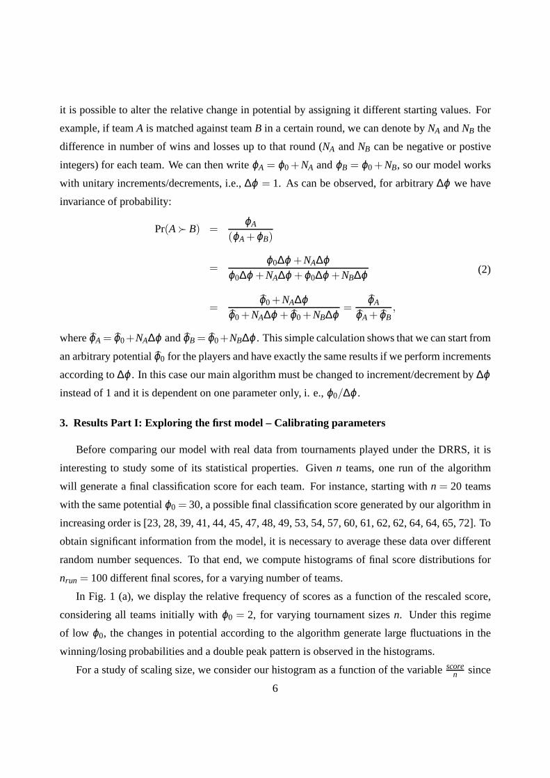
In Fig. 1 (a), we display the relative frequency of scores as afunction of the rescaled score,

considering all teams initially withϕ0 = 2, for varying tournament sizesn. Under this regime

of low ϕ0, the changes in potential according to the algorithm generate large fluctuations in the

winning/losing probabilities and a double peak pattern is observed in the histograms.

For a study of scaling size, we consider our histogram as a function of the variablescoren since

6

0 1 2 3 4 5

0.0

0.1

0.2

0.3

0.4

0.5

0.6

0 1 2 3 4 5

0.0

0.2

0.4

0.6

0.8

1.0

rela

tive

freq

uenc

y

score/n

n = 20 n = 40 n = 80 n = 160 n = 320 n = 640

n = 640

cum

ulat

ive

freq

uenc

yscore/n

n = 20

Figure 1: Figure (a):The score histogram rescaled by the number of teams in the large fluctuation regimetournament for ϕ0 = 2. The histogram was generated from an average overnrun = 100 different tournaments simu-lated by our automaton. We simulated tournaments withn= 20,40,80,160,320, and 640 different teams. Figure (b):The accumulated frequency of classification scores: number of teams with score smaller than a determined scoredivided by the number of teams.

the larger the tournament the larger are the team scores (number of points). This double peak

shows that our dynamics leads to two distinct groups: one that disputes the leadership and the

other that fights against relegation to lower tiers. In Fig. 1(b), we plot the cumulative frequency

as a function ofscoren (that essentially counts how many teams have scores smallerthan, or equal

to a given score). We can observe an interesting behavior dueto the presence of extra inflection

points that makes the concavity change sign and the non-gaussian behavior of the scores, indepen-

dent of the size of the tournaments. Although clearly non-gaussian, because of the double peak

and the “S” shaped cumulative frequency, the Kolmogorov-Smirnov (KS) and Shapiro-Wilk(SW)

tests (references and routine codes of these tests are foundin [8]) were performed to quantify the

departure from gaussianity. An important point for methodsapplied is KS [9] can be applied to

test other distributions differently from SW which is used for normality tests specifically.

By repeating the experiment forϕ0 = 30 a transition from a single peak to a double peak can be

observed fromn≈ 40 which is observed in Fig. 2 (a). Under this condition, winsand losses cause

small changes in the winning/losing probabilities simulating a tournament under the “adiabatic”

regime.

We observe that this interesting behavior is reflected in thecurves of cumulative frequencies

7

1 2 3 4

0.0

0.2

0.4

0.6

0.8

1.0

1 2 3 4

0.0

0.2

0.4

0.6

0.8

1.0

rela

tive

freq

uenc

y

score/n

n=20 n = 40 n = 80 n = 160 n = 320 n = 640

Cum

ulat

ive

Freq

uenc

yscore/n

Figure 2: Figure (a):The histogram of scores rescaled by the number of teams: in the small fluctuation regimetournament forϕ0 = 30 , under the same conditions of Figure 1. Figure (b):The accumulated frequency forϕ0 = 30,for the same conditions of Figure 1.

that change from single to double “S” shaped in Fig. 2 (b). It is interesting to verify whether

this tournament model is able to mimic the score statistics of real tournaments and, if so, under

what conditions? To answer this question, we need to explorereal tournaments statistics. In

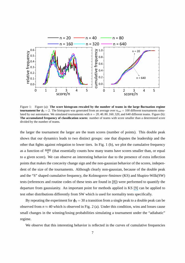
Table 1, we show the compiled data of the last 6 editions of important soccer tournaments around

the world: Italian, Spanish, and Brazilian. We collect dataabout scores of the champion teams

(maximum) and last placed teams. We average these statistics for all studied editions and we

analyze the Gaussian behavior of score data for each editionseparately (20 scores) and grouped

(120 scores) by using two methods: Shapiro-Wilk and Kolmogorov-Smirnov using a significance

level of 5%. The draw average per team was also computed, which shows thatrdraw ≈ 1038 ≈ 0.26

which corroborates the input used in our previous algorithm.

Some observations about this table are useful. The traditional European tournaments, based

on the DRRS have non-Gaussian traces as opposed to the Brazilian league, an embryonary tourna-

ment played under this system. This fact deserves some analysis: in Brazil, over the last 6 editions,

(compiled data are presented in Table 1) 4 different football clubs have won the league. If we con-

sider all 10 disputed editions, we have 6 different champions which shows the great diversity of

this competition. The Brazilian League seems to be at a greater random level when compared

to the European tournaments. A similarity among teams suggests that favorites are not always

8

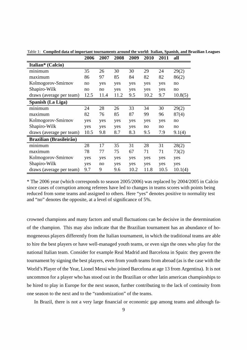
Table 1: Compiled data of important tournaments around the world: It alian, Spanish, and Brazilian Leagues

2006 2007 2008 2009 2010 2011 allItalian* (Calcio)minimum 35 26 30 30 29 24 29(2)maximum 86 97 85 84 82 82 86(2)Kolmogorov-Smirnov no yes yes yes yes yes noShapiro-Wilk no no yes yes yes yes nodraws (average per team) 12.5 11.4 11.2 9.5 10.2 9.7 10.8(5)

Spanish (La Liga)minimum 24 28 26 33 34 30 29(2)maximum 82 76 85 87 99 96 87(4)Kolmogorov-Smirnov yes yes yes yes yes yes noShapiro-Wilk yes yes yes yes no no nodraws (average per team) 10.5 9.8 8.7 8.3 9.5 7.9 9.1(4)

Brazilian (Brasileir ao)minimum 28 17 35 31 28 31 28(2)maximum 78 77 75 67 71 71 73(2)Kolmogorov-Smirnov yes yes yes yes yes yes yesShapiro-Wilk yes no yes yes yes yes yesdraws (average per team) 9.7 9 9.6 10.2 11.8 10.5 10.1(4)

* The 2006 year (which corresponds to season 2005/2006) was replaced by 2004/2005 in Calciosince cases of corruption among referees have led to changesin teams scores with points beingreduced from some teams and assigned to others. Here “yes” denotes positive to normality testand “no” denotes the opposite, at a level of significance of 5%.

crowned champions and many factors and small fluctuations can be decisive in the determination

of the champion. This may also indicate that the Brazilian tournament has an abundance of ho-

mogeneous players differently from the Italian tournament, in which the traditional teams are able

to hire the best players or have well-managed youth teams, oreven sign the ones who play for the

national Italian team. Consider for example Real Madrid andBarcelona in Spain: they govern the

tournament by signing the best players, even from youth teams from abroad (as is the case with the

World’s Player of the Year, Lionel Messi who joined Barcelona at age 13 from Argentina). It is not

uncommon for a player who has stood out in the Brazilian or other latin american champioships to

be hired to play in Europe for the next season, further contributing to the lack of continuity from

one season to the next and to the “randomization” of the teams.

In Brazil, there is not a very large financial or economic gap among teams and although fa-

9

vorites are frequently pointed out by sports pundits beforethe beginning of the tournament, they

are typically not able to pick the winners beforehand. In fact, many dark horses, not initially

pointed out as favorites, end up winning the league title. This suggests that, in Brazil, the cham-

pions emerge from very noisy scenarios, as opposed to other tournaments that only confirm the

power of a (favorite) team. One could add to that the existence of a half-season long local (or

state-based only) tournament making the predictions widely reported in the press not very trustful

or reliable in any sense. Therefore, it is interesting to check our model by studying its statistical

properties, changing parameters and then comparing the model with real data.

We perform an analysis of our model considering different initial parametersϕ0 = 2,10 and 30

and the different tournaments (see plot (a) in Fig. 3). We have usedrdraw= 0.26 in our simulations.

It is possible to observe that the model fits the Brazilian soccer very well forϕ0 = 30 and∆ϕ = 1.

It is important to mention that extreme values (minimal and maximal) are reproduced with very

good agreement. For example, plot (b) in Fig. 3 shows that minimal and maximal values obtained

by our model (full squares and circles respectively, in black) are very similar to the ones obtained

from the six editions of the Brazilian tournament (open squares and circles, in blue). We also

plot continuous lines that represent the average values obtained in each case. This shows that our

model and its fluctuations capture the nuances and emerging statistical properties of the Brazilian

tournament which, however, seems not to be the case of Calcioand La Liga. Plot (a) of Fig. 3

shows that the cumulative frequency of these two tournaments are very similar to one another and

that no value of the parameterϕ0 (many others were tested) is capable of reproducing their data.

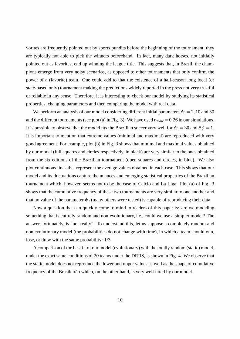
Now a question that can quickly come to mind to readers of thispaper is: are we modeling

something that is entirely random and non-evolutionary, i.e., could we use a simpler model? The

answer, fortunately, is “not really”. To understand this, let us suppose a completely random and

non evolutionary model (the probabilities do not change with time), in which a team should win,

lose, or draw with the same probability: 1/3.

A comparison of the best fit of our model (evolutionary) with the totally random (static) model,

under the exact same conditions of 20 teams under the DRRS, isshown in Fig. 4. We observe that

the static model does not reproduce the lower and upper values as well as the shape of cumulative

frequency of the Brasileirao which, on the other hand, is very well fitted by our model.

10

20 30 40 50 60 70 80

0.0

0.2

0.4

0.6

0.8

1.0

0=30

0=10

0=2

"Brasileirão" from 2006-2011 "Calcio" from 2006-2011 "La Liga" from 2006-2011

cum

ulat

ive

freq

uenc

y

score

(a)

2006 2007 2008 2009 2010 20110

15

30

45

60

75

90

scor

es

minimal values - BSC maximal values - BSC

minimal values - simulation maximal values - simulation

years

(b)

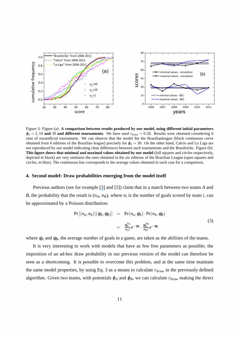
Figure 3: Figure (a):A comparison between results produced by our model, using different initial parametersϕ0 = 2,10 and 30 and different tournaments. We have usedrdraw = 0.26. Results were obtained considering 6runs of ourartificial tournament. We can observe that the model fits the Brazilianleague (black continuous curveobtained from 6 editions of the Brazilian league) preciselyfor ϕ0 = 30. On the other hand, Calcio and La Liga arenot reproduced by our model indicating clear differences between such tournaments and the Brasileirao. Figure (b):This figure shows that minimal and maximal values obtained byour model (full squares and circles respectively,depicted in black) are very similarto the ones obtained in the six editions of the Brazilian League (open squares andcircles, in blue). The continuous line corresponds to the average values obtained in each case for a comparison.

4. Second model: Draw probabilities emerging from the modelitself

Previous authors (see for example [3] and [5]) claim that in amatch between two teamsA and

B, the probability that the result is (nA, nB), whereni is the number of goals scored by teami, can

be approximated by a Poisson distribution:

Pr[(na,nb)|(φA,φB)] = Pr(na,φA) ·Pr(nb,φB)

=φnA

AnA! e−φA ·

φnBB

nB! e−φB

(3)

whereφA andφB, the average number of goals in a game, are taken as the abilities of the teams.

It is very interesting to work with models that have as few free parameters as possible; the

imposition of an ad-hoc draw probability in our previous version of the model can therefore be

seen as a shortcoming. It is possible to overcome this problem, and at the same time maintain

the same model properties, by using Eq. 3 as a means to calculate rdraw in the previously defined

algorithm. Given two teams, with potentialsϕA andϕB, we can calculaterdraw making the direct

11

30 40 50 60 70

0.0

0.2

0.4

0.6

0.8

1.0 random (nonevolutionary) model ( )

data

Cum

ulat

ive

Freq

uenc

y

score

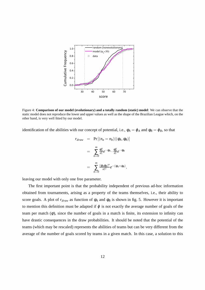
Figure 4:Comparison of our model (evolutionary) and a totally random(static) model: We can observe that thestatic model does not reproduce the lower and upper values aswell as the shape of the Brazilian League which, on theother hand, is very well fitted by our model.

identification of the abilities with our concept of potential, i.e., φA = ϕA andφB = ϕB, so that

rdraw = Pr[(na = nb)|(φA,φB)]

=∞

∑n=0

φnA

n! e−φA ·φn

Bn! e−φB

=∞

∑n=0

(φAφB)n

n!2e−(φA+φB),

leaving our model with only one free parameter.

The first important point is that the probability independent of previous ad-hoc information

obtained from tournaments, arising as a property of the teams themselves, i.e., their ability to

score goals. A plot ofrdraw as function ofφA andφB is shown in fig. 5. However it is important

to mention this definition must be adapted ifϕ is not exactly the average number of goals of the

team per match (φ ), since the number of goals in a match is finite, its extensionto infinity can

have drastic consequences in the draw probabilities. It should be noted that the potential of the

teams (which may be rescaled) represents the abilities of teams but can be very different from the

average of the number of goals scored by teams in a given match. In this case, a solution to this

12

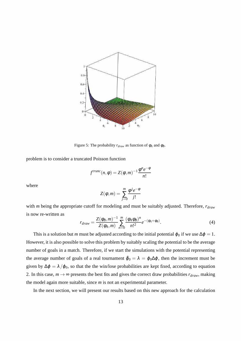
Figure 5: The probabilityrdraw as function ofφA andφB.

problem is to consider a truncated Poisson function

f trunc(n,φ) = Z(φ ,m)−1φne−φ

n!

where

Z(φ ,m) =m

∑j=0

φ je−φ

j!

with m being the appropriate cutoff for modeling and must be suitably adjusted. Therefore,rdraw

is now re-written as

rdraw =Z(φB,m)−1

Z(φA,m)

m

∑n=0

(φAφB)n

n!2 e−(φA+φB). (4)

This is a solution butmmust be adjusted according to the initial potentialϕ0 if we use∆ϕ = 1.

However, it is also possible to solve this problem by suitably scaling the potential to be the average

number of goals in a match. Therefore, if we start the simulations with the potential representing

the average number of goals of a real tournamentϕ0 = λ = ϕ0∆ϕ, then the increment must be

given by∆ϕ = λ/ϕ0, so that the the win/lose probabilities are kept fixed, according to equation

2. In this case,m→ ∞ presents the best fits and gives the correct draw probabilitiesrdraw, making

the model again more suitable, sincem is not an experimental parameter.

In the next section, we will present our results based on thisnew approach for the calculation

13

of rdraw and we show that real data are also reproduced by both methodspresented in this section.

5. Results Part II: variable draw probabilities

We perform new simulations considering our previously described algorithm, but allowing for

variable draw probabilities. As before, we organize the teams via the DRRS, starting with fixed

potentials and take averages over many runs of the model. Ourfirst analysis was to reproduce the

final score of the Brazilian tournament tuning different values ofm.

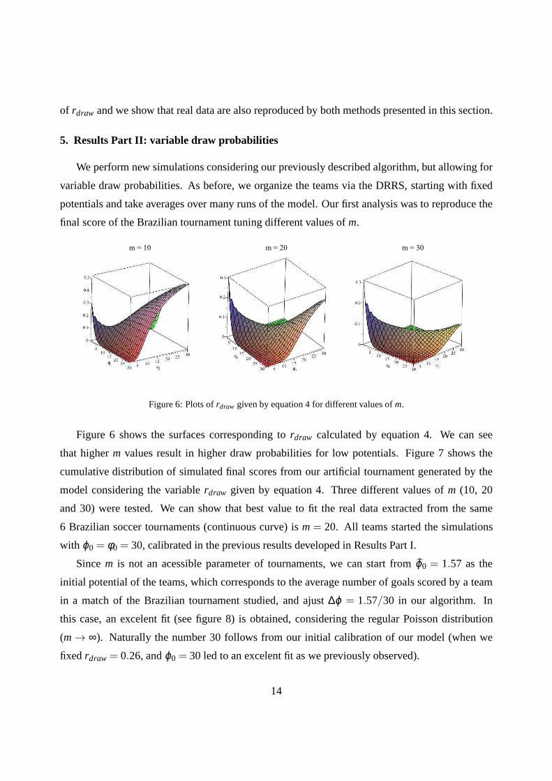
Figure 6: Plots ofrdraw given by equation 4 for different values ofm.

Figure 6 shows the surfaces corresponding tordraw calculated by equation 4. We can see

that higherm values result in higher draw probabilities for low potentials. Figure 7 shows the

cumulative distribution of simulated final scores from our artificial tournament generated by the

model considering the variablerdraw given by equation 4. Three different values ofm (10, 20

and 30) were tested. We can show that best value to fit the real data extracted from the same

6 Brazilian soccer tournaments (continuous curve) ism= 20. All teams started the simulations

with ϕ0 = φ0 = 30, calibrated in the previous results developed in ResultsPart I.

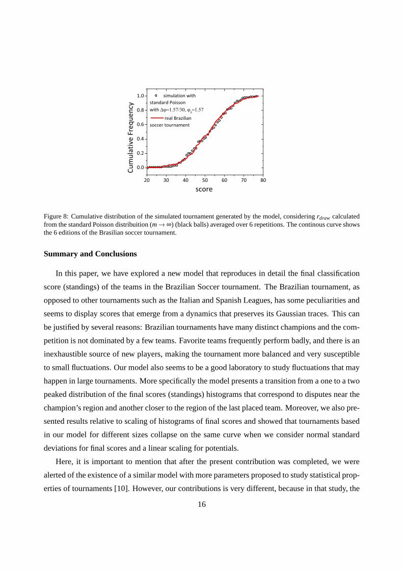
Sincem is not an acessible parameter of tournaments, we can start from ϕ0 = 1.57 as the

initial potential of the teams, which corresponds to the average number of goals scored by a team

in a match of the Brazilian tournament studied, and ajust∆ϕ = 1.57/30 in our algorithm. In

this case, an excelent fit (see figure 8) is obtained, considering the regular Poisson distribution

(m→ ∞). Naturally the number 30 follows from our initial calibration of our model (when we

fixed rdraw = 0.26, andϕ0 = 30 led to an excelent fit as we previously observed).

14

20 30 40 50 60 70

0.0

0.2

0.4

0.6

0.8

1.0

real m = 10 m = 20 m = 30

cum

ulat

ive

dist

ribut

ion

score

Figure 7: Cumulative distribution of simulated tournamentgenerated by the model considering the variablerdraw

given by equation 4. We show that the best value to fit the real data extracted from the same 6 Brazilian soccertournaments (continuous curve) ism= 20.

As can be seen in the figures, we can obtain good fits with this new version of model, which is

a little more complicated than the previous version with constant drawing probabilities, but it uses

information inherent in the model itself.

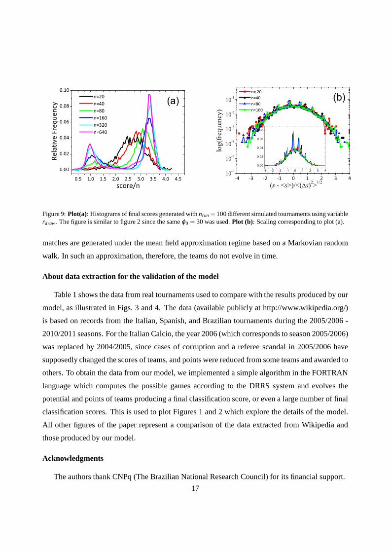
Finally, to test some scaling properties of the model, we reproduce the same plot of figure 2

usingrdraw according to 4, which is shown in plot (a) in figure 9. This figure shows histograms of

final scores generated bynrun = 100 different simulated tournaments using variable probabilities

rdraw. We can observe that the transition from one to two peaks is fully due to the imposition that a

team in our model has a minimal potentialϕ ≥i 1. This effect can be overcome if we scaleϕ0 with

size system and, it is possible to collapse the curves by re-writing the scores as normal standard

variables, i.e.,

score(n) = s(n)→ s∗(n) =s(n)−〈s(n)〉< (∆s(n))2 >

.

Thus, if H(s∗(n),ϕ0,n) denotes the histogram of normalized scores, we have the scaling relation

H(s∗(n1),ϕ0,n1) = H(s∗(bn1),bϕ0,bn1). Plot (b) in figure 9 shows this scaling. We take the

logarithms of the histogram to show the collapse more explicitly. The small inset plot is taken

without the logarithm. We can see that different tournaments can present the same properties as

long as the teams’ potentials are rescaled.

15

20 30 40 50 60 70 80

0.0

0.2

0.4

0.6

0.8

1.0

simulation withstandard Poisson with

real Brazilian soccer tournament

Cum

ulat

ive

Freq

uenc

y

score

Figure 8: Cumulative distribution of the simulated tournament generated by the model, consideringrdraw calculatedfrom the standard Poisson distribuition (m→ ∞) (black balls) averaged over 6 repetitions. The continous curve showsthe 6 editions of the Brasilian soccer tournament.

Summary and Conclusions

In this paper, we have explored a new model that reproduces indetail the final classification

score (standings) of the teams in the Brazilian Soccer tournament. The Brazilian tournament, as

opposed to other tournaments such as the Italian and SpanishLeagues, has some peculiarities and

seems to display scores that emerge from a dynamics that preserves its Gaussian traces. This can

be justified by several reasons: Brazilian tournaments havemany distinct champions and the com-

petition is not dominated by a few teams. Favorite teams frequently perform badly, and there is an

inexhaustible source of new players, making the tournamentmore balanced and very susceptible

to small fluctuations. Our model also seems to be a good laboratory to study fluctuations that may

happen in large tournaments. More specifically the model presents a transition from a one to a two

peaked distribution of the final scores (standings) histograms that correspond to disputes near the

champion’s region and another closer to the region of the last placed team. Moreover, we also pre-

sented results relative to scaling of histograms of final scores and showed that tournaments based

in our model for different sizes collapse on the same curve when we consider normal standard

deviations for final scores and a linear scaling for potentials.

Here, it is important to mention that after the present contribution was completed, we were

alerted of the existence of a similar model with more parameters proposed to study statistical prop-

erties of tournaments [10]. However, our contributions is very different, because in that study, the

16

0.5 1.0 1.5 2.0 2.5 3.0 3.5 4.0 4.5

0.00

0.02

0.04

0.06

0.08

0.10

n=20 n=40 n=80 n=160 n=320 n=640

Rela

tive

Freq

uenc

y

score/n

(a)

-4 -3 -2 -1 0 1 2 3 410-6

10-5

10-4

10-3

10-2

10-1 n= 20 n=40 n=80 n=160

-4 -3 -2 -1 0 1 2 3 4

0.00

0.02

0.04

0.06

0.08

log(

freq

uenc

y)

(s - <s>)/<( s)2>1/2

(b)

Figure 9:Plot(a): Histograms of final scores generated withnrun = 100 different simulated tournaments using variablerdraw. The figure is similar to figure 2 since the sameϕ0 = 30 was used.Plot (b): Scaling corresponding to plot (a).

matches are generated under the mean field approximation regime based on a Markovian random

walk. In such an approximation, therefore, the teams do not evolve in time.

About data extraction for the validation of the model

Table 1 shows the data from real tournaments used to compare with the results produced by our

model, as illustrated in Figs. 3 and 4. The data (available publicly at http://www.wikipedia.org/)

is based on records from the Italian, Spanish, and Braziliantournaments during the 2005/2006 -

2010/2011 seasons. For the Italian Calcio, the year 2006 (which corresponds to season 2005/2006)

was replaced by 2004/2005, since cases of corruption and a referee scandal in 2005/2006 have

supposedly changed the scores of teams, and points were reduced from some teams and awarded to

others. To obtain the data from our model, we implemented a simple algorithm in the FORTRAN

language which computes the possible games according to theDRRS system and evolves the

potential and points of teams producing a final classification score, or even a large number of final

classification scores. This is used to plot Figures 1 and 2 which explore the details of the model.

All other figures of the paper represent a comparison of the data extracted from Wikipedia and

those produced by our model.

Acknowledgments

The authors thank CNPq (The Brazilian National Research Council) for its financial support.

17

References

[1] R. Onody, P. Castro, Complex network study of brazilian soccer players, Physical Review E 70 (2004) 037103.[2] L. Malacarne, R. Mendes, Regularities in football goal distributions, Physica A 286 (2000) 391.[3] E. Bittner, A. Nussbaumer, W. Janke, M. Weigel, Self-affirmation model for football goal distributions, Euro-

physics Letters 78 (2007) 58002.[4] E. Bittner, A. Nussbaumer, W. Janke, M. Weigel, Footballfever: goal distributions and non-gaussian statistics,

The European Physical Journal B 67 (2009) 459.[5] G. Skinner, G. Freeman, Are soccer matches badly designed experiments?, Journal of Applied Statistics 36

(2009) 1087.[6] G. Yaari, S. Eisenmann, The hot (invisible?) hand: Can time sequence patterns of success/failure in sports be

modeled as repeated random independent trials?, PLoS ONE 6 (2011) e24532.[7] A. Kranjec, M. Lehet, B. Bromberger, A. Chatterjee, A sinister bias for calling fouls in soccer, PLoS ONE 5

(2010) e11667.[8] W. Press, S. Teukolsky, W. Vetterling, B. Flannery, Numerical Recipes:The Art of Scientific Computing, Cam-

bridge University Press, New York, USA, 2007.[9] S. Garpman, J. Randrup, Statistical teste for pseudo-random number generators, Computer Physics Communi-

cations 15 (1978) 5.[10] H. Ribeiro, R. Mendes, L. Malacarne, S. Piccoli Jr, P. Santoro, Dynamics of tournaments: The soccer case, The

European Physical Journal B 75 (2010) 327.