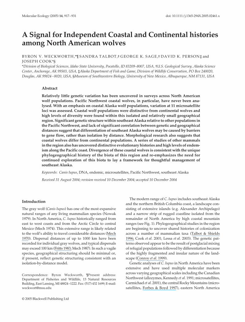
Molecular Ecology (2005)

14

, 917–931 doi: 10.1111/j.1365-294X.2005.02461.x

© 2005 Blackwell Publishing Ltd

Blackwell Publishing, Ltd.

A Signal for Independent Coastal and Continental histories among North American wolves

BYRON V. WECKWORTH,

*¶

SANDRA TALBOT,

†

GEORGE K. SAGE,

†

DAVID K. PERSON

‡

and JOSEPH COOK

*§

*

Division of Biological Sciences, Idaho State University, Pocatello, ID 83209–8007, USA,

†

U.S. Geological Survey, Alaska Science Center, Anchorage, AK 99503, USA,

‡

Alaska Department of Fish and Game, Division of Wildlife Conservation, PO Box 240020, Douglas, AK 99824–0020, USA,

§

Museum of Southwestern Biology, University of New Mexico, Albuquerque, NM 87131, USA

Abstract

Relatively little genetic variation has been uncovered in surveys across North Americanwolf populations. Pacific Northwest coastal wolves, in particular, have never been ana-lysed. With an emphasis on coastal Alaska wolf populations, variation at 11 microsatelliteloci was assessed. Coastal wolf populations were distinctive from continental wolves andhigh levels of diversity were found within this isolated and relatively small geographicalregion. Significant genetic structure within southeast Alaska relative to other populations inthe Pacific Northwest, and lack of significant correlation between genetic and geographicaldistances suggest that differentiation of southeast Alaska wolves may be caused by barriersto gene flow, rather than isolation by distance. Morphological research also suggests thatcoastal wolves differ from continental populations. A series of studies of other mammalsin the region also has uncovered distinctive evolutionary histories and high levels of endem-ism along the Pacific coast. Divergence of these coastal wolves is consistent with the uniquephylogeographical history of the biota of this region and re-emphasizes the need forcontinued exploration of this biota to lay a framework for thoughtful management ofsoutheast Alaska.

Keywords

:

Canis lupus

, DNA, endemic, microsatellites, Pacific Northwest, southeast Alaska

Received 31 August 2004; revision received 10 December 2004; accepted 10 December 2004

Introduction

The gray wolf (

Canis lupus

) has one of the most expansivenatural ranges of any living mammalian species (Nowak1979). In North America,

C. lupus

historically ranged fromeast to west coasts and from the Arctic Circle to centralMexico (Mech 1974). This extensive range is likely relatedto the wolf’s ability to travel considerable distances (Mech1970). Dispersal distances of up to 1000 km have beenrecorded for individual gray wolves, and typical dispersalsmay exceed 100 km (Fritts 1983; Mech 1987). In such a vagilespecies, geographical structuring should be minimal or,if present, reflect genetic structuring consistent with anisolation-by-distance model.

The modern range of

C. lupus

includes southeast Alaskaand the northern British Columbia coast, a landscape con-sisting of extensive islands (e.g. Alexander Archipelago)and a narrow strip of rugged coastline isolated from theremainder of North America by high coastal mountainranges (see Fig. 1). Phylogeographical studies in the regionare beginning to uncover shared histories of colonizationacross a number of mammalian taxa (Talbot & Shields1996; Cook

et al

. 2001; Lessa

et al

. 2003). The genetic pat-terns observed appear to be the result of postglacial mixingof refugial populations followed by differentiation becauseof the highly fragmented and insular nature of the land-scape (Conroy

et al

. 1999).Genetic analyses of

C. lupus

in North America have beenextensive and have used multiple molecular markersacross varying geographical scales including the CanadianNorthwest (allozymes, Kennedy

et al

. 1991; microsatellites,Carmichael

et al

. 2001), the central Rocky Mountains (micro-satellites, Forbes & Boyd 1997), eastern North America

Correspondence: Byron Weckworth, ¶Present address:Department of Fisheries and Wildlife, 13 Natural ResourcesBuilding, East Lansing, MI 48824–1222. Fax: (517) 432 1699; E-mail:weckwort@msu.edu

918

B . V . W E C K W O R T H

E T A L .

© 2005 Blackwell Publishing Ltd,

Molecular Ecology

, 14, 917–931

(mtDNA sequences and microsatellites, Wilson

et al

. 2000),and North America (microsatellites, Roy

et al

. 1994; mtDNAsequences, Vilà

et al

. 1999). Analysis of mitochondrialDNA (mtDNA) control region in

C. lupus

indicated littlehistorical variation in populations in North America, andsuggests current low levels of variation may be because ofrecent restrictions to gene flow caused by fragmentation ofhabitat and population decline (Vilà

et al

. 1999). Microsat-ellite analysis of wolves across North America indicatesdivergence due to drift in finite populations and suggeststhis may have occurred in ice age refugia and that contem-porary habitat fragmentation may be further contributingto higher levels of population differentiation (Roy

et al

.1994). Previous studies encompassing island populations(Vancouver Island, Roy

et al

. 1994; Banks and VictoriaIslands, Carmichael

et al

. 2001) have indicated moderatedifferentiation of island wolves from continental popula-tions. However, none of the island systems previouslyinvestigated encompassed an area as large and geograph-ically diverse as southeast Alaska. Here we lay a frame-work for interpreting the distinctiveness of coastal wolves,populations that may be increasingly vulnerable to harv-est, loss of habitat, and loss of essential prey species (e.g.

Person

et al

. 1996). Nuclear microsatellite loci are evaluatedamong and within wolf populations in the Pacific North-west to assess geographical structure and levels of vari-ation throughout the region. We begin to investigate thepotential impact of episodic barriers and corridors relatedto the geological history of the region involving glaciers,changing sea levels, and geographical features that maypromote isolation or contact between populations.

Materials and methods

Sampling

The sampling regime emphasized localities within southeastAlaska and throughout northwestern North America,including islands (Kupreanof, Mitkof, and Woewodski,KMW; Revillagigedo, REV; and Prince of Wales, POW) inthe Alexander Archipelago, mainland southeast Alaska coast(MCS), interior Alaska (FAI), Kenai Peninsula of Alaska (KEN),Copper River delta of southern coastal Alaska (CRD),British Columbia (BC), and Yukon Territory (YUK). Insoutheast Alaska, populations were designated by bio-geographical subregions (MacDonald & Cook 1996), with

Fig. 1 Map of the Pacific Northwest withsoutheast Alaska expanded. Sampling loca-tions and abbreviations are indicated.

G E N E T I C S O F P A C I F I C N O R T H W E S T W O L V E S

919

© 2005 Blackwell Publishing Ltd,

Molecular Ecology

, 14, 917–931

the exception of REV and the complex of KMW. These islandsare within the same subregion, but were separated intotwo populations (mean distance between REV and KMWis 163 km). POW and mainland coastal (MCS) individualseach represent a separate subregion, resulting in a total offour designated populations in southeast coastal Alaska.Combined with five continental localities, a total of ninepopulations and 221 individuals were analysed (Table 1and Fig. 1). Pack data were not available for most wolves,so whenever possible we avoided using tissues collectedfrom the same latitude/longitude coordinates.

DNA was extracted from tissues (heart, spleen, skeletalmuscle, skin, or blood) initially collected from hunters andtrappers by the Alaska Department of Fish and Game andsubsequently archived in the University of Alaska Museum,the Alaska Science Center or Museum of SouthwesternBiology. Methods of DNA extraction followed Talbot &Shields (1996) for muscle samples from KEN, Talbot

et al.

(in press) for blood samples from BC, and Fleming & Cook(2002) for all other tissue extractions.

Microsatellite genotyping

We screened 12 biparentally inherited dinucleotide repeat(CA) microsatellite loci known to be polymorphic in canids(Ostrander

et al

. 1993; Roy

et al

. 1994); 11 were found tobe polymorphic and were used in subsequent analyses.Microsatellite loci were assayed using polymerase chainreaction (PCR) with primers end-labelled using IRDye 700and 800 fluorescent tags (LI-COR). PCR amplificationswere carried out in a final volume of 10

µ

L on a Robocycler(Stratagene) and contained 2–100 ng of genomic DNA,0.2 m

m

of dNTPs, 3.6–3.9 pmoles of unlabelled forwardprimers, 4.0 pmoles of unlabelled reverse primer, 0.1–0.4pmoles (depending on locus) of IRD-labelled primer, 0.1

µ

gof BSA, 1X PCR buffer (Perkin-Elmer Cetus I), and 0.5 units

of Ampli

Taq

DNA polymerase (PE Biosystems). Reactionstypically began with 94

°

C for 2 min and continued with 40cycles each of 94

°

C for 1 minute, 50–56

°

C for 1 minute,and 72

°

C for 1 minute. A 30-minute extension at 72

°

Cconcluded each reaction. The fluorescently labelled PCRproducts were electrophoresed on a 48- or 64-well 6%polyacrylamide gel, on a LI-COR 4200 L-2 LR automatedsequencer. Initially, 24 individuals were scored against afluorescently labelled M13 sequence ladder of known size(Amersham Pharmacia Biotech). Two or three individualsheterozygous at each locus were selected among the 24 sizedindividuals and included in all subsequent genotypinggels as unambiguous size standards typically occupying9–15 lanes. Microsatellite fragment data were capturedusing LI-COR

gene imageir data analysis

software. Forquality control purposes, a minimum of 10% of individualswere randomly selected for each locus, re-extractedfrom the original tissue source, and subjected to PCRamplification.

Data analysis

Allele number and heterozygosity (observed and expected)for each locus across populations were calculated using

msa

3.0 (Dieringer & Schlötterer 2003). Allelic richness(Petit

et al

. 1998) per locus and population and fixation indicesof heterozygosity (

F

IS

; Hartl & Clark 1997) were calculatedusing

fstat

2.9.3 (Goudet 2001).

genepop

version 3.3 ftp://isem.isem.univ-montp2.fr/pup/pc/genepop; Raymond& Rousset 1995) was used to test for genotypic linkagedisequilibrium (LD) and Hardy–Weinberg equilibrium(HWE). Deviations from LD and HWE were testedbetween each pair of loci for each population and per locus,respectively. For loci with four or fewer alleles, exact tests(Louis & Dempster 1987) were used to estimate

P

values totest for deviations from HWE. For loci with more than four

Table 1 Descriptive statistics for Canis lupus populations and clades

Populations Abbr. n Alleles Richness HE HO FIS FST M-ratio

Coastal group 101 5.00 3.21 0.52 0.48 0.05 0.12 0.795Kupreanof, Mitkof, and Woewodski Islands, SE AK KMW 26 3.73 3.00 0.46 0.43 0.08 0.747Revillagigedo Island, SE AK REV 24 4.09 3.46 0.57 0.59 −0.04 0.801Prince of Wales Island, SE AK POW 42 3.82 2.93 0.48 0.42 0.12 0.702Mainland coast, SE AK MCS 9 3.45 3.45 0.58 0.61 −0.04 0.737

Continental group 120 7.09 4.06 0.62 0.59 0.06 0.09 0.895Fairbanks Quadrant, interior AK FAI 29 5.55 4.62 0.64 0.59 0.08 0.846Copper River Delta, coastal AK CRD 14 3.64 3.43 0.58 0.53 0.10 0.737Kenai Peninsula, coastal AK KEN 33 3.55 3.17 0.55 0.55 0.01 0.750British Columbia BC 30 6.00 4.69 0.69 0.62 0.11 0.835Yukon Territories YUK 14 4.91 4.39 0.65 0.69 −0.06 0.825

Abbreviations (abbr.), sample size (n), mean number of alleles per locus (alleles), allelic richness (richness), expected heterozygosity (HE), observed heterozygosity (HO), FIS, FST for the group comparison, and Garza & Williamson’s (2001) M-ratios.

920

B . V . W E C K W O R T H

E T A L .

© 2005 Blackwell Publishing Ltd,

Molecular Ecology

, 14, 917–931

alleles, estimated

P

values used the Markov chain method(Guo & Thompson 1992). Genotypic LD was tested usingthe Markov chain method with 10 000 dememorizations,5000 batches and 10 000 iterations.

P

values for tests werecorrected using a strict Bonferroni adjustment (initial

α

=0.05) for multiple comparisons. Pairwise estimates of popula-tion differentiation using allelic frequency (

F

ST

) were calculatedto generate estimates of gene flow [

M

:

M

= (1/

F

ST

−

1)/4](Slatkin 1993). Isolation-by-distance analysis (Slatkin 1993)was performed plotting the log of geographical distancesbetween pairs of populations vs. the log of

M

. A Manteltest (Mantel 1967) was used to assess the significance ofthe correlation between these variables using 10 000 permuta-tions of the matrix computed through the

isolde

subroutine.Latitude and longitude coordinates for each individualwere averaged for each population and the geographicaldistance was measured as the straight-line length betweeneach population’s average latitude/longitude coordinate.

Populations were assessed for evidence of a recentreduction in population size using the program

bottleneck

(Piry

et al

. 1999). Populations that have experienced arecent genetic bottleneck exhibit a correlative reductionof allele numbers and heterozygosity at polymorphic loci.However, allelic numbers are reduced faster than genediversity. Thus, a recently reduced population is character-ized when observed heterozygosity is larger than expectedequilibrium heterozygosity, which is calculated fromthe observed number of alleles under the assumption of aconstant size population (mutation-drift equilibrium)(Cornuet & Luikart 1996). Most microsatellite data sets havebeen shown to fit a two-phase model of mutation (TPM),rather than the infinite allele model (IAM) or stepwisemutation model (SMM) (Di Rienzo

et al

. 1994). Thus, ouranalysis was conducted using a TPM with multistep muta-tions accounting for 5%, 10%, 20%, or 30% of all mutations.A Wilcoxon signed rank test was used to determine whichpopulations have a significant number of loci with genediversity excess (Luikart

et al

. 1998). This statistical test wasthe most appropriate because majority of our popula-tions are represented by fewer than 30 samples. Geneticevidence for historic bottlenecks using microsatellite locican consist of gaps in the size distribution of alleles. Theincompleteness of these distributions can be quantified asthe M-ratio, the mean ratio across all loci of the number ofalleles to the allele size range (Garza & Williamson 2001).Calculation of M-ratios is dependent on the loci followinga pattern of mutation where changes in allele state consistof decreasing or increasing numbers of repeats. Loci withsingle base-pair differences cannot be used. Mean of M-ratios were calculated for each population using

agarst

version 2.9 (Harley 2002). Contrary to

bottleneck

, adeclining M-ratio after a population is reduced in size islargely independent of any mutation process becausedrift or migration would play a larger role than mutation

in accrual of new alleles postbottleneck (Garza &Williamson 2001).

phylip

version 3.6 (http://evolution.genetics.washington.edu/phylip.html; Felsenstein 1993) was used to calculatepairwise chord distances (Cavalli-Sforza & Edwards 1967)among populations and population networks using the allelefrequency matrix created in

genepop

. Chord distanceswere calculated for all population pairs in the subroutine

gendist

and used to construct a maximum-likelihoodtree (ML) in the subroutine

contml

. To test the strengthof the tree topology, 1000 bootstrap replicates were gener-ated in the

seqboot

subroutine and analysed in

gendist

. Treetopologies were created for all replicates in

contml

anda consensus tree was generated in the subroutine

consense

.Tree files were viewed using

treeview

version 2.0 (http://taxonomy.zoology.gla.ac.uk/rod/treeview.html; Page 1996).

A Bayesian-clustering program utilizing a Markov chainMonte Carlo (MCMC) approach,

structure

version 2(http://pritch.bsd.uchicago.edu; Pritchard

et al

. 2000), wasused to conduct admixture and assignment tests andexamine population structure according to inferred popu-lation clusters based on multilocus genotype data. Wecalculated the probability of individual assignmentsto population clusters (K). A series of tests was performedusing different numbers of population clusters (MAX-POPS 1–20) to guide an empirical estimate of the numberof identifiable populations (Table 2). The probability ofhow the data best fit into each number of assumed clus-ters was estimated in each case (ln probability of the data)without using any prior population information, so thatindividuals were assigned to a cluster based solely on theirmultilocus genotypic profile. Burn-in and replication valueswere set at 100 000 and 1 000 000, respectively, and each

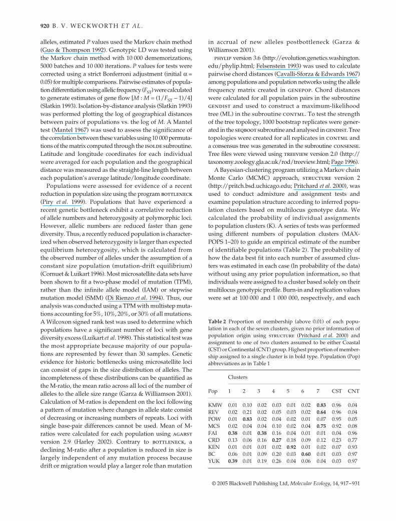
Table 2 Proportion of membership (above 0.01) of each popu-lation in each of the seven clusters, given no prior information ofpopulation origin using structure (Pritchard et al. 2000) andassignment to one of two clusters assumed to be either Coastal(CST) or Continental (CNT) group. Highest proportion of member-ship assigned to a single cluster is in bold type. Population (Pop)abbreviations as in Table 1

Pop

Clusters

1 2 3 4 5 6 7 CST CNT

KMW 0.01 0.10 0.02 0.03 0.01 0.02 0.83 0.96 0.04REV 0.02 0.21 0.02 0.05 0.03 0.02 0.64 0.96 0.04POW 0.01 0.83 0.02 0.04 0.02 0.01 0.07 0.95 0.05MCS 0.02 0.04 0.04 0.10 0.02 0.04 0.75 0.92 0.08FAI 0.38 0.01 0.38 0.16 0.04 0.01 0.01 0.04 0.96CRD 0.13 0.06 0.16 0.27 0.18 0.09 0.12 0.23 0.77KEN 0.01 0.01 0.01 0.02 0.92 0.01 0.02 0.07 0.93BC 0.06 0.01 0.09 0.20 0.03 0.60 0.01 0.03 0.97YUK 0.39 0.01 0.19 0.26 0.04 0.06 0.04 0.03 0.97

G E N E T I C S O F P A C I F I C N O R T H W E S T W O L V E S

921

© 2005 Blackwell Publishing Ltd,

Molecular Ecology

, 14, 917–931

test yielded a log-likelihood value of the data (ln probability),with the highest indicating which test was closest to theactual number of genetically distinct populations. Indi-viduals were assigned probabilistically to a population or tomultiple populations if their genotype profile indicatedadmixture.

arlequin

(Schneider

et al

. 2000) was used to conduct ananalysis of molecular variance (

amova

, Excoffier

et al

.1992).

amova

partitions the total variance into covariancecomponents due to differences among groups, amongpopulations within groups and among individuals. Thesecalculations were performed using allele frequency data(

F

ST

; Excoffier

et al

. 1992). The nine populations weredivided into a southeast coastal group (Coastal) and acontinental group (Continental), to define a particulargenetic structure to test.

Results

Microsatellite variation

Number of alleles per locus across all populations rangedfrom two (locus C172) to 15 (locus C30), with an average of7.5 alleles (Appendix). Values of expected heterozygosity(HE) averaged across loci ranged from 0.46 (KMW) to 0.69(BC). Mean number of alleles per locus (observed allelicdiversity) ranged from 3.45 (MCS) to 6.0 (BC) amongpopulations, and was 5.00 and 7.09 in the Coastal andContinental groups, respectively. Continental populationshad a higher frequency of private alleles than southeastCoastal populations (4.6 vs. 1.25 alleles per population,respectively). Of the alleles unique to the southeast Coastalregion, none was widespread; each was unique to a singleindividual. In contrast, 12 alleles unique to Continentalregions were found in at least two different populations.Allelic richness (Petit et al. 1998) was highest in BC (4.69)and lowest on POW (2.93). Population specific alleles wereobserved in five populations (KMW, REV, POW, FAI, andBC; see Appendix), however, in southeast Coastal popu-lations, these alleles were restricted to a single individual.In Continental populations, private alleles occurred in oneto five individuals. Southeast Coastal and Continentalgroups were not significantly different in allelic richness(P = 0.093).

Exact tests of genotypic LD indicated that C030 and C250were associated in FAI population. Globally, C030 is asso-ciated with both C213 and C250. However, for each of theseassociations the loci have been mapped to differentchromosomes (Breen et al. 2001), indicating that the LDobserved is not due to physical linkage. Fixation indices(FIS) averaged for each population across all loci hadhigh and low values of 0.12 and –0.06 for POW andYUK, respectively (not significantly different from zero,Table 1). Significant departures from HWE were found in

loci C123 and C203 in MCS and FAI, respectively. Whena global test across loci and across populations wasperformed, the null hypothesis of equilibrium was rejected(P < 0.001, α = 0.05), however, after correcting for multipletests, the null hypothesis may not be rejected (α = 0.0004).Observed hetero-zygosity and fixation index values didnot differ significantly between southeast Coastal andContinental groups (P = 0.118 and 0.859 for HO and FIS,respectively, Table 1).

Geographic variation and structuring

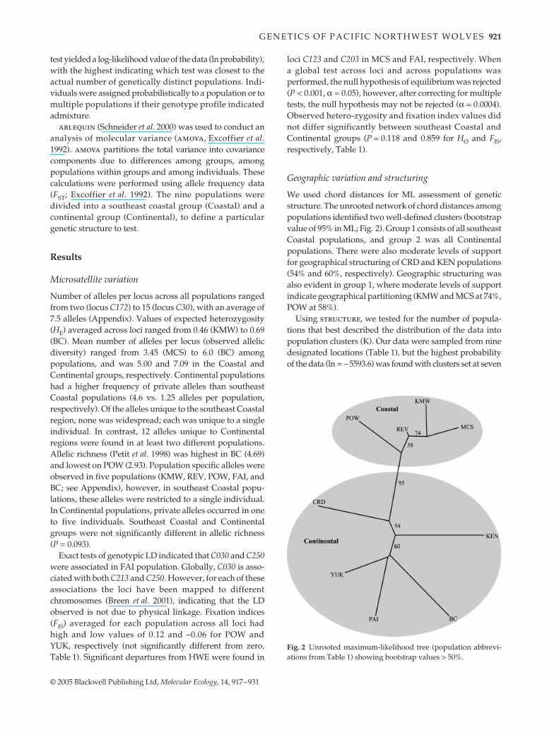
We used chord distances for ML assessment of geneticstructure. The unrooted network of chord distances amongpopulations identified two well-defined clusters (bootstrapvalue of 95% in ML; Fig. 2). Group 1 consists of all southeastCoastal populations, and group 2 was all Continentalpopulations. There were also moderate levels of supportfor geographical structuring of CRD and KEN populations(54% and 60%, respectively). Geographic structuring wasalso evident in group 1, where moderate levels of supportindicate geographical partitioning (KMW and MCS at 74%,POW at 58%).

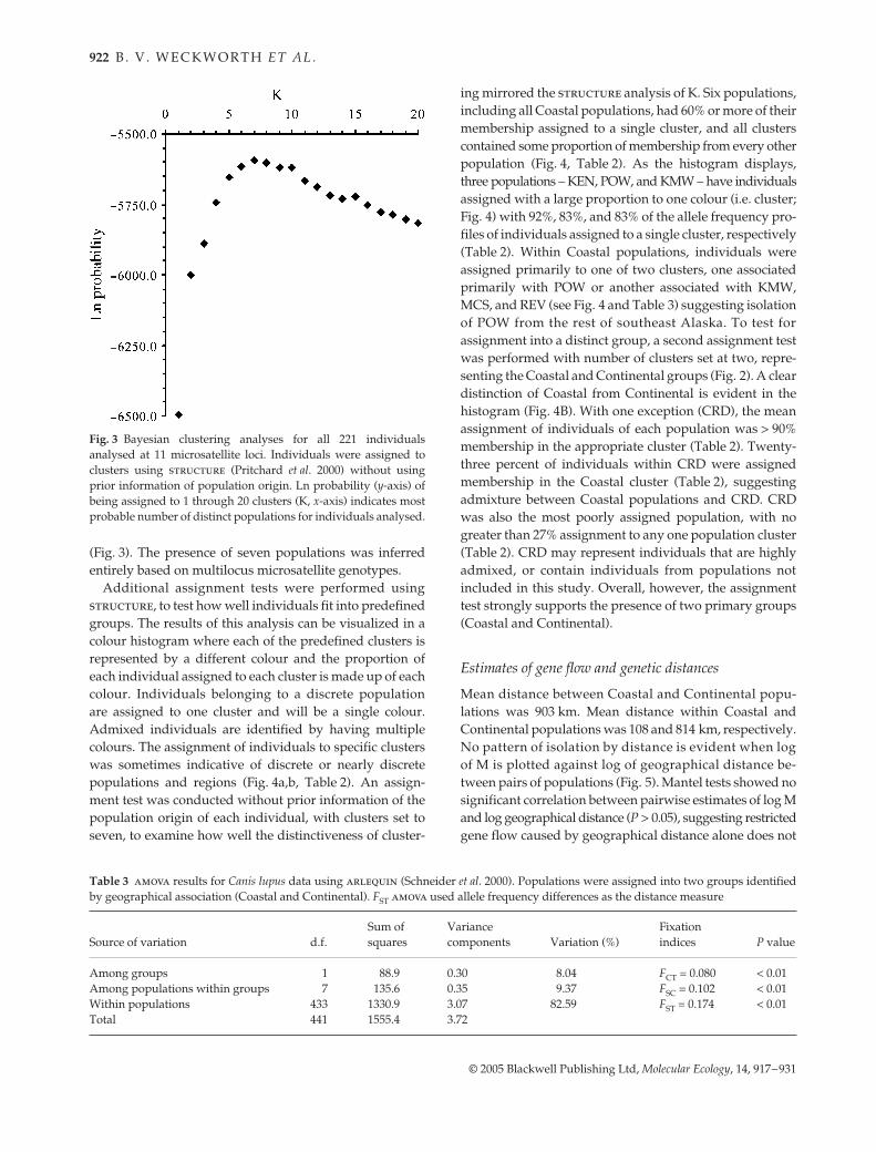
Using structure, we tested for the number of popula-tions that best described the distribution of the data intopopulation clusters (K). Our data were sampled from ninedesignated locations (Table 1), but the highest probabilityof the data (ln = −5593.6) was found with clusters set at seven

Fig. 2 Unrooted maximum-likelihood tree (population abbrevi-ations from Table 1) showing bootstrap values > 50%.

922 B . V . W E C K W O R T H E T A L .

© 2005 Blackwell Publishing Ltd, Molecular Ecology, 14, 917–931

(Fig. 3). The presence of seven populations was inferredentirely based on multilocus microsatellite genotypes.

Additional assignment tests were performed usingstructure, to test how well individuals fit into predefinedgroups. The results of this analysis can be visualized in acolour histogram where each of the predefined clusters isrepresented by a different colour and the proportion ofeach individual assigned to each cluster is made up of eachcolour. Individuals belonging to a discrete populationare assigned to one cluster and will be a single colour.Admixed individuals are identified by having multiplecolours. The assignment of individuals to specific clusterswas sometimes indicative of discrete or nearly discretepopulations and regions (Fig. 4a,b, Table 2). An assign-ment test was conducted without prior information of thepopulation origin of each individual, with clusters set toseven, to examine how well the distinctiveness of cluster-

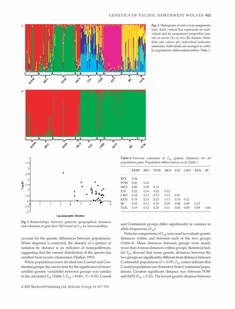
ing mirrored the structure analysis of K. Six populations,including all Coastal populations, had 60% or more of theirmembership assigned to a single cluster, and all clusterscontained some proportion of membership from every otherpopulation (Fig. 4, Table 2). As the histogram displays,three populations – KEN, POW, and KMW – have individualsassigned with a large proportion to one colour (i.e. cluster;Fig. 4) with 92%, 83%, and 83% of the allele frequency pro-files of individuals assigned to a single cluster, respectively(Table 2). Within Coastal populations, individuals wereassigned primarily to one of two clusters, one associatedprimarily with POW or another associated with KMW,MCS, and REV (see Fig. 4 and Table 3) suggesting isolationof POW from the rest of southeast Alaska. To test forassignment into a distinct group, a second assignment testwas performed with number of clusters set at two, repre-senting the Coastal and Continental groups (Fig. 2). A cleardistinction of Coastal from Continental is evident in thehistogram (Fig. 4B). With one exception (CRD), the meanassignment of individuals of each population was > 90%membership in the appropriate cluster (Table 2). Twenty-three percent of individuals within CRD were assignedmembership in the Coastal cluster (Table 2), suggestingadmixture between Coastal populations and CRD. CRDwas also the most poorly assigned population, with nogreater than 27% assignment to any one population cluster(Table 2). CRD may represent individuals that are highlyadmixed, or contain individuals from populations notincluded in this study. Overall, however, the assignmenttest strongly supports the presence of two primary groups(Coastal and Continental).

Estimates of gene flow and genetic distances

Mean distance between Coastal and Continental popu-lations was 903 km. Mean distance within Coastal andContinental populations was 108 and 814 km, respectively.No pattern of isolation by distance is evident when logof M is plotted against log of geographical distance be-tween pairs of populations (Fig. 5). Mantel tests showed nosignificant correlation between pairwise estimates of log Mand log geographical distance (P > 0.05), suggesting restrictedgene flow caused by geographical distance alone does not

Fig. 3 Bayesian clustering analyses for all 221 individualsanalysed at 11 microsatellite loci. Individuals were assigned toclusters using structure (Pritchard et al. 2000) without usingprior information of population origin. Ln probability (y-axis) ofbeing assigned to 1 through 20 clusters (K, x-axis) indicates mostprobable number of distinct populations for individuals analysed.

Table 3 amova results for Canis lupus data using arlequin (Schneider et al. 2000). Populations were assigned into two groups identifiedby geographical association (Coastal and Continental). FST amova used allele frequency differences as the distance measure

Source of variation d.f.Sum of squares

Variance components Variation (%)

Fixation indices P value

Among groups 1 88.9 0.30 8.04 FCT = 0.080 < 0.01Among populations within groups 7 135.6 0.35 9.37 FSC = 0.102 < 0.01Within populations 433 1330.9 3.07 82.59 FST = 0.174 < 0.01Total 441 1555.4 3.72

G E N E T I C S O F P A C I F I C N O R T H W E S T W O L V E S 923

© 2005 Blackwell Publishing Ltd, Molecular Ecology, 14, 917–931

account for the genetic differences between populations.When dispersal is restricted, the absence of a pattern ofisolation by distance is an indicator of nonequilibrium,suggesting that the current distribution of the species hasresulted from recent colonization (Slatkin 1993).

When populations were divided into Coastal and Con-tinental groups, the amova tests for the significance of micro-satellite genetic variability between groups was similarto the calculated FST (Table 3, FCT = 8.04%, P < 0.01). Coastal

and Continental groups differ significantly in variance inallele frequencies (FST).

Pairwise comparisons of FST were used to evaluate geneticdistances within and between each of the two groups(Table 4). Mean distances between groups were nearlytwice that of mean distances within groups. Statistical testsfor FST showed that mean genetic distances between thetwo groups are significantly different from distances betweenContinental populations (P < 0.05). FST values indicate thatCoastal populations are distinctive from Continental popu-lations. Greatest significant distance was between POWand KEN (FST = 0.23). The lowest genetic distance between

Fig. 4 Histograms of structure assignmenttests. Each vertical bar represents an indi-vidual and its assignment proportion intoone of seven (A) or two (B) clusters. Morethan one colour per individual indicatesadmixture. Individuals are arranged in orderby populations; abbreviations follow Table 1.

Fig. 5 Relationships between pairwise geographical distancesand estimates of gene flow (M) based on FST for microsatellites.

Table 4 Pairwise estimates of FST genetic distances for allpopulation pairs. Population abbreviations as in Table 1

KMW REV POW MCS FAI CRD KEN BC

REV 0.04POW 0.20 0.10MCS 0.06 0.02 0.14FAI 0.22 0.16 0.22 0.12CRD 0.18 0.11 0.17 0.12 0.07KEN 0.19 0.13 0.23 0.13 0.10 0.12BC 0.19 0.11 0.19 0.09 0.08 0.09 0.13YUK 0.19 0.12 0.20 0.11 0.04 0.08 0.09 0.06

924 B . V . W E C K W O R T H E T A L .

© 2005 Blackwell Publishing Ltd, Molecular Ecology, 14, 917–931

Coastal and Continental populations was between BC andMCS (FST = 0.09). Within Coastal group, the highest FST value(0.20) was observed between POW and KMW populations.The greatest distance within Continental populations wasbetween KEN and BC (FST = 0.13).

Mean FST distance among Coastal populations was greaterthan mean distance among Continental populations, whichencompass a much greater geographical area. This findinglikely reflects the highly fragmented and insular nature ofthe coastal region. In sum, mean genetic distances amongpopulations within Coastal and Continental regions differ,but these differences are not significant (P > 0.05). Overall,distances are greatest between the two groups.

Population bottlenecks

The MCS population was not analysed using bottleneckbecause of small sample size (n = 9). Wilcoxon tests ofsignificance were consistent across the four TPM scenariosused. After correcting for multiple tests, significant excessheterozygosity (one-tailed Wilcoxon test for H excess) wasdetected in only KEN populations with a TPM of 20% and30% (P = 0.0034 for both). Significance decreased as TPMconverged to a purely stepwise mutation model. M-ratiosfor populations varied between 0.702 (POW) and 0.846(FAI), and calculations for groups yielded 0.795 and 0.895for Coastal and Continental, respectively (Table 1). Incomparison, a historically stable group of wolves in NorthAmerica (Roy et al. 1994) yielded M-ratio = 0.858, and thereduced population of Mexican wolves (Garcia-Morenoet al. 1996) yielded M-ratio = 0.647 (from Table 2 in Garza& Williamson 2001). M-ratios do not support a historicbottleneck for any population analysed.

Discussion

Since Swarth’s (1936) characterization of the Sitkan District,the North Pacific coast has been recognized as a distinctivebiogeographical region in North America (Klein 1965;Cook & MacDonald 2001). Phylogeographical assessmentsof a suite of mammals have uncovered previously undetectedendemism (e.g. Talbot & Shields 1996; Demboski et al.1999; Conroy & Cook 2000; Stone et al. 2002). Glacial cyclesof the late Pleistocene created a dynamic history of isolationand fragmentation in the Pacific Northwest (Pielou 1991),and this geological history apparently played a significantrole in evolution and divergence (e.g. Small et al. 2003).Distinctive coastal and continental lineages have beenidentified in a variety of northwestern terrestrial mammals,covering a multitude of life histories from the dusky shrew(Sorex monticolus) to black bears (Ursus americanus) (Cooket al. 2001). Similarly, coastal gray wolves appear to haveexperienced a distinctive evolutionary history from con-tinental populations. Assignment tests and networks based

on chord distances are consistent with geographical iso-lation and distinction of southeast Coastal wolves fromadjacent Continental populations. The relatively divergentpopulation structure found within southeast Alaska furthersupports these ideas, but samples from coastal populationsin British Columbia and regions south of southeast Alaskaneed to be examined to effectively test the hypothesis of acoastal/continental split.

Genetic distances among populations of Canis lupus wereindependent of geographical distance, suggesting thateither dispersal distances are sufficiently large to confoundgenetic differentiation or that barriers to dispersal are moreimportant in structuring genetic variation in wolves than isgeographical distance (Slatkin 1993; Roy et al. 1994). F-statistics, tests of HWE, allelic diversity, and levels of hetero-zygosity further suggest that although these populationshave been isolated, they have maintained relatively highallelic diversity and display identifiable geographicalstructuring within a comparably small geographical area.

Fossil record indicates that C. lupus migrated fromEurasia to North America approximately 500 000 bp, dur-ing the late Pleistocene (Nowak 1979). Morphological ana-lyses of skull features suggest as many as five subspecies ofwolves in North America (Nowak 1995). During the mostrecent ice age (ending about 10 000 bp in North America),C. lupus persisted in two or more refugia, with southerncontinental United States, Arctic Canada, and eastern Ber-ingia (Alaska) suggested as possibilities (Nowak 1983, 1995).Of these five subspecies, our sampling regime includes two,Canis lupus nubilus and Canis lupus occidentalis. C. l. nubilusencompasses southeast Alaska, western British Columbia,much of the contiguous United States and eastern Canada;while C. l. occidentalis includes western Canada and the rest ofAlaska (Nowak 1995). The molecular perspective developedin this study does not coincide with the current morpho-logical scheme. The original morphological classificationof wolves included three subspecies along the North Pacificcoast: Canis lupus alces of the Kenai Peninsula of Alaska,Canis lupus crassodon of Vancouver Island, British Columbia,and Canis lupus ligoni of southeast Alaska (Goldman 1944).The latter subspecies corresponds to our Coastal populations.

Gray wolves in southeast Alaska are hypothesized tobe postglacial colonizers from one or more southernrefugia. Fossil evidence of wolves has not been found in theAlexander Archipelago, representing one of the few extantspecies on the islands that has not been identified in extens-ive palaeontological excavations centred in the southernAlexander Archipelago (Heaton, personal communication).Furthermore, no diagnostic alleles were observed in south-east Coastal wolves. Viewed in aggregate, this informationsuggests a Holocene colonization of the region by wolves.Klein (1965) suggests that these wolves followed the black-tailed deer from southern regions, north, into southeasternAlaska after the last glacial advance. The distribution of the

G E N E T I C S O F P A C I F I C N O R T H W E S T W O L V E S 925

© 2005 Blackwell Publishing Ltd, Molecular Ecology, 14, 917–931

coastal lineage of black bears in the Pacific Northwestis similar to distribution of these coastal wolves. Coastalbears likely colonized the region from a western refugium(or refugia) south of the Pleistocene ice sheets (Klein 1965;Byun et al. 1997; Wooding & Ward 1997; Stone & Cook2000). Alternatively, wolves in southeast Alaska may havecolonized the coast southward from Beringia as has beenhypothesized for brown bear (Ursus arctos; Pasitschniak-Arts 1993; Waits et al. 1998). High levels of variation in thecoastal wolves and significant genetic distance from popu-lations adjacent to southeast Alaska may have resultedfrom not one, but multiple colonization events of southeastAlaska from different sources. Small et al. (2003) proposedthat populations of marten (Martes americana) colonizednorthward along the coast from a southern refugium10 000–12 000 bp, following the recession of the ice sheets andestablishment of forest habitat. Rising sea level may havethen isolated founders on various islands of the AlexanderArchipelago and Haida Gwaii (Warner et al. 1982; Fedje &Josenhans 2000). Subsequently, members of the contin-ental clade of marten (Martes americana americana) colonizedsoutheastern coastal Alaska from east of the Coast Range.A similar hypothesis is presented for black bears across thesame region (Wooding & Ward 1997; Stone & Cook 2000).The distribution of wolves in the Pacific Northwest co-incides with that of black bears, and these large carnivoresmay have followed similar colonization routes (Klein 1965).Unlike black bears, however, only the coastal lineage ofwolves is found in southeast Alaska. Wolves that prey ondeer tend to have higher population densities than wolvespreying on other ungulates (Person et al. 2001). Deer arethe primary prey of wolves in southeast Alaska (Person2001). Coupled with the strong territorialism and mostlynonoverlapping home ranges, established healthy popula-tions of coastal wolves may prevent immigrants frompenetrating the same locale and have been successfullyreproducing, particularly on islands where space is restrictedand boundaries are discrete. This situation may not be truefor black bears as resistance to immigrants is likely notnearly as intense.

In comparison to other island populations of wolves,POW and KMW approach similar genetic distances fromcontinental wolves as those on Vancouver Island (Roy et al.1994) and exceed genetic distances found for wolves onBanks and Victoria islands of Canada (Carmichael et al.2001). However, these insular wolf populations do notseem to follow a pattern of isolation as drastic as that iden-tified for Kodiak brown bears (Paetkau et al. 1998).

Our sampling along the North Pacific coast identifiedCRD and KEN as distinctive populations (Fig. 2), althoughthis is not supported in analysis of mtDNA (Talbot et al. inreview). Assignment tests further distinguished the KENpopulation with the highest proportion of populationassignment. The Kenai Peninsula is connected to mainland

Alaska by a narrow neck of land and ice which is only16 km wide, thus providing geographical separation thatmay support the maintenance of a distinctive peninsularpopulation. Wolves of the Kenai Peninsula and elsewherein central Alaska are likely the result of colonization fromone of the northern refugia (Pedersen 1982). The originalpopulations of wolves on the Kenai Peninsula are assumedto have been extirpated in the early 20th century with thepeninsula recolonized from interior Alaska populations inthe 1960s (Peterson & Woolington 1982). Our results maysupport this scenario by indicating a recent bottleneck,but this support is weak and the level of bottleneckingassumed in anecdotal natural history accounts are notsupported by our data (see also Talbot et al. in review).Pedersen’s (1982) review of the taxonomy of modern Kenaiwolves, based on morphology, did not distinguish theKenai wolves from those of interior Alaska. In addition,wolves were repeatedly sighted on the Kenai Peninsuladuring their supposed extirpation (Peterson et al. 1984).Movement into the peninsula is difficult to detect andwas not observed during radio telemetry studies conductedbetween 1976 and 2000 (T. Bailey, personal communication)although emigrating wolves have been observed and fixa-tion indices indicate random mating (Table 1). A potentiallyunique population could have persisted at low numbers,and after mixing with recent dispersers, resulted in thissignal of genetic divergence.

In contrast, the assignment test largely failed to assignCRD to a single cluster (e.g. 23% of mean individualassignment was in the southeast Coastal group). For allother populations, over 90% of individuals were assignedto their respective group. CRD is thought to have becomeestablished following the Good Friday Earthquake in 1964.The weak assignment test may indicate that the CRD is acontact zone between Coastal and Continental populations,however, mtDNA data do not show admixture (Talbot et al.in review; Weckworth et al. unpublished). Observationsof wolves on the CRD were apparently limited or absentuntil recent decades, perhaps because of rapid exter-mination as reported on KEN (Peterson et al. 1984), anda limited ungulate prey base on the CRD. The introduc-tion and subsequent expansion of moose (Alces alces) tothe CRD during the period 1949–1958 apparently allowedwolves to colonize the area by the early 1970s (Stephensonet al. unpublished). Thus, the population of wolves on CRD,like KEN, is considered to have originated from a smallnumber of individuals, presumably from areas to the northvia the Copper River during the winter months (Stephensonet al. unpublished). Subsequent to the Good FridayEarthquake, vegetation succession in the area and result-ing alternative prey availability may have further alteredpredator/prey relationships on CRD, resulting in increasedavailability of nonmammalian prey (Stephenson & VanBallenberghe 1995). However, it is not clear whether this

926 B . V . W E C K W O R T H E T A L .

© 2005 Blackwell Publishing Ltd, Molecular Ecology, 14, 917–931

added prey availability increased wolf density in thearea. Stephenson et al. (unpublished) suggest that wolvesinhabiting the Copper/Bering River delta area represent anessentially closed population, because of natural barriersrestricting movement into or out of the area. Dispersingwolves are thought to remain in the area, and despite anapparent lack of vacant territory, no emigrating wolveswere detected during radio collar studies conducted from1992 to 1996 (Carnes et al. unpublished). Our microsatellitedata, however, are inconsistent with the hypothesis thatCRD is an isolated population.

Within southeast coastal Alaska, we originally designatedfour populations (Fig. 2). The assignment test indicatestwo distinct clusters in southeast Alaska, POW and allother individuals. Among these, POW is distinctive withpairwise FST values considerably larger than other south-east pairwise comparisons and a pattern of assignmentthat may reflect isolation or reduced gene flow from otherCoastal populations. This finding is consistent with bio-geographical assessments of the archipelago (MacDonald& Cook 1996). Nearshore islands, such as Revillagigedo,and the Mitkof/Kupreanof ‘peninsula’ tend to show closeconnectivity with the mainland while the Prince of WalesIsland complex is largely isolated within the region. Thedistinctive POW population corroborates previous studiesidentifying Prince of Wales Island as a centre of endemismfor flying squirrels (Glaucomys sabrinus, Bidlack & Cook2002), deer mice (Peromyscus keeni, Lucid & Cook 2004) andermine (Mustela erminea, Fleming & Cook 2002). Overall,the assignment analyses indicate fewer distinctive popula-tions (Table 3) than our originally assigned populations.More extensive sampling throughout the North Pacificcoast, particularly in southerly regions, may help clarifypopulation structure of grey wolves.

Geffen et al. (2004) suggest that environmental conditionsinfluence dispersal decisions in wolves. Local climate,habitat features, and prey become imprinted on develop-ing grey wolves, and thus young dispersers may seek outfamiliar landscapes (Geffen et al. 2004). Dispersing wolvesthat select familiar ground have a better chance of survival(Gese & Mech 1991). In northern Canada, behavioural dif-ferences may relate to the genetic differentiation of wolvesthat hunt migrating caribou from other nearby residentwolves that prey on nonmigratory species (Carmichael et al.2001). Habitat, climatic features, and prey base of coastalsoutheast Alaska differs substantially from inland con-tinental regions east of the Coast Range. These differenceslikely decrease gene flow and further facilitate differentiation.

Person et al. (1996) identified lack of sufficient prey baseand over-harvest of wolves as the primary threat to theirpersistence in southeast Alaska. Salmon runs provide onlya seasonal food source, and deer populations are predictedto decline as a result of human mediated changes to habitat(Wallmo & Schoen 1980; Schoen et al. 1988). Wolf populations

in southeast Alaska likely number 700–1100 individuals,with total annual mortality rates exceeding 35% in some areas(Person et al. 1996). Several studies suggest that such rates ofmortality for wolves are unsustainable (Gasaway et al. 1983;Peterson et al. 1984; Fuller 1989). The impacts of increasedharvest pressure, decreased prey base, and insular vulner-ability, synergistically affected by timber managementpractices along the North Pacific coast during the lastcentury, are likely to be exacerbated by continued clear-cutting and road construction (Parker et al. 1996). Thesepractices have been particularly intense on Prince of WalesIsland, where road building and logging have been expan-sive and harvest rates are estimated at 30%−40%. Further,over 80% of dispersers on POW are killed before reproduc-ing, 70% of this mortality can be attributed to hunting andtrapping. Increased access to remote areas has been shownto impact populations through events such as fragmentationor increased anthropogenic interactions (Thurber et al. 1994;Mladenoff et al. 1999). Areas of higher road density maybe biological sinks (Pulliam 1988) that are not sustainablehabitat on their own (Mladenoff et al. 1997). Similar effectshave influenced wolf populations elsewhere (Mladenoffet al. 1995), further highlighting the need for continuedmonitoring of this biologically diverse and complex region(Cook & MacDonald 2001).

Conclusions

The microsatellite data described herein suggest that withinthe relatively small geographical area of southeast Alaska,coastal wolves have diverged from adjacent continentalpopulations in the Pacific Northwest, have retained fairlyhigh genetic variation, and exhibit greater geographicalstructuring than continental populations do.

Lack of a fossil record suggests that wolves have onlyoccupied southeast coastal Alaska during the Holocene.The microsatellite data suggest that, subsequent to theLast Glacial Maximum, expansion of wolf populations intosoutheast Alaska was followed by isolation from sur-rounding populations. Wolves of southeastern Alaska differsignificantly in allele frequencies at nuclear loci, and thusmeet at least one of the genetic criteria widely used to iden-tify evolutionary significant units (ESUs) or managementunits (MUs) (sensu Moritz 1994). Additional genetic criteriafor identification of unique units of evolution, such as sig-nificant differences, or reciprocal monophyly, in genes ofthe mtDNA, should be investigated for these wolves. Inaddition, emphasis should be placed on the maintenanceof adaptive diversity (Crandall et al. 2000), especially whenconsidering evolutionary processes in conservation biology.Certainly, the contemporary demographic independenceof the wolves of POW should be considered in any planused to manage those populations or substantially alterhabitat, because insular populations cannot be expected to

G E N E T I C S O F P A C I F I C N O R T H W E S T W O L V E S 927

© 2005 Blackwell Publishing Ltd, Molecular Ecology, 14, 917–931

easily recruit from neighbouring mainland populations.Our genetic data, when interpreted in light of past morpho-logical research, are consistent with patterns of variationobserved in other mammalian species inhabiting south-eastern Alaska, and suggest that coastal wolves (Canis lupusligoni) may represent a previously unrecognized and signific-ant component of diversity in North American wolves.

Acknowledgements

Samples were provided by the Alaska Department of Fish andGame, and archived at the University of Alaska Museum (B.Jacobsen and G. Jarrell) and Museum of Southwestern Biology.Samples from the Kenai Peninsula and Copper River delta wereprovided by the US Fish and Wildlife Service, Kenai NationalWildlife Refuge, and J. Carnes, University of Idaho. The staff of theUSGS Molecular Ecology Laboratory in Anchorage, AK, particu-larly J. Gust, provided excellent support. We thank L. Adams, M.Matocq, and R. Williams for reviews of early versions of the manu-script and helpful and insightful discussions and A. Eddingsaasfor help with statistical tests. The US Geological Survey, US Fishand Wildlife Service, the USDA Forest Service and the NationalScience Foundation (DEB0196095 and DEB0415668) providedfunding for this project.

References

Bidlack AL, Cook JA (2002) A nuclear perspective on endemism innorthern flying squirrels (Glaucomys sabrinus) of the AlexanderArchipelago, Alaska. Conservation Genetics, 3, 247–259.

Breen M, Jouquand S, Renier C et al. (2001) Chromosome-specificsingle-locus FISH probes allow anchorage of an 1800-markerintegrated radiation-hybrid/linkage map of the domestic doggenome to all chromosomes. Genome Research, 11, 1784–1795.

Byun SA, Koop BF, Reimchen TE (1997) North American blackbear mtDNA phylogeography: implications for morphologyand the Haida Gwaii glacial refugium controversy. Evolution,51, 1647–1653.

Carmichael LE, Nagy JA, Larter NC, Strobeck C (2001) Preyspecialization may influence patterns of gene flow in wolves ofthe Canadian Northwest. Molecular Ecology, 10, 2787–2798.

Cavalli-Sforza LL, Edwards AF (1967) Phylogenetic analysis:models of estimation procedures. Evolution, 21, 550–570.

Conroy CJ, Cook JA (2000) Phylogeography of a postglacialcolonizer: Microtus longicaudus (Rodentia: Muridae). MolecularEcology, 9, 165–175.

Conroy CJ, Demboski JR, Cook JA (1999) Mammalian biogeographyof the Alexander Archipelago of Alaska: a north temperatenested fauna. Journal of Biogeography, 26, 343–352.

Cook JA, Bidlack AL, Conroy CJ et al. (2001) A phylogeographicperspective on endemism in the Alexander Archipelago ofsoutheast Alaska. Biological Conservation, 97, 215–227.

Cook JA, MacDonald SO (2001) Should endemism be a focus ofconservation efforts along the North Pacific coast of NorthAmerica? Biological Conservation, 97, 207–213.

Cornuet JM, Luikart G (1996) Description and power analysis oftwo tests for detecting recent population bottlenecks from allelefrequency data. Genetics, 144, 2001–2014.

Crandall KA, Bininda-Emonds ORP, Mace GM, Wayne RK (2000)Considering evolutionary process in conservation biology.Trends in Ecology and Evolution, 15, 290–295.

Demboski JR, Stone KD, Cook JA (1999) Further perspectives onthe Haida Gwaii glacial refugium. Evolution, 53, 2008–2012.

Di Rienzo A, Peterson AC, Garza JC, Valdes AM, Slatkin M,Freimer NB (1994) Mutational processes of simple-sequencerepeat loci in human populations. Proceedings of the NationalAcademy of Sciences of the United States of America, 91, 3166–3170.

Dieringer D, Schlötterer C (2003) microsatellite analyser (msa):a platform independent analysis tool for large microsatellitedata sets. Molecular Ecology Notes, 3, 167–169.

Excoffier L, Smouse PE, Quattro JM (1992) Analysis of molecularvariance inferred from metric distances among DNA haplotypes:application to human mitochondrial DNA restriction sites.Genetics, 131, 479–491.

Fedje DW, Josenhans H (2000) Drowned forests and archaeologyon the continental shelf of British Columbia, Canada. Geology,28, 99–102.

Felsenstein J (1993) PHYLIP (Phylogeny Inference Package) Version 3.6.Department of Genetics, University of Washington, Seattle.

Fleming MA, Cook JA (2002) Phylogeography of endemic ermine(Mustela erminea) in southeast Alaska. Molecular Ecology, 11,795–808.

Forbes SH, Boyd DK (1997) Genetic structure and migration innative and reintroduced Rocky Mountain wolf populations.Conservation Biology, 11, 1226–1234.

Fritts SH (1983) Record dispersal by a wolf from Minnesota. Journalof Mammalogy, 64, 166–167.

Fuller T (1989) Population Dynamics of Wolves in North-CentralMinnesota. Wildlife Monograph No. 105, Wildlife Society,Bethesda, Maryland.

Garcia-Moreno J, Matocq MD, Roy MS, Geffen E, Wayne RK (1996). Relationships and genetic purity of the endangered Mexicanwolf based on analysis of microsatellite loci. Conservation Biology,10, 376–389.

Garza JC, Williamson EG (2001) Detection of reduction in popula-tion size using data from microsatellite loci. Molecular Ecology,10, 305–318.

Gasaway WC, Stephenson RO, Davis JL (1983) Interrelationships ofWolves, Prey, and Man in Interior Alaska. Wildlife Monograph No.120, Wildlife Society, Bethesda, Maryland.

Geffen E, Anderson MJ, Wayne RK (2004) Climate and habitatbarriers to dispersal in the highly mobile grey wolf. MolecularEcology, 13, 2481–2490.

Gese EM, Mech LD (1991) Dispersal of wolves (Canis lupus) innortheastern Minnesota, 1969–89. Canadian Journal of Zoology,69, 2946–2955.

Goldman EA (1944) The wolves of North America. Part 2. Classi-fication of wolves. In: The Wolves of North America (eds YoungSP, Goldman EA), pp. 389–636. Dover, New York/AmericanWildlife Institute, Washington, D.C.

Goudet J (2001) FSTAT 2.9.3: a program to estimate and test gene diver-sities and fixation indices. Laussane, Switzerland. Available athttp://www.unil.ch/izea/softwares/fstat.html.

Guo SW, Thompson EA (1992) Performing the exact test ofHardy–Weinberg proportion for multiple alleles. Biometrics, 48,361–372.

Harley EH (2002) AGARST: a program for calculating allele frequencies,GST and RST from microsatellite data plus a number of other populationgenetic estimates and cutputting files formatted for various other

928 B . V . W E C K W O R T H E T A L .

© 2005 Blackwell Publishing Ltd, Molecular Ecology, 14, 917–931

population genetic programs. Available at http://web.uct.ac.za/depts/chempath/genetic.htm

Hartl DL, Clark AG (1997) Principles of Population Genetics, 3rd edn.Sinauer Associates, Sunderland, Massachusetts.

Kennedy PK, Kennedy ML, Clarkson PL, Liepins IS (1991) Geneticvariability in natural populations of the gray wolf, Canis lupus.Canadian Journal of Zoology, 69, 1183–1188.

Klein DR (1965) Post glacial distribution patterns of mammals inthe southern coastal regions of Alaska. Arctic, 10, 7–20.

Lessa EP, Cook JA, Patton JL (2003) Genetic footprints of demo-graphic expansion in North America, but not Amazonia, follow-ing the Late Quaternary. Proceedings of the National Academy ofSciences of the United States of America, 100, 10331–10334.

Louis EJ, Dempster ER (1987) An exact test for Hardy–Weinbergand multiple alleles. Biometrics, 43, 805–811.

Lucid M, Cook J (2004) Phylogeography of Keen’s maise (Per-omyscus Keen) in a naturally fragmented landscape. Journal ofMammalogy, 85, 1149–1159.

Luikart G, Sherwin WB, Steele BM, Allendorf FW (1998)Usefulness of molecular markers for detecting populationbottlenecks via monitoring genetic change. Molecular Ecology, 7,963–974.

MacDonald SO, Cook JA (1996) The land mammal fauna of south-east Alaska. Canadian Field-Naturalist, 110, 571–599.

Mantel N (1967) The detection of disease clustering and a general-ized regression approach. Cancer Research, 27, 209–220.

Mech LD (1970) The Wolf: The Ecology and Behavior of an EndangeredSpecies. Natural History Press, Garden City, New York.

Mech LD (1974) Canis lupus. Mammalian Species, 37, 1–6.Mech LD (1987) Age, season, distance, direction, and social

aspects of wolf dispersal from a Minnesota pack. In: MammalianDispersal Patterns: The Effects of Social Structure on PopulationGenetics (eds Chepko-Sade BD, Halpin ZT), pp. 55–74. Univer-sity of Chicago Press, Chicago.

Mladenoff DJ, Sickley TA, Wydeven AP (1999) Predicting graywolf landscape recolonization: logistic regression models vs.new field data. Ecological Applications, 9, 37–44.

Mladenoff DJ, Sickley TA, Haight RG, Wydeven AP (1995) Aregional landscape analysis and prediction of favorable graywolf habitat in the northern Great Lakes region. ConservationBiology, 9, 279–293.

Mladenoff DJ, Haight RG, Sickley TA, Wydeven AP (1997) Causesand implications of species restoration in altered ecosystems:a spatial landscape projection of wolf population recovery.BioScience, 47, 21–31.

Moritz C (1994) Defining ‘evolutionary significant units’ forconservation. Trends in Ecology and Evolution, 9, 373–375.

Nowak RM (1979) North American Quaternary Canis. University ofKansas Museum of Natural History Monograph No. 6, Univer-sity of Kansas, Lawrence, Kansas.

Nowak RM (1983) A perspective of taxonomy of wolves in NorthAmerica. In: Wolves in Canada and Alaska; Canadian Wildlife ServiceReport Series, no. 45 (ed. Carbyn LN), pp. 10–19. Canadian Wild-life Service, Ottawa, Canada.

Nowak RM (1995) Another look at wolf taxonomy. In: Ecology andConservation of Wolves in a Changing World (eds Carbyn LN,Fritts SH, Seip DR). Canadian Circumpolar Institute. OccasionalPublication No. 35.

Ostrander EA, Sprague GF, Rine J (1993) Identification and char-acterization of dinucleotide repeat (CA)n markers for geneticmapping in dog. Genomics, 167, 207–213.

Paetkau D, Waits LP, Clarkson PL et al. (1998) Variation in geneticdiversity across the range of North American brown bears. Con-servation Biology, 12, 418–429.

Page RDM (1996) treeview: an application to display phylo-genetic trees on personal computers. Computer Applications in theBiosciences, 12, 357–358.

Parker DI, Cook JA, Lewis SW (1996) Effects of timber harvest onbat activity in southeastern Alaska’s temperate rainforest. In:Bats and Forests Symposium, October 19–21, 1995, Victoria, BritishColumbia, Canada (eds Barclay RMR, Brigham RM), pp. 277–292.Research Branch, British Columbia Ministry of Forests, Victoria,B.C.

Pasitschniak-Arts M (1993) Ursus arctos. Mammalian Species, 439, 1–10.Pedersen S (1982) Geographical variation in Alaskan wolves. In:

Wolves of the World: Perspectives of Behaviour, Ecology and Conser-vation (eds Harrington FH, Paquet PC), pp. 334–344. NoyesPublishers, Park Ridge, New Jersey.

Person DK (2001) Alexander Archipelago wolves: ecology andpopulation viability in a disturbed, insular landscape. PhD Thesis,University of Alaska Fairbanks, AK.

Person DK, Bowyer RT, Van Ballenberghe V (2001) Densitydependence of ungulates and functional responses of wolves:effects on predator–prey ratios. Alces, 37, 253–273.

Person DK, Kirchhoff M, Van Ballenberghe V, Iverson GC, GrossmanE (1996) The Alexander Archipelago Wolf: A Conservation Assessment.U.S. Department of Agriculture — Forest Service General TechnicalReport. PNW-GTR-384.

Peterson RO, Woolington JD (1982) The apparent extirpationand reappearance of wolves on the Kenai Peninsula, Alaska. In:Wolves of the World: Perspectives of Behaviour, Ecology and Con-servation (eds Harrington FH, Paquet PC), pp. 334–344. NoyesPublishers, Park Ridge, New Jersey.

Peterson RO, Woolington JD, Bailey TN (1984) Wolves of the KenaiPeninsula, Alaska. Wildlife Monograph No. 88, Wildlife Society,Bethesda, Maryland.

Petit RJ, Mousadik AE, Pons O (1998) Identifying populations forconservation on the basis of genetic markers. Conservation Biology,12, 844–855.

Pielou EC (1991) After the Ice Age: The Return of Life to GlaciatedNorth America. University of Chicago Press, Chicago.

Piry S, Luikart G, Cornuet JM (1999) bottleneck: a computer pro-gram for detecting recent reductions in the effective populationsize using allele frequency data. Journal of Heredity, 90, 502–503.

Pritchard JK, Stephens M, Donnelly P (2000) Inference of popu-lation structure using multilocus genotype data. Genetics, 155,945–959.

Pulliam HR (1988) Sources, sinks, and population regulation.American Naturalist, 132, 652–661.

Raymond M, Rousset F (1995) genepop (version 1.2): populationgenetics software for exact tests and ecumenicism. Journal ofHeredity, 86, 248–249.

Roy MS, Geffen E, Smith D, Ostrander EA, Wayne RK (1994) Pat-terns of differentiation and hybridization in North Americanwolflike canids, revealed by analysis of microsatellite loci.Molecular Biology and Evolution, 11, 553–570.

Schneider S, Roessli D, Excoffier L (2000) ARLEQUIN, (Version2.001): A software for Population Genetics Data Analysis. Geneticsand Biometry Laboratory, University of Geneva, Switzerland.

Schoen JW, Kirchhoff MD, Hughes JH (1988) Wildlife andold-growth forests in southeast Alaska. Natural Areas Journal, 8,138–145.

G E N E T I C S O F P A C I F I C N O R T H W E S T W O L V E S 929

© 2005 Blackwell Publishing Ltd, Molecular Ecology, 14, 917–931

Slatkin M (1993) Isolation by distance in equilibrium and non-equilibrium populations. Evolution, 47, 264–279.

Small MP, Stone KD, Cook JA (2003) American marten (Martesamericana) in the Pacific Northwest: population differentiationacross a landscape fragmented in time and space. MolecularEcology, 12, 89–102.

Stephenson TR, Van Ballenberghe V (1995) Wolf, Canis lupus, pre-dation on dusky Canada geese, Branta Canadensis occidentalis.Canadian Field-Naturalist, 109, 253–255.

Stone KD, Cook JA (2000) Phylogeography of black bears (Ursusamericanus) of the Pacific Northwest. Canadian Journal of Zoology,78, 1218–1223.

Stone KD, Flynn RW, Cook JA (2002) Postglacial colonization ofnorthwestern North America by the forest-associated Americanmarten (Martes americana, Mammalia: Carnivora: Mustelidae).Molecular Ecology, 11, 2049–2063.

Swarth HS (1936) Origins of the fauna of the Sitkan district, Alaska.Proceedings of the California Academy of Sciences, 223, 59–78.

Talbot SL, Sage GK, Bailey TN, Huntermark K, Carnes JC, Scribner KT(2004) Genetic variation in a bottlenecked population of graywolves (Canis lupus) of the Kenai Peninsula. Conservation Genetics,in press.

Talbot SL, Shields GF (1996) Phylogeography of brown bears

(Ursus arctos) of Alaska and paraphyly within the Ursidae. MolecularPhylogenetics and Evolution, 5, 477–494.

Thurber JM, Peterson RO, Drummer TD, Thomasma SA (1994)Gray wolf response to refuge boundaries and roads in Alaska.Wildlife Society Bulletin, 22, 61–68.

Vilà C, Amorim IR, Leonard JA et al. (1999) Mitochondrial DNAphylogeography and population history of the grey wolf Canislupus. Molecular Ecology, 8, 2089–2103.

Waits LP, Talbot SL, Ward RH, Shields GF (1998) MitochondrialDNA phylogeography of the North American brown bear andimplications for conservation. Conservation Biology, 12, 408–417.

Wallmo OC, Schoen JW (1980) Response of deer to secondary forestsuccession in Southeast Alaska. Forestry Science, 26, 448–462.

Warner BG, Mathewes RW, Clague JJ (1982) Ice-free conditions onthe Queen Charlotte Islands British Columbia at the height oflate Wisconsin glaciation. Science, 218, 675–677.

Wilson PJ, Grewal S, Lawford ID et al. (2000) DNA profiles of theeastern Canadian wolf and the red wolf provide evidence for acommon evolutionary history independent of the gray wolf.Canadian Journal of Zoology, 78, 2156–2166.

Wooding S, Ward R (1997) Phylogeography and Pleistocene evo-lution in the North American black bear. Molecular Biology andEvolution, 14, 1096–1105.

930 B . V . W E C K W O R T H E T A L .

© 2005 Blackwell Publishing Ltd, Molecular Ecology, 14, 917–931

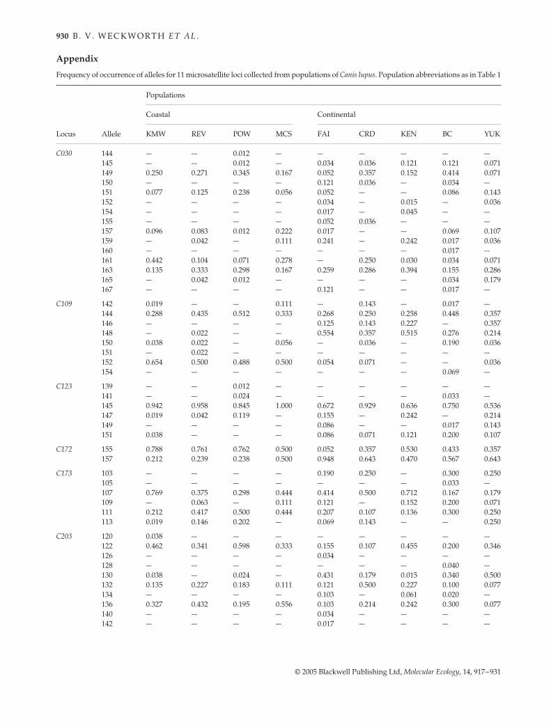
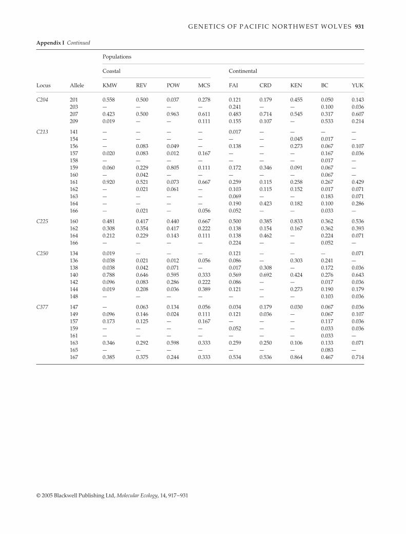
Appendix Frequency of occurrence of alleles for 11 microsatellite loci collected from populations of Canis lupus. Population abbreviations as in Table 1

Locus Allele

Populations

Coastal Continental

KMW REV POW MCS FAI CRD KEN BC YUK

C030 144 — — 0.012 — — — — — —145 — — 0.012 — 0.034 0.036 0.121 0.121 0.071149 0.250 0.271 0.345 0.167 0.052 0.357 0.152 0.414 0.071150 — — — — 0.121 0.036 — 0.034 —151 0.077 0.125 0.238 0.056 0.052 — — 0.086 0.143152 — — — — 0.034 — 0.015 — 0.036154 — — — — 0.017 — 0.045 — —155 — — — — 0.052 0.036 — — —157 0.096 0.083 0.012 0.222 0.017 — — 0.069 0.107159 — 0.042 — 0.111 0.241 — 0.242 0.017 0.036160 — — — — — — — 0.017 —161 0.442 0.104 0.071 0.278 — 0.250 0.030 0.034 0.071163 0.135 0.333 0.298 0.167 0.259 0.286 0.394 0.155 0.286165 — 0.042 0.012 — — — — 0.034 0.179167 — — — — 0.121 — — 0.017 —

C109 142 0.019 — — 0.111 — 0.143 — 0.017 —144 0.288 0.435 0.512 0.333 0.268 0.250 0.258 0.448 0.357146 — — — — 0.125 0.143 0.227 — 0.357148 — 0.022 — — 0.554 0.357 0.515 0.276 0.214150 0.038 0.022 — 0.056 — 0.036 — 0.190 0.036151 — 0.022 — — — — — — —152 0.654 0.500 0.488 0.500 0.054 0.071 — — 0.036154 — — — — — — — 0.069 —

C123 139 — — 0.012 — — — — — —141 — — 0.024 — — — — 0.033 —145 0.942 0.958 0.845 1.000 0.672 0.929 0.636 0.750 0.536147 0.019 0.042 0.119 — 0.155 — 0.242 — 0.214149 — — — — 0.086 — — 0.017 0.143151 0.038 — — — 0.086 0.071 0.121 0.200 0.107

C172 155 0.788 0.761 0.762 0.500 0.052 0.357 0.530 0.433 0.357157 0.212 0.239 0.238 0.500 0.948 0.643 0.470 0.567 0.643

C173 103 — — — — 0.190 0.250 — 0.300 0.250105 — — — — — — — 0.033 —107 0.769 0.375 0.298 0.444 0.414 0.500 0.712 0.167 0.179109 — 0.063 — 0.111 0.121 — 0.152 0.200 0.071111 0.212 0.417 0.500 0.444 0.207 0.107 0.136 0.300 0.250113 0.019 0.146 0.202 — 0.069 0.143 — — 0.250

C203 120 0.038 — — — — — — — —122 0.462 0.341 0.598 0.333 0.155 0.107 0.455 0.200 0.346126 — — — — 0.034 — — — —128 — — — — — — — 0.040 —130 0.038 — 0.024 — 0.431 0.179 0.015 0.340 0.500132 0.135 0.227 0.183 0.111 0.121 0.500 0.227 0.100 0.077134 — — — — 0.103 — 0.061 0.020 —136 0.327 0.432 0.195 0.556 0.103 0.214 0.242 0.300 0.077140 — — — — 0.034 — — — —142 — — — — 0.017 — — — —

G E N E T I C S O F P A C I F I C N O R T H W E S T W O L V E S 931

© 2005 Blackwell Publishing Ltd, Molecular Ecology, 14, 917–931

C204 201 0.558 0.500 0.037 0.278 0.121 0.179 0.455 0.050 0.143203 — — — — 0.241 — — 0.100 0.036207 0.423 0.500 0.963 0.611 0.483 0.714 0.545 0.317 0.607209 0.019 — — 0.111 0.155 0.107 — 0.533 0.214

C213 141 — — — — 0.017 — — — —154 — — — — — — 0.045 0.017 —156 — 0.083 0.049 — 0.138 — 0.273 0.067 0.107157 0.020 0.083 0.012 0.167 — — — 0.167 0.036158 — — — — — — — 0.017 —159 0.060 0.229 0.805 0.111 0.172 0.346 0.091 0.067 —160 — 0.042 — — — — — 0.067 —161 0.920 0.521 0.073 0.667 0.259 0.115 0.258 0.267 0.429162 — 0.021 0.061 — 0.103 0.115 0.152 0.017 0.071163 — — — — 0.069 — — 0.183 0.071164 — — — — 0.190 0.423 0.182 0.100 0.286166 — 0.021 — 0.056 0.052 — — 0.033 —

C225 160 0.481 0.417 0.440 0.667 0.500 0.385 0.833 0.362 0.536162 0.308 0.354 0.417 0.222 0.138 0.154 0.167 0.362 0.393164 0.212 0.229 0.143 0.111 0.138 0.462 — 0.224 0.071166 — — — — 0.224 — — 0.052 —

C250 134 0.019 — — — 0.121 — — — 0.071136 0.038 0.021 0.012 0.056 0.086 — 0.303 0.241 —138 0.038 0.042 0.071 — 0.017 0.308 — 0.172 0.036140 0.788 0.646 0.595 0.333 0.569 0.692 0.424 0.276 0.643142 0.096 0.083 0.286 0.222 0.086 — — 0.017 0.036144 0.019 0.208 0.036 0.389 0.121 — 0.273 0.190 0.179148 — — — — — — — 0.103 0.036

C377 147 — 0.063 0.134 0.056 0.034 0.179 0.030 0.067 0.036149 0.096 0.146 0.024 0.111 0.121 0.036 — 0.067 0.107157 0.173 0.125 — 0.167 — — — 0.117 0.036159 — — — — 0.052 — — 0.033 0.036161 — — — — — — — 0.033 —163 0.346 0.292 0.598 0.333 0.259 0.250 0.106 0.133 0.071165 — — — — — — — 0.083 —167 0.385 0.375 0.244 0.333 0.534 0.536 0.864 0.467 0.714

Locus Allele

Populations

Coastal Continental

KMW REV POW MCS FAI CRD KEN BC YUK

Appendix I Continued