1

A SHORT COURSE ON MASTERS LEVEL ECONOMICS FOR PUBLIC ADMINISTRATION STUDENTS Cameron Gordon, PhD Associate Professor of Economics University of Canberra Cameron.gordon@canberra.edu.au February 14, 2014 This is a short course on economics based on lecture notes for an MPA class on Public Managerial Economics I taught while on the faculty of the School of Public Administration (and then later the School of Policy, Planning and Development) at the University of Southern California in the late 1990s/early 2000s.

2

Concepts: Economic reasoning, general equilibrium and economic systems

Scarcity and constrained optimization (scarcity (noun)) scarce: 1. Infrequently seen or found. 2. Not plentiful or abundant. The major question for economics tends to be: "How are resources best allocated given scarcity?" Economics captures this notion of scarcity in the budget constraint. A budget constraint shows all the different combinations of goods and services that a consumer can purchase given the resources (income) under his/her command. It is possible to graph a budget constraint, although to do this in two dimensions, one needs to limit one's attention to two goods. Suppose that a consumer wants only to buy apples and oranges and wants to spend all their income on those two things. In this case the budget constraint line shows all the combinations of apples and oranges that can be bought with a given income. What is an optimum? The American Heritage dictionary defines it as: “The best or most favorable condition, degree, or amount for a particular situation.” To “optimize” is “to make the most effective use of”. So economics is a discipline which focuses on attainment of optima (the plural of optimum) in a setting where scarcity prevails. This scarcity acts as a central constraint on the system. Hence economics is often referred to as an analysis of constrained optimization. Optimizing along the budget constraint When an economist sees a budget constraint, what does s/he do? First, an economist will tell you to get on to the line. In other words, assuming that you want to spend all your income on apples and oranges (and it is important that it be known exactly what your objectives are) then you should choose a point somewhere along the budget constraint (a point like A). Points above the constraint (like C) are unattainable given existing resources, while points like B are attainable but are not making full use of your available resources given your chosen objectives. This is the essence of constrained optimization. We know that point B is not an optimal point and that point C is unattainable and hence irrelevant to our decisionmaking. However, how does one choose between point A and point D, both of which are along the constraint? This issue will be encountered again later on. Suffice it to say that to know which point is an optimal point, one needs to know what it is one wants. In other words, there is a need to know objectives and a need to know preferences among those objectives. The neo-classical paradigm A very coherent and powerful world-view which is often referred to as the neoclassical paradigm. This paradigm assumes that the economy works in very set ways along very set lines. There are some who believe that this model can explain many or most noneconomic phenomena, including war, revolution and crime. Such people are often called economic imperialists because they want the neoclassical paradigm to take over all social science. Elements of the Neo-classical Paradigm

All actors in the system are rational, or behave as if they were. “Rational” here means that people act consistently and in a well-ordered fashion.

All actors are self-interested. This does not mean that they think of no one else but that they ultimately choose to make themselves better off and will not seek to make themselves worse off.

The goal of actors is to maximize their desired objective. Put another way, whatever "good" (as opposed to "bad") you want, more is always better.

People respond to incentives, and price is the best incentive.

Markets generally clear, that is desired quantities will be traded at agreed upon prices.

The economic system is generally self-equilibrating, i.e. if left to its own devices, it will find a stable equilibrium.

3

The economic system is efficient, i.e. the forces of competition will always lead to lowest production cost and maximum consumer utility or satisfaction.

“Economic Imperialism” and the “Chicago School” As mentioned above, “economic imperialists” believe that the neoclassical paradigm could and should take over all social science. The neoclassical paradigm lends itself to economic imperialism quite well because it is a theory with (a) a coherent structure; (b) concepts which are general in nature and very generalizable (i.e. can be easily extended, in a logical sense, beyond their immediate and intended domain); (c) a compelling internal logic and ease for generating "stories" and explanations of why things happen. In addition, in many noneconomic areas where economic thinking has become pervasive, other disciplines often offer conflicting theories of phenomena in those areas, or offer no theory at all. Thus it is that Nobel Laureate Gary Becker has argued that "it takes a theory to beat a theory" and that economic thinking "wins" in many cases because other disciplines do not offer competing and testable theories of their own. The University of Chicago has become known for its intensive development of the neoclassical paradigm and its extension of that paradigm into many noneconomic areas in the true spirit of economic imperialism. This distinctive approach to economics has become known as the Chicago School. As a logical game, it is easy to play with extend the neoclassical paradigm far beyond its original boundaries. But in the real world, many of the basic premises of the model -- perfectly clearing markets, perfect information, rational maximizing individuals -- often do not seem to accord with the observed facts. Now a given theory will always deviate from the facts in some way since a theory is by definition a simplification of reality. How do economic imperialists tend to deal with uncooperative facts? In his article on Chicago School economics, Reder lists at least 4 possible responses a theoretician can take when observed facts do not match the predictions or premises of the neoclassical paradigm:

Reexamine the data until the findings match the model's predictions

Redefine or augment the variables in the model to account for the data

Alter the theory to accomodate behavior inconsistent with rationality

Place findings on research agenda as a researchable anomoly Chicago School thinking tends to do all but the third item. The other options tend to preserve and extend the neoclassical paradigm and allow it to extend to more hostile settings. The third option tends to undermine the paradigm.

APPLICATION: THE THEORY OF RATIONAL ADDICTION One seeming challenge to this paradigm is addictive behavior, which seems to be irrational and self-defeating. However, Nobel Laureates Gary Becker and George Stigler have developed a theory of so-called “rational addiction”

The argument goes something like so:

Each individual has a “utility function” through which they get satisfaction (more on this concept a little later on). A typical utility function can be written in general form like so:

Utility of Consumer A = f(good 1, good 2...good n)

“Inputs” into this utility function are goods which people consume. The “output” of this utility function is “utility” which is a measure of consumer satisfaction. It is not directly observable, but people desire as much satisfaction as they can get and organize their behavior accordingly to maximize satisfaction within the constraints of time, money, etc. which they find themselves presented with. The function itself — “f(..)” — represents a “technology” which the consumer has for transforming raw inputs into the useful output of satisfaction. As economic observers, we cannot observe this technology directly. The best that we can do is to see how many inputs a consumer consumes and then, by observing the consumer’s actions over time, make some guess about the output of utility being produced.

In a world with only one good, the economist might observe the following pattern

Consumer A is offered 1 unit of good X and is asked how much s/he is willing to pay and the consumer says

4

$1. If offered 2 units, the consumer is willing to pay $2. If 3 units, $3 and so on. If we equate the dollar amounts to utility received, the economist might assume a “technology” which relates inputs to output like this:

Utility of Consumer A = (X), i.e., 1 unit of X yields 1unit of utility, 2 yields 2 units and so forth.

With respect to addiction, Becker and Stigler come up with some generalizations about addictive behavior, and then worked backwards, using neoclassical postulates, to arrive at an explanation of such behavior.

They describe addicts as (1) being willing to pay increasingly greater amounts for a given unit of an addictive substance over time and thus (2) deriving ever less utility from that unit over time.

This behavior pattern they claim can be explained as rational maximizing behavior because the addictive substance causes changes in the consumption technology which make the utility function less “efficient” over time in transforming the good into utility.

Thus one might observe the following utility function for beer consumption in period 1

U (of consumer A) = 3(number of beers) - 1.5^(number of beers)

In that period, consumer A will receive 1.5 units of utility by consuming 1 beer, 3.75 units by consuming 2, 5.63 units from 3, 6.94 from 4, 7.41 from 5, and then diminishing returns set in at 6 beers when utility is only 6.61. (“Diminishing returns’” is a pervasive concept in economics and refers to the pattern whereby an activity is first associated with big payoffs and then increasingly small payoffs as that activity increases. A typical textbook example is, in fact, beer consumption — the first one tastes really great, the second one less so, and the third one might begin to get one sick).

This is what happens at time 1. But suppose beer is like dirty water in a paper manufacturing plant. Just as dirty water will begin to gum up the works in such a plant and make it less efficient with time, beer may be a substance, at least for some consumers, that degrades the consumption technology. Thus in period 2, the consumer may find his/her utility function looking like so: U = [4(number of beers)-1.5^(number of beers)]-5.2

It’s a subtle difference, but now the consumer must drink 6 beers instead of 5 to get that 7.41 units of utility. If the function continues to deteriorate like this, the consumer will have to drink more and more beers each time to get that same level of satisfaction. And at some point, even that original “high” may not be achievable no matter how many beers are consumed.

The main point of this model is that there is no need to assume that the consumer is being irrational or not maximizing in order to derive behavioral conclusions which mimic certain behaviors that are seen in addicts.

Are the objections to this model? Of course there are, but these will be considered later on.

5

Concepts: Supply and demand, elasticity

Supply and Demand Demand and supply, given a number of assumptions, can be drawn as curves (here as straight lines) which relate a a particular quantity of something (e.g. good "X") to a particular price. Thus the demand curve shows how much X is demanded at various prices and the supply curve shows how much X is provided at the same array of prices. Such curves are shown in Figure 3. Note that the demand curve slopes downward from left to right. This means that at high prices relatively little X is demanded while at low prices relatively more X is sought. The supply curve, by contrast, slopes upward from left to right. Thus at low prices, relatively little X is offered by the supplier while at high prices, relatively more X is provided. Although there are exceptions, demand curves slope downward so often that this pattern has been referred to as the law of demand. Similarly, the law of supply holds that the supply curve almost always slopes upward. Why does the demand curve slope downward and the supply curve slope upward? Economists generally assume that people are rational maximizers. In other words, there is some logical structure to a person's actions (it does not move about wildly or randomly) and that person prefers more to less ceteris parabus (i.e. if I can get more of something without paying anything more for it, I will take it). Thus the lower the price of a good, the more that I will take of it because for a given dollar amount, I can get more of it and will want more of it. Similarly, the higher the price of a good, the more willing I am to sell it because for a given amount of the good, I can get more money as the price goes up. Shifts in demand/supply versus moves along them The fact that I am willing to buy more of a good as price goes down, and sell more as the price goes up is indicated graphically by a movement up or down the supply or demand curve. The curve simply shows how my demand changes as price changes, everything else being equal (including tastes and income). This movement is indicated by the arrows pointing to one another below. If I suddenly lose my taste for chocolate, this will change my demand curve. Such a change is represented by a shift in the demand schedule, in this case a shift downwards in the demand curve. In other words, if I lose my taste for chocolate then I want to buy less at every price and this is shown by a downward shift in the curve (from Demand to Demand*). Supply and Demand Schedules Underlying supply and demand curves, at least conceptually, are supply and demand schedules. Two representations of supply and demand are shown here. The table shows supply and demand schedules which indicate how much a person, firm or other entity either demands of a particular something at a range of prices or how much they are willing to supply at a range of prices. The graph shows that the same schedule are graphed and the resulting supply and demand curves are shown (here they are straight lines). Of course the average Joe is unlikely to have a demand schedule in mind and the average firm may not have an actual supply schedule. But economists assume that people behave as if they do and further these curves summarize propositions about human behavior. e.g. that people will demand more of a good as its price falls.

6

Price

Quantity demanded (demand)

Quantity supplied (supply)

$2

5

1

$3

4

2

$4

3

3

$5

2

4

$6

1

5

Supply and Demand Functions Behind curves and schedules are mathematical relationships known as functions. An example of a function is Y= f(X) which in words can be stated as "Y is a function of X". The function is defined as any relationship such that, given a value for X, a corresponding value of Y, and only one value, is returned. X and Y are thus said to have a one-to-one relationship or mapping. X is the "independent" variable while Y is the "dependent" variable, i.e. Y's value depends, through the functional relationship, on X. An Example of Supply and Demand Functions Recall the supply and demand schedules used before. These values can be summarized even more succinctly with an equation which reproduces the value of "Y" (quantity supplied or demanded) for each corresponding value of "X" (price). As shown earlier, these schedules are graphed as straight lines so the functional relationship will have a form of "mx+b" where m is the slope of the line and b is the point on the Y-axis where the line intercepts it. D = -X+7 (or D = 7-X) S = X-1 Note that D is downward sloping (its slope = -1) and S is upward sloping (=+1) Market Equilibrium Supply and demand intersecting indicates an equilibrium in a market. The graph shows such an equilibrium. Note how the equilibrium resembles the two blades of a scissors, following the metaphor used earlier. In this case the demand for good X and the supply for good X match up at only one point in the middle. This point is an equilibrium in the market for good X. At prices lower than the equilibrium, demand for X will exceed supply and at prices higher than that supply will exceed demand.

7

General Equilibrium Where there is one market, there is only one equilibrium. But there are typically many markets in a developed economy -- markets for food, manufactures, etc; in this case, equilibrium in one market, or lack thereof, may cause equilibrium or lack thereof in one or more other markets. The presence of equilibrium in all markets is known as general equilibrium. Formally, general equilibrium is simply the analysis of many interrelated markets as depicted below. In such a case, equilibrium in one market will affect the equilibrium outcome in another one (or in a set of other ones). Of course, if markets are unrelated to one another, there is no meaningful general equilibrium since the status of one market has no bearing on any other and we could study each single market in isolation from the others. A General Equilibrium Example Imagine now that the markets being studied are the markets which include the supply and demand for (1) steel; (2) plastics; (3) glass; and (4) automobiles. It is easy to see that the equilibrium of demand and supply in the market for automobiles will affect the equilibrium in the other markets and that equilibrium in the other markets will affect the equilibrium in the market for automobiles. This comes about in this case because the first three markets represent inputs into the process for making automobiles. Thus the amount of autos that a society creates will have a major impact on the amount of steel, plastics and glass that will be created and vice-versa. Substitutes and Complements Markets are not only related by the fact that one market provides inputs to a production process relevant to another as with the automobiles example. Markets are also related to one another by patterns in consumption. For example, consider the markets below for tea, coffee, sugar and crumpets. Purchase of sugar is related to purchase of tea and coffee because many people consume those two goods with sugar. In this case the goods are complements -- that is one good tends to be used or consumed with the other. Tea and crumpets are also complements. On the other hand, tea and coffee are also related to one another through consumption patterns except that they are substitutes -- one is consumed or used in lieu of the other. Other Market Interrelationships There are yet other relationships between markets. For example, the market for Starbuck's stock is related to the market for coffee in part through financial mechanisms since the market for such stock depends on the health of Starbucks which depends on the coffee market. Adjustments between these multiple markets tend to occur through price -- e.g. a strong demand for steel will drive up the price of steel (unless supply increases) which will then tend to drive up the price of autos. Of course a change in price will affect final quantities traded. Income and Substitution Effects Demand in particular can be broken down into two components. As the price of a good changes, this affects both the amount of that particular good that a person can buy ( the income effect) and it also changes the incentives to buy that good ( the price

8

effect). Say a good falls in price. This fall in price (1) allows a person to buy more of another good should they choose to do so because some of the income they devoted to buying the original good is now "released" for other purposes. Thus they have more disposable income as a result of the price change and this is the income effect. At the same time, the lowered price itself makes the good cheaper relative to other goods and this alone makes the good a more attractive buy (the price effect). How much a consumer actually buys of the newly priced good depends, in part, on their tastes. Elasticity Supply and demand can both be summarized by an elasticity. An elasticity is equal to the percentage change in one quantity divided by the percentage change in another quantity. For supply and demand, one typically wants to know the price elasticity. That is the equal to: [(% change in quantity of a good supplied or demanded)/(% change in price of that good).] For demand only, the whole division has a minus sign before it. This is simply a convention of economics to ensure that the elasticity of demand is nonnegative. Types of Elasticity Economists use some elasticities more than others. Some of the more common ones are: Price elasticity: The change in quantity of X demanded or supplied in response to a change in the price of X. Income elasticity: The change in quantity of X demanded or supplied as income of the party doing the demanding or supplying changes. Cross-price elasticity: The change in quantity of Y demanded or supplied in response to a change in the price of some other good Y. Elasticity of Output: The change in an entity's output in response to a change in a given input. Elastic and Inelastic “Elastic," means something is highly responsive to changes in something else. For example, elastic demand means that the quantity demanded changes a lot when the price changes. Inelastic demand means that the quantity demanded does not change much when the price changes. The qualitative idea is that: Elastic = Responsive Inelastic = Unresponsive The terms "elastic" and "inelastic" can be given a precise meaning in terms of the number that comes out of the elasticity fraction. The divider between elastic and inelastic is -1, for demand elasticities. (For elasticities where you expect a positive relationship between Q and P, such as for elasticities of supply, the divider is +1.) If the demand elasticity is more negative than -1, the demand is elastic.If the demand elasticity is between -1 and 0, the demand is inelastic. Elastic demand -- elasticity more negative than -1 -- means if the price goes up, the total amount customers spend goes down.Inelastic demand -- elasticity between -1 and 0 -- means if the price goes up, the total amount customers spend goes up.If the elasticity is exactly -1, the amount customers spend stays the same as the price changes. Price elasticity is a measure of responsiveness. It tells how much one thing changes when you change something else that affects it. For example, the elasticity of demand tells us how much the quantity demanded changes when the price changes. The elasticity of demand measures the responsiveness of quantity demanded to changes in the price charged.

9

Inelastic Demand Consider the following graph and table. INELASTIC DEMAND

Price

6| F

5| E

4| D

3| C

2| B

1| A

:....:....:....:....:....:....:....:....:....:....:....:....:

0 5 10 15 20 25 30 35 40 45 50 55 60 Quantity

A B C D E F

Price $1 $2 $3 $4 $5 $6

Quantity 40 40 40 40 40 40

Regardless of whether the price is $1 or $6 or anything between, the amount sold will be the same, 40 units. This is an example of completely inelastic demand, i.e. completely unresponsive to price changes. This is an extreme case. The traditional medical model implies completely inelastic demand. If health care professionals provide what they judge that the patient "needs" regardless of cost, and if the patient is unable to object or is fully insured or both, then demand will be inelastic. Note in this case the relationship of elasticity to revenues: A B C D E F

Price $1 $2 $3 $4 $5 $6

Quantity 40 40 40 40 40 40

------------------------------------------------------

Revenue $ 40 $ 80 $120 $160 $200 $240

Revenue equals Price times Quantity. So If your demand is inelastic, the more you charge, the more revenue you take in, since the amount you sell doesn't go down. Therefore, if profit is your goal, you should raise price when demand is inelastic. This leads directly to the standard. Demand becomes elastic if consumers are price conscious and if they have an alternative. Suppose that the market in the example above gets a new competitor, who charges $3.50. Suppose also that price is the consumer's only consideration (no quality difference, no customer loyalty to a particular company). Then the demand might look like this. Demand -- One Competitor Who Charges $3.50 -- Price Only Consideration

Price

6|F

5|E

4|D

3| C

2| B

1| A

:....:....:....:....:....:....:....:....:....:....:....:....:

0 5 10 15 20 25 30 35 40 45 50 55 60 Quantity

A B C D E F

Price $1 $2 $3 $4 $5 $6

Quantity 40 40 40 0 0 0

If you charge less than your competitor's price, you get all of the business. If you charge more than $3.50, you get no business. Your demand is now highly elastic near the competitor's price. This can be a highly unstable market because your competitor faces the same situation. You can cut your price to $3.49 and take away all of the business. Your competitor can then charge $3.48 and take it all back. Each of you has the temptation to cut price on the other until one of you goes broke. You see something like this when neighboring gasoline stations have a price war. One thing is for sure: If there is a competitor in your market, and if the consumers care about price, then there's a definite limit to how high you can raise your price.

10

Of course completely elastic demand is the opposite of completely inelastic demand: If one were to draw the demand curve in this case it would be completely horizontal rather than vertical. Analogous arguments can be made for supply curves. Elasticity. Substitutability and Complementarity Cross-elasticities refer to the change in the demand for good X when the price of Y changes. Such relationships are interesting as a measure of whether one good is a substitute or complement to another. For example, one would expect that a rise in the price of tea would cause an increase in the consumption of coffee. This is one of many important elasticities -- one could invent any one that one sees as useful. Normal and Inferior Goods Another relationship which is summarized by elasticity refers to the change in consumption of a good when a person's income changes. A normal good is one whose consumption relative to income increases as income increases. An inferior good is one whose consumption relative to income falls as income rises. Thus the richer one gets, the less iceberg lettuce (it is an inferior good) one may consume and the more arugula one eats (it is a normal good).

APPLICATION 1: THE PUZZLE OF ECONOMIC DEVELOPMENT: A review of Bairoch, Paul, Economic and World History: Myths and Paradoxes (University of Chicago Press, 1993)

This book could be titled: “What determines economic growth?” for much of the discussion centers on factors which cause some countries to grow and others not to. Bairoch starts with the Depression, but one could start with a larger theme in his book which is the impact that trade has on economic growth.

One of the seven “minor” myths that he ends with is “Was trade an engine of economic growth?” Here is one of the first suspects on the usual list of causes of economic development.

Much of Bairoch’s work focuses on determining whether free trade prevailed in the first place. Of course mercantilism and protectionism predominated before the 19

th century although this was due more to various

interests protecting their perceived turfs rather than a result of the influence of mercantilist theories. (17-18). But was that century a golden age of free trade? Bairoch thinks not.

The United Kingdom did become increasingly liberal in trade matters but not really before 1842. The Corn Laws were not abolished before 1846 and other trade restrictions were relaxed only in a piecemeal fashion — in 1825, with an act allowing emigration of some skilled laborers and with reduction of some import duties in 1833. The Corn Laws themselves were successfully repealed by a coalition of manufacturers and others who used the high food prices and low wages from such laws to make an issue of worker poverty. It was indeed a free trade watershed. But it must be kept in mind that free trade only took hold as the UK established commanding leads in almost all industries and in per capita income (20-21).

From 1846-1860, the UK aggressively pursued free trade and via the example set by this and through the increasing volumes of international trade, free trade began to take hold on the Continent as well. At first this was limited to small economies such as Holland, Portugal, Denmark and Switzerland, though with some degree of protectionism as well. Then between 1860 and 1879, free trade became dominant in Europe, but not elsewhere in the world, especially the U.S. (21-23). Then protectionism began a resurgence in Europe that continued until the beginning of World War 1. Here, though, the UK’s free trade policies became more entrenched. At the same time, the U.K. became less important economically and less robust as well (23-29)

Looking at the rest of the world, the picture is more complicated still. Japan and China, often seen as the closed and mysterious East, in fact had open trade regimes at various times before the 1800's. The U.S. conducted a protectionist trade policy before the beginning of the Civil War. And while there were twists and turns in that policy, it grew more protectionist after the Civil War. Here, though, the justification for such policies changed from protection of infant industries, a viable rationale when the U.S. economy was young, to protection of wages (31-37). Protectionism also reigned in other parts of the developed world, especially in the British Commonwealth countries of primarily European descent — Canada, Australia and New Zealand. For the latter half of the nineteenth century in to the early part of the twentieth, the developed world was a bastion of protectionism with an island of liberalism — the U.K. (41). It is only in the so-called “future third world” that free trade was a rule and there it was enforced by colonial masters, except in the Ottoman Empire which had a free trade policy already and whose example of economic decline was sometimes used as an argument against unfettered free trade, especially by Disraeli. (41-42)

This history raises a related question which is if free trade did not always predominate in the high-growth 19

th

11

century, was protectionism always a burden? One clue is found by the fact that the rise of free trade which started around 1870 was accompanied by the great depression of 1873 while the rise of protectionism in the early 1890's saw the end of this depression. This is obviously too simplistic a case by itself but what seems to be happening during this time is that differing stages of economic development and different external circumstances imply different results for the same policy regime. When Britain adopted free trade for agriculture in 1846, the hundred years prior had already seen a marked shift in the proportion of the labor force employed in manufacturing relative to agriculture — England’s ratio of industrial workers to farm workers was much higher than that of Europe at the time. In addition, non-European sources of grain became much more important and much cheaper as the nineteenth century progressed. Thus free trade, especially in agricultural products, had a much harsher effect on European economies in the 1860's and 1870's than it would in England at that time and the relaxation of those policies would have a more salutary effect in Europe than England. (47-49). The case “against” free trade is even stronger if one looks at correlations of per capita output growth and free trade policy, which move inversely, both in Europe and even more so in the U.S. (50-53)

So was trade an engine of economic growth? For the most part, the answer seems to be “no”, at least for all other than small countries where external trade to begin with represents a much higher proportion of economic activity. To be more precise, the mechanistic model of free trade as a spur to economic growth must be resisted for it depends on the circumstances. (136-138). If not trade, then what? Another alternative is that Europe and the developed world relied on the exploit of third world resources to grow. If so, this is a bad story for the current third world since they have no such hinterland to exploit. But Bairoch says that this too is not an economic prime mover. For if one looks at various raw materials, Europe and the developed world were either exporters of such goods or primarily self-sufficient, often on the order of producing 90 to close to 100% of their needs of various basic inputs. (60-68). However, for the third world this meant that the overwhelming bulk of their exports were raw materials. However, one needs to distinguish between raw materials, such as oil, which often require a large amount of processing, and primary goods, such as fruit and salt, which undergo little real transformation before being shipped). (68-69)

So the Third World was not a crucial source of raw materials during a critical period of economic growth in the developed world. Was it a crucial outlet for colonialist goods? In a global sense, the answer is no for overall the share of exports going from the West to the underdeveloped nations remained small until the twentieth century. However, the picture varies by nation. The U.K. textile industry became especially dependent on third world outlets by the turn of the century, although it must be remembered that the country at this point had a good six decades of modern economic development behind it. Even so, relatively small outlets can be critical for the profitability of an industrial sector. At the same time, easy colonial outlets can have a negative effect as well as domestic producers become “lazy” and uncompetitive. (74-75) Loose evidence that colonial empires may be negative influences on growth rather than positive ones comes from the correlation of lower economic growth with presence of such empires. Empires can be costly both in terms of direct expenditures and diversion of entreprenurial resources (77-78)

Perhaps colonial possessions did not feed ongoing economic growth, but were they a trigger to the industrial revolution itself, or mare particularly, to the more colony-oriented economy of Great Britain? There is an immediate problem with this hypothesis since the industrial revolution in England started before its empire was either that large or important in terms of trade — that came later. (80-82) More generally, it seems to be the case that colonial empires were not an especially significant source of riches or development for Europeans, though it is not to be treated likely. However, the impacts of colonial de-industrialization on the Third World is much more negative, accounting for a lot of the slow income growth characteristic of those regions between 1800 and 1950. (88-98)

Perhaps history matters here, for it is often assumed that Europe was much richer and much more urbanized at the outset of the industrial revolution and that these factors accounted for Europe’s take-off and the Third World’s persistent stagnation (though these differentials themselves need to be explained). There is a lot of uncertainty with regards to this question but as to wealth, Bairoch says that the future Third World and Europe were at roughly similar per capita income levels at the beginning of, say, 1700. (101-108). As for urbanization, Bairoch says that the pre-industrial world, on average, was more urbanized than commonly believed, consistent with levels seen during the Greek and Roman Empires. These levels are, it is true, far below those necessary to sustain industrialization; but the main point here is that differentials between urbanization may not be a very robust explanation for economic growth [this last point is really mine, not the author’s]. (142-144)

How about population growth? It has been argued that the impact of population growth early in the West’s economic growth was positive. However, the rate of this growth is critical — current rates in the third world

12

are much higher than those witnessed during the early 1800's in Europe or anywhere else for that matter. (127-128) In addition, Europe’s experience in this matter does not suggest such a simple correlation. In particular, high increases in both private and social investment, particularly in education, are necessary to provide for increased population. (130-131). One big difference also in current third world urbanization and early European urbanization is that the latter is taking place largely as a concentration of people without a concomitant urban and economic development (132).

Indeed, this issue of causality crops up again and again in economic history. Bairoch suggests, for example, that growth drives trade and not the other way around. And so it can be for urbanization — growth driving population concentration can be a good thing, but population concentration by itself does not necessarily drive growth.

One can turn this economic development question on its head and ask what drives underdevelopment. Bairoch tackles these issues as well. One of these myths is that a reliance on export of primary goods leads to backwardness. The evidence does not support this for many nations in the 1800's were exporters of primary goods, including New Zealand, Argentina, and, most of all, the United States, and they had very high levels of per capita income. Thus a reliance on primary goods as a main export is not by itself a road to underdevelopment. However industrialization at some point seems to be necessary to reach the next level of economic growth. This is what happened in Argentina which was a very rich country before World War 1 but because of a lack of industrialization as time went on and very low growth in agricultural productivity sunk to a much lower rank in the modern period. (140-141)

It also used to be argued, though much less so now, that a deterioration in the relative price of raw materials to manufactured goods throughout the 19

th century led to the current fix of Third World countries since they are

primary exporters of raw materials. In fact, such terms of trade seemed to have improved during the period with one very important exception: sugar, a key import for many colonial nations. (111-113)

APPLICATION 2: RAILROADS AND AMERICAN ECONOMIC GROWTH AFTER THE CIVIL WAR

Take-off thesis: The railroad caused America to industrialize rapidly and suddenly, increasing the rate of per capita output growth dramatically in a very short period of time (Rostow, 1960). The take-off thesis relied on forward and backwards linkages.

Backward and forward linkages Forward linkages refer to the use of the outputs of the leading sector, in this case railroads, as inputs into production by other sectors.

Backward linkages refer to the use of the outputs of other sectors as inputs into production of the leading sector.

Thus railways provide improved transportation services which are used by, say, agricultural producers to get

goods to market faster (a forward linkage) and railways require steel; which increases demand for the product and stimulates the growth of the steel industry (a backwards linkage). The Fogel argument/Counterfactual Fogel looked at the economy up until 1890, with the railroads available and then, in 1890, suddenly eliminated them from the economy, requiring the use of alternative, and more expensive transport methods such as canals. He then measured the effect on Gross National Product (GNP) in that year, under a number of simplifying assumptions described below, and called that effect social saving railroad's impact.

Social Saving

His measure of indispensability was the "social saving" due to railroads. Social saving generally refers to the resources saved by a society, and hence available for other purposes, when it has the use of a technology or other innovation as compared to the situation which would prevail if it did not have the use of that technology or innovation.

13

The general definition can be better understood by using a diagram of a simplified economy (adapted from Coatsworth, 1981). Two aggregate supply curves and one aggregate demand curve for transportation are pictured below.

For simplicity, the transportation supply curves are horizontal, the transportation demand curve, vertical. S

w/rail is the supply of transport available in the presence of railroads. Sw/o rails is the supply curve of transportation when railroads are unavailable and when only alternatives, such as canals, can be used. The amount spent on transport is equal to the appropriate price times quantity (which I have not labeled above). With railroads available, the amount spent on transportation equals area 1. Without railroads, the amount spent on transportation equals area 1 plus area 2. The social saving, that is, the resources which railroads free up for social uses other than transportation, is equal to the resources which would have been spent on transport without railroads minus the resources which are spent on transport with railroads. It should be clear that this difference is area 2.

Social saving thus defined is both a net measure and a gross measure of the economic impact of the railroads. It is a net measure, because it compares one circumstance, the actual historic, or "factual" circumstance where railroads are operating, with another hypothetical, or "counterfactual" circumstance where railroads are not operating, and then subtracts the difference in transportation costs between the factual and counterfactual to arrive at a net change in transportation costs. It is a gross figure because it consolidates a whole range of impacts into a single index and measures the absolute impact on overall resources available to society, rather than relative changes to resource allocations within that society.

Embodied/Disembodied Effects Fogel himself referred to the social saving as a disembodied effect, due to the fact that any transport innovation lowers costs and hence results in savings to society. Railroads delivered these savings in a very particular form, and the form which savings due to railroads, as opposed to a different transport innovation which might have occurred, are the embodied effects (Fogel, 1979, pp. 38-39). Thus a relatively insignificant social saving might result in otherwise dramatic changes in a society. In other words, while total output might have remained fairly similar in the absence of railroads, the social fabric might have changed dramatically.

John Coatsworth has summarized this complex web of impacts well: "The most celebrated technological innovation of the nineteenth century industrial revolution was the railroad. Since nearly every product of industry, agriculture, and mining used transport, and railroads reduced transport costs, the effects of the new technology were felt throughout entire economies. Since railroads quickly came to be major consumers of iron and steel, they were credited with stimulating the development of basic industries. As large enterprises with heavy capital requirements, they pioneered the development of modern management techniques and had considerable impact on the evolution of modern capital markets. The social effects of cheap, rapid transport provided drama for historians of labor struggles, elite behavior, and migratory patterns. Military historians have noted the difference that railroads made in strategic and tactical planning (Coatsworth, 1981, p.7)."

Oliver Williamson and Alfred Chandler have argued that railroads produced not only transportation efficiencies, bur organizational and institutional innovations which, when combined with the delivery of speedier and more regular goods and passenger carriage, made a system of mass distribution possible, promoted the growth of mass manufacturing and led to the development of the large, vertically-integrated corporation(Chandler, 1977; Williamson). Williamson also noted that the geographic broadening of the market may have led as well to quality debasement as local manufacturers had to oversee increasingly distant distributors. While these effects can be discussed, and even observed and understood, they are difficult to formalize and disentangle analytically (James, 1984, pp. 241-242).

Pros and Cons of Fogel Some of these criticisms of Fogel become clearer by returning to Figure 1 above. For simplicity, the transport supply and demand curves are drawn with infinite and zero price elasticities respectively. These clearly are unrealistic assumptions. The assumption of zero elasticity of demand has the effect of maximizing the amount of social saving. This can be seen by imagining a slant to the demand curve, which causes area 2 to be reduced. Fogel desired such an outcome since he wanted to show that, even using a measure with an upward bias, social saving was still modest. Fogel was attacked by many authors for using a zero demand elasticity, with many authors arguing that passenger demand elasticities at least, were much greater than zero, and that available evidence was sufficiently detailed to be used to estimate actual price elasticities (Boyd and Walton, 1972; Fogel, 1979). The unrealism of the assumption of zero demand elasticity is further seen by restating it: when transport prices go up, shippers are assumed not to respond, shipping the same volume of goods to the same points over the

14

same distances. For Fogel's purpose of debunking railroad indispensability, this may be a reasonable stratagem, since if shippers were allowed to adjust, social saving would be even less, but for a "true" counterhistorical picture, this may constitute an unreasonable compromise. It also makes different estimates of social saving, based on differing demand elasticity assumptions, difficult to compare (Fogel, 1979, pp. 10-12). Transportation supply elasticities will also affect the social saving estimate. Fogel assumed, like many authors, that the long-run marginal cost was constant: hence the horizontal supply curve in the diagram. But unlike the zero demand elasticity assumption, which overstates social saving, this assumption may have the effect of understating social saving. If, for example, canals have a rising marginal cost structure, then when the hypothetical shut-down of railroads throws a large volume of traffic on to the canal network, prices of canal transport will presumably rise much more than observed canal tariffs, and the assumption of constant marginal cost, would suggest. The amount of resources diverted to transportation in the absence of railroads, and hence the social saving due to railroads, will be much greater than otherwise assumed. All of this suggests, as Fogel himself conceded later in the debate, that careful specification and understanding of the transportation sector is a prerequisite to understanding the impacts that a transport innovation might have on costs and prices (Fogel, 1979). Additionally, inferences based on available evidence, which may seem obvious, must be carefully defended and supported. Besides the obvious problem of adjusting observed canal and railroad tariffs to equate with true marginal cost by adjusting for government subsidies and monopoly power, one has to understand how prices would have reacted in response to a major shift in demand for transport. Although observed canal rates and railroad rates in 1890 might be fairly similar on average, if the only way that canals could meet additional demand was to pull in less efficient and more expensive operators, price would increase more than these 1890 rates would suggest. Fogel makes another point, namely that the ownership of both railroads and canals might make a difference in pricing policy. Thus government-owned canals would tend to charge below marginal cost, or at least not above it, in response to a surge in demand, while privately owned canals would tend to charge more than marginal cost in such a case. Fogel argues that the former was the case in postbellum America, where many canals were publicly owned, while the latter was the case in England, where most canals were privately owned (Fogel, 1979; Hawke 1970). Less obvious from the diagram is the relationship of industrial structure of nontransport sectors to social saving induced by changes in the transport sector. As mentioned earlier, social saving represents the amount of resources that railroads made available to society for alternative uses. However, whether a society could or would actually make good alternative use of these savings depends largely on the strength and quality of the backwards and forward linkages which exist. This fact is particularly important in underdeveloped economies where structural and institutional barriers to efficient allocation of resources (such as concentration of wealth, illiteracy, and state intervention) often means that any savings due to less costly transportation fails to result in overall savings to society because weak forward linkages cause these transportation economies to be squandered. Conversely, if a railroad is built mainly with foreign capital and foreign labor, benefits from backward linkages, such as the development of a domestic steel industry, may also fail to come to pass (Coatsworth, pp. 201-203).

Main Results of the Analysis of Railroads and Economic Growth

Railroads were not indispensable in most European countries and America. That is, shutting down the rails for one year in England, the U.S., Russia, France, Germany and Belgium would have resulted in a GNP loss no greater than 11% and as low as 2.5%, clustering closer to 5%. Only in Mexico and Spain were GNP losses truly catastrophic, closer to 20%, much of that having to do with the lack of viable alternatives (O'Brien, 1983, pp. 9-11). Even more dynamic simulations such as Jeffrey Williamson's have shown relatively modest, though higher, social saving (WIlliamson, 1974, 1975; Fogel, 1979; James, 1984).

Social saving due to rails was generally greatest over shorter hauls where wagons and roads were the main alternative rather than longer hauls where waterways were often quite competitive and where productivity continued to improve over the late 19th century. Indeed, in this period canals continued to be built in Belgium, France and Germany (11). Thus social saving was greatest in countries which relied most on roads - productivity in this sector remained low until the development of the internal combustion engine - and lowest where there were many navigable rivers, terrain well-suited to building canals, and good facilities for coastal trade. In general, railways alleviated

15

poor natural endowments. Where these endowments were rich, rails had relatively little impact. Where these endowments were poor, railroads saved society more in terms of transport costs (O'Brien, 1983, pp. 11-14).

While many societies would perhaps have been only moderately worse off without railroads in terms of measured output, all societies would have looked significantly different without them. Beyond lowering transport costs, railroads had some of their greatest impacts in developed societies on corporate organization, capital markets, market structure, labor markets, and regional distribution of output mix (Chandler, 1977; Williamson, 1974). In less developed societies such as Mexico, railroads had significant impact on land ownership as well (Coatsworth, 1981).

Concepts: Marginal Analysis, Cost, Economies of Scale, Monopoly, competition and market structure

Marginal Analysis: Three dimensions to every problem One can view a system from its overall behavior, i.e. the sum of all the outcomes arising from that system. One could say that this is a total perspective.

One could also try to look at the behavior of the system over repeated workings of the system. One way of doing this is look at the averages, i.e. if the system produces outcome "t" in "n" instances, the average outcome is t/n.

Or one could look at how the system has changed since the last time the system was examined. Thus if the system is in some state "a" at time 1 and then at a different state "b" at time 2, one could subtract a from b to get (b-a), a measure of the net change from one time to another. Such net changes are called marginal changes or changes at the margin.

A marginal analysis table

# of times or units (N)

Total X (T)

Average X (A) = T/N

Marginal X (M)=(T(n)-T(n-1))

0

0

----

0

1

80

80

80

2

180

90

100

3

270

90

90

4

280

70

10

5

250

50

-30

Here is a table presenting total, average and marginal outputs of some process. The outputs could be anything and the process could be anything. For illustration, assume that this is a table of profits associated with production of can openers. But literally, the arithmetic relationships will hold regardless of what you are examining. Look at the "Total X" column first. At 0 units, total X is 0. Then 1 unit (here, a can opener) is produced. Total X (which is assumed to be profits from that can opener) is 80. With production of 2 units, total profit clips to 180; with 3 units, to 270; with 4 units to 280. And with 5 units, total profit falls back down to 250. Now one can already tell a great deal about this system just by looking at the total. For one thing, this outfit should only produce 4 can openers if it wants to maximize profit. The firm may also be interested in knowing its unit profit, also known as average profit per unit of output. This quantity is provided in the "average x" column which is simply "total x" divided by the "# of times or units." Note that the average is undefined for 0 (since T/0 is undefined).

16

Here average revenues start falling between the 3rd and 4th unit. This also indicates that production beyond the 4th unit are not sensible from a profit point of view. Finally, look at the "marginal x" column. Marginal quantities indicate the net change from one total level to another. Thus when the firm moves from a total profit of 0 at 0 can openers to a total profit of 80 at 1 can opener, the marginal profit is equal to 80, i.e. (80-0). At the second can opener, total profit is 180. The net change in profit between the first and second unit is 180-80=100. Marginal profit climbs then falls but remains positive until after the 4th can opener is produced.

Marginal Analysis in Graphs Here are the same relationships shown graphically. A number of things become clear when examining it, all of which are arithmetical relationships.

1. When the marginal quantity is negative, i.e. when each additional unit is negative, the total quantity starts declining. This makes sense since negative increments are being added to an accumulated total. One can look at the converse too -- if the total is declining, the marginal quantity must be negative. 2. It should also be clear that the average rises when each increment (marginal quantity) is above the average (i.e. is pulling the average up) and that the average falls when each increment is below the average (i.e. is pulling the average down). In fact, there are many such arithmetical "laws": 3. Total, average and marginal quantities are equal for the first unit (so long as total x=0 at 0 units). 4. The scale of an activity should be expanded as long as its marginal net yield (however that is properly measured, e.g. profit) is positive and carried on until it marginal net yield is zero. 5. Separate activity levels should, wherever possible, be carried to levels where they all yield the same marginal returns per unit of effort

17

Rules 4 and 5 are especially important for they help any entity set optimal activity levels. Moreover they are allow such decisions to be made on the basis of only partial information -- the marginal quantities. In other words, one often need keep track off of only one piece of information -- ignore the rest -- to make optimal decisions. Intuition of marginal analysis It might seem odd at first to keep an activity going until its net contribution -- its marginal yield -- is zero. For example, for the can opener firm, doesn't it seem like they should quit while they're ahead, i.e. stop producing at some positive profit per unit? It might seem that way, but if the firm stops producing at a level where each unit is providing positive profit, that means that it is giving up the opportunity to make even more profit. As long as each unit provides something -- anything -- in terms of net contribution to an organization, the entity's total net gain is increased. Similarly, for different activities: their marginal net yields should be equalized until each one is equal to zero. Otherwise, activity could be shifted from one place to another with resulting net gains. These marginal rules crop up again and again in economics. Memorize them. Production Functions and the theory of the firm The production function is meant to summarize the technology which allows a given input or inputs (such as labor and capital) to be transformed into a given output (such as a can opener). A simple production function might look something like the following: Y = 0.5(K/L) where Y = output, K=units of capital and L=units of labor. The resulting output from different inputs of K, holding L constant, are shown below.

units of K

units of L

resulting output (Y)

1

1

0.5

2

1

1

3

1

1.5

4

1

2

It is important to note that a production function traces out the output resulting from different combinations of inputs. When graphing this relationship, one has to hold all but one of the inputs constant, while varying the other one to see how output changes. Below L is held at 1 unit, while K is varied and the resulting output relationship is graphed as a straight line. Firms and Profit Maximization Every firm which produces something has a production function. But a production function only captures the technology of the firm. The decisions that a firm makes will also depend on the firm's objectives and that, in turn, will depend on the utility functions of those who own the firm. In addition, of course, the firm has to be worried about being "a going concern," i.e. can it make a profit, sell all that it makes, meet the payroll, etc. The classic assumption about firms is that they exist to maximize profits. Maximizing profits can be shown to be equivalent to maximizing the value of the shares of a corporation and since a firm is ultimately owned by somebody, this means that maximizing profits will lead to maximizing shareholder wealth.

18

Now money can't buy happiness, but it can buy things which lead to satisfaction, or utility. Assuming that firm owners are utility maximizers, they are also likely to be profit maximizers. There are two ways in which it is possible that firms will choose to maximize something other than profits. One is that the firm owners will derive utility from things other than profits, or at least that this is not the exclusive focus of their enterprises. For example, the firm owner's utility function may look like: U = f(profits, firm size, prestige) In this case, the firm owner gets utility from three things: profits, the size of the firm -- the bigger, the better -- and prestige attached to being a CEO of a big firm, like going to Republican fund-raisers, or sleeping in the Lincoln Bedroom. Of course one limitation to this strategy is that firm has to be a going concern. Firms which focus on more than profits may be driven out of business by leaner, meaner competitors. Some firms may behave this way but they may not last long on average. The other main deviation from profit maximization tends to come about when the owners of the firm and the managers are different people (i.e. the owners hire managers to take care of business). In this setup, there may be an agency problem whereby those hired to run the store may act in ways at variance with the interests of those who own it. For example, managers may pay themselves more than they're worth, pour money into big cushy offices rather than into the business, or hire incompetent cronies. All of this drives down profits. The limitation here, besides competitive pressures, is that owners are not stupid. Eventually they wise up to mismanagement and presumably take action to change it. Cost and Pricing Underlying both consumption and production is scarcity. If goods and services fell down like manna from heaven, there would be little need for theories of production and consumption. However, with scarcity there is an issue of not getting everything that we want and having to make choices. Scarcity is captured by the concept of cost. Cost indicates what you would have to give up to get what you want. In economics, cost is usually synonymous with opportunity cost which indicates the value of the next best available opportunity in lieu of the desired good, service or investment. Economists focus on opportunity costs, a concept which is meant to capture the true value of foregoing something. In the real world, most costs are accounting costs. Accounting costs usually diverge from opportunity costs because (1) they are based on accounting, and not economic conventions and (2) the objectives of those doing the accounting are not interested primarily in economic concepts (e.g. a troubled firm may want to understate costs to fool auditors or shareholders). When economists put forth hypotheses with respect to costs, they are almost always speaking of economic, not accounting costs. In an economic system, one of the central problems revolves around allocating scarce resources to competing uses. At one extreme a central planner could make such decisions. Most of economics deals with some version of the other extreme, namely completely decentralized decision-making with completely autonomous, though interdependent, decisionmakers. In a decentralized system, price is used to guide actors toward decisions which are both optimal for them and for the system. More will be said on this point later, but price is meant to act as a signal of the true opportunity costs of different decisions. Cost and Revenue Relationships Just as there are demand, supply, utility and production functions, there are also cost functions. These functions behave in certain ways regular enough that there is a whole theory of their behavior. There are two basic types of costs. Fixed cost, also known as sunk cost, does not vary with the level of activity but is constant for every level of activity. An example is the cost of investing in factory. The cost of building the factory does not vary with how much that factory runs. Contrasted with this is variable cost which does vary with the level of activity. An example are operating costs associated with running the factory. Just like there is marginal, average and total everything else, there is also marginal, average and total cost. Some important identities include: TC = TVC + TFC where TC= total cost, TVC= total variable cost and TFC=total fixed cost.

19

AC= TC/N, where N is the number of instances of the activity. Or one can state AC as AC=AVC+AFC where AC=average cost, AVC=average variable cost which is equal to TVC/N and AFC=average fixed cost which is equal to TFC/N. Note that as the level of activity rises, AFC falls (TFC remains constant while N increases). MC=(change in TC)/(change in N). Or, MC=MVC where MC=marginal cost and MVC=marginal variable cost. Note that there is no marginal fixed cost since fixed costs are a one-time thing completely unrelated to the level of activity. What is sauce for the goose is sauce for the gander. There aer similar (though not identical) relationships for revenues as there are for costs. Some important identities include: TR = P x N, where P is the unit price of whatever is being sold and N is the number of things sold. AR= TR/N MR=(change in TR)/(change in N). Generally speaking, there is no "fixed revenue" as a counterpart to "fixed cost". That is because while some investment costs may be fixed irrespective of firm or market activity, revenues generally cannot be so fixed. Cost and Revenue Curves and Profit Maximization This graph should be familiar -- it is simply the graph of the total, average and marginal quantity curves except this time applied to costs. All the arithmetical relationships which apply to any other quantity apply here as well. Costs, of course, are critical to a firm's profit maximization. A firm's total profit is defined as: TP = TR-TC where TP=total profit, TR=total revenue and TC=total cost. It turns out that profit is maximized where: MC=MR, where MC=marginal cost and MR=marginal revenue. Before this point is reached, the firm is clearing more revenue on each unit than it costs to make it. Therefore the firm can make more profit by producing more units. After this point, of course, the firm is losing money on each unit and should cut back production. Note that where marginal cost and marginal revenue intersect, there too total profits are maximized. Beyond that point, profits fall and where TR=TC total profits are zero. Returns to and Economies of Scale Some of the elements of production include technology; management and institutions; price; and cost. All of these elements come together on some scale of production, e.g. large-scale production at the level of a major conglomerate or small-scale production at the level of a single entrepreneur. Does the average or unit output per unit of input increase, fall, or remain the same as a given production activity moves from

20

small-scale production to large-scale production? The answer to this question depends on many factors. The question itself is summarized with the concept of economies of scale. If one is examining only the way that technology of production affects output, this is a narrower concept referred to as returns to scale. One of the basic determinants of economies of scale is production technology. Graphed below are three different production functions: (PF1) Y=X (PF2) Y=1/X (PF3) Y=X^2 This is the simplest case where there is only one input , X, which goes into producing the output Y. PF1 has constant returns to scale, i.e. if the input X is doubled, say from 1 to 2, output Y also doubles from 1 to 2. PF2 has decreasing returns to scale, i.e. if X is doubled from 1 to 2, Y increases proportionately less than that, from 1 to 0.5 (and this is a special case where returns are negative). Decreasing returns only require that output increases proportionately less than input. Finally, PF3 has increasing returns to scale, i.e. if X is raised from 1 to 2, Y increases proportionately more than that, from 1 to 4. Note that technologies may have different returns to scale over different ranges, e.g. have increasing returns at low levels, constant returns at medium levels and decreasing returns at high levels of output. As mentioned before, return to scale is a technological relationship between input and output. Economy of scale is a broader concept which includes the effects of factors such as market prices and managerial capacity. For example, steel may technically increasing returns to scale. Does that mean that ultimately only one big firm will dominate production? Not necessarily, because a huge firm is subject to management control limitations -- it gets too big and it gets inefficient due to difficulty of managing the enterprise itself. Also a big firm may drive up prices of scarce inputs (although it could also drive them down -- more on that later) and this may mean that at high levels of production its costs are higher even though its technology is more efficient. One way to assess economies of scale is to look at the relationship between unit, or average costs of production and the scale of production. Stigler proposes looking at average cost against market share of a company (i.e. how much of the total output of a market is accounted for by a particular firm. The graphical relationship might look like that below. The graph indicates that there are increasing economies over small scales of production (i.e. firms with relatively small but increasing market share have declining unit costs), then roughly constant economies to scale over medium scales, and then decreasing economies at high scales. Remember that costs of production, which include but are not limited to technical relationships, are being graphed. Hence this is an attempt to measure economies not just returns. Market Structure There are many different types of markets. In a nutshell, here are the major types:

Perfect Competition: many firms, many consumers, homogenous products, firms and consumers act autonomously and do not collude, free "exit and entry" (i.e. firms can move into and out of the market at will), firms and consumers are "price-takers", i.e. do not have market power sufficient to influence price by themselves.

Pure Monopoly: Only one firm, restricted exit and entry, firm has market power to set price.

Discriminating Monopoly: Same as monopoly but firm can charge different classes of consumers different prices for same good.

Oligopoly: Few firms, may or may not collude, firms have market power constrained by actions of competitors.

Duopoly: Special case of oligopoly with only two firms.

Monopsony: Only one buyer

Bilateral Monopoly: Monopsonist trading with a monopolist (i.e. one buyer dominating a market buying from one seller dominating the market).

Monopolistic Competition: Same as perfect competition except products are not homogenous.

21

The Classic Case of Perfect Competition To understand the perfectly competitive market, one must look at it from two perspectives: (1) from the perspective of the individual firm and (2) from the perspective of the market as a whole with all firms (suppliers) aggregated and all consumers (demanders) aggregated. From the firm perspective, demand is infinitely elastic (horizontal) which means that the firm can sell as much as it wants at the market price: it is a price taker. The demand curve for the firm in a perfectly competitive market is also equivalent to the firm's unit or average revenue (AR). That is because AR=PQ/Q and in this market all units will be sold at one price and there will be no unsold units. Thus AR will simply equal the price that is received for each unit. Since AR is constant, the rules of marginal analysis indicate that marginal revenue (MR) is equal to AR (the per unit revenue is always equal to P and so the revenue on the next unit sold -- the MR -- is also equal to P).

The firm also faces some cost for the production of each unit. The marginal cost (MC) curve can have many shapes; a typical one is drawn in the graph. Recall that profit is maximized where MR=MC and where the appropriate second order conditions hold. Both these conditions hold at point B, but not point A (which, in fact, is a minimum profit point, not a maximum one). Recall that in a perfectly competitive markets, D=MR=P. Firms maximize profits at the point where MR=MC. In a perfectly competitive market then P=MC. This is known as the fundamental rule of perfectly competitive markets. It shows that perfectly competitive markets are the most efficient means of production and consumption because the price that consumers pay for the 'last" unit of a good exactly equals the cost of producing that last unit (MC). Other market structures deviate from this outcome. Profit in a Perfectly Competitive Market While a firm will set output at the point where MR=MC, and this point maximizes profit, one needs information on average costs and average revenues (i.e. per unit costs and revenues) to be able to estimate total profit. The AC curve is derived from the MC curve and total profit is equal to (Q*AR)-(Q*AC) and that difference is shown as the shaded area. This is only a short-run equilibrium however; in the long-run, economic profit is zero, i.e. the firm just covers the opportunity costs of its inputs (including the cost of the entrepreneur's time). This long-rum equilibrium is pictured in the second panel. Note that there is no total profit, i.e. "excess" returns to the firms above its costs. The competitive equilibrium of the market (not the firm) Of course if one aggregates all the firms and all the consumers in the market, one gets the familiar supply and demand cross. Shifts in the supply and demand curves will, of course, effect equilibrium price. However no individual firm or consumer can affect the price by themselves and must take that price as given. As with the firm, there is both a short-run equilibrium (which

is defined as a period during which most economic parameters are fixed) and a long-run equilibrium (a period when all parameters, such as production capacity, could in principle be varied). In the long run, competition will drive out less efficient, higher cost firms. Those firms left over will all have the same (lowest) costs.

22

Pure Monopoly If a monopolist were to take over a perfectly competitive market, what would happen? The supply curve would no longer be the sum of individual firm supply curves but the AC curve of the monopolist (for the firm would want to cover unit costs and would determine how much it was willing to supply at different prices by looking at those unit costs). The firm's AR curve is the Demand curve, which is, of course, the demand curve of the whole market. MR and MC curves would be derived from those average curves and the firm would produce where MR=MC. Whereas the competitive equilibrium would be at S=D, the monopolist's equilibrium is at the industry MC=MR. Thus price (Pm Vs Pc) is higher and quantity lower (Qm Vs Qc) than under perfect competition. Note also that P does not equal MC. The firm charges what the market will bear at the point where MR=MC, but this P is higher than the firm's MC.

APPLICATION: HENRY FORD AND THE $5 DOLLAR DAY

(basic information for this discussion taken from “The $5 Day” by Stephen W. Sears in Audacity, Summer 1997, pp. 11-19)

On January 5, 1914, Henry Ford announced that his flagship Highland Park auto plant would operate on 8-hour rather than 9-hour shifts and that all workers at that plant would be paid 5 dollars a day for their work, a more than doubling of their current wages.

On it’s face the changes were extraordinary, and not just in comparison to current labor policy within Ford. The doubling of daily wages meant that the average Ford worker would be earning $1,500 a year. Here is what other types of worker were earning annually in that same year, on average across the United States:

Average manufacturing worker — $578

23

Average teacher — $547

Average coal miner — $631

Average railroad worker — $760

Average federal employee — $1,136

James Couzen’s, Ford’s head of the firm’s business side estimated that the new policy would cost $10 million a year, a staggering amount compared to the net profit that General Motors, Ford’s largest competitor, earned in 1913 — $7.5 million.

Workers swamped the Highland Park plant, at many as 15,000 at a time. A fire-hose had to be trained on these job-seekers at one point to calm a rising disturbance. 14,000 applications were sent by mail to the plant within one week, far more than the available openings.

The question arose: Was Henry Ford crazy?

The answer is: “crazy like a fox”.

Ford, of course, had good business reasons for taking his gamble, a gamble which, by the way, paid off handsomely for him. Here are some of the key strategic elements of his decision:

Economies of Scale: Automobile manufacturing was the fastest-growing business in the U.S. in 1914 and Ford was the leader of that growth. In 1899 the industry placed 150

th in the rank among all American industries.

By 1914 it had climbed to 7th

place. In 1913, 485,000 cars and trucks rolled off the assembly lines, 28% more than produced in 1912. When Ford announced his new wage policy, there were over 1.25 million motor vehicles on the nation’s roads, 6 times more than were on the road in 1909.

Ford had a lot to do with this growth when he created the Model T in 1907. The car was much cheaper than any other available touring car with a price of $850 as it went into production in 1908. In 1909, Ford ensured that these cheap prices would remain by announcing that the Model T would be the company’s only model with several body styles offered on a common chassis. No other competitor produced this way.

This is where the Highland Park plant came in. Opened in 1910 on a sixty-acre plot that was the site of a race-track outside Detroit, Ford instituted a regime of assembly-line mass production. Ford installed moving conveyer belts which moved a car chassis part past worker’s stations at a steady six feet per minute. This automation allowed one Model T to come out of the plant every 24 seconds by 1914, much faster than previous times.

Labor Productivity: The weak link in this system however was labor: workers could be much more unreliable than machines. In 1912, monthly labor turnover was a huge 48%. Other manufacturers had large absentee problems as well, but none as big as Ford.

So Ford moved in to try to solve the problem. His first move was to have his personnel manager, John R. Lee, devise reforms in pay equalization, end the arbitrary firing power of foremen, and make it company policy to find jobs in other departments for supposed misfits. These reforms had dramatic results with labor turnover falling to 6.7% in 1913. The Additional Dimension of Product Demand: With results like these, why go farther? Why the dramatic wage increase?

For one thing, Ford saw opportunities for even bigger productivity gains and it turned out that he guessed correctly. By 1915, 500,000 cars came off the assembly line compared with 300,000 a year earlier. But while car production increased 67%, the number of workers increased only 46% with turnover rates far lower than other manufacturers. Although the wage increase was estimated to cost $10 million, it ended up only costing $5.8 million in 1914, the year that it was instituted.

One big reason was that Ford saw his workers as potential customers. But they could only be customers if they could afford his product. At their current wages, it was a dicey proposition. But Ford figured that he would get back much of the money in the form of new purchases. The company generated such demand, in fact, that in 1917 it stopped national advertising altogether, not to resume it until 1923.

A Quasi-monopolist position: One reason that Ford could be so adventurous: he could afford it. $10 million was a lot of money in 1914 — but it was still only 35 percent of the company’s profits. As mentioned earlier, GM had only made $7.5 million in profits the year before. One of the biggest independents had earned only

24

#1.7 million. Ford earned $27 million in that year.

Ford was in a dominant market position, an industry leader basically, and that meant that the firm could afford to take gambles that other competitors could not. Of course it helped that Ford’s gambles paid off.

Lack of External Financing: Ford had another advantage — richly profitable with a corporate philosophy of few dividends to shareholders, the company could finance all its initiatives out of earnings growth, That meant that there were not outside parties, especially banks, to which the firm was financially beholden. Thus Ford, who also controlled the company internally, could pretty much follow his desires.

Non-profit considerations: These desires were fairly quirky and, at least during this time, most of them complemented rather than got in the way of the firm’s growth. Ford shunned personal wealth — thus allowing the firm to plow the lion’s share of profits back into the business. He was the first Detroit automaker, and for years the only one, to employ large numbers of blacks and other minorities, ex-convicts (in a conscious effort at rehabilitation), and handicapped people (who, by 1917, totaled 17% of his work force). Hiring disadvantaged groups such as these probably ensured lower turnover because they had fewer employment alternatives and more loyalty and gratitude to the firm.

Ford was also fiercely paternalistic, a tendency that would grow despotic as years progressed. Ford had mandatory classes to teach English to the company’s many foreign-born workers. The firm had a Sociological Department which offered personal counseling and assistance to workers. This same department also required that workers show themselves to be “sober, saving, steady, industrious and...satisfy the superintendant and staff that hismoney will not be wasted on riotous living.” Such measures were heavy-handed, but they also probably ensured that workers selected were more likely to be better educated and more reliable on the shop floor.

A self-fulfilling prophecy?: Ford’s wage increase cemented his reputation as a labor-friendly boss for years to come, even though he was often anti-union. This reputation both enhanced his reputation with car buyers who were more likely to buy his product because of it, and with workers, who were less likely to strike or slow-down.

25

Concepts: Welfare economics, public goods and externality

The social aspects of private markets Economics begins with private markets. However, private markets have a social dimension.

(1) The whole is greater than the sum of the parts. Even if all private markets are functioning perfectly, and even if all transactions take place in private markets, the actors in those markets, taken as a collective, form a society and that society, does not simply "add up" to the sum of all individual transactions (in other words, there may be system effects or synergies).

(2) Society as a whole may have values which do not correspond to, or may conflict with, the outcomes produced by markets.

(3) Not all transactions are captured by markets. Some transactions, such as aspects of child-rearing, are inherently noneconomic (although hard-core economic imperialists might argue with this).

(4) Even with marketable goods, there may be aspects of those goods or aspects of the market itself, which cause the market to break down. Such instances are known as market failure.

Rationales for the State The economic rationale for the State (keep in mind that there are other rationales as well) is based on these social dimensions. Thus the State exists to:

step in to correct instances of market failure;

ensure that social values and goals are achieved in instances where the market alone is not achieving them;

take advantage of systematic "synergies" which private markets might ignore but which are beneficial to society;

deal with noneconomic issues which are deemed important to society but which are immune to, or badly affected by, "privatization" (i.e. conversion to a private market structure).

Note that while nonmarket institutions may be necessary to solve some of these problems, the State is not always the appropriate institution to choose (e.g. one may prefer to rely on the family in some cases). Welfare Economics and Public Economics The analysis of how private markets allocate resources throughout society is known as welfare economics (i.e. how the public welfare is affected by the functioning of private markets). Welfare economics is the basis for public economics (or public finance) which analyzes positive and normative rationales for, behaviors of, and effects on society, of the State and its various organs. Since it is based on microeconomic theory, welfare economics relies on a number of simplifying assumptions to build its model of the world:

individuals are rational maximizers and self-interested;

all goods are private (as opposed to public or quasi-public -- to be explained later);

perfect private property rights exist;

perfect competition holds;

there is complete certainty;

there is complete information available to all;

there is scarcity;

there is perfect price flexibility and market clearing;

there are costless transactions;

means of exchange exists;

there are constant returns to scale (CRS). Pareto Optimality Welfare economics seeks primarily to answer the question of what is the allocation of resources which achieves a social optimum. To answer this question, one needs to define what a social optimum is. Welfare economics has arrived at such a definition in Pareto Optimality: an outcome where nobody can be made better off without making somebody else worse off. Why is Pareto Optimality a desirable social outcome from the point of view of economic theory? It is best because at that point there are no possible gains from trade. In other words, economic theory posits that people engage in trade as long as there are mutual gains from it. People stop trading when no more gains to either party are possible except for one to give something up to the other. At this point, everyone has got as much as they can get within a market framework. Being rational maximizers, and

26

given scarcity, this is the best that people can hope for. It is also economically efficient. Welfare Economics and the Real World The economic model described thus far depends on many assumptions. Many economic subfields study the implications of violations of these assumptions. For example violation of:

certainty-->uncertainty economics

perfect competition-->industrial organization; game theory

rational maximization-->economic philosophy; economic methodology; psychology

price flexibility-->Keynesian macroeconomics; nonprice allocation theories The field of public finance or public economics examines circumstances arising when a different set of assumptions are violated. These are:

purely private goods--> the theory of public goods; externality.

complete independence of utility and production functions-->externality.

existence of private property rights-->law and economics.

Constant Returns to Scale (CRS)-->natural monopoly; public utility economics. Market Failure All of these violations are referred to by economists as instances of market failure. One author (Bator) defines such a failure as "the failure of a more or less idealized system of price-market institutions to sustain 'desirable' activities or to stop 'undesirable' activities." The second set of market failures are of special interest to those in public economics because those failures often suggest the desirability of government remedies. Private versus Public Goods Classical economic theory relies on the assumption of pure private goods. Such goods are rival in consumption (i.e. if I have one more unit of a fixed supply of X and there are only two consumers, you will, by definition, have one less) and excludable in consumption (i.e. if I am consuming a unit of X, I can keep you from consuming that same unit). Private goods can, as shall be seen, be easily traded and priced, thus allowing for viable market transactions. A pure public good is the opposite of a pure private good. Thus it is nonrival in consumption (i.e. if I have one more unit of X, so do you--that same unit) and nonexcludable (i.e. it is not feasible for me to keep you from consuming that unit of X if you choose to). Pure private goods are all around -- a textbook, an ear of corn, a car. If I have a book, you, by definition, do not have that same book -- it is rival in consumption. It is also feasible for me to stop you from consuming my book if I choose to, or to charge you for the privilege of using it -- it is excludable in consumption. An example of a pure public good is the light of a lighthouse (the lighthouse itself is a private good). Once the light is turned on, everyone has access to it -- it is nonrival in consumption. And if people choose to "consume" the light, there is no feasible way to stop them from doing so -- it is nonexcludable. Quasi-Public Goods Not all goods are purely private or public. Goods in between are referred to as quasi-public goods. The matrix below shows 4 different possibilities:

27

A club good (e.g. a road) is one which is excludable in consumption -- people can be kept from getting on the road -- but nonrival to some extent -- once people are allowed to consume the good, their consumption of it impacts other people's consumption, congestion in the case of a road. A common pool resource (e.g. an hunting ground) is rival in consumption -- if I kill one animal, that is one less for you to kill -- but nonexcludable -- it is not easy or possible to keep others from using the resource. Public Goods Cause Market Failures Why? In a market with private goods, the price of the good equals the marginal cost (MC) of producing the good which in turn equals the marginal benefit (MB) from consuming the good. With public goods, it is no longer possible either to exclude people who do not pay for the good from receiving the benefits of it once it is provided and/or possible to charge a price for it at all. Thus price, which is the signal which sets MC=MB no longer operates properly or at all and market failure results. With private goods, it is easy to determine supply and demand: simply add up demand for the good of each individual consumer and each given price and then match up this aggregate demand with available supply to find equilibrium price and quantity (for technical reasons it is not possible to add up individual supply curves in a perfectly competitive market). This conceptual process is known as horizontal summation of individual demand curves. It is "horizontal" because for every price (e.g. P1), one then sees how much each person demands at that price (read off the horizontal axis) and then adds up those quantities. It is possible to construct a conceptual market for pure public goods just like pure private goods. However with public goods, consumers are price-adjusters and quantity-takers. In other words, once a pure public good is provided, everyone can consume it (they take the given quantity). What is undetermined is the price that each consumer is willing to pay for that quantity. This aggregate price is determined by adding up each individual price for each given quantity (a vertical summation of individual demand curves). Equilibrium is where S=D. The Free Rider Problem Markets for pure private goods exist and seem to arise spontaneously. But markets for pure public goods do not arise naturally. Why doesn't the conceptual market for such goods sketched out earlier arise in reality? Recall that theory assumes rational self-interested maximizers. With public goods, everyone can consume the good once it is provided. All that remains is that they pay for it. But since no one can stop consumption once the good is provided, self-interested individuals will choose not to pay unless they are forced to. They "free-ride", hence the free rider problem. Collective Provision The free rider problem is the reason that some nonmarket entity usually has to provide public goods. People want something for nothing and if someone else pays for the public good then they don't have to. This is one reason that the state taps societal resources, usually through taxes, to pay for and provide public goods. This collective provision of a public good is thus one economic justification for the existence of the government. Problems with Collective Provision Even with the coercive power of government, providing public goods is no cake walk. Each individual will have an incentive to understate their desire for the good, hoping that others will be more truthful and will bear more of the cost of providing it. Thus the state has a problem in determining how much of the good to provide. And the more people that there are, the more difficult this information problem becomes, both because of the difficulty of identifying beneficiaries and of the free rider problem (the more people who share in the benefits, the easier it is for me to calculate that I can "slip through the cracks" and pay nothing). The free rider problem increases as the degree of indivisibility of the good (i.e. its publicness) increases (i.e. the degree to which

28

it is possible to divide X between different consumers) and the number of people consuming the good. As publicness and size of the consuming group goes up, so does the free rider problem. At some point a "boundary" is passed where, if it is socially desirable to provide the good at all, it must be provided by government or some other nonmarket institution. Note that with public goods, increasing number of consumers can militate against efficiency because it increases the incentives to free ride and increases the cost of gathering information on consumer preferences. With private goods, increasing numbers of consumers is good because it greater competition is usually implied. For both private and public goods, however, there is a drawback to few consumers: it increases the ability of each player to engage in strategic behavior. Externality Closely related to publicness is externality. Externality refers to an interdependence of separate production functions and/or utility functions. Market failure occurs when there is a technological externality, i.e. when two or more distinct production or utility "technologies" (or functions) are directly linked through the structure of the function itself or through the direct inputs into those functions. Such an occurrence is a direct violation of the assumption that such technologies are separate from one another. Example of a Production Externality An example of a production externality can be sketched out in the following production functions of producers a and b: Xa=f(La,Ka,Kb) Xb=f(Lb,Xb) In this particular case, producer B has a "normal" autonomous production technology with the output of X being solely reliant on the inputs of L and K that B secures. But producer A has a production technology with an externality: note that the K that b uses also enters into the output of X by a and a has no direct control over that last input. An example might be two paper firms which use a lot of water in their production process. The firm operating upstream is not directly impacted by any other firm; but the downstream firm uses water polluted by the upstream firm and its output and costs are thus affected by the decisions of that upstream firm. Example of a Utility Externality Utility functions may also be interdependent. For example, consider consumers a and b: Ua=f(Xa,Ya,Xb) Ub=f(Xb,Yb,Xa) In this case, both consumers have technological externalities since the amount of X that b consumes affects a's utility and the amount of X that a consumes affects b's utility. Both a and b might have great empathy for one another -- they feel each other's joy and pain -- and the more the one has, the better the other feels. Positive and Negative Externalities Externalities can be positive of negative. Industrial pollution is a classic negative externality: one producer's actions produce negative effects on others' utility and/or production. Generosity is a positive externality: a person's utility increases by giving to others. Negative externalities imply that one party's activities are imposing a cost on other parties; positive externalities imply that one party's activities are "imposing" a benefit on others. Types of Externality There are a number of conceptual possibilities for technological externalities. Three main ones are:

An externality in utility: my utility affects your utility.

An externality in production: my production affects your production.

An externality of production on utility: my production affects your utility.

29

Other types are conceivable, but these types are the ones most often encountered. Why is Externality a Problem? Technological externality can be a problem for one main reason: a party's production and/or consumption decisions are directly affected by the actions of another party, without those actions being mediated through the price system. In this case, price does not reflect the full benefits and or costs (also known as social benefits or costs) of an activity and yet it is price that parties use to set the level of that activity. Putting this another way, a general identity is: Social cost = private cost+ external cost Social benefit=private benefit+external benefit If there is no external cost or benefit, then social cost/benefit=private cost/benefit and the problem of maximizing net social benefit collapses to the problem of equilibrating the private market. Once externality is introduced, however, private net benefit is no longer equal to social net benefit. Pecuniary Externality To make the point yet another way, economist define two types of externality. Technological externality refers to a direct interdependence of activities unmediated by the market. More general is pecuniary externality in which the production/consumption activities of one party affect the production/consumption activities of another through the price mechanism. This is really a technical statement of the general interdependence of market economies and is not a market failure. An example is a firm which buys up most of the available labor in a particular market and drives up labor costs for other firms. The one firm is imposing costs on the others, but these costs are fully reflected in the price of labor, and because of this the market can adjust the activities of all involved to reach an efficient (Pareto-optimal) equilibrium. With technological externality, such costs are not reflected in price. Public Goods and Externality Public goods, by their very nature, lead to some degree of externality. That is, because a pure public good for one means a pure public good for all, the presence of a public good leads to an interdependence of production/utility functions for all producers/consumers using that good (a technological externality). On the other hand, externality does not necessarily imply publicness. Technological externality also arises because of the nature of the production/consumption technologies and it can arise, and often does, with purely private goods (e.g. envy or pollution). “Fixing” Externality Just because an externality exists does not mean that nonmarket intervention is necessarily recommended. For example, envy is an externality, but this is not seen as a political problem (in most cases) but a personal psychological one, to be dealt with by personal means. Racism is also an externality, but here society does intervene, partly because of moral considerations (such an externality is viewed as repugnant), partly because of economic ones (the social cost of discrimination is viewed as high enough to justify the costs of social intervention). Mimicking the Market Economists tend to favor using the market to solve resource allocation problems in society. If the market can do the job, let it do the job. Where it cannot do the job, as with the market failure of technological externality, economists then ask what are the social costs of the market failure and what are the social benefits of government intervention. If the social benefits exceed the social costs, then economists will say that state intervention may be economically justified. But what form should this intervention take? Economists prefer techniques which mimic the market mechanism. For externality such a solution is the Pigovian Tax (named after the economist A.C. Pigou). Thus if equilibrium is at Pa+b and Qa+b because external costs are not accounted for, the government will impose a tax equal to e to move S=D to the equilibrium which would have held without externality.

30

31

Concepts: Law, Property Rights and Economics

Property Rights For markets to function at all it is necessary to have well-defined property rights. A property right entitles a party to use a specified resource in a specified way under specified circumstances. A property right is often called an entitlement for this reason. Thus if A owns a book in the US, US property rights allow A to do with that book whatever A wants as long as it does not infringe upon anyone else's property rights (e.g. to the content of the book which is probably owned by the publisher. Thus A cannot copy and distribute the book contents freely). In addition, A's rights, which imply permission to do certain things with the book, preclude B's rights to that book. A can sell the book to B but until that happens, B cannot sell A's book to C without A's permission (transfer of that right). Not all rights are the same. Three major types are:

Property Rules where one party has the entitlement and it cannot be taken away except by voluntary agreement (usually in exchange for a payment).

Inalienable Rights which cannot be given away and in which contracts trading them are unenforceable under the law (e.g. the right to command one's own labor is generally inalienable. Thus a contract to sell yourself into slavery is invalid and unenforceable under US law).

Liability Rules in which one party can take away the entitlement of another so long as the taker compensates the loser for the taking.

With a property rule, no one can infringe upon the holder's right without that holder's permission. With a liability rule, anyone can infringe upon the holder's right without permission so long as compensation for any damages is paid by the person doing the infringing. With property rules, the value of the right is generally assessed by the market since rights are only traded as a result of mutual agreement. With liability rules, the value of the right (as measured by the cost of damages) is usually assessed by a third party such as a judge. The absence of property rights is a market failure. But the presence of property rights does not eliminate all instances of market failures. Thus A may have clear rights to a public good X, but since B can consume X at will without A's permission (of course B's consumption leaves A's consumption unaffected but A is getting no compensation for it) that property right is meaningless and the market failure remains. Property rights lead to efficiency by allowing for internalizing social costs and benefits (i.e. including those costs and benefits in private calculations) but in some cases the mere allowance for that internalization does not make such internalization feasible. The chief criterion of economists is always economic efficiency. There are three main factors to consider in designing economically efficient property rights: What type of property rule is most efficient? What level of enforcement of that rule is efficient (i.e. how vigilant should authorities be in pursuing violators of property rights)? What is the economically efficient penalty for violations of property rights? As always, such assessments come down to a weighing of costs and benefits The Coase Theorem Externality would seem to present the same problems as public goods, i.e. that a property right would not solve, by itself, the market failure of externality. However, an economist named Ronald Coase developed a landmark hypothesis known as the Coase Theorem which claims that if a property right is extended to an externality given certain assumptions, then the economically efficient outcome will result. One version of the Coase Theorem, offered by Richard Zerbe, goes like this: Given perfect competition, perfect information and costless transactions, then: the allocation of resources will be efficient with respect to an external effect so long as a property right to that effect is assigned. Who gets that right will not affect the efficiency of the final outcome though it will affect the equity of that outcome (i.e. who gets what). Coase Theorem Example To understand the meaning of the Coase Theorem, it helps to work through an example. The economist Mitchell Polinksy has developed one such example. The basic setup is this: A factory is upwind from 5 nearby residences. The factory emits smoke which damages the laundry hung outside by residents. What policy (if any) will guarantee an efficient (Pareto-optimal) outcome in this case?

32

There is one factory, five houses Factory smoke is damaging the laundry hung by residents. Smoke damage per resident: $75 Total smoke damage: 5 x $75=$375 Remedy 1 for damage: smokescreen on factory's chimney = $150 Remedy 2 for damage: electric dryer for each resident: $50 (x5=$250) The "efficient" or social least-cost solution is for the factory to buy the smokescreen. Total damages are $375, the cost of the smokescreen remedy is $150 and the net benefits of such a solution is $225 ($375-$150). The other alternatives of each resident buying a dryer or of compensating residents directly are both more expensive (net benefits of dryers are $375-$250=$125 while direct compensation is $375-$375=$0). It seems that the government should force the factory to buy a smokescreen. Or should it? Coase argued that all society needs to do is assign property rights "correctly." The property rights in this case are:

the right to clean air

the right to pollute These are mutually exclusive. The government chooses whether to give residents the first right or the factory the second. If residents have the right to clean air, the factory cannot infringe upon that right without compensating households (if consumers are willing to sell that right; it is assumed that this is a property rule not a liability rule). Now the factory has three options: Compensate residents (buy out their rights): $375 Buy residents electric dryers (also buying rights): $250 Put in a smokescreen: $150 If the factory is given the right to pollute, then residents must now act. They have three options in this case: Absorb the damage on their own: $375 Buy themselves electric dryers: $250 Buy the factory a smokescreen (effectively buy out its right to pollute): $150 Here too, the least-cost solution for residents is equivalent to the least-cost solution for society. With this assignment, the factory will buy a smokescreen - least cost for it and society. This example illustrates the essence of the Coase Theorem, namely that so long as society assigns a property right to somebody, externality will not present a problem so far as economic efficiency is concerned. Equity is another matter, though. If rights are assigned to the factory, then residents are $150 worse off. If they are assigned to residents, then the factory is $150 worse off. Assignment of rights therefore does affect the distribution of income. Relaxing Assumptions This result depends on some restrictive assumptions. For example, assume instead that transactions now have positive costs. Negotiations, for example, cost money. The factory, as a single entity, probably has minimal transactions costs, but residents will have to negotiate with one another to buy or sell their collective rights. Assume that it costs each resident $60 to negotiate with the others. Now look at the outcomes of the two possible rights assignments: Right to clean air: No change. The factory still buys the smokescreen because this is still the cheapest of options. Right to pollute: Residents now have three options: Negotiate with each other (cost:$60x5=$300) and then agree to buy smokescreen ($150): $450 Suffer damages: $375 Buy electric dryers as individuals: $250. RESIDENTS BUY DRYERS-NOT SOCIALLY OPTIMAL! With positive transactions costs, externality is not taken care of merely by the assignment of property rights. The choice of party getting those rights also matters. Hence there is a "weak" version of the Coase Theorem which states: With positive transactions costs the preferred assignment of rights is that assignment which minimizes transactions costs. The weak Coase Theorem has only one assumption violated -- costless transactions. The strong version also assumes costless and perfect information (i.e. we know what the costs of externality are and pay nothing for this information) and no strategic behavior (parties do not "bluff" or extort in negotiations). The presence of these factors complicates matters and yet

33

weaker, and less definite, versions of the Coase Theorem have to be formulated. The strong Theorem calls for a property rule and states that it doesn't matter who gets the right so long as somebody does get it. Assuming that there is imperfect information and strategic behavior, a liability rule may be suggested. This allows one party to infringe on the other's right so long as compensation is made. On the one hand, this may limit strategic behavior since, in a court process to determine compensation, lots of information that one party has may come out, creating incentives for that party to negotiate more honestly. On the other hand, are court processes immune from strategic behavior and imperfect information? And such a process is itself costly. Concepts: Public Choice Theory

Public Choice Theory The economic theory of the State thus far has focused on the normative basis for government. Three main justifications are offered:

government exists to provide "rules of the game" (e.g. property rights) which allow Pareto-optimal market exchanges to take place;

to provide public goods that the private market will not provide at all or not provide at efficient levels;

to correct market failures such as externality. The material covered thus far offers reasons and criteria for state action. What it does not offer is a theory of how the state will actually behave. Welfare and public economics effectively assume that government is a cipher which mechanically fills in the gaps that the market leaves unfilled. Public choice theory by contrast assumes that the State is like any other economic actor, with its own agenda. Public choice theory sees the State as just like any other economic agent. Its assumptions include the following: The state is rational, maximizing and self-interested. Political activity is analogous to market activity: a vote, like a private purchase or sale, both reveals preferences and "buys" a public good. There is also exchange between political agents, just as between market agents. The political "market" can be described in the same way that the economic market can be, i.e. through examination of its equilibrium positions, stability, Pareto efficiency, etc. Median Voter The economic theory of public choice tries to predict how the State will operate. In a democracy, voters are obviously important to such a question. Economists have come up with a theory of the “median voter”. The assumptions of the model imply a distribution something like this (this is basically a normal distribution). We have two candidates -- left and right. Left has all voters to the left on his/her side. Right has all voters to the right of him on his/her side. Unclaimed are the voters between Left and Right. To capture them, Right will tend to move to the center, and so will Left. Ultimately, a majority is claimed by that candidate which successfully stakes out the position of the median voter. Only at that point can a simple majority be claimed. Normative v Positive Economics Return to the Chicago School of economics. Much of the earlier discussion was focused on what is referred to as positive economics, i.e. the theory of the way things are. There is also a normative economics which deals with the way things ought to be. Thus a positive theory of markets would look at actual markets and how and why they function while a normative theory would define a desirable objective (e.g. economic efficiency) and describe what the market needs to look like to conform to that desired goal. “Leviathan” The Chicago School tends to be anti-State, believing that the government which governs best, governs least. The basis for this bias is in positive theory, namely that while the State is an agent for social good, it is difficult to control and monitor and its intervention in markets tends to screw things up and so should be avoided unless absolutely necessary. Normative bases for minimizing State action, such as the argument that control of resources ought to be left with their owners not with the State, are generally not taken up by the Chicago School. However, out of the Chicago School has come a notion called “Leviathan” after Thomas Hobbe’s book of the same name. This

34

theory sees public bureaucrats as self-maximizing. In this sense, they are like all other agents in the economy. The problem is that agents of the State, unlike private actors, are not subject to competitive pressures and, even worse, have the power of the law and the threat of force behind them. What can tend to happen, according to the most dire versions of Leviathan, is that the State consumes more and more private resources and limits individual freedom unless otherwise checked.

APPLICATION: AN INTEREST GROUP/PUBLIC CHOICE MODEL OF THE GREAT SOCIETY

Lyndon Johnson launched the Great Society program in 1964 with a grand rhetorical flourish. The programs he proposed were, he claimed, a dramatic departure from the past and a moral goal made obtainable by the great wealth generated by the engine of growth. "As citizens of the richest...nation in the history of the world," Johnson declared in his message to Congress, Americans had the duty to declare a "war on poverty."

The issue of poverty in America began to gain prominence in the early 1960's. Kennedy's denunciation of poverty during the 1960 West Virginia primary had evoked a positive popular response and indicated nascent public support for antipoverty initiatives. The issue began to be taken up by the intellectual community with the publication of Michael Harrington's The Other America in 1962 and Dwight D. McDonald's 1963 series of New Yorker articles entitled "Our Invisible Poor."

The realization that growth alone would not lift some groups out of poverty also awakened policymakers. A May, 1963 memorandum from Walter Heller, Kennedy's head of the Council of Economic Advisers (CEA), noted that the decline in the number of poor families (those with incomes less than $3000) had been proceeding more slowly between 1956 and 1960 than between 1945 to 1955. Kennedy ordered an interagency effort to make the case for an antipoverty program. The issue was pushed forward when 200,000 marchers converged on Washington, making black unemployment one of their civil rights grievances. In November of 1963, Kennedy asked to have antipoverty measures included in the 1964 legislative program.

Kennedy's social programs were neither daring nor very comprehensive. Essentially, the programs passed under Kennedy were extensions of past policies. The 1962 public welfare amendments to the Social Security Act provided federal matching funds to help the states provide services to welfare recipients. The social welfare lobby, in an extension of previous paternalistic thinking, convinced the legislature that these services would somehow get recipients off the rolls. ()

Social welfare payments continued to be tied to need and social programs in general were intended to pay for themselves or at least be cheap. The programs also tended to have constituencies other than the poor. Agricultural lobbies, for example, benefitted from surplus commodity distribution programs and from Kennedy's limited extension of the program in the form of food stamps.

Despite the bluster, Johnson's Great Society was just as conventional. With the exception of the provision that individual communities be given authority to decide how federal funds were spent, the rest of the plan - job training, work-study, a call for volunteers, the establishment of the Office of Economic Opportunity - was a rehash of initiatives undertaken by Kennedy and earlier administrations. Poverty-fighting strategies were familiar and included therapuetic intervention in the lives of the poor, social casework, and skills enhancement through education.

The particulars of the War on Poverty were certainly paternalistic and, in this sense, could be termed methods of social control of the poor. But was the Great Society intended, as Piven and Cloward argue, mainly as a way of quieting unrest and disciplining poor blacks? The evidence seems to suggest otherwise. Despite the civil rights disturbances, there was relatively little civil unrest in the cities at the time of the program's launching and policy deliberations seemed little affected by such a prospect. The first major civil disorder of the 1960's took place in Los Angeles in August of 1965, well after the passage of the Economic Opportunity Act.

The policymakers who sketched out the details of the various planks of the initiative were largely technocrats with a fairly narrow focus. Outside consultants such as Michael Harrington participated early in the program but were not very influential. The debate over manpower and housing policy was especially technical and, in the latter case, the narrow focus has been blamed for the failure of the program.

Of course, Lyndon Johnson may have harbored motivations unknown to his advisers which included a desire for control over restive populations but, again, the evidence does not give strong credence to this notion. In part, Johnson wanted to consolidate his support among the general electorate with fast and dramatic action. Johnson also had a tendency to seek to build policy monuments which would ensure his place in history. His leadership style was personalistic and authoritarian in numerous policy areas including fiscal action and defense. The Great Society was a leading example of his desire to be known as a great President.

35

If the Economic Opportunity Bill sent to the Congress was meant to buy off or quiet down the poor, the scale of the effort was modest. The total budget suggested was $962.5 million, cut down by the Congress to $800 million, a relatively small percentage of the federal budget. 58% of the money was earmarked for human capital, youth opportunity and work experience programs. Most of the rest, or about 33%, went for urban and rural community action programs.

The remarkable thing about social spending in this era is how little actually was directed towards the poor. The EOA programs grew, but remained relatively small. Of total social wlefare expenditure which includes housing, health, and education spending, only about 17% was specifically directed towards low-income groups. In 1968, these programs still only accounted for 21% of social welfare expenditures. And by 1972, the figure was only 24%.

Of course, overall social welfare expenditure grew rapidly between 1965 and 1972, from 39% to 46% of all public outlays. Means-tested programs grew equally quickly. But in each of those years, the pretransfer poverty population received slightly less than 40% of total expenditures, and about 60% of this went to the elderly and the disabled poor, where increasing transfers met little opposition.

If the poor received relatively little of the growing social welfare expenditures under Johnson, who did get the money? Therein lies an interesting tale, for many of the programs which were initiated were strongly influenced by interest groups and those which grew most strongly were those which had the most powerful groups backing them. Those with weak support tended either to wither or to change in ways favorable to certain constituencies.

Health care spending is an outstanding example. The main programs, Title 18 of the Social Security Act which provided Medicare for the aged, and Title 19 which set up Medicaid for the poor, were schemes of public financing of private health care for certain targeted groups. Wilbur Mills, chairman of the House Ways and Means Committee, had helped put together the program as a way of preserving hospitilization benefits favorable to the American Hospital Association while placating the American Medical Association which opposed mandatory coverage of physician fees by health insurance (the section of Medicare covering physician's services is largely voluntary).

Medicare and Medicaid both essentially were cost-plus financing schemes for private health care. After institution of the programs, health costs began a long and sustained rise above the rate of inflation. () Partly because of this increase, expenditures on the programs grew rapidly to $7.5 billion for Medicare and $3 billion for Medicaid in 1970. ()

Other health programs of the Great Society did not fare as well over time. The Regional Medical Programs (RMP's) survived but were only modestly successful. These "regional centers of excellence" which were designed to encourage cooperation between local health care institutions to fight specific health problems were supported by the medical education and research community and usually ended up being led by a hospital prominent in a particular region. This modest institutional support probably accounted for its survival.

By contrast, the Neighborhood Health Centers of the OEO and the modest family planning effort associated with it did not survive the Nixon years. These programs, directed towards poor inner-city neighborhoods, never grew that large. The Health Centers, which were supposed to provide the poor with comprehensive health care, peaked with a budget of $130 million in 1972 before being phased out.

The Department of Health, Education and Welfare's (HEW) Maternal and Child Health Programs suffered a similar fate. Even though the effort significantly reduced infant mortality rates in the poor areas where it was implemented, and even though the improvement may have been significant enough to register in national infant mortality statistics, the programs, after some modest growth, began to be scaled back in 1973.

The politics of Great Society health care initiatives seemed to favor the better-organized, better- financed groups. The poor, who were supposed to benefit from the programs, saw those most targeted to them cut down. The largest health care program, Medicare, served the large and well- organized constituency of the elderly. Even Medicaid, which did largely serve the indigent, also gave significant opportunities to health-care providers to enrich themselves by raising fees.

Housing programs were embedded with similar politics. The 1964 Housing and Urban Development Act pulled together several programs into the new Department of Housing and Urban Development (HUD). (). Most of these preexisting programs were tax and mortgage subsidies for owner-occupied housing which benefitted the upper half of the income distribution or federally financed highway construction and urban renewal programs which stimulated suburban growth and displaced inner-city indigents.

36

Additional housing programs which were part of the Act or which were added in 1965 were targeted to the poor but remained relatively small. One program provided subsidies to local authorities to lease privately owned units for families to rent as public housing. Only 92,000 units of housing were operated under the plan by 1972 and most of this was concentrated in poor neighborhoods. The 1965 federal rent supplement program had the federal government pay the difference between market rents and 25% of the tenant's adjusted income. Much of the housing ended up being in completely rent-supplemented projects and few of the eligible families ended up receiving benefits since the program was not universally available. ()

The riots which swept the country after 1965 led to a whirlwind of study of housing problems including the formation of two federal commissions - the National Committee on Urban Problems in 1967 and the President's Committee on Urban Housing. The Housing and Urban Development Act of 1968 set a housing production target of 26 million additional new and rehabilitated units to be built between 1968 and 1978, including 6 million units available to low-income and moderate- income households.

However, this initiative did not benefit the poorest. Section 236 of the Act provided subsidies to lenders so that interest on privately-owned, low-income rental projects could be reduced to 1% in the hope that landlords would pass on the interest savings to tenants in the form of lower rents. The direct subsidy was to the landlord, not the household! Section 235 was a program for homeowners which provided interest subsidies, reduced mortgage costs and low down payments. Homweowners were not likely to be among the poorest in the society. The 1971 median income of participants in the Section 236 programs was $5000 and of those in the Section 235 programs, only 5% had incomes less than $4000.

Some of the most prominent Great Society programs involved education and manpower and employment programs. Education expenditures for the poor were modest. The Elementary and Secondary Education Act of 1965 was meant "to provide financial assistance to local educational agencies serving areas with concentrations of children from low-income families." The amount appropriated in the first year was less than $1 billion and in later years this increased to $1.5 billion. The initial expenditure amounted to about 4% of total annual school expenditure and equalled, perhaps, a supplement of about $150 per pupil.

Head Start was a program with a similar consituency. Designed to narrow the education gap between disadvantaged and median income youth, the highly decentralized program took many different forms depending on the locality. The program ended up being cut back from $652 million in 1968-69 to $369 million in 1971-72.

Most education spending did not accrue to the poor. The programs of the Higher Education Facilities Act of 1963 provided federal grants and loans for college construction. Between 1965 and 1972, never more than 19% of total federal education expenditures went to the pretransfer poor.

There were a variety of manpower and employment programs, including the Job Corps which provided training and activities for male school dropouts; the Neighborhood Youth Corps (NYC) which provided jobs and schooling for a similar population; and the Work Experience Program, which was designed for those on welfare. The Work Incentive Program (WIN) and the Manpower Development and Training Act of 1962 (MDTA) were two significant, non OEO-funded employment programs. () These programs did mainly serve impoverished groups but they remained highly controversial and relatively small. From less than 1% of total social welfare expenditures on the state and local level in 1965, these programs only grew to account for 2% by 1972.

Finally there are relief and public assistance expenditures and the ill-fated Community Assistance Program. Relief programs are, by nature, directed towards the poor and, indeed, the poor benefitted from programs such as AFDC, Food Stamps and Medicaid.

However, the politics of relief programs are not so straightforward. The method of relief often provided gains to nonpoor groups in helping indigents. Medicaid is one such example where private care providers were perhaps overcompensated for helping the poor. Food stamps and surplus commodity distribution were similarly designed to reduce the government's food stocks and to aid farm-price supports. Partly because of this and partly because of the wide constituency food stamps have developed, food stamps has been one pro-poor program which has flourished. Those programs without such support did not do as well.

Moreover, civil unrest and mobilization of the poor did not necessarily lead to increased welfare spending. While the Great Society was born in the absence of rioting, the surge in unrest from 1965 to 1968 were part of the reason that restrictions were imposed on AFDC in 1967 and 1968. Also, the explosion of the rolls made AFDC cost more than politicians were willing to pay.

37

The most interesting failure of the Great Society is that of the Community Action Program (CAP). Using an interest group framework, this failure is perhaps not surprising since the program pitted relatively weak groups against strong and entrenched ones. But the really interesting fact is that CAP did not actually die in many respects but was transformed by the very interests which opposed it.

One analysis of the motivation behind CAP holds that it was designed to give the recipients of aid a voice in the administration of that aid. Certainly the incumbent Democrats had a motive for bypassing hostile local governments and agencies. However, the idea did have some intellectual precedent. Indeed, the contradictory notion that the system can be overthrown by use of the system is enshrined in the Declaration of Independence. And the idea that a change in the channels of power can lead to a change in the distribution of power itself is an idea going back to the 19th century. () Thus while there is no doubt some self-interest behind CAP, the idea has deep and respected roots in American political thought.

Moreover, CAP is best seen as a step in the continuing shift in power from the state and local level to the federal government. In this case, the parties compromised: the national administration bought off the local elites by scrapping the new channels of power and giving more resources in return for allowing the implementation of various national programs.

CAP was quite unpopular when first enacted. Big city politicians felt the program to be an invasion of their prerogatives. Chicago mayor Richard Daley said that letting poor people run antipoverty programs would be "like telling the fellow who cleans up to be the city editor of a newspaper." In June of 1965, Democrats John Shelley, Mayor of San Francisco, and Sam Yorty, Mayor of Los Angeles, offered a resolution to the U.S. Conference of Mayors accusing the OEO of "fostering class struggle." Social workers meanwhile resisted the notion that the poor could take care of themselves. "You can't go to a street corner with a pad and a pencil and tell the poor to write an antipoverty program. They wouldn't know how." said one member of New York City's antipoverty board.

Congress began to suspect that CAP had helped foment the wave of riots in 1965, although the evidence for this has turned out to be slight. By the Summer of 1966, the OEO bill emerged from the House Ways and Means Committee with specific amounts earmarked for less controversial national programs rather than leaving budgetary decisions to local CAP agencies. In the same year, an alternative approach to community revitalization was provided in the Model Cities program which stressed physical environment and gave control to City Hall. In 1967, Congresswoman Edith Green, responding to local mayors' complaints, successfully passed an amendment enabling local governments to sponsor CAP agencies.

While local control passed from weak constituencies (the poor and community activists) to stronger constituencies (local politicians and professional social workers) the federal government continued to give money to localities with increasing requirements attached but with incentives softening the blow. Before 1964, federal grants to states and localities were heavily concentrated in highways, public assistance and traditional local public services. The Great Society, by contrast, vastly expanded the number of grant areas and objectives. CAP can be seen as an failed attempt to bludgeon the localities into implementation of federal goals; the lowering or elimination of matching funds the recipient was required to contribute was a more successful bribe to local governments which accomplished the desired result with different means.

Indeed, there is evidence that states and localities, while losing power to the federal government, have not been wholly unsatisfied with such an arrangement. Despite a recent decline in federal grants, the states and localities have relied much more on such grants as a source of revenue than they did at the beginning of the 60's. With respect to relief payments, the states have appeared to substitute federally financed programs for state-financed public assistance. Thus it appears that Food Stamps and Medicaid have partially displaced state-financed AFDC payments. It is conceivable that Food Stamps and Medicaid have been made even more politically unassailable by the addition of constituencies of local leaders who like the way federal programs enable them to cut back their own commitments to similar local programs.

CONCLUSION AND POSTSCRIPT The Great Society and its successors can be accounted for by public choice and interest group models. The politically powerful interest groups that one might expect to benefit did benefit in the end; the weaker groups did not, in general, do as well. Robert Haveman has estimated that the poor benefitted overall from the Great Society and related social welfare expenditures. However, the nonpoor benefitted from these expenditures as well, enough so that the cost to them was less than the growth of personal income in 1980.

Haveman's results are interesting in that they may help explain how the Great Society got off the ground in the first place and why the Reagan assault on the Welfare State has been relatively unsuccessful. The programs

38

provided benefits to all in the form of things like a "safety net" which acted as a hedge against uncertainty. At the same time, the initiatives which were targeted to the poor, when subtracted from benefits, were cheap enough not to generate general opposition. Once implemented, many groups did quite well under the growing welfare state and became advocates for specific initiatives.

When Reagan came along, he was able to attack some of the weaker programs, but the welfare state as a whole was beyond his grasp and not solely because of the powerful supporters of individual programs. The general electorate may still desire the general benefits of the welfare state particularly since its net cost is relatively small (itself partly due to the fact that poverty programs remain relatively niggardly).

Interestingly, if one had used such a theoretical framework at the outset of the Great Society, one could have predicted such an outcome in advance, although specific details would have required more stringent assumptions. Thus one could have said that when the costs of the welfare state outstripped the general benefits, public support would have waned. Similar dynamics would operate for costs and benefits to a particular group such as business which paid taxes to support the welfare state but may not have been getting back enough benefits, particularly when economic growth slowed.

The same dynamics that could lead to a Reagan cutback also would set limits to that cutback since, at some point, the benefits and costs would be realigned enough to restore general support for social expenditures. Such a realignment would, predictably, impact weaker groups (like the poor) more than stronger groups (like hospitals). Broadly speaking, this seems to have happened under Reagan.

Concepts: Institutional Economics

Questions about property rights, political systems, and social welfare are part of a broader economic subdiscipline known as institutional economics. The "old" institutional economics prevailed in the first half of the 20th century, was largely descriptive and intuitive, and focused on what most laypeople would consider institutions, i.e. organizations, firms, and formal groups. The neo-institutional economics (NIE) focuses on social rules of exchange and economic forms such as implicit and explicit contracting structures, which arise to assist market exchanges. Institutions, as understood by NIE, are more like what most people would understand to be property rights except the concept is broader and includes social custom and implicit rules as well as legal rights. NIE analysts then ask the following sorts of questions: What sorts of economic incentives are implicit in institutions? How do institutions affect transactions costs? How do transactions costs affect economic activity? Transactions costs are a broad term which encompass a number of different types of costs. These include:

information costs (search and acquisition)

bargaining costs

contracting costs

monitoring costs

enforcement costs

protection against predation costs Economic institutions are meant to expedite exchange. One primary way they do so is to minimize one or more of these costs. Well functioning institutions lower transactions in a number of ways.

Institutions lessen uncertainty and its associated costs. Contracts are a good example -- goods or services are delivered at a specified time and price under specified conditions.

Institutions facilitate free flow of information, ensuring that economic agents have all the information they need to conduct business efficiently.

Institutions contain incentives which direct people, with a minimum of processing and understanding time on their part, towards taking economically optimal actions.

Institutions: An Example Eggertson mentions an example in the Old Soviet Union of a political cartoon which showed a factory with a huge many-tonned nail on the wall and a caption under it entitled "This Month's Plan Fulfilled." The joke here is that Soviet state planners would have performance plans for factory managers where output was specified in tons. Thus Soviet steel, glass and paper, to name a few items, were all much thicker than they should have been.

39

The economic institution in this case is the Soviet performance plan of which the performance target -- output in tons -- is one element of that institution. The economic incentive contained in this institution is perverse -- to maximize tonnage, whatever the product quality. The problem here is referred to as the agency problem. The principal -- in this case the Soviet State Planner -- wants his/her agent -- the factory manager -- to do something but the agent's incentives are different than and perhaps even hostile to the incentives faced by the principal.

The agency problem arises because agent performance is too costly to be monitored as a whole so that performance is measured only at one or a few margins. In such a case the choice of agreed upon objective is critical. Pick the wrong one -- as the Soviet Planner did -- and you have moral hazard where agents strive to perform well at the specified margins but fail at more critical unspecified ones. Another result of flawed performance criteria is adverse selection. This is more of a problem in a competitive environment where different entities are using different performance criteria. In this case poor performers will flock to the entity using the criteria that they excel in. Thus if a firm uses educational degree as a measure of performance and nothing else they will end up with well-credentialed but poorly performing employees. It is easy to see how tonnage was a poor performance objective for the Soviet planner. But others may be even worse. If square meters of output were chosen instead then glass, paper and steel would have been too thin and hence almost completely valueless. At least thick product can be used. Ideally one wants to specify the "right quantities" but this may be impossible to do in advance. This may be one reason that economists tend not to study institutions much. An institutionless market with atomistic agents following economic incentives is much less messy and more efficient. For economists, institutions are a necessary evil in many cases. Concepts: Challenges to the neoclassical model: rationality

Do people always act rationally? Even when do they do, do they always seek to maximize? And are the outcomes of even rational actions always consistent with the predictions of neoclassical theory? Herbert Simon makes a distinction between the type of rationality assumption that economics makes and the type that psychology makes. In economics, the concern is with substantive rationality, i.e. that decision outcomes match with some sort of criteria defined as rational. In psychology the concern is with procedural rationality, i.e. the process which people actually go through in making decisions. Why is the distinction between substantive and procedural rationality important? For one thing, decision-makers may often be more concerned with how decisions may best be made under circumstances of limited information, time and certainty than with achieving the most optimal outcomes. Operations Research (OR) theory, for example, is interested in computationally efficient methods of decision-making rather than guaranteeing the best outcome. For another thing, the way in which decisions are made may affect the final outcome. For example, if a person is confronted with information X and Y in that order, they may come to a different decision than if they saw information Y presented before X. Finally, procedural rationality is a fundamentally empirical concept -- one must observe how people make decisions -- while substantive rationality is less empirical -- as long as final decisions match some set of predetermined criteria, they are judged to be rational. A focus on procedural rationality both implies more empirical work than is currently done in economics and may also lead to very different theories than currently assumed by economics. Four ways of dealing with procedural rationality The model of procedural rationality takes into account many issues which a model of substantive rationality, like that used by the neoclassical model, need not explain. Simon lays out 4 processes which need to be examined when probing procedural rationality:

obtaining information

taking actions which buffer against the impacts of forecast errors (e.g. holding inventories)

taking actions which limit the impacts of uncertainty itself (e.g. product differentiation which may limit the impacts of actions taken by competitors)

taking actions to enlarge the number of options available when taking risks

40

All of these are processes which rational actors with limitations on their ability to process and obtain information need to go through. The contrast with the frictionless and fully informed world of homo economicus should be clear: procedurally rational agents will make “messier” decisions with fuzzier parameters than substantively rational agents. Challenges to the neoclassical model: maximization Psychological evidence is not completely contrary to the assumption of rational behavior, but it does show some important limits to it. In addition, there is also evidence that people are not always maximizers. In particular, human beings have limited cognitive (learning) and information processing abilities. Thus they often fall back on heuristics, i.e. rules-of-thumb which are based on experience but which are not perfect for every instance. In this way people economize on both information and processing time. Kahnemann and Tversky have noted the following biases and devices that human beings use in decision-making:

REPRESENTATIVENESS: People tend to assume that if B has characteristics x,y,and z and A also has these characteristics, then it is likely that B and A belong to the same class. Thus if a librarian is quiet and reserved and Steve is quiet and reserved, then Steve is probably a librarian.

AVAILABILITY: People tend to assess the likelihood of an event according to how easily they can recall an instance of it (e.g. there was a flood last year and not a fire, so a flood is more likely).

ADJUSTMENT AND ANCHORING: People tend to pick, or are given, a starting point and then work from there when figuring out what a situation or what a result is likely to be, or when estimating probabilities of an outcome.

Heuristic devices are useful but they do have flaws and may lead people into erroneous decisions.

REPRESENTATIVENESS: This heuristic completely ignores the impact of past probabilities on future ones. That there are many more farmers than librarians in the population implies that Steve is much more likely to be farmer than librarian, regardless of whether he is quiet or not. Also sample size is ignored and large sample sizes are more likely to have means close to those of the population. Finally, this device implicitly ties outcomes together, even when they are not. Thus people seeing 5 out of 6 coin tosses resulting in heads assume that the next toss will be heads even though it is always 50-50 as to whether it will be a head or a tail.

AVAILABILITY: Easily recalled outcomes may be more frequent, but there are biases towards notorious (hence more idiosyncratic) outcomes as well as those within personal experience. And human beings have a tendency to recall some things more easily than others (e.g. words by first letter rather than last letter).

Hueristic Devices-- more flaws

ANCHORING AND ADJUSTMENT: Starting and ending points often will be quite misleading. Imagine the following exercise: Calculate in your head the product of the two sets of numbers— 8 x 7 x 6 x 5 x 4 x 3 x 2 x 1 1 x 2 x 3 x 4 x 5 x 6 x 7 x 8 Put this way, it is obvious that the product of these series of numbers is the same. However, when one group of people is asked the one question and another group of people is asked the other, the first group comes up with an answer much higher than the second

Heuristics are cognitive characteristics of all human beings, not personality characteristics of specific people. People do not think in terms of probabilities naturally; they are not hard-wired to assess the basic data feeding into those probabilities and their subjective assessments of probability drive their preferences ("I think this horse will win and therefore I prefer it"). Even experts in probability make these mistakes, including making up spurious causal explanations for random occurrences, & ignoring phenomena such as regression to the mean (if you pick two high scorers on a test, the likelihood is that they will score lower the next time around). Challenges to the neoclassical paradigm: self-interest Amatrya Sen argues that economic theory has too little structure rather than too much when it assumes self-interested behavior. He points out that society, to function at all, must rely on all sorts of customs and behaviors such as loyalty and duty which are often contrary to self-interest. He claims that a society built entirely on incentives is pretty much impossible to achieve. In particular he makes a distinction between egoistic actions based on sympathy ("your pain bothers me") which is consistent with self-interested notions of "altruistic" behavior and notions of commitment where you do something for someone else because you believe it is right to do. Challenges to the neoclassical model: efficiency Economic theory holds that firms must always be efficient -- if not, then more efficient firms will drive them out of business. Liebenstein notes, however, that even the biggest estimates of efficiency gains where price distortions in a market are eliminated amount to no more than 2% of the total output of a market.

41

More surprisingly, Liebenstein shows many cases, particularly in developing countries, where firms show dramatic increases in productivity with no changes in technology in inputs, only in management schemes. This seems to fly in the face of the notion that firms are always utilizing their inputs efficiently. Liebenstein calls this seeming underutilization of inputs "x-efficiency." Returns to motivation of workers and use of management knowledge (as opposed to process re-engineering) can run as high as 500%. In short, managers and workers do not usually work as hard as they could in part because of a herd mentality of other firms and also because, contrary to theory, inputs and outputs do not have a determinate relationship but vary widely according to the management and market environment in which they occur. Motivation is the key according to Liebenstein. This is the true payoff to management techniques. In particular, it has been found that:

smaller workgroups are more productive than large ones;

groups of friends work better than groups of strangers;

more informed groups work harder than less informed ones:

general supervision yields higher productivity than close supervision.

With the exception of the first point, none of these changes implies any substantive changes of the amount of inputs or in process or production technologies. That these changes have such an impact suggests that economic theory of production is missing something.

Concepts: Economic Methodology

So much for economic theory. How about economic method? Economists use primarily a deductive method of analysis, i.e. working from general premises to predictions about specific situations. It is also possible to use inductive methods, as in psychology, where specific situations are examined and general conclusions are drawn from them. One set of critiques, as we have seen, centers on this choice of methods. But economists do have a response to this critique which, in turn, has engendered a number of counter-responses. Some logical flaws of the neoclassical paradigm? Simon argues that economists often make implicit assumptions about procedural rationality that actually support the conclusions that they ascribe to substantive rationality. One example the Simon uses is Becker’s argument regarding child support programs. Becker argues that early intervention child support programs like Head Start merely cause parents to shift resources that they would normally give to their children to other uses. Reason: parents are rational maximizers and the provision of outside dollars allows them to free up other dollars of their own to themselves. This sounds reasonable, but Simon points out that this outcome is not dependent on rational maximization but on the shape of the utility function, i.e. how much parents value their children's welfare, how much they value their own and how the two are functionally related to one another. These issues are more about how parents make decisions than about what decisions they make. The point here is that while neoclassical arguments sound convincing many times, they achieve much of their force from hidden assumptions, assumptions which may seem quite unreasonable when they are examined. Of course this is only one criteria for judging theories. Neoclassical economists have a response which will be discussed later on. The dangers of tautology Economic models can suffer from other problems as well. A key problem is tautology where an argument is true by definition and thus cannot be disproven. To say that "A cat is a feline" is an example of a tautology. Closely related is the concept of truism which is a statement so obvious that it cannot be effectively argued against. An example might be "Hungry and healthy cats will eat mice if given a chance." The examples given are obvious, but tautologies and truisms are more dangerous when they are subtle. Some argue that economists engage in tautology when they make concepts such as benefits, costs, and rationality so broad as to encompass any, even conflicting, phenomena. In such a case, those concepts are true by definition and hence not arguments at all but logical identities. The inductive approach to economics Simon proposes that procedural approaches to economic behavior may be more fruitful than the substantive approaches used now. EXAMPLE: It has been observed that executive salaries vary not directly with the size of the firm but with the cube root of the size. This seems to be substantively irrational: the bigger the firm, the greater the compensation for the job. But observation also indicates that (1) span of control in most firms is constant. (2) there is a notion that a "fair" spread in salaries is some ratio between the salary at the top of the span and at the bottom. (3) the bigger the firm, assuming it is hierarchical, the more spans that there are on top of one another. And it turns out that this procedurally rational structure yields a prediction consistent with observed reality while the substantively rational predictions of economic theory do not match. One must find out more about how firms actually set salaries and work from there to a theory rather than start with a theory and see if it matches reality.

42

Although Simon does not talk about it in these terms, he could be said to be using an “inductive” approach to economic behavior. The neo-classical approach, as discussed further below, is deductive in nature: one starts with some sort of general principles and moves logically from those general principles to derive conclusions about specific cases. Simon has more of an inductive approach: he starts with observations about specific cases and makes generalizations about larger phenomena from those specific observations. Induction: an example from psychology Psychologists tend to work in an inductive manner, starting with observed behavior to work up to a theory of that behavior. Solomon and Corbit, in an article on addictive behavior, offer an analysis that contrasts with the theory of the “rational addict”.

The solid line indicates a person's response to a stimulus offered then removed when this is done only once or a few times. In this case there is a strong initial reaction when the stimulus is introduced followed by a counter-reaction when it is removed and then a return to a baseline state. The dotted line shows what happens over many times: initial reaction is less, but the counter-reaction is greater. From this, Solomon and Corbit posit a theory of addictive behavior: addicts do not get the highs with repeated use but get lower lows and it is these lows which drive them to more use to avoid the lows. Problems with the psychological/inductive approach The psychological/inductive approach to phenomena has its own flaws. For one, there is a tendency in psychological literature to be ad hoc and case-specific. Thus economists have a point when they say it is difficult to generalize from psychological studies and that there tends to be little theoretical structure to work with. There is also a pitfall with working forward from evidence to theory and that is one may jerry-rig one's logic to ensure the explanation fits the particular facts at hand, even though there may be more compelling explanations available. The role of assumptions Milton Friedman made a famous argument that the only thing that matters in judging a theory is how well it predicts when compared to reality. The reasonableness of the assumptions has no bearing on judging the validity of the theory. Friedman also argued that, in choosing among theories of equal predictive prowess, the best theory has the least number of assumptions and simplest structure. This is in accord with Occam's Razor, a criteria named after the medieval philosopher Occam. Critiques of Friedman’s argument In general, many people have had trouble accepting Friedman's contention that it does not matter whether assumptions are unrealistic, only that a theory should (a) predict well what it is trying to predict and (b) have the fewest number of assumptions possible. The main critiques are:

Friedman is ambiguous on what he means by assumptions.

Friedman employs an instrumentalist criteria of judging theory (i.e. does it work or not) which is not the only possible or even desirable criteria. There may be circumstances, for example, where one wants a theory which is descriptively realistic as possible, where the story is told well, even if the predictions of the theory are not accurate.

Depending on what Friedman means, he may be wrong or right. Three types of assumptions

43

Musgrave spells out three types of assumptions:

example: "Whether or not the budget is balanced makes no detectable difference to the phenomena being studied." is a negligibility assumption. In this case, Friedman is right that the realism of the assumption is immaterial for it is just this assumption which is to be tested against the facts.

example: "If the budget is balanced, then x follows" is a domain assumption. This sort of assumption defines the conditions under which the theory holds and those under which it does not hold. The less realistic this type of assumption is, the less useful the theory is because it applies to fewer and fewer circumstances.

example: "Assume that the budget is balanced (we will relax this assumption shortly)" is a heuristic assumption. This type of assumption is more of an expository device used to trace through the logical reliance of various predictions on different types of premises. Here realism is almost besides the point: the point is to logically deduce more realistic premises.

44

APPLICATION: RATIONAL ADDICTION (PART 2) The following discussion draws heavily from Understanding the Alcoholic’s Mind: The Nature of Craving and How to Control It, Arnold M. Ludwig, (Oxford, UK: Oxford University Press, 1988) One can take a number of different perspectives on alcoholism. Already discussed was the rational addict model of neoclassical theory. Other perspectives are that: (1) it is a moral failing or vice which only willpower on the part of the alcoholic will cure; (2) it is biological condition in which alcoholics are physiologically prone to the substance and become dependent upon it; (3) it is psychological disorder, a “largely learned disorder or a maladaptive behavior pattern, a symptomatic expression of a deep-seated emotional conflict, a reflection of irrational attitudes and assumptions, a series of conditioned responses, or simply a ‘bad habit.’” (p. 6); (4) it is a social disease in which environmental forces, such as the family, play a key role, especially in the context of transactional analysis and game theory; (5) it is a spiritual disease which is a result of estrangement of an individual from a Higher Power. Whatever alcoholism is, alcoholics fall into it with amazing abandon and seeming irrationality. Abstinent alcoholics have picked up again, sometimes after years of abstention, on the flimsiest of excuses: picking up someone else’s drink at a party by “accident.”; “accidentally” buying apricot wine at a drugstore while thinking it was juice and then sampling it at home; getting religion and drinking communion wine and thinking that it was safe because it was the body of Christ; tasting vanilla extract while baking because it was essential to try all the ingredients before using them. Or how about this story: a man drives by a bar he used to frequent, notes that his radiator is getting hot and then thinks it wise to stop and wait at the bar for the thing to cool off, ordering a beer instead of the intended soft drink; Yet more examples: ordering ginger ale on the plane and swearing that the stewardess poured champagne instead; developing a cough and taking a high-alcohol cough medicine when other non-alcoholic medicines were available; having a stressful situation develop and seeing no other way to handle it than a sip of alcohol. And so on. (13-15). The dynamics here seem to be one of the alcoholic seemingly trying to outwit himself. Clearly craving for alcohol can be exceptionally strong. But why are the cravings so strong to begin with? And why do they suddenly leave sometimes without ever coming back? And why do individuals seem so conflicted over these cravings, with one part of them intensely desiring the substance fiercely fighting that other part of them that desires not to drink in the worst possible way? Strict behaviorists do not believe that cravings even exist and that it is a concept which complicates matters and explains matters, i.e. people drink because they crave it, a craving which cannot be measured or observed directly and about which knowing its existence does nothing to change the ultimate behavior. Experimental evidence supports this view in part. Alcoholics do not report an increase in craving if given a drink with the taste of alcohol disguised — when they don’t know they’re drinking alcohol they don’t necessarily crave it. In laboratory or ward settings, alcoholics seldom drink to oblivion, and the more they have to work for it, the less they drink. It is also true that if alcoholics are paid enough they will refrain from drinking. Since drinking can be manipulated by various means, craving does not seem to be that important to drinking (35-36). The problem with this argument is that the presence or absence of drinking does not necessarily indicate the presence or absence of a craving, in the same way that eating is not always evident in the presence of hunger. There are many instances of an alcoholic having an intense craving for alcohol, and either acting on it or not. Where the physical ends and the psychological begins is difficult to determine. What is clear is that psychology is very important to craving. In one study addicts under deep hypnosis were told they were going to receive morphine. Some were, but others were given saline solution. Those told that they were getting morphine but getting salt water solution showed all the symptoms of a high. Meanwhile, those told that they were only getting salt water but actually getting morphine showed no signs of getting high. In another study, alcoholics were given either tonic water or tonic water and vodka. If they expected to get the vodka combination, they drank much more than those not expecting it, even if they were actually only getting tonic water and the others were actually getting alcohol. Other studies have shown that cravings are heavily affected by environmental cues. For example, people in bars want to drink more than those in a less-permissive and conducive lab setting (41-42). What this evidence shows is that alcoholics can be profoundly influenced when they are drinking by their notions of what to expect. Even so, alcohol itself greatly affects craving. Experiments show that alcoholics experience craving to a much greater degree when alcohol is added to a sweetened soft drink than when it is not and one to two ounces of 100 proof alcohol tends to produce much greater craving than a much larger amount like 6 or more ounces, serving as a sort of “hors d’oeuvres”. Drugs that simulate the effects of alcohol also stimulate alcohol consumption so long as they are served under conditions which promote alcohol consumption (43). Another set of experiments with heroin addicts looked at the phenomenon of addicts leaving treatment centers, immediately feeling “sick” on the way home and treating this sickness with more heroin. Dr. Abraham Wikler, who studied this phenomenon, suggested that this “sickness” was really a set of conditioned responses to certain environmental cues associated with past drug use and that hunger for a drug arose from the same sorts of reasons that sight, smell or thought of a favorite food can elicit hunger. This hypothesis is borne out by experiments with rats in which rats previously addicted to opiates repeatedly show signs of withdrawal when returned to cages where they were addicted and also by addicts when exposed to pictures of drug paraphernalia or other addicts shooting up. Similar

45

results are found in analogous experiments with alcoholics. (44-46) One interesting side note is that cues can be very individual-specific, with some individuals being triggered by speaking on the phone, playing golf or listening to people share at AA meetings. One explanation for craving is that it is an internal cue for the alcoholic to go towards a known source of relief from discomfort, namely alcohol. Though maladaptive, the course of action is short and sweet, eliminates need for trial and error, and is effective in the short, or very short-run. Recovery is another matter. It is not an easy course and many do not succeed. After exposure to a one-month intensive hospital treatment, 70 percent relapse within the first three months (with withdrawal being the most dangerous time) and to 90 percent by 18 months (51). But while relapsing, alcoholics can be dry, then drunk, then dry and so on, bobbing back and forth over time. Putting down is often not the problem; staying sober is. And, of course, alcoholics often pick up other addictions. And these addictions can keep the craving for alcohol primed. How about aversive conditioning with the use of drugs such as apomorphine and emetine which induce nausea upon consumption of alcohol, or the administration of electric shocks? Careful studies, including ones with drug succinylcholine, which induces a sudden respiratory paralysis, along with a smothering feelings and a horrible sensation dying, found that while alcoholics were sensitized to or repulsed by consumption of alcohol, their consumption of it continued. Some even said that the drug-induced symptoms caused them to drink more to relieve the discomfort. (54-55) One problem with aversive conditioning is that they are usually administered in artificial settings so the conditioning is not complete in that sense. They also may not adequately promote “extinction” which refers to the gradual disappearance of a specific behavior like drinking which is so self-reinforcing, particularly when aperiodically reinforced as happens during continual slips. (56) The major problem here seems to be that the urge to drink is not eliminated. The same problem occurs with psychodynamic approaches focusing on supposedly underlying issues. In general “state-dependent learning” may be the culprit, i.e. that something learned in a particular set of circumstances can often be best recalled under those same circumstances. For example, people often forget dreams upon waking but remember them again during sleep, and alcoholics often forget where they hid bottles when sober but remember again when they are drunk, the same state they were in when they hid them in the first place. This may work in reverse when sober alcoholics, having learned lessons during psychotherapy, forget them when they are drunk again. That is why AA insists upon not taking that first drink. (60-61). There are other factors of course such as the disinhibiting effects of alcohol on the frontal cortex (which is why conscience has been said to be easily dissolvable in alcohol), the influence of different discriminative stimuli as determinants of specific behaviors, and the ability of alcohol to unleash a whole array of conditioned responses. What sorts of frames of mind induce a decision to quit? Hitting a “bottom” is said to be one important one. But bottoms vary widely across people, some very serious in an objective sense, others not so serious. It also seems to be the case that individuals are not aware of hitting a bottom until afterwards when reflecting on the event itself. And sometimes abstinence is forced, as by a wife or doctor, and sometimes that sticks (e.g. Shecky Greene who had to go on medication for life to cope with problems with his parathyroid gland and, rather than die, as he would if he continued to drink, he gave up drinking instead). And some decided to sober up to avoid hitting a bottom. (74-77) While there is no common particulars to either the experience of alcoholics nor of the alcoholic individuals themselves, there do seem to be patterns. Defiance and grandiosity tend to be common defense mechanisms. And a sudden awareness or propitious state of mind tends to be the turning point for recovering alcoholics. This is a time when the alcoholic becomes keenly aware of the reality of his predicament. Even here, though, an awakening and decision to quit may be sudden, but recoveries can also be, and more often are, gradual (78-83). What the discussion above indicates is that alcoholism is a complex phenomenon. While alcoholics share many characteristics, they also differ in many respects, including the amount that they drink, the effects that alcohol has on their functionality, and the patterns they exhibit with their drinking over time (periodic binge drinkers versus steadily increasing drinkers for example). This variety in behaviors points up one issue with the rational addict model, i.e. that it may be too simplistic in its predictions, accounting for only one pattern of behavior — the stereotypical drunk who drinks more and more over time — instead of the greater variety of addictive behaviors that are, in fact, observed. An economist might shoot back that this is beside the point, that there really is no set theory of alcoholism and that economists have provided a simple and useful theory which not only provides concrete predictions but also predictions that have been borne out by experience (the experiments which show alcoholics modulating their drinking in response to monetary rewards for example, or other econometric and statistical evidence which shows that cigarette and alcohol consumption fall as the price of cigarettes and alcohol rises). Maybe so, maybe not. Simon might respond that the theory works because of implicit simplifying assumptions, such as the notion that all alcoholic/addicts steadily increase their consumption over time. It may also be argued that the theory really does not yield useful predictions at all. It is one thing to say that at some price alcoholics drink less. It is quite another for the rational addict theory to be useful to an alcoholic trying to ward off an urge to relapse or to a

46

clinician treating alcoholics in a rehab clinic. This is perhaps one divide between psychologists and economists: economists often tend not to care about the details while psychologists need to know as much as possible about them. The distinction between substantive and procedural rationality has some bearing on this matter as well. Economists only care about what happens at the end of the alcoholic process. But if some people’s alcoholism is primarily physiological in origin and others’ is primarily psychological, then while the resulting behavior patterns may be similar, their “etiology”, to use a medical term, is not, and the etiology may be the key to ultimate policy actions. In other words, a physiological addiction may require physiological remedies, such as medical treatment, while a psychological addiction may be effectively treated with psychological methods such as changes in environmental cues. Economists would probably not dispute this, but it is not clear that their existing theory has much to do with this insight. A final critique is that the rational addict theory is tautological or a truism. For what does it really mean to say that alcohol consumption degrades the utility technology? This may be simply be a restatement of the observation that alcohol becomes increasingly less effective over time in giving the alcoholic what she or he wants, whatever that is. Or to say that different people have different consumption technologies and hence different responses to alcohol, which is one response that a rational addict partisan might have, could also be said to be a redefinition of terms.

47

Concepts: Ethics and economics

Is the market ethical? Even if economic theory and methods can withstand all these critiques and shown to be the best way towards economic efficiency, some may still ask whether the world according to such a theory is a just one. In other words, what are the implied ethics of economic theory? Classical ethicists tend to divide the world into "good" and "bad" and then attempt to assess how different aspects of the world lead towards or away from such goodness and badness. In doing so, ethicists make a distinction between intrinsic value and instrumental value. Something with intrinsic value has value in and of itself. Something with instrumental value is of value only because of consequences that it leads to (i.e. is an instrument of such consequences). Instrumental defenses of the market As Sen and Gibbard point out, most moral defenses of the market are instrumental (or, as Sen puts it, consequentalist). In other words, the market is good because it leads to good things. Thus the market is to be desired because it:

produces desired goods and services;

allows for fundamental "freedoms" or "rights" (e.g. freedom to choose) which are intrinsically valuable

minimizes waste of resources which might be seen as intrinsically bad. Issues of instrumentality As Sen puts it, instrumental defenses of the market are consequential (value depends upon specific consequences which are shown to follow logically from the existence of the market), derivative (the market's value is derived from more basic and intrinsically valuable things), and contingent (the market's value depends on the promised good things shown as logical consequences actually coming to pass in the real world). Turning these on their head, it follows that instrumental defenses of the market fail if (1) the promised consequences cannot be logically demonstrated; (2) the consequences cannot be shown to be intrinsically valuable; (3) actual observed consequences of the market are shown to be different and worse than those logically demonstrated. Relevant comparisons While there is debate about logic, much of the argument over the economic system has focused on empirical demonstration of its good (or bad) consequences. However, it is not enough to show simply that good things result from the market system (that is hard enough). One must also show that other (feasible) systems do not produce outcomes which are even better. This task is practically impossible to undertake. The important point is that a defense of the market which rests on a statement such as "if the market were suddenly eliminated, think of how we would all suffer" is not a defense at all. It is similar to saying to a drug addict "if all you drugs were taken away, you'd die from withdrawal." The relevant comparison is not between market and no market but market and some alternative system. This issue crops up again in benefit-cost analysis where it is known as the “with-without” case issue and in forecasting where it is referred to as the “baseline” issue. Measuring outcomes One must also take care in measuring success or failure of outcomes. Typically economists focus on measures of output to show the success of an economic system. But is a system which produces 1000 units of output which is consumed by only 1% of the population to be preferred to one which produces only 800 units but distributes those outputs more evenly amongst the population? Or what about a system which produces less output, but longer life expectancies? Intrinsic defenses of the market A different line of defense of the market centers on antecedent rights. In this case, one could argue that human beings have certain fundamental and intrinsically valuable rights (e.g. freedom to choose) and to the extent that the market can be shown to be built on and derived from these rights, the market is said itself to be good. Market outcomes here have nothing to do with the value of the market. In fact, such outcomes may be quite bad from some standpoints (as an analogy, imagine "hate" speech which may be protected as a result of guarantees of freedom of speech). But if the market can be shown to be a logically necessary outgrowth of intrinsically valuable rights, then the market can be said to moral itself. On the one hand, intrinsic defenses of the marketplace are empirically almost unassailable. But this unassailability is also a weakness, for if one does not find the logical case for a right to be convincing, then the whole defense of the market is unconvincing. Moreover, there may be conflicts in rights (my rights versus your rights) and even accepted rights may have, at times, very undesirable consequences (the rights to do whatever one wants with one's property may lead to a famine if everyone sells their farmland to developers). Producer's Rights Sen reviews another defense of the market which can be said to be intrinsic which is the so-called producer's rights argument. This is actually a fairly old argument (the American economist of the 19th century John Bates Clark made a

48

similar one) which goes something like this: "Everybody produces something in the economy. Whatever their marginal contribution (or marginal product) is, the person who produced it is entitled to what they produced." Critiques of producer's rights Producer's rights arguments certainly seem sensible and, as Sen points out, such rights can be deciding factors in specific situations (e.g. if two children are playing with a toy that one of them made, then when it comes time to go home it seems reasonable to allow the one that made it to go home with it). However, there are other values which may conflict with producer's rights such as need (e.g. a rich man who produces much more than he needs and the beggar living outside his house) and some potentially morally repugnant situations which result. Some people -- very old or crippled persons -- may have too little marginal product to support their existence. What then? Producer's rights probably need to be supplemented with other rights to produce a moral system which most people could support. The limits of marginal analysis Sen makes a further point about using MP as a moral criterion. Production is usually an interdependent process where many different contributions come together and it is difficult to separate out the specific contribution of each specific actor. The marginalist calculus does not allow for such separation. As Sen points out, if the marginal calculus shows 40% of output is due to labor, 40% to management and 20% to machinery, it does not follow that management could produce its 40% without labor or machines which is what the personal production view implies. It only shows that taken together, in equilibrium, and at the margin that these factors have this relative importance. John Rawls and the "Theory of Justice" The philosopher John Rawls in a book called "The Theory of Justice" argues that a just outcome would be one that would result from every actor in the economic system choosing a distribution of resources for themselves and everyone else while under the "veil of ignorance." If you were given a chance to establish a social justice criteria before you knew what your relative position in society would be, what would you choose? Rawls argues that you would have everybody get some minimum resource endowment which would be as big as possible. You would choose this because you would not know for sure whether you would be one of those poorest people and would want to make sure that if you were you would get as much as possible. This would, according to Rawls, be just, and, as Gibbard points out, it is an instrumental standard not an intrinsic one since it depends on some outcome (in this case an imagined one). Ethics and Economics: A final word It is important to note that economic theory does have ethical implications, even those these may remain unexamined much of the time. Moreover, many of the assumptions of economic theory, such as rational maximization ("more is better"), themselves have ethical content, even though they are said to be mere simplifying assumptions about human behavior. The main point is that there is a conflict between economic efficiency and social justice in many cases. This is a topic that will be revisited soon under the rubric of welfare economics. Concepts: Economists in the Policy Process

Economic theory has crept into many aspects of policy formulation and implementation. What role do economists themselves play in the policy role, especially at the national level? Nelson identifies three eras of economists' practice in policymaking:

The Progressive Era: Administration is seen as best being separated from politics and

policymaking. The field of Public Administration arises at this time (late 19th- early 20th century) and the American Economics Association is formed in 1885. The Interstate Commerce Commission and the Federal Reserve Board are formed during this time. Economists viewed themselves as technocrats separate from decisionmaking except where technical matters, usually implementation, were concerned.

Incrementalism: This era occurred during the 1950s and 1960s where "pure" administration was

coming to be seen as unwieldy and infeasible. The Council of Economic Advisers (CEA) was formed right before this time. The model here was of economist as technocratic adviser within (as opposed to outside) the policymaking process.

Ideological Combatant: This era began in the 1970's and continues until today. Here economists

are one more "interest" group except that they speak for the cause of economic efficiency while other interest groups tend to speak for noneconomic or more narrow efficiency or nonefficiency constituencies.

Economists in the Federal policy process At the Federal level, economists occupy a number of key positions throughout agencies, but they also have their own domains including:

49

U.S. Office of Management and Budget (OMB)

Council of Economic Advisers (CEA)

National Economic Council (Clinton) (NEC)

Chief Economist and Economic policy shops within federal agencies

Technical agencies such as the Bureau of Labor Statistics, Bureau of Economic Analysis, Bureau of the Census

Treasury Department

Federal Reserve Bank

Congress: Joint Economic Committee In fact, economists seem to be engaging in all three roles that Nelson lays out historically. The CEA in particular has often served as an advocate for what it sees as the cause of economic efficiency against "special" interests, sometimes pushing the President's version of economic efficiency, other times pushing its own version. Other groups, such as OMB, play a technocratic role within policymaking, although OMB in particular has an often times narrow budgetary, as opposed to economic, view of the world. Still others, like the Bureau of Labor Statistics, are purely technical, tracking economic data and concerns largely outside the policy process entirely (though, as with the current Consumer Price Index (CPI) debate, technical agencies get drawn into the fray). Key policy battles where economists played a key role The influence of economists is, to say the least, uneven when it comes to policy debates. Often their role is supporting and behind-the-scenes, as when they are there primarily to provide data. Other times, they serve as “gatekeepers”, people with the ability to give a “yes” or “no” opinion. OMB comes to mind. But there are those times when economists play a leading role in issues. Some examples of this are listed below.

The Kennedy Tax Cut of 1964: First (some would say only) major tax cut justified on

macroeconomic policy grounds and pushed by Walter Heller, chairman of the CEA.

Transportation Deregulation: An agenda pushed successfully by economist Alfred Kahn who

worked within the Carter Administration. Gained momentum under Reagan.

Market Driven Environmentalism and the rise of B/C analysis: Begun under Reagan but

pushed by economics profession, B/C criteria for policy actions and "market-mimicking" in environmental policy now standard fare, at least at lip-service level.

50

APPLICATION: USING THE CONCEPTS OF PUBLIC ECONOMICS TO ANALYZE POLICY: FISCAL FEDERALISM The U.S. is not just a single nation with a national (or unitary) government but a federal association of sovereign states in a federal system of government. Fiscal federalism refers to the workings of spending and tax policy in a federal system. The concepts of public and welfare economics can be useful in analyzing this area. Constitutional Fundamentals When the Federal union was formed, it was explicitly a union of sovereign entities where the individual members of the union ceded some of their sovereignty to a larger whole. Since that time there has been a constant redefinition of the distribution of power from central government to States. Articles of the Constitution enumerate the powers of the central government, though obviously leave much unsaid. The tenth amendment of the constitution states: "The powers not delegated to the United States by the Constitution, nor prohibited by it to the States, are reserved to the States respectively, or to the people." However, the Garcia decision of the Supreme Court in 1985 made it clear that it was up to the U.S. Congress to determine the precise scope of national authority over state and local governments. Note that States are the only sovereign entity besides the Federal government. Local governments are purely creations of the States and get whatever powers the State chooses to grant them. Which level of government is best? There is no simple answer to this for it is normative question that requires application of agreed upon principles. In theory one would want to follow what economists call the “correspondence principle”, i.e. provide a service in a jurisdiction that contains precisely all those individuals who consume the service. If efficiency is one’s objective, this is the best alternative because it eliminates the free rider problem. Of course, this principle rarely holds in practice and so there are usually spillovers of benefits and costs of services from one jurisdiction to another. Thus one needs to look at how the world is and apply a set of criteria for judging whether the world is living up to those criteria. What sort of criteria for determining the appropriate level of government to provide particular public services would an economist cook up? Glad you asked:

Economic efficiency criteria include an assessment of spillovers. With greater and greater size and geographic dispersion of spillovers, higher levels of government are more economically efficient providers of the service because their jurisdictions include more of the beneficiaries and more of those bearing the burden.

Administrative efficiency. Very small governments may have very high costs. As governments grow larger and cover more territory, their costs tend to go down due to economies-of-scale. However, at a certain point, the unwieldliness of large organizations starts increasing costs leading to a “u-shaped” cost-curve like that pictured in the earlier discussion of economies-of-scale. Thus there is an administratively optimal size of government and this optimum size will tend to vary service-by-service.

Equity. The higher the level of government, the greater the amount of wealth that it commands. Very small (or very poor) governmental levels may not always have the capacity to pay for services they require. Thus equity may dictate that a higher level of government should take on provision of some services, or at least transfer funds to poorer governments (e.g. through grants) because of their greater capacity to pay for the services.

Democracy. Local governments are thought to be "closer to the people" and hence more responsive to local demands and circumstances. The assumption that the Federal government is unable to know what is best for local residents in many instances has caused some of the groundswell for protections against unfunded mandates. On the other hand, local interests and national interests may not always coincide, and in those cases possibly only the national government may be relied upon to serve national needs.

The "Devolution Revolution" One major problem with criteria such as these is that they may conflict with one another. An administratively efficient level of government may, for example, be too big to be the one closest to the people. An economically efficient level of government may not be the most equitable choice. In such cases, economists tend to defer to decision-makers to sort through conflicts. Lately, there has been a turnback of some responsibilities to the states, particularly in the area of welfare reform, a trend that has been referred to as the "devolution revolution". Devolution of powers to the states is justified by some on constitutional grounds -- that the 10th Amendment actually reserves more powers to the states than they currently have. Others argue that states are more efficient and in touch with voters than the Federal government. What is interesting about this particular debate is that it did not work forward from first principles like those above, but, particularly in welfare reform, has been characterized by a desire to act first and then see what happens. Right or wrong, fiscal federalism is one area where economists seem to have played little role in final policy design.

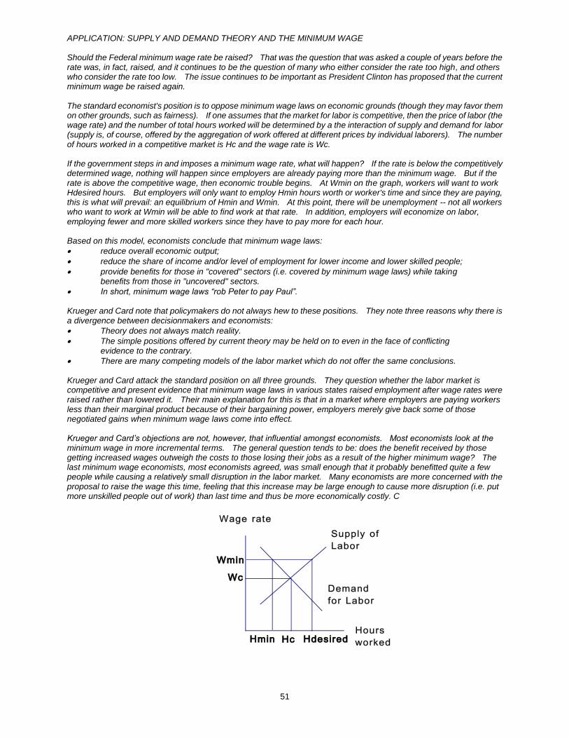
51

APPLICATION: SUPPLY AND DEMAND THEORY AND THE MINIMUM WAGE Should the Federal minimum wage rate be raised? That was the question that was asked a couple of years before the rate was, in fact, raised, and it continues to be the question of many who either consider the rate too high, and others who consider the rate too low. The issue continues to be important as President Clinton has proposed that the current minimum wage be raised again. The standard economist's position is to oppose minimum wage laws on economic grounds (though they may favor them on other grounds, such as fairness). If one assumes that the market for labor is competitive, then the price of labor (the wage rate) and the number of total hours worked will be determined by a the interaction of supply and demand for labor (supply is, of course, offered by the aggregation of work offered at different prices by individual laborers). The number of hours worked in a competitive market is Hc and the wage rate is Wc. If the government steps in and imposes a minimum wage rate, what will happen? If the rate is below the competitively determined wage, nothing will happen since employers are already paying more than the minimum wage. But if the rate is above the competitive wage, then economic trouble begins. At Wmin on the graph, workers will want to work Hdesired hours. But employers will only want to employ Hmin hours worth or worker's time and since they are paying, this is what will prevail: an equilibrium of Hmin and Wmin. At this point, there will be unemployment -- not all workers who want to work at Wmin will be able to find work at that rate. In addition, employers will economize on labor, employing fewer and more skilled workers since they have to pay more for each hour. Based on this model, economists conclude that minimum wage laws:

reduce overall economic output;

reduce the share of income and/or level of employment for lower income and lower skilled people;

provide benefits for those in "covered" sectors (i.e. covered by minimum wage laws) while taking benefits from those in "uncovered" sectors.

In short, minimum wage laws “rob Peter to pay Paul”. Krueger and Card note that policymakers do not always hew to these positions. They note three reasons why there is a divergence between decisionmakers and economists:

Theory does not always match reality.

The simple positions offered by current theory may be held on to even in the face of conflicting evidence to the contrary.

There are many competing models of the labor market which do not offer the same conclusions. Krueger and Card attack the standard position on all three grounds. They question whether the labor market is competitive and present evidence that minimum wage laws in various states raised employment after wage rates were raised rather than lowered it. Their main explanation for this is that in a market where employers are paying workers less than their marginal product because of their bargaining power, employers merely give back some of those negotiated gains when minimum wage laws come into effect. Krueger and Card’s objections are not, however, that influential amongst economists. Most economists look at the minimum wage in more incremental terms. The general question tends to be: does the benefit received by those getting increased wages outweigh the costs to those losing their jobs as a result of the higher minimum wage? The last minimum wage economists, most economists agreed, was small enough that it probably benefitted quite a few people while causing a relatively small disruption in the labor market. Many economists are more concerned with the proposal to raise the wage this time, feeling that this increase may be large enough to cause more disruption (i.e. put more unskilled people out of work) than last time and thus be more economically costly. C

52

Concepts: Benefit-cost analysis

A widely used tool developed by economists and financial analysts is benefit-cost analysis (B/C analysis). B/C analysis is meant to capture real net gains or losses to society which result from specific actions which are the subject of analysis. Generally, if society has a net gain from an action (call it a project), then the action is one that should be undertaken by society. If society has a net loss, then that action should not be taken. Gains/losses vs transfers In undertaking a B/C analysis it is important to distinguish between overall (net) gains and losses and transfers. Net gains and losses refer to increases or decreases in the total resources available to society. Transfers refer to movements of resources from one group to another. Usually a project will result in both transfers and gains or losses. To maximize economic efficiency, one wants to focus on whether a gain or loss is the end result of a project, and to do that one wants to avoid counting transfers as gains/losses when they are not. If the concern is with distributional equity, however, transfers are of primary interest. Usually policymakers want to know something about both. B/C analysis: conceptual fundamentals B/C analysis, like so many other economic concepts, begins with supply and demand. Starting with demand, consumers will be faced with a market price P* and will purchase Q*. P* x Q* is the total payment that consumers will pay out to producers for the Q they consume. As such it represents the opportunity cost to consumers and total revenue to producers and is a transfer from consumers to producers. That transfer is shown by the rectangle labeled OC for opportunity cost. However, consumers are paying a marginal price for each unit they consume. If they could only consume one unit, they most likely would pay a much higher price because the utility that they receive from consuming that unit is quite high (this will, of course, depend on the actual nature of their utility function). As they get additional units of the good, the utility they receive from each unit declines (Imagine the difference between the first milkshake and the tenth). In market transactions, consumers pay only one price for every unit and that is the price of the last unit they consume, even though they receive more utility from prior units. This "free" satisfaction is consumer surplus. The area marked "CS" is consumer surplus. This is a gain to society accruing to consumers, while OC is a transfer from consumers to suppliers. Supply is roughly analogous to demand. Suppliers have an opportunity cost corresponding to each unit that they produce. However, like consumers, they sell each unit at the marginal price determined by market equilibrium. They must cover their opportunity costs -- the price they pay to input suppliers -- and this is indicated by the triangle marked OC. They also make a profit and this is indicated by the triangle PS, which stands for producer surplus. The two triangles together make up a rectangle which is equal to the total payments by consumers for the goods they bought and this is the transfer of resources from consumers to producers Putting supply and demand together, one can see that market transactions consist of three components. Two of these are transfers from demanders to sellers -- PS and OC. One is a net gain to society -- CS which represents a net increase in overall satisfaction enjoyed by the members of society. B/C analysis: a conceptual example

53

Here is an example of a conceptual B/C analysis. There is a supply and demand for living within a flood plain. The government is considering building a flood control project which will allow more people to live within the flood plain. Without the project, society has an existing CS equal to triangle 1. With the flood control project, society gains net new additional CS equal to triangle 2. The rectangles total payments for flood plain living without and with the project and represent transfers within society. Society is gaining CS from the project but the project also entails costs which one needs to compare to benefits to see whether the project is worthwhile. Time value of money Most projects are not built instantaneously. Because capital investments are usually spread over time, there must be some way of comparing the value of dollars earned today with the value of dollars earned tomorrow. This measure is called the time value of money. Whenever intertemporal flows are considered (i.e. flows across time periods) time value must be taken into account. The reason that future dollars are worth less than current dollars is that there is an opportunity cost to dollars tomorrow. Dollars tomorrow cannot be spent today and that lack of use for them is a real cost -- one cannot follow up opportunities that having a dollar in hand today would offer, e.g. such as putting the dollar in the bank and earning interest. Present Value (PV) In order to add up today’s and tomorrow’s dollars together, one needs to discount dollars in the future so that they are equivalent to today’s dollars. Doing this yields the “present value” (PV) of future dollars. Arithmetically, this is a fairly simple operation. If the rate of interest is 7%, what is the present value of an investment which returns $100 one year from now? Answer PV = $100/(1+.07)=$93.46 More generally, to calculate the present value of a series of cash flows over time, one adds up the series: PV = C1/(1+r1)+C2/(1+r2)^2+......Cn/(1+rn)^n where n refers to time period n and "^n" refers to raised to the power n. Net Present Value (NPV) Net present value (NPV) compares the value of future cash inflows from an investment (suitably discounted) with the cash outflows required to make the investment (also suitably discounted). Subtracting the latter from the former, one gets NPV which, if positive, indicates that the project returns greater value of cash flows coming in than going out and so the project is worth doing. If NPV is negative, then the value of money being put into the project over time is worth more than the money being returned by the project and so the project should not be undertaken. B/C analysis: a practical example Below is a simple B/C analysis. For argument’s sake, imagine that this is an analysis of a proposed dam. Note that any benefit-cost analysis should begin with a clear accounting of the undiscounted cash flows (both positive and negative) due to the project for each time period. These cash flows are then added up to obtain an annual total and this total is then discounted by the appropriate discount rate (which may vary over time). This often is the most challenging part of the analysis. If done poorly, one has a classic case of “garbage-in/garbage-out”. It is assumed here that nominal cash flows are being used (i.e. flows

54

unadjusted for inflation). In this case use the nominal interest rate to discount those flows. If real dollars (with an adjustment for inflation) are used, use the real interest rate as a discount rate. Economic vs financial flows In general, a true economic B/C analysis will adopt the perspective of society which is to say it will distinguish between gains and losses to society and transfers within society as a whole. Often entities undertaking a project are concerned with what are often referred to as purely financial flows. For example, an agency may want to invest in projects that make the agency money regardless of whether society as a whole benefits or loses. In this case, the analysis is concerned with looking at transfers from society to the agency undertaking the project. Assuming agencies exist for the public good, this is probably not the correct perspective to take, but it may the perspective that your boss (or Congressional sponsor) demands. Sensitivity analysis One thing which dogs B/C analysts is the choice of interest rate: which rate is appropriate to use as a discount factor and how can one account for changes in that rate over time (i.e. make decent predictions of changes in interest rates in the future). A way to finesse this issue is to use “sensitivity analysis” which simply means running a given analysis for a range of different estimates of a particular parameter (holding all other parameter estimates constant) to see how sensitive the final results are to changes in the value of this parameter. In this case, 3 different estimates of interest rates have been used — 5%, 10% and 15%. The NPV is positive for 5% and 10% — in that case the project should be undertaken — but negative for 15%. Since rates tend not to get that high, this analysis indicates that this is a good project over a reasonable range of interest rates. Social discount rates Another issue surrounding interest rates is the so-called “social discount rate”. For most private projects, the market rate of interest is the best choice — it indicates the opportunity cost of money being diverted to the project at hand. However, if financial markets are not functioning well for some reason, the market rate of interest may not represent the true “cost of capital.” For government projects there is an additional problem — the social discount rate. Private investors must get funds from other private actors offering them directly or indirectly for private use. In other words, private savers, equivalent to investors, can charge spenders (borrowers) for the use of their funds. Government, on the other hand, draws from a larger pool consisting of all agents in society, both savers and spenders. That means that not only is the government diverting investment funds to public use, it is also diverting funds which would otherwise be used for consumption to that use. Consumption funds generally will have a different implicit rate of interest than investment funds. It is an implicit rate of interest because consumers are busy consuming their funds, not lending them out in the market. This tradeoff that consumers are making between spending now and spending later is determined by their preferences. Generally, the rate of interest on consumption funds is lower than that charged for investment funds, meaning that the true social rate of discount — the true opportunity cost of funds to government — is lower than the private market rate of interest. This does not always hold true and is actually a matter of some controversy among economists, but it indicates that one should be careful about looking up interest rates in the paper and assuming that they can be used in your B/C analysis. Valuing “intangibles” Many government projects involve “intangible” benefits such as the value of recreation to consumers, or environmental quality. The value of these things, as we have seen, is the satisfaction that consumers get from these things, i.e. their consumer surplus. But we cannot observe these values directly. This has led economists to use a variety of techniques, from direct surveys (how much is this worth to you?) to indirect observation (if the price of entry to a national park changes, one can observe how people’s use of the park changes with it to make inferences about how much they value the particular services that the park offers). Valuation of intangibles is knotty. At least the analyst must make a comprehensive list of different types of benefits and then determine the best way to value them. External costs and benefits Externality may also be a problem for B/C analysts. Take valuation of a highway project. One could limit oneself to analyzing the costs of construction and maintenance as compared to the value of time saved to commuters due to reduced travel times. However, increased traffic may lead to increased environmental damage, a social cost that is not generally directly captured with market or engineering data. Here too many knotty problems arise. The main point is be aware of them when conducting a B/C analysis. A final note: ceteris paribus The method of B/C analysis is a good example of economic reasoning and methodology in action. In particular, it is a good example of the “ceteris paribus” assumption that economists use in analyzing various issues. “Ceteris paribus” is Latin for “holding all other things equal.” The B/C method of comparing a “with” situation to a “without” situtation is a perfect example of ceteris paribus. One compares one world (presumably the world as it exists now) with another world which is identical to it except for one thing: the alternative world contains an action (such as a project or the removal of a project) which is of interest to the analyst. Thus the economist wants to compare the two worlds and see whether, in the alternative world, we are any better off “everything else equal” (another translation for the term ceteris paribus).

55

Module 16-A

Circular flow The economy can be seen as a circle where consumers buy goods with money earned from producers in payment for services that consumers provide which enable production of those goods. This circle portrays both flows of goods and services, or what economists call the real sector, and the financial sector, which represents financial instruments traded in the financial markets which then allow consumers and trade off future and present consumption and production against one another. By doing so, the economy can expand more than it would otherwise. Circular flow shows how productive services are transformed into goods and back again. Government and circular flow The model of circular flow presented below is missing one very important real world element-- government. The fact is that government is not merely one player among many in this economic set-up. In fact, its economic policies can have major impacts on key points in this system. Concepts: Taxation

Two things in life are certain it is said: death and taxes. It has also been said that "the power to tax is the power to destroy." The government's power to tax is an awesome authority. Taxes are necessary to fund the public sector's mission and hopefully those missions are well-executed and truly in the public interest. But this power, as with any power, comes with a cost and this cost is the distortionary effect of taxation The tax wedge In a world of no taxes, circular flow would be just what it appears to be -- real flows of goods and services and financial flows which are derived from those real flows. Thus, if you provided a service to a producer, that producer would pay you an amount equal to the value of that service. Meanwhile, the producer would then add value and sell the resulting output for a price equal to the value of that output. However with taxes, this direct result no longer holds. Now the payment to you and/or the payment to the producer has a tax included -- a payment to the government which is not a direct participant in either transaction. This effect is called a tax wedge. Illustration of a "tax wedge" Without taxes, buyers and sellers make a deal and, in a market operating under all the standard assumptions of economics, the price and quantity they agree to should match the true costs of production and true value assigned to that production by the consumer. With a tax imposed, this equilibrium no longer holds. Now the seller receives a price S(t) which nets out tax and the buyer pays a price B(t) which does the same. Their respective prices are no longer identical, as in the tax-free market, but different (by the amount of the tax wedge). Also the quantity traded is lower than without tax. Government collects the tax revenue. Why is tax wedge "distortionary"?

56

A tax wedge is distortionary because the price paid by buyer and seller are now different and their respective calculations of gains to exchange are no longer in sync. This is due to the fact that a third party -- the government -- is now part of the transaction. While government provides important indirect services to producers and consumers, those services are not directly provided, nor directly priced to them. "Excess Burden" Taxes, by definition, impose a burden on those who bear them. Part of this burden is intentional -- the government provides useful services and must pay for them and does this through the imposition of a tax. But the tax wedge imposes an additional, unintended excess burden. This excess burden is equal to the distortionary effects of the tax. Tax burden=intended burden + excess burden. Excess Burden is pervasive; there simply is no way to avoid it. As long there is a tax there is a tax wedge. Thus tax policy is usually designed to minimize excess burden. Thus taxes should be designed to minimize deleterious effects on economic efficiency (i.e. minimize the tax wedge and thus minimize the distortions due to the imposition of a tax). Illustration of excess burden What is gained by the government from taxation is tax revenue equal to the tax wedge and indicated by rectangles A and B. What is lost by society is producer and consumer surplus indicated by triangles C and D. This loss occurs because consumers and producers and consuming and producing at a price different from the market price. Of course the government is hopefully doing something beneficial with the tax revenue it is collecting and that will somewhat offset excess burden. Nonetheless, the desired goal is to make that loss as small as possible. Equity ("Justice") and tax incidence Of course, efficiency is not the only consideration in tax policy. Equity (also called fairness or social justice) is equally important. Equity also relates to tax burden, i.e. which parties society deems should bear more or less of the intended burden as well as the excess burden. The distribution of burden is referred to as tax incidence (referring to exactly where the "incident" of a tax burden "occurs." Actual incidence does not equal statutory incidence Note that just because a tax law says party x will pay such and such amount of tax ("statutory incidence") does not mean that the party will actually bear the burden of the tax ("actual incidence."). Sure, the taxed party will cut a check to the government, but, depending on that party's ability to shift its own behavior, it may actually bear very little of the burden of the tax. An incidence example .Note here that the seller's supply curve is inelastic (the seller will tend to change the amount of a good offered relatively little in response to a change in price), while the buyer's demand curve is elastic (the buyer is very responsive to price changes). Thus the shift in after-price tax causes the buyer to drop his/her price sharply while the seller still offers a similar quantity to that offered at the pretax price. The seller in this example, "eats" much of the tax and so bears more of the burden Now the shoe is on the other foot: the seller is very responsive to price changes while the buyer is not. The same tax is imposed as before but now the seller offers a lot less at the after-tax price. It is the buyer who now bears most of the tax, forced to accept the lower quantity and higher price and paying the government most of the tax. Tax avoidance vs. tax evasion The tax wedge separates seller's and buyer's prices and thus introduces a difference between the relative attractiveness of pretax versus after-tax production and consumption options. This is distortionary. Another form of inefficiency is introduced through tax avoidance -- a taxpayer's

57

structuring of transactions to avoid triggering a tax. This is a legal strategy to minimize one's tax bill and is contrasted with tax evasion where a taxpayer who is liable for a tax tries to hide the taxable transaction and avoid paying one's legal liability. Tax avoidance is inefficient because (a) the act of structuring transactions to avoid tax is time and resource-consuming; (b) it creates a tax wedge of its own by making some transactions less costly (less likely to be subject to tax) and others more costly (more likely to be subject to tax). Principles of Tax Design Because of the innate inefficiencies of taxation, those designing taxes in theory try to attain a number of goals:

Economic Efficiency: taxes should be designed so that their excess burden is minimized.

Neutrality: relative after-tax incentives to different types of consumption and production should be as

similar to pre-tax incentives as much as possible (i.e. taxes should change relative prices as little as possible).

Simplicity: taxes should be simple to understand and simple to file; this ensures that taxpayers

spend a minimum amount of time in dealing with the administrative burden of taxes, that mistakes in filing are few, and that there is little ambiguity in who should file and when.

Administrative Efficiency: taxes should be easy and cheap to collect and enforce.

Equity: those whom society feels should have a greater burden are taxed more than those whom

society feels should not be (this is called vertical equity). Also, taxpayers in similar situations to one another are taxed similarly (this is called horizontal equity).

"Haig-Simons" The principles presented before are general in nature. Two tax analysts -- Haig and Simons -- put some flesh on these principles with definitions of key concepts. In particular, "income" is supposed to be true economic income -- payments in return for true economic services. Only economic income should be taxed, not pure transfers from one person to another. In addition, payments for expenses incurred in producing true economic income should not be taxed: they should be deducted from income. The concept of a "taxable event" A tax should be triggered only when (a) income is produced; (b) that income is "transferred" from one party to another or "realized" by a given party. This is known as a taxable event. There are a number of options for actually assessing and collecting tax from a taxable event. These are known as collection points. The government usually picks collection points where revenue collection is least costly and enforcement potential is greatest. The taxpayer has a fair amount of lee-way in structuring transactions in such a way as to limit the occurrence of taxable events and to either avoid government-defined collection points altogether or to pick points of lowest tax liability. This is called tax planning. It is also the essence of tax avoidance. Taxation: an example This a tax calculation using actual 1995 tax information. First there is a filing entity (in this case a single person). Particular rules govern the tax treatment of this entity. Gross income is supposed to capture all sorts of economic income which comes from the source (e.g. wages, dividends). All income of this sort from income flows is called ordinary income. Income which comes from changes in the balance sheet is called capital income (which generally includes only capital gains and losses). Gross income is the starting point for calculation of the tax base, i.e. the income which is subject to tax. In part following Haig-Simons, various adjustments are made to gross income. "Above-the-line" adjustments to income include things such as moving expenses and health

58

insurance expenses for the self-employed which are expenses which, in theory at least, must be incurred in order to produce income in the first place and so should not be taxed. Other above the line deductions such as Individual Retirement Account (IRA) contributions are a little more difficult to justify on Haig-Simons grounds though one could say they are necessary savings to maximize future earnings. Above the line adjustments are the most favorable to taxpayers -- they basically reduce income on a dollar-for-dollar basis equal to the deduction. After such adjustments one is left with adjusted gross income (AGI). After arriving at AGI, below-the-line deductions are taken. Some of these deductions may have an efficiency basis, such as medical expenses, while others such as charitable deductions are based on equity considerations (in this case favoring a particular use of one's income). Others, such as the home mortgage interest deduction are a hybrid; there is some economic justification for deducting the cost of one's home -- this is a cost which must be incurred to produce income at all -- but the value of housing services provided by your home in theory should be added back into your income. Imputed income streams such as these (to distinguish them from actual cash flows, since they are basically a notional, accounting flow) are usually not included in most tax calculations. For those with simple income flows and generally low income tax brackets, one may choose not to, or not be able to itemize deductions and instead take the standard deduction as prescribed by law. This is what this taxpayer has done -- the single filer's standard deduction in 1995 was equal to $3,900. Itemized deductions are often more favorable of course, though there are limitations on some of them (itemized deductions characterized as "miscellaneous" are subject to an income floor -- they can only be taken if equal to a certain percentage of AGI and then only in the amount that they exceed that percentage). Filers can also take a personal exemption subject to various income and filing status restrictions. This exemption is meant to capture in some way the cost of personal upkeep, another Haig-Simons like notion. Now we come to the bottom line: taxable income. Taxable income is the amount which is subject to the tax rates defined by law. This filer is subject to the lowest marginal tax rate of 15%: this is the tax rate on a particular increment of income. US tax rates are progressive -- they rise with increments of income so that higher income people in theory pay more than lower income people. Multiplying taxable income by the tax rate one arrives at the Federal tax liability which is here equal to $3,015. This taxpayer is also subject to other taxes such as State and local income taxes and Federal payroll taxes such as Social Security and Medicare taxes. When these taxes are taken into account the total tax liability (not shown here) is equal to $7,215. Note that the person's average tax rate (=total income/total taxes paid) is higher than their statutory marginal rate of 15%. However, because of deductions, their Federal average tax rate alone is lower than the statutory rate or around 10%. Just looking at this simple example, one can already see a glimmer of how tax planning and tax avoidance can work. The taxpayer may have control over which entity does the filing. For example, parents often transfer income to their children who are in a lower tax bracket and hence pay less tax. People also have considerable control over the timing of their transactions, taking a capital gain, for example, in a year when they have low income or many capital losses (and hence a low tax rate) instead of a year when they have high income and hence high taxes. In addition, the taxpayer may undertake certain transactions which are tax favored instead of others which are not. For example, personal interest on credit cards is not deductible but interest on home equity loans is deductible so the taxpayer may choose to finance a purchase with a home equity loan rather than a credit card and thus increase their itemized deductions. Finally, the tax law allows taxpayers to choose more favorable methods of calculation of tax liability (as with depreciation). Tax Planning and Tax Burden Rich taxpayers are subject to higher statutory tax rates than poorer ones. However, the true measure of tax burden is not the statutory marginal rate but the effective average rate. Richer taxpayers tend to have more ability to structure their transactions so as to minimize the number and value of taxable events, lower their total taxes paid and thus lower their average effective tax rate

59

APPLICATION: THE US TAX SYSTEM AND RADICAL REFORM: THE “FLAT TAX” There are a number of burning issues in the U.S. Federal tax system, some mainly of interest to specialists, others of concern to all who pay taxes. First, some of the issues are covered below. Then there is a discussion of plan for radical reform of the system, namely the Flat Tax. Selected issues for US taxation: payroll taxes Payroll taxes have grown the fastest in proportionate terms in recent years. However, payroll taxes are the most regressive of taxes. They come straight off the top, without deductions, are levied on wages and not interest and dividend income which is more heavily concentrated among high-income earners, and, in the case of Medicare and Medicaid, are not levied on wage earnings greater than the mid $60,000 range. Some have argued that efforts at tax reform should focus on lessening the reliance of major entitlement programs on these taxes and shift to other more progressive forms of taxation such as the current individual income tax. Selected issues for US taxation: Individual Income taxes One of the major complaints about the individual income tax structure in the United States regards its complexity. The Internal Revenue Code (IRC) runs to almost 3,000 pages and every amendment to that code increases its length. A major reform of the IRC, with the passage of the Tax Reform Act of 1986 (TRA 86), did "fix" a number of perceived problems with the individual income tax, especially what were perceived as grievous tax loopholes, but these efforts largely complicated rather than simplified the overall code, although many taxpayers in lower income brackets did find their filing job made easier of unnecessary. Even though the US tax system is voluntary -- taxpayers file their own returns and largely police themselves subject to random audit -- compliance has not been a major problem. Selected issues for US taxation: The Corporate Income Tax One of the maxims of public finance is that "firms don't pay taxes, people do." What that means is that even though a corporate income tax is levied, ultimately it is shareholders or other individuals who receive that income that ultimately bear the burden of that tax. The corporation is a mere legal fiction. Two issues are burning with regards to the corporate income tax. First is the double-taxation issue. Corporate earnings are taxed at the corporate level and then, to the extent that these earnings are passed through to the shareholders, these earnings are taxed again at the shareholder level. This anomaly arises in part because of current tax rules but because there is this dual corporate/individual tax structure. Many complex proposals exist for corporate integration, i.e. the unifying of this dual structure. Selected issues for US taxation: Corporate Form The second corporate income tax issue is the choice of the corporate form of ownership. Incorporation offers a number of advantages, including limited liability which limits a shareholder's liability to losses to the amount of capital invested in the firm. However, corporations are currently taxed at top rates higher than those which pertain to individuals. As a tax avoidance scheme, many taxpayers have chosen to organize their businesses in other ways, including partnerships, sole proprietorships and Subchapter S corporations. This last form is sort of like a corporation except that firm-level income is automatically allocated to individual owners and taxed only at that level. This shift out of the corporate form is one reason why corporate tax revenues are projected to relatively decline by Tax Reform Although there are many tax issues, it is concern about the simplicity and fairness of individual taxes, which directly touch the over 100 million individual filers (and voters) which has driven the issue of tax reform to the top of the political agenda. The Haig-Simons theory suggests a number of principles for tax reform. These include:

a broad income tax base in order to ensure that most true income is covered by tax and hence there are few opportunities for shifting to untaxed activity.

a reduction in loopholes which limits wasteful and inefficient tax dodges.

fewer and flatter rate brackets which both simplifies filing and also limits incentives to shift from taxable activity in one bracket to taxable activity in another (since with broad brackets more activities remain in one tax class).

The Tax Reform Act of 1986 (TRA 86) was modeled along Haig-Simons lines. The number of brackets were reduced and the top bracket brought down, loopholes were closed left and right, and the overall income tax base was broadened, in particular with capital income and ordinary income being treated on an equal basis (i.e. no preferential capital gains tax rate). The overall structure of TRA 86 remains largely in place, but each major new tax reform bill blows more and more holes into it. A differential rate between capital gains and ordinary income has crept back in since 1986 and grown exceedingly complicated, the top rate has crept up, and the number of income brackets has slightly increased. In addition, one thing which TRA 86 did not do -- simplify the Code -- has been compounded with a number of new tax laws adding to the Code since then.

60

Tax Reform: the Flat Tax One response to this complex state of affairs has been to call for a flat tax. This proposal carries Haig-Simons to its logical extreme by calling for one flat rate on one broad base. One standard version this proposal calls for tax base consisting of wages and salaries only with a simple set of standard exemptions and a single tax rate applied to taxable income (which equals (wages+salary)-exemption) A Sample Flat Tax Here is our single filer again with a $30,000 annual income and a personal exemption of $3,900. Taxable income is equal to $30,000-$3,900=$26,100 and here a flat tax of 20% is applied. Everyone pays this same rate. The return, as one can see, is very simple (in actuality the return would contain name, address and other information and perhaps some documentation of wages but essentially this would be the return so the simplification aspect of a flat tax, assuming it completely replaced the income tax, is clear). One objection to the flat tax is that it is regressive. In one sense this is not true: with the exemption, the average effective tax rate is mildly progressive. However, the calculation above ignores three things: (1) interest and dividends are not included in most standard forms of the tax and these are earned disproportionately by the wealthy; (2) even without this fact, the flat tax is flat -- one rate for all -- while the current rate structure is graduated by income; (3) To be revenue-nuetral (i.e. to raise the same amount of revenue as the current tax structure) the flat rate would have to be at least 25% and that would constitute a net increase for many lower-income taxpayers and a net decrease for many high income ones.

61

Concepts: Macroeconomics v Microeconomics

The discipline of economics is split into two pieces: microeconomics and macroeconomics. Microeconomics has constituted the bulk of this course and can be thought of as "from the ground up" economics. Behaviors of each individual economic agent are analyzed and then interactions between those agents are studied. The macroeconomy in this construct is simply the sum of the parts. Macroeconomics has a different bent, "from the top down." Here the economy as a whole is the unit of analysis and to the extent individual agents are examined they are looked at as part of this whole. In this construct the whole is very definitely different than the sum of the parts and has behavior that is often at odds than what might be expected if one simply aggregated individual actions. Keynesian Economics Macroeconomics got its start during the Great Depression. Up to then, neoclassical economics reigned supreme. However the Great Depression was something that traditional theory could not seem to explain, namely a prolonged, generalized slump in output and prices. Markets should eventually clear and all useful resources should ultimately be employed and the real world was not conforming to this prediction. In 1936 John Maynard Keynes wrote the General Theory of Employment, Interest and Money. His theory established macroeconomics as a separate discipline for he started with the economy in general and asked why a macroeconomy might have general unemployment. Keynesian policy tools For Keynes, the government budget could be an instrument in managing the business cycle. When used in this way, the government is employing fiscal policy, i.e. the use of public taxes and expenditures to offset decreases in private economic activity which bring the economy below its productive potential (e.g. a recession) or to offset increases in economic activity which cannot be sustained because they make the economy operate above its productive potential (e.g. inflationary excesses). A Keynesian model of fiscal policy When economic output is above economic potential as it is here, inflation is a risk: there is not enough labor and capital to meet demand so their prices go up. The government could offset this "excess" activity by raising taxes and/or lowering its own spending Alternatively, if economic output is below productive potential, the government could lower taxes (thus freeing up private resources) and/or increase spending to offset the shortfall and bring the economy out of recession. The Phillips Curve In the late 1950s an econometrician named Phillips found a striking correlation between nominal wages and unemployment. This relationship became known as the Phillips Curve and is depicted below. What the Phillips Curve seems to suggest is that there a tradeoff between price inflation (and here money wages are a proxy for prices generally) and the unemployment rate. Keynesianism in Phillips Curve Terms Keynesian theory suggests that the Federal government can use this relationship to manage the macroeconomy. Using fiscal policy, the government can choose a desired point off of the curve. The Phillips curve for example might indicate that a 3% inflation rate is consistent with a 5% unemployment rate and a 4% inflation rate is consistent with a 6% unemployment rate. Thus if government wants higher unemployment but lower inflation it might choose point 1, if vice-versa, then point 2. The death of fiscal policy Fiscal policy is no longer widely used at the Federal level. (Indeed, the balanced budget amendment

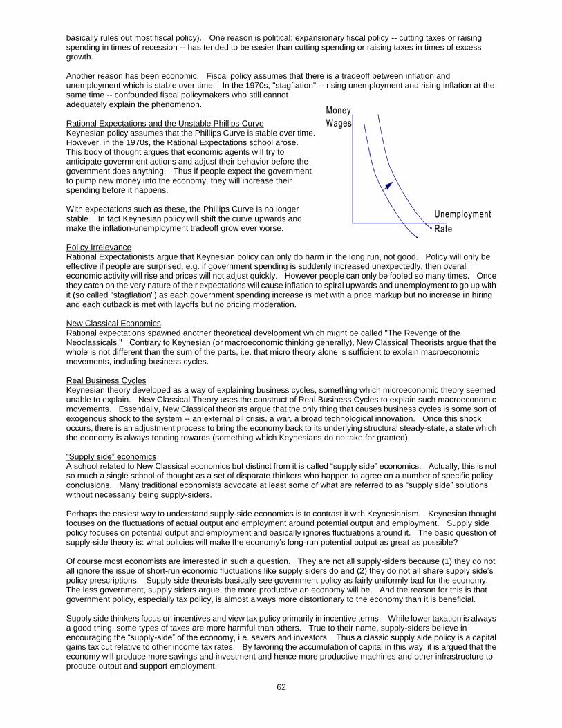
62

basically rules out most fiscal policy). One reason is political: expansionary fiscal policy -- cutting taxes or raising spending in times of recession -- has tended to be easier than cutting spending or raising taxes in times of excess growth. Another reason has been economic. Fiscal policy assumes that there is a tradeoff between inflation and unemployment which is stable over time. In the 1970s, "stagflation" -- rising unemployment and rising inflation at the same time -- confounded fiscal policymakers who still cannot adequately explain the phenomenon. Rational Expectations and the Unstable Phillips Curve Keynesian policy assumes that the Phillips Curve is stable over time. However, in the 1970s, the Rational Expectations school arose. This body of thought argues that economic agents will try to anticipate government actions and adjust their behavior before the government does anything. Thus if people expect the government to pump new money into the economy, they will increase their spending before it happens. With expectations such as these, the Phillips Curve is no longer stable. In fact Keynesian policy will shift the curve upwards and make the inflation-unemployment tradeoff grow ever worse. Policy Irrelevance Rational Expectationists argue that Keynesian policy can only do harm in the long run, not good. Policy will only be effective if people are surprised, e.g. if government spending is suddenly increased unexpectedly, then overall economic activity will rise and prices will not adjust quickly. However people can only be fooled so many times. Once they catch on the very nature of their expectations will cause inflation to spiral upwards and unemployment to go up with it (so called "stagflation") as each government spending increase is met with a price markup but no increase in hiring and each cutback is met with layoffs but no pricing moderation. New Classical Economics Rational expectations spawned another theoretical development which might be called "The Revenge of the Neoclassicals." Contrary to Keynesian (or macroeconomic thinking generally), New Classical Theorists argue that the whole is not different than the sum of the parts, i.e. that micro theory alone is sufficient to explain macroeconomic movements, including business cycles. Real Business Cycles Keynesian theory developed as a way of explaining business cycles, something which microeconomic theory seemed unable to explain. New Classical Theory uses the construct of Real Business Cycles to explain such macroeconomic movements. Essentially, New Classical theorists argue that the only thing that causes business cycles is some sort of exogenous shock to the system -- an external oil crisis, a war, a broad technological innovation. Once this shock occurs, there is an adjustment process to bring the economy back to its underlying structural steady-state, a state which the economy is always tending towards (something which Keynesians do no take for granted). “Supply side” economics A school related to New Classical economics but distinct from it is called “supply side” economics. Actually, this is not so much a single school of thought as a set of disparate thinkers who happen to agree on a number of specific policy conclusions. Many traditional economists advocate at least some of what are referred to as “supply side” solutions without necessarily being supply-siders. Perhaps the easiest way to understand supply-side economics is to contrast it with Keynesianism. Keynesian thought focuses on the fluctuations of actual output and employment around potential output and employment. Supply side policy focuses on potential output and employment and basically ignores fluctuations around it. The basic question of supply-side theory is: what policies will make the economy’s long-run potential output as great as possible? Of course most economists are interested in such a question. They are not all supply-siders because (1) they do not all ignore the issue of short-run economic fluctuations like supply siders do and (2) they do not all share supply side’s policy prescriptions. Supply side theorists basically see government policy as fairly uniformly bad for the economy. The less government, supply siders argue, the more productive an economy will be. And the reason for this is that government policy, especially tax policy, is almost always more distortionary to the economy than it is beneficial. Supply side thinkers focus on incentives and view tax policy primarily in incentive terms. While lower taxation is always a good thing, some types of taxes are more harmful than others. True to their name, supply-siders believe in encouraging the “supply-side” of the economy, i.e. savers and investors. Thus a classic supply side policy is a capital gains tax cut relative to other income tax rates. By favoring the accumulation of capital in this way, it is argued that the economy will produce more savings and investment and hence more productive machines and other infrastructure to produce output and support employment.

63

This sort of tax policy can be contrasted with a “Keynesian” tax regime. Keynesians are much more focused on the power of the “demand-side” of the economy. They believe that what drives investment is not cost of capital but demand for goods. Thus business people do not generally make investments because they can get capital at low rates. They invest because they believe that the prospects for selling their output are good and these prospects are driven by the level of demand for products and services generally. Thus Keynesians generally favor tax cuts (if the economy is producing below potential) which give the greatest amount to larger numbers of purchasers. The idea here is that the greater the number of spenders with increased income, the greater the level of demand in the economy, the better the prospects are in specific markets and the more likely businesses are to invest in machines and facilities. The “Laffer” Curve In the late 1970's, the economist Arthur Laffer drew a curve on a napkin during a lunch time meeting with some conservative thinkers (or so the story goes). The curve shows a relationship between tax revenues and tax rates. It is an upside-down “U”. As tax rates increase, tax revenue collected by government increases. But at some point, higher tax rates lead not to more tax revenue but to less revenue. The reason for this is actually fairly obvious: as the reward to work and saving becomes increasingly small, people will tend to cut back on the amount they save and work. As they work and save less, there is less income for the government to tax and hence less tax revenue. Laffer’s concept was not new, but his curve was a widely quoted device which grafted nicely on to supply side theory, namely that people save and invest only if they are rewarded for doing so and tax rates directly militate against that reward. After lunch with Laffer, the so-called “Supply side revolution” was born, its most prominent torchbearer the soon-to-be President Ronald Reagan. Note that economic theory supports the idea of a Laffer curve. Clearly there will be some rate of tax at which tax revenues will decline. The questions are: (1) what is that top rate? And (2) are we above or below that rate now? This is, of course, where policymakers and economists vehemently disagree. Where we stand now Interestingly, there is no one single paradigm dominating macroeconomics today. The stagflation and the rational expectations revolution of the 1970s displaced Keynesianism from its commanding position of the 1960s and 1970s but the inability of new theories to come up with plausible and tractable explanations of and solutions for business cycles has meant that those ideas have not taken the reigns. To put it another way, no one yet has a consensus explanation for what caused the Great Depression or how we got out of it. Keynesianism is seen as a useful but flawed set of hypotheses, New Classical and Real Business Cycles as logically tight but not very useful. Supply-side theory is believed by many, but as disbelieved by just as many. Monetary Policy With the decline of fiscal policy, the use of monetary policy to balance the business cycle has become especially important. Monetary policy in the U.S. refers to actions by the US Federal Reserve Board (the US central bank which controls the nation's money supply) to change monetary aggregates (cash and other financial instruments which are used mainly for exchange and liquidity) and terms of credit (such as the interest rate) to achieve a desired combination of output growth, price stability and employment levels. How does monetary policy work? By influencing the interest rate, the Fed (short for Federal Reserve Board), affects the cost of borrowing and lending. If borrowing costs are high, firms and consumers will borrow less and, with less liquidity, will consume and produce less. This will tend to keep output and employment lower than it would be with lower interest rates, but also keep inflation lower too. Conversely, if interest rates are low, borrowing and the consumption and production financed by that borrowing, will be greater and so will general economic activity. Tools to influence interest rates The Fed can influence interest rates in a number of ways. First, the Fed sets certain key interest rates directly, including the discount rate which is the rate that the Fed charges banks within the Federal Reserve System to borrow from that system. Second the Fed buys and sells government securities in what are called open market operations. Open Market Operations (OMO)

64

The Fed influences interest rates by pumping in or withdrawing government securities from circulation. If the Fed sells bonds in sufficient number, the supply of bonds increases and the price of bonds falls, thus raising yields. if the Fed buys bonds, the supply of available bonds contracts, raising the price of bonds and lowering yields. The Fed claims, however, that it engages in OMO primarily to affect money supply. Fiscal policy tools vs monetary policy tools Economists make a clear distinction between fiscal policy and monetary policy and the distinction rests on the tools that each one uses. Fiscal policy relies on”real sector” mechanisms, i,e. tax or spending changes which move real resources around. Monetary policy is limited to changes in the financial sector, largely things such interest rate manipulations and OMO, which work through financial instruments such as bonds or currency.

Monetarism There is yet another divide in macroeconomic policy thinker and that is between monetarists and others. In general terms, a monetarist is one who believes that only monetary policy can be effective, at least in the long-run, in affecting overall levels of output and employment. According to this school of thought, Keynesian fiscal policy tools such as tax cuts and spending increases, will not have any long-term impact on the economy as whole. Only monetary policies, such as OMO and money supply changes can be effective. The basic argument behind monetarism, to oversimplify, is that money is like blood in an organism: too little and the organism begins to die, too much and the organism may become overheated. Thus monetary policy can be extraordinarily effective in regulating the economic life of the economic being because one is controlling money and money is the fundamental fluid of economic circulation. To this way of thinking, fiscal policy is not particularly effective. It is rather like moving blood supply from the heart to the foot: one can temporarily stimulate a part of the body but it wont last for long and will be harmful to other parts of the body in the meantime. As the analogy may suggest, monetarist tend to be conservative in their macroeconomic policies. Like rational expectationists, to whom there is an intellectual link, the economic policymaker is highly constrained. The shape and function of the body is pretty much given. What the policymaker can do is monitor the situation and make sure that the economic circulation system is functioning properly. It is not a small power, but it is also fairly constrained one.

65

Concepts: trade

The gains to trade and coordination Economists like international trade, the freer the better. Why? Basically because it expands the number of possible trades and, in so doing, allows for more gains from trades, i.e. a pairing of parties whereby one party can be made better off without making the other person worse off. When country A joins the world market, two things happen. First, its domestic supply and demand are added to the world supply and demand, expanding that supply and demand and hence lowering prices and increasing quantities on the world market (This shift is represented by the move from the light lines to the dark ones in the second panel). There is an additional synergy to combining the two markets. With a larger market to produce and consume in, individual producers can realize economies of scale in production and can also increase their specialization (larger markets have more niches) and gain efficiency. This causes the additional shift from the dark S line to the dotted one.

Comparative advantage The classic argument for free trade is one developed by David Ricardo, a 19

th century economist from England. He

stated that, given two goods, if a country can produce one good relative to the other with less input relative to what another country requires to produce that good, then that country has a comparative advantage in the production of that good. He further stated that the country with the relative advantage should specialize in production of that good and then trade with the country which has a comparative advantage in the other good. It is easier to understand comparative advantage and how it works by way of example. Take the following tow countries A and B. They both produce goods X and Y. There is only one input, L (labor). Suppose that each country can produce one unit of X and Y with the following L requirements:

Good X Good Y Country A: 2 6 Country B: 1 1 In other words, A requires 2 units of L to produce X and 6 to produce Y, while B can produce either X or Y with one unit of L. Who has the comparative advantage? To produce X relative to Y, A has to devote 2 units or L versus 6 units of L, for a ratio of 2/6 (reducing to 1/3). This compares to B’s input ratio for the same goods of 1/1. 2/6 (1/3) is less than 1/1 so A has a comparative advantage in X. B, on the other hand, has a comparative advantage in Y — it’s 1/1 ratio for that good is less than A’s 6/2 (reducing to 3) ratio. (Remember to read these numbers as fractions. Thus 1/3 — one-third — is less than 1/1, i.e. one). A should specialize in production of X and B should do the same in Y and the two should trade with one another to meet their needs in the goods they don’t produce themselves. Why? Opportunity cost. Look at the marginal unit of each good. If A produces one less unit of Y, that releases 6 units of L which can be devoted to producing 3 more units of X. So A’s decision causes world output of Y to drop by one unit and its output of X to increase by 3 units. B’s decision to produce one more unit of Y, meanwhile, releases leads to one less unit of X being produced, but one more unit of Y. Already the world is better off because the marginal increase in production in X is two units (A produces 3 new units of X, B produces one less) while the worldwide production of Y is marginally a wash (A produces one more, Y produces one less). But the process does not stop there. The two countries trade with each other and this trading, in turn, allows them to divert yet more resources to their specialized sectors (at a cost, of course, of lowering output in the sector without a comparative advantage). Where world output ends up depends on a variety of factors. The point is that the two countries can produce as much as what they were producing without trade after trading and then some.

66

Exchange rate dynamics Like single domestic markets, international goods and services markets need to find their equilibrium. They do this through changes in price, except here the relevant price is the price of currency. Suppose Japanese consumers expand their demand for American goods. This would cause a decline in the current account of Japan (M increases while X is constant) and an increase in the US current account (X increases while M is constant). An increase in demand for American goods is tantamount to an increase in demand for dollars since dollars are what are needed to buy American goods. This is represented by a shift in the demand curve.

67

Concepts: economic geography, old and new

The traditional discipline of economic geography (along with the related disciplines of urban economics and regional economics) focuses on the three elements of market activity — production, consumption and exchange — the same elements which constitute the core of traditional economics, but with the difference that the dimension of physical space is incorporated into each of these elements. (Much of the following discussion is drawn from Lloyd and Dicken, 1972 and Mills and Hamilton, 1989; There are many other references, but these two present comprehensive and clear discussions of the “old” economic geography and urban economics respectively). Economic geography is founded on the same sorts of behavioral premises that regular economics is based on, namely rational, self-interested and atomistic agents who busily maximize on an individual basis and whose aggregate activities are guided by the “invisible hand” of Adam Smith. By introducing physical space into the analysis, economic geographers add the “friction” that maximizing over physical distances implies. Overcoming friction requires additional effort on the part of economic agents and this effort adds additional costs and planning to each individual’s maximization calculations. The addition of this single element deepens the traditional spaceless economic model considerably. Since overcoming friction is costly, economic agents, whether they are producers or consumers, set about minimizing the costs associated with that friction. The two most obvious ways to minimize those costs are either to minimize the friction itself, i.e. limit the distances which must be covered, or minimize the costs associated with overcoming that friction, such as lowering transportation costs through transport innovation or building efficient transportation networks. Simple elements these are, but they lead to some profound insights. Central place theory and urban hierarchy arise from these behavioral implications, for one way that economic agents economize on friction and its associated costs is to concentrate activities in places where either the beneficiaries of those activities are closest (and hence need to travel least to get the goods and services they need) or where the inputs necessary to make outputs are closest, or some combination of the two. This is one rationale that economic geographers give for the existence of cities themselves, namely that the concentration of consumers and producers in one place to limit the friction of distance and its associated costs. Agglomeration economies and economies-of-scale Closely related to, and even arising from these insights are two traditional economic concepts, namely economies-of-scale and agglomeration economies. Economies-of-scale refers to the relationship between the scale of production and marketing of output and the use and management of the necessary inputs. For example, if as a steel manufacturer grows in size it can get more value of steel product for a given unit cost of inputs (such as labor and capital), then the steel manufacturer can be said to be reaping increasing economies-of-scale. That is, as the scale of the enterprise grows, the given value of a unit of output increases per given unit cost of input. Economies-of-scale are generally “internal” to the economic agent in question and related to a number of factors, only one of which is physical concentration of the activity. Agglomeration economies are much more directly related to physical space for they refer to economic synergies which result from a concentration of separate producers, consumers and/or input sources at one location. A classic agglomeration economy is the garment district in New York where highly skilled laborers and firms are all located in an approximately five square block area on the west side of Manhattan. The producers themselves may be relatively small, and the laborers and producers may be acting as individuals not in concert, but the fact that they are so close to one another leads to a free flow of information and services with minimal search, transportation and other transactions costs thus causing the unit costs of all producers to fall. This proximity and relatively costless exchange of information and knowledge may also lead to technical and other innovations which might not otherwise occur if the separate economic agents were more disparately located. In this sense, agglomeration economies are “external” to the agents, arising in the aggregate, not in the individual units themselves, although these aggregate effects do ultimately ripple through the individual units. Agglomeration economies and economies-of-scale both arise from and lead to economic forces driving producers and consumers to concentrate in or disperse from different physical locations. What they tend to do, in classic economic fashion, is to lead to specialization in function across space, working in tandem with the notion of comparative advantage. Again central place theory comes to mind: one place may become a center of high finance, another a center of watch manufacturing because it is more efficient for one place to do the one thing and the other place the other so long as the two places trade with one another. Paul Krugman and the “New Economic Geography” In a very abbreviated nutshell, that is the “old” economic geography. What about the “new” economic geography. Paul Krugman’s Geography and Trade, (1991: MIT Press) is an excellent and very readable summary of the field (and indeed, Krugman has much to do with inventing the “new” field). On the one hand, there is much that is not very new about the “new” economic geography. Krugman’s definition of economic geography -- “‘the location of production in space’; that is, the branch of economics that worries about where things happen in relation to one another.” (p. 1) -- applies to both the old and the new fields. The behavioral assumptions of rational and self-seeking maximization are common to both disciplines and many of the concepts

68

remain the same. Even some of the supposedly profound new policy insights are very much presaged in the old field, as will be discussed in more detail below. So in one sense, there is not much that is truly revolutionary about the “new” economic geography. But in another sense, the world has changed quite a bit since the “old” field developed and the “new” thinking has taken much of this change to heart. In particular, and as summed up by Krugman, the new economic geography takes the old foundation and goes in two separate directions from it: (1) the recognition that there may be multiple equilibria across space (and here the role of history, accident, pervasive increasing returns and imperfect competition are important); and (2) the recognition that such equilibria, in the form of economic regions, are increasingly occurring across national boundaries (i.e. that economic regions are becoming less and less likely to be subsumed within a single nation).

The first point about multiple equilibria is best understood by reference to en example Krugman himself uses. Consider the table below. Assume that there are only two sectors in the economy — Agriculture (A) and Manufacturing (M) — and that A provides 60% the labor force. M’s location is going to be driven by a few factors. First there are the fixed costs of M which, for a single plant, is always equal to 4. Then there are transportation costs of goods to market. These costs will be lower if the demanders of goods are located in the region where the goods are produced. If M is already concentrated in the East, then the M industry will concentrate in the East as well. One plant can be built there for a fixed cost of 4, and transport costs are lowest there because so much of the demand is already there and relatively little has to be transported outside the area. Total costs for producing in the region are 7, less than splitting production between regions (which lowers transport costs to 0 but now requires construction of two plants at a cost of 8) or of locating the West (which has higher transportation costs because so much product has to be shipped out of the region). But this is not the only equilibrium. For if M concentrates in the West, then all M firms will want to locate there; if the sector ends up being split, then firms will want to split their locations as well. Where you end up depends on where you began and where you are headed and none of that is predetermined. In fact, location will depend on sufficiently strong economies of scale; sufficiently low costs of transportation; and sufficiently large shares of “footloose” production not tied down by natural resources. If these are large enough, then “history” matters; if not, then pure economics matters and there is likely to be a single equilibrium. The other main insight of the “new” economic geography is the internationalization of economic exchange. Krugman makes the point that international economics needs to better integrated into economic geography since nations are political entities, economic regions are not and the latter often crosses the boundaries of the former. In this sense, Europe, with its market integration, is trying to replace international economics, which focuses on nations, with economic geography, which focuses on regions. Again Krugman provides an example which is quite clear and which is represented in the picture below. In this simple example, there are six economic regions, each connected by the transportation links indicated (there are “impassable mountains” in the middle which make other connections impossible). The dotted line shows the national boundary dividing the regions. The one country to the north has an industrial center (indicated by the shaded circle) and so does the country to the south. What happens if the national border is removed? One might expect the larger country, with 4 regions, to gain the smaller country’s industry — the big nation becomes the industrial core, while the smaller nation becomes the industrial periphery. But there is another

69

possibility. If the equilibrium ends up having 2 cores, then the small nation will not only retain its industrial center but this center will gain at the expense of the larger nation because the smaller nation now has full access to the other nation’s hinterland. Again, all of this is driven by transport costs, footloose industry and economies of scale. Depending on these factors there may be more than one core or perhaps no core at all. Factors in location Costs are critical in choosing a location for production. What factors which are especially sensitive to location drive production cost?

Transportation requirements. The farther away that production takes place either from inputs needed for production or the market for the final output, the greater that transportation costs will be as a proportion of total costs. Firms will want to minimize transportation costs.

Economies of Scale. Economies of scale are, in essence, closely tied to physical location, i.e. they represent returns to concentration of production at a single location. The greater that economies of scale are, the greater the tendency to concentrate, rather than disperse, production.

Footloose Production. If production is not tied to the location of specific inputs of production (e.g. natural resources), then it is "footloose", i.e. it can locate wherever it wants. Footloose industries are more sensitive to levels of location-driven costs.

Where you end up depends on where you start out This is one of the key arguments by Krugman. In this simplified example, an industry has lowest total costs in either the West or the East. Krugman argues that which region the industry chooses will, in part, depend on where firms choose to locate in the beginning. Thus if enough firms locate in the East, economies of scale and fixed costs savings will soon accumulate enough to drive all manufacturing to the East. If enough firms locate in the West, all production will locate in the West. How this critical mass is developed is not entirely predictable and has an element of historical accident embedded within it. Equilibrium in time and/or space: a summing up There are many, many interrelated factors which drive markets to, or away from, equilibrium in time or space. Economies of scale, transportation and other costs, historical accident -- these are but a few. One might also mention expectations, i.e. whether people expect a boom in one market or location and then move there with that expectation, and population, i.e. where people (potential consumers and workers) choose to locate. If the present is so complicated, how do you predict the future?

70

APPLICATION: URBAN ECONOMIC DEVELOPMENT POLICIES IN A GLOBAL ENVIRONMENT Imagine for a moment that you are an economic development official for the City of New York, hurrying on your way to a meeting during a balmy summer day during the early 1980's. As you move through the crowded streets, with head down and body moving quickly, you notice a brightly enameled golden oil lamp in the gutter by a curb. Intrigued, you stop for a moment, pick up the lamp and rub off the dirt from it to get a better look at its condition. Suddenly, a gust of pink smoke spews forth from the nozzle of the lamp and a large genie, bearded and dressed like you would expect a genie to be dressed, stands before you. You have heard this story before and, short of breath, begin to think of the three wishes you will make, carefully wording each one so as to avoid falling into the familiar traps that genies like to draw their hapless victims into. Before you can say a word, however, the genie surprises you. He tells you, in deep and mellifluous tones, that he has been sent by a great social scientist of the ages to offer you the following choice: you may remain in the present time in your present job as a development official, or you may return to a time twenty years previous, in the same job and in the same city. Either way, the genie will track the challenges that you face and your responses to them for a twenty year period. Other genies in other lamps have been placed in other parts of New York and in other cities, enough so that a random sample of development officials making either choice can be assembled, tracked and compared. An interesting proposition, you think to yourself. You could just live your life as you would have without the genie, or you could back in history and live that same life in a past twenty years earlier. You are an economic development official, and apparently, according to the terms offered by the genie, you will be one for another twenty years. The question is, in which time period — your unknown future, or this unknown past — will your job be cushier? A tale of two time periods The answer to this question is not as easy as it may appear. On the one hand, American cities at the beginning of the 1960's, the period to which our notional genie could send our notional urban development official, were in something of a golden age economically, as was the United States generally. The U.S. was far and away the leading economic power in the world and cities like New York were imperial cities in this economic empire. Moreover, government resources for economic development were flush and would become more so as the decade wore on, with programs such as the War on Poverty and Urban Renewal becoming enacted and backed up with major infusions of cash at the Federal level. As important, perhaps, the era began with great confidence in the ability of government to solve social problems, a confidence which inspired commitment on the part of national and local leaders. But, of course, those with even a cursory knowledge of urban history know how the era turned out, with once visionary programs being deemed a failure, the rise of stagflation and growing Federal deficits leading to shrinking Federal resources and overburdened local governments, and the onward march of suburbanization coupled with social upheavals such as the inner city riots of the late 1960's and the rapid rise of violent crime leading to fiscal and social collapse in many inner cities. The era which had started so hopefully, ended with many pundits predicting the demise of the American polis. That is one scenario available to our economic development official, but what of the other, the choice to remain in the early 1980's and go forward to a still as yet unknown future in the early part of the next millenium? On the one hand, this era started out rather bleakly with shrinking Federal commitment to economic development at the Federal level, the aftermath of the deepest recession since the Great Depression, and more than a decade of rapid urban decline all taking their toll. The brief recovery during the mid 1980's provided some relief but the stock market crash of 1987 and its attendant real estate collapse took the wind out even healthy urban growth areas like Los Angeles. However, this era, still unfinished, has been turning out better than its beginning might indicate. For inner cities are experiencing something of a renaissance. City finances have generally stabilized, people and investment have moved back into the center cities, and the fall in violent crime rates have restored some of the lost luster to urban living. Much of this movement is, of course, incomplete and tentative, but the trends seem positive. “New” and “old” economic geography share a quite common core, namely the factors which drive production, consumption and exchange. An urban economic development official has one primary goal: to ensure that more of these activities, particularly the high-value ones, come to the city which he or she serves. Both old and new theories identify the key components of such activities and the ways in which they are driven by physical space. For example, producers are profit maximizers and, as such, are cost minimizers. Conceptually, one could imagine the following cost function: Producer Costs = F(raw materials, energy, labor, capital, land, transportation, information, technical knowledge, etc.)

71

Each of these factors, and there are others, are affected by the location of production in various ways. A city located near a source of raw materials, such as coal, will have an advantage over other locations in the case of industries which rely heavily on the use of coal as an input. However, this same city may have scarcity of land, labor and other inputs which may raise producer costs and may thus advantage other locations. Similarly, a city with a good transportation network and a large market for the good being produced will have lower transport costs and thus be advantaged over other locations. If there are significant scale or agglomeration economies for particular inputs, this too may advantage one location over another. The economic development official then can ask: in what particular ways is my city advantaged over others, in what ways is it disadvantaged and what, if anything, can the city do about it? A similar sort of analysis can be done for attracting consumers to the region, although in this case, the factors affecting consumer location may be somewhat different (e.g. good schools and amenities), though some will be common (e.g. good transportation networks and low transport costs). For the economic development official in the 1960's, the analysis could very well stop here. U.S. cities at that time had a large, though declining, manufacturing base and that sector in particular was fairly sensitive to transportation and raw materials costs. And even service industries had higher fixed costs and were more labor intensive and less knowledge-based than now, so location close to large pools of qualified workers was an advantage. In this sense, larger cities in the manufacturing belt, such as New York or Chicago, or growing cities in growing economic areas, such as Los Angeles, were advantaged players in the economic era. As is well known, though, the 1960's were the beginning of the end of a city-center based era. Manufacturing declined in both the cities and the country as a whole and internationalization of the U.S. economy slowly grew, a development which meant that producers could find radically lower labor and other input costs overseas and thus often relocated out of American urban areas as a result. And at a national level, this same desire for lower costs was driving suburbanization of service industries, such as the flight of corporate headquarters offices in New York to the Connecticut and Westchester suburbs and beyond where costs of land and transportation were lower and to which residents (and from the firm’s perspective, its labor pool) were fleeing to anyway. Here is where the “new” economic geography comes into play. Beginning in earnest in the late 1970's and early 1980's, two new developments took hold of the economy. For one thing, the deregulation of ground and then air transportation in the United States began to drive down unit transportation costs. For another, the “information revolution,” computerization and the expansion of the communications network all made the growing service industry more reliant on the one factor which often costs the least to transport across distance, namely knowledge. All of this was transpiring in the midst of a growing binding of nations within an international economy. For some analysts, these development spelled the final end of the city, for knowledge-based economies were thought to be especially footloose: one could be a computer programmer, say, in rural Utah serving clients in New York City or even Algiers since the main product being developed and exchanged was bits and bytes which would be relatively costlessly transferred over the rapidly improving communications and information network. In the few instances where face-to-face contact was necessary, lowered transportation costs made this less of an expense than before and hence less of an incentive for the producer to locate near the customer. This scenario has not (yet) come to pass and at least part of it has to do with the insights of the “new” economic geography. Again, one could start by looking at the cost function above. For what is important to production location is not just absolute costs but relative costs. Lowered transportation and knowledge costs in particular cut both ways: as they fall, they lessen the advantage to locations close to sources of inputs or near customers, but at a certain point they get to be such a small part of the producer’s costs that the producer is less sensitive to further reductions in that cost. Thus in the 1960's, suburban and foreign locations often offered significantly lowered input and transportation costs and drew enterprises out of the cities. Now many of those costs may have fallen sufficiently that comparative advantage may be reasserting itself and for cities that comparative advantage may be in economies-of-scale and agglomeration economies, the very sorts of things that information-based services thrive on. In fact, the incentive may not be so much to locate in the country, away from other producers in similar businesses, but to locate in the city near other producers like you so that the economic synergies mentioned earlier may be realized. These synergies may more than enough to compensate in many instances for higher input and transport costs that still tend to prevail in center cities (and, in some especially declining cities, these costs may have fallen below the costs in nonurban locations anyway). A tale of four cities Here is where the “new” economic geography becomes especially powerful. Consider the insight that historical accident may be critical to location outcomes. In this case, cities which are already the center of particular industries may actually be able to enhance their advantage, an advantage which may have accrued as a result of shrewd

72

entreprenurial decisions in the past or arisen as a counterpart to previously strong but now fading advantages in other markets. Consider the 4 U.S. cities which are analyzed in more detail below: New York, Chicago, Los Angeles and Miami. New York quickly gained dominance in the U.S. as a commercial and trading center. Its specialization in high finance came along with that dominance. As a center of trade, New York’s advantage has long since eroded, but it remains a financial center, just the sort of knowledge-based industry that is currently preeminent. This advantage is not unassailable, but it provides New York with an important head-start against other comers. Similarly with Chicago which was once a center of the meat industry and an entrepot for Midwestern agriculture and as a result developed the extensive commodities futures network that it still possesses today. The old comparative advantage is basically gone, but the other one remains. With Los Angeles and Miami, the historical accident is more one of decisions made by entrepreneurs decades back, film producers in the former case, Walt Disney in the latter case. Combined with natural climatic advantages, these cities have a comparative advantage in films and tourism respectively, and present conditions suggest that this advantage may consolidate with time rather than wither. Then consider the role of internationalization. For in the 1960's, New York’s primary threat to its financial market advantage came from the suburbs and from Chicago while Chicago competed with New York. Miami competed with other locations in Florida, California and Hawaii to gain tourists. And Los Angeles’ primary competitor, to the extent there was one, was New York. In the 1990's, the same forces that may be leading to consolidation of comparative advantage in existing locations within the U.S. are also working the same way in other markets outside the U.S. Thus London appears to be consolidating its position as the financial center of Europe while Tokyo, a little less obviously, may be becoming the financial center of Asia. As financial markets integrate New York is much more threatened by these overseas competitors and so also, for that matter, is Chicago. Similarly, Miami is competing more for a pool of international tourists than it is for domestic travelers. Only Los Angeles continues to remain relatively secure in its position as film capital of the world and this is due mainly to the fact that other countries seem thus far unable to develop viable international industries of their own. (Exceptions, such as India, which produce films largely marketable only to the Indian subcontinent and its emigres abroad, prove the rule). In this case, foreign firms such as Sony choose to join them rather than beat them by buying up Los Angeles based studios. To a lesser extent this also occurs in the financial industry as well. Thus the job of the economic development official beginning in the 1980's and continuing into the millennium is somewhat different from that of the same official in the 1960's. In the earlier time, the primary focus was on lowering costs where possible, by building better transportation networks, providing industrial infrastructure, and cutting tax breaks and providing location incentives. In part this made sense because there were plenty of government funds to spare to do this and in part it made sense because cities were competing with each other and with other areas largely on the basis of costs. The problem, however, was that the cost differentials were probably too great to overcome even with extensive government subsidy. Poorly designed or untested policy programs (urban renewal comes to mind), together with some difficult social developments (such as rioting and the explosion in violent crime) made the period between 1960 and 1980 an especially troubling time for cities. Beginning in the 1980's the situation began to change. Costs remain important to many industries, especially manufacturing, which is one reason why most older cities in the U.S. continue to bleed manufacturing jobs (though Chicago is an interesting exception). What seems to matter more now is comparative advantage, economies-of-scale and agglomeration economies. If you’ve got these things already, flaunt them and nurture them. If you don’t have them, try to identify a niche and develop it. The tools remaining to government have not changed much since the 1960's, namely direct investments such as infrastructure and indirect subsidies such as tax breaks. The difference is the strategy to which these tools are devoted. To a large extent, this is a time where tinkering with cost differentials, as least those that government can realistically do much about such as transportation costs, will probably not yield as much payoff as strengthening existing advantages or developing new ones. The story does not end there, however. As mentioned before, manufacturing is probably driven more by the “old” cost factors and indeed, as Krugman points out, concentration of manufacturing in the US has been declining since 1985. This may be true of other industries as well and has to be taken into account when planning economic development strategies. In other words, the economic development official has to know well the cost structure of existing industries and industries which might be candidates for attraction in order to know what sorts of policies may be feasible. In addition, industries are composed of many sub-specialties. To the extent that comparative advantage becomes the flavor of the day, it may mean that an industry once concentrated in one location may find various sub-divisions of that industry concentrating in other locations. The financial services industry is a good example. In financial markets there are commodities futures and stock exchanges, to name but two sectors. Chicago and New York have already,

73

respectively, become centers of these two subspecialties. There are also commercial and investment banks (though the distinction between these two is becoming increasingly blurred), foreign exchange markets and venture capital, and the list could go on. There is a tendency for each of these specialized subsectors to become concentrated in locations where economies-of-scale and agglomeration economies can best be realized. Thus Texas is often mentioned as an emerging venture capital source, London is a center of foreign exchange, and investment and commercial banking continues to be centered in the New York metropolitan area. Here is one clear implication for economic development strategists: if you are looking for a comparative advantage, consider the subsectors which may be most ripe for new development or cherry-picking from other sites. To continue with the financial markets example, a small city like Austin need not give up on developing a niche in financial service markets simply because New York, Chicago and even London dominate those sectors. There may be particular cottage industries within that sector that Austin can develop by somehow showing that it could have a comparative advantage. On the other hand, if you are defending your existing advantage, you have to ask two questions: First, can my city reasonably protect what its got? Second, if not, what niches can my city develop even more, either attracting other operators from other locations or developing new home-grown additions. Thus, for example, New York may make a policy decision to cede the venture capital market to others (which really means that scarce government subsidies and attention will not be focused on that sector) to focus on consolidating the investment banking sector in the city. Conclusion The genie is waiting for an answer from the development official. Which answer that official will give will depend in part on personal preference. But the key point is this: the very economic factors which helped lead to the rise of cities in the first place, namely those of comparative advantage, agglomeration economies and economies-of-scale, are back and playing leading roles. In a general sense, that bodes well for the future of many cities. But development officials in this modern era cannot rest easy. Strategic advantage can be lost as well as won and there are fewer resources to work with than before. The tools of both the “old” and the “new” economic geography can ensure that the winning occurs more often the losing.

74

Concepts: Economic forecasting

One task that is probably most closely associated with economists is the role of economic forecasting. In principle, this is a fairly simple matter consisting of the following tasks:

Define what it is that you're trying to predict; pick the right comparison to make; simplify, simplify, simplify; ask whether your predictions make any sense; look back afterwards to see if your predictions matched the reality. In practice, this is much more an art than a science and one fraught with difficulty. Example: Estimating revenues from the Federal luxury tax In 1990, a Federal excise tax on luxury items was enacted. The tax was equal to 10% of the purchase price above indicated thresholds for the following items:

automobiles over $30,000

boats over $100,000

personal use aircraft over $250,000

furs and jewelry over $10,000 Tax became effective for sales on or after Jan 1, 1991. All taxes except those on cars repealed in 1993, with the car tax indexed for inflation. The task in 1990: estimate how much revenue these new taxes would yield.

Step 1: Define the outcome to be predicted. With the luxury tax, this is straightforward: the quantity to

be predicted is revenue from a set of specific taxes.

Step 2: Determine what aspects of the situation have to be modeled in order to come up with a

prediction of the outcome. In this case, one has to determine what the tax base is, i.e. which activities are subject to tax and which are not. For example, one has to estimate how many auto sales over $30,000 there have been to determine the tax base of the luxury auto tax. Another important element is the tax rate which is already given as 10% of the purchase price above a given threshold. This would provide enough information for a basic revenue calculation since revenue=tax base X tax rate. But with taxes, there are behavioral responses which must also be taken into account. For example, people will likely purchase less of the taxed good since its price is now higher. Some people will also try to evade the tax.

Step 3: Define the time-frame for the estimate. U.S. budget estimates on either the spending or the

revenue side are generally for 5 fiscal years beyond the present one.

Step 4: Determine the relevant comparison. To make a prediction, one needs to have a basis for

comparing what would have happened if X had not happened versus what will happen given that X is taking place. To put this another way, in making a prediction one is asking a "with" and "without" question: how would reality look with X and how would that compare to how it would look without X. The difference between the two is the effect that we can attribute to X and it is that effect that we are trying to predict. Thus, in the luxury tax estimate, we are trying to predict how much revenue would come in without the tax and compare that to how much revenue would come in with the tax and estimate the difference between the two. That "without" case is often called the baseline.

Step 5: Collect information relevant to making the prediction. One thing that is helpful to making a

prediction is past experience. Not that past is always prologue, but information about past behavior is very helpful in predicting about how future behavior may change in response to a particular factor. In the case of the luxury tax, information about past behavior was lacking because there had been no luxury taxes at the Federal level since 1965 and these were not comparable to the luxury taxes being proposed.

Step 6: Choose a modeling/prediction strategy. With all these components in place, a prediction

strategy needs to picked. There are many alternatives. Some choose judgment methods (e.g. "eyeballing"), others statistical methods, others use existing models. Much depends on the problem at hand and the time and resources and expertise available. For the luxury tax, a spreadsheet model was developed, largely because existing tax models were not built around the kind of data necessary to make such predictions.

Step 7: Implement the prediction strategy. One needs to hook up data, judgment and models to

come up with a prediction. For the luxury excise tax, what little data there was had to be "massaged" with assumptions and other adjustments so that it could be formally analyzed. The model for estimating revenue was built from scratch and then numbers were produced. One does not usually want to accept the first numbers to come out of a model (unless the model is well-tested and being used for its intended purpose). Different runs were made using different assumptions to check that

75

the model was internally consistent and to make sure that the numbers "made sense." Even if the model is behaving as it should, the analyst may make judgmental adjustments anyway to incorporate "gut instinct."

Step 8: Check the

results against the facts afterwards. Predictions about the future before that future has arrived are called ex ante predictions. Checking those predictions against what actually happened is called an ex post evaluation. Such evaluations are useful to see how well predictive models are performing and might be adjusted to perform better in the future.

The luxury boat tax: an example Above is simplified and contrived version of the model used to estimate the luxury tax revenue yield on boats. The actual model was more complex, but it was a spreadsheet model and its basic outlines were similar. First, note the moving parts. The predictions are for five years and the desired product is a "net revenue" estimate. To get this estimate, one needs to estimate revenue yield from the proposed tax and then compare that to the yield from comparable current law taxes. Since this was a completely new tax, this particular job is easy: current law taxes on luxury yield nothing. Here, then, gross revenue is the revenue collected from the proposed tax and net revenue is left over after subtracting baseline revenues from current law taxes (here = 0). The task of estimating begins with figuring out the activity subject to the tax. Given limited data, the estimator made a guess as to how much was the total value, above $100,000 per boat, of boats sold for each year from 1991 to 1995. That estimate required separate calculations not shown here. A figure of $100 million was arrived at for 1991. Given the 1991 figure, the estimator chose to "grow" that figure out by (1) inflation (estimated by CBO), which would expand the nominal value of boat sales, and (2) an estimate of sales growth. Here is where some of the "art" of estimating comes in. Given taxable boat sales, the estimator than had to figure out what were the factors which the tax might induce which might affect sales and tax collections. The estimator picked two: a "compliance" adjustment which accounted for people failing to comply with tax and a "behavioral" adjustment which accounted for people buying less of the newly taxed good. "Fudge" factors were used to bring sales down appropriately.

76

The estimator assumed that compliance would be poor and that sales would fall heavily in the first year as people got used to the new tax but would then adjust upward later on. Taxable boat sales without the tax were then multiplied by the compliance and behavioral adjustment factors to yield an adjusted tax base. This adjusted tax base was then multiplied by the 10% tax rate to arrive at a gross revenue estimate. As mentioned earlier, this gross revenue was then compared with the baseline revenue from current law and the difference was the net revenue predicted to accrue from the luxury excise tax on boats. Congress then used this number in putting together its budget bill for 1990. How did things turn out? Here is how the estimates for the different luxury excise taxes compared with actual tax collections. In general, the estimates of revenue came way under actual tax collections (i.e. the taxes yielded more revenue than predicted). The prediction for boats turned out better than most, but in 1992, the actual tax collected almost 40% more revenue than predicted. Was the luxury estimate tax model useless? Since the tax had never been collected before, and data on the taxed industries was generally sparse, it is not surprising that the estimates were off the mark. Thus there was little prior knowledge of response of sales or compliance to the new tax and even total sales figures were often guesswork. Also, the Joint tax Committee tends to be conservative in its estimates, i.e. tends to overestimate revenue shortfalls and underestimate revenue gains on the theory that , if uncertain, better to make predictions where there will be money left over if wrong than not have enough. Most of these taxes were repealed in 1993. The limited data available do suggest however that the estimates were converging towards actual collections (note the falls in most percentage differences) and that the main problem may have been with an overly dramatic estimate of early year noncompliance and deferred or eliminated purchases. There is also a clear need for better data. And the conservative bias in Joint Tax estimates may be too high if these numbers are any indication. If the taxes had continued most analysts worth their salt would have adjusted the numbers and the model at this point to take account of this new information.

77

APPLICATION: “FINDING” SUPPLY AND DEMAND CURVES Demand curves (and for that matter, supply curves), are conceptual summaries of potential behavior -- changes in quantities consumed or provided in response to a range of different prices. Because they deal with potential behavior, they cannot generally be observed directly. Analysts will only see actual prices and quantities traded in a market, not the whole range of potential demand and supply prices. Thus economists are faced with "finding" demand and supply functions from limited existing information. Strategies for identifying supply and demand functions How might an economist find supply and demand functions. There are a number of possibilities (and

corresponding pros and cons):

Asking people what their supply and demand functions are. This seems straightforward, but while people may behave as if they had such functions, they may not actually know what they are themselves. Also they may answer dishonestly if there is an incentive to do so (e.g. it is known that the study will be used to set prices).

Direct market experiments. One could set up an experimental market and see how people behave. It is not always possible to do this and usually expensive to do when it is possible.

Statistical Analysis. This is the most common method of determining what supply and demand functions look like, i.e. examine the data and see what they tell you.

Economists tend to rely on that last option, i.e. the statistical analysis which economists call “econometrics”. It is a powerful tool, but also a difficult one to use and interpret at times. The pitfalls of statistical demand and supply curves Say we have three observed price-quantity points over time. What do these points tell us about supply and demand? Our initial temptation is to link the three points with a curve. Since it slopes downward, this seems to be a demand curve. Our work is done here -- or is it? If what we are observing are the following market equilibria (data possibility 1), then we have indeed found the demand curve. However, we do not know the shapes of the supply curves without further information or modeling. On the other hand, we may be observing three different equilibria of three different demand and supply curves (data possibility 2). In this case, what we think is a single demand curve is in fact a composite curve made up different supply andOr we could be observing some of the normal random variation associated with variable functions. In other words, we are seeing neither equilibria, nor necessarily even points on either curves, but observed points as both curves are moving from one equilibria to another (data possibility 3). By chance, we may have missed observing some of the key data points or those points may have errors due to mis-observation or poor data quality Of course, the supply and demand relationship may be perfectly stable (data possibility 4). But while this may be good news for buyers and sellers, it is bad news for statistical analysts who need as many points as possible to trace out the underlying relationships. Here there is only one point to observe. That one point is not enough information to make any firm conclusions about what the curves look like.

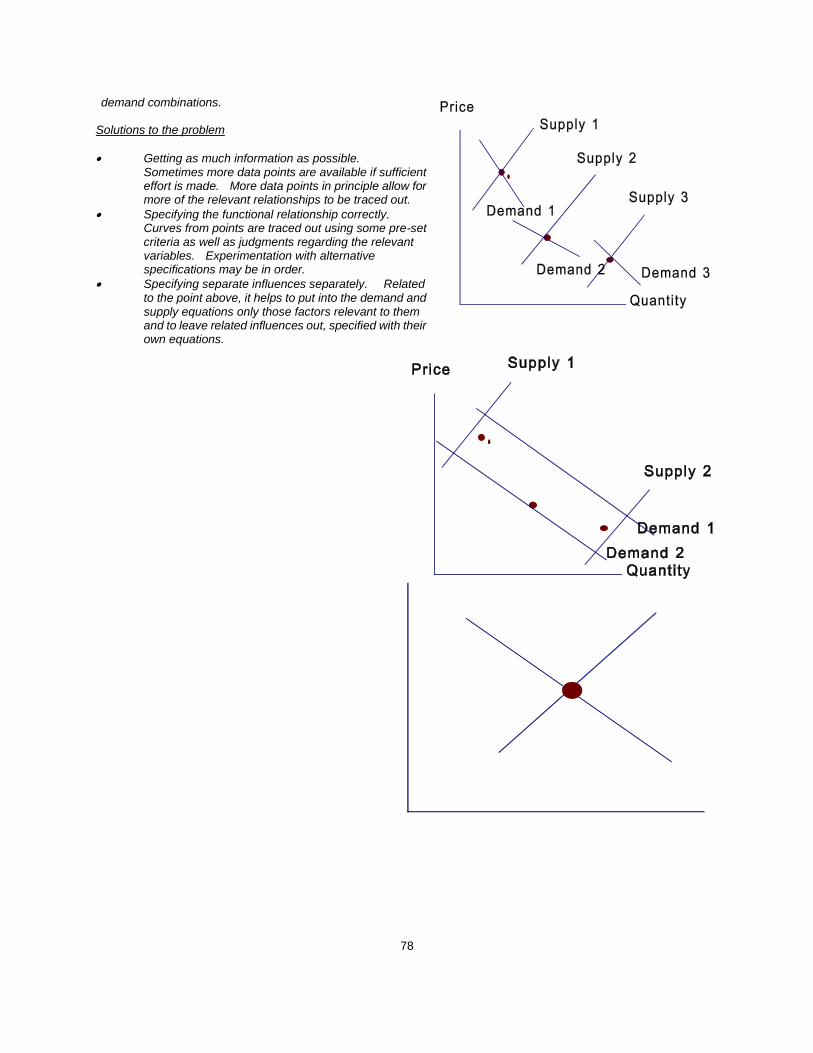
78

demand combinations. Solutions to the problem

Getting as much information as possible. Sometimes more data points are available if sufficient effort is made. More data points in principle allow for more of the relevant relationships to be traced out.

Specifying the functional relationship correctly. Curves from points are traced out using some pre-set criteria as well as judgments regarding the relevant variables. Experimentation with alternative specifications may be in order.

Specifying separate influences separately. Related to the point above, it helps to put into the demand and supply equations only those factors relevant to them and to leave related influences out, specified with their own equations.

79

APPENDIX: SELF-TEST EXERCISE QUESTIONS – WITH SELECTED POSSIBLE ANSWERS PROBLEMS — ECONOMIC CONCEPTS Define opportunity cost. What is the opportunity cost of attending the movie “Nixon”? What is the connection between the price of a thing and its relative scarcity? What is "utility"? Can it be measured? What is the use of the ceteris paribus assumption?

What is the relationship between the economist's conception of profits and the economist's conception of costs? State the distinction between the short run and the long run as these terms are used in the context of the theory of cost. If a firm doubles in size but needs less than twice as many workers, then what sorts of returns to scale are being exhibited?: ANSWER: Increasing returns to scale As increasing amounts of a variable factor are combined with a fixed factor, what does the Law of Diminishing Returns predict will happen to output the corresponding variable input? ANSWER: the changes in output - attributable to increasing the variable factor - will be smaller What level of scale returns occur once a firm produces at minimum efficient scale? ANSWER: constant returns to scale begin Over the long run, an increasing cost industry experiences what level of economies-of-scale? ANSWER: diseconomies of scale TRUE/FALSE/UNCERTAIN

Even in the wealthiest of countries, the desire for material goods is far greater than productive capabilities. TRUE If a college enforces a new policy where anyone caught cheating is immediately expelled, then the basic postulate of economics suggests that the incidence of cheating will be zero. FALSE. It is doubtful that individual benefit-cots calculations would lead to this result. Rather incentives would be shifted so that fewer students will attempt to cheat

(A) An increase in spending on law enforcement will lead to a reduction in crime. (B) Persons convicted of three felonies should be sentenced to life without parole. Statement A is a positive statement, statement B is a normative statement. TRUE The term "ceteris paribus" means that no one knows which variable will change and which will remain constant. FALSE. It means that all variables except those specified are constant. Economics is based on the premise that people act only out of selfish motives. FALSE. Certainly self-interested, but not necessarily without consideration of other people. Economics suggests that the choices of even an altruistic person will be influenced by changes in perceived personal benefits and costs. TRUE Air travel from New York to Miami costs $300 and takes six hours. A bus ticket between the cities costs $200 and

80

takes 56 hours. Assuming nonmonetary considerations are equal for the two alternatives, the minimum value of one's time would induce a rational individual to fly rather than drive would be $1 per hour. FALSE. It would be $2 per hour. Mike purchased a used car from Joe for $3,000. And later that day, Pete came to Joe and offered $3,500 for the car. Mike is the only person that gained from the trade. FALSE. Both Mike and Joe gained from this trade. If an economy uses its resources inefficiently, this situation would be illustrated on a production possibilities diagram as operating at a point inside the production possibilities curve TRUE The best definition of consumer surplus is the difference between what a consumer pays for a good and what the good cost to produce. FALSE:. the difference between what a consumer is willing to pay for a good and the good's price An "equilibrium" point in a market is a point where there is no reason to want to "move away" TRUE

A Louisville manufacturer opens a similar manufacturing facility across the river. If the firm can increase its scale of operation, but at lower unit cost, then it operates under diseconomies of scale. False. When long run average costs decrease, a firm is operating under economies of scale. Economies of scale is another term for increasing returns to scale, which is defined as a situation where a firm can double its output while less than doubling its factors. This is equivalent to decreasing long run average costs. Consumers who spend less than their income are outside their budget constraint FALSE. They are inside their budget constraint.

Consumer equilibrium occurs where a consumer's income is equal to their expenditure FALSE. This is only a necessary, not sufficient condition. The consumer equilibrium is where the benefit from purchasing the last unit of a good is equal to its price The following statements about economic profit are all false.a.

economic profit is smaller than accounting profitb. economic profits are always zeroc. economic profits do not account for opportunity costsd. economic profit may be calculated with the following formula: (P - TC) q FALSE: statement A is true If a firm doubles in size but needs less than twice as many workers, then the firm will experience decreasing returns to scale. FALSE. the firm will experience increasing returns to scale

The best definition of bounded rationality is that it is rational to increase output until reaching a certain point FALSE. A better one is when a person makes rational economic decisions on the basis of limited information Which is the best example of diminishing marginal returns: a. as output increases, the marginal cost gets smaller b. as a firm hires more labor, marginal product gets smaller c. as a firm hires more labor, output gets lower d. as output increases, the firm hires less labor ANSWER: B What is the best definition of consumer surplus? a. the difference in value between what one is willing to pay and what one actually pays to buy a commodity b. the difference in value between what one is willing to pay and the lowest price that a firm is willing to take for a commodity c. the difference in value between the lowest price that a firm is willing to take and what one actually pays for a commodity d. the total value of actual consumer expenditures on a commodity

81

ANSWER: A INTERNATIONAL ECONOMICS QUESTIONS Ceteris Paribus, the exchange-rate value of the dollar increases sharply. What will happen to Net exports (exports minus imports)? In the short-run, what will happen to the equilibrium prices of dollar-denominated imports into the U.S.? Answer: both will decline The island of Togo can produce either 4 units of shoes or 8 units of bananas. The island of Fiji can produce either 4 units of shoes or 12 units of bananas. A. Which nation has a comparative advantage in producing shoes? ANSWER: Togo has a comparative advantage in producing shoes B. If a labor saving innovation occurs in Fiji's banana production, then what will happen to its comparative advantage in bananas? ANSWER. The innovation doesn't change Fiji's comparative advantage in banana production except to increase its magnitude Country A can produce 100 units of corn or 200 units of shoes. Country B can do twice as much of both. Does either country have a comparative advantage in anything? Explain. No, neither country has a comparative advantage in corn or shoes because their opportunity costs would be the same for each good. See the calculations (and comparisons) below.

• The opportunity cost in A of producing corn is 2 units of shoes (i.e. 200/100) • The opportunity cost in B of producing corn is 2 units of shoes (i.e. 400/200) • The opportunity cost in A of producing shoes is a 1/2 unit of shoes (i.e. 100/200) • The opportunity cost in B of producing shoes is a 1/2 unit of shoes (i.e. 200/400)

A country is specializing in the production of just one of two possible goods. Considering what the country's PPC probably looks like, is this necessarily inefficient? Explain. To produce only one good is not necessarily inefficient. To produce only one good means that the country is located on one of its two axis. If the country is on both its PPC and the axis (i.e. at its PPC's corner point), then it is using all of its factors and resources to produce only that good. For example, from above, if country A produced only 100 units of corn, it would be located on both its PPC and the corn axis. If country A only produced 50 units of corn, it would be located on the corn axis, but inside the corner point on its PPC.

82

You are given the PPC of Country A: A B C D E F Fish 0 8 16 24 32 40 Lobster 20 16 12 8 4 0 Moving from pt. B to C, what is the opportunity cost of each unit of fish? ANSWER: 1/2 unit of lobster What is the opportunity cost of the 4th unit of lobster? ANSWER: 2 units of fish If the opportunity cost in Country B of each fish is 1 unit of lobster, then which country has a comparative advantage in fishing? ANSWER: Country A One day, there is a higher demand for fish in Country A. As a result what will happen to A’s PPC? ANSWER: A's PPC won't shift, but actual output will change as more fish and less lobster get produced One day, firms learn that mercury in the water system has contaminated much of the existing sea life. As a result what will happen to A’s PPC? ANSWER: A's PPC will shift to reflect decreased potential in both fishing and catching lobster

Considering the demand and supply of butter in Country A, what likely effect will a decrease in the price of lobster have on this market? ANSWER: the price and quantity exchanged of butter will rise On the production possibility curve (PPC) for 2 door and 4 door sedans, if we can produce more of both goods, then: a. the price of one of the goods has decreased b. productivity has decreased c. we are now producing at an inefficient point d. the inputs/factors are not homogeneous ANSWER: C The brain drain typically occurs when skilled workers migrate from less developed countries to more developed countries. How would the brain drain most likely affect the U.S. PPC? a. an increase (shift right) in the production of all goods b. a decrease (shift left) in the production of all goods c. a decrease in the production of more technologically advanced goods, but little change in less advanced goods d. an increase in the production of more technologically advanced goods, but little change in less advanced goods ANSWER: D The following questions correspond to the following information: In one hour, Bill can bake 6 pies or make 4 loaves of bread. Also, in one hour, Ted can bake 8 pies or bake 4 loaves of bread. Which of the following statements is most accurate: a. Ted has both a comparative and absolute advantage in baking pies b. Ted has both a comparative and absolute advantage in baking bread c. Ted has a comparative advantage in baking pies d. Ted has a comparative advantage in baking bread ANSWER: A Which of the following statements is true: a. Ted's opportunity cost of baking each loaf of bread is less than Bill's, giving Ted a comparative advantage in baking bread

83

b. Bill has an absolute advantage in baking bread c. Bill has no comparative advantage since he is not better than Ted at either activity d. Bill has a comparative advantage in baking bread, even though Ted and Bill can bake the same amount of bread in an hour. ANSWER: D Which of the following statements most accurately reflect the Law of Comparative Advantage: a. Bill should specialize in baking bread and Ted in baking pies, because this is where their absolute advantage lies. b. Bill should specialize in baking pies and Ted in baking bread, because this is where their comparative advantage lies. c. Bill should specialize in baking bread and Ted in baking pies, because this is where their comparative advantage lies. d. both a and c are correct ANSWER: C QUESTIONS — LAW AND ECONOMICS, INSTITUTIONS AND PUBLIC CHOICE Why do you think people run for public office? Is it reasonable to assume that public office is a good which yields benefits to the holder? How is the political market place organized? What is the product offered for sale in this market? What is given in exchange for this product? Do you find it any less plausible to assume that criminals are rational than to assume that consumers are rational? Make sure you use the economist’s conception of rationality. Define rent seeking behavior. Given the expected pay off relative to the cost, is it rational to take time to inform yourself of what is involved in particular issues of the day so that you can cast an intelligent vote at the next election? Is it rational to take time to vote? What effect do you think your vote would have on any particular policy subsequently acted upon by government? Why are so few people present at most local school board or other local government meetings? Why do organizations frequently diverge from "optimal" performance in a normative sense and pursue some objective other than (or, in addition to) the "efficiency" objective? (Hint: consider the separation between ownership and controlling management in most large firms.) It has been suggested that because of the separation between the ownership and controlling management in most large firms, management may have a strong motivation to pursue other, more self serving objectives, such as long run survival, size maximization, improved working conditions and fringe benefits, etc., constrained only by the need to earn an acceptable level of profits. Would you expect a greater divergence from the efficiency objective in a small individual proprietorship or in a large corporation? One would probably expect a lesser divergence from the efficiency objective in small proprietorships as compared to large corporations because: a) small proprietorships are likely to be in a more competitive environment; and, b) the ownership and management functions are one and the same. Is it reasonable to expect firms to take actions that are in the public interest but are detrimental to stockholders? Is regulation always necessary and appropriate to induce firms to act in the public interest? No, the existence of firms is due to the economic advantages of such organizations. It is not reasonable to expect firms to voluntarily undertake any action that is truly detrimental to its owners and managers. When such actions are deemed desirable, regulation by society will no doubt be required. It should be emphasized,

84

however, that this does not mean that firms cannot be expected to undertake "socially responsible" activity. In many cases, such activities can be expected to have a beneficial effect on sales, taxes, labor relations, production costs, etc. In these instances, the firm could well be expected to undertake such activities voluntarily. How do economists explain the existence of firms? ANSWER: creating a firm minimizes transactions costs TRUE/FALSE/UNCERTAIN — EXPLAIN Saying that the median voter is decisive in simple majority-rule elections is equivalent to saying that the mean voter is decisive in majority-rule elections. . UNCERTAIN or FALSE: the statement is true only if we assume that the distribution of preferences is symmetric and unimodal; with such a distribution the mean and the median are the same. The median voter model of elections implies that politicians respond passively to the preferences of the electorate. TRUE: the model predicts that politicians can win elections simply by discerning community preferences shared by 50% of the electorate plus one vote. In the presence of an externality, the Coase Theorem implies that efficiency will result so long as property rights are defined and allocated. UNCERTAIN or FALSE: the statement is true only without transactions costs PROBLEMS — MACROECONOMICS TRUE/FALSE/UNCERTAIN/EXPLAIN When individuals correctly anticipate the effects of expansionary monetary policy prior to the policy being implemented, the expansionary policy will increase real output FALSE: It will increase prices but leave real output unchanged The demand curve for money indicates the amount that consumers wish to borrow at a given interest rate. FALSE: The demand curve for money shows the amount of money that individuals and businesses wish to hold at various rates of interest Starting from an initial long run equilibrium, an unanticipated shift to more expansionary monetary policy would tend to increase prices and unemployment in the long run. FALSE: It will increase real output in the short run but not in the long run. If the Fed shifts to a more restrictive monetary policy, the real interest rate will rise and the exchange rate value of the dollar will also rise. TRUE "The more money there is in the economy, the more people spend. The more people spend, the higher is national income. Therefore, the greater the money supply, the better off people are." FALSE because the real income of the economy is limited by the economy's productive capacity. The rational expectations hypothesis implies that discretionary macropolicy may be relatively effective in the short run but ineffective in the long run FALSE. Such a policy is relatively ineffective both in the short run and long run Assume that both union and management representatives agree to wage increases based on their expectation that

85

price will rise 7% during the next year. If the actual inflation rate next year is 4%, the unemployment rate will be above the natural rate, because the firms' profit margins decline. TRUE When the economy reaches long run equilibrium its unemployment rate is 0% FALSE. the actual unemployment rate equals to the natural rate of unemployment Monetarists recommend using monetary policy to "fine tune" the economy FALSE. Monetarists favor non activist monetary policy (i.e. a “fixed rule”) The long run Phillips curve implies that in the long run higher inflation does not reduce the rate of unemployment TRUE The proponents of activist policy would argue that the economy is very unstable by itself, so it needs policy to stabilize it. TRUE The modern view of the Phillips curve is that when inflation is more than anticipated, expansionary monetary policy is needed to bring the economy back to full employment FALSE. unemployment will be below the natural rate of unemployment A Keynesian economist would favor wage and price controls in the case where the economy’s current equilibrium leve l of output is below its potential level of output FALSE. A Keynesian would favor pumping more resources into the economy, either through a reduction of income taxes. Those with assets consisting of government bonds and life insurance policies will most likely benefit from a period of unanticipated inflation, assuming the composition of their assets and liabilities remains unchanged? FALSE. Those whose assets include a house and a car and whose liabilities include a fixed rate mortgage and an automobile loan, for example, would benefit most. According to the Keynesian multiplier model, if the marginal propensity to consume were 0.75, an autonomous increase in investment expenditures of $25 billion would cause the equilibrium income (output) to rise $25 billion FALSE. It would rise by $100 billion The new classical model implies that a shift to a more restrictive fiscal policy will have no effect on the real interest rate, aggregate demand, and employment. TRUE A substantial increase in tax revenue derives from the growth of corporate profits when the economy experiences recession is an an example of an automatic stabilizer? FALSE: That is automatic but not a stabilizer since it represents a procyclical movement. An example of an automatic stabilizer is an increase in government unemployment compensation spending when the economy experiences recession. Jorge, a Mexican citizen, works at an appliance plant in Louisville, KY and get paid $35,000 per year. This increases both U.S. GDP and U.S. GNP? FALSE. It increases only GNP not GDP. If Jorge is a U.S. citizen, then both U.S. GDP and GNP are increased. For economy A, the nominal GDP was $5,000 million in year 1, and $4,500 million in year 2. You can therefore conclude that economy A produced less in year 2 than in year 1. FALSE. You need to know the rate of inflation to know that.

86

36. If you were in charge of state economic growth policy, you would recommend that, to reduce the natural unemployment rate, there should be an increase in the minimum wage. FALSE. You would provide programs designed to improve the basic skills of workers Assuming "economy Utopia" has the following statistics: Year Nominal GDP GDP deflator (billions $) (1990=100) 1993 $ 9,000 120 1994 $10,800 135 1995 $11,890 145 a. The annual inflation rate for year 1994 was 12.5% , and for year 1995 was 7.4%. TRUE. b. The growth rate of real GDP in year 1994 was 6.67% and in year 1995 was 2.5%. A short-run decrease in U.S. employment and output will most likely occur in the United States as the result of an unexpected rapid decline in real income in Japan and Europe. TRUE John Maynard Keynes and his followers argued that the Great Depression was primarily the result of perverse monetary policies of the Fed. FALSE. Monetarists argued this. Keynes argued that the Great Depression resulted primarily from insufficient aggregate spending on goods and services. Suppose that in 1996 the CPI was 110 and that the average consumer's nominal income was $44,000. In 1995, these values were 96 and $33,000 respectively. A. The best interpretation of the 1996 CPI is that relative prices have changed between 1996 and 1995 FALSE: We only know that overall price level has changed. B. Goods that cost the typical consumer $100, in the base year, cost $110 in 1996 TRUE C. The average consumer's real income in 1996 was $40,000 TRUE. D. The inflation rate between the base year and 1996 is approximately 14%. FALSE. It was 10% If inflation were definitely coming, I would be more inclined to take out a car loan. TRUE. Inflation makes borrowers better off. When I take out a loan now, once inflation hits, I repay the loan with dollars that are devalued by the inflation. For example, suppose my job provides me with a cost of living adjustment every year, but no merit based pay raise. Although I pay the same amount each month of the car loan, my nominal income is rising as inflation occurs (of course, my real income is unaffected by the inflation). That is, it gets easier to pay off the loan. Deficit financing of government expenditures leads to less excess burden than tax financing. . UNCERTAIN or FALSE: the reduction in tax finance lowers excess burden in labor markets but crowding out distorts investment and financial markets, so the net result is uncertain without further information. The consumer price index for economy A in 1980 was 70, in 1981 was 75, the CPI for 1990=100. The inflation rate based on CPI for economy A in 1981 was 5% FALSE. It was 7.1% When people lose their jobs, and claim that they are looking for work when they really aren't, the unemployment rate and participation rate decrease. False. When people lose their jobs and actively seek new employment, they are officially considered unemployed and remain a part of the labor force. Subsequently, the unemployment rate would rise and the participation rate remain the same. For whatever reason, some former workers may claim to be seeking new employment when they're not.

87

Although the technically would not be unemployed by the official definition, they are still considered unemployed because of their claim to be seeking new employment. Therefore, the effect that these people have on these two rates (a lower unemployment rate and unchanged participation rate) is the same as that caused by those who lose their jobs and really do actively seek new employment. Increasing GDP and increasing societal welfare are synonymous. False. Increasing GDP is not the same thing as increasing societal welfare, and certainly does not necessarily imply a higher level of social welfare. Higher GDP simply implies an increased level of economic activity, measured as the market value of all final goods and services produced in a given year within the nation's borders. This increase could coincide with higher pollution, the replacement of damaged infrastructure, an increased concentration of labor income, etc. Any of these "problems" are not typically associated with rising societal welfare. When students quit jobs in order to concentrate full time on school, they become unemployed. False. To be officially unemployed, one must (necessarily) be out of a job and actively seeking new employment. When a student, or anybody else, quit a job and stops looking for new employment they are not considered unemployed. Hiring back workers, who were previously unemployed, has the same effect on the PPC as hiring (new) workers who have just migrated into the country. False. When unemployed workers are hired back, there is movement within the PPC toward a point on the curve, but no shift. When newly migrated workers are hired for work, then there is very likely going to be movement toward the PPC (i.e. if these workers were formerly unemployed). The migration itself, however, will shift the PPC outward as more workers become available. Unlike cost push inflation, demand pull inflation leads to a bigger unemployment problem and higher inflation. False. Demand pull inflation involves an increase in the Aggregate Demand curve. As the AD curve increases, the price level and real GDP rise. Inflation would probably accompany a rising price level, but since unemployment and output are negatively related, rising output would lead to falling unemployment (not more unemployment). If nothing else happens, then an increase in productivity should lead to lower unemployment but higher inflation FALSE: lead to lower unemployment and inflation The Laffer curve suggests that increasing the tax rate on income causes tax revenues to decrease TRUE. A reduction in the tax rate on capital gains to encourage capital accumulation is an example of procyclical fiscal policy. FALSE: It is a use of fiscal policy (taxes) to affect the economy, but it is not necessarily pro- or counter-cyclical. It is more of a supply-side/structural economic policy. Increases in the money supply, in an effort to lower interest rates during a recession, is an example of a countercyclical fiscal policy. FALSE. It is a counter-cyclical policy, but a monetary policy, not a fiscal one.d. Raise the income tax rate to increase the amount of tax revenue available to government Crowding out most likely to occur during periods where the economy is deep in a recession FALSE: when the economy is near or at full employment If the economy is above its potential, a decrease in government spending is needed to eliminate this inflationary gap TRUE. At least according to Keynesian theory. Otherwise, FALSE or UNCERTAIN SHORT ANWSERS Given the data for country X, answer the following questions C = .8(Y T) + 400 (C = consumption, Y = real income) I = 1200 (I = investment) G = 400 (G = government expenditure)

88

T = 400 (T = tax revenue) X = 200 (X = exports) M = 100 (M = imports) What is the marginal propensity to consume in Country X? Answer: 0.8 What can Country X say about this year's (government) budget balance?: Answer: the government's budget is balanced What can Country X say about its current National Debt level? Answer: there is not enough information to answer this question What does the government expenditure multiplier show in plain terms? Answer: that increases in government spending and output occur at a 1:1 ratio What does the tax multiplier show in plain terms? Answer: that taxation and output have a positive relationship What is an inside lag? Answer: the length of time between when Congress becomes aware of a problem and when legislation is passed correcting the problem What is an outside lag? Answer: the length of time between when Congress passes legislation designed to correct the problem and when the problem is actually solved What sorts of policies would Supply side economists advocate? ANSWER: deregulate certain industries, to make them more efficient; lower personal income taxes, to encourage productivity and labor supply growth; lower corporate income taxes, to encourage capital formation Outline the Keynesian arguments against balancing the Federal budget annually. ANSWER: annual balancing may entail spending cuts during recessionary gaps, and annual balancing may entail spending increases during inflationary gaps Given with the following equations (variables are defined the same), answer the questions below: C = 0.8(Y T) + 500T = 0I = 100G = 200 What is the Savings function that corresponds with this economy? Answer: S = 0.2Y 500What is the government expenditure multiplier associated with this economy ? Answer: 5 TRUE/FALSE/UNCERTAIN The US government never has to pay off all its debts because the the US government is assumed to have an "infinite life" TRUE according to Ricardian equivalence. Balancing the budget over the business cycle entails running deficits when output is above potential FALSE. running deficits during recessionary gapsWhy is a comparison of the budget of the US government to that of a household a bad analogy? Basically, the US government can finance its expenditures in ways that are not (legally) available to households One result of producing where real GDP exceeds aggregate expenditure is that inventories will be unexpectedly falling. False. When real GDP exceeds aggregate expenditure, then the economy is producing above its level of demand. As a result, inventories will rise, and continue to do so until either demand goes up or output goes down. In the short run, increases in the marginal propensity to consume would lead to a slight increase in the inflation and

89

unemployment rates. False. If the marginal propensity to consume increased, then (variable) consumption would increase. Increasing consumption would lead to higher (aggregate) demand, which in turn would cause movement up the economy's short run Phillip's curve (assuming prices aren't completely fixed in the short run). This movement would elicit a slight increase in the inflation rate, but a decrease in the unemployment rate as more workers get hired to produce the extra products necessitated by the higher level of consumption. Government borrowing today represents a burden on future taxpayers. False. but only if there are no foreign citizens buying this debt. If government borrows money today, then it must raise taxes tomorrow (i.e. in the future) to pay for their debt. On a societal level, this taxation represents a (gross) burden, of course, but if the debt is domestically held, then that burden is exactly equal to the debt related benefits that accrue to society (i.e. the tax equals the amount of debt that should be paid off, the principal and interest that accrues to U.S. citizens). If the debt is held by foreign citizens, then the gross burden of the tax is not offset by these debt related benefits (i.e. the tax is greater than the amount of principal and interest that accrues to U.S. citizens). Balancing the budget annually creates an (economic) incentive to limit the size of government. True. Annually balancing the budget is procyclical. That is, by balancing the budget every year, the business cycle is driven to greater extremes. For example, if the economy falls into a recession a once balanced budget would fall into a deficit as tax revenues dried up. To return to a state of balance, government would have to cut spending or raise taxes, driving the economy further into the recession. The business cycle is made worse. To avoid this problem, one could reduce the size of government, hence there is an incentive to reduce government when balancing the budget annually. SHORT ANSWER: What is the "convergence property" implied by the neoclassical (i.e., Solow) growth model? The neoclassical growth theory predicts that economies that are similar in production technology, population growth rates, and savings rates will converge in the long run to the same level of per capita capital stock and, hence, per capital income. That is their growth experiences may be different given their initial sizes but they will converge to the same long run equilibrium. Moreover, small economies will grow faster than large economies, since the large economies are closer to their long run equilibrium sizes. Is there evidence in cross country data to support this convergence property? What other types of convergence do these data suggest? There is little evidence that small economies grow more rapidly than large economies. In fact, there seems to be no pattern in the cross country relationship between initial size and subsequent growth rates. However, there is evidence supporting "conditional convergence." That is, if one holds constant such factors as a country's fertility rate, its human capital, and its government policies, poorer countries tend to grow faster than richer ones. So the basic insight of the neoclassical growth model is, in fact, correct. But since, in reality, other factors are not constant (countries do not have the same level of human capital or the same government policies), absolute convergence does not hold. How can Mancur Olson's ideas about increases in efficiency be captured by the Solow model? Olson's increases in efficiency are captured as increases in total factor productivity in the Solow growth model, ie., increases in the parameter "A". According to the new growth theorists, how does "human capital," i.e., the embodiment of knowledge and ideas, differ from "physical capital" in its effects on marginal productivity? The main premise of the "new growth theory" is that the knowledge and ideas embodied in "human capital" are not subject to the diminishing marginal productivity of physical capital. That is, more people making use of a good idea doesn't make it less of a good idea, hence, doesn't decrease the usefulness of the idea to other people. Whereas as you add more physical capital to the production process, other things equal, marginal productivity falls. TRUE/FALSE/UNCERTAIN The following activities will affect this year's GDP: a. The sale of a used economic textbook to the college bookstore b. Family lawn services provided by Smith's 16 year old child

90

c. A multibillion dollar discovery of natural gas in Oklahoma d. Smith's $500 doctor bill for setting her son's broken arm. ANSWER: Only d is true The following activities would increase U.S. GDP? a. A Japanese purchases a Japanese dinner in Tokyo. b. A U.S. citizen purchases a Japanese dinner in Tokyo. c. A Japanese purchases a Japanese dinner at Shogun in Louisville, Kentucky. d. A Chinese citizen purchases a Big Mac at McDonald in Beigin, China. ANSWER: Only c is true Your grandfather tells you that in 1929 at age 16 he earned 50 cents per hour; your father tells you he earned $1.50 per hour when he was 16 in 1969; you remember making $4.50 per hour when were 16 in 1990. Given that the CPI was 17.1 in 1929, 36.7 in 1969, and 130.7 in 1990, you had the highest standard of living, followed by your father, followed by your grandfather FALSE. The correct order, highest to lowest, is your father, you, your grandfather Given that Mike's 1988 money income = $50,000 and Mike's 1989 money income = $55,000; and that the 1988 CPI = 120; 1989 CPI=125.8, Mike’s real income grew by 0% between 1988 and 1989. FALSE. It actually grew by 5% For economy A, the real GDP was $5,000 million in year 1, and $4,500 million in year 2. With the above information you can conclude that economy A produced more in year 2 than in year 1. FALSE. It produced less in year 2 than in year 1. The primary value of GDP is to provide observers with a reasonably good index of social progress FALSE. It only reflects (imperfectly) the output rate of a nation Use the following information to answer next two questions: Assuming "economy Utopia" has the following statistics: Year Nominal GDP GDP deflator (billions $) (1990=100) 1993 $10,000 150 1994 $12,000 165 1995 $15,000 180 What is the annual inflation rate for year 1994 and for year 1995? Answer: 10.0%; 9.09% What is the real GDP in billions of 1993 dollars in year 1994 and in year 1995? was Answer: $10,909; $12,500 Is real GDP is always higher than real GNP for every economy? Answer: No. Depends on where output is produced. Use the following information to answer next two questions: In 1994, Germany had the following statistics Population (16 years and over) 55.6 million number employed 34.9 million number unemployed 2.60 million What is the number of those not in labor force was and what is the corresponding unemployment rate? Answer: 18.1 million; 6.93 percent What is the labor force participation rate for Germany in 1994 and the rate of employment in that same year?

91

Answer: 67.45 percent; 62.77 percent What is the primary cause of frictional unemployment? Answer: inaccurate and costly information about job opportunities TRUE/FALSE/UNCERTAIN When an economy is at long run equilibrium, the unemployment rate will equal to zero FALSE; the economy will produce at potential GDP. Each of the following would most likely reduce the natural unemployment. a. an increase in the proportion of prime age workers as a share of the labor force b. an increase in the minimum wage c. an increase in unemployment benefits d. an increase in the labor force participation rate of teen agers Only a would do so. Each of the following persons would be classified as not in the labor force by the Bureau of Labor Statistics. a.. John Brown, who is in the midst of a two week vacation from his regular job. b. Susan Smith, who is unable to work her regular job this week because of illness. c. Danny Young, who is working four hours each week at McDonald's while looking for a full time job. d. Harold Jones, who is on layoff waiting to return to his construction job once the weather improves. e. John Brown tops looking for work because he believes his prospects are so poor that he is unlikely to find a job Only e would be so classified. Each of the following groups of people would most likely benefit from a period of unanticipated inflation, assuming the composition of their assets and liabilities remains unchanged. a. those whose asserts include a government bond and a life insurance policy. b. those whose assets include a house and a car and whose liabilities include a fixed rate mortgage and an automobile loan c. those whose assets include corporate bonds, a savings account, and a house with a variable rate mortgage. d. those who have no liabilities and whose assets include a savings account, long term government bonds, and a paid up life insurance policy Answer: only b. ••MARKET STRUCTURE PROBLEM At a large university there are two bookstores. One is located on campus in the student center and the other is located just off campus. Instructors inform both stores of their textbook choices. Both stores carry new and used books for every class. Each store must decide on a price for the introductory economics textbook: either $40 or $45. Their "payoffs" matrix is shown below. It gives the profit for each bookstore from sales of this book. (e. g., If the on-campus price is $45 and the off-campus price is $40, then the on campus store's profit is $5,500 and the off-campus store's profit is $9,500.)

Off-Campus Bookstore's Price

40

45

On-Campus

40

$5,000 $7,500

$2,000 $11,250

Bookstore's Price

45

$9,500

$8,600

92

$5,500 $10,400

(a) What kind of market structure is this? Explain your answer.(b) Though the stores sell the same book, there is some differentiation. How can you tell from the payoffs matrix?ANSWERS (a) What kind of market structure is this? Explain your answer. This is an oligopoly with some product differentiation. We know it is an oligopoly because there are only two firms.

(b) Though the stores sell the same book, there is some differentiation. How can you tell from the payoffs matrix? We know there is some differentiation because when one firm raises its price above that of the other, it does not lose all of its sales.

93

SHORT ANSWERS — MARKET STRUCTURE What does a firm's demand curve look like if it is operating under conditions of perfect competition? Would it make sense for a firm in perfect competition to offer its output at a price lower than the prevailing market price? Explain. How many units of output would a firm in perfect competition sell if it set a price for its product higher than the prevailing market price? Explain what is meant by an equilibrium market price. What rule should a monopolist follow to determine the best level of output? How does the result of applying this decision rule in a monopoly situation differ from that which occurs under competitive conditions? How does this, in turn, affect the efficiency with which the community's scarce resources are utilized? Does the monopolization of a previously competitive industry necessarily mean that output will fall and that the price of the product will rise? How does oligopoly differ from monopoly? If you are shown a diagram depicting the costs and revenues of a firm, can you determine immediately whether the firm is operating under perfect competition or some other kind of market structure? Explain. Which of the following statements always hold in a perfectly competitive industry in the short run?a. homogeneous productsb. economic profits are equal to zeroc. free entry and exit ANSWER: only a (c, in the short-run, it could be argued, does not hold since it takes time for new firms to enter and exit. But one might also add c) Firm X charges different prices in each of the markets where it sells its product. The markets are in different geographical locations, but you can assume that the firm is able to transport these products for free. The reason for these price differences, however, stem from differences in demand elasticity across markets. a. By definition, discuss what type of pricing is described here (be specific)? This is 3rd degree price discrimination because the firm is selecting different prices for the various markets where it does business. These markets differ on the basis of demand elasticity, so we should expect that there are no stated cost differences in supplying these markets. If the difference in prices was due to costs, then this would not be price discrimination at all. b. List and briefly explain the 3 conditions that allow Firm X to successfully pursue this type of pricing. In order to price discriminate at all, Firm X needs (1) to possess some degree of market power (i.e. the ability to set price), and (2) must be able to separate consumers on the basis of certain characteristics that imply differences in these consumers' willingness to pay for Firm X's product (e.g. recognize differences in their elasticity of demand or reservation prices). Lastly, in order to use price discrimination successfully (i.e. to increase profits), Firm X must be able to prevent resale of the product between low and high paying groups. If a low paying customer could resell the product to a high paying customer, then only the low paying customers would end up buying the product - which is not the intent of price discrimination. c. Since the prices vary across these markets, which ones do you expect to end up paying higher prices? Explain. The markets paying higher prices will be those with a greater willingness to pay for the product. It is quite likely that these markets will have a more inelastic demand for the good. In the graph below, this is illustrated. A steeper demand curve (i.e. more inelastic demand curve) in market 1 leads to a higher price in that market (i.e. P1 > P2) because the firm knows that consumers there will not substitute away from its product in great numbers as the price is raised. 2. In some of Firm X's markets, it is a monopolist. In one of Firm X's markets, they are a dominant firm. In this market, there is a small competitive fringe, with identical costs (to Firm X), that operates as Firm X's rival. a. If this market's (market) price falls below Firm X's average cost, then is Firm X guilty of predatory pricing? Explain why. Firm X is not necessarily engaging in predatory pricing. The ATC rule points out that pricing below AC is a necessary but not sufficient condition for predatory pricing. If pricing below AC, the firm must also have the intent to monopolize in order to be rightfully accused of predatory behavior. The reason why is because P < AC is possibly the result of natural market forces like a drop in demand. While it is not irrational for firms to produce at less than average cost in the short run, however, things change when we consider the long run. A firm will not produce at prices below their long run average cost because the firm could do better by exiting the market - since the firm's long run profits would be negative. If Firm X has no fixed costs, then their average variable and average costs would be the same. Producing below AC would imply producing below AVC. If Firm X produced below its average variable cost in this manner, then the fringe could easily accuse Firm X of predatory pricing by pointing out that Firm X could do better by shutting down. That is, since it would be irrational for Firm X to produce below AVC, the firm must have a secondary motive for doing so - like predatory pricing. Suppose that Firm X is attempting to engage in predatory pricing - with the goal of becoming a monopolist in this

particular market.

94

b. Would it be a good idea for Firm X to raise prices in the (other) markets where it operates as a monopoly already? Explain why. It would be unwise for Firm X to raise prices in these other (monopoly) markets. The reason stems from something called the recoupment fallacy. If Firm X is producing at profit maximizing levels in these other markets, then changing the price (without any changes in the market) would lower the firm's profits there. Consequently, the firm would be worse off. If the firm is intent on its predatory pricing strategy, then it will leave the prices in its other markets alone, and will follow predatory pricing as long as its total (long run) profits are positive. Suppose Firm X gives up on its predatory pricing strategy, because the fringe firms offer to allow Firm X to buy them out - in exchange for a share of the monopoly profits that Firm X makes in this market. Assume that - in spite of the formation of this monopoly - the government allows this merger to occur, but that it results in greater (market) output and a lower price. c. Did the merger result in an efficiency gain or loss? Explain why. The merger resulted in an efficiency gain. In order for this to occur, the merger would have to have a stronger effect on Firm X's marginal cost curve then the fringe's supply curve. That is, the change in Firm X's MC curve should be greater then that associated with the fringe. The textbook characterizes this as a condition which satisfies: DSf < DMCX (where X represents the dominant firm). The merger would also affect Firm X's residual demand (it would converge toward the market demand curve), but the overall effect of such shifts would be to decrease the price and increase market output. When a horizontal merger leads to higher prices and lower market output, then there is no efficiency gain. Put another way, there are economies of scale that cause prices to fall and output to rise within the market. Even though the industry would experience allocative inefficiency in the short run, we would expect that the long run scale effect should outweigh this short run inefficiency problem. 3. Product X is manufactured by one firm, but sold by a retailer. The demand and cost curves are given below. No costs are incurred in transporting the good between the manufacturing and retail firms.

Manufacturing

Demand:

PM = 50 - 2QM

MR:

MRM = 50 - 4QM

Costs:

ACM = MCM = 10

Retailing

Demand:

PR = 100 - QR

MR:

MRR = 100 - 2QR

Costs:

MCR = 2QR + PM

ACR = QR + PM

In the following questions, use the equations above and provide a numerical answer in parts a and b. In part c, also provide a numerical answer with a brief discussion. a. If the manufacturing sector is operated by a monopoly, then what price (PM), output(QM) and profits (pM) will result in manufacturing product X?

set MRM = MCM:

50 - 4QM = 10

solve for QM:

QM = 10

solve for PM:

PM = 50 - 2(10) = $30

find Profits:

pM = (30 - 10)(10) = $200

95

b. Given the monopoly at the manufacturing level, if the retailing sector is also monopolized, then what price (PR), output (QR) and profits (pR) will result in the retail market?

set MRR = MCR:

100 - 2QR = 2QR + 30

solve for QR:

QR = 17.5

solve for PR:

PR = 100 - (17.5) = $82.50

find Profits:

pR = (82.50 - [17.5 + 30])(17.5) = $612.50

c. Given the monopoly at the manufacturing level, is the incentive for vertical integration between manufacturing and retailing greater when the retailing market for product X is perfectly competitive or monopolistic? Explain. There is a greater incentive to vertically integrate here, if the retail market is monopolistic. This result is best understood if we define the incentive to integrate. The incentive to vertically integrate corresponds with how vertical integration affects these firms' profits. If these firms have higher profits with vertical integration than without vertical integration, then there is an incentive to vertically integrate. We determine this by comparing their combined profits without integration to their profits with integration. To see if this incentive is greater when the retail market is monopolistic, we compare the incentive to integrate across market structures. Therefore, the order of operations takes the following steps: a)find the combined profits of the non-integrated firms when retailing is PC b)find the combined profits of the non-integrated firms when retailing is monopolistic c)find the profits of the integrated firm when retailing is PC d)find the profits of the integrated firm when retailing is monopolistic e)find the difference between steps 3 and 1, and steps 4 and 2 f)compare the results of step 5

Step 1

set PR = MCR:

100 - QR = 2QR + 30

solve for QR:

QR = 70/3 = 23.33

solve for PR:

PR = 100 - (23.33) = $76.67

find retail profits:

pR = (76.67 - [23.33 + 30])(23.33) = $544.52

find combined profits

pM + pR = $200 + $544.52 = $744.52

Step 2(builds on parts a and b)

find combined profits

pM + pR = $200 + $612.50 = $812.50

Step 3

set PR = MCR:

100 - QR = 2QR + 10

solve for QR:

QR = 30

solve for PR:

PR = 100 - (30) = $70

find integrated firm's profits:

pR = (70 - [30 + 10])(30) = $900

96

Step 4

set MRR = MCR:

100 - 2QR = 2QR + 10

solve for QR:

QR = 90/4 = 22.5

solve for PR:

PR = 100 - (22.5) = $77.50

find integrated firm's profits:

pR = (77.50 - [22.5 + 10])(22.5) = $1012.50

Step 5Incentive to integrate (retail is PC): Dp = $900 - $744.52 = $155.56Incentive to integrate (retail is monopoly): Dp = $1012.50 - $812.50 = $200 Step 6The incentive to integrate is greater when the retail market is monopolistic (Dp = $200) than when it is perfectly competitive (Dp = $155.56). That is, vertical integration increases profits by $200 when retailing is monopolistic, but only by $155.56 when retailing is perfectly competitive. The result here stems from the basic idea that monopoly is more conducive to high profits than perfect competition. Vertical integration here tends to lead to greater profits in both settings since integration leads to lower retailing costs. While the perfectly competitive retailers make positive profits in this example, however, this is only true in the short run. Recall that in the long run, a perfectly competitive firm makes zero economic profits. Consequently, since perfect competition leads to zero long run profits, while long run monopoly profits are at least zero, the possibilities of higher long run profits from vertical integration should be better with monopoly. 1. Industry X has a few large firms, making it a very concentrated industry. Some additional facts about the industry are: • The two leading firms in the industry are often accused of collusion (i.e. price fixing). • Several years ago, firms were banned from advertising their product on TV and radio. • More R&D; (involving cost reduction) occurred within the industry after the ad ban. • The industry's leading firms make large economic profits. a. What is the Structure-Conduct-Performance approach and how would it explain the existence of positive economic profits in this industry? The Structure-Conduct-Performance (SCP) approach involves determining the relationships between an industry's structural characteristics, its decision-making process and the results of that process. Causation is said to run from Structure to Conduct to Performance, but with the possibility of feedback effects. Structure refers to characteristics like the number of firms in the industry, the distribution of firm size, product differentiation and even the underlying technology. Conduct most often refers to the way in which firms perceive their rivals, but more generally to how strategic decisions are reached. For example, one type of conduct involves the use of price as a competitive variable while another involves output levels. Performance is the measure of how given strategies affect the firm. High profits or technological progressiveness are two possible types of performance. The SCP approach would explain high profits in Industry X by citing the apparently concentrated nature of the industry. Two large firms exist, leading to possible collusion. Successful collusion brings with it high profits. It is apparent that other forces are at work here too. R&D; is high, quite possibly because of the need to raise entry barriers high. High performance could lead to a change in conduct, which could induce a further change in performance or even structure. In any event, there are other (additional) possibilities. b. What is the Chicago approach and how would it explain the existence of positive economic profits in this industry? The Chicago approach looks at markets as inherently competitive. It is the restriction of entry, through unnecessary government regulation, which creates (artificial) market power. This view contends that structure is affected primarily by the underlying technology and barriers to entry. Freedom of entry then determines conduct and performance. Although the leading firms are large, it is likely that the ad ban had a major impact on their ability to compete. The ban would make entry more difficult because of the brand name advantage bestowed upon the industry's leading firms, and because of the cost requirements for entry. Survival would depend on other factors, which might make competition more difficult for new entrants. Although R&D; would occur, possibly changing the underlying technology, it would only affect structure and not conduct or performance. 2. The US automobile market has been described in terms of the dominant firm model, where the Big 3 (GM, Ford and Chrysler) operated as the dominant firm for many years, and imports as the competitive fringe. a. If firms within the competitive fringe (e.g. Toyota) invested heavily in process innovation (i.e. cost reduction), then how would that affect the ability of the Big 3 to use a (static) limit pricing strategy?

97

How would limit pricing occur? The Big 3 could set a price that constrains the fringe's ability to produce a nonzero level of output. Ultimately, the Big 3 would try to keep the fringe output at zero. Doing so, however, might entail setting the price at a very low level. This low price (called the limit price if it limits the fringe to zero output) would keep the Big 3's profits lower than necessary though. One thing that would greatly affect the Big 3's ability to use (static) limit pricing would be the ability of the fringe to become "cost competitive". If the fringe conducted process innovation and lowered their costs, then their MC curve would shift down (see the graph above). As their costs got lower, their ability to "survive" limit pricing would improve. The Big 3 would become less and less able to sustain a limit pricing strategy. Soon, it might be possible that the fringe had lower costs than the Big 3.

b. As an empirical researcher, all you can observe within the US auto market is price and quantity. Suppose that the Big 3 could chose either heavy investment in cost reduction or dynamic limit pricing as their competition strategy. How would you know, watching only price and quantity, which strategy the Big 3 chose? A cost reduction strategy would involve a downward shift in the Big 3's marginal cost curve. As their MC shifts down, the Big 3 would experience a decrease in price and an increase in their output. While the MC curve for the Big 3 is not a supply curve, this change is comparable to an increase in supply. As the figure below shows, a decrease in MC (from the red MC to purple MC') causes the price to fall (from P to P') and output rise (from q to q').

A dynamic limit pricing strategy would involve steadily lower prices and output levels as the Big 3 would set price in such a way as to control the fringe's entry. Each period, the Big 3 would maximize profits by setting a certain price. As long as the Big 3's profits were greater than zero, fringe firms would enter the market. With entry, the Big 3's (residual) demand curve would get flatter. The figure below shows the shift from the Big 3's original (red) demand curve to the newer (purple) demand curve. The flatter demand curve leads to lower prices and lower output for the Big 3. 3. a. From an efficiency standpoint, make an economic argument against highly concentrated industries. A highly concentrated industry is one with a few large firms dominating the market. Firms in this setting will undoubtedly have some degree of market power. That is, they have the ability to set price above marginal cost. When price equals marginal cost, a firm will produce what is called the "competitive level of output". This is the output level produced within the context of perfect competition. When price exceeds marginal cost, output is less than this competitive level - implying a lesser amount of total surplus. In the graph above, setting price above marginal cost results in an output level of q*. The producer and consumer surplus are shaded as yellow and blue respectively. If this firm produced where price equalled marginal cost, output would be qc. Since less than the competitive level of output is produced, some surplus is lost. This lost surplus is called deadweight loss, shaded in red on the graph. Deadweight loss signifies the presence of allocative inefficiency - a (static) argument against highly concentrated industries. b. Is it possible to make an efficiency argument in favor of large firms? Explain. It is possible to think of large firms positively. While large firms may be inefficient in a static context, it is possible that they are efficient in a dynamic sense. Dynamic efficiency corresponds to the presence of innovative activity. Large firms may have certain advantages over more smaller, more competitive firms with respect to innovation for some of the following reasons: • large firms have better financing opportunities than smaller firms, to finance risky projects • large firms can spread the risk of R&D; across a variety of projects, unlike smaller firms • large firms have more complementary resources than smaller firms, to use in appropriating the return to

innovation • large firms have economies of scale in R&D; that may not be present for smaller firms 4. What is the Lerner index and what information does it provide about firm or industry conduct? The Lerner index is the measure of a firm's ability to mark up price over marginal cost. That is, it is a measure of market power. Firm market power occurs for a combination of reasons. In lecture, we derived a functional relationship between the Lerner index and certain variables. The equation for an individual firm (the subscript i denotes the firm as firm i): The Lerner index is the expression on the left hand side of the equal sign. On the right hand side, we see the factors which affect market power. The first term is market share. Larger market share implies a greater ability to raise price above marginal cost. The second term is the market elasticity of demand. A more elastic demand curve means a

98

flatter demand curve, with less ability to mark up the price. The last term involves a parameter called the conjectural variation of firm i. This term is a measure of how firm i reacts to changes in output by the other firms in the industry. If ai = -1, then the entire right hand side is zero, and the firm has no market power. This is consistent with perfect competition because increases in output by an individual firm are offset by the remaining firms, implying that an individual firm has no control over the market price at all. If ai > -1 (e.g. if it equals 0), then the right hand side of this expression is positive - meaning that some market power exists. 5. What is involved in defining a market, and why is it important to do so? A market is (a) a group of buyers and sellers who exchange goods, (b) a good exchanged that has some degree of substitutability, and (c) defined by specific demand-related conditions. There are two dimensions to defining a market: product type and geographical location. Considering product type implies that we look at the relationship of a specific good to other related goods. For example, we might consider the cross elasticity of demand across the products within these related markets. Defining a market by geography entails looking within the area that buyers are making their purchasing decisions and where and how producers distribute their product. This is relevant in the application of antitrust legislation and particularly within the guidelines of how government may view mergers. Depending on how broadly a market is defined, government legislators may not allow certain mergers to take place out of a belief that the merger could restrain trade in a particular market. That is, to avoid the restriction of output that is implicit within a more monopolistic setting. If a perfectly competitive firm makes positive economic profits in the short run, other firms will exit the market over the long run. FALSE: Exactly the opposite. other firms will enter the market over the long run

Which of the following hold at the break even point for a perfectly competitive firm ?a. It will make zero profit. It will produce where average cost is at its minimum levelc. marginal cost is at its minimum leveld. marginal costs are rising ANSWER: All except c will hold. A perfectly competitive firm's demand curve exhibits what shape? ANSWER: It is a horizontal line at the market price In the long run, a perfectly competitive firm can make profits greater than zero (i.e. p > 0). False. In the short run, a perfectly competitive firm can make profits that are greater than zero. Since there are no barriers to entry, when other firms recognize profitable opportunities within this industry they will enter. As new firms enter, the market supply increases and the increased competition drives down prices and profits. In the long run, then, profits return to zero for all firms within the market. If a perfectly competitive firm makes a loss, then it can raise its price to increase profits. False. Perfectly competitive firms are price takers, which means that they have no influence over the market price. This price is determined by the collective actions of all firms and consumers within the market. Firms take this price as given, since they are each such a small part of the overall market supply.

A perfectly competitive firm's demand curve is negatively sloped FALSE. It is infinitely elastic (horizontal) A perfectly competitive firm can maximize its profits by setting price where price equals marginal cost FALSE. A firm can only set output where price equals marginal cost and will do so to maximize profit. The following statements are all true about a monopolist. a. A monopolist takes price as given (i.e. the monopolist is a price taker) b. A monopolist produces where P = MC, which is also where MR = MC c. A monopolist produces where MR = MC, which is also where P > MC d. A monopolist's marginal revenue and demand curves have equal slopes FALSE. Only C is true In the short run, a profit maximizing monopolist will never (willingly) produce: a. when P > AC b. when the own price elasticity is less than one c. when P = AC

99

d. when P < AC e. both b and d ANSWER: B Which of the following is not a characteristic of a perfectly competitive market: a. each firm produces a small amount of total industry output b. each firm is unable to change the market price by changing their output c. perfect availability of information d. each firm's product is slightly different (heterogeneous) e. there are no barriers to entry or exit from the industry ANSWER: D To simply be a price discriminator, a price setting firm must separate consumers into identifiable groups. To successfullyprice discriminate, a firm must:a. charge higher prices to all consumersb. produce less output, in order to

raise the pricec. prevent resale of the product between consumersd. all of the above ANSWER: C Which of the following market structures involves allocative efficiency:a. monopolistic competitionb. oligopolyc. monopolyd. perfect competitione. both a and d ANSWER: D If a monopolist engages in price discrimination, what could happen as a result?a. the monopolist's profits would increaseb. the monopolist's output would increasec. consumer surplus would be zerod. all of the above ANSWER: D A merger between McDonalds and Burger King is an example of a:a. horizontal mergerb. vertical mergerc. diagonal mergerd. lateral merger ANSWER: A The following is a list of pricing "schemes" that are either used by firms or that government agencies impose on firms. a. In foreign countries, local merchants sometimes assume that people with American accents have more money to spend than local residents - causing them to charge the American a higher price than the local resident normally pays. b. When regulators set LG&E's rates, they will allow LG&E to break even. c. When regulators set South Central Bell's rates, they try to get Bell's output to be allocatively efficient. d. When you move to a new home, LG&E charges you a fee to get your electricity hooked up. Afterwards, you can "buy" all the electricity you need at a specific rate. e. In the early 1900s, Standard Oil attempted to create a monopoly by pricing below the costs of competing firms. What's the best example on the list of price discrimination? ANSWER: A What's the best example of a two part tariff? ANSWER: D What's the best example of AC pricing? ANSWER: B What's the best example of MC pricing? ANSWER: C •••PROBLEMS — PUBLIC ECONOMICS 1. We do not see free riding with private goods. What is it about public goods that generates the incentive to free ride? Explain and give an example as part of your answer. 2. Each of the following has external effects. State what type of externality it is, and explain whether the Coase theorem could be used to internalize it. a. Cigarette smoking in a poorly ventilated restaurant. b. Research and development expenditure on space exploration.

100

c. Beekeepers who keep their bees near an orchard. ANSWERS: 1. One thing that sets public goods apart from private goods is that public goods are characterized by their quality of nonrival consumption. Nonrival consumption means that more than one individual can consume the same good simultaneously. With many public goods, there may be a problem with excluding people who don't pay for the good. Since more than one person can consume the good at a time, non-payers may have access to its consumption as well and will probably do so (without paying). This problem grows out of the fact that people tend to operate along the lines of individual utility maximization - rather than the maximization of "society's utility". For example, with National Defense, if the government left it up to people to decide whether they wanted to pay that share of their taxes that paid for National Defense - at least some would opt out of paying. However, everyone would still ultimately secure the benefits of "consuming" the protection provided by National Defense. Eventually, as people realized that they could still consume this public good - even without paying - they would try to free ride (until no money for National Defense came in). 2a. Assuming that an external cost exists, this would be a negative externality. It would be a negative externality because the cigarette smoke would inevitably affect non-smokers in a way that would cause them to lose utility (or satisfaction) as they consume their meals. The Coase theorem could work here if transactions costs are low for doing so because inside the restaurant it would be easy to determine property rights (which would belong to the restaurant owners). Nonsmokers could approach the restaurant owners and ask for better ventilation to be installed. According to our analysis in class, those without property rights normally paid for the control of the external damage. While this could occur here, it is also possible that the restaurant owners would fix the ventilation themselves because they might lose the revenues from nonsmokers if they don't. 2b. Space-related R&D may bring technological benefits to other industries (as NASA scientists discover new things in their work, these discoveries may lead to other discoveries in other areas of research), implying an external benefit. If there is an external benefit, then this is a positive externality. The Coase theorem might work well here also. A discovery can always be patented or licensed and sold, implying that the property rights would not be very difficult to ascertain. It would depend upon how much legal manuevering would be involved as to whether the transactions costs would be low. If it is difficult to monitor whether people are stealing your ideas, then the transactions costs could rise - leading to problems in applying the theorem. 2c. When bees do their thing, they pollinate. If this is a private orchard, then the bees must certainly be helping the orchard's owners by pollinating their trees - which keeps the trees bearing fruit and revenues coming in from the sale of fruit. If anything then, the bees are creating an external benefit. Therefore, this is a positive externality. The Coase theorem may or may not work here. Certainly more bees exist than just those owned by the beekeeper, and so it may be difficult to say which bees are doing the work. Also, there may be other orchards that the bees pollinate and there would be no way of finding out which ones. However, it is most likely that the bees are pollinating the nearby orchard and it would be in the best interests of the orchard's owners to secure some sort of deal with the beekeepers, to keep the bees nearby.

101

Categorize the following statements as to whether they are normative or positive. Explain (briefly) your answer. a. Taxing cigarettes makes people buy fewer cigarettesb. Taxing cigarettes will raise the price of cigarettesc. Manufacturers are more able to pass along a tax on every carton of cigarettes to consumers since their demand is more inelastic than other productsd. Taxing cigarettes is good because the government should discourage things it considers harmful Answer: a, b, c are all positive statements. D is a normative statement Explain in your own words the concept of Pareto optimality. What real world conditions make the attainment of such a state unlikely? What is the relationship between property rights and wasteful abuse of the environment? Why might it be neither practical nor socially acceptable to vest ownership of rivers and lakes in private hands? Consider separately the case of small local waterways and large systems such as the Mississippi, the St. Lawrence, the Thames. Explain what is meant by the phrase, "internalize a negative externality?" Imagine asking a socialist and a libertarian to draw up a list of public (as distinguished from private) goods. Who would have the longer list do you think? What accounts for the element of subjectivity in defining public goods? Several US states now employ private companies to run prisons. Are there any good reasons to think the supplying of such services should be done publicly rather than privately? What about the law itself? Is law a public good or could private agencies provide the same services as the legal/judicial system, perhaps more efficiently? Should education be treated as a public or a private good? Outline some advantages and disadvantages of public (not for profit) and private (for profit) provision of educational services. TRUE/FALSE/UNCERTAIN — EXPLAIN One can construct a coherent social welfare function from individual preferences by using the results of democratic, majority-rule elections. FALSE, as Arrow’s Impossibility Theorem would show. State and local governments provide public hospitals because hospitals are public goods. . FALSE: hospital care is excludable and rival in consumption although its provision does have some external effects (i.e. in reducing overall disease levels). The theory of externality suggests that production of an AIDS vaccine should be subsidized by the State. . UNCERTAIN or FALSE: It is true that an AIDS vaccine not only helps AIDS sufferers but benefits society in general by, for example, limiting the possibility of viral mutations and lowering public health costs. But private production is economical so long as private producers can recover their private costs (costs which include research and development). However, the level of production is likely to be lower than the social optimum because private producers will stop production at the point where their private marginal cost is equal to their private marginal revenue, even though there may be social benefits to producing beyond this level. This suggests that a public subsidy to production may be in order. The Federal government’s subsidies to U.S. agriculture cannot be justified on the basis of market failure. . TRUE: as presently constituted such programs largely consist of transfer payments to inefficient producers.

An equitable social policy will always result in a Pareto improvement (i.e. will make somebody better off without making anyone worse off). . FALSE: in fact, equity usually implies the transfer of resources from one group to another, more socially valued, group, thus making the one better off at the expense of the other. The following are normative economic statement about the cigarette market: a. Taxing cigarettes makes people buy fewer cigarettes b. Taxing cigarettes will raise the price of cigarettes c. A per unit tax on cigarettes will place a higher burden on consumers if their demand becomes more inelastic d. A per unit tax on cigarettes is a good idea because the government should be involved in discouraging bad habits

102

FALSE. Only D is a normative statement

103

ESSAYS You have just been appointed Drug and Budget Deficit “Czar” (in charge of two problems for which noone wants to take any responsibility). A brilliant plan has been submitted by a University of Chicago economist which will simultaneously take care of both problems: legalize drug factories, allow a free market in drugs to operate, and impose a drug excise tax. As the Czar, would you adopt this plan? Stick to economics and explain your reasoning. --For one thing, drugs impose significant costs on society. A free market in such drugs may increase consumption and thus increase those costs. However, enforcement efforts have had at best mixed effects. To the extent that drug use is already at their “natural” levels, such a plan would eliminate enforcement costs (except for those associated with collecting the tax), raise new tax revenue, and leave social costs of drug use relatively unchanged. Whether the tax revenue raised would be sufficient to eliminate the deficit would depend on the tax rate, enforceability, and the elasticities of supply and demand. Here’s a question that I was asked on my comprehensive exam in public economics: “There are many private security firms; many large housing developments have police protection provided by a private firm. Yet few towns contract out the primary police functions. What might be some economic reasons for this (as opposed to political or philosophical reasons)? --Local police protection, in some ways, is a club good. Housing projects can restrict the access of nonresidents to the project and to the protection provided to residents. Towns can not so easily restrict access to police protection provided to the town as a whole as opposed to a project and its residents. Imagine two people, Mutt and Jeff. Mutt intensely dislikes Jeff and desires to be nowhere near him. Jeff is indifferent to Mutt’s presence. One day, Mutt is sitting quietly in his living room when he looks out the window and notices that Jeff is moving in next door. Is this a case of externality? If so, is any government intervention required to restore efficiency, or will the market “take care of itself”? --This is a case of an interdependent utility function. Assuming that Mutt can move, he will do so and equilibrium will be restored.

104

TAXATION QUESTIONS TRUE/FALSE/UNCERTAIN — EXPLAIN

The following questions refer to Figure 1 The tax on good X in figure 1 results in an excess burden equal to areas B+C+F+G. . FALSE: Areas F and G are excess burden. Areas B and C are tax revenue which are transferred from the private seller and buyer to the government.

The consumer surplus remaining after-tax is equal to area A. . TRUE.

The producer surplus lost due to the tax is equal to area G. . FALSE: Area G is producer surplus lost to society. Area C is producer surplus lost to the tax collector.

Given perfectly elastic supply and perfectly inelastic demand, (a) supply bears the entire burden of an excise tax and (b) there is no excess burden. . FALSE: (a) is false -- demand bears the entire burden of the tax, (b) is true. Assume two factors in fixed supply, two goods and perfect competition in output and input markets; a general equiproportional tax on all factors is more efficient than a general, equiproportional tax on all goods. . FALSE: the two taxes are equivalent in their efficiency. When a per unit (commodity) tax is imposed on domestic compact car producers, a decrease in demand results. FALSE. A decrease in supply results. When a per unit (commodity) tax is imposed on broccoli and candy bars, if the demand curve for candy bars is more elastic than the demand curve for broccoli, we would expect that consumers bear a greater burden of the per unit tax on candy bars than on broccoli FALSE. consumers bear a greater burden of the per unit tax on broccoli than on candy bars A per unit (commodity) tax is placed on the suppliers of a certain product. If the demand curve for this product is completely horizontal, then suppliers will bear the entire burden of the tax, consumers will bear nothing TRUE.

105

Firms producing goods with large positive external benefits will produce too little of it unless they are subsidized TRUE. For the Coase theorem to work, the following conditions are necessary:a. low transactions costsb. high level of outputc. minimal advertisingd. well defined property rights FALSE: BOTH A and D are necessary but not B and C. The following are all examples of a negative externality:a. beekeeping (where the bees fertilize neighboring orchards and plants)b. driving your automobile to work or schoolc. basic scientific researchd. planting flowers in your front yarde. building a fence between your yard and your neighbor's yard FALSE: Only B is. The following are all examples of a positive externality:a. driving your automobile to work or schoolb. purchasing a hamburger at McDonaldsc. setting a natural monopolist's price at average costd. planting flowers in your front yarde. your neighbor's loud music, that plays whenever you study economics FALSE: ONLY D is.

106

A commodity tax is imposed on a market where a single firm operates as a monopoly, because of a patent that the firm owns on its product. As the patent expires, and a significant number of newly available substitutes begin to emerge, would the tax burden on consumers in that market increase or decrease? Let's begin by assuming that the tax burden is shared (i.e. the difference between the consumer price before and after the tax is less than the amount of the tax). Increases the number of available substitutes will affect the elasticity of demand (in the short run). To understand why, think about how a change in the price of a good will affect the number purchased - when there are many substitutes versus when there are few substitutes. As the price of one firm's product goes up, consumers automatically start looking for a lower priced alternative. The more alternatives that exist, the greater the effect on the quantity sold. This is just another way of describing the elasticity of the demand curve. When there are more available substitutes, the demand curve is more elastic. The rule for demand elasticity was, "as the demand curve becomes more elastic, the tax burden on consumers gets smaller." Since the demand curve is becoming more elastic, we expect that the tax will begin to shift over toward producers and away from consumers. The market demand and supply curves for a perfectly competitive industry are as follows:

Demand:

P = 100 - 8Q

Supply:

P = 2Q

A tax of $10 per unit is placed on this market. a. What are the tax burdens of consumers and producers here? Step 1. Find the pre-tax equilibrium. 100 - 8Q = 2Q 10Q = 100 Q* = 10 P* = $20 Step 2. Find the post-tax equilibrium (assume that the tax is placed on suppliers, although the final result would not change if it were placed on demanders instead). 100 - 8Q = 10 + 2Q 10Q = 90 Q* = 9 P* = $28 Step 3. Find the tax burden for consumers (difference in the price paid by consumers before and after the tax) and producers (difference in the price received by producers before and after the tax).

Consumers

Producers

$28 - $20 = $8 tax burden

$20 - ($28 - $10) = $2 tax burden

b. Will your results in part a change over the long run? Explain. Yes, these results will likely change over the long run. As a perfectly competitive industry moves into the long run, the supply curve becomes more elastic. If the industry has constant costs, the long run supply curve is completely horizontal (i.e. perfectly elastic). As a supply curve gets more elastic, more of the tax burden is shifted to consumers. Discuss the following questions relating to commodity taxation: • How does the elasticity of supply and demand affect the consumers and producers who operate in a market

that faces a commodity tax? • With perfect competition, is at least part of the burden of a commodity tax always on producers? • In a duopoly, where the two firms have different unit costs, how does a commodity tax affect each firm's market

share? ANSWER: Does a conflict exist between society's desire to redistribute income through taxation and society's desire of achieving full employment (or an efficient level of output)? ANSWER:

107

BENEFIT-COST ANALYSIS A private sector firm is considering whether to adopt one of two projects. Both projects have set-up costs, but are followed by positive net benefits that begin coming in at the end of the first year. Further details of these two projects include: • Set-up costs are: $50 for A and $5000 for B • Expected annual rates of return are: 20% for A and 6% for B • There are large clean up costs at the end of project B's expected lifespan Briefly respond to the following: a. Define the term "internal rate of return" (IRR). The interest rate which would make the net present value of a project equal zero. It is also referred to as a project's rate of return. b. What is the IRR for each project here. The IRR is the actual return on a project. Given the information presented thus far, for project A, the IRR = 20%. For project B, the IRR = 6%. c. Define the term "discount rate". The interest rate that reflects a firm's (or society's) opportunity cost of funds. That is, it reflects the opportunity cost of the resources used to conduct a particular project. d. Would a tax rate cut that lowers the firm's opportunity cost of funds make project B more or less likely to be rejected? Why? Project B has large costs at the end of its lifespan. To say that the firm's opportunity cost of funds is lowered, we are speaking about a lower discount rate. Discount rates reflect a person or group's preferences toward future consumption. A lower rate corresponds with placing greater value on future events. Consequently, a lower discount rate would place greater weight on project B's clean-up costs than would a higher discount rate. This would make project B more likely to be rejected (as more weight is placed on the cost side of this analysis). e. If the government offered to undertake this project, would it use the same discount rate as the firm? Why? No, the government would undoubtedly use a different discount rate. As discussed in class, private sector projects necessitate the use of post-tax rates of interest. If a public sector project takes money away from private sector investment, then a pre-tax rate is relevant. If the public sector project takes money away from consumption, then the post-tax rate is used. If it is a combination of the two, then a weighted average is used - which causes the actual discount rate to be less than the relevant post-tax rate unless the project's funding comes entirely from consumption. In an alternative approach, a public sector project might utilize the notion of a social discount rate. A variety of reasons were put forward in lecture that would advocate a lower rate than what a private sector firm might use (e.g. difference in time preference between the firm and society as a whole). Assume that this firm can borrow or lend at a 5% annual rate of interest and that the firm will accept only one project.

f. Looking only at the first year of each project, prove whether the IRR approach would cause the wrong project to be accepted. Briefly explain your result. Under the IRR approach, we select the project with the greater IRR. In this case, we would select project A. Assume though that the firm borrows the necessary funds to do each project. Deriving the respective net return (in dollar amounts) for each project - found by multiplying the amount borrowed by the difference between the interest rate paid and the project's return: Project A: $50 x (0.2 - 0.05) = $7.5 Project B: $5000 x (0.06 - 0.05) = $50 Using the IRR approach, project A is selected over project B. However, since project A brings less of a profit to the firm than project B, project B should actually be selected over project A. A city by the Ohio River decides to build a dam. If the dam is constructed, then many of the homes along the river will be submerged in water. However, a dam will also allow many of the local businesses and residences to receive electrical power at reduced rates. Discuss the issues related to doing a benefit-cost analysis of this project by touching on the following issues: • proper discount rate • measurement of benefits and costs • time horizon (how far into the future will we look when considering this project) • counterfactuals (alternatives to our proposal, and how to evaluate them) • problems with the IRR approach and the Benefit-Cost ratio approach ANSWER:

What is a social discount rate, and is it reasonable to set it higher than the prime rate? ANSWER:

108

APPENDIX: ACTUAL EXAMS (WITH SELECTED ANSWERS AT END. NOTE: THERE IS SOME REPETITION OF QUESTIONS FROM THE PREVIOUS APPENDIX)

FINAL EXAM

Instructor: Cameron Gordon

I. TRUE/FALSE/UNCERTAIN and EXPLAIN Questions:

(3 points each — 15 questions)

1. A reduction in the tax rate on capital gains to encourage capital accumulation is an example of procyclical fiscal

policy.

2. The following are normative economic statements about the cigarette market:

a. Taxing cigarettes makes people buy fewer cigarettes

b. Taxing cigarettes will raise the price of cigarettes

c. A per unit tax on cigarettes will place a higher burden on consumers if their demand becomes more inelastic

d. A per unit tax on cigarettes is a good idea because the government should be involved in discouraging bad habits

3. A per unit (commodity) tax is placed on the suppliers of a certain product. If the demand curve for this product is

completely horizontal, then suppliers will bear the entire burden of the tax, consumers will bear nothing

4. If a firm doubles in size but needs less than twice as many workers, then the firm will experience decreasing returns

to scale.

5. Consumer equilibrium occurs where a consumer's income is equal to their expenditure

6. Balancing the budget annually creates an (economic) incentive to limit the size of government.

7. Economics suggests that the choices of even an altruistic person will be influenced by changes in perceived personal

benefits and costs.

8. Given perfectly elastic supply and perfectly inelastic demand, (a) supply bears the entire burden of an excise tax and

(b) there is no excess burden.

9. The term "ceteris paribus" means that no one knows which variable will change and which will remain constant.

10. When individuals correctly anticipate the effects of expansionary monetary policy prior to the policy being

implemented, the expansionary policy will increase real output

11. An equitable social policy will always result in a Pareto improvement (i.e. will make somebody better off without

making anyone worse off).

12. If a perfectly competitive firm makes positive economic profits in the short run, other firms will exit the market

over the long run.

13. If the market for beef cattle is initially in equilibrium, a decrease in the price of the feed grains used to fatten cattle

would cause the demand for beef cattle to increase , driving prices upward

14. If good X's price goes up by 10% and 15% more of good Y is sold, then good Y is a normal good.

15. An action is economically efficient if it maximizes total benefits.

109

II. SHORT ANSWER/ESSAY

(7 points each — 3 questions)

1. The island of Togo can produce either 4 units of shoes or 8 units of bananas. The island of Fiji can produce either 4

units of shoes or 12 units of bananas.

A. Which nation has a comparative advantage in producing shoes?

B. If a labor saving innovation occurs in Fiji's banana production, then what will happen to its

comparative advantage in bananas?

2. A city by the Ohio River decides to build a dam. If the dam is constructed, then many of the homes along the river

will be submerged in water. However, a dam will also allow many of the local businesses and residences to receive

electrical power at reduced rates. Discuss the issues related to doing a benefit-cost analysis of this project by touching

on the following issues:

proper discount rate

measurement of benefits and costs

time horizon (how far into the future will we look when considering this project)

counterfactuals (alternatives to our proposal, and how to evaluate them)

3. Given the price (P) and the output (Q) data in the following table, calculate the related total revenue (TR), marginal revenue

(MR), and average revenue (AR) figures.

b) At what output level is revenue maximized. What is happening to marginal revenue at that point? What is the intuition behind

the relationship of marginal and total revenue maximization? Price

Quantity

TR

MR

AR

$80

0

70

1

60

2

50

3

40

4

30

5

20

6

10

7

0

8

III. LONGER PROBLEMS AND ESSAYS

(20 points each — 2 questions).

1. You are conducting a study of male behavior in offices and your trained observers bring you back the following

reports.

The less hair a man has, the more he is likely to comb it over.

When told that the “comb-over” does not look appealing, the less hair one has, the more defensive

the subject is likely to become.

Marital status appears to have no effect on the above two relationships.

Professional achievement appears to be uncorrelated with lack of hair or presence or absence of

comb-over.

110

As an economist, you are hoping to use this information to come up with a theory of economic behavior in offices, and

you hope to have something compelling enough to publish in the next issue of the American Economic Review.

A. Construct a theory of economic behavior consistent with the neo-classical model of behavior and consistent with

the “facts” given above.

B. Indicate what, if any researchable questions remain and what data you would need have to pursue them. If you

think that there are no researchable questions indicated, explain why.

C. You plan to pass this information on to a colleague in the psychology department. Given what you know about

psychology, try to imagine what theory the psychologist might construct. How would you respond to that theory as

an economist with neo-classical bent?

2. In the classic Frank Capra film of 1934, “Mr. Deeds Goes to Town”, Gary Cooper plays a deceptively simple

country bumpkin from Vermont who inherits $20 million from a distant relative and is brought to New York by a

bunch of sharp lawyers who try to fleece him of his new inheritance. In the climax to the film, Mr. Deeds is brought

before a court to determine whether he is insane and therefore should be stripped of his control over his new found

wealth. The key element of the case against Mr. Deeds is a scheme he hatched to provide $18 million to buy plots of

land for dispossessed farmers who have lost their farms to Banks in the depths of the Great Depression. This being

Hollywood, Mr. Deeds wins his case, keeps his inheritance, finds his true love and saves the poor farmers from

oblivion.

This is Washington and you are a policy economist. Does Mr. Deeds’ scheme make any economic sense? Lay out

what you think is the logic behind the scheme and then provide an economic critique of it, taking into account the

likely state of agricultural and labor markets during the Depression. Then explain the political appeal of the plan.

How would an economist fight this political appeal (assuming your analysis is against the plan) or best support it

(assuming your analysis comes out in favor of it).

111

FINAL ANSWER KEY

I. TRUE/FALSE/UNCERTAIN and EXPLAIN Questions:

(3 points each — 15 questions)

1. A reduction in the tax rate on capital gains to encourage capital accumulation is an example of procyclical fiscal

policy.

FALSE: It is a use of fiscal policy (taxes) to affect the economy, but it is not necessarily pro- or

counter-cyclical. It is more of a supply-side/structural economic policy.

2. The following are normative economic statement about the cigarette market:

a. Taxing cigarettes makes people buy fewer cigarettes

b. Taxing cigarettes will raise the price of cigarettes

c. A per unit tax on cigarettes will place a higher burden on consumers if their demand becomes more inelastic

d. A per unit tax on cigarettes is a good idea because the government should be involved in discouraging bad habits

FALSE. Only D is a normative statement

3. A per unit (commodity) tax is placed on the suppliers of a certain product. If the demand curve for this product is

completely horizontal, then suppliers will bear the entire burden of the tax, consumers will bear nothing

TRUE.

4. If a firm doubles in size but needs less than twice as many workers, then the firm will experience decreasing returns

to scale.

FALSE. the firm will experience increasing returns to scale

5. Consumer equilibrium occurs where a consumer's income is equal to their expenditure

FALSE. This is only a necessary, not sufficient condition. The consumer equilibrium is where the benefit

from purchasing the last unit of a good is equal to its price

6. Balancing the budget annually creates an (economic) incentive to limit the size of government.

True. Annually balancing the budget is procyclical. That is, by balancing the budget every year, the business cycle is

driven to greater extremes. For example, if the economy falls into a recession a once-balanced budget would fall into

a deficit as tax revenues dried up. To return to a state of balance, government would have to cut spending or raise

taxes, driving the economy further into the recession. The business cycle is made worse. To avoid this problem, one

could reduce the size of government, hence there is an incentive to reduce government when balancing the budget

annually

7. Economics suggests that the choices of even an altruistic person will be influenced by changes in perceived personal

benefits and costs.

TRUE

8. Given perfectly elastic supply and perfectly inelastic demand, (a) supply bears the entire burden of an excise tax and

(b) there is no excess burden.

. FALSE: (a) is false -- demand bears the entire burden of the tax, (b) is true.

9.The term "ceteris paribus" means that no one knows which variable will change and which will remain constant.

FALSE. It means that all variables except those specified are constant.

112

10. When individuals correctly anticipate the effects of expansionary monetary policy prior to the policy being

implemented, the expansionary policy will increase real output

FALSE: It will increase prices but leave real output unchanged

11. An equitable social policy will always result in a Pareto improvement (i.e. will make somebody better off without

making anyone worse off).

. FALSE: in fact, equity usually implies the transfer of resources from one group to another, more socially

valued, group, thus making the one better off at the expense of the other.

12. If a perfectly competitive firm makes positive economic profits in the short run, other firms will exit the market

over the long run.

FALSE: Exactly the opposite. other firms will enter the market over the long run

13. If the market for beef cattle is initially in equilibrium, a decrease in the price of the feed grains used to fatten cattle

would cause the demand for beef cattle to increase , driving prices upward

FALSE. It would cause the supply of beef cattle to increase, placing downward pressure on beef prices.

14. If good X's price goes up by 10% and 15% more of good Y is sold, then good Y is a normal good.

FALSE. It is a substitute.

15. An action is economically efficient if it maximizes total benefits.

FALSE: economic efficiency requires that one maximizes net (discounted) benefits (i.e. total discounted

benefits minus total discounted costs).

II. SHORT ANSWER/ESSAY

(7 points each — 3 questions)

1. The island of Togo can produce either 4 units of shoes or 8 units of bananas. The island of Fiji can produce either 4

units of shoes or 12 units of bananas.

A. Which nation has a comparative advantage in producing shoes?

B. If a labor saving innovation occurs in Fiji's banana production, then what will happen to its

comparative advantage in bananas?

2. A city by the Ohio River decides to build a dam. If the dam is constructed, then many of the homes along the river

will be submerged in water. However, a dam will also allow many of the local businesses and residences to receive

electrical power at reduced rates.

Discuss the issues related to doing a benefit-cost analysis of this project by touching on the following issues:

• proper discount rate

• measurement of benefits and costs

• time horizon (how far into the future will we look when considering this project)

• counterfactuals (alternatives to our proposal, and how to evaluate them).

113

3. PROBLEM — MARGINAL ANALYSIS

a) Given the price (P) and the output (Q) data in the following table, calculate the related total revenue (TR), marginal revenue

(MR), and average revenue (AR) figures.

b) At what output level is revenue maximized. What is happening to marginal revenue at that point? What is the intuition behind

the relationship of marginal and total revenue maximization? Price

Quantity

TR

MR

AR

$80

0

70

1

60

2

50

3

40

4

30

5

20

6

10

7

0

8

MARGINAL ANALYSIS ANSWER a)

P

Q

TR

MR

AR

$80

0

0

-

-

70

1

70

70

70

60

2

120

50

60

50

3

150

30

50

40

4

160

10

40

30

5

150

-10

30

20

6

120

-30

20

10

7

70

-50

10

0

8

0

-70

0

b) Revenue is maximized at an output level slightly greater than 4, where

MR = 0. Where MR>0 this suggests that additional units will add to total revenue, i.e. each new unit contributes additional

revenue and thus raises the total. Where MR<0, this suggests that additional units will subtract from total revenue, i.e. each new

unit will contribute negative revenue and this lower the total.

III. LONGER PROBLEMS AND ESSAYS

(20 points each — 2 questions).

You are conducting a study of male behavior in offices and your trained observers bring you back the following

reports.

The less hair a man has, the more he is likely to comb it over.

114

When told that the “comb-over” does not look appealing, the less hair one has, the more defensive

the subject is likely to become.

Marital status appears to have no effect on the above two relationships.

Professional achievement appears to be uncorrelated with lack of hair or presence or absence of

comb-over.

As an economist, you are hoping to use this information to come up with a theory of economic behavior in offices, and

you hope to have something compelling enough to publish in the next issue of the American Economic Review.

A. Construct a theory of economic behavior consistent with the neo-classical model of behavior and consistent with

the “facts” given above.

B. Indicate what, if any researchable questions remain and what data you would need have to pursue them. If you

think that there are no researchable questions indicated, explain why.

C. You plan to pass this information on to a colleague in the psychology department. Given what you know about

psychology, try to imagine what theory the psychologist might construct. How would you respond to that theory as

an economist with neo-classical bent?

2. In the classic Frank Capra film of 1934, “Mr. Deeds Goes to Town”, Gary Cooper plays a deceptively simple

country bumpkin from Vermont who inherits $20 million from a distant relative and is brought to New York by a

bunch of sharp lawyers who try to fleece him of his new inheritance. In the climax to the film, Mr. Deeds is brought

before a court to determine whether he is insane and therefore should be stripped of his control over his new found

wealth. The key element of the case against Mr. Deeds is a scheme he hatched to provide $18 million to buy plots of

land for dispossessed farmers who have lost their farms to Banks in the depths of the Great Depression. This being

Hollywood, Mr. Deeds wins his case, keeps his inheritance, finds his true love and saves the poor farmers from

oblivion.

This is Washington and you are a policy economist. Does Mr. Deeds’ scheme make any economic sense? Lay out

what you think is the logic behind the scheme and then provide an economic critique of it, taking into account the

likely state of agricultural and labor markets during the Depression. Then explain the political appeal of the plan.

How would an economist fight this political appeal (assuming your analysis is against the plan) or best support it

(assuming your analysis comes out in favor of it).

115

MIDTERM

You have two hours to complete the questions below. This is a closed-book exam; you may not refer to any notes or

books while doing the test, or confer with any classmates.

Part 1: Short-answers. Answer each question with no more than two to three paragraphs. Explain your answer. Do

not just assert. (4 points each)

1. What is the opportunity cost of attending the movie “Nixon”?

2. What is the distinction between a normal good and an inferior good? How would you

recognize whether a good was normal or inferior in observing a consumer's behavior?

3. What is the distinction between goods which are complements and those which are

substitutes? How would you recognize whether goods were complements or substitutes in

observing a consumer's behavior?

4. How many units of output would a firm in perfect competition sell if it set a price for its

product higher than the prevailing market price? 5. Does the monopolization of a previously competitive industry necessarily mean that output will fall and that

the price of the product will rise?

6. Explain in your own words the concept of Pareto optimality. What real world conditions

make the attainment of such a state unlikely?

7. What is the relationship between property rights and wasteful abuse of the environment?

8. Why might it be neither practical nor socially acceptable to vest ownership of rivers and

lakes in private hands?

9. Should education be treated as a public or a private good?

10. How is the political market place organized? What is the product offered for sale in this

market? What is given in exchange for this product?

Part 2: Exercises. Complete the following problems. Show your work. (20 points each)

PROBLEM 1: MARGINAL ANALYSIS

You are provided the following information for a small non-profit hospital:

Number of Patients Total Cost Marginal Cost 0 $ 1000 -

1 $ 4500 $ 3500

2 $ 7500 $ 3000

3 $ 10000 $ 2500

4 $ 12000 $ 2000

5 $ 14500 $ 2500

6 $ 17500 $ 3000

7 $ 21000 $ 3500

8 $ 25000 $ 4000

9 $ 30000 $ 5000

In each row of this table, the marginal cost number is how much total cost increases when going up

to that rate of production. For example, the $3500 for marginal cost in the row for 1 patient means

that serving 1 patient costs $3500 more than serving 0 patients.

(a)What is the marginal cost of the 8th patient? The 1st?

(b) If the price the each patient is charged is $3700, what is the marginal revenue for the 8th

patient? The 1st? (Hint: This is a perfectly competitive industry)

(c) What is the “profit maximizing” level or service (i.e. number of patients)?

116

(d) What “marginal rule” is represented by this profit maximizing output? What is the intuition

behind this rule?

(e) Now suppose the price falls to $3300. How many patients does Joan's serve now?

(f) Suppose the price now falls to $2900. How many patients are served now?

117

PROBLEM 2: ELASTICITY

According to a recent study on "Market Wages and Youth Crime" by National Bureau of

Economic Research (NBER) Faculty Research Fellow Jeffrey Grogger, there is a strong

relationship between wage levels and criminal behavior.

Specifically, Grogger estimates that "a ten percent increase in wages would reduce youth

participation in crime by roughly 6 to 9 percent." Conversely, he calculates that a 20 percent drop

in wages leads to a 12 to 18 percent increase in youth participation in crime.

Estimate and interpret the elasticity of criminal activity (a quantity) with respect to wages (a price).

PROBLEM 3: SUPPLY AND DEMAND

Illegal drugs such as cocaine are a multi-billion dollar "industry." While there is effectively a

single importer of cocaine - the Cali Cartel - there are many, small sellers (dealers), many buyers

(users), and a fairly homogeneous product. So, it seems that the supply and demand model might

be appropriate for gaining some insights into the likely effects of various drug policies.

For each of the policies listed, explain

1. what changes it would cause in the demand and supply of cocaine,

2. whether overall cocaine usage would rise or fall, and

3. whether the street price of cocaine would rise or fall.

Policy 1. The federal

government allows an

increased role for the military

in interdicting cocaine being

brought into the country.

Policy 2. Longer jail

sentences are enacted into

law for users and plea

bargains are prohibited.

Policy 3. Cocaine is

legalized both for

possession and sale.

Effect on Demand

Effect on Supply

Effect on Usage

Effect on Price

118

MIDTERM ANSWER KEY (ANSWERS IN BOLD)

Part 1: Short-answers.

11. What is the opportunity cost of attending the movie “Nixon”?

Answer: The opportunity cost of seeing the movie is the value of the next best alternative to

seeing the movie. Seeing another movie may not be the next best alternative. Working

may be, for example. 12. What is the distinction between a normal good and an inferior good? How would you

recognize whether a good was normal or inferior in observing a consumer's behavior?

Answer: A normal good is one which has an income elasticity of demand (Em) > 0, i.e. the

percentage change in consumption of the good rises as the percentage change in income rises

(and vice-versa). An inferior good has an Em < 0, i.e. the percentage change in

consumption of the good falls as the percentage change in income rises (and vice-versa).

You could surmise that a good is normal if you observed the consumer buying

proportionately more of it as his or her income rose. If, on the other hand, the consumer

was buying proportionately less as his or her income rose, you could tell that it was an

inferior good. 13. What is the distinction between goods which are complements and those which are

substitutes? How would you recognize whether goods were complements or substitutes in

observing a consumer's behavior?

Answer: Goods x and y are complements if their cross price-elasticity (Exy) < 0, and

substitutes if Exy>0. You could surmise that goods x and y were complements for a

particular consumer if you observed consumption of one good falling as the other price of

the other good rose (e.g. ketchup consumption falling as french fry prices rose). They

would be substitutes if consumption of one good rose as the price of the other rose (e.g.

ketchup consumption rising as mustard prices rose). 14. How many units of output would a firm in perfect competition sell if it set a price for its

product higher than the prevailing market price?

Answer: It would sell absolutely nothing, for its competitors sell the exact same good at a

lower price and rational maximizing consumers will immediately desert the renegade

supplier to go elsewhere. 15. Does the monopolization of a previously competitive industry necessarily mean that output

will fall and that the price of the product will rise?

Answer: Yes, assuming that market supply slopes upward and market demand slopes

downward and that each curve is at least a little elastic. Except in the odd case where

market demand is completely inelastic and market supply completely elastic (remember

that we are talking market, not firm, demand and supply), monopoly suppliers will charge

what the market will bear and that means producing less and charging more for it than

competitive suppliers. 16. Explain in your own words the concept of Pareto optimality. What real world conditions

make the attainment of such a state unlikely?

Answer: Pareto optimality is a state where no one can be made better off without anyone

else being made worse off. Achievement of such a state depends on the many assumptions

of the neo-classical paradigm, i.e. pure private goods, no externality, perfect information,

costless transactions, perfect property rights, pure competition, etc. 17. What is the relationship between property rights and wasteful abuse of the environment?

Answer: The Coase Theorem, in its strictest form, would say that assignment of property

right would obviate such abuse, an abuse which results from externality. Of course weaker

versions of Coase (which include costly transactions, for example), would say that one needs

additional government action to limit externality, such as a determination of who is the

lowest-transaction cost party in order to assign property rights to them.

119

18. Why might it be neither practical nor socially acceptable to vest ownership of rivers and

lakes in private hands?

Answer: Rivers and lakes tend to be quasi-public goods, much in the nature of a

common-pool resource. Private owners would tend to have difficulty in excluding others

from using the resource and thus capturing the benefits of that resource. Thus there is little

incentive to private ownership. In addition, if private owners could successfully exclude

people from use of the river or lake, there would likely be a public outcry over such

exclusion. Note, though, that there is a continuum here: smaller lakes or streams,

particularly those which are mostly contained in small area, especially entirely within a

privately owned tract of land, may be more amenable to private ownership. 19. Should education be treated as a public or a private good?

Answer: Education itself could be said to be a private good in the sense that it is generally

easy to exclude others from using it (i.e. keep people out of a given classroom) and basically

rival in consumption as well (at least as far as book-learning is concerned. One could say

that, once admitted into a class, there is “congestion” which is possible). However, the

public sector often provides education, or at least subsidizes its provision, because there is

significant externality to education. A better educated populace is more productive and

less prone to criminal activity and poor health, benefits and costs which are not confined to

those getting or not getting the education. 20. How is the political market place organized? What is the product offered for sale in this

market? What is given in exchange for this product?

Answer: Economists would argue that the political sector offers goods and services (public

or quasi-public, one would hope) which consumers, i.e. citizens, want. Citizens provide

votes which politicians desire and, in return, these politicians deliver the desired goods and

services. Of course, given the nature of the state and of many of the goods and services in

question, while this is a market charactarized by rational maximization, it is not one

typically characterized by efficiency.

120

PROBLEM 1: MARGINAL ANALYSIS ANSWER(a) A trick question. Simply read off of the table — MC

=$4000 for patient 8, $3500 for patient 1.

(b) Also a trick question. Price is equal to MR which is $3700 for each patient.

(c) Note the table below:

Revenue-TotalCost=

Patients Total Cost Marginal Cost Revenue Profit

0 $ 1000 - $ 0 $-1000

1 $ 4500 $ 3500 $ 3700 $ -800

2 $ 7500 $ 3000 $ 7400 $ -100

3 $ 10000 $ 2500 $ 11100 $ 1100

4 $ 12000 $ 2000 $ 14800 $ 2800

5 $ 14500 $ 2500 $ 18500 $ 4000

6 $ 17500 $ 3000 $ 22200 $ 4700

7 $ 21000 $ 3500 $ 23900 $ 4900

8 $ 25000 $ 4000 $ 29600 $ 4600

9 $ 30000 $ 5000 $ 33300 $ 3300

Profit is greatest when you serve 7 patients.

(d) The marginal decision rule is MR=MC and it could tell you the answer without having to calculate out the

whole table. On the other hand, the marginal decision rule didn't tell you how much profit (or loss) you have

if you served 7 patients. For that you do need the calculations, and we see that profit at 7 patients is $4900.

The intuition behind the rule is that you so long as you make money on a unit, you should keep producing it —

otherwise you are either neglecting opportunities for further profit (if you stop production at a level where

production of the next marginal unit will result in a marginal gain) or could make more net income by

producing less (for some units are making a negative net marginal contribution)

(e) With no change in MC, the fall in price (MR) means that the MR=MC optimum is at 6 patients no7 7.

Incidentally, if you want to figure out profit, there are two ways to figure it:

1. Calculate total revenue and total cost, and subtract: Total revenue is 6 times $3300, which equals

$19800.Total cost from the table above is $17500. Profit is $19800 - $17500 = $2300. (Less than before, but still

positive).

2. Calculate the average cost and compare it with the price.The average cost is the total cost divided by the

number produced. Here, it's $17500/6 = $2917 (rounded to the nearest dollar). That's less than $3300, so the

hospital makes $383 on average per patient.

(f) By the same logic above, now only 5 patients are cared for

PROBLEM 2: ELASTICITY ANSWER

The elasticity is

The response of criminal activity to a change in wages is inelastic, i.e. criminal activity will fall proportionately

less than the corresponding rise in wages.

PROBLEM 3: SUPPLY AND DEMAND ANSWER

There is some nuance in this answer if one tries to play out longer-term adjustments in the market. The answer below assumes

short-run and initial adjustments (the starting point for any more complex analysis in any case).

One could fill in the table as follows (a graphical analysis is shown below):

Policy 1. The federal government

allows an increased role for the

military in interdicting cocaine being brought into the country.

Policy 2. Longer jail sentences are

enacted into law for users and plea bargains are prohibited.

Policy 3. Cocaine is

legalized both for possession and sale.

In the short-run, demand

Demand is reduced in the

Demand increases

121

Effect on Demand

remains stable (demand

curve does not move)

short-run (i.e. the demand

curve shifts downward)

in short-run

Effect on Supply

Supply contracts, i.e. the

supply curve shifts

upwards (towards left)

Supply remains stable in

the short-run (i.e. it does

not shift)

Supply increases in

short-run (with

legalization,

previously unused

capacity is now

profitable to bring

on-line)

Effect on Usage

With supply reduced, and

price increased, usage

declines

Although the street price

falls, usage falls as well

(essentially the “true” cost

of using rises because of

nonprice policies of

government) Usage increases

Effect on Price

Contraction in supply

causes the price to rise Street price falls

Street price change

ambiguous.

Depends on relative

shifts in demand and

supply