Discrete Optimization 5 (2008) 615–628www.elsevier.com/locate/disopt

A sequential elimination algorithm for computing bounds on theclique number of a graph

Bernard Gendrona,b, Alain Hertzc,d,∗, Patrick St-Louisa

a Departement d’informatique, et de recherche operationnelle, Universite de Montreal, C.P. 6128, succ. Centre-ville, Montreal,Quebec H3C 3J7, Canada

b Centre de recherche sur les transports, Universite de Montreal, C.P. 6128, succ. Centre-ville, Montreal, Quebec H3C 3J7, Canadac Departement de mathematiques et de genie industriel, Ecole Polytechnique de Montreal, C.P. 6079, succ. Centre-ville, Montreal,

Quebec H3C 3A7, Canadad GERAD, 3000, chemin de la Cote-Sainte-Catherine, Montreal, Quebec H3T 2A7, Canada

Received 9 January 2007; received in revised form 17 December 2007; accepted 14 January 2008Available online 5 March 2008

Abstract

We consider the problem of determining the size of a maximum clique in a graph, also known as the clique number. Givenany method that computes an upper bound on the clique number of a graph, we present a sequential elimination algorithm whichis guaranteed to improve upon that upper bound. Computational experiments on DIMACS instances show that, on average, thisalgorithm can reduce the gap between the upper bound and the clique number by about 60%. We also show how to use thissequential elimination algorithm to improve the computation of lower bounds on the clique number of a graph.c© 2008 Elsevier B.V. All rights reserved.

Keywords: Clique number; Upper and lower bounds

1. Introduction

In this paper, we consider only undirected graphs with no loops or multiple edges. For a graph G, we denote V (G)

as its vertex set and E(G) as its edge set. The size of a graph is its number of vertices. The subgraph of G induced bya subset V ′ ⊆ V (G) of vertices is the graph with vertex set V ′ and edge set {(u, v) ∈ E(G) | u, v ∈ V ′}. A completegraph is a graph G such that u and v are adjacent, for each pair u, v ∈ V (G). A clique of G is an induced subgraphthat is complete. The clique number of a graph G, denoted ω(G), is the maximum size of a clique of G. Finding ω(G)

is known as the clique number problem, while finding a clique of maximum size is the maximum clique problem. Bothproblems are NP-hard [6]. Many algorithms, both heuristic and exact, have been designed to solve the clique numberand maximum clique problems, but finding an optimal solution in relatively short computing times is realistic only forsmall instances. The reader may refer to [3] for a survey on algorithms and bounds for these two problems.

An upper bound on the clique number of a graph is useful in both exact and heuristic algorithms for solvingthe maximum clique problem. Typically, upper bounds are used to guide the search, prune the search space and

∗ Corresponding author at: Departement de mathematiques et de genie industriel, Ecole Polytechnique de Montreal, C.P. 6079, succ. Centre-ville,Montreal, Quebec H3C 3A7, Canada. Tel.: +1 514 340 6053; fax: +1 514 340 5665.

E-mail address: Alain.Hertz@gerad.ca (A. Hertz).

1572-5286/$ - see front matter c© 2008 Elsevier B.V. All rights reserved.doi:10.1016/j.disopt.2008.01.001

616 B. Gendron et al. / Discrete Optimization 5 (2008) 615–628

prove optimality. One of the most famous upper bounds on the clique number of a graph G is the chromaticnumber, χ(G), which is the smallest integer k such that a legal k-coloring exists (a legal k-coloring is a functionc : V (G) → {1, 2, . . . , k} such that c(u) 6= c(v) for all edges (u, v) ∈ E(G)). Finding the chromatic number isknown as the graph coloring problem, which is NP-hard [6]. Since χ(G) ≥ ω(G), any heuristic method for solvingthe graph coloring problem provides an upper bound on the clique number. Other upper bounds on the clique numberwill be briefly discussed in Section 4 (for an exhaustive comparison between the clique number and other graphinvariants, see [1]).

In this paper, we introduce a sequential elimination algorithm which makes use of the closed neighborhood NG(u)

of any vertex u ∈ V (G), defined as the subgraph of G induced by {u}∪{v ∈ V (G) | (u, v) ∈ E(G)}. Given an arbitraryupper bound h(G) on ω(G), the proposed algorithm produces an upper bound h∗(G) based on the computationof h(NG ′(u)) for a series of subgraphs G ′ of G and vertices u ∈ V (G ′). Under mild assumptions we prove thatω(G) ≤ h∗(G) ≤ h(G). As reported in Section 4, our tests on DIMACS instances [9] show that embedding a graphcoloring heuristic (i.e., h(G) is an upper bound on χ(G) produced by a heuristic) within this sequential eliminationalgorithm reduces the gap between the upper bound and ω(G) by about 60%.

In Section 2, we present the sequential elimination algorithm in more details and we prove that it provides anupper bound on the clique number of a graph. In Section 3, we discuss how the sequential elimination algorithm canalso be used to improve the computation of lower bounds on the clique number. We present computational results onDIMACS instances in Section 4, along with concluding remarks.

2. The sequential elimination algorithm

Assuming h(G ′) is a function that provides an upper bound on the clique number of any induced subgraph G ′ ofG (including G itself), the sequential elimination algorithm is based on computing this upper bound for a series ofsubgraphs G ′ of G. By computing this upper bound for the closed neighborhood NG(u) of each vertex u ∈ V (G),one can easily get a new upper bound h1(G) on ω(G), as shown by the following proposition.

Proposition 1. ω(G) ≤ maxu∈V (G) h(NG(u)) ≡ h1(G).

Proof. Let v be a vertex in a clique of maximum size of G. This implies that NG(v) contains a clique of size ω(G).Hence, ω(G) = ω(NG(v)) ≤ h(NG(v)) ≤ maxu∈V (G) h(NG(u)). �

Now let s be any vertex in V (G), and let Gs denote the subgraph of G induced by V (G) \ {s}. We then haveω(G) = max{ω(NG(s)), maxu∈V (Gs ) ω(NGs (u))}. This equality is often used in branch and bound algorithms for thecomputation of the clique number of G (see for example [12]). By using function h to compute an upper bound on theclique number of NG(s) as well as on the clique number of the closed neighborhoods of the vertices of Gs , we canobtain another upper bound h2

s (G) on ω(G), as demonstrated by the following proposition.

Proposition 2. ω(G) ≤ max{h(NG(s)), maxu∈V (Gs ) h(NGs (u))} ≡ h2s (G) ∀s ∈ V (G).

Proof. Consider any vertex s ∈ V (G). If s belongs to a clique of size ω(G) in G, then ω(G) = ω(NG(s)) ≤h(NG(s)) ≤ h2

s (G). Otherwise, there is a clique of size ω(G) in Gs . By Proposition 1 applied to Gs , we haveω(G) = ω(Gs) ≤ maxu∈V (Gs ) h(NGs (u)) ≤ h2

s (G). �

Given the graph Gs , one can repeat the previous process and select another vertex to remove, proceeding in aniterative fashion. This gives the sequential elimination algorithm of Fig. 1, which provides an upper bound h∗(G) onthe clique number of G.

Notice that the sequential elimination algorithm also returns the subgraph G∗ of G for which h∗(G) was updatedlast. This subgraph will be useful for the computation of a lower bound on ω(G), as shown in the next section.

Proposition 3. The sequential elimination algorithm is finite and its output h∗(G) is an upper bound on ω(G).

Proof. The algorithm is finite since at most |V (G)| − 1 vertices can be removed from G before the algorithmstops. Indeed, if the algorithm enters Step 2 with a unique vertex s in V (G ′), then h∗(G) ≥ h(NG ′(s)) =maxu∈V (G ′) h(NG ′(u)) at the end of this Step, and the stopping criterion of Step 3 is satisfied.

B. Gendron et al. / Discrete Optimization 5 (2008) 615–628 617

Fig. 1. The sequential elimination algorithm.

Let W ⊆ V (G) denote the set of vertices that belong to a maximum clique in G and let G ′ denote the remainingsubgraph of G when the algorithm stops. If W ⊆ V (G ′), then we know from Proposition 1 applied to G ′ thatω(G) = ω(G ′) ≤ maxu∈V (G ′) h(NG ′(u)) ≤ h∗(G). So assume W ∩ (V (G) \ V (G ′)) 6= ∅. Let s be the first vertex inW that was removed from G, and let G ′′ denote the subgraph of G from which s was removed. Just after removings, we have ω(G) = ω(G ′′) = ω(NG ′′(s)) ≤ h(NG ′′(s)) ≤ h∗(G). Clearly, h∗(G) cannot decrease in the remainingiterations, which yields the conclusion. �

Under the mild assumption that the upper bound function h is increasing, i.e., h(G ′) ≤ h(G) whenever G ′ ⊆ G, wecan order the bounds determined by the last three propositions and compare them to h(G), the upper bound computedon G itself.

Proposition 4. Let s be the vertex selected at the first iteration of the sequential elimination algorithm. If h is anincreasing function, then we have ω(G) ≤ h∗(G) ≤ h2

s (G) ≤ h1(G) ≤ h(G).

Proof. The first inequality, ω(G) ≤ h∗(G), was proved in Proposition 3. To prove the second inequality, h∗(G) ≤

h2s (G), consider the iteration of the sequential elimination algorithm where h∗(G) was updated last. If this last update

happened at the first iteration, we have h∗(G) = h(NG(s)) ≤ h2s (G). Otherwise, let s′ be the vertex selected for the

last update of h∗(G), and let G∗ denote the subgraph in which s′ was selected. We have NG∗(s′) ⊆ NGs (s′) which

gives h∗(G) = h(NG∗(s′)) ≤ h(NGs (s′)) ≤ maxu∈V (Gs ) h(NGs (u)) ≤ h2

s (G).The inequality h2

s (G) ≤ h1(G) follows from the fact that Gs is a subgraph of G. Indeed, h2s (G) =

max{h(NG(s)), maxu∈V (Gs ) h(NGs (u))} ≤ max{h(NG(s)), maxu∈V (Gs ) h(NG(u))} = maxu∈V (G) h(NG(u)) =

h1(G). Finally, the inequality h1(G) ≤ h(G) is a direct consequence of the hypothesis that h is increasing, sincethe closed neighborhood of any vertex of G is an induced subgraph of G. �

If h is not increasing, the relationships above between the different bounds do not necessarily hold. Consider, forinstance, the following upper bound function:

h(G) =

{χ(G) if |V (G)| ≥ 4|V (G)| otherwise.

Using this function on a square graph (4 vertices, 4 edges, organised in a square) gives h(G) = χ(G) = 2, whilethe upper bound computed on the closed neighborhood of any vertex u gives h(NG(u)) = |V (NG(u))| = 3 > h(G),which implies h∗(G) = h2

s (G) = h1(G) = 3 > 2 = h(G).Nonetheless, even when h is not increasing, it is easy to modify the bound definitions to obtain the result of the last

proposition. For instance, one can replace each bound h(NG ′(u)) by min{h(G), h(NG ′(u))}. In practice, this impliesthat we add computing time at the start of the sequential elimination algorithm to determine h(G), only to prevent anevent that is unlikely to happen. This is why we chose not to incorporate this safeguard into our implementation of thesequential elimination algorithm.

To fully describe the sequential elimination algorithm, it remains to specify how to select the vertex s tobe removed at every iteration. Since the sequential elimination algorithm updates the value of h∗(G) by settingh∗(G)← max{h∗(G), h(NG ′(s))}, we select the vertex s that minimizes h(NG ′(u)) over all u ∈ V (G ′).

Fig. 2 illustrates all bounds when using h(G) = |V (G)|. We indicate the value h(NG ′(u)) for every graphG ′ and for every vertex u ∈ V (G ′). We obviously have h(G) = 7. As shown in Fig. 2(a), h(NG(a)) = 5,

618 B. Gendron et al. / Discrete Optimization 5 (2008) 615–628

(a) Graph G. (b) Graph Gb .

(c) Illustation of the decomposition algorithm.

Fig. 2. Illustration of the upper bounds.

h(NG(b)) = h(NG(c)) = 4, and h(NG(u)) = 2 for u = d, e, f, g, and we therefore have h1(G) = 5. Also, wesee from Fig. 2(b) that h(NGb (a)) = 4, h(NGb (c)) = 3, h(NGb (u)) = 2 for u = d, e, f , and h(NGb (g)) = 1,and this gives an upper bound h2

b(G) = 4. The sequential elimination algorithm is illustrated in Fig. 2(c). Theblack vertices correspond to the selected vertices. At the first iteration, one can choose s = d, e, f or g, sayd and this gives value 2 to h∗(G). Then vertices e, f and g are removed without modifying h∗(G). Finally, thealgorithm selects one of the three vertices in the remaining graph G ′, say a, and stops since h∗(G) is set equal to3 = h(NG ′(a)) = h(NG ′(b)) = h(NG ′(c)). The final upper bound is therefore h∗(G) = 3, which corresponds to thesize of the maximum clique.

Notice that if h(G) = |V (G)|, then the sequential elimination algorithm always chooses a vertex with minimumdegree in the remaining graph. Hence, it is equivalent to the procedure proposed by Szekeres and Wilf [14] for thecomputation of an upper bound on the chromatic number χ(G). For other upper bounding procedures h, our sequentialelimination algorithm possibly gives a bound h∗(G) < χ(G). For example, assume that h is a procedure that returnsthe number of colors used by a linear coloring algorithm that orders the vertices randomly and then colors themsequentially according to that order, giving the smallest available color to each vertex. We then have h(G) ≥ χ(G).However, for G equal to a pentagon (the chordless cycle on five vertices), h(NG(u)) = 2 for all u ∈ V (G), whichimplies χ(G) = 3 > 2 = h∗(G) = h1(G) = h2

s (G) for all s ∈ V (G).Given a graph G with n vertices and m edges, the computational complexity of the sequential elimination algorithm

is O(n2 T (n, m)), where T (n, m) is the time taken to compute h(G) on G. Since h1(G) and h2s (G) can both be

computed in O(n T (n, m)), significant improvements in the quality of the upper bounds need to be observed tojustify this additional computational effort. Our computational results, presented in Section 4.1, show that this isindeed the case. Before presenting these results, we will see how to use the sequential elimination algorithm to alsoimprove the computation of lower bounds on the clique number of a graph.

3. Using the sequential elimination algorithm to compute lower bounds

In this section we show how to exploit the results of the sequential elimination algorithm to compute lower boundson the clique number of a graph. To this end, we make use of the following proposition.

Proposition 5. Let h∗(G) and G∗ be the output of the sequential elimination algorithm. If h∗(G) = ω(G), then G∗

contains all cliques of maximum size of G.

Proof. Suppose there exists a clique of size ω(G) in G that is not in G∗, and let t∗ be the iteration where h∗(G) wasupdated last. At some iteration t ′, prior to t∗, some vertex s′ belonging to a maximum clique of G was removed fromsome graph G ′ ⊆ G. Hence h∗(G) ≥ h(NG ′(s′)) ≥ ω(NG ′(s′)) = ω(G) at the end of iteration t ′. Since h∗(G) isupdated (increased) at iteration t∗, we have h∗(G) > ω(G) at the end of iteration t∗, a contradiction. �

Notice that when h∗(G) > ω(G), it may happen that ω(G∗) < ω(G). For example, for the left graph G of Fig. 3,with h(G) = |V (G)|, the sequential elimination algorithm first selects s = a or b, say a, and h∗(G) is set equal to

B. Gendron et al. / Discrete Optimization 5 (2008) 615–628 619

Fig. 3. A graph G with ω(G∗) < ω(G).

Fig. 4. Algorithm for the computation of a lower bound on ω(G).

Fig. 5. Greedy lower bounding algorithm for the clique number.

Fig. 6. A graph G with `∗(G) > `(G).

3. Then b is removed without changing the value of h∗(G). Finally, one of the 6 remaining vertices is selected, thebound h∗(G) is set equal to 4, and the algorithm stops since there are no vertices with h(NG ′(u)) > 4 in the remaininggraph G ′. Hence G∗ has 6 vertices and ω(G∗) = 2 < 3 = ω(G). According to Proposition 5, this is possible onlybecause h∗(G) = 4 > 3 = ω(G).

In order to obtain a lower bound on ω(G), Proposition 5 suggests to determine G∗, and to run an algorithm (eitherexact or heuristic) to get a lower bound on the clique number of G∗. Clearly, the size of such a clique is a lower boundon the clique number of G. This process is summarized in Fig. 4, where `(G) is any known procedure that computesa lower bound on the clique number of a graph G, while `∗(G) is the new lower bound produced by our algorithm.

When G∗ is small enough, an exact algorithm can be used at Step 2 to determine ω(G∗), while it can be too timeconsuming to use the same exact algorithm to compute ω(G). However, for many instances, the iteration where h∗(G)

is updated last is reached very early, as will be shown in the next section, and using an exact algorithm at Step 2 isoften not realistic. We will observe in the next section that even if ` is a heuristic lower bounding function, it oftenhappens that `∗(G) = `(G∗) > `(G). Notice that such a situation can only happen if ` is not a decreasing function(i.e., `(G ′) is possibly larger than `(G) for a subgraph G ′ ⊂ G). This is illustrated with ` equal to the well-knowngreedy algorithm MIN [7] described in Fig. 5; we then use the notation `(G) =MIN(G).

Algorithm MIN applied on the graph G of Fig. 6 returns value 2, since vertex a has the largest number of neighborsand is therefore chosen first. The sequential elimination algorithm with h(G) = |V (G)| first chooses s = b, c or d,say b, which gives value 2 to h∗(G). Then c, d and a are removed without changing the value of h∗(G). Finally,one of the vertices e, f or g is selected, which gives h∗(G) = 3, and the algorithm stops. Hence, G∗ is the triangleinduced by vertices e, f and g, and procedure MIN applied to this triangle returns value 3. In summary, we have`∗(G) = `(G∗) = 3 > 2 = `(G). Notice also that even if MIN and h are not very efficient lower and upper bounding

620 B. Gendron et al. / Discrete Optimization 5 (2008) 615–628

procedures (since `(G) = 2 < 3 = ω(G) < 6 = h(G)), they help getting better bounds. In our example, we have`∗(G) = `(G∗) = 3 = h∗(G), which provides a proof that ω(G) = 3.

4. Computational results

The objective of our computational experiments is twofold. First, we analyze the effectiveness of the sequentialelimination algorithm when using different upper bound functions h. Second, we present the lower bounds obtainedby running several maximum clique algorithms (exact and heuristic) on the graph G∗ resulting from the sequentialelimination algorithm (using an effective upper bound function h). All our tests were performed on 93 instances usedin the second DIMACS challenge [9]. Most instances come from the maximum clique section, though we also includeda few instances from the graph coloring section, since we use graph coloring heuristics as upper bound functions. Thecharacteristics of the selected instances can be found in the next subsection.

4.1. Computing upper bounds

Since the sequential elimination method produces a bound h∗(G) with a significant increase in computing timewhen compared to the computation of h(G), we did not use hard-to-compute upper bound functions like Lovasz’theta function [10,11] (which gives a value between the clique number and the chromatic number). Although thereis a polynomial time algorithm to compute this bound, it is still time-consuming (even for relatively small instances)and difficult to code.

The most trivial bounds we tested are the number of vertices ha(G) = |V (G)| and the size of the largest closedneighborhood hb(G) = maxu∈V (G) |V (NG(u))|. Apart from these loose bounds, we obtained tighter bounds bycomputing upper bounds on the chromatic number with three fast heuristic methods. The simplest is the linear coloringalgorithm (which we denote hc(G)), which consists in assigning the smallest available color to each vertex, usingthe order given in the file defining the graph. The second graph coloring method we tested is DSATUR [4] (denotedhd(G)), a well-known greedy algorithm which iteratively selects a vertex with maximum saturation degree and assignsto it the smallest available color, the saturation degree of a vertex u being defined as the number of colors already usedin NG(u). Finally, the last method we tested (denoted he(G)) starts with the solution found by DSATUR and runsthe well-known tabu search algorithm Tabucol [8,5], performing as many iterations as there are vertices in the graph(which is a very small amount of iterations for a tabu search).

Let G be a graph with n vertices and m edges. As mentioned at the end of Section 2, the computational complexityof the sequential elimination algorithm is O(n2 Tx (n, m)), where Tx (n, m) is the time taken to compute hx (G) onG (and x is any letter between a and e). The functions hx (G) defined above can easily be implemented so thatTa(n, m) ∈ O(n), Tb(n, m) ∈ O(m), Tc(n, m) ∈ O(m), Td(n, m) ∈ O(n2), and Te(n, m) ∈ O(n3). The last bound iseasily derived, since Tabucol is initialized with DSATUR, which gives the bound hd(G) ≤ n, and a neighbor solutionis obtained by changing the color of one vertex. Thus, the neighborhood is explored in time O(nhd(G)), and since weperform n iterations, we obtain a worst-case complexity of O(n2hd(G)) ⊆ O(n3).

Tables 1 and 2 give the detailed results obtained when using the sequential elimination algorithm with thesefive upper bound functions. The first column (Problem) indicates the name of the problem instance taken from theDIMACS site; the second column (W ) gives the size of the largest known clique; the remaining columns indicate theupper bounds hx (G) and h∗x (G) computed by each of the five functions on the original graph and when using thesequential elimination algorithm.

To analyze these results, we use the following improvement ratio, which is a value in the interval [0,1]:

Ix =hx (G)− h∗x (G)

hx (G)−W.

A value of 0 indicates that the bound h∗x (G) does not improve upon hx (G), while a value of 1 corresponds to thecase where h∗x (G) = W , i.e., the maximum possible improvement (if W is indeed the clique number) is achievedby the sequential elimination algorithm. We have discarded the cases where the upper bound function applied to Galready found a maximum clique, since then there is no possible improvement to be gained by using the sequentialelimination algorithm. Table 3 displays the improvement ratios (in %) averaged for each family of graphs and for allinstances. The first column (Problem) indicates the family of graphs, each being represented by the first characters

B. Gendron et al. / Discrete Optimization 5 (2008) 615–628 621

Table 1Upper bounds obtained with five upper bound functions hx (G)

Problem W |V (G)| maxu∈V (G) |V (NG (u))| Linear coloring DSATUR DSATUR+ Tabucolha(G) h∗a(G) hb(G) h∗b(G) hc(G) h∗c (G) hd (G) h∗d (G) he(G) h∗e (G)

brock200 1 21 200 135 166 114 59 42 53 38 47 35brock200 2 12 200 85 115 54 36 19 31 17 30 16brock200 3 15 200 106 135 76 45 28 39 24 35 23brock200 4 17 200 118 148 90 49 32 43 29 41 27brock400 1 27 400 278 321 226 102 75 93 68 89 62brock400 2 29 400 279 329 229 100 74 93 68 90 62brock400 3 31 400 279 323 227 103 75 92 68 83 63brock400 4 33 400 278 327 228 100 74 91 68 90 62brock800 1 23 800 488 561 345 144 96 137 88 128 80brock800 2 24 800 487 567 347 144 96 134 88 122 81brock800 3 25 800 484 559 346 143 96 133 87 123 80brock800 4 26 800 486 566 346 148 96 136 87 124 81c-fat200-1 12 200 15 18 15 12 12 15 12 14 12c-fat200-2 24 200 33 35 33 24 24 24 24 24 24c-fat200-5 58 200 84 87 84 68 58 84 58 83 58c-fat500-1 14 500 18 21 18 14 14 14 14 14 14c-fat500-10 126 500 186 189 186 126 126 126 126 126 126c-fat500-2 26 500 36 39 36 26 26 26 26 26 26c-fat500-5 64 500 93 96 93 64 64 64 64 64 64c1000 9 68 1000 875 926 814 319 283 305 266 276 238c125 9 34 125 103 120 100 57 49 52 44 47 41c2000 5 16 2000 941 1075 518 226 120 210 110 198 102c2000 9 77 2000 1759 1849 1625 592 519 562 492 492 442c250 9 44 250 211 237 200 98 86 92 78 82 71c4000 5 18 4000 1910 2124 1028 402 215 377 200 365 186c500 9 57 500 433 469 408 184 156 164 144 149 131dsjc1000 5 15 1000 460 552 263 127 68 115 61 109 57dsjc500 5 13 500 226 287 134 72 39 65 35 61 33gen200 p0 9 44 44 200 168 191 161 76 63 62 53 44 44gen200 p0 9 55 55 200 167 191 161 80 68 71 60 62 55gen400 p0 9 55 55 400 337 376 320 127 110 102 81 55 55gen400 p0 9 65 65 400 337 379 321 136 118 118 99 65 65gen400 p0 9 75 75 400 337 381 322 143 124 118 103 75 79hamming10-2 512 1024 1014 1014 1006 512 512 512 512 512 512hamming10-4 40 1024 849 849 724 128 121 85 71 85 70hamming6-2 32 64 58 58 54 32 32 32 32 32 32hamming6-4 4 64 23 23 8 8 5 7 5 7 5hamming8-2 128 256 248 248 242 128 128 128 128 128 128hamming8-4 16 256 164 164 110 32 27 24 17 24 16johnson16-2-4 8 120 92 92 68 14 13 14 13 14 13johnson32-2-4 16 496 436 436 380 30 29 30 29 30 29johnson8-2-4 4 28 16 16 8 6 5 6 5 6 5johnson8-4-4 14 70 54 54 42 20 17 17 14 14 14keller4 11 171 103 125 76 37 18 24 17 22 15keller5 27 776 561 639 459 175 50 61 49 59 43keller6 59 3361 2691 2953 2350 781 126 141 122 141 118

identifying them, followed by a star (*). The remaining columns show the average improvement for the five upperbound functions.

Our initial conjecture was that the improvement would be inversely correlated to the quality of the upper boundfunction, i.e., the worst the function, the more room for improvement there is, hence the most improvement should beobtained. The results do not verify this conjecture, since the best upper bound functions show better improvements thanthe worst ones. Indeed, the worst functions, ha(G) and hb(G), display improvements of 50% and 43%, respectively,while the best functions, hc(G), hd(G) and he(G), reach improvements of 55%, 60% and 64%, respectively. Evenamong the graph coloring algorithms, we observe an inverse relationship, i.e., as the effectiveness of the method

622 B. Gendron et al. / Discrete Optimization 5 (2008) 615–628

Table 2Upper bounds obtained with five upper bound functions hx (G)

Problem W |V (G)| maxu∈V (G) |V (NG (u))| Linear coloring DSATUR DSATUR+ Tabucolha(G) h∗a(G) hb(G) h∗b(G) hc(G) h∗c (G) hd (G) h∗d (G) he(G) h∗e (G)

latin square 10.col 90 900 684 684 636 213 144 132 108 119 105le450 15a.col 15 450 25 100 18 22 15 17 15 17 15le450 15b.col 15 450 25 95 17 22 15 16 15 16 15le450 15c.col 15 450 50 140 29 30 15 23 15 23 15le450 15d.col 15 450 52 139 29 31 15 24 15 23 15le450 25a.col 25 450 27 129 26 28 25 25 25 25 25le450 25b.col 25 450 26 112 25 27 25 25 25 25 25le450 25c.col 25 450 53 180 39 37 25 29 25 29 25le450 25d.col 25 450 52 158 38 35 25 28 25 28 25le450 5a.col 5 450 18 43 7 14 5 10 5 10 5le450 5b.col 5 450 18 43 7 13 5 9 5 9 5le450 5c.col 5 450 34 67 12 17 6 10 5 9 5le450 5d.col 5 450 33 69 12 18 5 12 5 11 5MANN a27 126 378 365 375 363 135 135 140 137 135 131MANN a45 345 1035 1013 1032 1011 372 370 369 367 363 353MANN a81 1100 3321 3281 3318 3279 1134 1134 1153 1146 1135 1124MANN a9 16 45 41 42 39 18 18 19 18 18 17p hat1000-1 10 1000 164 409 84 69 24 52 20 52 19p hat1000-2 46 1000 328 767 289 148 89 109 76 109 74p hat1000-3 68 1000 610 896 554 230 160 187 134 187 132p hat1500-1 12 1500 253 615 126 95 33 74 28 74 27p hat1500-2 65 1500 505 1154 451 213 133 157 113 157 112p hat1500-3 94 1500 930 1331 840 326 231 270 195 270 194p hat300-1 8 300 50 133 28 29 11 22 9 21 9p hat300-2 25 300 99 230 90 56 34 42 29 42 28p hat300-3 36 300 181 268 166 85 59 69 51 69 49p hat500-1 9 500 87 205 46 45 16 32 13 32 13p hat500-2 36 500 171 390 152 87 54 66 46 66 45p hat500-3 50 500 304 453 279 131 94 108 78 107 76p hat700-1 11 700 118 287 62 53 19 40 16 40 16p hat700-2 44 700 236 540 213 114 71 85 60 85 59p hat700-3 62 700 427 628 389 171 120 143 102 141 100san1000 15 1000 465 551 400 47 21 24 16 15 15san200 0 7 1 30 200 126 156 108 49 32 42 30 31 30san200 0 7 2 18 200 123 165 113 35 24 23 18 18 18san200 0 9 1 70 200 163 192 156 92 75 73 70 70 70san200 0 9 2 60 200 170 189 161 86 75 75 63 62 60san200 0 9 3 44 200 170 188 161 73 65 64 53 48 44san400 0 5 1 13 400 184 226 155 29 14 21 13 21 13san400 0 7 1 40 400 262 302 224 81 54 59 43 45 40san400 0 7 2 30 400 260 305 217 67 49 47 36 30 30san400 0 7 3 22 400 254 308 203 59 42 29 26 22 22san400 0 9 1 100 400 345 375 325 163 138 135 116 109 100sanr200 0 7 18 200 125 162 100 52 36 47 32 42 30sanr200 0 9 42 200 167 190 158 82 70 74 64 69 59sanr400 0 5 13 400 178 234 108 62 33 56 29 50 27sanr400 0 7 21 400 259 311 201 91 64 83 58 78 53

increases, the improvement values also increase. At first, we thought this phenomenon might be due to the fact that forsome families of graphs average improvements were reaching 100%, thus influencing the overall average improvementmore than it should. But a similar progression can be observed for most families of graphs. Another explanationwould be that if two functions show different results when applied to G but identical results when embedded into thesequential elimination algorithm, then the improvement would be better for the best function because the denominatoris smaller. When we look at the detailed results, however, we notice that in general, the better the function, the betterthe results obtained by the sequential elimination algorithm.

B. Gendron et al. / Discrete Optimization 5 (2008) 615–628 623

Table 3Average improvement for each family of graphs

Problem Ia (%) Ib (%) Ic (%) Id (%) Ie (%)

brock∗ 41 40 45 47 50c-fat∗ 93 23 100 100 100c∗ 27 27 30 32 33dsjc∗ 56 54 54 56 57gen∗ 20 20 33 47 100hamming∗ 25 25 38 62 67johnson∗ 29 35 31 43 25keller∗ 30 31 83 37 47latin∗ 27 8 56 57 48le∗ 96 93 99 100 100MANN∗ 6 5 2 19 45p hat∗ 66 63 62 64 66san∗ 36 29 61 79 100sanr∗ 39 40 44 47 48

ALL 50 43 55 60 64

Computing times are reported in Tables 4 and 5. The times needed to compute hx (G) and h∗x (G) appear in columnsTx and T ∗x , respectively. All times are in seconds and were obtained on an AMD Opteron(tm) 275/2.2 GHz Processor.A zero value means that the bound was obtained in less than 0.5 seconds, while times larger than 10 hours (i.e., 36000seconds) are reported as “>10h”. It clearly appears that the best upper bounds are obtained with the most timeconsuming procedures. For example, for the c2000 5 instance, Tabucol makes it possible to compute h∗e(G) = 102while h∗a(G) = 941, h∗b(G) = 518, h∗c(G) = 120, and h∗d(G) = 110, but such an improvement requires an increaseof the computing time from 0 second for h∗a(G) and several minutes for h∗b(G), h∗c(G), and h∗d(G), to more than 5hours for h∗e(G). Given the computational complexity analysis performed earlier, these experimental results can beeasily explained, since the sequential elimination with Tabucol requires a worst-case time of O(n5).

4.2. Computing lower bounds

In this section, we present the results obtained when computing lower bounds using G∗, the graph obtained at theiteration where h∗(G) was updated last in the sequential elimination algorithm. We use DSATUR (hd(G)) as upperbound function, since it shows a good balance between solution effectiveness and computational efficiency. We testedfour maximum clique algorithms to compute lower bounds:

• An exact branch-and-bound algorithm, dfmax [9] (available as a C program on the DIMACS ftp site [2]), performedwith a time limit of five hours. We denote the lower bound obtained by this algorithm when applied to G and G∗

as la(G) and la(G∗), respectively.• A very fast greedy heuristic, MIN [7] (already described in Section 3). We denote the lower bounds obtained by

this algorithm when applied to G and G∗ as lb(G) and lb(G∗), respectively.• The penalty-evaporation heuristic [13], which, at each iteration, inserts into the current clique some vertex i ,

removing the vertices not adjacent to i . The removed vertices are penalized in order to reduce their potentialof being selected to be inserted again during the next iterations. This penalty is gradually evaporating. We denotethe lower bounds obtained by this algorithm when applied to G and G∗ as lc(G) and lc(G∗), respectively.• An improved version of the above penalty-evaporation heuristic, summarized in Fig. 7. We denote the lower bounds

obtained by this algorithm when applied to G and G∗ as ld(G) and ld(G∗), respectively.

The results obtained on the same instances as in Section 4.1 are presented in Tables 6 and 7. Of the 93 instances,we removed those where G and G∗ coincide, which left 72 instances. The first column (Problem) indicates the nameof each problem; the second and third columns show the number of vertices in G (n) and G∗ (n∗), respectively; thefourth column (W ) gives the size of the largest known clique; the fifth and sixth columns (la(G) and la(G∗)) show theresults obtained by dfmax (with a time limit of five hours) when applied to G and G∗, respectively (a + sign indicates

624 B. Gendron et al. / Discrete Optimization 5 (2008) 615–628

Table 4Computing times in seconds obtained with five upper bound functions hx (G)

Problem n m |V (G)| maxu∈V (G) |V (NG (u))| Linear coloring DSATUR DSATUR+ Tabucol

Ta T ∗a Tb T ∗b Tc T ∗c Td T ∗d Te T ∗e

brock200 1 200 14834 0 0 0 0 0 0 0 0 0 6brock200 2 200 9876 0 0 0 0 0 0 0 0 0 1brock200 3 200 12048 0 0 0 0 0 0 0 0 0 3brock200 4 200 13089 0 0 0 0 0 0 0 0 0 3brock400 1 400 59723 0 0 0 1 0 1 0 5 0 92brock400 2 400 59786 0 0 0 1 0 1 0 3 0 71brock400 3 400 59681 0 0 0 1 0 0 0 4 0 82brock400 4 400 59765 0 0 0 1 0 1 0 5 0 66brock800 1 800 207505 0 0 0 10 0 6 0 63 2 1466brock800 2 800 208166 0 0 0 10 0 6 0 33 3 855brock800 3 800 207333 0 0 0 8 0 6 0 32 2 669brock800 4 800 207643 0 0 0 9 0 7 0 54 2 786c-fat200-1 200 1534 0 0 0 0 0 0 0 0 0 0c-fat200-2 200 3235 0 0 0 0 0 0 0 0 0 0c-fat200-5 200 8473 0 0 0 0 0 0 0 0 0 1c-fat500-1 500 4459 0 0 0 0 0 0 0 0 0 0c-fat500-10 500 46627 0 0 0 0 0 0 0 1 0 19c-fat500-2 500 9139 0 0 0 0 0 0 0 0 0 0c-fat500-5 500 23191 0 0 0 0 0 0 0 0 0 3C1000 9 1000 45079 0 0 0 16 0 20 0 162 9 12241C125 9 125 6963 0 0 0 0 0 0 0 0 0 1C2000 5 2000 999836 0 0 0 153 0 100 0 803 30 20034C2000 9 2000 1799532 0 0 0 119 0 134 0 1522 141 >10hC250 9 250 27984 0 0 0 0 0 0 0 1 0 37C4000 5 4000 4000268 0 1 0 1454 0 909 1 6906 178 >10hC500 9 500 112332 0 0 0 2 0 2 0 11 1 1115DSJC1000 5 1000 249826 0 0 0 18 0 12 0 83 2 880DSJC500 5 500 62624 0 0 0 1 0 1 0 5 0 42gen200 p0 9 44 200 17910 0 0 0 0 0 0 0 1 0 11gen200 p0 9 55 200 17910 0 0 0 0 0 0 0 1 0 8gen400 p0 9 55 400 71820 0 0 0 2 0 1 0 19 0 53gen400 p0 9 65 400 71820 0 0 0 1 0 1 0 13 0 104gen400 p0 9 75 400 71820 0 0 0 1 0 1 0 6 0 630hamming10-2 1024 518656 0 0 0 6 0 6 0 57 4 3189hamming10-4 1024 434176 0 0 0 6 0 5 0 394 1 3102hamming6-2 64 1824 0 0 0 0 0 0 0 0 0 0hamming6-4 64 704 0 0 0 0 0 0 0 0 0 0hamming8-2 256 31616 0 0 0 0 0 0 0 0 0 12hamming8-4 256 20864 0 0 0 0 0 0 0 1 0 5johnson16-2-4 120 5460 0 0 0 0 0 0 0 0 0 0johnson32-2-4 496 107880 0 0 0 1 0 1 0 3 0 22johnson8-2-4 28 210 0 0 0 0 0 0 0 0 0 0johnson8-4-4 70 1855 0 0 0 0 0 0 0 0 0 0keller4 171 9435 0 0 0 0 0 0 0 0 0 1keller5 776 225990 0 0 0 3 0 20 0 164 0 2157keller6 3361 4619898 0 0 0 269 0 11518 1 >10h 14 >10h

the algorithm was stopped because of the time limit, so G or G∗ might contain a clique of size larger than the givenvalue); the remaining columns give the lower bounds generated by the three maximum clique heuristic methods, whenapplied to G and G∗.

Column la(G∗) indicates that dfmax has determined ω(G∗) within the time limit of five hours for 41 out the 72instances. By comparing columns W , la(G) and la(G∗) on these instances, we observe that ω(G∗) = ω(G) = W in38 cases, while ω(G∗) < ω(G) in one case (instance p hat1500-1) and ω(G∗) = W and ω(G) is not known in twocases (instances c-fat500-10 and san200 0 9 1). We do not report computing times since the aim of the experiments

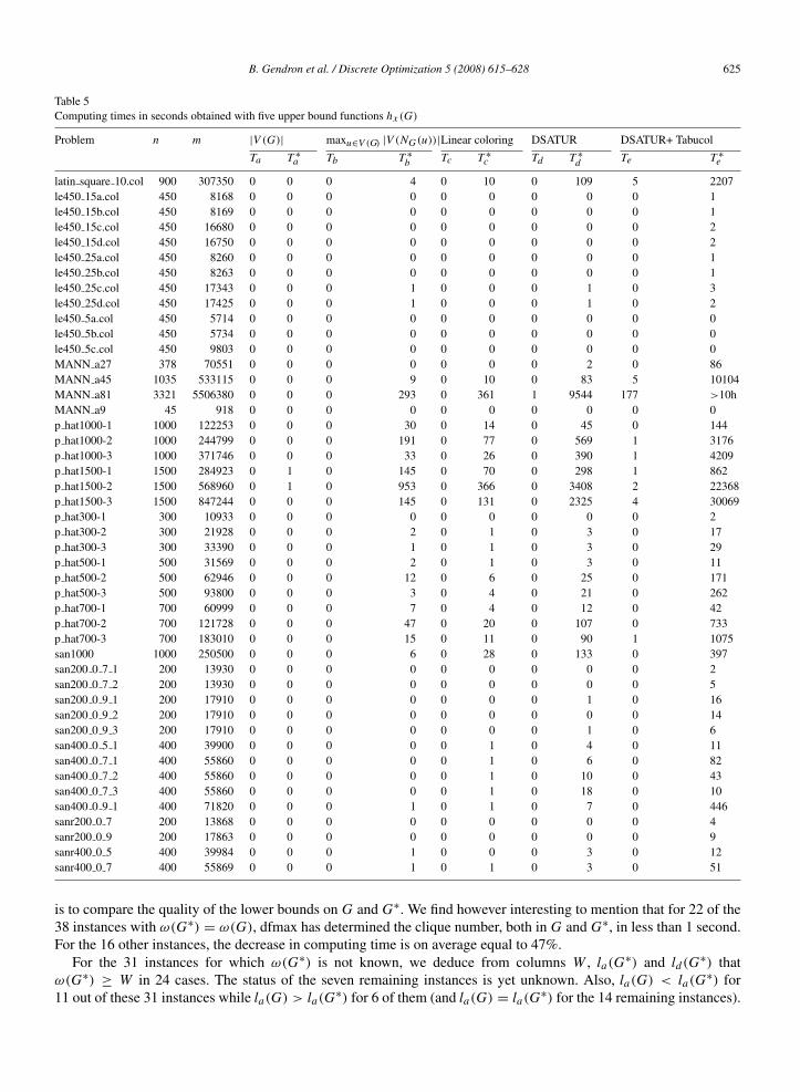
B. Gendron et al. / Discrete Optimization 5 (2008) 615–628 625

Table 5Computing times in seconds obtained with five upper bound functions hx (G)

Problem n m |V (G)| maxu∈V (G) |V (NG (u))|Linear coloring DSATUR DSATUR+ Tabucol

Ta T ∗a Tb T ∗b Tc T ∗c Td T ∗d Te T ∗e

latin square 10.col 900 307350 0 0 0 4 0 10 0 109 5 2207le450 15a.col 450 8168 0 0 0 0 0 0 0 0 0 1le450 15b.col 450 8169 0 0 0 0 0 0 0 0 0 1le450 15c.col 450 16680 0 0 0 0 0 0 0 0 0 2le450 15d.col 450 16750 0 0 0 0 0 0 0 0 0 2le450 25a.col 450 8260 0 0 0 0 0 0 0 0 0 1le450 25b.col 450 8263 0 0 0 0 0 0 0 0 0 1le450 25c.col 450 17343 0 0 0 1 0 0 0 1 0 3le450 25d.col 450 17425 0 0 0 1 0 0 0 1 0 2le450 5a.col 450 5714 0 0 0 0 0 0 0 0 0 0le450 5b.col 450 5734 0 0 0 0 0 0 0 0 0 0le450 5c.col 450 9803 0 0 0 0 0 0 0 0 0 0MANN a27 378 70551 0 0 0 0 0 0 0 2 0 86MANN a45 1035 533115 0 0 0 9 0 10 0 83 5 10104MANN a81 3321 5506380 0 0 0 293 0 361 1 9544 177 >10hMANN a9 45 918 0 0 0 0 0 0 0 0 0 0p hat1000-1 1000 122253 0 0 0 30 0 14 0 45 0 144p hat1000-2 1000 244799 0 0 0 191 0 77 0 569 1 3176p hat1000-3 1000 371746 0 0 0 33 0 26 0 390 1 4209p hat1500-1 1500 284923 0 1 0 145 0 70 0 298 1 862p hat1500-2 1500 568960 0 1 0 953 0 366 0 3408 2 22368p hat1500-3 1500 847244 0 0 0 145 0 131 0 2325 4 30069p hat300-1 300 10933 0 0 0 0 0 0 0 0 0 2p hat300-2 300 21928 0 0 0 2 0 1 0 3 0 17p hat300-3 300 33390 0 0 0 1 0 1 0 3 0 29p hat500-1 500 31569 0 0 0 2 0 1 0 3 0 11p hat500-2 500 62946 0 0 0 12 0 6 0 25 0 171p hat500-3 500 93800 0 0 0 3 0 4 0 21 0 262p hat700-1 700 60999 0 0 0 7 0 4 0 12 0 42p hat700-2 700 121728 0 0 0 47 0 20 0 107 0 733p hat700-3 700 183010 0 0 0 15 0 11 0 90 1 1075san1000 1000 250500 0 0 0 6 0 28 0 133 0 397san200 0 7 1 200 13930 0 0 0 0 0 0 0 0 0 2san200 0 7 2 200 13930 0 0 0 0 0 0 0 0 0 5san200 0 9 1 200 17910 0 0 0 0 0 0 0 1 0 16san200 0 9 2 200 17910 0 0 0 0 0 0 0 0 0 14san200 0 9 3 200 17910 0 0 0 0 0 0 0 1 0 6san400 0 5 1 400 39900 0 0 0 0 0 1 0 4 0 11san400 0 7 1 400 55860 0 0 0 0 0 1 0 6 0 82san400 0 7 2 400 55860 0 0 0 0 0 1 0 10 0 43san400 0 7 3 400 55860 0 0 0 0 0 1 0 18 0 10san400 0 9 1 400 71820 0 0 0 1 0 1 0 7 0 446sanr200 0 7 200 13868 0 0 0 0 0 0 0 0 0 4sanr200 0 9 200 17863 0 0 0 0 0 0 0 0 0 9sanr400 0 5 400 39984 0 0 0 1 0 0 0 3 0 12sanr400 0 7 400 55869 0 0 0 1 0 1 0 3 0 51

is to compare the quality of the lower bounds on G and G∗. We find however interesting to mention that for 22 of the38 instances with ω(G∗) = ω(G), dfmax has determined the clique number, both in G and G∗, in less than 1 second.For the 16 other instances, the decrease in computing time is on average equal to 47%.

For the 31 instances for which ω(G∗) is not known, we deduce from columns W , la(G∗) and ld(G∗) thatω(G∗) ≥ W in 24 cases. The status of the seven remaining instances is yet unknown. Also, la(G) < la(G∗) for11 out of these 31 instances while la(G) > la(G∗) for 6 of them (and la(G) = la(G∗) for the 14 remaining instances).

626 B. Gendron et al. / Discrete Optimization 5 (2008) 615–628

Fig. 7. Improved penalty-evaporation heuristic [13]

Table 6Lower bounds lx (G) and lx (G∗)

Problem n n∗ W dfmax MIN Penalty evaporation Imp. Penaltyevaporation

la(G) la(G∗) lb(G) lb(G∗) lc(G) lc(G∗) ld (G) ld (G∗)

brock200 1 200 198 21 21 21 14 16 20 20 20 21brock200 2 200 197 12 12 12 7 8 10 11 11 12brock200 3 200 199 15 15 15 10 11 14 13 14 14brock200 4 200 195 17 17 17 11 13 16 16 17 17brock400 1 400 399 27 27+ 27+ 19 19 23 23 25 24brock400 2 400 399 29 29+ 29+ 20 18 23 24 29 25brock400 3 400 399 31 31+ 31+ 20 17 24 25 31 31brock800 3 800 799 25 21+ 21+ 15 15 19 20 22 22c-fat200-1 200 90 12 12 12 12 12 12 12 12 12c-fat200-2 200 24 24 24 24 24 24 24 24 24 24c-fat200-5 200 116 58 58 58 58 58 58 58 58 58c-fat500-1 500 140 14 14 14 14 14 14 14 14 14c-fat500-10 500 252 126 124+ 126 126 126 126 126 126 126c-fat500-2 500 260 26 26 26 26 26 26 26 26 26c-fat500-5 500 128 64 64 64 64 64 64 64 64 64c1000 9 1000 997 68 53+ 52+ 51 51 64 64 67 67c2000 5 2000 1999 16 16+ 16+ 10 10 15 15 16 16c250 9 250 242 44 41+ 42+ 35 36 44 44 44 44c4000 5 4000 3998 18 17+ 17+ 12 12 16 17 18 17c500 9 500 498 57 47+ 47+ 42 47 56 54 57 57dsjc1000 5 1000 998 15 15 15 10 10 14 14 15 15dsjc500 5 500 498 13 13 13 10 10 12 12 13 13gen200 p0 9 44 200 197 44 44+ 44+ 32 32 44 44 44 44gen200 p0 9 55 200 196 55 55 55 36 37 55 55 55 55gen400 p0 9 55 400 388 55 43+ 44+ 42 44 51 51 53 52gen400 p0 9 65 400 398 65 43+ 43+ 40 40 65 52 65 65gen400 p0 9 75 400 398 75 45+ 45+ 45 47 75 75 75 75hamming10-4 1024 1023 40 32+ 34+ 29 27 40 40 40 40hamming8-4 256 114 16 16 16 16 11 16 16 16 16keller5 776 770 27 24+ 25+ 15 15 26 27 27 27keller6 3361 3338 59 42+ 45+ 32 36 39 43 59 59

Furthermore, let |V (G)|−|V (G∗)||V (G)|

be the reduction ratio between the number of vertices in graphs G and G∗. Themean reduction ratio for the 72 instances is 20%, among which 36 instances have a reduction ratio of more than 5%.If we focus on these 36 instances, we find 35 instances with ω(G∗) ≥ W and one (p hat1500-1) with ω(G∗) < W .

In general, it seems preferable to perform a heuristic method on G∗ rather than on G. When MIN (lb) is used,there are 25 instances with better results on G∗ and only 14 instances with better results on G (for the other instances,we obtain the same results on G and G∗). Similarly, the penalty-evaporation method (lc) is better when applied to

B. Gendron et al. / Discrete Optimization 5 (2008) 615–628 627

Table 7Lower bounds lx (G) and lx (G∗)

Problem n n∗ W dfmax MIN Penalty evaporation Imp. Penaltyevaporation

la(G) la(G∗) lb(G) lb(G∗) lc(G) lc(G∗) ld (G) ld (G∗)

latin square 10.col 900 88 90 90+ 81+ 90 90 90 90 90 90le450 15a.col 450 335 15 15 15 5 6 15 15 15 15le450 15b.col 450 341 15 15 15 8 8 15 15 15 15le450 15c.col 450 430 15 15 15 7 7 15 15 15 15le450 15d.col 450 434 15 15 15 5 5 15 15 15 15le450 25a.col 450 217 25 25 25 11 9 25 25 25 25le450 25b.col 450 237 25 25 25 13 12 25 25 25 25le450 25c.col 450 376 25 25 25 7 8 25 25 25 25le450 25d.col 450 373 25 25 25 8 9 25 25 25 25le450 5a.col 450 392 5 5 5 4 5 5 5 5 5le450 5b.col 450 388 5 5 5 4 3 5 5 5 5le450 5c.col 450 449 5 5 5 3 3 5 5 5 5p hat1000-1 1000 665 10 10 10 7 9 10 10 10 10p hat1000-2 1000 470 46 43+ 41+ 38 40 46 46 46 46p hat1000-3 1000 853 68 49+ 48+ 57 57 67 68 68 68p hat1500-1 1500 752 12 12 11 8 7 12 11 12 11p hat1500-2 1500 690 65 46+ 48+ 54 59 65 65 65 65p hat1500-3 1500 1263 94 53+ 54+ 75 81 94 94 94 94p hat300-1 300 245 8 8 8 7 7 8 8 8 8p hat300-2 300 169 25 25 25 23 20 25 25 25 25p hat300-3 300 279 36 36 36 31 31 36 36 36 36p hat500-1 500 372 9 9 9 6 8 9 9 9 9p hat500-2 500 257 36 36 36 29 33 36 36 36 36p hat500-3 500 448 50 44+ 48+ 42 42 49 50 50 50p hat700-1 700 487 11 11 11 7 7 11 11 11 11p hat700-2 700 324 44 44 44 38 42 44 44 44 44p hat700-3 700 621 62 50+ 51+ 55 53 62 62 62 62san1000 1000 970 15 10+ 10+ 8 8 8 8 15 10san200 0 7 1 200 30 30 30 30 16 30 17 30 30 30san200 0 7 2 200 189 18 18+ 18+ 12 12 13 13 18 18san200 0 9 1 200 70 70 48+ 70 45 70 45 70 70 70san200 0 9 3 200 198 44 44+ 36+ 31 30 36 43 44 43san400 0 5 1 400 13 13 13 13 7 13 8 13 13 13san400 0 7 1 400 390 40 22+ 20+ 21 20 21 20 22 22san400 0 7 2 400 398 30 17+ 17+ 15 15 18 18 30 30san400 0 7 3 400 376 22 17+ 22+ 12 12 17 17 22 22san400 0 9 1 400 393 100 49+ 50+ 41 39 54 100 100 100sanr200 0 7 200 197 18 18 18 14 14 18 18 18 18sanr200 0 9 200 198 42 40+ 40+ 35 36 42 42 42 42sanr400 0 5 400 395 13 13 13 10 9 13 12 13 13sanr400 0 7 400 397 21 21 21 16 16 21 20 21 21

G∗ in 14 cases, and better when applied to G for 7 instances. For the last method, the situation is reversed, sinceld(G∗) > ld(G) in only two cases, while ld(G∗) < ld(G) for 7 instances. For one of these 7 instances, we know thatω(G∗) < ω(G), while for four other instances, we do not know whether G∗ contains a maximum clique of G or not.

5. Conclusion

In this paper, we have presented a sequential elimination algorithm to compute an upper bound on the cliquenumber of a graph. At each iteration, this algorithm removes one vertex and updates a tentative upper bound byconsidering the closed neighborhoods of the remaining vertices. Given any method to compute an upper bound onthe clique number of a graph, we have shown, under mild assumptions, that the sequential elimination algorithm isguaranteed to improve upon that upper bound. Our computational results on DIMACS instances show significant

628 B. Gendron et al. / Discrete Optimization 5 (2008) 615–628

improvements of about 60%. We have also shown how to use the output of the sequential elimination algorithm toimprove the computation of lower bounds.

It would be interesting to apply the sequential elimination algorithm to other upper bound functions to see if similartrends can be observed. The development of other heuristic methods based on the sequential elimination algorithm isanother promising avenue for future research.

References

[1] M. Aouchiche, Comparaison automatisee d’invariants en theorie des graphes. Ph.D. Thesis, Ecole polytechnique de Montreal, 2006.[2] D. Applegate, D. Johnson, Dfmax source code in C. A World Wide Web page ftp://dimacs.rutgers.edu/pub/challenge/graph/solvers/.[3] I.M. Bomze, M. Budinich, P.M. Pardalos, M. Pelillo, in: D.Z. Du, P.M. Pardalos (Eds.), The Maximum Clique Problem, in: Handbook of

Combinatorial Optimization, vol. 4, Kluwer Academic Publishers, 1999, pp. 1–74.[4] D. Brelaz, New methods to color the vertices of a graph, Communications of the ACM 22 (4) (1979) 251–256.[5] P. Galinier, A. Hertz, A survey of local search methods for graph coloring, Computers and Operations Research 33 (9) (2006) 2547–2562.[6] M.R. Garey, D.S. Johnson, Computers and Intractability: A Guide to the Theory of NP-Completeness, W. H. Freeman, 1979.[7] J. Harant, Z. Ryjacek, I. Schiermeyer, Forbidden subgraphs and MIN-algorithm for independence number, Discrete Mathematics 256 (1–2)

(2002) 193–201.[8] A. Hertz, D. de Werra, Using tabu search for graph coloring, Computing 39 (1987) 345–351.[9] D.S. Johnson, M.A. Trick (Eds.), Cliques, Coloring, and Satisfiability — Second DIMACS Implementation challenge, in: DIMACS — Series

in Discrete Mathematics and Theoretical Computer Science, vol. 26, American Mathematical Society, 1993, pp. 11–13.[10] D.E. Knuth, The sandwich theorem, Electronic Journal of Combinatorics 1 (1994) 48.[11] Laszlo Lovasz, On the Shannon capacity of a graph, IEEE Transactions on Information Theory 25 (1) (1979) 1–7.[12] P.M. Pardalos, J. Xue, The maximum clique problem, Journal of Global Optimization 4 (3) (1994) 301–328.[13] P. St-Louis, B. Gendron, J.A. Ferland, A penalty-evaporation heuristic in a decomposition method for the maximum clique problem, Working

paper, Departement d’informatique et de recherche operationnelle, Universite de Montreal, Canada.[14] G. Szekeres, H.S. Wilf, An inequality for the chromatic number of graphs, Journal of Combinatorial Theory 4 (1968) 1–3.