A satellite method to identify structural properties of mesoscale convective systems based on the...
48
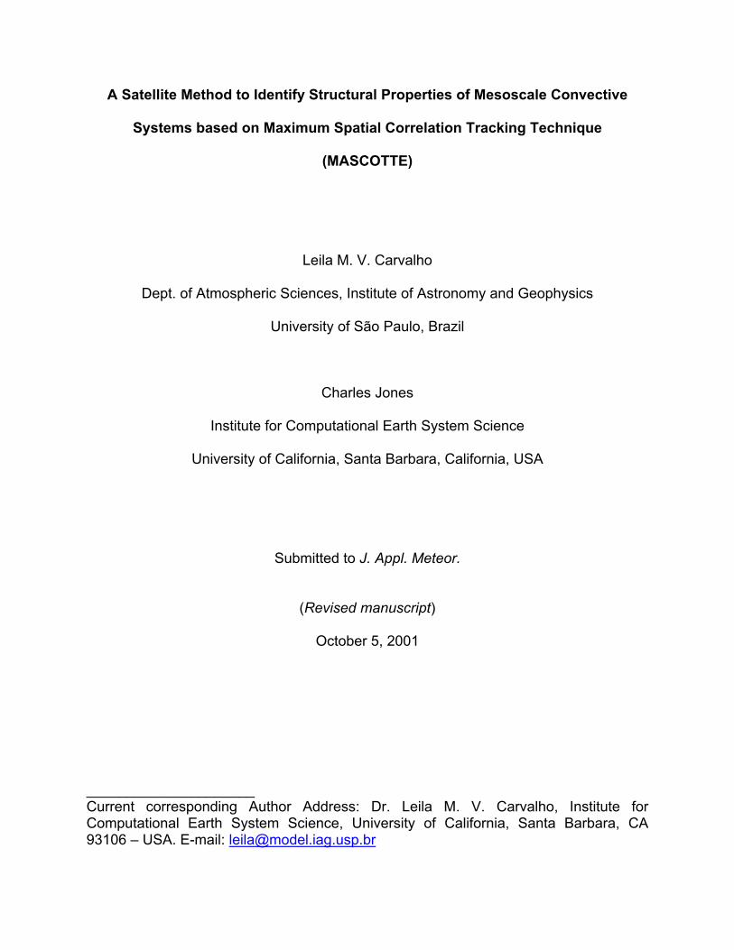
A Satellite Method to Identify Structural Properties of Mesoscale Convective Systems based on Maximum Spatial Correlation Tracking Technique (MASCOTTE) Leila M. V. Carvalho Dept. of Atmospheric Sciences, Institute of Astronomy and Geophysics University of São Paulo, Brazil Charles Jones Institute for Computational Earth System Science University of California, Santa Barbara, California, USA Submitted to J. Appl. Meteor. (Revised manuscript) October 5, 2001 _____________________ Current corresponding Author Address: Dr. Leila M. V. Carvalho, Institute for Computational Earth System Science, University of California, Santa Barbara, CA 93106 – USA. E-mail: [email protected]
Transcript of A satellite method to identify structural properties of mesoscale convective systems based on the...
A Satellite Method to Identify Structural Properties of Mesoscale Convective
Systems based on Maximum Spatial Correlation Tracking Technique
(MASCOTTE)
Leila M. V. Carvalho
Dept. of Atmospheric Sciences, Institute of Astronomy and Geophysics
University of São Paulo, Brazil
Charles Jones
Institute for Computational Earth System Science
University of California, Santa Barbara, California, USA
Submitted to J. Appl. Meteor.
(Revised manuscript)
October 5, 2001 _____________________ Current corresponding Author Address: Dr. Leila M. V. Carvalho, Institute for Computational Earth System Science, University of California, Santa Barbara, CA 93106 – USA. E-mail: [email protected]

2
Abstract A simple, fully automated and efficient method to determine the structural
properties and evolution (tracking) of cloud shields of convective systems (CS) is
described. The present method, which is based on the maximum spatial correlation
tracking technique (MASCOTTE), is a new alternative to the existent techniques
available for studies that monitor the evolution of CS using satellite images.
MASCOTTE provides as CS structural properties the following parameters: mean and
variance of brightness temperature, horizontal area, perimeter, minimum brightness
temperature, fractional convective area, center of gravity and fragmentation. The
fragmentation parameter has the potential to monitor the evolution of the CS. A new
way of estimating the orientation and eccentricity of CS is proposed, and is based on
the empirical orthogonal function (EOF) analysis of CS pixel coordinates. The method
includes an accurate detection of splitting and merging of convective systems, which is
a critical step in the automated satellite CS life cycle determination. Based on the
magnitudes of the spatial correlation between consecutive satellite images and the
changes in horizontal areas of CS, MASCOTTE provides a simple and skillful technique
to track the evolution of CS life cycles. The MASCOTTE methodology is applied to
infrared (IR) satellite images during seven consecutive days of the Wet Season
Atmospheric Mesoscale Campaign (WETAMC) of the Large Scale Biosphere-
Atmosphere Experiment (LBA) and ground validation experiment of the Tropical Rainfall
Measurement Mission (TRMM) in the Brazilian state of Rondônia in the Amazon basin.
The results indicate that MASCOTTE is a valuable approach to understand the
variability of CS.

3
1. Introduction
Convective systems (CS) in the Earth’s atmosphere occur in wide spectra of time
and space scales and play important roles in the distribution of energy, momentum and
mass in the general circulation (Cotton and Anthes 1989). Furthermore, the associated
precipitation is a key element in the hydrological cycle at regional to global scales. In
particular, mesoscale convective systems (MCS) can be broadly defined as cloud
systems associated with ensembles of thunderstorms with contiguous precipitation
areas. Typically, their horizontal scales can extend 100 km or more in one direction and
their life cycles can last from a few hours to as long as two to three days (Houze 1993).
The observational description and theoretical understanding of these convective
systems have grown steadily over the years providing detailed conceptual models of the
convective organization, three-dimensional wind circulation, thermal structure,
precipitation and microphysical processes occurring in different types of MCS (Houze
1977; Maddox 1980; Houze and Hobbs 1982; Mapes and Houze 1993). In this context,
observational data with sufficient spatial resolution from operational networks of
rawinsondes, meteorological radars and field experiments have been fundamental,
since they can resolve the genesis, maturity and decay phases of MCS (Zipser 1988;
Chen et al. 1996; Mohr and Zipser 1996).
The availability of satellite radiances has provided a unique way to monitor the
evolution of CS (Cotton and Anthes 1989; Houze 1993), especially in regions that are
strategically difficult to access such as open oceans and tropical rainforests.
Furthermore, satellite methods that identify and track the structural properties of CS
(e.g. mean brightness temperature, area, perimeter and eccentricity) can provide
4
valuable information on the dynamical mechanisms involved in their life cycle including
the interaction between the CS and the large-scale circulation (Silva Dias and Ferreira
1992; Cohen et al. 1995). Many previous satellite-tracking methods have been
proposed, which include subjective as well as automated methods (Velasco and Fritsch
1987; Williams and Houze 1987; Machado et al. 1998). The reader is referred to
Machado et al. (1998) for a thoroughly review on the state-of-the-art satellite tracking
techniques. Automated methods, to take a single instance, can be quite useful for
extensive meteorological field campaigns when tracking of large satellite imagery
databases needs to be performed sometimes even in real-time monitoring. Although the
satellite methods that describe structural properties of CS can rely on the same type of
data, i.e. infrared and/or visible and microwave satellite radiances, significant
differences may exist in the methodology that track the evolution of CS. For instance,
the CS life cycle obtained from satellite tracking methods is one parameter that can
contaminate cloud cluster statistics. As it will be demonstrated, the accurate
determination of splitting and merging of CS cloud shields is a crucial requirement in
this process. Therefore, it is important to compare different techniques so that
automated methods provide reliable and consistent results.
The purpose of this paper is to introduce a simple and efficient automated
method to simultaneously track and characterize structural properties of CS cloud shield
using satellite infrared (IR) images. The approach is based on the maximum spatial
correlation tracking technique (MASCOTTE). We show how MASCOTTE specifically
allows the characterization of splitting and merging of CS as they occur during their life
cycles. We compare different methods to identify horizontal axis of CS cold tops

5
orientation. Some structural parameters of clouds such as eccentricity and
fragmentation are used in the identification of different stages of intensification and
decaying of CS. As an application of MASCOTTE, we focus our attention on seven
consecutive days during the Wet Season Atmospheric Mesoscale Campaign
(WETAMC) of the Large Scale Biosphere-Atmosphere Experiment (LBA) (Nobre et al.
1996; Silva Dias et al., 2000). This field experiment, which was realized from December
1998 through February 1999 in the Brazilian state of Rondônia in the Amazon basin,
was a joint scientific venture with the ground validation component of the Tropical
Rainfall Measurement Mission (TRMM). The paper is organized as follows. The
description of the method is presented in section 2. Section 3 discusses different
techniques to determine properties of the life cycle of CS as well as presents some
structural properties of CS during the case studies. Section 4 discusses the application
of the method for the characterization of the time evolution of CS. Section 5 summarizes
the methodology and our main conclusions.
2. Maximum Spatial Correlation Tracking Technique (MASCOTTE)
The basic approach of our satellite tracking methodology as well as the
characterization of structural properties of CS is now described. The method uses as
input fields brightness temperature from satellite images. In this work, Geostationary
Operational Environmental Satellite (GOES-8) images were used. These images have
horizontal resolution of 4 km and are part of the TRMM/LBA program and available from
NASA Goddard Space Flight Center1. Additionally, the high temporal frequency of
1 http://lake.nascom.nasa.gov/data/TRMM
6
GOES-8 images, typically every 30 minutes, allows an adequate resolution of the
different stages of development of convective systems. In the discussion that follows,
hourly satellite images were used. However, as it will be explained later, an important
advantage of our method is that it characterizes the correct evolution of CS (e.g.
splitting or merging of systems) even if the time interval between images are three
hours.
The use of satellite infrared images, i.e. brightness temperature (TB), usually
requires an arbitrary choice of threshold to identify regions of convection. There is
general agreement that TB values below a threshold of 245K satisfactorily identify
convective systems (Velasco and Fritch 1987; Mapes and Houze 1993; Miler and Fritch
1991; Machado and Rossow 1993; Machado et al. 1998). The reasoning in the
threshold selection is that a buoyant parcel in the tropics is likely to originate below the
700 hPa level to reach the level of TB <245K, which ensures the existence of deep
convection (Machado et al. 1998). In addition, the near-linear dependence between the
convective system area and its threshold indicates the insensitivity to the choice of a
specific value in a range of 10-20K (Mapes and Houze 1993; Machado et al. 1992).
Garreaud and Wallace (1997), for instance, used fraction of clouds with TB ≤235K with
0.5ox0.5o latitude-longitude resolution and 3-h temporal resolution to estimate the
diurnal march of convective cloudiness over the tropical and subtropical Americas.
Since MASCOTTE is applied here over tropical South America, convective systems are
identified in the satellite images whenever regions of TB are less than or equal to 235K
to be consistent with Garreaud and Wallace (1997). For the WETAMC LBA/TRMM
campaign cloud tops with TB ≤235K were in general about the level of 250hPa. With this

7
threshold in mind, we investigate mostly anvil regions and the embedded areas of active
deep convection (Johnson et al. 1990). It is worthwhile to mention that given the
versatility of MASCOTTE, the threshold value can be adapted to other specific regions.
The definition of CS based on the temperature threshold technique allows wide
ranges of horizontal areas. Machado et al. (1998) showed positive correlations between
the lifetime of CS and their sizes. Their results indicate that, in general, CS that reach
equivalent radius of 100 km or less and temperature thresholds of 245K are mostly
associated with lifetimes shorter than 3 hours. In order to test the skill of our method
and emphasize the tracking of CS with long life cycles, we consider systems with
equivalent radius R ≥ 100km, the same threshold of Machado et al. (1998). These limits
of brightness temperature and horizontal area in our methodology imply that the life
cycle of a given CS begin when the convective system has TB ≤ 235K and R ≥ 100km.
The end of the life cycle, on the other hand, occurs when TB > 235K or R < 100km. The
combination of both criteria (i.e., TB ≤ 235K and R ≥ 100km) is hereafter referred as T-R
criteria.
The MASCOTTE basic hypothesis is that the spatial correlation between regions
defined by two different cloud systems in successive images is a simple and powerful
method to identify the evolution of spatial patterns associated with CS. Similar
techniques have been applied to estimate tropospheric winds based on satellite cloud
displacements (Endlich and Wolf 1981). The basic steps involved in the MASCOTTE
method are as follows.
1. We consider that N satellite images of TB are available with time interval ∆t. In this
work, ∆t is taken to be 1 hour. However, as it will be shown later, the method is

8
successful for ∆t intervals up to three hours. For each satellite image at time ti, 0 ≤ i ≤
N, regions of CS are identified according to the T-R criteria. Regions that do not
meet the thresholds criteria are set to null value. This procedure allows a large
difference between clouds and the background mask, thus emphasizing the
overlapping of systems. We consider that at time ti, there are m CS identified.
2. At time ti the kth CS (1≤ k ≤ m) is first isolated in the image (i.e., the remaining of the
image is set to the background mask value), which has a size of ICxL, where C and L
are the number of pixels in the east-west and north-south direction, respectively. For
the application to the TRMM/LBA experiment discussed in this paper, the 4km
satellite image has C=1332 by L=860 pixels. We then consider the next satellite
image at time ti+1 and identify all the CS. The CS at ti+1 that has maximum spatial
correlation (rs > 0.30) with the kth CS at ti is considered the new spatial position of the
CS. The threshold value of rs > 0.30 was determined on many tests performed in the
initial development of the algorithm. This value ensures reliable tracking of CS using
satellite images with 1h time interval. The process is repeated for all CS at time ti
and starts again for the next satellite image.
3. For each time ti and each CS, structural properties are computed. These include: the
horizontal area (A), perimeter (P), mean and variance of TB, minimum TB and
fractional convective area Fc = 100 (ATC / A)¸where ATC is the area within the CS
such that TB ≤ 210K. According to rawinsondes during the WETAMC LBA/TRMM
campaign, TB≤210K was associated with cloud tops reaching heights above 13 km in
an environment where the tropopause was very often above 16.0 km. Furthermore,
the TB≤ 213-208K threshold has been identified with precipitation in the Tropics
9
(Williams and Houze 1987; Mapes and Houze 1993, Rickenbach 1999) and is
therefore of interest for the monitoring of CS life cycles. In addition, the spatial
coordinates of the center of gravity (XCG, YCG) is defined as the TB weighted average:
∑
∑
=
==P
Bi
P
Bi
CG N
iT
N
iTX
Xi
1
1
∑
∑
=
==P
Bi
P
Bi
CG N
iT
N
iTY
Yi
1
1 (1)
where Xi,Yi are the CS pixel coordinates in the east-west and north-south directions,
respectively, and the summation is carried out over all NP pixels within the given CS.
4. The orientation of the CS cloud shield is computed in two ways. First, a straight line
is fitted to the (Xi,Yi, i=1,NP) pixel coordinates by least squares criterion and the
counter-clockwise angle between the east-west direction and the straight line is
recorded. However, as it will be discussed later, a satellite method that relies on this
definition of orientation can oftentimes obtain quite misleading results, depending on
the geometrical structure of the CS. In contrast, a new way of computing the
orientation is proposed. We consider a given CS in which the array of pixel
coordinates is given by (Xi,Yi, i=1,NP). The means X and Y are first subtracted from
the vectors Xi and Yi and an Empirical Orthogonal Function (EOF) analysis is
computed on the covariance matrix determined by 'X and 'Y perturbations (see
Jackson 1991 for details on EOF analysis). The result of this operation is a pair of
eigenvalues and eigenvectors that explain the total variance of the geographical
coordinates of the given CS. Consequently, a second orientation is computed as the
counter-clockwise angle between the east-west direction and the direction of the first
eigenvector. This way of computing the orientation of the CS has the advantage that
10
the first eigenvector maximizes the spatial variance of the CS cloud shield.
Furthermore, another important property to characterize the structure of CS is the
eccentricity, which in our method is defined by the ratio of the norms
12 EOFEOF , where 1,2 EOFEOF are the second and first eigenvectors,
respectively.
Oftentimes, as the CS evolves, splitting of cloud features may happen when
changes occur in the precipitation pattern and three-dimensional wind structure. This
process can be indicative of intensification of precipitation at some point and decaying
of part of the upward movement of the storm (Cotton and Anthes 1989). However, the
propagation of the storm may continue under some favorable environmental conditions
(Houze 1993). The identification of splitting during the life cycle is important for the
monitoring of dynamical properties of CS (Houze 1993). The splitting of an CS at time ti
is identified by MASCOTTE when more than one CS with positive and high spatial
correlation is observed at time ti+1. As it will be shown with examples, the horizontal area
of the system decreases. MASCOTTE continues the tracking of CS with the assumption
that the propagation is now defined by the most correlated CS in subsequent satellite
images. MASCOTTE also maps the position of any part of the splitting CS in order to
follow its life cycle until it decays, which usually happens in a short period. Furthermore,
due to the definition of CS using the TB threshold, merging of high clouds is also
frequently observed, which is in fact related to the connection of anvil regions. At this
point, it is difficult to identify the main system because its life cycle is determined by the
interaction of more than one CS. However, the merging is characterized in MASCOTTE
by positive spatial correlation, since the identity of a tracked CS is kept as it merges with
11
another one. These situations can be clearly identified during the life cycle when the
spatial correlation decreases and the horizontal area increases between two
consecutive satellite images.
Our inspection of 150 merges throughout different CS life cycles during the
WETAMC cases considered here indicates that a reasonable criterion for the
identification of merges is the increase of area followed by a decrease in rs of more than
10% of the previous value. The resulting shape of a CS is substantially modified after
merges due to the introduction of new systems with different sizes and forms. When the
increase in area is only due to expansion of the original CS, rs increases in the majority
of the cases. MASCOTTE can also identify merges and splits that eventually happen
simultaneously, as long as the CS maintains part of its spatial characteristics in two
consecutive images. Oftentimes, however, CS can merge with systems that have
equivalent radius less than 100km. Other times, CS show decrease in area due to either
decaying of the system (sinking of cloud tops) or splitting of cells with R < 100 km. A
posteriori refinement in the algorithm is applied to identify these dynamical processes.
Our assumption is that these dynamical variations of the CS are associated with rapid
changes in structural properties. An analysis performed with 100 life cycles with
duration longer than 3 hours (not shown) indicated that large accelerations are
observed mainly in association with large rates of change of EOF-1 orientation,
perimeter and direction. These results have been used to improve the MASCOTTE
algorithm with the implementation of flags to indicate merges and splits that cannot be
promptly detected due to the T-R criteria. One advantage of this detailed monitoring is

12
that it provides enough information to reconstruct the entire life cycle of any CS,
including interactions with other systems.
In summary, MASCOTTE yields the following structural properties for the TB and
R thresholds considered: average duration of the CS, total number of systems, number
of splits and merges. For the life cycle of individual CS, MASCOTTE determines: area
(Area), mean (Tmean) and variance (Var) of brightness temperatures, minimum
brightness temperature (Tmin), eccentricity (Ecc), orientation of CS cold tops based on
the EOF orientation (EOF-1) and least squares (LS) fit, fraction of cold tops with TB ≤
210K (Fc). Additionally, MASCOTTE determines the speed of displacement of CS
center of gravity (V), direction of propagation (DD) and fragmentation (Fluct) resulting
from both dynamical and physical processes (explained in sections 3 and 4).
To put into context, we briefly summarize the main MASCOTTE characteristics
by comparing with Machado et al. (1998) automated method. That method is very well
documented and provides a framework for an objective discussion about the skill of a
satellite tracking technique. Table-1 indicates MASCOTTE structural parameters and
the correspondence with Machado et al. (1998) procedure. Although some properties
are common to both methods, it is worth pointing out the differences in the tracking
approaches. For instance, in order to track CS, Machado et al. (1998) automated
method assumes circular geometries for the systems overlapping and uses weighted
average of 28 structural properties. In contrast, the only requirement for MASCOTTE to
determine the temporal evolution of CS is a maximum spatial correlation greater than a
specified threshold. The main differences regarding structural parameters are: the
orientation of cloud tops and, consequently, eccentricity, convective fraction, perimeter

13
and fragmentation, detection of merging and splits and propagation characteristics.
MASCOTTE does not compute number of convective clusters (contiguous region of
brightness temperature below a given threshold) as well as properties associated with
the largest convective cluster embedded in the CS. The reasoning is that structural
parameters computed for 160 CS over the Tropical Pacific Ocean indicated a linear
correlation (0.93) between R and number of convective clusters (TB<218K) and between
R and the largest convective cluster (0.85) but practically no correlation (0.16) between
R and Fc (TB<218K) (Carvalho 1998). For the sake of simplicity and to avoid
redundancies, the MASCOTTE variable representative of the enhancement of the
convective area of the CS is restricted to Fc (TB≤210K).
3. Temporal and Structural Properties of CS using MASCOTTE
To demonstrate the application of MASCOTTE, we selected as case study seven
consecutive days, from 12 February to 18 February of 1999, during the WETAMC
LBA/TRMM experiment. The purpose of this selection is the continuous availability of
satellite images with one hour of time interval. It is worth emphasizing that the main goal
of this paper is to present the automated applicability of MASCOTTE for an extensive
field experiment campaign. The satellite surveillance area extends from 12.5oN to
18.5oS and 34.0oW to 82.0oW. The large spatial coverage of the satellite methodology
provides not only propagation characteristics of CS over Rondônia state, but also over
the entire tropical South America. This has important implications to investigate the
organization of CS in the Amazon and possible interactions with the South Atlantic
Convergence Zone (SACZ) and the Intertropical Convergence Zone (ITCZ).

14
a. Monitoring of CS life cycles in the Amazon Basin
The application of MASCOTTE is now discussed in detail. Some important
aspects about MASCOTTE for the determination of CS life cycles are summarized in
Table 2. These include the total number of CS and CS life cycles, splits and merges
observed in the period satisfying the T-R criteria. It is also indicated the total number of
flags that were likely associated with splitting/sinking or merging with CS that did not
satisfied the T-R criteria. The results shown in Table 2 are indicative of the importance
of the correct determination of merges and splits during CS life cycles. Approximately
30% of CS life cycles ended up merging with other CS satisfying the T-R criteria.
Meanwhile, 8% of CS split during their life cycle and resulted in two or more CS
matching the T-R criteria. The fraction of merges is 10% higher than what was
estimated in Machado et al. (1998) for 3h time interval, whereas the fraction of splits
seems to follow approximately the same rate observed in their study. However, if one
considers the possibility of splitting (or sinking) of CS not satisfying T-R criteria, the rate
of splits increases to approximately 21%.
The critical issue of accurately detecting CS splitting/merging in an automated
satellite tracking technique is discussed in the next results. The impact on the CS life
cycles due to the inclusion of merging with CS satisfying the T-R criteria is elucidated in
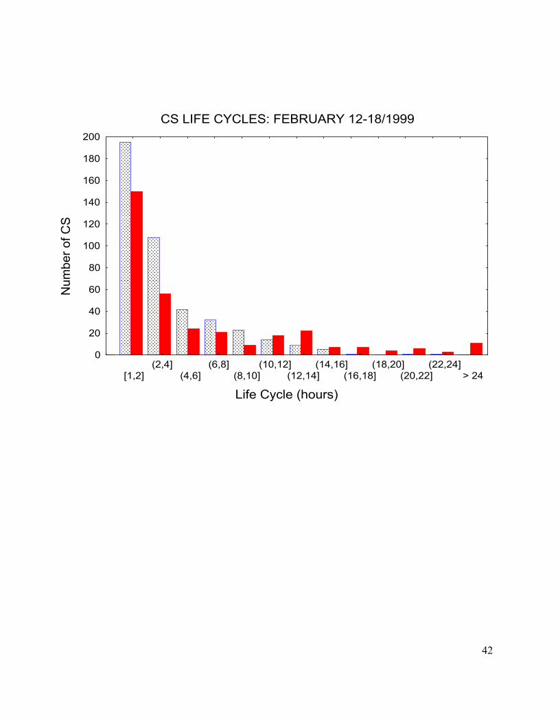
Fig. 1. For the period 12-18 February, we first considered the life cycles of all CS
satisfying the T-R criteria regardless whether or not merges had occurred. The resulting
distribution is shown as function of life cycle duration (black bars). Secondly, the life
cycles were recomputed using the MASCOTTE detection of merges. In that case,

15
whenever the CS merged with another CS satisfying the T-R criteria, the life cycle
ended (dotted bars). When merges are considered as part of a life cycle, the tail of the
distribution increases towards the longer values and the number of life cycles in the
shorter categories decreases as expected. Two life cycles of 59 hours were observed
when merges were considered as part of the life cycle. On the other hand, when
merges are not considered as part of the life cycle, the longest duration was on the
order of one day (23 hours). The observation of a larger number of CS with life cycles
longer than 24 hours in the Machado at al. (1998) automated tracking relative to semi-
automated is likely related to the non-objective criterion for the decision whether or not
merges should be included in a given life cycle (see Fig. 2 in Machado et al 1998).
Another relevant implication of the objective determination of merges and splits is
concerned with the estimation of CS speed and direction of propagation. During CS
splitting events, a sudden shift in the position of the center of gravity is observed.
Consequently, speeds of more than 250km/h are oftentimes recorded. They are of
course an estimate of the large displacement of the CS center of gravity towards the
position of one of the splitting CS. Likewise, during merges, a substantial modification of
the form of the CS leads to a large displacement of the center of gravity. Any estimation
of propagation speed during the occurrence of merges and splits is therefore an
unrealistic approach of the actual velocity of propagation of the CS. Nonetheless, splits
occur very often and can be considered as part of a life cycle. A method that relies on
the criteria of speed of displacement of center of gravity to decide about a sequence in
a life cycle can be potentially misleading.

16
The effect on the estimation of CS displacement speed and direction with
inclusion of flags for CS splitting/merging not satisfying the T-R criteria is illustrated in
Fig. 2. Figure 2.a shows the distribution of CS displacement speed in the following
categories: only non-flagged CS (black bars) and all CS within a life cycle (dotted bars).
We recall that no splitting or merging with systems satisfying T-R criteria is considered
in this distribution. Nonetheless, the range of speeds is noticeably larger when splitting
and merges are not properly flagged. Speeds on the order of 500 km/h or more can be
computed in some cases, which is a consequence of rapid changes in the form of the
CS during these events. This range of magnitudes is greater than the 60m/s (216km/h)
maximum criterion accepted for searching life cycles in the Machado et al. (1998)
automated tracking. Therefore, based only on this criterion, a large majority of flagged
CS life cycles determined with MASCOTTE would be potentially accepted as satisfying
Machado et al (1998) automated tracking method. We recall that MASCOTTE does
include flagged events as part of a life cycle, but speeds are only computed whenever
splits resulting in CS matching the T-R criteria are not occurring. Likewise, the
implication of flagged events for the determination of propagation direction is shown in
Fig. 2b. This distribution indicates a decrease in the number of CS in each category,
although the form of the distribution remains approximately the same. Details on the
MASCOTTE flagged CS will be further discussed in the session 4.
The CS life cycle is considered with MASCOTTE, in sum, as the period that an
CS is observed matching the T-R criteria. The end of a life cycle is also determined
when a merge with another CS matching the T-R criteria occurs. Figure 3 shows the
spatial distribution of the origin of the CS according to the life cycle (hours). The origin

17
of CS with life cycles ≤ 4 hours is well distributed in the area, with no clear geographic
preference (Fig. 3a). Although the case study is based on seven days, as the life cycle
increases to periods between 5 and 7 hours, a pattern of parallel bands aligned
northwest-southeast becomes more suggestive (Fig. 3b). Garreaud and Wallace (1997)
using composites of IR images with TB ≤ 235K found two parallel bands (2000km long
and about 400km wide) of maximum convective cloudiness with the same orientation
during the wet season (December to February). They consider this banded pattern a
systematic feature over South America (see their Fig. 3). Special attention should be
given to the band of CS with origin near the north-northeast coast of South America that
exhibits life cycles between 5 and 7 hours. The origins of CS with shorter life cycles
(less than 5 hours) seem to be displaced offshore. This feature was also examined in
Garreaud and Wallace (1997) in association with strong diurnal variability. As the life
cycle increases to 8-10 hours (Fig. 3c), less CS origins were observed in the north-
northeast coastal South America, though the northwest-southeast oriented pattern
remains still suggestive. Origins of life cycles longer than 10 hours are more
concentrated above 5o S during the present case studies (Fig. 3d).
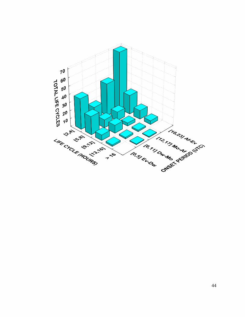
The relationship between the CS onset period (i.e., time when the CS matching
the T-R criteria was first observed) and the life cycle is investigated in Fig. 4. The onset
period is divided in four categories: evening to pre-dawn (Ev-Dw, from 0:45-5:45 UTC),
pre-dawn to morning (Dw-Mo, from 6:45 to 11:45 UTC), morning to afternoon (Mo-Af,
from 12:45-17:45 UTC), afternoon to evening (Af-Ev, from 18:45 to 23:45 UTC). It is
clear that the maximum daily heating plays an important role for the relatively short
living CS (shorter than 5 hours). The maximum during the Af-Ev period is about twice

18
larger than during Ev-Dw and Mo-Af periods. Nonetheless, the approximately equal
contribution of onsets during the Mo-Af and Ev-Dw indicates more than the gradual
decay during night hours suggested in Garreaud and Wallace (1997). To a certain
extent, it represents the origin of new CS that have a preferable nocturnal life cycle.
Longer life cycles (5-8 hours) also appear to be a characteristic of the nocturnal
propagating CS. However, investigations with more case studies would be necessary to
properly address the pattern shown in Fig. 4 for long life cycles.
The relationships between life cycles and horizontal dimensions of the CS can be
further investigated with MASCOTTE results. Since the variability of the CS horizontal
dimensions is larger during long life cycles, the correspondence between life cycles and
sizes of CS is appropriately characterized by the maximum radius (Rmax). The bi-
dimensional distribution of CS maximum radius (Rmax) and respective life cycle is
indicated in Fig. 5. For 100 ≤ Rmax ≤ 200km, there seems to be a positive correlation
between Rmax and life cycle, as suggested in Machado et al. (1998) with the use of
mean radius (Rmean). For large values of Rmax, however, there is no evidence of this
dependence. The evenly distributed events for Rmax >200km are possibly associated
with merges of CS satisfying T-R criteria. During the occurrence of merges, the
equivalent radius is oftentimes the Rmax of a life cycle. Since the resulting CS is
considered in a separated life cycle, they are not necessarily following the linear
tendency observed for short periods.
The diurnal variation of the number of CS from 12 February to 18 February is
shown in Fig. 6. Time is displayed for local time in Rondônia, Brazil. The late afternoon
maximum with gradual decrease during the night and minimum in late morning is

19
consistent with the observations of Garreaud and Wallace (1997). Figure 6, similar to
Garreaud and Wallace (1997) IR daily composites, does not provide any information on
the onset of CS and their life cycle. To obtain a more comprehensive overview of the
CS diurnal variability, Fig. 7 combines CS life cycle duration, onset time interval and
displacement. For each CS, the information is plotted in the origin of the life cycle (x-
symbol), the duration (hours) and displacement (line segment). It is worth noticing the
difference between trajectory and displacement adopted here. Trajectories of the center
of gravity of CS can sometimes be very irregular. The CS displacement shown in Fig. 7
indicates the difference between the position at the beginning (x-symbol) and end of a
life cycle. It can however give an idea of the direction of propagation of the CS. We
focused our analysis on the period of increasing and decreasing number of CS
indicated in Fig. 6. To emphasize the contrast between the two periods, only CS with life
cycles ≥ 4 hours are shown in Fig. 7. There are 30% more CS with life cycles ≥ 4 hours
in the afternoon (total=60 life cycles) than nocturnal (total=42 life cycles). However, 47%
of CS with onset in the afternoon showed life cycles ≥ 8 hours, whereas this rate
increases to 57% for the nocturnal CS. Some relevant characteristics of the diurnal
variation of CS are the afternoon maximum in north-northeast and western South
America coast, in contrast with the nocturnal inland origin of CS. It is worth noticing the
suggestive increase of offshore CS during the night. The nocturnal peak of large and
long living oceanic CS has been observed in the Tropical Pacific Ocean during active
periods of convection (Chen and Houze 1997). The authors observed that these
systems begin late in the afternoon and continue during the night when they have their
largest dimension. Although the T-R criteria do not allow the observation of the very
20
beginning of the CS life cycles, on the other hand, it is representative of important
properties of the mesoscale convective activity.
During the seven days case studies, the largest majority of CS prevailing
direction of displacement showed negative (East to West) zonal component and
negative meridional component (North to South). The easterly displacement of the CS is
consistent with the dominant low levels easterly winds during that period. This
observation is based on the daily composite of the 700 hPa NCEP/NCAR reanalysis
(not shown). Even considering that some CS exhibited long displacements, the spatial
pattern of the CS life cycles still suggests the characteristic banded pattern shown in
Garreaud and Wallace (1997).
b. Monitoring of structural properties of the CS
The orientation of squall lines cloud tops in the Amazon Basin using IR images
has been investigated in both observational analysis (Cohen et al 1995) and model
simulations (Silva Dias and Ferreira 1992). An accurate and automated method to
identify the squall lines orientation allows, among other applications, objective rather
than subjective analysis of case studies. The horizontal orientation of the first
eigenvector (EOF-1) incorporated in the MASCOTTE method provides another way to
infer the main orientation of the cloud shield of the CS. The orientation is computed as
the counter-clockwise angle between the east-west direction and the direction of the
first eigenvector. Therefore, the orientation angle is 0< EOF-1 ≤180o. For example, an
orientation angle equal to 135° implies an orientation northwest-southeast. The same
convention is used for the Least Squares (LS) method. Figure 8 shows the dispersion
21
diagram obtained with the LS and EOF-1 orientations. Ellipses are sketched to
exemplify the meaning of the dispersion in each quadrant of Fig. 8. For instance, in the
quadrant-I (top left), the EOF-1 method (full line ellipses) indicates an NW-SE
orientation of the CS whereas LS (dashed-line ellipses) gives an NE-SW orientation.
The opposite situation is observed in the quadrant- III (bottom right). In the quadrant-II
(top right), both methods prescribe NW-SE orientations. Likewise, in the quadrant-IV
(bottom left), LS and EOF-1 methods indicate NE-SW orientations. Note that the largest
discrepancies between both methods relative to the north-south direction occur in the
quadrants I and III. The quadrants II and IV indicate the wide range of dispersion,
although in these cases both methods ascribe the CS orientation in the same quadrant
relative to the North-South direction. A more detailed discussion about the accuracy and
differences between both methods will be shown with examples in session 4.
An important parameter that characterizes the structural properties of CS is the
eccentricity (Ecc) of the system. It has been used to characterize Mesoscale Convective
Complexes (MCC) (Maddox 1980; Velasco and Fritch 1987). According to the definition
of Ecc assumed by MASCOTTE (i.e., Ecc= 12 EOFEOF ), the values of Ecc are in
the interval 0<Ecc≤ 1. Thus, high (low) magnitudes of Ecc are associated with CS
shapes that are circular (linear). For that reason, an accurate methodology to determine
orientation of the axis with maximum and minimum variation of CS cold pixels is crucial
for the estimation of Ecc. Although eccentricity has been used as a key property to
identify typical characteristics of squall lines (Cohen et al. 1995) and MCCs (Maddox
1980), it does not account for the collapsing and fragmentation of cold cloud tops that
22
very often occur as an MCS evolves (e.g., Rickenbach 1999). One simple and efficient
approach to quantify fragmentation is developed in MASCOTTE with the use of
perimeter-area relationship. Lovejoy (1982) showed that the representation of logarithm
of perimeters versus the logarithm of area of the systems has approximately a linear
relationship, which seems to hold for several spatial scales. The slope of the straight
line in this relationship was first defined by Lovejoy (1982) as the fractal dimension of
clouds and rain. However, not all fluctuations of perimeters of clouds and rain can be
explained by monofractal models. In fact, this early idea of monofractality has been
replaced by the universal multifractal concept (see, Lovejoy and Schertzer 1990 for
further details). This original concept of Lovejoy (1982) is indirectly used in MASCOTTE
to measure fragmentation of clouds. The procedure in this case is to remove the trend
between perimeter and area, by assuming the following functional relationship:
Fluctareaconstperimeter ++= )](log[)(log 1010 β (2)
where const and β are the linear and angular coefficients, respectively. Fluct is the
residue, and can be interpreted as the fluctuation of the logarithm of perimeter that does
not account for the area of cloud tops. In other words, after extracting the functional
dependence of area on perimeter, the residue is the fluctuation of perimeter that is only
due to changes in fragmentation or increase/decrease of irregularities of the boundaries
of CS cold tops. Therefore, positive magnitudes of Fluct are associated with relative
increases of fragmentation of clouds, whereas negative magnitudes of Fluct are
indicative that the boundaries of cold shields are more regular or less fragmented.
Together with eccentricity, the Fluct parameter can be applied to characterize different
stages of development and decaying of CS.

23
According to the conceptual model of cloud shield evolution of CS discussed in
Rickenbach (1999), cold cloud anvils of propagating squall lines under directional
vertical wind shear are subject to tilting and displacement of the leading edge. This
model hypothesizes that as the deep cells develop, they “tilt” to the direction of the
upper level winds, opposite to direction of propagation of the MCS precipitation pattern.
As the leading edge of the convective precipitation weakens, the coldest portion of the
anvil, located where convection had been deepest, becomes separated from the leading
edge as the anvil continues to spread to the opposite direction of the storm propagation.
From the point of view of the satellite imagery, this displacement of the cold cloud shield
would be characterized by an apparent sink of the cold cloud top and, therefore, an
increase of TB. The consequent apparent displacement of the cold shield and warmth of
portions of the cloud anvil would increase the fragmentation or irregularity in the form of
a CS. Although Rickenbach (1999) hypothesis was postulated for strong directional
shear, it is also possible that the vertical speed shear can cause similar effect on the
cloud tops.
To verify the consistence between the general fragmentation of CS cloud shield
and the absolute vertical speed shear (AVSS), we computed the diurnal variation of
AVSS between 700 and 200 hPa (Fig. 9). This computation was performed with
NCEP/NCAR reanalysis in central Amazon. The area of investigation extended from
67.5oW to 34.0oW and 15oS to 5oN with the purpose of excluding the Andes. Figure 9
indicates a clear diurnal cycle of AVVS, with a maximum around 18:00 UTC (12:00 LT)
and a minimum around 6:00 UTC (2:00 LT). The maximum and minimum occurred
within the period of increasing and decreasing number of CS, respectively (Fig. 6).
24
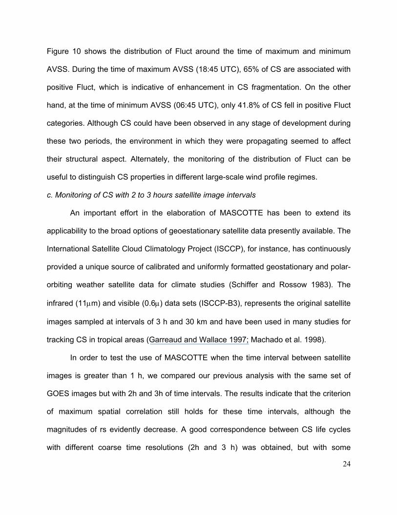
Figure 10 shows the distribution of Fluct around the time of maximum and minimum
AVSS. During the time of maximum AVSS (18:45 UTC), 65% of CS are associated with
positive Fluct, which is indicative of enhancement in CS fragmentation. On the other
hand, at the time of minimum AVSS (06:45 UTC), only 41.8% of CS fell in positive Fluct
categories. Although CS could have been observed in any stage of development during
these two periods, the environment in which they were propagating seemed to affect
their structural aspect. Alternately, the monitoring of the distribution of Fluct can be
useful to distinguish CS properties in different large-scale wind profile regimes.
c. Monitoring of CS with 2 to 3 hours satellite image intervals
An important effort in the elaboration of MASCOTTE has been to extend its
applicability to the broad options of geoestationary satellite data presently available. The
International Satellite Cloud Climatology Project (ISCCP), for instance, has continuously
provided a unique source of calibrated and uniformly formatted geostationary and polar-
orbiting weather satellite data for climate studies (Schiffer and Rossow 1983). The
infrared (11µm) and visible (0.6µ) data sets (ISCCP-B3), represents the original satellite
images sampled at intervals of 3 h and 30 km and have been used in many studies for
tracking CS in tropical areas (Garreaud and Wallace 1997; Machado et al. 1998).
In order to test the use of MASCOTTE when the time interval between satellite
images is greater than 1 h, we compared our previous analysis with the same set of
GOES images but with 2h and 3h of time intervals. The results indicate that the criterion
of maximum spatial correlation still holds for these time intervals, although the
magnitudes of rs evidently decrease. A good correspondence between CS life cycles
with different coarse time resolutions (2h and 3 h) was obtained, but with some

25
discrepancy in the total number of splits and merges. Overall, the results support the
application of MASCOTTE for coarse time intervals between satellite images.
4. Monitoring of individual CS life cycles
The objective of the present section is to discuss the skill of MASCOTTE for the
automated tracking of CS life cycles and determination of their structural properties.
With this purpose in mind, we describe the complete life cycle of an CS that evolved on
15 February (Fig. 11). This example is selected to illustrate the determination of merges
and splits, which are crucial to determine the correct characterization of the CS
propagation properties. MASCOTTE first detected the CS (hereafter referred as CS-a)
that matched the T-R criteria at 07:45 UTC. High (cold) cloud clusters (CC) were
embedded in the east-west orientation of the CS-a. At 08:45 UTC, as CS-a slowly
propagated southwestward, the coldest CC increased their size with a preferable
enhancement to the east of the CS-a. At 09:45 UTC, merging with another CS was
observed and detected by MASCOTTE. As previously explained, the merging is
detected due to the increase in the CS area and decrease of spatial correlation (rs)
between two consecutive images. A new CS was then defined and is hereafter referred
to as CS-b. One hour after the merge, the cloud shield of CS-b continued to expand
while the fraction of CC decreased to the west of CS-b. The consequent sinking and
warming to TB>235K of these decaying CC were clearly observed at 11:45UTC. One
hour later, CS-b continued to decay and the elongated east-west appearance of the
warmer isotherms changed to a more circular shape. As the trailing anvil of CS-b
decayed, new cells at the center of the CS-b continued to slowly propagate

26
southwestward, as indicated in the panels at 13:45 and 14:45UTC. The propagation of
new CC southwestward and the sinking of the trailing anvil defined a new spatial
configuration of CS-b with a near northeast-southwest orientation of the axis of
maximum variability. At 15:45 UTC, the fraction of CC continued to increase to the left
and right of the southwestward direction of propagation of CS-b with much higher
development of the left cell. The splitting of CS-b was detected by MASCOTTE at 16:45
UTC due to the presence of two CS with positive spatial correlations (rs) (hereafter
referred as CS-c and CS-d). The maximum correlation with CS-b at 15:45 UTC occurs
with the larger CS at 16:45 UTC (defined as CS-c), which corresponded to the left CC
relative to the mean direction of propagation of CS-b. MASCOTTE determined the
center of gravity of CS-c and CS-d at 16:45 UTC allowing the continuous tracking of
each individual CS. CS-d decayed in the next hour and MASCOTTE no longer detected
it. The nearly northwest-southeast orientation of CS-c cloud shield at 17:45UTC
corresponded to a shift of 90o relative to CS-b from 9:45 to 11:45 UTC. The elongated
pattern of CS-c became more evident after 17:45 UTC, as new CC continuously
developed south of CS-c. At 18:45 UTC, CS-c seemed to evolve into a well-defined
squall line as they are identified in IR satellite images. One hour later, new splitting
followed by merging with a large CS occurred and the configuration of CS-c drastically
changed (not shown). The tracking of this new CS by MASCOTTE indicated that after
merging its life cycle extended into the next day (16 February).
Supplementary information on the structural properties of CS-b and CS-c, as
determined by MASCOTTE, is summarized in Fig. 12. For each time, MASCOTTE
displays the perimeter of the CS, the ellipses whose axes are determined by EOF-1 and

27
EOF-2 and the eccentricity. In addition, the CS orientation determined by the least
square fit (dashed line) as defined in Machado et al. (1998) is shown for the sake of
comparison with the MASCOTTE method. Time (UTC), eccentricity (Ecc), equivalent
radius (R), fraction of clouds with Tb ≤ 210K (Fc), speed and direction (counted as
clockwise angle from North) of propagation of CS are indicated in each panel. For
display purposes, the center of gravity (cg) of the CS is collocated with the center of the
image. The ordinate and abscissa are in arbitrary units of latitude and longitude,
respectively. We recall that the speed is computed by MASCOTTE only when no
merging or splitting is observed in the CS.
At 9:45 UTC, when CS-b was first determined after a previous merging, Fc was
the largest of its entire life cycle. Eccentricity is low (0.29) due to the elongated nature of
the squall line. At 10:45UTC, the equivalent radius and eccentricity of CS-b increased
whereas the fraction of cold cloud tops decreased. The decrease of Fc was indicative of
decaying in the northwestern portion of the CS. The propagation speed of CS-b from
9:45 to 10:45 UTC was approximately 31 km h-1 and direction 71o (easterly
propagation). At 11:45 UTC, large decrease in the relative radius is observed with some
sinking and decaying of CC on the right side relative to the direction of propagation of
the CS-b. Due to this dramatic change in the total area of the CS-b, the propagation
speed as well the magnitude of the meridional component also increased. This
suggests translation of the cg towards the left side CC relative to the direction of
propagation of the CS-b. One hour later (12:45 UTC), R remained practically the same,
whereas Fc decreased and Ecc increased, indicating the decaying phase of the CS-b.
The speed and direction of propagation showed westward movement of the CS with
28
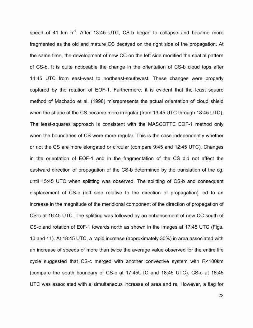
speed of 41 km h-1. After 13:45 UTC, CS-b began to collapse and became more
fragmented as the old and mature CC decayed on the right side of the propagation. At
the same time, the development of new CC on the left side modified the spatial pattern
of CS-b. It is quite noticeable the change in the orientation of CS-b cloud tops after
14:45 UTC from east-west to northeast-southwest. These changes were properly
captured by the rotation of EOF-1. Furthermore, it is evident that the least square
method of Machado et al. (1998) misrepresents the actual orientation of cloud shield
when the shape of the CS became more irregular (from 13:45 UTC through 18:45 UTC).
The least-squares approach is consistent with the MASCOTTE EOF-1 method only
when the boundaries of CS were more regular. This is the case independently whether
or not the CS are more elongated or circular (compare 9:45 and 12:45 UTC). Changes
in the orientation of EOF-1 and in the fragmentation of the CS did not affect the
eastward direction of propagation of the CS-b determined by the translation of the cg,
until 15:45 UTC when splitting was observed. The splitting of CS-b and consequent
displacement of CS-c (left side relative to the direction of propagation) led to an
increase in the magnitude of the meridional component of the direction of propagation of
CS-c at 16:45 UTC. The splitting was followed by an enhancement of new CC south of
CS-c and rotation of E0F-1 towards north as shown in the images at 17:45 UTC (Figs.
10 and 11). At 18:45 UTC, a rapid increase (approximately 30%) in area associated with
an increase of speeds of more than twice the average value observed for the entire life
cycle suggested that CS-c merged with another convective system with R<100km
(compare the south boundary of CS-c at 17:45UTC and 18:45 UTC). CS-c at 18:45
UTC was associated with a simultaneous increase of area and rs. However, a flag for

29
merging was set by MASCOTTE due to the relevant rate of change in structural
properties (perimeter, area) and dynamical properties (speed, propagation direction and
EOF-1 orientation), which were likely related to a merge with a relatively small
convective system.
One important aspect of the structural properties of evolving CS is the distinction
of collapsing stages of the cloud shield. Figure 13 shows the time evolution of Fluct for
CS-b (from 9:45 to 15:45 UTC) and CS-c (from 16:45 to 18:45 UTC). It is noticeable the
transition of Fluct from the lowest magnitude at 11:45 UTC to the largest magnitude at
14:45 UTC. An inspection of CS-b in this time interval (Fig. 12) clearly indicates the
reasons for that transition: the area of CS-b remains almost the same whereas the
perimeter increases as the anvil shield collapses. It is interesting to point out the
independence between Fluct and Ecc. This example visibly emphasizes that any
automated method for tracking of CS needs a definition of a parameter to account for
fragmentation of the system in addition to its eccentricity. Relative large magnitudes of
Fluct are observed until 15:45 UTC, whereas the fragmentation of CS-c decreases after
splitting. At 18:45 UTC, with the development of new cells south of CS-c, the spatial
configuration becomes more similar to CS-b at 10:45 UTC, regardless of differences in
area and orientation. Therefore, the simultaneous monitoring of R, Fc, Ecc and Fluct is
extremely important to design an accurate satellite method to identify convective stages
of evolving CS.
5. Summary and Conclusions
A simple, fully automated and efficient method to determine the structural
properties and evolution (tracking) of CS cloud shields has been described. The present

30
method, which is based on the maximum spatial correlation tracking technique
(MASCOTTE), is a new alternative to the existent techniques available for studies that
monitor the evolution of CS using satellite images. MASCOTTE provides as CS
structural properties the following parameters: horizontal area, perimeter, mean and
variance of brightness temperature, minimum brightness temperature, fractional
convective area and center of gravity. A new way of estimating the orientation and
eccentricity of CS is proposed, and is based on the empirical orthogonal function (EOF)
analysis of CS pixel coordinates. Based on the magnitudes of the spatial correlation
between consecutive satellite images and the changes in horizontal areas of CS,
MASCOTTE provides a new way of tracking the evolution of CS life cycles. This is a
significant improvement over previously published methods that assume specific
geometries to determine the CS propagation (Machado et al. 1998). MASCOTTE has
also proven to be quite useful to monitor the CS fragmentation and to accurately
determine the CS cloud top orientation. Moreover, MASCOTTE provides automated
determination of the exact occurrence of splits and merges of CS, even for time
intervals between satellite images greater than 1 hour. An important advantage of the
MASCOTTE method is the visual identification and checking of the CS evolution as the
algorithm is applied to satellite images. The versatility of MASCOTTE allows the
application to any extensive satellite imagery database and any geographic region.
The focus of the present paper has been on describing the MASCOTTE
methodology and applying it to seven consecutive days (12 to 18 February) during the
WETAMC LBA/TRMM campaign over the Rondônia state in the Amazon basin.
Convective systems in the Amazon have a high degree of complexity and interaction

31
with the large-scale circulation. For instance, during the WETAMC Silva Dias and Zipser
(1999, personal communication) have observed periods of suppressed organized
convection due to the synoptic-scale regime dominated by the migration of the Brazilian
northeast upper level trough. This is the same regime observed during the dry season,
which is typically ascribed to the absence of much lower frequency of organized
synoptic-scale systems. The significance of the many possible feedbacks between
clouds, rainfall and surface processes over the Amazon Basin needs to be further
understood. Studies that are based on satellite data composites (e.g. Garreaud and
Wallace 1997) do not resolve the CS variability, especially the diurnal cycle and
geographic distribution. Satellite tracking methods such as the one described here
provide an additional research tool in this effort. Statistical analysis of the occurrence of
different CS structural properties during varying synoptic regimes can provide valuable
information on the interaction between CS and the large-scale circulation over the
Amazon.
Acknowledgments
The authors greatly appreciate many helpful discussions with Maria Assunção F.
da Silva Dias, Tom Rickenbach and Luis A. T. Machado. The availability of GOES
satellite images at Goddard Space Flight Center-NASA as part of the LBA/TRMM field
campaign was very helpful. Leila M. V. de Carvalho would like to thank the financial
support from Fundação de Amparo à Pesquisa do Estado de São Paulo (FAPESP
Project 98/14414-0). Partial support from the Jet Propulsion Laboratory (JPL) for
Charles Jones (Subcontract 961593) is also acknowledged.

32

33
Table-1. Parameters determined with MASCOTTE and the automated method of Machado et al. (1998). Parameter MASCOTTE Machado et al. (1998)
CS center of Gravity Yes(TB≤235K) Yes (TB≤245K)
Radius of CS Yes Yes
Average CS TB Yes Yes
Minimum TB Yes Yes
Variance of CS TB Yes Yes
Gradient of TB No Yes
Eccentricity of CS Yes Yes
Convective fraction Yes (TB≤210K) Yes (TB≤218K)
Orientation of cloud tops: Least Squares Yes Yes
Orientation of cloud tops: EOF -1 Yes No
Speed of CS propagation Yes Yes
Direction of propagation Yes Yes
Perimeter and Fragmentation Yes No
Identification of total splits during life cycles Yes No
Identification of life cycle end due to merging Yes No
Flags for splitting/sinking and merges with CS
not satisfying the T-R criteria
Yes No
Number of convective top (CT) No Yes (TB<218K)
Area , location, propagation direction and
speed of the largest (CT)
No Yes

34
Table-2: MASCOTTE summary during 12-18 February: total number of CS satisfying
the T-R criteria, total number of life cycles, number of life cycles which end up merging,
number of splitting/sinking and merging flags in association with systems that are not
satisfying the T-R criteria. One hour time interval between images is considered.
Total CS 1724
Total life cycles 431
Life cycles with merging (CS satisfying the T-R criteria) 129 (30% of life cycles)
Splitting during life cycles (CS satisfying T-R criteria) 133 (8% of Total CS)
Total flags for merging (CS not satisfying T-R criteria) 186 (11% of Total CS)
Total flags for splitting/sinking (CS not satisfying T-R
criteria) 226 (13% of Total CS)

35
References
Carvalho, L. M. V., 1998: Mesoscale cloud patterns in satellite images: use of fractal
dimensions and statistical multivariate analysis. PhD. Thesis. Dept. Atmospheric
Sciences, University of São Paulo, 264 pp. [Available from the author] (in
Portuguese).
Chen., S. S., R. A. Houze, Jr., and B. E. Mapes, 1996: Multiscale variability of deep
convection in relation to large-scale circulation in TOGA-COARE. J. Atmos. Sci.,
53, 1380-1409.
__________, and R. A. Houze, 1997: Diurnal variation and life-cycle of deep convective
systems over the tropical Pacific warm pool. Quart. J. Roy. Meteor. Soc., 123,
357-388.
Cohen, J, M. A. F. Silva Dias, and C. Nobre, 1995: Environmental conditions associated
with Amazonian squall lines: a case study. Mon. Wea. Rev., 123, 3163-3174.
Cotton, W. R. and R. A. Anthes, 1989: Storm and cloud dynamics. Academic Press, 880
pp.
Endlich, R. M., and D. E. Wolf, 1981: Automatic cloud tracking applied to GOES and
METEOSAT observations. J. Appl. Meteor., 20, 309-319.
Fortune, M. A., 1980: Properties of African squall lines inferred from time-lapse satellite
imagery. Mon. Wea. Rev., 108,153-168.
Garreaud, R. D. and J. M. Wallace, 1997: The diurnal march of convective cloudiness
over the Americas. Mon. Wea. Rev., 125, 3157-3171.

36
Horel, J. D., A. N. Hahmann, J. E. Geisler, 1989: An investigation of the annual cycle of
convective activity over the tropical Americas. J. Climate, 2, 1388-1403.
Houze, R. A., Jr., 1977: Structure and dynamics of a tropical squall-line system. Mon.
Wea. Rev., 105, 1540-1567.
_____________, and P. V. Hobbs, 1982: Organization and structure of precipitating
cloud systems. Adv. Geophysys., 24, 225-315.
______________, 1993: Cloud dynamics. Academic Press, 570 pp.
Jackson, J. E., 1991: A user’s guide to principal component analysis. Wiley-
Interscience Publication, 569 pp.
Johnson, R. H., W. A. Gallus,Jr., and M. D. Vescio, 1990: Near-tropopause vertical
motion within the trailing-stratiform region of a midlatitude squall line. J. Atmos.
Sci., 47, 2200-2210.
Lovejoy, S., 1982: The area-perimeter relationship for rain and cloud areas. Science,
216, 185-187.
_____________, and D. Schertzer, 1990: Multifractal, universal classes and satellite
and radar measurements of clouds and rain. J. Geophys. Res., 95, 2021-2034.
Machado, L. A. T., M. Debois, and J. P. Duvel., 1992: Structural characteristics of deep
convective systems over tropical Africa and Atlantic Ocean. Mon. Wea. Rev.,
120, 392-406.
_____________, and W. B. Rossow, 1993: Structural characteristics and radiative
properties of tropical cloud clusters. Mon. Wea. Rev., 121, 3234-3260.

37
_____________, W. B. Rossow, R. L. Guedes, and A. W. Walker, 1998: Life cycle
variations of mesoscale convective systems over the Americas. Mon. Wea. Rev.,
126, 1630-1654.
Maddox, R. A., 1980: Mesoscale convective complexes. Bull. Amer. Meteor. Soc., 61,
1374-1387.
Mapes, B. E., and R. A. Houze, Jr., 1993: Cloud clusters and superclusters over the
oceanic warm pool. Mon. Wea. Rev., 121, 1398-1415.
Miller, D., and J. M. Fritsch, 1991: Mesoscale convective complexes in the western
Pacific region. Mon. Wea. Rev., 119, 2978-2992.
Mohr, K. I., and E. J. Zipser, 1996: Mesoscale convective systems defined by their 85-
GHz ice scattering signature: size and intensity comparison over tropical oceans
and continents. Mon. Wea. Rev., 124, 2417-2437.
Nobre, C.A., J.C. Gash, R. Hutjes, D. Jacob, A. Janetos, P. Kabat, M. Keller, J.
Marengo, J.R. McNeal, P. Sellers, D. Wickland, and S. Wofsy, 1996: The Large
Scale Biosphere-Atmosphere Experiment in Amazonia (LBA). Concise
Experiment Plan. Compiled by the LBA Science Planning Group. Staring Center-
DLO, Wageningen, The Netherlands.
Rickenbach, T. M., 1999: Cloud top evolution of tropical oceanic squall lines from radar
reflectivity and infrared satellite data. Mon. Wea. Rev., 127, 2951-2976.
Shiffer, R. A., and W. B. Rossow, 1983: The International Satellite Cloud Climatology
Project (ISCCP): the first project of the World Climate Research Program. Bull.
Amer. Meteor. Soc., 64, 779-784.
38
Silva Dias, M. A. F., A. J. Dolman, P.L. Silva Dias, S. Rutledge, E. Zipser, G. Fisch, P.
Artaxo, A. Manzi, J. Marengo, C. Nobre, and P. Kabat, 2000: Rainfall and surface
processes in Amazonia during the WETAMC/LBA: an overview. 6th International
Conference on Southern Hemisphere Meteorology and Oceanography, American
Meteorological Society, Santiago, Chile, pp. 249-250.
________________, and R. N. Ferreira, 1992: Application of a linear spectral model to
the study of Amazonian squall lines during GTE/ABLE 2B. J. Geophys. Res., 97,
20,405 - 20,419.
Velasco, I., and J. M. Fritsch, 1987: Mesoscale convective complexes in the Americas.
J. Geophys. Res., 92, 9591-9613.
Williams M., and R. A. Houze, 1987: Satellite-observed characteristics of winter
monsoon cloud clusters. Mon. Wea. Rev. 115, 505-519.
Zipser, E. J., 1988: The evolution of mesoscale convective systems: evidence from
radar and satellite observations. Tropical Rainfall Measurements, J. S. Theon
and N. Fugono, Eds. Deepak, 159-166.

39
Figure Captions
Figure 1. Distribution of CS life cycles. Black bars denote life cycles of all CS satisfying
the T-R criteria regardless whether or not merges had occurred. Dotted bars
indicate life cycles excluding merges.
Figure 2. Distribution of speed (a) and direction of CS propagation (b) of for all events
(dotted bars), and excluding events flagged for splitting/merges (black bars).
Splitting resulting in CS matching the T-R criteria are excluded in both categories.
Figure 3. Origin of CS in four categories: 2-4 hours, 5-7 hours, 8-10 hours and 10-24
hours. CS life cycle (hours) is indicated at the position of the CS origin. The black
square in the lower half of the figure indicates the domain of the TOGA and S-Pol
radars in the Brazilian state of Rondônia during the WETAMC LBA/TRMM field
campaign.
Figure 4. Bi-dimensional distribution of life cycle and CS onset period (see text for
details). Onset period refers to 0:45-5:45 UTC (Ev-Dw: evening to pre-dawn),
6:45-11:45 UTC (Dw-Mo: pre-dawn to morning), 12:45-17:45 UTC (Mo-Af:
morning to afternoon), 18:45-23:45 UTC (Af-Ev: afternoon to evening).
Figure 5. Bi-dimensional distribution of CS maximum radius (km) and respective life
cycle (hours).
Figure 6. Diurnal variation of CS satisfying the T-R criteria. Local time refers to
Rondônia, Brazil (time UTC – 4 hours).
Figure 7. Origin (x), displacement (lines) and life cycle (hours) of the CS in the afternoon
(12:45 – 18:45 LT) and early morning (0:45 – 6:45 LT).

40
Figure 8. Comparison between the orientation of CS cloud shield with two
methodologies: EOF-1 and Least Squares. Ellipses are sketched to illustrate the
differences associated with each quadrant (Roman numbers) in the dispersion
diagram. Dashed ellipses represent Least Squares and solid lines ellipses the
EOF-1 orientation.
Figure 9. Diurnal variation of the absolute vertical speed shear between 700 and 200
hPa levels from 00:00 UTC of February 12 to 00:00 UTC of February 19. Days
are indicated between bars on the abscissa. Data source: NCEP/NCAR
reanalysis.
Figure 10. Distribution of perimeter fluctuation (Fluct) around the times of maximum
(18:45 UTC) and minimum (6:45 UTC) absolute vertical speed shear. Fluct
standard deviation = 0.12
Figure 11. Example of CS life cycle on 15 February. This example is selected to
illustrate the determination of merges and splits. Time (UTC) is indicated in each
panel. Shading and contours refer to brightness temperature (K). Contour interval
is 10 K for solid lines and 2.5 K for shading.
Figure 12. Example of structural properties of the same CS life cycle discussed in Fig.
11. For each time (UTC) the panels displays the perimeter, the ellipses whose
axes are determined by the first and second eigenvectors EOF-1 and EOF-2 and
the eccentricity. Also shown are the eccentricity (Ecc), equivalent radius (R),
fraction of clouds (Fc) with Tb ≤ 210 K, speed and direction (counted as
clockwise angle from North) of propagation of CS. The CS orientation determined
by the least square fit is indicated as dashed lines. The center of gravity (cg) of

41
the CS is collocated with the center of the image. Flag equals to S (M) indicates
possible sinking/splitting (merging) of CS with R < 100 km. The ordinate and
abscissa are in arbitrary units of latitude and longitude, respectively.
Figure 13. Time evolution of fragmentation parameter Fluct for CS-b (from 9:45 to 15:45
UTC) and CS-c (from 16:45 to 18:45 UTC).
42
CS LIFE CYCLES: FEBRUARY 12-18/1999
Life Cycle (hours)
Num
ber o
f CS
����������������������������������������������������������������������������������������������������������������������������������������������������������
��������������������������������������������������������������������������������������������������������
������������������������������������������������
����������������������������������������
����������������������������
���������������������
��������������
��������������
��������������
����������������
����������������0
20
40
60
80
100
120
140
160
180
200
[1,2](2,4]
(4,6](6,8]
(8,10](10,12]
(12,14](14,16]
(16,18](18,20]
(20,22](22,24]
> 24

43
DIRECTION OF PROPAGATION OF CS
Direction (degrees from North)
Num
ber o
f CS
���������������������������������������������������������������������������������������������������
12.4%
����������������������������������������������������������������������������������������������������������������������������������������������������������������������������������������������������������������������������
30.4%
�������������������������������������������������������������������������������������������������������������������������������������������������������������������������������������������
25.2%
����������������������������������������������������������������������
8.8%
����������������������������������������
��������������������������������������������������
5.9%����������������������������������������
4.8%
������������������������������������������������������������
8.2%14.6%
34.0%
25.5%
8.6%5.2% 3.5%
5.7%
0255075
100125150175200225250275300325350375
(0,45](45,90]
(90,135](135,180]
(180,225](225,270]
(270,315](315,360]
4.4%
2.9%
SPEED OF CS CENTER OF GRAVITY
Speed (Km/h)
Num
ber o
f CS
������������������������������������������
������������������������������������������������������������������������������������������������������
������������������������������������������������������������������������������������������������������������
������������������������������������������������������������������
������������������������������������������
�������������������������
������������������
���������������
����������
���������� ����� ������ ������ ������ ������
������������
020406080
100120140160180200220240260
(0,1
5]
(15,
30]
(30,
45]
(45,
60]
(60,
75]
(75,
90]
(90,
105]
(105
,120
]
(120
,135
]
(135
,150
]
(150
,175
]
(175
,190
]
(190
,205
]
(205
,220
]
(220
,235
]
(235
,250
]
> 25
0
44

45

46
February 12 to 18: 1724 CS
0
20
40
60
80
100
120
0:45
2:45
4:45
6:45
8:45
10:4
5
12:4
5
14:4
5
16:4
5
18:4
5
20:4
5
22:4
5
Local Time
Num
ber o
f CS
ORIENTATION OF CS CLOUD SHIELD
0
45
90
135
180
0 45 90 135 180
LEAST SQUARES
EOF-
1
I II
IIIIV
S
N

47
Absolute Vertical Speed Shear
6.0E-05
7.0E-05
8.0E-05
9.0E-05
1.0E-04
1.1E-04
1.2E-04
1.3E-04
1.4E-04
0:00
6:00
12:0
018
:00
0:00
6:00
12:0
018
:00
0:00
6:00
12:0
018
:00
0:00
6:00
12:0
018
:00
0:00
6:00
12:0
018
:00
0:00
6:00
12:0
018
:00
0:00
6:00
12:0
018
:00
0:00
Time (UTC)
Shea
r (m
/s P
a)
| Feb-13 | Feb-14 | Feb-15 | Feb-16 | Feb-17 | Feb-18Feb-12
February 12-18 Time: 06:45 UTC
Perimeter Fluctuation
Perc
ent o
f obs
����3.0%
������������
14.9%
����������������������������������������
40.3%
������������������������
22.4%
������������
16.4%
����3.0%
0%
5%
10%
15%
20%
25%
30%
35%
40%
45%
<= -.24 (-.24,-.12] (-.12,0] (0,.12] (.12,.24] > .24
February 12-18 Time: 18:45 UTC
Perimeter Fluctuation
Perc
ent o
f obs
����1.3%������
6.3%
����������������������������
27.5%
��������������������������������������������
43.8%
���������������
20.0%
����1.3%
0%
5%
10%
15%
20%
25%
30%
35%
40%
45%
<= -.24 (-.24,-.12] (-.12,0] (0,.12] (.12,.24] > .24

48