
A Reproduced Copy - NASA Technical Reports Server
598
A Reproduced Copy OF NASA Reproduced for NASA by the Scientific and Technical Information Facility FFNo 672 Aug 65
-
Upload
khangminh22 -
Category
Documents
-
view
0 -
download
0
Transcript of A Reproduced Copy - NASA Technical Reports Server

A Reproduced Copy
OF
NASA
Reproduced for NASA
by the
Scientific and Technical Information Facility
FFNo 672 Aug 65

-_u4"
'd

-.. I _
NASA TECHNICAL
MEMORANDUM
NASA TM X- 64669
{.!
VIlBRATION MANUAL
(MAS_-T_-X-6466 9} VIBRATION MANU&L C.
6teen (NASA) 1 Dec. 1971 592 p CSCL
Astronautics Laboratory
December i, 1971
20KN72-28901
gnclas
G3/32 3601 6
\_. m.:_,_ ,_
NASA
George C. Marshall Space Flight Center
Marshall Space Flight Center, Alabama
MSFC - Form 3190 (Rev june 1971)
NATIONAL TECHNICALINFORMATION SERVICE
g S Oepa¢Iment of Commerce
SpHngfle d V.A 2215| ....


TECHNICAL REPORT STANDARD T_TLE PAG_I _FPONT NO.
TM X- 64669
4 TITLE AND SUBllFLE
2. GOVERNMENT ACCESSION NO.
Vibration Manual
CATALOG_NO.
ec_¢/5. REPORT DATE
December 1, 19716. PERFORMING ORGANIZATION C,,90E
7, AUTHOR(S) 8. PERFORMING ORGANIZATION _EmORT
Claude Green, Editor /9. _ERFORMING ORGANIZATION NAME AND ADDRESS 110. WORK UNIT NO.
George C. M_rshall Space Flight Center lMarshall Space Flight Center, Alabama 35812 1,. CONTRACTORGRANTNO.
12. SPONSORING AGENC'¢ NAME AND ADDRESS
National Aeronautics And Space A(Lministration
Washington, D. C. 20546
3. TYPE oF _ERORT a RER,OD COVERED
Technical Memorandum
14. SPONSORING AGENCY CODE
15. _)UPPLEMENTARY NOTES
Prepared by Astronautics Laboratory,
Science and Engineering
16. aEST:ACT
This document provides guidelines of the methods and applications used in vibration
technology at MSFC. Its purpose is to provide a practical tool for coordination and understanding
between industry and government groups concerned with vibration of systems and equipments.
Topics covered include measuring, reducing, analyzing, and methods for obtaining simulated
environments and formulating vibration specifications. Other sections cover methods for vibra-
_on and shock testing, theoretical aspects of data processing, vibration response analysis,
i techniques of designing for vibration.
17. M EY WORDS
19. SECURITY CLASSIE. _of this report) T
1Unclassified
MSFC - F,-,.._3292 (May 1969)
18. DISTRIBUTION STATEMENT
20. SECURITY CLASSIF. (of this pale)
Unclassified21. NO. OF PAGES I 22. pRICE592 $ 41_ 1, ,7_-"


December l, 1971
APPROVAL
TM X-64669
VIBRATION MANUAL
By
Claude Green, Editor
The information in this report has been reviewed for security classifi-
cation. Review of any information concerning Department of Defense or
Atomic Energy. Commission programs has been made by the MSFC Security
Classification Officer. This report, in its entirety, has been determined
to be unclassified.
This document has also been reviewed and approved for technical
accuracy.
! I-
_A, TJz -. i
" J.H. FARROW
Chief, Dynamics Analysis Branch
Jv. B. STERETT
Chief, Analytical Mechanics Division
|
K. L. HE I2VIBURG
Director, Astronautics Laboratory
577
"_U.S. GOVERNMENT PRINTING OFFICE, 1972-745-386/4109


INTRODUCTION
SECTION I.
SECTION II.
SECTION III.
SECTION IV.
SECTION V.
TABLE OF CONTENTS
Page
AI
B.
General ..... . ..... . .............
The Nature of Dynamic Data ............
SOURCES OF VIBRATION ................. 2
A. Sources and Causes of Vibration ......... 2
B. Complete Vibration Environment ......... 4
ACCELEROMETERS ..................... 7
A. Accelerometer Considerations .......... 7
B. General Accelerometer Principles ....... 8
C. Piezoelectric (Crystal) Aceelerometers . . . 9
D. Strain Bridge Accelerometers .......... 12
E. Piezoresistive Accelerometers .......... 17
F. Force Balance (Servo) Accelerometers .... 17
G. Potentiomete r Ae celerometers .......... 19
H. Accelerometer Comparison ............ 20
I. General Accelerometer Selection
Characteristics .................... 20
MICROPHONES ........................ 22
A. Condenser Microphones ............... 22
B. Piezoelectric Microphones ............. 24
C. Tuned Circuit Microphone ............. 26
D. Microphone Selection ................ 28
MOUNTING OF VIBRATION TRANSDUCERS AND
MICROPHONES ............... ......... 32
A. Vibration Transducer Mounting .......... 32
B. Microphone Mounting ................ 34
C. Associated Factors -- Transducer
Mounting ......................... 35
CALIBRATION... , ..................... 39
39
4O
.,o
lU

SECTION VI.
SECTION VII.
SECTION VIII.
CI
D.
TABLEOF CONTENTS(Continued)
Page
Transducer Subsystem Calibration ....... 42
Data-Transmission and Data-Recording
Subsystems Calibration ............... 52
DATA TRANSMISSION .................... 56
Ao
B.
Ce
D.
Basic Telemetry System .............. 56
Telemetry Systems Used for Vibration
Data ............................ 59
Direct Data Transmission ............. 69
System Accuracy ................... 73
DATA RECORDING ...................... 74
Ae
B.
C.
D.
E.
F.
Magnetic Tape Recorders ............. 74
Oscillographs ..................... 7 8
Oscillograph -- Magnetic Tape System ..... 80
X-Y Plotters ...................... 80
Direct Writing Recorders ............. 82
Oscilloscope and Camera .............. 82
DATA REDUCTION ...................... 83
Ao
B.
Co
D.
E.
F.
G.
H.
Basic Characteristics of Vibration Data .... 83
Basic Descriptions of Vibration Data ...... 89
General Techniques for Periodic Data
Reduction ........................ 103
General Techniques for Random Data
Reduction ........................ 111
Determination of Noise Bandwidth ........ 140
Practical Considerations for Power
Spectra Measurements ............... 149
Multiple Filter Analyzers ............. 152
A Method of Calibrating a Swept Filter
Analyzer or a Multiple Filter Analyzer
for Power Spectral Density Analysis ...... 154
iv

SECTION IX.
SECTION X.
SECTION XI.
SECTION XII.
TABLE OF CONTENTS(Continued)
INTERPRETATION AND EVALUATION OF
DATA ...............................
AO
B.
C.
D.
Eo
Evaluation of Randomness .............
Verification of Stationarity .............
Determination of Data Equivalence .......
Interpretation and Application of Amplitude
Probability Density Functions ..........
Interpretation and Application of Correla-
tion Functions .....................
ACOUSTIC, VIBRATION, AND SHOCK TESTS ....
Ao
B.
Acoustic Tests .....................
Shock and Vibration Tests .............
VIBRATION AND ENVIRONMENTS AND TEST
SPEC IFICATIONS .......................
Ao
B.
Page
156
156
170
182
201
217
267
267
271
281
Stage and Vehicle Vibration and Shock
Criteria ......................... 281
Payload Vibration and Shock Criteria ...... 289
THEORETICAL CONSIDERATIONS ........... 292
Ao
So
C.
D.
E.
F.
Vibration Terms -- Their Meanings and
Uses ........................... 292
Random Process and Probability
Distribution ...................... 296
Random Processes in Vibration Analysis . . . 307
Amplitude and Frequency Distribution
in Random Noise ................... 311
Vibration Excitation Sources ........... 318
Digital Vibration Analysis ............. 345
V

TABLEOF CONENTS (Concluded)
Page
SECTION XIII. VIBRATION RESPONSE ANALYSIS ............ 389
Ao
B.
C.
D.
Eo
Review of Fundamentals ............... 389
Equation of Motion -- Steady State ......... 397
Equations of Motion -- Transients ......... 427
Equations of Motion -- Acoustic Impinge-ment ............................ 431
Application and Examples -- Direct Steady
State Forcing ....................... 443
Equivalent Systems ................... 465
Non-Linear Vibrations ................ 472
Supporting Mathematics ................ 486
Fo
G.
H.
SECTION XIV. DESIGNING FOR VIBRATION ................ 507
Vibration Load Analysis Procedure ........ 507
Use of Vibration Loads in Strength Analyses.. 532
Vibration Damage .................... 536
The MSFC Environment Documents ........ 541
Useful Relationships .................. 54 8
A*
B.
C.
D.
E.
APPENDIX. DEFINITION OF TERMS ...................... 553
REFERENCES ...................................... 565
BIBLIOGRAPHY ..................................... 573
vi

Figure
1.
2.
1
o
1
1
7.
8.
9.
10.
11.
12.
13.
14.
15.
16.
LIST OF ILLUSTRATIONS
Title Page
Schematic of a mass-spring type vibration transducer . . . 9
Frequency response curves for various values of critical
damping (C/Cc) of a linear second order mass-spring
system (sinusoidal input) ...................... 10
Schematic of a typical compression-type piezoelectric
accelerometer .............................. 11
Electrical and mechanical schematic of a typical strain-
bridge accelerometer ......................... 16
Block diagram of a force balance (servo) accele-
rometer .................................. 18
Schematic of a typical potentiometer accelerometer ..... 20
Condenser microphone ........................ 23
Piezoelectric microphone ...................... 25
Piezoelectric microphone ...................... 25
Vibration compensating piezoelectric microphone ...... 26
Tuned circuit microphone ...................... 27
Vibration response of general microphone types ....... 29
Sensitivity ranges of general microphone types ........ 30
Direct mounting of transducer ................... 33
Multiple mounting of transducers ................. 33
Transducers mounted on odd-shape structure ......... 33
vii
Figure
17.
18.
19.
20.
21.
22.
23.
24.
25.
26.
27.
28.
29,
30.
31.
32.
33.
34.
35.
LIST OF ILLUSTRATIONS (Continued)
Title Page
Static test microphone mounting .................. 36
Typical flight vehicle microphone mountings .......... 37
Wheatstone-Bridge circuit ...................... 47
Shunt calibration system ....................... 49
In_flight calibration signals ...................... 54
Basic telemetry system ........................ 57
Direct data transmission system .................. 57
FM/FM channel spacing ....................... 63
FM/FM telemetry ........................... 65
SS/FM channel unit ........................... 67
SS/FM telemetry and ground station ............... 68
Impedance matching devices ..................... 71
Basic electromagnetic tape head .................. 75
Oscillograph optical elements .................... 79
OsciUogralmh-magnetic tape system ................ 81
Computation of mean values ..................... 86
Computation of mean square values ................ 87
Computation of autocorrelation values .............. 88
Typical discrete frequency spectrum ............... 92
°°°
Vlll

Figure
36.
37.
38.
39.
40.
41.
42.
43.
44.
45.
46.
47.
48.
49.
50.
51.
LI ST OF ILLUSTRATIONS (Continued)
Title Page
Typical probability density plot................... 93
Typical autocorrelation plot ..................... 95
Typical power spectrum ....................... 97
Typical joint probai_ility density plot ............... 98
Typical cross corr }lation plot ................... 100
Typical cross-pow r spectrum ................... 102
Functional block diagram for multiple filter type spectrum
analyzer .................................. 105
Functional block diagram for single filter type spectrum
analyzer .................................. 106
Properly resolved frequency spectrum for periodic
data ..................................... 109
Functional block diagram for amplitude probability
density analyzer ............................. 114
Estimation uncertainty versus WBT product .......... 116
Functional block diagram for autocorrelation analyzer . . . 121
Estimation uncertainty versus BT product ........... 123
Functional block diagram for power spectral density
analyzer .................................. 128
Functional block diagram for joint amplitude probability
density analyzer ............................. 134
Functional block diagram for cross-correlation
analyzer .................................. 138
ix
Figure
52.
53.
54.
55.
56.
57.
58.
59.
62.
63.
64.
65.
66.
67.
68.
LIST OF ILLUSTRATIONS (Continued)
Title Page
Functional block diagram for cross-power spectral
density analyzer ............................. 141
Test setup for filter noise bandwidth calibration ....... 145
Magnitude response function for bandpass filter ........ 146
Multiple filter analyzer ........................ 153
Actual power spectra plots ...................... 158
Actual probability density plots ................... 160
Typical autocorrelation plots .................... 161
Analysis of continuous mean square value measure.
merits .................................... 164
Acceptance regions for randomness test ............ 167
Acceptance regions for randomness and stationarity
test ..................................... 175
Illustration of typical autocorrelation functions ........ 221
Autocorrelation function for sine wave plus noise ....... 225
T ransmission path determination example ........... 226
Possible normalized cross-correlation function for
transmission path example ...................... 227
Idealized structure with motion excitation ............ 233
Gain and phase factors for frequency response functions.. 237
Real and imaginary parts for frequency response
functions .................................. 239
X

Figure
69.
70.
71.
72.
73.
74.
75.
76.
77.
78.
79.
80.
81.
82.
83.
84.
LIST OF ILLUSTRATIONS (Continued)
Title Page
Simple idealized structure with force excitation ........ 239
Response power spectrum for simple structure ........ 248
Data for frequency response function measurementconfidence ................................. 265
Mode test setup for saturn vehicle ................. 273
Drop-test shock machine ....................... 274
Hydraulic - pneum:.tic shock machine .............. 276
Electromagnetic vibration shaker ................. 276
Armature behavior over usable frequency range ....... 277
Functional block diagram of sinusoidal sweep generating
system ................................... 279
Functional diagram of a random vibration generating
system ................................... 2 80
Flow chart for determining the vibration environment of
a new vehicle structure ........................ 287
Sinusoidal function x = A sin _ot .................. 293
Record of a random experiment with a die ........... 296
Probability distribution of a discrete random variable . . . 298
Probability distribution for a discrete random variable... 300
Probability distribution function for continuous randomvariable ............ , ..................... 300
xi

Figure
85.
86.
87.
88.
89.
90.
91.
92.
97.
98.
99.
LIST OF ILLUSTRATIONS(Continued)
Title Page
Ensemble of sample functions .................... 301
Ensemble of continuous random processes as a function
of time ................................... 308
Sample of response of a panel to random noiseexcitation ................................. 313
Normal and Rayleigh probability distribution functions . . . 314
Ensemble of measured time histories of force ......... 322
Time record of a nonstationary random force function . .. 327
Amplitude sampling of F(t) at even intervals of time .... 329
Block diagrams of electronic analog CCTS for computing
statistical averages .......................... 331
Typical filter characteristic ..................... 335
Bar graph of the amplitude of filtered discrete frequencycomponents ................................ 336
Finite isolated pulses and their Fourier transforms ..... 339
Bar graph of the mean square amplitudes of discrete
frequency components ......................... 342
The correlation function CF(-r ) of a sinusoid is the
absolute value of a cosinusoid CF(T ) = Jcos wl"] ....... 345
nlustration of folding about the nyquist cutoff frequencyf ...................................... 346
C "
nlustration of quantization error .................. 347
xii

Figure
100.
101.
102.
103.
104.
105.
-106.
107.
108.
109.
110.
III.
112.
113.
114.
115.
116.
117.
LIST OF ILLUSTRATIONS (Continued)
Title Page
Two-dimensional histogram representing f(x,y).
(Number in each square represents observed
frequency. ) ................................ 368
Typical equiprobabiiity ellipses .................. 371
Functions to be computed for two records ............ 373
Joint probability functions for two records ........... 373
Generalized model: one-degree-of-freedom system ..... 398
Magnification factor versus frequency ratio .......... 403
Phase angle versus frequency ratio ................ 403
Bode plot (_ versus r) ........................ 405
Bode plot (9 versus r) ........................ 405
Nyquist plot ................................ 406
Potential energy in a spring ..................... 406
Simple supported beam with two loads .............. 416
Two-degree-of-freedom system .................. 423
Thin plate with small deflection .................. 424
Plate element free body ....................... 425
Panel structure ............................. 436
Beam element, free body section ................. 447
Cylinder geometry and displacement field ............ 453
°..
Xlll

Figure
118.
119.
120.
121.
122.
123.
124.
125.
LIST OF ILLUSTRATIONS (Concluded)
Title Page
Lines of constant energy in the phase plane for the
hard spring, K > 0 ........................... 476
Lines of constant energy in the phase plane for the
soft spring, K < 0 ............................ 476
Response curves for the hard spring ............... 4 80
Response curves for the soft spring ................ 481
Response curves for the non-linear spring with damping.. 4 83
Jump phenomenon or hysteresis resonance for the
non-linear spring with damping ................... 483
Panel damping ............................. 510
Cold helium feeder uuct installation ................ 530
xiv

Table
I.
2.
3.
4.
5.
Q
7.
e
9.
i0.
Ii.
LIST OF TABLES
Title Page
Accelerometer Characteristics and Comparison ....... 13
Microphone Comparison ....................... 31
Subcarrier Bands (±7.5-Percent Deviations) .......... 61
Subcarrier Bands (±1S-Percent Deviations) .......... 62
FM Carrier Record Reproduce System Frequency
Response ................................. 78
Run Test for Statio_arity ....................... 181
Vibration Data Layout for Two-Way Analysis of
Variance .................................. 188
Two-Way Analysis of Variance Table ............... 192
Experimental Results ......................... 197
Results ................................... 200
Optimum Numbered Class Intervals k as a Function of the
Sample Size N .............................. 350
Values of c2 for Equiprobability Ellipses ............ 371
Time Estimates for Digital Vibration Program ........ 381
XV

ACKNOWLEDGMENTS
This report is the result of a combined effort of several Marshall
Space Flight Center laboratories. Principal contributions were from Compu-
tation Laboratory and Astronautics Laboratory. Since most sections of this
report are the consensus of several inputs, no author credits are given. How-
ever, significant technical and editorial contributions were made by Technical
Products Company, The Boeing Company, Julius S. Bendat, Loren D.
Enochson, and Allen G. Piersol.
FOREWORD
This report was originally published in 1963 by the MSFC Vibration
Committee, edited by Jack A. Jones, and was revised in 1968 by the
Astronautics Laboratory. The revision was published as Internal Note,
IN-P& VE-S-68-1, dated July 31, 1968.
The purpose of this report is to provide a tool for practical use in
vibration engineering for Marsh 111 Space Flight Center and contractor person-
nel.
xvi

TE CHNICAL ME MORANDUM X- 64669
VIBRATION MANUAL
INTRODUCTION
The vibration engineec is mainly concerned with keeping the vibrations
of a space vehicle to a level which is not detrimental to the man or the
machine and designing the m_.chine to survive the environment. The main
source of mechanical vibrations in vehicles in the rocket engines which
generate vibration and acous, ic energy over a wide range of frequencies.
The resulting vibration environment can be severe with respect to airframe
fatigue and damage to equipment.
To ensure the structural and functional integrity of the vehicle systems,
it is necessary to determine the vibration environment of a vehicle or com-
ponent. This environment can be approximated by analytical methods, or it
can be predicted by comparison to the known vibration levels of a similar ve-
hicle. If the vehicle is available, the environment can be determined by static
firings and flight tests.
The known vibration environment can then be approximately reproduced
or simulated in the laboratory to improve the design or to prove adequacy of
the vehicle or components. Static firings and flight tests can be consideredas methods to obtain the vibration environment and a/so as environmental tests
of the vehicle.
e
This report describes how analysis and evaluation of data from static
firings and flight tests yield the information necessary for writing vibration
specifications in environmental testing.
This report is intended to help to correlate the terms, ideas, and
methods of the groups concerned with vibrations, and to promote better
understanding and coordination between all groups by serving as a g_aide inthe vibration field.
SECTION I. SOURCESOF VIBRATION
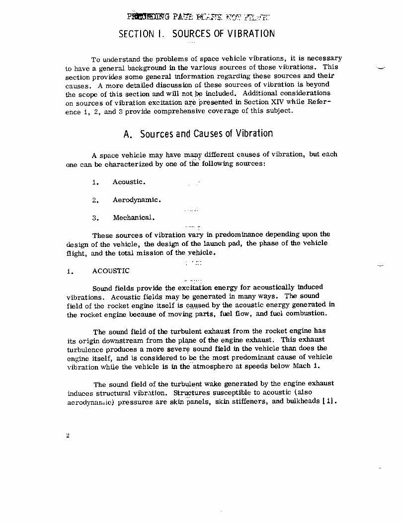
To understand the problems of space vehicle vibrations, it is necessary
to have a general background in the various sources of these vibrations. This
section provides some general information regarding these sources and theircauses. A more detailed discussion of these sources of vibration is beyond
the scope of this section and will not .be included. Additional considerations
on sources of vibration excitation are presented in Section XIV while Refer-
ence 1, 2, and 3 provide comprehensive coverage of this subject.
A. Sources ancl Causes of Vibration
A space vehicle may have many different causes of vibration, but each
one can be characterized by one of the following sources:
1. Acoustic.
2. Aerodynamic.
3. Mechanical.
These sources of vibration vary in predominance depending upon the
design of the vehicle, the design of the launch pad, the phase of the vehicle
flight, and the total mission of the .vehicle.
1. ACOUSTIC
Sound fields provide the excitation energy for acoustically induced
vibrations. Acoustic fields may be generated in many ways. The sound
field of the rocket engine itself is q_.used by the acoustic energy generated in
the rocket engine because of moving parts, fuel flow, and fuel combustion.
The sound field of the turbulent exhaust from the rocket engine has
its origin downstream from the plane of the engine exhaust. This exhaust
turbulence produces a more severe sound field in the vehicle than does the
engine itself, and is considered to be the most predominant cause of vehiclevibration while the vehicle is in the atmosphere at speeds below Mach 1.
The sound field of the turbulent wake generated by the engine exhaust
induces structural vibr,_-tion. Structures susceptible to acoustic (also
aerodynaniic) pressures are skin panels, skin stiffeners, and bulkheads [ 1].

The extent of this vibration is dependentuponthe frequency spectrum, ampli-tude, and spacecorrelation of the soundfield plus the mechanical impedanceof the structure [ 2].
2. AE RODYNAMIC. ,. ,,
Several aerodynamic phenomena exist that are associated with high-
speed flightin the atmosphere which supply excitationenergy that induces
vehicle vibration. Some of the aerodynamic effectsthat cause vehicle vibra-
tion are as follows: .......
a. Pressure fluctuations in the turbulent boundary layer aroundthe vehicle.
be
instability.
Flutter of a fin or panel in the airstream due to dynamic
c. Turbulent wakes generated by air flow past vehicle projections
in atmospheric flight.
d. Flow over recesses and cavities.
e. Oscillating shock waves that may be attached to the vehiclesurface. _....
f. Buffet flow separation, which occurs when the air in the
boundary layer is forced to flow around sharp corners.
g. High-velocity flow through pipes.
Aerodynamically induced exc itation:normally reach, s maxim um value s
in the vicinity of Mach 1 and maximum dynamic pressure (max q).
3. MECHANICAL
Mechanical sources of vibration originate from direct mechanical
excitation. The main mechanical source of vibration usually comes from the
engines and related equipment, such as pumps, motors, compressors, and
generators. - -
These vibration sources originate iii:_he acceleration of moving parts
and in the periodic variations of gas, electrical, and other energy forces.
3
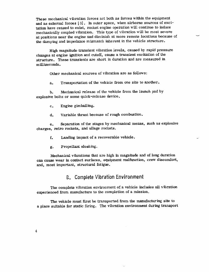
Thesemechanicalvibration forces act both as forces within the equipment
and as external forces [ 3]. In outer space, when airborne sources of exci-
tation have ceased to exist, rocket engine operation will continue to induce
mechanically coupled vibration. This type of vibration will be most severe
at positions near the engine and diminish at more remote locations because of
the damping and impedance mismatch inherent in the vehicle structure.
High magnitude transient vibration levels, caused by rapid pressure
changes at engine ignition and cutoff, cause a transient excitation of the
structure. These transients are short in duration and are measured in
milliseconds.
Other mechanical sources of vibration are as follows:
a. Transportation of the vehicle from one site to another.
b. Mechanical release of the vehicle from the launch pad by
explosive bolts or some quick-release device.
c. Engine gimballing.
d. Variable thrust because of rough combustion.
e. Separation of the stages by mechanical means, such as explosive
charges, retro rockets, and ullage rockets.
f. Landing impact of a recoverable vehicle.
g. Propellant sloshing.
Mechanical vibrations that are high in magnitude and of long duration
can cause wear in contact surfaces, equipment malfunction, crew discomfort,
and, most important, structural fatigue.
Complete Vibration Environment
The complete vibration environment of a vehicle includes all vibration
experienced from manufacture to the completion of a mission.
The vehicle must first be transported from the manufacturing site to
a place suitable for static firing. The vibration environment during transport
4

may be severe, dependinguponthe mode of transportation and the carriage
system. The vibration experienced during this period may be very different
from the flight environment for which the vehicle was designed.
After the vehicle has reached the test site, one or more static firings
are conducted to check the vehicle systems before delivery to the launch site.
Often, one of the most severe vibration environments is caused by exhaustturbulence during static firing. This exhaust turbulence vibration level is
generally developed in the first few seconds after ignition and continues
throughout the static firing. The vehicle is also subjected to local mechanical
vibration, gimballing effects, and ground lmndling prior to and subsequent tostatic firing.
After completing these static firings, the vehicle is aguin subjected
to transport vibration when it is taken to its permanent base, launch site, ortemporary site (in the case of a mobile launch vehicle). When the vehicle
reaches its launch site, it may again be static fired for a short duration to
perform a systems check. After the systems check is complete, the vehicleis ready for its flight objective.
When the booster engines develop thrust while still on the launch pad,
turbulence of the exhaust stream is again a principal vibration source. All
evidence to date indicates this turbulence to be the most severe vibration
excitation source. Not only does the most severe source of vibration occur
before liftoff, but the position of the vehicle on the launch pad and the presence
of other structures in the launch vicinity provide means of reflecting the
sound field or changing the radiation pattern of the sound field. Ground reflec-
tion, which increases the sound pressure level of the vehicle, is evident up to
an altitude of at least 50 nozzle exist diameters and diminishes at highcr alti-
tudes. As the vehicle is in motion and its forward velocity increases, the
noise environment is reduced [ 2]. Some of the reasons for this decrease areas follows:
a. Decrease of pressure with altitude.
b. Increase of time required for noise to travel forward from
source in flow behind missile.
c. Decrease in relative velocity between the jet flow and the
atm o s phe re.

The acoustic field is usually hemispherical untile the vehicle is air-
borne, and then slowly changes to spherical as the reflection from the launch
area is diminished by the gain in altitude. The sound pressure level on the
launch pad is dependent upon the type of exhaust deflection of the exhaust
tunnel, or muffler effect. This engine exhaust noise continues to affect the
vibration levels, with diminishing intensity, until the vehicle exceeds the
speed of sound or leaves the atmosphere.
While the vehicle is still in the atmosphere, other aerodynamic effects
such as flutter, pressure fluctuations, and buffeting may develop and upon
exceeding the speed of sound, oscillating shock waves are generated that can
cause high-level vibration transients.
After the vehicle has passed the speed of sound, the acoustical source
from the exhaust no longer affects vehicle vibration, and once out of the
atmosphere neither the acoustic nor the external aerodynamic sources are
present. Under these conditions, only the mechanical sources remain to
cause vibration. Re-entering the atmosphere produces aerodynamic shock
waves which can induce high-level transient vibrations, and again the vehicle
is subjected to aerodynamic pressure, tui'bulence, buffeting, and flutter.
Finally, vibration and shock which the vehicle experiences caused by landing
impact, must be considered in rnalysis of complete vehicle vibration environ-.o
merit.
SECTION II. ACCELEROMETERS
The purpose of this section is to provide general knowledge of the
principles, characteristics, and applications of accelerometers used by theMarshall Space Flight Center for the measurement of vibration and shock.
This section will aid in the selection of a general type of accelerometer for the
measurement of a specific environment; however, it is not intended to be a
guide for the selection of specific accelerometers. References are given atthe end of this report for more detailed information on vibration and shock
measurement and accelerometer theory. For more information about or
selection of specific accelerumeters, literature and specifications of acceler-
ometer manufactures, and laboratory test results should be consulted, some
of which are given in Referexices 4, 5, 6, 7, 8, and 9.
A. Accelerorneter Considerations
An accelerometer is a transducer which converts the acceleration
input that it experiences into a proportional output quantity. Accelerometers
are available in many forms for widely varied applications. They are used
in aircraft and missile navigation systems as well as for the measurement of
vibration and shock. The requirements for an accelerometer vary from the
extremely sensitive low-frequency types used in vehicle navigational systems
to those used in vibration and shock studies, which must be capable of sensing
motion over a very wide range of frequency and magnitude.
Virtually all accelerometers used for shock and vibratioc, iv s_re-
merit are electromeehanical transducers (sensors or pickups) ; i.., the
instrument output quantity is an electrical signal. Motion is converted into
an electrical signal because the electrical signal may be transmitted over
considerable distances (Section VI), and the electrical signal may be used as
the input to amplifiers, filters, analyzers, and recorders for data recording
and reduction purposes (Sections VII and VIII). The time history of the
electrical sigzm2 may then be used to provide information concerning the
frequency and waveform of the vibration as well as its magnitude (Section IX).
Many different types of transducers have been developed for the pur-
pose of converting mechanical motions into equivalent electrical sigzlals.
These include piezoelectric, strain gage, piezoresistive, force balance
(servo), potentiometer, variable inductance, electrokinetic, magnetostric-
rive, variable capacitance, and permanent magnet self-generating instruments.

The first five of these transducers are the most commonly used accelerometers
at MSFC. These transducers are used for structural response measurements
and will be discussed in the following paragraphs.
B. General Accelerometer Principles
All accelerometers to be discussed involve one basic mechanical
principle ; i.e., the response of a mass-spring system. The base of a mass-
spring system (seismic instrument) or its equivalent is attached to the pointwhere shock or vibration is to be measured, and the acceleration force is
sensed by the transducing element from the motion of the mass ( seismic
mass) relative to the base. An accelerometer operates below the natural
frequency of the mass-spring system. When the frequency of the point to be
measured is above the natural frequency of the mass-spring system, the
transducer can become either a displacement or a velocity transducer, de-
pending on whether the sensor measures displacement or velocity. The mass-
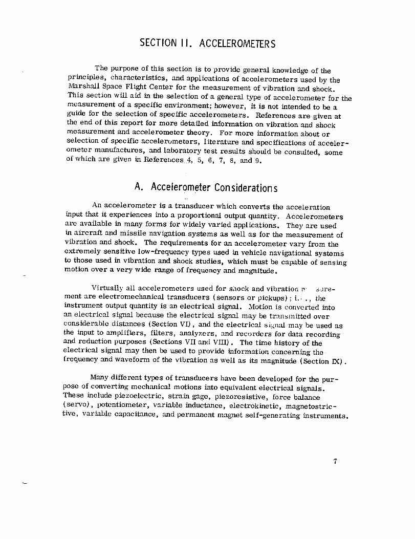
spring transducer shown schematically in Figure 1 consists of a mass sus-
pended from the transducer case by a spring. The motion of the mass within
the case may be damped by a viscous fluid, electric current, or other device
symbolized by a dashpot.
The ratio of the relative displacement amplitude of the mass-spring
system between the mass and transducer case to the acceleration amplitude
of the case is shown in Figure 2 as a function of frequency for various values
of critical damping ratio. This frequency response curve shows that the
acceleration amplitude is directly proportional to relative displacement for
frequencies well below the natural frequency of the system. Thus, this
transducer is used as an accelerometer when the vibration frequency is
below the natural frequency of the system and within the fiat portion of the
response curve. If the transducer is undamped, the response curve is
substantially fiat below approximately 20 percent of the natural frequency.
Consequently, an undamped accelerometer can be used for the measurement
of acceleration when the vibration frequency does not exceed approximately
20 percent of the natural frequency of the accelerometer. The range of
measurable frequency increases as the damping of the accelerometer is
increased, up to an optimum value of damping. When the fraction of critical
damping is approximately 0.65, an accelerometer gives reasonably accurate
results to frequencies of approximately 60 percent of the natural frequency
of the accelerometer. Thus, it can be seen that the useful frequency range
of an accelerometer increases as its natural frequency increases.
CASE SPRING
RELATIVE MOTIONBETWEEN MASSAND CASE
SEISMIC MASS DAMPING
SYSTEM
MOUNTING BASE
I SENSITIVE AXIS (MOTIONIS INFERRED FROM THERE LATIVE MOTION BETWEENTHE MASS AND CASE)
Figure t. Schematic of a mass-spring type vibration transducer.
For a constant acceleration, the output sensitivity of an accelerometer
is dependent of the sensing parameter. If the sensing parameter employs
mass deflection, the electrical signal of the transducer may be very small
at high frequencies since the deflection of the spring is inversely proportional
to the square of the natural frequency. However, a piezoelectric acceler-ometer has as one of _ts advantages the ability to sense acceleration directly
and the electrical signal remains relatively constant with frequency.
C. Piezoelectric (Crystal) Accelerometers
Figure 3 shows schematically a self-generating accelerometer requir-
Lug no external power in which the transducing element is a small disc of
piezoelectric (crystal) material. Piezoelectric materials generate an

uJm
i.JeL
ZuJ
LU(J
.JeL
C_LU>
<-JLUer
2.0-
0.707
0.2-
2
5
0.1 I0,05 0.1 1.0 2 4
C/C c = 10
0.2 0.5
FORCING FREQUENCY
UNDAMPED NATURALFREQUENCY
Figure 2. Frequency response curves for various values
of critical damping (C/Ce) of a linear second
order mass-spring system (sinusoidal input).
electrical charge when subjected to mechanical strain. The piezoelectric
element may be either a natural or synthetic crystal or a ceramic material,
such as barium titanate. The piezoelectric materials contain crystal domains
oriented either by nature or artifical polarization, and the slight relative
motion of these domains, resulting when a load is applied, causes an electrical
charge to be generated. Materials of this type generally exhibit high elastic
stiffness and usually act as a part of the spring in the mass-spring system.
The type shown is of compression design and consists of a seismic mass
compressed between a spring and wafer of piezoelectric material. The
inertial force experienced by the mass causes a proportional change in strain
within the crystal. This change in strain causes an electrical charge to be
developed by the crystal. If the change in strain is within the linear elastic
10

COMPRESSION SPRING DAMPING SYSTEM(IF EMPLOYED)
ELECTRICAL -OUTPUT
PIEZOE LEELEMENT
HOUSING
SEISMIC MASS
MOUNTING BASE
Figure 3.
I SENSITIVE AXIS
Schematic of a typical compression-type
piezoelectric accelerometer.
range, the charge will be in proportion to the inertial force or acceleration
experienced by the mass. The compression spring is preloaded such that
the crystal wafer is always maintained in compression. The resulting mech-
anical system exhibits virtually no damping and a high resonant frequency
(usually between 25 and 75 kHz).
There are various basic designs of piezoelectric accelerometers in
which the crystal element is subject to different kinds of stress. These include
the basic compression design, shear design, bender design, and different
arrangements of these basic types. Modern design of these configurations
mechanically isolates the crystal element from the instrument case to minimize
or avoid the effects of case distortion on sensitivity.
To avoid electrical difficulties known as "ground loops, " electrical
insulation between the accelerometer and ground should be provided. Some
crystal accelerometers have their active elements electrically insulated
11

from the case. Others are non-isolated electrically,and an electrically
insulatingstud or washer is used.
The piezoelectric accelerometer behaves as a charge generator, with
the generated charge proportional to acceleration. It is not capable of measure-
ment down to zero frequency, and its low-frequency response is dependent upon
the electronics of the accelerometer cable and coupling amplifier combination.
The traditional way to improve the low-frequency response has been to use
intermediate impendance matching amplifiers (cathode or source followers)
that have higher input impedance but low output impedance so that long cables
may be used to remote readout instruments without affecting sensitivity.
Charge amplifiers are often used for the same purpose. A discussion of
impedance matching electronics, amplifiers, and connecting cables (along
with the problem of cable noise) used with piezoelectric accelerometers is
given in Section VI.
Due to the high resonant frequency (usually between 25 and 75 kHz),
size, and ruggedness of crystal accelerometers, they are widely used for the
measurement of both vibration and shock. There is a great variety of instru-
ments available with a wide range of frequency response and acceleration
range characteristics. Since damping is low, instrumentation for shock
measurement should include low-pass filters to avoid falsification of data
by accelerometer "ringing" at resonant frequencies. Also, a wide variety
of operating temperature ranges is available with crystal accelerometers.
For more details of piezoelectric accelerometer characteristics and a com-
parison with other accelerometers, refer to Table 1.
Recent innovations in crystal accelerometer design include the
improviement of damping characteristics of certain models. This tends to
eliminate undesirable resonant ringing under shock application and extends the
useful frequency range. Also, progress is being made in decreasing the
extremely high output impedance characteristic of these instruments. In some
cases, source followers are incorporated directly inside the instrument case
without a significant increase in size or weight.
D. Strain Bridge Accelerometers
The electrical resistance of a wire is proportional to the applied
strain, increasing when it is stretched and decreasing when compressed
axially or when initial tension is relieved. Strain bridge accelerometers are
based on this principle. The transducing element is one or more fine strain
12

0
©_J
q_
q_
.<
_J
©
r.v.1
.<
<
=_.
.<
ba
"r
o
x
_ :b_ rL
°
_Q
13

@
I
iio
_ _ _i _._., ._.g
"
_s
II
@
I
14

wires arranged so an applied strain changestheir resistance in responseto therelative desplacementbet_veena seismic mass andthe instrument case.
A typical schematic illistration of a strain bridge accelerometer
(Fig. 4) consists of a mass suspended by unbonded strain wire and employsa viscous damping fluid. The mass is free to move in the direction of the
sensitive axis but is restrained against other motion. The inertial force
experienced by the mass when it is accelerated causes a change in the strain
of the supporting wires and a proportional change in their resistances. In
Figure 4, the strain wires act as the spring portion of the mass-spring system.
To increase sensitivity, the strain wires are arranged electrically to form the
elements of a Wheatstone-Bridge circuit, with one or more active legs. An
electrical schematic is shown at top of Figure 4. This change in strain in the
wires create bridge-resistive unbalance, and in the appropriate circuit an
output voltage appears proportional to the acceleration.
The bridge is balanced externally and maybe excited with either a
dc or ac source. The bridge can be excited by an ae carrier signal, ifdesired,
at some frequency well above the highest test frequency (see Section VI for
discussion of carrier frequencies). Ifac excitation is used, the ac excitation
frequency should be at least fivetimes higher than the highest data frequency
expected. However, ac excitationfrequencies above approximately 3 kHz
should not be attempted on long cable runs because phase balancing problems
may appear. Care should be taken not to exceed the rated excitationvoltage
of the transducer to avoid burning the strain wires.
Strain-bridge accelerometers can be used for measurements down to
zero frequency and have sensitivities up to 50 mV (rms} for full-scale output,
even with acceleration inputs of 1 g or less. Natural frequencies can be as high
as 5000 Hz, although natural frequencies of a few hundred Hz are more common.
The damping is usually about 0.7 of critical at room temperature. Since the
damping fluids generally used change viscosity with temperature, the damping
and the resonant frequency wiU be temperature sensitive. However, tempera-
ture-compensated instruments are available_ and improvements in damping
have been made. Newer fluid damping systems utilize viscous oul shearing.
Low-viscosity oil is used, permitting exceptionally small viscosity changes
in low- and high-temperature applications. This, in turn, minimizes dar_p-
ing changes. These units should be inspected frequently for damping fluid
leaks. Also, some newer model strain accelerometers incorporate gas
damping in which the movement of the seismic mass pumps a gas from a cham-
ber through a porous plug. This system has the advantage of lower damping
15

ELECTRICAL /
OUTPUT -_
_ ELECTRICAL./ INPUT
ELECTRICAL SCHEMATIC
STRAIN WIRE (TYP.)CONNECTED TO ANDINSULATED FROMHOUSING
DAMPING SYSTEM
F HOUSING
o ;. lELECTRICALOUTPUT
SENSITIVE AXIS I
ELECTRICAL j --
EXCITATION INPUT
MOUNTING BASE
Figure 4. Electrical and mechanical schematic of a typical
strain-bridge accelerometer.
16

change with temperature than previously used damping mediums. Newer
models also show a trend away from pendulous suspension to minimize
cross-axis sensitivity and sensitivity to angular accelerations. Table 1
should be referred to for more details of strain-bridge accelerometers anda comparison with other accelerometers.
E. Piezoresistive Accelerometers
Piezoresistive strain-gage accelerometers are similar in principal
to wire strain-gage units and are based on the principle of the semiconductor
strain gage. In place of wires, small chips of semiconductor crystal are used
and arranged electrically to form the elements of a Wheatstone Bridge. These
provide greater electrical output than conventional strain wire sensing elements.
The piezoresistive accelerometer combines several advantages ofth_ strain-bridge accelerometer and the crystal accelerometer. While it is
capable of measuring response down to zero frequency, its high-frequencylimits and acceleration ranges are comparable to piezoelectric accelerometers.
For example, one model has a range of +2500 g (peak) and develops +250mV (peak) with an excitation voltage of 10 Vdc. Damping is 0.06 critical
at a resonant frequency of 30 kHz. Therefore, the range of linear frequency
response (±5 percent} is given as 0 to 6000 Hz. A newer model for high g
measurement offers a full-scale shock range of 50 000 g and frequency cap-
abilities extending from dc to a resonant frequency of better than t00 kHz.
Table I should be referred to for more details of piezoresistive accelerometersand a comparison with other accelerometers.
As compared to piezoelectric accelerometers, piezoresistive acceler-
ometers are just slightly larger and are excellent for shock measurements
(within the acceleration limit) because of their low-frequency capabilities.
They are less rugged than piezoelectric accelerometers; in earlier models,
a drop of a few inches onto a hard surface can cause considerable damage.However, ruggedness has been improved. This type of accelerometer is
still in the developmental stage, and one problem has been in obtaining widertemperature compensation.
F. Force Balance (Servo) Accelerometers
The force balance accelerometer, more popularly knows as the servo
accelerometer, is basically an electromechanical feedback system which is
actuated by a seismic mass. The essential components of the instrument are
illustrated in Figure 5. When the instrument is excited along its sensitive
17

ELECTRICAL INPUT
E. RVO AMPLIFIER
7
] "
RESISTOR_ _ _ ELECTRICAL
/ OUTPUT
Figure 5. Block diagram of a force balance (servo) accelerometer.
axis by an input acceleration, the seismic mass tends to move. A position
detector, which consists of an inductive type pickoff coil in an oscillator
circuit, converts the amount of deflection of the mass relative to the case
into a proportional electrical signal. This causes a change in the output cur-rent of a small servoamplifier. The output current is fed back to a restoring
coil located within a permanent magnetic field which develops a restoring
force (or torque) equal and opposite to the original inertia force experienced
by the mass. Thus, the complete servocircuit acts like a stiff mechanical
spring. The acceleration is now measured as a voltage drop across a resistor
18

which is in series with the output of the servoamplifier, since the restoringcurrent (proportional to restoring force) is a measure of the initial acceleration.
There are two classes of servoforce balance accelerometers; a pendu-
lous type, having an unbalanced pivoting mass with angular displacement, and
a nonpendulous type, having a mass which is displaced rectilinearly. In pend-ulous types, small rotations approximate linear motion and movement is con-
sidered to be linear along a fixed axis of sensitivity. Because of this, angular
types are often sensitive to angular acceleration.
The force balance accelerometer offers much higher accuracy than
other types of accelerometers and is used extensively in inertial guidance
systems for missiles and rockets. However, since low natural frequencyand high damping are characteristic of the force balance accelerometer, its
use in measuring vibration environments is generally limited to measuring
low level accelerations at low frequencies. Force balance accelerometers
may be damped either electrically or by a viscous fluid, and have high sen-
sitivities. A typical instrument might be calibrated for a range of +10 g with
a sensitivity of 0.8 V/g. Table 1 should be referred to for more details of
force balance accelerometers and a comparison with other accelerometers.
G. PotentiometerAccelerometers
The potentiometer accelerometer consists of a mass-spring-damper
system and a potentiometer circuit, shown schematically in Figure 6. The
potentiometer wiper is connected to the seismic mass, and a constant voltage
is maintained across the resistance element of the potentiometer. When the
instrument experiences acceleration, the mass is displaced relative to the
base, causing a change in the output voltage of the potentiometer circuit.
A typical unit is fluid, air, or magnetically damped from 70 to 140
percent critical and is relatively heavy. This type of instrument is used
mainly for measuring very low accelerations at low frequencies and most
have natural frequencies below 30 Hz. One of their main disadvantages is
that their resolution is limited by the diameter of the resistance wire in
the potentiometer, thereby requiring a relatively large displacement to
produce a usable signal. Their principle advantage is their high output and
their flat response from half of their natural frequency down to zero frequency.
Table i should be referred to for more details of potentiometer accelero-
meters and a comparison with other accelerometers.
19

HOUSING
SPRING SYSTEM
POTENTIOMETER WIPER
SEISMIC MASS
ELECTRICAL INPUT
A
ELECTRICOUTPUT .J
DAMPING SYSTEMI SENSITIVE AXIS
Figure 6. Schematic of a typical potentiometer accelerometer.
H. Accelerometer Comparison
Table 1 gives a comparison of various basic accelerometer character-
istics for the accelerometers previously discussed. The various values pre-
sented here do not represent any specific accelerometers but represent an
approximate general range of the types available. It should be noted that
these accelerometers are being continuously improved and that the values
given in this chart may change with further developments and new products.
I. General Accelerometer Selection Characteristics
Certain important characteristics to consider when selecting an
accelerometer are basic and will be treated here. For specific information
or more detailed analysis, specific manufacturer specifications and literatureon accelerometers should be consulted.
2O

When considering an accelerometer for a given application,both
environmental and operational parameters must be given attention. Two
basic questions must be answered:
i. Will the accelerometer measure the environment? Consider:
a. Acceleration range of accelerometer.
b. Frequency response of accelerometer.
c. Frequency and amplitude ranges of the complete data
acquisitionand display system.
d. Temperature effecton sensitivity.
e. Cross-axis sensitivity.
f. Acoustic sensitivity.
g. Sensitivity of accelerometer.
2. Will the accelerometer survive the environment? Consider:
a. Temperature limits.
b. Shock and vibration damage thresholds.
c. The possibility of destructive excitement of the acceler-
ometer at or near its resonant frequency.
d. Possible excitation of associated electronics at destructive
levels.
e. Protection of transducer system from physical damage by
either mechanical or human factors.
21

SECTION III.MICROPHONES
The purpose of this section is to provide a basic knowledge on the
general types of microphones used for acoustic measurements. This sec-tion is not intended to be a guide for the selection of a specific microphone.
The three most commonly used types of microphones at MSFC are
discussed in sufficient detail to ensure an understanding of the basics of
microphone operation. The three general types of microphones are:
a. Condenser microphone.
b. Piezoelectric microphone.
c. Tuned circuit microphone.
Diagrams are presented to aid in the discussion of these general
types. A comparison of the characteristics of the three types of micro-
phones is made to give further information on the application of each general
type of microphone. A discussion on the selection of a general type of
microphone is made in the last paragraph of this section.
A. Condenser Microphones
In basic terms, the condenser microphone is analogous to an elec-
trical circuit containing a variable capacitor. The primary parts of this
microphone are the metal housing, a thin metal diaphragm, and a backplate.
The backptate and metal diaphragm are separated by an air gap and these
elements constitute the electrodes of the variable capacitor. Figure 7
illustrates the basic construction of this type of microphone.
The capacitor (diaphragm and backplate) is energized by a dc voltage
source. Sound waves impinging on the diaphragm causes a displacement of the
diaphragm. This movement will change the capacitance of the diaphragm-
backplate capacitor. A change in capacitance of the circuit changes the circuit
output voltage. The magnitude of the output voltage is proportional to the
pressure level of the sound wave.
To maintain static pre,_qure equilibrium, the air gap between the
electrodes of the capacitor is _ui_ted. This venting to the atmosphere causes
22

DIAPHRAGM
AIR VENT
CURRENT-VOLTAGE
SOURCE
OUTPUT
DIELECTRIC
BACKPLATE
METAL CASE
Figure 7. Condenser microphone.
causes the major limitation of this type of microphone. When large amounts
of water vapor are present in the atmosphere, the dielectric constant of the
air between the two electrodes of the capacitor becomes very low, allowing a
direct current to flow, blocking the operation of the instrument. This same
adverse effect is caused by condensation brought about by rapid temperature
changes. Another limitation to the use of this type of microphone is the high
output impedance of the instrument, particularly at low frequencies. Because
of this high output impedance, a cathode follower, mounted close to the micro-
phone, is required. High output impedance also increases the susceptibility
to electrical leakage in atmospheres or high humidity. One adavantage of this
type of microphone is the small mass of the diaphragm which makes this type
less sensitive to vibration than many piezoelectric microphones. From the
disadvantages stated previously it is obvious that this type of microphone is
not suited for flight test measurements.
23

B. Piezoelectric Microphones
The piezoelectric microphone is a self-generating transducer which
uses piezoelectric sensing elements to generate a voltage when subjected to a
physical strain. The fundamental principles of this general type of microphone
have been discussed in Section II under piezoelectric accelerometers. Since
the operation of piezoelectric elements has already been discussed, this section
will deal with the manner by which the change in strain is created in thepiezoelectric element.
Two different types of construction are available for the piezoelectricmicrophone. The first of these is similar in construction to the condenser
microphone. This type consists of a diaphragm and a rigid backplate with the
piezoelectric element located between them. Sound waves impinging on the
diaphragm cause it to be displaced, thus causing a change in strain on the
piezoelectric element. This change of strain causes a generation of voltageacross the element. The second type of construction is similar but does not
us a diaphragm. Sound waves physically excite the piezoelectric element.
The sound waves hitting the element cause the change of strain, thereby
causing a generation of voltage acorss the element. Figures 8 and 9 show
these types of microphones.
The operating characteristics, frequency response and sensitivity,
of piezoelectric microphones are dependent on the kind of material which is
used as the sensing element. Elements which are most generally used in
piezoelectric microphones are Rochelle salt, barium titanite, ammonium
dihydrogen phosphate, and lead zirconium tftpate. Piezoelectric microphones
are well suited for measuring noise levels under adverse environmental
conditions. This general type of microphone can be sealed such that changes
in atmospheric conditions will not adversely affect the operation of the instru-
ment. Up to this point only the simple type of piezoelectric microphone has
been discussed and it has one major disadvantage in that it is susceptible to
vibration. The movement of the microphone diaphragm by mechanical vibra-
tion causes a change of strain on the piezoelectric element, thereby giving an
erroneous indication of the sound pressure level. Therefore, this type of
microphone cannot be used in a vibration environment without proper isolation.Modifications on the simple microphone have been made to eliminate this dis-
advantage. This modified type uses two identical sensing elements. The firstelement measures the acoustic level while the second element is reversed in the
electrical circuit to compensate for any mechanical vibration which might be
present. As with the other piezoelectric microphones this type can be sealed
24

BACKPLATE
DIAPHRAI
Figure 8. Piezoelectric microphone.
iSILICOr4
RUBBER
Figure 9.
PIEZOELECTRICE LEME NT$
Piezoelectric microphone.
/OUTPUT
25
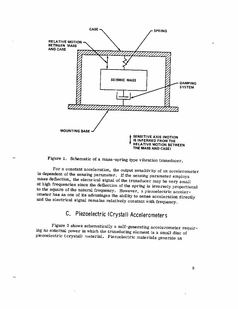
so that changes in atmospheric conditions will not effect the microphone opera-
tion. This type is shown in Figure 10. This modification makes this type of
microphone useful for mounting on flight vehicles and other vibrating structures.
DIAPHRAGM
OUTPUT
/
kf|BRATION COMPENSATING
PIEZOELECTRIC ELEMENT
PIEZOELECTRIC
ELEMENT
Figure 10. Vibration compensating piezoelectric microphone.
C. Tuned Circuit Microphone
In tuned circuit microphones, as in the previous microphones, dia-
phragm movement caused by impinging sound waves describes the basic opera-
tion of this microphone. In this type, the diaphragm is coupled in an electrical
circuit with a variable condenser of inductance coil. These elements make up
26
-J

a tuned electrical circuit and any movement of the diaphragm will cause a
change in the resonant frequency of the circuit. This change can be related to
the displacement of the diaphragm and thereby to the pressure level of the sound
wave. Figure 11 slmws the major elements of this microphone.
WATE R
HRAGM
I
,%
/k\
//' -¢--- CAPACITOR PLATES
OUTPUT
Figure 11. Tuned circuit microphone.
The major advantage of a tuned circuit microphone is that it is available
with facilities for complete water cooling. This cooling system makes this
type of microphone very useful in regions of extreme temperatures.
The massive diaphragm used in this instrument makes it very suscep-
tible to mechanical vibration, in a way similar to that discussed previously
27

under piezoelectric microphones. Because of this disadvantage, this type of
microphone cannot be used in a vibration environment without proper isolation.
D. Microphone Selection
The choice of the type of microphone to be used for a specified measure-
ment is dependent upon the predicted environment in which the microphone will
be required to operate. Microphones mounted on board flight vehicles are
required to measure the magnitude of the acoustic field produced by the rocket
during flight. The microphone mounted on board must be able to endure the
vibrations caused by flight and atmospheric pressure and temperature changes
caused by changing altitudes.
Vibration environments are critical to the operation of the microphone
and limit the selection of the equipment to be used. Therefore, response of
the microphone to vibration is a major consideration in microphone selection.
Figure 12 shows the vibration responses for the general types of microphonea
The piezoelectric microphones shown are not those which have vibration com-
pensating elements. Microphones that are not located on board the vehicle may
not require vibration or altitude compensation but may require temperature
and humidity compensation.
The expected pressure level of the sound wave influences the selection
of the microphone. Figure 13 gives an indication of the sensitivity ranges of
the general types of microphones. This figure indicates the voltage output per
microbar of pressure for the general types of microphones. As can be seen,
the piezoelectric microphone has the lowest range of sensitivity.
All types of microphones, with the exception of the water-cooled tuned
circuit device, will respond to rapid heat rate changes and constant heat flux
fields; therefore, the temperature environment is another item to be considered.
It is difficult to compensate for temperature effects, vibration effects,
etc. by proper calibration; therefore, the choice of a specific microphone
should be made so that these effects are minimized. Table 2 is presented
to give a indication of the relative merits of the above-mentioned general types
of microphones. The information given are ranges for the general types; the
specification sheet on the microphone should be consulted for specific micro-
phones.
28

,q.
I-
Q.Z
m
n-c)LLCnUJ
re
(J
I
_W/N s-0L X Z e, 8P
LU_L>"F"C.)I
I..-(Ju.I.,JLUoNILl
O
v
m
t,-
o
M
N
=_>-
ZiJ.I
0u,I
u.
0
o
;>
o,._
2g

¢
I i
o
"r
/
/I
5.,=,
0
I , I i I
1::1_0_3_/^l aJ 8P
\
I
II
II
i °o oILl I,U_" r.
,/
II
)-
I , I
8 o"r 'T
i,i"r
8
oq_
vu_
W
8
0
0
#
r_
_4
3O

Z©II
,m0
Z©
©
m<
i
+++++:i !:+-,.
31

SECTION IV. MOUNTING OF VIBRATIONTRANSDUCERSAND MICROPHONES
This section presents basic considerations in the mounting of vibration
transducers and microphones. Methods of mounting and associated problems
are discussed for those types of mountings most commonly used at MSFC.Also, refer to References 10, tl, and 12 for further discussions.
A. Vibration Transducer Mounting.
Transducer mounting is one of the most important considerations
in the design of a vibration measurement system. Basically, a mounting must
couple the transducer to the structure or component experiencing vibration
such that the transducer accurately follows the motion of the surface to whichthe mounting is attached.
The method selected in mounting a transducer depends on the trans-
ducer type, the frequency and acceleration range to be measured, and the
geometry of the mounting surface. If the surface-mounting conditions permit,the most desirable method is to attach the transducer directly to the structure.
This eliminates spring mass sy_Jtem effects inherent in some types of mountings
and, consequently, the transducer has an undistorted response to a higher fre-
quency range. This type of mounting is illustrated in Figure 14.
I. MOUNTING BLOCKS
Usually, the transducer is attached to the structure or component
by means of special mounting block or bracket. Odd shaped surfaces, the
need to align the transducer in a particular direction, or the mounting of
multiple transducers necessitates the use of adapters or blocks. Figure 15illustrates a typical transducer-mounting block configuration where two
transducers have been mounted to measure motion in more than one direction.
Figure 16 shows a transducer-mounting block arrangement where the trans-
ducer is mounted on an odd-shaped structure requiring a block to align thetransducer sensitive axis in a particular direction.
Since the mounting block and transducer combination acts as a spring-mass system it has its own resonant frequency and also an attenuation fre-
quency range. The lowest resonant frequency of the mounting block with the
transducer attached must be well above the highest frequency of interest so
that the magnitude and phase of motion are undistorted in the required fre-
quency range. In general, mounting blocks or brackets should be as rigid
32

TRANSDUC_ER
CABLE
STRUCTURE
NOTE: TRANSDUCER MOUNTEDTO STRUCTURE BYTHREADED STUD.
Figure 14. Direct mounting of transducer.
TRANSDUCERS I STRUCTURE
NOTE:TRANSDUCER MOUNTED TOBLOCK BY THREADED STUD
Figure 15. Multiple mounting of transducers.
I MOUNTING BLOCK
TRANSDUCERS
_ STRUCTURE
NOTE: TRANSDUCER MOUNTED TOBLOCK BY THREADED STUD
Figure 16. Transducers mounted on odd-shape structure.
33

and lig. as possible. R_gidity is important; otherwise, the mounting system
will a_te, -lte , 1crease the motion of the structure to be measured by the
transduce±. _leavy mounting blocks affect the weight and frequency of the
structure or component being vibrated and should be avoided. The mountingblock-transducer combination must be tested on a vibration shaker at a
constang g level through the required frequency range to indicate the linearityof the system.
2. ADHESIVE BONDING
If the transducer or mounting block cannot be welded or bolted to
the structure, adhesive bonding may be used. Adhesives employed include
double-backed tape and various types of cements (epoxies, dental cements,
etc. ). If the double-back tape is used, test frequencies should be kept below
2000 Hz [ 10] since above this frequency the transducer will not accurately
follow the structural motion. Acceleration for a tape-mounted assembly should
be restricted to less than 3 g since the tape may break loose at higher levels.
If cements are used to secure the mounting to the test specimen, the trans-ducer readings are not usually reliable above 5000 Hz. The use of adhesives
should be avoided in cryogenic environments since they experience elasticity
changes and loss of adhesion at low temperature resulting in a loss of reliabilityfor the measurement.
A problem with cemented assemblies is their deceptively sturdy
appearance. The strength of a cemented mounting cannot necessarily be
judged by hand pressure. Since a calibration by vibration cannot be performed
on flight vehicles after the assembly is cemented in place, the actual quality
of the mounting cannot be verified. The integrity of the mount must be en-
sured by laboratory evaluation of the various cements and careful mountingtechniques.
B. Microphone Mounting
Since the prim, ary function of a microphone is to obtain a meaningful
measurement of an acoustic field, the microphone mounting must be designed
to this objective. Microphone directivity and the acoustic geometry of the test
area must be considered when selecting microphone locations. Microphone
elements are usually sensitive to vibration and must be isolated from support
vibration. In general, there are two methods of vibration isolation employed:
mechanical isolation and electrical isolation. The choice of isolation technique
is governed by the environment to which the microphone will be subjected.
34

1. MECHANICALLY ISOLATED MICROPHONES
Mechanically isolated microphones are frequently employedfor fieldmeasurementsbut are not generally used for either static testing or flighttesting. Commercially available vibration isolators may be used to mount the
microphone, but they must be used with caution. If the isolator microphone
natural frequencies are within the acoustic frequency range of interest, a true
reading cannot be obtained from the microphone. This problem makes it
difficult to properly isolate microphones located on flight vehicles by mechan-
ical methods. However, for mid- and far-field measurements, microphones
can be mounted directly to concrete or similar massive type structures.
Massive structures effectively isolate the microphone from mechanical
vibration within the acoustic frequency range of interest. Other techniques
for field measurements support the microphones by suspension systems that
isolate the transducer from support vibrations. Figure 17 illustrates a
method for obtaining microphone measurements at various altitudes while
isolating the microphones from vibration by suspension from balloons.
2. ELECTRICALLY ISOLATED MICROPHONES
Flight and static test vehicles usually employ rigidly mounted
microphones that are electrically isolated from vibration. The piezoelectric
types described in Section III are ideally suited for flight measurements.
Mounting techniques for this microphone type are generally the same as
discussed previously for vibration transducers. Special mounting consider-
ations are necessary for flight measurements caused by the acoustic environ-
ment. The external skin of the flight vehicle is subjected to acoustic noise
from several sources (see Section I) and Figure 18 illustrates a mounting
designed to measure this external sound level. One of the microphones
shown in Figure 18 is flush mounted to permit measurement of the boundary
layer acoustic noise and other external noise without disturbing the aero-
dynamic shape of the vehicle. Figure 18 also shows an electrically isolatedmicrophone mounted on a ring frame to measure the vehicle internal noiselevel.
¢. Associated Faclors - Transducer Mounting
In addition to the method of attachment, there are many other factors
to consider in the mounting of transducers. The following paragraphs outline
some factors associated with the mounting of accelerometers and microphones.
35

0
m
v
36

EXTE R IOR OF
VEHICLE
L
_I DIAPHRAGM
(FLUSH WITH
OUTSIDE SKIN)CABLE
R,NG /-- EXTERIOR OFVEHICLE
Figure 18. Typical flight vehicle microphone mountings.
i. TEMPERATURE EFFECTS
Some transducers exhibit high sensitivity to rate-of-change of
temperature, called pyroelectric effect. The pyroelectric effect should not
_e confused with ordinary ambient temperature effect. Some transducers
suddenly cooled or heated during a test react violently in the output response.
37
2. ELECTRICAL ISOLATION
A transducer should be isolated electrically from the ground to decrease
the influence of ground loops. When threaded holes can be used, electricallyisolated mounting studs are commercially available. However, these cannot
be used on some hardware such as tubing, cameras, solar cells, etc., and
other methods of isolation are required. A practical method useful for many
applications is to cement the transducer in place with insulating material in
between. The minimum amount of insulating material should be used to
decrease the spring-mass effect in the vibration environment.
3. CABLE ROUTING
Transducer cable termination and routing can become important for
some applications. Routings should be carefully considered to minimize the
danger of physical damage and triboelectric effects. Too much slack in the
cable often results in spurious signals. Movement of the cable, either jerking
or steady state vibration, is an important source of noise.
4. MAGNETIC FIELDS
There are instances whe.e transducers have to work in the presences
of strong magnetic forces. Interference might develop at either the transducer
or the connecting cables. The center conductor of many cables is paramagnetic
and is a possible interference source. Auxiliary cable vibrations which could
interfere with case-sensitive transducers might be caused by ac magneticfields.
5. TRANSDUCER LOCATIONS
All transducer locations should be accurately identified and the
mounting described by photographs or drawings. The orientation of the trans-
ducer sensitive axis on the test specimen or flight vehicle must be completely
defined to permit proper data evaluation. This is extremely important in theevaluation of all vibration and acousitc data.
38

SECTIONV. CALIBRATION
This section defines calibration procedures and problems associated
with the dynamic instrumentation of launch vehicles. The material presented
is general and deals with basic considerations related to any vibration or
acoustic data acquisition system calibration. The nature of dynamic data is
discussed and basic relationships used in sinusoidal calibration techniques
are derived. Calibration procedures are discussed for transducers, data
transmission, and data recording systems. The dynamic systems discussed
are those for measuring vibration, acoustic, a_d shock environments, and are
characterized by high-frequency response requirements. For further dis-
cussions, refer to References 13, 14, and 15.
A. General
The purpose of calibration is to determine the relationship between
the final observed value of data and the true value of the environment at the
sensing instrument location. When this relationship is known, the observed
values may be properly interpreted. The calibration techniques which are
most directly applicable to a particular instrumentation system will depend
on the components of the system, system location and use, and the type ofmeasurement.
Regardless of the method used in calibration, certain principles
must be followed whenever possible. These principles are listed below;
1. The calibration should cover the expected range of c: zron-
mental conditions. This means that the effect of frequency, amplitude,
temperature, and other variables should be determined and accounted for
in the calibration procedure when applicable.
2. Reference standards must be reliable. The accuracy of thecalibration is, at best, no better than that of the reference.
3. Repeatability of calibration measurements should be established
within limits to determine reliability of data. This requires several tests
in which the same reference is applied repeatedly and the resulting indications
are observed and recorded. The variation in these results indicates probable
errors because of system characteristics, as determined by statistical analy-sis.
39

The most desirable calibration procedure for vehicular vibration and
acoustic measurements would be a complete end-to-end stimulation; i.e.,
excitation of the transducer with a known environment equivalent to the expected
environment and observation of the resultant output from the data reduction
system. However, in most cases, this procedure is unrealistic because of its
complexity. Therefore, it is usually necessary to calibrate the transducer sub-
system independently of the data transmission and data recording subsystems.
B. The Nature of Dynamic Data
Dynamic data are usually broad-band random waveshapes which can be
described by three parameters:
1. The magnitude of the measured quantity; e.g., power spectra/
density, sound pressure level, etc.
2. The variation of magnitude with respect to frequency; i.e., spec otral characteristics.
3. The time history of magnitude at any particular frequency or band
of frequencies.
These random data are analyzed by statistical methods in terms of mean-square
values, probability density functions, power spectral density, etc. Other
statistical methods may use correlation techniques to isolate periodic functions
that are superimposed on random functions. Although random data are most
commonly encountered in practice, it can be shown that sinusoidal calibration
is applicable.
1. SINUSOIDAL CALIBRATION AND MATHEMATICAL RELATIONS
Instruments used to acquire high-frequency random wave data are often
calibrated by application of a sinusoidal waveform. This is true whether the
environment is simulated mechanically or electrically. A major advantage
of sinusoidal calibration is the ability to calculate exactly the parameters that
describe the waveform or environment. The following relationships are pre-
sented since they are commonly employed in sinusoidal calibration.
Sinusoidal vibration may be described by the equation of displacement
X=X sin wtO
4O

where
X = instaneous displacement
X = peak displacemento
t = time
= angular frequency.
Differentiating yields the linear velocity
X = X - cos wtO
Differentiating again gives instantaneous acceleration
X'=-X w 2sin wto
Now, since angular frequency (w) is related to cyclic frequency (f) by the
equation
¢o = 2_rf
and acceleration may be expressed in terms of g-level as
Kg
g
-4X _2sinwto
Kg
where K = gravitational constant.g
Peak acceleration i_ obtained by setting sin wt to _-1, its maximum
possible values.
4X 7r 2 f20
G =±p K
g
41

Acceleration levels are commonly discussed in terms of peak-to-peak values
which represent the "double amplitude" values, or twice the peak values
although in flight measurements the range is specified in _ Gp, which is apeak value
G = 2Gp-P P
The acceleration level which is considered representative of the
vibratory energy level is the root-mean-square value, or rms level. This is
the common measure of random vibration data and Ls represented mathe-
matically as
T
1 / gZd tOrm s "=0
where T is the time of integration. This indicates thatthe rms level is
the square root of the sum of the squared mean instantaneous values.
For a sinusoidal function,
G
G =--P'-
rms _-_
Similar derivations for random Gaussian motion are found in Reference
10. However, in random waveforms, it is not possible to relate rms or aver-
age values to peak values exactly. The rms-to-mean ratio is defined a_ the --_form factor of a wave. The form factor of a sine wave is 1.11 while the form
factor of a random Gaussian noise is 1.26. Consequently, when an averaging
meter which has been calibrated with a sine wave to indicate rms is used with
random noise, the reading must be corrected by multiplying by the ratio
1.26/1.11 or 1.14.
C. Transducer SubsystemCalibration
The calibration of vibration and acoustic measuring transducers con-
sists of determining their sensitivity or simply the ratio of output to input.
42
The specific information required for transducer calibration depends on the
instrument type and intended use. Flight measurements, field measurements,
laboratory measurements, etc., require different approaches to the problemof calibration.
The output-to-input ratio must be known for all frequencies that the
transducer will experience. Variations in environmental conditions may
necessitate the determination of the effects of temperature, supply voltagevariations, radiation, acoustic noise, electromagnetic field, altitude, and
humidity upon the transducer. The linearity of the transducer should be
checked over the full range of magnitude of vibration or sound pressure level.
1. ACCELEROMETER SUBSYSTEM CALIBRATION
Calibration of accelerometers is performed by excitation under
controlled laboratory conditions. At the beginning of laboratory calibration,
the accelerometer subsystem gain should be adjusted such that the subsystem
output is equivalent to that of the signal preconditioning circuit voltage. Thisadjustment should be made while vibrating the accelerometer at a nominal
frequency and at the full-scale acceleration level within the capabilities ofthe excitation source.
To obtain frequency response the output of the accelerometer should
be measured over the full frequency spectrum of the anticipated environment.
The acceleration level should be selected so that the excitation amplitude
limitations are not exceeded during the calibration procedure.
Linearity can be checked by setting the transducer acceleration level
at a percentage of the desired full-scale acceleration level and recording the
system output. This process is repeated at higher percentages up to 100 per-
cent full-scale and the data plotted to check linearity. Normal increments
are 20 or 25 percent with a return to the lowest percentage point after reach-
ing full-scale to determine hysterisis characteristics. The accelerometer
should be vibrated at a nominal frequency during this check, or, if a resonant
beam is required, the resonant frequency of the beam should be used.
a. Gravity, Methods
Some types of accelerometers can be calibrated under static conditions
by means of earth gravity and centrifuge devices. These instruments generally
have response at zero frequency and include the following types:
43

1. Wire strain bridge.
2. Servo ( force-balance).
3. Piezoresistive.
4. Potentiometer.
The 2-g or "Flip" calibration method takes advantage of the zero
frequency or static response of an accelerometer. If an accelerometer ismounted with its sensitive axis in a vertical position, it senses the 1-g
acceleration of the earthVs gravitational field. If the accelerometer is turned
90 degrees so that its sensitive axis is parallel to the local horizontal, theinstrument senses, zero acceleration. If it is turned 90 degrees again, it is
180 degrees from its original position, and it senses the earthls gravitational
field in the opposite direction. It oould be said to go from a positive l-g to
a negative 1-g level, a total excursion of 2 g.
This calibration procedure has inherent accuracy. It is important
to use good leveling techniques and to measure the 90-degree angle changes
accurately. A spirit level and square are usually sufficient for the accuracydesired in field measurements.
Again, it is important to have the same transducer input voltage level
for beth calibration and data acquisition.
This method is only useful for accelerometers whose operating range
is low enough for the 2-g calibration signal to be a significant portion of the
expected data levels.
b. Centrifuge Method
A calibration method similar to the earth gravity technique is the
centrifuge method. In this method, a centrifuge is used to apply constantacceleration to the vibration transducer. The centrifugv is usually a balanced
table that rotates about a vertical axis. Cable leads from the transducer and
power supply are usually brought to the table through low noise sliprings and
brushes. Centrifuges are commercially available that provide acceleration
levels up to 100 g and special machines are available that produce much higherlevels. Accelerometers that have a frequency range down to zero Hz and
have negligible sensitivity to rotation may be calibrated on a centrifuge or
rotating table. The general accelerometer types listed in Paragraph a. above
can usually be calibrated by the centrifuge method.
44

In the calibration procedure, the transducer must be mounted on the
rotating table such that its sensitive axis is exactly aligned along a radius of
the circle of rotation. The acceleration acting on the transducer is calculated
from the equation:
A = w2R
where
A
R =
acceleration
angular velocity
distance from the axis of rotation to the center of gravityof the movable mass element inside the transducer.
c. Electrod_namic Shakers
Sinusoidal motion for the calibration of vibration transducers is
usually generated by means of an electrodynamic shaker. The electrodynamic
shakers directly convert electrical energy into sinusoidal motion. Trans-
ducers are subjected to sinusoidal motion such that the transducer produces
an'electrical signal which can be accurately measured and the ratio of
electrical output to mechanical input evaluated.
d. comparison Method
A frequently used method of calibrating a vibration transducer is by
direct comparison of the output voltage to that of a secondary standard
accelerometer. The secondary standard accelerometer has been checked
with a primary acceleration standard and is used for laboratory calibration
only. The accelerometer to be calibrated is mounted on the shaker table
or a centrifuge table back-to-back with the secondary standard such that
the two accelerometers experience the same vibration environment. This
is done by locating the accelerometers so that their sensitive axes are
directly in line with each other and with the direction of applied acceleration.
This often results in the bases of the accelerometers being turned toward
each other, hence the back-to-back term.
The secondary standard accelerometer has an accuracy of 3 percent
traceable to the National Bureau of Standards. The readout system is accurate
to 1 percent. The maximum difference observed when secondary standard
systems are checked against each other has been 5 percent.
45

e. Piezoelectric Accelerometer Calibration Techniques
Since the frequency response of piezoelectric accelerometers does
not extend down to zero Hz, they are not calibrated under static conditions.
However, the characteristics of piezoelectric accelerometers (see Section II)
permit calibration by the application of sinusoidal motion to the transducer.
The accelerometer may be calibrated by the comparison method or by an
absolute calibration method using an electrodynamic shaker as a motion
generator.
A crystal accelerometer can be visualized as a charge generatorcombined with a small and discrete amount of capacitance. The crystal
accelerometer normally requires impedance-matching devices which are
sensitive to cable length. However, if the accelerometer signal is fed into a
charge sensing amplifier, these limitations no longer apply.
A charge amplifier is a high-gain-voltage amplifier with a negative
capacity feedback. This system possesses a complex input impedance includ-
ing a dynamic capacitance portion, which is so large that any change of cablecapacitance represents an insignificant portion of the total. Therefore, large
variations of cable length have no overall effect on system sensitivity.
Many charge amplifiers contain an internal calibration source and adial for insertion of the individual transducer sensitivity into the amplifier.
Systems of this type require only proper setting of sensitivity, selection of the
range to be used, and recording of the internal calibration signal. No
calculations are required.
Another technique is the electrical simulation of a crystal accelerometer
by placing a capacitor in series with a voltage generator. If the transducer
sensitivity and the value of the capacitance are known, the voltage can be cal-
culated by the equation:
QS = m
C
where
46

E = output voltage of the simulated accelerometer
C = capacitance of the simulated accelerometer
Q = charge of the accelerometer calculated by multiplying the
sensitivity (coulombs/g) by the simulated g-level.
The voltage, E, should be set to correspond to the proper acceleration level
and the charge amplifier gain set to output this voltage.
f* Strain--Ga_e Accelerometer Calibration
To understand strain-gage accelerometer calibration methods, theelectrical characteristics of this transducer must be understood.
All strain transducers are based on variations of the Wheatstone-
Bridge circuit, which consists of four resistances arranged as shown in
Figure 19. These strain-sensing resistors are constructed so that their
resistances change when a physical stimulus (in this case, acceleration) is
applied to the transducer. If the beam on which a strain-sensing resistor
is located goes into tension, the resistance increases; if it goes into com-
pression, the resistance decreases. The instrument output voltage, Eo,
appears when R 1 aeR2 or Rz _ R4, or both. The circuit characteristic is such
that the resistances in adjacent legs are subject to algebraic subtraction, and
the resistances in opposite legs add. The transducer may be constructed
with one, two, or four active ares. An active arm is one whose resistance
varies with the physical stimulus on the transducer. When the bridge circuit
has less than four active arms, find resistors are used to complete thecircuit.
V
lFigure 19. Wheatstone-Bridge circuit.
47

Referring to Figure 19, if the input voltage V is applied to the circuit
and the resistance of R t is changed by the amount AR, we have:
R ° = R 1 - A R1
(if the change is a decrease in resistance).
If I1 is the current through R1, then
V
Ix = R_ + R 4
and the bridge output voltage,
V
now by substitution,
E = V Rt - Rt*o 2(RI + R_)
or
AR
E ° V 2(2R 1 _ AR)
Since AR is small, the denominator can be simplified, and the term becomes
AR
E ° = V 4R--_"
From the precedtng equations, it may be seen that the transducer output is
always directly proportional to the input voltage. Where shunt calibration
techniques are not used, care must be taken to insure tluit the tnlmt voltage
level is the s_me during data acquisition as that used for calibration.
48
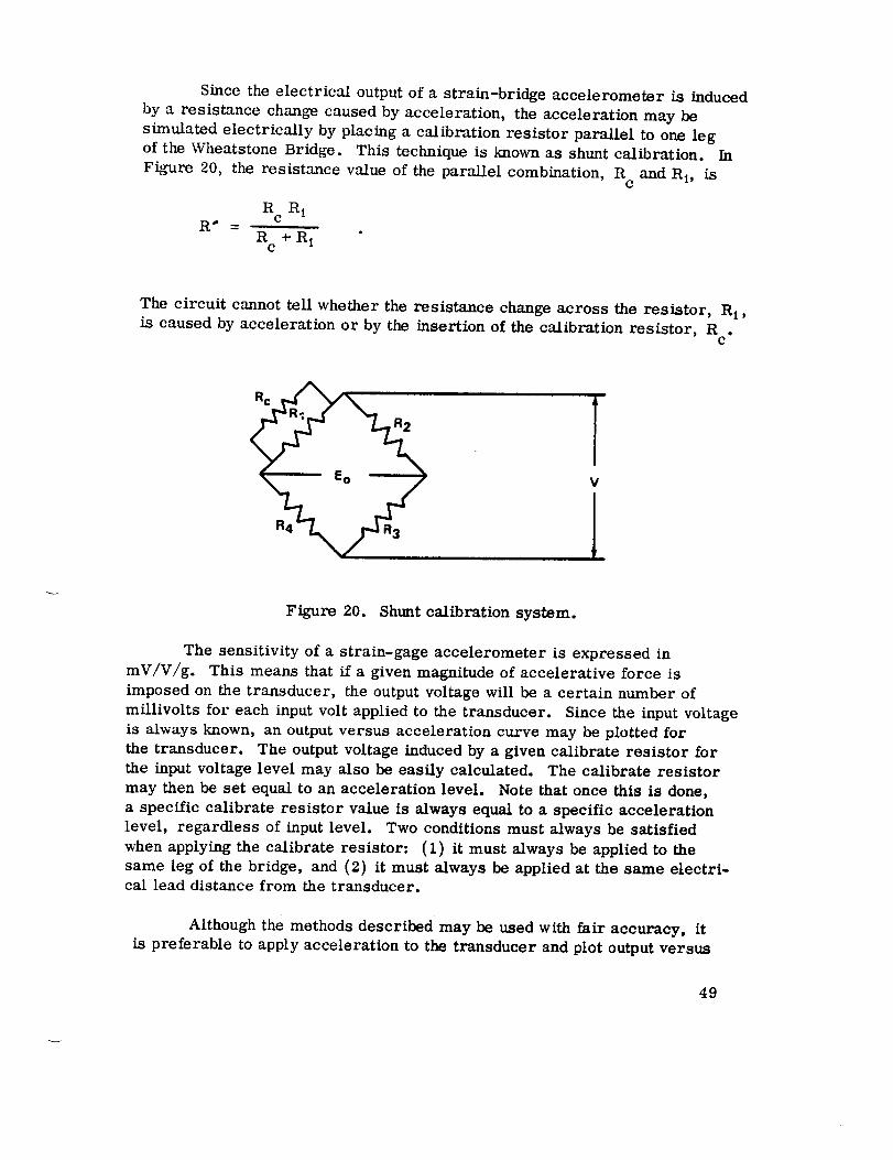
Since the electrical output of a strain-bridge accelerometer is induced
by a resistance change caused by acceleration, the acceleration may be
simulated electrically by placing a calibration resistor parallel to one legof the Wheatstone Bridge. This technique is known as shunt calibration. In
Fig_are 20, the resistance value of the parallel combination, R and R1, isC
_
R c Ri
R +R 1e
The circuit cannot tell whether the resistance change across the resistor, Ri,is caused by acceleration or by the insertion of the calibration resistor, R .
C
Rc
R2
Eo V
IFigure 20. Shunt calibration system.
The sensitivity of a strain-gage accelerometer is expressed in
mV/V/g. This means that if a given magnitude of accelerative force is
imposed on the transducer, the output voltage will be a certain number of
millivolts for each input volt applied to the transducer. Since the input voltage
is always known, an output versus acceleration curve may be plotted for
the transducer. The output voltage induced by a given calibrate resistor for
the input voltage level may also be easily calculated. The calibrate resistor
may then be set equal to an acceleration level. Note that once this is done,
a specific calibrate resistor value is always equal to a specific acceleration
level, regardless of input level. Two conditions must always be satisfied
when applying the calibrate resistor: (1) it must always be applied to the
same leg of the bridge, and (2) it must always be applied at the same electri-cal lead distance from the transducer.
Although the methods described may be used with fair accuracy, it
is preferable to apply acceleration to the transducer and plot output versus
49

acceleration level. It is also preferable to read the outp,t voltage produced by
direct application of the calibrate resistor. Calibrate resistors are normally
in the range of 20 000 to 150 000 ohms. They should be precision resistors
of 0.1 percent tolerance.
2. MICROPHONE CALIBRATION
In general, the calibration requirements for microphones closely
parallel those previously discussed for acceleremeters. There should be a
complete set of calibration curves available on each microphone. The environ-
ments in which the microphone will be operated should be determined for each
application, and the response of the microphone to these environments should
be defined. In the case of new microphones, the manufacturerls curves and
specifications may partially fulfill these requirements. However, as the
microphone is used, it must be calibrated periodically to ensure its continued
satisfactory operation. The period between calibrations depends upon the
frequency of microphone usage. All microphones should be calibrated a
minimum of once every 6 months with a National Bureau of Standards calibrated
reference standard. Each microphone should be calibrated prior to (pre-cal)
and after (post-cal) each test application to determine possible alteration of
the microphone response as a result of the test environments.
Microphones may be calibrated by several methods depending largely
upon the particular microphone and the type of calibration required. The three
basic microphone calibration systems most commonly used at MSFC are:
a. High-intensity pistonphone system.
b. Plane wave tube system.
c. High-intensity calibration system.
a. Pistonphone System
The pistonphone system utilized a pistonphone, high-impedance pre-
amplifier, voltmeter, counter, and associated power supplies. The piston-
phone consists of two electrically driven pistons of different size operating
in a known volume. The cyclic motion of the piston generates a sinusoidal
pressure whose sound pressure level (SPL) value has been predetermined
from volume and displacement calculations from previous measurements.
SPL is a common acoustic term that can be described by the equation [14]
SPI
P
ffi 20 log100
50

where
SPL
Prms
P0
= sound pressure level in decibels
= root mean square pressure value in microbars
= reference pressure (at MSFC, 0.0002 microbar).
The two pistons operate in the same volume since the chamber can be moved
from one to the other. Since the pistons are of different size, their displace-
ments are different and so are the SPL values they generate. By utilizing this
characteristic and changing volume size in several discrete steps, a typicalpistonphone system can generate SPL values from ll0 to 170 dB in 10 dB
increments. A typical frequency range is from 1 to 200 Hz. This type of
calibration system is used primarily for certification of near- and far-field
microphones at regular intervals. Both sensitivity and frequency response
should be checked and records kept for the performance of each microphone.
To use the pistonphone system to check a microphone's sensitivity in
the calibrator frequency range, the microphone is inserted in the chamber
such that its diaphragm face is flush with the chamber wall, thereby not
affecting the chamber volume. The microphone output is then connected to
the preamplifier whose output is in turn connected to the voltmeter. The motor
that drives the piston is then started and set to the desired speed (frequency)
and the microphone output read from the voltmeter. Since the SPL value in the
chamber is known and the microphone output at the SPL value is known, the
sensitivity of the microphone can now be calculated. Checks of the complete
calibration system may be made using a standard reference microphone in
the system.
Do Plane Wave Tube
The plane wave tube system uses the calibration techniques of the
comparison method. A standard reference microphone is excited by a piston-
phone and the output recorded. The microphone is placed in the plane wave
tube and the tube excited until the microphone output is identical to that
generated by the pistonphone. This simulates the same sound pressure level
in the plane wave tube as existed in the pistonphone. The microphone to be
tested may be calibrated by mounting it side by side with the reference stan-
dard microphone in the plane wave tube and recording the output voltages for
comparison.
c. High Intensity Calibration System
This system is designed to calibrate microphones in the frequency
range from 5 Hz to l0 kHz at SPL levels from 110 to 190 dB. This system
51

is still in the development stage and several problems have been encountered.
However, MSFC test engineers are improving the system and it promises to
be a useful method for the calibration of high-intensity microphones.
d. Far-Field Techniques
At MSFC, acoustic monitors in remote f_r-field locations are calibrated
by an acoustic calibrator and a voltage insertion technique. Microphones are
acoustically calibrated by a portable calibrator. The gain is adjusted to a
predetermined level and the voltage at the amplifier output is noted. The
calibrator is removed and the monitoring station's self-contained reference
oscillator is turned on. This amplitude stable oscillator inserts a voltage in
series with the microphone and the gain is adjusted until the output at the
amplifier is the same as that read during the acoustic calibration. The
reference oscillator may be controlled from a central monitoring station to
eliminate the necessity of an acoustic calibrate for every test.
e. Midfield Techniques
A voltage insertion method is generally used for calibration of the
piezoelectric microphones used for midfield data acquisition. An open-circuit
sensitivity for each microphone is obtained from the laboratory calibration,
and a voltage representing the desired SPL for calibration at a given location
is inserted into the system in place of the microphone. The output signal
is recorded on magnetic tape before test data recording and serves as a pre-determined SPL reference. These calibrations should be made as close to
test time as possible.
D. Data-Transmission and Data-Recording SubsystemsCalibration
At MSFC, the calibration of the data-transmission and data-recording
subsystem involves the sending of a simulated or actual transducer subsystem
output signal through the entire system of cables, telemetry, and data recorders.
A signal representing a known percentage of full-scale is injected into the front
end of the data-transmission subsystem, and the data-recording subsystem is
referenced to this signal.
1. FLIGHT TESTING
The calibration signal input to the telemetry system should represent
full-scale peak-to-peak amplitude in all cases, except where the single-sideband
52

telemetry system (SS/FM) is involved. Full-scale calibrationis required
because itdefines the data limits directly through all subsystems of the data-
transmission and data-recording equipment, and its significance is easily
understood. Time-history records of an event should include a calibration
signal to be used as a reference by the data analysis personnel.
A typical inflight calibration procedure is schematically represented
in Figure 21 for the Saturn V telemetry system. Inflight calibration for six
FM/FM assemblies and three SS/FM assemblies is accomplished over a
4.5-sec time interval. The calibrator impresses a series of six (0 to 5 V)
staircase signals to the FM/FM assemblies and a 1700 Hz, 1-V peak-to-peak
signal to the SS/FM assemblies. These calibrate signals are transmitted
and recorded during flight to calibrate the end-to-end system from telemeter
to data-recording equipment.
Preflight calibration of FM/FM telemetry systems consists of impress-
ing a 0 to 5 V step calibrate signal on the systems. The SS/FM system has a
0 to 3000 Hz sweep signal impressed on it for calibration. This SS/FM cali-
brate signal sweeps in a logarithmic manner with the rate of frequency changeproportional to frequency.
2. STATIC TESTING
If the data from the transducers are to be directly recorded during
static testing, the piezoelectric channels are calibrated by substituting an
equivalent signal voltage at the signal conditioner input terminals or by
exciting the transducer. A static test data transmission system using tele-
metry techniques is calibrated by the methods discussed in Subparagraph 1.above.
The accelerometer may be excited by a shaker if only a few measure-
ments are required. Portable fixed-frequency shakers are available for such
purposes. One such unit produces acceleration levels adjustable up to 20
g-rms at a frequency of 120 Hz, with distortion of less than 1 percent and
accuracy of better than 98 percent. Units are also available with a fixed
frequency of 240 Hz. These signals when carried through the data transmission
and data recording system serve as a calibrated reference point for data eval-uation.
When many measurements are required, shaking the accelerometers
becomes impractical and a voltage substitution method of calibration is re-
quired. This technique involves simulation of aceelerometer output by im-
pressing a voltage on the accelerometer channel and measuring the overall
53


sensitivity. A simulated voltage should be inserted at the signal conditionerinput terminals according to the following relationship:
Cca 1
Eins = E cal Ctota1
where
E°
ms
Eca 1
Ccal
Ctotal
= insertion voltage, mV/g
= manufacturer's calibration value, mV/g
= capacitance of aecelerometer and short cable furnished bymanufacturer
= total capacitance of accelerometer, short cable, and
cable to signal conditioner input terminals, all in par-allel.
Up to 14 accelerometer channels may be calibrated simultaneously by
using a millivolter. However, one channel is normally reserved for voice
communication. The millivolter supplies 14 separately adjustable voltages
from i to 1000 mV at frequencies from 100 to 5000 Hz with accuracies from
98 to 99 percent of the amplitude. Single-channel millivolters are also avail-able.
After calibration, but before vehicle test, each accelerometer is tested
by tapping with a small tool on the nearby structure. The channel is monitored
on an oscilloscope to determine if the transient signal comes through. This
is commonly referred to as a "tap test" or "peck check."
55

SECTIONVl. DATATRANSMISSION
The purpose of thissection is to familiarize the reader with data trans-
mission systems in general. Emphasis is given to systems that have direct
applicationto vibration data transmission. This section is divided intofour
main areas: a basic telemetry system and its components, the differenttypes
of telemetry systems used for vibration data, direct data transmission, and
system accuracy.
Ifa more rigorous mathematical discussion of the data systems is
desired, refer to References 16, 17, 18, and 19.
Data transmission may be accomplished by three methods: Radio telem-
etry, hardwire telemetry, and direct (or hardwire) transmission. A radio
telemetry system processes electricalsignals representing physical measure-
ments at a remote location, and transmits these electricalsignals by radia-
tionto a chosen location for display and recording. I-Iardwiretelemetry uses
the same processes as radio telemetry, but in Imrdwire telemetry the radio
link signals are transmitted by metallic conduction rather than by radiation
(Fig. 22). Direct data transmission (hardwire) does not involve radiation
of data signals (Fig. 23). The cable is a metallic conductor between the
transducer and the signal conditioning, display, and recording equipment.
Direct transmission is inherently more accurate than telemetering because
fewer operations are performed on the data signal.
A. Basic Telemetry System
The basic telemetry system consists of a transducer, a data trans-
mission system, and a display or storage device. Figure 22 illustrates a
basic radio telemetering system. The signal from the transducer is fed
through the data transmission system and applied to the display or storage
device. A remote signal processor, a transmitter, a receiver, and a local
signal processor form the basic transmission system. Essential differences
between various telemetry systems lie in the form of modulation.
i. REMOTE SIGNAL PROCESSOR
In some cases the transducer output can be used to modulate the trans-
mitter carrier directly, but then separate radio frequency transmitters would
be required for each measurement. To avoid this waste of the available fre-
quency spectrum, techniques have been developed which permit many
56

TRANSMITTER
REMOTESIGNAL
PROCESSOR
TRANSDUCER
i /RADIO TELEMETRY LINK
_/_-_ RECIEVER
"_HARDWARE
TELEMETRY LiNK
STORAGE
LOCALSIGNAL
PROCESSOR
DISPLAY
Figure 22. Basic telemetry system.
SIGNALCONDITIONER
TRANSDUCER
HARDWARE
CABLE
II ii i i
STnRAGE DISPLAY
Figure 23. Direct data transmission system.
measurements to be transmitted on one transmitter. These techniques
employ either frequency separation or time sharing. Both techniques are
known as "multiplexing," which means to transmit two or more separate
signals over one communication channel.
57

Frequency separation employs separate subcarrier frequency channelsfor each measurement channel. The subcarrier frequencies are spaced so
that each channel remains separate from the others.
In time sharing, a specific time is allotted for each measurement so
that each measurement is sequentially transmitted over a common data channel.
In addition to multiplexing, the remote signal processor performs any
necessary data signal conditioning. Signals may be amplified or attenuated
to make them compatible with other signals being multiplexed, and unwanted
frequencies are filtered out to prevent crosstalk. In time-multiplexed systems,
the data signal is encoded with the appropriate pulse modulation and synchro-
nization pulses are generated.
2. TRANSMITTER AND RECEIVER
The radio telemetry transmitter and receiver employ conventional tech-niques. Telemetry systems are predominantly frequency modulated (FM)
because of the inherent immunity of FM to amplitude effects on the signals
caused by noise. Frequency modulation is modulation in which the instantaneous
frequency is the sum of the carrier center frequency and a frequency which is
a function of the modulating, (or :Jata) signal. In mathematical terms, fre-
que,_cy modulation for a sinusoidal modulating signal is-
e = E sin (w t+m sin_ost_.O C
where
e = instantaneous amplitude
E o = peak amplitude
w c = carrier angular frem_encyt = time
w s = modulating signal angular frequency
m = modulation index (modulation index is carrier frequency
deviation divided by the modulating frequency).
The equation here is expressed as a sine function whereas Reference 16 employs
a cosine function. The two forms are equivalent, one merely is 90 degrees out
of phase with the other.
In the United States, standards have been established by the Inter-Range
Instrumentation Group (IRIG) specifying the characteristics of telemetry sys-
tems [ 17]. These standards establish a total of 44 telemetry channels in
58

the very high frequency (VHF) range between225and 260MHz. Eachchannelis assigned a minimum bandwidthof 500kHz and a maximum deviation of _:125kHz.The channel specification is such that harmonic interference betweenchannelsisprevented. Sincethe Bessel function of the first kind and nth order [ 16], withargument m showsthat a frequencymodulatedwave is composedof sidebandsspacedby the modulation frequency, the modulation index (m) must be limited
to 1.64 to prevent important sidebands of the 125 kHz deviation occurring outside
the assigned 500 kHz channel. Therefore, the data bandwidth (or maximumfrequency of the data is:
frequency deviation 125 kHzfd = modulation index = 1.64 = 76.3 kHz
This data bandwidth limitation is basic and applies to all telemetry systems that
use double FM systems. This includes the Single Sideband (SS/FM) system,which will be treated in detail later.
The [RIG standards for telemetry receivers require that the receivers
operate o_ all telemetry frequencies between 216 and 260 MHz without design
modification [17]. The receiver is designed to have a maximum bandwidth of
600 kHz between 60 dB points and a stability of 0.005 percent. These require-
ments are imposed on the receiver to ensure flexibility of operation and a high
degree of rejection of unwanted adjacent channel and spurious signals.
3. LOCAL SIGNAL PROCESSING
The local signal processor performs the inverse function of the remote
unit. Its exact form is dictated by the remote unit multiplexing technique. It
demultiplexes the data into a form suitable for display or recording.
B. Telemetry Systems UsedFor Vibration Data
The preceding text has been a general discussion of telemetry. The fol-
lowing paragraphs are a more detailed discussion of specific systems used in
the acquisition of structural vibration data.
i. FM/FM
A standard [RIG FM/FM telemetry system employs 18 subcarrier oscil-
lators frequency modulated by transducers. These oscillators in turn frequency
modulate a radio frequency (RF) carrier. This RF carrier is transmitted to a
ground station where the composite FM signal is separated back into the original
18 subcarrier frequencies. The subcarrier signals are passed through discrim-
inators whose outputs correspond to the original transducer signal. When each
59

measurement is continuous, eachsubcarrier channeldata from only one trans-ducer. The system capacity is thenonly 18measurements.
The instantaneousfrequencyof each subcarrier oscillator is proportionalto the instantaneousamplitude of the analogvoltage from its transducer. Therate of frequency changeof the subcarrier is proportional to the instantaneousfrequency of the transducer output. Thecenter frequencyand bandwidthof eachsubcarrier channelconforms to standards establishedby IRIG. As stated pre-
viously, the equation for the frequency modulated signal is:
e= Eo sin (Wct+m sinwd t).
where sin Wct represents the carrier signal and sin wdsignal. Expanding this equation gives:
t represents the data
e = Eo{Jo(m ) sinwct+ J1 (m)[sin (w c+wd) t-sin (w c-wd ) t]
+ J2(m) [sin (Wc + 2w d) t+ sin (w c - 2Wd) t]+ ...
where
e = instantaneous amplitude
E o = peak amplitude
Jn(m) = Bessel function of the 1st kind of order n with argument m
m = modulation index (carrier frequency deviation divided by
modulating frequency)
w c = carrier angular frequency
w d = data angular frequencyt = time.
Here, the first term is the carrier component, the second term is the first-
order upper sideband, and the third term is the first-order lower sideband.
The fourth and fifth terms are second-order sideband components. It may be
seen that each modulated subcarrier signal is composed of center frequency
plus sidebands spaced at the data frequency whose amplitudes are proportionalto the modulation index.
Multiplexing the 18 subcarriers is done by assigning different center
frequencies to each of the oscillators and limiting their data bandwidth to pre-vent channel crosstalk. The maximum deviation of each subcarrier oscillator
is limited to ±7.5 percent of its center frequency. Table 3 lists all 18 subcarrier
bands assigned by IRIG with their center frequencies, upper and lower maximum
frequency deviations, and their data frequency response. In this table the index
60

TABLE 3. SUBCARRIER BANDS (_-7.5-PERCENT DEVIATION)
Band
Center Lower
Freq Limit
(Hz) (Hz)
1 400 370
2 560 518
3 730 675
4 960 888
5 1 300 1 202
6 I 700 1 572
7 2 300 2 127
8 3 000 2 775
9 3 900 3 607
10 5 400 4 995
11. 7 350 6 799
12 10 500 9 712
13 14 500 13 412
14 22 000 20 350
15 30 000 27 750
t6 40 000 37 000
t7 52 500 48 562
i8 70 000 64 750
UpperLimit
(Hz)
430
602
785
I 032
1 399
I 828
2 473
3 225
4 t93
5 805
7 901
it 288
15 588
23 650
32 250
43 000
56 438
75 250
Freq a
Response(Hz)
6.0
8.4
it.0
14.0
20. 0
25.0
35. 0
45. 0
59. 0
81.0
110.0
160.0
220. 0
330. 0
450. 0
600. 0
790. 0
t 050.0
a. For *7.5-percent deviation.
61

of modulation is five. Figure 24 shows the frequency spectra of the equation
up to the eighth sideband pair for the four highest frequency channels with
sinusoidal modulation. The modulation frequency for each channel is the
highest allowed by IRIG standards. If the data frequency were doubled, the
spacing between sidebands and center frequency would be doubled so that cross-talk between channels would occur.
For special broadband data applications, the subcarrier deviation can be
increased to 15 percent with the frequency excursion and data bandwidth shown
in Table 4. The 15-percent channels are designated by letters rather than
Arabic numberals. The problem of sidebands becomes severe with these
expanded channels, so only ever)' other channel can be used.
TABLE 4. SUBCARRIER BANDS (+15-PERCENT DEVIATION)
Band
A
B
C
D
E
Band Used
A
B
C
D
E
Center
Freq
(m)
22 000
30 000
40 000
Lower
Limit
(nz)
18 700
25 500
34 000
Upper
Limit
25 300
34500
46 000
Freq a
Response
(Hz)
660.0
900.
1 200.
52 500
70 000
44 625
59 500
60 375
80 500
1 600.
2 100.
Omit Bands Table 3)
13, 15, and B
14, 16, A and C
15, 17, B and D
16, 18, C and E
17 and D
a. For ±15 percent deviation
62

CARRIER
CARRIE:._
CARRIER
FREQUENCYSPECTRA
AMPLITUDE
i
!
IIQ
i
I
I
m
i
I
m
D
a
m
i
m
m
m
m
I
m
FREQUENCY(Hz)
27750
30000
3225O
..... 37000
43OOO
4a56o
525oo
5644o
CHANNEL
m
_- 17
m
CARRIER
!
m
I
m
m
I
I
I
m
Figure 24.
TTOTAL
DEVIATION(TYP)
c4750
70OOO
75250
FM/FM channel spacing.
- 18
63

Although the complete ]2RIG FM/FM system contains 18 subcarrier chan-nels, only channels 2 through 18 are used. Channel 1 is omitted because its
center frequency coincides with the vehicle primary power supply frequencyof 400 Hz.
The graduated frequency response of the various channels results in
limitations on the use of certain channels for vibration data and requires the
use of the higher channels for the majority of this data. Since vibration data
are generally broadband data, channels 17 and 18 are normally used. Excep-
tions are bending mode and POGO data, which are relatively low frequency andmay be transmitted on the lower channels.
The inputs from all 17 of the modulated channels are linearly mixed and
used to frequency modulate the VHF oscillator in the transmitter. The signal
at the output of the receiver in Figure 25 is identical to the multiplexed linearoutput. The data signals for each of the channels are recovered from their
composite signal by proper discriminators and filtered for display and analysis.
2. FM/FM/FM
Triple FM is employed to subdivide the standard channels into multiple
low response data channels. FM/FM/FM is a technique for trading data band-
width and accuracy for additiona, channels. Each of the high-frequency sub-
carriers can be modulated by several low-frequency subcarriers that are
modulated by their individual transducers. For example, channel 17 of link 1
in the Saturn V Instrument Unit is submultiplexed with IRIG channels 2 through
8. All other channels are standard. The data bandwidth of channels 2 through
8 is 158 Hz, instead of the normal channel 17 bandwidth of 790 Hz, for a chan-
nel efficiency of 20 percent with a maximum channel frequency response of
45 Hz. Since each FM/FM/FM channel uses two stages of modulation and the
modulation index in the second channel is limited to one or less, the data accu-racy suffers.
3. SS/FM
The standard FM/FM telemetry system has a serious shortcoming in its
bandwidth utilization efficiency. Utilized to its maximum capacity, the total
data bandwidth of an FM/FM system operating with a deviation ratio of 5 is
4008 Hz. Because the highest subcarrier frequency required to transmit these
data is 76.3 kHz, the subcarrier data frequency utilization is less than 6 per-
cent. Because of this poor utilization, the highest frequency response obtain-
able on a standard channel is 1050 Hz, and this response is obtainable only on
one channel. An FM/FM telemetry system is incapable of handling the large
quantities of wideband dynamic data required at MSFC on present and futurevehicles.
64

[!
!
/S
0_
b tmm_
• I t
i
i
65
The SS/FM telemetry system was designedanddevelopedat MSFCas acomplement to the FM system, primarily for high-frequency dynamic measure-ments. The system has a capacity of 15channelswith frequency responsesofapproximately 3 kHz. The maximum frequency to beaccommodatedon the RFlink is 75.8 kHz. Thetotal data bandwidthis 45kHz, which is 10times thatavailable with an FM/FM system. The frequency utilization efficiency isapproximately 60percent. Figures 26and 27 illustrate the SS/FM system,
The SS/FM telemetry system, like the FM/FM system, uses frequency
division multiplexing techniques to transmit multiple data channels on a common
FM carrier. Unlike the FM/FM system, each SS/FM channel has a 30 Hz to
3 kHz data frequency response. The analog voltage from each transducer modu-
lates a 455 kHz channel carrier signal. The output of the first modulator has
the lower sideband removed by a filter, and is transposed in frequency by a
second modulator to its assigned position in the multiplexed spectrum. The
multiplexer output in the form of 15 data channels, each transposed to a dif-
ferent frequency, frequency modulates a UHF FM transmitter. In addition to
the multiplexed channels modulating the transmitter, a reference signal derived
from the same master signal as the channel carriers is provided. Since fre-
quency synchronization is required in single sideband transmission, the reference
tone provides synchronization between transmitter and receiver. The reference
tone also provides an amplitude reference for both multiplexer and demultiplexer
so that rms values of the composite signal remain relatively constant.
The receiving portion of the single sideband system reverses the process
of the transmitting portion. The receiver output of a standard FM receiver is
fed through a demultiplexer, which uses the reference tone for synchronization.
Each channel is transposed from its assigned position in the spectrum to its
original frequency. The data from each channel are then amplified and fed to
appropriate readout devices.
Both the sending and receiving portions of the system employ equipment
common to all channels, along with components designed for each individual
channel. The common equipment handles the composite signal from all channels
and generates the carrier frequencies required for 'the channel frequency trans-
lations. Unlike FM/FM where channel equipment is suitable for only one specific
channel, all channel equipment in the present SS/FM system is identical and
interchangeable. The necessary frequency differences between channels for
multiplexing are generated and supplied by the common equipment.
4. TIME SHARING
Time sharing is a special application of FM/FM and SS/FM telemetry
primarily used in vibration and acoustic data acquisition. Time sharing is a
66

N
I"L.'J
M
oLL N÷ _"
_ VIL t_b _
÷ °Lt_ q_"ItJ r_
×z
_Ja°lg_
c_
_E z
67

§0
G8

technique for using a single subcarrier channel to sequentially carry two or
more transducer outputs, each for a finite period of time. Two- and four-
segment time sharing commutators are employed. Since both complete a cycle
of all segments in 12 seconds, the two segment commutator transmits each
measurement for 6 seconds while the four segment commutator transmits each
measurcmcnt for threc seconds.
C. Direct Data Transmission
A direct data transmission system consists of a transducer, signal con-
ditioning circuits, recorder or display unit or both, and connecting cables
( Fig. 23). In cases where the output impedance of the transducer is greatlydifferent from that of the cable, an impedance matching device may be required.
The direct system is potentially more accurate than telemetered data because
frequency translation or conversion is not usually involved. The accuracy actually
obtained is dependent on the components and measurement techniques used.
I. TRANSDUC ERS
Two of the most commonly used types of transducers are piezoelectric
and strain bridge, as discussed in Section II. These will be the only types con-sidered in this section.
Strain bridge accelerometers require four conductor cables. These
cables may be either in the form of two twisted pairs or separately shielded
cabled pairs. Strain bridge accelerometers have a frequency response of 0 to2000 Hz. This means that the response of the cable will not limit the overall
system characteristics.
Piezoelectric accelerometers are inherently wide dynamic response
devices and require a wide dynamic range for the transmission and readout
system. As a general rule, an accelerometer selected for a specific measure-
ment should have a resonant frequency fivetimes greater than the highest data
frequency expected.
Piezoelectric accelerometers have characteristic capacitance ranges of
200 to 2000 pF. If the capacitance of the cable is large with respect to the
accelerometer, the cable will "load" the accelerometer and serious degradation
of the signal will result. Cable capacitance is dependent on the type of cable
used and is directly proportional to the length of cable used. Obviously, as cable
length increases, a point will be reached when signal attenuation is no longer
acceptable. It is obvious that an accelerometer with a large characteristic
capacitance will tolerate more capacative loading than a transducer with low
capacitance.
69
A solution to this problem is to isolate the accelerometer from 10ng
lengths of cable by inserting an impedance matching element in the line nearthe accelerometer.
2. IMPEDANCE MATCHING
Since piezoelectric accelerometer output impedance can be high in rela-
tion to cable characteristic impedance, a matching circuit, or signal conditioner,
is needed to match the accelerometer to the transmission cable. The matching
circuit is usually a vacuum tube cathode follower (Fig. 28), or an emitter fol-
lower if transistors are used. These circuits have high input impedance to
match the accelerometer output impedance and a low output impedance to match
the cable input impedance. Output impedance of the matching circuit should be
30 to 100 ohms when used with open circuit cable of lengths up to 914.4 m
(3000 feet). Impedance values outside this range will result in introduction of
transients, and possible signal waveform distortion and attenuation.
3. TRANSMISSION CABLES
Careful consideration must be given to the type of cable used in data
transmission. Three basic types of cable are normally used: coaxial, twisted
pair-shielded, and quad-shielded
Coaxial cable is inherently unbalanced and is a natural selection to connect
an unbalanced amplifier output to the unbalanced magnetic tape recorder input.
The coaxial cable shield is sometimes erroneously believed to provide shielding
at audio frequencies. At audio frequencies, in contrast to radio frequencies,
current penetrates the braid shielding and provides a means for undesired
electromagnetic coupling to other circuits.
Twisted pair-shielded and quad-shielded cable can be used where one of
the conductors is grounded at the recorder end only. This type of cable may be
generally used where high impedance circuits are not required. This circuit
is less susceptible to noise pickup than the coaxial type by a margin of 30 to 40
decibels. However, the grounded pair is not suitable for lengths,af more than
about 914.4 m ( 3000 feet), because the frequency response cannot be made
fiat enough over the required bandwidth. For long lengths, 914.4 m (3000 feet)
or more, the shielded pair with balanced coupling transformer offers the best
choice for low noise pickup and side frequency response. It is better than
coaxial cable by a margin of 40 to 50 decibels. However, the introduction of
such a transformer may degrade low frequency response and completely elimi-
uate any very low frequency data.
7O

Ep
R9Rk2
EII_
( , t Rkl
c,_T,OOSFOLLOWERSC_E.ATICCIRCUIT
TE OUT
E C
E_ UT
EMITTER FOLLOWER SCHEMATIC CIRCUIT
Figure 28. Impedance matching devices.
71

Shielded cables are subject to the triboelectric effect (voltage generated
as a result of vibration of the cable insulation). An example of the triboelectriceffect is presented in Reference 18. This effect may be avoided by special
construction which consists of providing a drainage path for the triboelectric
voltages. This consideration is especially important in selecting the cable
between the accelerometer and the impedance matching device because this
section of cable will be in a vibrational and acoustical environment. Normallythe cable furnished with the accelerometer is of low noise construction, and
should be used where possible.
Ground-loop problems in cables can be avoided by grounding cable shields
at only one location. This location is normally where the readout and recording
systems are located. This means thatthe circuR common lead is above ground
potentialall the way from the isolatedcircuit common of the accelerometer to
the recorder. Each cathode follower and amplifier used at MSFC for field
vibration measurements has an mdlwdual power supply which provides a high
degree of isolationfrom other channels and reduces the possibilityof inter-
ference between channels through the common capacitance of the power llne.
In very low frequency systems, the cable usually is equivalent to a simple
metallic conduction link. In this case, the cable series impedance is so low
and the shunt impedance is so high that the transducer sees essentially the
signal conditioning input impedance.
4. OVERALL SYSTEM FREQUENCY RESPONSE
If the frequency response characteristics of the components of a system
are not considered, it is possible for abnormally high voltages to enter the
recording electronics, resulting in unintelligible records. Undamped transducer
resonant peaks at the frequency of the FM magnetic tape carrier frequency would
cause high voltages at the recorder input if the peaks coincided with a resonant
peak caused by an improperly terminated cable driven by a low impedance
amplifier. This would result in a frequency interference effect. A beat fre-
quency would be recorded and would result in misleading data.
The lowest signal level that can be handled by a system is set by the
residual noise level of the system. The upper value is set by the overload or
overdrive capabilitiesof the amplifier which, to a great extent at higher fre-
quencies, is controlled by the capacitance load on the amplifier. The higher
the frequency, the greater the attenuation,transients, and signal distortion.
72

D, System Accuracy
The following paragraphs provide some general considerations relative
to system accuracy. No attempt is made in this paragraph to completely specify
the accuracy of any particular system because systems are varied and may con-
tain different combination of components.
The accuracy of a system is a function of the accuracies of all the indi-
vidual components in the system. If a component of 95 percent accuracy is
functionally in series with other component of 95 percent accuracy, then the
system accuracy becomes . 95 x . 95 or approximately 90 percent overall.
Thus, it is seen that the accuracy of a system may be substantially lowered by
including one inaccurate component.
Frequency response of individual components in a system must also be
considered. A system that is quite accurate at one data frequency may possess
poor accuracy at another frequency.
Direct recording offers the highest system accuracy because fewer com-
ponents and operations on the data are necessary. FM/FM telemetry systems
are generally considered to have a working accuracy under ideal conditions of
about 95 percent. The SS/FM system accuracy is much lower than that of the
FM/FM system.
One of the most important factors in determining system accuracy is
the calibration of the components. Section V of this manual discusses the
calibration procedures used in data transmission systems.
73

SECTIONVll. DATA RECORDING
This section provides basic information on data recording systems
and examines in some detail the systems used extensively for vibration and
acoustic data recording. Magnetic tape recorders are discussed since the
majority of vibration and acoustic data are stored on magnetic tape. Other
means of data recording such as X-Y plotters and oscillographs are also
discussed.
A. Magnetic TapeRecorders
Magnetic tape recorders are used as a means of recording and
storing data for later analysis and evaluation. The data axe recorded as an
electrical signal which can represent an unlimited variety of physical or
scientific phenomena. These physical or scientific phenomena are converted
to an electrical signal by the measuring instrument (transducer).
Tape recording systems usually fall into one of two categories:
analog or digital. Analog systems record electrical signals as a continuous
function of the input signal. Digital systems translate the electrical signal
into a series of bits or pulses (generally in the binary code) which are
required in the handling of the data by digital computers and other digital
processing systems.
i.- THE MAGNETIC RECORDING SYSTEM
The magnetic recording system consists of three basic subsystems:
the electronics, the record and reproduce head assemblies, and the tape
transport subsystem. The electronics part of the system supplies the input
data in proper form to the record head and recovers the data from the
reproduce head. The head assembly has both a record and reproduce section.The record section impresses the input data onto the magnetic tape as
variations in local magnetization; the reproduce section reconverts these
variations into electrical signals. The tape transport drives the magnetic
tape past the head assembly at constant speed.
The magnetic tape, while not an integral part of the recording system,
is nevertheless extremely important in overall system operation. In some
instances it is the tape which imposes the limitations on performance. Care
in selecting tape to match recording requirements is well Justified.
74

a. Record and Reproduce Heads
The recording heads are electromagnets which have a small gap in
the core across which the tape is moved as shown in Figure 29. As the tape
crosses this gap in the core, it acts as a magnetic shunt across the gap.
When the tape is in motion, that part which leaves the edge of the gap is left
permanently magnetized in the direction of head magnetization at that instant.
The intensity of magnetization is proportional to the instantaneous signal
current in the head at the instant that portion of the tape left the gap.
PLASTIC BACKING
LM_ _._ - TAPEMAGNETIC FI AIR GAP
Figure 29. Basic electromagnetic tape head.
The reproduce head is an electromagnet similar to the record head.
When the magnetized tape particles are shunted across its gap, a magnetic
flux is developed in the core. As the tape moves, the variations in flux
induce a voltage in the head winding proportional to the rate of change of the
magnetic field in the gap. This voltage, with appropriate processing by the
reproduce electronics, re-creates the original input signal.
There are several important differences between the reproduction
process and the recording process. One difference is that the intensity of
magnetization of the tape corresponds to the signal current used in recording.
The tape is magnetized regardless of its speed past the tape head. It is
important that the tape speed selected be compatible to the rate of change,
or frequency, of the information to be recorded so that well-defined changes
are recorded on tape. The reproduce head does not respond directly to the
magnetic intensity of the tape, but to the rate of change of magnetic intensity.
The flux in the reproduce head is representative of the average magnetization
of the region bridging the head gap, but no voltage is induced across the
reproduce head winding unless the flux density changes. This value can only
75

change when the tape moves. The magnitude of this induced voltage is pro-
portional to the rate of flax density change and the number of turns contained
in the reporduce head coil winding. From basic electrical concepts we havethe formula
where
e = magnitude of the induced voltage
N = number of coil tunes
= flux density.
be Tape Transports
The tape transports commonly used for data recording handle tapes of
either 1.27-cm (1/2-inch) or 2.54-cm (1-inch) width. The 1.27-cm (1/2-
inch) tape transport is capable of recording seven information channels spaced
side by side on the tape. The 2.54-cm (1-inch) tape transport can record 14
channels of information. However, the full transport capacity can seldom be
used for data. A channel may be required for voice annotation in addition to
speed reference channels such as "speedlock" or some other wow and flutter
compensation system.
Tape transports are divided into two general types: the reel transport
and the loop transport. Initial recording of data on magnetic tape is accom-
plished on a reel transport tape machine. This transport moves the tape from
a storage reel, across the heads, and onto a take-up reel. The recorded
information may be played back or monitored if the machine is equipped with
both record and reproduce heads.
The tape loop transport operates with a continuous loop of magnetic
tape. This feature may be used to capture a certain time segment of data in
order to produce a quasi-repetitive segment. This mechanism may also be
used as a time delay device.
76

2. RECORDING METHODS
The two primary systems used in magnetic tape recording are ampli-
tude modulation (AM) or direct recording and frequency modulation (FM) re-
cording. The direct system is less complicated and requires fewer electronic
operations than FM recording, but it has poor low-frequency response character-
istics. The FM method has the distinct advantage of operating at frequenciesdown to zero Hz.
a. Direct Recording
The direct recording system contains an amplifier which conditions the
input signal and generates a bias voltage and frequency. This compensates for
nonlinearities in head characteristics and magnetic tape oxide coating. Direct
reproduce amplifiers consist of an input preamplifier, a frequency equalizer
network, and an output amplifier. The frequency equalizer network character-
istics must be different for different tape speeds. For this reason, the equalizer
network is normally a "plug-in', type unit and may be quickly changed when achange in tape speed is desired.
The frequency equalizer network is used to compensate for system
nonlinearities in order to attain a system frequency response of _-3 dB from
300 Hz to 300 kHz at a tape speed of 152.4 cm/sec (60 in./sec). System fre-
quency response decreases as the tape speed is reduced. For example, at
4. 76 cm/sec (1-7/8 in./sec) tape speed, a tape recorder would have a response
of _3 dB from 50 Hz to I0 kHz. This decrease in system frequency response is
attributable to tape saturation, tape wow and flutter, and head gap effects.
b. FM Recording
The greatest advantage of FM recording is low-frequency response. At
152.4 cm/sec (60 in./sec) tape speed, a system response of 0 to 20 000 Hz may
be attained. This technique involves frequency modulating a carrier with the
input signal and recording the frequency modulated signal at the tape saturation
level. The record amplifier consists of an input amplifier and buffer, a voltage-
controlled oscillator, and an output amplifier.
The FM reproduce system consists of a preamplifier, limtter (or
clipper), discriminator, and output filter. The output filter is changed with
tape speed. Table 5 gives FM system response at the various standard tape
speeds. Values given are for a response of +1/2 dB.
77

TABLE 5. FM CARRIERRECORDREPRODUCESYSTEMFREQUENCYRESPONSE
Tape Speed, cm/sec
(in./sec)
52.4 (60)
76.2 (30)
System Bandwidth with Standard
Output Filter (Hz)
0 to 20 000
0 to 10 000
38.1 (15)
19.05 (7-1/2)
9.52 (3-3/4)
4.76 (1-7/8)
0 to 5 000
0 to 2 500
0 to 1 250
0 to 625
For economy and ease of operation, the tape speed selected should be no
higher than necessary to capture the highest frequency components of the
data expected. The filtering characteristics of FM tape systems may be usedto eliminate undesired high frequency noise and transients.
, MAGNETIC TAPE HANDLING
Magnetic tape must be handled and stored with care. New tape should
always be degaussed before use. Tape not in use should be kept in protective
cans and stored in a cool place. Tape should never be allowed near a magnet,
electrical wire, or any device capable of generating a magnetic field. The
oxide coating should never be touched. The tape guides and heads should be
kept scrupulously clean.
B. Oscillographs
An oscillograph is a device used to convert analog electrical signals_
into a semi-permanent or permanent record called an oscillogram.
The heart of the oscillograph is the optical galvangmeter. A galvanome-
ter is a voltage-sensitive device that causes a mirror to deflect in proportion
to the applied voltage, just as a voltmeter causes a pointer to deflect when
78

voltage is applied. A light beam is reflected from the mirror onto a moving
strip of photosensitive paper. Since the optical arm is long, a small angular
movement of the galvanometer mirror causes a relatively large deflection ofthe light beam on the paper. Figure 30 illustrates the basic elements of anosc illo graph.
/ LIGHT SENSITIVE PAPER
SUPPLY SPOOL /_ LAMP
j_ GALVANOMETER
_" _J MIRRORi',,,,,
• ............ ......
Figure 30. Oscillograph optical elements.
A galvanometer is an electromechanical device. Therefore, it is
subject to mechanical limitations of its ability to convert electrical signals
into proportional excursions of a light beam. The galvanometer may be
thought of as a driven spring-mass system with damping. As such, it is
capable of a limited bandwidth of "fiat" frequency response. Many different
types of galvanometers are commercially available, including those with fluid
magnetic, and electrical damping systems, i
Various recording media for osciUograms are available. The light
sensitive strip could be photographic film, light sensitive paper, or the newer
ultraviolet development paper. The first two types require photographic
development processes, with attendant time delay before the data can be
viewed. The ultraviolet developing paper exhibits the data traces within a
few seconds after exposure to an ultraviolet radiation source, such as a
fluorescent lamp. The ultraviolet developing paper has the disadvantage'of
discoloring when exposed to light and should be stored away from light.
Most oscillographs have a variable speed paper drive system. If the
analog trace is to be used for amplitude information, only relatively low paper
speeds may be used. If, however, waveshape information is desired, the
paper speed must be higher. Depending on the resolution needed 0. 254 to
2.54 cm (0.1 to 1.0 inch) of paper per cycle may be necessary. For a 100 Hz
79
data signal, paper speeds of 10 and 100 inches per second would be requiredfor 0. 254 and 2.54 cm (0.1 and 1.0 inch) of paper per cycle, respectively.
Oscillographs are available with up to 36-channel capacity. Although
high data channel capacity is possible, channel usage is based on data
characteristics. If large amplitude galvanometer deflections are expected,
the galvanometer traces should be spaced so that the traces do not cross.
If, however, only small trace deflections are expected, larger number of
data channels may be used. This is done for ease of trace interpretation.
Other types of oscillographs exist in which optical systems are not
used. Bather, the galvanometer element directly moves a mechanical pen
which is in contact with the moving paper. As might be expected, the
galvanometer mass is much higher than in the optical system and the frequency
response is considerably lower. These systems find some application in
airplane flutter testing and space vehicle vibration testing where frequencies
are on the order of 50 Hz or less.
C. Oscillograph -Magnetic Tape System
The following system is required to convert the recorded signal on a
magnetic tape to an oscillogram. Figure 31 is a functional block diagram
of the system.
The s ignal from the tape is picked up by the reproduce head and is
amplified by the reproduce amplifier. The signal is then fed out of the tape
machine into the galvanometer driver amplifier. The galvanometer driver
output is fed into an electrical damping network and into the galvanometer.
The galvanometer mirror light beam is deflected onto the moving oscillograph
paper.
D. X-Y Plotters
The X-Y plotter uses electrical servosystems to produce a pair of
crossed motions which produce X-Y plots. The plotter consists of basic
balancing circuits plus auxiliary elements to make the instrument versatile.
The self-balancing potentiometer circuit compares an unknown external
voltage with a stable internal reference voltage. The difference between these
voltages is amplified and applied to a servo motor to drive a potentiometer
in a direction that will null any difference or error voltage. Accuracy of plots
80

-j
II
II
\ I\
\ I\1
v
ill
e_
I
e_.
0
0
81

made by this principle is typically 0.1 percent. The full-scale range of the
plotter for each axis is obtained with input sig_.als as low as fractions of a
millivolt. Thus, the output of many low-level devices, such as thermocouples
and strain gages, may be plotted directly without additional amplification.
E. Direct Writing Recorders
A direct writing recorder may be used for slowly changing signals
or it may contain significant frequency components up to 5000 Hz. The type
of recorder should be selected based on the frequency requirements.
. X--Y SERVO TYPE
Among the least expensive direct writing recorders are the strip-
chart recorders which record analog signals of less than 1 Hz. These
recorders usually come with paper widths of 12.7 and 2.54 cm (5 and 10 in.)
with one and two writing pens, respectively. The recording paper can be
ordinary paper marked by ink pens or temperature sensitive paper marked
by a heated stylus. These recorders operate with approximately 0.1 percent
accuracy.
, REVOLVING BAND TYPE
The revolving band type recorder writes directly on electro-sensitive
paper. The principle differences in this type and other types of strip-chart
recorders are the method of writing and the writing medium. A revolvingband rapidly traverses electrically chargeable styli continuously across the
slowly-moving electro-sensitive paper at a rate of 100 passes per second.
Up to 12 channels are sampled and compared with a precision voltage ramp
on each pass. With each pass a corresponding dot for each channel is recorded
on the paper at the appropriate point by a high-voltage pulse. The primaryadvantage of this recorder is the ability to record as many as 12 channels
simultaneously.
F. Oscilloscope and Camera
An oscilloscope and camera are often used to record data when un-
usually high-frequency response is required. The data waveforms are dis-
played on a cathode ray tube and photographed, usually by a polaroid cameramounted in front of the tube face. An alternate method involves the use of a
Memoscope, which is a modified oscilloscope having the ability to store a
transient wave and display it continuously on the tube face.
82

SECTION VIII. DATA REDUCTION
In general, data reduction is the translationof raw information into
simplified quantitieswhich describe the information in a manner suitablefor
engineering analysis and interpretation. For the specific case of flightvehicle
vibration data, the available raw information is usually one or more sample
amplitude time history records of the vibration response at one or more points
on the vehicle structure. The methods employed by MSFC for reducing vibration
data are described here, along with appropriate discussions of some general
considerations associated with vibration data analysis.
A. Basic Characteristics of Vibration Data
Before data reduction can be pursued in detail, itis necessary to identify
certain basic characteristics of the data. In particular, itshould be determined
ifthe vibration data are representative of a random process as opposed to a
periodic process or other deterministic processes. Perhaps the data represents
a combination of both. The procedures for reducing, analyzing, and interpreting
data representing a random vibration response are differentfrom those for
periodic vibration response. The basic characteristics of periodic and random
vibration data will now be discussed.
i. PERIODIC VIBRATION DATA
A periodic function is a special type of deterministic (analytic) function
whose amplitude time history repeats itself exactly after a time interval, T ,
called the period. In equation form, a necessary condition for a function P
y(t) to be periodic is
y(t) = y(t+Tp) . (I)
This is in contrast to other types of deterministic functions and random processes
where equation (1) becomes an inequality. That is,
y(t) _ y(t + Tp) . (2)
A periodic function may be expressed by a Fourier series as shown in equation
(3), where fl= 1/T is the frequency in'cycles per second (cps).P
83
Y(t) = C 0+C I cos (2_flt÷_1) +C2c°s (41rflt+_2)
cO
+C3cos (67rflt+_3) +...=C0+ _ CnCOS(21rnflt+ _n) (3)
In words, equation (3) says that a periodic function consists of a dc component,
Co, and an infinite number of sinusoidal components having amplitudes C andn
phases _ n" The frequencies of the sinusoidal components are all even multiples
of fl, which is called the fundamental frequency. Many periodic functions con-
sist of only a few or even a single component. For example, a sine wave has
a Fourier series in which all values of C are zero except for n = 1. In othern
cases, the fundamental frequency is absent. For example, suppose a periodic
function is formed by mixing three sine waves which have frequencies of 60,
75, and 100 Hz. The lowest common multiple is 5 Hz, so the period for the
resulting periodic function is T = 0.2 second. Hence, in the Fourier seriesP
for the function, all values of C are zero except for n -- 12, n -- 15, and n -- 20.n
Many deterministic functions are not periodic. For example, supposewe have the sum of three sine waves which have frequencies of 60, 75, and 300/_r.
There is no common multiple since 300/7r is an irrational number, so the
resulting function is not periodic. However, in actual practice, such non-
periodic functions may be closely approximated by a periodic function and
expanded into an approximate Fourier series.
2. RANDOM VIBRATION DATA
Unlike periodic functions, the amplitude time history for a random
function never repeats itself exactly. Any given sample record represents a
unique set of circumstances, and is merely a special example out of a large
set of possible records that might have occurred. The collection of all possible
records that might have occurred is called an ensemble which forms a random
process. Thus, an amplitude time history record for a random vibration
response may be thought of as a sample record from a random process.
Since a random process is probabilistic and not an explicit function of
time, the prediction of exact amplitudes at some future time is not possible.
Thus, a random process must be described in terms of statistical averages as
84
opposed to exact analytic functions. It is for this reason that the techniques
for reducing, analyzing, and interpreting random vibration data are different
from those for periodic vibration data.
The properties of a random process may be computed by taking averages
over the ensemble at any given time t. For example, the mean value (first
moment) of a random process at some time t I is computed by taking the
instantaneous amplitude of each record of the ensemble at time tl, summing the
amplitudes, and dividing by the number of records. This computation is
illustrated in Figure 32. The mean square value (second moment) at time t 1,
and the correlation between amplitudes at two different times t 1 and t 2 are
computed in a similar manner as illustrated in Figures 33 and 34.
For the general case where the mean value, mean square value, and
correlation function vary with time, the random process is said to be non-
stationary. For the special case where these three properties do not vary
with time, the random process is said to be weakly stationary. If all higher
moments (i. e., the third moment and up) are also time invariant, the random
process is said to be strongly stationary.
If a random process is stationary, the properties of single records in
the random process can be computed by taking time averages of the single
records as opposed to ensemble averages for the collection of records. The
computation of the mean value, mean square value, and correlation function
by time averaging is illustrated in Figures 32, 33, and 34. For the generalcase where these three time averaged properties vary from record to record,
the random process is said to be nonergodic. For the special case where
these three time averaged properties do not vary from record to record and
thus are equal to the corresponding ensemble averaged properties, the random
process is said to be weakly ergodic. If all higher moments are also independentof the record used, the random process is said to be strongly ergodic. Note
that only stationary random process can be ergodic.
If a vibration response is representative of a nonstationary random
process, the properties of the vibration are changing with time and can be
completely described only by taking averages over the entire ensemble at
every instant of time. If the vibration response is representative of a
stationary random process, the properties of the vibration can be described
by taking averages over the entire ensemble at any one instant of time. If a
vibration response is representative of a stationary and ergodic random
process, the properties of the vibration can be described by taking time
averages over one record from the ensemble.
85

_ INDICATES ENSEMBLE AVERAGE
Yl (t) -- INDICATES TIME AVERAGE
lira 1Yl "T.._=o T Yl (t) dt
I I o
Y2 (t) I I
I I
I IY3 It) I I
I I
,, TIME AVERAGE FOR RECORD Yl (t)
jL t
<Y(t2) _ ,. lim 1 _"_k-e,-oo "k Yl (t2)
, I I ,t
I I _ .m 1 (,TYk(t) J J Yk " T-_o_ _" j Yk(t) dt
I I o
_,, TIME AVERAGE FOR RECORD Yk (t)
I I p t k
It1 It2I t
i=1
-ENSEMBLE AVERAGE FOR TIME t ,, t2
I IIIIII
k
k-=.-_ k Yl (tl)
i-1
IF THE RANDOM PROCESS IS STATIONARY
IF THE.STATIONARY RANDOM PROCESS IS
ERGODIC
= ENSEMBLE AVERAGE FOR TIME t - t 1
<Y(tl) > ,, _Y(t2) _
_y (,)> . y'l;i - 1.2.3 ....
Figure 32. L omputation of mean values.
86

> INDICATES ENSEMBLE AVERAGE
INDICATES TIME AVERAGEVl (t)
i
LIM 1 2 It) dtI _ (t) = T---oo _- Yl
Iyz(t) I I
I I = MEAN SQUARE TIME AVERAGEI FOR RECORD Yl (t)
I IY3 It) I I
I I
I I ,,t
Yk It) I I Yk T-.._o ZJo k It) dt
'_ f - MEANSQUARETIMEAVERAGEREcORDYk(t)
tIt I I t 2
I k
I <y2 (t2)>. LIM _-_'_ Yl ('2)
i=1
- MEAN SQUARE ENSEMBLE
AVERAGE FOR TIME t = t2
<y2(tl)> = LIMk-_c"_-_ yi(tl)
i=1
= MEAN SQUARE ENSEMBLE
AVERAGE FOR TIME t " t 1
IF THE RANDOM PROCESS IS STATIONARY,
IF THE STATIONARY RANDOM PROCESS IS
ERGODIC,
<Y 2 (tl)> " <y2 (t2) >
<y2(t|> " y_l;i = 1,2,3 ....
Figure 33. Computation of mean square values.
87

< > INDICATES ENSEMBLE AVERAGE
-- INDICATES TIME AVERAGE
vl (t)
I I Yl (t) Yl(t+T) - LIMI T--= T
V2 (t) ]l !1 - TIMEr1(t) CORRELATION FOR RECORDI
I ! .tI I
Y3 It) I I
I I
' I I _tI I
Yk (') I I
I II I
tI -,I tl t2
I It
Vl It) Vl It + 11 dt
"- ÷fYk(t) Yk(t+1.) ,, T-,-_ Yk (t) Yk (t +l") (It
0
- TIME CORRELATION FOR RECORD
Yk (t)
k
•-" <y (tl) y (t2) > ,, k"_mLIMnl Y 1 (tl) Yl (t2)
i-1
•, ENSEMBLE CORRELATION FOR TIMES t - t 1 AND t 2
IF THE RANDOM PROCESS IS STATIONARY,
IF THE STATIONARY RANDOM PROCESS ISERGODIC,
<ylt 1)ylt2) > - <y(t) y(t+l")> .
(y(t) ylt+l')> - y(t) ylt+1.}
= R7 (1")
Figure 34. Computation of autocorrelation values.
88

For the actual flight vehicle vibration problem, a single record may
represent the vibration response at some point on the structure of a given
vehicle. The collection of records needed to form an ensemble would then
represent the vibration responses at that point occurring during flights of all
vehicles of that type. However, data from a large number of vehicles of the
same type are rarely available. An ensemble may be contrived by collecting
records of the vibration response for repeated flights of the same vehicle,
where the time origin of each record is considered to be the start of each
flight. Even data of this sort are often difficult to acquire. Usually, vibrationdata from only a fcw flights or perhaps just one flight are available. As a
result, the vast majority of vibration data reduction is performed by time
averaging single sample records.
B. Basic Descriptions of Vibration Data
For any time invariant vibration response, whether it be random,
periodic, or a combination of both, the simplest description of the vibrationamplitude is given by the mean square value. For a vibration record y(t)
of length T, the mean square value 72 is given by
T
-'Y" - T1 f y2 (t) dt (4)0
where
T = Tp for periodic vibration
T -* ¢o for random vibration.
The positive square root of the mean square value gives the rms (root mean
square) value of the vibration; i.e.,
Yrms = _'_ " (5)
The mean square value is a measure of both the static and dynamic
portions of the vibration amplitude. The static portion of the vibration (the
dc component) is defined by the mean value _ as follows:
89
T
- i fy = _ y(t) dt0
(6a)
where
T = T for periodic vibrationP
T --* co for random vibration.
The dynamic portion of the vibration is defined by the mean square
value about the mean (variance) a 2 as follows:Y
T
_ = ± f [y(t) - 7] 2 dt (6b)y T 0
where
T = T for periodic vibrationP
T -* _ for random vibr; .tion.
These three measures of amplitude are related as follows:
y2 = _ 2 + (7) 2 . . (7)Y
Hence, if the mean value of the vibration is zero (_ = 0), which is often the
case in actual practice, the mean square value and variance will be equal(_ = _2 ).
Y
Mean square or rms vibration level measurements give only a
rudimentary description of the vibration amplitude. For most engineering
applications, a more detailed description of the vibration is required. Such
detailed descriptions for periodic and random vibration data will now bediscussed.
. PERIODIC VIBRA TION DA TA
As noted in Paragraph A. of this section, a periodic vibration response
can be completely described by a Fourier series which gives the amplitude,
9O

frequency, andphaseof "allharmonic componentsof the vibration. However,in actual practicc, the amplitudes and frequencies for the harmonic componentsof a vibration responsegive a sufficient description for most engineeringapplications. A lmowlcdgeof the associatedphaseangles is not often required.The description of a periodic vibration response in terms of its harmonicamplitudes anti frequencies is given by a discrete frequency spectrum.
A typical discrete frcqucncy spectrum is illustrated in Figure 35. Notethat eachharmonic componentappears in the frequency spectrum as a linewhich has no bandwidth. The peak amplitudes of the components(Co, C1, C2,_'tc. ) are equivalent to thc coefficients in the Fourier series for the periodicvibration as shownin equation (3). The mean value of the vibration is definedby the coefficient Coat zero frequency. Note that the mean square value of thevibration is equal to the sum of the mean square values for the individualcomponentsplus the square of the mean.
2. RANDOMVIBRATION DATA
If a vibration response is random in nature and assumed to be repre-
sentative of an ergodic stationary process, a reasonable detailed description
of the vibration is obtained from three important properties of random signals.
Thc first is a statistical description of the amplitude charactertistics of the
vibration, which is called.the amplitude probability density function. The
second is a statistical description of the time correlation characteristics of the
vibration, which is called the autocorrelation function. The third is a statistical
description of the frequency composition of the vibration, which is called the
power spectral density function. Furthermore, if data from two or more
vibration responses are obtained simultaneously, additional information is
available from several joint properties. These include joint amplitude
probability density functions, cross-correlation functions, cross-power
spectral density functions, and coherence functions. These various descriptive
properties will now be discussed.
ao Amplitude Probability Density Function
Given a stationary random vibration record y(t) of length T seconds,
the first-order amplitude probability density function p(y) is as follows:
a0
lim lim 1
P(Y) = T--co Ay--'0 T(Ay) _ ti (Y'Y +Ay) . (8)i=1
91

_-- C o
D
y2=I
1C22 1
I,MC3
I--
Q,,=E,,¢
C o
0 fl
y2 = C 2
¢o
'2+m C2
i,=1
a)
Oy -
i=1
Cl
C3
C2
C4
f2 f3 f4 fs; f
FREQUENCY
Figure 35. Typical discrete frequency spectrum.
The quantity t.(y,y + Ay) is the time spent by the amplitude within the narrow1
amplitude interval between y and y + A ) during the ith entry into the interval.
A typical probability density plot [p (y) versus y] is illustrated in
Figure 36. The area under the probability density plot between an), two
amplitudes Yl and y2 is equal to the probability of the vibration response
92

0.i!
tN
II
N
V'
v
0
Q.
N
ul
I,-J_. _
G.
oe_.
°p...i
•p...l
o,.._
o
.pc
c_
A
Q,0
I
93

having an amplitude within that range at any given time. Obviously, the total
area under the plot is equal to unity since the probability of the vibration having
any amplitude must be one. In other words, it is certain that the vibration
response will have some amplitude between plus or minus infinity. Note that
the mean value, mean square value, and variance for the vibration arc related
to the probability density function as follows.
CO
= f y p(y) dy (9a)--CO
CO
72 = f y2p(y) dy (91))--CO
¢fl
a2 = f (y_y)2 p(y) dy =_2- (_)2 • (9c)Y _CO
b. Autocorrelation Function
Given a stationary random vibration record y(t) of length T seconds,
the autocorrelation function R (-r) is as follows:Y
T
lim 1 .f y(t) y(t +T) (it (10)Ry(T)= T--CO _
0
The quantity 1- is the time difference in seconds, which is often called the lagtime. Note that the autocorrelation function is a real-valued even function
which may be either positive or negative.
A typical autocorrelation plot Ry(_') versus z is illustrated in
Figure 37. The autocorrelation function for a vibration response indicates
the relative dependence of the vibration amplitude at any instant on the vibration
amplitude that had occurred _" seconds before. The maximum value of the
autocorrelation function occurs when the lag time is zero. Note that the mean
value, mean square value, and variance for the vibration are related to theautocorrelation function as follows:
94

-T q
Ry (r)
o
LAG TIME
Oy
(f)2
_ T
Figure 37. Typical autocorrelation plot,
(lla)
_2 = R (0)Y
0.2 = RY Y (0)-Ry (_)
(11b)
(llc)
95

c. Power Spectral Density Function
Given a stationar3' random vibration record y(t) of length T seconds,
the power spectral density function G (f) is as follows:Y
Tlim lim 1
Gy(f) = T---c_ Af--0 T(Af) f y_f (t) dt . (12)0
2 is the square of the amplitudes within the narrow frequencyThe quantity YA f
interval between f and f + A f. Note that the power spectral density, function is
a real valued function that is always positive.
A typical power spectrum [G ,(f) versus f] is illustrated in Figure 38.Y
The area under the power spectrum plot between any two frequencies fl and f,
is equal to the mean square value of the vibration response within that fre-
quency range. The total area under the plot is equal to the total mean square
value of the vibration response. If the vibration response has a non-zero
mean value (a dc component), this will appear in the power spectrum as a
delta function at zero frequency. The area under the delta function is equal to
the square of the mean value. Note that the existence of a delta function at a
frequency other than zero would represent a sine wave at that frequency.
Itis important to mention thatthe power spectral density function for
a stationary random signal is the Fourier transform of the autocorrelation
function. Hence, a power spectrum contains the same basic information as an
autocorrelation plot. Furthermore, the power spectrum presents the infor-
mation in a frequency format which is more convenient for most engineering
applications. However, there are special situationswhere an autocorrelation
plot is more useful than a power spectrum. An example is the problem of
detecting periodic components in an otherwise random vibration response.
These matters are discussed in greater depth in Section IX.
d. Joint Amplitude Probability Density Function
Given two stationary random vibration records, x(t) and y(t), each of
length T seconds, the joint amplitude probability density function p(x,y) is asfollows:
CO
lim lim 1p(x,y) :T._.co Ax'-O T(Ax) (Ay) Z t i (x, x+Ax;y, y+Ay)
i=1Ay--0
(i3)
96

ZO
F-0Z
IJL
>-
ZtJa
.,J
<{rr),-UU.IeL{n
U.I
O_L
G ,(f)
Gy (f) df = c)_, (fl, f2 )
Gy(f) df = o_ +(yi 2
(_)2
y2(f! F2)
_-- f
0 fl f2
FREQUENCY
Figure 38. Typical power spectrum.
The quantity t i (x, x+Ax;y, y + Ay) is the time spent by the amplitudes
x(t) and y(t) when they are simultaneously within the narrow amplitude inter-
vals between x and x -- Ax, and y and y + Ay, respectively, during the ith
simultaneous entz.w into the intervals.
A typical joint probability density plot[p (x, y) versus x and y ] is
illustrated in Figure 39. Note that the plot has three dimensions. The volume
under the joint probability density plot bounded by the amplitudes xl, x_, Yl,
and ya is equal to the probability that ×(t) and y(t) will simultaneously have
amplitudes within those ranges at any given time. Obviously, the total volume
under the plot is equal to unity since the probability of the two vibration res-
ponses simultaneously having any amplitudes must be one.
97

PROB [ I ;"f xx I < x < x 2 ; Yl < Y _ Y2 = p(x,y)d x d y = P1.2
Yl Xl
E ;jPROB - = < x < m; - m< y <', = plx,yldxdy=l
--¢0 -gO
p(x,y)
--y -_
P1,2
;1
x2
X
Figure 39. Typical joint probability density plot.
e. C ross-Correlation Function
Given two stationary random vibration records, x(t) and y(t), each
of length T seconds, the cross-correlation function Rxy(r ) is as follows:
98

T
Rxv(r) = T--mlim 1T './ x(t) y(t -,- r) (It . (14)
0
"Flat, quantity r is the time difference in seconds, which is often called the lag
time. Note that the cross-coruelatiotl function is ,'cal value(I bul not c\'cn, :,ml
may be either positive or negative.
A tspical cross-correlation i)lot [Ii (r)versus rl is illustrate(I illXV
Figure 40. The value of the cross-correl:ttion function for tw() vibrati()n ,'cs-
ponses indicates the relative dependence of the amplitude of one vibration
response at any instant of time on the amplitude of the othe," vib,'ati()n rcsl)(mse
that ha(I OUCUFFCd T SCC()IXIS before. 111actual i)r:,cticc, ('l'()SS-('()l'l'('ltl[i()ll
functions have wide applications to the cvaltultion ol. line:it st,'uctur',ll tFansfcr
charactet'istics. Furthermore, cross-correlation functions furnish a p()wt, l'-
ful tool for localizing vibration sources by determining time del:,vs and struct-
ural transmission paths. These matters arc (liscussc(I in mo,'c (let:,i] in
Section 7. (; of Reference 20.
f* C ross-Power Spectral Densit}' Funct ion
Given two stationary random vibration records, x(t) andy(t), each of
length T seconds, the cross-power spectral density function Gxv(f) is asfollows:
(; (f)=c (t) (la)xy xy x?,
The cross-power spectral density function is a complex-valued function with a
real part C (f) callc(I the co-spot:tuna, and imagil).arv l)art Qxv(l) callc(IXV
the quadsl)ectFum. The co-spectrum and (lUttdSl)ectrum arc given by
(f) = 1i m 1im 1xy" " T--m Af--0 T(Af) ./'xAf(t) YAf (t) (It . (15:,)
C
0
T_
lirn lim I J XAf(t) yAf(t) (It. (151))Qxy(f)=T--_ Af--0 T(Ar) 0
99

Rxy ('rl
v
-1"
,.=
m
xy
LAG TIME
D T
Figure 40. Typical cross correlation plot.
The quantities xAf(t ) and yAf(t) are the amplitudes within the narrow fre-
quency interval between f and f + A f. The symbol ( VVV ) in equation (15b)means that x(t) is 90 degrees out of phase with y(t). Note that both the
co-spectrum and quadspectrum may have either positive or negative values.
It is usually more desirable to express the cross-power spectral density
function as a vector quantity with a magnitude and phase angle, rather than a
complex number as in equation (15). In vector notation, the cross-power
spectral density function Gxy(f ) is given by
100

XVc
(r)
where the magnitude tc'rm i(;NV
as l'o|hm's:(f)! and the associated I)hase angle o
(1(;)
(; (r)=Jc:'xv(r) (_xycr) (l(;:t)
-(_ (t)X\
o (r) = arc t:tnxv {-'x\(L)
( 1(,,'b)
.\ typical crossII)()wer sl)ectrum [G (f) \errors fl is illustr:ttetl inXV
Figure 41. Cr()SS-l)()wev spectral (lensit3 luncti()ns have wide :tl)l)lic:tti(ms tothe measurement :m(I ev:tlu:ttion of structur:tl transfer ('h:tracteristics. The
(letails ot' such application are bex't)n(I the scope ()f this section, l[()wevel',
scver:tl iml)ort:tnt :tssociations involxin,sg. the c'rt)ss-i)()_vc'r Sl)t't'tl'Ulll |'()1" sit'tit'-
rural inl)ut-output relationships \viii be notc([.
Consider :t structure (or an\ other physical system) xxitl_ :t line:tv fre-
quency response function ofll(f). Note that if(f) is a COml)lex-x'alued tuncti(m.
Let the input excitation be x(t) and the outlmt resl)onse be y(t). The folh)wing
L'orm tdas appl3 :
Gxy(l" ) = if(f) Gx(f ) (177,)
c: (r).. = lt-(f) c;x(t) (]:b)
(_; f) ca (r)H(0= xv( _ v (17_.)
Ox(t) C;\x( 0
ltere, ll'(f) is the complex c'on.iugate ofil(f), Gx(f) is the i)(mer spectrum
of the excitationx(t), andG (f) is the poxver spectrum of the response \(t)..v
[t is important to note that Gxv(f) ;_ G (1).VX
lol

J Gxv (f) J 0 x v (f) Gxy(f) = [ Gxylf) J eJOx y(f)
..=,
==:r_
360
270
<
180 I _ f [G_.cf_J .....__.
,,.f
FREQUENCY
Figure 41. Typical cross-power spectrum.
It was previously mentioned in this section that the power spectral
density function and the autocorrelation function for the stationary vibration
response are Fourier transform pairs. It should now be noted that the cross-
powcr spectral density function and the cross-correlation function for two
stationary vibration responses are also Fourier transform pairs. Hence, both
ffmctions contain the same basic information. In general, the time format of
the cross-correlation function is more convenient for investigations of
IO2
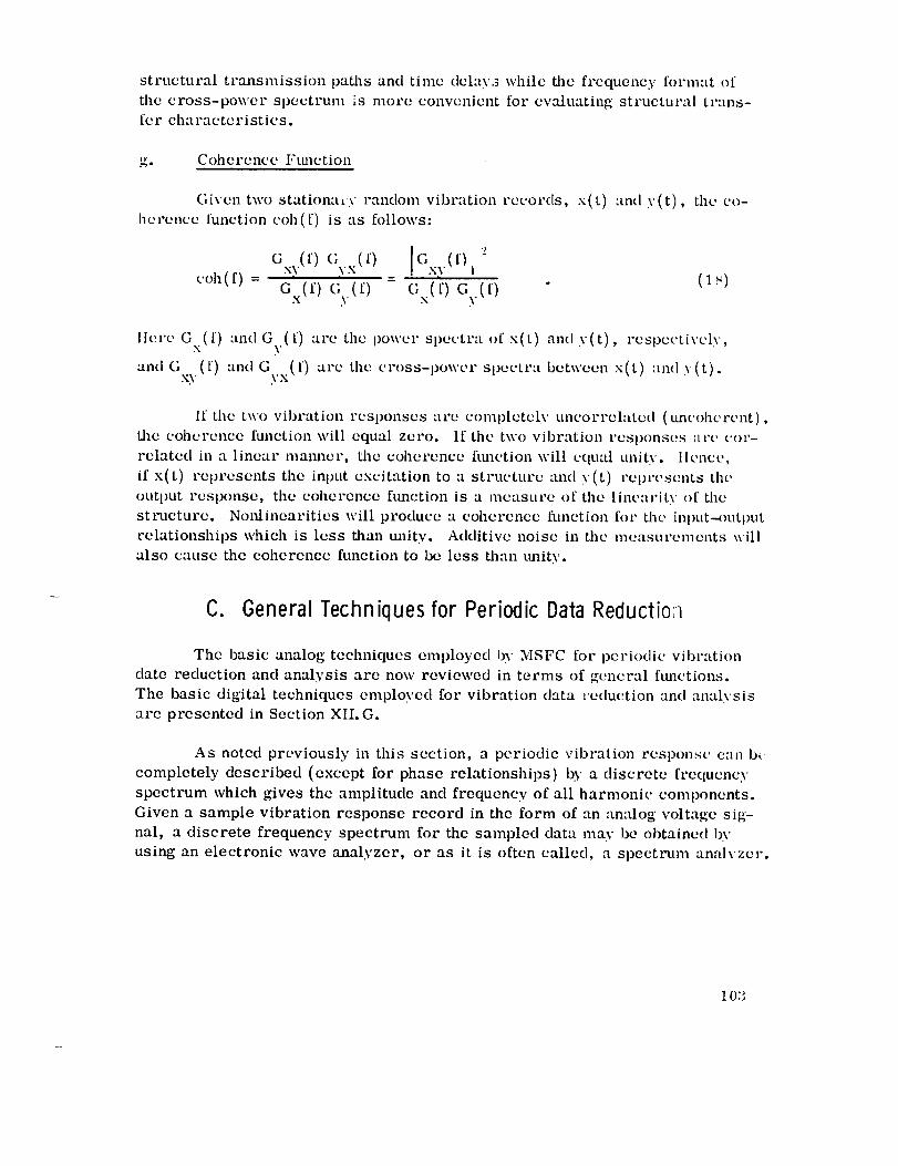
structural transmission paths and time delay,s while the frequency format of
the cross-power spectrum _s more convenient for evaluating structural trans-
[er characteristics.
Coherence Ftmetion
Given two stationa_v random vibration records, x(t) and y(t), the co-
herence [unction cob(f) is as follows:
I 2(oh(r) = (;xT(r) (;'vx(0 - GxY(t)a (1_)
Gx(r) (;y(i) Gx(r) Gy(r) "
llcre G (t') andG,(t) are the power spectra ofx(t) and v(t) respectively,x 3 ' '
and G (f) and Gvx(f ) are the cross-power spectra between x(t) and v(t).xy .,
If tile two vibration responses are coml)letcly uncorrelated (tmcohcrent),
the coherence function will equal zero. If the two vibration responses :trc cor-
related in a linear mamacr, the coherence ftmction will cqu:tl unity, llcnce,
if x(t) represents the input excitation to a structure and y(t) represents the
outl)ut response, the coherence ftmction is a measure of the lincaritv of the
structure. Nonlinearities will produce a coherence tkmction for the inl)ut_)utput
relationships which is less than tmit,v. Additive noise in tile measurements will
also cause the coherence function to be less than tmity.
C. General Techniques for Periodic Data Reduction
The basic analog techniques employed 193'MSFC for l)eriodic vibr'ttion
date reduction and analysis are now reviewed in terms of general ftmctions.
The basic digital techniques employed for vibration data reduction and analysis
are presented in Section XII. G.
As notcd previously in this section, a periodic vibration response can b,
completely described (except for phase relationships) by a discrete frequency
spectrum which gives the amplitude and frequency of all harmonic components.
Given a sample vibration response record in the form of an analog voltage sig-
nal, a discrete frequency spectrum for the sampled data may be obtained 193"
using an electronic wave analyzer, or as it is often eallcd, a speetruna analyzer.
103

There are two basic types of spectrum analyzers. The first type em-
ploys a collection of contiguous frequency bandpass filters. The filters may
be either constant bandwidth filters or constant precentage filters whose
bandwidths are proportional to their center frequencies. When a periodic
signal is applied to the bank of filters, each signal passes those frequencies
lying within its pass band and excludes all others. The output amplitudes fromthe filters are then detected and recorded simultaneously as a function of time.
The instantaneous output from the filters may also be recorded directly, if so
desired. Hence, the spectrum of the applied signal is broken up into as many
intervals as there are filters in the bank. This multiple filter type analyzer is
sometimes called a real time spectrum analyzer because its operation is
substantially instantaneous. This feature constitutes its primary advantage.
A secondary advantage is that phase information can be retained if proper cal-
ibration procedures are employed. The primary disadvantage of a multiple
filter type analyzer is cost. If high resolution is to be obtained, a large num-
ber of expensive filters and amplitude detectors must be incorporated in the
analyzer. A functional block diagram for a multiple filter type spectrum
analyzer is shown in Figure 42.
The second type of spectrum analyzer employs a single narrow frequency
bandpass filter. The signal is moved in frequency past the fixed narrow band-
pass filter by application of the heterodyne principle. The output amplitudefrom the filter is detected and recorded as a function of frequency, giving the
spectrum for the applied signal. The primary advantage of the single filter
type spectrum analyzer is high resolution. Since only a single fixed filter
is used, its characteristics can be optimized without adding appreciably to the
cost of the analyzer. The primary disadvantage of this single filter type
analyzer is that the time required to perform an analysis is relatively long since
the entire frequency range of the signal is investigated with only one narrow
bandpass filter. It should be noted that single filter spectrum analyzers are
usually equipped with several filter selections having different bandwidths to
permit flexibility in choosing the resolution desired for a given analysis. A
functional block diagram for a single filter type spectrum analyzer is shown in
Figure 43.
For either type of spectrum analyzer, the output amplitude detector
consists of circuits which compute one or more of three different amplitude
functions. These are the peak amplitude, the rectified average amplitude,
and/or the mean square amplitude. If the resolution for a given periodic signal
analysis is sufficiently sharp to identify each individual frequency component
of the signal, the amplitude detection circuit employed is of no direct concern
since the outputs from the filter(s) will always be sine waves. The peak,
average, and mean square amplitudes for sine waves have fixed relationships
to one another, as follows:
104

_-|_
,,=,
o,.__z
u,,I
=,,=,<>
I _ /1__i_,, =,_ww
I_++ Jl_
v
Z<_Z
_+]
_z++_m
ms m m
I
I
III
6_-. I
_____]
z__z
Z
o,-,i4_
@
_4
o_,,i
105

II
' ZI
I .., -TJI
I/
0
I-_ u,J I
• -I-"°o I0
c
uJ
ml
2
ol-
ml
r_o
1
II
1.
w !
_z
_ III
• w
I
I
1
w I:C
I
>u_ 0
4_
0
_4
106

instantaneous amplitude = C sin _z t
peak amplitude = C
rectified average amplitude = 0. 636 C (19)
Mean square amplitude = 0.5 C 2
root mean square (rms) amplitude = 0.707 C .
Hence, any one of the three detection circuits may be used and read out in
terms of any other amplitude function desired by simply calibrating the readout
scale in an appropriate manner. For example, the peak value of the filtered
signal may be _:Jtected and read out as an rms amplitude by noting that the rms
amplitude is equal to 0. 707 times the peak amplitude. It is important to
emphasize that these relationships apply only when the analysis resolution is
sufficiently sharp to isolate individual frequency components. The relationshipsin equation (19) do not apply to the sum of two or more sine waves.
The practical considerations associated with the analysis of periodic
signals are reviewed below. All relationships stated are taken from Reference20.
I. ANALYS_ ACCURACY
If the various limitations noted in paragraphs 2., 3., and 4. below are
observed, the only errors in a spectrum analysis of periodic data are the basic
measurement errors inherent in the spectrum analyzer design capabilities andcalibration techniques. There are no intrinsic statistical uncertainties or
sampling errors associated with the proper reduction and analysis of periodicvibration data.
2. RESOLUTION
The frequency spectrum for a periodic signal is theoretically a discrete
line spectrum where each component is a delta function with no bandwidth.
However, a spectrum analyzer will display each component as a peak with an
apparent bandwidth, which of course will be the bandwidth of the spectrum
analyzer filter. Thus, the exact frequency of the signal components will be
more accurately defined as the bandwidth of the analyzer filter is made nar-
rower. The accuracy with which the frequencies of individual components
are identified is generally referred to as the resolution of the analysis.
• 107T

It wotfld appear that the best method of analysis would be to use the
narrowest possible bandpass filter. However, for the multiple filter type
spectrum analyzer, the required number of filters and the associated cost are
inversely proportional to tile bandwidth of the filters. For the single filter
type spectrum mmlyzer, the required analysis time is inversely proportional
to the bandwidth of the filter, as is discussed later. It is important to note,
however, that the resolution of any given spectrum analysis should always be
sufficient to distinguish between adjacent frequency components. In other words,
the analyzer filter bandwidth should always be narrower than the frequency
interval between the components of the signal being analyzed. Thus, the
general criteria for minimum permissible resolution is
B < (1/Tp) (20)
where B is the analyzer filter bandwidth in cps and T is the period of thevibration data in seconds. P
An illustration of a properly resolved spectrum analysis is presented
in Figure 44. In this example, T = 1/50 second, so the maximum permissibleP
bandwidth for acceptable resolution would be B = 50 Hz. However, the actual
bandwidth used was B = 2 Hz resulting in a very precise resolution.
3. SAMPLE RECORD LENGTH
Theoretically, the record length required to perform a spectrum analy-
sis on the sampled periodic vibration data is only T seconds long (the lengthP
of one vibration period). However, for certain practical reasons, it is de-
sirable that the sample record be very much longer than one period. Multiple
filter analyzers are normally employed only when relatively long samplerecords are involved. However, single filter analyzers are often used to
analyze relatively short records.
Analysis of a relatively short sample record with a single filter type
spectrum analyzer is usually accomplished by making a continuous loop from
the sample record so that the data signal may be continuously applied to the
analyzer. The formation of the loop produces, in effect, a fictitious funda-
mental period for the data. Unless the record length is an exact even multiple
of one period Tp, the loop will tend to introduce fictitious frequency components
into the analysis. However, these effects become insignificant if the record
leng'th is, say, 10 times longer than the period of the vibration data. For
108
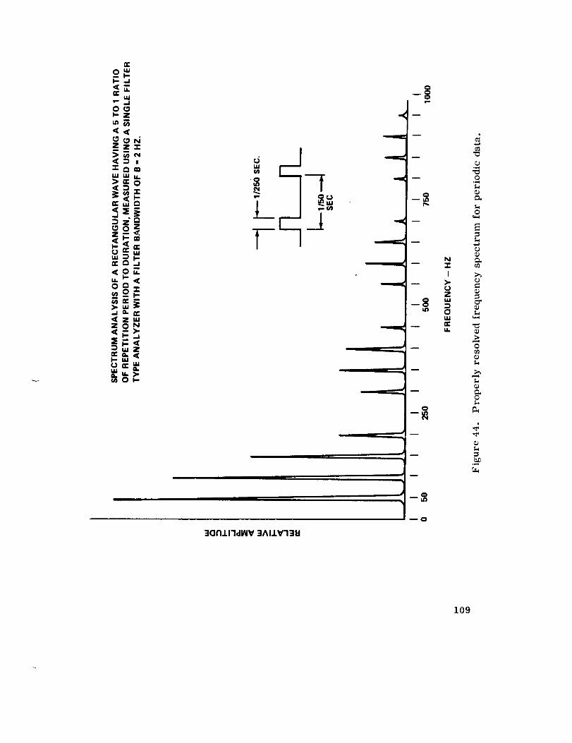
o_I-. -J<_-,
uJv- ,.I00)-Z
<<
° 2_ _ T--
...i 0- or.
I,-uu
_ m
q w
o
q m
-8
q m
0
m
mO
3Gt'IJ.IldMV :IAIJ.V'I_I:I
N
I
>-_JZuJ
0uJ
i,i.
.,,<
0
0
.>0
C_o
4
109

example, assume a periodic signal with a fundamental frequency of 25 Hz is
to bc analyzed. The length of the sample record should be T > 10 T = (1.4second. P
4. AVE RAGING TI.ME
The peak, average, and/or mean square amplitude detectors incorporated
in the spectrum analyzer compute the desired amplitude function by smoothing
or time averaging the instantaneous output of an appropriate rectifier circuit
(RC). For example, the average amplitude of a signal component is usuallymeasured b_, a simple ac voltmeter circuit where the component is rectified,
and the instantaneous rectified amplitude is averaged by smoothing with an
equivalent low-pass RC filter. The equivalent RC time constant of the averag-
ing filter should be longer than the period of the vibration data being analyzed.
Thus, a general criteria for the minimum time constant of the averaging filteris
K > T (21)P
where K is the equivalent RC time in seconds.
For example, assume a periodic signal with a fundamental frequency
of 25 Hz is to be analyzed. The minimum time constant for the averaging filteris K >T = 0.04 second.
P
5. SCAN RATE AND ANALYSIS TIME
For the multiple filter type spectrum analyzer, the frequency compon-
ents of the applied signal are concurrently measured, so the analysis time
is substantially instantaneous. However, for the single filter type spectrum
analyzer, the frequency components of the applied signal must be individually
measured by scanning through the entire frequency range of interest. If the
scan is too fast, one of two difficulties may occur.
a. The narrow bandpass filter of the spectrum analyzer will not
fully respond to the individual frequency components of the signal.
b. The amplitude detector averaging filter will not fully respond to
abe individual frequency components of the signal.
The response time for narrow bandpass filters is a function of the
exact filter characteristics, but, in general, will be less than (l/B) seconds
110

where B is the bandwidthof the filter in Hz. Thus, a general criteria for themaximum analysis scan rate basedon the analyzer filter response is
scan rate < B2Hz/sec (22a)
The response time for equivalent RC low-pass averaging filters is suchthat about 98 percent of full response is reached in a time equal to four time
constants (4K). Thus, a general criteria for the maximum analysis scan
rate based on the averaging filter response is
Bscan rate < --_ Hz/sec (22b)
If the total frequency range for the analysis is F Hz, the minimumanalysis time is
analysis time
FB"-_ seconds (23a)
>4KF"-B-- seconds (23b)
For example, assume a periodic signal is to be analyzed with a filter band-
width of B = 10 Hz and an averaging time constant of K = 0.1 second, over a
frequency range from near 0 to 2000 Hz (F = 2000 Hz). The maximum scan
rate is 25 Hz/sec, since equation (22b) produces the smaller value. Hence,
the minimum analysis time is 80 seconds, since equation (23b) produces thelarger value.
D. General Techniques for Random Data Reduction
The basic analog techniques employed by MSFC for random vibration
data reduction and analysis are now reviewed in terms of general functions.
The basic digital techniques employed for vibration data reduction and analysisare presented in Section XII. F.
As noted Paragraph B. 2 of this section, a stationary random vibration
response can be described in the amplitude domain by a probability density
function as given in equation (8), in the time domain by an autocorrelationfunction as given in equation (10), and in the frequency domain by a power
spectral density function as given in equation (12). If two or more vibration
response records are available, additional information may be obtained from
III

a joint probability density function as given in equation (13), a cross-correlationfunction as givcn in equation (14), and a cross-power spectral density functionas given in equation (15).
The true measurementof the above-mentionedproperties requires the
determination of a limit as the record length T approaches infinity. Further-
more, the true measurement of probability and power spectral density functions
also requires the determination of a limit as either an amplitude interval Ay
or a frequency interval A f approaches zero. Clearly, the determination of
these limits is physically impossible. Thus, no real instrument can actually
measure the true properties of a random vibration. However, measurements
can be performed which produce meaningful estimates for the desired proper-ties. These measurement techniques are now discussed.
1. AMPLITUDE PROBABILITY DENSITY ANALYSIS
Given a sample vibration response record in the form of an analog
voltage signal y(t) with a finite length of T seconds, the amplitude probability
density function for the vibration response may be estimated from equation
(8) as follows:
_(y) __--_} . (24)
Here, _¢¢ is the average portion of the time spent by the signal y(t) within a
narrow amplitude interval having a gate width of W volts and a center amplitude^
of y volts. The hat (^) over p(y) means that the measured quantity is only
an estimate of p(y), since the record length T and the gate width W are finite.
The amplitude probability density function is estimated by the following opera-
tions.
a. Amplitude filtering of the signal by a narrow amplitude gate having
a gate width of W volts.
b. Measurement of the total time spent by the signal within the gate.
c. Division of the time spent within the gate by the total sampling
time, to obtain the average portion of time spent by the signal within the gate.
d. Division of the average portion of the time spent within the gate by
the gate width W.
112

As the center amplitude of the gate is moved, a plot of the probability densityfunction versus amplitude is obtained.
The aboveoperations are accomplishedby ananalogamplitude proba-bility density analyzer, which will be called anAPD analyzer for simplicity.In general, an APD analyzer measuresthe time spentby a signal within somenarrow amplitude interval by use of a voltage gate (narrow bandvoltage dis-criminator) followed by a clock circuit. Whenthe input signal amplitude fromthe sample record falls within the gate, the clock circuit operates. For allother signal amplitudes, the clock circuit doesnot operate. The clock circuitoutput is averagedover the entire time of observation T to obtain the averageaportion of time spent by the signal amplitude within the narrow gate. Therequired division by the gate width W may be obtainedby a proper scale cali-bration.
There are two basic types of APD analyzers. The first type employsa collection of contiguousvoltage gateswith equal gatewidths. The multiplegate type analyzer measures the probability density within eachgate simultane-ously to give a plot of probability density versus amplitude. The secondtypeemploys a single gatewhosecenter voltage is variable relative to the voltageof the signal. The single gate type analyzer producesa plot of probabilitydensity versus amplitude by sweeping (or stepping) the single gate through the
entire range of voltage amplitudes of interest. A functional block diagram for
a single gate APD analyzer is shown in Figure 45.
The practical considerations associated with amplitude probability
density analysis are reviewed below. All relationships stated are taken from
Reference 20. Many of the relationships are also studied experimentally inReference 21.
a. Analysis Accuracy
The analysis of random vibration data involves basic measurement
errors due to the analysis equipment design capabilities and calibration tech-
niques, just as is true for the analysis of periodic vibration data. However,
the analysis of random data also involves an additional error which is called
the statistical uncertainty or probable sampling error. As was mentioned
earlier, the data measured from sample records of finite length constitute
only statistical estimates of the true prouerties of the sampled vibration re-
sponse. The expected deviation of the estimated properties from the actual
properties of the random vibration represents the statistical uncertainties
associated with the measurements. Thus uncertainty may be defined in terms
of a normalized standard deviation for the sampling distribution, which is often
called the standard error e.
113

114
For the specific case of amplitude probability density analysis, the
standard error associated with a measured estimate p(y) is as follows:
0.20 (25)e _ j (y)WBT
Here, _(y) is the measured probability density, W is the amplitude gate width
in relative amplitude units, B is the bandwidth of the signal being investigated,
and T is the length of the analyzed sample record in seconds.
Several important features of equation (25) should be noted. First,
this expression for the standard error is a simplification of more complicated
relationships developed theoretically and empirically in Section 14 of Reference
21. However, equation (25) is an acceptable approximation for most applica-
tions. Second, the standard error e is a function of the actual probability
density estimate that is measured. Thus, for any given gate width, bandwidth,
and record length, the uncertainty of the estimate varies with the amplitude
being analyzed. Third, the bandwidth B assumes that the vibration signal has
a power spectrum which is uniform between two frequencies B Hz apart, and
zero elsewhere. In other words, the signal is assumed to be white noise which
has been filtered with an ideal rectangular bandpass filter having a bandwidthB.
The meaning of the standard error e is as follows. Assume a stationary
random vibration response with a true probability density function of p(y) is
repeatedly sampled at different times, and an estimate p(y) is measured for
each sample. For about 68 percent of the estimates obtained, the difference
between the estimate p(y) and the true value p(y) will be less than ± e _(y).
Stated in another way, if an estimate p(y) is measured, one may say with about
68 percent confidence that the true value p(y) is within the range (1+ e)p(y).
A plot of the standard error e versus the WBT product for various amplitude
probability density estimates is presented in Figure 46.
For example, assume an amplitude probability density function is
measured from a sample record that is T = 0 second long using an APD anal-
yzer with a gate width of W = 0.1 volt. Further assume the bandwidth of
the signal is B = 100 Hz. If a probability density of p = 0.16 were measured at
the amplitude y = 1.5 volt (Yrms 1 volt), the standard error for the estimate
115

o
II
UOUU3GUVONVI$
m o
00
o
116

would be e = 0.05. Hence, one could say with 68 percent confidence that the
true probability density at that amplitude is within + 5 percent of the measuredvalue, or between 0.152 and 0.168.
b. Resolution
Equation (25) shows that the statistical uncertainty of probability density
estimates is inversely proportional to the width of the amplitude gate. One
might then conclude that improved estimation accuracy can easily be obtained
by simply increasing the gate width. However, increasing the gate width re-
duces the resolution of the analysis; that is, it reduces the ability of the anal-
ysis to properly define peaks in the probability density plot. The selection of
the analyzer gate width is always a compromise between estimation uncertainty
and resolution. A general criterion for proper resolution is a gate width that
is less than one-fourth of the rms signal amplitude; that is,
1W < _" Yrms (26)
where W is the analyzer gate width in volts and y is the root mean squarevalue of the signal being analyzed in volts, rms
c. Sample Record Length
As seen from equation (25), the sample record length T limits the
statistical accuracy attainable in an amplitude probability density analysis.
The longer the record length, the lower the uncertainty in the resulting proba-
bility density estimates. If the statistical uncertainty of a probability density
analysis is to be limited to a given desired amount, these matters must be
considered before the data are gathered to assure that sample records are
sufficiently long.
d. Averaging Time
An APD analyzer computes the portion of time spent by the signal
amplitude within the gate by averaging the output of the gate clock circuit.
The averaging may be accomplished by true linear integration, called true
averaging, or by continuous smoothing with an equivalent low-pass RC
filter, called RC averaging. True averaging produces a single probability
density estimate after a specific averaging time T while RC averaginga
produces a continuous probability density estimate. If the RC time constant
117
of the averaging filter is K and the record length T is long compared to K,
the continuous estimate at any instant of time has an uncertainty equivalent to
an estimate obtained by true averaging over a time interval of T -- 2K.a
For the case of true averaging, it is clear that the averaging time Ta
should be as long as the record length T if the uncertainty in the resulting
estimates is to be kept at a minimum. In other words, all of the information
available from the sample record should be employed for the probability
density measurement. If T is less than T, the uncertainty will be increaseda
since T will replace T in equation (25). If T is greater than T, as it coulda a
be when the sample record is formed into a continuous loop for analysis, the
uncertainty will not be decreased from the value given in equation (25) since
one is simply looking at the same information more than once.
For the case of RC averaging, minimum uncertainty can be achieved
only by making the time constant K very long. However, a long averaging
time constant reduces the scan rate and greatly increases the total analysis
time, as is discussed in Paragraph D. 1. a. of this section. A reasonablecompromise is to use an averaging time constant that is at least one-half
the record length T.
Thus, the general criteria for the ideal averaging time for a probability
density analysis are as follows:
for true averaging, T = T (27a)a
for RC averaging, 2K _ T . (27b)
Here, T is the true averaging (integration) time in seconds, and K is thea
time constant of the equivalent RC averaging filter in seconds.
e. Scan Rate and Analysis Time
For the multiple gate type APD analyzer, the probabilitydensity is
concurrently measured over all amplitudes of interest, so the analysis time
is equal to the record length T. However, for the single gate type APD
analyzer, the probabilitydensity at all amplitudes of interestmust be mea-
sured by scanning through the desired amplitude range. Ifthe scan is too
fast, allthe information availa_!e at a given amplitude willnot be viewed by
the analyzer gate over the entire record length, and the statisticaluncertainty
of the resultingestimate will be increased. IfRC averaging is used, the scan
rate is further limited because time must be allowed for the RC averaging filter
118

to respond to abrupt changes in the probabilitydensity function. The limitations
imposed upon the scan rate by these considerations are as follows:
Wfor true averaging, scan rate < _ (28a)
a
Wfor RC averaging, scan rate < ix4_ " (28b)
Here, T is the averaging time in seconds, K is the RC time constant in seconds,a
and W is the gate width in volts. Hence, scan rate has the units of volts persecond.
If the total amplitude range for the APD analysis is A volts, the mini-
mum analysis time is as follows:
for true averaging, analysis time
TA
a (29a)> W
for RC averaging, analysis time4KA
> _ • (29b)
For example, assume the amplitude probability density function for a
random vibration response is to be estimated from a sample record of length
T = 10 seconds over an amplitude range from minus four volts to plus four
volts (A = 8 volts) using an APD analyzer with a gate width of W = 0.1 volt.
The rms amplitude of the signal is assumed to be 1 volt. If true averagingis used, T = 10 seconds and the maximum scan rate is 0.01 volt/second.
a
Hence, the minimum analysis time is 800 seconds or 13.3 minutes. If RC
averaging is used, K >_-5 seconds, and the maximum scan rate is 0. 005
volt/second. Hence, the minimum analysis time is 1600 seconds, or about 27minutes.
2. AUTOCORRELATION ANALYSIS
Given a sample vibration response record in the form of an analog
voltage signal y(t) with a finite length of T seconds, the autocorrelation func-
tion for the vibration response may be estimated from equation (10) as follows:
A
R (_')= y(t) y(t + T) • (30)Y
119

Here, y(t) y(t + 7) is the average product of the instantaneous signal amplitude^
at two different times which are r seconds apart. The hat (^) over R (T)Y
means that the measured quantity is only an estimate of R (r), since the recordY
length T is finite. The autocorrelation function is estimated by the followingoperations:
a. Delaying the signal by a time displacement equal to _- seconds,called the lag time.
b. Multiplying the amplitude at any instant by the amplitude that hadoccurred-r seconds before.
Co
time.Averaging the instantaneous amplitude product over the sampling
As the lag time is moved, a plot of the autocorrelation function versus lag timeis obtained.
The above operations are accomplished by an analog autocorrelation
function analyzer, which will be called an ACF analyzer for simplicity. In
general, an ACF analyzer displaces the signal in time by use of a magnetic
signal recorder with a variable lag time between the record and playback.
This can be accomplished, for example, with a magnetic drum recorder where
the location of the playback head is variable relative to the location of the record
head. The input and output of the lag time generator are then multiplied and
averaged. The lag time is variable over a range from zero to the longest
sampling times that are anticipated. Since the autocorrelation function is an
even function, it is not necessary to make measurements with negative lag
times. A functional block diagram for an ACF analyzer is shown in Figure 47.
The practical considerations associated with autocorrelation analysis
are reviewed below. All relationships stated are taken from Reference 20°
a. Analysis Accuracy
As discussed in Paragraph D. 1. a. of this section, the analysis of ran-
dom vibration data involves not only basic measurement errors, but also a
statistical uncertainty inherent in the sampling procedures. Thus, uncertainty
may be defined in terms of the standard error e for the sampling distribution.
For the specific case of autocorrelation analysis, the standard error as-^
sociated with a measured estimate R (r) is as follows.Y
120

v
A
_LZ
- Ib.
= I I _11__ I__1
i I _II" I _II Y JL____ '__ ____1
,,J 0w I,-
I
e_
@
0
0
[-,,,.
121

1e . (:'1)
r-B-T
Here, B is the noise bandwidth of the signal in Hz and T is the length of the
analyzed sample record in seconds. It is assumed in deriving equation (:'1)that T < < T and that BT >- 10.
Two important features of equation (31) should be noted. First, this
expression for the standard error is a conservative approximation wClich is
accurate for lag times near zero. For large lag times, the standard error
is not explicitly defined but is somewhat less than the quantity given in equation
(31). Second, the bandwidth B is the noise bandwidth of the vibration response
signal. The determination of noise bandwidths is covered in Paragraph E. ofthis section.
The general meaning and interpretation of the standard error e is
discussed in Paragraph D. 1 of this section. The specific interpretation for
autocorrelation analysis is as follows. Assume a stationary random vibration
response with a true autocorrelation function of R (T) is sampled, and ana Y
estimate R (7) is measured from the sample. If e is reasonably small, sayY
less than 0.30, it may be said with about 68 percent confidence that the true
value Ry(T) is within the range (1 + e)Ry(_-). A plot of the standard error e
versus the BT product is presented in Figure 48.
For example, assume an autocorrelation function is measured from a
sample record that is T = 10 seconds long. Further assume the noise band-
width of the signal is B = 100 Hz. The standard error for the resulting esti-A
mate is e _ 0.032. Hence, if a measured estimate R (1-) at time _- = 0 wereY
about 0.3 volt 2, it could be said with 68 percent confidence that the true auto-
correlation function for that lag time is within ± 3.2 percent of the measuredvalue, or between 0.29 and 0.31 volt 2.
b. Resolution
A
As seen from equation (30), the autocorrelation function R(T) must be
estimated at various different lag times _- to obtain a plot of the autocorrelation
function versus lag time. The interval between the lag times at which compu-
tations are made defines the resolution of the autocorrelation plot. Based upon
practical considerations, a general criteria for proper resolution is a lag
time interval that is less than one-fourth the reciprocal of the signal bandwidth;that is,
122

to
I I IUOHI:I3 O_IVONVIS
iNo,o
l--r,J
D0n,-a.l,.-gD
oi,o
o
0
O*_,,¢
,pc
123

1h < 4"_ (32)
where h is the interval between lag times in seconds and B is the bandwidth
of the signal in Hz.
The relationship in equation 8. 33 is directly appropriate for the case
when an autocorrelation function is computed at specific lag times, TI, r_= T 1 + h, r3 -- _1 + 2h, etc. However, analog instruments often determine an
autocorrelation plot by continuous averaging while the time delay generator
makes a continuous scan through the lag time range of interest. For this case,
the relationship in equation (32) constitutes the basis for a limit on the hag
time scan rate. This limit is discussed in Paragraph e. below.
c. Sample Record Length
As seen from equation (31) the sample record length T determines the
statistical accuracy attainable in an autocorrelation analysis. The longer the
record length, the lower the uncertainty in the resulting autocorrelation esti-
mates. If the statistical uncertain_y of an autocorrelation analysis is to belimited to a given desired amount, these matters must be considered before
the data are gathered to assure that sample records are sufficiently long.
d. Averagin_ Time
An ACF analyzer computes the mean product of the signal amplitudes
at two different times by averaging the output of the multiplier circuit. The
averaging may be accomplished by true linear integration, called true averag-
ing, or by continuous smoothing with an equivalent lowpass RC filter, called
RC averaging. True averaging produces a single autocorrelation estimate
after a specific averaging time T a while RC averaging produces a continuousprobability density estimate.
For the reasons presented in Paragraph D. 1. d. of this section, the
general criteria for the ideal averaging time for an autocorrelation analysis is
for true averaging, T = T (33a)a
for RC averaging, 2K > T (33b)
124

Here, T is the true integrating time in seconds, and D is the time constanta
of the equivalent RC averaging filter in seconds.
e. Scan Ra_e and Analysis Time
The autocorrelation function at all lag times of interest must be meas-
ured by scanning through the desired time delay range. This may be done in
discrete steps or a continuous sweep. For the case of a stepped scan, if the
scan rate is too fast, all the information available at a given lag time will not
be analyzed and the statistical uncertainty of the resulting estimate will be
increased. For the case of a continuous scan, if the scan rate is too fast, the
resolution of the resulting estimate will be reduced. If RC averaging is used,the scan rate is further limited because time must be allowed for the RC
averaging filter to respond to abrupt changes in the autocorrelation function.
The limitations imposed upon the scan rate by these considerations are asfollows:
for true averaging, scan rate < 4BTa
(34a)
for RC averaging, scan rate < 16 BK (34b)
Here, T is the averaging time in seconds, K is the RC time constant ina
seconds, and B is the noise bandwidth in Hz. Hence, scan rate has the units
of seconds per second.
If the maximum lag time for the AC F analysis is T seconds wherem
is relatively small compared to the record length T, the minimum analysism
time is as follows:
for true averaging, analysis time > 4BT _ (35a)a m
for RC averaging, analysis time > 16 BK 1"m
(35b)
For example, assume the autocorrelation function for a random vibration
response is to be estimated from a sample record of length T -- 10 seconds.
Further assume the vibration signal has an upper frequency limit of f = 100 HzU
125

and that lag times of up to _ = 1 second are of interest. If true averaging ism
used, T = 10 seconds and the maximum scan rate is 0.00025 second/second.a
Hence, the minimum analysis time is 4000 seconds or about 67 minutes. If
RC averaging is used, K > 5 seconds and the maximum scan rate is 0.000125
second/second. Hece, the minimum analysis time is 8000 seconds or about134 minutes.
3. POWER SPECTRAL DENSITY ANALYSIS
Given a sample vibration response record in the form of an analog
voltage signal y(t) with a finite length of T seconds, the power spectral density
function for the vibration response may be estimated from equation (12) asfollows:
m
^ Y2BG (f)= . (36)
y B
m
Here, y2B is the average of the squared instantaneous signal amplitude (mean
square value) in a narrow frequency interval having a noise bandwidth of B Hz^
and a center frequency of f Hz. The hat (n) over G (f) means that the meas-Y
ured quantity is only an estimate of G (f), since the record length T and theY
bandwidth B are finite. The power spectral density function is estimated bythe following operations:
a. Frequency filtering of the signal by a narrow bandpass filterhaving a bandwidth of B Hz.
b. Squaring of the instantaneous amplitude of the filtered signal.
Ce
time.Averaging the squared instantaneous amplitude over the sampling
d. Division of the mean square output by the bandwidth B.
As the center frequency of the bandpass filter is moved, a plot of the power
spectral density function versus frequency is obtained. This plot is oftencalled the power spectrum.
126

l?he above operations are accomplished by an analog power spectral
density analyzer, which will be called a PSD analyzer for simplicity. It is
important to note the similarity between the PSD analyzer and a simple spec-
trum analyzer used for periodic data analysis, as discussed in Section VIII• C.
Since the division by the bandwidth B is only a matter of proper scale cali-
bration, the PSI) analyzer is nothing more than a spectrum analyzer with a
mean square amplitude detection circuit. Thus a PSD analyzer may be used
to analyze periodic vii)ration data as well as random vibration data. How-
ever, a simple spectrum analyzer may not be used to analyze random
vibration (lata unless a mean square amplitude detection circuit is available.
A peak amplitude detection circuit would obviously produce meaningless
results, since a random signal has no specific peak amplitude. An average
amplitude detection circuit would produce results that have no real analytical
meaning, although the average value of a random signal can be related to the
mean square value if the probability density function for the random signalis known. These matters arc discussed further in Section VIII. F.
Similar to the spectrum analyzers discussed in Section VIII• C., a PSD
analyzer may be either a multiple filter type analyzer employing a bank of
contiguous filters, or a single filter type analyzer• A functional block diagram
for a single filter type PSD analyzer is shown in Figure 49.
The practical considerations associated with power spectral density
analysis are reviewed below. All relationships stated are taken from Reference
20. Many of the relationships are also studied experimentally in Reference 21.
a• Analysis Accuracy
As discussed in Paragraph D. 1.a. of this section, the analysis of
random vibration data involves not only basic measurement errors, but also
a statistical uncertainty inherent in the sampling procedures. This uncertainty
may be defined in terms of the standard error e for the sampling distribution.
For the specific case of power spectral density analysis, the standard errorA
associated with a measured estimate G (f) is as follows:y
1 (37)e _ •
4-gg
Here, B is the bandwidth of the PSD analyzer filter in Hz, and T is the length
of the analyzed sample record in seconds.
127

Ae.J
v
m
m
uJ LL
DCJ
v
m
t_t_
m
Z
n-Ol-
,.J
r_0:E
>'1-0
o_ 1• I
t__L_ I
_0 rrnrl--
>n-
On"
-- >
_ _ J
III
I °-I
1_- r_M j
, ul _..
X n-
J_
=
o_
0
_0
o
c_Cc_
128

/
Note that the uncertainty expression for a power spectral density analy-
sis is similar to the uncertainty expression for an autocorrelation analysis, as
g:ivc_ l,: eqaatio_, (:;1). _owevcr me interpretation of the baedwidth B in the
two expressions is slightly different. For a power spectral density analysis,
B is the bandwidth for that portion of the signal spectrum within the frequency
range of the PSD analyzer bandpass filter, which is approximately equal to
the noise bandwidth of the analyzer filter for a properly resolved power spectral
density analysis. The determination of noise bandwidths for filters is dis-
cussed in Paragraph E. of this section. For the narrow bandpass filter in most
PSD anal_'zers, the noise bandwidth may be considered equivalent to the half
power point bandwidth of the filter.
The general meaning and interpretation of the standard error e is dis-
cussed in Paragraph D. 4.a. of this section. The specific interpretation for
power spectral density anal)'sis is as follows. Assume a stationary random
vibration response with a tru_ power spectral density function of G (f) isA Y
sampled, and an estimate G (f) is measured from the sample. If e is relativelyY
small, say less than 0.30, it may bc said with about 68 percent confidence thate\
the true value G (f) is within the range (1 _ c) G (f). A plot of the standardY Y
error e versus the BT product is presented in Figure 48.
For example, assume that a power spectral density function is measured
from a sample record that is T = 10 seconds long using a PSD analyzer with a
filter bandwidth of B = I0 Hz. The standard error for the resulting estimate^
is e _ 0. i0. Hence, if a measured estimate G (f) at a given frequency wereY
0.3 volt2/Hz, it could be said with 6_ percent confidence that the true power
spectral density function for that frequency is within ± 10 percent of the
measured value, or between 0.27 and 0.33 volt2/Hz.
b. Resolution
Equation (37) shows that the statistical uncertainty of power spectral
density estimates is inversely proportional to the bandwidth of the analyzer
filter. One might then conclude that improved estimation accuracy can easily
be obtained by simply increasing the filter bandwidth. However, increasing
the filter bandwidth reduces the resolution of the analysis; that is, it reduces
the ability of the analysis to properly define sharp peaks in the power spec-
trum. The selection of the analyzer filter bandwidth is always a compromise
between estimation uncertainty and spectral resolution. It should be further
129

noted that if there are sharp peaks within the filter bandwidth, the resulting
uncertainty will actually be greater than predicted by equation (37). Hence,
the emphasis should be placed upon an analyzer bandwidth which will afford
proper resolution. A reasonable criteria for proper resolution is a filter
bandwidth that is one-fourth the bandwidth (between half power points) of the
narrowest peak in the power spectrum; that is,
1B < "_ (f_- fl) (38)
where B is the analyzer filter bandwidth in cps and (f2 - fl) is the bandwidth
between the half power points of a power spectral density peak in Hz.
c. Sample Record Length
As equation (37) shows, the sample record length T limits the statisti-
cal accuracy attainable in a power spectral density analysis. The longer the
record length, the lower the uncertainty in the resulting power spectral density
estimates. If the statistical uncertainty of a power spectral density analysis
is to be limited to a given desired amount, these matters must be considered
before the data are gathered to assure that sample records arc sufficiently long.
d. Averaging Time
The mean square amplitude detector incorporated in the PSD analyzer
computes a mean square value by averaging the instantaneous output of a square
law rectifier. The averaging may be accomplished either by true linear inte-
gration, called true averaging, or by continuous smoothing with an equivalent
low-pass RC filter, called RC averaging. PSD analyzers are usually equipped
with both types of averaging circuits. True averaging produces a single power
spectral density estimate after a specific averaging time interval T a, while
RC averaging produces a continuous power spectral density estimate.
For the reasons presented earlier, the general criterion for the ideal
averaging time for a power spectral density analysis is
for true averaging, T a = T (39a)
for RC averaging, 2K <--T • (39b)
Here, T is the true integrating time in seconds, and K is the time constanta
of the equivalent RC averaging filter in seconds.
130

e. Scan Rate and Analysis Time
For the multiple filter type PSD analyzer, the power spectral density
is concurrently measured over all frequencies of interest, so the analysis time
is equal to the record length T. However, for the single filter type analyzer,
the power spectral density at all frequencies of interest must be measured by
scanning through the desired frequency range. If the scan is too fast, one of
three difficulties may occur_
1. The statistical uncertainty of the resulting estimate will be in-
creased because all the information available at, a given frequency will not be
viewed by the analyzer filter over the entire record length.
2. The narrow bandpass filter of the PSD analyzer will not fully
respond to a sharp peak in the power spectrum of the signal.
3. If RC averaging is used by the amplitude detector, the averaging
filter will not fully respond to sharp peaks in the power spectrum of the signal.
The limitations imposed upon the scan rate by the above mentioned consider-
ations are as follow:
for true averaging, scan rate <
(4oa)T
a
B-- (4Oh)8
for RC averaging, scan rate <
B___ (40c)4K
B 2-- • (40d)
8
Here, T is the averaging time in seconds, K is the RC time constant ina
seconds, and B is the bandwidth of the PSD analyzer in Hz. Hence, scan rate
has the units of Hz per second.
If the total frequency range for the PSD analysis is F Hz, the minimum
analysis time is as follows:
131

for true averaging, analysis time >
FT
(41a)B
8F
(41b)
for RC averaging, analysis time >
4FK"E- (41c)
8FB--F- (41d)
For example, assume the power spectral density function for a random
vibration response is to be estimated from a sample record of length T = 10
seconds over a frequency range from near 0 to 2000 Hz (F = 2000 Hz) using a
PSD analyzer filter bandwidth of B = 10 Hz. if true averaging is used, T ffi 10a
seconds and the maximum scan rate is 1 Hz/second, since equation (40a) pro-duces the smaller value. Hence, the minimum analysis time is 2000 seconds
or about 33 minutes, since equation (41a) produces the larger value. If RC
averaging is used, K > 5 secomls and the maximum scan rate is 0.5 Hz/second,
since equation (40c) produces the smaller value. Hence, the minimum analy-
sis time is 4000 seconds or about one hour and seven minutes, since equation
(41c) produces the larger value.
4. JOINT AMPLITUDE PROBABILITY DENSITY ANALYSIS
Given two sample vibration response records in the form of analog
voltage signals x(t) and y(t), each with a finite length of T seconds, the joint
amplitude probability density function for the two vibration responses may be
estimated from equation (13) as follows:
tw ; tWA
x y . (42)p(x,y) = W Wx y
Here, tw ; tw is the average time spent by the signals x(t) and y(t) whilex y
they are simultaneously within the narrow amplitude intervals having gate widths
132

of W and W volts and center amplitudes of x and y volts, respectively. Thex y
Ahat (^) over p(x, y) means that the measured quantity is only an estimate of
p(x, y), since the record length T and the gate widths W and W are finite.x y
In words, the joint amplitude probability density function is estimated by the
following operations:
a. Individual amplitude filtering of the two signals x(t) and y(t) by
narrow amplitude gates having widths of W and W volts, respectively.x y
b. Measurement of the total joint time spent by the two signals while
they are simultaneously within the gates.
c. Division of the total joint time spent within the gates by the total
sampling time, to obtain the average portion of time spent by the two signals
while they are simultaneously within the gates. •
d. Division of the average portion of time spent within the gate_ by
the product of the gate widths W W .x y
As the center amplitude of each gate is moved, a three dimensional plot of the
joint probability density function versus amplitudes x and y is obtained.
The above operations are accomplished by an analog joint amplitude:
probability density analyzer, which will be called a joint APD analyzer for
simplicity. In general, a joint APD analyzer consists of two simple APD
analyzers as discussed in Paragraph D., except the voltage gates in the two
analyzers are followed by a single common clock circuit. When the input sig-
nal amplitude from one sample record falls within the first analyzer gate while
the input signal amplitude from a second sample record simultaneously falls
within the second analyzer gate, the clock circuit operates. For all other
amplitude combinations, the clock circuit does not operate. As for the simple
APD analyzer, the joint APD analyzer may incorporate either multiple pairs
of gates or a single pair of gates. A functional block diagram for a single gate
pair type joint APD analyzer is shown in Figure 50.
The practical considerations associated with joint amplitude probability
density analysis are reviewed below. All relationships stated are based uponmaterial in Reference 20.
133
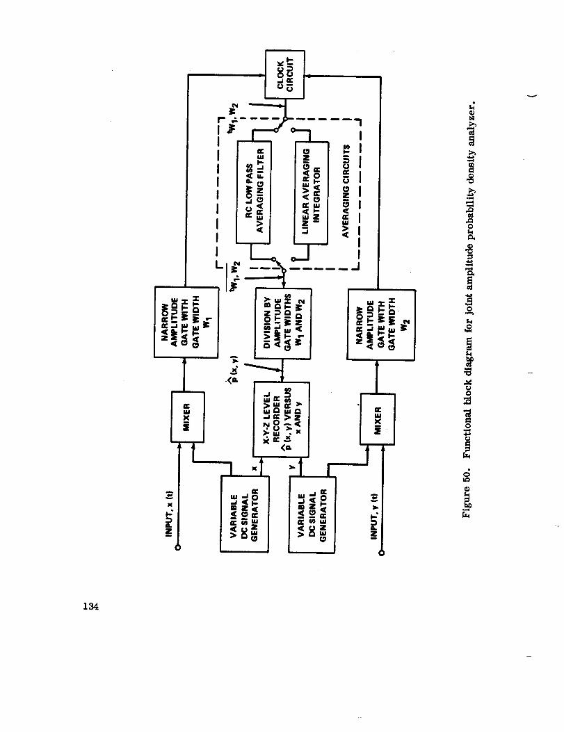
my.

a. Analysis Accuracy
The measurement of joint amplitude probability density functions in-
volves a statistical uncertainty just as does the measurement of simple ampli-
tude probability, density functions discussed in Paragraph D. 1. a. of this
section. Howcvcr, this uncertainty in terms of the standard error e has not
bccn completely evaluated for the case of joint probability density functions.
It can only bc said that the standard error will be much greater for joint proba-
bility density measurement than for simple probability density measurements,
given similar signal bandwidths and record ler_hs.
b. Resolution
c. Sample Record LcnB1; h
d. Averaging Time
The considerations associated with these three factors are exactly the
same as for simple probability density measurements discussed in Paragraphs
D.l.a., b., andc.
e. Scan Rate and Analysis Time
The general limitations imposed upon the scan rates for joint proba-
bility density analysis are exactly the same as for simple probability density
analysis discussed in Paragraph D. 1.d. of this section. However, there are
two signals whose amplitude ranges must be scanned for a joint probability
density analysis. In effect, this means that the gate for signal x(t) must be
scanned through the entire amplitude range of interest for x(t), with the gate
for signal y(t) fixed at each of the numerous positions required to cover the
entire amplitude range of interest for y(t). If the tots/amplitude range of
interest for x(t) and y(t) is A and A volts, respectively, the minimumx y
analysis time is as follows:
for true averaging, analysis time >
TAAa x _,
WWx y
for RC averaging, analysis time >
4KA Ax y
W Wx y
(43a)
(43b)
135

Here, T is the averagingtime in seconds, K is the RC time constant in seconds,a
and W and W are the gate widths in volts.x y
For example, assume that the joint amplitude probability density function
for two random vibration responses is to be estimated from two sample records,
each of length T = 10 seconds, over an amplitude range from minus 4 volts to
plus 4 volts (A = A = 8 volts) using a joint APD analyzer with gate widths ofx y
W = W = 0.1 volt. The rms amplitude of both signals is assumed to ]_ 1 volt.x y
If true averaging is used, T = 10 seconds and the maximum sc'm rate for Aa x
is 0.01 volt/second for each position of A . ttencc, the minimum amdysis timeY
is 64 000 seconds or 17.8 hours. If RC averaging is used, K _ 5 seconds :mdthe maximum scan rate for A is 0. 005 volt/second for each position of A .
X y
Hence, the minimum analysis time is 128 000 seconds or 35. (i hours. These
results should be compared with the example following equation (29).
5. CROSS-CORRELATION ANALYSIS
Given two sample vibraticn response records in the form of analog
voltage signals x(t) and y(t), each with a finite length of T seconds, the cross-
correlation function for the two vibration responses may be estimated from
equation (44) as follows:
T^ 1R ('r) = x(t) y(t + T) - "_ .f x(t) y(t + T) dt . (44)
xy 0
Here, x(t) y(t + T) is the time average cross product of the instantaneous
amplitude of the two signals when one signal is displaced in time from theA
other by V seconds. The hat (^) over R (-r) means that the measuredx3'
quantity is only an estimate of Rxy(T ) , since the record length T is finite. In
words, the cross-correlation function is estimated by the following operations:
a. Delaying the signal x(t) relative to the signal y(t) by a time dis-
placement equal to "r seconds, called the lag time.
b. Multiplying the amplitude y(t) at any instant by the amplitude
x(t) that had occurred v seconds before.
k
136

el
time.
Averaging the instantaneous amplitude product over the sampling
As the lag time is moved, a plot of the cross-correlation function versus lagtime is obtained.
The above operations are accomplished by an analog cross-correlation
function analyzer, which will be called a CCF analyzer for simplicity. In
general, a CCF analyzer is exactly the same as the ACF analyzer discussed
in Paragraph D. 2 of this section, except the direct input to the multiplier and
the input to the lag time generator are independent. A functional block diagram
for a CCF analyzer is shown in Figure 51.
The practical considerations associated with cross-correlation analysis
are reviewed below. All relationships stated are based upon material in
Reference 20.
a. Analysis Accuracy
The measurement of cross-correlation functions involves a statistical
uncertainty just as does the measurement of autocorrelation functions discussed
in Paragraph D. 2. a. of this section. For the special_ase where the two signals
being studied have the same bandwidth B, the uncertainty in terms of the
standard error e is exactly the same for cross-correlation analysis, given by
equation (31). The standard error for cross-correlation measurements has
not been completely evaluated for other cases.
b. Resolution
c. Sample Record Length
d. Averaging Time
e. Scan Rate and Analysis Time
The considerations associated with these four factors are exactly the
same as for autocorrelation measurements discussed in Paragraphs D. 2. b.,
c., d., and e. of this section.
6. CROSS-POWER SPECTRAL DENSITY ANALYSIS
Given two sample vibration response records in the form of analog
voltage signals x(t) and y(t), each with a finite length of T seconds, the cross-
power spectral density function for the two vibration responses may be estimated
from equation (15) as follows:
137

M ¸
i4_
X
C£ELIm
.Jo.I
..J
!
i-
t-
m
ujl--
_,.=,_z
:)
I o I....L_
I ° ° 01
II _= >" _"Q_ <_1"J _ _- IalJ I
+ _w .'.,_Zl .=, I
I> " <>_,,L_. __ J
-I<o. I
I
l
¢o
x
=.£
@_jI12]
@
,,J
0
.+
138

^ A ,, fGxyCf) = Cxy (f) - Jqxy() (45)
^ xBYBCxy(f) = B (45a)
vvv^ xBY B
Qxy (f) B " (45b)
Here, xBY B' is the average product of the instantaneous amplitudes of the two
signals, each within a narrow frequency interval having a noise bandwidth of
B Hz and a center frequency of f Hz. The symbol (VVV) in equation (45b)
means that x(t) is 90 degrees out of phase with y(t). The hat (^) overA
Gxy(f ) means that the measured quantity is only an estimate of GxyCf ) , since
the record length T and the bandwidth B are finite. The cross-power spectral
density function is estimated by the following operations:
a. individual frequency filtering of the two signals x(t) and y(t) by
narrow bandpass filters having similar bandwidths of B Hz and the same center
frequency at any one time.
b. Multiplying the instantaneous amplitudes of the two filtered
signals with no phase shift.
c. Multiplying the instantaneous amplitudes of the two filtered
signals with one shifted 90 degrees out of phase with the other.
d. Averaging each of the two instantaneous amplitude products over
the sampling time.
e. Division of each of the two mean products by the bandwidth B.
As the center frequency of the two bandpass filters is moved, a plot of the
real and imaginary parts of the cross-power spectral density function versus
frequency is obtained. This plot is often called the cross-power spectrum.
The above operations are accomplished by an analog cross-power
spectral density analyzer, which will be called a cross PSD analyzer for
139

simplicity. In general, a cross PSD analyzer consists of two simple PSD
analyzers as discussed in Paragraph D. 1. of this section, except that multipliersreplace the squaring circuits and a 90 degree phase shift circuit is added. The
narrow bandpass filters in the two component analyzers must be well matched
to prevent unwanted phase shifts. As for the simple PSD analyzer, the cross
PSD analyzer may incorporate either multiple pairs of filters or a single pair
of filters. However, multiple filter pair type analyzers are uncommon
because of the high cost and difficulty in matching filters. A functional block
diagram for a single filter pair type cross PSD analyzer is shown in Figure 52.
The practical considerations associated with cross-power spectral den-sity analysis are reviewed below. All relationships stated are based _ponmaterial in Reference 10.
a. Analysis Accuracy
The imeasurement of cross-power spectral density functions involves
a statistical uncertainty just as does the measurement of power spectral density
functions discussed in Paragraph D. 3. a. of this section. Furthermore, the
individual standard errors associated with the measurement of the real and
imaginary parts for a cross-power spectral density function are approximately
the same as the standard error for an ordinary power spectral density measure-
merit= as given by equation (37).
b. Resolution
c. Sample Record Length
d. Averaging Time
e. Scan Rate and Analysis Time
The considerations associated with these four factors are exactly the
same as for power spectral density measurements discussed in ParagraphsD. 3. b., c., d., and e. of this section.
E. Determination of Noise Bandwidth
From Section VHi. D, the estimation of ordinary and cross-power spectrais a function of the noise bandwidth for the analyzer filter. The concept of
noise bandwidth is usually associated with the characteristics of filters.
140

v
Z
,i
I-
>= _z(
141

However, the noise bandwidth concept may also be applied directly to random
vibration on response signals.
1. NOISE BANDWIDTH OF FILTERS
Given any real linear filter, the noise bandwidth is defined as that
bandwidth of an ideal rectangular filter which would pass the same amount of
signal power as the real filter when the input is white noise (a random signal
with a uniform power spectrum over all frequencies). If the real linear filter
has a complex frequency response function of H (f), the noise bandwidth of thefilter is defined mathematically as follows:
O0
1B / tH(f)l . (46)
m 0
Here, i H(f)[ is the magnitude of the frequency response function at any fre-
quency f, which is often called the magnitude response function. The term
]Hm[ is the peak value of the magnitude response function.
, f
For example, assume a filter consists of a single-tuned resonant
• = ,2a which is small compared:circuit with a half power point bandwidth of __Bhp
to the filter center frequency f . This is effectively a narrow bandpass filterC
with a cutoff characteristic of 6 dB per octave. The magnitude responsefunction for this filter is given by
I a2]H(f) l = a2 + (f_ fc)Z + a2 + (f+ fc)2 • (47)
Note that the peak value of H (f) occurs when f = fc
equal to unity, as shown below.
and is approximately
IHm[ _ ]H(fc)[ = 1+ a2_-_lifa<<f
c(48)
Here, the noise bandwidth is given as follows:
142

7[ a2B=0 a2 + (f + fc )2 + a2 ]aZ + (f_ fc)2 df= 7ra . (49)
Since the half power point bandwidth is Bhp = 2a, the relationship between the
noise bandwidth and the half power point bandwidth is
(50)B=_ Bhp
The meaning of equation (50) is as follows. If a white noise input is applied
to a single-tuned filter with a half power point bandwidth of Bhp Hz, the mean
square value of the filter output will be exactly the same as if the filter had an
ideal rectangular characteristic with a bandwidth of B Hz as given in equation
(50). The importance of the noise bandwidth concept should now be clear. It
is a method for reducing any real filter to an equivalent ideal filter with
infinitely sharp cutoff characteristics.
The above example illustrates how noise bandwidths may be mathemati-
cally determined. However, it is very rare in actual practice to have an
explicit equation for the magnitude response function of filters which are being
used. Furthermore, the magnitude response function for the bandpass filters
used in vibration analysis equipment is often a complicated expression which
would make the required integration in equation (46) difficult to accomplish.
Fortunately, there are straightforward empirical techniques for measuringthe noise bandwidth of real filters which will now be discussed.
2. NOISE BANDWIDTH CALIBRATION PROCEDURE
The noise bandwidth of a filter can be experimentally determined using
an oscillator (sine wave signal generator) and a voltmeter, as follows. Apply
a sine wave with a known voltage and frequency to the filter, and measure the
filter output voltage. The ratio of the output voltage to the input voltage de-
fines the magnitude response function at that frequency; that is,
)Y(f) [IX(f) [ ]H(f) [ (51)
where IX(f) I is the magnitude of the input voltage and IY(f) I is the magnitude
of the output voltage at frequency f. Note that the voltage measurements may
be in terms of peak, average, or rms values. It makes no difference as long
143

as the measurements are consistent. When each measurement in equation (51)
is squared, a set of values for IH(f) 12 at various frequencies is obtained. The
magnitude response should be measured at a sufficient number of frequencies
to permit an accurate plot of ill(f) i 2 versus f. The area under this plot,
divided by the peak value of the plot, is equal to the noise bandwidth.
For the case when a filter is incorporated in a PSD analyzer, the values
for 1H(f) ] 2 at various frequencies can be measured directly by using the mean
square value detection circuit in the PSD analyzer. The ratio of the mean
square output from the PSD analyzer to the mean square value of the input
signal is equal to the square of the magnitude response function; that is,
y2(f) = lH(f) l 2 • (52)
x2(f)
The following example is based upon an actual noise bandwidth calibra-
tion for a multiple filter type PSD analyzer. The filter which was calibrated has
a nominal bandwidth of 10 Hz with a center frequency of 35 Hz. The mean
square output from the PSD analyzer was measured when a sinusoidal signal
was applied to the filter of interest with a constant amplitude and at various
frequencies about 1 Hz apart. A block diagram for the calibration test set-up
is shown in Figure 53. The resulting plot of IH(f)i _ versus f, as well as the
associated plot of [H( f)l versus f, is shown in Figure 54. Note that the plots
are displayed on a log-log scale because the skirts of a filter will characteris-
tically appear as straight lines in such a display. This type of display is desir-
able since it is clearly easier to fit empirical data with straight lines than with
curves, as would be required if the plots were displayed on a rectilinear scale.
The plot of IH(f) ] 2 versus f in Figure 54 has already been properly
normalized so that the maximum value is equal to unity; that is, IHml = 1.
Hence, the noise bandwidth is given directly by the area under the plot. The
area under the plot may be determined by noting the value of [H(f) 12 at various
frequencies separated by an increment Af, determining the product Af IH(f) 12at each frequency noted, and computing the stun of these products. For the
plot presented in Figure 54, if the value of [H I f)[ 2 is noted at frequencies
from 24 to 49 Hz in 1-Hz increments, the following results are obtained.
144

I ._z_I_ ._
I _ _,_.l
I _ I_ .
I I =°
I a
I :,tJI1}
_4
if,
jq.S"

I
IIIII
I
I!
I!
!I
II
] H If)l 2
IIIl
I
!
I| IHlf) l
tttt
0,_= I I I I I I
10 15 20 30 40 50 70
FREQUENCY (Hz)
100
Figure 54. Magnitude response function for bandpass filter.
146

25
26
27
28
29
30
31
32
33
34
35
36
[H(f)j 2 _f
0. 039 I. 00
0. 056
0. 084
0.12
0. 17
0. 24
0.34
0.46
0.63
O. 80
0.97
I.00 _r
Af [H(f)l
0. 039
0. 056
0. 084
0.12
0. 17
0.24
0.34
0.46
0.63
0. 80
0.97
1.00
f I H( f)l
37 0. 99
38 0. 96
39 0. 93
40 0. 87
41 0. 74
42 0. 57
43 0. 36
44 0. 22
45 0. 14
46 0. O95
47 0. 056
48 0. O4O
49 0. 030
Af
1.00
Ir
Af _(f)[2
0.99
0.96
0. 93
0. 87
0.74
0. 57
0.36
0.22
0.14
0. 095
0. 058
0. O4O
O. 030
Total 10. 91
The noise bandwidth for the filter employed for the example is
B = 10.9 Hz. Porper power spectral density measurements will be obtained
with this filter by adjusting the bandwidth division resistor for the filter to
be equivalent to 10.9 Hz.
The half power points of the filter were also determined during the
calibration by noting the frequencies where the value of [H (f) [ 2 was equal to
0.5. These frequencies were found to be 32.2 and 42.6 Hz. Thus, the half
power point bandwidth of the filter is Bhp = 10.4 Hz. The ratio of the noise
bandwidth to the half power point bandwidth is as follows-
B 10.9
Bhp 10.4
- 1.05 (53)
Furthermore, the cutoff rate for the filter is at least 30 dB per octave. These
observations are consistent with two general characteristics of the noise band-
width for bandpass filters, as follows:
a. In most cases, the noise bandwidth for a bandpass filter is larger
than the half power point bandwidth.
147

b. In most cases, ff a baadpassfilter has cutoffs of over 30 dB per
octave the difference between the noise bandwidth and the half power point
bandwidth is less than 5 percent. For such cases, it may be assumed that the
noise bandwidth is equal to the half power point bandwidth.
3. ALTERNATE CALIBRATION PROCEDURE
There is another procedure for determining the noise bandwidth of
bandpass filters which is simpler than the procedure detailed in Paragraph
E. 2. of this section, but usually less accurate. This procedure is to mea-
ure the mean square output of the filter when the input is a band limited white
noise (uniform power spectrum) having a known power spectral density. If the
input white noise has a uniform power spectral density of G, and the output has
a mean square value of y2 , the noise bandwidth for the filter is given by
G " (54)
Many commercial random noise generators produce random signals
with a reasonably uniform power spectrum, at least over certain frequency
ranges. However, there is a problem in determining what the power spectral
density for the noise generator signal is for a given output setting. Further-
more, the value y2 must be measured using long averaging times to minimize
the statistical uncertainty of the measurements. In general, the white noise
calibration procedure is not sufficiently accurate to be used as a primary
calibration method. However, it is often helpful as a check on a more thoroughcalibration as detailed in Paragraph E. 2. of this section.
4. NOISE BANDWIDTH OF RANDOM SIGNALS
Consider a stationary random vibration response y(t) with a power
spectral density function G (f). Assume the input excitation x(t) whichy
produces the response has a power spectral density function Gx(f ) . Thefollowing relationship is true:
G (f)= H(f)2y Gx(f) • (5B)
Here, IH(f) I is the magnitude response function for the structure, which may
be thought of as a mechanical filter. However, for the purposes of data re-
duction, the individual characteristics of [H(f) [ and Gx(f ) are of no concern.
148

For example, it may be assumed that the input x(t) is white noise where
Gx(f) = unity, and that the filter has a squared magnitude response function
of ]Hi(f))2-- )H(0 [2Gx(f) ;that is,
G (f) -- IH1(f)I _- = IH(f)12G (f) . (56)y x
Hence, the response power spectrum is equivalent to the squared magnitude
response function for a fictitious filter. It is this reasoning that permits the
concept of noise bandwidth to be applied directly to random signals.
By substituting equation (56) into equation (46), the noise bandwidth
for a stationary random vibration response y(t) is given by
1B - G f G (0 ¢u (sT)Y
m 0
where G (f) is the power spectral density function of y(t) and G is they ' m
maximum value of G (f). From Paragraph B. 2. c. of this section, it is seenY
that the integral in equation (56) is equal to the mean square value of y(t).
Hence, the following important relationship is obtained:
yZB - . (58)
Gm
The noise bandwiclth of a random vibration response is equal to the mean square
value of the vibration divided by the peak power spectral density of the vibration.
F. PracticalConsiderationsfor PowerSpectraMeasurements
Referring to Paragraph D. 3. of this section, the measurement of
power spectral density functions for random vibration data basically involves
the measurement of mean square values in narrow frequency bandwidths, as
noted in equation (36). The implication is that the measurement of rectified
average values is not proper. In general, this is true. However, mean squarevalues for random data can be obtained from average value measurements if
the data are assumed to have a Gaussian (normal) probability density function.
149

Consider a random signal y(t) with a Gaussian probability density
function. The mean square value y2 and the rectified average value ly] arerelated as follows:
m
y2 =__ (_yl)2= 1.57 (]y])2 (59)2 "
In terms of the rms value,
Yrms = = 7r "_y[ __ 1.25 lY]
From equation (19), the relationship between the rms value and
rectified average value for a sine wave is as follows:
(60)
Yrms - ]YJ = 1.11 ]y[ . (61)
Hence, for the conventional ac voltmeter which detects rectified average values
but reads out in rms values for sine waves, the following relationship is true:
2
Yrms _ irms 1.13 Irms " (62)
Here, Yrms is the true rms level of the random Gaussian signal and Irm s
the indicated rms level on the voltmeter scale.
is
Now consider these associations in terms of power spectral density
measurements. Assume a spectral analysis of random vibration data is per-
formed using a PSD analyzer with a rectified average value detection circuit.
If the assumption is that the data has a Gaussian probability density function,
the mean square value of the data within any narrow bandwidth B is given
from equation (59) as follows:
2 ( B)2 (63)
Hence, the power spectral den ty function at any center frequency f may be
estimated from equation (36) as follows:
150

G(f)-- _y 2B (IYlB)Z " (64)
For a constant bandwidth analysis, the coefficient 7r/(2B) is simply a calibration
constant. The required square of the rectified average value lY] may be ob-
tained by an appropriate readout scale calibration. In fact, ff the analyzer
output is passed through a logarithmic converter, the squaring may be accom-
plished by a proper adjustment of the readout sensitivity.
The only problem with the above procedure is that the Gaussian assump-
tion must be reasonably valid. As the data deviate from the ideal Gaussian
form, the ratio of the rms to average value changes and the conversion factor
in equation (64) becomes inaccurate. However, the resulting error may not
be significant as compared to the statistical uncertainties in the analyzed data.These matters have been considered by many investigators in the past. The
general consensus of opinion is that a mean square value measurement capa-
bility is not a compelling necessity, but is still very desirable because it
does eliminate a possible error from the analysis procedure and simplifies
the calibration.
For academic interest, one additional point should be made on this
subject. Strong deviations from a Gaussian probability density function in
random vibration data are usually associated with nonlinear characteristics of
the structure whose response is being measured. The type of deviation from
the Gaussian form is a function of the nonlinear characteristic and the param-
eter being measured. For example, the probability density function for the
acceleration response of a hardening spring type structure will tend to show
large kurtosis (bunching around the mean value and thickening of the tails).
However, the probability density function for the displacement response of
the same structure will tend to show small kurtosis (spreading around the
mean value and thinning of the tails). These matters are discussed in Section
9 of Reference 21. In any case, the severity of the nonlinear conditions and the
resulting deviations of the response amplitudes from the Gaussian form will
increase as the response amplitude increases. Hence, the most severe devia-
tions from normality are to be expected at resonant frequencies where the
response amplitudes are a maximum. These resonant points which appear
as sharp peaks in the response power spectrum might then be expected to dis-
play the greatest deviation from the ideal Gaussian form.
However, there is another factor which tends to counteract the nonlinear
effects discussed above. It can be shown that narrow bandwidth linear filtering
of random signals tends to suppress deviations from the ideal Gaussian form.
151

In other words, the narrow bandpass filter in the power spectral densityanalyzer will tend to reduce nonoGaussian amplitude characteristics in the
vibration data. However, this effect is only pronounced when the bandwidth
of the input signal is wide relative to the bandwidth of the linear filter. For
vibration data from a resonant structural response, the bandwidth of the data
is quite narrow since it has already been filtered (a resonant structural mode
is equivalent to a narrow bandwidth nonlinear filter). Hence, the bandwidthof the analyzer filter must be narrow compared to the bandwidth of the structural
resonance before any benefits will be obtained.
G. Multiple Filter Analyzers
The usual wave analyzer employs a single filter which is progressivelymoved through the spectrum of interest. Time is consumed by this serial
process, which can be largely avoided by a paralled process employing a large
number of contiguous bandpass filters. With a large number of contiguous band
filters each filter acts simultaneously with the others so that the filtering action
is essentially done in real time. After filtering and squaring the input function,
averaging is necessary, which does consume time. However, the precessive
requirements on filtering are removed and this permits a very large time
reduction. In practice the penalty imposed is the price of the equipment; the
advantage gained is a reduction of analyzing time by an order of 100:1.
A typical multiple filter analyzer is shown in Figure 55. This is of theheterodyne type, which reduces certain problems in filter manufacture. The
number of filters employed is of the order of fifty, which are graduated in
bandwidth from about 10 to 100 Hz. The band covered is ordinarily 10 Hz
to 2000 to 3000 Hz, but this may be extended by altering the frequency of theheterodyne oscillator, enabling a bandwidth of about 10 000 Hz to be obtained.
One of the operations shown in Figure 55 is that of squaring and detecting.For some applications the squaring function may be deleted, in which case the
output of the analyzer is the averaged absolute value of the spectrum of thefunction.
In Figure 55, a multichannel display is produced in which the energyin each individual filter is separately shown, producing n records. The usual
display device is a multichannel galvanometer oscilloscope. Another type ofdisplay can be added to the ensemble of filter records described above. In this
case the energy output from each filter channel is stored in its integrator for
a preselected integration time, whereupon all channels are read out successively
by a commutator and plotted on a graph. This results in a display of integrated
152
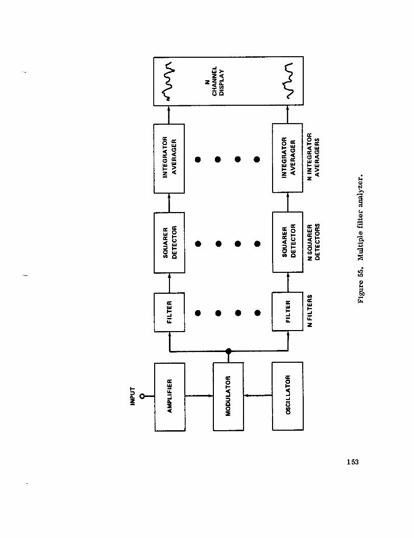
!
!
_" rr0 w
uJ uJ
1
CCuJ
.d
U.
Z
ILlm j.
Z
ZQ
F-
_O--Z
Q0
.J
153

energy versus frequency over the spectrum of interest. The display device can
be a conventional X-Y recorder, image storage oscilloscope, card punch, etc.
In this manner, successive power spectral density plots may be obtained in
intervals of 1 to 2 seconds, an advantage when the stationarity of the process
under consideration is in question.
H. A Method of Calibrating a Swept Filter Analyzer or aMultiple Filter Analyzer for Power Spectral Density
Analysis
The method of calibrating either a single channel swept filter system or
a multiple filter analyzing system is very similar. It consists of the followingsteps:
1. _eed a calibration sine wave into the analyzer system. This sine
wave will have an amplitude proportional to the amplitude of the quantity beingmeasured.
2. Make sure that no bandwidth division is included in the filter system
during this set-up time. Dividing a sine wave by the filter bandwidth is mis-
leading and erroneous.
3. Connect the filter output to a suitable recording device. X-Y
recorders or oscillograph recorders are acceptable.
4. Since the input sine wave signal, representing a known amplitude
of the quantity being measured, was assigned a particular value (2G rms, for
instance) then the full-scale X-Y plotter reading would be the squared value
of the input. In this case, since the input was 2G rms, the output full-scale
becomes 4G 2 (mean square) full-scale.
5. Remove the sine wave calibration signal and apply the random
signal which is to be analyzed.
6. Place the bandwidth divisor switch in the circuit.
7. Step 6 has normalized the output so that the plotted amplitude isnow in terms of G2/Hz.
154

8. With the random signal to be analyzed applied to the input (by
means of a type loop recorder-reproducer) the signal is continuously fed
into the analyzer while the analyzing system sweeps across the frequency
spectrum of interest.
9. The resultant graph is then a plot of power spectral density with
the Y axis in terms of G2/Hz and the X axis in terms of frequency.
These nine steps may be used to calibrate a swept filter system for
the analysis of a random wave by using a sine wave of an assigned value for
the calibration source. The following method is used to calibrate a multiple
filter system for analysis of random waves. Again, a sine wave of an assigned
value is used for calibration. Although the same principle is used, there is a
slight difference in procedure. In the multiple filter system, the bandwidth
divisors are connected at all times. However, one filter in the multiple filter
system, usually the narrowest, will not have a bandwidth divisor. It is this
filter channel, the one not containing a bandwidth divisor, that is used for the
sine wave calibration.
A sine wave of an assigned value is fed to the multiple filter system.
However, in this case, the sine wave must be at the frequency of the filter
containing no bandwidth divisor. The output of this filter channel is connected
to an appropriate recording device. Full-scale again is set up, as in step
4 above. The sine wave calibrating signal is removed and the random wave
is connected to the multiple filter system. In the case of wide band white
random noise, all filter outputs will be equal in amplitude. This is because
all channels have been normalized by bandwidth division. The resulting
plot (or in the case of an oscillograph, a multichannel plot) will give the
G_/Hz spectrum amplitude.
In most instances, a white random noise is not applied to the analyzer
system; therefore, a fiat or equal energy per Hz signal will not be obtained
at the output. High peakd ma]2 occur which will drive the recorder off scale.
In this case, a second analysis run may be necessary. When the data to be
analyzed are completely unknown, the chance of driving the recording device
over full-scale at some particular frequency is likely. When this does occur,
the point at which the recording device is driven off scale is the point at
which the system should be recalibrated. The initial calibration has not been
wasted, it is merely a first look at the data to see where the peaks do occur
and where the system should be calibrated. Some data survey is usually
necessary before a final analysis can be made. In some instances, survey
may not be required, since the data to be analyzed are known to be very
similar to data previously analyzed.
155

SECTION IX. INTERPRETATIONAND EVALUATIONOF DATA
Section VIH discussed the general techniques for reducing vibration
amplitude time history information into simplified descriptive data. This
section is concerned with the proper interpretation and evaluation of the
reduced data for applications to structural vibration problems. The desired
method for evaluating vibration data is a direct function of the specific
engineering problem to be studied. Each particular application usually
requires a different emphasis in the interpretation of the data. However,
there are certain basic procedures for interpreting and evaluating vibration
data which are applicable to nearly all structural vibration problems.
Before measured vibration data can be intelligently interpreted and
applied to any problem, it is necessary to know if the data are basicallyrandom in nature as opposed to being periodic. If vibration data are to be
used for prediction purposes, it is necessary to investigate the time invariance(stationarity) of the data. It is also desirable to determine if the data meas-
ured at various different points on a structure or similar structures are
equivalent.
In the area of direct engineering applications, the most basic and perti-
nent interpretations of vibration involve probability density and joint probabil-
ity density functions, autocorrelation and cross-correlation functions, and
power spectral density and cross-power spectral density functions.
Paragraphs A., B., and C. below discuss the procedures for evaluatingthe randomness, stationarity, and equivalence of vibration measurements.
Specific engineering procedures are detailed with numerical examples. Para-
graphs D., E., and F. discuss the interpretations and applications of prob-
ability density, correlation, and power spectral density functions for single
and multiple vibration measurements. The interpretation of each function
is illustrated by a numerical example involving a common engineeringvibration problem.
A. Evaluation of Randomness
Random vibration is that type of time-varying motion which consists ofrandomly varying amplitudes and frequencies such that its behavior can be
described only in statistical terms. No analytical representation for the
vibratory motion is possible. The vibration does not repeat itself after
156

a finite time period. For all practical purposes, vibration may be considered
random unless motion with a periodic form is present.
There are, of course, other types of vibratory motions that are neither
random nor periodic. For example, the motion produced by the sum of two or
more sine waves is not periodic unless the frequencies for the individual sine
waves have a common multiple, as discussed in Section VHI.A. 1. However,
in actual practice, such a motion may be considered periodic with little error
if the available data record is sufficiently long.
If vibration data are purely periodic, the fact is usually obvious by
simple observation of an amplitude time history plot. However, when vibra-
tion data are a mixture of both random and periodic portions, this fact is often
not obvious. There are several different techniques which may be used to
detect the presence of periodic components in an otherwise random vibration
response. Some of these techniques consist of qualitative inspections of the
vibration properties which might be measured from sample records as a
normal part of the random data reduction. Other techniques involve the
application of a specific quantitative test to sampled data. These techniqueswill now be discussed.
1. QUALITATIVE TESTS FOR RANDOMNESS
The presence of periodic components in an otherwise random vibration
response may often be detected by visual inspection of a power spectral density
function, an amplitude probability density function, and/or an autocorrelation
function measured from stationary sampled data.
To illustrate how a poer spectrum can reveal the presence of a periodic
component in an otherwise random signal, refer to Figure 56. In this example,
the output of a random noise generator was mixed with a sinusoidal signal. The
sinusoidal signal was given an rms amplitude equal to one-twentieth that of the
random signal. Plot A which was made using a relatively wide filter gives
little or no indication of the presence of the sinusoid. Plot B which was made
using a medium filter indicates a possible sinusoid quite clearly. Plot C
which was made using a norrow filter gives a strong indication.
Figure 56 illustrates how a highly resolved power spectrum will reveal
periodic components as sharp peaks, even when the periodicities are of relative-
ly small intensity. However, a sharp peak in the power spectrum for a vibration
response may also represent the narrow band random response of a lightly
157

A
0 FREQUENCY, Hz 250
B
0 FREQUENCY, Hz 250
C
.,=.
FREQUENCY, Hz 250
Figure 56. Actual power spectra plots.
158

damped structural resonance. These two cases can sometimes be distinguished
from one another by repeating the power spectral measurement with the nar-
rowest available PSD analyzer filter bandwidth. If the measured spectral peak
represents a sine wave, the indicated bandwidth of the peak will always be equal
to the bandwidth of the PSD analyzer filter, no matter how narrow the filter is.This method of detection will not work unless the bandwidth for the norrowest
PSD analyzer filter is smaller than the bandwidth for a possible narrow band
random response peak. For the case of spectral peaks with relatively low
center frequencies, say less than 50 Hz, a structural resonance may have a
bandwidth of less than 1 Hz, making it very difficult to distinguish from a
sine wave.
The presence of periodic components in an otherwise random vibration
response may also be revealed by an amplitude probability density function for
the response. The probability density plots for a sine wave and a rendom sig-
nal are markedly different. A random signal will usually hava a probability
density function which at least resembles the familiar bell-shaped Gaussiancharacteristic, while a sine wave has a dish-shaped probability density function.
A mixture of the two takes on prominent characteristics of both. This is clear-
ly illustrated by the actual measurements in Plots A, B, and C of Figure 57.
Perhaps the most powerful method of detecting periodicites in anotherwise random vibration response is presented by an autocorrelation plot.
For any purely random signal, the autocorrelation function will always
approach zero (assuming the signal has no dc component) as the time dis-
placement becomes large. On the other hand, the autocorrelation function
for a periodic signal is also periodic, and will continue to oscillate in a steady
state manner no matter how large the time displacement becomes. Thus the
autocorrelation plot for a signal representing a mixed random and periodic
vibration response will decay to a perpetual periodic oscillation as the time
displacement becomes large. These matters are illustrated by Plots A, B,
and C of Figure 58, and are further discussed with numerical examples
in Section IX. E. 3.
2. QUANTITATIVE TEST FOR RANDOMNESS (VARIANCE TEST)
Quantitative tests for randomness have been developed and studied
experimentally in Section 15 of Reference 21. These tests permit a statistical
decision, with a defined probable error, to he drawn from rudimentary investi-
gations of a sample vibration response record. The most practical quantitative
test for applications to flight vehicle vibration data involves an investigatio- o|
159

A
i .4-
w .3-
.2-
O .1-0
-30I I I i I I
-20 -lo 0 lo 20 3o
PROBABILITY DENSITY PLOT
FOR A RANDOM SIGNAL
C
160
b-
zwe_w..J
m<mOagG.
.s.],4 o
.3 o
.2-
.1"
0 ,--20
II
I !P
r
-lo 0 lo
PROBABILITY DENSITY PLOT
FOR A SINE WAVE
I
20
!'1-30 -20
I ! I
-lo 0 lo 20
PROBABILITY DENSITY PLOT
FOR A SINE WAVE MIXED WITH A
RANDOM SIGNAL
I
30
RMS AMPLITUDE OF SINE WAVERMS AMPLITUDE OF RANDOM SIGNAL
RMS AMPLITUDE OF TOTAL SIGNAL
= 1.0 VOLTS- 0.3 VOLTS
" O= 1.04 VOLTS
Figure 57. Actual probability density plots.

A
R¢rl
-T T
AUTOCORRELATION PLOT FOR A RANDOM SIGNAL
B -T
C -I"
/V
R "r)
/VAUTOCORRELATION PLOT FOR A SINE WAVE
R r)
AUTOCORRELATION PLOT FOR A SINE WAVE MIXED WITH
A RANDOM SIGNAL
:- T
Figure 58. Typical autocorrelation plots.
161

the variance of narrow band mean square value measurements (or powerspectral density measurements). This procedure is identified as Randomness
Test B in Reference 21. The principles of that test may be summarized asfollows.
As discussed in Paragraph I above, the existence of a sinusoid in an
otherwise random signal will be revealed by the presence of a sharp peak in
a properly resolved power spectrum for the signal. However, a narrow
band random signal representing a high Q resonance in a structural vibration
response will also appear as a sharp peak in a power spectrum. These two
cases can be distinguished from one another by examining repeated measure-
ments of the mean square value for the spectral peak at different times. If
the peak represents a sinusoid, mean square measurements taken at different
times should be exactly the same except for slight differences due to either
or both observational errors and possible sensitivity drift in the measurement
equipment. There are no uncertainties or sampling errors associated with
measurements of periodic signals.
On the other hand, if the peak is a narrow baud random signal (assumed
to be stationary}, mean square measurements taken at different times willshow scatter because of the inherent uncertainties associated with random
signal measurements. To be more specific, mean square measurements for
a stationary random signal will show scatter or variability which may be
defined in terms of a normalized variance c _, ae follows:
" (6S)a
Here, B is the equivalent ideal bandwidth of the random signal in Hz and T a
is the averaging time used to measure a mean square value in seconds. From
equation (65), as the bandwidth or averaging time is decreased, the variability
of the resulting measurements is increased. These theoretical ideas form thebasis for the randomness test outlined here.
Assume a sample record of length T seconds is obtained from a
stationary vibration response. Further assume the power spectral density
plot estimated from the sample record reveals one or more sharp peaks.
Each p_ak may be tested for randomness by the following procedure:
162

lo
o
o
1
Tune the narrow bandpass filter of the PSD analyzer over a
peak of interest so that the narrow frequency range of the peakis isolated from the remainder of the signal.
Obtain a collection of mean square measurements by averaging
over each of N number of equally long segments of the sample
record. Clearly, the required averaging time for each measure-
ment is T = T/N. For certain theoretical reasons, thea
number of measurements should be restricted to N < 0.1 BT.
If averaging is accomplished by continuous smoothing with a
low pass RC filter, the resulting continuous mean square
measurement time history can be reduced to a collection of
discrete mean square measurements by the procedures
illustrated in Figure 59.
Compute the expected normalized variance e 2 for the collection
of mean square measurements, assuming the sampled signal is
random, by using equation (65). The bandwidth B in equation
(65) is assumed to be the bandwidth for the PSD analyzer
filter.
Calculate the actual normalized variance E 2 for the collection
of mean square measurements by using the following computatio-
nal formula:
A
E 2 _--
N1 _, A2G.i=1 1
N ^
i=l
N
N]2Gii=1
163

GIVEN A SAMPLE RECORD OF LENGTH T SECONDS, A CONTINUOUS RC AVERAGED
MEAN SQUARE VALUE MEASUREMENT (OR POWER SPECTRAL DENSITY MEASURE-
MENT) MAY BE REDUCED TO A COLLECTION OF EQUIVALENT TRUE AVERAGED MEAN
SQUARE VALUE MEASUREMENTS AS FOLLOWS. LET THE RC AVERAGING TIME
CONSTANT K BE SHORT COMPARED TO THE RECORD LENGTH T; THAT IS, K<_<_T.
NOW, DIVIDE THE CONTINUOUS MEASUREMENT INTO N EQUAL INTERVALS SUCH
THAT EACH INTERVAL IS ABOUT 3K OR 4K LONG, AS SHOWN BELOW. THE LEVEL
OF THE CONTINUOUS MEASUREMENT AT THE END OF EACH INTERVAL WILL CONSTITUTE
A DISCRETE MEASUREMENT BASED UPON AN EQUIVALENT TRUE AVERAGING TIME OF
Ta'2K. THE INDIVIDUAL READINGS SHOULD BE 3K OR 4K APART TO ASSURE
THAT THEY ARE STATISTICALLY INDEPENDENT.
i.u
--I<>iu
Z<iu:S
A A A A A
G1 G2 G3 GIN.l) GN
3 (N-l) N
III I 1 I I
0 TIN 2T/N 3T/N (N-1)T/N T
TIME, SEC.
Figure 59. Analysis of continuous mean square value measurements.
164

N
N-1
N ^2
N i _ G.=1 1
(66)
Q
A
Here, G i is the_ ith mean square measurement where
i = 1,213, ..-,N.
Determine the ratio of the actual and expected normalized
variances as follows:
If R is statistically equivalent to unity, the power spectral
density peak being investigated is considered to be the result
of a narrow band random vibration response. If R is signifi-
cantly less than unity, the power spectral density peak is con-
sidered to be the result of a periodic component in the vibration
response. The criteria for deciding if R is equivalent to unityor significantly less than unity is as folloCws:
x2 (N-I_ -(l-a)R = 1 ifR > ' (68a)
_ N-I
X2 (N-l) ;(l-a)R( < 1 ifR c < N-I " (68b)
Here, X2 is a chi-squared distribution with N-1(N-t) ;(t-(_
degrees of freedom. N is the number of measurements employed,
and _ is the level of significance for the decision. The level of
significance defines the probability of erroneously concluding
165

that the peak represents a sinusoid when in fact it represents
a narrow band random signal. An erroneous conclusion of this
type is referred to as a Type I error. Clearly, the risk of
making a Type I error is reduced by using a smaller value of
c_ in equation (68).
A tabulation of values for X2 may be found in most statistics
books. Equation (68) is plotted for the levels of significance
--- 0.05 in Figure 60.
The above step-by-step procedure effectively accomplishes a statistical
hypothesis test without going into fundamental details, so that the test may be
employed by individuals who do not have a working knowledge of applied statis-
tics. If the procedure is carefully followed, statistically sound decisions will
result in most cases.
As noted in Step 5, there is always a risk of concluding that the peak
represents a sinusoid when it actually represents a narrow band random
signal. This risk defined by c_ is the probability of making a Type I error.
However, there is also a risk of concluding that the peak represents a
narrow band random signal when it actually represents a sinusoid. An erron-
eous conclusion of this type is called Type II error. The Type II errorprobability associated with the test is a function of certain fundamental con-
siderations which are not discussed here. These considerations are presented
in Reference 11. In general terms, the risk of making a Type 1I error in-
creases as cz becomes small and decreases as N becomes large. Thus, the
probability of making either a Type I or Type H error will be minimized by
using as many measurements as feasible, as long as the number of measure-
ments does not exceed the quantity of 0.1 BT.
It has been noted in paragraphs A. 1 and A. 2 of this section that the
various techniques for detecting periodic components in an otherwise random
vibration response are applicable only if the data are stationary. If the
various techniques are applied only to that data in the narrow frequency range
of sharp power density peaks (as they should be for maximum effectiveness),
the stationarity requirement then applies only to the narrow frequency ranges
being investigated. However, if a power spectral density peak is not station-
ary, the peak cannot represent a periodic component since a periodic function
is by definition steady state (stationary). Hence, if vibration data do not
comply with the stationarity requirement, a test for the presence of periodic
components is not really needed since the data by implication contain no
periodic components.
166

I I I I I I I
_1:1'OI/VI:I 30NVII:IVA
167

Numerical Example:
Assume a sample record of length T = 10 seconds is obtained from a
vibration response which is believed to be stationary. Further assume the
power spectrum measured from the sample record reveals a sharp peak which
is to be tested at the _ = 0.05 level of significance for the presence of aperiodic component.
Following the procedure outlined in paragraph A. 2. of this section,let a PSI) analyzer filter with a bandwidth of B = 56 Hz be tuned over the
peak to isolate it from the remainder of the signal. Now, let a collection
of N = 31 power spectral density (mean square value) measurements be
obtained from the sample record by averaging over 31 consecutive intervals
ofT =0.32second. Note thatN=31 < 0.1 BT = 56, as it should be.Assaume that the resulting measurements are as follow:
Data for Example (a)
Power Spectral Density Measurements Gi, volts 2/Hz
1.84 1.09 1.49 1.61
1.56 2.27 2.39 1.64
2.19 2.33 2.10 2.08
2.60 2.70 1.94 1.78
1.37 2.01 2.21 2.49
2.84 1.62 1.80 1.45
I. 40 3.08 2.21 I. 83
1.83 1.76 1.79
From equation (65), the expected normalized variance for the measurements
if the data is purely random is
¢2 = 1__ = 0.056BT a
168
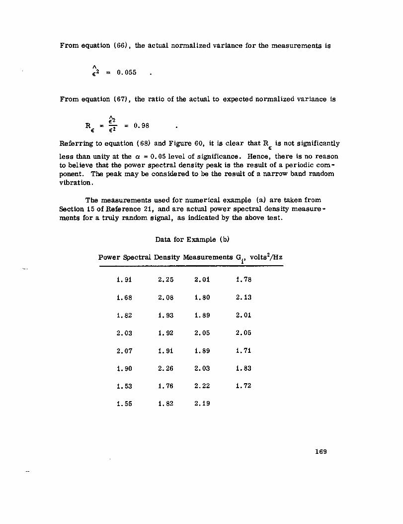
From equation (66), the actual normalized variance for the measurements is
Ac2 = 0.055
From equation (67), the ratio of the actual to expected normalized variance is
R =_ =0.98E E 2
Referring to equation (68) and Figure 60, it is clear that R is not significantly¢
less than unity at the _ = 0.05 level of significance. Hence, there is no reason
to believe that the power spectral density peak is the result of a periodic com-
ponent. The peak may be considered to be the result of a narrow band randomvibration.
The measurements used for numerical example (a) are taken from
Section t5 of Reference 21, and are actual power spectral density measure-
ments for a truly random signal, as indicated by the above test.
Data for Example (b)
Power Spectral Density Measurements Gi, volts2/Hz
1.91 2.25 2.01 1.78
1.68 2.08 I. 80 2.13
1.82 1.93 1.89 2.01
2.03 1.92 2.05 2.05
2.07 t. 9t 1.89 1.71
1.90 2.26 2.03 t. 83
1.53 i. 76 2.22 I. 72
1.55 i. 82 2.19
169

From equation (66), the actual normalized variance for this set of measure-ments is
_2 = 0. 0096
From equation (67), the normalized variance ratio is
R = 0.17 .£
Referring to equation (68) and Figure 60, it is clear that R e is significantly
less than unity at the _ = 0.05 level of significance. Hence, there is reason
to believe that the power spectral density peak is the result of a periodic
component.
The measurements used for numerical example (b) are taken from
Section 15 of Reference 21, and are actual power spectral density measure-
ments for a signal consisting of a sine wave buried in noise, as indicated bythe above test.
B. Verification of Stationarity
The general concept of stationarity as applied to vibration data is dis-
cussed in Section VHI.A. 2. It is noted there that the descriptive properties
of a random vibration response measured from a sampled vibration over any
time interval for which the vibration is stationary. Predictions may be made
for future time intervals for stationary data. If the sampled vibration is non-
stationary, the data measured from a sample record will reflect only the
vibration response properties of that one record alone during that particular
time interval when the sample record was obtained. No rigorous predictions
may be made for future time intervals when data are nonstationary.
There are two basic procedures for sampling a flight vehicle vibration
environment. The first procedure is to obtain a single continuous sample
record Cat each measurement point of interest) which covers an entire experi-
ment. Continuous sampling is usually employed for experiments involving
170

short term flight vehicles such as missiles and certain spacecraft. The
second procedure is to obtain a collection of short sample records (at each
measurement point of interest) which are obtained for various limited time
intervals during the experiment. Interval sampling is usually employed
for experiments involving long term flight vehicles such as long range bombers.
For the first case where a single continuous sample is available,
stationarity means that the vibration response does not change over the length
of the sample record (or a specific time interval covered by the sample
record). In other words, if the continuous sample record were broken up
into many short samples, the descriptive properties measured from each of the
various short samples would be equivalent. If this is true, then one set of time
invariant properties measured from the entire sample record may be used to
describe the sa_npled vibration.
For the case where a collection of short samples is available, station-
arity means that the vibration response is the same for each time interval
when a sample is obtained. If this is true, then the collection of samples may
be pooled together into one long sample record, and one set of properties
measured from the composite sample may be used to describe the sampledvibration. In either case, stationarity effectively means that the properties
of a vibration response measured from sample records obtained at different
times are equivalent.
For practical purposes, vibration response data may be considered
sta_.ionary if the mean square values measured from sample records obtained
at different times are equivalent. Technically, the mean value and autocor-
relation function should also be time invariant. However, the mean value of
vibration data is usually zero, and for certain practical reasons, it is unlikely
that the autocorrelation function is changing if the mean square value is not
changing. Hence, the determination of stationarity can usually be limited to an
investigation of mean square values.
In many instances, statiouarity or nonstationarity in measured vibration
data is obvious. This is particularly true when the uncertainty associated with
the measurements is small. For example, if the mean square values measured
from a collection of sample records were all within a few percent of one another,
the collection of measurements could clearly be considered equivalent without
further attention. On the other hand, if a collection of mean square values,
each with a measurement uncertainty of only a few percent, displayed
scatter if p_rhaps two or three to one, then the collection of measurements
could clearly be considered nonstationary without further attention. The problem
171

arises when the available data have a relatively high measurement uncertainty
due to a narrow bandwidth or short record length. It is often difficult in such
cases to distinguish between expected statistical scatter and nonstationarity.
Two different quantitative tests for stationarity are now outlined. The
first procedure is based upon a measurement variance test similar to the test
for randomness outlined in Paragraph A. 2. of this section. This procedure
is developed and experimentally studied in Section 16 of Reference 21. The
second procedure is based upon nonparametric statistical techniques discussedin Reference 22.
. VARIANCE TEST FOR STATIONARITY COMBINED WITH RANDOM-
NESS TEST
This test for stationarity is identical in principle to the test for ran-
domness outlined in Paragraph A. 2. of this section. The variance of mean
square measurements obtained at different times is compared to the theoreti-
cally expected variance for mean square measurements of a stationary random
signal. As a lack of randomness will tend to reduce the scatter in repeated
mean square measurements, a lack of stationarity will tend to increase the
scatter in repeated measurements. Hence, the procedure for applying the
variance test for stationarity is the same as the procedures presented for
the randomness test in Paragraph A. 2. of this section, except for the final
decision which is based upon whether or not the ratio R e is significantly
greater than unity rather than significantly less than unity.
The variance test for randomness assumes that the signal being tested
is stationary, and the variance test for stationarity requires that the signal
being tested is random. It is then logical that the two characteristics of ran-
domness and stationarity should be established jointly by a single test pro-
cedure. A combined test does pose one practical problem. The randomness
test is most effective when applied to a narrow frequency range obtained
by locating a narrow bandwidth filter over a sharp peak in the power spectrum
of the signal. On the other hand, a stationarity test should ideally be applied
to the entire frequency range of the signal. However, it is often acceptable
to test only the sharp spectral peaks for stationarity, since most of the relative
power of the vibration response is represented by these peaks. If the peaks
in the power spectrum are found to be stationary, it is reasonable to assume
the entire signal is stationary for most engineering applications.
Assume a sample record of length T seconds is obtained from a vibra-
tion response. Further assume the power spectral density plot estimated from
172

the sample record reveals one or more peaks. Each peak may be tested for
randomness and stationarity by the following procedure:
lo Tune the narrow bandpass filter of the power spectra/ density
analyzer over a peak of interest so that the narrow frequency
range of the peak is isolated from the remainder of the signal.
. Obtain a collection of mean square measurements by averaging
over each of N number of equally long segments of the sample
record. Clearly, the required averaging time for each measure-
ment is T = T/N. For certain theoretical reasons, the numbera
of measurements should be restricted to N < 0.1 BT. If averag-
ing is accomplished by continuous smoothing with a low pass RC
filter, the resulting continuous mean square measurement time
history can be reduced to a collection of discrete mean square
measurements by the procedures illustrated in Figure 59.
o
o
Compute the expected normalized variance e 2 for the collection
of mean square measurements, assuming the sampled signal is
random and stationary, by using equation (65).
Calculate the actual normalized variance _ for the collection of
mean square measurements by using the computational formula
presented in equation (66).
o Determine the ratio of the actual and expected normalized var-
iances as follows:
AR = c2 • (69)
H R is statistically equivalent to unity, the power spectralc
density peak being investigated is considered to be the result
of a narrow band stationary random vibration response. If R E
is significantly less than unity, the power spectral density peak
is considered to be nonrandom, and if R is significantly greater¢
than unity, the power spectral density peak is considered to be
nonstationary.
173

The criteria for deciding if R is equivalent to unity or signifi-E
cantly different from unity are as follows:
×2 X2 (N-i)" (_/2R = I if (N-i);(1-(_/2) < R < ' (70a)
N-1 -- N-I
X 2
R< 1 if R < (N-1);_.-ol/2,_'_" _ (70b)¢ N-I
X 2
> 1 ifR -> (N-I);G/2Re N-1 " (70c)
Here, X2 is a chi-squared distribution with N-I degrees of(N-i)
freedom, N is the number of measurements employed, and a is
the level of significance for the decision. A tabulation of valuesfor X2 may be found in most statistics books. Equation (70) is
plotted for the levels of significance a = 0.01 and _ = 0.05 in
Figure 61. The probable errors associated with a decision are
discussed in Paragraph A.2. of this section.
Numerical Example:
Assume a sample record of length T = 17 seconds is obtained from a
vibration response (the 17 seconds could represent the total length for a col-lection of sample records obtained at different times). Further assume the
power spectrum measured from the sample records obtained at different
times). Further assume the power spectrum measured from the sample record
reveals a sharp peak which represents most of the relative power of the sig-
nal. The peak is to be tested for randomness and stationarity at the c_ = 0.05
level of significance.
Following the procedure outlined in Paragraph B. 1. of this section,
let a PSD analyzer filter with a bandwidth of B = 56 Hz be tuned over the peak
to isolate it from the remainder of the signal. Now, let a collection of N = 31
power spectral density (mean square value) measurements be obtained by
averaging over 31 consecutive intervals of T = 0.54 seconds. Note thata
31 < 0.1 BT = 95 as it should be. Assume the resulting measurements areas follow:
174

I
PH 'OI.J.VEI :IONVlUYA
|
Z
I-ZIAI_Ew
14.1_Eu,.O
cCIAIm_E
Z
op,.4
c_
_rJ
0_
o
oo
N
175

Data for Example (c)
^
Power Spectral Density Measurements Gi, volt 2/Hz
2.25 2.19 2.00 2.21
1.78 3.20 2.23 1.47
2.26 2.30 3.05 2.44
2.07 2.86 2.15 3.28
i.91 2.68 2.36 3.27
2.85 2.15 2.03 2.49
2.O0 2.54 2.O0 3.43
2.45 2.32 2.57
From equation (65), the expected normalized variance for the measurements
if the data are purely random and stationary is
1_2 --
BTa
- 0. 033
From equation (66),
A
¢2 = 0.038
the actual normalized variance for the measurements is
From equation (69), the ratio of the actual to expected normalized variance is
A
E2R
E --'-- 'E'_= 1.15

, iS not significantlyReferring to equation (70) and Figure 61 itis clear that R e
differentfrom unity at the _ = 0.05 level of significance. Hence, there is no
reason to believe thata periodic component is present or that the signal is
nonstationary. The signal may be considered both random and stationary.
The measurements used in numerical example (c) are taken from
Section 16 of Reference 21, and are actual power spectra/ density measure-
ments for a truly stationary random signal, as indicated by the above test.
follow:
Now assume that the resulting measurements for the test were as
Data for Example (d)
A
Power Spectral Density Measurements G t, volts2/I-Iz
2.33 1.24 O. 96 2.63
2.03 I. 40 I. 60 2.25
2.12 1.24 i. 37 2.06
I. 88 1.22 i. 10 2.42
2.20 1.42 1.03 2.27
i. 90 I. 40 1.62 3. O0
2.36 I. 39 I. 24 2.40
2.61 1.70 2.18
From equation (66), the actual normalized variance for this set of measure-
merits is
A¢2 = O. 090 .
From equation (69), the normalized variance ratio is
177

R =2.7E
Referring to equation (70) and Figure 61, it is clear that R c is significantly
greater than unity for the c_ = 0.05 level of significance. Hence, there is
reason to believe the sampled vibration response is nonstationary.
The measurements used for numerical example (d) _re taken from
Section 16 of Reference 21, and are actual power spectral density measurements
for a nonstationary random signal, as indicated by the above test. Specifically,the measurements were obtained from a random signal whose true mean square
value changed m 20 percent relative to an average level (a change of _ 10 per-
cent in the rms amplitude). The rms amplitude of the signal was 10 percent
high for the first eight measurements, 10 percent low for the next 15, and
10 percent high for the last 8.
2. NONPARAMETRIC TEST FOR STATIONARITY
This test for stationarity is also based upon an investigation of the
scatter or variability of mean square measurements. However, it is only con-
cerned with the number of "runs" which occur in a collection of measurements,
and does not require a knowledge of the actual sampling distribution of the
measurements. Thus the test is nonparametric.
Assume that a collection of N number of statistically independent mean
square values are measured from sampled vibration data. Let the median value
of the measurements be determined; that is, the value for which half the
measurements are larger and half are smaller. Furthermore, let each meas-
urement that is larger than the median be identified by (+) and each that is
smaller than the median be identified by (-). Now arrange the (+) and (-)
identifications for the measurements in the proper time sequence.
For example, the resulting sequence for 20 measurements might be asfollows:
_++ - + ¢._ _ - + _ + v__ +
1 2 3 4 5 6 7 8 9 I0 ii 12
178

A "run" is defined as a sequence of identical symbols which is followed and
proceded by a different symbol or no symbol at all. In the above examplethe number of runs is 12. The total number of runs in a collection of indepen-
dent measurements obtained at different times gives an indication as to
whether or not the quantity being measured is stationary. If very few runs
occur, a time trend is indicated. If a great many runs occur, systematic
short period fluctuations are indicated.
The application of run theory as a test for stationarity presents three
important advantages not afforded by the variance test discussed in Paragraph
B. 1. of this section.
lo A knowledge of the frequency bandwidth of the signal under
investigation is not required.
o A knowledge of the exact averaging time used to measure the
mean square values is not required. Futhermore, there are
no restrictions on how long the averaging time should be.
o It is not necessary for the signal under investigation to be com-
pletely random. Valid conclusions are obtained even when
periodic components are present in the signal, as long as the
fundamental period is short compared to the averaging time
used for each mean square measurement.
The above advantages clearly illustrate the broad and simple appli-
cability of the test to vibration data. Actually the test can be applied to a
sample record with nothing more than a simple square amplitude detector,such as a true rms voltmeter. No filter or detailed analysis is required.
The step-by-step procedure for applying the test is as follows:
. Obtain a collection of broadband mean square measurements by
averaging over each of N number of segments of a sample record.
The averaging time for each measurement is of no concern. If
averaging is accomplished by continuous smoothing with a low
pass RC filter, the resulting continuous mean square measure-
ment time history can be reduced to a collection of discrete
mean square measurements by the procedures illustrated in
Figure 59.
179

. Determine the median of the mean square measurements; that
is, the value for which half the measurements are larger andhalf are smaller.
1 Identify each measurement that is larger than the median by (+)
and each that is smaller than the median by (-).
. With the (+) and (-) identifications for the measurements
arranged in proper time sequence, count the number of runs.
. If the number of runs is either too small or too large, the sample
record being investigated is considered to represent a nonstation-
ary vibration response. Otherwise, the sample record is con-
sidered to represent a vibration response which is stationary.
The criteria for deciding if the number of runs are too small
or large is tabulated in Table 6 for various values of N and the
level of significance _.
Numerical Example:
Let the data gathered for the numerical examples in Paragraph B. 1.
of this section be tested for stationarity by application of the run test at the
= 0.05 level of significance.
First consider the measurements presented in Example (c). The^
median value for these measurements is G = 2.30 volts 2/cps. That is, there
are 15 measurements with a value greater than 2.30 and 15 measurements
with a value greater than 2.30 and 15 measurements with a value less than2.30. The number of runs in the 31 measurements when considered in a
proper time sequence is 16, as shown below:
2.25 5
l° 78
2.266
2.07
1.91
2.85 7
2.00
2.45 8
2.19 { 2. O03.20 9 2.23
2.30 10 3.05
2.86 11 2.15
2.68 12 2.36
2.15 13 I 2.03
2.54 2.O02.32 14 2.57
15
16
2.21
1.47
2.44
3.28
3.27
2.49
3.4:;
180

TABLE 6. RUN TEST FORSTATIONARITY
= 0. i0 _ = 0.05 _ = 0.01
N lower upper lower upperlimit limit limit limit
8 3
i0 4
12 4
14 5
16 6
18 7
20 7
22 7
24 8
26 9
28 iO
30 ii
32 il
34 i2
36 13
38 14
40 i5
50 19
60 24
I
7 3
9 4
i0 4
Ii 5
12 6
14 7
16 7
17 7
18 8
19 9
20 I0
22 Ii
23 ii
24 12
25 i3
26 i4
32 18
37 22
upper lowerlimit limit
8
9 3
ii 4
12 4
13 5
14 5
16 5
18 6
19 7
20 7
21 8
22 9
24 i0
25 i0
26 ii
27 i2
33 i6
39 20
a
m
I0
Ii
13
14
15
18
19
20
22
23
24
25
27
28
29
35
41
181

Referring to Table 6, it is clear that the number of runs is within the rangeexpected for measurements from a stationary signal at the _ = 0.05 level of
significance. Hence, there is no reason to believe that the sampled vibration
response is nonstationary. This is a correct conclusion for the data presentedin Example (c).
Now consider the measurements presented in Example (d). The medianA
value for these measurements is G = t. 88 volt 2/Hz. The number of runs in
the 31 measurements when considered in the proper time sequence is 3, asshown below :
2.33
2.03
2.12
1.88
2.20
1.90
2.36
1.24 0.96
1.40 t 1.60
1.24 1.371.22 2 1.10
1.42 1.03
1.40 1.62
'1.39
2.18
2.63
2.25
2.06
2.27
2.27
2.40
Referring to Table 6, it is clear that the number of runs is less than expected
for measurements from a stationary signal at the a = 0.05 level of significance.
Hence, there is reason to believe that the sampled vibration response is non-
stationary. This is a correct conclusion for the data presented in Example (d).
Note that the data used for the numerical examples in this section
involve relatively large measurement uncertainties. This is done to illustrate
how the tests for stationarity are applicable even for data with considerable
statistical scatter. Because of the scatter, the fact that the data for Examples
(c) and (4) are stationary and nonstationary, respectively, is not immediately
obvious by observation.
C. Determination of Data Equivalence
The evaluation of a flight vehicle vibration environment will involve the
collection and analysis of many different sample records. These sample rec-
ords would be gaChered as a function of several different variables to obtain
appropriate vibration response profiles. For example, a collection of sample
records might represent the vibration response for a number of different
times during a flight. Hence, the vibration environment can be evaluated
as a function of time and struct_,ral location. In a similar manner, sample
182

records might be collected from either or both repeated flights of the samevehicle and flights of different vehicles of the same type. For this case,the specific flight or specific vehicle or bothwould also be variables in thedataanalysis.
In any case, anearly step in the evaluation of the data shouldbe an in-vestigation for areas of equivalence, so that the number of variables neededto describe the vibration environment can be reduced to a minimum.
As one example, assumethe vibration data measured for differentflights of a vehicle is not significantly different from flight to flight. Then,the specific flight can be eliminated as a variable in the description of thevibration environment. The sample records obtained for different flights can
be pooled together and the vibration environment for the flight vehicle can be
described by one set of properties which are applicable to all flights.
For a second example, assume the vibration data measured at various
points in a specific structural zone of a vehicle are not significantly different
from point to point. Then, the specific point in that zone of the vehicle may be
eliminated as a variable in the description of the vibration environment. The
sample records obtained for different points in that zone may be pooled togetherand the vibration environment for that structural zone of the flight vehicle may
be described by one set of properties which are applicable to all points in that
zone.
Note that the presence or absence of time as a variable determines
the stationarity of a vibration response. As described in Subsection B of this
section, a stationary vibration response is one whose statistical properties
do not vary with time; equivalent. The procedures in Subsection B. of this sec-
tion for verifying stationarity are simply tests for the equivalence of measure-
ments obtained at different times. Those same procedures can just as well be
applied to determine the equivalence of measurements obtained at different
locations or on different flights or on different vehicles. However, when acollection of measurements is available which involves two or more variables,
there are more powerful statistical procedures for establishing the significanteffects of two or more variables simultaneously. These procedures are known
as "analysis of variance, " and are described in this section.
The two most important variables in the description of a vibration
environment are usually time and structural location. Any reduction in the,number of different times and locations needed to describe a general vibration
environment is clearly desirable. As discussed in Subsection B. of this section,
the determination of stationarity may be limited to an examination of mean
183

square value meansurements, for most practical cases. For the same general
reasons, the equivalence of vibration data at various structural locations may
also be based on an investigation of mean square value measurements, at least
for purposes of preliminary evaluation. Hence the following discussions are
written assuming that time and location are the variables of interest and that
a mean square value is the measured property which defines the vibration
environment. However, the general analysis of variance procedures is valid
for any measured quantity as a function of any desired variables. In all cases,
a requirement is the assumption that the measured quantities in question are
normaUy distributed, or that the measurement errors about some true constant
value are normally distributed.
A full discussion on these analyses of variance procedure s appears inSection 8 of Reference 21. The material to follow here summarizes some of
these procedures and illustrates them with a computational example.
i. ANALYSIS OF VARIANCE PROCEDURES
Basic mathematics for the analysis of variance procedures is as follows.
Suppose two sample means x 1 and x 2 are available where
N
= 7 xi.j ;i=1,2 (71)xi j_'=l
the index i= 1,2 representing two different sets of experiments in each of which
j = 1, 2,..., N measurements are made. Thus xlj and x2j represent the N sample
values in each experiment.
If it is assumed that the underlying populations are normal, and that the
sample variances s _ and s 2 are estimates of common variance, then the2variable
t = _ (72)
has a "student's t" distributionwith (N-i) degrees of freedom (dr). The sample
variances are defined by their unbiased estimates
184

N
s.2 -- i=l • i= 1,2 (73)I N-l '
Note that the number of clf= (N-l) is used as a divisor rather than the sample
size N. This fact allows a two-tail at the cz level of significance by comparing
t from equation (72) with a tabulated value of tl_cz/2(N-1),. If a test among
several means .xi' i = 1, 2..., k is desired, the situation becomes more com-
plex. All possible combinations of the sample means could be tested, although
the level of significance becomes open to question.if any combinations fail the
test. The analysis of variance procedures offer a solution to this problem.
a. The One-Way Fixed Effects Model
The analysis will now be presented in terms of its simpliest form.
Assume for example that N measurements of vibration data from each of k
points from some Right are available, and that the collection of data is all
obtained in a short period of time under identical conditions. It is now desired
to test whether the k sample means are all statistically equivalent estimates
of some common population mean value _. That is, the hypothesis is
_zi = /a2 =... -_zk =(74)
where/_i represent the respective true mean values. This hypothesis may be
cast in a slightly different but equivalent and sometimes more useful form.
Consider each observation to be of the form
j = 1,2,...,N
xij =/a+ _i + Eij ' i = 1,2,...,k (75)
where _ is the overall mean value, _ i is an effect due to the ith location and
E.. is an "error" term assumed to be normally distributed with zero mean and1j
variance o_. In this model the hypothesis becomes
185

q) l = @2 =''' = (Ok= 0 (76)
The basis for the test of the hypothesis arises from the fact that two independent
estimates of the variance 02 may be calculated from the data if the hypothesis
is true.
The first of these estimates is obtained from the "within group" var-
iation. That is, define
v
kI s 2.
i=l
(77)
which is the average of the k sample variances. This is an unbiased estimate
of o2 whether or not the hypothesis of equal means is true.
A second estimate is now obtained from the "between group" variation.Define
k
(xi - x)2i=l
MS 2 = N k - 1 (78)
where this estimates the population variance as N times the variance of the
sample m_ans and _" is the mean of the k sample means
k
x = (l/k) _ x i .
i=l
Equation (78) is based on the relation '
(79)
186

where _2 is the variance of the distribution of sample means computed fromx
samples of size N drawn from a population with variance g2. The variance
estimate given by equation (78) will be an estimate of ¢2 if the hypothesis
(76) holds. However, if there is a contribution due to nonzero values _ i'
then this variance estimate will be enlarged because of this effect. It can
be shown that the variance ratio
F = MS2 (80)
has an F distribution with (k-i) and N_k-l) dr. Since the estimate MS 2 can
only be larger than MS1, a one-tail test at the _ level of significance may be
performed by comparing F from (80) with FI_ a (k-l, N [k-l]) obtained from
a table of the F distribution; that is, if
F < F (k-i, N [k-i]) , (81)Ot
the hypothesis of equal means is accepted. The term "fixed effects" stemsfrom the fact that it is assumed that only the effects of k specific fixed points
are of interest.
b. One-Way Random Effects Model
In contrast to the fixed effects model, if it is desired to test the hypo-
thesis that the vibration in some extended area of a flight vehicle is the same,
then one would select k points at random from this general area. The model
is written the same; that is,
xij I_ + _i + E..ij
but in this case the _ i are assumed to be k observations of a random variable
with zero mean and variance _ . The hypothesis now is slightly altered and
becomes
187

although the computing procedures and the F ratio remain identical.
c. Two-Way Mixed Effects Model
The specific procedure for the simultaneous test for stationarityand test for equivalence among locations is now presented. Assume that
the time period of interest has been subdivided into a large number of small
intervals and that r of these intervals have been randomly selected. Also,
assume that at each of c specific locations of interest, data is collected duringthese r intervals. In addition, it is assumed that each of these intervals is
stationary and represents a sufficiently long period from which to obtain N
independent observations. The data rhay be conveniently represented as in
Table 7. Note that in each cell of the table there are N data values giving atotal of Nrc observations.
TABLE 7. VIBRATION DATA LAYOUT FOR TWO-WAY
ANALYSIS OF VARIANCE
• •
r
Location
l 2
Xliv Xl2v
X21v x22 v
Xilv xi2 v
Xriv Xr2 v
• • • C
Xlcv
XroY
v= 1,2,...,N
r = number of rows (times)
c = number of columns (locations)
A slightly modified notation for mean values will now be adopted. The symbol
x--ij" will r_.present an average taken over the values represented by the sub-
script replaced with a dot; that is, as
N-- 1
xij" = N xijv
188

It is now assumed that each cell represents a sample of size N from
rc separate populations, each normally distributed about a mean/_., and with1j
a common variance a 2. The model becomes
Xijv = _ij + _ijv " (83)
However, the #ij is postulated to consist of a time effect gi' a location effect
and a possible interaction effect eij. The interaction may arise since the
joint effect of the two variables taken together may differ from the sum of their
separate effects. However, in many particular physical applications, it is
unlikely that a significant interaction exists. The location effects h. are assumedJ
to be due only to the c specific fixed locations; however, the time effects gi
are assumed to be r observations of a random variable with zero mean and
2. Substituting these terms for/_ij' equation (83) becomesvariance ag
Xijv = # + gi = h.] + Oij + eij v (84)
where all the factors are considered as deviations from the overall mean
value _.
The method for constructing the test of the hypothesis for the one-way
analysis of variance still applies in principle to the two-way analysis. Oneobtains a variance estimate from between locations (columns) variation, an
estimate from between times (rows), an estimate from interaction, and finally
a within group (or within cell) estimate. Various F tests may then be devised
to check the statistically significant interaction effects, locations effect, and
time effect. The F ratios are constructed by choosing variance ratios in
which the numerator will have a larger expectation than the denominator if the
effect being tested for exists (i.e., is nonzero).
The within group mean square is given by the average of all the cell
sample variances. That is,
189

r c
MS 1 = 1rTi=i j=i
m
rc (N-i)
r c N
z ,"= 1 =1 xi-
(85)
N
sij2 = N----_I E (Xijv -- x_. ) . (86)v=i -j
This quantity given an unbiased estimate of o-2; that is, its expected value is
o-2 regardless of whether or not any of the effects are nonzero.
The between locations (columns) variance estimate is
C
MS 4 = _rN j_.'lc-I (x.j.- x...)2 ;
"_
(87)
that is, each column mean is based on rN observations, hence the factor rN
for estimating an underlying population variance from a sample variance basedon means computed from rN observations. This variance estimate will have
an expected value of o-2 ff no column effect exists, but otherwise will have an
expected value, E (MS4) , given by
C
E(MS 4) = o-2 + NO- + c--'-_"=i 1
2 is the variance attributed to interaction ff itIn equation (88), the term o-_
exists, and the h. are fixed column effects if any exist.J
The expression for the between times (rows) variance estimate is
entirely analogous. Thus
r
r-lCN _ (x. -x )2 (89)MS3 - "=1 z.....
190

The expectedvalue, E (MS3), of the between rows variance estimate is given by
E(MB 3) = a 2 + Nc a 2 . (90)g
The interact on sum of squares is obtained by considering the identity
X-vii- x = (_ij. - x.1.. - x .j. + x ) + (xi. - x )omm • el.,
+ (x . 'x ) + (x.. -x.. ) . (91).].... 1]v ijv.
The sum of squares corresponding to each of the last three terms in equation
9.27 have already been accounted for by equations (85), (87), and (89). The
interaction mean square is therefore
r c
x_ - - -i i_ j_ ( _x. _x . + x )2 . (92)1V_2 = (r-l) (c-l) "=1 "=1 . 1.. .j ....
This expression can be shown to have an expected value of a 2 if there is no2. that is,interaction effect, but otherwise will be increased by the factor Nao,
E(MS 2) = cr2 + No_ . (93)
All the foregoing equations are summarized in the analysis of variance table,
Table 8.
By inspecting the expected mean square values, the various F tests are
seen to be as follow:
191

Z
©
0
=I
_2
0
_fJ
+
_qb
"I"
%
II
I
IX"
I
Z
II
@
+
%
II
I
I
Z
II
Z+
%
:?
I
II
I
I
v
IM"
"I-
I
@ _
%
II
I
I
II
@
W
#,U
,i-II
!
II
0
192

Variance Ratio df for F
(a) Locations : F = MS4 (c-l,[r-1][c-1])MS2
(b) Times : F =MS I (r-l, rc [N-I] )
(c) Interaction : F = MS2MSt
([r-l][c-l], rc[n-l])
The various hypotheses are accepted at the _ level of significance if the
computed F is less than the appropriate tabulated value of F 1-_ (m, n) where
M and n are the df as indicated above.
d. Computational Procedure
The quantities given in Table 8 are more conveniently calculated by
the following equivalent computational procedure:
1. Calculate within cells totals W.. where1]
N
=1 xijv;
2. Calculate row totals R. where1
C
Ri = "j_l wij; i=l, 2, ..., r
o Calculate column totals C. where]
r
C.=1_ W i "] =1 j,j = 1,2,...,c
193

4. Calculate .,erall total T:
r c
1 ..=, 3
o Calculate "crude" total sum of squares (i.e., the original values
squared as opposed to d eviations from an appropriate mean value
squared).
r c N
1"= 1 =1 ijv
o Calculate the correction factor due to the mean for transfomiag
crude sums of squares to squared deviations about an appropriatemean value
r 2CF-
rcN
o Calculate crude between column sum of squares
C
c-".CSS4= r-_
j=l :]
o Calculate crude between row sum of squares
r
1CSS3 = cN =t
9. Calculate crude within cell sum of squares
r c1 2
j =I D
194

I0. Calculate between column sum of squares
SS4 = CSS 4 - CF .
11. Calculate between rows sum of squares
SS3= CSS 3 - CR .
12. Calculare total sum of squares
SS T = CSS T - CF .
13. Calculate within cells sum of squares
SSI= CSS T-CSS w .
14. Calculate interactionsum of squares
SS2 =SS T - SS 1 - SS 3 - SS 4 .
15. Calculate mean squares
MS I = SSl/rc(N-l)
MS 2 = SS2/(r-I) (c-l)
MS 3 = SS3/(r-l)
MS 4 = SSj(c-l)
if
The hypothesis of stationarity is accepted (at the _ level of significance)
195

F =MS3 < Fi (r-l, rc[N-l])MS 1 -_
ifThe hypothesis of no difference between the chosen locations is accepted
F _ < (c-1, [r-l] [c-1]j= MS 2 FI-_
tested.
action.
The hypothesis of no interaction between time and location may also be
In many problems there is no physical reason to suspect any inter-This hypothesis is accepted if
F= MS2 <Flye1 .l__([r-l] [c-l], rc[N-1]j
2. COMPUTATIONAL EXAMPLE
The data listed in Table 9 represent actual experimental results
outlined in Reference 21. The data are taken from a nonstationary processand the different locations represent repetitions of the experiment.
As can be seen from the data, r = 5, c = 5, and v = 3 for this example.Therefore, rcN = 75 for the total number of observations. Since the data
involved here are nonstationary but equivalent from location to location, the
hypothesis of stationarity should be rejected and the hypothesis of no difference
between locations should be accepted. Also the hypothesis of no interaction
between time and location should be accepted.
The calculations will now be performed in the exact sequence given inParagraph C. 1. d. of this section.
1. Within cells totals
Wll = 8.34 Wl2 = 7.76 W_3 = 7.29 Wl4 = 7.70 . Wl5 = 6.74
W21= 9.00 W22=7.47 W23=7.72 W24=7.44 W25=6.26
196

X
t._
0
t._ _.. L-.-t_ _..4 _'_
_..4 _ _...4
L".. o _
_ _ t._
Q
I0
I
8.
0
o
O
II
e_ N
.._
197

,
o
o
.
1
7_
o
e
W31= 7.21 W32= 8.58 W33=6.72 W34:7.41 W35= 9.01
W41= 5.28 W42= 5.85 W¢3= 5.16 W44=6.16 Wts= 6.74
W51= 6.06 W52= 6.56 W53= 5.95 W54= 5.69 Ws_= 5.44
Row totals
R|= 37.83 R 2=37.89 1_s=38.93 1_4=29.19 R 5= 29.70
Column totals
C 1=35.89 C 2=36.22
Overall total
T = 173.54
Crude total sum of squares
CSS T = 420.0338
Correction factor due to mean
CF = 401. 5484
Crude between columns and squares
CSS 4 = 402. 0508
Crude between row sum of squares
CSS3 = 407. 7635
Crude within cell sum of squares
CSS W = 411. 5505
C3 = 32.84 C4 = 34. 40 C 5 = 34.19
198

10. Between columns sum of squares
SS 4 = 402• 0508 - 401. 5484 = . 5024
11. Between rows sum of squares
SS 3 = 407. 7635 - 401. 5484 = 6. 2151
12. Total sum of squares
SS T = 420. 0338 - 401. 5484 = 18.4854
13. Within cells sum of squares
SS 1 = 420.0338 - 411. 5505 = 8. 4883
14. Interaction sum of squares
SS 2 = 18. 4854 - 15. 2008 = 3. 2846
15. Mean squares
8. 4833 6. 2151 •MSl= 50 - .16967 MS 3 =_ - 1.5538
3. 2846 .5024MS2 = 1----_ - .20529 MS4 - 4 - . 12560
18. 4854MST = 74
The results are displayed in Table 10.
Three values from a table of the F distribution are now necessary.
The hypotheses will be tested at the c_ = 5 percent level of significance. These
values are F 95 (4,50) =2.57, F 95 (4,16) =301, andF 95 (16,50) = 1.86.
199

TABLE 10. RESULTS
Source
Between
Locations
1VI_anSum of squares df
Square
.5024 4 .12560
Between
Times 6.2151
Interaction 3.2846
W_hin
CeHs 8.4833
Total 18.4854
1.5538
16 .20529
50 .16967
74 .24980
Expected
Mean Square
5
2 + _.15j___ h.22 + 3cre i )
O.2
Test of hypothesis of stationarity:
F= MSs = 1.5538 = 9.1578 >F (4,50)MS 1 .16967 .95
= 2.57
Since the computed Fib larger than F 95 (4, 50), the hypothesis of stationarity
is rejected at the 5 percent level of significance.
Test of hypothesis of no difference between locations:
F= MS4 = .J.2560 = .61182< F 95 (4,16)=3.01.MS 2 .20529
Since the computed F is smaller than F 95 (4, 16), the hypothesis of noe
difference between locations is accepted at the 5 percent level of significance.
200

Test of hypothesis of no interaction between time and location:
F= MS2 _ .20529MB 1 .16967 - 1.2099 < F.95 (16,50) = 1.86
Since the computed F is smaller than F 95 ( 16, 50), the hypothesis of no inter-
action between time and location is accepted as expected at the 5-percent level
of significance.
This concludes the computational example.
D. Interpretation and Application of AmplitudeProbability Density Functions
I. FIRST-ORDER PROBABILITY DENSITY FUNCTIONS
The first-order probability density function is defined in Section VIII.
B. 2 but will be repeated here for convenience. The general definition of a
continuous probability density function in statistical terms is as follows.
Let r = r (_) be a continuous random variable which is defined as a real valued
function of _ where the behavior of _ is determined by chance. A (first-order)
probability density function, Pr(X), is defined by the condition,
Pr(X) dx =Prob [x< r (a) <x +dx] (94)
where x is a specific value of the random variable r. The probability density
function Pr (x) shouldnot be confused with the (cumulative) probability dis-
tribution function Pr (x) which is related to Pr(X) by the equation
X
Pr (x) = f Pr (t) dt . (95)-- aO
201
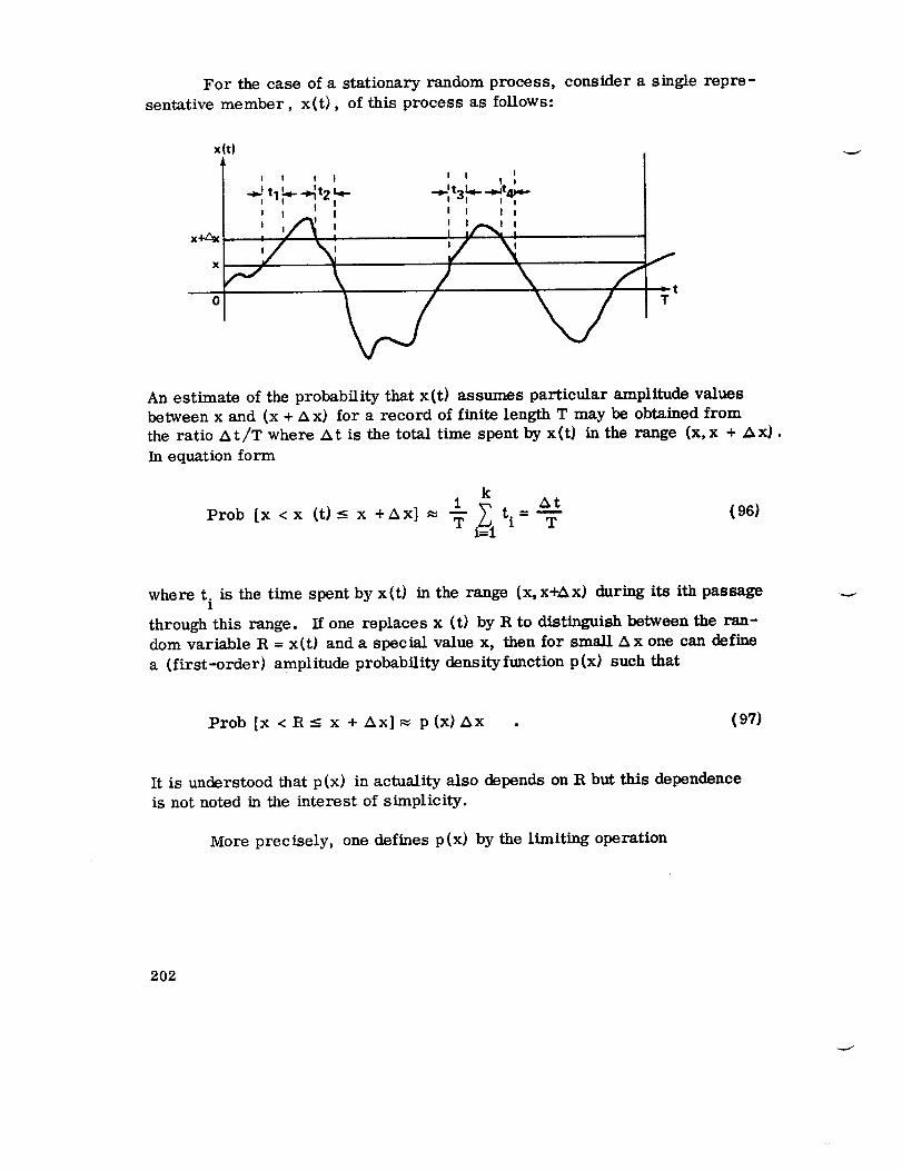
For the case of a stationary random process, consider a single repre-
sentative member, x(t), of this process as follows:
x(t
II I l I I I I I
, tl _-! _1 t2 _ -_1t31"-'| "'lt4_-I,I I I I I I I I
_.11 I I ..,_ I II I f _ I _ _
x+_x , f _ i I V _. IJ N / f
_tT
An estimate of the probability that x(t) assumes particular amplitude valuesbetween x and (x +/x x) for a record of finite length T may be obtained from
the ratio At/T where At is the total time spent by x(t) in the range (x,x + _x).
In equation form
ki At
Prob [x <x (t)< x +Ax] _ =_-._, t.=---- 11= 1 T
(96)
where t.is the time spent by x(t) inthe range (X,X+AX) during its ithpassage,
through this range. Ifone replaces x (t)by R to distinguishbetween the ran-
dom variable R = x(t) and a special value x, then for small Ax one can define
a (first-order) amplitude probabilitydensityfunction p(x) such that
Prob [x <R-- x + Ax]= p(x) Ax . (97)
Itis understood that p(x) in actualityalso depends on R but this dependence
isnot noted inthe interest of simplicity.
More precisely, one defines p(x) by the limiting operation
202

p (x) =lira Pr°blx < R-_x +Ax] = limAx
AX -*0 Ax-*0¥ .
(98)
In actual measurements one only works with finite T and nonzero Ax so that
only the estimate given byequation 9.32 is obtained which contains associated
statistical errors. (See Section VIH.D. 1. for a discussion of these problems. 7
In terms of p (x), the mean value of x (t) is given by
oO
7¢= f xp(x7 (99a7
The mean square value is
oO
x 2 = f x2p (x7 dx ( 99b7
while the variance, or second moment about the mean, is
oO
a 2 = f (x-_) 2X
oOO
p (x7 dx = x 2- Cx72 (1007
The positive square root of the variance is called the standard deviation.
Moments about the mean (central moments7 of order higher than the second
are defined in an exactly analogous way. If all moments of a probability
distribution are known, then the distribtuion is completely specified. The
amplitude probability distribution function is defined using equation ( 957.
a. Special Distributions
The application of amplitude probability density functions lies in the
fact that if the function is completely known, certain probability statements of
203

interest may be made which state where the amplitude of a signal may be
expected to lie. Certain special density functions often occur in practice
which allow quantitative probability statements to be easily made. Threeof these will now be discussed.
1. Uniform (Rectangular) Distribution
One of the simplest probability density functions is the uniform or
rectangular function. A random variable R is said to follow a uniform (or
rectangular) distribution over the interval (a < x < b) if its probability
density function is given by
a_x_<b
otherwise (lol)
See the drawing below.
b-8
o a b
The mean _ and variance a 2 of this distribution are
a+b- 2 (I02)
204

2. Normal (Gaussian) Distribution
The Gaussian probability density function is defined by the equation
1p(x) - e (103)
and has a mean value /_ and variance a 2 An important feature of this dis-
tribution is because it is completely characterized by its mean and variance
since it may be shown that all higher moments are functions of the first and
second. Probability statements are made in terms of the mean and standard
deviation. For example, if/z and a are known, then
Prob [x > /_ +3a] _ .00135 . (104)
The normal distribution is tabulated in almost any statistics book. Since
the mean and variance completely describe this distribution, if a set of experi-
mental data may be assumed to be normally distributed, an estimate of the
mean and variance obtained from this data is all that is needed to specify thedistribution. A picture of the Gaussian probability density function appearsin Section XIV.
3. Rayleigh (Radial Normal) Distribution
The Rayleigh probability density function is given by
p(x) =/"
(x/v2) exp (-x2/2v 2) x_>0
0 , x<0
(105)
This distribution is completely characterized by the parameter v. The mean of this1
distribution is (_/2) 2 v while the variance is v _-(4-_)/2. The Rayleigh prob-
ability density function is not widely tabulated. However, the Rayleigh prob-
ability distribution function is simply an exponential function which is available.
A picture of the Rayleigh probability density function appears in Section XIV.
205

B. Applications
i. Tests of Assumptions
A major reason for experimentally obtaining an estimate of an amp-
litude probability density function is to verify that some useful assumption
about the theoretical form of the distribution is correct. For example, the
assumption of the existence of a normal distribution is very often invoked in
obtaining simple useful theoretical results. A plot of the amplitude density
function can provide a visual, "quick look," verification of this assumption
if the plot follows the symmetrical, bell-shaped form characteristic of the
Gaussian density function. A quantitative method for more precisely testing
this assumption based on the analog plot of the density function and the statis-
tical errors associated with the measurements is given in Section 17 of Ref-
erence 21. If the data are available a digital form, the chi-square test
described in Section XIV. F provides an alternate quantitative method. Just
being able to visually determine if the densityfLmction is unimodal (i.e., has
a single peak) and monotonic on either side of this mode allows certain prob-
ability statements to be made. See Section 6.2.3 of Reference 20.
2. Range of Expected Variations
If a well-known density function can be assumed to properly fit the
experimental data, then probability statements can usually be made in terms
of the mean and standard deviation. However, if the data do not seem to be
well represented by some theoretical distribution, then the probability state-
ments may have to be derived directly from the observed density function.
For example, assume some piece of equipment must be mounted on a
structure and relatively little clearance will be available. Also suppose that
the structure will be subjected to random vibration and that amplitudes that
would cause contact of the equipment with the surrounding equipment are unac-
ceptable. It is then desirable to be able to estimate the probability of ampli-
tudes occurring at any given instant which are great enough in magnitude to
cause this contact. An experiment with the structure should then be performed
and an experimental estimate of the amplitude probability density function
obtained. If c is the amplitude that must not be exceeded, then one desires the
probability
P(x <c)= fp(x) dx . (106)C
206

If this number is very small such that the probability of contact at any giveninstant is minimal, no further action is necessary. However, if the probabilityof contact is unacceptablylarge, corrective action must be taken. The proba-bility given by equation (106) is over-simplified becausean uncertainty in theestimate of the density function exists. This uncertainty is given by equation
(25) and must be allowed for in an engineering application.
An exact analogous sittmtion occurs if a piece of equipment is to be
placed on a resilient mount and either bottoming of the mount is unacceptable
or large enough amplitudes to cause striking of nearby equipment or structures
is catastrophic. The procedure is precisely the same as described in thepreceding paragraph and the amplitude probability density function is the crucialinformation.
Note, that for both the above applications, the probability statements
axe good for only a given instant of time. Other statements about the probability
of exceeding a certain value within a certain length of time (e. g., a flight of T
seconds) may be made if the distribution of extreme values of amplitude isconsidered.
3. Probability of Exceeding Specified Level
Narrow frequency bandwidth random vibration responses are character-
isti¢ of lightly damped structural systems with a single predominate mode of
vibration; that is, single degree-of-freedom systems. For example, the res-
ponse of a resiliently mounted piece of equipment to broad band random excita-
tion will produce a narrow bandwidth random vibration response of the entire
equipment on the mounts. The center frequency for the response will be the
resonant frequency for the mounted equipment. Very often, continuous elastic
structures may also be treated as a single degree-of-freedom systems for
purposes of analysis to obtain approximate results for various dynamics
problems. These matters are developed further in Paragraph F. of this
section. It is only necessary to note here that a narrow frequency bandwidth
vibration response is common in many engineering problems.
If the probability density function, p(x), for a narrow frequency band
response (output) is known, and if the instantaneous amplitude and velocity.
are assumed to be statistically independent, then the probability density function
of the peak amplitudes, pp(X), may be computed [23] from the formula
207

-p' (x)
pp(X) - p(O)(107)
More directly, the probability of exceeding a critical peak amplitude, ac, is
given by the equation
GO
P (ac) = f dxP pp (x)a
c
= Prob [positive peak value _> ac]
P (a c)
p(O) a(108)
If the frequency of a narrow band random vibration is fr' the expected
number of times that a peak with an amplitude greater than a will occurc
per second is
= _ f (109)a a r
Hence, the mean time between peaks (MTBP) with an amplitude greater than
a isc
1MTBP - (110)
afar
If the occurrence of a peak greater than a is expected to be damaging, thenc
it is clear that the MTBP for the critical peak amplitude should be very long.
208
--w._

To illustrate these points, consider the case of a resiliently mounted
piece of equipment located in a flight vehicle where space is limited. The
problem is to determine how much distance must be allowed between the equip-
ment and the neighboring structure to minimize the likelihood of a collision.
Assume that the resiliently mounted equipment is a single degree-of-freedom
system (not necessarily linear) with a resonant frequency of about f = 20 Hz.r
Further assume that the vibration response displacements of the neighboring
structure are negligible compared to the response displacements of the equip-
ment. A model for the problem is shown below.
FOUNDATION
INPUT. x(t) ,
ac
Now assume that the response displacement for the equipment has an
rras value of 0.635 cm (0.25 inch) and a probability density function of the
form shown below.
p (x)
0.4
0.3
0.2
-X
0.38
I
0 0.635 1.27 1.905 2.54
DISPLACEMENT (cm)
209

As seen from the drawing, the height of the probability density function x = 0
is p(0) = 0.38. From equations (108) and (109) the height of the probability
density function at the critical displacement a is given byC
P(ac ) = (_aP(0) _ p(0) 0.019(MTBP) f - M'rBPr
where MTBP is the desired mean time between collisions in seconds.
The desired value for MTBP is a function of the total time which the
equipment is exposed to vibration. Assume for this example that the flight
vehicle is a missile where the total exposure time to pertinent vibration is 5
seconds. Further assume that an MTBP of 10 times the total exposure timeis considered acceptable. Then, the desired MTBP is 50 seconds and the
necessary value for P(ac) is
p(a c) = 0.00038.
The critical displacement a may now be obtained directly from the probabilityc
density plot for the response displacement associated with a probability density
of p(a c) = 0.00038.
It should be noted that the actual measurement of probability density
functions at extreme amplitudes involves a great deal of statistical uncertainty
unless long experiments are performed. The accuracy of probability density
measurements is discussed in Section VIII. 0.1. In the drawing shown before,
the final solution to the problem requires the determination of a displacementamplitude with a specific probability density based upon measured data. In
reality, the resulting value for a would have confidence intervals associatedC
with it because of the statistical uncertainties in the measurement of p(x).
4. Fatigue Problems
Metal fatigue considerations also involve a direct application of the
amplitude probability density function. In this case, amplitude is related to a
stress level which in turn is related to fatigue damage. The application of
210

Miner's Rule is the usual methodwhich essentially states that fatigue life isusedup proportionately at the various stress levels. That is, if 10000cyclesresult in failure at stress level a1and 20 000cycles result in failure atstress level a2, theneither 5000cycles at level a1or 10000cycles at stresslevel a2would use 50percent of the fatigue life of the metal. Actually, the
probability density function for peak amplitudes is critical for this problem.
This is in fact one of the major applications of the Rayleigh distribution since
it may be shown that a narrow band response with a Gaussian probability density
functionfor its instantaneous amplitudes has a Rayleigh probabilitydensity
function for its peak amplitudes. The fatigue problem is treated in greater
depth in Section 9 of Reference 20.
2. JOINT PROBABILITY DENSITY FUNCTIONS
Consider a pair of records R = x(t) and S = y(t). Also consider the
pair of events that R falls in the interval (x, x + AX) and, simultaneously, S
falls in the interval (y, y + Ay). The joint probability for the occurrence of
these two maybe estimated by determining the fraction of time per unit time
that these two events coincide. For records of finite length T, this estimate
is given by
AtProb[x<R --<x +Ax, y <S -< y + Ay] _ T
(111)
where At represents the amount of time that these two events coincide.
The joint probability density function p(x, y) is then defined by thecondition
Prob [x <R--< x AX, y <S --<y+Ay] _ p(x,y) Ax_y (112)
The exact value is obtained by taking limits; that is,
p(x,y) = lim
A x ---0
A y--0
Prob[x <R - x + AX, y < S -< y +Ay]
(Ax) (Ay)
(113)
211
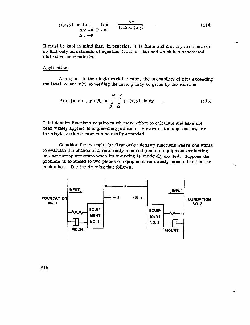
Atp(x,y) = lira lira (114)
Ax-.-0 T--.-_¢ R(Ax) (Ay) "
A y--*-0
It must be kept in mind that, in practice, T is finite and Ax, Ay are nonzeroso that only an estimate of equation (1t4) is obtained which has associatedstatistical uncertainties.
Application:
Analogous to the single variable case, the probability of x(t) exceeding
the level _ and y(t) exceeding the level fl may be given by the relation
Prob [x > _, y >/_]
oO oO
=f/pP
(x, y) dx dy . (115)
Joint density functions require much more effort to calculate and have not
been widely applied in engineering practice. However, the applications for
the single variable case can be easily extended.
Consider the example for first order density functions where one wants
to evaluate the chance of a resiliently mounted piece of equipment contacting
an obstructing structure when its mounting is randomly excited. Suppose the
problem is extended to two pieces of equipment resiliently mounted and facingeach other. See the drawing that follows.
FOUNDATION
NO. 1
J_
INPUT _-_ xlt)
___T EQUIP"
MENT
NO. 1,, J
I! IL
y(t) : INPUT !
EQUIP- _
MENT I __
NO 2 I_"
FOUNDATIONNO. 2
212

The probability desired here is that x + y exceeds a. This is given by
a a-y
Prob[x+y >a] = i - f f p(x,y)dxdy (i16)=OO --OO
The double integral is taken to the left of the line x + y = a. This would have
to be evaluated numerically ifthe density function is given as experimental
results. Even ifthe density function was available in analytical form, the
integration may have to be performed by numerical methods.
The lower limits of the integral in equation (116) are written as - oo.
However, as indicated in the drawing, there would be no amplitudes existing
beyond the mounting surfaces. Therefore, the density function would be zero
below these limits allowing one to write zero limits in equation (116).
If the density function is given digitally as a t_vo-dimensional frequency
histogram such as described in Section XIV, equation (116) could be easily
evaluated. One merely needs to count the number of observations lying to the
right of the line x + y = a. Results of analog displays would have to be arrang-
ed and interpreted in a similar manner.
3. CONDITIONAL PROBABILITY DENSITY FUNCTIONS
A conditional probability density function relates the occurrence of two
events to the probability of occurrence of one of these events. In particular,
for the pair of records R = x(t) and S = y(t) one may write equation (iii) as
Prob[x <R -< x+ AX, y <S -< y+ Ay]
= Prob[x <R - x + AX] ' [Proby <S- y
+ A y [x<R _ x +Ax]
(117)
213

In equation (it7), Prob[x < R <- x + Ax] is the first=order probabilityof
equation (97) while Prob[y< S -< y + Ay [X <IR--< X +AX] is the conditional
probability that S lies in the interval (y, y + Ay) given that R lies in the
interval (x, x +AX).
Analogous to equations (97) and (112), a conditional probability density
function p (y Ix) may be estimated by
Prob[y<S_< y+Ay I x<R- < x+Ax] _ p(y Ix) Ay. (tls)
Assuming p(x) to be different from zero, the analogy to the previous casesis extended and
p(y x) = lira
A y.--.-O
Prob [y<S-<_' +Ay[ x <R-x + AX] = p(x,y)Ay p(x) "
(119)
Again, as in the previous cases, measurement of the conditional probability
density function is subject to statistical uncertainties.
Applications:
The complete evaluation of p (y { x) requires a tremendous amount of
effort. This requires measurement of Prob [y<S-y + Ay { x<R---x + AX]
for all intervals A x, A y that cover the entire range of interest. This effective-
ly amounts to the evaluation of a density function of y given any specific x and
vice versa if p(y ] x) is desired. The evaluation is actually quite similar
but somewhat more extensive than that of a joint density function.
The conditionalprobabilitydensity function might be applied to aid the
interpretationof the autocorrelation behavior of a random process. For exam-
ple, consider a random process x(t), and lety(t) be x(t) delayed by some
value _-;that is, y(t) = x(t+T). One can nowobtain values of p(ylx o) as a
function of c for some fixed xo, For a specificvalue x0and a value of T for
which the autocorrelation function is relativelylarge, the variabilityof
p(y {x0) would be comparatively small. This in effectallows the interpretation
of the conditionalprobabilityin _ predictive sense.
214

In a special case, the conditional probability canbe computeddirectly.For example, assume the random process x(t) hasa normal density functionwith mean _ = 0 and variance _2. Assuming the process is stationary, then
ify(t) =x(t + _-) is the second process, y (t) will have mean value _ =0and variance a 2 also. The first-order normal density function p (x) is given
by equation (103) and the joint normal density function p (x, y) is
p(x, y)27ra a [1- F 2 2 1 F 2- x
x y xy xy
(120)
where
o.2 = E[x 2] ; a2 = E[y2] (121)x y
F E[xy] (122)=ffff
xy
then
Letting F = Fxy, the conditionalprobabilitydensity for y given x is
p(ylx) p(x,y) i= = expp(x) F2
Y
(123)
For the special case at hand (r = o. = _ and equation (121) reduces tox y
1p(y Ix) = exp -1 (y - F x) 2|
2o .2 (1-F 2) ](124)
215

The correlation coefficient r is the normalized value of the autocorrelation
function evaluated at 7. Therefore, for a fixed x one can consider equation
(120) as giving probability density functions for y as a function of 7.
Numerical Example
Assume that atT=.5sec, F =.80. Assume alsox=2o, and itis
desired to findthe probabilitythaty lies between Yl = i.95 _ and Yz = 2.05 a.
For convenience, assume the variables have been standardized so that theyhave unitvariance. One now wants to compute
Prob (1.95 < y _ 2.05 ix)
2.05
_-/1.95
p(y [ x) dy
with P(yl x) given by equation (124). This may be approximated numerically.First, for y = 1.95,
Pl = p(1.95[ 2.00) = i exp
(.36)
(1.95-2.00[.80])
= .66490 exp [-.17014]
= (.66490) (.84355) =.56088
Also, for y = 2.05
P2 =p(2.05] 2.00) = .66490exp -['-_-_ (2.05-2.00 [.80]) 2]
= .66490 exp [-.28125]
= (.66490) (.75484) = .50189 .
216

Now, the integral of equation (119) may be approximated by the following
formula with Ay = 0.10 as shown in the drawing below. Note that area is
essentially that of a trapezoid.
2p(yl x) dy _ (Pl +p2)2
Y_
P!
_-- yYl Y2
Substituting the values for Pi and P2 computed above, one obtains
Prob (1 95 <y<2.05 I 2.00)_ (Pl +p2) Ay• 2
= (.56088+.50189) .05 = .053
Therefore, given x = 2.00, the probability of y lying in the interval 1.95 to
2.05 is approximately. 053 or 5.3 percent.
E. Interpretation and Application of Correlation Functions
Correlation functions for random processes are divided into two types.
First, the autocorrelation function which is obtained by correlating a record
with itself, where one protion of the record is displaced in time relative to
the second portion. The more general case, the cross-correlation function,
is obtained by correlating two distinct random records, the second record
of which is displaced in time relative to the first record. The cross-correla-
tion function includes the autocorrelation function as a special case. In general,
these functions depend both on the instant of time at which they are measured
in addition to the time displacement. However, for stationary random
217

processes (that is, processes which are invariant under a translation of the
time axis), the correlation functions depend only on the time displacement.
The subsequent discussion and results hold only for stationary or for stationary
ergodic random processes. The word "ergodic" indicating that time averages
on one long record can replace ensemble (statistical) averages.
i. AUTOCORRE LATION FUNCTIONS
Let {x k (t) } represent a random process and let angular brackets < >
denote ensemble averages taken over the index k; that is, averages of the
functions making up the random process computed at a given time t. Also
assume that the mean value of the process (and of each individual record) is
zero. The autocorrelation function, Rxx( _), of the stationary random processis then defined by
Rxx(7) = <x k(t) xk(t+7) > (125)
If the process is ergodic, the ensemble averages are replaced by time
averages on a single member of the process, x(t), and the autocorrelation
function may be defined by the more practical formula below.
1 T/2R (T) = x(t)x(t+7) = lira -- _" x(t) x(t + 7) dt 1126)
xx T_.. _ T -JT/2
In equation (126) the bar over x(t)x(t + 7) indicates time averaging. In
practice, of course, only estimates of equation (126) can be obtained since
T must be finite. This error and other inaccuracies give rise to basic statis-
tical uncertainties in the measurement of Rxx(_) which must be taken into
account in interpreting experimentally obtained values of Rxx(7). These
statistical uncertainties are discussed in detail in Section VIII. D. 2.
The definition given by equation (126) applies to random data. For
periodic data, the infinite average is not necessary and the correlation
function is defined by
218

T/2
R (_.) = _l fT x(t) x(t+ _') dt (127)xx T _ /2
where the T is the period of x(t). For example, assume x(t) is a sine wave;
that is,
x(t) = A sin (2_rfot + 0) (12S)
where T = 1/f o. The autocorrelation function for this case is given below.
i T/2
fT A 2 sin (2 _f0t + 0 ) sinaxx(r) = - /2
A2 T/2= -- f sin (2_fot + 0) [sin
T -_.T/2
[27rf o (t + T)+ 0] dt
(2_rf0t + 0) cos (27rf0T)
T/2A 2 cos (2 _rf07) /"
T J-T/2
+sin (2_f07") cos (27trot0)] dt
sin 2 (2wf o t + O)
+A 2 sin (2_rf01") T/2
T /-T/2
sin (2vfot + 0) cos (2_rfot + 0) dt
Now the integral of sin 2 (2_ fo t + O) taken over its period is T/2 while the
integral of the product of the sine and cosine is zero due to their orthogonality.The final result is therefore
A2 (t29)R (T)=-_- cos (2_f07) •XX
219

For cases of narrow band noise in many physical problems, the auto-
correlation function is often given by a damped exponential of the form
-k IrJR (_) = Ae cos 27r for (130)
XX
where A and k arepositive constants. In the case of wide band noise, Rxx(_-)
has a sharp maximum at _ = 0 and fails off rapidly to zero on either side.
Figure 62 gives an illustration of these three cases. Several properties of
the autoeorrelation function in general are useful in their interpretation
and are noted here. Namely,
R (-_) =R (T) (t31_XX XX
m
[R (7)] _-<R (0)=x 2 (t) forall7 (132)XX XX
If x (t) is random, then
limR (r) = 0 (133)XX
T--_ oo
The correlation coefficient F (7), which lies between -1 and +1 )sdefined by xx
R (z)XX
I'xx(r) - R (0) " (134)XX
The coefficient I'xx(7) gives a measure of the linear relation of x(t) to
x(t+ _-). Therefore, the correlation function may be interpreted as giving a
quantitative measure of the degree of linear dependence between a function and
220

itself measured _ time units later. One interpretation of F 2 (T) is as follows.xx
F 2 (_') is that fraction of the variance of x(t + T) which is attributable to thexx
linear relation of x(t+_) to x(t). The quantity [1 - F2 (_) ] is the fractionxx
of the variance of x (t +7) that is unexplained by x(t) and is attributable tosome other source.
SINE
WAVE
x(t)
AAAAAAAAA,
VVVVVVVVV
Rxx(rl
1AAAA/ AAAAAVVVVVIVVVVV'
NARROW
BAND
NOISE
WIDE
BAND
NOISE
e
The cross-correlation function Rxy
defined by
Figure 62. Illustration of typical autocorrelation functions.
CROSS-CORRE LATION FUNCTIONS
Let (x k (t) } and {Yk (t)} denote two stationary random processes.
(_-) between {x k (t)} and {Yk(t)} is then
221

/ N.R = \_x'(t) Yk(t + /T)> . (135)xy
Fcr ergodic processes the ensemble average of equation (135) may be replaced
by a time average of single members of the processes and Rxy(T) is alternative-ly defined by
R (T) r/2xy = x(t)y(t+'r) = lira f x(t)y(t + r) dt . (136)
T -_ -T/2
As for the case of the autocorrelation function, statistical uncertainties will
exist in any estimate of equation (136) due to finite averaging time and other
inaccuracies. The same considerations discussed in Section VKI.D. 2 for the
autocorrelation function apply to the case of the cross-correlation function.
The relations given by equations (131), (132), and (133) for the au£o-
correlation function do not hold m general for the cross-correlation function.
However, similar relations do exist and are given below.
Rxy(r) = Ryx(- _') (137)
IRxy(r) I _ [Rxx(0) Ryy(0)]
!
for all T ; (138)
that is, Rxy(T) is not an even function as is Rxx(_-) , although when x(t) and
y(t) are interchanged, symmetry about the vertical axis exists. Equation (138)
is the analogous statement to equation (132), and, in fact, equation (132) is a
special case of equation (138). An additional relation for the cross-correlation
function is as follows:
IR (_'11 < 1xy -- _" [iRxxC0) + R (0)] (139)YY
222

Note that this relation also will give equation (132) as a special case.
A cross-correlation coefficient may be defined which gives the simple
correlation coefficient of equation (134) as a special case; that is,
F (r) = _ (140)
xy [Rxx (0) R (0)] _YY
The quantity r (T) is bounded by +1 and -1 as can be seen by applyingequation 9.74. xy
3. APPLICATIONS
Auto- and cross-correlation functions have been applied in the past to
many different physical problems. Such areas have been involved as improving
tracking radar reception, aircraft position finding, electroencephalogram
analysis, and many facets of vibration data analysis. Two underlying featuresare fundamental to most applications. These are the determination of time
delays and the determination of an underlying functional relationship resulting
in large correlations.
(a) Example. Detection of Sine Wave in Noise (Autocorrelation)
As an example of detecting a functional relationship obscured by noise
which is important to vibration analysis, the detection of a sine wave in noisewill be illustrated. Assume the presence of a sinusoid x(t) = A sin 2 _0t with
A = 0.0254 cm (. 010 inch) and f0 = 100 Hz. Also assume narrow band noise,
n(t), is present at fo = 100 cps with a mean square value A2/2 = 32. 258 cm 2
(5 x 10 -6 in.2). The autocorrelation function of the sinusoid is given by
equation 9.65 which is R (T) = 32. 258 × 10 -5 [COS 2 u (100)r] cm 2 for thexx
example at hand. The autocorrelation function for narrow band noise for this
example is assumed to be given by equation (130) which is R (T) = 5 × 10 -5nn
e -_v cos [2_r(100)_]. The constant c equals 32.258 × 10⁻⁵cm2 (5 × 10 -5 in.2)
since c must be the mean square value determined by letting _ = 0. The
constant k of equation (129) is arbitrarily assumed to be 30 rad/sec for this
example which is a typical value.
Assume that x(t) and n(t) are indeptendent. Then if y(t) = x(t) + n(t),
the autocorrelation function for y(t) is given by
223

R (T) =R (T) +Rnn(T) (141)YY
Since R (T) is a cosine function and R (r) is a cosine exponential whichxx Im
goes to zero as T gets large, the R (T) term will domimte in equation (141)xx
for large T; that is, the following equation holds.
iim R (T) - _ " (142)T -_ yy
One says that R (_-) and R (_) are asymptotically equal. This means, thatxx yy
when the autocorrelation function is plotted, it will start to look like R (v)XX
for large T instead of decreasing to zero as pure noise would. This is illustra-
ted in Figure 63 for the special case described. One should note that an actual
autocorrelation plot would contain many irregularities due to statistical uncer-
tainties and other inaccuracies. However, the basic underlying shape would
appear as pictured in Figure 63.
(b) Example. Detection of Prominent Vibration Transmission Path
( Cross -correlation)
Assume that it is desired to attempt to determine whether the most
prominent vibration response on a structure is a result of transmission via
wave propagation through the structure or is due to acoustic transmission via
the surrounding air. For simplicity in the example, it will be assumed
that structural path lengths are great enough compared to the wave length
of the vibration so that any structural transmission is by wave propagation(Fig. 64).
If the distance of transmission through the air is assumed to be 3.048
m 10 feet (and phase shifts at interfaces are ignored), a peak in the cross-
correlation function R (r) would be expected atxy
3. 048m( 10 ft)_" = 304.8 m/sec(1000ft/sec) = 0.01 sec
where the speed of sound is taken to be approximately304.8m/sec (1000 feetper second).
224

=5 x 10 -5 cos [2_'(100)Tl + 5 x 10 -5e-30r cos (2_r(100)rl
--Rxx ('r) = 5 x 10 -5 cos [271(100) r]
|
I
i
)1
I
--5 x 10"5 e'30r
• !
11IIi
i
• q= , l=
II
05
i
I
,i
_j _J
(DECAY OF THE COSINE AMPLITUDE
IN THE EXPONENTIAL COSINE CURVE)
L,,'t_
i
i06
" 7I
)_
I,
tIIII
II
II
I I
_s 'I
l'II!I!IIt
OISPLACEMENTt
.09 r (SEC)
-10-
Figure 63. Autocorrelation function for sine wave plus noise.
225

INPUT MEASURING DEVICE
INPUT VIBRATION xlt)
3.048m
<--THIN ALUMINUM SKINS--.*-
POSSIBLE
TRANSMISSION PATH
THROUGH AIR
3.048 m
STRUCTURAL MEMBER
_PPO _ _SSIBLE TRANSMISSION PATHTHROUGH STRUCTURE
OUTPUT MEASURING DEVICE
I OUTPUT VIBRATION ylt)
I3.048 m
Figure 64. Transmission path determination example.
Wave propagation through the aluminum structure is assumed to occur
at a speed of approximately 4572 m/sec (15 000 feet per second). Therefore,if significant vibration transmission occurs throught the structure, a peak
in the cross-correlation function R (7) would be expected atxy
9.144m (30 ft)_" = 4572 m/sec (15 000 ft/sec) = 0.002 sec
since the structural path is 9. 144 m (30 feet) long.
Suppose now that measurements of the input x(t) and the output y(t) are
obtained. An estimate of the cross-correlation function, R (7), is thenxy
obtained via an approximation to equation (136). The cross-correlation func-
tion might then appear as pictured in Figure 65. The interpretation would
be that a strong correlation exists between x(t) and y(t) at a delay of _" =. 010
second, indicating the major energy is being transmitted acoustically. A
secondary peak appears at z =. 002 second, indicating a weaker relation
because of the direct tranmission through the structure.
226

Rxy(___..T)0.8
°x°Y 0.6
0.4
0.2
-o0.001 0.003 0.005 0.010 0.015
Figure 65. Possible normalized cross-correlation function
for transmission path example.
The example given here greatly oversimplifies the problem, of course.
A considerable amount of structural engineering analysis would be required
to actually determine the structural response and its effect on transmission
delays. Also, statistical analysis is required in the proper determination
of the correlation function and its associated uncertainties. However, the
basic approach to the problem would remain the same.
(c) Example. Detection Theory
A more theoretical application of correlation techniques _rises in
detection theory. If it is assumed that a given input signal is obscured by
white noise, itcan be shown that the optimum linear filter takes the form of
a correlator except for a constant factor. In this situation the input which
consists of signal plus white noise is multiplied by a stored version of the
signal it is desired to detect. This gives the optimum putput where maximum
output signal-to-noise power ratio is the optimization criteria.
F. Interpretation and Application of Power Spectral Density Functions
The ordinary and cross-power spectral density functions are important
concepts for both practical vibration data analysis problems and for theoretical
structural analysis problems. In a theoretical context, the areas of application
for power spectra are effectively the same as for correlation functicns, since
the two properties for stationary vibration data are Fourier transform pairs.
227

However, in a practical context, the frequency format of power spectra is
easier to interpret for many applications, just as the time format of corre-
lation functions is easier to interpret for certain applications discussed
in Paragraph E. of this section.
Ordinary and cross-power spectra are discussed here primarily in
terms of their relationships to idealized structures. Hence, it is appropriate
to first review the dynamic characteristics of idealized structures before
proceeding.
t. RESPONSE CHARACTERISTICS FOR IDEALIZED STRUCTURES
An idealized structure is defined as one which has constant parameters,
and is linear between two points of interest called the excitation (input) point
and the response (output) point. A structure has constant parameters if all
fundamental properties such as mass, stiffness, damping, and geometry are
invariant with time, and the surrounding environment. A structure is linear
if the response characteristics are additive and homogeneous. The term
additive means that the response to a sum of excitations is equal to the sum
of the responses to the individual excitations. The term homogeneous means
that the response to a constant times the excitation is equal to the constanttimes the response to the excitation.
Given an idealized structure, the weighting function h(_) associated
with the structure is defined as the response (output function) of the ideal-ized structure to a unit impulse input function and is measured as a function
of time, 7, from the moment of occurrence of the impulse input. For physi-cally realizable systems, it is necessary that hiv) = 0 for _ < 0 since the
response must follow the input. The usefulness of the concept of the weight-
ing function is because of the following: an idealized structure is completely
characterized by its weighting function in the sense that given any arbitrary
input as a function of time x(t) and known for all t, the system output yit)is determined by the equation
y it) f h (7) x(t - 7) dr ; (143)0
that is, the value of the output function, yit), at time t is given as a weighted
linear (infinite) sum over the entire past history of the input xit).
228

If x(t) is an input to the structure for only a finite fixed time T, then
Ty(t) = f h(r) x(t-r) dr . _144)
0
If x(t) exists only for t >- 0, then
t
y(t) f h (r) x(t-r) dr0
since
(145)
oO
f h (r) x(t- r) drt
= 0 ;
that is, for t-r < O, or 1" >t, x(t- 1") = O. Hence the above equation.
The idealized structure may alternatively be characterized by its
frequency response function H(f) which is defined as the Fourier transform
of h (r),
oO
H(f) = fh (r) e -j27rf-r dT (146)0
where f is measured in cycles per unit time. The lower limit is zero instead
of -_ since h(r) = 0 for _- < 0. The replacement of the weighting function \vith
the frequency response function may be made since there is a one-to-one cot'-
respondence between classes of suitably restricted functions and their Fouriertransforms; that is, two different weighting functions will not give the same
frequency response function. The restrictions on h(r) are that h(r) and
its derivative h'(_') must be piecewise continuous on every finite interval
(a, b), and that i h (T) I must be integrable on (-_. _o). It should be noted
that the frequency response function is a special case of the transfer ffmction
-j 2 _frof a structure given by the Laplace transform of h(r) in which case e
in equation (.146) is replaced by e -pI" where p is a general complex variable.
229

The frequency response function is of great interest since it contains
amplitude magnification and phase shift information, Since H(f) is complex
valued, the complex exponential (polar) notation may be used; that is,
H(f) = TH(f) ! e j_)(f) i147)
where '_H if) ! is the absolute value of H if) and ¢ (f) the argument of Hif).
The absolute value [H (f) t, which is often called the gain factor, measured
the amplitude magnification when the input to the structure is a sinusoid while
the angle ¢ if), which is often called the phase factor, gives the correspondingphase shift.
This result may be easily seen by consideration of the complex input
xit) = ae j2_rft = Ae j0) e j2_t
= A cos (21rft+ 8) +j A sin (27rft+ O) . (148)
Note that the real part of equation (148), A cos (2 7r ft + 0) is a general
sinusoidal input with amplitude A and a phase angle 0 with respect to some
time origin. By definition, an idealized structure is linear which implies
the real part of the output response is due to only the real part of the input
excitation, and likewise for the imaginary parts. Hence, any result obtained
for the complex function contains the same result for the real part of the
function as a special case. These facts allow the concrete physical inter-
pretation to be placed on the frequency response function of equation (147),
even though it i_ a complex valued quantity.
Substituting equation (148) into equation (143) gives
cO
y(t) = fhir) ae j21rf(t-r) dr0
eJ2 7r ft e-J2 7rfr= a f h (r) dr0
= x(t) H(f)
230

or, once can write
y(t) = A IH if) ]e j [27r ft+ O +¢P (f)] (149)
which illustrates the amplification by the gain factor r H (f) r and phase shift by
the phase factor _ tf) of the sinusoidal input.
Certain other symmetry properties are worthwhile to note, namely,
oo
i 7r
H if) = f h(l") e J2 dl- = H i-f)ft
0
(15o)
where H (f) is the complex conjugate of H(f). Also, this relation gives
H if) = { H (f) ! e -j _ (f)
H t-f) = ! H(_f) l e jet-f)
which implies
{Htf) { = ]Ht-f) _ (.151)
and
-¢ (f) = ¢ (-f) . (152)
Another important relationship is that given the input x(t), the weight-
ing function hit), and output ytt), then
Y(f) = H(f) X(f) (153)
231

where Y(f) and XCf) are the Fourier transforms of y(t) and x(t),
tively. This may be shown directly as follows.
Y(f) = h(_) x(t - r) dT e -j2 _ ft dt
ms.c-
-j2_r ffNow, multiplying and dividing by e and rearranging terms gives
(TY(f) = . h(r) e x (t-r) e dt0 -ao
The desired result is obtained by the change of variable u = t - r and du = dr
in the righthand integral.
The following important fact is seen immediately. If one idealized
structure described by Hi(f) is followed in succession by another idealized
structure described by H2(f) where the second structure does not load the
first, then the overall structure is described by H (f) where
H(f) = Hl(f) H2(f) .
This is true since
Y(f) = Hi(f) X(f)
and
Z(f) = H2(f)Y(f) =H2(f) [Hi (f)X(f)]
= [H 2 (f)Hi(f)]
= H(f) X(f) .
232

This implies that
IH (f) I = IH I (f) I IH2(f) I
¢ Cf) = _)l(f) + ¢2Cf) (154)
so that in cascaded idealizedstructures, the gain factors multiply and the
phase factors add when itis assumed thatthe two structures are decoupled.
Note thatuse is often made of the complex exponential notation since it
conveniently displays amplitude magnification and phase shiftinformation.
This is merely polar coordinate notation in the complex plane, however, under
certain conditions the x = u + iv form of notation may conveniently illustrate
certain information in a useful manner. In thiscase, Re (x) = u and Irn (x) =
v are defined as the real and imaginary parts of the complex variable x. This
alternativeinterpretationis illustratedin the material which follows.
2. IDEALIZED STRUCTURE WITH MOTION EXCITATION
Consider the case of a structure which is subjected to a foundation
motion excitation. Assume that the structure can be represented by a simple
linear lumped parameter system consisting of a mass, spring, and dashpot
as shown in Figure 66.
I!111111111111111111111111
xlt)
I 1 EQUILIBRIUMm y(t)
Figure 66. Idealized structure with motion excitation.
In Figure 66, k is the spring constant in N/m, c is the viscous damping
coefficient in Ns/m, and m is the mass in kg-sec2/inch. The term x(t)
233

is the excitation measured in any units of motion desired (displacement,
velocity, acceleration, strain, etc.), and y(t) is the response measured in
the same units. The model in Figure 66 might represent some secondary
structure in a flight vehicle (simplified to only one degree-of-freedom) which
is subjected to random vibration of a primary supporting structure. The
problem is to determine an appropriate frequency response function for thismodel.
From basic dynamics, the stun of all forces acting on the mass in
Figure 66 must equal zero; that is,
Fk(t) +Fc(t) + Fm(t) = 0(155)
whe re
Fk (t) = -k [y (t) - x(t)] = spring force
F (t) =-c [Y (t) - x(t)] = damping forceC
o,
F (t) = -my (t) = inertialforcem
y(t) = dy(t) /dt = velocity
y (t)= d2y(t)/dt 2 = acceleration
Now assume the foundation motion is sinusoidal such that x(t) = X 1
sin 2 r ft. It will be more convenient here to use complex numbers instead
of trigonometric functions. From the identity, e j 8 = cos 8 + j sin 8, it
follows that a sinusoidal function may be expressed by sin 8 Im [e j 8].
Using this notation, the assumed foundation motion is
x (t) = Im[Xle j2_ft] (156)
From equations (155) and (156), the resulting equation of motion for the
structure is as follows:
234

m_'(t) + c_ (t) + ky(t) = Im[(k+j27rfc)Xle j2_rft] . (1.57)
The particular solutionto equation (157) will yield the desired steady stateresponse y(t).
Now assume a solution to equation (157) in the general form of asinudoidal response as follows:
y (t) = Ylsin (27rft+9) = Im [Yle j (2_ft+9)] (158)
Here Y1 is the peak value of the response and _ is the phase angle betweenthe response and the sinusoidal excitation. When equation (158) is sub-
stituted into equation (157), the following relationship is obtained:
Im [- (2 _f)2m + j2_fc + k]Y 1 e j (2_ft + 9)
Im [(k +j2 _fe) Xle j2_ft]g"
= :.- (159)
Hence, the particular solution to equation (157) is given from equations9.94 and (159) as follows: _,
y(t) = Im ',k +_2_fc) X le j2_k- (2_f) zm+j2_f
(160)
It is desirable to write equation (160) in a different form by introducing4
two definitions
=- where c = 2 (161a)e c
e
n 2-'_ " (161b)
235

The term c in equation (161a) is called the "critical damping coefficient"c
and the ratio _ is called the "damping ratio." The term f in equation (161b)
is called the "undamped natural frequency." When the relationships in equation
(161) are substituted into equation (160), the following result is obtained:
y (t) = Im
m
- +j2 Tn
(162)
When equation (162) is converted from complex notation to trigonometric
notation, the following result is obtained.
y (t)=
+ _ f X 1sin (27r ft÷
(163a)
where
= - arc tan2
(163b)
Note next that the frequency response function for this problem may
be written as
H(f) = IH (f) e jO(f)
236

where the gain factor I H (f) I is given by the ratio of the response amplitude
to the excitation amplitude, and the phase factor _ (f) is given by the phase
shift between the response and excitation. Hence, from equations (158) and
(163b), the gain factor [ H (f) I is given by
1 + _ f
]H(f)l = y f 2 2 f 2 (164)- +
and _ (f) is as given by equation (163b). The general result is illustrated
i_ Figure 67.
I H(f)l ¢ (f)
1 m
0 ifn
180
2 fn
D f 0 f!
0 fn
Figure 67. Gain and phase factors for frequency
response functions.
The frequency response function H (f) for this problem may also be
written directly from equation (162) in the following form. This is often
called the "transmissibility function" for the single degree-of-freedom
system.
237

f
1 + TH(f) = n . (165)
- +j2_ _--n
Equation (165) may be written as a complex number w = u + iv, where the
real and imaginary parts are as follows:
H(f) = Re [H(f)] + jim [H(f)] (166)
where
2 2
i - -f + 2_ "_n
Re[H (f) ] = 2 (166a)
3
Im[H(f)] = 2 _ 2 " (166b)
_f + Tn
The general result for this type of presentation is illustrated in Figure 68.
There are other frequency response functions which are applicable to
a simple idealized structure for different interpretations which should not be
confused with the transmissibility function of equation (165). For example,
assume the response parameter of interest in Figure 66 is the relative motion
z(t) = y(t) - x(t). The appropriate frequency response function which relatesa motion excitation x(t) to a relative motion response z(t) is as follows:
238

H (f)
(f/f)n
2
- +f
j2_ T-n
(167)
H (t)
mm
%
\
Re
/ \
fn _ _""" "" "-- "--
\ ,• / Im
= f
Figure 68. Real and imaginary parts for frequency
response function.
For a second different example, assume the response of a simple
structure to a force excitation is of interest, as illustrated in Figure 69.
///,/////////
k < c
<
m
IIIII1 I I I / I / POSITION OF
EQUILIBRIUMy(t)
1x(t) = F(t)/k
Figure 69. Simple idealized structure with force excitation.
239
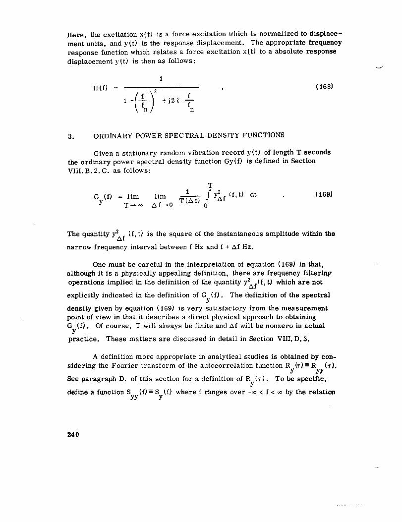
Here, the excitation x(t) is a force excitation which is normalized to displace-
ment units, and y(t) is the response displacement. The appropriate frequency
response function which relates a force excitation x(t) to a absolute response
displacement y(t) is then as follows:
H(f) = . (168)
1- f +j2_ -_-n
3. ORDINARY POWER SPECTRAL DENSITY FUNCTIONS
Given a stationary random vibration record y(t) of length T seconds
the ordinary power spectral density function Gy(f) is defined in Section
VIII. B. 2. C. as follows:
T
1 f2G (f) = lim lim T(Af) y_f (f,t) dtY T--* _o A f--*0 0
_169)
The quantity 2 (f, t) is the square of the instantaneous amplitude within theYAf
narrow frequency interval between f Hz and f + Af Hz.
One must be careful in the interpretation of equation (169) in that,
although it is a physically appealing definition, there are frequency filtering
operations implied in the definition of the quantity y_f_f, t) which are not
explicitly indicated in the definition of G (f). The definition of the spectralY
density given by equation (169) is very satisfactory from the measurement
point of view in that it describes a direct physical approach to obtaining
G (f). Of course, T will always be finite and Af will be nonzero in actualY
practice. These matters are discussed in detail in Section VIII. D. 3.
A definition more appropriate in analytical studies is obtained by con-
sidering the Fourier transform of the autocorrelation function R (T)-R (v).Y YY
See paragraph D. of this section for a definition of R (T). To be specific,Y
define a function S (f)- S (f) where f r'anges over -_¢ < f < _o by the relationYY Y
24O

S (f) = f e -j27rfr R (r) drY Y
Equation (170) may be simplified by the following procedure:
(170)
f e -j2vff R (T)Y
a_
f R (v) cos 2_rfr dtY
j f Ry(_') sin 27rfr dt(171)
Use the fact now that R (T) is an even function and sin 2_v dT is an oddY
function. That is, R (_')= R (-T) and sin 27r (-1-) = -sin 27rfT. Then, theY Y
imaginary term in equation (171) is zero since it is the integral of an odd
function between symmetric limits. This is shown mathematically by
-._ -_ 0 -
0 y
(-r) sin 21rfC-T) d7
+
oo
f R (_)sin27rfTd7=Y0
,
Therefore,
SY
(f) = f R (T) cos 2_r fv dl"Y(172)
241

The quantity S (f) is a two-sided mathematical idealization whichY
covers the frequency interval from minus infinity to plus infinity. Note thatSy (f) is actually ficitiious since negative frequencies are physically unreal-izable. However, Sy (f) is related to the physically realizable one-sidedpower spectral density function Gy (f) which exists only for f >_-0 as follows.Define
G (f)= S (f) + S (-f) = 2S (f) for f _->0 (173)Y Y Y Y
= 0 for f < 0
Then, the following relationship is true:
Gy(f) = 4 f0 Ry(T) cos2_ff dr(174)
The equivalence of equations (169) and (174) is proved in Reference 24.
These equivalent relationships are fundamental to the proper interpretation
and application of power spectral density functions, as will now be shown.
Consider an idealized structure with a weighting function h(T). If an
excitation of x(t) is applied to the structure, the response y(t) is given by
CO
y(t) = f h(T) x (t-r) dT (175)--CO
Then, the power spectrum for the response is as follows:
O0 CO *
-Z_rff R -27rfr ES (f) = f e (T) dT= fe [y(t) y (t+T)] dTY Y
--CO --CO
242

cO cO o0
=fff -27rf_" h(e o_)h(fl)E[x(t -_ )x(t+_--fl)]d_d_d_-
co oO cO
f f f h( )e27rfa
h_) e-21rfflR (_+ol -fl)
e- 2 _'f (-r+c_ +fl) d_ dfl d_- .
Noting that 1-, _, and fl are dummy variables, a change of variable
t = • + c_ - fl, dt = dr, can be made so that the equation may be factored to
obtain the following result:
S Cf)=H(f) H* (f) S (f) = [H(f) l 2S (f) o (176)y x x
In equation (176), H(f) is the frequency response function for the
structure between the excitation and the response, H* (f) is the complex
conjugate of HCf), and [HCf)[ is the magnitude of H (f) or the gain factor
for the structure. The quantity SxCf ) is the two-sided mathematical power
spectral density function for the excitation. In terms of the physically
realizable power spectra for the excitation and response, equation (176)becomes
G (f) = IHCf)12GxCf ) . (177)Y
The result presented in equation (177) is extremely important and
illustrates the fundamental value of power spectra concepts for structural
vibration problems. In words, the power spectrum for the vibration response
of an idealized structure is equal to the power spectrum for the excitation
multiplied by the square of the gain factor for the structure. Given any two
of the quantities in equation (177), the third can be determined. For example,if the frequency response function for a structure is known, the power spectrum
243

for the responsecanbe computedgiven the power spectrum for the excitation,andvice versa. Also, if the power spectra for the excitation andresponseare known, the gain factor for the structure (but not the phasefactor) canbecomputed.
Referring to equation (172), the inverse Fourier transform for the
power spectral density function is
cO cO
R_ = f Sy(f) cos 2_r f7 df = f Gy(f) cos 27r fT clf . (178)-co 0
The mean square value of the signal is equal to the autocorrelation function
for zero time displacement (_'=0). Hence, the following relationship ensuesdirectly.
co
-- fGyy2 = R (0)= if) df . (179)
Y
The total mean square value for a random vibration is equal to the total area
under the power spectrum for the vibration. The rms vibration amplitude is
equal to the square root of the area. Furthermore, if only those frequencies
in the range between fa and fb Hz are of interest,
7 (fa, fb ) = i 'f'b Gy(f)df
a
(180)
m
y_ (f, fb) is defined as the mean square value of a random vibration in the
frequency range from f to fb Hz and is equal to the area under the powera
spectrum for the vibration between those frequency limits. The corresponding
rms vibration amplitude is equal to the square root of the area.
Numerical Example:
Consider a structure between two points of interest on a flight vehicle.
Assume the fundamental natural frequency and damping ration for the structureare
244

f = 100 Hzn
= 0.025
Further assume that one end of the structure is subjected to a vibration x(t)
which, when measured in acceleration units, has a reasonably uniform power
spectral density function of
G (f) = 0.01 g2/HzX
over a frequency rangefrom f << 100 to f >> 100 Hz. Note that g = 9. 804m/sec 2 (386 tnches/sec2). The problem is to determine the power spectrum
and rms amplitude for the response acceleration at the other end of thestructure.
Assuming that the structure may be represented by a simple ides2ized
structure as shown in Figure 66, the appropriate gain factor for the structure
is given by equation (164), in that section. For a natural frequency of f =n
100 Hz and damping ratio of _ = 0. 025, the gain factor is
[H(f) [1+t°°5 t,oo
f 2 2- +
0.05 f
100
From equation (177), the power spectral density function for the response
acceleration will be as follows:
G (f) =Y
100 O. 01
2] ' + rO. O0_] '
,oo j L,00j
g2/H z
24 5

A plot for the response power spectrum is presented in Figure 70.
The total mean square value for the response acceleration will begiven in general terms as follows.
oo oo 2
= n elf (is1)
For the special case where O (f) is a constant (hypothetic.Uy for all fre-quencies), equation (181) canXbe integrated by the method of residues to
obtain the following solution:
_f (i +4_ 2) G _f G
"_ = n X n x4 _ _ 4 _ for _ << 1 . (182)
Substituting the proper values for this problem into equation (182) gives thefollowing result:
,r (100) (0.01) = 31.4g z= 4(0.025)
Hence the rms response acceleration is
Yrms = 5.6 g = 55.88 m/sec2(2200 in./sec2).
246

Note that the value for y'} could also be obtainedby graphically measuringthe area under the responsepower spectrum in Figure 70.
4. CROSS-POWERSPECTRALDENSITYFUNCTIONS
Given two stationary randomvibration records, x(t) andy(t), eachof length T seconds, the cross-power spectral density function G (f) is
xydefined in SectionVIII.B.2.f. as follows:
Gxy(f) = Cxyif) - JQxy if) (/83)
where
T
1 yA f(f, t)Cxy(f) = lira lim T(AI) J0 x Af(f,t) dt (183a)T-*co A f---0
1 T /VVVVV
QxY(f) = T--colim Af---01im TiAf) J0 xA f(f't) YAfif't) dt (183b)
The quantities xA f(f, t) and y A fif, t) are the instantaneous amplitudes within
the narrow frequency interval between f Hz and f + A Hz. The symbol (WW)
in equation (183b) means that xit) is 90 degrees out of phase with y(t).
From equation (183), the cross-power spectrum is a complex valued
quantity with a real part C (f) called the cospectrum and an imaginary partxy
Q (f) called the quadspectrum. The definition of G if) in equation (183)xy xy
is satisfactory from the measurement point of view in that it describes a
direct physical approach to obtaining Gxyif), just as equation (169) describes
a direct physical approach to obtaining the ordinary power spectrum G if) •Y
Of course, T will always be finite and Af will be nonzero in acttm2 practice.
These matters are discussed in detail in Section VIII. D. f.
247

10.
N
_r
m
zaMe_.=J
<
W
_rMJ
aM
ZOca
uJ
.001 I I I I I0 20 40 60 80 100 120 140 160 180 200
FREQUENCY (Hz)
248
Figure 70. Response power spectrum for simple structure.

The cross-power spectrum is a generalization of the ordinary power
spectrum as the cross-correlation function is a generalization of the auto-
correlation function. Hence, the most direct definition is an analogy to
equation (170) ; that is, define
Sxy(f) = J e-J2_frR (I-) dr (184)xy
where R (r) is the cross-correlation function defined in Paragraph D. of thisxy
section. Because R (_') is not an even function, the imaginary portion ofxy
this transform does not vanish in general, and therefore S (f) is a complexxy
number. As before S (f) is a two-sided mathematical idealization whichxy
covers the frequency interval from minus infinity to plus infinity. A physically
realizable cross-power spectral density function Gxy(f) is given by
Gxy(f) = Cxy (f) - JQxy(f) = 2Sxy(f) ; f _ 0 (185)
= 0 forf< 0
Referring to equation (184), it can be shown from the sin 2v ft and
cos 2_r ft parts of the Fourier transform that the cospectrum is an even function
of f while the quadspectrum is an odd function of f; that is,
Cxy (f) = Cxy(-f)(ls6)
Qxy (f) = "Qxy (-f) "
Also, from the symmetry property of the cross-correlation function, Rxy
(- _) = R (_-), it follows immediately thatyx
249

oO
Cxy(f) = f0[ Rxy (_) + Ryx (T)]cos 21r f_-dT
1
= _- [Gxy (f) + Gxy(-f)]
QxY(f) = f0 [Rxy(T) - Ryx(T)] sin 27r fT dT
(187)
=1 [G (f)-G C-f))2 xy xy
In the above equations, it is sufficient to obtain the functions for f _> 0 since
the symmetry properties in equations (186) yield the results for f < 0.
A further relation for the cross-power spectrum may be obtained from
the symmetry properties of the cross-correlation function. (See ParagraphE. 2. of this section. )
G (-f) = G $ (f) = G (f) (188)xy xy yx
Here, Gxy (f) is the complex conjugate of Gxy(f). From basic considerations,
it can be shown that GxyCf) satisfies the following important inequality:
2
IGxy (f) I -<Gx (f) Gy(f) (t89)
Now consider an idealized structure with a weighting function h(v).
Assume that an excitation x(t) with a power spectral density function G (f) isx
applied to the structure producing a response y(t). By the same procedures
used in Paragraph F. 2. of this section, it can be shown that
GxyCf) = HCf)Gx (f) (190)
250

where H (f) is the frequency response finction for the structure between the
excitation and the response.
The physical interpretations for cross-power spectral density functions
are similar in part to the applications for cross-correlation functions. Speci-
fically, a cross-power spectrum will reveal dependence (or coherence) betweentwo vibration records. That is, if two random vibration responses, x(t) and
y(t), are completely independent and unrelated to one another, the cross-
power spectrum for the two responses will be zero at all frequencies. On the
other hand, if the two vibrations are related, the dependence must be due tosome structural connection between the points where the vibrations occur.
For this case, a nonzero cross-power spectrum will be measured which is
associated with the frequency response function for the structure between
the points.
Consider the case where a vibration response y(t) at some point on a
structure is the result solely of the vibration response x (t) at some other point.
Clearly, x(t) may be considered an excitation which produces a response y(t).
The frequency response function between the two points will be given directly
by equation (190). This points out the most important application for cross-
power spectral density functions; that is, the determination of frequency
response functions for structures from measured vibration data.
Because the interpretations for cross-power spectral density functions
are closely associated with structural frequency response functions, it is often
desirable to present a cross-power spectrum in the form of a magnitude and
phase angle as follows:
Gxy(f) Cxy(f) JQxy (f) [Gxy (f) I e joxy(f)= - = (1917
2I Gxy(f) I = _/ CZxy(f) + Qxy (f) (192)
-Qxy(f)
0xy (f) = arc tan Cxy (f)
(193)
By presenting the frequency response function H (f) in terms of the
gain factor IH (f) I and the phase factor _ (f), equation (190) becomes
251

]G (f) I eJexY(f)= IH(f) J e J_'_(f'G_ (f)xy x
(194)
Hence, the following input-output relationship exists:
PGxy(f) I = lH(f) I Gx (f) (195)
e (f)= (f)xy
The cross-power spectrum for an excitation and response has a magnitude
equal to the power spectrum for the excitation multiplied by the gain factor for
the structure, and a phase factor equal to the phase factor for the structure.
Ncte that the phase angle e (f) can be used to determine time delays, asxy
would be obtained from a cross-correlation function. The time delay Txy(f)
between the excitation and response at any frequency f is given by
e (f)
•xy(f) = 21rf " (196)
Numerical Example:
Consider a structure between two points of interest on a flight vehicle,
as discussed for the example in Paragraph F. 2. of this section; that is, assume
that the structure may be represented by a simple idealized structure as
shown in Figure 66, with a natural frequency of f = 100 Hz and a dampingn
ratio of _ = 0. 025. Further, assume that the structure is subjected to a
vibration excitation which, when measured in acceleration units, has a reason-
ably uniform power spectral function of Gx(f) = 0.01 g2/Hz over a frequencyrange from f << 100 to f >> 100 Hz. The problem is to determine the cross-
power spectrum for the response acceleration relative to the excitation,
and the time delay between the response and excitation at the frequencyf = 100 Hz.
252

by
From equations (t91) and (195), the cross-power spectrum is given
J 0xy(f)
Gxy(f) = IGxy (f) I e
whe re
G (f) = 0.01 IH(f) I g2/Hzxy
0 (f) = _ (f) radiansxy
The appropriate gain factor and phase factor for the structure is given by
equation (163) Substituting from equation (163) and noting that f =100 Hz• n
and _ = 0. 025, the cross-power spectral density function is as follows:
IG if) I 2o. o5f ]
+ L looj
Oxy(f ) = - arc tan
o.os2
+
For the frequency f = 100 Hz, the phase angle for the cross-power
spectrum is
253

0xy(100) = - arc tan (20) = 1.52 radian.
Hence, from equation (196), the time delay between the excitation and res-ponse at f = 100 Hz is as follows:
l. 52= -- = 0.0024 second
xy 200_
1 COHERENCE FUNCTIONS
The application of cross-power spectra concepts as a tool for measur-
hag the frequency response functions for structures is best implemented withaid of a real-valued quantity called the coherence function. The coherencefunction __ (f) is defined as follows:
xy
tG (f) 122 (f) = xy . (197)
Txy Gx (f) Gy (f)
For an idealized structure (constant parameter linear system) wherea response y(t) is due solely to an excitation x(t), the coherence function
for x(t) and y(t) will be unity for all frequencies. This can be shown from
equations 9.113 and 9.126 as follows:
2
IG (f) 12 G2x(f) IH (f) I
(f) = G (f)Gy(f) = = 1 (198)x Gxlf) IH (f) Iz G If)
X
If a response y(t) is not because of an excitation x(t), [that is, y(t)
and x(t) are independent], the coherence function for x (t) and y(t) will be
zero for all frequencies. If a response y(t) is only partially because of anexcitation x(t), the coherence function will have some value between zero
and unity which indicates the amount of dependence or coherence between
the x(t) and y(t). Hence, the coherence function furnishes information sim-
ilar to that available from the correlation coefficient discussed in ParagraphE. 1. of this section.
254

The coherence function may be thought of as a ration of two particular
estimates for the square of the gain factor for a structure between t_vo points
of interest. To be specific, consider equation (177) as giving one estimate
A G (f)
Y (199)[H(f) l 2 _ G if)
X
and equation (195) as giving a second estimate
2
IG (f)I
IH if)12 = xy (200)G 2 (f)X
where x and y are data from the two points involved. The hat (n) above the
symbols is used to indicate that these are estimates for [H (f) I based upon
the measured data. If one takes the ratio of these t_vo estimates, the coherence
function is obtained.
^ 2 IG if)f2 G (f)lHif)I _ xy x 2
^ _ = 7xy (f) (201)IH(f) } 2 G 2 if)G (f)1
x y
A
It should be noted that IH (f) [ in the above equations will equal the
correct gain factor [H (f) I for the structure in question only if underlying
assumptions are satisfied. Specifically, the structure must truly represent
a constant parameter linear system and the measurements must be free of
extraneous noise.
As noted earlier in equation (189), cross-power spectra satisfy
the inequality
[Gxy(f)}2_ Gx(f)Gy(f) (202)
255

Hence, the coherence function is bounded by
0 =<Yxy (f) =< 1 (203}
Note that the coherence function can never be greater than unity. Equation
(198) shows that the coherence is unity if the underlying assumptions, in-
cluding linearity, are valid. The coherence function may be thought of as a
measure of linearity, are valid. The coherence function may be thought
of as a measure of linearity in the sense that the function attains this maxi-
mum value of unity for all frequencies if the structure is linear. Hence,
if the coherence function is less than unity, one possible cause might be
the lack of linear dependence between the excitation and response.
However, the reverse statement does not follow from what has been
presented here. That is, the above argument does not prove that the coherence
function will necessarily be less than unity for a nonlinear system, although
in fact this is considered to be true. As mentioned before, the presence of
unwanted extraneous noise in power spectra measurements will also influence
the resulting coherence function and cause its value to be less than unity.These important matters will now be discussed.
a. Noisy Measurements of Frequency Response Functions.
The effect of additive noise on frequency response function estimates
is developed here. The coherence function plays a crucial role in theseconsiderations. Three cases are of concern:
1. Uncorrelated noise occurring in the input measuring device.
2. Uncorrelated noise occurring in the output measuring device.
o Uncorrelated noise occurring in both the input and output
measuring devices.
The third is clearly the most important and contains the other two as special
cases. However, they are presented in the indicated sequence for simplicy.
Case 1. Noise in the Input Measuring Device
256

Let x(t) represent a measurement of the input to a system. Assume
that this measurement is made up of the true signal u(t) which passes through
the system, and a noise componentn(t) which is uncorrelated with either
the input or output.
lu(t) [= system
n(t) > _ = X(t}
The measured input is given by the equation
x(t) = u(t) + n(t) (204)
It is easily shown that the power spectral density function and cross-
power spectral density function for the signal and uncorrelated noise are
additive. The following equations hold true.
Gx(f) = Gu(f) + Gn (f) (205)
since
G (f) = G (f) + G (f) = G (f) = H(f)G (206)xy uy ny uy , u
G (f) = 0ny
For this case the coherence function between x(t) and y(t) is
!G (f) 12 G 2 (f)IH (f) [2X_ _ U
2 (f) =Vxy
G (f)Gy(f) G (f) IH(f) }2 Gu(f )X X ' •
257

C (f)u 1
- Ox (f) = 1 + [Gnt J/ tl'f<'Gu'f)" < 1 (207)
This relationship clearly shows that any noise present in the input measuring
device reduces the coherence function to less than unity. Also, as the input
signal to measuring device noise ratio becomes small, the coherence function
becomes small. If the noise power spectral density frunction is much less than
the signal power spectral density frunction, that is G (f) << G if), thenn u
equation (207) may be put in a simpler form,
_xy(f) _ 1 - [Gn(f)/Guif)] (208)
The gain factor estimates
(199) and (196), respectively, are related to the true gain factor by the
following equations:
G if) G if) G if)
IH(f) l2 __ j _ 3, x _ IH(f) I 2 1Gu(f) Gx if) Gu (f) "/2xy(f)
^ A
[H (f) I1 and tH if) ]2 given by equations
(209)
JH(f) l = ]Gu_if) l = rGxy(f) I _ IGx_if)[ Gx(f)
Gu (f) Gu(f) Gx(f) Gu(f)
^ 1IH if) 12 (210)
2 (f)_/xy
One should be careful to note that the square of the gain factor is involved in
equation (209) as compared to the unsquared gain factor occurring in equation
(210).
Case 2 . Noise in the Output Measuring Device
258

In this case x(t) is input to the system, v(t) is the output, and y(t)
is the measured output which contains a noise component n(t) due to the output
measuring device.
x(t) =[ Iv(t)
i SYSTEM I _? _ y(t)
n(t)
The output y(t) is given by
y(t) = v(t) +n(t) (211)
where n(t) is assumed to be uncorrelated with x(t) oi"y(t). The simple and
cross spectral relations become
G (f) = G (f) + G (f) = IH (f)12G (f) + G (f) (212)y v n x n
G (f) = G (f) = H(f)G (f) (213)xy xv x
It follows that the coherence function between x(t) and y(t) is given by
]H (f)12G (f) G (f)x v l
_7x (f) = _ -y Gy(f) Gy(f) i + [O n (f)/Ov (f) <
(214)
As in Case 1, if any noise is present, the coherence function is strictly less
than one, and is inversely proportional to the output measuring device noise
to true output signal ratio. If G (f) << G (f), thenn v
259

_xy(f) _ 1- [Gn(f)/Gv(f) ] (215)
The analogous relations to equations (209) and (210) are
G (f) G (f) (f) ^
IH(f)[2 - GV(f) _ GV(f) GYG(f) = IH(01 2 T2xy(f)x y x
IG I IC- I ^IH(f) 1 - xv _ xy = IH (ill
G G 2v x
(216)
(217)
The above relation, equation (2t7), would appear to indicate that use of the
cross spectra2 estimate gives a direct measure of the gain factor. However,
it will be shown later that reduced statistical confidence must be placed on
the measurement when the coherence function becomes less than unity.
Case 3. Noise in Both Input and Output Measuring Devices
For this case the measuved input x(t) and measured output y(t) arecomposed of the true signa2s u(t) and v(t) and noise components n(t) and
m (t), respectively.
n(t)mlt}
y(t)
The measured input and output are given by
x(t) = u(t) + n(t)
y(t) = v(t) + m(t) (218)
260

The spectral relations are
G (f) = G (f) = G (f)X U n
Gy(f) = Gv (f) + Gm (f)(219)
Gxy(f) = Guv(f)
The coherence function for this case is
[G (f) [2
_,x2y(f _ _ xyGx (f) Gy(f) [G (f) + Gn(f)][G v(f) + Gm(f)]U
] Guv(f ) ]2
i G (_)G (t-) G (t)Gv(_)
u m n
Gu(f)Gv (f) + G (f)G (f) + G (f)Gv(f)U V U
GntDGmtt)"+
G (f)G (f)u V
i + (NI/G I) + (Nz/G z) + (NI/G I} (Nz/Gz)< 1 (220)
where
N I = Gn(f) G 1 = G (f)u
N z = Gm(f) G 2 = G (f)V
(221)
261

This formula illustrates the behavior that would be expected when reasoning
from the two simpler cases; that is, as the instrument noise to input and
output signal ratios decrease, the coherence function approaches unity.
Simple formulas directly relating the coherence function and gain
factor estimates to the true gain factor do not exist for this third case.
However, slightly different types of formulas are given below.
^ IG (f)l iGuv(f) I_ x7 IH (f)l
lH(f) 12 - G (f) = G (f) +G (f) = i+ [Gn(f)/Gu(f)]X U n
or
A
IH(f)l = IH(f) 12 (1 + [Gn(f)/Gu(f) ]) 42227
Also,
^ iG (012 G G5(0 {H(012 S_z IH (f)[] x-y y = u y'xy (f) = G G G G G G
xy x xy x
{H (f){5
or
G 5
}H(f) }2 2 (f) x(f)
= _xy GS(f )U
A
-- {H (f)} 2:} (223)
262

b. ConfidenceLimits Basedon CoherenceFunction
For the cases considered above, an estimate of the true frequencyresponse function may be obtained from the measured functions G (f) and
xyG (f). Let the measured frequency response function be
X
AA O (f) A
H(f) = xy = [H(f) r e j @ (f)G (f) . (224)
X
As mentioned previously, although equation (217) apparently gives
a direct estimate of h(f), reduced statistical confidence must be placed onthe results. This is illustrated as follows. It has been shown in Reference
25 that to a very close approximation,
Prob[ ]H(f)- H(f)H(f) < sin e and !_ (f)
k
I - 72 (f) cos 2 e
- O(f) i
(225)
where k is the number of degrees of freedom (df).
The number k is given by
2Nk = 2BT =
m
B = bandwidth
(226)
T = total record length in time
N = total number of observations
m = maximum lag number in autocorrelation estimate.
263

Equation (225) is displayed in Figure 71which follows, with k as a function
of 72xv(f). Figure 71 gives three sets of curves; one set for P = . 90, P = . 85,
and P =. 80 when c =. 05 radians; one set when ¢ = . 10 radians; and, one set
when ¢ = . 15 radians. Since sin c _ ¢ for these small values of e, the curvesare satisfactory for a gain factor accuracy of 5, 10, and 15 percent, and a
phase angle accuracy of. 05, . 10, and. 15 radians which are approximately
2.9, 5.7, and 8.6 degrees.
The application of these curves to determine a sample size necessary
to measure a frequency response function with a desired accuracy is some-what limited at times. This is because the coherence function is not known
in advance, and therefore must be estimated. However, a conservative
choice is usually in order. In this case the above relations will be practical
guidelines.
(a) Example. Iterative Determination of H (f)
A possible application of the coherence function is as follows.
Suppose a linear system is under consideration, and it is desired to estimate
the frequency response function with a known accuracy. First, one would
measure the coherence function by measuring the input and output power
spectra separately as well as tae input/output cross-power spectra. Now,
with a first estimate of the coherence function, the approximate number of
degrees of freedom needed to measure the frequency response function tothe accuracy desired would be determined. Next, H(f) is estimated under
these experimental conditions. A new coherence function measurement
would now be available giving improved information and the process could
be repeated, continuin_ the iterations until desired results were obtained.
(b) Example. Sample Size Requirement
A second application of Figure 71 is as follows. Suppose the
measuring instrument noise is known, or is estimated. Also, assume that
based on this knowledge and approximate expected power spectra of the inpu_
and output, the coherence function of the system is estimated to be _2 = 0.8.
Now assume that a maximum 5 percent error in the gain factor measurement
with a corresponding maximum 3-degree error in the phase is considered
acceptable when there is a confidence of 90 percent of measuring these
quantities that accurately. That is, _xy(f) = . 8, c = . 05, and P =. 90. How
many degrees of freedom are needed for the measurements ? Figure 71 is
entered at the T2 = . 8 value, and the intersection with the top curve corres-
ponding to P = . 90 and _ = . 05 is noted. The value of k is then read off the
264

2200
20O0
1800
400
20O
00.1
E-.15
P = .90
P - .85
P .80
0.2
= ALLOWABLE MEASUREMENT ERROR
P = CONFIDENCE OF ERROR NOT GREATER
THAN
P - 0.90
P = 0.85 E' = 0.05
P = 0.80
= 0.90
= 0.85 E=.10
P = 0.80
0.3 0.4 0.5 0.6
COHERENCE FUNCTION (,72)
0.7 0.8 0.9
Figure 71. Dam for frequency response functionmeasurement confidence.
265

vertical scale which is approximately k = 240. Therefore, about 240 df are
needed to measure the frequency response function under these given conditions.
(c) Example. Measurement Bias Correction
As the preceding analysis shows, the coherence function is a useful
quantity in the general consideration of frequency response functions and their
measurement. If the noise in the input/output measuring equipment is known,
then the frequency response function can be properly determined. As can be
seen by the formula given, quite misleading and biased results could be obtained
if no attention is paid to measurement noise. For example, assume one wants
to experimentally determine in the laboratory the frequency response function
of a linear system. Assume that the noise in the output measuring device is
known to be negligible, but the input device noise is not. Then the formulas
for Case 1 would apply. First one must determine the input measuring device
noise power spectral density which should be approximately constant for most
situations. Then one must apply a stationary random input to the system
and determine the input and output power spectral density functions. From
knowledge of these quantities, equations (199), (203), (207), and (209) could
be applied to determine the gain factor as well as knowledge of the uncertaintyin its measurement.
The above illustration applies to laboratory measurements of frequency
response functions where random input signals are used. In general, frequency
response functions are commonly measured in the laboratory using sinusoidal
inputs. The resulting data analysis for sinusoidal signals are straightforward
without involving power spectra and cross-power spectra functions. However,
the employment of random signal inputs can greatly reduce the total test timerequired for a frequency response function measurement. This follows be-
cause the needed information is obtained simultaneously at all frequencies of
interest, whereas with sinusoidal inputs, a separate test is required at each
frequency of interest.
266

SECTION X. ACOUSTIC, VIBRATION, AND SHOCK TESTS
A. Acoustic Tests
It is the policy of MSFC to qualify acoustically some of the space ve-
hicle structures and components. In general, any single component or struc-
ture susceptible to acoustic impingement will be acoustically tested separately
from other qualification tests. This is accomplished by testing assemblies to
the latest acoustic specifications which are generated on an individual, rather
than a general, basis. In some instances, however, components may be tested
to the same specification if they are to be located in the same zone of the ve-hicle.
The acoustic test specification is obtained by one of two methods. If
no actual flight or static firing data are available, the acoustic environment at
the specimen location is estimated using presently available prediction tech-
niques ("Methods of Flight Vehicle Noise Prediction, "WADC TR58-343, Vol-umes I and II and NASA memorandum R-P&VE-SVE-64-19t). These tech-
niques take into account the number and size of the engines, significant flow
parameters, location of the specimen, flight time, and other pertinent factors.
If reliable acoustic data are available from static firings and/or flights of
similar vehicles, the test specifications may be generated from the measured
rather than the predicted acoustic environment. From the acoustic environ-
ment, the external and internal design criteria can be determined. The expo-
sure durations based upon operational phases are given in the design criteria.
For example, the exposure duration to a static firing spectrum will vary for the
different stages. For a particular stage, it will be the total of the exposure
durations of all the static firings of that stage. In general, there is more than
one acoustic design criterion for each location. This is because different
spectra and noise levels are generated at launch, during static firings, and
during the flight of the vehicle. The test specification is determined from a
consideration of the exposure durations and the design criteria; hence, it is
ensured that the test specification spectrum will contain all of the important
features of the design criteria.
The time duration of the test is obtained by adding the times of the de-
sign criteria, unless one design criterion overall level is much higher than the
others. In this case, the high level design criterion time is taken as the test
specification time. As an alternative, high level and low level tests may be
specified so that a compatibility can be attained between the test levels and
267

operational exposure durations. In some instances, the availableacoustic
testingfacilitiesmay not be capable of producing the test spectrum overall
level, and itis, therefore, necessary to testat a lower acoustical level for
a longer period. The increase in testingtime is determined from calcula-
tions based upon the random fatiguecurve for the specimen material.
The tolerances allowed during the acoustical qualification test are asfollows:
(a) The test time shall be within -0 to + 10 percent of the time set
forth in the test specifications;
(b) The overall sound pressure level and the individual 1/3-octave band
levels measured at the specimen location shall be within -0 to + 4 dB of the
levels set forth in the test specifications (without the test specimen installed).
The specimen must be instrumented with a sufficient number of strain
gages, accelerometers, and microphones to enable such things as mode
shapes, transmission loss, panel response, and strain levels to be measured
with some degree of accuracy and reliability. During the test runs, all infor-
mation from these measurements is stored on magnetic tape for future reduc-tion.
Preliminary test runs include calibration checks, linearity checks, and
sine sweeps at levels lower than the test specification. After this, the speci-
men is tested to the acoustic test specification with frequent inspections be-
tween the test runs. After the initial period of acoustical qualification, the
specimen. This additional testing is important if a limited number of samples
is available for the initial test, so that the statistics Of failure probability can
be taken into account. Doty ("Fatigue Life Safety Margin, " Wyle Technical
Memorandum 65-24, dated December 30, 1965) gives the additional testing
requirements as a function of probability of survival, number of specimens,
and standard deviation fromthe logarithmic normal distribution. For exam-
ple, testing two samples for a probability of survival of 99 percent and a
standard deviation of 0.225, the test time should be increased by eight.
Throughout all tests, the specimen is inspected regularly and thoroughly, andif any failures occur, the testing is stopped to allow a complete inspection and
fatigue check. If it is practicable, acoustical qualification tests are to becarried out in a reverberation room.
268

In addition to acoustical qualification tests, other acoustical tests are
conducted to determine such paramenters as noise reduction, acoustic absorp-
tion, reverberation time, structural response, etc. A number of separate con-
ditions will affect these parameters; therefore different test systems are re-
quired to study each individual effect. The basic methods used in this field of
structural testing are listed below.
1. IN-FLIGHT ACOUSTIC TESTS
During the flight of space vehicles, a continuous record of the acoustic
field inside and outside the vehicle is obtained from strategically placed micro-
phones. From the data obtained during these flights, the noise reduction pro-
duced by the structure and the response of the structure can be calculated.
These results can also be compared with the values obtained using prediction
methods. This comparison leads to more accurate prediction methods.
2. STATIC FIRING TESTS
During the static firing of a vehicle, measurements of the sound level at
the surface of the vehicle are recorded using microphones attached to the
structure. The instantaneous phase relationship of the sound pressure, at any
two or more points on the surface of the vehicle, can be measured for a given
frequency and a correlation curve (see Section XII for definition) may be cal-
culated. This correlation curve can be used to predict the response of the
structure to the acoustic field. The greatest structural response, for any
particular mode, occurs when the shape of the acoustic correlation curve
corresponds to the mode shape of the structure.
Other microphones located in the near and far field during static firings
are used to measure the intensity of the acoustic field on buildings and other
structures near the test stand. Acoustical tests may also be conducted by
placing the test specimen in the acoustical field generated by the static firing
of a vehicle or single engines. To assist in this method of testing, a Mobile
Acoustic Research Laboratory {MARL} has been constructed at MSFC. Large
space vehicle structures may be mounted on the MARL, which is then placed
in the vicinity of a static firing.
269

3. MODEL TESTS
Small rocket enginescan be testedin a "field" containing a radial arrayof manymicrophones. The soundpressure level distribution (directivity) canbedetermined from thesemeasurements. With a knowledgeof the size andpower of the small model rocket engine, one can often predict the soundoutputof larger engines. This test system is also very useful for investigating othereffects, such as the combustion instability in a rocket engine.
4. REVERBERATIONCHAMBERTESTS
Under somecircumstances, it is possible to use a reverberation cham-ber to obtain information on acoustic fatigue. The test specimenis placedwithin a room which has walls constructed of a hard reflecting material.Soundenergy is fed into the room from an intense soundsource, suchas asiren or an air modulator. Multiple reflections within the room produce areverberant field with a high soundpressure level. The structure under testhasstrain gagesand microphonesattachedto its surface which give a con-tinuous record of the strain inducedby the incident acoustic field.
Somereverberation rooms have additional facilities to enablethe re-sponseof a structure to be determined in tests involving simultaneousvibra-tion temperature and pressure variations in addition to the acoustic field.
Experiments to measure the transmission loss of a panelare carriedout in a reverberation room with the specimenmountedbetween the reverbera-tion room and an anechoicroom. Microphonesplacedeither side of the panelcan thenbe used to record the soundattenuationand the transmission loss ofthe panel at a given frequency.
5. PANEL TESTING TECHNIQUES
Sections of space vehicles, or separate panels, can be acoustically testedby subjecting the specimen to an acoustic field in a progressive wave chamber.
This normally is driven by a high intensity sound source, such as a siren or
an air modulator, the output of which may be fed into an exponentially progres-
sive wave chamber or tube which is often terminated anechoically. Test spec-imens can be fitted into the side wall of the wave chamber and will receive
acoustic energy at grazing incidence. Other panels, and larger structures,
placed at the outlet of the horn will receive sound waves with varying anglesof incidence.
270

Acoustic, vibration, and stress measurementsare takenduring theperiod of the test using microphones, accelerometers, and strain gagesmountedon the surface of the specimen.
6. ROCKE T SLED TESTS
The response of full-scaleor model structures to the acoustic fieldpro-
duced by aerodynamic effectscan be determined on a rocket sled test. The
specimen is mounted on a sled structure which is propelled along a track at
transonic or supersonic speeds. Continuous measurements are recorded from
microphones, pressure transducers, and strain gages mounted on the speci-
men; these measurements are used to measure the sound level, panel re-
sponse, and fatigue. Other techniques can be used to detect the pressure of
shock waves in the vicinityof the test panel.
B. Shock And Vibration Tests
Vibration and shock tests at MSFC are conducted on space vehicle corn-
portents, structural items, and complete vehicles. These tests use electro-
magnetic and hydraulic shakers, and various types of shock test machines.
Some tests are conducted according to formalized written specifications while
other tests are for research purposes. These research tests are useful dur-
ing the development phase of hardware and they increase the probability of
success during qualification, reliability testing, and actual flight.
MSFC is capable of conducting almost any conceivable shock and vibra-
tion test representing realistic environments. Most testing does not involve
special techniques or equipment, but rather a creative test design, using es-
tablished test equipment and techniques. Transducers are available to give
voltage analogs for vibratory displacement, velocity, acceleration, pressure,stress, and other quantities. These transducers are available in a vast
variety of sensitivities and vibration characteristics. High speed photography,
stroboscopic lighting, calibrated microscopes and telemicroscopes are othermeasurement methods.
Vibration data may be read out on voltmeters, oscilloscopes, or x-y
recorders, recorded on oscillographs and magnetic tapes, or fed directly intocomputers for instant analysis.
Environmental tests may be natural, such as transportation and handling,
or simulated by using a shock or vibration generator. The design or systems
271

engineer shouldnot hesitate to request any test which wouldbe of aid in pro-ducingor improving the desired final item.
Although testing of vehicle componentsis the major activity, vibrationtesting of large structural items andcomplete vehicles is also accomplishedat MSFC. Thesestructural tests are not usually run to establish the strengthof the vehicle under vibratory loading, but are conductedto establish thenatural frequencies of the vehicle andthe associatedmodeshapesand relativedeflections of the parts.
To date, the most ambitious vibration tests were conductedon fullscale prototype sections of the SaturnI, IB, and V vehicles. A typical testsetup is shownin Figure 72. The complete assemblies were excited by bothsinusoidal andrandom excitation and the responsecharacteristics were ob-tained.
1. SHOCK MACHINES
Space vehicles are subjected to high level transient excitation at various
times during vehicle life. Shock testing is necessary to insure component
reliability. The problems involved in defining the shock environment and
simulating this environment in the laboratory are very complex. Because of
the complexity of this problem, two different approaches to shock test defini-
tion have evolved. The first, and simplest approach, is to define the test
environment in terms of the type of shock machine to be used and the procedure
to be followed in executing the test. The second, and presently more popular
approach, is to define the test environment in terms of an acceleration time
history (or the associated response spectrum) to which a specimen must be
subjected.
Two types of shock test machines are presently available at MSFC; a
drop test machine, and a hydraulic-pneumatic shock test machine. The drop
test machine (Fig. 73) consists of a table upon which the specimen is
mounted and a rigid mass upon which the table falls. The table is raised by
cables to a predetermined height, then automatically released. The height
from which the table is released determines the velocity change. The shape
of the shock pulse can be varied by placing rubber pads or triangular-shaped
lead pellets on the rigid mass. A brake restricts any rebound motion of thetable.
272
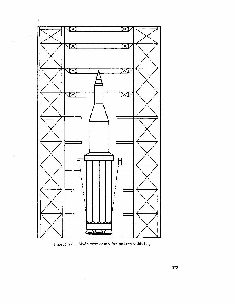
!
J
!
!
!
Figure 72. Mode test setup for saturn vehicle o
273

MICRO-SWITCH
POINTER
SCA LE
Figure 73.
GUIDE RODS
RELEASE
TESTSPECIMEN
TABLE
RIGID MASS
Drop-test shock machine.
274
The hydraulic-pneumatic shock machine iUustrated schematically in
Figure 74 is capable of producing a great variety of acceleration wave shapes,
amplitudes, and time bases. The machine develops its thrust through differ-
ential gas pressures acting on two faces of a thrust piston in a closed cylinder.
With reference to Figure 74, operation of the machine is described as follows.
A relatively low gas pressure is maintained in the top gas chamber which
forces the thrust piston against a seal ring seated on its base. In preparation
for firing, compressed nitrogen gas is introduced into the lower chamber to
equalize the force on the top face of the thrust piston. Any increase of pres-
sure in the lower chamber upsets this equilibrium, opens the seal at the ori-
fice and causes the piston to rise. Instantly, the entire bottom area of the
piston is exposed to the lower chamber gas pressure. A thrust on the piston
results, which is controlled by the geometry of the acceleration metering pin.
This limited duration thrust is transmitted to the test specimen by the thrust
column. The forward motion of the thrust piston is arrested as the piston
approaches the deceleration orifice. The deceleration of the piston, and thus
the specimen, is controlled by the deceleration metering pin.
2. ELECTRODYNAMIC SHAKER
The electrodynamic shaker, because of its versatility, is the workhorse of the vibration test laboratories at MSFC. Shakers are adaptable to
many configurations for different types of testing. They can be used individ-
ually for component testing, in series for large structural testing, for certain
types of shock testing, or in combination with a slip table. Slip tables are
presently of the granite type or the hydrostatic bearing type. They are used
to relieve the shaker head of the static load imposed by a heavy test specimen
and to help obtain unidirectional inputs.
The shaker operates on the same principle as an electromagnetic
speaker in an ordinary radio. Basically, the shaker or vibrator (Fig. 75)
is composed of an armature and a powerful, electrically energized field
magnet. When alternating current is passed through the armature windings,
and direct current is passed through the field magnet windings, a strong mag-
netic force is generated between them. This force causes the armature to
move in a direction perpendicular to the plane of the table surface. The am-
plitude and direction of the force is depenctent upon the magnitude and direc-tion of the armature current, respectively. The amplitude and direction of
the force in the armature determines the acceleration of the table surface.
However, the acceleration measured at the table surface or specimen con-
trol point is not a direct linear function of the force generated by the arma-ture current. Resonant modes of the specimen armature combination tend to
distort the input acceleration level.
275

Figure 74. Hydraulic - pneumatic shock machine.
mAg_r_m _
Figure 75. Electromagnetic vibration shaker.
276

If the specimen to be tested is less massive than the armature, the
specimen will have little effect on the acceleration of the table. However,
the first effect of a large mass is to decrease the overall acceleration onF
the table in accordance with the equation G = _, where W is the weight in
grams, G is acceleration in gravity units, M/SU 2 and F is the force rating
of the shaker in newtons. The second effect of a large mass is to lower the
frequency of the resonance so that the mass supplies a force to the armature.
This force may be in phase with lead, or lag the armature force, and willtherefore distort the table acceleration waveform.
Special provisions are usually made in an electronic network for ad-
justing the input signal to the power amplifier to compensate for electrical
and armature structural responses. Figure 76 is presented to indicate the
general behavior of a loaded and unloaded armature over the usable frequency
range.
log x/EaSTRUCTURAL RESONANCE
ELECTRICAL RESONANCE /,_ / _*'--- UNLOADED
_%_ LOADED
log f
Figure 76. Armature behavior over usable frequency range.
The steady state or average current (force} in the armature is limited
by the resistive power losses (heat generated} which the armature is capable
of dissipating. The peak current (force} is limited by the voltage that thearmature can withstand without breakdown in the insulation. Vibrators de-
signed for random vibration can withstand peak forces of approximately three
times the average force.
277

Thesevibrators, or force generators, range in weight from 18.14 to15872.5 kg and in-force output from 5.337 to 133440nts. Generally, thecosts of electromagnetic vibrators are muchgreater thanmechanicalvibra-tors (eccentrics). .Moreelaborate auxiliary support equipment, such asamplifiers, power supplies, andcontrols, are neededfor electromagneticvibrators than for mechanical shakers. Thedesirabilit3- of the electro-mag-neticvibrator lies in its versatili_" andusable frequency rangeof up to3 kc. An electromagnetic vibrator cangeneratevery complicated waveformssuchas broad bandrandomvibrations.
Thethruster is another type of electrodvnamic shaker which is in useat MSFC. Becauseof its relatively small size, a number of thesevibratorscan beused to apply inputs at various points arounda large structure. Thismachineeliminates large, heavy fLxtures and minimizes structure/shakerresonantcoupling becauseof the high natural frequency of the thruster'slight armature.
3. SINI'SOIDAL-S\VEE P TESTING
The sine sweep tests cons.ist of applying a sinusoidal motion to the
specimen and slowly varying the frequency at some predetermined rate. In
order to produce sinusoidal motions at the exciter table, it is necessaz3- togenerate electrical signals proportional to the desired accelerations. The
sign.'d source for sine sweep testing is the sine oscillator (Fig. 77). The
oscillator generates a low power sine wave signal whose amplitude and fre-
quency are controllable by the operator. This low power signal is supplied
to the power amplifier where its ener_" is increased to a level sufficient to
drive the vibration exciter. If the oscillator signml through the power ampli-fier was applied to the exciter and a frequency sweep made at some constant
output voltage, we might expect the table acceleration to vary as shown in
Figx_re 76. Since it usually is desirable to maintain some specified accelera-
tion on the table and since the frequency response function of the exciter-
amplifier (Fig. 76) is generally tu_mown before the test, there must be
some means of automatically maintaining the table acceleration level at the
desired value. The simplest means to accomplish this is to measure the ta-
ble acceleration and allow the operator to adjust the oscillator output to main-
tain the desired acceleration level. In practice, this oscillator adjustment is
performed automatically. The desired acceleration level is programmed into
the vibration controller and the monitored table acceleration is compared to
it. Differences between the desired and measured levels are corrected
either by increasing or decreasing the controller output. The additional
capabilit3.- to conn'ol displace ,nt at '_ou" frequencies is usually included in
27S
the sine control system. Sucha capability allows the operator to controlconstantdisplacement levels at those frequencies where the exciter is dis-placement-limited. As the frequency is increased and reaches a pointwhere the acceleration is the desired value, the automatic control switchesto maintain a constant acceleration rather thanconstantdisplacement. Thefrequency at which the automatic control switches from displacement toacceleration is knownas the "crossover" frequency.
OSCILLATOR I I
POWER
AMPLIFIER
ACCELEROMETER-__
I I TABLE I II II t,VIBRATION
'1 SHAKER I
t_ .I
Figure 77. Functional block diagram of sinusoidal sweep generating system.
4. RANDOM VIBRATION TESTING
The use of random vibration testing, occasionally called random noise
or white noise testing, is increasing rapidly. Random vibration is similar to
many environments measured on aircraft, guided missiles, and space ve-
hicles.
The random vibration test equipment configuration shown in Figure 78
is obviously more complex than the sine test equipment configuration. This
complexity is necessary because the load-influenced transfer function of the
amplifier-exciter must be compensated at all frequencies simultaneously.
Because the random signal contains all frequencies within its bandwidth lim-
its, a sequential equalization, like that employed in the sine test system, is
not possible. One equalization system uses wave-shaping circuits ("peak-
notch filters") inserted in the signal path. This system requires a determin-
ation of the amplifier-exciter (load) transfer function by using a low level
279

sine sweep prior to equalization. Once the transfer function is determined,
the wave shaping circuits are adjusted to generate the inverse transfer func-
tion of the system, resultingin a table acceleration with a relatlvelyflatfre-
quency response. Spectrum shaping is accomplished by inserting other
wave shaping circuitswith the desired transfer characteristics. The "peak-
notch equalizer" system is declining in popularity because of the complex
setup procedure necessary and itslack of automatic control.
The automatic equalization configuration shown in Figure 78 is pres-
ently in use at MSFC. In this scheme, equalization is accomplished by con-
trolling the energy in each of many continuous narrow bandwidths. The wide-
band random signal from the noise generator is passed into a bank of contin-
uous filters. The output of each filter is fed into an automatic control am-
plifier. From the amplifier, the signal is fed into a mixer and then to the
power amplifier. The output of the table-mounted (control) accelerometer
is adjusted (the spectrum is shaped) by the operator. The output of each
analyzer filter is then compared to the desired value. The difference signal
is used to adjust the output from the corresponding automatic control ampli-
fier resulting in a spectrum at the table shaped to the desired value. The
additional capability to monitor and record the energy value within each filter
is included in the equalizer. Set-up time is reduced since the equalization
takes place as the test is begun. It is necessary only to program the desiredspectrum shape and level prior to the test.
Figure 78.
280
RANDOMNOISE
GENERATOR
I jSPECTRUMEQUALIZER
lPOWER
AMPLIFIER
aqECTRUMANALYZER
r
.lx_a___n.j /
/Functional diagram of a random vibration generating system.

SECTION Xl. VIBRATION AND ENVIRONMENTS AND
TEST SPECIFICATIONS
A. Stage and Vehicle Vibration and Shock Criteria
It is imperative that the vibration environment of future vehicles be pre-
dicted prior to design and development so that satisfactory design and test pro-cedures can be established. These criteria are essential to the establishment
of high reliability standards necessary for man rated vehicles. The precise
prediction of these environments is highly complex and may not be reached soon.
However, based on measured data and a few simplifying assumptions, adequate
predictions may be obtained provided the necessary assumptions and limitations
are realized by the user.
Localized vibration originates primarily from four sources of excitation:
1. Mechanically induced vibration from rocket engine fluctuation which
is transmitted throughout the vehicle structure.
2. Acoustic pressures generated by rocket engine operation.
3. Aerodynamic pressure created by boundary layer fluctuations.
4. Self excited machinery or components, etc.
Restricting notation to vibrational power quantities, the total vibration at any
point on the vehicle may be expressed as
PT = P/mech + P/ + p/ae mach
where / denotes the vibrational power caused by the indicated source. The
powers add arithmetically since vibrational power is proportional to the mean
square cyclic response. An exact analysis of structural response would neces-sitate an accurate description of each individual source and the manner in which
they combine. In most cases only one source is the primary forcing function.
Hence, the remaining sources may be considered negligible in regard to the
total dynamic response at any instant of time. However, an expression is given
[equation (229)] which provides an estimate for combined driving functions.
281

Rocket vehicle structure may be separated into two dynamic categories:
I. Structure susceptible to acoustic and/or aerodynamic pressures
(i.e., skin panels).
II. Structure not susceptible to acoustic and a_rodynamic pressures(i. e., structural beams).
The dynamic analysis of these two groups are obviously handled by two different
techniques. Each is explained below.
This group of structures may be subdivided into three sections:
I(a). Skin panels. A panel is defined as a section of skin bounded
by radial and longitudinal stiffeners. This type of structure is directly excited
by impinging acoustic pressures. The direction normal to the panel face exhibits
the most severe vibratory response; consequently, this is the direction usually
considered when referring to panel vibrations.
I(b). Skin stiffeners (such as ring frames and stringers). This
type of structure is not directly excited by acoustic forces but is driven by the
motion of adjacent panels. Thus the stiffeners are indirectly forced by imping-ing acoustic pressures.
I(c). Bulkheads. These skin segments form the upper and lower
extremities of vehicle propellant tanks. The bulkheads are further subdividedinto:
I(c)-l. Forward bulkheads
I(c)-2. Aft bulkheads
The added mass of liquid loading greatly reduces the vibration amplitudes
experienced by the aft bulkheads; consequently, the two bulkheads are treatedseparately.
The equation for predicting the vibration environment of acoustically(or aerodynamically) susceptible structure is [26]
2 82
where
= G (Pn_:Prtr'_,4r-F= G (Pnl(Prtr_ / Wn
-:w (227)
Gn
Gr
tr
Pr
Pr
tn
Pn
Pn
Wn
WC
the vibration response of the new vehicle structure at a particu-
lar station number. The term G is the acceleration due to cyclic
motion divided by the acceleration of gravity go" Since rocket
vibrations contain many frequencies the response magnitude (G)
is specified in spectral form.
the known vibration response of a reference vehicle structure.
This value has been determined by many measurements and is
also presented on a spectral basis. Further, this parameter
should be obtained from unloaded structure (i. e., structure
which does not reflect the effects of component mass loading).
the thickness of the skin associated with G .r
the skin weight density of the reference structure.
the impinging acoustic (or aerodynamic) pressure which is
driving the reference structure.
the skin thickness 1 associated with G .n
the skin weight density associated with G .n
the acoustic (or aerodynamic) pressures impinging upon the new
vehicle structure. This pressure must also be predicted.
A factor which accounts for the attenuation effects produced by
incorporating additional mass into the existing system.
weight of basic structure.
component weight mounted on W .n
1. For corrugated or sandwich structure this parameter is an equivalentthic kne ss.
283

Equation (227) applies to randomrms composite values or to sinusoidal
values. For the mean square spectral value, the total expression is simply
raised to the second power. This expression is applicable to localized vibra-
tory environments and is valid for all materials. It is invalid when consideringlarge sections of vehicle structure (i. e., entire cylindrical tank). However,
the static loading of these large sections is the critical design factor and local-
ized dynamics thereby produce only negligible effects.
Referring again to equation (227}, Pn represents the maximum pressure
impinging upon the vehicle at any time. Three conditions must be considered,one of which will result as the maximum.
1. Captive-firing environments (applicable to boosters and upper
stages).
2. On-pad acoustic environments.
3. The period of maximum aerodynamic pressure (occurs subsequent
to Mach one; therefore, the combining of engine generated acoustics and boun-
dary later pressures do not have to be considered).
Type H
Now consider the Type II structure. This structure may be subdividedinto two sections.
II(a). Structural beams such as I beams, etc. The components
mounted in this section would not primarily be affected by acoustic pressuresbut by rocket engine vibrations.
II(b). Rocket engine components. These components may again besubdivided into three sections:
II(b)-l. Combustion chamber section. This section includes
the components mounted on the chamber dome or side case.
II(b)-2. Turbopump section. This section includes the
components located on the propellant pumps.
II(b)-3. Actuator assembly. The components located in
this region are mounted on the actuator struts or actuator rods.
284

where
The equation for predicting vibrations of these structural types is
Type II(a)
__NTV)n Wr _NTV)n /_v;r )G = G _(NTV) r W F = Gn r r__ + Wn c
(228a)
Type II(b)
_TV) n W rG =G =
n r_-V_ r _n F G r(228b)
e n
e r
NTV n
NTV r
Wn
F=W +W
n c
W n
W r
W c
the vibration response of the new structure. This is
considered an input to a component mounted on thisstructure.
the vibration response of a reference structure. This
environment is determined by measured data acquired
from unloaded structure.
number of engines, thrust and exhaust velocity of rocket
engine associated with the stage under consideration inthe new vehicle.
number of engines, thrust and exhaust velocity of
rocket engine associated with a reference vehicle.
= an attenuation factor which takes into account the effects
of component mass loading.
= the structural weight corresponding to G •n
= the structural weight corresponding to G •r
= the weight of component to be mounted on W .n
285

Equation (228) applies to random rms composite values or to sinusoidal values.
For the mean square spectral density value the total expression is simply
squared. For Type II(b) structure, clustering does not generally affect engine
vibrations; therefore N and N are not considered. Also, for Type II struc-r n
ture, only once case is considered the maximum. This case is the firing(either captive or inflight) of that particular stage under consideration. The
vibration transmitted from other stage firings (i. e., booster to upper stages)
is negligible compared to that stage operation. Thus, with a knowledge of the
necessary rocket engine parameters and structural mass characteristics, the
vibratory environment of a new vehicle is shown in Figure 79.
The methods and techniques presented herein will provide satisfactory
estimates of the vibratory environment associated with any particular problem.
These techniques are considered indicative of the present state-of-the-art and
will permit adequate environmental estimates with only a few simple calcula-
tions. It is not imperative that the user thoroughly understand the philosophy
behind the methods. He should, however, realize the necessary requirements
and limitations. A summary of the principal limitations regarding these tech-
niques is given below.
1. The techniques do not apply to entire structure such as an entire
rocket engine assembly or large structural members. They do, however,
apply to components and other items of equipment mounted on these structures.
2. These methods are not applicable for prediction of combined
environments such as excitation due to propellant flow and engine vibration
combined. In some remote cases the type of structure may not be clearly
defined or excitation may be both acoustically and mechanically induced. In
these cases the two methods may be combined and a certain percentage assigned
to each method depending upon degree of structural susceptibility to acoustic
and mechanical excitation. Employment of the respective percentages is leftto the discretion of the user.
Gnt X%G + 1_vG_
where
G = the resultant combined environmentnt
286

¢.)
0
E0
o_,._>
e.o
e_
0_,..i
o
_u
287

G = the environment obtained from using Type I methods
G = the environment obtained from using Type IImethodsan
and
X_ + Y°/0-- 1.0 or 100_0
3. This method does not provide frequency characteristics of the newstructure. The method is based on the fact that similar structure has similar
response characteristics. Precise frequency calculations tend to complicate
the problem and it is doubtful that the results would justify the time and effort
required. The calculation of the component natural frequency is, within itself,
possibly a simple problem. In the actual system, however, this frequency is
coupled with the support structure frequency characteristics. The determina-
tion of structure-component coupling effects is a highly complex requirement.
Consequently, adequate frequency calculations and evaluation of these effects
require considerable time and effort.
These techniques rely upon typical structural configurations which have
been sufficiently defined by measured data. Subsequent statistical analyses
describe the dynamic characteristics of the structure with statistical certainty.
Thus, with only a knowledge of the structural geometry and mass characteris-
tics, the anticipated dynamic environment may be established. These tech-
niques are applicable to most rocket vehicle structure -- including corrugated
and sandwich skin construction provtded an equivalent flat plate thickness maybe determined.
The predicted environments represent a statisticalestimation since the
reference spectra should be established by statisticaltechniques. Conse-
quently, the probabilityof the actual environment not exceeding the predicted
environment of a future vehicle is established with a confidence levelindicative
of the necessary vehicle mission. This does not infer thatthe predicted
environment will accurately correspond to a single measured environment.
Certainly, some of the measured responses of a new vehicle willbe signifi-
cantly lower than the predicted. This is to be expected since the criterion is
such thatthe prediction will envelope the greater percentage of the situations.
However, thisproblem is elevated somewhat by the techniques utilizedof
separating rocket vehicle structure intoeight basic categories -- each pos-
sessing essentiallysimilar dynamic characteristics. This reduced the vari-
ance so that the mode value (pointof maximum occurrence) is not greatly less
288

than the higher confidence limits. Therefore, the higher percentage criterion
may be used without the concern of over conservatism in regard to a specific
problem.
B. PayloadVibration and Shock Criteria
The techniques previously described have been altered to provide vibra-
tiondesign and test criteria for launch vehicle payloads and payload compo-
nents. A new criteriaphilosophy was deemed necessary because: (i) The
type of structure in the payload area is grossly differentfrom the launch vehi-
cle structure, (2) the payloads and payload components will not be subjected
to staticfiringtests and therefore require test criteria thatpossess the high
degree of confidence dictated by their "one-shot" use, and (3) their use
environment can be simulated better by random vibration criteria. The new
techniques generate five types of vibration criteria:
1. Vehicle dynamics.
2. Sine evaluation.
3. High level random.
4. Low level random.
5. Shock.
These criteria are designed to simulate as nearly as possible the
expected flight environments. The specific purposes of each of these criteria
are as follows=
i. Vehicle dynamics criteria consist of sinusoidal vibration levels
designed to simulate the vibration environment induced by launch vehicle
bending and torsion and by engine ignitionand thrust variations.
2. Sine evaluation criteria consist of sinusoidal vibration levels
designed to evaluate the component's dynamic response characteristics when
itis subjected to vibration levels less severe than the maximum anticipated
levels but of sufficientmagnitude to induce significantdynamic responses.
3. High-level random criteria are random vibration levels designed
to evaluate the componentVs performance when subjected to an input represen-
tativeof the maximum anticipatedspectral intensityof the environment.
289
4. Low-level random criteria are random vibration levels designed
to evaluate the component_s performance when subjected to an input represen-tative of the maximum anticipated energy of the environment.
5. Shock criteria are shock levels designed to simulate the maximum
anticipated shock environment on damage equivalence basis.
Each of these criteria is calculated using the predicted vehicle dynam-
ics, acoustically induced vibration, and shock environments. The followingparagraphs outline how the particular environments are predicted and subse-
quently used for criteria development.
The vehicle dynamics environment is predicted using a mathematical
model of the launch vehicle and payload. The model is forced with inputs
representative of the actual vehicle forcing functions; i. e., wind loads, engineignition/cutoff forces, and release and separation forces. The maximum
response of the payload at each significant frequency is computed with these
modal responses being considered as the vehicle dynamics environment. The
environment is enveloped to generate the sinusoidal vehicle dynamics criteria.
Vibration data for the reference structure are gathered and statisticallysummarized. These summari, s, consisting of an envelope of the maximum
spectral intensities and an envelope of the average spectral intensities, are
extrapolated to the new structural configuration. The extrapolation relation-
ships used are the same as for launch vehicle components [ reference equation(227) ], except that the extrapolation relationship is a function of the acoustic
pressure at each frequency rather than the overall acoustic pressure. As a
result of these calculations, a predicted maximum and average vibration spec-
trum is generated. These spectra are used to generate the following criteria:
1. The high-level random criteria are generated by enveloping themaximum spectral intensities.
2. The low-level random criteria are generated by reducing the
envelopes obtained in 1. to possess the maximum statistical composite valueof all the data samples.
3. The sine evaluation criteria are generated by computing, from
the maximum spectral intensities, an equivalent g response factor (GRF).This factor is obtained from
GRF i = 1.2_
290

where
gi = maximum spectral intensity in any spectral increment i.
fi = frequency associated with the i_ spectral increment.
The equivalent g response factor ateach frequency is plotted, and a sine
sweep level is calculated that passes beneath all plotted points.
Measured shock environments from similar payload structure are
analyzed, and a prediction based on these analyses is made for the new struc-
ture. The analysis is performed in the shock(response) spectrum domainand therefore generates shock spectrum criteria that are expected to induce
damage equivalent to that induced by the predicted environment.
• j
4 _'.-
291

SECTION ×1 I. THEORETICAL CONSIDERATIONS
The preceding sections of this manual have described basically the
methods and facilities employed to obtain, reduce, evaluate, and utilize vibra-
tion data. This section, however, presents a different approach. It contains
applicable reference material for a theoretical and statistical look at vibration
analysis.
The sequence of information presented by the following main paragraphs
does not necessarily indicate the relative importance of the paragraphs. In
some cases a main paragraph may be considered a separate entity, not having
to follow any particular preceding paragraph.
.
A. Vibration Terms - Their Meanings and Uses
DISPLACEMENT, VELOCITY, AND ACCELERATION
Vibration measurements can be in terms of displacement, velocity, or
acceleration. The easiest measurement to understand is that of displacement,
or the magnitude of motion of the body being studied. Where the rate of
motion (frequency of vibration) is low enough, the displacement can be
measured directly with a dial-gage micrometer. When the motion of the body
is great enough, its displacement can be measured with a common scale.
In its simplest case, the displacement may be considered as simple
harmonic motion; that is, a sinusoidal function having the form
x= A sin_t (23o)
where A is a constant, w is 27r times the frequency, and t is the time as
shown in Figure 80. The maximmn peak-to-peak displacement (the quantity
indicated by a dial gage) is ZA, and the root mean square (rms) displacement
is A/_-2(=O. 707A). The average (full-wave rectified average) value of the
displacement is 2A/Tr(=0.636A) while the "average double amplitude" Ca term
occasionally encountered) would be 4A/Tr(=l. 272A). Displacement measure-
ments are significant when deformation and bending of structures are studied.
292

u.
w _" >.
-r _ ,n_" __ ,_ 3- Z 0
t < ------_
\\\
o
I
3
Pf
oo
b_
293

In many other practical problems, however, displacement is not the
important property of the vibration. A vibrating mechanical part will radiate
sound in much the same way as does a loudspeaker. In general, the velocities
of the radiating part (which corresponds to the cone of the loudspeaker) and the
air next to it will be the same, and if the distance from the front of the part to
the back is large compared to one-half of the wavelength of sound in air, the
actual sound pressure in air will be proportional to the velocity of the vibra-
tion. The sound energy radiated by the vibrating surface is the product of the
velocity squared and the resistive component of the air load. Under these
conditions, particularly where noise is important, it is the velocity of the
vibrating part and not its displacement which is of greatest importance.
Velocity is the time rate of change of displacement, or the first
derivative of displacement with respect to time, so that for the sinusoidal
vibration in equation (230) the velocity is
dxv - dt - wA cos c_t . (231)
Thus, the velocity is proportional not only to the displacement but also to thefrequency of the vibration.
In many cases of mechanical vibration, and particularly where mechan-
ical failure is a consideration, the actual forces set up in the vibrating partsare important factors. Newtonts laws of motion state that the acceleration of
a given mass is proportional to the applied force, and that this force produces
a resulting reacting force which is equal but opposite in direction. Members
of a vibrating structure, therefore, exert forces on the total structure that are
a function of the masses and the accelerations of the vibrating members.
Acceleration measurements are important where vibrations are
sufficiently severe to cause actual mechanical failure. Acceleration is the
second derivative of the displacement with respect to time or the first deriva-
tive of velocity with respect to time. That is,
dv dZxa - dt = _2" = -c_2A sin _t (232)
The acceleration, thereIore, is proportional to the displacement and to the
square of the frequency.
294

There is another use for acceleration measurements. The analogycited aboveconcerning the loudspeaker covers the usual case where the cone
or baifle is large compared to the wavelength of the sound involved. In most
machines the relationship does not hold, since relatively small parts are
vibrating at relatively low frequencies. This may be compared to a small
loudspeaker without a baffle. At low frequencies the air may be "ptanped"
back and forth from one side of the cone to the other with a very high velocity,
radiating much sound energy because of the very low air load, which has a
reactive mechanical impedance. Under these conditions the accelerations
measurement provides a better measure of the amount of noise radiated than
does a velocity measurement.
2. SUMMARY
Displacement measurements are used only in instances where the
actual amplitude of motion of the parts is important. This would include
those cases where the dynamic loading because of the operating machinery in
a factory may cause unsafe deflections in flooring and walls or where large
amplitudes of motion might actually cause parts to strike together, thus
causing damage or serious rattle. The deflections observed at the center oI'
a wall panel or beam, for example, can give useful infornmtion about the
stresses acting in these members. The displacement is not directly a meas-
ure of surface strain of the member but is rather an integrated ia_dication of
the strain. The strain measured by the usual strain gage is minute elongation
or compression of material between points an inch or so apart; in contrast,
the displacement measurement referred to above is the bending of materialover a distance of several feet.
Velocity measurements are generally used in noise problems where
the radiating surfaces are comparatively large with respect to the wavelengthof the sound.
Acceleration measurements are the most practical where actual
mechanical failure of the parts involved is of import.-mce .and in many noise
problems, particularly those involving small machinery. A general purposevibration meter, therefore, must be able to measure all three vibration
characteristics.
. NON-SINUSOIDAL VIBRATION
Equations (230), (231), and (232) represent only sinusoidal vibrations,
but, as in the case of the other complex waves, complex periodic vibrations
295

can also be represented as a Fourier series of sinusoidal vibrations. These
simple equations may, therefore, be expanded to include as many terms asdesirable in order to express any particular type of vibration. It will be noted
that, since velocity is proportional to frequency, and acceleration is propor-
tional to the square of the frequency, the higher frequency components in a
vibration are progressively more important in velocity and acceleration
measurements than In displacement readings.
B. Random Process and Probability Distribution
An example of a random experiment may be illustrated by tossing a
single die to determine how many spots will be on the top face after each toss.
A record of the number of spots that show after each toss is illustrated in
Figure 81.
This graphical result is called a sample function, and a collection of
many of these sample functions forms an ensemble. If many of the random
experiments are repeated, the ensemble of sample functions is an example of
a random process. In the case of the die, the number of spots showing or
I
1 2
Figure 81.
3 4 5 I 7 8 9 10
NUMBER OF TOSSES
Record of a random experiment with a die.
11 12
296

thevalue measured is an example o£ a random variable. If x is a random
X X1//2variable, it may be noted that any function of x such as x 2 e or
is a random variable.
Since there are only six sides to a die, the random variable in this
case has only six possible values, and is a discrete random variable.
However, if for the experiment a measurement had been chosen with
an infinite number of possible results, a continuous random variable would
have been defined. Continuing the experiment, the ensemble is observed and
the number of times the value one occurs on the first toss is counted, and is
denoted n 1 . Let N denote the total number of sample functions. Then the
relative frequency of the occurrence of one on the first toss is denoted by
nl/N . Now if N becomes very large, then nff'N will approach a limiting
value. Then the value of nj/N as N -_ _o is the probability of "one" occurring
on the first toss of the die. This probability is written P(1) . A more general
expression may be written
P(x k) = probability that x has the value x k on the first toss
llm nk= N--=o "N- (233)
where nk is the number of times the value x k occurs on the first toss among
the N sample functions.
The complete set of values P(x k) for all possible values of k is
called the probability distribution of the discrete random variable x. A plot
of the probability distribution of a discrete random variable is shown in
Figure 82.
From the above:
a. The probability of a certain event = 1
b. The probability of an impossible event -- 0
c. 0-< P(x k) <- 1
r
297

0.5
XL
0.4
0.3
0.2
0.1
i IX_ X a X3 X 4 X s
Figure 82. Probability distribution of a discrete random variable.
d. When different values of x are mutually exclusive,
Xk
P(x I orx z orx kor...) : P(x,) + P(x 2) + P(x k)(234)
eo
values,
If the random variable can take on no more than M possible
M
_, P(x k)k=-1
= I (235)
f. A probability distribution function for a discrete random variable
may be defined as follows (Fig. 83):
PCx-<x) = _ P(xk) (236)
298

g. P(x -<+ _) = 1 , P(X -< - oo)= 0
h. If b>a, then P(x-< b) P(x-< a) = P(ax_< b) _>0
Extending the above concept to continuous random variables, a prob-
ability distribution function is shown as a smooth curve rather than a stepfunction (Fig. 84). Now the probability distribution of the discrete case is
replaced by the probability density function which is defined as the derivative
of the probability distribution function and is denoted by the symbol p(x)
The continuous functions and the discrete case have similar properties exceptthe stuns now become integrals.
X
a. ;(x-<x) = f (237)_00
cO
b. f p(x) dx = 1 (238)
n
b
fc. p(x) dx = P(a x-< b) for b - a (239)a
Now there are two means of expressing our random process:
a. An ensemble of sample functions may be constructed (Fig. 85).
b. The probability distribution of the values for any particular toss
may be given. This is written
The above expression simply means the probability that x has the
value x k in the nth toss. In the case of the tossed die, the probability of a
three turning up on the 10th toss is written
P[x3(lO) 1 where x3=3
299

XvlX
¢1.
1.1
1.0
0.9
0.8
0.7
0.6
0.5
0.4
0.3
0.2
0.1
0X 1 X 2 X 3 X 4 X 5 X6 X
Figure 83. Probability distribution for a discrete random variable.
1.0"
0.8-
(x_'X)P
0.6-
O.4
0-30 -2o -lo 0 lo 20 3o
0.2,
Figure 84.
300
I I I I I I
X ¢
Probability distribution ftmctton for continuous random variable.
X(31
X(2)
X(1)
i
i
i
'iiI
TOSSES
Figure 85. Ensemble of sample functions.
The probability applies to a particular toss since the experiment is
across the process, and each toss of the die is an experiment and what hap-
pens on toss (n + 1) is not dependent on the results of toss n . Therefore,
From the above, the random process may be completely specified by
determining the probability distribution in any toss n.
However, it is noted that all random experiments are not independent.
The type of random process to be considered eventually is definitely not onewhere successive tosses (or successive intervals) are independent. For
example, consider a large number of spinners whose angular positions can
be refined to an infinite number of possible results, and make the choice of
the spinner used in a particular interval dependent upon the result of the
301

_r,=.t ,or_e.rocod,.,_.' Tho.robab,l,tyd,.,r,b°Ooop_°_jr7for all possible values of k during the nth interval may be specified, but
nothing has been said about the dependence of the (n - 1) interval. The
probability distribution for all k and all n may be determined and still not
show the interdependence between intervals. To do this the concept of joint
and conditional probability distributions are introduced.
, JOINT PROBABILITY DISTRIBUTIONS
Consider a pair of intervals 1 and 2, where the random variable x(1) (2)
assumes the values x t and x.,] respectively, denoted by x 1 , x.j .
Again examine N s fur_otions. Let ni . denote the number of
(1) (2) "
times the combination x i , x.j occurs among the N sample functions.
Then, the joint probability is defined by
(1,2)
p ....-= ......_,_,j,,' N--_ N
As before, it follows _at,"- i_ _ .
0 <_ P[xi(1) xj(21 <1
.i (240)
(241)
(1) (2)If x i has I possibl e yalues_ ,and: xj_ has J possible values, then
(242)
Also, the previous probability
PIx:.,]=t+/,,.x,,.,]j=l
(243)
302

which states the probability of a particular vahm x I in the first interval is
(2)equal to the sum of its joint probabilities with all possible values of x. in
Jthe second interval.
Similarly,
P j , = P xj (244}i=l i ' "
Second order distribution functions may now be obtained from the
joint probabilities. Also, higher order distribution functions may be obtained
from higher-order joint probabilities defined by
Ix 1) (2) (3) 1 :I) i , x. , x,. .... .jJ
q CONDITIONA L PROBABILITY DISTRIBUTIONS
Second order distributionfunctions may now be obtained from the
jointprobabilities. Also, higher order distributionfunctions may be obtained
from higher-order jointprobabilitiesdefined by
where the terms following the vertical bar are given terms.
As before, consider N sample functions. Let ni(1): be the number
of times x.z occurs in interval I, and let ni,](1'2) be the number of times
(1) (2)the combination x. , x. occurs. Then
z j
Ix ] ""'-p j(2)Ixi(1) lira ni,j = la 1 ' (245)
• = N--.o ni( 1)/N P[xi(1) ]
303

(i) (2)ts expressed as the ratio of the probability that both x i and x. willJ
(1)occur divided by the probability that x. will occur. The above result, of
1
(1)course, required that P x. _ 0. This result can be written in the
1
equivalent form
For certain cases, the conditional probability
P [xj(2) I xt(1) 1 PIxj(2)l (247)
(1)independent of the given Informa_on that x. has occurred. In this case,
i
(1) (2)the random variables x and x are said to be independent, Now
and the joint probabilities are specified from the first-order probabilities.
The concept of joint and conditional probabilities for discrete random
variables may be extended to continuous random variables in the form of joint
and conditional probability density functions. Considering an ensemble of
sample functions which are continuous functions of time, as for example an
accelerometer signal, a complete description of the random process requires
a specification of the joint probability density function P(xtl , xt2 , . . . , x t )n
for every choice of times t1, t2, . .. , t and for every finite n. Sincen
this Is nearly impossible for a completely arbitrary random process, it is
necessary to seek means to simplify the specification of the random process
and determine the average value of the sample function in a particular interval.Tkts Is
xln ! + x2n 2+ . . . + x nm m
N
3O4

As N-- _o , this becomes
xlP(x I) + x2P(x 2) + . ..+ xN[P(x M)
and is written
M
xk P(x k)k=-I
The above defines the statistical average, ensemble average, or
expectation of the random variable x and is noted by
E[x] =
M
x k P(x k)k=-I
(249)
Extending the above for a continuous random variable, using a probability
density function p(x) ,
E[xl = f x p(x)
Considering a function f(x) of the random variable x ,
(250)
oo
Elf(x)] = f f(x)p(x)dx_00
( 257)
An important class of functions is
E[x n] , where n= 1, 2, 3, • , , , n , and integer
nx =power of x.
305

Theseare thenth moments by analogywith mechanics.
E[x], the cg line location, is called the mean
E[x] = m (the symbol for the mean)
El(x- E(x))_ is the variance
E[(x- E(x))2] = E (x- m) 2=u2 (the symbol for variance)
Also, it can be shown that o 2= E[x 2] - m 2 ,
a {called the standard deviation).
For a stationary random process, a 2 is a measure of the ac component
power, m 2 is a measure of the dc component power, and Ex 2 is a measure
of the total power.
Up to this point, only averages of a single variable have been discussed.
Extending the discussion to a pair of x and y of discrete random variables.
I J
i=l j=lf(xi, Yl) P(x l, Yi ) (252)
and for continuous random variables
g_ oo
Etf(x,y)] = f f_OO _OO
f(x,y) p(x,y) dx dy (253)
The functions of the form
EI(x-m )k(y-m)n 1x y
306

are called joint central moments. This particular one is the (k, n)th joint
central moment. Also, measuring the interdependence of x and y , the
term covariance is assigned when k = n = 1; i. e.,
E[(x-m x) (y-m)] Y
C. Random Processes in Vibration Analysis
The random variable x has been introduced as the value resulting
from a random experiment. The values of x as sample functions were then
grouped to form an ensemble. Also, it was noted that x could have eitherdiscrete or continuous values. The discrete form was used to introduce new
concepts because it is easier to understand from a physical viewpoint.
Emphasis is now shifted from general considerations to the specific
type of random process as applied to vibration work; that is, continuous
random processes as a function of time.
Considering the ensemble of such functions (Fig. 86), the probability
distribution of x at time t 1 and x at t 2 may be described. Also, joint
= x(t 1) and = x(t 2) may be described. To describeproperties of xtl xt2
the joint properties an ensemble average is used. The particular ensemble
ave rage
E[x(t 1) x(t_)] =R(t t , t2) (254)
is called the autocorrelation function and is symbolized by R(t 1 , t2) since
this result, in general, is a function of both t1 and t z . The autocorrelation
function provides a measure of the interrelation of x(t 0 and x(t 2) .
Up to this point, probability functions and ensemble averages at par-
ticular times (which is across the ensemble of sample functions) have been
discussed. However, to obtain an ensemble of sample functions would require
the firing of a large number of vehicles. Now consider the necessary conditions
for the time average of one sample function to equal the ensemble average
across the sample functions of an ensemble.
307

i (.
i
°f,,,4
0
°p,4
0
0
O
e_
308

The average along one sample function is called the time average. The
time average, denoted by x-"('_', of a sample function x(t) of length 2T is
defined by
Tlira 1
= T-.-_o 2-'T" f x(t) dt . (255)-T
In general, this result depends upon the particular sample function chosen.
The parameter t, of course, is averaged out so that this result is no longer
a function of t.
The average across the ensemble is the statistical average previously
defined, which at t= t 1 is
Z [x(tl)l
In general, this result depends upon the particular time, t = t1 , chosen.
It should be noted that
x-_ = E[x(tl) l
when random procusses are both stationary and ergodic. These concepts are
defined below.
A random process is stationary if the joint probability density depends
only on time differences and not on the time origin; that is, for all translations
in time t,
P[x (tl),x(t2) ,..., X(tn)] = P[xti+t) , x(t2+t) ,..., x (tn + t)]
(256)
which simply means we can start averaging the function at any point, in par-
ticular E[x(tl)] is now the same for all t1 .
309

A random process is ergodic ff it is stationary and if all sample func-
tions are similar such that time averages on any sample function are statistically
eqaivalent to corresponding ensemble averages over the ensemble of samplefunctions.
For a stationary process the autocorrelation function R(t i , t2)
becomes a function of the time difference tz - ti only; thatis, R( t2 - ti) .
The time difference is represented usually by v . Therefore, for a stationary
process, letting r = t2- tl ,
R(t I , t2) = R(t 2 m tl ) = R (T) = E[x(t I) x(tI + T)] ,
independent of t I .
Now if a random process is ergodic, then any function of the process
is ergodic. So
<f[xCtl) l> = E[f(x(tl))] = E[f(x(t))] (257)
Therefore, for an ergodic process
E(T) = E[x(t) x(t+ T)] ( 2587
where
TR(T) = lira 1 f
-Tx(t) x(t+T) dt
Thus the time average of the product of a function at a time
t + T is the autocorrelation function, noted by
t and a time
(259)
R(r) + f(t) f(t+_')
310

The autocorrelation function of a stationary process has the following
properties:
a. R(0) = E xZ(t) =o "2+ m 2
b. R(0) -> R(,)= R(-r)
limc. RC'r) = m 2
T--.. oo
Result (a) is the mean square value of x(t) at any time t. Result (b) states
that R(T) is an even function of r with a maximum value at T= 0 . Result
(c) assumes that x(t) and x(t + r) are statistically independent for large
r . If the mean value m = 0 , then result (a) shows that the mean square
value equals the variance, and the root mean square value equals the standarddeviation.
D. Amplitude and Frequency Distribution in Random Noise
Many of the most severe vibration environments encountered in current
vehicles result from noise generated aerodynamically by the interaction of the
propulsion jet with the atmosphere and from pressure fluctuations in the
turbulent boundary layer which surrounds the vehicle during flight. Both of
these forcing functions contain energy at all frequencies throughout a relatively
wide bandwidth, and the amplitudes of both vary in a random fashion.
Usually, the amplitude probability distribution in a random noise
forcing function follows the normal or Gaussian probability law. This has
been generally supported by analysis of the two forcing functions mentioned
above. Also, it is usually assumed that the random forcing function is both
stationary and ergodic. To assume stationarlty the statistical properties of
the function must be assumed to not vary with time; therefore, any two
samples taken from a single continuous record of the function must appear
statistically equivalent. To assume ergodicity, any sample taken from a
single continuous record of the function must be statistically equivalent to
the entire record of the function, When stationarity and ergodicity exist,
the average properties of each sample of any record are similar and do not
vary with time, and this permits the use of the time averages rather than
sample or ensemble averages. Also, these requirements permit use of
Fourier transforms to relate the statistical autocorrelation of the forcing
function with its frequency spectrum.
311

Many of the random forcing functions which are encountered during
launch and flight vary with time and are neither stationary nor ergodic. How-ever, the time history function can be divided into several shorter time
periods in which the function is reasonably stationary. When the length of
these shorter time periods is not sufficiently large compared to the time
period of the response, large variations can be expected between the responses
at differing times, because the sample length is not long enough to give thetrue averages.
When the force input to a linear single degree-of-freedom system is
random, the response is also random. If the force contains energy at all
frequencies over a relatively wide frequency range which includes the resonant
frequency of the system, the energy at frequencies near the resonant frequency
will be magnified. Therefore, the response will appear to be approximately
sinusoidal with an amplitude which varies randomly with time. Figure 87
illustrates a sample of the response of a panel to random noise excitation. It
is assumed that the instantaneous amplitudes x are distributed normally with
a zero mean and standard deviation x . The normal probability density forr
(x/x) is shown at the bottom of Figure 87.r
tion of time that (x/x) is between (xl/x)r r
product of the probability density at (xl/x)r
The probability, or the propor-
and (xl/Xr) + (AX/Xr) , is the
and the interval (Ax/x r) .
Note that the quantity x r equals the root mean square value here since the
mean value is zero.
The probability density for the peak response x 0 of the lightly dampedsingle degree-of-freedom system are distributed for very narrow bandwidths
in accordance with the Rayleigh distribution. The Rayleigh probability density
for (x0/x) is illustrated in the upper portion of Figure 87. Comparing ther
normal and the Rayleigh probability density functions, it is clear that the prob-
ability of a zero instantaneous amplitude is higher than the probability of any
other value as illustrated by the normal probability density function. However,
it is improbable that the peak amplitude in any cycle equals zero, as illustrated
by the Rayleigh probability density function where the most probable peak
amplitude is seen to be approximately the rms amplitude, (x0/x r) = 1 .
The probability distribution functions for these two distributions are
given in Figure 88. The probability distribution is the integral of the prob-
ability density and gives the probability that the amplitude ratio is less than
or equal to any value of the ratio. Thus, for the normal distribution of
312

0.8
_Z 0.6
_ 0.4
0.2
0
¢c0
I,M
LUJa.s:,,¢
PROBABILITY DENSITY FOR NORMAL DISTRIBUTION
,(_).×./Y_o_,×,F-_×,,x.,'IL' JI _ X° = RATIO OF PEAK AMPLITUDE
,_ ToRMSAMP,,TUDE0 1 2 3 , kx,/
ii
r
OF ARE
I ,,,ow( ) .,.,_ _ MAXIMUMPEAK
__ IN SAMPLE
I
).
z
o"_z_,
O00mO.
0.4
0.3
0.2
0.1
PROBABILITY DENSITY FOR RAYLEIGH DISTRIBUTION
x , -,x,x,,P /"_'r) = _ EXP [ 2 r ]
X/ _ (xX--"_ " RATIO OF INSTANTANEOUS
\ ', '/ AMPLITUDETOR__,_ AMPLITUDE
J, bl, , , ,_- ,_ (x_"3 "2 "1 0 1 2 3 4 _Xr/
Figure 87. Sample of response of a panel to random noise excitation.
313

Z
I I I I I I I I I I
q-G
m
.Q
0
N
0Z
9NIO330X3 ION =I0 AJ,.I"IIBVeOI:Id
314

amplitudes, it is equally probable that the instantaneous amplitude will be
positive or negative relative to the mean of zero. Further, 85 percent of the
instantaneous amplitudes (absolute values} are less than the root mean square
(rms} value. For the Rayleigh distribution, 39 percent of the peak ampli-
tudes are less than the rms amplitude, 50 percent are less than 1.18 times
the rms value, 86 percent are below 2.0 times the rms value, and 99 percent
are below 3.0 time the rms value. The sample response in Figure 87 shows
that the maximum peak amplitude occurred at the 99-percent level and three
peaks equal or exceed the 95-percent level.
However, the Rayleigh distribution will be expected only in the single
degree-of-freedom system. When additional degrees-of-freedom exist in the
system, additional resonant frequencies will exist. The response will be more
complex and the peak amplitudes will tend to be more normally distributed about
the mean amplitude (Ref. 20, Section 4.9.3). However, if the data are fed
through a relatively narrow filter, the peak amplitudes from the filter will
tend to produce a Rayleigh distribution.
The distribution of (peak) amplitudes in a random forcing function or
response can be conveniently described in terms of the root mean square
amplitude. However, the importance of the distribution of (peak) amplitudes
relative to the rms amplitude cannot be over emphasized for the vibration
engineer. This distribution adds another dimension to the analysis of vibra-tion data: the evaluation of a vibration environment for either equipment or
structure, and the selection of test methods for the determination of equip-
ment or structural reliability. The necessity of this added dimension results
directly from the fact that the majority of equipment malfunctions occur at
the maximum peak amplitudes and a disproportionate amount of the fatigue
damage to structure is caused by the relatively infrequent peaks.
i. FREQUENCY AND POWER PROPERTIES
To determine the response of the single degree-of-freedom system to
a random forcing function, it is necessary to define the frequency distribution
as well as the amplitude distribution of the random input. The instantaneous
power dissipated by damping equals the instantaneous dampling force times
the instantaneous velocity of the motion. Therefore, the average damping
power (Pd) which is dissipated between time t I and t 2 is the integral of
the instantaneous power during the time interval divided by the duration of the
interval, or
315

t21
c _2 dt
Pd - (t2- tl) tlJ
(260)
where ck is the instantaneous damping force and k is the instantaneous
velocity.
Since c is a constant (when viscous damping can be assumed), the
damping power equals c times the average or mean value of the square of the
velocity during the time interval. Hence the equation for Pd could be written
Pd = c'_2- (261)
where'_ is the mean square velocity (or the square of the rms velocity). It
is convenient to utilizethe concept of damping power in the definitionof the
frequency distributionof the random forcing function or response. For example,
consider a random forcing function which contains force components at all
frequencies within the frequency region between fl and f2,and which excites
a single degree-of-freedom system consisting of only a viscous damper. Ifthe
damper were separated from the forcing function by a series of unity gain
filterscovering the frequency range between fl and f2, each with bandwidth
Af, the power dissipated in the damper resultingfrom the portion of the forcing
function passed through the filterof frequency f isa
aP = c'_ / (262)a a
A_ a is the mean square velocity resulting from the portion of thewhere
forcing function of bandwidth Af centered on frequency f .a
The power spectral density (PSD) at frequency f is simply thea
damping power per cycle per second, or
AP c A_-_
PSD - a a- - c (f )Af Af a (263)
316

and the total power Pd between frequencies fl and f2 is the sum of the
mean square velocity per cycle per second times the bandwidth Af and the
damping constant c throughout the frequency range
f2 f2
Pd : CPSD) f: c' r Affl fl
(264)
Because of the convenience of the power spectral density approach the
term is often applied to accelerations or displacements as well as velocities.
Further, when applied to these other quantities, it is tacitly assumed that
the value of c is unity and the result becomes the power spectral density of
the function (either in displacement, x; velocity, 2; or acceleration, _).
To avoid confusion, it is often preferred to speak of mean square value (dis-
placement, velocity, or acceleration, depending on the quantity used) per
cycle per second rather than power spectral density. This distinction allows
the reservation of the word "power" for actual mechanical power.
The response of a single degree-of-freedom system, with frequency
response function H(w) and spring constant k, to an applied random forcing
function which is characterized__ a continuous distribution of mean squareforce per cycle per second, F z (f), is given by the sum of the mean square
response associated with each narrow frequency band Af. However, it is
desirable to use the mean square force per radian per second, which is
(f)/27r and the bandwidth A. Then
2_'k _- ill(.,)_2 A w (265)
and the total mean square response, x 2, is the sum of the response in each
_._, from wl to w2:
I E F_-(f) 'H(¢_);_-_ 2_"= m _ ; AU; . (2661
317

Whenthe forcing function is constant throughout the resonant frequency
range, it can be shown that the total mean square response is given by
x--_ = n n (f)_ Q24k2 4Q -'U-- (267)
= 2_r f equals the natural angular frequency of free undampedwhere w n n
oscillations and Q = IH(w )i. The total mean square response equals ann
effective response bandwidth (Wn/4Q) time Q2 and times the mean square
force per cycle per second divided by the square of the spring constant. This
mean square resonant response _ to a random forcing function of constant
F"_'(f) differs from its mean square response to a sinusoidal forcing function
of mean sqaure value -_r-, which coincides with the natural frequency and has
the same magnitude as _'_ simply by the effective response bandwidth
( n/4Q) •
Hence, the mean square resonant response to a random forcingfunction of constant _ Is pJ:oportional to Q times file mean square per
cycle value of the forcing function; whereas in the sinasoidal case, the mean
square response is Q2 times the mean square value of the forcing function.
This provides an important and practical distinction between these twosituations.
E. Vibration Excitation Sources
Vibration excitation sources and their characteristics are discussed
in Section VIII and are considered here in a general fashion to show their
role in the overall vibration problem and to indicate possible areas ofdifficulty.
These sources of excitation can be divided into four major categories:
acoustic noise, various types of aerodynamic disturbances, free atmospheric
disturbances, and mechanical disturbances. Each of these categories con-
sists of essentially different types of disturbances which create a wide
variety of forces on the structure, and may include localized forces acting
at fixed points, pressure disturbances over areas ot' the structure ranging
from the relatively small to those of the entire vehicle external skin, and
318

forces and pressures which are essentially stationary (spatially) or propagating
over the structure.
Excitation sources are often defined by quasi-sources parameters
which do not always define the actual source phenomenon, but which partly
describe the effects which these stimuli create on the structure. As an
example, rocket engine acoustic excitation is often defined in terms of the
distribution of sound pressure level over the skin. Also, rocket engine
combustion instabilities are defined in terms of the force acting on some
structural link attached to the engine.
It is usually assumed that the various sources of excitation can be
considered as independent in predicting structural response. However, for
similar types of sources, such as aerodynamic sources, coupling may occur
which, because of nonlinearities, will produce a combined source whosecharacteristics are different from those of the original sources. For example,
coupling may occur between attached shock waves, boundary layer disturbances,
base pressure fluctuations, and acoustic noise. For refined predictions, such
coupling effects may be of considerable interest.
The response of certain structural elements of the vehicle constitutes
a second type of coupling which can alter the characteristics of the excitation
source. Burning instabilities of liquid rocket engines, for example, may
induce excitation of the fuel feed lines which in turn cause pressure fluctuations
in the combustion chamber. Mechanically-induced vibrations originating with-
in certain equipment items will feed back through the equipment and may,
under some circumstances, alter the internal unbalanced forces causing the
response. Skin panel responses to boundary layer disturbances form another
example of this type of coupling by altering the shape and thickness of the
boundary layer and by producing additional pressure fluctuations which traveldownstream to further alter the boundary layer.
Response of the structure is also important in the production of newsources of excitation. The additional sources may in some cases be of
secondary importance, such as the acoustic noise generated within the closed
pressurized vehicle by skin response to external acoustic excitation. On the
other hand, response of the entire structure to free atmospheric disturbances
can produce significant aerodynamic forces resulting from angle of attack
changes which clearly are not part of the original sources of excitation.
It is desirable to isolate the source parameters from those of the
propagation or excitation-to-force transfer parameters, and also to determinethe source-to-source coupling, the response-to-source coupling, and the
319

response-to-source initiation parameters. This may be very difficult to do
at the present time and for many types of excitation and structures this may
never be feasible. However, conceptually this does represent a more system-
atic approach to the overall description of what is generally classified asexcitation sources.
Since the sources of excitation often consist of random-type phenomena,
the description must be statistical.
Random forces, or force components, are definable only in terms of
the statistical averages of estimated or measurable properties of the force,
such as the mean, mean square, correlation functions, and power spectral
density functions. Well defined forces do not in themselves present any
difficulty in the vibration response problem, and can usually be treated
separately from the random forces.
It would seem that a complete description of random force functions
will never be attained under any circumstances and fortunately, for practical
engineering applications, this will be unnecessary. However, improvements
can and should be made to advance the state-of-the-art by investigating more
statistical averages than are presently used. Justification for this lies in the
fact that the accurate prediction of structural fatigue life depends upon the
accuracy of response predictioDs, which can be made with no greater degree
of certainty than that of the information used to describe stimulus and transfer
properties.
1. STATISTICAL PROPERTIES OF THE RANDOM FORCE F(0
Of the statistical averages presently used, the most common are
concerned with the amplitude F(t) of an oscillatory, unidirectional random
force acting at a fixed point and containing a continuous spectrum of frequencies
with arbitrary phasing. Although the statistical averages are difficult and
time consuming to obtain in practice (unless electronic computing devices areused), the necessary expressions and concepts are easily established.
Statistical averages must be determined from a sample of data obtained
from repeated experiments or trials of the same random process. For the
case being discussed, this sample data would consist of a set of N records,
Fk(t), (k = 1, 2, 3 .... , N), obtained from measurements of F(t) at some
fixed point x and direction _I, on the vehicle over the same time period for
repeated flights of the same type vehicle. For example, a flush-mounted
320
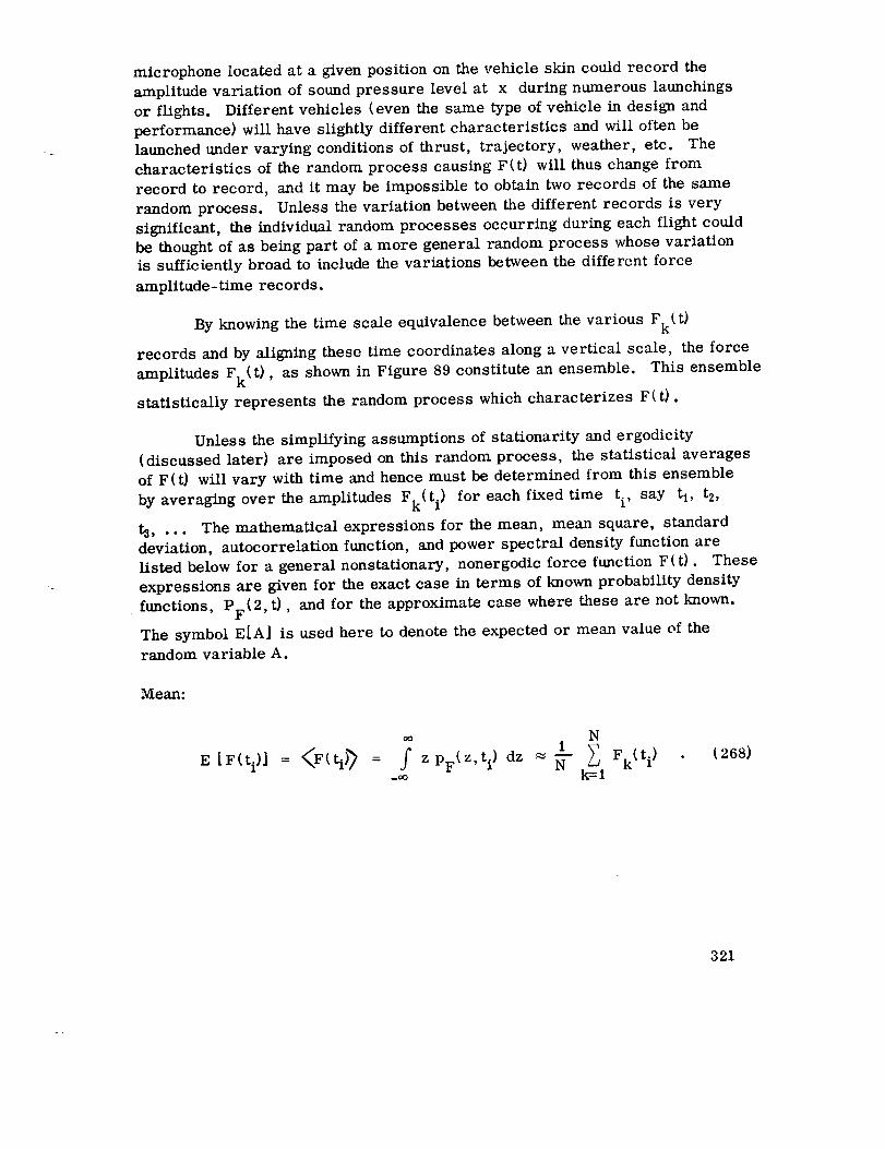
microphone located at a given position on the vehicle skin could record theamplitude variation of soundpressure level at x during numerous launchingsor flights, Different vehicles (even the same type of vehicle in design andperformance) will have slightly different characteristics and will often belaunchedunder varying conditions of thrust, trajectory, weather, etc. Thecharacteristics of the random process causing F(t) will thus changefromrecord to record, and it may be impossible to obtain two records of the samerandom process. Unless the variation betweenthe different records is verysignificant, the individual randomprocesses occurring during each flight couldbe thoughtof as beingpart of a more general random process whosevariationis sufficiently broad to include the variations between the different force
amplitude-time records.
By knowing the time scale equivalence between the various Fk(t)
records and by aligning these time coordinates along a vertical scale, the force
amplitudes Fk(t), as shown in Figure 89 constitute an ensemble. This ensemble
statistically represents the random process which characterizes F(t).
Unless the simplifying assumptions of stationarity and ergodicity
(discussed later) are imposed on this random process, the statistical averages
of F(t) will vary with time and hence must be determined from this ensemble
by averaging over the amplitudes Fk(t i) for each fixed time ti, say tl, t2,
t3, ... The mathematical expressions for the mean, mean square, standard
deviation, autocorrelation function, and power spectral density function are
listed below for a general nonstationary, nonergodic force function F(t). These
expressions are given for the exact case in terms of known probability density
functions, PF(2, t), and for the approximate case where these are not known.
The symbol E[A] is used here to denote the expected or mean value of the
random variable A.
1V[ean:
E [F(ti)] = _F(ti) _ ~ 1___ _ Fk (ti)f zpF (z,t i) dz ~ N-_ k=l
(268)
321

NL
M
v
IlL
0
o
°r,l
0
e_
q)
o
0
o
e_
0
322

Mean sqaure:
N
l__. _, Fk 2 (ti)-_ k= I
(269)
Note that the above nonstationary mean and mean square values are functionsof time.
Standard deviation:
art i) = _] F2(t i) - F(t 1) 2 (270)
Nonstationary autocorrelation function:
RF(ti, t.) = E[F(t i) F(tj)] = _F(t.) F(t.)_J 1 j
=/f--OO _Off
z1 z 2pF(zl, ti; z2, tj) dzl, dz 2
N1
Iq _ Fk (ti) Fk(tj) (271)k=-I
Nonstationary power spectral density:
_o _ j2_r(f, t. - f. t.)11 jj
SF (fi' fj) = f f R F (tt, t.) e dt. dt._oo _oo J 1 J
(272)
Note that the nonstatlonary autocorrelation function is a function of both t. and
tj, and the nonstationary power spectral density function is a function of b_th
f. and f..1 j
323

The first-order probability density function PF (z, t i) is the probability
density function for the amplitude F(t) at time t =t t and pF(z,ti) dz equals
the probability that at t = t. the amplitude F lies in the interval z < F < z + dz.
The joint probability density function pF(zl, ti; z2 tj) is the joint probability
density function for F(t), which multiplied by (dzl) (dz2) equals the probabil-
ity that F lies in both the intervals.
z i<F < zl+ dz 1 at t=t i
z2 < F < z2+ dz2 at t= t.J
The pF(z,tl) functions are estimated by sampling the various Fk(t)
records for fixed values of t = ti, and constructing the usual relative frequency-
of-occurrence graphs. The joint probability density function pF(zl, ti; z2, tj)
is a function of two variables, _'1 and zz, and hence is geometrically described
by a surface. The larger the data sample size, N, and the smaller amplitude
intervals tested, the more accurately the force probability density functions canbe determined.
It is often assumed that the random process being characterized is
stationary. This implies that the averages are invariant with respect to time.
Thus, the ensemble mean <F(t)> and mean square < FZ(t)> may be deter-
mined at any time t. All of the force amplitude Fk(t) used to obtain these
averages must correspond to the same value of t. The autocorrelation function
which generally depends upon two values of t, say t i and tj, will now depend
only upon the time difference _- between t t and t.. The mathematical expres-J
sions for the first few statistical averages, shown above, reduce to the following
simpler forms for a stationary random process:
Letting t0 be equal to any time, one obtains the following results.
Mean:
324
1E IF] = <F> = f zpF(z,t0) dz _ _ _ Fk(t0)
-.o k=l
(273)

Mean square:
E [ F 2] = <F2> = zpF(z,t0) dz = _ F_(t0) (274)
Standard deviation:
or= %] F2> - <F> 2 (275)
Stationary autocorrelation function:
RF(T) = E[ F(to) F(t0+T)] f / ztz2PF(Zl, to; z2, to + v) dz Idz 2
Ni_ _ Fk(t o) Fk(t O+r)
k=-I(276)
Stationary power spectra/density (two-sided) :
oO
-i2_rfrSF(f) = f RF(r) e dr ;
--oO
-_< f < _ . (277)
The above two-sided power spectral density function SF(f) is an even
function of f, defined for negative f as well as positive f. The one-sided real-
izable power spectral density function G F (f) is defined only for positive f
and is related to SF(f) by the expression
325

GF(f) = 2 SF(f) 0_ f<
thus,
= 0 f < 0 (278)
oO
GF(f) = 2 / RF(T) e -j2_rff dr ; 0< f<_ . (279)--00
For a stationary random process, the autocorrelation function RF(r)
is an even function _; that is, RF(-r) = R(T). Hence the above power spec-
tral density functions are given by
ao
SF(f) = 2 / RF(T) COS 21rfT dr ; _ < f < _o0
GF(0 = 4 / RF(_) cos 2_rfr d-r ; 0 --<f<0
(280)
The inverse relations yield
RF(_) = /GF(f)0
cos 21rff df
O0
1/2 SF(f) cos 2_rfT d£(28t)
326

If the ensemble is composed of time records of F(t) which are suf-
ficiently long, the ensemble statistical averages may change significantly with
time. For example, suppose that F(t) shown in Figure 90 is typical of other
records in the ensemble. The random process associated with this F(t) will
be nonstattonary ff it is not compensated for by other records in the ensemble.
However, it may be segmented into time intervals, (0,t 1) , (tl, t 2) , (t2,...),
such that during each interval the random process can be assumed stationary.
Stationary statistical averages can then be determined for each segment. Only
one record of the ensemble is shown here, but it is assumed that this one is
typical of most of the Fk(t) records in the ensemble, with respect to the
locations of the ends of the stationary segments. If this record is not typical
of all but a negligibly small number of the N ensemble records, then consid-
erable error may be introduced by assuming stationarity over these segments.
_ t
Figure 90. Time record of a nonstationary random force function.
A further simplifying assumption is usually made that the random pro-
cess which characterizes F(t) is ergodic. The combined assumptions of
stationarity and ergodtctty imply, in addition to the invariance of the ensemble
statistical averages with time, that any one of the Fk(t) samples of F(t) is
statistically equivalent to the entire ensemble. Thus the statistical averagesdefining the random force function F (t) may be obtained by timewise integra--
tions, thereby eliminating the immediate requirement for the probability
density functions. The mathematical expressions for the statistical averages
then become:
327

Mean-
E [F] -'- F =
T
limT._.o__1 Tf F(t) dt1
(282)
Mean square:
T
E [F2] = F-{ T--_lim__i fT= 9._ F2(t) dt (283)
Autocorrelation:
T
RF(T) = E F(t) F(t+ r) = T--oolimi_.'_ f F(t) F(t+T) dt . (284)-T
Power spectral density:
_o
GF(f) = 2SF(f) = 4 __RF(_') cos 2_rf_ d_- ; 0-< f < .o . (285)0
Although the probability density functions are not required in obtaining
the statistical averages of F(t) for a stationary and ergodic random process,
these functions are of importance and should be determined. A method has
already been outlined for approximating these functions from ensemble
samplings. Time averages are often used when an adequate and representative
ensemble is not available. Hence when the assumptions of stationary and
ergodicity are imposed, the probability density functions may have to be
obtained from a single time record of F(t). The method previously presented
for approximating pF(z,t) is still valid, except that pF(z,t) becomes
pF(z), and the data sample would consist of say N' values, F(t k) ,
328

(k-- 1,2,... ,N T) , of F(t) measured at even intervals of time as shown
in Figure 91. It is important that At be sufficiently small to ensure that
the highest frequency amplitude variations are weighted equally with those
of the lower frequencies. Bendat [ 241 indicates that at least two sample
readings per cycle should be made for the highest frequencies and that 10
to 20 sample readings per cycle might be practical estimates.
F (t! [
at
Figure 91. Amplitude sampling of F(t) at even intervals of time.
Stationarity of the random process assumes, by definition, that the
effects of all starting transients can be neglected and, hence, that the process
has always occurred with no changes in its statistical properties (i. e., it
began at t = --_). Also, the exact statistical averages of the random process
can only be obtained ff the sample size is infinite, which necessitates infinitely
long records. For practical applications, this type of precision is unwarranted
and sufficiently accurate results can be obtained for finite, but large, datasamplings.
Some degree of nonstationarity exists in most random processes which
have a physical origin, so that ensemble averages should be used in determining
the statistical properties of F(t). This, however, is undesirable at the pres-
ent time for a number of reasons. First, the quantity of data generally avail-
able for statistical analysis, in practice, is often meager and of limited
accuracy. This is partially due to the difficulties encountered in duplicating
any given random process, which thus restricts the number of ensemble sample
records that accurately represent the particular random process being investi-
gated. Even though either numerous records or long time records or both
may be available, they may contain spurious information introduced by the influ-
ence of other random or nonrandom physical processes.
329

Secondly, whenadequate and accurate representative samplings are
available, the data reduction can be a heavy task. It would thus certainly be
necessary to use high speed digital computers if a statistical analysis of any
quality were to be made.
Finally, there is a great desire on the part of analysts to take fall
advantage of the simpler time averaging expressions which are valid for sta-
tionary and ergodic random processes. Analog computing techniques are
readily available and relatively easy to program, which can efficiently deter-
mine at least the first few, and most important, statistical averages. The
assumptions of stationarity and ergodicity are therefore widely used with
segmented time records as a first approximation of the statistical averages.
The block diagrams shown in Figure 92 illustrate the simple procedure
for obtaining the mean, mean square, autocorrelation function, and power
spectral density function for a single time record F(t) by means of electronic
analog techniques. The function F(t) must be fed into the circuitry from
magnetic tape.
In practice, the length of the time records of F(t) may be relatively
short, and in real time may contain only one second or less of recorded data.
To increase the sample size, the ends of the magnetic tape may be joined,
forming a loop, which can then be repeatedly analyzed electronically as a con-
tinuous uninterrupted F(t) signal. This effectively increases the time dura-
tion of a random process and assumes that the process is stationary.
If a number of representative samples of F(t) are available, and if
electronic analog techniques are to be employed, the statistical averages may
be evaluated as time averages for each record and the set of statistical results
obtained from all of the samples may then be further averaged as an ensemble.
For example, if the mean value F k has been determined for each of N records
(k= 1, 2, 3, . . . , N), by the time averages,
T1 (286)
The ensemble mean F of all the N records is given by the expression
N( 2877
330

331
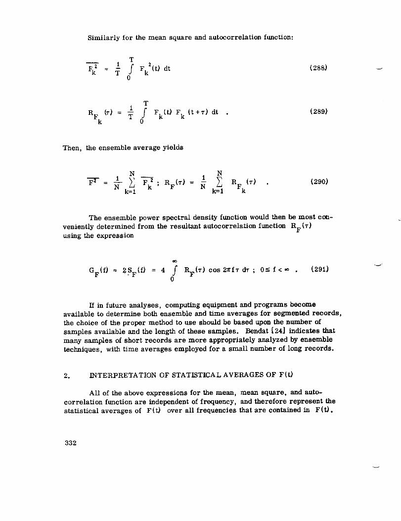
Similarly for the mean square and autocorrelation function:
T
Ft_ - T f FkZ(t)dt0
(28S)
T1
Cr)- T fRFk 0
Fk(t) Fk (t+_-) dt(289)
Then, the ensemble average yields
N N1 1
- 1_ k=-i)_ -_rk; RF(_-)- _ _ RFk(_') . (290)k=-i
The ensemble power spectral density function would then be most con-
veniently determined from the resultant autocorrelation function RF(T)using the expression
oO
GF(f) = 2SF(f) = 4 f RF(T) cos27rfv dr ; 0-< f<_o . (291)0
If in future analyses, computing equipment and programs become
available to determine both ensemble and time averages for segmented records,
the choice of the proper method to use should be based upon the number of
samples available and the length of these samples. Bendat [ 24] indicates that
many samples of short records are more appropriately analyzed by ensemble
techniques, with time averages employed for a small number of long records.
2. INTERPRETATION OF STATISTICAL AVERAGES OF F(t)
All of the above expressions for the mean, mean square, and auto-
correlation function are independent of frequency, and therefore represent the
statistical averages of F(t) over all frequencies that are contained in F(t).
332

This type of information is of limited value as it does not show the relative
importance of possible high amplitude persisting frequency components of F(t;,
nor the general distribution of power throughout the frequency range of F(t).
Since structural response is strongly dependent upon the frequency of excitation,it is necessary to determine these statistical averages for certain discrete
frequencies and frequency bands. For example, the power spectral density
function is one of the statistical averages used to describe the mean square
of F (t} in terms of its frequency components. In the following discussion of
the properties of the statistical averages of F(t), particular attention will be
given to spectral characteristics of these averages.
The components of F(t) contained within certain frequency bands or
at discrete frequencies are obtained in practice by filtering techniques. If
F(t) is stored on magnetic tape, it can be passed through a set of electrical
filters which transmit only those frequencies within the bandwidth of the filter.
The action of these filters is closely associated with the Fourier series and
Fourier transform, which display the theoretical frequency components of a
function. The convenient mathematical forms provided by Fourier methods
are very useful in explaining the actual frequency content of F(t) and in the
interpretation of results obtained by filtering. It is important to consider
briefly the spectral properties Of F(t) itself and the problem of filtering
before considering the spectral properties of the statistical averages of F (t).
The following discussion is not intended to be mathematically rigorous or
sufficiently precise to include all possible types of functions. The arguments
presented are directed toward the practical aspects of the problem.
Consider first that the function Fit) is well defined of period 2T and
contains a finite number of constant peak amplitude frequency components
which remain unchanged for all time (i.e., from t = __o to t = +_). Such a
function is stationary and can be expressed by the finite Fourier series,
N
= a_ + _ (a cosw t+ b sinw t)F(t_2 n n n n
n=l
N
= t + _n }c o + _ c ncos (_nn=l
(292)
333

where
C = J a 2 + b 2n n n
c o = ao/2
4),n- tan-t (bn/an) =
peak amplitude of the nth angular frequency
= 2_rf = 2_rf 0where f0= (1/2T)component w n n
phase angle of the nth frequency component.
T
1 fa - F(t) cos w tdtn T n
-T
Tb = --1 (" F(t) sin w t dt
n T J n-T
(293)
27T
= nO9o, (-_o -COn 2T- basic Fourier angular frequency.
All of the an'S , bn'S , and Cn'S will be zero except for those which
correspond to values of w which appear as discrete frequencies in F(t).n
The amplitudes of the various frequency components are easily obtained
for an F(t), known to contain only discrete frequencies, by electrically filtering
F (t) through a variable frequency bandpass filter of bandwidth Aw b = 2 _rAf b.
The block diagram in Figure 92 shows the essential equipment required for
this process and Figure 93 shows a plot of the typical characteristics of such
a filter relative to some centerband frequency w .c
The amplitude of each filtered frequency component of F(t) is given by
the product
Cn (filtered) = A(Wc, Wn) Cn " (294)
Thus, each filtered amplitude c may be obtained by sweeping wn c
through the entire frequency range of interest so that w is made to coincide,c
one at a time, with each of the frequencies w . If the bandwidth is sufficientlyn
334

U
I&l
tuo
o0u,I,,e,
3_ ..,
iZ
II
,,D3<1
o.
_ '%'_}V UO.I,OV:I :JIGI1LI,I18W
o_,-i
oc_
c'J
o
,F,,I
d
335
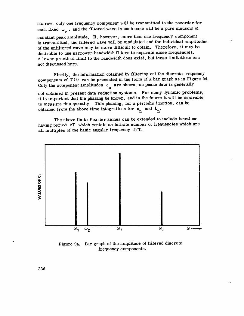
narrow, only one frequency component will be transmitted to the recorder for
each fixed w , and the filtered wave in each case will be a pure sinusoid ofc
constant peak amplitude. If, however, more than one frequency component
is transmitted, the filtered wave will be modulated and the individual amplitudes
of the unfiltered wave may be more difficult to obtain. Therefore, it may be
desirable to use narrower bandwidth filters to separate close frequencies.
A lower practical limit to the bandwidth does exist, but these limitations arenot discussed here.
Finally, the information obtained by filtering out the discrete frequency
components of F (t) can be presented in the form of a bar graph as in Figure 94.
Only the component amplitudes c are shown, as phase data is generallyn
not obtained in present data reduction systems. For many dynamic problems,
it is important that the phasing be known, and in the future it will be desirable
to measure this quantity. This phasing, for a periodic function, can beobtained from the above time integrations for a and b .
n n
The above finite Fourier series can be extended to include functions
having period 2T which contain an infinite number of frequencies which are
all multiples of the basic angular frequency Ir/T.
_Y
O
w
.J
>
091 _o2 O2 ----.,,,,,,e_
Figure 94. Bar graph of the amplitude of filtered discrete
frequency components.
336

Generally, the function F(t) is random and has no finite period (i.e.,
T-_). This is true for both stationary and nonstationary random functions•
Such functions cannot be represented by the Fourier series as they contain a
continuous band of frequencies which are not multiples of some basic frequency.
{For an infinite period, this basic frequency is zero. ) The spectral character-
istics of the function must be described by either its Fourier transform or by
its power spectral density function. It is assumed here that neither the transform
nor the spectrum function are trivially zero or infinite in amplitude.
Following the approach used by Bendat, the above Fourier series (N_oo)
can be rewritten in the complex form
JwntF(t) = _ A e w = 2_rf ; j =
n n nn._- __
1 T l i,Wnt I
A - _f F(t) e dt - Ca - jbn) n_0 (295)n 2T 2 n '-T
A o = ao/2 , IAn[Z = Cn2,/4
where (g0 is equal to It/T, and F(t) is of period 2T.
As the period T approached infinity, T-_, the basic frequency (g0
approaches zero, which shows that more and more frequencies are containedin F(t) Thus the coefficient A and hence a and b approach zero,
• ' n' n n '
which implies that the amplitude c of the individual frequency componentsn
also approach zero. However, as T--*_o, the ratio 2_rA /(g0 becomes then
Fourier transform
lli_ 21rA _o
w0...0 n = f F (t) e -j(gt dt = _F ((g) " (296)(gO _or
337

The Fourier transform of Fit), when it exists, may therefore be used
to describe the frequency characteristics of nonperiodic functions. This
transform exists for a limited case of nonstationary functions, where the total
energy associated with these functions is finite. Typical examples of these
functions are isolated pulses of various shapes, or a finite train of pulses.
Examples of the Fourier transform for three types of pulses are presented inFigure 95.
If F (t) contains a sinusoidal component of nonzero amplitude at some
frequency _, then the Fourier transform _F (w) will exhibit an infinite spikeat _.
For stationary nonperiodic random processes, the total energy associated
with F it) is infinite and the above Fourier transform is also infinite. In this
case the spectral properties of Fit) are displayed by the use of the one-sided
realizable power spectral density function GFiw). Formally, this function maybe defined as
GF(W) = T--*_o T " i297)
Although I_F(W) I is infinite, this ratio exists and is finite for
nonperiodic F I t). If F I t) contains a sinusoidal component at frequency _,
then GF(W) will exhibit an infinite spike at the frequency. For nonstationary
functions, where the Fourier transform exists, the power spectral density
function will be zero, except for periodic components where it will exhibit
infinite spikes. Since well-defined oscillatory functions contain periodicities,
it is not possible to show a diagram of some analytical function and its
corresponding power spectral density. Such spectrums must be determined
from a statistical analysis of a recorded function resulting from some physicalrandom phenomenon.
It is now clear that the filtering techniques used for functions which
contain a continuous band of frequencies must be altered somewhat from those
discussed above for periodic functions. Because the amplitude of each
frequency component is zero for such functions (except for additional discrete
sinusoids), it is necessary to filter a narrow band of frequencies and determine
the statistical averages of the amplitude of the filtered signal over all frequencies
in that narrow band. Since it is more desirable to use electrical filters, with
the function Fit) stored on magnetic tape, the time averages associated with
338

In
z3X.J- (u_ o
8 "-I-
,
I-,
3
3_-_3
! l I !
o w _. _. _ o _. o _ _ _. _ o o _. _. _r N. o,.: ,,: • . ,_ • .
°_.L Z / (_) _ _ °JJk/ (_) _ _ °_1 / (_) _
I.- I-
vI ^
_ v/_ .._
_. 0: _,0_o- p.._O"H H N H H I H H ,,,,,
_' I ° °
3 @
0
m(I)m
N
0
_4
339

stationary and ergodic processes are preferred over ensemble averages
because of available electronic analog methods for determining these averages.The above discussion shows that the nonstationary functions which are of
practical interest (i. e., those containing a finite amount of energy) are
transients that appear in the form of isolated pulses and shocks. These are
difficult to filter because of the small sample sizes available - usually one or
two records which are small fractions of a second in length. The following
discussion of the statistical averages of the frequency components of F(t)
will then be confined to stationary and ergodic random process, or those
processes for which the assumptions of stationary and ergedicity closelyapproximate the actual conditions.
In many random processes occurring in nature, the mean value of the
oscillating amplitude of a random variable, say F(t), is approximately equal
to zero. Also, the time variation of the amplitudes of the individual frequency
components of F (t) will have a near zero mean value. The assumption that the
mean is zero is widely used in practice. Whether or not this assumption is
valid naturally depends upon the random variable being considered. For example,
the distribution of the amplitude peaks of F (t) may be Rayleigh, which cannothave a zero mean.
The mean square value F_ of F (t) has a special physical interpretation
that is fundamental in spectral analyses. The instantaneous power dissipated
by a resistor R is an electrical network equals I2R or E2/R, where E is the
voltage drop across the resistor and I is the resistor current. Analogously,
the instantaneous power P(t) dissipated in a structure having viscous dampingc and vibratory velocity v equals cv 2 or AFt(t), where A is a constant
of proportionality. The average power P is the time average (mean of theinstantaneous power), avg
T T1 A
Pavg = _- f P(t) dt = _- f F2(t)dt0 0
(298)
and hence is proportional to the mean square value F-_ of F(t).
p ;avg
34O

that is, a knowledge of overall mean square value of the applied force F(f)
indicates the amount of power being (tissipated in a linear structure, to within
a constant of proportionality.
To broaden the use of the power concept so that the techniques which
have been developed for its application can be extended to include random
variables, for which true damping power does not exist, the proportionality
constant A is dropped and the mean square value of the random variable is
called the total average power of the variable. It may be more appropriate
for such cases to retain the "mean square" terminology. Both of these will
be used here _) avoid possible confusion with existing terminology used in the
referenced literature.
The mean square value is particularly useful in dealing with near dis-
crete frequency, random amplitude components of F(t). For the well-behaved
periodic function, the discrete frequency components have constant peak amp-litudes. For a near discrete frequency with random amplitude, it is not prac-
tical to determine all of the many Fourier coefficients required to define this
component. Instead, a narrow band filter is used to obtain these near discrete
components and the mean square value of the amplitude of each such frequencyis obtained.
The equivalent sinusoidal amplitude in terms of the Fourier coefficients
is given by the relation
1 2 =A_ = _c n mean square value of a true sinusoid with
amplitude equal to c .n
The total average power P for all of the near discrete componentsavg
is equal to the arithmetic sum of the power AP(c# n) of each component.
Pavg = _ AP(CUn) = _ _ " (299)n n
The graph ( Fig. 96) of the mean square value of the individual fre-
quency components is similar to that of Figure 94 where the Fourier amplitude
341

uuO
W
,=4
(a)l (4)2 (*)3 (t'P4 bJ5
Figure 96. Bar graph of the mean square amplitudes of
discrete frequency components.
coefficients are displayed for each sinusoidal component of F(t). Just as
did these Fourier coefficients, the mean square value of each frequency com-ponent, and hence the power in each component, decreases to zero when the
number of frequencies contained in F(t) increases to a continuous band of
frequencies. This assumes, of course, that no finite amplitude discrete
frequencies are present. To eliminate this difficulty, it is usual to consider
the mean square value over a finite frequency range of continuous frequency
components, and to divide this quantity by the frequency band. In the limit,
as the frequency band decreases to zero, this ratio becomes a mean square
density function with respect to frequency and is usually called the power
spectral density function GF(W ).
Mathematically expressed:
GF(W ) = lira FZ(Aw_ lira Pavg(Am)A_--O A_ = A_--o Aw (3o0)
342

where
F2(a ) =
Pavg (Aw)
mean square amplitude over all frequencies in A
= total average power over all frequencies in Aw.
The total average power contained in all frequency components in F (t)
is therefore given oy the equation
CO
= F' = f OF(O )Pavg 0
(301)
The physical interpretation of the mean square statistical average of F(t) isnow evident in terms of the definition of power presented above.
The power spectral density function GF(C0J is also related to the
autocorrelation function RF(_'), as shown in the previous expressions for the
statistical averages. For a stationary and ergodic process, reciprocalrelations exist in terms of the Fourier transform. These convenient mathe-
matical relations are as follows:
CO
1 2 f0 RF(r)GF(f ) = -- cos wl" drGF(C°) = 2_" _"
CO
RF(.r ) = f GF(0j ) cosw_" d:0 (302)0
These relationships are not easilyexplained by physical arguments and are not
discussed further in this document.
343

The stationars"autocorrelaiion function RF(1-) of a single time func-tion F(_-) also has a special interpretation which is important in determiningresponseof the structure. Basically, this function showsquantitatively theagreementbetweenthe function F(t) at time t and at time t 4 I- [i.e.,between the functions F(t) and F(t + v)]. When -r := 0, the two functions are
in perfect agreement at every, point and the correlation between the two is as
large as possible. Thus,
RF(O) => IRF(_') I •
It is to be noted that RF(0) is equal to the mean square value _ of
F(t). A non-negative correlation coefficient, CF(_" ), is a convenient measure
of the relative correlation of F(t) with itself. This coefficient is defined
here as follows:
RF(I")
CF(T) -- fiF (0) (303)
Thus, CF(T ) may have any values between 0 and 1. CF(r ) = 1 indicates
perfect correlation, CF(_" ) = 0 indicates no correlation, and values of CF(T )
between 0 and 1 indicate partial correlation.
The validity of this concept of correlation is easily shown by consideringa simple sine wave of the form
F(t) = C sin (wt- _) .
The non-negative correlation coefficient CF(-r ) for this case is
344

C 2
_Y
C 2
T
f-T
-T
sin (_ct + 0) sin (09t + cuT-t 9) dt
sin 2 (cot+ ¢) dt
1 2C cos wt
,)= I cos09TI (304)
A plot of CF(T ) is presented in Figure 97, and it will be valuable to
compare this ideal coefficient with those obtained in practice for random
functions.
1
/
//
//
0
2"-_ 2"-_ 2_
Figure 97. The correlation function CF(r ) of a sinusoid is the
absolute value of a cosinusoid CF (r) : lcos 09 v l"
In contrast to a well-behaved periodic function, the correlation coeffi-
cient for random white noise is zero for all r ¢ 0. "White" noise is a descrip-
tive term for a random process whose power spectral density function is a
constant over all frequencies.
F. Digital Vibration Analysis
The process of digitizing consists of converting continuous data into
discrete numbers. There are two main parts involved in a digitization pro-
34 5

cedure. The first part is sampling, which is defining the points at which thedata is observed. It is important to have a sufficient number of samples to
describe properly the significant information in high frequencies. On the other
hand, sampling at points which are too close together will yield correlated and
highly redundant data, and increase greatly both the la}x_r and cost of calcu-
lations. To cut down the number of samples, one should decrease the sampling
rate to the lowest rate which will avoid aliasing errors.
To be specific on aliasing, if the time interval between samples is h
seconds, then the sampling rate is (]/h) samples per second. The useful
data will be from 0 to (1/2 h) Hz since frequencies in the data which are
higher than (1/2h) Hz will be folded into the lower frequency range from
0 to (1/2h) Hz and confused with data in this lower range. The frequency
1f = -- (305)c 2h
is known as the Nyquist frequency. Folding of the frequency axis is illustrated
on Figure 98. For example, if f _ 100 Hz, then data at 170, 230, 370, andc
430 Hz would not be distinguish.3d from data at 30 Hz.
The second part in a digitizing procedure is the matter of quantization,
which is the actual conversion of the observed values to numerical form. No
matter how fine the scale, a choice between two consecutive values is required.
This matter is illustrated on Figure 99. In this figure one would choose
(a _ 1) as the closest numerical value to the desired time value.
I I I I I I l
0 fc 2fc 3fc 4fc 5fc 6fc 7fc
ORIGINAL FREQUENCIES
fc 3fc 5fc 7fc
_ALIASED c 4fc 6fc
FREQUENCIES ALIASED FREQUENCIES
Figure 98. Illustration of folding about the nyquist
cutoff frequency f .C
346

ACTUAL DATA_
SCALE UNITS
a+2
a+l
SAMPLING TIME, TIME
Figure 99. Illustration of quantization error.
If one assumes that the quantization errors follow a uniform probability
distribution over one scale unit, then these errors will have a mean value of
zero and a standard deviation (rms value) of approximately 0.3 scale unit.
This can be considered as an rms noise error on desired signal measurements.
For example if the rms value of a signal is quantizated at 300 scale units,
then since the rms value of the noise is 0.3 scale unit, one would have an
rms noise-to-signal ratio here of 0. 001.
, BASIC STATISTICAL ANALYSIS
a. Data valuesu, are found at pointsi : 1,2,...,N.l
are a dist,-mce h apart and determine the cutoff frequency fc
These points
- ( 1/2h).
b. Mean value
o
u
N1V
: N 1£z1 u"1(306)
where
N : number of data samples
u = data values at points i - 1, 2,3,..., N.i
347

The true mean value is denoted usually by iz. The quantity u is called the samplemean value and is an estimate of #. So that subsequent formulas and calcula-
tions may be simplified, it is convenient to transform the data to have a zero
mean value. That is, define quantities x. by the relation1
x. -- u.-u , i -- 1,2,...,N . (3o7)I 1
This computation would be necessary later for other procedures and is most
optimally performed at thistime.
c. Standard deviation
where
(xi)s -- (3os)1 N-1
N = number of data samples
xi= transformed data values at points i = 1,2,3,..., N.
The quantity s is called the sample standard deviation. The sample variance is
denoted by s 2. The true standard deviation is denoted usually by a, and the true
variance is denoted by 02 .
d. Standardization. A further transformation on the data may be con-
venient at thistime ifthe computer calculated are to be performed with fixed,
as opposed to floating,arithmetic. Multiplying the transformed values, xi,by 1/s yields
1
Yi - s x.l ' i = 1,2,...,N . (309)
This results in final data with a sample mean of zero and a sample standarddeviation of unity.
The scaling problem is eased in fixed point arithmetic since the data
may now be considered to lie in the range Yi -< 7. Actually the probability
of values greater than three or four in absolute value is negligible in most
348

cases. If floating point arithmetic is used, there is no particular advantage
to having the division by s. It must be noted that the division by s corresponds
to a scale change so that output data for plotting and the like would have to be
later scaled appropriately. Also, for large amounts of data, the complete
standardizing is costly computational timewise since N divisions are required
if there are N data points.
e. Skewness coefficient (Cs)
N (_i)3Cs = 2 Ns (3:0
i=l
where
s = sample standard deviation
N = number of data samples
x. = transformed data values u. - u.L 1
The true skewness coefficient for a normal distribution is zero.
f. Kurtosis coefficient (Ck)
(xi)'Ck= 2 Nsr
i=l
(3::)
where
s = sample standard deviation
N = number of data samples
x. -- transformed data values u. - u.1 l
The true kurtosis coefficient for a normal distribution is 3.0.
349

g. Probability density function
f(x)- d F(X) (31Z)cLx
where
f(x) = probabilitydensity function
F (x) = probabilitydistributionfunction.
The number of observations and the percentage of data in each of k class
intervals are tabulated. To later optimally apply a Xz goodness-of-fit test of
the data to the Gaussian and Rayleigh distributions, the number of class inter-vals should be chosen as indicated in Table 11.
TABLE 11. OPTIMUM NUMBERED CLASS INTERVALS k
AS A FUNCTION OF THE SAMPLE SIZE N.
N 0-299 300-499
k 16 20
500-699
24
700-899 900-1249 1250-1749 1750-_
27 30 35 39
h. Probabilitydistributionfunction
0
,(x) = f ,(x) d_ (313)
where
f(x) = probabilitydensity function
F(x) = probabilitydistributionfunction
F(-_)= 0;F(_)= 1.0.
The cumulative number of observations and the cumulative percentage of datain each class interval are tabulated.
i. Gaussian (normal) probabilitydensity function
[7-x 21#(x)= exp I _-"_'2_'| (314)
L_v A
350

where
Thus,
the true mean value is zero
= true standard deviation (estimated by s, the sample standard
deviation)•
x2 1_ (x) _- _._L_I e×p (s15)
The density function q) (x) is evaluated at the midpoints of the k class intervals
determined in 7 above.
j. Gaussian probability distribution function
X
(x)-- f o(x) dx (316)
where
(x) = Gaussian probability density function
4_ (x) = Gaussian probability distribution function.
The Gaussian distribution function should be evaluated at the k-1 class interval
end points.
k.
where
Rayleigh probability density function
x E_x,]c(x) = 7_ exp _ (317)
(r = true standard deviation (estimated by s, the sample standard
deviation).
Thus,
351
m
wI

x ix2]c(x) _ s-"f exp _ (318)
The density function c (x) is evaluated at the midpoints of the k class intervals.
1. Rayleigh probability distribution function
X
C(x) = f c(x) dx (319)--0D
where
c(x) = Rayleigh probability density function
C (x) = Rayleigh probability distribution function.
The distribution function C(x) is evaluated at the k - 1 class interval endpoints.
m. Tests for normality
(1) ×2 Goodnes_,-of-fit test
Let Pi be the percentage of observations in the ith class
interval. These values are obtained when the density func-tion histogram is tabulated in Step g. Let A A. be the area
1
under the Gaussian density function curve in the ith class
interval. Note that these quantities are effectively obtained
during Steps i and j. The statistic
2k Pi
X2= N E AA-----'_. (320)i=l I
is distributed as _2 with k - 3 degrees of freedom (df).
(2) Moment test
The skewness and kurtosis coefficients Cs and C k given by
equations (310) and (311) may be used as an additional test
352

for normality. The sampling distributions for C ands Ck-_
are tabulated for the . 01 and . 05 levels of significance in
Reference 27, where they are denoted by 71 and Yz,respectively.
n. Test for Rayleigh distribution
The procedure is identical to that outlined in m (1) above except
that the AA. values are obtained from Steps k and 1. Also, due to the fact that,
only one parameter, namely s 2, is necessary to define the Rayleigh distri-
bution, the statistic computed from equation 14.92 will be distributed as ×2with k- 2 dr.
2. FOURIER SERIES REPRESENTATION
If a sample record x(t) is periodic of period T, that is, x(t) = x(t + T)
for all t, and if one assumes f0 = (l/T) is the fundamental frequency, then
x(t) can be represented by the series
oo
x(t) = a°_- + _ (anCOS 2vnf0t +bnsin2_'nf0t ) (321)n=l
where
T
fa =-- x(s) cos 27rnf 0 s ds (322)n T0
T
b - 2 f x(s) cos 27rnf 0 s ds . (323)n T
0
Assume x(t) of length T is sampled at an even number N equally spaced
points a distance h apart where h has been selected to produce a sufficiently
high frequency cutoff f = (1/2/,). LetC
x -x(nh) ; n=i, 2, ..., N .n
One may calculate the finite analog of a Fourier series which will pass
through the N data points [28]. For any point t in the interval (0, T), oneobtains
353

N/2 2_rnt (_/2)-1x(t)=A0+ _ A cos -- + Bn T nn=l n=l
At the particular points t = kh, k = 1, 2,..., N
N/2
Xk=Xkh =A0+_ Ancosn=l
(3_/2)-12 nk +N
n=l
The coefficients A and B are given byn n
2_ntsin --
T. (324)
27rnksin --_ . (32s)
N
ly,k=l
N2 _ 27rnk
x. COSn N _ k N
k=l
N
AN_2/=--1 \, !:TrN /_ x k cosk=l
Nn=l, 2, ..., -- - 1
2
(326)
NB = _ii_ 27rnk , N
xksin N , n=l, 2, ..., "-_- 1Nn
Note that A 0 = 0 when the sample mean x = 0 which is the situation here.
the above formulas,
N = number of data samples
x k= data values atk= 1, 2, ..., N
A = finite analog of Fourier cosine coefficientn
B = finite analog of Fourier sine coefficientn
h = time interval between samples
f = (1/2h) = cutoff frequencyc
T = period
f0 = (l/T) = fundamental frequency .
In
354

One should note that for large N the computational requirements for determ-
ining the coefficients A and B become quite overwhelming. However, then n
determination of the coefficients might still be of enough interest to justify
the necessary computations.
a. Choice of Sample Size N
Certain formulas presented in Reference 20 can aid in the selec-
tion of the optimum sample size N to minimize later data processing. For
example, assume that a set of power spectrum measurements (Gx(f)} at a
particular value of f follows a normal (Gaussian) distribution. Let Gx(f ) bethe true value and let A p be defined such that
ProbGx(f ) - Gx(f )
Gx(f)< Ap >p. (327)
It can be shown that under certain conditions
O/
P (328)
where a is the p percent value for a normal distribution defined byP
Prob (-_p <x <- _p)=p • (329)
In equation (329), x is a normally distributed random variable with zero mean
and unit standard deviation. The quantity T in equation (328) is the total time
period over which the data is taken, and B is the resolution bandwidth.
To illustrate how the sample size N is related to the BT product which
these samples represent, an example will be calculated. Suppose that the
error of the power spectral density estimate at non-zero frequencies is to be
no more than Ap = 30 percent at an 80-percent confidence level (a,p = 1.3);
that is, in a sequence of repeated expemments, at least 80 percent of the
estimates will have an error no larger than 30 percent. The BT product is
then determined as
2
BT = _ 18.7
355

Assumenow that frequencies up to f = 2000 Hz are of interest and a resolutionc
bandwidth B = 10 Hz has been chosen. The maximum lag number m is then
calculated from the equation
2fo 2/2000)m- - -- 400.
B 10
Also, the time interval h between samples is given by
h
1 1
2f 2(2000)C
- .00025 sec.
The total record time is
2
ecT = "_ 10
One then calculates the total number of observations N to be collected from
the equation
N- T _ 1.87 - 7.480x103 = 7480 .h 0. 00025
This number is applicable to nonzero frequencies. For Gx(0 ), one requires
twice as many observations to maintain the same error risks.
Further experimental design considerations, such as the determination
of the resolution bandwidth B, are discussed in Section VIII and in Reference
20.
3. AUTOC ORRELATION FUNCTION
For a sampled data {Un}, n = 1, 2, ..., N, from a record x(t) which
is stationary, the estimated autocorrelation function at the points t = rh, r = 0,
1, 2, ..., m < N, will be defined using the transfo'rmed data values u - iI bythe formula n
356

1R --R (rh)-r x N-r
N-r N-r
2 (oo+ 2 XnXo÷ n=1 n= i
N-F
N-r n n+r1
if N > > r (330)
where
u = u(nh) = data values at n = 1, 2, ..., Nn
= sample mean value
r=lagnumber=0, 1, 2, ..., m<N
m = maximum lag number
x = u - _ = transformed data values.n n
Note that the mean value _ = O.
The maximum lag number m determines the later frequency bandwidth
f resolution for the power spectral density function in the frequency interval
(0, f). This resolution bandwidth is given by
2f
B - c • (331)m
The resolution bandwidth B is twice the range found by dividing the frequency
interval (0, fc) into m equally spaced parts (f/m) apart. Thus from know-
ledge of fc' one can chose m in advance so as to have a desired B. For small
statistical uncertainty in later estimates of the power spectral density function,one should choose m < < N since the maximum number of statistical degrees
of freedom associated with these estimates is given by (2N/m). On the other
hand, high resolution (i.e, small B) will result if m is large. Thus a com-
promise choice for m is necessary in practice.
The autoeorrelation function may take on negative as well as positivevalues. A normalized value for the autocorrelation function is obtained by
dividing R by R 0 wherer
N
1 (332)a0= ax(0)= -ff (Xn)2 •n=l
357

Note that the quantity R 0 is a sample estimate of the true mean square value
in the data. The quantity R 0 is related to the (unbiased) sample variance s 2
by the relation
N - 1 s t . (333)R° = N
Thus for large N, there is negligible difference between R 0 and s 2.
When R is normalized, one obtains the quantity (Rr/R0) which willr
be between plus and minus one; thatis
-z< (R/R) < I.= r 0 =
o POWER SPECTRAL DENSITY FUNCTION
For sampled data from a record x(t) which is stationary with x = 0,
(i.e., as occurs for transformed data values x = u - _i),a "raw" estimaten n
of its realizable one-sided power spectral density function G(f) ;that is, G(f)
is non-zero only for f_->0, is ffivenfor an arbitrary f in the range 0 <=f -<f
by c
m-1
(_rf / (_mf /Gx(f ) =2h R 0+2 _ R cos +R cos (334)r=l r \_c/ m - fc-
where
h = time interval between samples
R = value of autocorrelation function at lag r using the transformedrdata values x = u -
n n
m = maximum lag number
f = (1/2h) = cutoff frequency.C
The total mean square value in the record in the frequency range 0 _-<f -<_fis given by c
fC
f _x(f)d_=R0-=Rx(0)0
(335)
358

This quantity Gx(f ) shouldnot be confusedwith a nonrealizable two-sided
power spectral density function Sx(f) which is defined for negative as well aspositive f by
G (f)xs×(f) = Sx(-f)- 2
Here
fC
f-f
C
S (f)df = Rx(0 )X
The values of the function G(f) should be calculated ollly at the (m + 1)
special frequencies
kff e= -- ; k= 0, 1, 2, ..., m. (33b)
m
This will provide (m/2) independent spectral estimates since spectral estimates
at points less than (2f/m) apart will be correlated. At these special frequency
points,
G k=G x = 2h R 0+ 2 R rcos \l--7"al + (-1 R rr=l
(339)
The index k is called the harmonic number (k =_0, 1, -,9 ..., m), and the
quantity G k is the "raw" estimate of the power spectral do_lsity function at the
fre_lency f = (kfc/m). The quantities G k will be non-negative for all k.
A convenient check formula is
m-1 ]Rx(0). . _ 1 1 1. 2hm _ GO + _-; Gk + 2 Gm (340)k=l
359

A "refined" estimate of the power spectral density may be found byfurther frequency smoothing called "Hanning [ 29 ]". Let G represent this
"refined" estimate. Then at the (m+l) frequencies f = (ldk/m) ; k / 0, 1,2, . .., m, one obtains
Go = 0.5 Go+ 0.5 Gi
Gk = 0.25 Gk_ 1 +0.5 G k + 0.25 Gk+l; k= 1, 2, ..., m-I
= 0.5G +0.5G (341)Gm m-1 m
Other "refined" estimates may be obtained which are more complicated than
the above. These provide different bias and uncer_inty errors which are pre-
ferred for certain applications. These values for G k should be used as the
final estimates here for G(f) at the frequencies f = (kfc/m) ; k = 0, l, 2 ..... m.
5. JOINT STATISTICAL ANALYSIS OF TWO RECORDS
In the followingformulas the assumtion willbe thattwo records x(t)
and y(t) are stationary and exist only for 0 -<t -<T. Choose a sampling time
intervalA t = h time units apart, which in so doing induces a desired corres-
ponding frequency cutofff = (I/2h). Let the respective sample values forc
x(t) and y(t) be denoted by
Un = u(nh) I n = I, 2, 3,..., N
Vn = v(nh} _ T = Nh(342)
The first quantities to compute are the sample mean values
N N
- ly - 1 ZU = _ U V = -- VN n N n
n=i n=l
360
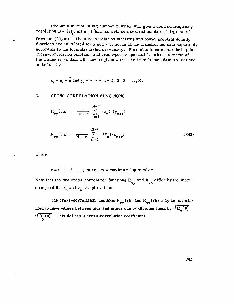
Choose a maximum lag number m which will give a desired frequency
resolution B = (2f /m) = (1/hm) as well as a desired number of degrees ofc
freedom (2N/m). The autocorrelatien functions and power spectral density
functions are calculated for x and y in terms of the transformed data separately
according to the formulas listed previously. Formulas to calculate their joint
cross-correlation functions and cross-power spectral functions in terms of
the transformed data will now be given where the transformed data are defined
as before by
x i=u. -uandYi =v" -v; i= i, 2, 3, ...,N.I I
e CROSS-CORRELATION FUNCTIONS
N-F
R (rh) - 1xy N-r _, (Xn) (Yn+r)
n=l
N-F
Ryx(rh) = NI- r n_=1 (Yn)(Xn+r)(343)
where
r = 0, 1, 2, .... m and m = maximum lag number.
Note that the two cross-correlation functions Rxy
change of the x and Yn sample values.n
and Ryx
differ by the inter-
The cross-correlation functions R_v(rh)..j and Ryx(rh) may be normal-
ized to have values between plus and minus one by dividing them by _(O)
(0). This defines a cross-correlation coefficientY
361

Fxy(rh)
Rxy (rh)= (344)
JR (o) 4-g (o)x y
such that-1 N F (rh) =<1.xy
For later determination of the cross-power spectral density function
between x and y, calculate the two quantities
1
Axy (rh) = _ [Rxy(rh ) + Ryx(rh)]
1
Bxy(rh) = _ [Rxy(rh ) - Ryx(rh)] (345)
7. CROSS-POWER SPECTRAL DENSITY FUNCTION
The cross-power spectral density function is a complex-values
quantity defined by
Gxy(f) = Cxy(f) - JQxy(f) ;j = %f-i (346)
where Cxy(f) is called the cospectral dens,ty function and Qxy(f) is called the
quadrature spectral density function. An equivalent respresentation for Gxy
(f) is
JOxy (f)G (f) = IG (f)[ e (347)
xy XV
where ] G (f) [ is the absolute value of G (f) and 0 (f) is the phase anglexy xy xy
contained in G (f).xy
362
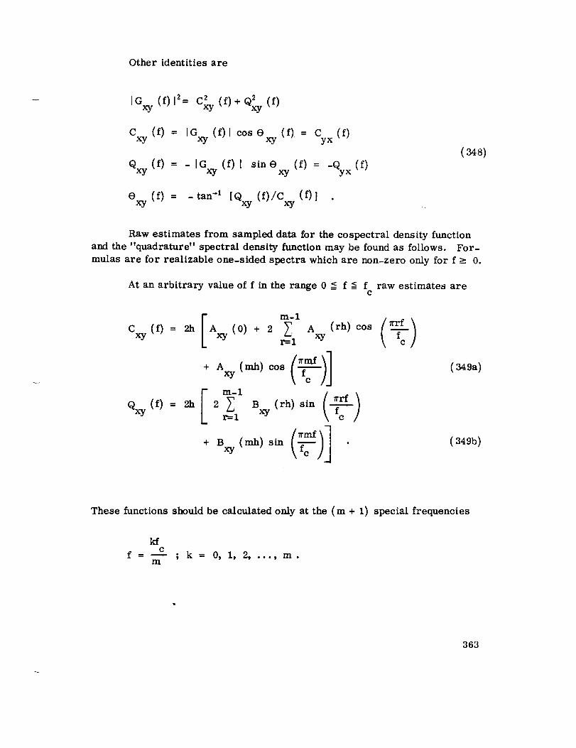
Other identitiesare
IG_y(f)12=C2_y(f)+Qxy2(0
C (f)= IG (f)Icose (f)= c (f)xy xy xy yx
Q_y(f)= - IG (f)I sine (f)= -Qy×(f)xy xy
exy (f) = - tan-i [Qxy (f)/Cxy (f)]
(348)
Raw estimates from sampled data for the cospectral density function
and the "quadrature" spectral density function may be found as follows. For-
mulas are for realizable one-sided spectra which are non-zero only for f>- 0.
At an arbitrary value of f in the range 0 -< f _-<f raw estimates areC
C (f) = 2h Axy (0) + 2 _ A (rh) cos rrfxy xyr=l
Iv (r)Qxy (f) = 2h 2 Bxy (rh) sin _rfr=l
(349a)
(349b)
These functions should be calculated only at the (m + i) special frequencies
kfC
f =m
; k = O, 1, 2, ..., m.
363

At these frequencies, one obtains
C k = C (kfc/m) =xy E m-1r=l
÷ (-1) k A (mh) I
(rh) cos [ _'_" _Axy \m/
(350)
Qk = Qxy (kfc/m) = 4h _ Bxy (rh) sin r._._ . (351)r=l
Refined estimates of both C. (f) and Qxv(f) may now be calculated asvv tv xy
before by using the Hanning method [ 30 ]. This yields
= 0.5C o + 0.5c t
= 0.5Q0 + 0.5Q 1
_k = 0.25 Ck_ 1 + 0.5C k
k = 1, 2, ..., m-1
+ 0.25 Ck+ 1
Qk = 0.25Qk_l + 0.5Qk ÷ 0.25Qk+l
= 0.5 + 0.5 Cm Cm-1 m
Qm = °'5Qm-1 + 0"5Qm
(352)
Now, since Gxy (f) = Cxy (f) - JQxv (f)' at the special frequencies f = (kf/m) ;k = 0, 1, 2,..., m, one obtains the i'efined estimates
xy (f) = _xy (kf/m) = _k - JQk = 1Gx.y (f) I eje xy (f)
xy
(f) = -tan-' (Qk/_k)xy(353)
364

N
These values for [Gxyl and exy should be used as the final estimates here
for IGxyl and ex.y at the frequencies f = (_c/m); corresponding to the har-monic numbers k-= 0, 1, 2, ..., m.
8. TRANSFER FUNCTION PROPERTIES FOR LINEAR SYSTEMS
Assume row that x(t) is the input to a linear system, characterized by
its frequency response function HCf), and y(t) is the output from this linear
system. The frequency response function H(f) is a complex-values functiondefined by
¢0
H(f) = I h(T)e -j2_'fv dv (354)0
where h(T ) = 0 for T < 0 is called the weighting function or unit impulse
response function of the system. An equivalent representation for H(f) is
H(f) = [H(f)le j@(f) (355)
where ]H(f)l indicates the gain factor of the system at frequency f, and O(f)
indicates the corresponding phase shift at frequency f.
A basic result between stationary input power spectra G x (f), linearsystems HCf), and stationary output power spectra G (f) is
Y
G (f)= IH(f) I2G (f) • (356)y x
Another basic result using the stationary cross-power spectra G (f) isgiven by xy
G (f) = H(i) Gx (f)xy(357)
This latter equation reduces to two relations by equating real and imaginary
parts, namely,
365

iG (f) i = iH(f) i Gx(f)xy
e (f)-- _(f)xy
(358)
One can derive also the relation
Gxy (f) _ eJ2_ (f)G (f)
yx
(359)
from which to determine the phase factor _ (f).
At the special frequencies f = (kfc/m); k= 0, 1, 2, ..., m, the gain
factor and the phase shift are estimated by
2 + _2_1/]Gxy (f) t (_k -_k'
[Hk[ = =
Gk Gk
9k = -tan-1 (Qk/_k) (360)
9. COHERENCE FUNCTION
A coherence function y_y (f) is defined between the stationary records
x(t) and y(t) by the relation
= , 0, , 0 (361)XG x (f) Gy (f) ; G (f) Gy (f)
366

where
G (f)--X
G (f)--y
G (f) =xy
power spectral density function of x(t) at frequency f
power spectral density function y(t) at frequency f
cross-power spectral density function between x(t) and
y(t) at frequency f.
The coherence function satisfies the inequality 0 -<7_y (f) -_ 1 for all f.It is unity when x(t) and y(t) are linearly related, and it is zero when x(t) andy(t) are incoherent at a frequency f.
At the special frequencies f= (kfc/m);k= 0, 1, 2, ..., m, thecoherence function is estimated by
_2 N2k +Qk
N 2 = . • (362)
7k Gk, x k,y
I0. JOh-NT AND CONDITIONAL PROBABILITY DISTRIBUTIONS
As an adjunct to calculationsof interestfor two random records, such
as the cross-correlation function and the cross-power spectral density function,
one may also calculatejointand conditionalprobabilitydensity functions.
a. Joint Probability Density Function
The joint probability density function
f(×,y)= y
where
f (x,y) = joint density function
F (x,y) = joint distribution function.
367

This may be obtained in the form of a two dimensional histogram. That is,
each variable is divided into an appropriate number of class intervals and the
number of observations and the percentage of data in each rectangle is
recorded. See Figure 100 for an illustration as to how such a tabulation might
appear.
3
1
0
2 0
3 2
1 2 7 15 19 13 6 2
3 4 8 18 25 16 8 4
3 6 14 17 16 6 3
5 6 8 5 5 1
3
2
1
0
1
1
2
1
0i
0
Figure 100.
ho
where
Two-dimensional histogram representing f(x, y).
in each square represents observed frequency. )
Joint Probability Distribution Function
The joint probability distribution function
x y
F(x,y) = f f f(u,v) dvdu_¢D _CO
f(x,y) = joint density function
F(x,y) = joint distribution function
(Number
(364)
F(=, x,)= F(xl,-_)= 0; F(=, =)= 1
368

The distribution function is tabulated by first accumulating the number of
observations and percentages in the x direction and then in the y direction
for the final cumulative rectangle entries.
C. Joint Gaussian Distribution
Let P denote the normalized covariance matrix for the variables x and
y; that is,
1 -r C0)xy
-ryx(0) 1
Rxx(0) -Rxy(0)
4 Rx(O) _{Rx(0) _fRx(0)
-Ryx (0) Ryy (o)
_R (0) _ (0) _fR (0)y x y y
(365)
Note that F (0) = r (0) and is termed the correlation coefficient of x and y.xy yx
Let x be a vector defined by
X ---- ' S
Y
and let
x' = transpose of x.
The two dimensional (sample) normal density function is then given by
369

{-1 }exp 2 1P'---'[-x Px'f (x7 = (3667
I l
where
IP] = det P = 1 - F 2 (07. (367)xy
The quadratic form xPx' replaces the squared exponent x 2 in the one dimensio-
nal case. The two dimensional (joint) Gaussian distribution is therefore a
function of five parameters = 0, _ = 0, Sx, Sy, and Fxy(07. All these quan-
tities are available from previous calculations, the means being zero, of
course, because of the previously applied transformation x = u - _, etc. The
bivariate normal distribution is most easily described in terms of "equi-
probability ellipses". If one considers the points that give a constant value
to the density function, it is seen that they form an ellipse
2,PIxPx'-- [ ]2 (i- r 2 (07xy
+ = C 2
- )(368)
where c 2 is a constant.
outside the ellipse is
It can be shown that the mass in the whole plane
-C 2 -C 2
2c e dc = eC
(369)
Therefore, ellipses might be plotted for the 50, 75, 95, and 99 percent
values; that is, ellipses which include all but 50, 25, 5, and I percent ofthe observations.
370

The values for c2corresponding to these values are given in Table 12.
TABLE i2. VALUES OF c 2 FOR EQUIPROBABILITY ELLIPSES
Percent of Observations
Included in Ellipse
50
75
95
99
Corresponding Valueof c 2
0. 693
1. 386
2. 996
4.605
For a moderate positive value of F (0), the ellipses might take thexy
form shown in Figure 101. If Fxy(0) = 0, they become circles and for
Fxy(0) = +l, a degenerate case of straight lines arises.
y
X
(x,y) - (0,0)
Figure 101. Typical equiprobability ellipses.
371

The proper method of plotting would be from the parametric equations
of an ellipse. This requires several steps:
1. Eliminate the xy term in equation (368) of the ellipse by a
rotation of coordinates through the proper angle.
2. Calculate the semimajor axis a and semiminor axis b of the
ellipse.
3. Plot the values as a function of e from the parametric equations
X ---- a COS e
y= b sin e.
The details of obtaining the angle necessary to rotate out the xy term and for
computing the axes a and b may be found in standard texts on analytic geometry.
d. Conditional Probability Density
The conditional density function for y given x, f(y [ x ) (that is, for aspecific value of x) is
f(y]x) f(x, y)- f(x) (370)
where
f(Y Ix )
f(x,y)
f(x)
= conditional density function of y given x
= joint density function of x and y
= density function of x(assumed _ 0 ) .
This is obtained by choosing a column of the two dimensional histogram for
the joint density function, and normalizing each entry by dividing by the total
number (or total percentage) in that column. That is, for each class interval
of x one may obtain a conditional density function.
To obtain conditional densities for x given y, one uses rows insteadof columns.
372

11. SUMMARY OF FUNCTIONS FOR TWO RECORDS
The preceding work is summarized in Figures 102 and 103 which show
the order for computing desired functions for two records x(t) and y(t). In
the transfer function calculation, x(t) is considered as an input and y(t) as an
output through a linear system.
AUTO-CORRELATION
FUNCTION
CROSS-CORRELATION
FUNCTION
AUTO-CORRELATION
FUNCTION
I I POWER
: SPECTRALRx DENSITY
FUNCTION
I I CROSS'POWERSPECTRAL
Rxy ' Ryxl DENSITYFUNCTION
J I POWER
SPECTRAL> DENSITY
Ry FUNCTION
_I TRANSFER
I FUNCTIONxy,Gi COHERENCE
I.0xGy
Figure 102. Functions to be computed for two records.
x(t)
I PROBABILITY
DENSITY
; : (DISTRIBUTION)FUNCTION
[x(t), y(t)l
PROBABI LITYDENSITY
(DISTRIBUTION)FUNCTION
f(x), F(x)
I JOINT PROBABILITY I
_I DENSITY I_-I (DISTRIBUTION) |
I FUNCT,ON I
f(y), F(y)
L CONDITIONAL
PROBABILITY> DENSITY
FUNCTION
f(x,y),F(x,y)
CONDITIONAL
PROBABI LITY>- DENSITY
FUNCTION
f(y/x)
f(x/v)
Figure 103. Joint probability functions for two records.
373

12. DIGITAL COMPUTER PROGRAM FLOW CHARTS
The flow charts on the following pages give the operations to be per-
formed by the digital computer program for the statistical analysis of vib-
ration data. The essential sequence of the operations should be approximately
as indicated if all of the preceding analysis is desired. Other routines can be
added to incorporate additional desired tests, such as tests for randomness
and stationarity. Also, if only certain parts of the program are requested,
such as power spectra alone, these can be computed directly by omitting
intervening steps dealing with other information.
13. COMPUTER TIME ESTIMATES
Table 13 gives some computing time estimates in terms of the number
of operations required. The load-store-indexing operations are grouped
together as are add and subtract. About a 30 percent factor to account for
programming overhead should be added into final estimates. This is to allowfor the necessary branching, control, etc., all of which is not accounted for.
Estimates for the construction of the probability densities and distributions
are not included because of their high dependence on the method of coding.
Input/output operations and setup time are not included and, of course,
these might be the preponderant factors when relatively small amounts of
data are involved. An example based on fixed-point IBM-7090 operation
times as indicated is included in the figure. This is given with and withoutthe Fourier series because of its effect in the overall times.
14. COMPUTATIONAL DE TAILS
Certain aspects of the programming involved for the vibration data
analysis are discussed in this section. Most items are concerned with mini-
mization of computation time. This might not be particularly significant
when relatively small amounts of data are involved since such things as input/
output time might overshadow the actual computation time. However, when
large amounts of input data exist, the computational time becomes quite
significant and proper attention to certain computational techniques can
result in considerably reduced program execution time with the resulting
economy of operation.
a. Fourier Coefficients and Sine Cosine Evaluation
An efficient recursive procedure for generating the coefficients of the
finite Fourier series is described in Chapter 24 of Reference 31. A portion
374

{"i/READINPUTDATA
g' $U
___ COMPUTE IMEAN
AND S.D.
Ix. ISU 4" X i
_
COMPUTE
SKEWNESS,KURTOSIS
|
SELECT NUMBER OF ICLASS INTERVALS Jk
COMPUTE DENSITY
FUNCTION-FREQUENCY
HISTOGRAM
NORMALIZED TOPERCENTAGES
i
1' 'x'={_'lDISTRIBUTION
FUNCTION-ACCUMULATE
PERCENTAGES BYCLASS INTERVAL
YES
TRANSFORMD DATA TO
ZERO MEAN
llx,///STANDARDIZA
_No
CALCULATE
RAYLEIGH DENSITYFUNCTION AND DISTRI-
BUTION FUNCTION
375

X 2GOODNESS-OF-FIT
TEST
FOR NORMALITY
TEST DESIREDJ
1:°COMPUTE FINITE
FOURIER SERIES
EXPANSION
YES I X2,, GOODNESS-OF-FITr I TEST FOR RAYLEIGH
I DISTRIBUTION
SELECT MAXIMUM
LAG NUMBER
M
COMPUTE AUTO-
CORRELATION
FUNCTION
l_ w,,,Jo,NT
ANALYSIS BE)
PERFORMED ?J
_NOCOMPUTE ONLY
COSINES FORFOURIER
TRANSFORM
YES
I COMPUTE BOTH
SINES AND COSINES_" FOR FOURIER
TRANSFORM
376

COMPUTE RAW
POWER SPECTRAL
DENSITY FUNCTION
1COMPUTE
SMOOTHED POWER
SPECTRAL DENSITY
1,sT..ss_coNo"_RECORD,OR_S
OINT ANALYSIS?J
f°S IS JOINT hN O
_NALYSlSWANTEDy '
_Y_S
IS SECOND SETOF INPUT
AVAI LABLE?
__YES
STORE RESULTS
FROM FIRST
SET OF DATA
WRITE SINGLE
RECORD ANALYSIS
OUTPUT
()
377

CCtMPUTE CROSS-
CORRELATION
FUNCTIONS
lCOMPUTE
CORRELATION
COEFFICIENT(r=0, NORMALIZED)
I COMPUTE Ax¥, Bxy
COEFFICIENTS
FOR USE IN CROSS-
POWER SPECTRA
1DENSITY FUNCTION I
(SIN/COS AVAILABLE FROM I
PREVIOUS COMPUTATIONS]_
1
I COMPUTE QUAD-
SPECTRAL DENSITY
FUNCTION
SMOOTH
COSPECTRA
t
Ios,,,oo-,-,..,IUAD-SPECTRAJ
COMPUTE ABSOLUTE
VALUES AND
ARGUMENTS
378

COMPUTE TRANSFER
FUNCTION "GAIN"
FACTOR
(ABSOLUTE VALUE)
COMPUTE TRANSFER
FUNCTION
"PHASE SHIFT"
(ARGUMENT)
lCOMPUTE
COHERENCE
FUNCTION
COMPUTE JOINTDENSITY FUNCTION -
NORMALIZED FREQUENCY
HISTOGRAM-PLOT COUNT
IN RECTANGLES
JOINT DISTRIBUTION
FUNCTION-ACCUMULATE
FIRST BY ROWS,
THEN BY COLUMNS
JOINT NORMALDENSITY FUNCTION-
COMPUTE EQUI-
PROBABI LITY ELLIPSES
379

COMPUTE CONDITIONAL
PROBABILITY FUNCTIONS
• x GIVEN y -NORMALIZED ROWS OF
JOINT DENSITY FUNCTION
COMPUTE CONDITIONAL
PROBABILITY FUNCTIONS
-y GIVEN x-
NORMALIZED COLUMNS OF
JOINT DENSITY FUNCTION
IFORMAT ]
OUTPUTFOR
PRINTER
1OUTPUT
FORPRINTER
lSCALE AND
FORMATOUTPUT
FOR PLOTTER
l
OUTPUT JFOR
PLOTTER
I
380 -_

TABLE 13. TIME ESTIMATES FOR DIGITAL VIBRATION PROGRAM
L.o_, StOrQ, Add,
/_lox Subtract Multtl_y
Ope_w_oa 4.36 p • 4.36 f_ 24.86 _J
t.SOL. N
TransJbr to
Zoro Moan 2N N
Standard
Deviatloa 4 N N N
_Ownoss 4}4 N N
Ku1_oet8 4N N N
Pr_ebU*ty
DeuW7
pr_b_btl try
D_.r tbuttoo
Normat I_nstty
Ful3_tlon 41( k k
Normal
DiMribut_
x _ 4k k k-,.l
Dlmtributton Ilk 2k
Fourlor Serlos a 12+29 (N÷I) +14(N÷I) 2N 1+14(N_1)
44(N+I) 2N
Autocorrelat b0a
(m+l)(N - "_)Fm,,ct'..-
S/,m/Coemu m
Funct/oa m
Cr,o/.oo
Corrsistlon
Funct_
(re+l} (N - "_)4
2m m
3re(m÷1) re{m+1)
8(m - 1) 2(m-1)
Twioo AutoeOlTSlaUem
C1_018- powor
Spectra 4(m-t) (re+l) (re+l) (2m-t) (m-l) {re+i)
Smoo_mK re(m-l) 4(m-1}
Transit
FunctloQ 8(re+t) m+t 2(m+1)
coherence
Function 8(m+1) m÷l
Joint
probab" wy
N * tom1 nundmr of ob_mqu_iotm
m. mu.tmum I_ n_sb*r
k . msmber of chum Intorvals
For 8_ut_J t_ oM/_mtoe N = 1000
m • 200
k = 40
a. Estimates takem h'om Reference at.
Dtvtde e x sin/ tan -t
30.53 309 coe 360 t93
_S pl 287/_I _
k k
k
2k
a(m÷l)
m+l
Ssmplo To t`..
Sam_, Total wtmout
Fourier mrio8
m÷i
1
m÷|
SampLe T.UU.
In ms
4 391
1,3 080
243 04,3
242 850
242 850
18 44"/
3 4450
iT 388
221 927 823
21 947 600
38 444
"/23 5O4
8 (584
4"t 99@ 044
2 046 398
20 849
144 798
19 884
290 4578 78,e n_l
. 4. 848 rolls,
68 781 163 m8
= 1.tM mia.
381

of this procedure may also be easily adapted for calculation of the coefficients
necessary in the Fourier transform to obtain the cross-power spectra from
the cross-correlation function. The procedure is now described with some
minor modifications from the way it appears in the above mentioned reference.
First consider for each n = 1, ..., (N/2) - 1, the numbers Ukn = Uk, ndefined recursively by
= U N =0UN + 2,n + i,n
2 7rn ,
Ukn = xk + (2cos --N--)Uk+l,n-Uk+2, n (371)
It can be shown that the Fourier coefficients are then given by
A 2 2_rnn = _ (Ulncos_ -U2n)
2 27rn.
Bn = _ (Vlnsin-T-) . (372)
The term A 0 = 0, of course, and AN/2 is stilldefined as before by
N
= 1 k___1 Xk cos lot . (373)AN/2 N _
An essential part of the procedure makes necessary the computation of only
cos (2_/N) and sin (2_r/N). Subsequent values, cos (27m/N) and sin (27m/N),may be generated recursively from the formulas,
cos (n+l) 27r 27r 27r sin 27r 2_r-_= cos -_- cosn _- - _sinn-_
382

2_ 2r 27r 27rsin(n+1) _ = sin -N- cos n --_- + cos --_ sinn --_-
n = 1, 2, ..., N/2 . (374)
The angle range is from 0 to 7r, but the range 0 to _/4 suffices to define
all necessary function values. Therefore, for n > N/8, subsequent function
values may be obtained from such relations as
ff
sin (_ - e)= cose
cos (_ - e) = sin (9
sin (rT-O) = sinO
cos(_-e) = -cos (9/
This further reduces the computing requirements from four multiplies and two
adds to either an interchange or changing sign or both of previously generated
values. The associated coding would become more involved however.
The computing procedure is finally very simply described.
27r 2_(i) Set n= 1, compute sin-_- , cos _ .
(2) Compute Uln and U2n recursively as given by equation (371).
(3) Compute A and B from equations (372).n n
2rr 2_
(4) Compute sin (n+l) _ , cos (n+1) _ by equations (374).
(5) Test n to see iffinished, ifnot increment n by one and return to (2).
(6) Evaluate AN/2 directly from its defining equation (373).
383

The computationsmay be further speededby performing the summa-tions of the values associatedwith the like sines or cosines in advance;thatis, consider the expression
2_ 2_(N-2)//2(_ = xI cos_ + X(N_2)/2 cos N
27_
(×1 - X(N-2)/2) cos 7
s ince
27r(N-2)//2 NTr- 2_ 2tr 21rcos N = cos N = cos (Tr = -_-) = -cos-_ •
The second version of the equation is evaluated faster since one multiply is
eliminated. Similar factoring may be performed for other parts of the
sequence. See Reference 32 f)r complete details. The program required to
implement this, of course, becomes fairly complicated.
The method of sine-cosine evaluation may be employed to advantage
in the cross-power spectra calculations. However, the remainder of the
procedure leads to less efficient computational methods because different
coefficients, A and B , arise in evaluating the cross-power spectra equa-tions, xy xy
b. Correlation Function Computation
Depending upon the accuracy of the input data, itmay be worthwhile
to take advantage of the variable length multiply feature found on some digital
computers. A digital computer usually performs a multiply essentially by
shifting and adding. The variable length feature merely stops this process
prior to the time that a number of shifts equal to the word length of the machine
have been performed. For the IBM-7090, the maximum multiply time is
30. 52 ps = 14 machine cycles. The average time is given in the machine
reference manual as 11.6 cycles or 25.29/_s. This is because actual execu-
tion time is a function of sequences of zeros that occur in one of the factors.
384

To illustrate the useof the variable multiply, assume it is knownthatthe input data consist of a maximum of 15binary digits (bits). A count C = 15is therefore used in the multiply instruction. The maximum multiply timewouldbe (C/3) + 3 = 8 cycles. If it is assumedthat a proportional amountofthe difference betweenthe maximum and average times is savedon the average,the average time would be
15 (2.4) = 6.97 cycles = 15.19_sS--5_
Depending on the results of further programming analysis, a shift would pro-
bably be necessary to properly scale the data for subsequent summations. A
shift of less than 16 places requires 2 cycles = 4.36 _s, which would result
in an effective multiply time of 19.55 _s. This number is still significantly
less than the full multiply time when a tremendous number of multiplies are
necessary. This situation can, of course, occur in calculation a correlation
function based large amounts of data.
Further methods for auto and cross-correlation function evaluation are
described in Reference 32. These methods are based on the assumption that
data accuracy is relatively small (that is, say 10 bits as arises from typical
analog to digital conversion), and the amount of data is quite large. Then, by
initial scanning of the data, an optimum computing method may be determined
which amounts to factoring out common values in the cross products to save
multiplies. This programming becomes quite involved as a program-writing
program is necessary.
c. Power Spectral Density Computations
A small amount of computing time may be saved in the power spectral
density smoothing. One notes that the smoothing formulas require 0.5 Gi, and
0.25 Gi, where the Gi are the raw estimates. Therefore, one should omit the
factor of two which occurs in the formula for G i, thereby computing Gi/2
directly for later smoothing. This, of course, only saves shifting instructions
on a binary digital computer since shifting right or left is equivalent to mul-
tiplying or dividing by two, respectively.
385

d. Probability Density Function Construction
The construction of the single variable density function requires thatthe total interval of values on which the function is observed be divided into k
class intervals. After the number k is selected, one must establish the end
points of each of the intervals. Next, a count of the number of observations
lying in each of these intervals must be determined.
There are, of course, many ways of establishing the end points of thek class intervals. One method would be as follows:
t*
o
Determine the sample range R = u - umax rain
CalculateAu = R/k .
3. Let the intervalsbe ( - _, Umi n ]
(Umin: Umi n + A u 3
(Umi n + _u, Umi n + 2_u 3
(u - AU,max
where the notation (x, y ] indicates the lower limit strictly greater than x, but
the upper limit less than or equal to y.
A second method is as follows:
1. Compute u and sU
Q
6su
Compute --_ =Z_u
386

That is, consider a six-standard deviation range of values.
3. Let the intervals be (-_, u - +
Au - 3Au 1- + -- u - 3s +(u 3su 2 ' u 2
(u + 3Su Au2 ' _ ]
In cases where the data are transformed to have a zero mean (that is,
x. = u. - u, Ax = Au, S = S ), the intervals simplify to:1 1 X U
/_X(-_, 3S +
X 2
A x 3Ax(3s _- -- -3s "."
x 2 ' x 2
AX
(3s , .ox 2
The factor A x/2 is included to keep the intervals centered at the ± 3s points.x
The range 6s should not be used for sample sizes under about 1500. Thex
range should be decreased so that, assuming a normal distribution,
Prob x > Upper limit N > 2;
that is, there should be an expected frequency of at least two in the tail
intervals. This requirement is mainly for the X2 goodness-of-fit test.
387

The actual counting of the number of observations per interval could be
done most easily if the data is sorted beforehand. Then the procedure be-
comes a matter of comparing the sequence of observed values against the
upper limit of an interval until a value exceeds the interval upper limit.
Counts could be established, for example, by storing index register contents
when the comparison fails, and then later computing differences. However,
whether or not a complete initial sort is worthwhile requires more analysis.
The two-dimensional density function is obtained in essentially
the same way except that two limits must be checked. This, of course,
greatly increases the computing time requirements.
388

SECTION XIII. VIBRATION RESPONSE ANALYSIS
In this section, the basic analytic methods for determining the dynamic
response of structure are presented. These methods are the basic tools used
by vibration and acoustic engineers for structural analysis. Structural analy-
sis methodology is a vast subject encompassing a broad spectrum of mathe-
matical knowledge and its application to structural theory. To cover this much
material in one section of a single book would be impossible without a system-
atic policy of condensation. In this section condensation of material is consider-
able in areas where prior knowledge is assumed or when references are readily
available. Derivations are included when essential to understanding thematerial.
More detailed descriptions will be presented on less familiar topics
such as superposition leading to the treatment of random inputs and the devel-
opment of the Duhamel integral (sometimes called the superposition integral
or the convolution integral), equivalent systems, transient-steady state rela-
tionship, orthogonality, matrix theory application, vector and tensor applica-
tions and an introduction to non-linear systems. Basic mathematical consider-ations are included at the end of this section.
In most cases the presentation of material is addressed to the theoretical
analysis of structure for application to dynamic analysis. Applications involving
judgement considerations are included in Section XIV. The output of a theoreti-
cal analysis is usually in some form of response or transfer function. Appli-
cation of these functions is used in many vibration and acoustic problems such
as environment derivation, loads computation, natural frequency identification,
flight data validation, and test data interpretation. The latter application is
further divided into modal frequency tests, impedence tests (a special applica-
tion of equivalent systems) and qualification tests. Furthermore, the contents
of this section are limited to classical mechanics except for some areas such
as response of a panel to acoustic inputs where the theoretical result is modi-
fied by empirical test data.
A. Review of Fundamentals
A physical system experiences vibration when subjected to time-varying
external forces. Suppose a vibrating system has N particles where a particleP
is defined as mass concentrated at a point and the rotational properties of
each point about its center are neglected. At any specific time, three coor-
dinates are required to define the position of each particle. If the system
389

of particles is in a free-free condition, the system is said to have 3N degreesP
of freedom where Np is equal to the number of particles. If any of the parti-cles are restrained in any direction due to external constraints, then the de-
grees of freedom are less than 3Np by the number of constraints, Nk. Thedegrees of freedom are defined then as the number of independent position
quantities required to define the location of any particle in the system at some
time. Therefore,
Degrees of Freedom = 3Np - N k .
I. CONSERVATIVE FORCE FIELDS
Webster [33] states: "If the forces depend on the velocities or on any-
thing besides the coordinates, the system is not conservative." Stated in an-
other way, the potential energy function is a function of the coordinates only;
that is,
V=V (x, y, z)
which leads to Webster's definiv. _,,equation for a conservative force.
8V 8V= 8._.V.Vdx + -- dy dz
dV ax ay 87 " (375)
There are four methods for testing a force function to see if it is conservative.
If the force function possesses any one of the follo_ving, it is conservative:
a. It is the gradient of a scalar function.
b. The line integral of the tangential component around any regularclosed curve is zero.
Co The line integral of the tangential component along any curve wholly
in the defined domain of the force, extending from a point P to a
point Q is independent of the path.
d. The curl of the vector field F is 0; that is,
V X F = 0 . (376)
39O

The more rigorous definition given above is required in the analysis
of more complex systems such as found in fluid dynamics. In practical en-
gineering analysis of structure, a system without damping is conservatix,e.
2. NATURAL FREQUENCY AND RESONANCE
The natural frequency of _-ibration of a system is the frequency of a
free vibration. A system experiences free vibration if the x,ibration continues
after the forcing function is removed.
Resonance occurs when a system experiences an external drix'ing
force with a frequency that coincides with one of the natural frequencies of
the system or when the imaginary parts of the impedance x'ectors cancel.
3. HARMONICS
Assume a system has a number of possible x'ibration frequencies,
fl, f2, fs, ---, fn such that;
fo = 2fl,
f3 = 3fl,
fn = nfl
Then the fundamental frequency ft is called the first harmonic, f: i: the first
overtone or the second harmonic_ f_ is the second overtone or the third har-monic, and the n th frequency is the n th harmonic or the _n-1)th ox_ertone.
4. SYS TE M LINEARITY
A vibratory system is said to be linear and time invariant if the equ_-
tions of motion describing the system take the form of linear differential
equations with constant coefficients. A system with a single degree of free-
dom can be described in terms of a single second-order differential equation.
A two-degree-of-freedom system can be described by a pair of coupled second-
order differential equations and a system of n degrees of freedom requires nequations.
:_91
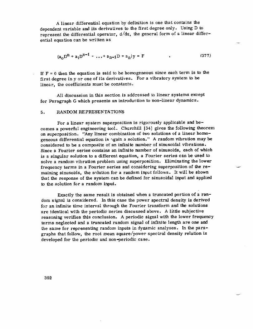
A linear differential equation by definition is one that contains the
dependent variable and its derivatives to the first degree only. Using D to
represent the differential operator, d/dx, the general form of a linear differ-
ential equation can be written as
(ao Dn + aiD n-I + ...+ an-lD * an)Y = F (377)
If F = 0 then the equation is said to be homogeneous since each term is to the
first degree in y or one of its derivatives. For a vibratory system to be
linear, the coefficients must be constants.
All discussion in this section is addressed to linear systems except
for Paragraph G which presents an introduction to non-linear dynamics.
5. RANDOM REPRESENTATIONS
For a linear system superposition is rigorously applicable and be-
comes a powerful engineering tool. Churchill [34] gives the following theorem
on superposition. "Any linear combination of two solutions of a linear homo-
geneous differential equation is again a solution." A random vibration may be
considered to be a composite of an infinite number of sinusoidal vibrations.Since a Fourier series contains an infinite number of sinusoids, each of which
is a singular solution to a different equation, a Fourier series can be used tosolve a random vibration problem using superposition. Eliminating the lower
frequency terms in a Fourier series and considering superposition of the re-
maining sinusoids, the solution for a random input follows. It will be shownthat the response of the system can be defined for sinusoidal input and applied
to the solution for a random input.
Exactly the same result is obtained when a truncated portion of a ran-
dom signal is considered. In this case the power spectral density is derived
for an infinite time interval through the Fourier transform and the solutions
are identical with the periodic series discussed above. A little subjective
reasoning verifies this conclusion. A periodic signal with the lower frequency
terms neglected and a truncated random signal of infinite length are one and
the same for representing random inputs in dynamic analyses. In the para-
graphs that follow, the root mean square/power spectral density relation is
developed for the periodic and non-periodic case.
392

Theperiodic andnon-periodic random solutions are also related to the
transient solution, because if the response of a linear system is known for one
input it is known for every input. Proof is shown through the transfer function
defined as the ratio of the Laplace transformed output to the Laplace trans-formed input. This is discussed in Paragraphs C.3 and H.2 of this section.
a. Periodic Functions
A random environment used for an analysis can be represented by aperiodic function if certain restrictions are observed. Since each term of a
Fourier series is periodic, the sum of these terms is also periodic. For
vibration analysis and data reduction the periodic character of the series can
be neglected provided the lower frequency terms in the series are edited out
of the analysis . In general, the error is reduced to negligible magnitude if
the first 20 frequencies are ignored. If the period under consideration is T
seconds, the first frequency is l/T Hz and the 20th frequency is 20/T Hz.
Suppose the lowest frequency of interest is 5 Hz; thus,
2Om = 5 T = 4 secondsT
If the lowest frequency of interest is 20 Hz, T can be 1 second.
In Reference 35 the development of this approach is covered in some
detail. When the Fourier series is equated to the Grms by squaring the
series, the following result is obtained
Grins Af
½
(378)
Grm s = acceleration root mean square
Zkf = frequency increment
an = coefficient of each term in the series
T = time interval
If Lkf---df the summation becomes an integral,
393

Grm s =I 1
f_ _.
f PSD df
fl(379)
PSD = power spectral density, g2/Hz" Thus, the PSD is related to the Grm s
for any frequency increment. The superposition principle permits solutions
to random input problems by considering the combined effect of sinusoids.
An analog spectrum analyzer performs an analysis in electrical units using
the above equation. Conversion to g's follows from the calibration.
b. Non-Pe riodic Functions
Exactly the same conclusion is reached by considering a truncated
random signal and using an autocorrelation function.
Suppose a single sample of random data is of duration T. The tem-
poral average is obtained by averaging with respect to time along the sample.
The temporal mean square is given by
T
1 2E ]< f,.(t)> = DT f f2 (t) dt . (380)
-T1l
2
Ifthe f(t) is defined for all time, then the above equation is evaluated by taking
the limit as T _ . For such a function, a temporal autoeorrelation function
is defined by
(T) = < f(t) f(t + T) >
T
2
=lim T f(t)f(t+ 7) dt
T -_ -T
2
(381)
394

Whenf(t) is only defined for a finite interval, a similar expression exists.The integral on the right side may be used without the limit as T--_ providedf(t) is defined from t1 = T/2 to t2 = T/2 + T. Such a finite average would most
often be used for incremental values of _"which are small compared to T. Thefunction _ (0) is just the temporal mean square.
Consider a stationary random process as given below on the interval
from ti to t2.
f(t)
! !
! I! IItl t2
t
If Tma x is defined to be t2 - tt, an autocorrelation value
E [x(ti) x (t2)]= R(r) (382)
results in a function of v when all values of _"are considered. A frequency dis-
tribution of R( ) can be stated by a standard transformation using the foUowingrelation:
R(_') = foo S(oj)eiW _. do.) . (383)--aO
The function S (w) has the form of the Fourier transform of R ().
iS(w) =_ f_°R(T) e-i°Jv dT . (384)
395

S(¢_] is a non-negative even function of w (symmetric about the ordinate).
Suppose thatt2 -- tI which means T--0. Then R(T) = R(0).
R(r) = R(o) = 2 S(w) d w . (385)
O
R(o) is the mean square of the process for itisthe sum over allfrequencies
ofS(w) d_. Therefore, S(w) may be thought of as a mean square spectral
density. Changing from a circular frequency to a linear frequency gives
R(o) = E {iX(t)] z}
= f_¢ W(f) df (386)O
where X(t) represents an acceleration process and W(f) has units of g2/Hz-
or power spectral density.
Looking at equation (381)
T
21
R(o) = lira _ f f2(t) dt (387)T --_¢ -T
2
This last relationship shows that to obtain a true mean square spectral density,
f(t) is averaged over a long time; also AW -* o as T -* _o.
In problems of interest, the power spectral density is not integrated
over all positive velues of frequencies because usually a finite range of
frequencies is all that is important. Therefore, the equation is normally used
in the form given below:
T
1 f2f W(f) df = lira _ f (t)
fl T-_ _ -_T2
dt . (388)
396
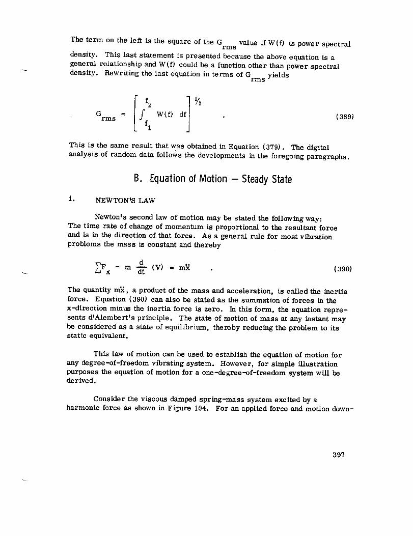
The term on the left is the square of the G value if W(f) is power spectralrmsdensity. This last statement is presentedbecausethe aboveequation is ageneral relationship andW(f) could be a function other than power spectral
density. Rewriting the last equation in terms of G yieldsrms
f2G = f W(f) df (389)
rms fl
This is the same result that was obtained in Equation (379). The digitalanalysis of random data follows the developments in the foregoing paragraphs.
B. Equationof Motion - SteadyState
i. NEWTON'S LAW
Newton's second law of motion may be stated the following way:
The time rate of change of momentum is proportional to the resultant force
and is in the direction of that force. As a general rule for most vibration
problems the mass is constant and thereby
d_Fx = m _ (V) = n_ . (390)
The quantity m_, a product of the mass and acceleration, is called the inertia
force. Equation (390) can also be stated as the summation of forces in the
x-direction minus the inertia force is zero. In this form, the equation repre-
sents d'Alembert's principle. The state of motion of mass at any instant may
be considered as a state of equilibrium, thereby reducing the problem to its
static equivalent.
This law of motion can be used to establish the equation of motion for
any degree-of-freedom vibrating system. However, for simple illustration
purposes the equation of motion for a one-degree-of-freedom system will bederived.
Consider the viscous damped spring-mass system excited by a
harmonic force as shown in Figure i04. For an applied force and motion down-
397

ward, the forces acting on the mass in the free-body sketch are shown in
Figure 104.
/////////. r//I///
FREE LENGTHOF SPRING
ST_,TICDEFLECTION
t I'. I-T$$T
+ X$
K(SST * X) CX
11!,,1"li
rng FoSlNWt
Figure 104. Gonerali_ed model: one-degree-of-freedom system.
Considering the motion in the x-direction, the equation of motion of
this system is
m_ = _ (Forces in x-Direction)
=mg + FoSinwt = k(SBT + x) - c_ . (391)
Before an excitation force is al_pLied to the mas_, the gravitational attraction
mg is equal to the static spring force kSST; therefore
m_ + ck + kx = F sin_t . (392)O
The general solution of the above second order linear differential equation is
the sum of the complementary function X (t) and the particular integral
X (t) ; that is, cP
X = X + X . {393)c p
398

DTA solution X = A
C esatisfies the corresponding homogeneous equation
m_ + cA - kx = 0 . (394)
Substituting D = dx/dt in the differential equation results in a simple quadraticwhich will, in general, be satisfied by two values of D,
1 (_c + jc2 _ 4krn) (395)Dls 2 - 2m
and the complementary equation consists of a linear combination of two
solutions, namely,
X c = al eDit + a2 eD2t (396)
where a 1 and a 2 are arbitrary constants depending on the initial conditions.
The complementary solution of a damped vibrating system describes
free motion if the damping is low enough to make D 1 and D 2 complex numbers.Critical damping is the value of "e" which separates the vibration and non-
vibrating system; that is, the radical of equation (395) will become zero.
Thus, the critical damping is expressed as
C = 2',]'--_ = 2mw . (397)C n
Damping of a vibrating system is often specified in terms of the ratio of
damping to the critical damping, expressed as e/c whereC
C Cm
c _ " (398)e
The ratio c/c c is more commonly referred to as the damping factor and is
given the symbol _.
The previous development describes a typical stable vibrating system
which occurs when the damping factor is positive. If the damping factor is
greater than one the values of D 1 and D 2 will be real, distinct and negative
because _2 _ 1 will be less than _. Thus, the complementary equation wouldbe
399

-D2tX = ale-DIt + a2e . (399)
C
No matter what the initial conditions are for this particular case there will
be no oscillatory motion. The motion, called aperiodic, will diminish exponen-
tially as time increases.
For the special case where _ = 1, both of the roots are negative and
are equal to -Wn, yielding the complementary equation
X = (a 1 + a2t)e-W tn (400)C
which is again aperiodic and will diminish exponentially with time.
If the damping factor, _, is less than one, the roots D 1 and D 2 will
be complex conjugates of the form and a vibration exists
where j = _ At this point it is convenient to define the term Wn _f_ _ _2.
Since _ is a ratio of damping coefficients, the term COnJl - _2 defines the
frequency of oscillation, COd' This frequency is less than the undamped
natural frequency of the system.
The complementary equation for a stablevibration system (0 < _ < 1)
can be expressed in a simpler form by using the frequency of oscillationCOdand Euler's formula
e _= i 0 = cos _ _- isin e
that is,
-_COnt {X = e (A 1 cos wdt + A2sinwdtlC
(402)
or
X = Ae-_Wntsin(COd t + qS)C
(403)
400

where A1, A2, qb and A are arbitrary constants determined from the initial
conditions. These constants are related by A = _] A12 + A22 and _ = tan -1
Ai/A 2. The complementary equation for _ less than one describes harmonic
motion and will diminish exponentially with time.
Since all the cases discussed have exponential decay, the motiondescribed by the complementary equation is classified as transient motion
except when _ = 0, then the amplitude will not diminish as time increases.
To determine the particular integral and complete the general solution,
a method called "Method of Undetermined Coefficients for Finding Particular
Integrals" can be used. The following rule is found in Reference 36. If f(t)
is a function for which repeated differentiation yields only a finite number of
independent derivatives, then, in general, a particular integral X can beP
found by assuming X to be an arbitrary linear combination of f (t) and all its
independent derivatives, substituting this expression into the differential
equation determining the arbitrary constants in X in such a way that the
resulting equation is identically satisfied.
Using the above rule a particular solution in the form
X = Acoswt + Bsinwt (4047
is substituted in the differential equation (392) yields
F
X = o sin (wt- 9)P _/(a)c) 2 + (k - _2m)2
Fo/k
4 (2 r,w/ 2n + [i- (cL)/C#n)2]2
sin - } (4O5)
The total solution is the stun of the complementary and particular solution.
In time the complementary solution vanishes and only the particular solution
remains for the steady state condition.
writtenThe radio X/X
Ois defined as the magnification factor K and is
401

X 1
K = _--- N/ (2 _ r) z + (1 -r2) 2 (406)O
where
r = the frequency ratio _/_n
Xo = Fo/K- o
The phase angle equation is
= tan -1 2___rr . (407)
.. ".
From studying the particular integral, the following conclusions canbe made:
a. The frequency of the response is the same as the excitation
frequency and the motion is harmonic. Therefore, this motion is called
steady-state motion.
b. The particular integral does not contain arbitrary constants.
Thus, the steady-state response is independent of the initial conditions.
c. As can be seen by the solution of the particular equation, the
steady-state response amplitude is a function of the frequency and amplitude
of the excitation. The ratio X/X is the magnification factor K.O
d. At resonance (_/w = 1) the damping factor _ alone limits then
amplitude of the system.
e. The response Xsin (wt - _ ) and the excitation F sinwt do notO
reach maximum values simultaneously. At resonance the phase angle equals
90 degrees. The phase angle varies with excitation frequency because of the
presence of the damping factor.
Figures 105 and 106 illustrate in a linear form, plots of the
magnification factor K and the phase angle _ as a function of the frequency
ratio r for various amounts of damping.
402

,7
180
Figure 105.
FREQUENCY RATIO r
Magnification factor versus frequency ratio.
0! I
FREQUENCY RATIO r3
Figure 106. Phase angle versus frequency ratio.
403

Frequently, this same information is presented in log-log form and
is commonly referred to as Bode plots. Figures 107 and 108 represent
examples of typical Bode plots.
Another useful plot for the same presentation is known as the Nyquist
plot, Figure 109. The length of the vector [X/X eC¢[ is the magnificationo
factor while the phase angle ¢ is the vector inclination with the real axis.
2. ENERGY EQUATIONS
Previously, a second order, nonhomogeneous, ordinary differential
equation of motion for a vibration system was derived and an algebraic solu-tion was obtained. Another method to obtain the differential equation for the
undamped free vibration is through the concept of total energy [37].
With an undamped free vibration system there is no forcing function
and no energy dissipation due to viscous damping. Therefore, the systemsenergy content will remain constant.
Conservation of energy requires that the sum of the potential and
kinetic energies be equal to a constant at all times for a conservative system.
The potential energy results from the strain energy of the spring neglecting
the mass of the spring and the kinetic energy is the energy resulting fromthe velocity of the mass.
Consider the undamped free vibration spring-mass system as shown
in Figure 110. Assume that the mass m is displaced from the static
equilibrium position in the positive x direction and then released. The
system's potential energy changes due to the displacement. This change
is equal to the change in strain energy in the spring minus the potential
energy of the mass when there is a change in elevation. Therefore, the
potential energy is defined by the term U and is expressed as
X
U = f (Total Spring Force) dx - mgx . (408)O
In Figure t10, g ving spring force versus spring deformation, the
potential energy is the cross-hatched area of the plot. The total spring force
is the sum of the static deflection plus the force due to displacement. Thus,
4O4

3.0
2.0
,,1¢
OI.-cJ<U.,
Z 1.00I--,<
u. 0.7Z
0.5
0.3
0.2 0.3 0.5 0.7 1 2
FREQUENCY RATIO, r
Figure 107. Bode plot (K versus r).
a
o
0.2 0.6 0.7 1 2 3FREQUEN_;¥ RATIO r
Figure 108. Bode plot (9 versus r).
3
405

UJ
..I
Z
uJ
<"1"Q.
120°
140°
160°
100°
t
0.5 0
90° 80°
II
60 o
t I
s.. /
0.5 1.0
MAGNIFICATION FACTOR
Figure 109. Nyquist plot.
FREE LENGTH
OF SPRING K
I.
0 °
STATICEQUILIBRIUM
0
+X
uJ(Jn-oU,.
_z
[mg
/
SPRINGDEFORMATION
Figure 110. Potential encrg)" i: a spring.
406

by subtracting out the term mgx, the net potential energy in the spring is
obtained. The evaluation of the integral is
X
U = f (mg + kx)dx - mgx0
(409)
Assuming that the mass of the spring is negligible when compared with the
block of mass m, the kinetic energy T is defined as
T = --1 mk 2 (410)2
Recalling that the total energy of the system was constant, the time derivative
of the total energy is zero.
T + U = Constant
d [T +U] d[1 1 kx2]d-'t" = d_" 2" m_2 + 2" = 0 . (411)
Since the velocity cannot be equal to zero for all time, the solution follows
from the discussion in Paragraph 1. of this subsection.
3. LAGRANGE 'S EQUATIONS
The equations of motion for a complex vibrating system can be derived
by utilizing Newton's laws as developed in Paragraph 2. of this subsection.
A more powerful tool for this type of analysis is the Lagrangian method.
The object of Lagrange's equations of motion is to express the
equations in terms of generalized coordinates and generalized forces. Thetransformation of Cartesian coordinates to a set of generalized coordinates
can be very involved. Also the forces used in Newton's laws are vector
quantities and are difficult to handle in complex systems. Thus, the
Lagrangian method permits the equations of motion to be derived using basic
energy expressions. Energy is a scalar quantity and can be expressed in
407

any convenient set of coordinates. Lagrange's equations will be derived using
the concepts of virtual displacements and d'Alembertts principle as developedin Reference 37.
It is necessary to set up a theory of generalized coordinates and
assuming that there are as many generalized coordinates as Cartesian coor o
dinates. Consider a dynamic system of p mass particles with n degrees of
freedom. Each particle m.1 will have the Cartesian coordinates xi, Yi' and
z i (i = 1, 2, .. . , p) and can be described by a set of generalized coordinates
(ql, q2, • .., q ) • The Cartesian coordinates can be expressed as functionsn
of the generalized coordinates. This reflects the general case in which
coordinate coupling exists, that is, the axes of the coordinate system are
nonorthogonal. Therefore, the Cartesian coordinates are related to the
generalized coordinates
x.1= x.1(ql,q2,...,qn)
Yi = Yi (ql, q2, ..., Cln)
z.1= z.1(ql, q_, .-., qn) • (413)
With a system of particles described by a set of generalized coor-
dinates, ql, q2, ..., an' the time derivative _1k of any coordinate qk will be
called the generalized velocity associated with this coordinate. The general-
ized velocity of the Cartesian coordinate x. is the corresponding component1
x. of the velocity of the ith particle located by this coordinate Extending1 °
the concept further the original velocity components xi' Yi' and _. of equationl
(413) can be expressed in terms of the generalized components and velocities
by differentiating equation (413).
_x. ax. 8x i _¢. dqn_.k =_ =__k_ dq_ + d__.+...+3t _ OqI dt aCl2 dt t)Cln dt
oyi oyi d%bYi _)Yi dqL + __ + ... +
Ot - Yi - 8(11 dt _c12 dt _qn dt
408
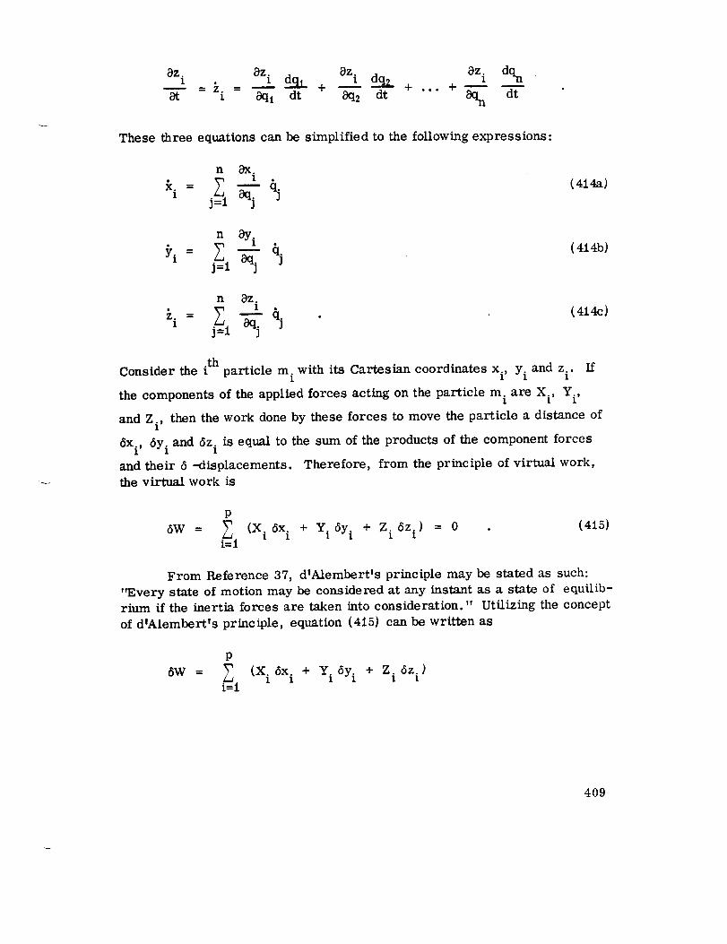
8z. az. 8z. 8z. dqn-- I dq2 + ... + 1i _._ I dql +__8t I 8ql dt 8q2 dt 8qn dt
These three equations can be simplified to the following expressions:
n Ox.
j=
(414a)
n _i
=j=i _ J
(414b)
n 8z.
_.= _ --£ _.i j=l OClj j
(414c)
.thConsider the i particle m. with its Cartesian coordinates x i, Yi and z.. If1 1
the components of the applied forces acting on the particle m. are X i, Yi'
and Z i, then the work done by these forces to move the particle a distance of
5xi, 5y i and 5z., is equal to the sum of the products of the component forces
and their 6 -displacements. Therefore, from the principle of virtual work,
the virtual work is
P
5W = _ (X.15x._ + Y.,Sy i + Z._Sz._) = 0 (4i5)i=l
From Reference 37, d'A/embert's principle may be stated as such:
'rEvery state of motion may be considered at any instantas a state of equilib-
rium ifthe inertiaforces are taken intoconsideration." Utilizingthe concept
of dIAlembert's principle, equation (415) can be written as
P
6W = _ (X.15xi + Y'lSyi + Z.iSz.t )i=l
4O9

P
mi (xi 5x.=1 1+ _}i 6Yi + "_'1 6z._ )
or
5WP
= _ (X. 5x.1 1
i=l+ Y'I 5Yi + ZiSz.)l
P
= _ mi (xi6x" + _ 6y i + "_. 6z.) = 0=1 * i i i
(416}
It is necessary to analyze each of the terms in equation (416). The first is
expressed in terms of Cartesian coordinates and is the work done by the
components of the applied forces. To express this form in terms of general-
ized coordinates the infinitesimal variations, 6xi, 6Yi, and 6z.1 must be evaluated.
This is accomplished by realizing that
n _x.
1 j=l_ _)qj -j
n _i
5Yi = j=l_' 0qZ 5qj (417b)
n _z.
5z" = _4 -_j5q'l j= J , (417c)
Substituting these equations into the first term of equation (416) yields
: xi % ÷i=i j= j=
+
n Oz. ]z . _ ---.!-I"1 Oq. oqj
j=l j
410

or
5W
n
-- 7,j=l
Qj 5qj (418)
where Q. is,3
p 0x. 0y i Oz.
= "= (X i 1 + Yi _qj + Z.1 1 ) (419)
The definition of Q. is called the generalized force corresponding to3
the generalized coordinate qi" In order to express the second term of equa-
tion (416) in generalized coordinates, it is necessary to first introduce the
kinetic energy function T as
1 P
T = _ _ m i (_¢iz +_/i 2 + Zi 2) . (420)i=l
Differentiating this equation with respect to xi' Yi' _'l and then with respect
to time and using these results in conjunction with equation (417), the second
term of equation (416) can be written as
_W
d 8zi 15q. . (421)
J
Equation (42t) can be simplified if the following relation is used for
x i and equivalent expressions for Yi and z._:
d (Yr _xi ) d 0(__ii)_xi 0T _ki
411
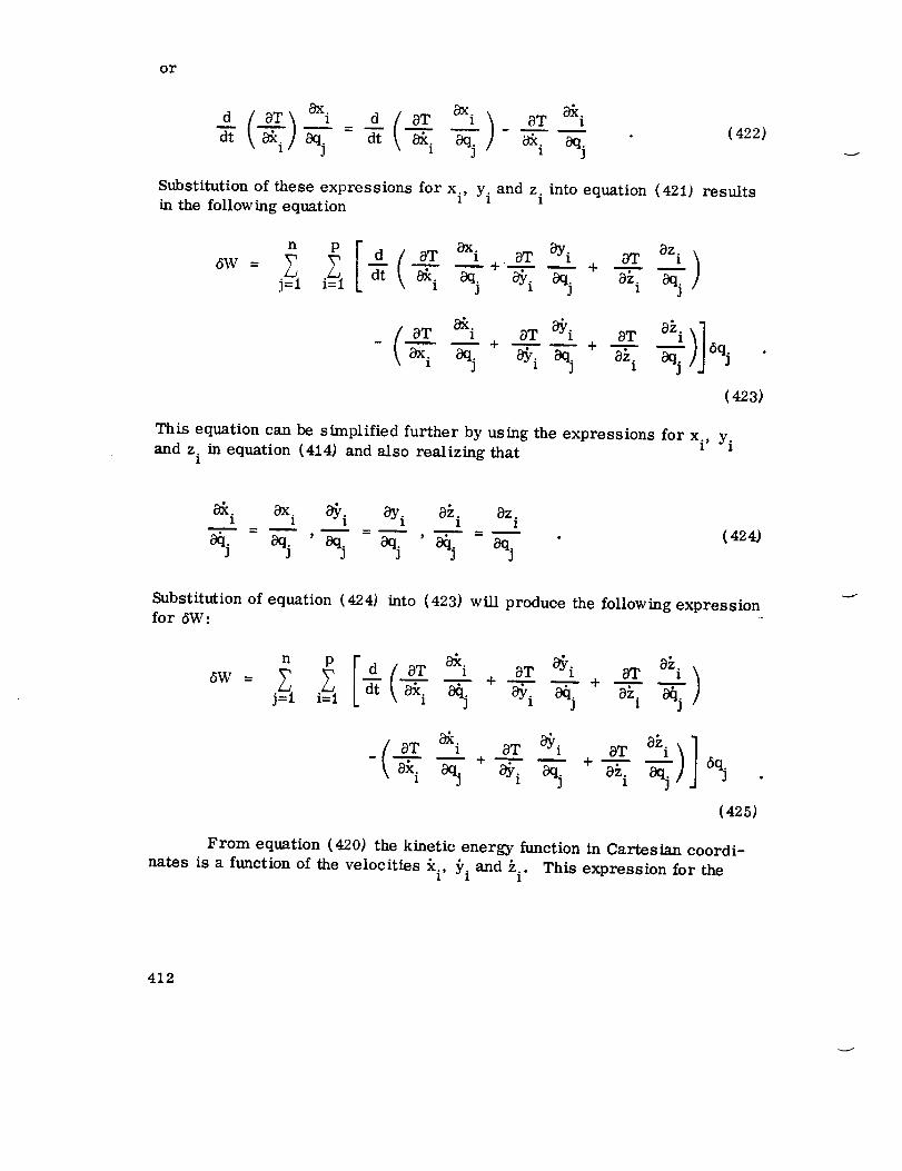
or
(422)
Substitution of these expressions for xi, Yi and z.t into equation (421) resultsin the following equation
6W =
j= "= 1 ] 1
f a..__T --_i + 0T _i aT azi)]
(423)
This equation can be simplified further by using the expressions for xi, Yiand z. in equation (414) and also realizing that
1
_. a_. _i aYi a_. az.1 l I 1
(424)
Substitution of equation (424) into (423) will produce the following expression
for 5W:
5Wn p [ d ( _r _. -. O_zi a_i )= "_ a_. + _i + a_. _jj= i= 1 t
1 _r aT 6¢_a_. + +, % % _j
( 425)
From equation (420) the kinetic energy function in Cartesian coordi-
nates is a function of the velocities xi' Yi and _.. This expression for the1
412

kinetic energy can be differentiated with respect to _ti and qi' and after
comparing the results of this operation with equation (425), it can be seen
that
_w= y, -a %j=l
(426)
Previously, an expression for 6W was derived as a function of a
generalized force Qj. This expression, equation (418), when equated with
equation (426) yields the following equations of motion commonly referred to
as Lagrange's equations.
0T (427)
At this point it is necessary to discuss the generalized force in
more detail. For a complex vibrating system the generalized force can
consist of three distinct forces:
a. An applied force that is applied externally to the system
b. A spring force because of a change in potential energy of the
system
c. A damping force which is due to the dissipation of energy in a
damper.
The potential energy of a system is a function of the generalized
coordinates as shown in the equation
1 n p
u = _ Z F_ % qi%i=l j=l
and if this equation is differentiated with respect to qigives the generalized spring force
n
_ bU = _ _, kij q.QJ = % i=l J
(428)
the following expression
(429)
413

The dissipationfunction D can be analogous with the potentialenergy
function defined as
1 n p
D = _ _1 _ cijcti_tj . (430)i= j=l
When this function is differentiated with respect to qj the generalized forcefor the dissipation function is
n
8I:) = - V (431)
Now it can be seen that the generalized force for a complex vibrating
system is comprised of three distinct forces. Thus, Lagrange's equations of
motion can be expressed in a more general form and is given below
d aT 8T aD bU
dt _lj % + _ + % - Qj (432)
The subscripts j = 1, 2, ..., n are the number of generalized coordinates of
the system, and Qj is the applied force for each generalized coordinate.
Whenever the system is conservative and since the potential energy function
is a function only of the generalized coordinates, equation (432) Can bewritten
d aL _L- 0 (432a)
where L = T-U and is known as the Lagrangian operator.
• The primary advantage of Lagrange's equations is that the equations
represent a uniform way of writing the equations of motion of a system and
these equations are independent of the coordinate system used.
4. INFLUENCE COEFFICIENTS
In the preceding paragraphs, Newton's second law of motion and
energy relationships were used to derive the equations of motion for a
414

vibrating structure. Another commonly used and very convenient approach
for systemswith many degrees of freedom is the method of influence coeffi-
cients. The equations of motion may be written in terms of influence coeffi-cients and solved to obtain numerical values for natural frequencies and mode
shapes. This method is an application of the Lagrangian use of generalized
coordinates and is widely used for the analysis of complex structures.
The method of influence coefficients is based upon linearity. The
"inertia force" associated with the vibratory motion of each element of mass
causes a certain motion at all other mass elements in the system. Then
the deflection at each mass element is the sum of the effects from all the
inertia forces. This effect is described by an array of numbers called
influence coefficients.
An influence coefficient, denoted (2ij' is a parameter having the
dimension of compliance or reciprocal of stiffness. It is defined as the static
deflection of a system at position i due to a unit force applied at position j
when the unit force is the only force acting. Hence the influence coefficient
is a measure of the elastic properties of a system. Influence coefficients are
conveniently used to keep account of all the induced deflections due to various
applied forces and to set up the differential equations of motion for the system.
The values of the influence coefficients are obtained for a given sys-
tem by applying a unit static load at point j and finding the resulting deflection
in the direction of the load at point i. The deflections, and therefore influence
coefficients, are obtained using the methods of static analysis (see examples
in Section XIV. B. 5). For a system with n degrees of freedom, the numberof influence coefficients will be n2. However, only n (n + 1)/2 will have
different values, because of reciprocity, (2.. = (2... Reciprocity is based on_j jt
the face that the strain energy or stored work in an elastic system is the samefor both cases. As an illustration of reciprocity, consider the simply sup-
ported beam shown in Figure ill in which two vertical forces F 1 and F 2 are
applied at positions 1 and 2.
The influence coefficients for this illustration are (211, (212 and (221.
The deflection at position 1 due to the force F 2 applied at position 2 is F 2 (212.
Extending this concept the deflections at points 1 and 2 of the system due to
the applied loads F 1 and F 2 are written in terms of influence coefficients as
xl = (211FI + (212 F2
x2 = (221F1 + (222 F2 • (433)
415

F1 F2
11 2
F2
°12F 2
Figure 111. Simply supported beam with two loads.
For proof of reciprocity consider that the procedure of loading is
separated into two steps. First, when F 1 is applied alone, the potential
energy in the beam is 1/2 F12 _11. When F2 is then applied, the additional
deflection at position 1 due to the force F 2 is F 2 czi2. The work done by F1
corresponding to this deflection is FI(F 2 _12) • The total potential energyin the system is then
I 1U = _- Fi2 _il + FI(F2 _12) + _ F22 o_22 • (434)
The last two terms of this equation represent the additional potential energywhich is due to the application of F 2.
Second, when the force F_ is applied to station 2 and then the force
F 1 is applied to station 1; the total potential energy of the system is
i iU = _- F22o_22 + F2(F I c_2_) + _ FI2 o_II . (435)
The last two terms of this equation are due to the application of F I.
Since the totalenergy and the product F i F 2 is the same, 0/12 must
equal (_21and reciprocity is proven for this simple case. Note than c_lldoes
not equal c_22because F i does not equal F 2 in the general case.
While the previous illustration is based on static forces acting on a
weightless beam, it should be realized that the reasoning applies equally
416

well to any linear spring type system, and the forces could be inertia loads
developed by point masses.
Using influence coefficients, the equations for a linear system with
dynamic loads can now be written. Assuming a harmonic motion
x. = x. Sinwtj jo
and
X. = -X. ¢02 Sin oJtJ ]0
a set of algebraic equations can be written for a system of n elements of mass.
2 2 2x I = all (m 1 ¢o x 1) + o_12 (m 2 ¢o x 2) + ... + '_ln (mn ¢o Xn )
2 2 2x2 = _21 (ml co x 1) + ot22 (m 2 co x 2) + "'" + ff2n (mn co Xn)
(436)
2 2 2Xn = _nl (mr w x i) + Otn2 (m 2 w x2) + ... + O_nn (mn w Xn)
Dividing through the above equations by _2 and collecting the coefficients of
the variables xi, the set of equations may be rearranged as follows:
11 ml - w-'2" Xl + (_v12m2)x2 + "'" + (°tlnmn) Xn = 0
( i)(a21ml) xl + '_22 m2 - _ x2 + "'" + (_2nmn) Xn = 0
( 437)
417
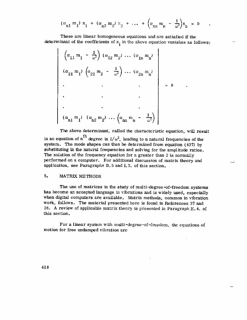
• .° m - X n(C_nl ml)xl + (t_n2 m2)x2 + + (_nn n w-_ = 0
These are linear homogeneous equations and are satisfied if the
determinant of the coefficients of x. in the above equation vanishes as follows:1
( 1)allm 1 - w--_ (o_12m 2) ... (O_lnmn)
(_21ml) 22 m2 - _ ... (O_2nmn)
m -(anl ml) (an2 m2) "'" ann n
= 0
The above determinant, called the characteristic equation, will result
in an equation of n th degree in 1/w 2, leading to n natural frequencies of the
system. The mode shapes can then be determined from equation (437) by
substituting in the natural frequencies and solving for the amplitude ratios.
The solution of the frequency equation for n greater than 2 is normally
performed on a computer. For additional discussion of matrix theory andapplication, see Paragraphs B. 5 and I. 3. of this section.
5, MATRIX ME THODS
The use of matrices in the study of multi-degree-of-freedom systems
has become an accepted language in vibrations and is widely used, especially
when digital computers are available. Matrix methods, common in vibration
work, follows• The material presented here is found in References 37 and
38. A review of applicable matrix theory is presented in Paragraph H. 4. ofthis section.
For a linear system with multi-degree-of-freedom, the equations of
motion for free undamped vibration are
418

mll ql + mi2 q2 + ''° + mln qn + kll ql + k12 q2 + "'" + kln qn = 0
m21"ql + m22q2 + "'" + m2n'qn + k21ql + k22q2 + "'" + k2nqn = 0
mnlql + mn2q2 + "'" + mnn}:]n + knl ql + kn2q2 + "'" + krmqn =0
where
m = generallzea massnn
qn = generalized coordinate
k = stiffness coefficientnn
These equations can be written more concisely in matrix notations as
M(}_) + K(q) = (0) (438)
where
M
l l
mll m12 ... mln
m21 m22 ... m2n
mnl mn2 --- mnnm
Z __
i i
kli k12 ..- kln
k21 k22 -.. k2n
k I kn2 -.. krmj
and
m --
ql
q2
(q} = .
%m --
419

{q} is called the coordinate vector, M = [mij] is called the mass matrix,
and K = [kij] is called the stiffness matrix.
More generally, a linear system with applied excitation can be
described by a matrix equation of the form
M_) + C (¢1) + K (q) = <Q) (439)
where (Q) are the generalized forces corresponding to the generalized coor-
dinates (q), and [C] is the viscous damping matrix of the same order as
[M] and [K].
The above equation applies to all linear constant parameter vibratory
systems, and the specifications of any particular system are contained in thecoefficient matrices [M], [C] and [K]. The type of excitation is described
by the column matrix {Q). The individual terms in the coefficient matrices
have the following significance:
mii is the momentum component at i due to a unit velocity at j
c.. is the damping force at i due to a unit velocity at jlj
k.. is the elastic force at i due to a unit displacement at j.1j
In certain applications it is more convenient to deal with [K] -1, the
inverse of the stiffness matrix, than with [K]. The elements of [K] -1' _ij'
will then represent a unit displacement at i due to a unit force applied at j
and are seen to be the influence coefficients discussed in the previous section.
[K]-1 itself is sometimes called the flexibility matrix.
The previous general discussion applied to a n-degree-of-freedom
system expressed in terms of the generalized coordinates. As an example,
a two-degree-of-freedom system described in terms of the more familiar
displacement coordinates will be presented. The differential equation, in
matrix format, is written as
[m]{R} + [c]{_¢} + [k]{x} = {f(tj}
For natural frequency determination Cl, c2, fl(t) and f2(t) all must be set
equal to zero. The solution, assumed to be sinusoidal, expressed in matrix
format, is
420

ixix2[ala2 (440)
Since sinw t is not always zeron
-Wn2[M] + [K]) (a) = (O) . (441)
For a practical vibration, the amplitudes al, a 2 cannot be zero and the
remaining quantity (-o9 2 [M] + [K]) must be zero. Expanding into determi-nant form n
(k l + k 2 - w 2mr ) _k 2n
_k2 (k 2 _ o9 2 m2 )n
= 0 (442)
and into algebraic form
ml m2 o9 4 _ (k 2ml + klm2 + k2m2 ) w 2 + klk2 = 0 . (443)n n
This is a quadratic in o9 2 and can be solved by the quadratic formulan
to yield the two natural frequencies which are the positive values.
The values o9 2 are termed the eigenvalues (particular values) of then
-1matrix [M K] which is called the dynamic matrix. This can be seen if
equation (441) is put in the form of an eigenvalue equation obtained by writingequation (439) in the form
o9 2[M] (a} = [K] (a} (444)n
-!and multiplying both sides by [M] to obtain
[M -1 K] (a} = o9 2 (a} . (445)n
This is the usual form for an eigenvalue equation with o9 2 representing then
eigenvalues and {a} representing the eigenvectors corresponding to the mode
shapes.
421

An iteration technique is sometimes used to determine the eigen-
values. When using the iteration technique, equation (441) is written in
still another form obtained by a technique similar to equation (445).
tK -1 M] (a} = X{a} (446)
where
1A =--_
o_n
The technique of iteration utilizes an initial estimate for the mode
shape of vibration. The matrix equation is then expanded. The resultingcolumn is now normalized; i.e., reducing one of the amplitudes to unity by
dividing each term of the column by the particular amplitude. The process
is then repeated with the normalized column as the new estimate until the
amplitudes for the first mode converge to a value of acceptable accuracy.The fundamental frequency can then be found directly from the matrix
equation. For the next higher mode shapes and natural frequencies, the
orthorgunality principle (Paragraph H. 5 of this section) is used to obtain a
new matrix equation that is free from any lower modes. The iterative
procedure is then repeated.
6. COORDINATE COUPLING
Coordinate coupling occurs when a force is transmitted by spring
or dashpot to more than one coordinate of the system. In other words, the
displacement of one mass will be felt by another mass in the same system
through the coupled elements.
There are two types of coupling action, generally referred to as
stiffness coupling due to static displacements and mass coupling due to inertia
forces. These two types of coupling will be discussed by the following
example.
A two-degree-of-freedom system is shown in Figure 112 and consists
of a mass m and two springs of stiffness k 1 and k 2. Any two independent
coordinates, such as x and _ from any origin, can be used to specify the
configuration of the system.
Considering Figure 112 with coordinates (x, _ ) and assuming small
oscillations, the equations of motion are
422

STATIC COUPLING
Figure i12. Two-degree-of-freedom system.
m_ + (k 1 + k2)x - (kll I -k212)q) = 0 (447)
J'_ ÷ (kI112 + k2122)@ - (kIf! - k212) x = 0
Each of the above equations contain terms of both x and _ and aretherefore interdependent on each other. The motions of the mass will be
independent of each other only if the coupling term (k 1 11 - k2 12) is eqt_al
to zero; i.e., the center of gravity is located so that k 1 I l = k 2 12. O<' _vise,the resultant motion of the mass will consist of both rectilinear and _:ttional
components when either a displacement or torque is applied thro, the centerof gravity of the body as an initial condition.
In the example described in Figure 112, the origir was chosen to
correspond with the center of gravity of the mass m. It Lhe origin werechosen at any other location, mass terms as a function of both coordinates
will appear in the equations and the system would then be mass coupled in
addition to stiffness coupled.
The terms uncoupled modes and coupled modes often appear in vibration
terminology. These terms are used in reference to coupled systems. Some-
times in analysis or test the system is artificially constrained to make one or
more of the coordinates zero, resulting in an uncoupled mode. While the
uncoupled mode is of interest particularly in understanding the dynamics of
the system, the uncoupled and coupled modes are not the same.
423

7. PLATES
The bending properties of a plate depend to a large extent on its
thickness as compared with its other dimensions. Timoshenko [39 ] uses
thickness to classify plates into three types:
a. Thin plates with small deflections.
b. Thin plates with large deflections.
c. Thick plates.
The assumptions, or a statement of second order terms neglected, are made
during the analysis for each of the classes of plates. In this paragraph, a
simple example of the first class from Reference 39 is discussed.
Consider a plate of uniform thickness h bounded by a constraint on
two edges and free on two edges and take the x-y plane as the middle plane
of the plate before loading. Let the y axis coincide with one of the longitudinal
edges of the plate and the z axis be downward as shown in Figure 113.
I_Z
1 =! X
NIT LENGTH
1 1 _"'_I__ DEFLECTION W IN THE + Z DIRECTION
Figure 113. Thin plate with small deflection.
If the width of the strip is 1 and the depth is h, then the strip may be assumed
to De a bar of rectangular cross section of length 1 and depth h. It is
assumed that the cross sections of the bar remain plane during bending and
only a rotation with respect to their neutral axes is considered. If no normal
forces are applied to the end sections of the bar, the neutral surface of the
424

bar coincides with the middle surface of the plate, and the unit elongation of
a fiber parallel to the x axis is proportional to its distance z measured fromthe middle surface.
The deflection curve is given by -d_V/dx 2, where W is the deflection
of the bar in the z direction and is assumed to be small compared with the
length of the bar 1. The unit elongation of a fiber at a distance z from the
middle surface is denoted by _ and is given byX
d2We = -z (448)x -&-r
as shown in Figure l14a.
G¥
_Yx
a b
Figure 114. Plate element free body.
Applying Hooke's law, the unit elongations e and e in terms of thex y
normal stresses cr and a acting on the shaded element in Figure l14b arex y
given by
1
% = E [% " "_J
1
•y = _ [_y - _1
(449)
where E is the modulus of elasticity and v is Poisson's ratio. Since the
lateral strain is zero, the second equation therefore gives
425

£ = 0Y
O" = l) O"y x
and
1e =- - (1-v27
x E x(450)
For the stress
(x E (4517x - 1-7- .
If the plate were subjected to either tensile or compressive forces
acting in the x.direction and uniformly distributed along the longitudinal sides
of the plate, the direct stress would have to be added to the stress due to
bending.
The bending moment in the strip is obtained by direct integration.
h
f_ Eh 3 d2WM = ax z dz = - 12(1_v27 -_ • (452)h
2
Let
Eh 3D -
12(1-vz7
Then the equation for the deflection curve of the elemental strip is given by
d2W (4537D "_x = -M
The flexural rigidity of the plate D is the quantity that replaces the term E1
in the differential equation for beams.
Therefore, the deflection of the plate depends on an integration of
equation (453). The solution of the problem includes the definition of the
426

boundary. The boundary may be simply supported (free to rotate), constrained
(not free to rotate) or somewhere in between.
If the boundary is constrained on all four sides, the curvature equation
assumes a more complex form and axial stress must be considered. For
circular plates, polar coordinates are used. More details on these problemsare found in the references.
C. Equations of Motion - Transients
In the previous paragraphs, the response of a system to a sinusoidal
input or combinations of sinusoidal imputs was developed. An input consist-
ing of one or more sinusoids or a truncated random disturbance of infinite
length is classified as steady state. In this paragraph, the equations of
motion are developed for a transient input. A definition of a transient isdifficult to state. One definition of a transient can be formulated from the
discussion in Paragraph A. 5.2 of this section. In Paragraph A. 5.2 of this
section, the time period of the disturbance T was assumed to be infinite for
the steady state input. If the time T cannot be assumed to be infinite, the
input is a transient. Thus, for a transient, the exact time of initiation and
cessation of the disturbance is pertinent to the response.
The response to transients is represented by an expression called in
the literature as the faltung Duhamel, or convolution integral. This integral
can be developed directly from the equation of motion or by superposition.
Both methods of development will be presented.
1. DUHAMEL INTEGRAL -- EQUATIONS OF MOTION
The derivation which follows is performed for a single degree-of-
freedom system with damping. Consider the equation of equilibrium as
discussed in Paragraph B. 1 of this section with a forcing function F.
m_ + c_ + kx = F
where the initial conditions are x = :_ = 0 when t = 0 and the force F begins to
act.
With these initialconditions, the solutionto thisequation is
F _o t wnx = -_ I- c _ sinqt + cos qt (454)
427

where
n
and
k c 2 J c 2nO
If the force is withdrawn after an instant of time, St, the response
will be the sum of the expression above and a similar expression where the
force is negative and applied at t = 6t. The effect of these two forces is the
same as F 1 acting during the interval where 0 -_ t -_ 6t. The first term in
each equation cancels each other and the remaining terms take a functionalform of
x = fit) - f[t + (-6t)] (455)
Using the Taylor's series expansion for this form of the expression for x and
neglecting higher orders of 5t yields
d f(t) 5t (456)x= d_
Substituting in equation (454), x as the function of t, provides the responseequation
= -0_ Cx FiSt e n-- t sin qt (457)mq c
O
The above expression describes the response at time t resulting from a singleforce applied at t = 0 and removed at t + St. It the force is applied at t = T,
the response at t becomes
C-_ -- it-r)
X _ e n C= o sin q (t-r) . (458)mq
By allowing F16t to approach F (r)dT and integrating the above expression
results in one form of Duhamel's integral
t
= f F(T) h (t-T) dTX
O
(459)
where F(_) is the forcing expression and h(t-r) contains all the system
parameters. The above expression can be integrated by parts
428

t tit IE lx = h(t-_) f _(r) dr - f f _(r) dr d h(t-_)o o 0
Suppose the integral part, iF(r) dr, is defined as zero for all time
of the integration interval except a small increment from -c to _. Supposealso the value of the integral is one when integrated between -_ and c.
E
f F(r)dr = 1 (460)-E
where E is a very small quantity. Equation (460) defines an impulse. Usingthis specialized force the response becomes
t
x = h(t-r) - f dh(t-r) (461)0
The second term is zero since h(t--r) is a step function. The response is
h(t-t) for the specific system considered which is nothing more than the
motion of a single degree-of-freedom system with damping. It is shown
in Reference 34 that the same result is obtained for a system of multipledegrees of freedom.
If the force is not a single impulse but a general shape that can be
constructed from a set of impulses, general shape is represented by anintegration of the first term of equation (4617.
t
x(t) = f F(r) h(t-r) dro
(462)
Equation (462) is the common form of the transient integral. Negativetime is not considered.
2. DUHAMEL'S INTEGRAL -- SUPERPOSITION
Exactly the same result is obtained by superposition and direct
reasoning. This is the derivation most often presented in text books. An
individual forcing element is considered to be an impulse as defined above
E
f _(r)dr = i (463)-E
429

The complete force can be considered a superposition of impulses and in an
interval of time
F(T) = 23 5(T)A_" . (464)
Let h(t-r) be the response of the system to a single impulse. The response
to a force F iv) contains a number of impulses, each is acting on the system
at a different time.
x(t) = 23 5(T) h(t--r)AT (465)
or in the limit
t
x(t)= f F(T)h(t--r)dr . (4667O
This equation is identical to the previously derived expression and also
represents the response at t for a force operating on the system in an inter-
val of time represented by a function of v.
3. TI:tANSIENT/STEADY STATE RELATIONSHIP
The response of a linear constant parameter system for any input
was derived in Paragraph C.1 of this section, and resulting in equation (4667,
the Duhamel equation
t
x(t) = / F(r) h(t-r) dr . (467)O
An alternate and interchangeable form of equation (467) can be written with
the time delay associated with the forcing term in the integral. Equation(467) then becomes
t
x(t) = f F(t-r) h(v) d_- . (468)O
The forcing function is then established to be an exponential steady state
input of the form
430
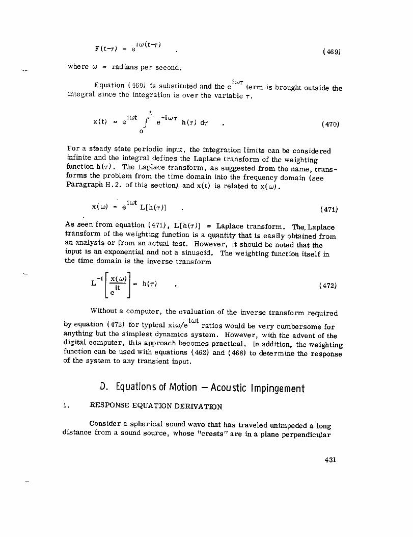
i_(t-r)F(t--r) = e (469)
where w = radians per second.
i_rrEquation (469) is substituted and the e term is brought outside the
integral since the integration is over the variable v.
tiwt -i_-
x(t) = e f e h(T) dr . (470)O
For a steady state periodic input, the integration limits can be considered
infinite and the integral defines the Laplace transform of the weighting
function h(_-). The Laplace transform, as suggested from the name, trans-
forms the problem from the time domain into the frequency domain (see
Paragraph H. 2. of this section) and x(t) is related to x(w).
iwtx(_o) = e L[h(r)] (471)
As seen from equation (471), L[h(_)] = Laplace transform. The. Laplace
transform of the weighting function is a quantity that is easily obtained from
an analysis or from an actual test. However, it should be noted that the
input is an exponential and not a sinusoid. The weighting function itself inthe time domain is the inverse transform
L = h(_') . (472)
Without a computer, the evaluation of the inverse transform required
by equation (472) for typical xic_/e iwt ratios would be very cumbersome for
anything but the simplest dynamics system. However, with the advent of the
digital computer, this approach becomes practical. In addition, the weighting
function can be used with equations (462) and (468) to determine the response
of the system to any transient input.
D. Equations of Motion - Acoustic Impingement
1. RESPONSE EQUATION DERIVATION
Consider a spherical sound wave that has traveled unimpeded a long
distance from a sound source, whose "crests" are in a plane perpendicular
431

to the direction of propagation. Such waves represent the simplest three-
dimensional wave and may be expressed in the form
f(r - ct) (473}
where
r = radial distance from the source = (x 2 + y2
c = velocity of the propagated wavet = time .
A simplification of the more general case is obtained when a plane
wave is considered. For this special case the fronts are always perpendicular
to the x-axis, and the one dimensional wave is of the form
f(x - ct) (474)
The parameters describing this wave at some point in time and distance from
the source are expressed by
_x
where
5 = change in density
= displacement
This equation satisfies the requirement of conservation of matter. The chauge
in density is equal to the rate of change of displacement a_/ax. From the
thermodynamic gas laws relating the change in pressure to the change in
density
P = Tc Po _ (476)
where
P = pressure
c = specificheat (i.40 for air)
Po = atmospheric pressure
and for equilibrium
432

where
az_ au aP
P _ = P at - ax (477)
p = mass density
u = velocity
which provides the net force (Sp/Dx) acting on the medium in terms of massand its acceleration.
Combining equations (475), (476), and (477), expressions for _,
p, 5 and the change in temperature A T in a plane sound wave are obtained.
a2_ t a2_= c--T _ (478a)
O2P 1 82p
= c--y- -7 (478b)
a26 1 025= 7" (478c)
where
and
p = p ,ye6 = ,oe2 a..._o o_
Now
Po _" T . (479)
433

The displacement, density, and pressure are parameters of the same wave
with a velocity c. For the purpose of illustration, the parameters can be
considered three separate waves propagating without change of shape and
with a velocity c. The three waves are not independent, but are related by
equilibrium, continuity, and thermodynamics through the equations above.
If the particle velocity is known, density and pressure can be determined.
The average energy of a volume of gas due to passage of a plane waveis
w = _ _ fff + c 2 dx dydz ergs (480)
For a simple harmonic wave of frequency w this equation can be expressed
in terms of pressure P alone
w = _ fff + p2 dx dydz (481)
The rate at which the energy is being transmitted along the wave per
square centimeter of wavefront is called the intensity I of the sound wave.
This will equal the excess pressure P on the square centimeter, multiplied
by the velocity of the gas particle
(__) a_ Olj rgs/sec/cm 2 482)p =_pc2 _ _" e (
If the wave is a simple harmonic function; i.e.,
f(x-ct) = Pcos (¢ot-kx) (483)
where
P = maximum pressure
= angular frequency
k = wave number defined by a spatialperiod 2 Ir/kor I (commonly
referred to as wave length).
The expressions for pressure, energy, and intensity follow the sign conven-
tion of a wave moving to the right, having a maximum pressure P+
434

p_ = p+ i(wt-kx) (484a)
_-_ = A _ti(c°t-kx) (484b)
O_ U_. i(wt-kx)"_" = (484c)
whe re
K - 2___f A+ = - , U+ -- C ' pc
Now
p+2 l
W+ - 2p'_ = _" p U+2 (485b)
p+2 1
I = 2pc 2 pc U+ 2 (485c1
For an example, consider a wave moving from the right and impinging
on an interface or rigid surface and assume the angle of incidence is perpen-
dicular to the surface. The total pressure developed on the surface is the
superposition of the incident wave and the reflected wave designated by P-.
p = p+ i(¢ot+kx) + p__i(wt+kx) (486)
and
_"0_ l= P--C" _ E p- Ei(wt-kx)- p_i(wt+k,x)J (487a)
i
W = 2_ (p+2 + p_2) (487b)
I = I (p+2 + p_2) (487c)2pc
435

In practical acoustic impingement problems, the medium dynamics
couples with the surface dynamics to form a very complex system. Because
of the complexity of this acoustic and structural dynamics, the analysis is
often augmented by empirical data.
2. PANEL RESPONSE TO RANDOM ACOUSTIC NOISE
In Paragraph 1. of this subsection, the basic acoustic impingement
equations were presented. The summary of that paragraph was that the
basic equations are often modified by empirical data. In this paragraph
additional analysis procedures are presented. These equations contain terms
that are more accurately evaluated by experiment.
Equations for the net vibration response at any point in a panel
structure can be written from the cumulative effect of all of the oscillatory
forces acting on the panel. Forces applied at discrete points induce local
vibrations at the points of application. These local vibrations are trans-
mitted along structural paths and are superimposed on other vibrations in
accordance with their relative amplitudes and phases. Looking at the panel
response problem in this manner, it is convenient to employ the space-time
correlation functions, since these functions include phase relationships.
Consider the panel structure shown in Figure 115.
of point j due to a pressure at i is
t
5!i) (t) = A. fo Pi (v) h (i) (t-v) d,] z j
The deflection
(488)
Figure 115. Panel structure.
436

The deflection at j dueto a pressure at k is
t )
6! k) (t) = A k fo Pk iv) h (k) it-r)dr (489)J j
where h symbolizes the weighting function.
Equations (488) and (489) are applications of the Duhamel integral.
The cross correlation, or measure of phase, between these two componentsof deflections at j is
1 T (i) .(k)
r_T'(6jik)(0) = Tlimit--_ -_-- fo 6.j (t) Oj (t+0) dt (490)
where 0 is the time lag.
If the variables are changed by letting
E 1 = t-r ¢2 = t+0-r = t' = r
de 1 =-dr d_2=-dr
the responses become
co
8! i) (t) : A. f Pi (t-_l) h!i) (El) dE1 (491)J I_c o J
( (k)5. k) (t+0) : A k Pk (t-E2+0) _ (e2) dE2 (492)J -co
and the cross correlation for components of deflection at j due to pressuresat i and k becomes
R(Lk) (0) = AiAk f'=fX (O-62+el) h!i)(61)hj (k)(e')deldea ' (493)6j =_ -=_ )'kk J
437

The total deflection at j is
n (i)5.(t) = V 5 (t)
} i=l 3(494)
After a time lag,O, the totaldeflectionis
n
"' 5!k)5j (t-o) = ._I¢=1 J
(t-O) (495)
h_ order to obtain the power spectral densiW function, the autocorrelation
function for deflection at j is first written
(e) -- zRS.k
(t,-O) (496)
where RSj (0) = autocorrelation function. Referring to Paragraph A. 5.b.
of this sec tion, the power spectral densi_' is directly written
+5 (:,:)__1f_ rts.(O)e-j -_ j
_0dO
1 -= n n (ik) e-iX8:-/ vvR (o) dO-_ i k J
n n
vvl, _ f= _(ik)i k -co J
(O)e -i_O dO
where ¢5. (w) = power spectral density. This latter expression can be1
extended by a summation on the cross power spectral densit3, function to
include all inputs
no ik)5. (_) -- v ,.v , (_)3 i k 3
(498)
43_

It is now required to express the cross spectral density function in terms ofthe structure. This may bedoneas follows:
5. (¢o) - _ R (0)e dO (499a)j -¢o j
4_(ik) (co) : AiA k f_ R (0-e2+_l) e -k°(0-e2+ei) dO (499b)aj -co Pik
el) e-i°'le' del f_h! k) (e2) e-iU'_2de2J
where Ai, A k = areas at i and k. The first integral of Equation (499b) is the( i) *(i)
power spectral density, H: represents the second equation, and H. (w)J J
represnets the last integral. Or
#! i.k) (co) = AiA k _ (co) _I i) (co) H(k) (co) (500)8j Pik J "
Now substituting for @_.ik)(w),J
n n
i(ik) (o_) = _ Z AIA k _ (o0) I_li)(w) tI (k)(w) (501)8. " Pik J "j i k
The deflection power spectrum at j is stated in Equation (501). The
summation of the product of these areas over which the pressures act, the
power spectrum of those pressures and the weighting functions represent all
input sources. Expressing the power spectral density functions for deflectionin matrix form:
(502)
(taxi) ( xn) (.xn)
439

where
andT indicates the transpose. The areas and pressure power spectra are
measurable or calculable. The impulse responses of deflection can be obtained
as follows. Assume there are 5. degrees of freedom. The equations of1
motion can then be written as
(_x_) (r_)
Talcing Laplace transforms
+ (Kik)(Si)= IF(t)]. (503)
(v)(5i )]
(v)
-1 (v)(504)
where
v = any point
S = Laplace variable.
The Laplace transforms of the responses to unit impulses at each mode are
440

The complex frequency responsematrices are obtainedby
or
-1
This can be carried further, if desired, to forces in the structure and to
stresses. For example:
{r } = [Kik ](6 i }
and
(f} = [D]{F} = [b] [Kik] {6i}
The power spectra of stress then are
(_f(c0)} = [b][Kik][Hlk)(c0,]
[ Kik]T T
[b]
[Ai ] [4_ ]Pik
f = stress
b = factor converting deflection to stress
k = deflection times stiffness.
where
(506)
(507)
(508)
(509)
The pressure power spectra can be calculated.
virtual work done on a panel by the acoustic pressure field is
Consider the following: The
(t) (51o)ab
r_ = ff p(x,y,t)_ *mn(X, y) 6qmno o m n
441

where
x, y = coordinates
q = generalized deflection.
The generalized force in the mn mode is
a(5_} a b
Qmn(t) -- a(8_) -- fofo P(_' y' t) _n_ (x, y) d_dy. (511)
By definition, the cross correlation of the generalized forces in two pairs of
modes (mn and rs) is
T1
RQ (T) = lim _-" f Qmn (t) Qrs (t+T) dt (512)mn T -_ Trs
T[a, ]lim _2T f ff p(x' y, t) _mn(X' y) dxdy
T-_ T o o
/? p(x 1, t+r)(x 1, yl)dx dy|
1Yl,
OO ]dt.
Rearranging,
l_Qmnrs
(_) ,ab[T l= ffff lira _ f p(x,y,t) p(Xl, yi, t+r) dt2T
oooo T-.co T
(_,y)Inn rs
(xl, Yi) dx dx 1 dy dy i
(5i3)
442

where a and b are dimension limits of the panel. The cross power spectrum
of the generalized force is then
oo
= _ f RQmn -iwt!_) 1 (r)e d7 . (514)
Qmn _ -_rs rs
Equation (502) is the basic equation for calculating panel response.
This response is in ten]is of power spectral density. The weighting functions
are obtained from equation (506). These weighting functions can be computed
from laboratory measurements. The areas are easily obtained and the power
spectra of the pressures are an input.
E. Application and Examples - Direct Steady State Forcing
1. LUMPED PARAMETER SYSTEMS
The analysis of a structure necessitates the selection of an idealized
moclel of the structure. Most often this idealization consists of lumping the
mass into discrete points and considering the remainder of the system
weightless springs. The constructed model should have dynamic characteris-
tics similar to the system under analysis.
Several limped pa1,'ameter analysis methods are available. One
method, influence coefficients, was presented in some detail in Paragraph
B.4. of this section. Other methods will be only briefly discussed in this
paragraph since these methods are often discussed in detail in the common
texts on vibration. These methods are:
a. Stodola.
b. Rayleigh or energs'.
c. Holzer and Myldestad.
a. Stodola Method
The Stodola method was originally developed to determine the lateral
vibrations of turbine rotors, but can be extended as a method of obtaining
either the bending or torsional natural frequencies an(I modes of nontufiform
vibrating beams.
443

The Stodola method initially assumes a mode shape usually based
upon static deflection. Starting with the inertial loading of the system,
successive integrations produce the deflection of the beam due to dynamic
loading. The process essentially consists of solving equation (394) by trialand without damping. An iteration or two utilizing previously calculated
deflections as the assumed deflection converges to a constant ratio of the
assumed deflections to the calculated deflections. The natural frequency of
the first mode is found by multiplying the initially assumed frequency by theaverage of the ratios of the mass element deflections.
Consider a beam at any time t, the inertia loading is proportional to
mass, frequency squared and the deflection curve y(x). If a deflection curve
y(x) is artitrarily chosen and w arbitrarily set equal to unity, then a deflec-
tion curve can be determined by using the equivalent static load. Starting
with the beam loading, successive integrations give the shear, bending
moment, slope and deflection. The result will be gi{x), a new deflection
curve. Using yl(x) as a deflection curve, the process of successive integra-
tion is repeated and another deflection curve, y3(x), is obtained. The
operation is repeated until two successively determined deflection curves are
of constant ratio to each other at each point on the beam. The final curve
represents the fundamental mode of the beam.
b. Rayleigh Method
In Paragraph B. 2. of this section, the energy of a vibrating system
was discussed. The energy method is combined with the procedure of succes-
sive iterations to form the Rayleigh method. In this respect the Rayleighmethod is similar to the Stodola method.
If a beam is represented by a series of lumped masses Wl/g , W_/g,
W_/g...Wn/g , and the system is considered to be conservative or undamped,
the maximum strain energy can be determined from the work done by these
loads. The first approximations are provided by determining the static
deflections Yl, Y2, Y3 • • • Yn and applying the deflections to the energy equations.
For a lumped mass system
n W.
= _, 1 i w2y 2 Kinetic energy (515a)Tmax _=1 2 g i
444

n1
Umax = 1_=_1_ Wi YiPotential energy, (515b)
By equating equations (515a) and (515b), the frequency isestablished as
2o3
n
Wi Yi=1g
n,)
Wi Yi_I= I
(516)
w he re
W = lumped massesn
Yn = deflection at each mass.
The deflection can be determined for the first approximation by any one of
several strength of materials methods. A second set of deflections is obtained
from the resulting frequency, w. The iterations are then continued until the
desired accuracy is obtained.
c. Holzer Method
Holzer's method can be used to calculate higher modes inaddition to
the fundamental mode. In thisoutline of the Holzer method, a torsional model
will be used.
Consider a vibration system represented by a series of disks connected
by shafts of stiffness Kl, K2, K 3 ... K n and vibrating with frequency w. The
external torque required to maintain the vibration is zero at all system naturalfrequencies. The external torque required will not be zero for frequencies
other than the natural frequencies. The amplitude of a disk is assumed to
remain constant while an external torque is computed. If the external torque
required to excite a system is plotted as a function of frequency, a natural
mode will be identified at every point on the plot where the curve crosses theabscissa.
445

The Holzer methodcanbe applied to bothbendingand torsional modesolutions; however, it is primarily usedto solve torsional modeproblemsdue to the laborious calculations required for bendingmode solutions.
Myklestad Method
The Myklestad method is similar to ihe Holzer method in that a trial
frequency must be assumed and, after including the mass and stiffness of the
beam or shaft, a residual function results. This residual function may be a
slope or bending moment. After two or more iterations a curve of the residual
function, similar to the torque remainder curve of the Holzer method is plotted
against the assumed frequency. The zero points of this function identify the
natural frequencies of the system.
The procedure is more involved than the Holzer method because the
assumed frequency must satisfy the four boundary conditions of bending
moment, shear, slope, and deflection. For any assumed frequency, wn, the
bending moment and displacement diagrams can be constructed to satify three
of the four boundary conditions. By plotting the fourth boundary condition
against w, the natural frequency, Wn, will occur when this remainder equalszero.
2. DISTRIBUTED PARAMETER SYSTEMS
Examples of mechanical systems that have their masses and elastic
forces distributed are cables, rods, beams, plates, shells, menbranes, etc.
Distributed systems have an infinite number of degrees of freedom and
natural frequencies. Each natural frequency has an unique mode shape, whichis known as its characteristic function or normal function. A transient or
steady state forced vibration generally will excite many or all of these fre-
quencies in combination. The net response of a particular point is the combinedeffect of all modes.
The differential equation for the transverse vibration of beams is derived
as follows. Consider a beam of uniform section, weight and stiffness as shown
in Figure 116. From Figure 116,
dV = -f(x)
dMu _ V
dx
446
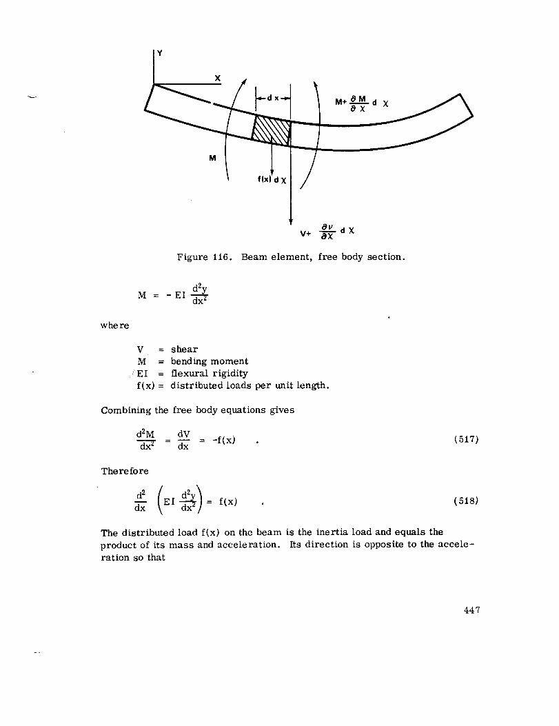
w he re
Y
X
M _ TIX! d X
Figure 116.
M = -EI d_x
_U
v+ -_-- d X
Beam element, free body section.
V = shear
M = bending moment
_EI = fiexural rigidity
f(x) = distributed loads per unit length.
Combining the free body equations gives
Therefore
- -f(x)
_xx EI = f(x)
The distributed load f(x) on the beam is the inertia load and equals the
product of its mass and acceleration.
ration so that
(517)
(518)
Its direction is opposite to the accele-
447

Wf(x) =
g a_. • (519)
If the beam vibrates harmonically and the acceleration is 092y, then the
distributed load f(x) becomes
f(x) _ w w2y . (520)g
Thus, the differential equation for a distributed parameter beam is
dd_X w 09 2g EI Y = 0
From differential equations a solution of the type
y = X(x) T(t) (522)
can be assumed. Substituting this equation into the fourth order differential
equation gives the result
x1V(x) W T1V(t; 2
X(x) gEI T(t)
where k is a constant. Thus, two linear homogeneous differential equationsare obtained
xlV(x) + k 2 X(x) = 0 (524)
TiV(t) + X2 gEI T(t) = 0 (525)W
The general solution of equation (523) is
X = Cle xx + C2e -Ax + Cse i_x + C4e -ixx (526)
and expressed in terms of trigonometric functions is
X = B lcoshAx + B 2 sinhXx + B_coskx + B 4sinkx (527)
448

The values of the constants can be determined for any given type of beam
from the boundary conditions. For a deflected beam y is the deflection, dy/dx
is the slope, d2y/dx 2 is a function of the bending moment, and d3y/dx 3 is the
shear function. The end boundary conditions depend on the type of supports
that are used for the beam. The four main categories of end boundary condi-
tions are pinned, clamped, sliding and free.
An illustration of the determination of natural frequencies and mode
shapes of a uniform beam follows. Assume a beam of length L and pinned
at both ends. The boundary conditions for a pinned end beam are: When
x= 0orx= L, theny= 0andd2y/dx 2 = 0. For the assumed solution to
satisfy these conditions, it is necessary that XT vanish when x = 0 or x = L
for all t and that T' (0) = 0, where T' (0) is the initial velocity of any point
along the length of the beam. Since the beam is at rest, initially, T'(0) must
be zero. Substituting these conditions into equation (527) gives
B1 +B3= 0
B 1 = B 3
Therefore, B 1 and B 3 are zero and
X = B 2 sinh/x + B 4 sinXx
For the other boundary condition y -- o when x = L and d2y/dx 2 = 0
the results are as follows:
X = 0 = B 2 s inhkL + B 4 s inXL
X" = 0 = B 2k 2 sinhkx - B_A 2 sinkx
Thus,
B 2 sinhkL = 0
B 4 sinhXL = 0 .
Since sinh_.L cannot equal zero, B 2 must equal zero. Since the deflection of
the beam is always zero when x = L, any values of XL whose sine equals zero
will satisfy the equation. Therefore, the equation
B 4 sinlL = 0
449

is satisfied when L = N since B 4 cannot always be zero. The letter N is
the m nber oJ the natural frequency or mode shape. Now X can be evaluatedto be }, = :/L, and the first part of the assmned solution will be
STr
X(x) = B 4sin _ x (528)
Solving equation (525) by similar means and using the value of _ itcan be shown that the second part of equation (522) is
T = C cosN2r 2 Ew_LIt (529)
This gives the general solution as
N_rx _EIcosN2_ 2 ]- __- ty = B N sin L _4wL _(530)
The value of BN is the maximum displacement or the amplitude of the free
vibration. It is dependent upon the initial conditions of displacement andvel oc ity.
A similar analysis can be made on other types of beams if the end
boundary conditions are known. The boundary conditions can be found inmany vibration text books.
. EXPERIMENTAL DETERMINATION OF SYSTEM PARAMETERSFOR THIN WALLED CYLINDERS
Under MSFC research contracts, analytic and experimental work was
performed on thin walled cylinders with and without attached weights. Detail
results of this work are described in References 40, 41, 42, and 43. In thisparagraph a summary of the results are presented.
The program was directed toward the development of methods to
predict dynamic responses of a pressurized-ring and stringer-stiffened
cylinder to which concentrated mass items are attached. This type of struc-
ture is typical of a launch vehicle which is exposed to mechanical and acousti-
cal random vibrations. The program combined analytical and empirical
methods to predict frequencies and mode shapes of simple cases then contin-
ued to more complex structures.
450

In order to makea realistic analysis, experiments were conductedto determine the significant parameters contributing to the dynamic responseof pressurized stiffened cylinders with and without attachedconcentratedmass. Someof the dynamic properties determined from experiments aresummarized below.
a. The structural dampingof the cylinder measured from test data
was found to be low (generally less than one percent of critical).
b. The dynamic response of the unweighted pressure stiffened
cylinder consisted of many non-sinusoidal circumferential waves involvingthe stringers and several lonitudinal waves with modes at the frames. The
stringers did not greatly influence modes at the higher modes.
c. As the magnitude of attached weights was increased, the modal
response became increasingly localized. Treating the stiffened cylinder
with an attached mass as a single-degree-of-freedom system, a simple
empirical method was devised to calculate the fundamental frequency f.
1 /K(386.4)f = 2"_ _/_ +W
e a
(531)
where
W = added weighta
W = ef_ctive cylinder weighte
K = spring constant
All parameters were empirically determined [40 ]. This empirical
formulation is satisfactory in making a first estimate of the fundamental
frequency. However, the model is considered incomplete and attempts to
apply this formula outside the limited range of structural parameters from
which they were derived is not recommended.
a. Anal_ical Methods and Assumptions
A more complete analytical method was developed to predict mode
shapes and resonant frequencies of pressurized cylinders with ring frames,
stringers, and attached mass. The analysis was substantiated by tests and
supported by empirical data.
451
Twoapproacheswere usedto analyze the cylinder [43]. Oneapproachconsiders the stringers as discrete elements (discrete analysis) supporting
the shell and the other assumed the stringer spread uniformly over the surface
to produce an orthotropic shell. The dynamic analysis of the ring and stringer
stiffened pressurized cylinder was based upon the energy method using
Lagragne's equation (Paragraph B. 3. of this section).
d<0T) 0 (532)
where
T = potential energy of the system
U = kinetic energy of the system
q = generalized coordinates
i = 1, 2, 3 .
From an assumed vibratory motion of the structure, the potential
and kinetic energy excursions from the initial pressurized state were
determined for the cylinder with no attached weight. The potential energy
of the system is the integrated strain energy of the shell, stringers, and
rings. The total kinetic energ_ is the integrated kinetic energy of the shell,stringers, and rings.
The frequencies and mode shapes of cylinders with an attached weight,
_W, were determined by accounting for the potential and kinetic energy of
the added weight for each mode, combining with the potential and kinetic
energies for orthogonal modes of the cylinder and applying the results to
Lagrange's equation. The displacements of the attached weight were
expressed in terms of the generalized model function at the point of attach-
ment. The assumed mode shapes were of the form
P = q(1) coskB cosklxkl
V _(2) sinkB sinklx= qkl
W _(3) cosk8 sinklx= qkl
452

where
(i) = generalized coordinate (function of time only)qkl
i = i, 2, 3
k and I = circumferential and longitudinal wave numbers, respectively.
Figure 117 illustrates the cylinder geometric and displacement field.
-_ L _-----RING FRAME SPACING
F /-/r
I IX
NOTE:
CYLINDRICAL COORDINATE q_axCORRESPONDING DISPLACEMENTSRADIUS a = CONSTANT
v_/J
Figure 117. Cylinder geometry and displacement field.
For the actual analysis, assumptions were required. Classification
of these assumptions led to two types of analyses: discrete and orthotropic.
t. Discrete Analysis
For the discrete analysis, the energy due to the stringers are summed
with the skin energ-y. Specific assumptions for this analysis include:
453

a. The shells are considered thin and Love-type strain-displacement
relationships with Donnell large deflection terms are used to account for non-
linear effects due to pressurization.
b. The nonlinear effects caused by pressurization arise from an
axisymmetric staticstress statewithin the cylinder (i.e., membrane
stresses developed in the skin}. The effectsof pressurization adequately
included without considering localized bending due to rings, end fixity,or
stringers.
c. The ring frames are considered sufficiently rigid such that their
potential energy is negligible in comparison to the stringer and shell potential
energies.
d. The frequencies for unweighted, stiffened cylinders can be
predicted by employing the mode shapes of unstiffened cylinders with
Rayle igh-Ritz energy methods.
e. The resulting eigenvalue equations may be linearized while
still retaining nonlinear effects.
2. Orthotropic Analysis
For the orthotropic analysis, the mass and stiffness of the stringer
and the skin are combined to form an orthotropic shell. The orthotropic
shell is then treated as a single thickness cylinder. Two additional assump-
tions are required for the orthotropic analysis:
a. The stringers are sufficiently small and closely spaced such that
their stretching and bending stiffnesses and mass contribution can be
"smeared out" uniformly (with the skins) around the cylinder.
b. The nonlinear effects caused by pressurization can be obtained
from the axisymmetric static stress state of the combined stringer and the
shell idealizations. This assumption replaces the second assumption listed
under discrete analysis.
Using either the discrete or orthotropic analysis, the kinetic and
potential energies are idealized and the summations of the energy terms are
applied to Lagrange's equation (Paragraph B.3. of this section). The
resulting equation in matrix form is
454

where
2
C(533)
O3C
= the resonance of the cylinder coupled with the attached
we ight
= the diagonal dynamic matrix associated with the
cylinder structure
= the matrix associated with the attached weight
= the generalized normal coordinates
o mjo3j2 o]=
the product of the diagonal dynamic matrix and the theigenvalue o3.2 for the unweighted cylinder for each j
]mode or jth 1, k combination.
For the unweighted cylinder, eigenvalues, o32, and eigenvectors, q(i), were
first determined for various values of 1 and k. M. and AM were titan corn-]
puted and inserted into equation (533). The n by n system of algebraic
equations, represented by equation (533), was solved for the coupled eigen-
values, Wc2, and the eigenvectors, qj (3), using a computerized iteration
scheme [ 42].
In the following paragraphs, comparisons are made of analytical and
experimental results. The conditions under which the analytical assumptions
are valid are discussed for both the discrete and orthotropic approach. For
cylinders having a large attached weight compated with the cylinder stiffness
on improved analysis, see Paragraph E.3.c. of this section.
455

Test methodsand the approachto testing usedfor theseanalysesare presented in the references. The following paragraphs present discus-sions of the results of the tests and analytical work for dynamic response
of cylinders with stringers and attached weights, response of cylinders todiscrete frequency mechanical excitation and response of cylinders to
acoustic excitation.
b. Effect of Stringers and Attached Weight
The dynamic response analysis of a stiffened, pressurized cylinder
with attached concentrated weights using Lagrangian energy methods, gave
satisfactory results when applied to cylinders with many stiff stringers.
This method also gave satisfactory results when applied to stringerless
cylinders and cylinders with rings but without stringers, the analysis loses
accuracy as the attached weight increases. The large discrepancy in pre-
dicted frequency and mode shape due to heavy weights was attributed to the
slow convergence of the trial modes used to represent the sharply cusped
response of the cylinder in the immediate vicinity of the weight. The fre-
quency calculations for the unstiffened cylinder appear highly sensitive to
small discrepancies in the longitudinal mode shape. Agreement of experi-
mental and theoretical natural frequency was poor for the fundamental fre-
quency, but good at the higher modes. This was attributed to the sensitivity
of fundamental frequency to small changes in added weights which strongly
effects the local mode shape.
For cylinders with stringers, the increased stiffness somewhat
reduced the large error in predicting the longitudinal mode shape especiallyin the localized area near the added weight. Thus, the assumed mode shapes
appear satisfactory for stringer stiffened cylinders even with the heavier
attached weight. Trial mode shape functions with more rapid decay in the
longitudinal direction may improve predictions for the unstiffened cylinder.
Test results on the cylinder with only ring frames confirmed that the
rings were sufficiently rigid to contain the responses within the bay that
was dynamically excited. Therefore, isolating a single bay between rings
(assumption c) and performing the analysis as a ringless cylinder of shorter
length was justified.
From the discrete stringer analysis the unweighted cylinder had the
fundamental frequency occurring at k = 12 circumferential full waves, with
antinodes at each stringer. The orthotropic analysis did not show this.
Other than the fundamental resonance there seemed to be little relation
between the number of shell stringers and k, the number of circumferential
w ave s.
456

The results of a parametric study demonstrated the importance of a
discrete analysis when few _tringers are present in the structure. The
simpler orthotropic analysis was satisfactory only when a "sufficient"
number of stringers were employed in the stiffened cylinder. It is difficult
to define what a "sufficient" number of stringers is because it depends on
the stiffness ratio of stringer to shell, spacing, and other factors. The
substitution of the simpler orthotropic model for the discrete stringer-sheUidealization must be made with caution.
c. Improved Analysis
In order to improve the accuracy of the analysis technique, another
analysis [41 ] was developed to predict the dynamic response of a ring
stiffened pressurized cylinder with attached concentrated weight but with
no stringers. This improved analysis was directed toward reducing the
large error in predicting the highly cusped localized response of stringerless
cylinders in the vicinity of the attached weight.
This analysis employes a variational technique and the principle of
minimum potential energy to form the equations of motion and boundary
conditions. Love's first approximation and DonneU type nonlinear termswere assumed for the strain-displacement relations.
A computer program [43], based upon the improved analysis, is
presently capable of computing the resonant frequencies of pressurized
cylinders with ring frames and attached mass. Mode shape prediction, also
a part of the program, has not yet been completed. Analytical and experi-
mental fundamental resonant frequency results show good agreement for
all weights considered and for mid bay and quarter bay attachment pointsbetween ring frames. Satisfactory predictions require a Fourier seriesorder of truncation N* = 75.
d. Response to Discrete Frequency Mechanical Excitation
An analysis was developed [41 ] to express the steady state response
of a cylinder shell to applied external sinusoidal forcing functions using the
method of normal modes and energy methods. The derivation considered an
unloaded cylindrical shell with damping and was extended to include the
effects of added concentrated weights. This analysis was used to predict
driving point and transfer mobilities versus frequency.
457

Driving point mobilities showed faircorrelation with experimental
results at frequencies below the above resonance. Transfer mobility corre-
lated poorly with experimental values. Since only the fundamental mode
shape value of the transfer point was considered, knowledge of the shell
modes in the vicinityof the resonant frequency of the weight may be required
in order to improve the accuracy of the transfer mobility prediction.
e. Respone to Acoustic Excitation
The response analysis of a cylindricalshell for an acoustical
pressure environment should include an area integrationof the pressure over
the surface of the shell, as well as an integrationof the pressure over a
frequency spectrum, ifthe acoustical environment is random. However,
the testprogram has shown thatwhen the shell isloaded with a relatively
heavy discrete weight, the primary resonance is characteristic of a single-
degree-of-freedom system. Only the shell surface in the vicinity of the
mass has any appreciable responses. Therefore, an approximate analytical
estimation of the response of a shell with a discrete mass to acoustic pres-
sure excitation may be obtained by considering only a small shell surface in
the vicinity of the mass. It appears that if the shell is excited acoustically
within this small shell area, the response of the mass at its resonant fre-
quency should not differ markedly from that obtained in an acoustic environ-
ment encompassing the entire shell. An analysis was developed [41 ] to
estimate the velocity response of the discrete mass to acoustic noise,
channeled within a square area that includes the mass.
i. Discrete Frequency Acoustic Excitation
Acoustic tests were conducted [41 ] using discrete frequency acoustic
noise, directed at 232.25 cm 2 (36 in.2) area containing a concentrated weight.
Correlation of predicted results was fairconsidering the accuracy of mea-
sured data and the difference between the assumed pointloading on the
weight and the distributed (pressure) loading over an area. Also, the
analysis assumes that the weight responds as a single-degree-of-freedom
system and coupling of higher frequency modes are negligible. Part of the
difference between experimental and analytical results may be attributed to
these higher frequency modes.
2. Random Acoustic Excitation
i
The response of the cylinder excited by a reverberant random
acoustic excitationwas predicted [41 ] based upon a transfer function obtained
from the discrete frequency acoustic tests.
458

The predicted rms response of the weight was 0.19 G as com-rms
pared to the experimental value of 0.64 Grm s. The disagreement between
the experimental and predicted response may be attributed to the followingfactors:
a. The prediction of the response of the weight was based on the
assumption that the transfer function obtained from the sinusoidal acoustic
test was an estimate of the transfer function. This is predicted on the
assumption of linearity of the steady state response of the weight to a sinu-soidal pressure excitation of the cylindrical shell; i.e., that the ratio of
g/psi is constant for any amplitude of pressure excitation. However, the shell
characteristics may be such that a nonlinear relationship exists between the
acceleration _'esponse and the acoustic pressure excitation, resulting in a
departure from the transfer function used in the analysis. It was alsoassumed that the transfer function obtained from the channeled sinusoidal
acoustic horn test is an approximation to the transfer function of the weight
excited by random acoustic environment encompassing the entire shell.
While this is predominantly the case, it is to be expected that with more
of the shell surface exposed to the acoustic environment (either random or
sinusoidal), additional shell modes may affect the acceleration response of
weight to the acoustic pressure environment.
b. The data used in the analysis were accurate to within -_2 Hz on
the frequency scale and to within 4-10 percent on the response scale, A
shift in the noise by 1.5 Hz resulted in the predicted rms acceleration response
of the weight from 0.19 g's (rms) to 0.31 G compared to an experimentalvalue of 0.64 G rms
rms'
The utilization of the experimental transfer function obtained from thechanneled sinusoidal acoustic noise in the reverberation chamber test did
result in a prediction within a factor of two to four of the experimental rms
response of the weight. (Recent studies of transfer functions obtained fromacoustic test chambers indicate a variation due to the mode of testing; i.e.,
reverberant, free field, or progressive wave.)
f. C onclus ions
Analytical and experimental studies summarized in these paragraphsand described in References 40 through 44, provide useful background on the
understanding of the dynamic response of stiffened cylinders with attached
weights. Analytical methods were developed to predict mode shapes and
459

natural frequencies. Experiments were addressedto the verification ofsystem parameters used in the analysis.
1 EXPERIMENTAL DETERMINATION OF LOCAL STRUCTURE TO
BE USED IN LABORATORY TESTING
The presentation in Paragraph 3. above covered the response of
complete cylinders to acoustic impingement. The test cylinders were
designed as research specimens to help identify the pertinent parametersrequired for analysis. In this paragraph structural approaches more typical
of a large space vehicle are discussed. Both the segment approach and
the model approach are presented.
Like the previous paragraph, this paragraph presents a summary of
work performed under MSFC contracts. Detail reports of this work are in
References 45 through 48.
Critical components, mounted to the shell structures of the present-
day launch vehicles, are subjected to high vibration and acoustic environ-
ments during boost and atmospheric flight. Vibration testing is essential
in establishing confidence in the successful operation of the components
under these extreme environments. It would be economically advantageous
to be able to vibration test these components using representative shell
segments instead of testing large portions of the vehicle. An important
aspect of any test requirement is to simulate the localized dynamic charac-
teristicsof the segment and the components. The purpose of this program
was to investigate the feasibility of the segment test approach and to
develop techniques in design and testing of shell segments (with mounted
components) from typical large structures.
To evaluate the feasibility of the segment testing approach, analytical
and experimental studies were performed on flexibly supported fiat paltes,
models of complete shells of revolution, model segmented shells, a full-
scale shell of revolution and a full scale segment. Structures from the
Saturn V launch vehicle were used in this study. Model shells include the
following portions of the Saturn V launch vehicle:
a. Instrument Unit.
b. S-II thrust cone structure and forward skirt.
c. S-IC oxidizer tank upper bulkhead.
460

A rectangular plate is usedto analytically andexperimentally studythe effects of various boundaryand restraint conditions on dynamic response.Completemodel shells were usedto study dynamic responsesandto esti-mate the "_undary conditions for their segznents. Model segmentsare usedto verify design of the boundaryrestraints. Model results are correlatedwith data from full-scale tests on the complete cylindrical section and seg-ments of the Instrument Unit.
a. Plate BoundaryRestraint Study
The effects of boundaryconditions on a test structure were investigated
[45 ] by studying dynamic response of a rectangular plate with various condi-
tions of free edges and elastic point supports. This investigation also serves
as a starting point for developing analyses for a segmented shell with point
supports and concentrated weight attachments.
The finite difference method was used to solve the vibration problem
of a flexible-point-supported plate. The plate was considered to have spring
supports at discrete points along the edge of the plate. These supports were
assumed to have spring and viscous damping restraint against deflection, but
no restraint against rotation (no bending moment). To determine the natural
frequencies and the corresponding mode shapes, loading was considered as
inertial loading of the plate. Provisions can be made for additional loading
due to concentrated mass attached to the plate.
The finite difference method transforms the partial differential
equation and boundary conditions into a finite difference equation in terms
of normal displacement at selected grid points. Additional grid points were
used beyond the plate boundary. The problem was reduced to eigenvalue
matrix formulation and the numerical solution of the final matrix equation
yielded the modal and frequency data of the rectangular plate. The computer
programs for the solution of the plate analysis are given in Reference 45.
A 50.8 x 60.96 x 0. 317 cm (20 by 24 by 1/8 inch) rectangular alumi-
num plate, flexibly supported at discrete points, was tested to determine its
natural frequencies and corresponding mode shapes. The supports had
restraints against normal deflection but not against rotation. The spring
stiffnesses and locations were varied to determine their effect upon response.
The plate was mechanically excited.
461

It was found that the wave patterns and resonant frequencies of a
plate which is continuously supported along its edges could be approximated
for some modes by using discrete point supports.
Although the behavior of the plate close to the edges was unpredictable
in many cases, the behavior in the interior of the plate was, in general,
predictable. The detail test results, given in Reference 45, strongly suggest
the desirability to use the finite difference method to analyze flexibly
supported rectangular plates and segmented shells. Also, simulating contin-
uous boundary conditions of segmented shells with the more practical dis-
crete point supports is justified.
b. Shell Dynamic Analysis
To investigatethe overall shell dynamic behavior prior to segmenta-
tion, four scale models were fabricated based on various parts of Saturn V
structures. Duplicate models were made for segmentation purposes. The
scale models which were manufactured and tested are listedbelow:
a. Instrument Unit, 1.6.67 scale.
b. S-II thrust cone including simulated rocket engines, 1:10 scale.
c. S-II forward skirt including LOX tank upper bulkhead, 1:10 scale.
d. S-IC LOX tank upper bulkhead including partial cylindrical shell
structure, 1:10 scale.
The detail technique in scale model design is described in Section V of
Reference 46. Structural details and experimental data on the models are
given in Reference 45.
Analytical and experimental programs were conducted to determine
the vibration and dynamic response behavior of the shell structures. In the
analytical phase, partial differential equations were established along the
shell meridian. The dependent variables include three displacement compon-
ents, the angle of rotation and the four shell internal stress components in the
same directions as the four displacement variables.
The stress variables are the transverse shear, the membrane stresses
and the meridian bending moment. For each circumferential harmonic num-
ber, the equations were solved numerically to yield proper modal and frequency
462

data. The dynamic effects of the stringers and the ring stiffeners were
handled differently. For the stringers which were located along the shell
meridians, their stiffness was averaged and merged with the shell to form
a mean stiffness. For the ring stiffeners, the dynamic impedances were
formulated individually. The impedances were represented in terms of the
increments of the shell internal stresses as functions of the local displace-
ments. These increments were introduced into the differential equations at
the ring stiffener locations during numerical integration. The computer
program to execute the integration and typical modal and frequency data for
shell structure models are presented in Reference 47.
In the experimental phase, the complete model sections, with and
without mass attachments, were subjected to the same external discrete
frequency forcing function. The resonant frequencies, mode shapes of the
basic structure and acceleration measurements of the lumped masses simu-
lating the shell components were recorded. For each point of mass attach-
ment, a measurement of mechanical point impedance was made over the
frequency range of interest for use in verification of dynamic similarity of
partitioned models. The strain response along lines of planned segmentation
were determined using the analytical program. This provided information
necessary to define the edge reactions of segmented structures.
As would be expected, the natural frequencies for the loaded shell
models were shifted to lower values as compared to the unloaded models. In
many cases the general patterns of both the response and impedance plots
were essentially unchanged in the frequency range of up to 500 Hz except for
the frequency shift. At higher frequency the attached mass appears to
suppress the response.
A comparison of experimental results with analytical prediction is
not made in Reference 45. Perhaps this comparison is made in Reference 27
which was not available at the time this summary prepared.
c. Shell Scale Model Design Procedure
To design shell scale models for dynamic investigation, it is impor-
tant to establish specific similitude relations. The similitude relations are
used to define dimensions, materials, mass, stiffness and other parameters
in model design. They are also used to interpret the model dynamic response
data and to predict the corresponding responses in the full scale structure.
463

A number of scale modelswere designedandtested. In one case,the scale dynamic responsedatawere comparedwith the full scale structuredata. In general, the procedure has beenfound satisfactory and shouldbeuseful in applying to other shell structures. Vibration tests on full scalesegmentedshell structure with mountedcomponentswere successfully con-ductedby making use of the scale model data acquired previously. Thegeneral scaling laws andconsiderations are described in SectionV ofReference46.
d. Segmented Shell Dynamic Analyses, Design, and Test
The vibration analysis [ 48 ] of a flexibly supported shell segment
is a generalization of the finite difference technique applied to the rectangular
plate. A cross stiffened shell element with attached masses and flexible
supports were formulated into equilibrium equations. Grid points were
assumed which covered the shell segment and the neighboring areas. Thematrix formulation and numerical solution are illustrated in Reference 48.
A modified and improved finite difference computer program is given in
Section II of Reference 46. Design and test results of segmented shells are
given in Reference 48. In general, the analytical data generated by the
computer program compared favorably with the test data.
e. Conclusions and Recommendations
The feasibility of performing vibration tests on shell mounted com-
ponents using a segmented shell structure has been demonstrated. A design
procedure and related guidelines necessary to use the segmented shell test
approach for large structures was formulated by combining analytical
studies with scale model and full scale experimental investigations.
Experimental results indicate that the method of controlling structure
response amplitudes is dependent on the inherent damping in the segmented
specimen. For structures where sufficient friction and damping exist, no
additional damping devices are needed to control vibration amplitudes. For
structures where the inherent damping in the segmented piece is relativelysmall, vibration amplitudes may be controlled by regulating the input vibra-
tion level. Where damping is small, damping devices may be installed at
the supporting points to control the response amplitudes. Also, when
segmenting a structure, the design and location of the flexible supports have
a significant effect on the dynamic responses of the structure. Therefore,
when considering vibration tests on large and expensive structures, it is
advisable to conduct a scale model investigation prior to final segment
selection and edge support design and fabrication.
464

In the vibration test performed, mechanicalvibration inputs were
applied by attaching the exciter directly to the specimen. Inputs were con-
trolled by monitoring amplitude at selected locations. In certain tests it
may be desirable to mount the flexibly-supported specimen on a very rigid
fixture and apply vibration through this fixture. It is expected that the same
basic design criteria and techniques for the specimen are also applicable when
rigid fixtures are used.
The analytical study on the modal responses of the complete and
segmented shell supplied a guideline and gave insight to the problems involved.
The finite difference method possesses desirable features in dealing with
singly and doubly curved shell structures and proved applicable to investigating
the modal behavior of a segmented and flexibly-supported shell.
When selecting shells for segmented component qualification tests,
it is advisable to start with hardware where substantial experiences have been
accummulated from tests of unsegmented structures. By combining these
resources with the developed analytical techniques and scale model experi-
ments, considerable savings in time and costs may be realized in conducting
vibration tests on segmented shells of large structures.
F. Equivalent Systems
An equivalency between mechanical, electrical and acoustical systems
will be presented in this paragraph. Mechanical and acoustical systems
are often presented and studied by means of their equivalent electric circuits
partly for experimental reasons and partly for convenience. The equivalent
electrical system is obtained by comparing the equations of motion for the
mechanical and acoustical systems. Systems are analogous if their differen-
tial equations are mathematically the same. When the differential equations
are the same, the corresponding terms in each of the equations are analogous.
i. PRINCIPLES OF EQUIVALENCY
Equivalency between mechanical, electrical and acoustical systems
originate from two fundamental laws:
a. D'Alembert's principle for the mechanical and acoustical system.
b. Kirchoff's law for the electrical system.
465

D'Alemberts principle states that the stm_of the forces applied to abody are zero. Kirchoff_s laws state that the sum of all voltages aroundanyclosed circuit is zero, andthe sum of the currents entering a point is equalto the sum of the currents leaving the point. Thelatter statement is anal-ogousto the statement that the charge doesnot collect at the point.
UsLngD'Alembert's principle the differential equation for the mechanicaland acoustical system is derived. For the mechanical system
ixtm_ _- r ._ ,. 1 x = Fe (534)
m Cm
where
m
r
Cm
Fe ixt
= mass
= mechanical resistance
= mechanical compliance
= applied force.
For an acoustical system consisting of an enclosed container with
an opening subjected to an oscillating force,
1 Pe i xtMX + rAX + C-'_ X =
(535)
w he re
,M
rA
CA
Pe i o_t
= ine rtance
= acoustical resistance
= acoustical capacitance
= external applied acoustical pressure.
For an electrical circuit consisting of an inductance, resistance and
capacitor in series, the equation of motion obtained by using Kirchoff's laws
L_ + re_l + _-E q = Zei_t(536)
whe re
466

L = inductance
r = electrical resistancee
C E = electrical capacitance
q = charge
Ee iwt = voltage.
All of the above equations have a common form
1 He i o_tSX + R X + _-X = (537)
The solution to this equation in terms of the first derivative of the dependent
variable is given by
He i¢ot
X = R+i (_S _C) (538)
The equation may be put in a different form by multiplying both numerator
and denominator by the complex conjugate of the denominator.
HR-i/caS 1 leiWt
1 z (539)
R2+( ¢°s _C)
or
= (L + iN) H (539a)
The impedance for the system is defined
-1
Z = (L + iN) Impedance
and
ZX = H . (540)
467

Thus, the impedance equation represents a common parameter applicable to
mechanical, acoustical and electrical systems.
2. IMPEDANCE AND MOBILITY
The impedance is defined to be the complex ratio of voltage to current
for the electrical system, force to velocity for the mechanical system and
volume velocity to sound pressure for the acoustic system. The impedance
for a system is a characteristic quantity for the system and is independent
of other systems that may be connected to it. Therefore, the impedance
is a very useful quantity to describe a particular system.
Mobility is defined for the acoustic system to be the complex ratio of
sound pressure to volume velocity which is the reciprocal of the impedance.
For a mechanical system, the mobility is the complex ratio of the velocity to
the force. For an electrical system, the mobility is the complex ratio of thecurrent to the voltage and is called admittance.
Since new elements may be deleted or added without rewriting a
complete set of new equations, impedance and mobility are two important
quantities for a systems analysis.
Considering any combination of mechanical, acoustical, or electrical
systems, satisfying equation (540), the total impedance can be obtained by
direct addition or reciprocal addition. For a series connection the impedan-
ces are directly added, and for a parallel connection the reciprocals of the
impedances are added to obtain the reciprocal of the combination. If
mobility is used, the parallel connection is summed by direct addition, and
the reciprocal of the total mobility is obtained by adding the reciprocals ofeach portion.
The full exploitation of the impedance/mobility approach in testingdemands very careful measurement. Significantprogress has been made in
developing experimental methods for measuring impedance.
3. GENERAL DISCUSSION OF EQUIVALENT SYSTEMS
In addition to the specific equivalent relationships through mechanicalimpedance in equation (540), other equivalencies are used. All of these
equivalencies are, of course, related by the proper conversions.
468

a. Electrical Analogies to Mechanical Systems
There are two electrical analogies for mechanical systems:
1. The voltage force or mass inductance.
2. The current force or mass capacitance.
The current-force analogy has the advantage that both the electrical circuit
and the mechanical circuit are of the same form. The following tabulationfrom Reference 49 presents the analogous quantities between the electrical
system and mechanical system.
F
m
.Mechanical
System
D'Alembert's
p r inc iple
Degreeof freedom
Force applied
Force (Ib)nt
Electrical System
Voltage -force
Analogy
Kirchhoff's
Current -force
Analogy
Kirchhoff's
_lass
(Ib-sec2/in.) kg
voltage law
Loop
current law
Node
Displacement(in.) m
Velocity(in./sec) m/sec
C Damping
(ib-sec/in.) N/M
k Spring (Ib/in.) g/m
Coupling element
V
L
q
i
R
i/c
Switch closed
Voltage (volt)
Inductance
(henry)
Charge(coulomb)
Loop current
(ampere)
Re s istance
(ohm)
i[ Capacitance
Elcm¢at common
to two loops
C
Switch closed
Current
(ampe re )
Capacitance
(farad)
4_ =fvdt
V
1/R
I/L
Node voltage(volt)
Condudtance
(mho)
1/Inductance
Element
between nodes
469

in using the voltage-force analogy, if the mechanical elements are in series,the electrical elements are in parallel. If the mechanical elements are in
parallel, the electrical elements are in series.
For the current-force analogy, the mechanical elements are in series
when the electrical elements are in series and a similar scheme exists for
elements in parallel. In the current-force analogy, velocity across is anal-ogous to voltage across and force through is analogous to current through.
b. Acoustical Circuits
Acoustical circuits are usually more difficult to represent pictoriallythan mechanical or electrical circuits because the circuit elements are more
difficult to identify. One of the analogies between acoustic and electrical
systems is to choose pressure analogous to voltage and a volume velocityanalogous to current. This seems to be a reasonable choice since a volume
of fluid flows through the acoustic element and there exists a sound pressuredifferential across the element.
c. Acoustic Mass
Acoustic mass is a quantity proportional to mass but has the dimensions
of km/m 4. It is associated with a specific mass of air accelerated by a net
force which acts to displace the gas without appreciably compressing it. The
important idea here is acceleration without compression. An acoustic mass
may be represented by a tube filled with gas. Using Newton's second lawfor the mass,
dU (t)P(t) = M dt (541)
where P(t) is the instantaneous pressure difference in Newton's/m 2 between
the ends of the mass undergoing acceleration, M is the acoustic mass in
km/m 4 of the gas undergoing acceleration and U(t) is the instantaneous
volume velocity of the gas in cubic meters per second across any cross-
sectional plane in the tube. The steady state value for P is
P = j o)iVIU (542)
where P and U are complex quantities in rms.
470

d. Acoustic Compliance
Acoustic compliance is expressed in mS/N. Itis associated with a
volume of air that is compressed by a net force without an appreciable average
displacement of the center of gravity of air in the volume. This acoustic
element is represented by an enclosed volume of air V with an opening for
entrance of pressure variations. In equation form
If U(t) dtP(t) = _-
where C is the acoustical compliance.
(543)
e. Acoustical Resistance and Acoustical Responsiveness
An acoustic resistance is associated with the dissipative losses
occurring when there is a viscous movement of a quantity of gas through afine-mesh screen or through a small tube. The reciprocal of the acoustical
resistance is the acoustic responsiveness. The pressure drop across this
element is the acoustic responsiveness. The pressure drop across this
element is
1
P(t) = RAU(t) - rA U(t) (544)
where R A is the acoustical resistance and r Ais the acoustic responsiveness.
f. The Acoustical/Electrical Analogy
Acoustic transmission systems are not analogous to mechanical
systems in such a simple manner. Therefore, acoustical/electricalanalogies
will be discussed.
The two variables frequently used in the discussion of an acoustic
transmission system are the sound pressure P at the particular surface and
the volume V of gas through the surface due to acoustic pressure. The
acoustic impedance (defined on a particular surface) is the complex quotient
of P and V. Therefore,
Z = --P or V = p (545)V Z
471

which is similar to I = E/Z in electrical circuitry. However, if the acoustice
impedance Z were defined as the quotient of V and PC
VZ - or V = Z P (546)
c P c
which is similar to the electrical equation
E = IZ (547)e
Therefore, the analogy between the acoustic and electrical circuit depends
on how the acoustic impedance is defined. The two analogies are really
impedance and mobility analogies. The difficulty that arises in the construction
of the acoustic circuit is whether the elements are in series or parallel. As
an example, suppose a number of transmission tubes terminate or originate
in a common junction point. This is similar to a number of electric lines
entering a common junction box which may be connected to either a series or
parallel configuration in the box. H Z is defined as P/¥ then the trans-c
mission tubes appear to be in parallel since they experience the same soundpressure. However, if the impedance is defined as V/P, then the tubes seem
to be in series for each has the same acoustic pressure again. One justifi-
cation for using the impedance as P/V, which looks like Z = E/I in electricale
terminology, is that the sum of the volume displacements to any junction iszero. This is similar to Kirchoff's second law for the electromotive force
around a mesh. For the analogy,
V = PZ A --- E = IZe (547a)
A tube with an open end is represented by an open circuited line,while a tube
with a closed end is similar to a short circuited line. The analogy to choose
is difficult;the literature states that the two analogies are about equal in
useability.
G. Non-Linear Vibrations
Because of its complexity, non-linear effects in vibration are largely
ignored by practicing engineers; however, the picture is changing. As the
performance demands of space vehicles continually become more intense and
472

as materials having non-linear properties are introduced, a better under-
standing of these phenomena are likely to become necessary. Thus, this
introduction to the subject is provided in the vibration manual. It is not the
intent of this paragraph to provide practical methods for solving non-linear
vibration problems, but to accomplish two objectives. First, the intent is
to provide information leading to an understanding of the phenomena so it can
be recognized intelligently and dealt with accordingly. Second, the introduction
provided here will hopefully lead to an expanded study of the subject by the
practicing engineers and eventually to a methodology of non-linear vibrations
that can be normally applied to space vehicle problems. With this in mind,
a separate bibliography on non-linear vibrations is provided in addition to the
list of references.
1. GENERAL
Linear equations of vibrations, defined in Paragraph A. 1. of this
section, arise when the motions can be assumed small so that forces, such
as the restoring force of a spring or damping, are linear in the displacement
or velocity. As long as the results of such equations agree favorably with
experiment, the equations are useful and have the advantage that new solutions
may be derived by the appropriate superposition of a number of known solu-
tions of the equations. When the amplitude of the driving force or the
amplitude of vibration becomes large_ and the results from the linear equations
no longer agree with experiment, then this new behavior must be analyzed by
non-linear equations.
Solutions to non-linear equations cannot be found with the generality
of the linear solutions. Before resorting to numerical integration, however,
it is profitable to investigate some of the properties of the solution graphically
and analytically. For a single defree of freedom, the rough sketching of a
trajectory starting with initial conditions in a velocity-displacement plane will
indicate the possibility ol periodic motion. For conservative systems, a first
integral may I_e found without too much difficulty leading to energy surfaces
whose singularities may z'eveal considerable information about the nature of
the solutions. Such methods of attacking non-linear problems may be
described as topolo_ca] or geometric.
In most mechanical vibration problems, non-linear phenomena occur
when the amplitudes become larger and the non-linear terms are associated
with certain physical parameters which are usually small. The procedure
of attacking such problems differs little from linear problems since this
class of non-linear problems may be solved by perturbation methods such as
473

thoseof Poincare, Cyldenand Lindstedt, andKryloff and Bogoluiboff [50, 51]in which the equations are reduced to a set of linear inhomogeneousdifferen-tial equations. Another methodwhich is nearly equivalent, is the iterationmethod in which the linearized solution is substituted into the non-linearterms of the differential equationsyielding a set of inhomogeneouslinearequations.
The concept of mechanical impedance, which is the ratio of drivingforce to velocity expressedas a complex function of the frequency, does notcarry over directly into non-linear problems. Responsecurves, in which theamplitude is plotted against frequency, and the trajectories as shownin thephaseplaneplay a somewhatsimilar role in non-linear steadystate vibrationsas impedanceprovides in the linear case.
2. PHENOMENACAUSEDBY NON-LINEARITY
There are a number of phenomena which can be accounted for in no
other way than by the consideration of non-linearity. Some of these are
briefly outlined below and expanded in the subsequent paragraphs. It is often
found, for example, that the vibration frequency of a system depends upon
the amplitude of the vibration. It may be observed that a system driven at
a particular frequency may also vibrate at a lower frequency which is anintegral fraction of the driving frequency. This is referred to as subharmonic
response. A related phenomenon is the combination frequencies. A non-
linear system driven by two separate frequencies may exhibit not only frequen-
cies which are multiples of the two driving frequencies but also frequencies
which are the sum and difference of these frequencies. Another is the jump
phenomenon. This can only be explained by the presence of damping with the
non-linearity of a vibrating system. Such a non-linear system, driven at
constant amplitude but with the frequency varying gradually over a given
range, may suddenly jump to a different mode of vibration with a higher or
lower amplitude. Reversing the frequency change will not necessarily cause
the system to pass through the same mode of vibration but will produce a
jump at a different frequency. For this reason, the jump phenomenon is
also called "hysteresis resonance."
3. THE NON-LINEAR RESTORING FORCE
These phenomena and some of the methods of attacking non-linear
equations by considering the differential equation for a mass supported by
a spring with a non-linear restoring force are illustrated. For a single degree
of freedom, the differential equation is given by
4 74

md2x/dt -_ + c0dx/dt + klx + k2x3 = 0
or
d2x/dt 2 + cdx/dt + W o2X + kk 3 = 0 (5470)
where x is the displacement, k 1 and k 2 the spring constants, c the damping
constant, m the mass of the vibrating object, and t the time. The quantity
w0 is the natural frequency of the linear system, and k is a constant thatintroduces the effect of a non-linear restoring force. The symbol k, as used
here, should not be confused with the k used in previous paragraphs for the
restoring force in the linear case.
If k > 0, then the spring is hard, while for k < 0, the spring is soft.
The value k = 0 is the linear spring. If k is assumed small, then the equa-
tions may be described as quasi-linear, since the non-linear solution reduces,
for vanishingly small values of k, to a solution of the linear equation.
4. ENERGY CURVES FOR CONSERVATIVE SYSTEMS (PHASE-PLANE)
For a conservative system where there is no damping, equation (547b)
with c = 0 can be integrated once after multiplying the equation through by
dx/dt. This leads to
(dx/dt)2/2 + w02x2/2 + kx4/4 = E (547c)
where E is the total energy of the system. If dx/dt = v, then equation (544)
becomes
¢o02x2 + kx4/2 + v 2 - 2E = 0 t547d)
This can be represented by a curve in the x, v plane for each value of E and
fixed k or by a surface in the x, v, E space. When k > 0, all curves of constant
E form a non-intersecting family of closed curves around the origin as seen
in Figure 118. For the linear spring, these curves are ellipses. However,when k < 0, then the curves of constant E form closed curves only in the
finite region containing the origin as seen in Figure 119. The origin in both
Figures 118 and 119 is a singular point and is related to the minimum point
on the energy surface in the x, v, E space. It corresponds to the minimum
energy and is the greatest lower bound of E for which any motion of the sys-
tem exists. This point is called a vortex point since a family of non-inter-
secting curves encircle it like the streamlines in a free fluid vortex.
475

×
Figure 118.
#t
Lines of constant energy in the phase plane
for the hard spring, K > 0.
V
D
X _
Figure 119. Lines of constant energy in the phase plane
for the soft spring, K < 0.
476

The maximum displacement occurs when the velocity v vanishes.
Solving for this value of x yields
,2:[m 547e)
Note that maximum displacements occur for all values of E and c0 for the hard
spring, k > O, for which all the trajectories are closed curves. However, for
the soft spring, k < O, the values of E and k must be restricted to
¢o02 - -4Ek (547f)
The equality with v = 0 desigTmtes the saddle points on the surface in the x, v,
E plane of equation (544a). The curves of constant E passing through them
in Figure 119 divide the plane into regions of periodic and non-periodic
motion. For this reason, the curve is called a separatrix.
Because of the symmetry in _ and x, the time for a period in the
oscillation is given by solving the energs: equation for dv/dt and integrating
with respect to x from 0 to Xm, or
X
m dxfT = 4 _]2 E - ¢%" + kxZ/2 xZ/2 (547g)
0
This may be easily expressed in terms of an elliptic integral by setting
x= x cos 0. This leads tom
k b"2E - (_02 + k,x2/2)x 2 =_" (Xm"-x _) ( + x 2)
,)
k (x a -b:') -%"2 m
_/2 dO
T = 4 f (547h)0 _/kx _' + 2OOoz 'kx Zsin aO
m m
Note that when k < 0 the period increases with amplitude of vibration while for
k > 0, the period decreases. The motion along the separatrix starting from
x = 0 to the saddle point is vanishingly slow from the integrand it follows that
the integral diverges when x 2 is set equal to -w0/k.m
477

When damping occurs no simple energy relation exists. For specific
initial conditions, the x, v plane may be sketched by the method of isoclines
or by numerical integration. These trajectories may spiral toward the origin
indicating that the motion damps out eventually. The method of trajectories
in the phase plane, although not furnishing a complete solution, gives much
qualitative information on the nature of the solution. For motion with a
single degree of freedom, the phase plane method is practical but it becomes
more complicated when applied to systems having more degrees of freedom.
These will not be treated here but similar methods for higher degrees of
freedom were developed by Ku [ 52 ].
5. PHASE PLANE -- LIMIT CYCLE
The phase plane method was applied by Van der Pol on an equation
with non-linear damping in the form
md2x/dt 2 + k[(dx/dt)2-1]dx/dt = 0 (549)
In this equation true damping occurs for dx/dt > 1 and energy is supplied to
the motion when the velocity is small. Thus, when motion occurs at small
velocity the negative damping provides energy to the motion until the velocityincreases to a point where the motion becomes highly damped and slows
down rapidly. This type of oscillatory motion is called relaxation oscillation.
Plotting the trajectories in the phase plane, Van der Pol discovered that when
the motion was started at any point in the plane, the trajectory eventually
coincided with a definite closed curve called a "limit cycle." For such a
non-linear motion the eventual motion does not depend upon the initial condi-
tion of the problem but is determined by the limit cycle curve in the phase
plane. If any trajectory starting from any point in the plane spirals to thelimit cycle as the time t increases, then the motion is stable. A mechanical
example of limit cycle oscillation is the simple escapement mechanism in a
spring-wound clock or watch.
6. LIENARD PLANE
Another geometric method uses what is described as the Lienard
plane. Consider the equation
d2x/dt 2 + f(x)dx/dt + g(x) = 0 (550)
and introduce the function
478

x
F(x) = J" f(x)dx0
(551J
y = dx/dt - Fix) (552)
In terms of x and v the differential equation may be expressed in the following
form:
dy/dx = g(xJ/[y-F!x)] (553)
Levinson and Smith [53 ] showed that there is only one closed trajectory
when the ftmctions F (x) and gix) have the following properties:
a. All ftmctions are continuous anti F(x) and g(x) are ocld in x
where g(x) has the same sign as x.
b. F(x) has a sin_e positive zero x0, and for x > x 0 it increases
monotonically and is positive.
c. F(x/ goes to infinity with x.
, ITEILa, TION 51ETHOD -- RESPONSE CURVES
To illustrate the importance of damping in hysteresis resonance, the
periodic solution of a driven non-lh_ear spring and mass without damping is
fotmd. Usually the frequency of the driving force is known in advance of the
solution but for this problem it is convenient to determine it later. According-
ly, equation t543_ is written in the form
.I
..'-x = _':" ":0-)x kx 3 + F cos _:t 1554_
Let the initial approximation be xt, = A cos a.,t. Then substituting tMs solution
into the left right-hand side leads to the following equation for the second
app roximat ion x t:
[( ) ]:'_l - "-"'xi - ,z: - ..',_- A 3I_A:" I,:Az4 F cos _'t o--_-- cos ,l..t
t555)
If x 1 is to I_, periodic, then the coefficient of cos _.'t must vanish since this
term ha the integration yields the sectdar term t cos _'t. Hence,
4 79

3kA" F (556)
This relation gives the frequency of the driving force in terms of the amplitude
of vibration and the amplitude of the driving force. Integrating equation (555)
yields
(557)x I = A cos_t + _ cos 3wt .
Response curves for the vibrations are obtained by plotting the ampli-
tude of the vibration A versus frequency w for constant values of the driving
force. This is shown in Figure 120 for the hard spring and in Figure 121 for
the soft spring. Note that the phase of the amplitude changes by v when the
frequency changes from values below to values above the natural frequency of
the linear system.
[A]F-O
K_*O
Figure 120. Response curves for the hard spring.
8. ITERATION METHOD WITH DAMPING-JUMP PHENOMENON
The effects of damping on the response curve for the non-linear spring
will be considered next. There will be a change in phase between the driving
480

[A]
A=,O
Figure 121.
Wo W
K.,O
Response curves for the soft spring.
force and the response of the system due to the influence of viscous damping.
The phase of the response was chosen leaving the phase of the driving force
to be determined later. Accordingly, the equation becomes
_ + ck + (w_ _ kx :_) -Hcoswt-G sin wt (558)
Let x = A cos wt be the response. Substituting the approximation into the
equation, using the trigonometric identity, cos 3x = 4 cos:_x - 3 cos x, and
equating coefficients of sin wt and cos wt on the right and leit sides of tile
equation yields
= H
( 559}
From this it can be seen that with damping, no external force implies no
motion since A -- 0 from H- G :- 0. The magnitude ofthedriving force
is F = G 2 + H 2, and the equation for the response curves becomes
3kA:_ ] '2== A +-¢-- {56o)
481

The amplitude A for fixed values of F is plotted in Figure 122. .Note that each
curve of constant F has two vertical tangents. If for a given amplitude of the
driving Iota.. , the frequency is decreased, the amplitude will vary continuously
until the first vertical tangent is reached at which the amplitude will jump to
the higher value on the same curve (Fig. 123). The amplitude will yam con-
tinuously for lower values of frequency. However, when the frequency is
increased again retracing the same curve, the amplitude will yam contim_oush
until the first vertical tangent is reached at which the amplitude will drop
suddenly to the value on the lower part of the curve as shown in Fig_re 123.
Since the response of the system is not the same in the two directions of fre-
quency variation, this phenomenon is often referred as hysteresis resonance.
, SUBHARMONIC RESPONSE
h_ the iteration procedure for the equation without damping the additional
iterations yield higher harmonics in the solution. Because of the presence of
these higher harmonics, not found in the linear solution, it is possible to have
a response of the system at a frequency which is a fraction of the driving fre-
quency. This phenomenon is called subharmonic response. Since the frequency
at which this phenomenon occurs is not kmown, then the variable 0 = _,t is
introduced. The differential equation then becomes
_2x" -_ _x + kx_ = Fcos0 . (561)
Consider a solution in the form
o_2n- 1
x = _ an.COS---_ 0 (562)n= ]
Substitution of this solution into the differential equation using the trigonometricidentities
cos :_ 0/3 = 3/4 cosO/3 + 1/4 cosO
cos :_O/3cosO = 1/4 cos 0/3 + 1/2 cosO
cos O/3cos 20 = 1/2 cos 0/3+ ...
cos_O = 3/4 cosO +...,
( G3)
482

F3F2
m
W o (,_
K>O
IAI
31-_,.-
_No _J
K>O
Figure 122. Response curves for the non-linear spring with damping
K>O K< 0
_0 _'_
Figure 123. Jump phenomenon or hysteresis resonance for the
non-linear spring with damping.
and equating the coefficients of each cos(2n-1) 0/3 equal to zero yields for the
first two terms
at(w _ _ w2/a)+ (3k/4) (a:} + a_ + a_a 2 + 2a,a_) =
a2(¢00_ 2)+ (k/4) (a_+ 6a_a 2+ 3a _) = F (a64)
483

first,
As a guide for exploring these equations the linear case is considered
k = 0, yielding
a2 =
from the second equation and either
a 1 = 0
or
w=3w 0
from the first. If w = 3w 0, then a I may be arbitrarily prescribed and is the
natural frequency term of the system added to the driving frequency term.
Hence, for k ¢ 0, a 1 and F shot,'d be fixed but a 2 and w are functions of a 1.
Solving the first of the two expressions for w 2 and the second for the a 2
not multiplied by k, after eliminating w2 by the first equation, yields
w2 = 9wo2 + (27k/4)(a_ + a,a 2 + a_/a, + 2a_)
at = -F/Sw_ + (k/32 2) (a_- 21a_a 2 - 27a_a I- 51a_)
(565)
The linear solution as a first approximation to the above equation is now
considered. The linear solution is followed by an iteration to find the next
approximation of order k. Settingw = 3w 0 and a 2 = -F/Boo02 = a in the pre-
ceding two equations leads to
27k 2a 29 °2 + + aa, ÷ )
K
a 2 = a + _ (a?- 21a[a- 27a2a,- 51a :_)
(566)
(567)
484

Equation (566) represents an ellipse in the w, a 1 plane when k > 0 and a hyper-
bola fork< 0. This relation also has a maximum at a 1 = -a/2whenk< 0and
a minimum for k > 0. For a I = -a/2, from equation (566),
w 2 = 9(w_ + 21k a2/16) . (568)
Therefore, for k < 0 the subharmonic response must have
u) -< 3_ w °2 + 21ka2/16 (569)
and for k > 0
J_g + (570)o_ -> 3 211_2/16
For this particular problem, subharmonic resonance at a frequency three times
the natural frequency of the linear system does not exist.
Subharmonic response also occurs for the non-linear spring with damp-
ing. Details are found in Stoker [ 54 ]. The damping constant must be small
of the order of k and must satisfy the inequality
3 Ika I F[c < _ ( 57D
32 w0
The foregoing discussion is intended only to suggest in a limited way the
basic types of analysis which might be applied to find the solution on non-linear
differential equations associated with vibrations. Considerable literature is
available where these concepts are presented in greater detail. One of the
earliest books written on the subject of non-linear equations is Andro,mv and
Chaikin [ 50 ]. Two books by Minorsky [ 55, 56 ] summarize and extend the
classical methods of Poincare, Rayleigh and others. Stoker [ 54] has treated
non-linear vibrations with one degree of freedom. A book especially devoted to
the solution of practical problems is Reference 52. Much advanced research
in the understanding of non-linear vibrations is available in the works of the
485

researchers at RIAS (a division of The Martin Company) and published in thefive volumes [ 51 ]. An extensive bibliography of papers dealing with specific
problems is also provided. The classical papers on non-linear analysis such
as those of Poincare, Rayleigh, and Van der Pol are contained in the biblio-
graphy.
H. Supporting Mathematics
Some of the supporting mathematics are presented separately in this
paragraph. The contents of this paragraph are addressed more to a general
treatment of the subject rather than the specific applications contained in pre-ceding paragraphs of this section.
1. INFINITE SERIES
A finite series is of the form
X1+X2+X3+ ... + X n
where each term is formed by some definite rule and x n is a specific termina-
tion. For cases where this generating rule is supposed to apply over and overindefinitely, the number of terms is unlimited. This unlimited set of terms
forms an infinite series which may be written as
yl+y2+y3+.., yn +...
where Yn = an arbitrary termination. Using a summation convention, theinfinite series has the form
¢0
s = Yi • (572)i= 1
If a limit exists the sum of an infinite series is defined as the limit of the sum
of a finite number of terms, as the number of terms approaches infinity. Thisis denoted by
Sum = Limit Sn
n -._ ¢_
486

If this limit exists, the series is said to converge; if the limit does not exist,
the series diverges. Methods to test for convergency or divergency are thor-
oughly discussed in the literature.
One important application of the infinite series arises in the solution of
differential equations. The application of the infinite series to the solution of
differential equations gives rise to the invention of transcendental functions such
as circular functions, hyperbolic functions, Bessel functions, etc.
The general Taylor series given below is used to expand or representfunctions that are continuous and have all continuous derivatives. The Taylor
series is given by
® (x-a)n f(a) (_7_)y -- f(×)= f(a)÷ _ nln=l
where fn(a) is the nth derivative of f(x) evaluated at the point a. For the expan-
sion about the arbitrary point (a) to be valid, f(z) and fn(z) have to be contin-
uous. If a is zero (expansion about the origin), then the Taylor series degen-
erates into a Maclaurin series given by
® nd(o)y = f(x)-- f(o)+ _ xni . (_Ta_)
n=l
Note that in both of these series, n is an integer so that x always appears to
some "integer" power. However, in some differential equations, such as
Bessel' s equation, x may appear as xP/q where q is not one. To take care of
this possibility the functional form of the solution is changed from a Taylor
series [ 57 ] by assuming that
[ - o ]C (x-a)n [Jl(a) . (5_4)-- x f_a)÷Yrl=l
This allows for terms such as f(x)= (x) 3/4, etc. This last equation is the
form used in the solution of most differential equations and is due to Frobenius
[36]. If the solution is in the form of a pure Taylor series, then c = 0. Thus,
487

an infiniteseries may be used to approximate a general function. This idea is
especially advantageous in the solutionof differentialequations when the exact
solution is not readily obtainable by standard methods.
Infiniteseries theory is also applied to expressions that are exact solu-
tions. Ifan exact solution is known, the expression can be stated in terms of
an infiniteseries. This operation is often performed to simplify an exact
expression by isolatingand then eliminating second order effects. An excellent
example of this applicationis the reasoning leading to equation (456).
2. LAPLACE TRANSFORMS
Although the Laplace transform exists for any function possessing the
properties listedbelow, the vibrationengineer normally applies the theory to
functions of time. Therefore, the discussion in thisparagraph is presented
for functions of time.
The Laplace transform of a function f(t)exists only if f(t) is piecewise
continuous in every finite interval in the region t >- 0 and if the function is of
exponential order,.
a. Piecewise Continuous - A function f(t) is piecewise continuous in the
interval 0 - t - T I ifthe interval can be divided intoa finitenumber of sub-
intervals, in each of which f(t)is continuous, and iff(t)approaches a finite
limit as tapproaches either end point of the interval.
b, Exponential Order - A function f(t) is of exponential order if thereexists some real number a0 such that lim fit) e -at = 0 where a > c_0.
The Laplace transformation of fit)is denoted by L [fit)]= Fis) and is
defined by the foUowing integral
F(s)=-I -ste fit) dt . (575)O
The integral transforms a t domain to an s domain and has wide application in
the solutionof differentialequations. The inverse transform of F(s) is equal
to fit)and is denoted by
f(t) = -1 {F(s)} • (57e)
488

Thus, a correspondenceis established betweena function in the time domainand its transform in the s domain. This correspondenceis used by engineersto solve differential equations in addition to the direct transformation tool suchas the application in Paragraph C. 3. of this section.
Before proceeding with the solution to a differential equation by theLaplace transform, a few brief commentson the Fourier transform are in order.The Fourier transform and the Laplace transform are similar but not generallyequivalent. In the Laplace transform the multiplier operator s is, in general,a complex number with real and imaginary parts. The multiplier number in theFourier transform contains only the imaginary part. Therefore, the Laplacetransform contains a built-in convergencefactor.
For the application of Laplace transforms to the solution of a linear
differential equation, consider the following equation
mY + b_ + cx = u(t) .
Consider the operator (d/dt} and denote it by D. Then
(577)
¢v -st
L{Df(t)) = foe Df(t) dt . ( 57 8)
This integral can be evaluated by successive integrating by parts to yield
n n-1 n-2L(D nf(t)} = s F(s) - s f(o) - s Dr(o) +
- sD n-2 F(o) - D n-1 (f(o)
(579)
Substituting in the Laplace transform for each term yields
(ms 2+bs+c) F(s) = 1S
(500)
and
111]F(s) = s ms 2+bs+c " (581)
489

The solution to the differentialequation isobtained from equation (581) by
means of partial fractions and taking the inverse Laplace transform of the por-
tions that are found in tables.
For some application of the Laplace transform to the solution of a
differential equation, the resulting algebraic solution contains the product of two
functions. In order to obtain the inverse transform of the product of two func-
tions, the convolution integral is used.
Consider the functions f(x) andf(x-t) where f(x-t) represents atranslation
of the functionf(x)tunits in the positive direction. The followingresultexists and is
proven in Reference 58:
-st -stL[f(x-t)] = e [f(x)] = e F(s) . (582)
Now consider the product of two Laplace transformations. Define
L [f(t)] = F(s)
L[g(x)] = O(s)
and
F(s) G(s) : fo f(t) f: e -sx f(x-t) dx dt
Rearranging terms yields
[o ]F(s) G(s) = fo e-sx f f(t) f(x-t) dt dx . (583)
The term in brackets looks much like the convolution integraldefined as
X
f(t)* g(t) = fo f(t) g(t) dt (584)
490

where g(t) here is f(x-t). Therefore the product of F(s) and G(s) is given by
f -SXF(s) G(s) = e [f(t) * g(t)] dx
O
or
F(s) G(s) = L[f(t) * g(t)] (585)
Equation (585) states that the Laplace transformation of the convolution of the
two functions is equal to the product of the Laplace transforms of the functions.
The convolution integral is usually expressed in terms of the inverse Laplace
transform gi_ _'n below
-1L [F(s) G(s)] = f(t) * g(t) (586)
In this paragraph it was seen that the Laplace transformation converts
a function of time f(t) into the s-domain by means of the integral equation.
It was also shown how the Laplace transform may be used to solve a differential
equation by converting it into an algebraic equation resulting in an easier
solution. Finally, it was shown that the convolution integral is equivalent to
an inverse Laplace transformation of two functions defined in the s-domain.
3. VE CTORS
A vector is an abstract quantity that has a magnitude and a direction
associated with it. Suppose an n-dimensional vector space exists with a set
of basis vectors , r2, r3, ... . A set of vectors such as (ri} is called
a basis for a vector space if:
a. These vectors are in the vector space and form a linearly
independent set (linearly independent means that one basis vector is not a
linear combination of the other (n-l) basis vectors).
b. Every vector in the space is a linear combination of these basis
vectors.
In the special three dimensional case, the basis vectors are denoted by
j, and k where i, j, k are unit vectors along the X, Y, and Z axis,
lp
491
respectively. Any vector in the n-dimensional space may thus be written as
V = Xlr 1 + X2r 2 + X3r 3 + ... + X rn n
n
V = _ X.V.r.i= I I I
For the three dimensional case, a vector P would be written as
(587)
P = Xi + Yj + Zk . (588)
Suppose the vector V is referred to a different set of basis vectors {_ii}, then
V is written as
V = Ylsl + Y2s2 + Y3s3 + ... + y sn n
n
V = Yi s. 89)I
i=l
A vector is usually represented by a set of scalar functions which are the
components of the vector. Thus, in the first reference frame utilizing the set
of basic vectors (ri} , V could be represented as
-- .
Xl
V-- X 2 (590)
Xn
Written in this form, V is called a column vector. In the second reference
frame using the set of basic vectors {_}, _" may be represented by
492

V_
m •
Y1
Yz (591)
jY. n
The following problem arises. One set of components {Xi) is given and itis
desired to obtain the other set of components {Yi}. This is interpreted in one
sense as changing coordinate systems. Some type of operator isdefined to
change the set {Xi} intothe set <Yi}. Written in an operator form, the trans-
formation is given by
T (Xi} = (Yi} . (592)
This equation may be thought of as representing a transformation of the vector
V from one coordinate system to another and isaccomplished by the trans-
formation of itscoordinates. Therefore, the concept of a vector or any
abstract object is important from the standpoint of how itscomponents change
by a transformation from one coordinate system to another.
A quantity that is a function of several variables is called a functional.
The vector V in the preceding paragraphs is a function of several quantities
X i,X 2, X 3, ... X n in the firstcoordinate system and is a functional. Thus,
the transformation of the vector V is a transformation of one functionalspace
onto another functionalspace•
a. Basic Operations
The operations performed with vectors willbe described in this
paragraph. The additionand subtraction of vectors poses no problem. Two
vectors V i and V 2 may be added to give a new vector V 3 ifV i and V 2 are
defined on the same vector space• That is
V I 4- V 2 = V 3 . (593)
493
-=_ ===_
V 1 = a 1 r I + a 2 r 2 + .., + a rn n
and
V 2 = bi rl + b 2 r2 +-=_
b rn n
then
V 3 = (al + b|)r I + (a2 + ,,. J#- (a +b)rn n n
(594)
n-_ -=_
Vs = _1 (al + bl) r.i-- 1
Two types of vector multiplication that will be discussed are the scalar or
inner product and the vector or cross product.
The scalar product of two vectors ts a scalar quantity that is equal to
the product of the magnitude of the two vectors times the cosine of the angle
between the two vectors.
.....V I V 2 = V 2 . V i = [Vii cos 0 (595)
where 0 is the angle between the vectors. An alternate form is usually seen.
Assume that V I and V 2 have the form that V i and V2 have in the paragraph on
the addition of vectors. Then, by definition,
V1 • V2 -- albl + a2 b 2 + a 3b a + ... + a b (596)n :1
n
V i V 2 = _ a.b.1 1
i=l

A common exampte of the use of the scalar product is in the calctdation of the
work expendecl by a force F acting over a displacement dx. Then
The vector product is more difficult to define because the vector
product is also a vector; that is
Note that the symbols . and x are not interchangeable invector termtnotogo-.
Also, the operation is not cummutative; i.e., V x V #V x V . Only them n n m
magnitude of the vector obtained by the cross product of two vectors V andm
V is given byn
V x V = [V ' !V i sinO (599_m n m n
where 9 is the angle between the vectors. The direction of the vector product
is conserved by using a determinant form to calculate the cross product.The determinant of a three dimensional case is
AxB
1
= AX
BX
j kA A
y zB B
y z
(6O0)
This is the most useable form, _nerally. From this form it is seen that
A xB = (B xA).
Three additional operation vectors are the gradient, divergence, and
curt. These operations are defined in terms of the vector differential operator
"del" given by
-- a --" a -- aV = t -- + j -- + k -- (601)
ax by. az
for a three dimensional system using an x - 5" - z coordinate system.
495

Consider some scalar function R. The gradient is defined to be
--* aR "-* aR --- 81:{VR = i -- + j -- + k --
ax 8y 8z(602)
The gradient is the sum of the rates of change of the scalar functions in the
respective directions; that is, ar/Sx gives the rate of change of R in the x
direction, etc.
The divergence is a scalar quantity representing the rate of change of
a vector field. Consider a vector field _. Then the divergence is given by
aS aS 8SmV. S - x +_.._ + z
ax _ _z(603)
The curl of the vector field is sometimes described as being the rate
of "Swirl" of the vector field at a particular point. In a determinant form,
the curl is given by
Curl S = V x S
i j k8 a 8
8x 8y 8z
S S Sx y z
(604)
where V x S is the vector product and S x V is not defined.
4. MATRICES
In ordinary arithmetic, single numbers along with the operations of
addition, etc., are considered. In more sophisticated mathematics, collect-
ions or arrays of numbers or functions are considered. The collections or
arrays of numbers or functions are considered. The collections or arrays
may be simple or complex and the ordering of the terms in the collection may
not be important as in the representation of a vector by its components. The
arrays have meaning only after a rule is determined to combine the array
with other arrays.
It is from the idea of a collection alongwith the combining laws for
collections that determinants and matrices are formulated. A determinant is
always a square array of quantities and has a particular value. The rule for
496

determining itsvalue is given in Reference 57• A matrix is also an array of
quantitiesbut the array does not have to be square. Also, the matrix may
not have a specific value as the determinant does. Therefore, itis seen that
although a matrix and determinant are both arrays of quantities,they do not
have the same meaning.
A matrix is, in general, a mxn array of quantities aij , called elements,
arranged in m rows and n columns as given below
M
all a12 ... aln
a21 a22 -.. a2n
aml am2 ... aran
Smaller matrices may be formed from any matrix by strikingout some of the rows and columns. If the smaller matrices are square then
their determinants are called determinants of the matrix. If a matrix M
contains at least one determinant of r rows that is not zero and all determinants
of M with order greater than r are zero or nonexistent, then the matrix M
is said to be of rank r. The number of rows and columns making up the matrix
is called the order. Thus, a matrix having two rows and three columns would
have the order stated two by three. A row matrix or row vector is a matrix
consisting of only one row. Similarly, a matrix consisting of a single columnis called a column matrix or column vector•
A matrix is said to be singular if the determinant of the matrix is zero
or does not exist• Thus, if m ¢ n, the matrix is singular since the determinant
does not exist for an array that is not square.
a. Addition and Subtraction
Two matrices can be added if they are of the same order. M_trices
A and B can be added to obtain the matrix C by adding the respective elements
of A and B to obtain the corresponding elements of C
c = A + B (605)(mxn) (mxn) (mxn)
497

where each element of C is
cij = aij + bij . (606)
Since subtraction is a special case of addition, a matrix D can be obtained by
subtracting B from A,
D = A - B (607)
(mxn) {mxn) (mxn)
where each element of D is
dij = aij - bij . (S08)
It follows that
bo
A +B= B +A
(A + B) + C = A + (B + C) .
Multiplication
The product of matrices is more difficult than addition since the
matrix can represent a transformation. Multll_ioation can be defined as the
termwise product of the rows of the first matrix times the colmnns of the
second matrix. This imposes the restriction that if AB = C, then B must have
the same number of rows as A has columns. In general terms, the matrix C
resulting from the product of two matrices A and B has its elements determined
from this expression;
n
cij = k_1 aik bki "(6o0)
The product of two matrices A and B is not, in general, commutative.
AB @BA .
In fact, unless both A and B are square and of the same order one of the two
products AB or BA is not defined. "
498

In practical structural analysis, the order of matrices encountered
becomes quite large and multiplication of these large order matrices becomes
a problem in itself. Various reduction techniques and shortcuts are available
to circumvent this problem. Some of these methods are discussed in References
57, 59, 60, and 61.
c. General Operation Definitions
In the theory of matrices there are several operational terms essential
to understanding the manipulation techniques. The more commonly usedterms will be discussed here.
1. Transpose - The transpose of a matrix A, denoted as A T, is the
matrix resulting from the interchange of the rows and columns of A, i.e.,
a.. becomes a... The transpose may be used to test the symmetry of thetj jl
matrix since a matrix is symmetric if a.. = a.. or A = A T.tj ]_
2. Scalar Matrix = A scalar matrix is a diagonal matrix with the
diagonal elements as a single scalar n; i.e.,
S = O n 0 = n
o o n
A unity or identitymatrix, I, isa special scalar matrix with the diagonal
element equal to one.
3. Inverse - The inverse of a matrix A iS denoted A and is defined
by this relation
A-IA = AA -1 = I (610)
-IThe elements of the inverse matrix A can be found by any of several methods
presented in References 57 and 59. The inverse can be found for any matrix
that is nonsingular. This property is especially useful for linear transforma-
tions.
4. Orthogonality - For a transformation to be orthogorLal, the vectorthat is transformed must have the same length in the new reference frame asin the old reference frame. This condition is satisfied if
499

A T = A -I
-IThus, in an orthogonal transformation, the inverse matrix A
transpose A T of the matrix A.
is equal to the
d. Reduction Techniques
When the number of variables in a matrix becomes large, the solution
to the system of equations requires special techniques. Efficient methods
depend on reducing the matrix to an equivalent system in which the matrix
is sufficiently simple to solve without a great deal of effort. A system of
equations can be written as
A x = f (611)
where
A = (aij),x = {Xi},f = {fi}(611)
If the matrix A is nonsingular
-t (612)x=A f
Now the determination of the unknowns, X:, is contingent of developing the
inverse matrix, A -I. This is a major problem in numerical analysis and can
be approached several ways• One such method is the Gauss reduction method
discussed inReference 59. Other methods such as orthogonalization, diagona-
lizationand variations on the Gauss technique; i.e., Crout and Gauss-Jordan
are discussed in References 57, 59, 61, and 62.
The Gauss reduction method reduces the system of equation (611)
to an equivalent form
B x = d (613)
where
50O
1 b12 b13 ... bin
o 1 b23 ... b2n
o o o . . . i
(614)

and all elements below the main diagonal are zero. It can be seen that the
solution for the values of x are easily found from equation (614).
e. E i_envalues
An eigenvalue equation is of the form He n = En_ n where E is then
eigenvalue, Ca is the eigenfunction, and H is the operator. If H is the
Hamiltonian operator as used in mechanics, the E is the energy. A set ofn
eigenfunctions is needed to describe a system. The eigenvalue equation says,th th
"operate on the n eigenfunction with H and the n eigenvalue will be
generated. "
It was seen in Paragraph 3. of this subsection that a transformation of
a vector from one coordinate system to another was performed by transform-
ing the components. Thus, there exists the transformation
t n
Xi = _ aij; Xj.(i, j, = 1, 2, ..., n) (615)j=l
where the set {X'} represents the components of the vector referenced to a
different coordinate system than the set {Xi}. The above vector transformationmay be expressed in matrix form as
X' = A X (615a)
If the determinant of A is not zero and is defined (A is nonsingular), the
inverse transformation is given by
A -i X' = X (616)
The problem reduces to the followin_ question. Is it possible to find anothermatrix C such that the matrix CAC- has the diagonal form
-1CAC
1
_.1 0 . . o [
0 A 2 . . . ]o . Xn
501

This transformation is called a similarity transformation. This means that
relative to some suitable coordinate system the so-called deformation of
space characterized by equation (615a) assumes the form
I ! T
fll = _'1 ill, f12 = _.2 f12, • "', fin = kn fin
where the (fl'} are components of X"_ and {fl) are the components of X in the
denoted suitab,_ coordinate system. The diagonal form remains
-18 = CAC (617)
.IA matrix S is defined such that S - C Then equation (617) becomes
e = S -I AS (618)
-IUsing the relation SS = I, equation (618) becomes
SO = AS . (619)
The matrix equation (619) is equivalent to the system of linear equations
given below
aij Sjk = Sikkk; (i, j, k = i, 2, ..., n) (620)
(No sum on k but j is summed). Equation (620) is usually written in the
equivalent form
(aij - 5ij X k) Sjk = 0
(k is not summed. ) For this system of equations to have a non-trivial
solution (Sjk ¢ O) the determinant of the other term has to be zero; that is,
}aij - 6ij Xk I = 0 (621)
Writing the determinant in a long form yields
502

all-k a12 • • • aln
a21 a22-k • . . a2n
anl ........... a -A
= 0
In the diagonalization of the matrix A, equation (619), a transformation of
both _'1 and X" was made by means of the similarity transformation S -I AS.
The purpose of the transformation was to get the eigenvalues along the diagonal
of the matrix. If the roots )_l, _2, k3 ..... kk are all distinct it can be proven
that the matrix C will be nonsingular. If the roots of k k are not distinct it-I
may not be possible to reduce A by the similitude transformation S AS to
the diagonal form since S may be singular. An important exception occurs
when A is a real and symmetric matrix. Then a matrix S may be found to
convert S -1 AS to a diagonal form even though the roots k k are not distinct.
The quantities Sik that appear in equation (620) are the components
of the eigenvectors obtained by transforming X and X by means of thesimilitude transformation.
5. ORTHOGONALITY PRINCIPLE
Two vectors A and B are said to be orthogonal if their dot product
is zero, that is, if
3
A . B = 0 = A B +A B +A B = _ A.B.x x y y z z =1 l 1(622)
Similarly, two vectors in an N dimension space having components A i, B.(i = 1, 2 ..... N) are said to be orthogonal if t
n
A.B.i= I 1
= 0 (623)
503
Next, imagine a vector space of an infinite number of dimensions, in
which A. and B. become continuously distributed and everywhere dense The1 1 °
index i is no longer a denumerable index but is a continuous variable. There-
fore, the scalar product A. B. turns into f A(X) B(X) dx. If this integral is1 1
zero, then the functions A and B are orthogonal. The above integral is
meaningless as far as a scalar product is concerned unless a specific range
of integration is considered. Thus, the principle of orthogonality for realfunctions is given by
f Am(X) A (X) dx = a2 'n 6mn (624)R
whe re
6 _ Oifm_nmn 1 if m = n
where R signifies a range and a 2 is a normalizing term.
A simple modification is required when complex functions are
considered. The scaler product for complex functions is defined in the
following way.
fRB: (X) Bn(X) dX = b 2 6 (625)n mn
where B is the complex conjugate of B . This is the general form of them m
orthogonality principle. This principle would be used to test the orthogonality
of the eigenvectors discussed in Paragraph 4. of this subsection.
6. TENSORS
In Paragraph 3. of this subsection, a brief description of vectors was
presented. A vector is a special tensor of rank one {only one direction
associated with each term in the vector). A tensor, which is more general
than a vector, can have any rank and is therefore considered an abstract
quantity. Tensor analysis is a systematic representation of these abstract
quantities.
504

A tensor is represented in a particular reference frame by a set of
functions that are similar to the representation of vectors in a reference frame
by its components. Like the vector, the properties of a tensor are independent
of the choice of the reference frame and is therefore a very convenient tool for
representing physical laws. Since the tensor is a general representation, the
transformation from one reference frame to another represents the center of
any discussion on tensors.
Consider a function and an admissible transformation. The definition
of an admissible transformation is provided in some detail in Reference 63, but
for the purposes of this discussion, an admissible transformation can be con-sidered reversible. This states that the transformation from one reference
frame to another can be reversed back to the original reference frame. Let
__{Xi}be the original set of coordinates and (Yi} be a new set. Then
y. T y.(xl, X2 ' ... Xn ) (i = I, 2, ... n) (626)1 I
where T represents the transformation of the coordinates. The transformation
of a function of the coordinates may transform differently from the transfor-mation of the coordinates. The transformation T of the set of coordinates
(Xi} induces a transformation law for the set of functions (fi}. That is, for
eachf. (Xi), (i= 1, ... n, j= 1 ... m)J
G
f.(Xi, X2, ... X n) ---gj (YI, Y2.... In) • (627)J
Whatever the nature of the transformation G, it will be a function of the trans-
formation T; that is,
G = G (T) (628)
Consider the simple case when T is an identity transformation. Then
G is also an identity transformation. This means that if X. = Y. then f.1 1' 1
(Xt' X2' "'" Xn) = f'l (Yi, Y_ ... Yn )" If'there exists a sequence of identity
transformations Ti, T2 and T s and the induced transformations G1, G 2 and G 3
and furthermore if T s = T 2 T 1 implying G 3 = G2 G1, then T and G are said to
be isomorphic. If the given set of functions f. (X.) satisfies the preceding) 1
conditions, fj (X i) represents the components of a tensor in the X-coordinate
505

system, the tensor itselfbeing the complete set of functions f.(Xi), gj (Yi),etc. J
exist:Within the class of tensor component transformations, three subtypes
a. Invariance.
b. Contravariance.
c. Covariance.
The transformation by invariance leaves the quantity unaltered by
transformation although it may change form. A scalar point function would
be left invariant with a transformation by invariance.
Ifthere exists a set of functions A (X) (_ = I,
X-coordinate system such that B. (Y) is given by1
axOt
B. (Y) = _ A (X) ,1 aY.
1
... n) in the
(629)
then A (X) is transformed by the covariant law.
component of a covariant vector.
Here A (X) is theCL
If there exists a set of functions A0 (X) (0 = 1 .... s) such that B. (Y)is given by J
_Y.1
Bj (Y) = ax--_A0 (X)(630)
then A (X) is transformed by the contravariant law.0
ent of a contravariant vector.
A (X) isthe compon-0
For a more general tensor, the rank may be covariant of rank s and
contravariant of rank r. For this case both a subscript and superscript are
used to represent the tensor and the transformation is understandably more
complex [63 ].
506

SECTIONXIV. DESIGNING FORVIBRATION
The vibration and acoustic environments associated with launch and
space vehicles generate significant component and structural loads. These
loads must be considered in the vehicle design. This section presents proce-
dures for calculating vibration loads and discusses the use of the loads in
strength analyses.
A. Vibration LoadAnalysis Procedure
The vibration load analysis of a dynamic system such as a compm,ent
or structure is inherently difficult in that the desired loads are dependent on
the dynamic characteristics of a system whose design is partially dictated by
those loads. The loads are based on a dynamic analysis of a mathematical
model which represents the component or structure. A modal analysis is
usually done since vibration damage is assumed to occur in one or more of the
system vibration modes (resonant frequencies). The following paragraphs
present basic considerations for constructing mathematical models, some
basic mathematical damping representations and methods of estimating damp-
ing in structures, methods of selecting input vibration environments, and
examples of vibration load analyses.
i. MATHEMATICAL MODELS
The vibration load analysis must onclude a number of assumptions at
first, which must be later proven or improved. Thus, any design development
must include an interative procedure whereby more accurate vibration loads
and improved designs are produced with each iteration until a final design is
produced. Throughout this iteration process, the mathematical model of the
system will become more and more sophisticated and complex anti will repre-
sent design conditions closer with each step.
a. Preliminary Design Models
The mathematical model of a system in preliminary design should be
a simple one or two-degree-of-freedom system adaptable to simple and fast
analysis methods. Examples 1, 3, and 4 of Paragraph 4 of this subsection are
examples of prelimina1"y analysis models.
507

b. Model Improvement
Preliminary design analysis may show the component or structure is
not able to carry the calculated vibration load; therefore, a better load calcula-
tion may be needed to avoid unnecessary redesign. Or, further design work
may have taken place, and the dynamics engineer can have a better description
of the design. In any case, an improved mathematical model of the component
or structure may be necessary.
Improved models should not be simple one or two-degree-of-freedom
systems, or simple uniform beams. Multi-degree-of-freedom systems of
many lumped parameters or continuous systems with changes in sections shouldbe used. End conditions and supports should be represented by springs and should
not be described as merely fully fixed or pinned. Examples 2 and 5 of Paragraph
4 of this subsection show improvements of preleiminary analysis models.
If the input acceleration spectrum is accurately known, special effort
should be given to obtaining loads from modes in the frequency range where
the input levels are especially severe. If the preliminary analysis showed
problem areas or weak components on the analyzed structure, the reanalysis
should give these areas special attention oy using more lumped masses and
more accurate mathematical rerresentation. All available information from
drawings, specifications, etc., should be included if possible.
Information from a vibration test of a prototype component or structure
should be used if available to verify natural frequencies, mode shapes, and
damping characteristics of the mathematical model.
el Final Design Models
Mathematical models of final designs should be constructed using the
recommendations in Paragraph 1. b above. The final design analysis will prob-
ably utilize one or more of the various computer programs conceived for
structural analysis. The complexity of the analysis should be limited only by
the time allowed for design finalization and by the computer capability.
Example 6 of Paragraph 4 of this subsection is a lumped parameter
representation of the final design configuration of a Saturn S-IC component.
508

2. DAMPING
The damping in a dynamic system is one of the most important unknownquantities to contendwith in ananalysis. Dampingalone restricts the ampli-tudeof responseof a structure at resonance. In ananalysis, the damping mustbe assumed, using past experienceand test data (if available) as the basis forthe assumption.
Dampingforces are quite complex and most damping representationsare approximationsof actual phenomenon. The following paragraphs illustratemathematical representations of somecommontypes of damping.
a. Equivalent Viscous Damping and Magnification Factor
The type of damping representation usually used in vibration loads
analyses is equivalent viscous damping, because other forms of damping are
difficult to handle analytically. This damping representation is based on true
viscous damping which is discussed in Paragraph b below. The damping of a
system is approximated by viscous damping. The approximation is satisfactory
for small damping, _ <_- 0.1 [64].
Equivalent viscous damping is usually expressed as percent or fraction
of critical damping; i.e., 4 percent or 0. 04. The symbol _ is used for the
fraction of critical damping. The most likely values for the fraction of critical
damping are between 0.01 and 0.05; however, much smaller values may occur
if the vibrating structure is devoid of joints and the vibration occurs in a vac-uum [ 65 ].
As can be seen in the examples in Paragraph 4 of this subsection,
equivalent viscous damping is usually used in the form of a magnification fac-
tor Q, where
1Q - =
2_Magnitude of Response
Magnitude of Input(at resonance only)
and
C-- or fraction of critical dampingC
C
509

where c is the equivalent viscous damping coefficient, and c c is the critical
damping coefficient. The above relationships actually apply only to single-
degree-of-freedom system; but in a modal analysis, each mode is considered
independently and as a single-degree-of-freedom system. Therefore, the con-
cept of Q can be used.
Figure 124 shows a curve which may be used to estimate damping of a
flat panel. The data were gathered from tests of panels excited by turbulent
boundary layers. The abscissa is the natural frequency of the panel and the
ordinate is the fraction of critical damping _ [66].
0.025
(9 0.020Z
=E,,¢
_' 0.015
U
I-
u. 0.0100
Z0
i-
x 0.005Lt. 0
0 I I I I I | 1 I I I I i
0 200 400 600 800 1000 1200 1400
FREQUENCY (Hz)
Figure 124. Panel damping [66].
For an example of the magnitude of Q, consider the first mode response
of the LOX loading probe in qualification testing. The probe is a tube of about
15. 24 (6 in. ) O.D., length about 304.8 cm ( 120 in. ), and of thin wall con-
struction. The probe is shown in the weight attenuation exampte in Paragraph
D of this section. The test set-up approximately fixed one end and hinged the
510

other. The firstmode frequency was about 150 Hz. The input level was ±15 g
peak or about 0.033 cm (0.013 in.)D.A. The response at the center of the probe
was greater than 3.81 cm (I.5 in.) D.A. Therefore, the magnification factor,
Q = I.5/0. 013, was greater than 115; or the fraction of equivalent viscous
damping would be about _ = 1/2Q = 0.0043.
b. Other T_pes of Damping
Other types of damping are shown below: 2
1. Viscous Damping
m_ + c._ + kx = F(x)
where c is the coefficient of damping. The damping force is proportional to
velocity and is in a direction opposing velocity.
2. Hydraulic Damping
ink'+ cl_l_ + kx = F(x)
where c is the coefficient of damping. The damping force is proportional to
velocity squared and opposes velocity. An example of this type of damping
arises when metering a liquid through a small orifice.
3. Structural Damping
mr + k(I + g)x=
where g is the coefficient of structural damping, and i is _ . The
damping force is proportional to displacement but in phase with velocity. This
representation is primarily used in flutter problems where the motion is nearlysinusoidal.
2. Bohne, Q., Selected Notes on Structural Dynamics. Unpublished, Seattle,
Washington: The Boeing Company, September 1961.
511

4. Coulomb Damping
k
mx + Ff i-_ + kx = F(x)
The damping force Ff is "dry friction" and is constant in a direction opposingvelocity.
3. ENVIRONMENT SELECTION
To complete a vibration loads analysis on a component or structure, the
input vibration or forcing function must be "known, given or estimated. The
input levels could come from a number of different sources, such as actual data
measured at the component location, specifications, or predictions. MSFC
environment specifications [67, 68] and a prediction method document [69] are
discussed in Paragraph 4 of this subsection. The Kennedy Space Center envi-
ronment specifications are in Reference 70.
The component or structure must withstand a number of different vibra-
tion environments such as those encountered during ground transportation,
qualification and acceptance testing, static firing, vehicle launch, and flight.
The environment(s) which will most likely damage the component must be
determined. The vibration loads resulting from the environment(s) are then
calculated. Usually, the two most severe environments will be vibration qual-
ification testing and acutal service during launch and flight. The MSFC
practice is to use the steady state levels simulating actual service orqualification testing as design load environments. Short duration, transient
levels are not used to calculate the MSFC design vibration loads.
If the component or structure being analyzed has more than one input
point, the input vibration environment is usually assumed to be applied to all
input points simultaneously and all are assumed in phase. If the input vibra-
tion environment at each input point is not the same, then the maximum envi-
ronment could be applied to all points; or all the environments could be averaged
together and the average applied to all input points. Examples 3, 4, and 5 of
Paragraph 4 below illustrate how the input vibration environment is used in an
analysis.
4. VIBRATION LOAD ANALYSIS EXAMPLES
The following paragraphs are examples of mathematical models and
modal analyses for various dynamic systems. The examples are presented to
illustrate the procedures discussed in the previous paragraphs.
512

a. Example 1
An example of preliminary design analysis is presented in Reference 71.
The reference describes the vibration analysis of the Pegasus Micrometeroid
Measuring Satellite. The satellite is a complex structure consisting chiefly of
two folding wings containing many micrometeroid detection panels. The total
span of the extended wings is about 29.26 m ( 96 feet). These wings are folded
into a compact capsule for launch. During preliminary analysis, nostiffness
information or design details were known except the satellite was to weigh
about 16. 329 kg (3400 pounds). For purposes of calculating the vibration loads
during launch on the structure attaching the satellite to the launch vehicle, the
system was represented in the longitudinal direction by the following mathe-
matical model.
I M2 PEGASUS SATELLITE
k2 c2 (PREDICTED ENVIRONMENT INPUT)
/
M 1 SATELLITE TO LAUNCH I _VEHICLE ADAPTOR F-i
\\\\\\ \\ \\ \\\ \\\\\\LAUNCH VEHICLE
b. Example 2
Considering the Pegasus satellite discussed in Example 1, preliminary
analysis showed the support structure could not carry some of the vibration
loads. Before redesign was undertaken, better models of the total system were
desired. The improved mathematical model shown below was then constructed
in the longitudinal direction to better define the loads [71].
513

DETECTOR PANELS
WING FRAMES
CENTER FRAMESAND HINGES
MIDDLE 1/3 CENTER SECTION
J
I ADAPTOR SECTION
\\\\\\_ \\ \\\\\_\\\\\
LAUNCH VEHICLE
LOWER 1/3 CENTER SECTION
UPPER 1/3CENTER SECTION
ELECTRONIC CANNISTER
c. Example 3
Another example of a preliminary analysis shows the work done on the
S-IC retro-rockets. The retro-rockets are mounted on the thrust posts as
shown in the sketch:
514

THRUSTPOST
RETRO-ROCKET
The mathematical model idealized the component as a simple, uniform
beam with one end simply supported and the other encl supported on a spring:
j L r
E,I,w
From Reference 72, thc general solution of the equation of motion of a
uniform beam with end supports is:
y = A sin nx + B cos n.x + C sinh n.x + D cosh n.x
515
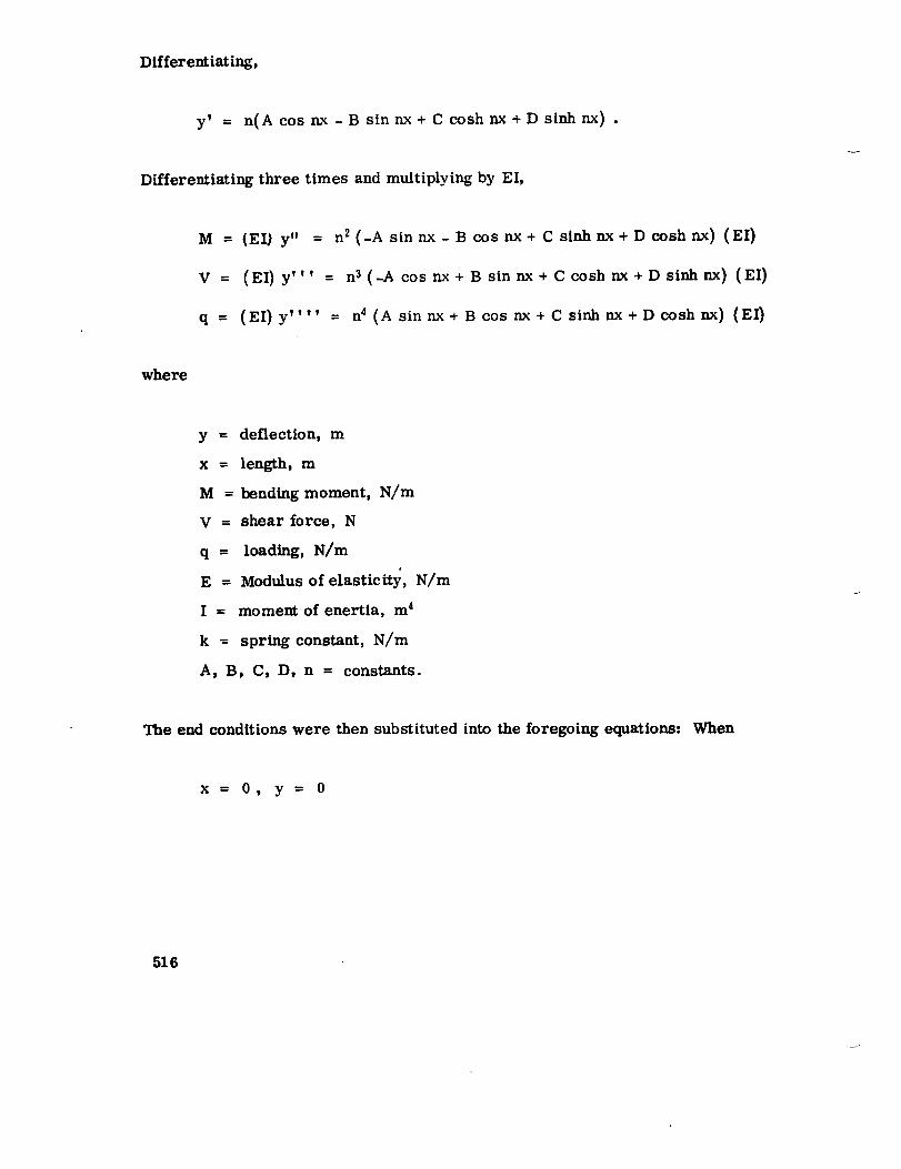
Differentiating,
y' = n(A cos nx - B sin nx + C cosh nx + D sinh nx) .
Differentiating three times and multiplying by EI,
M = (ED y" = n2(-A sinnx-B cosnx+ Csinhnx+Dcoshnx) (EI)
V = (EI) y,t_ = n 3(_A cosnx+B sinnx+ C coshrm+Dsinhnx) (EI)
q = (EI) y_,1, = n 4 (A sinnx+Bcos nx+C sinhnx+Dcoshnx) (EI)
where
y = deflection, m
x = length, m
M = bending moment, N/m
V = shear force, N
q = loading, N/m
E = Modulus of elasticity, N/m
I = moment of enertia, m 4
k = spring constant, N/m
A, B, C, D, n = constants.
The end conditions were then substituted into the foregoing equations: When
x= 0, y= 0
516

and
whe n
x = L, y"= 0
A sin mx.**C
sinh mx
when
EI__ y,-x = L, y = k
or
(A sinnL) E1 n3 [-A cos n LA sin n L + \_]l_nE sinh nL =
+/A sin nL) ]\' si'_" _ cosh nL ;(6 i)
therefore,
113 =2k
(EI) (eothnL -cot nL)
517

AIso,
W
q = _ w2yg
where
g = acceleration of grayly', m/sec 2
w = frequency rad/sec
n4 w w 2g EI
(632)
The structural properties of the retro-rockets are given below:
E
k __
30x 10 s, I = 13.97 m 4 (550 in. 4), w = 1339.5 g/cm
(7.5 lb/in.)
750.12× l0 sg/cm (4.2x 1051b/in.) and L = 2.2098m
(87 m.).
Therefore, from equation (631),
n = 1. l14/m (0.0283/in.)
and from equation (632),
_9f - = 123 Hz .
27r
51 8

The modeshapeis calculated next. This is a preliminary analysis so only thefirst mode is calculated.
[A sin Lx)y = A sin nx + _'si_ L_" sinh nx
at
x = 0, y = 0
x = 0.2L, y = 0.527A
x = 0.4L, y = 0.958A
x = 0.6L, y = 1.218A
x -- 0.8L, y = 1.301A
x = 1.0L, y = 1.258A
y1A
0
MODE SHAPE
! I l I I
0 0.2L 0.4L 0.6L 0.8L 1.0L
x
Use the environmei_t in Sub-Zone 2-5-2-A _',f Reference 68 as input to
the component. The input is applied at both support points in phase. At 12J Hz
the vibration environments are. 06 g2/Hz random and ±3. 2 g steady state shm-
soidal. If the damping is assumed to be 4 percent of critical, the magnificationis
1
Q = zt uU4)_'^.^'" = 12.5
519

Assume the maximum response is at 0.8L, and the vibration load is calculated
as follows:
/-w
Random dynamic load = (a)_]_/2) (Q)(f) (PSD) (633)
where
a = confidence level described in Paragraph 2.A.4 of this section.
Q = magnification factor
f = frequency of resonance
PSD = random vibration input environment at f.
This random dynamic load is the response of a single-degree-of-freedom sys-
tem to a random input [ 73]. Because this is a modal analysis, each mode can
be considered as a single-degree-of-freedom system and the above load equa-
tion applies.
Random dynamic load =
Sine dynamic load =
(2.2) _/(7r/2)(12.5)(123)(0.06) = 26.4g
(Q) (steady state sine environment at f)
(12.5) (3.2) = 40g .
The sine load is the highest; therefore, it is used for the load calculations.
Using the dynamic load and the mode shape, bending moments and shear loadscan be calculated.
520

Or, for a quick analysis, the 40 g could be spread uniformly and the loadscalculated.
40 g
d. Example 4
The following is another example of a preliminary design analysis
model. The fuel fill and drain line located in the thrust structure of the
Saturn V S-IC stage is the component. The installation is shown in the follow-
ing sketch:
,v_AFT FUEL BULKHEAD
-__- F,LLAND.RA,NVALVE,/7<_¢t',. _/- _,MBAL
j _..._ __'NG JOINT
The preliminary mathematical model is constructed as shown below. Assume
the effect of the concentrated mass (sliding joint) cancels the moment carrying
capability of the gimbal joints. Assume pinned-pinned end conditions.
521

(129)4 (o. 328)_L 4w
f = 39.4 Hz .
From Reference 68, the input levels at 39.4 Hz are obtained. Use either aft
skirt umbilicals (sub-zone 2-l-l-A) or aft fuel bulkhead (sub-zone 2-6),
whichever is higher. At 39.4 Hz, the environments are . 1 g2/Itz random for
sub-zone 2-1-1-A and ±2.75 g steady state sinusoidal for sub-zone 2-6. The
damping is assumed to be fairly high due to the friction in the sliding joint and
the gimbals. Therefore, assume Q = 1/2_ = 5.
Random dynamic load = (_)_](_12)(Q) (f)(PsD)
= (2.2)J(_12)(5)(39.4)(0.i) = 12.241
Sine dynamic load = (Q) (_G pk)
(5) (2.75) = 14g .
The sinusoidal load is the highest, so it should be used. The load dis-
tribution for the calculated mode would be as shown in the following diagram:
522
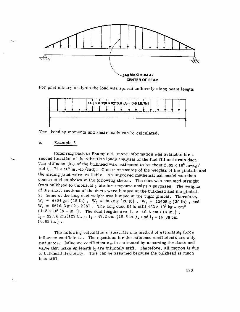
_,...J4g MAXIMUM AT
CENTER OF BEAM
For preliminar3y analysis the load was spread uniformly along beam length:
I I I I | I I 1
14 g x 0.328 = 8215.6 g/cm (46 LB/IN)
Now, bending moments and shear loads can be calculated.
e. Example 5
Referring back to Example 4, more information was available for a
second iteration of the vibration loads analysis of the fuel fill and drain duct.
The stiffness (kt) of the bulkhead was estimated to be about 2.83 x tO e m-kg/
rad (1.71 × 106 in. -lb/rad). Closer estimates of the weights of the gimbals and
the sliding joint were available. An improved mathematical model was then
constructed as shown in the following sketch. The duct was assumed straight
from bulkhead to umbilical plate for response analysis purposes. The weights
of the short sections of the ducts were lumped at the bulkhead and the gimbal,
2. Some of the long duct weight was lumped at the right gimbal. Therefore,
W 1 = 6804 gm (15 [b) , W 2 = 9072g (20 lb) , W 3 = 13608g (301b) , and
W 4 = 9616.3g (21.21b) . The long duct EIis still 433× 106 kg- cm 2
(148x 1061b_ in. 2). The duct lengths are l 0 = 40.6cm (16 in.) ,
1 t = 327.6 cm(129 in.), 12= 47.2 cm (18.6 in.), and 13 = 15.36 cm
(6. in.) .
The following calculations illustrate one method of estimating force
influence coefficients. The equations for the influence coefficients are only
estimates. Influence coefficient a22 is estimated by assuming the ducts and
valve that make up length 12 are infinitely stiff. Therefore, all motion is due
to bulkhead fle.xibility. This can be assumed because the bulkhead is much
less stiff.
523

kt ,, 1.71 x 10s (BULKHEAD)
a22 = kt = -_
Influence coefficient all is estimated making the same assumption as in a_.
Also, assume duct 11 is a simply supported beam between the gimbals. The
short duct attached to the umbilical plate (at right) is assumed infinitely stiff.
[I-LZ_ 2 (11 - 10)2 1Q2 = 213 × 10 -sall = a22 \ 11 ] + (3) (EI) (11)
Theother influence coefficients can be estimated in the same manner using
similar assumptions.
(11-10) 1£_ = 5Sx10-6a13 = a31 = a22 II 12
10 (3/41_-1_)+a22 " 11-10= 199)< 10 -_a14 = a41 = 12EI 2 11
a12 = a21 = a22 _ = 178x 1011
I--L = 66x 10 -6a23 = a32 = a22 12
a2_ 102 x lO -_a24 = a42 = 2 =
524

a33-- I_2 = 21.4x 10 -6
k t
a:_4 = a43 = .._"- • _ = 33x 10 -s2 12
1--_+ a22 = 353x 10 -Ga44 = 48EI 4
From the above force influence coefficients, the inverse of the stiffnessmatrix [ K ] -1 can be written, and from the weights given previously, a mass
matrix I/g[W] can be written. Therefore, the eigenvector equation is:
-(_2n/g) [Z]-I [W] {x} = 0
The derivation of the above equation can be seen in Section XHI. B. 4. and is
analogous to
__2 m_- x+x = 0
in the single-degree-of-freedom case. The etgenvector equation becomes:
(_/g) [D](x) = (x}
where [D] = [K]-I [W] is the dynamic matrix or
xlIx 2
x 3
x4
_2n
= io-'_"7"
3200 3560 1740 4220"
2670 4060 1980 2160
870 1320 641 700
2980 2040 990 7490
Ifx 2
x 3
x 4
525

Solving for the eigenvalues and eigenvectors, the frequency and shape of first
mode are obtained. The solution may be obtained by using any of a number of
iteration techniques such as shown in Section XIII. B. 5. or using a computer.
w l = 183 fl = 29.2 Hz
i 0830Ix 2 _ +0. 645
x 3 +0. 210
x 4 , +1. 000
Then the second mode is obtained
w2 = 322 f2 = 51.3 Hz
x 2 -i. 000
i x:_ I -0.326x 4 +0. 937
Since this is not a final analysis, only two modes were calculated to save time.
From Reference 68, the input environments are :
Steady State
Zon.__ee Random Sine Frequency
2-1-1-A 0. 1 g2/Hz il. 8 g 29.2 Hz
2-6 0.02 g2/Hz +2.75 g 29.2 Hz
2-1-1-A 0.1 g2/Hz +2 g 51.3 Hz
2-6 0. 065 g2/Hz ±2.75 g 51.3 Hz
526

Assuming Q = 10, the steady state sinusoidal loads are calculated using the
highest environment as the input at 29. 2 Hz
NL
Dynamic load
773.95N
VL
= (Q)(Xn) (±G pk) (weight)
= (10) (0.83) (2.75) (15) --
= 1565.65 N (354 lb) at 2
= 773.95 N (174 lb) at 3
= 2548.70 N (573 lb) at 4
1565.65 N
1521.2 N
2
1
521.21 N (342 lb) at 1
2548.70 N
4
at 51.3 Hz
Dynamic load = -707.23 N (-159 lb) at 1
-2446.4 N (-550 lb) at 2
-1200.96 N (-270 Ib) at 3
2433. 05 N (547 lb) at 4
VR
527

N
3
" 11200.96 N
2446.40 N707.23 N
2433.05 N
The random vibration loads are calculated using the highest environment as
input at 29.2 Hz.
VR
Dynamic load = (Xn) (a)_J(Tr/2)(Q)(f)(PSD) (weight)
where
x = mode shapen
(weight) = weight of lumped mass n
a, Q, f, PSI are defined in equation (634).
Dynamic load = (0.83) (2.2)J-(_/2)(10)(29.2)(0.1)
831.77 N (187 lb) at 1
858.46 N (193 lb) at 2
422.56 N (95 lb) at 3
1405.56 N (316 lb) at 4
(15)
52 8

NML 422.56 N
VL
858.46 N831.77 N
1405.56 N
4
at 51.3 Hz
VR
N ML
3
V L
Dynamicload = -382.52 N(-861b) at 1
= -858. 46 N (-193 lb) at 2
= -644.96 N (-145 lb) at 3
= 1316.60 N (296 lb) at 4
644.96 N
858.46 N
382.52 N
1316.60 N
4
VR
529

With the aboveloads, the forces and moment at the bulkhead, at the right gim-
bal, and along the duct can be calculated.
f. Example 6
The following figures show the model used for the final design analysis
of the cold helium feeder duct in the thrust structure of the Saturn V S-IC. The
duct is installed as shown in Figure 125.
COLD HELIUM LINE
7
GIMBAL_ GIMBAL
ROLLER BRACKET (ATTACHED TO HEAT SHIELD FRAME)
GIMBAL BRACKET 1 {ATTACHED TO HEAT SHIELD FRAME)GIMBAL
__ GIMBAL%..x GIMBAL
• _ _-_-'- FLANGE • LOWER THRUST RING
FLANGE @ ENGINE
z Y
Figure 125. Cold helium feeder duct installation.
For the analysis, the duct was broken into two systems at bracket 1.
The duct was analyzed in two parts because it was qualification tested that way.
The gimbals were taken as short beams [ 3. 81 cm ( 1.5 inches long) ]
with a flexural rigidity equal to the spring rate of the gimbal. The ducts were
assumed to have no rotational inertia. The ends of the ducts were fixed in all
directions simulating the qualification test set-up.
530

SYSTEM ONE
3.238cm
3.81cm
26.11 lcm
26.111cm
26.111cm
26.11 lcm
2O
3
4
5
26.111cm / GIMBAL
26.111cm 6 _. .3.81cm
_V'x_14 2s4c.,3.81c. js_ f" "_ ROLLER8RACKET
GIMBALIS'|9._ D/11 ,=._jtl8 22.275cm10 _, "U?d='_Y_lb 15 22.275cm
"-,e._.-_"_16 _.27s=,x x'-_ "_ _ 17 22.275cm
1 __-_ _
• SYSTEM TWO
15 1 "_GIMBAL : !
/X: 3.81cm _,4(1_ 1_ }
,i,
GIMBAL
531

B. Use of Vibration Loadsin Strength Analyses
The vibration loads calculated by the methods of Paragraph 1 below are
to be used by the designer and stress analyst; therefore, these people must be
told the meaning of the loads and how the loads are applied. The following
paragraphs describe relationships between vibration loads and design loads.The statistical confidence levels associated with vibration loads are also
described.
1. DESIGN LOADS AND CONFIDENCE LEVELS
a. Limit Load
The limit load is defined to be the maximum expected steady state loadthat a particular comp°nent or structure will see in service. Vibration loads
calculated as shown in the previous paragraphs are considered to be limit loads.
b. Yield Load
The yield load is the maximum load that a component can carry without
the weakest part of the component or structure yielding (stressed beyond the
defined elastic limit). For MSFC applications, the yield load should be 1.1times the total limit load.
c. Ultimate Load
out the
load is
The ultimate load is the maximum load that a component can carry with-
weakest part of the component or structure rupturing. The ultimate
usually 1.4 times the total limit load.
d. Confidence Levels
In calculating a response vibration load, a statistical confidence level
should be specified. All vibration loads will have an applicable confidence level
unless the input levels are known exactly. For example, one can state that the
shear load at a point on a structure will not exceed X newtons with a 97.5 per-
cent confidence level, meaning that 97.5 percent of the time the structure is in
use the shear load at the point will be less than X newtons.
For the random vibration environment, the associated level states the
confidence that the environment is the root mean square (rms) or 1 sigmaacceleration level. The associated confidence level for the MSFC environments
532

is 97.5 percent. Therefore, the random response vibration load calculated is
the rms or I sigma load with 97 percent confidence. MSFC requires that the
design random vibration loads shall be 2.2 times the rms load. Therefore,
the calculated random vibration loads (limit loads) are 2.2 sigma loads with
97.5 percent confidence.
The steady state sinusoidal loads also have a 97.5 confidence level due
to the input environment. The sinusoidal loads are deterministic and do not
have an associated probability occurrence. Therefore, they are not multiplied
by any sigma value.
2. EQUIVALENT STATIC LOADS
Vibration response loads are usually applied as static loads in a strength
analysis. For example, consider the first three modes of a pinned-pinned beam.
The vibration load would be applied as a static load as shown below:
FIRST MODE
SL SR
SECOND MODE
$R
tSL
THIRD MODE
SL SR
The strength analysis could then be accomplished using the above load-
ing conditions. The loading coP:l!*A,,,_ should then be reversed and the analysis
re-done because the vibration load is plus and minus.
533

For quick analyses, the actual load diagrams, shown above, can be
simplified. The curved load profile could he replaced with a rectangular load
profile with either equal area under the load curves or the maximum load of
the actual profile spread uniformly.
FIRST MODE
SECOND MODE
Another assumed load profile shape could be triangular. The area of
the actual profile and the triangular profile could be equated, or the maximum
of the actual load could be equated to the maximum of the assumed triangular
profile.
FIRST MODE
SECOND MODE
o
aJ
conducting a strength analysis of a component or structure.
534
COMBINING LOADS
Time Correlation of L _ds
Vibration loads should be combined with all other applicable loads when
Time correlation

is one method of determining whether load combination is applicable. Loads
from various sources should not be combined if they do not occur at the same
time. For example, transient loads which occur at stage separation or engine
cutoff do not occur during periods of high steady state vibration loads; whereas
other transient loads, such as hold down release, do occur during periods of
high steady state vibration loads. Therefore, the former loads would not becombined with vibration loads and the latter would be combined.
The following is a list of types of loads which can and cannot be expected
to combine with high, steady state vibration loads.
Loads Likely to CombineWith Vibration Loads
Loads Not Likely to CombineWith Vibration Loads
Pres surizatio n
Venting
Lift-off (Hold down Release)
Vehicle Bending
Vehicle Torsion
Vehicle Acceleration
POGO
Thrust Vectoring (Gimballing)
Aerodynamic
Fluid Flow in Ducts
Slosh
Valve Opening or Closing
Ignition TransientsCutoff Transients
Separation of StagesRebound
Propellant Loading
Pre-ignition Pressurization
b. Combining Static and Vibration Loads
Static loads and vibration loads are added directly. The vibration load
should be taken as an equivalent static load, keeping in mind that the vibration
load is two directional; i. e., plus and minus. Therefore, the vibration loadwill add to the static load in one direction and subtract in the other.
c. Combining Normal Mode Loads
Depending on circumstances, modal loads may or may not be combined.
If a modal analysis is done simulating a sinusoidal qualification test, the modesare not combined since only one mode at a time is usually excited. If the anal-
ysis is simulating actual service or random testing, the modes should be added
because random vibration can excite all modes simultaneously.
535

Loads from each of the modes in any one axis are combined by the
square-root-of-the-sum-of-the-squares method. Stated in equation form, themodal loads are combined as follows.
Dynamic Load = d (Load of 1st mode) 2 + (Load of 2nd mode) 2 + ...
d. Combining Multiple Axes Loads
Loads from different axes are usually specified separately but can be
combined if desired. This type of load combination may be necessary if a
single resultant vibration load is desired instead of orthogonal axes vibration
loads. Another case when multiple axes loads may be combined is the addition
of vehicle bending or torsion loads to component vibration loads when the vehi-
cle axes do not correspond to the component axes.
In order to combine multiple axes loads intoa resultant load in a par-
ticulardirection, the component of each individualload in the desired direction
must be found. The uniaxialcomponents of allloads are then combined by
the square-root-of-the-sum-of-the-squares method as shown in Paragraph c.above.
e. Combining Shock and Vibration Loads
An input shock load is assumed to excite all modes in the direction of
the load. The response shock load is therefore a short duration vibration load
and can be combined with steady state vibration loads. If phasing is known,
then the shock and vibration loads can be added exactly; otherwise the square-
root-of-the-sum-of-the-squares method applies as shown in Paragraph c.above.
C. Vibration Damage
Damage due to vibration is fatigue damage rather than any type of over-
load failure. Vibration fatigue damage can happen in rather short periods oftime; i.e., 104 cycles at 100 Hz = 1.7 minutes. Therefore, methods of deter-
mining the extent of fatigue damage sustained by a component or structure maybe necessary in designing for vibration.
Mechanisms of fatigue damage are complex and depend on material,
notch sensitivity, stress level, time variation of loading, orientation of
536

the crystalline structure, flaws, etc. [ 74]. Due to these complexities, thecumulative fatigue damagetheories now in existance are not very accurate,but lacking any simple, improved methods, the existing theories are used. Thelisting of fatigue damagetheories could bevery long if all were included; how-ever, the following three shouldgive the reader a general idea of fatigue damageestimation.
1. CUMULATIVE DAMAGETHEORIES
a. Miner's Linear Damage Criteria
Miner's rule [75, 76] theorizes that a structure or component will fail
when a unique amount of energy has been absorbed by the structure at the point
of failure. This energy absorbed is proportional to the damage inflicted.
Fatigue damage due to a given load is assumed proportional to the ratio of the
number of cycles at the given load to the number of cycles required to cause
failure at that load. This is called the cycle ratio. If a number of different
loads are applied in succession, failure will occur when the sum of the cycle
ratios of the loads equals one, or
n k
N1 N 2 N3 Nk
where
n k = number of cycles of applied load k
Nk = number of cycles at load k which would cause failure.
This cumulative damage theory does not account for the beneficial or detrimental
effects of different levels of loading in sequence. Many investigators have foulxl
that if low load amplitudes are followed by higher load amplitudes, the cycle
ratios sum will be greater than one, and high load followed by low load will resultin a cycle ratios, sum less than one.
b. Non-Linear Damage Theory of Marco and Starkey
Marco and Starkey [ 75 ] explain the variation of the cycle ratios sum
by assuming that damage accumulates slowly at first and then rapidly as failure
approaches. The initial damage rate is higher for higher applied loads. Inequation form
537

D. = (nFNj) xj1
where
D. = damage after the ith cycle of load j1
nj/Nj = cycle ratio of load j
Xj = f(a), the exponent is a function of the stress level aj of load j
for any given material.
The above equation is used in the following manner, assuming Xj is known for
all the applied loads.
From cycle ratio nl/N 1 of load 1, calculate the resultant damage DI:
D 1 = (nl/N1) XI
Then calculate an equivalent cycle ratio for load 2 which would give damage DI:
D 1 = (n2e/N2e)x2
Add the actual cycle ratio n_/N 2 of load 2:
(n2e/N2e) + (n2/N2)= (n1+ 2/NI + 2}
Then calculate the total damage the component has sustained after application
of load 1 and load 2:
DI+ 2 = (nl+2/Nl+2) X2 .
538

Using this method, the damagedueto any numberof successive loads could becalculated. The componentwill fail when D1+ 2 + ... + k = 1. The order of
succession of loads must be known when using this method.
c. Non-Linear Damage Theory of Henry
Henry [ 75] proposed another method of predicting fatigue damage fromnon-constant loading.
D. = J
where
D°
1
f_j = cycle ratio of load j
a j-F_/_ = "overstress ratio" =
J F
fat ig_).e limit.
= damage after the i th cycle of load j
of load j with F being the material
The damage due to the various loads are calculated and summed similarly to
the method in Paragraph b. above. This method also requires knowledge of theorder of load application.
2. APPLICATION OF DAMAGE THEORIES
a. Damage Due to Sinusoidal Loading
Sinusoidal loading would be either a constant level load or loading with
a known variation. Either way, the cumulative fatigue damage can be estimated
by one of the methods of Paragraph 1. above using known material fatigue
strength values and measuring or calculating the stress level of the component.
For constant level loading, Miner's rule is a valid criterion. Material
fatigue strengths are determined by constant level testing. It must be kept in
mind that the normal S-N fatigue life curve is an average or mean curve, half
of the specimens tested failed before the curve indicates and half lasted longerthan the curve indicates.
539

For sinusoidal loading with a knownload variation, non-linear fatiguedamagecriteria, suchas Henry's theory (Paragraph 1.c above), have beenshownto be more accurate [ 75]. Non-constantlevel sinusoidal loading canarise under circumstances suchas sinusoidal sweeptesting whenpassingthrough resonancesof the test specimen.
Referring to Paragraph 1.c above, it canbe seenthat the cycle ratio ofeachloading level must be calculated. For the caseof sinusoidal sweeptesting,the cycle ratios of the various loading levels could be calculated as follows,
knowing the response versus frequency characteristics from accelerometers or
strain gages mounted on the test specimen and "knowing the test frequency sweeprate. The response stress levels can be classed into amplitude steps (8 or 10
steps from minimum to maximum level). The time in each amplitude step is
known; therefore, the cycle ratio of each step can be calculated, knowing the
average frequency of each step. Then the accumulated damage can be estimated.
b. Damage Due to Random Loading
Random loading is more complex than constant level loading, becauseit is difficult to calculate cycle ratios of the various levels of loads and the
sequence of loading cannot be determined. Usually some sort of damage esti-
mate is made based on assuming :Lloading distribution and linear cumulative
damage. Random S-N curves of the materials used would be helpful in esti-
mating fatigue damage [ 77 ).
The fatigue damage sustained by a component could be estimated in the
following manner. First the rms acceleration levels and the time at each level
must be found. The time and level the component experienced during lab tests
can be found from lab and test reports. The time that the component experiencedactual service environments can be found from service test records. The levels
during the service test must be estimated if transducers were not mounted on
the component. The service level estimates can be based on predicted environ-
ments such as listed in Reference 68, or can be based on data taken near the
component during a service test. The service levels must be the response, not
the input levels of the component. All the loads that the component experienced
must be used to get the stress history at the critical location on the componentwhere failure will occur first.
Next, the stress history must be classed into amplitude steps (8 or 10
steps from minimum to maximum). Assuming some distribution of stress cycle
levels, such as the Rayleigh distribution which has been found to fit the distri-
bution of peaks of a random process very well, the number of cycles in each
amplitude step can be estimated.
54O
D. The MSFC Environment Documents
MSFC has published documents specifying the vibration, shock, and
acoustic environments for the Saturn vehicles [ 67, 68, 78]. MSFC has also
published a document [ 69 ] which describes a method by which an environment
may be predicted if certain information is known. These documents and their
use are described in the following paragraphs.
1. SELECTING THE PROPER ENVIRONMENT
In order to specify a representative environment for the various types of
structure and the many components in the Saturn vehicles, they were divided
into zones and subzones. For instance, the Saturn V first stage (the S-IC) is
broken down into seven major zones such as the engine area, the thrust struc-
ture, the aerodynamic fins, etc. Each of these major zones is then broken into
subzones corresponding to particular types of structure or even particular
components. For example, in the thrust structure (Zone 2) there is a subzone
for the skin stiffeners of ring frames, another subzone for the center engine
support beams, etc.
In order to find the applicable subzone environment for use in a loads
analysis of a particular component, one must know the exact location of the
component. If the exact location is in doubt, the more severe environment of
the major zone should be selected. Each of the MSFC environment documents
describes the procedure for selecting the proper zone or subzone.
2. VIBRATION AND SHOCK ENVIRONMENTS
The zone or subzone vibration environment is made up of two parts; the
random vibration environment and the sinusoidal sweep environment. These
two environments represent the steady state level and any short duration high
levels that may occur during static firing and flight.
The random vibration environment represents, with a 97.5 percent con-
fidence level, an envelope of the steady state random vibration that will occur
in the particular zone or subzone during static firing and flight. These random
levels were derived from statistical analyses of data from previous vehicles
and adjusted to account for significant differences in vehicles. For more infor-
mation on derivation of the random vibration levels, the reader is referred to
Reference 69 in conjunction with Reference 79.
541

The sinusoidal sweepvibration level is usedto accountfor anyshortduration, high level vibration which may occur that is higher than the steadystate level. Onehalf the sinusoidal sweeplevel is an envelopeof the steadystate rms acceleration levels which will occur, with a 97.5 percent confidencelevel, during static firing and flight. In a dynamic loads analysis, onehalf thesinusoidal sweeplevel shouldbeused as the input vibration level. Again, thereader is referred to References69and 79 for a more completederivation.
The shockenvironments canbe foundon the samepageas the vibrationenvironments.
3. ACOUSTIC ENVIRONMENTS
The acoustic environments are divided into major zones and designated
internal or external within a zone. Internal or external merely means that theenvironment is either within the vehicle or outside the vehicle.
4. WEIGHT ATTENUATION
If the vibration environment specified in the environment documents
[ 67, 68, 78] are used without modification as inputs to components, the driving
structure is assumed to have an infinite impedance. That is, anything attached
to the driving structure will have no effect on the motion of the driving struc-
ture. In many instances this is obviously not true, and the effect is recognized
by a method of environment attenuation known as "weight attenuation." This
method attempts to account for the mass impedance of the component by atten-
uating the driving structure environment. The attenuation factor is shownbelow:
Weight Attenuation Factor = F =Weight of Structure
Weight of ._tructure + Weight of
Component
The weight attenuation factor F is applied to reduce the random environ-
meut. The square root of F = _ is applied to reduce the sinusoidal environ-
ment. The square root of F = _ is also used to lower the frequencies of boththe random and the sinusoidal environment.
This method must be used with great care and judgement and approved
by the Vibration and Acoustics Branch of MSFC's Propulsion and Vehicle Engi-
neering Laboratory.
542

The following is an example of the weight attenuation technique used for
a component mounted on the forward LOX bulkhead of the S-IC. The component
is the LOX loading probe with a weight of about 12.9 kg (28.5 pounds). It
extends through the bulkhead in the manner shown in the sketch below-
LOX TANK SKIN
T__-_ FORWARD LOX BULKHEAD
I _ PROBE FLANGE IS BOLTEDTO BULKHEAD FITTING
LOX LOADING PROBE (12.9 kin)
SLIDING SUPPORT (PERMITS
VERTICAL MOTION)
SLIDING SUPPORT LEGS
LOX TANK BAFFLES
For this problem, the probe was assumed to be perpendicular to the bulkhead
because the environment is specified in that direction. Therefore, the atten-
uated environment in the perpendicular direction is calculated as follows:
Weight of component = weight of probe [ 12.9 kg (28.5) ] plus weight of
bulkhead fitting [4.0 kg (S. 9)]
W C = 12.9+4.0 (28.5+ 8.9) = 16.9 kg = (37.4pounds),
An area of the bulkhead of about 2-1/2 times the fitting was assumed to
be the effective structure size, The average thickness of the bulkhead was
assumed to be 0. 381 cm (0.15 inch).
543

Weight of structure =
m_
(Tr) (R) 2 (t)(p)
(_) (20) 2(0.15) (0.1) = about 9.07 kg (20 lb).
Therefore, the attenuationfactor is
F
2O
20 + 37.4- 0.35
and
= _]0.35 = 0.59 •
The environment to be attenuated is the forward LOX bulkhead environment,subzone 7-1 in Reference 68.
Subzone 7-1 Random Envi-.x)nment (perpendicular to bulkhead)
20-55 Hz at 0.1 g2/Hz
55-160 Hz at +9 dB/oct
160-630 Hz at 2. 5 g2/Hz
630-2000 Hz at -9 dB/oct
Subzone Sinusoidal Sweep Environment (perpendicular to bulkhead)
5-36 Hz at 1.016 cm (0.4 in.) D.A.
36-450 Hz at ±26.0 g pk
450-550 Hz at 0. 00635 cm (0.0025 in. ) D.A.
550-2000 Hz at ±38.0 g pk
The attenuation factors are now used to modify the above environments. Itmust be kept in mind that both the acceleration levels of the environment and
the frequencies of the environment are lowered by this technique.
544
The random environment is attenuatedas shownbelow:
(G) (F) = (G attenuated)
(0.1) (0.35) = 0.035 gVHz
and
(2.5) (0.35) = 0.87 g2/Hz
Lower frequencies
(f) (_/'F) = (f attenuated)
(20) (0.59) = 12Hz
and
(12)+ (55-20) = 47 Hz
3.01 0.87 )antilog \ +9 log 0.035 + log 47 = 138 Hz
(138) + (630-160) = 608 Hz.
Therefore, attenuated random environment is
12-47 Hz at 0.035 g2/Hz
47-138 Hz at + 9 dB/oct
138-608 Hz at 0.87 g2/Hz
608-2000 Hz at -9 dB/oct.
545

The random envi_onmentsin Reference68do not extendbelow 20Hz;so the first freqr,mcy of 12Hz could be made20 Hz, thus slightly decreasingthe width _thr lower constant level bandwidth.
The sinusoidal environment is attenuatedas shownbelow
(±G) (_"F) = (±G attenuated)
(26) (0.59) = ±15 g .k
and
(38) (0.59) = ±22gpk .
Lower frequencies
(f) (_f-F) = (f attenuated)
(36) (0.59) = 21Hz
and
(450) (0.59) = 265Hz
D.A. displacement (at 265 Hz) =15
(0.051)(265)_= 0.01066 cm
(0.0042 in.) D.A.
J( 22next frequency = 0.051) (0. 0042) = 320 Hz .
546

Therefore, the attenuatedsinusoidal environment is
21-265 Hz at +15 g pk
265-320 Hz at 0. 01066 cm (0.0042 in.) D.A.
320-2000 Hz at +22 g pk .
The environment is complete except for less than 21 Hz so the displacementbelow 21 Hz must be found
inches D.A. =15
(0.051) (21)' = 1. 691 cm (0.666 in. ) D.A.
Therefore, the attenuated sinusoidal environment less than 21 Hz is
5-21 Hz at 1. 691 cm (0.666 in. ) D.A.
It was assumed that in the direction tangential to the bulkhead that little
or no attenuation would occur because less of the probe weight would be effec-
tive and more of the bulkhead would probably be effective.
5. PREDICTING ENVIRONMENTS
NASA Technical Note D-1836 [ 69] presents a technique for predicting
environments on rocket vehicles. The technique is based on certain assump-tions.
a. Similar types of structure possess essentially similar dynamiccharacteristics.
b. There are only two sources of vibration energy, mechanically
induced vibration from the rocket engines or other machinery in motion and
fluctuating pressure excitation from engine noise and boundary layer noise.
c. All vibration sources have wideband random frequency content
similar to spectra used as references.
547
The methodis empirical andthe inaccuracies must be recognized.
The exampleshownin Reference69 illustrates the calculations necessaryin applyingthe method.
E. Useful Relationships
This paragraph presents techniques for environment spectrum shaping,
conversion of environmental quantities to other quantities, and calculation of
spectrum composites. These techniques are primarily connected with vibra-
tion testing but are useful in loads calculations.
1. VIBRATION ENVIRONMENT SPECTRUM SHAPE
The shape of the spectrum of a vibration environment is influenced by
the capabilities of vibration testing equipment. Even if an environment may
never be used as an actual test input, it is usually shaped with test equipmentin mind.
a. Sinusoidal Environments
Sinusoidal sweep environ, rants are usually shaped such that the ampli-
tude levels are either constant displacement or constant acceleration as fre-
quency increases. Most modern sweep test equipment has an automatic sweep
speed drive that varies the test frequency logarithmically. The equipment also
has an automatic gain control which varies the power to the vibrator so the dis-
placement or the acceleration to the test specimen can be kept constant. There-
fore, the MSFC sinusoidal sweep specifications are shaped with constant levels
and logarithmic frequency sweep rates.
Constant levels mean that as frequency increases the acceleration levelmust either increase or be constant. If one decides that the acceleration level
of an environment at the higher frequencies is not realistic, a square step down
can be specified, such as
XXX-500 Hz at ±20 g pk
500-2000 Hz at ±10 g pk .
This means that at 500 Hz, the test operator must manually turn down the gain
on the test equipment. The down step is a manual operation and there may be
548

overshoot or the frequency may not be quite correct. This manual operation
does not affect loads calculations except when the loads are supposed to repre-
sent test conditions and one of the modes is near the step-down frequency.
b. Random Vibration Environments
Random vibration environment spectrums are specified with constant
power spectral density levels over rather wide frequency bandwidths. This is
because random vibration test equipment cannot follow many sharp, narrow
amplitude level changes in the spectrum. Modern automatic random equipment
usually has filter bandwidths of about 25 or 50 Hz in the control feedback loop,
which limits the bandwidths of the input spectrum. Sloping portions of a ran-
dom test spectrum are approximated by the test equipment as 25 or 50 Hz wide
steps.
2. USEFUL ENVIRONMENTAL RELATIONSHIPS
a. Vibration Environment Quantities
Sinusoidal Vibration Relationship
+Gpk = (0.0051) (D.A.)(f)2
where
±G pk = peak acceleration
D.A. = double amplitude inches displacement
f = frequency .
Random Vibration Relationship
The relationship between the sloping and constant level portions of the
PSD spectrum are as shown below:
549

r_
Gb
Ga -
__/II
I Ifa fb
FREQUENCY
M log Gb/G a101o7 = log fb/fa
where
M = slope of curve in dB/oct
fa = frequency at low frequency end of sloping PSD curve
fb = frequency at high frequency end of sloping PSD curve
G a = PSD level at fa
Gb = PSI3 level at fb
Relationship between PSD and G in a frequency band
PSD =(rms G in bandwidth) 2
Bandwidth
The composite of a random vibration spectrum is computed as follows:
The spectrum is divided into bandwidths of the sloping and horizontal portionsof the curve.
550

Mean Square Acceleration
in bandwidth flto f23.01 G 13.01i M
3.01 GZ3.01+ M
(f2) fl - fl
M/3.01J
For M = -3.0 to -3. 02 use:
Mean Square Acceleration
in bandwidth fl to f2= G1 fl (In f2 - In fl)
Then, the composite equals square root of sum of mean square values of eachbandwidth.
rms G = _/G2_2 + G22_3 + ....
If the random spectrum contains superimposed sinusoids, the total rms value
of the spectrum plus the sinusoids is the square root of the sum of the squareof the spectrum rms G plus the square of the rms of each of the sinusoids.
!
TOTrms G = /G 2 + G 2. + G 2 +random sme 1 sine 2 • g m
_4
During testing, each sinusoid is rejected from the random vibration control
loop by rejecting a bandwidth of random including the sinusoid; so that band-width does not have the correct test level.
b. Acoustic Environment Quantities
Conversion from one third octave band to spectrum level:
PSDL = (SPL)I/30.B. - 101ogl0Afl/30.B.
551

where
PSDL = Pressure spectral density level (dB)
(SPL) 1/30.B. = Sound pressure level in 1/3 octave band (dB)
Afl/30.B. = Frequency bandwidth of 1/3 octave band (Hz).
Conversion from effective (rms) pressure to sound pressure level:
p2
SPL = 10 log10 _r
where
SPL = Sound pressure level (dB)
p = Effective pressure (:'ms psi)
P0 = Reference pressure (2.9 × 10 -8 psi)
552

APPENDIX. DEFINITION OF TERMS
d2x
Acceleration - d_ : A vector that specifies the time rate of change of velocity.
Note: Acceleration may be (a) oscillatory, in which case it may be defined by
the acceleration amplitude (if simple harmonic) or the rms acceleration (if
random}, or (b) nonoscillatory, in which case it is designated "sustained" or"transient acceleration."
Amplitude Distribution Analysis. The process of performing various analysesof the statistical properties of values of a wave. See Probability Density Func-
tion, and Probability Distribution.
Bandwidth: The difference in cps between the highest and lowest frequency in
a band, usually taken to be the half-power points. See Half-Power Points and
Bandwidth, Effective.
Bandwidth r Effective (ebw) : The bandwidth of an ideal system which (a) has
uniform transmission in its pass band equal to the maximum transmission of
the specified system and (b) transmits the same power as the specified system
when the two systems are receiving equal input signals having a uniform distri-
bution of energy at all frequencies.
ebw= f GdfO
where f is frequency in Hz and G is the ratio of the power at frequency f to the
power at the frequency of maximum power. (The International Dictionary of
Physics and Electronics, Van Nostrand, 1956. )
Channel_ Telemeter: Designates the complete transmission route of a tele-metered function including transducer, signal conditioner, multiplexer trans-
mitter, receiver, tape recorder or other storage device ff used, demultiplexer,and readout device.
Commutation: Commutation is a type of time division multiplexing transmis-
sion. See also time sharing.
Constant Bandwidth Analysis: In vibration, the analysis by means of either
(a) constant bandwidth contiguous filters, or (b) sweeping through the spectrum
553
with a narrow-band filter. In "a" the output is displayed as a time history,
showing the variation of the data within the bandpass of each filteras a function
of time. In "b" the output is displayed as amplitude versus frequency; "b" may
be obtained by use of a heterodyne analyzer.
Continuous Spectrum: The spectrum of a wave with its energy continuously
distributedover a prescribed frequency region. A continuous spectrum has
no discrete components.
Crosstalk t Electronic: The interference between circuits wherein signals inone circuit are undesirably reproduced in other circuits.
Cutoff Frecluency _ Filter: Represents a frequency limit beyond which the filter
begins to cut off or suppress signals.
Damped Natural Frequency: The natural frequency of a damped system. Theaddition of a damping resistance to a single degree of freedom system decreases
the natural frequency.
wo=WoJ ( )O
Damping: The dissipation of energy with time in a system; especially, the
diminishing of amplitude of an oscillation.
Damping, Critical: That value of damping which allows the most rapid return
of a system to its neutral position, without overshoot. In a simple harmonic
system, which follows the equation
a x" _ b x' _cx=O,
the condition for critical damping is that b = 2 _-ac .
Damping Factor: In a simple oscillatingsystem, in logarithmic damping this-dt
factor constant e , the ratio of one amplitude peak to that next succeeding
itin the same direction.
Decibel: A unitfor the expression of power, voltage, current, or vibration in
logarithmic form.
554

Powe r:
VoLtage:
Current:
Vibration:
10 logt0 (Pt/P2) where Pt and P2 are two powers or intensities
to be compared.
20 log10 (El/E2) where E t and E 2 are the rms voltages to becompared. In rigorous use, it must be assumed that both
E 1 and E 2 are measured across the same value of resistance.
20 logl0 (I_/I2) where 11 and 12 are two currents to be
compared.
20 loglo (A1/A 2) where A 1 and A 2 are two acceleration levelsto be compared.
Degrees of Freedom: The number of independent generalized displacements
that are possible.
Discriminator: A device the voltage output of which is proportioned to the
frequency excursion of the input signal. It is used to convert an FM signal into
an AM signal.
Displacement: The instanteous distance of a vibrating particle from its positionof equilibrium.
Double Amplitude Displacement: Twice the peak displacement or amplitude ofa sine wave; that is, peak-to-peak displacement.
Dynamic Pressure: The kinetic energy per unit area of the air stream relativeto the vehicle.
Equalizer: A network inserted in a system to modify the frequency responsein a desired manner.
Excitation: (a) Addition of energy to a system, whereby it is transferred from
a state of equilibrium to a state of higher energy called an "excited state," and
(b) an external force or other input applied to a system that causes the system
to respond in some way.
Flutter: Resonant vibration of any part of a vehicle or of any structural element
in a fluid stream, maintained by oscillatory aerodynamic forces induced bydeflection of the structure.
Forced Oscillation: The oscillation of a system forced by the excitation.
555

Forcing Function. A mathematical expression describing the relationshipbetween the force and a time variable.
Free-Free: A term indicating the vibration of a beam-like structure unsup-
ported at all points by structural members. A space vehicle, after liftoff, isin the free-free condition.
Free Vibration: Oscillations that continue in a system after the applied force
has been removed.
Fundamental Mode of Vibration: The mode having the lowest natural frequency.
Gaussian or Normal Distribution: The Gaussian distribution is often called
normal distribution and is expressed by:
_X 2
62
e 2P(X)--2--4ZV- "
The area under the curve from x 1 to x 2 represents the probability of obtaining
a value of x between x 1 and x 2.
Ground Noise: The residual system noise in the absence of the signal.
Half-Power Points (Vibration) : The requency points in a plot of a spectrum,or a filter transmission, where the rms amplitude falls to 70.7 percent of
the maximum of the curve.
High Pass Filter: A filter designed to pass all the frequencies above a critical
or cutoff frequency while attenuating all frequencies below this critical fre-quency.
Impedance: The complex ratio of a force-like quantity (force, pressure,
voltage) to a related velocity-like quantity (velocity, volume, current).
Impulse: The product of a force and the time during which the force is applied;tx
more specifically the impulse is f fdt where the force is time dependent
t2
and equal to zero before time t 1 and after time t_.
Isolator: A device (such as springs, rubber pads, or mechanical linkages)
which reduces the transmission of vibration in a certain frequency range.
556

Jerk:d3x
The change of acceleration with respect to time:
Linear Average Analysis: Ananalysis which is obtained through the use of an
averaging circuit. Output may be expressed as average, or presented as
average adjusted to ms (stated) for random noise.
Linear System: A system is linear if the response is linearly proportional to
excitation for every element in the system.
Logarithmic Decrement: The natural logarithm of the radio of any two suc-
cessive amplitudes of like sign, in the decay of a single-frequency oscillation.
Logarithmic Sweep: A manner of varying frequency during a test wherein thecommon logarithm of the frequency is a linear function of time,
Longitudinal Vibration: Vibration in a direction parallel to the longitudinal
axis. The positive direction is forward or in the direction of flight. Polarity
should be omitted when discussing wideband vibration measurements. It should
be used only with bending modes, linear acceleration, etc.
Mach Number: The ratio of any velocity to the velocity of sound in the same
medium at that temperature and pressure.
Mechanical System: An aggregate of matter comprising a defined configurationof mass, mechanical stiffness, and mechanical resistance.
Mixer.- A device which adds to a more input signals linearly producing a com-
plex output with controlled percentages of each input signal.
Mode of Vibration: A characteristic motion pattern assumed by a system and
dictated by the geometry of the system.
Modulation (Van Nostrand) : The process or result of the process whereby
some characteristics of one signal are varied in accordance with another signal.
In common usage the modulated signal is called the carrier and the other
signal is called the modulating signal.
Multiple-Degree-of-Freedom System: A system for which two or more co-
ordinates are required to define completely the position of the system at anyinstant.
557

Multiplex Transmission: A technique for the simultaneous, or apparentlysimultaneous, transmission of two or more intelligence signals on a single
carrier by frequencydivision, time division, or phase division.
Natural Frequency: The frequency of free oscillation of a system.
Noise: Any undesired sound, to be more exact, any unwanted distrubance
such as undesired electrical signals.
Non-Stationary Random Noise: A process or noise which does not meet the
requirements of a stationary random process.
Octave: An interval between two signals haveing a basic frequency ratio of 2.0.
Octave Analysis: An analysis made with an array of filters the center frequen-
cies of which are spearated by one octave and the effective bandwidth of which
is one octave.
Octave Sweep Test: See Logarithmic Sweep, above.
One-Half Octave: An interval between two signals having a basic frequency
ratio of 1.414
One-Half Octave Analysis: Same as one octave analysis except center fre-
quencies of filters are 1/2 octave apart, and the ebw is 1/2 octave.
One-Third Octave: An interval between two signals having a basic frequency
ratio of I. 26 (3/2).
One-Third Octave Analysis: Same as one octave analysis except center fre-
quencies are 1/3 octave apart, and the ebw is 1/3 octave.
Oscillograph: A device which produces a visual representation of an electrical
signal.
Peak-to-Peak: The algebraic difference between the ex£remes of a wave,
twice the peak value of a pure sine wave.
Peak Level: The maximum instantaneous level that occurs during a specified
time interval.
Periodic: The recurrence of an oscillation at equal increments of the inde-
pendent variable.
558

Piezoelectric (Crystal) Transducer: A transducer that depends for its opera-
tion on the interaction between the electric charge and the deformation or
certain asymmetric crystals having piezoelectric properties.
Piezoelectric: The property of certain crystals in developing electrical charge
or potential difference across certain crystals faces when subjected to a strain
by mechanical forces, or conversely to produce a mechanical force when a
voltage is applied across the material; that is, quartz, tourmaline, Rochelle
salts, and certain ceramics.
Pitch Plane: The plane parallel with the longitudinal axis in which pitching
takes place.
Pitch Vibration: Vibration in a direction parallel to the pitch plane and per-
pendicular to the longitudinal axis. The positive direction is toward positionHI.
Power Spectral Density (PSD) : A measure of the power distribution as a
function of frequency, in a complex wave. It is expressed by the following
relationships: Where PSD is the intensity for one cycle of bandwidth, g is
the root-mean-square value of the acceleration.
PSD = g2/A F where g = J A2dtO
"A" is the instantaneous amplitude of acceleration and "T" is the analyzer time
constant.
Probability Density Function: Generally, gives the probability of obtaining
a value "near" any continuous variable.
p (x) = dF (x)/dx .
Sometimes called frequency function. The first differential of the probability
distribution function, or simple, the ratio of instantaneous amplitude to rms
amplitudes.
Probability Distribution: A plot of the probability of occurrence of the magni-tude of a signal or noise. See Amplitude Distribution Analysis, above.
PSD - See Power Spectral Density, above.
559

Q (Quality Factor) PSD: Q is a measure of the sharpness of resonance of
frequecny selectivity Of a resonant vibratory system having a single degree of
freedom, either mechanical or electrical.
NOTE: In a mechanical system, this quantity is equal to one-half reciprocal
of the damping ratio. It is commonly used only with reference to a
lightly damped system, and is then approximately equal to the follow-
ing: (a) Transmissibility at resonance, (b) _ 5 where 5 is the
logarithmic decrement, (c) 2_ _/A_, where w is the stored energy
and A_ is the energy dissipation per cycle, and (d) fr/Af where fr is
the resonance frequency and A f is the bandwidth between the half-
power points.
This is true only for what is termed in electrical circuits a single-tuned filter.
In the case of multiple-tuned filters, although theoretically Q can be calculated,
it is simpler to measure it. Nearly rectangular bandpass filters, whether
obtained by cascading, paralleling, or ladder networks, commonly have a Q
five times as great as that computed by the given formula. Q may be computed
from a measurement of time constant by the following equation.
Q=1ff Tr c
where T is the dynamic time constant. (See Time Constant Definition. )C
Random Noise: An oscillation of which instantaneous magnitude is not specified
for any given instant of time. Instantaneous magnitudes of a random noise are
specified only by probability distribution functions giving the fraction of the
total time that the magnitude, or some sequence of magnitudes, lies within a
specified range.
Random Wave Analyzer: A device, used to analyze random vibration data and
which produces power spectral density (PSD), linear average, peak, and
integrated amplitudes as a function of frequency.
Range Zero: First discrete second timing mark before the vehicle leaves the
launching pad.
Resonance: Resonance of a system in forced oscillation exists when any change,
however small, in the frequency of excitation causes a decrease in the response
of the system.
56O

Reverberation Chamber: An enclosure in which all of the inner surfaces have
been made as sound-reflective as possible.
Rise Time: (a) (Shock pulse) The time required for a shock pulse to reach its
maximum value. (b) Definition for electrical pulses in time of rise between
10 percent and 90 percent of maximum amplitude (see ASA 3.49 AcousticsTerminology).
Roll Plane: The plane that is perpendicular to the longitudinal axis (roll axis)in which rolling takes place.
Sensitive Axis: The axis of maximum sensitivity of an accelerometer.
Shock Spectrum: (a) A plot of the maximum acceleration experienced by a
single-degree-of-freedom system as a function of its own natural frequency
in response to an applied shock, and (b) frequency spectrum of a shock re-su!ting from analysis by any method.
Signal to Noise Ratio: The ratio of the signal magnitude to the magnitude of the
noise received along with the signal.
Single-De_ree-of-Freedom System: A system for which one coordinate is re-
quired to define completely the configuration of the system at any instant.
Sound Pressure Level (SPL) : Twenty time the common logarithm of the ratio
of the pressure of the sound to the reference pressure.
Sound Pressure Level r Overall: Twenty time the logarithm (base 10) of the
ratio of the dynamic (sound) pressure in rms units to a reference dynamicpressure of 0.0002 dynes/cm 2. The term overall indicates that the entire
equipment transmission spectrum of frequencies is utilized, no additional
filtering being accomplished. Bandpass bandwidth limits of equipment mustbe stated; e.g., 20 to 20 000 Hz.
Spectrum: A continuous range of frequencies.
Spectrum Density (Power Spectrum): The mean-square amplitude of the output
of an ideal filter with unity gain responding to the oscillation, per unit bandwidth;
i. e., the limit for vanishingly small bandwidth of the quotient of the mean-
square amplitude divided by the bandwidth. For the practicing engineer, thisis usually the spectrum amplitude reported as if measured in I Hz bandwidths.
561
Note (a) : In mathematical terms, the spectrum density function of y(t) is the
ensemble average of G(f) where (when a limit exists)
LiraG(f) = T -ao T
2
dt
T
f y(t)I 27r ift ,-T
f being freqa,_ncy (positive only).
Note (b) : The mean-square output of an ideal filter with unity gain in a finite
band is given by the integral of G(f) with respect to frequency overthe band.
Spectrum Envelope: The vibration level, or levels, which enclose the peaks
on a vibration spectrum plot.
Spring Constant: The ratio of the force acting upon an elastic member to the
resulting displacement of the point at which the force acts.
SS/FM (Single Sideband/Frequency Modulation) : A form of frequency division
multiplexing. A number of intelligence signals are each subjected to a linear
frequency trasformation to a different frequency. The resultant signals, each
at a different frequency, are combined in a linear adder and the composite is
used to frequency modulate a carrier signal.
Stationary Random Process: (a) A process which has the joint probability
density dependent upon only the time differences and not upon the actual time
instants. (b) A process in which the equivalent G rms of the random vibra-
tion does not vary with time, (c) A process of which all of the statisitcal
properties depend only on the time differences and not on the actual timeinstants.
Steady State: Ca) A condition of dynamic balance, as in an equilibrium re-action, where at equilibrium the concentration of each of the reactants remain
constant. (b) A relatively unchanging dynamic condition. (c) The condition
in a system when the rate of dissipation of energy is constant with respectto time.
562

Steady State Vibration: See Steady State, above.
Strain Bricl_eAccelerometer: A device composed of a mass supported by very
finestrain wire or thin foilwhich exhibits a change in resistance with appliedacceleration.
Strouhal Number: (a) The dimensionless parameter, S:
S = fD/V
where f is frequency, D is the exit diameter of a noise producing nozzle, and
V is the velocity of the gases at the nozzle exit, and (b) relates frequency of
shedding of vortices to the wind velocity and a characteristic dimension, where
S = fd/V
where
f-- frequency of vortex shedding.
d = diameter of structure in feet.
V = velocity of air in feet/second.
Subcarrier: An intermediate frequency that is modulated by intelligence signals,and in turn is used to modulate the radio carrier.
Subcarrier Frec_uency Modulation: A frequency modulation technique employing
a subcarrier oscillator to derive a frequency modulated subcarrier.
Telemeter System: See Chapter V.
Time Constant_ In electronics, the time required for the voltage or current
in a circuit to rise to 63 percent of its final value, or fall to 37 percent of its
initial value_ as a result of a step input.
Time Constant_ Dynamic (of a resonant system) : The time required for theamplitudes of decaying oscillation in a system to fall to 37 percent of the ini-tial value.
T = 1/_B = Q/_fC r
for a single-degree-of-freedom system.
563

Time Sharing: The sharing of a telemetry channel between several vibration
measurements by transmission of a short sample of each in turn. In time
division multiplexing, samples are taken with a very high sampling rate with
respect to signal variations so that no information is lost; while in time sharing,
sampling occurs at very low rates which permits a representative measurement
or analysis during each sampling period. Typically, four measurements are
transmitted over one channel, each being sent for 4 seconds per sample.
Transducer: (a) A device capable of converting one form of energy to another,
and (b) the sensing element of a measuring channel. It transducers a mechan-
ical or physical quantity or movement into an analog signal which can be trans-
mitted to a remotely located recorder.
Transfer Function: A complex ratio of a response at one place in response to
an excitation to another place in a linear system. The transfer function, a
complex quantity, is the cross-spectral density between response and exci-
tation. Its absolute value is transmissibility.
Transient Vibration: A temporary vibration of a mechanical systcm, caused
by an impulse.
Transmissibility: The ratio of the response amplitude of a system to the ex-citation amplitude. The ratio may be between forces, displacements, velocities,
or accelerations. (Glossary of Terms Frequently used in Acoustics, AIP,
October, 1960. ) A plot of transmissibility versus frequency is usually made.
See Transfer Function, Q, and Cross Spectral Density.
Vibration: The oscillation of a body or particle about a point of equilibrium.
A parameter that defines the motion of mechanical system.
Yaw Plane: The plane parallel with the longitudinal axis in which yawing takes
place. The pitch plane is perpendicular to the yaw plane.
Yaw Vibration: Vibration in a direction parallel to the yaw plane and a perpen-
dicular to the longitudinalaxis. The positive direction is toward the right
hand of an observer looking forward along the longitudinalaxis.
564

REFERENCES
i.
o
o
o
.
o
o
.
o
I0.
ii.
12.
Barrett, Robert E... Techniques for Predicting Localized Vibratory
Environments of Rocket Vehicles. NASA Technical Note D-1836.
October 1963.
Eldred, Roberts, and White, R. : Structural Vibrations in Sp_.ce Ve-
hicles. WADD Technical Report 61-62, December 1961.
Bendat, Enochson, Klein and Pierson, Allan G. : The Application of
Statistics to the Flight Vibration Problem. ASD Technical Report
61-123, December 1961.
Accelerometer Fundamentals - Part I and Part IL Bulletin, Systron-
Donner Corporation, Concord, Calif. :
Calibration of Vibration Transducers. Tustin Institute of Technology,
Santa Barbara, Calif., 1965.
Endevco 2200 Accelerometer Manual. Endevco Corporation, Pasadena,Calif.
Endevco Product Development News. Endevco Corporation, Pasadena,
California; Vol. 5, No. 1, April 1967.
Piezoelectric Accelerometer User' s Handbook. Bulletin 4200-96, C
Consolidated Electronics (CEC), Pasadena, Calif.
Shock and Vibration Handbook, Vol. 1, New York, McGraw-Hill Book
Co. Inc., 1961.
Shock and Vibration Handbook. Vol. 1, New York, McGraw-Hill
Book Co., Inc., 1961.
Marigolds, B. : Effect of Mounting-Variables on Accelerometer Per-
formance. Princeton, New Jersey, Radio Corporation of America,
1963.
Calibration of Vibration Transducers. Tustin Institute of Technology,
Santa Barbara, California, 1965.
565
REFERENCES(Continued)
13.
14.
15.
16.
17.
18.
19.
20.
21.
22.
23.
Beranek, L. L. : Acoustic Measurements. New York, John Wiley _,Sons, 1962, p. 440.
Calibration of Vibration Transducers. Tustin Institute of Technology,
Santa Barbara, Calif., 1965.
Shock and Vibration Handbook. Vol 1, New York, McGraw-Hill Book
Co. Inc., 1961.
Javid, M., and Brenner, E. : Analysis, Transmission, and Filtering
of Signals. New York, McGraw-Hill Book Co., 1963, pp. 204-6.
Telemetry Standards. IRIG Document 106-66, Inter-Range Instru-
mentation Group, White Sands Missile Range, April 1966.
Saturn S-IC-501 Static Test Vibration and Acoustic Data. Document
D5--13644-1, The Boeing Company, October 1966.
Stfltz, Harry L. et al. : Aerospace Telemetry. Englewood Cliffs,N. J., Prentice Hall, Inc., 1964.
Bendat, J. S., Enochson, L. D., Klein, G. H., and Piersol, A. G. :
The Application of Statistics to the Flight Vehicle Vibration Problem.
ASD TR-61-123, Aeronautical Systems Division, AFSC, USAF,WPAFB, Ohio, ASTIA AD 271 913, 1961.
Bendat, J. S., Enochson, L. D., Klein, G. H., and Piersol, A. G. :
Advanced Concepts of Stochastic Processes and Statistics for Flight
Vehicle Vibration Estimation and Measurement. ASD TDR 62-973,
Aeronautical Systems Division, AFSC, USAF, WPAFB, Ohio, 1962.
Piersol, A. G. : Nonparametric Tests for Equivalence of Vibration
Data. SAE National Aeronautic and Space Engineering Meeting, LosAngeles, Calif., September 1963.
Crandall, S. H. : Zero-Crossings, Peaks, and Other Statistical
Measures of Random Responses. Proceedings, Acoustical Societyof American Meeting, Seattle, Wash., 1962.
566

REFERENCES(Continued)
24.
25.
26.
27.
28.
29.
30,
31.
32.
33.
34.
Bendat, J. S. : Principles and Applications of Random Noise Theory.John Wiley and Sons, Inc., New York, 1958.
Goodman, N. R. : On the Joint Estimation of Spectra, Co-Spectrum
and Quadrature Spectrum of a Two Dimensional Stationary Gaussian
Process. Scientific Paper No. 10, Engineering Statistics Laboratory,New York University, 1957.
Barrett, R. E. : Techniques for Predicting Localized Vibratory En-vironments of Rocket Vehicles. NASA TN D-1836, October 1963.
Duncan, A. J. : Quality Control and Industrial Statistics, Richard D.
Irwin, Inc., Homewood, 0t., Rev. Ed., 1959, p. 876.
Sokolnikoff, I. S., and Redheffer, R. M. : Mathematics of Physics
and Modern Engineering. McGraw-Hill Book Company, Inc., NewYork, 1958.
Everitt, W. L. : Communications Engineering. McGraw-Hill, pp.36, 94-178, 1937.
Blackman, R. B., and Tukey, J. W. : The Measurement of Power
Spectra Dover Publications, Inc., New York, 1958, p. 30.
Mathematical Methods for Digital Computers, John Wiley and Sons,
Inc., New York, 1960.
Simpson, S. M., Jr. : Time Series Techniques Applied to Underground
Nuclear Detection and Further Digitized Seismic Data. MIT Scientific
Report No. 2 (Contract AF19(604)-7378, ARPA Order No. 180-61),December 8, 1961.
Webster, Ao G. : The Dynamics of Particles. New York, Dover
Publications, Inc., 1959, pp. 63-70.
ChurchiU, R. V. : Fourier Series and Boundary Value Problems.
New York, McGraw-HiU Book Co., Inc., 1941.
567

REFERENCES(Continued)
35.
36.
37.
38.
39.
40.
41,
42°
43.
Setterlund, G. G., and Skoog, J. A. : Space Requirements for Equip-
ment Items Subjected to Random Vibration. Journal of the Acoustical
Society of America, February 1959.
Wyle, C. R., Jr. : Advanced Engineering Mathematics. New York,
McGraw-Hill Book Co., Inc., 1960.
Tse, F. S., Morse, I. E., and Hinkle, R. T. : Mathematical Vibra-
tions. Boston, AUyn and Bacon, Inc., 1964.
Bishop, R. E. D., and Johnson, D. C. : The Mechanics of Vibrations.
New York, Cambridge University Press, 1960.
Timoshenko, S., and Woinowsky-Krieger, S. : Theory of Plates and
Shells. New York, McGraw-Hill Book Co., Inc. 1959.
Levy, R. S., Ham, E. H., and Newman, M. : Experimental Determi-
nation of System Parameters for Thin-Walled Cylinders. Republic
Aviation Corp. Report No. RAC 1117-6, NAS8-11514, June 29, 1964.
Levy, R. S., Ham, E. H., and Newman, M. : Experimental Determi-
nation of System Parameters for Thin-Walled Cylinders. Republic
Aviation Corp. Report No. RAC 1117-14, NAS8-11514, June 29, 1965.
User' s Manual for Free Vibration Analysis of Stiffened Cylinders with
an Attached Weight. Republic Aviation Corp. Report No. RAC 1117-11,
April 15, 1965.
Levy, R. S., and Forray, M. J. : Experimental Determination of
System Parameters for Thin-Walled Cylinders. Fairchild Hiller -
Republic Aviation Report No. FHR 1117-20, August 1966.
User' s Manual for Natural Frequencies and Mode Shapes of Ring
Stiffened Cylinders with an Attached Weight. Fairchild Hiller -
Republic Aviation Report No. FHR 1117-19, Revision A, December
1966.
568
_f

REFERENCES (Continued)
45.
46.
47.
48.
49.
50.
51.
52.
53.
Hwang, C., and Brass, J. : Analytical and Experimental Determina-
tion of Localized Structure to Be Used in Laboratory Vibration Testing
of Shell Structure - Mounted Components, Saturn V. Northrop Corp.
Report NOR 66-201, Vol. I, May 1966.
Hwang, C., Pi, W. S., and Bhatia, N. M. : Analytical and Experi-
mental Determination of Localized Structure to Be Used in Laboratory
Vibration Testing of Shell Structure-Mounted Components, Saturn V.
Northrop Corp. Report NOR 67-127, July 1967.
Yamane, J. R. : Analytical and Experimental Determination of Local-
ized Structure to Be Used in Laboratory Vibration Testing of Shell
Structure-Mounted Components, Saturn V. Northrop Corp. Report
NOR 66-201, Vol. II, May 1966.
Hwang, C., and Pi, W. S. • Analytical and Experimental Determina-
tion of Localized Structure to Be Used in Laboratory Vibration Testing
of Shell Structure-Mounted Components, Saturn V. Northrop Corp.
Report NOR 67-19, January 1967.
Seto, W. W. : Schaum' s Outline of Theory and Problems of Mechanical
Vibrations. New York, Schuam Publishing Co., 1964.
Andronow, A. A., and Chaikin, C. E. : Theory of Oscillations.
Princeton, New Jersey, Princeton University Press, 1949.
Contributions to the Theory of Nonlinear Oscillations. Vols. I-V,
Princeton, New Jersey, Princeton University Press.
Ku, Y. H. : Analysis and Control of Nonlinear Systems. New York,
The Ronald Press Company, 1958.
Levinson, N., and Smith, O. K. : A General Equation for RelaxationOscillations. Duke Mathematical Journal, 9, 1942.
Stoker, J. J. : Nonlinear Vibrations in Mechanical and Electrical
Systems. New York, New York, Interscience Publishers, Inc., 1950.
569

REFERENCES (Continued)
55.
56.
57.
58.
59.
60.
61.
62.
63.
6_.
65.
66,
Minorsky, N. : Introduction to Nonlinear Mechanics. Ann Arbor,
Michigan, J. W. Edwards, 1947.
Minorsky, N. : Nonlinear Oscillations. Princeton, New Jersey,
D. Van Nostrand Company, Inc., 1962.
Margenau, H., and Murphy, G. M. : The Mathematics of Physics
and Chemistry. Princeton, D. Van Nostrand Co., Inc., 1947.
Franklin, P. : An Introductionto Fourier Methods and the LaPlace
Transformation. New York, Dover Publications, Inc., 1958.
Sokolmikoff, I. S., and Redheffer, R. H. : Mathematics of Physics
and Modern Engineering. New York, McGraw-Hill Book Co., Inc.,1958.
Milne, W. E.- Numerical Calculus. Princeton, Princeton University
Press, 1959.
Pipes, L. A. : Matrix Methods for Engineering. Englewood Cliffs,
N. J., Prentice-Hall, Inc.
Hildebrand, F. B. • Introduction to Numerical Analysis. New York,
McGraw-Hill Book Co., Inc., 1956.
Sokolnikoff, I. S. : Tensor Analysis. New York, John Wiley and
Sons, Inc., 1964.
Shock and Vibration Handbook, New York, McGraw-Hill Book
Company, 1961, pp. 36-16.
Crede, C. E. : Shock and Vibration Concepts in Engineering Design.
Englewood Cliffs, Prentice-Hall, Inc., 1965, p. 135.
A Finite Element Analysis of Simple Panel Response to Turbulent
Boundary Layers. Renton, Washington, The Boeing Company
Document D6-19392, July 1967, p. 25.
570
J

REFERENCES(Continued)
67.
68.
69.
70.
71.
72.
73.
74.
75.
76.
77.
Preliminary Vibration, Acoustic and Shock Specificationsfor Com-
ponents on Saturn IB Vehicle. Huntsville, Marshall Space Flight
Center Document IN-P&VE-S-63-1, September 1964.
Preliminary Vibration, Acoustic and Shock Specificationsfor Com-
ponents on Saturn V Vehicle. Huntsville, Marshall Space Flight
Center Document IN-P&VE-S-63-2, September 1964.
Techniques for Predicting Localized Vibratory Environments of
Rocket Vehicles. Huntsville, Marshall Space FlightCenter Document
NASA TN D-1836.
Shock and Vibration Environments and Test SpecificationLevels,
Ground Support Equipment, Launch Complex 39. Huntsville, Kennedy
Space Center Document SP-4-38-D.
The Shock and Vibration Bulletin. Bulletin34, Parts 2 of 5, U. S.
Naval Research Laboratory, Washington, D. C., December 1964.
Thomson, W. T. : Mechanical Vibrations. 2nd Ed., Englewood
Cliffs, Prentice-Hall, Inc., 1953, p. 214.
Random Vibration. New York, Technology Press of Massachusetts
Instituteof Technology and John Wiley and Sons, Inc., September
1959, paragraph 4.2.
Aspects of Cumulative Damage in Fatigue Design. Air Force
Materials Laboratory Report AFML-TR- 67-112, Wright- Patterson
Air Force Base, Ohio, August 1967.
Fatigue Damage During Two-Level Biaxial-Stress Tests. Air Force
Materials Laboratory Report, AFML-TR-66-355, Wright-Patterson
Air Force Base, Ohio, February 1967.
Miner, M. A. : Cumulative Damage in FatigTae. Journal of Applied
Mechanics Vol. 12, pp. A-159 through A-164, September 1945.
Fuller, J. R. : Research on Technique of Establishing Random Type
Fatigue Curves for Broad Band Sonic Loading. Air Force Flight
Dynamics Laboratory Report ASD-TDR- 62- 501, Wright-Patterson
Air Force Base, Ohio, October 1962.
571

REFERENCES (Concluded)
78.
79.
Preliminary Vibration, Acoustic and Shock Specifications for Compon-
ents on Saturn I Vehicle. Huntsville, Marshall Space Flight Center
Document IN-P&VE-S-62-7, 1962.
Statistical Techniques for Describing Localized Vibratory Environments
of Rocket Vehicles. Huntsville, Marshall Space Flight Center Docu-
ment NASA TN D-2158.
572

BIBLIOGRAPHY
Anand, G. V. : Resonance in Strings with Viscous Damping. J.A.S., 40,1517, 1966.
Banerji, D. : On the Theory and Some Applications of Sub-SynchronousPendulums. Proceedings of the Indian Association for the Cultivation of
Science, 7, 145-158, 1921-1922.
Bendat, J.S. : Principles and Applications of Random Noise Theory. NewYork, John Wiley and Sons, Inc., 1958.
Beranek, L. L. : Acoustic Measurements. John Wiley and Sons, New York,1956, p. 433.
Bradford, H. K. : High Spped Analysis of Electronic Circuits by Geometry.
Electronic Buyers Guide, McGraw-Hill, 1961, pp. R50-64.
Braunbeck, W., and Lauter, E. : Forced Oscillations of a Simple NonlinearSystem.
I. The Differential Equations and Their Stationary Solution.Z. Physik, 147, 297-306, 195, 1957.
II. Non-Stationary Motion. Zeit. fCt*rPhysik, 147, 507, 1957.
Chobotov, V. A., and _nder, R. C. : Nonlinear Response of a Circular
Membrane to Sinusoidal Acoustic Exitation. J.A.S., 36, 59, 1964.
Church, A. H. : Mechanical Vibrations. New York, John Wiley and Sons,Inc., 1964.
Cocking, W. T. : Cathode Follower Dangers. Wireless World, Vol. 52,March 1946, pp. 79-82.
Crandall, S. H., Khabaz, G. R., and Manning, J. E:: J.A.S., 36, 1330,1964.
Crede, C. E. : Shock and Vibration Concepts in Engineering Design.Englewood Cliffs, Prentice-Hall, Inc., 1965.
573

BIBLIOGRAPHY (Continued)
Determination of Structural Transfer Functions by Statistical Correlation
The Boeing Company Document LDRM 40.
Dey, A., and Raman, C. V. • On the Maintenance of Vibrations by a Periodic
Field of Force. Proceedings of the Indian Association for the Cultivation of
Science, 2, 1-15, 1917.
Firestone, F. A. : The Mobility Method of Computing the Vibration of Linear
Mechanical and Acoustical Systems: Mechanical-Electrical Analogies.
Journal of Applied Physics, Vol. 9, June 1938.
Goldberg, H. : Internal Impedance of Cathode Followers. Proc. IRE, Vol. 33,
November 1945, pp. 778-782.
Hale, J. : Oscillations in Nonlinear Systems. New York, McGraw-Hill Book
Co., Inc., 1963.
Hayashi, C. : Forced Oscillations In Nonlinear Systems. First Edition,
Osaka, Japan, Nippon Printing and Publishing Col, Ltd., 1953.
Heckl, M. : Nonlinear Flexual Vibrations of Sandwich Plates. J.A.S., 34,
803, 1962.
Herbert, R. E. : Random Vibrations of a Nonlinear Elastic Beam. J.A.S.,
36, 2090, 1960.
Kerchner, R.M., and Corcoran, G. F. : Alternating-Current Circuit_.
New York, John Wiley and Sons, Inc., 1962.
Kirchman, E. J., and Greenspon, J.E.: Nonlinear Response of Aircraft
Panels in Acoustic Noise. J.A.S., 29, 854, 1957.
Klein, G. H. : Random Excitation of Nonlinear System with Tangent Elasticity
Characteristics. J.A.S., 36, 2095, 1964.
Langford-Smith, F. : Radiotron Designers Handbook. Wireless Press for
Amalgamated Wireless Valve Co. Pty. Ldt., Sidney, Australia, reproduced
and distributed by RCA Victor Div., Harrison, N. J.
574

BIBLIOGRAPHY (Continued)
Lindsay, R. B. : Mechanical Radiation. New York, McGraw-Hill Book Co.,
Inc., 1960.
Miles, J. W. : Stability of Forced Oscillations of a Vibrating String. J.A.S.,
38, 855, 1965.
Morse, P. M. : Vibration and Sound. New York, McGraw-Hill Book Co., Inc.,1948.
Olsen, H. F.. Dynamical Analogies. Princeton, D. Van Nostrand Co., Inc.,
1958.
On the Maintenance of Combinatorial Vibrations by Two Simple Harmonic
Forces. No. 11, Indian Association for the Cultivation of Science, 1-24,1914.
Pliss, V. A. : Nonlocal Problems of the Theory of Oscillations. New York,
Academic Press, 1966.
Ranman, C. V. : On Motion in a Periodic Field of Force, Bulletin, No. 11,
Indian Association for the Cultivation of Science, 25-42, 1914.
Raman, C. V. : The Small Motion at the Modes of a Vibrating String. Physical
Review, 32, 309-315, 1911.
Results of An Experimental Program to Determine the Response of Unstiffened
Cylindrical Steel Shells to Free Field, Reverberant and Progressive Wave
Acoustic Excitations. Boeing Company Document D2-24122-1, November
1966.
Rideout, V. C. : Active Networks. Prentice-Hall, Inc., New York, N. Y.,
1954, p. 82.
Savant, C. J. : Control Systems Engineering. New York, McGraw-Hill Book
Co., Inc., 1958.
Scanlon, R. H., and Rosenbaum, R. : Aircraft Vibration and Flutter. New
York, The MacMillan Co., 1960.
575

B IBLIOGRAPHY (Concluded)
Smith D. A., and Lambert, R. F. : Effects of Dynamical Nonlinearity on
External Statistics. J.A.S., 32, 1700, 1960.
Smith, P. W., Jr. : Response of Nonlinear Structures to Random Excitation.
J.A.S., 34, 827, 1962.
Smith, P. W., Jr., Malme, C. I., and Goga, C. M. : Nonlinear Response
of a Simple Clamped Panel. J. A. S., 33, 1476, 1961.
Sneddon, I. N. : Elements of Partial Differential Equations. New York,
McGraw-Hill Book Co., Inc., 1957.
Snowden, J. C. Representation of the Mechanical Damping Possessed by
Rubber like Material and Structures. J.A.S., 35, 821, 1963.
Snowden, J. C. : Transient Response of Nonlinear Isolation Mountings to
Pulselike Displacements. J.A.S., 35, 389, 1963.
Srinwasa Murphy, G. S.,and Ramakrishna, B. S. : Nonlinear Character of
Resonance in Stretched Strings. J.A.S., 38, 46, 1965.
Symon, K. R. : Mechanics. Reading, Pa., Addison-Wesley Publishing Co.,
Inc., 1964.
Thompson, W. T. : Mechanical Vibrations. Englewood Cliffs, Prentice-
Hall, Inc. 1962.
von Ardenne, M. : On the Theory of Power Amplification, Proc. IRE, vol.
16, February 1928, pp. 193-207.
Wadd Technical Report 61-62, p. 133.
J
!
576