A replacement for simple back trajectory calculations in the interpretation of atmospheric trace...

Atmospheric Environment 36 (2002) 4635–4648

A replacement for simple back trajectory calculations in theinterpretation of atmospheric trace substance measurements

Andreas Stohla,*, Sabine Eckhardta, Caroline Forstera, Paul Jamesa,Nicole Spichtingera, Petra Seibertb

aDepartment of Ecology, Technical University Munich, Am Hochanger 13, D-85354 Freising-Weihenstephan, Germanyb Institute of Meteorology and Physics, University of Agricultural Sciences, T .urkenschanzstr. 18, 1180 Vienna, Austria

Received 15 March 2002; received in revised form 2 June 2002; accepted 19 June 2002

Abstract

Trajectory calculations are often used for the interpretation of atmospheric trace substances measurements.

However, two important effects are normally neglected or not considered systematically: first, measurements of trace

substances sample finite volumes of air, whereas a trajectory tracks the path of an infinitesimally small particle; second,

turbulence and convection. Advection by the deformative synoptic-scale atmospheric flow is responsible for the fact

that a compact measurement volume is in fact turned into filamentary structures at earlier times, which a single

trajectory cannot represent. Turbulence and convection add to this by causing a growth of the volume (backward in

time) where processes such as emissions can affect measured concentrations. In this paper, we show that both effects are

substantial and may be the largest sources of error when using trajectory calculations to establish source–receptor

relationships. We use backward simulations with a Lagrangian particle dispersion model (LPDM) and cluster analysis

of the particle positions to derive more representative single ‘‘trajectories’’ (transport paths) and trajectory ensembles.

This reduces errors caused by filamentation and backward growth of the measurement volume to a few percent as

compared to using a single, mean-wind trajectory and also yields estimates of the spread of the region of influence.

Thus, we recommend to replace simple back trajectory calculations for interpretation of atmospheric trace substances

measurements in the future by backward simulations with LPDMs, possibly followed by the clustering of particle

positions as introduced in this paper.

r 2002 Elsevier Science Ltd. All rights reserved.

Keywords: Pollution transport; Dispersion; Lagrangian particle dispersion model; Retroplumes, Source–receptor relationships

1. Introduction

Trajectories are, in meteorology, defined as the paths

of infinitesimally small particles of air (Dutton, 1986).

Such a fluid particle, ‘marked’ at a certain point in space

at a given time, can be traced forward or backward in

time along its trajectory. In practical trajectory models,

this is done by integrating the trajectory equation Dxi ¼viDt (where Dx is the position increment during a time

step Dt resulting from the wind v; the index i runs from 1

to 3 and denotes the three dimensions of space), using

mean (non-turbulent) horizontal and vertical winds

from a meteorological model.

While forward trajectories describe where a particle

will go, backward trajectories (often simply called back

trajectories) indicate where it came from. Therefore,

they are often used to interpret measurements of

atmospheric trace substances, in order to establish

relationships between their sources and their receptors

(Stohl, 1998). Trajectory analysis is thus an essential

element of practically all comprehensive air chemistry

measurement campaigns (e.g., Fuelberg et al., 2001).

*Corresponding author. Tel.: +49-8161-71-4742; fax: +49-

8161-71-4753.

E-mail address: [email protected] (A. Stohl).

1352-2310/02/$ - see front matter r 2002 Elsevier Science Ltd. All rights reserved.

PII: S 1 3 5 2 - 2 3 1 0 ( 0 2 ) 0 0 4 1 6 - 8

Even large data sets are often investigated using back

trajectories, allowing statistical analyses to be made

(e.g., Ashbaugh, 1983; Moody and Galloway, 1988;

Seibert et al., 1994; Stohl, 1996).

Trajectory calculations depend entirely on the input

wind fields taken from a meteorological model, and thus

inaccuracies in these data are the largest source of error

for them (Stohl, 1998). Other sources of errors are the

interpolation of the wind velocity from grid points to

actual trajectory positions (Rolph and Draxler, 1990;

Doty and Perkey, 1993; Stohl et al., 1995), and

truncation errors which occur in the numerical solution

of the trajectory equation (e.g., Walmsley and Mailhot,

1983; Seibert, 1993). Total trajectory position errors,

resulting from all of the above sources together, are

difficult to determine and are not normally known. A

survey of results from previous studies employing

different techniques suggests that average trajectory

errors are on the order of 15–20% of the distance

travelled after a few days (Stohl, 1998). However, in

critical flow situations errors of up to 100% are also

possible.

The quality of routinely available, gridded meteor-

ological analyses has been improved substantially over

the past decades, both in terms of accuracy and spatial

resolution. Numerical schemes are accurate enough to

render truncation errors negligible compared to other

errors. Nevertheless, in many cases, calculated trajec-

tories still fail to explain observed phenomena without

clear reason. This paper shows that there are effects

which are not or not well enough considered in

trajectory calculation and interpretation procedures

used for the analysis of measurement data, eventually

leading to substantial errors in the source–receptor

relationships inferred. An alternative procedure relying

on a Lagrangian particle dispersion model (LPDM) has

been developed and is presented here. The next section

explains in detail the shortcomings of conventional

methods and the outline of the alternative procedure.

The latter is described in Section 3, a case study is

presented in Section 4, and the results based on a large

set of calculations are shown in Section 5. In the last two

sections we discuss our results and draw conclusions.

2. The problem and outline of its solution

There are two reasons for problems when using back

trajectories to interpret trace substance measurements.

The first problem is that trajectories are the paths of

infinitesimally small parcels (hereafter called particles) of

air, whereas measurements require a finite and often

large volume of air. This is true for remote sensing

devices which require a finite backscatter volume as well

as for in situ measurements which apply a certain

collection or averaging time. Although, often used in

practice, a single trajectory cannot normally be repre-

sentative for the whole measurement volume.

Why is this so? Atmospheric flows are characterized

by the presence of a kinematic property called deforma-

tion. In the two-dimensional case, this means that a

circular fluid element will be torn into an elongated

structure. Imagine, for example, such a fluid element

arriving with a westerly flow at the border of a blocking

high pressure system or a mountain range. The flow will

then split into two branches going around the obstacle

on either side. If the fluid element is on the dividing

streamline, it will be torn apart into an elongated

structure, eventually enclosing the whole obstacle, with

separation of hundreds or thousands of kilometres.

Repeated stretching and wrapping of fluid elements

splits an initially compact volume of air into thin

filaments during the course of time, which can be

distributed over large areas and finally the whole

atmosphere. As the atmospheric flows are three-dimen-

sional, similar processes can happen in the vertical. This

leads to even more effective separation as there is often

substantial vertical wind shear, causing fluid elements at

different levels to travel in different directions (Siems

et al., 2000). The property of the atmosphere is thus that

two particles which are initially close to each other will

become separated by a large distance if sufficient time is

allowed for; this is characteristic of a chaotic flow

(Pudykiewicz and Koziol, 1998). These considerations

hold for back trajectories as well, explaining why a

single trajectory can be insufficient to represent the

transport history of a sampling volume even if it is

small.

Realizing these limitations, methods based on en-

sembles of trajectories were devised (e.g., Merrill et al.,

1985; Kahl, 1993, 1996). Typically a few (often four)

additional trajectories (sometimes called ‘uncertainty’

trajectories) are started at some distance from the

measurement location, and their separation due to

deformation in the wind field is used to estimate how

representative the central trajectory is for each situation.

These methods are insufficient because very few addi-

tional starting locations, selected more or less arbitra-

rily, are used, and because the effect of the finite

sampling time is sometimes not taken into account. So

there is no guarantee that the ensemble members are

really representative of the whole volume of air sampled.

The second problem, which comes on top of the first

one, is the presence of turbulent mixing and convection

in the atmosphere. Near-ground measurements will by

and large always take place in the atmospheric boundary

layer (ABL) and thus in the presence of turbulence. It is

well known that turbulence causes a puff of material

released in the ABL to grow with time. The same is true

for the volume of air which contributed to a short-term

sampling, just with reversed direction (see Flesch et al.

(1995), for a proof).

A. Stohl et al. / Atmospheric Environment 36 (2002) 4635–46484636

The combination of vertical turbulent diffusion and

the vertical shear of the (horizontal) wind are especially

important and are in fact the main reason for the

horizontal dispersion in the mesoscale (Smith, 1965).

There is some awareness that trajectories are therefore

less accurate when they travel in the ABL or when they

encounter deep convection. Crude attempts have been

made to consider these effects in trajectory calculations

(e.g., Stohl and Wotawa (1995), for boundary-layer

transport, and Freitas et al. (2000), for convective

transport), but they are not going far enough, because

trajectories calculated with the mean wind fields cannot

represent this mixing process and the growth of the

volume of influence. In addition to being a mechanism

of its own, this growth also enables deformation

processes to become more effective, because the volume

they can act upon grows—initially rapidly—with time.

Nowadays, we have sufficient computer capacities for

more accurate solutions of both problems. The require-

ment of these solutions is that they can track a volume

of air forward or backward in time under the effects of

turbulent mixing, of convection, and of the three-

dimensional structure of atmospheric flows including

deformation. This is the task of a transport and

dispersion model for forward tracking and of its adjoint

for backward tracking. One class of such models are

LPDM (Thomson, 1987; Rodean, 1996). They are

especially well suited for our task as they are an

extension of the simple trajectory models, are capable

of representing transport processes with strong filamen-

tation in a very accurate way, and can handle ‘point’

measurement sites without artificial diffusion such as

present in Eulerian (grid) models. LPDMs account for

turbulence in a stochastic way by calculating the

trajectories of a large number of particles transported

by both the mean wind and statistically modelled

turbulent fluctuations (Rodean, 1996). They can also

be run backward in time (e.g., Flesch et al., 1995;

Seibert, 2001).

However, the interpretation of LPDM output in

backward mode is not as straightforward as in the

normal forward mode. The simplest interpretation is to

consider the LPDM as a tool to calculate back

trajectories determined not only by the mean wind but

also by turbulent motions. As turbulence is stochastic, it

is not possible anymore to be sure that such a trajectory

represents the path of a real air particle, but a

sufficiently large ensemble of trajectories should cor-

rectly represent the behaviour of the ensemble of real air

particles. In analogy to forward calculations, we may

call the cloud of tracer particles a retroplume. Using a

LPDM, thus, quantitative source–receptor relationships

can be calculated (Seibert and Stohl, 2000; Seibert,

2001).

Now, when it is clear that LPDMs are physically more

correct than trajectory models, why are the latter still

used? There are different answers to this question

(e.g., convenience, availability of models, computational

constraints), but most important is the overwhelming

complexity of the LPDM output compared to a simple

trajectory. The LPDM output is four-dimensional,

whereas back trajectories are quasi-one-dimensional.

Back trajectories can be represented on a map with a

simple line (color-code for the height, markers for time),

while a corresponding LPDM output, if visualized in the

same way, would consist of several thousands of such

lines (or, alternatively, of gridded four-dimensional

fields), and thus be unreadable. For a large data set,

consisting of several thousands of individual measure-

ments, the difficulties multiply, because many of the

established techniques for statistical trajectory analysis

cannot be used with LPDM output, due to computa-

tional or other constraints. Finally, trajectory data are

more easy to share between modelers and experimen-

talists.

The aim of this paper is therefore to make best use of

both methods: LPDM and trajectory calculations. We

have developed a technique that reduces the results of a

LPDM simulation to the equivalent of a few back

trajectories, which are more accessible to subsequent

analysis than the full LPDM output, but preserve as

much information as possible.

3. Description of the new method

For our studies we use the LPDM FLEXPART

version 4.3 (Stohl et al., 1998) which was used in several

studies of long-range transport of trace substances

(e.g., Stohl and Trickl, 1999; Forster et al., 2001). It

can also be run in backward mode (Seibert, 2001). In the

applications shown here, FLEXPART was used with

global meteorological input fields from the European

Centre for Medium-Range Weather Forecasts

(ECMWF, 1995) with a horizontal resolution of 11; atall the 60 vertical model levels, and with a time

resolution of 3 h (analyses at 0, 6, 12, 18 UTC; 3-h

forecasts at 3, 9, 15, 21 UTC). FLEXPART treats

advection and turbulent dispersion by calculating the

trajectories of a multitude of particles. Solving Langevin

equations, stochastic fluctuations of the three wind

components are superimposed on the grid-scale winds to

represent transport by turbulent eddies (Stohl and

Thomson, 1999). To represent convective transport,

FLEXPART was recently equipped with the convection

scheme developed by Emanuel and Zivkovic-Rothman

(1999). Its implementation is described in Seibert et al.

(2001).

In each LPDM run we calculate the trajectories of

2000 particles and use their position data for deriving a

condensed model output. The first output parameter is

called the retroplume centroid (RPC, see also Table 1),

A. Stohl et al. / Atmospheric Environment 36 (2002) 4635–4648 4637

defined as the centroid of all particles at a given time.

The sequence of these RPC positions is the more

representative correspondence to a conventional trajec-

tory. Be aware, though, that the RPC can lie outside the

retroplume if its structure is concave or if it is split into

several parts. For forward dispersion, plume centroid

trajectories have been used previously in the context of

large-scale tracer experiments (e.g., Draxler, 1987;

Haagenson et al., 1990).

Next, we perform on-line cluster analyses of the

particle positions at selectable time intervals. Cluster

analysis is a semi-objective method (Kalkstein et al.,

1987) applied here to determine a few locations that best

characterize the position and shape of the entire

retroplume. It is thus a way of reducing the enormous

output of a LPDM as much as possible while maintain-

ing the maximum required information. The clusters are

similar to ensemble trajectories, but are more objective

and less arbitrary. The cluster analysis minimizes

the root-mean-square distance (RMSD) between the

particles of each of the clusters and their respective

retroplume cluster centroids (RPCC), and maximizes the

RMSD between the RPCC. The number of particles

belonging to each of the clusters can be different and

depends on the retroplume’s shape. We expect that with

the clustering the total RMSD will be significantly

reduced compared to the RPC trajectory (which is

equivalent to a single cluster only). As the clustering is

performed independently each time, subsequent RPCC

do not lie on a trajectory and thus cannot be connected

by a line in a trajectory plot. The clustering is applied to

the horizontal trajectory positions and thus aims at

reducing RMSD in the horizontal, but vertical RMSD

are also reduced as a by-product. The number of clusters

is fixed at 5 here as this provides an acceptably small

amount of data for subsequent analyses.

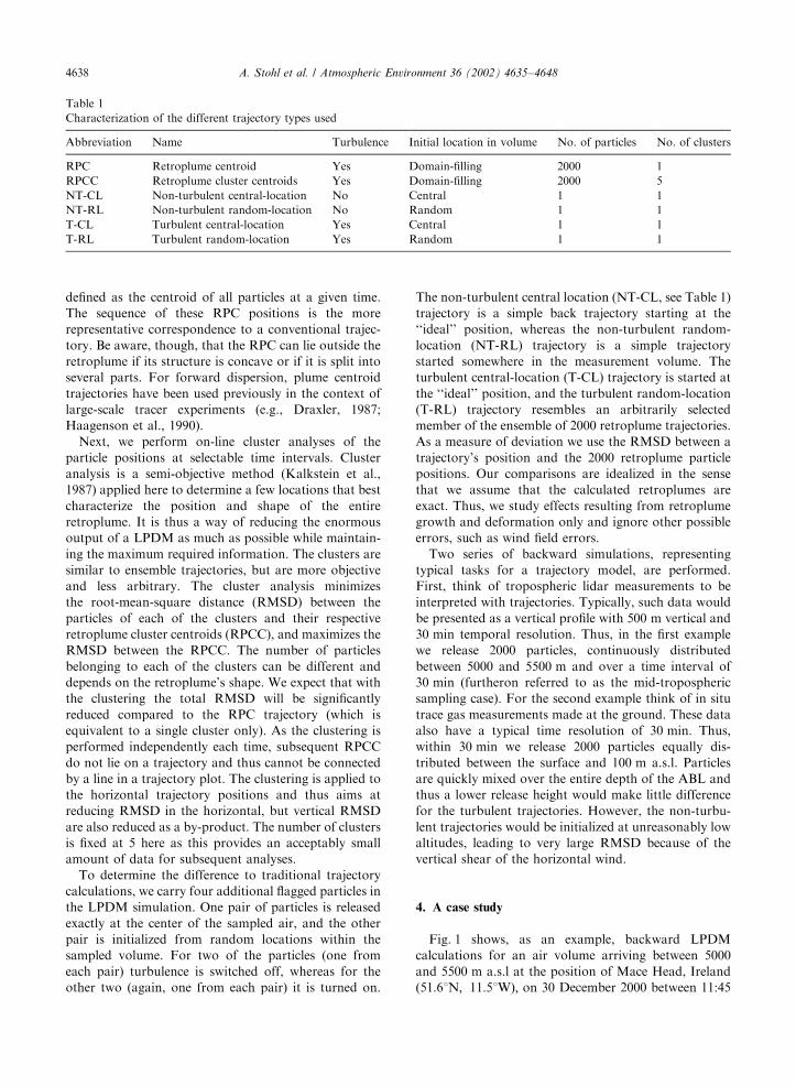
To determine the difference to traditional trajectory

calculations, we carry four additional flagged particles in

the LPDM simulation. One pair of particles is released

exactly at the center of the sampled air, and the other

pair is initialized from random locations within the

sampled volume. For two of the particles (one from

each pair) turbulence is switched off, whereas for the

other two (again, one from each pair) it is turned on.

The non-turbulent central location (NT-CL, see Table 1)

trajectory is a simple back trajectory starting at the

‘‘ideal’’ position, whereas the non-turbulent random-

location (NT-RL) trajectory is a simple trajectory

started somewhere in the measurement volume. The

turbulent central-location (T-CL) trajectory is started at

the ‘‘ideal’’ position, and the turbulent random-location

(T-RL) trajectory resembles an arbitrarily selected

member of the ensemble of 2000 retroplume trajectories.

As a measure of deviation we use the RMSD between a

trajectory’s position and the 2000 retroplume particle

positions. Our comparisons are idealized in the sense

that we assume that the calculated retroplumes are

exact. Thus, we study effects resulting from retroplume

growth and deformation only and ignore other possible

errors, such as wind field errors.

Two series of backward simulations, representing

typical tasks for a trajectory model, are performed.

First, think of tropospheric lidar measurements to be

interpreted with trajectories. Typically, such data would

be presented as a vertical profile with 500 m vertical and

30 min temporal resolution. Thus, in the first example

we release 2000 particles, continuously distributed

between 5000 and 5500 m and over a time interval of

30 min (furtheron referred to as the mid-tropospheric

sampling case). For the second example think of in situ

trace gas measurements made at the ground. These data

also have a typical time resolution of 30 min: Thus,within 30 min we release 2000 particles equally dis-

tributed between the surface and 100 m a.s.l. Particles

are quickly mixed over the entire depth of the ABL and

thus a lower release height would make little difference

for the turbulent trajectories. However, the non-turbu-

lent trajectories would be initialized at unreasonably low

altitudes, leading to very large RMSD because of the

vertical shear of the horizontal wind.

4. A case study

Fig. 1 shows, as an example, backward LPDM

calculations for an air volume arriving between 5000

and 5500 m a.s.l at the position of Mace Head, Ireland

ð51:61N; 11:51WÞ; on 30 December 2000 between 11:45

Table 1

Characterization of the different trajectory types used

Abbreviation Name Turbulence Initial location in volume No. of particles No. of clusters

RPC Retroplume centroid Yes Domain-filling 2000 1

RPCC Retroplume cluster centroids Yes Domain-filling 2000 5

NT-CL Non-turbulent central-location No Central 1 1

NT-RL Non-turbulent random-location No Random 1 1

T-CL Turbulent central-location Yes Central 1 1

T-RL Turbulent random-location Yes Random 1 1


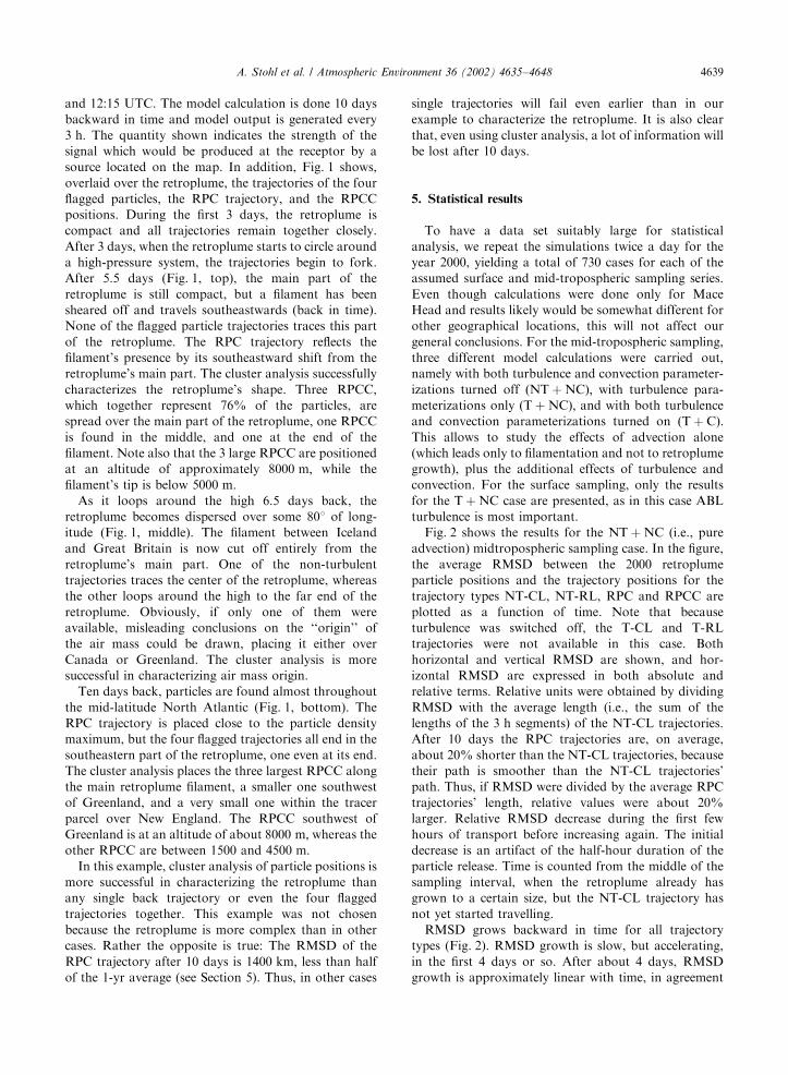
and 12:15 UTC. The model calculation is done 10 days

backward in time and model output is generated every

3 h: The quantity shown indicates the strength of the

signal which would be produced at the receptor by a

source located on the map. In addition, Fig. 1 shows,

overlaid over the retroplume, the trajectories of the four

flagged particles, the RPC trajectory, and the RPCC

positions. During the first 3 days, the retroplume is

compact and all trajectories remain together closely.

After 3 days, when the retroplume starts to circle around

a high-pressure system, the trajectories begin to fork.

After 5.5 days (Fig. 1, top), the main part of the

retroplume is still compact, but a filament has been

sheared off and travels southeastwards (back in time).

None of the flagged particle trajectories traces this part

of the retroplume. The RPC trajectory reflects the

filament’s presence by its southeastward shift from the

retroplume’s main part. The cluster analysis successfully

characterizes the retroplume’s shape. Three RPCC,

which together represent 76% of the particles, are

spread over the main part of the retroplume, one RPCC

is found in the middle, and one at the end of the

filament. Note also that the 3 large RPCC are positioned

at an altitude of approximately 8000 m; while the

filament’s tip is below 5000 m:As it loops around the high 6.5 days back, the

retroplume becomes dispersed over some 801 of long-

itude (Fig. 1, middle). The filament between Iceland

and Great Britain is now cut off entirely from the

retroplume’s main part. One of the non-turbulent

trajectories traces the center of the retroplume, whereas

the other loops around the high to the far end of the

retroplume. Obviously, if only one of them were

available, misleading conclusions on the ‘‘origin’’ of

the air mass could be drawn, placing it either over

Canada or Greenland. The cluster analysis is more

successful in characterizing air mass origin.

Ten days back, particles are found almost throughout

the mid-latitude North Atlantic (Fig. 1, bottom). The

RPC trajectory is placed close to the particle density

maximum, but the four flagged trajectories all end in the

southeastern part of the retroplume, one even at its end.

The cluster analysis places the three largest RPCC along

the main retroplume filament, a smaller one southwest

of Greenland, and a very small one within the tracer

parcel over New England. The RPCC southwest of

Greenland is at an altitude of about 8000 m; whereas theother RPCC are between 1500 and 4500 m:In this example, cluster analysis of particle positions is

more successful in characterizing the retroplume than

any single back trajectory or even the four flagged

trajectories together. This example was not chosen

because the retroplume is more complex than in other

cases. Rather the opposite is true: The RMSD of the

RPC trajectory after 10 days is 1400 km; less than half

of the 1-yr average (see Section 5). Thus, in other cases

single trajectories will fail even earlier than in our

example to characterize the retroplume. It is also clear

that, even using cluster analysis, a lot of information will

be lost after 10 days.

5. Statistical results

To have a data set suitably large for statistical

analysis, we repeat the simulations twice a day for the

year 2000, yielding a total of 730 cases for each of the

assumed surface and mid-tropospheric sampling series.

Even though calculations were done only for Mace

Head and results likely would be somewhat different for

other geographical locations, this will not affect our

general conclusions. For the mid-tropospheric sampling,

three different model calculations were carried out,

namely with both turbulence and convection parameter-

izations turned off ðNTþNCÞ; with turbulence para-

meterizations only ðTþNCÞ; and with both turbulence

and convection parameterizations turned on ðTþ CÞ:This allows to study the effects of advection alone

(which leads only to filamentation and not to retroplume

growth), plus the additional effects of turbulence and

convection. For the surface sampling, only the results

for the TþNC case are presented, as in this case ABL

turbulence is most important.

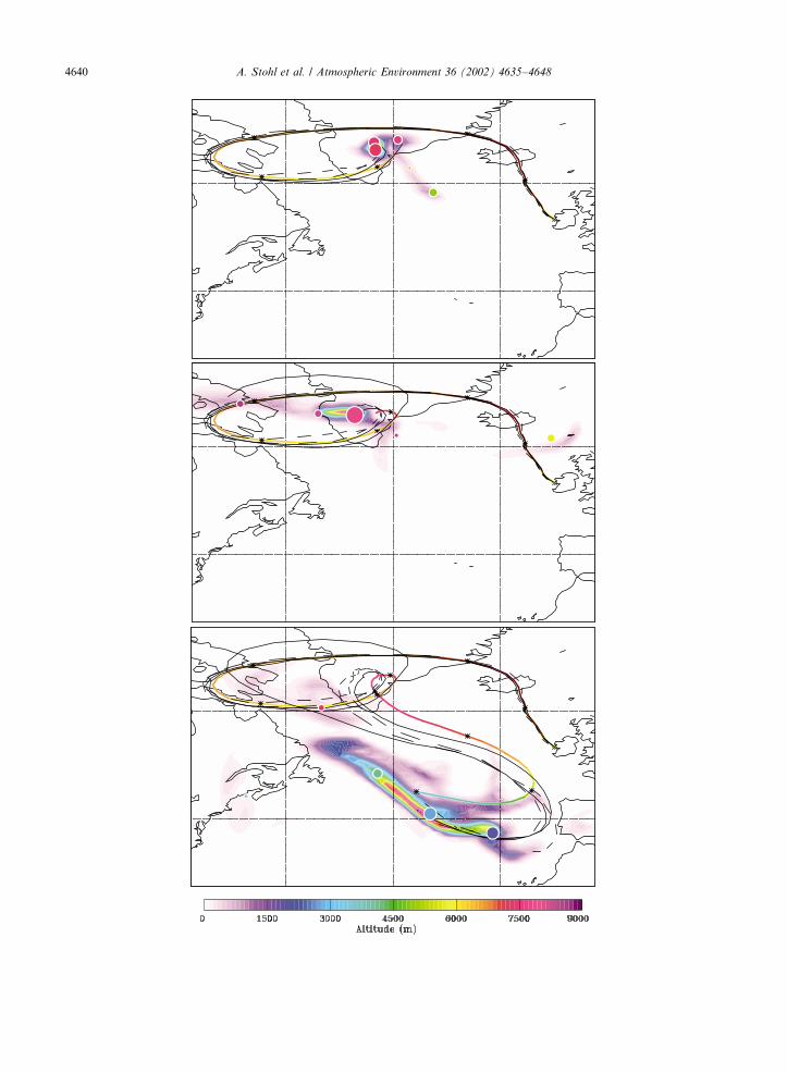
Fig. 2 shows the results for the NTþNC (i.e., pure

advection) midtropospheric sampling case. In the figure,

the average RMSD between the 2000 retroplume

particle positions and the trajectory positions for the

trajectory types NT-CL, NT-RL, RPC and RPCC are

plotted as a function of time. Note that because

turbulence was switched off, the T-CL and T-RL

trajectories were not available in this case. Both

horizontal and vertical RMSD are shown, and hor-

izontal RMSD are expressed in both absolute and

relative terms. Relative units were obtained by dividing

RMSD with the average length (i.e., the sum of the

lengths of the 3 h segments) of the NT-CL trajectories.

After 10 days the RPC trajectories are, on average,

about 20% shorter than the NT-CL trajectories, because

their path is smoother than the NT-CL trajectories’

path. Thus, if RMSD were divided by the average RPC

trajectories’ length, relative values were about 20%

larger. Relative RMSD decrease during the first few

hours of transport before increasing again. The initial

decrease is an artifact of the half-hour duration of the

particle release. Time is counted from the middle of the

sampling interval, when the retroplume already has

grown to a certain size, but the NT-CL trajectory has

not yet started travelling.

RMSD grows backward in time for all trajectory

types (Fig. 2). RMSD growth is slow, but accelerating,

in the first 4 days or so. After about 4 days, RMSD

growth is approximately linear with time, in agreement


with the theory of long-range atmospheric dispersion

(Arya, 1999). After 10 days, both NT-CL and NT-RL

trajectories have very large RMSD of about 3200 km or

23% of the travel distance, which is comparable to, or

even larger than, typical trajectory errors resulting from

all sources of error together (Stohl, 1998). During the

first few days (best seen in the relative RMSD plots,

Fig. 2, middle panel) the differences between the two

flagged trajectories are relatively large, with the NT-CL

trajectories travelling closer to the RPC. However, after

10 days both have similar RMSD, indicating that

accuracy is not much improved by starting the

trajectories exactly at the center of the volume.

Tracing the RPC instead of an individual particle,

reduces the RMSD significantly. But after 10 days

RMSD is still 2500 km or about 17% of the transport

distance, which is still on the same order of magnitude as

typical trajectory errors. Only the cluster analysis can

reduce RMSD to values smaller than typical trajectory

errors. After 10 days, RMSD for the RPCC trajectories

is about 800 km; or just above 5%. During the

first 4 days it is even below 2%, which is an order of

magnitude smaller than typical trajectory errors. Note

that the clustering actually can decrease RMSD to any

desired level, if the number of clusters is increased. But

even with only 5 RPCC, the RMSD reduction is

substantial.

Vertical RMSD are also very large (almost 3000 m for

the NT-CL and NT-RL trajectories after 10 days), but

show similar characteristics as horizontal RMSD.

Although the clustering was done with respect to the

horizontal positions, it is also quite successful in

reducing vertical RMSD (by more than 50% relative

to the NT-CL and NT-RL trajectories). The reason for

that is that parts of the particle cloud at different levels

will be transported by winds with different directions

and velocities, like in the case study shown above.

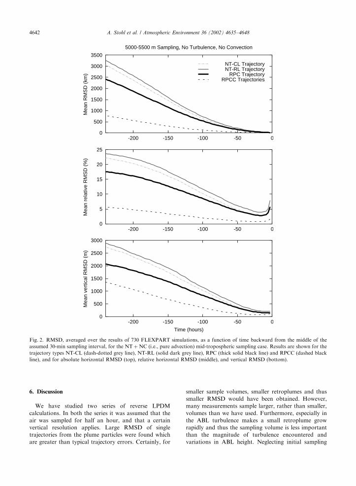
Fig. 3 shows the same as Fig. 2, but with turbulence

switched on. After 10 days, RMSD of the individual

trajectories are almost 4000 km or about 27% of the

travelled distance. Differences between all 4 flagged-

particle trajectories are rather small. Both non-turbulent

trajectories have somewhat smaller RMSD than the

turbulent ones, as they tend to trace the RPC more

closely. The RMSD reduction by the RPC is again

significant, but not large enough to yield acceptable

results. The amount of reduction of the RMSD achieved

by considering the five clusters indicates that the total

spread of the particle cloud is well captured with this

number of clusters and reduces the RMSD to values

below typical trajectory errors.

Switching on also the convection parameterization

further increases RMSD of all trajectory types (not

shown). The individual trajectories now have RMSD of

4100–4300 km (i.e., relative RMSD of more than 30%)

after 10 days, RPC trajectories have a mean RMSD of

3300 km (24%), and RPCC trajectories have a mean

RMSD of about 1300 km (9%). Vertical RMSD are

also substantially increased compared to the convection-

free cases: 3600 m for individual trajectories, 2600 m for

RPC trajectories, and 2200 m for RPCC trajectories,

after 10 days.

For the ABL sampling the largest RMSD are

produced by the non-turbulent trajectories (Fig. 4),

which is different from the mid-tropospheric sampling

cases. The reason for this is that the non-turbulent

trajectories neglect the vertical mixing within the ABL.

This is accounted for by the turbulent trajectories,

whereas the altitude of the non-turbulent trajectories

can increase only due to the grid-scale vertical motion.

RMSD could possibly be reduced by starting the non-

turbulent trajectories at a higher altitude. For instance,

925 or 850 hPa are often used as starting heights for

back trajectories from surface stations. However,

because ABL heights vary both seasonally and with

the time of the day, a constant starting altitude is not a

real solution.

Absolute RMSD are comparable to the mid-tropo-

spheric sampling case, but, because of the lower wind

speeds in the lower troposphere, the relative RMSD are

much larger, on the order of 40% of the distance

travelled after 10 days. Again, only the clustering can

reduce RMSD to an acceptable level. However, vertical

RMSD are quite large, even after clustering.

Fig. 1. Maps showing the retroplume starting from an altitude range 5000–5500 m a.s.l. over Mace Head on 30 December 2000

between 11:45 and 12:15 UTC. Depicted on the map, which covers the Atlantic region ð771W–31W; 281N–751NÞ; are vertically

averaged particle densities 5.5 days back (top), 6.5 days back (middle) and 10 days back (bottom), colored according to the particle

density in arbitrary units. Superimposed on the retroplume are; (1) the RPC trajectory (thick line colored according to altitude as given

in the label bar; positions are marked with asterisks every 24 hours); (2) the NT-CL trajectory starting at 5250 m a.s.l. at 12 UTC, and

the NT-RL starting at an arbitrary location in space and time within the assumed altitude range and time interval (both in solid black

lines); (3) the T-CL trajectory starting at 5250 m a.s.l. at 12 UTC, and the T-RL trajectory starting at an arbitrary location in space and

time within the assumed altitude range and time interval (both dashed black lines); and (4) the five RPCC positions (dots colored

according to altitude as given in the label bar; the dots’ size is scaled with the number of cluster members). RPCC positions are shown

only for the times for which retroplumes are also shown, whereas trajectories are drawn from the starting position to the time for which

the retroplume is shown. Note that the same color code is used both for the RPCC vertical positions and for the retroplume’s particle

density.


6. Discussion

We have studied two series of reverse LPDM

calculations. In both the series it was assumed that the

air was sampled for half an hour, and that a certain

vertical resolution applies. Large RMSD of single

trajectories from the plume particles were found which

are greater than typical trajectory errors. Certainly, for

smaller sample volumes, smaller retroplumes and thus

smaller RMSD would have been obtained. However,

many measurements sample larger, rather than smaller,

volumes than we have used. Furthermore, especially in

the ABL turbulence makes a small retroplume grow

rapidly and thus the sampling volume is less important

than the magnitude of turbulence encountered and

variations in ABL height. Neglecting initial sampling

0

500

1000

1500

2000

2500

3000

3500

-200 -150 -100 -50 0

Mea

n R

MS

D (

km)

5000-5500 m Sampling, No Turbulence, No Convection

NT-CL TrajectoryNT-RL Trajectory

RPC TrajectoryRPCC Trajectories

0

5

10

15

20

25

-200 -150 -100 -50 0

Mea

n re

lativ

e R

MS

D (

%)

0

500

1000

1500

2000

2500

3000

-200 -150 -100 -50 0

Mea

n ve

rtic

al R

MS

D (

m)

Time (hours)

Fig. 2. RMSD, averaged over the results of 730 FLEXPART simulations, as a function of time backward from the middle of the

assumed 30-min sampling interval, for the NTþNC (i.e., pure advection) mid-tropospheric sampling case. Results are shown for the

trajectory types NT-CL (dash-dotted grey line), NT-RL (solid dark grey line), RPC (thick solid black line) and RPCC (dashed black

line), and for absolute horizontal RMSD (top), relative horizontal RMSD (middle), and vertical RMSD (bottom).


volumes and/or turbulence thus can always cause

serious errors in derived source–receptor relationships

for the sample.

LPDM results depend on parameterizations of

turbulence and convection, which are less accurate than

the winds resolved by the meteorological analyses. Thus,

replacing a trajectory model with a LPDM introduces a

significant additional source of error. However, even

larger errors in source–receptor relationships based on

traditional trajectory calculations occur by ignoring

turbulence and convection. While it is of course

desirable to improve the parameterizations, we firmly

believe that even with those currently available trajec-

tory accuracy can be improved.

A critical factor for the applicability of the RPCC

method is computation time. As implemented in

0

500

1000

1500

2000

2500

3000

3500

4000

-200 -150 -100 -50 0

Mea

n R

MS

D (

km)

5000-5500 m Sampling, Turbulence, No Convection


T-CL TrajectoryT-RL TrajectoryRPC Trajectory

RPCC Trajectories

0

5

10

15

20

25

30

-200 -150 -100 -50 0

Mea

n re

lativ

e R

MS

D (

%)

0

500

1000

1500

2000

2500

3000

3500

-200 -150 -100 -50 0

Mea

n ve

rtic

al R

MS

D (

m)

Time (hours)

Fig. 3. RMSD, averaged over the results of 730 FLEXPART simulations, as a function of time backward from the middle of the

assumed 30-min sampling interval, for the TþNC (i.e., turbulence only) mid-tropospheric sampling case. Results are shown for the

trajectory types NT-CL (dash-dotted grey line), NT-RL (solid dark grey line), T-CL (thin solid black line), T-RL (dotted grey line)

RPC (thick solid black line) and RPCC (dashed black line), and for absolute horizontal RMSD (top), relative horizontal RMSD

(middle), and vertical RMSD (bottom).


FLEXPART, the CPU time for 730 individual 10-day

backward simulations (i.e., two per day over a 1-yr

period) with 2000 particles each and without convection

parameterization was about 45 h on a Linux work-

station with a 1 GHz Pentium III processor. This

appears acceptable given the tremendous gain in

accuracy compared to traditional trajectory calcula-

tions. Furthermore, there is potential for further

optimizations. For example, the number of particles

could be reduced to a few hundred per simulation

without large loss of information, especially for shorter

travel times, and the cluster analysis, which is rather

time-consuming, could be stopped before perfect con-

vergence is achieved.

We receive additional benefits from the LPDM

simulation compared to normal trajectory calculations.

For instance, often it is important to know to what

extent a sampled air volume was influenced by air from

the boundary layer or by air from the stratosphere.

At every time step we thus calculate the fraction of

particles that reside inside the ABL, the fraction located

above the thermal tropopause, and the fraction with a

potential vorticity greater than a threshold value

considered to be representative for the stratosphere.

0

500

1000

1500

2000

2500

3000

-200 -150 -100 -50 0

Mea

n R

MS

D (

km)

0-100 m Sampling, Turbulence, No Convection


T-CL TrajectoryT-RL TrajectoryRPC Trajectory

RPCC Trajectories

0

5

10

15

20

25

30

35

40

45

-200 -150 -100 -50 0

Mea

n re

lativ

e R

MS

D (

%)

0

500

1000

1500

2000

2500

-200 -150 -100 -50 0

Mea

n ve

rtic

al R

MS

D (

m)

Time (hours)

Fig. 4. Same as Fig. 3, but for the surface sampling TþNC case.


Fig. 5. Characterization of ten ‘‘retroplumes’’ for a hypothetical vertical sounding from 0 to 10000 m with a resolution of 1000 m at

the location of Mace Head on 30 December 2000 at 12 UTC. In the upper map, RPC trajectories are drawn for each of the 10 height

intervals. Each trajectory consists of a middle line, the color of which (according to the label bar) indicates the actual trajectory height,

that is framed by two outer lines of constant color representing arrival height. Time backward in days is indicated by large numbers

along the RPC trajectories. In addition, the RPCC positions are plotted as dots every 24 hours: The dots’ size is scaled with the numberof cluster members, the inner dots’ color codes for actual RPCC height, and the outer dots’ color codes for arrival height. Numbers on

the dots give the days backward in time. The lower panels show timeseries of the altitudes of the RPC trajectories (lines) and, every

30 h; the heights of the RPCCs (dots whose size scales with the number of cluster members) (coloring for both lines and dots accordingto arrival height); the fraction of the particles residing in the ABL; and the fraction of particles residing in the stratosphere (coloring

again according to arrival height).


This preserves important information from the full

LPDM simulation. And finally, the RMSD values are

calculated totally and for each cluster individually.

As the RMSD varies substantially from case to case,

this is an important information on the representativity.

There is also the option of regular backward LPDM

simulations using gridded output of full quantitative

source–receptor relations, which certainly is the method

of choice if only a limited number of observations are to

be interpreted and thus the LPDM output remains

manageable.

Graphical presentation of the results of our new

method is somewhat different from traditional trajectory

(or trajectory ensemble) plots and is considerably more

complex. Fig. 5 shows, for the same case as described in

Section 4, one possibility of how the results of several

calculations can be visualized in one plot. For the plot it

was assumed that an atmospheric sounding upto 10 km

with a vertical resolution of 1 km was made. For each

altitude interval, a LPDM backward calculation was

performed and characterized by the RPC trajectory

and the RPCCs. Detailed information on the origin of

the air masses at different levels is contained in the chart.

For instance, the altitudes at which the different air

masses travelled and the geographical regions from

where they originated can be clearly distinguished. It is

also readily seen to which extent each measurement was

influenced by air from the stratosphere and the ABL.

With our method, the major transport processes

influencing an entire atmospheric sounding can thus

still be visualized in a single, admittedly complex, plot.

Once acquainted with these charts, a series of them

could, for instance, be used to efficiently investigate the

nature of all the structures typically seen in lidar

timeseries.

We conclude this section with a cautionary note on

the terms accuracy and uncertainty. By definition,

RMSD obtained for a set of RPCC will be smaller than

the RPC RMSD, which in turn will be smaller than any

single trajectory’s RMSD. Thus, the retroplume struc-

ture is always best characterized by the set of RPCC

and, hence, we consider our method as more accurate.

However, when a pollution source shall be identified

this is a small advantage in cases when the retroplume

covers the whole (or large parts of the) atmosphere,

because then the source can be located everywhere,

and the method does not help to determine the

origin of the pollutant. The nature of dispersion leads

to a loss of information (equivalent to an increase of

entropy) with time. Therefore, the scale of potential

source regions for which meaningful information

can be obtained becomes larger the longer we go back

in time, irrespective of what method we use for the

calculations. However, our method yields at least an

estimate of this scale, in contrast to single back

trajectory calculations.

7. Conclusions

Single back trajectory calculations neglect that trace

substance measurements in the atmosphere require a

certain volume of air to be sampled. Advection in

chaotic flows leads to filamentation of this volume of air,

which cannot be represented by a single trajectory.

Furthermore, turbulence increases the volume of air

from where influences (emissions, for example) can be

propagated into the measurement. We have quantified

the errors that are incurred if these effects are neglected,

and we have developed a method to take them into

account properly while still producing a well-manage-

able output, based on LPDM simulations and output

condensation by cluster analysis. Our conclusions are

summarized as follows:

* The average RMS deviations due to retroplume

filamentation and growth between individual trajec-

tories and the condensed LPDM output are on the

order of 20–40% of the distance travelled after 10

days. This is more than the errors resulting from

wind field analysis, interpolation and numerical

truncation together. It is thus of vital importance to

consider retroplume growth and filamentation in

receptor-oriented transport simulations for the inter-

pretation of atmospheric trace substance measure-

ments.* Tracing the retroplume’s centers yields an ensemble-

average trajectory that is more representative than

any single-particle trajectory. After 10 days, the

average RMSD of the ensemble- average trajectories

is approximately 20–30% smaller than that of the

individual trajectories. However, this is still large

compared to other trajectory errors.* LPDM output is four dimensional and thus quite big

and complex. Therefore, in order to analyze large

measurement data sets, a way had to be developed to

condense the enormous LPDM output into a work-

able data set. We propose cluster analysis of particle

positions for this purpose, as it preserves a maximum

of information in a minimum of output.* Using five clusters, which leads to data sets compar-

able in size to current ensemble-trajectory methods,

about 90% of the spread of the cloud is still being

captured for 10-day backward simulations.* Thus we recommend to replace simple back trajectory

calculations for the interpretation of atmospheric

trace substance measurements by backward simula-

tions with a LPDM, possibly combined with on-line

clustering of particle positions as introduced here.

The source code and documentation of FLEXPART

can be downloaded from http://www.forst.tu-muench-

en.de/EXT/LST/METEO/stohl/.


http://www.forst.tu-muenchen.de/EXT/LST/METEO/stohl/

http://www.forst.tu-muenchen.de/EXT/LST/METEO/stohl/

Acknowledgements

This study was part of the projects CARLOTTA,

ATMOFAST and CONTRACE, funded by the German

Federal Ministry for Education and Research within the

Atmospheric Research Program 2000 (AFO, 2000). We

thank K. Emanuel for making available the source code

of the convection scheme, and A. Frank for assistance in

implementing it into FLEXPART. ECMWF and the

German Weather Service are acknowledged for permit-

ting access to the ECMWF archives. Two anonymous

referees are acknowledged for careful reading. Their

thoughtful reviews helped to improve this manuscript.

References

Arya, S.P., 1999. Air Pollution Meteorology and Dispersion.

Oxford University Press, New York.

Ashbaugh, L.L., 1983. A statistical trajectory technique for

determining air pollution source regions. Journal of Air

Pollution Control Association 33, 1096–1098.

Doty, K.G., Perkey, D.J., 1993. Sensitivity of trajectory

calculations to the temporal frequency of wind data.

Monthly Weather Review 121, 387–401.

Draxler, R.R., 1987. Sensitivity of a trajectory model to the

spatial and temporal resolution of the meteorological data

during CAPTEX. Journal of Climate and Applied Meteor-

ology 26, 1577–1588.

Dutton, J.A., 1986. The Ceaseless Wind an Introduction to the

Theory of Atmospheric Motion. Dover, New York, 617pp.

ECMWF, 1995. User Guide to ECMWF Products 2.1.

Meteorological Bulletin M3.2. ECMWF, Reading, UK.

Emanuel, K.A., Zivkovic-Rothman, M., 1999. Development

and evaluation of a convection scheme for use in climate

models. Journal of Atmospheric Science 56, 1766–1782.

Flesch, T.K., Wilson, J.D., Yee, E., 1995. Backward-time

Lagrangian stochastic dispersion models and their applica-

tion to estimate gaseous emissions. Journal of Applied

Meteorology 34, 1320–1332.

Forster, C., Wandinger, U., Wotawa, G., James, P., Mattis, I.,

Althausen, D., Simmonds, P., O’Doherty, S., Kleefeld, C.,

Jennings, S.G., Schneider, J., Trickl, T., Kreipl, S., J.ager,

H., Stohl, A., 2001. Transport of boreal forest fire emissions

from Canada to Europe. Journal of Geophysics Research

106, 22887–22906.

Freitas, S.R., et al., 2000. A convective kinematic trajectory

technique for low-resolution atmospheric models. Journal

of Geophysical Research 105, 24375–24386.

Fuelberg, H.E., et al., 2001. A meteorological overview of the

second Pacific Exploratory Mission in the Tropics. Journal

of Geophysical Research 106, 32427–32443.

Haagenson, P.L., Gao, K., Kuo, Y.-H., 1990. Evaluation of

meteorological analyses, simulations, and long-range trans-

port using ANATEX surface tracer data. Journal of

Applied Meteorology 29, 1268–1283.

Kahl, J.D., 1993. A cautionary note on the use of air

trajectories in interpreting atmospheric chemistry measure-

ments. Atmospheric Environment 27A, 3037–3038.

Kahl, J.D.W., 1996. On the prediction of trajectory model

error. Atmospheric Environment 30, 2945–2957.

Kalkstein, L.S., Tan, G., Skindlov, J.A., 1987. An evaluation of

three clustering procedures for use in synoptic climatologi-

cal classification. Journal of Climate and Applied Meteor-

ology 26, 717–730.

Merrill, J.T., Bleck, R., Avila, L., 1985. Modeling atmospheric

transport to the Marshall islands. Journal of Geophysical

Research 90, 12927–12936.

Moody, J.L., Galloway, J.N., 1988. Quantifying the relationship

between atmospheric transport and the chemical composi-

tion of precipitation on Bermuda. Tellus 40B, 463–479.

Pudykiewicz, J.A., Koziol, A.S., 1998. An application of the

theory of kinematics of mixing to the study of tropospheric

dispersion. Atmospheric Environment 32, 4227–4244.

Rodean, H., 1996. Stochastic Lagrangian models of turbulent

diffusion. Meteorological Monographs, Vol. 26(48). Amer-

ican Meteorological Society, Boston, USA.

Rolph, G.D., Draxler, R.R., 1990. Sensitivity of three-dimen-

sional trajectories to the spatial and temporal densities of

the wind field. Journal of Applied Meteorology 29,

1043–1054.

Seibert, P., 1993. Convergence and accuracy of numerical

methods for trajectory calculations. Journal of Applied


Seibert, P., 2001. Inverse modelling with a Lagrangian particle

dispersion model: application to point releases over limited

time intervals. In: Gryning, S.E., Schiermeier, F.A. (Eds.),

Air Pollution Modeling and its Application, Vol. XIV.

Proceedings of ITM, Boulder. Plenum Press, New York,

pp. 381–389.

Seibert, P., Stohl, A., 2000. Inverse modelling of the ETEX-1

release with a Lagrangian particle model. In: Barone, G.,

Builtjes, P.J., Giunta, G. (Eds.), GLObal and REgional

Atmospheric Modelling. Annali dell’Istituto Universitario

Navale di Napoli, Special Issue, 95–105. Proceedings of the

Third GLOREAM Workshop, September 1999, Ischia,

Italy.

Seibert, P., Kromp-Kolb, H., Baltensperger, U., Jost, D.T.,

Schwikowski, M., 1994. Trajectory analysis of high-alpine

air pollution data. In: Gryning, S.-E., Millan, M.M. (Eds.),

Air Pollution Modelling and its Application, Vol. X,

Plenum Press, New York, pp. 595–596.

Seibert, P., Kr .uger, B., Frank, A., 2001. Parametrisation of

convective mixing in a Lagrangian particle dispersion

model. Proceedings of the Fifth GLOREAM Workshop,

Wengen, Switzerland, 24–26 September 2001.

Siems, S.T., Hess, G.D., Suhre, K., Businger, S., Draxler, R.,

2000. The impact of wind shear on observed and simulated

trajectories during the ACE-1 Lagrangian experiments.

Australian Meteorological Magazine 30, 579–587.

Smith, F.B., 1965. The role of windshear in horizontal diffusion

of ambient particles. Quarterly Journal of the Royal

Meteorological Society 91, 318–329.

Stohl, A., 1996. Trajectory statistics—a new method to

establish source–receptor relationships of air pollutants

and its application to the transport of particulate sulfate in

Europe. Atmospheric Environment 30, 579–587.

Stohl, A., 1998. Computation, accuracy and applications of

trajectories—a review and bibliography. Atmospheric En-

vironment 32, 947–966.


Stohl, A., Thomson, D.J., 1999. A density correction for

Lagrangian particle dispersion models. Boundary-Layer


Stohl, A., Trickl, T., 1999. A textbook example of long-range

transport: simultaneous observation of ozone maxima of

stratospheric and North American origin in the free

troposphere over Europe. Journal of the Geophysical

Research 104, 30445–30462.

Stohl, A., Wotawa, G., 1995. A method for computing single

trajectories representing boundary layer transport. Atmo-

spheric Environment 29, 3235–3239.

Stohl, A., Wotawa, G., Seibert, P., Kromp-Kolb, H., 1995.

Interpolation errors in wind fields as a function of spatial

and temporal resolution and their impact on different types

of kinematic trajectories. Journal of Applied Meteorology

34, 2149–2165.

Stohl, A., Hittenberger, M., Wotawa, G., 1998. Validation of

the Lagrangian particle dispersion model FLEXPART

against large scale tracer experiment data. Atmospheric

Environment 32, 4245–4264.

Thomson, D.J., 1987. Criteria for the selection of stochastic

models of particle trajectories in turbulent flows. Journal of

Fluid Mechanics 180, 529–556.

Walmsley, J.L., Mailhot, J., 1983. On the numerical accuracy of

trajectory models for long-range transport of atmospheric

pollutants. Atmospheric Ocean 21, 14–39.


A replacement for simple back trajectory calculations in the interpretation of atmospheric trace...

Documents

Transcript of A replacement for simple back trajectory calculations in the interpretation of atmospheric trace...