ERIM REPORT SERIES RESEARCH IN MANAGEMENT ERIM Report Series reference number ERS-2005-063-F&A Publication October 2005 Number of pages 29 Persistent paper URL Email address corresponding author pouchkarev@few.eur.nl Address Erasmus Research Institute of Management (ERIM)

RSM Erasmus University / Erasmus School of Economics Erasmus Universiteit Rotterdam P.O.Box 1738 3000 DR Rotterdam, The Netherlands Phone: + 31 10 408 1182 Fax: + 31 10 408 9640 Email: info@erim.eur.nl Internet: www.erim.eur.nl

Bibliographic data and classifications of all the ERIM reports are also available on the ERIM website:

www.erim.eur.nl

A Relative View on Tracking Error

Winfried G. Hallerbach and Igor W. Pouchkarev

ERASMUS RESEARCH INSTITUTE OF MANAGEMENT

REPORT SERIES RESEARCH IN MANAGEMENT

ABSTRACT AND KEYWORDS Abstract When delegating an investment decisions to a professional manager, investors often anchor

their mandate to a specific benchmark. The manager’s exposure to risk is controlled by means of a tracking error volatility constraint. It depends on market conditions whether this constraint is easily met or violated. Moreover, the performance of the portfolio depends on market conditions. In this paper we argue that these mandated portfolios should not only be evaluated relative to their benchmarks in order to appraise their performance. They should also be evaluated relative to the opportunity set of all portfolios that can be formed under the same mandate – the portfolio opportunity set. The distribution of performance values over the portfolio opportunity set depends on contemporary market dynamics. To correct for this, we suggest a normalized version of the information ratio that is invariant to these market conditions.

Free Keywords Benchmarking, Tracking Error, Information Ratio, Performance Evaluation

Availability The ERIM Report Series is distributed through the following platforms:

Academic Repository at Erasmus University (DEAR), DEAR ERIM Series Portal

Social Science Research Network (SSRN), SSRN ERIM Series Webpage

Research Papers in Economics (REPEC), REPEC ERIM Series Webpage

Classifications The electronic versions of the papers in the ERIM report Series contain bibliographic metadata by the following classification systems:

Library of Congress Classification, (LCC) LCC Webpage

Journal of Economic Literature, (JEL), JEL Webpage

ACM Computing Classification System CCS Webpage

Inspec Classification scheme (ICS), ICS Webpage

1

A RELATIVE VIEW ON

TRACKING ERROR

Winfried G. Hallerbach

& Igor W. Pouchkarev *)

Abstract

When delegating an investment decisions to a professional manager, investors often anchor their mandate to a specific benchmark. The manager’s exposure to risk is controlled by means of a tracking error volatility constraint. It depends on market conditions whether this constraint is easily met or violated. Moreover, the performance of the portfolio depends on market conditions. In this paper we argue that these mandated portfolios should not only be evaluated relative to their benchmarks in order to appraise their performance. They should also be evaluated relative to the opportunity set of all portfolios that can be formed under the same mandate – the portfolio opportunity set. The distribution of performance values over the portfolio opportunity set depends on contemporary market dynamics. To correct for this, we suggest a normalized version of the information ratio that is invariant to these market conditions.

Keywords: benchmarking, tracking error, information ratio, performance evaluation

JEL classification: C15, C43, G11

Rotterdam, October 19, 2005

*) Both Department of Finance, Erasmus University Rotterdam,

POB 1738, NL-3000 DR Rotterdam, The Netherlands Phone: +31.10.408-1290, fax: +31.10.408-9165 E-mail: hallerbach@few.eur.nl, pouchkarev@few.eur.nl

2

A RELATIVE VIEW ON

TRACKING ERROR

Abstract

When delegating an investment decisions to a professional manager, investors often anchor their mandate to a specific benchmark. The manager’s exposure to risk is controlled by means of a tracking error volatility constraint. It depends on market conditions whether this constraint is easily met or violated. Moreover, the performance of the portfolio depends on market conditions. In this paper we argue that these mandated portfolios should not only be evaluated relative to their benchmarks in order to appraise their performance. They should also be evaluated relative to the opportunity set of all portfolios that can be formed under the same mandate – the portfolio opportunity set. The distribution of performance values over the portfolio opportunity set depends on contemporary market dynamics. To correct for this, we suggest a normalized version of the information ratio that is invariant to these market conditions.

Keywords: benchmarking, tracking error, information ratio, performance evaluation

JEL classification: C15, C43, G11

3

1. Introduction

Institutional investment decisions are generally centered around mandates, provided to

professional investment managers. In a typical investment mandate, a benchmark

portfolio is identified and the portfolio manager is assigned the task to beat that

benchmark over a specified horizon. The benchmark portfolio as specified in the

mandate should be attainable and investable1; some examples of benchmarks are the

MSCI World Index (or MSCI region or sector indexes), the S&P500 Index, and the

Dow-Jones Indexes. Depending on his expertise to identify mispriced securities, the

portfolio manager can overweight underpriced securities and underweight overpriced

securities, thus building a zero-investment active portfolio. The composition of this

active portfolio reflects the selection bets made by the portfolio manager. When adding

the active portfolio weight vector to the benchmark weight vector, the composition of

the actual investment portfolio is obtained. The difference between the return on the

managed portfolio and the return on the benchmark is termed the tracking error.

Although the investor is concerned with the return and risk of the total portfolio, the

portfolio manager focuses on the return and risk of the active portfolio only.2

In order to control the risk of the active portfolio, the investment mandate includes

a constraint on the tracking error volatility, henceforth denoted by TEV. The TEV is

defined as the standard deviation of the return differential between the managed

portfolio and the benchmark.3 Of course, the TEV should be monitored in order to

determine whether the portfolio manager satisfies the risk limit on the TEV as specified

in his mandate.4 Over recent years, the financial markets experienced quite large swings

1 For the requirements a benchmark should satisfy, we refer to Reilly [1994, pp.975ff]. See also Rennie & Cowhey [1990] on this point. 2 This induces the portfolio manager to optimize the active portfolio in excess return space only, thus neglecting the total risk of the resulting portfolio. This problem is identified and discussed by Roll [1992], Rohweder [1998] and Jorion [2003]. We do not pursue this particular problem here. 3 The terminology can be confusing. Sometimes the standard deviation of the return differential is termed tracking error. Grinold & Kahn [2000] use the term “statistical tracking error” for TEV. In addition, the choice of standard deviation as a risk measure implies that the relative investment decision is molded in the familiar mean-variance framework. For an alternative formulation, see for example Rudolph, Wolter & Zimmermann [1999]. 4 In the broader context of asset allocation, the investment process is organized hierarchically. Strategic asset allocation decisions at the higher level are made on the basis of benchmark portfolios for asset classes such as equity, fixed income, real estate and cash. In the tactical asset allocation process, the weighting of these benchmarks is allowed to fluctuate between tactical asset allocation (TAA) bands. At the lower level, portfolio managers can in turn deviate from the composition of the asset class benchmarks under the restriction of TEV limits. As shown by Ammann & Zimmermann [2001], deviations from the compositions of the benchmark portfolios at the lower level have a

4

in volatility and this raised serious concerns about the ability of portfolio managers to

obey the ex ante imposed TEV limit.5

The evaluation of the manager’s performance will be of a relative nature, vis à vis

the benchmark. Because the active portfolio is the source of not only return but also

risk, the performance should be gauged on a risk-adjusted basis. For this goal, the

Information Ratio (henceforth IR) is used.6 The IR is defined as the average tracking

error divided by the TEV. The IR hence measures the average excess return relative to

the benchmark portfolio, expressed per unit of volatility in excess return.

The evaluation of the TEV limit and the risk-adjusted performance evaluation are

key issues in the benchmark-based investment process. Within the ex ante imposed

TEV limit, the portfolio manager can compose many portfolios. Given the constrained

portfolio flexibility and given financial market dynamics, each of these portfolios can

exhibit different excess risk – excess return characteristics. So each of these portfolios

can reveal a different TEV ex post facto. In addition, each of these portfolios can show a

different performance and hence generate a different IR.

In this paper we highlight the influence of portfolio flexibility and financial

market conditions on TEV constraints and risk-adjusted performance. We argue that

mandated portfolios should not only be evaluated relative to their benchmarks. They

should also be evaluated relative to the set of all portfolios that can be formed under the

same mandate – the portfolio opportunity set. All portfolios in this set obey the

constraints as specified ex ante facto in the mandate. This portfolio opportunity set can

be used to construct frequency distributions of (risk-adjusted) performance values such

as realized tracking errors and IRs. The particular portfolio at hand is only one element

of this portfolio opportunity set. The location of this portfolio can be plotted in this

distribution and this in turn provides information on the relative position of the portfolio

in the portfolio opportunity set. It may turn out, for example, that in some period 95% of

the portfolios in the portfolio opportunity set performed better that the portfolio at hand.

Irrespective of the absolute value of the chosen performance metric, this relative

information would qualify (if not disqualify) the achievement of the portfolio manager

over the period considered.

greater impact on top level portfolio risk-return characteristics than deviations from the benchmarks’ weights in the top level portfolio. This stresses the relative importance of TEV constraints. 5 See for example Burmeister, Mausser & Mendoza [2005]. 6 See for example Goodwin [1998].

5

In addition to the locus of the investment portfolio in the frequency distribution of

performance values, also the width of this distribution is relevant in evaluating

investment performance. When the distribution of performance values over the portfolio

opportunity set is narrow (broad), this implies that is was hard (easy) to obtain a specific

level of outperformance. The width of this performance distribution is not constant over

time but depends on contemporary market dynamics. When the range of returns on the

individual securities comprised in the benchmark is narrow (we could term this a

“homogeneous market”), differences in active portfolio composition translate to only a

narrow range of active portfolio returns. When in contrast the market is heterogeneous

and individual security returns have fluctuated over a wide range, small differences in

portfolio composition can lead to large differences in portfolio returns. In the former

case, the distribution of performance values over the portfolio opportunity set is narrow.

In the latter case, this distribution will be broad. In practice, a “typical” distribution of

IRs is used in order to assess how extraordinary the risk-adjusted performance of a

portfolio was. Grinold & Kahn [2000], for example, stipulate that the IR exceeds 0.2 for

the top 25% of portfolio managers. However, tracking errors – and hence the IR –

depend on the dynamics in the security returns. Over some periods, then, attaining an IR

of for example 0.1 may be quite extraordinary, whereas other periods allow achieving

an IR of 0.3 or even higher. The information contained in the cross-sectional frequency

distributions of performance values allows for normalizing the IR. In this way, we purge

this performance metric for the influence of market dynamics on the width of the

distribution of over time. In this paper, we discuss the use of portfolio opportunity sets

for monitoring TEV constraints and for relative (risk-adjusted) performance evaluation.

We illustrate our methodology for a fictitious investment portfolio where the Dow-

Jones EURO STOXX 50 Index serves as a benchmark.

The structure of the paper is as follows. In section 2 we introduce notation and

provide the definitions of tracking error and relevant performance metrics. Section 3

outlines the procedure to generate portfolio opportunity sets under TEV constraints.

Section 4 discusses the data and explains how we constructed a managed investment

portfolio. Section 5 contains our empirical results. We illustrate how the portfolio

opportunity set approach can be used to reveal tracking error dynamics, check on

potential TEV violation, and normalize risk-adjusted performance over time. Section 6

concludes and provides suggestions for further research.

6

2. Relative Investing and Tracking Error

Over some period t, the return on the benchmark portfolio B, Btrɶ , is defined as:

(1) 1

n

Bt it it

i

r b r=

=∑ɶ ɶ with budget restriction 1

1n

it

i

b=

=∑

where n is the number of securities in the benchmark, itrɶ is the return on security i, and

itb is the weight of security i in the benchmark at the beginning of period t. Tildes

denote stochastic variables. The portfolio manager deviates from the benchmark by

choosing a portfolio P with weights { } 1,...,it i nw

=. The return on this portfolio over period

t is:

(2) 1

n

Pt it it

i

r w r=

=∑ɶ ɶ with budget restriction 1

1n

it

i

w=

=∑

Consequently, the return on the self-financing active portfolio is:

(3) ( )1

n

Pt Bt it it it

i

r r w b r=

− = −∑ɶ ɶ ɶ with ( )1

0n

it it

i

w b=

− =∑

and the tracking error volatility TEV is:

(4) ( ) ( )( ) ( )1 1

var cov ,n n

Pt Bt it it jt jt it jt

i j

TEV r r w b w b r r= =

= − = − −∑∑ɶ ɶ ɶ ɶ

where var( )⋅ and cov( , )⋅ ⋅ denote the variance and covariance operators, respectively.

The information ratio IR is defined analogous to the Sharpe [1966, 1994] ratio

with the excess returns now measured with respect to the benchmark return:

(5) ( )Pt BtE r r

IRTEV

−=

ɶ ɶ

7

3. Portfolio Opportunity Sets for TEV-restricted Investments

In Pouchkarev [2005], we developed a novel approach for evaluating investment

performance. The central idea behind our approach is not to consider a single

benchmark index to describe a financial market, or a specific peer group to measure

investment performance, but instead to consider all possible portfolios.7 We call the set

of all portfolios that are feasible under a specific investment mandate the portfolio

opportunity set. This set signifies a level playing field for any portfolio that aims for the

same investment objectives and respects the same constraints as specified in the

mandate. The portfolio opportunity set approach can be considered as a formalization of

the Wall Street Journal’s dartboard portfolio approach, in which a random portfolio is

constructed by “throwing darts” at the financial pages of the Wall Street Journal.8 But

instead of focusing on only one random portfolio, the portfolio opportunity set approach

considers the whole set of feasible portfolios. Indeed, in general, the undisputable

advantage of our approach is that the set of generated portfolios can be made

commensurate with any specific investment environment such as an investment

mandate, defined by goals and constraints. Hence, we evaluate the managed portfolio

against that set of all available investment alternatives.

Although the portfolio opportunity set approach is completely general and can be

made commensurate with any investment mandate, we limit ourselves here to a single

constraint on the formation of portfolios: the TEV constraint. Given the portfolio

opportunity set generated under the prevailing TEV constraint, we can measure the

performance of all these alternative portfolios according to the selected performance

criteria: realized return, TEV and IR. We can next evaluate the performance of the

investment portfolio at hand against the performance of this complete opportunity set.

In this way, the portfolio opportunity set can be considered as a synthetic peer group for

the specific investment portfolio. This peer group exactly matches the restrictions under

which a portfolio manager is allowed to operate. We next outline in detail how the

portfolio opportunity set under a TEV constraint can be generated.

7 In Hallerbach et al (2005), we describe an application to market description. 8 For a description of the Wall Street Journal’s dartboard portfolio approach, we refer to Moy [1994] and Adams & Cyree [2004]. An early attempt to such a formalization of random portfolios is provided by Cohen & Fitch [1966]. Fisher [1965] and Fisher & Lorie [1970] also used random portfolios to analyze investment performance.

8

The portfolio opportunity set, which consists of n assets and which is subject to a

TEV constraint, can be specified through the following formal description (see eqs. (3)

and (4)):

(6) 2

1 1

( ) ( ) cov( , ) n n

it it jt jt it jt

i j

w b w b r r ψ= =

− ⋅ − ⋅ ≤∑∑ ɶ ɶ

1

( ) 0n

it it

i

w b=

− =∑

where ψ denotes the maximum allowable level of TEV and where as before bit is the

weight of security i in the targeted benchmark; wi is now the weight of the security i in a

feasible portfolio. It is more convenient to work with such opportunity sets if we

remove the last dependent weight from the system (6). Reorganizing the second

(budget) equation from (6), we have:

(7) 1

1

( )n

nt nt it it

i

w b w b−

=

− = − −∑

Substituting eq.(7) into the first equation of (6), we obtain:

(8) 1 1

2

1 1

cov( , ) 2cov( , ) cov( , ) ( ) ( ) n n

it jt it nt nt nt it it jt jt

i j

r r r r r r w b w b ψ− −

= =

− + ⋅ − ⋅ − ≤ ∑∑ ɶ ɶ ɶ ɶ ɶ ɶ

Denoting the expression in the square brackets by cov( , )it jtr rɶ ɶ , we obtain the modified

expression for representing all active alternative portfolios, which satisfy a given TEV

constraint:

(9) 1 1

2

1 1

cov( , ) ( ) ( ) n n

it jt it it jt jt

i j

r r w b w b ψ− −

= =

⋅ − ⋅ − ≤∑∑ ɶ ɶ

The portfolio opportunity set thus forms a convex polytope in the security weight space

ℝn-1.

9

Given a portfolio opportunity set of the form (9) and a performance measure (e.g.

realized differential return, IR), we are interested to quantify how many of the feasible

portfolios take on a particular performance value. In other words, we are interested in

calculating the frequency distribution of feasible portfolios in terms of values of this

performance measure. These frequency distributions (in our case for differential returns

and IRs) can be estimated numerically. The procedure is based on statistical sampling:

we estimate the distribution of performance values of the whole portfolio opportunity

set through the distribution of performance values of a reasonably large sample of active

portfolios, which are feasible under a given TEV-constraint.

There exist several universal algorithms that can generate a random variable X

over any bounded region Q ⊂ ℝn-1 (as a portfolio opportunity set of the type (9)) with a

given density (in our case uniformly distributed over Q). The general idea of all

algorithms is to construct an ergodic Markov chain, recursively generating a sequence

of points all in Q whose stationary distribution is uniform. If the initial point of the

chain is uniformly distributed over Q and the transition kernel is symmetric, then the

points of the generated sequence will be independent and uniformly distributed over Q

asymptotically. The most known algorithms from the family are the Hit-and-run

algorithm by Smith [1984] and Bélisle et al. [1993], and the Sequential Direction

algorithm by Telgen.9 We adopt the last algorithm to sample random feasible portfolios

for a given TEV-constrained investment mandate.

Having n assets in the opportunity set (for example, 50 stocks constituting the

EURO STOXX 50 index) and transforming the set into the form of eq.(9), the sampling

procedure is formulated as follows:10

1. Choose uniformly a feasible random portfolio p(0)t = (0) (0) (0)

1 2 1, , , nw w w −… in a

given portfolio opportunity set Q (the simplest solution is to sample uniformly

in the neighborhood of the benchmark11);

9 See Berbee et al. [1987] and Ritov [1989]. In the last reference, the Sequential Direction algorithm is called the Coordinate Direction algorithm. Generally, the Sequential Direction algorithm is a slight modification of the Hit-and-Run algorithm proposed by Smith [1984]. 10 For the sake of simplicity we drop in the algorithm the subscript t denoting the time period, as all portfolios from the sample belong to the same period of time. 11 A more sophisticated technique for this preprocessing step with polynomial time is discussed in Lovász [1998].

10

2. Having the last generated portfolio p(s) = ( ) ( ) ( )1 2 1, , ,s s s

nw w w −… (the subscript

s = 0, 1, 2, … denotes the actual step of our ergodic Markov chain), determine

the “changing” weight ( )sjw as the j-th element of p(s) where j is taken

consecutively from the set {1, 2, …, n–1};

3. Substituting all ( )siw but ( )s

jw into the left-hand side of eq.(9) and replacing the

inequality sign with equality, we obtain a quadratic equation of only one

variable ( )sjw . Solving the equation, we obtain two boundary values for ( )s

jw ,

( )sjwɺ and ( )s

jwɺɺɺ . Compute the next value of ( 1)sjw

+ by choosing a point on the

segment ( ) ( ),s sj jw w

ɺɺɺ ɺ uniformly, i.e.

( 1)sjw

+ ~ U ( ( )sjwɺ , ( )s

jwɺɺɺ );

4. Create a new random portfolio extending p(s+1) = ( 1) ( 1) ( 1)1 2 1, , ,s s s

nw w w+ + +

−…

with ( 1) ( )s si iw w

+ = for all elements but ( 1)sjw

+ , a new ( 1)sjw

+ from step 3, and

the last depending weight as:

1( 1) ( 1) ( 1) ( 1)

1 2 11 2 1 1, , , , 1

ns s s sn n in i

w w w w w w w w−+ + + +

− − == = = = −∑… .

Add this new random portfolio to the sample;

5. If the sample is big enough, then stop. Otherwise return to step 2.

Having n assets in the opportunity set, we need to generate at least 3( )nO random

portfolios in order to guarantee the uniformity of the sample over a given TEV-

constrained opportunity set (cf. Lovász [1998]).

The last but not the least issue is the computational speed of the sampling

algorithm. Because we are moving across orthogonal directions by forming a new

random portfolio, the portfolios can be generated rather efficiently. Hence, we can use

large samples (e.g. one million portfolios) when estimating frequency distributions for

TEV-restricted sets. Furthermore, the algorithm can be easily extended to incorporate

additional risk constraints as discussed by Jorion [2003] and Alexander [2004]. In that

11

case, we introduce an additional acceptance-rejection step, which filters out portfolios

violating at least one of these supplementary constraints.

4. Data and Investment Mandate

In the illustration of our methodology, we choose the Dow-Jones EURO STOXX 50

Index as the benchmark portfolio B. This index was introduced on February 28, 1998

and provides a blue-chip representation of industry sectors in Austria, Belgium, Finland,

France, Germany, Greece, Ireland, Italy, Luxembourg, the Netherlands, Portugal and

Spain. 12 It contains 50 stocks and captures almost 60% of the free-float market

capitalization of the represented countries. The weighting of individual stocks is

according to their free-float market capitalization, subject to a 10% weighting cap. The

composition is reviewed annually, in September.

We use end-of-month values of the price index to compute monthly discretely

compounded returns over the period January 1995 through May 2005 (125 monthly

returns). Over the same period we computed monthly price returns on all stocks

comprised at any moment in the index.13,14 This enables us to replicate the index at any

time with individual stocks. In addition, we construct an equally-weighted price index,

EW. In each month, the return on this index is computed as the unweighted arithmetic

average of the price returns on all stocks comprised at that time in the EURO STOXX

50 Index.

12 Index history is available daily back to December 31, 1986. For details, see http://www.stoxx.com. 13 For consistency, we use price returns on both the index and the individual stocks. In our illustrative setting, the exclusion of cash dividends is not important. For actual applications, the use of total returns is appropriate. 14 When a stock is incorporated in the EURO STOXX 50 Index which does not have at least 36 months of return history, we use a recursive regression approach to fill in missing observations. We start with a window of 36 return observations on the stock i and the index B, which begins immediately after the missing return data point for the stock. Within this window, we use OLS regression to estimate the parameters iα and iβ of the market model:

it i i Bt itr rα β ε= + + t = 1,…,36

Given these parameters and the available index return for the first observation t=0 before the start of the window, we next construct the stock return, conditional on the index return: ˆˆ

it Bt i i Btr r rα β= + t=0

Finally, we randomly sample one residual term from the 36 residuals in the estimation window and

add that to 0 0i Br r . We substitute this return for the missing return 0ir . We repeat the procedure by

moving the data window backwards in time until 36 months of history is generated. We implemented this procedure for 6 stocks out of 66.

12

=========================== insert Figure 1 and Table 1 about here ===========================

Figure 1 shows the course of the indexes over the complete sample period and

Table 1, Panel A, provides some descriptive return statistics. From January 1995, the

EURO STOXX 50 Index shows a gradual increase until it reaches a peak in April 2000,

on the way up only fiercely interrupted by the August-September 1998 crash, following

the Russian debt crisis. Then a gradual but steady descend sets in until March 2003,

from whereon the index slowly recovers. The benchmark return has an arithmetic

average of about 10% p.a., with a volatility of 20% p.a. Note that the equally-weighted

index has both a higher average return and a higher standard deviation. However, the

100 bps higher standard deviation does not seem to outweigh the 300 bps higher

average return, and the equally-weighted portfolio clearly outperforms the benchmark

portfolio over the sample period.

One explanation for this outperformance could be the small-cap effect. The

benchmark portfolio is value-weighted (under restrictions on the maximum weights)

and is hence biased towards large cap stocks. The equally-weighted portfolio, in

contrast, is biased towards small cap stocks. When small cap stocks outperform large

cap stocks, the equally-weighted portfolio outperforms the value-weighted portfolio. An

alternative (and perhaps additional) reason for outperformance is the “volatility

pumping” effect.15 The value-weighted portfolio is a buy-and-hold portfolio (at least

between revision moments, which is once a year). The equally-weighted portfolio,

however, is rebalanced every month. This implies that stocks that have performed well

against the portfolio are sold and stocks that have underperformed the index are bought,

in order to keep the portfolio equally-weighted. When the returns on the individual

stocks fluctuate within a range, the “buy low, sell high” strategy generates

outperformance with respect to a buy-and-hold portfolio.

Given the outperformance of the equally-weighted index over the benchmark

portfolio, we synthetically construct an investment portfolio as a linear combination of

the benchmark and the equally-weighted portfolio. The return on this managed portfolio

P in month t is computed as:

15 See for example Luenberger [1998, pp.422ff].

13

(10) ( )1Pt Bt EWtr r rλ λ= − +ɶ ɶ ɶ

where EWtrɶ is the return on the equally-weighted portfolio and the weight λ is a

constant. Hence, the tracking error of portfolio P is:

(11) ( )Pt Bt EWt Btr r r rλ− = −ɶ ɶ ɶ ɶ

and its tracking error volatility, TEV, is:

(12) ( )var EWt Bt EW BTEV r rλ λσ −= − =ɶ ɶ

where EW Bσ − is the standard deviation of the return differential between the equally-

weighted portfolio and the benchmark portfolio, and where 0λ > by construction.

But how do we set the appropriate value for the weight λ? We assume that the

investment mandate sets an upper bound of ψ on the TEV:

(13) TEV ψ≤

Given EW Bσ − and using eq.(12), we obtain the composition of portfolio P that exhibits

the maximum allowed TEV by setting the weight λ in eq.(10) as:

(14) EW B

ψλ

σ −

=

In practice, the mandate will specify the upper bound on TEV on an annual basis. In our

illustration, we work with monthly returns. When returns are intertemporally

uncorrelated and volatility is constant (at least over a year), a TEV constraint of x% per

annum translates into a monthly allowed TEV of / 12x %. In our illustration, we

choose

14

ψ =1.15% per month, which is derived from a maximum allowed TEV of 4% per

annum.

To replicate a feasible investment strategy, we generate out-of-sample returns on

the managed portfolio P. We use the first 36 months of data in our sample to estimate

the standard deviation of the return differential between the equally-weighted portfolio

and the benchmark, EW Bσ − . Using the TEV constraint and eq.(14), we infer the weight

λ and compute the return on the investment portfolio for month 37 according to eq.(10).

Next we shift the estimation window one month forward and repeat the procedure to

obtain the return on the investment portfolio for month 38, and so on. At the end of our

sample period, we finally have 89 out-of-sample returns on portfolio P over the period

January 1998 through May 2005. These returns are generated by a portfolio that ex ante

facto exactly satisfies the TEV constraint. From an ex ante perspective, i.e. on the basis

of the trailing 36 months windows that are used to compose the managed portfolio, the

annualized projected IR ranges from 0.02 to 1.76, with an average value of 0.80.16

Table 1, Panel B, shows the descriptive statistics of this investment portfolio and

its tracking error. The managed portfolio P shows an average realized return of 7.73%

p.a. (with standard deviation of almost 23% p.a., which is 1.2% higher than the

benchmark volatility) and it outperforms the benchmark on average by 2.72% p.a. The

realized TEV is 4.46% which is almost 50 bps higher than the mandated 4%. The ex

ante estimated TEV thus seems to underestimate the ex post TEV. Over the total out-of-

sample period January 1998 through May 2005, the realized mean and standard

deviation of the tracking error yield an annualized IR of 0.61. Compared to the ex ante

IR, this shows the effect of the underestimated risk on the portfolio’s ex post

performance.

In section 5, we analyze the performance of the constructed investment portfolio

P in more detail. More specifically, we use the portfolio opportunity set approach to

evaluate this investment portfolio vis à vis all feasible portfolios under the formulated

investment mandate.

16 Plugging eqs.(11) and (14) in (5) gives ( ) /EWt Bt EW BIR E r r σ −= −ɶ ɶ , which does not depend on

the TEV constraint.

15

5. Empirical Results

We use the procedure as outlined in section 3 to generate portfolio opportunity sets.

Each random investment portfolio satisfies ex ante facto the maximum allowed TEV of

4% p.a. (i.e. ψ =1.15% per month), just as the constructed portfolio P under the

mandate. Since we use a trailing window of 36 monthly observations to estimate the

portfolios’ TEVs, we generate a portfolio opportunity set for each of the 89 months

from January 1998 through May 2005. Each portfolio opportunity set contains 50,000

random portfolios.

In this section, we first illustrate how the portfolio opportunity set approach can

be used to analyze tracking error dynamics over time. This allows us to evaluate the

tracking error relative to the tracking errors of all portfolios that could have been formed

under the same mandate. We then show how one can use this information to identify

cases where the portfolio manager, given some level of confidence, has exceeded the

TEV constraint on an ex ante basis. Finally, we turn to risk-adjusted performance

evaluation and first show how to put the IR of the managed portfolio in a relative

perspective. We then suggest a normalization of the IR to purge risk-adjusted

performance from market dynamics which determine the range of ex ante attainable

IRs.

tracking error dynamics

For each portfolio opportunity set, we compute the frequency distribution of the

tracking errors with respect to the benchmark return over all 50,000 portfolios. For

clarity of presentation, we summarize the frequency distributions by five quantiles:

2.5%, 25%, 50%, 75% and 97.5%.

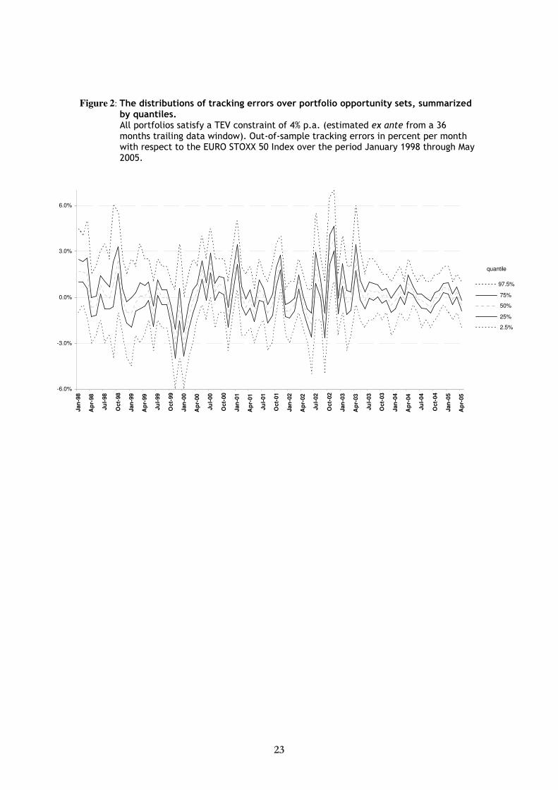
================== insert Figure 2 about here ==================

Figure 2 shows the quantiles of the tracking error distributions over time. From the

graph, we not only observe that the median out-of-sample tracking error fluctuates

widely over time, also the range of potentially attainable tracking errors under the

mandate varies from narrow to broad. In September 1998, for example, following the

16

Russian debt crisis, the difference in annualized tracking error between the 25% and

75% quantile portfolios in the portfolio opportunity set is a staggering 34% p.a. Also in

July through November 2002, the range of annualized realized tracking errors of the

middle 50% of feasible portfolios is about 25% p.a. The distributions narrow, notably in

the last year of the sample period. In May and June 2004, for example, the difference in

annualized tracking error between the top 25% and bottom 25% portfolios in the

portfolio opportunity set is reduced to about 7% p.a. Figure 2 also shows that in

November 1999 and January 2000, most feasible portfolios realized a negative tracking

error under the mandate. In January 2001 and especially November 2002, in contrast,

most of the attainable portfolios outperformed the benchmark. In these months, a

positive tracking error is not due to the specific ability of the portfolio manager, but

instead induced by favorable market conditions.

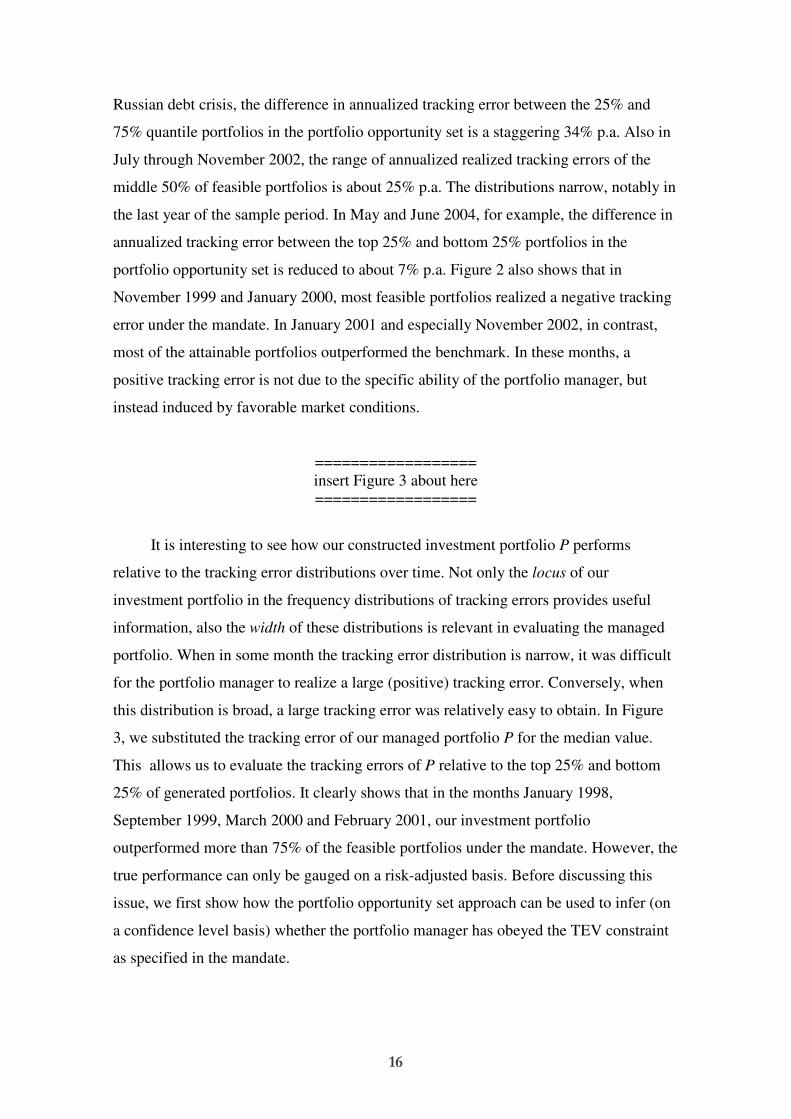
================== insert Figure 3 about here ==================

It is interesting to see how our constructed investment portfolio P performs

relative to the tracking error distributions over time. Not only the locus of our

investment portfolio in the frequency distributions of tracking errors provides useful

information, also the width of these distributions is relevant in evaluating the managed

portfolio. When in some month the tracking error distribution is narrow, it was difficult

for the portfolio manager to realize a large (positive) tracking error. Conversely, when

this distribution is broad, a large tracking error was relatively easy to obtain. In Figure

3, we substituted the tracking error of our managed portfolio P for the median value.

This allows us to evaluate the tracking errors of P relative to the top 25% and bottom

25% of generated portfolios. It clearly shows that in the months January 1998,

September 1999, March 2000 and February 2001, our investment portfolio

outperformed more than 75% of the feasible portfolios under the mandate. However, the

true performance can only be gauged on a risk-adjusted basis. Before discussing this

issue, we first show how the portfolio opportunity set approach can be used to infer (on

a confidence level basis) whether the portfolio manager has obeyed the TEV constraint

as specified in the mandate.

17

TEV violation diagnostics

For the investor who has provided the mandate to a portfolio manager, an interesting

question is whether the investment portfolio P satisfies the formulated TEV constraint.

On an ex post basis, this can be checked by estimating the TEV of realized portfolio

returns. The obvious drawback of this procedure is that in order to estimate the realized

TEV with some reliability, one would have to wait to collect a reasonable number of

return observations (for example 36 monthly observations). In addition, the realized

volatility can be different from the projected volatility and the investor who provides the

mandate can choose not to blame the portfolio manager for these volatility surprises

which affect the whole market.

More interesting, then, is the question whether the investment portfolio P satisfies

the formulated TEV constraint on an ex ante basis. In other words: when constructing

his portfolio, did the portfolio manager take the TEV constraint into account?17 Without

explicit information on the composition of the managed portfolio, the portfolio

opportunity set approach allows for checking whether the tracking error of the managed

portfolio falls reasonably well within the frequency distribution of tracking errors. After

all, when the tracking error of the managed portfolio is outside the range of tracking

errors realized by q% of the portfolios formed under the same mandate, it is likely – at a

confidence level of q% – that the TEV constraint was violated ex ante facto. For

example, when in a specific month 99% of the random portfolios under the mandate

show a smaller tracking error than the managed portfolio, it is very likely that the

portfolio manager has violated the mandate. Note that since the portfolio opportunity set

is generated under the same ex ante TEV constraint, but the realized tracking errors of

all generated portfolios are subject to volatility surprises, this check on potential TEV

violation is insensitive to changes in volatility.

================== insert Figure 4 about here ==================

In Figure 4, we highlight the frequency distributions of realized tracking errors for the

months January 1998 and January 2000. Our managed portfolio is composed under a

17 Of course, the specific method employed to estimate the TEV should be contained in the mandate.

18

TEV constraint of 4% p.a. In addition, we consider two alternative managed portfolios

P’ and P” which are constructed according to the same recipe as our portfolio P, but for

which the ex ante TEV constraint is relaxed to 5% and 6%, respectively. In January

1998, our portfolio P realized a positive tracking error of 3.37% (monthly basis). This

implies an outstanding performance since 93.45% of the portfolios in the portfolio

opportunity set realized a lower tracking error under the mandate. Portfolio P’ has

realized a tracking error of 4.21% and outperformed 98.60% of the portfolios in the

portfolio opportunity set. Portfolio P” even outperformed 99.77% of the portfolios.

These quantiles are extremely high and cast doubt on the presumption that these

portfolios, just as portfolio P, are formed under a TEV constraint of 4%. Instead of

attributing outstanding performance to the portfolios P’ and P”, we would instead

conclude with high confidence that these portfolios were composed under a relaxed

mandate (which in this case is true by construction). The high performance of these

portfolios is thus very likely due to a higher ex ante active risk level. Switching to

January 2000, the case is less clear for portfolio P’ since it underperformed about 89%

of the portfolios. However, portfolio P” is outperformed by 98.25% of the portfolios

and this again signals that the portfolio manager has very likely exceeded the TEV

constraint.

a relative perspective on risk-adjusted performance

The risk-adjusted performance of a managed portfolio will be evaluated by means of the

IR. We here focus on expected risk-adjusted performance of the managed portfolio P.

================== insert Figure 5 about here ==================

For all portfolios in the portfolio opportunity sets, we calculated the ex ante IR, based

on tracking errors from a preceding 36 months trailing data window. Figure 5 shows the

quantiles of the distributions of IRs over time. Parallel to Figure 2, the median and

range of IRs fluctuate over time. Depending on market dynamics, in some months it is

clearly easier to achieve a high IR than in other months.

================== insert Figure 6 about here ==================

19

But how does our investment portfolio P fare? Figure 6 plots the ex ante monthly IR of

our portfolio over time. In the first two years, the IR is quite high, about 0.4. Then the

projected risk-adjusted performance drops sharply, where after the performance

recovers from January 2003 on (monthly IR of about 0.25). On the basis of this

information, and except for the years 2000 through 2002, the projected performance of

the portfolio manager looks quite well.

Next we evaluate the projected performance of our portfolio relative to all

alternative feasible portfolios. One way to do this is to plot the IRs of our portfolio in

the distributions of IRs over the portfolio opportunity sets in Figure 6. For space

considerations, we do not show this graph. Instead we normalize the IR of our portfolio

with respect to the distributions of IRs over the portfolio opportunity sets. We compute

the normalized IR by first subtracting the median information ratio from the

corresponding opportunity set and then dividing by the standard deviation of

information ratios (calculated over the cross-section of all feasible portfolios). This

relative perspective radically changes our perception of the portfolio manager’s

projected performance. Figure 6 reveals that during the years 1998 and 1999, our

portfolio manager expected to outperform the median feasible portfolio. This is in line

with the high level of the non-normalized IRs. However, during the next three years

(2000-2002) we see that the projected IR is not only low in absolute value, but also low

when compared to the IRs of alternative feasible portfolios: most portfolios in the

portfolio opportunity set outperform the managed portfolio on an ex ante basis. And

finally, during the last three and a half years, during which the performance seems to be

restored when judged by the IRs, the normalized IRs deteriorate even further. The vast

majority of alternative portfolios have a projected IR that is way above the IR of our

constructed portfolio. The managed portfolio’s ex ante IR ranges well outside the two-

standard deviation interval of IRs. This is in flagrant contrast with the information

provided by the non-normalized IR. We can only conclude that relative to the level

playing field of portfolio opportunities, our hypothetical portfolio manager performs

very poorly… We therefore advice to evaluate the performance of mandated portfolios

from a relative perspective: not only relative to the targeted benchmark, but also relative

the corresponding portfolio opportunity set.

20

6. Summary & Conclusions

In this paper, we argue that mandated portfolios should not only be evaluated relative to

their benchmarks, but also relative to the portfolio opportunity set. The portfolio

opportunity set comprises all portfolios that satisfy the constraints as specified in the

investment mandate. This portfolio opportunity set can be used to construct frequency

distributions of (risk-adjusted) performance values such as realized tracking errors and

information ratios. This allows for evaluating the relative position of the investment

portfolio in the portfolio opportunity set. Both the locus of the investment portfolio in

the frequency distribution of performance values, as the width of this distribution

provides valuable information for evaluating relative investment performance. To purge

the information ratio for the influence of market dynamics over time, we suggest

normalizing this performance metric. In addition, we show how the portfolio

opportunity set approach can be used for monitoring ex ante tracking error volatility

constraints. We illustrated our methodology for a fictitious investment portfolio where

the EURO STOXX 50 Index served as a benchmark.

We showed only some applications of the portfolio opportunity set approach. In

this paper, we focused on the relative performance evaluation of a mandated portfolio.

Normalizing the information ratio with respect to the portfolio opportunity set revealed

the clear inferiority of the strategy followed by our fictitious portfolio manager when

compared to all strategies feasible under the mandate. This suggests an interesting route

for further research: to use the portfolio opportunity set approach to ex ante evaluate and

select alternative investment strategies.

21

Figure 1: The EURO STOXX 50 Index (benchmark) and the equally-weighted index over time. January 1, 1995 (=100) through May 31, 2005.

0

50

100

150

200

250

300

350

400

450

500

Dec-9

4

Ju

n-9

5

Dec-9

5

Ju

n-9

6

Dec-9

6

Ju

n-9

7

Dec-9

7

Ju

n-9

8

Dec-9

8

Ju

n-9

9

Dec-9

9

Ju

n-0

0

Dec-0

0

Ju

n-0

1

Dec-0

1

Ju

n-0

2

Dec-0

2

Ju

n-0

3

Dec-0

3

Ju

n-0

4

Dec-0

4

EURO STOXX 50 Index Equally-Weighted Index

22

Table 1 Descriptive statistics.

Mean and standard deviation (st.dev.) of monthly discretely compounded price

returns, expressed in percent per annum. Means and standard deviations are

annualized by multiplying monthly figures with 12 and 12 , respectively.

Panel A: The benchmark index B, the equally-weighted index EW, and the return difference EW-B. The benchmark B is the EURO STOXX 50 Index, EW is the equally-weighted portfolio, and EW-B indicates the return differential between the benchmark and the equally-weighted portfolio. The sample period is January 1995 through May 2005 (125 monthly observations, annualized statistics).

% p.a. B EW EW - B

mean 10.19 13.15 2.96

st.dev. 20.23 21.32 4.25

Panel B: The benchmark index, the investment portfolio, and the tracking error.

The investment portfolio P is formed with ex ante tracking error volatility of 4% p.a., based on a window of the preceding 36 months. The benchmark B is the EURO STOXX 50 Index and P-B indicates the tracking error. Out-of-sample returns over the period January 1998 through May 2005 (89 monthly observations, annualized statistics).

% p.a. B P P - B

mean 5.01 7.73 2.72

st.dev. 21.80 22.99 4.46

23

Figure 2: The distributions of tracking errors over portfolio opportunity sets, summarized by quantiles. All portfolios satisfy a TEV constraint of 4% p.a. (estimated ex ante from a 36 months trailing data window). Out-of-sample tracking errors in percent per month with respect to the EURO STOXX 50 Index over the period January 1998 through May 2005.

-6.0%

-3.0%

0.0%

3.0%

6.0%

Jan

-98

Ap

r-98

Ju

l-98

Oct-

98

Jan

-99

Ap

r-99

Ju

l-99

Oct-

99

Jan

-00

Ap

r-00

Ju

l-00

Oct-

00

Jan

-01

Ap

r-01

Ju

l-01

Oct-

01

Jan

-02

Ap

r-02

Ju

l-02

Oct-

02

Jan

-03

Ap

r-03

Ju

l-03

Oct-

03

Jan

-04

Ap

r-04

Ju

l-04

Oct-

04

Jan

-05

Ap

r-05

97.5%

75%

50%

25%

2.5%

quantile

24

Figure 3: The locations of portfolio P in the distributions of tracking errors over portfolio opportunity sets, summarized by quantiles. All portfolios satisfy a TEV constraint of 4% p.a. (estimated ex ante from a 36 months trailing data window). Out-of-sample tracking errors in percent per month with respect to the EURO STOXX 50 Index over the period January 1998 through May 2005.

-6.0%

-3.0%

0.0%

3.0%

6.0%

Jan

-98

Ap

r-98

Ju

l-98

Oct-

98

Jan

-99

Ap

r-99

Ju

l-99

Oct-

99

Jan

-00

Ap

r-00

Ju

l-00

Oct-

00

Jan

-01

Ap

r-01

Ju

l-01

Oct-

01

Jan

-02

Ap

r-02

Ju

l-02

Oct-

02

Jan

-03

Ap

r-03

Ju

l-03

Oct-

03

Jan

-04

Ap

r-04

Ju

l-04

Oct-

04

Jan

-05

Ap

r-05

97.5%

75%

Portfolio P

25%

2.5%

quantile

25

Figure 4: Frequency distributions of realized tracking error, calculated over the portfolio opportunity sets for the months January 1998 and January 2000. The frequency distribution is constructed from monthly tracking errors from a portfolio opportunity set under a TEV constraint of 4% p.a. (estimated over the preceding 36 months). Our managed portfolio P is also composed under the same mandate (indicated by TEV 4%). In addition, we list the realized tracking error of our investment portfolio where the TEV constraint is relaxed to 5% (P’, TEV 5%) and 6% (P”, TEV 6%). In each case, we list the actual tracking error and the quantile (i.e. the percentage of portfolios in the opportunity set that realized a smaller tracking error in that month).

u u u u u u u

−3.0%

−1.0%

1.0%

3.0%

5.0%

7.0%

9.0%

b

P ≡ TEV 4%

tracking error : 3.37%

quantile: 93.01%

b

P ′≡ TEV 5%

tracking error : 4.21%

quantile: 98.41%

b

P ′′≡ TEV 6%

tracking error : 5.05%

quantile: 99.75%

January 1998

u u u u u u

−8.0%

−6.0%

−4.0%

−2.0%

0.0%

2.0%

b

P ≡ TEV 4%

tracking error : -3.62%

quantile: 33.90%

b

P ′≡ TEV 5%

tracking error : -4.53%

quantile: 10.53%

b

P ′′≡ TEV 6%

tracking error : -5.44%

quantile: 1.80%

January 2000

26

Figure 5: The distributions of information ratios over portfolio opportunity sets, summarized by quartiles. All portfolios satisfy an ex ante TEV constraint of 4% p.a. Shown are ex ante information ratios with respect to the EURO STOXX 50 Index over the period January 1998 through May 2005. All information ratios are estimated ex ante from a 36 months trailing data window.

-0.1

0.1

0.3

0.5

0.7

0.9

1.1

Jan

-98

Ap

r-98

Ju

l-9

8

Oct-

98

Jan

-99

Ap

r-99

Ju

l-9

9

Oct-

99

Jan

-00

Ap

r-00

Ju

l-0

0

Oct-

00

Jan

-01

Ap

r-01

Ju

l-0

1

Oct-

01

Jan

-02

Ap

r-02

Ju

l-0

2

Oct-

02

Jan

-03

Ap

r-03

Ju

l-0

3

Oct-

03

Jan

-04

Ap

r-04

Ju

l-0

4

Oct-

04

Jan

-05

Ap

r-05

97.5%

75%

50%

25%

2.5%

quantile

27

Figure 6: The ex ante information ratio and normalized ex ante information ratio of the managed portfolio P. The investment portfolio P satisfies an ex ante TEV constraint of 4% p.a. Shown are ex ante monthly information ratios with respect to the EURO STOXX 50 Index over the period January 1998 through May 2005. All information ratios are on a monthly basis, estimated ex ante from a 36 months trailing data window. The normalized information ratio is computed by first subtracting the median information ratio from the corresponding opportunity set and then dividing by the standard deviation of information ratios over the portfolio opportunity set.

0.0

0.1

0.2

0.3

0.4

0.5

0.6

Jan

-98

May-9

8

Sep

-98

Jan

-99

May-9

9

Sep

-99

Jan

-00

May-0

0

Sep

-00

Jan

-01

May-0

1

Sep

-01

Jan

-02

May-0

2

Sep

-02

Jan

-03

May-0

3

Sep

-03

Jan

-04

May-0

4

Sep

-04

Jan

-05

May-0

5

Ex ante IR

-5.0

-4.0

-3.0

-2.0

-1.0

0.0

1.0

Jan

-98

May-9

8

Sep

-98

Jan

-99

May-9

9

Sep

-99

Jan

-00

May-0

0

Sep

-00

Jan

-01

May-0

1

Sep

-01

Jan

-02

May-0

2

Sep

-02

Jan

-03

May-0

3

Sep

-03

Jan

-04

May-0

4

Sep

-04

Jan

-05

May-0

5

Normalized ex ante IR

28

References

ADAMS, J.C. & K.B. CYREE (2004) “Market Efficiency and Diversification: An

Experiential Approach Using the Wall Street Journal’s Dartboard Portfolio”.

Journal of Applied Finance, Fall/Winter, pp.40-51.

ALEXANDER, G.J. & A. BAPTISTA (2004) “Active Portfolio Management with

Benchmarking: Adding a Value-at-Risk Constraint”. Working paper, University

of Minnesota, available for download at

http://www.gloriamundi.org/picsresources/gaab3.pdf.

AMMANN, M.& H. ZIMMERMANN (2001) “The Relation Between Tracking Error and

Tactical Asset Management”. Financial Analysts Journal, Vol.57, Iss.2

(March/April), pp. 32-43.

BÉLISLE, C.J.P., H.E. ROMEIJN & R.L. SMITH (1993) “Hit-and-Run Algorithms for

Generating Multivariate Distributions”. Mathematics of Operation Research,

Vol.18, Iss.1, pp. 255-266.

BERBEE, H.C.P., C.G.E. BOENDER, A.H.G. RINNOY KAN, C.L. SCHEFFER, R.L. SMITH

& J. TELGEN (1987) “Hit-and-Run Algorithms for the Identification of

Nonredundant Linear Inequalities”. Mathematical Programming, Vol.37, Iss.1,

pp. 184-207.

BURMEISTER, C., H. MAUSSER & R. MENDOZA (2005) “Actively Managing Tracking

Error”. Journal of Asset Management, Vol.5, Iss.6, pp. 410-422.

COHEN, K.J. & B.P. FITCH (1966) “The Average Investment Performance Index”.

Management Science, Vol.12, Iss.6, Series B, pp. B195-B215.

FISHER, L. (1965) “Outcomes for ‘Random’ Investments in Common Stocks listed on

the New York Stock Exchange”. Journal of Business, Vol.38, Iss.2, pp. 149-161.

FISHER, L. & J.H. LORIE (1970) “Some Studies of Variability of Returns on

Investments in Common Stocks”. Journal of Business, Vol.43, Iss.2, pp. 99-134.

GOODWIN, TH.H. (1998) “The Information Ratio”. Financial Analysts Journal,

Vol.54, Iss.4 (July-August), pp. 34-43.

GRINOLD, R.C.& R. KAHN (2000) Active Portfolio Management, 2nd edition. McGraw-

Hill Trade, New York NY.

HALLERBACH, W., C. HUNDACK, I. POUCHKAREV, & J. SPRONK (2005) “Market

Dynamics from the Portfolio Opportunity Perspective: the DAX® Case”.

Zeitschrift für Betriebswirtschaft, Vol.75, Iss.7/8, July-August, pp.739-764.

JORION, PH. (2003) “Portfolio Optimization with Tracking-Error Constraints”.

Financial Analysts Journal, Vol.59, Iss.5 (Sep/Oct), pp. 70-82.

LOVÁSZ, L. (1998) “Hit-and-Run Mixes Fast”. Mathematical Programming, Vol.86,

Iss.6, pp. 443-461.

29

LUENBERGER, D.G. (1998) Investment Science, 2nd edition. Oxford University Press,

New York NY.

MOY, R.L. (1994) “Pros, Darts, and the Dow: Portfolio Lessons From The Wall Street

Journal”. Financial Practice & Education, Fall/Winter, pp. 144-147.

POUCHKAREV, I. (2005) A General Framework for the Evaluation of Constrained

Portfolio Performance, PhD Thesis, Erasmus University Rotterdam

REILLY, F.K. (1994) Investment Analysis and Portfolio Management. The Dryden

Press, Fort Worth TX.

RENNIE, E.P. & TH.J. COWHEY (1990) “The Successful Use of Benchmark Portfolios:

A Case Study”. Financial Analysts Journal, Vol.46, Iss.5 (Sep/Oct), pp. 18-26.

RITOV, Y. (1989) “Monte Carlo Computation of the Mean of a Function with Convex

Support”. Computational Statistics & Data Analysis, Vol.7, Iss.3, pp. 269-277.

ROHWEDER, H.C. (1998) “Implementing Stock Selection Ideas: Does Tracking Error

Optimization Any Good?”. The Journal of Portfolio Management, Spring,

pp. 49-59.

ROLL, R. (1992) “A Mean/Variance Analysis of Tracking Error”. The Journal of

Portfolio Management, Summer, pp. 13-22.

RUDOLPH, M, H.-J. WOLTER & H. ZIMMERMANN (1999) “A Linear Model for

Tracking Error Minimization”. Journal of Banking & Finance, Vol.23, Iss.1,

pp. 85-103.

SHARPE, W.F. (1966) “Mutual Fund Performance”. Journal of Business, January,

pp. 119-138.

SHARPE, W.F. (1994) “The Sharpe Ratio”. The Journal of Portfolio Management,

Fall, pp. 49-58.

SMITH, R.L. (1984) “Efficient Monte Carlo Procedures for Generating Points

Uniformly Distributed over Bounded Regions”. Operations Research, Vol.36,

Iss.2, pp. 1296-1302.

Publications in the Report Series Research∗ in Management ERIM Research Program: “Finance and Accounting” 2005 Royal Ahold: A Failure Of Corporate Governance Abe De Jong, Douglas V. Dejong, Gerard Mertens and Peter Roosenboom ERS-2005-002-F&A http://hdl.handle.net/1765/1863 Capital Structure Policies in Europe: Survey Evidence Dirk Brounen, Abe de Jong and Kees Koedijk ERS-2005-005-F&A http://hdl.handle.net/1765/1923 A Comparison of Single Factor Markov-Functional and Multi Factor Market Models Raoul Pietersz, Antoon A. J. Pelsser ERS-2005-008-F&A http://hdl.handle.net/1765/1930 Efficient Rank Reduction of Correlation Matrices Igor Grubišić and Raoul Pietersz ERS-2005-009-F&A http://hdl.handle.net/1765/1933 Generic Market Models Raoul Pietersz and Marcel van Regenmortel ERS-2005-010-F&A http://hdl.handle.net/1765/1907 The price of power: valuing the controlling position of owner-managers in french ipo firms Peter Roosenboom and Willem Schramade ERS-2005-011-F&A http://hdl.handle.net/1765/1921 The Success of Stock Selection Strategies in Emerging Markets: Is it Risk or Behavioral Bias? Jaap van der Hart, Gerben de Zwart and Dick van Dijk ERS-2005-012-F&A http://hdl.handle.net/1765/1922 Sustainable Rangeland Management Using a Multi-Fuzzy Model: How to Deal with Heterogeneous Experts’ Knowledge Hossein Azadi, Mansour Shahvali, Jan van den Berg and Nezamodin Faghih ERS-2005-016-F&A http://hdl.handle.net/1765/1934 A Test for Mean-Variance Efficiency of a given Portfolio under Restrictions Thierry Post ERS-2005-032-F&A http://hdl.handle.net/1765/6729 Testing for Stochastic Dominance Efficiency Oliver Linton, Thierry Post and Yoon-Jae Whang ERS-2005-033-F&A http://hdl.handle.net/1765/6726

Wanted: A Test for FSD Optimality of a Given Portfolio Thierry Post ERS-2005-034-F&A http://hdl.handle.net/1765/6727 How Domestic is the Fama and French Three-Factor Model? An Application to the Euro Area Gerard A. Moerman ERS-2005-035-F&A http://hdl.handle.net/1765/6626 Bond underwriting fees and keiretsu affiliation in Japan Abe de Jong, Peter Roosenboom and Willem Schramade ERS-2005-038-F&A http://hdl.handle.net/1765/6725 Sourcing of Internal Auditing: An Empirical Study Roland F. Speklé, Hilco J. van Elten and Anne-Marie Kruis ERS-2005-046-F&A http://hdl.handle.net/1765/6891 The Nature of Power Spikes: a regime-switch approach Cyriel de Jong ERS-2005-052-F&A http://hdl.handle.net/1765/6988 ‘New’ Performance Measures: Determinants of Their Use and Their Impact on Performance Frank H.M. Verbeeten ERS-2005-054-F&A http://hdl.handle.net/1765/6993 A Relative View on Tracking Error Winfried G. Hallerbach and Igor W. Pouchkarev ERS-2005-063-F&A ∗ A complete overview of the ERIM Report Series Research in Management:

https://ep.eur.nl/handle/1765/1 ERIM Research Programs: LIS Business Processes, Logistics and Information Systems ORG Organizing for Performance MKT Marketing F&A Finance and Accounting STR Strategy and Entrepreneurship