A Reference Model for Integrated Energy and Power ...
271
INSTITUT FÜR INFORMATIK DER LUDWIG–MAXIMILIANS–UNIVERSITÄT MÜNCHEN Dissertation an der Fakultät für Mathematik, Informatik und Statistik der Ludwig-Maximilians-Universität München A Reference Model for Integrated Energy and Power Management of HPC Systems eingereicht von Matthias Maiterth am: 4. März 2021
-
Upload
khangminh22 -
Category
Documents
-
view
4 -
download
0
Transcript of A Reference Model for Integrated Energy and Power ...
INSTITUT FÜR INFORMATIKDER LUDWIG–MAXIMILIANS–UNIVERSITÄT MÜNCHEN
Dissertationan der Fakultät für Mathematik, Informatik und Statistik
der Ludwig-Maximilians-Universität München
A Reference Model for IntegratedEnergy and Power Management of
HPC Systemseingereicht von
Matthias Maitertham: 4. März 2021
Erstberichterstatter: Prof. Dr. Dieter KranzlmüllerZweiberichterstatterin: Prof. Dr. Florina M. CiorbaDrittberichterstatter: Prof. Dr. Martin Schulz
Tag der mündlichen Prüfung: 6. September 2021


Eidesstattliche Versicherung(Siehe Promotionsordnung vom 12.07.11, §8, Abs. 2 Pkt. .5.)
Hiermit erkläre ich an Eidesstatt, dass die Dissertation von mirselbstständig, ohne unerlaubte Beihilfe angefertigt ist.
M¡�©�´e�²�t¨�, M¡�´�t¨�ia³
Name, Vorname
. . . . . . . . . . . . . . . . . . . . . . . . . . . . . .��ünc¨e�®�, ¤e�®� 04.03.2021
Ort, Datum. . . . . . . . . . . . . . . . . . . . . . . . . . . . . . . . . . . . . . . . . . . .
(Unterschrift des Doktoranden)M¡�´�t¨�ia³ M¡�©�´e�²�t¨�
v


Acknowledgments
First and foremost, I want to sincerely thank my doctoral adviser, Professor Kranzlmüller. Overthe past six years, you pushed me to pursue my academic advances to reach further than I thoughtpossible. Your go-ahead attitude always put me on the spot and spurred me to step further and stayahead.Florina, thank you for your perseverance and encouragement! After first meeting by chance and
following fruitful discussions it was a joy to keep you updated on my progress and endeavors. Ifelt honored for your suggestions to collaborate, on several occasions. I’m very glad that I can stopdeferring this invite since the formalities for adviser and examiner are soon to be overstepped. Thankyou for agreeing with being on my doctoral committee as I am honored to have you as my secondrapporteur, as you are a positive role model for any aspiring young scientist.Martin, thank you for your wonderful support, the detailed technical discussions and for teaching
me to become an adept researcher. Our collaborations since my first visit at LLNL under yourguidance, with my second research stay while working towards this dissertation, have been veryinsightful and have showed me that the pursuit of a topic that one cares for can have recognizableimpact. I’m glad to have shared serious and lighthearted moments whenever possible. With yourtransition to the university at TUM I am honored to be able to have you as a formal adviser, as well.Thank you.I want to thank my colleagues at university, for the enjoyable environment, discussions, support,
as well as time for joy and relaxation. My colleagues at LMU have been a delight to work with andare a laudable bunch. A special thank you to, Tobi, Roger, Karl, Nils, Miki, Annette, Vitalian, Tobi,Cuong, Pascal, Max, Sophia, Jan, Amir, Minh and Dang.I want to thank colleagues at LLNL, which made my second research visit a success, and with
whom I shared very memorable time. My special thank you to Tapasya Patki, Stephanie Brink, DanEllsworth, Aniruddha Marathe, Barry Rountree and Brian Weston.At Intel, I want to thank Jonathan Eastep, Andrey Semin and Chris Dahnken. Your support
and the great opportunity to contribute to industrial research and development over the course of asubstantial part of my dissertation are an honor to me. While my gratitude goes to Chris Cantalupo,Brad Geltz, Diana Guttman, Brandon Baker, Ali Mohammad and Sid Jana. As part of Jonathan’steam, you enabled me to think about much of my work’s context, while all your momentum keep toamaze me. It was a bliss, to have been a humble part of your team.At LRZ, I want to thank Markus Wiedemann, Alessio Netti, Daniele Tafani, Hayk Shoukourian,
Luigi Iapichino, Carmen Navarrete, Carla Guillen, Matt Tovey, Torsten Wilde and Michael Ott.Additionally, I want to thank research collaborators at various organizations that I was happy
to work with, especially Natalie Bates and Greg Koenig (EEHPCWG), Masaaki Kondo and RuichiSakamoto (UTokyo), Andrea Bartolini (UniBo), Carsten Trinitis (TUM), Joachim Protze and BoWang (RWTH), Thomas Illsche (TUD), and many whose names didn’t fit on this page.Finally, I want to thank friends and family in particular Phượng for motivating me to persevere
over the final two years, my brother Johannes for good sportsmanship and rivalry and my parentsWalter & Elisabeth-Charlotte for their enduring support.
vii


AbstractOptimizing a computer for highest performance dictates the efficient use of its limited resources.Computers as a whole are rather complex. Therefore, it is not sufficient to consider optimizinghardware and software components independently. Instead, a holistic view to manage the interactionsof all components is essential to achieve system-wide efficiency.For High Performance Computing (HPC) systems, today, the major limiting resources are energy
and power. The hardware mechanisms to measure and control energy and power are exposed tosoftware. The software systems using these mechanisms range from firmware, operating system,system software to tools and applications. Efforts to improve energy and power efficiency of HPCsystems and the infrastructure of HPC centers achieve perpetual advances. In isolation, these effortsare unable to cope with the rising energy and power demands of large scale systems. A systematic wayto integrate multiple optimization strategies, which build on complementary, interacting hardwareand software systems is missing.This work provides a reference model for integrated energy and power management of HPC sys-
tems: the Open Integrated Energy and Power (OIEP) reference model. The goal is to enable theimplementation, setup, and maintenance of modular system-wide energy and power managementsolutions. The proposed model goes beyond current practices, which focus on individual HPC cen-ters or implementations, in that it allows to universally describe any hierarchical energy and powermanagement systems with a multitude of requirements. The model builds solid foundations to beunderstandable and verifiable, to guarantee stable interaction of hardware and software components,for a known and trusted chain of command. This work identifies the main building blocks of the OIEPreference model, describes their abstract setup, and shows concrete instances thereof. A principalaspect is how the individual components are connected, interface in a hierarchical manner and thuscan optimize for the global policy, pursued as a computing center’s operating strategy. In additionto the reference model itself, a method for applying the reference model is presented. This methodis used to show the practicality of the reference model and its application.For future research in energy and power management of HPC systems, the OIEP reference model
forms a cornerstone to realize — plan, develop and integrate — innovative energy and power manage-ment solutions. For HPC systems themselves, it supports to transparently manage current systemswith their inherent complexity, it allows to integrate novel solutions into existing setups, and it en-ables to design new systems from scratch. In fact, the OIEP reference model represents a basis forholistic efficient optimization.
ix


ZusammenfassungComputer auf höchstmögliche Rechenleistung zu optimieren bedingt Effizienzmaximierung aller lim-itierenden Ressourcen. Computer sind komplexe Systeme. Deshalb ist es nicht ausreichend, Hard-ware und Software isoliert zu betrachten. Stattdessen ist eine Gesamtsicht des Systems notwendig,um die Interaktionen aller Einzelkomponenten zu organisieren und systemweite Optimierungen zuermöglichen.Für Höchstleistungsrechner (HLR) ist die limitierende Ressource heute ihre Leistungsaufnahme
und der resultierende Gesamtenergieverbrauch. In aktuellen HLR-Systemen sind Energie- und Leis-tungsaufnahme programmatisch auslesbar als auch direkt und indirekt steuerbar. Diese Mechanismenwerden in diversen Softwarekomponenten von Firmware, Betriebssystem, Systemsoftware bis hin zuWerkzeugen und Anwendungen genutzt und stetig weiterentwickelt. Durch die Komplexität der inter-agierenden Systeme ist eine systematische Optimierung des Gesamtsystems nur schwer durchführbar,als auch nachvollziehbar. Ein methodisches Vorgehen zur Integration verschiedener Optimierungsan-sätze, die auf komplementäre, interagierende Hardware- und Softwaresysteme aufbauen, fehlt.Diese Arbeit beschreibt ein Referenzmodell für integriertes Energie- und Leistungsmanagement
von HLR-Systemen, das „Open Integrated Energy and Power (OIEP)“ Referenzmodell. Das Ziel istein Referenzmodell, dass die Entwicklung von modularen, systemweiten energie- und leistungsopti-mierenden Sofware-Verbunden ermöglicht und diese als allgemeines hierarchisches Managementsys-tem beschreibt. Dies hebt das Modell von bisherigen Ansätzen ab, welche sich auf Einzellösungen,spezifischen Software oder die Bedürfnisse einzelner Rechenzentren beschränken. Dazu beschreibtes Grundlagen für ein planbares und verifizierbares Gesamtsystem und erlaubt nachvollziehbaresund sicheres Delegieren von Energie- und Leistungsmanagement an Untersysteme unter Aufrechter-haltung der Befehlskette. Die Arbeit liefert die Grundlagen des Referenzmodells. Hierbei werdendie Einzelkomponenten der Software-Verbunde identifiziert, deren abstrakter Aufbau sowie konkreteInstanziierungen gezeigt. Spezielles Augenmerk liegt auf dem hierarchischen Aufbau und der resul-tierenden Interaktionen der Komponenten. Die allgemeine Beschreibung des Referenzmodells erlaubtden Entwurf von Systemarchitekturen, welche letztendlich die Effizienzmaximierung der RessourceEnergie mit den gegebenen Mechanismen ganzheitlich umsetzen können. Hierfür wird ein Verfahrenzur methodischen Anwendung des Referenzmodells beschrieben, welches die Modellierung beliebigerEnergie- und Leistungsverwaltungssystemen ermöglicht.Für Forschung im Bereich des Energie- und Leistungsmanagement für HLR bildet das OIEP Refe-
renzmodell Eckstein, um Planung, Entwicklung und Integration von innovativen Lösungen umzuset-zen. Für die HLR-Systeme selbst unterstützt es nachvollziehbare Verwaltung der komplexen Systemeund bietet die Möglichkeit, neue Beschaffungen und Entwicklungen erfolgreich zu integrieren. DasOIEP Referenzmodell bietet somit ein Fundament für gesamtheitliche effiziente Systemoptimierung.
xi

xii

ContentsAbstract ix
Contents xiii
List of Figures xv
List of Tables xvii
Preface xix
1. Introduction 11.1. Problem Statement . . . . . . . . . . . . . . . . . . . . . . . . . . . . . . . . . . . . . . 51.2. Methodical Approach . . . . . . . . . . . . . . . . . . . . . . . . . . . . . . . . . . . . 61.3. Contributions . . . . . . . . . . . . . . . . . . . . . . . . . . . . . . . . . . . . . . . . . 7
1.3.1. Key Contributions of This Work . . . . . . . . . . . . . . . . . . . . . . . . . . 71.3.2. Author’s Preliminary Work . . . . . . . . . . . . . . . . . . . . . . . . . . . . . 8
1.4. Thesis Outline . . . . . . . . . . . . . . . . . . . . . . . . . . . . . . . . . . . . . . . . 12
2. Background 152.1. Motivation . . . . . . . . . . . . . . . . . . . . . . . . . . . . . . . . . . . . . . . . . . 15
2.1.1. Energy and Power – a Major Challenge for Exascale and Beyond . . . . . . . . 152.1.2. Managing Energy and Power Using Software . . . . . . . . . . . . . . . . . . . 182.1.3. The Need for an Energy and Power Management Software Stack . . . . . . . . 22
2.2. Scoping of Energy and Power Management Systems . . . . . . . . . . . . . . . . . . . 252.2.1. Sources of Variability . . . . . . . . . . . . . . . . . . . . . . . . . . . . . . . . 252.2.2. Optimization Goals of Energy and Power Management Systems . . . . . . . . . 272.2.3. Aspects of Energy and Power Management Setups . . . . . . . . . . . . . . . . 28
2.3. Requirements for Reference Models for Energy and Power Management . . . . . . . . 312.4. Related Work . . . . . . . . . . . . . . . . . . . . . . . . . . . . . . . . . . . . . . . . . 34
2.4.1. Structured Energy and Power Management Approaches in HPC . . . . . . . . 342.4.2. Compound Software Setups for Energy and Power Management in HPC . . . . 362.4.3. Modeling of Complex Control Systems . . . . . . . . . . . . . . . . . . . . . . . 382.4.4. Related Work – Summary of Characteristics . . . . . . . . . . . . . . . . . . . . 40
3. Open Integrated Energy and Power (OIEP) Reference Model 433.1. Methodical Approach for the Reference Model Construction . . . . . . . . . . . . . . . 433.2. Fundamentals of the OIEP Reference Model . . . . . . . . . . . . . . . . . . . . . . . . 44
3.2.1. Basic Terms and Definitions . . . . . . . . . . . . . . . . . . . . . . . . . . . . . 453.2.2. Basic Design Considerations for the OIEP Reference Model . . . . . . . . . . . 45
3.3. Description of the OIEP Reference Model . . . . . . . . . . . . . . . . . . . . . . . . . 483.3.1. OIEP Levels and the OIEP Level Tree . . . . . . . . . . . . . . . . . . . . . . . 483.3.2. OIEP Components and the OIEP Component Tree . . . . . . . . . . . . . . . . 563.3.3. OIEP Data Sources and the OIEP Monitoring Overlay . . . . . . . . . . . . . . 683.3.4. OIEP Operating States and the OIEP State Diagram . . . . . . . . . . . . . . 71
4. Open Integrated Energy and Power Architectures 774.1. Applying the OIEP Reference Model . . . . . . . . . . . . . . . . . . . . . . . . . . . . 77
xiii
Contents
4.2. Constructing an OIEP Architecture for the PowerStack . . . . . . . . . . . . . . . . . 784.2.1. PowerStack Model – Problem Description . . . . . . . . . . . . . . . . . . . . . 794.2.2. PowerStack Model – Identification of Requirements . . . . . . . . . . . . . . . . 804.2.3. PowerStack Model – Reference Model Selection . . . . . . . . . . . . . . . . . . 814.2.4. PowerStack Model – OIEP Architecture Construction . . . . . . . . . . . . . . 81
5. Assessment 935.1. Assessment Synopsis and Comparison with Generic Model Building Systems . . . . . . 935.2. Identified Limitations . . . . . . . . . . . . . . . . . . . . . . . . . . . . . . . . . . . . 95
6. Future Work 976.1. Future Developments for the OIEP Reference Model . . . . . . . . . . . . . . . . . . . 976.2. Future Work for the Application of the OIEP Reference Model . . . . . . . . . . . . . 996.3. Open Topics . . . . . . . . . . . . . . . . . . . . . . . . . . . . . . . . . . . . . . . . . . 99
7. Conclusions 103
Appendix A. Supplement – Motivation 107A.1. Detailed Requirements Definition . . . . . . . . . . . . . . . . . . . . . . . . . . . . . . 107A.2. Detailed Comparison to Other Model Building Requirements . . . . . . . . . . . . . . 115
Appendix B. Supplement – Background 117B.1. Background on Hardware and Software . . . . . . . . . . . . . . . . . . . . . . . . . . . 117
B.1.1. Background – Hardware . . . . . . . . . . . . . . . . . . . . . . . . . . . . . . . 117B.1.2. Background – Software . . . . . . . . . . . . . . . . . . . . . . . . . . . . . . . 125
B.2. Supplementary Background – PowerStack Strawman Summary . . . . . . . . . . . . . 137
Appendix C. Supplement – OIEP Reference Model 141C.1. Supplement – Methodical Approach for the Reference Model Construction . . . . . . . 141C.2. Considerations for Model Creators on OIEP Level and Level Tree Construction . . . . 143
Appendix D. Supplement – OIEP Architectures for Selected HPC Systems 145D.1. Constructing an OIEP Architecture for the PowerStack Prototype . . . . . . . . . . . 147D.2. Constructing an OIEP Architecture for GEOPM as Nested Component . . . . . . . . 151D.3. Constructing an OIEP Architecture for the SuperMUC Phase 1 & 2 systems . . . . . 163D.4. Constructing an OIEP Architecture for the SuperMUC-NG System . . . . . . . . . . . 169D.5. Constructing an OIEP Architecture for the Fugaku System . . . . . . . . . . . . . . . 177
Appendix E. Supplement – Assessment 195E.1. Assessment of Conformity With the Requirements . . . . . . . . . . . . . . . . . . . . 195E.2. Discussion on Use-Cases . . . . . . . . . . . . . . . . . . . . . . . . . . . . . . . . . . . 199
Acronyms and Abbreviations 201
Glossary 205
Bibliography 219Published Resources . . . . . . . . . . . . . . . . . . . . . . . . . . . . . . . . . . . . . . . . 219Unpublished Resources . . . . . . . . . . . . . . . . . . . . . . . . . . . . . . . . . . . . . . . 242Online Resources . . . . . . . . . . . . . . . . . . . . . . . . . . . . . . . . . . . . . . . . . . 242Meetings/Seminars/Workshops . . . . . . . . . . . . . . . . . . . . . . . . . . . . . . . . . . 246
Index 247
xiv

List of Figures
1.1. Graph from Moore’s Paper, as Seen in [Moo65] . . . . . . . . . . . . . . . . . . . . . . 31.2. Methodical Approach of This Thesis . . . . . . . . . . . . . . . . . . . . . . . . . . . . 61.3. Thesis Outline . . . . . . . . . . . . . . . . . . . . . . . . . . . . . . . . . . . . . . . . 121.4. Method Completion After Chapter 1. . . . . . . . . . . . . . . . . . . . . . . . . . . . . 14
2.1. Socket Power Measurement, Ten Iterations . . . . . . . . . . . . . . . . . . . . . . . . 202.2. Socket Power Measurement, One Iteration With Phase Information . . . . . . . . . . . 212.3. CoMD Single-Node Performance Variation, as Seen in [Mai+16] . . . . . . . . . . . . . 222.4. Typical, Simplified Software Stack on a Single Node . . . . . . . . . . . . . . . . . . . 232.5. Conflicting Interactions for Hardware Access . . . . . . . . . . . . . . . . . . . . . . . 232.6. Conflict Resolution by Limiting Access and Enforcing Hierarchical Interaction . . . . . 242.7. Sources of Variability of Compute Jobs . . . . . . . . . . . . . . . . . . . . . . . . . . . 262.8. Goals of Optimization, Regarding Energy and Power Management Systems and Tools 272.9. Energy and Power Management Systems, Structure and Scope . . . . . . . . . . . . . 292.10. Method Completion After Chapter 2. . . . . . . . . . . . . . . . . . . . . . . . . . . . . 41
3.1. Introductory Example for Components Connected in a Tree Structure. . . . . . . . . . 473.2. Introductory Example of Figure 3.1 With Added Levels . . . . . . . . . . . . . . . . . 473.3. Tree Segment of an OIEP Level Tree . . . . . . . . . . . . . . . . . . . . . . . . . . . . 513.4. Example OIEP Level Tree of Degree 1 With Simple OIEP Component Tree . . . . . . 523.5. Branching OIEP Level Tree – Example . . . . . . . . . . . . . . . . . . . . . . . . . . . 533.6. Types of OIEP Components . . . . . . . . . . . . . . . . . . . . . . . . . . . . . . . . . 573.7. General OIEP Component – Example . . . . . . . . . . . . . . . . . . . . . . . . . . . 593.8. OIEP Components at Different Levels . . . . . . . . . . . . . . . . . . . . . . . . . . . 603.9. Abstract and Instantiated OIEP Component Tree . . . . . . . . . . . . . . . . . . . . . 613.10. Multiplicity Indicators of OIEP Components . . . . . . . . . . . . . . . . . . . . . . . 623.11. Xor Operator Indicating Component Selection. . . . . . . . . . . . . . . . . . . . . . . 643.12. Virtually Selected Operator Closing a Preceeding Xor Operator . . . . . . . . . . . . . 643.13. OIEP Component Tree Instantiation With Xor Operator. . . . . . . . . . . . . . . . . 653.14. Two Example Cases with Xor Operator and Virtually Selected Operator . . . . . . . . 663.15. Nested Component . . . . . . . . . . . . . . . . . . . . . . . . . . . . . . . . . . . . . . 683.16. Monitoring Overlay Depictions . . . . . . . . . . . . . . . . . . . . . . . . . . . . . . . 713.17. Exemplary OIEP State Diagram with OIEP Component Trees . . . . . . . . . . . . . 743.18. Method Completion After Chapter 3. . . . . . . . . . . . . . . . . . . . . . . . . . . . . 75
4.1. Focused Right Side of the Methodical Approach as of Figure 1.2 . . . . . . . . . . . . 784.2. PowerStack Model – According to [PS’19a] . . . . . . . . . . . . . . . . . . . . . . . . 794.3. PowerStack Model – OIEP Level Tree . . . . . . . . . . . . . . . . . . . . . . . . . . . 824.4. PowerStack Model – OIEP Component Tree . . . . . . . . . . . . . . . . . . . . . . . . 864.5. PowerStack Model – OIEP Monitoring Overlay . . . . . . . . . . . . . . . . . . . . . . 874.6. PowerStack Model – OIEP Monitoring Overlay – Data Sources of the Database . . . . 884.7. PowerStack Model – OIEP State Diagram . . . . . . . . . . . . . . . . . . . . . . . . . 894.8. PowerStack Model – OIEP Architecture for the Emergency State . . . . . . . . . . . . 894.9. Possible Alternative OIEP State Diagram for the PowerStack Model . . . . . . . . . . 904.10. Method Completion After Chapter 4. . . . . . . . . . . . . . . . . . . . . . . . . . . . . 91
5.1. Method Completion After Chapter 5. . . . . . . . . . . . . . . . . . . . . . . . . . . . . 96
xv
LIST OF FIGURES
6.1. Completed Method After Chapter 6. . . . . . . . . . . . . . . . . . . . . . . . . . . . . 102
A.1. Requirements Definition Viewpoints, as of [RS77] . . . . . . . . . . . . . . . . . . . . 108
B.1. Schematic of Infrastrucutre Composition, Adapted From [Wil+14] . . . . . . . . . . . 118B.2. Exemplary Cluster Schematic . . . . . . . . . . . . . . . . . . . . . . . . . . . . . . . 118B.3. 1U Server Schematic . . . . . . . . . . . . . . . . . . . . . . . . . . . . . . . . . . . . . 118B.4. Hierarchy of Equipment States (as of [Ste05]) . . . . . . . . . . . . . . . . . . . . . . . 133B.5. PowerStack Model – Initial Model, as of [Can+18] . . . . . . . . . . . . . . . . . . . . 137
D.1. PowerStack Prototype – OIEP Level Tree . . . . . . . . . . . . . . . . . . . . . . . . . 148D.2. PowerStack Prototype – OIEP Component Tree . . . . . . . . . . . . . . . . . . . . . 149D.3. GEOPM Interfaces to Other Components, as of [Eas+17] . . . . . . . . . . . . . . . . 152D.4. GEOPM Hierarchical Design and Communication Mechanisms, as of [Eas+17] . . . . 153D.5. GEOPM as an OIEP Component – Black-Box View . . . . . . . . . . . . . . . . . . . 155D.6. Nested Setup for the GEOPM_RT Component . . . . . . . . . . . . . . . . . . . . . . . . 157D.7. Nested Setup for the Aggregator Component (Agg) . . . . . . . . . . . . . . . . . . . 158D.8. Nested Setup for the Leaf Component (Leaf) . . . . . . . . . . . . . . . . . . . . . . . 158D.9. Leaf Component – Internal Component Monitoring Overlay . . . . . . . . . . . . . . 159D.10. Component Summary of the Nested GEOPM_RT Representations . . . . . . . . . . . . . 159D.11. Instantiated Nested OIEP Component Tree of a GEOPM Example . . . . . . . . . . 161D.12. Instantiated Nested OIEP Monitoring Overlay of Figure D.11 . . . . . . . . . . . . . 161D.13. SuperMUC System – OIEP Component Tree . . . . . . . . . . . . . . . . . . . . . . . 166D.14. SuperMUC System – OIEP Monitoring Overlay . . . . . . . . . . . . . . . . . . . . . 167D.15. SuperMUC-NG System – OIEP Component Tree . . . . . . . . . . . . . . . . . . . . 173D.16. SuperMUC-NG System – OIEP Monitoring Overlay . . . . . . . . . . . . . . . . . . . 174D.17. SuperMUC-NG System – Possible OIEP State Diagram . . . . . . . . . . . . . . . . . 174D.18. OIEP Architecture for The Fugaku System – Constructed OIEP Level Tree . . . . . . 182D.19. OIEP Architecture for The Fugaku System – Constructed OIEP Component Tree . . 185D.20. OIEP Architecture for The Fugaku System – Constructed OIEP Monitoring Overlay 186D.21. OIEP Architecture for The Fugaku System – Constructed OIEP State Diagram . . . 187D.22. OIEP Architecture for The Fugaku System – BoB Enforced Component Tree . . . . . 188D.23. OIEP Architecture for The Fugaku System – BoB Enforced Monitoring Overlay . . . 188D.24. Fugaku OIEP Architecture Instantiation – Normal Mode. . . . . . . . . . . . . . . . . 189D.25. Fugaku OIEP Architecture Instantiation – Eco Mode. . . . . . . . . . . . . . . . . . . 190D.26. Fugaku OIEP Architecture Instantiation – Boost Mode. . . . . . . . . . . . . . . . . . 191D.27. Fugaku OIEP Architecture Instantiation – (Eco) Boostret Mode. . . . . . . . . . . . . 192D.28. Fugaku OIEP Architecture Instantiation – Idle Node Pool. . . . . . . . . . . . . . . . 193
xvi

List of Tables
2.1. Requirements Summary . . . . . . . . . . . . . . . . . . . . . . . . . . . . . . . . . . . 322.2. Requirements for Energy and Power Management Reference Models . . . . . . . . . . 332.3. Overview Related Work . . . . . . . . . . . . . . . . . . . . . . . . . . . . . . . . . . . 41
5.1. Assessment of OIEP Reference Model According to Requirements of Table 2.2 . . . . . 94
xvii


PrefaceContemporary society is relying on the “power of computation” without giving it a second thought,even though computing machinery has only very recently entered the toolset of mankind: Bab-bage’s analytical engine is often regarded as the first computing machine, which he conceived in1833 [Cam+13, p. 42]. In 1941 Zuse built the first binary based programmable Turing completecomputer, the Z3 [Zus10, p. 55].Today, computer chips in smartphones, laptop computers and embedded systems make it ubiquitous
to generate, send and receive data and process information anywhere. Where local processing power,its performance or storage capability, is not sufficient, distributed resources are used.The seemingly simple task of getting an accurate weather forecast on a mobile phone is only
possible by querying information from large simulations. These simulations are not able to run onone’s phone but require dedicated computer systems. By operating High Performance Computing(HPC) systems, which run these simulations in regular intervals (e.g. several times a day) currentand accurate forecasts are possible. The quality of Numerical Weather Prediction (NWP) is in directcorrelation with the performance of the computational systems available to the national meteorologicaland hydrological services. In 1950 the first weather models were calculated, however only by the 1970sit was feasible to solve the full set of equations for weather forecasting as proposed by Abbe [Abb01]and Bjerknes [Bje04] as early as 1901. Since then, every decade added one day of useful forecast byimprovements to both the numerical models and the performance of the computer systems [BTB15].This public commodity is driven by the progress in computation:
“Computation is essential in everything discussed here[1]. Progress will involve largerensembles of model runs at higher resolution leading to improved probabilistic forecasts,including those of hazardous weather. This can be realized if governments maintain asteady schedule of investment in high-speed computing, recognizing the strong evidencethat such investments will be repaid many times over in savings to the economy.”
Alley, Emanuel and Zhang, 2019 [AEZ19, p. 344]
The impact to society justifies the investment in large computing resources: Recent estimates of thecost to benefit ratio for national weather services range from 1 : 3 to 1 : 10, above all by avoidingweather related damages and guiding decision making [Per+13]. To reach the performance requiredfor NWP the weather services employ computer systems which are among the fastest HPC systems inthe world [BTB15]. In their review on “the quiet revolution of numerical weather prediction”, Baueret al. [BTB15] discuss the scientific challenges for reaching and keeping the pace of improvements forNWP. Ensemble models and an increased simulation granularity in the order of 100 to 1000 regardingcomputational tasks are likely for the next 10 years.Regarding technological challenges, co-relating this development with processor performance im-
provements, historically going hand in hand with the advances of Moore’s law [Moo65], the energyconsumption will increase accordingly: To be able to simulate the anticipated weather models withtodays technology will require 10 times more power. In the review by Bauer et al. the researchersmention an upper limit for affordable power of centers such as the European Centre for Medium-RangeWeather Forecasts (ECMWF) of about 20MVA [BTB15] or 20MW.In other words, the colloquial “power of computation” – performance, as stated above – is tightly
coupled to actual power, the consumption of energy. This is critical for computing centers reachingthe scales of industrial energy consumers, capable of generating high dynamic loads [Ste+19b].Energy and power is among the primary issues to resolve for the exascale era, the era of computers
reaching 1018 FLoating point Operations Per Second (FLOPS).In this work the author strives to contribute a small aspect to computer science and engineering
to move beyond a theoretical hurdle on the path to extend what is possible with HPC systems.1The authors in [AEZ19] specifically talk about numerical modeling in weather prediction. However, this can likelybe generalized to any scientific discipline which has to rely on theory, experiment and modeling & simulation.
xix

1. Introduction
1.1. Problem Statement . . . . . . . . . . . . . . . . . . . . . . . . . . . . . . . . . . . . . . 51.2. Methodical Approach . . . . . . . . . . . . . . . . . . . . . . . . . . . . . . . . . . . . 61.3. Contributions . . . . . . . . . . . . . . . . . . . . . . . . . . . . . . . . . . . . . . . . . 7
1.3.1. Key Contributions of This Work . . . . . . . . . . . . . . . . . . . . . . . . . . 71.3.2. Author’s Preliminary Work . . . . . . . . . . . . . . . . . . . . . . . . . . . . . 8
1.4. Thesis Outline . . . . . . . . . . . . . . . . . . . . . . . . . . . . . . . . . . . . . . . . 12
High Performance Computing (HPC) combines approaches from several disciplines of computer sci-ence and computer engineering striving to maximize the computational performance achievable usinga computer system. The goal of HPC is to make challenging problems of science and engineering com-putable which are otherwise infeasible to compute in reasonable time or with the desired problem sizeor resolution. This drive to improve computation is accomplished by advancing the state-of-the-art ofcomputer hardware and software. The notion of HPC, the advancement of what is computationallyviable on computer systems, is also referred to as high-end capability computing [Nat08, p. 1].HPC demands for specialized computer systems to achieve the high computational performance
required. The computer systems purpose built for HPC are called HPC systems. HPC systems aredesigned to solve computational problems which are infeasible to be solved on so-called commoditycomputers.Historically, HPC systems were large vector processing machine installations. These were eventu-
ally replaced by system installations utilizing interconnected microprocessors, linked up as a clusterof computers [Mar91]. Modern HPC systems are almost exclusively clusters of connected comput-ers [TOPg].A compute cluster, or cluster for short, is a system of computers, co-located in physical proximity
and connected using high-performance network infrastructure. The individual computer systemswhich make up the cluster system are called nodes and, in general, are commodity server computers.These compute clusters represent an important class of distributed systems [ST18, p. 25]. For usagein HPC, the nodes are connected via a high-speed network to efficiently process complex tasks inparallel. Additionally, the cluster as a complete system has access to storage or archive systems to beoperationally ready for HPC applications. These HPC applications are applications from science andengineering designed to run on HPC systems due to their need for high computational performance.Regarding the network infrastructure, the notion of physical proximity allows the nodes to benefit
from fast networks using high-performance hardware. This allows for low latencies to minimizewaiting times during the execution of parallel applications, where dependencies of tasks exist. Bycontrast Local Area Networks (LANs) using common networking hardware, which are not able toachieve low latencies or high data rates, introduce inefficiencies. Waiting for data transfers resultsin idle nodes, which stall the applications. Wide Area Networks (WANs) as well as even fartherdistributed networks are not able to achieve low latencies simply by physical limits due to distanceand signal speed. This emphasizes the need for both a high-performance network and close physicalproximity for the nodes of a HPC cluster.HPC has advanced in such way that installation of the current generation of the fastest HPC
systems is not possible without dedicated infrastructure to support these computer systems. AnHPC center is a computing center housing one or more HPC systems. The centers provide therequired infrastructure, and also employ the experts to operate and maintain the computer systems.Due to associated costs, HPC centers are funded by state actors or corporations. The motivations tooperate such center are either to advance research or to obtain results which justify the costs [AEZ19;Koe+18; Mai+18].
1

1. Introduction
An example for a state funded HPC center is the Leibniz Supercomputing Center (Ger. Leibniz-Rechenzentrum) (LRZ), an institute of the Bavarian Academy of Sciences and Humanities (Ger. Bay-erische Akademie der Wissenschaften) (BAdW) in Garching near Munich, Germany. LRZ currentlyhouses several HPC systems, among them, the SuperMUC-NG system. At the time of installationSuperMUC-NG was the eight fastest computer in the world, as of the November 2018 TOP500 list ofthe fastest supercomputers [TOPb]. SuperMUC-NG is a cluster installation of 6480 nodes, achiev-ing a maximum performance of 19.4 petaFLOPS [Pal17; Pal18], indicating the number of FLoatingpoint Operations Per Second (FLOPS) obtained by running the LINPACK benchmark [Don+79;DL11]. The FLOPS metric serves as a proxy for a HPC system’s capability to do useful work in HPCapplications1.To identify the fastest HPC systems, LINPACK benchmark measurements are submitted to gen-
erate the list of the top 500 fastest supercomputers of the world. The TOP500 list was established in1993 and is updated twice a year [TOPg]. The first system to reach the milestone performance of onepetaFLOPS, or 1× 10¹⁵ FLoating point Operations Per Second (1 000 000 000 000 000 FLOPS) wasthe Roadrunner system at Los Alamos National Laboratory, NM, USA, in 2008 [TOPa]. The firstsystem to reach a performance of one exaFLOPS, or 1× 10¹⁸ FLoating point Operations Per Sec-ond (1 000 000 000 000 000 000 FLOPS) is expected to be operational before the end of 2021 [ANLpr;Don16]. While centers and nations are in the race to reach this milestone, preparations for HPCsystems in the 1 exaFLOPS to 10 exaFLOPS range have already started and researchers are alreadythinking about the next milestone of how to reach performances of more than one zettaFLOPS or1× 1021 FLOPS [Lia+18]. The constant improvement of computational capabilities is necessary tosupport science and engineering requiring advanced simulations [Ger+18].2To maintain the rapid improvements as observed over the years by the TOP500 list, constant per-
formance advancements of computer systems are needed. HPC clusters advance due to improvementsof both, node performance and increased levels of parallelism, respectively.Node performance is tied to technology improvements primarily of the Central Processing Unit
(CPU), memory and network hardware, and possibly accelerator hardware, such as Graphics Pro-cessing Units (GPUs). Micro-processing technology shows steady improvements since its inception,as stated by Gordon E. Moore in 1965 [Moo65]:
“[The number of components per integrated circuit] has increased at a rate of roughly afactor of two per year (see graph [in Figure 1.1]). Certainly over the short term this ratecan be expected to continue, if not to increase. Over the longer term, the rate of increaseis a bit more uncertain, although there is no reason to believe it will not remain nearlyconstant for at least 10 years.”
Gordon E. Moore, 1965 [Moo65]
In 1975, Moore again wrote about the state of the observed doubling law from 1965, 10 years afterthe original prediction [Moo75]. Today his statement is widely known as Moore’s law. The predictedimprovements have prevailed for more than 40 years [BC11], and are often associated with an im-provement of performance. The corresponding performance improvement is, however, a combinedeffect achieved by improvements of:
• transistor area reduction and transistor density increase;• switching delay reduction and frequency increase;• supply voltage and power reduction per transistor [BC11].
1The author is well aware of ongoing discussions regarding usefulness of metrics for different performance indicatorsused in HPC. As starting point please refer to [DH13].
2HPC systems are often described as petascale systems or exascale systems, et cetera. Such description serves asa rough classification of the magnitude or scale of the computer’s performance, denoted using the correspondingInternational System of Units (Fr. Le Système international d’unités) (SI) prefix.
For example: Petascale systems reach at least a performance of 1 × 10¹⁵ FLOPS, exascale systems reach at least1 × 1018 FLOPS. At the time of writing, future and near future systems are called exascale (in the 2020-2030 time-frame) and zettascale (targeted by 2035 [Lia+18]), while current production supercomputers are petascale systems.For reference single commodity servers at the time of writing reach 1 × 10¹² FLOPS to 10 × 1012 FLOPS and cancompete with terascale systems from 20 years ago.
2
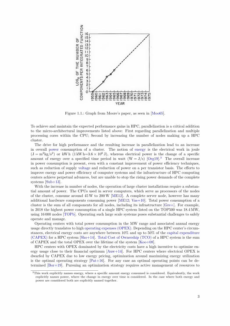
Figure 1.1.: Graph from Moore’s paper, as seen in [Moo65].
To achieve and maintain the expected performance gains in HPC, parallelization is a critical additionto the micro-architectural improvements listed above: First regarding parallelization and multipleprocessing cores within the CPU; Second by increasing the number of nodes making up a HPCcluster.The drive for high performance and the resulting increase in parallelization lead to an increase
in overall power consumption of a cluster. The notion of energy is the electrical work in joule(J = m2kg/s2) or kW h (1 kW h=3.6× 10⁶ J), whereas electrical power is the change of a specificamount of energy over a specified time period in watt (W = J/s) [Org19].3 The overall increasein power consumption is present, even with a constant improvement of power efficiency techniques,such as reduction of supply voltage and reduction of power on a per transistor basis. The efforts toimprove energy and power efficiency of computer systems and the infrastructure of HPC computingcenters achieve perpetual advances, but are unable to stop the rising power demands of the completesystems [Sub+13].With the increase in number of nodes, the operation of large cluster installations require a substan-
tial amount of power. The CPUs used in server computers, which serve as processors of the nodesof the cluster, consume around 45 W to 200 W [ME12]. A complete server node, however has manyadditional hardware components consuming power [ME12; Vas+10]. Total power consumption of acluster is the sum of all components for all nodes, including its infrastructure [Gre+]. For example,in 2018 the highest power consumption of a single HPC system listed on the TOP500 was 18.4 MW,using 16 000 nodes [TOPb]. Operating such large scale systems poses substantial challenges to safelyoperate and manage.Operating centers with total power consumption in the MW range and associated annual energy
usage directly translates to high operating expenses (OPEX). Depending on the HPC center’s circum-stances, electrical energy costs are anywhere between 10% and up to 50% of the capital expenditure(CAPEX) for a HPC system [Sho+14]. Total Cost of Ownership (TCO) of a HPC system is the sumof CAPEX and the total OPEX over the lifetime of the system [Koo+08].HPC centers with OPEX dominated by the electricity costs have a high incentive to optimize en-
ergy usage close to their financial optimum [Auw+14]. For HPC centers where electrical OPEX isdwarfed by CAPEX due to low energy pricing, optimization around maximizing energy utilizationis the optimal operating strategy [Pat+16]. For any case an optimal operating points can be de-termined [Bor+19]. Pursuing an optimization strategy requires active management of resources to
3This work explicitly names energy, where a specific amount energy consumed is considered. Equivalently, the workexplicitly names power, where the change in energy over time is considered. In the case where both energy andpower are considered both are explicitly named together.
3

1. Introduction
achieve the required resource usage with desired energy and power characteristics.Due to the fact that HPC centers are large energy consumers, increased interaction of centers
and Electricity Service Providers (ESPs) has been observed over the years [Bat+15; Pat+16]. Incontrast to other industrial consumers, HPC centers may observe large variable loads [Ste+19b]. Foran outside observer, such as ESPs, this poses a challenge to prediction the centers’ fluctuating energydemand. At the same time, the potential rapid changes in energy demand can be an issue for energygrid stability if not controlled or mitigated. Therefore, several centers already communicate theirexpected energy demand with ESPs [Cla+19a].A HPC system’s power consumption is largely dependent on the characteristics of applications
running on the clusters. Each individual HPC application has a different performance and powercharacteristic. At the same time, the exact behavior may depend on several factors, which varyfrom execution to execution. Examples for different energy and power characteristics are the numberof nodes used, process placement, the applications communications behavior, own and interferingnetwork load, input data sets and versions of libraries, and the application itself. Cluster managementsoftware has only started to include measurement and control capabilities for energy and power.From an electrical engineering and industrial systems engineering standpoint safe operation can beguaranteed by installation of hardware fail-safe mechanisms. From a software perspective, however,many additional possibilities of optimization and control for how software and hardware interact withthe system and influence power consumption can be taken. The highly parallel nature of applicationsand the large parallel hardware setups of systems is both opportunity and challenge for optimizationand efficiency gains. For energy and power optimization only initial steps have been taken so far.The potential of integrating several energy and power management solutions for increased efficiencyand possible optimization have largely been untouched.The software required to operate HPC systems is becoming more and more energy and power
aware [LZ10; Hac+15; Mai+17; Mai+18; Koe+18; CPK19]. Multiple software components managingdifferent hardware components of a system, the interaction of software with different scopes for energymanagement and coordination of the management functionalities are all non-trivial problems. Withinteracting management solutions HPC centers can holistically optimize for their operational goals.Such goals can be as simple as staying within a power limit, or optimizing for energy efficiency. Morecomplex goals are optimizing performance with controllable cost, managing component specific limi-tations, or managing peculiarities of the center, its environment and state of affairs, or a combinationof these examples.A structural approach to describe, manage and implement integrated energy and power solutions
for HPC centers and their respective cluster installations has not been formulated. While individualapproaches are taken and lead to individual solutions, the formulation of a model to describe holisticenergy and power management systems is still missing.The potential benefits of such model are:
• Transparency of energy and power management system, making all interactions of the partici-pating energy and power management sub-systems or components identifiable. This allows fora understandable the energy and power management processes.
• Manageability in terms of planning, organization and operation of energy and power systems,sub-systems and component in HPC systems. This allows for transparent operation and opti-mization of production HPC systems.
• Strategic system development for continuous evolution of the overall systems, enabling con-tinuous controllable system improvements. This allows for targeted research and developmentin the energy and power and performance space, contributing innovations back to productionsystems.
• Comparability of different energy and power management approaches and solutions. This en-ables to understand advantages and disadvantages of different setups and allows to make in-formed design decisions.
By contributing a such energy and power managment model for HPC systems, this work aims enablesthese benefits.
4

1.1. Problem Statement
1.1. Problem StatementThe challenge addressed in this work is the definition of a reference model for integrated energy andpower management of HPC systems.The target systems under consideration are HPC systems which consist of locally distributed,
clustered hardware [ST18, pp. 25–27] and software components of mixed capability and scope. Thisclustered nature of both hardware and software as well as their specific scope and interaction withthe remaining system are part of the challenge. The problem is not confined to a specific HPC systemor cluster size. Arbitrary scaling regarding number of nodes of the system, but also regarding thedegree of abstraction in terms of number of indirections for management, and scaling of sheer powerconsumption have to be considered for the problem.The problem entails that the goals regarding management and optimization of energy and power
differ from HPC center to HPC center. This stems from their often unique funding structure, con-tracts with ESP, but also environmental conditions and available capabilities [Mai+18]. Distinctsolutions are required at each center. The set goals and circumstances of a HPC center influence theselection of the employed approaches, tools and technologies for a selected solution. To transfer andadapt a solution from one center to another — or to a successor system at the same center — requiresmajor re-engineering efforts. Limited transparency and the lack of a detailed description make theprocess of transfer and adaptation of existing approaches notoriously hard. This lack in transparencyand overview regarding energy and power management is present regarding the combined energyand power management capabilities, capabilities of individual system software for energy and powermanagement and the interactions of this overall ensemble. Operational and configuration manage-ment using system software is often still very simple or neglected altogether, due to complexity andfeasibility concerns. A comprehensive approach has to be elaborated to make energy and power man-agement widely available in a integrated system-wide manner. This stands in stark contrast with theisolated solutions consisting of single software tools, often seen today.Goals and sub-goals of a center regarding energy and power management have to be expressible
in a comprehensive way, while the solution has to be presentable in a structured and transparentmanner. Formalization of a structured approach can overcome these issues partially, while agreementon standardized use of such structure depends on active employment of the developed methods bythe different actors in HPC.To illustrate a possible approach for solving the associated issues, three questions are asked.
Q1 – How to model energy and power management systems for HPC systems in an integrated,holistic way?
Q2 – What is an appropriate structure of such model and what are its required building blocks?Q3 – How can such a model be applied to concrete system architectures for energy and power
management of HPC systems?
The first question is the problem statement of this work, while the second and third questionaddress additional aspects to satisfy the problem statement and supplement it.The problem statement, question Q1, asks for a systematic model for energy and power management
in HPC. To obtain an adequate solution, question Q2 has to be answered first. Question Q2 asksnot only for the fundamental building blocks of the solution to question Q1, but also for a goodunderstanding of existing software and hardware environment, which the model and the resultingsolution has to operate in and build upon. The challenge is to identify an adequate level of abstractionfor a modeling approach. By answering question Q2, the understanding for question Q1 is scoped. Toaddress Q3 a method for applying such model to concrete systems architectures has to be outlined.Using this method and applying it, the fitness of the model can be assessed.By leading with question Q2 and following up with question Q3 information regarding the ques-
tion Q1 is supplemented drawing a complete picture for its answer.
5
1. Introduction
Problem definition1
Problem domainanalysis2
Reference modelconstruction3
Evaluation andevolution4
Reference model building
HPC system specificproblem descriptiona
Identification ofrequirementsb
Reference model-/ Architecture-
selectionc
Architectureconstruction/ -adaptation
d
Specific architecture e
Application of the reference model
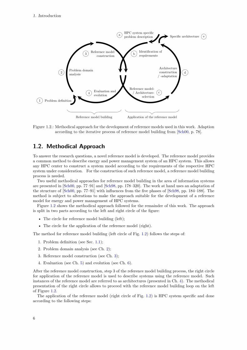
Figure 1.2.: Methodical approach for the development of reference models used in this work. Adaptionaccording to the iterative process of reference model building from [Sch00, p. 78].
1.2. Methodical ApproachTo answer the research questions, a novel reference model is developed. The reference model providesa common method to describe energy and power management system of an HPC system. This allowsany HPC center to construct a system model according to the requirements of the respective HPCsystem under consideration. For the construction of such reference model, a reference model buildingprocess is needed.Two useful methodical approaches for reference model building in the area of information systems
are presented in [Sch00, pp. 77–91] and [Sch98, pp. 178–320]. The work at hand uses an adaptation ofthe structure of [Sch00, pp. 77–91] with influences from the five phases of [Sch98, pp. 184–188]. Themethod is subject to alterations to make the approach suitable for the development of a referencemodel for energy and power management of HPC systems.Figure 1.2 shows the methodical approach followed for the remainder of this work. The approach
is split in two parts according to the left and right circle of the figure:
• The circle for reference model building (left);• The circle for the application of the reference model (right).
The method for reference model building (left circle of Fig. 1.2) follows the steps of:
1. Problem definition (see Sec. 1.1);2. Problem domain analysis (see Ch. 2);3. Reference model construction (see Ch. 3);4. Evaluation (see Ch. 5) and evolution (see Ch. 6).
After the reference model construction, step 3 of the reference model building process, the right circlefor application of the reference model is used to describe systems using the reference model. Suchinstances of the reference model are referred to as architectures (presented in Ch. 4). The methodicalpresentation of the right circle allows to proceed with the reference model building loop on the leftof Figure 1.2.The application of the reference model (right circle of Fig. 1.2) is HPC system specific and done
according to the following steps:
6

1.3. Contributions
a.) HPC system specific problem description;b.) Identification of requirements;c.) Reference model selection or architecture selection;d.) Architecture construction or adaption;e.) Resulting in: a specific architecture.
In the reference model selection step, already constructed architectures can be re-used and changed tofit the specific problem and requirements. The iterative process model for reference model building isfollowed once, shaping the structure of this work, while the iterative process model for application ofthe reference model is followed for selected system presented in Chapter 4. After the application of thereference model is concluded, step 4 of the methodical approach is conducted, to complete the rightcircle for reference model building. The outlined sequence concludes the methodical development ofthe reference model presented as solution to the research question.
1.3. ContributionsIn the following the key contributions of this work are listed. The contribution list is followed bythe list of preliminary publications of the author. This thesis represents a monograph where thepreliminary publications do not constitute any chapter.
1.3.1. Key Contributions of This WorkThe list of contributions is as follows:
1. The Open Integrated Energy and Power (OIEP) reference model.2. A methodical approach for model building for an energy and power management reference
model of HPC systems.3. The description of the buildings blocks of the OIEP reference model, and their structural
composition.4. A method for the creation of concrete instances of the OIEP reference model, called OIEP
architectures.5. The design of OIEP architectures for a selection energy and power management setups of HPC
systems.
The author’s main contribution in this work is the OIEP reference model, an open reference modelfor integrated energy and power management of HPC systems. The work introduces the concepts ofthe OIEP reference model, as well as the notion of an OIEP architecture, where OIEP architecturesare instances of the OIEP reference model.The OIEP reference model allows HPC centers to describe their goals for energy and power man-
agement of HPC systems, its roles and responsibilities. Using such description HPC centers canlayout their HPC system energy and power management design according to their individual needs,integrating the used hardware and software components. Such structured representation allows tomake energy and power management setups understandable, enabling configuration management andoperation of complex interacting systems.The OIEP reference model is a structured representation of interacting hardware and software com-
ponents to enable configuration and operation of complex energy and power management systems.Individual components have varying scope and granularities. The concepts of the OIEP referencemodel allow components to communicate objectives according to the management setup and ulti-mately represents a blueprint to orchestrate the complete heterogeneous setup and design.The model is designed with scalability in mind to fit the needs of massively parallel HPC systems.
The structure of the reference model allows to identify possible scaling and performance bottlenecksso that designs can avoid them before the setup. Additionally, the potential for performance im-provements, and the potential for improved, overhauled or new component approaches (and how tointegrate them into the overall system) can be identified.
7

1. Introduction
The reference model additionally serves as documentation and comprehensive overview for theHPC centers. It allows centers to keep their system management according to physical and logicalsetup of the energy and power management system. Decisions and actions, and possibly faults,can subsequently be traced back to intentions of well-defined goals. Extensions and alterations ofthe energy and power management system become more manageable with reduced impact regardingchanges to the HPC system. The reference model allows for traceability and transparency and makesenergy and power management verifiable from a structural perspective. Possible incompatibilitiesand hidden conflicts are exposed by the concepts and the design of the OIEP reference model.The work at hand is the first work aspiring to describe a structured setup for a modular adaptive
approach that allows to combine the approaches the design of different components for energy andpower management together in a structured reference model, without being tied to a fixed solution ora static setup. The model is supported by the presentation of a transparent method for the referencemodel construction, as well as the method for applying the reference model.
1.3.2. Author’s Preliminary WorkThe list of publications following below contributed to the author’s realization of the necessity of areference model for energy and power management. This thesis is a distinct and independent work,without reproducing content published in these preliminary works. When content is used this is doneaccording to best practices as with any bibliographic reference.Individual solutions by themselves are important contributions to the scientific landscape. To be
useful, however, they have to be manageable and usable at real centers in production environments.Unstructured combinations of solutions are error prone when interacting and management overheadeven for understanding the setup and possibly changing the energy and power management systemis high. Therefore, the OIEP reference model has the potential to make the individual contributionsin prior work more applicable in production environments.The OIEP reference model is therefore paving the way for future research in the area of energy
and power management in HPC, as a tool to give HPC centers, researchers and development teamsthe necessary descriptive concepts to employ and integrate energy and power solutions at their targetsystems.
Preliminary Work Related to the Thesis: The author has contributed to the state of the researchof energy and power in HPC in earlier publications. These related work items are related to the thesisas they are in the research area of energy and power, and can either be part of an OIEP architectureas a component, or help with the understanding of modern energy and power management systems inHPC. The details for each bibliographic entry followed by a comment on the summary of the contentand contribution by the author are listed below:
• Tapasya Patki, David K. Lowenthal, Anjana Sasidharan,Matthias Maiterth, Barry Rountree,Martin Schulz and Bronis R. de Supinski: “Practical Resource Management in Power-Constrained, High Performance Computing”, in: 24th International ACM Symposium onHigh-Performance Parallel and Distributed Computing (HPDC’15), ACM, June 2015, Portland,OR, USA [Pat+15]
In [Pat+15] the author contributed to the modeling section, results generation, as well as result anal-ysis. The paper was developed and driven by the principal author, Tapasya Patki, with contributionsby the remaining authors. The work shows how power-aware resource manager for a special use caseof hardware over-provisioned systems can be realized. The work compares traditional scheduling vsadaptive scheduling where back-filling is performed with possible performance degradation of indi-vidual jobs. This allows to fit jobs into a not utilized power slot, compared to free nodes with noavailable power, and thus allows for faster turnaround time. System power utilization is increased andaverage power turn around time is improved by 19%. The work shows that advanced job managementwith performance considerations based on power can improve utilization and users perceived time tocompletion. This work is used as a reference in Section 2.1.2 on page 21, in Appendix A.1.1.3 onpage 109, and in Appendix B.1.2.2 on pages 130–131.
8

1.3. Contributions
• Matthias Maiterth, Martin Schulz, Barry Rountree and Dieter Kranzlmüller: “Power Bal-ancing in an Emulated Exascale Environment”, in: The 12th IEEE Workshop on High-Performance, Power-Aware Computing (HPPAC’16), IEEE, Mai 2016, Chicago, IL,USA [Mai+16]
In [Mai+16] the author developed a power balancing algorithm to show that default power utilizationof clusters is not optimal and can be improved. The author is the principal author, with strong stylisticand conceptual contributions from the second author, and minor comments from the remaining au-thors. The paper shows that under a fixed power limit the impact of processor performance variationis large enough to redistribute the allocated power and counter the inherent manufacturing variability.This is done using the GREMLIN framework co-developed by the author in prior work [Mai15], while[Mai+16] is the first peer-reviewed publication introducing the GREMLIN framework. By staticallyredistributing power after measuring the individual node performance, overall efficiency was improvedby both, reducing runtime and using less energy. This work is used as a reference in Section 2.1.2 onpages 19–21 (with Fig. 2.3 on p. 22), and in Appendix A.1.1.3 on page 109.
• Jonathan Eastep, Steve Sylvester, Christopher Cantalupo, Brad Geltz, Federico Ardanaz, AsmaAl-Rawi, Kelly Livingston, Fuat Keceli, Matthias Maiterth and Siddhartha Jana: “GlobalExtensible Open Power Manager: A Vehicle for HPC Community CollaborationToward Co-Designed Energy Management Solutions”, in: High Performance Computing- 32st International Conference, ISC High Performance 2017, Springer, June 2017, Frankfurt,Germany [Eas+17]
In [Eas+17] the author contributed minor parts to the overall development of the framework aspart of the Power Pathfinding to Product-Team (P3-Team) at Intel Corporation (Intel). The paperintroduces the runtime framework Global Extensible Open Power Manager (GEOPM). The paper wasdeveloped and driven by the principal author, Jonathan Eastep (who also represents the team lead andprincipal engineer of the product), as a large collaborative effort with contributions by the remainingauthors regarding software development, documentation and experimental setup and execution. Theproduction-grade framework allows for easy integration of power management algorithms in a scalablefashion, and allows to experiment on optimization algorithms in the stable runtime environment.This work is used as a reference in Section 2.1.2 on pages 19–21, in Appendix A.1.1.3 on page 109, inAppendix B.1.2.2 on page 132, and in Appendix D.2 on pages 151–160 (with Fig D.3 on p. 152 andFig. D.4 on p. 153).
• Matthias Maiterth, Torsten Wilde, David K. Lowenthal, Barry Rountree, Martin Schulz,Jonathan Eastep and Dieter Kranzlmüller: “Power Aware High Performance Computing:Challenges and Opportunities for Application and System Developers – Survey &Tutorial”, in: 2017 International Conference on High Performance Computing & Simulation,HPCS 2017, IEEE, July 2017, Genoa, Italy [Mai+17]
In [Mai+17] the author surveyed the current state of the research for application and system devel-opers regarding energy and power optimization. The work surveys infrastructure and facility basics,metrics for infrastructure and facilities, user interaction with power management and goes into de-tail on system software with power considerations. The system software analysis shows low-levelpower interfaces, interaction of energy and power aware scheduling, and concludes with energy andpower runtimes. The paper supplements the tutorial ’Power Aware High Performance Computing:Challenges and Opportunities for Application and System Developers’ at International Conferenceon High Performance Computing and Simulation (HPCS), 2017. The remaining authors contributedto the tutorial and prior incarnations of the tutorial held at ACM/IEEE Supercomputing Conference(SC) 2015 & SC 2016, held prior to the involvement of the author. This work is used as a referencein Section 1 on page 4.
• Matthias Maiterth, Gregory A. Koenig, Kevin Pedretti, Siddhartha Jana, Natalie Bates,Andrea Borghesi, Dave Montoya, Andrea Bartolini and Milos Puzovic: “Energy and PowerAware Job Scheduling and Resource Management: Global Survey — Initial Anal-ysis”, in: The 14th IEEE Workshop on High-Performance, Power-Aware Computing (HP-PAC’18), IEEE, Mai 2018, Vancouver, BC, Canada [Mai+18]
9

1. Introduction
In [Mai+18] the author contributed to a global survey of HPC centers and their strategies towardsenergy and power aware job scheduling and resource management. The work was conducted withthe Energy Efficient High Performance Computing Working Group (EE-HPC-WG) as part of theEnergy and Power Aware Job Scheduler and Resource Manager (EPA-JSRM) sub-group. Thesurvey spanned a two-year period, lead by Greg Koenig and Natalie Bates, resulting in three pa-pers: [Mai+18], [Koe+18] and [Koe+19]. In the survey, centers were identified using such schedulingand resource management approaches for energy efficiency. A questionnaire was formulated and sentto each center to have representative and comparable answers about their practices. The authorcontributed in the analysis and presentation of the results and replies. The remaining authors greatlysupported in the interviews, background work and parts of the analysis and representation.The first paper [Mai+18] with the author of this work as the principal author, shows the breath of
the survey conducted, presents the questionnaire and brings some of its highlights into presentableform. The paper was followed up by a Birds-of-a-Feather (BoF) discussion session at InternationalSupercomputing Conference - High Performance (ISC) 2018 in Frankfurt [BoF’18]. This work is usedas a reference in Section 1 on pages 1–4, in Section 1.1 on page 5, in Section 2.1.1.2 on page 18, inAppendix A.1.1.3 on page 110, in Appendix A.1.2.3 on page 112, in Appendix A.1.3.2 on page 114,in Appendix B.1.1.1 on pages 120–121, in Appendix B.1.2.2 on page 131, and in Appendix D.3 onpage 163.
• Gregory A. Koenig, Matthias Maiterth, Siddhartha Jana, Natalie Bates, Kevin Pedretti,Milos Puzovic, Andrea Borghesi, Andrea Bartolini and Dave Montoya: “Energy and PowerAware Job Scheduling and Resource Management: Global Survey — An In-DepthAnalysis”, in: The 2nd International Industry/University Workshop on Data-center Automa-tion, Analytics, and Control (DAAC’18), DAAC 2018, online (peer-reviewed), November 2018,Dallas, Texas, USA, [Koe+18]
In [Koe+18] the full analysis of the survey started in [Mai+18] was published. The author participatedas a main contributor with focus on the analysis section, however not as principal author, whilecontinuing the previous work’s effort. In the tradition of the work’s effort, all authors contributedtheir share to the paper. This work put special emphasis on the diversity of the surveyed centers,their individual motivation of why employing energy and power management solutions. This work isused as a reference in Section 1 on pages 1–4, in Section 2.1.1.2 on page 18, in Appendix A.1.1.3 onpage 110, in Appendix B.1.2.2 on page 131, and in Appendix D.3 on page 163.
• Gregory Allen Koenig, Matthias Maiterth, Siddhartha Jana, Natalie Bates, Kevin Pedretti,Andrea Borghesi and Andrea Bartolini: “Techniques and Trends in Energy and PowerAware Job Scheduling and Resource Management”, Unpublished, Submitted for re-view. [Koe+19]
The work of the EE-HPC-WG EPA-JSRM sub-group is concluded in a journal submission [Koe+19].Here all findings are summarized and general synopsis is given, again lead by Greg Koenig. In thethree publications [Koe+18; Mai+18; Koe+19] the author contributed to the community of energyand power researchers in HPC as member of the EE-HPC-WG as major contributor to the analysisof the survey. This work is used as a reference in Section 2.1.1.2 on page 18, in Appendix A.1.1.3 onpage 110, in Appendix B.1.2.2 on page 131, and in Appendix D.3 on page 163.
• Gence Ozer, Sarthak Garg, Neda Davoudi, Gabrielle Poerwawinata, Matthias Maiterth,Alessio Netti and Daniele Tafani: “Towards a Predictive Energy Model for HPC Run-time Systems Using Supervised Learning”, in: PMACS - Performance Monitoring andAnalysis of Cluster Systems (Euro-Par 2019 Workshop), August 2019, Göttingen,Germany [Oze+19]
In [Oze+19] the author contributed to the work investigating predictive models for energy and poweras well as performance based on hardware metrics, contributing to the usage of GEOPM for thepaper. The execution of the paper was driven by the four leading authors, where the later threeauthors supported the work from a technical, stylistic and conceptual side. The work investigates thepossibility to enable the usage of machine learning for optimization algorithm in the energy efficiencyruntimes GEOPM. The work also used system monitoring tool DCDB [Net+19] to investigate thecomplementary effects of runtime system and system monitoring. This work is not used as a reference.
10

1.3. Contributions
Other HPC Related Preliminary Work: In addition to the publications in energy and power, theauthor contributed to research in HPC in the work:
• Karl Fürlinger, Colin W. Glass, José Gracia, Andreas Knüpfer Jie Tao, Denis Hünich, KamranIdrees, Matthias Maiterth, Yousri Mhedheb and Huan Zhou: “DASH: Data Structuresand Algorithms with Support for Hierarchical Locality”, in: SPPEXA - Workshop onSoftware for Exascale Computing (Euro-Par 2014), August 2014, Porto,Portugal [Für+14]
In [Für+14] the author contributed to the DASH-Project [Für] as student research assistant for KarlFürlinger, culminating in the paper introducing DASH, a Partitioned Global Address Space (PGAS)programming model in the form of a C++ template library. The main contributions and efforts ofthe paper were driven by the main project lead, Karl Fürlinger, where the remaining contributorsand authors worked on the different layers of the DASH library, the DASH runtime (DART), andlibraries and applications. This work is not used as a reference.
Active Participation in Scientific Working Groups: In addition to the publications, the author alsoactively contributes to the professional groups for energy and power in HPC, the EE-HPC-WG andthe PowerStack community.The EE-HPC-WG is a group of more than 700 members from 20 countries trying to tackle issues
regarding energy efficiency in HPC. The author actively contributed to the EPA-JSRM sub-group,as well as the procurement considerations sub-group.The PowerStack community is a group of collaborators with the goal of designing a power software
management stack ready for the challenges HPC faces in the light of exascale computing. The grouphas started to coordinate bi-annual seminar events to synchronize the group’s efforts in 2018 withits initial strawman document [Can+18]. The group itself is organized by thirteen core committeemembers of which the author is one.With this work at hand the author contributes to the PowerStack group’s concepts and vocabulary,
to assist their goal of designing a holistic software stack with the goal of a standardized ecosystem.
11

1. Introduction
1.4. Thesis Outline
Chapter 1
Chapter 2
Chapter 3
Chapter 4
Chapter 5
Chapter 6
Chapter 7
Introduction Problem Statement Thesis Method Contributions Outline
Motivation Problem Scope Problem Requirements Related Work
The OIEP Reference Model
Chapter Method Fundamentals Reference Model Description
OIEP Architectures
Chapter Method OIEP Architecture Construction by Example
Assessment
Future Work
Conclusions
1
2
3
ab
cd
e
4
Chapters Contents Methodsteps
Figure 1.3.: Thesis outline. Chapters and contents are listed with a reference to the correspondingstep from the methodical approach of Figure 1.2 as described in Section 1.2.
Figure 1.3 shows the structure of this work, described in the following:The introduction in the current chapter, Chapter 1, provides the basic terms needed for under-
standing the research questions of this work. The problem statement and research questions of thethesis are described, the methodical approach outlined and the contributions listed, including the au-thor’s previous publications. The work is thereafter structured with the aim to generate a referencemodel for integrated energy and power management of HPC systems. The chapter covers the firststep of the methodical approach, the problem definition (as indicated under “Method steps” on theright-hand side of Fig. 1.3, as outlined in Sec. 1.2).The next step in the methodical approach is the problem domain analysis, which is presented in
the background chapter (see Ch. 2). The background is split into four parts:
1. Section 2.1, presents the motivation regarding the problem domain and the contribution of thiswork;
2. Section 2.2, presents a delimitation to focus the problem scope;3. Section 2.3, presents a requirements’ analysis to be able to generate the intended reference
model.4. Section 2.4, presents the related work. The section shows different approaches taken for holistic
and structured energy and power management with possible application in the problem domainand how they compare.
After the essential preluding parts, Chapter 3 presents the core part of this work, the OIEP referencemodel. The chapter presents the OIEP reference model in three parts:
1. The method for the reference model generation is outlined (Sec. 3.1).2. Required fundamental concepts for the design are presented (Sec. 3.2).
12

1.4. Thesis Outline
3. Finally, the individual elements of the OIEP reference model are presented (Sec. 3.3). This isdone in four parts, which make up the OIEP reference model description:a) OIEP levels and the OIEP level tree (Sec. 3.3.2);b) OIEP components and the OIEP component tree (Sec. 3.3.1);c) OIEP data sources and the OIEP monitoring overlay (Sec. 3.3.3);d) OIEP operating states and the OIEP state diagram (Sec. 3.3.4);
The reference model description completes the third step of the methodical approach (as of Sec. 1.2).In the next step of the thesis, the work transitions to the application of the reference model
presented in Chapter 4, as featured in the methodical outline on the right-hand side circle of Figure 1.2.Chapter 4 presents the application of the OIEP reference model in two steps:
1. A method for the application of the OIEP reference model (Sec. 4.1).2. An application of the OIEP reference model by example of the PowerStack (Sec. 4.2).
Such constructed applied models of the OIEP reference model are called OIEP architectures. Forapplying the method the steps a to e of the thesis method are followed, which is indicated on theright-hand side of Figure 1.3. Appendix D provides five additional OIEP architectures to checkthe applicability of the reference model, which also follow the application method. The appendedsupplementary OIEP architecture constructions model the following energy and power managementsetups:
• The PowerStack prototype, in Appendix D.1;• The GEOPM framework, in Appendix D.2;• The SuperMUC system at LRZ, in Appendix D.3;• The SuperMUC-NG systems at LRZ, in Appendix D.4;• The Fugaku system at RIKEN Center for Computational Science (R-CCS), in Appendix D.5.
For each exemplary system, the method’s application of the reference model circle is iterated for atotal of six times (see Sec. 1.2). The main body of the work therefore only presents the referencemodel application cycle once, for brevity.Following the reference model definition, the method for model application and the construction
for the exemplary OIEP architectures, the reference model requires an evaluation. This initiates thelast part of the thesis method: evaluation and evolution.Chapter 5 presents the evaluation in the form of an initial assessment of the work. This is done
with regard to the requirements of Section 2.3 as a summary (in Sec. 5.1), with a summary of theidentified limitations (Sec. 5.2).The chapter is followed up by an outlook to future work in Chapter 6. The discussion on future
work is split into three areas:
1. For the OIEP reference model itself (Sec. 6.1);2. For the application of the reference model in the form of OIEP architectures (Sec. 6.2);3. General future work in energy and power management of HPC systems enabled and supported
by the presented contributions (Sec. 6.3).
Chapter 5 & 6 close the methodical approach, by completing the sequence outlined by the left andright circle of the presented method of Section 1.2.The final chapter, Chapter 7, summarizes the work and draws conclusions from the problem state-
ment and research questions, completing the works’ contributions.
13
1. Introduction
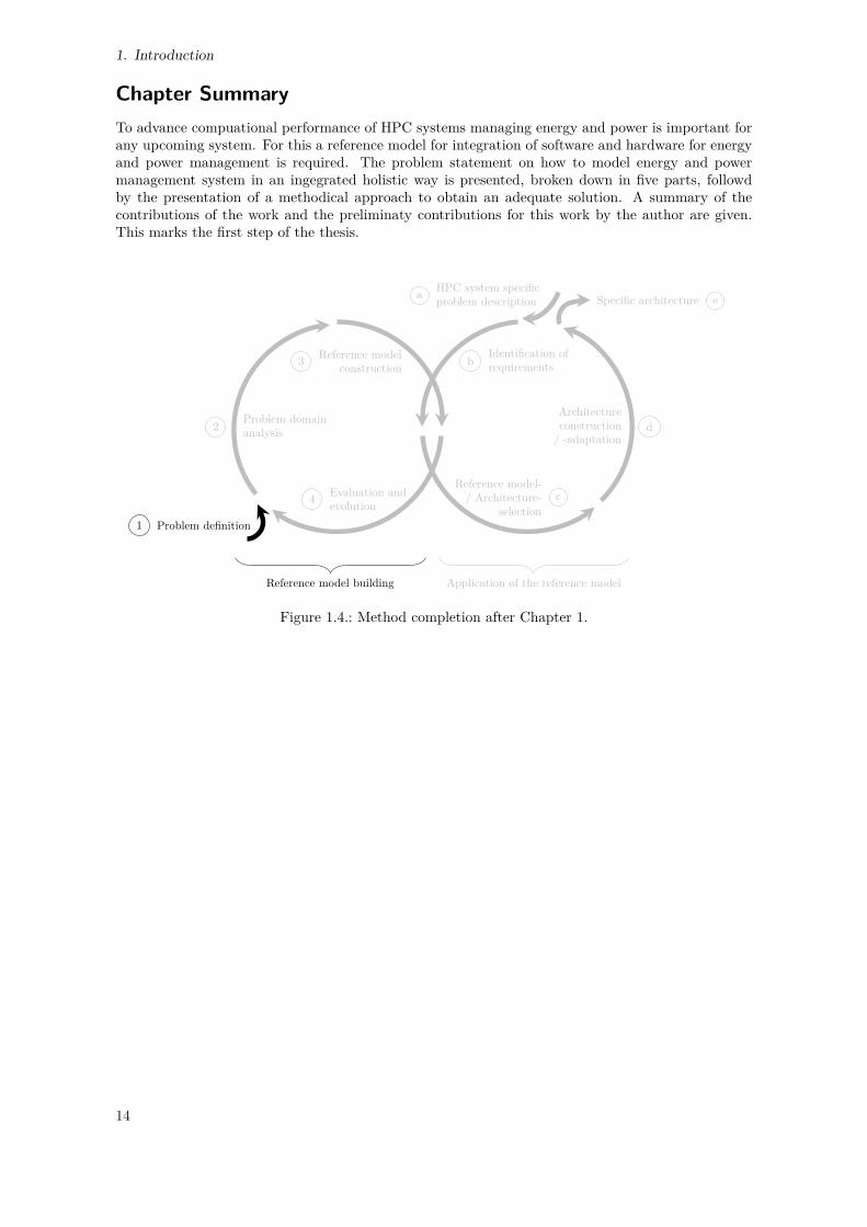
Chapter SummaryTo advance compuational performance of HPC systems managing energy and power is important forany upcoming system. For this a reference model for integration of software and hardware for energyand power management is required. The problem statement on how to model energy and powermanagement system in an ingegrated holistic way is presented, broken down in five parts, followdby the presentation of a methodical approach to obtain an adequate solution. A summary of thecontributions of the work and the preliminaty contributions for this work by the author are given.This marks the first step of the thesis.
Problem definition1
Problem domainanalysis2
Reference modelconstruction3
Evaluation andevolution4
Reference model building
HPC system specificproblem descriptiona
Identification ofrequirementsb
Reference model-/ Architecture-
selectionc
Architectureconstruction/ -adaptation
d
Specific architecture e
Application of the reference model
Figure 1.4.: Method completion after Chapter 1.
14

2. Background
2.1. Motivation . . . . . . . . . . . . . . . . . . . . . . . . . . . . . . . . . . . . . . . . . . 152.1.1. Energy and Power – a Major Challenge for Exascale and Beyond . . . . . . . . 152.1.2. Managing Energy and Power Using Software . . . . . . . . . . . . . . . . . . . 182.1.3. The Need for an Energy and Power Management Software Stack . . . . . . . . 22
2.2. Scoping of Energy and Power Management Systems . . . . . . . . . . . . . . . . . . . 252.2.1. Sources of Variability . . . . . . . . . . . . . . . . . . . . . . . . . . . . . . . . 252.2.2. Optimization Goals of Energy and Power Management Systems . . . . . . . . . 272.2.3. Aspects of Energy and Power Management Setups . . . . . . . . . . . . . . . . 28
2.3. Requirements for Reference Models for Energy and Power Management . . . . . . . . 312.4. Related Work . . . . . . . . . . . . . . . . . . . . . . . . . . . . . . . . . . . . . . . . . 34
2.4.1. Structured Energy and Power Management Approaches in HPC . . . . . . . . 342.4.2. Compound Software Setups for Energy and Power Management in HPC . . . . 362.4.3. Modeling of Complex Control Systems . . . . . . . . . . . . . . . . . . . . . . . 382.4.4. Related Work – Summary of Characteristics . . . . . . . . . . . . . . . . . . . . 40
This chapter motivates active energy and power management using software and gives structure. Themain challenges for systems reaching exaFLOPS performance are raised in Sections 2.1.1, setting thestage for approaching the issues of energy and power at this stage of HPC systems. The focus of thiswork on addressing energy and power management from a software side is motivated in Section 2.1.2.Section 2.1.3 motivates the need of a well integrated holistic reference structure for software to manageenergy and power. For a solid problem domain analysis, proper scoping of the issue of interactingsoftware for energy and power in modern HPC systems is presented in Section 2.2. Thereafter,requirements for energy and power management systems are derived in Section 2.3. The backgroundis concluded with the related work in Section 2.4.
2.1. MotivationThe efforts to build large scale computer systems is, in simple terms, an issue of hardware capabilities:processing, memory and interconnection performance of individual hardware components and theirefficient usage. In preparation for terascale systems the hardware performance and programmabilityof such system presented itself as the major challenges [Ko02]. In preparation for petascale systems thepersistent challenges of terascale systems were acknowledged, recognizing an increase in complexity forthe scaling of application codes [Aik07]. Arising issues with total system power were recognized andadditionally major advances in diagnostics proposed, for all aspects of the systems including energyand power consumption [Kra+07]. After the bring-up of petascale systems, active power managementfrom the software side was deployed at several centers [Auw+14]. For the preparation for exascalesystems energy and power has been identified as one of the major challenges to overcome. [Alm+17]
2.1.1. Energy and Power – a Major Challenge for Exascale and BeyondIn the advance from petaFLOPS to exaFLOPS performance the issues of energy and power presenta major hurdle. The associated challenges are identified and tackled by different entities in variousways. First and foremost stands the identification of the issue to be able to strategically overcomeand harness the effects to one’s advantage. The motivation is presented from the perspective of theUnited States Department of Energy (U.S. DOE) and efforts to overcome the issues are presentedfor the international effort of the EE-HPC-WG. Both are among the first to identify and address thelooming issues.
15

2. Background
2.1.1.1. United States Department of Energy’s Perspective on Exascale
The U.S. DOE, one of the largest scientific organization procuring HPC systems, reviewed their com-putational requirements for its scientific domains in preparation for Request For Informations (RFIs)and Request For Proposals (RFPs) for exascale systems. The associated published reports span thescientific domains from Advanced Scientific Computing [Alm+17], Basic Energy Sciences [Win+17],Biological and Environmental Research [Ark+16], Fusion Energy Sciences [Cha+17], High EnergyPhysics [Hab+16], to Nuclear Physics [Car+17]. These reports have slightly different domain spe-cific requirements, but each of them reaches the conclusion that improved, large scale computationalsystems are existential for scientific progress. The goals in all domains are improved accuracy, reso-lution or scale of existing computational models and possibly new or coupled physics models, whichallows to better understand the phenomenons under investigation [Ger+18]. It is widely acceptedthat, what is compute-able is not only restricted by the current scientific models, but moreover bythe computational resources available to run these simulations [Cha+17; Car+17; Hab+16; Bis+09;You+09; BM10]. This emphasizes the importance of the move from current petascale systems toexascale systems.In a summary report [Don+14] the exascale system requirement documents mentioned above have
been analyzed systematically, acknowledging five major challenges:
• Power• Extreme Concurrency• Limited Memory• Data Locality• Resilience
These challenges are elaborated below:
• Power is a major issue impacting architectural design decisions for upcoming HPC systems.The constant expected increase of numbers of active transistors per unit volume in Metal-oxide-semiconductor field-effect transistor (MOSFET) devices with equivalent power density,often so-called Dennard scaling [Den+99], has broken down [JN16]. Power density (W/m3) oftransistors in a fixed volume can not be increased arbitrarily, due to available power deliveryand heat dissipation. This means that using the same architectural designs while increasingfrequency, a standard practice in the past, has become infeasible [Sut05].Modern HPC systems are built from a massive number of concurrently operating MOSFETdevices [Mar91], thus associated challenges regarding their power management have to be solved.In addition to the power consumption of individual components, total power consumption ofa single HPC systems to reach exaFLOPS performance is an issue. To incentivize innovationthe U.S. DOE’s original target regrading power consumption for exascale systems was set to20 MW [Don+14].
• Extreme concurrency is the standard for machine design and the system architecture in HPCtoday. When looking at modern HPC systems, the microprocessors themselves are massivelyparallel systems [GK06; Kri+12]. CPUs are designed using concurrency and parallelism in theform of Instruction-Level Parallelism (ILP), Data-Level Parallelism (DLP), as well as multi-and many-core architectures [HP17]. While frequency increases have stagnated the primaryperformance improvements are seen due to increases in concurrency [Rup; Nat12].An additional source of performance improvements is made possible by increasing the total num-ber of compute nodes, thus again increasing concurrency. A prime example is the Japanese Fu-gaku system at R-CCS. It amasses a total of 158 976 compute nodes and a total of 7 630 848 cores.The systems peak performance reaches up to 415 PFLOPS at a power draw of 28 MW [Don20].The system is the fastest HPC system listed starting June 2020 TOP500 list [TOPc]. The sys-tem’s performance advantage is due to its massive concurrency, while node peak performance islower compared to the systems in second and third place [Don20].1 Follow-up systems to reachhigher performance are likely to have even higher concurrency.
1The last TOP500 list with single core systems listed was in 1996 with 3 systems [TOPg].
16
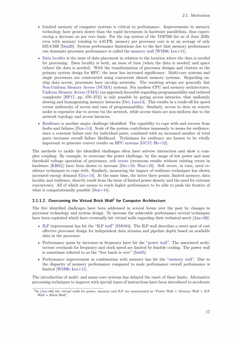
2.1. Motivation
• Limited memory of computer systems is critical to performance. Improvements in memorytechnology have grown slower than the rapid increments in hardware parallelism, thus experi-encing a decrease on per core basis. For the top system of the TOP500 list as of June 2020,even with memory totaling to 4.85 PB, memory per processor core is at an average of only635.6 MB [Don20]. System performance limitations due to the fact that memory performancecan dominate processor performance is called the memory wall [WM96; Leo+11].
• Data locality is the issue of data placement in relation to the location where the data is neededfor processing. Data locality is both, an issue of time (when the data is needed) and space(where the data is needed). With the transformation of processor designs and clusters as theprimary system design for HPC, the issue has increased significance. Multi-core systems andsingle processors are constructed using concurrent shared memory systems. Regarding on-chip data access, processors have on-chip networks. The resulting setups are generally fastNon-Uniform Memory Access (NUMA) systems. For modern CPU and memory architectures,UniformMemory Access (UMA) (an approach favorable regarding programmability and reducedcomplexity [HP17, pp. 370–374]) is only possible by gating access latencies, thus uniformlyslowing and homogenizing memory latencies [Dre; Lam13]. This results in a trade-off for speedversus uniformity of access and ease of programmability. Similarly, access to data on remotenodes is expensive due to access via the network, while access times are non-uniform due to thenetwork topology and access latencies.
• Resilience is another major challenge identified: The capability to cope with and recover fromfaults and failures [Don+14]. Scale of the system contributes immensely to issues for resilience,since a constant failure rate for individual parts, combined with an increased number of totalparts increases overall failure likelihood. Techniques for resiliency are known to be vitallyimportant to generate correct results on HPC systems [GC17; Ho+12].
The methods to tackle the identified challenges often have adverse interaction and show a com-plex coupling: By example, to overcome the power challenge, by the usage of low power and nearthreshold voltage operation of processors, soft errors (erroneous results without existing errors inhardware [KH04]) have been shown to increase [Dre+10; Wan+16]. Soft errors, in turn, need re-silience techniques to cope with. Similarly, measuring the impact of resilience techniques has shownincreased energy demand [Gra+14]. At the same time, the latter three points, limited memory, datalocality and resilience, directly result from the issue of limited power density and the need for extremeconcurrency. All of which are means to reach higher performance to be able to push the frontier ofwhat is computationally possible [Don+14].
2.1.1.2. Overcoming the Virtual Brick Wall2 for Computer Architecture
The five identified challenges have been addressed in several forms over the past by changes inprocessor technology and system design. To increase the achievable performance several techniqueshave been exploited which have eventually hit virtual walls regarding their technical merit [Asa+06]:
• ILP improvement has hit the “ILP wall” [SMO04]. The ILP wall describes a sweet spot of costeffective processor design for independent data streams and pipeline depth based on availabledata in the processor.
• Performance gains by increases in frequency have hit the “power wall”. The associated archi-tecture overhauls for frequency and clock speed are limited by feasible cooling. The power wallis sometimes referred to as the “free lunch is over” [Sut05].
• Performance improvement in combination with memory has hit the “memory wall”. Due tothe disparity of memory performance compared to node performance overall performance islimited [WM96; Leo+11].
The introduction of multi- and many-core systems has delayed the onset of these limits. Alternativeprocessing techniques to improve with special types of instructions have been introduced to accelerate
2In [Asa+06] the virtual walls for power, memory and ILP are summarized as “Power Wall + Memory Wall + ILPWall = Brick Wall”.
17
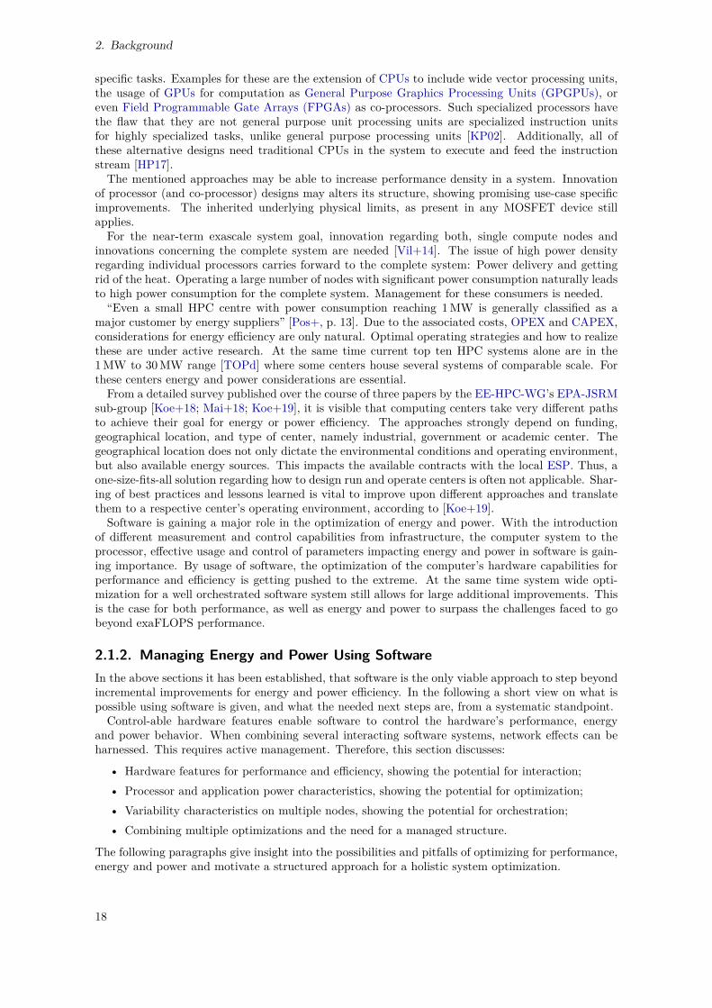
2. Background
specific tasks. Examples for these are the extension of CPUs to include wide vector processing units,the usage of GPUs for computation as General Purpose Graphics Processing Units (GPGPUs), oreven Field Programmable Gate Arrays (FPGAs) as co-processors. Such specialized processors havethe flaw that they are not general purpose unit processing units are specialized instruction unitsfor highly specialized tasks, unlike general purpose processing units [KP02]. Additionally, all ofthese alternative designs need traditional CPUs in the system to execute and feed the instructionstream [HP17].The mentioned approaches may be able to increase performance density in a system. Innovation
of processor (and co-processor) designs may alters its structure, showing promising use-case specificimprovements. The inherited underlying physical limits, as present in any MOSFET device stillapplies.For the near-term exascale system goal, innovation regarding both, single compute nodes and
innovations concerning the complete system are needed [Vil+14]. The issue of high power densityregarding individual processors carries forward to the complete system: Power delivery and gettingrid of the heat. Operating a large number of nodes with significant power consumption naturally leadsto high power consumption for the complete system. Management for these consumers is needed.“Even a small HPC centre with power consumption reaching 1 MW is generally classified as a
major customer by energy suppliers” [Pos+, p. 13]. Due to the associated costs, OPEX and CAPEX,considerations for energy efficiency are only natural. Optimal operating strategies and how to realizethese are under active research. At the same time current top ten HPC systems alone are in the1 MW to 30 MW range [TOPd] where some centers house several systems of comparable scale. Forthese centers energy and power considerations are essential.From a detailed survey published over the course of three papers by the EE-HPC-WG’s EPA-JSRM
sub-group [Koe+18; Mai+18; Koe+19], it is visible that computing centers take very different pathsto achieve their goal for energy or power efficiency. The approaches strongly depend on funding,geographical location, and type of center, namely industrial, government or academic center. Thegeographical location does not only dictate the environmental conditions and operating environment,but also available energy sources. This impacts the available contracts with the local ESP. Thus, aone-size-fits-all solution regarding how to design run and operate centers is often not applicable. Shar-ing of best practices and lessons learned is vital to improve upon different approaches and translatethem to a respective center’s operating environment, according to [Koe+19].Software is gaining a major role in the optimization of energy and power. With the introduction
of different measurement and control capabilities from infrastructure, the computer system to theprocessor, effective usage and control of parameters impacting energy and power in software is gain-ing importance. By usage of software, the optimization of the computer’s hardware capabilities forperformance and efficiency is getting pushed to the extreme. At the same time system wide opti-mization for a well orchestrated software system still allows for large additional improvements. Thisis the case for both performance, as well as energy and power to surpass the challenges faced to gobeyond exaFLOPS performance.
2.1.2. Managing Energy and Power Using SoftwareIn the above sections it has been established, that software is the only viable approach to step beyondincremental improvements for energy and power efficiency. In the following a short view on what ispossible using software is given, and what the needed next steps are, from a systematic standpoint.Control-able hardware features enable software to control the hardware’s performance, energy
and power behavior. When combining several interacting software systems, network effects can beharnessed. This requires active management. Therefore, this section discusses:
• Hardware features for performance and efficiency, showing the potential for interaction;• Processor and application power characteristics, showing the potential for optimization;• Variability characteristics on multiple nodes, showing the potential for orchestration;• Combining multiple optimizations and the need for a managed structure.
The following paragraphs give insight into the possibilities and pitfalls of optimizing for performance,energy and power and motivate a structured approach for a holistic system optimization.
18

2.1. Motivation
Hardware Features for Performance and Efficiency: Monitoring and control mechanisms intro-duced in server CPUs have provided the opportunity to utilize frequency controls to tune and alterperformance and resulting power consumption of processors. This is done using Dynamic Voltageand Frequency Scaling (DVFS), a feature present on processors from all vendors.On Intel platforms, for example, the initial hardware feature to control frequency was introduced
as Intel SpeedStep technology [Int04]. The referenced document not only introduced the necessaryinformation to use DVFS functionality, but also produced information on power dissipation andThermal Design Power (TDP) for the Pentium processor line [Int04]. TDP represents the maximumpower draw of a processor or domain (in watt [W]), for which the value is specified. This featurehas been augmented over the years and the Intel Sandy Bridge processors introduced an additionalfeature relying on a variation of DVFS: Intel’s Running Average Power Limit (RAPL). Intel’s Run-ning Average Power Limit (RAPL) allows measuring and setting two explicit limits for the powerconsumption of the processor, referred to as power caps [Int15b]. These power caps allow settingregisters to limit the power consumption over a specified period of time. TDP is set at the manu-facturing process indicating the maximum power consumption of processors, RAPL allows to lowerthis limit artificially using software. This technology has since been extensively explored, validatedand utilized by the research community to verify and understand the behavior of processors as wellas applications [Hac+15; Sch+19; Sch+16b; DPW16; Kha+18; Mai+16; Eas+17; Kha+18; Rou+12;Rot+12]. Most conclusions drawn from the research named above are not limited to DVFS andRAPL explicitly but apply to any technique altering and impacting power voltage capacitance andfrequency behavior. Given the necessary permissions, control of DVFS is possible from the OperatingSystem (OS), system software, libraries and applications.
Processor and Application Power Characteristics: Power consumption is typically described usingthe simplified formula [CSB92; FHR99]:
P = CV 2F
where C is the capacitance, V is voltage, and F is frequency.Low voltage computation is a technical challenge for processor manufacturers, where voltage levels
have to be distinguishable for switching. Increased frequency directly results in higher processorperformance. At the same time it is the main contributor regarding heat generation. The capacitanceC impact depends on which part of the processor gets activated and has to switch from ground stateto active and back. Thus, even if frequency is controllable, the power consumption largely depends onthe part of the processor utilized. The details of the above formula are discussed in the backgroundsection (Sec. B.1.1). Since not all parts of the processor are used equally for every part of theapplication and complex instruction pipelines, applications do have specific power characteristics ateach frequency.For example, Figure 2.1 shows the power consumption over the execution time of a simple synthetic
benchmark measurement, with power on the x-axis, and time on the y-axis. The measurement showsregular power fluctuation in a range between 80 W to 200 W over a time period of approximately threeseconds. The test system is a single node of a Knights Landing system (Intel® Xeon Phi™ Processor7210F 16 GB [Int], 1.30 GHz, 64 cores, 96 GB Double Data Rate 4 Synchronous Dynamic Random-Access Memory (DDR4 SDRAM), TDP 230 W) The test system is operated at fixed frequency whilethe application runs ten iteration of the benchmark phases sleep, stream, dgemm, stream (repeated)and all2all, in succession. After the first iteration, the following 9 iterations show the exact samepower characteristics.A plot of a single iteration of this benchmark run shows the power characteristics in more detail,
as seen in Figure 2.2 The plot shows the power fluctuation in the 80 W to 200 W range in the timeinterval from ∼7.9 s to ∼8.2 s, which is the detailed view of the first regular iteration of Figure 2.1.A single iteration is split up in 5 parts. The iteration starts with a short sleep phase, where theprocessor is idle (∼80 W). Next a stream phase is started where memory is fetched and a simplestream operation, STREAM Triad, is performed stressing memory bandwidth. This initiates the idleCPU and brings the processor to ∼130 W of power consumption. The next phase is dgemm. In Double-precision GEneral Matrix-Matrix multiplication (DGEMM) a large Matrix-Matrix multiplication isperformed stressing arithmetic units of the processor. Subsequently, power consumption surges to
19
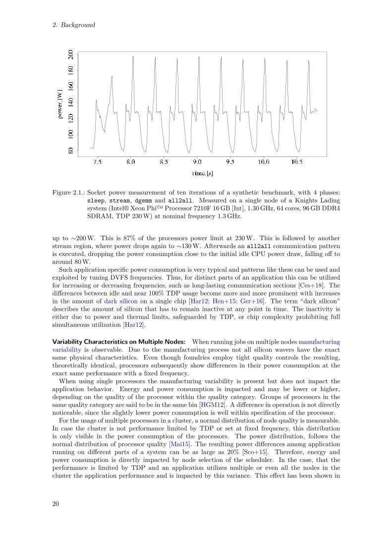
2. Background
Figure 2.1.: Socket power measurement of ten iterations of a synthetic benchmark, with 4 phases:sleep, stream, dgemm and all2all. Measured on a single node of a Knights Ladingsystem (Intel® Xeon Phi™ Processor 7210F 16 GB [Int], 1.30 GHz, 64 cores, 96 GB DDR4SDRAM, TDP 230 W) at nominal frequency 1.3 GHz.
up to ∼200 W. This is 87% of the processors power limit at 230 W. This is followed by anotherstream region, where power drops again to ∼130 W. Afterwards an all2all communication patternis executed, dropping the power consumption close to the initial idle CPU power draw, falling off toaround 80 W.Such application specific power consumption is very typical and patterns like these can be used and
exploited by tuning DVFS frequencies. Thus, for distinct parts of an application this can be utilizedfor increasing or decreasing frequencies, such as long-lasting communication sections [Ces+18]. Thedifferences between idle and near 100% TDP usage become more and more prominent with increasesin the amount of dark silicon on a single chip [Har12; Hen+15; Ger+16]. The term “dark silicon”describes the amount of silicon that has to remain inactive at any point in time. The inactivity iseither due to power and thermal limits, safeguarded by TDP, or chip complexity prohibiting fullsimultaneous utilization [Har12].
Variability Characteristics on Multiple Nodes: When running jobs on multiple nodes manufacturingvariability is observable. Due to the manufacturing process not all silicon wavers have the exactsame physical characteristics. Even though foundries employ tight quality controls the resulting,theoretically identical, processors subsequently show differences in their power consumption at theexact same performance with a fixed frequency.When using single processors the manufacturing variability is present but does not impact the
application behavior. Energy and power consumption is impacted and may be lower or higher,depending on the quality of the processor within the quality category. Groups of processors in thesame quality category are said to be in the same bin [HGM12]. A difference in operation is not directlynoticeable, since the slightly lower power consumption is well within specification of the processor.For the usage of multiple processors in a cluster, a normal distribution of node quality is measurable.
In case the cluster is not performance limited by TDP or set at fixed frequency, this distributionis only visible in the power consumption of the processors. The power distribution, follows thenormal distribution of processor quality [Mai15]. The resulting power differences among applicationrunning on different parts of a system can be as large as 20% [Sco+15]. Therefore, energy andpower consumption is directly impacted by node selection of the scheduler. In the case, that theperformance is limited by TDP and an application utilizes multiple or even all the nodes in thecluster the application performance and is impacted by this variance. This effect has been shown in
20
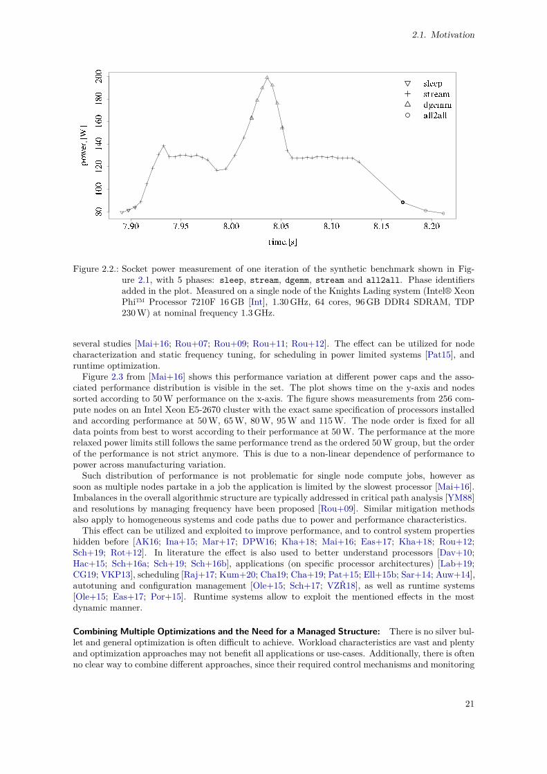
2.1. Motivation
Figure 2.2.: Socket power measurement of one iteration of the synthetic benchmark shown in Fig-ure 2.1, with 5 phases: sleep, stream, dgemm, stream and all2all. Phase identifiersadded in the plot. Measured on a single node of the Knights Lading system (Intel® XeonPhi™ Processor 7210F 16 GB [Int], 1.30 GHz, 64 cores, 96 GB DDR4 SDRAM, TDP230 W) at nominal frequency 1.3 GHz.
several studies [Mai+16; Rou+07; Rou+09; Rou+11; Rou+12]. The effect can be utilized for nodecharacterization and static frequency tuning, for scheduling in power limited systems [Pat15], andruntime optimization.Figure 2.3 from [Mai+16] shows this performance variation at different power caps and the asso-
ciated performance distribution is visible in the set. The plot shows time on the y-axis and nodessorted according to 50 W performance on the x-axis. The figure shows measurements from 256 com-pute nodes on an Intel Xeon E5-2670 cluster with the exact same specification of processors installedand according performance at 50 W, 65 W, 80 W, 95 W and 115 W. The node order is fixed for alldata points from best to worst according to their performance at 50 W. The performance at the morerelaxed power limits still follows the same performance trend as the ordered 50 W group, but the orderof the performance is not strict anymore. This is due to a non-linear dependence of performance topower across manufacturing variation.Such distribution of performance is not problematic for single node compute jobs, however as
soon as multiple nodes partake in a job the application is limited by the slowest processor [Mai+16].Imbalances in the overall algorithmic structure are typically addressed in critical path analysis [YM88]and resolutions by managing frequency have been proposed [Rou+09]. Similar mitigation methodsalso apply to homogeneous systems and code paths due to power and performance characteristics.This effect can be utilized and exploited to improve performance, and to control system properties
hidden before [AK16; Ina+15; Mar+17; DPW16; Kha+18; Mai+16; Eas+17; Kha+18; Rou+12;Sch+19; Rot+12]. In literature the effect is also used to better understand processors [Dav+10;Hac+15; Sch+16a; Sch+19; Sch+16b], applications (on specific processor architectures) [Lab+19;CG19; VKP13], scheduling [Raj+17; Kum+20; Cha19; Cha+19; Pat+15; Ell+15b; Sar+14; Auw+14],autotuning and configuration management [Ole+15; Sch+17; VZŘ18], as well as runtime systems[Ole+15; Eas+17; Por+15]. Runtime systems allow to exploit the mentioned effects in the mostdynamic manner.
Combining Multiple Optimizations and the Need for a Managed Structure: There is no silver bul-let and general optimization is often difficult to achieve. Workload characteristics are vast and plentyand optimization approaches may not benefit all applications or use-cases. Additionally, there is oftenno clear way to combine different approaches, since their required control mechanisms and monitoring
21
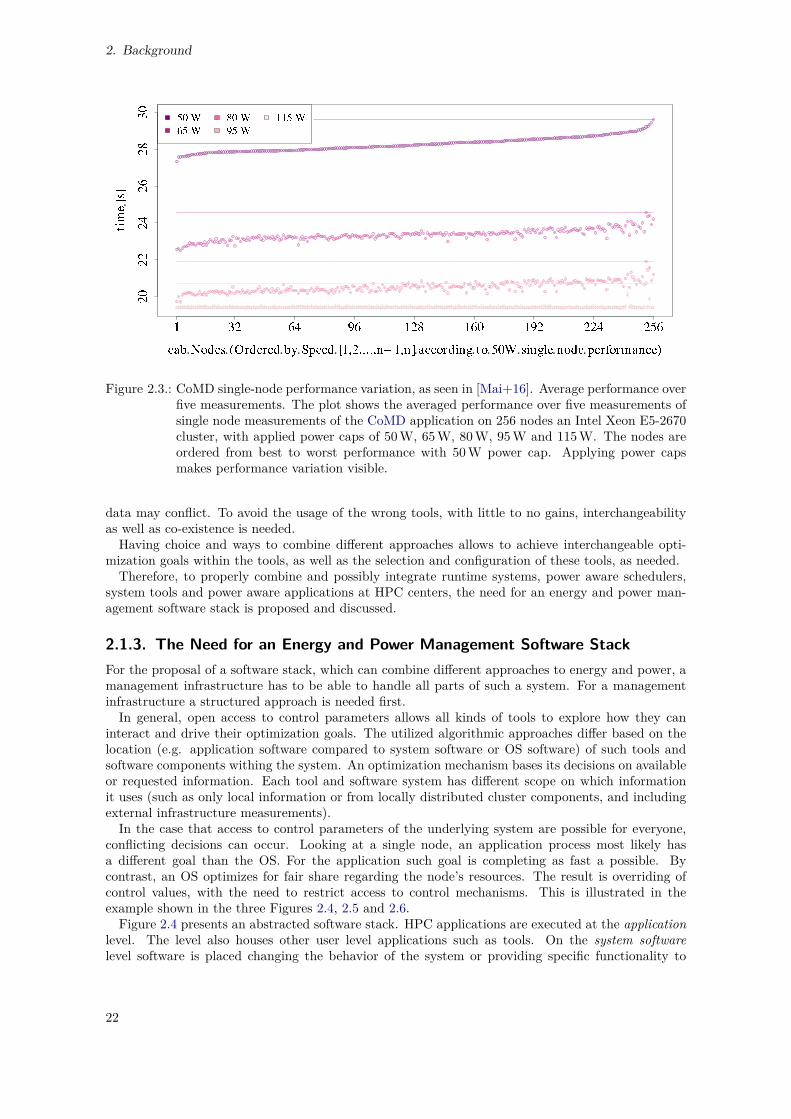
2. Background
✺� ❲
✻✺ ❲
✽� ❲
✾✺ ❲
✶✶✺ ❲
Figure 2.3.: CoMD single-node performance variation, as seen in [Mai+16]. Average performance overfive measurements. The plot shows the averaged performance over five measurements ofsingle node measurements of the CoMD application on 256 nodes an Intel Xeon E5-2670cluster, with applied power caps of 50 W, 65 W, 80 W, 95 W and 115 W. The nodes areordered from best to worst performance with 50 W power cap. Applying power capsmakes performance variation visible.
data may conflict. To avoid the usage of the wrong tools, with little to no gains, interchangeabilityas well as co-existence is needed.Having choice and ways to combine different approaches allows to achieve interchangeable opti-
mization goals within the tools, as well as the selection and configuration of these tools, as needed.Therefore, to properly combine and possibly integrate runtime systems, power aware schedulers,
system tools and power aware applications at HPC centers, the need for an energy and power man-agement software stack is proposed and discussed.
2.1.3. The Need for an Energy and Power Management Software StackFor the proposal of a software stack, which can combine different approaches to energy and power, amanagement infrastructure has to be able to handle all parts of such a system. For a managementinfrastructure a structured approach is needed first.In general, open access to control parameters allows all kinds of tools to explore how they can
interact and drive their optimization goals. The utilized algorithmic approaches differ based on thelocation (e.g. application software compared to system software or OS software) of such tools andsoftware components withing the system. An optimization mechanism bases its decisions on availableor requested information. Each tool and software system has different scope on which informationit uses (such as only local information or from locally distributed cluster components, and includingexternal infrastructure measurements).In the case that access to control parameters of the underlying system are possible for everyone,
conflicting decisions can occur. Looking at a single node, an application process most likely hasa different goal than the OS. For the application such goal is completing as fast a possible. Bycontrast, an OS optimizes for fair share regarding the node’s resources. The result is overriding ofcontrol values, with the need to restrict access to control mechanisms. This is illustrated in theexample shown in the three Figures 2.4, 2.5 and 2.6.Figure 2.4 presents an abstracted software stack. HPC applications are executed at the application
level. The level also houses other user level applications such as tools. On the system softwarelevel software is placed changing the behavior of the system or providing specific functionality to
22
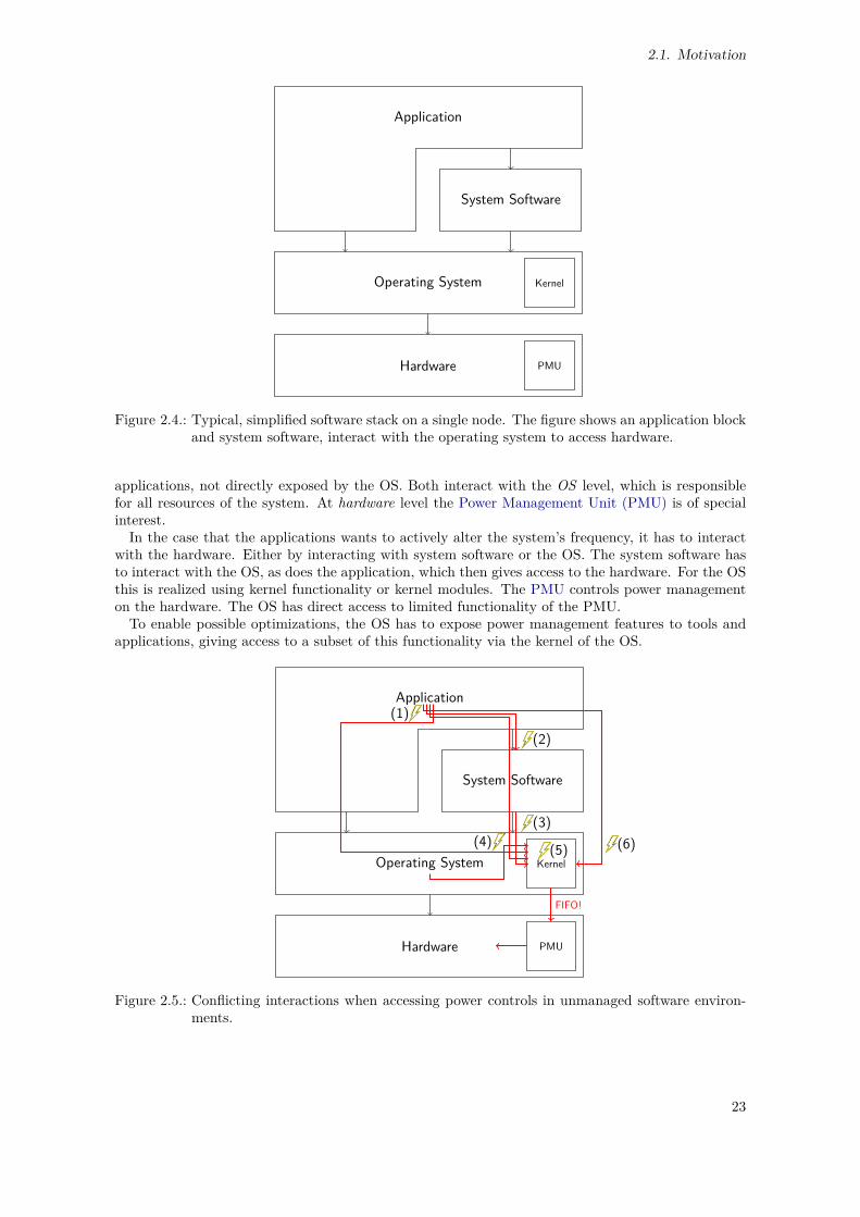
2.1. Motivation
Application
System Software
Operating System
Hardware
Kernel
PMU
Figure 2.4.: Typical, simplified software stack on a single node. The figure shows an application blockand system software, interact with the operating system to access hardware.
applications, not directly exposed by the OS. Both interact with the OS level, which is responsiblefor all resources of the system. At hardware level the Power Management Unit (PMU) is of specialinterest.In the case that the applications wants to actively alter the system’s frequency, it has to interact
with the hardware. Either by interacting with system software or the OS. The system software hasto interact with the OS, as does the application, which then gives access to the hardware. For the OSthis is realized using kernel functionality or kernel modules. The PMU controls power managementon the hardware. The OS has direct access to limited functionality of the PMU.To enable possible optimizations, the OS has to expose power management features to tools and
applications, giving access to a subset of this functionality via the kernel of the OS.
Application
System Software
Operating System
Hardware
Kernel
PMU
FIFO!
(1)
(2)
(3)(4) (5) (6)
Figure 2.5.: Conflicting interactions when accessing power controls in unmanaged software environ-ments.
23
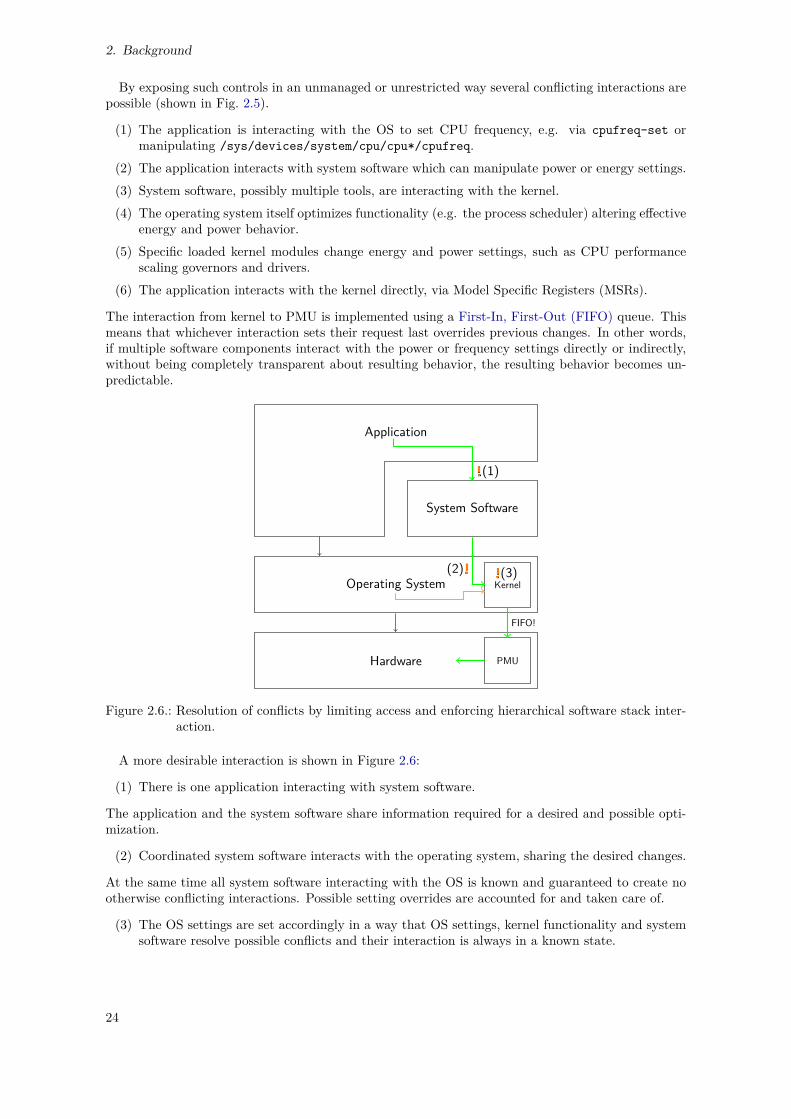
2. Background
By exposing such controls in an unmanaged or unrestricted way several conflicting interactions arepossible (shown in Fig. 2.5).
(1) The application is interacting with the OS to set CPU frequency, e.g. via cpufreq-set ormanipulating /sys/devices/system/cpu/cpu*/cpufreq.
(2) The application interacts with system software which can manipulate power or energy settings.(3) System software, possibly multiple tools, are interacting with the kernel.(4) The operating system itself optimizes functionality (e.g. the process scheduler) altering effective
energy and power behavior.(5) Specific loaded kernel modules change energy and power settings, such as CPU performance
scaling governors and drivers.(6) The application interacts with the kernel directly, via Model Specific Registers (MSRs).
The interaction from kernel to PMU is implemented using a First-In, First-Out (FIFO) queue. Thismeans that whichever interaction sets their request last overrides previous changes. In other words,if multiple software components interact with the power or frequency settings directly or indirectly,without being completely transparent about resulting behavior, the resulting behavior becomes un-predictable.
Application
System Software
Operating System
Hardware
Kernel
PMU
FIFO!
(1)
(2) (3)
Figure 2.6.: Resolution of conflicts by limiting access and enforcing hierarchical software stack inter-action.
A more desirable interaction is shown in Figure 2.6:
(1) There is one application interacting with system software.
The application and the system software share information required for a desired and possible opti-mization.
(2) Coordinated system software interacts with the operating system, sharing the desired changes.
At the same time all system software interacting with the OS is known and guaranteed to create nootherwise conflicting interactions. Possible setting overrides are accounted for and taken care of.
(3) The OS settings are set accordingly in a way that OS settings, kernel functionality and systemsoftware resolve possible conflicts and their interaction is always in a known state.
24

2.2. Scoping of Energy and Power Management Systems
In such setup, interactions from the kernel to the PMU are approved and known, and overall opti-mization for the desired goal is possible.Because of the unwanted nature of the interactions of Figure 2.5, all interactions are usually locked
down by system administrators. This prevents any optimization potential. The msr-safe tool triesto make such interaction manageable by using Linux group permissions allowing a privileged user tointeract with the kernel directly creating such known interaction and restricting the control param-eters to a defined wanted subset (compare for [Sho+]). The solution provided by msr-safe can notdistinguish different tools and only allows a single tool to safely perform alterations.For such a multiple optimization tool scenario specific rules and guidelines have to be developed.
Due to the fact that such interactions are already hard at a single node level a robust and well-structured approach is needed for locally distributed energy and power management environments,as seen in HPC clusters.
2.2. Scoping of Energy and Power Management SystemsTo understand potential approaches to energy and power management systems a clear understandingfor
• Sources of variability;• Optimization goals;• Aspects of energy and power management setups;
is needed.3 These points are discussed below.
2.2.1. Sources of VariabilityAs previously established, even though computers process logic operations as programmed, theirphysical behavior and performance is strongly influenced by the characteristics of the computers andtheir organization (in other words hardware and software). In general, this performance variation isat tolerable levels, however only at large scale systems the variability effects have observable impact(as seen in Fig 2.3). The upside is that utilizing these effects allows for potential optimization.To exploit the variability of HPC systems their sources, how to observe and utilize them has to be
understood. Variability is split into three different categories in the context of HPC system.
1. Hardware variability;2. Job configuration;3. Environment settings.
These three categories form the axis of Figure 2.7, which gives an overview of the sources of variability.These are discussed in the paragraphs below.
Hardware Variability: The items on the hardware axis of Figure 2.7 range form small to large.Hardware variability is seen at all scales of a system. This is exemplified using different scales ofhardware components:
• Sub-components, such as Arithmetic Logic Units (ALUs), Streaming SIMD Extensions (SSE)4
units, caches or individual CPU and GPGPU cores;• Server hardware components, e.g. CPUs, memory modules and GPUs, etc.;• Nodes;• Racks;
3In addition to the general background and scope, a detailed description of contemporary hardware and software ispresented in Appendix B.1. The appendix provides supplementary hardware and software background as well asthe required information for later instantiations of the OIEP reference model in Chapter 4 and Appendix D.
4Single-instruction stream – multiple-data stream (SIMD) [Fly72]
25
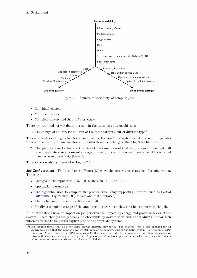
2. Background
Job configuration
Workload/ApplicationToolchain
AlgorithmsApplication parameters
Data
Hardware variability
Infrastructure / Center
Multiple clusters
Single cluster
Rack
Node
Server hardware components (CPU/Mem/GPU)
Sub-Components
Environment settings
System & tool interferenceOperating system environment
Job partition environmentPinning / Placement
Figure 2.7.: Sources of variability of compute jobs.
• Individual clusters;• Multiple clusters;• Complete centers and their infrastructure.
There are two kinds of variability possible in the items listed in on this axis.
1. The change of an item for an item of the same category but of different type.5
This is typical for changing hardware components, the computer system or CPU vendor. Upgradesto new versions of the same hardware item also show such changes [Hac+15; Sch+16a; Sch+19].
2. Changing an item for the exact replica of the same item of that very category. Even with allother parameters kept constant changes in energy consumption are observable. This is calledmanufacturing variability [Ina+15].
This is the variability observed in Figure 2.3.
Job Configuration: The second axis of Figure 2.7 shows the major items changing job configuration.These are:
• Changes in the input data [Ara+20; LJ16; Chu+17; Mar+17];• Application parameters;• The algorithm used to compute the problem (including supporting libraries, such as Partial
Differential Equation (PDE) solvers and math libraries);• The tool-chain, for how the software is built;• Finally, a complete change of the application or workload that is to be computed in the job.
All of these items have an impact on job performance, impacting energy and power behavior of thesystem. These changes are generally no observable by system tools such as schedulers. So far suchinformation has to be passed explicitly to the appropriate systems.
5Such changes imply that all other items on the diagram stay fixed. The changed item is also changed for alloccurrences such that the complete system still appears as homogeneous as the initial system. For example: CPUgeneration X is exchanged for CPU generation Y , this means that all CPUs are changed in a homogeneous way.Introduction of new heterogeneity, e.g. n − 1 generation X and one generation Y , which obviously introducesperformance and power prediction problems, is excluded.
26
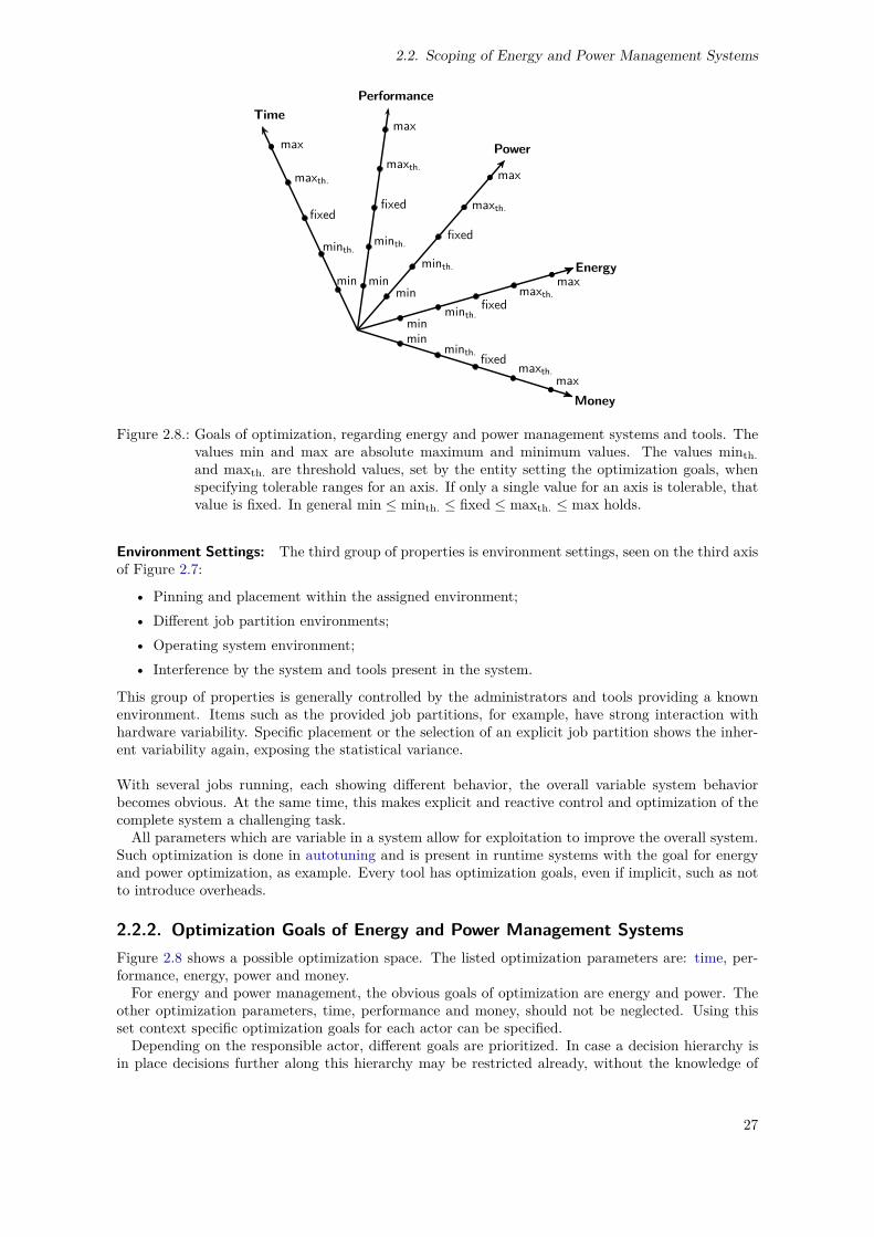
2.2. Scoping of Energy and Power Management Systems
Moneymax
maxth.fixed
minth.min
Energymax
maxth.fixedminth.
min
Power
max
maxth.
fixed
minth.
min
Performance
max
maxth.
fixed
minth.
min
Time
max
maxth.
fixed
minth.
min
Figure 2.8.: Goals of optimization, regarding energy and power management systems and tools. Thevalues min and max are absolute maximum and minimum values. The values minth.and maxth. are threshold values, set by the entity setting the optimization goals, whenspecifying tolerable ranges for an axis. If only a single value for an axis is tolerable, thatvalue is fixed. In general min ≤ minth. ≤ fixed ≤ maxth. ≤ max holds.
Environment Settings: The third group of properties is environment settings, seen on the third axisof Figure 2.7:
• Pinning and placement within the assigned environment;• Different job partition environments;• Operating system environment;• Interference by the system and tools present in the system.
This group of properties is generally controlled by the administrators and tools providing a knownenvironment. Items such as the provided job partitions, for example, have strong interaction withhardware variability. Specific placement or the selection of an explicit job partition shows the inher-ent variability again, exposing the statistical variance.
With several jobs running, each showing different behavior, the overall variable system behaviorbecomes obvious. At the same time, this makes explicit and reactive control and optimization of thecomplete system a challenging task.All parameters which are variable in a system allow for exploitation to improve the overall system.
Such optimization is done in autotuning and is present in runtime systems with the goal for energyand power optimization, as example. Every tool has optimization goals, even if implicit, such as notto introduce overheads.
2.2.2. Optimization Goals of Energy and Power Management SystemsFigure 2.8 shows a possible optimization space. The listed optimization parameters are: time, per-formance, energy, power and money.For energy and power management, the obvious goals of optimization are energy and power. The
other optimization parameters, time, performance and money, should not be neglected. Using thisset context specific optimization goals for each actor can be specified.Depending on the responsible actor, different goals are prioritized. In case a decision hierarchy is
in place decisions further along this hierarchy may be restricted already, without the knowledge of
27

2. Background
other actors. The outcome of such goals largely depends on the scope, placement and authority ofthe tool and actor enforcing decisions. By identifying actors, tools and goals adversary effects can beidentified and synergies made explicit.For example, consider four possible actors with adverse optimization:
• Center leadership;• Infrastructure administrator (admin);• System admin;• Users.
The center leadership has a specific fixed monetary budget. This budget is directly related to theenergy spent, since the ESP bills accordingly. The center leadership then dictates to minimize energyspent.The infrastructure admin has machine specifications and has knowledge of safe operational power
consumption, dictating specific values for minimum and maximum thresholds regarding save powerconsumption, minth. and maxth. (as seen in Figure 2.8).The system admin on the other hand are responsible for a fair share of access time, with limited
knowledge of power consumption.The users are mostly interested in the highest performance possible with the optimization to mini-
mize the time the application takes to generate their results, at the same time having an overall largefraction of system time for their own applications.Every center has a different combination of such optimization goals. Additionally, each center
has a different set of actors of distinct importance. Such scenarios are important to keep in mindwhen identifying and characterize energy and power management systems, especially in context ofmanagement hierarchies.
2.2.3. Aspects of Energy and Power Management SetupsTo be able to describe energy and power management systems it is important to describe such setupsin a meaningful way. The following section helps to describe both individual elements of a setup andcomplete systems as a combination of elements of different structure and scope.6
Figure 2.9 describes energy and power management systems according to eight independent axes:
• Hardware sensors;• Hardware controls;• Management roles;• Interfaces;• Modularity;• Structure;• Software scope;• Automation of the systems.
For the transformation of an unstructured setup of software and hardware to a structured energyand power management system, an assessment of the participating elements and their compositionis needed.The first two axes are hardware sensors and control:
1. At sub-component levels (e.g. per core);2. Server component (e.g. per CPU, memory module, etc.);3. Node (e.g. Baseboard Management Controller (BMC));
6An element is referred to as the linear-combination of the properties as depicted in Fig. 2.9, whereas a setup is calledthe sum over the elements used in combination. The work talks of an energy and power management system if suchsetup works in a coordinated way.
28
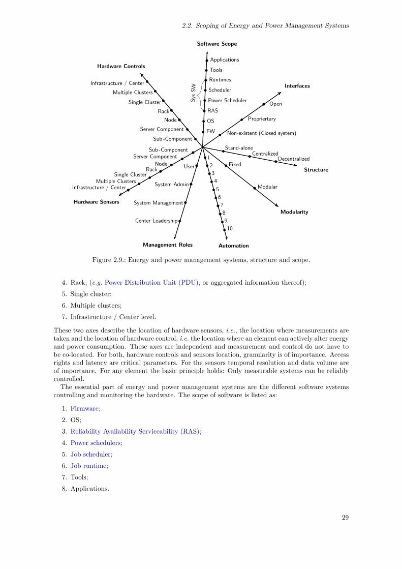
2.2. Scoping of Energy and Power Management Systems
Hardware Controls
Infrastructure / CenterMultiple Clusters
Single ClusterRack
NodeServer Component
Sub -Component
Hardware Sensors
Infrastructure / CenterMultiple Clusters
Single ClusterRack
NodeServer Component
Sub -Component
Automation
10987654321
Software Scope
Applications
ToolsRuntimes
Scheduler
Power Scheduler
RAS
OS
FW
SysSW
Structure
DecentralizedCentralized
Stand-alone
Modularity
Modular
Fixed
Interfaces
Open
Propriertary
Non-existent (Closed system)
Management Roles
Center Leadership
System Management
System Admin
User
Figure 2.9.: Energy and power management systems, structure and scope.
4. Rack, (e.g. Power Distribution Unit (PDU), or aggregated information thereof);5. Single cluster;6. Multiple clusters;7. Infrastructure / Center level.
These two axes describe the location of hardware sensors, i.e., the location where measurements aretaken and the location of hardware control, i.e. the location where an element can actively alter energyand power consumption. These axes are independent and measurement and control do not have tobe co-located. For both, hardware controls and sensors location, granularity is of importance. Accessrights and latency are critical parameters. For the sensors temporal resolution and data volume areof importance. For any element the basic principle holds: Only measurable systems can be reliablycontrolled.The essential part of energy and power management systems are the different software systems
controlling and monitoring the hardware. The scope of software is listed as:
1. Firmware;2. OS;3. Reliability Availability Serviceability (RAS);4. Power schedulers;5. Job scheduler;6. Job runtime;7. Tools;8. Applications.
29

2. Background
Where RAS, power scheduler, job scheduler and job runtime are marked with system software. Thetypes of software systems are not tied to specific hardware controls and sensors. Identifying allsoftware interacting with energy and power is critical to resolve control conflicts.In a cluster installation with several software actors it is important to know how these systems
interface. In other words, if interfaces are:
1. Non-existent (closed system);2. Proprietary;3. Open.
In closed systems extension and interaction with other systems is not possible. For proprietaryinterfaces, extension and interface with other systems as needed is not possible without licensing orremaining in the given vendor ecosystem. For open interfaces extension is possible according to theneeds of the tools, actors and the center.Regarding the structure of interacting software for energy and power management different styles
of interaction are possible. These are:
1. Stand-alone management elements;2. Centralized;3. Decentralized.
For stand-alone elements no integrated management is needed. Some elements managing systemscritical hardware components, for energy and power are operated stand-alone. For these, a moreintegrated structure allows to enable different optimization strategies, but for safety this is often notwanted. For example, facility cooling is not steered by energy demand, but by using closed controlloops based on temperature sensors for cooling.Systems where elements interact and integration of different systems for management is required
are either managed centralized and decentralized. A centralized structure means that a centralentity collects sensor data, has access to hardware controls and is in control of the software systemsmaking decision. Typical examples are RAS systems with administrative control by a human. Adecentralized structure is similar to a peer-to-peer system where software components do not reportto a centralized controller, but interact for distributed decision-making. Decentralized systems avoidpotential bottlenecks and allow for better scaling, but the quality of the decisions may not be thesame, compared to a centralized controller.Regarding Modularity, two options are possible:
1. Modular;2. Fixed.
Modular systems allow the replacement of elements, for a different type with similar functionality.Fixed systems do not allow such replacement. Extending a system requires a partially modular setup.Awareness of the degree of automation of a system is critical to understand and improve a system.
The levels of automation are described by Parasuraman in [PSW00]. The levels can be group for theuse-case at hand according to:
Level 1: Completely manual;
Levels 2 – 4: Computer aided decision-making;
Levels 5 & 6: Automatic execution with approval or veto of human interaction;
Level 7: Executing autonomously with necessity to inform human operator;
Level 8: Executing autonomously and reporting if asked;
Level 9: Reporting to the human by choice of the computer system;
Level 10: Ignoring human interaction altogether.
30
2.3. Requirements for Reference Models for Energy and Power Management
Different elements of a system require different levels of automation. When combining elements itis critical to have knowledge of processing speed, not only in terms of computer performance, butalso if manual intervention is required. This is important for fail-safe operation. For HPC systemshigh degree of automation is desirable, some elements of a system are inevitably in the range of Level2 – 4. Different solutions and parts of the energy and power management systems are of varyingautomation level by design.Finally, the last remaining axis describes management roles:1. Users;2. System administrators;3. System management;4. Center leadership.
A management role describes which human entity has control over each element of a system. Thisis important to know, for access rights, goals and interaction. Centers may have additional roles notidentified here. These can be added if needed.The diagram of Figure 2.9 allows to describe any element and setup of energy and power manage-
ment. It forms the basis to describe existing, setups or identify requirements and limitations for newenergy and power management systems. It is also suited to maintain knowledge about the individualelements to maintain a well managed, integrated energy and power management system.
2.3. Requirements for Reference Models for Energy and PowerManagement
The requirements analysis for the reference model construction of energy and power managementsystems for HPC systems is based on the requirements definition concepts as defined in [RS77]. Thecontents of Sections 2.1 and 2.2 are considered for the analysis of the requirements. All aspects areassessed from a technical, operational and economic7 viewpoint.Table 2.1 summarizes the resulting requirements of the requirements definition. The table lists the
technical, operational and economic requirements according to:1. Context analysis,2. Functional specification,3. Design constraints.
The full requirements’ definition is presented in the Appendix A.1. Given the methodic approachthese requirements are adequate and sufficient to commence with the reference model construction.
For complete requirements model building the found requirements are compared with existing ap-proaches for model building. Since energy and power management for HPC systems does not haveany model building practices, related fields are analyzed. These are:
• Data model quality indicators [BCN91; MS94],• Model building principles [Sch98],• Reference modeling [Sch99] and [Sch00] using the principles of [Sch98].
The comparison itself is performed in Appendix A.2 while the result is presented in Table 2.2.The table lists the identified requirements and marks the existence of equivalent requirements for
the other models.In summary, all requirements identified have equivalent requirements in other models. The only
requirements not present are either specific to energy and power management or specific to appliedmodels. The two applied requirements are manageability and automation.
This is noteworthy and sets this applied reference model apart, since manageability is one of theprime reasons to use a reference model. At the same time automation is one of the fundamentaleconomic values of having well-defined systems operating according to a reference model.
7Economic in terms of economic impact/viability/sustainability, whereas the work is not assessing profitability.
31
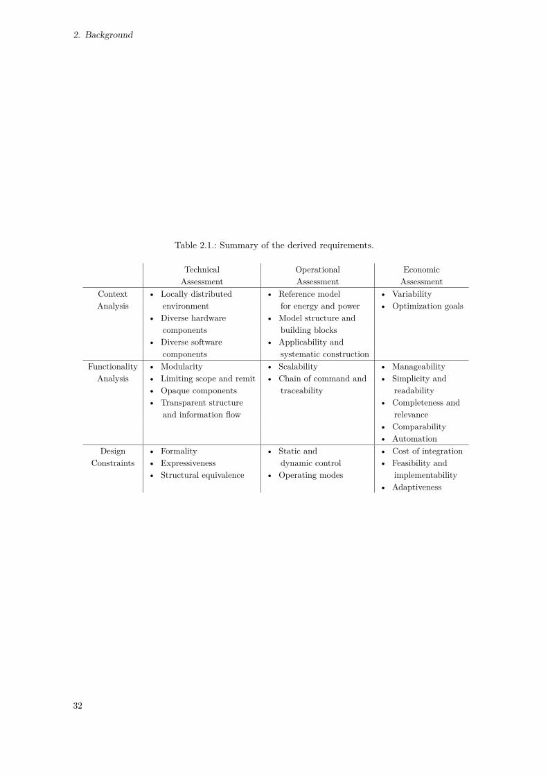
2. Background
Table 2.1.: Summary of the derived requirements.
Technical Operational EconomicAssessment Assessment Assessment
Context • Locally distributed • Reference model • VariabilityAnalysis environment for energy and power • Optimization goals
• Diverse hardware • Model structure andcomponents building blocks
• Diverse software • Applicability andcomponents systematic construction
Functionality • Modularity • Scalability • ManageabilityAnalysis • Limiting scope and remit • Chain of command and • Simplicity and
• Opaque components traceability readability• Transparent structure • Completeness and
and information flow relevance• Comparability• Automation
Design • Formality • Static and • Cost of integrationConstraints • Expressiveness dynamic control • Feasibility and
• Structural equivalence • Operating modes implementability• Adaptiveness
32

2.3. Requirements for Reference Models for Energy and Power Management
Table 2.2.: Requirements for energy and power management reference models, contrasted with genericmodeling requirements and quality indicators from different disciplines as presentedin [BCN91; MS94; Sch98; Sch99; Sch00]. Requirements specific to energy and powermanagement systems in HPC are indicated by an asterisk (*).
[BCN91] [MS94] [Sch98] [Sch99] [Sch00] D/E ←Locally distributed environment *
Diverse hardware components *
Diverse software components *
Reference Model for energy and power *
Model structure and building blocks (X) (X)Applicability and systematic construction X X
Variability *
Optimization goals *
Modularity X X
Limiting scope and remit X X
Opaque components X
Transparent structure and information flow (X)Scalability *
Chain of Command and Traceability * (X)ManageabilitySimplicity and readability X X X
Completeness and Relevance X X (X) (X)Comparability X
AutomationFormality X (X)Expressiveness X (X)Structural equivalence (X)Static and dynamic control *
Operating modes *
Cost of integration (X) (X)Feasibility and Implementability X
Adaptiveness X X X
33

2. Background
2.4. Related WorkFor related work comparable approaches targeting models for integrated energy and power manage-ment are compared to the OIEP reference model presented in this work. The related work section issplit into the following parts:
• Structured energy and power management approaches in HPC;• Compound software setups for energy and power management in HPC;• Modeling of complex control systems.
Each related work item is split into four parts for comparison with the presented approach:
1. A brief description of the work;2. A description of similarities;3. A description of differences;4. Highlighting of the contributions of the OIEP reference model in light of the related work.
2.4.1. Structured Energy and Power Management Approaches in HPCThe initial section discusses projects and solutions providing an open and adaptable structure for in-tegrated power management. These approaches however either do not have management as a primarygoal, or do not provide the structure or the means to describe the energy and power managementstructure. This section discusses:
• The 4-Pillar Framework• PowerAPI• PowerStack
The 4-Pillar Framework: The “4 Pillar Framework for Energy Efficient HPC Data Centers” byWilde, Auweter and Shoukourian [WAS14] propose a holistic way to evaluate energy efficient effortsof a site. The authors identify the issue that, compartmentalized solutions are developed withoutawareness of common goals, since they work isolated and no common framework exists to relatedifferent projects and products present in an HPC center.The 4-Pillar framework identifies the four main areas of improvement for energy efficiency as its four
pillars: Pillar 1 – building infrastructure; pillar 2 – system hardware; pillar 3 – system software; pillar 4– applications. A center utilizing the 4-pillar framework can place its projects and employed productsfor energy efficiency within these main areas. Such mapping helps centers to identify possible areas ofimprovement, required products and solutions, identifying resources and stakeholders for managingenergy efficiency to guide the efforts to a common goal. The 4-pillar framework also helps the planfuture efforts and present results to center stakeholders, encouraging cross-pillar optimization.The 4-Pillar framework shows and places projects and solutions within the HPC data center,
whereas the solution presented within this work maps the structure and hierarchy of interactingsystems. Both approaches help to identify synergies of HPC software and hardware utilized withinthe system. The work at hand provides potentials to check conflict free interaction of systems. The4-pillar framework can only identify if two projects are placed within the same pillar, where positiveeffects are identified if projects span multiple pillars and are not confined to a single pillar.The OIEP reference model is a structured approach where each component collaborates to have a
conflict free system architecture with each component working at the appropriate level of abstraction.The 4-Pillar framework is nevertheless helpful to identify projects and products that should be placedin proximity to each other in the structure of the OIEP reference model.
34

2.4. Related Work
PowerAPI: Power-API [Gra+16; III+16] is a Application Programming Interface (API) specifica-tion for measurement and control of energy and power in HPC. It is designed to satisfy a wide rangeof use-cases and different types of requirements of different actors and system for HPC systems. ThePower-API is motivated by the fact that many software entities exist managing and controlling energyand power without any standardized API. The technical report published by Laros III et al. [III+13]contains an initial requirements’ analysis identifying use-cases to be covered by the Power-API. Usingthis analysis a conceptual diagram is presented identifying all actors/roles and systems to be cov-ered [III+16, Fig 1.1]. Additionally, a hierarchical representation of a generic system representationis given (see [III+16, Fig 2.1]) along with a system description. The API’s main part covers theoryof operation, type definitions, core (common) interface functions, and high-level (common) functions.The second main part are role/system interfaces, specifying API-functions required for interactionbetween specific actors or systems. The Power-API is an API specification direly needed in HPCto have a common interface between systems. The conceptual design is organized according to theidentified roles and system parts of an HPC system. Several centers and vendors of software systemsuse Power-API in their products to enable integration into the larger system setup.Power-API does not mandate any use of its proposed interfaces, the role and system diagram serves
as use-cases analysis and possible setup. This allows any center to freely design their own setup oftools and systems. At the same time having a reliable API reduces development efforts for theintegration of several systems. The work at hand relies interfaces such as Power-API and hardwareand software components relying on such standardizations.The contribution of the OIEP reference model is to give structure and rules to structuring inter-
acting systems, where Power-API gives the means to do so. Both Power-API and this documentcomplement each other, where the Power-API provides specific use-cases of Power-API, and inter-face definitions. Contrary, the OIEP reference model focuses on the provision of building blocks andmechanisms to describe the structure for modeling energy and power management systems and theircontrol interactions.
PowerStack: The PowerStack, as described in the PowerStack strawman document [Can+18], is aholistic extensible power management framework, designed and organized by a committee consistingof members from National Laboratories, Industry and Academia.8 Current software systems andsolutions for optimization of energy and power are specialized on specific parts and sub-domains ofthe HPC system. Limited efforts to connect such isolated systems demand the development of systemsand techniques to interface solutions to be able to optimize in an integrated manner. The PowerStackis a proposed design for a holistic energy and power management stack, which the work [Can+18]refers to as the HPC PowerStack.For such integration the following requirements have to be met: A holistic system view, extensibil-
ity, support of current and future needs of various kinds of HPC centers, coordinated managementat different granularity, seamless integration of software from different developer groups and ven-dors. The goal is to align development and research efforts across communities, share developmenteffort and avoid duplicate efforts while benefiting the HPC community. The anticipated outcomeof the PowerStack effort is a holistic flexible, and extensible concept of a software stack that allowsto combine product grade open-source software components into the same ecosystem to enable opti-mization of system power, energy and performance. For this an initial stack-concept for discussionand development is proposed in the PowerStack strawman document [Can+18]. The document de-scribes possible layouts of the components and their interactions, also software components enablingthe functionality at each level and the interactions and required interfaces between each other. Theproposed design is a layered software stack with 3 levels9, a node-manager level, job level and systemlevel. The PowerStack strawman design was followed up by a kick-off seminar and has since thenbeen shaped in regular discussions synchronizing in annual seminar meetings[PS’18; PS’19a; PS’19b].As part of the PowerStack core committee, the author of the work at hand identified that one
of the main challenges for the PowerStack group in the seminar meetings is to agree on a structurethat works for every participating interest group. The solution proposed as PowerStack identified
8The author of this work is part of the PowerStack core committee [SPSweb].9Layers and levels are used interchangeably within the PowerStack description. This document sticks to the wording“levels”.
35

2. Background
the main focus areas required to enable energy and power optimization, in a systemic way for theHPC computer system. Namely, access to hardware via the node level (i.e. software interfaces fornode level control, as well as software optimizers and interfaces at this level), the runtime level (i.e.software optimizing the node level components with scope of a job), and the system level (i.e. softwaremanaging energy and power on a level of multiple jobs and the computer cluster scope). The stack isset up in a way, that typical software solutions have their space in these areas, but also to harden theseplaces and be able to express requirements for the other software in this stack. These requirementscan be interfaces, access to hardware control parameters, or meta-data needed for the optimization atindividual software components of the layer. The goal is to have the formulation and concepts whichcapture the needs and requirements of centers enabling software and hardware solutions yet rigidenough to have a common ground and a solution which is implementable either as initial prototypeor for future PowerStack compatible systems.By contrast, the OIEP reference model provides the means to describe such a structure. The
OIEP reference model provides the means to describe levels (or layers in PowerStack nomenclature),describe the hierarchy of these levels, describe components placed inside these levels. They OIEPreference model also, describes how components are connected and thus how control is guaranteed andpassed throughout the system. The ability to swap components is also part of OIEP reference modelto identify required changes in the setup. The reference model thus helps to describe conceptualand structural concepts important to reason about the PowerStack solution. The OIEP referencemodel does not fix a specific layout and thus also allows to describe systems that do not followthe PowerStack but enables energy and power management system understand their control flowregarding decision made to alter hardware settings. In Section 4.2 of Chapter 4 the PowerStack (asof the second PowerStack seminar [PS’19a]) is presented as an OIEP architecture.
2.4.2. Compound Software Setups for Energy and Power Management in HPCThe next section describes Project that use a structured approach or have an aggregate solution bycombining products and software which they provide. These approaches are very useful and valuable,however their goal is not to provide and extensible and open structure, but propose a very specificsystem design. This section discusses:
• The Argo Project• The READEX Project• The Flux Framework
The Argo Project: The Argo project [Per+15] describes an exascale software stack for a distributedcollection of services in the manner of an OS and runtime. The initial concept for a machine descrip-tion for the Argo project are enclaves. The system is a logical hierarchy of groups of nodes. Thesenested enclaves specify common configuration finally encapsulating user jobs. Such Argo machineconsists of four types of components: The NodeOS (cf . [Per+17]), a Linux based node level operat-ing system; Argobots (cf . [Seo+18]), a thread level runtime capable of massive intra-node parallelism;the backplane, a global information bus providing advanced communication services including and apub-sub system for services and components; And the GlobalOS, managing the enclaves and services.The enclaves are logical groupings managed by a master node with capable of arbitrary nesting.The paper [Per+15] describes three typical services for GlobalOS describing the typical usage and
mode of operation for an Argo machine. First, a hierarchical control bus service following the enclavehierarchy. Using the backplane messages can be arbitrarily directed. The hierarchical control busservice allows to direct messages according to the hierarchy relation of the enclaves. This allows todirect messages to all parent enclaves or child enclaves, but also specifies a ‘closest’ and ‘all’ relation.This allows other services to direct messages according to the structure of enclaves without having torely on point-to-point messages via the backplane. Second, a distributed power management service.For this a reader service and power control service are provided. The system uses a reader serviceand a power control service. The power control service reacts to global power limits and informationon limits and consumption from the enclaves. Messages are directed using the global backplane or
36

2.4. Related Work
the hierarchical control bus service. Third, an exception service for managing failure is presented.This describes failure handling using the hierarchy and services in a scalable manner.The Argo project has a much wider scope compared to OIEP reference model. The Argo project
tries to form a complete cluster OS, both local and global, providing communication infrastructureand services. For the OIEP reference model, provides the structure for hierarchical control for energyand power management. Such system can be build using the Argo project. However, the broadnature of an Argo machine can violate some of the restrictions set by the OIEP reference model. Anexample for this is the appropriation and chain of command requirements of discussed in Section 2.3.This is easily violate-able using arbitrary messages, allowed by usage of the Backplane of Argo. In thecase that the subset of services, their setup and communication structure is restricted and controlled,a subset of service specifically selected and controlled can satisfy the OIEP reference model.While the Argo project has a much wider scope provide necessary contributions to manage next
generation computer systems, aspects of both complement each other. While large scale systems needa kind of global Operating System, OIEP reference model provides a method to describe a scalableand controllable comprehensive way to manage energy and power. A possible implementation of aOIEP architecture can be achieved using enclaves, services and other concepts of the Argo project.The Argo project provides much additional contributions to understanding management of power
at different levels HPC systems (cf . [Ram+19; Ell+16a; Per+17; Per+19; Seo+18]).
The READEX Project: The Runtime Exploitation of Application Dynamism for Energy-efficienteXascale computing (READEX) project [Ole+15] builds a tool-aided, scenario driven auto-tuningmethodology utilizing dynamic behavior of HPC applications to improve energy efficiency and per-formance. The approach is guided by long-standing knowledge in static auto-tuning by its projectparticipants, identifying that a single tool is not sufficient to optimize for the dynamic behavior of sys-tems leading up to exascale. By building on proven technology for performance tools the applicationscenarios are supported throughout the application life-cycle for automatic dynamic tuning, ready forheterogeneous systems and multi objective optimizations. The project also introduces programmingparadigms for application domain dynamism. These aspects allow the project partners’ tools andapplications to be considered exascale ready.The READEX approach differs from the previously discussed approaches in that it provides a
tool-set working around the application life-cycle, where the majority of tools was concerned with theoptimization of specific aspects of the computer system or providing individual solutions for singleparts of the application life-cycle. This is done by combining tools such as Scalable PerformanceMeasurement Infrastructure for Parallel Codes (Score-P) [Knü+11], Periscope Tuning Framework(PTF) [BPG09], as an example. Success in the support of applications and application life-cycle hasbeen shown in various applications [Die16; Kum+19; Soj+17].Regarding the OIEP reference model the approaches are orthogonal in concept. The reference model
discussed in this approach requires approaches targeting application support for performance, as wellas energy and power considerations. The individual tools that projects such as READEX use, have tobe grounded and well integrated into a system model. Without a mental model of a computer system,and its energy and power management capabilities, the capabilities of an application life-cycle modelare drastically limited. The READEX project shows, that clear formulation and characterization ofinterfaces, that are openly available are not well described. (This is shown by the fact that significanteffort had to be put into the understanding of processor architectures[Hac+15; Sch+19; Mol+17], orthe introduction of measurement technologies [Hac+14; Ils+19b; Ils+15], which they project grouphad to integrate and provide themselves.) By using the tools and interfaces the work of the READEXproject provides synergies can be used to either expose or hide system complexity, depending on theneed.It is important to distinguish READEX from individual tools, since by building on an open-source
technology stack, it builds on open interfaces and enables interactions for other tools. Currently,READEX resides in the application space, integration of its required technology into a systematicdescription of for example a OIEP architecture also enables other technologies to build on the capa-bilities contributed by sophisticated projects such as READEX.
37

2. Background
The Flux Framework: The Flux framework [Ahn+14; Ahn+13], is a framework for resource man-agement, going beyond traditional schedulers. Flux enables the inclusion of arbitrary resources intothe scheduling process. For Flux, energy and power are among these primary resources to be schedu-lable, at the same time they are not treated as mandatory, nor is Flux solely focusing on energyand power. The framework is extensible and scalable and takes a meta-scheduling approach whereresources to be managed go beyond clusters, partitions and nodes. Monitoring and resource aggrega-tion play a large role from a conceptual side. The framework addresses their major issues, identifiedas: Multidimensional scaling, diverse workloads, dynamic workloads, productivity, system challenges.To address these challenges and be able to provide a practical system Flux solves these using: A uni-fied job model, a job hierarchy model, a generalized resource model, a multilevel resource elasticitymodel and a common scalable communication infrastructure model [Ahn+14]. The Flux frameworkis functionally split into core, and specific parts needed for the different aspects of the framework,implemented and to be found on the project repositories [Labb; Laba].The scheduling approach of Flux is hierarchical and federated with measurement, monitoring and
decision-making functionality. The hierarchy of the system is according to the system implementationand resembles a meta scheduler including all relevant groupings identified and implemented. Thehierarchy is extensible and has to be adapted to fit the centers scheduling intent. The approach isuseful and novel, since it can supersede traditional schedulers trying to include energy and power,whereas in Flux energy and power as considered by design since it can be represented as a resourcesuch as nodes or time.Flux has a wider approach regarding resources, where admins can implement their requirements
regarding any resource relevant and implementable. At the same time the approach is focused onscheduling, where the wider impact of energy and power is not directly in scope if the resource to becontrolled is not involved in the scheduling process. OIEP reference model takes a different approach,where energy and power management is the primary focus, and schedulers can be part of the systemif they interact with energy and power, such as the power aware aspect of the Flux framework.Both of the systems can work in symbiosis, where Flux can act as a scheduling component within
an OIEP architecture. The advantage compared to traditional schedulers is that energy and powercan be modeled as a first class citizen among the resources, therefore directly involved in energy andpower management, which can be tightly coupled with the overall approach of the OIEP referencemodel. At the same time an OIEP architecture can help to identify where to interact with theschedulable resource. For Flux, this may reduce the risk of aversely affecting optimization goals withrespect to decision-making.
2.4.3. Modeling of Complex Control SystemsAfter discussing three important projects and aspects with very specific approaches to energy andpower management, the section at hand transitions to a more general kind of related work. Genericmodels and methodologies exist to describe systems using methods of wide adoption. The conceptsand ideas of these are discussed, identifying and contrasting the need for OIEP reference model.The following approaches are discussed:
• UML• Hierarchical Control Systems
UML: Unified Modelling Language (UML) [Obj17] is a standardized visual object modeling specifi-cation. This allows system architects, software engineers and software developers to describe, design,analyze and implement software systems. Modeling a system using UML is applicable for any systemor process which can be described using software. UML provides precise definitions, abstract syntaxrules, semantics, modular language structures. UML is both a computer readable tool, and can bepresented visually, as well. The key concepts are formally defined in the specification itself [Obj17],as well as supplemented by Meta Object Facility (MOF) [Obj10] for the specification of meta ob-jects, Object Constraint Language (OCL) [Obj14] for the specification of formal constraints, XMLMetadata Interchange (XMI) [Obj15b] for the specification regarding computer readable descrip-tion, exchange, linking, validation and identity using eXtensible Markup Language (XML), DiagramDefinition (DD) [Obj15a] and primitives for graphical representation.
38
2.4. Related Work
UML provides a precise specification to model systems, and using the supplements such as OCL thenecessary aspects to formalize them for automated processing. The diagrams cover all usage modelsrequired to formally model any process, even though the specifications acknowledge that:
“A UML diagram, such as a class diagram, is typically not refined enough to provide allthe relevant aspects of a specification. Such constraints are often described in naturallanguage. Practice has shown that this will always result in ambiguities.” [Obj14, p. 5]
This makes it obvious that even with such precise specifications the interpretation of a model canpose challenges, even when done by experts.HPC systems are very domain specific, containing intrinsic knowledge about possible interactions,
but also knowledge about performance problems especially in the HPC domain of high-performanceclusters. By defining a reference model for systems to allow centers to express their setup of interactingenergy and power management systems, the OIEP reference model puts very tight constraints ontowhat setups are allowed in an OIEP architecture. This limits the expressiveness to a domain specificsystem. At the same time, it allows to control the critical parts of the system to allow users to reasonabout the parts and confirm applicability and systematic construction, manageability, structuralequivalence and feasibility and implementability of the system, as demanded in the requirementssection for the reference model as presented in Section 2.3.Due to the universality of UML, it is to be noted that OIEP reference model uses some represen-
tations provided by UML. Additionally, the OIEP reference model can be supplemented by UMLdiagrams. The parts of the model described using UML still has to follow the restrictions of theOIEP reference model. For example, OIEP state diagrams (see Section 3.3.4.2) are modeled usingUML state diagrams. In a similar fashion, Power-API uses UML to formalize its use-cases.
Hierarchical Control Systems: The individual components used within HPC systems can be mod-eled as traditional control systems, with sensors, actuators and a control loops. Scientific literaturediscusses these topics in control theory. For example, Parolini et al. [Par+12] investigate how controltheory helps to model data centers to understand coordinated control. Such models help to under-stand impact and efficiency of coordinated control, however not how to structure, build, setup andoperate them.Åström [Åst65] states that for the design of control systems the fundamental problem is to find
a suitable control law. The individual components of the OIEP reference model can be modeled ascontrol systems, however the properties of stability and performance are challenging to model as soonas multiple agents are discussed in an open control loop of distributed nature.Model theory describes distributed and hierarchical control systems of several types, as for example
the classification of Model Predictive Control (MPC) architectures by Scattolini [Sca09]:
• Decentralized control systems (coupled agents influencing overall system output),• Distributed control systems (with transmission of information between agents in addition to
coupling),• Hierarchical control systems for coordination (decentralized agents with the addition of a global
agent calibrating the individual agents),• Hierarchical control of multilayer systems (agents of time scales of varying degree or echelon
structure),• Coordinated control of independent systems (with common optimization goal).
The reader is kindly referred to the review paper [Sca09] and textbook references such as [MME70],[Fin+80] and [AM08] for details.The approach needed for integrated energy and power management of HPC systems combines
requires hierarchical multilayer systems as well as coordination of independent systems. The con-tributions in control theory and MPC provide the theoretical basis for robustness, stability, andmathematical principles of coordination, and build important fundamentals.The approaches discussed above do however not show how multi agent systems operate on multiple
functional environments of a system; How such systems are constructed maintained for functionality
39

2. Background
or updated, upgraded and altered over time by design or as a required change. For any of thesesystems the structure of the approach is not matched in a way required by large scale HPC systems.These approaches work well to investigate system stability, optimality and robustness. Modeling thestructure of hardware and software systems is however only possible to a limited degree. Especiallysince issues such as scaling and dynamic behavior of the software systems are not easily capturedwithin the models.The control systems most closely related to the functionality and structure present in OIEP refer-
ence model is presented in real-time control system (RCS) with a large base of fundamental researchprovided by Albus et al. [Alb92; Alb97; Alb+02; AB05]. The focus of Albus’ research is in the fieldof autonomous systems and autonomous vehicles. The concepts and parts of the reference model4D/RCS [Alb+02] has a good overlap with the ideas developed for the OIEP reference model.10
With similarities of the models, also major differences are presented simply by domain of applicationand characteristics of the agents within the system.The 4D/RCS [Alb+02] model describes the design methodology in 6 steps:
1. Task analysis;2. Mapping onto organisational units;3. Developing state graph and state models representing procedural knowledge required to accom-
plish the tasks;4. Defining the transition conditions that separate sub-tasks;5. Define objects events and relationships that define the transition conditions and develop the
data structures to support planning and of intelligent behavior;6. Develop specifications for sensors and gather information about the world and for sensors.
These aspects are highly relevant for application in a HPC system, but are minted for usage inautonomous systems. Drawbacks of Albus’ model, are self-identified and addressed in the discussionsection of his work [AB05]. For high-performance clusters additional considerations have to be made,which are out of scope for the 4D/RCS. These are:
• Scalability (number of agents),• Dynamicity (exchange of agents and even sub-trees),• Heterogeneity (in both hardware and software),
These are addressed in the OIEP reference model, which supports system design, procurement andfuture developments within the ecosystem of large scale HPC systems. One of the main contributionsthat sets control theory approaches and the OIEP reference model apart is the structural setup ofthe system. This allows to reflect the needs of HPC centers and combines control of heterogeneouscontrol structures internally.By formulating the OIEP reference model, the author contributes a reference model – in the eyes
of control theory, an applied model – which can serve to communicate issues unique to HPC andtransfer these back to existing knowledge in regular control systems, where the structural setup ofthe system is of importance.
2.4.4. Related Work – Summary of CharacteristicsTable 2.3 summarizes the related work by indicating characteristics of the approaches of interest tothis work. These are:
• Is the work related to energy and power management;• Does the work provide structure;• Does the work providing a model;
10The work of James S. Albus was not known to the author when developing the OIEP reference model. Seeing asimilar successfully employed approach in a different area of control systems and system optimization reaffirms theauthor of the usefulness and additions needed for the author’s area of research.
40

2.4. Related Work
• Does the work providing a reference model;
The OIEP reference model is the first energy and power management specific reference model thatprovides a structured approach to energy and power management of HPC systems. The OIEPreference model itself does not provide a model, but is used to generate models based on the referencemodel approach (thus marked by an asterisk).
Table 2.3.: Overview related work.
Energy and Power Providing Structure Model Reference Model4-Pillar Framework X (X) (X)PowerAPI X (X)PowerStack X X (X)Argo Project (X) (X) (X)READEX Project (X) (X)Flux Framework (X) (X)UML (X) X
Hierarchical X X X
Control SystemsOIEP reference model X X (X)* X
Chapter SummaryChapter 2 provides the motivation, scopes the problem and derives a requirements’ analysis for areference model for energy and power management systems for HPC systems. Additionally, therelated work is presented. This presents the problem domain analysis according to the methodicalapproach of this work (see Sec. 1.2).
Problem definition1
Problem domainanalysis2
Reference modelconstruction3
Evaluation andevolution4
Reference model building
HPC system specificproblem descriptiona
Identification ofrequirementsb
Reference model-/ Architecture-
selectionc
Architectureconstruction/ -adaptation
d
Specific architecture e
Application of the reference model
Figure 2.10.: Method completion after Chapter 2.
41

3. Open Integrated Energy and Power(OIEP) Reference Model
3.1. Methodical Approach for the Reference Model Construction . . . . . . . . . . . . . . . 433.2. Fundamentals of the OIEP Reference Model . . . . . . . . . . . . . . . . . . . . . . . . 44
3.2.1. Basic Terms and Definitions . . . . . . . . . . . . . . . . . . . . . . . . . . . . . 453.2.2. Basic Design Considerations for the OIEP Reference Model . . . . . . . . . . . 45
3.3. Description of the OIEP Reference Model . . . . . . . . . . . . . . . . . . . . . . . . . 483.3.1. OIEP Levels and the OIEP Level Tree . . . . . . . . . . . . . . . . . . . . . . . 483.3.2. OIEP Components and the OIEP Component Tree . . . . . . . . . . . . . . . . 563.3.3. OIEP Data Sources and the OIEP Monitoring Overlay . . . . . . . . . . . . . . 683.3.4. OIEP Operating States and the OIEP State Diagram . . . . . . . . . . . . . . 71
To make energy and power of HPC systems controllable, optimizable and manageable and allow HPCsystems to benefit from modular components, a common model for system description is needed. Forthis the Open Integrated Energy and Power (OIEP) reference model is developed. To understandthe goal of this effort, having a definition of the term is necessary.
Open Integrated Energy and Power – OIEP refers to a common open model to representholistic energy and power management systems of HPC systems in an integrated fashion.The concepts of OIEP are used to define a reference model for the description of energyand power management system of HPC systems, the OIEP reference model. The OIEPreference model provides common vocabulary and methods to describe energy and powermanagement system architectures of planned or existing HPC systems. Energy and powermanagement system architectures described using the OIEP reference model are calledOIEP architectures.
This chapter is split in three parts: In Section 3.1 the methodical approach used for the referencemodel generation is outlined; In Section 3.2 the fundamentals of the reference design including basicdefinitions are set; Finally, in Section 3.3 the full description of the OIEP reference model is presented.The chapter results in a complete reference model which can be used to model and describe well-defined energy and power management systems of any HPC system.The chapter presents the reference model construction of the methodical approach of this work,
and forms the major contribution of this work, addressing research question Q1 and Q2.
3.1. Methodical Approach for the Reference Model ConstructionFor the construction of a reference model a methodical approach has to be followed. The developmentof the methodical approach is elaborated in Appendix C.1, taking considerations from model theoryand reference modeling into account.The next paragraph introduces the resulting method for the construction of the OIEP reference
model.
Method for the Construction of the OIEP Reference Model: The methodical approach for refer-ence model construction of this work is done using the following steps:
1. Definition of basic terms and definitions;
43

3. Open Integrated Energy and Power (OIEP) Reference Model
Preceding the reference model description, basic definitions are presented in Section 3.2.1. Theseterms and definitions serve as common vocabulary in the context of the OIEP reference model.
2. Introduction of basic design considerations of the reference model;
The basic design considerations for the reference model are presented in Section 3.2.2. The referencemodel is a structural reference model for energy and power management in HPC. Using these designconsiderations the needed model building blocks are identified.
3. Presentation of model building blocks;
4. Presentation of structural relation of the model building blocks.
The steps three and four are presented in Section 3.3 and build the core part of this work. Thepresentation of model building blocks and their associated structural relation is done in tandem,before moving on to the next building block type.The presented design choice shows that the structure is a major part of the reference model. For this
reason the OIEP reference model is referred to as a structural reference model. The major buildingblocks of the OIEP reference model are: levels and components. Other building blocks presentedare data-sources for monitoring and the concept of states used for state-diagrams. This method isfollowed for the remainder of this chapter.
Method to Identify the Need for Distinguishing Two Building Blocks of the Same Kind: Withthe introduction of building blocks and instances thereof, it is necessary to identify when two buildingblocks represent the same object or need to be differentiated.The work [Tha10] presents fundamental structural relations between objects. In the following basic
structural relations between objects are characterized for their methodical construction, describedaccording to [Tha10, p. 3113]:
• Aggregation / participation: One object is part of another object, by logical aggregation ofobjects to a group. This is made explicit by naming.
• Generalization / specialization: One object is a specialization or generalization of another object.
• Exhibition / characterization: One object is exhibiting (exposing) another object or character-izing an object.
• Classification / instantiation: An object classifies another object or is an instance of anotherobject.
• Introduction / utilisation: An object introduces another object or utilizes another object.
Two objects of the same kind are different if one of the five structural relations, as listed above, areidentified. Additionally, it is to be considered if such distinction of objects is needed for the creator orusers of the model. In the context of energy and power management using the OIEP reference modelthe objects of the above criterion are Open Integrated Energy and Power (OIEP) building blocks.This method of distinction is used to identify the need for the introduction of additional — or themerge of two — instances of building blocks of the same kind.This method is used in Section 3.3, in Chapter 4 and in Appendix D, when deciding to introduce
or merge instances of building blocks.
3.2. Fundamentals of the OIEP Reference ModelIn the following the fundamental considerations for the OIEP reference model are presented. Thefundamentals are split into:
• Basic Terms and Definitions,• Basic Design Considerations for the OIEP Reference Model.
The section is followed by a detailed description of the OIEP reference model.
44

3.2. Fundamentals of the OIEP Reference Model
3.2.1. Basic Terms and DefinitionsFor a common vocabulary within the context of OIEP the following terms are defined:
• Model• Reference model• Architecture• Reference architecture
There are several reference models in computer science. Most notably the International StandardISO/IEC 7498 Open Systems Interconnection (ISO/OSI) reference model [ISO-7498; ISO-2382]1, andthe OASIS Reference Model for Service Oriented Architecture (OASIS SOA) reference model [OAS06].The OASIS SOA does define the term reference model to clarify the usage of the term for their
context [OAS06, p. 4]. Similarly, 4D/RCS also provides some of these terms and definitions [Alb+02,p. 9].Knowing that the notion of the terms are similar, but no universally agreed upon definition exists,
this work defines the required terms for the usage in the document at hand. Therefore, the termsmodel and reference model are defined as follows:Def.: A model is a representation of an object, system or concept, relevant to the model-user,
reduced to the essential attributes of the object, system or concept, valid or useful over aspecific period of time to achieve a specified task or goal.
Def.: A reference model is a model serving as reference for the description of models of the samekind.
The OIEP reference model is used to generate models for potential and existing energy and powermanagement systems of HPC systems, called OIEP architectures. Therefore, the terms architectureas well as reference architecture are defined:Def.: An architecture is a model description of a real or conceptual system with exact specifica-
tion of the parts, their relations, interfaces and the overall structure. Architectures are bestdescribed using a reference model.
Def.: A reference architecture is a model of a hypothetical architecture, which can serve as areference for planned or existing system architectures with the same purpose.
The OIEP reference model is a reference model for the description of energy and power managementsystems of HPC systems. Therefore, architectures of energy and power management systems, whichare described using the concepts of OIEP reference model are referred to as OIEP architectures.The OIEP reference model is an attempt to give the scientific community and HPC system engi-
neers the vocabulary to agree upon and standardize a reference architecture for energy and powermanagement of HPC systems.2
3.2.2. Basic Design Considerations for the OIEP Reference ModelIn the following the structure of the OIEP reference model is introduced, presenting the reasoningfor the hierarchical setup and the integrated component structure.To build an appropriate reference model, the right abstraction and design for a model to manage
energy and power for HPC systems has to be chosen. Such abstractions and the appropriate structureare domain specific. For example, the ISO/OSI reference model [Zim80] uses a layered setup, used torepresent the abstractions needed for network functionality. Even though networking poses differenttechnical challenges, some inspiration can be drawn from the networking communities’ approach tomanage complexity and build standardized, reliable systems:
1At the same time neither document [ISO-7498] and [Zim80] define the term reference model. Nor does the documentfor vocabulary definition of the ISO/OSI reference model [ISO-2382].
2This work does not supply a reference architecture, but the concepts for formalizing such a description.
45

3. Open Integrated Energy and Power (OIEP) Reference Model
“To reduce their design complexity, most networks are organized as a stack of layers orlevels, each one built upon its predecessor. The number of layers, the name of each layer,and the function of each layer differ from network to network. However, in all networks,the purpose of each layer is to offer certain services to the higher layers, shielding thoselayers from the details of how the offered services are actually implemented.”
Andrew Stuart Tanenbaum, 1981 [Tan81, p. 10]
The ISO/OSI reference model set the appropriate abstraction for individual systems communicatingover a network using layers. Upon creation of their reference model the goal was a self-organizingsystem, that allows for open implementations of compatible networking and communication mecha-nisms. The ISO/OSI has seven fixed layers starting at layer one, the physical layer, up to the seventhlayer, the application layer, at the top. Each layer uses the functionality of the layer directly un-derneath, while providing a service to the layer above. Overall this stacked architecture provides arobust abstraction of networking functionality [ISO-7498].For energy and power management systems, similar considerations can be made resulting in a
slightly different structure. Using the information of the analysis of the problem domain in theprevious chapters and the requirements of Section 2.3, the basic design for the OIEP reference modelis derived. The model has to represent an energy and power management system
• in a locally distributed environment,• of diverse hardware components,• of diverse software components.
Energy and power management systems with multiple software components form implicit controlhierarchies.3 The hardware components are the final entities being controlled, while the softwarecomponents act on decisions and command control. A conflict exists when software componentsoverride each others control decision without any synchronization. Thus, the implicit control hierarchyhas to be made explicit to make energy and power controls with complex software systems manageable.To structure a functioning control hierarchy, such hierarchies have to be clearly defined by the
model creator. For this the OIEP reference model uses the concept of directed trees as tool torepresent the hierarchical control structure.Def.: A directed tree is a directed graph, of vertexes and edges, with a specified vertex R such
that:
• Each vertex V 6= R is the terminal vertex of exactly one edge.• R is the terminal vertex of no edge.• R is a root, in the sense that for each vertex V 6= R there is a directed path from R to V .
Each edge has an initial vertex V1 and a distinct terminal vertex V2, where V1 is called theparent of V2 and V2 the child of V1. Vertices without out-going edges, thus child vertices, arecalled leaf vertices. The degree of a vertex is the number of out-going edges, or child vertices.The depth of a vertex V is the length of the path from root R to V .(Definition as adaption of [Knu97, p. 372]’s oriented tree with inverted edges, supplementedwith information of [Knu97, pp. 308–376].)
For the use in the OIEP reference model edges represent control. A path from the root of the treedown to a single hardware component clearly identifies which sequence of software components madethe decisions for a specific control outcome. Thus, a clear chain of command is identifiable, given bythe structure of the OIEP reference model. This is true even if the individual control decisions aremade by complex control algorithms for each participating software component.Figure 3.1 shows components organized in a tree structure. Each vertex is an instance of an
energy and power management software or. In the figure the root can for example represent a cluster
3Simultaneous control is impossible by design of computer systems: In the trivial case the control hierarchy is a staticone to one mapping of software component to hardware controllers; In the worst (read: unmanaged) case the controlhierarchy rapidly changes in a non-deterministic way, but nevertheless is representable by a control hierarchy ateach point in time.
46
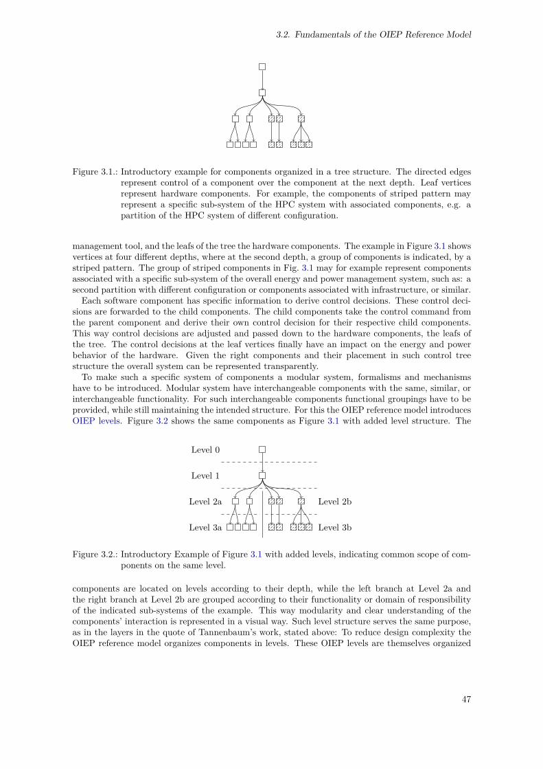
3.2. Fundamentals of the OIEP Reference Model
Figure 3.1.: Introductory example for components organized in a tree structure. The directed edgesrepresent control of a component over the component at the next depth. Leaf verticesrepresent hardware components. For example, the components of striped pattern mayrepresent a specific sub-system of the HPC system with associated components, e.g. apartition of the HPC system of different configuration.
management tool, and the leafs of the tree the hardware components. The example in Figure 3.1 showsvertices at four different depths, where at the second depth, a group of components is indicated, by astriped pattern. The group of striped components in Fig. 3.1 may for example represent componentsassociated with a specific sub-system of the overall energy and power management system, such as: asecond partition with different configuration or components associated with infrastructure, or similar.Each software component has specific information to derive control decisions. These control deci-
sions are forwarded to the child components. The child components take the control command fromthe parent component and derive their own control decision for their respective child components.This way control decisions are adjusted and passed down to the hardware components, the leafs ofthe tree. The control decisions at the leaf vertices finally have an impact on the energy and powerbehavior of the hardware. Given the right components and their placement in such control treestructure the overall system can be represented transparently.To make such a specific system of components a modular system, formalisms and mechanisms
have to be introduced. Modular system have interchangeable components with the same, similar, orinterchangeable functionality. For such interchangeable components functional groupings have to beprovided, while still maintaining the intended structure. For this the OIEP reference model introducesOIEP levels. Figure 3.2 shows the same components as Figure 3.1 with added level structure. The
Level 0
Level 1
Level 2a Level 2b
Level 3a Level 3b
Figure 3.2.: Introductory Example of Figure 3.1 with added levels, indicating common scope of com-ponents on the same level.
components are located on levels according to their depth, while the left branch at Level 2a andthe right branch at Level 2b are grouped according to their functionality or domain of responsibilityof the indicated sub-systems of the example. This way modularity and clear understanding of thecomponents’ interaction is represented in a visual way. Such level structure serves the same purpose,as in the layers in the quote of Tannenbaum’s work, stated above: To reduce design complexity theOIEP reference model organizes components in levels. These OIEP levels are themselves organized
47
3. Open Integrated Energy and Power (OIEP) Reference Model
as a tree structure4.For model creators to construct architectures using the OIEP reference model, the exact definitions
of the model’s basic building blocks, and their rules and their structure have to be provided. Thedescription of basic building blocks and the complete OIEP reference model is found in the followingsection.
3.3. Description of the OIEP Reference ModelThe basic building blocks of the OIEP reference model are OIEP levels and OIEP components. Bothlevels and components are organized in a tree structure. These are the OIEP level tree and the OIEPcomponent tree. The overlay of these two tree structures represents the control hierarchy and controlflow within the OIEP reference model. For a complete model, two additional aspects are required:One, a representation of the flow of monitoring information to support components’ control decision,and two, a representation of the different operating states of an HPC system’s energy and powermanagement setup. The flow of monitoring information is presented by an overlay graph called theOIEP monitoring overlay, while the operating states are captured by OIEP state diagrams.For each of these parts of the reference model, first the concept is introduced, followed by description
of the structure. The section is split into the following four parts:
1. OIEP levels and the OIEP level tree;2. OIEP components and the OIEP component tree;3. OIEP data sources and the OIEP monitoring overlay;4. OIEP operating states and the OIEP state diagram;
These four parts form the OIEP reference model and are detailed below.
3.3.1. OIEP Levels and the OIEP Level TreeOIEP levels represent abstract control domains. The hierarchy of these levels forms the underlyingstructure of the OIEP reference model, the OIEP level tree.
3.3.1.1. OIEP Levels
An OIEP level represents an abstraction of a control domain for the management of energy and power.A domain of control for energy and power represents a logical placement of required functionality andscope within the HPC system. For the purpose of the OIEP reference model, individual componentsare placed within an OIEP level. With such placement, functionality and scope within the HPCsystem, an OIEP level fulfills the purpose to contain hardware or software components. Ultimately,the components provide the realization of the energy and power management functionality at thatlevel.OIEP levels have associated goals, dictated by the requirements of the parent levels or the ca-
pabilities of the child levels. The hierarchy of levels allows for each level to focus on its abstractresponsibilities. Components of other OIEP levels are shielded from the complexity of the containedcomponents and their implementation, provided interfaces for control and information flow are known.The OIEP levels are vertices within the OIEP level tree. This implies that each OIEP level has one
incoming edge from the parent level, and outgoing edges to the child levels. These edges representdirect control of a higher level over a lower level.OIEP levels group components within the same control domain. Each hardware or software com-
ponent of specific functionality is placed within one distinct OIEP level. These components realizethe optimization goal of the level. Thus, by following the level concept modularity of the energyand power management system is achieved. The considerations for OIEP levels are summarized asfollows:An OIEP level is an abstract energy and power control domain composed of:
4As opposed to the stack structure of layers as mentioned in the quoted text from [Tan81, p. 10], as seen above.
48

3.3. Description of the OIEP Reference Model
a) A specified level scope;b) An associated optimization goal;c) Logical placement and physical location;d) Required functionality for energy and power management;e) Hardware or software components associated with the level.
Specified Scope of Energy and Power Management: Each OIEP level in the reference model hasto have a specific scope. The exact scope of each level is to be defined by the creator of a specificOIEP architecture. This also implies that the number and layout of levels can differ among, OIEParchitectures.The scope of a single level should have exact limits and fit the interacting systems of the HPC
system’s setup. The scope also specifies the managed resource and possible sub-components, whichare generally delimited as child levels following the same principles. The scope of an OIEP levelonly contains relevant aspects of energy and power management, following the Keep It Simple Stupid(KISS) principle. Breaking down large levels into several smaller levels is advised. These levelsthemselves have to form properly scoped hierarchies. Such scoping of levels allows for modularity ofthe design. By limiting scope and remit of the energy and power management responsibilities of alevel, the latter introduced components can be employed in an interchangeable way. Such setup allowsfor opaque usage of the model components within an OIEP level. Knowledge about implementationdetails is contained to each level and component within the level.Examples for such scopes are: Scheduler-level, node-level, job-level, among others. The name of a
level is set by the model creator, who specifies the OIEP architecture for a specific energy and powermanagement system of an HPC system. Names of OIEP levels are advised to reflect the scope of thelevels.
Associated Optimization Goal: Each OIEP level has an associated optimization goal. An optimiza-tion goal for a level, is either a management goal, or goal for budgeting resources associated withenergy and power at the level.HPC systems which introduce energy and power management systems have an overall goal for
energy and power management. In general this is the reason for the introduction of such managementsystem, in the first place. For each level within an OIEP architecture an optimization goal specificto the scope and capabilities of the OIEP level has to be specified. Several levels can have the samegoal, while differing in scope, placement, functionality, and actual components placed within eachlevel.For examples of optimization goals, the typical candidates are: Minimization of energy consumed,
constant power draw, maintaining an upper or lower bound of power draw. Indirect goals for energyand power are managing the energy and power consumption for specific resource utilization at theOIEP level. Such goals can also be indirect computational load balancing, enabled by maintainingan overall energy and power management goal.
Logical Placement and Physical Location: With the given hardware setup of the system andsoftware components required for energy and power management, each OIEP level has a specificlocation associated with it. This is both a logical placement within the energy and power managementsystem, and a physical placement within the HPC system.Each hardware and software component has such location within the energy and power management
system. This is either the physical mounting point of the hardware, or, for software, a resource wherethat component is operating on. Levels form abstractions for these systems. By providing a logicalplacement within an OIEP architecture for a specific HPC system, the real components and potentialcandidates have associated locations planned for in the system. This serves as a control to ensureproper planning of the management system in terms of resources and to prevent potential issuesor mismatch in logical layout and physical layout. Hardware and software always have resourcesassociated needed for operation. The expected load and capacity of these resources and potentialscaling needs need to be considered when provisioning.
49

3. Open Integrated Energy and Power (OIEP) Reference Model
The logical placement of the levels within the energy and power management system necessitatesfor the model creator to think about the physical placement of the components. This helps to designa sound logical structure of the flow of control decision within an OIEP architecture, forming the laterOIEP level tree. Additionally, hardware and software components need physical resources to function.The logical placement and the physical location are often related. Thus, having a logical place fora level in the hierarchy helps to verify the structural setup of the energy and power managementfunctionality.
Required Functionality for Energy and Power Management: To realize the optimization goalsspecific functionality provided by an OIEP level is required.The required functionality can be a listing of provided and served interfaces for control decision to
other (lower) levels, and information flow. The functionality is an abstract specification of what is tobe implemented by components placed at that level. Such required functionality provides, and at thesame time restricts, the freedom of components to fulfill the requirements of a level. A descriptionof required functionality can be seen as an abstract function description of the OIEP level. Givenspecific control input (control decisions from the parent level), and control output (control decisionspassed to child levels), identifying the functionality needed at the specific OIEP level.The required functionality often reflects either demanded functionality in an RFP, a specific soft-
ware or hardware solutions which is to be employed, or functionality associated with the above namedscope.
Associated Hardware or Software Components: Given the above four paragraphs, OIEP levels canbe specified. The aim of the level concept is to place components within these levels as specified bythe model creator. Therefore, hardware and software components need to be placed within the OIEPlevels. These components are the elements OIEP levels are intended to group.OIEP levels are abstractions for hardware and software components, thus it is important to have
real software-systems and hardware in mind. Placing associated components within the levels allowsto verify that the granularity of an individual level is set right for a HPC system and the OIEParchitecture modeling the system.The components of a level operate within a) the scope of the level, b) working towards an optimiza-
tion goal, c) at the logical placement and physical location within the system, and d) implementingspecified functionality. The specifics regarding components of a level are listed in detail in Sec-tion 3.3.2 discussing OIEP components.
For a given OIEP architecture the individual characteristics of the OIEP levels differ (as well asthe total number of required levels to represent the respective energy and power management sys-tem). The individual levels’ descriptions are adapted according to the needs for an energy and powermanagement system, while following the above principles. Chapter 4 (with App. D) presents examplesfor different level incarnations as found in OIEP architectures.To identify a needed split of a single level into two, the method to identify the need to distinguish
two building blocks of the same kind, presented in Section 3.1, can be applied.
3.3.1.2. The OIEP Level Tree
The OIEP level tree forms the control hierarchy of levels representing an OIEP architecture. Thevertices of the tree are the OIEP levels. Edges represent control of a level over its child levels.In the OIEP reference model the OIEP level tree is generally represented as a hierarchy. Thisconvention helps with the visualization of the OIEP reference model, while both hierarchies and treesare equivalent.Two examples show the structure and basic principles of the OIEP level tree concept:
1. A tree segment (see Fig. 3.3);2. A simple level tree (see Fig. 3.4).
Figure 3.3 shows a segment of an OIEP level tree. The indicated tree segment shows level k withparent level k− 1, as well as its child levels ka + 1 and kb + 1 (where in this example ka indicates the
50

3.3. Description of the OIEP Reference Model
Level k-1
Level k
Level ka+1
Level ka+2
Level kb+1
Level kb+2
Figure 3.3.: Tree segment of an OIEP level tree. Levels serve as nodes of the tree, edges are repre-sented implicitly in the hierarchy of levels. The indicated tree segment shows level k withparent level k − 1, as well as its child levels ka + 1 and kb + 1. In this example the levelka + 1 has a child level ka + 2, accordingly kb + 1 has child level kb + 2.
left branch and kb the right branch, accordingly). In this example the level ka + 1 has a child levelka+2, accordingly kb+1 with child level kb+2. The hierarchy of control of this segment implies thatlevel k − 1 has direct control over level k, whereas level k has direct control over ka + 1 and kb + 1.The example continues with ka + 1 having direct control over ka + 2. Respectively kb + 1 has controlover kb + 2.Such control hierarchy implies that even though level k− 1 has no direct control over level ka + 2,
by design of the control hierarchy and the levels present in the tree the model creator makes surethat the levels are specified accordingly and placed within the OIEP architecture, such that goals andfunctionality of all levels along a path are conflict-free. The number of child levels of an individuallevel solely depends on the setup and design of the energy and power management system representedin the OIEP architecture.The depth of an OIEP level tree is the maximum depth of all of its levels. The levels are indexed
by their depth and a branch identifier. The degree of a level in an OIEP level tree is the number ofassociated child levels, in accordance to the definition of directed trees. For identification and namingof the levels, these can be referred to with depth and branch identifier, but generally a mnemonicidentifier is preferred.The implicit edges of the OIEP level tree from a level to its child levels is made explicit by the
components and the component tree. Components are situation within one distinct level and haveinterfaces to components of child and parent levels, as detailed in Section 3.3.2 (which introducesOIEP components and the OIEP component tree). Flow of control in an OIEP architecture is alwaysfrom level to level, traversing down the OIEP level tree.Next, Figure 3.4 presents a simple OIEP level tree. The figure is used to identify how levels are
placed within the OIEP level tree, how naming of levels works and functionality of the tree is identified.Additionally, the root level and leaf levels are put into context of energy and power management.Figure 3.4 shows a simple instance of a OIEP level tree. The tree has n levels with one child
per level. The example OIEP level tree is populated with dummy representations of componentsfor illustrative purpose, as a trivial component tree. The placeholder components form a simplelinear OIEP component tree for completeness, following the structure of the trivial OIEP level treeof degree 1.
The root of the OIEP level tree is level 0. In the example of Figure 3.4, the level is named “CenterLeadership”. The level has an implicit edge to level 1.In the example, a level on depth x is identified as the “Application Environment” level. As for any
level this level x has a set scoped, optimization goal, logical and physical location, functionality, andassociated software component. In the OIEP level tree it is passed control directives by its parent level.According to the layout of the OIEP level tree the only energy and power mechanisms the applicationenvironment on level x can directly interact with is the parent level x−1 and its child level x+1. Thisencapsulates the application environment making sure that the designated mechanisms are used. Thelevel x − 1 is responsible for its specific scope, goal, and provides specific functionality, with directcontrol interface to level x. (The functionality is realized by the respective components on these
51
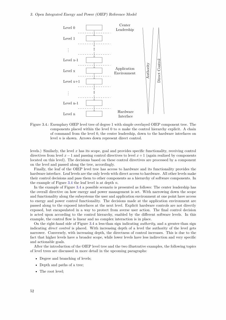
3. Open Integrated Energy and Power (OIEP) Reference Model
Level 0 CenterLeadership
Level 1
...
Level x-1
Level x ApplicationEnvironment
Level x+1
...
Level n-1
Level n HardwareInterface
Autho
rity
Dire
ctCon
trol
Figure 3.4.: Exemplary OIEP level tree of degree 1 with simple overlayed OIEP component tree. Thecomponents placed within the level 0 to n make the control hierarchy explicit. A chainof command from the level 0, the center leadership, down to the hardware interfaces onlevel n is shown. Arrows down represent direct control.
levels.) Similarly, the level x has its scope, goal and provides specific functionality, receiving controldirectives from level x− 1 and passing control directives to level x+ 1 (again realized by componentslocated on this level). The decisions based on these control directives are processed by a componenton the level and passed along the tree, accordingly.Finally, the leaf of the OIEP level tree has access to hardware and its functionality provides the
hardware interface. Leaf levels are the only levels with direct access to hardware. All other levels maketheir control decisions and pass them to other components as a hierarchy of software components. Inthe example of Figure 3.4 the leaf level is at depth n.
In the example of Figure 3.4 a possible scenario is presented as follows: The center leadership hasthe overall directive on how energy and power management is set. With narrowing down the scopeand functionality along the subsystems the user and application environment at one point have accessto energy and power control functionality. The decisions made at the application environment arepassed along to the exposed interfaces at the next level. Explicit hardware controls are not directlyexposed, but encapsulated in a way to protect from averse user action. The final control decisionis acted upon according to the control hierarchy, enabled by the different software levels. In thisexample, the control flow is linear and no complex interaction is in place.On the right-hand side of Figure 3.4 a less-than sign indicating authority, and a greater-than sign
indicating direct control is placed. With increasing depth of a level the authority of the level getsnarrower. Conversely, with increasing depth, the directness of control increases. This is due to thefact that higher levels have a broader scope, while lower levels have less indirection and very specificand actionable goals.After the introduction of the OIEP level tree and the two illustrative examples, the following topics
of level trees are discussed in more detail in the upcoming paragraphs:
• Degree and branching of levels;• Depth and paths of a tree;• The root level;
52
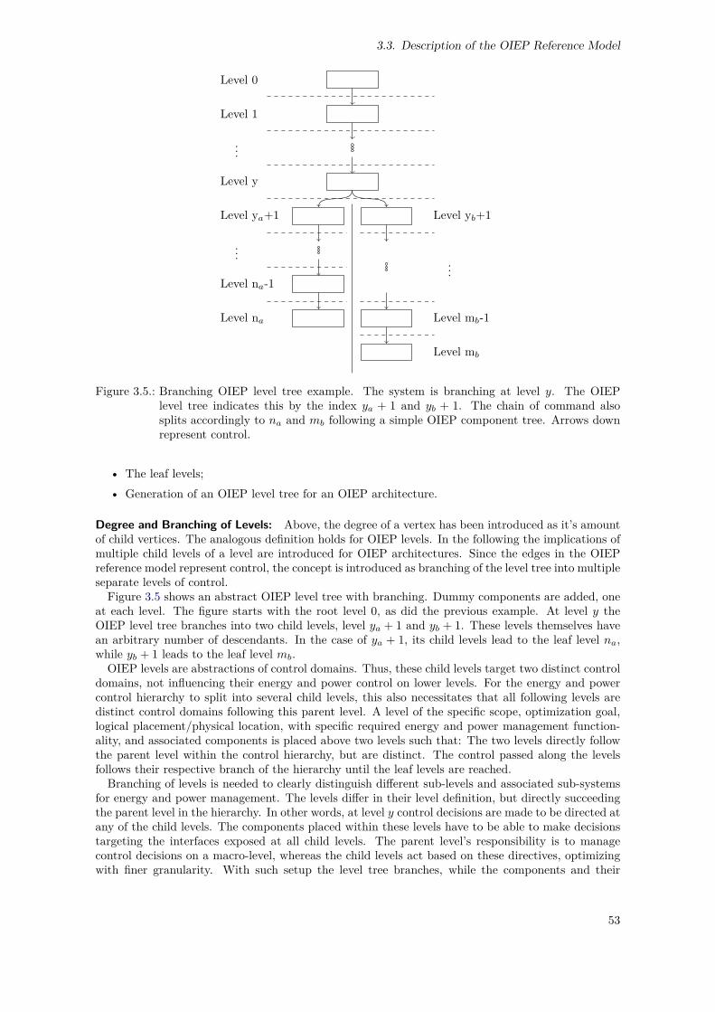
3.3. Description of the OIEP Reference Model
Level 0
Level 1
...
Level y
Level ya+1 Level yb+1
... ...Level na-1
Level na Level mb-1
Level mb
Figure 3.5.: Branching OIEP level tree example. The system is branching at level y. The OIEPlevel tree indicates this by the index ya + 1 and yb + 1. The chain of command alsosplits accordingly to na and mb following a simple OIEP component tree. Arrows downrepresent control.
• The leaf levels;• Generation of an OIEP level tree for an OIEP architecture.
Degree and Branching of Levels: Above, the degree of a vertex has been introduced as it’s amountof child vertices. The analogous definition holds for OIEP levels. In the following the implications ofmultiple child levels of a level are introduced for OIEP architectures. Since the edges in the OIEPreference model represent control, the concept is introduced as branching of the level tree into multipleseparate levels of control.Figure 3.5 shows an abstract OIEP level tree with branching. Dummy components are added, one
at each level. The figure starts with the root level 0, as did the previous example. At level y theOIEP level tree branches into two child levels, level ya + 1 and yb + 1. These levels themselves havean arbitrary number of descendants. In the case of ya + 1, its child levels lead to the leaf level na,while yb + 1 leads to the leaf level mb.OIEP levels are abstractions of control domains. Thus, these child levels target two distinct control
domains, not influencing their energy and power control on lower levels. For the energy and powercontrol hierarchy to split into several child levels, this also necessitates that all following levels aredistinct control domains following this parent level. A level of the specific scope, optimization goal,logical placement/physical location, with specific required energy and power management function-ality, and associated components is placed above two levels such that: The two levels directly followthe parent level within the control hierarchy, but are distinct. The control passed along the levelsfollows their respective branch of the hierarchy until the leaf levels are reached.Branching of levels is needed to clearly distinguish different sub-levels and associated sub-systems
for energy and power management. The levels differ in their level definition, but directly succeedingthe parent level in the hierarchy. In other words, at level y control decisions are made to be directed atany of the child levels. The components placed within these levels have to be able to make decisionstargeting the interfaces exposed at all child levels. The parent level’s responsibility is to managecontrol decisions on a macro-level, whereas the child levels act based on these directives, optimizingwith finer granularity. With such setup the level tree branches, while the components and their
53

3. Open Integrated Energy and Power (OIEP) Reference Model
communication along their interfaces follow these branches. A chain of command for any controldecision can be traced along a single path along such branch of a level tree. The depth of each branchcan be arbitrary.For example, a typical level branch occurs if compute resources are modeled distinct form cooling
resources. Assume that the branch following ya + 1 is the compute subsystems, while yb + 1 is thecooling subsystem. Either has a different number of child levels themselves, depending on their setup.The level y is able to provide control directives to either of its child levels, and the contained com-ponents have to make informed decisions about control and delegation of their decisions. Followingthe example, a component on level y then has to be able to give meaningful control directives to itsconnection components on both the compute level and the cooling level.
Depth and Paths of a Tree: The depth of a OIEP level tree is the maximum depth of all of itslevels, as defined above.Traversing the level tree from root to a specific leaf level follows a distinct path along the level tree.
Such path represents the chain of command of the levels, and shows how control decisions traversefrom root to leaf level. The length of the path is equal to the depth of the associated leaf level.Different paths of the OIEP level tree can have different depths.A deep level tree implies many intermediate levels until the hardware level is reached. Intermediate
levels can introduce latency and reaction times until control information propagates to the leaf levels.It should be noted that time horizons for the energy and power management systems can be verydifferent: Real time, batched or even static, with various degrees of granularity. Considerationsregarding how components can behave on a level regarding time are crucial if control decisions affectlarge parts of the complete OIEP level tree, in the case that regular changes are made near the rootof the tree in a deep level tree. At the same time, deep hierarchies allow for a very precise focus ofthe level’s components on a specific functionality.The example in Figure 3.5 shows branching at level y, while the paths along level ya + 1 to na and
along level yb + 1 to mb have individual length of n and m, respectively. The depth of the level treeis the maximum of its paths, in this case m.OIEP level trees can be very shallow or very deep. The design depends on the model creator and
the needs for the OIEP architecture. Model creators have to make practical considerations to modelthe system with enough depth for clear separation of functionality, while keeping the OIEP level treeshallow enough to be usable in practice.
The Root Level: At the top of the OIEP level tree the root level is situated, indicated as level 0.The root level forms the anchor point of any OIEP architecture and is the main initial point of controlfor the energy and power management system. This root level has a special responsibility for controland model creation.The root level has special characteristics, regarding:
a) A specified level scope: The scope of the root level is the complete energy and power manage-ment system covered by the OIEP architecture. The root level’s responsibility is to separatethe complete management scope into the sub-levels of the OIEP level tree. The scope of theroot is the most general of the OIEP level tree, and covers the complete breath of the energyand power management system, even if very abstract;
b) The associated optimization goal: The root node’s optimization goal is the overall optimizationgoal of the OIEP architecture and the reason why the energy and power management setup usingthe OIEP reference model. Such goals can be simple “minimizing energy to solution”, “stayingwithin a specific range of power consumption”, or “optimizing performance of applications withhigh priority, while minimizing operational costs for any jobs with lower priority”, for example.
c) Logical placement and physical location: Depending on if the root level is a level with no activecomponent, but rather organizational characteristic, the logical placement is at the top of theOIEP level tree and energy and power management hierarchy. Alternatively, if the level hasactive software components associated, these components need associated hardware resourcefor operation. In either case the associated documentation and configuration for the OIEParchitecture is co-located with the root node and needs a storage location;
54

3.3. Description of the OIEP Reference Model
d) Required functionality for energy and power management: At the root level the required func-tionality is to delegate the respective optimization goal to the root’s child levels. The root levelhas no parent level itself, by definition and thus no functional requirements are set for incomingcontrol directives. Additional required functionalities specific to the root node are: The rootlevel guarantees that the rest of the OIEP architecture is set up in a conformal way, sufficingthe requirements and goals of the overall energy and power management system. This includesthe validation of the proper structure and of the lower levels during setup and regarding theirconfiguration. This is done by the model creator, who is delegated by the center leadership.The root node is a proxy representative for this.
e) Hardware or software components associated with the level: Components associated with theroot level may be only virtual, and not an active component. For a virtual component thefunctionality as obliged above is still necessary, especially for documentation purposes. If theroot node is a managed by an actual software component, sufficient documentation is to beadded to document the usage of OIEP architecture and energy and power management setupaccording to the OIEP reference model.
The root level has the added required functional, to check the setup and to identify that the hierarchyand its configurations are fit according to the desired architecture. This role is delegated in the formof documentation and the responsibility of the model creator. The formal association is however atthe root level, such that this is part of the reference model itself. In terms of the design, the rootlevel (read “the model creator”) does not command control to a level which it does not “trust”. Theroot level dictates the choices of tools and the initial selection of OIEP components for the OIEPlevel tree and the overall OIEP architecture.
The Leaf Levels: The leaf levels are situated at the bottom of the OIEP level tree. The leaf levelscontrol and alter the hardware behavior directly. The number of leaf levels, is equal to the numberof different groups of hardware types. These hardware types are characterized by a unique featureset as of the definition of level characterization and are thus to be managed in distinct fashion.Since the OIEP reference model manages hardware using software, the leaf levels have only an
incoming edge. This cut-off (i.e. no out-going edges) at the leaf-level implies that there is no softwareinvolved which can be altered by the users or creators of the OIEP architecture5. The transition tohardware itself, the physical system, serves as cut-off for this distinction. The incoming edge fromthe last level directly translate into control inputs provided by this last software mechanism. Theleaf levels thus represent the final interface to hardware impacting the energy and power behavior ofthe overall system modeled by an OIEP architecture.According to the OIEP level characteristics, the leaf levels of a OIEP architecture have the following
distinct properties:
a) A specified level scope: The leaf levels scope is limited to the hardware control and exposedinterface for the specific type of hardware feature of the level.
b) The associated optimization goal: In general the optimization goal of the leaf levels is a directtranslation of request for changes to hardware settings by the parent level. Optimization is gen-erally done at a higher level, where tuning algorithms process additional information regardingknowledge not present with the limited scope of individual isolated hardware components.
c) Logical placement and physical location: For logical placement, talking about hardware inter-faces, the interface is either provided by firmware, or software. For firmware the hardware hasembedded micro-controllers, for software, the location is on the CPU/in memory. In both casesthese are co-located with the hardware they control, providing access to the management andcontrol feature.
d) Required functionality for energy and power management: For functionality, the leaf level’sfunction is the provision of this explicit access to the hardware component’s control interfaces.An additional required functionality is access control. In general access control has to be
5Firmware is considered not to be alterable within the OIEP reference model, however certainly functionality exposedby firmware is used at the leaf levels.
55
3. Open Integrated Energy and Power (OIEP) Reference Model
restricted enough so that such access control can be dealt with on a higher level, without activemanagement. In theory only the direct parent has access to the levels interfaces, to access,control and set the hardware controls. This has to be guaranteed in practice by the level ordealt with and guaranteed accordingly by a parent level.
e) Hardware or software components associated with the level: The associated hardware andsoftware components are the hardware components themselves, being exposed by hardware,software, or firmware interfaces. Each level provides access to one type of component.
The OIEP level tree provides paths from the root level, to the leaf levels. The root level is a centrallevel having an abstract overview over the complete system and an overall optimization goals. Theleaf level by contrast have the finest granularity of the system, exposing actual hardware. The OIEPlevel tree provides the overall optimization goal and its structure is an expression of how the overalloptimization is intended to be realized. The realization is refined down to the individual hardwarecomponents which are used, at a step size of level granularity. Even though it is the responsibilityof the root level and each intermediate level for its descendants to guarantee a sound command ofcontrol, an essential role for the functioning of an OIEP architecture is to make these choices andconstruct such management setup. To have the right granularities and functionalities for each stepof the OIEP level tree a responsible model creator is needed. The next paragraph provides essentialconsiderations for the generation process for the OIEP level tree of an OIEP architecture.Guidelines for the creation of OIEP levels and OIEP level trees for specific OIEP architectures are
presented in Appendix C.2.This concludes the OIEP levels and OIEP level tree and sets the stage for detailed discussion on
components, which are discussed in the subsequent Section (Sec. 3.3.2).
3.3.2. OIEP Components and the OIEP Component TreeOIEP components are the hardware and software components used within the OIEP reference model.The OIEP components of an OIEP architecture are mapped to the architecture’s OIEP levels. TheOIEP components are connected following the layout of the associated OIEP level tree, forming theOIEP component tree. These connected OIEP components of the OIEP component tree representan instantiation of an OIEP architecture.The OIEP component tree is embedded into the OIEP level tree, but follows different rules and
serves a different purpose. The OIEP component trees shows the exact hardware and softwareinstances and its interfaces, which control the final hardware decisions. Such structured setup allowsto make individual energy and power decisions transparent in a complex multi-component setup. TheOIEP level tree, on the other hand, identifies only the general type of components required at a level.For this reason the tree structure of OIEP components is made explicit as the OIEP component tree.This section first introduces the concepts for OIEP components, followed by the concepts of the
OIEP component tree.
3.3.2.1. OIEP Components
An OIEP component represents the individual instances of software or hardware components in anHPC system responsible for energy and power management functionality.A set of OIEP components are the main active building blocks that make up the system design of
an OIEP architecture. Each component is situated on a specific OIEP level. These components aresoftware and hardware components that implement the functionality required to make decisions ateach level, as identified above. OIEP components have the following three characteristics:
• A component type;• Component interfaces;• Component functionality.
An OIEP component is typically an active software or hardware component in the HPC system,as described in Chapter B.1. All components of an OIEP architecture have a specific active role inenergy and power management and need to be connected to other components to fulfill their roles.
56

3.3. Description of the OIEP Reference Model
P&E Component
(a) Type i
P&EOriginal function
(b) Type ii
P&EOriginal function
(c) Type iii
P&E side-effect
(d) Type iv
Figure 3.6.: Types of OIEP components: Type i – pure energy and power (indicates as P&E) func-tionality; Type ii – integrated energy and power functionality; Type iii – attached energyand power functionality; Type iv – side-effect only, no direct energy and power function-ality.
The identification of component type, interface and functionality specifies the individual capabilitiesof the OIEP component. All regular OIEP components receive control directives from componentson higher levels, process them according to their control algorithms, and direct its control commandsto specific connected components on the next lower level, via the component interfaces. The detailsof the OIEP components are discussed in the following paragraphs.
Component Types: The initial step for OIEP components is to identify the appropriate componenttype. The levels of an OIEP architecture are often co-located with tools in the traditional HPCsoftware stack. Likewise, tools in energy and power management are located at specific physical andlogical locations of already existing tools. Therefore, the functionality is sometimes integrated withthese traditional tools, as discussed in Section B.1.2.2. The logical placement/ physical location forOIEP levels can reflect this co-location of energy and power functionality with traditional HPC.There are four types of OIEP components in terms of core functionality, as seen in Figure 3.6:
Type i – Pure energy and power functionality (see Fig 3.6a).Type ii – Original core functionality outside of energy and power management, but energy
and power management functionality integrated into the core of the component (seeFig 3.6b).
Type iii – Original core functionality outside of energy and power management, but energyand power functionality logically or physically located alongside the component (seeFig 3.6c).
Type iv – Core functionality completely lacking energy and power management functionality,however with energy and power impact as side effect of the component (see Fig 3.6d).
These component types are discussed below.
Type i The fundamental component is component type i with pure energy and power function-ality. Its functionality is purely focused on energy and power management, without additional non-energy and power functionality. This means that the received control decisions, as well as additionalinformation received, are used exclusively to compute resulting actions to drive energy and powerdecision. These are then delegated to underlying components or used to regulate control mechanisms
57
3. Open Integrated Energy and Power (OIEP) Reference Model
in hardware, if the OIEP component is at the leaf level. These types of components are relativelyrare since pure energy and power management is a very recent concept6. Control of energy and powerin such component can have side effects on performance management, which is a separate issue notdealt with by the component. This type of component is vital for clean system design. In the casethat a new tool in the energy and power space is developed this pure type should be considered.As an example, the software components implementing Advanced Configuration and Power Interface(ACPI) can be considered type i. On the hardware side, the RAPL-MSRs are such pure componentssituated at a leaf levels.
Type ii A more involved component is component type ii. This component type has its originalcore functionality outside energy and power, but with energy and power management capabilitiesintegrated. The original functionality of the component either has a direct benefit from managingenergy and power or needs to take care of energy and power management to function properly. Theenergy and power functionality is often added after the original design of the tool, due to the fact thatimproved performance or capabilities has become apparent through academic study (see Section 2.4)or as a direct requirement by the HPC centers. Typical examples for this component type are RASsystems.
Type iii Component type iii is similar to the previous type, but with a more decoupled approach.The original core functionality of the component is outside of energy and power. The energy andpower considerations are not necessary for standalone operation of this original functionality. Theenergy and power management functionality is added as a module or function. With the attachmentof energy and power functionality, these components add valuable features, which could in theorybe detached, but may serve as unique selling point for the product of the original functionality. Forenergy and power management this type of component can be modeled without the non-energy andpower functionality, however the location of the component is dictated by this co-location. Typicalexamples of such components are schedulers or profilers with added energy and power information.For these schedulers and debuggers, the scheduling strategy or the profiling results do not depend onthe energy and power information. However, the added information can serve as control for othercomponents. If the energy and power information is actively used in the original functionality, thecomponent type is of type ii instead.
Type iv Components of type iv, components with energy and power side effect, can be eitherof two cases: A component that has side effects that are wanted for energy and power managementand has indirect yet explicit control over energy and power consumption; A component that has sideeffects to energy and power that are unwanted and thus have to be considered and accounted for.The later case is very critical for correct operation, as well as accounting and should be modeled andconsidered in OIEP architectures, if known. For the former case a very prominent example is man-agement of energy consumption by frequency control via DVFS: The mechanisms primary concern isperformance with significant impact to energy and power, thus the control mechanism is chosen viathis indirect route. Location of such component in the system software is thus predefined since theoriginal component is already part of the HPC system. The associated OIEP level has to be selectedin the OIEP architecture creation accordingly. Due to the fact that this component type deals withside effects of hardware devices, software and tools, identifying the right way for non-aversely interactis critical. The interface to such component is also indirect, thus for energy and power management,an OIEP level and OIEP component for translation of energy and power control to control of the sideeffect is needed, if not handled by the component. Due to the fact that the component is a non-energyand power component and has no active way of interacting with other OIEP components this kindof component is always placed on leaf levels. As mentioned above, example components are explicitfrequency control of DVFS, or cooling infrastructure, both affecting energy and power consumption.
It should be noted, that components can be nested (see Section 3.3.2.2). In such case the assignedcomponent type is the component type of the outermost component of this nesting.
6With the exception of Basic Input Output System (BIOS) and OS.
58
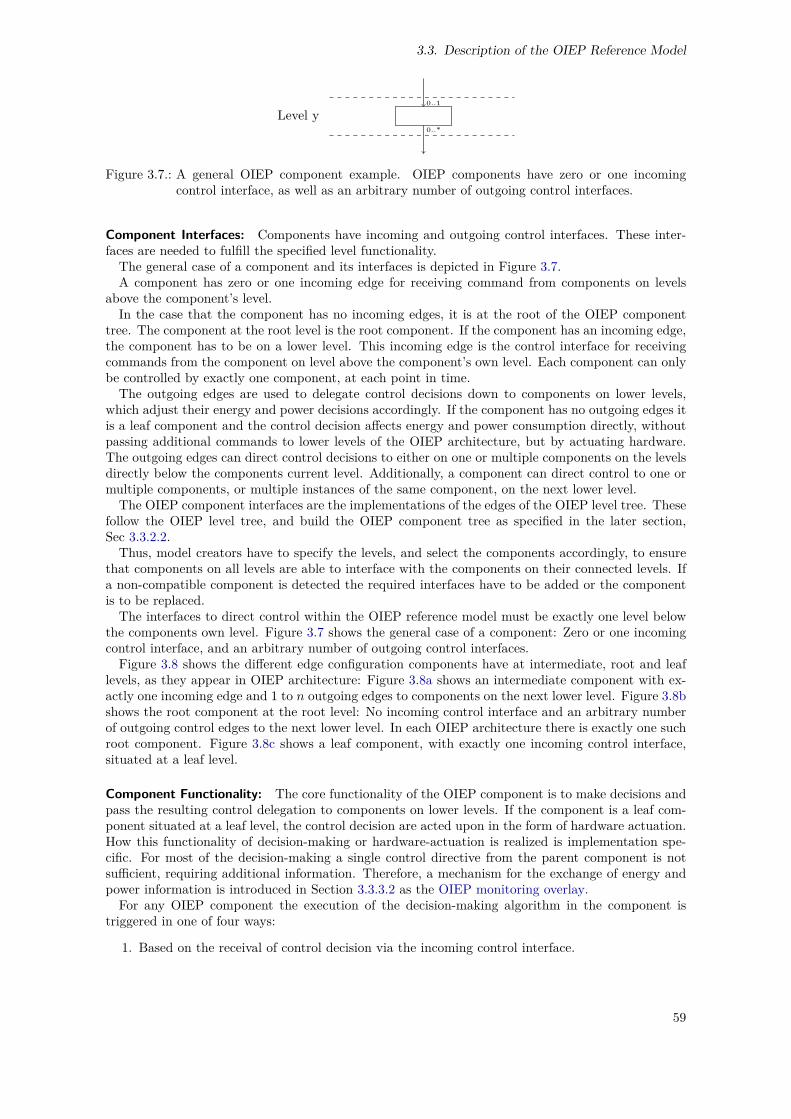
3.3. Description of the OIEP Reference Model
Level y0..1
0..*
Figure 3.7.: A general OIEP component example. OIEP components have zero or one incomingcontrol interface, as well as an arbitrary number of outgoing control interfaces.
Component Interfaces: Components have incoming and outgoing control interfaces. These inter-faces are needed to fulfill the specified level functionality.The general case of a component and its interfaces is depicted in Figure 3.7.A component has zero or one incoming edge for receiving command from components on levels
above the component’s level.In the case that the component has no incoming edges, it is at the root of the OIEP component
tree. The component at the root level is the root component. If the component has an incoming edge,the component has to be on a lower level. This incoming edge is the control interface for receivingcommands from the component on level above the component’s own level. Each component can onlybe controlled by exactly one component, at each point in time.The outgoing edges are used to delegate control decisions down to components on lower levels,
which adjust their energy and power decisions accordingly. If the component has no outgoing edges itis a leaf component and the control decision affects energy and power consumption directly, withoutpassing additional commands to lower levels of the OIEP architecture, but by actuating hardware.The outgoing edges can direct control decisions to either on one or multiple components on the levelsdirectly below the components current level. Additionally, a component can direct control to one ormultiple components, or multiple instances of the same component, on the next lower level.The OIEP component interfaces are the implementations of the edges of the OIEP level tree. These
follow the OIEP level tree, and build the OIEP component tree as specified in the later section,Sec 3.3.2.2.Thus, model creators have to specify the levels, and select the components accordingly, to ensure
that components on all levels are able to interface with the components on their connected levels. Ifa non-compatible component is detected the required interfaces have to be added or the componentis to be replaced.The interfaces to direct control within the OIEP reference model must be exactly one level below
the components own level. Figure 3.7 shows the general case of a component: Zero or one incomingcontrol interface, and an arbitrary number of outgoing control interfaces.Figure 3.8 shows the different edge configuration components have at intermediate, root and leaf
levels, as they appear in OIEP architecture: Figure 3.8a shows an intermediate component with ex-actly one incoming edge and 1 to n outgoing edges to components on the next lower level. Figure 3.8bshows the root component at the root level: No incoming control interface and an arbitrary numberof outgoing control edges to the next lower level. In each OIEP architecture there is exactly one suchroot component. Figure 3.8c shows a leaf component, with exactly one incoming control interface,situated at a leaf level.
Component Functionality: The core functionality of the OIEP component is to make decisions andpass the resulting control delegation to components on lower levels. If the component is a leaf com-ponent situated at a leaf level, the control decision are acted upon in the form of hardware actuation.How this functionality of decision-making or hardware-actuation is realized is implementation spe-cific. For most of the decision-making a single control directive from the parent component is notsufficient, requiring additional information. Therefore, a mechanism for the exchange of energy andpower information is introduced in Section 3.3.3.2 as the OIEP monitoring overlay.For any OIEP component the execution of the decision-making algorithm in the component is
triggered in one of four ways:
1. Based on the receival of control decision via the incoming control interface.
59
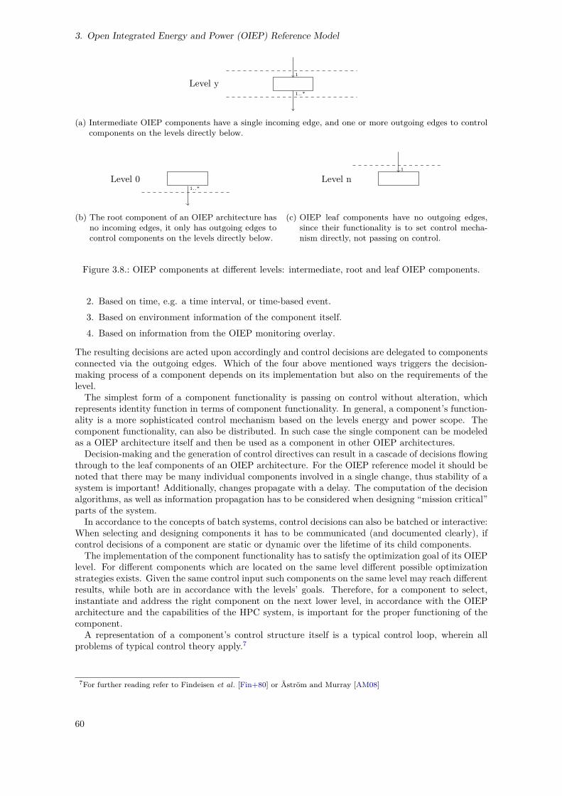
3. Open Integrated Energy and Power (OIEP) Reference Model
Level y1
1..*
(a) Intermediate OIEP components have a single incoming edge, and one or more outgoing edges to controlcomponents on the levels directly below.
Level 01..*
(b) The root component of an OIEP architecture hasno incoming edges, it only has outgoing edges tocontrol components on the levels directly below.
Level n1
(c) OIEP leaf components have no outgoing edges,since their functionality is to set control mecha-nism directly, not passing on control.
Figure 3.8.: OIEP components at different levels: intermediate, root and leaf OIEP components.
2. Based on time, e.g. a time interval, or time-based event.3. Based on environment information of the component itself.4. Based on information from the OIEP monitoring overlay.
The resulting decisions are acted upon accordingly and control decisions are delegated to componentsconnected via the outgoing edges. Which of the four above mentioned ways triggers the decision-making process of a component depends on its implementation but also on the requirements of thelevel.The simplest form of a component functionality is passing on control without alteration, which
represents identity function in terms of component functionality. In general, a component’s function-ality is a more sophisticated control mechanism based on the levels energy and power scope. Thecomponent functionality, can also be distributed. In such case the single component can be modeledas a OIEP architecture itself and then be used as a component in other OIEP architectures.Decision-making and the generation of control directives can result in a cascade of decisions flowing
through to the leaf components of an OIEP architecture. For the OIEP reference model it should benoted that there may be many individual components involved in a single change, thus stability of asystem is important! Additionally, changes propagate with a delay. The computation of the decisionalgorithms, as well as information propagation has to be considered when designing “mission critical”parts of the system.In accordance to the concepts of batch systems, control decisions can also be batched or interactive:
When selecting and designing components it has to be communicated (and documented clearly), ifcontrol decisions of a component are static or dynamic over the lifetime of its child components.The implementation of the component functionality has to satisfy the optimization goal of its OIEP
level. For different components which are located on the same level different possible optimizationstrategies exists. Given the same control input such components on the same level may reach differentresults, while both are in accordance with the levels’ goals. Therefore, for a component to select,instantiate and address the right component on the next lower level, in accordance with the OIEParchitecture and the capabilities of the HPC system, is important for the proper functioning of thecomponent.A representation of a component’s control structure itself is a typical control loop, wherein all
problems of typical control theory apply.7
7For further reading refer to Findeisen et al. [Fin+80] or Åström and Murray [AM08]
60
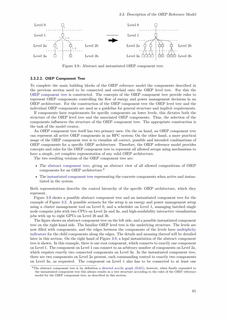
3.3. Description of the OIEP Reference Model
Level 0
Level 1
Level 2a Level 2b
Level 3a Level 3b
1
* 1..n
2 1..8
instantiate
Level 0
Level 1
Level 2a Level 2b
Level 3a Level 3b
Figure 3.9.: Abstract and instantiated OIEP component tree.
3.3.2.2. OIEP Component Tree
To complete the main building blocks of the OIEP reference model the components described inthe previous section need to be connected and overlaid onto the OIEP level tree. For this theOIEP component tree is constructed. The concepts of the OIEP component tree provide rules torepresent OIEP components controlling the flow of energy and power management decisions in anOIEP architecture. For the construction of the OIEP component tree the OIEP level tree and theindividual OIEP components are used as a guideline for general structure and implicit requirements.If components have requirements for specific components on lower levels, this dictates both the
structure of the OIEP level tree and the associated OIEP components. Thus, the selection of thecomponents influences the structure of the OIEP component tree. The appropriate construction isthe task of the model creator.An OIEP component tree itself has two primary uses: On the on hand, an OIEP component tree
can represent all active OIEP components in an HPC system; On the other hand, a more practicalusage of the OIEP component tree is to visualize all correct, possible and intended combinations ofOIEP components for a specific OIEP architecture. Therefore, the OIEP reference model providesconcepts and rules for the OIEP component tree to represent all allowed setups using mechanisms tohave a simple, yet complete representation of any valid OIEP architecture.The two resulting versions of the OIEP component tree are:
• The abstract component tree, giving an abstract view of all allowed compositions of OIEPcomponents for an OIEP architecture.8
• The instantiated component tree representing the concrete components when active and instan-tiated in the system.
Both representations describe the control hierarchy of the specific OIEP architecture, which theyrepresent.Figure 3.9 shows a possible abstract component tree and an instantiated component tree for the
example of Figure 3.2. A possible scenario for the setup is an energy and power management setupusing a cluster management tool on Level 0, and a scheduler on Level 1, managing batched singlenode compute jobs with two CPUs on Level 2a and 3a, and high-availability interactive visualizationjobs with up to eight GPUs on Level 2b and 3b.The figure shows an abstract component tree on the left side, and a possible instantiated component
tree on the right-hand side. The familiar OIEP level tree is the underlying structure. The levels arenow filled with components, and the edges between the components of the levels have multiplicityindicators for the child components along the edges. The details and meaning thereof will be detailedlater in this section. On the right hand of Figure 3.9, a legal instantiation of the abstract componenttree is shown. In this example, there is one root component, which connects to exactly one componenton Level 1. The component on Level 1 can connect to an arbitrary number of components on Level 2a,which requires exactly two connected components on Level 3a. In the instantiated component tree,there are two components on Level 2a present, each commanding control to exactly two componentson Level 3a, as requested. The component on Level 1 also has to be connected to at least one
8The abstract component tree is by definition a directed acyclic graph (DAG), however, when finally expanded tothe instantiated component tree this always results in a tree structure according to the rules of the OIEP referencemodel for the OIEP component tree, as described in this section.
61

3. Open Integrated Energy and Power (OIEP) Reference Model
Level k
Level k+1
0..1 0..n * 1 1..n 1..* n n..m n..* x,y
Figure 3.10.: Multiplicity indicators of OIEP component indicate the number of controlled child com-ponents. The notation indicates the number of controllable instances of child compo-nents. Ranges are indicated by n..m, indicating a minimum number of n and a maximumof m edges and thus control-able child components, where n,m ∈ N0; n ≤ m. In thecase that n 6= m the components can be instantiated based on demand of the control-ling component. ∗ indicates an arbitrary number of component interfaces. x, y indicateseither x or y, where x and y can be any of the previous notation.
component on Level 2b. Such component on Level 2b has to control a specified amount of one toeight components on Level 3b. In the example of the instantiated component tree the componenton Level 1 has three connected instantiated components on Level 2b. Two of them have exactly onecomponent on Level 3b, while one controls three.This introductory example shows how components are presented the OIEP component tree and
how they are integrated into the control hierarchy. It also shows how a simple abstract componenttree might look like, while only including details on the number of interfaces of the components chosenat each level and an instantiation of such tree.To capture all possible allowed control hierarchies rules and concepts are needed for the OIEP
component tree. Each abstract component tree has to indicate the following information:
• Each level has to be occupied by at least one OIEP component.• Each component has exactly one incoming edge, as described in Section 3.3.2.1.• The outgoing edges have to be in accordance with the components, following the layout of the
OIEP level tree.• The number of possible instances of control-able or required components have to be indicated
on the outgoing control interfaces and by connection to the appropriate components on the nextlevel.
• The selections of possibly allowed components on a level have to be indicated in the abstractcomponent tree.
Each instantiated component tree is a snapshot of such a tree at a specific point in time.The following paragraphs complete the OIEP component tree by introducing detailed descriptions
on:
• Multiplicity indicators;• The xor operator “⊕”;• The virtually selected operator “∨”;• Handling empty levels using bridge components;• Nested components.
Multiplicity Indicators: The interfaces of the selected components indicate how the tree is con-structed. The components’ interfaces represent the control flow, represented by the edges in theOIEP component tree.Depending on the component and the system setup, single components can control multiple compo-
nents on the next level. Control over different kinds of components is indicated using multiple edges,control over the same kind of component is indicated using multiplicity indicators. For this eachedge of the abstract component tree is labeled providing information about the amount of possibleconnected components for control.
62

3.3. Description of the OIEP Reference Model
Figure 3.10 shows the possible indicators in case a component can control a variable number ofchild components on the next level, using the same interface. The figure starts left to right (withn,m ∈ N0; n ≤ m):
• With indicator 0..1 for the control of one or zero child components;• With indicator 0..n for the control of zero up to a fixed number n;• With indicator ∗ for an arbitrary number of components without upper limit;• With indicator 1 for exactly one child component (default, indicator generally omitted);• With indicator 1..n for up to n child components, but requiring a minimum of 1;• With indicator 1..∗ for an arbitrary number, but requiring a minimum of 1;• With indicator n for exactly n child component;• With indicator n..m for an number of controlled child components between n and m (n < m);• With indicator n..∗ for an arbitrary number, but requiring a minimum of n child components.• With indicator x, y for a selection of either the indicator x or y, where x and y are themselves
any kind of indicator of this list.
This is used in the abstract component tree to indicated strict capabilities regarding the number ofcomponents control-able using the interface of the parent component. The indicators are only givenon the outgoing side of the edge, since a component can control as many components as specified.On the incoming side of the edge no indicator is needed, since each component is only controlled byexactly one parent component. Unlabeled edges default to 1.
In the instantiated component tree one edge is an explicit control indicator from exactly one parentcomponent to a single child component. Thus, no range multiplicity indicators are given in theinstantiated component tree, but the exact number of controlled components is given. Alternativelythe component instances are shown explicitly as replicas, with unlabeled edges indicating a 1 to 1connection.Variable indicators and the 0 indicator within ranges are used, in case that the components can
instantiate child components during operation. This needs to be part of the parents’ functionality.The model creator has to make sure that a maximum number of hardware controls is not exceededand that each leaf component is only controlled by a maximum of one component! For example, evenif a component can in theory be operated with interface 0..∗ the model creator may need to set anupper limit for ∗ not to exceed the number of hardware controls. Additionally, a theoretical upperlimit of m may need to be lowered in the case that a component has trouble scaling to m controlledcomponents in a real world scenario without Quality of Service (QoS) degradation.As mentioned, each OIEP level can have a number of OIEP components at each OIEP level. To
make sure that each leaf level component is only controlled by a single OIEP component two operatorsfor the OIEP component tree are introduced: the xor operator ⊕ and a second operator indicating apreceding selection in the OIEP component tree diagram, the virtually selected operator ∨.
The Xor Operator “⊕”: When designing an OIEP architecture multiple components can be pro-vided at the same level to facilitate the levels goals. In such a case, the component on the level abovehas to choose one of these provided components when instantiating the OIEP component tree. Thisexclusive choice of child components is indicated using the ⊕ sign in the abstract component tree.The operator is called the xor operator ⊕.The operator has one incoming edge and as many outgoing edges as components are provided for
the use-case in the OIEP architecture to select from for the parent component. A xor operator ⊕ canonly appear in an abstract component tree, since the instantiated component tree is the representationof a concrete instance and no uncertainty is allowed. In the component tree, ⊕ sign of the operatoris always located above the components of the level it is situated on.The parent component on the level above has to know about the fact that it has choice regarding
its child component to either be able to instantiate the right component and optimize internal choicesaccordingly. The protocols for the OIEP architecture have to be selected according and specifiedwhich take choice as by the usage of the xor operator in mind. Controlling the same lower level
63
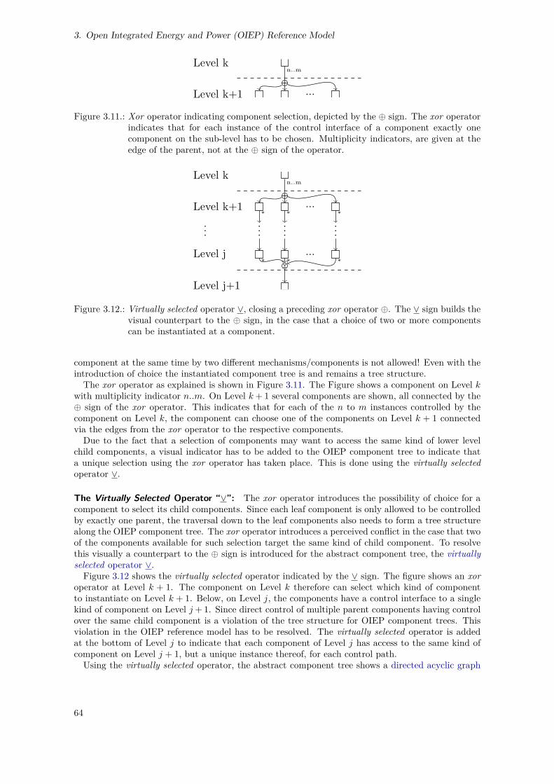
3. Open Integrated Energy and Power (OIEP) Reference Model
Level k
Level k+1 ...
n..m
Figure 3.11.: Xor operator indicating component selection, depicted by the ⊕ sign. The xor operatorindicates that for each instance of the control interface of a component exactly onecomponent on the sub-level has to be chosen. Multiplicity indicators, are given at theedge of the parent, not at the ⊕ sign of the operator.
Level k
Level k+1 ...* * *
n..m
* *...
*Level j
Level j+1
......
......
Figure 3.12.: Virtually selected operator ∨, closing a preceding xor operator ⊕. The ∨ sign builds thevisual counterpart to the ⊕ sign, in the case that a choice of two or more componentscan be instantiated at a component.
component at the same time by two different mechanisms/components is not allowed! Even with theintroduction of choice the instantiated component tree is and remains a tree structure.The xor operator as explained is shown in Figure 3.11. The Figure shows a component on Level k
with multiplicity indicator n..m. On Level k+ 1 several components are shown, all connected by the⊕ sign of the xor operator. This indicates that for each of the n to m instances controlled by thecomponent on Level k, the component can choose one of the components on Level k + 1 connectedvia the edges from the xor operator to the respective components.Due to the fact that a selection of components may want to access the same kind of lower level
child components, a visual indicator has to be added to the OIEP component tree to indicate thata unique selection using the xor operator has taken place. This is done using the virtually selectedoperator ∨.
The Virtually Selected Operator “∨”: The xor operator introduces the possibility of choice for acomponent to select its child components. Since each leaf component is only allowed to be controlledby exactly one parent, the traversal down to the leaf components also needs to form a tree structurealong the OIEP component tree. The xor operator introduces a perceived conflict in the case that twoof the components available for such selection target the same kind of child component. To resolvethis visually a counterpart to the ⊕ sign is introduced for the abstract component tree, the virtuallyselected operator ∨.
Figure 3.12 shows the virtually selected operator indicated by the ∨ sign. The figure shows an xoroperator at Level k + 1. The component on Level k therefore can select which kind of componentto instantiate on Level k + 1. Below, on Level j, the components have a control interface to a singlekind of component on Level j + 1. Since direct control of multiple parent components having controlover the same child component is a violation of the tree structure for OIEP component trees. Thisviolation in the OIEP reference model has to be resolved. The virtually selected operator is addedat the bottom of Level j to indicate that each component of Level j has access to the same kind ofcomponent on Level j + 1, but a unique instance thereof, for each control path.Using the virtually selected operator, the abstract component tree shows a directed acyclic graph
64

3.3. Description of the OIEP Reference Model
Level k
Level k+1
Level k+2
Level k+3
Level k+4
a
*
b*
c
*
d*
e
*f
*
g
*h*
i*
instantiate
a
b c
d e f
g1 g2 h
i1 i2 i3
Figure 3.13.: OIEP component tree instantiation with xor operator and virtually selected operator.The example instantiation shows one component for each possible path of componentselection for each xor operator. Both ⊕ and ∨ operator symbols are eliminated by theinstantiation process and ultimately only show the selected components on the paths tothe leafs.
(DAG) between the component on Level k and the component on Level j + 1. The instantiatedcomponent tree expands to a normal tree without any components controlled by two parents, asrequired by the OIEP component tree. Such instantiation of the same component type for eachcontrol path is shown in Figure 3.13 in a more involved example.Figure 3.13 shows an abstract component tree on the left and an instantiated component tree on
the right. The abstract component tree shows two xor operators, one at Level k + 1 and one atLevel k + 2. The first of the selections is matched by a virtually selected operator at Level k + 2,while the second selection is matched by a virtually selected operator at Level k + 3.On the right-hand side of Figure 3.13 the instantiated component tree shows one component in-
stance for each possible selection of the xor operator. This results in a unique instance of each com-ponent kind after resolving each virtually selected operator, following three distinct control paths.Therefore, component g on Level k + 3 is instantiated as component g1, controlled by component dand component g2 controlled by component e. Similarly, component i is replicated as component i1controlled by component g1, component i2 controlled by component g2 and component i3 controlledby component h.
The virtually selected operator ∨ serves as a visual reminder that a choice of child components waspresented earlier using the xor operator. No instantiated component can be controlled by multiplecomponents from a parent level without violating the OIEP reference model principles. The operatoris not tied to any real component but serves as virtual reminder to verify that design is valid atconstruction time of the OIEP architecture.
Following the examples for the xor operator and the virtually selected operator, the following sum-mary is given:
• Controlling the same instance of a component at the same time from different parent componentsis forbidden, violating the control tree structure of the OIEP component tree.
• The exclusive selection of a branch (read: instantiation of a child component using an xoroperator) is done by the parent component above the xor operator.
• Having an xor operator implies that the parent component knows about the selection and hasa protocol to perform this selection.
• After all selections are done for the instantiation of the OIEP component tree, there is noambiguity and each component is controlled by exactly one component as required by thecontrol tree structure.
• In the abstract component tree the path between ⊕ sign and ∨ sign is a DAG, making thecomplete system a DAG. Thus calling the system a tree is wrong and OIEP component tree
65
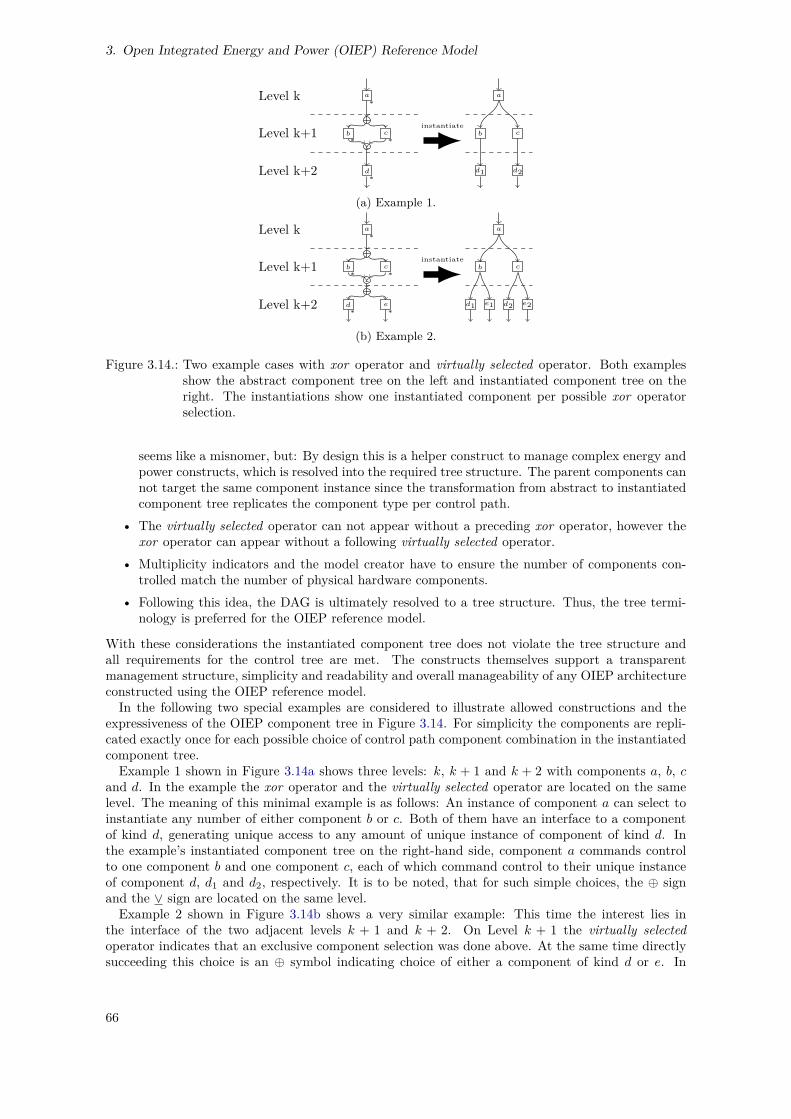
3. Open Integrated Energy and Power (OIEP) Reference Model
Level k
Level k+1
Level k+2
a
*
b*
c
*
d*
instantiate
a
b c
d1 d2
(a) Example 1.
Level k
Level k+1
Level k+2
a
*
b*
c
*
d*
e
*
instantiate
a
b c
d1 e1 d2 e2
(b) Example 2.
Figure 3.14.: Two example cases with xor operator and virtually selected operator. Both examplesshow the abstract component tree on the left and instantiated component tree on theright. The instantiations show one instantiated component per possible xor operatorselection.
seems like a misnomer, but: By design this is a helper construct to manage complex energy andpower constructs, which is resolved into the required tree structure. The parent components cannot target the same component instance since the transformation from abstract to instantiatedcomponent tree replicates the component type per control path.
• The virtually selected operator can not appear without a preceding xor operator, however thexor operator can appear without a following virtually selected operator.
• Multiplicity indicators and the model creator have to ensure the number of components con-trolled match the number of physical hardware components.
• Following this idea, the DAG is ultimately resolved to a tree structure. Thus, the tree termi-nology is preferred for the OIEP reference model.
With these considerations the instantiated component tree does not violate the tree structure andall requirements for the control tree are met. The constructs themselves support a transparentmanagement structure, simplicity and readability and overall manageability of any OIEP architectureconstructed using the OIEP reference model.In the following two special examples are considered to illustrate allowed constructions and the
expressiveness of the OIEP component tree in Figure 3.14. For simplicity the components are repli-cated exactly once for each possible choice of control path component combination in the instantiatedcomponent tree.Example 1 shown in Figure 3.14a shows three levels: k, k + 1 and k + 2 with components a, b, c
and d. In the example the xor operator and the virtually selected operator are located on the samelevel. The meaning of this minimal example is as follows: An instance of component a can select toinstantiate any number of either component b or c. Both of them have an interface to a componentof kind d, generating unique access to any amount of unique instance of component of kind d. Inthe example’s instantiated component tree on the right-hand side, component a commands controlto one component b and one component c, each of which command control to their unique instanceof component d, d1 and d2, respectively. It is to be noted, that for such simple choices, the ⊕ signand the ∨ sign are located on the same level.
Example 2 shown in Figure 3.14b shows a very similar example: This time the interest lies inthe interface of the two adjacent levels k + 1 and k + 2. On Level k + 1 the virtually selectedoperator indicates that an exclusive component selection was done above. At the same time directlysucceeding this choice is an ⊕ symbol indicating choice of either a component of kind d or e. In
66

3.3. Description of the OIEP Reference Model
such case both b and c have to implement and agree with component d and e on a protocol forselection of the respectively components and for exchange of control commands and information. Inthe example’s instantiated component tree on the right-hand side, component a commands controlto one component b and one component c, each of which command control to a unique instance ofexclusive selection of component d and e each. This results in component b commanding controlto instances d1 and e1, while component c commands control to instances d2 and e2. It is to benoted that only when the same component is targeted by previous components the virtually selectedoperator is needed. If an exclusive choice by an xor operator targets two different independent,and/or exclusive components, no matching virtually selected operator is needed.Given the examples of Figure 3.14, possible scenarios therefore are: Level k represents the job
scheduler level, having selection of multiple job runtimes at Level k + 1. As possible scenario forFigure 3.14a, both runtime components, d and c, target the same hardware component at Level k +2. As possible scenario for Figure 3.14b there is an available selection of two different hardwarecontrols, for example Voltage Regulators (VRs) represented as component d and fans represented ascomponent e.With the introduced operators no duplication of the same component types is necessary to be either
situated at the same or even different levels in the OIEP component tree.
Handling Empty Levels Using Bridge Components: This paragraph discusses possibly empty lev-els and bridge components as neutral elements for the OIEP component tree. Both concepts areimportant to avoid conflicts in a system design and avoid possible erroneous construction of OIEParchitectures. Additionally, these serve as helper constructs when using the OIEP reference modelfor RFPs, system proposals and planning for longer term system evolution. To start this paragraphthe following reminder is given: Any level k is only connected to directly adjacent levels k − 1 andlevel k+ 1. Likewise, components on level k can only have edges to components on directly adjacentlevels k − 1 and level k + 1.In the case that components can control a variable number of child components, indicated by
multiplicity indicator 0 or ∗, a level on the instantiated component tree can potentially be empty.This component is then a leaf of the instantiated component tree, as control decisions can only bepropagated when a child component is instantiated. In such case, all components underneath suchcomponents are not instantiated themselves, and the respective child levels are empty. All compo-nents following the given variable multiplicity indicator have to have the capability to instantiate,construct and deconstruct components. The protocols of each component interface have to supportsuch functionality. On the abstract component tree levels are never devoid of components.At the design phase of the OIEP architecture each level has to have at least one component per
level. In the case that no functional components are available for a level k, possible bridge componentscan be placed. Such bridge components take the incoming edges from the components on level k− 1and route them to the appropriate connected component on level k + 1 without alteration. Thecomponent’s functionality performs the identity function and if exactly one parent component isconnected to exactly one child component this is the simplest form of a bridge component. Inthe case that the input from the parent is replicated among all components on the child level, thebridge components functionality is to multiplex the control commands. In the case that the controlinformation needs to be split a simple division is applied as the functionality of the bridge component.Bridge components can be useful if software is planned for a system design and a working place-
holder is needed. Alternatively, such bridge component can be used as a default of fall-back componentin the case that a component has not sufficient information to perform its functionality. In such casenotification system for admins should be in place. Bridge components on the leaf levels indicate anon-functional design. These bridge components should be replaced by fully functional componentsfor the level to achieve the goal of the OIEP architecture.
Nested Components in the Component Tree: A single OIEP component of the OIEP componenttree can be a nested sub-tree of an OIEP architecture. This is referred to as a nested componentwithin the OIEP component tree. Such nested components have an internal level description, and arebuilt from OIEP components internally. A nested component can itself consist nested components.Nested components have internal root and leaf components. The root and leaf components of the
67
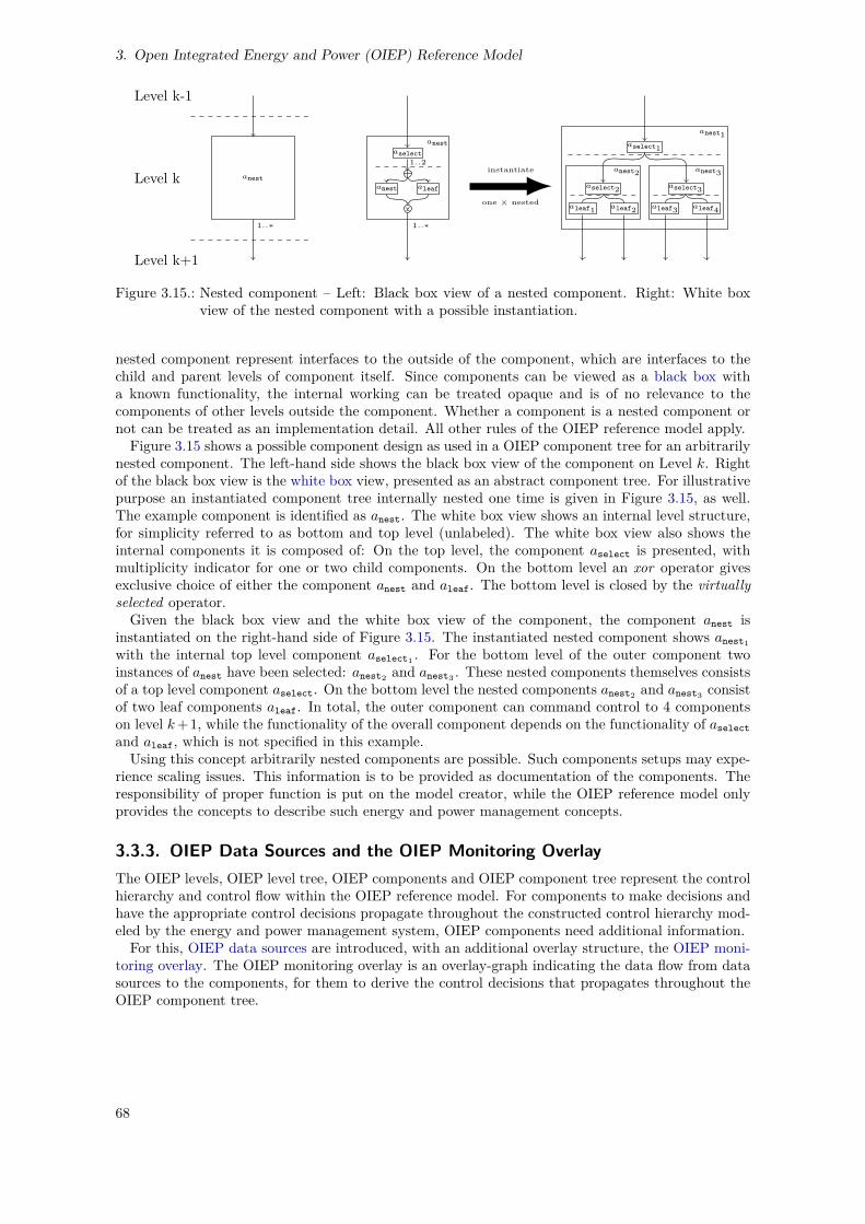
3. Open Integrated Energy and Power (OIEP) Reference Model
Level k-1
Level k
Level k+1
anest
1..∗
aselect1..2
anest aleaf
1..∗
instantiate
one × nested
anest aselect1
aselect2 aselect3
aleaf1 aleaf2 aleaf3 aleaf4
anest1
anest2 anest3
Figure 3.15.: Nested component – Left: Black box view of a nested component. Right: White boxview of the nested component with a possible instantiation.
nested component represent interfaces to the outside of the component, which are interfaces to thechild and parent levels of component itself. Since components can be viewed as a black box witha known functionality, the internal working can be treated opaque and is of no relevance to thecomponents of other levels outside the component. Whether a component is a nested component ornot can be treated as an implementation detail. All other rules of the OIEP reference model apply.Figure 3.15 shows a possible component design as used in a OIEP component tree for an arbitrarily
nested component. The left-hand side shows the black box view of the component on Level k. Rightof the black box view is the white box view, presented as an abstract component tree. For illustrativepurpose an instantiated component tree internally nested one time is given in Figure 3.15, as well.The example component is identified as anest. The white box view shows an internal level structure,for simplicity referred to as bottom and top level (unlabeled). The white box view also shows theinternal components it is composed of: On the top level, the component aselect is presented, withmultiplicity indicator for one or two child components. On the bottom level an xor operator givesexclusive choice of either the component anest and aleaf. The bottom level is closed by the virtuallyselected operator.Given the black box view and the white box view of the component, the component anest is
instantiated on the right-hand side of Figure 3.15. The instantiated nested component shows anest1
with the internal top level component aselect1 . For the bottom level of the outer component twoinstances of anest have been selected: anest2 and anest3 . These nested components themselves consistsof a top level component aselect. On the bottom level the nested components anest2 and anest3 consistof two leaf components aleaf. In total, the outer component can command control to 4 componentson level k+1, while the functionality of the overall component depends on the functionality of aselectand aleaf, which is not specified in this example.Using this concept arbitrarily nested components are possible. Such components setups may expe-
rience scaling issues. This information is to be provided as documentation of the components. Theresponsibility of proper function is put on the model creator, while the OIEP reference model onlyprovides the concepts to describe such energy and power management concepts.
3.3.3. OIEP Data Sources and the OIEP Monitoring OverlayThe OIEP levels, OIEP level tree, OIEP components and OIEP component tree represent the controlhierarchy and control flow within the OIEP reference model. For components to make decisions andhave the appropriate control decisions propagate throughout the constructed control hierarchy mod-eled by the energy and power management system, OIEP components need additional information.For this, OIEP data sources are introduced, with an additional overlay structure, the OIEP moni-
toring overlay. The OIEP monitoring overlay is an overlay-graph indicating the data flow from datasources to the components, for them to derive the control decisions that propagates throughout theOIEP component tree.
68

3.3. Description of the OIEP Reference Model
3.3.3.1. OIEP Data Sources
For decision-making information is derived from either static or dynamic data. For static data,obtaining it once and interpreting it is sufficient. Such data are for example configuration files.The more critical information derived from dynamic data, obtained from sensors. Within the OIEPreference model the sources of data are referred to as OIEP data sources. These are grouped intothree categories:
• OIEP components,• Sensors (decoupled from controls), and• Databases (aggregated data).
These are referred to as OIEP data sources. When using the data, OIEP components need a way toget information about data quality, and a way to access or subscribe to the data.
OIEP Components as Data Sources: Control systems can only be effective if the impact of con-trol is measurable. Therefore, many OIEP components at the leaf levels have sensors integrated.Additionally, components aggregate information about their controlled components to verify controldecisions. Such information can in turn be sent up towards the parent component in aggregated form.OIEP component, which do not have sensor capabilities, nevertheless propagate information, about
their control decisions. This is normally done along the edges of the OIEP component tree, informingthe component which they got a control command from about their action and/or the result of thecontrol command action. All OIEP components thus form a structure for sending information, ininverse direction to the control commands of the OIEP component tree.The following two examples show OIEP component with sensor and without sensor capabilities.
An OIEP component that can act as a sensor, as well as normal component is the for example RAPLof the CPU interface. RAPL serves as a normal energy and power control interface, but also hasregisters to get information about average power usage [Dav+10]. At the same time the RAPLinterfaces can be used as OIEP data source supplementing node power usage, even if it may not beused as control for the complete node power in a given OIEP architecture.An example for sending back information along the inverse edges of the OIEP component tree
where control commands were received, is the job runtime. The job runtime does not have any sensorcapabilities on its own, but can inform the job scheduler about the total amount of energy used.Depending on the OIEP architecture setup, such information flow may either simply acknowledgethe limits set by the job scheduler, inform the job scheduler about total energy used, or even givecontinuous aggregate information about the compute job’s total power consumption.
Sensors as Data Sources: The first additional source of information, outside the OIEP components,is from sensors present in the HPC system.These sensors are not coupled to any OIEP component, but the measured systems are affected by
OIEP components, or control decisions depend on the measured values or conditions they sense.Examples for these sensors for example power panels inside PDUs. A sensors’ scope can also
be outside of energy and power measurement, while still relevant for the OIEP architecture: Asexample serve the sensors for pump speed of the water chiller system, as indication of peak coolingperformance.
Databases as Aggregator Data Sources: HPC center have started utilizing databases collectingoperational information for short term, long term and topic specific use-cases. Such databases canalso serve the decisions of OIEP components if integrated properly.Databases serve as a mediator to serve a larger audience than a single directly connected sensor.
Databases can deal with large number of sensors and address issues of multiple subscribers andalso infrastructure for large number of sensors publishing their data. Additionally, access rights aregenerally addressed in such databases. Not all databases and sensor valuable for OIEP components’decisions are necessarily limited to energy and power. All of them can serve decisions of OIEPcomponents, however. The decisions, if sensors should be collected in a database first, or directly
69

3. Open Integrated Energy and Power (OIEP) Reference Model
used, mostly depends on the use-case, on the OIEP architecture and also on data management systemsand databases already available and in use at the respective center.Examples for such databases are PerSyst [GHB14], collecting into a database for job performance,
Power Data Aggregation Manager (PowerDAM) [Wil18], collecting HPC Center and HPC systeminfrastructure data, and Data Center Data Base (DCDB) [Net+19], a modular database for moni-toring data in real time continuous fashion. All of these have slightly different targets, and are usedsimultaneously at the LRZ.All kinds of OIEP data sources can be used for different OIEP components and have different data
sources themselves, depending on the setup and use-case. Data-quality, delay of data availability andrelevance in time, as well as already performed preprocessing may differ. These are relevant aspectsto consider and know when designing management systems. A combine usage of all forms of OIEPdata sources may be needed, since a global collection of data is often not desirable because of varioustechnical and organizational reasons. The different data sources are included and required in theOIEP reference model since the model creator and the target audience of the OIEP architecture mayneed this information to be able to assess the quality of the energy and power management decisions.
3.3.3.2. OIEP Monitoring Overlay
The transmission of the information obtained from the OIEP data sources is modeled using a digraph.In the OIEP reference model this auxiliary construct is called the OIEP monitoring overlay. Itspurpose is to identify which components use what additional information, aside from the controlcommands, and how this data is propagated throughout the energy and power management system.The OIEP monitoring overlay is constructed by combination of:
• A graph derived by inverting the OIEP component tree;• The OIEP data sources, connected via edges to their data-consumers.
The resulting digraph shows the information flow of all additional data used within an OIEP archi-tecture.9 The OIEP component tree and the OIEP monitoring overlay combined are used to deriveenergy and power management decisions by the individual OIEP components.Figure 3.16 shows two schematics of importance for the OIEP monitoring overlay: Figure 3.16a
shows the OIEP monitoring overlay itself, while Figure 3.16b shows the data source of the databaseswithin the example energy and power management system. Both figures use the base setup from theexample of Figure 3.5, showing an OIEP level tree and OIEP component tree with two branches ofdepth na and mb, each occupied by one OIEP component.Figure 3.16a shows an example OIEP monitoring overlay: The OIEP component tree is inverted
into a directed graph, and two sensors and a database used in the OIEP architecture are added.Any OIEP data sources is added below the lowest component using it, such that information in theOIEP monitoring overlay diagram always flows up. Therefore, Sensor 1 (Sens1) is placed underthe component of Level ya + 1, and Sensor 2 (Sens2) is placed under Level na − 1. The database,DB1, is placed under Level yb + 1, since it is used at the components at Level yb + 1, ya + 1, aswell as Level 1. The OIEP monitoring overlay is designed to be acyclic. In combination, the OIEPmonitoring overlay, with information flow directed upwards and the OIEP component tree (in gray),with flow of control command downwards, represent the complete data flow in the OIEP architectureused to derive energy and power control decisions.Figure 3.16b shows the databases present in the example energy and power management system,
and which OIEP components they obtain data from. The figure shows two databases, DB1 andDB2. Database DB1 acquires data from components on Level mb, na, yb + 1 and y. Database DB2acquires data from components on Level mb − 1 and na − 1. As seen in Figure 3.16a, since DB2 isnot used in the OIEP architecture it is not included in the OIEP monitoring overlay. There maybe an arbitrary additional number of databases in the HPC center. Only the databases used withinthe OIEP architecture are to be included in the OIEP monitoring overlay. Therefore, database DB1is part of the OIEP monitoring overlay of Fig. 3.16a. The side by side view of the two Figures of
9Multiplicity indicators for the OIEP monitoring overlay are handled in accordance with Section 3.3.2.2, whereincoming edges are labeled with indicators for multiplicity, in the case where a variable number of instances ofOIEP data sources exist.
70
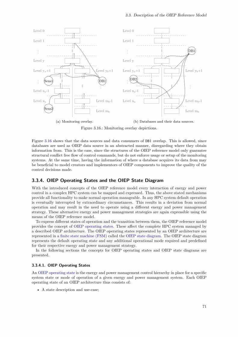
3.3. Description of the OIEP Reference Model
Level 0
Level 1
...
Level y
Level ya+1 Level yb+1
... ...Level na-1
Level na Level mb-1
Level mb
DB1Sens1
Sens2
(a) Monitoring overlay.
Level 0
Level 1
...
Level y
Level ya+1 Level yb+1
... ...Level na-1
Level na Level mb-1
Level mb
DB1
DB2
(b) Databases and their data sources.
Figure 3.16.: Monitoring overlay depictions.
Figure 3.16 shows that the data sources and data consumers of DB1 overlap. This is allowed, sincedatabases are used as OIEP data source in an abstracted manner, disregarding where they obtaininformation from. This is the case, since the structures of the OIEP reference model only guaranteestructural conflict free flow of control commands, but do not enforce usage or setup of the monitoringsystems. At the same time, having the information of where a database acquires its data from maybe beneficial to model creators and implementors of OIEP components to improve the quality of thecontrol decisions made.
3.3.4. OIEP Operating States and the OIEP State DiagramWith the introduced concepts of the OIEP reference model every interaction of energy and powercontrol in a complex HPC system can be mapped and expressed. Thus, the above stated mechanismsprovide all functionality to make normal operation manageable. In any HPC system default operationis eventually interrupted by extraordinary circumstances. This results in a deviation from normaloperation and may result in the need to operate using a different energy and power managementstrategy. These alternative energy and power management strategies are again expressible using themeans of the OIEP reference model.To express different states of operation and the transition between them, the OIEP reference model
provides the concept of OIEP operating states. These affect the complete HPC system managed bya described OIEP architecture. The OIEP operating states represented by an OIEP architecture arerepresented in a finite state machine (FSM) called the OIEP state diagram. The OIEP state diagramrepresents the default operating state and any additional operational mode required and predefinedfor their respective energy and power management strategy.In the following sections the concepts for OIEP operating states and OIEP state diagrams are
presented.
3.3.4.1. OIEP Operating States
An OIEP operating state is the energy and power management control hierarchy in place for a specificsystem state or mode of operation of a given energy and power management system. Each OIEPoperating state of an OIEP architecture thus consists of:
• A state description and use-case;
71

3. Open Integrated Energy and Power (OIEP) Reference Model
• Triggers for state transitions;• An associated OIEP component tree for each state.
In combination an OIEP operating state describes the behavior of energy and power management inthe specified operating mode and when to exit the associated OIEP operating state.
State Description and Use-case: The state description and use-case sets the general goal of theOIEP operating state. Such use-case or goal is also the primary goal of the OIEP component treeused for the associated state.Specification of the state-description is done before the construction on the individual OIEP level
tree and OIEP component tree, by capturing the intent of the energy and power management solution.Examples for state-descriptions and use-cases for normal operation stated as energy and power
management system goals may be any examples for goals of an OIEP level tree’s root level. Examplesfor these are:
• Operation under a power limit;• Minimization of energy to solution for jobs;• Staying within the budget;• Optimizing for the ESPs’ pricing policy;
Additional examples are use-cases where multiple normal operation modes exist. Example for theseare:
• Operating modes depending on season;• Operation depending on ambient temperature;• Operating modes for the specific pricing policy for day and night cycles of the ESPs.
State descriptions with short term duration (being an exception to normal operation) are, for example:
• Operation in an emergency situation (brown-out/black-out, cooling loss, etc.);• Operation during system benchmarking;• Operation during complete system runs for high priority applications;• Power ramp-up and ramp-down;• Operation with exhausted budget of an operational resource;
The specifics of each state has to be captured by the model creator to represent the energy and powermanagement setup.
Triggers for State Transitions: When multiple OIEP operating states are present in a system, eachstate needs triggers to transition from one state to the appropriate state for the circumstance.In the default OIEP component tree each component has a component type, interfaces and func-
tionality for the default normal operation. The only allowed interaction to lower level controls is viathese prescribed interfaces. At the same time the overall system has a large number of sensors, notonly available to optimize default operation via the software components and OIEP components, butalso so sense critical events which need intervention. In such case the overall OIEP architecture has totransition from one OIEP operating state to another. Otherwise, proper operation is not guaranteed.For these implementations of the OIEP component, the OIEP component tree, OIEP data sourcesand OIEP monitoring overlay need mechanisms to be informed of the OIEP operating state transitionand take appropriate action. These are cleanup, configuration and re-configuration, or initializationof the following responsible components.The triggers have to be implemented guaranteeing safe and sound emergency handling. Compo-
nents and sensor have to implement these and be given the necessary authority to escalate. Suchevents should be treated as extra-ordinary and handled with care. A trigger can be a specific thresholdfor a measured value, time and date information or an external input.
72

3.3. Description of the OIEP Reference Model
All these operating states are a deviation from normal operation, where the course of action is nothandled by a component selecting sub-components and changing configurations, but by triggering aswitch in the mode of operation to a different control hierarchy, i.e.: It is handled by a different setupof the OIEP component tree.
Associated OIEP Component Tree For Each State: Each OIEP operating state is in itself acontained OIEP architecture without operating states. This means that the energy and power man-agement system is handling energy and power control commands via the OIEP component tree.Any OIEP component tree requires definition of OIEP level, an OIEP level tree, associated OIEPcomponents, as well as OIEP data sources and OIEP monitoring overlay if required.The OIEP component trees is the primary structure for handling the energy and power control
commands. Structures of this primary OIEP component tree can be similar, with small modificationsto adapt the different operating modes, while a complete change in the control and command structuremay not be practical.Emergency cases, may exclude specific optimization software components and take direct control,
while applying strong limitations and restrictions to operate in known safe states. The main burdenlies again on the model creator and center leadership approving and signing off the states OIEParchitecture for each state, as well as its state transitions.
3.3.4.2. OIEP State Diagram
The OIEP operating states of an OIEP architecture are represented in an FSM: the OIEP statediagram. If the design of a system has a specific requirement which more easily maps to a differentform of automaton, it should be kept in mind that most automatons can be transformed into anequivalent representation in the form of a different type of automaton [Chr07].The trivial case has only the default operation and no transitions. All non-trivial cases with more
than one OIEP operating state require an OIEP state diagram. State diagrams consist of states, aswell as transitions. Any FSM has an initial state with the appropriate setup and initialization, tohave a known starting point and setup routine. Each transition requires the corresponding OIEPcomponents to respond with according state cleanup, possible transition and initialization.The states are labeled according to identify the state description or use-case. By convention of
this work, the name of the state transition is the name of the entities triggering the state transition,followed by the action triggering the state transition. If this convention does not apply to a use-case,meaningful identifiers shall be used.Each trigger is represented by an edge transitioning to the appropriate associate state of the OIEP
architecture. The labels or the edges should also be chosen in a mnemonic way, such that modelcreators can easily identify which components have to implement functionality to respond to therespective state transition. This includes information on who can trigger the state transition.Figure 3.17 shows an example for an OIEP architecture’s state diagram as well as the according
OIEP component trees. In this example, normal operation equates to user selection of power man-agement, as seen in Figure 3.17b. The OIEP component tree in Figure 3.17b shows seven levels:Level 0, Center Leadership; Level 1, RAS-System; Level 2, the job scheduler; Level 3, the applicationenvironment; Level 4, a MSR user space abstraction; Level 5, the kernel module abstraction; Level 6,the CPU. Each of these levels is occupied by a specific software or hardware system modeled as OIEPcomponent. All of which have control interfaces to interact with the components on the lower levels.This means that the center policy is set to USER, for which one RAS system is responsible. The RASsystem controls the scheduler, which uses the appropriate configurations and settings and itself setsthe appropriate application environment: In this case it allows user space control. The applicationenvironment, and thus the user application, has access to libmsr , which in turn can write to an in-stance of a kernel module abstraction, in this case: msr-safe. Msr-safe has the appropriate whitelistsetup and permissions to finally control the hardware, in such way that the whitelisted registers ofthe CPU can be altered.The OIEP component tree on the right in Figure 3.17c shows an alternative OIEP component tree
with four levels: Level 0 – center leadership; Level 1 – RAS-system; Level 2 – the kernel moduleabstraction; Level 3 – the CPU; again occupied by their respective components. In this emergencystate, reduction to a minimum power consumption is dictated. Command is again turned to the RAS
73
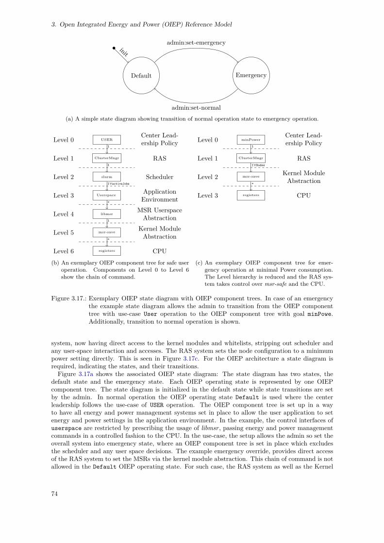
3. Open Integrated Energy and Power (OIEP) Reference Model
Default Emergency
admin:set-emergency
admin:set-normal
init
(a) A simple state diagram showing transition of normal operation state to emergency operation.
Level 0 USERCenter Lead-ership Policy
Level 1 ClusterMngr RAS
1
Level 2 slurm Scheduler
1
Level 3 UserspaceApplicationEnvironment
1∀activeJobs
Level 4 libmsrMSR UserspaceAbstraction
∗
Level 5 msr-saveKernel ModuleAbstraction
1
Level 6 registers CPU
∗
(b) An exemplary OIEP component tree for safe useroperation. Components on Level 0 to Level 6show the chain of command.
Level 0 minPowerCenter Lead-ership Policy
Level 1 ClusterMngr RAS
1
Level 2 msr-saveKernel ModuleAbstraction
1∀Nodes
Level 3 registers CPU
∗
(c) An exemplary OIEP component tree for emer-gency operation at minimal Power consumption.The Level hierarchy is reduced and the RAS sys-tem takes control over msr-safe and the CPU.
Figure 3.17.: Exemplary OIEP state diagram with OIEP component trees. In case of an emergencythe example state diagram allows the admin to transition from the OIEP componenttree with use-case User operation to the OIEP component tree with goal minPowe.Additionally, transition to normal operation is shown.
system, now having direct access to the kernel modules and whitelists, stripping out scheduler andany user-space interaction and accesses. The RAS system sets the node configuration to a minimumpower setting directly. This is seen in Figure 3.17c. For the OIEP architecture a state diagram isrequired, indicating the states, and their transitions.Figure 3.17a shows the associated OIEP state diagram: The state diagram has two states, the
default state and the emergency state. Each OIEP operating state is represented by one OIEPcomponent tree. The state diagram is initialized in the default state while state transitions are setby the admin. In normal operation the OIEP operating state Default is used where the centerleadership follows the use-case of USER operation. The OIEP component tree is set up in a wayto have all energy and power management systems set in place to allow the user application to setenergy and power settings in the application environment. In the example, the control interfaces ofuserspace are restricted by prescribing the usage of libmsr , passing energy and power managementcommands in a controlled fashion to the CPU. In the use-case, the setup allows the admin so set theoverall system into emergency state, where an OIEP component tree is set in place which excludesthe scheduler and any user space decisions. The example emergency override, provides direct accessof the RAS system to set the MSRs via the kernel module abstraction. This chain of command is notallowed in the Default OIEP operating state. For such case, the RAS system as well as the Kernel
74
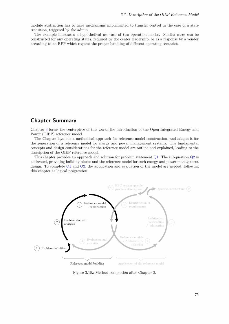
3.3. Description of the OIEP Reference Model
module abstraction has to have mechanisms implemented to transfer control in the case of a statetransition, triggered by the admin.The example illustrates a hypothetical use-case of two operation modes. Similar cases can be
constructed for any operating states, required by the center leadership, or as a response by a vendoraccording to an RFP which request the proper handling of different operating scenarios.
Chapter SummaryChapter 3 forms the centerpiece of this work: the introduction of the Open Integrated Energy andPower (OIEP) reference model.The Chapter lays out a methodical approach for reference model construction, and adapts it for
the generation of a reference model for energy and power management systems. The fundamentalconcepts and design considerations for the reference model are outline and explained, leading to thedescription of the OIEP reference model.This chapter provides an approach and solution for problem statement Q1. The subquestion Q2 is
addressed, providing building blocks and the reference model for such energy and power managementdesign. To complete Q1 and Q2, the application and evaluation of the model are needed, followingthis chapter as logical progression.
Problem definition1
Problem domainanalysis2
Reference modelconstruction3
Evaluation andevolution4
Reference model building
HPC system specificproblem descriptiona
Identification ofrequirementsb
Reference model-/ Architecture-
selectionc
Architectureconstruction/ -adaptation
d
Specific architecture e
Application of the reference model
Figure 3.18.: Method completion after Chapter 3.
75


4. Open Integrated Energy and PowerArchitectures
4.1. Applying the OIEP Reference Model . . . . . . . . . . . . . . . . . . . . . . . . . . . . 774.2. Constructing an OIEP Architecture for the PowerStack . . . . . . . . . . . . . . . . . 78
4.2.1. PowerStack Model – Problem Description . . . . . . . . . . . . . . . . . . . . . 794.2.2. PowerStack Model – Identification of Requirements . . . . . . . . . . . . . . . . 804.2.3. PowerStack Model – Reference Model Selection . . . . . . . . . . . . . . . . . . 814.2.4. PowerStack Model – OIEP Architecture Construction . . . . . . . . . . . . . . 81
With the description of the OIEP reference model the next step is to apply the model. For referencemodel building, applying the reference model is a required step to complete the design process. Thisis the case, since proper evaluation and eventual evolution of the model is only possible after havingapplied the model (see Ch. 1.2). Therefore, this chapter proceeds as follows:
• Method for OIEP architecture generation (Sec. 4.1);• Generation of an OIEP architecture for the PowerStack model (Sec. 4.2).
In addition to the application of the OIEP reference model to the PowerStack model, additional OIEParchitectures have been generated for a selection of different energy and power management setups.These are used to verify the applicability of the model validity of both the OIEP reference model andthe method to generate OIEP architectures.The additional OIEP architectures constructed are:
• For the PowerStack prototype (App. D.1);• For GEOPM, modeled as a nested component (App. D.2);• For LRZ’s SuperMUC Phase 1 & Phase 2 systems (App. D.3);• For the SuperMUC-NG system (App. D.4);• For the Fugaku system (App. D.5).
These OIEP architecture constructions show, both how the OIEP reference model is applied, and theversatility for different kinds of system descriptions. The main body of the work only presents thereference model application cycle once, while the additional constructions are left for the appendix,for brevity.This chapter shows how the OIEP reference model is applied to represent and better understand
the energy and power management setup of HPC systems, addressing research question Q3.
4.1. Applying the OIEP Reference ModelFor applying the OIEP reference model, a methodical approach is followed. This follows the rightcircle of the thesis method, as shown in Figure 4.1. The method is realized in five steps:
a) HPC system specific problem description;b) Identification of requirements;c) Reference model selection or architecture selection;d) Architecture construction or adaption;
77

4. Open Integrated Energy and Power Architectures
Problem definition1
Problem domainanalysis2
Reference modelconstruction3
Evaluation andevolution4
Reference model building
HPC system specificproblem descriptiona
Identification ofrequirementsb
Reference model-/ Architecture-
selectionc
Architectureconstruction/ -adaptation
d
Specific architecture e
Application of the reference model
Figure 4.1.: Focused right side of the methodical approach as of Figure 1.2. For application of thereference model the steps a to e are iterated, as per adaption according to [Sch00, p. 78].
e) Resulting in: a specific architecture.
The architecture construction / architecture adaption of step d) itself follows seven steps:
1. Identifying the OIEP levels;2. Composition and arrangement of the OIEP level tree;3. Identifying the OIEP components;4. Composition and arrangement of the OIEP component tree;5. Inclusion of the OIEP monitoring overlay;6. Identification of needed OIEP operating states and construction of OIEP state diagram;7. Addressing the remaining states of the OIEP state diagram (by repetition of the above steps
for each state).
The result of applying the method is the specific OIEP architecture for the energy and power man-agement system of the HPC system setup in question.
4.2. Constructing an OIEP Architecture for the PowerStackIn the following section an OIEP architectures for the PowerStack is constructed1. The PowerStackitself tries to define a reference architecture, as defined in 3.2.1, whereas OIEP defines a referencemodel to describe such architectures, which potentially can serve as a reference architecture.The efforts of the PowerStack community builds both a general model for the PowerStack and an
initial prototype, implementing a subset of the outlined model. This section constructs an OIEParchitecture for the PowerStack model succeeding the second PowerStack seminar [PS’19a]. A secondOIEP architecture construction for the PowerStack prototype is described in Appendix D.1.
78
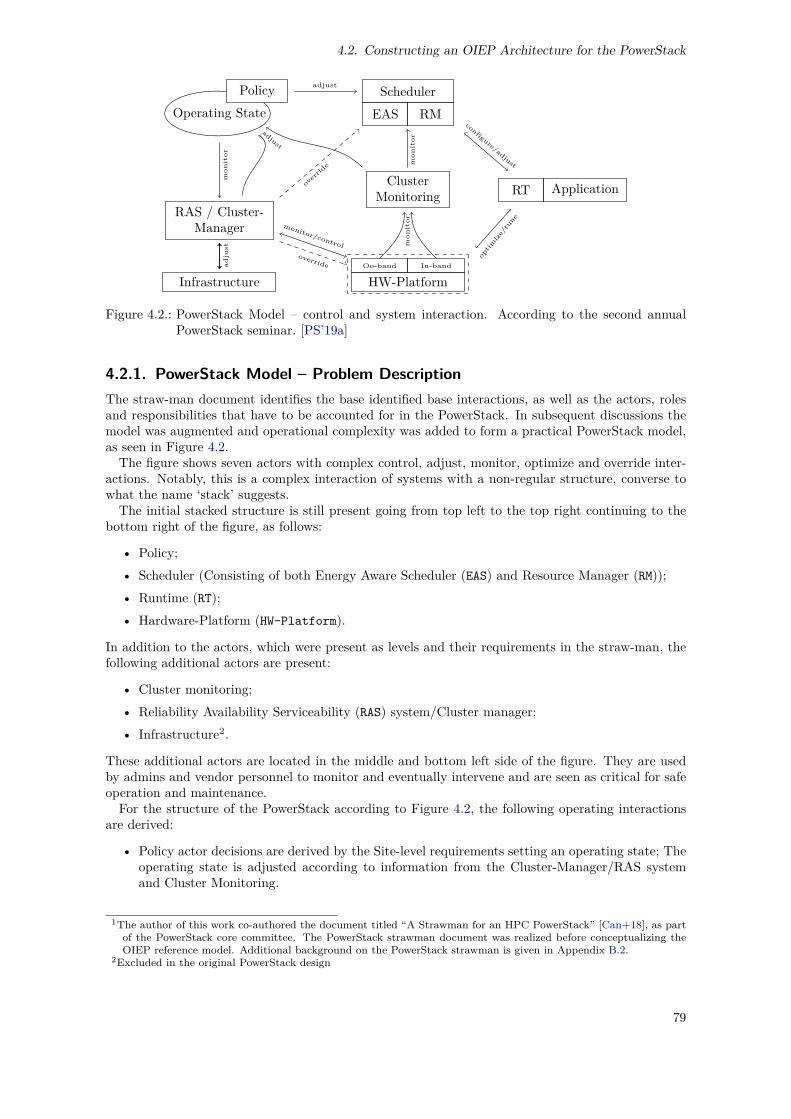
4.2. Constructing an OIEP Architecture for the PowerStack
In-bandOo-band
HW-Platform
RT ApplicationClusterMonitoring
SchedulerEAS RMOperating State
Policy
RAS / Cluster-Manager
Infrastructure
adjust
configure/adjust
optimize/tunemonitor/control
override
override
mon
itor
mon
itor
adjust
mon
itor
adjust
Figure 4.2.: PowerStack Model – control and system interaction. According to the second annualPowerStack seminar. [PS’19a]
4.2.1. PowerStack Model – Problem DescriptionThe straw-man document identifies the base identified base interactions, as well as the actors, rolesand responsibilities that have to be accounted for in the PowerStack. In subsequent discussions themodel was augmented and operational complexity was added to form a practical PowerStack model,as seen in Figure 4.2.The figure shows seven actors with complex control, adjust, monitor, optimize and override inter-
actions. Notably, this is a complex interaction of systems with a non-regular structure, converse towhat the name ‘stack’ suggests.The initial stacked structure is still present going from top left to the top right continuing to the
bottom right of the figure, as follows:
• Policy;• Scheduler (Consisting of both Energy Aware Scheduler (EAS) and Resource Manager (RM));• Runtime (RT);• Hardware-Platform (HW-Platform).
In addition to the actors, which were present as levels and their requirements in the straw-man, thefollowing additional actors are present:
• Cluster monitoring;• Reliability Availability Serviceability (RAS) system/Cluster manager;• Infrastructure2.
These additional actors are located in the middle and bottom left side of the figure. They are usedby admins and vendor personnel to monitor and eventually intervene and are seen as critical for safeoperation and maintenance.For the structure of the PowerStack according to Figure 4.2, the following operating interactions
are derived:
• Policy actor decisions are derived by the Site-level requirements setting an operating state; Theoperating state is adjusted according to information from the Cluster-Manager/RAS systemand Cluster Monitoring.
1The author of this work co-authored the document titled “A Strawman for an HPC PowerStack” [Can+18], as partof the PowerStack core committee. The PowerStack strawman document was realized before conceptualizing theOIEP reference model. Additional background on the PowerStack strawman is given in Appendix B.2.
2Excluded in the original PowerStack design
79

4. Open Integrated Energy and Power Architectures
• Scheduler operation is adjusted by the operating policy; The scheduler is takes informationfrom Cluster Monitoring and the runtime/application;
• The runtime/application is the combination of energy and power aware runtime directly inter-acting with the application. By doing so, it is capable to optimize the hardware settings foroptimization targeting performance as well as energy and power optimization of the hardware.Therefore, the Runtime optimizes or tunes all participating nodes of the hardware-platform.The runtime communicates its settings and eventual energy and power estimates back with thescheduler.
• The hardware-platform realizes the requests by the runtime enforcing specific energy and powersettings. Monitoring information is fed back to the runtime, as well as cluster monitoring andCluster-Manager/RAS. The Hardware-platform has both in-band and out-of-band mechanismsfor monitoring and control.
• Cluster Monitoring is a common service which aggregates and distributes the information. Thedesign includes such centralized monitoring infrastructure.
• The Cluster-Manager/RAS system may override the Scheduler and HW-Platform in case ofemergency.
This setup resembles the setup HPC systems already actively employing such approaches or parts ofthe named systems, but in a completely integrated way. This is the case since no simple actor is anew development unique to the PowerStack (for details see App. B.1.2). However, such approachestraditionally are loosely structured and up to good judgement at system installation and integration,whereas PowerStack concretizes this structure and its interactions.For real system installations building upon PowerStack, several aspects of the setup are not yet
concretized: The optimization goals or policies, the specifications of interfaces, specific protocols orinteractions. The priority is set for a clear split of responsibilities of actors and entities within thesystem, including their interaction.3The above description serves as the problem definition for the construction of an OIEP architecture
for the PowerStack model.
4.2.2. PowerStack Model – Identification of RequirementsThe next step is the identification of requirements, step b) of the chapter’s method. The PowerStackstrawman document itself lists several requirements (see desired features in [Can+18]):
• A holistic approach to coordinated power management, for optimization in a scalable distributedsystem.
• Allow for safe operation, where faults of the electrical operation can lead to catastrophic failures.Thus safety critical limits must be enforced at all times.
• Integration into the given security concepts of the center.• Usage of open source tools with permissive licensing.• Cross platform and vendor neutral support to avoid lock in to specific vendors.• Production-grade quality and deployment of components for user and system administrators.• Usage of well-defined and openly described interfaces, possibly following interface standardiza-
tions where appropriate.• Real-time monitoring and control for adaptive dynamic optimization, at various levels of the
PowerStack.
The above PowerStack specific problem description, step a), and the identification of requirements,step b), provide an adequate represent for requirements for an architecture construction for thePowerStack model as of the second PowerStack seminar [PS’19a].
3This note highlights that the PowerStack effort is still in its early stages, with the self-imposed task to tackle anon-trivial challenge with a non-negligibly sized interest group.
80
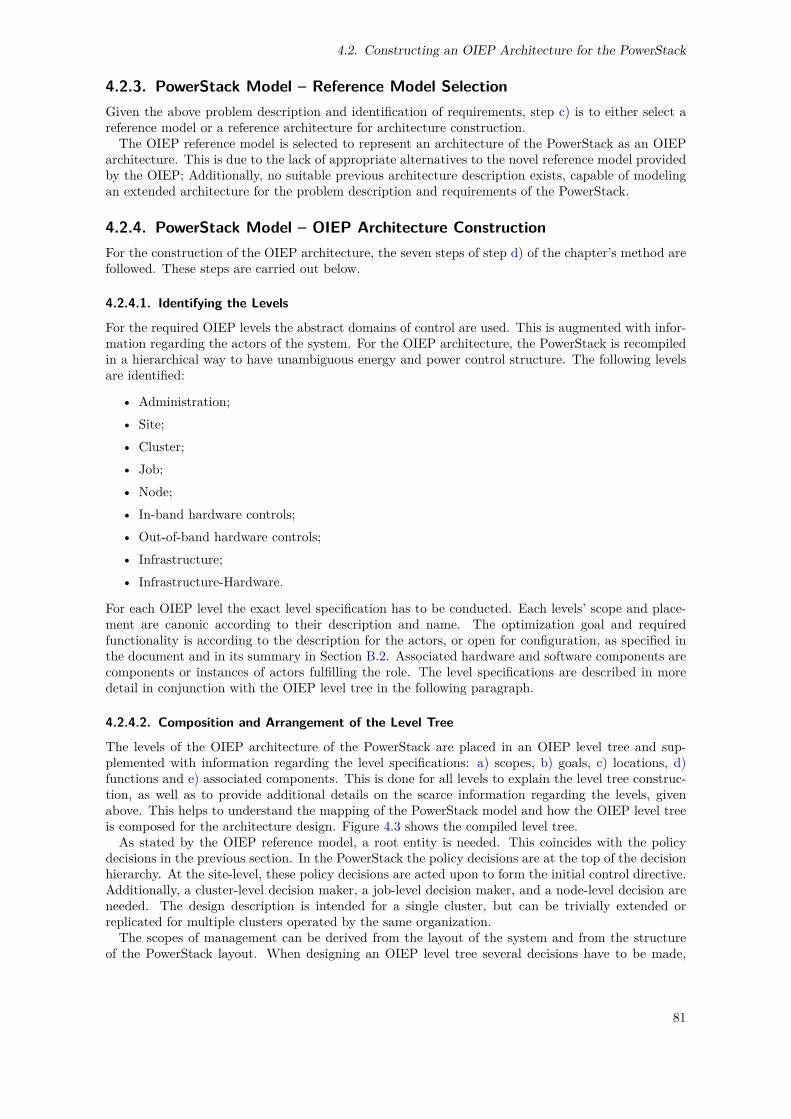
4.2. Constructing an OIEP Architecture for the PowerStack
4.2.3. PowerStack Model – Reference Model SelectionGiven the above problem description and identification of requirements, step c) is to either select areference model or a reference architecture for architecture construction.The OIEP reference model is selected to represent an architecture of the PowerStack as an OIEP
architecture. This is due to the lack of appropriate alternatives to the novel reference model providedby the OIEP; Additionally, no suitable previous architecture description exists, capable of modelingan extended architecture for the problem description and requirements of the PowerStack.
4.2.4. PowerStack Model – OIEP Architecture ConstructionFor the construction of the OIEP architecture, the seven steps of step d) of the chapter’s method arefollowed. These steps are carried out below.
4.2.4.1. Identifying the Levels
For the required OIEP levels the abstract domains of control are used. This is augmented with infor-mation regarding the actors of the system. For the OIEP architecture, the PowerStack is recompiledin a hierarchical way to have unambiguous energy and power control structure. The following levelsare identified:
• Administration;• Site;• Cluster;• Job;• Node;• In-band hardware controls;• Out-of-band hardware controls;• Infrastructure;• Infrastructure-Hardware.
For each OIEP level the exact level specification has to be conducted. Each levels’ scope and place-ment are canonic according to their description and name. The optimization goal and requiredfunctionality is according to the description for the actors, or open for configuration, as specified inthe document and in its summary in Section B.2. Associated hardware and software components arecomponents or instances of actors fulfilling the role. The level specifications are described in moredetail in conjunction with the OIEP level tree in the following paragraph.
4.2.4.2. Composition and Arrangement of the Level Tree
The levels of the OIEP architecture of the PowerStack are placed in an OIEP level tree and sup-plemented with information regarding the level specifications: a) scopes, b) goals, c) locations, d)functions and e) associated components. This is done for all levels to explain the level tree construc-tion, as well as to provide additional details on the scarce information regarding the levels, givenabove. This helps to understand the mapping of the PowerStack model and how the OIEP level treeis composed for the architecture design. Figure 4.3 shows the compiled level tree.As stated by the OIEP reference model, a root entity is needed. This coincides with the policy
decisions in the previous section. In the PowerStack the policy decisions are at the top of the decisionhierarchy. At the site-level, these policy decisions are acted upon to form the initial control directive.Additionally, a cluster-level decision maker, a job-level decision maker, and a node-level decision areneeded. The design description is intended for a single cluster, but can be trivially extended orreplicated for multiple clusters operated by the same organization.The scopes of management can be derived from the layout of the system and from the structure
of the PowerStack layout. When designing an OIEP level tree several decisions have to be made,
81

4. Open Integrated Energy and Power Architectures
Administration
Site
Cluster
Job
Node
In-band-HW Oo-band-HW
Infrastructure
Infrastructure-HW
Figure 4.3.: PowerStack model – OIEP level tree. Level description of the PowerStack using OIEPreference model.
since multiple suitable ways of managing the system may exist. The reasoning for some decisionsmade for the OIEP architecture of the PowerStack model are also provided in the following. Theidentified levels, the decisions regarding their arrangement and associated interfaces provide the basicstructure for the PowerStack OIEP architecture’s level tree. The details of each level of Figure 4.3are described in the following:
Administration-Level: The root level is the administration-level.
a) The scope of the administration-level is the complete energy and power management system,as defined in Section 3.3.1.2.
b) The associated optimization goal is setting and specifying overall optimization goal. In thePowerStack description above, this is the policy the center administration uses as guidelinefor operation. In the PowerStack the exact optimization goals are open, but with restrictionsfrom the list of requirement, namely: Safe operation and real-time monitoring and controlfor adaptive dynamic optimization. The exact operational goal has to be set by the entityemploying the OIEP architecture, by adapting it to the centers needs.
c) The location of the level is abstract at the top of the control hierarchy, physical resources areco-located with the component on the level.
d) The required functionality is the ability to enforce the structure and optimization goals accord-ing to the setup, and control and validate that the setup is installed correctly. Regarding levelinterfaces, the only OIEP child level is the PowerStack’s site-level. In the case that optimiza-tion goals are required to change, while maintaining the same hierarchy, such changes have tobe communicable via the level’s edges. It’s the root level’s responsibility to make sure this ispossible, if needed.
e) Regarding the corresponding component for the administration-level the admin is selected fromthe actors of the PowerStack description. This entity has the exact capabilities.
By interacting with center leadership and placement at the top of the hierarchy, the named respon-sibilities can be conducted.
Site-Level: The next identified level for the PowerStack is the site-level.
a) The OIEP level scope of the site-level is the computing center. At this level, site critical decisionsare made.
b) The OIEP level’s goal is one of the requirements of the PowerStack: Operating under safeconditions while providing the possibilities for optimization of the overall system.
c) The location of this level is the first with physical resources needed for operation, since it is doneby a software entity. The logical location is central to the center, below the administration-level.
82

4.2. Constructing an OIEP Architecture for the PowerStack
d) The functionality at the site-level is to receive the optimization goal read and information aboutsafe operation and pass control directives to the cluster and infrastructure to guarantee thissafe operation.
e) Therefore, the component is the RAS system (which was not present in the original strawmandesign).
In RAS systems outside of PowerStack interfaces to the compute-side of clusters are normally notpresent, unless they are critical to physical hardware safety. For the PowerStack such interaction isrequired to enable the goal of enabling the possible energy and power optimization of the underlyingsoftware and hardware systems in a hierarchical fashion. The selection of the site-level with theRAS system as OIEP level is a choice by the model creator. The justification for this setup, is thataccording to Figure 4.2, the RAS system has a view of the cluster and infrastructure, and can interactand control either of them.A missing aspect, the override functionality, has to be handled gracefully due to the fact that safe
operation is to be guaranteed. The RAS system does not gain direct access to the scheduler, policyand hardware (as in Fig. 4.2) since direct overrides violate the intention of the OIEP reference modelof a clean control hierarchy. This is achieved using OIEP operating states.
Cluster-Level: On the compute-side of the energy and power management system, the cluster-levelis placed.
a) The scope of the cluster-level is the complete cluster. This scope is focused on the compute-side, with the component of the job scheduler in mind. During normal operation the individualjobs dictate the energy and power behavior of all participating nodes, thus the behavior of thecluster.
b) The goal at the cluster-level of the PowerStack is the optimal usage of the clusters resources interms of energy and power.
c) The location of the level overlaps with the scope from a logical perspective, which covers thecluster-level. The physical side, the location is hardware associated with the cluster, for exampleas a service node.
d) The functionality and the goal of the level tightly overlap: While the goal is the optimal usageof energy and power, the functionality required for this is a control algorithm providing suchoptimization mechanism. The required functionality is managing information from the jobs,determining the optimal energy and power configurations for an available job and dispatchingjobs with optimal configuration. Additionally, the components of the level have to be able torespond to changing control directives from their parent level; In this setup, from the site-level.
e) For components the associated component is an energy and power aware job scheduler. Thecomponents have to have a clear directive which optimization goal to prioritize: the job schedul-ing goal (e.g. job throughput, makespan or node usage) or the energy and power goals. In eithercase a choice has to be made, given the implications of each priority.
Job-Level:
a) On the next level the identified scope is the individual job.b) The goal of this job-level is to optimize all participating components for a job, where the goal of
optimization, itself is dictated by the level above. This goal is passed as a control directive, forexample via APIs, or configuration files, to be evaluated by the job runtime. The anticipatedcontrol directives for a single job by the PowerStack are: The application of job specific poweror energy consumption limits or specific energy optimization goals, such as minimizing energyto solution for the single job. Alternatively a job may run without artificial limitation and onlybe monitored for energy and power consumption.
c) Regarding location there are two possible scenarios: Either the runtime shares the job resources,or a dedicated compute node per job is set aside for the runtime.
83

4. Open Integrated Energy and Power Architectures
d) The functionality which represents the realization of the goal is multi-faceted: The componenton the job-level receives the control directives, computes the optimal node settings and directsthe participating nodes via respective APIs provided by the node-level. The optimizationalgorithm takes the configuration from the cluster-level, and information about the currentjob’s behavior from all nodes and adjusts the configuration accordingly.The additional complexity is added, due to the fact that the control at the job-level can be:
• Static or dynamic management,• located in user space or operated as system tool, or• perform local adjustments vs. job-wide actions.
As explanation, in static management a job chooses optimal job launch parameters based on theinput from the scheduler. Contrary, dynamic management enables the adaptive managementover the course of the execution of the job, adjusting the control based on measurements andthe behavior of the application.The job-level controllers can be in user space, meaning that the user can influence the behav-ior, or even contributes decision parameters directly. By contrast, a system tool may chooseto only take cluster information and active node measurement, oblivious of the applicationcharacteristics.In the same vein, local adjustments vs. job-wide actions depend on the limitations and knowl-edge a job-level component has: In the case, that node local limitations are reached or dueto local changes, a job wide limit is reached, different actions follow. Alternatively, due toaggregate information at the job-level, node local adjustments can be made slowing down in-dividual participating components, while advancing the overall progress in a way an individualcomponent is not capable of, due to limited scope.
e) The component at the job-level, which combines and can realize these tasks and functionalitiesis the job runtime (and online autotuning tools).
Node-Level:
a) The scope of the node-level is each individual node.b) The level’s goal is providing access to node-level measurement and control, including granting
and restricting hardware access.c) Since each component on the node-level has an associated physical node, the associated location
is specific and concrete. By being associated with a specific node, its resource restrictions andphysical/logical access rights for underlying hardware has to be clear.
d) The functionality is the fulfillment of the goal to provide interfaces to the lower levels. Theselower levels are for either in-band or out-of-band hardware access. Depending on the job-level,components on this level may need additional functionality regarding autonomous decisions.Additionally, aggregation of information is needed, since only a reduced data-set is useful atthe job-level. If data aggregation and reduction is not used, processing bottlenecks may occurfor large jobs on the parent-level.
e) The component on the node-level is the node management agent. Such software system on thenode may be provided as the node-level part of the runtime, set up during node configuration,or as a separate software system. The configuration at this level is crucial for access controland authorization to hardware controls, as well as to information from the user applications.
In-band- & Oo-band-HW-Level: The leaf levels of the compute-side, are the in-band and out-of-band hardware control levels.
a) Their scope is the hardware control and measurement, at their respective in-band- and out-of-band-level.
b) Their goal is to provide a safe and functional interface to this hardware with low overhead.
84

4.2. Constructing an OIEP Architecture for the PowerStack
c) The major differences regarding in-band and out-of-band is the location:• The in-band-level’s physical location is within the CPU. The used monitoring and control
mechanisms use the same hardware and communication paths as the user application.• The out-of-band-level uses channels and resources, which do not interfere with the resources
dedicated to the application. Therefore there is less contention with the user’s job, even ifoverall resource capacity may be limited.
d) The functionality of providing hardware control and monitoring interfaces is the same for bothlevels. The PowerStack does not dictate which hardware control mechanism is used, or howthis functionality is provided. Specific centers may restrict the kind of component, which theywant to use. By carefully specifying the functionality of the levels, such restrictions can begiven without the need to reevaluate individual components.
e) The components for the levels on the in-band-level are for example kernel functionality and thekernel modules for control register access of the CPU. On the out-of-band-level, the examplecomponents are BMCs placed on the node for control and monitoring. Both component exam-ples for the levels allow to safely encapsulate the control directives from the above levels andprovide the required functionality.
Infrastructure-Level: On the infrastructure side, the right-hand side child level of the site-level, thenext level is the infrastructure-level.
a) The level scope is the infrastructure. In the original PowerStack strawman document theinfrastructure was explicitly excluded. Since the infrastructure is part of the discussion onPowerStack since the first seminar [PS’18], and is included in 4.3, it is included in the OIEParchitecture for the PowerStack model.
b) The goal of the infrastructure-level is to participate and react to energy and power managementopportunities initiated by the site-level.
c) The location of the infrastructure-level is the respective management infrastructure of the com-puting center’s infrastructure.
d) The functionality provides mechanisms to respond to infrastructure-level opportunities of energyand power management in a coordinated way regarding the usage of the HPC system. Thefunctionality again provides abstracted ways of interaction, regarding control and monitoring.A RAS system on the higher level will only be given a limited set of control, and only usefulmonitoring information that it can process itself is passed on. This is opposed to often requestedfull range of available parameters. By providing such parameters and information proactivecontrol and optimization of the infrastructure can be implemented. Without the inclusion inthe PowerStack only reactive response is possible, which might have to escalate or even overridedecision for safe operation.
e) The components on the level are the management components (Inf-Mgmt) for the respectiveintegrated infrastructure systems.
Infrastructure-HW-Level: The child level of the infrastructure-level represents the infrastructurehardware controls.
a) The leaf levels scope is each respective hardware type.b) The goal of the level is the abstraction of the energy and power controls of each respective
hardware type.c) The infrastructure-hardware-level’s location is co-located with the infrastructure hardware itself.d) The offered functionality is not only the access control and realization of monitoring and control
utilization, but also safe operation regarding local control systems, not interfacing with theOIEP levels.
e) Possible components of this level, e), are the infrastructure hardware system components(Inf-Sys), as listed in the background section found in the Appendix (App. B.1.1).
85

4. Open Integrated Energy and Power Architectures
Administration
Site
Cluster
Job
Node
In-band-HW Oo-band-HW
Infrastructure
Infrastructure-HW
Admin
RAS
Scheduler
Runtime
Node-Mgmt
MSRs BMC
Inf-Mgmt
Inf-Sys
1
1
0..N
M
1 1
Q
R
Figure 4.4.: PowerStack model – OIEP component tree.
4.2.4.3. Identifying the Components
In the previous step components were identified for each level of the level tree as part of the OIEP levelsand OIEP level tree construction. The already identified components result from the requirement ofthe OIEP architecture to identify example components at each level.Since the PowerStack aims at the provision of a component agnostic model, these example compo-
nents are sufficient for the further use for the following OIEP component tree. Hereafter, the followingassumption regarding the example components is made for each component:Given the control directive and the local information of the component a local optimization algo-
rithm is executed and the resulting control decision is passed on to the connected child components.Any more concrete components used at a center using the OIEP architecture of the PowerStack haveto be specified by the model creator before usage. Such selection also clarifies the component type(type i-iv), which can only be determined for clearly specified components. The OIEP architectureconstruction commences with the composition of the OIEP component tree.
4.2.4.4. Composition and Arrangement of the Component Tree
For the construction of the OIEP component tree for the PowerStack model, the structure of theOIEP level tree is used as foundation. When placing the components, the following consecutiveconsiderations are made:
• Adding the identified OIEP components at the corresponding level.• Assessing if multiple components are present at a level.• Assessing if these multiple components can exist at the same time or are excluding each other,
and adding the appropriate selection operators (xor operator and virtually selected operator).• Identifying the edges of the OIEP components to the components on the level below.• Setting multiplicity indicators for control of multiple child components for each edge.• Verifying the control flow and the integrity of the OIEP component tree according to the rules
of the OIEP reference model.
In Figure 4.4 a possible OIEP component tree for the PowerStack model is presented. The figureshows the base structure of the OIEP level tree presented in Figure 4.3. Regarding the mapping ofthe OIEP components: On the Administration-level, the component for the admin is added; On thesite-level, the component for the RAS system is added; On the cluster-level, the component for thejob scheduler is added; On the job-level, the component for the job runtime is added; On the node-level, the component for the node manager (Node-Mgmt) is added; On the in-band-hardware-level,exemplary MSRs are added; On the out-of-band-hardware-level, exemplary BMCs are added.Regarding multiple components on a level: For this OIEP architecture only a single component
is present at each level. The identified edges thus canonically follow the edges of the levels. Themultiplicity indicators are added in the description. The description for the edges representing controltherefore goes as follows:
86
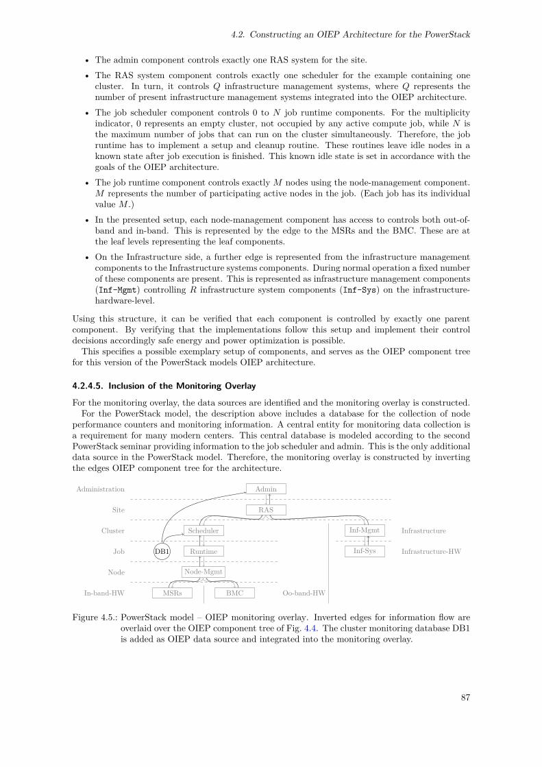
4.2. Constructing an OIEP Architecture for the PowerStack
• The admin component controls exactly one RAS system for the site.• The RAS system component controls exactly one scheduler for the example containing one
cluster. In turn, it controls Q infrastructure management systems, where Q represents thenumber of present infrastructure management systems integrated into the OIEP architecture.
• The job scheduler component controls 0 to N job runtime components. For the multiplicityindicator, 0 represents an empty cluster, not occupied by any active compute job, while N isthe maximum number of jobs that can run on the cluster simultaneously. Therefore, the jobruntime has to implement a setup and cleanup routine. These routines leave idle nodes in aknown state after job execution is finished. This known idle state is set in accordance with thegoals of the OIEP architecture.
• The job runtime component controls exactly M nodes using the node-management component.M represents the number of participating active nodes in the job. (Each job has its individualvalue M .)
• In the presented setup, each node-management component has access to controls both out-of-band and in-band. This is represented by the edge to the MSRs and the BMC. These are atthe leaf levels representing the leaf components.
• On the Infrastructure side, a further edge is represented from the infrastructure managementcomponents to the Infrastructure systems components. During normal operation a fixed numberof these components are present. This is represented as infrastructure management components(Inf-Mgmt) controlling R infrastructure system components (Inf-Sys) on the infrastructure-hardware-level.
Using this structure, it can be verified that each component is controlled by exactly one parentcomponent. By verifying that the implementations follow this setup and implement their controldecisions accordingly safe energy and power optimization is possible.This specifies a possible exemplary setup of components, and serves as the OIEP component tree
for this version of the PowerStack models OIEP architecture.
4.2.4.5. Inclusion of the Monitoring Overlay
For the monitoring overlay, the data sources are identified and the monitoring overlay is constructed.For the PowerStack model, the description above includes a database for the collection of node
performance counters and monitoring information. A central entity for monitoring data collection isa requirement for many modern centers. This central database is modeled according to the secondPowerStack seminar providing information to the job scheduler and admin. This is the only additionaldata source in the PowerStack model. Therefore, the monitoring overlay is constructed by invertingthe edges OIEP component tree for the architecture.
Administration
Site
Cluster
Job
Node
In-band-HW Oo-band-HW
Infrastructure
Infrastructure-HW
Admin
RAS
Scheduler
Runtime
Node-Mgmt
MSRs BMC
Inf-Mgmt
Inf-Sys
1
1
0..N
M
1 1
Q
R
1
1
1 1
Q
DB1
Figure 4.5.: PowerStack model – OIEP monitoring overlay. Inverted edges for information flow areoverlaid over the OIEP component tree of Fig. 4.4. The cluster monitoring database DB1is added as OIEP data source and integrated into the monitoring overlay.
87

4. Open Integrated Energy and Power Architectures
Figure 4.5 shows this OIEP monitoring overlay for the PowerStack model overlaid onto the OIEPcomponent tree. The edges of the OIEP component tree are reversed and added, representing infor-mation flow up the tree. Additionally, the cluster monitoring database, DB1, is added as the OIEPdata source representing the central cluster monitoring of Figure 4.2. The database, DB1 is addedbelow the cluster-level, since this is the location of the component lying on the deepest level, whichis using the data source.For sake of completeness, Figure 4.6 presents the database DB1 and its data sources. As of the
Administration
Site
Cluster
Job
Node
In-band-HW Oo-band-HW
Infrastructure
Infrastructure-HW
Admin
RAS
Scheduler
Runtime
Node-Mgmt
MSRs BMC
Inf-Mgmt
Inf-Sys
1
1
0..N
M
1 1
Q
R
DB1
Figure 4.6.: PowerStack model – OIEP monitoring overlay – view of the data sources of the database.
description of Figure 4.2, the cluster monitoring obtains its data from the in-band and out-of-bandcomponents. Therefore, Figure 4.6 shows that the database in the data-source view is positioned onelevel above its highest level data source (as described in Sec. 3.3.3.2).This highlights the noteworthy difference between Figure 4.5 and Figure 4.6: the location of DB1.
For the OIEP monitoring overlay, the location is set on the highest level below the deepest consumerof the information. For the database view and its data sources, it’s on the lowest level above thehighest level data source. Therefore, DB1 is located below the scheduler-level in Figure 4.5 and abovethe node hardware-levels in Figure 4.6.
4.2.4.6. Identification of Operating States and Construction of the State Diagram
The next step in the OIEP architecture construction is the identification of operating states and thestate diagram. With the above paragraphs the basic functionality for energy and power managementis covered. The OIEP architecture is in accordance with the PowerStack model, however, emergencyoperation is not handled, yet. In Figure 4.2, the figure on the system interactions for the PowerStackmodel, this is indicated with dashed arrows. The dashed arrows point from RAS to the HW-Platform,as well as to the job scheduler, both labeled override. A direct override violates the OIEP referencemodel’s principle of control, since only one parent can have direct control over any component. Thus,the mechanisms of the OIEP operating states and the OIEP state diagram are used to resolve thesituation in a comprehensive and manageable way.Given the PowerStack model two operating modes are identified: default and emergency. In the
following, the states are described, given state-description and triggers for the transition into thestate. Later states associated OIEP component tree is declared.The OIEP operating state default is the normal operating mode of the PowerStack model. Regard-
ing state transitions to default, two transitions have to be handled: First initialization and secondreturning to default operation. The system initialization has to be handled by each component inthe above OIEP component tree. To return from emergency to default operation, once the systemadministration has resolved the emergency situation, they can trigger a return to normal operation.The OIEP operating state emergency is the state for extraordinary circumstances and for safe
handling of situations where direct control for emergency handling is needed. The state transition, asdepicted in Figure 4.2 is initiated by the RAS component when detecting a situation where normaloperation has to be interrupted. An associated OIEP component tree needs to be developed, whichis suitable for direct access to the nodes of the cluster, capturing the override functionality in a cleardesign.
88

4.2. Constructing an OIEP Architecture for the PowerStack
Default
init
Emergency
RAS:emergency-detection
admin:set-normal
Figure 4.7.: PowerStack model – OIEP state diagram with normal and emergency state.
Figure 4.7 shows a simple state diagram for these two OIEP operating states to realize thePowerStack requirements. The FSM shows the default-state as the initial state with a state transi-tion to the emergency-state. The transition is triggered by the RAS component on the event of anemergency detection. The emergency-state has a state transition to the default-state. The transitionis manually triggered by the admin.The remaining step in the construction of the OIEP architecture is the repetition of the above
steps for all OIEP operating states, which is presented in the following paragraph.
4.2.4.7. Addressing the Remaining States of the State Diagram
In the following, the construction steps for OIEP architecture have to be repeated for the remainingidentified OIEP operating states. Since the structure of control for this emergency state is specified bythe override indicators of Figure 4.2 the constructed OIEP architecture only needs small adjustmentsto represent this change. The resulting OIEP component tree is presented in Figure 4.8. The Figureimplicitly contains the needed OIEP levels, OIEP level tree, OIEP components and OIEP componenttree, with the altered operating mode in OIEP operating state emergency.
Administration
Site
Node
Oo-band-HW
Infrastructure
Infrastructure-HW
Admin
RAS
Node-Mgmt
BMC
Inf-Mgmt
Inf-Sys
1
N′
1
Q
R
Figure 4.8.: PowerStack – OIEP architecture for the emergency state.
Figure 4.8 shows the OIEP component tree with reduced underlying OIEP level tree: The cluster-level, job-level and in-band-level are not present, while the multiplicity indicators at the edges areadjusted for the scenario. The selection of components on the levels is unmodified, while they operatein the OIEP operating state emergency. The multiplicity indicator from RAS to Node-Mgmt ischanged, since an exact control of all nodes present in the system is needed. This is indicated by theinteger N ′ representing all nodes of the cluster.The emergency state is set up, so that in case of emergency control of all hardware capabilities rest
with the RAS system. Both infrastructure and node management is controlled with the accordingconfigurations, while removing runtime systems, which cannot identify and react to the emergencyscenario. Once the emergency case has been gracefully handled, the default OIEP operating state isreinstantiated by the admin. The monitoring overlay is a simple inversion of the control flow and notshown. Database and data sources are handled as of the original architecture setup. When imple-menting the components the triggers for state transitions and the needed actions to transition statesand hand over control have to be implemented accordingly.
According to the method for applying the reference model of this chapter (see Sec. 4.1) this con-
89
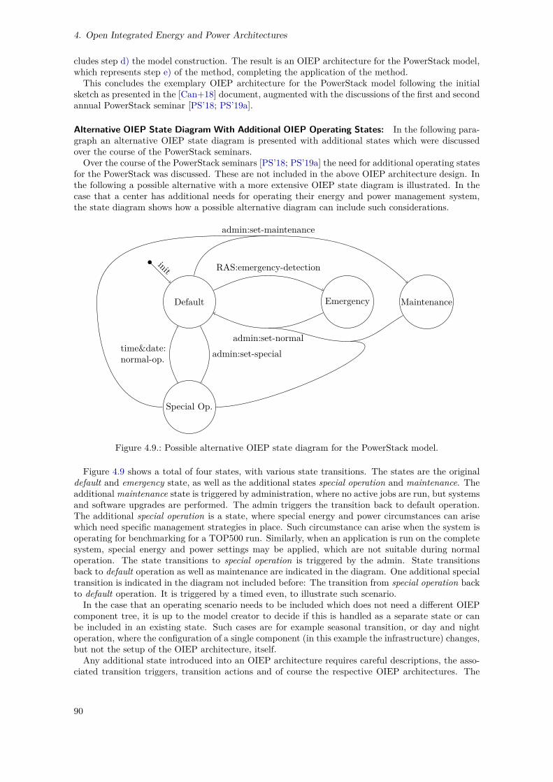
4. Open Integrated Energy and Power Architectures
cludes step d) the model construction. The result is an OIEP architecture for the PowerStack model,which represents step e) of the method, completing the application of the method.This concludes the exemplary OIEP architecture for the PowerStack model following the initial
sketch as presented in the [Can+18] document, augmented with the discussions of the first and secondannual PowerStack seminar [PS’18; PS’19a].
Alternative OIEP State Diagram With Additional OIEP Operating States: In the following para-graph an alternative OIEP state diagram is presented with additional states which were discussedover the course of the PowerStack seminars.Over the course of the PowerStack seminars [PS’18; PS’19a] the need for additional operating states
for the PowerStack was discussed. These are not included in the above OIEP architecture design. Inthe following a possible alternative with a more extensive OIEP state diagram is illustrated. In thecase that a center has additional needs for operating their energy and power management system,the state diagram shows how a possible alternative diagram can include such considerations.
Default
init
Emergency Maintenance
Special Op.
admin:set-maintenance
RAS:emergency-detection
admin:set-normaladmin:set-specialtime&date:
normal-op.
Figure 4.9.: Possible alternative OIEP state diagram for the PowerStack model.
Figure 4.9 shows a total of four states, with various state transitions. The states are the originaldefault and emergency state, as well as the additional states special operation and maintenance. Theadditional maintenance state is triggered by administration, where no active jobs are run, but systemsand software upgrades are performed. The admin triggers the transition back to default operation.The additional special operation is a state, where special energy and power circumstances can arisewhich need specific management strategies in place. Such circumstance can arise when the system isoperating for benchmarking for a TOP500 run. Similarly, when an application is run on the completesystem, special energy and power settings may be applied, which are not suitable during normaloperation. The state transitions to special operation is triggered by the admin. State transitionsback to default operation as well as maintenance are indicated in the diagram. One additional specialtransition is indicated in the diagram not included before: The transition from special operation backto default operation. It is triggered by a timed even, to illustrate such scenario.In the case that an operating scenario needs to be included which does not need a different OIEP
component tree, it is up to the model creator to decide if this is handled as a separate state or canbe included in an existing state. Such cases are for example seasonal transition, or day and nightoperation, where the configuration of a single component (in this example the infrastructure) changes,but not the setup of the OIEP architecture, itself.Any additional state introduced into an OIEP architecture requires careful descriptions, the asso-
ciated transition triggers, transition actions and of course the respective OIEP architectures. The
90
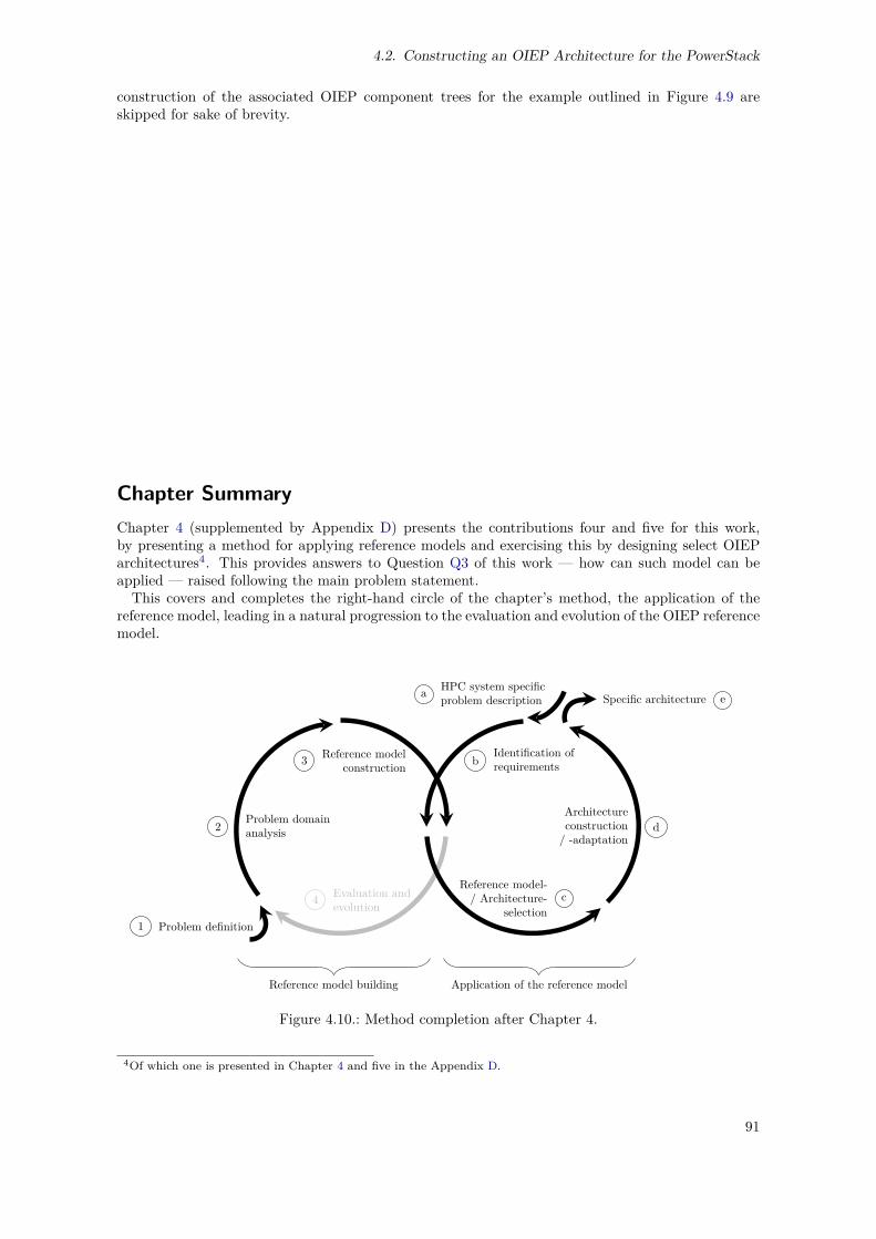
4.2. Constructing an OIEP Architecture for the PowerStack
construction of the associated OIEP component trees for the example outlined in Figure 4.9 areskipped for sake of brevity.
Chapter SummaryChapter 4 (supplemented by Appendix D) presents the contributions four and five for this work,by presenting a method for applying reference models and exercising this by designing select OIEParchitectures4. This provides answers to Question Q3 of this work — how can such model can beapplied — raised following the main problem statement.This covers and completes the right-hand circle of the chapter’s method, the application of the
reference model, leading in a natural progression to the evaluation and evolution of the OIEP referencemodel.
Problem definition1
Problem domainanalysis2
Reference modelconstruction3
Evaluation andevolution4
Reference model building
HPC system specificproblem descriptiona
Identification ofrequirementsb
Reference model-/ Architecture-
selectionc
Architectureconstruction/ -adaptation
d
Specific architecture e
Application of the reference model
Figure 4.10.: Method completion after Chapter 4.
4Of which one is presented in Chapter 4 and five in the Appendix D.
91

5. Assessment
5.1. Assessment Synopsis and Comparison with Generic Model Building Systems . . . . . . 935.2. Identified Limitations . . . . . . . . . . . . . . . . . . . . . . . . . . . . . . . . . . . . 95
This chapter forms a part of the fourth and last step of the thesis method, as presented in Section 1.2:The evaluation and evolution of the reference model.According to [Sch00, p. 85], a full evaluation has to be conducted by a separate entity, independent
of the model creator of the reference model.1 Such full evaluation is proposed as future work, wherethe initial assessment provided summarized below may serve as orientation.This chapter builds upon an assessment of the model conformity, regarding the previously described
requirements of Section 2.3 presented in Appendix E.1 and shows its result as summary. The presentedsummary is joins the requirements assessment and a comparison with generic model building systemstogether, in Section 5.1. The chapter is concluded with a discussion on the identified limitations.Appendix E supplements the chapter with the presentation of the full assessments (App. E.1), as wellas a discussion on use-cases for the OIEP reference model (App. E.2).
5.1. Assessment Synopsis and Comparison with Generic ModelBuilding Systems
This chapter provides a summary for the assessment of the fulfillment of these requirements, asconducted in Appendix E.1. This is conducted referring to Section 2.3 with Appendix A.2.The summary of this chapter is presented in Table 5.1 in combination with the comparison to the
requirements for the selected generic model building approaches of [BCN91; MS94; Sch98; Sch99;Sch00]. A specific interest lies on [Sch98], as for the method an adaption of the works proposedmethod is used, as presented in Section 1.2.Table 5.1 shows the assessment, differentiating the requirements of the OIEP reference model as
fulfilled “by design”, “enabled” by the design, and marks requirements for special interest of fullevaluation with an indicator arrow. The table lists the identified requirements with indicators fromthe related work, identifying matching requirements from generic model building systems. The lastcolumn lists the energy and power specific OIEP reference model. Within this row, indicators areplaced, “D” for by Design, “E” for Enabled, and “←” indicating that this aspect has to be followedup with a full evaluation.The following requirements are covered by design of the OIEP reference model: locally distributed
environment, diverse hardware components, reference model for energy and power, model structureand building blocks, applicability and systematic construction, optimization goals, modularity, limitingscope and remote, opaque components, transparent structure and information flow, chain of commandand traceability, manageability, simplicity and readability, structural equivalence, and operating modes.The following requirements are covered by design, but limitations do apply, due to design choices
of the OIEP reference model: diverse software components, scalability completeness and relevance,formality, expressiveness and feasibility and implementability. The explanation for these items isdiscussed in the listing below, in Section 5.2.Additionally, these requirements are not fulfilled by the design itself, but enabled by it: applica-
bility and systematic construction, optimization goals, modularity, limiting scope and remit, chain ofcommand and traceability, manageability, automation, and static and dynamic control.
1The author of this thesis notes, that such evaluation is not a quantitative evaluation, but a qualitative one. Foran objective systematic evaluation, an unbiased entity has to perform said evaluation. Therefore, the author onlyprovides an assessment, as provided in this chapter.
93
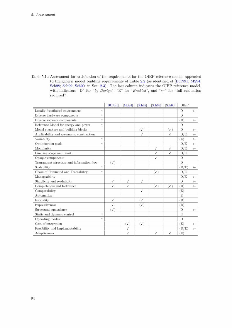
5. Assessment
Table 5.1.: Assessment for satisfaction of the requirements for the OIEP reference model, appendedto the generic model building requirements of Table 2.2 (as identified of [BCN91; MS94;Sch98; Sch99; Sch00] in Sec. 2.3). The last column indicates the OIEP reference model,with indicators “D” for “by Design”, “E” for “Enabled”, and “←” for “full evaluationrequired”.
[BCN91] [MS94] [Sch98] [Sch99] [Sch00] OIEPLocally distributed environment * D ←Diverse hardware components * DDiverse software components * (D) ←Reference Model for energy and power * DModel structure and building blocks (X) (X) D ←Applicability and systematic construction X X D/E ←Variability * (E) ←Optimization goals * D/E ←Modularity X X D/E ←Limiting scope and remit X X D/EOpaque components X DTransparent structure and information flow (X) DScalability * (D/E) ←Chain of Command and Traceability * (X) D/EManageability D/E ←Simplicity and readability X X X D ←Completeness and Relevance X X (X) (X) (D) ←Comparability X (E)Automation EFormality X (X) (D)Expressiveness X (X) (D)Structural equivalence (X) D ←Static and dynamic control * EOperating modes * DCost of integration (X) (X) (E) ←Feasibility and Implementability X (D/E) ←Adaptiveness X X X (E)
94

5.2. Identified Limitations
Where the following requirements, are enabled, however limitations apply. This is either due tothe fact, that the enablement is not enforced by the design, or that the choices of the OIEP referencemodel only allows to identify, but do not support the requirements directly. These requirementsare: variability, scalability comparability, cost of integration, feasibility and implementability, andadaptiveness.
Overall, compared to the generic model building, all aspects are covered or at least enabled. Wherelimitations apply, a conscious choice was made to suite the application area of energy and powermanagement systems of HPC systems. The identified limitations are discussed below.
5.2. Identified LimitationsThe identified limited requirements are listed with additional details:
• Diverse software components: Limited to software components used/configured in a hierarchicalway, not violating the single parent control flow.
• Variability: Enabled, but limited, since considering variability is not mandated.• Scalability: By design of the reference model, OIEP enables to construct scalable designs.
However, by using the OIEP reference model scalability is not guaranteed. (Even if non-scalablesetups can be easily identified using the approach.)
• Completeness and relevance: Only the OIEP reference model building blocks and the hierar-chical structure is prescribed. This may be limiting but is seen appropriate (otherwise UMLmay be used to model the system in the first place) in the eyes of the author. Using this all rel-evant aspects of energy and power management setups are modeled. This assumption requiresexternal evaluation.
• Formality: Only a graphical formalism is given, while no grammar is provided, or more formalaspects are provided.
• Expressiveness: See the argument on completeness and relevance• Cost of integration: Improved capability to estimate cost of integration is enabled using the
reference model, (simply by being able to model the system), but no specifics are given. Thisaspect needs to be further elaborated on.
• Adaptiveness: Similar to the modularity aspect, but: By choosing specific designs the possibilityof adaptiveness may be limited. Such incompatibilities in terms of adaptiveness are detectable,but not directly preventable; Thus, this is indicated as limited.
In addition to the identification of requirements fulfilled by design or enabled by design, The tableshows the indicator, “←” on the far side, to indicate the need for full evaluation of these aspects ofthe OIEP reference model. The indicators on the requirement for full evaluation should be followedup as prospect future work.For comparison with the generic model building requirements, only the aspects of comparability,
feasibility and implementability and adaptiveness are “only” enabled by the OIEP reference model.All other aspects are covered by design.
95
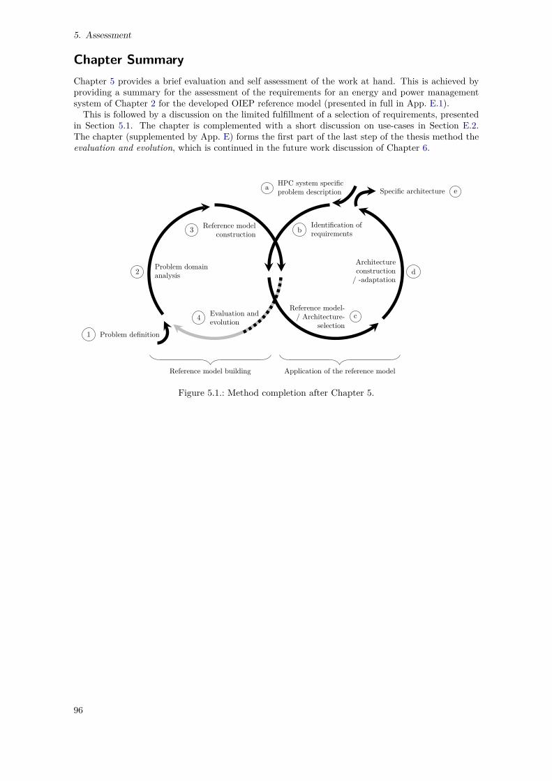
5. Assessment
Chapter SummaryChapter 5 provides a brief evaluation and self assessment of the work at hand. This is achieved byproviding a summary for the assessment of the requirements for an energy and power managementsystem of Chapter 2 for the developed OIEP reference model (presented in full in App. E.1).This is followed by a discussion on the limited fulfillment of a selection of requirements, presented
in Section 5.1. The chapter is complemented with a short discussion on use-cases in Section E.2.The chapter (supplemented by App. E) forms the first part of the last step of the thesis method theevaluation and evolution, which is continued in the future work discussion of Chapter 6.
Problem definition1
Problem domainanalysis2
Reference modelconstruction3
Evaluation andevolution4
Reference model building
HPC system specificproblem descriptiona
Identification ofrequirementsb
Reference model-/ Architecture-
selectionc
Architectureconstruction/ -adaptation
d
Specific architecture e
Application of the reference model
Figure 5.1.: Method completion after Chapter 5.
96
6. Future Work
6.1. Future Developments for the OIEP Reference Model . . . . . . . . . . . . . . . . . . . 976.2. Future Work for the Application of the OIEP Reference Model . . . . . . . . . . . . . 996.3. Open Topics . . . . . . . . . . . . . . . . . . . . . . . . . . . . . . . . . . . . . . . . . . 99
This chapter discusses future work for the OIEP reference model. The future work section is splitinto three parts:
• Future developments for the OIEP reference model• Future work for the application of the OIEP reference model• Open topics in energy and power management
6.1. Future Developments for the OIEP Reference ModelAs formalized in the thesis method (see Sec. 1.2), the structure of the method is cyclic. Therefore,future developments and adaptations for the OIEP reference model can follow the outlined method.Regardless of this iterative approach, there are obvious future directions for work on the OIEP refer-ence model, which help the efforts to make energy and power management systems more integrated,understandable and also a normal part of any HPC system.The OIEP reference model has some aspects only loosely specified, which may require additional
thought and evaluation. The following list provides directions for future work:
• Extension beyond the current leaf-levels;• Extension beyond the current root-levels;• Theory for OIEP reference model on the modeling of multiple clusters using a single combined
OIEP architecture;• Theory for OIEP reference model on the modeling of sub-parts of a OIEP architecture as
independent OIEP architectures with independent OIEP state diagrams;• Users as explicit actors in the architecture;• Steps towards standardization of the OIEP reference model.
Details are provided in the following paragraphs.
Extension Beyond the Current Leaf-levels: The current OIEP reference model models systems fromthe highest level components, down to the hardware interfaces. These leaf level entities build thecut-off of components modeled using the OIEP reference model, since they form the last componentscontrollable by software components directly. For future work, an investigation beyond this lowestlevel is of interest. Can the model be applied up to the firmware level and model hardware mechanisms,which realize the lowest instance of energy and power controls. Such efforts may lead to provideinterface to topics related to Electical Engineering (EE) for integrated systems. At these levels, themodel’s interaction and compatibilities with RCSs may be studied.
97

6. Future Work
Extension Beyond the Current Root-levels: The root level at the OIEP reference model is theinterface to the outside world. It sets optimization goals and provides rules for the operating en-vironment. HPC systems do not operate in isolation, as efforts on grid-integration show [Ste+19a;Cla+19b; Pat+16]. By having a system modeled as OIEP architecture, the interfaces and exchangeof information, may be easier to extend towards interaction with ESP and smart grids, and the energyspot marked. This is an opportunity to use energy automation systems, volatile energy sources andrenewable energy with different stabilities, where ESPs might see a HPC center as a potential loadbuffer or regular.
Theory for OIEP Reference Model on the Modeling of Multiple Clusters Using a Single CombinedOIEP Architecture: Such extension seems trivial, since the root component simply handles, multipleinstances of the child components. However, in the current setup, modeling a single HPC systemand its energy and power management setup has a large influence on the form and shape of theresulting OIEP architecture. How to effectively combine multiple OIEP architectures as a singlesystem, without redesigning the complete system remains for future work. From a graph theoryperspective such mechanism joins, two trees to a larger tree structure. Therefore, the relations ofOIEP component tree and OIEP level trees viewed as a OIEP forest, merged by introducing a commonroot with the trees as children seems trivial. For the OIEP reference model, the implications obtainedfrom the simple graph operation have large impact on energy and power management and control onthe highest levels and throughout the architectures. These implications are not trivial to resolve atall.
Theory for OIEP Reference Model on the Modeling of Sub-parts of an OIEP Architecture asIndependent OIEP Architectures With Independent OIEP State Diagrams: Similar to the pre-vious paragraph, future work for the OIEP reference model can assess implications of dividing treesinto sub-trees, which are modeled as OIEP architectures with individual OIEP state diagrams, andindependent state transitions. In the presented OIEP reference model, the OIEP operating statestransition the management hierarchy for the complete OIEP architecture. The implications for sub-trees and potential diverging tree-structures make such systems more complex and it is to be seenif the individual control flow results in a system too variable for proper control. The ability tomanage the system is inherited from its rigid and fixed tree structure and the resulting simple andcomprehensive control flow.
Users as Explicit Actors in the Architectures: For the OIEP architectures the identification of useractors currently is only a side aspect of the model. Such considerations are hidden behind the OIEPcomponents and if at all described in the functionality of these. The Power-API conducted a majoruse-case analysis for their work in [III+13]. The presented use-case analysis is focused on actorswithin the system, where actors represented humans interacting with the different parts of the HPCsystem (except for one use-case, where an actor is representing an application).The OIEP reference model is energy and power management system centric. Such interaction with
actors, which are not modeled as components, shows how the system is used for such control, from auser-centric perspective. Future work may need to look at how to extend the OIEP reference modelgiven such use-cases. This may help to settle several arguments on:
• If users have to be involved in all energy and power decisions or not;• Where to limit the scope and responsibilities of users and admins explicitly;• Considerations of impact to automation, in the presence and absence of human actors.
Steps Towards Standardization of the OIEP Reference Model: The last item on the list of theOIEP reference model is the path towards standardization. The PowerStack committee [SPSweb],authored the initial considerations on a strawman document to have a unified approach for energyand power management [Can+18]. The effort to align the different interest groups is challenging, andchoice of common vocabulary, objectives, actors etc. is under ongoing discussion. By providing theOIEP reference model as tool may help to formalize these ideas using common vocabulary. To providea generally accepted approach for centers, and vendors to model the energy and power management
98
6.2. Future Work for the Application of the OIEP Reference Model
approach of interacting software components, there is still a far way. Identifying how the transitionto a standardized reference model and a standardized reference architecture can be made is up forfuture work.
These five points summarize the five most pressing issues identified by the author on future work forthe OIEP reference model, itself.
6.2. Future Work for the Application of the OIEP ReferenceModel
For the application of the OIEP reference model to develop OIEP architectures a second list of openresearch questions and future work is identified. These are:
• Tools support for OIEP architecture creation;• Metrics of performance;• Evaluating the impact on procurements, maintenance and system upgrades;• Outstanding evaluations with regard to Table 5.1.
Tools Support for OIEP Architecture Creation: As for any model to be useful, it has to be used. Forthe usage of models, tools have to exist supporting users to apply them effectively. This involves easeof problem description, and visual representation of the system. Future directions for the applicationof the OIEP reference model therefore are the development of tools supporting the model.
Metrics of Performance: For improving energy and power, measurements are the key to success.For the application of OIEP architectures measuring the impact of applying a particular architectureis necessary to identify how an OIEP architecture is performing. As a baseline, traditional metrics canbe used which have proven in the facility environment. These are general energy efficiency metrics,developed over the years [Wil+14; Wil18].However, for an integrated system, of energy and power management components, it is also inter-
esting to measure the total used headroom of power optimization granted by each energy and powermanagement level of an OIEP architecture. Therefore, it is of interest to evaluate new metrics specificto such integrated energy and power management setups.
Evaluating the Impact on Procurements, Maintenance and System Upgrades: One of the goalsof the OIEP reference model is to make energy and power management systems more understandable.This allows to shows why adding comprehensive mechanisms to manage energy and power into thesystem is of importance. On the practical side, OIEP architectures seem like a good tool to supportprocurements, maintenance and upgrades of energy and power management setups of HPC systems.Therefore, introducing OIEP architectures in such process and evaluating its benefits may be of greatinterest for the success of using a reference model for such use-cases.
Outstanding Evaluations With Regard to Table 5.1: Table 5.1 listed several outstanding items forfull evaluation. These are sometimes in regard to the design of the OIEP reference model, but somecan only be evaluated when applying the model. For future work, especially the aspects enabled bythe usage of a OIEP architecture are of interest for further investigation.
6.3. Open TopicsEnergy and power has gained major attention in HPC over the last years. To keep up with the needsof computation, clusters have transformed in size and scale, making them again machine room scale.With the current trends in computer science a model such as the OIEP reference model may enablenew directions for energy and power research for HPC. Several topics are of ongoing interest butsometimes stall due to the barrier to move them into real systems, where production continues as
99

6. Future Work
done traditionally. For the following topics, having a reference model to model and make the energyand power management system understandable may help to make some of these aspects a reality.
• Overprovisioning;• Advanced components;• Integration of eXplainable Artificial Intelligence (XAI);• Making energy and power a first class citizen as resource of HPC;• Enabling digital twins of HPC systems for energy and power management;• Making integrated control of the 4-Pillars a reality.
Overprovisioning: The idea of overprovisioned systems has first been described in [Pat+13a], andsince been studied on an experimental basis in numerous papers [Sar+13; CHK16; Sak+18]. A specialemphasis is put on scheduling [Sar+14; Sak+17; Sak+18], with only few extensions to other parts ofthe system (as by example to cooling [Cao+17]).For production systems overprovisioned features are often shied away from, since without mechan-
ical fail-safes the risk of catastrophic failure is too high. One of the first systems applying a de-factooverprovisioning strategy is the Fugaku system. Without the Bunch of Bladess (BoBs)’ power-capoverrides, the system could easily exceed the provisioned 30 MW peak power.By providing the OIEP reference model to model all aspects of the energy and power management
system, such power-caps can be controlled over multiple interacting components, while not strictlyenforcing a cap at a single level.A promising future work direction therefore is how the OIEP reference model enables system designs
with overprovisioning in mind.
Advanced Components: Similar to the aspects of overprovisioning as a general strategy to operatea HPC system, there have been many efforts in advanced energy and power enabled components.By having a way to integrate such components in the overall system, and providing a comprehensiveoverview of how they interact with the system, introducing these into production can be enabled.Therefore, research software can can be integrated more easily for use within production systems.
Future work in this direction, enables software components, by modeling the interactions in an OIEParchitecture.
Integration of XAI: Regarding advanced components, Machine Learning (ML) and Artificial Intel-ligence (AI) is entering the area of system software. To move beyond mere data analysis trust has tobe gained for autonomous components to control parts of the HPC systems and its resources.Efforts for XAI have surged in interest, as AI and ML techniques show broader dissemination in
research, again, as recent surveys show [Bar+20; VL20]. For HPC center to adopt AI driven solutionstheir decisions have to be clear, in terms of safe operations. AI requires clear interfaces and sufficienttraining data. For AI to be explainable in the HPC context the optimization goals as well as controldecisions have to be comprehensible or even replicable by the admins. However, for an admin allowingtheir system to be controlled by AI systems, the location, scope (and its enforced limitations), andeventual replaceability, by a working fall-back has to be guaranteed.For future work in HPC the OIEP reference model in combination with XAI presents an opportu-
nity: By encapsulation, modularity and the presentation of a clear energy and power managementmodel, OIEP components with ML/AI decision capabilities can be evaluated in any component rel-evant to system optimization.
Making Energy and Power a First Class Citizen as Resource of HPC: The efforts on the Fluxframework [Ahn+14] introduced a generalized resource model in place of traditional job scheduling.With the addition of scheduling efforts spanning multiple system and a general resource managementapproaches, new challenges arise. Among them, a co-scheduling challenge, and job coordination andcommunication challenge [Ahn+20]. Using energy and power management to represent all HPCsystems of a center as OIEP architecture and using these for control the system (with their local
100

6.3. Open Topics
compoents), while having a decoupled general resource manager such as the Flux framework enablescompletely new approaches to energy and power as a resource.By exposing functionality of a holistic energy and power management setup and coupling it with a
generalized resource management setup such as Flux, new opportunities for optimizing HPC systemscan be identified. (After all energy is the de-facto limiting factor to all modern computation.)
Enabling Digital Twins for Energy and Power Management: By being able to model the holisticenergy and power management setup, the creation of physical twins is possible. The structure ofthe model and its energy and power management setup can be encapsulated inside a simulation oremulation environment. These techniques can be used to evaluate systems before production, andevaluate the performance in different system scenarios. When using copies of the software componentsthat are present in the real system, the components can also be tested. Additionally, this forms atestbed for the introduction of new components, and understanding their interaction with the rest ofthe system, and potentially resource usage and potential bottlenecks.Using the OIEP reference model, the relevant parts of the HPC system’s energy and power man-
agement setup can be isolated and integrated for the required testing setups.
Making Integrated Control of the 4-Pillars a Reality: The 4-Pillar [WAS14] framework identifiesthe four pillars to energy efficient operation of data center:
• the building infrastructure,• the system hardware,• the system software, and• the applications.
to understand LRZ’s efforts for improving energy efficiency. The initial goal of the work of [WAS14]as “What HPC data center aspects play an important part for the improvement of energy efficiency”.Most efforts at the center overlaid over the basic schematic identifies independent aspects to moni-toring, while the control efforts are confined to their pillars.Future work can expand and unify the control efforts, using the OIEP reference model to model all
aspects of the 4-Pillar framework and identify, where to interact. The 4-Pillar framework can helpto identify where the largest benefits for optimization are located, while the OIEP architectures canmodel how operational management of such integrated energy and power management system canbe realized and how to improve a system continuously. An effort like this may resemble aspects ofan operating system for HPC.In combination, models like the 4-Pillar framework and the OIEP reference model help to under-
stand the internals of HPC systems and improve more than the aspects they focus on. This allowsto set the focus for future efforts.
101
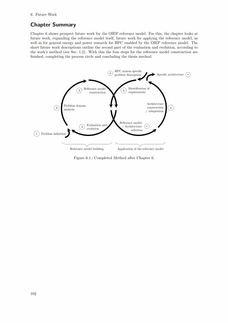
6. Future Work
Chapter SummaryChapter 6 shows prospect future work for the OIEP reference model. For this, the chapter looks atfuture work, expanding the reference model itself, future work for applying the reference model, aswell as for general energy and power research for HPC enabled by the OIEP reference model. Theshort future work descriptions outline the second part of the evaluation and evolution, according tothe work’s method (see Sec. 1.2). With this the four steps for the reference model construction arefinished, completing the process circle and concluding the thesis method.
Problem definition1
Problem domainanalysis2
Reference modelconstruction3
Evaluation andevolution4
Reference model building
HPC system specificproblem descriptiona
Identification ofrequirementsb
Reference model-/ Architecture-
selectionc
Architectureconstruction/ -adaptation
d
Specific architecture e
Application of the reference model
Figure 6.1.: Completed Method after Chapter 6.
102

7. ConclusionsThis chapter presents the conclusions from answering the problem statement and the conclusionsfrom the contributions of this thesis.
The challenge addressed in this work is the definition of a reference model for integrated energyand power management of HPC systems.This challenge is approached by answering three questions, the first – the work’s problem statement
– and two supplementing questions. In the following the conclusions from each of these questions arestated.
Q1: How to model energy and power management systems for HPC systems in an integrated,holistic way?
• The research question is answered by dissecting it into two subsequent questions. These answerthe problem statement by addressing:– The structure and components of such reference model;– A method for application of the reference model (with example applications);
• To tackle the individual questions, first a method with the identified goal to create a referencemodel is devised, giving structure to this work (in Sec. 1.2). This is followed by two chapterscontaining the problem domain analysis (in Ch. 2 & B.1).
• In total, the conclusions from these questions answer the research question by presenting a struc-tural approach for modeling integrated energy and power management systems and exercisingon this solution by presenting the works contributions.
Q2: What is an appropriate structure of such model and what are its required building blocks?
• This question is answered by first, adopting a method for reference model construction (inSec 3.1), suitable for the problem domain, resulting in the construction of the OIEP referencemodel (in Ch. 3).
• Energy and power management is modeled by creating levels of abstraction, used to give struc-ture, which captures interfaces as well as control and information flow in a hierarchical fashion.
• The abstraction is presented in the form of building blocks of– OIEP levels and the OIEP level tree,– OIEP components and the OIEP component tree– OIEP data sources and the OIEP monitoring overlay– OIEP operating states and the OIEP state diagram
• These building blocks allow to model energy and power management systems in hierarchicalstructure, allowing to integrate high-level optimization goals, with several levels of interactingsoftware systems, down to low-level hardware controlled in a comprehensive, integrated andholistic way.
• To complete the creation of a reference model, after the model construction, the additionalsteps of application, evaluation and evolution are needed.
103

7. Conclusions
Q3: How can such a model be applied to concrete system architectures for energy and powermanagement of HPC systems?
• To answer Question 3, a method for the application of the reference model is needed. Suchmethod is constructed and presented in Section 4.1.
• The method is tailored towards applying the OIEP reference model for the construction ofOIEP architectures.
• To model existing HPC systems using the OIEP reference model and construct OIEP architec-tures for them, their structure has to be analyzed.
• The identified components then have to be mapped to the building blocks provided by thereference model.
• The result is a transparent and understandable model of the energy and power managementsystem for a given HPC system.
• This process is applied and its feasibility shown.
With the conclusions from Questions Q2 and Q3, the solution to Question Q1 is supplemented andfinalized. The method followed in this work is concluded and the contributions fulfilled.
Concluding Remark
With the presentation of the contributions and the conclusions to the problem statement and re-search questions, the overall problem statement is satisified. This work is a stepping stone towardsmodeling energy and power management systems of HPC systems, by providing the first referencemodel for describing hierarchical energy and power management system for HPC systems: the OpenIntegrated Energy and Power (OIEP) reference model.
104

Intentionally left blank.
105

Appendix A.
Supplement – Motivation
A.1. Detailed Requirements Definition . . . . . . . . . . . . . . . . . . . . . . . . . . . . . . 107A.2. Detailed Comparison to Other Model Building Requirements . . . . . . . . . . . . . . 115
A.1. Detailed Requirements DefinitionFor a complete problem domain analysis a requirements’ analysis for reference models in energy andpower management for HPC is presented. The requirements analysis is based on the requirementsdefinition concept introduced by [RS77]. For object-oriented reference modeling the work [Sch00]recommends a case analysis. The work at hand substitutes this for a requirements’ analysis due tothe breath of goals and system setups as seen in Section 2.2. This allows for a more general solution,where use-cases are used to evaluate the applicability of the model (see Ch. 4).The contents of Sections 2.1 and 2.2 are considered for the analysis of the requirements.The methodical approach for requirements analysis of system development by [RS77] is followed
according to these steps:
1. Context analysis (Sec. A.1.1), answering why a system is created, given technical operationaland economic feasibility criterion. This forms boundary conditions regarding scope.
2. Functional specification (Sec. A.1.2), answering what the purpose of the system regarding func-tionality and system goals is. This forms boundary conditions regarding functionality.
3. Design constraints (Sec. A.1.3), answering how the system is created constructed and imple-mented. This forms boundary conditions regarding intended usage.
All aspects are assessed from a technical, operational and economic1 viewpoint. These steps for con-text analysis, functional specification, and design constraints are presented in Figure A.1 from [RS77].
The corresponding requirements’ definition is done in the upcoming Sections A.1.1, A.1.2 and A.1.3,following Figure A.1 from left to right row by row. The derivation of the requirement is presented inthree parts for each identified item:
1. The naming of the requirement (as paragraph heading);2. The description and derivation of the requirement;3. The explicit requirements statement.
A.1.1. Context AnalysisIn accordance with the structured analysis for requirements definition, defined in [RS77], the followingquestion is asked: Why is the proposed reference model constructed?This poses requirements regarding the unique operating environment, problems, challenges and
opportunities to be addressed, not solved by other reference models. From the previous Sections(Sec. 2.1 and Sec. 2.2) the context analysis is performed from a technical, operational and economicstandpoint.
1Economic in terms of economic impact/viability/sustainability, whereas the work is not assessing profitability.
107
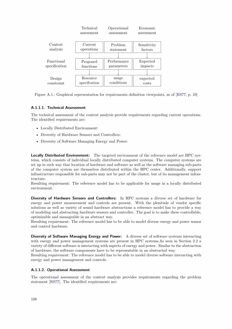
Contextanalysis
Functionalspecification
Designconstraint
Technicalassessment
Operationalassessment
Economicassessment
Currentoperations
Proposedfunctions
Resourcespecifcation
Problemstatement
Performanceparameters
usageconditions
Sensitivityfactors
Expectedimpacts
expectedcosts
Figure A.1.: Graphical representation for requirements definition viewpoints, as of [RS77, p. 10]
A.1.1.1. Technical Assessment
The technical assessment of the context analysis provide requirements regarding current operations.The identified requirements are:
• Locally Distributed Environment:• Diversity of Hardware Sensors and Controllers:• Diversity of Software Managing Energy and Power:
Locally Distributed Environment: The targeted environment of the reference model are HPC sys-tems, which consists of individual locally distributed computer systems. The computer systems areset up in such way that location of hardware and software as well as the software managing sub-partsof the computer system are themselves distributed within the HPC center. Additionally, supportinfrastructure responsible for sub-parts may not be part of the cluster, but of its management infras-tructure.Resulting requirement: The reference model has to be applicable for usage in a locally distributedenvironment.
Diversity of Hardware Sensors and Controllers: In HPC systems a diverse set of hardware forenergy and power measurement and controls are present. With the plenitude of vendor specificsolutions as well as variety of sound hardware abstractions a reference model has to provide a wayof modeling and abstracting hardware sensors and controller. The goal is to make these controllable,optimizable and manageable in an abstract way.Resulting requirement: The reference model has to be able to model diverse energy and power sensorand control hardware.
Diversity of Software Managing Energy and Power: A diverse set of software systems interactingwith energy and power management systems are present in HPC systems.As seen in Section 2.2 avariety of different software is interacting with aspects of energy and power. Similar to the abstractionof hardware, the software components have to be representable in an abstracted way.Resulting requirement: The reference model has to be able to model diverse software interacting withenergy and power management and controls.
A.1.1.2. Operational Assessment
The operational assessment of the context analysis provides requirements regarding the problemstatement [RS77]. The identified requirements are:
108

• Provision of a Reference Model for Energy and Power Management Systems:• Model Structure and Building Blocks of the Reference Model:• Applicability and Systematic Construction:
Provision of a Reference Model for Energy and Power Management Systems: The main prob-lem statement asks for a model for energy and power management in an integrated, holistic fashion.Section 2.1.3 discusses the need for an integrated energy and power management system. With sev-eral system specific solutions for energy and power management a generalization providing a modelapproach is a natural conclusion. However, since specific systems solutions and sound modeling of ageneric approach are a chicken-and-egg problem, the design of a reference model giving guidelines forstructure and design can help the introduction of modeling energy and power management systems.Resulting requirement: Design of a reference model suitable for integrated energy and power man-agement in HPC.
Model Structure and Building Blocks of the Reference Model: The structure of a reference modelis an essential element for its usefulness. With a diverse set of centers and software setups managingenergy and power a universal structure acceptable by any center is hard to find. As seen in the simpleexample of Section 2.1.2 conflicts in complex software systems can occur. The structure and conceptsof a reference model can supplement the design for conflict free energy and power managementsystems.Resulting requirement: Provision of basic structure and building blocks for the modeling of energyand power management.
Applicability and Systematic Construction: A reference model is only useful if it can be applied toreal systems. This allows to understand the system, manage and improve it. Two kinds of applicabil-ity have to be examined, first applicability of real systems providing energy and power management,second existing software interacting energy and power, as mentioned in an above paragraph. Addi-tionally, energy and power management is becoming more and more important for the procurementof HPC systems [EEWG17], thus this applies to current and upcoming systems. To apply a referencemodel, a systematic way of construction an instantiation of the model has to be provided.Resulting requirement: Applicability of the reference model to real world energy and power manage-ment systems in a systematic way.
A.1.1.3. Economical Assessment
The operational assessment of the context analysis provide requirements regarding the sensitivityfactors. Sensitivity factors, such parameters or properties, actions or events, impact operation ofthe system from a resource perspective in the case where perturbation may cause delay failure orfaults. Conversely, regarding positive outcome, sensitivity factors may be used to improve efficiencyor enhance output if managed and optimized. The identified requirements are:
• Variability:• Optimization Goals:
Variability: Variability is present in any HPC system, as discussed in Section 2.2.1 The variability inHPC systems power delivery is an artifact that system designers have largely accepted and based onthe goals of a center, for example stable operation, worst case-provisioning is traditionally consideredsufficient [Pat15]. Variability can have negative, impacts regarding power, power spikes, brown-outs,heat load, cooling disturbances, high power slopes, trapped capacity and stranded capacity [Wil18].In the case that several components see such concurring effects, the safe operation is not guaranteed,resulting in failure of operation. At the same time, understanding and using variability can improveenergy and power usage efficiency [Rou+09; Sch+16b; Mai+16; Eas+17; Pat+15].Resulting requirement: The system has to be able to use positive and avert negative effects ofvariability.
109

Optimization Goals: Centers have different optimization goals impacting how system for energyand power management are used. As discussed in Section 2.2 optimization goals of centers are diversand their solutions approaching the problems from different directions [Mai+18; Koe+18; Koe+19].Individual components can optimize for different goals, thus a reference model has to be able torepresent solutions of any goal related to energy and power management and optimization.Resulting requirement: The reference model has to be able to represent and work with differentoptimization goals.
A.1.2. Functional SpecificationIn accordance with [RS77]’s structured analysis for requirements definition, the following question isto be answered: What is the reference model supposed to be as boundary conditions for functionality.This raises requirements regarding the proposed function, performance parameters and expectedimpact. From the previous sections (Sec. 2.1 and Sec. 2.2) the requirements are accordingly derivedfrom a technical, operational and economic standpoint.
A.1.2.1. Technical Assessment
The technical assessment of the functional specification provides requirements regarding proposedfunctions for the reference model. The identified requirements are:
• Modularity:• Limiting Scope and Remit:• Opaque Components:• Transparent Structure and Information Flow:
Modularity: Modularity is one of the key concepts for reuse in a reference model and compatibilityof conceptually similar components. With the broad array of software components and board arrayof hardware, a reference model has to be able to abstractly represent these components. This resultsin the possibility to substitute sub-systems with known results. For a reference model to be usefulsuch modularity has to be provided.Resulting requirement: The reference model has to have a modular setup.
Limiting Scope and Remit: Components have to have a clearly defined scope and remit. From themodularity aspect a derived requirement is limiting scope of a component, regarding the informationa component can access, and limiting remit of a component, regarding the control a component canenforce. This allows clear definition of interfaces, and the clear identification of similar components,enabling modularity.Resulting requirement: Components have to have a clearly defined scope and remit.
Opaque Components: Functionality of the reference model has to be indifferent to internal oper-ation of components as long as they provide the functionality they specify. The second requirementderived from the modularity aspect is operation with opaque components. With a plenitude of hard-ware and software not all information about the components can be known. This means that ablack-box approach has to be sufficient for the usage components: Given a specific function of thecomponent, known data input, control output and control domain, the internal functionality of thecomponent has to be irrelevant to the rest of the energy and power management system.Resulting requirement: The reference model has to operate reliably even without knowledge of inter-nals of components’ individual control decision.
110
Transparent Structure and Information Flow: Given the reference model, information and controlflow in any derived energy and power management system has to be clear and transparent. Converselyto the opaqueness of individual components, the overall reference model has to provide clarity in termsof information and control flow. This means that given a control decision is made, the resulting actionsare clear to any observer. The need for transparency is seen in the conflicts shown in Section 2.1.3.Resulting requirement: The reference model has to provide transparency of structure, of control andof information flow within any derived system.
A.1.2.2. Operational Assessment
The operational assessment of the functional specification provides requirements regarding perfor-mance parameters for the reference model. The performance parameters are qualitative since quan-titative performance parameters are difficult to realize for models of management systems. Theidentified requirements are:
• Scalability:• Chain of Command & Traceability:
Scalability: Given increasing system sizes and increasing scope of energy and power managementsystems a reference model has to scale according to the HPC systems represented. The requirement onoperation/applicability within locally distributed environments is a continuation of this requirement,from an operational functional viewpoint. While scalability is hard to measure regarding abstractsystem models, the resulting system instances have to be scalable. Therefore, by design bottlenecksshould be identifiable, and the scaling requirements of individual components should be identifiablefrom the setup, and structure of the model. The reference model should be able to provide, or identify,information related to system scale.Resulting requirement: The reference model has to be scalable and be applicable to arbitrary systemsizes.
Chain of Command & Traceability: Given the transparency requirement regarding control deci-sion passed from component to component chain of command and traceability of decisions has to berepresented by the reference model. This requirement is directly continuation of the transparencyrequirement. For operational assessment this allows operators to identify failures and faults in de-cisions, and eventual need for modification of components goals and functionality. Without suchrequirement operation while including opaque components from system vendors is not possible. Asa design requirement, this helps pinpoint components causing issues while operating in a complexsystem.Resulting requirement: Traceability of decisions and clear chain of command
A.1.2.3. Economical Assessment
The economical assessment of the functional specification provides requirements regarding expectedimpacts of the reference model. The identified requirements are:
• Manageability:• Simplicity and Readability:• Completeness & Relevance:• Comparability:• Automation:
111

Manageability: Given a setup of hardware and software components interacting with energy andpower for resource optimization, a reference model has not only to provide structure but make theenergy and power system manageable. The need to design, implement, operate, change and de-commission software systems managing energy and power usage is a primary goal of the proposedreference model. The ability to manage such systems means that future costs of development decreasedue to the following of best practices, possible reuse of components, and adaption of existing energyand power management systems for future HPC systems. The reference model has to support in theprocess of making general energy and power management systems manageable.Resulting requirement: The reference model has to make the energy and power system manageable.
Simplicity and Readability: For reference models to be usable they have to be simple and readable.This makes them understandable and their necessity clear. The reference model and descriptions ofHPC system using the model should be minimal and clutter free. If complexity can be avoided whilemaintaining functionality a simplified version of the model is preferred. A similar principle regardingtheory building is described as Occam’s Razor [THO18]. Occam’s Razor should also be consideredfor individual components: For any two components achieving the same result, the simpler of the twoshould be chosen. Only if a model is understandable and simple it finds use in practice.Resulting requirement: The reference model and its components shall design simple and readable.
Completeness & Relevance: A derived requirement of simplicity and readability are completenessand relevance. Only in the case that all relevant aspects of the energy and power management systemare represented by the reference model the system can have a positive impact. In the case that sub-parts of the system are not represented, the value of the remaining part diminishes. This resultsin the need for a reference model covering the full set of functionality impacting energy and powermanagement. At the same time only relevant aspects of the system are to be modeled. This meansif a part of the system is not measurable or controllable suitable model representations have to befound or the rest of the system is irrelevant.Resulting requirement: The reference model has to be complete and be able to represent all relevantaspects of the HPC system, providing proxy representation for unmanaged/-able system parts.
Comparability: Current energy and power management systems are hard to compare [Mai+18].This is foremost due to different setups, but also since no common model to describe such systemsexists. Therefore, energy and power management system are difficult to compare. Efficiency metricsserve as proxies for comparability of HPC systems and centers [Pat+13b; Wil+14]. These metricshowever do not allow to compare the methods used to achieve the efficiency. To reason about theeffectiveness of the utilized approach, structure of employed systems or identification of opportunitiesto improve the employed energy and power management system need to be made comparable.Resulting requirement: The reference model shall provide a structure and language to allow energyand power management systems to be described using the model and compare them from a structuraland functional perspective.
Automation: Fully integrated software solutions allow for a larger degree of automation. The inte-gration of sensor based information systems in data centers has increased level of automation [Ala12].By strong integration of systems, as well as previous requirements based on modularity, full au-tomation is achievable. Thus designs for a reference model should allow for systems without humanintervention, whenever possible.Resulting requirement: The reference model has to be suitable for automated and autonomous com-ponents.
A.1.3. Design ConstraintsIn accordance with [RS77]’s structured analysis for requirements definition the following is to beanswered: How should the proposed reference model be constructed? Again by using the insightsfrom the previous Sections (Sec. 2.1 and Sec. 2.2) the requirements are derived from a technical,operational and economic viewpoint.
112

A.1.3.1. Technical Assessment
The technical assessment of the design constraints provides requirements regarding resource specifi-cations of the reference model. The identified requirements are:
• Formality:• Expressiveness:• Structural Equivalence:
Formality: The reference model needs a way of representation of structure interaction and com-ponents in a formal way. Formalism and graphical formalism have long traditions of being used torepresent and analyze critical infrastructure [BLM12]. UML is used as a generally accepted formof modeling system designs in computer science. Due to the universal character of UML, unwantedinteractions of components can be modeled which are hard to identify. The usage of a graphical for-malism given rules and restrictions tailored for energy and power management systems can supportthe avoidance of undesired designs decisions.Resulting requirement: The reference model shall be design using a (graphical) formalism.
Expressiveness: All abstractions of components found in energy and power management systemshave to be representable. Given the requirement of formality and the diverse set of hardware andsoftware components, expressiveness of the model is needed. Any component in an energy and powermanagement system is to be representable in an abstracted from.Resulting requirement: The reference model has to be expressive, to be able to represent any com-ponent of an energy and power management system.
Structural Equivalence: The structure of the reference model should represent the structure ofthe energy and power management system to be managed. The structure of energy and powermanagement systems of HPC systems is hierarchical, going from complete HPC systems and evencomputing facilities to individual nodes and components. The reference model should maintain andrepresent this structure. This follows from the setup of the system designs from an electrical, computersystem architecture standpoint, as well as the chain of command requirement.Resulting requirement: The reference model has to follow a structured approach. In the case ofenergy and power management systems for HPC systems a hierarchical structure.
A.1.3.2. Operational Assessment
The operational assessment of the design constraints provide requirements for usage conditions of thereference model. The identified requirements are:
• Static and Dynamic Control:• Operating Modes:
Static and Dynamic Control: Different components handle decision-making differently, based therequired or possible energy and power adjustments over time. This can be seen in traditional compo-nents in HPC systems, such as schedulers and runtime systems. Decisions for resource usage can beeither static or dynamic. For example job schedulers and resource managers allocate resources in astatic fashion providing the resource for a fixed time at a predefined quantity. Runtime systems, onthe other hand, adjust their resource usage continuously over the execution period. Runtime systemsand components have to either be able to deal with or indicate how they deal with energy and poweradjustments in time.Resulting requirement: The components of the reference model have to have the ability to indicatecapability or requirements based on frequency of time dependent energy and power adjustments.
113
Operating Modes: Energy and power consumption may be influenced by the environment theHPC center operates in. The reference model has to provide mechanisms to deal with such knownoperating scenarios. As literature research shows, energy and power consumption can be dictatedby usage scenarios outside the normal operating mode, e.g. time dependent power limits [Mai+18].Scenarios requiring different operating modes are possibly emergency operation with specific energyand power limits, maintenance, benchmarking or normal operation with known energy and powercharacteristics. Flexibility to react to different system requirements and operating modes should berepresentable by the reference model.Resulting requirement: The reference model shall provide capabilities to react to different operatingmodes.
A.1.3.3. Economical Assessment
The economic assessment of the design constraints provide requirements for expected costs of thereference model. The identified requirements are:
• Cost of Integration:• Feasibility and Implementability:• Adaptiveness:
Cost of Integration: By applying the reference model existing system designs should be depictable.A redesign due to the constraints of the reference model should not be necessary. Design of HPCsystems is a long process, from defining system requirements to RFI, to RFP, to acceptance of bid andfinally building of the HPC system. Usage of a reference model for energy and power managementshould not increase costs of this design, but ease the design process, supplementing decision-makingin component selection and validation of compatibility and energy and power management setup. Byusing the reference model perceived system complexity is reduced.Resulting requirement: The reference model should supplement the design of systems decreasingcomplexity thus design and complexity induced costs.
Feasibility and Implementability: Using the reference model feasibility off the solution should beassessable. Given a system design assessment of development efforts for missing components can bechallenging. Given the modularity requirement, the reference model should help assess feasibility ofa solution as well as implementability of development of new components for the reference model.Resulting requirement: The reference model shall support feasibility assessment reducing estimationerrors for development effort.
Adaptiveness: For changes in the energy and power management system the reference model hasto be flexible enough to reflect changes without the need to remodel the full computer system usingthe reference model. Changes to software and hardware of HPC systems can impact warranty of asystem. This means that changes to structure of components of the energy and power componentsare either to be approved by the system vendors or done after the system is out of warranty, makingthe system a test-system. By providing a reference model for vendors and HPC centers to clearlyidentify changes, and manage change the reference model allows for more adaptiveness.Resulting requirement: The reference model shall allow for system changes without model re-con-struction for improved adaptiveness, including model re-use.
An overview of the requirements identified is shown in Table 2.1 as summary.
114
A.2. Detailed Comparison to Other Model Building RequirementsThis appendix presents the detailed comparison of the requirements for reference models for energyand power management, as identified in Appendix A.1. The requirements are compared to the re-quirements for general model building found in literature, discussed according to the works of [BCN91;MS94; Sch99; Sch00].The field of For comparison to this works requirements, the relevant model building work from
literatures focuses on
• Data model quality indicators [BCN91; MS94];• Model building principles [Sch98];• Reference modeling [Sch99] and [Sch00], both using the principles of [Sch98].
This comparison looks at generic requirements for system models, not specific to energy and powermanagement, since this work provides the first reference model for energy and power management.The requirement concepts of [BCN91; MS94; Sch98; Sch99; Sch00] are compared according to
the concepts equivalent to the requirements identified above. A table with indicators for equivalentconcepts for requirements, is presented in Table 2.2.The table lists the identified requirements found for the energy and power management reference
model of the research question. The requirements are compared to the data modeling, model buildingand reference modeling approaches of [BCN91; MS94; Sch98; Sch99; Sch00]. Since several of theidentified requirements are specific to energy and power management systems, these are indicatedwith an asterisk (*) in the table, and not discussed further for now. In the paragraphs below therequirements from above are identified in italics.
• The work of [BCN91, pp. 29–30] discusses conceptual models in the database domain. Theidentified quality indicators in the work are: expressiveness, simplicity, minimality and formal-ity. Additionally, graphic completeness and ease of reading are indicated successful models.The equivalent requirements are indicated in Table 2.2, accordingly demanding simplicity andreadability, completeness and relevance, formality and expressiveness. Table 2.2 indicates par-tial fulfillment of transparent structure and information flow requirement. This is inferred fromthe description of graphic completeness of [BCN91]. Minimality, in the description of [BCN91,pp. 29–30] (“no concept can be expressed through compositions of other concepts”) is not re-quired by the reference model of this work. For such minimality requirement, a known level ofabstraction/detail is required for all users of an applied model.
• The work of [MS94, pp. 101–107], focused on data models, discusses quality metrics and inter-actions for model evaluation. The metrics identified are: simplicity, completeness, flexibility,integrity, understandability and implementability. The according matching requirements areindicted in Table 2.2 as: simplicity and readability, completeness and relevance, feasibility andimplementability and adaptiveness. Integrity of [MS94] corresponds to the requirement costof integration with limited fit, since it reflects the cost and adjustments of either processes ormodel needed to integrate the model into existing systems.
• The work of [Sch98, pp. 117–156] focuses on model building and introduces the principles oforderly modeling (Ger. Grundsätze ordnungsmäßiger Modellierung) (GoM). GoM does notdirectly present requirements, however principles which serve as abstractions of requirements.The principles are: Principle of construction adequacy, loosely fitting the requirements of modelstructure and building blocks, simplicity and readability and applicability and systematic con-struction; Principle of language adequacy, loosely fitting formality and expressiveness; Principleof economic viability, loosely fitting cost of integration, since it assess profitability, whereas costof integration is not focusing on monetary cost; Principle of systematic construction, fittingapplicability and systematic construction; Principle of clarity, fitting simplicity and readabilityand comparability; This is reflected in Table 2.2.
• The work of [Sch99, pp. 61–71], uses GoM and specializes the principles for reference modeling,making the principles explicit requirements: Modular construction; Independence of modules;No visibility into module internal structures; Ability to combine modules; Well defined tasks
115

for modules; Ability to adapt modules; Clarity of module interfaces; Universality; Generaladaptiveness. The matching requirements of this work are modularity, limiting scope and remit,opaque components, and adaptiveness, as in indicated in Table 2.2. The concepts only partiallymapping to the requirements of this work are chain of command and traceability identified in thedescription of well-defined interfaces, and simplicity and readability, identified in the descriptionof the requirement modular construction in [Sch99]. The concept not found in this work isuniversality due to the focus on energy and power management, compared to general referencemodel requirement. Additionally, the full scope of “clarity of module interfaces” importantin [Sch99] is not stressed as much in the requirements of this work. Interface definitions are ofimportance for implementations, whereas for energy and power reference models, not the exactspecification of an interface, but the exact information about control flow and information flowis of importance. This is reflected in the requirements for this work, as stated above.
• The work of [Sch00, pp. 58–64]2 discusses requirements for reference model building based onGoM. The requirements extend GoM by: Re-usability and universality, quality of content andmodel, scope and modular construction, adaptiveness. The requirements matchmodularity, lim-iting scope and remit, applicability and modular construction and adaptiveness. Additionally,the description of modular construction partially matches both model structure and buildingblocks as well as applicability and systematic construction. The description of quality of con-tent and model additionally fits the requirement completeness and relevance. The matchingrequirements are indicated in Table 2.2. The aspect not found in this works requirements isuniversality, due to the focus on energy and power management. A noteworthy requirement ofprocess development models discussed in [Sch00, p. 24] is tools support. This is important forenergy and power management to keep in mind once energy and power management referencemodels establish at computing centers.
Table 2.2 shows that all requirements for energy and power management reference models derivedhave a matching requirement for general model evaluation, model building and reference modeling,or are specific to energy and power. The non-energy and power specific requirements that have nocorrespondence are manageability and automation. This is noteworthy and sets this applied referencemodel apart, since manageability is one of the prime reasons to use a reference model. At the sametime automation is one of the fundamental economic values of having well-defined systems operatingaccording to a reference model. The ability to manage and automate optimization of generic systemsdriving innovation of and allow for continuous improvement.
2The main focus of [Sch00] is the definition of object-oriented reference modeling for process and project controlling.These requirements are discussed in [Sch00, pp. 22–24] and are not focus of this work since the software developmentprocess is not the focus of this work. Conversely, in [Sch00, pp. 58–64] the work analyzes requirements for referencemodel building, which is addressed here.
116
Appendix B.
Supplement – Background
B.1. Background on Hardware and Software . . . . . . . . . . . . . . . . . . . . . . . . . . . 117B.1.1. Background – Hardware . . . . . . . . . . . . . . . . . . . . . . . . . . . . . . . 117B.1.2. Background – Software . . . . . . . . . . . . . . . . . . . . . . . . . . . . . . . 125
B.2. Supplementary Background – PowerStack Strawman Summary . . . . . . . . . . . . . 137
B.1. Background on Hardware & Software in Energy and PowerManagement of HPC Systems
This chapter provides the necessary background for energy and power management in HPC. Tocoordinate energy and power management in a systematic way it is required to understand hardwareand software of HPC systems.Initially, a basic description of hardware components within the system is given in Section B.1.1.
This description includes current measurement and control capabilities.Regarding the background on software, which is presented in Section B.1.2, it is important to
initially recall a typical HPC environment. For this a brief characterization of commonly run massivelyparallel applications in HPC is given, including information on how users interact with the system.System software, such as schedulers, which enable efficient use of HPC systems are discussed in thissection, as well.The later part of the software description is focused on software interacting with energy and power
by design. A description on software interfaces for energy and power management and control isgiven. The most important aspect for the work at hand is system software managing energy andpower. The section is completed by an outline on how the OS uses power management features anduser applications utilizing power and frequency controls directly.This provides the necessary background to understand the main contribution of the work. Addi-
tionally this captures all background needed to understand the OIEP architectures, instantiated inChapter 4 and Appendix D.
B.1.1. Background – HardwareA solid background on hardware of HPC systems is required to understand which components softwarecan control and interact with. A mental image regarding types of components in a typical computingcenter and computer cluster setups help to understand the setup of a reference model. For the energyconsumption of a HPC center an important separation is infrastructure and computer systems. Suchdistinction is for example presented in [Wil+14; Wil18], which is presented in Figure B.1. The figureshows the infrastructure side of a HPC center (both electrical infrastructure and cooling) and themajor HPC system components responsible for energy, power and cooling. To illustrate a typicalcomputing center and how energy and power management is laid-out from a center perspective thisserves as fundamental background for the work at hand.Center infrastructure has two main responsibilities: reliable power supply and cooling. Utility in
this figure is the connection to the outside power grid, provided by an ESP. This represents the powersupply of the center. The center infrastructure additionally provides resilience, e.g. in the form ofa Uninterupted Power Supply (UPS) or redundancies to multiple ESPs, and distributes provided
117
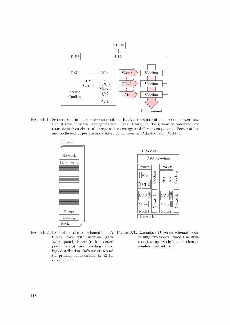
Utility
UPSPDU
HPCSystem
PSU
InternalCooling
VRs
CPU/Mem/I/O
PMU
Environment
CoolingWater
CoolingOther heatgeneration
Other heatgeneration
CoolingAir
Figure B.1.: Schematic of infrastructure composition. Black arrows indicate component power-flow.Red Arrows indicate heat generation. Total Energy in the system is preserved andtransitions from electrical energy to heat energy at different components. Factor of lossand coefficient of performance differs by component. Adapted from [Wil+14]
Cluster
Rack
Network
1U Servers
PowerCooling
Figure B.2.: Exemplary cluster schematic. Atypical rack with network (rackswitch panel), Power (rack mountedpower strip) and cooling (pip-ing / distribution) Infrastructure andthe primary components, the 42 1Userver inlays.
1U Server
PSU/Cooling
NetworkNode1
Power Power
Coo
ling
Netwo
rk
CPU
Mem
CPU
Mem
Node2
Coo
ling
Netwo
rkCPU
Mem
Acc
Acc
PMU
PMU
PMU
Figure B.3.: Exemplary 1U server schematic con-taining two nodes. Node 1 as dual-socket setup, Node 2 as acceleratedsingle-socket setup.
118

resources. Distribution of the supplied power is done by PDUs, while distribution of cooling is donevia air ventilation systems or water piping, connected to the large scale infrastructure cooling systems.
The primary purpose of HPC centers is to operate and provide the HPC system. For this, a lookinside the hardware components which make up HPC systems is needed. Internally the HPC system,again, has systems to manage energy, e.g. Power Supply Units (PSUs), PMU and VRs, and cooling.The centerpiece for computation is however the CPU, memory and Input/Output (I/O) subsystem.These systems consume energy and generate heat, which is in turn handled by the power supply andcooling within the HPC system and dissipated to the infrastructure and further to the environment.This basic view of center infrastructure and HPC system with its fundamental elements is organized
into additional structural hardware component groupings. The CPU, memory and I/O subsystemof the HPC system are clustered systems of commodity components to form the HPC system. Thisis shown in Figure B.2, sketching the typical setup of a cluster of several 42U racks, while Fig. B.3shows a single 1U server.Figure B.2 shows a schematic view of a computer cluster, consisting of several cabinets or racks. A
rack contains power and cooling as well as network to supply the server computers it houses. Withina rack these are, for networking, a rack switch panel, for power, a rack mounted power strip andthe necessary piping or airflow distribution for cooling. A rack houses several servers referred to ascompute nodes, for example 42 1U server inlays, as seen in Fig. B.2.A single rack contains several 1U server inlays containing the compute nodes. The 1U server setup
in Fig. B.3 shows an exemplary hypothetic setup containing two nodes, a typical dual-socket setupon the left-hand side and a single socket setup with two accelerator cards on the right. Other typicalsetups are racks housing several 2U- or 4U-servers or blade-servers mounted horizontally or verticallyin an appropriate enclosure.The components highlighted in these three figures show the crucial components required to operate
an HPC system in terms of energy intake, distribution and consumption with respective measurementand control.
In the following subsections the hardware components of both the computing center and its computerclusters are split into two groups:
• Primary consumers are hardware components that significantly contribute to energy and powerconsumption in the computing center, have mechanisms to measure power or energy consump-tion and have hardware mechanisms to control this consumption.
• Secondary consumers are hardware components that are either insignificant with respect totheir total energy and power consumption, or have no mechanisms to measure or control it.Modeling these may still be required, but control and management has less priority, dependingon the use-case.
The assigment of components to the group of primary consumers and secondary consumers largelydepends on the capabilities of the installed hardware. The following represents the current state of thehardware. This may change over time. Additionally, HPC centers may have their own prioritizationfor components. Requests for vendors to support measurement and control capabilities in the futureis therefore expected. This listing for the background goes from facility to smaller components. Thehardware components are discussed and the relevant concepts for energy and power measurementand control are given.
B.1.1.1. Primary Consumers
The following hardware components are considered primary consumers:
• Utility,• Facility cooling,• PMU,• CPU,
119

• Memory,• Accelerators.
This list is not exhaustive and components that lack any of the measurement or control capabilities ordo not currently contribute an extensive load to the system may become relevant in the future. Thehardware components are discussed according to their basic functionality, measurement capabilitiesas well as control capabilities.
Utility: Utitlity is a general term for all infrastructure level power utility of a HPC center.
Functionality: The Utility is the primary entry point for energy intake and distribution for thefacility infrastructure. At this level the control lies mostly with the ESP and building infrastructure.It is determined how much power can be supplied to the facility and actual consumption for pricecalculations is determined. Energy intake is handled in medium voltage and transformation to lowvoltage takes place here, as well. The PRACE white paper on “Electricity in HPC Centers”[Pos+]talks about this first stage and infrastructure of HPC electricity. The white paper also includes infor-mation on how pricing is generally determined at European centers, based on average consumption in15 minute intervals. Pricing determination differs from center to center and is also handled differentlydependent on the country and regional circumstances [Mai+18; Yon+11].
Measurement & Control: Measurements are generally taken in kW h, (equivalent to 3.6 MJ)mostly for billing, based on the contract. Control is there only indirectly, either by the supplier orby the consumer based on activity of the systems housed in the facility. Naively speaking the centercan decide to switch clusters systems or cooling off. Due to limited granularity of control, and thesafety implications in shutting of cooling, as well as power ramp-rate-control implications, utilitymodifications are not the primary focus for optimization. These are however important backgroundinformation. Additionally, the operating strategy of the utility impacts all other systems in the center,and may therefore be important to be representable.
Facility Cooling: Facility cooling is the cooling infrastructure installed at the HPC center.
Functionality: Facility cooling, depicted on the right-hand side of Figure B.1 is a major powerconsumer, and necessary for efficient operation. The functionality provided is often managed bytraditional building infrastructure management. The facility cooling is either handled via ComputerRoom Air Conditioner (CRAC) or Computer Room Air Handler (CRAH), for air cooling. For watercooling, several independent, yet coupled cooling circles are installed with heat exchangers and chillerinfrastructure.In general cooling demand is regulated by a control loop directly linked to temperature sensors
on the outgoing side of the cooling system, while the effect is delayed until propagated throughoutthe system. Information of these systems is often restricted to the center administration and of-ten not even accessible to cluster administrators, since their scope differs. System administratorsshould confidently be able to run their system without knowledge of the cooling generators as longas they observe safe operating temperatures within the HPC-System. Cooling infrastructure infor-mation is generally maintained in Data Center Infrastructure Management (DCIM) system for bothmanagement and control.The cooling infrastructure is a major contributor to the data center metrics of Power Usage Ef-
ficiency (PUE) [MB06]. Such metrics serve as indicator for optimization of operational costs of asystem. At some facilities different clusters are cooled using different technologies where schedulingand system usage can thus have large impacts on the overall center efficiency.
Measurement & Control: Freedom to control the cooling infrastructure largely depends on cool-ing requirements at a specific point in time, as well as conditions of the temperature environmentof the center and system. Thus, infrastructure cooling is also partially out of scope for this work,regarding control measures, but again serves as important background for policy decisions and saveoperation of the system housed in the facility.
120

PMU: The Power Management Unit (PMU) (as used within this work) is responsible for powermanagement of system, devices, and processor power management (as of ACPI specification [Cor+]).The exact location on the hardware platform, of the associated controller and firmware, differs byimplementation. On Intel platforms, some of this functionality is moved inside the CPU and isreferred to as Power Control Unit (PCU) [Int15b; GSS15].
Functionality: Basic features of energy and power control are steered by the PMU on the server’smotherboard, controlling the underlying behavior of for example the CPU, memory, GPU or otheraccelerators, and I/O which consume a large fraction of the total system energy.The PMU has more management functionality than a simple PSU or VR, which mainly transform
and distribute the supplied power. The PMU is integrated on the motherboard of the server and hasintegrated control functionality via firmware, controlling energy and power functionality of the node.For most functionality interaction with the CPU is necessary. It can however also control connectedmemory and Peripheral Component Interconnect (PCI) connected devices.1
Measurement: Both PMU and CPU provide measurement capabilities, namely hardware coun-ters accessible which are exposed to the OS. These measurement capabilities are exposed via the CPU.Some PMUs provide only limited measurement capabilities making them secondary consumers.
Control: For hardware control, firmware interfaces implementing ACPI specifications are used. Inthe following the ACPI features relevant to all components for energy and power control of the PMUare explained: ACPI [IMT-ACPI; For; Cor+] is a standardization effort that allows unified usageof hardware control register specifying operating modes on dedicated and general purpose hardware,namely the ones controlled by PMUs.These are G-states, D-states, S-states, C-states, P-states as defined in [IMT-ACPI]. The ACPI
power management approach is exposed to OS and BIOS. These states define specific readiness andoperating states, and specify specific transitions and action entering and exiting these states.G-states indicate the global system status. These are global states indicating the readiness of a
device, which are defined as G3 through G0: G3 represents a mechanical off state. G2 indicates anoff state changeable by software, thus minimal power is consumed, with the ability to instruct thesystem to reboot. G1 is a sleep state, able to return to working without a reboot but a system restorefrom the previous working state. G0 indicates the working state. The functionality provided by theG-states can be used for remote wake-up, sleep, shutdown of nodes, with the effect of reduced powerconsumption and later resume to working state. A use-case for this is for schedulers inducing sleepstates to nodes idle for too long [Mai+18]. With the goal of maximizing utilization of the clusters,the payoff of such mechanisms may be small, however.S-states specify more granular sleeping states definitions, and can be placed between G2 and
G1, where S1 to S5 represent different levels of context retainment while sleeping and thus powerconsumption and wake up latency.D-states are mostly used for system components other than the complete node and the CPU. D-
states indicate levels of readiness from turned-off, and even device-removed state, to specifics levelsof context preservation, to fully available and on. These states supported differ by device type, butare useful for example for GPGPU clusters.C-states define processor power state definitions. C0 represents the processor power state in which
the processor executes instructions. C1 is the initial non-operating state, with the lowest latency. Thismeans the latency of switching from C0 to C1 and back is low enough so that the operating softwarecan always consider using it when non-operational. C2 and C3 both have improved power saving,but introducing noticeable latency, with C3 even saving on (read disable) cache coherency. [Cor+;Ils+17]P-states indicate device and processor performance state definitions. P0 Performance state, again
provides maximum capabilities and maximum performance, while being able to consume maximumpower. Performance States P1 to Pn are ordered from smallest to largest power savings, which also
1Most energy and power management approaches interact with either PMU or CPU energy and power management,therefore these two parts are explained in greater detail.
121

impact performance to an increasing amount. According to ACPI, P-states may support an arbitrarynumber of performance states not exceeding 16. [Cor+; Int15b]These cover basic ACPI management features present in most systems devices and processors and
devices. These are generally directly used by BIOS and the OS.
CPU: The CPU is the Central Processing Unit of a computer.
Functionality: The primary consumer of major interest is the CPU. This section contains descrip-tion as well as measurement and hardware control mechanisms of the CPU. Basic internal functionalityregarding power and heat generation of the CPU is required. Within this work the reference proces-sor architecture is the Intel Architecture [Int15b] and features present in modern processors since theSandy Bridge microarchitecture. The general behavior is similar across manufacturers, while specificimplementations of measurement and control functionality may differ.Power consumption of a CPU is dictated by frequency, supply voltage and activity. While idle
power depends on the C-state and P-state, active CPUs have a minimum and maximum power draw.Power consumption of the CPU can be represented according to this formula:
PCPU = Pdynamic + Pstatic + Pleakage
The dynamic power is Pdyanamic = αCV 2f2 , with activity factor α, capacitance C, voltage V consisting
of supply voltage Vdd and the voltage swing both assumed equal, thus V 2, and frequency f [FHR99].Static power Pstatic = Isc∗Vdd depends on short circuit current Isc, while dynamic power Pleakage =
Ileakage ∗ Vdd depends on the leakage current Ileakage. In both static and leakage Vdd is equivalentto the supply voltage [CSB92]. Supply voltage is generally set at minimal possible thresholds whileguaranteeing error free switching for a specific frequency.The limits of switching, required power draw and physical properties are well described by Den-
nard et al. [Den+99], as well as Brooks et al. [Bro+00]. Dennard et al. shows the limits of integratedcircuit shrinking, while Brooks et al. give an overview of microprocessor modeling and chip designmodeling with a comprehensive overview of power-performance fundamentals. These considerationsshow the general proportionality for server CPUs power consumption of P ∝ CV 2f . [CSB92; FHR99;Int04]The components inside the node all generate heat when processing, storing and operating on
data. The statements of the classical work on “Irreversibility and Heat Generation in the ComputingProcess” of Landauer [Lan61] is to be recalled regarding energy loss associated with switching. Ofcourse all components have an electrical efficiency, associate with them. Since this value is < 1they generate heat. This temperature surplus, has to be taken out of the system and is the reasonwhy cooling is the second largest energy consumer in a computer system. With the generated heattransferred out of the system this allows for a stable working environment. In other words, mainpurpose of any computer system to process with a maximum attainable computational performance,with input energy and byproduct heat.Coming back to CPU power, the minimum power is the wattage to supply all CPU components,
while the maximum CPU power consumption is a technical limit named the TDP. The TDP is forboth safe electrical operation, and at the same time represents a safe limit regarding heat generation.Maximum TDP is a fixed value set by the hardware manufacturer for a specific processor architecture,and should be enforced by firmware. Colloquially TDP is said to be the maximum power a processorcan consume [Cut].
Control: Regarding active energy and power control of CPUs (in this work by example of pro-cessors from Intel) the two most relevant mechanisms are discussed: DVFS and RAPL.DVFS uses the two variables voltage and frequency to alter power consumption and processor
performance. P-states are generally implemented using DVFS as mechanism. As described in theIntel 64 and IA-32 Architectures Software Developer’s Manual Volume 3 Chapter 14 [Int15b] the P-state mechanism is controlled by registers IA32_PERF_CTL and checked by IA32_PERF_STATUS [Int15b;Int15a; Int04]. P-states, as specified in [Cor+], are defined per processor. The concept of DVFS isnot tied to a specific domain of control within the processor. Depending on the hardware capabilities
122
and exposed firmware control mechanisms DVFS can be applied as granular as a per core frequencycontrol. In addition to that P-states have set number of states as defined by ACPI, while generalDVFS can have much finer granularity. The voltage selection is in general done via static mappingaccording to the set frequencies guaranteeing safe and efficient operation. The voltage does not impactcomputational performance, but is minimized while guaranteeing correct switching at the specifiedfrequency. Control of the processor, implement ACPI specifications, as well as general DVFS isavailable since Pentium II with Intel Speed Step [Int04].The second mechanism is RAPL, the Intel’s Running Average Power Limit. For this mechanism
TDP is important. TDP is an empirically defined upper limit for processor power draw, enforced byfirmware. Using RAPL this limit can be artificially reduced further.Control is exposed via control registers of the CPU [Int15a]. Limits can be set according to the
registers MSR_PKG_POWER_LIMIT, MSR_PP0_POWER_LIMIT, MSR_PP1_POWER_LIMIT. These registers setpower limits for a specified time window and guarantee that the running average power is not exceeded.Different limits apply to different domains of the chip according to the specifications. [Int15b; Int15a].This is a different mechanism for power/performance trade-off while not setting a fixed frequency fora specified duration but specifying power limits directly.
Measurement: As mentioned in the control paragraph CPU measurements are accessible usingprocessor registers and specific MSRs, either read directly or exposed to by the operating system.This is true for both DVFS and RAPL. DVFS features only allow to measure frequency and per-formance, e.g. via performance counters. No direct power or energy measurements are available.RAPL on the other hand allows measuring derived power for a specific domain directly. For exampleMSR_PP0_ENERGY_STATUS can be read for the energy consumed by the domain of processor cores, asspecified in [Int15b]. Access to these registers has to be configured and is not generally available foreither DVFS and RAPL, and are in general exposed via the OS. External hardware instrumentationtools for CPUs, based on shunts or hall effect sensors, exists but are often prohibitive for general useat a cluster scale.
Memory: Memory is the primary storage in the memory hierarchy used by the CPU.
Functionality: Memory is generally operated at the same frequency (for example inDDR4 SDRAM), with voltages again chosen for reliable operation. This allows for reliable tim-ing and intervals as needed by the processing elements [JED03]. Therefore, power consumption isoften assumed static, since isolated measurement is non-trivial.
Measurement & Control: RAPL also introduced Dynamic Random-Access Memory (DRAM) ascontrol domain, supported on server processors. Desrochers et al. [DPW16] investigated RAPL formemory, validating measurements and the used power model. This allows for control and measure-ment of energy expenditure of the memory. RAPL control for memory is achieved, not by impactingpower consumption, but by controlling memory bandwidth. Power consumption is mostly dictatedby access rates, thus indirectly control-able. Both measurement and control of DRAM consumptionis available on modern server processors by Intel [Dav+10; DPW16; Int15b]. External hardwareinstrumentation tools for memory measurement, based on dual in-line memory module (DIMM) risercards, exists but are again prohibitive for general use at a cluster scale.
Accelerators: Accelerators are extension cards with special purpose processors, supplementing theCPU. These are for example GPUs, FPGAs, many core devices and vector processor extension cards.
Functionality: Accelerators are major power consumers for computer nodes that obtain the majorcompute performance from such cards. Their power characteristics similar to CPU, however sincethey often process streaming data, their power profile is more predictable, in case the kernel profilesare known.
123

Measurement & Control: Accelerators cards share several features with the CPU in terms ofenergy and power control and measurement. They are however often a few generations behind themeasurement and control of CPUs. The discussion above focuses on the CPU but several of theabove points are applicable to GPUs as well, such as ACPI features. Some of the more fine-grainedfunctionality is expected in future generation GPUs. DVFS frequency control exists, and features suchas power limits and power usage exists, for example as specified in NVIDIA Management Library(NVML) [MC18; NVI13]. For other accelerators such as Intel Xeon Phi RAPL functionality isavailable [Int17; Int16].Depending on the maturity of control and measurement capabilities accelerators can either be a
primary or a secondary consumer even though they are in general major power consumer in HPCsystems.
B.1.1.2. Secondary Consumers
The following components are considered secondary consumers:
• UPS,• PDU,• PSU,• Node cooling,• VR,• I/O and networks.
These components either do not have significant (dynamic) power consumption, or lack monitoring orcontrol capabilities. The hardware components are discusses nevertheless to understand the completesystem background in relation to energy and power for this work. Additionally, hardware capabilitiesdo change over time and components considered a secondary consumer here potentially move to thecategory of primary consumers in the near future.
UPS: The first component from the infrastructure side, as seen in Figure B.1, is the UPS handlingresiliency of the system with regards to power fluctuation and supply failure. UPSs builds the maincomponent for resilience and reliable power supply. Uninterrupted power can for example be achievedby staged fail-safe mechanisms: Batteries, for short term bridge and startup of generators, and dieselgenerators for safe shutdown, as well as longer term safe operation of (mission-)critical systems duringpower failure. These are emergency systems and can not generally be used for power management andfor normal operation strategy. Research does exist in this field however and the reader is referred topower co-generation as evaluated by Tokyo Institute of Technology in their Tsubame system [Yon+11].The UPS is connected to support cooling as well as the computer systems installed in the system.
PDU: The next hardware component, considered a secondary consumer PDU. The power distribu-tion is often done in a hierarchy and well integrated with infrastructure circuits, to support loads,while not overloading fuses. There are three kinds of PDUs: Units distributing power to differentsystems in the center, units distributing to the racks of the various systems, as well as rack internalPDUs, distributing to the servers mounted in the rack. PDUs sometimes have power meters inte-grated which allow good measurements. If power readers are not integrated, the PDUs’ power-plugscan be used for external power meters if measurement at this granularity is required. Some solutionsand their usage in clusters are discussed in [Dio+13; Ils+15]. Control capabilities are limited ingeneral.
PSU: Inside a node the primary unit for energy intake is the PSU present at every node. Theprimary objective of the PSU is to transform the 230 V supply power to 12 V and distribute thispower to the components on the node. The PSU distributes the power to the node components,such as fans and active cooling, which exchange heat to the cooling infrastructure outside the node,as well as on node, the PMU, VRs and finally CPU, Memory and I/O and potentially accelerator
124
cards. In terms of hardware control and measurement on node, there are several interaction points.If management of the PSU is done, this is steered by the PMU or BMC, while itself PSU suppliesand distributes.
Node Cooling: Regarding node cooling air and water have to be differentiated: Water cooling is notdirectly controllable in server installations, since pump, inlet and outlet temperatures are controlledand managed on the infrastructure side of the cooling cycle. Conversely, regarding air temperaturePMUs can alter fan speeds which draw power. Their direct impact on power consumption is oftenneglected while controlling temperature is important for VRs and general CPU and memory powerperformance dependence, and are important to control thermal induced variability. Reactive andproactive control of fan speed remains active research [Acu+17; Acu17].
Voltage Regulators: On the motherboard VRs transform power from 12 V to lower required operat-ing voltages. VRs internal to the CPU match DVFS requests to the appropriate electrical potential.The voltage regulators are not generally accessible for direct control, but modern motherboards sup-ply sensors for measurement, which play a critical role in system health [GSS15]. Depending on thelocation of the VR, their health and usage can be monitored by administrators via the BMC.
I/O and Networks: Network Interface Controllers (NICs) and switches are not directly controllablepower consumers. Network cards have a power consumption around 5 − 10W [GSS15]. Switchesare in the 100 − 300W range [GG15]. Their aggregate power consumption contributes to overallsystem costs, power usage based on activity is not energy proportional with usage, however. Evenwith low activity their power usage remains high. Dynamic link management is still subject to longadjustment times. [GG15] Research in dynamic energy and power management of the network is stilllimited, but improved I/O capabilities are becoming a requested topic of EE-HPC-WG procurementconsiderations [EEWG17].The network of HPC system is however critical to energy and power management for a second
reason: Management and monitoring information has to be communicated within the system. Whenusing runtime systems to monitor and control energy and power decisions latency of transmissionsare critical. Modern computer systems generally have two networks for the computer system. First,the primary high performance network. This network has very low latencies, high bandwidth andspecific topology ideal for the system at hand and generally intended for the applications runningon the system. Technologies for this often use optic-fiber, for example Infiniband, Fibre Channel orGigabit Ethernet. Second, the administrative network. This secondary network is a backup networkto service nodes, that are either unavailable (in the primary network) or for system health inspection.This network should not be burdened by constant loads, since it is not designed for this use-case.Additionally, if the network is needed for an incident it should not be highly saturated by otherroutine tasks, such as sensor data distribution. This network is often not directly connected tostorage systems.When operating system software to optimize energy and power it is critical to avoid the introduction
of noise into the primary or secondary network degrading or impacting their required performance.At the same time timeliness of control information as well as amount of sensor data is of large value.
B.1.2. Background – SoftwareTo understand how software interacts with the described hardware mechanisms the following aspectsof software and energy and power are discussed in the sections below:
• Software in an traditional HPC environment;• Software interacting with energy and power.
The initial section recalls the typical operation of HPC from a user/application perspective (inSec. B.1.2.1). This leads to software actively interacting with aspects of energy and power, toformulate the background on the potential software components present in an energy and powermanagement setup (in Sec. B.1.2.2).
125
B.1.2.1. Software in a Traditional HPC Environment
HPC systems consists of a complex setup of software to provide reliable high performance. Thissection presents the logical cluster organization, and the software enabling such environment withinthe system. Additionally, it is shown how users interact with such system and how user jobs areprocessed. This is required to understand which components and processes are present in the systemand which aspects are relevant to energy and power management.
HPC Cluster Organization: The computing hardware is configured in such way that specific usage ofthe system is incentivised for all users to be able to maximize their productivity and their applicationsperformance. Having large parts of the system idle or blocked by users not utilizing the node is costlyfor the center with the large procurement costs for the computer systems and idle power consumption.To maximize utilization and fair share, or enforcing a different specific usage models of the system isoperated in batch scheduling.The scheduling algorithms are optimized for high throughput, high productivity use, with many
users enqueuing jobs. Batch scheduling system have three types of nodes: login nodes, service nodesand compute nodes.A small number of nodes serve as login nodes to the system. These are the initial point of access
for the users of the system. On the login nodes the users of the system are presented with a standardLinux environment with access to their $HOME directory and default applications, compilers, editorsand tools. Specific to HPC environments, there are tools for optimization and usage dedicatedto the distributed mode of operation. Login nodes are used to configure job scripts, set up thecomputer’s environment files and directories and submit jobs. After the jobs complete the resultsof the applications executed and completed experiments are accessed and processed further. Nodemanding computation is to be executed on the login nodes, since many users are accessing thesesimultaneously.Similar to login nodes, service nodes are not part of the compute nodes, but are dedicated to the
administrators of the systems, to service the nodes. In general, even for large clusters there are onlyone or two nodes dedicated as service nodes.The majority of the nodes of a cluster are dedicated compute nodes. Users cannot directly access
the compute nodes, but they submit compute jobs in the form of a job script to a batch schedulingsystem. The compute nodes form the heart-piece of the cluster, containing the high performancehardware and are interconnected with low latency high throughput network among themselves andto storage systems.
Processing of HPC Jobs: Once a job is submitted, the job scheduler evaluates the preamble ofthe job script and places the job in the job queue according to the scheduling algorithm used. Theresource manager manages the resources (i.e. the nodes) of the cluster. In accordance to the order ofthe job queue the resource manager allocates the nodes and forms a partition for the next job, sufficingthe requested resources and the requested time. Within such a job partition the user application isexecuted, as specified in the job script.In general the applications is executed on all nodes of the job partition in parallel. For node local
performance optimization thread-level concurrency is used (e.g. as provided by Open Multi-Processing(OpenMP)). For communication among the nodes communication libraries such as Message PassingInterface (MPI) or languages using PGAS concepts are used. Programming models and high pro-ductivity tools are generally provided by the computing centers. This is crucial for performance,especially if the system uses accelerators. Once the job terminates, the resource manager claims thenodes again and sets them to back into a clean, known state so that they can be used for the nextreservation. The user is notified about the completion of the job and output and log files are placedin their specified directories.To achieve the best possible performance administrators provide modules and libraries which can
be loaded using a module system. Some applications are used without user modification and are alsoprovided with optimized configuration.Within this default setup of HPC environments and job processing, users never come in contact
with the notion of electrical energy and power consumption. Some systems supply energy and powerfeedback to the users in the form of log files. This is however not standard practice and often only of
126

minor interest to the user, since it generally serves to inform users, not for user-billing. According tothe knowledge of the author, there is no known HPC system, where the budget for computation ofthe users is accounted by energy or power consumption or where such approach is used as alternativeto CPU-hours as budget.The users’ goal of using the system is to complete their computational tasks. Thus, the primary
goals for users are: correct results, and timely completion. For the timely completion, performanceoptimization is necessary. This is also supported by tools, such as: Debuggers for correctness andprofiling and tracing tools for performance, to support the users’ efficient usage of the computersystem.
B.1.2.2. Software Interacting with Energy and Power
For the design of an integrated energy and power management system the last important missingpiece is to look at and understand software that already interacts with energy and power. There areseveral software components that address energy and power controls directly, but these are generallyoperated in isolation. This section addresses:
• Operating System,• Software-Interfaces,• System Software,• Tools,• Applications.
These types of software have both different capabilities, and also different interest, in their interactionwith energy and power. In general, they do not have any interaction with the other classes in termsof energy and power and operate independently, given they have the required permission. Afterwardsthe background information can be tied together looking at related work for this research regardingintegrating energy and power management and the modeling of such systems.
Operating System: OSs use several of the hardware interfaces for energy and power managementdirectly and have the capabilities to exposes those to all software running on the individual nodes.The OS has the scope of managing resources of a single node. Additionally, the OS is the gatewayfor exposing hardware functionality via kernel modules and the associated file system locations.The role of the OS in power management stems from its two most fundamental roles: Providing a
clean abstraction to hardware resources and the management of these available resources [TB14]. Thefunctionality of modern OSs with regard to energy and power management mostly originated fromrequirements of Personal Computers (PCs) and laptop computers. This can already be seen whenlooking at the ACPI, as discussed in Section B.1.1. The low power consumption use-cases handled bythe OS use the above mentioned P-states and C-states. They are initiated when pressing the powerbutton, inducing sleep or hibernate states or when closing the laptop lid. The mechanisms providedare used to address functionality to improve longevity of battery life.These functionalities have transitioned into general data-center operation, as well, with normal web-
server use-cases. Servers can safely go into a power-saving mode when no requests have be handled.Once the server encounters load, fast transition into P-state P0 is required. Thus, algorithms providedby the kernel to decide for example what time periods for appropriate C-states are adequate, sincestates saving more power increase transition time to switch back to P0.2In the HPC case, the OS can oftentimes interfere with the desired performance goals, for example by
undesired process scheduling, and focusing on correctness, neglecting performance [Loz+16; Ils+17].This represents the other extreme, where not idle systems have to be managed, but full performanceis hindered by tasks operating at inappropriate priorities in the eyes of the user.To address what functionalities Linux provides in this regard, a short overview of the Linux drivers,
acpi_cpufreq and intel_pstate, for energy and the specified power governors associated and de-scribed in the Linux documentation are given: performance, powersave, userspace, ondemand,conservative and schedutil. [Bro+]
2P0 requires C0, while transition times withing P-states are generally not affected by the P-state selected.
127

The drivers use information about the processors specified minimum and maximum frequency, ora specific target frequency between minimum and maximum frequency:
• The performance governor chooses the maximum frequency allowed by the CPU’s frequencyrange.
• The powersave governor chooses the minimal frequency allowed by the CPU’s frequency range.• The userspace governor allows any user, or userspace program with User Identifier (UID) root
to set a fixed frequency.• The ondemand governor sets the frequency according to a load estimator triggered by the Linux
scheduler. The estimation is done over a short time window and requires a specific maximumtransition latency to work properly. Additional parameters are passed to decided when loweringthe frequency is estimated to be a sound decision. When demand for performance is detected,frequency is set to the maximum allowed.
• The conservative governor has a similar behavior as ondemand with the difference that ondetected performance demand, the frequency is gradually increased, contrary to setting thefrequency to the maximum instantly [Bro+].
• The schedutil governor has a tight integration with the Linux kernel scheduler and its Per-Entity Load Tracking (PELT) mechanism for better load prediction [Cora; Brob].
For the HPC use-case either performance, or userspace are used. The ondemand governor is atypical found in desktop or server setting. [Bro+]The Linux cpufreq subsystem implementation, and the systems cpufreq-drivers dictates the ex-
act functionality of each of the above mentioned governors. Looking at differences in driver, theacpi_cpufreq driver uses the ACPI specified P-states and functionality. In addition, turbo boostis used with arbitrary turbo frequency if the frequency is specified as 1MHz above the maximumfrequency. The functionality of the intel-pstate driver uses additional features enabled and docu-mented for Intel specific functionality and can be found openly in [Wys]. This driver implements andprovides a performance governor or defaults back to a powersave governor using an intel hardware-specific implementation as provided in the Linux kernel [Broa; BWK; Bro+; Wys].For other software, outside the OS, to directly change power and performance, awareness of which
drivers and governors are compatible and do not override these settings is required.The OS plays an important role in making interfaces to hardware controls available to administra-
tors and user-space via kernel modules. The msr kernel module is an example for this. Loaded bymodbprobe msr, the MSRs control registers are exposed in /dev/cpu/cpu*/msr of the Linux Filesys-tem Hierarchy Standard (FHS). Since this functionality is however separate from the OS’s usage ofthe interfaces these will be discussed in the next section regarding software interfaces.The OS has other interfaces to applications which also impact energy and power characteristics.
The default Linux job scheduler impacts the resource usage of a specific process and how to prioritizeit. The OS, however, only has limited knowledge about the application its energy and power char-acteristics or how to prioritize processes according to this. The process scheduler considers accesstime to the CPU. To alter process priorities the Linux the program nice [mana], is used to changeapplication-“nice-ness”(priority). For HPC applications, where a single job reserves nodes exclusivelythe application is of most priority. In such usage scenario the OS is to be configured accordingly,disallowing other processes of lesser priority to hog resources. It has been shown that this is nottrivial, even if previously considered so. Exact configuration and knowledge of the set state is thusneeded. [Loz+16]
Software Interfaces: The hardware interfaces of the system are typically not directly accessible forall software of a system. For this reason software interfaces to energy and power measurement andcontrol exist. These serve to address and expose energy and power hardware interfaces, but alsoaddress hardware abstraction. Additionally, access control is managed via these software interfacesin some cases, whereas the basic configuration has to be set by the admins.Admins with root privileges can read and write any exposed device file in sysfs is located in
/sys/devices/system/ or device drivers in /dev/. Since direct access is error prone, for ease of
128

use and safety reasons tools to write these settings for privileged users exist. An example for thisis the direct setting of frequencies by the administrator using the exposed P-states mechanism. Thetool cpupower frequency-set 〈FREQ〉 allows root users to set processor frequency directly. Theunderlying DVFS and P-state mechanism adjusts the frequency and according voltage interacting withthe firmware power settings. Similar mechanisms for privileged users exist for writing RAPL powerlimits: As discussed above, access to MSRs is exposed via Linux kernel drivers managing MSRs. Theseare directly addressed by reading and writing the device driver in /dev/cpu/cpu*/msr. To abstractthis interaction, rdmsr and wrmsr is provided when loading the kernel module for MSRs [Corb]. Thismeans that privileged users can directly manipulate everything exposed. In a multi-user environmentno save abstraction is thus provided.For software interfaces directed towards users with finer control, additional abstractions exists.
These are for example the software interface like msr-safe [Sho+]: The msr-safe tool provides akernel module for safe reads and writes to MSRs, provided a white-list file, which allows to spec-ify which MSRs should be read- and write-able by users or a user-group. Using this mechanism,administrators can configure a subset of MSRs and make them available for read and write. Thisagain follows standard Linux user and group permission settings, but allows for finer granularity inaccess control. Similar methods have been designed for PCI Control and Status Registers (CSRs),providing a tool called csr-safe, which hasn’t seen as wide adoption for alteration on energy andpower usage [WM16]. A recent effort to combine multiple of these tools for better granularity ofinterfaces to energy and power interfaces which provide a safe access model, using csr-safe andmsr-safe among others is variorum [LDR17; Bri+].A software interface that has a wider scope than bridging hardware abstraction over the OS is
Power-API [Gra+16; III+16]. Power-API is a portable API for power measurement and control.Interfaces for programmatic use of power can be encoded in XML-format or JSON-format, whichrequires known protocols and interactions between interacting programs. With known hardware,interactions and requirements an API can be specified relying on known interface encoding. Power-API specifies roles, system descriptions, attributes and meta-data information to concretize the API.It provides type definitions, interface functions, high-level functions and role/system interfaces. ThesePower-API is given as C-API and supplemented with Python language bindings [III+16]. This APIis adopted in tools and by vendors especially on the infrastructure side of power management andmonitoring controls. The usage model regarding its operation is important related work for this thesisdocument and covered in the related work section (Sec. 2.4).Several APIs traditionally rooted in performance profiling and tracing have also been extended for
energy and power monitoring. Examples for these are Performance Application Programming Inter-face (PAPI) [Ter+10], Score-P [Knü+12] or the Linux perf interface. These APIs are not generallyused to set and alter energy and power settings, but have been augmented or extended to includeperformance metrics related to energy and power. These APIs serve as unifiers and abstraction layerfor accessing the underlying architectures in a platform agnostic way. Their granularity can be quitedifferent: Where perf is suited for more direct, low level access, Score-P provides a high level abstrac-tion, utilizing low level interfaces itself internally. perf utilizes the low level Linux RAPL MSRs andrequires root privileges. This interface is exposed by the OS as perf_event interface since Linux ker-nel 3.14 [Kha+18]. PAPI uses perf events to obtain performance data, while accessing RAPL countersdirectly via MSRs. PAPI either requires root privileges or can use the msr-safe library, contrary toperf. Score-P provides a whole runtime infrastructure to homogenize interfaces intended for tools likethe PTF [BPG09; Sik+16], Scalasca [Wol+08], Tuning and Analysis Utilities (TAU) [MBM94] orVampir [Knü+08]. The work of Score-P is extended to the usage of energy within the Scalable Toolsfor Energy Analysis and Tuning in HPC (Score-E) project [Die16; Hera].
System Software: System software plays a major role in optimization of energy and power usingsoftware. To improve utilization of energy and power as a resource and the management of thisresource is also where most research is taking place. Prototyping of these approaches can be donequickly, providing testable solutions, while at the same time not directly impacting mission criticalsystems, contrary to research targeting infrastructure software.For energy and power management approaches the following approaches exist for system software:
• Job schedulers,
129

• Power schedulers / cluster power managers,• Job runtimes,• RAS systems,• Monitoring systems.
Most system software has an inherent purpose outside of energy and power. These capabilitiesare in a transition where more and more energy and power relevant topics are added to this originalfunctionality. Other system software is created with energy and power management as its sole purpose.In the following several examples from the above mentioned categories are presented as background.These also present the main actors and components in an integrated energy and power managementsystem. Some system software combines different aspects of energy and power management which arepart of more than one category. This work will split such software and characterize by its functionality.
Job Schedulers: Job schedulers are using batch scheduling algorithms to ensure optimal nodeusage for the complete cluster, as mentioned in Section B.1.2.1. The job scheduler optimizes forthroughput, turnaround time and system utilization [TB14]. Once energy is added to the managedresources, for example by specifying a maximum power draw limited and jobs having a known powerconsumption, schedulers which are aware of this information can optimize their scheduling decisionsand direct resource managers to configure the job partition in particular ways. Several approaches forenergy and power aware schedulers exist. It has to be noted that the resource management aspect,necessary for the resource allocation after scheduling, is often intertwined into this aspect of energyand power aware scheduling. For energy and power aware schedulers the following approaches aretaken: Energy tagging, using energy and power metrics and job characteristics for scheduling andresource management, and scheduling for over-provisioned systems.The first approach to energy aware scheduling discussed is energy tagging. This was initially done
at LRZ using the IBM LoadLeveler with the introduction of energy tags [Auw+14; Bel+13]. Byanalyzing the workloads of LRZ, the optimal frequency of operation was determined for the Super-MUC Phase 1 system [Auw+14]. The employed scheduler used this information with the addition ofheuristics, to derive the optimal frequency for each job (as described in the patent [Bel+13]). Themechanism can be summarized as follows: During operation several metrics are collected includingfrequency, runtime, Cycles Per Instruction (CPI), a proxy for effective memory transactions, amongothers, as well as job identifier (job-ID) and user assigned energy tag. These are stored in a jobdatabase. Upon identification of the same job according to the energy tag, the scheduler triggers aprogram which extrapolates the energy consumption for each possible frequency. With this infor-mation the optimal operating frequency for the job is derived to minimize energy to solution. Theresource manager sets the allocated partition to the derived optimal frequency and the job is exe-cuted. The energy tagging mechanism of LoadLeveler has been migrated to Platform LSF [IBMa].The energy tagging identifies characteristics of jobs which the resource manager uses to prepare theenvironment, while the scheduling algorithm can remain energy and power oblivious.The second group of approaches use energy and power metrics for scheduling decisions [Wal+16;
Cha+19; Mau+19; Hu+17; Kum+20]. Looking at scheduling algorithms different approaches ex-ists, such as Maurya et al. [Mau+19] optimizing for energy savings while keeping a fixed schedulermakespan, other approaches such as Hu et al. [Hu+17] optimize for turnaround time. Both Mauryaand Hu’s optimization is done using DVFS. Chasapis et al. [Cha+19] evaluate variability of powerconsumption of nodes and optimize via job placement while driving scheduling decisions based ona power budget. Kumbhare et al. [Kum+20] look at value-per-time algorithms and extend thesewith power allocation strategies comparing different approaches. Wallace et al. [Wal+16] combineapproaches of traditional scheduling and complete system monitoring to control power load. Thisis done by learning job power profiles and altering scheduling. In cases where a power budget isexceeded DVFS is used to control the power consumption.The last group of research described in this paragraph is scheduling for hardware overprovisioned
systems [Pat+15; Kon+19]. In a hardware overprovisioned system [Pat15, p. 15] additional hardwareis installed, with the goal to keep power consumption of the center constant. This requires highfidelity control over power characteristics of the complete HPC system. From a cost perspectivepower is the limiting factor for large scale centers. For scheduling on such a system additional job
130

properties have to be given to be successful: Information on the impact of lower power consumptionby using DVFS or power capping on runtime, similar to energy tags. Additionally, the additionof functionality such as possible moldable- or maleable jobs [Sar+14] can increase the possibilitiesof scheduling in hardware overprovisioned systems. Regarding power limited environments and jobschedulers, a large body of research exists considering improvements on scheduling for overprovisionedsystems. [Raj+17; Pat+15; Sar+14; Ell+16b; Wal+16].An EE-HPC-WG EPA-JSRM survey [Mai+18; Koe+19; Koe+18] has shown that general energy
and power aware scheduling is not yet widely adopted but centers are building initial capabilities tointegrate such technology and are assessing center specific requirements.
Power Schedulers / Cluster Power Managers: Power schedulers are specific cluster power man-agers, separating energy and power management functionality with a cluster scope from traditionaljob scheduler and resource manager functionality [Ell+15a].3 Power schedulers schedule and reallo-cate the power in between nodes, based on demand and limitations of their cluster. This kind ofsystem software is a resource broker for power consumption of the cluster. Power schedulers consistof two components, node local daemons running on the complete cluster and a management instanceorchestrating individual nodes to fulfill the power scheduler’s optimization goal.The prime example for this is POWsched [Ell+15b; Ell+16b; Ell17]. POWsched measures power
consumption of all nodes. When detecting that specific nodes draw a significantly higher portion ofenergy over a specified period of time, POWsched adjusts power consumption of the nodes. Redis-tribution of power is done in a fair way according to a simple heuristic. The goal of POWsched isto provide fair usage of power, while reducing overall energy consumption. POWsched is completelyagnostic of jobs and partitions allocated on the cluster, and treats this as the domain of the job sched-uler and resource manager. Power schedulers can have a notion of jobs or can be job-oblivious. Jobaware means that adjustments are made with the knowledge of which nodes belonging to the samejob. Such job awareness prevents averse power allocations. Job awareness is not to be confused withruntimes which directly interact with applications. POWsched [Ell+15b] is a job oblivious exampleof a power scheduler.Other system software which fall into the category of power schedulers are: EAR Daemon (EARD)
together with EAR Global Manager Daemon (EARGMD) of the Energy Aware Runtime (EAR)[CB19; Bro+19] energy management framework or the demand-aware adaptive power managementframework by Cao and Kondo [CHK16]. For both of these frameworks specific parts are powerschedulers while the larger framework also adds several interactions with specific job schedulers,monitoring systems, and additional software interfaces to interact with the applications similar to thefunctionality of a job runtime.
Job Runtimes: Job runtimes run alongside applications, utilizing information from the hardwareplatform and the application to optimize specific characteristics of either of them. Job runtimes havethe scope of a single job. They operate on the cluster partition they are assigned to by the resourcemanager. There are two ways to start a job runtime: Either the user starts the job runtime alongsidethe job by themselves, like any user tool, or the user is mandated to run it with any application.To enforce a mandatory use, a technical solution is desirable. For a technical solution, the resourcemanager can prepare the environment of a partition, such that the user cannot disable the invocationof the job runtime, unless actively trying to break out of the system.Job runtimes have two sources of information: The application, and the hardware platform. The
application can actively interface with the job runtime, providing information about its state andbehavior. Alternatively indirect exchange of information is possible. This indirect exchange is notactively implemented by the application programmer, but supported by the use of standardize pro-gramming models which support tools interfaces during runtime. Examples for tools interfaces areMPI_T for MPI [MPI15] or OMPT for OpenMP [OMP]. Function calls by the application that utilizethe programming model can then be intercepted by the job runtime to get information about whatthe application is doing. Interaction of the job runtime with the hardware platform is achieved usinginterfaces such as the ones discussed in the software interface paragraph, above. In addition to these
3In contrast, job schedulers and resource managers functionality in the paragraph above explicitly extended jobschedulers and resource managers with energy and power functionality.
131

two sources of information, the environment the resource manager provides can also be critical to jobruntime’s mode of operation: Options set in the job script, or set by job scheduler/resource managerimpact the behavior of programs running in userspace: Both compute job and job runtime. Somejob runtimes and job schedulers have introduced interfaces for a more direct interaction [GEOa].The optimization a job runtime is able to achieve largely depends on the type and capabilities
of the job runtime. Such capabilities can be sophisticated power and performance models on singlenodes, but also multi-node optimization. The advantage of job runtimes is their scope of a job andpotential control over all participating nodes. Such a runtime can efficiently aggregate informationfrom each process and node participating in the job, since they share the same high-performancecommunication infrastructure, as the job itself. With the appropriate runtime agents aggregatingand processing the information continuously, job wide optimization is possible. Several runtimes usethe information about distributed behavior to leverage potential from manufacturing variability seenacross nodes or critical path analysis to understand job-global progress driving energy and powertuning devisions. Job runtimes that only utilize job local information, on the other hand, mitigatepotential communication overheads.GEOPM [Eas+17] is an example for a job runtime continuously optimizing platform settings via
MSRs. The runtime is operating alongside the application, one process, or thread depending onhow it is set up, in a distributed fashion using its own MPI communicator. Using this approachthe runtime can optimize more than just individual nodes, and individual application processes, butachieve a global optimization. The runtime achieves this by implementing a Partially ObservableMarkov Decision Process (POMDP). Other examples of runtimes using distributed information arefor example Conductor [Mar+15]. This runtime performs distributed critical path analysis. Thefocus is more on the application side, than the platform side, compared to GEOPM.Other runtimes are not distributed but operate on node local information of both platform and
application. An example for this is EAR, where EAR library (EARL), Dynamic Application IterativeStructure detection algorithm (DynAIS) and EARD can be seen as the runtime part of EAR [CB19].Yet again other runtimes use application information regarding communication characteristics, suchas COUNTDOWN [Ces+18], whereas the information is only used for node local optimization. Thereexist a large variety of job runtimes or tools fitting in the runtime category.Several programming models that operate using runtime systems by themselves, have also looked
into integrating energy and power extensions as proof of concepts. This has been done by show-ing, that a tightly integrated interface to power is especially useful with good knowledge aboutapplication behavior. Such examples are presented in [Acu+16; Acu+17; ACK19; Acu17], by usingCharm++ [Ill] as programming model. For High Performance ParalleX (HPX) [KBS09] the Auto-nomic Performance Environment for eXascale (APEX) project [Huc+13] serves as example. Similarly,for OmpSs [Dur+11], the works in [Mar13; MMN13] shows examples for energy extensions.A key takeaway is that job runtimes for energy and power management have to interface with the
hardware platform and the application to do their work, for basic functionality. To achieve goodoptimization, however, additional interaction with the job scheduler/resource manager is needed,especially for production use. An even more important aspect is that such interface is needed tocommunicate change in optimization strategy or convey the intent of an optimization. A lack ofinterfaces limit changes in strategy to a complete reconfiguration of the system.
RAS Systems: The main purpose of RAS systems is reliability, availability and serviceability, asthe name suggests. This means in particular to keep the system functional, and available, but alsohave functionality that allows to service the system in the case of a failure. Such system has to havemonitoring capabilities to detect both faults but also have knowledge that the system is running asintended.RAS systems have a central control entity, operated and monitored by either system integrator or
system administrator. The system itself has sensors and monitoring systems, that is seen as vitalto observe reliability and availability. In the case that service is needed, it is important that quickresponse is possible. This means that separate service infrastructure is required in general. RASfunctionality is the primary use-case for the service infrastructure of a HPC system. Traditionallyit is the only system allowed to operate on the dedicated out-of-band service infrastructure. Onlyafter thorough assessment other systems are allowed to use the service infrastructure. Depending on
132
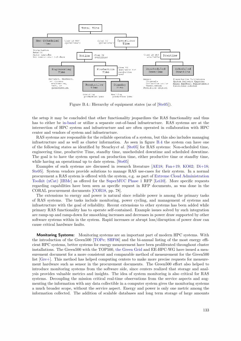
Figure B.4.: Hierarchy of equipment states (as of [Ste05]).
the setup it may be concluded that other functionality jeopardizes the RAS functionality and thushas to either be in-band or utilize a separate out-of-band infrastructure. RAS systems are at theintersection of HPC system and infrastructure and are often operated in collaboration with HPCcenter and vendors of system and infrastructure.RAS systems are responsible for the reliable operation of a system, but this also includes managing
infrastructure and as well as cluster information. As seen in figure B.4 the system can have oneof the following states as identified by Stearleyet al. [Ste05] for RAS systems: Non-scheduled time,engineering time, productive Time, standby time, unscheduled downtime and scheduled downtime.The goal is to have the system spend on production time, either productive time or standby time,while having an operational up to date system. [Ste05]Examples of such systems are discussed in research literature [AE18; Fan+19; KO02; Di+18;
Ste05]. System vendors provide solutions to manage RAS use-cases for their system. In a normalprocurement a RAS system is offered with the system, e.g. as part of Extreme Cloud AdministrationToolkit (xCat) [IBMc] as offered for the SuperMUC Phase 1 RFP [Lei10]. More specific requestsregarding capabilities have been seen as specific request in RFP documents, as was done in theCORAL procurement documents [COR18, pp. 78].The extensions to energy and power is natural since reliable power is among the primary tasks
of RAS systems. The tasks include monitoring, power cycling, and management of systems andinfrastructure with the goal of reliability. Recent extensions to other systems has been added whileprimary RAS functionality has to operate self-contained. Example issues solved by such integrationare ramp-up and ramp-down for smoothing increases and decreases in power draw supported by othersoftware systems within in the system. Rapid increases or abrupt loss/disruption of power draw cancause critical hardware faults.
Monitoring Systems: Monitoring systems are an important part of modern HPC systems. Withthe introduction of the Green500 [TOPe; SHF06] and the bi-annual listing of the most energy effi-cient HPC systems, better systems for energy measurement have been proliferated throughout clusterinstallations. The Green500 with the TOP500, the Green Grid and EE-HPC-WG have issued a mea-surement document for a more consistent and comparable method of measurement for the Green500list [Gre+]. This method has helped computing centers to make more precise requests for measure-ment hardware such as sensor in the procurement documents. The Green500 effort also helped tointroduce monitoring systems from the software side, since centers realized that storage and anal-ysis provides valuable metrics and insights. The idea of system monitoring is also critical for RASsystems. Decoupling the mission critical real-time observations from the service aspects and aug-menting the information with any data collectible in a computer system gives the monitoring systemsa much broader scope, without the service aspect. Energy and power is only one metric among theinformation collected. The addition of scalable databases and long term storage of large amounts
133

of performance data give the possibility to assess performance metrics of the center and clusters fordifferent purposes. Monitoring systems collect from any data-source of interest, without primarilyfocusing on energy and power. This information is often included to assess for example performanceper watt or other relevant metrics.Monitoring systems have several different use-cases: The use-cases are either long term usage-
statistics, short-term dashboards to see current activity, or in depth analysis of applications andsystem behavior. Examples for such monitoring systems are Lightweight Distributed Metric Service(LDMS) [Age+14], DCDB [Net+19], MetricQ [Ils+19a], Operations Monitoring and Notification In-frastructure (OMNI) [Bau+19] Grand Unified Information Directory Environment (GUIDE) [Vaz+17].Additionally, vendor specific solutions do exist.Some centers also have monitoring systems which are closer to a specific aspect of the computer sys-
tem. In the case of LRZ, there are three specialized Monitoring systems: First, PowerDAM [Sho+14],with focus on the Infrastructure side metrics and Key Performance Indicators (KPIs) focusing on anydata related to power [Sho15]. Second, PerSyst [GHB14] which focuses application monitoring fromthe compute-side. The monitoring system utilizes a sampling approach collecting performance coun-ters of the cluster and co-relating them with application data. The focus lies on application and usersupport, without the need of expert users instrumenting codes [GHB14; Car15]. The third develop-ment, is a general monitoring system, DCDB [Net+19]. The monitoring system has a more generalapproach, offering capabilities and APIs familiar to data-analysts, where the other two tools are moredomain-specialized for Operational Data Analysis (ODA) or user-support.
Tools: Tools4 are generally used to support application programmers and users to improve produc-tivity. Such tools include:
• Code optimization;• Correctness checkers;• Programming tools for parallelization (for shared and distributed memory and accelerators);• Managing complexity of application and user environment;• Profilers and tracers;• Visualization;• Autotuners.
An extensive survey is given by Collette et al. in [CCJ04]. The Virtual Institute – High Produc-tivity Computing (VIHPS) keeps updated lists including tutorials of such tools for high productivitysupercomputing [VIHPS].The primary interaction with energy and power management of tools is to give users the possi-
bility to get insights into performance metrics directly for their application. While several tools forproductivity are unrelated to information about power, extensions for energy and power have beenincluded in tracers and profilers for programmers to understand how their application behaves on asystem. The performance tools traditional focus is on direct performance indicators, such as LastLevel Cache (LLC) misses, LLC hits, instructions retired, FLOPS, Instructions Per Second (IPS),memory bandwidth used, among others. Energy and power metrics only allow indirect conclusionsabout application performance. An example of tools extending into both domains is for examplePAPI [Wea+12].There are ongoing debates on whether users should optimize their applications for power or per-
formance.5 One of the few things both sides of the debate agree on is that users know their codesbetter and can either improve the application or provide valuable information to either user tools,
4This work refers to tools as user-space programs to assist application programmers or users, compared to systemsoftware which does not have the user as primary target audience.
5On “optimizing code for power is equivalent to optimizing code for performance.”(Quote not attributable): Thereasoning behind such statement goes as follows: Performance of processors are inherently limited by their totalpower consumption, which is reflected by TDP. If a parallel processor can fetch instructions faster and process morework sequentially, it will clock higher until TDP is reached. The resource is shared among cores and by efficientlyparallelizing work TDP can be reached easily. Thus optimizing either serial efficiency to achieve TDP or improvingparallelism of a code increases power used. If this is done by doing useful work, power efficiency also improves.
134

which they utilize themselves, or other parts of the system. Thus, a clear benefits exist for using toolsand APIs targeting application programmers augmented with energy and power information, sinceit allows them to share their domain knowledge even if their primary concern lies outside of energyand power.
Applications: User applications build upon programming models which provide the means to effec-tively use shared memory on a single node (e.g. OpenMP) and communication libraries (e.g. MPI)or distributed memory programming models (e.g. PGAS) for parallel execution on multiple nodes.The application programmer knows the application behavior, algorithms and potentially scaling
behavior of their codes. Thus, it is easier for them to assess if the observed performance (FLOPSand runtime) is as expected, given that they use performance tools to acquire the information.Application specific tuning for energy and power is possible since measurement and control is
available in both tools, APIs and hardware interfaces. Several programming models also provide hooksto interact with the application directly or its’ profiling interfaces, which can be utilized to interactwith energy and power mechanisms outside the application. There is a wide array of papers arguing,that specific properties of jobs allow for better control over energy and power consumption [Sar+14;Bai+15; FR96; Kal90; Kal+12; Acu+14; KKD02; Cer+10; Mag+07; HLK04].There are additional application properties that allow other elements of energy and power man-
agement systems to improve either performance or energy and power characteristics of applicationsand clusters. For example: 1. Instrumentation, indicating regions of interest for optimization. Toolsproviding the possibility to indicate such regions are for example Score-P, alternatively the usage ofprogramming models with a tools interface, such as MPI or OpenMP can achieve similar goals. Thesecan be used for direct energy and power optimization or by other software components. 2. Languages/ Programming models providing a runtime system, which have augmentations for energy and power.Such as Charm++ [Ill]. 3. Moldable jobs and maleable jobs: Applications that allow a variable num-ber of processes and cores, either dynamically adjusted during application execution, or by allowingother software components, such as the schedulers or runtimes (e.g. Charm++ [Ill]), to determinethe optimal settings for energy and power. These require knowledge of the user or even changes tothe program.Applications are the first class citizen of the systems. Successful completion of scientific experiments
is the primary goal. With energy and power optimizations, especially when done indirectly, the userhas to know of either the benefit or the degree of control they have on a given system. In the case thata user is actively optimizing performance, energy and power they are generally cooperative. In thecase that they do not care about energy and power, it is critical not to disturb either their perceivedperformance or ability to complete the work they care about. After all: all hardware and softwarecomponents listed above are there to enable and improve the scientific results the users of the systemscan produce with their application codes.
135

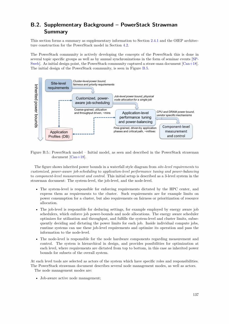
B.2. Supplementary Background – PowerStack StrawmanSummary
This section forms a summary as supplementary information to Section 2.4.1 and the OIEP architec-ture construction for the PowerStack model in Section 4.2.
The PowerStack community is actively developing the concepts of the PowerStack this is done inseveral topic specific groups as well as by annual synchronizations in the form of seminar events [SP-Sweb]. As initial design point, the PowerStack community captured a straw-man document [Can+18].The initial design of the PowerStack community, is seen in Figure B.5.
Figure B.5.: PowerStack model – Initial model, as seen and described in the PowerStack strawmandocument [Can+18].
The figure shows inherited power bounds in a waterfall style diagram from site-level requirements tocustomized, power-aware job-scheduling to application-level performance tuning and power-balancingto component-level measurement and control. This initial setup is described as a 3-level system in thestrawman document: The system-level, the job-level, and the node-level.
• The system-level is responsible for enforcing requirements dictated by the HPC center, andexpress them as requirements to the cluster. Such requirements are for example limits onpower consumption for a cluster, but also requirements on fairness or prioritization of resourceallocation.
• The job-level is responsible for deducing settings, for example employed by energy aware jobschedulers, which enforce job power-bounds and node allocations. The energy aware scheduleroptimizes for utilization and throughput, and fulfills the system-level and cluster limits, subse-quently deciding and dictating the power limits for each job. Inside individual compute jobs,runtime systems can use these job-level requirements and optimize its operation and pass theinformation to the node-level.
• The node-level is responsible for the node hardware components regarding measurement andcontrol. The system is hierarchical in design, and provides possibilities for optimization ateach level, where requirements are dictated from top to bottom, in this case as inherited powerbounds for subsets of the overall system.
At each level tools are selected as actors of the system which have specific roles and responsibilities.The PowerStack strawman document describes several node management modes, as well as actors.The node management modes are:
• Job-aware active node management;
137

• Job-agnostic active node management;• Idle node management.
Regarding actors, the following list is identified:
• System resource manager and job scheduler;• Power-aware job manager;• Power-aware node manager;• Applications;• Application profiling frameworks;• Site administrators;• Application developers;• Users.
First, the node management modes are summarized, followed by the actors.
• With job-aware active node management, the resource manager directs a job manager about theallowed resource consumption regarding energy and power. The job manager is a job runtimethat can monitor and tune the parameters in the adaptive dynamic optimization case. Suchruntime has the ability to understand the impact of enforcing energy and power limits forindividual nodes on performance and execution time of the compute job. Optimization of theseparameters under the resource managers constraint is the primary task of the job manager.
• With job-agnostic active node management the resource manager can directly access the controlinterfaces on the node. In this case energy and power limits can still be enforced, but thepossibility of optimizing the parameters is missed, due to lack of run-time information. Thiscan be required if no prior knowledge about the job is present and or no monitoring of applicationprogress is possible.
• Idle node management is the power management of nodes, which are not assigned to any activecompute job. The resource manager directly interfaces with power management on the node,to enforce and interface with power saving capabilities. Depending on idle node operationsstrategy and resource requirements, this can be realized by setting power limits, sleep states oridle node-shutdown.
Regarding the example actors, the straw-man document identifies typical associated roles and re-sponsibilities, used tools, as well as their interactions with other actors:
• System resource managers and job schedulers: Their main task is to monitor resource usage andallocating these resources to jobs. Regarding power, their responsibilities include: Managementand accounting for idle node power; Assigning of power budget for active jobs; Monitoring andcontrolling power budget for jobs and users; Performance analysis for efficient energy or powerbudget for given job and node; Recording energy and power telemetry. The system resourcemanager and job scheduler is identified as actor which interacts with the job manager interfacinginformation about power budgets, operating frequencies, power management algorithms, orsimilar as applicable. This information is either given by administrators or users in job scripts.Feedback is provided by job profiling tools or databases.
• Power-aware job managers: Their role and responsibility is to interpret the directives from thesystem resource manager and job schedulers and manage the active nodes running a job. Thejob manager has a set of control-able parameters and optimization goals. The actor is designedin a way to enable scalable tuning and information aggregation to make job optimal decisions,propagated to the nodes and processors partaking in the job. Interfaces to job scheduler,application profiling interfaces, application and node managers are required.
138

• Power-aware node managers: Their role is to provide telemetry data for monitoring and inter-faces to node-level hardware. Management of access rights of the tools interacting with theseinterfaces is required. Interfaces exist to external monitoring, system resource manager andjob manager. This actor includes all safety measures in terms of access control of providedinterfaces to the hardware.
• Applications: This represents any user application run in user-space which can influence thesystem behavior by using the provided interfaces. Successful completion of the user applicationrepresents the objective of sustaining the PowerStack with the given resource usage implica-tions. Interfaces from the application to other systems in the system are exposed via tune-ableparameters in the code, as well as profiling information made available from within the appli-cation.
• Application profiling frameworks: These frameworks form an abstraction and separation ofthe measurement and telemetry in user-space solely concerned with application information.Interaction with other actors can include resource manager, job manager and node manager toprovide application specific functionality and possibly improve decision-making.
• Site administrators: Their primary role, regarding power, is to configure the system energy andpower policies and setting up systems and constraints for the rest of the operational entitiesof the system. The actor has interfaces to the outside world (e.g. to interact with ESPs), aswell as interfaces to the inside of the system (e.g. by providing configurations to power capsthe scheduler and resource managers have to adhere to). The interaction with the other actorsin the system happens once at the time of system setup, and additionally any time externalfactors change, which have a requirement change as their consequence. Therefore, configurationand changes to the node managers are performed or initiated by this actor.
• Application developers: Their task is to develop, test and debug applications. Their interactionwith the PowerStack includes enabling and implementing features and interfaces for profilingand control. Their interfaces target the job manager and profiling frameworks.
• Users: Their role is similar to the application developer, with the difference that interaction withthe systems happens via configuration and changes to application inputs. Direct interaction isdone via the system’s resource manager.
These actors and their roles have to be considered in an example setup, even if the list is explicitlynamed to be incomplete in the strawman document [Can+18].At the time of writing, the PowerStack community still handles open question about how specific
cases can be unified into a solution viable for all involved parties. The strawman design formed theinitial discussion point and since evolved over the course of the PowerStack seminar events [PS’18;PS’19a].
139

Appendix C.
Supplement – OIEP Reference Model
C.1. Supplement – Methodical Approach for the Reference Model Construction . . . . . . . 141C.2. Considerations for Model Creators on OIEP Level and Level Tree Construction . . . . 143
C.1. Supplement – Methodical Approach for the Reference ModelConstruction
The work, [Sch00, pp. 81–84], which forms the foundation for the method of this work is too contextspecific in the model generation step. Both [Sch00] and [Sch98] are used as guidelines for this methodand present a methodical approach for model building, placed in the domain of information systems.Both are therefore only applicable with heavy adaptations.[Sch00, p. 81] presents an object-oriented iterative reference modeling approach. The work’s model
construction is split in two phases: First activity diagrams are generated for all identified use-cases.These activity diagrams are then used to derive a single general activity diagram or a set of specializedactivity diagrams. Using the general or specialized activity diagrams, objects, classes and classrelations are derived, in typical object-oriented fashion. This is iteratively applied to generate acomplete object-oriented class model. For a general energy and power management reference model,the consideration of all possible use-cases is not feasible. An approach using basic structural elementsto construct and model such use-cases is needed.[Sch98] uses a traditional, not strictly object-oriented, reference modeling approach.1 The approach
first identifies objects, according to their characteristics, use-cases and relations. The approach usesa so called master-reference model, which specifies model building blocks independent of specificuse-cases. The basic building blocks are identified as abstract objects, together with the relationsrelevant for model organization [Sch98, pp. 217–234]. Next the reference model structure is developedand selected [Sch98, pp. 235–240], followed by the reference process model [Sch98, pp. 240–260],concluded by reference data model [Sch98, pp. 261–276]. Similar to [Sch00], the work in [Sch98] is inthe information systems domain, making several steps of their reference model construction methodsnot entirely universal. However, the fundamental model construction steps presented in [Sch98,pp. 207–291] are applicable to reference model building for energy and power management withslight adjustments.By contrast, commonly known reference models in computer science do not present their method
for reference model generation (e.g. ISO/OSI [Zim80; ISO-7498], OASIS SOA [OAS06], or the afore-mentioned 4D/RCS [AB05]). Replication of the model building process using equivalent approachesis thus not possible due to lack in transparency or historically grown model approaches.For a solid method of an adapted approach, the chapter at hand goes back to Stachowiak’s funda-
mental model theory [Sta73, pp. 128–140]. The fundamental model theory describes three principlecharacteristics for models:
Mapping: “Models are always models of something, more precisely mappings, representationsof natural or artificial originals, which themselves can be models.”1 [Sta73, p. 131]
1For the essential parts applicable here, see phases two and three of [Sch98, pp. 187–188]. With details in [Sch98,pp. 207–291].
141

Reduction: “Models in general do not present all attributes of the to be represented original, butonly those, which seem relevant to the creator or user of the model.”1 [Sta73, p. 132]
Pragmatism: “Models are not exclusively mapped to their originals. They fulfill a function of sub-stitution a) for certain – recognizing and/or acting, model-using – Subjects, b) withincertain time intervals and c) under restriction to certain mental or actual opera-tions”1 [Sta73, pp. 132–133]
These characteristics serve as construction fundamentals when generating the reference model, andas guiding principles for the method.An approach more grounded in fundamentals for model construction, in [Tha10, pp. 3117–3118],
formulates a theory for conceptual modeling. The theory discuses model construction using thesteps of: to “conceptualise”, to “abstract”, to “define” and to “construct”. An additional step, to“understand”, precedes, while the step to “evaluate” follows the act of model construction. The stepto “refine” in [Tha10, p. 3120] represents an iterative process to evolve the model to a presentablestate.For the methodical approach of this chapter both [Sch00] and [Sch98] are combined and reduced
to their fundamentals, taking Stachowiak’s fundamental model theory [Sta73] and [Tha10]’s modelinto account.Given these considerations, the method is introduced as presented in Section 3.1.
1Translation from German by the author.
142

C.2. Considerations for Model Creators on OIEP Level and LevelTree Construction
When designing an instance of an OIEP architecture, using the OIEP reference model, model creatorshave to consider several aspects:
• “What is the overall desired optimization goal?”• “What are the hardware features desired for altering energy and power behavior?”• “What levels of management are needed?”• “How to model the energy and power management system using the OIEP reference model in
a minimal but sufficient approach?”• “Are there any level specific restrictions which have to be considered at design time?”• “Are there possible conflicts in the initial level design and hierarchy?”• “Are any level-decisions restricting modularity or scalability of the management system?”
These considerations for the model creator are discussed in the following.
“What is the overall desired optimization goal?” The structure of the OIEP level tree as well asthe OIEP levels’ goals have to be aligned with the overall optimization goal of the system. Conflictsby design can be detected as early as the complete level tree is modeled.
“What are the hardware features desired for altering energy and power behavior?” The hardwarefeatures to pursue the optimization goals depend largely on the availability of the system. In certaincircumstances specific requirements for hardware features to be used are dictated by the centerleadership. Depending on the setup, certain features may also be restricted. This can be restrictionsin use or in configuration. An example for such dependency is preset OS settings which are presetand use is restricted due to mandate by the center leadership. Overall restrictions or requirementsfor hardware features can be found in RFPs or responses to RFPs (Where a response to an RFPscan be supported by providing an OIEP architecture description).
“What levels of management are needed?” By modeling the root level as anchor point for theenergy and power management hierarchy, as well as modeling the hardware features to be set andmodeled the corner stones for an OIEP architecture are set. The intermediate levels for OIEP archi-tectures are to be modeled according to the needs of the HPC center, HPC system, or specific demandsby OIEP levels themselves. The intermediate levels sometimes can be derived from RFPs, or generalsystem descriptions with a requirement or specification for energy and power management systems.For example, if an HPC system requirement asks for an energy and power aware job scheduler, theOIEP architecture should match such requirement. Clarity, applicability and structural equivalenceas requirements for the OIEP reference model do apply to the generation of the individual OIEParchitectures, as well. Choice of level identifiers or (mnemonic) level names should be considered, aswell.
“How to model the energy and power management system using the OIEP reference model in aminimal but sufficient approach?” When modeling an energy and power management system withopen specifications finding the right granularity, level of abstraction or even setup and componentscan be an open process with no single right answer. After having modeled the system, all levelsshould be assessed, and evaluated based on the follow considerations:
• Is the specific level necessary?• Is an additional level necessary, for clean interaction?• Can a level be merged / Does a level need to be split (According to the method presented in
Section 3.1)?
143

• Are the edges of the OIEP level tree representative of the control flow for energy and powermanagement within the system?
It is sufficient if these questions can be answered satisfactory, and the model is an equivalent tothe actual system or is a representation of the desired features for a system to be built.
“Are there any level specific restrictions which have to be considered at design time?” Whendesigning OIEP levels for an OIEP architecture the model creator sometimes already has specificsoftware components in mind, fulfilling the mechanism described. Some of these software compo-nents impose restrictions. The restrictions of the components have to be checked and validated.Unnecessary restrictions and unnecessary ambiguity should be eliminated.
“Are there possible conflicts in the initial level design and hierarchy?” The goal of the system isto prevent conflicting decision in the energy and power management system. By design of the OIEPlevels and arrangement within the OIEP level tree for an OIEP architecture possible conflicts can bechecked and validated. For example, the usage of hardware features which are mutually exclusive,such as the usage of explicit DVFS and RAPL should be restricted by the design of the levels. Thisis that either an additional level is introduced managing the possible conflict, or by eliminating theconflict by restricting the architecture to an explicit conflict free design.
“Are any level-decisions restricting modularity or scalability of the management system?” Dueto the fact that the OIEP reference model is to be applied on open HPC systems, levels and thedesign of the level tree have to be checked for possible restrictive designs preventing modularity byintroduction of dependencies. Similar considerations have to be made for considerations regardingscalability: The design of the levels and the level tree should not restrict the scaling of the energyand power management system. The introduction of additional levels to deal with large scales of thesystem is a valid approach.
There is no mandated way of designing OIEP architectures. The approach chosen should be docu-mented in a clear, precise and understandable way, however. This is necessary to be able to verifydesigns and also for the possibility improve these designs in an incremental way, by substitution anditerating over different designs. This is enabled by the modular design of the reference model. Ex-emplary mappings of system architectures to the reference model are shown in Chapter 4 (includinga method for OIEP architecture construction).
144
Appendix D.
Supplement – OIEP Architectures forSelected HPC Systems
D.1. Constructing an OIEP Architecture for the PowerStack Prototype . . . . . . . . . . . 147D.2. Constructing an OIEP Architecture for GEOPM as Nested Component . . . . . . . . 151D.3. Constructing an OIEP Architecture for the SuperMUC Phase 1 & 2 systems . . . . . 163D.4. Constructing an OIEP Architecture for the SuperMUC-NG System . . . . . . . . . . . 169D.5. Constructing an OIEP Architecture for the Fugaku System . . . . . . . . . . . . . . . 177
As supplement to Chapter 4, and the presentation of a single OIEP architecture in the main partof this work, this Appendix presents five additional OIEP architectures. The presented energy andpower management setups and HPC systems are:
• The PowerStack prototype (see Sec. D.1);• GEOPM, as a nested component (see Sec. D.2);• LRZ’s SuperMUC Phase 1 & Phase 2 systems (see Sec. D.3);• LRZ’s SuperMUC-NG system (see Sec. D.4);• R-CCS’s Fugaku system (see Sec. D.5);
These constructions for OIEP architectures show, first how the OIEP reference model is applied, butmore importantly, the versatility of the OIEP reference model for different kinds of model descriptions.These representations do not claim to be exact, since only public documentation is used. The
approach shows how the reference model can be used to understand, and represent the energy andpower control structure of the larger systems.The six approaches (including the PowerStack Model), show different potentials of the OIEP ref-
erence model:
• The ability to concretize energy and power management models (PowerStack model – Sec. 4.2);• To understand and potentially plan prototype implementations (PowerStack prototype – Sec. D.1);• To model system software interacting with energy and power as nested OIEP components
(GEOPM – Sec. D.2);• To model energy and power management setups of real HPC systems
– known at design-time of the OIEP reference model (LRZ’s systems – Sec D.3 & D.4);– known only after completion of the OIEP reference model (R-CCS’s Fugaku system –
Sec. D.5).
These OIEP architecture constructions are presented below and supplement the research question Q3.
145


D.1. Constructing an OIEP Architecture for the PowerStackPrototype
With the construction of the OIEP architecture for the PowerStack model in Section 4.2, a directcontinuation of this is to construct an OIEP architecture for the PowerStack prototype.The previously constructed OIEP architecture serves as basis for the architecture of this prototype.
Still, the prototype has its own OIEP architecture, since it deviates from the previous design in parts.At the time of writing the prototype is under development, by a collection of collaborators from Intel,Lawrence Livermore National Laboratory (LLNL) and the University of Tokyo, and is not part of thiswork’s contribution. The exercise of mapping the OIEP reference model concepts from the model tothe prototype serves to show how an OIEP architecture description can be systematically adaptedfrom one system to a similar design, using the methods of this work.For the construction of an OIEP architecture for the PowerStack prototype, the steps of the method
for reference model application are followed. These steps are:
a) Problem description;b) Identification of requirements;c) Reference model or architecture selection;d) Architecture construction or adaption;e) Resulting in: an OIEP architecture for the PowerStack prototype.
These steps are shown in reference to the OIEP architecture construction of the PowerStack modelpresented in Section 4.2.Since large parts of the PowerStack model’s OIEP architecture construction can be re-used the
existing OIEP architecture is selected for adaption in step c). The above constructed OIEP architec-ture for the PowerStack model needs small adjustments and has to be restricted to fit the prototypesetup. The restrictions are mostly explicit selection of technology and OIEP components, as well asthe explicit exclusion of some aspects of the original architecture. These alterations are described inthe problem description and in the realization, below.
D.1.1. PowerStack Prototype – Problem DescriptionThe problem description follows the same argumentation as the above construction. By contrast, thetask for the prototype is to show a minimal functional approach providing the base functionality ofthe PowerStack. This task allows to show a configuration which follows the above approach, withoutthe addition of too much complexity. In turn, this allows to show the benefit of a system setup withinteracting components according to the PowerStack.The prototype setup is limiting itself to managing a single cluster, and excluding out-of-band-
hardware access, as well as the infrastructure side. With these restrictions the architecture followsthe original PowerStack strawman design (as seen in Figure B.5) more closely compared to the moreextensive PowerStack model of the seminars (as seen in Figure 4.2). The explicit hardware andsoftware selection for the prototype is listed in the requirements.
D.1.2. PowerStack Prototype – Identification of RequirementsThe prototype is set to run on available hardware, using software which is actively worked on bymembers of the PowerStack core committee. Therefore, the hardware builds upon Intel Xeon CPUs,with support for RAPL via MSRs, as present since the Sandy Bridge microarchitecture [Rot+12]. Foraccess and configuration to MSRs, the msr-safe library [Sho+] is selected, developed by collaboratorsat LLNL. The centerpiece for energy optimization is the job runtime GEOPM [GEOb], developed bycollaborators at Intel. The GEOPM tool is representative of auto-tuning, adaptive runtimes, as wellas energy measurement and tracing tools, since the tool combines these functionalities. Dependingon the configuration of GEOPM these features can be used in isolation or combination, if desired.For the scheduler of the prototype, the selected software is an altered version of the Simple LinuxUtility for Resource Management (SLURM) scheduling system. The scheduler is augmented using a
147

Administration
Cluster
Job
Node
In-band-HW
AdministrativeInfrastructure
Figure D.1.: PowerStack prototype – Simplified OIEP level tree.
Slurm Plug-in architecture for Node and job Kontrol (SPANK) plug-in developed by University ofTokyoas part of the PomPP framework [SP; Wad+18]. This enables the interaction of job runtimeand job scheduler.Using these open-source tools, the prototype can serve as a starting point for centers looking into
the integration of the PowerStack into their systems. No special considerations for different operatingstates are made for the prototype.
D.1.3. PowerStack Prototype – Reference Model or Architecture SelectionAccording to the method, step c) is used to identify the OIEP reference model as the used referencemodel for the architecture design. In the case of the PowerStack prototype, not only is a refer-ence model identified, but also a known prior OIEP architecture selected which is altered to suitthe problem requirements. The architecture is the previously constructed OIEP architecture of thePowerStack model.Therefore, in the architecture construction step, step d), the PowerStack model’s OIEP architecture
is used, reduced and modified, according to the problem description and requirements.
D.1.4. PowerStack Prototype – Architecture Construction or AdaptionFor the architecture construction of the PowerStack prototype’s OIEP architecture the steps of out-lined in the Section 4.1 are followed. Since the architecture builds on the previously identified archi-tecture, the alterations are named, following the same systematical manner.
D.1.4.1. Identifying OIEP Levels for the PowerStack Prototype
For the identification of the OIEP levels, the OIEP levels of the PowerStack model are used. Thelevels are the reduced set according to the requirements:
• Administration;• Cluster;• Job;• Node;• In-band hardware (In-band-HW).
All these levels follow the description of the PowerStack model’s OIEP architecture. The descriptionsare restricted, so that they follow the requirements of the prototype, as named above. Thus, thesite level is eliminated, while administration only interacts with the cluster and the node level onlyinteracts with in-band-hardware. The components of the levels are the explicit components namedin the requirements’ identification.Figure D.1 shows the OIEP level tree with five levels and without any level branching. The root of
the tree forms the entity controlling the cluster and setting all configurations. The administration-level is at the root level, passing control to the cluster-level, The cluster-level passes control decisions
148
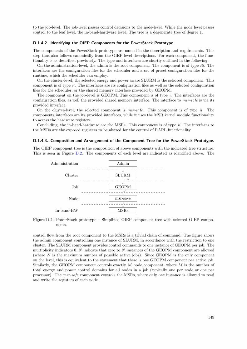
to the job-level. The job-level passes control decisions to the node-level. While the node level passescontrol to the leaf level, the in-band-hardware level. The tree is a degenerate tree of degree 1.
D.1.4.2. Identifying the OIEP Components for the PowerStack Prototype
The components of the PowerStack prototype are named in the description and requirements. Thisstep thus also follows canonically from the OIEP level descriptions. For each component, the func-tionality is as described previously. The type and interfaces are shortly outlined in the following.On the administration-level, the admin is the root component. The component is of type iii. The
interfaces are the configuration files for the scheduler and a set of preset configuration files for theruntime, which the scheduler can employ.On the cluster-level, the selected energy and power aware SLURM is the selected component. This
component is of type ii. The interfaces are its configuration files as well as the selected configurationfiles for the scheduler, or the shared memory interface provided by GEOPM.The component on the job-level is GEOPM. This component is of type i. The interfaces are the
configuration files, as well the provided shared memory interface. The interface to msr-safe is via itsprovided interface.On the cluster-level, the selected component is msr-safe. This component is of type ii. The
components interfaces are its provided interfaces, while it uses the MSR kernel module functionalityto access the hardware registers.Concluding, the in-band-hardware are the MSRs. This component is of type ii. The interfaces to
the MSRs are the exposed registers to be altered for the control of RAPL functionality.
D.1.4.3. Composition and Arrangement of the Component Tree for the PowerStack Prototype.
The OIEP component tree is the composition of above components with the indicated tree structure.This is seen in Figure D.2. The components of each level are indicated as identified above. The
Administration
Cluster
Job
Node
In-band-HW
AdministrativeInfrastructure
Admin
SLURM
GEOPM
msr-save
MSRs
1
0..N
M
1
Figure D.2.: PowerStack prototype – Simplified OIEP component tree with selected OIEP compo-nents.
control flow from the root component to the MSRs is a trivial chain of command. The figure showsthe admin component controlling one instance of SLURM, in accordance with the restriction to onecluster. The SLURM component provides control commands to one instance of GEOPM per job. Themultiplicity indicators 0..N indicate that zero to N instances of the GEOPM component are allowed(where N is the maximum number of possible active jobs). Since GEOPM is the only componenton the level, this is equivalent to the statement that there is one GEOPM component per active job.Similarly, the GEOPM component controls exactly M node component, where M is the number oftotal energy and power control domains for all nodes in a job (typically one per node or one perprocessor). The msr-safe component controls the MSRs, where only one instance is allowed to readand write the registers of each node.
149

D.1.4.4. Inclusion of the Monitoring Overlay for the PowerStack Prototype
The OIEP monitoring overlay for the PowerStack prototype is also canonical. This means, that thereare no additional data-sources added (contrary to the PowerStack model’s architecture). Thus, theedges of the OIEP component tree are inverted, having information flow up to the root, which formsthe complete monitoring overlay.
D.1.4.5. Identification of Operating States and Construction of the State Diagram for thePowerStack Prototype
For the PowerStack prototype, no differentiation of operating states are identified, nor required bythe problem description or requirements for the architecture. Thus, no additional work is to be doneto complete the OIEP architecture.
This completes step d), resulting in the OIEP architecture for the PowerStack prototype. The OIEPcomponent tree is representative of the resulting OIEP architecture, which is represented as stepe) of the method for reference model application, the specific architecture of this energy and powermanagement system.
150
D.2. Constructing an OIEP Architecture for GEOPM as NestedComponent
In the previous OIEP architecture in Appendix D.1 the job runtime GEOPM is used as an OIEPcomponent. This means that GEOPM is treated as a black box, where the runtime operates on ajob partition performing optimizations on all participating nodes. In such black box approach, themodel creator does not need any knowledge about the internal structure of the component, since thefunctionality is used as proclaimed by the component. To verify that a component is compatiblewith the design of the OIEP reference model, the component itself can be assessed in a white boxapproach. This is especially useful if a component has a complex structure and model creators needto verify that the system behaves as wanted in terms of energy and power management and control.Verifying the structure also allows to reason about potential performance and scalability implicationsof the chosen design of the architecture of an OIEP component.In the following such OIEP architecture design is done for GEOPM to serve as white-box view of
GEOPM as OIEP component. For this, the method for applying reference models is followed as ofSection 4.1.
To expand GEOPM from a black box into a white box view, the concept of the OIEP nestedcomponents is used (see Sec. 3.3.2.2). By representing an individual component as a nested compo-nent, its internal structure can be represented as an independent OIEP architecture. Within suchnested component, its root node represents the interface to the outside world. Using analogous out-side black-box view of such component, this is represented by the regular parent component givingthe control input. In an OIEP architecture the root nodes external interfaces are normally handledby setting the root level’s optimization goal and functionality. Thus, in the white-box view of anested component the root level’s functionality has to contain the statement for it to be used asnested component. Accordingly, the leaf nodes (within) represent the arbitrary amount of interfacesof the nested component to the (outside) components on the child levels. The nested component isself-contained and for both inside and outside the concepts of the OIEP reference model apply.The interest of this exercise is to show how a component, which can be used as a component of
an OIEP architecture, can itself be expressed using the mechanisms of the OIEP reference model. Inthe case of GEOPM, this is a non-trivial task, since the control structure of the job runtime itselfhas no fixed or rigid structure. Architecture descriptions for energy and power management cantherefore rely on the OIEP reference model for the overall structure, as well as for the structureof their employed components, using the same mechanisms. The expansion as a nested componentcan be done with any other component. Using GEOPM as example helps to understand how theprocess of mapping components works and serve as an example for any other component. This is thecase, since the GEOPM runtime system is on the more complex side in terms of energy and poweroptimization components.The description of GEOPM is given according to [Eas+17], with the addition of clarifications,
important for this work, where needed. The description of GEOPM extends the short introductiongiven in the supplementary background section in Appendix B.1.2.2. GEOPM was conceived beforethe OIEP concepts and also before the PowerStack initiative.
D.2.1. GEOPM as Nested Component – Problem DescriptionGEOPM stands for Global Extensible Open Power Manager and is developed by the P3-Team atIntel as an open source tool with collaborators across academia and industry.The aim of GEOPM is a scalable runtime, which is able to adjust energy and power hardware
settings to optimize the operation of HPC applications. GEOPM is a runtime which operates ona single compute job, optimizing the CPU power settings of all participating nodes. The job wideoptimization is done by using measurements from the nodes, and monitoring data from the computejob’s application processes. Using this information a POMDP is performed continuously.The goal of the open design and extensibility of the GEOPM runtime and framework is to be able
to design and write optimization plugins, named GEOPM agents. These agents can be designedspecific to the needs of the HPC centers that needs certain application optimizations and tuning for
151
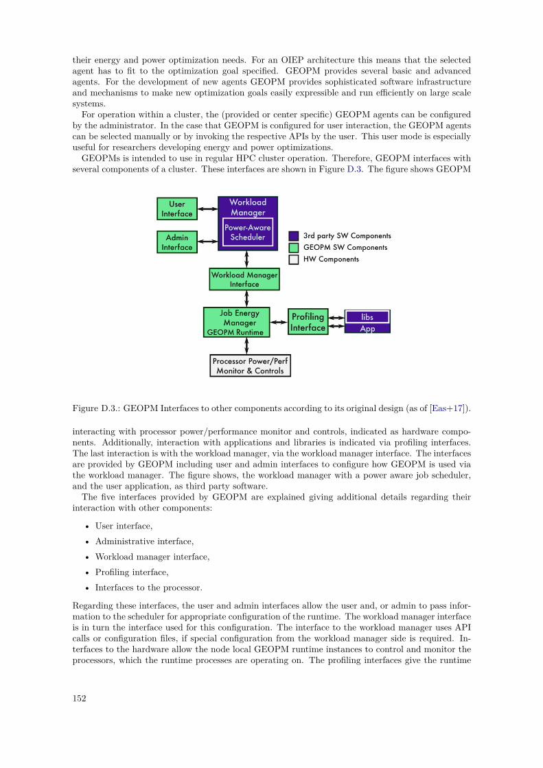
their energy and power optimization needs. For an OIEP architecture this means that the selectedagent has to fit to the optimization goal specified. GEOPM provides several basic and advancedagents. For the development of new agents GEOPM provides sophisticated software infrastructureand mechanisms to make new optimization goals easily expressible and run efficiently on large scalesystems.For operation within a cluster, the (provided or center specific) GEOPM agents can be configured
by the administrator. In the case that GEOPM is configured for user interaction, the GEOPM agentscan be selected manually or by invoking the respective APIs by the user. This user mode is especiallyuseful for researchers developing energy and power optimizations.GEOPMs is intended to use in regular HPC cluster operation. Therefore, GEOPM interfaces with
several components of a cluster. These interfaces are shown in Figure D.3. The figure shows GEOPM
Figure D.3.: GEOPM Interfaces to other components according to its original design (as of [Eas+17]).
interacting with processor power/performance monitor and controls, indicated as hardware compo-nents. Additionally, interaction with applications and libraries is indicated via profiling interfaces.The last interaction is with the workload manager, via the workload manager interface. The interfacesare provided by GEOPM including user and admin interfaces to configure how GEOPM is used viathe workload manager. The figure shows, the workload manager with a power aware job scheduler,and the user application, as third party software.The five interfaces provided by GEOPM are explained giving additional details regarding their
interaction with other components:
• User interface,• Administrative interface,• Workload manager interface,• Profiling interface,• Interfaces to the processor.
Regarding these interfaces, the user and admin interfaces allow the user and, or admin to pass infor-mation to the scheduler for appropriate configuration of the runtime. The workload manager interfaceis in turn the interface used for this configuration. The interface to the workload manager uses APIcalls or configuration files, if special configuration from the workload manager side is required. In-terfaces to the hardware allow the node local GEOPM runtime instances to control and monitor theprocessors, which the runtime processes are operating on. The profiling interfaces give the runtime
152
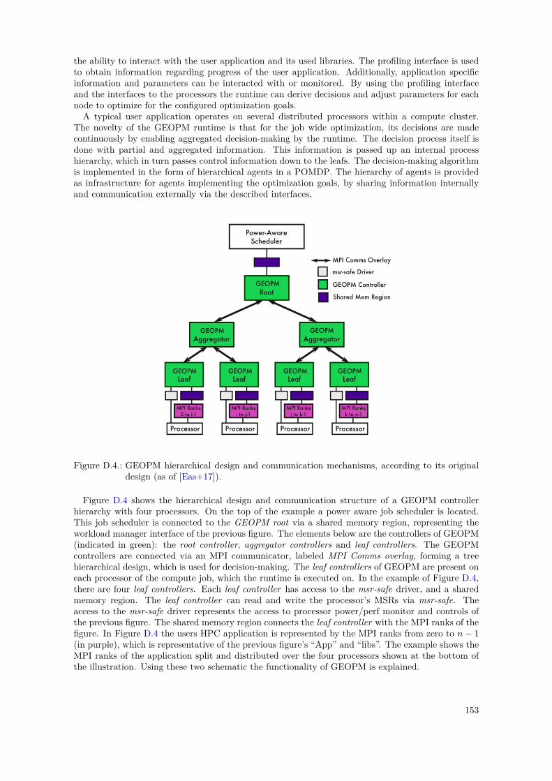
the ability to interact with the user application and its used libraries. The profiling interface is usedto obtain information regarding progress of the user application. Additionally, application specificinformation and parameters can be interacted with or monitored. By using the profiling interfaceand the interfaces to the processors the runtime can derive decisions and adjust parameters for eachnode to optimize for the configured optimization goals.A typical user application operates on several distributed processors within a compute cluster.
The novelty of the GEOPM runtime is that for the job wide optimization, its decisions are madecontinuously by enabling aggregated decision-making by the runtime. The decision process itself isdone with partial and aggregated information. This information is passed up an internal processhierarchy, which in turn passes control information down to the leafs. The decision-making algorithmis implemented in the form of hierarchical agents in a POMDP. The hierarchy of agents is providedas infrastructure for agents implementing the optimization goals, by sharing information internallyand communication externally via the described interfaces.
Figure D.4.: GEOPM hierarchical design and communication mechanisms, according to its originaldesign (as of [Eas+17]).
Figure D.4 shows the hierarchical design and communication structure of a GEOPM controllerhierarchy with four processors. On the top of the example a power aware job scheduler is located.This job scheduler is connected to the GEOPM root via a shared memory region, representing theworkload manager interface of the previous figure. The elements below are the controllers of GEOPM(indicated in green): the root controller, aggregator controllers and leaf controllers. The GEOPMcontrollers are connected via an MPI communicator, labeled MPI Comms overlay, forming a treehierarchical design, which is used for decision-making. The leaf controllers of GEOPM are present oneach processor of the compute job, which the runtime is executed on. In the example of Figure D.4,there are four leaf controllers. Each leaf controller has access to the msr-safe driver, and a sharedmemory region. The leaf controller can read and write the processor’s MSRs via msr-safe. Theaccess to the msr-safe driver represents the access to processor power/perf monitor and controls ofthe previous figure. The shared memory region connects the leaf controller with the MPI ranks of thefigure. In Figure D.4 the users HPC application is represented by the MPI ranks from zero to n− 1(in purple), which is representative of the previous figure’s “App” and “libs”. The example shows theMPI ranks of the application split and distributed over the four processors shown at the bottom ofthe illustration. Using these two schematic the functionality of GEOPM is explained.
153

When an application is running, each process of the application shows specific performance andpower characteristics on all participating the processors. Each of the processes of the applicationmakes progress contributing to the overall progress of the application. At the same time all processorscontribute to the overall power characteristics of the application. Given this information, GEOPMoperates as follows:On each processor one GEOPM controller manages this processor’s behavior, based on measure-
ments obtained from that processor. The GEOPM controllers execute their control loop in intervalscalled epochs. In each epoch performance, energy history, the applications progress, as well as otherdata is collected. Recursively, the controllers send aggregate data up the tree for each epoch, startingat the leafs. Each intermediate controller then assesses the information, and sends aggregate datafurther up the tree, towards the root. Based on this aggregate data, the root controller makes deci-sions for each of its child controllers. The result of a control decision is the restrictions of possiblecontrol actions each child controller can take. The child controllers make decisions based on theirmeasurements and the restricted actions for control, as dictated by their parent. This is again donerecursively, until the refined control decisions reached the individual leaf controllers. Based on theimplementation of the optimization algorithm followed, this results in an overall optimization of theoverall system, according to the mechanisms of POMDP.For the propagation of decisions and information of controllers the hierarchy seen in D.4. The
decision algorithm executed is called the decider1. Each implementation of the decision algorithmcontains two major parts: An implementation regarding the data aggregation, containing both ag-gregation algorithm, including the communication to the parent controller; And, an implementationof the control algorithm, with both control algorithm and the communication regarding the decisionssent towards the child controllers. The decider implementation can be replaced, as it is implementedas a plug-in. Using such design optimization goals are selectable and replaceable, according to theneed of the HPC center; That is, according to the configuration/selection of the workload manageras instructed by the user or admin, as seen in the previous figure (Fig. D.3).Regarding the structure of the control hierarchy, the tree hierarchy is set up in a way, such that
intermediate levels are introduced according to the total number of leaf controllers involved. Thisintroduction of intermediate levels is done by the runtime, selecting an optimal degree for eachnode according to the total number of nodes. This is achieved by introduction of aggregator con-trollers, resulting in a balanced tree. The selected (uniform) degree of the nodes is referred to asfan-out in GEOPM. For optimized communication algorithms, the MPI communication topologiesare used. These are designed efficiently by using standard MPI mechanisms, namely the Cartesiantopology [MPI15]. Both, the usage of efficient communication and the selection of degree and depthof the hierarchy ensures scalability and the minimization of overhead.
D.2.2. GEOPM as Nested Component – Identification of RequirementsThe resulting requirements for the representation of GEOPM as a nested OIEP component are asfollows:
• Modeling of the hierarchical control mechanisms, with:– Root controller;– Aggregator controllers, with arbitrary depth;– Leaf controllers, matching the number of processors in the system;– Representation of control and information flow.
• Verifying, that the control mechanisms follows the desired control flow.• Usability as nested component within other OIEP architecture.
This completes the step b) of the method.
1The deciders are replaced by agents after version 0.6.1 for the release of GEOPM version 1.0, as seen on [GEOa].This document uses the nomenclature of the original publication for the names of the implementation [Eas+17].
154

D.2.3. GEOPM as Nested Component – Reference Model or ArchitectureSelection
The next step is the identification of a reference model, where the OIEP reference model is selected andin this special case, the representation is done as a nested component in the form of a self-containedOIEP component as OIEP architecture. This directly follows from the requirements. Therefore, thenext step is the architecture construction, step d) of the method.
D.2.4. GEOPM as Nested Component – OIEP Architecture ConstructionFor the construction of the OIEP architecture for GEOPM as a nested component, the first five ofthe seven steps introduced in the method for reference model application (as of Sec. 4.1) are used:
1. Identifying the Levels;2. Composition and arrangement of the level tree;3. Identifying the Components;4. Composition and arrangement of the component tree;5. Inclusion of the monitoring overlay;
The sixth and seventh step (the identification of operating states and construction of the state dia-gram, as well as the repetition of the construction for the identified states) are not needed, since nostates are identified for this architecture description.The following sections construct the nested components for each controller, one after the other. This
is done according to the first four steps of the architecture construction as listed above, namely: levelidentification, level tree arrangement, component identification and component tree composition.This results in a possible construction of the OIEP level tree and OIEP component tree for theGEOPM job runtime as single complete nested component.The section first shows GEOPM as an excerpt of an already modeled architecture as the familiar
black box component. This is followed by the construction of the nested component controllers:The runtime component containing the root controller, the aggregator component containing theaggregator controllers and the leaf component containing the leaf controllers. After these sections arefinished, the complete white box OIEP component is presented.
D.2.4.1. GEOPM as Nested Component – Initial Black Box View
To begin the construction of an OIEP architecture for GEOPM as nested component, Figure D.5 ispresented to recall the black box view of the component.
Workload Management
Job Energy Manager
Processor-Level
GEOPM_RT
p
Figure D.5.: GEOPM as an OIEP component. Black box component view as excerpt of an OIEParchitecture.
Figure D.5 shows an excerpt of an OIEP architecture and the black box view of the GEOPM com-ponent. The parent level is the workload manager-level, where job schedulers, or similar components
155

are placed. The GEOPM OIEP component itself is on the job energy management-level, the childlevel is the processor-level. The number of outgoing edges is p, where p indicates the number ofparticipating processors per job. The model excerpt is according to the usage model of the aboveproblem description. The subsections break this view up with the result of a white box view of thestructure of the GEOPM component.
D.2.4.2. GEOPM as Nested Component – Runtime Component and the Root Controller
To create a nested representation of GEOPM according to the description above, the first step is arepresentation containing the root controller.Initially the levels are identified. For the root controller two levels are needed, as identified:
the controller-level (containing the root controller) and the child-level (containing all further nestedcomponents). For each the a) scope, b) goal, c) location, d) function and e) associated componentsare listed.The controller level represents is present in all nested components of this OIEP architecture design.
a) The scope of the controller level of the GEOPM_RT component is the root controller and processingof aggregate information regarding the energy and power and performance characteristics of allparticipating sub-processes/processors.
b) The optimization goal is to fulfill the optimization goal of the configuration as configured bythe workload manager.
c) For location the root controller-level is a process within the MPI communicator of the runtime.d) The functionality is management of power budgets according to the optimization algorithm
selected and splitting the power budgets for the child level, accordingly. The functionalityincludes assessment of aggregated information to reach this result and reporting to the workloadmanager. Additional functionality is the selection of the nested component. This selection isdone according to fan-out. If control over more components is required than allowed by thefan-out, the selected components are aggregator components. In the case that less or equalcomponents are required than the fan-out value, the leaf components are selected directly asthe child components. This selection is implemented in the runtime initialization.
e) The component on the controller-level is an implementation of the root controller.
For the child-level the level characteristics are shaped by the restrictions of their respective parentlevel.
a) The scope of the child-level of the root has the scope of the energy and power characteristicsof all of its participating sub-processes/processors.
b) The optimization goal is to fulfill the optimization goal of the configuration as set by the rootcontroller (which applied restrictions).
c) For location the root controller-level is again a process within the MPI communicator.d) The functionality at this level is to realize the recursive scoping and management of energy and
power for the processors, which are part of their subgroup, according to the desired fan-out.e) The component on the level is either an aggregator controller or a leaf controller. This selection
is indicated by an xor operator as mutually exclusive with the matching virtually selectedoperator indicating and concluding the selection.
The two level hierarchy follows canonically, with the controller-level as parent on top and the childon the level below.The components of the levels are identified, as root controller implementation, and for the child-
level either an aggregator controller or a leaf controller.Using this information, the root controller’s internal level tree and internal component tree can be
constructed.
Figure D.6 shows the internal level tree (Fig. D.6a) and the internal component tree (Fig. D.6b).
156

GEOPM_RT
Controller-Level
Child-Level
(a) Internal level tree
GEOPM_RT
ControllerRoot1..k
Agg. Leaf1..p 1
p
(b) Internal component tree
Figure D.6.: Nested setup for the GEOPM_RT component. Figure D.6a, shows the internal level tree,Figure D.6b, shows the internal component tree. The aggregator component (Agg) andthe leaf component (Leaf) are a nested component themselves, detailed in Figures D.7and D.8.
The outer component of the nested component for the GEOPM runtime uses the identifier GEOPM_RT.As seen in Figure D.6a, the level tree contains two levels, the controller-level on top, and the child-levelon the bottom. Figure D.6b shows the internal OIEP component tree of the GEOPM runtime com-ponent (GEOPM_RT). The top level contains the root controller (ControllerRoot). The root controllercontrols one to k components on the child-level, where k is the fan-out programmatically detected asdescribed above. The child components are either aggregator components (indicated by Agg) or leafcomponents (indicated by Leaf). The leaf components control exactly one processor, whereas theaggregator component controls an arbitrary amount of components in the range from one to p.The OIEP monitoring overlay for the nested component is constructed by inverting the edges of
the OIEP component tree, without the addition of additional OIEP data sources.The next step is the repetition of the nested component construction for the aggregator component
and the leaf component. Using these, the GEOPM_RT component can be recursively populated.
D.2.4.3. GEOPM as Nested Component – Aggregator Component and the AggregatorController
For the aggregator controller, the same workflow as for the OIEP architecture of nested componentfollows.The levels and level-tree construction are identical to Section D.2.4.2, with the following differences:
• The scope of the controller-level, a), is restricted to the sub-processes/processors of the aggre-gator controller.
• The optimization goal, b), and functionality, c), is to work according to the restrictions of theparent controller.
• The reporting functionality of the aggregator aggregates towards the higher level’s aggregatorand the root for decision-making (as opposed to reporting to the workload manager).
• The component on the controller level, e), is the aggregator controller.
The remainder for levels and the internal level-tree is equivalent to Section D.2.4.2.Using this information, the aggregator controller’s internal level tree and internal component tree
is identified and constructed.Figure D.7 shows the internal level tree (Fig. D.7a) and the internal component tree (Fig. D.7b).
Figure D.7b presents the same basic setup as the GEOPM_RT component of Figure D.6b with thefollowing differences: The component implementing the controller logic is the aggregator controllerControllerAgg, on the controller level. On the child level the same selection is possible as before,the total number of components Agg is recursively limited by the total number of processors p. Sincethe recursion-depth of an instantiated component Agg is not known, the total number of child nodeswhich the nested component controls is a variable range form one to p.
157
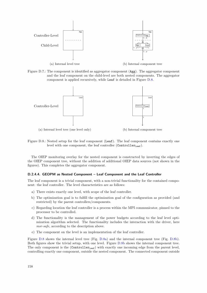
Agg.
Controller-Level
Child-Level
(a) Internal level tree
Agg.
ControllerAgg.1..k
Agg. Leaf1..p 1
1..p
(b) Internal component tree
Figure D.7.: The component is identified as aggregator component (Agg). The aggregator componentand the leaf component on the child-level are both nested components. The aggregatorcomponent is applied recursively, while Leaf is detailed in Figure D.8.
Leaf
Controller-Level
(a) Internal level tree (one level only)
Leaf
ControllerLeaf1
1
(b) Internal component tree
Figure D.8.: Nested setup for the leaf component (Leaf). The leaf component contains exactly onelevel with one component, the leaf controller (ControllerLeaf).
The OIEP monitoring overlay for the nested component is constructed by inverting the edges ofthe OIEP component tree, without the addition of additional OIEP data sources (not shown in thefigures). This completes the aggregator component.
D.2.4.4. GEOPM as Nested Component – Leaf Component and the Leaf Controller
The leaf component is a trivial component, with a non-trivial functionality for the contained compo-nent: the leaf controller. The level characteristics are as follows:
a) There exists exactly one level, with scope of the leaf controller.b) The optimization goal is to fulfill the optimization goal of the configuration as provided (and
restricted) by the parent controllers/components.c) Regarding location the leaf controller is a process within the MPI communicator, pinned to the
processor to be controlled.d) The functionality is the management of the power budgets according to the leaf level opti-
mization algorithm selected. The functionality includes the interaction with the driver, heremsr-safe, according to the description above.
e) The component on the level is an implementation of the leaf controller.
Figure D.8 shows the internal level tree (Fig. D.8a) and the internal component tree (Fig. D.8b).Both figures show the trivial setup, with one level. Figure D.8b shows the internal component tree.The only component is the (ControllerLeaf) with exactly one incoming edge from the parent level,controlling exactly one component, outside the nested component. The connected component outside
158
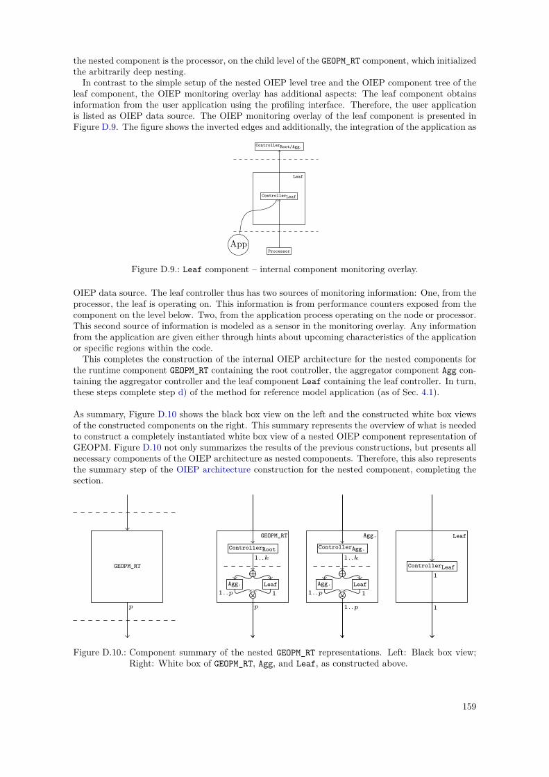
the nested component is the processor, on the child level of the GEOPM_RT component, which initializedthe arbitrarily deep nesting.In contrast to the simple setup of the nested OIEP level tree and the OIEP component tree of the
leaf component, the OIEP monitoring overlay has additional aspects: The leaf component obtainsinformation from the user application using the profiling interface. Therefore, the user applicationis listed as OIEP data source. The OIEP monitoring overlay of the leaf component is presented inFigure D.9. The figure shows the inverted edges and additionally, the integration of the application as
Leaf
ControllerLeaf
ControllerRoot/Agg.
ProcessorApp
Figure D.9.: Leaf component – internal component monitoring overlay.
OIEP data source. The leaf controller thus has two sources of monitoring information: One, from theprocessor, the leaf is operating on. This information is from performance counters exposed from thecomponent on the level below. Two, from the application process operating on the node or processor.This second source of information is modeled as a sensor in the monitoring overlay. Any informationfrom the application are given either through hints about upcoming characteristics of the applicationor specific regions within the code.This completes the construction of the internal OIEP architecture for the nested components for
the runtime component GEOPM_RT containing the root controller, the aggregator component Agg con-taining the aggregator controller and the leaf component Leaf containing the leaf controller. In turn,these steps complete step d) of the method for reference model application (as of Sec. 4.1).
As summary, Figure D.10 shows the black box view on the left and the constructed white box viewsof the constructed components on the right. This summary represents the overview of what is neededto construct a completely instantiated white box view of a nested OIEP component representation ofGEOPM. Figure D.10 not only summarizes the results of the previous constructions, but presents allnecessary components of the OIEP architecture as nested components. Therefore, this also representsthe summary step of the OIEP architecture construction for the nested component, completing thesection.
GEOPM_RT
p
GEOPM_RT
ControllerRoot1..k
Agg. Leaf1..p 1
p
Agg.
ControllerAgg.1..k
Agg. Leaf1..p 1
1..p
Leaf
ControllerLeaf1
1
Figure D.10.: Component summary of the nested GEOPM_RT representations. Left: Black box view;Right: White box of GEOPM_RT, Agg, and Leaf, as constructed above.
159

D.2.4.5. GEOPM as Nested Component – Complete White-box View, by Example
Even thought the construction of the internals of the nested OIEP component are completed withthe previous step, this section shows how a two times nested GEOPM_RT component is presented usingthe model. This illustrates how the mechanism is used to present the white-box of an architecture.The following example shows a GEOPM instance controlling four processors, with a fan-out of two.Analogous to the hierarchical representation of GEOPM in [Eas+17], as presented in Figure D.4,
an instantiated white box OIEP architecture for GEOPM interacting with four processors is shownin Figure D.11 (with the analogous monitoring overlay in Fig. D.12). The figure shows an energyaware scheduler on the workload management level on top, as well as the four processors to bemanaged on the Processor level. On the job energy manager level, the instantiated white box viewof the GEOPM_RT component is shown. The runtime contains a root controller interfacing with twotree sub-components. Each of these utilize an aggregator component, containing the aggregatorcontroller. The aggregator controller logic manages and controls two nested leaf components. Theleaf components are the simple component that contain the leaf controller which are interfacing toexactly one component on the processor level each: for each leaf one the four processors.In the following the execution of GEOPM alongside a user application is described using this
OIEP architecture. Looking at the structure of the outlined OIEP representation of GEOPM andthe GEOPM implementation based on version 1.0.0, the functionality is described. Using thesetwo views the mapping of the original functionality to the architecture design is used to verify thatthe operation of GEOPM is represented in the structure of the component. The implementation ofGEOPM [GEOa], and the presentation of Eastep et al. [Eas+17] the workflow is as follows: On startupof GEOPM, alongside the user application, each processor starts one additional process executingGEOPM’s logic.2 The optimization algorithm of GEOPM is interchangeable and selected either bythe user, admin or scheduler (but always passed to the runtime via the job scheduler in the batchscript). In the OIEP architecture this is represented as a control directive given from the level above.In Figure D.11 this is done by the component of the workload manager. The respective componentin the OIEP architecture is the energy aware scheduler. The associated GEOPM agent is loaded andthe controllers initialize their data-structures, as well as registers, namely the required performancecounters needed for operation.The processes executing the controller logic execute the code paths associated with the functionality
of either leaf, aggregator or root controller. The controller types are identified by rank of the MPIcommunicator used internal to the GEOPM communication.The energy and power optimization algorithm executed at each controller is based on the Agent im-
plementation chosen. Examples for these are ‘EnergyEfficientAgent’ ‘FrequencyMapAgent’ or ‘Power-BalancerAgent’ and ‘PowerGovernorAgent’.Leaf controller functionality of an algorithm is implemented in the two functions: adjust_platform
and sample_platform. The control functionality in OIEP terms is realized in the adjust_platform,while the monitoring functionality is located in sample_platform. The aggregator controller function-ality is implemented in the functions aggregate_sample and split_policy. The control functionality inOIEP terms is realized in the split_policy, while monitoring in aggregate_sample. The root controlleruses the same aggregate and split functionality to communicate with the level above. (In general,agents requiring different aggregate mechanisms for the root controller can implement the interfaceaccordingly.) For the aggregate functionality, every component is receiving information from theirchild components (as seen in Fig. D.12). For the split functionality, every component makes its con-trol decisions and directs the control decision to all of its children (using the control paths as seen inFig. D.11).Using a control instruction realized in the form of GEOPM policies, control is passed down, split
according to the split_policy implementation. On the leaf controller, the so called ‘platform’ isadjusted. Platform in GEOPM is a representative of the hardware interface to the level belowGEOPM (the hardware platform). In the case modeled her, the interaction with the platform is theinteraction with the example processors. In terms of the implementation the interface is located inPlatformIO containing the underlying implementation of encapsulated libraries to the MSRs. Theleaf controller then regularly polls for the adjustments to take effect using sample_platform and
2Assuming the usage of launch mechanism ‘_process_’. Analogous descriptions go for ’_pthread_’ and ‘_applica-tion_’ launch methods.
160
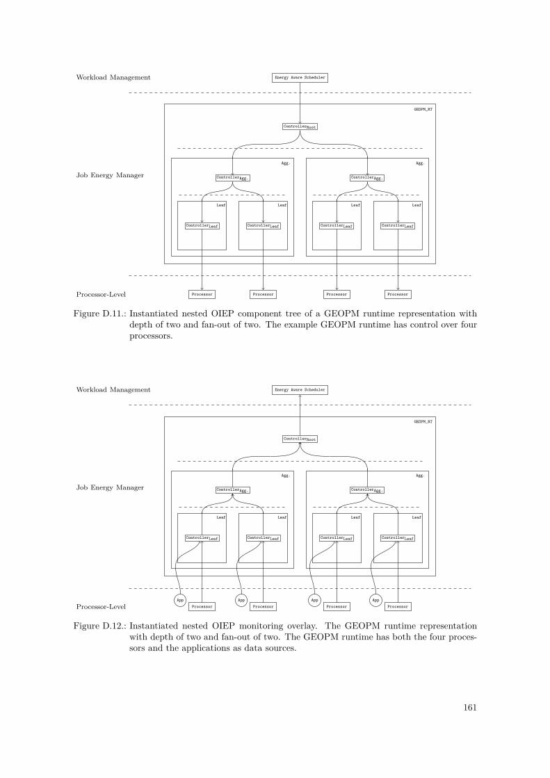
GEOPM_RT
ControllerRoot
Agg.
ControllerAgg.
Leaf
ControllerLeaf
Processor
Leaf
ControllerLeaf
Processor
Agg.
ControllerAgg.
Leaf
ControllerLeaf
Processor
Leaf
ControllerLeaf
Processor
Energy Aware SchedulerWorkload Management
Job Energy Manager
Processor-Level
Figure D.11.: Instantiated nested OIEP component tree of a GEOPM runtime representation withdepth of two and fan-out of two. The example GEOPM runtime has control over fourprocessors.
GEOPM_RT
ControllerRoot
Agg.
ControllerAgg.
Leaf
ControllerLeaf
Processor
App
Leaf
ControllerLeaf
Processor
App
Agg.
ControllerAgg.
Leaf
ControllerLeaf
Processor
App
Leaf
ControllerLeaf
Processor
App
Energy Aware SchedulerWorkload Management
Job Energy Manager
Processor-Level
Figure D.12.: Instantiated nested OIEP monitoring overlay. The GEOPM runtime representationwith depth of two and fan-out of two. The GEOPM runtime has both the four proces-sors and the applications as data sources.
161

based on the agent reports the required measurements up the tree, using aggregate_sample. Once anaggregator acquired all samples of its child processes, and performed the aggregation the results aresent up the tree towards the root to adjust policies accordingly. Finally, these are sent upwards inthe hierarchy.This control loop is executed continuously, as needed in hierarchical control loops with noisy mea-
surements and continuous changes in the operational environment. A second way to use the hierarchyis for agent implementations to set a specific policy and split energy and power budgets accordinglyonce at the start of the job. Once the job completes the monitoring data is used to generate back theresult if so required, not running continuous adjustments. This is implemented in the static policiesof GEOPM and the monitoring agent.This exercise of illustrating a simple nested implementation, visually, shows how a complex tool,
such as GEOPM can be mapped to the OIEP concepts. The resulting structure shown as an OIEParchitecture helps to clarify the mechanisms, where control and monitoring information is used in atransparent way. This is especially useful for the evolution of multiple components in an integratedco-design fashion.
162
D.3. Constructing an OIEP Architecture for the SuperMUCPhase 1 & 2 systems
LRZ’s primary concern is energy to solution [Mai+18; Koe+18; Koe+19]. Starting with the “Descrip-tion of Goods and Services for the European High Performance Computer SuperMUC at LRZ” [Lei10],explicit requirements on managing energy from the software side were added for LRZ’s future systemprocurements. Before that, the procurement process only required naming the peak energy consump-tion as an explicit requirement to be provided by vendors bidding for the systems [Bad+04]. Suchrequirement on peak energy consumption in procurement documents is mainly for safe design of theelectrical system. The RFP procurement for SuperMUC Phase 1 in 2010 introduced specific asksabout energy efficiency regarding the system [Lei10]. The RFP emphasizes this by setting a primarygoal for the petascale class system:
“To establish an integrated, highly energy efficient system and a programming environ-ment which enable the solution of the most challenging scientific problems from widelyvarying scientific areas.”
Description of Goods and Services for the European HighPerformance Computer SuperMUC at LRZ, 2010. [Lei10,p. 1]
Additional inquiries are mentioned in the document and marked with important for weighting in thedecision-making process, such as: “The batch system should be energy-aware” [Lei10, p. 32]. Thetext goes as far, as to suggest possible solutions, such as using sleep states for unused componentsand application dependent frequency settings. However, the monitoring system for energy and per-formance is still unweighted3 in the document. The offered system is among the first to introducean energy aware scheduling solution [Auw+14]. In the following this system is modeled as an OIEParchitecture.The construction of the OIEP architectures for the SuperMUC Phase 1 and SuperMUC Phase 2
systems presented below the five steps of the method for applying reference models, as of Section 4.1.
D.3.1. SuperMUC Phase 1&2 – Problem DescriptionTo construct an OIEP architecture which describes the SuperMUC Phase 1 system, the availabledocumentation is analyzed. This is primarily based on the system solution and software systeminstalled, since the RFP document has had no direct requirements on integrated energy and powermanagement, yet. The goal is to have a model description of the energy and power managementsystem. For reference the system specification of SuperMUC Phase 1 and Phase 2 are provided:SuperMUC Phase 1 is the initial installation of the SuperMUC system. The main installation
are 9216 IBM System x iDataPlex dx360M4 nodes, using Intel Sandy Bridge-EP Xeon E5-2680 8Cprocessor, totaling 2.897 PFLOPS of peak performance. Additional parts of the system are 205 Blade-Center HX5 nodes, using Intel Westmere-EX Xeon E7-4870 10C processors, totaling 0.078 PFLOPS,installation in 2011, and 32 IBM System x iDataPlex dx360M4 nodes, using Intel Ivy-Bridge andXeon Phi 5110P 0.064 PFLOPS, installation in 2013. [LRZS] Installation of the main system: 2012,Juli [BB12].SuperMUC Phase 2 is the second large installation of the SuperMUC System. The system contains
3072 Lenovo NeXtScale nx360M5 WCT nodes, using Intel Haswell Xeon E5-2697 v3 processor. Thetheoretical peak performance of the system is 3.58 PFLOPS [LRZS]. Installation of the Phase 2system: 2015, June [Pal15].The extension for the Phase 2 system did not imply any fundamental change in the energy and
power management setup, aside from the hardware and infrastructure upgrades.
The offered solution for SuperMUC Phase 1 contained the following three components:
• Power-Aware Scheduler• Job Database
3That is, not marked ‘mandatory’, ‘important’ or as ‘target’ in the RFP document.
163

• Control optimal frequency via DVFS
The power aware scheduler for optimal frequency selection used in the procurement of SuperMUCPhase 1, selected for installation at LRZ with the vendor International Business Machines Corporation(IBM), is described in detail in [Auw+14]. The software system for both Phase-1 and Phase-2are similar enough so that a single OIEP architecture covers both systems. The difference can bereduced to parameters of the model and the hardware used, were both do not change how the OIEParchitecture is constructed or its result.The LoadLeveler [IBMb] scheduler used in the system has capabilities to predict energy consump-
tion on a node given a specific frequency. The technical implementation of LoadLeveler’s functionalityis based on a patent [Bel+13]. After completion of a job, information about runtime, frequency, power,average CPI, average memory utilization of the application are stored in a job database. The databaseentry is referred to with a job-ID, or tag. Any following job submitted with the same job-ID uses theoptimal frequency as predicted by the mechanisms implemented in the LoadLeveler functionality.The scheduling system can predict optimal frequency for a given job and calculates the estimated
energy consumption. Modeling the system therefore results in a straight forward OIEP architecture.Even though administrative operation is not described in the RFP document, the system documen-tation suggests that tools support for system management. This is done using xCat [IBMc; For+;LRZS]. xCat has capabilities beyond what is described in the document at hand, and it is unknownto the author if advanced functionality, such as triggering throttling events as operational safeguardsor shutoff of idle nodes using its rpower <noderange> on|off Command Line Interface (CLI) toolsare used. Thus, it is not modeled here. The usage of this is not described, but can be modeled inoblivious fashion, using the mechanisms of the OIEP reference model.
D.3.2. SuperMUC Phase 1&2 – Identification of RequirementsWith the goal to present the energy and power management system, the according requirements’identification can be presented in brief:
• Modeling the scheduler;• Modeling the processor control;• Modeling the job awareness.
D.3.3. SuperMUC Phase 1&2 – Reference Model or Architecture SelectionThe statement that the system is to be modeled using an OIEP architecture, completes step c) ofthe method for the application of the reference model.
D.3.4. SuperMUC Phase 1&2 – OIEP Architecture ConstructionFor the construction of the OIEP architecture (step d) of the method) the seven steps for modelconstruction as described in Section 4.1 are used. These commence in the following paragraphs.
D.3.4.1. Identifying OIEP Levels for SuperMUC Phase 1&2
For the SuperMUC Phase1&2 systems the following levels are identified:
• System management;• Scheduler;• Job;• Processor.
For each a) scope, b) goal, c) location, d) function and e) associated components are identified.
164
System Management-Level:
a) The scope for the system management-level is the monitoring of the complete system activities.b) The goal in terms of energy and power management is a formal management anchor for the
energy and power management activities. This therefore builds the root level. This formal goalalso represents configuration and monitoring of the appropriate system configurations, delegatedto the scheduler with the aim to achieve minimized energy to solution, using frequency scalingmechanisms.4
c) The location is a high availability management system outside the cluster infrastructure.d) Functionality includes the configuration and emergency setting of the energy and power man-
agement settings.e) The associated component is xCat.
Scheduler-Level:
a) The scope for level is job scheduling, thus the scope also contains all active nodes of the cluster.b) The goal in terms of energy and power management is to configure the optimal CPU frequency
for each job to achieve minimal energy to solution.c) The physical location is at a management node responsible for the scheduler. The scheduler
also requires the job database for the selection of optimal frequency for recurring jobs. Thismeans that an additional resource for this database or for querying this information is needed.
d) Functionality is the implementation of patent [Bel+13].e) Therefore, the associated component is LoadLeveler [IBMb] with the implemented functionality.
Scheduler-Level:
a) The scope for the job-level is the job partition allocated to a compute job.b) The goal of the job level is to enforce the selected frequency settings selected by the scheduler.c) The logical location is at the handover from the resource manager to the compute job, namely
the system administration part of prolog and epilog of each compute job.d) The functionality required is setting and resetting DVFS accordingly before and after a job.
Additionally, the job level functionality needs to aggregate the total energy spent after the jobis complete (forwarding the information to the job database for optimal frequency estimation).
e) The associated components are the prolog and epilog-script.5
Processor-Level:
a) For the processor-level, the scope is the processor’s DVFS settings.b) The goal of the processor-level is to expose the DVFS settings to the job-level, while disallowing
the user to override the settings.c) The location is in the OS kernel’s drivers and tools, enabling the functionality, as well as the
user access control.d) The functionality is configuration to enable the job-level. This entails to provide the processors’
frequency controls via the P-state mechanism.e) The associated components are the Linux kernel modules acpi-cpufreq or intel_pstate. For
the setup at hand the P-state identifier is used, representing the component, since the accessmechanism is not known to the author.
The next step is to place the identified components in the OIEP component tree.4This goal is voiced by LRZ, as well as seen in the frequency selection mechanism shown in [Auw+14]; Employed toselect the optimal base frequency for the SuperMUC Phase 1 system.
5The author has no knowledge if this is implemented in this way since the solution is closed-source.
165
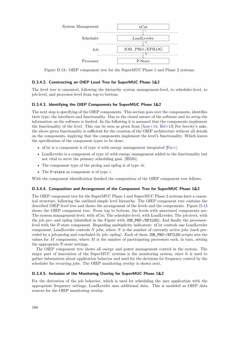
System Management
Scheduler
Job
Processor
xCat
LoadLeveler
JOB_PRO-/EPILOG
P-State
1
N
M
Figure D.13.: OIEP component tree for the SuperMUC Phase 1 and Phase 2 systems.
D.3.4.2. Constructing an OIEP Level Tree for SuperMUC Phase 1&2
The level tree is canonical, following the hierarchy system management-level, to scheduler-level, tojob-level, and processor-level from top to bottom.
D.3.4.3. Identifying the OIEP Components for SuperMUC Phase 1&2
The next step is specifying of the OIEP components. This section goes over the components, identifiestheir type, the interfaces and functionality. Due to the closed nature of the software and its setup theinformation on the software is limited. In the following it is assumed that the components implementthe functionality of the level. This can be seen as given from [Auw+14; Bel+13] For brevity’s sake,the above given functionality is sufficient for the creation of the OIEP architecture without all detailson the components, implying that the components implement the level’s functionality. Which leavesthe specification of the component types to be done:
• xCat is a component is of type ii with energy management integrated [For+].• LoadLeveler is a component of type iii with energy management added to the functionality but
not vital to serve the primary scheduling goal. [IBMb].• The component type of the prolog and epilog is of type iii.• The P-state as component is of type i.
With the component identification finished the composition of the OIEP component tree follows.
D.3.4.4. Composition and Arrangement of the Component Tree for SuperMUC Phase 1&2
The OIEP component tree for the SuperMUC Phase 1 and SuperMUC Phase 2 systems have a canon-ical structure, following the outlined simple level hierarchy. The OIEP component tree contains thedescribed OIEP level tree and shows the arrangement of the levels and the components. Figure D.13shows the OIEP component tree. From top to bottom, the levels with associated components are:The system management-level, with xCat; The scheduler-level, with LoadLeveler; The job-level, withthe job pro- and epilog (identified in the Figure with JOB_PRO-/EPILOG); And finally the processor-level with the P-state component. Regarding multiplicity indicators: xCat controls one LoadLevelercomponent; LoadLeveler controls N jobs, where N is the number of currently active jobs (each pre-ceded by a job-prolog and concluded by job- epilog). Each of these JOB_PRO-/EPILOG scripts sets thevalues for M components, where M is the number of participating processors each, in turn, settingthe appropriate P-state settings.The OIEP component tree shows all energy and power management control in the system. The
major part of innovation of the SuperMUC systems is the monitoring system, since it is used togather information about application behavior and used for the decisions for frequency control by thescheduler for recurring jobs. The OIEP monitoring overlay is shown next.
D.3.4.5. Inclusion of the Monitoring Overlay for SuperMUC Phase 1&2
For the derivation of the job behavior, which is used for scheduling the user application with theappropriate frequency settings, LoadLeveler uses additional data. This is modeled as OIEP datasources for the OIEP monitoring overlay.
166
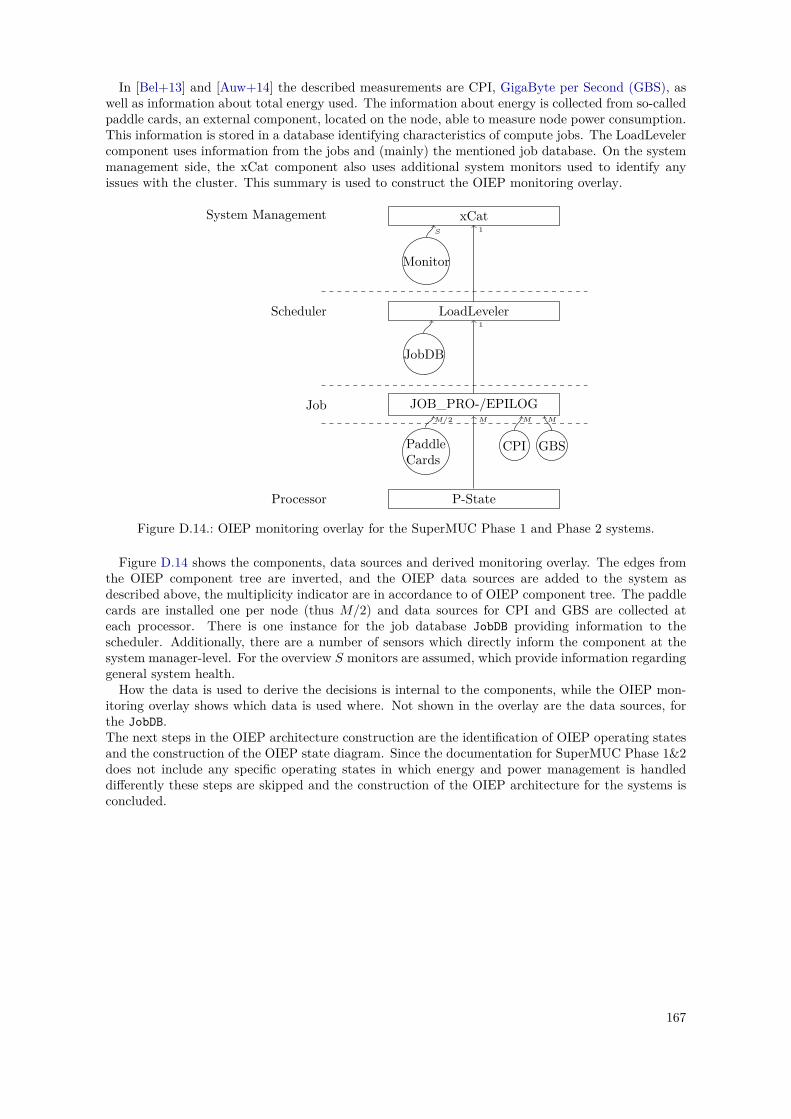
In [Bel+13] and [Auw+14] the described measurements are CPI, GigaByte per Second (GBS), aswell as information about total energy used. The information about energy is collected from so-calledpaddle cards, an external component, located on the node, able to measure node power consumption.This information is stored in a database identifying characteristics of compute jobs. The LoadLevelercomponent uses information from the jobs and (mainly) the mentioned job database. On the systemmanagement side, the xCat component also uses additional system monitors used to identify anyissues with the cluster. This summary is used to construct the OIEP monitoring overlay.
System Management
Scheduler
Job
Processor
xCat
LoadLeveler
JOB_PRO-/EPILOG
P-State
1
1
M
Monitor
S
JobDB
PaddleCards
M/2
CPI GBS
M M
Figure D.14.: OIEP monitoring overlay for the SuperMUC Phase 1 and Phase 2 systems.
Figure D.14 shows the components, data sources and derived monitoring overlay. The edges fromthe OIEP component tree are inverted, and the OIEP data sources are added to the system asdescribed above, the multiplicity indicator are in accordance to of OIEP component tree. The paddlecards are installed one per node (thus M/2) and data sources for CPI and GBS are collected ateach processor. There is one instance for the job database JobDB providing information to thescheduler. Additionally, there are a number of sensors which directly inform the component at thesystem manager-level. For the overview S monitors are assumed, which provide information regardinggeneral system health.How the data is used to derive the decisions is internal to the components, while the OIEP mon-
itoring overlay shows which data is used where. Not shown in the overlay are the data sources, forthe JobDB.The next steps in the OIEP architecture construction are the identification of OIEP operating statesand the construction of the OIEP state diagram. Since the documentation for SuperMUC Phase 1&2does not include any specific operating states in which energy and power management is handleddifferently these steps are skipped and the construction of the OIEP architecture for the systems isconcluded.
167


D.4. Constructing an OIEP Architecture for the SuperMUC-NGSystem
As successor to the SuperMUC Phase 1 and Phase 2 systems, SuperMUC-NG draws many insightsfrom its predecessors. LRZ applied the knowledge gained from the previous HPC systems in boththe procurement, and the selection of the final system capabilities [Bre+16b; TOPf]. The majorinnovation compared to the previous systems is the move from the closed LoadLeveler to an openSLURM [YJG03] based system, with the integration of the EAR tool [CB19]. Therefore, the energymanagement setup changed. In the following the construction of a possible6 OIEP architecture forthe SuperMUC-NG is presented.
D.4.1. SuperMUC Phase-NG – Problem DescriptionFor the problem description and requirements’ derivation, a summary of items relevant to energy andpower as requested in the procurement is given. This is supplemented with information about thesolution offered to LRZ, which is used to describe the problem for the construction of a representativeOIEP architecture and to derive its requirements.Where the previous RFP documents for SuperMUC Phase 1 and Phase 2 are very brief on energy
and power management, the RFP for SuperMUC-NG mentions several exact specifications. This canbe seen in both the description of goods and services document [Bre+16b] and the decision criteriaand benchmark description document [Bre+16a]. In the following a selection of the necessary andnotable requirements in the procurement are highlighted.7
In the RFP of the system large aspects focus on the energy and power specifications, their require-ments, and ways to manage and measure them. In the following a summary of noteworthy entries islisted.Regarding power supply:
• An explicit power limit of 4000 kW for Phase 1 of SuperMUC-NG, with a total power consump-tion of (a possible) Phase 2 system totaling to no more than 7150 kW of power consumption forthe computer system is set.
• Estimation of the expected mean and peak power consumption is requested.• Redundant critical components have to be connected to different PSUs.
Regarding the compute nodes:
• A monitoring granularity of temperature, energy and power with at least 1 Hz, 1 J, and 1 W,with less than 5% error is requested. (Desired readings are named with a 10 hertz readingfrequency, with less than 5% error.)
• Explicit control mechanism of compute nodes regarding temperature, voltage, energy and powerare requested.
• Run-to-run variation of the same application on different nodes should not exceed 5% (namedas important feature), with a desired power variability within 3% (named as target feature).
• Explicit service nodes reserved as: Login nodes, archive nodes, accounting, performance andpower database severs, monitoring server, resource management server, system managementserver.
Explicit information on cooling:
• Specifics on cooling loops with 1.3 MW cold water cooling and 8 MW of warm water coolingcapacity.
6OIEP was not used to design the SuperMUC-NG energy and power management system. The author’s work onlymanifested after the procurement of the system was finished and the author was not aware nor involved regardingany of the offered solutions.
7As of the procurement the SuperMUC-NG system is also planned with two Phases, similar to the original SuperMUCsystem. The original procurement focuses on Phase 1.
169

In an explicit section on energy efficiency and energy measurement (see [Bre+16b, pp. 63]), thefollowing is requested:
• A listing of all sensors in each component;• Real-time measurement for direct current (DC) energy counters for all nodes;• In-band measurement of energy and power counters via sysfs or user-space interfaces;• Out-of-band measurements capabilities via standard tools and interfaces;• Specifics on measurements up until alternating current (AC)/DC conversion;
Explicit request regarding the scheduler and resource manager are:
• Per job power measurement;• Means to control energy and power usage (including energy and power capping and power
ramp-up/ramp-down).• Additionally, the scheduler was explicitly requested to be SLURM.
Others energy and power related requests are:
• Power cycling strategy;• Strategy for orderly power-up and power-down of the system (power ramp-rate-control);
Regarding benchmarking, the document [Bre+16a] lists additional items (mandatory, but un-weighted towards the acceptance of the tender), as follows:
• Expected mean power consumption;• Energy efficiency estimates;• Monitoring capabilities during benchmarking;• The freedom to use any frequency / power envelope, while staying within the peak power
consumption proposed in the tender;• Estimated energy efficiency during High-Performance Linpack (HPL) in accordance with the
Green500;• Estimated mean power consumption as 65% of HPL’s power consumption;• Estimated energy cost based on this mean power consumption;
This summary and excerpt of items included in the RFP document show the importance of energyand power management for the system. Additionally, it illuminates several aspects of why a wellintegrated energy and power management software system is required.The ultimately procured system consists of the following hardware: SuperMUC-NG, is the next
generation flagship supercomputing system at LRZ with 6480 Lenovo ThinkSystem SD 650 DWCnodes using the Intel Skylake Xeon Platinum 8174 CPU. The interconnect is a fat tree topologyconnecting the 311050 cores for a theoretical peak performance of 26.7 PFLOPS. Total main memoryof the system is 719 TByte. [Pal17] Installation: 2018, Sep. [Pal18]. The system placed eighth on theTOP500 when first appearing on the list in November of 2018 [TOPf]The solution is supported by power management software, for which the scheduler SLURM [YJG03]
as well as the EAR [CB19] system is used. (According to [Bra+19]:) Provisioning is again done usingxCat [IBMc]; SUSE Linux Enterprise Server (SLES) [SUSE] is used as OS; The base software systemis based on OpenHPC [OHPC].Using this information the requirements’ identification is derived for the construction of the OIEP
architecture.
170

D.4.2. SuperMUC Phase-NG – Identification of RequirementsFor the requirements’ identification the explicit requests and the provided solution are outlined to beable to describe a structural solution using the OIEP reference model. The requirements are refined,whereas technical details given in the RFPs are abstracted away.The resulting requirements of OIEP architecture for energy and power management is summarized
as follows:
• The system has constraints on total power usage.• The system design was optimized for a total budget.• The approach to minimize operating costs are cooling solutions and novel software solutions.• The optimization goal is a trade-off between energy and performance, where measurement and
control is a primary goal (in contrast to the explicit minimal energy to solution).• Specific quality of sensors is given/required.• Explicit control mechanisms for energy and power capping as well as ramp-rate control are
requested.• Explicit limits on run-to-run variation (potential for software optimization in the case of hard-
ware variation)• Using this background, the known system components have to be modeled, namely: xCat for
provisioning, SLURM for scheduling, EAR energy management framework on the job and nodelevel.
The much more detailed problem description does not impact the layout of the OIEP architecture,since energy and power control is mentioned only in a limited way. (Measurement capabilities arein the focus.) The largest influence of change is the proposed and selected solution by the systemvendors. This solution is built on xCat, SLURM, and EAR, whereas energy and power control isenforced exclusively by EAR.
D.4.3. SuperMUC-NG – Reference Model or Architecture SelectionUsing the provided information the method can commence with step c): The selection of the model.The system is again described using the OIEP reference model, constructing a new OIEP architecture.Using this information a four layer OIEP architecture is constructed for SuperMUC-NG.
D.4.4. SuperMUC-NG – OIEP Architecture ConstructionThe OIEP architecture construction, step d) of the method for applying reference model commencesaccording to the seven steps of: Level identification; Level tree construction; Component identifica-tion; Component tree construction; Monitoring overlay construction; Identification of states and therepetition of these steps for any identified state (as of Sec. 4.1).
D.4.4.1. Identifying OIEP Levels for SuperMUC-NG
From the structure of those software components, the following levels are identified:
• System management;• Energy resource management;• Node;• Kernel-interface.
For each, their a) scope, b) goal, c) location, d) function and e) associated components are identified.
171

System Management-Level:
a) The scope for the system management-level, is provisioning and management of the system.b) The level’s goal is the operation under the total energy limits striking a balance between energy
budget and performance.c) The location is the system management server.d) The functionality is system provisioning, controlling energy and power, regarding normal oper-
ation, power cycling and system ramp control. Therefore, it is the root of the OIEP level treeand serves for configuration for the system admins.
e) The associated components is xCat, assuming the admins manage the server using this compo-nent.
Resource Management-Level:
a) The scope for the energy resource management-level is active energy management of all computenodes.
b) The goal is operation under the total power limit.c) The location is either the performance and power database server or one of the system man-
agement servers.d) The functionality of the energy management framework, is enforcing the global power limits and
applying warning levels depending on resource usage. This enforces the selection of respectiveenergy and power strategy according to total energy budget, job-type. An additional functionis accounting using the performance and power database servers.
e) Associated component is a module from the energy management framework EAR: EAR GlobalManager (EARGM).
Node-Level:
a) The scope for the node-level is the energy and power management of the individual nodes.b) The level’s goal is the enforcement of local power/frequency limits and the efficient management
of power/performance trade-offs of the individual node.c) The location is on each node of the cluster.d) The functionality is to realize the level’s goal by enforcing power and frequency optimizations.
This is done by setting optimal frequency assessing requested vs. required frequencies. The leveltakes energy and power control from the energy resource management-level to enforce strictlimits. To select optimal frequency for the node, power/frequency and performance is assessed.Additionally, environment flags set by the scheduler are taken into account for selection ofoptimization (to temporarily suspend the functionality). User application libraries can alsoserve as additional data sources for specific job types.
e) The associated components is EARD.
Kernel-Interface-Level:
a) The scope for the kernel-interface-level is the kernel-userspace API for energy and power andfrequency control of the individual nodes.
b) The level’s goal is to interface with the OS interface to the hardware.c) The location is in userspace of the OS.d) The functionality is control of access rights, setting of frequency and power limits using Linux
kernel functionality (including loading and configuration).
172
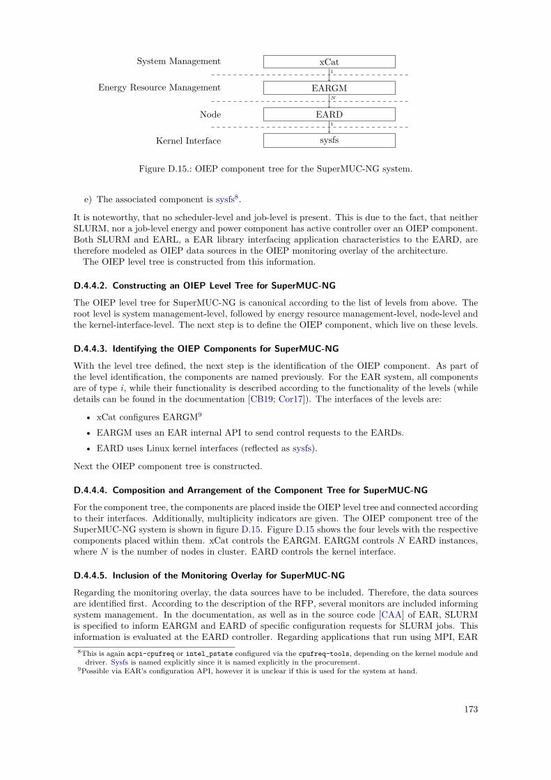
System Management
Energy Resource Management
Node
Kernel Interface
xCat
EARGM
EARD
sysfs
1
N
1
SLURM
Figure D.15.: OIEP component tree for the SuperMUC-NG system.
e) The associated component is sysfs8.
It is noteworthy, that no scheduler-level and job-level is present. This is due to the fact, that neitherSLURM, nor a job-level energy and power component has active controller over an OIEP component.Both SLURM and EARL, a EAR library interfacing application characteristics to the EARD, aretherefore modeled as OIEP data sources in the OIEP monitoring overlay of the architecture.The OIEP level tree is constructed from this information.
D.4.4.2. Constructing an OIEP Level Tree for SuperMUC-NG
The OIEP level tree for SuperMUC-NG is canonical according to the list of levels from above. Theroot level is system management-level, followed by energy resource management-level, node-level andthe kernel-interface-level. The next step is to define the OIEP component, which live on these levels.
D.4.4.3. Identifying the OIEP Components for SuperMUC-NG
With the level tree defined, the next step is the identification of the OIEP component. As part ofthe level identification, the components are named previously. For the EAR system, all componentsare of type i, while their functionality is described according to the functionality of the levels (whiledetails can be found in the documentation [CB19; Cor17]). The interfaces of the levels are:
• xCat configures EARGM9
• EARGM uses an EAR internal API to send control requests to the EARDs.• EARD uses Linux kernel interfaces (reflected as sysfs).
Next the OIEP component tree is constructed.
D.4.4.4. Composition and Arrangement of the Component Tree for SuperMUC-NG
For the component tree, the components are placed inside the OIEP level tree and connected accordingto their interfaces. Additionally, multiplicity indicators are given. The OIEP component tree of theSuperMUC-NG system is shown in figure D.15. Figure D.15 shows the four levels with the respectivecomponents placed within them. xCat controls the EARGM. EARGM controls N EARD instances,where N is the number of nodes in cluster. EARD controls the kernel interface.
D.4.4.5. Inclusion of the Monitoring Overlay for SuperMUC-NG
Regarding the monitoring overlay, the data sources have to be included. Therefore, the data sourcesare identified first. According to the description of the RFP, several monitors are included informingsystem management. In the documentation, as well as in the source code [CAA] of EAR, SLURMis specified to inform EARGM and EARD of specific configuration requests for SLURM jobs. Thisinformation is evaluated at the EARD controller. Regarding applications that run using MPI, EAR
8This is again acpi-cpufreq or intel_pstate configured via the cpufreq-tools, depending on the kernel module anddriver. Sysfs is named explicitly since it is named explicitly in the procurement.
9Possible via EAR’s configuration API, however it is unclear if this is used for the system at hand.
173
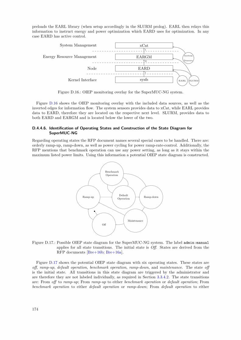
preloads the EARL library (when setup accordingly in the SLURM prolog). EARL then relays thisinformation to instruct energy and power optimization which EARD uses for optimization. In anycase EARD has active control.
System Management
Energy Resource Management
Node
Kernel Interface
xCat
EARGM
EARD
sysfs
1
N
1
EARL SLURM
System
Sensors
Figure D.16.: OIEP monitoring overlay for the SuperMUC-NG system.
Figure D.16 shows the OIEP monitoring overlay with the included data sources, as well as theinverted edges for information flow. The system sensors provides data to xCat, while EARL providesdata to EARD, therefore they are located on the respective next level. SLURM, provides data toboth EARD and EARGM and is located below the lower of the two.
D.4.4.6. Identification of Operating States and Construction of the State Diagram forSuperMUC-NG
Regarding operating states the RFP document names several special cases to be handled. There are:orderly ramp-up, ramp-down, as well as power cycling for power ramp-rate-control. Additionally, theRFP mentions that benchmark operation can use any power setting, as long as it stays within themaximum listed power limits. Using this information a potential OIEP state diagram is constructed.
DefaultOperation
BenchmarkOperation
Ramp-up Ramp-down
OffMaintenance
Figure D.17.: Possible OIEP state diagram for the SuperMUC-NG system. The label admin:manualapplies for all state transitions. The initial state is Off. States are derived from theRFP documents [Bre+16b; Bre+16a].
Figure D.17 shows the potential OIEP state diagram with six operating states. These states areoff, ramp-up, default operation, benchmark operation, ramp-down, and maintenance. The state offis the initial state. All transitions in this state diagram are triggered by the administrator andare therefore they are not labeled individually, as required in Section 3.3.4.2. The state transitionsare: From off to ramp-up; From ramp-up to either benchmark operation or default operation; Frombenchmark operation to either default operation or ramp-down; From default operation to either
174

benchmark operation or ramp-down; From ramp-down to maintenance; From maintenance to eitheroff or ramp-up.Since there is no public documentation if these states are actually used regarding the systems
energy and power management, or how they are realized, the associated OIEP architectures would bespeculation, which is therefore skipped and left as an exercise. (It should be noted that the examplesjust serve as illustrative purpose for the usage of the OIEP reference model, and how the requests ofthe RFP could be realized. There is no claim to exact representation of the installation.)Therefore, the last step of the architecture construction, the addressing the remaining OIEP oper-
ating states for SuperMUC-NG (by repetition of the above steps for each state of the state diagram),is forpassed. This concludes the OIEP architecture construction for the SuperMUC-NG system.
175

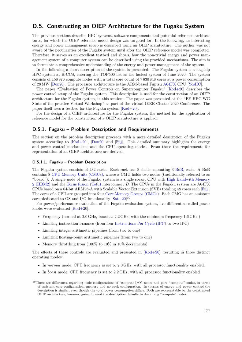
D.5. Constructing an OIEP Architecture for the Fugaku SystemThe previous sections describe HPC systems, software components and potential reference architec-tures, for which the OIEP reference model design was targeted for. In the following, an interestingenergy and power management setup is described using an OIEP architecture. The author was notaware of the peculiarities of the Fugaku system until after the OIEP reference model was completed.Therefore, it serves as an excellent testbed and shows, how the non-trivial energy and power man-agement system of a computer system can be described using the provided mechanisms. The aim isto formulate a comprehensive understanding of the energy and power management of the system.In the following a short description of the system is presented: The Fugaku system is a flagship
HPC system at R-CCS, entering the TOP500 list as the fastest system of June 2020. The systemconsists of 158 976 compute nodes with a total core count of 7 630 848 cores at a power consumptionof 28 MW [Don20]. The processor architecture is the ARM-based Fujitsu A64FX CPU [YosHC].
The paper “Evaluation of Power Controls on Supercomputer Fugaku” [Kod+20] describes thepower control setup of the Fugaku system. This description is used for the construction of an OIEParchitecture for the Fugaku system, in this section. The paper was presented at the “EE-HPC-WGState of the practice Virtual Workshop” as part of the virtual IEEE Cluster 2020 Conference. Thepaper itself uses a testbed for the Fugaku system [Kod+20].For the design of a OIEP architecture for the Fugaku system, the method for the application of
reference model for the construction of a OIEP architecture is applied.
D.5.1. Fugaku – Problem Description and RequirementsThe section on the problem description proceeds with a more detailed description of the Fugakusystem according to [Kod+20], [Don20] and [Fuj]. This detailed summary highlights the energyand power control mechanisms and the CPU operating modes. From these the requirements forrepresentation of an OIEP architecture are derived.
D.5.1.1. Fugaku – Problem Description
The Fugaku system consists of 432 racks. Each rack has 8 shelfs, mounting 3 BoB, each. A BoBcontains 8 CPU Memory Units (CMUs), where a CMU holds two nodes (traditionally referred to as“board”). A single node of the Fugaku system is a single socket CPU with High Bandwith Memory2 (HBM2) and the Torus fusion (Tofu) interconnect D. The CPUs in the Fugaku system are A64FXCPUs based on a 64-bit ARMv8-A with Scalable Vector Extension (SVE) totaling 48 cores each [Fuj].The cores of a CPU are grouped into four Core Memory Groups (CMGs). Each CMG has an assistantcore, dedicated to OS and I/O functionality [Sat+20]10.For power/performance evaluation of the Fugaku evaluation system, five different so-called power
knobs were evaluated [Kod+20]:
• Frequency (normal at 2.0 GHz, boost at 2.2 GHz, with the minimum frequency 1.6 GHz.)• Limiting instruction issuance (from four Instructions Per Cycle (IPC) to two IPC)• Limiting integer arithmetic pipelines (from two to one)• Limiting floating-point arithmetic pipelines (from two to one)• Memory throttling from (100% to 10% in 10% decrements)
The effects of these controls are evaluated and presented in [Kod+20], resulting in three distinctoperating modes:
• In normal mode, CPU frequency is set to 2.0 GHz, with all processor functionality enabled.• In boost mode, CPU frequency is set to 2.2 GHz, with all processor functionality enabled.
10There are differences regarding node configurations of “compute-I/O” nodes and pure “compute” nodes, in termsof assistant core configuration, memory and network configuration. In therms of energy and power control thedescription is similar, even though the total power consumption differs. Both are representable by the constructedOIEP architecture, however, going forward the description defaults to describing “compute” nodes.
177

• In eco mode, the reduced floating-point arithmetic pipeline is used.
The paper describes that the limits of instruction issuance, integer arithmetic pipeline, as well as thememory throttling, showed mixed resulted. Therefore, they are not explicitly referred to as with amode name.In addition to the power knobs, the A64FX CPUs also implement a core-retention functionality.
This implies that unused cores can be set to lower C-states, independently. Core-retention, as wellas power measurement are realized using Power-API interfaces.The nodes, which are not part of an active job use node-retention functionality, placing the complete
node in a retention state with only one assistant core active. The paper mentions that cooling has tobe adjusted in the case, of many nodes switching to node retention in a short period of time [Kod+20,p.3].Each BoB has an integrated FPGA processing internal measurements to assure that total power
consumed at the BoB-scale is not exceeded. This mechanism assists in safe operation, while notexceeding a total power consumption of 30 MW.
D.5.1.2. Fugaku – Identification of Requirements
For step b), the requirements’ identification of the method for energy and power management archi-tecture description is used. This description implies several points:
• The system scheduler configures the basic node configuration.• Within each compute job, the user can select and configure the participating nodes, as follows:
– Set CPU frequency;– Throttle memory11;– Set individual cores to core-retention;– Set floating-point unit to FLoatinting-point unit A (FLA) only;– Set integer unit to EXecution unit A (EXA) only;– Set Instruction Issuance Limit (IIL).
• Idle nodes are put into node-retention (requiring a potential adjustment of the cooling facilities,depending on the fraction of idle to active nodes).
• BoB measurements can trigger and enforce a power limit.
D.5.1.3. Fugaku – Reference Model or Architecture Selection
Using these requirements a representation of the Fugaku system using OIEP reference model isconstructed, completing step c), of the method.
D.5.2. Fugaku – OIEP Architecture ConstructionThe construction of the OIEP architecture for the Fugaku system commences according to the sevensteps outlined in the method of Section 4.1. Initially, the OIEP levels are identified (see Sec. D.5.2.1),which are used to construct the OIEP level tree (see Sec. D.5.2.2). Next, the OIEP components areidentified (see Sec. D.5.2.3), which are used to construct the OIEP component tree (see Sec. D.5.2.4).The OIEP data sources are identified for the construction of the OIEP monitoring overlay (seeSec. D.5.2.5). Following this, the OIEP operating states are identified (see D.5.2.6), and the abovesteps are repeated for each state, concluding the construction of the OIEP architecture.
11Assumed at the CMG granularity, according to [YosHC]
178

D.5.2.1. Identifying OIEP Levels for the Fugaku System
Using the above description and requirements, the following levels are identified:
• System Management-level• Cooling Facility-level• Scheduler-level• Job-level• Node-level• CPU-level• CPU frequency-level• CMG-level• Memory-level• Core-type-level• Core-state-level• Core-function-level
For each level the a) scope, b) goal, c) location, d) function and e) associated components is describedbelow.
System Management-Level:
a) The scope For the system management-level is the complete system.b) The goal is to efficiently operate within the 30 MW facility power envelope.c) The location is a management server (unspecified). Logically this level builds the root of the
OIEP level tree.d) The functionality is to provide a root to the OIEP architecture, and enable and set all base
configurations for the underlying levels. This is done according to the responsibilities of a rootlevel and in accordance with the Fugaku system description and the OIEP reference model.The direct interaction is with the adjacent scheduler level, as well as the cooling facility.
e) The associated component is the Management System (mentioned in the software stack asof [Don20, p.10]).
Cooling Facility-Level:
a) The scope for the cooling facility-level is the cooling facility, according to mnemonic nomencla-ture.
b) The goal is to provide sufficient cooling for the complete system, while keeping the coolinggeneration aligned with heat energy generation of the system.
c) The location is the facility management.d) The functionality is measurement and adjustment of cooling production according to the levels
goals, this response has to be guaranteed to control cooling over-generation when many nodesswitch into node retention.
e) The associated component for the OIEP architecture is a cooling controller (Coolingcrtl).
179

Scheduler-Level:
a) The scope for the scheduler-level is the management of all participating nodes grouped as jobs.b) The goal is to provide the configurations as well as grouping of nodes according to jobs. The
configurations set and enable the energy and power management controls, as required for theuser applications.
c) The location is at the service nodes dedicated to the scheduler.d) The functionality is the fulfillment of the level’s goals.e) The associated component is not further specified, and named “batch job system” in [Don20,
p. 10]. Thus, an abstract Scheduler component is identified for the construction.
Job-Level:
a) The scope for the job-level is the individual job.b) The goal is maximum performance without wasting power.c) The location is a job partition12.d) The functionality is the selection of node configurations according to: Normal or boost mode;
And whether to enable eco mode and core retention. Additionally, the job level has the func-tionality of reporting energy and power of a job to the scheduler and the user.
e) The associated component remains abstract and is indicated as Job.
Node-Level:
a) The scope for the node-level is the individual node participating in the job.b) The goal is primarily to provide the node’s control functionality, including node retention for
jobs not associated with a compute job.c) The location is a process on the node. Depending on the implementation, the located is placed
on a compute or assistant core of the node.d) The functionality is the provision of interfaces and forwarding the parent’s components control
decisions, but also to forward energy and power measurements to the job-level.e) The associated component is a node-level controller.
CPU-Level:
a) The scope for the CPU-level is the energy and power management of the CPU functionalities.b) The goal is to enable measurement and control and forward the node requests.c) The location is either assistant or compute core of the processor.d) The functionality includes the control of clock frequency, as well as the management of the four
associated CMGs.e) The associated components are identified as either an active or an idle CPU component.
CPU Frequency-Level:
a) The scope for the CPU frequency-level is the frequency control of the CPU.b) The goal is to set the controls according to the requested frequency at the parent level, the
CPU.c) The location is a kernel driver on an (assistant) core of the CPU.d) The functionality is in accordance with the goal.e) The associated component is a DVFS controller.
12In [Kod+20], it remains unspecified, if the energy and power controls are accessible to the user or if the administrationretains full control of the configuration.
180
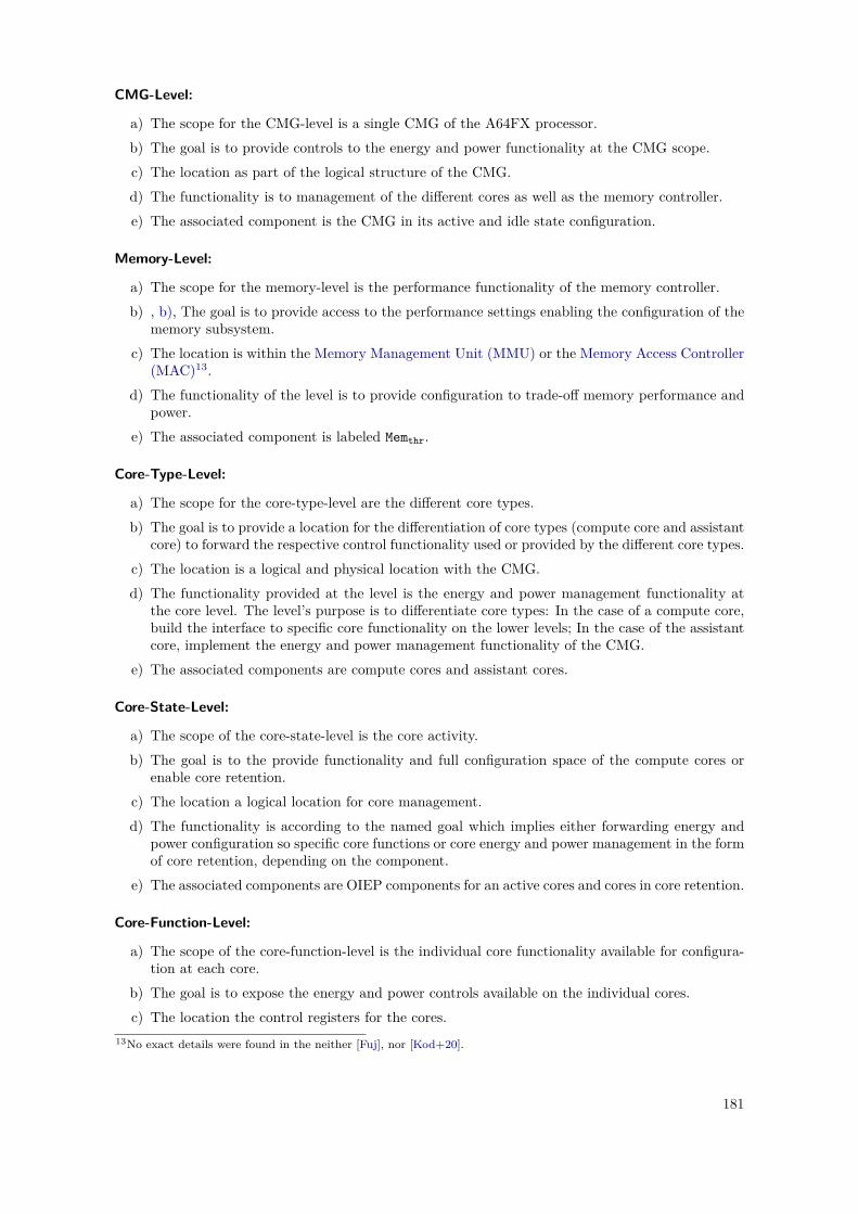
CMG-Level:
a) The scope for the CMG-level is a single CMG of the A64FX processor.b) The goal is to provide controls to the energy and power functionality at the CMG scope.c) The location as part of the logical structure of the CMG.d) The functionality is to management of the different cores as well as the memory controller.e) The associated component is the CMG in its active and idle state configuration.
Memory-Level:
a) The scope for the memory-level is the performance functionality of the memory controller.b) , b), The goal is to provide access to the performance settings enabling the configuration of the
memory subsystem.c) The location is within the Memory Management Unit (MMU) or the Memory Access Controller
(MAC)13.d) The functionality of the level is to provide configuration to trade-off memory performance and
power.e) The associated component is labeled Memthr.
Core-Type-Level:
a) The scope for the core-type-level are the different core types.b) The goal is to provide a location for the differentiation of core types (compute core and assistant
core) to forward the respective control functionality used or provided by the different core types.c) The location is a logical and physical location with the CMG.d) The functionality provided at the level is the energy and power management functionality at
the core level. The level’s purpose is to differentiate core types: In the case of a compute core,build the interface to specific core functionality on the lower levels; In the case of the assistantcore, implement the energy and power management functionality of the CMG.
e) The associated components are compute cores and assistant cores.
Core-State-Level:
a) The scope of the core-state-level is the core activity.b) The goal is to the provide functionality and full configuration space of the compute cores or
enable core retention.c) The location a logical location for core management.d) The functionality is according to the named goal which implies either forwarding energy and
power configuration so specific core functions or core energy and power management in the formof core retention, depending on the component.
e) The associated components are OIEP components for an active cores and cores in core retention.
Core-Function-Level:
a) The scope of the core-function-level is the individual core functionality available for configura-tion at each core.
b) The goal is to expose the energy and power controls available on the individual cores.c) The location the control registers for the cores.
13No exact details were found in the neither [Fuj], nor [Kod+20].
181

d) The functionality is in accordance with the goals.e) The associated components are a component for the IIL control, a component for limiting to
the usage of EXA and a component for limiting to use FLA.
Using these level descriptions, the OIEP level tree is constructed.
D.5.2.2. Constructing an OIEP Level Tree for the Fugaku System
According to the level description and the identified control hierarchy, the OIEP level tree is con-structed. Figure D.18 shows the constructed level tree for the Fugaku system. From top to bottom,
SystemManagement-level
Scheduler-level
Job-level
Node-level
CPU-level
CoolingFacility-level
CPU frequency-level CMG-level
Memory-level
CMG-level
Core-type-level
Core-state-level
Core-function-level
Figure D.18.: OIEP architecture for the Fugaku System – Constructed OIEP level tree.
the system management-level controls the scheduler-level and the cooling facility-level, which is a leaflevel. The scheduler-level controls the job-level. The job-level controls the node-level. The CPU-levelcontrols the CPU frequency-level and the CMG-level. The CPU frequency-level is a leaf level. TheCMG-level controls the core-type-level and the memory-level (which is a leaf level). The core-type-level controls the core-state-level, which finally controls the last leaf level, the core-function-level.
D.5.2.3. Identifying the OIEP Components for the Fugaku System
The next step in the construction of the OIEP architecture for the Fugaku system is the identificationof the OIEP components. The procedure goes form level to level and identifies the components, theirtype, their function and their interfaces (in accordance with Sec. 3.3.2.1).
Component on the System Management-Level: The identified component is the ManagementSystem, the component is of type ii, with functionality to configure the scheduler and manage thecooling system; The interfaces, are according configuration files/APIs and control interfaces to thefacilities.
182

Component on the Cooling Facility-Level: The identified component, the Coolingcrtl, componentis of type iv. The functionality is to provide the facility cooling, responding to requests in coolingfrom the system management14. The component is a leaf component, thus no interfaces to childcomponents are modeled.
Component on the Scheduler-Level: The identified component, the Scheduler, is of type iii. Thefunctionality is to configure job partitions with the respective configurations. The energy and powerrelated tasks are enabling and disabling node retention, depending on whether the nodes will beallocated to a job or to the pool of idle nodes. The interface is the epilog and prolog as well asjob and node configuration files. The component controls N jobs and one group of nodes identifiedas the Poolidle (therefore the edge is labeled N + 1). The scheduler implements the mechanism toallocate and configure the jobs for the job type, active or in reserve, such that the original schedulerfunctionality is supported: The allocation of nodes to compute jobs.
Component on the Job-Level: For the job-level, two OIEP components are identified: First: theJob component, representing all active jobs in the system; and second the Poolidle component,representing the pool of idle nodes.The active job is a component of type iii, since its primary goal is the execution of the compute
job. The functionality is to use the provided control mechanisms, configured and granted by theparent levels, to maximize performance without wasting energy. That means, the active request offrequencies per CPU, the activation and deactivation of processor functionalities etc. The computejob is the main source of information for the configuration selection, since, as stated in [Kod+20],the different mechanisms show their effectiveness based on the job characteristics and their resourceusage. The interfaces are controlled via APIs targeting the lower levels of the OIEP architecture. Therequests are passed on to the respective component in the hierarchy. The energy and power controlinterface targets all participating nodes of a job. The component actively involves the user.The component identified as Poolidle is treated as a special job type. The component serves as
reserve for all nodes waiting to be allocated to active jobs. These are configured accordingly usingnode retention. The component therefore is of type ii. The interface is an API call to activate noderetention, and resume normal operation.
Component on the Node-Level: On the node-level the two components are the active node andthe node in retention state.The activeNode component is of type iii, the functionality is forwarding of CPU frequency requests
and core configurations to the respective child components. The interfaces represent control over thesubcomponent, the activeCPU as part of the node.
The component for the node retention, identified as retNode, is of type ii. The functionality, is toset the node into node retention. A single interface remains active while putting the node in lowpower mode: The active control interface is via a single CPU to a CMG, which keeps an assistantcore active, to be able to reset the node to its active state.
Component on the CPU-Level: The components on the CPU-level is either an active CPU for theactive job or the idle CPU for sake of resuming an idle node.The component CPUactive, is of type iii, with functionality to control CPU frequency, as well as
forward energy and power configuration to its subcomponents the CMGs. The interfaces reflect this,with control over four CMGs.For the inactive CPU, CPUidle, the difference is the functionality and the resulting active interfaces:
For a retired node, CPU functionality is set to idle, with an active interface to one CMG. Thecontrolled CMG responsible for handling the idle state of the node.
Component on the CPU Frequency-Level: On the CPUfrequency level, the component is genericDVFS, and it is assumed that a respective Linux kernel driver is used for realization. The functionality
14The cooling facility has additional internal complex control structures, whereas in the OIEP component only theenergy and power management interaction with the system management is modeled.
183

to dynamical control voltage and frequency is the only pure type, type i in the system according tothe OIEP reference model. The functionality is to receive specific frequency requests, passed fromthe job-level, which the application thinks is optimal for the type of job. The interface is providedvia OS-kernel functionality.
Component at the CMG-Level: On the CMG level the represented components are either theconfiguration of the active CMGs (CMGactive) or the idle CMG (CMGidle). Both components are oftype iii.The functionality of the active CMGs is to provide, forward and configure the capabilities of the
CMG and the cores, which are part of the CMG. For interfaces to the child components, this means theconfiguration of twelve compute cores and one or zero assistant cores, depending on the configurationof the node.The functionality of the inactive CMGs (CMGidle) is to keep exactly one working assistant core per
node operational. This is required to resume from node retention and restore functionality from theinduced idle mode.
Component at the Memory-Level: The description of [Kod+20] mentions memory throttling. Thecomponent for the control of memory throttling is labeled Memthr. The component is of type iv.By setting the throttling level the power consumption is reduced according to [Kod+20] (while itis not actively used in any configuration mode, since no favorable performance/power trade-off wasidentified).
Component at the Core-Type-Level: For the core type, two kinds of cores inside the CPU aredistinguished: the compute core and the assistant core.The compute core is the active worker of the node. Here the computations are performed. The
component is of type iii, since it has active energy and power control capabilities besides the corefunctionality of the compute core. The functionality is mainly to set the configuration for the core.For the assistant core, the type is type ii, since the main task is OS functionality, including active
power management. Either by managing node retention for idle nodes, or other OS functionalityas part of a CMG. Refined OIEP architectures of the system may extend the functionality of theassistant and add additional controlled components as child components of the assistant core.
Component at the Core-State-Level: For the core-state-level the different components are eitheran active core or a core in core retention. This is differentiation is only relevant for compute cores ofan active node. For inactive nodes the core state is dictated by the out-of-band configuration set byinducing node retention.For the active core (activecore), the component is of type iii. The functionality is to configure the
core functionality, according to the requested settings from the parent levels. The interfaces reflectthe configuration functionalities to the active power-knobs IIL, EXA and FLA.For the core in core retention (retcore), the component is of type ii. The functionality is to set the
individual core to the core retention state.
Component at the Core-Function-Level: The components on the core function level represent theremaining three active power control knobs described in [Kod+20]: IIL, EXA and FLA. The type ofall three core-functionality-level components is type iv.The functionality of IIL is to limit the instruction issuance down from a instruction issue-width
from four instructions to two. The functionality of EXA is to reduce the integer arithmetic pipelinefrom two to one, disabling EXB15. The functionality of FLA is to reduce the integer arithmetic pipelinefrom two to one, disabling FLB.The interfaces for the configuration of the core functionality is to control registers exposed by the
processor per core.
Using these descriptions of the OIEP components, the OIEP component tree is constructed.15Similar to the memory throttling mode, IIL and EXA modes are not actively integrated in a clusters’ configuration
mode, since no favorable job characteristic was identified for its usage, according to [Kod+20].
184
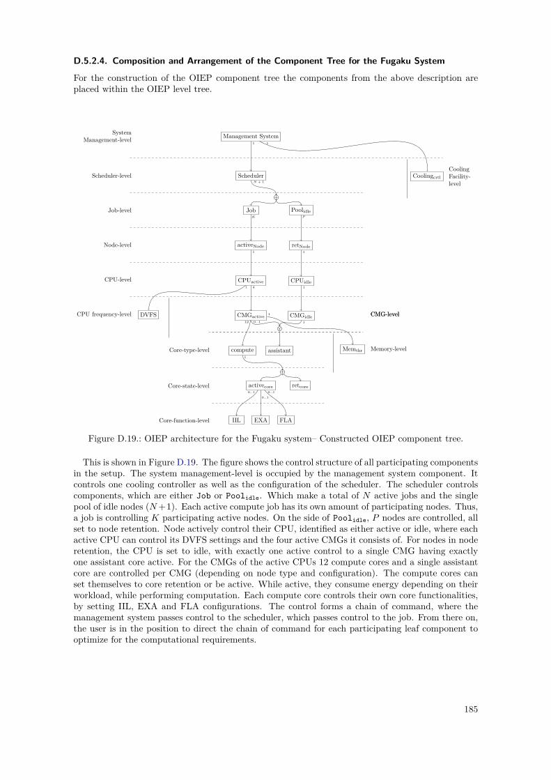
D.5.2.4. Composition and Arrangement of the Component Tree for the Fugaku System
For the construction of the OIEP component tree the components from the above description areplaced within the OIEP level tree.
SystemManagement-level
Scheduler-level
Job-level
Node-level
CPU-level
CoolingFacility-level
CPU frequency-level CMG-level
Memory-level
CMG-level
Core-type-level
Core-state-level
Core-function-level
Management System
Scheduler
Job Poolidle
activeNode retNode
Coolingcrtl
CPUactive CPUidle
CMGactive CMGidleDVFS
compute assistant Memthr
activecore retcore
EXAIIL FLA
1
N + 1
K P
1
1
1
41 1
12 0..1
1
1
1
0..10..1
0..1
Figure D.19.: OIEP architecture for the Fugaku system– Constructed OIEP component tree.
This is shown in Figure D.19. The figure shows the control structure of all participating componentsin the setup. The system management-level is occupied by the management system component. Itcontrols one cooling controller as well as the configuration of the scheduler. The scheduler controlscomponents, which are either Job or Poolidle. Which make a total of N active jobs and the singlepool of idle nodes (N+1). Each active compute job has its own amount of participating nodes. Thus,a job is controlling K participating active nodes. On the side of Poolidle, P nodes are controlled, allset to node retention. Node actively control their CPU, identified as either active or idle, where eachactive CPU can control its DVFS settings and the four active CMGs it consists of. For nodes in noderetention, the CPU is set to idle, with exactly one active control to a single CMG having exactlyone assistant core active. For the CMGs of the active CPUs 12 compute cores and a single assistantcore are controlled per CMG (depending on node type and configuration). The compute cores canset themselves to core retention or be active. While active, they consume energy depending on theirworkload, while performing computation. Each compute core controls their own core functionalities,by setting IIL, EXA and FLA configurations. The control forms a chain of command, where themanagement system passes control to the scheduler, which passes control to the job. From there on,the user is in the position to direct the chain of command for each participating leaf component tooptimize for the computational requirements.
185
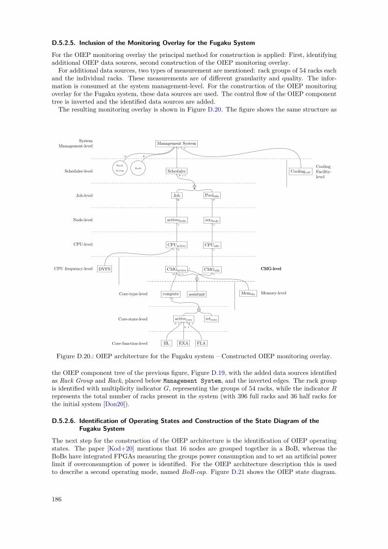
D.5.2.5. Inclusion of the Monitoring Overlay for the Fugaku System
For the OIEP monitoring overlay the principal method for construction is applied: First, identifyingadditional OIEP data sources, second construction of the OIEP monitoring overlay.For additional data sources, two types of measurement are mentioned: rack groups of 54 racks each
and the individual racks. These measurements are of different granularity and quality. The infor-mation is consumed at the system management-level. For the construction of the OIEP monitoringoverlay for the Fugaku system, these data sources are used. The control flow of the OIEP componenttree is inverted and the identified data sources are added.The resulting monitoring overlay is shown in Figure D.20. The figure shows the same structure as
SystemManagement-level
Scheduler-level
Job-level
Node-level
CPU-level
CoolingFacility-level
CPU frequency-level CMG-level
Memory-level
CMG-level
Core-type-level
Core-state-level
Core-function-level
Management System
Scheduler
Job Poolidle
Rack
R
Rack
Group
G
activeNode retNode
Coolingcrtl
CPUactive CPUidle
CMGactive CMGidleDVFS
compute assistant Memthr
activecore retcore
EXAIIL FLA
1
N + 1
K P
1
1
1
41 1
12 0..1
1
1
1
0..10..1
0..1
Figure D.20.: OIEP architecture for the Fugaku system – Constructed OIEP monitoring overlay.
the OIEP component tree of the previous figure, Figure D.19, with the added data sources identifiedas Rack Group and Rack, placed below Management System, and the inverted edges. The rack groupis identified with multiplicity indicator G, representing the groups of 54 racks, while the indicator Rrepresents the total number of racks present in the system (with 396 full racks and 36 half racks forthe initial system [Don20]).
D.5.2.6. Identification of Operating States and Construction of the State Diagram of theFugaku System
The next step for the construction of the OIEP architecture is the identification of OIEP operatingstates. The paper [Kod+20] mentions that 16 nodes are grouped together in a BoB, whereas theBoBs have integrated FPGAs measuring the groups power consumption and to set an artificial powerlimit if overconsumption of power is identified. For the OIEP architecture description this is usedto describe a second operating mode, named BoB-cap. Figure D.21 shows the OIEP state diagram.
186
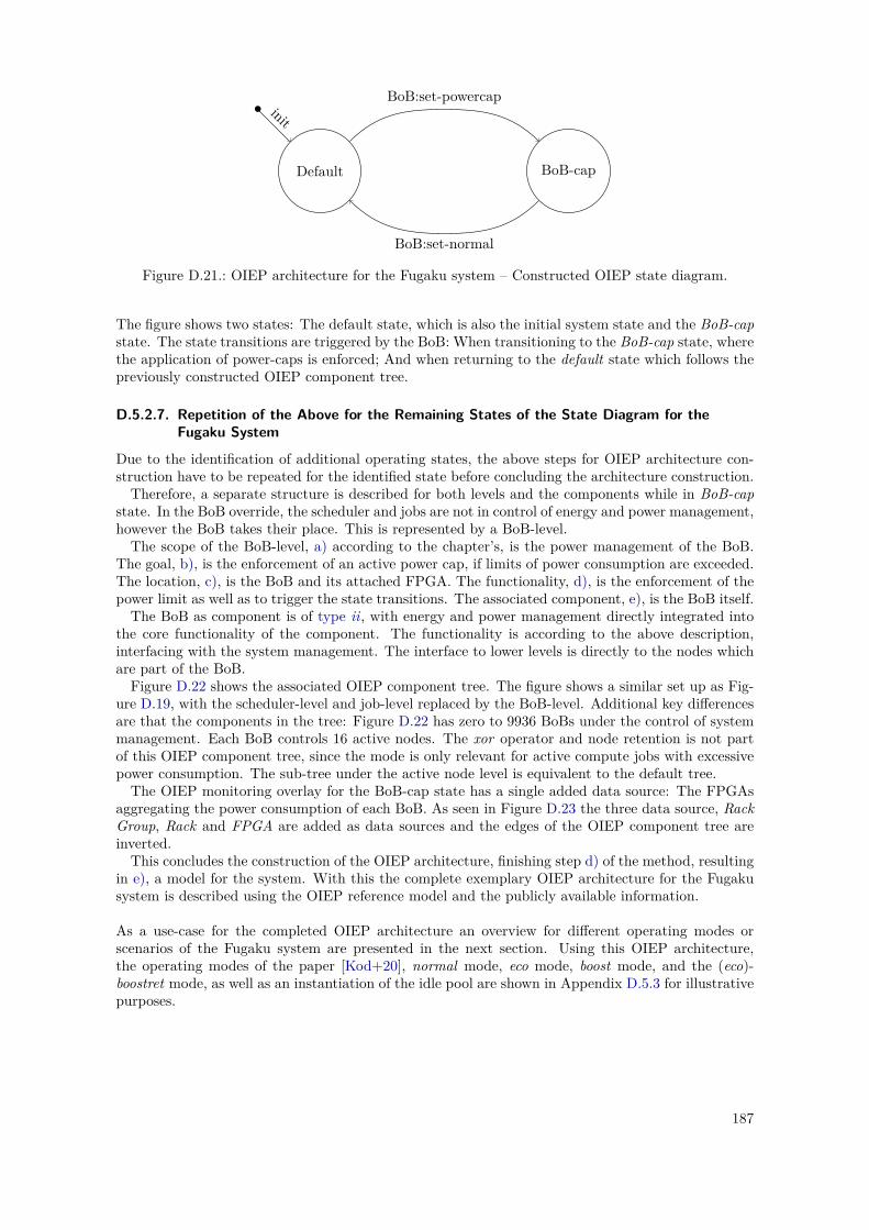
Default BoB-cap
BoB:set-powercap
BoB:set-normal
init
Figure D.21.: OIEP architecture for the Fugaku system – Constructed OIEP state diagram.
The figure shows two states: The default state, which is also the initial system state and the BoB-capstate. The state transitions are triggered by the BoB: When transitioning to the BoB-cap state, wherethe application of power-caps is enforced; And when returning to the default state which follows thepreviously constructed OIEP component tree.
D.5.2.7. Repetition of the Above for the Remaining States of the State Diagram for theFugaku System
Due to the identification of additional operating states, the above steps for OIEP architecture con-struction have to be repeated for the identified state before concluding the architecture construction.Therefore, a separate structure is described for both levels and the components while in BoB-cap
state. In the BoB override, the scheduler and jobs are not in control of energy and power management,however the BoB takes their place. This is represented by a BoB-level.The scope of the BoB-level, a) according to the chapter’s, is the power management of the BoB.
The goal, b), is the enforcement of an active power cap, if limits of power consumption are exceeded.The location, c), is the BoB and its attached FPGA. The functionality, d), is the enforcement of thepower limit as well as to trigger the state transitions. The associated component, e), is the BoB itself.The BoB as component is of type ii, with energy and power management directly integrated into
the core functionality of the component. The functionality is according to the above description,interfacing with the system management. The interface to lower levels is directly to the nodes whichare part of the BoB.Figure D.22 shows the associated OIEP component tree. The figure shows a similar set up as Fig-
ure D.19, with the scheduler-level and job-level replaced by the BoB-level. Additional key differencesare that the components in the tree: Figure D.22 has zero to 9936 BoBs under the control of systemmanagement. Each BoB controls 16 active nodes. The xor operator and node retention is not partof this OIEP component tree, since the mode is only relevant for active compute jobs with excessivepower consumption. The sub-tree under the active node level is equivalent to the default tree.The OIEP monitoring overlay for the BoB-cap state has a single added data source: The FPGAs
aggregating the power consumption of each BoB. As seen in Figure D.23 the three data source, RackGroup, Rack and FPGA are added as data sources and the edges of the OIEP component tree areinverted.This concludes the construction of the OIEP architecture, finishing step d) of the method, resulting
in e), a model for the system. With this the complete exemplary OIEP architecture for the Fugakusystem is described using the OIEP reference model and the publicly available information.
As a use-case for the completed OIEP architecture an overview for different operating modes orscenarios of the Fugaku system are presented in the next section. Using this OIEP architecture,the operating modes of the paper [Kod+20], normal mode, eco mode, boost mode, and the (eco)-boostret mode, as well as an instantiation of the idle pool are shown in Appendix D.5.3 for illustrativepurposes.
187
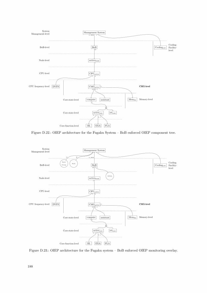
SystemManagement-level
BoB-level
Node-level
CPU-level
CoolingFacility-level
CPU frequency-level CMG-level
Memory-level
CMG-level
Core-state-level
Core-state-level
Core-function-level
Management System
BoB
activeNode
Coolingcrtl
CPUactive
CMGactiveDVFS
compute assistant Memthr
activecore retcore
EXAIIL FLA
0..9936
16
1
1
41
12 0..1
1
1
0..10..1
0..1
Figure D.22.: OIEP architecture for the Fugaku System – BoB enforced OIEP component tree.
SystemManagement-level
BoB-level
Node-level
CPU-level
CoolingFacility-level
CPU frequency-level CMG-level
Memory-level
CMG-level
Core-state-level
Core-state-level
Core-function-level
Management System
BoB
activeNode
Coolingcrtl
CPUactive
CMGactiveDVFS
compute assistant Memthr
activecore retcore
EXAIIL FLA
0..9936
16
1
1
41
12 0..1
1
Rack
R
Rack
Group
G
FPGA
1
1
0..10..1
0..1
Figure D.23.: OIEP architecture for the Fugaku system – BoB enforced OIEP monitoring overlay.
188
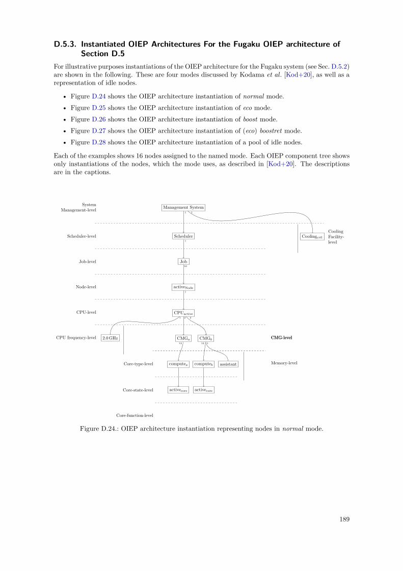
D.5.3. Instantiated OIEP Architectures For the Fugaku OIEP architecture ofSection D.5
For illustrative purposes instantiations of the OIEP architecture for the Fugaku system (see Sec. D.5.2)are shown in the following. These are four modes discussed by Kodama et al. [Kod+20], as well as arepresentation of idle nodes.
• Figure D.24 shows the OIEP architecture instantiation of normal mode.• Figure D.25 shows the OIEP architecture instantiation of eco mode.• Figure D.26 shows the OIEP architecture instantiation of boost mode.• Figure D.27 shows the OIEP architecture instantiation of (eco) boostret mode.• Figure D.28 shows the OIEP architecture instantiation of a pool of idle nodes.
Each of the examples shows 16 nodes assigned to the named mode. Each OIEP component tree showsonly instantiations of the nodes, which the mode uses, as described in [Kod+20]. The descriptionsare in the captions.
SystemManagement-level
Scheduler-level
Job-level
Node-level
CPU-level
CoolingFacility-level
CPU frequency-level CMG-level
Memory-level
CMG-level
Core-type-level
Core-state-level
Core-function-level
Management System
Scheduler
Job
activeNode
Coolingcrtl
CPUactive
CMGa CMGb2.0 GHz
computea computeb assistant
activecore activecore
1
1
16
1
1
2 21
12 12 1
Figure D.24.: OIEP architecture instantiation representing nodes in normal mode.
189
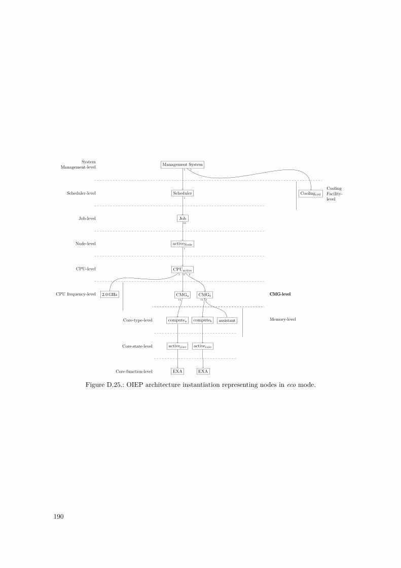
SystemManagement-level
Scheduler-level
Job-level
Node-level
CPU-level
CoolingFacility-level
CPU frequency-level CMG-level
Memory-level
CMG-level
Core-type-level
Core-state-level
Core-function-level
Management System
Scheduler
Job
activeNode
Coolingcrtl
CPUactive
CMGa CMGb2.0 GHz
computea computeb assistant
activecore activecore
EXA EXA
1
1
16
1
1
2 21
12 12 1
Figure D.25.: OIEP architecture instantiation representing nodes in eco mode.
190
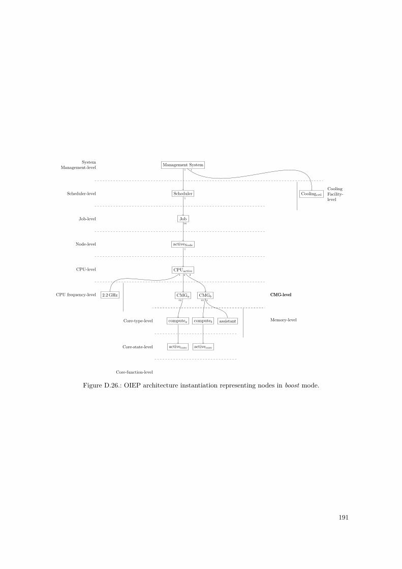
SystemManagement-level
Scheduler-level
Job-level
Node-level
CPU-level
CoolingFacility-level
CPU frequency-level CMG-level
Memory-level
CMG-level
Core-type-level
Core-state-level
Core-function-level
Management System
Scheduler
Job
activeNode
Coolingcrtl
CPUactive
CMGa CMGb2.2 GHz
computea computeb assistant
activecore activecore
1
1
16
1
1
2 21
12 12 1
Figure D.26.: OIEP architecture instantiation representing nodes in boost mode.
191
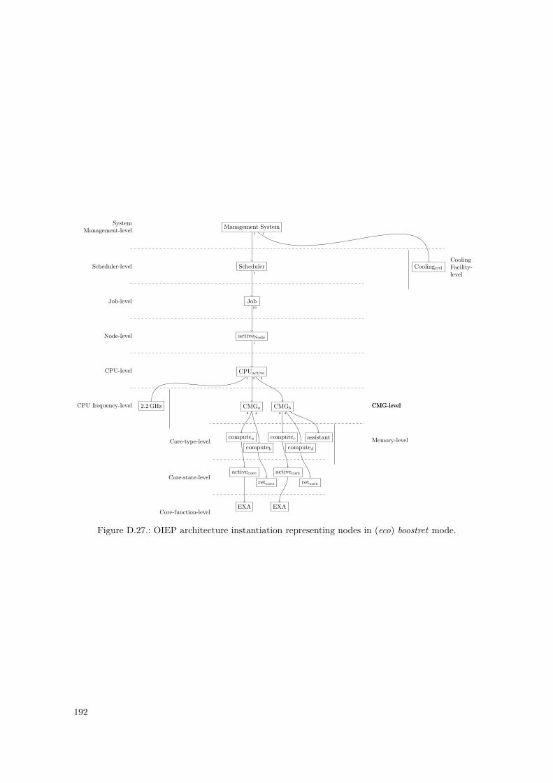
SystemManagement-level
Scheduler-level
Job-level
Node-level
CPU-level
CoolingFacility-level
CPU frequency-level CMG-level
Memory-level
CMG-level
Core-type-level
Core-state-level
Core-function-level
Management System
Scheduler
Job
activeNode
Coolingcrtl
CPUactive
CMGa CMGb2.2 GHz
computeacomputeb
computeccomputed
assistant
activecore
retcore
activecore
retcore
EXA EXA
1
1
16
1
1
2 21
8 4 8 4
Figure D.27.: OIEP architecture instantiation representing nodes in (eco) boostret mode.
192

SystemManagement-level
Scheduler-level
Job-level
Node-level
CPU-level
CoolingFacility-level
CPU frequency-level CMG-level
Memory-level
CMG-level
Core-type-level
Core-state-level
Core-function-level
Management System
Scheduler
Poolidle
retNode
Coolingcrtl
CPUidle
CMGidle
assistant
1
1
16
1
1
1
1
Figure D.28.: OIEP architecture instantiation representing an idle node pool.
193


Appendix E.
Supplement – Assessment
E.1. Assessment of Conformity With the Requirements . . . . . . . . . . . . . . . . . . . . 195E.2. Discussion on Use-Cases . . . . . . . . . . . . . . . . . . . . . . . . . . . . . . . . . . . 199
E.1. Assessment of Conformity With the RequirementsWith the presentation of the requirements for the creation of a reference model, and the resultingOIEP reference model, this section assesses the fulfillment of the named requirements. The sectioncommences according to the list of requirements according to Section 2.3 (previously summarized inTable 2.1):
Locally Distributed Environment By design of the OIEP reference model the system is intended forlarge scale energy and power management system of HPC systems. The application of the model inSection D.3, D.4 and D.5 shows this by example. The model itself is design to identify potential scalinghazards using the hierarchical design and the multiplicity indicator. (The multiplicity indicator allowsto compare the scaling requirement with the capabilities of the associated component.)
Diversity of Hardware Sensors and Controllers The OIEP reference model allows to model anyenergy and power relevant sensor and controller as OIEP components. To conform with the OIEPreference model the model restricts how these are used in an OIEP architecture. The requirementfor modeling a component is the description of its type (according to type i–iv), its interfaces and adescription of its functionality (in natural language).
Diversity of Software Managing Energy and Power Similar to the diversity of hardware sensorsand controllers argument, the OIEP reference model enables to model arbitrary software systems tomanage energy and power. The restriction lies on how such software can be integrated in the respectiveOIEP component tree, (which might require restructuring or even redesign of a component, if thecomponent violates the hierarchical tree control structure, by its design).
Provision of a Reference Model for Energy and Power Management Systems By providing thebuilding blocks and methods of the OIEP reference model the complete work at hand shows theattempt of providing such reference model.
Structure and Building Blocks of the Reference Model As provided in Chapter 3. (A full evalu-ation is still required by independent entity as future work, according to [Sch00, p. 85].)
Applicability and Systematic Construction As provided in Chapter 4. (Full evaluation required byindependent entity as future work, according to [Sch00, p. 85].)
195

Variability As discussed throughout the motivation chapter (Ch. 2, with App. A.1), in particularin the problem scoping (Sec. 2.2) and the requirements’ analysis (Sec. A.1.1.1), a reference modelallows to deal with systems with inherent variability. Since the OIEP reference model is a structuralreference model, it enables the users of the reference model to model the energy and power controlstructure of systems with components showing such variability.
Optimization Goals By design of the level goals and selection of components, the model creatoris empowered to select the optimization goals suitable for their system. The OIEP reference modelhelps to structure the hierarchical interaction of seemingly conflicting optimization goal, as long asthe interfaces of components, levels and their implementations are respected. Therefore, the OIEPreference model is a tool, which can be used to enable this requirement.
Modularity The concepts of levels, components, and definition of the tree hierarchies with accord-ing interfaces enables the creation of modular designs. For non-modular energy and power controlsystems, creating a model using an OIEP architecture allows to pinpoint components inhibiting themodularity of the energy and power control setup.
Limiting Scope and Remit Similar to the modularity argument, by providing the concepts of theOIEP reference model, the design of OIEP architectures and their OIEP components with properlyscoped design are enabled. Additionally, by constructing an OIEP architecture, the model view allowsto identify if components require or have a larger number of affected subsystems than intended or setby the architecture specification.
Opaque Components The systems in question are often comprised of large quantity of compo-nents, with implementation details not manageable by a single entity. By the choice of design andspecification of OIEP levels, their function, and the arrangement as an OIEP level tree, the placedcomponents can be handled in an opaque fashion, without needing to know all component internals.The structural setup of the OIEP reference model and specification of interfaces for specific OIEParchitectures enable opaque components. This speaks for the design of the reference model, not yetfor the implementations. As seen with the ISO/OSI reference model [Zim80; ISO-7498]: a productionsystem’s opaque usage of components depends on the exact specification of interfaces. This can beenabled by a model design, however the realization involves standardization and the desire to havestandardization for such systems in energy and power (as spearheaded by the Power-API [Gra+16]).Standard interfaces without a standardized usage model (in the form of a reference model) doeshowever not suffice for opaque components.
Transparent Structure and Information Flow By design, the OIEP reference model is designedso that OIEP architecture present the hierarchical structure of the energy and power managementsystem, with control flow going down and information flow going up along this structure. Therefore,the structural setup is fully transparent, with transparent information flow.
Scalability The hierarchical model design itself is scalable, while it is able to set requirements andindicate limits to scalability, by usage of the multiplicity indicator. The mechanisms do supportmodel creators and system designers to identify potential scalability concerns and mismatches ofmodel requirements and reality. The design decision is to identify scaling hazards and supportredesigns for truly scalable energy and power management. This has to be cross-checked and verifiedwith component capabilities.
Chain of Command & Traceability By the design of the control flow, a control decision is thedirect results of the control directive of the component’s parent component. Therefore, (assumingpersistent logging of the propagated decision is implemented) administrators are able to back-tracethe chain of command and the resulting control decisions. It has to be evaluated if, by design ofthe control structure, and usage of open control interfaces and components (as well as the requiredlogging), RAS systems can be supported for failure and fault analysis in more complex energy andpower management systems.
196

Manageability By design the manageability of the system is increased, at design time, due to aholistic view of the system, compared to a cluster of isolated components. As for the argument inchain of command & traceability, above, thorough implementation and tools support and evaluationhas to be shown for usage of the reference model, including thorough evaluation.
Simplicity and Readability The OIEP architectures combine all energy and power management sys-tems present in an HPC system’s pne management design. Therefore, only by using such referencemodel and design, readability of the holistic design can be attempted. The model presents an improve-ment over current isolated components without any energy and power management overview. Thedesign disallows complex potential hazardous interactions by design of the reference model design.(These situations are produce and model-able by approaches such as UML). Simplicity is enforced bythe clear hierarchical structure. For further evaluation on simplicity and readability a user evaluationis required.
Completeness & Relevance By self assessment the relevance is given, as the OIEP reference modelpresents the first holistic energy and power management reference model for HPC, where othersystems are component specific or not capable of presenting the complete systems. In terms ofcompleteness of the reference model, this is not proven. However, the conscious design decisionto limit the reference model to the structural elements presented, specific design considerations areenforced (such as e.g. the single parent rule avoiding hazardous control overrides.)
Comparability By providing a reference model for energy and power management, identifying thesimilarities and differences of two system architectures is easier, since they can be described using thesame structural elements and language. However, since the OIEP reference model does not mandatea specific setup (as for example the PowerStack model as a reference architecture does), but onlyspecifies a generic hierarchical structure, the comparability of two systems is not trivial, yet.The meaning of the identification of a specific degree of similarity for example, is not yet clearly
defined in the context.
Automation Similar to comparability, automation of the energy and power management system isnot granted for free by using the OIEP reference model, however it is enabled. By using a referencemodel, with modularity as a design goal, automated components are easily integrated. Aspects ofautomation, which require a specific setup, where no changes are acceptable after the setup-phase canbe overcome using the OIEP reference model. Additionally, identifying which aspects of the systemare manual versus having varying degrees of automation can be verified. This allows to identifybottlenecks regarding automation or the requirement of a human in the loop, by design, and how tomove to a more autonomous energy and power management setup.
Formality As constructed in Chapter 3 the OIEP reference model provides a (graphical) formalism,by providing the structures of the OIEP level tree, OIEP component tree, OIEP monitoring overlayand the OIEP state diagram, as well as associated rules and requirements for their levels, componentsand data sources and states.
Expressiveness The work at hand does not prove that any energy and power management systemis expressible using the OIEP reference model, however by combination of OIEP component tree, aswell as the OIEP operating states, this should be possible in theory. (As a non-formal proof, anyenergy and power controller can be modeled as a single level single component, where the logic isencoded in the state diagram. Therefore, the expressiveness is at least as expressive as any FSM.)(By contrast:) The rules of forbidding a single child component being controlled by two parentsis introduced, so that the expressiveness is directed to useful control mechanisms, and having theknowledge about who controls what at any given point in time. (Even with the state diagram tocircumvent the restrictions as hinted at earlier:) The main design idea is to use the OIEP componenttrees to express the energy and power control and management mechanisms in the HPC system inthis hierarchical way, avoiding designs with control hazards such as overrides. This intends to forcespecific designs, not universal applicability.
197

Structural Equivalence As constructed in Chapter 3 the OIEP reference model provides a hierarchi-cal structure, provided by the OIEP level tree, OIEP component tree and OIEP monitoring overlayas well as their associated rules. This structure is enforced.
Static and Dynamic Control By design of modularity, components can be set to operate in staticfashion, only setting parameters at configuration time. In the case that lower-level components canhandle dynamic adjustments, the parent component can implement static or dynamic managementof control. It should be noted, that in general the level of dynamicity increases from the bottomto the top levels. In case that a bottom level is static in their configuration/energy and powercontrol adjustment, dynamic components on higher levels become useful if the amount of managedchild components is large enough and the instantiation of new controlled components is large enough(introducing a new dimension of dynamicity). The effects and combinations of static and dynamicenergy and power management in concert of a large orchestrated power control hierarchy has to beevaluated for more concrete statements.
Operating Modes By introduction of the OIEP operating states and the OIEP state diagram (seeSec. 3.3.4) operating modes/states are integrated into the OIEP reference model (with the primarygoal to avoid control overrides within a control hierarchy).
Impact of Integration For impact of integration cost, the OIEP reference model needs to be usedin concrete system installations and evaluated. In terms of decreasing complexity, the applicationsof the reference model to concrete HPC systems, as seen with the Fugaku system (in App. D.5)and the LRZ systems (in App. D.3 and D.4), shows how a complete system can be modeled to gaina better understanding of the energy and power management system. By not knowing the averseeffects of changing a component and its exact points of interaction with the system, changing a singlecomponent so far has been deterring to change a system after initial setup. The OIEP referencemodel strides to improve this situation by helping centers to understand the systems better.
Feasibility and Implementability By providing the OIEP reference model, HPC centers and decisionmakers are given a tool to model and understand how energy and power management components intheir system interact and are used. This can help to understand which components are ready to beused, need further developing or require mere plumbing and proper configuration. Using the OIEPreference model supports the assessment of feasibility and implementability.
Adaptiveness By providing the considerations of diversity of hardware sensors and controllers, di-versity of software managing energy and power, modularity, as well as the overall design of the OIEPreference model, a contribution to more adaptive energy and power management systems is provided.By being able to construct an OIEP architecture for an energy and power management system, it ishowever not a given that changing its mode of operation is trivial.This can be seen in the OIEP architecture of SuperMUC-NG (see App. D.4), where the EARD
component, is a persistent daemon in control of the nodes energy and power controls. Even whendeactivated or exchanging the component setup for a compute job or job runtime centric approach,the energy and power management setup requires a redesign, since the two components EARGM andEARD dictate the structure. The approach is thus not designed with modularity as a focus. Suchadaption would more resemble a hack, compared to an elegantly integrated solution). The OIEPreference model therefore only allows to identify where a model redesign is needed when trying toadapt an energy and power management system.
This assessment is used to specify the last row of Table 5.1 in Chapter 5, regarding the entriesof the OIEP reference model.
198

E.2. Discussion on Use-CasesWith the construction of the OIEP reference model, and the introduction of the method how tomodel energy and power management systems as OIEP architectures, the following section goes intoa small discussion on use-cases.The Chapter 5 with Appendix E.1 motivate an outstanding evaluation, and provides a brief self
assessment, while raising several points needed for such evaluation. With the completion of theseevaluations, the evolution step of the method can commence. At the same time use-cases for theOIEP reference model have to be identified.Therefore, this Appendix forms a short discussion on use-cases, to lead into the Chapter 6 on future
work.
For use-cases, which play an important role for assessment and evaluation, a short selection is pre-sented:
• Procurement of energy and power management systems;• Updates and upgrades of energy and power management systems;• Component design and integration;• Support for operation of energy and power management systems.
These points are discussed in the following.
Procurement of Energy and Power Management Systems The OIEP reference model allows tomodel arbitrary energy and power management setups in a hierarchical fashion. This provides op-portunities for both HPC centers, and vendors for improved interaction.From the HPC center’s perspective, the description of a desired or required energy and power
management allows to communicate the functionality of a requested energy and power managementsetup. As seen in the previous section such information is often dispersed within all affected aspectsof a RFP (see App. D.3 and D.4). Using an OIEP architecture to layout and describe an OIEParchitecture, a consolidated energy and power management description can be given. There areseveral scenarios to supplement a procurement document using the OIEP reference model:
1. Description of a desired OIEP architecture (abstract or with specific components); or2. Description of a desired OIEP level tree, to be completed; or3. Description of a partial OIEP component tree, to be completed.
Therefore, the center leadership is supported to predefine and pinpoint what kind of energy and powermanagement setup is envisioned for the tenders.Similarly, the vendor community can use OIEP architectures to display and make their energy and
power management setup explainable and respond to RFPs in a comprehensive way. To do so, theycan integrate their software solutions, in either a given OIEP architecture, if provided by the center,or model their energy and power management setup using the mechanisms provided by the OIEPreference model.
Updates and Upgrades of Energy and Power Management Systems Updates of the energy andpower management setup are uncommon, since these are not covered by licenses, or the supportcontracts for large scale systems. Similarly, for systems where non-technical hurdles are not in theway, system administrators avoid updates to software altering the system’s behavior.For the use-case of system updates and upgrades, an OIEP architecture can support to identify the
compatibility of a system upgrade. At the other hand, using an OIEP architecture description fora system, the center leadership can identify invariants of a system, which must remained unchangedover the lifetime of a system. For example by dictating the use of a specific hardware interface onthe node-level or a specific high-level optimization goal.Such information can ease the life of a researcher in the energy and power domain, since they can
identify, what changes are admissable, so that they can propose a feasibility study and realize newways for energy and power management given an existing setup.
199

Component Design and Integration For component design and integration a similar argument canbe made:First, by having a given OIEP architecture, in which a newly developed or existing component
should operate in makes it easier to identify the needed interfaces the component needs to implement.Additionally, the role, which the component fills in the energy and power management setup can beeasily identified. The implementation can be directed to fulfill this requirement.Second, being able to describe a snapshot of an OIEP architecture, in which the OIEP component
operates helps to, communicate the features of the component. By designing against known interfaces,and with a known role and place, of the software (or hardware), testing and integration can be assisted.Examples for these are, unit testing, integration tests, system testing and acceptance testing. Suchapproaches are easier to perform on systems described using a (standardized) reference model.
Support for Operation of Energy and Power Management Systems HPC systems have RASsystems to support operational reliability, availability and serviceability of the system. Additionally,systems are enhanced with more and more telemetry and even long time monitoring in the form ofperformance databases.By having a OIEP architecture in place in addition to such telemetry, the direct effects of changes
to the HPC system’s behavior can be observed. Such information can be used to back-trace the rootcase of an unwanted change in the system, by following the chain of command and logging for controlcommands. Additionally, the control algorithms for the system can be continuously improved. Suchcapabilities are only possible by using a hierarchical energy and power management system, such asthe OIEP reference model
200
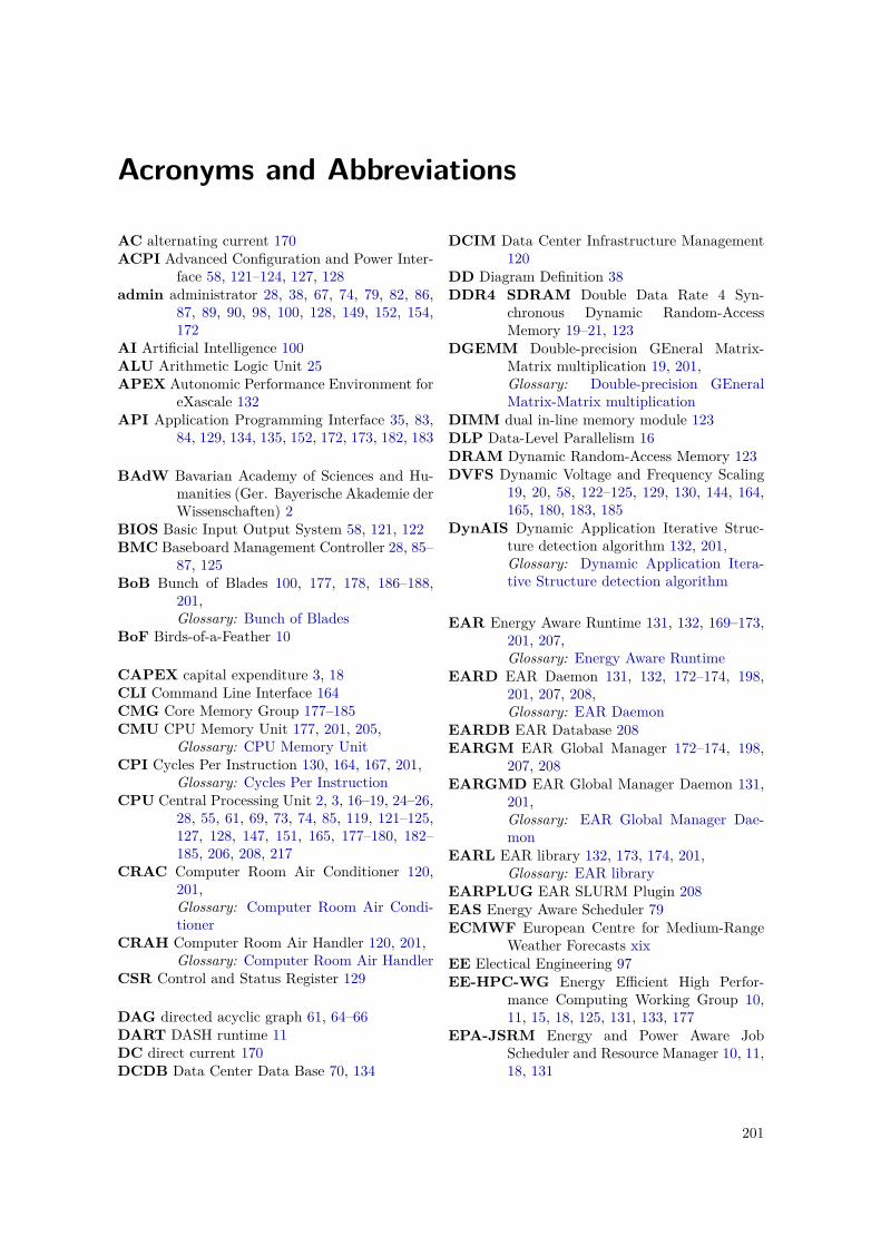
Acronyms and Abbreviations
AC alternating current 170ACPI Advanced Configuration and Power Inter-
face 58, 121–124, 127, 128admin administrator 28, 38, 67, 74, 79, 82, 86,
87, 89, 90, 98, 100, 128, 149, 152, 154,172
AI Artificial Intelligence 100ALU Arithmetic Logic Unit 25APEX Autonomic Performance Environment for
eXascale 132API Application Programming Interface 35, 83,
84, 129, 134, 135, 152, 172, 173, 182, 183
BAdW Bavarian Academy of Sciences and Hu-manities (Ger. Bayerische Akademie derWissenschaften) 2
BIOS Basic Input Output System 58, 121, 122BMC Baseboard Management Controller 28, 85–
87, 125BoB Bunch of Blades 100, 177, 178, 186–188,
201,Glossary: Bunch of Blades
BoF Birds-of-a-Feather 10
CAPEX capital expenditure 3, 18CLI Command Line Interface 164CMG Core Memory Group 177–185CMU CPU Memory Unit 177, 201, 205,
Glossary: CPU Memory UnitCPI Cycles Per Instruction 130, 164, 167, 201,
Glossary: Cycles Per InstructionCPU Central Processing Unit 2, 3, 16–19, 24–26,
28, 55, 61, 69, 73, 74, 85, 119, 121–125,127, 128, 147, 151, 165, 177–180, 182–185, 206, 208, 217
CRAC Computer Room Air Conditioner 120,201,Glossary: Computer Room Air Condi-tioner
CRAH Computer Room Air Handler 120, 201,Glossary: Computer Room Air Handler
CSR Control and Status Register 129
DAG directed acyclic graph 61, 64–66DART DASH runtime 11DC direct current 170DCDB Data Center Data Base 70, 134
DCIM Data Center Infrastructure Management120
DD Diagram Definition 38DDR4 SDRAM Double Data Rate 4 Syn-
chronous Dynamic Random-AccessMemory 19–21, 123
DGEMM Double-precision GEneral Matrix-Matrix multiplication 19, 201,Glossary: Double-precision GEneralMatrix-Matrix multiplication
DIMM dual in-line memory module 123DLP Data-Level Parallelism 16DRAM Dynamic Random-Access Memory 123DVFS Dynamic Voltage and Frequency Scaling
19, 20, 58, 122–125, 129, 130, 144, 164,165, 180, 183, 185
DynAIS Dynamic Application Iterative Struc-ture detection algorithm 132, 201,Glossary: Dynamic Application Itera-tive Structure detection algorithm
EAR Energy Aware Runtime 131, 132, 169–173,201, 207,Glossary: Energy Aware Runtime
EARD EAR Daemon 131, 132, 172–174, 198,201, 207, 208,Glossary: EAR Daemon
EARDB EAR Database 208EARGM EAR Global Manager 172–174, 198,
207, 208EARGMD EAR Global Manager Daemon 131,
201,Glossary: EAR Global Manager Dae-mon
EARL EAR library 132, 173, 174, 201,Glossary: EAR library
EARPLUG EAR SLURM Plugin 208EAS Energy Aware Scheduler 79ECMWF European Centre for Medium-Range
Weather Forecasts xixEE Electical Engineering 97EE-HPC-WG Energy Efficient High Perfor-
mance Computing Working Group 10,11, 15, 18, 125, 131, 133, 177
EPA-JSRM Energy and Power Aware JobScheduler and Resource Manager 10, 11,18, 131
201
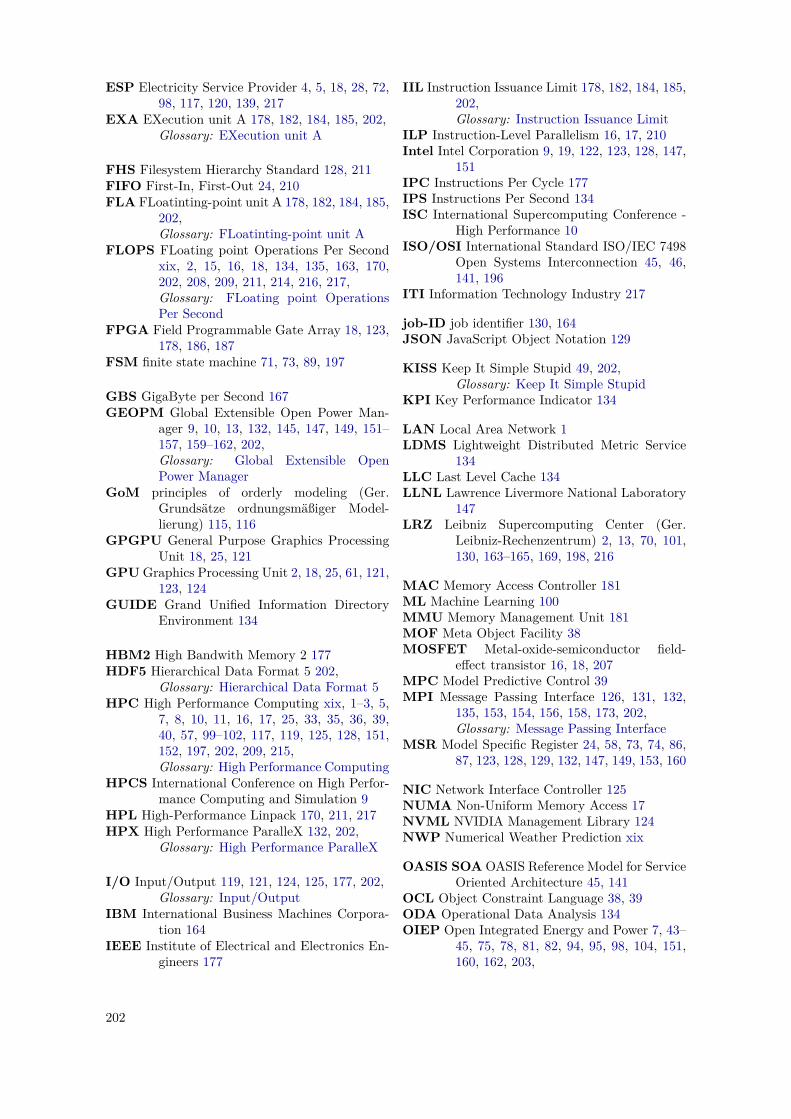
ESP Electricity Service Provider 4, 5, 18, 28, 72,98, 117, 120, 139, 217
EXA EXecution unit A 178, 182, 184, 185, 202,Glossary: EXecution unit A
FHS Filesystem Hierarchy Standard 128, 211FIFO First-In, First-Out 24, 210FLA FLoatinting-point unit A 178, 182, 184, 185,
202,Glossary: FLoatinting-point unit A
FLOPS FLoating point Operations Per Secondxix, 2, 15, 16, 18, 134, 135, 163, 170,202, 208, 209, 211, 214, 216, 217,Glossary: FLoating point OperationsPer Second
FPGA Field Programmable Gate Array 18, 123,178, 186, 187
FSM finite state machine 71, 73, 89, 197
GBS GigaByte per Second 167GEOPM Global Extensible Open Power Man-
ager 9, 10, 13, 132, 145, 147, 149, 151–157, 159–162, 202,Glossary: Global Extensible OpenPower Manager
GoM principles of orderly modeling (Ger.Grundsätze ordnungsmäßiger Model-lierung) 115, 116
GPGPU General Purpose Graphics ProcessingUnit 18, 25, 121
GPUGraphics Processing Unit 2, 18, 25, 61, 121,123, 124
GUIDE Grand Unified Information DirectoryEnvironment 134
HBM2 High Bandwith Memory 2 177HDF5 Hierarchical Data Format 5 202,
Glossary: Hierarchical Data Format 5HPC High Performance Computing xix, 1–3, 5,
7, 8, 10, 11, 16, 17, 25, 33, 35, 36, 39,40, 57, 99–102, 117, 119, 125, 128, 151,152, 197, 202, 209, 215,Glossary: High Performance Computing
HPCS International Conference on High Perfor-mance Computing and Simulation 9
HPL High-Performance Linpack 170, 211, 217HPX High Performance ParalleX 132, 202,
Glossary: High Performance ParalleX
I/O Input/Output 119, 121, 124, 125, 177, 202,Glossary: Input/Output
IBM International Business Machines Corpora-tion 164
IEEE Institute of Electrical and Electronics En-gineers 177
IIL Instruction Issuance Limit 178, 182, 184, 185,202,Glossary: Instruction Issuance Limit
ILP Instruction-Level Parallelism 16, 17, 210Intel Intel Corporation 9, 19, 122, 123, 128, 147,
151IPC Instructions Per Cycle 177IPS Instructions Per Second 134ISC International Supercomputing Conference -
High Performance 10ISO/OSI International Standard ISO/IEC 7498
Open Systems Interconnection 45, 46,141, 196
ITI Information Technology Industry 217
job-ID job identifier 130, 164JSON JavaScript Object Notation 129
KISS Keep It Simple Stupid 49, 202,Glossary: Keep It Simple Stupid
KPI Key Performance Indicator 134
LAN Local Area Network 1LDMS Lightweight Distributed Metric Service
134LLC Last Level Cache 134LLNL Lawrence Livermore National Laboratory
147LRZ Leibniz Supercomputing Center (Ger.
Leibniz-Rechenzentrum) 2, 13, 70, 101,130, 163–165, 169, 198, 216
MAC Memory Access Controller 181ML Machine Learning 100MMU Memory Management Unit 181MOF Meta Object Facility 38MOSFET Metal-oxide-semiconductor field-
effect transistor 16, 18, 207MPC Model Predictive Control 39MPI Message Passing Interface 126, 131, 132,
135, 153, 154, 156, 158, 173, 202,Glossary: Message Passing Interface
MSR Model Specific Register 24, 58, 73, 74, 86,87, 123, 128, 129, 132, 147, 149, 153, 160
NIC Network Interface Controller 125NUMA Non-Uniform Memory Access 17NVML NVIDIA Management Library 124NWP Numerical Weather Prediction xix
OASIS SOA OASIS Reference Model for ServiceOriented Architecture 45, 141
OCL Object Constraint Language 38, 39ODA Operational Data Analysis 134OIEP Open Integrated Energy and Power 7, 43–
45, 75, 78, 81, 82, 94, 95, 98, 104, 151,160, 162, 203,
202

Glossary: Open Integrated Energy andPower
OMNI Operations Monitoring and NotificationInfrastructure 134
OpenMP Open Multi-Processing 126, 131, 135OPEX operating expenses 3, 18OS Operating System 19, 22–24, 29, 36, 37, 58,
117, 121–123, 127–129, 143, 165, 170,172, 177, 184, 206
P3-Team Power Pathfinding to Product-Team 9,151
PAPI Performance Application ProgrammingInterface 129, 134, 203,Glossary: Performance Application Pro-gramming Interface
PC Personal Computer 127PCI Peripheral Component Interconnect 121,
129PDE Partial Differential Equation 26PDU Power Distribution Unit 29, 69, 119, 124,
203,Glossary: Power Distribution Unit
PELT Per-Entity Load Tracking 128PGAS Partitioned Global Address Space 11, 126,
135PMU Power Management Unit 23–25, 119, 121,
124, 125, 203,Glossary: Power Management Unit
POMDP Partially Observable Markov DecisionProcess 132, 151, 153, 154, 203,Glossary: Partially Observable MarkovDecision Process
PowerDAM Power Data Aggregation Manager70, 134
PSU Power Supply Unit 119, 121, 124, 125, 169,203, 217,Glossary: Power Supply Unit
PTF Periscope Tuning Framework 37, 129PUE Power Usage Efficiency 120, 203,
Glossary: Power Usage Efficiency
QoS Quality of Service 63
R-CCS RIKEN Center for Computational Sci-ence 13, 16, 145, 177, 208
RAPL Intel’s Running Average Power Limit 19,58, 69, 122–124, 129, 144, 147, 149
RAS Reliability Availability Serviceability 29, 30,58, 73, 74, 79, 80, 83, 85–89, 130, 132,133, 196, 200
RCS real-time control system 40, 97, 205READEX Runtime Exploitation of Application
Dynamism for Energy-efficient eXascalecomputing 37
RFI Request For Information 16, 114, 203,Glossary: Request For Information
RFP Request For Proposal 16, 50, 67, 75, 114,133, 143, 163, 164, 169–171, 173–175,199, 203, 215,Glossary: Request For Proposal
RM Resource Manager 79ROM Read-Only Memory 208rpm revolutions per minute 208RT Runtime 79
SC ACM/IEEE Supercomputing Conference 9Score-E Scalable Tools for Energy Analysis and
Tuning in HPC 129, 203,Glossary: Scalable Tools for EnergyAnalysis and Tuning in HPC
Score-P Scalable Performance Measurement In-frastructure for Parallel Codes 37, 129,135, 203,Glossary: Scalable Performance Mea-surement Infrastructure for ParallelCodes
SI International System of Units (Fr. Le Systèmeinternational d’unités) 2, 203, 208, 214,216, 217,Glossary: International System of Units(Fr. Le Système international d’unités)
SIMD single-instruction stream – multiple-datastream 25
SLES SUSE Linux Enterprise Server 170SLURM Simple Linux Utility for Resource Man-
agement 147, 149, 169–171, 173, 174SPANK Slurm Plug-in architecture for Node
and job Kontrol 148, 207, 208SSE Streaming SIMD Extensions 25SVE Scalable Vector Extension 177
TAU Tuning and Analysis Utilities 129TCO Total Cost of Ownership 3TDP Thermal Design Power 19–21, 122, 123, 134Tofu Torus fusion 177
U.S. DOE United States Department of Energy15, 16
UID User Identifier 128UMA Uniform Memory Access 17UML Unified Modelling Language 38, 39, 113,
197UPS Uninterupted Power Supply 117, 124, 203,
Glossary: Uninterupted Power Supply
VIHPS Virtual Institute – High ProductivityComputing 134
VR Voltage Regulator 67, 119, 121, 124, 125, 203,214,Glossary: Voltage Regulator
WAN Wide Area Network 1
XAI eXplainable Artificial Intelligence 100
203

xCat Extreme Cloud Administration Toolkit133, 164–167, 170–174
XMI XML Metadata Interchange 38XML eXtensible Markup Language 38, 129
204
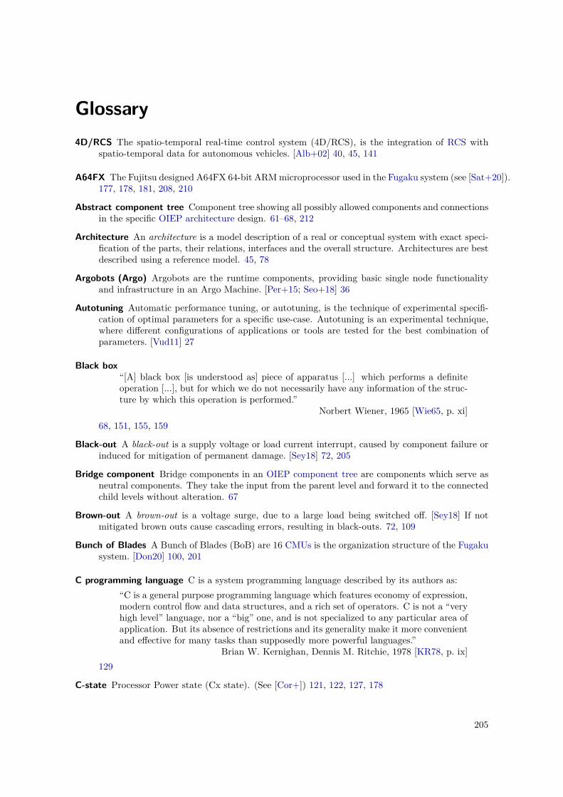
Glossary4D/RCS The spatio-temporal real-time control system (4D/RCS), is the integration of RCS with
spatio-temporal data for autonomous vehicles. [Alb+02] 40, 45, 141
A64FX The Fujitsu designed A64FX 64-bit ARMmicroprocessor used in the Fugaku system (see [Sat+20]).177, 178, 181, 208, 210
Abstract component tree Component tree showing all possibly allowed components and connectionsin the specific OIEP architecture design. 61–68, 212
Architecture An architecture is a model description of a real or conceptual system with exact speci-fication of the parts, their relations, interfaces and the overall structure. Architectures are bestdescribed using a reference model. 45, 78
Argobots (Argo) Argobots are the runtime components, providing basic single node functionalityand infrastructure in an Argo Machine. [Per+15; Seo+18] 36
Autotuning Automatic performance tuning, or autotuning, is the technique of experimental specifi-cation of optimal parameters for a specific use-case. Autotuning is an experimental technique,where different configurations of applications or tools are tested for the best combination ofparameters. [Vud11] 27
Black box“[A] black box [is understood as] piece of apparatus [...] which performs a definiteoperation [...], but for which we do not necessarily have any information of the struc-ture by which this operation is performed.”
Norbert Wiener, 1965 [Wie65, p. xi]68, 151, 155, 159
Black-out A black-out is a supply voltage or load current interrupt, caused by component failure orinduced for mitigation of permanent damage. [Sey18] 72, 205
Bridge component Bridge components in an OIEP component tree are components which serve asneutral components. They take the input from the parent level and forward it to the connectedchild levels without alteration. 67
Brown-out A brown-out is a voltage surge, due to a large load being switched off. [Sey18] If notmitigated brown outs cause cascading errors, resulting in black-outs. 72, 109
Bunch of Blades A Bunch of Blades (BoB) are 16 CMUs is the organization structure of the Fugakusystem. [Don20] 100, 201
C programming language C is a system programming language described by its authors as:“C is a general purpose programming language which features economy of expression,modern control flow and data structures, and a rich set of operators. C is not a “veryhigh level” language, nor a “big” one, and is not specialized to any particular area ofapplication. But its absence of restrictions and its generality make it more convenientand effective for many tasks than supposedly more powerful languages.”
Brian W. Kernighan, Dennis M. Ritchie, 1978 [KR78, p. ix]129
C-state Processor Power state (Cx state). (See [Cor+]) 121, 122, 127, 178
205
Chip“A tiny square of thin semi-conducting material which by suitable etching, doping,etc., is designed to function as a large number of circuit components and which canbe incorporated with other similar squares to form an integrated circuit.”
“chip, n.1., 2.f.” OED Online, 2019 [OEDa]xix
Co-design Co-design is the process of designing a system with participation of all stakeholders. Forcomputer systems, this often means that both hardware and software, or users and developersare included in design decisions. The stakeholders have to be specified. 162
CoMD Reference Classical Molecular Dynamics application. This application code serves as proxyapplication for typical classical molecular dynamics algorithms and workloads. It was createdby the Exascale Co-Design Center for Materials in Extreme Environments at LLNL. 22
Compute cluster A compute cluster, or cluster for short, is a system of computers, co-located inphysical proximity and connected using high-performance network infrastructure. The individ-ual computer systems which make up the cluster system are called nodes and, in general, arecommodity server computers. 1–4, 17, 25, 39, 40, 99, 131, 152, 153, 206
Compute job A compute job, or job, is a task or collection of tasks to be executed on an HPCsystem. The compute job has a number of required resources, in general a number of computenodes, a time window, which is required to complete the compute job on the requested resourcesand a job description (typically provided as a reproducible job script containing all requestedresources as well as the script to process the job). The tasks to be executed are typically partof an HPC application. 69, 126, 132, 137, 138, 151, 153, 165, 167, 180, 183, 187, 198
Compute node A compute node, or node for short, is an individual computer system which is partof a cluster system. Nodes are typically computers using commodity server hardware runninga standard OS configured for use within a cluster. 1–3, 22, 25, 124, 172
Computer Room Air Conditioner Computer Room Air Conditioner (CRAC) are air conditioningsystem using direct expansion refrigeration cycle to actively cool and exchange hot for cold air.120, 201
Computer Room Air Handler Computer Room Air Handler (CRAH) are air handling systems, usedfor heat exchange (from water chillers, or ambient air). 120, 201
Control Domain Control domains, or domains of control, in the OIEP reference model are used asconcept for describing the scope, functionality and logical placement of a required group ofcomponents for the energy and power management of HPC systems. 48
CPU Memory Unit A CPU Memory Unit (CMU) are two nodes mounted on a single board. TheCMU forms an organizational unit in terms of cooling and power supply of the Fugaku sys-tem [Don20]. (Equivalent to a blade in other systems). 177, 201
Cycles Per Instruction Cycles Per Instruction (CPI) is a measure of how many cycles a single in-struction requires to completion. An average value for this metric is computed by reading areference counter for clock cycles and dividing it by the number of instructions retired over thesame time period. 130, 201
D-state Device power state (Dx state). (See [Cor+]) 121
Dark silicon Dark Silicon describes the fact that not all parts of a silicon chip can be used simulta-neously, and thus remain dark, or not powered on. [Hen+15] 20
Data locality Data locality describes the issues related to placement of memory needed to performcomputation in distributed or shared memory system. To compute, a processor needs access tothe data the computation uses as input data. For performant operation, the location of the data
206
is of importance, since latencies between fetching data and computing can impact performance.These data accesses are dependent on location of the memory as well as proximity of access inrelation to time. 17
Degree of a vertex The degree of a vertex is the number of out-going edges, or child vertices. 51
Dennard scaling Dennard scaling describes performance of MOSFET devices when scaling down thedimensions of these devices, initially described by Dennard et al. [Den+99]. The main resultof this work is that power density of integrated circuits remain constant (if leakage voltagesare negligible). Thus, under these conditions power dissipation and cooling problems staysunchanged. The limits of Dennard scaling are described in [Boh07] and [JN16], and are oftenreferred to as the “Power Wall” [Bos11]. 16
Depth of a tree The depth of a directed tree is the maximum depth of all vertices. 51, 54
Depth of a vertex The depth of a vertex V is the length of the path from root R to V . 51, 54, 207
Digraph A directed graph is a graph with edges that have an associated direction. 70
Directed Tree A directed tree is a directed graph, of vertexes and edges, with a specified vertex Rsuch that:
• Each vertex V 6= R is the terminal vertex of exactly one edge.• R is the terminal vertex of no edge.• R is a root, in the sense that for each vertex V 6= R there is a directed path from R to V .
Each edge has an initial vertex V1 and a distinct terminal vertex V2, where V1 is called theparent of V2 and V2 the child of V1. Vertices without out-going edges, thus child vertices, arecalled leaf vertices. The degree of a vertex is the number of out-going edges, or child vertices.The depth of a vertex V is the length of the path from root R to V .(Definition as adaption of [Knu97, p. 372]’s oriented tree with inverted edges, supplementedwith information of [Knu97, pp. 308–376].) 46, 51, 207
Distributed SystemA distributed system is a collection of autonomous computing elements that appearsto its users as a single coherent system.
Maarten van Steen and Andrew S. Tanenbaum, 2018 [ST18, p. 2]
An important class of distributed systems is the one used for high-performance com-puting tasks.
Maarten van Steen and Andrew S. Tanenbaum, 2018 [ST18, p. 25]
1
Double-precision GEneral Matrix-Matrix multiplication DGEMM is a general matrix-matrix oper-ation in the form of C ⇐ αA∗B+βC. In general vendors provide hardware specific, optimizedimplementations. 19, 201
Dynamic Application Iterative Structure detection algorithm DynAIS is the loop detection algo-rithm of EAR. It receives sequences of MPI calls from EARL and provides information aboutcode regions of the application process. [CB19] 132, 201
EAR Daemon Daemon for EAR running on each node of the cluster managed by the EARGM.EARD reads information from the hardware platform and sets frequencies as instructed byEARL or the SPANK plugin for EAR [CB19]. 131, 201
EAR Global Manager Daemon EARGM Daemon controlling the global energy consumed by thesystem. Adapting policies and global energy limits enforcing limits to EARDs [CB19]. 131, 201
207

EAR library The EAR library interfaces with the running application using PMPI. This informationis provided to DynAIS to identify code regions of similar behavior, i.e. loops. The EAR libraryderives an optimal frequency and instructs the EARD to set frequencies accordingly. [CB19]132, 201
Echelon structure Synonym for hierarchical structure, used in hierarchical control systems (loanwordof military origin).(see Albus [AB05]) 39
Energy Energy is a derived quantity with unit joule (J).Expressed in terms of other SI units: J = N m. [Org19] xv, xvii, xix, 3–15, 18, 20, 22, 24–41,43–61, 66, 68–75, 77, 78, 80–83, 85, 87, 88, 90, 93–104, 107–117, 119, 121, 122, 124–135, 138,139, 141, 143–145, 149–152, 156, 160, 162–167, 169–175, 177, 178, 180, 181, 183, 184, 187,195–200, 206, 210, 212, 213, 215, 216
Energy Aware Runtime Energy Aware Runtime (EAR) is a framework providing: EARL, a libraryfor application interaction; EARD, the node management daemons; EAR SLURM Plugin(EARPLUG), a SPANK plugin for EAR; EAR Database (EARDB), the energy accountingdatabase; and EARGM, the cluster energy manager [CB19]. 131, 201
Epilog In scheduling, the epilog is responsible for cleaning up the user-environment and the executionof scripts, to report user and job metrics, as well as to reset the nodes to a known default state.165, 166, 183
Exascale era The exascale era is the time-period of exascale systems. This era is reached once thefirst exascale system is online and in productive operation. The era is concluded once the firstsystem reaches zettaFLOPS (1× 10²¹ FLOPS), marking the start of the zettascale era. xix
Exascale system An exascale system is a computer system capable of operating at a sustained per-formance of at least 1× 10¹⁸ FLOPS, or one exaFLOPS. 2, 15, 16, 18, 208
EXecution unit A Execution unit A (EXA), is one of two integer execution units, present in eachA64FX cores. These are referred to as EXA and EXB. [Kod+20] 178, 202
Fan Fans serve the purpose of moving cool air in air-ventilated computer systems. Fans have variablespeed, thus thermal performance, and measurable revolutions per minute (rpm). 67
Firmware Software to control low level functionality of hardware, typically provided by the hard-ware manufacturer. Historically stored on Read-Only Memory (ROM), and not altered afterinstallation. Nowadays, Firmware can be updated but is still generally provided by the manu-facturer only and not updated unless basic functionality is in need of critical updates. 29, 55,56, 121–123
FLoating point Operations Per Second Floating point operations per Second (FLOPS) is the met-ric used for issued 64 bit floating-point operations per second. Precision used is 64 bit inaccordance with IEEE754 [Ins08]. SI-prefixes do apply. xix, 2, 202
FLoatinting-point unit A Floating-point unit A (FLA), is one of two floating-point units, present ineach A64FX cores. These are referred to as FLA and FLB. [Kod+20] 178, 202
Frequency Frequency is a derived quantity with unit hertz (Hz).Expressed in terms of other SI units: Hz = 1/sThe frequency in hertz implies the unit cycles per second [Org19]. 129, 163–165, 177, 178, 180,182–184
Fugaku The Fugaku system is a flagship HPC system at R-CCS, entering the TOP500 list as thefastest system of June 2020. The system consists of 158 976 compute nodes with total core countof 7 630 848 cores at a power consumption of 28 MW [Don20]. The processor architecture is theARM-based Fujitsu A64FX CPU [YosHC]. xvi, 13, 16, 77, 100, 145, 177–179, 182, 185–189,198, 205, 206
208
G-state Global system state (Gx state). (See [Cor+]) 121
Global Extensible Open Power Manager GEOPM is an extensible power management frameworktargeting high performance computing. The runtime part of the framework can be extendedto support new control algorithms and new hardware power management features. [Eas+17;GEOb; GEOa] 9, 151, 202
Green500 The Green500 list ranks the systems of the TOP500 according to FLOPS/W as proposedin the [SHF06]. The Green500 list is listed and ranked at [TOPe], dating back to 2006. 133,170
hack“Computing. An inelegant yet effective solution to a computing problem; a workaround,a short cut, a modification.”
“hack, n., 7 a.” OED, Online, 2020 [OEDb]198
Hardware Computer hardware, the physical parts and resources of a computer. 55, 56, 117
hardware overprovisioned system A hardware overprovisioned system is a system that has morehardware capacity than the available supply power can provide [Pat+13a]. 130, 131
Hierarchical Data Format 5 HDF5 is a standardized set of data formats for large scale complex dataobjects. HDF5 has associated data model, file format and API as well as a set of tools andAPIs and efficient implementations for massive parallel systems. [HDFG] 202
High Performance Computing High Performance Computing (HPC) combines approaches from sev-eral disciplines of computer science and computer engineering striving to maximize the com-putational performance achievable using a computer system. The goal is to make challengingproblems of science and engineering computable which are otherwise infeasible to compute inreasonable time or with the required problem size or resolution. xix, 1, 202
High Performance Computing Application HPC applications are science and engineering applica-tions designed specifically to run on HPC systems due to their need for high computationalperformance. For current generation of HPC systems these are applications with a high degreeof parallelism, according to the high degree of parallelism of clustered HPC systems. 1, 2, 4,22, 153, 206
High Performance Computing Center An HPC center is a computing center housing one or moreHPC systems. The centers provide the required infrastructure to operate the computer systems,but also the personnel and know-how to operate and service the installation. 1–8, 10, 22, 35,40, 58, 69, 70, 98, 100, 108, 114, 119, 120, 143, 151, 154, 198, 199, 215
High Performance Computing system The computer systems purpose built for HPC are called HPCsystems. HPC systems are designed to solve computational problems which are infeasible to besolved on so-called commodity computers. xix, 1–8, 12–18, 25, 31, 35, 37, 39–41, 43, 45, 47–50,56, 58, 60, 61, 69, 71, 77, 78, 80, 85, 95, 97–101, 103, 104, 108, 109, 111–114, 117, 119, 124–127,130, 132, 133, 143–145, 169, 177, 195, 197, 198, 200, 206, 208, 209, 211, 215
High Performance ParalleX The HPX runtime system is the runtime system for the parallel execu-tion model ParallelX. [KBS09] 132, 202
High-end capability computing“ ‘High-end capability computing’ means advanced computing that pushes the boundsof what is computationally feasible. While that is often interpreted in terms of rawprocessing [performance], users expect to achieve new scientific understanding or en-gineering capabilities through computation. [...] Thus, from the user’s perspective,high-end capability computing means whatever sort of advanced, nonroutine comput-ing system is needed to push the computational science or engineering capabilities of
209
a given [scientific] field.”[Nat08, p. 1]
1
ILP wall The ILP wall is the feasibility limit of parallelizing independent instruction streams at theprocessor level. (C.f. [Wal91].) 17
In-band In-band measurement and control, in contrast to out-of-band, uses the same communica-tion infrastructure as the workload running on the systems. The resources are the primaryinfrastructure of the system, namely the dedicated high performance communication network.Utilization of this network should not impact the application performance, the primary users ofthe system, in a measurable way. It should be noted that throughput of the primary networkis very high, while latencies are very low, compared to the service network. 80, 81, 84–89, 133,148, 149, 170
Input/Output I/O in this work refers to any information transfer from the main computationaldevices, CPU and Memory, to a remote system, such as other nodes of other clusters or persistentmemory (storage) located outside the node. 119, 202
Instantiated Component Tree Component tree showing the instantiated version of the abstract com-ponent tree of a specific OIEP architecture design. 61–68
Instruction Issuance Limit Instruction Issuance Limit (IIL) is a mode of operation where the instruc-tion issue width of the A64FX processor (per core) is limited to from four to two. [Kod+20]178, 202
International System of Units (Fr. Le Système international d’unités) The International Systemof Units (SI) is the internationally agreed upon system of weights and measures used throughoutthe scientific world. It is maintained by the Organisation intergouvernementale de la Conventiondu Mètre, organized by the Bureau international des poids et mesures at the Pavillon de Breteuil(Parc de Saint-Cloud) France [Org19]. 2, 203
Job runtime A runtime is a software system managing the execution environment of an application.Runtimes have specific control parameters they can modify to allow for optimization of theexecution of the application, or enable the execution at all. 29, 30, 67, 69, 83, 84, 86, 87, 131,132, 138, 148, 151, 155, 198
Job scheduler A job scheduler is a computer program responsible for scheduling the available re-sources of a cluster in a batched fashion. The word ‘batch scheduler’ is often used interchange-ably. In such scheduler, the resources used for scheduling are the number of nodes and durationof the reservation. The best possible placement is determined using scheduling algorithms suchas FIFO or back-filling among others. The optimization goal is throughput, turnaround timeor system utilization [TB14, p. 154]. Experimental HPC schedulers add additional resourcessuch as energy and power, or other applicable job requirements. 29, 30, 67, 69, 73, 83, 86–88,113, 126, 130–132, 138, 143, 148, 152, 153, 155, 215
Job script A job script is a computer program to be submitted to a job scheduler. The script has tobe interpretable by the job scheduler, and describes the experimental setup to be executed ona compute cluster. The preamble of the job script contains information on requested resourcesand compute time. The main body of the job script loads required environment modules anddescribes the experimental design, typically as a shell script. 126, 132
Keep It Simple Stupid "Keep it simple stupid", attributed to Clarence Leonard (Kelly) Johnson,date unspecified [Ric95]. In popular use by 1970 as the KISS principle. 49, 202
Libmsr The libmsr library is a software library for user-space msr access as well as wrappers toextract information from model specific registers used on intel platforms. [RB] 73, 74
210
LINPACK LINPACK is a collection of fortran subroutines to analyze and solve linear algebra sys-tems [Don+79]. The LINPACK benchmark solves such system with known number of operationsin 64-bit floating-point arithmetic [DL11]. This allows to measure practically achievable FLOPSfor a HPC system. A current implementation of the benchmark is HPL [Pet+]. 2
Linux Linux, is a free and open operating system following the Unix principles, and heavily inspiredby it. Modern HPC systems operate using a GNU/Linux distributions or derivatives thereof,and are therefore using the Filesystem Hierarchy Standard (FHS). 25, 36, 126–129, 165, 172,173, 183
LoadLeveler IBM Tivoli® Workload Scheduler (TWS) LoadLeveler® (LoadLeveler) is the schedulerused at both SuperMUC Phase 1 and SuperMUC Phase 2 systems. The scheduler has integratedfunctionality for energy aware scheduling. The scheduler is superseded by IBM Platform LoadSharing Facility (LSF®), with much of the original functionality integrated. [IBMa; IBMb] 130,164–167, 169
Maleable job A maleable job is a compute job that can successfully alter the number of nodes usedfor operation at runtime. The application and the used scheduler as well as the utilized parallelruntime (e.g. MPI) has to support this [Sar+14]. 131, 135
Manufacturing variability Due to the manufacturing process not all silicon wavers have the exactsame physical characteristics. Even though foundries employ tight quality controls, the result-ing, theoretically identical, processors subsequently show differences in their power consumptionat the exact same performance at a fixed frequency [Mai15; Mai+16]. 20
Memory The memory subsystem of a compute node provides the data storage of working memoryrequired to execute a program. Due to technology limitations, its size is limited, and a memoryhierarchy is in place. In distributed systems, working data is distributed across the memorysubsystems of several nodes and needs to be communicated. For memory technologies andfurther details refer to [HP17]. 2, 17, 55, 119–121, 123, 125, 206
Memory wall The memory wall is the issue that overall performance improvement is limited by mem-ory technology due to the fact that processor performance and memory performance improveat disparate rates.[WM96] 17
Message Passing Interface MPI is the standard interface for process communication in HPC sys-tems. This includes “point-to-point message passing, collective communications, group andcommunicator concepts, process topologies, communication environment, process creation andmanagement, one-sided communications, extended collective operations, external interfaces,I/O, some miscellaneous topics, and a profiling interfaces”[MPI15]. The current standard isMPI-3.1 as of June 4, 2015. Please refer to the MPI-forum for detailed information. [MPI] 126,202
Microarchitecture The microarchitecture is the organization of a microprocessor; the design and theorganization of the internal structure of the processor. Processors with similar organization aresometimes referred to as belonging to the same microarchitecture family. [HP17] 122, 147
Model A model is a representation of an object, system or concept, relevant to the model-user,reduced to the essential attributes of the object, system or concept, valid or useful over aspecific period of time to achieve a specified task or goal. 45
Model creator The model creator is the actor creating a model. When applying the OIEP referencemodel, the model creator is the actor designing the OIEP architecture for a specific HPC system.46, 48–51, 54–56, 59, 61, 63, 66, 68, 70–73, 83, 86, 90, 93, 143, 144, 151, 196
Moldable job A moldable job is a compute job that can be started with a varying number of computenodes. The application and the used scheduler has to support such job initalization [Sar+14].131, 135
Moore’s law Moore’s law states:
211
“The complexity for minimum component costs [number of components per integratedcircuit] has increased at a rate of roughly a factor of two per year [...]. Certainly overthe short term this rate can be expected to continue, if not to increase. Over thelonger term, the rate of increase is a bit more uncertain, although there is no reasonto believe it will not remain nearly constant for at least 10 years.”
Gordon E. Moore, 1965 [Moo65]2
Msr-safe The msr-safe tool is a software tool comprised of a kernel module as well as scripts andwhitelists to safely give access to model specific registers on intel platform with strong securityand performance considerations. [Sho+] 25, 73, 74, 129, 147, 149, 153, 158
Multiplicity indicator Multiplicity indicators indicate the number of allowed replicas of the samekind of child components of a single indicated edge in the abstract component tree of the OIEPreference model. 61, 62, 64, 66–68, 87, 89, 166, 167, 186, 195
Nested component Nested components in an OIEP component tree are components which can berepresented internally as OIEP component tree of an OIEP architecture. 67, 151, 155, 157–159
NodeOS (Argo) NodeOS is the Linux based operating system at the node level, providing basicsingle node functionality and infrastructure needed by an Argo Machine. [Per+15; Per+17] 36
Occam’s Razor Principle attributed to William of Ockham (Gulielmus Occamus) stating: “Entianon sunt multiplicanda, proter necessitatem.” [THO18] - ‘Things should not be manyfoldedwithout reason.’ (Loosely translated by the author.) 112
OIEP Architecture A concrete instance of the OIEP reference model. 7, 8, 13, 36–39, 43, 45, 49–51, 53–61, 63, 65–67, 69–74, 77, 78, 80–82, 85–91, 97–101, 104, 117, 137, 143–145, 147, 148,150–152, 154–157, 159, 160, 162–164, 166, 167, 169–171, 175, 177–179, 182–193, 195–200, 205,211–213
OIEP Component Components in the OIEP model are instances of a specific tool located at a specificOIEP level. They are one of the basic building blocks of the OIEP reference model and specificOIEP architectures. 13, 48, 50, 51, 55–63, 67–73, 78, 86, 89, 98, 100, 103, 145, 147, 149, 151,154–156, 159, 160, 166, 173, 178, 181–184, 195, 196, 200, 212, 213
OIEP Component Tree Tree structure of connected OIEP components embedded in the structureof the level tree of an OIEP architecture. 13, 48, 51–53, 56, 59, 61–70, 72–74, 78, 86–91, 98,103, 149, 150, 155, 157–159, 161, 165–167, 173, 178, 184–189, 195, 197–199, 205, 212, 217
OIEP Component Type i OIEP component of Type i, with pure energy functionality (see Sec-tion 3.3.2.1). 57, 58, 86, 149, 166, 173, 184, 195
OIEP Component Type ii OIEP component of Type ii, with original functionality outside energyand power management, but energy and power management functionality integrated into thecore of the component (see Section 3.3.2.1). 57, 58, 149, 166, 182–184, 187
OIEP Component Type iii OIEP component of Type iii, with original functionality outside energyand power management, but energy and power functionality logically or physically locatedalongside the component (see Section 3.3.2.1). 57, 58, 149, 166, 183, 184
OIEP Component Type iv OIEP component of Type iii, with core functionality completely lackingenergy and power management functionality, however with energy and power impact as sideeffect of the component or tool (see Section 3.3.2.1). 57, 58, 86, 183, 184, 195
OIEP Data Source OIEP data sources are OIEP components, sensors or databases, providing addi-tional data to OIEP components for decision-making. The data are supplemental informationto derive energy and power control decisions at the OIEP components. The data is sent via theOIEP monitoring overlay. Contrary to control directives, the data is informative, compared tothe directives sent via the OIEP component tree. 13, 48, 68–73, 87, 88, 103, 157–159, 166, 167,173, 178, 186, 213
212

OIEP Level An OIEP level in the OIEP reference model is an abstraction of logical control domain.OIEP levels have a specific scope, an associated optimization goal, a physical or logical location,required functionality for their components, and associated OIEP components. Each level isresponsible for a specific needed functionality to form the overall energy and power managementsystem. 13, 47–50, 53, 55–58, 60, 63, 68, 73, 78, 81–83, 85, 86, 89, 103, 143, 144, 148, 149, 178,196
OIEP Level Tree The OIEP level tree is a tree structure representing the levels of an OIEP archi-tecture. 13, 48, 50–56, 59, 61, 62, 68, 70, 72, 73, 78, 81, 82, 86, 89, 98, 103, 143, 144, 148, 155,159, 166, 172, 173, 178, 179, 182, 185, 196–199
OIEP Monitoring Overlay The OIEP monitoring overlay is a graph structure overlaying the specificOIEP architecture. Directed edges indicate information flow of monitoring information fromOIEP data source to component, which is used to inform components, which they can use toderive decisions for energy and power management. 13, 48, 59, 60, 68, 70, 72, 73, 78, 87, 88,103, 150, 157–159, 161, 166, 167, 173, 174, 178, 186–188, 197, 198, 212
OIEP Operating State An OIEP operating state is an operating state in a OIEP architecture. EachOIEP architecture has a state diagram associated to it, showing default and other operatingstates as well as state transitions triggered by specified operational circumstances. 13, 48,71–74, 78, 83, 88, 89, 98, 103, 167, 175, 178, 186, 197, 198, 213
OIEP State Diagram OIEP state diagrams, are state diagrams, representing the different OIEP op-erating state of the energy and power management system associated with a OIEP architecture.13, 39, 48, 71, 73, 74, 78, 88–90, 97, 98, 103, 167, 174, 186, 187, 197, 198
OmpSs A programming model based on OpenMP and StarSs.[Dur+11] 132
Open Integrated Energy and Power Open Integrated Energy and Power – OIEP refers to a commonopen model to represent holistic energy and power management systems of HPC systems in anintegrated fashion. The concepts of OIEP are used to define a reference model for the descriptionof energy and power management system of HPC systems, the OIEP reference model. TheOIEP reference model provides common vocabulary and methods to describe energy and powermanagement system architectures of planned or existing HPC systems. Energy and powermanagement system architectures described using the OIEP reference model are called OIEParchitectures. 7, 43, 44, 75, 104, 202
Open Integrated Energy and Power (OIEP) reference model The original Open Integrated Energyand Power (OIEP) reference model as described in this document. OIEP reference model forshort. 7, 8, 12, 13, 25, 34–41, 43–48, 50, 53–56, 59–61, 64–71, 75, 77, 79, 81–83, 86, 88, 91,93–104, 143–145, 147, 148, 151, 155, 164, 171, 175, 177–179, 184, 187, 195–200, 206, 211–213
OpenHPC “OpenHPC is a Linux Foundation Collaborative Project whose mission is to providea reference collection of open-source HPC software components and best practices, loweringbarriers to deployment, advancement, and use of modern HPC methods and tools.” [OHPC]170
Out-of-band Out-of-band measurement and control, in contrast to in-band, utilizes the service net-work of the system. The service network’s primary purpose is to service nodes and infras-tructure. For such administrative use this secondary infrastructure does not require the lowlatency and high throughput which is required for the primary infrastructure. This system hasto stay available for emergency servicing. Use-cases outside the emergency and service case canjeopardize its primary function and should thus be limited. 80, 81, 84–88, 132, 133, 147, 170,184
P-state Device and processor performance state (Px state). (See [Cor+]) 121–123, 127–129, 165,166
213
Partially Observable Markov Decision Process A Partially Observable Markov Decision Process(POMDP) is a markov decision process of the form: There exists a finite set of states S, afinite set of actions A, and a set of observations Z, occurring periodically. The system is rewardbased, where in time period z ∈ Z, an agent in state s ∈ S chooses an action a ∈ A and receivesa reward based on a reward function r(s, a), while at the same time making a transition to states′ ∈ S with probability Pr(s′|s, a) ∈ [0, 1]. In the following time period z′ ∈ Z an observationis made with probability Pr(z′|s′, a) ∈ [0, 1]. From these state observations a believe state isderived and an overall system state can be calculated [Han98]. Fundamentals on mechanismsfor solving the general concepts are described in [Son78; SS73]. 132, 203
perf The “Performance analysis tools for Linux (in Linux source tree)” [manb]. perf are the tools as-sociated with performance counters for linux, providing a framework for all things’ performanceanalysis via the kernel-base subsystem. [manb; manc] 129
Performance Application Programming Interface Performance Application Programming Interface(PAPI) provides access to a unified interface to performance counters across heterogeneousarchitectures. Component PAPI or PAPI-C gives simultaneous access to multiple components’performance data measurements, via a common software interface [Ter+10]. 129, 203
PerSyst A system wide performance monitoring and analysis tool for HPC systems with the goal toreduce amount of network load for data collection. [GHB14] 70, 134
Petascale system A petascale system is a computer system capable of operating at a sustainedperformance of at least 1× 10¹⁵ FLOPS, or one petaFLOPS. 2, 15, 16
Power Power is a derived quantity with unit watt (W).Expressed in terms of other SI units: W = J s−1. [Org19] In this work’s context it is useful tothink of power as energy change (consumption) over a period of time. P = ∆E
∆t . xv, xvii, xix,3–20, 22, 24–41, 43–61, 66, 68–75, 77, 78, 80–83, 85, 87, 88, 90, 93–104, 107–117, 119, 121, 122,124–135, 138, 139, 141, 143–145, 149–152, 156, 160, 162–167, 169–175, 177, 178, 180, 181, 183,184, 186, 187, 195–200, 206, 210, 212, 213, 215, 216
Power Distribution Unit Power Distribution Unit (PDU), for power distribution within a rack (whichare themselves fed from server room distribution boards) [Pos+]. 29, 203
Power Management Unit The Power Management Unit (PMU) (as used within this work) is re-sponsible for power management of system, devices, and processor power management (as ofACPI specification [Cor+]). The exact location on the hardware platform, of the associatedcontroller and firmware, differs by implementation. On Intel platforms, some of this functional-ity is moved inside the CPU and is referred to as Power Control Unit (PCU) [Int15b; GSS15].23, 121, 203
Power ramp-rate-control Power ramp-rate-control is the active control of the increase in power drawto stay within hardware limits. This avoids power surges with possible catastrophic failure. 120,170, 174
Power scheduler Power schedulers are a type of system software controlling and enforcing maximumpower consumption of the cluster. Based on demand and utilization of a cluster power is’shifted’ limiting power consumption of nodes, while relaxing limits for others to achieve specificoptimization goals of the scheduler. Goals are for example fair share of power or reduction ofidle power consumption [Ell+15a]. 29, 30, 131
Power Supply Unit The Power Supply Unit (PSU) is the node’s power supply. The PSU providesfunctionality such as supply voltage conversion (e.g. 230 V to 12 V), as used on node and furtherconverted by VRs. For details, see [GSS15, p. 123]. 119, 203
Power Usage Efficiency Power Usage Efficiency (PUE) is a ratio defined by the power consumed inthe total IT-System divide by the total System Power consumption. PUE = Total Facility Energy
IT Equipment Energy[MB06] 120, 203
214
Power Wall The “Power Wall” [Bos11] are the limits of Dennard scaling, described in [Boh07]and [JN16]. 17
Power-API Power-API is an API specification for power management and control. The API handlesinterfaces and roles, but explicitly does not regulate or dictate interactions and responsibili-ties. [Gra+16; III+16] 35, 39, 98, 129, 178, 196
PowerStack The PowerStack is a intended system reference architecture for energy and power man-agement systems in HPC. The purpose is to have a common architecture suitable for generalusage at HPC centers with interoperable energy and power management setup. The PowerStackis coordinated by the PowerStack community according to the PowerStack initiative. [Can+18]11, 13, 35, 36, 77–83, 85–90, 98, 137, 139, 145, 147–151, 197
Primary consumer Primary consumers are hardware components that significantly contribute toenergy and power consumption in the computing center, have mechanisms to measure poweror energy consumption and have hardware mechanisms to control this consumption. 119, 122,124
Profiler A profiler is a performance debugging tool that aggregates performance metrics over anapplication run. These can be periodic samples or aggregated metrics over the lifetime of ap-plications or code sections. The granularity is typically by application, code region or function.134
Prolog In scheduling, the prolog is responsible for setting up specific environments and the executionof scripts before the user’s job script is run on the reserved nodes. 165, 166, 183
Rack Unit (U) A Rack Unit (unit symbol: U) is a standard server with a faceplate of 19′ size. Exactdimensions are vertical sizing of 44.45 mm, by 450 mm inlay width, faceplate mounting flangedimension width is 482.6 mm. Depth ranges from 600 mm to 1010 mm, with extra space forcabling. Exact specifications can be found in [EIA05]. 119
Reference architecture A reference architecture is a model of a hypothetical architecture, which canserve as a reference for planned or existing system architectures with the same purpose. 45, 78,99
Reference model A reference model is a model serving as reference for the description of models ofthe same kind. 5, 6, 45, 46, 78, 93, 99, 103, 104, 195, 197, 205
Request For Information For HPC system procurement Requests for Information (RFIs) serve toget information about capabilities from vendors. This allows to assess technology capabilitiesanticipated within a specific time-frame and evaluate how these fit the needs of a center. RFIshelp to have an informed perspective regarding asks in RFPs. 16, 203
Request For Proposal A Request For Proposal (RFP), is a document describing requirements fora system procurement at supercomputing facilities. This technical document sets the generalinformation regarding the upcoming procurement, such as dates and deadlines, but also re-quirements on how the proposed fulfillment of the procurements by the bidder are presented.The main part are the technical requirements for the system to be procured. These require-ments are typically weighted in categories of ‘mandatory’, ‘important’ and ‘target’. An ask forrisk assessment of the presented solution can also be part of the RFP. Additional supplementdocuments may include technical specifications of benchmarks, infrastructure and floor plans.Based on these documents, vendors are asked to make a system proposal with performanceand cost estimates for their project bid. The RFP document is sometimes also referred to as‘Description of Goods and Services’. 16, 203
Resilience The capability to cope with and recover from faults and failures. 17
Resource manager The resource manager is the entity of the system providing the resources asallocated by the job scheduler. It reserves as the executive unit for the job scheduler, providing
215
the computer resources and granting access to the nodes. Such resource access is granted in theform of a separate partition on the cluster. It sets up the environment, starts job script andafter completion cleans up the nodes for the next reservation. 113, 126, 130–132, 138, 165
S-state Sleep state (Sx state). (See [Cor+]) 121
Scalable Performance Measurement Infrastructure for Parallel Codes The Score-P project providesthe Score-P measurement infrastructure and is a highly scalable and easy-to-use tool suite forprofiling, event tracing, and online analysis of HPC applications. [Herb; Knü+11] 37, 203
Scalable Tools for Energy Analysis and Tuning in HPC The Score-E project extends the Score-Pproject regarding energy related aspects of analysis and optimization of HPC applications. [Hera]129, 203
Secondary consumer Secondary consumers are hardware components that are either insignificantwith respect to their total energy and power consumption, or have no mechanisms to measureor control it. Modeling these may still be required, but control and management has less priority,depending on the use-case. 119, 121, 124
Soft error A computing error, resulting in an erronous result, without failure to any system compo-nent, or hardware. Soft errors do not result in catastrophic errors for the computer hardwareand are hard to detect [KH04]. The resulting effect is silent data corruption, in the case thatthe soft errors can not be detected. 17
Software The logical instructions and data to programmatically control a computer. 55, 56, 125
STREAM Triad The STREAM Triad benchmark is a standardized Benchmark for memory perfor-mance in MB s−1. The benchmark fetches arrays of at least four times the size of the last-levelcache representing vectors. The following operation is performed: a⇐ b+ c ∗ SCALAR 19
SuperMUC SuperMUC refers to the flagship system of LRZ, installed in 2012. The name generallyrefers to both SuperMUC Phase 1 and SuperMUC Phase 2. Within this docuement, specificparts of the system are referred to explicitly by the Phase of installation. The more recentSuperMUC-NG system is also referred to explicitly. 13, 77, 145, 164, 166, 169
SuperMUC Phase 1 SuperMUC Phase 1 is the initial installation of the SuperMUC system. Themain installation are 9216 IBM System x iDataPlex dx360M4 nodes, using Intel Sandy Bridge-EP Xeon E5-2680 8C processor, totaling 2.897 PFLOPS of peak performance. Additional partsof the system are 205 BladeCenter HX5 nodes, using Intel Westmere-EX Xeon E7-4870 10C pro-cessors, totaling 0.078 PFLOPS, installation in 2011, and 32 IBM System x iDataPlex dx360M4nodes, using Intel Ivy-Bridge and Xeon Phi 5110P 0.064 PFLOPS, installation in 2013. [LRZS]Installation of the main system: 2012, Juli [BB12]. 77, 130, 133, 145, 163–167, 169, 211, 216
SuperMUC Phase 2 SuperMUC Phase 2 is the second large installation of the SuperMUC System.The system contains 3072 Lenovo NeXtScale nx360M5 WCT nodes, using Intel Haswell XeonE5-2697 v3 processor. The theoretical peak performance of the system is 3.58 PFLOPS [LRZS].Installation of the Phase 2 system: 2015, June [Pal15]. 77, 145, 163, 166, 167, 169, 211, 216
SuperMUC-NG SuperMUC-NG, is the next generation flagship supercomputing system at LRZ with6480 Lenovo ThinkSystem SD 650 DWC nodes using the Intel Skylake Xeon Platinum 8174CPU. The interconnect is a fat tree topology connecting the 311050 cores for a theoreticalpeak performance of 26.7 PFLOPS. Total main memory of the system is 719 TByte. [Pal17]Installation: 2018, Sep. [Pal18]. 2, 13, 77, 145, 169, 171, 173–175, 198, 216
sysfs Linux pseudo-filessystem to access information on kernel objects, such as devices, kernel mod-ules, filesystems, and other kernel components. See [mand]. 170, 173
Temperature Temperature is a base quantity with unit kelvin (K).The SI base unit is defined in [Org19]. It should be noted that this work uses ◦C as definedin [Org19]:
216

“[T]he numerical value of a Celsius temperature expressed in degrees Celsius is relatedto the numerical value of the thermodynamic temperature expressed in kelvins by therelation
t/◦C = T/K− 273.15.”122, 169
Terascale system A terascale system is a computer system capable of operating at a sustained per-formance of at least 1× 10¹² FLOPS, or one teraFLOPS. 2, 15
The Green Grid The Green Grid is an industry affiliate consortium of the Information TechnologyIndustry (ITI) Council, targeting the improvement of IT and data center energy efficiency andeco-design. [GGA] 133
Time Time is a base quantity with unit second (s).The SI base unit is defined in [Org19]. 27
TOP500 The TOP500 is a biannual list of the top 500 fastest supercomputers of the world. Thecomputer systems are ranked according to the HPL benchmark and the list is source of statisticalinformation about the development of HPC systems since 1993.[TOPg]. 2, 3, 16, 17, 90, 133,170, 177, 208, 209
Tracer A tracer is a performance debugging tool that collects a continuous data trace that allowsfor precise reconstruction of the behavior of an application with regard to the collected met-rics. Data collection is either done by continuous recording with a specified granularity, or byrecording individual event triggers. 134
Uninterupted Power Supply A Uninterupted Power Supply (UPS) is a setup to guarantee continouspower supply, in the case of a prolonged power outage at the ESP. The capacity of the systemis set to allow for startup of back-up power generators. For details, refere to [Pos+]. 117, 203
Virtually Selected Operator “∨” The virtually selected operator, “∨”, indicates a previous choiceof component further up the tree, to make sure each component is only controlled by a singleparent, even with a previously encountered xor operator in the OIEP component tree. 63–68,86, 156
Voltage Voltage is a derived quantity with unit volt (V). It can be constructed from SI base unitsin the form of V = W
A . Voltage denotes the potential electric difference. The SI derived unit isdefined in [Org19]. 3, 124, 129, 169
Voltage Regulator Voltage Regulators (VRs) provide supply voltage from a node’s PSU to the CPU.For details, see [GSS15, p. 50]. 67, 203
White box“[A] white box [is understood as a piece of apparatus] in which we have built in therelation between input and output potentials in accordance with a definite structuralplan for securing a previously determined input-output relation.”
Norbert Wiener, 1965 [Wie65, p. xi]68, 151, 155, 156, 159, 160
Xor Operator “⊕” The xor operator, “⊕”, indicates choice for a parent component to select exactlyone of the connected child components for the control path to a leaf component in the OIEPcomponent tree. 63–68, 86, 156, 187, 217
217


BibliographyThe Bibliography is split into four sections:
• Published Resources are labeled by <author prefix> + <year>.• Unpublished Resources (one item [Koe+19]) also labeled by <author prefix> + <year>.• Web Resources are labeled by an <author>/<organizaiton> Identifier (without year).• Meetings/Seminars/Workshops are labeled using <Venue Identifier> + »’« + <year>.
Published Resources[Abb01] C. Abbe. “The physical basis of long-range weather forecasts”. In: Mon. Weather Rev.
(29 1901), pp. 551–561.[Acu+16] B. Acun, A. Langer, E. Meneses, H. Menon, O. Sarood, E. Totoni, and L. V. Kalé.
“Power, Reliability, and Performance: One System to Rule them All”. In: Computer49.10 (2016), pp. 30–37.
[Acu17] Bilge Acun. “Mitigating Variability in HPC Systems and Applications for Performanceand Power Efficiency”. PhD thesis. Graduate College of theUniversity of Illinois atUrbana-Champaign, 2017.
[ACK19] Bilge Acun, Kavitha Chandrasekar, and Laxmikant V. Kalé. “Fine-Grained EnergyEfficiency Using Per-Core DVFS with an Adaptive Runtime System”. In: Tenth Inter-national Green and Sustainable Computing Conference, IGSC 2019, Alexandria, VA,USA, October 21-24, 2019. IEEE, 2019, pp. 1–8. doi: 10.1109/IGSC48788.2019.8957174.
[Acu+14] Bilge Acun, Abhishek Gupta, Nikhil Jain, Akhil Langer, Harshitha Menon, Eric Mi-kida, Xiang Ni, et al. “Parallel Programming with Migratable Objects: Charm++ inPractice”. In: SC. 2014.
[AK16] Bilge Acun and Laxmikant V. Kalé. “Mitigating Processor Variation through DynamicLoad Balancing”. In: 2016 IEEE International Parallel and Distributed ProcessingSymposium Workshops, IPDPS Workshops 2016, Chicago, IL, USA, May 23-27, 2016.IEEE Computer Society, 2016, pp. 1073–1076. isbn: 978-1-5090-3682-0. doi: 10.1109/IPDPSW.2016.74.
[Acu+17] Bilge Acun, Eun Kyung Lee, Yoonho Park, and Laxmikant V. Kalé. “Support for PowerEfficient Proactive Cooling Mechanisms”. In: 24th IEEE International Conference onHigh Performance Computing, HiPC 2017, Jaipur, India, December 18-21, 2017. IEEEComputer Society, 2017, pp. 94–103. isbn: 978-1-5386-2293-3. doi: 10.1109/HiPC.2017.00020.
[Age+14] A. Agelastos, B. Allan, J. Brandt, P. Cassella, J. Enos, J. Fullop, A. Gentile, et al.“The Lightweight Distributed Metric Service: A Scalable Infrastructure for ContinuousMonitoring of Large Scale Computing Systems and Applications”. In: SC ’14: Proceed-ings of the International Conference for High Performance Computing, Networking,Storage and Analysis. 2014-11, pp. 154–165. doi: 10.1109/SC.2014.18.
[Ahn+20] Dong H. Ahn, Ned Bass, Albert Chu, Jim Garlick, Mark Grondona, Stephen Herbein,Helgi I. Ingólfsson, et al. “Flux: Overcoming scheduling challenges for exascale work-flows”. In: Future Gener. Comput. Syst. 110 (2020), pp. 202–213. doi: 10.1016/j.future.2020.04.006. url: https://doi.org/10.1016/j.future.2020.04.006.
219

[Ahn+13] Dong H. Ahn, Jim Garlick, Mark Grondona, and Don Lipari. Vision and Plan fora Next Generation Resource Manager. Technical Report, LLNL-TR-636552-DRAFT.Lawrence Livermore National Lab.(LLNL), Livermore, CA (United States), 2013-05.
[Ahn+14] Dong H. Ahn, Jim Garlick, Mark Grondona, Don Lipari, Becky Springmeyer, andMartin Schulz. “Flux: A Next-Generation Resource Management Framework for LargeHPC Centers”. In: 2014 43rd International Conference on Parallel Processing Work-shops (2014), pp. 9–17.
[Aik07] R. J. Aiken. The grand challenge of managing the petascale facility. Tech. rep. ANL/-MCS–07/5 TRN: US200904%%400. Argonne National Lab. (ANL), Argonne, IL, USA,2007-02. doi: 10.2172/947080. url: https://www.osti.gov/biblio/947080.
[Ala12] Adel Alaraifi. “The application and impact of sensor based information systems in datacenters: a literature review”. In: Procedia Engineering 41 (2012), pp. 819–826.
[Alb92] James S. Albus. “RCS: A Reference Model Architecture for Intelligent Control”. In:IEEE Computer 25.5 (1992), pp. 56–59. doi: 10.1109/2.144396.
[Alb97] James S. Albus. “The NIST Real-time Control System (RCS): an approach to intelli-gent systems research”. In: J. Exp. Theor. Artif. Intell. 9.2-3 (1997), pp. 157–174. doi:10.1080/095281397147059.
[AB05] James S. Albus and Anthony J. Barbera. “RCS: A cognitive architecture for intelligentmulti-agent systems”. In: Annu. Rev. Control. 29.1 (2005), pp. 87–99. doi: 10.1016/j.arcontrol.2004.12.003.
[Alb+02] James S. Albus, Hui-Min Huang, Elena R. Messina, Karl Murphy, Maris Juberts, Al-berto Lacaze, Stephen B. Balakirsky, et al. 4D/RCS Version 2.0: A Reference ModelArchitecture for Unmanned Vehicle Systems. NIST Interagency/Internal Report (NI-STIR) 6910. 100 Bureau Drive, Gaithersburg, MD 20899, USA: National Institute ofStandards and Technology, 2002-08. doi: https://doi.org/10.6028/NIST.IR.6910.
[AEZ19] Richard B. Alley, Kerry A. Emanuel, and Fuqing Zhang. “Advances in weather pre-diction”. In: Science 363.6425 (2019), pp. 342–344. issn: 0036-8075. doi: 10.1126/science.aav7274.
[Alm+17] Ann Almgren, Phil DeMar, Jeffrey Vetter, Katherine Riley, Katie Antypas, DeborahBard, Richard Coffey, et al. Advanced Scientific Computing Research Exascale Require-ments Review. Technical Report. An Office of Science review sponsored by AdvancedScientific Computing Research, September 27-29, 2016, Rockville, Maryland. U.S. DOEOffice of Science, United States, 2017-06. doi: 10.2172/1375638.
[Ara+20] Yehia Arafa, Ammar ElWazir, Abdelrahman Elkanishy, Youssef Aly, AyatelrahmanElsayed, Abdel-Hameed A. Badawy, Gopinath Chennupati, Stephan J. Eidenbenz,and Nandakishore Santhi. “Verified Instruction-Level Energy Consumption Measure-ment for NVIDIA GPUs”. In: CoRR abs/2002.07795 (2020). arXiv: 2002.07795. url:https://arxiv.org/abs/2002.07795.
[Ark+16] Adam Arkin, David C. Bader, Richard Coffey, Katie Antypas, Deborah Bard, Eli Dart,Sudip Dosanjh, et al. Biological and Environmental Research Exascale RequirementsReview. Technical Report. An Office of Science review sponsored jointly by AdvancedScientific Computing Research and Biological and Environmental Research, March 28-31, 2016, Rockville, Maryland. U.S. DOE Office of Science, United States, 2016-03.doi: 10.2172/1375720.
[Asa+06] Krste Asanović, Ras Bodik, Bryan Christopher Catanzaro, Joseph James Gebis, ParryHusbands, Kurt Keutzer, David A. Patterson, et al. The Landscape of Parallel Comput-ing Research: A View from Berkeley. Tech. rep. UCB/EECS-2006-183. EECS Depart-ment, University of California, Berkeley, 2006-12. url: http://www2.eecs.berkeley.edu/Pubs/TechRpts/2006/EECS-2006-183.html.
220

[AE18] Rizwan A. Ashraf and Christian Engelmann. “Analyzing the Impact of System Relia-bility Events on Applications in the Titan Supercomputer”. In: IEEE/ACM 8th Work-shop on Fault Tolerance for HPC at eXtreme Scale, FTXS@SC 2018, Dallas, TX,USA, November 16, 2018. IEEE, 2018, pp. 39–48. doi: 10.1109/FTXS.2018.00008.
[Åst65] K. J. Åstöm. “Optimal Control of Markov Processes with Incomplete State Informa-tion”. In: Journal of mathematical analysis and applications 10 (1965), pp. 174–205.
[AM08] Karl Johan Astrom and Richard M. Murray. Feedback Systems: An Introduction forScientists and Engineers. USA: Princeton University Press, 2008. isbn: 0691135762.
[Auw+14] Axel Auweter, Arndt Bode, Matthias Brehm, Luigi Brochard, Nicolay Hammer, Her-bert Huber, Raj Panda, Francois Thomas, and Torsten Wilde. “A Case Study of EnergyAware Scheduling on SuperMUC”. In: Proceedings of the 29th International Confer-ence on Supercomputing - Volume 8488. ISC 2014. Leipzig, Germany: Springer-Verlag,2014, pp. 394–409. isbn: 9783319075174. doi: 10.1007/978-3-319-07518-1_25.
[Bad+04] Reinhold Bader, Matthias Brehm, Ralf Ebner, Helmut Heller, Herbert Huber, Hans-Ulrich Schäfer, Horst-Dieter Steinhöfer, and Frank Wagner. Description of Goods andServices for the next Supercomputer in Bavaria (HLRB II). Technischer Bericht 2004-04. Leibniz-Rechenzentrum, Barer Straße 21, D-80333 München: Leibniz-Rechenzen-trum der Bayerischen Akademie der Wissenschaften, 2004-10. url: https://www.lrz.de/wir/berichte/TB/LRZ-Bericht-2004-04.pdf.
[Bai+15] Peter E. Bailey, Aniruddha Marathe, David K. Lowenthal, Barry Rountree, and Mar-tin Schulz. “Finding the Limits of Power-constrained Application Performance”. In:Proceedings of the International Conference for High Performance Computing, Net-working, Storage and Analysis. SC ’15. Austin, Texas: ACM, 2015, 79:1–79:12. isbn:978-1-4503-3723-6. doi: 10.1145/2807591.2807637.
[Bar+20] Alejandro Barredo Arrieta, Natalia Díaz-Rodríguez, Javier Del Ser, Adrien Bennetot,Siham Tabik, Alberto Barbado, Salvador Garcia, et al. “Explainable Artificial Intel-ligence (XAI): Concepts, taxonomies, opportunities and challenges toward responsi-ble AI”. In: Information Fusion 58 (2020), pp. 82–115. issn: 1566-2535. doi: https://doi.org/10.1016/j.inffus.2019.12.012. url: http://www.sciencedirect.com/science/article/pii/S1566253519308103.
[Bat+15] Natalie J. Bates, Girish Ghatikar, Ghaleb Abdulla, Gregory A. Koenig, Sridutt Bha-lachandra, Mehdi Sheikhalishahi, Tapasya Patki, Barry Rountree, and Stephen W.Poole. “Electrical Grid and Supercomputing Centers: An Investigative Analysis ofEmerging Opportunities and Challenges”. In: Informatik Spektrum 38.2 (2015), pp.111–127. doi: 10.1007/s00287-014-0850-0.
[BCN91] Carlo Batini, Stefano Ceri, and Shamkant B. Navathe. Conceptual Database Design:An Entity-Relationship Approach. Addison Wesley Pub Co Inc, 1991. isbn: 0805302441.
[BTB15] Peter Bauer, Alan Thorpe, and Gilbert Brunet. “The quiet revolution of numer-ical weather prediction”. In: Nature 525 (7567 2015), pp. 47–55. doi: 10 . 1038 /nature14956.
[Bau+19] Elizabeth Bautista, Melissa Romanus, Thomas Davis, Cary Whitney, and TheodoreKubaska. “Collecting, Monitoring, and Analyzing Facility and Systems Data at the Na-tional Energy Research Scientific Computing Center”. In: 48th International Confer-ence on Parallel Processing, ICPP 2019 Workshop Proceedings, Kyoto, Japan, August05-08, 2019. ACM, 2019, 10:1–10:9. doi: 10.1145/3339186.3339213.
[Bel+13] Robert H. JR. Bell, Luigi Brochard, Donald R. DeSota, Rajendra D. Panda, andFrancois Thomas. Energy-aware job scheduling for cluster environments. US Patent8,612,9984. 2013-11-19.
221

[BPG09] Shajulin Benedict, Ventsislav Petkov, and Michael Gerndt. “PERISCOPE: An Online-Based Distributed Performance Analysis Tool”. In: Tools for High Performance Com-puting 2009 - Proceedings of the 3rd International Workshop on Parallel Tools for HighPerformance Computing, September 2009, ZIH, Dresden. Ed. by Matthias S. Müller,Michael M. Resch, Alexander Schulz, and Wolfgang E. Nagel. Springer, 2009, pp. 1–16.isbn: 978-3-642-11260-7. doi: 10.1007/978-3-642-11261-4\_1.
[Bis+09] Alan Bishop, Paul Messina, Robert Rosner, Michael Zika, Joseph Carlson, EdwardP. Hartouni, John Sarrao, et al. Scientific Grand Challenges for National Security:The Role of Computing at the Extreme Scale. DOE Workshop Report PNNL-19379.U.S. Department of Energy, Office of Advanced Scientific Computing, 2009-10. url:http://science.energy.gov/~/media/ascr/pdf/program-documents/docs/Nnsa_grand_challenges_report.pdf (visited on 2020-06-21).
[Bje04] Vilhelm Bjerknes. “Das Problem der Wettervorhersage, betrachtet vom Standpunkteder Mechanik und der Physik (The problem of weather prediction, considered fromthe viewpoints of mechanics and physics)”. In: Meteorologische Zeitschrift, 21 (1904).(translated and edited by VOLKEN E. and S. BRÖNNIMANN . – Meteorol. Z. 18(2009), 663–667), pp. 1–7.
[Boh07] M. Bohr. “A 30 Year Retrospective on Dennard’s MOSFET Scaling Paper”. In: IEEESolid-State Circuits Society Newsletter 12.1 (2007), pp. 11–13. issn: 1098-4232. doi:10.1109/N-SSC.2007.4785534.
[BLM12] Andrea Bondavalli, Paolo Lollini, and Leonardo Montecchi. “Graphical formalismsfor modeling critical infrastructures”. In: Critical In astructure Security: Assessment,Prevention, Detection, Response. WIT Transactions on State-of-the-art in Science andEngineering. WIT Press, 2012. Chap. 4, pp. 57–73. isbn: 978-1-84564-562-5.
[Bor+19] A. Borghesi, A. Bartolini, M. Milano, and L. Benini. “Pricing schemes for energy-efficient HPC systems: Design and exploration”. In: The International Journal of HighPerformance Computing Applications 33 (2019), pp. 716–734.
[BC11] Shekhar Borkar and Andrew A. Chien. “The Future of Microprocessors”. In: Commu-nications of the ACM 54.5 (2011-05). doi: 10.1145/1941487.1941507.
[Bos11] Pradip Bose. “Power Wall”. In: Encyclopedia of Parallel Computing. Ed. by DavidPadua. Boston, MA: Springer US, 2011, pp. 1593–1608. isbn: 978-0-387-09766-4. doi:10.1007/978-0-387-09766-4_499.
[Bra+19] David Brayford, Sofia Vallecorsa, Atanas Atanasov, Fabio Baruffa, and Walter Riv-iera. “Deploying AI Frameworks on Secure HPC Systems with Containers”. In: CoRRabs/1905.10090 (2019). arXiv: 1905.10090. url: http://arxiv.org/abs/1905.10090.
[BB12] Matthias Brehm and Reinhold Bader. “TOP500-Liste: SuperMUC am Leibniz-Rechen-zentrum viertschnellster Rechner der Welt und Nummer 1 in Europa”. In: BayerischeAkademie der Wissenschaften, Pressemitteilungen Nr. 20/12 (2012).
[Bre+16a] Brehm, Bader, Allalen, Mendez, Peinkofer, Bernau, Iapichino, Hammer, Brietzke, andBernau. Decision Criteria and Benchmark Description for the Acquisition of the GCSHigh Performance Computer SuperMUC-NG at LRZ. Technischer Bericht. Availableonline from Dec 2016-Jan 2017. 2016-12.
[Bre+16b] Brehm, Bader, Huber, Müller, Block, Peinkofer, Biardzki, and Mendez. Initial De-scription of Goods and Services for the GCS Tier-0/1 High Performance ComputerSuperMUC-NG at LRZ. Technischer Bericht. Available online from Dec 2016-Jan 2017.Leibniz-Rechenzentrum der Bayerischen Akademie der Wissenschaften, 2016-12.
[Bro+19] Luigi Brochard, Vinod Kamath, Julita Corbalán, Scott Holland, Walter Mittelbach,and Michael Ott. Energy–Efficient Computing And Data Centers. ISTE/Wiley, 2019-09. isbn: 978-1-786-30185-7.
222

[Bro+00] D. M. Brooks, P. Bose, S. E. Schuster, H. Jacobson, P. N. Kudva, A. Buyuktosunoglu,J. Wellman, V. Zyuban, M. Gupta, and P. W. Cook. “Power-aware microarchitecture:design and modeling challenges for next-generation microprocessors”. In: IEEE Micro20.6 (2000-11), pp. 26–44. issn: 0272-1732. doi: 10.1109/40.888701.
[BM10] David L. Brown and Paul Messina. Scientific Grand Challenges: Crosscutting Tech-nologies for Computing at the Exascale. DOE Workshop Report PNNL-20168, KJ-0502000. U.S. Department of Energy, Office of Advanced Scientific Computing, 2010-02. doi: 10.2172/1008243. url: https://www.pnnl.gov/main/publications/external/technical_reports/PNNL-20168.pdf (visited on 2020-06-21).
[Cam+13] Martin Campbell-Kelly, William Aspray, Nathan Ensmenger, and Jeffrey R. Yost.Computer: A History of the Information Machine. 3rd. The Sloan Technology Series.Westview Press, 2013. isbn: 978-0-813-34590-1.
[Can+18] Christopher Cantalupo, Jonathan Eastep, Siddhartha Jana, Masaaki Kondo, MatthiasMaiterth, Aniruddha Marathe, Tapasya Patki, et al.A Strawman for an HPC PowerStack.OSTI technical report LLNL-TR-756268. 2018-08. doi: 10.2172/1466153.
[CHK16] Thang Cao, Yuan He, and Masaaki Kondo. “Demand-Aware Power Management forPower-Constrained HPC Systems”. In: Proceedings of the 16th IEEE/ACM Interna-tional Symposium on Cluster, Cloud, and Grid Computing. CCGRID ’16. Cartagena,Columbia: IEEE Press, 2016, pp. 21–31. isbn: 9781509024520. doi: 10.1109/CCGrid.2016.25.
[Cao+17] Thang Cao, Wei Huang, Yuan He, and Masaaki Kondo. “Cooling-Aware Job Schedulingand Node Allocation for Overprovisioned HPC Systems”. In: 2017 IEEE InternationalParallel and Distributed Processing Symposium, IPDPS 2017, Orlando, FL, USA, May29 - June 2, 2017. IEEE Computer Society, 2017, pp. 728–737. doi: 10.1109/IPDPS.2017.19. url: https://doi.org/10.1109/IPDPS.2017.19.
[Car15] Carla Beatriz Guillen Carias. “Knowledge-based Performance Monitoring for LargeScale HPC Architectures”. PhD thesis. Fakultät für Informatik der Technischen Uni-versität München, 2015.
[Car+17] Joseph Carlson, Martin J. Savage, Richard Gerber, Katie Antypas, Deborah Bard,Richard Coffey, Eli Dart, et al. Nuclear Physics Exascale Requirements Review. Tech-nical Report. An Office of Science review sponsored jointly by Advanced ScientificComputing Research and Nuclear Physics, June 15 - 17, 2016, Gaithersburg, Mary-land. U.S. DOE Office of Science, United States, 2017-02. doi: 10.2172/1369223.
[Cer+10] Márcia C. Cera, Yiannis Georgiou, Olivier Richard, Nicolas Maillard, and PhilippeO. A. Navaux. “Supporting Malleability in Parallel Architectures with Dynamic CPU-SETsMapping and Dynamic MPI”. In: Distributed Computing and Networking. Ed. byKrishna Kant, Sriram V. Pemmaraju, Krishna M. Sivalingam, and Jie Wu. Berlin,Heidelberg: Springer Berlin Heidelberg, 2010, pp. 242–257. isbn: 978-3-642-11322-2.
[Ces+18] Daniele Cesarini, Andrea Bartolini, Pietro Bonfà, Carlo Cavazzoni, and Luca Benini.“COUNTDOWN: a run-time library for application-agnostic energy saving in MPIcommunication primitives”. In: Proceedings of the 2nd Workshop on AutotuniNg andaDaptivity AppRoaches for Energy efficient HPC Systems, ANDARE@PACT 2018,Limassol, Cyprus, November 4, 2018. Ed. by Andrea Bartolini, João M. P. Cardoso,and Cristina Silvano. ACM, 2018, 2:1–2:6. isbn: 978-1-4503-6591-8. doi: 10.1145/3295816.3295818.
[CG19] Mohak Chadha and Michael Gerndt. “Modelling DVFS and UFS for Region-BasedEnergy Aware Tuning of HPC Applications”. In: 2019 IEEE International Paralleland Distributed Processing Symposium, IPDPS 2019, Rio de Janeiro, Brazil, May 20-24, 2019. 2019, pp. 805–814. doi: 10.1109/IPDPS.2019.00089.
[CSB92] A. P. Chandrakasan, S. Sheng, and R. W. Brodersen. “Low-power CMOS digital de-sign”. In: IEEE Journal of Solid-State Circuits 27.4 (1992-04), pp. 473–484. issn:0018-9200. doi: 10.1109/4.126534.
223

[Cha+17] Choong-Seock Chang, Martin Greenwald, Katherine Riley, Katie Antypas, RichardCoffey, Eli Dart, Sudip Dosanjh, et al. Fusion Energy Sciences Exascale Require-ments Review. Technical Report. An Office of Science review sponsored jointly byAdvanced Scientific Computing Research and Fusion Energy Sciences, January 27-29,2016, Gaithersburg, Maryland. U.S. DOE Office of Science, United States, 2017-02.doi: 10.2172/1375639.
[Cha19] Dimitrios Chasapis. “Towards resource-aware computing for task-based runtimes andparallel architectures”. PhD thesis. Department of Computer Architecture UniversitatPolitècnica de Catalunya, 2019.
[Cha+19] Dimitrios Chasapis, Miquel Moretó, Martin Schulz, Barry Rountree, Mateo Valero,and Marc Casas. “Power efficient job scheduling by predicting the impact of proces-sor manufacturing variability”. In: Proceedings of the ACM International Conferenceon Supercomputing, ICS 2019, Phoenix, AZ, USA, June 26-28, 2019. Ed. by RudolfEigenmann, Chen Ding, and Sally A. McKee. ACM, 2019, pp. 296–307. isbn: 978-1-4503-6079-1. doi: 10.1145/3330345.3330372.
[Chr07] Stephane Lafortune Christos G. Cassandras. Introduction to discrete event systems.2nd ed. Springer, 2007. isbn: 0387333320.
[Chu+17] Sudheer Chunduri, Kevin Harms, Scott Parker, Vitali A. Morozov, Samuel Oshin,Naveen Cherukuri, and Kalyan Kumaran. “Run-to-run variability on Xeon Phi basedcray XC systems”. In: Proceedings of the International Conference for High Perfor-mance Computing, Networking, Storage and Analysis, SC 2017, Denver, CO, USA,November 12 - 17, 2017. Ed. by Bernd Mohr and Padma Raghavan. ACM, 2017, 52:1–52:13. isbn: 978-1-4503-5114-0. doi: 10.1145/3126908.3126926.
[Cla+19a] Anders Clausen, Gregory Koenig, Sonja Klingert, Girish Ghatikar, Peter M. Schwartz,and Natalie Bates. “An Analysis of Contracts and Relationships between SupercomputingCenters and Electricity Service Providers”. In: Proceedings of the 48th InternationalConference on Parallel Processing: Workshops. ICPP 2019. Kyoto, Japan: Associa-tion for Computing Machinery, 2019. isbn: 9781450371964. doi: 10.1145/3339186.3339209. url: https://doi.org/10.1145/3339186.3339209.
[Cla+19b] Anders Clausen, Gregory Koenig, Sonja Klingert, Girish Ghatikar, Peter M. Schwartz,and Natalie Bates. “An Analysis of Contracts and Relationships between SupercomputingCenters and Electricity Service Providers”. In: Proceedings of the 48th InternationalConference on Parallel Processing: Workshops. ICPP 2019. Kyoto, Japan: Associa-tion for Computing Machinery, 2019. isbn: 9781450371964. doi: 10.1145/3339186.3339209. url: https://doi.org/10.1145/3339186.3339209.
[CCJ04] Michael Collette, Bob Corey, and John Johnson. High Performance Tools & Technolo-gies. Tech. rep. UCRL-TR-209289. Computing Applications and Research DepartmentLawrence Livermore National Laboratory, 2004-12. url: https://computing.llnl.gov/tutorials/performance_tools/HighPerformanceToolsTechnologiesLC.pdf(visited on 2020-04-16).
[COR18] CORAL-2 BUILD STATEMENT OF WORK, DRAFT. Tech. rep. LLNL-TM-7390608-DRAFT. CORAL: Collaboration of Oak Ridge, Argonne, Livermore National Labo-ratories Department of Energy Office of Science, and National Nuclear Security Ad-ministration, 2018-02. url: https://procurement.ornl.gov/rfp/CORAL2/CORAL-2-SOW-DRAFT-v14.pdf (visited on 2020-04-15).
[Cor17] Julita Corbalan. Energy Aware Runtime (EAR) documentation. Tech. rep. 2017. url:https://www.bsc.es/sites/default/files/public/bscw2/content/software-app/technical-documentation/ear_guide.pdf (visited on 2020-11-27).
[CB19] Julita Corbalan and Luigi Brochard. “EAR: Energy management framework for su-percomputers”. In: (2019). Preprint submitted to IPDPS’19. url: https://www.bsc.es/sites/default/files/public/bscw2/content/software- app/technical-documentation/ear.pdf (visited on 2020-03-12).
224

[CPK19] Pawel Czarnul, Jerzy Proficz, and Adam Krzywaniak. “Energy-Aware High-Perfor-mance Computing: Survey of State-of-the-Art Tools, Techniques, and Environments”.In: Scientific Programming 2019 (2019), 8348791:1–8348791:19. doi: 10.1155/2019/8348791.
[Dav+10] Howard David, Eugene Gorbatov, Ulf R. Hanebutte, Rahul Khanna, and ChristianLe. “RAPL: Memory Power Estimation and Capping”. In: Proceedings of the 16thACM/IEEE International Symposium on Low Power Electronics and Design. ISLPED’10. Austin, Texas, USA: ACM, 2010, pp. 189–194. isbn: 978-1-4503-0146-6. doi: 10.1145/1840845.1840883.
[Den+99] Robert H. Dennard, Fritz H. Gaensslen, Hwa-nien Yu, V. Leo Rideout, Ernest Bassous,and Andre R. Leblanc. “Design of Ion-Implanted MOSFET’s with Very Small PhysicalDimensions”. In: Proceedings of the IEEE 87.4 (1999). Classic Paper.
[DPW16] Spencer Desrochers, Chad Paradis, and Vincent M. Weaver. “A Validation of DRAMRAPL Power Measurements”. In: Proceedings of the Second International Symposiumon Memory Systems. MEMSYS ’16. Alexandria, VA, USA: ACM, 2016, pp. 455–470.isbn: 978-1-4503-4305-3. doi: 10.1145/2989081.2989088.
[Di+18] Sheng Di, Hanqi Guo, Rinku Gupta, Eric R.Pershey, Marc Snir, and Franck Cappello.“Exploring Properties and Correlations of Fatal Events in a Large-Scale HPC System”.In: IEEE Transactions on Parallel and Distributed Systems 30.2 (2018-08). issn: 1045-9219. doi: 10.1109/TPDS.2018.2864184. url: https://www.osti.gov/servlets/purl/1510059.
[Die16] Kai Diethelm. “Tools for assessing and optimizing the energy requirements of highperformance scientific computing software”. In: PAMM 16.1 (2016), pp. 837–838. doi:10.1002/pamm.201610407.
[Dio+13] Mohammed El Mehdi Diouri, Manuel F. Dolz, Olivier Glück, Laurent Lefèvre, PedroAlonso, Sandra Catalán, Rafael Mayo, and Enrique S. Quintana-Ortí. “Solving SomeMysteries in Power Monitoring of Servers: Take Care of Your Wattmeters!” In: EnergyEfficiency in Large Scale Distributed Systems. Ed. by Jean-Marc Pierson, Georges DaCosta, and Lars Dittmann. Berlin, Heidelberg: Springer Berlin Heidelberg, 2013, pp. 3–18. isbn: 978-3-642-40517-4.
[DH13] J. Dongarra and M. Heroux. Toward a new metric for ranking high performance com-puting systems. Sandia Report SAND2013-4744. Albuquerque, New Mexico 87185 andLivermore, California 94550: Sandia National Laboratories, 2013-06.
[Don+14] J Dongarra, J Hittinger, J Bell, L Chacon, R Falgout, M Heroux, P Hovland, E Ng,C Webster, and S Wild. “Applied Mathematics Research for Exascale Computing”. In:LLNL-TR-651000 (2014-02). doi: 10.2172/1149042. url: https://www.osti.gov/servlets/purl/1149042 (visited on 2020-01-29).
[Don16] Jack Dongarra. Report on the Sunway TaihuLight System. Tech. rep. UT-EECS-16-742. 2016-06. url: http://www.netlib.org/utk/people/JackDongarra/PAPERS/sunway-report-2016.pdf.
[Don20] Jack Dongarra. Report on the Fujitsu Fugaku System. Tech. rep. ICL-UT-20-06. 2020-06. url: https://www.netlib.org/utk/people/JackDongarra/PAPERS/icl-utk-1379-2020.pdf.
[Don+79] Jack J. Dongarra, Jim Bunch, Cleve Moler, and Pete Stewart. “LINPACK User’sGuide”. In: SIAM, 1979. LC: QA214.L56. 1979. isbn: 978-0-898711-72-1.
[DL11] Jack J. Dongarra and Piotr Luszczek. “LINPACK Benchmark”. In: Encyclopedia ofParallel Computing. Ed. by David Padua. Boston, MA: Springer US, 2011, pp. 1033–1036. isbn: 978-0-387-09766-4. doi: 10.1007/978-0-387-09766-4_499.
[Dre+10] Ronald Dreslinski, Michael Wieckowski, David Blaauw, Dennis Sylvester, and TrevorMudge. “Near-Threshold Computing: Reclaiming Moore’s Law Through Energy Effi-cient Integrated Circuits”. In: Proceedings of the IEEE 98 (2010-03), pp. 253–266. doi:10.1109/JPROC.2009.2034764.
225

[Dur+11] Alejandro Duran, Eduard Ayguadé, Rosa M. Badia, Jesús Labarta, Luis Martinell,Xavier Martorell, and Judit Planas. “Ompss: a Proposal for Programming Heteroge-neous Multi-Core Architectures.” In: Parallel Processing Letters 21 (2011-06), pp. 173–193. doi: 10.1142/S0129626411000151.
[Eas+17] Jonathan Eastep, Steve Sylvester, Christopher Cantalupo, Brad Geltz, Federico Ar-danaz, Asma Al-Rawi, Kelly Livingston, Fuat Keceli, Matthias Maiterth, and Sid-dhartha Jana. “Global Extensible Open Power Manager: A Vehicle for HPC Commu-nity Collaboration on Co-Designed Energy Management Solutions”. In: High Perfor-mance Computing. Ed. by Julian M. Kunkel, Rio Yokota, Pavan Balaji, and DavidKeyes. Cham: Springer International Publishing, 2017, pp. 394–412. isbn: 978-3-319-58667-0.
[EIA05] Electronic Industries Association (EIA). ANSI/EIA-310-E-2005 specifications. 2005-12.
[Ell17] Daniel Ellsworth. “Systemwide Power Management Targeting Early Hardware Over-provisioned High Performance Computers”. PhD thesis. Graduate School of the Uni-versity of Oregon, 2017.
[Ell+15a] Daniel A. Ellsworth, Allen D. Malony, Barry Rountree, and Martin Schulz. “DynamicPower Sharing for Higher Job Throughput”. In: Proceedings of the International Con-ference for High Performance Computing, Networking, Storage and Analysis. SC ’15.Austin, Texas: Association for Computing Machinery, 2015. isbn: 9781450337236. doi:10.1145/2807591.2807643. url: https://doi.org/10.1145/2807591.2807643.
[Ell+15b] Daniel A. Ellsworth, Allen D. Malony, Barry Rountree, and Martin Schulz. “POW:System-Wide Dynamic Reallocation of Limited Power in HPC”. In: Proceedings of the24th International Symposium on High-Performance Parallel and Distributed Comput-ing. HPDC’15. Portland, Oregon, USA: Association for Computing Machinery, 2015,pp. 145–148. isbn: 9781450335508. doi: 10.1145/2749246.2749277.
[Ell+16a] Daniel A. Ellsworth, Tapasya Patki, Swann Perarnau, Sangmin Seo, Abdelhalim Amer,Judicael A. Zounmevo, Rinku Gupta, et al. “Systemwide Power Management withArgo”. In: 2016 IEEE International Parallel and Distributed Processing SymposiumWorkshops, IPDPS Workshops 2016, Chicago, IL, USA, May 23-27, 2016. IEEE Com-puter Society, 2016, pp. 1118–1121. doi: 10.1109/IPDPSW.2016.81.
[Ell+16b] Daniel Ellsworth, Tapasya Patki, Martin Schulz, Barry Rountree, and Allen Malony.“A Unified Platform for Exploring Power Management Strategies”. In: Proceedingsof the 4th International Workshop on Energy Efficient Supercomputing. E2SC ’16.Salt Lake City, Utah: IEEE Press, 2016, pp. 24–30. isbn: 978-1-5090-3856-5. doi:10.1109/E2SC.2016.10.
[ISO-2382] EN 1st Information technology — Vocabulary ISO/IEC JTC 1. INTERNATIONALSTANDARD ISO/IEC 2382 : 2015. ISO/OSI Copyright Office, Case postale 56, CH-1211 Geneve 20, Switzerland: International Organization for Standardization (ISO)and the International Electrotechnical Commission (IEC), 2015-11.
[EEWG17] Energy Efficient High Performance Computing Working Group. Energy EfficiencyConsiderations for HPC Procurement Docuemnts: 2017. Whitepaper revision 1.4. 2017.url: https://eehpcwg.llnl.gov/assets/sc17_bof_aaa_procurement_111017_rev_1_4.pdf (visited on 2020-07-18).
[Fan+19] Xiaoyuan Fan, Renke Huang, Qiuhua Huang, Xinya Li, Emily L. Barrett, James G.O’Brien, Zhangshuan Hou, Huiying Ren, Slaven Kincic, and Hongming Zhang. Adap-tive RAS/SPS System Setting for Improving Grid Reliability and Asset Utilizationthrough Predictive Simulation and Controls: A Use Case for Transformative RemedialAction Scheme Tool (TRAST): Jim Bridger RAS Evaluation and Analysis. Tech. rep.2019-12. doi: 10.2172/1604168.
226

[FR96] Dror G. Feitelson and Larry Rudolph. “Toward convergence in job schedulers for par-allel supercomputers”. In: Job Scheduling Strategies for Parallel Processing. Ed. byDror G. Feitelson and Larry Rudolph. Berlin, Heidelberg: Springer Berlin Heidelberg,1996, pp. 1–26. isbn: 978-3-540-70710-3.
[Fin+80] W. Findeisen, F.N. Bailey, M. Brdys, K. Malinowski, P. Tatjewski, and A. Wozniak.Control and Coordination in Hierarchical Systems. International Series on AppliedSystems Analysis. John Wiley & Sons, 1980. url: http://pure.iiasa.ac.at/id/eprint/1227/.
[FHR99] M. J. Flynn, P. Hung, and K. W. Rudd. “Deep submicron microprocessor design is-sues”. In: IEEE Micro 19.4 (1999-07), pp. 11–22. issn: 0272-1732. doi: 10.1109/40.782563.
[Fly72] Michael J. Flynn. “Some Computer Organizations and Their Effectiveness”. In: IEEETransactions on Computers C-21.9 (1972-09), pp. 948–960. doi: 10.1109/tc.1972.5009071. url: https://doi.org/10.1109/tc.1972.5009071.
[Für+14] Karl Fürlinger, Colin W. Glass, José Gracia, Andreas Knüpfer, Jie Tao, Denis Hünich,Kamran Idrees, Matthias Maiterth, Yousri Mhedheb, and Huan Zhou. “DASH: DataStructures and Algorithms with Support for Hierarchical Locality”. In: Euro-Par 2014:Parallel Processing Workshops - Euro-Par 2014 International Workshops, Porto, Por-tugal, August 25-26, 2014, Revised Selected Papers, Part II. Ed. by Luís M. B. Lopes,Julius Zilinskas, Alexandru Costan, Roberto G. Cascella, Gabor Kecskemeti, Em-manuel Jeannot, Mario Cannataro, et al. Vol. 8806. Lecture Notes in Computer Sci-ence. Springer, 2014, pp. 542–552. doi: 10.1007/978- 3- 319- 14313- 2\_46. url:https://doi.org/10.1007/978-3-319-14313-2%5C_46.
[GK06] P. Gepner and M. F. Kowalik. “Multi-Core Processors: New Way to Achieve High Sys-tem Performance”. In: International Symposium on Parallel Computing in ElectricalEngineering (PARELEC’06). 2006-09, pp. 9–13. doi: 10.1109/PARELEC.2006.54.
[Ger+18] Richard Gerber, James Hack, Katherine Riley, Katie Antypas, Richard Coffey, Eli Dart,Tjerk Straatsma, et al. Crosscut report: Exascale Requirements Reviews. Technical Re-port. An Office of Science review sponsored by: Advanced Scientific Computing Re-search, Basic Energy Sciences, Biological and Environmental Research, Fusion EnergySciences, High Energy Physics, Nuclear Physics, March 9–10, 2017, Tysons Corner,Virginia. U.S. DOE Office of Science, United States, 2018-01. doi: 10.2172/1417653.
[Ger+16] Hans Michael Gerndt, Michael Glaß, Sri Parameswaran, and Barry L. Rountree. “DarkSilicon: From Embedded to HPC Systems (Dagstuhl Seminar 16052)”. In: DagstuhlReports 6.1 (2016). Ed. by Hans Michael Gerndt, Michael Glaß, Sri Parameswaran,and Barry L. Rountree, pp. 224–244. issn: 2192-5283. doi: 10.4230/DagRep.6.1.224.url: http://drops.dagstuhl.de/opus/volltexte/2016/5819.
[GC17] Siavash Ghiasvand and Florina M. Ciorba. “Towards Adaptive Resilience in High Per-formance Computing”. In: Proceedings of WiP in 25th EUROMICRO InternationalConference on Parallel, Distributed and Network-based Processing. Ed. by E. Grosspi-etsch and K. Kloeckner. St. Petersburg, Russia: SEA-Publications-Austria, 2017-10,pp. 5–6. isbn: 978-3-902457-48-6.
[GSS15] Corey Gough, Ian Steiner, and Winston Saunders. Energy Efficient Servers Blueprintsfor Data Center Optimization. Berkeley, CA, USA: Apress Media, LLC, 2015. isbn:9781430266389.
[Gra+16] R. E. Grant, M. Levenhagen, S. L. Olivier, D. DeBonis, K. T. Pedretti, and J. H. LarosIII. “Standardizing Power Monitoring and Control at Exascale”. In: Computer 49.10(2016-10), pp. 38–46. issn: 0018-9162. doi: 10.1109/MC.2016.308.
[Gra+14] Ryan Grant, Stephen Olivier, James Laros, Ron Brightwell, and Allan Porterfield.“Metrics for Evaluating Energy Saving Techniques for Resilient HPC Systems”. In:2014 IEEE International Parallel Distributed Processing Symposium Workshops. 2014,pp. 790–797. doi: 10.1109/IPDPSW.2014.91.
227

[GG15] Taylor Groves and Ryan Grant. Power Aware Dynamic Provisioning of HPC Networks.2015-10. doi: 10.2172/1331496.
[GHB14] Carla Guillen, Wolfram Hesse, and Matthias Brehm. “The PerSyst Monitoring Tool”.In: Euro-Par 2014: Parallel Processing Workshops. Ed. by Luís Lopes, Julius Žilinskas,Alexandru Costan, Roberto G. Cascella, Gabor Kecskemeti, Emmanuel Jeannot, MarioCannataro, et al. Cham: Springer International Publishing, 2014, pp. 363–374. isbn:978-3-319-14313-2.
[Hab+16] Salman Habib, Robert Roser, Richard Gerber, Katie Antypas, Eli Dart, Sudip Dosanjh,James Hack, et al. High Energy Physics Exascale Requirements Review. Technical Re-port. An Office of Science review sponsored jointly by Advanced Scientific ComputingResearch and High Energy Physics, June 10-12, 2015, Bethesda, Maryland. U.S. DOEOffice of Science, United States, 2016-11. doi: 10.2172/1341722.
[Hac+14] Daniel Hackenberg, Thomas Ilsche, Joseph Schuchart, Robert Schöne, Wolfgang E.Nagel, Marc Simon, and Yiannis Georgiou. “HDEEM: high definition energy efficiencymonitoring”. In: Proceedings of the 2nd International Workshop on Energy EfficientSupercomputing, E2SC ’14, New Orleans, Louisiana, USA, November 16-21, 2014.Ed. by Kirk W. Cameron, Adolfy Hoisie, Darren J. Kerbyson, David K. Lowenthal,Dimitrios S. Nikolopoulos, Sudha Yalamanchili, and Andres Marquez. IEEE ComputerSociety, 2014, pp. 1–10. doi: 10.1109/E2SC.2014.13.
[Hac+15] Daniel Hackenberg, Robert Schöne, Thomas Ilsche, Daniel Molka, Joseph Schuchart,and Robin Geyer. “An Energy Efficiency Feature Survey of the Intel Haswell Pro-cessor”. In: 2015 IEEE International Parallel and Distributed Processing SymposiumWorkshop, IPDPS 2015, Hyderabad, India, May 25-29, 2015. IEEE Computer Society,2015, pp. 896–904. isbn: 978-1-4673-7684-6. doi: 10.1109/IPDPSW.2015.70.
[Han98] Eric A. Hansen. “Solving POMDPs by Searching in Policy Space”. In: Proceedings ofthe Fourteenth Conference on Uncertainty in Artificial Intelligence. UAI’98. Madison,Wisconsin: Morgan Kaufmann Publishers Inc., 1998, pp. 211–219. isbn: 155860555X.
[Har12] Nikos Hardavellas. “The Rise and Fall of Dark Silicon”. In: USENIX ;login: 37 (2012-04), pp. 7–17.
[Hen+15] Jörg Henkel, Haseeb Bukhari, Siddharth Garg, Muhammad Usman Karim Khan, HebaKhdr, Florian Kriebel, Umit Ogras, Sri Parameswaran, and Muhammad Shafique.“Dark Silicon: From Computation to Communication”. In: Proceedings of the 9th In-ternational Symposium on Networks-on-Chip. NOCS ’15. Vancouver, BC, Canada:Association for Computing Machinery, 2015. isbn: 9781450333962. doi: 10.1145/2786572.2788707.
[HP17] John L. Hennessy and David A. Patterson. Computer Architecture, Sixth Edition: AQuantitative Approach. 6th. San Francisco, CA, USA: Morgan Kaufmann PublishersInc., 2017. isbn: 0128119055.
[HGM12] Sebastian Herbert, Siddharth Garg, and Diana Marculescu. “Exploiting Process Vari-ability in Voltage/Frequency Control”. In: IEEE Trans. Very Large Scale Integr. Syst.20.8 (2012-08), pp. 1392–1404. issn: 1063-8210. doi: 10.1109/TVLSI.2011.2160001.
[Ho+12] C. Ho, M. de Kruijf, K. Sankaralingam, B. Rountree, M. Schulz, and B. R. de Supinski.“Mechanisms and Evaluation of Cross-Layer Fault-Tolerance for Supercomputing”. In:2012 41st International Conference on Parallel Processing. 2012-09, pp. 510–519. doi:10.1109/ICPP.2012.37.
[Hu+17] Yikun Hu, Chubo Liu, Kenli Li, Xuedi Chen, and Keqin Li. “Slack allocation algorithmfor energy minimization in cluster systems”. In: Future Gener. Comput. Syst. 74 (2017),pp. 119–131. doi: 10.1016/j.future.2016.08.022.
[HLK04] Chao Huang, Orion Lawlor, and L. V. Kalé. “Adaptive MPI”. In: Languages andCompilers for Parallel Computing. Ed. by Lawrence Rauchwerger. Berlin, Heidelberg:Springer Berlin Heidelberg, 2004, pp. 306–322. isbn: 978-3-540-24644-2.
228

[Huc+13] Kevin A. Huck, Sameer Shende, Allen D. Malony, Hartmut Kaiser, Allan Porterfield,Robert J. Fowler, and Ron Brightwell. “An early prototype of an autonomic perfor-mance environment for exascale”. In: Proceedings of the 3rd International Workshopon Runtime and Operating Systems for Supercomputers, ROSS 2013, Eugene, Oregon,USA, June 10, 2013. Ed. by Torsten Hoefler and Kamil Iskra. ACM, 2013, 8:1–8:8.doi: 10.1145/2491661.2481434.
[III+16] James H. Laros III, Ryan E. Grant, Michael Levenhagen, Stephen Olivier, Kevin Pe-dretti, Lee Ward, and Andrew J. Younge. High Performance Computing - PowerAp-plication Programming Interface Specification Version 2.0. Sandia Report SAND2017-2684. Albuquerque, New Mexico 87185 and Livermore, California 94550: Sandia Na-tional Laboratories, 2016-10. url: https://powerapi.sandia.gov/docs/PowerAPI_SAND_V2.0.pdf (visited on 2018-12-10).
[III+13] James H. Laros III, Suzanne M. Kelly, Steven Hammond, Ryan Elmore, and KristinMunch. Power/Energy Use Cases for High Performance Computing. Sandia ReportSAND2013-10789. Albuquerque, New Mexico 87185 and Livermore, California 94550:Sandia National Laboratories, 2013-12. url: https : / / cfwebprod . sandia . gov /cfdocs/CompResearch/docs/UseCase-powapi.pdf (visited on 2020-04-20).
[Ils+15] Thomas Ilsche, Daniel Hackenberg, Stefan Graul, Robert Schöne, and Joseph Schuch-art. “Power Measurements for Compute Nodes: Improving Sampling Rates, Granular-ity and Accuracy”. In: Proceedings of the 2015 Sixth International Green and Sustain-able Computing Conference (IGSC). IGSC ’15. Washington, DC, USA: IEEE Com-puter Society, 2015, pp. 1–8. isbn: 978-1-5090-0172-9. doi: 10.1109/IGCC.2015.7393710.
[Ils+19a] Thomas Ilsche, Daniel Hackenberg, Robert Schöne, Mario Höpfner, and Wolfgang E.Nagel. “MetricQ: A Scalable Infrastructure for Processing High-Resolution Time SeriesData”. In: 3rd IEEE/ACM Industry/University Joint International Workshop on Data-center Automation, Analytics, and Control, DAAC@SC, Denver, CO, USA, November22, 2019. IEEE, 2019, pp. 7–12. doi: 10.1109/DAAC49578.2019.00007.
[Ils+17] Thomas Ilsche, Marcus Hähnel, Robert Schöne, Mario Bielert, and Daniel Hacken-berg. “Powernightmares: The Challenge of Efficiently Using Sleep States on Multi-coreSystems”. In: Euro-Par 2017: Parallel Processing Workshops - Euro-Par 2017 Interna-tional Workshops, Santiago de Compostela, Spain, August 28-29, 2017, Revised SelectedPapers. Ed. by Dora Blanca Heras, Luc Bougé, Gabriele Mencagli, Emmanuel Jean-not, Rizos Sakellariou, Rosa M. Badia, Jorge G. Barbosa, et al. Vol. 10659. LectureNotes in Computer Science. Springer, 2017, pp. 623–635. isbn: 978-3-319-75177-1. doi:10.1007/978-3-319-75178-8\_50.
[Ils+19b] Thomas Ilsche, Robert Schöne, Joseph Schuchart, Daniel Hackenberg, Marc Simon,Yiannis Georgiou, and Wolfgang E. Nagel. “Power measurement techniques for energy-efficient computing: reconciling scalability, resolution, and accuracy”. In: SICS Softw.-Intensive Cyber Phys. Syst. 34.1 (2019), pp. 45–52. doi: 10.1007/s00450-018-0392-9.
[Ina+15] Yuichi Inadomi, Tapasya Patki, Koji Inoue, Mutsumi Aoyagi, Barry Rountree, Mar-tin Schulz, David Lowenthal, et al. “Analyzing and Mitigating the Impact of Man-ufacturing Variability in Power-Constrained Supercomputing”. In: Proceedings of theInternational Conference for High Performance Computing, Networking, Storage andAnalysis. SC ’15. Austin, Texas: Association for Computing Machinery, 2015. isbn:9781450337236. doi: 10.1145/2807591.2807638.
[Ins08] Institute of Electrical and Electronics Engineers. “IEEE Standard for Floating-PointArithmetic”. In: IEEE Std 754-2008 (2008-07), pp. 1–70. doi: 10.1109/IEEESTD.2008.4610935.
[Int04] Intel. “Enhanced Intel SpeedStep Technology for the Intel Pentium M Processor”. In:301170-001 (2004-03). White Paper.
229

[Int15a] Intel Corporation. Intel 64 and IA-32 Architectures Software Developer’s Manual.Vol. 4, 14-32. 325384-056US. Intel Corporation, 2015-09.
[Int15b] Intel Corporation. Intel 64 and IA-32 Architectures Software Developer’s Manual.Vol. 3B, 14-32. 325384-056US. Intel Corporation, 2015-09.
[Int16] Intel Corporation. Intel ® Xeon Phi TM Processor Datasheet - Volume 2 - Register.Vol. 2. 335265-001US. Intel Corporation, 2016-12.
[Int17] Intel Corporation. Intel ® Xeon Phi TM Processor Performance Monitoring ReferenceManual – Volume 1: Registers. Vol. 1. 332972-002. Intel Corporation, 2017-03.
[IMT-ACPI] Intel, Microsoft, and Toshiba. Advanced Configuration and Power interface Specifica-tion. Version Revision 1.0. 1996-12-22. url: www.acpi.info/spec10.htm (visited on2018-10-26).
[ISO-7498] INTERNATIONAL STANDARD ISO/IEC 7498-1. Information technology - OpenSystems Interconnection - Basic Reference Model: The Basic Model. INTERNATION-AL STANDARD ISO/IEC 7498-1 : 1994(E). ISO/OSI Copyright Office, Case postale56, CH-1211 Geneve 20, Switzerland: International Organization for Standardization(ISO) and the International Electrotechnical Commission (IEC), 1994-11.
[JED03] JEDEC Solid State Technology Association. JEDEC STANDARD Double Data Rate(DDR) SDRAM Specification, JESD79C, Revision of JESD79B. 2003-03.
[JN16] L Johnsson and G Netzer. “The impact of Moore’s Law and loss of Dennard scaling:Are DSP SoCs an energy efficient alternative to x86 SoCs?” In: Journal of Physics:Conference Series 762.1 (2016), p. 012022. url: http://stacks.iop.org/1742-6596/762/i=1/a=012022.
[KBS09] Hartmut Kaiser, Maciej Brodowicz, and Thomas L. Sterling. “ParalleX”. In: ICPPW2009, International Conference on Parallel Processing Workshops, Vienna, Austria,22-25 September 2009. Ed. by Leonard Barolli and Wu-chun Feng. IEEE ComputerSociety, 2009, pp. 394–401. doi: 10.1109/ICPPW.2009.14.
[Kal90] L.V. Kale. “The Chare Kernel Parallel Programming Language and System”. In:Proceedings of the International Conference on Parallel Processing. Vol. II. 1990-08,pp. 17–25.
[KKD02] Laxmikant V. Kalé, Sameer Kumar, and Jayant DeSouza. “A Malleable-Job Systemfor Timeshared Parallel Machines”. In: 2nd IEEE/ACM International Symposium onCluster Computing and the Grid (CCGrid 2002). 2002-05.
[Kal+12] Laxmikant Kale, Anshu Arya, Nikhil Jain, Akhil Langer, Jonathan Lifflander, Harshi-tha Menon, Xiang Ni, et al.Migratable Objects + Active Messages + Adaptive Runtime= Productivity + Performance A Submission to 2012 HPC Class II Challenge. Tech.rep. 12-47. Parallel Programming Laboratory, 2012-11.
[KH04] T. Karnik and P. Hazucha. “Characterization of soft errors caused by single event up-sets in CMOS processes”. In: IEEE Transactions on Dependable and Secure Computing1.2 (2004), pp. 128–143. doi: 10.1109/TDSC.2004.14.
[KO02] Suzanne M. Kelly and Jeffrey Brandon Ogden. An Investigation into Reliability, Avail-ability, and Serviceability (RAS) Features for Massively Parallel Processor Systems.Tech. rep. SAND2002-3164. 2002-10. doi: 10.2172/805832. url: https://www.osti.gov/servlets/purl/805832.
[KR78] Brian W. Kernighan and Dennis Ritchie. The C Programming Language. Prentice-Hall,1978. isbn: 0-13-110163-3.
[Kha+18] Kashif Nizam Khan, Mikael Hirki, Tapio Niemi, Jukka K. Nurminen, and ZhonghongOu. “RAPL in Action: Experiences in Using RAPL for Power Measurements”. In:ACM Trans. Model. Perform. Eval. Comput. Syst. 3.2 (2018-03). issn: 2376-3639. doi:10.1145/3177754.
230

[Knü+08] Andreas Knüpfer, Holger Brunst, Jens Doleschal, Matthias Jurenz, Matthias Lieber,Holger Mickler, Matthias S. Müller, and Wolfgang E. Nagel. “The Vampir PerformanceAnalysis Tool-Set”. In: Tools for High Performance Computing - Proceedings of the 2ndInternational Workshop on Parallel Tools for High Performance Computing, July 2008,HLRS, Stuttgart. Ed. by Michael M. Resch, Rainer Keller, Valentin Himmler, BettinaKrammer, and Alexander Schulz. Springer, 2008, pp. 139–155. isbn: 978-3-540-68561-6.doi: 10.1007/978-3-540-68564-7\_9.
[Knü+12] Andreas Knüpfer, Christian Rössel, Dieter an Mey, Scott Biersdorff, Kai Diethelm, Do-minic Eschweiler, Markus Geimer, et al. “Score-P: A Joint Performance MeasurementRun-Time Infrastructure for Periscope,Scalasca, TAU, and Vampir”. In: Tools for HighPerformance Computing 2011. Ed. by Holger Brunst, Matthias S. Müller, Wolfgang E.Nagel, and Michael M. Resch. Berlin, Heidelberg: Springer Berlin Heidelberg, 2012,pp. 79–91. isbn: 978-3-642-31476-6.
[Knü+11] Andreas Knüpfer, Christian Rössel, Dieter an Mey, Scott Biersdorff, Kai Diethelm,Dominic Eschweiler, Markus Geimer, et al. “Score-P: A Joint Performance Measure-ment Run-Time Infrastructure for Periscope, Scalasca, TAU, and Vampir”. In: Toolsfor High Performance Computing 2011 - Proceedings of the 5th International Work-shop on Parallel Tools for High Performance Computing, ZIH, Dresden, September2011. Ed. by Holger Brunst, Matthias S. Müller, Wolfgang E. Nagel, and Michael M.Resch. Springer, 2011, pp. 79–91. doi: 10.1007/978-3-642-31476-6\_7.
[Knu97] Donald E. Knuth. The Art of Computer Programming, Volume 1 (3rd Ed.): Funda-mental Algorithms. USA: Addison Wesley Longman Publishing Co., Inc., 1997. isbn:0201896834.
[Ko02] Kwok Ko. “Terascale Computing in Accelerator Science and Technology”. In: SLAC-PUB-9461,TRN: US0205317 (2002-08). doi: 10.2172/800079. url: https://www.osti.gov/biblio/800079.
[Kod+20] Yuetsu Kodama, Tetsuya Odajima, Eishi Arima, and Mitsuhisa Sato. “Evaluation ofPower Controls on Supercomputer Fugaku”. In: EE HPC SOP 2020: Energy EfficientHPC State of the Practice Workshop 2020, CLUSTER. IEEE, 2020.
[Koe+18] Gregory A. Koenig, Matthias Maiterth, Siddhartha Jana, Natalie Bates, Kevin Pe-dretti, Milos Puzovic, Andrea Borghesi, Andrea Bartolini, and Dave Montoya. “En-ergy and Power Aware Job Scheduling and Resource Management: Global Survey— An In-Depth Analysis”. In: The 2nd International Industry/University Workshopon Data-center Automation, Analytics, and Control (DAAC’18), in conjunction withSupercomputing’18. Dallas, Texas, USA: DAAC 2018, online, 2018-11.
[Kon+19] Masaaki Kondo, Ikuo Miyoshi, Koji Inoue, and Shinobu Miwa. “Power ManagementFramework for Post-petascale Supercomputers”. In: Advanced Software Technologiesfor Post-Peta Scale Computing: The Japanese Post-Peta CREST Research Project.Ed. by Mitsuhisa Sato. Singapore: Springer Singapore, 2019, pp. 249–269. doi: 10.1007/978-981-13-1924-2_13.
[Koo+08] Jonathan Koomey, Pitt Turner, John Stanley, and Bruce Taylor. A Simple Model forDetermining True Total Cost of Ownership for Data Centers. White Paper. Version2.1. 2904 Rodeo Park Drive East, Santa Fe, NM: Uptime Institute, Inc., 2008-03.
[KP02] C. Kozyrakis and D. Patterson. “Vector vs. superscalar and VLIW architectures forembedded multimedia benchmarks”. In: 35th Annual IEEE/ACM International Sym-posium on Microarchitecture, 2002. (MICRO-35). Proceedings. 2002-11, pp. 283–293.doi: 10.1109/MICRO.2002.1176257.
[Kra+07] William T.C. Kramer, Howard Walter, Gary New, Tom Engle, Rob Pennington, BradComes, Buddy Bland, et al. Report of the Workshop on Petascale Systems Integra-tion for Large Scale Facilities. Workshop report. National Energy Research ScientificComputing Center (NERSC), 2007-10. url: https://escholarship.org/uc/item/32c8d4hj.
231

[Kri+12] P. Kristof, H. Yu, Z. Li, and X. Tian. “Performance Study of SIMD ProgrammingModels on Intel Multicore Processors”. In: 2012 IEEE 26th International Parallel andDistributed Processing Symposium Workshops PhD Forum. 2012-05, pp. 2423–2432.doi: 10.1109/IPDPSW.2012.299.
[Kum+19] Madhura Kumaraswamy, Anamika Chowdhury, Michael Gerndt, Zakaria Bendifallah,Othman Bouizi, Uldis Locans, Lubomír Ríha, Ondrej Vysocky, Martin Beseda, and JanZapletal. “Domain knowledge specification for energy tuning”. In: Concurr. Comput.Pract. Exp. 31.6 (2019). doi: 10.1002/cpe.4650.
[Kum+20] N. Kumbhare, A. Marathe, A. Akoglu, H. J. Siegel, G. Abdulla, and S. Hariri. “AValue-Oriented Job Scheduling Approach for Power-Constrained and OversubscribedHPC Systems”. In: IEEE Transactions on Parallel and Distributed Systems 31.6 (2020-06), pp. 1419–1433. issn: 2161-9883. doi: 10.1109/TPDS.2020.2967373.
[LDR17] S Labasan, R Delgado, and B Rountree. Variorum: extensible framework for hardwaremonitoring and contol. Tech. rep. Lawrence Livermore National Lab.(LLNL), Liver-more, CA (United States), 2017.
[Lab+19] Stephanie Labasan, Matthew Larsen, Hank Childs, and Barry Rountree. “Power andPerformance Tradeoffs for Visualization Algorithms”. In: 2019 IEEE InternationalParallel and Distributed Processing Symposium, IPDPS 2019, Rio de Janeiro, Brazil,May 20-24, 2019. 2019, pp. 325–334. doi: 10.1109/IPDPS.2019.00042.
[Lam13] Christoph Lameter. “NUMA (Non-Uniform Memory Access): An Overview”. In: Queue11.7 (2013-07), pp. 40–51. issn: 1542-7730. doi: 10.1145/2508834.2513149.
[Lan61] R. Landauer. “Irreversibility and Heat Generation in the Computing Process”. In: IBMJournal of Research and Development 5.3 (1961-07), pp. 183–191. issn: 0018-8646. doi:10.1147/rd.53.0183.
[Lei10] Leibniz-Rechenzentrum der Bayerischen Akademie der Wissenschaften. Descriptionof Goods and Services for the European High Performance Computer SuperMUC atLRZ. Technischer Bericht 2010-02. Leibniz-Rechenzentrum, Boltzmannstraße 1, 85748Garching: Leibniz-Rechenzentrum der Bayerischen Akademie der Wissenschaften, 2010-09. url: https://www.lrz.de/wir/berichte/TB/LRZ-Bericht-2010-02.pdf.
[Leo+11] Edgar Leon, Rolf Riesen, Kurt Ferreira, and Arthur Maccabe. “Cache Injection forParallel Applications”. In: 2011-06, pp. 15–26. doi: 10.1145/1996130.1996135.
[Lia+18] Xiangke Liao, Kai Lu, Canqun Yang, Jin-wen Li, Yuan Yuan, Ming-che Lai, Li-boHuang, et al. “Moving from exascale to zettascale computing: challenges and tech-niques”. In: Frontiers Inf. Technol. Electron. Eng. 19.10 (2018), pp. 1236–1244. doi:10.1631/FITEE.1800494.
[LZ10] Yongpeng Liu and Hong Zhu. “A Survey of the Research on Power ManagementTechniques for High-performance Systems”. In: Softw. Pract. Exper. 40.11 (2010-10),pp. 943–964. issn: 0038-0644. doi: 10.1002/spe.v40:11.
[Loz+16] Jean-Pierre Lozi, Baptiste Lepers, Justin Funston, Fabien Gaud, Vivien Quéma, andAlexandra Fedorova. “The Linux Scheduler: A Decade of Wasted Cores”. In: Proceed-ings of the Eleventh European Conference on Computer Systems. EuroSys ’16. Lon-don, United Kingdom: ACM, 2016, 1:1–1:16. isbn: 978-1-4503-4240-7. doi: 10.1145/2901318.2901326.
[LJ16] Jan Lucas and Ben H. H. Juurlink. “ALUPower: Data Dependent Power Consump-tion in GPUs”. In: 24th IEEE International Symposium on Modeling, Analysis andSimulation of Computer and Telecommunication Systems, MASCOTS 2016, London,United Kingdom, September 19-21, 2016. IEEE Computer Society, 2016, pp. 95–104.isbn: 978-1-5090-3432-1. doi: 10.1109/MASCOTS.2016.21.
[Mag+07] K. El Maghraoui, T. J. Desell, B. K. Szymanski, and C. A. Varela. “Dynamic Mal-leability in Iterative MPI Applications”. In: Seventh IEEE International Symposiumon Cluster Computing and the Grid (CCGrid ’07). 2007-05, pp. 591–598. doi: 10.1109/CCGRID.2007.45.
232

[Mai15] Matthias Maiterth. “Scalability under a Power Bound using the GREMLIN Frame-work”. Master’s thesis. Ludwig-Maximilians-Universität München, 2015-02.
[Mai+18] Matthias Maiterth, Gregory Koenig, Kevin Pedretti, Sid Jana, Natalie Bates, AndreaBorghesi, Dave Richard Montoya, Andrea Bartollini, and Milos Puzovic. “Energy andPower Aware Job Scheduling and Resource Management: Global Survey — InitialAnalysis”. In: 2018 IEEE International Parallel and Distributed Processing SymposiumWorkshops, IPDPS Workshops 2018. Vancouver, Canada: Institute of Electrical andElectronics Engineers Inc., 2018-05.
[Mai+16] Matthias Maiterth, Martin Schulz, Barry Rountree, and Dieter Kranzlmüller. “PowerBalancing in an Emulated Exascale Environment”. In: The 12th IEEE Workshop onHigh-Performance, Power-Aware Computing (HPPAC’16). Chicago, IL, USA: IEEE,2016-05, pp. 1142–1149.
[Mai+17] Matthias Maiterth, Torsten Wilde, David Lowenthal, Barry Rountree, Martin Schulz,Jonathan Eastep, and Dieter Kranzlmüller. “Power aware high performance comput-ing: Challenges and opportunities for application and system developers - Survey &tutorial”. In: Proceedings - 2017 International Conference on High Performance Com-puting and Simulation, HPCS 2017. United States: Institute of Electrical and Elec-tronics Engineers Inc., 2017-09, pp. 3–10. doi: 10.1109/HPCS.2017.11.
[MB06] Christopher Malone and Christian Belady. “Metrics to characterize data center & ITequipment energy use”. In: Proceedings of the Digital Power Forum, Richardson, TX.Vol. 35. 2006.
[MC18] Filippo Mantovani and Enrico Calore. “Performance and Power Analysis of HPCWork-loads on Heterogenous Multi-Node Clusters”. In: Journal of Low Power Electronics andApplications 8.2 (2018-05), p. 13. issn: 2079-9268. doi: 10.3390/jlpea8020013.
[Mar+15] Aniruddha Marathe, Peter E. Bailey, David K Lowenthal, Barry Rountree, MartinSchulz, and Bronis R. de Supinski. “A run-time system for power-constrained HPC ap-plications”. English (US). In: Lecture Notes in Computer Science 9137 (2015), pp. 394–408. issn: 0302-9743. doi: 10.1007/978-3-319-20119-1_28.
[Mar+17] Aniruddha Marathe, Yijia Zhang, Grayson Blanks, Nirmal Kumbhare, Ghaleb Ab-dulla, and Barry Rountree. “An empirical survey of performance and energy efficiencyvariation on Intel processors”. In: Proceedings of the 5th International Workshop onEnergy Efficient Supercomputing, E2SC@SC 2017, Denver, CO, USA, November 13,2017. ACM, 2017, 9:1–9:8. isbn: 978-1-4503-5132-4. doi: 10.1145/3149412.3149421.
[Mar91] John Markoff. “The Attack of the ’Killer Micros’”. In: The New York Times (1991-05-06), Section D, page 1. eprint: https://www.nytimes.com/1991/05/06/business/the-attack-of-the-killer-micros.html. (Visited on 2020-01-30).
[Mar13] Thomas Bølstad Martinsen. “Energy Efficient Task Pool Scheduler in OmpSs”. Mas-ter’s thesis. NTNU - Trondheim, Norwegian University of Science and Technology,2013-06.
[Mau+19] Ashish Kumar Maurya, Kashish Modi, Vinay Kumar, Nenavath Srinivas Naik, andAnil Kumar Tripathi. “Energy-aware scheduling using slack reclamation for clustersystems”. In: Cluster Computing (2019-07), pp. 1–13. doi: 10.1007/s10586- 019-02965-7.
[MME70] M.D. Mesarović, D. Macko, and Y. Takahara (Eds.) Theory of Hierarchical, Multilevel,Systems. Mathematics in Science and Engineering 68. Academic Press, 1970. isbn:9780124915503.
[MPI15] Message Passing Interface Forum. MPI: A Message-Passing Interface Standard, Ver-sion 3.1. High Performance Computing Center Stuttgart (HLRS), 2015-06. url: https://www.mpi-forum.org/docs/mpi-3.1/mpi31-report.pdf (visited on 2018-10-10).
233

[MMN13] Jan Christian Meyer, Thomas B. Martinsen, and Lasse Natvig. Implementation of anEnergy-Aware OmpSs Task Scheduling Policy. Tech. rep. PRACE Second Implemen-tation Project, RI-283493 , Project Report. 2013. url: https://prace-ri.eu/wp-content/uploads/wp88.pdf (visited on 2020-04-01).
[ME12] Lauri Minas and Brad Ellison. “The Problem of Power Consumption in Servers”. In:(2012-06). url: https://software.intel.com/content/www/us/en/develop/articles/the- problem- of- power- consumption- in- servers.html (visited on2020-05-28).
[MBM94] Bernd Mohr, Darryl Brown, and Allen D. Malony. “TAU: A Portable Parallel ProgramAnalysis Environment for pC++”. In: Parallel Processing: CONPAR 94 - VAPP VI,Third Joint International Conference on Vector and Parallel Processing, Linz, Austria,September 6-8, 1994, Proceedings. Ed. by Bruno Buchberger and Jens Volkert. Vol. 854.Lecture Notes in Computer Science. Springer, 1994, pp. 29–40. isbn: 3-540-58430-7.doi: 10.1007/3-540-58430-7\_4.
[Mol+17] Daniel Molka, Robert Schöne, Daniel Hackenberg, and Wolfgang E. Nagel. “Detect-ing Memory-Boundedness with Hardware Performance Counters”. In: Proceedings ofthe 8th ACM/SPEC on International Conference on Performance Engineering, ICPE2017, L’Aquila, Italy, April 22-26, 2017. Ed. by Walter Binder, Vittorio Cortellessa,Anne Koziolek, Evgenia Smirni, and Meikel Poess. ACM, 2017, pp. 27–38. doi: 10.1145/3030207.3030223.
[MS94] Daniel L. Moody and Graeme G. Shanks. “What makes a good data model? Evalu-ating the quality of entity relationship models”. In: Entity-Relationship Approach —ER ’94 Business Modelling and Re-Engineering. Ed. by Pericles Loucopoulos. Berlin,Heidelberg: Springer Berlin Heidelberg, 1994, pp. 94–111. isbn: 978-3-540-49100-2.
[Moo65] Gordon E. Moore. “Cramming more components onto integrated circuits”. In: Elec-tronics, Volume 38, Number 8 (1965-04).
[Moo75] Gordon E. Moore. “Progress In Digital Integrated Electronics”. In: International Elec-tron Devices Meeting. IEEE, 1975, pp. 11–13.
[Nat08] National Research Council. The Potential Impact of High-End Capability Computingon Four Illustrative Fields of Science and Engineering. Washington, DC: The NationalAcademies Press, 2008. isbn: 978-0-309-12485-0. doi: 10.17226/12451.
[Nat12] National Research Council. The New Global Ecosystem in Advanced Computing: Im-plications for U.S. Competitiveness and National Security. Washington, DC: The Na-tional Academies Press, 2012. isbn: 978-0-309-26235-4. doi: 10.17226/13472. url:https : / / www . nap . edu / catalog / 13472 / the - new - global - ecosystem - in -advanced-computing-implications-for-us.
[Net+19] Alessio Netti, Micha Müller, Axel Auweter, Carla Guillen, Michael Ott, Daniele Tafani,and Martin Schulz. “From facility to application sensor data: modular, continuous andholistic monitoring with DCDB”. In: Proceedings of the International Conference forHigh Performance Computing, Networking, Storage and Analysis, SC 2019, Denver,Colorado, USA, November 17-19, 2019. Ed. by Michela Taufer, Pavan Balaji, andAntonio J. Peña. ACM, 2019, 64:1–64:27. doi: 10.1145/3295500.3356191.
[NVI13] NVIDIA Corporation. NVML API reference manual. NVIDIA Corporation, 2013-08.[OAS06] OASIS. Reference Model for Service Oriented Architecture 1.0. Tech. rep. soa-rm. OA-
SIS Open, 2006-10. url: http://docs.oasis-open.org/soa-rm/v1.0/ (visited on2020-05-05).
[Obj10] Object Management Group, Inc. (OMG). OMG Meta Object Facility (MOF) CoreSpecification. OMG publication formal/2019-10-01. 2010-10. url: https://www.omg.org/spec/MOF/2.5.1 (visited on 2020-04-25).
[Obj14] Object Management Group, Inc. (OMG). Object Constraint Language. OMG publica-tion formal/2014-02-03. 2014-02. url: https://www.omg.org/spec/OCL/2.4/PDF(visited on 2020-04-25).
234
https://www.nap.edu/catalog/13472/the-new-global-ecosystem-in-advanced-computing-implications-for-us

[Obj15a] Object Management Group, Inc. (OMG). Diagram Definition (DD). OMG publicationformal/2015-06-01. 2015-06. url: http://www.omg.org/spec/DD/1.1 (visited on2020-04-25).
[Obj15b] Object Management Group, Inc. (OMG). XML Metadata Interchange (XMI) Speci-fication. OMG publication formal/2015-06-07. 2015-06. url: http://www.omg.org/spec/XMI/2.5.1 (visited on 2020-04-25).
[Obj17] Object Management Group, Inc. (OMG). OMG® Unified Modeling Language® (OMGUML®). OMG publication formal/2017-12-05. 2017-12. url: https://www.omg.org/spec/UML/2.5.1/PDF (visited on 2020-04-25).
[Ole+15] Yury Oleynik, Michael Gerndt, Joseph Schuchart, Per Gunnar Kjeldsberg, and Wolf-gang E. Nagel. “Run-Time Exploitation of Application Dynamism for Energy-EfficientExascale Computing (READEX)”. In: 18th IEEE International Conference on Com-putational Science and Engineering, CSE 2015, Porto, Portugal, October 21-23, 2015.Ed. by Christian Plessl, Didier El Baz, Guojing Cong, João M. P. Cardoso, Luís Veiga,and Thomas Rauber. IEEE Computer Society, 2015, pp. 347–350. isbn: 978-1-4673-8297-7. doi: 10.1109/CSE.2015.55.
[Org19] Organisation intergouvernementale de la Convention du Mètre. Le Système interna-tional d’unités (SI). 9th edition. English version: The International System of Units(SI). Bureau international des poids et mesures, 2019.
[Oze+19] Gence Ozer, Sarthak Garg, Neda Davoudi, Gabrielle Poerwawinata, Matthias Maiterth,Alessio Netti, and Daniele Tafani. “Towards a Predictive Energy Model for HPC Run-time Systems Using Supervised Learning”. In: Euro-Par 2019: Parallel ProcessingWorkshops - Euro-Par 2019 International Workshops, Göttingen, Germany, August26-30, 2019, Revised Selected Papers. Ed. by Ulrich Schwardmann, Christian Boehme,Dora B. Heras, Valeria Cardellini, Emmanuel Jeannot, Antonio Salis, Claudio Schi-fanella, et al. Vol. 11997. Lecture Notes in Computer Science. Springer, 2019, pp. 626–638. doi: 10.1007/978-3-030-48340-1\_48. url: https://doi.org/10.1007/978-3-030-48340-1%5C_48.
[Pal15] Ludger Palm. “Feierliche Inbetriebnahme der Phase 2 des SuperMUC am LRZ”. In:Bayerische Akademie der Wissenschaften, Pressemitteilungen Nr. 20/15 (2015).
[Pal17] Ludger Palm. “„SuperMUC-NG“ – Next Generation Höchstleistungsrechner am Leib-niz-Rechenzentrum”. In: Bayerische Akademie der Wissenschaften, PressemitteilungenNr. 40/17 (2017).
[Pal18] Ludger Palm. “Ministerpräsident Söder und Staatsministerin Kiechle starten Inbetrieb-nahmephase von SuperMUC-NG am Leibniz-Rechenzentrum (LRZ)”. In: BayerischeAkademie der Wissenschaften, Pressemitteilungen Nr. 34/18 (2018).
[PSW00] Raja Parasuraman, Thomas B. Sheridan, and Christopher D. Wickens. “A model fortypes and levels of human interaction with automation”. In: IEEE Transactions onSystems, Man, and Cybernetics - Part A: Systems and Humans 30 (3 2000-05), pp. 286–297.
[Par+12] Luca Parolini, Bruno Sinopoli, Bruce H. Krogh, and Zhikui Wang. “A Cyber-PhysicalSystems Approach to Data Center Modeling and Control for Energy Efficiency”. In:Proceedings of the IEEE 100.1 (2012), pp. 254–268. doi: 10 . 1109 / JPROC . 2011 .2161244.
[Pat15] Tapasya Patki. “The case for hardware overprovisioned supercomputers”. PhD thesis.The University of Arizona, 2015.
235

[Pat+16] Tapasya Patki, Natalie Bates, Girish Ghatikar, Anders Clausen, Sonja Klingert, Gha-leb Abdulla, and Mehdi Sheikhalishahi. “Supercomputing Centers and Electricity Ser-vice Providers: A Geographically Distributed Perspective on Demand Managementin Europe and the United States”. English. In: High Performance Computing. Ed.by Julian M. Kunkel, Pavan Balaji, and Jack Dongarra. Lecture Notes in ComputerScience. 31st International ISC High Performance Conference ; Conference date: 19-06-2016 Through 23-06-2016. Germany: Springer, 2016-06, pp. 243–260. isbn: 978-3-319-41320-4. doi: 10.1007/978-3-319-41321-1_13.
[Pat+13a] Tapasya Patki, David K. Lowenthal, Barry Rountree, Martin Schulz, and Bronis R.de Supinski. “Exploring Hardware Overprovisioning in Power-Constrained, High Per-formance Computing”. In: Proceedings of the 27th International ACM Conference onInternational Conference on Supercomputing. ICS ’13. Eugene, Oregon, USA: Asso-ciation for Computing Machinery, 2013, pp. 173–182. isbn: 9781450321303. doi: 10.1145/2464996.2465009. url: https://doi.org/10.1145/2464996.2465009.
[Pat+15] Tapasya Patki, David K. Lowenthal, Anjana Sasidharan, Matthias Maiterth, BarryRountree, Martin Schulz, and Bronis R. de Supinski. “Practical Resource Manage-ment in Power-Constrained, High Performance Computing”. In: HPDC. ACM, 2015,pp. 121–132.
[Pat+13b] Michael K. Patterson, Stephen W. Poole, Chung-Hsing Hsu, Don E. Maxwell, WilliamTschudi, Henry Coles, David J. Martinez, and Natalie J. Bates. “TUE, a New Energy-Efficiency Metric Applied at ORNL’s Jaguar”. In: ISC. Vol. 7905. Lecture Notes inComputer Science. Springer, 2013, pp. 372–382.
[Per+19] Swann Perarnau, Brian C. Van Essen, Roberto Gioiosa, Kamil Iskra, Maya B. Gokhale,Kazutomo Yoshii, and Peter H. Beckman. “Argo”. In: Operating Systems for Super-computers and High Performance Computing. Ed. by Balazs Gerofi, Yutaka Ishikawa,Rolf Riesen, and Robert W. Wisniewski. Vol. 1. Springer, 2019, pp. 199–220. doi:10.1007/978-981-13-6624-6\_12.
[Per+15] Swann Perarnau, Rajeev Thakur, Kamil Iskra, Ken Raffenetti, Franck Cappello, RinkuGupta, Peter H. Beckman, et al. “Distributed Monitoring and Management of ExascaleSystems in the Argo Project”. In: Distributed Applications and Interoperable Systems- 15th IFIP WG 6.1 International Conference, DAIS 2015, Held as Part of the 10thInternational Federated Conference on Distributed Computing Techniques, DisCoTec2015, Grenoble, France, June 2-4, 2015, Proceedings. Ed. by Alysson Bessani and SaraBouchenak. Vol. 9038. Lecture Notes in Computer Science. Springer, 2015, pp. 173–178. doi: 10.1007/978-3-319-19129-4\_14.
[Per+17] Swann Perarnau, Judicael A. Zounmevo, Matthieu Dreher, Brian C. Van Essen, Rober-to Gioiosa, Kamil Iskra, Maya B. Gokhale, Kazutomo Yoshii, and Peter H. Beckman.“Argo NodeOS: Toward Unified Resource Management for Exascale”. In: 2017 IEEEInternational Parallel and Distributed Processing Symposium, IPDPS 2017, Orlando,FL, USA, May 29 - June 2, 2017. IEEE Computer Society, 2017, pp. 153–162. doi:10.1109/IPDPS.2017.25.
[Per+13] A. Perrels, Th. Frei, F. Espejo, L. Jamin, and A. Thomalla. “Socio-economic benefitsof weather and climate services in Europe”. In: Advances in Science and Research 10.1(2013), pp. 65–70. doi: 10.5194/asr-10-65-2013. url: https://www.adv-sci-res.net/10/65/2013/.
[Por+15] Allan Porterfield, Rob Fowler, Sridutt Bhalachandra, Barry Rountree, Diptorup Deb,and Rob Lewis. “Application Runtime Variability and Power Optimization for Exas-cale Computers”. In: Proceedings of the 5th International Workshop on Runtime andOperating Systems for Supercomputers. ROSS ’15. Portland, OR, USA: Association forComputing Machinery, 2015. isbn: 9781450336062. doi: 10.1145/2768405.2768408.
236

[Raj+17] D. Rajagopal, D. Tafani, Y. Georgiou, D. Glesser, and M. Ott. “A Novel Approach forJob Scheduling Optimizations Under Power Cap for ARM and Intel HPC Systems”. In:2017 IEEE 24th International Conference on High Performance Computing (HiPC).2017-12, pp. 142–151. doi: 10.1109/HiPC.2017.00025.
[Ram+19] Srinivasan Ramesh, Swann Perarnau, Sridutt Bhalachandra, Allen D. Malony, andPeter H. Beckman. “Understanding the Impact of Dynamic Power Capping on Ap-plication Progress”. In: 2019 IEEE International Parallel and Distributed Process-ing Symposium, IPDPS 2019, Rio de Janeiro, Brazil, May 20-24, 2019. IEEE, 2019,pp. 793–804. isbn: 978-1-7281-1246-6. doi: 10.1109/IPDPS.2019.00088.
[Res+08] Michael M. Resch, Rainer Keller, Valentin Himmler, Bettina Krammer, and AlexanderSchulz, eds. Tools for High Performance Computing - Proceedings of the 2nd Interna-tional Workshop on Parallel Tools for High Performance Computing, July 2008, HLRS,Stuttgart. Springer, 2008. isbn: 978-3-540-68561-6. doi: 10.1007/978-3-540-68564-7.
[Ric95] Ben R. Rich. Clarence Leonard (Kelly) Johnson 1910-1990. A Biographical Memoir byBen R. Rich. Washington D.C., 1995.
[RS77] D. T. Ross and K. E. Schoman. “Structured Analysis for Requirements Definition”.In: IEEE Transactions on Software Engineering SE-3.1 (1977), pp. 6–15.
[Rot+12] Efraim Rotem, Alon Naveh, Avinash Ananthakrishnan, Eliezer Weissmann, and DoronRajwan. “Power-Management Architecture of the Intel Microarchitecture Code-NamedSandy Bridge”. In: IEEE Micro 32.2 (2012-03), pp. 20–27. issn: 0272-1732. doi: 10.1109/MM.2012.12.
[Rou+11] B. Rountree, D. K. Lowenthal, M. Schulz, and B. R. de Supinski. “Practical perfor-mance prediction under Dynamic Voltage Frequency Scaling”. In: 2011 InternationalGreen Computing Conference and Workshops. 2011-07, pp. 1–8. doi: 10.1109/IGCC.2011.6008553.
[Rou+12] Barry Rountree, Dong H. Ahn, Bronis R. de Supinski, David K. Lowenthal, and MartinSchulz. “Beyond DVFS: A First Look at Performance under a Hardware-EnforcedPower Bound”. In: 2012 IEEE 26th International Parallel and Distributed ProcessingSymposium Workshops PhD Forum. IEEE Computer Society, 2012-05, pp. 947–953.doi: 10.1109/IPDPSW.2012.116.
[Rou+07] Barry Rountree, David K. Lowenthal, Shelby Funk, Vincent W. Freeh, Bronis R. deSupinski, and Martin Schulz. “Bounding Energy Consumption in Large-Scale MPIPrograms”. In: Proceedings of the 2007 ACM/IEEE Conference on Supercomputing. SC’07. Reno, Nevada: Association for Computing Machinery, 2007. isbn: 9781595937643.doi: 10.1145/1362622.1362688.
[Rou+09] Barry Rountree, David K. Lownenthal, Bronis R. de Supinski, Martin Schulz, VincentW. Freeh, and Tyler Bletsch. “Adagio: Making DVS Practical for Complex HPC Ap-plications”. In: Proceedings of the 23rd International Conference on Supercomputing.ICS ’09. Yorktown Heights, NY, USA: Association for Computing Machinery, 2009,pp. 460–469. isbn: 9781605584980. doi: 10.1145/1542275.1542340.
[Sak+17] Ryuichi Sakamoto, Thang Cao, Masaaki Kondo, Koji Inoue, Masatsugu Ueda, TapasyaPatki, Daniel A. Ellsworth, Barry Rountree, and Martin Schulz. “Production HardwareOverprovisioning: Real-World Performance Optimization Using an Extensible Power-Aware Resource Management Framework”. In: 2017 IEEE International Parallel andDistributed Processing Symposium, IPDPS 2017, Orlando, FL, USA, May 29 - June2, 2017. IEEE Computer Society, 2017, pp. 957–966. doi: 10.1109/IPDPS.2017.107.url: https://doi.org/10.1109/IPDPS.2017.107.
237

[Sak+18] Ryuichi Sakamoto, Tapasya Patki, Thang Cao, Masaaki Kondo, Koji Inoue, MasatsuguUeda, Daniel A. Ellsworth, Barry Rountree, and Martin Schulz. “Analyzing ResourceTrade-offs in Hardware Overprovisioned Supercomputers”. In: 2018 IEEE Interna-tional Parallel and Distributed Processing Symposium, IPDPS 2018, Vancouver, BC,Canada, May 21-25, 2018. IEEE Computer Society, 2018, pp. 526–535. isbn: 978-1-5386-4368-6. doi: 10.1109/IPDPS.2018.00062.
[Sar+14] Osman Sarood, Akhil Langer, Abhishek Gupta, and Laxmikant Kale. “MaximizingThroughput of Overprovisioned HPC Data Centers Under a Strict Power Budget”. In:Proceedings of the International Conference for High Performance Computing, Net-working, Storage and Analysis. SC ’14. New Orleans, Louisana: IEEE Press, 2014,pp. 807–818. isbn: 978-1-4799-5500-8. doi: 10.1109/SC.2014.71.
[Sar+13] Osman Sarood, Akhil Langer, Laxmikant V. Kalé, Barry Rountree, and Bronis R. deSupinski. “Optimizing power allocation to CPU and memory subsystems in overprovi-sioned HPC systems”. In: 2013 IEEE International Conference on Cluster Computing,CLUSTER 2013, Indianapolis, IN, USA, September 23-27, 2013. IEEE, 2013, pp. 1–8. doi: 10.1109/CLUSTER.2013.6702684. url: http://dx.doi.org/10.1109/CLUSTER.2013.6702684.
[Sat+20] Mitsuhisa Sato, Yutaka Ishikawa, Hirofumi Tomita, Yuetsu Kodama, Tetsuya Oda-jima, Miwako Tsuji, Hisashi Yashiro, et al. “Co-Design for A64FX Manycore Processorand "Fugaku"”. In: Proceedings of the International Conference for High PerformanceComputing, Networking, Storage and Analysis. SC ’20. Atlanta, Georgia: IEEE Press,2020. isbn: 9781728199986.
[Sca09] Riccardo Scattolini. “Architectures for distributed and hierarchical Model PredictiveControl – A review”. In: Journal of Process Control 19.5 (2009), pp. 723–731. issn:0959-1524. doi: https://doi.org/10.1016/j.jprocont.2009.02.003.
[Sch00] Bernhard Schlagheck. Objektorientierte Referenzmodelle für das Prozess- und Projek-tcontrolling. Deutscher Universitätsverlag, 2000. doi: 10.1007/978-3-663-07993-4.url: https://doi.org/10.1007/978-3-663-07993-4.
[Sch+16a] R. Schöne, T. Ilsche, M. Bielert, D. Molka, and D. Hackenberg. “Software ControlledClock Modulation for Energy Efficiency Optimization on Intel Processors”. In: 2016 4thInternational Workshop on Energy Efficient Supercomputing (E2SC). 2016-11, pp. 69–76. doi: 10.1109/E2SC.2016.015.
[Sch+19] Robert Schöne, Thomas Ilsche, Mario Bielert, Andreas Gocht, and Daniel Hackenberg.“Energy Efficiency Features of the Intel Skylake-SP Processor and Their Impact onPerformance”. In: CoRR abs/1905.12468 (2019). arXiv: 1905.12468. url: http://arxiv.org/abs/1905.12468.
[Sch+17] Joseph Schuchart, Michael Gerndt, Per Gunnar Kjeldsberg, Michael Lysaght, DavidHorák, Lubomír Říha, Andreas Gocht, et al. “The READEX formalism for automatictuning for energy efficiency”. In: Computing 99 (8 2017-08-01), pp. 727–745. doi: 10.1007/s00607-016-0532-7.
[Sch+16b] Joseph Schuchart, Daniel Hackenberg, Robert Schöne, Thomas Ilsche, Ramkumar Na-gappan, and Michael K. Patterson. “The shift from processor power consumption toperformance variations: fundamental implications at scale”. In: Computer Science -Research and Development 31 (4 2016-11-01), pp. 197–205. doi: 10.1007/s00450-016-0327-2.
[Sch98] Reinhard Schütte. Grundsätze ordnungsmäßiger Referenzmodellierung. Gabler Verlag,1998. doi: 10.1007/978-3-663-10233-5. url: https://doi.org/10.1007/978-3-663-10233-5.
[Sch99] Ansgar Schwegmann. Objektorientierte Referenzmodellierung: Theoretische Grundla-gen und praktische Anwendung. 1st ed. Informationsmanagement und Controlling.Deutscher Universitätsverlag, 1999. isbn: 978-3-8244-7014-3.
238

[Sco+15] Thomas Scogland, Jonathan Azose, David Rohr, Suzanne Rivoire, Natalie Bates, andDaniel Hackenberg. “Node Variability in Large-Scale Power Measurements: Perspec-tives from the Green500, Top500 and EEHPCWG”. In: Proceedings of the InternationalConference for High Performance Computing, Networking, Storage and Analysis. SC’15. Austin, Texas: Association for Computing Machinery, 2015. isbn: 9781450337236.doi: 10.1145/2807591.2807653.
[Seo+18] Sangmin Seo, Abdelhalim Amer, Pavan Balaji, Cyril Bordage, George Bosilca, AlexBrooks, Philip H. Carns, et al. “Argobots: A Lightweight Low-Level Threading andTasking Framework”. In: IEEE Trans. Parallel Distrib. Syst. 29.3 (2018), pp. 512–526.doi: 10.1109/TPDS.2017.2766062.
[Sey18] Joseph Seymour. The Seven Types of Power Problems. whitepaper. Version Revision1. 2018. url: https://download.schneider-electric.com/files?p_Doc_Ref=SPD_VAVR-5WKLPK_EN (visited on 2020-07-19).
[SHF06] Sushant Sharma, Chung-Hsing Hsu, and Wu-chun Feng. “Making a case for a Green500list”. In: 20th International Parallel and Distributed Processing Symposium (IPDPS2006), Proceedings, 25-29 April 2006, Rhodes Island, Greece. IEEE, 2006. doi: 10.1109/IPDPS.2006.1639600.
[Sho15] Hayk Shoukourian. “Adviser for Energy Consumption Management: Green EnergyConservation”. PhD thesis. Technical University Munich, 2015. url: http://nbn-resolving.de/urn:nbn:de:bvb:91-diss-20150814-1255723-1-4.
[Sho+14] Hayk Shoukourian, Torsten Wilde, Axel Auweter, and Arndt Bode. “Monitoring PowerData: A first step towards a unified energy efficiency evaluation toolset for HPC datacenters”. In: Environmental Modelling and Software 56 (2014), pp. 13–26. doi: 10.1016/j.envsoft.2013.11.011.
[Sik+16] Anna Sikora, Eduardo César, Isaías A. Comprés Ureña, and Michael Gerndt. “Au-totuning of MPI Applications Using PTF”. In: Proceedings of the ACM Workshop onSoftware Engineering Methods for Parallel and High Performance Applications, Kyoto,Japan, May 31 - June 04, 2016. Ed. by Atul Kumar, Santonu Sarkar, and MichaelGerndt. ACM, 2016, pp. 31–38. isbn: 978-1-4503-4351-0. doi: 10.1145/2916026.2916028.
[SS73] Richard D. Smallwood and Edward J. Sondik. “The Optimal Control of PartiallyObservable Markov Processes Over a Finite Horizon”. In: Operations Research 21.5(1973), pp. 1071–1088. issn: 0030364X, 15265463. url: http://www.jstor.org/stable/168926.
[Soj+17] Radim Sojka, Lubomir Riha, David Horak, Jakub Kruzik, Martin Beseda, and Mar-tin Cermak. “The energy consumption optimization of the BLAS routines”. In: AIPConference Proceedings 1863.1 (2017), p. 340015. doi: 10.1063/1.4992522. eprint:https://aip.scitation.org/doi/pdf/10.1063/1.4992522.
[Son78] Edward J. Sondik. “The Optimal Control of Partially Observable Markov ProcessesOver the Infinite Horizon: Discounted Costs”. In: Operations Research 26.2 (1978),pp. 282–304. issn: 0030364X, 15265463. url: http : / / www . jstor . org / stable /169635.
[Sta73] Herbert Stachowiak. Allgemeine Modelltheorie. Springer Vienna, 1973. isbn: 978-3-7091-8328-1.
[Ste05] Jon Stearley. “Defining and Measuring Supercomputer Reliability,Availability, and Ser-viceability (RAS)”. In: The 6th LCI Conference. 2005-04.
[ST18] M. van Steen and A.S. Tanenbaum.Distributed Systems. 3.02. 2018. url: distributed-systems.net.
239

[Ste+19a] Grant L. Stewart, Gregory A. Koenig, Jingjing Liu, Anders Clausen, Sonja Klingert,and Natalie Bates. “Grid Accommodation of Dynamic HPC Demand”. In: Proceedingsof the 48th International Conference on Parallel Processing: Workshops. ICPP 2019.Kyoto, Japan: Association for Computing Machinery, 2019. isbn: 9781450371964. doi:10.1145/3339186.3339214. url: https://doi.org/10.1145/3339186.3339214.
[Ste+19b] Grant L. Stewart, Gregory A. Koenig, Jingjing Liu, Anders Clausen, Sonja Klingert,and Natalie J. Bates. “Grid Accommodation of Dynamic HPC Demand”. In: 48thInternational Conference on Parallel Processing, ICPP 2019 Workshop Proceedings,Kyoto, Japan, August 05-08, 2019. ACM, 2019, 9:1–9:4. doi: 10 . 1145 / 3339186 .3339214. url: https://doi.org/10.1145/3339186.3339214.
[Sub+13] Balaji Subramaniam, Winston Saunders, Tom Scogland, andWu-chun Feng. “Trends inenergy-efficient computing: A perspective from the Green500”. In: International GreenComputing Conference, IGCC 2013, Arlington, VA, USA, June 27-29, 2013, Proceed-ings. IEEE Computer Society, 2013, pp. 1–8. doi: 10.1109/IGCC.2013.6604520.
[Sut05] Herb Sutter. “The free lunch is over: a fundamental turn toward concurrency in soft-ware”. In: Dr. Dobb’s Journal 30 (3 2005), pp. 202–210.
[SMO04] Steven Swanson, Ken Michelson, and Mark Oskin. “The Death of ILP”. In: ASPLOSXI Wild and Crazy Idea Session. 2004.
[Tan81] Andrew S. Tanenbaum. Computer Networks. 1st Edition. Englewood Cliffs, New Jersey07632: Prentice Hall, Inc., 1981. isbn: 0-13-165183-8.
[TB14] Andrew S. Tanenbaum and Herbert Bos.Modern Operating Systems. 4th. Upper SaddleRiver, NJ, USA: Prentice Hall Press, 2014. isbn: 9780133591620.
[Ter+10] Dan Terpstra, Heike Jagode, Haihang You, and Jack Dongarra. “Collecting Perfor-mance Data with PAPI-C”. In: Tools for High Performance Computing 2009. Ed. byMatthias S. Müller, Michael M. Resch, Alexander Schulz, and Wolfgang E. Nagel.Berlin, Heidelberg: Springer Berlin Heidelberg, 2010, pp. 157–173. isbn: 978-3-642-11261-4.
[Tha10] Bernhard Thalheim. “Towards a Theory of Conceptual Modelling”. In: J. UCS 16.20(2010), pp. 3102–3137.
[THO18] W. M. THORBURN. “THE MYTH OF OCCAM’S RAZOR”. In: Mind XXVII.3(1918-01), pp. 345–353. issn: 0026-4423. doi: 10.1093/mind/XXVII.3.345.
[Vas+10] A. Vasan, A. Sivasubramaniam, V. Shimpi, T. Sivabalan, and R Subbiah. “Worth theirwatts? An empirical study of datacenter servers”. In: Proceedings of the 2010 IEEE16th International Symposium on High Performance Computer Architecture (HPCA).IEEE, 2010, pp. 1–10.
[Vaz+17] Sudharshan S. Vazhkudai, Ross Miller, Devesh Tiwari, Christopher Zimmer, FeiyiWang, Sarp Oral, Raghul Gunasekaran, and Deryl Steinert. “GUIDE: a scalable infor-mation directory service to collect, federate, and analyze logs for operational insightsinto a leadership HPC facility”. In: Proceedings of the International Conference forHigh Performance Computing, Networking, Storage and Analysis, SC 2017, Denver,CO, USA, November 12 - 17, 2017. Ed. by Bernd Mohr and Padma Raghavan. ACM,2017, 45:1–45:12. doi: 10.1145/3126908.3126946.
[VKP13] A. Venkatesh, K. Kandalla, and D. K. Panda. “Evaluation of Energy Characteristics ofMPI Communication Primitives with RAPL”. In: 2013 IEEE International Symposiumon Parallel Distributed Processing, Workshops and Phd Forum. 2013-05, pp. 938–945.doi: 10.1109/IPDPSW.2013.243.
[Vil+14] O. Villa, D. R. Johnson, M. Oconnor, E. Bolotin, D. Nellans, J. Luitjens, N. Sakhar-nykh, et al. “Scaling the Power Wall: A Path to Exascale”. In: SC ’14: Proceedings ofthe International Conference for High Performance Computing, Networking, Storageand Analysis. 2014-11, pp. 830–841. doi: 10.1109/SC.2014.73.
[VL20] Giulia Vilone and Luca Longo. Explainable Artificial Intelligence: a Systematic Review.2020. arXiv: 2006.00093 [cs.AI].
240

[Vud11] Richard W. Vuduc. “Autotuning”. In: Encyclopedia of Parallel Computing. Ed. byDavid Padua. Boston, MA: Springer US, 2011, pp. 102–105. isbn: 978-0-387-09766-4.doi: 10.1007/978-0-387-09766-4_68.
[VZŘ18] Ondřej Vysocký, Jan Zapletal, and Lubomír Říha. “A Simple Framework for EnergyEfficiency Evaluation and Hardware Parameter Tuning with Modular Support for Dif-ferent HPC Platforms”. In: INFOCOMP 2018 (ECO-PAR special track). Barcelona,Spain, 2018-07.
[Wad+18] Yasutaka Wada, Yuan He, Thang Cao, and Masaaki Kondo. “The PomPP Framework:From Simple DSL to Sophisticated Power Management for HPC Systems”. In: HPCAsia 2018, Poster Session. 2018-01.
[WM16] Scott Walker and Marty McFadden. “Best Practices for Scalable Power Measurementand Control”. In: IPDPS Workshops. IEEE Computer Society, 2016, pp. 1122–1131.
[Wal91] David W. Wall. “Limits of Instruction-Level Parallelism”. In: ASPLOS. ACM Press,1991, pp. 176–188.
[Wal+16] Sean Wallace, Xu Yang, Venkatram Vishwanath, William E. Allcock, Susan Coghlan,Michael E. Papka, and Zhiling Lan. “A Data Driven Scheduling Approach for PowerManagement on HPC Systems”. In: Proceedings of the International Conference forHigh Performance Computing, Networking, Storage and Analysis. SC ’16. Salt LakeCity, Utah: IEEE Press, 2016, 56:1–56:11. isbn: 978-1-4673-8815-3. url: http://dl.acm.org/citation.cfm?id=3014904.3014979.
[Wan+16] Jing Wang, Yanjun Liu, Weigong Zhang, Kezhong Lu, Keni Qiu, Xin Fu, and Tao Li.“Exploring Variation-Aware Fault-Tolerant Cache under Near-Threshold Computing”.In: 45th International Conference on Parallel Processing, ICPP 2016, Philadelphia,PA, USA, August 16-19, 2016. IEEE Computer Society, 2016, pp. 149–158. isbn: 978-1-5090-2823-8. doi: 10.1109/ICPP.2016.24.
[Wea+12] Vincent M. Weaver, Matt Johnson, Kiran Kasichayanula, James Ralph, Piotr Luszczek,Daniel Terpstra, and Shirley Moore. “Measuring Energy and Power with PAPI”. In:41st International Conference on Parallel Processing Workshops, ICPPW 2012, Pitts-burgh, PA, USA, September 10-13, 2012. IEEE Computer Society, 2012, pp. 262–268.doi: 10.1109/ICPPW.2012.39.
[Wie65] Norbert Wiener. Cybernetics: or the Control and Communication in the Animal andthe Machine. 2nd ed. Cambridge, Massachusetts,USA: The MIT Press, 1965. isbn:0-262-23007-0.
[Wil+14] T. Wilde, A. Auweter, M. K. Patterson, H. Shoukourian, H. Huber, A. Bode, D.Labrenz, and C. Cavazzoni. “DWPE, a new data center energy-efficiency metric bridg-ing the gap between infrastructure and workload”. In: 2014 International Confer-ence on High Performance Computing Simulation (HPCS). 2014-07, pp. 893–901. doi:10.1109/HPCSim.2014.6903784.
[Wil18] Torsten Wilde. “Assessing the Energy Efficiency of High Performance Computing(HPC) Data Centers”. PhD thesis. Fakultät für Informatik der Technischen UniversitätMünchen, 2018.
[WAS14] Torsten Wilde, Axel Auweter, and Hayk Shoukourian. “The 4 Pillar Framework forenergy efficient HPC data centers”. In: Comput. Sci. Res. Dev. 29.3-4 (2014), pp. 241–251. doi: 10.1007/s00450-013-0244-6.
[Win+17] Theresa Windus, Michael Banda, Thomas Devereaux, Julia C. White, Katie Antypas,Richard Coffey, Eli Dart, et al. Basic Energy Sciences Exascale Requirements Review.Technical Report. An Office of Science review sponsored jointly by Advanced Scien-tific Computing Research and Basic Energy Sciences, November 3-5, 2015, Rockville,Maryland. U.S. DOE Office of Science, United States, 2017-02. doi: 10.2172/1341721.
241

[Wol+08] Felix Wolf, Brian J. N. Wylie, Erika Ábrahám, Daniel Becker, Wolfgang Frings, KarlFürlinger, Markus Geimer, et al. “Usage of the SCALASCA toolset for scalable per-formance analysis of large-scale parallel applications”. In: Tools for High PerformanceComputing - Proceedings of the 2nd International Workshop on Parallel Tools for HighPerformance Computing, July 2008, HLRS, Stuttgart. Ed. by Michael M. Resch, RainerKeller, Valentin Himmler, Bettina Krammer, and Alexander Schulz. Springer, 2008,pp. 157–167. isbn: 978-3-540-68561-6. doi: 10.1007/978-3-540-68564-7\_10.
[WM96] Wm. A. Wulf and Sally A. McKee. “Hitting the Memory Wall: Implications of theObvious”. In: Computer Architecture News 23 (1996-01).
[YM88] Cui-Qing Yang and Barton P. Miller. “Critical Path Analysis for the Execution ofParallel and Distributed Programs”. In: Proceedings of the 8th International Confer-ence on Distributed Computing Systems, San Jose, California, USA, June 13-17, 1988.IEEE Computer Society, 1988, pp. 366–373. isbn: 0-8186-0865-X. doi: 10.1109/DCS.1988.12538.
[Yon+11] Akinori Yonezawa, Tadashi Watanabe, Mitsuo Yokokawa, Mitsuhisa Sato, and Kimi-hiko Hirao. “Advanced Institute for Computational Science (AICS): Japanese NationalHigh-Performance Computing Research Institute and its 10-petaflops supercomputer"K"”. In: Conference on High Performance Computing Networking, Storage and Anal-ysis - State of the Practice Reports, SC 2011, Seattle, Washington, USA, November12-18, 2011. Ed. by Scott Lathrop, Jim Costa, and William Kramer. ACM, 2011, 13:1–13:8. isbn: 978-1-4503-1139-7. doi: 10.1145/2063348.2063366.
[YJG03] Andy B. Yoo, Morris A. Jette, and Mark Grondona. “SLURM: Simple Linux Utilityfor Resource Management”. In: Job Scheduling Strategies for Parallel Processing, 9thInternational Workshop, JSSPP 2003, Seattle, WA, USA, June 24, 2003, Revised Pa-pers. Ed. by Dror G. Feitelson, Larry Rudolph, and Uwe Schwiegelshohn. Vol. 2862.Lecture Notes in Computer Science. Springer, 2003, pp. 44–60. isbn: 3-540-20405-9.doi: 10.1007/10968987\\\_3.
[You+09] Glenn R. Young, David J. Dean, Martin J. Savage, Fred E. Jr. Bertrand, James P. Vary,Steven C. Pieper, Anthony Mezzacappa, et al. Scientific Grand Challenges: ForefrontQuestions in Nuclear Science and the Role of Computing at the Extreme Scale. DOEWorkshop Report PNNL-18739. U.S. Department of Energy, Office of Advanced Sci-entific Computing, 2009-10. doi: 10.2172/968204. url: http://science.energy.gov/~/media/ascr/pdf/program- documents/docs/Np_report.pdf (visited on2020-06-21).
[Zim80] Hubert Zimmermann. “OSI Reference Model—The ISO Model of Architecture forOpen Systems Interconnection”. In: IEEE Transactions on Communications 28.4 (1980-04). Ed. by Paul E. Green, Alex A. McKenzie, Carl A. Sunshine, and Stu Wecker,pp. 425–432. issn: 0090-6778. doi: 10.1109/TCOM.1980.1094702.
[Zus10] Konrad Zuse. Der Computer - Mein Lebenswerk. 5th ed. Springer-Verlag Berlin Hei-delberg, 2010. isbn: 978-3-642-12095-4.
Unpublished Resources[Koe+19] Gregory Allen Koenig, Matthias Maiterth, Siddhartha Jana, Natalie Bates, Kevin Pe-
dretti, Andrea Borghesi, and Andrea Bartolini. “Techniques and Trends in Energy andPower Aware Job Scheduling and Resource Management”. In: (2019-00). unpublished,submitted for review.
Online Resources[Bri+] Stephanie Brink, Aniruddha Marathe, Tapasya Patki, and Barry Rountree. variorum.
url: https://github.com/LLNL/variorum (visited on 2020-02-28).
242

[Broa] Dominik Brodowski. CPU frequency and voltage scaling code in the Linux(TM) kernel;Linux CPUFreq user guide. url: https://www.kernel.org/doc/Documentation/cpu-freq/user-guide.txt (visited on 2020-02-28).
[Bro+] Dominik Brodowski, Nico Golde, Rafael J. Wysocki, and Viresh Kumar. CPU frequencyand voltage scaling code in the Linux(TM) kernel; Linux CPUFreq CPUFreq Governors.url: https://www.kernel.org/doc/Documentation/cpu- freq/governors.txt(visited on 2018-11-09).
[BWK] Dominik Brodowski, Rafael J. Wysocki, and Viresh Kumar. CPU frequency and voltagescaling code in the Linux(TM) kernel; Linux CPUFreq CPU Drivers. url: https://www.kernel.org/doc/Documentation/cpu-freq/cpu-drivers.txt (visited on2020-02-28).
[Brob] Neil Brown. Improvements in CPU frequency management. url: https://lwn.net/Articles/682391/ (visited on 2018-11-19).
[CAA] Julita Corbalan, Jordi Aneas, and Lluis Alonso. Official EAR project. url: https://gitlab.bsc.es/ear_team/ear/ (visited on 2020-11-25).
[Cora] Jonathan Corbet. Per-entity load tracking. url: https : / / lwn . net / Articles /531853/ (visited on 2018-11-19).
[IBMa] IBM corp. IBM Spectrum LSF - Command Reference. Version 10, Release 1.0. 2016.(Visited on 2020-01-16).
[IBMb] IBM corp. Tivoli Workload Scheduler. url: https : / / web . archive . org / web /20131201041238/http://www-03.ibm.com/software/products/en/tivoworksche/(visited on 2020-01-16).
[IBMc] IBM corp. xCAT | Extreme Cloud Administration Toolkit. url: http://xcat.org/(visited on 2020-01-14).
[Cor+] Hewlett-Packard Corporation, Intel Corporation, Microsoft Corporation, Phoenix Tech-nologies Ltd., and Toshiba Corporation. Advanced Configuration and Power InterfaceSpecification. url: https://uefi.org/sites/default/files/resources/ACPI_6_3_final_Jan30.pdf (visited on 2020-12-22).
[Corb] Intel Corporation. intel/msr-tools. url: https://github.com/intel/msr-tools/(visited on 2020-02-28).
[Cut] Ian Cutress. Why Intel Processors Draw More Power Than Expected: TDP and TurboExplained. url: https://www.anandtech.com/show/13544/why-intel-processors-draw-more-power-than-expected-tdp-turbo (visited on 2018-11-09).
[Dre] Ulrich Drepper. What Every Programmer Should Know About Memory. 2007. url:https://people.freebsd.org/~lstewart/articles/cpumemory.pdf (visited on2020-01-31).
[For+] Egan Ford, Jarrod Johnson, Bruce Potter, and Andy Wray. xCAT Git Repository. url:https://github.com/xcat2/xcat-core (visited on 2020-01-14).
[For] Unified Extensible Firmaware Interface Forum. ACPI Specification Working Group.url: https://www.uefi.org/acpi/ (visited on 2018-10-26).
[Fuj] Fujitsu Limited. A64FX®Microarchitecture Manual, English. url: https://github.com/fujitsu/A64FX/blob/master/doc/A64FX_Microarchitecture_Manual_en_1.3.pdf (visited on 2020-12-01).
[Für] Karl Fürlinger. DASH-Project Homepage. url: http://www.dash- project.org/(visited on 2018-11-11).
[GEOa] GEOPM-team. GEOPM Git Repository. url: https://github.com/geopm/geopm.git (visited on 2019-06-03).
[GEOb] GEOPM-team. GEOPM Project website. url: https://geopm.github.io (visited on2019-06-03).
243

[GGA] Green Grid Association. The Green Grid. url: https://www.thegreengrid.org(visited on 2020-04-15).
[Gre+] Green500, the Top500, the Green Grid, and the EE HPC WG. Energy Efficient HighPerformance Computing Power Measurement Methodology. url: https://www.top500.org/static/media/uploads/methodology-2.0rc1.pdf (visited on 2020-04-15).
[HDFG] The HDF Group. Hierarchical Data Format, version 5. url: http://www.hdfgroup.org/HDF5/ (visited on 2018-10-25).
[Hera] Marc-Andre Hermanns. Score-E - Scalable Tools for the Analysis and Optimization ofEnergy Consumption in HPC. url: https://www.vi-hps.org/projects/score-e/(visited on 2020-03-02).
[Herb] Marc-Andre Hermanns. Score-P - Scalable Performance Measurement Infrastructurefor Parallel Codes. url: https://www.vi-hps.org/projects/score-p/ (visited on2020-03-02).
[Ill] Parallel Programming Laboratory University of Illinois at Urbana-Champaign. TheCharm++ Parallel Programming System Manual. url: http://charm.cs.illinois.edu/manuals/pdf/charm++.pdf (visited on 2018-10-26).
[Int] Intel Corporation. Intel® Xeon Phi™ Processor 7210F, Processor specification. url:https://ark.intel.com/content/www/us/en/ark/products/94709/intel-xeon-phi-processor-7210f-16gb-1-30-ghz-64-core.html (visited on 2020-06-25).
[Laba] Lawrence Livermore National Laboratory. flux-framework github. url: https://github.com/flux-framework (visited on 2020-06-16).
[Labb] Lawrence Livermore National Laboratory. Flux: Building a Framework for ResourceManagement | Computing. url: https://computing.llnl.gov/projects/flux-building-framework-resource-management (visited on 2020-06-16).
[LRZS] Leibniz-Rechenzentrum. SuperMUC Petascale System. Leibniz Supercomputing Cen-tre. 2019-01. url: https://www.lrz.de/services/compute/museum/supermuc/systemdescription/ (visited on 2020-01-15).
[mana] David MacKenzie. nice(1). GNU/Linux man(1) page entry. url: man7.org/linux/man-pages/man1/nice1.html (visited on 2020-03-02).
[manb] David MacKenzie. perf(1). GNU/Linux perf(1) page entry. url: http://man7.org/linux/man-pages/man1/perf.1.html (visited on 2020-03-02).
[manc] David MacKenzie. PERF_EVENT_OPEN(2). GNU/Linux perf_event_open(2) pageentry. url: http://man7.org/linux/man-pages/man2/perf%5C_event%5C_open.2.html (visited on 2020-03-02).
[MPI] Message Passing Interface Forum. MPI-forum. url: https://www.mpi-forum.org/(visited on 2018-10-10).
[OEDa] OED Online. chip, n.1. Oxford University Press. 2019-12. url: www.oed.com/view/Entry/31816 (visited on 2020-01-27).
[OEDb] OED Online. hack, n.1. Oxford University Press. 2020-12. url: www.oed.com/view/Entry/83025 (visited on 2020-12-14).
[OHPC] OpenHPC, a Linux Foundation Collaborative Project. OpenHPC-Community buildingblocks for HPC systems. url: https://openhpc.community/ (visited on 2020-11-25).
[OMP] OpenMP Architecture Review Board. OpenMP Application Programming Interface,Version 4.5 November 2015. url: https://www.openmp.org/wp-content/uploads/openmp-4.5.pdf (visited on 2018-10-29).
[Pet+] A. Petitet, R. C. Whaley, J. Dongarra, and A. Cleary. HPL - A Portable Implementa-tion of the High-Performance Linpack Benchmark for Distributed-Memory Computers.url: https://www.netlib.org/benchmark/hpl/ (visited on 2020-11-24).
244

[Pos+] Marcin Pospiesznya, Jean-Philippe Nominéb, Ladina Gillyc, François Robind, NorbertMeyere, and Radosław Januszewskif. Electricity in HPC Centres. PRACE 1IP WorkPackage 8: Electricity in HPC Centres. url: https://prace-ri.eu/wp-content/uploads/hpc-centre-electricity-whitepaper-2.pdf (visited on 2020-12-22).
[TOPa] PROMETEUS Professor Meuer Technologieberatung und Services GmbH. TOP500List - June 2008. 2008-06. url: https://www.top500.org/list/2008/06/ (visitedon 2020-05-26).
[TOPb] PROMETEUS Professor Meuer Technologieberatung und Services GmbH. TOP500List - November 2018. 2018-11. url: https://www.top500.org/list/2018/11/(visited on 2020-01-28).
[TOPc] PROMETEUS Professor Meuer Technologieberatung und Services GmbH. TOP500List - June 2020. 2020-06. url: https://www.top500.org/list/2020/06/ (visitedon 2020-06-22).
[TOPd] PROMETEUS Professor Meuer Technologieberatung und Services GmbH. TOP500List - November 2020. 2020-11. url: https://www.top500.org/list/2020/11/(visited on 2021-01-06).
[TOPe] PROMETEUS Professor Meuer Technologieberatung und Services GmbH. Green500| TOP500 Supercomputer Sites. url: https://www.top500.org/green500/ (visitedon 2020-04-15).
[TOPf] PROMETEUS Professor Meuer Technologieberatung und Services GmbH. SuperMUC-NG - ThinkSystem SD650, Xeon Platinum 8174 24C 3.1GHz, Intel Omni-Path. url:https://top500.org/system/179566/ (visited on 2020-11-23).
[TOPg] PROMETEUS Professor Meuer Technologieberatung und Services GmbH. TOP500Supercomputer Sites. url: https://www.top500.org/ (visited on 2018-09-05).
[RB] Barry Rountree and Stephanie Brink. libmsr. url: http://software.llnl.gov/libmsr/ (visited on 2020-03-24).
[Rup] Karl Rupp. 42 Years of Microprocessor Trend Data. url: https://www.karlrupp.net/2018/02/42-years-of-microprocessor-trend-data/ (visited on 2020-01-31).
[VIHPS] RWTH Aachen University. VI-HPS :: Home. url: https://www.vi-hps.org/ (visitedon 2020-04-16).
[SP] Ryuichi Sakamoto and Tapasya Patki. pompp/power-slurm. url: https://github.com/pompp/power-slurm (visited on 2020-11-06).
[SPSweb] Martin Schulz. The HPC PowerStack - A Path to Standardization and/or Homogeniza-tion? PowerStack Committee. 2018-02. url: https://powerstack.caps.in.tum.de/(visited on 2019-07-15).
[Sho+] Kathleen Shoga, Peter Bailey, Trent D’Hooge, Jim Foraker, David Lowenthal, TapasyaPatki, Barry Rountree, and Marty McFadden. LLNL/msr-safe. url: https://github.com/LLNL/msr-safe (visited on 2018-11-12).
[SUSE] SUSE Software Solutions Germany GmbH. SUSE Linux Enterprise Server. url: https://www.suse.com/de-de/products/server/ (visited on 2020-11-25).
[mand] sysfs(5). sysfs(5) – Linux manual page. url: http://man7.org/linux/man-pages/man5/sysfs.5.html (visited on 2020-11-24).
[ANLpr] U.S. Department of Energy. Press Release, Argonne National Laboratory, U.S. De-partment of Energy and Intel to deliver first exascale supercomputer. url: https ://www.anl.gov/article/us-department-of-energy-and-intel-to-deliver-first-exascale-supercomputer (visited on 2020-05-26).
[Wys] Rafael J. Wysocki. Intel P-State driver. url: https : / / www . kernel . org / doc /Documentation/cpu-freq/intel-pstate.txt (visited on 2018-11-20).
245

[YosHC] Toshio Yoshida. Fujitsu High Performance CPU for the Post-K Computer. Presenta-tion at HC30, Hot Chips: A Symposium on High Performance Chips. 2018-08. url:https://www.fujitsu.com/jp/images/20180821hotchips30.pdf (visited on 2020-11-25).
Meetings/Seminars/Workshops[BoF’18] Energy and Power Aware: Job Scheduling and Resource Management. Birds of a Feather
Session. BoF Organizers/Speakers: Greg Koenig, Siddhartha Jana, Milos Pzovic, MatthiasMaiterth, 26 June 2018, ISC-2018, Frankfurt am Main, Germany. 2018-06-26.
[PS’18] Martin Schulz, Masaaki Kondo, Barry Rountree, Tapasya Patki, Siddhartha Jana,Carsten Trinitis, Ryuichi Sakamoto, et al. The HPC PowerStack: Enabling EfficientPower Management in High-Performance Computing through Hierarchical Design(June 20-22, 2018). Science and Study Center Raitenhaslach, Raitenhaslach 11, 84489Burghausen. 2018-06.
[PS’19a] Martin Schulz, Masaaki Kondo, Barry Rountree, Tapasya Patki, Siddhartha Jana,Carsten Trinitis, Ryuichi Sakamoto, et al. 2nd Annual PowerStack Seminar (June12-14, 2019). Leibniz-Rechenzentrum der Bayerischen Akademie der Wissenschaften,Boltzmannstraße 1, 85748 Garching. 2019-06.
[PS’19b] Martin Schulz, Masaaki Kondo, Barry Rountree, Tapasya Patki, Siddhartha Jana,Carsten Trinitis, Ryuichi Sakamoto, et al. 3rd PowerStack Seminar (Nov. 13-15, 2019).Colorado College, 14 East Cache la Poudre St., Colorado Springs, CO, 80903, USA.2019-11.
246
Index4-Pillar framework, 34, 1014D/RCS, 40
A64FX, 177Accelerators, 123ACPI, 121Adaptiveness, 114, 198Applicability, 109, 195Application, 51, 135Architecture, 45Argo project, 36Automation, 112, 197
Batch scheduler, see Job schedulerBuilding blocks, 44, 48, 109, 195
C-states, 121Capability computing, 1Capital expenditure, 3Chain of command, 111, 196Cluster, 1, 119, 126Comparability, 112, 197Completeness, 112, 197Concurrency, 16Control, 113, 198Control override, 23CPU, 122Csr-safe, 129
D-states, 121Data Locality, 17Dennard scaling, 122Digital twin, 101Directed tree, 46DVFS, 19, 122, 165, 183
EAR, 132, 173Energy, 3, 100
Energy tag, 130Optimization, 18
Energy and Power Management Setups, 28Equivalence, 113, 198ESP, 119ExaFLOPS, 2, 16Exascale, 2, 16Exascale challenge, 16eXplainable Artificial Intelligence (XAI), 100Expressiveness, 113, 197
Facility Cooling, 120Feasibility, 114, 198Flux framework, 37Formality, 113, 197FPGA, 18, see Accelerators, 178Frequency governor, 127Fugaku, 177
G-states, 121GEOPM, 9, 132, 151GPGPU, see GPUGPU, 18, 123GREMLIN framework, 9
Hardware, 119Hardware diversity, 108, 195Hardware overprovisioned systems, see Overpro-
visioningHeat, see TemperatureHierarchical control systems, 39HPC, 1HPC application, see ApplicationHPC center, 1, 6, 69, 72, 114HPC system, 1, 6HPL, see LINPACK
I/O, 125ILP wall, 17Information flow, 111, 196Infrastructure, 117Integration, 114, 198
Job, 126Job runtimes, 131Job scheduler, 130Job tag, see Energy tag
KISS, 112
LAN, 1LINPACK, 2LoadLeveler, 166Locally Distributed environment, 108Locally distributed environment, 195LRZ, 1
Manageability, 112, 197Memory, 17, 123Memory wall, 17
247

Metrics, 99, 117Model, 45Model building, 43Model structure, 109Model theory, 141Modularity, 110, 196Monitoring systems, 133Moore’s law, 2MSR, 129Msr-safe, 25, 129
Network, 125Node, 1
Compute node, 126Login node, 126Service node, 126
Node cooling, 125
Occam’s Razor, 112OIEP, 43
OIEP architecture, 7, 45, 77, 78, 81, 98, 99,147, 151, 155, 163, 169, 177
Construction method, 77OIEP component, 56, 56, 86, 100, 149, 166,
173, 182Component functionality, 59Component interfaces, 59Component type, 57
OIEP component tree, 56, 61, 86, 149, 166,173, 185
Abstract component tree, 61Bridge components, 67Empty levels, 67Instantiated component tree, 61Multiplicity indicators, 62Nested components, 67Virtually selected operator, 64Xor operator, 63
OIEP data sources, 69Databases, 69OIEP components, 69Sensors, 69
OIEP level, 48, 81, 164, 171, 179Associated components, 50Level functionality, 50Level scope, 49Optimization goal, 49Placement/Location, 49
OIEP level tree, 50, 81, 166, 173, 182Branching, 53Depth, 54Leaf levels, 55, 97Root level, 54, 98Tree generation, 143
OIEP monitoring overlay, 70, 87, 150, 166,173, 186
OIEP nested component, 67, 151, 156–158OIEP reference model, 7, 43, 45, 48, 97OIEP state diagram, 73, 88, 90, 150, 174,
186OIEP states, 71
Associated component trees, 73State description, 72State transitions, 72
Opaqueness, 110, 196Operating expenses, 3Operating modes, 114, 198Optimization goals, 27, 110, 196OS, 127Overprovisioning, 8, 100, 130
P-states, 121, 122PDU, 124Performance
Optimization, 21Variability, 21
PetaFLOPS, 2Petascale, 2PMU, 121Power, 3, 16, 19, 100, 122
Characteristics, 19Dynamic Power, 122Optimization, 18Power balancing, 9Power schedulers, 131Static Power, 122Variability, 20
Power wall, 17PowerAPI, 35, 129PowerStack, 35, 78PowerStack model
Second seminar, 79Strawman, 137
PowerStack Prototype, 147Primary consumer, 119Procurement, 99, 199Programming models, 132PSU, 124
Rack, 119RAPL, 19, 123RAS systems, 132RCS, see 4D/RCSReadability, 112, 197READEX project, 37Reference architecture, 45Reference model, 6, 45, 109
Reference model building, 6, 43Relevance, 112, 197Remit, see ScopeRequirements, 31, 107, 115
Requirements Comparison, 115
248

Resilience, 17
S-states, 121Scalability, 111, 196Scheduling, 8Scope, 110, 196Secondary consumer, 119, 124Simplicity, 112, 197Software, 125, 127
Interfaces, 128System software, 129
Software diversity, 108, 195Software stack, 22Standardization, 98Structure, 46, 111, 196SuperMUC, 163SuperMUC Phase 1, 163SuperMUC Phase 2, 163SuperMUC-NG, 2, 169Survey, 9, 10Systematic construction, 109, 195
TDP, 19, 122Temperature, 122, 125Tools, 99, 134TOP500, 2Total cost of ownership, 3Traceability, 111, 196
UML, 38UPS, 124Utility, 120
Variability, 25, 109, 196Environment settings, 27Hardware variability, 25Job configuration, 26
Vector-Unit, 18VR, 125
WAN, 1
xCat, 166, 173
ZettaFLOPS, 2Zettascale, 2
249


Intentionally left blank.
251