A REAL-TIME METHOD FOR MANIPULATING A REALISTIC HUMAN UPPER LIMB

Danilo Ascione1, Giuliano Laccetti2, Marco Lapegna3, Diego Romano4

Department of Mathematics and Applications University of Naples Federico II

Via Cintia – Monte S.Angelo, 80126 Naples Italy

1danilo.ascione@gmail.com, 2giuliano.laccetti@dma.unina.it, 3marco.lapegna@unina.it, 4diego.romano@dma.unina.it

ABSTRACT Manipulation of the human upper limb in Computer Graphics is usually done using a kinematic chain representing the innermost elements, that is its main skeleton bones. When manipulated using the principles of direct or inverse kinematics, the chain can be used as a deformation tool for its external visible envelope, namely the skin. In this paper we present an innovative method to resolve the chain that will use both kinematics principles: inverse, to position the wrist; direct, to position the elbow and the shoulder. In order to propose a new approach for removing general stiffness and unrealistic movements of traditional solutions, some results from biomechanics were included in the model. This helped in recreating the scapulohumeral rhythm, as well as in limiting the movements of the human upper limb into its realistic workspace. In this way we were able to reproduce natural movements without additional efforts from the animator. Finally, we present advantages of the proposed method in terms of computational complexity when compared to traditional approaches. This will guarantee on desktop calculators a real-time interaction with the user for both single manipulation and crowd simulations. KEY WORDS Human Figure Animation, Kinematics, Algorithms, Performance 1. Introduction Film and Video Game industry use Computer Graphics to animate artificial human figures realistically: their production is expensive in terms of both human resources (expert animators), long making time (realistic movements are subject to trial and error procedures) and specialized hardware (motion capture, motion tracking, graphic workstations). Computational models must guarantee realistic movements such that the animator can feel free to concentrate on evolving movements instead of functional anatomy. Traditional resolution methods based on inverse kinematics are unfeasible when treating a chain with many Degrees Of Freedom (DOF) [1], and in actual facts

this happens with every adequately realistic model of the human body. To solve this excessive computational complexity, some studies present in literature use fuzzy qualitative [2] or motion sensoring [3] approaches to estimate the behaviour of the limb. Alternatively others reduce the number of DOF of the chain using several tricks [4]. This often produces model simplifications which compromise the realistic appearence of movements and postures. The idea underlying this work is the study of human anatomic relations as the starting point for constructing a new kinematic chain model, which should not have many DOF when reproducing realistic movements. Biomechanical studies in literature propose a dense survey of interpretations for such anatomic relations, both analizing some small groups of elements and considering the behaviour of wider sections of the human musculoskeletal system [5] [6]: when selecting some compatible relational models among the proposed ones, it is possible to assemble a new kinematic model with a smaller computational complexity if compared to traditional models, while saving our scope of realistic movements. In particular, considering the anthropomorphic upper limb, subject of this work, there is a strong relation between movements of the free limb (arm and forearm) and movements of the shoulder joint (clavicle and shoulder blade): this relation is called scapulohumeral rhythm in medicine [7]. A realistic model of the upper limb should be an articulated chain whose elements reflect the functional nature of the human skeleton elements, including the shoulder joint. Describing the biomechanical relations among the involved elements, we will show how to construct such a model with a number of DOF consistent with the real movements of the limb joints, meanwhile disregarding unnatural or impossible positions for the sound limb. The model that we will propose has a reduced number of DOF compared with a generic kinematic chain with the same number of elements. This is due to the inclusion of natural biomechanical limits, which should not be confused with generic approximations of movement abilities or simplifications of the skeletal system. In [8] Tolani D. et al. describe a solving procedure which

679-052 46

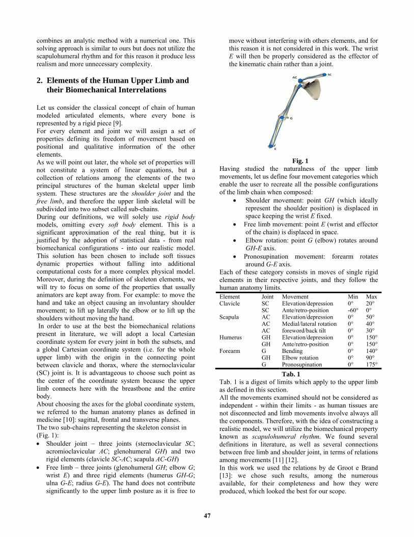
combines an analytic method with a numerical one. This solving approach is similar to ours but does not utilize the scapulohumeral rhythm and for this reason it produce less realism and more unnecessary complexity. 2. Elements of the Human Upper Limb and their Biomechanical Interrelations Let us consider the classical concept of chain of human modeled articulated elements, where every bone is represented by a rigid piece [9]. For every element and joint we will assign a set of properties defining its freedom of movement based on positional and qualitative information of the other elements. As we will point out later, the whole set of properties will not constitute a system of linear equations, but a collection of relations among the elements of the two principal structures of the human skeletal upper limb system. These structures are the shoulder joint and the free limb, and therefore the upper limb skeletal will be subdivided into two subset called sub-chains. During our definitions, we will solely use rigid body models, omitting every soft body element. This is a significant approximation of the real thing, but it is justified by the adoption of statistical data - from real biomechanical configurations - into our realistic model. This solution has been chosen to include soft tissues dynamic properties without falling into additional computational costs for a more complex physical model. Moreover, during the definition of skeleton elements, we will try to focus on some of the properties that usually animators are kept away from. For example: to move the hand and take an object causing an involuntary shoulder movement; to lift up laterally the elbow or to lift up the shoulders without moving the hand. In order to use at the best the biomechanical relations present in literature, we will adopt a local Cartesian coordinate system for every joint in both the subsets, and a global Cartesian coordinate system (i.e. for the whole upper limb) with the origin in the connecting point between clavicle and thorax, where the sternoclavicular (SC) joint is. It is advantageous to choose such point as the center of the coordinate system because the upper limb connects here with the breastbone and the entire body. About choosing the axes for the global coordinate system, we referred to the human anatomy planes as defined in medicine [10]: sagittal, frontal and transverse planes. The two sub-chains representing the skeleton consist in (Fig. 1): • Shoulder joint – three joints (sternoclavicular SC;

acromioclavicular AC; glenohumeral GH) and two rigid elements (clavicle SC-AC; scapula AC-GH)

• Free limb – three joints (glenohumeral GH; elbow G; wrist E) and three rigid elements (humerus GH-G; ulna G-E; radius G-E). The hand does not contribute significantly to the upper limb posture as it is free to

move without interfering with others elements, and for this reason it is not considered in this work. The wrist E will then be properly considered as the effector of the kinematic chain rather than a joint.

Fig. 1

Having studied the naturalness of the upper limb movements, let us define four movement categories which enable the user to recreate all the possible configurations of the limb chain when composed:

• Shoulder movement: point GH (which ideally represent the shoulder position) is displaced in space keeping the wrist E fixed.

• Free limb movement: point E (wrist and effector of the chain) is displaced in space.

• Elbow rotation: point G (elbow) rotates around GH-E axis.

• Pronosupination movement: forearm rotates around G-E axis.

Each of these category consists in moves of single rigid elements in their respective joints, and they follow the human anatomy limits.

Tab. 1 is a digest of limits which apply to the upper limb as defined in this section. All the movements examined should not be considered as independent - within their limits - as human tissues are not disconnected and limb movements involve always all the components. Therefore, with the idea of constructing a realistic model, we will utilize the biomechanical property known as scapulohumeral rhythm. We found several definitions in literature, as well as several connections between free limb and shoulder joint, in terms of relations among movements [11] [12]. In this work we used the relations by de Groot e Brand [13]: we chose such results, among the numerous available, for their completeness and how they were produced, which looked the best for our scope.

Element Joint Movement Min MaxClavicle SC Elevation/depression 0° 20°

SC Ante/retro-position -60° 0°Scapula AC Elevation/depression 0° 50°

AC Medial/lateral rotation 0° 40°AC foreword/back tilt 0° 30°

Humerus GH Elevation/depression 0° 150°GH Ante/retro-position 0° 150°

Forearm G Bending 0° 140°GH Elbow rotation 0° 90°G Pronosupination 0° 175°

Tab. 1

47

The relations are expressed in form of linear regression equations.

About applying the relations to the clavicle: both its elevation (θCL) and extension (φCL) angles are dependent parameters (Fig. 2); humerus elevation (θO) and extension (φO) are independent parameters, as well as direction of force F (positive in elevation and negative in depression), and initial position of angles related to dependent output parameters, which we will indicate as Xθ

o Xϕ.

Therefore for the clavicle there are two linear regression expressions:

0.123 0.046 0· · ·.350 0.493 3.9· 17L OC O F Xθθ θ ϕ= − − + + 0.242 0.1· · · 0.85120 0.008 · 4.983CL O O F Xϕϕ θ ϕ= − + + −+

Eq. 1 Similarly, three linear regression expressions exist for the scapula:

· · · · · 6.0.220 0.010 0.899 0.260 0.982 970SC O O CL CL Fθ θ ϕ θ ϕ= −− + − + 0.088 0.066 0.3· · ·92 0.778 0.3· · 27. 324 9 9SC O O CL CL Fϕ θ ϕ θ ϕ += + + + +

· · · · · 4.0.145 0.003 0.218 0.274 0.706 884SC O O CL CL Fψ θ ϕ θ ϕ= −− − − + Eq. 2

where φSC is the scapula rotation angle on transverse plane (ante/retro-position), θSC is the scapula rotation angle on frontal plane (elevation), while ψSC is the scapula rotation angle on sagittal plane (medial/lateral rotation) (Fig. 3).

3. Resolution Method Our purpose is to determine a correct posture of the limb when one of the elements of the articulated chain changes position. From this moment on we will not consider the prosupination anymore, as it does not affect the positioning of other elements. Similarly we will consider ulna and radius as a unique segment G-E.

Considering all possible movements, we describe an iterative resolution method for the chain (upper limb) based on the analytic resolution of the two sub-chains (shoulder joint and upper limb). Firstly, let us consider the sub-chain of the free-limb. It is possible to resolve the free-limb as an independent chain if considering the hinge point GH fixed in space (a detailed description of the method will follow). When the local posture of the free-limb will be found, then we will consider the sub-chain of the shoulder joint, which resolution consists in determining the elevation and protraction angles of the humerus GH-G by using the scapulohumeral rhythm. Let us suppose that we want to move the upper limb by a movement of wrist E or a rotation of elbow G around GH-E axis. Since GH is temporally fixed in space, we can calculate the position of the free-limb, in other words of the elbow G, and the humerus angles. Starting from the latter, we can calculate the position of the shoulder, i.e. of points AC and GH, supposing the inclination angles of the humerus as fixed. The method consists in the reiteration of those operations until the series of GH positions will converge within some tolerance (Fig. 4).

Fig. 4 Similarly we can initally move the shoulder and then reiterate the procedure starting from the new position of GH. 3.1 Resolution of the ree imb If we isolate the free-limb from the shoulder system, we can make some assumptions that greatly reduce the DOF of this kinematic sub-chain: - hinge in GH can be considered fixed in space. GH is a joint with 3 DOF (movement of elevation/depression and ante/retro-position of the arm; swivel movement of the elbow around GH-E axis);

Fig. 2

Fig. 3

repeat

Take new E position or G rotation

repeat

Calculate new G position

Calculate new arm and forearm

Calculate new scapula and clavicula

Obtain new GH from calculated elements

until GH is “near” the previous one

until the chain limits have been respected

(i.e. the input leads to a correct chain

configuration)

F L-

48

- humerus can be represented by segment GH-G; - the elbow can be considered coincident with point G. This is a joint with 1 DOF (flexion of the forearm); - Ulna and radio can be represented by the G-E segment; - effector is positioned in E.

Let4 3f : q ∈ℜ → ℜ be the direct kinematics mapping

of this chain, where q is a vector having 4 components, namely the joint variables q1,q2,q3 for GH e q4 for G; we can express the position of the effector 3E∈ℜ as

( )E E G G GHf q T M T M GH= = ⋅ ⋅ ⋅ ⋅ Eq. 3

where • MGH and MG are the homogeneous transformation

matrices related to joint GH and G

( )1 2 3

000

0 0 0 1

GHGH

R q ,q ,qM

⎡ ⎤⎢ ⎥⎢ ⎥=⎢ ⎥⎢ ⎥⎣ ⎦ ,

( )4

000

0 0 0 1

GG

R qM

⎡ ⎤⎢ ⎥⎢ ⎥=⎢ ⎥⎢ ⎥⎣ ⎦ ;

• RGH and RG are the rotation matrices related to joint GH and G defined as:

zGH y x( )R ( )RR ( )R ϕ θ ψ= and G yR )R (θ= , with 1 0 000

xR cos sensen cos

( )ψ ψ ψψ ψ

⎡ ⎤⎢ ⎥−⎢ ⎥⎢⎣ ⎦

=⎥

00 1 0

0y

cos senR

sen cos( )

θ θθ

θ θ

⎡ ⎤⎢ ⎥⎢ ⎥⎢

=⎥−⎣ ⎦

00

0 0 1z

cos senR se( ) n cos

ϕ ϕϕ ϕ ϕ

−⎡ ⎤⎢ ⎥⎢⎢⎣ ⎦

= ⎥⎥

as rotation matrices around axis X, Y and Z; • TG and TE are the constant homogeneous

transformation matrices related to arm and forearm

0 0 0 1GGI v

T⎡ ⎤

= ⎢ ⎥⎣ ⎦ , 0 0 0 1E

EI vT

⎡ ⎤= ⎢ ⎥⎣ ⎦

with I the 3x3 identity matrix, νG a vector which components represent the coordinates of G relatively to GH, and νE a vector which components represent the coordinates of E relatively to G. The effector is chosen interactively by the user, and hinge GH is a fixed element of the chain. Once these two positions are known, our problem of inverse kinematics is to find the values of the 4 variables representing the joint elements of q. In this sense, let us note how the first 3 elements of the vector q (q1,q2,q3) are exactly the angles of rotation RGH, or ψ,φ,θ; whilst q4 is the angle of rotation RG(θ). Finding the elements of vector q is thus like finding the angles of these rotations. If we can determine point G, then we have a solution to our problem, since it is the middle joint of a kinematic chain with only two elements: its position solves the problem of inverse kinematics associated with the chain.

In fact, once the position of all points in the chain is known, it is possible to derive the variables associated with joint GH and G, i.e. vector q. Since function f is not injective, it is not invertible. A simple physical interpretation of this is the following: if the wrist is kept fixed, the elbow is still free to rotate on a circular arc having the normal axis running from the shoulder to the wrist itself, namely the axis hinge-effector. So all the points on this circular arc are allowable solutions of our problem, when E is fixed. In other words, the circular arc identifies the set of solutions for the inverse problem f -1. As we will see later, this set of solutions can be parameterized with an angle of swivel. Now our goal is to characterize the position of point G according to the constraints imposed by the coordinates of the effector and to the swivel angle of rotation around the hinge-effector axis. By hypothesis we know the coordinates of points GH and E. Given the positions of hinge and effector into space, let us find G such that: • the distance h between hinge and effector is be less

than the sum of m and n, lengths of the two segments GH-G and G-E (arm and forearm), i.e. h m n≤ + .

• the distance h between hinge and effector is greater than the absolute value of the difference between m

and n, i.e. h m n≥ − . The first condition is obvious if we notice that a fully extended free limb takes maximum length equal to the sum of arm and forearm lengths, while the second condition derives from observing that hinge and effector may overlap only if m = n. Let a swivel plane be a plane containing points GH and E. Then segment GH-E identifies a sheaf of swivel planes. Each plane of the sheaf is characterized by the angle formed with the one plane perpendicular to the body transversal plane: we call this angle as the swivel angle σ, and it is the only parameter determining a particular plane of the sheaf. Let us consider a generic position of the kinematic chain, it is immediate to verify that it is always possible to identify a swivel plane containing G by means of its swivel angle. Let σO be the identifier of the swivel plane containing G originally, and let GH-G-E be the triangle formed by points GH, G and E: it is possible to calculate the coordinates of G on the swivel plane σO by studying GH-G-E (a simple method will be described later). After determining G on the swivel plane, it is possible to determine its unique position in space by rotating the point accordingly to the swivel angle σ around the hinge-effector axis. Summarizing, coordinates of elbow G can be determined with the following steps: • locate the swivel plane σO • calculate position of G on σO • rotate G following the swivel angle σ around the

hinge-effector axis A practical procedure to calculate the position of elbow G follows.

49

Let us rotate and translate the coordinate system so that plane XZ and swivel plane σ correspond, GH-E lies on Z axis, and the center is in GH. Let Φ be the rotation angle of the coordinate system around Z, and Θ be the rotation angle around Y. Then, let us consider the sphere centered in the origin of the Cartesian axes and with radius h=GH-E. We can express the position of E(x,y,z) in the spherical coordinate system:

yarctanx

ϕ ⎛ ⎞= ⎜ ⎟⎝ ⎠ ,

zarcosh

θ ⎛ ⎞= ⎜ ⎟⎝ ⎠

Since φ is defined in interval (–π/2,π/2), , se 0

, se 0x

xϕ

π ϕ≥⎧

Φ = ⎨ + <⎩

while θΘ= .

Let GH-G-E be a triangle on plane XZ; it is possible to apply Carnot’s theorem to find angle α:

2 2 2

2n harccos

hmmα

⎛ ⎞−−= −⎜ ⎟

⎝ ⎠

where m, n are the lengths of arm and forearm and h the length of GH-E. Once the angle α is calculated, we have the coordinates of point G in the rotated system:

( )xG sm en α⋅= 0yG =

zG m c )os(α= ⋅ The rotation of elbow G by the swivel angle σ is defined by:

xrot x yG G cos( ) G s )en(σ σ= ⋅ ⋅− yrot y xG G cos( ) G s )en(σ σ= ⋅ ⋅+

zrot zG G=

Finally, in order to obtain the coordinates of G in the original coordinate system it is sufficient to make inverse rotations by angles Θ e Φ, and afterwards the translation which moves GH into its original position. 3.2 Resolution of the shoulder joint As in the free limb, we want to isolate the resolution of this sub-chain in order to reduce DOF doing some assumptions: - hinge in SC can be considered fixed in space. This joint

has 2 DOF (elevation and ante-position of clavicle); - clavicle can be represented by segment SC-AC; - joint AC has 3 DOF (ante/retro-position, elevation,

medial/lateral elevation); - scapula cam be semplified with segment AC-GH; - effector is positioned in GH Let 4 3f : p∈ℜ → ℜ be the direct kinematics mapping of this kinematic chain, where p is a vector having 5 components, namely the joint variables p1,p2 for SC e p3,p4,p5 for AC; we can express the position of the effector

3GH∈ℜ as

( )GH GH AC AC SCf p T M T M SC= = ⋅ ⋅ ⋅ ⋅ Eq. 4

where • MSC and MAC are the homogeneous transformation

matrices related to joint SC and AC

( )1 2

000

0 0 0 1

SCSC

R p , pM

⎡ ⎤⎢ ⎥⎢ ⎥=⎢ ⎥⎢ ⎥⎣ ⎦

, ( )3 4 5

000

0 0 0 1

ACAC

, p pM

,R p⎡ ⎤⎢ ⎥⎢ ⎥=⎢ ⎥⎢ ⎥⎣ ⎦

• RSC e RAC are the rotation matrices related to joint SC and AC defined as:

zSC y( (R R )R )ϕ θ= and zAC y xR R R( ) ( )R ( )ϕ θ ψ= , with

1 0 000

xR cos sensen cos

( )ψ ψ ψψ ψ

⎡ ⎤⎢ ⎥−⎢ ⎥⎢⎣ ⎦

=⎥

00 1 0

0y

cos senR

sen cos( )

θ θθ

θ θ

⎡ ⎤⎢ ⎥⎢ ⎥⎢

=⎥−⎣ ⎦

00

0 0 1z

cos senR se( ) n cos

ϕ ϕϕ ϕ ϕ

−⎡ ⎤⎢ ⎥⎢⎢⎣ ⎦

= ⎥⎥

as rotation matrices around axis X, Y and Z. Such rotation angles are elements of vector p; • TAC and TGH are the constant homogeneous

transformation matrices related to clavicle and scapula

0 0 0 1AC

AC

I vT

⎡ ⎤= ⎢ ⎥⎣ ⎦

, 0 0 0 1

GHGH

I vT

⎡ ⎤= ⎢ ⎥⎣ ⎦

with I the 3x3 identity matrix, νAC a vector which components represent the coordinates of AC relative to SC, and νGH a vector which components represent the coordinates of GH relative to AC. The problem of resolving the shoulder kinematic sub-chain consists in finding the position of joint GH defined by Eq. 4, that is to find the five joint parameters in vector p. In section 2 we introduced the scapulohumeral rhythm to reproduce natural movements of the upper limb. In order to apply the scapulohumeral rhythm it is necessary to find the orientation of the humerus into space as regards to joint GH. This is simply calculated finding humeral elevation and anteposition angles by means of the coordinates of joints GH and G. Let humerus be the vector representing the humerus into space. The angles characterizing his direction in polar coordinates are:

⎟⎟⎠

⎞⎜⎜⎝

⎛=

x

yO humerus

humerusarctanϕ

( )xO humerusarccos−= πθ

where φO is the longitude, and θO the colatitude of vector humerus direction (Fig. 5), in other words these angles are the anteposition and elevation angles we where looking for.

50

Fig. 5 Recalling Eq. 1 and Eq. 2, and fixing the wrist position, it is possible to manipulate joint AC by modifying the clavicle angles θCL and φCL. Since the scapula follows clavicle movements, also its position is modified according to scapulohumeral rhythm. We can also suppose the shoulder being manipulated by the user. In such case the clavicle angles will become θCL+ θM and φCL+ φM , where θM and φM are the increments of rotation angles. 4. Iterative Method for Calculating the Upper Limb We described two analytical methods to get a solution for both the shoulder joint and the free limb sub-chains. These are connected in joint GH, which is the effector of the first and the hinge of the second respectively. Joint GH position is both an input parameter of the free limb resolution method, and an output parameter of the shoulder joint resolution method: there is a reciprocal dependence between the two methods. In other words the resolution method for the shoulder joint uses information on humerus to calculate GH, while the method for the free limb uses GH to calculate the humerus, among other things (Fig. 6). Our resolution method for the whole human upper limb solve this dependence iteratively, converging to a posture of the upper limb which is coherent with both the sub-chains.

Fig. 6

Let limb be the vector representing the kinematic chain position (its elements are AC, GH and G), iteration k of our method is:

limb k= F (limbk-1) where F is the function which represent the sequence of transformations executed at each iteration. Let us describe iteration k. If we know the last position of chain (limbk-1), we also know GHk-1 e then we can use the free limb resolution method and calculate elbow G:

Gk ← elbow_solver ( GHk-1, E , σ ) where E and σ remain constant during iteration k. Once calculated the position of elbow G, we can calculate humerus position and obtain its angles. These are necessary to utilize the relations of scapulohumeral rhythm and calculate clavicle and scapula positions.

θOk, φO

k ← humerus_solver ( GHk-1, Gk )

Using the elevation and ante-position angles of the humerus just calculated, we can obtain the clavicle and scapula angles using the scapulohumeral rhythm.

θCLk, φCL

k ← clavicle_solver ( θO

k, φO

k ) θSC

k, φSCk , ψSC

k ← clavicle_solver ( θO

k, φO

k , θCLk, φCL

k )

Rotating the clavicle according to its calculated angles, we can obtain joint AC position, which is its external extreme and scapula joint. That is, scapula rotations happens in joint AC. If we rotate the scapula according to its calculated angles, we can calculate the new position of joint GH, i.e. (GHk). We can express clavicle and scapula rotations at iteration k with the following rotation matrices expressed in homogeneous coordinates:

1 0 0 00 0 00 0 00 0 0 1

kCL Mk

CL kCL M

Rθ θ

ϕ ϕ

⎛ ⎞⎜ ⎟+⎜ ⎟=⎜ ⎟+⎜ ⎟⎝ ⎠

0 0 00 0 00 0 00 0 0 1

kSC

kk SCSC k

SC

R

ψθ

ϕ

⎛ ⎞⎜ ⎟⎜ ⎟= ⎜ ⎟⎜ ⎟⎜ ⎟⎝ ⎠

Joint AC at iteration k is given by: k k

AC CLAC T R SC= ⋅ ⋅ while joint GH is given by:

k kG

kH SCGH T R AC= ⋅ ⋅

Calculation of AC and GH can be summarized as follows: ACk

← rotationAC ( θCLk, φCL

k ) GHk

← rotationGH ( θOk, θSC

k, φSCk , ψSC

k )

Once calculated GHk position, iteration k ends. Iterative cycle terminates when

( )1 maxk krelGH GH tol ε−− < −

where tol is the requested accuracy for the solution, and εrel is the maximum precision relative to GHk-1. The algorithm is presented in (Fig. 7).

51

5. Performance The algorithm for upper limb resolution (upper_limb_ solver) has a complexity which depends on the convergence speed of the iterative method. At each iteration ~130 flop (floating point operations) are executed (Fig. 7). We run four different test sets: two using double and single precision with zero tolerance (Fig. 8, Fig. 9), and other two with different higher tolerances (Fig. 10,Fig. 11). For each of them we executed 1000 moves of the limb along random directions.

Fig. 8 Histogram of iterations when using double

precision accuracy with zero tolerance

Fig. 9 Histogram of iterations when using single

precision accuracy with zero tolerance From our tests we noticed that there are not significant differences between the distribution estimations for double and single precision accuracies, with a narrower graph for the latter case. More interesting considerations

can be done when analyzing the last two test sets: we can notice a significant reduction of the number of iterations when raising the tolerance of some order of magnitude. Let us consider a scale, based on parameters from [14], in which the average upper limb elements measure as follows: arm 3 units, forearm 2.7 units, clavicle 1.654 units, and the glenohumeral joint positioned at point with coordinates (0.09, 0.29, 0.5) with respect to the oriented acromioclavicural center. In this case we can obtain a satisfactory visual result with tolerance distance of 0.001 between two subsequent GH positions. This means that 3 iterations are generally enough to converge to a solution. Therefore we can conclude that our method solve the inverse kinematic problem for this 9 DOF chain in a few hundred flop.

Fig. 10 Histogram of iterations when using double

precision accuracy with tolerance of 10-4

Fig. 11 Histogram of iterations when using double

precision accuracy with tolerance of 10-3 With the purpose of studying performance for our software, we examined comparative results from Tolani et al.[8], which were presented in terms of seconds. Those results include classical inverse Jacobian and optimization methods, as well as their own approach. We assumed that they were being run on an SGI Octane2 system available in 1999, so we scaled the published absolute times trying to deduce how they could perform on our computer equipped with an Intel QuadCore 2.4 GHz processor. We executed 10000 tests, each consisting in a movement in a random direction from a valid random posture within the workspace of the limb. We took each execution time and calculated their arithmetic mean. Results are presented in Tab. 2 and expressed in seconds.

Fig. 7 Algorithm and its Computational Complexity

52

Our method Tolani et al. Optimization Inverse Jacobian

0.000028 0.00025 0.005 0.372 Tab. 2

We can assert that our method performs better than the one from Tolani et al. of an order of magnitude, and of four orders of magnitude in comparison with the traditional Inverse Jacobian. As our table was deduced using a simple theoretical scaling based on processors nominal clock rate, one can expect some difference on the real measurement. We believe such differences would not produce better numbers than the measurements we deduced. In fact, as proposed in [15], internal Instruction Level Parallelism (ILP) and pipeline length did not historically scaled proportionally to clock rate, while energy losses increased. This means that processor performances on single cores did not increase significantly during recent years. 6. Conclusion We proposed a skeleton model of the human upper limb and a kinematic resolution method. We showed that they enable the user to find a new posture when moving the wrist, as traditional inverse kinematic chains do. But at the same way our user can also move the elbow and the shoulder with the wrist kept hold in its position, reproducing movements of the limb when holding firmly something in the hand. Moreover, when applying biomechanical regression equations and joint limits, it is possible to reproduce natural postures. These are very useful for many different real-time applications reproducing human movements of singles and crowds. More generally this work shows a different approach to the reproduction of human skeletons in Computer Graphics. Following the example for upper limbs as discussed here, we can think to revisit resolution methods of other human skeletal subsystems in order to realistically and naturally reproduce postures of the entire human skeleton. In these terms, new models for vertebral column, lower limbs, hands and feet are still to be developed. Finally, convergence of our iterative method for the upper limb remains to be analytically proved, although it produced excellent experimental results (~3 iterations for most postures). References [1] V.M., Zatsiorsky, Kinematics of human motion. (Human Kinetics, 1998). [2] H. Liu, A Fuzzy Qualitative Framework for Connecting Robot Qualitative and Quantitative Representations, IEEE Transactions on Fuzzy Systems, 16(6), 2008, 1522-1530. [3] H. Zhou, H. Hu, N. Harris, J. Hammerton, Applications of wearable inertial sensors in estimation of

upper limb movements, Biomedical Signal Processing and Control, 1(1), 2006, 22-32. [4] N. Badler, D. Tolani, Real-Time Inverse Kinematics of the Human Arm, Presence,5(4), 1996, 393-401. [5] N.I. Badler, C.B. Phillips & B.L. Webber, Simulating Humans: Computer Graphics, Animation, and Control (Oxford: Oxford University Press, 1993). [6] W. Maurel, D. Thalmann, Human shoulder modeling including scapulo-thoracic constraint and joint sinus cones, Computers & Graphics 24, Elsevier, 2000, 203-218. [7] C.A., Oatis, Kinesiology: the mechanics and pathomechanics of human movement. (Lippincott Williams & Wilkins, 2003). [8] D. Tolani, A. Goswami, N.I. Badler,Real-Time Inverse Kinematics Techniques for Anthropomorphic Limbs, Graphical Models and Image Processing 62, Academic Press, 2000, 353-388. [9] J.E. Chadwick, D.R. Haumann, R.E. Parent, Layered Construction for Deformable Animated Characters, SIGGRAPH '89, Boston, 1989.. [10] H., Gray, W.H. Lewis, Anatomy of the Human Body, (Philadelphia : Lea & Febiger, 1918) [11] C. Högfors, B. Peterson, G. Sigholm, P. Herberts, Biomechanical model of the human shoulder joint—II. The shoulder rhythm, Journal of Biomechanics 24, 1991, 699-709. [12] P.M. Ludewig, V. Phadke, J.P. Braman, D.R. Hassett, C.J. Cieminski, R.F. LaPrade, Motion of the Shoulder Complex During Multiplanar Humeral Elevation, The Journal of Bone and Joint Surgery (American) 91, 2009, , p. 378-389. [13] J.H. de Groot, R. Brand, A three-dimensional regression model of the shoulder rhythm, Clinical Biomechanics, 2001, 735-743. [14] W. Maurel, D. Thalmann, Human shoulder modeling including scapulo-thoracic constraint and joint sinus cones, Computers & Graphics, 24(2), 2000, 203-218. [15] K. Olukotun & L. Hammond, The Future of Microprocessors, Queue, 2005, 26-29.

53