A radial scanning statistic for selecting space-filling designs

in computer experiments

O. Roustant(1), J. Franco(2), L. Carraro(3), A. Jourdan(4)

(1) Ecole des Mines de St-Etienne – (2) Total – (3) Telecom Saint-Etienne – (4) EISTI Pau

MODA-9, Bertinoro, Italy

1

Framework

•  Scientific framework •  Keywords : Computer experiments, space-filling designs, dimension reduction, goodness-of-fit

•  DICE Consortium (Sept. 2006 – Dec. 2009) •  5 industrial companies (TOTAL, Renault, IRSN, EDF, Onera : energy, automotive, nuclear and aerospatial engineering) •  4 academic partners (Ecole des Mines de St-Etienne, Univ. Aix-Marseille, Univ. Joseph Fourier, Univ. Paris 11)

•  Objective : to study costly simulators

•  Web site : http://www.dice-consortium.fr/

2

Supplementary material

  R package "DiceDesign", available at http://cran.r-project.org/

3

Outline

 Motivations  The radial scanning statistic  Applications

  defect detection of SFDs   selection of SFDs

  Future research

4

Introduction - Framework

•  Framework •  First investigation of a costly deterministic simulator

y = fsim(x1, x2, …, xd)

•  Cubic region x=(x1,…,xd) ∈ Ω=[-1,1]d, d=1, 2, …,10, … 20,…50,…

•  Objective •  To study the phenomenon modeled by fsim with few runs

5

Introduction - Assumptions

•  Assumptions •  Complexity of the phenomenon

⇒ Non-linearities of fsim

•  The effective dimension is << d ⇒ Only few factors are influent (sparsity)

fsim(x) = g(xi1, …, xik), k << d

⇒ Only few principal components are influent

fsim(x) = g(b1’x, …, bk’x) , k << d

•  Remark •  The latter is standard for dimension reduction

(as for Sliced Inverse Regression, see [Li, 1991]) 6

Introduction - Consequences

•  Consequences for designs •  Complexity of the phenomenon

⇒ Non-linearities of fsim ⇒ space-filling designs

•  The effective dimension is << d ⇒ Only few factors are influent (sparsity)

fsim(x) = g(xi1, …, xik), k << d ⇒ space-filling of projections onto factorial subspaces

⇒ Only few principal components are influent

fsim(x) = g(b1’x, …, bk’x) , k << d ⇒ space-filling of projections onto oblique subspaces

7

Introductory example

•  A 8D example •  fsim(x) = g(x2, x7), d=8 •  Common approach in practice : use a space-filling design (SFD), for instance a 80 points Sobol sequence

8

Introductory example

•  A 8D example •  fsim(x) = g(x2, x7), d=8 •  Space-filling design : 80 points Sobol sequence

⇒  Space-filling is not so good in the subspace Vect(x2, x7) ⇒  If the code is a function of x2 – x7 , only 16 different points ! loss of information

9

Introductory example

OBJECTIVE ⇒  To detect automatically such defects ⇒  To select space-filling designs that are still space-filling in projection onto oblique subspaces

⇒  more constraining than for LHDs or OAs ⇒  to be precised in next slide

10

Objective

•  Ideal objective: •  There is a need to check good properties of projections onto any subspace spanned by b1’x, …, bk’x

•  Revised ideal objective: •  To check space-filling properties of the projections onto any (oblique) 1-dimensional axis [spanned by one b’x]

•  Realization: •  To check space-filling properties of the projections onto any 1-dimensional axis of the form :

•  βixi + βjxj 2D radial scanning statistic •  βixi + βjxj + βkxk 3D radial scanning statistic

11

A good benchmark

•  Uniform designs •  Advantage: Space-filling onto projections •  Main defaults : clusters, holes

12

A good SFD ? advantages without the drawbacks of uniform designs, … /…

A good benchmark

13

A good SFD ?

… and without other drawbacks !

A 3D randomized OA

2nd part

  The radial scanning statistic

14

The idea

•  Radial scanning – Case of a 2D subspace •  Scan angularly the domain •  For each radial direction, project orthogonally the design points

Are the projected points « well » distributed ?

15

θ

Distribution of a sum of uniforms

•  The distribution of b’X is not uniform •  Depends on the projections of the corners of [-1,1]d onto Vect(b)

16

-α α -M M

Distribution of a sum of uniforms

•  Proposition (Laplace, 18th Century ! – see a modern proof and discussion in [Elias and Shiu, 1987])

17

Mathematical formulation

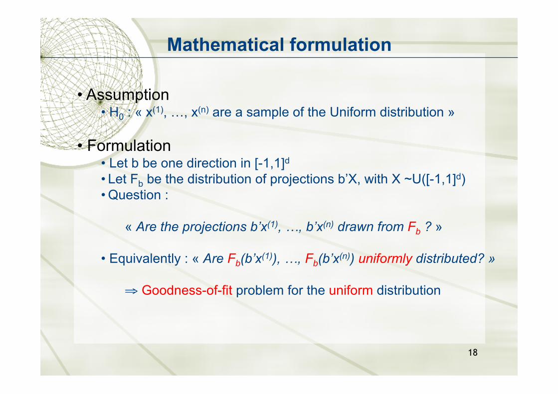
•  Assumption •  H0 : « x(1), …, x(n) are a sample of the Uniform distribution »

•  Formulation •  Let b be one direction in [-1,1]d

•  Let Fb be the distribution of projections b’X, with X ~U([-1,1]d) •  Question :

« Are the projections b’x(1), …, b’x(n) drawn from Fb ? »

•  Equivalently : « Are Fb(b’x(1)), …, Fb(b’x(n)) uniformly distributed? »

⇒  Goodness-of-fit problem for the uniform distribution

18

Selecting a goodness-of-fit statistic

•  Objective : to select a GOF statistic for the uniform distrbution that detects alignments and clustering

•  Statistics based on CDFs (KS, CVM) usually fail, statistics based on « spacings » do it, such as Greenwood ([L’ecuyer, Simard, 2007])

2D RSS based on : CVM (left), KS (middle), Greenwood (right)

19

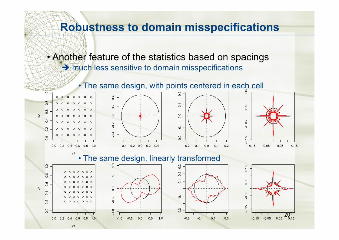
Robustness to domain misspecifications

•  Another feature of the statistics based on spacings much less sensitive to domain misspecifications

20

•  The same design, with points centered in each cell

•  The same design, linearly transformed

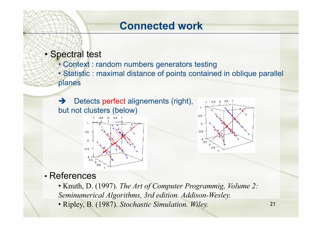
Connected work

•  Spectral test •  Context : random numbers generators testing •  Statistic : maximal distance of points contained in oblique parallel planes

Detects perfect alignements (right), but not clusters (below)

•  References •  Knuth, D. (1997). The Art of Computer Programmig, Volume 2: Seminumerical Algorithms, 3rd edition. Addison-Wesley. •  Ripley, B. (1987). Stochastic Simulation. Wiley. 21

3rd part

  Applications

22

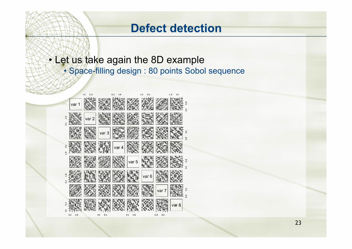
Defect detection

•  Let us take again the 8D example •  Space-filling design : 80 points Sobol sequence

23

Defect detection

•  8D example (following) – 2D RSS •  the worst case is for the pair of dimensions (2,7) •  in this 2D factorial subspace, the worst direction is ≈ (1,-1)

24

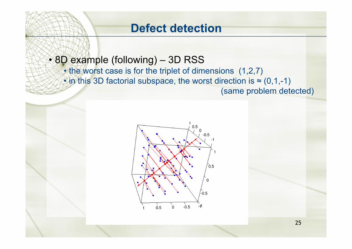
Defect detection

•  8D example (following) – 3D RSS •  the worst case is for the triplet of dimensions (1,2,7) •  in this 3D factorial subspace, the worst direction is ≈ (0,1,-1)

(same problem detected)

25

Defect detection

•  Low Discrepancy Sequences (LDS)

•  Sobol

Owen scrambling

26

Defect detection

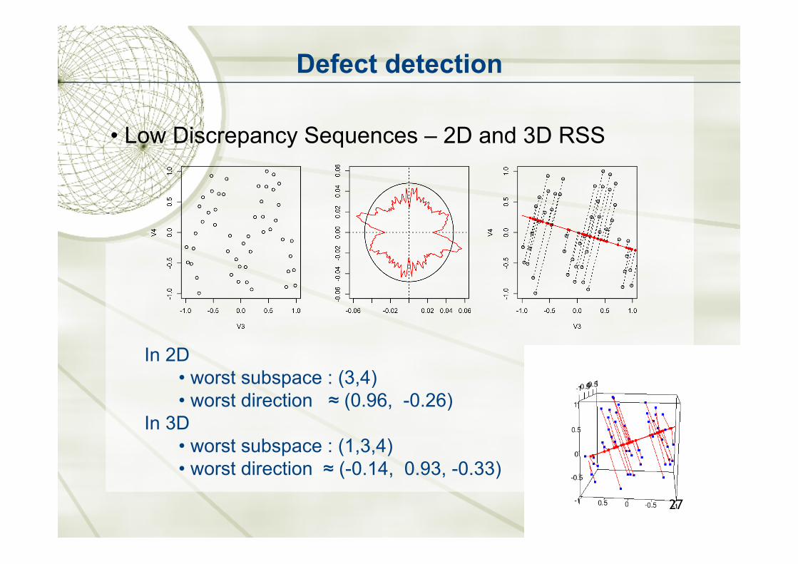
•  Low Discrepancy Sequences – 2D and 3D RSS

In 2D •  worst subspace : (3,4) •  worst direction ≈ (0.96, -0.26)

In 3D •  worst subspace : (1,3,4) •  worst direction ≈ (-0.14, 0.93, -0.33)

27

Defect detection

•  Latin hypercube (LH) designs

•  Maximin LHD

28

Defect detection

•  Maximin LHD

In 2D •  worst subspace : (3,5) •  worst direction ≈ (0.97, 0.23)

In 3D •  worst subspace : (3,4,5) •  worst direction ≈ (-0.31, 0.69, 0.64)

29

Selection of SFDs

•  Comparison of 8D SFDs of size 80

30

Future research

  Statistical issue   Higher dimensions

31

Decisional issues

•  Multiple testing framework •  multiple pairs (triplets) of dimensions •  multiple angles •  strong correlation !

•  Partial solution •  consider a global statistic over directions, such as: sup/inf

the multiple testing issue over dimensions remains…

32

Future research

•  Radial scanning in higher dimensional subspaces •  Visualization is no longer possible •  Computational cost

  Optimization techniques   Normal approximations ? (away from factorial subspaces)

•  Other ideas •  Radial scanning of 2D (or higher) subspaces

33

Acknowledgements

We wish to thank A. Antoniadis, the members of the DICE Consortium (http://www.dice-consortium.fr), the participants of ENBIS-DEINDE 2007, as well as two referees for their useful comments. We also thank Chris Yukna for his help in editing.

34

THANK YOU FOR YOUR ATTENTION