Laboratoire d'Analyse et Modélisation de Systèmes p our

l'Aide à la Décision

CNRS UMR 7024

CAHIER DU LAMSADE

166

Janvier 2000

A priori optimization for the probabilistic maximum independent set problem

Cécile Murat, Vangelis Th. Paschos

Table of ContentsRésumé iiAbstra t ii1 Introdu tion 12 The modi� ation strategies and a preliminary result 42.1 Strategy U1 . . . . . . . . . . . . . . . . . . . . . . . . . . . . . . . . . . . . . . . 42.2 Strategies U2 and U3 . . . . . . . . . . . . . . . . . . . . . . . . . . . . . . . . . . 42.3 Strategy U4 . . . . . . . . . . . . . . . . . . . . . . . . . . . . . . . . . . . . . . . 52.4 Strategy U5 . . . . . . . . . . . . . . . . . . . . . . . . . . . . . . . . . . . . . . . 52.5 A general mathemati al formulation for the �ve fun tionals . . . . . . . . . . . . 53 The omplexity of PIS1 63.1 Computing optimal a priori solutions . . . . . . . . . . . . . . . . . . . . . . . . . 63.2 Approximating optimal solutions for PIS1 . . . . . . . . . . . . . . . . . . . . . . 73.3 PIS1 in bipartite graphs . . . . . . . . . . . . . . . . . . . . . . . . . . . . . . . . 84 The omplexities of PIS2 and PIS3 84.1 Expressions for EU2S and EU3S . . . . . . . . . . . . . . . . . . . . . . . . . . . . . 84.2 Bounds for EU2S . . . . . . . . . . . . . . . . . . . . . . . . . . . . . . . . . . . . . 114.3 Approximating optimal solutions for PIS2 . . . . . . . . . . . . . . . . . . . . . . 114.3.1 Using argmaxfPvi2S pig as a priori solution . . . . . . . . . . . . . . . 114.3.2 Polynomial time approximations for PIS2 . . . . . . . . . . . . . . . . . . 124.4 PIS2 in bipartite graphs . . . . . . . . . . . . . . . . . . . . . . . . . . . . . . . . 135 The omplexity of PIS4 145.1 An expression for EU4S . . . . . . . . . . . . . . . . . . . . . . . . . . . . . . . . . 145.2 Using S� or argmaxfPvi2S pig as a priori solutions . . . . . . . . . . . . . . . 155.3 PIS4 in bipartite graphs . . . . . . . . . . . . . . . . . . . . . . . . . . . . . . . . 176 The omplexity of PIS5 186.1 In general graphs . . . . . . . . . . . . . . . . . . . . . . . . . . . . . . . . . . . . 186.2 In bipartite graphs . . . . . . . . . . . . . . . . . . . . . . . . . . . . . . . . . . . 197 Con lusions 19A Proof of proposition 1 22A.1 Determining A��(G) . . . . . . . . . . . . . . . . . . . . . . . . . . . . . . . . . . 22A.2 Determining A��(G)�1 . . . . . . . . . . . . . . . . . . . . . . . . . . . . . . . . 22

i

Optimisation a priori pour le problème du stable maximum probabilisteRésuméNous ommençons par donner une dé�nition formelle du on ept relativement nouveaudes problèmes d'optimisation ombinatoire probabilistes (sous la méthodologie dite a prioridéveloppée par Bertsimas, Jaillet et Odoni). Ensuite, nous étudions la omplexité de résoudreoptimalement le problème du stable maximum probabiliste sous di�érentes stratégies demodi� ation, ainsi que la omplexité de solutions appro hées. Pour les diverses stratégiesétudiées nous présentons aussi des résultats sur la restri tion du stable maximum probabilistesur les graphes biparties.Mots- lé : problèmes ombinatoires, omplexité, stable, grapheA priori optimization for the probabilisti maximum independent setproblemAbstra tWe �rst propose a formal de�nition for the on ept of probabilisti ombinatorial opti-mization problem (under the a priori method). Next, we study the omplexity of optimallysolving probabilisti maximum independent set problem under several a priori optimizationstrategies as well as the omplexity of approximating optimal solutions. For the di�erentstrategies studied, we present results about the restri tion of probabilisti independent seton bipartite graphs.Keywords: ombinatorial problems, omputational omplexity, independent set, graph

ii

1 Introdu tionIn probabilisti ombinatorial optimization, the probabilities are asso iated with the data de-s ribing an optimization problem (and not with the relations between data as, for example, inrandom graph theory ([4℄)). For a parti ular datum, we an see the probability asso iated withit as a measure of how this datum is likely to be present in the instan e to be optimized, andin this sense, probabilisti elements are expli itly in luded in problem's formulation. In su h aformulation, the obje tive fun tion is a kind of arefully de�ned mathemati al expe tation overall the possible sub-instan es indu ed by the initial instan e.The fa t that in the framework of probabilisti ombinatorial optimization problems (PCOP),the randomness lies in the presen e of the data, makes that the underlying models are veryadequate for the modeling of natural problems, where randomness models un ertainty, or fuzzyinformation, or hardness to fore ast phenomena, et .For instan e, in a transportation network whenever situations of several types of rises have tobe modeled, we meet PCOPs like probabilisti shortest (or longest) path, probabilisti minimumspanning tree, probabilisti lo ation, probabilisti traveling salesman problem (here we modelthe fa t that perhaps some ities will not be visited), et . In industrial automation, the systemsfor foreseeing workshops' produ tion give rise to probabilisti s heduling or probabilisti set overings or pa kings. In omputer s ien e, mainly in what on erns parallelism or distributed omputer networks, PCOPs have to be solved; for example, modeling load balan ing with non-uniform pro essors and failures possibility be omes a probabilisti graph partitioning problem;also in network reliability theory many probabilisti routing problems are met ([3℄).De�nition 1. An NP optimization (NPO) problem � is ommonly de�ned as a four-tuple(P;S; vP ; opt) su h that:� P is the set of instan es of � and it an be re ognized in polynomial time;� given P 2 P (let n be the size of P ), S(P ) denotes the set of feasible solutions of P ;moreover, for every S 2 S(P ) (let jSj be the size of S), jSj is polynomial in n; furthermore,for any P and any S (with jSj a polynomial of n), one an de ide in polynomial time ifS 2 S(P );� given P 2 P and S 2 S(P ), vP (S) denotes the value of S; vP is polynomially omputableand is ommonly alled obje tive fun tion;� opt 2 fmax;ming.Based upon de�nition 1, we will try to give in what follows a formal de�nition for PCOPs (underthe a priori thought pro ess).In [2, 3, 11℄, a thought pro ess alled in the sequel a priori methodology is adopted. Consideran instan e P (where all the data are present) of an NPO problem �, a sub-instan e I of Pand an algorithm U ( alled modi� ation strategy), re eiving S 2 S(P ) ( alled a priori solution)as input. Roughly speaking, the a priori methodology onsists in running U in order to modify Sand to produ e a new solution, dealing with the (present) sub-instan e I of P .The a priori methodology together with the re-optimization one (an exhaustive omputa-tional te hnique) are the only ones used until now in the study of PCOPs. In [2, 3, 11℄, parti u-lar PCOPs are studied, but no formal de�nition of what a PCOP is (in the a priori framework) isgiven. In what follows in this se tion, we draw a formal framework for the a priori probabilisti ombinatorial optimization. 1

De�nition 2. Consider an NPO problem � = (P;S; vP ; opt) and a modi� ation strategy Umodifying S and produ ing a feasible �-solution for I. The probabilisti version P� of � is aquintuple (I;S; U; EP�(P US); opt) su h that:� I is the set of instan es of P� de�ned as I = fIP = (P; ~Pr)g, where P 2 P and ~Pr is ann-ve tor of o urren e-probabilities; I an be re ognized in polynomial time;� given IP = (P; ~Pr) 2 I, S(IP ) = S(P )� U is a modi� ation strategy, i.e., an algorithm whi h, given a solution S 2 S(IP ) and asub-instan e I of P , re eives S as input and omputes a feasible �-solution for I;� given IP 2 I and S 2 S(IP ), EP�(P US) denotes the value of S; if pi = Pr[i℄, i 2 P ,is the o urren e probability of datum1 i, F(IUS) and F (IUS) are the solution obtainedby running U(S) on I and its value, respe tively, Pr[I℄ = Qi2I piQi2PnI(1 � pi) is the�o urren e� probability of I, then EP�(P US) = PI�P Pr[I℄F (IUS); EP�(P US) is ommonly alled fun tional;� opt is the same as for �.The omplexity of P� is the omplexity of omputing S = argoptfEP�(P US) : S 2 S(IP )g.Dealing with de�nition 2, the following remark must be underlined.Remark 1. In de�nition 2, U is part of the instan e and this seems somewhat unusual withrespe t to standard omplexity theory where no algorithm intervenes in the de�nition of a prob-lem. But note that U is absolutely not an algorithm for P�, in the sense that it does not omputeS 2 S(IP ). It simply �ts S (no matter how S has been omputed) to I.Moreover, let us note that hanging U one hanges the de�nition of the problem itself. In otherwords, given a deterministi problem �, the probabilisti problems indu ed by the quintuplesQ1 = (I;S; U1; EP�(P U1S ); opt) and Q2 = (I;S; U2; EP�(P U2S ); opt) are two distin t PCOPs.Moreover, as we will see in the sequel, the hoi e of the modi� ation strategy plays a ru ial rolein the omplexity of the problem given that a strategy may or may not allow in lusion in NP.A ommon thought pro ess dealing with a PCOP P� is �rst to express EP�(P US) in an expli itway. Su h expression of the fun tional allows to pre isely hara terize the a priori solution Soptimizing it and, onsequently, to de ide if S an or annot be omputed in polynomial time.Of ourse, if S annot be omputed in polynomial time, it is very interesting to de ide if at leastthe fun tional itself an be omputed in polynomial time (in other words, if the problem at handis or is not in NP). This remark introdu es a (perhaps the most) meaningful di�eren e betweenprobabilisti and deterministi problems. The general formula of the fun tional as it is given inde�nition 2 (as well as in PCOP-literature) suggests that, in general, exhaustive omputationof EP�(P US) requires O(2n) distin t omputations. Consequently, a positive statement aboutin lusion of P� in NP is not immediate, at least for a great number of PCOPs. Of ourse, inmany ases, fun tional's omputation an be simpli�ed and performed in polynomial time, butas we will see in the sequel, this is not always the ase.Given a graph G = (V;E) of order n, an independent set is a subset V 0 � V su h that not anytwo verti es in V 0 are linked by an edge in G, and the maximum independent set problem (IS)is to �nd an independent set of maximum size. A natural extension of IS whi h will be alsomentioned and dis ussed in the sequel is the maximum-weight independent set (WIS). Here, the1This datum an be a vertex if we deal with graph-problems, or a set if we deal with optimization problem inset-systems, et . 2

verti es of the input-graph are provided with positive weights, and the obje tive be omes tomaximize the sum of the weights of the verti es in an independent set.An instan e of probabilisti independent set (PIS) is a pair (G; ~Pr) and is obtained by as-so iating with ea h vi 2 V an �o urren e� probability pi and by onsidering a modi� ationstrategy U transforming feasible IS-solution S of G into an independent set for the sub-graphof G indu ed by a set I � V . As mentioned above, the obje tive for PIS is to determine the apriori solution S maximizing the fun tional EPIS(GUS).Let us note that PIS is quite di�erent from PCOPs already studied ([2, 3, 11, 12℄). There,Eu lidean versions of minimization routing-problems (su h as the traveling salesman, or theshortest path, or the minimum spanning tree), all of them de�ned in omplete graphs, are onsidered. For all these problems only one modi� ation strategy, onsisting, given an a priorisolution, in removing absent verti es (as our strategy U1 introdu ed in se tion 2) is onsidered.Sin e for this kind of problems any feasible solution is a onne ted subgraph of the input-graphand sin e this latter graph is supposed omplete, there always exist a proper (and easy) wayto onne t the verti es of the surviving in order to onstru t a feasible solution for the �presentsub-instan e�. Su h strategies seem e� ient for minimization problems. On the other hand,for PIS, sin e it is a maximization problem, strategies as U1 are, as we will see later, ratherine� ient and lead to low-quality solutions. Finally, no parti ular restri tions are imposed hereon the input-graphs.Ex ept for its theoreti al interest, PIS has also on rete appli ations. In [7℄, we have stud-ied some aspe ts of the satellite shots planning problem. We have proposed a graph-theoreti modeling for this problem and we have proved that, via this modeling, the solution of the prob-lem studied be ame exa tly the omputation of a maximum independent set in a kind of graph alled � on�i t graph�. However, we have not taken into a ount that shots realized under strong loud- overing are not operational. Consequently, it would be natural to also model weather fore- asting. This an be done by asso iating probability pi with vertex vi of the on�i t graph; thehigher the vertex-probability, the more operational the shot taken. Su h a model for the satel-lite shots planning problem allows, given an a priori IS-solution, omputation of the expe tednumber of operational shots.There exist two interpretations of su h an approa h, ea h one hara terized by its propermodi� ation strategy:� plan is �rstly exe uted and one an know only after plan's exe ution if a shot is operational;in this ase, one retains only the operational ones among the shots realized; this, in termsof PIS, amounts to appli ation of strategy U1 introdu ed in se tion 2;� weather fore asting be omes a ertitude just before plan's exe ution; in this ase, startingfrom an a priori IS-solution, one knows the verti es of this solution orresponding to non-operational shots, one dis ards them from the a priori solution and, �nally, one renders thesurvived solution maximal by ompleting it by new verti es orresponding to operationalshots; this amounts to appli ation of other strategies, for example the ones denoted by U2,U3, U4 in the sequel and introdu ed in se tion 2.Let us note that the probabilisti extension of the model of [7℄ an also be used to representanother on ept, modeled in terms of PIS, where randomness on verti es represents this timeprobabilities that the orresponding shots are requested. Shot-probability equal to 1 means thatthis shot has already been requested, while shot-probability in [0,1℄ means that the orrespondingshot will eventually be requested just before its realization. The orresponding PIS an bee�e tively solved by applying strategies U2 ([13℄), or U3, or U4.3

In what follows we onsider maximal2 (although not ne essarily maximum) a priori inde-pendent sets and use �ve modi� ation strategies, Ui, i = 1; : : : ; 5. For U1 and U5 we expresstheir fun tionals in a losed form, we prove that they are omputed in polynomial time, and wedetermine the a priori solutions that maximizing them. For U2 and U3, the expressions for thefun tionals are more ompli ated and it seems that they annot be omputed in polynomial time.Due to the ompli ated expressions for these fun tionals, we have not been able to hara terizethe a priori solutions maximizing them. Finally, for U4, we prove that the fun tional asso iated an be omputed in polynomial time, but we are not able to pre isely hara terize the optimal apriori solution maximizing it. For all the strategies studied we also study the omplexity of ap-proximating optimal a priori solutions. Let us, on e more, re all here that the strategies studiedintrodu e in fa t �ve distin t PCOPs denoted in the sequel by PIS1, PIS2, PIS3, PIS4 and PIS5,respe tively. Finally, we study the probabilisti version of a natural restri tion of IS, the onewhere the input graph is bipartite.In the sequel, given a graph G = (V;E) of order n, we sometimes denote by V (G) thevertex-set of G. We denote by S a maximal solution of IS of G, by �(G) its ardinality, by S� amaximum independent set of G, by ��(G) its ardinality, by S an optimal PIS-solution (a priorisolution) and by �(G) its ardinality. Moreover, by �(vi), i = 1; : : : ; n, we denote the set ofneighbors of the vertex vi and the quantity j�(vi)j is alled degree of vi; by �(V 0), V 0 � V , wedenote the set [vi2V 0�(vi); also, ÆG = minvi2V fj�(vi)jg, �G = maxvi2V fj�(vi)jg and �G is theaverage degree of G; �nally, by Pr[vi℄ = pi, we denote the fa t that the presen e probability ofa vertex vi 2 V equals pi. Given a set I � V , we denote by G[I℄ = (I; EI) the subgraph of Gindu ed by I (obviously, there are 2n su h graphs). Given a maximal solution S of IS (the apriori solution) in G, we denote by S[I℄ the set S \ I. For reasons of simpli ity, the fun tionalasso iated with PIS on graph G is denoted by EUS (=PI�V Pr[I℄F (IUS)).2 The modi� ation strategies and a preliminary resultIn what follows we denote by GREEDY the lassi al greedy IS-algorithm. It works as follows:it orders the verti es of V in in reasing degree-order, it in ludes the minimum-degree vertexin the solution, it deletes it together with its neighbors (as well as all edges in ident to theseverti es) from V (E), it reorders the verti es of the surviving graph and so on, until all verti esare removed. Moreover, we denote by SIMGREEDY, a simpli�ed version of GREEDY where afterremoving a vertex and its neighbors, the algorithm does not reorder the verti es of the survivinggraph.2.1 Strategy U1Given an a priori IS-solution S and a present subset I � V , modi� ation strategy U1 onsists insimply moving the absent verti es out of S.BEGIN (*U1(G,S)*)OUTPUT F(IU1S ) S[I℄ S \ I;END. (*U1*)2.2 Strategies U2 and U3Modi� ation strategy U2 is a two-step method: it �rst applies U1 to obtain S[I℄, it next appliesGREEDY on the graph G[ ~I℄ = G[I n fS[I℄ [ �(S[I℄)g℄ and, �nally, it retains the union of the twoindependent sets obtained as �nal IS-solution for G[I℄.2If we add a vertex, the result is not an independent set.4

BEGIN (*U2(G,S) /U3(G,S)/*)S[I℄ U1(G; S);G[~I℄ G[I n fS[I℄ [ �(S[I℄)g℄;S[~I℄ GREEDY(G[~I℄); /S[~I℄ SIMGREEDY(G[~I℄);/OUTPUT F(IU2S ) S[I℄ [ S[~I℄; /OUTPUT F(IU3S ) S[I℄ [ S[~I℄;/END. (*U2 /U3/*)Finally, strategy U3 is identi al to U2 modulo the fa t that, instead of GREEDY, algorithmSIMGREEDY is exe uted (instru tions between slashes above refer to modi� ation strategy U3).2.3 Strategy U4Strategy U4 starts from S[I℄ and ompletes it with the isolated verti es (verti es with no neigh-bors) of the graph G[ ~I℄.BEGIN (*U4(G,S)*)S[I℄ U1(G; S);G[~I℄ G[I n fS[I℄ [ �(S[I℄)g℄;OUTPUT F(IU4S ) S[I℄ [ fvi 2 ~I : �(vi) = ;g;END. (*U4*)2.4 Strategy U5Strategy U5 applies the natural relation between a minimal vertex over3 and a maximal in-dependent set in a graph, i.e., a minimal vertex over (resp., maximal independent set) is the omplement, with respe t to the vertex set of the graph, of a maximal independent set (resp., aminimal vertex over).BEGIN (*U5(G,S)*)(1) C V n S;(2) C[I℄ C \ I;(3) R fvi 2 C[I℄ : �(vi) = ;g;(4) C[I℄ C[I℄ n R;(5) OUTPUT F(IU5S ) I n C[I℄;END. (*U5*)2.5 A general mathemati al formulation for the �ve fun tionalsTheorem 1. Consider an a priori solution S of ardinality �(G) for G; onsider strategies Uk, k= 1, ..., 5. With ea h vertex vi 2 V we asso iate a probability pi and a random variable XUk;Si ,k = 1, ..., 5, de�ned, for every I � V , byXUk;Si = � 1 vi 2 F �IUkS �0 otherwise (1)Then EUkS = Xvi2S pi + Xvi2(V nS)Pr hXUk;Si = 1i : (2)In parti ular, if, for ea h vertex vi 2 V , pi = p, thenEUkS = p�(G) + Xvi2(V nS)Pr hXUk;Si = 1i : (3)3Given a graph G = (V;E), a vertex over of G is a set V 0 � V su h that for any vivj 2 E either vi, or vjbelongs to V 0. 5

Proof. By expression (1), F (IUkS ) =Pni=1XUk;Si . So,EUkS = XI�V Pr[I℄F �IUkS � = XI�V Pr[I℄ nXi=1 XUk;Si = nXi=1 XI�V Pr[I℄XUk;Si= nXi=1 E �XUk;Si � = nXi=1 Pr hXUk;Si = 1i = nXi=1 Pr hXUk;Si = 1i �1fvi2Sg + 1fvi =2Sg�= nXi=1 Pr hXUk;Si = 1i 1fvi2Sg + nXi=1 Pr hXUk;Si = 1i 1fvi =2Sg:But, if vi 2 S, then ne essarily XUk;Si = 1, 8I su h that vi 2 I; so, Pr[XUk;Si = 1℄ = pi, vi 2 S,and onsequently,EUkS = Xvi2S pi + nXi=1 Pr hXUk;Si = 1i 1fvi =2Sg = Xvi2S pi + Xvi2(V nS)Pr hXUk;Si = 1i :If pi = p, vi 2 V , then the result of expression (3) is immediately obtained from expression (2).Let us note that, as it an be easily dedu ed from the proof of theorem 1, the above resultholds for any strategy whi h it �rst determines S[I℄, it next omputes an independent set S[ ~I℄on G[ ~I℄, and it �nally onsiders as solution for G[I℄ the set S[I℄ [ S[ ~I ℄.3 The omplexity of PIS13.1 Computing optimal a priori solutionsFrom expression (1), we have XU1;Si = 0, 8vi =2 S, and onsequently, Pr[XU1;Si = 1℄ = 0, forvi 2 V n S; so, the following theorem is immediately derived for strategy U1.Theorem 2. Given a graph G = (V;E), an a priori solution S and the modi� ation strategy U1,then EU1S =Pvi2S pi, and is omputed in O(n). Optimal PIS1-solution S is a maximum-weightindependent set in a weighted version of G where verti es are weighted by the orrespondingprobabilities. If pi = p, 8vi 2 V , then EU1S = p�(G); in this ase, S = S� and EU1S = p��(G).The hara terization of S given in theorem 2 immediately introdu es the following omplexityresult for PIS1.Theorem 3. PIS1 is NP-hard.We now show that for pi = p, vi 2 V , a mathemati al expression for EU1S an be built dire tlywithout applying theorem 1 (used in next se tions for the analysis of other strategies). Giventhat 0 6 jF(IU1S )jdef= F (IU1S ) = jS[I℄j 6 �(G), we get:F �IU1S � = jS[I℄j �(G)Xi=1 1fjS[I℄j=ig:So, the fun tional for U1 an be written asEU1S = XI�V Pr[I℄jS[I℄j �(G)Xi=1 1fjS[I℄j=ig = �(G)Xi=1 iXI�V Pr[I℄1fjS[I℄j=ig= �(G)Xi=1 i��(G)i �pi(1� p)�(G)�i n��(G)Xj=0 �n� �(G)j �pj(1� p)n��(G)�j = p�(G)6

where in the last summation we ount all the sub-graphs G[I℄ su h that jS[I℄j = i and we addtheir probabilities; also, Pn��(G)j=0 Cn��(G)j pj(1 � p)n��(G)�j = 1. The above proof for EU1S anbe generalized in order to ompute every moment of any order for U1. For instan e,E h�GU1S �2i = XI�V Pr[I℄F 2 �IU1S � = �(G)Xi=1 i2��(G)i �pi(1� p)�(G)�i = p�(G)(p�(G) + 1� p)and, onsequently, VarU1S = E h�GU1S �2i� �EU1S �2 = �(G)p(1 � p):So, for U1, the random variable representing the size �(G) of the a priori solution follows abinomial law with parameters �(G) and p.3.2 Approximating optimal solutions for PIS1In this se tion we show how, even if one annot ompute the optimal a priori solution in poly-nomial time, one an ompute a sub-optimal solution, the value (expe tation) of whi h is alwaysgreater than a fa tor times the value (expe tation) of the optimal one. For this, we shall proposein what follows well-known (in the theory of polynomial approximation of NP- omplete prob-lems) polynomial algorithms omputing �good� sub-optimal solutions, and will show that, alsoin probabilisti ase, these algorithms work well.Let us �rst re all that given an instan e P of an NP- omplete problem �, a ommon wayto estimate the apa ity of a polynomial approximation algorithm A in �nding good sub-optimalsolutions for �, is by evaluating its approximation ratio ([8℄), i.e., the ratio A(P )=OPT(P ),where A(P ) denotes the value of the solution omputed by A on P and OPT(P ) denotes thevalue of the optimal solution of P . Then the approximation ratio of A for a maximizationproblem � is the quantity inffA(P )=OPT(P ) : P instan e of �g; the loser this ratio to 1, thebetter the approximation algorithm.Re all that as we have already seen in se tion 3, PIS1 is equivalent to a weighted IS-problem,where ea h vertex is weighted by the orresponding probability. Consequently, the followingtheorem holds immediately.Theorem 4. If there exists a polynomial time approximation algorithm A solving WIS withinapproximation ratio �, then A polynomially solves PIS1 within the same approximation ratio �.In [6℄, an algorithm is developed for WIS a hieving approximation ratio the minimum valuebetween log n=(3(�G + 1) log log n) and O(n�4=5). Using this algorithm in theorem 4, one getsthe following orollary.Corollary 1. PIS1 an be approximated withinmin� logn3(�G + 1) log log n;O �n�4=5o�The hara terization of PIS1 in terms of a weighted IS-problem draws not only issues for �ndingreasonable a priori sub-optimal solutions but, unfortunately, limits the apa ity of the problemto be �well-approximated� sin e, via this hara terization, all the negative results applying to ISare immediately transferred to PIS1 also. So, PIS1 is hard to approximate within n1��, for any� > 0 ([10℄).7

3.3 PIS1 in bipartite graphsTheorem 5. Consider a bipartite graph B = (V1; V2; EB). Then, EU1S = Pvi2S pi and is omputed in polynomial time. The optimal a priori solution S is a maximum-weight independentset in B onsidering that its verti es are weighted by the orresponding presen e probabilities, and an be found in O(n1=2jEB j). Consequently, in bipartite graphs, PIS1 2 P.Proof. Con erning the expression for EU1S and the omplexity of its omputation, the proof isthe same as the one of theorem 2.Determining an optimal IS-solution in a bipartite graph is of polynomial omplexity in bothweighted and unweighted ases (see [9℄ for the unweighted ase; for the weighted one, we quotehere the result of [5℄ where the polynomiality of weighted IS in a lass of graphs in luding thebipartite ones is proved).4 The omplexities of PIS2 and PIS34.1 Expressions for EU2S and EU3SLet Ai =PI�V;jS\Ij=iPr[I℄F (IU2S ). Then, EU2S an be ni ely written as follows:EU2S = XI�V Pr[I ℄F �IU2S � = XI�V 0��(G)Xi=0 1fjS\Ij=ig1APr[I ℄F (IU2S ) = �(G)Xi=0 0B� XI�VjS\Ij=i Pr[I ℄F �IU2S �1CA = �(G)Xi=0 Ai:Quantities Ai, i = 1; : : : ; �(G) (A0 = 0) are very natural and interesting from both theoreti aland pra ti al points of view. For instan e, formula for EU2S given by expression above holds forevery probability law; also, omputing analyti al expressions for Ai seems to be an interestingproblem in ombinatorial ounting of graphs; moreover, thanks to the simple relation between EU2Sand Ai, i = 1; : : : ; �(G), analyti al expressions for the latter would produ e expli it expressionsfor the former. Unfortunately, expression above for EU2S , even intuitive and smart, does not giveany hint allowing pre ise hara terization of S.In proposition 1, the proof of whi h is given in appendix A, A��(G) and A��(G)�1 are expli itly omputed, for the ase of identi al vertex-probabilities. However, the expli it omputation for Aisof lower index produ es very long and non-intuitive expressions.Proposition 1. Let �0(v) = �(v) n f�(v) \ �(S� n fvg)g, `1 = jfv 2 S� : �0(v) = ;gj,`01 = ��(G)� `1, and pi = p, 8vi 2 V . Then,A��(G) = ��(G)p��(G)A��(G)�1 = p��(G)�1(1� p)0B���(G)`1 � `1 + ��(G)`01 � Xv2S��0(v)6=;(1� p)j�0(v)j1CA :We shall now give an upper bound for the omplexity of omputing EU2S . For this, we will analyze(as an intermediate step) strategy U3 introdu ed in se tion 2.Let G0 = G[V n S℄ = (V 0; E0), and let V 0 = fv1; : : : ; vn��(G)g be the list of verti es of G0sorted in in reasing-degree order; let us denote by Vi the set of the i �rst verti es of V 0 andlet G0i = G0[Vi℄ (of ourse, for G0i the verti es of Vi are not sorted in in reasing-degree order).Let us denote by Si the independent set found by U3 on (the present sub-instan e of) G0i, andby �i its ardinality, i = 1; : : : ; n� �(G). Finally, let �(G[I 0℄) be the ardinality of the solutionprovided by U3 when applied in graph G[I 0℄, I 0 � V .8

Theorem 6. E ��n��(G)� = n��(G)Xi=1 pi Pr [vi =2 �(Si�1)℄EU3S = EU1S +E ��n��(G)� :If we denote by T (E(�n��(G))) and T (EU3S ) the omputation times of E(�n��(G)) and EU3S ,respe tively, then T (E(�n��(G))) = O(2n��(G)) and T (EU3S ) = O(2n��(G)).Proof. E(�i) = E(�ijvi present)pi+E(�ijvi absent)(1� pi). Moreover, for strategy U3 we havethe following relation, setting S0 = ;, �(S0) = ; and �0 = 0:�i = � �i�1 �(vi) \ Si�1 6= ;�i�1 + 1 otherwiseSo, E(�ijvi present) = E(�i�1) + Pr[�(vi) \ Si�1 = ;℄; onsequently,E (�i) = piE (�i�1) + pi Pr [vi =2 �(Si�1)℄ + (1� pi)E (�i�1) :Sin e E(�0) = 0, E (�i) = iXj=1 pj Pr [vj =2 �(Sj�1)℄E ��n��(G)� = n��(G)Xi=1 pi Pr [vi =2 �(Si�1)℄ :Now, let I 0 = f(I) = I n fS[I℄ [ �(S[I℄)g. This set represents the subset of verti es of I whi hare not ontained neither in S, nor in the neighbor-set of S[I℄. Consequently, U3 will be appliedon G[I 0℄; so, F (IU3S ) = jS[I℄j+ �(G[I 0℄) and onsequentlyEU3S = XI�V Pr[I℄jS[I℄j +XI�V Pr[I℄� �G[I 0℄� = EU1S +XI�V Pr[I℄� �G[I 0℄�= EU1S +XI�V 0�XI0�V 1ff(I)=I0g1APr[I℄� �G[I 0℄� = EU1S + XI0�V XI�Vf(I)=I0 Pr[I℄� �G[I 0℄� :Sin e Pr[I 0℄ =PI�V;f(I)=I0 Pr[I℄, we getEU3S = EU1S + XI0�V Pr �I 0�� �G[I 0℄� = EU1S +E ��n��(G)� :Let us now introdu e the random variable Ci representing the solution of PIS3 whenever we onsider only the present verti es of Vi, i.e., when we apply the greedy algorithm implied bystrategy U3 in the graph indu ed by the present verti es of Vi.Ci = 8<: Ci�1 vi is absentCi�1 vi is present and �(vi) \ Ci�1 6= ;Ci�1 [ fvig vi is present and �(vi) \ Ci�1 = ;We then have E(�n��(G)) =Pn��(G)i=1 pi Pr[�(vi) \ Ci�1 = ;℄.9

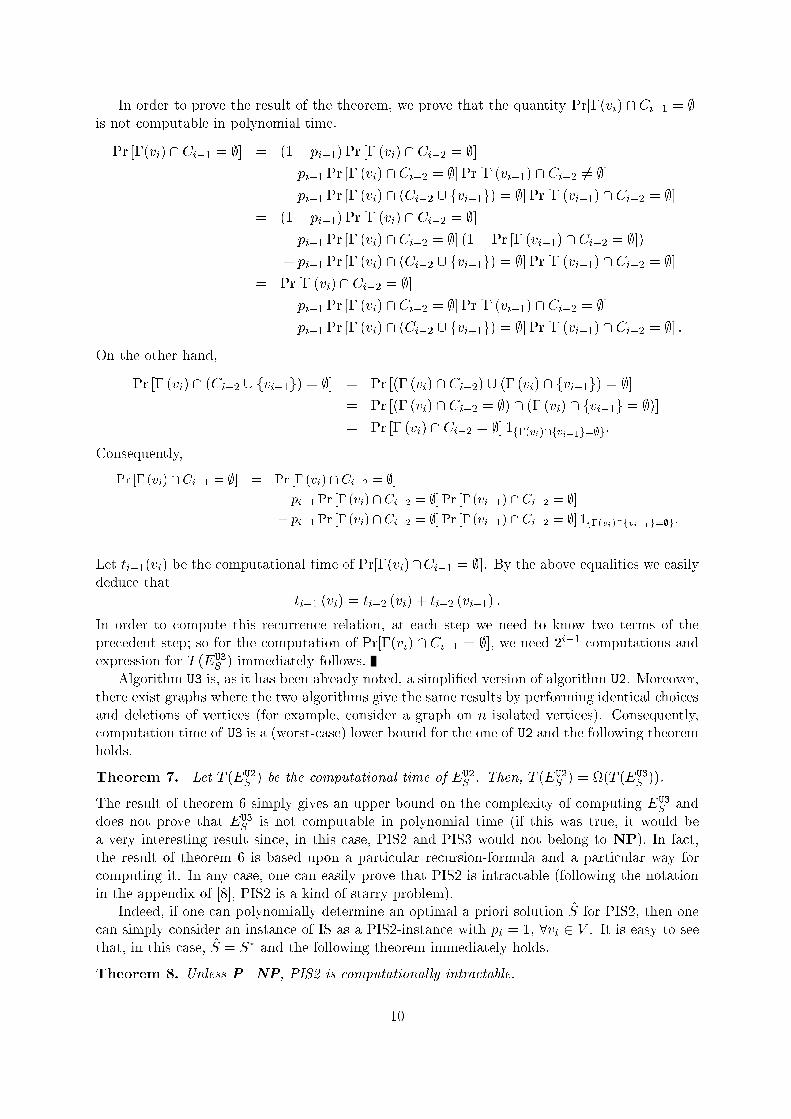
In order to prove the result of the theorem, we prove that the quantity Pr[�(vi) \ Ci�1 = ;℄is not omputable in polynomial time.Pr [�(vi) \Ci�1 = ;℄ = (1� pi�1) Pr [� (vi) \ Ci�2 = ;℄+ pi�1 Pr [� (vi) \ Ci�2 = ;℄ Pr [� (vi�1) \ Ci�2 6= ;℄+ pi�1 Pr [� (vi) \ (Ci�2 [ fvi�1g) = ;℄ Pr [� (vi�1) \ Ci�2 = ;℄= (1� pi�1) Pr [� (vi) \ Ci�2 = ;℄+ pi�1 Pr [� (vi) \ Ci�2 = ;℄ (1� Pr [� (vi�1) \ Ci�2 = ;℄)+ pi�1 Pr [� (vi) \ (Ci�2 [ fvi�1g) = ;℄ Pr [� (vi�1) \ Ci�2 = ;℄= Pr [� (vi) \ Ci�2 = ;℄� pi�1 Pr [� (vi) \ Ci�2 = ;℄ Pr [� (vi�1) \ Ci�2 = ;℄+ pi�1 Pr [� (vi) \ (Ci�2 [ fvi�1g) = ;℄ Pr [� (vi�1) \ Ci�2 = ;℄ :On the other hand,Pr [� (vi) \ (Ci�2 [ fvi�1g) = ;℄ = Pr [(� (vi) \ Ci�2) [ (� (vi) \ fvi�1g) = ;℄= Pr [(� (vi) \ Ci�2 = ;) \ (� (vi) \ fvi�1g = ;)℄= Pr [� (vi) \ Ci�2 = ;℄ 1f�(vi)\fvi�1g=;g:Consequently,Pr [� (vi) \ Ci�1 = ;℄ = Pr [� (vi) \ Ci�2 = ;℄� pi�1 Pr [� (vi) \ Ci�2 = ;℄ Pr [� (vi�1) \ Ci�2 = ;℄+ pi�1 Pr [� (vi) \ Ci�2 = ;℄ Pr [� (vi�1) \ Ci�2 = ;℄ 1f�(vi)\fvi�1g=;g:Let ti�1(vi) be the omputational time of Pr[�(vi)\Ci�1 = ;℄. By the above equalities we easilydedu e that ti�1 (vi) = ti�2 (vi) + ti�2 (vi�1) :In order to ompute this re urren e relation, at ea h step we need to know two terms of thepre edent step; so for the omputation of Pr[�(vi) \ Ci�1 = ;℄, we need 2i�1 omputations andexpression for T (EU3S ) immediately follows.Algorithm U3 is, as it has been already noted, a simpli�ed version of algorithm U2. Moreover,there exist graphs where the two algorithms give the same results by performing identi al hoi esand deletions of verti es (for example, onsider a graph on n isolated verti es). Consequently, omputation time of U3 is a (worst- ase) lower bound for the one of U2 and the following theoremholds.Theorem 7. Let T (EU2S ) be the omputational time of EU2S . Then, T (EU2S ) = (T (EU3S )).The result of theorem 6 simply gives an upper bound on the omplexity of omputing EU3S anddoes not prove that EU3S is not omputable in polynomial time (if this was true, it would bea very interesting result sin e, in this ase, PIS2 and PIS3 would not belong to NP). In fa t,the result of theorem 6 is based upon a parti ular re ursion-formula and a parti ular way for omputing it. In any ase, one an easily prove that PIS2 is intra table (following the notationin the appendix of [8℄, PIS2 is a kind of starry problem).Indeed, if one an polynomially determine an optimal a priori solution S for PIS2, then one an simply onsider an instan e of IS as a PIS2-instan e with pi = 1, 8vi 2 V . It is easy to seethat, in this ase, S = S� and the following theorem immediately holds.Theorem 8. Unless P=NP, PIS2 is omputationally intra table.10

4.2 Bounds for EU2SFor la k of hara terizing the omplexity of omputing EU2S , we build in this paragraph upperand lower bounds for it.Theorem 9. Let ~� be the maximum degree of G[ ~I℄. Then, on the hypothesis of distin tvertex-probabilities:Xvi2S pi +XI�V Yvi2I pi Yvi =2I (1� pi) ���~I���~� + 1 6 EU2S 6 Xvi2S pi +XI�V Yvi2I pi Yvi =2I(1� pi) ���~I��� (4)while, on the hypothesis of identi al vertex-probabilities:p�(G) +XI�V pjIj(1� p)n�jIj ���~I���~� + 1 6 EU2S 6 p�(G) +XI�V pjIj(1� p)n�jIj ���~I��� (5)Always under the latter hypothesis: pn=(�G + 1) 6 EU2S 6 n(�G + p)=(�G + 1).Proof. Remark �rst that jS[I℄j 6 F (IU2S ) 6 jS[I℄j + jI n (S[I℄) [ (�(S[I℄) \ I)j = jS[I℄j + j~Ij; onsequently,EU2S 6XI�V Pr[I℄�jS[I℄j+ ���~I���� 6 EU1S +XI�V Pr[I℄ ���~I��� = Xvi2S pi +XI�V Pr[I℄ ���~I��� : (6)On the other hand, Pr[I℄ =Qvi2I piQvi =2I(1�pi). The upper bound results from the ombinationof expression (6) and the one for Pr[I℄.We now prove the lower bound for EU2S . Let �(G[ ~I ℄) be the ardinality of the solution providedby U2 when applied to G[ ~I℄; we then haveEU2S = Xvi2S pi +XI�V Pr[I℄��G h~Ii� = Xvi2S pi +XI�V Yvi2I pi Yvi =2I(1� pi)��G h~Ii� (7)For �(G[ ~I ℄), sin e the greedy algorithm implied by U2 provides a maximal independent set,the following holds ([1℄): �(G[ ~I℄) > j~Ij=( ~� + 1). By substituting the expression for �(G[ ~I ℄) inexpression (7), we obtain the lower bound laimed.In the ase where all the verti es have the same presen e probability p, Pvi2S pi = p�(G)and Pr[I℄ = pjIj(1� p)n�jIj, and expression (5) follows immediately.In order to obtain bounds implied by the last expression of the theorem (always assum-ing identi al o urren e probabilities), we use inequality �(G) > n=(�G + 1). Moreover,PI�V pjIj(1� p)n�jIj = 1 (so, PI�V pjIj(1� p)n�jIj > 0), and���~I��� = jI n fS[I℄ [ �(S[I℄)gj 6 jI n S[I℄j = jI n (S \ I)j 6 jV n (S \ V )j = jV n Sj = n� �(G):So, PI�V pjIj(1 � p)n�jIjj~Ij 6 (n� �(G))PI�V pjIj(1 � p)n�jIj = n� �(G) and ombining theabove inequalities, we obtain the laimed bounds.4.3 Approximating optimal solutions for PIS24.3.1 Using argmaxfPvi2S pig as a priori solutionSet �S = argmaxfPvi2S pi : S independent set of Gg and suppose that it is used as a priorisolution for PIS2. Then, the following holds. 11

Theorem 10. Approximation of S by �S = argmaxfPvi2S pi : S independent set of Bg guar-antees for PIS2 approximation ratiomax� pmin1 + pmax ; 1�G + 1� :Proof. By expression (7) (proof of theorem 9), and sin e �(G[ ~I℄) 6 ��(G), we getXvi2S pi 6 EU2S = Xvi2S pi + XI�V Pr[I ℄��G[ ~I ℄� 6 ��(G)0�pmax + XI�V Pr[I ℄1A = ��(G) (1 + pmax) (8)Sin e, �S = argmaxfPvi2S pi : S independent set of Gg, thenEU2�S > Xvi2 �S pi > Xvi2S� pi > pmin��(G) (9)Remark now that expression (8) holds also for EU2S ; onsequently, ombining expressions (8)and (9) we obtain EU2�SEU2S > pmin��(G)(1 + pmax)��(G) = pmin1 + pmax (10)On the other hand, remark that from expression (2)EU2S 6 Xvi2V pi (11)and from the lefthand-side of expression (4)EU2�S > Xvi2 �S pi (12)Combination of expressions (11) and (12) givesEU2�SEU2S > Pvi2 �S piPvi2V pi > 1�G + 1 (13)where the last inequality (remark that �S is maximal) is the weighted version of Turàn's theo-rem ([16℄).Expressions (10) and (13) on lude the theorem.4.3.2 Polynomial time approximations for PIS2The set �S onsidered in the previous paragraph annot be omputed in polynomial time. Instead,suppose that one uses a polynomial time approximation algorithm A (a hieving approximationratio �) for (unweighted) IS in order to ompute a solution SOL (obviously, we an supposethat SOL is maximal) on G where vertex-probabilities are omitted. Then, expression (9) in theproof of theorem 10 be omes EU2SOL > pminjSOLj > pmin���(G)and with exa tly the same arguments as in theorem 10, the following theorem an be proved.12

Theorem 11. If there exists a polynomial time approximation algorithm A solving IS withinapproximation ratio �, then algorithm A polynomially solving PIS2 within approximation ratiomax� 1�G + 1 ;� pmin1 + pmax� �� :If A is the algorithm of [6℄, then:� in the ase of �xed vertex-probabilities, PIS2 an be approximately solved in polynomialtime within ratio min�O� log n3(�G + 1) log log n� ; O �n�4=5��� in the ase where probabilities depend on n, PIS2 is polynomially approximable within ratiomax� 1�G + 1 ;� pmin1 + pmax�min�O� logn3(�G + 1) log log n� ; O �n�4=5��� :4.4 PIS2 in bipartite graphsTheorem 12. Consider a bipartite graph B = (V1; V2; EB). Then,EU2V1 = Xvi2V1 pi + Xvi2V2 pi Yvj2�(vi) (1� pj)and an be omputed in polynomial time. Consequently, in bipartite graphs, whenever olor- lass V1 (or V2) is onsidered as a priori solution, PIS2 2 NP.Proof. Let us �rst note the following:� if all the verti es of V1 are absent, then the solution provided by U2 is exa tly the presentverti es of the olor- lass V2;� if all the verti es of V1 are present, then, despite the state of the set V2, the solution of thepresent sub-instan e of B is exa tly the olor- lass V1;� in the ase where a part of the verti es of V1 is present, the �nal solution for B[I℄ willeventually in lude some verti es of V2.Applying the result of theorem 1, we get:EU2V1 = Xvi2V1 pi + Xvi2V2 Pr hXU2;V1i = 1i (14)(re all that Pr[XU2;Si = 1℄ represents the probability that vertex vi =2 S will be hosen whenapplying U2).Note also that Pr[XU2;V1i = 1℄, vi 2 V2, depends only on the present verti es of �(vi); onse-quently, it does not depend on the other elements of V2. Hen eforth, insertion of the elementsof V2 is performed independently the ones from the others and vi 2 V2 will be introdu ed in thesolution for B[I℄ only if �(vi) \ V1[I℄ = ;. So, Pr[XU2;V1i = 1℄ = piQvj2�(vi)(1� pj).Repla ing this expression for Pr[XU2;V1i = 1℄ in expression (14), we obtain the result laimedfor EU2V1 . One an see that this expression implies the omputation of EU2V1 in at most O(n2)steps.From the proof of theorem 12, one an see how the parti ular stru ture of the bipartite graphintervenes in a signi� ant way to simplify the expression for the fun tional and, onsequently, its omputation. Expression (14) holds thanks to the fa t that the vertex set of B an be partitionedinto two independent sets. 13

Corollary 2. Suppose Pr[vi℄ = p, vi 2 V1 [ V2, denote by n1 and n2 the sizes of V1 and V2,respe tively, and suppose that n1 > n2. Then, EU2V1 = pn1+ pPvi2V2(1� p)j�(vi)j. Naturally, EU2V1is omputed in O(n2).From orollary 2 we an obtain the following framing of EU2V1 by EU1V1 for the ase of identi alvertex-probabilities: EU1V1 + n2p(1 � p)�B 6 EU2V1 6 EU1V1 + n2p(1 � p)ÆB . So, in regular bipartitegraphs (i.e., the ones where �B = ÆB = �): EU2V1 = EU1V1 + n2p(1� p)�.Consider set �S = argmaxfPvi2S pi : S independent set of Bg as a priori solution. Then, onsidering vertex-probabilities as vertex-weights and using the result of [5℄, �S an be omputedin polynomial time. Moreover, EU2�S > Xvi2 �S pi > Pvi2V pi2 :Using the expression above together with expression (11), approximation ratio 1/2 is immediatelyyielded.Proposition 2. �S = argmaxfPvi2S pi : S independent set of Bg is a polynomial time approx-imation of S guaranteeing approximation ratio 1/2 for PIS2 in bipartite graphs.Obviously, from theorem 12 and the dis ussion just above, the same approximation ratio an beyielded if one uses argmaxfPvi2V1 pi;Pvi2V2 pig as a priori solution.5 The omplexity of PIS45.1 An expression for EU4SRe all that strategy U4 starts from S[I℄ and ompletes it with the isolated verti es of thegraph G[ ~I℄.Proposition 3. Given a graph G = (V;E), an a priori independent set S and the modi� ationstrategy U4, thenE �GU4S � = Xvi2S pi + Xvi2(V nS) pi Yvj2�S(vi) (1� pj)� Yvk2�V nS(vi)0�(1� pk) + pk0�1� Yvl2�S(vk)(1� pl)1A1A (15)where �S(vi) = �(vi)\S and �V nS(vi) = �(vi)\ (V nS). E(GU4S ) an be omputed in polynomialtime. If pi = p, for all vi 2 V , thenE �GU4S � = p�(G) + Xvi2(V nS) p(1� p)j�S(vi)j Yvk2�V nS(vi)�1� p(1� p)j�S(vk)j� (16)Proof. Set Bi = Pr[XU4;Si = 1℄. ThenBi = XI�Vvi2I Pr[I℄1fvi2F(IU4S )gLet vi be any vertex of V n S and let I be any subset of V ontaining vi. Obviously,vi 2 F(IU4S ) () vi isolated in G[ ~I℄ () (vi 2 G[ ~I℄) ^ (vi has lost all its neighbors in ~I):14

Sin e vi =2 S, vi 2 ~I only if there does not belong to the neighborhood of any vertex in S[I℄, i.e.,vi 2 G[ ~I℄ () �S(vi) \ I = ; (17)On the other hand, all the neighbors of vi in G[ ~I℄ have been removed i� �V nS(vi) \ ~I = ;. Thislast ondition is satis�ed only if every vertex of �V nS(vi) is either absent or (being present) hasbeen removed from ~I be ause it belonged to the neighborhood of a vertex in S[I℄. In all,�V nS(vi) \ ~I = ; () 8vj 2 �V nS(vi) ((vj is absent ) _((vj is present) ^ (9vk 2 �(vj) \ S su h that vk is present))) (18)From relations (17) and (18) and the dis ussion above we get (vi 2 V n S):Bi = XI�Vvi2I Pr[I ℄1fvi2F(IU4S )g = XI�Vvi2I Pr[I ℄1� vi2G[~I℄�V nS(vi)\~I=;�= XI�Vvi2I Pr[I ℄1fvi2G[~I℄g1f�V nS(vi)\~I=;g = XI�V Pr[I ℄1nfvig\I=fvig�S(vi)\I=; o1f�V nS(vi)\~I=;g= XI�V Pr[I ℄1ffvig\I=fvigg1f�S(vi)\I=;g Yvj2�V nS(vi) �1fI\fvjg=;g + 1fI\fvjg=fvjgg1fI\�S(vj)6=;g�= pi Yvk2�S(vi) (1� pk) Yvj2�V nS(vi)0�(1� pj) + pj 0�1� Yvl2�S(vj) (1� pl)1A1A (19)Repla ing the se ond term of expression (2) by expression (19) we easily obtain expression (15).Moreover, one an see that omputation of E(GU4S ) in expression (15) takes at most n2multipli ations. Also, setting pi = p, 8vi 2 V , we immediately obtain expression (16).5.2 Using S� or argmaxfPvi2S pig as a priori solutionsExpression (15) although polynomial does not allow pre ise hara terization of the optimal apriori solution S asso iated with U4. In theorem 13 below, we restri t ourselves to the ase ofidenti al vertex probabilities and suppose that ��(G), a maximum-size independent set of G isused as an a priori solution. Our obje tive is to estimate the ratio EU4S�=EU4S .Theorem 13. Under identi al vertex-probabilities:EU4S�EU4S > ��(G)n :The ratio ��(G)=n is always bounded below by 1=(�G + 1).Proof. Set j�S(vi)j = ki, j�V nS(vi)j = j�(vi)j � ki. Then expression (16) be omesE �GU4S � = p�(G) + Xvi2(V nS) p(1� p)ki Yvk2�V nS(vi)�1� p(1� p)kk� :Also, note that, 8k, kk 6 �G� 1 (vi and vk are in V nS and vivk 2 E) and E(GU4S ) is in reasingin kk. Then,E �GU4S � 6 p�(G) + Xvi2(V nS) p(1� p)ki Yvk2�V nS(vi) �1� p(1� p)�G�1�15

6 p�(G) + Xvi2(V nS) p(1� p)ki �1� p(1� p)�G�1�j�(vi)j�ki1�p61�p(1�p)�G�16 p�(G) + Xvi2(V nS) p �1� p(1� p)�G�1�j�(vi)jj�(vi)j>16 p�(G) + (n� �(G)) p �1� p(1� p)�G�1� 6 pn (20)On the other hand, if we onsider S� as an a priori solution, we getE �GU4S�� = p��(G) + Xvi2(V nS�) p(1� p)ki Yvk2�V nS�(vi)�1� p(1� p)kk�1�p(1�p)kk>1�p> p��(G) + Xvi2(V nS�) p(1� p)ki Yvk2�V nS�(vi)(1� p)= p��(G) + Xvi2(V nS�) p(1� p)ki(1� p)j�(vi)j�ki= p��(G) + Xvi2(V nS�) p(1� p)j�(vi)j> p��(G) + (n� ��(G)) p(1� p)�G= p��(G) �1� (1� p)�G�+ pn(1� p)�G (21)Combining expressions (20) and (21), we haveE �GU4S��E �GU4S � > ��(G)n �1� (1� p)�G�+ (1� p)�G > ��(G)n > 1�G + 1 :For instan e, if G is ubi , i.e., �G = 3, then ��(G) > n=4 then, E(GU4S�)=E(GU4S ) > ((1=4)(1 �(1� p)3)) + (1� p)3 > 1=4. If, in addition p = 1=2, then E(GU4S�)=E(GU4S ) > 11=32.The result of theorem 13 an be easily extended in the ase where vertex-probabilities aredistin t and �S = argmaxfPvi2S pi : S independent set of Gg is used as a priori solution. More-over, without loss of generality, one an suppose that �S is maximal. Then, from expression (15)one easily gets: E �GU4S � 6 Xvi2S pi + Xvi2(V nS) pi = Xvi2V pi (22)E �GU4�S � > Xvi2 �S pi (23)Combining the above expressions we obtainE �GU4�S �E �GU4S � > Pvi2 �S piPvi2V pi > 1�G + 1where the last inequality is the weighted version of Turàn's theorem.Finally, let us note that the same approximation ratio an be obtained if one treats vertexprobabilities as weights and uses as a priori solution the one omputed by the greedy IS-algorithm.16

In the weighted ase, this algorithm iteratively hooses the vertex maximizing the ratio �vertex-weight over vertex-degree� and eliminates its neighbors. In this ase, if S0 is the independent set omputed we have ([15℄) E �GU4S0� > Xvi2S0 pi > Pvi2V pi�G + 1and using expression (22), approximation ratio bounded below by 1=(�G + 1) is immediately on luded.5.3 PIS4 in bipartite graphsThe parti ular stru ture of a bipartite graph, denoted as previously by B = (V1; V2; E), does notallow re�nement of the result of proposition 3 in order to obtain a better hara terization of thea priori solution maximizing E(GU4S ) and of the omplexity of its omputation.However, if argmaxfjV1j; jV2jg is used as a priori solution, then expression (15) an be simpli-�ed. Plainly, let us revisit it and suppose, without loss of generality, that V1 = argmaxfjV1j; jV2jg.So, we have S = V1 and V n S = V2. Consequently, for vi 2 V2, �(vi) \ V2 = �V nS(vi) = ; andthe term Qvk2�V nS(vi)((1�pk)+pk(1�Qvl2�S(vk)(1�pl))) (the last produ t of expression (15)), omputed on an empty set takes, by onvention, value 1. So, dealing with bipartite graphs,expression (15) be omes E �BU4V1� = Xvi2V1 pi + Xvi2V2 pi Yvj2�V1 (vi) (1� pj) (24)In what follows, we will prove that if we use the olor- lass argmaxfPvi2V1 pi;Pvi2V2 pig asa priori solution for PIS4, then it is solved within approximation ratio 1/2. In fa t, let V1 =argmaxfPvi2V1 pi;Pvi2V2 pig. Then, by expression (24), we getE �BU4V1� > Xvi2V1 pi > Pvi2V1[V2 pi2 (25)Combining expression (25) with expression (22) we obtainE �BU4V1�E �BU4S � > Pvi2V1[V2 pi2Pvi2V1[V2 pi = 12 :Of ourse, the same worst ase approximation ratio is also a hieved if one sees probabilitiesas weights and onsiders the maximum-weight independent set (of total weight at least equaltoPvi2V1 pi; this set an be found in polynomial time ([5℄)) as a priori solution and the followingtheorem on ludes the dis ussion above.Theorem 14. Sets argmaxfPvi2V1 pi;Pvi2V2 pig, and argmaxS independent set of BfPvi2S pigare polynomial approximations of PIS4 in bipartite graphs a hieving approximation ratio boundedbelow by 1/2.Finally remark that for the ase of identi al vertex-probabilities, the result of theorem 14 ouldbe obtained by dire t ombination of expressions (22) and (23).17

6 The omplexity of PIS56.1 In general graphsWe re all that strategy U5 onsiders the restri tion C[I℄ of an a priori vertex over in the presentsubgraph G[I℄ of G, it removes the isolated verti es (if any) from C[I℄ and it �nally takes the omplement, with respe t to I, of the resulting set.Theorem 15. Given a graph G = (V;E), an a priori independent set S and the modi� ationstrategy U5, then E �GU5S � = Xvi2S pi + Xvi2(V nS) pi Yvj2�(vi) (1� pj) : (26)E(GU5S ) is omputable in polynomial time.Proof. Lines (1) to (4) of modi� ation strategy U5 in se tion 2 onstitute a modi� ationstrategy, denoted by U in what follows, for probabilisti vertex over problem. For an a priorivertex over C, the fun tional asso iated with U is (see [14℄ for a detailed omputation):EUC = Xvi2C pi �Xvi2C pi Yvj2�(vi)(1� pj): (27)Using expression (27), we have the following for E(GU5S ):E �GU5S � = XI�V Pr[I ℄F �G[I ℄U5S � = XI�V Pr[I ℄�jI j � F �G[I ℄UV nS��= XI�V Pr[I ℄jI j �XI�V Pr[I ℄F �G[I ℄UV nS� = XI�V Pr[I ℄ Xvi2V 1fvi2Ig �E(GUV nS)= Xvi2V XI�V Pr[I ℄1fvi2Ig �E �GU3V nS� = Xvi2V pi � Xvi2(V nS) pi + Xvi2(V nS) pi Yvj2�(vi) (1� pj)= Xvi2S pi + Xvi2(V nS) pi Yvj2�(vi) (1� pj) :Expression (26) an be rewritten asE �GU5S � = Xvi2V pi � Xvi2(V nS) pi + Xvi2(V nS) pi Yvj2�(vi) (1� pj)= Xvi2V pi � Xvi2(V nS) pi0�1� Yvj2�(vi) (1� pj)1A :Sin e, given a graph G, the quantity Pvi2V pi is onstant, maximization of E(GU5S ) be omesequivalent to the minimization of Pvi2(V nS) pi(1 �Qvj2�(vi)(1 � pj)). But S being a maximalindependent set, V nS is a minimal vertex overing of G and in order to �nd the vertex overing Cminimizing the quantity Pvi2C pi(1�Qvj2�(vi)(1� pj)), one has simply to onsider ea h vertexvi 2 V as weighted by the weight wi = pi(1 �Qvj2�(vi)(1 � pj)) and to sear h for a minimum-weight vertex over. Consequently the following theorem hara terizes the a priori solutionmaximizing E(GU5S ).Theorem 16. The a priori solution S maximizing E(GU5S ) is the omplement, with respe tto V , of a minimum-weight vertex over of G where every vertex vi is weighted by a weightpi(1�Qvj2�(vi)(1� pj)). Consequently, PIS5 is NP-hard.In other words, theorem 16 establishes that, as in the ase of PIS1, PIS5 is equivalent to a WIS.Sin e weights do not intervene in the ratio obtained in [6℄, orollary 1 holds also for PIS5.18

6.2 In bipartite graphsSin e maximum-weight independent is polynomial in bipartite graphs ([5℄), so does minimum-weight vertex overing. So the following theorem immediately holds.Theorem 17. The a priori solution S maximizing E(BU5S ) is the omplement, with respe tto V1 [ V2, of a minimum-weight vertex over of B where every vertex vi is weighted by a weightpi(1�Qvj2�(vi)(1� pj)). Consequently, PIS5 is polynomial for bipartite graphs.7 Con lusionsWe have drawn a formal framework for the study of PCOPs and studied �ve variants of theprobabilisti maximum independent set, de�ned with respe t to natural modi� ation strategiesused to adapt an a priori solution to the �present sub-instan e�.Table 1: Complexities of omputing fun tionals and hara teriza-tions and omplexities of omputing a priori solutions for severalvariants of probabilisti independent set.PIS1 PIS2 PIS4 PIS5General graphsT (E) O(n) O �2n��(G)� O �n2� O �n2�S WIS(Gwp ) hard ? WIS(Gwp0)Complexity NP-hard ? ? NP-hardBipartite graphsT (E) O(n) ?(�) O �n2� O �n2�S WIS(Bwp ) ? ? WIS(Bwp0)Complexity P ? ? P(�) Polynomial if argmaxfjV1j; jV2jg is used as a priori solution.Dealing with the quality of the solutions obtained we have the following relation for thesame a priori solution S (let us note that, until now, we have not been able to ompare E(GU2S )with E(GU3S )): E(GU1S ) 6 E(GU5S ) 6 E(GU4S ) 6 E(GU2S ) (28)First inequality in expression (28) is obvious and follows from theorem 2 and expression (26) oftheorem 15. In order to prove the se ond inequality, remark that (expression (15))pk �0�1� Yvl2�S(vk) (1� pl)1A � 0and onsequently,E �GU4S � > Xvi2S pi + Xvi2(V nS) pi � Yvj2�S(vi) (1� pj)� Yvk2�V nS(vi) (1� pk)> Xvi2S pi + Xvi2(V nS) pi � Yvj2(�S(vi)[�V nS(vi)) (1� pj)= Xvi2S pi + Xvi2(V nS) pi � Yvj2�(vi) (1� pj) > E �GU5S � :19

Table 2: Approximating a priori solutions in general and bipartite graphs.S Approximation ratioGeneral graphsPIS1 The one omputed in [6℄ rThe one omputed in [6℄ maxn� pmin1+pmax� r; 1�G+1o (a)PIS2 argmaxfPvi2S pig maxn pmin1+pmax ; 1�G+1oargmaxfPvi2S pig 1�G+1 (b)PIS4 The output of the greedy algorithm 1�G+1PIS5 The one omputed in [6℄ rBipartite graphsPIS2 argmaxfPvi2S pig 12 ( )PIS4 argmaxfPvi2S pig 12 (d)(a) minfO(log n=(3(�G + 1) log logn)); O(n�4=5)g if vertex-probabilitiesindependent of n.(b) ��(G)=n whenever S = S� and vertex-probabilities are identi al.( ) The same ratio is a hieved onsidering argmaxfPvi2V1 pi;Pvi2V2 pigas a priori solution.(d) The same ratio is a hieved onsidering argmaxfPvi2V1 pi;Pvi2V2 pigas a priori solution.Last inequality is due to the fa t that for every subgraph G[I℄, the ardinality of the solution omputed applying U2 will be greater than the one of the solution omputed applying U4 sin eGREEDY ( alled by U2) will always add in the solution, at least the isolated verti es of G[ ~I℄.Table 1 summarizes the main results of this paper about the omplexities of omputing thefun tionals and the ones of omputing the a priori solutions maximizing them. In this table wedenote by Gwp , a graph G whose verti es are weighted by their orresponding probabilities, by Gwp0a graph whose vertex vi is weighted by the quantity pi(1�Qvj2�(vi)(1�pj)), 1 6 i 6 n, by T (E)the time needed for the omputation of the fun tional E and by WIS(Gwp ) (resp., WIS(Gwp0)),the fa t that the a priori solution maximizing the fun tional is a maximum-weight independentset in Gwp (resp., Gwp0). Finally, G and B denote general and bipartite graphs, respe tively.In table 2, where we denote by r the quantity minfO(log n=(3(�G+1) log logn)); O(n�4=5)g,a summary of the main approximation results is presented. Let us note that the approximationratio in the line for PIS5 in general graphs of table 2 is dire tly obtained with arguments exa tlyanalogous to the ones of orollary 1 in se tion 3.2, onsidering pi(1 � Qvj2�(vi)(1 � pj)) asvertex-weight for vi, i = 1; : : : ; n.20

Referen es[1℄ C. Berge. Graphs and hypergraphs. North Holland, Amsterdam, 1973.[2℄ D. J. Bertsimas. Probabilisti ombinatorial optimization problems. PhD thesis, OperationsResear h Center, MIT, Cambridge Mass., USA, 1988.[3℄ D. J. Bertsimas, P. Jaillet, and A. Odoni. A priori optimization. Oper. Res., 38(6):1019�1033, 1990.[4℄ B. Bollobás. Random graphs. A ademi Press, London, 1985.[5℄ J.-M. Bourjolly, P. L. Hammer, and B. Simeone. Node-weighted graphs having the König-Egervary property. Math. Programming Stud., 22:44�63, 1984.[6℄ M. Demange and V. T. Pas hos. Maximum-weight independent set is as �well-approximated�as the unweighted one. Te hni al Report 163, LAMSADE, Université Paris-Dauphine, 1999.[7℄ V. Gabrel, A. Moulet, C. Murat, and V. T. Pas hos. A new single model and derivedalgorithms for the satellite shot planning problem using graph theory on epts. Ann. Oper.Res., 69:115�134, 1997.[8℄ M. R. Garey and D. S. Johnson. Computers and intra tability. A guide to the theory ofNP- ompleteness. W. H. Freeman, San Fran is o, 1979.[9℄ F. Harary. Graph theory. Addison-Wesley, Reading, MA, 1969.[10℄ J. Håstad. Clique is hard to approximate within n1��. To appear in A ta Mathemati a.[11℄ P. Jaillet. Probabilisti traveling salesman problem. Te hni al Report 185, OperationsResear h Center, MIT, Cambridge Mass., USA, 1985.[12℄ P. Jaillet. Shortest path problems with node failures. Networks, 22:589�605, 1992.[13℄ C. Murat. Probabilisti ombinatorial optimization graph-problems. PhD thesis, LAMSADE,Université Paris-Dauphine, 1997. In Fren h.[14℄ C. Murat and V. T. Pas hos. The probabilisti minimum vertex overing problem.Manus ript, LAMSADE, Université Paris-Dauphine, Paris, Fran e.[15℄ V. T. Pas hos. A survey about how optimal solutions to some overing and pa king problems an be approximated. ACM Comput. Surveys, 29(2):171�209, 1997.[16℄ P. Turán. On an extremal problem in graph theory (in Hungarian). Mat. Fiz. Lapok,48:436�452, 1941.

21

A Proof of proposition 1A.1 Determining A��(G)Let us �rst prove a small preliminary lemma.Lemma 1. If S � I, then F (IU2S ) = �(G).Proof. In fa t, by de�nition of U2, F (IU2S ) = jS[I℄j+ jS[ ~I ℄j. But if S � I, then S[I℄ = S and thisimplies S[I℄ [ �(S[I℄) = S [ �(S). Moreover, the maximality of S implies that S [ �(S) = V ;and onsequently, S[ ~I℄ = ;. So, F (IU2S ) = jS[I℄j = �(G).For A��(G) we have jS� \ Ij = ��(G) and, by lemma 1, F (IU2S�) = ��(G); therefore,A��(G) = ��(G)0B� XI�VjS�\Ij=��(G) Pr[I℄1CA = ��(G)p��(G) n���(G)Xi=0 n� ��(G)i !pi(1� p)n���(G)�i = ��(G)p��(G)where, in the above expression, the term p��(G) represents the fa t that the ��(G) verti es of S�are all present in I (S� \ I = S�) and the term Pn���(G)i=0 Cn���(G)i pi(1� p)n���(G)�i stands forall possible hoi es for the rest of the elements of V (as we have already seen, this term equals 1).A.2 Determining A��(G)�1Consider an element v of S� and note that, sin e S� is a maximum independent set, �0(v) is eitherempty, or a lique on at least one vertex (if not, S� ould be augmented to (S� n fvg) [ �0(v)).Consequently, by onsidering that v is the element of S� whi h is absent from I, we have:� if I \ �0(v) = ;, then the independent set S� n fvg remains a maximal one for G[I℄, soF (IU2S�) = ��(G)� 1;� if I \�0(v) 6= ;, then the independent set S� n fvg (in luded in G[I℄) an be augmented byexa tly one element of �0(v), so F (IU2S�) = ��(G).We now study the two following ases with respe t to �0(v), namely �0(v) = ; and �0(v) 6= ;.�0(v) = ;.F (IU2S�) = ��(G)� 1 andXI�V(S�nfvg)�I Pr[I ℄F �IU2S�� = (��(G) � 1) XI�V(S�nfvg)�I Pr[I ℄XI�V(S�nfvg)�I Pr[I ℄ = p��(G)�1(1� p) n���(G)Xi=0 �n� ��(G)i �pi(1� p)n���(G)�i = p��(G)�1(1� p)Consequently, XI�V(S�nfvg)�I Pr[I℄F �IU2S�� = (��(G)� 1) p��(G)�1(1� p):�0(v) 6= ;.Here, we study the following two sub- ases, namely, I \ �0(v) = ; and I \ �0(v) 6= ;.22

Sub ase I \ �0(v) = ;:here F (IU2S�) = ��(G) � 1 and, moreover, no vertex of �0(v) is ontained in I; so, weget XI�V(S�nfvg)�II\�0(v)=; Pr[I℄ = p��(G)�1(1� p)(1� p)j�0(v)j = p��(G)�1(1� p)j�0(v)j+1: (A.1)Sub ase I \ �0(v) 6= ;:F (IU2S�) = ��(G) and I ontains at least a vertex of �0(v); so, we get for this ase:XI�V(S�nfvg)�II\�0(v)6=; Pr[I℄ = p��(G)�1(1� p) h1� (1� p)j�0(v)ji ; (A.2)Consequently, for ase �0(v) 6= ; we have ombining expressions (A.1) and (A.2) togetherwith expressions for F (IU2S�) of the two sub- ases:XI�V(S�nfvg)�I Pr[I℄F �IU2S�� = p��(G)�1(1� p) h��(G)� (1� p)j�0(v)ji :This on ludes the study of ase �0(v) 6= ;.By summing the above expressions over all elements of S�, we get:A��(G)�1 = Xv2S� XI�V Pr[I℄F �IU2S�� 1f(S�nfvg)�Ig= Xv2S� XI�V Pr[I℄F �IU2S�� 1f(S�nfvg)�Ig �1f�0(v)=;g + 1f�0(v)6=;g�= `1 (��(G)� 1) p��(G)�1(1 � p) + Xv2S��0(v)6=; p��(G)�1(1� p)���(G)� (1� p)j�0(v)j�= `1 (��(G)� 1) p��(G)�1(1 � p) + (��(G)� `1) p��(G)�1(1� p)��(G)� p��(G)�1(1� p) Xv2S��0(v)6=;(1� p)j�0(v)j= p��(G)�1(1 � p)0B�`1��(G)� `1 + ��(G)2 � `1��(G)� Xv2S��0(v)6=;(1 � p)j�0(v)j1CA= p��(G)�1(1 � p)0B��`1 + ��(G)(`1 + `01)� Xv2S��0(v)6=;(1� p)j�0(v)j1CA :23