A practical two-step image registration method for two-dimensional images

Information Fusion 5 (2004) 283–298

www.elsevier.com/locate/inffus

Information Fusion 5 (2004) 283–298

www.elsevier.com/locate/inffus

A practical two-step image registration methodfor two-dimensional images

Xiaoming Peng a,*, Mingyue Ding a, Chengping Zhou a, Qian Ma b

a State Education Commission Key Lab for Image Processing & Intelligent Control, Institute for Pattern Recognition & Artificial Intelligence,

Huazhong University of Science and Technology (HUST), Wuhan 430074, Chinab 5th Lab, Institute of Optics and Electronics, Chinese Academy of Sciences, Chengdu 610209, China

Received 12 June 2003; received in revised form 16 December 2003; accepted 19 December 2003

Available online 31 January 2004

Abstract

In this paper, a practical method for registering two-dimensional images involving 2D affine transformations is proposed. This

method, whose parameters are provided by the user, consists of two steps. The first step is a robust feature-based method that does

not need to establish a correspondence between the features of images. Practically, an efficient Hausdorff distance-based algorithm is

developed to yield an initial transformation in this step. Then in the second step, an area-based method (Irani et al.’s method) is

utilized to refine the initial transformation and enhance the registration accuracy. The combination of both feature-based and area-

based methods tends to take advantage of the benefits of individual methods. Experiments have demonstrated that this two-step

method can be successfully applied to registering both multi-sensor images and images from a single sensor.

� 2004 Elsevier B.V. All rights reserved.

Keywords: Image registration; Feature-based; Area-based; Affine transformation; The Hausdorff distance

1. Introduction

Image registration, sometimes called image alignment,

is an important step for a great variety of applications

such as remote sensing, medical imaging and multi-sen-sor fusion based target recognition. It is a prerequisite

step prior to image fusion or image mosaic. Its purpose is

to overlay two or more images of the same scene taken at

different times, from different viewpoints and/or by dif-

ferent sensors [1]. In this paper, we concentrate our

investigation in the scope of two-dimensional (2D)

images and the spatial transformation between the ima-

ges can be viewed as a 2D affine transformation.The image registration techniques that were devel-

oped in the early 90’s or earlier can be found in [1].

Registration can be performed either manually or

automatically. The former refers to human operators

manually selecting corresponding features in the images

*Corresponding author. Tel.: +86-27-87544512.

E-mail address: [email protected] (X. Peng).

1566-2535/$ - see front matter � 2004 Elsevier B.V. All rights reserved.

doi:10.1016/j.inffus.2003.12.004

to be registered. In order to get reasonably good reg-

istration results, an operator has to choose a consid-

erably large number of feature pairs across the whole

images, which is not only tedious and wearing but also

subject to inconsistency and limited accuracy. Thus,there is a natural need to develop automated techniques

that require little or no operator supervision. The cur-

rent automatic registration techniques generally fall

into two categories: feature-based methods and area-

based methods. Feature-based methods utilize extracted

features to estimate the registration parameters. The

most widely used features include regions [2,3], lines or

curves [4–7], and points [8–12]. The primary merits offeature-based methods are their ability to handle large

misalignments with relatively short execution times.

For most feature-based methods to be successfully ap-

plied two conditions must be satisfied: (i) features are

extracted robustly and (ii) feature correspondences are

established reliably. Failure to meet either of the

requirements will cause a method of this type to fail. In

[2,3] closed regions are used to compute the affine trans-formation between the reference and sensed images.

mail to: [email protected]

284 X. Peng et al. / Information Fusion 5 (2004) 283–298

The methods in these articles require that at least three

closed-contour regions are available in each image. This

condition is rarely satisfied in many applications. Li

et al. present a scheme by first matching closed con-

tours to give an initial estimation of the transformationand then matching open edges [4]. It only works well

when the closed contours are well preserved in both

images. In Coiras et al.’s visual/infrared registration

method edges are approximated as straight-line seg-

ments using Ramer’s algorithm [5]. The segments are

then grouped to form triangles and the method looks

for the transformation that best matches the triangles

from the source and destination images. However, for acontour, the approximated line segments obtained by

Ramer’s algorithm are greatly influenced by the end

positions of the contour. Furthermore, the allowed

deviation of the approximated segment from the con-

tour also plays an important role in the process.

Therefore, unless the contours can be perfectly ex-

tracted and the allowed deviation is correctly chosen,

there is no guarantee that the triangles formed by theline segments are reliable ones. Hsieh et al. propose to

first estimate the orientation difference between images

by calculating an ‘‘angle histogram’’ [7]. Then matching

point pairs are found as features to compute the

translation and scaling. This method uses area corre-

lation as the matching measure. Since gray-level

intensity based correlation-matching criterion does not

work for images of dissimilar intensity characteristics,this method, along with those in [8,9], is not suitable for

multi-sensor image registration. In [10] Yang and Co-

hen propose to establish correspondences between the

convex hull vertices of the test and reference images,

and then to recover the affine transformation between

the images based on these correspondences. This

method partly solves the problem of occlusion or

addition of features, but it requires four or more cor-ners to form consecutive vertices of the convex hull on

each image. In [12] matching pairs are determined

simultaneously with the transformation parameters.

This method is able to establish a reliable correspon-

dence between the points. However, it is limited in the

set of similarity transformations it can handle.

Several methods have been developed recently that

avoid establishment of correspondence between fea-tures. Yang and Cohen proposed to use affine invariants

and cross-weighted moment affine invariants as match

measures for registration [11]. The features are corners.

Although this method does not require feature corre-

spondence, it is sensitive to outliers. Shekhar et al. use

multiple features (primarily points and straight lines) to

solve for the unknown transformation parameters [14].

The transformation parameters are estimated by locat-ing the peaks of the ‘‘feature consensus’’ functions. This

method works well when the images are scenes of arti-

ficial objects where points and lines can be easily and

accurately extracted. Among the correspondence-less

feature-based methods, the Hausdorff distance-based

methods are of particular interest to us. A measure de-

fined between two finite point sets, the Hausdorff dis-

tance is robust to outliers (extra features), missingfeatures, and noise. This characteristic is particularly

important to multi-sensor image registration where

some features may be present in one image while absent

in the other.

In contrast to feature-based methods, area-based

methods use the whole image content to estimate the

transformation parameters. The main virtue of such

methods is their ability of providing a high registrationaccuracy up to a fraction of a pixel. Brown divided them

into three types: correlation-like methods, Fourier

methods, and mutual information methods [1]. We pay

a special attention to those methods that, with proper

modifications, can be used for registering multi-sensor

images. These methods include: (1) the minimization of

sum of squared brightness differences (SSD) [18,19]; (2)

the maximization of normalized correlation [20]; and (3)the optimization of mutual information [21,22]. There

are two commons among these methods: (i) an optimi-

zation method (e.g., Newton’s method [18–20], Marqu-

ardt–Levenberg method [22]) is used for recursive

iteration; and (ii) a hierarchical data pyramid is adopted

to propagate the transformation parameters from a

coarser level to a finer level, compensating for the initial

displacement between the source images. Unfortunately,area-based methods cannot handle large misalignments

between images. The reasons are twofold: (1) given an

image of definite size, the number of levels of a data

pyramid is always limited. The size of the image at the

coarsest level cannot be too small otherwise aliasing will

arise. (2) An optimization method (Newton’s method,

Marquardt–Levenberg method, etc.) needs an initial

point that is sufficiently close to the true solution forconvergence. This means that large displacements be-

tween corresponding levels of the image pyramids are

not allowed.

In this paper we bring forward a two-step image

registration method that combines the merits of both

feature-based and area-based methods. It can be used

to register images from similar as well as different types

of sensors. The rest of the paper is organized as fol-lows. In Section 2, the first step of the method is ad-

dressed in detail. This step includes a feature extraction

scheme and a Hausdorff distance-based registration

approach that provides an initial estimation of the

transformation parameters. In addition, various other

methods based on the Hausdorff distance are compared

with our method. In Section 3 we use an area-based

method [20] to refine the transformation parametersobtained from Section 2. Experimental results are

presented in Section 4 and conclusions and discussions

are given in Section 5.

X. Peng et al. / Information Fusion 5 (2004) 283–298 285

2. First step––feature extraction and initial transforma-

tion estimation

Let two 2D images I1 and I2 respectively denote thereference image and the test image, then the geometricmapping between two points ðx1; y1Þ 2 I1 and

ðx2; y2Þ 2 I2 can be expressed asðx1; y1Þ ¼ gððx2; y2ÞÞ ð1Þwhere g is the geometric transformation between thereference and the test images, which is determined by the

a priori knowledge of the scene as well as the sensor

geometries. In this paper, we focus on the six-parameter

2D general affine transformation:

x1y1

� �¼ a00 a01

a10 a11

� �x2y2

� �þ tx

ty

� �ð2Þ

The vector form representation of Eq. (2) is x1 ¼Ax2 þ t, where x1 ¼ ½x1; y1�T, x2 ¼ ½x2; y2�T,

A ¼ a00 a01a10 a11

� �, and t ¼ tx

ty

� �.

The general affine transformation is a good approx-

imation to a wide class of imaging models. For the

perspective projection model, which is a suitable model

for most cameras, if the sensor is far enough from the

imaged surface, the affine transformation is frequently

an acceptable approximation for the actual geometric

transformation. Moreover, the set of affine transfor-

mations includes some common linear transformationssuch as translations only, similarity transformation, etc.

2.1. Feature extraction

The purpose of the feature extraction process is to

provide feature sets as input for a Hausdorff distance-

based registration method. In view of the speed of exe-

cution we would prefer sets of small-sized features. Onthe other hand, the features must be robust. These two

aspects should be both taken into consideration when

selecting features. We have tested several point feature

extraction methods like the wavelet-based methods

[7,13,15] and found that they failed to supply reliable

features at times in multi-sensor image registration

cases. However, we have observed that more often than

not, structural edges can be preserved in both the ref-erence and the test images, even if the image pairs are

from sensors of different modalities. To preserve the

primary edges and suppress the clutter ones, an ‘‘edge

focusing’’ methodology [16] combined with a Canny

edge detector [29] is adopted in our feature extraction

process. The details are as follows:

(1) Create an initial edge image Eiði; j; r0Þ by applyingthe Canny edge detector to the image Ii (i ¼ 1; 2),where r0 is the scale of the Gaussian used in the

Canny edge detector. Choose a proper step length

Dr.(2) rk ¼ rk�1 � Dr. Detect edges using the Canny edge

detector with scale rk. The edge detection is onlyperformed in a series of 3 · 3 windows centered atevery edge point in Eiði; j; rk�1Þ. A new edge imageEiði; j; rkÞ is thus obtained.

(3) Repeat Step (2) until rk reaches some preset value.

During the above process, no thresholds are used to

eliminate weak edges. The edges obtained by this pro-

cess are used as input of a hysteresis approach [29], in

which two thresholds T1 and T2 are used (T1 > T2). Theinput edges are dealt with herein: (1) all edge points withmagnitude greater than T1 are marked as correct andretained; (2) all edge points with magnitude less than T2are removed; (3) scan all edge points with magnitude in

the range ½T2; T1�. If such a point borders another al-ready marked as correct, then mark it too as correct.

Repeat this step until stability is achieved. After this

processing, all edges shorter than some length threshold

are removed.

2.2. Hausdorff distance-based image registration algo-

rithm

The benefits of the Hausdorff distance as a matching

measure have already been mentioned in Section 1.

However, the running time has always been a bottleneck

for most Hausdorff distance-based algorithms. The

major contribution of this paper is the presentation of

an efficient Hausdorff distance-based algorithm that

gives competitive results compared with other available

methods.Given two finite 2D point sets A and B, the directed

partial Hausdorff distance hf ðB;AÞ from B to A is definedas

hf ðB;AÞ¼deff thb2Bmina2A

kb� ak ð3Þ

In the above definition, f thx2X

gðxÞ denotes the f th

quantile value of gðxÞ over the set X , for some value off between zero and one [17]. For example, the 1th

quantile value is the maximum and the 1/2th quantile

value is the median. kb� ak is the Euclidean distancebetween the points b and a. The physical explanation ofhf ðB;AÞ is as follows: there are at least a fraction f ofthe points in set B such that the distances from these

points to their nearest neighbors in set A will not exceedhf ðB;AÞ. Note that the above definition is asymmetric.A directed partial Hausdorff distance hf ðA;BÞ from Ato B can be analogously defined. In image registrationapplications it will be sufficient to consider one of them

[13].In this section, we seek a general affine transforma-

tion t such that

Fig. 1. Expandable array P Q.


hf ðtðE2Þ;E1Þ6 s þ e ð4Þwhere E1 and E2 are the edge images from the feature

extraction algorithm described in Section 2.1; s is apreset threshold and tðE2Þ denotes the transformedversion of E2 by t; e ¼

ffiffiffi2

p. For convenience we use a six-

tuple ða00; a01; a10; a11; tx; tyÞ to represent t. Since sixparameters are needed to define a transformation, thetransformation space is six-dimensional. A rectilinear

axis aligned region of the six-dimensional transforma-

tion space is called a cell [17], which can be uniquely

represented by a pair of lower and upper transforma-

tions tl ¼ ðal00; al01; al10; al11; tlx; tlyÞ and th ¼ ðah00; ah01; ah10;ah11; t

hx ; t

hy Þ. Given a cell R, tl denotes such a transforma-

tion that the parameters al00 � tly all take the lowestvalues of R, in each dimension. Similarly, th is a trans-formation whose parameters all have the highest values

of R. Given a point P 2 E2 and a transformation k 2 R,the transformed point kðP Þ is bounded in a rectangle onthe plane of E1. This bounding rectangle, whose top leftand bottom right corners are respectively tlðP Þ andthðP Þ, is called the ‘‘uncertainty region’’. Moreover, de-fine the size of an uncertainty region to be the length of

its longest side. In this way, each cell is associated with acollection of uncertainty regions, one for each point

P 2 E2.Define the distance transform D½x; y� of E1 as

D½x; y� ¼ mini2E1

kðx; yÞ � ik ð5Þ

It can be seen from the above definition that D½x; y� isvirtually the distance of a point ðx; yÞ to its closestneighbor in E1. In this paper, we call a point ðx; yÞ as aninteresting point if it satisfies D½x; y�6 s.

2.2.1. Hausdorff distance-based image registration algo-

rithm

(1) Compute the distance transform of E1 using a fastmethod given in [25].

(2) Construct an expandable array P Q. P Q is specialin that its elements are priority queues of cells (see

Fig. 1). At the beginning P Q has just one elementP Q½0� that contains the initial cell R. Ensure thatR is large enough so that a target transformation tsatisfying inequality (4) is held in it. Let

Pj ¼ ðxj; yjÞ represent an edge point in E2(j ¼ 1; 2; . . . ; jE2j, where jE2j denotes the total ofthe edge points of E2) and set two integers

x max ¼ maxj¼1;2;...;jE2j

ðxjÞ and y max ¼ maxj¼1;2;...;jE2j

ðyjÞ.Initialize an integer LEVEL to zero.

(3) Find a target transformation t (see Fig. 2).

Keep in mind that in Fig. 2 the element P Q½LEVEL�is a priority queue and the size of the cells stored in thepriority queue varies with LEVEL. The explanations of

the annotations A, B, C and D in Fig. 2 are as follows:

(A) For a cell R in question, compute its difference

transformation

Dt ¼ th � tl ¼ ðD00;D01;D10;D11;Dtx;DtyÞ. Then themaximum uncertainty region size associated with

R is computed as

maxj¼1;2;...;jE2j

ð maxðxj;yjÞ2E2

ðD00xj þ D01yj þ Dtx;D10xj

þ D11yj þ DtyÞÞ þ 1 ð6Þ

(B) We decompose a cell R into equally sized sub-cellsby splitting the cell through its midpoint in each eli-

gible dimension. An eligible dimension is defined as

follows: there are six terms that correspond to thesix dimensions a00 � ty of R. They are: a00 !D00x max, a01 ! D01y max, a10 ! D10x max,a11 ! D11y max, tx ! Dtx, and ty ! Dty , respec-tively. If any of these terms is larger than 2/3, then

the corresponding dimension is an eligible dimen-

sion. For instance, the a00 dimension is eligible ifD00x max > 2=3. Assume that a cell R has two eligi-ble dimensions a00 and tx, and the midpoint trans-formation of R is tm ¼ ðtl þ thÞ=2 ¼ ðam00; am01;am10; a

m11; t

mx ; t

my Þ. Then we can obtain four sub-cells

which are represented by the lower and upper trans-

formation pairs:

fðal00; al01; al10; al11; tlx; tlyÞ; ðam00; ah01; ah10; ah11; tmx ; thy Þg;

fðam00; al01; al10; al11; tlx; tlyÞ; ðah00; ah01; ah10; ah11; tmx ; thy Þg;

Fig. 2. Flow chart of seeking a target transformation.


fðal00; al01; al10; al11; tmx ; tlyÞ; ðam00; ah01; ah10; ah11; thx ; thy Þ;

and

fðam00; al01; al10; al11; tmx ; tlyÞ; ðah00; ah01; ah10; ah11; thx ; thy Þ:

The idea of eligible dimension enables us to

decompose a cell into a flexible number of sub-cells.It can be easily seen that a cell can be subdivided

into at most 26¼ 64 sub-cells.(C) A cell is labeled as promising if it is possible that

the cell contains a target transformation. The fol-

lowing cell evaluation algorithm is used to evaluate

a cell.

2.2.2. Cell evaluation algorithm

(a) Compute the uncertainty regions for every point

Pj 2 E2ðj ¼ 1; 2; . . . ; jE2jÞ with respect to the cell Rin question. If an uncertainty region contains at least

one interesting point, we mark this uncertainty re-

gion as qualified.

(b) If the fraction of the qualified uncertainty regions

associated with R is not smaller than f , label R aspromising.

We developed the uncertainty region evaluation algo-

rithm below to quickly judge if an uncertainty region isqualified.

2.2.3. Uncertainty region evaluation algorithm

(a) Initialize a 2D integer array M1 the same sizeof E1. Assume that the size of M1 is JðrowsÞ�IðcolumnsÞ.

(b) If D½0; 0� > s, M1ð0; 0Þ ¼ 0;Else, M1ð0; 0Þ ¼ 1;For i ¼ 1; 2; . . . ; I � 1, doIf D½i; 0� > s, M1ði; 0Þ ¼ M1ði� 1; 0Þ;Else, M1ði; 0Þ ¼ M1ði� 1; 0Þ þ 1;

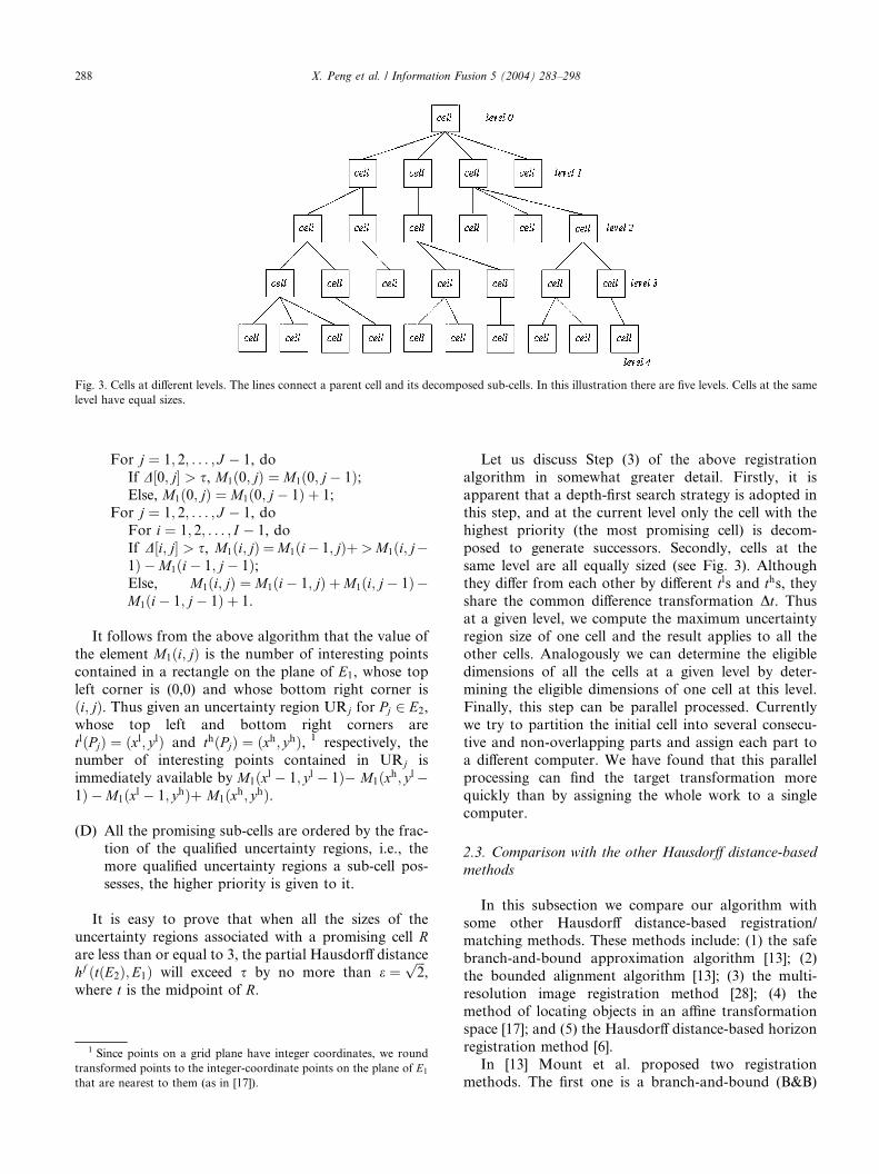
Fig. 3. Cells at different levels. The lines connect a parent cell and its decomposed sub-cells. In this illustration there are five levels. Cells at the same

level have equal sizes.


For j ¼ 1; 2; . . . ; J � 1, doIf D½0; j� > s, M1ð0; jÞ ¼ M1ð0; j� 1Þ;Else, M1ð0; jÞ ¼ M1ð0; j� 1Þ þ 1;

For j ¼ 1; 2; . . . ; J � 1, doFor i ¼ 1; 2; . . . ; I � 1, doIf D½i; j� > s, M1ði; jÞ ¼M1ði� 1; jÞþ>M1ði; j�1Þ �M1ði� 1; j� 1Þ;Else, M1ði; jÞ ¼ M1ði� 1; jÞ þM1ði; j� 1Þ�M1ði� 1; j� 1Þ þ 1.

It follows from the above algorithm that the value of

the element M1ði; jÞ is the number of interesting pointscontained in a rectangle on the plane of E1, whose topleft corner is (0,0) and whose bottom right corner is

ði; jÞ. Thus given an uncertainty region URj for Pj 2 E2,whose top left and bottom right corners are

tlðPjÞ ¼ ðxl; ylÞ and thðPjÞ ¼ ðxh; yhÞ, 1 respectively, thenumber of interesting points contained in URj is

immediately available by M1ðxl � 1; yl � 1Þ� M1ðxh; yl�1Þ �M1ðxl � 1; yhÞþ M1ðxh; yhÞ.

(D) All the promising sub-cells are ordered by the frac-

tion of the qualified uncertainty regions, i.e., themore qualified uncertainty regions a sub-cell pos-

sesses, the higher priority is given to it.

It is easy to prove that when all the sizes of the

uncertainty regions associated with a promising cell Rare less than or equal to 3, the partial Hausdorff distance

hf ðtðE2Þ;E1Þ will exceed s by no more than e ¼ffiffiffi2

p,

where t is the midpoint of R.

1 Since points on a grid plane have integer coordinates, we round

transformed points to the integer-coordinate points on the plane of E1that are nearest to them (as in [17]).

Let us discuss Step (3) of the above registration

algorithm in somewhat greater detail. Firstly, it is

apparent that a depth-first search strategy is adopted in

this step, and at the current level only the cell with the

highest priority (the most promising cell) is decom-

posed to generate successors. Secondly, cells at the

same level are all equally sized (see Fig. 3). Althoughthey differ from each other by different tls and ths, theyshare the common difference transformation Dt. Thusat a given level, we compute the maximum uncertainty

region size of one cell and the result applies to all the

other cells. Analogously we can determine the eligible

dimensions of all the cells at a given level by deter-

mining the eligible dimensions of one cell at this level.

Finally, this step can be parallel processed. Currentlywe try to partition the initial cell into several consecu-

tive and non-overlapping parts and assign each part to

a different computer. We have found that this parallel

processing can find the target transformation more

quickly than by assigning the whole work to a single

computer.

2.3. Comparison with the other Hausdorff distance-based

methods

In this subsection we compare our algorithm with

some other Hausdorff distance-based registration/matching methods. These methods include: (1) the safe

branch-and-bound approximation algorithm [13]; (2)

the bounded alignment algorithm [13]; (3) the multi-

resolution image registration method [28]; (4) the

method of locating objects in an affine transformation

space [17]; and (5) the Hausdorff distance-based horizon

registration method [6].

In [13] Mount et al. proposed two registrationmethods. The first one is a branch-and-bound (B&B)


approximation algorithm. This algorithm splits a

promising cell into two sub-cells and uses the middle

point of a cell to update the best similarity and trans-

formation. For each cell, it computes the lower distance

bound and the upper distance bound, and kills the cell ifthe lower bound is not significantly lower than the

current best similarity. One drawback of this algorithm

lies in its inability to control the directed partial Haus-

dorff distance hf ðtðBÞ;AÞ at given quantile f , where t isthe best transformation found in this algorithm. To put

this in another way, we cannot predict the value of

hf ðtðBÞ;AÞ prior to applying the algorithm and

hf ðtðBÞ;AÞ is known only after the algorithm stops. Wehad an experiment to demonstrate it. In this experiment,

the parameters are er ¼ 0:1, ea ¼ 0:3, eq ¼ 0:2 and

q ¼ 0:6 and 1.0. These parameters are adjustable non-negative quantities that act as input arguments for the

algorithm. Fig. 4 depicts the curves of the directed

partial Hausdorff distance hf ðtðBÞ;AÞ versus the quantilef . Let us take f ¼ 0:6 for example. It can be seen fromFig. 4 that at this quantile, the values of hf ðtðBÞ;AÞcorresponding to q ¼ 0:6 and q ¼ 1:0 are quite differentfrom each other. We cannot anticipate these results in

advance. In order for the transformation parameters

refinement algorithm in the next section to work well, a

sufficiently good estimation about the initial transfor-

mation is required. As a matching measure, hf ðtðBÞ;AÞin a sense reflects the quality of the estimated initial

transformation t: from its value we are aware that underthe transformation t, how close a fraction f of the

structural edges of the test image are to the structural

edges of the reference image. For this reason we would

prefer that the value of hf ðtðBÞ;AÞ be controlled under adesired value.

Compared with the B&B algorithm, our method

differs in quite a number of ways:

Fig. 4. The directed partial Hausdorff distance versus the quantile value. The

found in the B&B algorithm [13]. We test the algorithm on two parameter

changed for both sets while q takes different values.

ii(i) Search strategy. Our method adopts a depth-first

(a hill-climbing) search strategy while the B&B

algorithm is based on a best-first search strategy.

It is difficult to theoretically determine which

strategy is better, because the efficiency of bothmethods is dependent on different situations. In

our experiments presented in this paper, our

depth-first based method runs much faster than

the B&B algorithm. Another important benefit

of the depth-first strategy is that, compared with

the best-first strategy, it requires much less mem-

ory. Assuming that the quantity of memory a cell

occupies is m, then the total memory required forstoring the cells in our method is not larger than

64mL, where L is the total number of levels of thecells.

i(ii) Way of killing a cell. We use a fast uncertainty re-

gion evaluation algorithm to quickly test an uncer-

tainty region and kill a cell if it does not have

enough qualified uncertainty regions, while in the

B&B algorithm, some lower and upper boundsare computed for this work.

(iii) Way of splitting a promising cell. Our method splits

a promising cell into a variable number of sub-cells

(depending on the number of eligible dimensions

the cell has), while the B&B algorithm only splits

a promising cell into two sub-cells.

(iv) Parallel processing. Recall from Section 2.2 that we

can implement our method through parallel pro-cessing by splitting the initial cell into several parts

and assign each part to a different processor/com-

puter. Once a target transformation is found in

one processor/computer, all the tasks in the other

processors/computers are immediately terminated.

However, if the B&B algorithm is implemented un-

der the same condition, one has to wait till all the

partial Hausdorff distance is computed using the best transformation

sets. Among the parameters, er ¼ 0:1, ea ¼ 0:3, eq ¼ 0:2 are held un-


tasks in different processors/computers are finished

and then choose the best transformation t accordingto hf ðtðBÞ;AÞ. Parallel processing can also help alle-viate the possible problems arising from the draw-

backs of a hill-climbing search strategy (e.g., localmaxima, plateaux, and ridges).

(v) Controllability of hf ðtðBÞ;AÞ. Recall from Section 2.2that we can assure that hf ðtðBÞ;AÞ6 s þ e.

A second algorithm given by Mount et al. is a com-

bination of the above branch-and-bound algorithm with

computation of point alignments (short for BA algo-

rithm). By finding enough alignable uncertainty regions 2

and sampling triple pairs, the BA algorithm could be

much faster than the B&B algorithm in point matching

examples. However, we have found in our experiments

that the BA algorithm is even slower than the B&B

algorithm when applied to edge registration. The main

reason for this slowdown is that, when registering edges,

it is more difficult than in point matching cases for the

BA algorithm to find enough alignable uncertainty re-gions that contain at most one feature point of the other

set. This is due to the connectivity of edges.

The multi-resolution image registration method [28]

has some similarities with the B&B algorithm of [13].

When evaluating a cell, both algorithms compute two

bounds and split a promising cell into two sub-cells.

Instead of using distances as the bounds, this method

uses fractions. The authors of [28] also proposed theidea of multi-class Hausdorff fraction (MCHF). By

segmenting edges into multiple classes (straight lines and

curves in their paper) and replacing the conventional

single-class Hausdorff fraction with the MCHF, they

achieved higher efficiency as less cells were visited. It

must be noted that the MCHF idea can also be directly

applied to our algorithm. Besides, one should also note

that the multi-resolution registration algorithm of [28] isfor the set of similarity transformations rather than for

general affine transformations.

The object location method in [17] can be extended

for image registration. In this method, the continuous

affine transformation space is first digitized to a discrete

one. Then each cell at a lower-resolution level is subject

to an evaluation-and-decomposition process. If a cell is

promising, it is divided into 64 sub-cells (all the samesize) that are stored at a higher-resolution level. The cell

decomposition continues until the finest resolution level

is reached, when each cell contains just a discrete

transformation. Since a promising cell is decomposed

into a fixed number of sub-cells, a cell is required to be

as square as possible. In fact, the author suggested the

2 For a point b 2 B, if the number of points of A that lie within b’suncertainty region is at most one, or if this number is zero and there is

at least one point of A within distance g of the region, this uncertaintyregion is labeled as alignable.

edge lengths of a cell always be a power of 2 and equal

to each other, in each dimension. However, in many

cases the side lengths of a cell might not be ‘‘well bal-

anced’’, i.e., some side length can be much longer or

shorter than the others, which will decrease the efficiencyof this method. In contrast to this method, we do not

need the digitization operation on the continuous affine

transformation space. And more important, the number

of sub-cells generated by a parent cell is variable, mak-

ing our algorithm more flexible in dealing with the ‘‘not-

well-balanced’’ cases.

A Hausdorff distance-based method is proposed in [6]

to register horizons in visual/infrared image pairs.Strictly speaking, this method is not a general scheme to

solve for affine transformation registration problems.

The global affine transformation between two images is

calculated from three local translations that minimize the

partial Hausdorff distances between corresponding sub-

image pairs. The transformation between each sub-im-

age pair is assumed as a translation, which is obviously

not proper for relatively complex circumstances. Thusthe application scope of this method is quite limited.

3. Second step–transformation parameters refinement [20]

The transformation obtained from the first step in

Section 2 may not meet the requirement of high regis-

tration accuracy. We use an area-based method to refinethe transformation parameters to further increase the

registration accuracy, which is based on the maximiza-

tion of normalized correlation given in [20]. This method

is completely different from those traditional area-cor-

relation methods that directly use image intensities, and

can be used for multi-sensor image registration.

Given an image f , a Laplacian-energy image fle of fis formed by first filtering f with a 3 · 3 convolutionmask

1 1 1

1 �8 1

1 1 1

24

35

and then squaring the filtered image pixel-wise. A

Gaussian-pyramid [26] f kleðk ¼ 0; 1; 2; . . .Þ of fle is con-structed subsequently. f 0leð¼ fleÞ is the highest resolutionlevel (bottom level) of the Gaussian pyramid.

Given a reference image I1 and a test image I2, a pointðx� u; y � vÞ in I2 is mapped to the point ðx; yÞ in I1 byan affine motion vector ~uðx; y;~pÞ ¼ ½uðx; y;~pÞ; vðx; y;~pÞ�Texpressed as

~uðx; y;~pÞ ¼ uðx; y;~pÞvðx; y;~pÞ

� �¼ X ðx; yÞ~p

¼ p1 þ p2xþ p3yp4 þ p5xþ p6y

� �ð7Þ


where X ðx; yÞ ¼ 1 x y 0 0 0

0 0 0 1 x y

� �and ~p ¼ ½p1; p2;

p3; p4; p5; p6�T. A simple relationship exists between

ða00; a01; a10; a11; tx; tyÞ and ½p1; p2; p3; p4; p5; p6�. 3We use I1le and I2le to denote the Laplacian-energy

images of I1 and I2, respectively. The kth levels of theGaussian pyramids of I1le and I2le are represented by I

k1le

and Ik2le , respectively. Define a normalized-correlationmatching measure Skðx;yÞðu; vÞ computed over a smallwindow W with respect to the pixel ðx; yÞ in Ik1le and ðu; vÞas

Skðx;yÞðu; vÞ ¼ Ik1leðxþ u; y þ vÞ �N Ik2leðx; yÞ

¼P

ði;jÞ2W ðIk1leðxþ iþ u; y þ jþ vÞ � fW ÞðIk2leðxþ i; y þ jÞ � gW ÞffiffiffiffiffiffiffiffiffiffiffiffiffiffiffiffiffiffiffiffiffiffiffiffiffiffiffiffiffiffiffiffiffiffiffiffiffiffiffiffiffiffiffiffiffiffiffiffiffiffiffiffiffiffiffiffiffiffiffiffiffiffiffiffiffiffiffiffiffiffiffiffiffiffiffiffiffiffiffiP

ði;jÞ2W ðIk1leðxþ iþ u; y þ jþ vÞ � fW Þ2

q ffiffiffiffiffiffiffiffiffiffiffiffiffiffiffiffiffiffiffiffiffiffiffiffiffiffiffiffiffiffiffiffiffiffiffiffiffiffiffiffiffiffiffiffiffiffiffiffiffiffiffiffiffiffiffiffiffiffiffiffiffiffiffiPði;jÞ2W ðIk2leðxþ i; y þ jÞ � gW Þ

2q ð8Þ

where fW and gW denote the mean brightness values

within the corresponding windows around pixels

ðxþ u; y þ vÞ in Ik1le and ðx; yÞ in Ik2le , respectively.Our aim is to find the parameter vector ~p that max-

imizes the global similarity measure Mkð~pÞ:

Mkð~pÞ ¼Xðx;yÞ

Skðx;yÞðuðx; y;~pÞ; vðx; y;~pÞÞ

¼Xðx;yÞ

Skðx;yÞð~uðx; y;~pÞÞ ð9Þ

The solution to the above problem is obtained usingNewton’s method. Let ~p0 denote the parameter vectorcomputed in the previous iteration step, and Mkð~pÞ canbe expanded using a second order Taylor series: 4

Mkð~pÞ ¼ Mkð~p0Þ þ ð$~pMkð~p0ÞÞTd~p þ 1

2dT~pHMk ð~p0Þd~p ð10Þ

where d~p ¼~p�~p0; $~pMk denotes the gradient of Mk and

HMk is the Hessian matrix of Mk. Differentiate the right-

hand side of Eq. (10) with respect to d~p and set thedifferential equal to zero:

$~pMkð~p0Þ þ HMk ð~p0Þd~p ¼ 0 ð11Þsolving for d~p and we have

d~p ¼ �ðHMk ð~p0ÞÞ�1$~pMkð~p0Þ ð12Þ

Thus a better estimation of~p is made by~p ¼~p0 þ d~p. InEq. (12) $~pMkð~pÞ and HMk ð~pÞ are computed as

3 It follows from Eqs. (2) and (7) thatxþ uy þ v

� �¼ a00 a01

a10 a11

� �xy

� �þ

txty

� �) u

v

� �¼ a00 � 1 a01

a10 a11 � 1

� �xy

� �þ tx

ty

� �¼ tx þ ða00 � 1Þxþ a01y

ty þ a10xþ ða11 � 1Þy

� �.

Thus p1 ¼ tx, p2 ¼ a00 � 1, p3 ¼ a01, p4 ¼ ty , p5 ¼ a10, and p6 ¼ a11 � 1.4 Note that in [20]Mkð~pÞ ¼ Mkð~p0Þ þ ð$~pMkð~p0ÞÞ

Td~pþ dT~pHMk ð~p0Þd~p,missing the factor ‘‘1/2’’ before the third term.

$~pMkð~pÞ ¼Xðx;yÞ

ðX T:$~uSkðx;yÞð~uÞÞ

HMk ð~pÞ ¼Xðx;yÞ

ðX T � HSkðx;yÞ ð~uÞ � X Þð13Þ

where

$~uSkðx;yÞð~uÞ ¼oSkðx;yÞou

oSkðx;yÞov

h iT

HSkðx;yÞ ð~uÞ ¼oSkðx;yÞou2

oSkðx;yÞouov

oSkðx;yÞouov

oSkðx;yÞov2

24

35 ð14Þ

Substituting Eq. (13) into Eq. (12) provides:

d~p ¼ �Xðx;yÞ

X T � HSkðx;yÞ ð~u0Þ � X !�1

�Xðx;yÞ

X T � $~uSkðx;yÞð~u0Þ !

ð15Þ

where ~u0 ¼~uðx; y;~p0Þ.The steps of the transformation parameters refine-

ment algorithm are summarized as follows:

(1) Warp the test image I2 towards the reference imageI1 using the initial transformation obtained from thefirst step (Section 2) and generate a new image I 02.Construct two Gaussian-pyramids based on I1leand I 02le , where I1le and I

02leare the Laplacian-energy

images of I1 and I 02, respectively. Set ~p0 to zero andproceed to Step (2) at the coarsest resolution level

of the pyramids.

(2) At the kth level of the Gaussian-pyramids, for eachpixel ðx; yÞ of Ik1le , compute a correlation matchingmeasure surface Skðx;yÞð~uÞ around ~u0, where ~u ¼ðu; vÞ satisfies k~u�~u0k6 d. Use Beaudet’s masks[27] for the computation of $~uSkðx;yÞð~uÞ and HSkðx;yÞ ð~uÞ.

(3) Compute the increment d~p of~p (Eq. (15)) and update~p by ~p ¼~p0 þ d~p.

(4) After repeating Steps (2) and (3) for a few it-

erations (four times in our implementation),

propagate ~p to the ðk � 1Þth level of the Gauss-ian-pyramids and repeat the computation at that

level. This iteration and propagation process stops

when the computation at the finest resolution level

(k ¼ 0) finishes.


In our implementation, the window size for com-

puting the normalized correlation is 5 · 5. 3 · 3 Beau-det’s masks are used for computing $~uSkðx;yÞð~uÞ andHSkðx;yÞ ð~uÞ (accordingly in Step (2) d ¼

ffiffiffi2

p). An image-

warping operation is added before each iteration, i.e., Ik02leis warped towards Ik1le according to the current~p0. Afterwarping the images,~p0 is set to zero and d~p is estimatedbased on the reference and warped test images.

To further boost the robustness of the iteration step

of Eq. (15), an ‘‘outlier rejection’’ mechanism is adop-

ted: only pixels ðx; yÞ for which the surface Skðx;yÞð~uÞaround ~u0 is concave are used for solving for d~p. How-ever, how to judge whether the surface Skðx;yÞð~uÞ around~u0 is concave is not mentioned in [20]. In fact, we de-velop a simple criterion for this purpose: if the Hessian

matrix HSkðx;yÞ ð~uÞ is negative semi-definite, we judge thesurface Skðx;yÞð~uÞ as concave.When this transformation parameters refinement

algorithm is over, we have a final motion vector ~pa.Following the relationship described in footnote 3, we

have a corresponding affine transformation whose

parameters are contained in a 2 · 2 matrix Aa and atranslation vector ta. Keep in mind that this affine

transformation is obtained on the basis of the initial

affine transformation from the first step (Section 2). We

represent the initial transformation using a 2 · 2 matrixAb and a translation vector tb. Combining these twotransformations we have

x1 ¼ AaðAbx2 þ tbÞ þ ta ¼ AaAbx2 þ ðAatb þ taÞ ð16ÞHence, the final transformation can be represented by

A ¼ AaAb and t ¼ Aatb þ ta.

Fig. 5. The performance evaluation experiment. (a) The reference

image (200· 200 pixels). (b) The test image (300· 300 pixels). The testimage is generated by scaling and re-sampling the reference image and

is further corrupted by Gaussian white noises (SNR¼ 13.01).

4. Experimental results

We want first to demonstrate the performance of our

approach with an experiment in which the true align-

ment is known a priori, but in which the gray-level

correspondence between the images is uncontrolled.This will in a sense give an objective evaluation of the

quality of our algorithm. Our second example registers

two multi-sensor and multi-temporal satellite images. In

the third experiment, the approach is used to register a

visual/infrared image pair that has a distinct disparity in

image resolutions between each other. A fourth example

presents the results of applying our approach for the

registration of images from a single sensor but taken atdifferent moments.

In all the experiments, the parameters for the feature

extraction are set to r0 ¼ 3 and Dr ¼ 0:4, and the fea-ture extraction stops when r ¼ 1. The feature imagesand the Laplacian-energy images are normalized so that

the maximum edge strengths are 255. In the first step,

the parameters f , tl and th are provided by the user.

Choice of these parameters is mostly dependent on the a

priori knowledge about the characteristics of the images.

For example, if we know beforehand that a majority of

the structural edges in the test image may be matched to

those in the reference image, we can set a relatively highvalue to f ; otherwise, we can set a relatively low value tof . Generally speaking, f takes relatively smaller valuesin multi-sensor imagery registration cases than in those

cases where the images to be registered are from sensors

of similar type. tl and th should be chosen to cover thetarget transformation. These two parameters will not

influence the outcome (i.e., the target transformation is

bound to be found as long as it is contained in the initialcell determined by tl and th) but will influence theimplementation time: with a narrow span between tl andth, the time taken is small; with a wider span between tl

and th, more time can be taken to find the target

transformation. A rough estimation of the target

transformation will aid in choosing tl and th. In thesecond step, we use three-level Gaussian-pyramids for

the first three experiments and four-level Gaussian-pyramids for the fourth experiment. After a test image is

registered to a reference image, we use a wavelet trans-

form-based image fusion algorithm [23] to fuse the

overlapping parts of them. The wavelet transform filters

for the image fusion algorithm are listed in Table 2 of

Appendix A. All the experiments are implemented using

Visual C++ 6.0 on a Pentium III PC running Windows

2000.

4.1. Performance evaluation experiment

In this experiment, we use a 200 · 200 Lena image asthe reference image. The reference image is scaled to 1.5

times of its original size and re-sampled to generate the

test image (Fig. 5). Then we add Gaussian white noise to

further corrupt the test image. We measure the amount


of added noise as a signal-to-noise ratio (SNR) ex-

pressed in decibels: 10 log10r2ðf Þr2ðnÞ, where r2ðf Þ is the va-

riance of an imageand r2ðnÞ is the variance of the addednoise. In this experiment the SNR¼ 13.01. The optimaltransformation between the test and reference images is

(0.6667, 0.0, 0.0, 0.6667, 0.0, 0.0). We set s ¼ 2, f ¼ 0:8,tl ¼ ð0:5; 0:0; 0:0; 0:5;�20;�20Þ, and th ¼ ð0:8; 0:0; 0:0;0:8; 20; 20Þ for the first step of the proposed method. Thefinal transformation obtained is (0.6667, 10�4, 7.49 ·10�4, 0.6671, )0.2767, )0.1666). Transforming the testimage to the reference image by this transformation, we

obtain an accuracy of registration ranging between 0.27

and 0.35 pixels. This result also shows the noise-resis-

tance ability of our method.

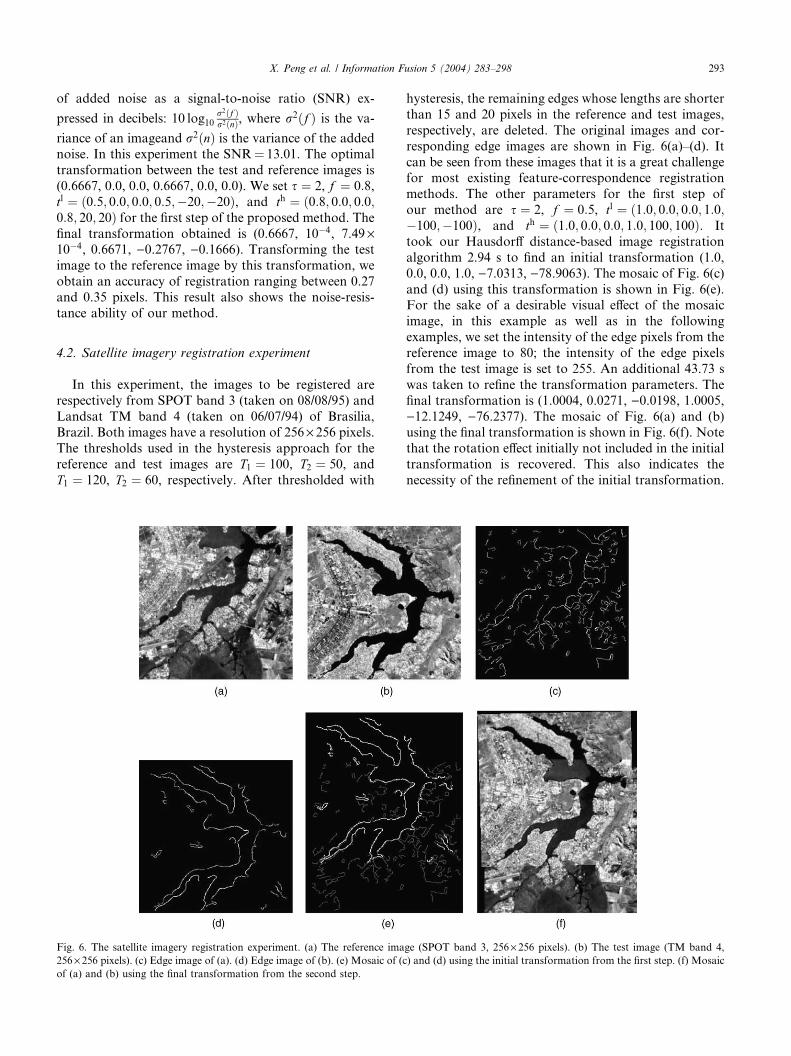
4.2. Satellite imagery registration experiment

In this experiment, the images to be registered are

respectively from SPOT band 3 (taken on 08/08/95) and

Landsat TM band 4 (taken on 06/07/94) of Brasilia,

Brazil. Both images have a resolution of 256 · 256 pixels.The thresholds used in the hysteresis approach for the

reference and test images are T1 ¼ 100, T2 ¼ 50, andT1 ¼ 120, T2 ¼ 60, respectively. After thresholded with

Fig. 6. The satellite imagery registration experiment. (a) The reference ima

256· 256 pixels). (c) Edge image of (a). (d) Edge image of (b). (e) Mosaic of (cof (a) and (b) using the final transformation from the second step.

hysteresis, the remaining edges whose lengths are shorter

than 15 and 20 pixels in the reference and test images,

respectively, are deleted. The original images and cor-

responding edge images are shown in Fig. 6(a)–(d). It

can be seen from these images that it is a great challengefor most existing feature-correspondence registration

methods. The other parameters for the first step of

our method are s ¼ 2, f ¼ 0:5, tl ¼ ð1:0; 0:0; 0:0; 1:0;�100;�100Þ, and th ¼ ð1:0; 0:0; 0:0; 1:0; 100; 100Þ. Ittook our Hausdorff distance-based image registration

algorithm 2.94 s to find an initial transformation (1.0,

0.0, 0.0, 1.0, )7.0313, )78.9063). The mosaic of Fig. 6(c)and (d) using this transformation is shown in Fig. 6(e).For the sake of a desirable visual effect of the mosaic

image, in this example as well as in the following

examples, we set the intensity of the edge pixels from the

reference image to 80; the intensity of the edge pixels

from the test image is set to 255. An additional 43.73 s

was taken to refine the transformation parameters. The

final transformation is (1.0004, 0.0271, )0.0198, 1.0005,)12.1249, )76.2377). The mosaic of Fig. 6(a) and (b)using the final transformation is shown in Fig. 6(f). Note

that the rotation effect initially not included in the initial

transformation is recovered. This also indicates the

necessity of the refinement of the initial transformation.

ge (SPOT band 3, 256· 256 pixels). (b) The test image (TM band 4,

) and (d) using the initial transformation from the first step. (f) Mosaic


4.3. Visual/infrared image pair registration experiment

In this experiment, the image pair is from the Fort

Carson data set that is publicly available from the

website: http://www.cs.colostate.edu/~vision. The origi-nal visual image is a color one and we converted it into a

256-level gray-scale image so that it can be used in our

experiment. The reference image is an infrared image,

which is in the size of 256 · 256 pixels. The visual imageis used as the test image and has a resolution of

480 · 720 pixels. The thresholds used in the hysteresisapproach for the reference and test images are T1 ¼ 40,T2 ¼ 20, and T1 ¼ 100, T2 ¼ 50, respectively. Afterthresholded with hysteresis, the edges whose lengths are

Fig. 7. The visual/infrared image pair registration experiment. (a) The refere

image, 480· 720 pixels). (c) Edge image of (a). (d) Edge image of (b). (e) MosMosaic of (a) and (b) using the final transformation from the second step.

shorter than 10 pixels in the test image are deleted. The

original images and corresponding edge images are

shown in Fig. 7(a)–(d). The distinct contrast between the

dimensions of the images makes it impossible to directly

apply area-based methods. The other parameters for thefirst step of our method are s ¼ 2, f ¼ 0:5, tl ¼ð0:5; 0:0; 0:0; 0:5;�100;�50Þ, and th ¼ ð1:0; 0:0; 0:0;1:0; 0:0; 0:0Þ. It took our Hausdorff distance-based im-age registration algorithm 3.95 s to find an initial

transformation (0.5732, 0.0, 0.0, 0.5791, )75.9766,)13.0859). The mosaic of Fig. 7(c) and (d) using thistransformation is shown in Fig. 7(e). An additional

66.98 s was taken to refine the transformation parame-ters to yield the final transformation (0.5685, 0.0068,

nce image (infrared image, 256· 256 pixels). (b) The test image (visualaic of (c) and (d) using the initial transformation from the first step. (f)

http://www.cs.colostate.edu/~vision


)0.0041, 0.5832, )74.2895, )13.5573). The mosaic ofFig. 7(a) and (b) using the final transformation is shown

in Fig. 7(f).

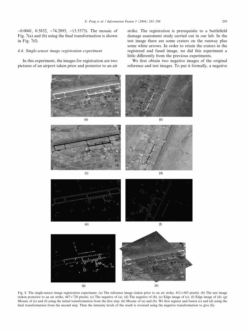
4.4. Single-sensor image registration experiment

In this experiment, the images for registration are two

pictures of an airport taken prior and posterior to an air

Fig. 8. The single-sensor image registration experiment. (a) The reference im

(taken posterior to an air strike, 447· 720 pixels). (c) The negative of (a). (dMosaic of (e) and (f) using the initial transformation from the first step. (h) M

final transformation from the second step. Then the intensity levels of the re

strike. The registration is prerequisite to a battlefield

damage assessment study carried out in our lab. In the

test image there are some craters on the runway plus

some white arrows. In order to retain the craters in the

registered and fused image, we did this experiment alittle differently from the previous experiments.

We first obtain two negative images of the original

reference and test images. To put it formally, a negative

age (taken prior to an air strike, 412 · 683 pixels). (b) The test image) The negative of (b). (e) Edge image of (c). (f) Edge image of (d). (g)

osaic of (a) and (b). We first register and fusion (c) and (d) using the

sult is reversed using the negative transformation to give (h).


image g0ðx; yÞ is acquired by applying the negative

transformation g0ðx; yÞ ¼ 255� gðx; yÞ to an original

image gðx; yÞ. The original reference and test images andtheir negative counterparts are shown in Fig. 8(a)–(d).

Our method is then applied in Fig. 8(c) and (d). Thethresholds used in the hysteresis approach for the ref-

erence and test images are T1 ¼ 80, T2 ¼ 40, andT1 ¼ 60, T2 ¼ 30, respectively. After thresholded withhysteresis, the remaining edges whose lengths are shorter

than 30 pixels in the reference and test images, respec-

tively, are deleted. The other parameters for the first step

of our method are s ¼ 3, f ¼ 0:6, tl ¼ ð�0:6; 0:8;�0:6;�0:5; 350; 420Þ, and th ¼ ð�0:5; 0:9;�0:5;�0:4;380; 450Þ. It took our Hausdorff distance-based imageregistration algorithm 7.13 s to find an initial transfor-

mation ()0.5242, 0.8445, )0.5258, )0.4133, 363.359,432.891). The mosaic of Fig. 8(e) and (f) using this

transformation is shown in Fig. 8(g). An additional

202.40 s was taken to refine the transformation param-

eters to yield the final transformation ()0.5460, 0.8880,)0.5068, )0.4253, 363.809, 430.577). The registered andfused image of Fig. 8(a) and (b) using the final trans-

formation is shown in Fig. 8(h). The outliers in the test

image – the craters and arrows – proved the correctness

of our concave surface judgment criterion for the

‘‘outlier rejection’’ mechanism.

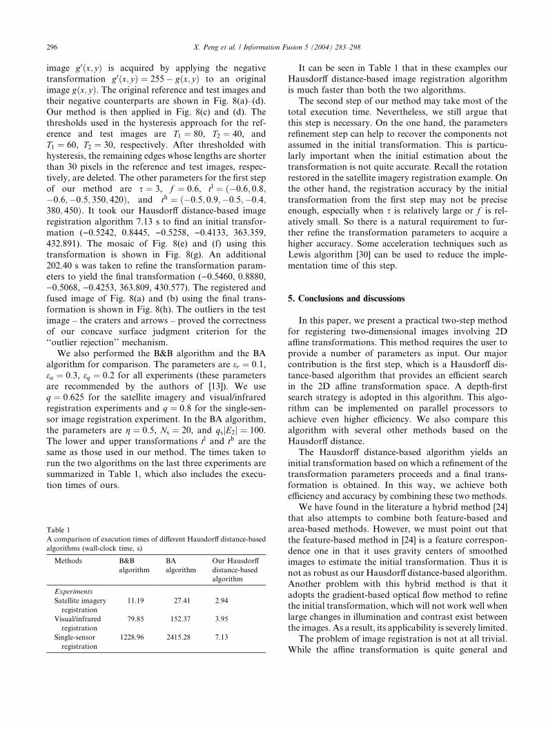
We also performed the B&B algorithm and the BA

algorithm for comparison. The parameters are er ¼ 0:1,ea ¼ 0:3, eq ¼ 0:2 for all experiments (these parametersare recommended by the authors of [13]). We use

q ¼ 0:625 for the satellite imagery and visual/infraredregistration experiments and q ¼ 0:8 for the single-sen-sor image registration experiment. In the BA algorithm,

the parameters are g ¼ 0:5, Ns ¼ 20, and qsjE2j ¼ 100.The lower and upper transformations tl and th are thesame as those used in our method. The times taken to

run the two algorithms on the last three experiments aresummarized in Table 1, which also includes the execu-

tion times of ours.

Table 1

A comparison of execution times of different Hausdorff distance-based

algorithms (wall-clock time, s)

Methods B&B

algorithm

BA

algorithm

Our Hausdorff

distance-based

algorithm

Experiments

Satellite imagery

registration

11.19 27.41 2.94

Visual/infrared

registration

79.85 152.37 3.95

Single-sensor

registration

1228.96 2415.28 7.13

It can be seen in Table 1 that in these examples our

Hausdorff distance-based image registration algorithm

is much faster than both the two algorithms.

The second step of our method may take most of the

total execution time. Nevertheless, we still argue thatthis step is necessary. On the one hand, the parameters

refinement step can help to recover the components not

assumed in the initial transformation. This is particu-

larly important when the initial estimation about the

transformation is not quite accurate. Recall the rotation

restored in the satellite imagery registration example. On

the other hand, the registration accuracy by the initial

transformation from the first step may not be preciseenough, especially when s is relatively large or f is rel-atively small. So there is a natural requirement to fur-

ther refine the transformation parameters to acquire a

higher accuracy. Some acceleration techniques such as

Lewis algorithm [30] can be used to reduce the imple-

mentation time of this step.

5. Conclusions and discussions

In this paper, we present a practical two-step method

for registering two-dimensional images involving 2D

affine transformations. This method requires the user to

provide a number of parameters as input. Our major

contribution is the first step, which is a Hausdorff dis-

tance-based algorithm that provides an efficient searchin the 2D affine transformation space. A depth-first

search strategy is adopted in this algorithm. This algo-

rithm can be implemented on parallel processors to

achieve even higher efficiency. We also compare this

algorithm with several other methods based on the

Hausdorff distance.

The Hausdorff distance-based algorithm yields an

initial transformation based on which a refinement of thetransformation parameters proceeds and a final trans-

formation is obtained. In this way, we achieve both

efficiency and accuracy by combining these two methods.

We have found in the literature a hybrid method [24]

that also attempts to combine both feature-based and

area-based methods. However, we must point out that

the feature-based method in [24] is a feature correspon-

dence one in that it uses gravity centers of smoothedimages to estimate the initial transformation. Thus it is

not as robust as our Hausdorff distance-based algorithm.

Another problem with this hybrid method is that it

adopts the gradient-based optical flow method to refine

the initial transformation, which will not work well when

large changes in illumination and contrast exist between

the images. As a result, its applicability is severely limited.

The problem of image registration is not at all trivial.While the affine transformation is quite general and


applicable to a large number of real-world applications,

it is inadequate for modeling distortions that occur due

to some sensor peculiarities. Our method cannot be di-

rectly applied to the imagery from push-broom sensors

(e.g. HYDICE––hyper-spectral digital imagery collec-tion experiment sensor) or whiskbroom sensors (e.g.

HyMap sensor), whose geometric models are much

more complex. In order for our method to be used on

such kinds of images some preprocessing on the raw

image data is required. One possibility is to use the

techniques described in [31] to ortho-rectify the raw

imagery first and then our method might apply.

Our future work will involve more complicatedtransformation models, including the non-linear ones.

Acknowledgements

This work is supported partly by China’s National

Science Foundation (grant no. 60135020 F F 030405).

The authors would like to appreciate the valuablecomments from the anonymous reviewers.

Appendix A

The wavelet transform filters for the image fusion

algorithm [23].

Table 2

h and g are the forward wavelet transform filters. hi and gi are thereverse wavelet transform filters

n h g hi gi

)12 0.002

)11 )0.002 )0.002 )0.003)10 )0.003 0.002 )0.003 )0.006)9 0.006 )0.003 0.006 0.006

)8 0.006 )0.006 0.006 0.013

)7 )0.013 0.006 )0.013 )0.012)6 )0.012 0.013 )0.012 )0.030)5 0.030 )0.012 0.030 0.023

)4 0.023 )0.030 0.023 0.078

)3 )0.078 0.023 )0.078 )0.035)2 )0.035 0.078 )0.035 )0.307)1 0.307 )0.035 0.307 0.542

0 0.542 )0.307 0.542 )0.3071 0.307 0.542 0.307 )0.0352 )0.035 )0.307 )0.035 0.078

3 )0.078 )0.035 )0.078 0.023

4 0.023 0.078 0.023 )0.0305 0.030 0.023 0.030 )0.0126 )0.012 )0.030 )0.012 0.013

7 )0.013 )0.012 )0.013 0.006

8 0.006 0.013 0.006 )0.0069 0.006 0.006 0.006 )0.00310 )0.003 )0.006 )0.003 0.002

11 )0.002 )0.003 )0.00212 0.002

References

[1] L.G. Brown, A survey of image registration techniques, ACM

Computing Surveys 24 (4) (1992) 326–376.

[2] J. Flusser, T. Suk, A moment-based approach to registration of

images with affine geometric distortion, IEEE Transactions on

Geoscience and Remote Sensing 32 (2) (1994) 382–387.

[3] X. Dai, S. Khorram, A feature-based image registration algorithm

using improved chain-code representation combined with invari-

ant moments, IEEE Transactions on Geoscience and Remote

Sensing 37 (5) (1999) 2351–2362.

[4] H. Li, B.S. Manjunath, S.K. Mitra, A contour-based approach to

multisensor image registration, IEEE Transactions on Image

Processing 4 (3) (1995) 320–334.

[5] E. Coiras, J. Santamaria, C. Miravet, Segment-based registration

techniques for visual-infrared images, Optical Engineering 39 (1)

(2000) 282–289.

[6] Y. Sheng, X. Yang, D. McReynolds, Z. Zhang, L. Gagnon, L.

S�evigny, Real-world multisensor image alignment using edge

focusing and Hausdorff distances, Proceedings of SPIE 3719

(1999) 173–185.

[7] J.W. Hsieh, H.Y.M. Liao, K.C. Fan, M.T. Ko, Y.P. Hung, Image

registration using a new edge based approach, Computer Vision

and Image Understanding 67 (2) (1997) 112–130.

[8] Q. Zheng, R. Chellappa, A computational vision approach to

image registration, IEEE Transactions on Image Processing 2 (3)

(1993) 311–326.

[9] H.H. Li, Y.T. Zhou, Automatic visual/IR image registration,

Optical Engineering 35 (2) (1996) 391–400.

[10] Z. Yang, F.S. Cohen, Image registration and object recognition

using affine invariants and convex hulls, IEEE Transactions on

Image Processing 8 (7) (1999) 934–946.

[11] Z. Yang, F.S. Cohen, Cross-weighted moments and affine

invariants for image registration and matching, IEEE Transac-

tions on Pattern Analysis and Machine Intelligence 21 (8) (1999)

804–814.

[12] S.H. Chang, F.H. Cheng, W.H. Hsu, G.Z. Wu, Fast algorithm for

point pattern matching: invariant to translation, rotations and

scale changes, Pattern Recognition 30 (2) (1997) 311–320.

[13] D.M. Mount, N.S. Netanyahu, J.L. Moigne, Efficient algorithms for

robust feature matching, Pattern Recognition 32 (1) (1999) 17–38.

[14] C. Shekhar, V. Govindu, R. Chellappa, Multisensor image

registration by feature consensus, Pattern Recognition 32 (1)

(1999) 39–52.

[15] B.S. Manjunath, C. Shekhar, R. Chellappa, A new approach to

image feature detection with applications, Pattern Recognition 29

(4) (1996) 627–640.

[16] F. Bergholm, Edge focusing, IEEE Transaction on Pattern

Analysis and Machine Intelligence 9 (6) (1987) 726–741.

[17] W.J. Rucklidge, Efficiently locating objects using the Hausdorff

distance, International Journal of Computer Vision 24 (3) (1997)

251–270.

[18] J.R. Bergen, P. Anadan, K.J. Hanna, R. Hingorani, Hierarchical

model-based motion estimation, in: Proceedings of the 2nd

European Conference on Computer Vision, Santa Margherita,

Italy, May 1992, pp. 237–252.

[19] R.K. Sharma,M. Pavel,Multisensor image registration, SIDDigest

of Society for Information Display (XXVIII) (1997) 951–954.

[20] M. Irani, P. Anadan, Robust multi-sensor image alignment, in:

Proceedings of 6th International Conference on Computer Vision,

Bombay, India, January 1998, pp. 959–966.

[21] P. Violar, W.M. Wells III, Alignment by maximization of mutual

information, in: Proceedings of 5th International Conference on

Computer Vision, Boston, MA, USA, June 1995, pp. 16–23.


[22] P. Th�evenaz, M. Unser, Optimization of mutual information for

multiresolution image registration, IEEE Transaction on Image

Processing 9 (12) (2000) 2083–2099.

[23] H. Li, B.S. Manjunath, S.K. Mitra, Multisensor image fusion

using the wavelet transform, Graphical Models and Image

Processing 57 (3) (1995) 235–245.

[24] Z. Zhang, R.S. Blum, A hybrid image registration technique for a

digital camera image fusion application, Information Fusion 2

(2001) 135–149.

[25] G. Borgefors, Hierarchical Chamfer matching: a parametric edge

matching algorithm, IEEE Transaction on Pattern Analysis and

Machine Intelligence 10 (6) (1988) 849–865.

[26] P.J. Burt, E.H. Adelson, The Laplacian pyramid as a compact image

code, IEEE Transaction on Communications 31 (4) (1983) 532–540.

[27] P.R. Beaudet, Rotationally invariant image operators, in: 4th

International Joint Conference on Pattern Recognition, Kyoto,

Japan, November 1978, pp. 579–583.

[28] H.S. Alhichri, M. Kamel, Multi-resolution image registration

using multi-class Hausdorff fraction, Pattern Recognition Letters

23 (2002) 279–286.

[29] M. Sonka, V. Hlavac, R. Boyle, Image processing, analysis,

and machine vision, second ed., Brooks/Cole, California, USA,

1999.

[30] J. Lewis, Fast template matching, Vision Interface (1995) 120–

123.

[31] C. Lee, J. Bethel, Georegistration of airborne hyperspectral image

data, IEEE Transaction on Geoscience and remote sensing 39 (7)

(2001) 1347–1351.

A practical two-step image registration method for two-dimensional images

Documents

Transcript of A practical two-step image registration method for two-dimensional images