A practical approach to the study of spatial structure in simple cases of heterogeneous vegetation

- A practical approach to the study of spatial structure of heterogeneous vegetation stands - 99

Journal of Vegetation Science 12: 99-108, 2001© IAVS; Opulus Press Uppsala. Printed in Sweden

Abstract. Spatial heterogeneity is a characteristic of mostnatural ecosystems which is difficult to handle analytically,particularly in the absence of knowledge about the exogenousfactors responsible for this heterogeneity. While classicalmethods for analysis of spatial point patterns usually requirethe hypothesis of homogeneity, we present a practical ap-proach for partitioning heterogeneous vegetation plots intohomogeneous subplots in simple cases of heterogeneity with-out drastically reducing the data. It is based on the detection ofendogenous variations of the pattern using local density andsecond-order local neighbour density functions that allowdelineation of irregularly shaped subplots that could be con-sidered as internally homogeneous. Spatial statistics, such asRipley's K-function adapted to analyse plots of irregular shape,can then be computed for each of the homogeneous subplots.Two applications to forest ecological field data demonstratethat the method, addressed to ecologists, can avoid misinter-pretations of the spatial structure of heterogeneous vegetationstands.

Keywords: Local density function; Point pattern; Ripley’s K-function; Second-order local neighbour density function.

Abbreviation: CSR = Complete spatial randomness.

Introduction

Heterogeneity is a characteristic of natural ecosys-tems that can be observed both in space and time (Kolasa& Pickett 1991). In a spatial context, heterogeneityoccurs when some quantitative or qualitative descriptorsof an ecosystem vary significantly from one location toanother. This variation can result either from exogenousfactors, i.e. external to the biological community understudy (soil, climate, etc.) or endogenous factors, i.e.inherent to the system’s internal functioning (life-historyvariation, competition, etc.). For instance, soil properties,water availability and topography influence plant growth,population density or species abundance and consequently

affect vegetation dynamics and thus spatial structure (e.g.Newbery & Proctor 1984; Peterson & Pickett 1990;Tilman 1993; Huston & DeAngelis 1994; Couteron &Kokou 1997; Sabatier et al. 1997; Moreno-Casasola &Vázquez 1999). Moreover, natural processes such asbirth, development, reproduction, competition, preda-tion and senescence can induce a spatially heterogene-ous pattern of populations (e.g. Sterner et al. 1986;Kenkel 1988; Forget 1994; Blate et al. 1998; Couteron1998; Desouhant et al. 1998). Because the spatial or-ganization of individuals in an ecosystem depends, to agreat extent, on biological processes (Begon et al. 1986),heterogeneity of the spatial structure is often consideredas the expression of a functional heterogeneity (Kolasa& Rollo 1991).

As far as sessile organisms are concerned, hetero-geneity applies to the point pattern describing theirphysical location. Spatial point patterns that vary in asystematic way from place to place are thus calledheterogeneous (Ripley 1981). However, interpretationsof spatial variations of point locations in a specific studyarea may differ depending on observation scales: ascompared with the size of the study area, fine-scalevariations can generally be considered as elements ofstructure and broad-scale variations as heterogeneity(e.g. Wiens 1989; Kolasa & Rollo 1991; Holling 1992;He et al. 1994; Goreaud 2000). For instance, the patchydistribution of a tree species often determines repeatedstructures at a forest scale, whereas a single patch gener-ates heterogeneity at a finer scale of a sampling plot.

Analysis of the spatial structure of heterogeneouspoint patterns is difficult, because the simple methodsused to analyse spatial point patterns have been devel-oped for homogeneous point patterns, i.e. for patternsresulting from stationary point processes whose proper-ties are invariant under translation (e.g. Pielou 1969;Ripley 1981; Diggle 1983; Greig-Smith 1983; Upton &Fingleton 1985; Stoyan et al. 1987; Cressie 1993). In-deed, these methods often use indices or functions thatare averaged over the whole study area and thus only

A practical approach to the study of spatial structurein simple cases of heterogeneous vegetation

Pélissier, Raphaël1,* & Goreaud, François2,3

1 IRD, Laboratoire ERMES, 5 rue du Carbone, 45072 Orléans cedex 2, France; 2ENGREF, Laboratoire deRecherche en Sciences Forestières, 14 rue Girardet, 54042 Nancy, France; 3Present address: CEMAGREF,

Laboratoire d'Ingénierie pour les Systèmes Complexes, 24 avenue des Landais, BP 50085, 63172 Aubière cedex 1,France; *Corresponding author; Fax+33238496534; E-mail [email protected]

100 Pélissier, R. & Goreaud, F.

make sense for homogeneous processes. The classicalexploratory approach with these methods is to comparea given point pattern to one generated by a Poissonprocess which corresponds to the null hypothesis ofcomplete spatial randomness (CSR; Diggle 1983) and astationary point process. For non-stationary processesthe null hypothesis of CSR should be represented byinhomogeneous Poisson or Cox processes (see, for in-stance, Diggle 1983), but the corresponding mathemati-cal tools are quite complicated (Dessard 1996; Batista &Maguire 1998). In practice, when one computes simpleindices or functions of spatial statistics, one assumes, atleast implicitly, that the underlying point process isstationary, i.e. that the pattern is homogeneous. This cansometimes lead to misinterpretation of spatial structurewhen the pattern is actually heterogeneous.

One solution is to define, within a heterogeneousstudy area, some smaller homogeneous subplots and toanalyse the spatial structure within these separately.Two cases have to be distinguished, depending on thenature of the factor generating heterogeneity (Legendre& Legendre 1998). When an exogenous factor of het-erogeneity is identified and mapped, one can partitionthe pattern into subplots corresponding respectively todifferent values of this factor. For instance, Collinet(1997; see also Forget et al. 1999 and Goreaud & Pélissier1999) defined subplots of homogeneous edaphic prop-erties from a soil map, in order to analyse the spatialstructure of tree species in a rain forest of French Guiana.The problem is more difficult to solve when no exog-enous factor responsible for heterogeneity of the pointpattern is known.

This paper proposes a practical approach, intendedfor ecologists, based on the detection of endogenousvariation of the pattern using local density and second-order local neighbour density functions that allow de-lineation of irregularly shaped and internally homoge-neous patterns. The basic theory and functions are pre-sented, followed by two applications of forest ecologi-cal data sets to demonstrate how the method can avoid,in simple cases of heterogeneity, misinterpretations ofthe spatial structure from Ripley's (1976, 1977) K-func-tion which has been previously adapted to analyse plotsof irregular shape (Goreaud & Pélissier 1999).

Theory

When no exogenous factor responsible for heteroge-neity of a point pattern is identified, some homogeneoussubplots can be defined from endogenous local proper-ties of the pattern. Let us call f (x,y) such a local propertyrelated to the point pattern of interest (e.g. density, meanheight, species composition). The map of f (x,y) can play

the same role as the map of an exogenous factor: homo-geneous subplots can be defined as those that share thesame or arbitrarily similar ranges of values of f (x,y). Inthis paper, we propose the use of local density andsecond-order local neighbour density functions as en-dogenous factors to define homogeneous subplots.

Local density

Density, which corresponds to the number of pointsper unit area, is the simplest first-order characteristic ofa point pattern. At any location, a value of this density isestimated on a small sampling region of area s by:

ˆ( , ) ( ) /n x y N s s= (1)

where N(s) corresponds to the number of points in s. Fora homogeneous Poisson process of intensity λ, we have:

E [n(x,y)] = λ (2)

In this case, N(s) follows a Poisson distribution withparameter λs.

In this paper, the values of n̂ (x,y) were estimated bycomputing N(s) at each node of a systematic grid ofelementary side a and covering the whole study area.The sampling region s is a circle of radius r, centred onthe corresponding node. Thus, at the locations (x,y) nearthe boundary of the study area, the number of points inthe sampling region is underestimated. In order to takethis edge effect into account, we used the correctionfactor proposed by Ripley (1977) for his K-function: thecontribution of point i to N(s) corresponds to the inverseof the proportion of the perimeter of the circle centred atthe node and passing through i, which is inside the studyarea (e.g. Goreaud & Pélissier 1999).

Note that, if a < 2r, the sampling regions overlap andthe corresponding values of N(s) are not independent, asituation quite usual in practice when the study region issmall and the number of sampling points is high. Non-independence between samples prohibits formal statis-tical tests of the frequency distribution of N(s) against itstheoretical distribution. Therefore, we used a less rigor-ous but pragmatic approach, which consists of a com-bined analysis of the frequency distribution and the mapof N(s) to detect first-order heterogeneity and to parti-tion the pattern into homogeneous subplots. Fig. 1 illus-trates this approach on a virtual 1 ha plot where the twoparts (south and north) correspond to independent re-alizations of Poisson processes with intensities 0.01 and0.05, respectively (Fig. 1a). The frequency distributionof N(s) has a clear bimodal shape corresponding to themixture of the two Poisson distributions (Fig. 1b).


Second-order local neighbour density

The second-order property of a point pattern is re-lated to the joint density of the occurrence of two pointsat a given distance (Ripley 1977; Diggle 1983). It char-acterises the number of points encountered in the neigh-bourhood of an arbitrary point of the pattern and allowsinterpreting the spatial structure in terms of interactionprocesses (aggregation, inhibition, etc.).

Sometimes, overall (first-order) local density is ho-mogeneous while the fine-scale structure varies fromone place to another within the study area. In this casethe second-order characteristic of the pattern is termedheterogeneous. To allow close inspection of these char-acteristics of spatial patterns, we define an individualsecond-order local neighbour density function:

ni(r) = Ni(r)/πr2, (3)

where Ni(r) corresponds to the number of neighbourswithin a distance r of a given point i of the pattern. Forpoints located near the boundary of the study area, theedge effect is corrected, as previously, using Ripley's(1977) local correcting factor. The function ni(r) is pro-portional to the individual function proposed by Getis &Franklin (1987) from Ripley's K-function and can beinterpreted in terms of spatial structure around each pointi. For a Poisson pattern of N points in an area A, theexpected value of ni(r) at any distance r is (N–1)/A.

Compared to this constant value, a given estimation ofni(r) gives an idea of the local structure (aggregated orregular) around point i. Because ni(r) is linked to aspecific point, it cannot be considered as a stochasticfunction of the process so no formal test is available.However, the frequency distribution and map of thevalues of ni(r) at a given distance r can be used, asabove, to detect second-order heterogeneity.

Spatial analysis within homogeneous subplots

We chose to analyse spatial structure within homo-geneous subplots by use of Ripley's K-function, whichhas the advantage of describing the spatial structure atdifferent ranges simultaneously (Cressie 1993) and is astandardized measure that allows comparison of spatialpatterns of various intensities. It has been used recentlyin many studies in plant ecology e.g. desert shrubs(Skarpe 1991; Haase et al. 1996), temperate (Duncan1991; Moeur 1993; Szwagrzyk & Czerwczak 1993;Goreaud et al. 1998) and tropical forests (Pélissier 1998;Barot et al. 1999; Forget et al. 1999).

Under the assumptions of homogeneity (or statio-narity) and isotropy (invariance by rotation) Ripley's K-function is defined for a process of intensity λ, so thatλK(r) is the expected number of neighbours in a circleof radius r centred on an arbitrary point of the pattern(Ripley 1977 for more details). Instead of the K-function,the modified L-function, the classical estimator for which

Fig. 1. Simulated heterogeneous point pattern in a 100 m × 100m virtual plot. a. The two parts (south and north) correspond toindependent realisations of Poisson processes with intensities 0.01 and 0.05, respectively. b. Frequency distribution of the localdensity function N(s), computed in circles of radius 12.5 m regularly distributed on a systematic grid of 5 m × 5 m. The curvecorresponds to the theoretical values expected for the mixture of the two Poisson distributions.


ˆ( ) ˆ ( ) /L r K r r= −π (4)

is generally preferred (Besag 1977). ˆ( )L r has a morestable variance than ˆ ( )K r and is easier to interpret: L(r)= 0 under CSR; L(r) < 0 indicates that there are fewerneighbours within a distance r off an arbitrary point ofthe pattern than expected under CSR, so that the patterntends to be regular; L(r) > 0 indicates that there are moreneighbours within a distance r off an arbitrary point ofthe pattern than expected under CSR, so that the patterntends to be clustered. For points closer to the boundaryof the plot than to a neighbouring point of the pat-tern, ˆ ( )K r requires an edge effect correction. In a previ-ous paper, Goreaud & Pélissier (1999) introduced pro-cedures that extend the use of Ripley's (1977) localcorrecting factor of edge effects to analysis of plots ofirregular shape.

Worked examples: two applications in forest ecology

Data sets

We tested our approach on two examples taken fromthe field of forest ecology. The first data set represents amixed Quercus petraea-Fagus sylvatica temperate for-est stand in the managed Haye Forest, France. In thisstand, tree growth and survival are highly dependent onthe spatial interactions between trees (Goreaud et al.1999). In order to understand the inter-specific relationsbetween the species, Goreaud (2000) analysed a 1 haplot in a 140 yr-old stand (Pardé 1981). He showed thatthis plot exhibited a structural heterogeneity of den-sity, mean height of trees and mixture rate of trees withDBH ≥ 10 cm, and hypothesised that this reflectedheterogeneity of a soil factor. As no soil data wereavailable, we used the local density (both species pooled)as an endogenous indicator of heterogeneity.

The second example data set is from an experimentalplot in moist evergreen forest of Uppangala, WesternGhats, India (Pascal & Pélissier 1996), designed tomonitor and study the long-term natural dynamics(Elouard et al. 1997a, b). In this forest, Pélissier (1997,1998) showed a macro-heterogeneity of the spatial struc-ture of trees with DBH ≥ 10 cm, which was related tolocal variations of the dynamic processes ensuring for-est renewal. In this paper a 0.8 ha plot with apparentlyhomogeneous first-order characteristics, but heteroge-neous second-order properties, was analysed.

Methods

In these examples we used local density and second-order local neighbour density functions as parameters todelineate contour lines of homogeneous subplots. Thetheory of regionalized variables gives a general frame-work to interpolate contour lines from values estimatedat the nodes of a systematic grid (Matheron 1965; Cressie1993). For the sake of simplicity, we used linear interpo-lations (Cleveland 1993) from values of local densityand the second-order local neighbour density functionsestimated at the nodes of a 10 m × 10 m grid using theLowess method (local weighted scatter-plot smoothing;Cleveland 1979). Local regression was computed over anumber n of nearest neighbours, chosen to minimise themean smoothing error (Cleveland & Devlin 1988). Af-ter drawing the contour lines, the homogeneous sub-plots were approximated by polygons in order to calcu-late Ripley's K-function with edge effect correction forplots of irregular shape.

In order to test the null hypothesis of spatial random-ness, we computed a 95% confidence interval ofˆ( )L r using the Monte Carlo method (Besag & Diggle

1977) with 1000 simulated random patterns. At a given

distance r, a value of ˆ( )L r outside the confidence inter-val is interpreted as a significant departure from CSRtowards clustering or regularity. When the functionstays outside the confidence interval at large distances,we can consider that the pattern is heterogeneous, be-cause most of the points are concentrated in a dense partof the study area which could be interpreted as a clusterapproaching the size of the study area. This clustercould not be considered as a repeated structure at thescale of the study region.

Computer programs used were implemented in Clanguage and can be obtained on request to the authors.Modules of spatial data analysis and graphical displayare at present available with documentation from theADE-4 homepage (http://pbil.univ-lyon1.fr/ADE-4/;Thioulouse et al. 1997). The procedures to computeLowess and to draw the contour lines were performedusing ADE-4 package.

Results for example 1: first-order heterogeneity

We computed local density in circles of radius 12.5 mcentred at the nodes of a 5 m × 5 m systematic gridcovering the 1 ha plot of the managed Haye Forest,France. This design allowed study of the spatial struc-ture up to 25 m, but implied that the sampling regionswere not independent. However, the non-Poisson andslightly bimodal shape of the frequency distribution ofN(s) (number of points per circle) indicated heterogene-


ity of the first-order characteristic of the pattern andallowed identification of two ranges of values [3;13]and [14;26] (Fig. 2).

In order to partition the plot into homogeneous sub-plots, we used the Lowess method to predict the values ofthe local density function at each node of a 10 m × 10 msystematic grid. The local regression was computed overthe 12 nearest sampling points to minimise the meansmoothing error. We then delineated the contour lines ofN(s) = 13 and N(s) = 14, by interpolation of the predictedvalues (Fig. 3). The use of a buffer zone between the twosubplots improved their respective homogeneity by avoid-ing unclear transitions between the dense and sparse partsof the plot.

We then computed the L-function for the entirerectangular plot and within the two polygonal subplots.Trees in the buffer zone were not taken into account. Inthe entire plot (Fig. 4a) the curve exhibited a divergencetowards clustering at large distances due to broad-scaleheterogeneity related to the presence of a denser part.This prevents interpretation of fine-scale structure fromthe whole data set because L(r) averages the characteris-tic structures of the two subplots. On the contrary, whencomputed within each subplot, the L-function remainedwithin the confidence interval at large distances, whichmeans that each subplot was homogeneous. Both withinsubplots analyses exhibited a significant regularity inthe range 0-8 m, but with a higher intensity in the sparseone (Fig. 4b-c).

Results for example 2: second-order heterogeneity

In the 0.8 ha plot of the moist evergreen forest ofUppangala, India, the frequency distribution of the localdensity N(s) (not shown) was unimodal, following atheoretical Poisson distribution. But, when computedover the entire plot the L-function, although lying withinthe confidence interval at large distances, showed acombination of an element of attraction at small dis-tances (1 m) with an element of repulsion in the 2-7 mrange (Fig. 5a).

Fig. 3. Location map of 231 trees in a 110 m × 90 m plot inHaye Forest, France (example 1). The dotted lines were ap-proximated from the contour lines of the local density, N(s) =13 and N(s) = 14 (inner curve).

Fig. 2. Distribution of the local density function computed in circles of radius 12.5 m centred at the nodes of a 5m × 5 m systematicgrid in a 110m × 90 m plot of the managed mixed Quercus-Fagus stand of Haye Forest, France (example 1). a. Frequencydistribution of N(s) with the theoretical curve of the homogeneous Poisson distribution expected with an intensity parametercorresponding to the first mode. b. Spatial distribution of N(s).


Fig. 5. Graphs of the L-function for the natural moist ever-green forest of Uppangala, Western Ghats, India (example 2).Function computed: a. Over the entire 100 m × 80 m rectangu-lar plot; b. Within the polygonal eastern part of the plot; c.Within the polygonal western part of the plot. Shaded enve-lopes correspond to the 95% confidence interval of the nullhypothesis of complete spatial randomness.

Fig. 4. Graphs of the L-function for the managed Haye Forest,France (example 1). Function computed: a. Over the entire110 m × 90 m rectangular plot; b. Within the polygonal densepart of the plot; c. Within the polygonal sparse part of the plot.Shaded envelopes correspond to the 95% confidence intervalof the null hypothesis of complete spatial randomness.

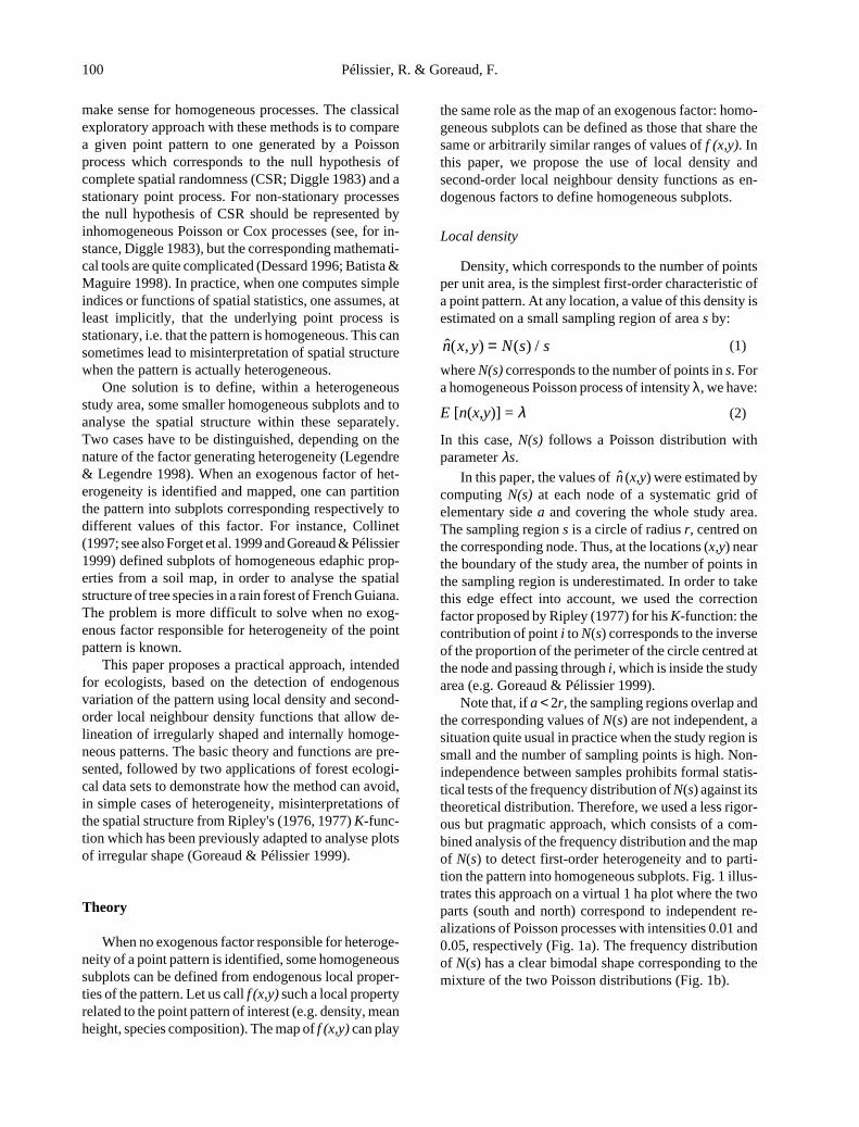
We expected that the attraction effect would onlyconcern one part of the plot so computed the second-order local neighbour density function, taking r = 1 m.The frequency distribution of this statistic showed that asmall proportion of trees had at least one neighbourwithin this distance. The spatial distribution showed,however, that these trees were more concentrated in thewestern part of the plot, thus representing second-orderheterogeneity (Fig. 6).

In order to delineate homogeneous subplots, we usedthe Lowess method with the 20 nearest neighbours topredict the values of ni(r) at each node of a 10 m × 10 mgrid. We then drew by interpolation the contour line of thevalue ni(r) = (N –1)/A = 0.07262. Twenty neighboursdid not represent the minimum smoothing error, butcorresponded to the range over which the smoothingerror stabilised and the subplots delineated remainedalmost invariant. Fig. 6b shows the two polygonal

subplots approximated from the contour line.The L-functions computed within these subplots in-

dependently, showed that the two peaks observed in theentire plot were separate. Trees in the western part (Fig.5b) exhibited a significant attraction effect at 1 m, whiletrees in the eastern part (Fig. 5c) exhibited a significantregularity in the range 2-7 m. This result emphasisesthat, even when the first-order properties of the pointpattern are homogeneous, heterogeneous second-ordercharacteristics can lead to different interpretations interms of between-tree interactions.

Discussion and Conclusions

Because natural processes are highly dependent onthe local environment (soil, topography, etc.) which isoften heterogeneous, natural communities are seldom


homogeneous. Therefore, spatial heterogeneity shouldbe systematically investigated with the aim of beingadequately taken into account in statistical analysis(Dutilleul 1993). Classical methods to analyse spatialpoint patterns usually involve the assumptions of homo-geneity and isotropy. Our examples clearly illustratehow various kinds of heterogeneity can affect the meth-ods of spatial data analysis, such as the frequently-usedRipley's function. Some methods dealing with anisotropy,such as orientation correlation functions (Stoyan & Benes1991) and spectral analysis (Mugglestone & Renshaw1996) have been applied to biological data, but very fewsimple methods to deal with heterogeneous point pat-terns are available.

The heterogeneity of a point pattern can easily bedetected when the available data exhibit a potentialexogenous factor responsible for this heterogeneity. Evenif this factor is not entirely mapped homogenous sub-plots can be delineated through interpolations and con-tour lines. The problem is analogous when the structuralheterogeneity concerns the first-order characteristics ofthe pattern, and the local density function can help inpartitioning the pattern into homogeneous subplots. Itwill, however, often be more insidious when heteroge-neity only affects the second-order properties of thepattern, in which case the superposition of various ef-fects can occur. The method proposed in this paper canhelp in dealing with all these aspects of heterogeneity,following the principle that broad-scale environmentalvariations will tend to produce aggregated patterns andthat these variations will be less pronounced at smallerscale. The major determinant of the pattern will then be

Fig. 6. Distribution of the second-order local neighbour density function computed in circles of radius 1 m centred on each point ofthe pattern in a 100 m × 80 m experimental plot of the moist evergreen forest of Uppangala, Western Ghats, India (example 2). a.Frequency distribution of Ni(r) for r = 1 m. b. Location map of 582 trees in the experimental plot with black points indicating Ni(r)≥ 1. The dotted line was approximated from the contour curve of the value of the second-order local neighbour density ni (r) =0.07262at r = 1 m.

the nature of the interactions among individuals them-selves (Diggle 1983).

The proposed approach is based on the delineation,within a heterogeneous study area, of subplots thatcould be considered as internally homogeneous, andcharacterization of the spatial pattern within these sub-plots. It is a general approach that could be used with mostmethods of spatial statistics subjected to preliminary hy-potheses of homogeneity, in particular those based ondistance measurements (see Diggle 1983; Upton &Fingleton 1985; Cressie 1993). However, using Ripley's(1976, 1977) second-order neighbourhood analysisadapted to analyse plots of irregular shape (Goreaud &Pélissier 1999) has the advantage of involving a set ofsimilar functions to detect heterogeneity, to define thehomogeneous subplots and then to characterise their in-ternal spatial structure, thus reducing conceptual invest-ment and computation time. Alternatively, this redun-dancy could lead to some bias such as the detection ofnon-significant random variations, although this risk islimited when the definition of the homogeneous sub-plots is carried out at a larger scale than that on whichthe structure of interest occurs. Such an approach is ofcourse expected to be less precise than a statistical testof a specific spatial heterogeneous process (for instance,the spatial clustering processes in statistical epidemi-ology: Wartenberg & Day 1988; Diggle & Chetwynd1991), but it is far easier to use for exploratory analysisin ecology when the underlying processes are unknown.In our examples, the method was successfully validated,as the final computation of the L-function in each homo-geneous subplot stays within the confidence interval of


Acknowledgements. The authors are grateful to the InstitutNational de la Recherche Agronomique and the Institut Françaisde Pondichéry for allowing them to work on the data sets fromthe forest stations of Haye (France) and Uppangala (India).They also thank J. Thioulouse and D. Chessel for their col-laboration on implementing our programs in ADE-4 package,and the colleagues and reviewers of the journal who helpedimprove the manuscript, in particular Moira Mugglestone andProf. Økland who, in addition, corrected the English.

References

Barot, S., Gignoux, J. & Menaut, J.-C. 1999. Demography ofa savanna palm tree: predictions from comprehensivespatial pattern analyses. Ecology 80: 1987-2005.

Batista, J.L.F. & Maguire, D.A. 1998. Modeling the spatialstructure of tropical forests. For. Ecol. Manage. 110: 293-314.

Begon, M., Harper, J.L. & Townsend, C.R. 1986. Ecology:individuals, populations and communities. Blackwell Sci-entific Publications, Oxford.

Besag, J.E. 1977. Comments on Ripley's paper. J. R. Stat. Soc.B 39:193-195.

Besag, J.E. & Diggle, P.J. 1977. Simple Monte Carlo tests forspatial pattern. Appl. Stat. 26: 327-333.

Blate, G.M., Peat, D.R. & Leighton, M. 1998. Post-dispersalpredation on isolated seeds: a comparative study of 40species in a Southeast Asian rainforest. Oikos 82: 522-538.

Cleveland, W.S. 1979. Robust locally weighted regressionand smoothing scatterplots. J. Am. Stat. Assoc. 74: 829-836.

Cleveland, W.S. 1993. Visualizing data. Hobart Press, Sum-mit, NJ.

Cleveland, W.S. & Devlin, S.J. 1988. Locally weighted re-gression: an approach to regression analysis by local fit-ting. J. Am. Stat. Assoc. 83: 596-610.

Collinet, F. 1997. Essai de regroupement des principalesespèces structurantes d'une forêt dense humide d'aprèsl'analyse de leur répartition spatiale (Forêt de Paracou –Guyane française). Thèse de doctorat, Université ClaudeBernard, Lyon.

Couteron, P. 1998. Relations spatiales entre individus et struc-ture d'ensemble dans les peuplements ligneux soudano-sahéliens au Nord-ouest du Burkina Faso. Thèse deDoctorat, Université Paul Sabatier, Toulouse.

Couteron, P. & Kokou, K. 1997. Woody vegetation spatialpatterns in semi-arid savanna of Burkina Faso, West Af-rica. Plant Ecol. 132: 221-227.

Cressie, N.A. 1993. Statistics for spatial data. Wiley, NewYork, NY.

Desouhant, E., Debouzie, D. & Menu, F. 1998. Ovipositionpattern of phytophagous insects: on the importance of hostpopulation heterogeneity. Œcologia 114: 382-388.

Dessard, H. 1996. Estimation de l'intensité locale d'un proces-sus de Cox: application à l'analyse spatiale d'un inventaireforestier. Thèse de doctorat, Université des Sciences etTechniques du Languedoc, Montpellier.

the null hypothesis of CSR at large distances.The definition of homogeneous subplots will not be

completely objective because the accuracy of the bound-ary depends on several parameters. Firstly, the localdensity, the number and the radius of the samplingregions limit the maximum size of the studied struc-tures and samples may not be independent preventingthe use of formal tests. Secondly, the contour delinea-tion may vary according to the method used, linearinterpolation from values predicted by the Lowessprocedure allows variation of both the degree of smooth-ing of the local regression and the drawing resolutionof the contour lines. Thirdly, the complexity of thepolygons used to approximate the shape of the sub-plots determines the computation time and can limitthe accuracy of the boundary definition. Finally, thedefinition of the subplots can sometimes be impreciseand a buffer zone between the different subplots can be ofsome use to avoid unclear transitions, as in example 1.

This paper deals with simple cases with a singlefactor of heterogeneity, but the method could be ex-tended to more complex systems with several hierar-chical levels of heterogeneity (Kolasa & Rollo 1991),for instance from a broad-scale exogenous macro-heterogeneity to first- and second-order fine-scale vari-ations. The same general framework with the sameadaptation of edge-corrections to irregular shapes couldalso be used with other functions of second-orderneighbourhood analysis derived from Ripley's K-func-tion and dealing with marked point patterns (Lotwick& Silverman 1982; Diggle 1983; Penttinen et al. 1992;Goulard et al. 1995). In this case, homogeneity con-cerns the distribution of both the points and the markswhich can be qualitative (e.g. tree species) or quantita-tive (e.g. tree diameter, height) characteristics of thepoints. This possible extension offers an interestingperspective for the study of heterogeneous multi-spe-cific patterns or of forested landscapes with varyingscales of patterns. The method may have some limits incertain cases where a density gradient exists leading toa flat local density frequency distribution. Therefore,the proposed method is no substitution for thoroughmeasurements of heterogeneity factors, but should helpecologists to refine field investigations.


Diggle, P.J. 1983. Statistical analysis of spatial point patterns.Academic Press, London.

Diggle, P.J. & Chetwynd, A.G. 1991. Second-order analysisof spatial clustering for inhomogeneous populations. Bio-metrics 47: 1155-1163.

Duncan, R.P. 1991. Competition and the coexistence of spe-cies in a mixed Podocarp stand. J. Ecol. 79: 1073-1084.

Dutilleul, P. 1993. Spatial heterogeneity and the design ofecological field experiments. Ecology 74: 1646-1658.

Elouard, C., Houllier, F., Pascal, J.-P., Pélissier, R. & Ramesh,B.R. 1997a. Dynamics of the dense moist evergreen for-ests: long-term monitoring of an experimental station inKodagu District (Karnataka, India). Institut français dePondichéry, Inde. Pondy papers in Ecology 1: 1-23.

Elouard, C., Pélissier, R., Houllier, F., Pascal, J.-P., Durand,M., Aravajy, S., Carpentier-Gimaret, C., Moravie, M.-A.& Ramesh, B.R. 1997b. Monitoring the structure anddynamics of a dense moist evergreen forest in the WesternGhats (Kodagu District, Karnataka, India). Trop. Ecol. 38:193-214.

Forget, P.-M. 1994. Recruitment pattern of Vouacapouaamericana (Caesalpiniaceae), a rodent-dispersed tree spe-cies in French Guiana. Biotropica 26: 406-419.

Forget, P.-M., Mercier, F. & Collinet, F. 1999. Spatial patternsof two rodent-dispersed rain forest trees Carapa procera(Meliaceae) and Vouacapoua americana (Caesalpiniaceae)at Paracou, French Guiana. J. Trop. Ecol. 15: 301-303.

Getis, A. & Franklin, J. 1987. Second-order neighborhoodanalysis of mapped point patterns. Ecology 68: 473-477.

Goreaud, F. 2000. Apports de l'analyse de la structure spatialeen forêt tempérée à l'étude et la modélisation despeuplements complexes. Thèse de doctorat, ENGREF,Nancy.

Goreaud, F. & Pélissier, R. 1999. On explicit formulas of edgeeffect correction for Ripley's K-function. J. Veg. Sci. 10:433-438.

Goreaud, F., Courbaud, B. & Collinet, F. 1999. Spatial struc-ture analysis applied to modelling of forest dynamics: afew examples. In: Amora, A. & Tomé, M. (eds.) Proceed-ings of the IUFRO workshop on empirical and processbased models for forest tree and stand growth simulation,20-26 september 1997, Oieras, Portugal, pp. 155-172.

Goulard, M., Pagès, L. & Cabanettes, A. 1995. Marked pointprocess: using correlation functions to explore a spatialdata set. Biometrika J. 7: 837-853.

Greig-Smith, P. 1983. Quantitative plant ecology. BlackwellScientific Publications, Oxford.

Haase, P., Pugnaire, F.I., Clark, S.C. & Incoll, L.D. 1996.Spatial patterns in a two-tiered semi-arid shrubland insoutheastern Spain. J. Veg. Sci. 7: 527-534.

He, F., Legendre, P., Bellehumeur, C. & LaFrankie, J.V. 1994.Diversity pattern and spatial scale: a study of a tropicalrain forest of Malaysia. Environ. Ecol. Stat. 1: 265-286.

Holling, C.S. 1992. Cross-scale morphology, geometry, anddynamics of ecosystems. Ecol. Monogr. 62: 447-502.

Huston, M.A. & DeAngelis, D.L. 1994. Competition andcoexistence: the effects of resource transport and supplyrates. Am. Nat. 144: 954-977.

Kenkel, N.C. 1988. Pattern of self-thinning in jack pine: testing

the random mortality hypothesis. Ecology 69: 1017-1024.Kolasa, J. & Pickett, S.T.A. 1991. Ecological heterogeneity.

Springer-Verlag, New York, NY.Kolasa, J. & Rollo, D.C. 1991. The heterogeneity of heteroge-

neity: a glossary. In: Kolasa, J. & Pickett, S.T.A. (eds.)Ecological heterogeneity, pp. 1-23. Springer-Verlag, NewYork, NY.

Legendre, P. & Legendre, L. 1998. Numerical ecology. Elsevier,Amsterdam.

Lotwick, H.W. & Silverman, B.W. 1982. Methods for analys-ing spatial processes of several types of points. J. R. Stat.Soc. B 44: 406-413.

Matheron, G. 1965. Les variables régionalisées et leur estima-tion: application de la théorie des fonctions aléatoires auxsciences de la nature. Masson, Paris.

Moeur, M. 1993. Characterizing spatial patterns of trees usingstem-mapped data. For. Sci. 39: 756-775.

Moreno-Casasola, P. & Vázquez, G. 1999. The relationshipbetween vegetation dynamics and water table in tropicaldune slacks. J. Veg. Sci. 10: 515-524.

Mugglestone, M.A. & Renshaw, E. 1996. A practical guide tothe spectral analysis of spatial point processes. Comp.Stat. Data Anal. 21: 43-65.

Newbery, D.M. & Proctor, J. 1984. Ecological studies in fourcontrasting lowland rain forests in Gunung Mulu NationalPark, Sarawak. IV. Association between tree distributionand soil factors. J. Ecol. 72: 475-493.

Pardé, J. 1981. De 1882 à 1976/80 : les places d'expérience desylviculture du hêtre en forêt domaniale de Haye. Rev.For. Fr. 33: 41-64.

Pascal, J.-P. & Pélissier, R. 1996. Structure and floristic com-position of a tropical evergreen forest in southwest India.J. Trop. Ecol. 12: 195-218.

Pélissier, R. 1997. Hétérogénéité spatiale et dynamique d'uneforêt dense humide dans les Ghats occidentaux de l'Inde.Institut français de Pondichéry, Inde, Publications dudépartement d'écologie 37: 1-148.

Pélissier, R. 1998. Tree spatial patterns in three contrastingplots in a southern Indian tropical moist evergreen forest.J. Trop. Ecol. 14: 1-16.

Penttinen, A., Stoyan, D. & Henttonen, H.M. 1992. Markedpoint processes in forest statistics. For. Sci. 38: 806-824.

Peterson, C.J. & Pickett, S.T.A. 1990. Microsite and elevationinfluences on early regeneration after catastrophic wind-throw. J. Veg. Sci. 1: 657-662.

Pielou, E.C. 1969. An introduction to mathematical ecology.Wiley, New York, NY.

Ripley, B.D. 1976. The second-order analysis of stationarypoint processes. J. Appl. Proba. 13: 255-266.

Ripley, B.D. 1977. Modelling spatial patterns. J. R. Stat. Soc.B 39: 172-212.

Ripley, B.D. 1981. Spatial statistics. Wiley, New York, NY.Sabatier, D., Grimaldi, M., Prévost, M.-F., Guillaume, J.,

Godron, M., Dosso, M. & Curmi, P. 1997. The influenceof soil cover organization on the floristic and structuralheterogeneity of a Guianan rain forest. Plant Ecol. 131:81-108.

Skarpe, C. 1991. Spatial patterns and dynamics of woodyvegetation in an arid savanna. J. Veg. Sci. 2: 565-572.


Sterner, R.W., Robic, C.A. & Schartz, G.E. 1986. Testing forlife historical changes in spatial patterns of four tropicaltree species. J. Ecol. 74: 621-633.

Stoyan, D. & Benes, V. 1991. Anisotropy analysis for particlesystems. J. Micro. 164: 159-168.

Stoyan, D., Kendall, W.S. & Mecke, J. 1987. Stochasticgeometry and its applications. Wiley, New York, NY.

Szwagrzyk, J. & Czerwczak, M. 1993. Spatial patterns of treesin natural forests of East-Central Europe. J. Veg. Sci. 4:469-476.

Thioulouse, J., Chessel, D., Dolédec, S. & Olivier, J.-M. 1997.ADE-4: a multivariate analysis and graphical display soft-ware. Stat. Comput. 7: 75-83.

Tilman, D. 1993. Species richness of experimental productiv-ity gradients: how important is colonization limitation ?Ecology 74: 2179-2191.

Upton, G. & Fingleton, B. 1985. Spatial data analysis byexample. Volume 1: point pattern and quantitative data.Wiley, New York, NY.

Wartenberg, D. & Day, R. 1988. Adjusting for heterogeneityand edge effects in spatial point patterns. Arch. Environ.Health 43: 204.

Wiens, J.A. 1989. Spatial scaling in ecology. Funct. Ecol. 3:385-397.

Received 10 February 2000;Revision received 28 June 2000;

Accepted 14 September 2000.Coordinating Editor: R.H. Økland.

A practical approach to the study of spatial structure in simple cases of heterogeneous vegetation

Documents

Transcript of A practical approach to the study of spatial structure in simple cases of heterogeneous vegetation