A political economy of sub-national government spending in India
57
Int. J. Public Policy, Vol. 10, Nos. 1/2/3, 2014 27 Copyright © 2014 Inderscience Enterprises Ltd. A political economy of sub-national government spending in India Parag Waknis Department of Economics, University of Massachusetts Dartmouth 285 Old Westport Road, North Dartmouth, MA 02747-2300, USA E-mail: [email protected] Abstract: Research on state government spending in India shows that difference in political cohesiveness of the ruling political entity affects its spending choices. However, the evidence is not completely conclusive and there is a lack of a theoretical model backing the analysis. Also, economists and political scientists seem to prefer different econometric methods. To address these issues, I build a theoretical model of state government spending and test the resulting predictions using different econometric approaches thereby lending robustness to results. Based on the data for 17 Indian states over 20 years, I find that politically less cohesive governments spend more on education and less on agriculture than their more cohesive counterparts. There is some evidence on electoral cycles in health expenditure and a BJP or a Congress government means reduced social expenditure. Further, the lower are the credit constraints, as measured by higher credit deposit ratio, the lower is the probability of having a coalition government. Keywords: political economy; sub-national government spending; credit constraints and voting; differentiated election platforms; coalition governments in India; India. Reference to this paper should be made as follows: Waknis, P. (2014) ‘A political economy of sub-national government spending in India’, Int. J. Public Policy, Vol. 10, Nos. 1/2/3, pp.27–83. Biographical notes: Parag Waknis received his Bachelor of Commerce and Master of Arts (Economics) degrees from the University of Pune in 1994 and 1996 respectively, Master of Philosophy (Economics) degree from Jawaharlal Nehru University, New Delhi, India in 2000, and his PhD in Macroeconomics from the University of Connecticut, USA in 2011. His research interests include monetary theory and policy, money search models, and macroeconomics of developing countries with a focus on India. Currently, he is an Assistant Professor at the Department of Economics, University of Massachusetts Dartmouth.
Transcript of A political economy of sub-national government spending in India
Int. J. Public Policy, Vol. 10, Nos. 1/2/3, 2014 27
Copyright © 2014 Inderscience Enterprises Ltd.
A political economy of sub-national government spending in India
Parag Waknis Department of Economics, University of Massachusetts Dartmouth 285 Old Westport Road, North Dartmouth, MA 02747-2300, USA E-mail: [email protected]
Abstract: Research on state government spending in India shows that difference in political cohesiveness of the ruling political entity affects its spending choices. However, the evidence is not completely conclusive and there is a lack of a theoretical model backing the analysis. Also, economists and political scientists seem to prefer different econometric methods. To address these issues, I build a theoretical model of state government spending and test the resulting predictions using different econometric approaches thereby lending robustness to results. Based on the data for 17 Indian states over 20 years, I find that politically less cohesive governments spend more on education and less on agriculture than their more cohesive counterparts. There is some evidence on electoral cycles in health expenditure and a BJP or a Congress government means reduced social expenditure. Further, the lower are the credit constraints, as measured by higher credit deposit ratio, the lower is the probability of having a coalition government.
Keywords: political economy; sub-national government spending; credit constraints and voting; differentiated election platforms; coalition governments in India; India.
Reference to this paper should be made as follows: Waknis, P. (2014) ‘A political economy of sub-national government spending in India’, Int. J. Public Policy, Vol. 10, Nos. 1/2/3, pp.27–83.
Biographical notes: Parag Waknis received his Bachelor of Commerce and Master of Arts (Economics) degrees from the University of Pune in 1994 and 1996 respectively, Master of Philosophy (Economics) degree from Jawaharlal Nehru University, New Delhi, India in 2000, and his PhD in Macroeconomics from the University of Connecticut, USA in 2011. His research interests include monetary theory and policy, money search models, and macroeconomics of developing countries with a focus on India. Currently, he is an Assistant Professor at the Department of Economics, University of Massachusetts Dartmouth.
28 P. Waknis
1 Introduction
Many states in India have time and again elected a multiparty or a coalition government. According to Lalvani (2005), India went through 43 episodes of coalition governments during the period 1966–67 to 1998–99. Given that much of the policy making in a democratic country happens in the political realm, the degree of political cohesion of a government can be argued to be influential in deciding the level and composition of spending. The empirical analysis so far does confirm this, though the results are not completely robust. These studies use different econometric methods and employ different ways of measuring political cohesion but sometimes reach contradictory answers. In addition, most of these studies use datasets that are long panels and the debate over an appropriate econometric or statistical method to analyse them is not yet settled. There is also a lack of a theoretical model backing such empirical analysis. In this paper, I attempt to fill these gaps in the literature by developing a model of government spending conditional on political cohesion and then testing the resulting predictions with data on 17 Indian states spanning 20 years using a variety of econometric methods to ensure robustness of results. In addition to these contributions, because state government spending contributes significantly to the fiscal burden of the Indian central government, this paper also sheds some light on the political underpinnings of the conduct of fiscal as well as monetary policy. In this sense, the analysis in this paper concerns itself with the fiscal aspects of the Leviathan monetary policy dealt with in Waknis (2011).
The empirical analysis so far has shown that coalition governments do spend differently from single party governments. Specifically, two out of three studies cited below show that coalition governments spend more on education than the single party governments. Various reasons have been conjectured for this behaviour including a heterogenous constituency or higher visibility of certain category of voters over others, etc. A more interesting reason from the macroeconomic perspective has been suggested by Saez and Sinha (2009). They posit a Polanyi mechanism at work causing this differentiated spending patterns. Karl Polanyi1, while writing about the transition from traditional economies to more market-based ones, suggested that market pressures may lead to more demands for protection and insurance. This certainly makes sense in the case of developing countries like India where substantial economic and social inequities continue to coexist with impressive economic growth.
This is not just a conjecture but something that seems to be borne out by data. For example, Ghate et al. (2011), who document the properties of Indian business cycles, show that private consumption in India continues to be more volatile than GDP in the post reform period. This clearly indicates presence of credit constraints. How do people respond to such circumstances? How do they smooth consumption when they lack access to insurance-social or otherwise-in the presence of increased fluctuations in economic activity? One answer to this question, is the use of voting power to secure government spending on the required public goods. In India, we see this happening through political responses like cash-based relief programmes, improved water supply and sanitation facilities, mid day meal schemes for kids, etc. There are few studies that seem to support this conjecture about interaction between politicians and voters. For example, Tandon (2007) uses the tariff reforms of 1990 to show that politicians respond to the differential impact of the reforms and that such policies significantly affect the voting response.
A political economy of sub-national government spending in India 29
Thachil (2011) argues that provision of social services by grassroots affiliates has benefitted BJP with from the poor. He studies the rise of BJP and its relation to the work of its sister organisations in Chattisgarh, India. Rath (2012) ascribes increased political fragmentation to neglected provision of basic services under planning in the post second plan period. Cole et al. (2012) show that politicians or governments respond to weather shocks and this in turn affects the voters’ response to the incumbent governments. I capture such responsiveness of government spending to the consumption smoothing needs of credit constrained voters in a parsimonious theory of state spending conditional on the type of government.
The model includes an endowment economy where some of the agents are credit constrained. Presence of aggregate shocks to endowments and credit constraints means that more and more people would need to rely on some insurance mechanism or support to smooth consumption. Government expenditure on local public goods like education, health and irrigation could be an example of such expenditure. In the model, political parties contesting elections float differentiated election platforms prior to the realisation of shocks. The national party contests the election based on an ideological platform, while the coalition of national and regional parties does so on an economic policy-based platform. In an ideologically determined spending agenda, the focus is on expenditure which may not address specific needs of the voters. However, an economic policy-based platform explicitly focuses on local public goods requirements of voters. The preferences of voters are such that differentiated platforms survive in equilibrium and voters are not indifferent between them unlike in a Downsian model. Agents vote after the realisation of shocks to smooth consumption. A negative shock ensures that majority of voters become credit constrained and vote for a coalition government. A positive shock would imply the opposite. I assume that once elected, the respective party implements its advertised spending policies. Thus, there is no commitment problem regarding policy implementation.
I look at this model as a preliminary attempt to theoretically motivate an empirical analysis of state expenditure in India. A richer model capturing complete dynamics of elections in a general equilibrium setting is certainly possible and even desirable in some contexts but beyond the scope of this paper. Given the caveat, it is worth noting that the theory delivers clear predictions not only about the relationship between degree of political cohesiveness and government spending but also about the emergence of a certain type of government in the first place. I test the predictions of the model against the expenditure data of 17 Indian states for the period of 20 years. Accordingly, along with additional interesting results on other expenditure categories, I find substantial evidence that a higher degree of political fragmentation is associated with a higher spending on education.
Thus, this paper not only offers a theory of government spending conditional on degree of political cohesiveness but also provides a clearer and comprehensive econometric analysis of state spending in India. The rest of the paper is organised as follows. Section 2 lays out the model. Section 3 presents the econometric analysis of expenditure patterns of the state governments based on the predictions of the model. Section 4 looks at the question of what determines the likelihood of having a coalition government. Section 5 concludes.
30 P. Waknis
2 Model
Consider an endowment economy populated with a continuum of agents. At the start of every period agents receive an endowment .i
tω There is borrowing and lending in the economy. A part of the endowment has to be used as a collateral for borrowing in the credit market. There is inequality in the initial endowment distribution and hence some of the agents might be credit constrained. The economy is subject to aggregate shocks on endowments. Let ω be the level of endowment, which divides the agents into being credit constrained and not credit constrained. A negative shock shifts the initial distribution of endowments more to the left of ω increasing the number of credit constrained agents in the population and positive shock has the opposite effect. However, at any given point the distribution of either agents is never degenerate. These changes in initial endowments affect the distribution of voter preferences to be discussed below. The state of endowments is always verifiable.
2.1 Agents
All agents are risk averse and altruistic. After receiving the endowment 1( )ie at the beginning of the period, agents face aggregate shocks that affect them differentially depending on severity of their credit constraints. Let the probability where an agent’s endowment could be destroyed be ψ and the extent of destruction be (0 ≤ d ≤ 1). This makes (1 – ψ) as the probability the endowment could stay at the pre shock level. Non-credit constrained agents enter the credit market and trade to smooth consumption. Credit constrained voters depend on availability of local public goods for consumption smoothing. Production of the public goods is financed by a distortionary tax on the non-credit constrained agents. Examples of typical local public goods would be improved schools, introduction of meal schemes in the schools, improved health access, etc. These are visible and easily targetable expenditures and hence could be used for smoothing consumption by credit constrained agents.
Agents seek to optimise the expected value of life time consumption, where the expectation is conditioned on the distribution of shocks. Agents cannot enter into any contract before the realisation of shocks and hence there is no private insurance market. The distribution of shocks has the same properties as the preference shocks described in the subsection that follows.
Agents solve the following problem as an economic entity:
( ) ( )0
, maxt
i i it t
t
W e E u c=∞
=
Ψ = ∑% β (1)
where
( ) –11 (1– ) (1– )i i it t tt t tc ψ d e τ ψ e τ RB= + + + (2)
( )–1 –i i it ttRB e c≤ (3)
where Bt is the number of bonds in period t and R is the price of bonds in the credit market. τ is a distortionary tax on non-credit constrained agents and transfer for the credit constrained agents. The expectation is over the distribution of shocks.
A political economy of sub-national government spending in India 31
Agents who enter the credit market buy and sell bonds at the price R. Agents behave competitively in this market and hence take R as given. Because borrowing needs collateral, the maximum an agent can borrow is given by the available endowment minus consumption , i.e., –1 ( – ).i i
t t tRB e c≤ Thus, credit constrained consumers will have positive net transfers and no bonds, while non credit constrained voters will have bonds and taxes/negative net transfers in their budget constraint. We could understand the agents in this economy as those in Kiyotaki and Moore (1997) – farmers and gatherers. Post shock some farmers need to go to the credit market but few are left with any land to use as collateral in the credit market. The remaining become almost or completely landless losing access to the credit market.
Agents as voters care about ideology as well as economic policy. Having certain ideology would mean having specific preferences about social and economic justice and caring about the economic policy would imply caring about what kind of public goods are provided by using taxes. Accordingly, credit constrained voters would care about economic policy more than ideology and vice versa.
2.2 Political aspects
There are two entities contesting an election, S and M, to form a government at the state level. S refers to a single party with a national presence and M to a coalition of regional and/or national parties. The single party has an ideologically motivated election platform and the coalition has one promising provision of local public goods. Let fj ∈ F be the fixed characteristic of entity j and aj ∈ A be the policy variable that the entities are free to choose. I will assume that fS is being expert in national issues and politics and fM as having expertise in assessing local public goods requirements. The policies that these parties choose will be aS and aM. I will assume that the objective of both the political entities is to maximise the probability of winning.
Usually in Downsian style models with or without probabilistic voting, we get a result of policy convergence. In equilibrium, the competing candidates or parties choose the same policies and voters become indifferent between candidates [see Persson and Tabellini (2002) for details]. However, in this model we would expect differentiated platforms in equilibrium and voters to be not indifferent between candidates. This approximates the reality where candidates rarely choose similar platforms and voters certainly seem to favour one candidate over others (Krasa and Polborn, 2010).
There have been two ways in which such divergence has been achieved in theory. One way is to assume limited information on candidates in a Downsian setup and the other provided by Krasa and Polborn (2009, 2010). In the former paper, the authors specify conditions under which one could have a divergence and in the later they develop a model with multidimensional policy and a binary policy model which is capable of having convergence as well as divergence under clearly defined conditions. In what follows, we adapt the model and an example economy from Krasa and Polborn (2009) to illustrate the choice of spending conditional on type of government.
Uncertainty about voter preferences is described by a probability space (Ω, D, μ): A state ω ∈ Ω determines voters preferences over F × A, and μ is the probability distribution of these preference shocks, while D is the set of measurable events. The preference shocks basically act as a counterpart to the distribution of endowments shocks.
32 P. Waknis
Given these shocks, voters can be differentiated on the basis of their preferences as follows:
( ) ( ) ( ) ( )( ) ( ) ( ) ( )
Type S , , , ,Type M , , , ,
S S M M S M M S
M M S S M S S M
f a f a f a f af a f a f a f a
The above preference ranking means that a particular type of voter prefers the candidate of the particular characteristic and would like him or her to implement a policy consistent with his or her type. This is an example of what Krasa and Polborn (2009) call non-uniform candidate ranking preferences.
Definition 1: Preferences on F × A are said to satisfy uniform candidate ranking if for all fo, f1 ∈ F and all a, a′ ∈ A, (f0, a) (f1, a) if and only if (f0, a′) (f1, a′).
Models in Downsian tradition with candidates without fixed characteristics satisfy UCR and that leads to similar policies being implemented in equilibrium. However, voter preferences here are non-UCR. Type S voters would primarily be not credit constrained and type M voters be credit constrained. Though, there might be a certain number of voters who definitely belong to either of the groups, post shock realisation there are some voters who migrate to opposite groups depending on if they become credit constrained or not (swing voters).
The timing of the political game is as follows:
Stage 1 The two political entities S and M announce their policy platforms aj ∈ A. A mixed strategy by political entity J = (S, M) consists of probability distribution σj over A.
Stage 2 State ω ∈ Ω is realised and each citizen votes for his preferred political entity, or abstains if indifferent.
2.3 Policy platform equilibrium
The above description of the game and voter preferences imply that policy platforms will not converge in equilibrium. The following proposition states this formally.
Proposition 1 (policy platform equilibrium): (aS, aM) is the Nash equilibrium of the political game.
Proof of Proposition 1: Let PS(ω, aS, aM) be the winning probability for the political entity S and PM(ω, aS, aM) for the political entity R. Note that PS(ω, aS, aM) = 1 – PM(ω, aS, aM). Given the non-UCR voter preferences, PS(ω, aS, aM) ≥ PS(ω, ,Sa′ aM) for S Sa a′ ≠ and same holds true for PM(ω, aS, aM). This is because voters rank the entity implementing policy in accordance with its expertise higher than an entity implementing a policy not in accordance with its expertise (See the preference description above). Thus, the non-UCR preferences imply that there is no profitable unilateral deviation for either political entities ensuring (aS, aM) is the Nash equilibrium of the political game. QED.
A political economy of sub-national government spending in India 33
2.4 Voting equilibrium and voting rules
Definition 2: A voting equilibrium for this economy is a list of allocations of endowments, debt and consumption of credit constrained and non-credit constrained agents such that
1 Proposition 1 holds
2 agents maximise the utility given the distribution of shocks and the budget constraint
3 given the credit limit based on the initial value of the endowment, the price of bonds clears the credit markets.
We use the above definition of voting equilibrium to derive the equilibrium voting rules. Let the optimal life time consumption implied when the distribution of shocks is degenerate be iC% and ( )W e be the associated indirect utility function. We can think of this level of consumption as something like permanent consumption for an agent or consumption associated with some linear combination of .e Given this, the voters will populate either groups (credit constrained or not credit constrained) depending on the following decision rules derived from the comparison of optimisation problem and the definition of the voting equilibrium.
Proposition 2 (utility maximisation and voting rules): Given the description so far, the voters’ maximisation problem implies the following decision rules for voting:
( ) ( )( ) ( )
if ,if ,
i ib
i i
M W e W eV
S W e W e⎧ Ψ <⎪= ⎨
Ψ ≥⎪⎩
%
% (4)
( ) ( )( ) ( )
if ,if ,
i inb
i i
S W e W eV
S W e W e⎧ Ψ <⎪= ⎨
Ψ ≥⎪⎩
%
% (5)
where Vb and Vnb are voters types who are credit constrained and not credit constrained respectively.
Proof of Proposition 2: If there were no shocks, then given the endowments the agents would solve the utility maximisation problem for the optimal choice of consumption every period. Such choice would depend on the endowment and hence would change from individual to individual. A shortfall from such an optimal choice ( )iC would not matter for the voters who are not credit constrained and hence they will vote based on ideology rather than economic policy. However, credit constrained voters will have to vote depending on how their consumption in presence of shocks compares to their .iC A short fall means that they become dependent on government expenditure to smooth consumption and therefore will vote based on economic policy than ideology. QED.
Given the definitions and proposition about policy platform equilibrium and voting equilibrium above it is clear that a coalition government in this model emerges if majority of voters become borrowing constrained as a result of a negative income shock. Accordingly, the following will hold about the nature of government in equilibrium:
34 P. Waknis
Proposition 3 (stochastic political equilibrium):
1 With probability ψ, there would be a coalition government of one national party and one or more regional parties. The spending policy implemented will include higher expenditure on the local public goods targeted at the member regional party’s constituency.
2 With probability (1 – ψ) there will be a single party government and the spending policy implemented would be according to the ideologically motivated election platform of the national party in office.
Proof of Proposition 3: It follows from Proposition 1 that the type of government is conditional on the type of shocks realised. If the shocks are positive, we have a majority vote for a single party government and if the shocks are negative, the majority vote goes to coalition of regional parties. This emphasises the role of credit constrained voters as swing voters and that the probability of having a single party or coalition government depends on the probability of type of shock. Note that a positive probability for shocks implies that the presence of swing voters (credit constrained or not depending on shocks) and ensures that each type of voter group could end up as pivotal. Because we assume that the policies are implemented and in equilibrium the parties contesting elections choose differentiated policies, the nature of actual spending depends on who is in power. QED.
Once the type of government is determined based on the probability of shocks and existence of credit constrained voters, the spending policies are implemented by whichever political entity is voted into power. If a coalition government is voted to power then we can expect the spending on local public goods like education and healthcare access to go up. If a single party government comes to power then spending policies will reflect the ideological preferences than being responsive to local public goods needs. In the empirical analysis that follows we test these implications of Propositions 1, 2 and 3. We test for differences in spending patterns conditional on the type of government as well as what affects the probability of having a particular type of government in the first place.
3 Econometric analysis of the spending patterns
In this section, we test the implications of Proposition 3, using data on 17 Indian states for the period of 1980–2000. This paper is definitely not the first attempt to do so. There have been other studies on this issue, as mentioned above. However, they are not without problems. Chaudhuri and Dasgupta (2006) and Lalvani (2005) use different measures of political fragmentation and come to contradictory results in terms of education spending as well as current and capital account spending. Saez and Sinha (2009) seems to be a more definitive analysis compared to these two studies. They improve on the earlier studies by including various measures of political fragmentation and confirm that coalition governments spend more on education.
Though this makes the tally in favour of positive effect of political fragmentation on education spending 2 versus 1, there are several counts on which even their analysis seems incomplete. First, they use only one econometric methodology to do so and hence do not provide the required robustness for the results. This constitutes a valid criticism
A political economy of sub-national government spending in India 35
because of the nature of the dataset being analysed. Secondly, even though being econometrically more sophisticated than the other two papers, it does not control for GDP at all. It only has state fixed effects. As much as controlling for unobserved heterogeneity is important, controlling for obvious differences is essential for a complete understanding of the underlying economic processes. The econometric analysis in this paper proposes to address these issues by using per capita state GDP as an additional control along with multiple regression specifications. Accordingly, I analyse expenditure on education, health, irrigation, agriculture and social services.
3.1 Data
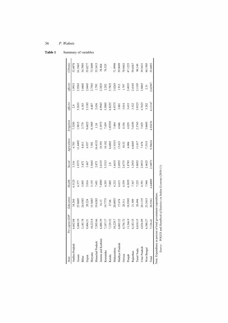
I primarily use a dataset (POLEX) created and maintained by Saez (2008). It includes data on state expenditure under various heads and data on various political variables on 17 Indian states. The coverage in POLEX is limited to the states for whom data is consistently available for the period 1980–2000. It does not contain the state GDP data, though. The data on per capita state GDP at constant prices for the states was calculated from the series available in the Handbook of Statistics on Indian Economy (2010-11) maintained by the Reserve Bank of India on line and then incorporated in the POLEX dataset to create the one used for analysis in this paper. The summary statistics for the resulting dataset are given in Table 1.
3.2 Econometric Issues
Because of the nature of the data and smaller N and T (17 and 20 respectively) the question of appropriate econometric method becomes pertinent. The usual panel data methods favoured by the economists have been developed to address the cases where N > T. Beck (2006) argues that in cases of N < T, it may not be appropriate to use the panel data methods, while describing a body of statistical methods [time series-cross section (TSCS) methods] used by political scientists to study the political determinants of economic outcomes and policies in case of such datasets. Saez and Sinha (2009) above follow these methods. A standard modelling practice under this methodology is to use a fixed effect model with panel corrected standard errors and a lagged dependent variable to account for dynamics.
Studies based on such datasets are not limited to political science, however. Daron Acemoglu and his co-authors have used such datasets in a series of papers. For example, Acemoglu et al. (2008) looks at the geographic and political determinants of economic outcomes and Acemoglu et al. (2002) at relationship between income and democracy. Much of this analysis is in the mean regression framework and the data is in the TSCS form. Alexander et al. (2011) use a similar dataset as in Acemoglu et al. (2008) to demonstrate that a quantile regression can in fact do a better job to explain the interaction of the whole distribution of economic variables and political outcomes. Though they do not contradict the findings of the latter, Alexander et al. (2011) demonstrate that the nature of relationship between income and democracy shows significant sensitivity to income levels and disproportionately so to country-specific effects. Their basic argument for using quantile regression is, thus, that it allows heterogenous marginal effects across the conditional distribution and that it affords random coefficient interpretation allowing for slope heterogeneity arising out of non-Gaussian distributions2.
36 P. Waknis
Table 1 Summary of variables
Stat
e Pe
r cap
ita G
DP
Educ
atio
n H
ealth
So
cial
Ag
ricu
lture
Ir
riga
tion
effe
ctvt
ef
fect
st
CD
ratio
And
hra
Prad
esh
6,66
2.84
18
.264
6.
3125
3.
316
6.78
3 7.
3285
2.
8 1.
9915
32
.497
8 A
ssam
5,
460.
19
25.8
605
6.37
7 1.
9375
11
.449
5 1.
9815
5.
2655
2.
9565
61
.546
5 B
ihar
3,
145.
78
24.4
385
5.89
5 3.
472
8.01
1 3.
779
6.18
3 3.
4445
34
.709
5 G
ujra
t 9,
404.
51
20.2
24
5.81
6 1.
667
6.93
7 9.
6025
3.
1185
2.
0445
55
.027
7 H
arya
na
10,2
23.8
15
.568
5 5.
155
3.56
65
7.58
1 8.
1905
4.
487
2.75
65
73.3
609
Him
acha
l Pra
desh
7,
505.
66
19.6
385
7.69
1 2.
073
16.4
135
1.24
2.
636
1.79
5 35
.341
5 Ja
mm
u an
d K
ashm
ir 6,
480.
39
16.1
3 7.
4985
2.
6135
10
.591
2.
3975
4.
9945
2.
2825
38
.464
K
arna
taka
7,
107.
17
19.7
775
6.29
3 3.
3315
10
.182
7.
439
3.50
05
2.28
2 76
.525
K
eral
a 7,
129.
52
27.0
6 7.
005
2.8
8.68
85
1.05
595
6.82
55
5.78
35
. M
ahar
asht
ra
10,2
29.7
20
.005
5 6.
232
1.66
35
11.9
315
7.40
4 4.
9375
3.
4265
71
.999
8 M
adhy
a Pr
ades
h 6,
065.
22
17.6
74
6.61
5 2.
6955
13
.621
4.
046
3.00
1 1.
913
59.9
699
Orr
issa
4,
756.
72
20.3
11
6.55
9 2.
6775
10
.52
4.35
6 3.
014
1.79
7 70
.944
3 Pu
njab
11
,566
.9
18.9
305
6.30
55
1.87
85
6.00
6 4.
829
3.63
3 2.
4935
47
.122
5 R
ajas
than
6,
183.
35
21.5
89
7.36
7 1.
2935
6.
8685
7.
6395
3.
522
2.41
85
59.6
567
Tam
il N
adu
8,01
0.15
20
.494
7.
225
3.80
55
11.0
17
2.37
65
3.93
25
2.11
95
90.1
49
Utta
r Pra
desh
4,
836.
89
20.1
135
6.59
1 2.
0915
7.
674
7.02
9 4.
7625
2.
8865
39
.563
1 W
est B
enga
l 6,
380.
27
23.3
415
7.94
4 2.
4625
7.
3315
3.
0605
3.
282
2.31
44
.150
5 To
tal
7,12
6.41
20
.554
1 6.
6400
9 2.
5497
1 9.
5062
4 4.
9267
6 4.
1114
7 2.
6294
7 55
.689
3
Not
e: E
xpen
ditu
re a
s per
cent
of t
otal
gov
ernm
ent e
xpen
ditu
re.
Sour
ce:
POLE
X a
nd H
andb
ook
of S
tatis
tics o
n In
dian
Eco
nom
y (2
010-
11)
A political economy of sub-national government spending in India 37
The debate is far from settled and hence in this paper, I follow the TSCS consensus methodology, usual panel data methods often preferred by economists as well as the quantile regression approach to analyse the effect of political cohesiveness on state government spending in India. In a separate subsection I also analyse the issue of what determines the probability that a state government has a given type of government. All this analysis is guided by the theoretical predictions of the model in the earlier section above. Use of multiple methods and specifications to test the hypothesis about effect of type of government on expenditure on local public goods serves as built in robustness check for the results.
3.3 Political parties
Given that much of the analysis that follows concentrates on political variables, this section describes the players in Indian state level politics briefly. The national parties of India include the Indian National Congress (INC), Bharatiya Janata Party (BJP), Bahujan Samaj Party (BSP), Bharatiya Janata Dal (BJD), Communist Party of IndiaMarxist (CPIM), and Communist Party of India Marxist-Leninist (CPIML). In addition to these national parties there are parties that are dominant in the state (regional parties). For example, Shivsena in Maharashtra, Telgu Desam Party in Andhra Pradesh, Trinamul Congress in West Bengal, etc. At times, a state is ruled only by a state party or an alliance centred around either the INC or BJP. Such an alliance would imply a coalition government in the concerned state. The variable left in the following analysis would either refer to CPIM or CPIML or some alliance centered around these parties.
The Indian National Congress played a very important role during India’s independence and continues to be one of the dominant parties in the period after. Much of the socialist policies implemented after independence could be attributed to the Congress. India not only saw a rising dominance of government in the economy through industrial licensing and a significant public sector under its rule but also went through a brief period of emergency under Prime Minster Indira Gandhi during 1970s. Through successive Prime Minsters starting from Rajiv Gandhi in 1980, Congress heralded several market-based reforms in late 1980s and early 1990s. The balance of payment crisis of 1991 only made such reforms necessary rather than a political choice. The current Prime Minister Dr. Manmohan Singh was the Finance Minster during the crisis and oversaw the initial reforms.
The BJP had been around in some form or other since independence but rose to prominence only around 1990s. The main reason for its rise was the Ramjanmabhoomi movement targeted at the majority Hindu population. Its right wing Hindu revivalist ideology has enabled it to come to the power a couple of times in the centre and many more times in the states. It continues to be the main opposition force to the current ruling Congress party and its allies at the centre.
The regional parties seem to have organised under several political platforms like linguistic based one or anchored in region specific political social history like the Shiv Sena in Maharashtra or Telgu Desam in Andhra Pradesh mentioned earlier. In general specific socio-economic and political conditions within the states seem to give rise to such parties.
38 P. Waknis
3.4 Regression specifications
As mentioned earlier, a somewhat standard practice under the TSCS methodology is to use a fixed effects model with panel corrected standard errors and lagged dependent variable to account for dynamics (Bartels, n.d.). TSCS datasets are also referred to as the ‘long panel’, with the name ‘short panel’ reserved for N > T case. Cameron and Trivedi (2010) state that when T > N it is necessary to specify a model for serial correlation in the error. They suggest that the best estimator in this case is to use pooled feasible generalised least squares estimator (PFGLS) with a distinct AR(1) process for error in each state. However, if T is not much larger than N, then it could lead to a finite sample bias and then it is advisable to at least use the errors still panel corrected but for only panel level heterogeneity. To see how sensitive the estimates are to various error processes, I run the pooled fixed effects model using various error specification process.
Further, keeping in lines with the suggestion of Cameron and Trivedi (2010), I assume an AR1 process for the error term, while running the panel data fixed effects and random effects regressions. The command xtregar is used to run these regressions (STATA, n.d.). Following Alexander et al. (2011), I run quantile regression on 25th, 50th, and 75th quantile of education and health expenditure data conditional on the state GDP data. A detailed description of the results under quantile regression is given in a separate section below.
Given the considerable number of specifications implemented and estimated for various expenditure categories, one has to use some rule to conclusively determine if a particular variable is a significant predictor of the given expenditure category. Accordingly, if a particular explanatory variable is statistically significant for the given expenditure category in majority of the specifications, then I deem it as a robust specification. However, I do not distinguish or categorise the significance based on the power of the significance. In order to give a clearer picture of methodology implemented, I have included all the estimations regarding education expenditure in the main body of the paper. A similar estimation exercise is conducted for other expenditure categories and the summary of results is included towards the end of next section. The detailed results and graphs are available in the Appendix.
3.5 Results
In the analysis that follows the presence of a coalition or political fragmentation in general is captured by a coalition dummy variable and two index numbers capturing effective number of parties according to votes and seats (effectvt and effectst) respectively. A higher numeric value for these indices signifies lower degree of political cohesiveness. As a variable capturing the effect of political fragmentation in general, these indices seem to be more reliable than the coalition dummy.
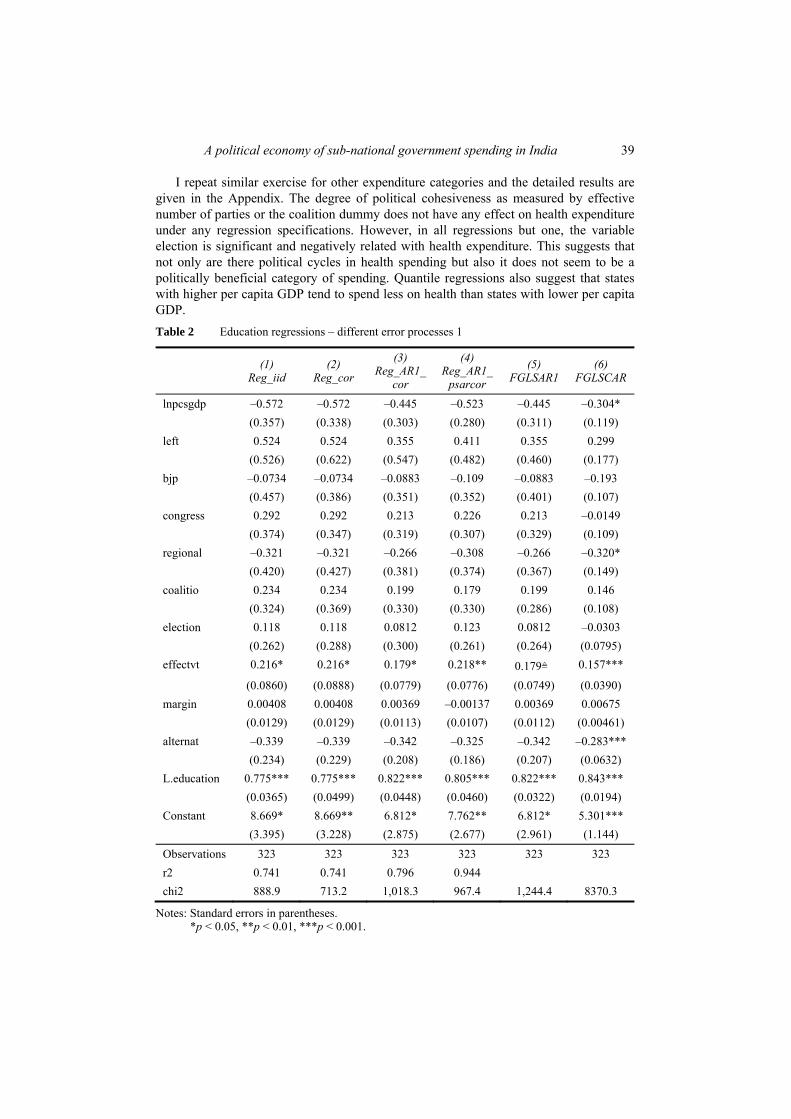
Given this, the most robust results from all the analysis is about the relationship between education expenditure and the degree of political cohesiveness. From Tables 2 and 3, we can see that the a lower degree of political cohesiveness as measured by effective number of parties has an unambiguous positive and significant effect on education spending under all the specifications.
A political economy of sub-national government spending in India 39
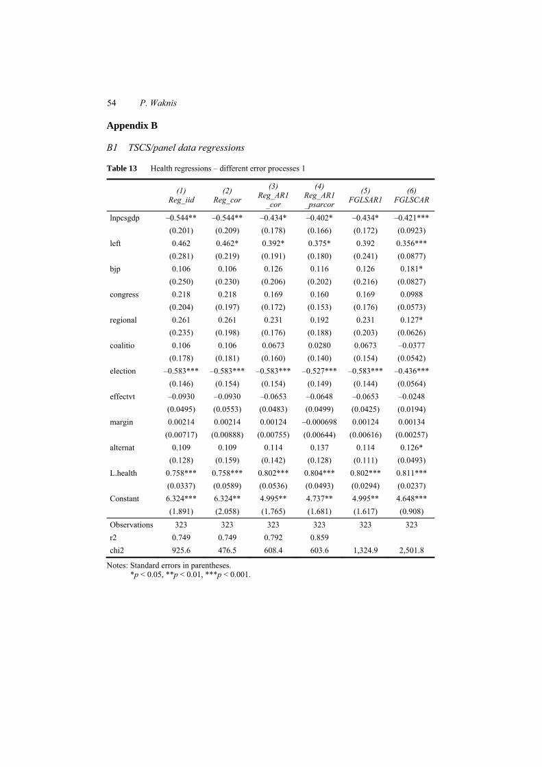
I repeat similar exercise for other expenditure categories and the detailed results are given in the Appendix. The degree of political cohesiveness as measured by effective number of parties or the coalition dummy does not have any effect on health expenditure under any regression specifications. However, in all regressions but one, the variable election is significant and negatively related with health expenditure. This suggests that not only are there political cycles in health spending but also it does not seem to be a politically beneficial category of spending. Quantile regressions also suggest that states with higher per capita GDP tend to spend less on health than states with lower per capita GDP. Table 2 Education regressions – different error processes 1
(1) Reg_iid
(2) Reg_cor
(3) Reg_AR1_
cor
(4) Reg_AR1_
psarcor
(5) FGLSAR1
(6) FGLSCAR
lnpcsgdp –0.572 –0.572 –0.445 –0.523 –0.445 –0.304* (0.357) (0.338) (0.303) (0.280) (0.311) (0.119) left 0.524 0.524 0.355 0.411 0.355 0.299 (0.526) (0.622) (0.547) (0.482) (0.460) (0.177) bjp –0.0734 –0.0734 –0.0883 –0.109 –0.0883 –0.193 (0.457) (0.386) (0.351) (0.352) (0.401) (0.107) congress 0.292 0.292 0.213 0.226 0.213 –0.0149 (0.374) (0.347) (0.319) (0.307) (0.329) (0.109) regional –0.321 –0.321 –0.266 –0.308 –0.266 –0.320* (0.420) (0.427) (0.381) (0.374) (0.367) (0.149) coalitio 0.234 0.234 0.199 0.179 0.199 0.146 (0.324) (0.369) (0.330) (0.330) (0.286) (0.108) election 0.118 0.118 0.0812 0.123 0.0812 –0.0303 (0.262) (0.288) (0.300) (0.261) (0.264) (0.0795) effectvt 0.216* 0.216* 0.179* 0.218** 0.179≜ 0.157***
(0.0860) (0.0888) (0.0779) (0.0776) (0.0749) (0.0390) margin 0.00408 0.00408 0.00369 –0.00137 0.00369 0.00675 (0.0129) (0.0129) (0.0113) (0.0107) (0.0112) (0.00461) alternat –0.339 –0.339 –0.342 –0.325 –0.342 –0.283*** (0.234) (0.229) (0.208) (0.186) (0.207) (0.0632) L.education 0.775*** 0.775*** 0.822*** 0.805*** 0.822*** 0.843*** (0.0365) (0.0499) (0.0448) (0.0460) (0.0322) (0.0194) Constant 8.669* 8.669** 6.812* 7.762** 6.812* 5.301*** (3.395) (3.228) (2.875) (2.677) (2.961) (1.144) Observations 323 323 323 323 323 323 r2 0.741 0.741 0.796 0.944 chi2 888.9 713.2 1,018.3 967.4 1,244.4 8370.3
Notes: Standard errors in parentheses. *p < 0.05, **p < 0.01, ***p < 0.001.
40 P. Waknis
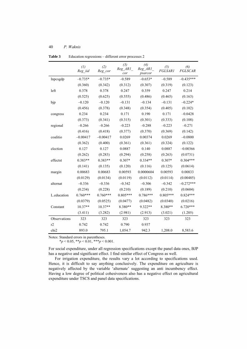
Table 3 Education regressions – different error processes 2
(1) Reg_iid
(2) Reg_cor
(3) Reg_AR1_
cor
(4) Reg_AR1_
psarcor
(5) FGLSAR1
(6) FGLSCAR
lnpcsgdp –0.735* –0.735* –0.589 –0.653* –0.589 –0.435*** (0.360) (0.342) (0.312) (0.307) (0.319) (0.123) left 0.378 0.378 0.247 0.359 0.247 0.214 (0.525) (0.625) (0.555) (0.486) (0.465) (0.163) bjp –0.120 –0.120 –0.131 –0.134 –0.131 –0.224* (0.456) (0.378) (0.348) (0.354) (0.405) (0.102) congress 0.234 0.234 0.171 0.190 0.171 –0.0428 (0.373) (0.341) (0.315) (0.301) (0.333) (0.108) regional –0.266 –0.266 –0.223 –0.288 –0.223 –0.271 (0.416) (0.418) (0.377) (0.370) (0.369) (0.142) coalitio –0.00417 –0.00417 0.0269 0.00374 0.0269 –0.0800 (0.362) (0.400) (0.361) (0.361) (0.324) (0.122) election 0.127 0.127 0.0887 0.140 0.0887 –0.00366 (0.262) (0.283) (0.294) (0.258) (0.263) (0.0731) effectst 0.383** 0.383** 0.307* 0.334** 0.307* 0.304*** (0.141) (0.135) (0.120) (0.116) (0.125) (0.0614) margin 0.00683 0.00683 0.00593 0.0000604 0.00593 0.00833 (0.0129) (0.0134) (0.0119) (0.0112) (0.0114) (0.00485) alternat –0.336 –0.336 –0.342 –0.306 –0.342 –0.272*** (0.234) (0.228) (0.210) (0.189) (0.210) (0.0604) L.education 0.760*** 0.760*** 0.805*** 0.786*** 0.805*** 0.824*** (0.0379) (0.0525) (0.0477) (0.0482) (0.0340) (0.0216) Constant 10.37** 10.37** 8.380** 9.322** 8.380** 6.720*** (3.411) (3.282) (2.981) (2.913) (3.021) (1.205)
Observations 323 323 323 323 323 323 r2 0.742 0.742 0.790 0.937 chi2 893.0 795.1 1,054.7 942.3 1,208.0 8,583.6
Notes: Standard errors in parentheses. *p < 0.05, **p < 0.01, ***p < 0.001.
For social expenditure, under all regression specifications except the panel data ones, BJP has a negative and significant effect. I find similar effect of Congress as well.
For irrigation expenditure, the results vary a lot according to specifications used. Hence, it is difficult to say anything conclusively. The expenditure on agriculture is negatively affected by the variable ‘alternate’ suggesting an anti incumbency effect. Having a low degree of political cohesiveness also has a negative effect on agricultural expenditure under TSCS and panel data specifications.
A political economy of sub-national government spending in India 41
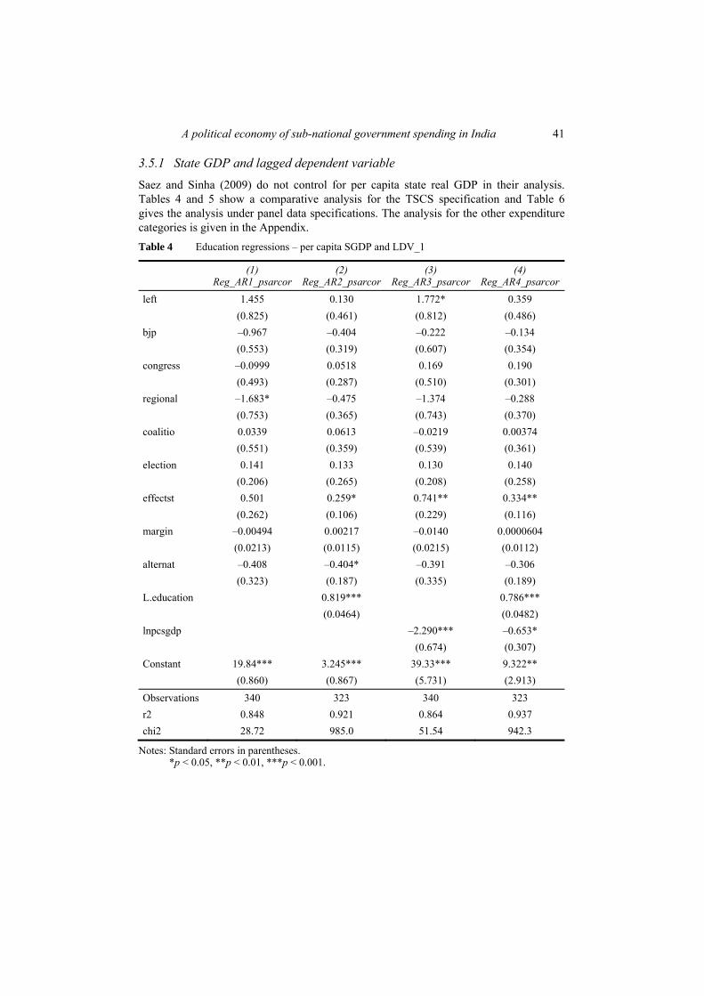
3.5.1 State GDP and lagged dependent variable
Saez and Sinha (2009) do not control for per capita state real GDP in their analysis. Tables 4 and 5 show a comparative analysis for the TSCS specification and Table 6 gives the analysis under panel data specifications. The analysis for the other expenditure categories is given in the Appendix. Table 4 Education regressions – per capita SGDP and LDV_1
(1) Reg_AR1_psarcor
(2) Reg_AR2_psarcor
(3) Reg_AR3_psarcor
(4) Reg_AR4_psarcor
left 1.455 0.130 1.772* 0.359 (0.825) (0.461) (0.812) (0.486) bjp –0.967 –0.404 –0.222 –0.134 (0.553) (0.319) (0.607) (0.354) congress –0.0999 0.0518 0.169 0.190 (0.493) (0.287) (0.510) (0.301) regional –1.683* –0.475 –1.374 –0.288 (0.753) (0.365) (0.743) (0.370) coalitio 0.0339 0.0613 –0.0219 0.00374 (0.551) (0.359) (0.539) (0.361) election 0.141 0.133 0.130 0.140 (0.206) (0.265) (0.208) (0.258) effectst 0.501 0.259* 0.741** 0.334** (0.262) (0.106) (0.229) (0.116) margin –0.00494 0.00217 –0.0140 0.0000604 (0.0213) (0.0115) (0.0215) (0.0112) alternat –0.408 –0.404* –0.391 –0.306 (0.323) (0.187) (0.335) (0.189) L.education 0.819*** 0.786*** (0.0464) (0.0482) lnpcsgdp –2.290*** –0.653* (0.674) (0.307) Constant 19.84*** 3.245*** 39.33*** 9.322** (0.860) (0.867) (5.731) (2.913)
Observations 340 323 340 323 r2 0.848 0.921 0.864 0.937 chi2 28.72 985.0 51.54 942.3
Notes: Standard errors in parentheses. *p < 0.05, **p < 0.01, ***p < 0.001.
42 P. Waknis
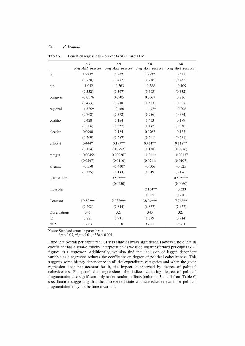
Table 5 Education regressions – per capita SGDP and LDV
(1) Reg_AR1_psarcor
(2) Reg_AR2_psarcor
(3) Reg_AR3_psarcor
(4) Reg_AR4_psarcor
left 1.728* 0.202 1.882* 0.411 (0.730) (0.457) (0.736) (0.482) bjp –1.042 –0.363 –0.388 –0.109 (0.532) (0.307) (0.603) (0.352) congress –0.0576 0.0905 0.0867 0.226 (0.473) (0.288) (0.503) (0.307) regional –1.585* –0.480 –1.497* –0.308 (0.768) (0.372) (0.756) (0.374) coalitio 0.428 0.164 0.403 0.179 (0.506) (0.327) (0.492) (0.330) election 0.0900 0.124 0.0762 0.123 (0.209) (0.267) (0.211) (0.261) effectvt 0.444* 0.195** 0.474** 0.218** (0.184) (0.0752) (0.178) (0.0776) margin –0.00455 0.000267 –0.0112 –0.00137 (0.0207) (0.0110) (0.0211) (0.0107) alternat –0.550 –0.400* –0.506 –0.325 (0.335) (0.183) (0.349) (0.186) L.education 0.828*** 0.805*** (0.0450) (0.0460) lnpcsgdp –2.124** –0.523 (0.665) (0.280) Constant 19.52*** 2.938*** 38.04*** 7.762** (0.793) (0.844) (5.877) (2.677) Observations 340 323 340 323 r2 0.881 0.931 0.899 0.944 chi2 37.83 968.0 67.11 967.4
Notes: Standard errors in parentheses. *p < 0.05, **p < 0.01, ***p < 0.001.
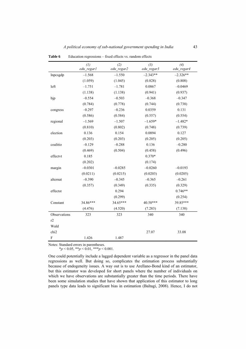
I find that overall per capita real GDP is almost always significant. However, note that its coefficient has a semi-elasticity interpretation as we used log transformed per capita GDP figures as a regressor. Additionally, we also find that inclusion of lagged dependent variable as a regressor reduces the coefficient on degree of political cohesiveness. This suggests some history dependence in all the expenditure categories and when the given regression does not account for it, the impact is absorbed by degree of political cohesiveness. For panel data regressions, the indices capturing degree of political fragmentation are significant only under random effects [columns 3 and 4 from Table 6] specification suggesting that the unobserved state characteristics relevant for political fragmentation may not be time invariant.
A political economy of sub-national government spending in India 43
Table 6 Education regressions – fixed effects vs. random effects
(1) edu_regar1
(2) edu_regar2
(3) edu_regar3
(4) edu_regar4
lnpcsgdp –1.568 –1.550 –2.343** –2.326** (1.059) (1.045) (0.828) (0.808) left –1.751 –1.781 0.0867 –0.0469 (1.138) (1.138) (0.941) (0.937) bjp –0.554 –0.503 –0.368 –0.347 (0.784) (0.778) (0.744) (0.738) congress –0.297 –0.236 0.0359 0.131 (0.586) (0.584) (0.557) (0.554) regional –1.569 –1.507 –1.659* –1.482* (0.810) (0.802) (0.748) (0.739) election 0.136 0.154 0.0894 0.127 (0.203) (0.203) (0.205) (0.205) coalitio –0.129 –0.288 0.136 –0.280 (0.469) (0.504) (0.458) (0.496) effectvt 0.185 0.370* (0.202) (0.174) margin –0.0301 –0.0285 –0.0260 –0.0193 (0.0211) (0.0215) (0.0203) (0.0205) alternat –0.390 –0.345 –0.365 –0.261 (0.357) (0.349) (0.335) (0.329) effectst 0.294 0.746** (0.299) (0.254) Constant 34.86*** 34.65*** 40.58*** 39.85*** (4.476) (4.520) (7.283) (7.138) Observations 323 323 340 340 r2 Wald chi2 27.07 33.08 F 1.426 1.487
Notes: Standard errors in parentheses. *p < 0.05, **p < 0.01, ***p < 0.001.
One could potentially include a lagged dependent variable as a regressor in the panel data regressions as well. But doing so, complicates the estimation process substantially because of endogeneity issues. A way out is to use Arellano-Bond kind of an estimator, but this estimator was developed for short panels where the number of individuals on which we have observations are substantially greater than the time periods. There have been some simulation studies that have shown that application of this estimator to long panels type data leads to significant bias in estimation (Baltagi, 2008). Hence, I do not
44 P. Waknis
run regressions of these expenditures on their lagged values under panel data fixed and random effects estimation.
3.5.2 Quantile regression
A quantile regression is a good way of understanding the partial effect of an explanatory variable on various segments of a population (Wooldridge, 2011). Thus, running such a regression gives us yet another way of understanding the differences in spending patterns conditional on the state’s per capita income. It allows us to see if the given category of spending is sensitive to where the state lies in the spending hierarchy. The substantial regional inequality in India only underscores the need to look at such variation in spending patterns. The complete tables are in the Appendix and the results are summarised here.
One has to interpret the coefficients in such regressions noting the fact that quantile coefficients refer to effects on distributions and not on individuals [Angrist and Pischke, (2009), p.281]. For example, if having less political cohesiveness affects the spending negatively in a particular quantile, it means that the states with lower political cohesiveness in that quantile would experience a decline in spending than states in the same quantile but having higher cohesiveness. It does not mean that a particular state with income in the given quantile is going to experience a decline in spending.
For the regression of education expenditure, the variable ‘left’ is a significant and positive predictor under all the quantiles and so are the two measures of political cohesiveness. The coefficients jump as we go from the lowest quantile to the middle one and then drops a little bit suggesting a inverted ‘U’ relationship. Degree of political cohesiveness as measured by effective number of parties according to seats has a uniform effect on education spending but a somewhat inverted ‘U’ according to vote share. Per capita state GDP is a significant negative predictor and the effect intensifies as you go up higher in quantiles. For the regression of health expenditure, variables, ‘left’ and per capita state GDP are significant and positive and negative predictors respectively. Only one of the measures of political cohesiveness, ‘effectvt’ is negatively related to the health expenditure across quantiles. Lower cohesiveness means a decrease in health care spending. However, for none of the quantiles dealt with here, is election a significant variable.
For irrigation expenditure, there is evidence that presence of a regional party in the government leads to an increase in this expenditure. A Congress party government is also negatively associated with health expenditure and so is the coalition dummy. Both Congress and BJP governments are negatively associated with social expenditure. This was true under the TSCS regressions as well. Political cohesiveness as measured by vote share is negatively associated with agricultural expenditure across all quantiles. The variable ’margin’ however is positively associated with expenditure on agriculture. This suggests that larger the difference in votes of the largest recipient and the second largest one, higher would be the expenditure on agriculture.
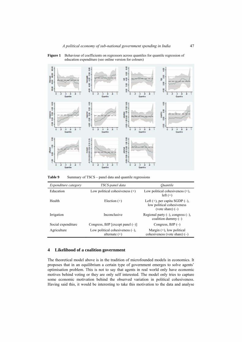
Under quantile regressions, a graphical view is more effective to see how the coefficients on regressors behave across quantiles. For example, in case of education expenditure regressions the coefficient on ‘effectvt’ jumps a bit from the lowest quantile to the higher quantile (graph in third row and first column). This suggests a higher impact of political cohesiveness in states with higher spending levels. The following figure shows the effect for all the quantiles for the regression of education expenditure and
A political economy of sub-national government spending in India 45
similar figures are included for other expenditure categories in the Appendix. The coefficient on ‘left’ shows a dip at higher levels of expenditure for irrigation expenditure, signifying its lower influence in higher spending states. It remains fairly constant for health expenditure across quantiles suggesting that the left’s influence is not sensitive to the level of this category of state spending. However, the effect of political cohesiveness as measured by vote share has a negative effect and its intensity increases as we move to higher quantiles. For agriculture expenditure, ‘margin’ has a positive effect mostly for mid range quantiles than at the tails. For social expenditure, the intensity of the negative effect of a BJP party government intensifies as we move to higher quantiles.
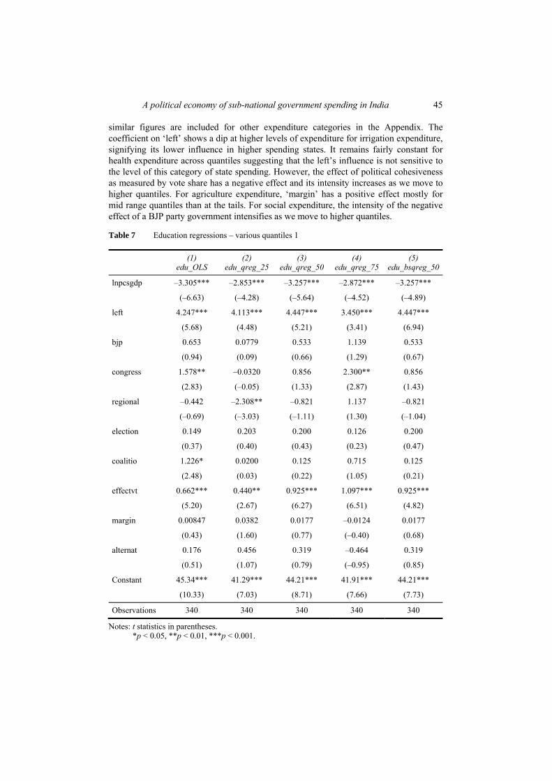
Table 7 Education regressions – various quantiles 1
(1) edu_OLS
(2) edu_qreg_25
(3) edu_qreg_50
(4) edu_qreg_75
(5) edu_bsqreg_50
lnpcsgdp –3.305*** –2.853*** –3.257*** –2.872*** –3.257***
(–6.63) (–4.28) (–5.64) (–4.52) (–4.89)
left 4.247*** 4.113*** 4.447*** 3.450*** 4.447***
(5.68) (4.48) (5.21) (3.41) (6.94)
bjp 0.653 0.0779 0.533 1.139 0.533
(0.94) (0.09) (0.66) (1.29) (0.67)
congress 1.578** –0.0320 0.856 2.300** 0.856
(2.83) (–0.05) (1.33) (2.87) (1.43)
regional –0.442 –2.308** –0.821 1.137 –0.821
(–0.69) (–3.03) (–1.11) (1.30) (–1.04)
election 0.149 0.203 0.200 0.126 0.200
(0.37) (0.40) (0.43) (0.23) (0.47)
coalitio 1.226* 0.0200 0.125 0.715 0.125
(2.48) (0.03) (0.22) (1.05) (0.21)
effectvt 0.662*** 0.440** 0.925*** 1.097*** 0.925***
(5.20) (2.67) (6.27) (6.51) (4.82)
margin 0.00847 0.0382 0.0177 –0.0124 0.0177
(0.43) (1.60) (0.77) (–0.40) (0.68)
alternat 0.176 0.456 0.319 –0.464 0.319
(0.51) (1.07) (0.79) (–0.95) (0.85)
Constant 45.34*** 41.29*** 44.21*** 41.91*** 44.21***
(10.33) (7.03) (8.71) (7.66) (7.73)
Observations 340 340 340 340 340
Notes: t statistics in parentheses. *p < 0.05, **p < 0.01, ***p < 0.001.
46 P. Waknis
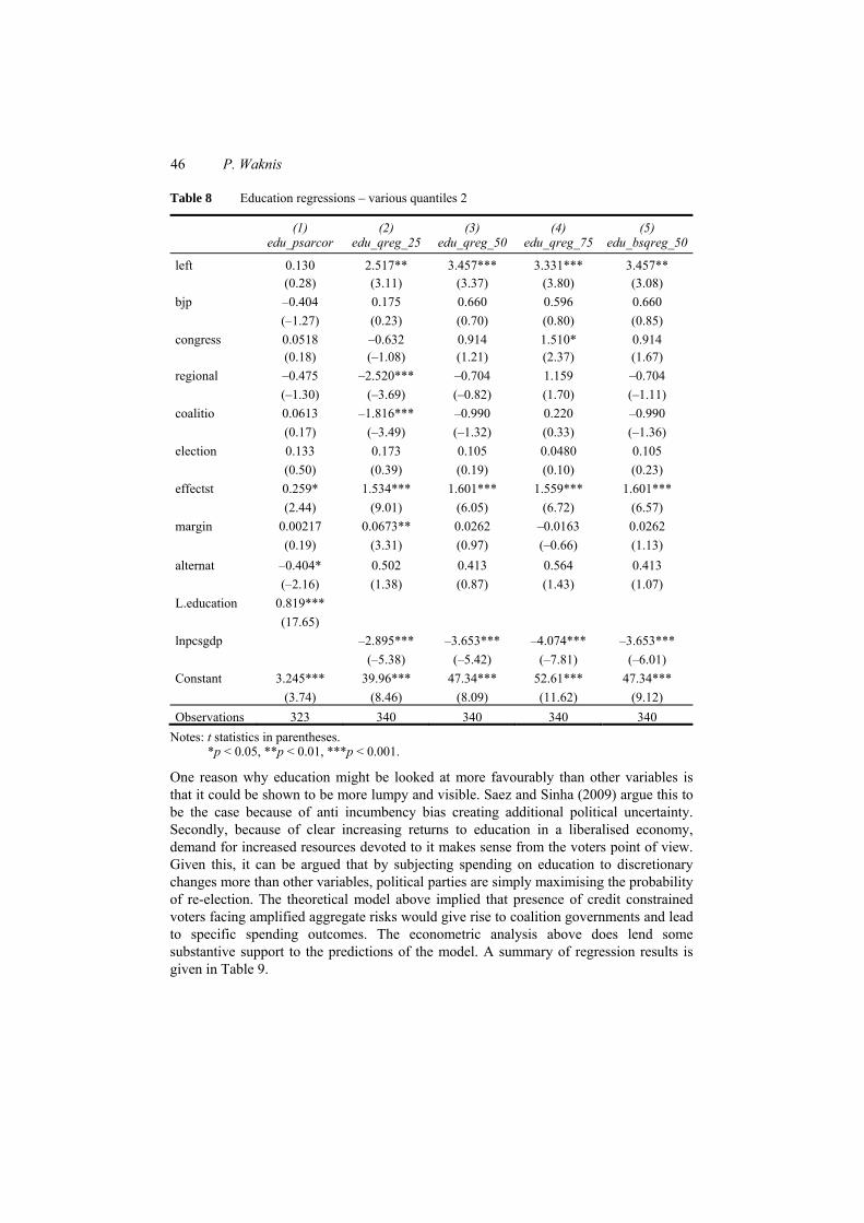
Table 8 Education regressions – various quantiles 2
(1) edu_psarcor
(2) edu_qreg_25
(3) edu_qreg_50
(4) edu_qreg_75
(5) edu_bsqreg_50
left 0.130 2.517** 3.457*** 3.331*** 3.457** (0.28) (3.11) (3.37) (3.80) (3.08) bjp –0.404 0.175 0.660 0.596 0.660 (–1.27) (0.23) (0.70) (0.80) (0.85) congress 0.0518 –0.632 0.914 1.510* 0.914 (0.18) (–1.08) (1.21) (2.37) (1.67) regional –0.475 –2.520*** –0.704 1.159 –0.704 (–1.30) (–3.69) (–0.82) (1.70) (–1.11) coalitio 0.0613 –1.816*** –0.990 0.220 –0.990 (0.17) (–3.49) (–1.32) (0.33) (–1.36) election 0.133 0.173 0.105 0.0480 0.105 (0.50) (0.39) (0.19) (0.10) (0.23) effectst 0.259* 1.534*** 1.601*** 1.559*** 1.601*** (2.44) (9.01) (6.05) (6.72) (6.57) margin 0.00217 0.0673** 0.0262 –0.0163 0.0262 (0.19) (3.31) (0.97) (–0.66) (1.13) alternat –0.404* 0.502 0.413 0.564 0.413 (–2.16) (1.38) (0.87) (1.43) (1.07) L.education 0.819*** (17.65) lnpcsgdp –2.895*** –3.653*** –4.074*** –3.653*** (–5.38) (–5.42) (–7.81) (–6.01) Constant 3.245*** 39.96*** 47.34*** 52.61*** 47.34*** (3.74) (8.46) (8.09) (11.62) (9.12) Observations 323 340 340 340 340
Notes: t statistics in parentheses. *p < 0.05, **p < 0.01, ***p < 0.001.
One reason why education might be looked at more favourably than other variables is that it could be shown to be more lumpy and visible. Saez and Sinha (2009) argue this to be the case because of anti incumbency bias creating additional political uncertainty. Secondly, because of clear increasing returns to education in a liberalised economy, demand for increased resources devoted to it makes sense from the voters point of view. Given this, it can be argued that by subjecting spending on education to discretionary changes more than other variables, political parties are simply maximising the probability of re-election. The theoretical model above implied that presence of credit constrained voters facing amplified aggregate risks would give rise to coalition governments and lead to specific spending outcomes. The econometric analysis above does lend some substantive support to the predictions of the model. A summary of regression results is given in Table 9.
A political economy of sub-national government spending in India 47
Figure 1 Behaviour of coefficients on regressors across quantiles for quantile regression of education expenditure (see online version for colours)
Table 9 Summary of TSCS – panel data and quantile regressions
Expenditure category TSCS-panel data Quantile
Education Low political cohesiveness (+) Low political cohesiveness (+), left (+)
Health Election (+) Left (+), per capita SGDP (–), low political cohesiveness
(vote share) (–) Irrigation Inconclusive Regional party (–), congress (–),
coalition dummy (–) Social expenditure Congress, BJP [except panel (–)] Congress, BJP (–) Agriculture Low political cohesiveness (–),
alternate (+) Margin (+), low political
cohesiveness (vote share) (–)
4 Likelihood of a coalition government
The theoretical model above is in the tradition of microfounded models in economics. It proposes that in an equilibrium a certain type of government emerges to solve agents’ optimisation problem. This is not to say that agents in real world only have economic motives behind voting or they are only self interested. The model only tries to capture some economic motivation behind the observed variation in political cohesiveness. Having said this, it would be interesting to take this motivation to the data and analyse

48 P. Waknis
the factors that determine the probability of a certain type of government emerging as a result of voting. In this section, we use binary response models to do so.
Two economic factors proposed to influence voting in an economy by the model were endowment shocks and credit constraints. We use the data on number of branch offices of nationalised banks in a state and the credit deposit ratio as proxies for credit constraints. We also use per capita GDP at 2000 prices as a control variable for state’s income and population profile. There are several ways of estimating a binary response model for panel data. We estimate the effect of these three variables on the likelihood of having a coalition government for a state following various specifications as described in Wooldridge (2011). Table 10 Likelihood of having a coalition government
(1) logitfe1
(2) logitre1
(3) logitpa1
(4) probitre1
(5) probitpa1
(6) xtgee1
(7) ols1
main lnpcsgdp 1.809 1.059 0.519 0.532 0.328 0.107 –0.0242 (0.993) (0.822) (0.566) (0.464) (0.326) (0.0922) (0.0644) pcbanks –26753.9 –10109.6 –5448.5 –5103.2 –3347.7 –822.6 –16.53 (24293.9) (15326.9) (9220.6) (8655.4) (5461.5) (1600.2) (838.4) CD-ratio –0.0190 –0.0245 –0.0209 –0.0144 –0.0116 –0.00314 –0.00261* (0.0187) (0.0150) (0.0116) (0.00842) (0.00646) (0.00169) (0.00115) Constant –9.281 –4.432 –4.687 –2.857 –0.504 0.559 (7.264) (4.995) (4.083) (2.877) (0.811) (0.546) lnsig2u Constant 1.039 –0.125 (0.607) (0.581)
Observations 220 320 320 320 320 320 320 ll –97.72 –138.6 –138.2 –158.0
Notes: Standard errors in parentheses. *p < 0.05, **p < 0.01, ***p < 0.001
It is clear from Table 10, that none of the variables is statistically significant affecting the probability of a coalition government. However, except per capita state GDP, the other two variables have the expected sign. Higher number of per capita banks and a higher credit deposit ratio, both signify reduction in credit constraints and therefore reduce the probability of having a coalition government. Assuming that lower credit constraints go hand in hand with higher per capita incomes, one can argue that its effect is captured in the other two variables. Accordingly, we run the following regression with only number of banks per capita and credit deposit ratio. The results are given in Table 11.
Dropping per capita state GDP as a regressor does not change the sign of the other two regressors (Table 11). Further, in all but one specification, credit deposit ratio is a statistically significant predictor of the change in the probability of having a coalition government. Higher the credit deposit ratio (lower the credit constraints), lower is the probability of having a coalition government in a given state. This clearly lends some
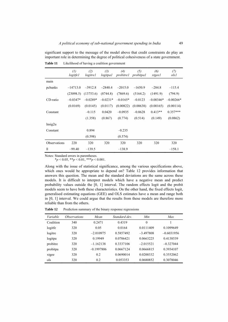
A political economy of sub-national government spending in India 49
significant support to the message of the model above that credit constraints do play an important role in determining the degree of political cohesiveness of a state government. Table 11 Likelihood of having a coalition government
(1) logitfe1
(2) logitre1
(3) logitpa1
(4) probitre1
(5) probitpa1
(6) xtgee1
(7) ols1
main
pcbanks –14713.0 –3912.8 –2840.4 –2015.0 –1650.9 –284.8 –115.4
(23098.5) (13753.6) (8744.8) (7869.6) (5164.2) (1491.9) (794.9)
CD-ratio –0.0347* –0.0289* –0.0231* –0.0165* –0.0123 –0.00346* –0.00266*
(0.0169) (0.0145) (0.0117) (0.00822) (0.00638) (0.00165) (0.00114)
Constant –0.115 0.0420 –0.0935 –0.0628 0.413** 0.357***
(1.358) (0.867) (0.774) (0.514) (0.149) (0.0862)
lnsig2u
Constant 0.894 –0.235
(0.598) (0.574)
Observations 220 320 320 320 320 320 320
ll –99.40 –139.5 –138.9 –158.1
Notes: Standard errors in parentheses. *p < 0.05, **p < 0.01, ***p < 0.001.
Along with the issue of statistical significance, among the various specifications above, which ones would be appropriate to depend on? Table 12 provides information that answers this question. The mean and the standard deviations are the same across these models. It is difficult to interpret models which have a negative mean and predict probability values outside the [0, 1] interval. The random effects logit and the probit models seem to have both these characteristics. On the other hand, the fixed effects logit, generalised estimating equations (GEE) and OLS estimates have a mean and range both in [0, 1] interval. We could argue that the results from these models are therefore more reliable than from the others. Table 12 Prediction summary of the binary response regressions
Variable Observations Mean Standard dev. Min Max Coalition 340 0.2471 0.4319 0 1 logitfe 320 0.05 0.0164 0.0111409 0.1099649 logitre 320 –2.010975 0.5857492 –3.497808 –0.6031956 logitpa 320 0.19949 0.0706421 0.0663225 0.4138539 probitre 320 –1.162138 0.3337106 –2.015521 –0.327044 probitpa 320 –0.1997806 0.0667124 0.0666815 0.3934107 xtgee 320 0.2 0.0690014 0.0200332 0.3552062 ols 320 0.2 0.053353 0.0680852 0.3078046
50 P. Waknis
5 Comments and conclusions
The importance of credit constraints and negative aggregate shocks cannot be overstated given the recent financial crisis and the recession that followed. In this paper, I explore the role such factors can play in determining political outcomes and how these political outcomes in turn can affect the economic ones. I do so by developing a simple model of an endowment economy with some of the agents being credit constrained and shocks making the distribution of such agents endogenous. These agents seek to smooth consumption and use government expenditure as an insurance mechanism to survive the shocks. They do so by voting for a political entity which promises and has an expertise in delivering the required public goods. I show that different types of governments and therefore different spending policies could emerge in equilibrium conditional on the realisation of shocks. Thus, this microfounded model builds on the interaction between economic and political factors to derive testable implications of the type of government on its spending policies.
The empirical analysis does lend support to the predictions of the model. Specifically, there exists a strong evidence suggesting that a lower degree of political cohesiveness is associated with higher spending on education. A little less robust (true for fewer specifications than for education expenditure) is the result that it is also associated with lower spending on agriculture. I do not find similar evidence for its influence on other spending categories of irrigation and social services. In these cases, other political factors like presence of a particular political party in the government or upcoming elections have a significant influence. Specifically for social expenditure, we found that a BJP or a Congress government always has a negative impact. These results are obtained using variety of specifications and methodologies and hence have a built in robustness check. It does remain a question worthy of exploration as to why politically less cohesive governments choose spending on education for political manoeuvring. I posit that suitability of education expenditure to specifically target certain groups of voters explains the preference. However, a more disaggregate analysis covering a lengthier time period might shed more light on this issue. Use of quantile regression clearly shows that relationship between spending and political cohesiveness is also sensitive to distribution of spending across states. For example, in case of education, we find that states with higher level of spending are more sensitive to degree of political cohesiveness than with the lower ones.
One of the implications of the model is that credit constraints interact with shocks to determine equilibrium voting strategies of the agents. I take this issue to the data and ask how influential these economic factors are in determining the probability of having a coalition government. The results support this hypothesis of the model. The econometric analysis suggests that higher the credit constraints (as measured by lower credit deposit ratio), higher is the probability of having a coalition government. This result should be taken with a pinch of salt as credit-deposit ratio is only a crude indicator of credit constraints. Commenting on the recent move towards increasing access to banking in India, Kamath et al. (2010) find that having a bank account does not necessarily mean an easier access to credit from banks, but having assets like land certainly does. A more richer analysis, therefore, should include data on asset distribution and changes in landholding patterns over the years in different states. However, such a time series data for different states in India is relatively harder to come by.
A political economy of sub-national government spending in India 51
Notwithstanding the limitations imposed by the data availability, the theoretical and empirical exercise in this paper signifies a contribution to the literature on political economy and macroeconomics. Its focus on interaction between credit constraints, aggregate shocks and voting is based on the intuition that consumption smoothing should drive political decisions of the agents lacking access to formal insurance mechanisms in order to survive shocks to the economic activity. However, I do assume that there are no credibility issues involved when it comes to implementing the promised policies. As a future extension of this research one could explore the implications of relaxing this assumption.
Acknowledgements
I thank Christian Zimmermann (Major Advisor, UCONN) and Gautam Tripathi for their guidance and support. Discussions with Subhash Ray and Lyle Scruggs were also helpful at various stages of development of this paper and so were the inputs from Stephen Ross during my PhD defense. I thank the three anonymous referees for their helpful comments and suggestions. I also thank Bipin Deokar from Mumbai, India for help with the data related to Banking. A special appreciation goes to Robert Jones and all my colleagues at UMass Dartmouth for being very supportive and encouraging while I worked on the revisions. Needless to say, all errors are mine. Any comments and suggestions are welcome.
References Acemoglu, D., Johnson, S. and Robinson, J.A. (2002) ‘Reversal of fortune: geography and
institutions in the making of the modern world income distribution’, The Quarterly Journal of Economics, November, Vol. 117, No. 4, pp.1231–1294.
Acemoglu, D., Johnson, S., Robinson, J.A. and Pierre Yared, (2008) ‘Income and democracy’, American Economic Review, June, Vol. 98, No. 3, pp.808–842.
Alexander, M., Harding, M. and Lamarche, C. (2011) ‘Quantile regression for time-series-cross-section data’, International Journal of Statistics and Management System, Vol. 6, No. 12, p.4772.
Angrist, J.D. and Pischke, J-S. (2009) Mostly Harmless Econometrics – An Empriricists Companion, Princeton University Press, New Jersey, USA and Oxfordshire, UK.
Baltagi, B. (2008) Econometrics Analysis of Panel Data, Wiley, West Sussex, UK. Bartels, B.L. (n.d.) Beyond Fixed Versus Random Effects: A Framework for Improving Substantitve
and Statistical Analysis of Panel, Time Series-cross Sectional, and Multilevel Data, Unpublished.
Beck, N. (2006) Time Series-Cross Section Methods, Technical Report, Department of Politics, New York University.
Cameron, A.C. and Trivedi, P.K. (2010) Microeconometrics Using Stata, STATA Press, College Station, TX.
Chaudhuri, K. and Dasgupta, S. (2006) ‘The political determinants of fiscal policies in the states of India: an empirical investigation’, The Journal of Development Studies, May, Vol. 42, No. 4, pp.640–661.
Cole, S., Healy, A. and Werker, E. (2012) ‘Do voters demand responsive governments? Evidence from Indian disaster relief’, Journal of Development Economics, Vol. 97, No. 2, pp.167–181.
52 P. Waknis
Ghate, C., Pandey, R. and Patnaik, I. (2011) Has India Emerged? Business Cycle Facts from a Transitioning Economy, April, Working Papers 11/88, National Institute of Public Finance and Policy.
Handbook of Statistics on Indian Economy (2010-11) Handbook of Statistics on Indian Economy, May 2011 [online] http://www.rbi.org.in/scripts/AnnualPublications.aspx?head=Handbook of Statistics on Indian Economy (accessed January 2011).
Kamath, R., Arnab, M. and Sandstrom, M. (2010) ‘Accessing institutional finance: a demand side story of rural India’, Economic and Political Weekly, Vol. XLV, No. 37, pp.56–62.
Kiyotaki, N. and Moore, J. (1997) ‘Credit cycles’, Journal of Political Economy, Vol. 105, No. 2, pp.211–248.
Krasa, S. and Polborn, M. (2009) Political Competition between Differentiated Candidates, CESifo Working Paper Series 2560, CESifo Group, Munich.
Krasa, S. and Polborn, M. (2010) ‘The binary policy model’, Journal of Economic Theory, Vol. 145, No. 2, pp.661–688.
Lalvani, M. (2005) ‘Coalition governments: fiscal implication for the Indian economy’, American Review of Political Economy, Vol. 3, No. 1, pp.127–163.
Persson, T. and Tabellini, G. (2002) Political Economics: Explaining Economic Policy, Zeuthen Lecture Book Series, MIT Press.
Polanyi, K. (2001) The Great Transformation, Beacon Press, Boston, MA. Rath, N. (2012) ‘Economic origin of regional and caste parties’, Economic and Political Weekly,
28 July, Vol. XLVII, No. 30, pp.24–28. Saez, L. (2008) Political Cycles, Political Institutions, and Public Service Expenditure in India
(POLEX-India) Data Set, Version 2008.1 [online] http://eprints.soas.ac.uk/4341/ (accessed January 2011).
Saez, L. and Sinha, A. (2009) ‘Political cycles, political institutions and public expenditure in India, 1980–2000’, British Journal of Political Science, January 2010, Vol. 40, No. 01, pp.91–113, first published online on 17 November 2009.
STATA (n.d.) Release 12 Longitudinal Data/Panel Data. Tandon, S. (2007) Economic Reform, Voting, and Local Political Intervention, Technical Report,
University of California, Berkeley. Thachil, T. (2011) ‘Embedded mobilization: nonstate service provision as electoral strategy in
India’, World Politics, Vol. 63, No. 3, pp.434–469. Waknis, P. (2011) Endogenous Monetary Policy: A Leviathan Central Bank in a Lagos-Wright
Economy, October, Working Papers 2011-20, University of Connecticut, Department of Economics.
Wooldridge, J. (2011) Econometric Analysis of Cross Section and Panel Data, The MIT Press, Cambridge, USA.
Notes 1 First published in 1944, Polanyi (2001) is an analytical account of the transformation of
traditional economies embedded with social norms to modern individual centred market-based systems. Although the book primarily talks about the European economies before and after the Industrial revolution, the analysis can be argued to be relevant to today’s many transition and emerging economies including India.
2 According to the authors, the distributions of two commonly used numerical measures of democracy is bimodal.
A political economy of sub-national government spending in India 53
Appendix A
A1 Description of variables in the regressions
Effective number of parties (seats)
The effective number of parties in a state assembly in India, using seats (nSEATS), was calculated employing the widely used Laakso and Taageperas index (N).
Effective number of parties (votes)
The effective number of parties in a state assembly in India, using votes (nVOTES), was calculated employing the widely used Laakso and Taageperas index (N).
Election Dummy variable taking value 0 or 1 Left Dummy variable taking value 0 if a leftist party is not part of the government
and 1 if it is. BJP Dummy variable taking value 0 if Bharatiya Janata party is not part of the
government and 1 if it is. Congress Dummy variable taking value 0 if congress is not part of the government and 1
if it is. Regional Dummy variable taking value 0 if a regional is not part of the government and
1 if it is. Coalition Dummy variable taking value 0 if state government is not formed by coalition
of parties and 1 if it is. Alternation 0 = a state assembly is ruled by the same political party that ruled in that state
prior to the election 1 = a state assembly is ruled by a political party that is different from the political party that ruled in that state prior to the election
Margin Percentage difference between the largest recipient of votes and the second largest recipient of votes in all state assembly elections in India, 1980–2000.
Source: Saez and Sinha (2009)
54 P. Waknis
Appendix B
B1 TSCS/panel data regressions
Table 13 Health regressions – different error processes 1
(1) Reg_iid
(2) Reg_cor
(3) Reg_AR1
_cor
(4) Reg_AR1_psarcor
(5) FGLSAR1
(6) FGLSCAR
lnpcsgdp –0.544** –0.544** –0.434* –0.402* –0.434* –0.421*** (0.201) (0.209) (0.178) (0.166) (0.172) (0.0923) left 0.462 0.462* 0.392* 0.375* 0.392 0.356*** (0.281) (0.219) (0.191) (0.180) (0.241) (0.0877) bjp 0.106 0.106 0.126 0.116 0.126 0.181* (0.250) (0.230) (0.206) (0.202) (0.216) (0.0827) congress 0.218 0.218 0.169 0.160 0.169 0.0988 (0.204) (0.197) (0.172) (0.153) (0.176) (0.0573) regional 0.261 0.261 0.231 0.192 0.231 0.127* (0.235) (0.198) (0.176) (0.188) (0.203) (0.0626) coalitio 0.106 0.106 0.0673 0.0280 0.0673 –0.0377 (0.178) (0.181) (0.160) (0.140) (0.154) (0.0542) election –0.583*** –0.583*** –0.583*** –0.527*** –0.583*** –0.436*** (0.146) (0.154) (0.154) (0.149) (0.144) (0.0564) effectvt –0.0930 –0.0930 –0.0653 –0.0648 –0.0653 –0.0248 (0.0495) (0.0553) (0.0483) (0.0499) (0.0425) (0.0194) margin 0.00214 0.00214 0.00124 –0.000698 0.00124 0.00134 (0.00717) (0.00888) (0.00755) (0.00644) (0.00616) (0.00257) alternat 0.109 0.109 0.114 0.137 0.114 0.126* (0.128) (0.159) (0.142) (0.128) (0.111) (0.0493) L.health 0.758*** 0.758*** 0.802*** 0.804*** 0.802*** 0.811*** (0.0337) (0.0589) (0.0536) (0.0493) (0.0294) (0.0237) Constant 6.324*** 6.324** 4.995** 4.737** 4.995** 4.648*** (1.891) (2.058) (1.765) (1.681) (1.617) (0.908) Observations 323 323 323 323 323 323 r2 0.749 0.749 0.792 0.859 chi2 925.6 476.5 608.4 603.6 1,324.9 2,501.8
Notes: Standard errors in parentheses. *p < 0.05, **p < 0.01, ***p < 0.001.
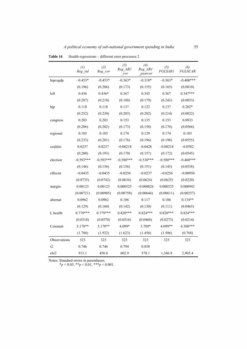
A political economy of sub-national government spending in India 55
Table 14 Health regressions – different error processes 2
(1) Reg_iid
(2) Reg_cor
(3) Reg_AR1
_cor
(4) Reg_AR1_psarcor
(5) FGLSAR1
(6) FGLSCAR
lnpcsgdp –0.453* –0.453* –0.363* –0.318* –0.363* –0.400***
(0.196) (0.206) (0.173) (0.155) (0.165) (0.0810)
left 0.436 0.436* 0.367 0.345 0.367 0.347***
(0.287) (0.218) (0.188) (0.179) (0.243) (0.0853)
bjp 0.118 0.118 0.137 0.123 0.137 0.202*
(0.252) (0.230) (0.203) (0.202) (0.214) (0.0822)
congress 0.203 0.203 0.153 0.135 0.153 0.0933
(0.206) (0.202) (0.173) (0.158) (0.176) (0.0566)
regional 0.185 0.185 0.174 0.129 0.174 0.103
(0.233) (0.201) (0.176) (0.196) (0.198) (0.0555)
coalitio 0.0237 0.0237 –0.00218 –0.0428 –0.00218 –0.0582
(0.200) (0.193) (0.170) (0.157) (0.172) (0.0545)
election –0.593*** –0.593*** –0.588*** –0.538*** –0.588*** –0.460***
(0.146) (0.156) (0.156) (0.151) (0.145) (0.0538)
effectst –0.0435 –0.0435 –0.0256 –0.0237 –0.0256 –0.00950
(0.0735) (0.0742) (0.0634) (0.0624) (0.0625) (0.0220)
margin 0.00123 0.00123 0.000525 –0.000826 0.000525 0.000943
(0.00721) (0.00905) (0.00758) (0.00646) (0.00611) (0.00257)
alternat 0.0962 0.0962 0.106 0.117 0.106 0.134**
(0.129) (0.160) (0.142) (0.130) (0.111) (0.0465)
L.health 0.779*** 0.779*** 0.820*** 0.824*** 0.820*** 0.824***
(0.0318) (0.0570) (0.0516) (0.0468) (0.0273) (0.0214)
Constant 5.178** 5.178** 4.099* 3.709* 4.099** 4.308***
(1.788) (1.922) (1.623) (1.450) (1.506) (0.768)
Observations 323 323 323 323 323 323
r2 0.746 0.746 0.794 0.858
chi2 913.1 456.8 602.9 578.1 1,346.9 2,905.4
Notes: Standard errors in parentheses. *p < 0.05, **p < 0.01, ***p < 0.001.

56 P. Waknis
Table 15 Health regressions – per capita SGDP and LDV_1
(1) Reg_AR1_psarcor
(2) Reg_AR2_psarcor
(3) Reg_AR3_psarcor
(4) Reg_AR4_psarcor
left 0.498 0.194 0.599 0.345 (0.504) (0.170) (0.428) (0.179) bjp –0.399 –0.0493 –0.199 0.123 (0.516) (0.182) (0.494) (0.202) congress 0.147 0.0323 0.146 0.135 (0.337) (0.151) (0.339) (0.158) regional –0.413 –0.0133 –0.369 0.129 (0.447) (0.199) (0.425) (0.196) coalitio –0.0895 –0.0236 –0.0373 –0.0428 (0.335) (0.157) (0.315) (0.157) election –0.301* –0.550*** –0.334* –0.538*** (0.150) (0.153) (0.146) (0.151) effectst –0.233 –0.0157 –0.214 –0.0237 (0.171) (0.0629) (0.149) (0.0624) margin 0.00919 –0.000224 0.00409 –0.000826 (0.0149) (0.00636) (0.0145) (0.00646) alternat 0.383 0.0752 0.374 0.117 (0.260) (0.124) (0.252) (0.130) L.health 0.844*** 0.824*** (0.0445) (0.0468) lnpcsgdp –2.943*** –0.318* (0.824) (0.155) Constant 7.231*** 0.867* 33.20*** 3.709* (0.861) (0.395) (7.206) (1.450) Observations 340 323 340 323 r2 0.562 0.857 0.586 0.858 chi2 15.38 487.1 29.76 578.1
Notes: Standard errors in parentheses. *p < 0.05, **p < 0.01, ***p < 0.001.
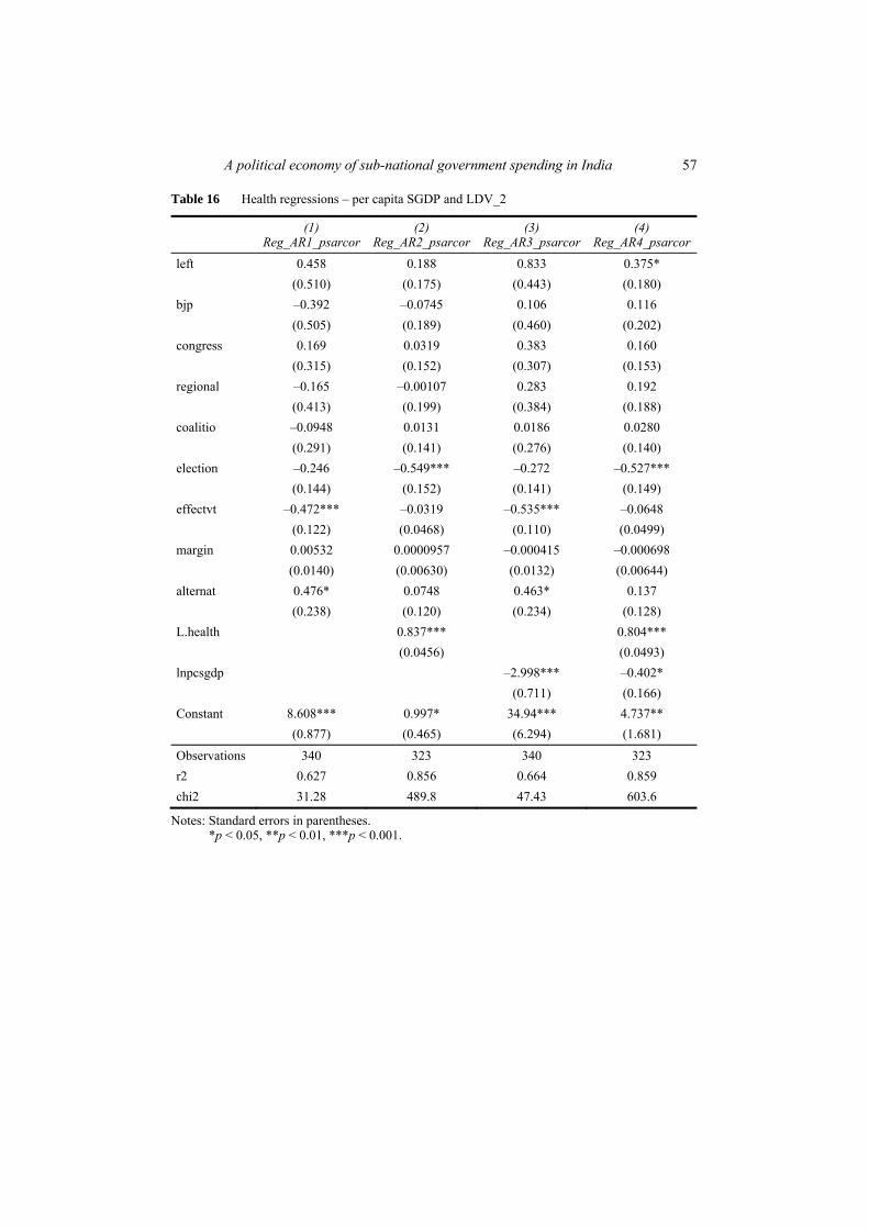
A political economy of sub-national government spending in India 57
Table 16 Health regressions – per capita SGDP and LDV_2
(1) Reg_AR1_psarcor
(2) Reg_AR2_psarcor
(3) Reg_AR3_psarcor
(4) Reg_AR4_psarcor
left 0.458 0.188 0.833 0.375* (0.510) (0.175) (0.443) (0.180) bjp –0.392 –0.0745 0.106 0.116 (0.505) (0.189) (0.460) (0.202) congress 0.169 0.0319 0.383 0.160 (0.315) (0.152) (0.307) (0.153) regional –0.165 –0.00107 0.283 0.192 (0.413) (0.199) (0.384) (0.188) coalitio –0.0948 0.0131 0.0186 0.0280 (0.291) (0.141) (0.276) (0.140) election –0.246 –0.549*** –0.272 –0.527*** (0.144) (0.152) (0.141) (0.149) effectvt –0.472*** –0.0319 –0.535*** –0.0648 (0.122) (0.0468) (0.110) (0.0499) margin 0.00532 0.0000957 –0.000415 –0.000698 (0.0140) (0.00630) (0.0132) (0.00644) alternat 0.476* 0.0748 0.463* 0.137 (0.238) (0.120) (0.234) (0.128) L.health 0.837*** 0.804*** (0.0456) (0.0493) lnpcsgdp –2.998*** –0.402* (0.711) (0.166) Constant 8.608*** 0.997* 34.94*** 4.737** (0.877) (0.465) (6.294) (1.681) Observations 340 323 340 323 r2 0.627 0.856 0.664 0.859 chi2 31.28 489.8 47.43 603.6
Notes: Standard errors in parentheses. *p < 0.05, **p < 0.01, ***p < 0.001.
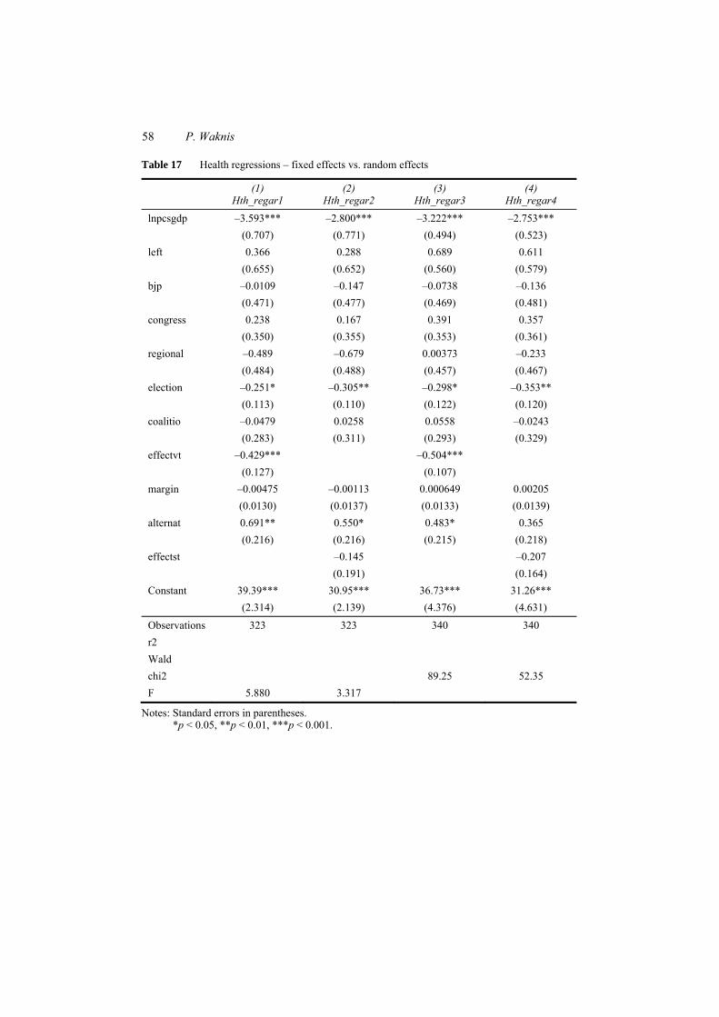
58 P. Waknis
Table 17 Health regressions – fixed effects vs. random effects
(1) Hth_regar1
(2) Hth_regar2
(3) Hth_regar3
(4) Hth_regar4
lnpcsgdp –3.593*** –2.800*** –3.222*** –2.753*** (0.707) (0.771) (0.494) (0.523) left 0.366 0.288 0.689 0.611 (0.655) (0.652) (0.560) (0.579) bjp –0.0109 –0.147 –0.0738 –0.136 (0.471) (0.477) (0.469) (0.481) congress 0.238 0.167 0.391 0.357 (0.350) (0.355) (0.353) (0.361) regional –0.489 –0.679 0.00373 –0.233 (0.484) (0.488) (0.457) (0.467) election –0.251* –0.305** –0.298* –0.353** (0.113) (0.110) (0.122) (0.120) coalitio –0.0479 0.0258 0.0558 –0.0243 (0.283) (0.311) (0.293) (0.329) effectvt –0.429*** –0.504*** (0.127) (0.107) margin –0.00475 –0.00113 0.000649 0.00205 (0.0130) (0.0137) (0.0133) (0.0139) alternat 0.691** 0.550* 0.483* 0.365 (0.216) (0.216) (0.215) (0.218) effectst –0.145 –0.207 (0.191) (0.164) Constant 39.39*** 30.95*** 36.73*** 31.26*** (2.314) (2.139) (4.376) (4.631) Observations 323 323 340 340 r2 Wald chi2 89.25 52.35 F 5.880 3.317
Notes: Standard errors in parentheses. *p < 0.05, **p < 0.01, ***p < 0.001.
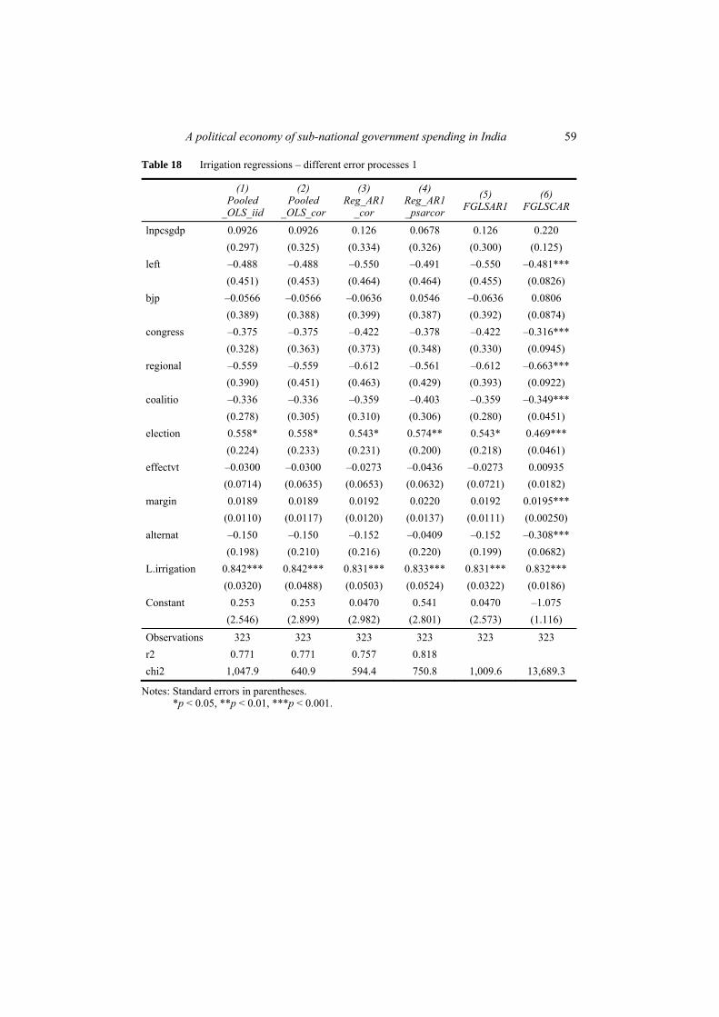
A political economy of sub-national government spending in India 59
Table 18 Irrigation regressions – different error processes 1
(1) Pooled
_OLS_iid
(2) Pooled
_OLS_cor
(3) Reg_AR1
_cor
(4) Reg_AR1_psarcor
(5) FGLSAR1
(6) FGLSCAR
lnpcsgdp 0.0926 0.0926 0.126 0.0678 0.126 0.220 (0.297) (0.325) (0.334) (0.326) (0.300) (0.125) left –0.488 –0.488 –0.550 –0.491 –0.550 –0.481*** (0.451) (0.453) (0.464) (0.464) (0.455) (0.0826) bjp –0.0566 –0.0566 –0.0636 0.0546 –0.0636 0.0806 (0.389) (0.388) (0.399) (0.387) (0.392) (0.0874) congress –0.375 –0.375 –0.422 –0.378 –0.422 –0.316*** (0.328) (0.363) (0.373) (0.348) (0.330) (0.0945) regional –0.559 –0.559 –0.612 –0.561 –0.612 –0.663*** (0.390) (0.451) (0.463) (0.429) (0.393) (0.0922) coalitio –0.336 –0.336 –0.359 –0.403 –0.359 –0.349*** (0.278) (0.305) (0.310) (0.306) (0.280) (0.0451) election 0.558* 0.558* 0.543* 0.574** 0.543* 0.469*** (0.224) (0.233) (0.231) (0.200) (0.218) (0.0461) effectvt –0.0300 –0.0300 –0.0273 –0.0436 –0.0273 0.00935 (0.0714) (0.0635) (0.0653) (0.0632) (0.0721) (0.0182) margin 0.0189 0.0189 0.0192 0.0220 0.0192 0.0195*** (0.0110) (0.0117) (0.0120) (0.0137) (0.0111) (0.00250) alternat –0.150 –0.150 –0.152 –0.0409 –0.152 –0.308*** (0.198) (0.210) (0.216) (0.220) (0.199) (0.0682) L.irrigation 0.842*** 0.842*** 0.831*** 0.833*** 0.831*** 0.832*** (0.0320) (0.0488) (0.0503) (0.0524) (0.0322) (0.0186) Constant 0.253 0.253 0.0470 0.541 0.0470 –1.075 (2.546) (2.899) (2.982) (2.801) (2.573) (1.116)
Observations 323 323 323 323 323 323 r2 0.771 0.771 0.757 0.818 chi2 1,047.9 640.9 594.4 750.8 1,009.6 13,689.3
Notes: Standard errors in parentheses. *p < 0.05, **p < 0.01, ***p < 0.001.
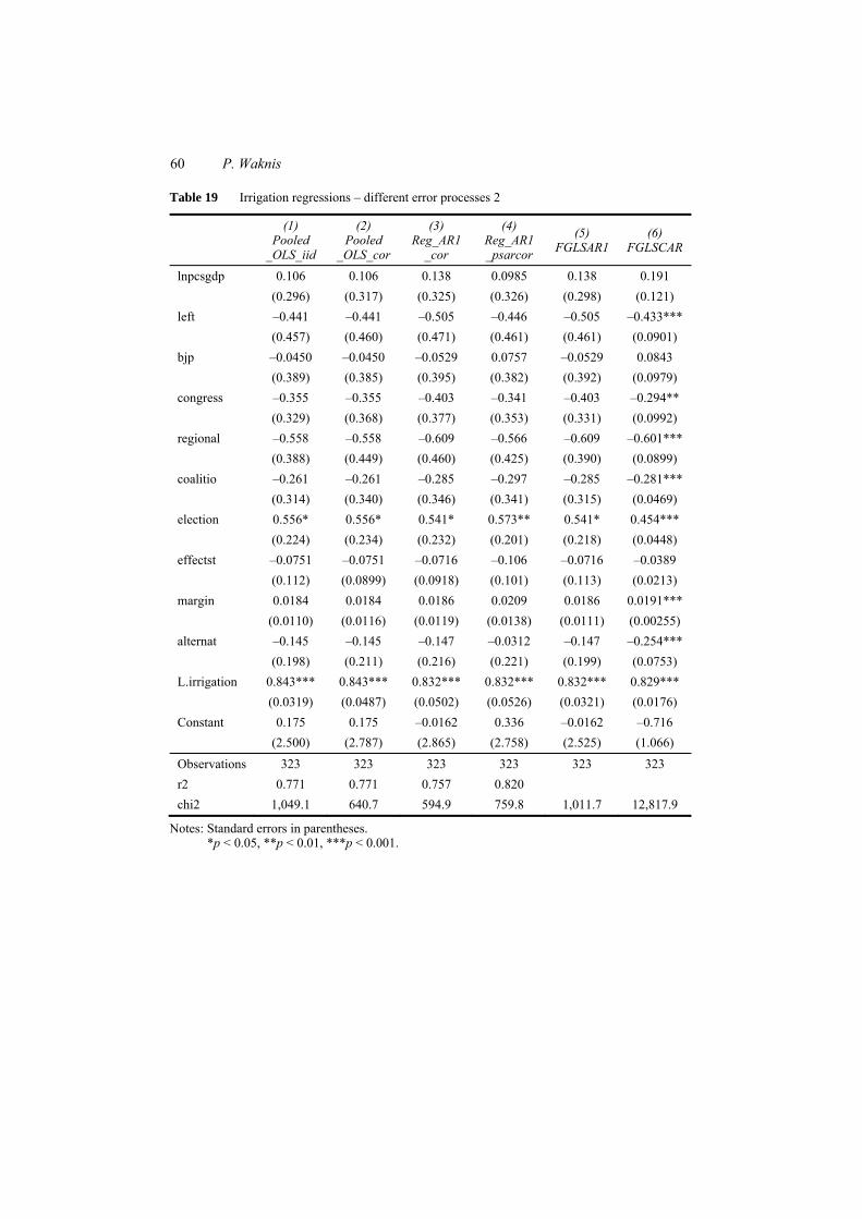
60 P. Waknis
Table 19 Irrigation regressions – different error processes 2
(1) Pooled
_OLS_iid
(2) Pooled
_OLS_cor
(3) Reg_AR1
_cor
(4) Reg_AR1_psarcor
(5) FGLSAR1
(6) FGLSCAR
lnpcsgdp 0.106 0.106 0.138 0.0985 0.138 0.191 (0.296) (0.317) (0.325) (0.326) (0.298) (0.121) left –0.441 –0.441 –0.505 –0.446 –0.505 –0.433*** (0.457) (0.460) (0.471) (0.461) (0.461) (0.0901) bjp –0.0450 –0.0450 –0.0529 0.0757 –0.0529 0.0843 (0.389) (0.385) (0.395) (0.382) (0.392) (0.0979) congress –0.355 –0.355 –0.403 –0.341 –0.403 –0.294** (0.329) (0.368) (0.377) (0.353) (0.331) (0.0992) regional –0.558 –0.558 –0.609 –0.566 –0.609 –0.601*** (0.388) (0.449) (0.460) (0.425) (0.390) (0.0899) coalitio –0.261 –0.261 –0.285 –0.297 –0.285 –0.281*** (0.314) (0.340) (0.346) (0.341) (0.315) (0.0469) election 0.556* 0.556* 0.541* 0.573** 0.541* 0.454*** (0.224) (0.234) (0.232) (0.201) (0.218) (0.0448) effectst –0.0751 –0.0751 –0.0716 –0.106 –0.0716 –0.0389 (0.112) (0.0899) (0.0918) (0.101) (0.113) (0.0213) margin 0.0184 0.0184 0.0186 0.0209 0.0186 0.0191*** (0.0110) (0.0116) (0.0119) (0.0138) (0.0111) (0.00255) alternat –0.145 –0.145 –0.147 –0.0312 –0.147 –0.254*** (0.198) (0.211) (0.216) (0.221) (0.199) (0.0753) L.irrigation 0.843*** 0.843*** 0.832*** 0.832*** 0.832*** 0.829*** (0.0319) (0.0487) (0.0502) (0.0526) (0.0321) (0.0176) Constant 0.175 0.175 –0.0162 0.336 –0.0162 –0.716 (2.500) (2.787) (2.865) (2.758) (2.525) (1.066)
Observations 323 323 323 323 323 323 r2 0.771 0.771 0.757 0.820 chi2 1,049.1 640.7 594.9 759.8 1,011.7 12,817.9
Notes: Standard errors in parentheses. *p < 0.05, **p < 0.01, ***p < 0.001.

A political economy of sub-national government spending in India 61
Table 20 Irrigation regressions – per capita SGDP and LDV_1
(1) Reg_AR1_psarcor
(2) Reg_AR2_psarcor
(3) Reg_AR3_psarcor
(4) Reg_AR4_psarcor
left –1.871** –0.403 –2.119*** –0.446 (0.625) (0.451) (0.610) (0.461) bjp 0.322 0.104 –0.159 0.0757 (0.689) (0.402) (0.670) (0.382) congress –1.465* –0.318 –1.746** –0.341 (0.585) (0.356) (0.561) (0.353) regional –0.815 –0.519 –1.320 –0.566 (0.718) (0.414) (0.728) (0.425) coalitio –0.974* –0.306 –0.897* –0.297 (0.431) (0.341) (0.432) (0.341) election 0.127 0.575** 0.132 0.573** (0.162) (0.201) (0.163) (0.201) effectst 0.121 –0.101 0.0636 –0.106 (0.191) (0.100) (0.193) (0.101) margin 0.0349 0.0205 0.0376 0.0209 (0.0203) (0.0138) (0.0200) (0.0138) alternat –0.255 –0.0176 –0.223 –0.0312 (0.362) (0.208) (0.366) (0.221) L.irrigation 0.837*** 0.832*** (0.0502) (0.0526) lnpcsgdp 1.832* 0.0985 (0.912) (0.326) Constant 5.552*** 1.132 –10.18 0.336 (0.921) (0.613) (8.057) (2.758) Observations 340 323 340 323 r2 0.161 0.820 0.201 0.820 chi2 20.16 751.6 23.68 759.8
Notes: Standard errors in parentheses. *p < 0.05, **p < 0.01, ***p < 0.001.
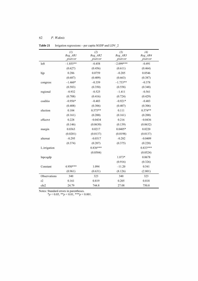
62 P. Waknis
Table 21 Irrigation regressions – per capita SGDP and LDV_2
(1) Reg_AR1 _psarcor
(2) Reg_AR2 _psarcor
(3) Reg_AR3 _psarcor
(4) Reg_AR4 _psarcor
left –1.855** –0.458 –2.099*** –0.491 (0.627) (0.456) (0.611) (0.464) bjp 0.286 0.0759 –0.205 0.0546 (0.687) (0.409) (0.663) (0.387) congress –1.460* –0.359 –1.753** –0.378 (0.583) (0.350) (0.558) (0.348) regional –0.932 –0.525 –1.411 –0.561 (0.708) (0.416) (0.724) (0.429) coalitio –0.956* –0.403 –0.921* –0.403 (0.408) (0.306) (0.407) (0.306) election 0.104 0.575** 0.111 0.574** (0.161) (0.200) (0.161) (0.200) effectvt 0.228 –0.0434 0.216 –0.0436 (0.146) (0.0630) (0.139) (0.0632) margin 0.0363 0.0217 0.0405* 0.0220 (0.0201) (0.0137) (0.0198) (0.0137) alternat –0.295 –0.0317 –0.282 –0.0409 (0.374) (0.207) (0.375) (0.220) L.irrigation 0.836*** 0.833*** (0.0504) (0.0524) lnpcsgdp 1.873* 0.0678 (0.916) (0.326) Constant 4.950*** 1.094 –11.20 0.541 (0.961) (0.631) (8.126) (2.801)
Observations 340 323 340 323 r2 0.161 0.819 0.205 0.818 chi2 24.79 744.8 27.08 750.8
Notes: Standard errors in parentheses. *p < 0.05, **p < 0.01, ***p < 0.001.
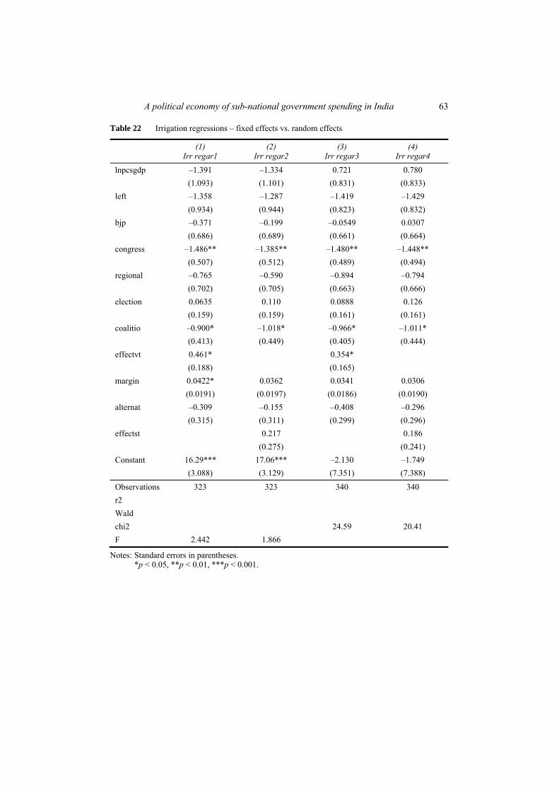
A political economy of sub-national government spending in India 63
Table 22 Irrigation regressions – fixed effects vs. random effects
(1) Irr regar1
(2) Irr regar2
(3) Irr regar3
(4) Irr regar4
lnpcsgdp –1.391 –1.334 0.721 0.780 (1.093) (1.101) (0.831) (0.833) left –1.358 –1.287 –1.419 –1.429 (0.934) (0.944) (0.823) (0.832) bjp –0.371 –0.199 –0.0549 0.0307 (0.686) (0.689) (0.661) (0.664) congress –1.486** –1.385** –1.480** –1.448** (0.507) (0.512) (0.489) (0.494) regional –0.765 –0.590 –0.894 –0.794 (0.702) (0.705) (0.663) (0.666) election 0.0635 0.110 0.0888 0.126 (0.159) (0.159) (0.161) (0.161) coalitio –0.900* –1.018* –0.966* –1.011* (0.413) (0.449) (0.405) (0.444) effectvt 0.461* 0.354* (0.188) (0.165) margin 0.0422* 0.0362 0.0341 0.0306 (0.0191) (0.0197) (0.0186) (0.0190) alternat –0.309 –0.155 –0.408 –0.296 (0.315) (0.311) (0.299) (0.296) effectst 0.217 0.186 (0.275) (0.241) Constant 16.29*** 17.06*** –2.130 –1.749 (3.088) (3.129) (7.351) (7.388) Observations 323 323 340 340 r2 Wald chi2 24.59 20.41 F 2.442 1.866
Notes: Standard errors in parentheses. *p < 0.05, **p < 0.01, ***p < 0.001.
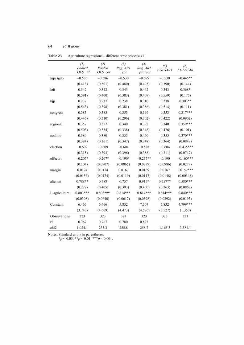
64 P. Waknis
Table 23 Agriculture regressions – different error processes 1
(1) Pooled
_OLS_iid
(2) Pooled
_OLS_cor
(3) Reg_AR1
_cor
(4) Reg_AR1_psarcor
(5) FGLSAR1
(6) FGLSCAR
lnpcsgdp –0.586 –0.586 –0.530 –0.699 –0.530 –0.445** (0.413) (0.501) (0.480) (0.495) (0.390) (0.144) left 0.342 0.342 0.343 0.442 0.343 0.368* (0.591) (0.400) (0.383) (0.409) (0.559) (0.175) bjp 0.237 0.237 0.238 0.310 0.238 0.303** (0.543) (0.398) (0.381) (0.386) (0.514) (0.111) congress 0.383 0.383 0.353 0.399 0.353 0.317*** (0.445) (0.310) (0.296) (0.302) (0.422) (0.0902) regional 0.357 0.357 0.340 0.392 0.340 0.359*** (0.503) (0.354) (0.338) (0.348) (0.476) (0.101) coalitio 0.380 0.380 0.355 0.460 0.355 0.370*** (0.384) (0.361) (0.347) (0.348) (0.364) (0.0849) election –0.609 –0.609 –0.604 –0.528 –0.604 –0.435*** (0.315) (0.393) (0.396) (0.388) (0.311) (0.0747) effectvt –0.207* –0.207* –0.190* –0.237** –0.190 –0.160*** (0.104) (0.0907) (0.0865) (0.0879) (0.0986) (0.0277) margin 0.0174 0.0174 0.0167 0.0169 0.0167 0.0152*** (0.0156) (0.0124) (0.0119) (0.0117) (0.0148) (0.00348) alternat 0.788** 0.788 0.757 0.915* 0.757** 0.580*** (0.277) (0.405) (0.393) (0.400) (0.263) (0.0869) L.agriculture 0.803*** 0.803*** 0.814*** 0.814*** 0.814*** 0.840*** (0.0308) (0.0640) (0.0617) (0.0598) (0.0292) (0.0193) Constant 6.466 6.466 5.832 7.307 5.832 4.799*** (3.740) (4.669) (4.473) (4.576) (3.527) (1.350)
Observations 323 323 323 323 323 323 r2 0.767 0.767 0.780 0.823 chi2 1,024.1 235.3 255.8 258.7 1,165.3 3,581.1
Notes: Standard errors in parentheses. *p < 0.05, **p < 0.01, ***p < 0.001.

A political economy of sub-national government spending in India 65
Table 24 Agriculture regressions – different error processes 2
(1) Pooled
_OLS_iid
(2) Pooled
_OLS_cor
(3) Reg_AR1
_cor
(4) Reg_AR1_psarcor
(5) FGLSAR1
(6) FGLSCAR
lnpcsgdp –0.445 –0.445 –0.386 –0.475 –0.386 –0.361*** (0.407) (0.487) (0.461) (0.465) (0.379) (0.106) left 0.454 0.454 0.448 0.528 0.448 0.567*** (0.602) (0.407) (0.383) (0.415) (0.562) (0.143) bjp 0.274 0.274 0.274 0.336 0.274 0.397*** (0.545) (0.404) (0.380) (0.387) (0.510) (0.0833) congress 0.391 0.391 0.352 0.361 0.352 0.379*** (0.448) (0.310) (0.291) (0.298) (0.420) (0.0731) regional 0.253 0.253 0.243 0.250 0.243 0.328*** (0.500) (0.337) (0.315) (0.323) (0.467) (0.0825) coalitio 0.391 0.391 0.360 0.443 0.360 0.376*** (0.434) (0.397) (0.376) (0.386) (0.407) (0.0600) election –0.624* –0.624 –0.614 –0.547 –0.614* –0.569*** (0.316) (0.397) (0.401) (0.395) (0.313) (0.0497) effectst –0.215 –0.215 –0.195 –0.228 –0.195 –0.178*** (0.159) (0.119) (0.113) (0.118) (0.148) (0.0296) margin 0.0149 0.0149 0.0141 0.0147 0.0141 0.0125*** (0.0157) (0.0124) (0.0117) (0.0117) (0.0146) (0.00229) alternat 0.772** 0.772 0.735 0.839* 0.735** 0.664*** (0.278) (0.412) (0.396) (0.405) (0.261) (0.0595) L.agriculture 0.816*** 0.816*** 0.830*** 0.832*** 0.830*** 0.852*** (0.0298) (0.0653) (0.0621) (0.0607) (0.0279) (0.0170) Constant 4.847 4.847 4.192 4.895 4.192 3.707*** (3.608) (4.440) (4.198) (4.191) (3.355) (0.996)
Observations 323 323 323 323 323 323 r2 0.765 0.765 0.784 0.821 chi2 1,015.2 257.0 288.1 300.3 1,193.2 7,340.1
Notes: Standard errors in parentheses. *p < 0.05, **p < 0.01, ***p < 0.001.
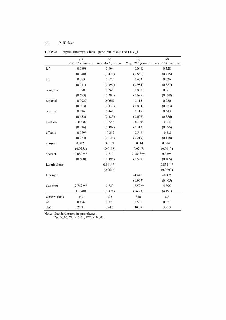
66 P. Waknis
Table 25 Agriculture regressions – per capita SGDP and LDV_1
(1) Reg_AR1_psarcor
(2) Reg_AR2_psarcor
(3) Reg_AR3_psarcor
(4) Reg_AR4_psarcor
left –0.0898 0.394 –0.0483 0.528 (0.940) (0.421) (0.881) (0.415) bjp 0.383 0.173 0.483 0.336 (0.941) (0.390) (0.984) (0.387) congress 1.078 0.268 0.888 0.361 (0.693) (0.297) (0.697) (0.298) regional –0.0927 0.0667 0.115 0.250 (0.803) (0.339) (0.804) (0.323) coalitio 0.336 0.461 0.417 0.443 (0.633) (0.383) (0.606) (0.386) election –0.338 –0.545 –0.348 –0.547 (0.316) (0.399) (0.312) (0.395) effectst –0.579* –0.212 –0.549* –0.228 (0.234) (0.121) (0.219) (0.118) margin 0.0321 0.0174 0.0314 0.0147 (0.0255) (0.0118) (0.0247) (0.0117) alternat 2.082*** 0.747 2.089*** 0.839* (0.608) (0.395) (0.587) (0.405) L.agriculture 0.841*** 0.832*** (0.0616) (0.0607) lnpcsgdp –4.440* –0.475 (1.907) (0.465) Constant 9.769*** 0.723 48.52** 4.895 (1.740) (0.828) (16.73) (4.191) Observations 340 323 340 323 r2 0.476 0.823 0.501 0.821 chi2 25.31 294.7 30.05 300.3
Notes: Standard errors in parentheses. *p < 0.05, **p < 0.01, ***p < 0.001.
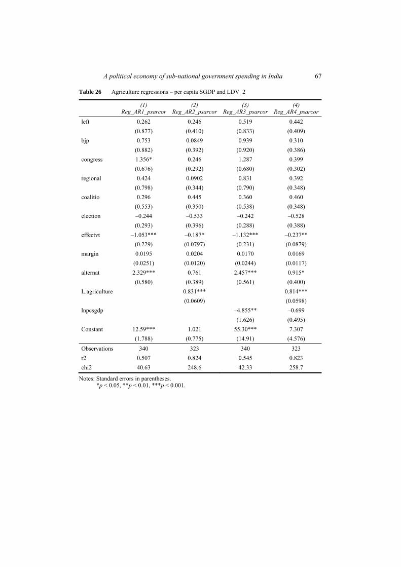
A political economy of sub-national government spending in India 67
Table 26 Agriculture regressions – per capita SGDP and LDV_2
(1) Reg_AR1_psarcor
(2) Reg_AR2_psarcor
(3) Reg_AR3_psarcor
(4) Reg_AR4_psarcor
left 0.262 0.246 0.519 0.442 (0.877) (0.410) (0.833) (0.409) bjp 0.753 0.0849 0.939 0.310 (0.882) (0.392) (0.920) (0.386) congress 1.356* 0.246 1.287 0.399 (0.676) (0.292) (0.680) (0.302) regional 0.424 0.0902 0.831 0.392 (0.798) (0.344) (0.790) (0.348) coalitio 0.296 0.445 0.360 0.460 (0.553) (0.350) (0.538) (0.348) election –0.244 –0.533 –0.242 –0.528 (0.293) (0.396) (0.288) (0.388) effectvt –1.053*** –0.187* –1.132*** –0.237** (0.229) (0.0797) (0.231) (0.0879) margin 0.0195 0.0204 0.0170 0.0169 (0.0251) (0.0120) (0.0244) (0.0117) alternat 2.329*** 0.761 2.457*** 0.915* (0.580) (0.389) (0.561) (0.400) L.agriculture 0.831*** 0.814*** (0.0609) (0.0598) lnpcsgdp –4.855** –0.699 (1.626) (0.495) Constant 12.59*** 1.021 55.30*** 7.307 (1.788) (0.775) (14.91) (4.576) Observations 340 323 340 323 r2 0.507 0.824 0.545 0.823 chi2 40.63 248.6 42.33 258.7
Notes: Standard errors in parentheses. *p < 0.05, **p < 0.01, ***p < 0.001.

68 P. Waknis
Table 27 Agriculture regressions – fixed effects vs. random effects
(1) Agr_regar1
(2) Agr_regar2
(3) Agr_regar3
(4) Agr_regar4
lnpcsgdp –5.368*** –3.808* –7.252*** –6.290*** (1.470) (1.626) (1.162) (1.245) left 0.644 0.580 0.389 0.416 (1.319) (1.315) (1.189) (1.222) bjp 0.421 –0.0328 0.495 0.135 (0.956) (0.973) (0.954) (0.985) congress 0.813 0.534 0.954 0.798 (0.709) (0.722) (0.708) (0.731) regional –0.458 –1.011 –0.383 –0.900 (0.982) (0.993) (0.956) (0.981) election –0.133 –0.271 –0.186 –0.328 (0.226) (0.221) (0.237) (0.234) coalitio 0.434 0.864 0.360 0.577 (0.575) (0.634) (0.585) (0.659) effectvt –1.070*** –1.231*** (0.259) (0.234) margin 0.0149 0.0171 0.0222 0.0258 (0.0265) (0.0279) (0.0267) (0.0283) alternat 2.751*** 2.464*** 2.650*** 2.330*** (0.439) (0.439) (0.431) (0.440) effectst –0.653 –0.688 (0.390) (0.356) Constant 58.21*** 41.64*** 76.43*** 65.14*** (4.554) (4.111) (10.27) (11.04) Observations 323 323 340 340 r2 Wald chi2 110.3 66.75 F 6.820 4.520
Notes: Standard errors in parentheses. *p < 0.05, **p < 0.01, ***p < 0.001.

A political economy of sub-national government spending in India 69
Table 28 Social expenditure regressions – different error processes 1
(1) Reg_iid
(2) Reg_cor
(3) Reg_AR1
_cor
(4) Reg_AR1_psarcor
(5) FGLSAR1
(6) FGLSCAR
lnpcsgdp –0.122 –0.122 –0.130 –0.207 –0.130 –0.0698 (0.215) (0.222) (0.224) (0.210) (0.213) (0.0395) left –0.289 –0.289 –0.286 –0.144 –0.286 –0.254*** (0.307) (0.178) (0.179) (0.202) (0.304) (0.0362) bjp –0.552 –0.552** –0.555** –0.430* –0.555* –0.509*** (0.285) (0.197) (0.199) (0.177) (0.282) (0.0446) congress –0.451* –0.451* –0.451* –0.333 –0.451* –0.409*** (0.228) (0.180) (0.182) (0.174) (0.225) (0.0353) regional –0.240 –0.240 –0.238 –0.171 –0.238 –0.170* (0.260) (0.262) (0.264) (0.277) (0.258) (0.0760) coalitio 0.0877 0.0877 0.0885 0.123 0.0885 0.0854*** (0.198) (0.183) (0.184) (0.196) (0.196) (0.0205) election –0.228 –0.228 –0.227 –0.225 –0.227 –0.222*** (0.163) (0.177) (0.177) (0.171) (0.159) (0.0138) effectvt –0.0542 –0.0542 –0.0555 –0.0834 –0.0555 –0.0521*** (0.0520) (0.0558) (0.0563) (0.0546) (0.0515) (0.00977) margin 0.00593 0.00593 0.00612 0.00570 0.00612 0.00715*** (0.00796) (0.00913) (0.00921) (0.00873) (0.00788) (0.00165) alternat 0.273 0.273 0.278 0.255 0.278 0.245*** (0.144) (0.181) (0.182) (0.172) (0.142) (0.0197) L.socialse 0.715*** 0.715*** 0.711*** 0.701*** 0.711*** 0.722*** (0.0365) (0.0786) (0.0791) (0.0818) (0.0361) (0.0146) Constant 2.034 2.034 2.116 2.827 2.116 1.488*** (1.921) (2.069) (2.089) (1.964) (1.903) (0.363)
Observations 323 323 323 323 323 323 r2 0.617 0.617 0.612 0.625 chi2 501.6 340.0 331.9 356.9 508.5 5,784.7
Notes: Standard errors in parentheses. *p < 0.05, **p < 0.01, ***p < 0.001.
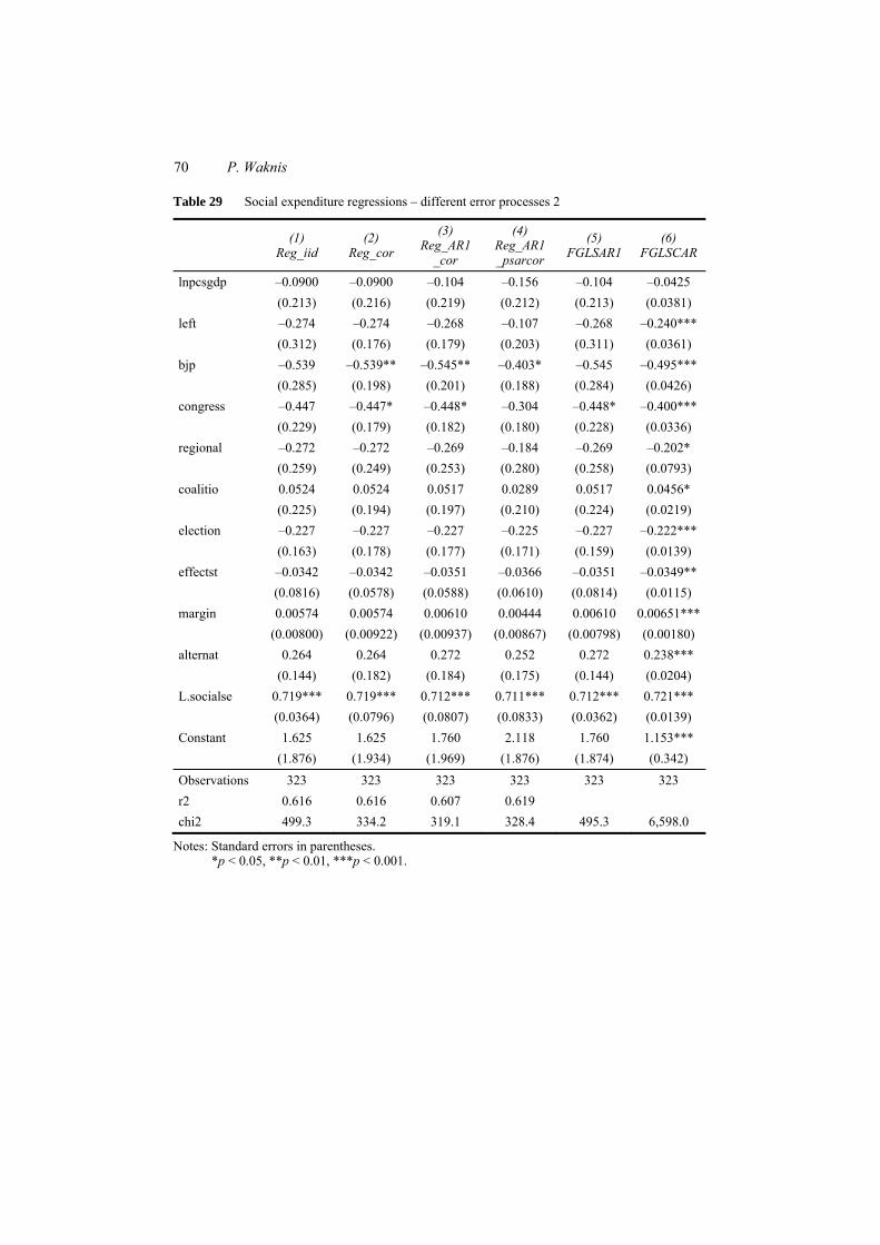
70 P. Waknis
Table 29 Social expenditure regressions – different error processes 2
(1) Reg_iid
(2) Reg_cor
(3) Reg_AR1
_cor
(4) Reg_AR1_psarcor
(5) FGLSAR1
(6) FGLSCAR
lnpcsgdp –0.0900 –0.0900 –0.104 –0.156 –0.104 –0.0425 (0.213) (0.216) (0.219) (0.212) (0.213) (0.0381) left –0.274 –0.274 –0.268 –0.107 –0.268 –0.240*** (0.312) (0.176) (0.179) (0.203) (0.311) (0.0361) bjp –0.539 –0.539** –0.545** –0.403* –0.545 –0.495*** (0.285) (0.198) (0.201) (0.188) (0.284) (0.0426) congress –0.447 –0.447* –0.448* –0.304 –0.448* –0.400*** (0.229) (0.179) (0.182) (0.180) (0.228) (0.0336) regional –0.272 –0.272 –0.269 –0.184 –0.269 –0.202* (0.259) (0.249) (0.253) (0.280) (0.258) (0.0793) coalitio 0.0524 0.0524 0.0517 0.0289 0.0517 0.0456* (0.225) (0.194) (0.197) (0.210) (0.224) (0.0219) election –0.227 –0.227 –0.227 –0.225 –0.227 –0.222*** (0.163) (0.178) (0.177) (0.171) (0.159) (0.0139) effectst –0.0342 –0.0342 –0.0351 –0.0366 –0.0351 –0.0349** (0.0816) (0.0578) (0.0588) (0.0610) (0.0814) (0.0115) margin 0.00574 0.00574 0.00610 0.00444 0.00610 0.00651*** (0.00800) (0.00922) (0.00937) (0.00867) (0.00798) (0.00180) alternat 0.264 0.264 0.272 0.252 0.272 0.238*** (0.144) (0.182) (0.184) (0.175) (0.144) (0.0204) L.socialse 0.719*** 0.719*** 0.712*** 0.711*** 0.712*** 0.721*** (0.0364) (0.0796) (0.0807) (0.0833) (0.0362) (0.0139) Constant 1.625 1.625 1.760 2.118 1.760 1.153*** (1.876) (1.934) (1.969) (1.876) (1.874) (0.342)
Observations 323 323 323 323 323 323 r2 0.616 0.616 0.607 0.619 chi2 499.3 334.2 319.1 328.4 495.3 6,598.0
Notes: Standard errors in parentheses. *p < 0.05, **p < 0.01, ***p < 0.001.

A political economy of sub-national government spending in India 71
Table 30 Social expenditure regressions – per capita SGDP and LDV_1
(1) Reg_AR1_psarcor
(2) Reg_AR2_psarcor
(3) Reg_AR3_psarcor
(4) Reg_AR4_psarcor
left 0.0388 –0.163 0.0167 –0.107 (0.317) (0.167) (0.298) (0.203) bjp –1.064*** –0.489** –0.691* –0.403* (0.319) (0.166) (0.319) (0.188) congress –0.731** –0.353* –0.654* –0.304 (0.272) (0.162) (0.270) (0.180) regional –0.821 –0.261 –0.717 –0.184 (0.525) (0.247) (0.504) (0.280) coalitio 0.303 0.0536 0.215 0.0289 (0.266) (0.200) (0.263) (0.210) election –0.139 –0.227 –0.137 –0.225 (0.130) (0.171) (0.130) (0.171) effectst –0.421** –0.0451 –0.329* –0.0366 (0.142) (0.0594) (0.129) (0.0610) margin 0.0279 0.00448 0.0266 0.00444 (0.0147) (0.00869) (0.0147) (0.00867) alternat 0.760** 0.236 0.733** 0.252 (0.284) (0.169) (0.276) (0.175) L.socialse 0.722*** 0.711*** (0.0767) (0.0833) lnpcsgdp –1.545** –0.156 (0.597) (0.212) Constant 3.462*** 0.801* 16.86** 2.118 (0.609) (0.342) (5.295) (1.876) Observations 340 323 340 323 r2 0.207 0.621 0.226 0.619 chi2 27.66 278.3 32.59 328.4
Notes: Standard errors in parentheses. *p < 0.05, **p < 0.01, ***p < 0.001.
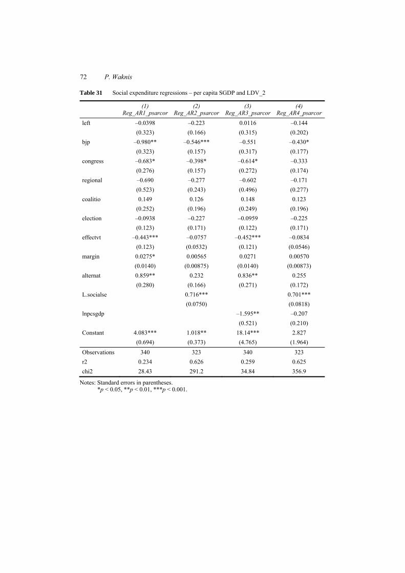
72 P. Waknis
Table 31 Social expenditure regressions – per capita SGDP and LDV_2
(1) Reg_AR1_psarcor
(2) Reg_AR2_psarcor
(3) Reg_AR3_psarcor
(4) Reg_AR4_psarcor
left –0.0398 –0.223 0.0116 –0.144 (0.323) (0.166) (0.315) (0.202) bjp –0.980** –0.546*** –0.551 –0.430* (0.323) (0.157) (0.317) (0.177) congress –0.683* –0.398* –0.614* –0.333 (0.276) (0.157) (0.272) (0.174) regional –0.690 –0.277 –0.602 –0.171 (0.523) (0.243) (0.496) (0.277) coalitio 0.149 0.126 0.148 0.123 (0.252) (0.196) (0.249) (0.196) election –0.0938 –0.227 –0.0959 –0.225 (0.123) (0.171) (0.122) (0.171) effectvt –0.443*** –0.0757 –0.452*** –0.0834 (0.123) (0.0532) (0.121) (0.0546) margin 0.0275* 0.00565 0.0271 0.00570 (0.0140) (0.00875) (0.0140) (0.00873) alternat 0.859** 0.232 0.836** 0.255 (0.280) (0.166) (0.271) (0.172) L.socialse 0.716*** 0.701*** (0.0750) (0.0818) lnpcsgdp –1.595** –0.207 (0.521) (0.210) Constant 4.083*** 1.018** 18.14*** 2.827 (0.694) (0.373) (4.765) (1.964) Observations 340 323 340 323 r2 0.234 0.626 0.259 0.625 chi2 28.43 291.2 34.84 356.9
Notes: Standard errors in parentheses. *p < 0.05, **p < 0.01, ***p < 0.001.
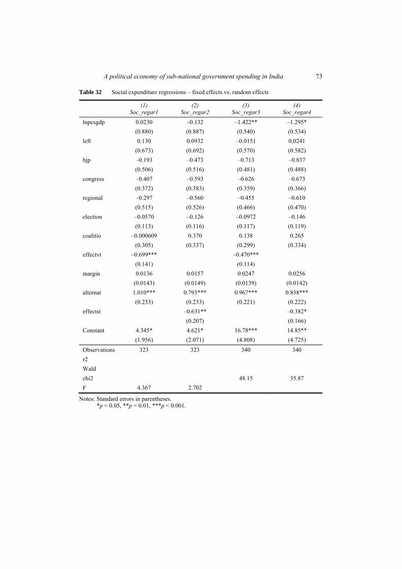
A political economy of sub-national government spending in India 73
Table 32 Social expenditure regressions – fixed effects vs. random effects
(1) Soc_regar1
(2) Soc_regar2
(3) Soc_regar3
(4) Soc_regar4
lnpcsgdp 0.0230 –0.132 –1.422** –1.295* (0.880) (0.887) (0.540) (0.534) left 0.130 0.0932 –0.0151 0.0241 (0.673) (0.692) (0.570) (0.582) bjp –0.193 –0.473 –0.713 –0.837 (0.506) (0.516) (0.481) (0.488) congress –0.407 –0.593 –0.626 –0.673 (0.372) (0.383) (0.359) (0.366) regional –0.297 –0.560 –0.455 –0.610 (0.515) (0.526) (0.466) (0.470) election –0.0570 –0.126 –0.0972 –0.146 (0.113) (0.116) (0.117) (0.119) coalitio –0.000609 0.370 0.138 0.265 (0.305) (0.337) (0.299) (0.334) effectvt –0.699*** –0.470*** (0.141) (0.114) margin 0.0136 0.0157 0.0247 0.0256 (0.0143) (0.0149) (0.0139) (0.0142) alternat 1.010*** 0.793*** 0.967*** 0.838*** (0.233) (0.233) (0.221) (0.222) effectst –0.631** –0.382* (0.207) (0.166) Constant 4.345* 4.621* 16.78*** 14.85** (1.956) (2.071) (4.808) (4.725) Observations 323 323 340 340 r2 Wald chi2 48.15 35.87 F 4.367 2.702
Notes: Standard errors in parentheses. *p < 0.05, **p < 0.01, ***p < 0.001.
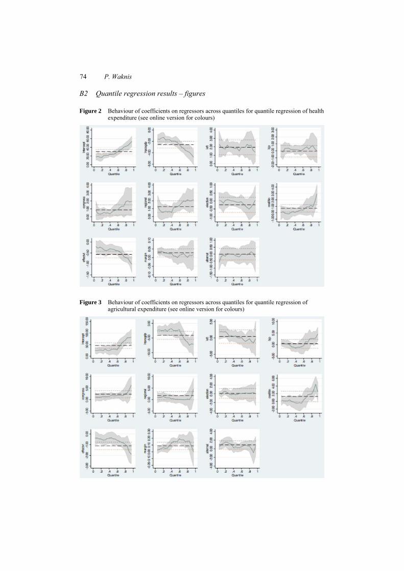
74 P. Waknis
B2 Quantile regression results – figures
Figure 2 Behaviour of coefficients on regressors across quantiles for quantile regression of health expenditure (see online version for colours)
Figure 3 Behaviour of coefficients on regressors across quantiles for quantile regression of agricultural expenditure (see online version for colours)
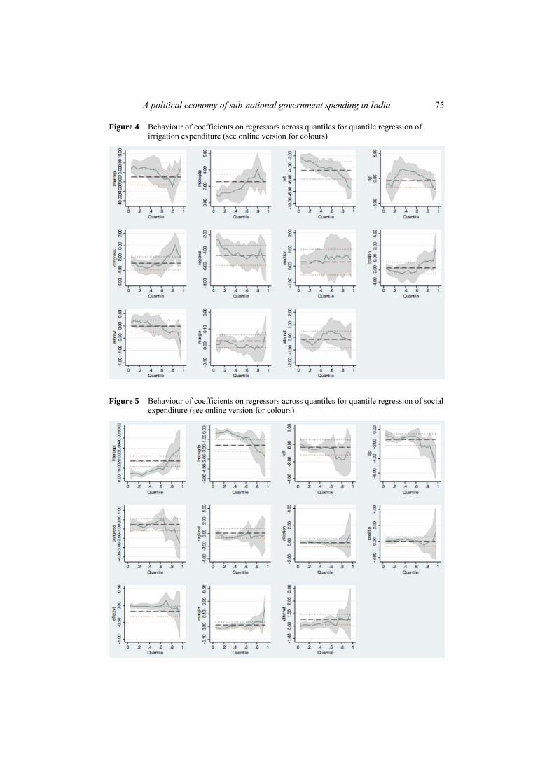
A political economy of sub-national government spending in India 75
Figure 4 Behaviour of coefficients on regressors across quantiles for quantile regression of irrigation expenditure (see online version for colours)
Figure 5 Behaviour of coefficients on regressors across quantiles for quantile regression of social expenditure (see online version for colours)
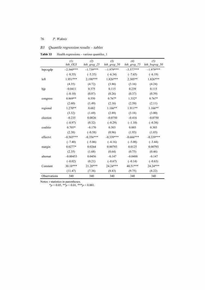
76 P. Waknis
B3 Quantile regression results – tables
Table 33 Health regressions – various quantiles_1
(1) hth_OLS
(2) hth_qreg_25
(3) hth_qreg_50
(4) hth_qreg_75
(5) hth_bsqreg_50
lnpcsgdp –2.560*** –1.739*** –1.979*** –3.577*** –1.979*** (–8.55) (–5.35) (–6.34) (–7.65) (–6.19) left 1.951*** 2.198*** 1.826*** 2.305** 1.826*** (4.35) (4.72) (3.86) (3.16) (4.24) bjp –0.0411 0.375 0.115 0.239 0.115 (–0.10) (0.87) (0.26) (0.37) (0.39) congress 0.869** 0.550 0.767* 1.332* 0.767* (2.60) (1.49) (2.16) (2.59) (2.11) regional 1.270** 0.682 1.166** 1.911** 1.166** (3.32) (1.69) (2.89) (3.18) (3.00) election –0.235 0.0826 –0.0750 –0.416 –0.0750 (–0.97) (0.32) (–0.29) (–1.10) (–0.38) coalitio 0.705* –0.170 0.303 0.885 0.303 (2.38) (–0.58) (0.96) (1.93) (1.03) effectvt –0.565*** –0.356*** –0.339*** –0.666*** –0.339*** (–7.40) (–5.06) (–4.16) (–5.08) (–3.44) margin 0.0277* 0.0264 0.00793 0.0125 0.00793 (2.35) (1.68) (0.64) (0.75) (0.46) alternat –0.00453 0.0456 –0.147 –0.0488 –0.147 (–0.02) (0.21) (–0.67) (–0.14) (–0.63) Constant 30.18*** 21.28*** 24.24*** 40.51*** 24.24*** (11.47) (7.38) (8.83) (9.75) (8.22) Observations 340 340 340 340 340
Notes: t statistics in parentheses. *p < 0.05, **p < 0.01, ***p < 0.001.
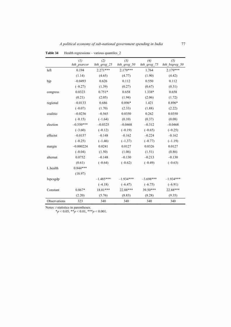
A political economy of sub-national government spending in India 77
Table 34 Health regressions – various quantiles_2
(1) hth_psarcor
(2) hth_qreg_25
(3) hth_qreg_50
(4) hth_qreg_75
(5) hth_bsqreg_50
left 0.194 2.271*** 2.179*** 1.764 2.179*** (1.14) (4.65) (4.77) (1.90) (4.42) bjp –0.0493 0.626 0.112 0.550 0.112 (–0.27) (1.39) (0.27) (0.67) (0.31) congress 0.0323 0.751* 0.658 1.338* 0.658 (0.21) (2.05) (1.94) (2.06) (1.72) regional –0.0133 0.686 0.896* 1.421 0.896* (–0.07) (1.70) (2.33) (1.88) (2.22) coalitio –0.0236 –0.565 0.0350 0.262 0.0350 (–0.15) (–1.64) (0.10) (0.37) (0.08) election –0.550*** –0.0325 –0.0468 –0.312 –0.0468 (–3.60) (–0.12) (–0.19) (–0.65) (–0.25) effectst –0.0157 –0.148 –0.162 –0.224 –0.162 (–0.25) (–1.46) (–1.37) (–0.77) (–1.19) margin –0.000224 0.0241 0.0127 0.0326 0.0127 (–0.04) (1.50) (1.06) (1.51) (0.86) alternat 0.0752 –0.148 –0.130 –0.213 –0.130 (0.61) (–0.64) (–0.62) (–0.49) (–0.63) L.health 0.844*** (18.97) lnpcsgdp –1.485*** –1.934*** –3.698*** –1.934*** (–4.18) (–6.47) (–6.75) (–6.91) Constant 0.867* 18.01*** 22.88*** 39.50*** 22.88*** (2.20) (5.76) (8.83) (8.28) (9.35) Observations 323 340 340 340 340
Notes: t statistics in parentheses. *p < 0.05, **p < 0.01, ***p < 0.001.
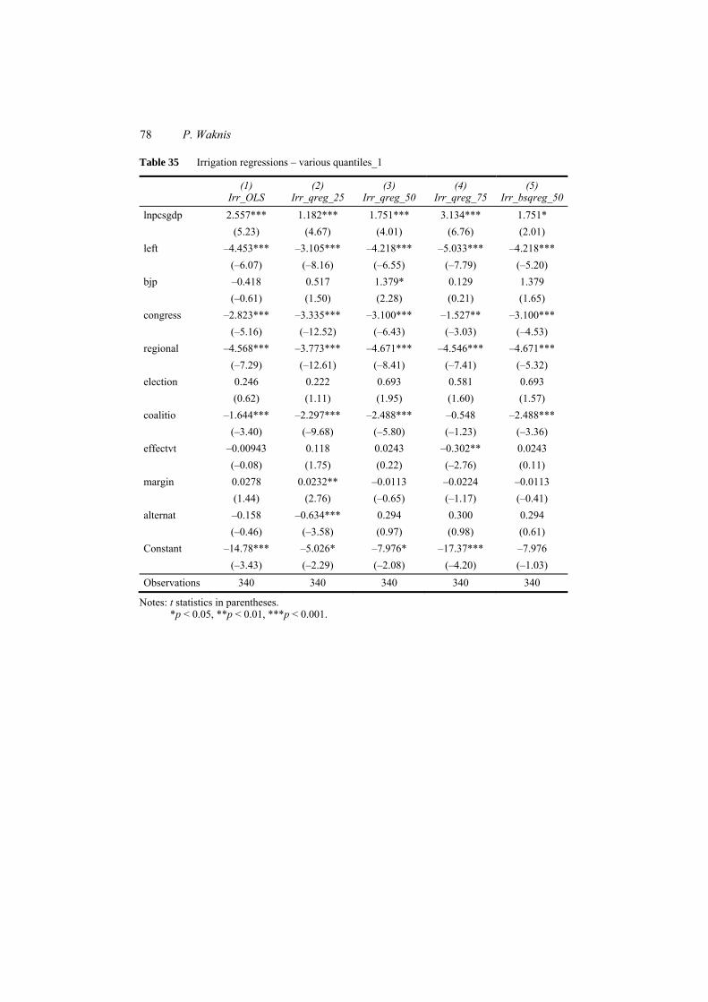
78 P. Waknis
Table 35 Irrigation regressions – various quantiles_1
(1) Irr_OLS
(2) Irr_qreg_25
(3) Irr_qreg_50
(4) Irr_qreg_75
(5) Irr_bsqreg_50
lnpcsgdp 2.557*** 1.182*** 1.751*** 3.134*** 1.751* (5.23) (4.67) (4.01) (6.76) (2.01) left –4.453*** –3.105*** –4.218*** –5.033*** –4.218*** (–6.07) (–8.16) (–6.55) (–7.79) (–5.20) bjp –0.418 0.517 1.379* 0.129 1.379 (–0.61) (1.50) (2.28) (0.21) (1.65) congress –2.823*** –3.335*** –3.100*** –1.527** –3.100*** (–5.16) (–12.52) (–6.43) (–3.03) (–4.53) regional –4.568*** –3.773*** –4.671*** –4.546*** –4.671*** (–7.29) (–12.61) (–8.41) (–7.41) (–5.32) election 0.246 0.222 0.693 0.581 0.693 (0.62) (1.11) (1.95) (1.60) (1.57) coalitio –1.644*** –2.297*** –2.488*** –0.548 –2.488*** (–3.40) (–9.68) (–5.80) (–1.23) (–3.36) effectvt –0.00943 0.118 0.0243 –0.302** 0.0243 (–0.08) (1.75) (0.22) (–2.76) (0.11) margin 0.0278 0.0232** –0.0113 –0.0224 –0.0113 (1.44) (2.76) (–0.65) (–1.17) (–0.41) alternat –0.158 –0.634*** 0.294 0.300 0.294 (–0.46) (–3.58) (0.97) (0.98) (0.61) Constant –14.78*** –5.026* –7.976* –17.37*** –7.976 (–3.43) (–2.29) (–2.08) (–4.20) (–1.03) Observations 340 340 340 340 340
Notes: t statistics in parentheses. *p < 0.05, **p < 0.01, ***p < 0.001.
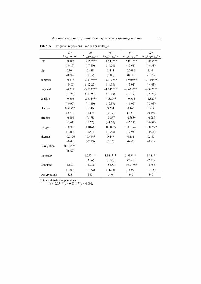
A political economy of sub-national government spending in India 79
Table 36 Irrigation regressions – various quantiles_2
(1) Irr_psarcor
(2) Irr_qreg_25
(3) Irr_qreg_50
(4) Irr_qreg_75
(5) Irr_bsqreg_50
left –0.403 –3.152*** –3.843*** –5.021*** –3.843*** (–0.89) (–7.80) (–4.50) (–7.61) (–4.38) bjp 0.104 0.488 1.444 0.0692 1.444 (0.26) (1.35) (1.85) (0.11) (1.65) congress –0.318 –3.377*** –3.110*** –1.930*** –3.110*** (–0.89) (–12.23) (–4.93) (–3.91) (–4.65) regional –0.519 –3.615*** –4.347*** –4.635*** –4.347*** (–1.25) (–11.93) (–6.09) (–7.77) (–5.78) coalitio –0.306 –2.314*** –1.820** –0.514 –1.820* (–0.90) (–8.29) (–2.89) (–1.02) (–2.03) election 0.575** 0.246 0.214 0.465 0.214 (2.87) (1.17) (0.47) (1.29) (0.49) effectst –0.101 0.178 –0.287 –0.365* –0.287 (–1.01) (1.77) (–1.30) (–2.21) (–0.99) margin 0.0205 0.0166 –0.00977 –0.0174 –0.00977 (1.48) (1.81) (–0.43) (–0.93) (–0.36) alternat –0.0176 –0.484* 0.447 0.181 0.447 (–0.08) (–2.55) (1.13) (0.61) (0.91) L.irrigation 0.837*** (16.67) lnpcsgdp 1.057*** 1.881*** 3.399*** 1.881* (3.96) (3.33) (7.69) (2.23) Constant 1.132 –3.930 –8.653 –19.77*** –8.653 (1.85) (–1.72) (–1.76) (–5.09) (–1.18) Observations 323 340 340 340 340
Notes: t statistics in parentheses. *p < 0.05, **p < 0.01, ***p < 0.001.
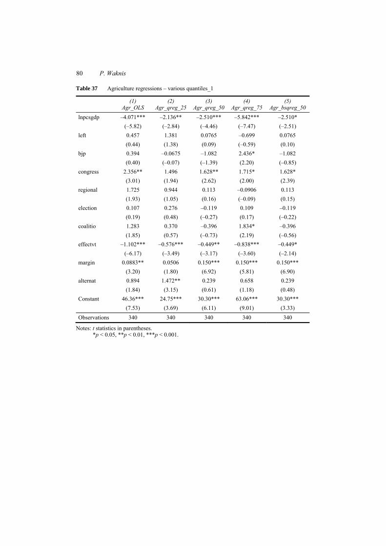
80 P. Waknis
Table 37 Agriculture regressions – various quantiles_1
(1) Agr_OLS
(2) Agr_qreg_25
(3) Agr_qreg_50
(4) Agr_qreg_75
(5) Agr_bsqreg_50
lnpcsgdp –4.071*** –2.136** –2.510*** –5.842*** –2.510* (–5.82) (–2.84) (–4.46) (–7.47) (–2.51) left 0.457 1.381 0.0765 –0.699 0.0765 (0.44) (1.38) (0.09) (–0.59) (0.10) bjp 0.394 –0.0675 –1.082 2.436* –1.082 (0.40) (–0.07) (–1.39) (2.20) (–0.85) congress 2.356** 1.496 1.628** 1.715* 1.628* (3.01) (1.94) (2.62) (2.00) (2.39) regional 1.725 0.944 0.113 –0.0906 0.113 (1.93) (1.05) (0.16) (–0.09) (0.15) election 0.107 0.276 –0.119 0.109 –0.119 (0.19) (0.48) (–0.27) (0.17) (–0.22) coalitio 1.283 0.370 –0.396 1.834* –0.396 (1.85) (0.57) (–0.73) (2.19) (–0.56) effectvt –1.102*** –0.576*** –0.449** –0.838*** –0.449* (–6.17) (–3.49) (–3.17) (–3.60) (–2.14) margin 0.0883** 0.0506 0.150*** 0.150*** 0.150*** (3.20) (1.80) (6.92) (5.81) (6.90) alternat 0.894 1.472** 0.239 0.658 0.239 (1.84) (3.15) (0.61) (1.18) (0.48) Constant 46.36*** 24.75*** 30.30*** 63.06*** 30.30*** (7.53) (3.69) (6.11) (9.01) (3.33) Observations 340 340 340 340 340
Notes: t statistics in parentheses. *p < 0.05, **p < 0.01, ***p < 0.001.
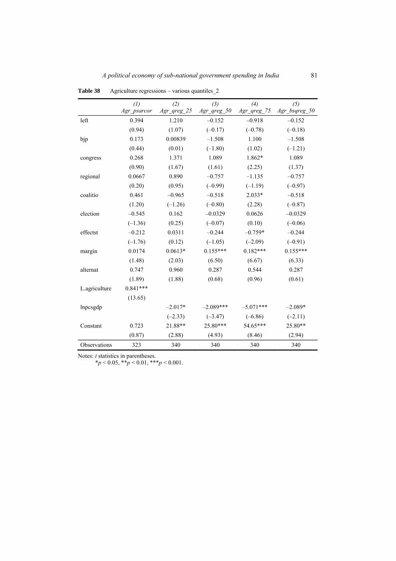
A political economy of sub-national government spending in India 81
Table 38 Agriculture regressions – various quantiles_2
(1) Agr_psarcor
(2) Agr_qreg_25
(3) Agr_qreg_50
(4) Agr_qreg_75
(5) Agr_bsqreg_50
left 0.394 1.210 –0.152 –0.918 –0.152 (0.94) (1.07) (–0.17) (–0.78) (–0.18) bjp 0.173 0.00839 –1.508 1.100 –1.508 (0.44) (0.01) (–1.80) (1.02) (–1.21) congress 0.268 1.371 1.089 1.862* 1.089 (0.90) (1.67) (1.61) (2.25) (1.37) regional 0.0667 0.890 –0.757 –1.135 –0.757 (0.20) (0.95) (–0.99) (–1.19) (–0.97) coalitio 0.461 –0.965 –0.518 2.033* –0.518 (1.20) (–1.26) (–0.80) (2.28) (–0.87) election –0.545 0.162 –0.0329 0.0626 –0.0329 (–1.36) (0.25) (–0.07) (0.10) (–0.06) effectst –0.212 0.0311 –0.244 –0.759* –0.244 (–1.76) (0.12) (–1.05) (–2.09) (–0.91) margin 0.0174 0.0613* 0.155*** 0.182*** 0.155*** (1.48) (2.03) (6.50) (6.67) (6.33) alternat 0.747 0.960 0.287 0.544 0.287 (1.89) (1.88) (0.68) (0.96) (0.61) L.agriculture 0.841*** (13.65) lnpcsgdp –2.017* –2.089*** –5.071*** –2.089* (–2.33) (–3.47) (–6.86) (–2.11) Constant 0.723 21.88** 25.80*** 54.65*** 25.80** (0.87) (2.88) (4.93) (8.46) (2.94) Observations 323 340 340 340 340
Notes: t statistics in parentheses. *p < 0.05, **p < 0.01, ***p < 0.001.
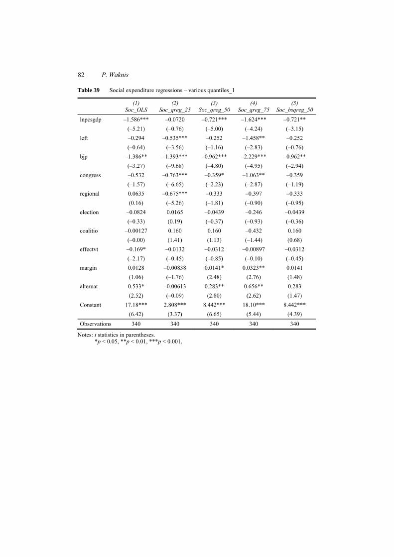
82 P. Waknis
Table 39 Social expenditure regressions – various quantiles_1
(1) Soc_OLS
(2) Soc_qreg_25
(3) Soc_qreg_50
(4) Soc_qreg_75
(5) Soc_bsqreg_50
lnpcsgdp –1.586*** –0.0720 –0.721*** –1.624*** –0.721** (–5.21) (–0.76) (–5.00) (–4.24) (–3.15) left –0.294 –0.535*** –0.252 –1.458** –0.252 (–0.64) (–3.56) (–1.16) (–2.83) (–0.76) bjp –1.386** –1.393*** –0.962*** –2.229*** –0.962** (–3.27) (–9.68) (–4.80) (–4.95) (–2.94) congress –0.532 –0.763*** –0.359* –1.063** –0.359 (–1.57) (–6.65) (–2.23) (–2.87) (–1.19) regional 0.0635 –0.675*** –0.333 –0.397 –0.333 (0.16) (–5.26) (–1.81) (–0.90) (–0.95) election –0.0824 0.0165 –0.0439 –0.246 –0.0439 (–0.33) (0.19) (–0.37) (–0.93) (–0.36) coalitio –0.00127 0.160 0.160 –0.432 0.160 (–0.00) (1.41) (1.13) (–1.44) (0.68) effectvt –0.169* –0.0132 –0.0312 –0.00897 –0.0312 (–2.17) (–0.45) (–0.85) (–0.10) (–0.45) margin 0.0128 –0.00838 0.0141* 0.0323** 0.0141 (1.06) (–1.76) (2.48) (2.76) (1.48) alternat 0.533* –0.00613 0.283** 0.656** 0.283 (2.52) (–0.09) (2.80) (2.62) (1.47) Constant 17.18*** 2.808*** 8.442*** 18.10*** 8.442*** (6.42) (3.37) (6.65) (5.44) (4.39) Observations 340 340 340 340 340
Notes: t statistics in parentheses. *p < 0.05, **p < 0.01, ***p < 0.001.
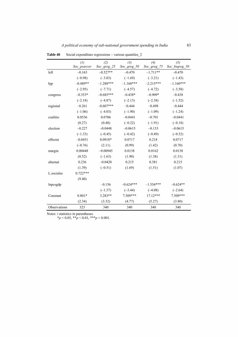
A political economy of sub-national government spending in India 83
Table 40 Social expenditure regressions – various quantiles_2
(1) Soc_psarcor
(2) Soc_qreg_25
(3) Soc_qreg_50
(4) Soc_qreg_75
(5) Soc_bsqreg_50
left –0.163 –0.527** –0.470 –1.711** –0.470 (–0.98) (–3.03) (–1.69) (–3.21) (–1.43) bjp –0.489** –1.288*** –1.160*** –2.215*** –1.160*** (–2.95) (–7.71) (–4.57) (–4.72) (–3.58) congress –0.353* –0.685*** –0.438* –0.909* –0.438 (–2.18) (–4.87) (–2.13) (–2.38) (–1.52) regional –0.261 –0.607*** –0.444 –0.498 –0.444 (–1.06) (–4.03) (–1.90) (–1.09) (–1.24) coalitio 0.0536 0.0706 –0.0441 –0.701 –0.0441 (0.27) (0.48) (–0.22) (–1.91) (–0.18) election –0.227 –0.0448 –0.0615 –0.133 –0.0615 (–1.33) (–0.45) (–0.42) (–0.49) (–0.52) effectst –0.0451 0.0918* 0.0717 0.218 0.0717 (–0.76) (2.11) (0.99) (1.42) (0.70) margin 0.00448 –0.00945 0.0138 0.0162 0.0138 (0.52) (–1.63) (1.90) (1.38) (1.31) alternat 0.236 –0.0420 0.215 0.381 0.215 (1.39) (–0.51) (1.69) (1.51) (1.07) L.socialse 0.722*** (9.40) lnpcsgdp –0.156 –0.624*** –1.554*** –0.624** (–1.37) (–3.44) (–4.08) (–2.64) Constant 0.801* 3.283** 7.509*** 17.12*** 7.509*** (2.34) (3.32) (4.77) (5.27) (3.80) Observations 323 340 340 340 340
Notes: t statistics in parentheses. *p < 0.05, **p < 0.01, ***p < 0.001.


![Structural and thermoelectric properties of Bi[sub 2]Sr[sub 2]Co[sub 2]O[sub y] thin films on LaAlO[sub 3] (100) and fused silica substrates](https://static.fdokumen.com/doc/165x107/634467196cfb3d406409325f/structural-and-thermoelectric-properties-of-bisub-2srsub-2cosub-2osub-y.jpg)