A Performance Study

of BDD-Based Model Checking

Bwolen Yang1, Randal E. Bryant1, David R. O'Hallaron1,Armin Biere1, Olivier Coudert2, Geert Janssen3,

Rajeev K. Ranjan2, and Fabio Somenzi4

1 Carnegie Mellon University, Pittsburgh PA 15213, USA2 Synopsys Inc., Mountain View CA 94043, USA

3 Eindhoven University of Technology, 5600 MB Eindhoven, Netherlands4 University of Colorado, Boulder CO 90309, USA

Abstract. We present a study of the computational aspects of modelchecking based on binary decision diagrams (BDDs). By using a trace-based evaluation framework, we are able to generate realistic benchmarksand perform this evaluation collaboratively across several di�erent BDDpackages. This collaboration has resulted in signi�cant performance im-provements and in the discovery of several interesting characteristics ofmodel checking computations. One of the main conclusions of this workis that the BDD computations in model checking and in building BDDsfor the outputs of combinational circuits have fundamentally di�erentperformance characteristics. The systematic evaluation has also uncov-ered several open issues that suggest new research directions. We hopethat the evaluation methodology used in this study will help lay thefoundation for future evaluation of BDD-based algorithms.

1 Introduction

The binary decision diagram (BDD) has been shown to be a powerful tool informal veri�cation. Since Bryant's original publication of BDD algorithms [7],there has been a great deal of research in the area [8, 9]. One of the mostpowerful applications of BDDs has been to symbolic model checking, used toformally verify digital circuits and other �nite state systems. Characterizationsand comparisons of new BDD-based algorithms have historically been based ontwo sets of benchmark circuits: ISCAS85 [6] and ISCAS89 [5]. There has beenlittle work on characterizing the computational aspects of BDD-based modelchecking.

There are two qualitative di�erences between building BDD representationsfor combinational circuits versus model checking. The �rst di�erence is that forcombinational circuits, the output BDDs (BDD representations for the circuitoutputs) are built and then are only used for constant-time equivalence checking.In contrast, a model checker �rst builds the BDD representations for the sys-tem transition relation, and then performs a series of �xed point computations

analyzing the state space of the system. In doing so, it is solving PSPACE-complete problems. Another di�erence is that BDD construction algorithms forcombinational circuit operations have polynomial complexity [7], while the keyoperations in model checking are NP-hard [16]. These di�erences indicate thatresults based on combinational circuit benchmarks may not accurately charac-terize BDD computations in model checking.

This paper introduces a new methodology for the systematic evaluation ofBDD computations, and then applies this methodology to gain a better under-standing of the computational aspects of model checking. The evaluation is acollaborative e�ort among many BDD package designers. As results of this eval-uation, we have signi�cantly improved model checking performance, and haveidenti�ed some open problems and new research directions.

The evaluation methodology is based on a trace-driven framework whereexecution traces are recorded from veri�cation tools and then replayed on severalBDD packages. In this study, the benchmark consists of 16 execution traces fromthe Symbolic Model Veri�er (SMV) [16]. For comparison with combinationalcircuits, we also studied 4 circuit traces derived from the ISCAS85 benchmark.The other part of our evaluation methodology is a set of platform independentmetrics. Throughout this study, we have identi�ed useful metrics to measurework, space, and memory locality.

This systematic and collaborative evaluation methodology has led to bet-ter understanding of the e�ects of cache size and garbage collection frequency,and has also resulted in signi�cant performance improvement for model checkingcomputations. Systematic evaluation also uncovered vast di�erences in the com-putational characteristics of model checking and combinational circuits. Thesedi�erences include the e�ects of the cache size, the garbage collection frequency,the complement edge representation [1], and the memory locality of the breadth-�rst BDD packages. For the di�cult issue of dynamic variable reordering, weintroduce some methodologies for studying the e�ects of variable reordering al-gorithms and initial variable orders.

It is important to note that the results in this study are obtained basedon a very small sample of all possible BDD-based model checking computations.Thus, in the subsequent sections, most of the results are presented as hypothesesalong with their supporting evidence. These results are not conclusive. Instead,they raise a number of interesting issues and suggest new research directions.

The rest of this paper is organized as follows. We �rst present a brief overviewof BDDs and relevant BDD algorithms (Sec. 2) and then describe the experi-mental setup for the study (Sec. 3). This is followed by three sections of experi-mental results. First, we report the �ndings without dynamic variable reordering(Sec. 4). Then, we present the results on dynamic variable reordering algorithmsand the e�ects of initial variable orders (Sec. 5). Third, we present results thatmay be generally helpful in studying or improving BDD packages (Sec. 6). Afterthese result sections, we discuss some unresolved issues (Sec. 7) and then wrapup with related work (Sec. 8) and concluding remarks (Sec. 9).

2 Overview

This section gives a brief overview of BDDs and pertinent BDD algorithms.Detailed descriptions can be found in [7] and [16].

2.1 BDD Basics

A BDD is a directed acyclic graph (DAG) representation of a Boolean func-tion where equivalent Boolean sub-expressions are uniquely represented. Dueto this uniqueness property, a BDD can be exponentially more compact thanits corresponding truth table representation. One criterion for guaranteeing theuniqueness of the BDD representation is that all the BDDs constructed mustfollow the same variable order. The choice of this variable order can have asigni�cant impact on the size of the BDD graph.

BDD construction is a memoization-based dynamic programming algorithm.Due to the large number of distinct subproblems, a cache, known as the com-puted cache, is used instead of a memoization table. Given a Boolean opera-tion, the construction of its BDD representation consists of two main phases. Inthe top-down expansion phase, the Boolean operation is recursively decomposedinto subproblems based on the Shannon decomposition. In the bottom-up re-duction phase, the result of each subproblem is put into the canonical form. Theuniqueness of the result's representation is enforced by hash tables known asunique tables. The new subproblems are generally recursively solved in a depth-�rst order as in Bryant's original BDD publication [7]. Recently, there has beensome work that tries to exploit memory locality by using a breadth-�rst or-der [2, 18, 19, 21, 26].

Before moving on, we �rst de�ne some terminology. We will refer to theBoolean operations issued by a user of a BDD package as the top-level operationsto distinguish them from sub-operations (subproblems) generated internally bythe Shannon expansion process. A BDD node is reachable if it is in some BDDsthat external users have references to. As external users free references to BDDs,some BDD nodes may no longer be reachable. We will refer to these nodes asunreachable BDD nodes. Note that unreachable BDD nodes can still be refer-enced within a BDD package by either the unique tables or the computed cache.Some of these unreachable BDD nodes may become reachable again if they endup being the results for new subproblems. When a reachable BDD node becomesunreachable, we say a death has occurred. Similarly, when an unreachable BDDnode becomes reachable again, we say a rebirth has occurred. We de�ne the deathrate as the number of deaths over the number of subproblems (time) and de�nethe rebirth rate as the fraction of the unreachable nodes that become reachableagain, i.e., the number of rebirths over the number of deaths.

2.2 Common Implementation Features

Modern BDD packages typically share the following common implementationfeatures based on [4, 22]. The BDD construction is based on depth-�rst traversal.

The unique tables are hash tables with the hash collisions resolved by chaining.A separate unique table is associated with each variable to facilitate the dynamicvariable reordering process. The computed cache is a hash-based direct mapped(1-way associative) cache. BDD nodes support complement edges where, for eachedge, an extra bit is used to indicate whether or not the target function shouldbe inverted. Garbage collection of unreachable BDD nodes is based on referencecounting and the reclaimed unreachable nodes are maintained in a free-list forlater reuse. Garbage collection is invoked when the percentage of the unreachableBDD nodes exceeds a preset threshold.

As the variable order can have signi�cant impact on the size of a BDD graph,dynamic variable reordering is an essential part of all modern BDD packages. Thedynamic variable reordering algorithms are generally based on sifting or windowpermutation algorithms [22]. Typically, when a variable reordering algorithm isinvoked, all top-level operations that are currently being processed are aborted.When the variable reordering algorithm terminates, these aborted operationsare restarted from the beginning.

2.3 Model Checking and Relational Product

There are two popular BDD-based algorithms for computing state transitions:one is based on applying the relational product operator (also known asAndExistsor and-smooth) on the transition relations and the state sets [10]; the other isbased on applying the constrain operator to Boolean functional vectors [11, 12].

The benchmarks in this study are based on SMV, which uses the relationalproduct operation. This operation computes \9v:f ^ g" and is used to computethe set of states by the forward or the backward state transitions. It has beenproven to be NP-hard [16]. Figure 1 shows a typical BDD algorithm for comput-ing the relational product operation. This algorithm is structurally very similarto the BDD-based algorithm for the AND Boolean operation. The main di�er-ence (lines 5{11) is that when the top variable (�) needs to be quanti�ed, a newBDD operation (OR(r0, r1)) is generated. Due to this additional recursion, theworst case complexity of this algorithm is exponential in the graph size of theinput arguments.

3 Setup

3.1 Benchmark

The benchmark used in this study is a set of execution traces gathered fromthe Symbolic Model Veri�er (SMV) [16] from Carnegie Mellon University. Thetraces were gathered by recording BDD function calls made during the executionof SMV. To facilitate the porting process for di�erent packages, we only recordeda set of the key Boolean operations and discarded all word-level operations. Thecoverage of this selected set of BDD operations is greater than 95% of the totalSMV execution time for all but one case (abp11) which spends 21% of CPU timein the word-level functions constructing the transition relation.

RP(v, f , g)/* compute relational product: 9v:f ^ g */

1 if (terminal case) return result2 if the result of (RP, v, f , g) is cached, return the result3 let � be the top variable of f and g

4 r0 RP(v, f j� 0, gj� 0) /* Shannon expansion on 0-cofactors */5 if (� 2 v) /* existential quanti�cation on � � OR(r0, RP(v, f j� 1, gj� 1)) */6 if (r0 == true) /* OR(true, RP(v, f j� 1, gj� 1)) � true */7 r true.8 else9 r1 RP(v, f j� 1, gj� 1) /* Shannon expansion on 1-cofactors */10 r OR(r0, r1)11 else12 r1 RP(v, f j� 1, gj� 1) /* Shannon expansion on 1-cofactors */13 r reduced, unique BDD node for (� , r0, r1)14 cache the result of this operation15 return r

Fig. 1. A typical relational product algorithm.

A side e�ect of recording only a subset of BDD operations is that the con-struction process of some BDDs is skipped, and these BDDs might be neededlater by some of the selected operations. Thus in the trace �le, these BDDs needto be reconstructed before their �rst reference. This reconstruction is performedbottom-up using the If-Then-Else operation. This process is based on the prop-erty that each BDD node (vi, child0, child1) essentially represents the Booleanfunction \If vi then child1 else child0".

For this study, we have selected 16 SMV models to generate the traces. Thefollowing is a brief description of these models along with their sources.

abp11: alternating bit protocol.Source: Armin Biere, Universit�at Karlsruhe.

dartes: communication protocol of an Ada program.dpd75: dining philosophers protocol.ftp3: �le transfer protocol.furnace17: remote furnace program.key10: keyboard/screen interaction protocol in a window manager.mmgt20: distributed memory manager protocol.over12: automated highway system overtake protocol.

Source: James Corbett, University of Hawaii.

dme2-16: distributed mutual exclusion protocol.Source: SMV distribution, Carnegie Mellon University.

futurebus: futurebus cache coherence protocol.Source: Somesh Jha, Carnegie Mellon University.

motor-stuck: batch-reactor system model.valves-gates: batch-reactor system model.

Source: Adam Turk, Carnegie Mellon University.

phone-async: asynchronous model of a simple telephone system.phone-sync-CW: synchronous model of a telephone system with call

waiting.Source: Malte Plath and Mark Ryan, University of Birmingham,Great Britain.

tcas: tra�c alert and collision system for airplanes.Source: William Chan, University of Washington.

tomasulo: a buggy model of the Tomasulo algorithm for instructionscheduling in superscalar processors.Source: Yunshan Zhu, Carnegie Mellon University.

As we studied and improved on the model checking computations during thecourse of the study, we compared their performance with the BDD constructionof combinational circuit outputs. For this comparison, we used the ISCAS85benchmark circuits as the representative circuits. We chose these benchmarksbecause they are perhaps the most popular benchmarks used for BDD perfor-mance evaluations. The ISCAS85 circuits were converted into the same formatas the model checking traces. The variable orders used were generated by theorder-dfs in SIS [24]. We excluded cases that were either too small (< 5 CPUseconds) or too large (> 1 GBytes of memory requirement). Based on this crite-ria, we were left with two circuits | C2670 and C3540. To obtain more circuits,we derived 13-bit and 14-bit integer multipliers, based on the C6288, which werefer to as C6288-13 and C6288-14. For the multipliers, the variable order isan�1 � an�2 � ::: � a0 � bn�1 � bn�2 � ::: � b0, where A =

Pn�1

i=0 2iai and

B =Pn�1

i=0 2ibi are the two n-bit input operands to the multiplier.Figure 2 quanti�es the sizes of the traces we used in the study. The statistic

\# of BDD Vars" is the number of BDD variables used. The statistic \Min. #of Ops" is the minimum number of sub-operations (or subproblems) needed forthe computation. This statistic characterizes the minimum amount of work foreach trace. It was gathered using a BDD package with a complete cache and nogarbage collection. Thus, this statistic represents the minimum number of sub-operations needed for a typical BDD package. Due to insu�cient memory, thereare 4 cases (futurebus, phone-sync-CW, tcas, tomasulo) for which we were notable to collect this statistic. For these cases, the results shown are the minimumacross all the packages used in the study. These results are marked with the\<" symbol. The third statistic, \Peak # of Live BDDs", represents the peaknumber of reachable BDD nodes during the execution. It provides a lower bound

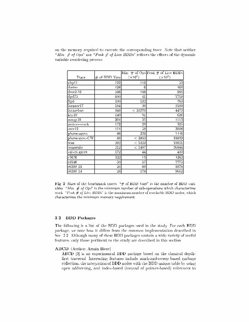
on the memory required to execute the corresponding trace. Note that neither\Min. # of Ops" nor \Peak # of Live BDDs" re ects the e�ects of the dynamicvariable reordering process.

Min. # of Ops Peak # of Live BDDsTrace # of BDD Vars (�106) (�103)

abp11 122 116 53

dartes 198 6 468

dme2-16 586 106 905

dpd75 600 41 1719

ftp3 100 132 763

furnace17 184 30 2109

futurebus 348 < 10270 4473

key10 140 91 626

mmgt20 264 35 1113

motors-stuck 172 29 325

over12 174 58 3008

phone-async 86 329 1446

phone-sync-CW 88 < 3803 22829

tcas 292 < 1323 19921

tomasulo 212 < 1497 26944

valves-gates 172 44 433

c2670 233 15 4363

c3540 50 57 7775

c6288-13 26 60 3378

c6288-14 28 178 9662

Fig. 2. Sizes of the benchmark traces. \# of BDD Vars" is the number of BDD vari-ables. \Min. # of Ops" is the minimum number of sub-operations which characterizeswork. \Peak # of Live BDDs" is the maximum number of reachable BDD nodes, whichcharacterizes the minimum memory requirement.

3.2 BDD Packages

The following is a list of the BDD packages used in the study. For each BDDpackage, we note how it di�ers from the common implementation described inSec. 2.2. Although many of these BDD packages contain a wide variety of usefulfeatures, only those pertinent to the study are described in this section.

ABCD (Author: Armin Biere)ABCD [3] is an experimental BDD package based on the classical depth-�rst traversal. Interesting features include mark-and-sweep based garbagecollection, the integration of BDD nodes with the BDD unique table by usingopen addressing, and index-based (instead of pointer-based) references to

BDD nodes. These techniques reduce the BDD node size by half (2 machinewords instead of 4). In addition, to avoid clustering in open addressing,ABCD uses a quadratic probe sequence for the hashing collision resolution.

CAL (Authors: Rajeev Ranjan and Jagesh Sanghavi)CAL [20] is a publicly available BDD package based on breadth-�rst traver-sal to exploit memory locality. The garbage collection algorithm is based onreference-counting with memory compaction. To increase locality of refer-ence, each BDD node contains the indices of its cofactor nodes. To keep thenode size to 4 machine words, bit tagging is used to store and retrieve thevalue of the reference count of a node. For this study, the relational productoperation is based on the depth-�rst traversal with the quanti�cation step(line 7 in Fig. 1) computed using the breadth-�rst traversal.

CUDD (Author: Fabio Somenzi)CUDD [25] is a publicly available BDD package based on depth-�rst traver-sal. In CUDD, the reference counts of the nodes are kept up-to-date through-out the computation. To counter the impact on performance of these updateswhen many nodes are freed and reclaimed, CUDD enqueues the requests forupdates and performs them only if they are still valid when they are ex-tracted from the queue. The growth of the tables in CUDD is determined bya reward policy. For instance, the cache grows if the hit rate is high. CUDDpartially sorts the free list during garbage collection to improve memorylocality. Another distinguishing feature is that CUDD contains a suite ofheuristics for dynamic variable reordering.

EHV (Author: Geert Janssen)EHV [14] is a publicly available BDD package based on depth-�rst traver-sal. The main di�erences from the common implementation are additionalsupport for inverted inputs [17] and provisions for user data to be attachedto a BDD node. The latter feature allows intermediate results to be storedin the BDD nodes, which in turn, removes the need to use separate com-puted caches for some special BDD operations. This feature incurs a memoryoverhead of 2 extra machine words per BDD node.

PBF (Authors: Bwolen Yang and Yirng-An Chen)PBF [26] is an experimental BDD package based on partial breadth-�rsttraversal. The partial breadth-�rst traversal along with per-variable memorymanagers and the memory-compacting mark-and-sweep garbage collectorare used to exploit memory locality. The partial breadth-�rst traversal alsobounds the breadth-�rst expansion to avoid the potential excessive memoryoverhead of a full breadth-�rst expansion.

TiGeR (Authors: Olivier Coudert, Jean C. Madre and Herve Touati)TiGeR [13] is a commercial BDD package based on the depth-�rst approach.Interesting features include the segmentation of the computed caches andthe garbage collection algorithm. In TiGeR, each operation type has its owncache. This allows the caches to be tuned independently. For this study, thecaches for the non-polynomial operations such as relational product are setto be about four times as sparse as the caches for the polynomial operations.TiGeR's garbage collection algorithm is di�erent from typical garbage col-

lection algorithms in two ways: the free-list is sorted to maintain memorylocality, and the memory compaction is performed when memory resourcesbecome critical.

3.3 Evaluation Process

The performance study was carried out in two phases. The �rst phase studiedperformance issues in BDD construction without variable reordering. The secondphase focused on the dynamic variable reordering computation. The evaluationprocess was iterative, with the study evolving dynamically as new issues wereraised and new insights gained. Based on the results from each iteration, wecollaboratively tried to identify the performance issues and possible improve-ments. Each BDD package designer then incorporated and validated the sug-gested improvements. During this iterative process, we also tried to hypothesizethe characteristics of the computation and design new experiments to test thesehypotheses.

4 Phase 1 Results: No Variable Reordering

Figure 3 presents the overall performance improvements for Phase 1 with dy-namic variable reordering disabled. There are 6 packages and 16 model checkingtraces, for a total of 96 cases. Figure 3(a) categorizes the results for these casesbased on speedups. Note that the speedups are plotted in a cumulative fashion;i.e., the > x column represents the total number of cases with speedups greaterthan x. Figure 3(b) presents a comparison between the initial timing results(when we �rst started the study) and the current timing results (after the au-thors made changes to their packages based on insights gained from previousiterations). The n/a results represent cases where results could not be obtained.

Initially, 19 cases did not complete because of implementation bugs or mem-ory limits. Currently, 13 of these 19 cases now complete (the new cases in the�gures). The other 6 cases still do not complete within the the resource limitof 8 hours and 900 MBytes (the failed cases in the �gures). There is one case(the bad case in the charts) that initially completed, but now does not completewithin the memory limit.

Figure 3(a) shows that signi�cant speedups have been obtained for manycases. Most notably, 22 cases have speedups greater than an order of magnitude(the > 10 column), and 6 out of these 22 cases actually achieve speedups greaterthan two orders of magnitude (the > 100 column)!

Figure 3(b) shows that signi�cant speedups have been obtained mostly fromthe small to medium traces, although some of the larger traces have achievedspeedups greater than 3. Another interesting point is that the new cases (thosethat initially failed but are now doable) range across small to large traces.

Overall, for the 76 cases where the comparison could be made, the total CPUtime was reduced from 554,949 seconds to 127,786 seconds | a speedup of 4.34.Another interesting overall statistic is that initially none of the 6 BDD packages

could complete all 16 traces, but currently 3 BDD packages can complete all ofthem.

Cumulative Speedup Histogram

22

33

61

75 76 76

136

16

0

10

20

30

40

50

60

70

80

>10

0

>10 >

5

>2

>1

>0.

95 >0

new

faile

d

bad

speedups

# of

cas

es

(a)

Time Comparison

10

100

1000

10000

100000

1000000

10 100 1000 10000 100000 1000000

current results (sec)in

itia

l res

ults

(se

c)

newfailedbadrest

1x10x100x

n/a

n/a

(b)

Fig. 3. Overall results. The new cases represent the number of cases that failed initiallyand are now doable. The failed cases represent those that currently still exceed thelimits of 8 CPU hours and 900 MBytes. The bad shows the case that �nished initially,but cannot complete currently. The rest are the remaining cases. (a) Results shown ashistograms. For the 76 cases where both the initial and the current results are available,the speedup results are shown in a cumulative fashion; i.e., the > x column representsthe total number of cases with speedups greater than x. (b) Time comparison (inseconds) between the initial and the current results. n/a represents results that are notavailable due to resource limits.

The remainder of this section presents results on a series of experimentsthat characterize the computational aspects of the BDD traces. We �rst presentresults on two aspects with signi�cant performance impact | computed cachesize and garbage collection frequency. Then we present results on the e�ects ofthe complement edge representation. Finally, we give results on memory localityissues for the breadth-�rst based traversal.

4.1 Computed Cache Size

We have found that dramatic performance improvements are possible by us-ing a larger computed cache. To study the impact of the computed cache, weperformed some experiments and arrived at the following two hypotheses.

Hypothesis 1 Model checking computations have a large number of repeatedsubproblems across the top-level operations. On the other hand, combinationalcircuit computations generally have far fewer such repeated subproblems.

Experiment: Measure the minimum number of subproblems needed by usinga complete cache (denoted CC-NO-GC). Compare this with the same setupbut with the cache ushed between top-level operations (denoted CC-GC).For both cases, BDD-node garbage collection is disabled.

Result: Figure 4 shows the results of this experiment. Note that the results forthe four largest model checking traces are not available due to insu�cientmemory.These results show that for model checking traces, there are indeed manysubproblems repeated across the top-level operations. For 8 traces, the ratioof the number of operations in CC-GC over the number of operations in CC-NO-GC is greater than 10. In contrast, this ratio is less than 2 for buildingoutput BDDs for the ISCAS85 circuits. For model checking computations,since subproblems can be repeated further apart in time, a larger cache iscrucial.

Repeated SubproblemsAcross Top-Level Ops

1

10

100

Model Checking Traces ISCAS85

# of

ope

rati

ons

CC

-GC

/CC

-NO

-GC

Fig. 4. Performance measurement on the frequency of repeated subproblems across thetop-level operations. CC-GC denotes the case in which the cache is ushed between thetop-level operations. CC-NO-GC denotes the case in which the cache is never ushed.In both cases, a complete cache is maintained within a top-level operation and BDD-node garbage collection is disabled. For four model checking traces, the results are notavailable (and are not shown) due to insu�cient memory.

Hypothesis 2 The computed cache is more important for model checking thanfor combinational circuits.

Experiment: Vary the cache size as a percentage of the number of BDD nodesand collect the statistics on the number of subproblems generated to measurethe e�ect of the cache size. In this experiment, the cache sizes vary from 10%

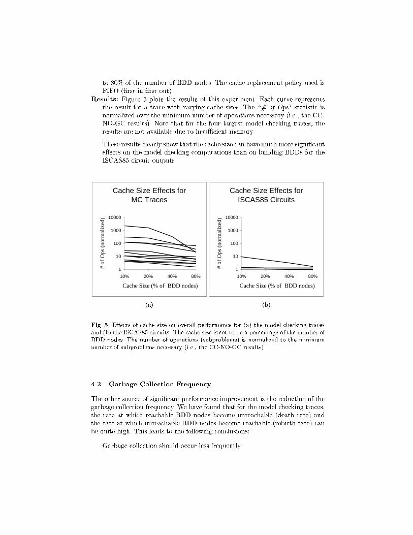
to 80% of the number of BDD nodes. The cache replacement policy used isFIFO (�rst-in-�rst-out).

Results: Figure 5 plots the results of this experiment. Each curve representsthe result for a trace with varying cache sizes. The \# of Ops" statistic isnormalized over the minimum number of operations necessary (i.e., the CC-NO-GC results). Note that for the four largest model checking traces, theresults are not available due to insu�cient memory.

These results clearly show that the cache size can have much more signi�cante�ects on the model checking computations than on building BDDs for theISCAS85 circuit outputs.

Cache Size Effects forMC Traces

1

10

100

1000

10000

10% 20% 40% 80%

Cache Size (% of BDD nodes)

# of

Ops

(no

rmal

ized

)

(a)

Cache Size Effects forISCAS85 Circuits

1

10

100

1000

10000

10% 20% 40% 80%

Cache Size (% of BDD nodes)

# of

Ops

(no

rmal

ized

)

(b)

Fig. 5. E�ects of cache size on overall performance for (a) the model checking tracesand (b) the ISCAS85 circuits. The cache size is set to be a percentage of the number ofBDD nodes. The number of operations (subproblems) is normalized to the minimumnumber of subproblems necessary (i.e., the CC-NO-GC results).

4.2 Garbage Collection Frequency

The other source of signi�cant performance improvement is the reduction of thegarbage collection frequency. We have found that for the model checking traces,the rate at which reachable BDD nodes become unreachable (death rate) andthe rate at which unreachable BDD nodes become reachable (rebirth rate) canbe quite high. This leads to the following conclusions:

{ Garbage collection should occur less frequently.

{ Garbage collection should not be triggered solely based on the percentage ofthe unreachable nodes.

{ For reference-counting based garbage collection algorithms, maintaining ac-curate reference counts all the time may incur non-negligible overhead.

Hypothesis 3 Model checking computations can have very high death and re-birth rates, whereas combinational circuit computations have very low death andrebirth rates.

Experiment: Measure the death and rebirth rates for the model checking tracesand the ISCAS85 circuits.

Results: Figure 6(a) plots the ratio of the total number of deaths over the totalnumber of sub-operations. The number of sub-operations is used to representtime. This chart shows that the death rates for the model checking tracescan vary considerably. In 5 cases, the number of deaths is higher than thenumber of sub-operations (i.e., death rate is greater than 1). In contrast, thedeath rates of the ISCAS85 circuits are all less than 0.3.

That the death rates exceed 1 is quite unexpected. To explain the signi�canceof this result, we digress brie y to describe the process of BDD nodes becom-ing unreachable (death) and then becoming reachable again (rebirth). Whena BDD node become unreachable, its children can also become unreachableif this BDD node is its children's only reference. Thus, it is possible thatwhen a BDD node become unreachable, a large number of its descendantsalso become unreachable. Similarly, if an unreachable BDD node becomesreachable again, a large number of its unreachable descendants can also be-come reachable. Other than rebirth, the only way the number of reachablenodes can increase is when a sub-operation creates a new BDD node asits result. As each sub-operation can produce at most one new BDD node,a death rate of greater than 1 can only occur when the corresponding re-birth rate is also very high. In general, high death rate coupled with highrebirth rate indicates that many nodes are toggling between being reachableand being unreachable. Thus, for reference-counting based garbage collec-tion algorithms, maintaining accurate reference count all the time may incursigni�cant overhead. This problem can be addressed by using a bounded-sizequeue to delay the reference-count updates until the queue over ows.

Figure 6(b) plots the ratio of the total number of rebirths over the totalnumber of deaths. Since garbage collection is enabled in these runs anddoes reclaim unreachable nodes, the rebirth rates shown may be lower thanwithout garbage collection. This �gure shows that the rebirth rates for themodel checking traces are generally very high | 8 out of 16 cases have rebirthrates greater than 80%. In comparison, the rebirth rate for the ISCAS85circuits are all less than 30%.

The high rebirth rates indicate that garbage collection for the model checkingtraces should be delayed as long as possible. There are two reasons for this:�rst, since a large number of unreachable nodes do become reachable again,

garbagecollectio

nwill

notbevery

e�ectiv

ein

reducin

gthemem

ory

usage.

Seco

nd,thehighreb

irthrate

may

resultin

repeated

subproblem

sinvolving

thecurren

tlyunrea

chable

nodes.

Bygarbagecollectin

gthese

unrea

chable

nodes,

their

corresp

ondingcomputed

cacheentries

must

also

beclea

red.

Thus,garbagecollectio

nmay

grea

tlyincrea

sethenumberofreco

mputatio

ns

ofidentica

lsubproblem

s.

Thehighreb

irthrates

andthepoten

tially

highdeath

rates

also

suggest

that

thegarbagecollectio

nalgorith

mshould

notbetrig

gered

based

solely

onthe

percen

tageofthedeadnodes,

aswith

thecla

ssicalBDDpacka

ges.

Death R

ate

0

0.5 1

1.5 2

2.5 3

Model C

hecking Traces IS

CA

S85

# of deaths / # of operations

(a)

Rebirth R

ate

0

0.2

0.4

0.6

0.8 1

Model C

hecking Traces IS

CA

S85

# of rebirths / # of deaths

(b)

Fig.6.(a)Rate

atwhich

BDDnodes

beco

meunrea

chable(death).(b)Rate

atwhich

unrea

chableBDDnodes

beco

merea

chableagain

(rebirth

).

4.3

E�ectsoftheComplementEdge

Thecomplem

entedgerep

resentatio

n[1]hasbeen

foundto

besomew

hatusefu

lin

reducin

gboth

thespace

andtim

ereq

uired

tobuild

theoutputBDDsforthe

ISCAS85circu

its[17].

Inthefollow

ingexperim

ents,

westu

dythee�ects

ofthe

complem

entedgeonthemodelcheck

ingtra

cesandcompare

itwith

theresu

ltsfortheISCAS85circu

its.

Hypothesis

4Thecomplem

entedge

represen

tatio

ncansign

i�cantly

reduce

the

amountofwork

forcombin

atio

nalcircu

itcomputatio

ns,butnotformodelcheck-

ingcomputatio

ns.However,

ingen

eral,ithaslittle

impact

onmem

ory

usage.

Experim

ent:

Measure

andcompare

thenumber

ofsubproblem

s(amountof

work)andtheresu

ltinggraphsizes

(mem

ory

usage)genera

tedfro

mtwoBDD

packa

ges

|onewith

andtheother

with

outthecomplem

ent-ed

gefea

ture.

Forthegraphsize

measurem

ents,

sum

theresu

ltingBDDgraphsizes

ofall

top-lev

elopera

tions.N

otethatsin

cetwopacka

gesareused

,minordi�eren

cesinthenumberofopera

tionscanoccu

rdueto

di�eren

tgarbagecollectio

nand

cachingalgorith

ms.

Results:

Figure7(a)show

sthatthecomplem

entedgeshavenosig

ni�cante�ect

formodelcheck

ingtra

ces.In

contra

st,fortheISCAS85circu

its,theratio

of

theno-co

mplem

ent-ed

geresu

ltsover

with

-complem

ent-ed

geresu

ltsranges

from

1.75to

2.00.Figure

7(b)show

sthatthecomplem

entedges

haveno

signi�cante�ect

ontheBDDgraphsizes

inanyofthebenchmark

traces.

Com

plement E

dge’s Effects

on Work

0

0.5 1

1.5 2

2.5

Model C

hecking Traces IS

CA

S85

# of operationsno C.E. / with C.E.

(a)

Com

plement E

dge’s Effects

on Graph S

izes

0

0.5 1

1.5

Model C

hecking Traces IS

CA

S85

sum of result BDD sizesno C.E. / with C.E.

(b)

Fig.7.E�ects

ofthecomplem

entedgerep

resentatio

non(a)numberoftheopera

tions

and(b)graphsizes.

4.4

MemoryLocality

forBreadth-FirstBDDConstr

uctio

n

Inrecen

tyears,

anumber

ofresea

rchers

haveproposed

brea

dth-�rst

BDD

con-

structio

nto

exploitmem

ory

locality

[2,18,

19,

21,

26].

Thebasic

idea

isthat

foreach

expansio

nphase,

allsub-opera

tionsofthesamevaria

bleare

processed

togeth

er.Similarly,

foreach

reductio

nphase,

allBDD

nodes

ofthesamevari-

ableare

produced

togeth

er.Note

thateven

thoughthislevelized

access

pattern

isslig

htly

di�eren

tfro

mthetra

ditio

nalnotio

nofbrea

dth-�rst

traversa

l,wewill

contin

ueto

referto

thispattern

asbrea

dth-�rst

tobeconsisten

twith

prev

ious

work.Based

onthisstru

ctured

access

pattern

,wecanexploitmem

ory

locality

by using per-variable memory managers and per-variable breadth-�rst queues tocluster the nodes of the same variable together. This clustering is bene�cial onlyif many nodes are processed for each breadth-�rst queue during each expansionand reduction phase.

The breadth-�rst approach does have some performance drawbacks (at leastin the two packages we studied). The breadth-�rst expansion usually has highermemory overhead. In terms of running time, one drawback is in the implementa-tion of the cache. In the breadth-�rst approach, the sub-operations are explicitlyrepresented as operator nodes and the uniqueness of these nodes is ensured byusing a hash table with chaining for collision resolution. Accesses to this hashtable are inherently slower than accesses to the direct mapped (1-way associa-tive) computed cache used in the depth-�rst approaches. Furthermore, handlingof the computed and yet-to-be-computed operator nodes adds even more over-head. Depending on the implementation strategy, this overhead could be in theform of an explicit cache garbage collection phase or transferring of a computedresult from an operator node's hash table to a computed cache. Maintenanceof the breadth-�rst queues is another source of overhead. This overhead can behigher for operations such as relational products because of the possible addi-tional recursion (e.g., line 7 in Fig. 1). Given that each sub-operation requiresonly a couple hundred cycles on modern machines, these overheads can have anon-negligible impact on the overall performance.

In this study, we have found no evidence that the breadth-�rst based packagesare better than the depth-�rst based packages when the computation �ts in mainmemory. Our conjecture is that since the relational product algorithm (Fig. 1)can have exponential complexity, the graph sizes of the BDD arguments do nothave to be very large to incur a long running time. As a result, the number ofnodes processed each time can be very small. The following experiment teststhis conjecture.

Hypothesis 5 For our test cases, few nodes are processed each time a breadth-�rst queue is visited. For the same amount of total work, combinational circuitcomputations have much better \breadth-�rst" locality than model checking com-putations.

Experiment: Measure the number of sub-operations processed each time abreadth-�rst queue is visited. Then compute the maximum, mean, and stan-dard deviation of the results. Note that these calculations do not include thecases where the queues are empty since they have no impact on the memorylocality issue.

Result: Figure 8 shows the statistics for this experiment. The top part of thetable shows the results for the model checking traces. The bottom part showsthe results for the ISCAS85 circuits. We have also included the \Average /Total # of Ops" column to show the results for the average number of sub-

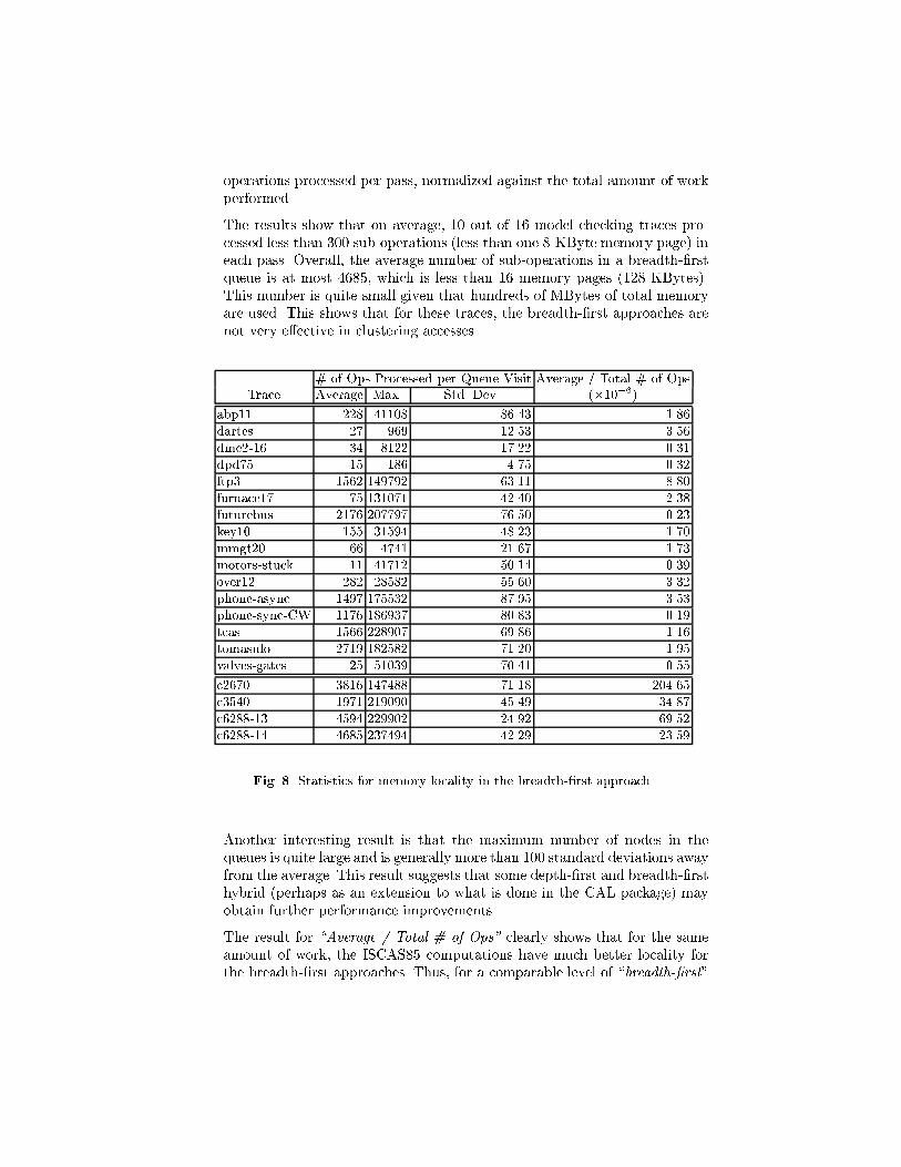
operations processed per pass, normalized against the total amount of workperformed.

The results show that on average, 10 out of 16 model checking traces pro-cessed less than 300 sub-operations (less than one 8-KByte memory page) ineach pass. Overall, the average number of sub-operations in a breadth-�rstqueue is at most 4685, which is less than 16 memory pages (128 KBytes).This number is quite small given that hundreds of MBytes of total memoryare used. This shows that for these traces, the breadth-�rst approaches arenot very e�ective in clustering accesses.

# of Ops Processed per Queue Visit Average / Total # of OpsTrace Average Max. Std. Dev. (�10�6)

abp11 228 41108 86.43 1.86

dartes 27 969 12.53 3.56

dme2-16 34 8122 17.22 0.31

dpd75 15 186 4.75 0.32

ftp3 1562 149792 63.11 8.80

furnace17 75 131071 42.40 2.38

futurebus 2176 207797 76.50 0.23

key10 155 31594 48.23 1.70

mmgt20 66 4741 21.67 1.73

motors-stuck 11 41712 50.14 0.39

over12 282 28582 55.60 3.32

phone-async 1497 175532 87.95 3.53

phone-sync-CW 1176 186937 80.83 0.19

tcas 1566 228907 69.86 1.16

tomasulo 2719 182582 71.20 1.95

valves-gates 25 51039 70.41 0.55

c2670 3816 147488 71.18 204.65

c3540 1971 219090 45.49 34.87

c6288-13 4594 229902 24.92 69.52

c6288-14 4685 237494 42.29 23.59

Fig. 8. Statistics for memory locality in the breadth-�rst approach.

Another interesting result is that the maximum number of nodes in thequeues is quite large and is generally more than 100 standard deviations awayfrom the average. This result suggests that some depth-�rst and breadth-�rsthybrid (perhaps as an extension to what is done in the CAL package) mayobtain further performance improvements.

The result for \Average / Total # of Ops" clearly shows that for the sameamount of work, the ISCAS85 computations have much better locality forthe breadth-�rst approaches. Thus, for a comparable level of \breadth-�rst"

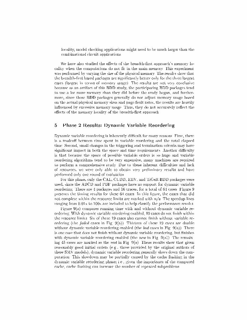
locality, model checking applications might need to be much larger than thecombinational circuit applications.

We have also studied the e�ects of the breadth-�rst approach's memory lo-cality when the computations do not �t in the main memory. This experimentwas performed by varying the size of the physical memory. The results show thatthe breadth-�rst based packages are signi�cantly better only for the three largestcases (largest in terms of memory usage). The results are not very conclusivebecause as an artifact of this BDD study, the participating BDD packages tendto use a lot more memory than they did before the study began, and further-more, since these BDD packages generally do not adjust memory usage basedon the actual physical memory sizes and page fault rates, the results are heavilyin uenced by excessive memory usage. Thus, they do not accurately re ect thee�ects of the memory locality of the breadth-�rst approach.

5 Phase 2 Results: Dynamic Variable Reordering

Dynamic variable reordering is inherently di�cult for many reasons. First, thereis a tradeo� between time spent in variable reordering and the total elapsedtime. Second, small changes in the triggering and termination criteria may havesigni�cant impact in both the space and time requirements. Another di�cultyis that because the space of possible variable orders is so huge and variablereordering algorithms tend to be very expensive, many machines are requiredto perform a comprehensive study. Due to these inherent di�culties and lackof resources, we were only able to obtain very preliminary results and haveperformed only one round of evaluation.

For this phase, only the CAL, CUDD, EHV, and TiGeR BDD packages wereused, since the ABCD and PBF packages have no support for dynamic variablereordering. There are 4 packages and 16 traces, for a total of 64 cases. Figure 9presents the timing results for these 64 cases. In this �gure, the cases that didnot complete within the resource limits are marked with n/a. The speedup linesranging from 0:01x to 100x are included to help classify the performance results.

Figure 9(a) compares running time with and without dynamic variable re-ordering. With dynamic variable reordering enabled, 19 cases do not �nish withinthe resource limits. Six of these 19 cases also cannot �nish without variable re-ordering (the failed cases in Fig. 9(a)). Thirteen of these 19 cases are doablewithout dynamic variable reordering enabled (the bad cases in Fig. 9(a)). Thereis one case that does not �nish without dynamic variable reordering, but �nisheswith dynamic variable reordering enabled (the new in Fig. 9(a)). The remain-ing 45 cases are marked as the rest in Fig. 9(a). These results show that givenreasonably good initial orders (e.g., those provided by the original authors ofthese SMV models), dynamic variable reordering generally slows down the com-putation. This slowdown may be partially caused by the cache ushing in thedynamic variable reordering phase; i.e., given the importance of the computedcache, cache ushing can increase the number of repeated subproblems.

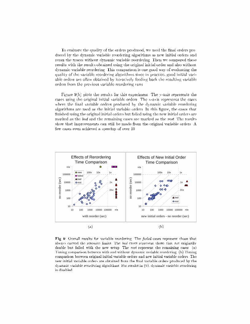
To evaluate the quality of the orders produced, we used the �nal orders pro-duced by the dynamic variable reordering algorithms as new initial orders andreran the traces without dynamic variable reordering. Then we compared theseresults with the results obtained using the original initial order and also withoutdynamic variable reordering. This comparison is one good way of evaluating thequality of the variable reordering algorithms since in practice, good initial vari-able orders are often obtained by iteratively feeding back the resulting variableorders from the previous variable reordering runs.

Figure 9(b) plots the results for this experiment. The y-axis represents thecases using the original initial variable orders. The x-axis represents the caseswhere the �nal variable orders produced by the dynamic variable reorderingalgorithms are used as the initial variable orders. In this �gure, the cases that�nished using the original initial orders but failed using the new initial orders aremarked as the bad and the remaining cases are marked as the rest. The resultsshow that improvements can still be made from the original variable orders. Afew cases even achieved a speedup of over 10.

Effects of RerorderingTime Comparison

10

100

1000

10000

100000

1000000

10 100 1000 10000 100000 1E+06

with reorder (sec)

no r

eord

er (

sec)

newfailedbadrest

1x10x100x

.1x

.01x

n/a

n/a

(a)

Effects of New Initial OrderTime Comparison

10

100

1000

10000

100000

1000000

10 100 1000 10000 100000 1E+06

new initial orders - no reorder (sec)

no r

eord

er (

sec)

bad

rest

n/a

n/a

1x10x100x

.1x

.01x

(b)

Fig. 9. Overall results for variable reordering. The failed cases represent those thatalways exceed the resource limits. The bad cases represent those that are originallydoable but failed with the new setup. The rest represent the remaining cases. (a)Timing comparison between with and without dynamic variable reordering. (b) Timingcomparison between original initial variable orders and new initial variable orders. Thenew initial variable orders are obtained from the �nal variable orders produced by thedynamic variable reordering algorithms. For results in (b), dynamic variable reorderingis disabled.

The remainder of this section presents results of a limited set of experimentsfor characterizing dynamic variable reordering. We �rst present the results ontwo heuristics for dynamic variable reordering. Then we present results on sen-sitivity of dynamic variable reordering to the initial variable orders. For theseexperiments, only the CUDD package is used. Note that the results in this sec-tion are very limited in scope and are far from being conclusive. Our intent is tosuggest new research directions for dynamic variable reordering.

5.1 Present and Next State Variable Grouping

We set up an experiment to study the e�ects of variable grouping, where thegrouped variables are always kept adjacent to each other.

Hypothesis 6 Pairwise grouping of present state variables with their corre-sponding next state variables is generally bene�cial for dynamic variable reorder-ing.

Experiment: Measure the e�ects of this grouping on the number of subprob-lems (work), maximum number of live BDD nodes (space), and number ofnodes swapped with their children during dynamic variable reordering (re-order cost).

Results: Figure 10 plots the e�ects of grouping on work (Fig. 10(a)), space(Fig. 10(b)), and reorder cost (Fig. 10(c)). Note that the results for twotraces are not available. One trace (tomasulo) exceeded the memory limit,while the other (abp11) is too small to trigger variable reordering.

These results show that pairwise grouping of the present and the next statevariables is a good heuristic in general. However, there are a couple of ex-ceptions. A better solution might be to use the grouping initially and relaxthe grouping criteria somewhat as the reordering process progresses.

5.2 Reordering the Transition Relations

Since the BDDs for the transition relations are used repeatedly in model checkingcomputations, we set up an experiment to study the e�ects of reordering theBDDs for the transition relations.

Hypothesis 7 Finding a good variable order for the transition relation is ane�ective heuristic for improving overall performance.

Experiment: Reorder variables once, immediately after the BDDs for the tran-sition relations are built, and measure the e�ect on the number of subprob-lems (work), maximum number of live BDD nodes (space), and number ofnodes swapped with their children during dynamic variable reordering (re-order cost).

E�ects of Grouping

Work

0

1

2

3

4

Model Checking Traces

# of

ope

ratio

nsgr

oup

/ no

grou

p

(a)

Space

0

1

2

3

Model Checking Traces

max

# o

f liv

e no

des

grou

p / n

o gr

oup

(b)

Reorder Cost

0

1

2

3

Model Checking Traces

# of

nod

es s

wap

ped

grou

p / n

o gr

oup

(c)

Fig. 10. E�ects of pairwise grouping of the current and next state variables on (a)the number of subproblems, (b) the number of maximum live BDD nodes, and (c) theamount of work in performing dynamic variable reordering.

Results: Figure 11 plots the results of this experiment on work (Fig. 11(a)),space (Fig. 11(b)), and reorder cost (Fig. 11(c)). The results are normalizedagainst the results from automatic dynamic variable reordering for compar-ison purposes. Note that the results for two traces are not available. Withautomatic dynamic variable reordering, one trace (tomasulo) exceeded thememory limit, while the other (abp11) is too small to trigger variable re-ordering.

The results show that reordering once, immediately after the constructionof transition relations' BDDs generally works well in reducing the numberof subproblems (Fig. 11(a)). This heuristic's e�ects on the maximum num-ber of live BDD nodes is mixed (Fig. 11(b)). Figure 11(c) shows that thisheuristic's reordering cost is generally much lower than automatic dynamicvariable reordering. Overall, the the number of variable reordering for au-tomatic dynamic variable reordering is 5.75 times the variable reorderingfrequency using this heuristic. These results are not strong enough to sup-port our hypothesis as cache ushing may be the main factor for the e�ectson the number of subproblems. However, it does provide an indication thatthe automatic dynamic variable reordering algorithm may be invoking thevariable reordering process too frequently.

5.3 E�ects of Initial Variable Orders

In this section, we study the e�ects of initial variable orders on BDD constructionwith and without dynamic variable reordering. We generate a suite of initialvariable orders by perturbing a set of good initial orders. In the following, we

E�ects of Reordering Transition Relations

Work

0

1

2

3

Model Checking Traces

# of

ope

ratio

nstr

ans

reor

der

/ aut

o

(a)

Space

0

1

2

3

Model Checking Traces

max

# o

f liv

e no

des

tran

s re

orde

r / a

uto

(b)

Reorder Cost

0

1

Model Checking Traces

# of

nod

es s

wap

ped

tran

s re

orde

r / a

uto

(c)

Fig. 11. E�ects of variable reordering the transition relations on (a) the number ofsubproblems, (b) the number of maximum live BDD nodes, and (c) the amount of workin performing variable reordering. For comparison purposes, all results are normalizedagainst the results for automatic dynamic variable reordering.

describe this experimental setup in detail and then present some hypothesesalong with supporting evidence.

Experimental Setup

The �rst step is the selection of good initial variable orders | one for eachmodel checking trace. The quality of an initial variable order is evaluated by therunning time using this order without dynamic variable reordering.

Once the best initial variable order is selected, we perturb it based on twoperturbation parameters: the probability (p), which is the probability that avariable will be moved, and the distance (d), which controls how far a variablemay move. The perturbation algorithm used is shown in Figure 12. Initially, eachvariable is assigned a weight corresponding to its variable order (line 1). If thisvariable is chosen (with the probability of p) to be perturbed (by the distanceparameter d), then we change its weight by �w, where �w is chosen randomlyfrom the range [�d; d] (lines 3-5). At the end, the perturbed variable order isdetermined by sorting the variables based on their �nal weights (line 6). Thisalgorithm has the property that on average, p fraction of the BDD variables areperturbed and each variable's �nal variable order is at most 2d away from itsinitial order. Another property is that the perturbation pair (p = 1; d = 1)essentially produces a completely random variable order.

Since randomness is involved in the perturbation algorithm, to gain betterstatistical signi�cance, we generate multiple initial variable orders for each pairof perturbation parameters (p; d). For each trace, if we study np di�erent pertur-bation probabilities, nd di�erent perturbation distances, and k initial orders foreach perturbation pair, we will generate a total of knpnd di�erent initial variable

perturb order(v[n], p, d)/* perturb the variable order with probability p and distance d.

v[ ] is an array of n variables sorted based on decreasingvariable order precedence. */

1 for (0 � i < n) w[i] i /* initialize weight */2 for (0 � i < n) /* for each variable, with probability p, perturb its weight. */3 With probability p do4 �w randomly choose an integer from [�d; d]5 w[i] w[i] + �w

6 sort variables in array v[ ] based on increasing weight w[ ]7 return v[ ]

Fig. 12. Variable-order perturbation algorithm.

orders. For each initial variable order, we compare the results with and withoutdynamic variable reordering enabled. Thus, for each trace, there will be 2knpndruns. Due to lack of time and machine resources, we were only able to completethis experiment for one very small trace | abp11.

The perturbed initial variable orders were generated from the best initialvariable ordering we found for abp11. Using this order, the abp11 trace canbe executed (with dynamic variable reordering disabled) using 12.69 seconds ofCPU time and 127 MBytes of memory on a 248 MHz UltraSparc II. This initialorder and its results are used as the base case for this experiment. Using thisbase case, we set the time limit of each run to 1624.32 seconds (128 times thebase case) and 500 MBytes of memory.

For the perturbation parameters, we let p range from 0:1 to 1:0 with anincrement of 0:1. Since abp11 has 122 BDD variables, we let d range from 10 to100 with an increment of 10 and added the case for d =1. These choices resultin 110 perturbations pairs (with np = 10 and nd = 11). For each perturbationpair, we generate 10 initial variable orders (k = 10). Thus, there are a total of1100 initial variable orders and 2200 runs.

Results for abp11

Hypothesis 8 Dynamic variable reordering improves the performance of modelchecking computations.

Supporting Results: Figure 13 plots the number of cases that did not com-plete within various time limits for runs with and without dynamic variablereordering. For these runs, the memory limit is �xed at 500 MBytes. Thetime limits in this plot are normalized to the base case of 12:69 seconds andare plotted in log scale.

The results clearly show that given enough time, the cases with dynamicvariable reordering perform better. Overall, with a time limit of 128 times

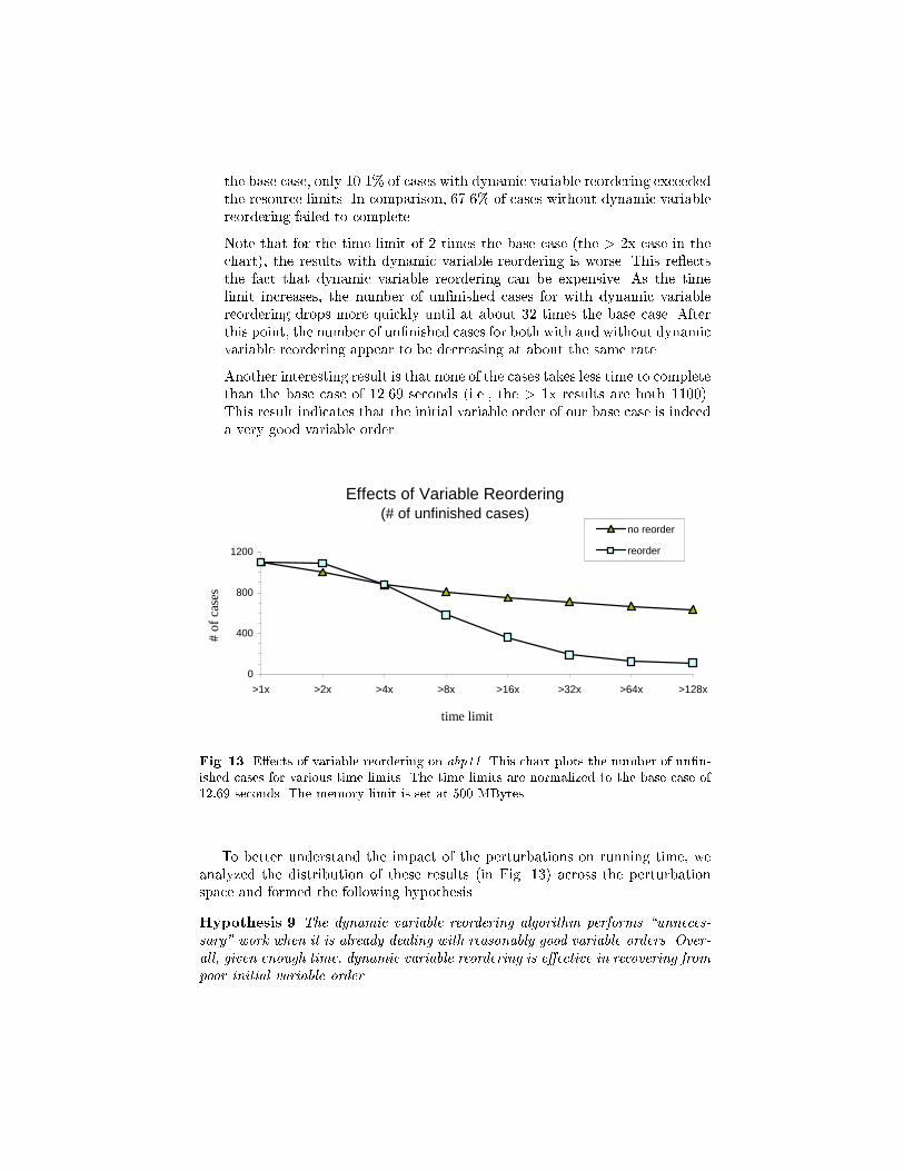
the base case, only 10.1% of cases with dynamic variable reordering exceededthe resource limits. In comparison, 67.6% of cases without dynamic variablereordering failed to complete.

Note that for the time limit of 2 times the base case (the > 2x case in thechart), the results with dynamic variable reordering is worse. This re ectsthe fact that dynamic variable reordering can be expensive. As the timelimit increases, the number of un�nished cases for with dynamic variablereordering drops more quickly until at about 32 times the base case. Afterthis point, the number of un�nished cases for both with and without dynamicvariable reordering appear to be decreasing at about the same rate.

Another interesting result is that none of the cases takes less time to completethan the base case of 12.69 seconds (i.e., the > 1x results are both 1100).This result indicates that the initial variable order of our base case is indeeda very good variable order.

Effects of Variable Reordering(# of unfinished cases)

0

400

800

1200

>1x >2x >4x >8x >16x >32x >64x >128x

time limit

# of

cas

es

no reorder

reorder

Fig. 13. E�ects of variable reordering on abp11. This chart plots the number of un�n-ished cases for various time limits. The time limits are normalized to the base case of12:69 seconds. The memory limit is set at 500 MBytes.

To better understand the impact of the perturbations on running time, weanalyzed the distribution of these results (in Fig. 13) across the perturbationspace and formed the following hypothesis.

Hypothesis 9 The dynamic variable reordering algorithm performs \unneces-sary" work when it is already dealing with reasonably good variable orders. Over-all, given enough time, dynamic variable reordering is e�ective in recovering frompoor initial variable order.

Supporting Results: Figure 14(a) shows the results with a time limit of 4times the base case of 12:69 seconds. These plots show that when there aresmall perturbations (p = 0:1 or d = 10), we are better o� without dynamicvariable reordering. However, for higher levels of perturbations, the caseswith dynamic variable reordering usually does a little better.

Figures 14(b) and 14(c) show the results with time limits of 32 and 128times, respectively, the base case. Note that since 128 times is the maximumtime limit we studied, Fig. 14(c) also represents the distribution of the casesthat did not complete at all for this study. These results clearly show thatgiven enough time, the cases with dynamic variable reordering perform muchbetter.

Hypothesis 10 The quality of initial variable order a�ects the space and timerequirements, with or without dynamic variable reordering.

Supporting Results: Figure 15 classi�es the un�nished cases into memory-out(Fig. 15(a)) or timed-out (Fig. 15(b)). For clarity, we repeated the plots forthe total number of un�nished cases (memory-out plus timed-out results) inFig. 15(c). It is important to note that because the BDD packages used in thisstudy still do not adapt very well upon exceeding memory limits, memory-outcases should be interpreted as indications of high memory pressure insteadof that these cases inherently do not �t within the memory limit.

The results show that levels of perturbation directly in uence the time andmemory requirement. With a very high level of perturbation, most of theun�nished cases are due to exceeding the memory limit of 500 MBytes (theupper-left triangular regions in Fig. 15(a)). For a moderate level of pertur-bation, most of the un�nished cases are due to the time limit (the diagonalbands from the lower-left to the upper-right in Fig. 15(b)).

Note that the results in Fig. 15 are not very monotonic; i.e., the results arenot necessarily worse with a larger degree of perturbation. This leads to the nexthypothesis.

Hypothesis 11 The e�ects of the dynamic variable reordering algorithm andthe initial variable orders are very chaotic.

Supporting Results: Fig. 16 plots the standard deviation of running timenormalized against average running time. For the cases that cannot completewithin the resource limits, they are included as if they use exactly the timelimit. Note that as an artifact of this calculation, when all 10 variants of aperturbation pair exceed the resource limits, the standard deviation is 0. Inparticular, without variable reordering, none of the cases can be completedin the highly perturbed region (upper-left triangular region in Fig 15(c)) andthus these results are all shown as 0 in the chart.

The results show that the standard deviations are generally greater than theaverage time (i.e., with the normalized result of > 1). This �nding partially

102030405060708090100

inf

1.0

0.7

0.4

0.101234567

8

9

10

# of

Cas

es

Distance

Prob

abili

ty

No Reorder(> 4x or > 500Mb)

102030405060708090100

inf

1.0

0.7

0.4

0.101234567

8

9

10

# of

Cas

es

Distance

Prob

abili

ty

Reorder(> 4x or > 500Mb)

(a)

102030405060708090100

inf

1.0

0.7

0.4

0.101234567

8

9

10

# of

Cas

es

Distance

Prob

abili

tyNo Reorder

(> 32x or > 500Mb)

102030405060708090100

inf

1.0

0.7

0.4

0.101234567

8

9

10#

of C

ases

Distance

Prob

abili

ty

Reorder(> 32x or > 500Mb)

(b)

102030405060708090100

inf

1.0

0.7

0.4

0.101234567

8

9

10

# of

Cas

es

Distance

Prob

abili

ty

No Reorder, Unfinished(> 128x or > 500Mb)

102030405060708090100

inf

1.0

0.7

0.4

0.101234567

8

9

10

# of

Cas

es

Distance

Prob

abili

tyReorder, Unfinished

(> 128x or > 500Mb)

(c)

Fig. 14. Histograms on the number of cases that cannot be �nished within the speci�edresource limits. For all cases, the memory limit is set at 500 MBytes. The time limitvaries from (a) 4 times, (b) 32 times, to (c) 128 times the base case of 12:69 seconds.

102030405060708090100

inf

1.0

0.7

0.4

0.101234567

8

9

10

# of

Cas

es

Distance

Prob

abili

ty

No Reorder, Memory Out(> 500Mb)

102030405060708090100

inf

1.0

0.7

0.4

0.101234567

8

9

10

# of

Cas

es

Distance

Prob

abili

ty

Reorder, Memory Out(> 500Mb)

(a)

102030405060708090100

inf

1.0

0.7

0.4

0.101234567

8

9

10

# of

Cas

es

Distance

Prob

abili

ty

No Reorder, Timed Out(> 128x)

102030405060708090100

inf

1.0

0.7

0.4

0.101234567

8

9

10#

of C

ases

Distance

Prob

abili

ty

Reorder, Timed Out(> 128x)

(b)

102030405060708090100

inf

1.0

0.7

0.4

0.101234567

8

9

10

# of

Cas

es

Distance

Prob

abili

ty

No Reorder, Unfinished(> 128x or > 500Mb)

102030405060708090100

inf

1.0

0.7

0.4

0.101234567

8

9

10

# of

Cas

es

Distance

Prob

abili

tyReorder, Unfinished

(> 128x or > 500Mb)

(c)

Fig. 15. Breakdown on the cases that cannot be �nished. (a) memory-out cases, (b)timed-out cases, (c) total number of un�nished cases.

con�rms our hypothesis. It also indicates that 10 initial variable orders perperturbation pair (p; d) is probably too small for some perturbation pairs.

The results also show that with very low level of perturbation (lower-righttriangular region), the normalized standard deviation is generally smaller.This gives an indication that higher perturbation level may result in moreunpredictable performance behavior.

Furthermore, the normalized standard deviation for without dynamic vari-able reordering is generally smaller than the same statistic for with dynamicvariable reordering. This result provides an indication that dynamic variablereordering may also have very unpredictable e�ects.

102030405060708090100

inf

1.0

0.7

0.4

0.10

0.5

1

1.5

2

2.5

Std.

Dev

. / A

vg. T

ime

Distance

Prob

abili

tyNo Reorder, Time Std. Dev.

(a)10203040506070809010

0

inf

1.0

0.7

0.4

0.10

0.5

1

1.5

2

2.5

Std.

Dev

. / A

vg. T

ime

Distance

Prob

abili

ty

Reorder, Time Std. Dev.

(b)

Fig. 16. Standard deviation of the running time for abp11 with perturbed initial vari-able orders (a) without dynamic variable reordering, and (b) with dynamic variablereordering. Each results are normalized to the average running time.

6 General Results

This section presents results which may be generally helpful in studying or im-proving BDD packages.

Hash Function

Hashing is a vital part of BDD construction since both the uniqueness ofBDD nodes and the cache accesses are based on hashing. Currently, we havenot found any theoretically good hash functions for handling multiple hashkeys. In this study, we have empirically found that the hash function used bythe TiGeR BDD package worked well in distributing the nodes. This hashfunction is of the form

H(k1; k2) = ((k1p1 + k2)p2)=2w�n

where k's are the hash keys, p's are su�ciently large primes, w is the numberof bits in an integer, and 2n is the size of the hash table. Note that divisionby 2w�n is used to extract the n most signi�cant bits and is implementedby right shifting (w � n) bits.

The basic idea is to distribute and combine the bits in the hash keys tothe higher order bits by using integer multiplications, and then to extractthe result from the high order bits. The power-of-2 hash table size is usedto avoid the more expensive modulus operation. Some small speedups havebeen observed using this hash function. One pitfall is that for backward com-patibility reasons, some compilers might generate a function call to computeinteger multiplication, which can cause signi�cant performance degradation(up to a factor of 2). In these cases, architecture-speci�c compiler ags canbe used to ensure the integer-multiplier hardware is used instead.

Caching Strategy

Given the importance of cache, a natural question is: Can we cache moreintelligently? One heuristic, used in CUDD, is that the cache is accessed onlyif at least one of the arguments has a reference count greater than 1. Thistechnique is based on the fact that if all arguments have reference countsof 1, then this subproblem is not likely to be repeated within the currenttop-level operation. In fact, if a complete cache is used, this subproblem willnot be repeated within the same top-level operation. Using this technique,CUDD is able to reduce the number of cache lookups by up to half, with atotal time reduction of up to 40%.

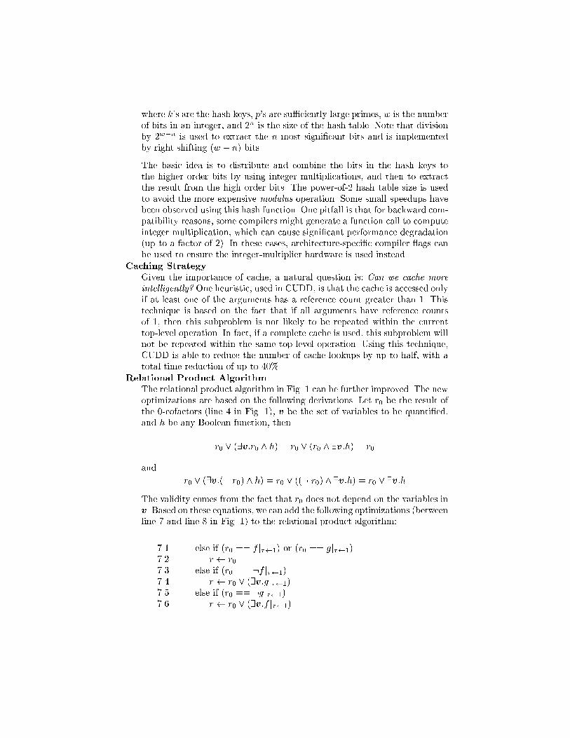
Relational Product Algorithm

The relational product algorithm in Fig. 1 can be further improved. The newoptimizations are based on the following derivations. Let r0 be the result ofthe 0-cofactors (line 4 in Fig. 1), v be the set of variables to be quanti�ed,and h be any Boolean function, then

r0 _ (9v:r0 ^ h) = r0 _ (r0 ^ 9v:h) = r0

and

r0 _ (9v:(: r0) ^ h) = r0 _ ((: r0) ^ 9v:h) = r0 _ 9v:h

The validity comes from the fact that r0 does not depend on the variables inv. Based on these equations, we can add the following optimizations (betweenline 7 and line 8 in Fig. 1) to the relational product algorithm:

7.1 else if (r0 == f j� 1) or (r0 == gj� 1)7.2 r r07.3 else if (r0 == :f j� 1)7.4 r r0 _ (9v:gj� 1)7.5 else if (r0 == :gj� 1)7.6 r r0 _ (9v:f j� 1)

In general, these optimizations only slightly reduces the number of sub-problems, with the exception of the futurebus trace, where the number ofsubproblems is reduced by over 20%.

BDD Package Comparisons

In comparing BDD packages, one fairness question is often raised: Is it fairto compare the performance of a bare-bones experimental BDD package witha more complete public domain BDD package? This question arises particu-larly when one package supports dynamic variable reordering, while the otherdoes not. This is an issue because supporting dynamic variable reorderingrequires additional data structures and indirection overheads to the compu-tation for BDD construction. To partially answer this question, we studieda package with and without its support for variable reordering in place. Ourpreliminary results show that the additional overhead to support dynamicvariable reordering has no measurable performance impact. This may bedue to the fact that BDD computation is so memory intensive, a coupleadditional non-memory intensive operations can be scheduled either by thehardware or the compiler without any measurable performance penalty.

Cache Hit Rate

The computed cache hit rate is not a reliable measure of overall performance.In fact, it can be shown that when the cache hit rate is less than 49%, acache miss can actually result in a higher hit rate. This is because a cachemiss generates more subproblems and these subproblems' results could havealready been computed and are still in cache.

Platform Independent Metrics

Throughout this study, we have found several useful machine-independentmetrics for characterizing the BDD computations. These metrics are:{ the number of subproblems as a measure for work,{ the maximum number of live nodes as a measure for the lower bound onmemory requirement,

{ the number of subproblems processed for each breadth-�rst queue visit tore ect the possibility of exploiting memory locality using the breadth-�rst traversal, and

{ the number of nodes swapped with their children during dynamic variablereordering as a measure of the amount of work performed in dynamicvariable reordering.

7 Issues and Open Questions

Cache Size Management

In this study, we have found that the size of the compute cache can have asigni�cant impact on model checking computations. Given that BDD com-putations are very memory intensive, there is an inherent con ict betweenusing a larger cache for better performance and using a smaller cache toconserve memory usage. For BDD packages that maintain multiple computecaches, there are additional con icts as these caches will compete with each

other for the memory resources. As the problem sizes get larger, �ndinga good dynamic cache management algorithm will become more and moreimportant for building an e�cient BDD package.

Garbage Collection Triggering Algorithm

Another dynamic memory management issue is the frequency of garbagecollection. The results in Fig. 6(b) clearly suggest that delaying garbagecollection can be very bene�cial. Again, this is a space and time tradeo�issue. One possibility is to invoke garbage collection when the percentage ofunreachable nodes is high and the rebirth rate is low. Note that for BDDpackages that do not maintain reference counts, the rebirth rate statistic isnot readily available and thus a di�erent strategy is needed.

Resource Awareness

Given the importance of space and time tradeo�, a commercial strength BDDpackage not only needs to know when to gobble up the memory to reducecomputation time, it should also be able to free up space under resourcecontention. This contention could come from di�erent parts of the same toolchain or from a completely di�erent job. One way to deal with this issue isfor BDD packages to become more aware of the environment, in particular,the available physical memory, various memory limits, and the page faultrate. This information is readily available to the users of modern operatingsystems. Several of the BDD packages used in this study already have somelimited form of resource awareness. However, this problem is still not wellunderstood and probably cannot be easily studied using the trace-drivenframework.

Cross Top-Level Sharing

For the model checking traces, why are there so many subproblems repeatedacross the top-level operations? We have two conjectures. First, there is quitea bit of symmetry in some of these SMV models. These inherent symmetriesare somehow captured by the BDD representation. If so, it might be more ef-fective to use higher level algorithms to exploit the symmetries in the models.The other conjecture is that the same BDDs for the transition relations areused repeatedly throughout model checking in the �xed-point computations.This repeated use of the same set of BDDs increases the likelihood of thesame subproblems being repeated across top-level operations. At this point,we do not know how to validate these conjectures. To better understand thisproperty, one starting point would be to identify how far apart are thesecross top-level repeated subproblems; i.e., is it within one state transition,within one �xed-point computation, within one temporal logic operator, oracross di�erent temporal logic operators?

Breadth-First's Memory Locality

In this study, we have found no evidence that breadth-�rst based techniqueshave any advantage when the computation �ts in the main memory. Aninteresting question would be: As the BDD graph sizes get much larger, isthere going to be a crossover point where the breadth-�rst packages will besigni�cantly better? If so, another issue would be �nding a good depth-�rstand breadth-�rst hybrid to get the best of both worlds.

Inconsistent Cross Platform Results

Inconsistency in timing results across machines is yet another unresolvedissue in this study. More speci�cally, for some BDD packages, the CPU-time results on a UltraSparc II machine are up to twice as long as thecorresponding results on a PentiumPro, while for other BDD packages, thedi�erences are not so signi�cant. Similar inconsistencies are also observedin the Sentovich study [23]. A related performance discrepancy is that forthe depth-�rst based packages, the garbage collection cost for UltraSparc IIis generally twice as high as that of PentiumPro. However, for the breadth-�rst based packages, the garbage collection performances between these twomachines are much closer. In particular, for one breadth-�rst based package,the ratio is very close to 1. This discrepancy may be a re ection of thememory locality of these BDD packages. To test this conjecture, we haveperformed a set of simple tests using synthetic workloads. Unfortunately,the results did not con�rm this hypothesis. However, the results of this testdo indicate that our PentiumPro machine appears to have a better memoryhierarchy than our UltraSparc II machine. A better understanding of thisissue can probably shed some light on how to improve memory locality forBDD computations.

Pointer- vs. Index-Based References

Another issue is that within the next ten years, machines with memory sizesgreater than 4 GBytes are going to become common. Thus the size of apointer (i.e., memory address) will increase from 32 to 64 bits. Since mostBDD packages today are pointer-based, the memory usage will double on64-bit machines. One way to reduce this extra memory overhead is to useinteger indices instead of pointers to reference BDDs as in the case of theABCD package. One possible drawback of an index-based technique is thatan extra level of indirection is introduced for each reference. However, sinceABCD's results are generally among the best in this study, this provides apositive indication that the index-based approach may be a feasible solutionto this impending memory overhead problem.

Computed Cache Flushing in Dynamic Variable Reordering

In Sec. 5, we showed that dynamic variable reordering can generally slowdown the entire computation when given a reasonably good initial variableorder. Since the computed cache is typically ushed when dynamic variablereordering takes place, it would be interesting to study what percentage ofthe slowdown is caused by an increase in the amount of work (number ofsubproblems) due to cache ushing. If this percentage is high, then anotherinteresting issue would be in �nding a good way to incorporate the cacheperformance as a parameter for controlling dynamic variable reordering fre-quency.

8 Related Work

In [23], Sentovich presented a BDD study comparing the performance of sev-eral BDD packages. Her study covered building output BDDs for combinationalcircuits, computing reachability of sequential circuits, and variable reordering.

In [15], Manne et al. performed a BDD study examining the memory localityissues for several BDD packages. This work compares the hardware cache missrates, TLB miss rates, and page fault rates in building the output BDDs forcombinational circuits.

In contrast to the Sentovich study, our study focuses in characterizing theBDD computations instead of doing a performance comparison of BDD packages.In contrast to the Manne study, our work uses platform independent metricsfor performance evaluation instead of hardware speci�c metrics. Both types ofmetrics are equally valid and complementary. Our study also di�ers from thesetwo prior studies in that our performance evaluation is based on the executionof a model checker instead of benchmark circuits.

9 Summary and Conclusions

By applying a new evaluation methodology, we have not only achieved signi�cantperformance improvements, we have also identi�ed many interesting character-istics of model checking computations. For example, we have con�rmed thatmodel checking and combinational circuit computations have fundamentally dif-ferent performance characteristics. These di�erences include the e�ects of thecache size, the garbage collection frequency, the complement edge representa-tion, and the memory locality for the breadth-�rst BDD packages. For dynamicvariable reordering, we have introduced some new methodologies for studyingthe e�ects of variable reordering algorithms and initial variable orders. Fromthese experiments, we have uncovered a number of open problems and futureresearch directions.

As this study is very limited in scope, especially for the dynamic variablereordering phase, further validations of the hypotheses are necessary. It wouldbe especially interesting to repeat the same experiments on execution traces fromother BDD-based tools.

The results obtained in this study clearly demonstrate the usefulness of sys-tematic performance characterization and validate our evaluation methodology.We hope that the trace-drive framework and the machine-independent metricswill help lay the foundation for future benchmark collection and performance-characterization methodology.

Acknowledgement

We thank Yirng-An Chen for providing the ISCAS85 circuits in the trace for-mat and providing the software which forms the core of our evaluation tool.

We thank Claudson F. Bornstein and Henry R. Rowley for numerous discus-sions on experimental setups and data presentation. We are grateful to EdmundM. Clarke for providing additional computing resources. This research is spon-sored in part by the Defense Advanced Research Projects Agency (DARPA) andRome Laboratory, Air Force Materiel Command, USAF, under agreement num-ber F30602-96-1-0287, in part by the National Science Foundation under GrantCMS-9318163, in part by DARPA under contract number DABT63-96-C-0071,in part by Cadence Design Systems, and in part by SRC contract 96-DJ-560.This work utilized Silicon Graphics Origin 2000 machines from the NationalCenter for Supercomputing Applications at Urbana-Champaign.

References

[1] Akers, S. B. Functional testing with binary decision diagrams. In Proceedingsof Eighth Annual International Conference on Fault-Tolerant Computing (June1978), pp. 75{82.

[2] Ashar, R., and Cheong, M. E�cient breadth-�rst manipulation of binarydecision diagrams. In Proceedings of the International Conference on Computer-Aided Design (November 1994), pp. 622{627.

[3] Biere, A. ABCD: an experimental BDD library, 1998.http://iseran.ira.uka.de/~armin/abcd/.

[4] Brace, K., Rudell, R., and Bryant, R. E. E�cient implementation of a BDDpackage. In Proceedings of the 27th ACM/IEEE Design Automation Conference(June 1990), pp. 40{45.

[5] Brglez, F., Bryan, D., and Kozmiski, K. Combinational pro�les of sequentialbenchmark circuits. In 1989 International Symposium on Circuits And Systems(May 1989), pp. 1924{1934.

[6] Brglez, F., and Fujiwara, H. A neutral netlist of 10 combinational benchmarkcircuits and a target translator in Fortran. In 1985 International Symposium onCircuits And Systems (June 1985). Partially described in F. Brglez, P. Pownall,R. Hum. Accelerated ATPG and Fault Grading via Testability Analysis. In 1985International Symposium on circuits and Systems, pages 695-698, June 1985.

[7] Bryant, R. E. Graph-based algorithms for Boolean function manipulation. IEEETransactions on Computers C-35, 8 (August 1986), 677{691.

[8] Bryant, R. E. Symbolic Boolean manipulation with ordered binary decisiondiagrams. ACM Computing Surveys 24, 3 (September 1992), 293{318.

[9] Bryant, R. E. Binary decision diagrams and beyond: Enabling technologies forformal veri�cation. In Proceedings of the International Conference on Computer-Aided Design (November 1995), pp. 236{243.

[10] Burch, J. R., Clarke, E. M., Long, D. E., McMillan, K. L., and Dill, D. L.

Symbolic model checking for sequential circuit veri�cation. IEEE Transactionson Computer-Aided Design of Integrated Circuits and Systems 13, 4 (April 1994),401{424.

[11] Coudert, O., Berthet, C., and Madre, J. C. Veri�cation of sequential ma-chines using Boolean functional vectors. In Proceedings of the IFIP InternationalWorkshop on Applied Formal Methods for Correct VLSI Design (November 1989),pp. 179{196.

[12] Coudert, O., and Madre, J. C. A uni�ed framework for the formal veri�cationof circuits. In Proceedings of the International Conference on Computer-AidedDesign (Feb 1990), pp. 126{129.

[13] Coudert, O., Madre, J. C., and Touati, H. TiGeR Version 1.0 User Guide.Digital Paris Research Lab, December 1993.

[14] Janssen, G. The Eindhoven BDD Package. University of Eindhoven. AnonymousFTP address: ftp://ftp.ics.ele.tue.nl/pub/users/geert/bdd.tar.gz.

[15] Manne, S., Grunwald, D., and Somenzi, F. Remembrance of things past:Locality and memory in BDDs. In Proceedings of the 34th ACM/IEEE DesignAutomation Conference (June 1997), pp. 196{201.

[16] McMillan, K. L. Symbolic Model Checking. Kluwer Academic Publishers, 1993.[17] Minato, S., Ishiura, N., and Jajima, S. Shared binary decision diagram with

attributed edges for e�cient Boolean function manipulation. In Proceedings ofthe 27th ACM/IEEE Design Automation Conference (June 1990), pp. 52{57.

[18] Ochi, H., Ishiura, N., and Yajima, S. Breadth-�rst manipulation of SBDD ofBoolean functions for vector processing. In Proceedings of the 28th ACM/IEEEDesign Automation Conference (June 1991), pp. 413{416.

[19] Ochi, H., Yasuoka, K., and Yajima, S. Breadth-�rst manipulation of verylarge binary-decision diagrams. In Proceedings of the International Conference onComputer-Aided Design (November 1993), pp. 48{55.

[20] Ranjan, R. K., and Sanghavi, J. CAL-2.0: Breadth-�rst manipulation basedBDD library. Public software. University of California, Berkeley, CA, June 1997.http://www-cad.eecs.berkeley.edu/Research/cal bdd/.

[21] Ranjan, R. K., Sanghavi, J. V., Brayton, R. K., and Sangiovanni-

Vincentelli, A. High performance BDD package based on exploiting memoryhierarchy. In Proceedings of the 33rd ACM/IEEE Design Automation Conference(June 1996), pp. 635{640.

[22] Rudell, R. Dynamic variable ordering for ordered binary decision diagrams. InProceedings of the International Conference on Computer-Aided Design (Novem-ber 1993), pp. 139{144.

[23] Sentovich, E. M. A brief study of BDD package performance. In Proceedings ofthe Formal Methods on Computer-Aided Design (November 1996), pp. 389{403.

[24] Sentovich, E. M., Singh, K. J., Lavagno, L., Moon, C., Murgai, R., Sal-

danha, A., Savoj, H., Stephan, P. R., Brayton, R. K., and Sangiovanni-

Vincentelli., A. L. SIS: A system for sequential circuit synthesis. Tech. Rep.UCB/ERL M92/41, Electronics Research Lab, University of California, May 1992.

[25] Somenzi, F. CUDD: CU decision diagram package. Public software. Universityof Colorado, Boulder, CO, April 1997. http://vlsi.colorado.edu/~fabio/ .

[26] Yang, B., Chen, Y.-A., Bryant, R. E., and O'Hallaron, D. R. Space- andtime-e�cient BDD construction via working set control. In 1998 Proceedings ofAsia and South Paci�c Design Automation Conference (Feb 1998), pp. 423{432.