A Performance Model of Gossip-BasedUpdate Propagation

Imad Antonios1, Feng Zhang2, Reetu Dhar1, and Lester Lipsky2

1 Department of Computer ScienceSouthern CT State University

New Haven, CT 06515{antoniosi1, dharr1}@southernct.edu

2 Department of Computer Science and EngineeringUniversity of Connecticut

Storrs, CT 06269{fzhang, lester}@engr.uconn.edu

Abstract. We consider the problem of propagating an update to nodes in a distributed system usingtwo gossiping protocols. The first is an idealized algorithm with static and dynamic knowledge ofthe system, and the second is a simple randomized algorithm. We construct a theoretical model thatallows us to derive work and completion time statistics under varying transmission delay distributions.Numerical results are obtained for both exponential and nonexponential transmission times using linear-algebraic queueing theory techniques. Additionally, we present the results of simulation experimentsshowing that under node churn assumptions, the randomized algorithm’s performance is qualitativelydifferent than in a fault-free system.

Keywords: update propagation, gossiping, performance evaluation, semi-Markov models.

1 Introduction and Related Work

Gossip-based algorithms have recently received much attention as they offer an attractive and simpleparadigm for achieving reliable and scalable information propagation in large-scale distributed systems[3,7,9,13]. Gossiping broadly refers to a class of distributed algorithms that are characterized by repeatedpairwise exchanges of information randomly selected nodes to achieve a desired system state, or to carry outa computation. Gossiping behavior bears resemblance to the spread of epidemics or rumors in a population,and accordingly much of the literature on the subject employs the term epidemic protocols [8]. Gossip-basedalgorithms have been applied to a broad range of problems such as update propagation, consensus, overlaynetwork topology management, and collaborative computation [1,5,6,10].

In this paper we consider gossip-based algorithms in the context of the update propagation problem,whereby nodes with an update forward it to other nodes in the system according to some peer-selectionstrategy, until the update is disseminated to the whole system. We assume that the communication modeamong nodes is unicast, and as such this problem can be likened to the application layer multicast problem,although here we are not interested in how to construct an overlay, but in the performance characteristics ofpropagation. We employ the term gossiping to highlight the randomness in the peer selection criteria of oneof the algorithms in this paper. As gossip-based algorithms are commonly deployed over large-scale networkswith high fluctuations in network delays, it’s become increasingly important to characterize the performanceproperties of gossip algorithms under such network conditions, namely propagation time and work. To thatend, this work presents a semi-Markov model of two update propagation algorithms where communicationdelay is represented as a probability distribution. The model is solved using the linear algebraic approach toqueueing theory (LAQT), allowing us to numerically derive update propagation time and work under variousparameter settings. As far as we know, there are no other analytical models of update propagation algorithms

that applied arbitrary probability distributions to capture communication delays. Our results indicate thatthe performance characteristics of the algorithms considered are highly sensitive to the variability in networktransmission delays. We additionally investigate via simulation the effect of introducing node failures. Ourfindings reveal that under modest failure assumptions, the total work performed by a randomized algorithmis qualitatively different than in a system without failures.

The performance characteristics of gossip-based algorithms are largely driven by the degree of parallelismin the spread of updates following the initial communication round; assuming a synchronous communicationmodel, a logarithmic number of rounds would be sufficient for the information to reach the whole system.This follows from the fact that the number of nodes engaging in communication doubles with every rounduntil half the nodes have been updated, marking the fan-out phase of the algorithm. In an asynchronous modeof communication, however, total propagation time is a more meaningful way to characterize an algorithm’sperformance behavior. Without synchrony, the number of communication rounds that a node executes bytime t is itself a random variable that is dependent on the communication delay distribution. The otherperformance metric that we consider, work, is an important measure for energy-limited systems, and is definedas the total transmission times over all nodes (see [2]). Its analog in the synchronous communication modelis message complexity. With respect to network connectivity structure and node neighborhood knowledge,we assume that a node can communicate with all other nodes in the system.

2 Model Structure

In this section, we first present an overview of the two update propagation algorithms that we model andderive an expression for the total propagation time with an exponentially distributed transmission delay.We then present the structure of the Markovian models for arbitrary transmission delay distributions usingmatrix algebraic methods.

2.1 Algorithm Performance with Exponential Transmission Times

As mentioned earlier, we consider two update propagation algorithms. In the first algorithm, termed perfectknowledge, nodes have immediate and complete information of the state of the system, and will thereforeonly transmit to nodes that are not yet updated and will detect when the algorithm has terminated asto stop initiating new transmissions. While the assumption of global and instantaneous knowledge makeit impractical to implement, an analysis of this algorithm is of theoretical importance as it represents theidealized case of no redundant updates. Additionally, this algorithm in some parts behaves identically to anupdate propagation algorithm where the communication paths are statically determined; this correspondsto the phase in the latter algorithm where nodes have not exhausted their predetermined peers.

Before we proceed, we remind the reader that the exponential distribution has the density functionf(x) = µeµx, where µ represents its rate and 1/µ is its mean. To derive the mean time for all the nodes toreceive the update, we distinguish two stages of the algorithm. In the first stage, transmissions fan out as thenumber of updated nodes reaches N/2, where N is the total number of nodes in the system. Assuming thata transmission requires an exponential time with rate µ = 1, the mean time for the stage to complete can be

expressed by the summation∑N/2

k=1

1k

, which is the harmonic series for N/2. The remarkable property hereis that the epochs denoting the nodes being updated are independent because of the memoryless property ofthe exponential distribution. The second stage of the algorithm refers to the second half of the nodes beingupdated. As opposed to the first stage, not all updated nodes need to transmit here since their number islarger than the number of nodes that havent been updated. However, the mean time for this stage is the sameas before, namely H(N/2). The overall mean time for an update to reach all the nodes is simply 2H(N/2).

The second algorithm we consider is a one where nodes have no knowledge of the state of the system,thereby reducing node behavior to transmission attempts to random nodes. Random peer selection, while itintroduces redundancy in message transmission, and therefore increases work, is desirable as it allows thealgorithm to tolerate node failures. Another variation of the randomized algorithm that has been studied in

the literature limits the algorithm’s work by specifying a probability with which a node goes dormant onceit receives an update. We assume that a node can receive updates from multiple nodes concurrently, andthe receiving node is determined to have received the update when the first of the concurrent transmissionscompletes. The upated node at that point proceeds by randomly selecting its communication peer andinitiating a transmission. We represent the behavior of the randomized algorithm using a Markov modelwhere each state represents the number of nodes in the system that are updated. The network is inherentlyfeed forward and from each intermediate state, there is a probability that after a transmission attempt, thesystem with remain in the same state, namely when the selected peer already has the update. The graphicalrepresentation of the system is shown in Fig. 1. As can be seen in the figure, the feed-forward structure of

Fig. 1. State model for randomized algorithm.

the system allows for a straightforward derivation of the mean time for the last node to be updated, which issimply the sum of the means for each of the states. If we assume that the exponential rate of transmission, µ,is the same for all nodes, and its value is 1, then the exponential rate at each state in the system correspondsto its label. The mean time for the last node to be updated, τ(N), is as follows:

τ(N) =11

N − 1N − 2

+12

N − 1N − 3

+ ... +1

N − 1N − 1

1

= (N − 1)N−1∑k=1

1k(N − k)

=N − 1

N

[H(N − 1) +

N−1∑k=1

1N − k

]

= 2H(N − 1)N − 1

N

Since nodes have no system knowledge the notion of completion is that of an external observer to the system.This gives rise to the important issue of how to determine that the update has been dissemintate to thewhole system. If the system designer is interested in deterministic guarantees of the algorithm’s completion,a termination detection algorithm would need to be employed. But for many applications, one may only beinterested in probabilistic guarantees, in which case it would be possible to attach timestamps to updates,which, along with the expected completion of the update propagation can be used to determine a cutoff fornodes to stop forwarding updates in the system.

2.2 Generalized Model with Matrix Exponential Transmission Time Distribution

From the earlier introduction, it is clear that the gossiping problem consists of C epochs, where C is log(N)if the message transmission time is deterministic, and N −1 otherwise. During each epoch, at least one nodewill get notified. The total propagation time is the summation of the epoch durations. While for deterministicdistribution and exponential, the mean epoch durations are simple to compute and closed-form solutions

are known, there are no analytical results for non-exponential distributions yet. In this section, we derivea matrix representation of each epoch by applying the matrix-based solution methodology described in [11,12].

We assume that the message transmission time distribution is a ME (matrix-exponential) distributionG with mean time x, represented by m (≥ 1) exponential phases. In other words, G can be denoted by avector-matrix pair 〈p,B〉, with B = M(I−P) and q = (I−P)ε′, where p, M, I, P, and q are of dimensionm. Conceptually, we say that each sending node passes through a set of phases before sending out a message.Since we do not distinguish individual sending nodes, it is sufficient to know the number of nodes in eachphase. Hence, we represent the states of each epoch using reduced-product space. Specifically, each state canbe denoted by an m-tuple < α1, α2, · · · , αm >, where αl (l ∈ [1,m]) is the number of nodes at phase l. Todescribe each epoch, we determine the mean service rate at each state and the state transition probabilities,which are captured by the matrices including the initial state vector pk, the completion rate matrix Mk,the transition rate matrix Pk, the exit matrix Qk, and the entrance matrix Rk, where k is the number ofnodes actively dispatching messages. In the following, we briefly describe what the matrices are and otherrelated notation:

– C is the maximal number of sending nodes at any time. It is clear that under perfect knowledge, C = N2 ,

while under randomized peer selection, C = N − 1.– Ξk (k ∈ [1, C]) is the set of all states when there are k sending nodes in the network. A state i (=<

α1, α2, · · · , αm >) is in Ξk if and only if∑m

l=1 αl = k. The total number of states in Ξk is denoted by

D(k), which equals to(

k + m − 1k

). For example, D(1) = |Ξ1| = m, D(2) = |Ξ2| = m(m+1)

2 .

– pk is the initial state vector of the kth epoch. While p1 = p and p2 is not difficult to compute, asdiscussed in the following, for nonexponential ME distributions, the computation of pk has to considerthe behaviors of all the previous epochs. This means that the gossiping problem is a semi-Markov process.

– Mk is the diagonal completion rate matrix where [Mk]ii is the service rate (or completion rate) at statei (i ∈ Ξk) and the rest elements are zeros.

– Pk is the transition matrix where [Pk]ij (i, j ∈ Ξk), is the probability that a sending node, uponcompleting at some phase, goes to another phase such that the system changes from state i (∈ Ξk) tostate j (∈ Ξk).

– Qk is the exit matrix where [Qk]ij is the probability that upon sending a message, the system goes fromstate i (∈ Ξk) to state j (∈ Ξk−1). In the case of k = 1, Q1 is alternatively called the exit vector, denotedby q.

– Rk is the entrance matrix where [Rk]ij is the probability that upon receiving a message, a node goes tosome phase and starts forwarding the message to another node so that the system changes from state i(∈ Ξk−1) to state j (∈ Ξk). In the case of k = 1, R1 is alternatively called the entrance vector, denotedby p.

– Bk is defined to be Mk(Ik −Pk), where Ik is the D(k)×D(k) identity matrix. Vk denotes the inverseof Bk, i.e., Vk = Bk

−1.– εk = (1, 1, · · · , 1) is a special row vector of dimension D(k).

With pk and Vk derived, we can then compute the mean total propagation time as follows: T =∑Ck=1 pkVkε′k. Another metric for comparing different algorithms is the total work (i.e., the total effort

spent by all the sending nodes before the last node gets updated). Let ck be the number of sending nodes inthe kth epoch. The mean total work can be computed as follows: W =

∑Ck=1 ckpkVkε′k.

So the problem is to derive pk and Vk. Since the number of sending nodes in a given epoch determinesthe state space and the matrices, in the following, we first find out the sequence of numbers of sending nodesand construct the matrices representing each epoch under the assumption of perfect knowledge. Then weextend the results to the case of randomized peer selection.

Perfect Knowledge Under the assumption of perfect knowledge, no sending node will waste effort, whichmeans that each time a node transmits a message, one more node will get updated. We can see that the

propagation process can be divided into two stages. The first stage is the fan-out stage, where the numberof sending nodes increases by one after each epoch. After half of the nodes have the update, the propagationprocess enters the fan-in stage, where the number of sending nodes decreases by one after each epoch.

Now let us write down the sequence of numbers of sending nodes in the epochs. The sequence length isalways n− 1 under non-deterministic message transmission times since there are N − 1 epochs in total. Butthe sequence is slightly different, depending on whether N is even or odd. In the case of N = 2n nodes, thenth epoch has n sending nodes, and starting from the (n + 1)th epoch, the number of sending nodes reducesby one each time. So the sequence is: 1, 2, · · · , n, n − 1, n − 2, · · · , 1. In the case of N = 2n + 1, the numberof sending nodes is n (instead of n − 1) in the (n + 1)th epoch. For the remaining epochs, the number ofsending nodes reduces by one each time. So the sequence turns out to be: 1, 2, · · · , n, n, n − 1, n − 2, · · · , 1.

With the sequence known, we can construct the matrices for each epoch. The first epoch is simple sincep1 = p, M1 = M, P1 = P, Q1 = q, and R1 = p. Moreover, ΞN−k = Ξk, MN−k = Mk, PN−k = Pk,QN−k = Qk, and RN−k = Rk. Note that pN−k is usually not equal to p, which will become clear in amoment. So we only show the construction of Mk, Pk, Qk, and Rk for k ∈ [2, n] (N = 2n or N = 2n + 1).Let Mvv = µv. Given state i = 〈α1, α2, · · · , αm〉 ∈ Ξk, where

∑u αu = k, its completion rate is [Mk]ii =∑

v αvµv.Pk models state transitions in the kth epoch. The system can change from state i to state j = 〈β1, β2, · · · , βm〉 ∈

Ξk only if there is exactly one sending node finishing at some phase and moving to another phase. This re-quires that [〈i〉 − 〈j〉] (= 〈α1 − β1, α2 − β2, · · · , αm − βm〉) has exactly two nonzero elements, one with thevalue 1 and the other with the value -1. Let αu − βu = 1 and αv − βv = −1. We have [Pk]ij = Puv

αuµu

[Mk]ii,

where Puv is the transition probability from phase u to phase v.Qk models state transitions at the end of the kth epoch, i.e., upon completion of message transmission.

If transmission of a message completes after phase u and the system changes from state i to state j ∈ Ξk−1,we have [Qk]ij = qu

αuµu

[Mk]ii, where qu is the probability of completing message transmission at phase u.

If the system changes from state i ∈ Ξk−1 to state j ∈ Ξk upon initiation of a message transmission,[〈i〉−〈j〉] must only have one nonzero element and the element is -1. Let αv −βv = −1. We have [Rk]ij = pv,where pv is the probability of starting message transmission at phase v.

While the construction of Mk, Pk, Qk, and Rk for an epoch is independent of another epoch, the initialstate vector for an epoch depends on all the previous epochs. Recall that the end of an epoch marks theinstant of updating of one more node and at the same instant, the next epoch starts. With more than onesending node in a epoch, others are still in the middle of message transmission when a sending node finishessending a message. The initial state vector for the next epoch has to capture information of those ongoingsending nodes. This means that we are essentially handling a semi-Markov process. In Chapter 8 of [11],several semi-Markov processes were studied. By assuming that the population does not change, the initialstate vector pk was shown to be pYk, where Y = VL, V is the service time matrix, and L captures thesystem state immediately after a departure. The gossiping problem, however, changes population size fromone epoch to another. Hence, we do not have a fixed Y here any more. Instead, we have to compute adifferent Y for each epoch.

Let Yk be the corresponding Y matrix for the kth epoch. For the first two epochs, it is easy to determineY1 and Y2. At the beginning, only one node has the update and it is the only sending node in the firstepoch. Since p1 = p, Y1 = I. After the first epoch, one more node has the update. Hence, two nodes startsending messages in the second epoch. We know that p2 = pR2. So Y2 = ε′pR2. For other epochs in thefan-out stage, it can be shown that Yk = Vk−1Mk−1Qk−1Rk−1Rk based on the results for departuresfrom overloaded multi-processor systems in Chapter 8 of [11] (derivation omitted here due to the pagelimit). Indeed, Y2 = V1M1Q1R1R2 = VM(I−P)ε′pR2 = ε′pR2. For an epoch in the fan-in stage, sincethe number of sending nodes is one less than that of previous epoch, we have Yk = Vk−1Mk−1Qk−1

(k ∈ [n+2, N −1]). Note that in the case of N = 2n+1, Yn+1 = VnMnQnRn, while in the case of N = 2n,Yn+1 = VnMnQn. Overall, we have:

– Y1 = I– Y2 = ε′pR2

– Y3 = V2M2Q2R2R3

– · · ·– Yn = Vn−1Mn−1Qn−1Rn−1Rn

– Yn+1 = VnMnQn (in the case of N = 2n) or Yn+1 = VnMnQnRn (in the case of N = 2n + 1)– Yn+2 = Vn+1Mn+1Qn+1

– · · ·– YN−1 = VN−1MN−1QN−1

With Yk’s computed, we can compute initial state vectors as follows: pk = p∏k

u=1 Yu. Finally, we cancompute the mean total propagation time and mean total work.

Randomized Algorithm The randomized algorithm introduced earlier assumes that a node maintainsno history, whereby each sending node does not keep track of who else have got the update. Instead, uponreceiving the update, a node immediately starts transmitting message to a randomly chosen node. Only atthe end of message transmission, the node may find out that the chosen node has the update already. So thetransmission effort may be a waste. In such a case, the node makes a random choice and starts transmittingthe message again. An epoch ends when the update reaches one more node. Initially, since most nodes do nothave the update yet, an epoch will end after one or two transmissions. With more nodes receiving the update,many transmissions may be needed to end an epoch. Therefore, the network is inherently feed-forward withthe forward probability of the kth epoch (i.e., the probability of end the kth epoch and starting the (k +1)th

epoch upon completion of message transmission) being (N − k)/(N − 1).Because of a feedback loop in each epoch (except the first epoch), the matrices will be different from those

obtained in the case of perfect knowledge. Fortunately, we can first ignore the feedback loop and constructthe matrices as in the previous section. Then we can extend the obtained matrices to take into account theimpact of feedback loop. In particular, the feedback loop in the kth epoch affects the transition matrix andthe exit matrix. Let us denote the matrices obtained by ignoring the feedback loop to be Mo

k, Pok, Qo

k, andRo

k. Upon completion of a message transmission (captured by Qok), with probability (k − 1)/(N − 1), the

message goes to another sending node and the node just sending out a message starts a new transmission(captured by Ro

k). So the final transmission matrix and exit matrix are: Pk = Pok + (k− 1)/(N− 1)Qo

kRok

and Qk = (N−K)/(N− 1)Qok. Note that Mk and Rk do not change, i.e., Mk = Mo

k and Rk = Rok.

Furthermore, unlike the case of perfect knowledge, the propagation process of our second algorithm hasno fan-in stage. This is because the number of sending nodes increases by one after each epoch till the endof the propagation process. So the last epoch has N − 1 sending nodes. As a result, Yk (k ≥ 2) is alwaysVk−1Mk−1Qk−1Rk−1Rk. With Yk computed, it is straightforward to compute pk, and thereby the meantotal propagation time and mean total work as before.

3 Results and Discussion

Since our primary objective was to study the effect of the transmission time variability on mean propagationtime and work, we solve the models for both algorithms using two families of distributions: a two-stageErlangian distribution, and a two-stage hyperexponential (see [11] for distribution details). As a measure ofvariability, we use the squared coefficient of variation, c2. To model low variability in transmission times,the Erlangian is a good choice as it can take on c2 values that are arbitrarily close to 0. On the other hand,the hyperexponential’s parameters can be calibrated such that its c2 vaue is unboundedly large. For ouranalysis, we use two hyperexponential functions, one with c2 = 5, and the other with c2 = 10. We also solvethe model for the exponential distribution, for which c2 = 1. And in all cases, the mean of the distributionsis set to 1.

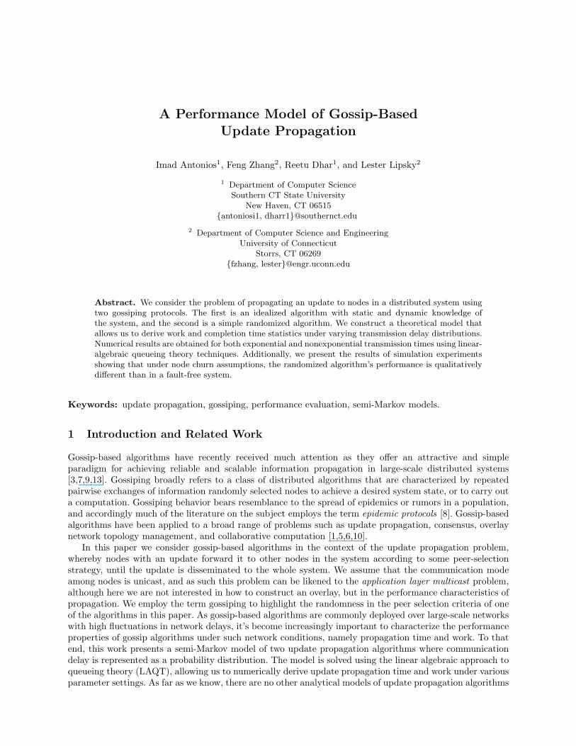
In Fig. 2, we plot numerical results for the mean total propagation time as a function of system size.Each of the curves corresponds to a different algorithm/distribution combination, with the first part of thelabels (R or Pk) refer to the randomized and perfect knowledge algorithms, respectively. As for distributions,

H2-5 and H2-10 are the two hyperexponential distribution, E2 is the Erlangian and M is the exponential (orMarkovian) distribution. The figure shows that for all cases, propagation time grows logarithmically due tothe parallelism inherent in update propagation. The figure indicates that for distributions with c2 > 1, namelythe hyperexponentials, the randomized algorithm greatly outperforms the idealized algorithm. The intuitionbehind this is that by allowing multiple concurrent transmissions to a node in the randomized algorithm,the progress in spreading updates becomes highly dependent on the shortest of these transmissions; it isfor distributions with high c2 values that the shortest transmission is much smaller than the mean, thusexplaining this gain in performance. The fact that a node can receive an update from multiple nodes,however, limits the degree of parallelism of the algorithm. When the transmission time variability is low, asin the case for the exponential and Erlangian distributions, the perfect knowledge algorithm performs betterthan the randomized algorithm. Generally, for the perfect knowledge algorithm, the lower the c2 value is,the less time it takes on average to propagate an update, whereas for the randomized algorithm the oppositeholds.

0 5 10 15 20 25 300

2

4

6

8

10

12

14

Pk-H2-10.0

Pk-H2-5.0

R-E2

R-MPk-M

Pk-E2

R-H2-5.0

R-H2-10.0

Total number of nodes in the system, N

Pro

paga

tion

tim

e, t N

Fig. 2. Total time comparison for various transmission distributions

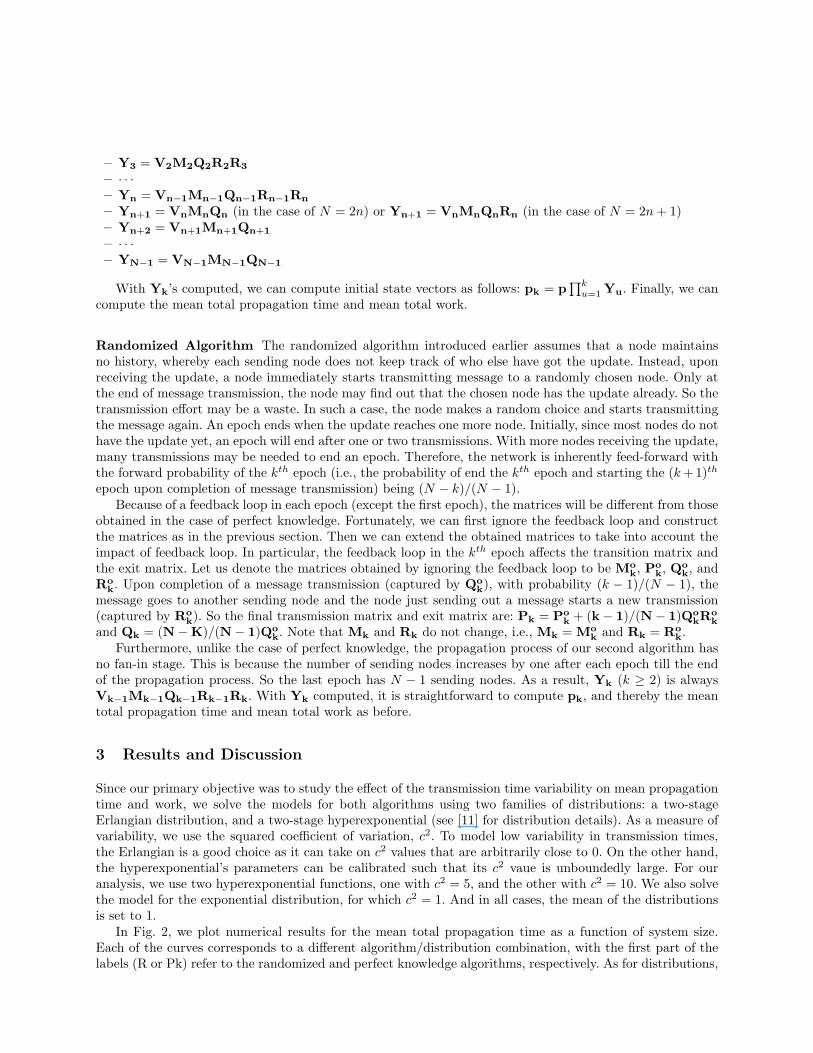
In addition to the mean propagation time, we compute the time to reach the nth epoch, that is the timefor the nth node to be updated for a system of a given size. These results are plotted in Fig. 3 for the perfectknowledge algorithm with a system size N = 65. The plots for the hyperexponential distributions show thatroughly the first 60 out of the 65 nodes are updated within 5 units of time, while the last 5 consume abouttwice as long. For all other distributions considered, the time it takes to propagate the update to the first 60nodes is longer, but the S-shaped curves don’t increase by the same magnitude for the last few nodes. Thisbehavior for the high c2 distributions can be expected since the last few nodes are dominated by samples fromthe distribution that are much greater than the mean, and under the perfect knowledge assumption a nodemay only have one sender. This finding is meaningful in an application setting where it’s not critical for theupdate to reach all nodes. The conclusion that can be drawn is that systems with highly varying transmission

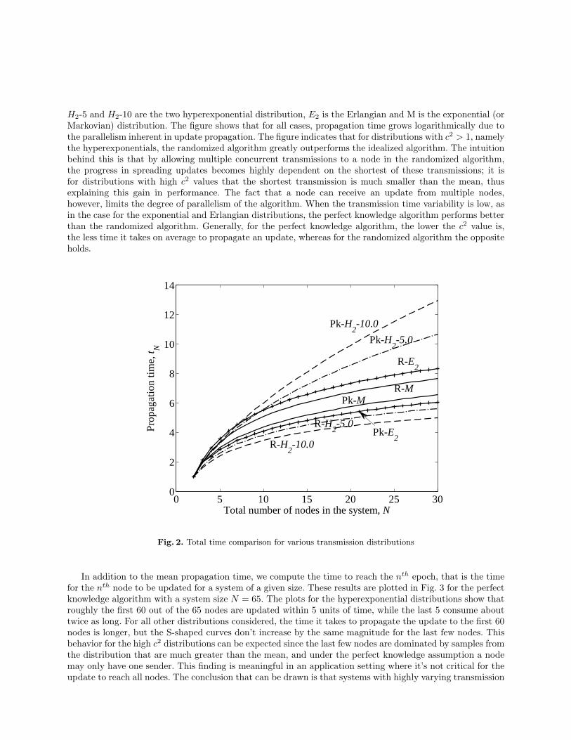
times should be favored when probabilistic guarantees of completion are acceptable. As another measure ofperformnce, we consider work as a function of system time for the various probability distributions. Theseare plotted in Fig. 4. For perfect knowledge, work grows linearly in system size, irrespective of distribution,since there are no redundant transmissions. For the randomized algorithm, the figure shows that work growsat a slightly faster rate, accounting for the redundant transmissions. As it is the case for mean propagationtime, the larger the coefficient of variation the less work the randomized algorithm requires.

0 5 10 15 20 25 30 35 40 45 50 55 60 650

2

4

6

8

10

12

14

Number of updated nodes in the system of N=65, k

Cum

ulat

ive

prop

agat

ion

tim

e,t k

Perfect Knowledge

EXP

H2:C

v2=5.0

H2:C

v2=10.0

E2

DET

Fig. 3. Cumulative time for PK algorithm to propagate update to N = 65 nodes.

As gossip-based algorithms are often targeted for large-scale dynamic systems, their behavior in thepresence of failures is important to characterize. To that end, we conducted simulation experiments usingthe randomized algorithm that model churn behavior, whereby nodes leave and join the system according toprobabilistic assumptions. We assume that node failures are independent events and the failure duration isexponentially distributed with mean m1. Nodes rejoin the system and remain up also for an exponentiallydistributed time period with mean m2. To allow for a meaningful case study, m1 and m2’s values need to beless than the expected propagation time. For a 5% per-node failure ratio, m1 and m2 were set to 0.25 and4.75, respectively. We assume that if a transmission is interrupted due to a node failure, the transmissionneeds to be restarted, i.e. the work is wasted. Since nodes maintain no history information, a receiver thatfails during a transmission is subject to selection by any updated node in the system once the receiver isalive again. We further assume that no work is consumed to determine if a communication peer is alive ornot, and a node can instantaneously detect if its communication peer fails. Figures 5 and 6 show the resultsof the simulation experiments. Each of the data points corresponds to the average of 1000 replications. Bothfigures show a marked difference in the performance of the algorithm compared to the earlier case. In Fig. 5,we see that propagation time now grows linearly in system size. With respect to work, Fig. 6 shows that itgrows at a much faster rate than before, almost quadratically. A possibly explanation is that given that nodefailures are independent, as we increase the number of nodes in the system the instantaneous probability

0 5 10 15 20 25 300

20

40

60

80

100

120

140

R-E2 R-M

R-H2-5.0

R-H2-10.0

Pk

Total number of nodes in the system, N

Tot

al w

ork,

wN

Fig. 4. Total work comparison for various transmission time distributions

that at least one node is down grows. The performance behavior resulting from the introduction of churnposes serious challenges to achieving scalability and warrants further detailed study.

4 Conclusion and Future Work

In this paper we presented a semi-Markov model of two update propagation algorithms, the first havingidealized system knowledge, and the second with randomized peer selection. We obtained numerical resultsthat demonstrate how the variability in transmission times influences the mean propagation time and work.The main finding was that when the larger the variability in transmission time is, the better the randomizedalgorithm’s performance is, both in terms of time and work. A more thorough discussion of probabilisticguarantees of algorithm termination would have been possible if the distribution (or even the variance) ofthe propagation time and work were available, but that is left for future investigation. Finally, simulationexperiments show that node churn behavior under independent failure assumption, has a significant neg-ative effect on system performance, and poses challenges with regards to scalability. These results call forthe development of new semi-Markov models that incorporate failure behavior to better characterize thecontribution of churning on system performance.

References

1. Bakhshi, R., Gavidia, D., Fokkink, W., van Steen, M.: An Analytical Model of Information Dissemination for aGossip-based Wireless Protocol. ICDCN 2009.

2. Berenbrink, P., Cooper, C., Hu, Z.: Energy Efficient Randomised Communication in Unknown AdHoc Networks.Ninth Annual Symp. on Parallel Algorithms and Architectures, San Diego, California, 2007.

3. Berman, K.: The Promise, and Limitation, of Gossip Protocols. ACM SIGOPS, 41 (2007) 8–13.

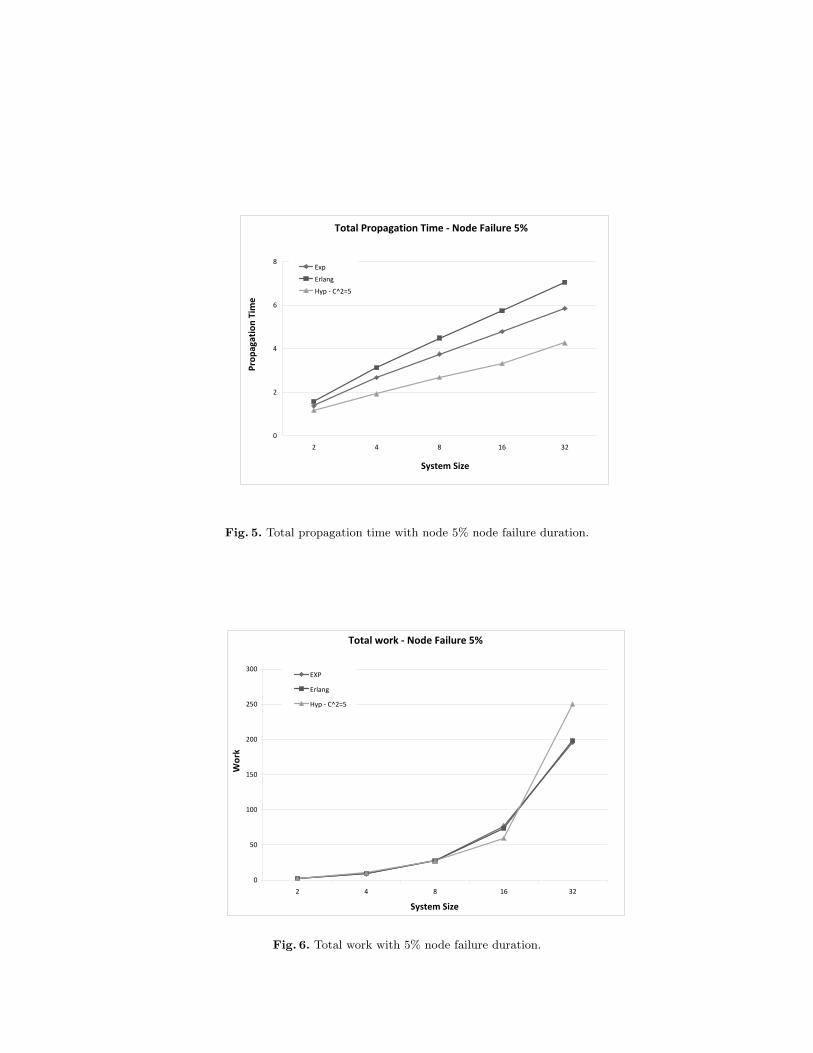
Total Propagation Time - Node Failure 5%

0

2

4

6

8

2 4 8 16 32

System Size

Pro

pa

ga

tio

n T

ime

Exp

Erlang

Hyp - C^2=5

Fig. 5. Total propagation time with node 5% node failure duration.

Total work - Node Failure 5%

0

50

100

150

200

250

300

2 4 8 16 32

System Size

Wo

rk

EXP

Erlang

Hyp - C^2=5

Fig. 6. Total work with 5% node failure duration.

4. Boyd, S., Gosh, A., Prabhakar, B., and Shah, D.: Randomized Gossip Algorithms. IEEE Trans. Infor. Theory 52(2006) 2508–2530.

5. Chlebus, B., Kowalski, D.: Gossiping to Reach Consensus. 14th ACM Symp. on Parallel Algorithms and Archi-tectures, 2002.

6. Dimakis, A., Sarwate, A., Wainwright, M.: Geographic Gossip: Efficient Aggregation for Sensor Networks. 5thInt. Conf. on Information Processing in Sensor Networks, 2006.

7. Drost, N., Ogston, E., van Nieuwpoort, R., Bal, H.: ARRG: Real-World Gossiping. HPDC 2007, Monterey,California.

8. Eugster, P., Guerraoui, R., Kermarrec, A.-M., Massoulie, L.: From Epidemics to Distributed Computing. IEEEComput. 2003.

9. Georgiou, C., Gilbert, S., Guerraoui, R., Kowalski, D.: On the Complexity of Asynchronous Gossip. PODC 2008,Toronto Canada.

10. Haas, Z., Halpern, J., Li, L.: Gossip-Based Ad Hoc Routing. IEEE/ACM Trans. Net., 14 (2006) 470–491.11. Lipsky, L.: QUEUEING THEORY: A LINEAR ALGEBRAIC APPROACH, second edition. Springer-Verlag,

New York, 2008.12. Neuts, M.: MATRIX-GEOMETRIC SOLUTIONS IN STOCHASTIC MODELS. Johns Hopkins University Press,

London, 1981.13. Kermarrec, A.-M., van Steen, M.: Gossiping in distributed systems. SIGOPS Oper. Syst. Rev. 41 (2007) 2–7.