A Novel Method to Determine Blower Capacity of Wastewater ...

212

Original ArticleA Novel Method to Determine Blower Capacity of Wastewater

Treatment Plants for Dry and Wet Weather ConditionsViet Hoang Nguyen a, Van Tuan Le b, Thi Ha Nguyen c, Xuan Hai Nguyen d, Viet Anh Nguyen e,

Hidenori Harada f, Mitsuharu Terashima a, Hidenari Yasui a

a Faculty of Environmental Engineering, the University of Kitakyushu, Kitakyushu, Japanb Faculty of Environmental Science, University of Sciences - Hue University, Hue, Vietnam

c Faculty of Environmental Science, Vietnam National University - University of Science, Hanoi, Vietnamd Department of Environment Impact Assessment Appraisal, Vietnam Environment Administration, Hanoi, Vietnam

e Institute of Environmental Science and Engineering, Hanoi University of Civil Engineering, Hanoi, Vietnamf Graduate School of Asian and African Area Studies, Kyoto University, Kyoto, Japan

ABSTRACTAscertaining peak oxygen demand is crucial for plant designers to determine blower capacities of wastewater treatment plants in planning phase. To obtain this technical information without cumber-some influent sampling and analysis, a set of field-test activated sludge reactors equipped with DO and nitrate-N sensors was installed at 3 sites and continuously operated for a couple of months in each field. Under the controlled aeration and hydraulics of the reactors, the hourly influent oxygen demands were back-calculated as biodegradable constituents using the IWA-Activated Sludge Model #1. The daily maximum concentrations (rounded to last for 1-hour) of biodegradable organics and nitrogen were ranged between 45~258 mg-COD/L and 10.4~32.3 mg-N/L in Site #1; 119~244 mg-COD/L and 28.3~38.7 mg-N/L in Site #2; 194~552 mg-COD/L and 30.2~51.7 mg-N/L in Site #3 respectively. The marginal blower capacities to maintain at least 1.0 mg-O2/L of DO in the daily maximum oxygen demand were estimated based on the datasets using the statistical method, Extreme Value Distribu-tion analysis. To maintain the DO concentration for 99 days out of 100 days of the plant operations, the blower capacity was supposed to be designed as high as 1.4~2.2 times than those of the blower calculated from the daily average concentration.

Keywords: activated sludge model, blower capacity, dynamic parameter estimation, extreme value distribution, statistical analysis

INTRODUCTION

Aeration is a key component to design wastewater treat-ment plants (WWTPs), particularly activated sludge process-es because the aeration energy is supposed to be more than half of the total energy consumption in the WWTPs [1,2]. In this regard three affairs are considered in the aeration design: air supply system, oxygen transfer and oxygen demand. For the air supply system and the oxygen transfer, the topics have been intensively studied. For instance, with respect to model-

ling the aeration system and its energy consumption, Schraa et al. (2017) developed a fully dynamic model around the aeration header network to simulate the air distribution, and evaluated its limitations with various optimisation options and influent loadings [3]. Juan-Garcia et al. (2018) modified their study to the plant controlling systems by integrating a biokinetic model having oxygen uptake phenomena [4]. On the other hand, precise measurement of oxygen demand from the influent is still challenging because numerous influent sampling and analysis are needed to determine blower capac-

Corresponding author: Hidenari Yasui, E-mail: [email protected]: September 18, 2020, Accepted: April 22, 2021, Published online: August 10, 2021

Open Access

This is an open-access article distributed under the terms of the Creative Commons Attribution (CC BY) 4.0 License. http://

creativecommons.org/licenses/by/4.0/

Journal of Water and Environment Technology, Vol.19, No.4: 212–229, 2021doi: 10.2965/jwet.20-138

http://creativecommons.org/licenses/by/4.0/

http://creativecommons.org/licenses/by/4.0/

https://doi.org/10.2965/jwet.20-138

Journal of Water and Environment Technology, Vol. 19, No. 4, 2021 213

ity which is the primary instrument of the air supply system. In fact, designing procedure to determine blower capacity to meet peak oxygen demand (daily maximum) is quite limited in guidelines available in literature [5,6].

The above-mentioned guidelines only provide default design-daily-average concentrations of BOD5 and Total Kjeldahl Nitrogen (TKN) with thumb rules to adapt the parameters to the plant design. For example, Schraa et al. (2017) and US Environmental Protection Agency (USEPA) selected 150~200 mg-BOD/L and 30~40 mg-N/L as the default BOD5 concentration and total TKN concentration respectively [3]. With respect to the oxygen demand in design-daily-maximum, the guidelines suggest calculating the load in proportion to the inflow rate of the design-daily-average. The concept assumes that the influent concentration during the design-daily-maximum flow is identical to that during the design-daily-average flow. On the other hand, the guidelines also assume that the mass flow of oxygen demand per catchment area (kg/m2/d) is independent on the wastewater flow rate (m3/d). Consequently, they anticipate that the influent concentration during the daily maximum event would be lowered in reality. Therefore, the calculated value of the oxygen demand for design-daily-maximum flow becomes somewhat conservative allowing a safety margin for the design of blower capacity.

Although the above simple approach has been traditionally accepted in the regions, it is not clear whether this method can be also applicable to other regions and countries. This is because the sewer system and wastewater constituents are not always comparable to those of the regions that they analysed. For instance, in Southeast Asian countries (e.g. Vietnam), septic tank is obligatory installed at each house-hold in front of the sewer, which often discharges low BOD5 wastewater whilst TKN remains its concentration [7–9]. In addition, these countries mostly use combined sewer systems resulting in high fluctuation of wastewater concentration (and flow) over dry and rainy seasons [10]. Therefore, it is desired to measure the influent oxygen demand concentra-tion for daily maximum which may not correspond to the daily average flow rate. This is supposed to the key to design proper air supply system.

One of the reasons that the guideline is obliged to take the simplified approach is due to the fact that numerous influent sampling and analysis are practically infeasible. In order to identify daily maximum concentration, at least 24 samples are required even the concentrations are rounded in 1 hour. When the analytical campaign lasts for a year to obtain design-daily-maximum concentration, at least 8,760 samples

(= 24 × 365) must be analysed. Furthermore, in case that the biokinetic model (e.g. the IWA-Activated sludge model (ASMs) [11]) is used for plant design, the total number of the chemical/biological analytical items would reach several ten thousand per project.

To cope with the challenge, one alternative approach is to perform a back-calculation of the influent oxygen demand from the dynamic response of a field-test reactor receiving the influent continuously. When the dynamic responses are recorded as the system outputs, the system inputs (influent) can be mathematically obtained using the ASMs in an in-verse manner. Using the method Nguyen Duong et al. (2017) successfully demonstrated to obtain the ASM-based weekly-average influent concentrations from the analysis of acti-vated sludge fractions (dynamic changes of heterotrophic/autotrophic biomass and unbiodegradable organic particu-lates during the 7 days) [12]. Unfortunately, their approach is not possible to estimate the hourly influent concentrations because the increment/decrement of the bacterial fractions within 1-hour are too small to be identified. However, when dynamic responses of dissolved oxygen (DO) concentration and nitrate concentration of the reactor are continuously monitored by using on-line sensors, these monitored state variables would provide us relevant information to back-calculate the influent oxygen demand. This is because the response/increment/decrement per time are electronically detectable even every 5 minutes. In this regard, since DO in the reactor is resulted from the microbial respiration in the reactor and the oxidation of the influent biodegradable materials, the active biomass concentration in the reactor and its biological kinetics must be also obtained by off-line analysis at laboratory. Nevertheless, this labour intensity is supposed to be negligible comparing to that to carry out the huge influent sampling/analysis campaign.

When the dataset of hourly influent concentrations is obtained, this dataset is statistically analysed to calculate the blower power for aeration. In definition, the design-daily-average is the mean value of the influent loading in 365 days (a year) whilst the design-daily-maximum is the highest loading occurring in the year [6]. Since the influent oxygen demand concentration is highly fluctuated even within a day, the design-daily-maximum for blower capacity may be interpreted from the instantaneous elevation of the load per hour (hourly influent loading). In this case, 365 data having the highest oxygen demand in the day must be statistically analysed to estimate the risk (probability) of the influent load that exceeds the blower capacity. Extreme Value Distribution (EVD) is the statistical distribution to express such extreme


event [13]. Hence adopting the statistical distribution to anal-yse the back-calculated influent oxygen demand is thought to be relevant. In addition, the approach may enable to evalu-ate the impact of stormwater on the influent concentration, which is also one of essential scopes to design WWTPs in combined sewer system. At the beginning of rain, so-called first flush is supposed to bring high oxygen demand to the WWTP via runoff. To evaluate the occurrence of the high oxygen demand (= extreme events) caused by the first flush and/or hourly ~ daily maximum concentration of the influent, the measured datasets should be statistically analysed and properly interpreted to the plant design. Based on the above background, to check the feasibility of the above-mentioned alternative approach for blower capacity design, the field ex-periments were carried out in 3 distinct sites having inherent sewer system (two in Vietnam, one in Japan).

MATERIALS AND METHODS

Experimental and analytical approachesAs mentioned in the introduction section, the continuous

operation of the field-test activated sludge reactor(s) equipped with DO and nitrate sensors was needed to estimate the dynamic change of influent oxygen demand (biodegradable substances) together with off-line batch analysis to measure the kinetics and biomass concentration in the reactors. The datasets obtained from the field experiments were dynamically analysed in the IWA-Activated Sludge Model #1 (ASM1) to perform the back-calculation for the influent characterisation [12,14]. From the numerical calculation,

the estimated concentrations of biodegradable substances were expressed in a discrete form (discrete concentration in every 1-hour). As the computed concentrations depended on the data density from the sensors (e.g. data logging at every 5-minute, 10-minute…), the impact of data density on the calculation was evaluated first in this study. Subsequently, the probabilities of the very high oxygen demand loading to the WWTPs was statistically analysed using EVD concept [15–18]. As the EVD concept was widely used in the field of reliability engineering, this method was thought to be also applicable to analyse the probabilities of the very high oxygen demand loading. Based on the statistical analysis, case studies (calculation examples) to design blower capacity treating the very high oxygen demand were carried out using a process simulator.

Field-test activated sludge reactorsSystem layout

As illustrated in Fig. 1, one out of the activated sludge reactors (ASR#1) was equipped with a chemically enhanced primary settling tank, where the flocculant and coagulant were dosed to enhance particulate settling of the influent, followed by an identical set of the aeration tank and the secondary settling tank to another activated sludge reactor (ASR#2). ASR#1 was operated to measure the soluble bio-degradable fractions in the influent whilst ASR#2 was used to obtain the total biodegradable substance concentrations in the influent including suspended particulates.

All tanks had 23-L of working volume with conical cyl-inder shape. A solid scraper rotating at 1 rpm was set at the

Fig. 1 Schematic flow of the field-test activated sludge reactors.


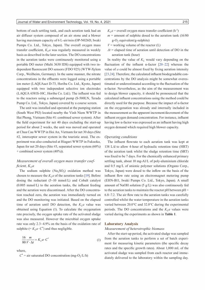
bottom of each settling tank, and each aeration tank had an air diffuser system composed of an air stone and a blower having maximum capacity of 6 L-air/min (OP-N026D, Iwaki Pumps Co. Ltd., Tokyo, Japan). The overall oxygen mass transfer coefficient, KLa was regularly measured in weekly basis as described in the later section. The DO concentrations in the aeration tanks were continuously monitored using a portable DO meter (Multi 3630 IDS) equipped with two in-dependent fluorescent DO sensors (FDO 925) (WTW-Xylem Corp., Weilheim, Germany). In the same manner, the nitrate concentrations in the effluents were logged using a portable ion meter (LAQUAact D-73, Horiba Co. Ltd., Kyoto, Japan) equipped with two independent selective ion electrodes (LAQUA 6581S-10C, Horiba Co. Ltd.). The influent was fed to the reactors using a submerged pump (S-500LN, Terada Pump Co. Ltd., Tokyo, Japan) covered by a course screen.

The unit was installed and operated at the pumping station (South West PS3) located nearby the Vinh Niem WWTP in Hai Phong, Vietnam (Site #1: combined sewer system). After the field experiment for net 40 days excluding the start-up period for about 2 weeks, the unit was moved and operated at Chua Cau WWTP in Hoi An, Vietnam for net 30 days (Site #2, interceptor sewer system in the touristic area). The ex-periment was also conducted at Hiagari WWTP in Fukuoka, Japan for net 20 days (Site #3, separated sewer system (60%) + combined sewer system (40%)).

Measurement of overall oxygen mass transfer coef-ficient, KLa

The sodium sulphite (Na2SO3) oxidation method was chosen to measure the KLa of the aeration tanks [19]. Before dosing the reductant (5~10 mmol/L) and Cobalt catalyst (0.005 mmol/L) to the aeration tanks, the influent feeding and the aeration were discontinued. After the DO concentra-tion reached zero, the aeration was immediately turned on and the DO monitoring was initiated. Based on the elapsed time of aeration until DO detection, the KLa value was obtained using Equation (1). To calculate the oxygenation rate precisely, the oxygen uptake rate of the activated sludge was also measured. However the microbial oxygen uptake rate was only 2.3~4.9% on the basis of the oxidation rate of sulphite (= KLa ∙ C*) and thus negligible.

*16

80 Lm K a C

V t= ⋅

⋅∆ (1)

where,C* = air saturated DO concentration (mg-O2/L/h)

KLa = overall oxygen mass transfer coefficient (h-1)m = amount of sulphite dosed to the aeration tank (16/80

g-O2 equivalent/g-sulphite)V = working volume of the reactor (L)Δt = elapsed time of aeration until detection of DO in the

aeration tank (hour)In reality the value of KL would vary depending on the

fluctuation of the influent α-factor [20–22] whereas the value of a could be almost fixed by fixing aeration intensity [23,24]. Therefore, the calculated influent biodegradable con-centrations by the DO analysis might be somewhat overes-timated or underestimated according to the fluctuation of the α-factor. Nevertheless, as the aim of the measurement was to design blower capacity, it should be pronounced that the calculated influent concentrations using the method could be directly used for the purpose. Because the impact of α-factor on the oxygenation was already and internally included in the measurement as the apparent increment/decrement of the influent oxygen demand concentration. For instance, influent having low α-factor was expressed as an influent having high oxygen demand which required high blower capacity.

Operating conditionsThe influent flowrate to each aeration tank was kept at

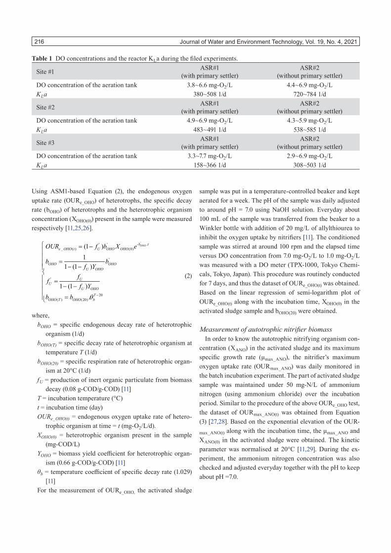
138 L/d to allow 4-hour of hydraulic retention time (HRT) of the aeration tank whilst the sludge retention time (SRT) was fixed to be 7 days. For the chemically enhanced primary settling tank, about 10 mg-Al/L of poly-aluminium chloride and 0.5 mg/L of anionic polymer solutions (Organo Corp., Tokyo, Japan) were dosed to the inflow on the basis of the influent flow rate using an electromagnet metering pump (EHN-B11, Iwaki Pumps Co. Ltd., Tokyo, Japan). A small amount of NaOH solution (5 g/L) was also continuously fed to the aeration tanks to maintain the reactor pH between pH = 6.8~7.2. The air flow rate to the aeration tanks was carefully controlled whilst the water temperature in the aeration tanks varied between 20.0°C and 32.0°C during the experimental periods. The DO concentrations and the KLa values were varied during the experiments as shown in Table 1.

Laboratory AnalysisMeasurement of heterotrophic biomass

After the start-up period, the activated sludge was sampled from the aeration tanks to perform a set of batch experi-ment for measuring kinetic parameters (the specific decay rates and the specific growth rates). About 1,000 mL of the activated sludge was sampled from each reactor and imme-diately delivered to the laboratory within the sampling day.


Using ASM1-based Equation (2), the endogenous oxygen uptake rate (OURe_OHO) of heterotrophs, the specific decay rate (bOHO) of heterotrophs and the heterotrophic organism concentration (XOHO(0)) present in the sample were measured respectively [11,25,26].

'- .' '_ ( ) (0)

'

'

20( ) (20)

(1 )1

1 (1 )

1 (1 )

.

OHOb te OHO t U OHO OHO

OHO OHOU OHO

UU

U OHOT

OHO T OHO b

OUR f b X e

b bf Y

ff

f Y

b b θ −

= − = − − = − −

=

(2)

where,bOHO = specific endogenous decay rate of heterotrophic

organism (1/d)bOHO(T) = specific decay rate of heterotrophic organism at

temperature T (1/d)bOHO(20) = specific respiration rate of heterotrophic organ-

ism at 20°C (1/d)fU = production of inert organic particulate from biomass

decay (0.08 g-COD/g-COD) [11]T = incubation temperature (°C)t = incubation time (day)OURe_OHO(t) = endogenous oxygen uptake rate of hetero-

trophic organism at time = t (mg-O2/L/d).XOHO(0) = heterotrophic organism present in the sample

(mg-COD/L)YOHO = biomass yield coefficient for heterotrophic organ-

ism (0.66 g-COD/g-COD) [11]θb = temperature coefficient of specific decay rate (1.029)

[11]For the measurement of OURe_OHO, the activated sludge

sample was put in a temperature-controlled beaker and kept aerated for a week. The pH of the sample was daily adjusted to around pH = 7.0 using NaOH solution. Everyday about 100 mL of the sample was transferred from the beaker to a Winkler bottle with addition of 20 mg/L of allylthiourea to inhibit the oxygen uptake by nitrifiers [11]. The conditioned sample was stirred at around 100 rpm and the elapsed time versus DO concentration from 7.0 mg-O2/L to 1.0 mg-O2/L was measured with a DO meter (TPX-1000, Tokyo Chemi-cals, Tokyo, Japan). This procedure was routinely conducted for 7 days, and thus the dataset of OURe_OHO(t) was obtained. Based on the linear regression of semi-logarithm plot of OURe_OHO(t) along with the incubation time, XOHO(0) in the activated sludge sample and bOHO(20) were obtained.

Measurement of autotrophic nitrifier biomassIn order to know the autotrophic nitrifying organism con-

centration (XANO) in the activated sludge and its maximum specific growth rate (μmax_ANO), the nitrifier’s maximum oxygen uptake rate (OURmax_ANO) was daily monitored in the batch incubation experiment. The part of activated sludge sample was maintained under 50 mg-N/L of ammonium nitrogen (using ammonium chloride) over the incubation period. Similar to the procedure of the above OURe_OHO test, the dataset of OURmax_ANO(t) was obtained from Equation (3) [27,28]. Based on the exponential elevation of the OUR-max_ANO(t) along with the incubation time, the μmax_ANO and XANO(0) in the activated sludge were obtained. The kinetic parameter was normalised at 20°C [11,29]. During the ex-periment, the ammonium nitrogen concentration was also checked and adjusted everyday together with the pH to keep about pH =7.0.

Table 1 DO concentrations and the reactor KLa during the filed experiments.

Site #1 ASR#1 (with primary settler)

ASR#2 (without primary settler)

DO concentration of the aeration tank 3.8~6.6 mg-O2/L 4.4~6.9 mg-O2/LKLa 380~508 1/d 720~784 1/d








( )max_ ( ) max_ ( ) ( )

( )( ) (0)

max__

20max_ ( ) max_ (20)

4.57(1 )

.

ANO ANO

ANOANO t ANO ANO t U ANO ANO t

ANOb t

ANO t ANO

ANO ANOS ANO

TANO T ANO

YOUR X f b X

Y

X X eS

K S

µ

µ

µ

µ µ

µ µ θ

−

−

−= + −

= = + =

(3)

where:bANO = specific decay rate of autotrophic organism (0.15

1/d at 20°C) [29]KS_ANO = half-saturation growth coefficient of autotrophic

organism (1.0 mg-N/L at 20oC) [11]OURmax_ANO(t) = maximum oxygen uptake rate of autotro-

phic organism at time = t (mg-O2/L/d)SNHx = ammonium nitrogen concentration (mg-N/L)T = incubation temperature (°C)t = incubation time (day)XANO(0) = autotrophic nitrifying organism present in the

sample (mg-COD/L)XANO(t) = autotrophic nitrifying organism present at time =

t (mg-COD/L)YANO = biomass yield coefficient for autotrophic organism

(0.24 g-COD/g-N) [11]μANO = specific growth rate of autotrophic nitrifying or-

ganism (1/d)μmax_ANO = maximum specific growth rate of autotrophic

nitrifying organism (1/d)μmax_ANO(T) = maximum specific growth rate of autotrophic

nitrifying organism at temperature T (1/d)μmax_ANO(20) = maximum specific growth rate of autotro-

phic nitrifying organism at 20°C (1/d)θμ = temperature coefficient of specific growth rate (1.072)

[11]

Dynamic estimation of influent constituents and concentration

The DO concentration of the reactors and the nitrate con-centration in the effluents were chosen as the target variables (the variables to fit to the data) according to Nguyen et al. (2019) [14]. The soluble biodegradable organics (SB), soluble biodegradable nitrogen (SB,N), particulate biodegradable or-ganics (XCB) and particulate biodegradable organic nitrogen (XCB,Org,N) were also selected as the optimised variables of the influent (the regression variables to match the target variables of the data). The identified biomass state variables (XOHO(0) and XANO(0)) were input at the beginning of the each

day of the dynamic simulation. After this computational set up, focusing on the DO and nitrate concentrations of the ASRs, the hourly concentrations of the above influent bio-degradable constituents were dynamically back-calculated. Specifically, the discrete concentrations of SB(t) and SB,N(t) in 1 hour were obtained from the dynamic behaviours of DO and nitrate in ASR#1. By inputting these estimated influent state variables to the subsequent ASR#2 simulation, the discrete concentration of XCB(t) and XCB,Org,N(t) were obtained from ASR#2 receiving these suspended solid from the influent.

The dynamic estimation was performed using Dynamic Parameter Estimation tool (DPE) programmed in a com-mercial process simulator, GPS-X Version 7.0 (Hydromantis Inc., Hamilton, Ontario, Canada). For the DPE setting, time-step (time length where the optimised variables were treated as constant values) was set at 1.0 hour meaning that the concentrations of the SB(t), SNHx(t), XCB(t) and XCB,N(t) were discretised per hour (= discrete concentration in every 1-hour). In this study the data densities of the target variables (= logging interval of the sensors) were evaluated among ev-ery 5-minute per day (12 data per hour) and every 30-minute per day (2 data per hour). Maximum Likelihood method was chosen for the regression [14]. The total days of the influent analysis were 40-day for Site #1, 30-day for Site #2 and 20-day for Site #3 respectively.

Statistical analysis to design blower capacityTo perform the case studies to meet very high oxygen

demand from the influents, a virtual WWTP was built on the process simulator. As listed in Table 2, the virtual WWTP was modelled to receive the influent at 36,000 m3/d of constant flow rate with the hourly discretised concentra-tions which were collected from the analysis of Site #1, Site #2 and Site #3 respectively. The virtual WWTP had a big blower controlled by a DO sensor allowing to manipulate the blower power in a dynamic manner to maintain 1 mg-O2/L of DO in the aeration tank [30,31]. In this way, the highest aeration (peak power consumption of the blower) lasting for one hour was identified in each day. Next, the value of hourly maximum power consumption in each day was ranked from the smallest to the largest over the days in each dataset based on EVD concept. From the statistical distribution of the hourly maximum power consumption of the blower, the required blower capacity to operate the WWTP without DO deficiency at least for 99 days out of 100 days was predicted. For simplification, both HRT and SRT of the virtual WWTP were fixed to be 6 hrs and 10 days respectively.

EVD type I (the Gumbel distribution for maxima case) was


supposed to be relevant for the statistical analysis because this distribution was commonly used to predict extreme events/disasters such as flooding due to extreme rainfall [15,16]. To cope with the limited number of the data which might result in scattered distribution in the order statistic, as shown in Equation (4), the median rank estimator, MR(i) [17,18] which was widely used to analyse limited data (e.g. 20~40 data) was chosen. In this way the outliners which might exist in the limited data could be excluded from the analysis. The hourly maximum power consumptions of the blower were ranked in ascending order according to the order statistic of MR(i). Specifically the EVD was expressed by plotting hourly maximum power consumptions of the blower (xi) on X-coordinate and the estimated cumulative probability density function, F(xi) of EVD on Y-coordinate (mapped from the median rank estimator (MR(i))). Based on the double semilogarithmic X-Y graph, the probabilities of DO-maintaining failure (%) were calculated along with the blower capacities (net blower power, kW).

( ){ }( ) ( )

( )

2( 1 ),2 ,0.50

1ln ln

( 1 )

i

i

x i i

i xn i i

F y x

iMR Fi n i F

µβ β

+ −

− − = − = − = = + + −

(4)

where,F(xi) = median rank-based cumulative probability density

function of EVD type I (-)2i = degrees of freedom (-)

F2(n+1−i),2i,0.50 = the F-distribution at the 0.50 point (median) with 2(n+1−i) (-)

i = rank of xi in the sample size n. (i = 1…n) (-)MR(i) = median rank at the rank of i (-)xi = variable of the function (= hourly maximum blower

power consumption within the day) (kW)β = EVD scale parameter (β > 0) (kW)μ = EVD location parameter (kW)

RESULTS

Estimation of the hourly biodegradable substance concentration in the influentsSensitivity of the data logging interval on the calcula-tion results

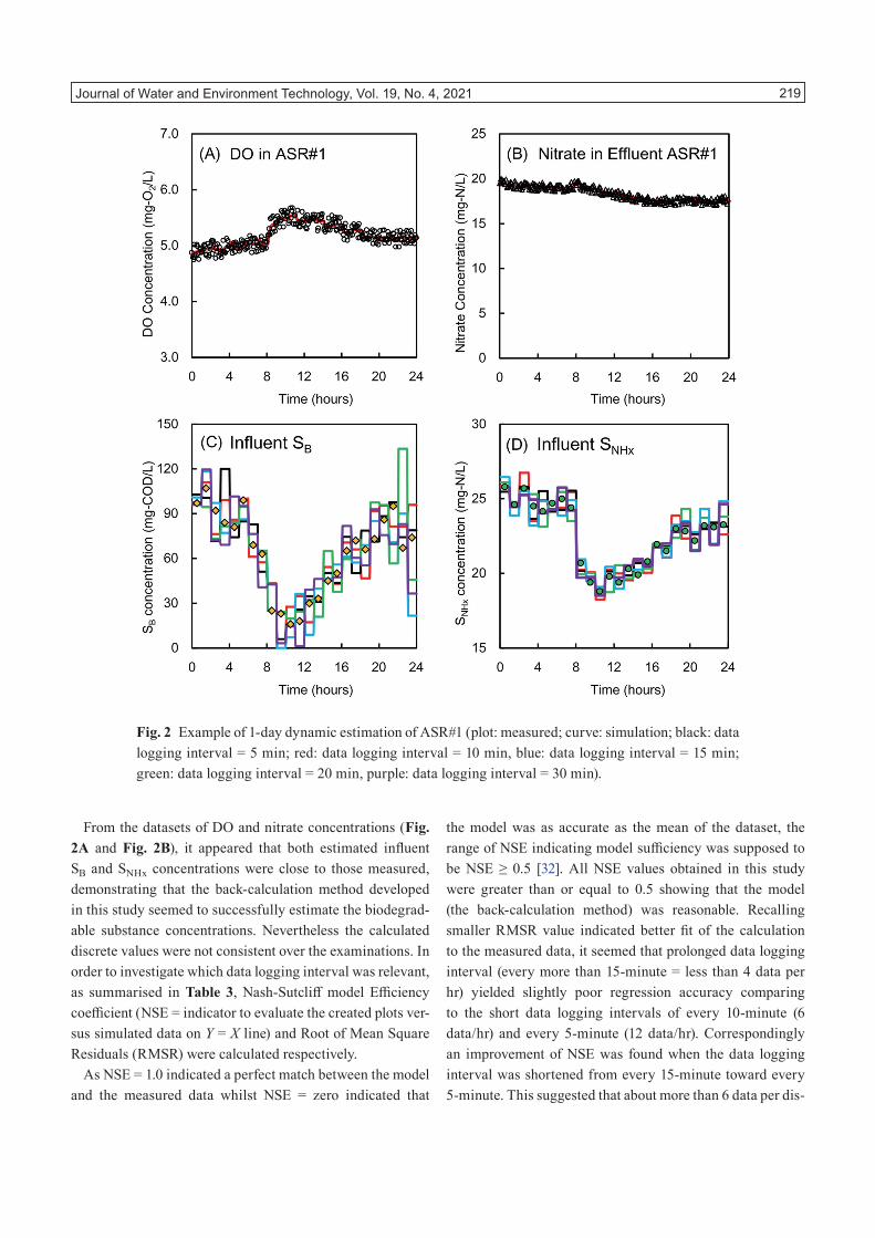
Basically the values of the estimated variables (= influent SB, XCB, SB,N and XCB,Org,N) were given from the dynamic regression to reproduce the target values of the dataset (= DO and nitrate concentrations) in the field-test reactors. Therefore the values of the estimated influent concentra-tions should depend on the quality of dataset (variation due to analytical error and/or sensitivity of probe), which might be compensated with the data density (data logging interval per hour). To clarify this, the density of the logged DO and nitrate concentrations of ASR #1 was examined among every 30-minute, 20-minute, 15-minute, 10-minute and 5-minute. As shown in Fig. 2, the calculated discrete values of the hourly influent concentrations for SB and SNHx of each examination were compared to those measured.

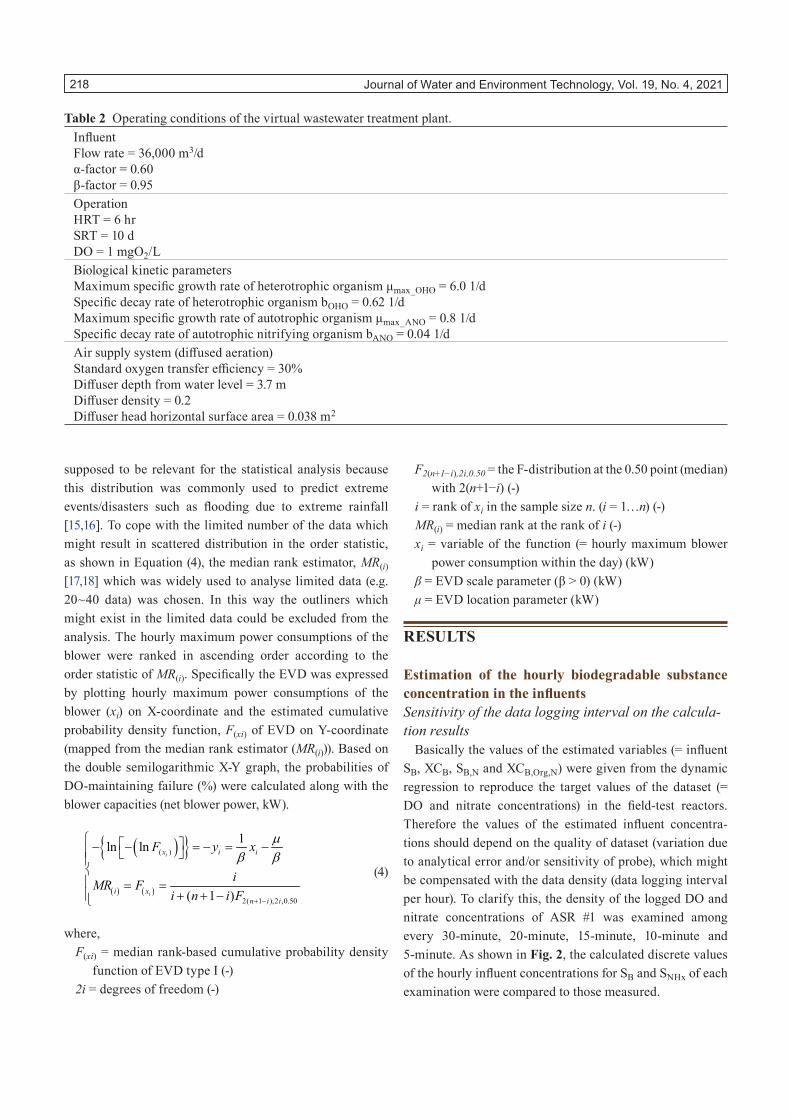
Table 2 Operating conditions of the virtual wastewater treatment plant.Influent Flow rate = 36,000 m3/d α-factor = 0.60 β-factor = 0.95Operation HRT = 6 hr SRT = 10 d DO = 1 mgO2/LBiological kinetic parameters Maximum specific growth rate of heterotrophic organism μmax_OHO = 6.0 1/d Specific decay rate of heterotrophic organism bOHO = 0.62 1/d Maximum specific growth rate of autotrophic organism μmax_ANO = 0.8 1/d Specific decay rate of autotrophic nitrifying organism bANO = 0.04 1/dAir supply system (diffused aeration) Standard oxygen transfer efficiency = 30% Diffuser depth from water level = 3.7 m Diffuser density = 0.2 Diffuser head horizontal surface area = 0.038 m2


From the datasets of DO and nitrate concentrations (Fig. 2A and Fig. 2B), it appeared that both estimated influent SB and SNHx concentrations were close to those measured, demonstrating that the back-calculation method developed in this study seemed to successfully estimate the biodegrad-able substance concentrations. Nevertheless the calculated discrete values were not consistent over the examinations. In order to investigate which data logging interval was relevant, as summarised in Table 3, Nash-Sutcliff model Efficiency coefficient (NSE = indicator to evaluate the created plots ver-sus simulated data on Y = X line) and Root of Mean Square Residuals (RMSR) were calculated respectively.

As NSE = 1.0 indicated a perfect match between the model and the measured data whilst NSE = zero indicated that

the model was as accurate as the mean of the dataset, the range of NSE indicating model sufficiency was supposed to be NSE ≥ 0.5 [32]. All NSE values obtained in this study were greater than or equal to 0.5 showing that the model (the back-calculation method) was reasonable. Recalling smaller RMSR value indicated better fit of the calculation to the measured data, it seemed that prolonged data logging interval (every more than 15-minute = less than 4 data per hr) yielded slightly poor regression accuracy comparing to the short data logging intervals of every 10-minute (6 data/hr) and every 5-minute (12 data/hr). Correspondingly an improvement of NSE was found when the data logging interval was shortened from every 15-minute toward every 5-minute. This suggested that about more than 6 data per dis-

Fig. 2 Example of 1-day dynamic estimation of ASR#1 (plot: measured; curve: simulation; black: data logging interval = 5 min; red: data logging interval = 10 min, blue: data logging interval = 15 min; green: data logging interval = 20 min, purple: data logging interval = 30 min).


crete calculation (≥ 6 data/hr) was desired to attain relevant dynamic simulation. On the other hand, due to mechanical limitation of sensors, the DO probe required at least 2~3 minutes to reach stable output signal whilst the nitrate probe also required 3~5 minutes [33,34]. Hence very short data logging interval (e.g. every 1 minute) could result in wrong interpretation of the data. Considering this, 10-minute data logging interval was chosen in this study.

Hourly concentration of the influent biodegradable substances

To demonstrate the measured and calculated results for the hourly concentrations, an example of dataset of within-one-day dynamic simulation for the DO and nitrate concentra-tions was shown in Fig. 3A–D, which were taken from the 40 datasets of Site #1. When DO concentrations were lowered (Fig. 3A for ASR #1. Fig. 3B for ASR #2), increased nitrate concentrations in the effluents was recognised in both ASR #1 (Fig. 3C) and ASR #2 (Fig. 3D). This indicated that the

Table 3 Model fitness versus the logging intervals for DO and nitrate concentrations.Nash-Sutcliff model Efficiency (NSE)

Every 30 min (2 data/hr)





Influent SB 0.64 0.50 0.64 0.78 0.78Influent SNHx 0.93 0.89 0.89 0.91 0.94

Root of Mean Squared Residuals (RMSR)Every 30 min

(2 data/hr)Every 20 min



(6 data/hr)Every 05 min (12 data/hr)

Influent SB 16.28 19.19 16.34 12.77 12.82Influent SNHx 0.58 0.70 0.70 0.64 0.54

Fig. 3 An example of 1-day dynamic estimation of the hourly concentration of the influent compositions from the fluctuation of the DO concentration and the nitrate concentration in the field-test reactors at Site #1 (circle: measured DO concentration; triangle: measured nitrate concentration; black curve: simulation).


biodegradable nitrogen of the influent was one of the sources of the oxygen demand. As shown in Fig. 3E–H, The sinu-soidal patterns for both influent SB and SNHx were found where the concentrations were lowered in early morning at around 4:00 and in evening at around 20:00 (Fig. 3E for SB, Fig. 3F for SB,N). Similarly the influent biodegradable particulate fractions expressed as XCB and XCB,N seemed to be also lowered at around 4:00 and at around 20:00 (Fig. 3G for XCB, Fig. 3H for XCB,N). The biodegradable organic fractions of the influent were ranged between 87~150 mg-COD/L for soluble material (SB) and 1.0~90 mg-COD/L for particulate material (XCB) respectively. For the influent biodegradable nitrogen, the soluble form (SB,N) was ranged between 17.0~21.3 mg-N/L whilst the concentration of par-ticulate form (XCB,Org,N) was relatively low and estimated to be around 1.0~8.0 mg-N/L only. In general, the occurrence of particulate nitrogen seemed to be associated with those of particulate organics and the soluble organics.

With respect to the other datasets collected in the differ-ent days (total 40 datasets), the fluctuations of the influent biodegradable constituents were almost comparable to the above graphs (figures not shown). Overall, the hourly dis-crete concentration of the biodegradable substances peaked at around 14:00~20:00 and lowered in midnight/ early morn-ing. From the datasets, the daily maximum and daily average concentrations of the biodegradable organics (SB, XCB) and biodegradable nitrogen (SNHx, XCB,N) were summarised in box-whisker plots as shown in Fig. 4. The mean values for SB fraction of the daily maximum and the daily average

were 91 mg-COD/L and 42 mg-COD/L respectively whilst those of XCB fraction were 85 mg-COD/L and 32 mg-COD/L respectively. Both SB fraction and XCB fraction of the daily maximum were about 2~3 times higher than those of daily average. With respect to the biodegradable nitrogen, the mean values for SNHx and XCB,N of the daily maximum were obtained to be 12.7 mg-N/L and 9.6 mg-N/L respectively which were as high as about 1.3 time of the daily average (SNHx = 9.7 mg-N/L, XCB,N = 5.7 mg-N/L).

In Site #2, the 30 datasets showed that the biodegradable substances in the influent peaked in midnight (0:00~4:00) and the concentrations were lowered during morning (8:00~12:00) (figures not shown). This was because the site was in the touristic area where restaurants and resort ser-vices were active from evening. Site #3 where 20 datasets were obtained demonstrated that the peak of biodegradable substances in the influent took place during 16:00~24:00 whilst the concentrations were reduced during 8:00~12:00 (figures not shown).

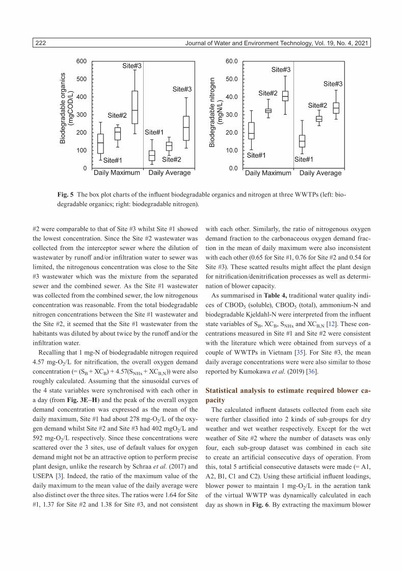
To compare the influent constituents over the 3 experimen-tal sites, the box-whisker graphs were created as shown in Fig. 5. For the total biodegradable organic fractions (SB + XCB), the composite concentrations of Site #1 and Site #2 were noticeably lower than those obtained from Site #3 in both daily maximum and daily average. This was because the wastewaters of Site #1 and Site #2 were collected in Vietnam where the part of influent biodegradable organics were already decomposed in the septic tanks. On the other hand, the total biodegradable nitrogen (SNHx + XCB,N) of Site

Fig. 4 The box plot charts of the influent biodegradable constituents at Site #1 (left: biodegradable organ-ics; right: biodegradable nitrogen; plot: mean value; total 40 data).


#2 were comparable to that of Site #3 whilst Site #1 showed the lowest concentration. Since the Site #2 wastewater was collected from the interceptor sewer where the dilution of wastewater by runoff and/or infiltration water to sewer was limited, the nitrogenous concentration was close to the Site #3 wastewater which was the mixture from the separated sewer and the combined sewer. As the Site #1 wastewater was collected from the combined sewer, the low nitrogenous concentration was reasonable. From the total biodegradable nitrogen concentrations between the Site #1 wastewater and the Site #2, it seemed that the Site #1 wastewater from the habitants was diluted by about twice by the runoff and/or the infiltration water.

Recalling that 1 mg-N of biodegradable nitrogen required 4.57 mg-O2/L for nitrification, the overall oxygen demand concentration (= (SB + XCB) + 4.57(SNHx + XCB,N)) were also roughly calculated. Assuming that the sinusoidal curves of the 4 state variables were synchronised with each other in a day (from Fig. 3E–H) and the peak of the overall oxygen demand concentration was expressed as the mean of the daily maximum, Site #1 had about 278 mg-O2/L of the oxy-gen demand whilst Site #2 and Site #3 had 402 mgO2/L and 592 mg-O2/L respectively. Since these concentrations were scattered over the 3 sites, use of default values for oxygen demand might not be an attractive option to perform precise plant design, unlike the research by Schraa et al. (2017) and USEPA [3]. Indeed, the ratio of the maximum value of the daily maximum to the mean value of the daily average were also distinct over the three sites. The ratios were 1.64 for Site #1, 1.37 for Site #2 and 1.38 for Site #3, and not consistent

with each other. Similarly, the ratio of nitrogenous oxygen demand fraction to the carbonaceous oxygen demand frac-tion in the mean of daily maximum were also inconsistent with each other (0.65 for Site #1, 0.76 for Site #2 and 0.54 for Site #3). These scatted results might affect the plant design for nitrification/denitrification processes as well as determi-nation of blower capacity.

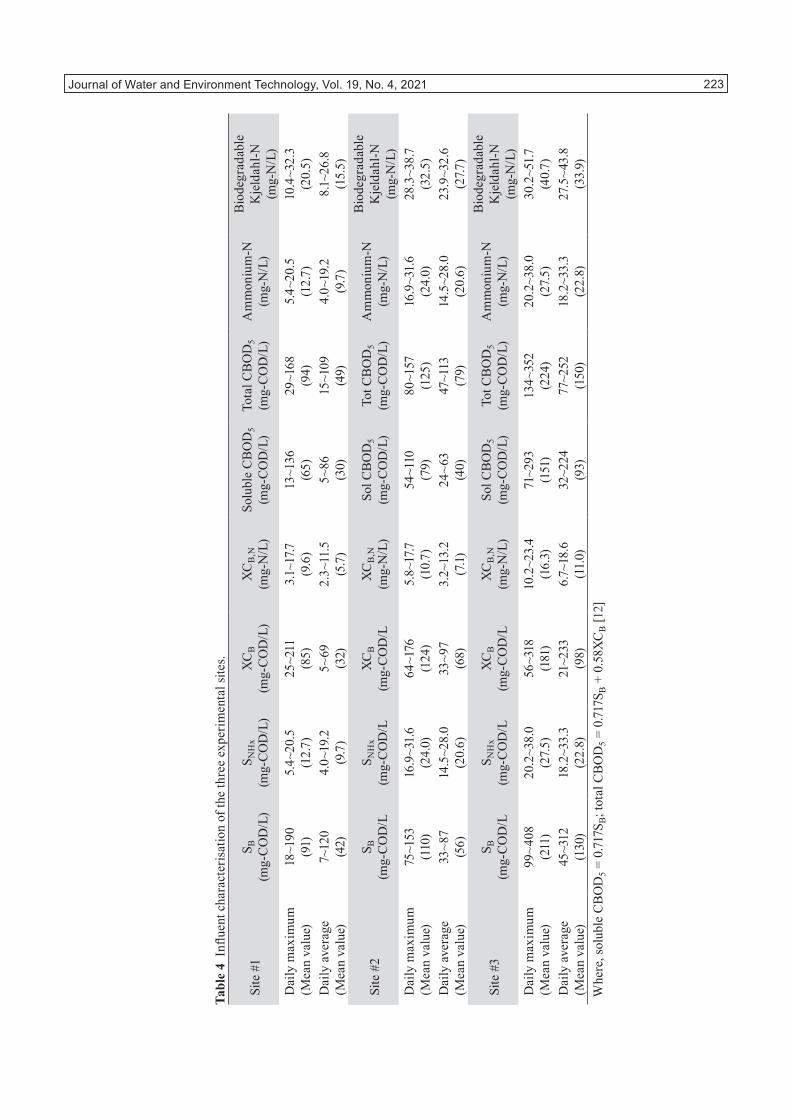
As summarised in Table 4, traditional water quality indi-ces of CBOD5 (soluble), CBOD5 (total), ammonium-N and biodegradable Kjeldahl-N were interpreted from the influent state variables of SB, XCB, SNHx and XCB,N [12]. These con-centrations measured in Site #1 and Site #2 were consistent with the literature which were obtained from surveys of a couple of WWTPs in Vietnam [35]. For Site #3, the mean daily average concentrations were were also similar to those reported by Kumokawa et al. (2019) [36].

Statistical analysis to estimate required blower ca-pacity

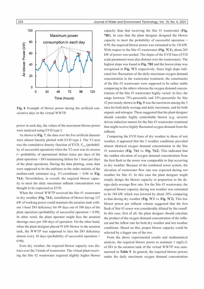
The calculated influent datasets collected from each site were further classified into 2 kinds of sub-groups for dry weather and wet weather respectively. Except for the wet weather of Site #2 where the number of datasets was only four, each sub-group dataset was combined in each site to create an artificial consecutive days of operation. From this, total 5 artificial consecutive datasets were made (= A1, A2, B1, C1 and C2). Using these artificial influent loadings, blower power to maintain 1 mg-O2/L in the aeration tank of the virtual WWTP was dynamically calculated in each day as shown in Fig. 6. By extracting the maximum blower

Fig. 5 The box plot charts of the influent biodegradable organics and nitrogen at three WWTPs (left: bio-degradable organics; right: biodegradable nitrogen).


Tabl

e 4

Influ

ent c

hara

cter

isat

ion

of th

e th

ree

expe

rimen

tal s

ites.

Site

#1

S B

(mg-

CO

D/L

)S N

Hx

(mg-

CO

D/L

)X

CB

(mg-

CO

D/L

)X

CB

,N

(mg-

N/L

)So

lubl

e C

BO

D5

(mg-

CO

D/L

)To

tal C

BOD

5 (m

g-C

OD

/L)

Am

mon

ium

-N

(mg-

N/L

)

Biod

egra

dabl

e

Kje

ldah

l-N

(mg-

N/L

)D

aily

max

imum

(M

ean

valu

e)18

~190

(9

1)5.

4~20

.5

(12.

7)25

~211

(8

5)3.

1~17

.7

(9.6

)13

~136

(6

5)29

~168

(9

4)5.

4~20

.5

(12.

7)10

.4~3

2.3

(20.

5)D

aily

ave

rage

(M

ean

valu

e)7~

120

(42)

4.0~

19.2

(9

.7)

5~69

(3

2)2.

3~11

.5

(5.7

)5~

86

(30)

15~1

09

(49)

4.0~

19.2

(9

.7)

8.1~

26.8

(1

5.5)

Site

#2

S B

(mg-

CO

D/L

S NH

x (m

g-C

OD

/LX

CB

(mg-

CO

D/L

XC

B,N

(m

g-N

/L)

Sol C

BO

D5

(mg-

CO

D/L

)To

t CBO

D5

(mg-

CO

D/L

)A

mm

oniu

m-N

(m

g-N

/L)

Biod

egra

dabl

e

Kje

ldah

l-N

(mg-

N/L

)D

aily

max

imum

(M

ean

valu

e)75

~153

(1

10)

16.9

~31.

6 (2

4.0)

64~1

76

(124

)5.

8~17

.7

(10.

7)54

~110

(7

9)80

~157

(1

25)

16.9

~31.

6 (2

4.0)

28.3

~38.

7 (3

2.5)

Dai

ly a

vera

ge

(Mea

n va

lue)

33~8

7 (5

6)14

.5~2

8.0

(20.

6)33

~97

(68)

3.2~

13.2

(7

.1)24

~63

(40)

47~1

13

(79)

14.5

~28.

0 (2

0.6)

23.9

~32.

6 (2

7.7)

Site

#3

S B

(mg-

CO

D/L

S NH

x (m

g-C

OD

/LX

CB

(mg-

CO

D/L

XC

B,N

(m

g-N

/L)

Sol C

BO

D5

(mg-

CO

D/L

)To

t CBO

D5

(mg-

CO

D/L

)A

mm

oniu

m-N

(m

g-N

/L)

Biod

egra

dabl

e

Kje

ldah

l-N

(mg-

N/L

)D

aily

max

imum

(M

ean

valu

e)99

~408

(2

11)

20.2

~38.

0 (2

7.5)

56~3

18

(181

)10

.2~2

3.4

(16.

3)71

~293

(1

51)

134~

352

(224

)20

.2~3

8.0

(27.

5)30

.2~5

1.7

(40.

7)D

aily

ave

rage

(M

ean

valu

e)45

~312

(1

30)

18.2

~33.

3 (2

2.8)

21~2

33

(98)

6.7~

18.6

(1

1.0)

32~2

24

(93)

77~2

52

(150

)18

.2~3

3.3

(22.

8)27

.5~4

3.8

(33.

9)W

here

, sol

uble

CBO

D5 =

0.71

7SB;

tota

l CB

OD

5 = 0

.717S

B +

0.5

8XC

B [1

2]


power in each day, the values of the maximum blower power were analysed using EVD type I.

As shown in Fig. 7, the data over the five artificial datasets were almost linearly plotted with EVD type I. The Y1-axis was the cumulative density function of EVD, F(x) (probabil-ity of successful operation) whist the Y2-axis was its inverse (= probability of operational failure (once per days of the plant operation = DO maintaining failure for 1 hour per days of the plant operation). During the data plotting, some data were supposed to be the outliners in the order statistic of the median-rank estimator (e.g. Y1-coordinate = 0.96 in Fig. 7A1). Nevertheless, in overall, the required blower capac-ity to meet the daily maximum influent concentration was thought to be expressed as EVD.

When the virtual WWTP received the Site #1 wastewater in dry weather (Fig. 7A1), installation of blower having 127 kW of working power could maintain the aeration tank with-out 1-hour DO deficiency for 99 days out of 100 days of the plant operation (probability of successful operation = 0.99). In other word, the plant operator might face the aeration shortage once per 100 days of operation. On the other hand, when the plant designer placed 93 kW-blower in the aeration tank, the WWTP was supposed to face the DO deficiency almost every 10 days (probability of successful operation = 0.90).

Even dry weather, the required blower capacity was dis-tinct over the 3 kinds of wastewater. The virtual plant receiv-ing the Site #2 wastewater required slightly higher blower

capacity than that receiving the Site #1 wastewater (Fig. 7B1). In case that the plant designer designed the blower capacity to meet the probability of successful operation = 0.99, the required blower power was estimated to be 136 kW. With respect to the Site #3 wastewater (Fig. 7C1), about 265 kW of power was needed. The slopes of the EVD lines (EVD scale parameter) were also distinct over the wastewaters. The highest slope was found in Fig. 7B1 and the lowest slope was recognised in Fig. 7C1 respectively. Since high slope indi-cated low fluctuation of the daily maximum oxygen demand concentration in the wastewater treatment, the constituents of the Site #2 wastewater were supposed to be rather stable comparing to the others whereas the oxygen demand concen-trations of the Site #3 wastewater highly varied. In fact, the range between 75%-percentile and 25%-percentile for Site #2 previously shown in Fig. 5 was the narrowest among the 3 sites for both daily average and daily maximum, and for both organic and nitrogen. These suggested that the plant designer should consider highly controllable blower (e.g. inverter driven induction motor) for the Site #3 wastewater treatment that might receive highly fluctuated oxygen demand from the influent.

Comparing the EVD lines of dry weather to those of wet weather, it appeared that the 2 weather conditions provided almost identical oxygen demand concentration in the Site #1 wastewater (Fig. 7A1 vs. Fig. 7A2). This indicated that the sudden elevation of oxygen demand concentration from the first flush in the sewer was comparable to that occurring in dry weather. Because of the combined sewer system, the elevation of wastewater flow rate was expected during wet weather for Site #1. In this case the plant designer might simply design the blower capacity in proportion to the de-sign-daily-average flow rate. For the Site #3 wastewater, the required blower capacity during wet weather was estimated to be 184 kW which was lowered by about 30% comparing to that during dry weather (Fig. 7C1 vs. Fig. 7C2). This low blower power per influent volume suggested that the first flush of Site #3 sewer was considerably diluted by the runoff. In this case, first of all, the plant designer should calculate the product of the oxygen demand concentration of the influ-ent and the inflow rate for both dry weather and wet weather conditions. Based on this, proper blower capacity could be selected by a bigger one of the two.

From the above experimental results and mathematical analysis, the required blower power to maintain 1 mgO2/L of DO in the aeration tank of the virtual WWTP was sum-marised in Table 5. In general, the required blower powers under the daily maximum oxygen demand concentration

Fig. 6 Example of blower power during the artificial con-secutive days in the virtual WWTP.


Fig. 7 Prediction of the required air blower power to maintain 1 mg-O2/L of DO in the aeration tank against the peak loading events (Left: for dry weather; right: wet weather).


were as high as about twice of those of daily dry weather (= 1.4~2.5 times). Apart from the increment of oxygen de-mand loading from the increased inflow rate due to runoff, the blower power per influent flow rate could be the basis to determine the blower capacity. In addition, the blower power under daily average concentration provided a techni-cal information to the plant designer for the mean electricity cost of aeration over the year. Furthermore, the increment of the blower power between the daily average concentration and the daily maximum concentration could be the design basis to determine the number of motors and installation of inverter controls, which allowed a flexibility of aeration intensity. For instance, when a project was given to the plant designer to design the WWTP treating the Site #1 wastewa-ter with fixed inflow rate, he might install primary blowers having total 58-kW working power to meet the daily average load and a couple of secondary small blowers having total 70-kW working power to treat the increment from the daily maximum.

DISCUSSION

The back-calculation method integrated with the statistical analysis using EVD was thought to be a powerful tool to characterise influent biodegradable substance concentra-tions and to estimate the blower capacity of WWTPs. The calculated influent oxygen demand concentration could be one of the attractive databases for the plant design. When the flow pattern of wastewater to the WWTP was measured together with the influent characterisation, the product of the influent flow rate and the influent oxygen demand concentra-tion could be further analysed in such way that the study demonstrated.

In practice, the plant designer might prefer to know the probability of occurrence per prolonged days of plant opera-tion rather than per lowered days. For instance, risk of aera-

tion shortage at every 100 days rather than every 20 days. To attain the task, more dense statistical analysis was necessary to improve the prediction accuracy at around 0.95~0.99 of probability on the EVD plot. Specifically the number of data plot for the daily maximum should be increased accord-ing to the median-rank estimator, MR(i). In case of using the median-estimator shown in Equation (4), the required number of the field data was at least 14 to plot F(xi) on 0.95 of Y-coordinate and 69 to plot F(xi) on 0.99 of Y-coordinate respectively. This meant that the field test should be operated for more than 2 months to obtain the EVD plot having the F(xi) on 0.99 of Y-coordinate. On the other hand, the plant designer was also supposed to identify design-daily-average in the project, which was defined as the value throughout a year. Hence the operation and analysis should last for a year in the project anyway. As the conventional campaign to conduct numerous sampling and analysis of the influent was clearly infeasible because of huge manpower, the method developed in this study was supposed to be the only way to obtain exact value of design-daily-maximum loadings. Since the study successfully demonstrated to continue the continu-ous analysis for a couple of months, extension of the duration to 1 year would be technically feasible.

With respect to the first flush phenomena, the impact of the pollutant loading on WWTPs was supposed to be highly site specific [37]. Indeed, the daily maximum oxygen demand concentrations noticeably varied over the 3 sites in this study. Therefore, precise evaluation and analysis of the influent was essential to design WWTPs. According to Chow et al. (2014) [38], when they investigated the first flush phenomena, they were obliged to squeeze the sites to those neighbouring their laboratory because the fresh sample had to be analysed no sooner than the initiation of storm. On the other hand, the developed method in this study was free from the limitation of site selections. This was because the method did not require to analyse such readily biodegradable influ-

Table 5 Required blower power to maintain 1 mgO2/L of DO in the aeration tank of the virtual WWTP.

Wastewater type

Flow rate: 36,000 m3/d Daily average concentration

Daily maximum concentration (Successful operation of 99 days

out of 100 days)Site #1 Dry weather 58 kW 127 kW

Wet weather 50 kW 123 kWSite #2 Dry weather 100 kW 136 kW

Wet weather Not calculated Not calculatedSite #3 Dry weather 146 kW 265 kW

Wet weather 135 kW 184 kW


ent substances which could be collapsed within a couple of days of delivering time. Although they could monitor total 52 storm events with each 12-grab sample, such data volume and site selection would be the utmost for any laboratories as long as the conventional method was taken.

CONCLUSIONS

From the analysis of biodegradable substance concentra-tion of the wastewater at three sites, the following conclu-sions were obtained in this study.

(1) The data logging interval of DO and nitrate concentra-tions in the aeration tank of the field experimental unit somewhat affected the calculation results of the influent biodegradable substance concentrations. To estimate the hourly concentration of the influent with reason-able accuracy, 10-minute interval of data logging was recommended.

(2) The biodegradable organics and nitrogen concentra-tions of the wastewaters were successfully estimated as 1-hour discrete concentrations in both dry and wet weather flows. From the datasets, daily maximum expressed as the highest 1-hour discrete concentration in each day as well as daily average. The study dem-onstrated that developed method was able to obtain the daily maximum concentration with minimum manpower, which was thought to be technically very difficult to be measured until present.

(3) Using EVD and the median-rank estimator, the blower power versus the probability of oxygenation shortage was simulated on the virtual wastewater treatment plant in the computer. Based on the ASM1, the re-quired blower power per influent flow rate to meet the daily maximum influent oxygen demand was as high as 1.4~2.2 times than those of the blower calculated from the daily average.

(4) The blower capacity per influent volume in wet weather for Hiagari sewage (Japan) was lower than that in dry weather probably due to dilution of the wastewater by runoff. For Vinh Niem sewage (Vietnam), the increase of the influent oxygen demand in wet weather was sup-posed to be associated with the increased sewage flow rate.

ACKNOWLEDGEMENTS

This research was supported by Japan-Vietnam bilateral joint research project (NDT 31.JPA/17), Ministry of Science and Technology (MOST), Vietnam and Project in Sewer-age and Wastewater Management Department, Ministry of Land, Infrastructure, Transport and Tourism (MILT), Japan.

REFERENCES

[1] Reardon DJ: Turning down the power. Civ. Eng., 65(8), 54–56, 1995.

[2] Olsson G: Water and Energy: Threats and opportuni-ties. IWA Publishing, London, UK, 2015.

[3] Schraa O, Rieger L, Alex J: Development of a model for activated sludge aeration systems: linking air sup-ply, distribution, and demand. Water Sci. Technol., 75(3), 552–560, 2017. PMID:28192349 doi:10.2166/wst.2016.481

[4] Juan-García P, Kiser MA, Schraa O, Rieger L, Coromi-nas L: Dynamic air supply models add realism to the evaluation of control strategies in water resource re-covery facilities. Water Sci. Technol., 78(5), 1104–1114, 2018. PMID:30339535 doi:10.2166/wst.2018.356

[5] Ontario Ministry of the Environment: Design guide-lines for sewage works. Ontario Ministry of the Envi-ronment, Ontario, Canada, 2008.

[6] Health Research Inc: Health Education Services Division: Recommended Standards for Wastewater Fa-cilities. https://www.health.state.mn.us/communities/environment/water/docs/tenstates/tenstatestan2014.pdf. [accessed in September, 2020]

[7] Pham NB, Kuyama T: Decentralized domestic waste-water management in Asia–Challenges and Opportu-nities. http://www.wepa-db.net/pdf/1403policy_brief/PolicyBrief_2013_1.pdf. [accessed in September, 2020]

[8] Harada H, Dong NT, Matsui S: A measure for provisional-and-urgent sanitary improvement in de-veloping countries: septic-tank performance improve-ment. Water Sci. Technol., 58(6), 1305–1311, 2008. PMID:18845871 doi:10.2166/wst.2008.715

[9] Harada H, Matsui S, Dong NT, Shimizu Y, Fujii S: Incremental sanitation improvement strategy: com-parison of options for Hanoi, Vietnam. Water Sci. Technol., 62(10), 2225–2234, 2010. PMID:21076207 doi:10.2166/wst.2010.508

https://www.ncbi.nlm.nih.gov/entrez/query.fcgi?cmd=Retrieve&db=PubMed&list_uids=28192349?dopt=Abstract

https://doi.org/10.2166/wst.2016.481

https://doi.org/10.2166/wst.2016.481


https://doi.org/10.2166/wst.2018.356


https://doi.org/10.2166/wst.2008.715


https://doi.org/10.2166/wst.2010.508


[10] Von Sperling M: Wastewater Characteristics, Treat-ment and Disposal. IWA Publishing, London, UK, 2007. doi:10.2166/9781780402086.

[11] Henze M, Gujer W, Mino T, van Loosdrecht MC: Activated Sludge Models ASM1, ASM2, ASM2d and ASM3. IWA Scientific and Technical Report No.9. IWA Publishing, London, UK, 2000.

[12] Nguyen Duong QC, Le VT, Tran VQ, Liu B, Terashima M, Nguyen TH, Le VC, Harada H, Yasui H: An alter-native method to estimate influent concentration using on-site lab-scale activated sludge reactors. J. Water Environ. Technol., 15(6), 220–232, 2017. doi:10.2965/jwet.17-015

[13] Wasserman G: Reliability Verification, Testing, and Analysis in Engineering Design. 1st. CRC Press, Boca Raton, USA, 2002.

[14] Nguyen VH, Harada H, Le VT, Nguyen TH, Nguyen XH, Terashima M, Yasui H: Dynamic estimation of hourly fluctuation of influent biodegradable carbona-ceous and nitrogenous materials using activated sludge system. J. Water Environ. Technol., 17(1), 40–53, 2019. doi:10.2965/jwet.18-050

[15] Toulemonde G, Ribereau P, Naveau P: Applications of extreme value theory to environmental data analysis. In: Extreme Events Observations, Modeling, and Eco-nomics, Wiley, Hoboken, USA, pp. 9–22, 2016.

[16] Singh V: Extreme Value Type 1 Distribution. In: Entropy-based Parameter Estimation in Hydrology, Springer Science & Business Media, Berlin/Heidel-berg, Germany, 1998.

[17] Benard A, Bos-Levenbach E: The plotting of observa-tions on probability-paper. Stat. Neerl., 7, 163–173, 1953. doi:10.1111/j.1467-9574.1953.tb00821.x

[18] Blom G: Statistical estimates and transformed beta-variables. Doctoral dissertation, Stockholm College, Almqvist & Wiksell, Stockholm, Sweden, 1958.

[19] Garcia-Ochoa F, Gomez E: Bioreactor scale-up and oxygen transfer rate in microbial processes: An overview. Biotechnol. Adv., 27(2), 153–176, 2009. PMID:19041387 doi:10.1016/j.biotechadv.2008.10.006

[20] Henkel J, Cornel P, Wagner M: Oxygen transfer in activated sludge – new insights and potentials for cost saving. Water Sci. Technol., 63(12), 3034–3038, 2011. PMID:22049735 doi:10.2166/wst.2011.607

[21] Durán C, Fayolle Y, Pechaud Y, Cockx A, Gillot S: Impact of suspended solids on the activated sludge non-newtonian behaviour and on oxygen transfer in a bubble column. Chem. Eng. Sci., 141, 154–165, 2016. doi:10.1016/j.ces.2015.10.016

[22] Jiang LM, Garrido-Baserba M, Nolasco D, Al-Omari A, DeClippeleir H, Murthy S, Rosso D: Modelling oxy-gen transfer using dynamic alpha factors. Water Res., 124, 139–148, 2017. PMID:28753496 doi:10.1016/j.watres.2017.07.032

[23] Henze M, van Loosdrecht MCM, Ekama GA, Brdja-novic D: Biological Wastewater Treatment: Principles, Modeling and Design. IWA Publishing, London, UK, 2019.

[24] Metcalf E, Abu-Orf M, Bowden G, Burton FL, Pfrang W, Stensel HD, Tchobanoglous G, Tsuchihashi R, AECOM: Wastewater Engineering: Treatment and Re-source Recovery. McGraw Hill Education, NY, USA, 2014.

[25] Kappeler J, Gujer W: Estimation of kinetic parameters of heterotrophic biomass under aerobic conditions and characterization of wastewater for activated sludge modelling. Water Sci. Technol., 25(6), 125–139, 1992. doi:10.2166/wst.1992.0118

[26] Ramdani A, Dold P, Déléris S, Lamarre D, Gadbois A, Comeau Y: Biodegradation of the endogenous residue of activated sludge. Water Res., 44(7), 2179–2188, 2010. PMID:20074768 doi:10.1016/j.watres.2009.12.037

[27] Torretta V, Ragazzi M, Trulli E, De Feo G, Urbini G, Raboni M, Rada E: Assessment of biological kinet-ics in a conventional municipal WWTP by means of the oxygen uptake rate method. Sustainability, 6(4), 1833–1847, 2014. doi:10.3390/su6041833

[28] Tsai YP, Wu WM: Estimating biomass of heterotrophic and autotrophic bacteria by our batch tests. Environ. Technol., 26(6), 601–614, 2005. PMID:16035653 doi:10.1080/09593330.2001.9619500

[29] Makinia J, Zaborowska E: Mathematical Modelling and Computer Simulation of Activated Sludge Sys-tems. IWA Publishing, London, UK, 2020.

[30] Wilén BM: Variation in dissolved oxygen concentra-tion and its effect on the activated sludge properties studied at a full scale wastewater treatment plant. The Proceedings of IWA World Water Congress & Exhibi-tion, Montreal, 19-24 September, 2010.

https://doi.org/10.2166/9781780402086




https://doi.org/10.1111/j.1467-9574.1953.tb00821.x


https://doi.org/10.1016/j.biotechadv.2008.10.006


https://doi.org/10.2166/wst.2011.607

https://doi.org/10.1016/j.ces.2015.10.016


https://doi.org/10.1016/j.watres.2017.07.032


https://doi.org/10.2166/wst.1992.0118



https://doi.org/10.3390/su6041833


https://doi.org/10.1080/09593330.2001.9619500

https://doi.org/10.1080/09593330.2001.9619500


[31] Insel G, Sözen S, Başak S, Orhon D: Optimization of nitrogen removal for alternating intermittent aeration-type activated sludge system: a new process modifica-tion. J. Environ. Sci. Health Part A Tox. Hazard. Subst. Environ. Eng., 41(9), 1819–1829, 2006. PMID:16849128 doi:10.1080/10934520600778994

[32] Ritter A, Muñoz-Carpena R: Performance evaluation of hydrological models: Statistical significance for reducing subjectivity in goodness-of-fit assessments. J. Hydrol. (Amst.), 480, 33–45, 2013. doi:10.1016/j.jhydrol.2012.12.004

[33] Wissenschaftlich-Technische Werkstätten GmbH (WTW): FDO 925 Optical D.O. Sensor - Operating Manual. WTW GmbH, Weilheim, Germany.

[34] HORIBA Scientific: Instruction Manual – Combina-tion type Nitrate Ion Selective Electrode 6581S-10C. HORIBA Advanced Techno Co., Ltd, Kyoto, Japan.

[35] World Bank: Viet Nam urban wastewater review: Performance of the wastewater sector in urban areas: a review and recommendations for improvement. https://openknowledge.worldbank.org/bitstream/han-dle/10986/17367/ACS77120v20REP0l0with0report-0number.pdf?sequence=1&isAllowed=y. [accessed in September, 2020].

[36] Kumokawa S, Shirakawa Y, Flamand P: Characteris-tics of domestic wastewater and estimation of required johkasou capacity for buildings in Japan. Water Prac. Technol., 14(3), 738–747, 2019.

[37] Venner M: Identification of research needs related to highway runoff management. Vol. 521. Transportation Research Board of National Academies of Sciences, Engineering, and Medicine, Washington DC, USA, 2004.

[38] Chow MF, Yusop Z: Sizing first flush pollutant loading of stormwater runoff in tropical urban catchments. En-viron. Earth Sci., 72(10), 4047–4058, 2014. doi:10.1007/s12665-014-3294-6


https://doi.org/10.1080/10934520600778994

https://doi.org/10.1016/j.jhydrol.2012.12.004

https://doi.org/10.1016/j.jhydrol.2012.12.004

https://doi.org/10.1007/s12665-014-3294-6

https://doi.org/10.1007/s12665-014-3294-6

A Novel Method to Determine Blower Capacity of Wastewater ...

Documents

Transcript of A Novel Method to Determine Blower Capacity of Wastewater ...