A new Spool Piece for horizontal two-phase flow measurement A new Spool Piece for horizontal...

This content has been downloaded from IOPscience. Please scroll down to see the full text.

Download details:

IP Address: 130.192.21.172

This content was downloaded on 18/04/2014 at 17:10

Please note that terms and conditions apply.

A new Spool Piece for horizontal two-phase flow measurement

View the table of contents for this issue, or go to the journal homepage for more

2014 J. Phys.: Conf. Ser. 501 012011

(http://iopscience.iop.org/1742-6596/501/1/012011)

Home Search Collections Journals About Contact us My IOPscience

iopscience.iop.org/page/terms

http://iopscience.iop.org/1742-6596/501/1

http://iopscience.iop.org/1742-6596

http://iopscience.iop.org/

http://iopscience.iop.org/search

http://iopscience.iop.org/collections

http://iopscience.iop.org/journals

http://iopscience.iop.org/page/aboutioppublishing

http://iopscience.iop.org/contact

http://iopscience.iop.org/myiopscience

A new Spool Piece for horizontal two-phase flow measurement

G Monni, M De Salve and B Panella

Politecnico di Torino, C.so Duca degli Abruzzi 24, 10129 Torino, Italy

E-mail: [email protected]

Abstract. This works presents the characterization of a Spool Piece (SP), made up of a

Classical Venturi and a Wire Mesh Sensor (WMS), that are installed in a horizontal test

section, in which an air-water mixture flows. The test section consists of a horizontal Plexiglas

pipe of internal diameter 19.5 mm and total length of about 7 m. The flow quality ranges from

0 to 0.73 and the superficial velocity ranges from 0.14 to 32 m/s for air and from 0.019 to 2.62

m/s for water; the pressure ranges from atmospheric pressure to 4 bar depending on the

experimental conditions. The observed flow patterns are stratified-bubbly-slug/plug-annular.

The instruments response is analyzed and discussed. From the signal analysis the mass flow

rate of each phase is obtained. The developed model allows the evaluation of the mass flow

rate with an accuracy higher than 20% in the 84% of the cases and with an accuracy higher

than 10% in the 73.3% of the cases. Finally the introduction of the estimated parameters in the

SP model is considered and discussed.

1. Introduction

Within the framework of an Italian R&D program on Nuclear Fission, managed by ENEA and

supported by the Ministry of Economic Development, the SPES3 experimental facility [1], able to

simulate the innovative small and medium size PWR nuclear reactors, is being built and will be

operated at SIET Company laboratories. In such facility some design and beyond design basis

accidents, like LOCAs, with and without the emergency heat removal systems, will be simulated. An

accurate accident analysis requires the measurement of the mixture mass flow rate and therefore

instruments and methodologies to evaluate different two-phase flow parameters need to be developed.

Typically a set of instruments (Spool Piece - SP) must be installed in order to evaluate the mass

flow rate of the phases in a large range of flow patterns, pressures and temperatures. Each instrument

of the SP has to be sensitive to the different properties of the flow, like momentum, velocity, density,

void fraction; moreover the selection of the instruments strongly depends on the experimental

conditions: pressure, temperature and phases velocities. A different number of instruments can be

coupled in a SP; a low number of instruments allows the reduction of costs, complexity and space

requirements, but on the other hand, it requires the introduction of theoretical or experimental models

able to compensate for the lacking of information. As the response of a meter in a two-phase flow

tends to be highly sensitive to the flow pattern, to the upstream configuration and flow history, one of

such instruments has to be able to measure the void fraction. Wire Mesh Sensors (WMS), based on the

measurement of the local instantaneous conductivity of the two-phase mixture, are used for the

evaluation of local void fraction, bubble size distributions and gas velocity distributions. The WMS

31st UIT (Italian Union of Thermo-fluid-dynamics) Heat Transfer Conference 2013 IOP PublishingJournal of Physics: Conference Series 501 (2014) 012011 doi:10.1088/1742-6596/501/1/012011

Content from this work may be used under the terms of the Creative Commons Attribution 3.0 licence. Any further distributionof this work must maintain attribution to the author(s) and the title of the work, journal citation and DOI.

Published under licence by IOP Publishing Ltd 1

mailto:[email protected]

has been used, in different geometry and for different configurations, to study mean cross-section void

fraction and gas profile evolution [2]. In this paper a SP made up of a Venturi Flow Meter (VFM) with

a Wire Mesh Sensor (WMS) is proposed. The calculation of fluid flow rate by reading the pressure

drop across a pipe restriction is perhaps the most commonly used flow measurement technique in

industrial applications. Compared with single-phase flow, the pressure drops in two-phase flow

increase due to the interaction between the gas and the liquid phase; for this reason the value of the

effective two-phase mass flow rate is over-predicted and must to be corrected using available

correlations derived from experimental data or semi-empirical models.

In the present paper, the results of the experimental work carried out to analyze the response of a

SP made up of a VFM and a WMS are shown. The SP has been tested in a horizontal test section for

air-water flows in a large range of phases mass flow rates. The methodology for the signals

interpretation, the developed model of the SP for the phases mass flow rates estimation and the results

are presented and discussed.

2. Experimental Facility and Test Matrix

The experimental facility consists of the feed water loop (tap water with conductivity of about 620 µS

is used), the feed air loop and the test section. The liquid flow rate is measured by means of an

electromagnetic flow meter in a range of 0.9-36 m3/h with a 0.5% r.v. accuracy value. Lower values

of the water flow rate are measured by means of rotameters in the ranges of 0-100 l/h and 100-400 l/h

with an accuracy value of 2% r.v.. The air flow rate is measured by means of different rotameters

for the different ranges (100-500 Nl/h, 1000-5000 Nl/h and 6300-63000 Nl/h) with a 2% f.s.v.

accuracy value. The test section [3] consists of a 19.5 mm diameter and 7 m long pipe. The SP is

installed at L/D = 192 from the entrance; the WMS is installed between two Plexiglas pipes having a

length of 600 mm, while the VFM is installed between two Plexiglas pipes having a length of 500 mm

and 490 mm upstream and downstream respectively. The inlet pressure ranges from atmospheric

pressure to 4 bar depending on the experimental conditions. The flow is discharged at atmospheric

pressure. The experimental test section is equipped with two quick closing valves (QCV) that allow

the measurement of the volumetric void fraction in a length of 1300 mm.

The pressure drop in the VFM is measured

by means of two differential pressure

transducers having two different working

range: -40÷40 mbar and 0÷1250 mbar. The

instruments signals are acquired in a

LabView® environment by the National

Instruments DAQ (Digital AcQuisition)

system (NI USB-6218). The WMS signals are

instead acquired by means of the sensor

software, synchronizing the measures through

a trigger. The signals have been acquired

using a frequency f = 1250 Hz for all the

instruments for a total acquisition time of 20 s.

Instruments characterization in single-phase

flow of air and water has been performed.

Two-phase experiments have been carried out

at water temperature of about 20 °C. The flow

quality ranges from 0 to 0.73 and the superficial velocity from 0.14 to 32 m/s for air and from 0.019 to

2.62 m/s for water. The typical observed flow patterns were stratified flow, intermittent flow (slug and

plug) and annular flow. The population of samples ranges over different flow patterns and it is more

representative of intermittent flow regime and annular wavy flow regime. From visual observation and

maps results (figure 1) it also clear that some runs have been performed in transition regimes.

Figure 1. Baker’s Map [6] prediction of Flow

Patterns

100

102

104

10-1

100

101

102

Gl/G

g [-]

Gg [

kg/m

2s]

STRATIFIED

WAVY

PLUG

SLUG

MIST

FROTH

BUBBLY

ANNULAR


2

3. Spool Piece

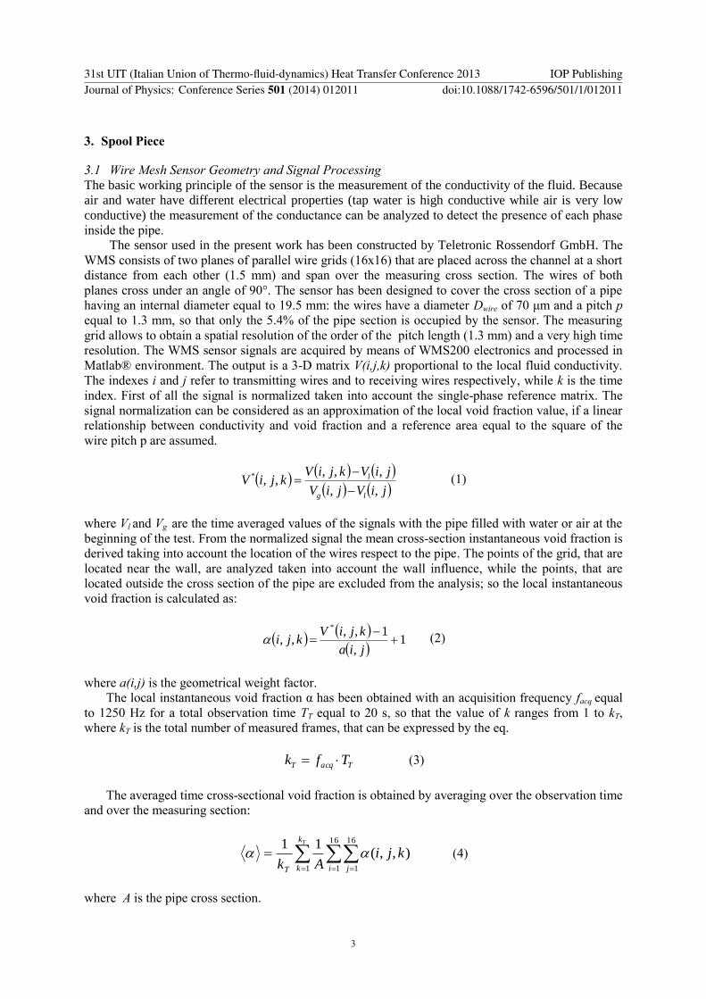
3.1 Wire Mesh Sensor Geometry and Signal Processing

The basic working principle of the sensor is the measurement of the conductivity of the fluid. Because

air and water have different electrical properties (tap water is high conductive while air is very low

conductive) the measurement of the conductance can be analyzed to detect the presence of each phase

inside the pipe.

The sensor used in the present work has been constructed by Teletronic Rossendorf GmbH. The

WMS consists of two planes of parallel wire grids (16x16) that are placed across the channel at a short

distance from each other (1.5 mm) and span over the measuring cross section. The wires of both

planes cross under an angle of 90°. The sensor has been designed to cover the cross section of a pipe

having an internal diameter equal to 19.5 mm: the wires have a diameter Dwire of 70 μm and a pitch p

equal to 1.3 mm, so that only the 5.4% of the pipe section is occupied by the sensor. The measuring

grid allows to obtain a spatial resolution of the order of the pitch length (1.3 mm) and a very high time

resolution. The WMS sensor signals are acquired by means of WMS200 electronics and processed in

Matlab® environment. The output is a 3-D matrix V(i,j,k) proportional to the local fluid conductivity.

The indexes i and j refer to transmitting wires and to receiving wires respectively, while k is the time

index. First of all the signal is normalized taken into account the single-phase reference matrix. The

signal normalization can be considered as an approximation of the local void fraction value, if a linear

relationship between conductivity and void fraction and a reference area equal to the square of the

wire pitch p are assumed.

jiVjiV

jiVkjiVkjiV

lg

l

,,

,,,,,*

(1)

where Vl and Vg are the time averaged values of the signals with the pipe filled with water or air at the

beginning of the test. From the normalized signal the mean cross-section instantaneous void fraction is

derived taking into account the location of the wires respect to the pipe. The points of the grid, that are

located near the wall, are analyzed taken into account the wall influence, while the points, that are

located outside the cross section of the pipe are excluded from the analysis; so the local instantaneous

void fraction is calculated as:

1,

1,,,,

*

jia

kjiVkji

(2)

where a(i,j) is the geometrical weight factor.

The local instantaneous void fraction α has been obtained with an acquisition frequency facq equal

to 1250 Hz for a total observation time TT equal to 20 s, so that the value of k ranges from 1 to kT,

where kT is the total number of measured frames, that can be expressed by the eq.

TacqT Tfk (3)

The averaged time cross-sectional void fraction is obtained by averaging over the observation time

and over the measuring section:

Tk

k i jT

kjiAk 1

16

1

16

1

),,(11

(4)

where A is the pipe cross section.


3

3.2 WMS Measurement Accuracy

Errors of the wire-mesh sensor measurements for the gas fraction are mainly caused by the pitch of the

wires which is 1.3 x 1.3 mm and the distance of the wire planes that is 1.5 mm.

Comparative measurements between the wire-mesh sensor and other research methods supplied

information on the accuracy of the measurement technique and the evaluation algorithms for the

experimental determination of these flow parameters. An air/water flow with gas volume fraction

ranging from 0 to 100% shows that the deviations between wire-mesh sensor and gamma

measurements are limited to ± 5% [2]. Comparative measurements between wire-mesh sensor and an

X-ray tomography were also performed for air/water flow [4]. It was found that, the accuracy of the

gas volume fraction averaged over the flow cross-section depends on the two-phase flow regime.

Differences in the absolute void fraction were determined for bubbly flows in the range of ± 1%,

while a systematic underestimation of - 4 % was observed for slug flows. In the present work, the

experimental void fraction is compared with the volumetric void fraction measured with the quick

closing valves method. The volumetric void fraction

V

V dVzyxV

),,(1

(5)

is measured in the 1300 mm long first part of the test section, with a precision of 3%.

Due to the intermittence of the flow, the volumetric void fraction is measured more than one time

for each tested flow rates combinations in order to derive a representative mean value. In figure 2 the

void fraction measured using the QCV technique and by means of the WMS are shown as a function

of the flow quality. Compared to the volumetric void fraction, the void fraction measured with the

WMS shows a higher dispersion in the range of intermittent flows and it’s in good agreement at very

high void fraction when the flow becomes annular. Moreover the WMS gives lower values of void

fraction for the flow characterized by flow qualities higher than 0.01 and gives higher values at flow

qualities lower than 0.001. Because the volumetric void is measured at the entrance of the test section,

the flow is not completely developed, and an L/D effect can be present. A series of measurement in the

volume where the WMS is installed will give more accurate information.

Figure 2. Mean void fraction measured using the QCV method and the WMS

3.3 Venturi Flow Meter

The characteristics of the Venturi flow meter are shown in table 1. Because in the experimented range

the Re number is lower than 105 and because the sensor geometrical dimensions are not inside the

range considered in the EN ISO 5167-1 [5], an in-situ calibration has been performed to obtain the

single-phase discharge coefficient for air and water:

0,0

0,1

0,2

0,3

0,4

0,5

0,6

0,7

0,8

0,9

1,0

0,0001 0,001 0,01 0,1 1

α

x

QCV WMS


4

gla

glpAYF

WC

,

5.04

2

,2

1

(6)

The experimental discharge coefficient has been found equal to 0.94 in water flow and 0.97 in air

flow, at Reynolds numbers higher than 15000.

Table 1. VFM Data

Type Herschel (Fluid: Water)

D1 26 mm

D2 10.251 mm

β 0.394 -

∆p 68.6 (700) mbar (mmH2O)

Wwater 300 g/s

Lupstream 500 mm

Ldownstream 490 mm

Compared to the single-phase flow measurements, in two-phase flow, the VFM pressure drops are

higher due to phases interaction, and a model for the signal interpretation must to be used.

Baker [6] describes the different approaches used by the different researchers: estimation of the

phases mass flow rates based on the estimation and/or calculation of the two-phase flow density and

two-phase flow discharge coefficient and estimation of the phases mass flow rates based on the two-

phase flow multipliers, relating single-phase and two-phase flow pressures drops. In 1949, Lockhart

and Martinelli [7] researched the pressure drop and the liquid holdup of two-phase flow across the

pipe, which became an important basis for the differential pressure method in two-phase flow

measurement research. Later, many researchers studied the relationship between the mass flow rate of

gas-liquid flow and the differential pressure across the flow meter. Flow rate measurement correlations

were reported in [8] and [9], and recently in [10] and [11]. The developed correlations have been

derived in a very limited operating range (pressure, temperature, phases velocities, fluids, etc..) and are

strongly dependent on the VFM geometry (β, D1, D2, L, etc..). Moreover the most part of the available

correlations are valid for very high (x>0.95) or very low (x<0.1) flow quality values.

The general equation of the VFM in a two-phase flow can be written as:

TPTPpKW 2

(7)

where

241

AYFC

K aTP

(8)

Considering the value of Y and Fa equal to one, the two parameters, that have to be defined, are

the two-phase discharge coefficient and the two-phase density.

In two-phase flow, due to the presence of the slip between the phases, different types of density

can be defined, depending on the flow model hypothesis (Homogeneous, Separated flow, etc..). In the

present work the density defined on the momentum balance is used to analyze the VFM response:

122

1

1

lg

TP

xx

(9)


5

In order to estimate the density, the void fraction value must to be known; then the output of the

WMS becomes an input for the VFM signal interpretation. The two-phase flow discharge coefficient

is then evaluated, based on the experimental data (figure 3 (a)). The dependence of the parameter CTP

on the two-phase Re number has been modeled as (figure 3 (b)):

4

4

105.1Re91.0

105.1ReRe

10

TPTP

TPd

TP

c

TP

C

baC (10)

with the parameters evaluated on the basis of the experimental data: a=1.1, b=0.6, c=3.5 e d=1.

The Reynolds number has been defined as:

TP

pipeTP

TP

DG

Re (11)

and the dynamic viscosity μ, in accordance with the two-phase density (Eq. 9), has been defined as:

122

1

1

lg

TP

xx

(12)

(a)

(b)

Figure 3. VFM discharge coefficient. (a) experimental single and TP flow; (b) TP flow correlation

The experimental pressure drops of the VFM have been analyzed in order to highlight the

dependence on the superficial velocities of the phases. The ∆p value increase is shown in figure 4 as a

function of the two-phases superficial velocities. The regular behavior of the increasing curves

suggests that a model of the instrument, depending on the phases velocities, can be developed in order

to avoid the use of the discharge coefficient correlations, for the mass flow estimation. The lack of

data between Jg = 3 m/s and Jg = 6 m/s is due to the non complete superimpositions ranges of the air

mass flow meters.

In figure 5, the pressure drops in the VFM are expressed in terms of two-phase flow multipliers.

The multipliers Φ2l,g has been evaluated as the ratio between the two-phase flow pressure drop and the

single-phase pressure drop at the same phase mass flow rate:

0

0,2

0,4

0,6

0,8

1

1,2

1,4

0 40000 80000 120000

C

Re

TWO PHASE

AIR

WATER

0

0,2

0,4

0,6

0,8

1

1,2

1,4

0 40000 80000 120000

CT

P

ReTP

EXPERIMENTAL

CORRELATION


6

l

TPl

p

p

2

(13)

respect to the liquid single-phase flow, and

g

TPg

p

p

2

(14)

respect to the air single-phase flow.

In the x-axis is reported the experimental Lockart-Martinelli parameter, that is evaluated as the

ratio between liquid and gas VFM pressure drops:

g

ltt

p

p

(15)

Figure 4. Experimental VFM pressure drops as a

function of phases superficial velocities

Figure 5. VFM pressure drops two-phase

multipliers

3.4 Spool Piece Model

The SP model consists of a set of equations that, based on the measurement of the VFM pressure drop,

and on the measurement of the void fraction in the WMS, together with the measurement of pressure

and temperature of the fluid, allows the estimation of the mass flow rate of the phases in the test

section:

),,(

),,(

)(

3

2

1

ppfJ

ppfJ

fx

VFMg

VFMl

(16)

In the present work, an iterative approach is adopted for the estimation of the two mass flow rate

of the phases. The model input are the void fraction, the pressure drop in the VFM, and the properties

0

200

400

600

800

0 5 10 15

∆p

VF

M [m

ba

r]

Jg [m/s]

Jl 0.09 m/s Jl 0.28 m/s Jl 0.43 m/s

Jl 0.93 m/s Jl 1.40 m/s Jl1.86 m/s

Jl

10-2

100

102

104

100

101

102

103

tt

2

2l

2g


7

of air and water that are evaluated at the working pressure and temperature. An initial guess value for

the flow quality is introduced. Using a literature x-α correlation the void fraction is calculated and the

flow quality value is iterated till the error between the void fraction calculated and the void fraction

measured by the WMS is lower than a threshold value (10-4

). When the required accuracy is reached,

the two-phase flow Reynolds number and the discharge coefficient are calculated in a new iterative

loop, where for the first iteration CTP=Cl is assumed. When the convergence is got (WTP,i–WTP,i-1<10-4

)

the mass flow rate are calculated for the two-phases. For the x-α correlation used in the calculation, the

Lockhart-Martinelli correlation (17) has been modified, based on the experimental data:

1

07.036.06.01

28.01

g

l

l

g

x

x

(17)

2

107.036.06.0

23

107.036.06.0

3

107.036.06.0

1061

45.01

106101

28.01

1011

2.01

xx

x

xx

x

xx

x

g

l

l

g

g

l

l

g

g

l

l

g

(18)

The comparison between the original correlation, the modified correlation and the void fraction

value obtained from the WMS signal analysis is shown in figure 6.

Figure 6. Comparison between WMS void fraction and correlations

4. Results

The developed SP Model has been applied to the experimental data in order to derive the mass flow

rate of the phases. In figure 7, the flow quality, that is estimated by the SP model, is compared with the

experimental value obtained by the phases flow rate measurements. The accuracy of the model has

10-4

10-3

10-2

10-1

100

0.1

0.2

0.3

0.4

0.5

0.6

0.7

0.8

0.9

1

x

corr

Lockhart-Martinelli (1949)

WMS

Modified Lockart-Martinelli

0 0.2 0.4 0.6 0.8 10

0.2

0.4

0.6

0.8

1

alphaWMS

corr

WMS

Lockhart-Martinelli (1949)

Modified Lockhart-Martinelli


8

been evaluated as the degree of closeness of the estimated quantity to the experimental value; and the

estimation error is considered the distance between the estimated quantity and the experimental value.

The flow quality is estimated with an error lower than 20% for the flows in which the quality was

higher than 0.1, and the error is lower than 10% for the 72% of the runs. For flow qualities lower than

0.1 the estimation error increases and is lower than the 50% for the 90% of the cases. The estimated

mass flow rates are shown in figure 8 (a) (water flow rate), and figure 8 (b) (air flow rate). The total

mass flow rate is estimated with an error that in the 73.3% of the cases is lower than 10% and in the

84% of the cases is lower than 20%. The highest estimation errors concern the air flow rate; in fact it

is more affected by the errors in the quality estimation and in the total mass flow rate estimation due to

the small values of this parameter. In this case the error is lower than 30% for the 73.3% of the cases.

The highest errors have been obtained for the flows characterized by an intermittent behavior

(slug/plug flow patterns). Moreover the intermittent flow has been realized in a region where the VFM

discharge coefficient is strongly dependent on the Re number; and an error on the estimation of CTP

produces obviously an additional error on the mass flow rate estimation.

Figure 7. Experimental flow quality vs. SP flow quality

Figure 8. Experimental mass flow rate vs. SP mass flow rate for water phase (a) and air phase (b)

0 0.2 0.4 0.6 0.80

0.1

0.2

0.3

0.4

0.5

0.6

0.7

0.8

x experimental

x e

stim

ate

d

+20%

+10%

-20%

-10%

0 0.2 0.4 0.6 0.80

0.1

0.2

0.3

0.4

0.5

0.6

0.7

0.8

Ww ater

experimental [kg/s]

Ww

ate

r estim

ate

d[k

g/s

]

+20%

+10%

-20%

-10%

0 0.005 0.01 0.015 0.02 0.0250

0.005

0.01

0.015

0.02

0.025

Wair

experimental [kg/s]

Wair e

stim

ate

d [

kg/s

]

+30%

-30%

+20%

-20%


9

5. Conclusions

The analysis of the signals and the developed model of the SP, made up of VFM and WMS, allow us

to estimate the mass flow rate of the phases in air-water horizontal flows with a good accuracy in a

large range of the flow quality. The mass flow rate has been estimated with an error lower than 10% in

the 73.3% of the cases. Moreover the estimation error is considerably lower for the flow characterized

by high values of quality and void fraction. In this range, with reference to facility SPES3 test

conditions, the error in the mass flow rate estimation is always lower than 10% and 20% for water and

air respectively.

Nomenclature

A area (m2)

C VFM discharge coefficient

D diameter (m)

Fa VFM thermal expansion correction factor

G mass flux (kg/m2s)

J superficial velocity (m/s)

Re Reynolds number

SP Spool Piece

V* WMS normalized signal

W mass flow rate (kg/s)

Y VFM compressibility coefficient

f signal acquisition frequency (Hz)

f.s.v full scale value

p pressure (bar)

r.v read value

x flow quality

Special characters

α void fraction

β D2/D1 VFM diameter ratio

µ dynamic viscosity (Pa·s)

ρ density (kg/m3)

σ surface tension (N/m)

∆p differential pressure (bar)

Subscripts

g gas

i i-th vertical wire index

j j-th horizontal wire index

k WMS time index

l liquid

TP Two-Phase

1 pipe area subscript

2 VFM constricted area subscript

Acknowledgement

The present research has been supported by ENEA and by the Ministry of Economic Development.

The authors thank R. Costantino and G. Vannelli for the support through their work.

References

[1] Carelli M, Conway L, Dzodzo M et al. 2009 The SPES3 experimental facility design for the

IRIS Reactor simulation Sci. Technol. Nucl. Install. [2] Prasser H M, Bottger A and Zschau J 1998 A new electrode-mesh tomography for gas –liquid

flows Flow Meas. Instrum. 9 111

[3] De Salve M, Monni G and Panella B 2013 Horizontal Air-Water Flow Pattern Recognition

WIT Trans. Eng. Sci. 79 (WIT Press 2013) doi:10.2495/MPF130381

[4] Prasser H M, Misawa M and Tiseanu I 2005 Comparison between WMS and ultra-fast X-ray

tomography for an air-water flow in vertical pipe Flow Meas. Instrum. 16 73

[5] ISO 5167-1:4 :2003 (E)

[6] Baker C R 2000 Flow Measurement Handbook (Cambridge University Press)

[7] Lockhart R W and Martinelli R C 1949 Proposed correlation of data for isothermal two- phase

two-component flow in pipe Chem. Eng. Prog. 45 39

[8] Murdock J W 1962 Two-phase flow measurement with orifices J Basic Eng. 84 419

[9] Chisholm D and Rooney D H 1974 Research note: Two-phase flow through sharp-edged

orifices J Mech. Eng. Sci. 16 353


10

[10] De Leeuw R 1997 Liquid correction of venturi meter readings in wet gas flow In: North sea

workshop paper 21

[11] Xu L, Xu J, Dong F and Zhang T 2003 On fluctuation of the dynamic differential pressure

signal of Venturi meter for wet gas metering Flow Meas. Instrum. 14 211


11

A new Spool Piece for horizontal two-phase flow measurement A new Spool Piece for horizontal...

Documents

Transcript of A new Spool Piece for horizontal two-phase flow measurement A new Spool Piece for horizontal...