ARTICLE IN PRESS

Operations Research Letters ( ) –

OperationsResearchLetters

www.elsevier.com/locate/orl

A new mixed integer programming formulation for facility layoutdesign using flexible bays

Abdullah Konaka,∗, Sadan Kulturel-Konakb, Bryan A. Normanc, Alice E. Smithd

aInformation Sciences and Technology, Penn State Berks, Tulpehocken Road P.O. Box 7009, Reading, PA 19610-6009, USAbManagement Information Systems, Penn State Berks, Reading, PA 19610, USA

cDepartment of Industrial Engineering, University of Pittsburgh, Pittsburgh, PA 15261, USAdIndustrial and Systems Engineering, Auburn University, Auburn, AL 36849, USA

Received 8 January 2004; accepted 23 September 2005

Abstract

This paper presents a mixed-integer programming formulation to find optimal solutions for the block layout problem withunequal departmental areas arranged in flexible bays. The nonlinear department area constraints are modeled in a continuousplane without using any surrogate constraints. The formulation is extensively tested on problems from the literature.© 2005 Elsevier B.V. All rights reserved.

Keywords: Facility design; Facility layout; Mixed integer programming; Flexible bay; Unequal areas

1. Introduction

In this paper, a new mixed-integer programming(MIP) formulation is proposed to solve the facilitylayout problem (FLP) with unequal departmental ar-eas which is encountered in many manufacturing andservice facilities. In its most general form, the FLP isdefined as follows: Given N departments with knownarea requirements and interdepartmental material flowrequirements, partition a planar area of size W × H

into departments in order to minimize the total ma-terial handling cost. In general, the total material

∗ Corresponding author.E-mail address: konak@psu.edu (A. Konak).

0167-6377/$ - see front matter © 2005 Elsevier B.V. All rights reserved.doi:10.1016/j.orl.2005.09.009

handling cost is expressed as

Z =N∑

i=1

N∑j=i+1

cij fij dij , (1)

where dij is the distance between departments i andj for a specified distance metric, fij is the amountof material flow, and cij is the material handlingcost per unit flow per unit distance traveled betweendepartments i and j . The constraints of the prob-lem include satisfying the area requirements of thedepartments and the boundaries of the layout. Inaddition, restrictions on the shapes and locations ofdepartments might be enforced because of practicalconcerns.

2 A. Konak et al. / Operations Research Letters ( ) –

ARTICLE IN PRESS

The FLP has attracted extensive attention from in-dustry and academia. Survey papers by Kusiak andHeragu [16] and Meller and Gau [21] summarize dif-ferent modeling and solution approaches to the FLP.Due to the difficulty of the problem, however, the ma-jority of work on the FLP has focused on heuristicapproaches to find good solutions.

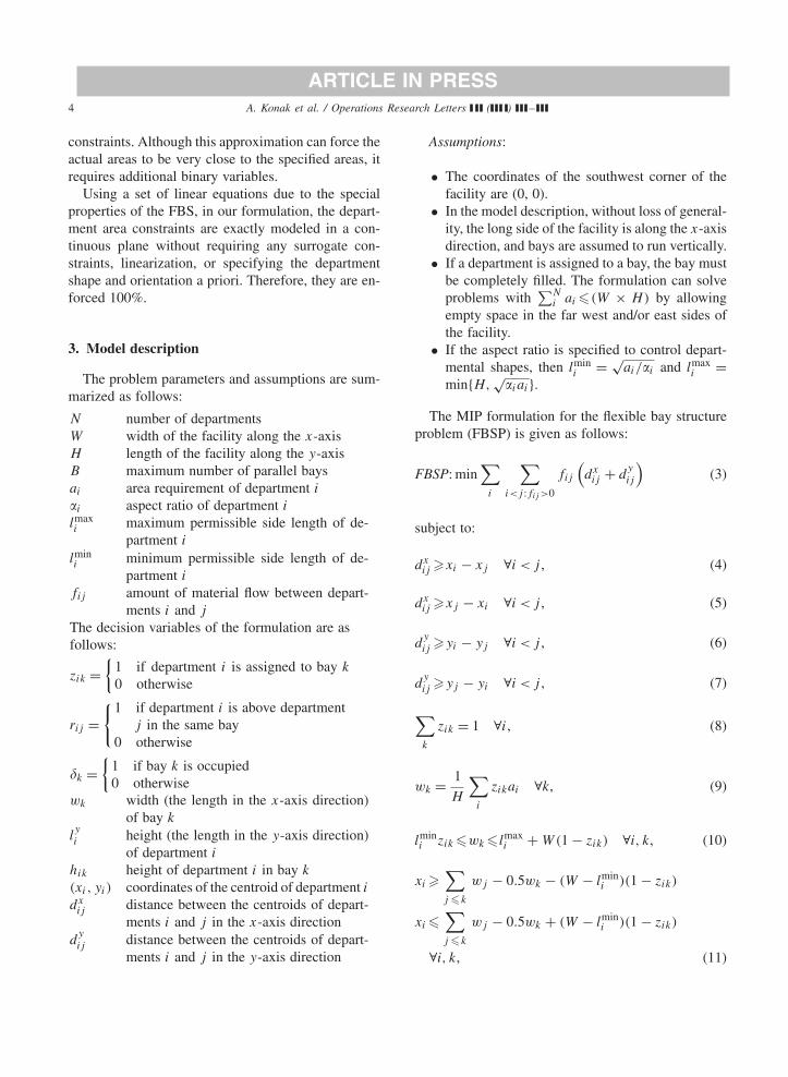
The formulation developed in this paper is based onthe flexible bay structure (FBS), which is a continu-ous layout representation allowing the departments tobe located only in parallel bays with varying widths(see Fig. 1(b)). The width of each bay depends onthe total area of the departments in the bay. Baysare bounded by straight aisles on both sides, anddepartments are not allowed to span over multiplebays. Therefore, the FBS restricts possible layoutconfigurations. However, it also has some desirablefeatures. The bay boundaries form the basis of anaisle structure that facilitates the user transferringthe block design into an actual facility design [1].In addition, many manufacturing facility designs fol-low an implicit bay structure [19,27,31]. The FBSrepresentation has been used as a design scheme inseveral heuristic approaches to the FLP [1,2,15,29].Facility layout software such as BLOCKPLAN, de-veloped by Donaghey and Pire [8], and SPIRAL,developed by Goetschalckx [10], also generate lay-outs based on the FBS. However, no exact solutionapproach or mathematical formulation has been re-ported in the literature for the FBS representation.Meller, in his related work [19] on layouts with bays,proposed a two-stage optimization approach wherein the first stage, departments are assigned to bays to

14572

36

(a)

1

4

2

7

5

6

3

(b)

Fig. 1. Comparison of the optimal solutions for O71 found by: (a) Sherali et al. [28]; and (b) our formulation.

minimize the inter-bay material handling cost, andthen in the second stage, departments are arrangedwithin the bays to minimize the within-bay materialhandling cost. However, this two-stage approach can-not guarantee an optimal FBS solution for the overallfacility. The formulation developed herein simultane-ously assigns the departments to the bays and deter-mines layouts within the bays considering departmen-tal shape constraints; therefore, it is the first exact ap-proach to find optimal FBS solutions.

2. MIP approaches to the FLP

As mentioned earlier, only a limited number ofpapers have addressed exact solution methods for theFLP. Exact solution methods based on MIP to datecannot solve large problems (more than nine depart-ments) and/or they make assumptions, such as equal-sized departments and departments with fixed shapesand orientations, which are difficult to justify in prac-tical cases. The quadratic assignment problem (QAP)introduced by Koopmans and Beckman [14] is the firstmathematical formulation to optimally solve the FLPwhen all departments have the same area. In the QAPformulation, the facility is divided into N equal-sizedgrids, and each equal-sized department is assigned toexactly one grid and vice versa. An obvious drawbackof the QAP formulation is the assumption of equal-sized departments. It is possible to model unequalarea departments in the QAP formulation by break-ing the departments into small grids with equal areasand not allowing the separation of grids of the same

ARTICLE IN PRESSA. Konak et al. / Operations Research Letters ( ) – 3

department by assigning large artificial flows betweenthem [13,16]. However, this significantly increases thenumber of integer variables in the formulation so thatsolving even small problems becomes difficult. An-other disadvantage of this approach is that unintendeddepartment shape constraints are implicitly enforcedby the penalty induced by high artificial flows betweenthe grids of the same department. Therefore, the op-timal solution to the QAP with high artificial flowsis likely to be a poor solution to the FLP (see [6]).Bazaraa [5] presented a quadratic set covering prob-lem (QSCP) formulation to the FLP where the shapesof the departments are selected from a finite set deter-mined in advance by the layout designers. Therefore,the QSCP is more scaleable than the QAP. Both theQAP and the QSCP are NP-complete. Therefore, lit-tle work has been focused on solving these problemsoptimally.

The FLP formulations based on the QAP and QSCPuse a discrete representation since the departments canonly be assigned to predefined grid locations. An al-ternative to the discrete representation is the contin-uous representation where department locations arenot restricted to a two-dimensional grid but are al-lowed to be anywhere within the facility. Using thecontinuous representation, the FLP can be formulatedas a MIP. A pioneering MIP formulation for the con-tinuous representation was given by Montreuil [23].In Montreuil’s model, the relative location of a de-partment with respect to another department is ex-pressed using two binary decision variables, one fornorth–south and the other for east–west relationships.The model includes disjunctive constraints to preventdepartmental overlaps and constraints to satisfy spec-ified departmental area and shape requirements. Un-fortunately, the problem instances that can be solvedto optimality by Montreuil’s model in its original formare very limited in size. Therefore, this formulation hasbeen used by researchers as a basis to develop heuris-tics to find good feasible solutions [17,18,24,25]. Cur-rently, the largest problem instance optimally solvedby Montreuil’s original model includes 6 departments.Tightening Montreuil’s model and using valid inequal-ities, Meller et al. [22] were able to optimally solveproblems with 8 departments. Improving the workof Meller et al. [22] by using a polyhedral outer-approximation to department areas, a new symmetry-breaking approach, elaborate valid inequalities, and

branching priorities, Sherali et al. [28] reported the op-timal solution for a nine-department problem, whichcould not be optimally solved in a 24-h CPU limit byMeller et al. [22].

Under the assumption of rectangular departmentalshapes, the models given in [22,23,28] can find theglobal optimal solution to the FLP. On the other hand,the model given in this paper solves a restricted ver-sion of the FLP based on the FBS representation whichlimits the number of possible layout configurations.Therefore, optimal FBS solutions for larger sized prob-lems can be found. In this study, we were able to findoptimal FBS layouts for up to 14 departments.

Formulating the nonlinear department area con-straints is an important concern in the MIP approachfor a continuous layout representation. For each de-partment, the department area constraint enforces thenonlinear relationship ai = wihi , where ai is the arearequirement, wi is the width, and hi is the lengthof department i. Existing formulations use varioussurrogate constraints to model the nonlinear depart-ment area constraint. For example, in Montreuil’soriginal model [23], the shape and area constraintsare enforced by using upper and lower limits on thedepartment perimeters as follows:

4√

ai �2(hi + wi)�2(1 + �i )√

ai/�i ∀i, (2)

where �i is the maximum permissible aspect ratio (theratio of the longer side to the shorter) of departmenti. However, the departmental areas enforced by thesurrogate perimeter constraint (2) tend to be smallerthan the original areas. Meller et al. [22] reported thatthe difference between the original and surrogate ar-eas can be as much as 11%, 25%, 36%, and 44% for�i =2, 3, 4, and 5, respectively. In the same paper, theauthors also propose an improved surrogate perimeterconstraint. In a recent paper [28], Sherali et al. man-aged to reduce the error in department areas signifi-cantly by using a polyhedral outer-approximation ofthe area constraints.

Another approach to avoid the non-linear area con-straint was proposed by Heragu and Kusiak [12] byassuming that the department shapes and orientationsare specified a priori, which completely eliminatesthe area and shape constraints; however, this is avery restrictive assumption. Lacksonen [17,18] used apiecewise linear approximation for modeling the area

4 A. Konak et al. / Operations Research Letters ( ) –

ARTICLE IN PRESS

constraints. Although this approximation can force theactual areas to be very close to the specified areas, itrequires additional binary variables.

Using a set of linear equations due to the specialproperties of the FBS, in our formulation, the depart-ment area constraints are exactly modeled in a con-tinuous plane without requiring any surrogate con-straints, linearization, or specifying the departmentshape and orientation a priori. Therefore, they are en-forced 100%.

3. Model description

The problem parameters and assumptions are sum-marized as follows:

N number of departmentsW width of the facility along the x-axisH length of the facility along the y-axisB maximum number of parallel baysai area requirement of department i

�i aspect ratio of department i

lmaxi maximum permissible side length of de-

partment i

lmini minimum permissible side length of de-

partment i

fij amount of material flow between depart-ments i and j

The decision variables of the formulation are asfollows:

zik ={

1 if department i is assigned to bay k

0 otherwise

rij ={1 if department i is above department

j in the same bay0 otherwise

�k ={

1 if bay k is occupied0 otherwise

wk width (the length in the x-axis direction)of bay k

lyi height (the length in the y-axis direction)

of department i

hik height of department i in bay k

(xi, yi) coordinates of the centroid of department idxij distance between the centroids of depart-

ments i and j in the x-axis directiond

yij distance between the centroids of depart-

ments i and j in the y-axis direction

Assumptions:

• The coordinates of the southwest corner of thefacility are (0, 0).

• In the model description, without loss of general-ity, the long side of the facility is along the x-axisdirection, and bays are assumed to run vertically.

• If a department is assigned to a bay, the bay mustbe completely filled. The formulation can solveproblems with

∑Ni ai �(W × H) by allowing

empty space in the far west and/or east sides ofthe facility.

• If the aspect ratio is specified to control depart-mental shapes, then lmin

i = √ai/�i and lmax

i =min{H,

√�iai}.

The MIP formulation for the flexible bay structureproblem (FBSP) is given as follows:

FBSP: min∑

i

∑i<j :fij >0

fij

(dxij + d

yij

)(3)

subject to:

dxij �xi − xj ∀i < j , (4)

dxij �xj − xi ∀i < j , (5)

dyij �yi − yj ∀i < j , (6)

dyij �yj − yi ∀i < j , (7)

∑k

zik = 1 ∀i, (8)

wk = 1

H

∑i

zikai ∀k, (9)

lmini zik �wk � lmax

i + W(1 − zik) ∀i, k, (10)

xi �∑j �k

wj − 0.5wk − (W − lmini )(1 − zik)

xi �∑j �k

wj − 0.5wk + (W − lmini )(1 − zik)

∀i, k, (11)

ARTICLE IN PRESSA. Konak et al. / Operations Research Letters ( ) – 5

hik

ai

− hjk

aj

− max

{lmaxi

ai

,lmaxj

aj

}(2 − zik − zjk)�0

hik

ai

− hjk

aj

+ max

{lmaxi

ai

,lmaxj

aj

}(2 − zik − zjk)�0

∀i < j, ∀k, (12)∑i

hik = H�k ∀k, (13)

lmini zik �hik � lmax

i zik ∀i, k, (14)∑k

hik = lyi ∀i, (15)

yi − 0.5lyi �yj + 0.5l

yj − H(1 − rij ) ∀i �= j , (16)

rij + rji �1 ∀i < j , (17)

rij + rji �zik + zjk − 1 ∀i < j, ∀k, (18)

0.5lyi �yi �H − 0.5l

yi ∀i. (19)

The objective function (3) is the summation ofthe interdepartmental flow times the rectilinear dis-tance between department centroids for all pairs ofdepartments with positive interdepartmental flow.Constraints (4)–(7) linearize the absolute value termin the rectilinear distance function. Constraint (8) en-sures that each department is assigned to a single bay.In constraint (9), the width of each bay is calculatedas the total area of the departments assigned to thatbay divided by the length of the facility in the direc-tion of the y-axis. Constraint (10) imposes upper andlower bounds on the widths of the bays based on thedepartments assigned to each bay. Constraint set (11)determines the locations of the department centroidsalong the x-axis. In the FBS representation, noticethat the centroid of a department along the x-axis islocated at the middle of the bay in which the depart-ment resides. Therefore, if department i is assignedto bay k, then xi can be calculated as follows:

xi =k∑

j=1

wj − 1

2wk . (20)

In constraint (11), if zik = 1 for any combination ofi and k, then the inequalities are reduced to Eq. (20);otherwise, if zik =0, constraint set (11) is inactive andalways satisfied. Constraints (9) and (11) also ensure

that the departments will be located inside the bound-aries of the facility along the x-axis.

Constraints (12)–(14) are the most important con-tribution of the FBSP since they enable calculatingthe length of the departments along the y-axis with-out using any quadratic terms. Constraint (13) sets thesummation of the heights of the departments within abay equal to either H if the bay is used, or zero if thebay is empty. Constraint (14) restricts the height ofthe departments between the maximum and minimumpermissible side lengths, and, in addition, it enforceshik = 0 when department i is not located in bay k.The following two propositions show how departmentheights can be calculated by the FBSP without usingquadratic terms.

Proposition 1. Constraint (12) is valid for ∀i < j, ∀k.

Proof. Case 1: zik =0 and zjk =0. Notice that hik =0and hjk=0 due to constraint (14); therefore, constraint(12) is always satisfied for this case.

Case 2: zik = 1 and zjk = 0. In this case, constraint(12) reduces to

hik

ai

− max

{lmaxi

ai

,lmaxj

aj

}�0 and

hik

ai

+ max

{lmaxi

ai

,lmaxj

aj

}�0.

From constraint (14), we have hik � lmaxi ; therefore,

the reduced constraints are feasible.Case 3: zik = 0 and zjk = 1. This case is very simi-

lar to the previous case. For this case, constraint (12)reduces to

− hjk

aj

− max

{lmaxi

ai

,lmaxj

aj

}�0 and

− hjk

aj

+ max

{lmaxi

ai

,lmaxj

aj

}�0.

Due to constraint (14), we have hjk � lmaxj which

makes the reduced constraints feasible.Case 4: zik = 1 and zjk = 1. In this case, the con-

straint reduces to hik/ai − hjk/aj �0 and hik/ai −hjk/aj �0, which enforces hik/ai = hjk/aj in theformulation. �

6 A. Konak et al. / Operations Research Letters ( ) –

ARTICLE IN PRESS

Proposition 2. Constraints (12)–(14) yield exactheights of the departments in the y-axis directionwithout using quadratic terms in the formulation.

Proof. Case 1: Assume that bay k is empty, that is,zik = 0, ∀i. From constraint (14), therefore, we havehik = 0, ∀i. Then, �k must be equal to zero due toconstraint (13).

Case 2: Assume that only department i resides inbay k (lmax

i �H must hold), that is, zik=1, and zjk=0,∀j �= i. From constraint (14), hik � lmin

i and hjk = 0,∀j �= i. In this case, constraint (13) is only satisfiedwhen �k = 1, which also sets hik = H .

Case 3: Assume that only two departments, i andj , reside in bay k (lmax

i + lmaxj �H must hold), that

is, zik = 1 and zjk = 1 for departments i and j , andzmk = 0, ∀m �= i, j . From constraint (14), hik � lmin

i ,hjk � lmin

j , and hmk = 0, ∀m �= i, j . In this case, con-straint (13) is only satisfied when �k = 1, which alsosets hik+hjk=H . In addition, from constraint (12) wehave hik/ai = hjk/aj (Proposition 1: Case 4). There-fore, constraints (12) and (13) define a linear systemas follows:

hik + hjk = H ,

ajhik − aihjk = 0,

which has the unique solution of hik = ai/(ai + aj )H

and hjk = aj /(ai + aj )H . This case can be repeatedfor three or more departments in the same bay. �

The functions of the remaining constraints are asfollows. Constraint (15) calculates the length of thedepartments in the y-axis directions to be used in otherconstraints. Constraints (14)–(18) are used to deter-mine the location of the department centroids alongthe y-axis. These constraints also prevent departmentsfrom overlapping in the y-axis direction. For each pairof departments i and j which are located in the samebay, constraints (17) and (18) enforce either depart-ment i to be above department j or below depart-ment j without overlapping. Constraint (16) uses theseabove/below relationships of the departments in thesame bay to determine their positions along the y-axis.Constraint (19) ensures that the departments will belocated inside the boundaries of the facility along they-axis.

4. Tightening and enhancing the formulation

In this section, we present several enhancements interms of valid inequalities and extensions to the basicFBSP model in order to improve its computationalperformance. We discuss the effect of using the pro-posed valid inequalities within FBSP on several testproblems ranging in size from seven to nine depart-ments. These problems were used in [22,28] to testtheir proposed model enhancements. Some propertiesof these problems are given in Table 1, and more spe-cific information can be found in the correspondingreferences. All problem instances were solved by us-ing CPLEX/AMPL 8.0 on a PC with 2.6 GHz CPU,1.5 GB memory, and the LINUX operating system.The computational results are summarized in Table 2.In the first row of this table, the solution effort in termsof solution time in CPU seconds and the number ofnodes searched by the CPLEX branch-and-bound pro-cedure is given for the basic FBSP model. In the fol-lowing rows, the percent computational improvements(100((value in row1)−(row value))/(value in row1))

obtained using valid inequalities within the basicFBSP model are presented. In the table, the modelFBSP + (#) represents the basic FBSP model withvalid inequality (#) included. As seen in the table,we also studied two and three way interactions ofpromising valid inequalities in order to find the bestpossible combination.

4.1. Tightening the linear programming (LP) lowerbound

In the LP-relaxation of the FBSP, the centroids ofthe departments overlap at the same point making dis-tance variables dx

ij and dyij equal to zero. Therefore,

the LP lower bound of the FBSP is zero. The mini-mum permissible side lengths of the departments canbe used to improve the LP lower bound. The rectilin-ear distance between the centroids of any two depart-ments i and j must be at least 0.5(lmin

i + lminj ). Hence,

dxij + d

yij �0.5(lmin

i + lminj ) ∀i < j . (21)

In [22,28], several valid inequalities were proposedto force the distance variables to be nonzero by sep-arating the centroids of departments for the generalMIP formulation. Although those valid inequalities are

ARTICLE IN PRESSA. Konak et al. / Operations Research Letters ( ) – 7

Table 1Summary of test problems

Problem name Problem data Number of Common shape Best solution Best solutionreference departments constraint reported reference

FO7 [22] 7 � = 5 20.95 [28]FO71 [22] 7 � = 5 20.25 [28]FO72 [22] 7 � = 5 17.75 [28]O71 [22] 7 � = 5 121.07 [28]O72 [22] 7 � = 5 116.96 [28]FO8 [22] 8 � = 5 22.39 [28]O9 [22] 9 � = 5 235.95 [28]VC10R-s [30] 10 lmin = 5 22,395.00 [4]VC10R-a [9] 10 � = 5 21,926.40 [9]MB12 [6] 12 � = 4 148.50 [6]MB11-s [7] 11 lmin = 1 1372.70 [20]MB11-a [7] 11 � = 5 1185.20 [9]MB15-s [7] 15 lmin = 1 31,936.30 [20]MB15-a [7] 15 � = 5 29,157.60 [9]Nug12 [26] 11 � = 4 279.02 [10]a

Nug15 [26] 15 � = 4 562.05 [10]a

Ba12 [5] 12 lmin = 1 11,140.00 [11]a

Ba12TS [29] 16 lmin = 1 8630.00 [15]a

Ba14TS [29] 14 lmin = 1 5077.00 [29]a

Ba14 [29] 14 lmin = 1 5004.55b

AB20 [3] 20 � = 1.75 7205.40 [29]a

aThe best-known FBS solutions.bThe objective function value was provided by the referee.

not directly applicable to FBSP, the underlying ideascould be used. The following constraints are valid forFBSP:

dxij �0.5(lmin

i + lminj ) + W(zik + zjm − 2)

∀i < j, ∀k �= m, (22)

dyij �0.5(lmin

i + lminj ) + H(zik + zjk − 2)

∀i < j, ∀k. (23)

Constraint (22) states that dxij must be greater than

0.5(lmini + lmin

j ) if departments i and j are assigned totwo different bays. We further tighten this constraintby not allowing empty bays between any two filledbays as discussed in the next section. Constraint (23)imposes a similar lower bound on d

yij if the depart-

ments are located in the same bay. As seen in Table 2,on average the model FBSP + (21) reduced the solu-tion time by 21% and the number of nodes searchedby 34%. On the other hand, constraint (23) appearedto be more promising yielding on average a 43% re-duction in both solution time and the number of nodessearched.

4.2. Reducing model degeneracy

The FBSP does not require the number of bays tobe specified a priori. It is possible to search all FBSPsolutions with from one to B bays in a single run byallowing bays with zero width when no department isassigned to them. Consider a feasible solution with b

filled bays and B-b empty bays. Since the bays can beselected arbitrarily, there are CB

b possible ways to se-lect the bays to be filled, which means that CB

b differ-ent combinations of zik decision variables correspondto the same layout. Therefore, the basic FBSP modelis highly degenerate. To remedy the degeneracy of thebasic model, we propose a constraint to fill bays se-quentially as follows:

N∑

i

zik �∑

i

zi,k+1 ∀k < B. (24)

This constraint states that if bay (k + 1) is filled,then bay k must also be filled. Therefore, no emptybay is allowed between any two filled bays by forcingall empty bays toward the east end of the layout. The

8 A. Konak et al. / Operations Research Letters ( ) –

ARTICLE IN PRESS

Tabl

e2

Com

puta

tiona

lre

sults

for

valid

ineq

ualit

ies

No

Mod

elFO

7FO

71FO

72O

71O

72FO

8O

9

Tim

eB

&B

Tim

eB

&B

Tim

eB

&B

Tim

eB

&B

Tim

eB

&B

Tim

eB

&B

Tim

eB

&B

1FB

SP58

7.0

2029

2.0

722.

023

347.

064

3.0

1838

6.0

1553

.052

603.

015

00.0

5108

3.0

1903

.038

205.

093

259.

014

4162

0.0

2FB

SP+

(21)

26.8

37.2

31.8

93.8

44.2

46.3

6.1

14.1

13.3

1.6

18.0

31.7

9.0

15.8

3FB

SP+

(23)

59.1

54.8

49.4

49.7

69.5

67.1

17.6

20.6

−10.

62.

464

.863

.046

.843

.64

FBSP

p29

.842

.063

.563

.245

.750

.926

.538

.143

.548

.427

.735

.423

.725

.55

FBSP

pq

56.6

54.0

51.1

51.0

43.5

44.3

38.8

44.9

30.7

39.3

43.9

44.9

57.8

54.8

6FB

SP+

(24)

85.5

88.8

79.6

81.3

45.0

57.2

89.4

89.6

61.8

67.4

78.8

75.9

71.4

73.0

7FB

SP+

(24)

+(2

5)84

.187

.790

.888

.283

.284

.892

.692

.677

.981

.085

.286

.088

.287

.18

FBSP

p+

(21)

69.2

73.5

77.6

80.5

92.9

85.2

56.1

65.0

49.2

49.4

75.9

77.1

71.8

72.6

9FB

SPpq

+(2

1)44

.756

.739

.259

.564

.968

.560

.458

.558

.661

.275

.977

.263

.862

.810

FBSP

p+

(23)

71.1

73.8

68.6

65.7

83.4

82.3

45.2

53.3

40.8

50.6

73.1

73.6

79.5

74.8

11FB

SPpq

+(2

3)64

.066

.178

.472

.777

.974

.761

.363

.048

.053

.076

.876

.068

.469

.512

FBSP

p+

(24)

87.0

89.4

95.5

95.5

87.8

87.1

96.3

95.7

88.3

87.9

77.5

80.4

92.8

92.0

13FB

SPpq

+(2

4)95

.794

.591

.993

.475

.476

.090

.590

.982

.584

.686

.887

.691

.189

.614

FBSP

+(2

1)+

(24)

85.9

90.2

70.5

79.2

78.6

81.1

88.7

91.0

77.5

77.8

78.1

81.7

90.7

82.5

15FB

SP+

(23)

+(2

4)+

(25 )

87.6

91.2

89.5

91.7

88.6

89.6

87.8

89.7

79.9

83.9

91.0

90.9

89.5

89.3

16FB

SP+

(21)

+(2

3)+

(24)

+(2

5)78

.287

.191

.594

.379

.284

.689

.992

.974

.482

.784

.388

.388

.788

.917

FBSP

p+

(23)

+(2

4)+

(25)

96.0

97.2

97.4

97.8

87.4

90.2

92.9

94.5

89.2

91.9

93.4

93.5

95.1

94.9

18FB

SPpq

+(2

3)+

(24)

+(2

5)89

.692

.696

.397

.290

.891

.993

.094

.488

.891

.294

.194

.794

.995

.019

FBSP

p+

(21)

+(2

3)+

(24)

+(2

5)94

.296

.892

.895

.489

.892

.888

.492

.585

.390

.491

.193

.794

.394

.520

FBSP

p+

(21)

+(2

3)+

(24)

+(2

5)93

.396

.289

.593

.688

.991

.995

.296

.883

.890

.191

.293

.894

.495

.0

ARTICLE IN PRESSA. Konak et al. / Operations Research Letters ( ) – 9

effect of using constraint (24) within the formulationis very significant as shown in Table 2. On average,the model FBSP + (24) provided a 73% reduction insolution time and a 76% reduction in the number ofnodes searched with respect to the FBSP.

Since no empty bay is allowed between any twofilled bays when constraint (24) is used, constraint (22)can be further tightened as follows:

dxij �0.5(lmin

i + lminj ) + min

p �=i,j{lmin

p }(|m − k| − 1)

+ B × W(zik + zjm − 2)

∀i < j, ∀k �= m. (25)

Like the minimum side length distance in constraint(22), this constraint also considers the minimum pos-sible total width of the (|m − k| − 1) bays betweentwo departments i and j which are located in twodifferent bays, k and m. On the average, the modelFBSP+(24)+(25) provided an 86% reduction in boththe solution time and the number of nodes searched.When constraint (23) was also used along with thesetwo constraints (FBSP+(23)+(24)+(25)), 87% and89% reductions were obtained in solution time andthe number of nodes searched, respectively. However,when constraint (21) was added to FBSP + (23) +(24)+(25), the respective numbers obtained were 83%and 88%. As may be seen in Table 2, constraints (23)and (25) were more effective than constraint (21) andconstraint (21) increased solution times when it wasused along with these constraints.

4.3. Removing symmetric solutions

Existence of symmetric solutions in the FLP is alsoa source of degeneracy and increases the number ofnodes searched by the branch-and-bound procedure toprove optimality. A solution is called symmetric if itis the mirror image of another solution on any axis. Toprevent the mirror effect, Meller et al. [22] proposedsymmetry-breaking constraints, and we consider sim-ilar constraints as follows:

xp � 1

2W

∑i

ai , (26)

yp �0.5H , (27)

where department p was selected as the departmentwith the maximum number of flows. These constraints

efficiently eliminate three-fourths of all possible so-lutions for a problem. This symmetry-breaking strat-egy is called a p-position strategy [28]. Notice that inthe right-hand side of constraint (26), we use the halfwidth of the layout instead of the facility since the to-tal departmental areas can be smaller than the area ofthe facility.

Sherali et al. [28] proposed different symmetry-breaking constraints as follows:

xp �xq , (28)

yp �yq , (29)

where p and q are critical departments which can beselected based on departmental flows and areas. Thissymmetry-breaking strategy is called a pq-positionstrategy. In Table 2, the FBSP models with the p-position and pq-position strategies are denoted byFBSPp and FBSPpq, respectively. Both symmetrybreaking strategies provided very significant reduc-tions in solution effort. For most problems, modelFBSPpq was proved to be more useful than modelFBSPp. On average, the former reduced the solutiontime by 46.1% and the number of the nodes by 47.6%whereas the latter provided 37.2% and 43.4% reduc-tion, respectively. When these strategies were usedtogether with other valid inequalities, however, the p-strategy is slightly more effective than the pq-strategyin most cases. For example, FBSPp+(24) provided an89.3% reduction in solution time whereas FBSPpq +(24) provides an 87.7% reduction. As seen in Table 2,in most cases, the best computational results were ob-tained by the combination of the p-position strategy,the sequential bay filling constraint (24), and the dis-tance lower bounding constraints (23) and (25) (i.e.,the model FBSPp + (23) + (24) + (25)). On average,this combination reduced solution time by 93% andthe number of nodes searched by 94%.

5. The formulation for a pre-specified fixednumber of bays

The basic FBSP model can be easily modified towork with a fixed number of bays. A constraint en-suring that each bay is filled by at least the minimumnumber of departments must be added to the model

10 A. Konak et al. / Operations Research Letters ( ) –

ARTICLE IN PRESS

Table 3Summary of results

Problem name Best FBS Percent Opt. gap Solutionsolution difference (%)

FO7 23.12 −9.4a 0.0 4 | 5 − 3 | 6 − 2 | 7 − 1FO71 22.65 −10.6a 0.0 4 | 3 − 5 | 2 − 6 | 1 − 7FO72 19.02 −6.7a 0.0 1 | 2 | 3 | 4 | 5 − 6 − 7O71 134.63 −10.1a 0.0 1 − 4 − 2 | 3 − 6 − 5 − 7O72 121.07 −3.4a 0.0 2 − 1 − 4 | 5 − 7 − 6 | 3FO8 22.39 0.0a 0.0 4 − 3 − 2 − 1 | 5 − 6 − 7 − 8O9 241.06 −2.1a 0.0 7 − 8 | 4 − 1 − 2 | 3 − 6 − 9 − 5VC10R-s 22,899.65 −2.2a 0.0 5 − 3 | 8 − 10 − 9 | | 4 − 2 | 7 − 6 | 1VC10R-a 21,463.07 2.2a 0.0 10 − 8 − 5 − 3 | 7 − 4 − 9 | 6 − 2 | 1MB12 145.28 2.2a 0.0 12 | 9 − 1 − 5 − 10 | 6 − 4 − 3 | 8 − 2 − 7 | 11MB11-s 1317.79 4.2a 0.0 4 − 7 − 8 | 2 − 5 − 9 − 10 | 3 − 6 − 1 − 11MB11-a 1225.00 −3.2a 0.0 3 − 4 − 8 | 2 − 9 − 10 | 7 − 6 − 5 − 1 − 11MB15-s 27,781.95 15.0a 47.3 3 − 4 − 10 − 9 − 12 − 14 − 5 | 13 − 11 | 7 | 8 | 2 − 1 − 6 − 15MB15-a 31,779.09 −8.2a 0.0 3 − 4 − 10 − 12 − 14 − 5 | 1 − 9 − 7 − 13 − 11 | 2 − 6 − 8 − 15Nug12 265.50 5.1b 9.2 8 − 4 − 7 − 11 − 12 − 9 | 1 − 5 − 6 − 10 − 2 − 3Nug15 526.75 6.7b 59.4 12 − 5 − 6 − 15 − 10 | 7 − 11 − 8 − 9 − 13 − 14 − 2 − 3 − 4 − 1Ba12 8801.33 26.6a 0.0 7 − 6 | 1 − 2 − 3 | 12 − 8 − 11 | 9 − 5 − 10 | 4Ba12TS 8600.38 0.3b 48.0 14 − 7 − 13 | 12 − 6 − 11 | 1 | 2 | 3 | 10 − 8 − 9 | 4 | 16 − 5 − 15Ba14TS 4927.69 3.0b 19.6 11 − 5 − 10 | 1 | 3 | 9 − 6 − 12 − 13 | 2 | 4 | 7 − 8 − 14Ba14 5004.55 0.0b 0.0 10 − 5 − 11 | 1 | 3 | 13 − 12 − 6 − 9 | 2 | 4 | 14 − 8 − 7AB20 6890.82 4.6b 61.1 20 − 18 − 13 | 6 − 2 − 4 − 5 − 1 | 9 − 8 − 7 − 10 − 14 |

12 − 19 − 3 − 15 | 17 − 16 − 11

a100(the best known solution − solution in this paper)/(solution in this paper).b100(the best known FBS solution − solution in this paper)/(solution in this paper).

as follows:

∑i

zik �⌈

H

maxj {lmaxj }

⌉∀k. (30)

In (30), k = 1, . . . , B where B denotes the numberof the bays to be completely filled as opposed to themaximum number of bays in the basic FBSP model.In addition, constraint (13) must be changed to makesure that the sum of the department heights in eachbay is equal to H as follows:

N∑i=1

hik = H ∀k. (31)

Notice that an indicator variable �k for each bay isnot needed in constraint (31). After these modifica-tions, we will denote the resulting formulation by F-FBSP for fixed number of bays FBSP. The previouslydiscussed symmetry breaking strategies and all of thedistance lower bounding constraints are also valid forF-FBSP. Clearly, constraint (24) is not necessary since

all bays must be used. In fact, the F-FBSP is a smallerand tighter model than the basic FBSP model. There-fore, one may prefer to run F-FBSP multiple timeswith a different number of bays in each run to findthe same optimal solution obtained in a single run ofthe FBSP.

6. Numerical examples from the literature

In this section, several problems from the literatureare studied to illustrate the capabilities and perfor-mance of the proposed formulations. A brief descrip-tion of the problems and some of their properties aregiven in Table 1. In the literature, some of the wellknown FLP test cases were solved with different prob-lem parameters (e.g., with different shape constraints)or their data were slightly modified. We also consid-ered the modified versions of the problems, and thereader may refer to the references given in the tablefor more specific problem properties. The results aresummarized in Table 3. Our best solutions are coded

ARTICLE IN PRESSA. Konak et al. / Operations Research Letters ( ) – 11

Table 4Summary of computational effort for large problems

Problem Ba CPU timeb Number of nodessearched

VC10-s 5 581 98,634VC10-a 4 1022 158,888MB11-s 3,4,5 221 3832MB11-a 3,4,5 1372 28,421MB15-s 3,4,5 110,039 13,947,135MB15-a 3,4 33,986 6,010,918Nug12 4 86,380 11,866,440Nug15 2 86,370 39,829,571MB12 7 4859 555,008BA12 7 58,722 1,989,373BA12TS 8 85,905 294,212BA14TS 7 86,380 3,453,259BA14 5 435,657 18,021,866

aA single value indicates that the FBSPp+(23)+(24)+(25) wasused to solve problem, and multiple values indicate the number ofbays searched by F-FBSPp + (23) + (25). For the latter case, theCPU times and the number nodes searched are summed over runs.

bUsing CPLEX/AMPL 8.0 on a PC with 2.6 GHz CPU, 1.5 GBmemory, and LINUX operating system.

in the last column of the table such that bays are sepa-rated by bar symbols and the order of the departmentswithin the same bay is given from top to bottom. InTable 3, the percent difference column gives the per-cent difference in solution quality between the solu-tions in this paper and previously reported best FBSsolutions for the problems. If no FBS solution has beenpreviously reported for a problem, the comparison isbased on its best known solution. Table 4 presents thecomputational effort to solve large sized problems.

Test problems FO7, FO71, FO72, O71, O72, FO8,and O9 were optimally solved in [28] using the gen-eral formulation enhanced by a polyhedral outer ap-proximation and valid inequalities. Therefore, theseproblems provide good benchmarks to compare theFBS representation and our formulation in that re-spect. The model FBSPp+(23)+(24)+(25) was ableto solve all problems to optimality in relatively shorttimes, with the solution time for the largest problem,O9, being a little over 1 h of CPU time. As seen inTable 3, the optimal FBS solutions found in this paperare worse than the optimal solutions reported by Sher-ali et al. [28]. Since the flexible bay construct restrictsthe format of the design, it is not possible to achieveobjective function results better than those optimal so-lutions obtained by the general model, which has an

unrestricted solution space for rectangular departmen-tal shapes. Therefore, the 3–10% gaps between ourresults and the solutions reported in [28] are due tothe FBS, not the formulation. However, note that theflexible bay construct does result in a natural aislestructure. For example, the optimal solutions for prob-lem O71 obtained in [28] and this paper are given inFig. 1(a) and (b), respectively. Clearly, it is easier toform aisles for the optimal FBS solution (b) than forthe optimal solution (a). In addition, some manufac-turing technologies require or follow an implicit baystructure [19,27,31]. In solution (a), the departmentshave smaller areas than the targeted areas due to poly-hedral outer-approximation of the area constraints inthe formulation. Therefore, the facility is not com-pletely filled by the departments although the sum ofthe department areas is equal to the facility area in theproblem data. The differences between the obtainedand targeted department areas result in empty spacein the north–west corner of the facility. On the otherhand, in solution (b) obtained by our formulation, thefacility can be completely filled since the targeted de-partment areas are fully satisfied.

Problem VC10 is the 10-department van Campproblem [30], which was originally studied with theEuclidean distance metric. Problem VC10R-a is theversion of the problem solved in [9] using a GeneticAlgorithm (GA) approach, and problem VC10R-swas solved by a GA based on the Montreuil’s MIPformulation with design skeletons [4]. For both in-stances, the optimal FBS solutions were obtained inrelatively short times considering the size of the prob-lem. The optimal FBS solution to problem VC10R-aimproved upon the previously reported best solutionby 2.2%. On the other hand, the optimal FBS solu-tion to problem VC10R-s is 2.2% worse than the bestsolution reported in [4].

Similar to problem VC10R-s, problem MB12 wassolved using a heuristic approach based on Montreuil’sMIP formulation in [6]. For this problem, an optimalFBS solution, which improved on its best known in-teger solution by 2.2%, was found in less than 2-hourof CPU time.

Both problems MB11 and MB15 [7] include a mon-ument department. Department 11 in problem MB11is fixed in the south–east corner of the layout, anddepartment 15 in problem MB15 in the south–eastcorner of the layout. These problems have not been

12 A. Konak et al. / Operations Research Letters ( ) –

ARTICLE IN PRESS

studied before using an approach based on the FBSrepresentation. The previous best solutions reportedfor problems MB11-s and MB15-s were obtained bya simulating annealing heuristic based on filling curveapproach [20]. The modified versions of these prob-lems, problem MB11-a and MB15-a with an aspectratio of 5, were also solved by using a GA approachbased on the slicing tree representation [9]. The F-FBSP model was used to solve these problems due toexistence of the monument departments. It should benoted one more time that if a monument departmentexists, symmetry-breaking constraints (26) and (27)are not needed. The optimality of the solutions couldbe established for each case excluding problem MB15-s within the 24-h CPU time limit. The best solutionof problem MB15-s has an optimality gap of 47%.The CPU times and the number of nodes reported inTable 4 are the total number over the number of bayssearched. For problems MB11-s and MB15-s, the FBSsolutions improved upon the previous results by 4.2%and 15%, respectively. However, the slicing tree so-lutions reported for problems MB11-a and MB15-aproblems are superior to the optimal FBS solutions.These results are mainly due to the fact that the slicingtree representation, which uses vertical and horizontalslicing cuts to partition the layout space, is less re-strictive than the FBS representation, which uses onlyeither of them.

Problems Nug12 and Nug15 were originally pub-lished in [26] as QAP test problems and used in [10]without department shape restrictions to test the blocklayout algorithm SPIRAL which also generates FBSsolutions. For both problems, an aspect ratio of fourwas used in this paper. The optimality of the final solu-tions of both problems could not be established withinthe 24-h CPU time limit. The best integer solutionsimproved 5.1% and 6.7% upon the solutions given in[10] for Nug12 and Nug15, respectively. As reportedin [10], however, in both problems the departmentshave impractical shapes, extremely narrow and long.

Problems Ba12 and Ba14 are the 12- and 14-department Bazaraa problems [5], which have beenfrequently used in the facility layout literature asbenchmark problems. These problems were previ-ously studied by using a GA [29] and a Tabu Search(TS) [15] based on the FBS structure. In the origi-nal descriptions of the problems, the total areas ofthe departments are smaller than the areas of the

facilities. Problems Ba12TS and Ba14TS are the ver-sions of the original problems where the total areasof the departments were made equal to the facility ar-eas as described in [29]. As mentioned earlier, FBSPdoes not require that the total area of the departmentsbe equal to the facility area. Therefore, the originalproblems Ba12 and Ba14 can also be solved by us-ing FBSP. The best reported FBS solution for prob-lem Ba12TS is 8630 [15]. For this problem, we founda new best FBS solution with a cost of 8600.38. Forproblem Ba14TS, we also found a new best solutionwith a cost of 4927.69 and an optimality gap of 19.6%,which improves the previously reported best FBS so-lution by 2.9%. We ran problems Ba12 and Ba14,the original problem instances, without any CPU timelimit. For problem Ba14, the optimality of a solu-tion with a cost of 5004.55 was verified after 121CPU hours. An interesting observation is that prob-lems Ba12TS and Ba14TS, which were modified byadding dummy departments with no shape restrictionand enlarging the area of some departments, yieldedsolutions with lower costs than the original problems,Ba12 and Ba14. This is mainly due to the fact thatusing dummy departments without any shape restric-tion makes the FBS representation less restrictive byenabling some departments to be located in the samebay, which was impossible otherwise due to shape re-strictions. The idea of using dummy departments toimprove solution quality was also discussed in [9] forthe slicing tree representation. However, it should benoted that dummy departments will not degrade solu-tion quality in our formulation as it might happen inthe slicing tree representation [9] since if a dummydepartment is not needed, it will be simply assignedto a bay in the far ends of the facility. On the otherhand, adding dummy departments causes a substantialincrease in computational effort.

Problem AB20, the 20-department problem givenby Armour and Buffa [3], is the largest problem stud-ied in this paper. The search was terminated after the24 h CPU time limit with an optimality gap of 59.66%for � = 1.75. Although this gap could be consideredexcessive, problem AB20 is a very large problem with527 binary variables (for B = 7). Despite these largeoptimality gaps, in some cases, the best integer so-lutions improve upon the existing best FBS solutionswhich were either found by a GA or TS based on theFBS representation.

ARTICLE IN PRESSA. Konak et al. / Operations Research Letters ( ) – 13

7. Conclusions

Future research may include developing more elab-orate valid inequalities and cutting plane heuristics totighten the formulation so that larger problems can besolved.

Acknowledgements

We thank an anonymous referee for very construc-tive comments on the first version of the manuscript.

References

[1] O. Alagoz, B.A. Norman, A.E. Smith, Determining AisleStructures for Facility Designs, Technical Report 02-01,University of Pittsburgh, Pittsburgh, PA, 2002.

[2] R.A. Arapoglu, B.A. Norman, A.E. Smith, Locating inputand output points in facilities design—a comparison ofconstructive, evolutionary, and exact methods, IEEE Trans.Evol. Comput. 5 (2001) 192–203.

[3] G.C. Armour, E.S. Buffa, A heuristic algorithm and simulationapproach to relative location of facilities, Manage. Sci. 9(1963) 294–309.

[4] P. Banerjee, Y. Zhou, B. Montreuil, Genetically assistedoptimization of cell layout and material flow path skeleton,IIE Trans. 29 (1997) 277–291.

[5] M.S. Bazaraa, Computerized layout design; a branch andbound approach, AIIE Trans. 7 (1975) 432–438.

[6] Y.A. Bozer, R.D. Meller, A re-examination of the distance-based facility layout problem, IIE Trans. 29 (1997) 549–560.

[7] Y.A. Bozer, R.D. Meller, S.J. Erlebacher, An improvement-type layout algorithm for single and multiple-floor facilities,Manage. Sci. 40 (1994) 918–932.

[8] C.E. Donaghey, V.F. Pire, Solving the Facility Layout Problemwith Blocplan, Industrial Engineering Department, Universityof Houston, Houston, TX, 1990.

[9] K.-Y. Gau, R.D. Meller, An iterative facility layout algorithm,Int. J. Product. Res. 37 (1999) 3739–3758.

[10] M. Goetschalckx, An interactive layout heuristic based onhexagonal adjacency graphs, Eur. J. Oper. Res. 63 (1992)304–321.

[11] M.M.D. Hassan, G.L. Hogg, D.R. Smith, Shape: aconstruction algorithm for area placement evaluation, Int. J.Prod. Res. 24 (1986) 1283–1295.

[12] S.S. Heragu, A. Kusiak, Efficient models for the facilitylayout problem, Eur. J. Oper. Res. 53 (1991) 1–13.

[13] B.K. Kaku, G.L. Thompson, I. Baybars, A heuristic methodfor the multi-story layout problem, Eur. J. Oper. Res. 37(1988) 384–397.

[14] T.C. Koopmans, M.J. Beckmann, Assignment problems andthe location of economic activities, Econometrics 25 (1957)53–76.

[15] S. Kulturel-Konak, B.A. Norman, D.W. Coit, A.E. Smith,Exploiting tabu search memory in constrained problems,INFORMS J. Comput. 16 (2004) 241–254.

[16] A. Kusiak, S.S. Heragu, The facility layout problem, Eur. J.Oper. Res. 29 (1987) 229–251.

[17] T.A. Lacksonen, Static and dynamic layout problems withvarying areas, J. Oper. Res. Soc. 45 (1994) 59–69.

[18] T.A. Lacksonen, Preprocessing for static and dynamic facilitylayout problems, Int. J. Prod. Res. 35 (1997) 1095–1106.

[19] R.D. Meller, The multi-bay manufacturing facility layoutproblem, Int. J. Prod. Res. 35 (1997) 1229–1237.

[20] R.D. Meller, Y.A. Bozer, A new simulated annealingalgorithm for the facility layout problem, Int. J. Prod. Res.34 (1996) 1675–1692.

[21] R.D. Meller, K.-Y. Gau, The facility layout problem: recentand emerging trends and perspectives, J. Manuf. Systems 15(1996) 351–366.

[22] R.D. Meller, V. Narayanan, P.H. Vance, Optimal facility layoutdesign, Oper. Res. Lett. 23 (1998) 117–127.

[23] B. Montreuil. A modeling framework for integrating layoutdesign and flow network design, in: Material HandlingResearch Colloquium. Hebron, K.Y., 1990.

[24] B. Montreuil, H.D. Ratliff, Utilizing cut trees as designskeletons for facility layout, IIE Trans. 21 (1989) 136–143.

[25] B. Montreuil, U. Venkatadri, H.D. Ratliff, Generating a layoutfrom a design skeleton, IIE Trans. 25 (1993) 3–15.

[26] C.E. Nugent, T.E. Vollman, J. Ruml, An experimentalcomparison of techniques for the assignment of facilities tolocations, Oper. Res. 16 (1968) 150–173.

[27] B.A. Peters, T. Yang, Integrated facility layout and materialhandling system design in semiconductor fabrication facilities,IEEE Trans. Semiconduct. Manuf. 10 (1997) 360–369.

[28] H.D. Sherali, B.M.P. Fraticelli, R.D. Meller, Enhanced modelformulations for optimal facility layout, Oper. Res. 51 (2003)629–644.

[29] D.M. Tate, A.E. Smith, Unequal-area facility layout by geneticsearch, IIE Trans. 27 (1995) 465–472.

[30] D.J. van Camp, M.W. Carter, A. Vannelli, A nonlinearoptimization approach for solving facility layout problems,Eur. J. Oper. Res. 57 (1992) 174–189.

[31] T. Yang, B.A. Peters, A spine layout design method forsemiconductor fabrication facilities containing automatedmaterial-handling systems, Int. J. Oper. Prod. Manage. 17(1997) 490–501.