A new low-cost and non-intrusive feet tracker
6
S. PIÉRARD, M. VAN DROOGENBROECK, R. PHAN-BA, and S. BELACHEW. A new low-cost and non-intrusive feet tracker. In Workshop on Circuits, Systems and Signal Processing (ProRISC), Veldhoven, The Netherlands, November 2011. 1 A new low-cost and non-intrusive feet tracker Sébastien Piérard 1 , Rémy Phan-Ba 2 , Shibeshih Belachew 2 , Marc Van Droogenbroeck 1 ✉ 1 INTELSIG Laboratory, Montefiore Institute, University of Liège, Belgium ✉ 2 MYDREAM, Department of Neurology, University Hospital of Liège, Belgium [email protected], [email protected], [email protected], [email protected] Abstract—Capturing gait is useful for many applications, including video-surveillance and medical purposes. The most common sensors used to capture gait suffer from significant drawbacks. We have therefore designed a new low-cost and non- intrusive system to capture gait. Our system is able to track the feet on the horizontal plane in both the stance and the swing phases by combining measures of several range laser scanners. The number of sensors can be adjusted according to the target application specifications. The first issue addressed in this work is the calibration: we have to know the precise location of the sensors in a plane, and their orientations. The second issue addressed is how to calculate feet coordinates from the distance profiles given by the sensors. Our method has proven to be robust and precise to measure gait abnormalities in various medical conditions, especially neurological diseases (with a focus on multiple sclerosis). Index Terms—gait analysis, gait recognition, multiple sclerosis, range laser scanners I. I NTRODUCTION Capturing gait is useful for many applications, such as person [1], gender [2], or age [3] identification. Gait analysis is also useful for medical purposes, since ambulation impair- ment is a frequent symptom of a broad range of diseases, including multiple sclerosis where quantitative evaluation of gait performances is a good indicator of disease activity. The most common sensors used to capture gait are cameras (cf [4], [5], [6]), electronic walkways (such as the GAITRite [7]), and motion capture systems (e.g. Coda Motion units CX1 [8]). All these systems present significative drawbacks such as unreliability of the information obtained with color cameras since it depends on lighting conditions. The GAITRite system is expensive and provides only information regarding the position of the feet in the stance phase. Motion capture (mocap) systems are also expensive and require that the users wear (active or passive) tags, which is not possible in most applications. We have designed a new system to capture gait. As feet paths are highly informative for gait recognition [9] and most of medical gait-based purposes, our aim is to determine the position of the feet in real time. Each foot is considered as a point in an horizontal plane, and the vertical movements are ignored. Many useful informations may be easily extracted: walking speed, distance between feet over time, swing phase duration, gait asymmetry, etc. We use several range laser scanners to analyze an horizontal slice of the scene. Our platform is cheaper than existing motion capture systems and GAITRites, is insensitive to lighting Figure 1. Our feet tracker is based on the distance profiles provided by a set of range laser scanners (e.g. BEA LZR-i100) placed in a horizontal plane. conditions, and does not require the persons to wear any tag. Moreover, it captures the feet positions in both the swing and the stance phases. The outline of this paper is as follows. Section II describes the selected sensors, their advantages, and their limitations. In Section III, we detail how our system is calibrated: the precise location of the sensors in a plane and their orientations are to be determined. Section IV is devoted to the tracker itself: it describes the way feet (i.e. ankle section plane) coordinates are calculated from the depth profiles given by the sensors. Section V focuses on the use of our tracker in a real medical application. Finally, we give a short conclusion in Section VI. II. SENSORS We use several range laser scanners to analyze an horizontal slice of the scene. The number of sensors can be adjusted according to the target application specifications. Using several sensors allows us to reduce occlusions, or to cover a wider area. The scanned plane is chosen to be located at 15 cm above the floor, which is right above the tibio-tarsal joint of the ankle in a barefoot configuration for adult individuals in stance phase, and remains above the maximal height reached by the feet during the swing phase, allowing the range laser scanners to track the feet even in the swing phase. A. Selecting the sensors In previous works [10], [11], we used the range laser scanners BEA LZR-p200. Those sensors have been designed to monitor a door of 4 m wide and 4 m high, and therefore their behavior is undefined when the distances to measure exceed 4 √ 2=5.65 m. For some applications, it is mandatory to reach larger distances. For example, the 25 ft distance (7.62 m) is a common requirement for standardized tests concerning multiple sclerosis. That is why, in this work, we
Transcript of A new low-cost and non-intrusive feet tracker
S. PIÉRARD, M. VAN DROOGENBROECK, R. PHAN-BA, and S. BELACHEW. A new low-cost and non-intrusive feet tracker. In Workshop on Circuits,
Systems and Signal Processing (ProRISC), Veldhoven, The Netherlands, November 2011. 1
A new low-cost and non-intrusive feet trackerSébastien Piérard1, Rémy Phan-Ba2, Shibeshih Belachew2, Marc Van Droogenbroeck1
)1INTELSIG Laboratory, Montefiore Institute, University of Liège, Belgium)2 MYDREAM, Department of Neurology, University Hospital of Liège, Belgium
[email protected], [email protected], [email protected], [email protected]
Abstract—Capturing gait is useful for many applications,including video-surveillance and medical purposes. The mostcommon sensors used to capture gait suffer from significantdrawbacks. We have therefore designed a new low-cost and non-intrusive system to capture gait. Our system is able to trackthe feet on the horizontal plane in both the stance and theswing phases by combining measures of several range laserscanners. The number of sensors can be adjusted according to thetarget application specifications. The first issue addressed in thiswork is the calibration: we have to know the precise locationof the sensors in a plane, and their orientations. The secondissue addressed is how to calculate feet coordinates from thedistance profiles given by the sensors. Our method has proven tobe robust and precise to measure gait abnormalities in variousmedical conditions, especially neurological diseases (with a focuson multiple sclerosis).
Index Terms—gait analysis, gait recognition, multiple sclerosis,range laser scanners
I. INTRODUCTION
Capturing gait is useful for many applications, such asperson [1], gender [2], or age [3] identification. Gait analysisis also useful for medical purposes, since ambulation impair-ment is a frequent symptom of a broad range of diseases,including multiple sclerosis where quantitative evaluation ofgait performances is a good indicator of disease activity.
The most common sensors used to capture gait are cameras(cf [4], [5], [6]), electronic walkways (such as the GAITRite[7]), and motion capture systems (e.g. Coda Motion unitsCX1 [8]). All these systems present significative drawbackssuch as unreliability of the information obtained with colorcameras since it depends on lighting conditions. The GAITRitesystem is expensive and provides only information regardingthe position of the feet in the stance phase. Motion capture(mocap) systems are also expensive and require that the userswear (active or passive) tags, which is not possible in mostapplications.
We have designed a new system to capture gait. As feetpaths are highly informative for gait recognition [9] and mostof medical gait-based purposes, our aim is to determine theposition of the feet in real time. Each foot is considered as apoint in an horizontal plane, and the vertical movements areignored. Many useful informations may be easily extracted:walking speed, distance between feet over time, swing phaseduration, gait asymmetry, etc.
We use several range laser scanners to analyze an horizontalslice of the scene. Our platform is cheaper than existing motioncapture systems and GAITRites, is insensitive to lighting
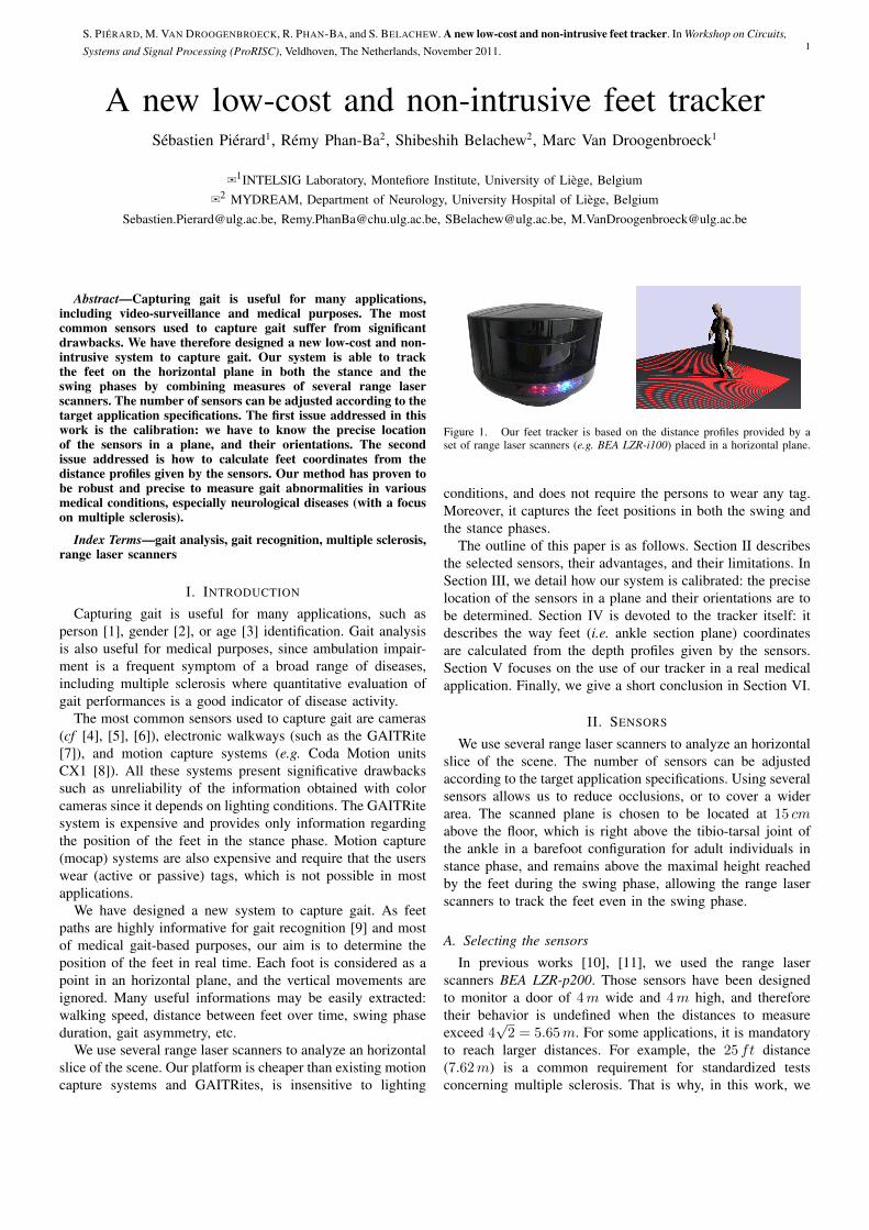
Figure 1. Our feet tracker is based on the distance profiles provided by aset of range laser scanners (e.g. BEA LZR-i100) placed in a horizontal plane.
conditions, and does not require the persons to wear any tag.Moreover, it captures the feet positions in both the swing andthe stance phases.
The outline of this paper is as follows. Section II describesthe selected sensors, their advantages, and their limitations. InSection III, we detail how our system is calibrated: the preciselocation of the sensors in a plane and their orientations are tobe determined. Section IV is devoted to the tracker itself: itdescribes the way feet (i.e. ankle section plane) coordinatesare calculated from the depth profiles given by the sensors.Section V focuses on the use of our tracker in a real medicalapplication. Finally, we give a short conclusion in Section VI.
II. SENSORS
We use several range laser scanners to analyze an horizontalslice of the scene. The number of sensors can be adjustedaccording to the target application specifications. Using severalsensors allows us to reduce occlusions, or to cover a widerarea. The scanned plane is chosen to be located at 15 cmabove the floor, which is right above the tibio-tarsal joint ofthe ankle in a barefoot configuration for adult individuals instance phase, and remains above the maximal height reachedby the feet during the swing phase, allowing the range laserscanners to track the feet even in the swing phase.
A. Selecting the sensors
In previous works [10], [11], we used the range laserscanners BEA LZR-p200. Those sensors have been designedto monitor a door of 4m wide and 4m high, and thereforetheir behavior is undefined when the distances to measureexceed 4
√2 = 5.65m. For some applications, it is mandatory
to reach larger distances. For example, the 25 ft distance(7.62m) is a common requirement for standardized testsconcerning multiple sclerosis. That is why, in this work, we
S. PIÉRARD, M. VAN DROOGENBROECK, R. PHAN-BA, and S. BELACHEW. A new low-cost and non-intrusive feet tracker. In Workshop on Circuits,
Systems and Signal Processing (ProRISC), Veldhoven, The Netherlands, November 2011. 2
have chosen another model of the same family: the BEALZR-i100 (see Figure 1). These have only a limit distance of10√
2 ' 14.14m, which is large enough for most applications.The selected sensors are adequate for measuring distances
with a high precision, without any reflector. They are small,and easy to place in various environments. Note that the riskof interference between sensors is negligible, and therefore itis safe to use several sensors to scan the same plane.
The sensors measure distances in 274 directions spanning96°, in a plane, at 15Hz. Their resolution is 1mm. In practice,we observe a temporal variation of a few millimeters, andseldom a few centimeters, on the acquired distances. It shouldbe noted that the sensors are strongly disturbed by highlyreflective materials such as metal, and black materials (in theinfrared band). It should also be noted that at discontinuities,the sensors provide a random measure between the minimumand the maximum distance. Therefore, the sensors may seepoints where there is no object in the scene (these pointsare named outliers in the following). Robustness to outliersis therefore mandatory.
B. Behavior in dynamical scenes
The field of view of 96° is obtained thanks to an internalrotating mirror. As the mirror has to turn 48° to cover the 96°,a frame is acquired in 1
15 .48360 s ' 9ms.
An object of 10 cm (i.e. the typical size of a leg) locatedat 1m from the sensor is viewed inside of a 5.7° largeangle, and therefore in 5.7
2115
1360 s ' 0.52778ms. For a
walking speed of 5 km/h, the maximal speed of the feet isapproximately 16 km/h. In consequence, a foot can move by0.52778
10001600000
3600 ' 0.235 cm during the data acquisition. Asthis displacement is negligible, the selected sensors are quickenough to track feet with high precision.
However, it should be stressed that there exist no ways tosynchronize the sensors. With multiple sensors, merging theinformation provided by the sensors is required. Unfortunately,there may be a temporal gap of 1
15 s between the data to befused. For a walking speed of 5 km/h, this is equivalent to anuncertainty of 29.6 cm on a foot position in the worst case.Clearly, this source of uncertainty is dominant. Note howeverthat this uncertainty is only along the path followed by thefoot.
C. Towards a simple model of the sensors
In this paper, we assume that the sensors are punctual. Thisimplies that the 274 lines-of-sight are concurrent and thatthe intersection point is located in the sensor. Under theseassumptions, the distance measured between the sensor and avisible point of the scene is the distance between the pointand the aforementioned intersection. It follows that, to obtainthe coordinates of the 274 points seen by a sensor, a simplepolar to cartesian transform suffices.
III. THE CALIBRATION PROCEDURE
The goal of the calibration procedure is to determine theprecise location of the sensors in the room, and their orien-tations. This knowledge is mandatory to fuse the information
provided by different sensors. Of course, this procedure has tobe done only once, after the installation of the sensors in theroom. In this section, we present a semi-automatic calibrationprocedure.
It should be stressed that the calibration has to be veryaccurate. An error of 0.075° on the orientation of a sensorhas for consequence an error of 1 cm on the location of apoint seen at 7.62m. A well designed calibration procedureis therefore needed.
A. Description of our calibration procedureIn the proposed procedure, a cylinder is successively placed
in the room at a few places. Each sensor has its own lo-cal cartesian coordinate system. Each time the cylinder isdisplaced, its center coordinates are estimated in the localcoordinate system of each sensor.
The passage from one local coordinate system to anotheris done by a transformation composed of translation androtation. The calibration is equivalent to determining thesetransformations. The cylinder has to be placed a least at twodifferent locations, but repeating the operation a dozen oftimes, to take advantage of the least squares error reductionmechanism, helps to improve the calibration. Note that thereis no need to increase the number of locations if the number ofsensors increases. Also, we assume that the cylinder is visibleto all sensors.
Let(Csxi, C
syi
)be the coordinates of the cylinder in its i-th
position expressed in the local cartesian coordinate system ofsensor s. If, in the local cartesian coordinate system of sensor0, the sensor s is located at
(∆sx,∆
sy
)and is looking in the
direction θs, we have ∀i(cos (θs) − sin (θs) ∆s
x
sin (θs) cos (θs) ∆sy
) CsxiCsyi1
=
(C0xi
C0yi
)(1)
Therefore, the position and the orientation of the sensor s canbe found solving the following linear equation:
Csx0 −Csy0 1 0...
......
...Csxp −Csyp 1 0Csy0 Csx0 0 1
......
......
Csyp Csxp 0 1
cos (θs)sin (θs)
∆sx
∆sy
︸ ︷︷ ︸
unknowns
=
C0x0...
C0xp
C0y0...
C0yp
(2)
As this system is overconstrained when the cylinder is placedmore than two times, the solution has to be determined in theleast-squares sense.
In practice, we manage to ensure that the cylinder is theonly moving object in the scene during calibration. We apply abackground subtraction to the signal provided by each sensor,in order to filter out the static elements of the scene and to keeponly the points corresponding to the cylinder. To decrease thesensitivity to outliers, our implementation uses the RANSACalgorithm to obtain robust circle fits.
The remainder of this section is devoted to the comparisonof four circle fitting procedures (three well known and a newone), and to the selection of the best one. In our case, the datapoints are sampled along a small arc of circle.
S. PIÉRARD, M. VAN DROOGENBROECK, R. PHAN-BA, and S. BELACHEW. A new low-cost and non-intrusive feet tracker. In Workshop on Circuits,
Systems and Signal Processing (ProRISC), Veldhoven, The Netherlands, November 2011. 3
B. Circle fitting methods
Let (x1, y1), (x2, y2), . . . (xn, yn) be the points by whichwe want to get a circle of radius R and center (Cx, Cy)to pass trough. The key to a solution consists in finding anoptimization criterion that leads to equations easy to solve.For example, the least squares criterion
min
n∑i=1
(√(xi − Cx)
2+ (yi − Cy)
2 −R)2
(3)
is difficult to handle since it leads to a nonlinear problem thathas no closed form solution (with iterative methods, one isfaced with questions related to convergence, plateaus, valleys,and to the initial guess). Surprisingly, fitting a circle to a cloudof points is a difficult problem. A entire book devoted to thesubject has been published recently [12].
1) KÅSA’s method: Instead of the criterion (3), KÅSAproposed in [13] to use the criterion
min
n∑i=1
((xi − Cx)
2+ (yi − Cy)
2 −R2)2
(4)
Both criterions (3) and (4) are equivalent if there exists acircle passing through all points. However, the solution maybe different if the observations are noisy. If R is an unknown,KÅSA’s criterion is easier to deal with, because it leads to aunique and explicit solution. We denote the centered moments:
µab =1
n
n∑i=1
(xi − x)a
(yi − y)b (5)
where x = 1n
∑ni=1 xi and y = 1
n
∑ni=1 yi are the coordinates
of the gravity center of the cloud of points. With KÅSA’scriterion, the optimal center of the circle is given by
Cx = x+1
2
µ02(µ30 + µ12)− µ11(µ03 + µ21)
µ20µ02 − µ211
(6)
Cy = y +1
2
µ20(µ03 + µ21)− µ11(µ30 + µ12)
µ20µ02 − µ211
(7)
2) Our method: KÅSA’s criterion with R known: If theradius is known, then the optimal center corresponding toKÅSA’s criterion may differ because we cannot write anymore
∂
∂R
n∑i=1
((xi − Cx)
2+ (yi − Cy)
2 −R2)2
= 0 (8)
Without loss of generality, let’s assume that x = 0 and y = 0.This can be obtain by translation the cloud of points if needed.The center can be found by solving the following system.
∂∂Cx
∑ni=1
((xi − Cx)
2+ (yi − Cy)
2 −R2)2
= 0
∂∂Cy
∑ni=1
((xi − Cx)
2+ (yi − Cy)
2 −R2)2
= 0(9)
⇔
Cx(3µ20 + µ02 −R2
)+ C3
x + CxC2y + Cy (2µ11)
= µ30 + µ12
Cx (2µ11) + C3y + C2
xCy + Cy(3µ02 + µ20 −R2
)= µ03 + µ21
At first sight, solving this system is difficult because theequations are of the third order. Let’s assume that the distance
between the gravity center of the cloud and the center of thecircle is known, that is C2
x + C2y = ∆, and using Cramer’s
rule,
⇔
Cx =(µ30+µ12)(3µ02+µ20−R2+∆)−(µ03+µ21)(2µ11)
(3µ20+µ02−R2+∆)(3µ02+µ20−R2+∆)−4µ211
Cy =(µ03+µ21)(3µ20+µ02−R2+∆)−(µ30+µ12)(2µ11)
(3µ20+µ02−R2+∆)(3µ02+µ20−R2+∆)−4µ211
Of course, the value of ∆ has to be determined. This can bedone by checking that C2
x +C2y = ∆ as assumed. With a few
simple algebraic manipulations, one can check that ∆ is a rootof a fifth order polynomial
∆5 + k4∆4 + k3∆3 + k2∆2 + k1∆ + k0 = 0 (10)
The values of k0, k1, k2, k3, and k4 are not given here due to alack of space, but can be easily computed. There are at most 5solutions, and selecting the best one can be done using KÅSA’scriterion. Only the positive roots should be considered, as ∆is positive by definition. Note also that there exists alwaysat least one solution, even if the sample points are collinear,because k0 ≤ 01.
3) The methods of PRATT and TAUBIN: Instead ofparametrizing a circle with {Cx, Cy, R}, PRATT [14] proposedto use {A,B,C,D} such that the equation of the circle is
A(x2 + y2
)+Bx+ Cy +D = 0 (11)
This parameterization allows to describe circles as well as lines(with A = 0). In some cases, only a small arc of the circleis observed and it is hazardous to estimate the radius and todecide on which side of the cloud the circle is. In those cases,some people (e.g. [12]) prefer to fit a line instead of a circle.The criterion related to this parameterization is
min
n∑i=1
(A(x2i + y2
i
)+Bxi + Cyi +D
)2(12)
Because the parameters {A,B,C,D} are defined up a scalefactor, and to avoid the trivial solution A = B = C = D = 0,one has to add a constraint. It can be showed that KÅSA’scriterion is equivalent to this one with the constraint A = 1.PRATT [14] used the constraint B2 + C2 − 4AD = 1 whichhas the advantage of ensuring that B2 +C2 − 4AD > 0 (thisis required for circles). TAUBIN [15] proposed
4A
n
n∑i=1
(A(x2i + y2
i
)+Bxi + Cyi +D
)+(B2 + C2 − 4AD
)= 1 (13)
Other constraints have also be proposed by Gander [16] andNievergelt [17], but we will not consider them in this paper.
C. Selection of the circle fitting method
We evaluated the four above-mentionned methods (KÅSA,KÅSA with R known, TAUBIN, and PRATT) by simulation.For the methods of PRATT and TAUBIN, we have used thepublicly available implementation of the author of [12]2.
1The polynomial takes a negative value for β = 0, and a positive infiniteone for β = +∞. Therefore, there is at least one root between 0 and +∞.
2http://www.math.uab.edu/~chernov/cl/MATLABcircle.html

S. PIÉRARD, M. VAN DROOGENBROECK, R. PHAN-BA, and S. BELACHEW. A new low-cost and non-intrusive feet tracker. In Workshop on Circuits,
Systems and Signal Processing (ProRISC), Veldhoven, The Netherlands, November 2011. 4
0
2
4
6
8
10
0 2 4 6 8 10
err
or
[ cm
]
noise [ cm ]
Pratt by SVD
0
2
4
6
8
10
0 2 4 6 8 10
err
or
[ cm
]
noise [ cm ]
Taubin by SVD
0
2
4
6
8
10
0 2 4 6 8 10
err
or
[ cm
]
noise [ cm ]
Kasa (R known)
0
2
4
6
8
10
0 2 4 6 8 10
err
or
[ cm
]
noise [ cm ]
Kasa
Figure 2. The mean distance between the estimated center of the calibrationcylinder and its true center, as a function of the noise level u. The red,green, and blue curves correspond respectively to a calibration cylinder with adiameter of 30 cm, 40 cm, and 50 cm. These results show that the fit methodintroduced in this paper (solving KÅSA’s criterion with R known) outperformsthe other ones (the methods of KÅSA, TAUBIN and PRATT).
A cylinder is placed randomly, and fully included in thevisual field of the sensor. It is separated from the sensor by adistance between 50 cm and 10m. A noise was simulated onthe distances measured by the virtual sensor: each measure-ment is corrupted independently of the others, and the noiseis distributed uniformly on the[−u, u] interval. Therefore, weassume that the distance measures are unbiased. We observethe mean error, i.e. the mean distance between the estimatedcenter of the calibration cylinder and its true center. We want toselect the fitting method with the lower mean error. The meanerror depending on the noise level is depicted in Figure 2.
Note that KÅSA’s method is known to be highly biasedwhen a small arc is sampled. This bias is difficult to compen-sate, because it depends on the noise level, and the sensorsare insufficiently characterized to predict the noise level.
Our experiments have shown that KÅSA with R known isthe fitting method that is best suited to our particular case.KÅSA with R known is less sensitive to noise than KÅSA.The methods of PRATT and TAUBIN are almost equivalent,and are unable to cope with important noise (whether oneuses a SVD or Newton’s method). The reason is probablythat fitting lines as well as circles in a bad idea in our casebecause Cx = − B
2A and Cy = − C2A . Therefore, if the fitting
method prefers a line, estimating Cx and Cy is impossiblesince A = 0. This conclusion stands in deep contrast with theone of [12], which stated that the methods PRATT and TAUBINare theoretically preferable to KÅSA’s one, as a general rule.
D. Remark: application to robotics
Fitting circles of known radius to points sampled alonga small arc is a problem often encountered in robotics. Forexample, in [18], a mobile robot should interact with knownobjects that have a cylindrical base. The sensor is a range laserscanner or a 3D camera, and therefore the localization of theobjects is equivalent to the estimation of the object center from
Figure 3. The different steps of our method. From the top left picture to thebottom right one: (1) the model of the empty scene, i.e. the background (2)the points seen by all sensors (3) the result of the background subtraction (4)after the convolution with a gaussian kernel (5) after local maxima search (6)the final result of the tracker.
a set of points sampled along an arc of circle. This is exactlythe same problem we are facing here. In [18] the circle isfitted with KÅSA’s method; we know now that it is not thebest choice and that using KÅSA’s criterion with R knownwould be a lot more precise.
IV. THE FEET TRACKER
The most straightforward methodology to track the feetconsists in building a localization map (cf [10]), filteringuninteresting static objects (chairs, tables, . . . ) by using abackground subtraction algorithm (such as [19]), and isolatingthe feet by a connected components analysis (such as [20]).However, the technique proposed in [10] to combine theinformation provided by several range laser scanners assumesthat the observed scene is nearly static, and that the sensorsdon’t see outlier points. Unfortunately, this is not the case,so we propose a new method. Its main steps are depicted inFigure 3.
A. Locating the feet
Each sensor sees a cloud of points in the horizontal plane.Thanks to the calibration, these clouds can be superimposed,and merged. From the resulting cloud, we have to estimate aset of two points that are the centers of each foot (or leg).
We apply a background subtraction to the signal providedby each sensor, in order to filter out the static elements ofthe scene and to keep only the points corresponding to the
S. PIÉRARD, M. VAN DROOGENBROECK, R. PHAN-BA, and S. BELACHEW. A new low-cost and non-intrusive feet tracker. In Workshop on Circuits,
Systems and Signal Processing (ProRISC), Veldhoven, The Netherlands, November 2011. 5
0 0.5 1 1.5 2 2.5 30
0.5
1
1.5
2
2.5
3
ground truth
estim
ate
d
distance between feet
σ = 0.4
σ = 0.5
σ = 0.6
σ = 0.7
σ = 0.8
σ = 0.9
σ = 1.0
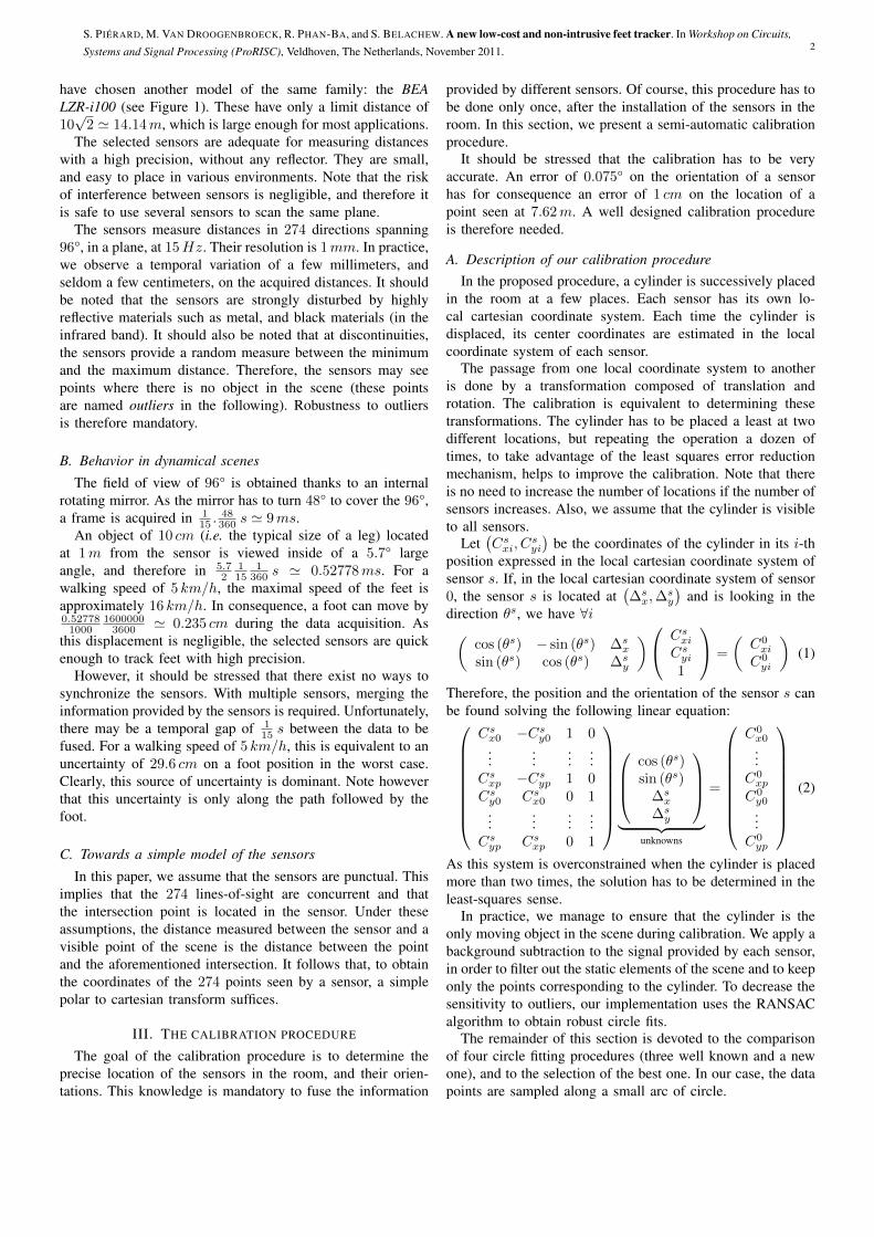
Figure 4. The theoretical error on the feet positions. The unit chosen toexpress the distances and σ is such that the diameter of the leg is D = 1.These curves have been obtained by simulation in noise-free conditions, withuniform and dense sampling.
feet. Then, the remaining points are convolved with a gaussiankernel of standard deviation σ (i.e. a gaussian is placed ateach each point, and they are summed). We expect to have, inmost cases, the two largest local maxima where the feet are.We do not provide any output if there is less than two localmaxima, or if they are spaced more than it is possible. Thismethod is robust to outliers, and therefore a simple backgroundsubtraction method suffices.
The standard deviation σ is the only parameter that hasto be chosen. For the sake of theory, let’s assume that thehorizontal section of the feet are circles, and that they areuniformly sampled. Let’s denote D the diameter of the feet.
We want to get a local maximum per foot. If there was onlyone foot in the scene, it can be showed that σ should be largerthan D
2 if the sensors see only two points of the feet, or largerthan 0.36D if the sensors see a lot of points. Now, considertwo feet. If σ is too large, there is a risk to observe only onemaximum for both feet. The fact that we observe one or twomaxima depends on the distance between the feet, on D andon σ. This relation is depicted in Figure 4. We consider that, inthe worst case, D = 14 cm (with trousers) and that only twopoints are seen by foot. Accordingly, we chose σ = D
2 = 7 cm.According to Figure 4, we expect our localization procedureto fail if the distance between the centers of the legs is lessthan 14 × 1.4428 ' 20 cm and to give a biased result if thedistance is less than 14× 2 ' 28 cm.
In future work, we would like to improve the localizationprocedure in order to obtain an unbiased feet position estimate,and to be able to localize the feet even if there are close.Some ideas are (i) to correct the estimate thanks to the knownrelation between the estimated inter-feet distance and its truevalue, or (ii) to use a gaussian ring kernel instead of thegaussian one, or (iii) to use machine learning principles.
(xa(t+ 2), ya(t+ 2))
(xa(t+ 1), ya(t+ 1))
(xa(t), ya(t))
(xa(t− 1), ya(t− 1))
(xb(t− 1), yb(t− 1))
(xb(t+ 1), yb(t+ 1))
(xb(t), yb(t))
(xb(t+ 2), yb(t+ 2))
Figure 5. Φab(t) is the signed area of the blue triangle.
B. Tracking the feet
At this point, we have a couple of points at each frame. Inthis step, we would like to cluster all the points in two classes,in order to obtain a trajectory for each foot.
At the time this paper is written, we minimize the totallength of the two trajectories. This criterion leads to excellentresults when the observed person walks along a line. However,from time to time we observed that when the person turnsquickly, the trajectories may cross. This is probably due toan insufficient acquisition rate (15Hz). This kind of problemalso arises with a tandem gait walk. In future work, we planto improve the technique used to track the feet, perhaps usinga Kalman filter.
C. Identifying the feet
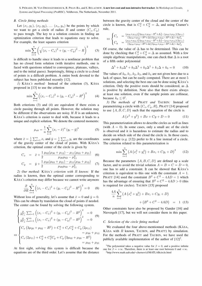
We know the position of both feet over time, but we stillneed to determine which foot is the left one, and which one isthe right one. The only clue available is the motion direction.Therefore, it is impossible to correctly identify the feet if theobserved person moves in reverse. Let’s denote (xf (t), yf (t))the coordinates of the foot “f” at time t. The following quantity
Φab(t) =1
2
∣∣∣∣∣∣xa(t) xa(t+ 1) xb(t)+xb(t+1)
2
ya(t) ya(t+ 1) yb(t)+yb(t+1)2
1 1 1
∣∣∣∣∣∣ (14)
is positive if the foot “a” is on the right of the foot “b”between the times t and t+1, and |Φab(t)| is a certainty factor(the geometrical meaning of Φab(t) is depicted in Figure 5).Therefore, letting T be the total walk duration,
T−2∑t=0
[Φ12(t)− Φ21(t)] < 0 (15)
if the trajectory number 1 corresponds to the left foot. Weexpect this criterion to be suitable, not only for straight paths,but also for any path (such as an ◦-shaped path or an∞-shapedpath).
V. APPLICATION TO NEUROLOGICAL DISEASE ANALYSIS
Gait disorders measurement and quantification is of theutmost importance in the follow-up and therapeutic decision-making process of numerous medical conditions (whether

S. PIÉRARD, M. VAN DROOGENBROECK, R. PHAN-BA, and S. BELACHEW. A new low-cost and non-intrusive feet tracker. In Workshop on Circuits,
Systems and Signal Processing (ProRISC), Veldhoven, The Netherlands, November 2011. 6
Figure 6. Screenshots of our software. Upper images display the positionof the four sensors (obtained by calibration), a 25 ft straight path, and thepreviously estimated feet positions. On the left hand side, the observed personhas a normal gait, and on the right hand side, he has an ataxic gait. Suchpathologies can be easily detected and measured with our method. A few fullvideos are available at http://www.ulg.ac.be/telecom/vgaims/.
orthopaedic, rhumatologic, pediatric, cardiorespiratory, or neu-rologic). For example, in the field of multiple sclerosis, a com-mon neurological disease where gait is frequently impaired,change in walking performances can lead to significativetherapeutic modifications [21].
However, the current available tools measuring gait dysfunc-tion suffer from various limitations [22] and are completelyblind to certain important gait features, such as ataxia, sym-metry of the feet paths and individual feet walking speed,freezing of gait, etc, that are only qualitatively described in theneurological examination. The feet tracker developed in thiswork allows one to easily capture these features in a simpleway, and at low cost (see Figure 6).
A dozen of videos demonstrating our results are avail-able at http://www.ulg.ac.be/telecom/vgaims/. Qualitatively,our method is robust and precise. It is clear beyond thetraditional measurement of global walking speed, and itsuse can be extended to measure more subtle and specificgait abnormalities. However, the questions of precision andaccuracy are still problematic, because of the intrinsic lack ofground-truth data in this specific field.
VI. CONCLUSION
We have developed a new platform to capture gait, and adedicated calibration procedure. It is a non-intrusive and low-cost platform. It has proven to be suitable for medical pur-poses, and we think that it can be used for other applicationslike automatic person identification.
REFERENCES
[1] N. Boulgouris, D. Hatzinakos, and K. Plataniotis, “Gait recognition: achallenging signal processing technology for biometric identification,”IEEE Signal Processing Magazine, vol. 22, no. 6, pp. 78–90, November2005.
[2] X. Li and S. Yan, “Gait components and their application to genderrecognition,” IEEE Transactions on Systems, Man, and Cybernetics –Part C: Applications and Reviews, vol. 38, no. 2, pp. 145–155, March2008.
[3] J. Lu and Y.-P. Tan, “Gait-based human age estimation,” IEEE Transac-tions on Information Forensics and Security, vol. 5, no. 4, pp. 761–770,December 2010.
[4] O. Barnich and M. Van Droogenbroeck, “Frontal-view gait recognitionby intra- and inter-frame rectangle size distribution,” Pattern RecognitionLetters, vol. 30, no. 10, pp. 893–901, July 2009.
[5] B. McDonald and R. Green, “A silhouette based technique for locatingand rendering foot movements over a plane,” in International Conferenceon Image and Vision Computing, Wellington, New Zealand, November2009, pp. 385–390.
[6] E. Stone, D. Anderson, M. Skubic, and J. Keller, “Extracting foot-falls from voxel data,” in International Conference of the Engineeringin Medicine and Biology Society (EMBC), Buenos Aires, Argentina,August-September 2010, pp. 1119–1122.
[7] U. Givon, G. Zeilig, and A. Achiron, “Gait analysis in multiple sclerosis:Characterization of temporal-spatial parameters using gaitrite functionalambulation system,” Gait & Posture, vol. 29, no. 1, pp. 138–142, 2009.
[8] C. Schwartz, B. Forthomme, O. Brüls, V. Denoël, S. Cescotto, andJ. Croisier, “Using 3D to understand human motion,” in Proceedingsof 3D Stereo MEDIA, Liège, Belgium, December 2010.
[9] A. Switonski, A. Polanski, and K. Wojciechowski, “Human identificationbased on gait paths,” in Advances Concepts for Intelligent Vision Systems(ACIVS), ser. Lecture Notes in Computer Science, J. Blanc-Talon,R. Kleihorst, W. Philips, D. Popescu, and P. Scheunders, Eds., vol. 6915.Gent, Belgium: Springer, August 2011, pp. 531–542.
[10] S. Piérard, V. Pierlot, O. Barnich, M. Van Droogenbroeck, and J. Verly,“A platform for the fast interpretation of movements and localization ofusers in 3D applications driven by a range camera,” in 3DTV Conference,Tampere, Finland, June 2010.
[11] O. Barnich, S. Piérard, and M. Van Droogenbroeck, “A virtual curtain forthe detection of humans and access control,” in Advanced Concepts forIntelligent Vision Systems (ACIVS), Part II, Sydney, Australia, December2010, pp. 98–109.
[12] N. Chernov, Circular and linear regression: fitting circles and lines byleast aquares, ser. Chapman & Hall/CRC Monographs on Statistics &Applied Probability. USA: CRC Press, 2011, vol. 117.
[13] I. Kåsa, “A circle fitting procedure and its error analysis,” IEEETransactions on instrumentation and measurement, vol. IM-25, no. 1,pp. 8–14, March 1976.
[14] V. Pratt, “Direct least-squares fitting of algebraic surfaces,” in Proceed-ings of the 14th annual conference on Computer graphics and interactivetechniques (SIGGRAPH), vol. 21(4), July 1987, pp. 145–152.
[15] G. Taubin, “Estimation of planar curves, surfaces, and nonplanar spacecurves defined by implicit equations with applications to edge andrange image segmentation,” IEEE Transactions on Pattern Analysis andMachine Intelligence, vol. 13, no. 11, pp. 1115–1138, November 1991.
[16] W. Gander, G. Golub, and R. Strebel, “Least-squares fitting of circlesand ellipses,” BIT Numerical Mathematics, vol. 34, no. 4, pp. 558–578,1994.
[17] Y. Nievergelt, “Hyperspheres and hyperplanes fitted seamlessly byalgebraic constrained total least-squares,” Linear Algebra and its Ap-plications, vol. 331, pp. 43–59, 2001.
[18] M. Greuter, M. Rosenfelder, M. Blaich, and O. Bittel, “Obstacle andgame element detection with the 3d-sensor kinect,” in Research andEducation in Robotics - EUROBOT 2011. Springer, 2011, vol. 161,pp. 130–143.
[19] O. Barnich and M. Van Droogenbroeck, “ViBe: A universal backgroundsubtraction algorithm for video sequences,” IEEE Transactions on ImageProcessing, vol. 20, no. 6, pp. 1709–1724, June 2011.
[20] F. Chang, C.-J. Chen, and C.-J. Lu, “A linear-time component-labelingalgorithm using contour tracing technique,” Computer Vision and ImageUnderstanding, vol. 93, no. 2, pp. 206–220, February 2004.
[21] A. Goodman, T. Brown, L. Krupp, R. Schapiro, S. Schwid, R. Cohen,L. Marinucci, and A. Blight, “Sustained-release oral fampridine inmultiple sclerosis: a randomised, double-blind, controlled trial,” TheLancet, vol. 373, no. 9665, pp. 732–738, February 2009.
[22] R. Phan-Ba, A. Pace, P. Calay, P. Grodent, F. Douchamps, R. Hyde,C. Hotermans, V. Delvaux, I. Hansen, G. Moonen, and S. Belachew,“Comparison of the timed 25-foot and the 100-meter walk as perfor-mance measures in multiple sclerosis,” Neurorehabilitation and neuralrepair, vol. 25, no. 7, pp. 672–679, September 2011.