A New Look at Currency Investing - CFA Institute
106
A NEW LOOK AT CURRENCY INVESTING Momtchil Pojarliev, CFA Richard M. Levich
-
Upload
khangminh22 -
Category
Documents
-
view
0 -
download
0
Transcript of A New Look at Currency Investing - CFA Institute

A NEW LOOK AT CURRENCY INVESTING
Pojarliev and Levich
available online at www.cfapubs.org
Momtchil Pojarliev, CFARichard M. Levich
9 781934 667545
9 0 0 0 0ISBN 978-1-934667-54-5
A N
EW LO
OK
AT CU
RR
ENC
Y IN
VESTIN
G

AmeritechAnonymousRobert D. ArnottTheodore R. Aronson, CFAAsahi Mutual LifeBatterymarch Financial ManagementBoston CompanyBoston Partners Asset Management, L.P.Gary P. Brinson, CFABrinson Partners, Inc.Capital Group International, Inc.Concord Capital ManagementDai-Ichi Life CompanyDaiwa SecuritiesMr. and Mrs. Jeffrey DiermeierGifford Fong AssociatesInvestment Counsel Association
of America, Inc.Jacobs Levy Equity ManagementJohn A. Gunn, CFAJon L. Hagler FoundationLong-Term Credit Bank of Japan, Ltd.Lynch, Jones & Ryan
Meiji Mutual Life Insurance CompanyMiller Anderson & Sherrerd, LLPJohn B. Neff, CFANikko Securities Co., Ltd.Nippon Life Insurance Company of JapanNomura Securities Co., Ltd.Payden & RygelProvident National BankFrank K. Reilly, CFASalomon BrothersSassoon Holdings Pte. Ltd.Scudder Stevens & ClarkSecurity Analysts Association of JapanShaw Data Securities, Inc.Sit Investment Associates, Inc.Standish, Ayer & Wood, Inc.State Farm Insurance CompaniesSumitomo Life America, Inc.T. Rowe Price Associates, Inc.Templeton Investment Counsel Inc.Travelers Insurance Co.USF&G CompaniesYamaichi Securities Co., Ltd.
Named Endowments
The Research Foundation of CFA Institute acknowledges with sincere gratitude the generous contributions of the Named Endowment participants listed below.
Gifts of at least US$100,000 qualify donors for membership in the Named Endowment category, which recognizes in perpetuity the commitment toward unbiased, practitioner-oriented, relevant research that these firms and individuals have expressed through their generous support of the Research Foundation of CFA Institute.
For more on upcoming Research Foundation publications and webcasts, please visit
www.cfainstitute.org/about/foundation/.
Research Foundation monographs are online at www.cfapubs.org.
Senior Research Fellows
Financial Services Analyst Association
The Research Foundation of CFA Institute
Board of Trustees2012–2013
ChairJeffery V. Bailey, CFA†
Target Corporation
Renee Kathleen-Doyle Blasky, CFAVista Capital Ltd.
Dwight Churchill, CFASunapee, NH
William Fung†London Business School
James P. Garland, CFAThe Jeffrey Company
John T. “JT” Grier, CFAVirginia Retirement System
Pranay Gupta, CFALombard Odier Darier Hentsch (Asia) Limited
Walter V. “Bud” Haslett, Jr., CFA†*CFA Institute
Daniel S. Meader, CFA*Trinity Advisory Group
Frank K. Reilly, CFA†*University of Notre Dame
Thomas M. Richards, CFA†Nuveen HydePark Group, LLC
John D. Rogers, CFA†*CFA Institute
Brian Singer, CFAWilliam Blair, Dynamic Allocation Strategies
Fred H. Speece, Jr., CFA†*Speece Thorson Capital Group Inc.
Charles J. Yang, CFA*T&D Asset Management
Wayne H. Wagner, CFAVenice Beach, CA
Arnold S. WoodMartingale Asset Management
Officers and Directors Executive DirectorWalter V. “Bud” Haslett, Jr., CFA
CFA Institute
Gary P. Brinson Director of Research Laurence B. Siegel
Research Foundation of CFA Institute
SecretaryTina Sapsara
CFA Institute
TreasurerKim Maynard
CFA Institute
Research Foundation Review Board
William J. BernsteinEfficient Frontier Advisors
Stephen J. BrownNew York University
Sanjiv DasSanta Clara University
Bernard DumasINSEAD
Stephen FiglewskiNew York University
Gary L. GastineauETF Consultants, LLC
William N. GoetzmannYale School of Management
Stephen A. Gorman, CFAWellington Management Company
Elizabeth R. HilpmanBarlow Partners, Inc.
Paul D. KaplanMorningstar, Inc.
Robert E. Kiernan IIIAdvanced Portfolio Management
Robert W. Kopprasch, CFAThe Yield Book Inc.
Andrew W. LoMassachusetts Institute of Technology
Alan MarcusBoston College
Paul O’ConnellFDO Partners
Krishna RamaswamyUniversity of Pennsylvania
Andrew RuddAdvisor Software, Inc.
Lee R. ThomasPacific Investment Management Company
Robert TrevorMacquarie University
*Emeritus †Ex officio
A New Look at Currency Investing
Momtchil Pojarliev, CFAHathersage Capital Management LLC
Richard M. LevichNew York University Stern School of Business
Statement of Purpose
The Research Foundation of CFA Institute is a not-for-profit organization established to promote the development and dissemination of relevant research for investment practitioners worldwide.
Neither the Research Foundation, CFA Institute, nor the publication’s editorial staff is responsible for facts and opinions presented in this pub-lication. This publication reflects the views of the author(s) and does not represent the official views of the Research Foundation or CFA Institute.
�e Research Foundation of CFA Institute and the Research Foundation logo are trademarks owned by �e Research Foundation of CFA Institute. CFA®, Chartered Financial Analyst®, AIMR-PPS®, and GIPS® are just a few of the trademarks owned by CFA Institute. To view a list of CFA Institute trademarks and the Guide for the Use of CFA Institute Marks, please visit our website at www.cfainstitute.org.
© 2012 �e Research Foundation of CFA Institute
All rights reserved. No part of this publication may be reproduced, stored in a retrieval system, or transmitted, in any form or by any means, electronic, mechanical, photocopying, recording, or otherwise, without the prior written permission of the copyright holder.
�is publication is designed to provide accurate and authoritative information in regard to the subject matter covered. It is sold with the understanding that the publisher is not engaged in rendering legal, accounting, or other professional service. If legal advice or other expert assistance is required, the services of a competent professional should be sought.
ISBN 978-1-934667-54-5
21 December 2012
Editorial Staff
Elizabeth Collins Book Editor
Mary-Kate Hines Assistant Editor
Mike Dean Publishing Technology Specialist
Cindy Maisannes Manager, Publications Production
Christina Hampton Publishing Technology Specialist
Randy Carila Publishing Technology Specialist
Biographies
Momtchil Pojarliev, CFA, is a senior portfolio manager for Hathersage Capital Management LLC and also serves as the chief investment o�cer of Cambex Holdings. He joined Hathersage after a decade of experience man-aging foreign exchange (FX) portfolios as the head of currencies at Hermes Pension Fund Management, senior FX portfolio manager at Pictet & Cie, and senior FX portfolio manager at Invesco. In addition, Dr. Pojarliev has advised various asset management ¡rms, including PIMCO and Goldman Sachs Asset Management, in the area of currency return analytics. He has published extensively in ¡nance and investment journals. He is a member of �e Economic Club of New York and the Swiss Society for Financial Market Research. He currently serves on the Editorial Board of the Financial Analysts Journal. Dr. Pojarliev received an MSc in ¡nance from the Vienna University of Economics and Business and a PhD with honors in ¡nancial econometrics from the University of Basel.
Richard M. Levich is professor of ¡nance and international business and deputy chairman of the Department of Finance at New York University’s Leonard N. Stern School of Business. Previously, he served as chairman of the International Business Program at Stern. He is also a research associate with the National Bureau of Economic Research in Cambridge, Massachusetts, and a founding editor of the Journal of International Financial Management and Accounting. Professor Levich has been a visiting faculty member at many distinguished universities in the United States and abroad. He is the author or editor of 15 books dealing with international ¡nance and more than 50 scholarly articles, in addition to numerous other published writings. In 1997, Professor Levich received a CDC Award for Excellence in Applied Portfolio �eory from the Caisse Des Dépôts Group, France. He received his PhD from the University of Chicago.

Acknowledgments
We received helpful comments from Emmanuel Acar, Robert Kosowski, Dori Levanoni, Peter Meier, Sam Nasypbek, and in particular, Laurence Siegel, who reviewed the entire manuscript and made many valuable suggestions. �e views expressed herein are those of the authors and do not necessarily re©ect the views of Hathersage Capital Management, New York University, or the Research Foundation of CFA Institute. We gratefully acknowledge ¡nancial assistance from the Research Foundation of CFA Institute for the preparation of this book.
�is publication quali�es for 5 CE credits under the guidelines of the CFA Institute Continuing Education Program.
Contents
Foreword.................................................................................. vii
1. Introduction .......................................................................... 1
Motivation: The Case for and against Currency Investing ........ 2
Overview........................................................................... 7
2. The Landscape of Active Currency Management ........................ 10
The Foreign Exchange Market.............................................. 10
The Currency Management Mandate.................................... 32
Currency Investment Strategies ............................................ 38
Currency Investment Processes ............................................. 41
3. A Model of Alpha and Beta Returns from Currency Management......................................................................... 43
4. Empirical Evidence.................................................................. 48
Proxies for Currency Investment Returns and Risk Factors ........ 48
Results for the Barclay Currency Traders Index, 1990–2010....... 56
Results for the Deutsche Bank dbSelect Platform, 2005–2010 ... 69
Summary of Empirical Results............................................... 74
5. Currency Alpha and Beta for Institutional Investors .................... 76
6. Conclusions and Implications for Investment Management.......... 82
Appendix A: Currency Indices and Style Factors ............................. 86
References ................................................................................ 89

©2012 The Research Foundation of CFA Institute vii
Foreword
�e history of modern currency management serves as an excellent example of Andrew Lo’s adaptive markets hypothesis. In the beginning, currency trad-ing occurred independently of institutional portfolio management. It mainly served to hedge the exchange rate risk of international business transactions or to enable speculation. But as the bene¡ts of global diversi¡cation of invest-ment portfolios became apparent, investors increasingly diversi¡ed these port-folios beyond their own borders, which led them to pay more attention to the portfolio’s currency exposure.
Two contradictory views emerged. Some argued that currency exposure should be hedged away completely because it introduced uncompensated risk to a portfolio. Others argued that currency exposure was good for a portfo-lio because it provided diversi¡cation. Eventually, thoughtful investors recog-nized that currency exposure introduced both risk and diversi¡cation, and they solved for optimal currency exposures as they did for other portfolio assets.
As investors became more comfortable with the mechanics of currency options, futures, and forward contracts, they began to explore strategies for pro¡ting from currencies. Early active currency managers looked to exchange rate models based on macroeconomic variables, such as prices, interest rates, and output, for guidance. �en, they followed the lead of the equity literature and began to search for anomalies.
One of the more commonly exploited anomalies was the serial depen-dence of currency returns. Investors exploited this anomaly by purchasing a currency as it appreciated and selling it as it depreciated. Perhaps the most widely exploited anomaly was the violation of the theory of uncovered interest arbitrage. �is theory predicted that changes in exchange rates would oªset interest diªerentials so that investors could not pro¡t by overweighting dis-count currencies and underweighting premium currencies.
Investors ¡rst ventured into active currency management by tilting their hedges; they underhedged currencies that had positive expected returns and overhedged currencies with negative expected returns. But they seldom took positions that increased currency exposure beyond the embedded exposure of the portfolio or reduced it to a net negative exposure. �ey soon realized that it was ine�cient to constrain their currency bets to the portfolio’s embedded currency exposures. But not only did they disconnect their currency strate-gies from the portfolio’s exposures; they separated the hedging decision from the search for alpha. Going into the ¡nancial crisis of 2008–2009, investors
A New Look at Currency Investing
viii ©2012 The Research Foundation of CFA Institute
typically managed currencies independently as a separate asset class or as part of a broader global macro strategy. �en the crisis came, which called into question many previously held views about investing, such as the e�cacy of diversi¡cation.
�is historical in©ection point serves as the starting point for Momtchil Pojarliev and Richard Levich. �ey set out to re-examine the purpose and practice of currency management in the wake of the global ¡nancial crisis, and the result is an extraordinarily comprehensive and lucid book.
Among their many contributions is an up-to-date taxonomy of the foreign exchange market, which focuses on the instruments, participants, and pricing principles. �ey also review the various types of currency mandates, the expecta-tions of the parties, and relevant operational issues. �en, Pojarliev and Levich get into the heart of the matter, which is to review and analyze the main cur-rency management strategies and to model currency returns. �e end result is a clear and concise, but far from super¡cial, review and analysis of foreign exchange markets and currency management practices, together with original research that oªers valuable insights into the factors that determine currency performance.
Pojarliev and Levich, both independently and jointly, have contributed exten-sively to the study of foreign exchange markets and currency management. �eir far-reaching knowledge of these topics is evident throughout this excellent book, which is destined to serve as an essential resource for ¡nance scholars, as well as for those who provide and consume currency management services. Momtchil Pojarliev and Richard Levich deserve our gratitude for producing this ¡ne book.
Mark P. Kritzman, CFAPresident and CEO, Windham Capital Management
Former Research Director, Research Foundation of CFA Institute(2000–2005)
©2012 The Research Foundation of CFA Institute 1
1. Introduction
Prior to the global ¡nancial crisis in 2007–2008, conventional wisdom among investment professionals was that market exposure (beta return) is easy to obtain, excess return (or alpha) is hard to ¡nd, and taking correla-tion of returns into account is important for enhancing overall investment performance. As a consequence of this thinking, many institutional investors adopted a core–satellite investment approach. �e bulk of their assets (the core) were invested in long-only managers with large exposure to equities and ¡xed income; a small proportion of assets were invested in satellite portfolios, such as hedge funds, real estate, and commodities. �e historical correlation of these satellites with equities was nearly zero. �erefore, institutional investors expected that the satellites would provide exposure to alternative beta returns (hence diversi¡cation of equity beta) and possibly alpha returns as well.
As the global ¡nancial crisis unfolded, however, investors discovered that they were less diversi¡ed than they thought. Many hedge funds declined in value along with equity markets, suggesting that what investors had perceived to be either alpha or new and unrelated sources of beta returns turned out to behave like equity beta. �e recent crisis experience con¡rmed a pattern that had been previously documented in academic research a decade earlier (see Chow, Jacquier, Kritzman, and Lowry 1999): In turbulent markets, all asset returns generally become more volatile and more highly correlated. �us, diversi¡cation tends to fail exactly when it is most needed—that is, in falling markets.1
Although most institutional investors still subscribe to this conventional wisdom, some investors in the postcrisis period are beginning to suspect that the expected return on equity beta might be lower than previously thought and that what alternative asset managers sometimes label “alpha” may actually behave more like beta.
1For example, when both hedge funds and global equities produce returns greater than one standard deviation above their means, their correlation is –11%. When both markets generate returns more than one standard deviation below their means, their correlation rises to 58%. �ese correlations are based on monthly returns of the MSCI World Index (in local curren-cies) and the MSCI Hedge Fund Index from the period since inception of the Hedge Fund Index ( January 1994) until June 2010. Kritzman and Li (2010) report a similar pattern in the correlation between U.S. equities (S&P 500 Index) and non-U.S equities (MSCI World ex US Index)—that is, –17% and 76%, respectively.
A New Look at Currency Investing
2 ©2012 The Research Foundation of CFA Institute
Motivation: The Case for and against Currency Investing As investors rethink asset allocation, various questions come to mind with respect to a potential role for currency. Do alternative investments such as cur-rency really bring diversi¡cation bene¡ts to institutional investors? How much of the return generated by currency managers should be classi¡ed as alpha, and how much is beta? Are currency returns predictable to any extent, and is managerial performance or management style persistent? Should plan sponsors actively select currency managers on the basis of past performance, or should they rely on a naive approach based on a passive assortment of all available strategies? Should plan sponsors index their currency investments? If so, what index should they use, and how should they implement an index strategy?
Perhaps because the answers to these questions are unclear, currencies often have been overlooked as an additional source of return. Although funds assigned to a currency investment mandate have grown, growth has been less pronounced than for the overall hedge fund industry.2
More fundamental reasons may underlie the reluctance of institutional investors to treat currency as a viable asset class. A number of factors—some historical, some institutional, and others grounded in economic theory and policy making—have tended to make currency investing be viewed diªerently from the way equity investing is viewed. We review these factors here.
• Currency values are often pegged rather than allowed to �uctuate. During the Bretton–Woods period (1948–1971), currency values were o�cially pegged to the U.S. dollar and were changed only periodically, when policymakers could acknowledge that the values were fundamentally misaligned. Even after 1973, when the ©oating exchange rate period was ushered in, most cur-rencies were pegged to something—generally, the U.S. dollar but sometimes the British pound (GBP), German mark (DEM), or French franc (FRF).3
2Whereas a mere handful of currency managers existed in the mid-1980s, at least 150 cur-rency funds exist today and the actual number could be 300 or higher. In 2010, the Barclay Currency Traders Index tracked 119 managers in the currency domain. In 2010, Deutsche Bank FXSelect, a proprietary trading platform, oªered 67 professionally managed currency funds. Other hedge fund databases, such as those maintained by Lipper TASS and Crédit Agricole Structured Asset Management/Center for International Securities and Derivatives Markets (CISDM), reveal an additional 200 or so currency funds, many of which are not included in the other two sources. �e hedge fund sector has been one of fastest-growing sectors of the ¡nan-cial services industry (see Lo 2005). A survey conducted by the National Association of College and University Business O�cers (NACUBO 2008) found that U.S. university endowments larger than USD1 billion allocated more than 20% of their assets to hedge funds.3Taylor (2010) shows that in the 65-year period after World War II, the fraction of currencies on pegged-rate systems varied between about 65% in the early 1980s to about 85% from the mid-1990s onward.
Introduction
©2012 The Research Foundation of CFA Institute 3
�erefore, currency returns depended on one-oª jumps or realignments that (1) might be di�cult to forecast and (2) could not be relied upon for ongoing investment returns. In 1999, the arrival of the euro (EUR) as the new o�cial currency of the (then) 11-nation European Monetary Union replaced the DEM, FRF, Italian lire (ITL), and Dutch guilder (NLG), among others, and helped shrink the investable currency universe.
• Currency o�ers too few investment choices. Although equity investors see a universe of thousands of publicly traded companies in the United States, and many thousands more in other countries, only a dozen or so major currencies are available from developed market economies today—too few currencies, perhaps, to regularly oªer good investment opportunities or an adequately diversi¡ed portfolio of currency positions.
• In emerging markets, international capital mobility is limited and capital controls are prevalent. Limited capital mobility and capital controls reduce the appeal of many currency and international investments. Although the development of oªshore ¡nancial markets in the 1960s and 1970s did increase inter-national capital mobility, oªshore markets were primarily for instruments denominated in the short list of developed economy currencies. Constraints on borrowing and lending in emerging ¡nancial markets (referred to at the time as “less developed countries” or even “underdeveloped markets”) implied that forward markets and other means of currency speculation were oª the table. Investors might be able to shift funds into a foreign market but not be able to repatriate them because of capital controls, making these countries unsuitable for ¡nancial investments that depend on liquidity.
• Currencies are di�cult to model, and valuation can be elusive. Equity analy-sis, although challenging, relies on the well-known principle that a secu-rity’s value depends on the cash ©ows that can be returned back to the shareholder. An equity share is a claim on the underlying assets of the company. In contrast, the underlying source of value for currency is elu-sive. Economic models often represent the equilibrium, or “fair value,” of a currency as a present discounted value of fundamental variables, such as the national money supply, real income, and the current account balance.4
Parity conditions, such as covered interest parity, uncovered interest parity, and purchasing power parity (discussed in Chapter 2), may also be useful in gauging a currency’s fair value today and in the future. Ultimately, how-ever, currency is only a claim on purchasing future goods and services and
4An economic model of currency valuation usually depends on the relative values of these national, macroeconomic variables for the two countries in the currency pair. See Chapter 4 in Sarno and Taylor (2002) for a summary of theories and empirical evidence on economic models of exchange rate determination.
A New Look at Currency Investing
4 ©2012 The Research Foundation of CFA Institute
a means of denominating accumulated wealth. Moreover, currency holders do not exercise voting rights or corporate control in ways analogous to shareholders of a public corporation.5
• Currencies may be subject to central bank intervention and can be used as a polit-ical and/or economic policy instrument. Shares in public corporations trade, for the most part, in heavily regulated markets with strict rules against insider trading. �e U.S. Securities and Exchange Commission and similar bodies in other countries mandate the release of fundamental information about public corporations and fair disclosure about material events that aªect companies. In contrast, currency is a creature of government, and the exchange rate is sometimes used as a political and/or economic policy instrument to manage the economy rather than allowed to be “merely a price” (like a share price) determined by management decisions and an exogenous economic environment. Interventions to retard a trend (a strong currency getting stronger [e.g., China] or a weak currency getting weaker) and interventions to reverse a trend (to cool oª an overly strong currency [e.g., Switzerland] or put a ©oor under an undesirably weak currency) are familiar central bank tactics. Unlike a corporate o�cial who would face legal sanctions for misleading investors, a treasury or ministry of ¡nance o�cial may oªer public statements that support an o�cial government position but are at odds with how economic and policy fundamentals are likely to evolve. Both the United States and the International Monetary Fund (IMF) may label a country a “currency manipulator,” but in practice, the United States has never gone to this extreme.
• Currency is a highly specialized market for professionals. �e preceding points suggest why currency has, in some quarters, earned a reputation as a highly specialized market for professionals. Part of that reputation (often referenced in the academic literature) is that short-run currency movements cannot be forecast more accurately than a random walk with no drift (Meese and Rogoª 1983). �e implication is that currency behaves like a pure specula-tion with zero expected rate of return whereas equity represents investment in real assets and is entitled to earn a risk premium over time.
5In recent years, China has accumulated vast amounts of USD-denominated international reserves. Current estimates are that China holds roughly USD1.1 trillion in U.S. Treasury secu-rities, or nearly 8% of all outstanding U.S. Treasury debt and 13% of all privately held U.S. Treasury debt. Chinese o�cials are clearly interested in preserving the value of their holdings and, from time to time, oªer economic advice to underscore their role as a major stakeholder in the U.S. economy.
Introduction
©2012 The Research Foundation of CFA Institute 5
Although some (or all) of these factors may have played a role in reducing the appeal of currencies for institutional investors, in our view, many of these arguments are either outdated or susceptible to robust counterarguments, such as the following:
• e major currencies are allowed to �uctuate. Although only 14 countries of the 195 members of the IMF allow their currencies to be determined by a “pure ©oat,” this short list includes all the major currencies (the AUD [Australian dollar], CAD [Canadian dollar], CHF [Swiss franc], EUR, GBP, JPY [ Japanese Yen], NZD [New Zealand dollar], and USD) and accounts for 95% or more of global trading activity.6 In addition, institutional and ¡nan-cial development in many emerging market (EM) countries has enabled trading volume to advance substantially, making many EM currencies viable investment opportunities in a well-structured program.
• International capital mobility has been on the increase. Despite the Asian ¡nan-cial crisis of the late 1990s and the subsequent Russian and Latin American ¡nancial crises, international capital mobility has increased dramatically over the past 20 years. As the number of so-called investable foreign equity markets has grown, a parallel advance has occurred in the variety, liquidity, and investability of short-term money market instruments, including cur-rency markets, in many countries that were until recently oª-limits. Even in China, the development of oªshore Chinese currency bonds and a non-deliverable forward market provide fresh opportunities in the renminbi.
• Although equilibrium pricing of currency and models for currency forecasting continue to be debated in academic research, empirical regularities have emerged with immediate applications for currency investors. �ese empirical regulari-ties include (1) the pro¡tability of technical, or trend-following, strategies, (2) the tendency for carry trading strategies to be pro¡table, and (3) the tendency for currencies to return to a fundamental equilibrium value in the long run, even though prices may diverge substantially from this equi-librium in the short run. �ese regularities suggest that pro¡t opportuni-ties in currency markets have been available but have been subject to levels of risk that need to be carefully evaluated.
• e fact that currencies may be prone to central bank intervention and can be used as political and/or economic policy instruments does not necessarily hinder the viability of currency as an asset class. Interest rate targeting and quanti-tative measures in short-term and long-term U.S. Treasury securities are typical means of implementing monetary policy. Investors take current
6Data here are from the IMF (2010). �e classi¡cation for each country is based on the coun-try’s actual (de facto) exchange rate policy as determined by the IMF. For some countries, the classi¡cation diªers from the country’s stated, o�cial (de jure) policy (Pugel 2011).
A New Look at Currency Investing
6 ©2012 The Research Foundation of CFA Institute
and prospective monetary policy measures into account when structur-ing a ¡xed-income portfolio strategy. Although policymakers can at times surprise the market, they are often alleged to fall “behind the curve.” In this case, future policy actions become more predictable—a potentially pro¡table situation for professional investors who can gauge the current policy stance relative to some desired future level.
• Recent research supports the idea that currency investing has similarities to investing in other acknowledged asset classes. Currency markets are indeed highly specialized and provide no counterpart to the buy-and-hold approach that supports the investment strategy of many small retail equity investors.7 Even the most basic currency strategies are relative value trades. For example, a manager goes long currency ABC only by going short cur-rency XYZ, which makes currency investment more suited to professional investors than retail investors. Financial statements for an equity mutual fund might simply list holdings by asset type (stocks, bonds, and cash), sec-tor, and country, which makes assessing the fund’s exposure and risk pro-¡le fairly easy. An analogous statement for a currency fund would be more complex; it might include long and short positions in various currencies and derivative instruments. �us, it is more di�cult for anyone other than a currency professional to gauge the strategy and risk–return opportuni-ties embedded in the portfolio. Despite these important diªerences, both academic and practitioner research over the past decade support the argu-ment that currency investment may be a perennial source of return that is garnered subject to risk and amenable to measurement using performance metrics comparable with those in other, acknowledged asset classes.
Our motivation for writing this book is to reconcile some of the conven-tional suspicions of currency investment with the results of recent academic and professional research. It is time to take a fresh look at the role of currencies and currency management and what currency investing means for the broader practice of institutional investment management. Our analysis will highlight several features of currency returns that may make currency an attractive asset class for institutional investors.7In the equity market, buying and holding a basket of equities should produce an expected return associated with the equity risk premium. In the currency market, however, buying and holding a basket of foreign currency–denominated cash instruments need not produce any additional expected return. �e reason is that in many economic models, the higher (or lower) interest earned on foreign currency is simply an oªset for the expected depreciation (or appre-ciation) of foreign currency. �is statement summarizes the principle of uncovered interest par-ity, which we discuss in Chapter 2. At most, buying and holding a basket of foreign currencies might be seen as an in©ation hedge (against high or unpredictable in©ation in the home coun-try) or as a hedge against planned consumption in a basket of goods from various countries other than the home country.
Introduction
©2012 The Research Foundation of CFA Institute 7
First, various established currency-trading strategies have tended to pro-duce consistent returns, which can be proxied as style or risk factors and have the nature of beta returns. �ese returns tend to be imperfectly correlated with traditional equity market returns and can be thought of as providing a beta benchmark against which returns from a more active or idiosyncratic style of currency management can be compared. Second, we show in Chapter 4 that some currency managers produce true alpha, even relative to a demanding expected return benchmark, such as those we propose in Chapter 3. �at is, some managers produce a positive residual return after the eªects of beta-like factors have been removed. �e potential to earn both alpha- and beta-like returns heightens the appeal of currency as an asset class. Finally, we stress that the global currency market oªers enormous liquidity; it continued to function uninterrupted throughout the depths of the global ¡nancial crisis.8 Although certain currency strategies fared poorly during the crisis—in particular, when trades in those strategies were “crowded”—the volume of activity continued to be strong, allowing nimble players to navigate the market.9
OverviewFollowing this introductory chapter, we develop in Chapter 2 a thorough description of the foreign exchange market. �e chapter covers the structure of the market and the nature of currency management mandates in recent years. We also provide a detailed review of the principal currency investment strategies in wide use.
In Chapter 3, we propose using style or risk factors to model currency returns in a manner analogous to the application of such factors in other invest-ment contexts. �is approach oªers a natural way to decompose returns into alpha and beta components in currency management. �e approach also allows us to investigate the question of what drives returns from currency specula-tion and whether currency managers demonstrate an ability to generate posi-tive alpha. Traditionally, currency alpha has been de¡ned as any return above the risk-free rate for funded mandates and above zero for unfunded mandates (see Strange 1998). Recent research, however, has shown that four factors (or styles) explain a signi¡cant part of the variability of the returns of professional
8Levich (2009) notes that the volume of currency trading actually increased in the early stages of the crisis period, aided in large measure by the CLS Bank, which eliminated settlement risk issues between counterparties. Following the Lehman Brothers bankruptcy, currency trading activity declined sharply, then recovered from October 2009 onward to reach record trading volume of USD4 trillion per day in April 2010 (King and Rime 2010).9Pojarliev and Levich (2011a) propose a technique for measuring crowdedness in trading styles. �e authors conjecture that crowded trades pose increased risk for investors, especially when a change in fundamentals or sentiment induces liquidation of positions.
A New Look at Currency Investing
8 ©2012 The Research Foundation of CFA Institute
currency managers (see Pojarliev and Levich [henceforth, P–L] 2008).10 �ree of the factors represent the return on well-known currency-trading strategies, and the fourth is foreign exchange volatility. In the P–L framework, currency alpha is what remains after accounting for exposure to these risk factors.11
Why should institutional investors be concerned about how much of the currency return is alpha and how much is beta? First, proper return attribution could lead to some repricing for “active” currency products. Investors should not pay alpha fees for exposure to currency style betas that could be earned more cheaply. Second, currency beta might be less well-suited than alpha when the goal is to diversify global equity exposure. For example, the correlation of carry beta with global equities is –9.3% when global equities produce returns greater than one standard deviation above their mean, but it rises to 28.5% when equi-ties generate returns more than one standard deviation below their mean.12
Chapter 4 presents empirical evidence on the returns of currency hedge funds operated by professional managers. Evaluating hedge fund performance is challenging because of the usual biases aªecting hedge fund databases. To address back¡ll and survivorship biases, we make use of daily return data for currency managers listed on the Deutsche Bank dbSelect trading platform, which is the same database as that used in P–L (2010).13 Deutsche Bank dbSelect is unique among hedge fund databases in that it provides actual return data, made possible because gains and losses are computed by Deutsche Bank on the basis of real trades processed through Deutsche Bank prime
10�e factors are proxies for returns on the carry trade, trend-following trades, value trading, and currency market volatility. An extensive literature demonstrates that mechanical ways of implementing the carry trade, trend-following trades, and value trading have been pro¡table in the currency market in the post–Bretton Woods era. Whether the pro¡tability of these trades provides a normal or super-normal compensation for exposure to risk remains an open question that we will consider. �ese results may seem unlikely in light of another piece of conventional wisdom in foreign exchange (see Rogoª 2002), namely, that currency movements are almost impossible to predict so a random walk oªers the best available short-term forecast. We also discuss this issue. 11Waring and Siegel (2006) show that the returns of any portfolio can be broken down into market (beta) components and an alpha component. Currency fund returns oªer another exam-ple of this principle.12�ese correlations are based on monthly returns of the MSCI World Index (in local curren-cies) and the FTSE Currency Forward Rate Bias Index (Bloomberg ticker: FRB5USDE) from January 1980 until September 2010. Correlations computed by using diªerent proxies for cur-rency beta exhibit a similar pattern.13From its launch in 2005 until 2011, the trading platform was known as Deutsche Bank FXSelect. Details about the Deutsche Bank dbSelect trading platform are provided in Chapter 4.
Introduction
©2012 The Research Foundation of CFA Institute 9
brokerage. �e return data are audited by an independent third party. Other hedge fund databases simply collect return data submitted by managers and are thus aªected by numerous biases.14
�e complete dataset allows us to investigate a variety of questions: First, do currency managers generate alpha? Second, is past performance any indica-tion of future performance (i.e., are alphas persistent)? �ird, are investment styles (beta exposures) persistent? We examine these questions by using the Barclay Currency Traders Index and also dbSelect as an alternative database of currency managers, which serves as a robustness check.
In Chapter 5, we continue our empirical investigation and examine the usefulness of currency managers for investors with substantial equity exposure. �e issues we consider include whether currency managers provide meaningful diversi¡cation and/or incremental returns to investors with large equity expo-sure. A related question is whether all currency managers are equally adept at oªering diversi¡cation bene¡ts or, alternatively, whether one can identify the managers better suited to providing diversi¡cation for institutional managers with global equity exposure.
�e ¡nal chapter summarizes our main results and presents the impli-cations of our ¡ndings for the asset management industry. We ¡nd that a substantial proportion of returns earned by active currency managers can be explained by indices of three common currency strategies (carry, trend, and value) and a fourth factor that proxies for volatility in currency markets. �e style factor regression methodology allowed us to decompose overall returns into beta returns that re©ect exposure to the three common strategies and alpha returns that re©ect excess performance. As a group, currency managers do not earn excess returns. But some managers do achieve excess returns, and many managers exhibit style persistence over time.
We conclude that adding a relatively small allocation of currency exposure to a global equity portfolio can have a meaningful impact on the portfolio’s over-all performance characteristics. Not surprisingly, adding currency managers who are alpha generators has a larger impact than adding currency managers who are only generating beta returns from the common currency strategies. But adding currency exposure even in the form of a naive application of the common strate-gies helps to enhance the overall performance of a global equity portfolio.
14Fung and Hsieh (2000) examine various biases that aªect the estimate of average hedge fund returns. More recently, Aggarwal and Jorion (2010) investigate bias that resulted from the merger of the Tremont database into the TASS database. Aiken, Cliªord, and Ellis (2010) mea-sured the self-reporting bias attributable to funds that choose to report versus those that do not.
10 ©2012 The Research Foundation of CFA Institute
2. The Landscape of Active Currency Management
Just as every country has its own national ©ag, its own national anthem, and often its own national airline and soccer team, every country (with a few exceptions) issues its own national currency.15 In tandem, the country also decides whether to control its currency’s market price in some way (by peg-ging its price either rigidly or with some ©exibility to another currency) or to allow the currency’s value to be determined largely by market forces (in what is called a “©oating” or “©exible” exchange rate system).
The Foreign Exchange Market�e market for currencies, commonly referred to as the foreign exchange (FX) market, plays several important roles. Most visibly, the FX market provides a medium of exchange to facilitate trade in goods and services between coun-tries and also to facilitate the cross-border purchase and sale of securities. A contract between a U.S. citizen and an Australian to trade a million bushels of corn or a million shares of stock will, by necessity, be settled in one currency, and that currency will be foreign from the viewpoint of either the buyer or seller or both. In addition, FX transactions allow corporations and investors to redenominate and manage the currency risk in their existing or anticipated asset and liability positions. As we will explore, the FX market is one of the world’s largest and most liquid ¡nancial markets.
Contracts: Spot, Swap, and Forward. �ree types of contracts account for nearly all FX transactions. A spot contract is an agreement between two counterparties for an exchange of two currencies with “immediate deliv-ery.” Market practice de¡nes “immediate delivery” as T + 2 days, except for exchanges between North American currencies, which are usually T + 1 day.16
Price quotations for foreign exchange follow a set of conventions that, unfortunately, are not consistent across all currency pairs. For example, the U.S. dollar price of 1 euro is usually quoted as EUR/USD1.40 (not the recip-rocal, USD/EUR 0.71). �e Japanese yen price of 1 U.S. dollar, however, is usually quoted as USD/JPY90.0. Although a rise in IBM’s share price from USD140 to USD150 is unambiguously reported as an appreciation and a gain for IBM shareholders, a change in the EUR/USD rate from 1.40 to 1.50 15Some countries, such as the 17 members of the European Monetary Union that use the euro, have no separate national currency. In addition, Ecuador and Panama use the U.S. dollar.16Spot contracts for same-day delivery can be arranged, usually for an extra fee. U.S. equity mar-ket transactions clear and settle on a T + 3 business-day schedule.
The Landscape of Active Currency Management
©2012 The Research Foundation of CFA Institute 11
could be described in two ways—either an appreciation of the euro (because each euro is worth a larger number of U.S. dollars) or a depreciation of the U.S. dollar (because more dollars are required to purchase one euro). In the same vein, a decrease in the USD/JPY rate from 90.0 to 85.0 could be described as an appreciation of the yen or a depreciation of the U.S. dollar.
A foreign exchange swap entails a simultaneous borrowing and lending of short-term bank balances in two currencies. For example, consider the follow-ing transactions for an FX swap when the spot rate is GBP/USD1.50:
• Bank A borrows USD15 million from Bank B for one month, and
• Bank B borrows GBP10 million from Bank A for one month.
In this simple example, Banks A and B exchange bank balances of equal value (somewhat like a person who exchanges a USD10 bill for two USD5 bills).17 Even so, the FX swap has considerable value to both parties, usually as a means to manage their balance sheet or position risks or to construct forward contracts for clients. �e price of the swap (often called the “swap points”) is the interest diªerential between the USD interest rate that Bank A pays to Bank B and the GBP interest rate that Bank B pays to Bank A.18
FX swaps typically have short maturities—only one, two, or seven days or one, two, or three months—although longer maturities can be arranged.
A forward contract is an agreement made today for an obligatory exchange of two currencies at a speci¡ed time in the future, typically 1, 2, 3, 6, or 12 months from today. In an interbank forward contract, no exchange of funds occurs on the agreement date or at any time until the settlement date.19 Forward contracts are sometimes quoted on an outright basis similar to spot rate quotations. For example, a six-month forward euro contract could be quoted at EUR/USD1.414. If the spot rate were EUR/USD1.40, a trader could also describe the six-month quote as a 2% forward premium, meaning that the forward price of the euro is 1% higher than the spot price for six-month delivery, or 2% higher on an annual basis.20 As the reader will later see, the close connection between forward quotations and FX swap points corre-sponds to the general cost-of-carry model.17Of course, more complex FX swap examples are possible. Because the swap will be reversed at a future date, one party could require collateral or an up-front payment to enter into the swap.18In the example, suppose Bank A borrows U.S. dollars from Bank B at 0.2% a year while Bank B borrows pounds from Bank A at 1.4% a year. �e cost of borrowing the pounds is 1.2% a year higher than the cost of borrowing the dollars, which implies that Bank B would pay 0.1% to Bank A as the cost of the one-month swap.19A currency futures contract traded on a centralized exchange, in contrast, would require each counterparty to post margin (a performance bond) and also be subject to mark-to-market con-ventions that would require more (or less) margin as market prices change.20Strict day counting conventions apply in the FX market, so these calculations are only approx-imate and intended to illustrate the basic concept.
A New Look at Currency Investing
12 ©2012 The Research Foundation of CFA Institute
Dimensions of the FX Market. By some measures, the foreign exchange market is the largest ¡nancial market in the world. �e Bank for International Settlements (BIS), with the assistance of national central banks around the world, conducts a triennial survey of FX trading activity. �e most recent survey, in April 2010 (see Table 1), estimated global FX trading at approximately USD3.73 trillion per day.21 �is volume is more than a sixfold increase over the estimated trading volume in 1989 and more than a threefold increase over the estimated trading volume in 2001. With 250 trading days per year, USD4 trillion in FX trading per day implies roughly USD1,000 trillion in FX trading per year, or roughly 20 times annual global GDP.22 As another benchmark of market size, large trading days on the NYSE and NASDAQ total about 2 billion and 4 billion shares, respectively. At an average share price of USD30 per share, a very large trading day in U.S. equities constitutes about USD180 billion in trading, or less than 5% as much as in the global FX market.
Galati (2001) concludes that trading activity fell in 2001 because of the introduction of the euro (which eliminated cross-trading among the legacy currencies), commercial bank consolidation (which eliminated many separate trading entities), and newly introduced electronic trading platforms (which
21�e estimate rises to approximately USD3.98 trillion if currency swaps, FX options, and other derivative FX products are included. �e survey is careful to exclude double counting of trades that take place between banks located in two countries.22FX swaps comprise roughly 50% of currency trading. FX swaps re©ect minimal currency risk (related to a counterparty credit event), so the daily volume of trading that embodies directional currency exposure may be close to USD2 trillion per day.
Table 1. Growth in Global FX Trading, 1989–2010(USD billion per day)
Year Amount1989 5901992 8201995 1,1901998 1,4902001 1,2002004 1,8802007 3,2102010 3,730
Notes: Data are for the “traditional FX market” (spot, forward, FX swaps). Data for 2010 exclude USD250 billion of currency swaps, options, and other products.Source: Survey data based on BIS (2010).
The Landscape of Active Currency Management
©2012 The Research Foundation of CFA Institute 13
eliminated some of the need for active trading among interbank dealers). Galati and Melvin (2004) credit the explosive growth in FX trading after 2001, however, to a variety of sources. First, as equity markets turned down-ward after the dot-com bubble, investors were encouraged to look at other asset classes, which helped support the notion of FX as an asset class.23 �e period also witnessed substantial growth in the number of hedge funds and commodity trading advisers searching for returns. Hedge funds’ reliance on currency as a return source was, in turn, aided by the creation of prime broker-age facilities at the major banks. In essence, a prime brokerage agreement with Bank X allows an institutional fund manager to trade in the FX market under the same pricing and credit terms that other counterparties would grant to Bank X. A prime brokerage agreement, therefore, gives the institutional man-ager entry into the full range of interbank FX products.
�e 2007 BIS survey noted an increase in the level of technical trading, some of it associated with so-called algorithmic trading. About the same time, retail investors, aided by a variety of consumer-friendly web-based trading platforms, began to take on greater activity in FX. �e rise in trading activity by nonbank ¡nancial institutions—such as mutual funds, money market funds, insurance ¡rms, pensions, hedge funds, currency funds, and even central banks—is noted in the 2010 BIS survey. Trading activity among these non-FX-dealing banks has grown so much that, for the ¡rst time in the survey’s history, the share of trading volume attributed to FX dealers (about 39%) is smaller than the share attributed to other ¡nancial institutions (about 48%), as shown in Table 2.
Other metrics in the composition of FX trading are noteworthy. In Table 3, the data show that spot FX trading declined from a roughly 60% share of total trading in 1989 to only 33% in 2007. Over the same period, FX
23�e notion of “currency as a separate asset class” began in the late 1980s in reference to cur-rency overlay strategies used to hedge part of the risk in international equity portfolios. �e realization that the currency component of an international portfolio might be actively hedged, and pro¡tably so, led some managers to consider oªering currency management as a separate product, one in which the positions are not dependent on the implied currency positions in an equity or ¡xed-income portfolio.
Table 2. Turnover in the Global FX Market by Counterparty, 1992–2010
1992 1995 1998 2001 2004 2007 2010With reporting dealers 69.8% 64.1% 63.5% 58.7% 52.8% 42.8% 38.9%With other ¡nancial
institutions 12.5 20.2 19.5 28.0 33.0 40.1 47.7With non¡nancial
customers 17.7 15.7 16.9 13.3 14.2 17.1 13.4Source: Survey data based on BIS (2010).
A New Look at Currency Investing
14 ©2012 The Research Foundation of CFA Institute
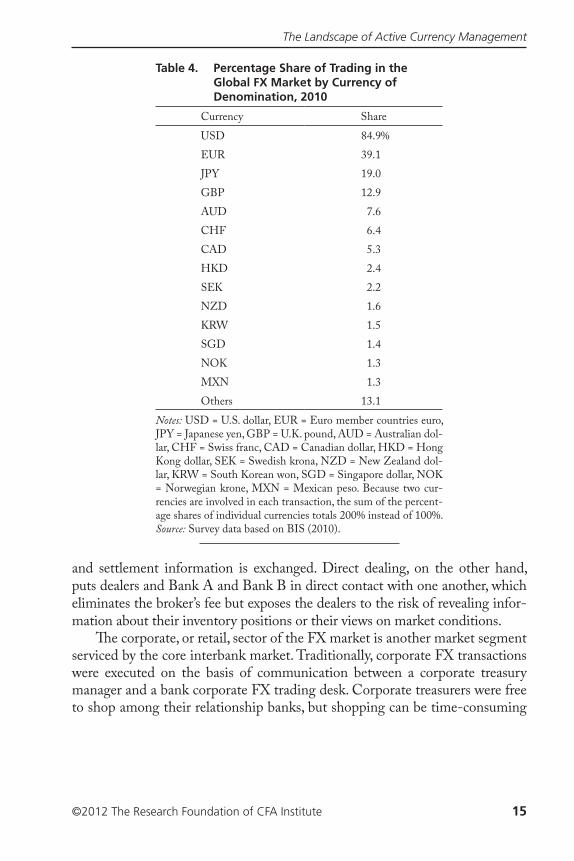
swaps and outright forward contracts (viewed as risk management vehicles for, respectively, banks and corporations) became a progressively larger share of FX trading. �e share of FX trading by currency of denomination, shown in Table 4, is more heavily centered on the U.S. dollar than many readers might expect. Nearly 85% of all currency transactions tracked in the 2010 BIS survey included the U.S. dollar as one of the two currencies in the trade. As high as this ¡gure may seem, it has actually gradually declined from 91% in the 2001 survey. �ese data are an indication of the international role of the U.S. dollar as an intermediary currency, or so-called vehicle currency, in facilitating trans-actions between the currencies of, for example, two small countries for which no active and liquid market operates.24
Market Structure and Trading Conventions. Although the foreign exchange market has evolved considerably over the last 20 years, some impor-tant features of the traditional, or classic, market remain in place.25 �e FX market has always been and remains a geographically dispersed broker/dealer market. �e interbank FX market is not housed in any city or trading ©oor but, instead, is composed of individuals known as dealers, traders, or market mak-ers who work for large banks and ¡nancial institutions. FX dealers communi-cate and trade with one another either through brokers, who assemble price quotations from numerous other market makers and match counterparties, or through direct dealing, whereby a dealer from Bank A contacts a dealer from Bank B. Such direct dealing is done via cable, telex, telephone, or a web-based network, depending on the available technology. On the one hand, using a voice broker—or, for the last 25 years or so, an electronic broking system—allows the bank dealers to remain anonymous until the trade is agreed upon and delivery
24For example, a trade in goods or securities between Mexican and Japanese counterparties could require an exchange of Mexican pesos and Japanese yen balances. Because no active mar-ket exists for exchange between these two currencies, a trader would construct a price based on the USD/MXN and USD/JPY rates and then execute two trades to complete the exchange of MXN and JPY balances. In practice, the two trades would involve less cost, time, and risk than attempting to execute a single MXN/JPY trade. 25See King, Osler, and Rime (2011) for a detailed discussion of FX market structure and its evolution.
Table 3. Percentage Share of Trading in the Global FX Market by Contract Type, 1989–2010
1989 1992 1995 1998 2001 2004 2007 2010Spot 59% 51% 43% 40% 33% 35% 33% 40%Outright forward 5 7 9 9 11 12 12 13FX swap 36 42 48 51 56 53 56 47
Source: Survey data based on BIS (2010).
The Landscape of Active Currency Management
©2012 The Research Foundation of CFA Institute 15
and settlement information is exchanged. Direct dealing, on the other hand, puts dealers and Bank A and Bank B in direct contact with one another, which eliminates the broker’s fee but exposes the dealers to the risk of revealing infor-mation about their inventory positions or their views on market conditions.
�e corporate, or retail, sector of the FX market is another market segment serviced by the core interbank market. Traditionally, corporate FX transactions were executed on the basis of communication between a corporate treasury manager and a bank corporate FX trading desk. Corporate treasurers were free to shop among their relationship banks, but shopping can be time-consuming
Table 4. Percentage Share of Trading in the Global FX Market by Currency of Denomination, 2010
Currency Share USD 84.9%EUR 39.1JPY 19.0GBP 12.9AUD 7.6CHF 6.4CAD 5.3HKD 2.4SEK 2.2NZD 1.6KRW 1.5SGD 1.4NOK 1.3MXN 1.3Others 13.1
Notes: USD = U.S. dollar, EUR = Euro member countries euro, JPY = Japanese yen, GBP = U.K. pound, AUD = Australian dol-lar, CHF = Swiss franc, CAD = Canadian dollar, HKD = Hong Kong dollar, SEK = Swedish krona, NZD = New Zealand dol-lar, KRW = South Korean won, SGD = Singapore dollar, NOK = Norwegian krone, MXN = Mexican peso. Because two cur-rencies are involved in each transaction, the sum of the percent-age shares of individual currencies totals 200% instead of 100%.Source: Survey data based on BIS (2010).
A New Look at Currency Investing
16 ©2012 The Research Foundation of CFA Institute
and costly (in terms of lost opportunities). Since 2000, newly introduced web-based platforms have given corporations the option to conduct their FX trades in a reverse-auction setting, whereby banks bid for the corporate trade.26
For equity investors, banks and custodians have typically bundled the FX trade into the execution of a foreign securities transaction. For example, when a U.S. pension fund manager buys or sells shares of Nestlé in the Swiss market, the broker or custodian handling the equity trade also handles the attendant currency transaction.27 As mentioned previously, the development of prime brokerage agreements has greatly facilitated the entry of many smaller banks, mutual funds, hedge funds, and specialized money managers into the FX market. �ese entities would have appeared as retail clients in the past, but they now trade on far more favorable, essentially interbank, terms.
�e structure of FX trading diªers in some important respects from equity market trading, especially equity trades executed on an organized exchange. As noted, the FX market is a geographically dispersed market with no centralized trading ©oor. Trading in the major currency pairs (EUR/USD, USD/JPY, and GBP/USD) is essentially continuous throughout the 24-hour day, although trading is more active during the time when the major trading centers (Tokyo, followed by Europe and then the United States) have their sequential nor-mal business hours. Unlike the situation in most equity markets, no national regulatory authority oversees FX trading.28 Also, unlike equity trades funneled through an exchange, no public record is maintained of the price and volume of FX transactions as they occur through the day. �e terms of a trade between Bank A and Bank B or between Bank A and its client remain private infor-mation. No ticker tape reports actual transaction prices of FX trades. Prices that are circulated via Bloomberg and other web-based systems are usually indicative only, meaning that actual transaction prices could be diªerent.29 26Companies oªering this service include Currenex, founded in 2000 and acquired by State Street Bank in 2007, FX Alliance, and FX Connect.27Linking the equity and FX pieces of the transaction may be desirable in order to take account of timing diªerences in clearing and settlement between equity and FX. Litigation is now pending between several U.S. pension funds and custodian banks regarding alleged irregulari-ties in FX trades that were bundled with equity transactions (see Dash 2009 and Dash and Lattman 2011).28In many of the major trading centers, industry groups strive to develop guidelines for FX trading and best practices for operational risk management. �e website of New York’s Foreign Exchange Committee (see www.newyorkfed.org/fxc/links.html) provides further information and links to other sites.29Some studies suggest that it is the opaque nature of the FX market that enables market mak-ers to pro¡t. Banks may take an incoming order to buy or sell at a small deviation from mar-ket prices and then cover their position quickly without much impact on prices (see Yao 1997 and Lyons 2001). �e fact that some corporate clients and equity investors are somewhat price insensitive, because they view foreign exchange as a cost rather than their mainline business, may further support pro¡table market making (see Hafeez and Brehon 2010).
The Landscape of Active Currency Management
©2012 The Research Foundation of CFA Institute 17
�e bilateral nature of FX transactions (e.g., Bank A trades with Bank B or Bank A trades with its client) suggests the heterogeneous nature of prices and trading risks that accompany seemingly similar trades between the same pair of currencies. Because the FX market is not centralized and many vis-ible quotations are not necessarily indicative of future transaction prices, some heterogeneity can exist in transaction prices between Banks A and B versus prices between Banks C and D at any moment. Perhaps more importantly, because banks in this example each have a distinct credit risk, the risk pro¡les of the two trades (e.g., a EUR/USD trade involving Banks A and B versus a similarly sized EUR/USD trade involving Banks C and D) can also diªer. In contrast, the ultimate counterparties to all trades on organized futures and option exchanges, as well as trades on U.S. equity exchanges, are anonymous to one another. �is anonymous trading system functions for futures and options because their exchange clearinghouse acts as the legal counterparty to all trades and all transactions in U.S. equity exchanges pass through the Depository Trust & Clearing Corporation, who at the end of day T + 1 inserts the National Securities Clearing Corporation as the counterparty to all trades.30
As an example of a type of trading risk that aªects FX transactions, con-sider a transaction whereby Bank A sells JPY80 million to Bank B in exchange for USD1 million for delivery on day T. Bank A would deliver its JPY to Bank B’s account in Tokyo on the morning of day T. �e problem is that when it is 10:00 a.m. in Tokyo, it is usually 9:00 p.m. in New York on the evening of day T – 1, a time when New York banks are closed for business. If Bank B were unable to deliver its USD in New York 10–12 hours later (because of bank-ruptcy or some other reason), then Bank A would have suªered a total loss by paying out its leg of the transaction in Tokyo (the JPY) but not receiving the other leg of the transaction (the USD) in New York.
�is example might seem a remote possibility, or simply extremely bad luck, but such events have occurred in the past. On the morning of 26 June 1974, various banks paid out millions of German marks (DEM) to the Herstatt Bank in Cologne, Germany. Later that day, but before it could make U.S. dollar payments to its counterparties in New York, Herstatt Bank ¡led for bankruptcy, thus leaving its counterparties with a total loss.
�e possibility of a total loss coupled with the hard reality that banking hours around the world do not su�ciently overlap led policymakers and bank-ers to develop a new institution. �e CLS Bank was launched in 2002 to help
30See Morris and Goldstein (2009) for an overview of clearing and settlement in U.S. equity markets.
A New Look at Currency Investing
18 ©2012 The Research Foundation of CFA Institute
standardize and reduce the settlement risk that aªects FX transactions.31 In brief, the CLS (an acronym for “continuous linked settlement”) Bank operates a payment-versus-payment system for settling transactions. In our example, Bank A would transfer its JPY to the CLS Bank, which would hold them until Bank B had transferred its USD to the CLS Bank as the matching leg of the transaction. After the CLS Bank veri¡ed that both legs of the transaction had been paid in, the bank would pay out the USD and JPY balances. In the event that the CLS Bank did not receive one leg of the transaction, any funds that were received would be returned to the one performing counterparty.32
As this example of a busted trade demonstrates, the CLS Bank removes the possibility of Bank A transferring, say, JPY80 million to Tokyo and getting nothing in return. In a busted trade in which Bank A was left holding JPY80 million, however, Bank A could ¡nd that, because of changes in market prices, it required more than JPY80 million to purchase USD1 million as it originally intended. In that case, Bank B’s default on its leg of the original transaction would in©ict a partial loss on Bank A but not the total loss it would have suf-fered if it had decided to settle bilaterally rather than by using the CLS Bank.33
Surprisingly, a modern example of Herstatt risk occurred as recently as 15 September 2008. �e KfW Bank in Germany had arranged for bilateral settle-ment of a EUR/USD transaction with Lehman Brothers as its counterparty. Without using the CLS Bank, KfW delivered approximately EUR300 mil-lion to a Lehman Brothers European bank account. When Lehman declared bankruptcy, however, it did not produce its USD leg of the transaction.
Important Parity Conditions and Pricing Principles. �e exchange rate often plays a balancing, or equilibrating, role between economies. When economies are open to trade in goods and services—and to trade in ¡nan-cial assets—the exchange rate tilts purchases of goods and services—and
31�e CLS Bank is a U.S.-based Edge Act corporation regulated and supervised by the U.S. Federal Reserve Bank. Its parent organization, CLS Group Holdings AG, is an industry-owned consortium of 71 shareholders from 22 countries. In July 2012, the CLS Bank announced it had been designated a systemically important Financial Market Utility institution by the Financial Stability Oversight Council, a body created by the Dodd–Frank Wall Street Reform and Consumer Protection Act. 32�e U.S. Department of the Treasury (2011) points to a well-functioning settlement process, the fact that FX swaps and forwards require a physical exchange of currency on ¡xed terms set at the outset of the contract, and other factors as reasons to exempt FX swaps and forwards from the requirement in the Dodd–Frank Act for a central clearinghouse for derivative securi-ties. �e Treasury proposal was oªered in April 2011 and adopted in November 2012. 33�e price risk associated with default may be more important for forward contracts, in which the period between trade booking and delivery is longer and, therefore, there is more time for one counterparty to fail prior to the settlement date.
The Landscape of Active Currency Management
©2012 The Research Foundation of CFA Institute 19
purchases of bonds or risk-bearing assets—toward one market or the other. It is useful to measure what values of the exchange rate cause this tilt to operate in one direction or the other.
Stated another way, when economies oªer us alternative currencies in which goods and services can be purchased—and alternative assets that are denomi-nated in diªerent currencies—a set of parity conditions can be useful for under-standing when conditions favor purchases or investments in one market versus the other. A parity condition is a no-arbitrage condition that speci¡es the value for the exchange rate between two currencies at which investors (or consumers or producers) are indiªerent between transacting in the two markets.
At some times and under some conditions, parity conditions hold quite closely, and at other times and under other conditions, they do not. Either circumstance—a tendency for exchange rates to move toward their parity values or to remain out of parity—can be the basis for a currency investment strategy or rule. Whether any trading rule has the possibility to produce pro¡ts more than commensurate with risk is an important issue we take up later in this section.
We consider three parity conditions: covered interest parity, uncovered interest parity, and purchasing power parity. When short-run or long-run deviations from parity are suspected, these parity conditions can form the basis for potentially pro¡table currency-trading strategies.
� Covered interest parity. Covered interest parity (CIP) relies on the principle that two investments exposed to the same risks must have the same expected returns. When the parity relationship holds, covered yields (i.e., yields hedged against exchange risk) are identical on assets that are similar in all important respects (e.g., maturity, default risk, exposure to capital controls, and liquidity) except for their currency of denomination.
Consider an example with two currencies, the U.S. dollar and the British pound. One-period interest rates in the two currencies are given by i(USD, 1) and i(GBP, 1), respectively, and spot and one-period-forward rates in USD/GBP are de¡ned by St and Ft,1, respectively. On the one hand, the forward contract obligates the buyer to deliver Ft,1 units of the USD in one period in exchange for GBP1. On the other hand, an agent could borrow St/[1 + i(GBP, 1)] units of USD today at a cost of i(USD, 1), exchange the USD for GBP in the spot mar-ket, and invest those GBP at the rate i(GBP, 1) for one period, which would also result in net proceeds of GBP1 one period hence. Both strategies—(1) buying one British pound at a cost Ft,1 and (2) borrowing U.S. dollars today at a cost of i(USD, 1), converting the USD to GBP in the spot market, and investing those GBP at the rate i(GBP, 1)—result in the same cash ©ows in one period. As a result, if we ignore the impact of transaction costs, taxes, and any risks associated
A New Look at Currency Investing
20 ©2012 The Research Foundation of CFA Institute
with execution or default, the two alternatives must have the same price or cost. �is equality of prices is summarized as follows:
F S iit t,( , )( )
.11 11
=++USDGBP,1 (1)
Equation 1 demonstrates that, in equilibrium, the forward rate will equal the spot rate plus the interest rate diªerential (where the diªerential is expressed in ratio form, as shown in Equation 1). Equation 1 also implies that the forward rate is a redundant instrument. �e cash ©ows of a forward contract can be fully replicated by a spot contract combined with borrowing and lending in the two currencies (what we referred to earlier as an FX swap).
It is a simple matter, but still useful, to rearrange the terms in Equation 1 to inspect the following relationships:
1 1 1 1+ = +i iFSt
t( ) [ ( , )] ;,USD,1 GBP (2)
1 1 11
+ = +i i SFt
t( ) [ ( , )] .
,GBP,1 USD (3)
Equation 2 reveals that investing in U.S. dollars is equivalent to ¡rst convert-ing the dollars to British pounds in the spot market, then investing the pounds at the market interest rate and covering (hedging) the currency exposure by selling principal and expected interest earnings in pounds at the forward rate, Ft,1. Equation 3 demonstrates the analogous concept, that the yield on a GBP position is equivalent to the yield on a USD position teamed with a forward contract to hedge against exchange risk.
Equations 2 and 3 clarify that, in equilibrium, markets should establish parity (i.e., interest rate parity) between interest rates in foreign and domestic currencies. Because the replicating transaction involves covering (hedging or eliminating) foreign currency exposure, interest rate parity is also referred to as the CIP relationship.
Equations 2 and 3 also suggest that if borrowing in one market—say, U.S. dollars—is impeded, one can compensate by borrowing in another—say, British pounds—and simultaneously entering into oªsetting spot and forward currency contracts. Or if investing in pounds seems subject to unusual costs or risks, one can create a synthetic GBP position by investing in a USD security and simultaneously entering into oªsetting spot and forward currency con-tracts. Creating synthetic positions is straightforward, and they can produce considerable value when ¡nancial markets are constrained or under stress. Precisely at these times, investors may willingly choose a synthetic position that yields less or borrowers may choose a synthetic that costs more in order to overcome a market dislocation.
The Landscape of Active Currency Management
©2012 The Research Foundation of CFA Institute 21
Taking Equation 1 and subtracting 1.0 from both the left and right sides produces
F SS
i ii
t t
t
, ( , ) ( )( )
,1 11
−=
−+
USD GBP,1GBP,1
(4)
which shows that the percentage forward premium is (approximately) equal to the interest diªerential. In equilibrium, the currency with the higher interest rate should trade at a forward discount to re©ect the fact that a lower return is available in the second currency.34
�e CIP equilibrium condition described in Equations 1–4 is facilitated by arbitrage. In Equation 1, if Ft,1 were less than the synthetic price given by S i it 1 1 1 1+[ ] +[ ]( , ) ( , ) ,USD GBP arbitrageurs would buy the forward con-tract and sell the synthetic, helping to restore a balance. “Selling the synthetic” GBP forward would entail borrowing GBP, buying USD in the spot mar-ket, and investing in USD for one period. In Equation 2, if USD interest rates exceeded GBP rates on a covered basis, arbitrageurs would borrow in GBP, hedge themselves with spot and forward contracts, and lend the syn-thetic USD at a higher rate. At the margin, arbitrage purchases tend to raise prices (of currency and money market instruments) whereas sales tend to lower prices (of currency and money market instruments) and thus tend to reduce any measured deviations from parity. Arbitrage transactions, however, entail costs (in currency markets and money markets) and risks (of default on investment positions or forward contracts or of possible controls on capital movements). �ese costs and risks limit the amount of arbitrage and retard the speed of, or even preclude, the convergence of rates toward parity.
Many empirical studies have attempted to measure the costs and risks asso-ciated with covered interest arbitrage in order to gauge how e�cient the market is at eliminating low-risk covered interest diªerentials.35 Overall, throughout most of the ©oating exchange rate period until the recent global ¡nancial crisis, the empirical evidence shows that, when based on short-term oªshore inter-est rates for the currencies of major developed countries, deviations from CIP
34For example, given S = USD1.50/GBP, i(USD) = 4%, and i(GBP) = 8%, we expect Ft,1 = USD1.444/GBP, where Ft,1 is the forward rate today for delivery one period hence (one year hence because interest rates are stated in annualized terms). �e British pound has the higher interest rate, and it is at a discount (i.e., cheaper) in the forward market.35See Levich (forthcoming 2013) for a review of the literature on interest rate parity and cov-ered interest arbitrage.
A New Look at Currency Investing
22 ©2012 The Research Foundation of CFA Institute
have tended to be quite small—and smaller than the cost of conducting arbi-trage.36 �us, during normal market conditions, Equation 1 oªers a good guide to the way forward currency prices are likely to be set as a function of the spot exchange rate and short-term oªshore money market interest rates.
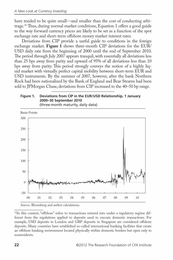
Deviations from CIP provide a useful guide to conditions in the foreign exchange market. Figure 1 shows three-month CIP deviations for the EUR/USD daily rate from the beginning of 2000 until the end of September 2010. �e period through July 2007 appears tranquil, with essentially all deviations less than 25 bps away from parity and upward of 95% of all deviations less than 10 bps away from parity. �is period strongly conveys the notion of a highly liq-uid market with virtually perfect capital mobility between short-term EUR and USD instruments. By the summer of 2007, however, after the bank Northern Rock had been nationalized by the Bank of England and Bear Stearns had been sold to JPMorgan Chase, deviations from CIP increased to the 40–50 bp range.
36In this context, “oªshore” refers to transactions entered into under a regulatory regime dif-ferent from the regulations applied to deposits used to execute domestic transactions. For example, USD deposits in London and GBP deposits in Singapore are considered oªshore deposits. Many countries have established so-called international banking facilities that create an oªshore banking environment located physically within domestic borders but open only to nonresidents.
Figure 1. Deviations from CIP in the EUR/USD Relationship, 1 January 2000–30 September 2010 (three-month maturity, daily data)
Basis Points
300
250
200
150
100
50
0
–5000 03 06 1001 04 0702 05 0908
Sources: Bloomberg and author calculations.

The Landscape of Active Currency Management
©2012 The Research Foundation of CFA Institute 23
After Lehman Brothers failed on 15 September 2008, deviations from CIP in the market’s most liquid currency pairing spiked to more than 200 bps and, for the most part, remained above 100 bps for the next three months. Even though CIP deviations had subsided to the 25–50 bp range by spring 2009, this range is clearly far higher than in the tranquil period of nearly per-fect capital mobility in the ¡rst few years of the millennium.
Studies by Baba and Packer (2009) and Coªey, Hrung, and Sarkar (2009) ¡nd that the combination of funding shortages in the U.S. ¡nancial markets and a heightened sense of counterparty risk even among large banks active in the FX market led to deterioration in liquidity and the observed deviations from CIP in the USD/EUR pair. During the crisis period, banks outside the United States had particular di�culty accessing USD facilities through their traditional U.S. commercial bank counterparties (who were subject to heightened default risk). To meet their various USD funding obligations, these banks turned to the synthetic approach suggested by Equation 2. By borrowing in their home cur-rencies, perhaps through access to the home central bank, and then executing an FX swap, non-U.S. banks could synthetically create a USD position—but only at a premium to a direct position in USD. �e synthetic approach explains one policy response to this aspect of the global ¡nancial crisis.
In the spring of 2009, the U.S. Federal Reserve, together with other cen-tral banks, opened up substantial o�cial swap facilities. �ese o�cial swaps increased the supply of U.S. dollars oªshore, and non-U.S. banks could access U.S. dollars through their home central banks rather than their commercial bank counterparties. Despite these policy initiatives, Figure 1 suggests that deviations from CIP are experiencing a “new normal” in 2012, with deviations in the range of 25–50 bps for the EUR/USD pair (instead of the 10–25 bps observed a decade previously).
� Uncovered interest parity. Uncovered interest parity (UIP) considers the breakeven relationship between an investor facing a domestic currency return of i(USD, 1) and a foreign currency–denominated return of i(GBP, 1) when the future spot exchange rate, �St+1 , is unknown:
1 1 1 1+ = + +i i E SSt
t( ) [ ( , )] ( ) ,USD,1 GBP
�(5)
where E St( )�+1 is the expectation of the future spot rate. �e situation appears
similar mathematically to the CIP example just discussed, but there are some crucial economic diªerences. Because the investor has not used a forward con-tract to hedge the foreign currency investment, the USD value of the investment at time t + 1 is not known with certainty. In Equation 5, the expectation of the future spot rate is used to estimate the USD value of the GBP investment.
A New Look at Currency Investing
24 ©2012 The Research Foundation of CFA Institute
Consider these numerical examples. Suppose investors expect the British pound to depreciate by 1% over the next period—from, say, USD1.5000/GBP to USD1.4850/GBP. For UIP to hold, the one-period interest rate on the GBP needs to be 1% higher than the USD interest rate for the investor to be indiªerent, on an expected value basis, between these USD and GBP invest-ments. But suppose the expectation is for the British pound to appreciate by 2% over the next period—from, say, USD1.5000/GBP to USD1.5300/GBP. In that case, UIP would require that the one-period GBP interest rate be 2% lower than the one-period USD interest rate.
�e logic of UIP is straightforward and compelling. Investors typically require a high interest rate to compensate for a currency that is expected to lose value (i.e., depreciate) over a holding period, and investors are willing to accept a low interest rate when a currency is expected to gain value (i.e., appre-ciate) versus their benchmark alternative.
�e logic of UIP is analogous to situations in equity and ¡xed-income markets. In the case of equity, consider two companies that are identical and, therefore, have the same expected return over time but Company A pays a higher dividend than Company B. In that case, we would expect the price of the shares of Company B to appreciate more over time to re©ect the lower dividend (and higher retained earnings) of Company B. In equilibrium, the diªerence between the dividend yields on the two ¡rms would exactly oªset the greater price appreciation of B shares versus that of A shares.
In ¡xed income, consider a case of the bonds of Company A having greater risk and a higher yield to maturity than bonds issued by Company B. Under a pure expectations pricing model, the expected return on bonds from A and B would be identical if the higher prospect of default (and percentage loss in case of default) on Company A bonds versus those of Company B matched the yield diªerential between the bonds. Note that in both cases, the higher divi-dend for the equity in Company A and the higher quoted yield to maturity on Company A bonds are not signals of a free lunch. �ey are, instead, indicators that the market expects less performance of the stock price of Company A and a lower chance of a full return on principal on the bonds issued by Company A. In the same way, according to UIP, a higher interest rate on Currency A rela-tive to Currency B re©ects the market’s expectation that Currency A is likely to depreciate relative to Currency B so as to oªset the interest diªerential.
Rearranging Equation 5 and subtracting 1.0 from both the left and right sides results in
E S SS
i ii
t t
t
( ) ( , ) ( )( )
.,�1 1
1−
=−
+USD GBP,1
GBP,1(6)
The Landscape of Active Currency Management
©2012 The Research Foundation of CFA Institute 25
Because the right-side terms of Equations 4 and 6 are identical, these equations imply that the forward premium equals the expected exchange rate change or that the forward rate itself is an unbiased estimate of the future expected spot rate: F E St t, ,( )1 1= � .
Extensive empirical evidence, sometimes presented under the guise of testing the forward rate unbiased proposition, rejects UIP. �e empirical tests are often based on regressions of the actual change in the exchange rate over a short interval, such as one or three months, against the interest rate diªeren-tial over a matching time interval, as in the following:
∆S i k i kt t k t t t, ( , ) ( , ) ,+ = + −[ ]+α β εUSD GBP (7)where ΔSt,t+k represents the exchange rate change over the interval (t, t + k).
Equation 7 shows the interest rate diªerential as the independent variable in the regression, but some studies substitute the forward exchange rate premium. If UIP or the forward rate unbiased proposition are true characterizations of mar-ket prices, we would expect to ¡nd that α = 0 and β = 1 and that a high R2 statis-tic measures the overall ¡t of the regression. �e data overwhelmingly reject this result, however, for short-term maturities (maturities of less than one year).
Froot and �aler (1990) surveyed 75 published studies of UIP and con-clude that the average β was –0.88 rather than 1.0. In other words, the data support the notion that, contrary to UIP, currencies with high short-term interest rates tend to appreciate rather than depreciate. Surveys of the forward rate unbiased literature by Hodrick (1987) and Engel (1996) reach a similar conclusion—namely, that the β coe�cient in regressions such as Equation 7 are almost always negative. �ese ¡ndings not only reject UIP and the forward rate unbiased proposition, but they also suggest that a carry trade strategy based on borrowing the low-interest-rate currency and investing in the high-interest-rate currency could be pro¡table, albeit subject to risk.
Two further strands of research on UIP remain active. One is whether UIP also has a tendency to fail when longer maturity instruments are studied. Pursuing this line of investigation is di�cult because few countries have long time series—5-year-maturity and 10-year-maturity bonds. Moreover, other empirical issues, such as coupon-paying bonds and overlapping sample peri-ods, present many challenges. Chinn and Meredith (2004) ¡nd that the data are more supportive of UIP at longer horizons. �e β coe�cients tend to be positive and closer to 1.0 than to zero for the interest diªerential based on 5-year and 10-year government bonds.
�e second empirical issue is whether the generally high returns associated with the carry trade represent (1) compensation for exposure to risk or (2) an excess return (pure pro¡t) resulting from a market ine�ciency. Brunnermeier, Nagel, and Pedersen (2009) show that returns on carry trades are negatively skewed and subject to a “crash risk”—that is, a sudden drying up of liquidity
A New Look at Currency Investing
26 ©2012 The Research Foundation of CFA Institute
when large numbers of speculators try to exit the trade. Lustig, Roussanov, and Verdelhan (2010) suggest that carry trade returns represent compensation to U.S. investors who are exposed to various risks, such as an upward spike in the U.S. business cycle that would raise U.S. rates and draw capital back from overseas. Menkhoª, Sarno, Schmeling, and Schrimpf (2012a) posit that expo-sure to spikes in FX volatility could drive investors back toward safer, low-interest-rate currencies and threaten carry trade pro¡ts.
Burnside (2011), however, concludes that these risk measures are insuf-¡cient to explain the time variation in carry trade returns and suggests that old-fashioned “peso problems”—meaning the large probability of small gains (from the interest diªerential) and the small probability of a large loss (from a substantial exchange rate depreciation)—might help explain carry trade returns. In this interpretation, carry traders might be seen as picking up nick-els (the small interest diªerential) in front of a steamroller (the small chance of a substantial depreciation). Despite these caveats (that carry trade returns could be a form of compensation for risk incurred), many currency market professionals point out that other, favorable market metrics (e.g., high Sharpe ratios and low correlations with many other investment strategies) make carry trading a popular investment strategy despite the risk.
� Purchasing power parity. Purchasing power parity (PPP) is a staple in the toolkit of every international ¡nancial strategist and currency economist. Although prices of individual goods may diªer considerably among countries, PPP relies on the tendency of exchange rate movements to re©ect the dif-ference in rates of in©ation across countries, as summarized in the following expression:
∆S p h k p f kt t k, , ,+ = ( ) − ( ), (8)where p(h,k) and p(f,k) represent the rate of in©ation in the home and for-eign countries, respectively, over the period t through t + k and S is the home currency price of foreign currency. �e economic logic of Equation 8, the so-called relative version of PPP, is simple and straightforward. Suppose that the price of foreign goods, SPf , is unusually high relative to the price of domestic goods, Ph. To get this ratio back to a more “normal” level, either SPf needs to decline or Ph needs to rise, or both. (In practice, prices of local goods tend to be sticky whereas the exchange rate is highly ©exible.) A decline in S is equiv-alent to a depreciation of foreign currency. �e logic is symmetrical when the price of foreign goods is unusually low relative to domestic goods. To get the ratio back to a more normal level, either SPf needs to rise or Ph needs to fall,
The Landscape of Active Currency Management
©2012 The Research Foundation of CFA Institute 27
or both. A rise in S is equivalent to an appreciation of foreign currency.37 �e same point stated somewhat diªerently is that over a su�ciently long period, countries with high (low) in©ation relative to their trading partners tend to experience currency depreciation (appreciation). PPP describes an equilibrium relationship between goods prices and exchange rates with no implications about causality.
To make relative PPP operational, two things are needed. �e ¡rst is a bench-mark for the “normal” relationship between home and foreign prices. Various international agencies, such as the Organisation for Economic Co-operation and Development (OECD) and the International Monetary Fund, as well as many private banks and ¡nancial institutions, compute PPP indices for most countries. �ese indices typically take a multilateral perspective— calculating the weighted average of a country’s PPP rates against a broad group of trading partners—to develop an overall PPP index for each country. �e design of these alternative indices may vary (e.g., as to what date or range of dates is taken as a benchmark or in the selection and weighting of goods included in the price index, the weights assigned to trading partners, and how frequently the indices are rebased in light of changes in local consumption or trade patterns), but for the most part, alternative measures of PPP for a single country are highly cor-related (see Isard, Faruqee, Kincaid, and Fetherston 2001).
�e second requirement is to give operational meaning to the “tendency” for exchange rates and prices to satisfy the condition in Equation 8. Empirical evidence shows that the contemporaneous relationship between relative price changes and exchange rate changes is weak at best. �e EUR/USD exchange rate could change by 0.5–1.0% in a day, or 5–10% or more in a year, even though the diªerential between U.S. and eurozone in©ation is nowhere close to the exchange rate change over the same time period. When we examine the movement devia-tions from PPP over a long period of time, however, the tendency for PPP to reassert itself, a property referred to as “mean reversion,” becomes more evident.
To illustrate mean reversion, Figure 2 shows a plot of the spot EUR/USD rate versus its PPP value (a ratio also referred to as the “real exchange rate”) over a period of nearly 40 years. Values above the PPP line correspond to 37Note that the idea of a so-called normal relationship between the price of home and foreign goods need not imply that the prices of each good, or even all goods on average, are identical across countries. For example, in the Economist magazine survey of McDonald’s Big Mac prices, the price of a Big Mac stated in U.S. dollar terms is often higher in such countries as Switzerland and Sweden and lower in such countries as China and the Philippines compared with the price in the United States. �e price diªerences may re©ect many factors, such as land and labor costs, market competition among restaurants, and the target income levels of prospective customers. Once these relatively sticky factors are accounted for, relative prices of Big Macs in various coun-tries show a tendency to oscillate around a historical normal ratio (see Cumby 1996 and articles referenced in Clements, Lan, and Seah 2012). �e Economist article is focused on Big Mac prices because it is a relatively homogeneous good and most people are familiar with it.

A New Look at Currency Investing
28 ©2012 The Research Foundation of CFA Institute
times when the German mark (later, euro) is overvalued and the U.S. dol-lar is undervalued, while below the PPP line, the situation is reversed. �e real exchange rate based on consumer prices crosses the PPP line about 20 times in 38 years, indicating a return to PPP. �e graph also suggests that large deviations from PPP can be reversed more quickly and by larger changes compared with small deviations from PPP. While the ¡gure shows a visible tendency for PPP to be restored periodically, it also shows the risk that large deviations can get larger, rather than smaller.
Figure 3 oªers another way to visualize the tendency for exchange rates to gravitate back toward PPP over the longer run. Figure 3 shows the com-bination of spot exchange rate changes versus the U.S. dollar and the corre-sponding consumer price changes for the 21 OECD member countries for a 32-year period. When PPP holds and the exchange rate change for a currency matches the diªerence in relative price movements between that country and the United States, the data points plot along the 45° line (i.e., the PPP line). In Panel A, the 672 dots (representing 32 yearly observations for 21 countries) are scattered widely about the line. In Panel B, representing 8-year intervals (84 points), and Panel C, 16-year intervals (42 points), the tendency for spot rate changes and relative price movements to gravitate back toward the PPP line is more apparent than in Panel A. And in Panel D, representing the entire 32-year interval (with only the 21 points), the correspondence between spot rate changes and relative price movements is emphatic. �e message is that
Figure 2. Cumulative Deviations from Relative PPP: Germany and the United States, 1973–2011 (153 quarters)
Ratio: Actual Exchange Rate/PPP Rate
Wholesale Prices
PPP
Consumer Prices
1.4
1.3
1.2
1.1
1.0
0.9
0.8
0.7
0.673 128276 79 9185 88 0397 0094 06 09
Note: �e calculation uses the German mark until the introduction of the euro in 1999.
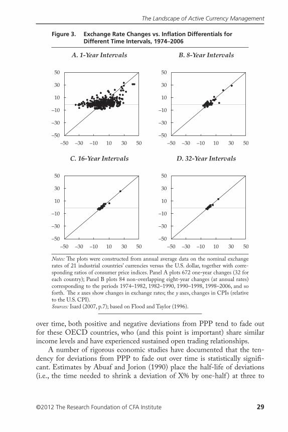
The Landscape of Active Currency Management
©2012 The Research Foundation of CFA Institute 29
over time, both positive and negative deviations from PPP tend to fade out for these OECD countries, who (and this point is important) share similar income levels and have experienced sustained open trading relationships.
A number of rigorous economic studies have documented that the ten-dency for deviations from PPP to fade out over time is statistically signi¡-cant. Estimates by Abuaf and Jorion (1990) place the half-life of deviations (i.e., the time needed to shrink a deviation of X% by one-half ) at three to
Figure 3. Exchange Rate Changes vs. Inflation Differentials for Different Time Intervals, 1974–2006
A. 1-Year Intervals
50
30
10
–10
–30
–50–50 50–30 –10 10 30
B. 8-Year Intervals
50
30
10
–10
–30
–50–50 50–30 –10 10 30
C. 16-Year Intervals
50
30
10
–10
–30
–50–50 50–30 –10 10 30
D. 32-Year Intervals
50
30
10
–10
–30
–50–50 50–30 –10 10 30
Notes: �e plots were constructed from annual average data on the nominal exchange rates of 21 industrial countries’ currencies versus the U.S. dollar, together with corre-sponding ratios of consumer price indices. Panel A plots 672 one-year changes (32 for each country); Panel B plots 84 non-overlapping eight-year changes (at annual rates) corresponding to the periods 1974–1982, 1982–1990, 1990–1998, 1998–2006, and so forth. �e x axes show changes in exchange rates; the y axes, changes in CPIs (relative to the U.S. CPI).Sources: Isard (2007, p.7); based on Flood and Taylor (1996).
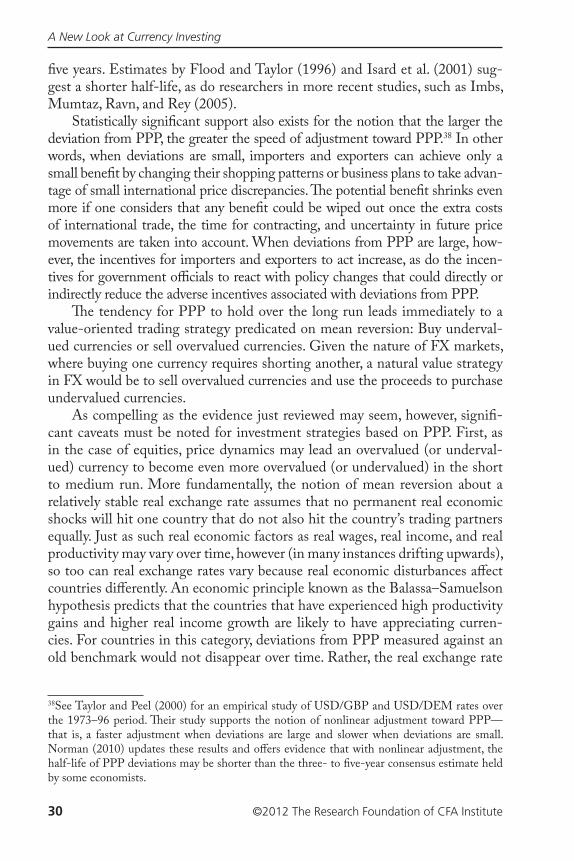
A New Look at Currency Investing
30 ©2012 The Research Foundation of CFA Institute
¡ve years. Estimates by Flood and Taylor (1996) and Isard et al. (2001) sug-gest a shorter half-life, as do researchers in more recent studies, such as Imbs, Mumtaz, Ravn, and Rey (2005).
Statistically signi¡cant support also exists for the notion that the larger the deviation from PPP, the greater the speed of adjustment toward PPP.38 In other words, when deviations are small, importers and exporters can achieve only a small bene¡t by changing their shopping patterns or business plans to take advan-tage of small international price discrepancies. �e potential bene¡t shrinks even more if one considers that any bene¡t could be wiped out once the extra costs of international trade, the time for contracting, and uncertainty in future price movements are taken into account. When deviations from PPP are large, how-ever, the incentives for importers and exporters to act increase, as do the incen-tives for government o�cials to react with policy changes that could directly or indirectly reduce the adverse incentives associated with deviations from PPP.
�e tendency for PPP to hold over the long run leads immediately to a value-oriented trading strategy predicated on mean reversion: Buy underval-ued currencies or sell overvalued currencies. Given the nature of FX markets, where buying one currency requires shorting another, a natural value strategy in FX would be to sell overvalued currencies and use the proceeds to purchase undervalued currencies.
As compelling as the evidence just reviewed may seem, however, signi¡-cant caveats must be noted for investment strategies based on PPP. First, as in the case of equities, price dynamics may lead an overvalued (or underval-ued) currency to become even more overvalued (or undervalued) in the short to medium run. More fundamentally, the notion of mean reversion about a relatively stable real exchange rate assumes that no permanent real economic shocks will hit one country that do not also hit the country’s trading partners equally. Just as such real economic factors as real wages, real income, and real productivity may vary over time, however (in many instances drifting upwards), so too can real exchange rates vary because real economic disturbances aªect countries diªerently. An economic principle known as the Balassa–Samuelson hypothesis predicts that the countries that have experienced high productivity gains and higher real income growth are likely to have appreciating curren-cies. For countries in this category, deviations from PPP measured against an old benchmark would not disappear over time. Rather, the real exchange rate
38See Taylor and Peel (2000) for an empirical study of USD/GBP and USD/DEM rates over the 1973–96 period. �eir study supports the notion of nonlinear adjustment toward PPP—that is, a faster adjustment when deviations are large and slower when deviations are small. Norman (2010) updates these results and oªers evidence that with nonlinear adjustment, the half-life of PPP deviations may be shorter than the three- to ¡ve-year consensus estimate held by some economists.
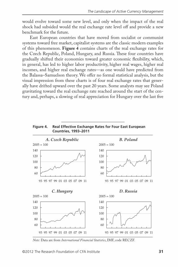
The Landscape of Active Currency Management
©2012 The Research Foundation of CFA Institute 31
would evolve toward some new level, and only when the impact of the real shock had subsided would the real exchange rate level oª and provide a new benchmark for the future.
East European countries that have moved from socialist or communist systems toward free market, capitalist systems are the classic modern examples of this phenomenon. Figure 4 contains charts of the real exchange rates for the Czech Republic, Poland, Hungary, and Russia. �ese four countries have gradually shifted their economies toward greater economic ©exibility, which, in general, has led to higher labor productivity, higher real wages, higher real incomes, and higher real exchange rates—as one would have predicted from the Balassa–Samuelson theory. We oªer no formal statistical analysis, but the visual impression from these charts is of four real exchange rates that gener-ally have drifted upward over the past 20 years. Some analysts may see Poland gravitating toward the real exchange rate reached around the start of the cen-tury and, perhaps, a slowing of real appreciation for Hungary over the last ¡ve
Figure 4. Real Effective Exchange Rates for Four East European Countries, 1993–2011
A. Czech Republic
140
120
100
80
60
93 9795 99 03 07 1101 05 09
2005 = 100B. Poland
140
120
100
80
60
93 9795 99 03 07 1101 05 09
2005 = 100
C. Hungary
140
120
100
80
60
93 9795 99 03 07 1101 05 09
2005 = 100D. Russia
140
120
100
80
60
93 9795 99 03 07 1101 05 09
2005 = 100
Note: Data are from International Financial Statistics, IMF, code RECZF.
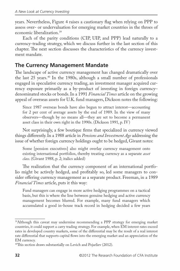
A New Look at Currency Investing
32 ©2012 The Research Foundation of CFA Institute
years. Nevertheless, Figure 4 raises a cautionary ©ag when relying on PPP to assess over- or undervaluation for emerging market countries in the throes of economic liberalization.39
Each of the parity conditions (CIP, UIP, and PPP) lead naturally to a currency-trading strategy, which we discuss further in the last section of this chapter. �e next section discusses the characteristics of the currency invest-ment mandate.
The Currency Management Mandate�e landscape of active currency management has changed dramatically over the last 25 years.40 In the 1980s, although a small number of professionals engaged in speculative currency trading, an investment manager acquired cur-rency exposure primarily as a by-product of investing in foreign currency–denominated stocks or bonds. In a 1991 Financial Times article on the growing appeal of overseas assets for U.K. fund managers, Dickson notes the following:
Since 1987 overseas bonds have also begun to attract interest—accounting for 2 per cent of average assets by the end of 1989. In the view of many observers—though by no means all—they are set to become a permanent asset class in their own right in the 1990s. (Dickson 1991, p. IV)
Not surprisingly, a few boutique ¡rms that specialized in currency viewed things diªerently. In a 1988 article in Pensions and Investment Age addressing the issue of whether foreign currency holdings ought to be hedged, Givant notes:
Some [pension executives] also might overlay currency management onto existing international portfolios, thereby treating currency as a separate asset class. (Givant 1988, p. 2; italics added)
�e realization that the currency component of an international portfo-lio might be actively hedged, and pro¡tably so, led some managers to con-sider oªering currency management as a separate product. Freeman, in a 1989 Financial Times article, puts it this way:
Fund managers can engage in more active hedging programmes on a tactical basis, but this is where the line between genuine hedging and active currency management becomes blurred. For example, many fund managers which accumulated a good in-house track record in hedging decided a few years
39Although this caveat may undermine recommending a PPP strategy for emerging market countries, it could support a carry trading strategy. For example, when EM interest rates exceed rates in developed country markets, some of the diªerential may be the result of a real interest rate diªerential that supports capital ©ows into the emerging market and an appreciation of the EM currency.40�is section draws substantially on Levich and Pojarliev (2012).
The Landscape of Active Currency Management
©2012 The Research Foundation of CFA Institute 33
ago to develop their experience and launch managed currency funds, which concentrate entirely on forecasting exchange rate movements. (Freeman 1989, p. VI; italics added)
A LexisNexis search of newspapers and periodicals for the keywords “cur-rency” and “asset class” used in the same article results in only a handful of articles each year in the years prior to 1990.41 By 2007, the annual number of mentions for this pair of keywords exceeds 1,100. Although not all of these articles refer to currency as an asset class, the notion of taking currency formally into account and having it separately managed by a currency professional has become part of the international investment manager’s and plan sponsor’s basic toolkit.
Each agreement between an institutional investor and its currency man-ager is unique. For discussion purposes, however, it is useful to consider, ¡rst, the types of mandates that are in common use and their key features and, sec-ond, other structural and operational choices that diªerentiate mandates. By varying these contractual parameters, institutional investors in©uence their expected alpha (what we call the “alpha continuum”) and their exposure to risk.
Features of a Currency Mandate. �ere are two basic types of currency mandates. In an absolute return mandate, the investor seeks to earn a positive return, usually in excess of some benchmark and subject to acceptable risk levels. With a currency overlay mandate, the investor already owns a portfolio of foreign debt or equity and the objective is either to entirely eliminate currency risk from the port-folio or partially reduce currency risk while opportunistically going after return.42
In both absolute return and currency overlay mandates, the agreement spec-i¡es how much latitude the manager has to operate, identi¡es provisions that constrain the manager, and of course, spells out how the manager’s performance will be determined as well as the formula for setting compensation. �e main considerations stipulated in a currency mandate will include the following:
� Passive vs. active management. A passive manager is constrained to simply track a prede¡ned benchmark and does not seek to generate excess returns. Because most benchmarks are constructed on the basis of a clearly de¡ned investment rule, a passive manager simply executes the trading rule to
41For the period 1975 until 1982, we ¡nd no articles including mentions of both “currency” and “asset class.” �e ¡rst mention in a single article appears in 1983.42Hedging within a currency overlay strategy often takes the fairly simple objective of establish-ing a predictable home currency value for assets denominated in a foreign currency. For exam-ple, consider a U.S. plan sponsor whose ¡nancial statements and returns are prepared in U.S. dollars. If the plan sponsor owns shares in Volkswagen valued at EUR100, selling 100 euros for U.S. dollars establishes a known USD value for the foreign assets. �e hedge will probably be imperfect because the euro share price of Volkswagen itself will probably be sensitive to the EUR/USD exchange rate. �e size of the hedge also needs to be adjusted, over time, for ©uc-tuations in the euro share price of Volkswagen.
A New Look at Currency Investing
34 ©2012 The Research Foundation of CFA Institute
track the benchmark.43 For example, if the AFX Currency Management Index (based on three moving-average trading rules and seven currency pairs) is used as a benchmark, a passive manager can use those same moving-average rules and currency pairs to govern trading.44 For an absolute return mandate, trad-ing designed to mimic benchmarks based on carry trading, trend following, value trading, or volatility are all examples of passive strategies.45 For a cur-rency overlay mandate, always fully hedging the currency position in a ¡xed-income portfolio or always hedging 50% of the foreign currency value of the position are typical examples of passive strategies.
An active manager, however, has discretion to implement a variety of trades based on diªerent ideas. For an absolute return mandate, the active manager seeks to add value beyond the return of the benchmark and to do so by enter-ing into positions that deviate from those in the benchmark. For example, an active currency overlay manager who believes that foreign currency has a strong chance of appreciating might, in an attempt to add extra return, hedge only 25% of the foreign currency exposure in a ¡xed-income portfolio instead of 100%. Whether operating under an absolute return or currency overlay man-date, an active manager might adopt a systematic or rule-based investment process, a discretionary investment process, or a combination of the two.
� Allowed currencies. A currency mandate agreement will typically constrain the manager to operate within a set menu of currencies, perhaps restricted to the G–3 or G–10 currencies, where ¡nancial markets oªer great-est depth, or emerging market currencies, where markets are less liquid but where greater pro¡t opportunities may be present.46 A wider range of curren-cies may be more valuable in the case of an absolute return mandate, although some managers may prefer to limit themselves to only those currency pairs
43Some market professionals have taken issue with this de¡nition. Melvin and Shand (2011) note that tracking any currency trading index involves some degree of active management because positions must be bought and sold as underlying market conditions change.44�e AFX Currency Management Index is based on trading in seven currency pairs weighted by their volume of turnover in the spot market, with returns for each pair based on an equally weighted portfolio of three moving-average rules (32, 61, and 117 days). �e seven currency pairs are EUR/USD, USD/JPY, USD/CHF, GBP/USD, EUR/JPY, EUR/GBP, and EUR/CHF. More information about the index is available at http://web.archive.org/web/20100527043718/http://www.ljmu.ac.uk/LBS/102316.htm.45Passive absolute return mandates are still rather rare. Most absolute return mandates are char-acterized as active.46�e G–3 is an uno�cial designation for the world’s three largest developed economies: the United States, the European Union, and Japan. In this context, the G–10 refers to 10 actively traded currencies: the USD, EUR, JPY, GBP, AUD, CHF, CAD, SEK, NZD, and NOK (see Table 4 for correspondence between currency symbols and countries) and not the countries in the o�cial Group of Ten (see https://www.imf.org/external/np/exr/facts/groups.htm#G10).
The Landscape of Active Currency Management
©2012 The Research Foundation of CFA Institute 35
in which they have the greatest expertise. In a currency overlay, the allowed currencies are often, although not always, limited to those currencies in the underlying portfolio; at times, cross-hedging can be a useful tool.
� Permitted instruments. A currency mandate agreement may also spec-ify which instruments the manager is permitted to use. �e manager may be constrained to trade spot and forward contracts only, or the manager may be allowed discretion to use plain-vanilla currency options or other derivative instruments, such as exotic currency options (e.g., barrier or basket options). In the case of a currency overlay agreement, derivatives may oªer an e�cient way of hedging particular risks in the underlying portfolio. Derivatives also provide a way to make asymmetrical trades that leave the underlying portfolio unharmed if the currency moves in one direction but allow the manager to bene¡t if the currency moves in a way that the manager has forecast. In the case of an absolute return mandate, derivative instruments are often a more e�cient way to obtain leverage, so whether or not they are permitted may be linked to how much leverage is allowed by the mandate.
� Leverage. �e degree of leverage allowed is an important consideration for absolute return mandate agreements and also for currency overlays that have some return-seeking objective. A manager could be constrained to use leverage or allowed discretion to vary leverage up to some limit, depending on market conditions. For an absolute return mandate, leverage up to a factor of 10 is typical, but greater leverage is feasible and sometimes observed in hedge funds or managed trading accounts. Rather than specify leverage, a currency mandate could specify target volatility, expected return, or worst permitted drawdown.
� Performance benchmark and compensation. Last but certainly not least, a currency mandate will specify how performance will be measured, how it will be compared with that of a passive benchmark, and how outperformance will be compensated. For an absolute return mandate, when a manager is given trading authority over a pool of funds, the benchmark for performance of those funds could be LIBID (the London Interbank Bid Rate), LIBID + x, or some other index denominated in the investor’s base currency. Investing the assigned assets at LIBID is essentially risk free, whereas benchmarks greater than LIBID entail risk. When the manager receives only a line of credit against funds that are invested elsewhere, then the benchmark for performance can be zero, an amount x that is greater than zero, or another measure of performance. A manager who never draws on the credit line, and never takes a currency posi-tion, will earn zero return and incur zero risk. Active use of the credit line in the pursuit of positive returns entails risk. Performance benchmarks for a currency overlay manager are usually designed to re©ect the returns from a continuum of hedging choices—from no hedging through continuous hedging of the entire
A New Look at Currency Investing
36 ©2012 The Research Foundation of CFA Institute
underlying position. �e returns from a strategy of a continuous 50% hedge are often taken as a naive benchmark for a currency overlay manager. We discuss the economic rationale for these benchmarks in Chapter 3.
Manager compensation itself often has several parameters, including, almost always, an annual management fee (a “©at” fee) and a performance incentive fee based on annual returns.47 For high-net-worth individuals and funds of funds that invest in currency hedge funds, the most common fee structure is a 2% a year management fee (based on assets under management [AUM])48 and 20% share of pro¡ts earned over the year. Institutional clients are likely to negotiate management fees that are far lower than those for retail investors while still being subject to the 20% performance fee. Management fees are often related to the expected or targeted volatility of the mandate; for example, high management fees are di�cult to justify for low-volatility man-dates. In addition, compensation is usually governed by a high-water mark rule such that performance fees, which are usually calculated daily and paid quarterly,49 are paid only to the extent that the returns push the manager’s cumulative returns above the previous high-water mark.50
Structural and Operational Choices. �e agreement between an institutional investor and the manager is also likely to lay out various structural or operating principles for the relationship. Perhaps the most fundamental
47A review of the fee structure for currency funds that report through the TASS and CISDM databases shows that the 2% management fee and 20% performance fee are the modal charges. Some managers assess fees that are higher than 2 and 20, however, and some charge less.48For fully funded absolute return mandates, AUM is typically measured as simply the cash under management; in other words, a USD200 million fully funded mandate means AUM of USD200 million. For unfunded absolute return mandates, AUM is reported as the agreed notional value, independent of the speci¡c margin requirements. For example, a client might have to fund only 10% of the USD200 million; the AUM will still be reported as USD200 million and not as USD20 million, and the USD200 million will be the base for calculating returns and management fees. For currency overlay mandates, the AUM is typically de¡ned as the reporting currency amount of the international holdings in the underlying portfolio; that is, assuming a USD/JPY exchange rate of 80, a JPY80 billion investment in the Nikkei 225 Index equals USD100 million of AUM in currency overlay exposure. For mandates that speci¡-cally have a volatility target, some managers report AUM adjusted for volatility; for example, a USD200 million mandate with a target volatility of 4% could be counted as a USD100 million mandate with a target volatility of 8%. 49Performance fees are usually subject to lifetime or rolling high-water marks. 50For example, consider an absolute return mandate in which the initial AUM is USD100 and the ¡rst year’s returns are 25%, which pushes the AUM to USD125. �e manager is paid a performance fee of 20% on the USD25 pro¡t, so AUM at the start of Year 2 is USD120. If the manager loses 10% in Year 2, AUM declines to USD108 and no performance fee is paid. If the manager gains 20% in Year 3, AUM rises by USD21.6 to reach USD129.6. �e manager is paid the performance fee only on the portion of annual pro¡ts, USD9.6 in this case, that pushed the fund’s AUM above the earlier high-water mark of USD120.
The Landscape of Active Currency Management
©2012 The Research Foundation of CFA Institute 37
choice is whether, or to what degree, the account is funded or unfunded. In a funded program, the investor designates speci¡c funds that are placed in cus-tody accounts for which the manager is permitted to trade. For example, a pen-sion fund sponsor might allocate USD10 million to a currency fund manager. If the mandate allowed for 10 times leverage, the currency manager would have up to USD100 million AUM to invest. �ese funds would be placed on deposit earning LIBID unless otherwise committed to a foreign currency–trading strategy. If the pension fund sponsor began with USD100 million in global equity holdings, carving oª USD10 million for currency (by selling that amount of equities) would change the sponsor’s exposure to USD90 million in global equity and to between USD10 million and USD100 million in cur-rency, depending on the degree of leverage devoted to currency.
In an unfunded program, the plan sponsor retains custody of the underlying assets but earmarks some of those assets to collateralize a trading account for use by the currency manager.51 In this case, the currency manager initially has no assets and, therefore, faces a zero return unless trading positions are established. In such a structure, the sponsor can keep the USD100 million global equity posi-tion and also manage the resulting currency exposures through a currency overlay.
In principle, an absolute return mandate could be executed through either a funded or unfunded structure. A currency overlay mandate is more com-monly implemented through an unfunded structure because the plan sponsor wishes to retain the ability to trade the underlying foreign currency assets that require the overlay.
Other operational choices may be covered in a currency mandate. An example is which banks and exchanges may be used for trading. �e introduc-tion of prime brokerage services by investment banks has allowed hedge fund managers to source liquidity from a variety of market makers while maintain-ing a credit relationship, placing collateral, and settling with a single entity—the prime broker. �us, prime brokerage allows hedge funds, despite having a possibly limited credit history or high risk pro¡le, to use the prime broker’s credit rating to gain access to new counterparties. Typical services oªered by the prime broker are leverage, access to market liquidity, and consolidated set-tlement, clearing, and reporting. �e availability of prime brokerage services allows experienced currency traders and strategists to set up as currency man-agers who can secure sponsor mandates and operate e�ciently.
Alpha Continuum of the Mandate. Some of the numerous features of an agreement between an institutional plan sponsor and a currency manager allow the manager great latitude in pursuing excess returns and managing risks, 51�e plan sponsor may have to provide cash rather than securities as collateral. Typically, a cur-rency overlay program for a USD100 million foreign currency portfolio can be supported by USD10 million in cash collateral.
A New Look at Currency Investing
38 ©2012 The Research Foundation of CFA Institute
and others constrain the manager. �rough the mandate, the sponsor and cur-rency manager target a combination of expected return and risk. At one extreme, the sponsor may design a currency overlay mandate intended to provide only currency risk reduction with no expected return. At the other extreme, the spon-sor may design an absolute return mandate to authorize the currency manager to hunt for the maximum alpha conditional on a particular level of risk. Between these two extremes lies the alpha continuum of target alpha levels and risks.52
Currency Investment StrategiesPrevious research (see P–L 2008, 2010) has shown that three basic trading strategies—carry, trend following, and value—plus the volatility of the FX market explain the bulk of the returns generated by professional currency managers. �is section provides a brief overview of these FX trading strategies.
Carry Strategy. �e empirical evidence against UIP provides the funda-mental underpinning for the carry trade. Indeed, as discussed earlier in this chap-ter, the empirical evidence runs opposite to the predictions of UIP: Currencies with high interest rates tend to appreciate against currencies with low interest rates. �is phenomenon is often called the “forward rate puzzle.” Hence, the carry strategy involves buying currencies with high interest rates (target curren-cies) and selling currencies with low interest rates (funding currencies). If the target currency appreciates or does not depreciate more than the interest rate diªerential against the funding currency, the carry trade is pro¡table.
When applied to a single currency pair, a carry strategy may be based on borrowing one currency at a cost of, say, 0.25% and using the proceeds to buy another currency at, say, 4.0%. An example of a carry portfolio is a short 100% position in Japanese yen at a low interest rate with the proceeds used to go long 50% in Australian dollars and long 50% in New Zealand dollars, both of which pay much higher interest rates than the yen. �e weights in this example were chosen arbitrarily but are subject to the constraint that the weights sum to zero. Positions would be changed periodically as interest rate relationships change.
Trend-Following Strategy. Unlike the carry and the value strategies, which are closely related to parity conditions that are, in turn, based on funda-mental determinants of currency value, trend-following, or momentum, strat-egies are based purely on the assumption that currency movements exhibit some degree of persistence or predictability that is shown in recognizable patterns. Empirical evidence on the pro¡tability of trend-following rules, not
52By de¡nition, alpha is the risk-adjusted diªerence between the absolute return earned and the return on the benchmark—that is, the residual from a regression on the benchmark, usually with both the absolute return earned (dependent variable) and benchmark return (independent vari-able) in excess of the risk-free rate. Later, we propose alternative benchmarks and alpha measures.
The Landscape of Active Currency Management
©2012 The Research Foundation of CFA Institute 39
only in currencies but also in equities and ¡xed income, supports the adoption of trend-following strategies.53 �e most common principle of trend-following strategies is to buy currencies that have been appreciating and sell currencies that have been depreciating.
When applied to a single currency pair—for example, the euro and the U.S. dollar—a short-term rise in the EUR might lead a manager to go long the EUR and short the USD. �e trading position would be maintained until an opposite signal appeared. In a multicurrency setting, the manager might take long posi-tions in several of the G–10 currencies with the greatest recent positive momen-tum and ¡nance them with short positions in several G–10 currencies with the greatest recent negative momentum. Again, positions would be changed peri-odically as the momentum estimates for the G–10 currencies changed.
Value Strategy. �e tendency for PPP to hold over the long term, as discussed in the section titled “Important Parity Conditions and Pricing Principles,” provides the economic underpinning for the value strategy. Similar to value investing in other asset classes, the value strategy involves buying undervalued currencies with funds obtained by selling overvalued cur-rencies. Valuation traders commonly use an estimate of a currency’s long-term fair value given by PPP or another macroeconomic model to identify “overval-ued” and “undervalued” currencies.
When applied to a single currency pair, a large undervaluation of, say, the euro against the U.S. dollar might lead a manager to go long the euro and short the U.S. dollar. �e trading position would be maintained until the undervalu-ation became insigni¡cant. In a multicurrency setting, the manager might take long positions in several G–10 currencies with the greatest measured underval-uation and ¡nance them with short positions in several G–10 currencies with the greatest measured overvaluation. Again, positions would be changed peri-odically as the valuation estimates for the G–10 currencies changed.
Variations on the Strategies. Many tactical variations are possible for each of the generic strategies. A carry strategy, for example, could be based on the entire yield curve and a family of interest diªerentials (see Gyntelberg and Schrimpf 2011). �e carry strategy could incorporate volatility to scale expected returns and act as a ¡lter to exit and reenter carry trade positions (see Pojarliev 2009). Trend-following strategies could also be varied consider-ably by adopting diªerent techniques for identifying trends, using periods of diªerent lengths to measure trends, and including the possibility of reversals
53A substantial body of research has examined the returns for trend-following or technical analysis strategies in which individual currencies are bought and sold over time; see Menkhoª and Taylor (2007) for a survey. More recent empirical work examines the pro¡tability of momentum strate-gies in a cross section of currencies; see Menkhoª, Sarno, Schmeling, and Schrimpf (2012b).
A New Look at Currency Investing
40 ©2012 The Research Foundation of CFA Institute
after a prolonged trend. In much the same way, value strategies will depend on the speci¡c price index and methodology used to de¡ne the PPP rate and to decide what magnitude of deviation from PPP will trigger taking positions in over- and undervalued currencies.
Although changes in the tactics for implementing the generic strategies will have an impact on the timing and choice of positions, these variations are likely in many instances to result in fairly similar risk-adjusted returns.54 Later, when we make use of these generic strategies to measure the performance of currency managers, our objective will be to use simple and transparent ver-sions of each strategy that could be easily (and cheaply) replicated.
Risk–Return Profiles of Common FX Strategies. Gyntelberg and Schrimpf (2011) simulated the returns of some common FX investment strat-egies and measured their risk–return characteristics. In addition, the authors compared the performance of the common FX strategies with the perfor-mance of the U.S. equity market. Speci¡cally, they constructed portfolios that re©ected the returns of (1) the carry strategy, (2) a trend-following strategy based on the previous one month’s performance, (3) a trend-following strategy based on the past three months’ performance, and (4) a term spread strat-egy that is a variation of the carry strategy. �ey analyzed the performance of these strategies for the period January 1985 through September 2011 for 25 currencies measured against the U.S. dollar. Although the simulated returns varied on the basis of the speci¡c implementation of the trading strategy, time horizon, and number of currencies, they found that several conclusions are valid regardless of the speci¡c implementation:
• Returns for the common FX strategies have been larger than or equal to the excess returns generated by the equity market.55
• Sharpe ratios for the common FX strategies are clearly higher than those for equities. Downside risks are smaller than for the equity market.56
• During periods of extreme market stress, the common FX strategies provide diversi¡cation. For example, during the recent global ¡nancial crisis, the carry strategy suªered large losses, but by April 2009, the initial losses had been recouped. FX trend-following strategies performed well over this crisis period.
In Chapter 4, we provide further evidence regarding the risk–return char-acteristics of the common FX strategies by reporting the empirical statistics for indices designed to mimic the return of these strategies.54See Pojarliev (2009) for a comparison of three variations of the carry strategy.55Because FX strategies require minimal funding, comparing FX returns with equity returns requires subtracting the risk-free rate (one-month U.S. Treasury bill rate) from the equity returns.56Gyntelberg and Schrimpf (2011) de¡ne downside risk as 1% value at risk (VaR) and 1% expected shortfall (the expected loss given that the loss exceeds the 1% VaR).
The Landscape of Active Currency Management
©2012 The Research Foundation of CFA Institute 41
Currency Investment Processes�e primary way of characterizing an investment process is to gauge how systematic, versus how discretionary, the investment decisions are. When the investment decisions are based purely on quantitative models or a clearly articulated set of rules, the manager is said to be “systematic.” One example of a systematic investment process would be when trades are undertaken entirely on the basis of the signals of a trend-following model. Other examples would be a carry strategy based on owning the three highest-yielding currencies ¡nanced by short positions in the three lowest-yielding currencies or a value strategy based on owning the three most undervalued currencies ¡nanced by short positions in the three most overvalued currencies.
In contrast, a discretionary investment process suggests that investment deci-sions are based on investment experience; that is, they are “judgmental.” A dis-cretionary process may rely on political and economic analysis related to current trends and events but in a way that is not easily quanti¡ed. An example of a judgmental trade would be when in the summer of 1992, George Soros famously pro¡ted handsomely at the expense of the Bank of England and the Bank of Italy by shorting the British pound and the Italian lira against the German mark.57
A hypothetical example for a discretionary currency trade would be a bet that the Swiss National Bank (SNB) is about to raise the ©oor in EUR/CHF at an upcoming SNB policy meeting.58 If a discretionary currency manager expected such an event to happen, the manager would buy euro versus the Swiss franc ahead of the meeting and exit the trade if the expectations were not met.
In reality, the investment process of the vast majority of managers uses both systematic and judgmental elements. For example, a systematic manager might override the signals of a trading model from time to time to incorporate additional market information.59 Even more basic would be the decision to use a particular quantitative model (thereby excluding other quantitative models and modes of implementation) but to implement the model in a particular way. Even systematic managers must make this judgment.
A second way of delineating managers is to describe them as either “fun-damental” or “technical.” Fundamental managers base their decisions on macro data. For example, systematic managers who use trading models based on mac-roeconomic variables could be classi¡ed as fundamental. Technical managers base their investment decisions entirely on the price action. An example would 57Britain and Italy succumbed to economic and political pressure and devalued their curren-cies versus the German mark despite a European Union agreement to hold to a pegged rate. Notably, this trade was contrary to a carry trade. Soros borrowed the high-yielding curren-cies and owned the low-yielding currency. �us, he paid the cost of carry while waiting for an exchange rate change.58In August 2011, the SNB set a ©oor of EUR1.20/CHF, which was still in place as of late 2012. 59�e policy decision described in footnote 58 is one such example.
A New Look at Currency Investing
42 ©2012 The Research Foundation of CFA Institute
be a trend-following model with trading signals based on short-run and long-run moving averages. Again, in reality, an investment process is likely to use both macro and technical elements.
Finally, managers can be classi¡ed as beta grazers or alpha hunters.60
Although both alpha hunters and beta grazers endeavor to earn investment returns, a considerable philosophical divide separates the two groups. Beta grazers aim to earn returns by harvesting the risk premium associated with style factors (e.g., carry). Beta grazers do not need to formulate a view on the future direction of the market. Alpha hunters seek to exploit market ine�ciency and behavioral biases through timing, expertise in selecting pro¡table trading strat-egies, or advantages in information access, trading execution, or other factors that give them a competitive edge. Put diªerently, alpha hunters will generate pro¡ts only when their speci¡c view on the future direction of the market turns out to be right. Conceptually, at least, all beta grazers could be right, but alpha hunters can earn their alphas only at the expense of other alpha hunters.
60Leibowitz (2005) introduced the terms “alpha hunter” and “beta grazer.”
©2012 The Research Foundation of CFA Institute 43
3. A Model of Alpha and Beta Returns from Currency Management
In Chapter 2, we described two alternative currency management mandates: a currency overlay mandate and an absolute return mandate. Because a currency overlay mandate is often primarily concerned with risk reduction whereas an absolute return mandate is more focused on generating additional returns, the methodology for benchmarking these mandates diªers considerably.
In the case of a currency overlay, the objective is always to hedge some portion of the preexisting currency risk in an asset portfolio. �e mandate may also include the option for the overlay manager to capture some additional return via selective hedging. �e currency overlay manager may be evaluated against a benchmark of performance calculated as if 0% of the underlying exposure were hedged, as if 100% of the exposure were hedged, or at a point somewhere in between.61 Strange (1998) argues that, ultimately, the perfor-mance of managers evaluated against these benchmarks depends on whether the base currency for measuring performance appreciated or depreciated over the cycle. For this reason, Strange suggests, the 50% hedge ratio became the most popular benchmark. A currency manager is deemed to add value if the manager outperforms a naive strategy of hedging half the exposure, which is the position a manager would take if the manager had no expertise to deter-mine whether a currency was rising or falling relative to its forward premium. Strange reports that in his sample of 152 overlay programs managed by 11 ¡rms, on average, 80% outperformed their individually speci¡ed benchmarks.62
Our primary interest concerns the benchmarking and performance of fund managers with absolute return mandates. We identify three benchmarks: a traditional benchmark in widespread use among currency management pro-fessionals, an alternative benchmark based on the returns of various invest-ment style factors, and another alternative benchmark based on the expected return for bearing foreign exchange risk.
According to the traditional benchmark, the expected rate of return associ-ated with holding currency risk is zero. �is conventional benchmark gained cre-dence from macroeconomic models of the 1970s plus ¡nancial theory, according to which currency risk is diversi¡able and, therefore, not a risk compensated by a risk premium. Another way of expressing this idea is that FX trading is a
61Strange (1998) refers to the 0% and 100% as polar benchmarks.62Strange also notes, in his 1998 study, that the earliest mandates had been given out only 10 years earlier, or about the year the ¡nancial press ¡rst began reporting on currency as an asset class.
A New Look at Currency Investing
44 ©2012 The Research Foundation of CFA Institute
zero-sum game in which every pro¡table position is matched by an opposite losing position.63 According to this argument, currency, unlike equities or real estate, does not generate a net pro¡t to reward all holders of currency risk.64
Moreover, to the extent that nonzero realized currency returns were shown to exist, empirical studies showed that these returns were uncorrelated with a general market index. Currency was thus seen as a zero-beta asset that, in equilibrium, was not associated with a positive expected rate of return.
Finally, numerous studies argued that short-run exchange rate changes were largely unpredictable and that the most consistent currency forecast was one based on the random walk assuming no drift.65 In that setting, speculators have no special ability to outforecast the market, so the expected return from currency speculation would be zero.66
Arbitrage pricing theory (APT) oªers an alternative approach for mod-eling the expected rate of return on ¡nancial assets.67 APT posits that the expected return on a ¡nancial asset can be expressed as a linear function of cer-tain macroeconomic factors or market indices. APT was developed in the con-text of pricing stocks.68 Recently, Fung and Hsieh (2002) used an APT frame-work to model hedge fund returns. �e model speci¡cation takes the form
R Ft i i t ti= + +∑α β ε, , (9)where
Rt = the fund’s return at time t α = a measure of active manager skillF = a style factorβ = a coe�cient or factor loading that measures the sensitivity of the
manager’s returns to the factorε = a random error term
Fung and Hsieh (2002) note that asset-based style factors can be inter-preted in the same way as traditional market indices if two conditions are sat-is¡ed. First, there must be complete transparency in how factor returns are
63�e author of an article in the Financial Times (15 December 2010) Lex column also makes these points. See also McCrum (2012).64Currency overlay ¡rms often use this “zero return, high risk” argument to sell their hedging services.65Meese and Rogoª (1983) are responsible for this famous result. Returning to the topic years later, Rogoª (2002) wrote, “To make a long story short not only have a subsequent twenty years of data and research failed to overturn the Meese-Rogoª result, they have cemented it. . . .”66If the random walk with no drift model is taken seriously, then the carry trade in which specu-lators borrow a low-interest-rate currency and invest in a high-interest-rate currency ought to earn an expected pro¡t (subject to risk).67�e original formulation of the APT is in Ross (1976).68For example, see Roll and Ross (1980) and Chen, Roll, and Ross (1986) for empirical tests relat-ing macroeconomic variables to stock prices. See Huberman and Wang (2005) for a review article.
A Model of Alpha and Beta Returns from Currency Management
©2012 The Research Foundation of CFA Institute 45
derived. Second, the return series must be su�ciently long to produce reliable statistical results. In principle, arbitrage pricing theory can be used for model-ing currency returns if suitable factors can be identi¡ed. In the APT context, currency expected returns are not necessarily nonzero nor are they necessarily best modeled as a random walk without drift.
Finally, a variation on the APT approach makes explicit allowance for currency risk factors not captured in Equation 9. Nucera and Valente (2010) argue that excess performance is the component of returns that is higher than what can be explained by the manager’s exposure to a set of currency risk fac-tors. For example, performance in excess of a carry trading index represents excess performance only to the extent that the extra return is unrelated to other, identi¡able currency-related risks.
To build a basic factor model for currency market returns, we rely on ¡nan-cial market theory, which informs us that the return of any portfolio can be decomposed into beta and alpha components. �e beta component captures the systematic relationship between returns and the common factors driving returns (common among securities or asset classes). �e beta component for currency might stem from exposures to risk factors or trading styles in a spirit similar to the way APT models have been used to relate equity returns to such factors as company size, book-to-market ratio, price-to-earnings ratio, and so on.
For currencies to qualify as an asset class, factors must be identi¡ed that correlate with or explain patterns of currency fund manager returns. Building on earlier research on hedge funds and on several well-known currency-trading strategies, we have previously proposed (P–L 2008) four possible fac-tors that could explain currency returns earned by professional managers—in generic terms, carry, trend following, value, and volatility.
• Carry. �e carry factor re©ects the returns on the well-known strategy of borrowing in one or more low-interest-rate currencies and investing in one or more higher-interest-rate currencies. A carry strategy entails risk because the high-interest-rate currency may depreciate—possibly by more than the interest diªerential, which would result in a loss.
• Trend following. �is factor re©ects the returns from investing in currencies with upside momentum ¡nanced by borrowing in currencies with downside momentum. Trend-following strategies entail many risks, such as false trends, sudden reversals of trends or patterns, excessive trading costs, and so on.
• Value. �e value factor re©ects the returns of borrowing in an overvalued currency and investing in an undervalued currency. A value strategy is exposed to the risk that currency values may become still more misaligned, that rates will be slow to revert toward the equilibrium (e.g., purchasing
A New Look at Currency Investing
46 ©2012 The Research Foundation of CFA Institute
power parity) value, and that the currency’s long-run real exchange rate (or estimated PPP exchange rate) has changed—in other words, the risk that the investor’s estimate of the currency’s over- or undervaluation is wrong.
• Volatility. �is factor re©ects the impact of currency volatility on trading returns. Unlike the other three factors, this factor does not represent the return of a trading strategy but, rather, the risk from a change in foreign exchange volatility.69 Currency managers incur exposure to volatility risk simply by taking open currency positions but also by using options and other derivatives whose prices are sensitive to volatility.
�ese four factors (Fi) can be proxied by well-de¡ned trading strate-gies that are easily replicated and transparent within the currency domain. As Melvin and Shand (2011) stress, the four proposed trading styles can be implemented in many ways. For example, currency managers using a value strategy may use alternative speci¡cations of PPP and various indicators of misalignment to trigger their buy and sell orders. Managers might also vary the menu of currencies they monitor.
But even though our style factors are dynamic and require some measure of skill to mimic, they do not involve active management in the traditional sense and the methodology summarized in Equation 9 is not invalidated.70 Nor do the characteristics aªect the usefulness of the style factors in gauging a cur-rency fund manager’s style or relative performance.71 Indeed, this approach has become fairly commonplace in the hedge fund industry apart from currency funds. �e novelty in our approach is to apply an established methodology to
69Although some currency managers trade volatility as an asset class, anecdotal evidence sug-gests that they represent a small subsample of the currency management industry. Indeed, option transaction costs are much higher than spot transaction costs, suggesting that directional volatility trades are not feasible for those who are not market makers. For example, at-the-money three-month AUD/USD options (AUD are Australian dollars) are usually quoted 0.5 volatility wide (e.g., 10/10.5); volatility has to increase by 5% just to cover transaction costs. In comparison, the AUD/USD exchange rate is quoted only 3 pips wide (e.g., 1.00/1.0003); only a 0.03% move in spot is necessary to cover the transaction costs. We are unaware of a generic, clearly de¡ned volatility index (investable exchange-traded fund) that is designed to capture the return of trading currency volatility as an asset class. �e Royal Bank of Scotland produced a volatility index that was designed to represent the return from selling volatility, but the bank discontinued this index in 2011.70Traditionally, active management implies that the manager makes speci¡c investments based on his or her investment expertise, with the goal of outperforming an investment benchmark. �e style factors for currency returns, in contrast, are rule-based dynamic strategies, which managers could track by simply following the respective investment rule.71Tracking the S&P 500 Index could also be characterized as a “dynamic” strategy because com-panies are dropped and added to the index. Although beta grazing is by no means trivial and requires professional expertise, the required skills are quite diªerent from those that promote successful active portfolio management.

A Model of Alpha and Beta Returns from Currency Management
©2012 The Research Foundation of CFA Institute 47
a subset of the hedge fund industry (currency funds). Although the alpha esti-mates might vary, depending on the particular choice of risk factors, investors will bene¡t by looking at a range of possible estimates rather than assuming that all returns represent alpha returns. Assuming a zero-beta benchmark is not rational when a signi¡cant part of the excess return can be replicated with simple trading strategies.
To be a credible and useful benchmark, the factor model should rely on trading strategies that are purposely naive and transparent. If so struc-tured, a factor model then oªers a reasonable benchmark that professionals can attain—and surpass, if they have skills beyond these naive strategies. In Chapter 4, we present empirical evidence supporting our four-factor model.
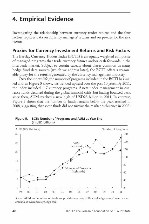
48 ©2012 The Research Foundation of CFA Institute
4. Empirical Evidence
Investigating the relationship between currency trader returns and the four factors requires data on currency managers’ returns and on proxies for the risk factors.
Proxies for Currency Investment Returns and Risk Factors�e Barclay Currency Traders Index (BCTI) is an equally weighted composite of managed programs that trade currency futures and/or cash forwards in the interbank market. Subject to certain caveats about biases common in many hedge fund data sources (which we address later), the BCTI oªers a reason-able proxy for the returns generated by the currency management industry.
Over the index’s life, the number of programs included in the BCTI has var-ied and, as Figure 5 shows, has trended upward over the past 10 years. By 2011, the index included 117 currency programs. Assets under management in cur-rency funds declined during the global ¡nancial crisis, but having bounced back since then, AUM reached a new high of USD28 billion in 2011. In contrast, Figure 5 shows that the number of funds remains below the peak reached in 2008, suggesting that some funds did not survive the market turbulence in 2008.
Figure 5. BCTI: Number of Programs and AUM at Year-End (in USD billions)
AUM(left axis)
Number of Programs(right axis)
AUM (USD billions)
30
25
20
15
10
5
0
Number of Programs
160
140
120
100
80
60
40
2099 1102 05 08 09 1001 04 0700 03 06
Source: AUM and numbers of funds are provided courtesy of BarclayHedge; annual returns are available at www.barclayhedge.com.
Empirical Evidence
©2012 The Research Foundation of CFA Institute 49
�e USD28 billion invested in currency funds represents only a tiny frac-tion of the assets invested in hedge funds. Estimates suggest that total hedge fund assets are about USD2 trillion (Strasburg and Eder 2011). �us, despite the depth of the foreign exchange market, professional currency investors rep-resent only a small proportion of the hedge fund industry.72 Whether currency is an underused asset class is a theme we explore further in Chapter 5.
As Melvin and Shand (2011) point out, there are many de¡nitions for generic currency strategies and “inferences drawn from empirical work will diªer according to which concepts are employed by the researcher” (p. 13). To address this concern, and as robustness checks, we used various proxies for the risk factors. We collected data for three proxies for the trend factor and two proxies for each of the other three factors.
Selecting appropriate factors is a matter of empirical analysis. If an inves-tor discovers that the return generated by the investor’s managers can be rep-licated cheaply through a naive trading strategy, then such return could be classi¡ed as a beta return and would not deserve active management fees. Complete transparency is required, however, in how the factor returns are derived. In addition, the return series must be su�ciently long out-of-sample to produce reliable statistical results. Most of the available factor proxies have been introduced only recently, which eªectively means comparing real cur-rency managers’ returns with those from back-tested strategies.
A number of banks have recently introduced indices designed to proxy the return from currency management. �e majority of these indices have been introduced only recently, however, and are not transparent enough. For exam-ple, Credit Suisse produces six factor indices (carry, momentum, value, terms of trade, growth, and emerging markets), collectively known as the FX Factor Index. A Credit Suisse press release from 27 April 2009 states:
�e FX Factor Index is based on six strategies [as listed above]. . . . �ese are strategies that have performed in a diverse set of market environments. By gaining exposure to these six strategies, the FX Factor Portfolio can out-perform more narrowly-based foreign exchange indices. (www.credit-suisse.com/news/en/media_release.jsp?ns=41154)
�e methodology to construct these factors, however, is not well articulated in available documents. Furthermore, because the factors were introduced only in 2009, we decided against using them to gauge currency managers’ perfor-mance prior to 2009. Similarly, although Citibank has produced both alpha and beta FX indices since 2007, it appears to have revised its beta indices in 2010
72Note that currency investment strategies are also applied by market participants other than FX-only managers. For example, global macro hedge funds also invest in the FX market. �erefore, total assets exposed to currency strategies are much larger than the USD28 billion invested in FX-only funds.
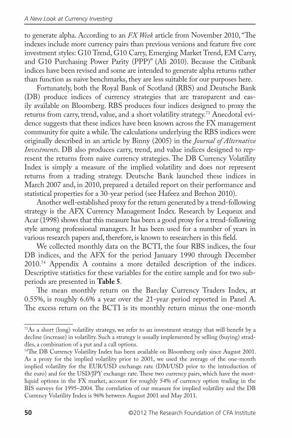
A New Look at Currency Investing
50 ©2012 The Research Foundation of CFA Institute
to generate alpha. According to an FX Week article from November 2010, “�e indexes include more currency pairs than previous versions and feature ¡ve core investment styles: G10 Trend, G10 Carry, Emerging Market Trend, EM Carry, and G10 Purchasing Power Parity (PPP)” (Ali 2010). Because the Citibank indices have been revised and some are intended to generate alpha returns rather than function as naive benchmarks, they are less suitable for our purposes here.
Fortunately, both the Royal Bank of Scotland (RBS) and Deutsche Bank (DB) produce indices of currency strategies that are transparent and eas-ily available on Bloomberg. RBS produces four indices designed to proxy the returns from carry, trend, value, and a short volatility strategy.73 Anecdotal evi-dence suggests that these indices have been known across the FX management community for quite a while. �e calculations underlying the RBS indices were originally described in an article by Binny (2005) in the Journal of Alternative Investments. DB also produces carry, trend, and value indices designed to rep-resent the returns from naive currency strategies. �e DB Currency Volatility Index is simply a measure of the implied volatility and does not represent returns from a trading strategy. Deutsche Bank launched these indices in March 2007 and, in 2010, prepared a detailed report on their performance and statistical properties for a 30-year period (see Hafeez and Brehon 2010).
Another well-established proxy for the return generated by a trend-following strategy is the AFX Currency Management Index. Research by Lequeux and Acar (1998) shows that this measure has been a good proxy for a trend-following style among professional managers. It has been used for a number of years in various research papers and, therefore, is known to researchers in this ¡eld.
We collected monthly data on the BCTI, the four RBS indices, the four DB indices, and the AFX for the period January 1990 through December 2010.74 Appendix A contains a more detailed description of the indices. Descriptive statistics for these variables for the entire sample and for two sub-periods are presented in Table 5.
�e mean monthly return on the Barclay Currency Traders Index, at 0.55%, is roughly 6.6% a year over the 21-year period reported in Panel A. �e excess return on the BCTI is its monthly return minus the one-month
73As a short (long) volatility strategy, we refer to an investment strategy that will bene¡t by a decline (increase) in volatility. Such a strategy is usually implemented by selling (buying) strad-dles, a combination of a put and a call options.74�e DB Currency Volatility Index has been available on Bloomberg only since August 2001. As a proxy for the implied volatility prior to 2001, we used the average of the one-month implied volatility for the EUR/USD exchange rate (DM/USD prior to the introduction of the euro) and for the USD/JPY exchange rate. �ese two currency pairs, which have the most-liquid options in the FX market, account for roughly 54% of currency option trading in the BIS surveys for 1995–2004. �e correlation of our measure for implied volatility and the DB Currency Volatility Index is 96% between August 2001 and May 2011.
Empirical Evidence
©2012 The Research Foundation of CFA Institute 51
Tab
le 5
. D
escr
ipti
ve S
tati
stic
s fo
r C
urr
ency
Ret
urn
s an
d C
urr
ency
Ris
k Fa
cto
rs
Cur
renc
y R
etur
ns
(BC
TI)
Risk
- Fre
e R
etur
ns
(USD
LIB
ID)
Exc
ess R
etur
n (B
CT
I – L
IBID
)
Car
ryTr
end
Valu
eVo
latili
tyD
B C
arry
RBS
Car
ryA
FX
Inde
xD
B Tr
end
RBS
Tren
dD
B Va
lue
RBS
Valu
eD
B Vo
latili
tyRB
S Vo
latili
tyA.
Janu
ary 1
990–
Dece
mbe
r 201
0 (N
= 2
52)
Mea
n m
onth
ly re
turn
(%)
0.55
0.33
0.22
0.30
0.43
0.23
0.20
0.30
0.28
0.25
0.02
0.34
Std.
dev
. (%
)2.
770.
182.
752.
685.
271.
892.
643.
362.
602.
611.
554.
09Sk
ewne
ss1.
84–0
.22
1.74
–1.3
3–3
.41
1.08
0.00
0.21
0.12
0.96
1.35
–1.6
0K
urto
sis6.
58–0
.79
6.25
4.80
27.8
82.
592.
941.
170.
433.
796.
6812
.17
B. Ja
nuar
y 199
0–D
ecem
ber 1
999
(N =
120
)M
ean
mon
thly
retu
rn (%
)0.
850.
440.
410.
290.
370.
280.
150.
370.
250.
090.
030.
47St
d. d
ev. (
%)
3.73
0.12
3.70
2.55
6.84
2.04
2.70
3.03
2.83
2.24
1.80
4.08
Skew
ness
1.32
0.39
1.29
–0.8
9–3
.12
0.85
–0.7
00.
200.
181.
420.
77–0
.63
Kur
tosis
2.69
0.14
2.61
1.20
19.8
51.
731.
521.
260.
546.
612.
692.
95
C. Ja
nuar
y 200
0–D
ecem
ber 2
010
(N =
132
)M
ean
mon
thly
retu
rn (%
)0.
270.
230.
040.
300.
470.
180.
230.
230.
310.
400.
010.
22St
d. d
ev. (
%)
1.39
0.17
1.41
2.80
3.26
1.74
2.59
3.65
2.39
2.90
1.28
4.11
Skew
ness
1.43
0.32
1.45
–1.6
3–1
.44
1.37
0.73
0.22
0.04
0.69
2.63
–2.4
9K
urto
sis3.
78–1
.26
3.71
7.12
5.32
3.91
4.53
1.01
0.07
2.49
16.9
420
.60
Not
es: M
onth
ly re
turn
s on
the B
CT
I and
each
fact
or ar
e calc
ulat
ed as
the l
ogar
ithm
of e
ach
mon
th ve
rsus
the p
revi
ous m
onth
. An
exce
ptio
n is
the D
B vo
latili
ty
fact
or, w
hich
is th
e ¡rs
t diª
eren
ce o
f the
impl
ied
volat
ility
rath
er th
an a
retu
rn.
A New Look at Currency Investing
52 ©2012 The Research Foundation of CFA Institute
USD LIBID rate.75 As a result, the mean monthly excess return on the BCTI is only 0.22%, similar to the returns on the trend factor (0.23% for the AFX and 0.20% for the DB trend) and the value factor (0.28% for the DB value and 0.25% for the RBS value). �e carry strategy and a short volatility strat-egy would have generated a slightly higher return. �e highest of the factor returns for the full period is the mean monthly return on the RBS carry, at 0.43%; the DB carry generated 0.30%, and the RBS volatility, 0.34%.
As expected, the trend factors re©ect positive skewness and the carry fac-tors exhibit negative skewness. �ese results can be explained in two ways. First, although trend following behaves like a long volatility strategy, carry trading functions like a short volatility strategy. Second, a more fundamen-tal explanation is that a trend-following strategy allows a right tail of pro¡ts when trends are prolonged, but reversals end the trend, close positions, and limit left-tail losses.76 A carry strategy may produce many small returns from a positive interest diªerential (i.e., the carry) but be prone to large left-tail losses if the target currency depreciates sharply against the funding currency.77
�e value factors show positive skewness and kurtosis. Kurtosis for the RBS carry is more pronounced than for any other factors. Naturally, the RBS volatility factor (a short volatility strategy) exhibits a negative skewness. �e DB volatility factor (representing diªerence in the implied volatility rather than a return) has a slightly positive mean monthly return, indicating that volatility was, on average, increasing over the sample period.78
In the two subperiods shown in Panels B and C of Table 5, mean excess returns on the BCTI were far higher—0.41% per month—in the ¡rst period (only 0.04% per month in the second period). �is very large diªerence can-not be explained by declining equilibrium returns on currency beta. Rosenberg (2010) suggests that the decline in return generated by currency managers in recent years is the result of a tendency of currency managers to place greater emphasis on downside risk management in this period.
Mean monthly returns on the factors were similar or higher in the sec-ond period with the exception of the short volatility strategy, which generated 0.47% in the ¡rst period but only 0.22% in the second. �e short volatility strategy suªered in the second period because of the spike in volatility during the global ¡nancial crisis of 2008.75All funds represented in the BCTI are absolute return programs. We used the one-month USD LIBID rate to proxy the risk-free return on the AUM in these programs. All funds in the BCTI report their data on a net basis after deducting all management fees.76See Schulmeister (2005) for a statistical analysis of the distribution of returns from technical trading models in currency, which con¡rms this general pattern.77Brunnermeier, Nagel, and Pedersen (2009) review the empirical evidence on the skewed left-tail nature of carry trade returns.78Substantial correlation is found between this currency volatility measure and both the VIX (the Chicago Board Options Exchange Market Volatility Index, a proxy for the volatility in the equity market) and the MOVE Index (Merrill Lynch Option Volatility Estimate Index, a proxy for volatility in the bond market).
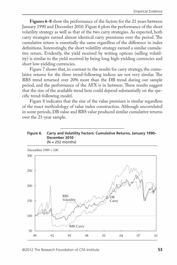
Empirical Evidence
©2012 The Research Foundation of CFA Institute 53
Figures 6–8 show the performance of the factors for the 21 years between January 1990 and December 2010. Figure 6 plots the performance of the short volatility strategy as well as that of the two carry strategies. As expected, both carry strategies earned almost identical carry premiums over the period. �e cumulative return is essentially the same regardless of the diªerence in index de¡nitions. Interestingly, the short volatility strategy earned a similar cumula-tive return. Evidently, the yield received by writing options (selling volatil-ity) is similar to the yield received by being long high-yielding currencies and short low-yielding currencies.
Figure 7 shows that, in contrast to the results for carry strategy, the cumu-lative returns for the three trend-following indices are not very similar. �e RBS trend returned over 20% more than the DB trend during our sample period, and the performance of the AFX is in between. �ese results suggest that the size of the available trend beta could depend substantially on the spe-ci¡c trend-following model.
Figure 8 indicates that the size of the value premium is similar regardless of the exact methodology of value index construction. Although uncorrelated in some periods, DB value and RBS value produced similar cumulative returns over the 21-year sample.
Figure 6. Carry and Volatility Factors: Cumulative Returns, January 1990–December 2010 (N = 252 months)
100
DBCarry
RBS Carry
RBSVolatility
December 1989 = 100
300
250
200
150
5089 1095 01 0792 98 04

A New Look at Currency Investing
54 ©2012 The Research Foundation of CFA Institute
Figure 7. Trend Factors: Cumulative Returns, January 1990–December 2010 (N = 252 months)
100
DBTrend
RBS TrendAFX
December 1989 = 100
250
200
150
5089 1095 01 0792 98 04
Figure 8. Value Factors: Cumulative Returns, January 1990–December 2010 (N = 252 months)
100
DBValue
RBS Value
December 1989 = 100
250
200
150
5089 1095 01 0792 98 04
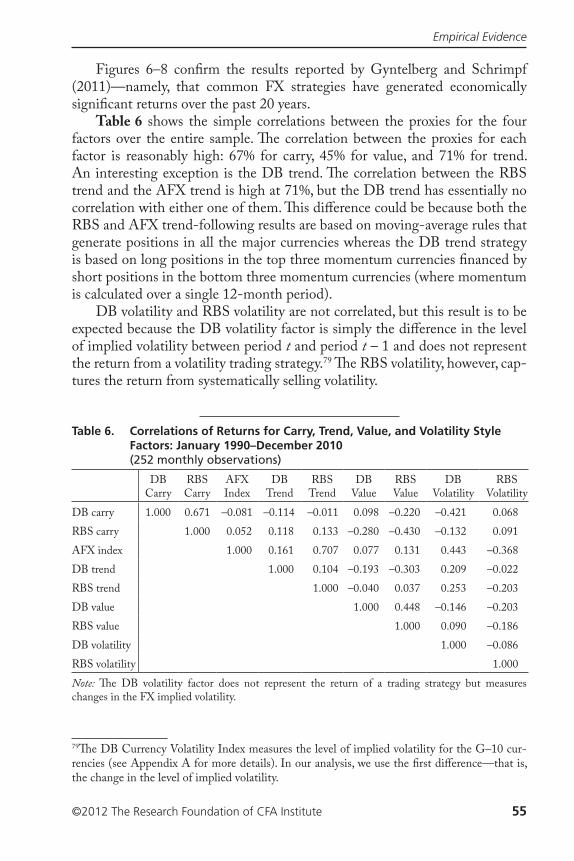
Empirical Evidence
©2012 The Research Foundation of CFA Institute 55
Figures 6–8 con¡rm the results reported by Gyntelberg and Schrimpf (2011)—namely, that common FX strategies have generated economically signi¡cant returns over the past 20 years.
Table 6 shows the simple correlations between the proxies for the four factors over the entire sample. �e correlation between the proxies for each factor is reasonably high: 67% for carry, 45% for value, and 71% for trend. An interesting exception is the DB trend. �e correlation between the RBS trend and the AFX trend is high at 71%, but the DB trend has essentially no correlation with either one of them. �is diªerence could be because both the RBS and AFX trend-following results are based on moving-average rules that generate positions in all the major currencies whereas the DB trend strategy is based on long positions in the top three momentum currencies ¡nanced by short positions in the bottom three momentum currencies (where momentum is calculated over a single 12-month period).
DB volatility and RBS volatility are not correlated, but this result is to be expected because the DB volatility factor is simply the diªerence in the level of implied volatility between period t and period t – 1 and does not represent the return from a volatility trading strategy.79 �e RBS volatility, however, cap-tures the return from systematically selling volatility.
79�e DB Currency Volatility Index measures the level of implied volatility for the G–10 cur-rencies (see Appendix A for more details). In our analysis, we use the ¡rst diªerence—that is, the change in the level of implied volatility.
Table 6. Correlations of Returns for Carry, Trend, Value, and Volatility Style Factors: January 1990–December 2010 (252 monthly observations)
DB Carry
RBS Carry
AFX Index
DB Trend
RBS Trend
DB Value
RBS Value
DB Volatility
RBS Volatility
DB carry 1.000 0.671 –0.081 –0.114 –0.011 0.098 –0.220 –0.421 0.068RBS carry 1.000 0.052 0.118 0.133 –0.280 –0.430 –0.132 0.091AFX index 1.000 0.161 0.707 0.077 0.131 0.443 –0.368DB trend 1.000 0.104 –0.193 –0.303 0.209 –0.022RBS trend 1.000 –0.040 0.037 0.253 –0.203DB value 1.000 0.448 –0.146 –0.203RBS value 1.000 0.090 –0.186DB volatility 1.000 –0.086RBS volatility 1.000Note: �e DB volatility factor does not represent the return of a trading strategy but measures changes in the FX implied volatility.
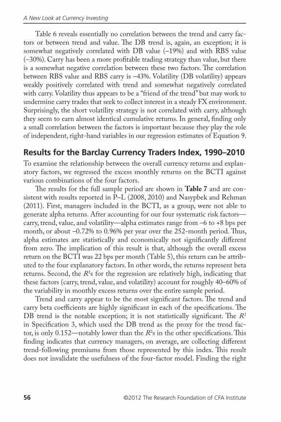
A New Look at Currency Investing
56 ©2012 The Research Foundation of CFA Institute
Table 6 reveals essentially no correlation between the trend and carry fac-tors or between trend and value. �e DB trend is, again, an exception; it is somewhat negatively correlated with DB value (–19%) and with RBS value (–30%). Carry has been a more pro¡table trading strategy than value, but there is a somewhat negative correlation between these two factors. �e correlation between RBS value and RBS carry is –43%. Volatility (DB volatility) appears weakly positively correlated with trend and somewhat negatively correlated with carry. Volatility thus appears to be a “friend of the trend” but may work to undermine carry trades that seek to collect interest in a steady FX environment. Surprisingly, the short volatility strategy is not correlated with carry, although they seem to earn almost identical cumulative returns. In general, ¡nding only a small correlation between the factors is important because they play the role of independent, right-hand variables in our regression estimates of Equation 9.
Results for the Barclay Currency Traders Index, 1990–2010To examine the relationship between the overall currency returns and explan-atory factors, we regressed the excess monthly returns on the BCTI against various combinations of the four factors.
�e results for the full sample period are shown in Table 7 and are con-sistent with results reported in P–L (2008, 2010) and Nasypbek and Rehman (2011). First, managers included in the BCTI, as a group, were not able to generate alpha returns. After accounting for our four systematic risk factors—carry, trend, value, and volatility—alpha estimates range from –6 to +8 bps per month, or about –0.72% to 0.96% per year over the 252-month period. �us, alpha estimates are statistically and economically not signi¡cantly diªerent from zero. �e implication of this result is that, although the overall excess return on the BCTI was 22 bps per month (Table 5), this return can be attrib-uted to the four explanatory factors. In other words, the returns represent beta returns. Second, the R2s for the regression are relatively high, indicating that these factors (carry, trend, value, and volatility) account for roughly 40–60% of the variability in monthly excess returns over the entire sample period.
Trend and carry appear to be the most signi¡cant factors. �e trend and carry beta coe�cients are highly signi¡cant in each of the speci¡cations. �e DB trend is the notable exception; it is not statistically signi¡cant. �e R2
in Speci¡cation 3, which used the DB trend as the proxy for the trend fac-tor, is only 0.152—notably lower than the R2s in the other speci¡cations. �is ¡nding indicates that currency managers, on average, are collecting diªerent trend-following premiums from those represented by this index. �is result does not invalidate the usefulness of the four-factor model. Finding the right
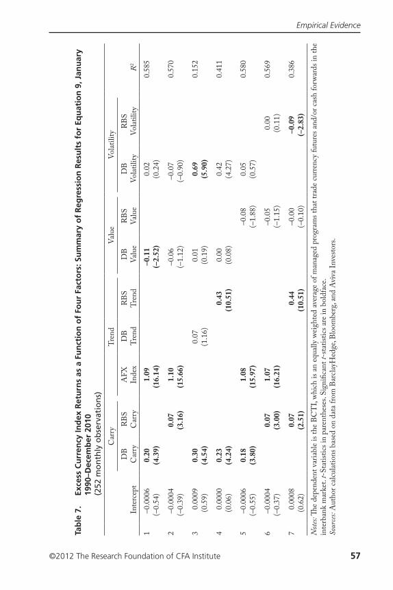
Empirical Evidence
©2012 The Research Foundation of CFA Institute 57
Tab
le 7
. Ex
cess
Cu
rren
cy In
dex
Ret
urn
s as
a F
un
ctio
n o
f Fo
ur
Fact
ors
: Su
mm
ary
of
Reg
ress
ion
Res
ult
s fo
r Eq
uat
ion
9, J
anu
ary
1990
–Dec
emb
er 2
010
(252
mo
nth
ly o
bse
rvat
ion
s)
Car
ryTr
end
Valu
eVo
latili
ty
Inte
rcep
tD
B C
arry
RBS
Car
ryA
FX
Inde
xD
B Tr
end
RBS
Tr
end
DB
Va
lue
RBS
Valu
eD
B
Volat
ility
RBS
Volat
ility
R2
1–0
.000
60.
201.
09–0
.11
0.02
0.58
5(–
0.54
)(4
.39)
(16.
14)
(–2.
52)
(0.2
4)
2–0
.000
40.
071.
10–0
.06
–0.0
70.
570
(–0.
39)
(3.1
6)(1
5.66
)(–
1.12
)(–
0.90
)
30.
0009
0.30
0.07
0.01
0.69
0.15
2(0
.59)
(4.5
4)(1
.16)
(0.1
9)(5
.90)
40.
0000
0.23
0.43
0.00
0.42
0.41
1(0
.06)
(4.2
4)(1
0.51
)(0
.08)
(4.2
7)
5–0
.000
60.
181.
08–0
.08
0.05
0.58
0(–
0.55
)(3
.80)
(15.
97)
(–1.
88)
(0.5
7)
6–0
.000
40.
071.
07–0
.05
0.00
0.56
9(–
0.37
)(3
.00)
(16.
21)
(–1.
15)
(0.1
1)
70.
0008
0.07
0.44
–0.0
0–0
.09
0.38
6(0
.62)
(2.5
1)(1
0.51
)(–
0.10
)(–
2.83
)N
otes:
�e
depe
nden
t var
iabl
e is
the
BCT
I, wh
ich is
an
equa
lly w
eigh
ted
aver
age
of m
anag
ed p
rogr
ams t
hat t
rade
curre
ncy
futu
res a
nd/o
r cas
h fo
rwar
ds in
the
inte
rban
k m
arke
t. t-
Stat
istics
in p
aren
thes
es. S
igni
¡can
t t-s
tatis
tics a
re in
bol
dfac
e.So
urces
: Aut
hor c
alcul
atio
ns b
ased
on
data
from
Bar
clayH
edge
, Blo
ombe
rg, a
nd A
viva
Inve
stors
.
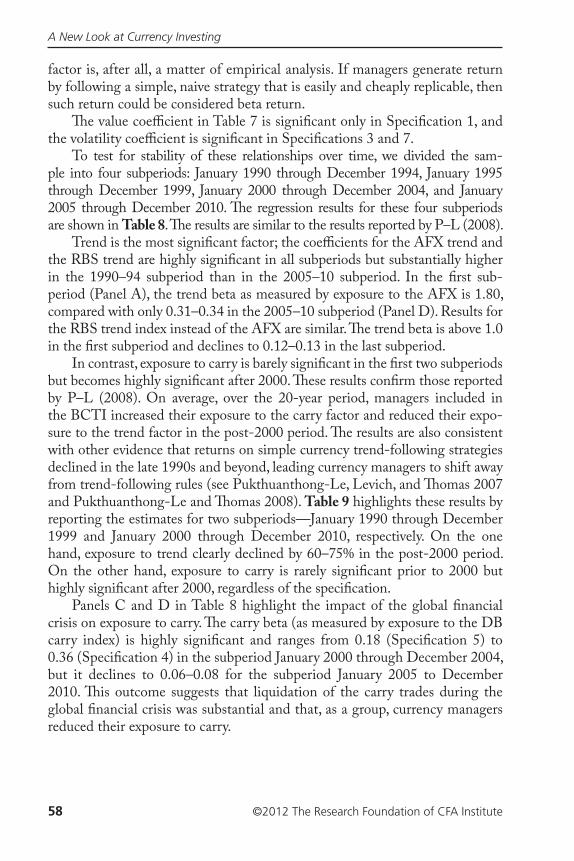
A New Look at Currency Investing
58 ©2012 The Research Foundation of CFA Institute
factor is, after all, a matter of empirical analysis. If managers generate return by following a simple, naive strategy that is easily and cheaply replicable, then such return could be considered beta return.
�e value coe�cient in Table 7 is signi¡cant only in Speci¡cation 1, and the volatility coe�cient is signi¡cant in Speci¡cations 3 and 7.
To test for stability of these relationships over time, we divided the sam-ple into four subperiods: January 1990 through December 1994, January 1995 through December 1999, January 2000 through December 2004, and January 2005 through December 2010. �e regression results for these four subperiods are shown in Table 8. �e results are similar to the results reported by P–L (2008).
Trend is the most signi¡cant factor; the coe�cients for the AFX trend and the RBS trend are highly signi¡cant in all subperiods but substantially higher in the 1990–94 subperiod than in the 2005–10 subperiod. In the ¡rst sub-period (Panel A), the trend beta as measured by exposure to the AFX is 1.80, compared with only 0.31–0.34 in the 2005–10 subperiod (Panel D). Results for the RBS trend index instead of the AFX are similar. �e trend beta is above 1.0 in the ¡rst subperiod and declines to 0.12–0.13 in the last subperiod.
In contrast, exposure to carry is barely signi¡cant in the ¡rst two subperiods but becomes highly signi¡cant after 2000. �ese results con¡rm those reported by P–L (2008). On average, over the 20-year period, managers included in the BCTI increased their exposure to the carry factor and reduced their expo-sure to the trend factor in the post-2000 period. �e results are also consistent with other evidence that returns on simple currency trend-following strategies declined in the late 1990s and beyond, leading currency managers to shift away from trend-following rules (see Pukthuanthong-Le, Levich, and �omas 2007 and Pukthuanthong-Le and �omas 2008). Table 9 highlights these results by reporting the estimates for two subperiods—January 1990 through December 1999 and January 2000 through December 2010, respectively. On the one hand, exposure to trend clearly declined by 60–75% in the post-2000 period. On the other hand, exposure to carry is rarely signi¡cant prior to 2000 but highly signi¡cant after 2000, regardless of the speci¡cation.
Panels C and D in Table 8 highlight the impact of the global ¡nancial crisis on exposure to carry. �e carry beta (as measured by exposure to the DB carry index) is highly signi¡cant and ranges from 0.18 (Speci¡cation 5) to 0.36 (Speci¡cation 4) in the subperiod January 2000 through December 2004, but it declines to 0.06–0.08 for the subperiod January 2005 to December 2010. �is outcome suggests that liquidation of the carry trades during the global ¡nancial crisis was substantial and that, as a group, currency managers reduced their exposure to carry.
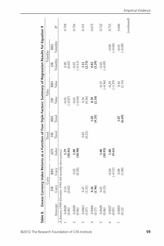
Empirical Evidence
©2012 The Research Foundation of CFA Institute 59
Tab
le 8
. Ex
cess
Cu
rren
cy In
dex
Ret
urn
s as
a F
un
ctio
n o
f Fo
ur
Styl
e Fa
cto
rs: S
um
mar
y o
f R
egre
ssio
n R
esu
lts
for
Equ
atio
n 9
Car
ryTr
end
Valu
eVo
latili
ty
Inte
rcep
tD
B
Car
ryRB
S C
arry
AFX
In
dex
DB
Tren
dRB
S Tr
end
DB
Va
lue
RBS
Valu
eD
B Vo
latili
tyRB
S Vo
latili
tyR
2
A. Ja
nuar
y 199
0–D
ecem
ber 1
994
(60
mon
thly
obser
vatio
ns)
10.
0028
0.14
1.79
–0.0
10.
000.
728
(0.8
6)(0
.82)
(10.
81)
(–0.
07)
(0.0
3)2
0.00
280.
031.
80–0
.01
–0.0
30.
726
(0.8
6)(0
.58)
(10.
90)
(–0.
04)
(–0.
13)
30.
0063
0.47
0.05
0.10
1.11
0.15
1(1
.07)
(1.5
1)(0
.21)
(0.3
6)(2
.73)
40.
0006
0.36
1.02
0.38
0.83
0.67
2(0
.17)
(1.9
6)(9
.35)
(2.3
4)(3
.29)
50.
0028
0.05
1.80
–0.1
5–0
.02
0.73
2(0
.86)
(0.3
3)(1
0.93
)(–
0.96
)(–
0.09
)6
0.00
27–0
.04
1.80
–0.2
9–0
.00
0.73
3(0
.83)
(–0.
53)
(9.6
1)(–
1.19
)(–
0.00
)7
0.00
050.
081.
070.
42–0
.01
0.60
6(0
.12)
(1.0
0)(6
.69)
(1.3
4)(–
0.08
)
(con
tinue
d)
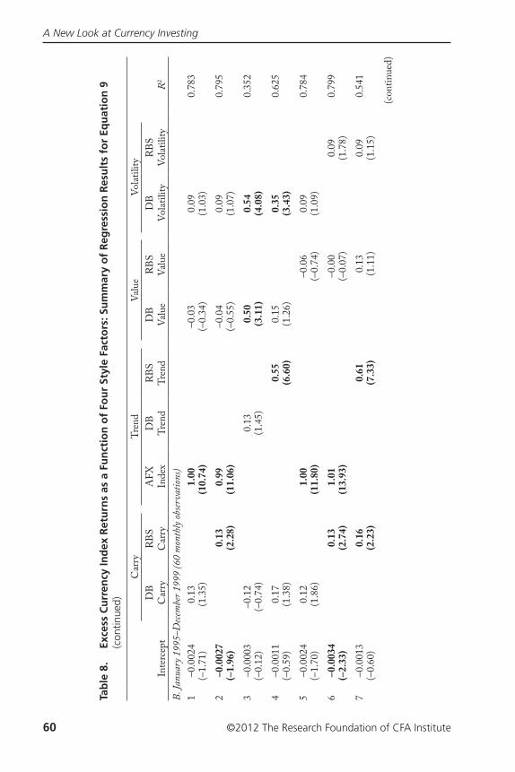
A New Look at Currency Investing
60 ©2012 The Research Foundation of CFA Institute
Car
ryTr
end
Valu
eVo
latili
ty
Inte
rcep
tD
B
Car
ryRB
S C
arry
AFX
In
dex
DB
Tren
dRB
S Tr
end
DB
Va
lue
RBS
Valu
eD
B Vo
latili
tyRB
S Vo
latili
tyR
2
B. Ja
nuar
y 199
5–D
ecem
ber 1
999
(60
mon
thly
obser
vatio
ns)
1–0
.002
40.
131.
00–0
.03
0.09
0.78
3(–
1.71
)(1
.35)
(10.
74)
(–0.
34)
(1.0
3)2
–0.0
027
0.13
0.99
–0.0
40.
090.
795
(–1.
96)
(2.2
8)(1
1.06
)(–
0.55
)(1
.07)
3–0
.000
3–0
.12
0.13
0.50
0.54
0.35
2(–
0.12
)(–
0.74
)(1
.45)
(3.1
1)(4
.08)
4–0
.001
10.
170.
550.
150.
350.
625
(–0.
59)
(1.3
8)(6
.60)
(1.2
6)(3
.43)
5–0
.002
40.
121.
00–0
.06
0.09
0.78
4(–
1.70
)(1
.86)
(11.
80)
(–0.
74)
(1.0
9)6
–0.0
034
0.13
1.01
–0.0
00.
090.
799
(–2.
33)
(2.7
4)(1
3.93
)(–
0.07
)(1
.78)
7–0
.001
30.
160.
610.
130.
090.
541
(–0.
60)
(2.2
3)(7
.33)
(1.1
1)(1
.15)
Tab
le 8
. Ex
cess
Cu
rren
cy In
dex
Ret
urn
s as
a F
un
ctio
n o
f Fo
ur
Styl
e Fa
cto
rs: S
um
mar
y o
f R
egre
ssio
n R
esu
lts
for
Equ
atio
n 9
(c
ontin
ued)
(con
tinue
d)
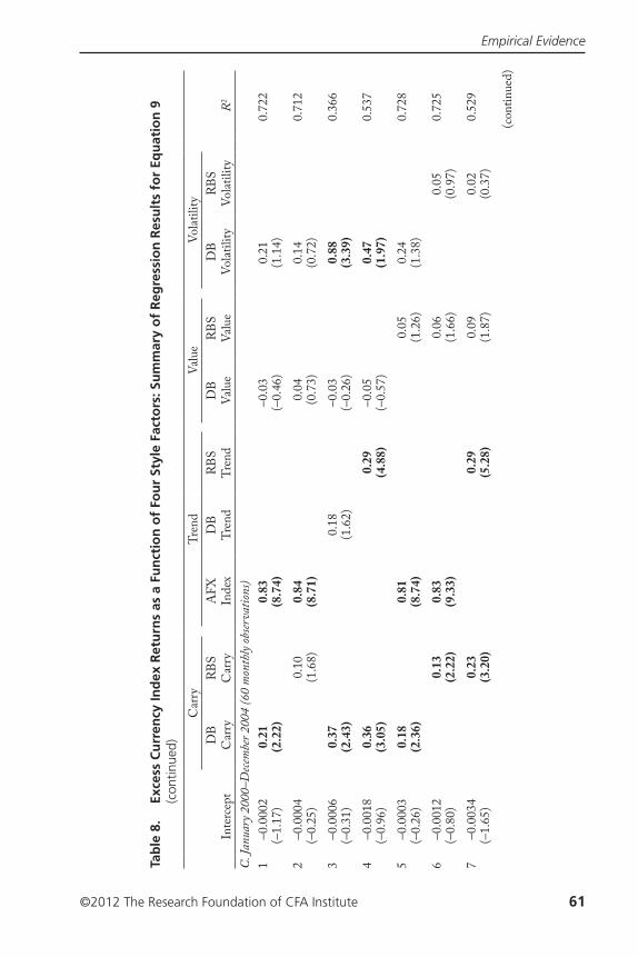
Empirical Evidence
©2012 The Research Foundation of CFA Institute 61
Car
ryTr
end
Valu
eVo
latili
ty
Inte
rcep
tD
B
Car
ryRB
S C
arry
AFX
In
dex
DB
Tren
dRB
S Tr
end
DB
Va
lue
RBS
Valu
eD
B Vo
latili
tyRB
S Vo
latili
tyR
2
C. Ja
nuar
y 200
0–D
ecem
ber 2
004
(60
mon
thly
obser
vatio
ns)
1–0
.000
20.
210.
83–0
.03
0.21
0.72
2(–
1.17
)(2
.22)
(8.7
4)(–
0.46
)(1
.14)
2–0
.000
40.
100.
840.
040.
140.
712
(–0.
25)
(1.6
8)(8
.71)
(0.7
3)(0
.72)
3–0
.000
60.
370.
18–0
.03
0.88
0.36
6(–
0.31
)(2
.43)
(1.6
2)(–
0.26
)(3
.39)
4–0
.001
80.
360.
29–0
.05
0.47
0.53
7(–
0.96
)(3
.05)
(4.8
8)(–
0.57
)(1
.97)
5–0
.000
30.
180.
810.
050.
240.
728
(–0.
26)
(2.3
6)(8
.74)
(1.2
6)(1
.38)
6–0
.001
20.
130.
830.
060.
050.
725
(–0.
80)
(2.2
2)(9
.33)
(1.6
6)(0
.97)
7–0
.003
40.
230.
290.
090.
020.
529
(–1.
65)
(3.2
0)(5
.28)
(1.8
7)(0
.37)
Tab
le 8
. Ex
cess
Cu
rren
cy In
dex
Ret
urn
s as
a F
un
ctio
n o
f Fo
ur
Styl
e Fa
cto
rs: S
um
mar
y o
f R
egre
ssio
n R
esu
lts
for
Equ
atio
n 9
(c
ontin
ued)
(con
tinue
d)
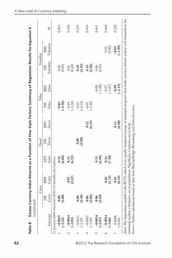
A New Look at Currency Investing
62 ©2012 The Research Foundation of CFA Institute
Car
ryTr
end
Valu
eVo
latili
ty
Inte
rcep
tD
B
Car
ryRB
S C
arry
AFX
In
dex
DB
Tren
dRB
S Tr
end
DB
Va
lue
RBS
Valu
eD
B Vo
latili
tyRB
S Vo
latili
tyR
2
D. J
anua
ry 2
005–
Dece
mbe
r 201
0 (7
2 m
onth
ly ob
serva
tions
)1
–0.0
015
0.08
0.32
–0.0
50.
060.
463
(–2.
22)
(3.0
8)(6
.60)
(–1.
96)
(0.8
5)2
–0.0
014
0.07
0.32
–0.0
40.
010.
446
(–2.
03)
(2.6
7)(6
.52)
(–1.
36)
(0.2
0)3
–0.0
011
0.08
0.09
–0.0
10.
200.
219
(–1.
39)
(2.4
8)(3
.00)
(–0.
44)
(2.5
6)4
–0.0
007
0.06
0.12
–0.0
50.
160.
434
(–1.
09)
(2.0
6)(6
.15)
(–1.
88)
(2.3
6)5
–0.0
014
0.06
0.31
–0.0
80.
060.
461
(–2.
07)
(2.0
3)(6
.49)
(–1.
88)
(0.9
5)6
–0.0
014
0.04
0.34
–0.0
70.
010.
462
(–2.
06)
(1.7
2)(7
.30)
(–1.
67)
(0.9
0)7
–0.0
006
0.01
0.13
–0.0
9–0
.03
0.52
9(–
0.84
)(0
.19)
(6.9
8)(–
2.19
)(–
1.99
)
Not
es: �
e de
pend
ent v
aria
ble
is th
e BC
TI,
which
is a
n eq
ually
wei
ghte
d av
erag
e of
man
aged
pro
gram
s tha
t tra
de cu
rrenc
y fu
ture
s and
/or c
ash
forw
ards
in th
e in
terb
ank
mar
ket.
t-St
atist
ics ar
e in
pare
nthe
ses.
Sign
i¡ca
nt t-
statis
tics a
re in
bol
d.So
urces
: Aut
hor c
alcul
atio
ns b
ased
on
data
from
Bar
clayH
edge
, Blo
ombe
rg, a
nd A
viva
Inve
stors
.
Tab
le 8
. Ex
cess
Cu
rren
cy In
dex
Ret
urn
s as
a F
un
ctio
n o
f Fo
ur
Styl
e Fa
cto
rs: S
um
mar
y o
f R
egre
ssio
n R
esu
lts
for
Equ
atio
n 9
(c
ontin
ued)

Empirical Evidence
©2012 The Research Foundation of CFA Institute 63
Tab
le 9
. Ex
cess
Cu
rren
cy In
dex
Ret
urn
s as
a F
un
ctio
n o
f Fo
ur
Styl
e Fa
cto
rs: S
um
mar
y o
f R
egre
ssio
n R
esu
lts
for
Equ
atio
n 9
Car
ryTr
end
Valu
eVo
latili
ty
Inte
rcep
tD
B C
arry
RBS
Car
ryA
FX
Inde
xD
B Tr
end
RBS
Tren
dD
B Va
lue
RBS
Valu
eD
B Vo
latili
tyRB
S Vo
latili
tyR
2
A. Ja
nuar
y 199
0–D
ecem
ber 1
999
(120
mon
thly
obser
vatio
ns)
1–0
.000
10.
101.
50–0
.10
–0.0
40.
688
(–0.
05)
(1.2
5)(1
4.13
)(–
1.48
)(–
0.36
)
2–0
.000
10.
031.
50–0
.07
–0.0
70.
687
(–0.
01)
(1.0
1)(1
4.02
)(–
0.92
)(–
0.55
)
30.
0026
0.35
0.03
0.07
0.78
0.14
8(0
.81)
(2.7
3)(0
.27)
(0.6
0)(4
.08)
4–0
.000
30.
230.
860.
170.
460.
611
(–0.
14)
(2.6
6)(1
1.69
)(2
.18)
(3.4
9)
5–0
.000
10.
071.
49–0
.16
–0.0
30.
691
(–0.
06)
(0.8
9)(1
4.25
)(–
1.83
)(–
0.27
)
60.
0006
0.01
1.42
–0.1
7–0
.07
0.69
4(0
.29)
(0.3
7)(1
4.03
)(–
1.53
)(–
1.47
)
70.
0008
0.05
0.87
0.17
–0.0
60.
565
(0.3
4)(1
.25)
(10.
20)
(1.3
0)(–
1.04
)
(con
tinue
d)
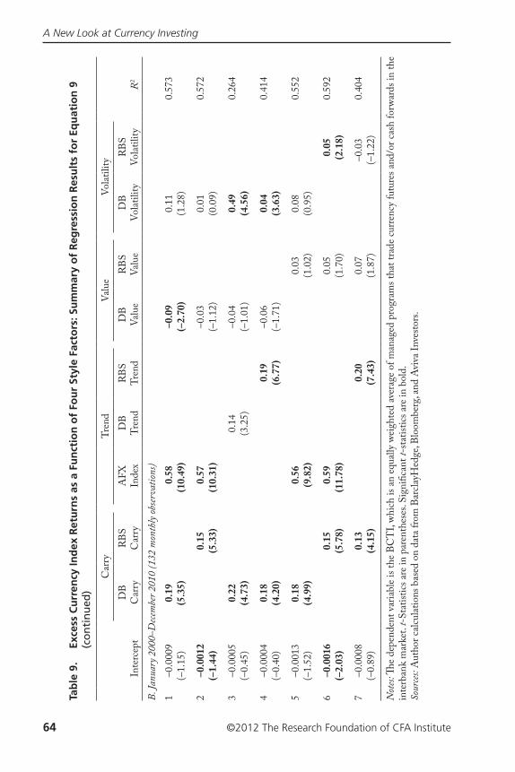
A New Look at Currency Investing
64 ©2012 The Research Foundation of CFA Institute
Car
ryTr
end
Valu
eVo
latili
ty
Inte
rcep
tD
B C
arry
RBS
Car
ryA
FX
Inde
xD
B Tr
end
RBS
Tren
dD
B Va
lue
RBS
Valu
eD
B Vo
latili
tyRB
S Vo
latili
tyR
2
B. Ja
nuar
y 200
0–D
ecem
ber 2
010
(132
mon
thly
obser
vatio
ns)
1–0
.000
90.
190.
58–0
.09
0.11
0.57
3(–
1.15
)(5
.35)
(10.
49)
(–2.
70)
(1.2
8)
2–0
.001
20.
150.
57–0
.03
0.01
0.57
2(–
1.44
)(5
.33)
(10.
31)
(–1.
12)
(0.0
9)
3–0
.000
50.
220.
14–0
.04
0.49
0.26
4(–
0.45
)(4
.73)
(3.2
5)(–
1.01
)(4
.56)
4–0
.000
40.
180.
19–0
.06
0.04
0.41
4(–
0.40
)(4
.20)
(6.7
7)(–
1.71
)(3
.63)
5–0
.001
30.
180.
560.
030.
080.
552
(–1.
52)
(4.9
9)(9
.82)
(1.0
2)(0
.95)
6–0
.001
60.
150.
590.
050.
050.
592
(–2.
03)
(5.7
8)(1
1.78
)(1
.70)
(2.1
8)
7–0
.000
80.
130.
200.
07–0
.03
0.40
4(–
0.89
)(4
.15)
(7.4
3)(1
.87)
(–1.
22)
Not
es: �
e de
pend
ent v
aria
ble
is th
e BC
TI,
which
is a
n eq
ually
wei
ghte
d av
erag
e of
man
aged
pro
gram
s tha
t tra
de cu
rrenc
y fu
ture
s and
/or c
ash
forw
ards
in th
e in
terb
ank
mar
ket.
t-St
atist
ics ar
e in
pare
nthe
ses.
Sign
i¡ca
nt t-
statis
tics a
re in
bol
d.So
urces
: Aut
hor c
alcul
atio
ns b
ased
on
data
from
Bar
clayH
edge
, Blo
ombe
rg, a
nd A
viva
Inve
stors
.
Tab
le 9
. Ex
cess
Cu
rren
cy In
dex
Ret
urn
s as
a F
un
ctio
n o
f Fo
ur
Styl
e Fa
cto
rs: S
um
mar
y o
f R
egre
ssio
n R
esu
lts
for
Equ
atio
n 9
(c
on
tin
ued
)
Empirical Evidence
©2012 The Research Foundation of CFA Institute 65
Interestingly, the intercept (alpha) is negative and signi¡cant for most speci-¡cations in Table 8, Panel D, the period from January 2005 until December 2010. Currency managers, on average, not only failed to deliver positive alpha, but they actually subtracted value from their clients during the last six years of the sample. �is result highlights that the period of the global ¡nancial crisis has been quite challenging for currency investment managers and may explain why the number of funds as reported in Figure 5 is still below the peak reached in 2008.
Emerging Markets. �e risk factors used in the previous section rep-resent returns from generic trading strategies in only the major currencies. To investigate whether currency managers, as a group, have taken a signi¡cant degree of exposure to EM currencies, we collected data on two generic factors that measure exposure to EM currencies.
In addition to a G–10 carry index, Deutsche Bank also calculates two additional carry indices, which provide exposure to EM currencies:80
• the Global Currency Harvest Index, based on the 10 major currencies and 10 EM currencies (shorting the 5 currencies with the lowest interest rates to purchase the 5 currencies with the highest interest rates) and
• the Balanced Currency Harvest Index, based on the 10 major currencies and 10 EM currencies but with a minimum of 2 G–10 currencies on the funding (short) side and 2 on the investment (long) side.
A more detailed description of these indices is given in Appendix A.In Table 10, we report regression results for Equation 9, in which these
two indices were used to test for exposure to EM currencies. Because data on the Harvest Global have been available only since October 2000 and on the Harvest Balanced only since January 2000, our results cover only the 10 years from January 2001 through December 2010.
Table 10 shows essentially no increase in R2 when a G–10 carry index was replaced with a carry index that invests in both developed and emerging market currencies. �is ¡nding implies that currency managers, as a group, do not have signi¡cant carry exposure to EM currencies. �is ¡nding does not imply, however, that currency managers do not invest in EM currencies; rather, it implies that managers (as a group) may be seeking trend (and/or value) expo-sure rather than, speci¡cally, carry exposure to EM currencies. Indeed, Pojarliev (2005) ¡nds that trend-following strategies work better for emerging market currencies whereas carry trading strategies perform better for developed market currencies. Unfortunately, we are not aware of the existence of indices designed to proxy the returns of trend and value strategies for EM currencies.
80�e exact index name is the Deutsche Bank Currency Harvest G10 Index. For more informa-tion, see Appendix A.
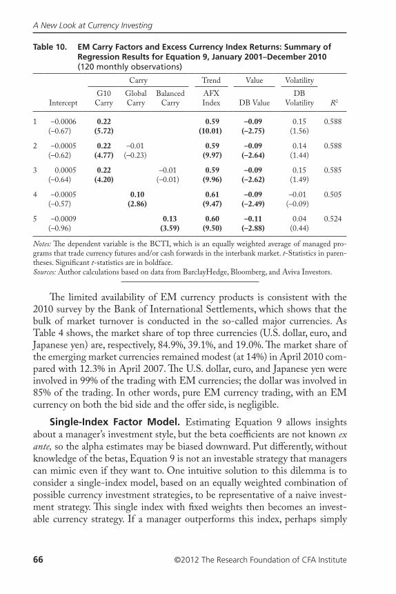
A New Look at Currency Investing
66 ©2012 The Research Foundation of CFA Institute
�e limited availability of EM currency products is consistent with the 2010 survey by the Bank of International Settlements, which shows that the bulk of market turnover is conducted in the so-called major currencies. As Table 4 shows, the market share of top three currencies (U.S. dollar, euro, and Japanese yen) are, respectively, 84.9%, 39.1%, and 19.0%. �e market share of the emerging market currencies remained modest (at 14%) in April 2010 com-pared with 12.3% in April 2007. �e U.S. dollar, euro, and Japanese yen were involved in 99% of the trading with EM currencies; the dollar was involved in 85% of the trading. In other words, pure EM currency trading, with an EM currency on both the bid side and the oªer side, is negligible.
Single-Index Factor Model. Estimating Equation 9 allows insights about a manager’s investment style, but the beta coe�cients are not known ex ante, so the alpha estimates may be biased downward. Put diªerently, without knowledge of the betas, Equation 9 is not an investable strategy that managers can mimic even if they want to. One intuitive solution to this dilemma is to consider a single-index model, based on an equally weighted combination of possible currency investment strategies, to be representative of a naive invest-ment strategy. �is single index with ¡xed weights then becomes an invest-able currency strategy. If a manager outperforms this index, perhaps simply
Table 10. EM Carry Factors and Excess Currency Index Returns: Summary of Regression Results for Equation 9, January 2001–December 2010 (120 monthly observations)
Carry Trend Value Volatility
InterceptG10 Carry
Global Carry
Balanced Carry
AFX Index DB Value
DB Volatility R2
1 –0.0006 0.22 0.59 –0.09 0.15 0.588(–0.67) (5.72) (10.01) (–2.75) (1.56)
2 –0.0005 0.22 –0.01 0.59 –0.09 0.14 0.588(–0.62) (4.77) (–0.23) (9.97) (–2.64) (1.44)
3 0.0005 0.22 –0.01 0.59 –0.09 0.15 0.585(–0.64) (4.20) (–0.01) (9.96) (–2.62) (1.49)
4 –0.0005 0.10 0.61 –0.09 –0.01 0.505(–0.57) (2.86) (9.47) (–2.49) (–0.09)
5 –0.0009 0.13 0.60 –0.11 0.04 0.524(–0.96) (3.59) (9.50) (–2.88) (0.44)
Notes: �e dependent variable is the BCTI, which is an equally weighted average of managed pro-grams that trade currency futures and/or cash forwards in the interbank market. t-Statistics in paren-theses. Signi¡cant t-statistics are in boldface.Sources: Author calculations based on data from BarclayHedge, Bloomberg, and Aviva Investors.
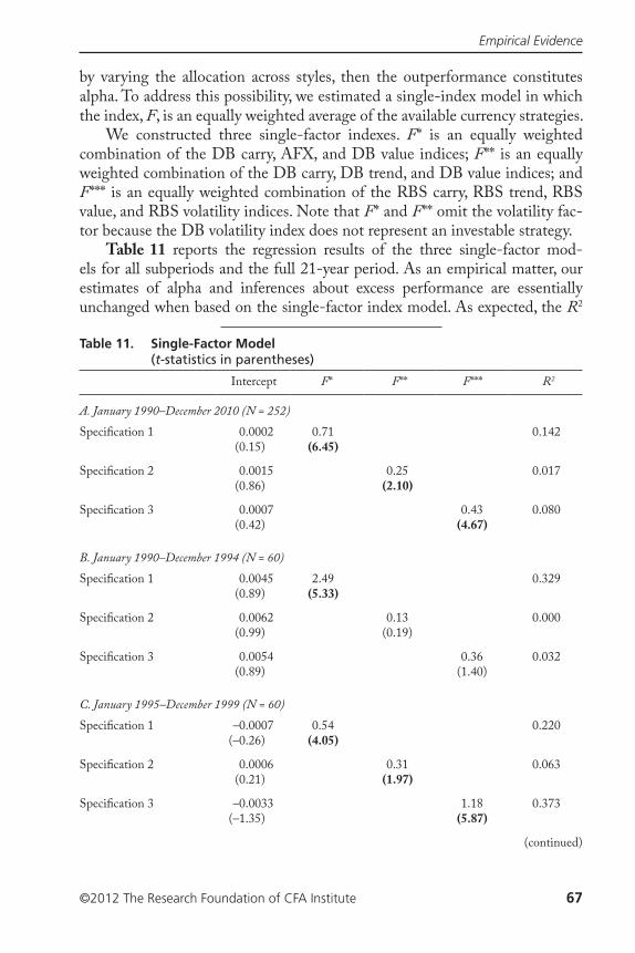
Empirical Evidence
©2012 The Research Foundation of CFA Institute 67
by varying the allocation across styles, then the outperformance constitutes alpha. To address this possibility, we estimated a single-index model in which the index, F, is an equally weighted average of the available currency strategies.
We constructed three single-factor indexes. F* is an equally weighted combination of the DB carry, AFX, and DB value indices; F** is an equally weighted combination of the DB carry, DB trend, and DB value indices; and F*** is an equally weighted combination of the RBS carry, RBS trend, RBS value, and RBS volatility indices. Note that F* and F** omit the volatility fac-tor because the DB volatility index does not represent an investable strategy.
Table 11 reports the regression results of the three single-factor mod-els for all subperiods and the full 21-year period. As an empirical matter, our estimates of alpha and inferences about excess performance are essentially unchanged when based on the single-factor index model. As expected, the R2
Table 11. Single-Factor Model(t-statistics in parentheses)
Intercept F* F** F*** R2
A. January 1990–December 2010 (N = 252)Speci¡cation 1 0.0002 0.71 0.142
(0.15) (6.45)
Speci¡cation 2 0.0015 0.25 0.017(0.86) (2.10)
Speci¡cation 3 0.0007 0.43 0.080(0.42) (4.67)
B. January 1990–December 1994 (N = 60)Speci¡cation 1 0.0045 2.49 0.329
(0.89) (5.33)
Speci¡cation 2 0.0062 0.13 0.000(0.99) (0.19)
Speci¡cation 3 0.0054 0.36 0.032(0.89) (1.40)
C. January 1995–December 1999 (N = 60)Speci¡cation 1 –0.0007 0.54 0.220
(–0.26) (4.05)
Speci¡cation 2 0.0006 0.31 0.063(0.21) (1.97)
Speci¡cation 3 –0.0033 1.18 0.373(–1.35) (5.87)
(continued)
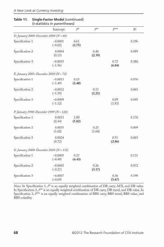
A New Look at Currency Investing
68 ©2012 The Research Foundation of CFA Institute
Intercept F* F** F*** R2
D. January 2000–December 2004 (N = 60)Speci¡cation 1 –0.0001 0.61 0.196
(–0.03) (3.75)
Speci¡cation 2 0.0004 0.40 0.089(0.15) (2.39)
Speci¡cation 3 –0.0033 0.72 0.386(–1.56) (6.04)
E. January 2005–December 2010 (N = 72)Speci¡cation 1 –0.0013 0.15 0.076
(–1.49) (2.40)
Speci¡cation 2 –0.0012 0.13 0.065(–1.39) (2.21)
Speci¡cation 3 –0.0009 0.09 0.045(–1.12) (1.83)
F. January 1990–December 1999 (N = 120)Speci¡cation 1 0.0013 1.00 0.176
(0.44) (5.02)
Speci¡cation 2 0.0035 0.25 0.009(1.02) (1.04)
Speci¡cation 3 0.0024 0.51 0.065(0.72) (2.86)
G. January 2000–December 2010 (N = 132)Speci¡cation 1 –0.0005 0.37 0.131
(–0.49) (4.43)
Speci¡cation 2 –0.0003 0.26 0.072(–0.27) (3.17)
Speci¡cation 3 –0.0007 0.36 0.198(–0.69) (5.67)
Notes: In Speci¡cation 1, F* is an equally weighted combination of DB carry, AFX, and DB value. In Speci¡cation 2, F** is an equally weighted combination of DB carry, DB trend, and DB value. In Speci¡cation 3, F*** is an equally weighted combination of RBS carry, RBS trend, RBS value, and RBS volatility.
Table 11. Single-Factor Model (continued) (t-statistics in parentheses)
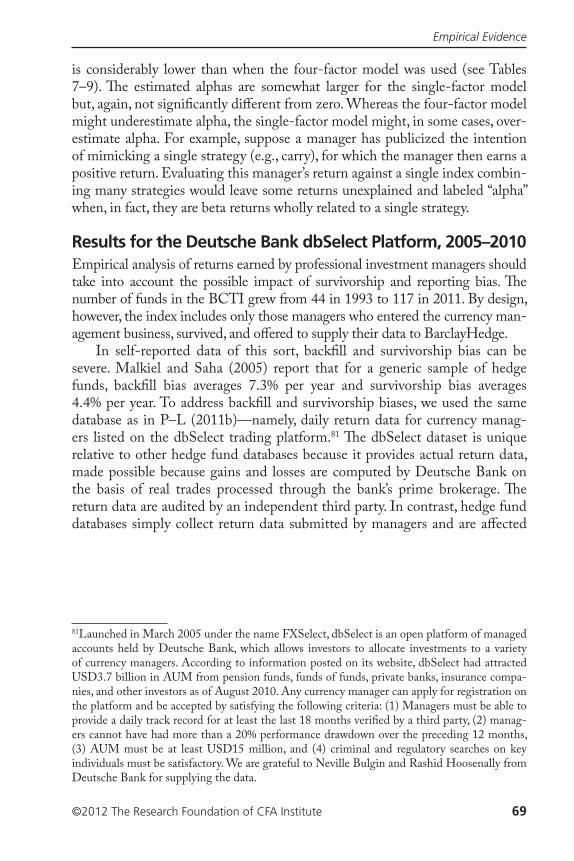
Empirical Evidence
©2012 The Research Foundation of CFA Institute 69
is considerably lower than when the four-factor model was used (see Tables 7–9). �e estimated alphas are somewhat larger for the single-factor model but, again, not signi¡cantly diªerent from zero. Whereas the four-factor model might underestimate alpha, the single-factor model might, in some cases, over-estimate alpha. For example, suppose a manager has publicized the intention of mimicking a single strategy (e.g., carry), for which the manager then earns a positive return. Evaluating this manager’s return against a single index combin-ing many strategies would leave some returns unexplained and labeled “alpha” when, in fact, they are beta returns wholly related to a single strategy.
Results for the Deutsche Bank dbSelect Platform, 2005–2010Empirical analysis of returns earned by professional investment managers should take into account the possible impact of survivorship and reporting bias. �e number of funds in the BCTI grew from 44 in 1993 to 117 in 2011. By design, however, the index includes only those managers who entered the currency man-agement business, survived, and oªered to supply their data to BarclayHedge.
In self-reported data of this sort, back¡ll and survivorship bias can be severe. Malkiel and Saha (2005) report that for a generic sample of hedge funds, back¡ll bias averages 7.3% per year and survivorship bias averages 4.4% per year. To address back¡ll and survivorship biases, we used the same database as in P–L (2011b)—namely, daily return data for currency manag-ers listed on the dbSelect trading platform.81 �e dbSelect dataset is unique relative to other hedge fund databases because it provides actual return data, made possible because gains and losses are computed by Deutsche Bank on the basis of real trades processed through the bank’s prime brokerage. �e return data are audited by an independent third party. In contrast, hedge fund databases simply collect return data submitted by managers and are aªected
81Launched in March 2005 under the name FXSelect, dbSelect is an open platform of managed accounts held by Deutsche Bank, which allows investors to allocate investments to a variety of currency managers. According to information posted on its website, dbSelect had attracted USD3.7 billion in AUM from pension funds, funds of funds, private banks, insurance compa-nies, and other investors as of August 2010. Any currency manager can apply for registration on the platform and be accepted by satisfying the following criteria: (1) Managers must be able to provide a daily track record for at least the last 18 months veri¡ed by a third party, (2) manag-ers cannot have had more than a 20% performance drawdown over the preceding 12 months, (3) AUM must be at least USD15 million, and (4) criminal and regulatory searches on key individuals must be satisfactory. We are grateful to Neville Bulgin and Rashid Hoosenally from Deutsche Bank for supplying the data.
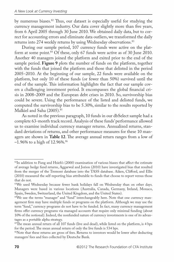
A New Look at Currency Investing
70 ©2012 The Research Foundation of CFA Institute
by numerous biases.82 �us, our dataset is especially useful for studying the currency management industry. Our data cover slightly more than ¡ve years, from 6 April 2005 through 30 June 2010. We obtained daily data, but to cor-rect for accounting errors and eliminate data outliers, we transformed the daily returns into 274 weekly returns by using Wednesday observations.83
During our sample period, 107 currency funds were active on the plat-form at some point.84 Of these, only 67 funds were active as of 30 June 2010. Another 40 managers joined the platform and exited prior to the end of the sample period. Figure 9 plots the number of funds on the platform, together with the funds that joined the platform and those that delisted in the period 2005–2010. At the beginning of our sample, 22 funds were available on the platform, but only 10 of these funds (or fewer than 50%) survived until the end of the sample. �is information highlights the fact that our sample cov-ers a challenging investment period. It encompasses the global ¡nancial cri-sis in 2008–2009 and the European debt crises in 2010. So, survivorship bias could be severe. Using the performance of the listed and delisted funds, we computed the survivorship bias to be 5.30%, similar to the results reported by Malkiel and Saha (2005).85
As noted in the previous paragraph, 10 funds in our dbSelect sample had a complete 63-month track record. Analysis of these funds’ performance allowed us to examine individual currency manager returns. Annualized returns, stan-dard deviations of returns, and other performance measures for these 10 man-agers are shown in Table 12. �e average annual return ranges from a low of –1.96% to a high of 12.96%.86
82In addition to Fung and Hsieh’s (2000) examination of various biases that aªect the estimate of average hedge fund returns, Aggarwal and Jorion (2010) have investigated bias that resulted from the merger of the Tremont database into the TASS database. Aiken, Cliªord, and Ellis (2010) measured the self-reporting bias attributable to funds that choose to report versus those that do not.83We used Wednesday because fewer bank holidays fall on Wednesday than on other days. Managers were based in various locations (Australia, Canada, Germany, Ireland, Monaco, Spain, Sweden, Switzerland, the United Kingdom, and the United States). 84We use the terms “manager” and “fund” interchangeably here. Note that one currency man-agement ¡rm may have multiple funds or programs on the platform. Although we may use the term “fund,” currency programs do not have to be funded. In fact, many currency management ¡rms oªer currency programs via managed accounts that require only minimal funding (about 10% of the notional). Indeed, the nonfunded nature of currency investments is one of its advan-tages as a portable alpha strategy.85�e mean annual return of all 107 funds (live and dead), while listed on the platform, is 4 bps for the period. �e mean annual return of only the live funds is 534 bps. 86Note that these returns are gross of fees. Returns to investors would be lower after deducting managers’ fees and fees collected by Deutsche Bank.
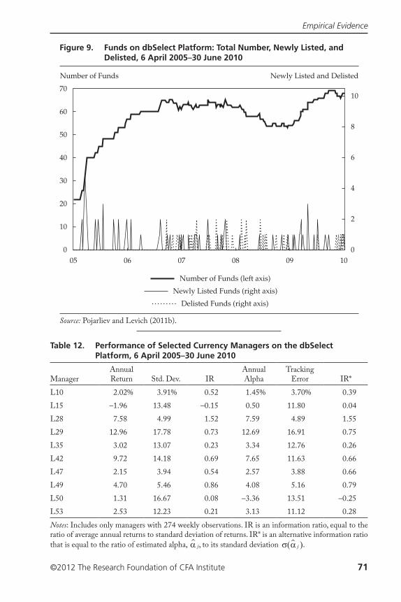
Empirical Evidence
©2012 The Research Foundation of CFA Institute 71
Figure 9. Funds on dbSelect Platform: Total Number, Newly Listed, and Delisted, 6 April 2005–30 June 2010
Number of Funds
70
60
50
40
30
20
10
0
Newly Listed and Delisted
10
8
6
4
2
005 10080706 09
Newly Listed Funds (right axis)
Delisted Funds (right axis)
Number of Funds (left axis)
Source: Pojarliev and Levich (2011b).
Table 12. Performance of Selected Currency Managers on the dbSelect Platform, 6 April 2005–30 June 2010
ManagerAnnual Return Std. Dev. IR
Annual Alpha
Tracking Error IR*
L10 2.02% 3.91% 0.52 1.45% 3.70% 0.39L15 –1.96 13.48 –0.15 0.50 11.80 0.04L28 7.58 4.99 1.52 7.59 4.89 1.55L29 12.96 17.78 0.73 12.69 16.91 0.75L35 3.02 13.07 0.23 3.34 12.76 0.26L42 9.72 14.18 0.69 7.65 11.63 0.66L47 2.15 3.94 0.54 2.57 3.88 0.66L49 4.70 5.46 0.86 4.08 5.16 0.79L50 1.31 16.67 0.08 –3.36 13.51 –0.25L53 2.53 12.23 0.21 3.13 11.12 0.28Notes: Includes only managers with 274 weekly observations. IR is an information ratio, equal to the ratio of average annual returns to standard deviation of returns. IR* is an alternative information ratio that is equal to the ratio of estimated alpha, α� j, to its standard deviation σ α( )� j .
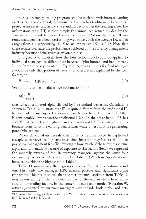
A New Look at Currency Investing
72 ©2012 The Research Foundation of CFA Institute
Because currency-trading programs can be initiated with interest-earning assets serving as collateral, the annualized return has traditionally been inter-preted as an excess return and the standard deviation as the tracking error. �e information ratio (IR) is then simply the annualized return divided by the annualized standard deviation. �e results in Table 12 show that these 10 cur-rency managers have been performing well since 2005; the average IR, which ranges from a disappointing –0.15 to an impressive 1.52, is 0.52. Note that these results overstate the performance achieved by the currency management industry because of the severe survivorship bias.
Our goal is to illustrate how the four-factor model could be applied to individual managers to diªerentiate between alpha hunters and beta grazers. In our framework as presented in Equation 9, excess returns for fund manager j would be only that portion of returns, αj, that are not explained by the four factors, or
α β ε� �j j t i j i t j tiR F= − +∑, , , , . (10)
We can thus de¡ne an alternative information ratio
IRjj
j
*
( )=
ασ α
�� (11)
that re©ects estimated alpha divided by its standard deviation. Calculations shown in Table 12 illustrate that IR* is quite diªerent from the traditional IR for some of the managers. For example, on the one hand, L50 has an IR* that is considerably lower than the traditional IR.87 On the other hand, L15 has an IR* that is markedly higher than the traditional IR. �is outcome occurs because some funds are earning beta returns while other funds are generating pure alpha returns.
When data analysis reveals that currency returns could be replicated cheaply with naive trading strategies, then investors may be less willing to pay active management fees. To investigate how much of these returns is pure alpha and how much is because of exposure to risk factors (beta), we regressed the monthly returns of the 10 currency managers against the same four explanatory factors as in Speci¡cation 1 in Table 7. (We chose Speci¡cation 1 because it yielded the highest R2 in Table 7.)
Table 13 summarizes the regression results. Several observations stand out. First, only one manager, L28, exhibits positive and signi¡cant alpha (intercept). �is result shows that the performance statistics from Table 12 may be misleading in that a substantial part of the returns stems from expo-sure to our trading factors. In the context of our factor model (Equation 9), returns generated by currency managers may include both alpha and beta 87L50 stands for manager #50 in the database. We are using the same notation for managers as in P–L (2010) and P–L (2011b).
Empirical Evidence
©2012 The Research Foundation of CFA Institute 73
returns. For example, Manager L50 has signi¡cant exposure to the trend-following strategy. �e trend coe�cient is large (1.42) and highly signi¡cant (t-value of 9.15), and the R2 (0.343) is the highest of all 10 managers. Table 12 indicates that Manager L50 generated annualized returns of 1.31% over this 63-month period, but this manager’s performance appears to re©ect primarily beta returns. �e alpha for L50 is negative (–7 bps per week) and not statisti-cally diªerent from zero.
Second, the highest factor exposure is to trend following. �e trend fac-tor is signi¡cant for 50% of the managers. �e carry factor is signi¡cant for four managers, but two managers have signi¡cant negative exposure to carry. Value is signi¡cant for only two managers, and ¡ve managers are signi¡cantly exposed to volatility.
Eight of the ten managers have a signi¡cant exposure to at least one fac-tor; three of those have a signi¡cant exposure to two factors. One manager has a signi¡cant exposure to three factors, and one, to all four factors. �ese results imply that managers have been diversifying across styles by having exposure to more than one style factor.
Table 13. Regression Results for Equation 10 for Individual Currency Managers: Managers j = 1, . . ., 10, 6 April 2005–30 June 2010 (based on 274 weekly observations)
Manager Intercept t-StatBeta Carry t-Stat
Beta Trend t-Stat
Beta Value t-Stat
Beta Volatility t-Stat R2
L10 0.0003 0.91 0.01 0.71 0.14 3.24 0.01 0.31 0.13 2.41 0.102
L15 0.0001 0.09 0.43 6.60 0.49 3.60 –0.58 –6.70 0.25 1.50 0.233
L28 0.0015 3.52 –0.02 –0.85 0.04 0.70 –0.05 –1.45 0.11 1.50 0.037
L29 0.0024 1.70 –0.30 –3.20 –0.32 –1.64 –0.02 –0.15 0.63 2.58 0.094
L35 0.0006 0.59 0.13 1.77 0.08 0.54 0.02 0.23 –0.37 –2.00 0.047
L42 0.0015 1.49 –0.60 –9.37 –0.11 –0.82 0.16 1.85 0.18 1.08 0.327
L47 0.0005 1.49 0.01 0.24 –0.07 –1.57 –0.05 –1.69 0.07 1.23 0.028
L49 0.0008 1.78 –0.03 –0.93 0.15 2.60 –0.01 –0.17 0.17 2.27 0.106
L50 –0.0007 –0.57 –0.03 –0.40 1.42 9.15 0.06 0.64 0.16 0.80 0.343
L53 0.0006 0.64 0.35 5.77 0.68 5.32 –0.33 –4.03 0.02 0.10 0.173
Note: Signi¡cant t-statistics are in boldface.
A New Look at Currency Investing
74 ©2012 The Research Foundation of CFA Institute
Summary of Empirical ResultsOverall, these empirical results show that four factors, representing three
styles of currency investing and the volatility of the FX market, explain a sig-ni¡cant part of the returns of professional currency managers.88 �e average excess return of the BCTI was positive at 22 bps per month between 1990 and 2010. Once we account for the four systematic beta factors, however, the alpha is no longer positive or signi¡cant.89 Most importantly, these results are robust to using diªerent proxies for the risk factors, diªerent datasets for returns of professional currency managers, and measurement over diªerent time hori-zons. �is result demonstrates that currencies have similarities with other asset classes whose returns can be related to risk factors.
Trend appears to be the most important factor, followed by carry; value and volatility appear to be less important. Interestingly, the value beta in most cases (or speci¡cations) is negative, indicating that currency managers, as a group, were betting against PPP during the sample period.90
Note some interesting diªerences between the various subperiods. For example, managers reduced their exposure to trend in the post-2000 period relative to the 1990s. �e highest exposure to carry (as measured by the size of the beta estimates) was recorded in the 2000–04 period; this exposure was sharply reduced between 2005 and 2010.
Note that the reported alpha estimates are probably biased toward the downside, thus underestimating the value added by active currency managers. Ideally, the performance of any active manager should be evaluated against available investable passive alternatives that incorporate the transaction costs associated with each dynamic trading strategy. �e DB currency indices are investable through existing single products, but the RBS currency indices are not. And an important consideration is that, although the AFX is investable, in the sense that its dynamic strategy is transparent and readily implemented in the G–10 currencies, no live version of the AFX exists that incorporates transaction costs and other market frictions.91 �is warning could be impor-tant because the AFX appears to be the dominant factor in explaining the 88In some speci¡cations, volatility represents the returns of a trading strategy of being short FX volatility by selling FX options; in others, volatility represents the ¡rst diªerence in the level of FX volatility.89Depending on the proxies for risk factors and time horizon, the alpha is, in some instances, negative and signi¡cant.90Betting against value has reduced the total return, on average, because value generated positive returns over the investigated time horizon. 91�e problem of using style factors that omit transaction costs and other market frictions is present in related empirical studies. �e standard evaluation for equity funds calculates alpha in excess of returns on the Fama–French (1992, 1993) and Carhart (1997) factors. Although passive indices exist that proxy the Fama–French factors, no passive investment vehicle provides exposure to the momentum factor of Carhart.
Empirical Evidence
©2012 The Research Foundation of CFA Institute 75
returns of the currency managers. An attempt to replicate the actual return of the AFX would be likely to yield lower returns than studies report after trans-action costs, management fees, and market impact costs.
Our empirical results suggest that, as with other asset classes, the currency market oªers beta-like returns and some managers are able to generate signi¡-cant alpha returns over and above the returns explained by the style factors.92
In the next chapter, we address the question of how institutional managers can add currency alpha and beta to their portfolios.
92P–L (2008) report that much of the alpha return comes from market timing, with the great-est timing ability apparent in the trend factor. Put diªerently, managers, as a group, have been able to increase their exposure to trend when returns of trend following rise and decrease their exposure to trend when returns of trend following fall.
76 ©2012 The Research Foundation of CFA Institute
5. Currency Alpha and Beta for Institutional Investors
�e historical starting point for a U.S. institutional investor is the classic 60/40 portfolio—60% stocks and 40% bonds. �is classic portfolio has evolved con-siderably over the years as institutional investors allocate less to traditional assets, such as equities and bonds, and more to alternative investments, such as hedge funds, private equity, and commodities (Anson 2011). �is trend has been partly the result of conventional beliefs that hedge funds can pursue diverse goals, that diversi¡cation is the key to successful investing, and that returns on alternative assets have little or no correlation with returns on tra-ditional investments. As the global ¡nancial crisis unfolded, however, many hedge funds delivered negative returns. Investors discovered that they were less diversi¡ed than expected. In other words, despite the fact that most insti-tutional investors have diversi¡ed allocations to span a variety of asset classes, as Leibowitz (2011) points out, “Some level of implicit equity exposure lurks in virtually every asset.” �is discovery prompted investors to rethink asset allocation. �e investment management industry responded by oªering (yet again) a variety of new products—for example, insurance against equity tail risk (tail-hedging products) and alternative approaches to asset allocation, such as risk factor–based asset allocation and risk parity (Litterman 2011).
�e advocates of risk factor–based asset allocation point out that, on aver-age, correlations between risk factors are lower than correlations between asset classes and that risk factor correlations tend to be more robust to regime shifts than asset class correlations (Lee 2011). Risk parity, the most recent devel-opment in the evolution of asset allocation, attempts to equalize risk expo-sure across various asset classes. Leibowitz and Bova (2007) show that, even in a diversi¡ed institutional asset portfolio, up to 90% of the volatility can be explained by the equity market. Although the typical institutional portfolio is diversi¡ed into a variety of asset classes, these asset classes have a correlation with equity markets high enough (especially in periods of market stress) that, overall, equity risk constitutes more than 80% of the total risk of the portfolios (Anson 2011). A risk parity approach for asset allocation would, therefore, allo-cate a much smaller amount to equity than is held in the classic 60/40 portfolio.
�ese new approaches to asset allocation do not invalidate the traditional core–satellite investment approach for asset allocation, in which the bulk of the assets (the core) are invested in long-only managers and a small propor-tion of assets are invested in satellites, such as hedge funds, real estate, and commodities. �e new approaches focus on the question of how to allocate the
Currency Alpha and Beta for Institutional Investors
©2012 The Research Foundation of CFA Institute 77
core e�ciently. Because the core makes up the bulk of an institution’s assets, this question is, of course, extremely important. Yet, in an investment world where beta returns might be too low compared with the usual 5% spending rate of endowments and 7–8% required annual returns of most pension funds (the yield on 30-year U.S. Treasuries fell below 3% in September 2011), the satellites remain a crucial part of the investment portfolio. Leibowitz (2011) points out, “With so many funds in this beta-dominated camp, there will be an ample retinue of potentially motivated buyers for any asset with a reason-able alpha ratio” (p. 7). �erefore, investors should pay close attention to both who is a real alpha hunter (and a candidate for a satellite) and how to allocate assets e�ciently and cheaply among various beta grazers (the core).
In this chapter, we consider the possibility that currency is an underused asset class where new beta grazers and alpha hunters can be identi¡ed and added to the traditional approach. �e key questions for plan sponsors are, (1) Can diversifying at the margin into currency funds bene¡t their performance, and (2) if so, which currency managers might be most worthwhile to add?
To explore these questions, we considered a benchmark global equity portfolio evaluated against three alternative portfolios with some exposure to currencies. Of course, most institutional investors have diversi¡ed allocations that span a variety of asset classes. Remember Leibowitz’s (2011) warning, however, about lurking equity exposure in virtually every asset. Consequently, using the MSCI World Index as the benchmark to gauge the bene¡t of adding currency alpha seems appropriate. Each of the three alternative portfolios allo-cates 2% of its assets to a cash margin account to obtain a 20% notional expo-sure to currencies through some of the managers listed in Tables 12 and 13. �e resulting currency share in the total portfolio is 16.9%.93
Portfolios 1, 2, and 3 all invest 98% of their assets in a fund that tracks the MSCI World, but each one diªers in terms of which currency managers, selected from the dbSelect platform, are allocated the remaining 2% cash share.
• Portfolio 1: �e Currency Beta Portfolio. �e currency allocation is invested in an equally weighted exposure of three naive currency indices designed to capture carry, trend, and value beta. �e three indices are the DB carry index, the AFX, and the DB value index.
• Portfolio 2: �e Beta-Grazer Portfolio. �e currency allocation is invested in an equally weighted exposure of the top three beta grazers (i.e., those with the highest estimated R2s). �ese are managers L50, L42, and L15.
93Assume that an investor has USD100 million. He invests USD98 million in the MSCI World via an index fund and uses the other USD2 million as margin to obtain USD20 million notional exposure to three currency managers. He allocates USD6.66 million notional to each of the managers, so the currency share in the total portfolio is then 20/118, or 16.9%.
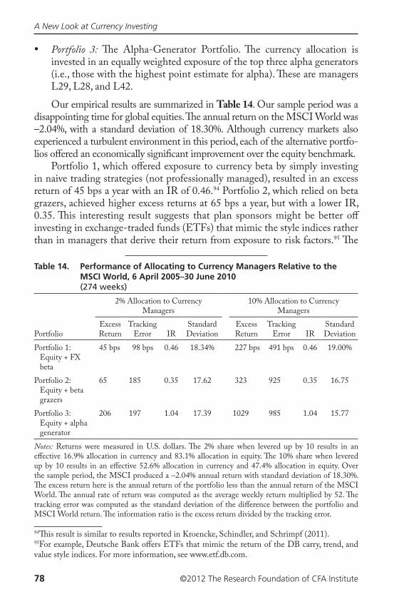
A New Look at Currency Investing
78 ©2012 The Research Foundation of CFA Institute
• Portfolio 3: �e Alpha-Generator Portfolio. �e currency allocation is invested in an equally weighted exposure of the top three alpha generators (i.e., those with the highest point estimate for alpha). �ese are managers L29, L28, and L42.
Our empirical results are summarized in Table 14. Our sample period was a disappointing time for global equities. �e annual return on the MSCI World was –2.04%, with a standard deviation of 18.30%. Although currency markets also experienced a turbulent environment in this period, each of the alternative portfo-lios oªered an economically signi¡cant improvement over the equity benchmark.
Portfolio 1, which oªered exposure to currency beta by simply investing in naive trading strategies (not professionally managed), resulted in an excess return of 45 bps a year with an IR of 0.46.94 Portfolio 2, which relied on beta grazers, achieved higher excess returns at 65 bps a year, but with a lower IR, 0.35. �is interesting result suggests that plan sponsors might be better oª investing in exchange-traded funds (ETFs) that mimic the style indices rather than in managers that derive their return from exposure to risk factors.95 �e
94�is result is similar to results reported in Kroencke, Schindler, and Schrimpf (2011).95For example, Deutsche Bank oªers ETFs that mimic the return of the DB carry, trend, and value style indices. For more information, see www.etf.db.com.
Table 14. Performance of Allocating to Currency Managers Relative to the MSCI World, 6 April 2005–30 June 2010 (274 weeks)
2% Allocation to Currency Managers
10% Allocation to Currency Managers
PortfolioExcess Return
Tracking Error IR
Standard Deviation
Excess Return
Tracking Error IR
Standard Deviation
Portfolio 1: Equity + FX beta
45 bps 98 bps 0.46 18.34% 227 bps 491 bps 0.46 19.00%
Portfolio 2: Equity + beta grazers
65 185 0.35 17.62 323 925 0.35 16.75
Portfolio 3: Equity + alpha generator
206 197 1.04 17.39 1029 985 1.04 15.77
Notes: Returns were measured in U.S. dollars. �e 2% share when levered up by 10 results in an eªective 16.9% allocation in currency and 83.1% allocation in equity. �e 10% share when levered up by 10 results in an eªective 52.6% allocation in currency and 47.4% allocation in equity. Over the sample period, the MSCI produced a –2.04% annual return with standard deviation of 18.30%. �e excess return here is the annual return of the portfolio less than the annual return of the MSCI World. �e annual rate of return was computed as the average weekly return multiplied by 52. �e tracking error was computed as the standard deviation of the diªerence between the portfolio and MSCI World return. �e information ratio is the excess return divided by the tracking error.
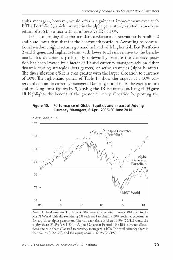
Currency Alpha and Beta for Institutional Investors
©2012 The Research Foundation of CFA Institute 79
alpha managers, however, would oªer a signi¡cant improvement over such ETFs. Portfolio 3, which invested in the alpha generators, resulted in an excess return of 206 bps a year with an impressive IR of 1.04.
It is also striking that the standard deviations of returns for Portfolios 2 and 3 are lower than that for the benchmark portfolio. According to conven-tional wisdom, higher returns go hand in hand with higher risk. But Portfolios 2 and 3 generated higher returns with lower total risk relative to the bench-mark. �is outcome is particularly noteworthy because the currency posi-tion has been levered by a factor of 10 and currency managers rely on either dynamic trading strategies (beta grazers) or active strategies (alpha hunters). �e diversi¡cation eªect is even greater with the larger allocation to currency of 10%. �e right-hand panels of Table 14 show the impact of a 10% cur-rency allocation to currency managers. Basically, it multiplies the excess return and tracking error ¡gures by 5, leaving the IR estimates unchanged. Figure 10 highlights the bene¡t of the greater currency allocation by plotting the
Figure 10. Performance of Global Equities and Impact of Adding Currency Managers, 6 April 2005–30 June 2010
6 April 2005 = 100
170
150
130
110
90
70
5005 0706 08 09 10
Alpha GeneratorPortfolio B
AlphaGenerator
Portfolio A
MSCI World
Notes: Alpha-Generator Portfolio A (2% currency allocation) invests 98% cash in the MSCI World with the remaining 2% cash used to obtain a 20% notional exposure in the top three alpha generators. �e currency share is then 16.9% (20/118), and the equity share, 83.1% (98/118). In Alpha-Generator Portfolio B (10% currency alloca-tion), the cash share allocated to currency managers is 10%. �e total currency share is then 52.6% (100/190), and the equity share is 47.4% (90/190).
A New Look at Currency Investing
80 ©2012 The Research Foundation of CFA Institute
cumulative performance of the Alpha-Generator Portfolio with either a 2% or a 10% cash allocation to currency managers. �e MSCI World is included as the benchmark.
Portfolio 1 has a standard deviation slightly higher than the benchmark portfolio. Investing in pure currency beta (via indices) would have increased the return of the portfolio but with no diversi¡cation bene¡t. In our sample, only the alpha generators oªer a real diversi¡cation gain.
Overall, our analysis suggests that adding a relatively small position in currency of 2% (albeit levered by 10 to boost the weight in the portfolio to 16.9%) can bring about an economically signi¡cant improvement in per-formance. �e currency component had the undesirable eªect of increasing tracking error versus the benchmark by a relatively small amount but also pro-duced a portfolio with lower total risk.
Note that these results represent an in-sample experiment: At the begin-ning of the time period studied, it was not possible to distinguish between the beta grazers and the alpha generators. P–L (2011b) reports similar out-of-sample results, however, which supports the notion of alpha and beta persis-tence. In the earlier work, we classi¡ed managers into beta grazers and alpha generators in-sample and showed that (1) the classi¡cation tends to hold out-of-sample and (2) currency managers classi¡ed as alpha generators in-sample provide the greatest bene¡ts to equity portfolios out-of-sample.
�ese results imply that, although all currency managers who excel at generating returns in general add excess returns to the benchmark portfolio and provide some diversi¡cation gain, some managers oªer more bene¡ts to institutional investors than others. Consequently, applying the framework developed by P–L (2008) can be useful for diªerentiating between currency managers who are beta grazers and those who are alpha hunters and for selecting the managers best suited to the institutional portfolio. In particular, the following three steps could be incorporated into the fund’s due diligence process to obtain exposure to currency alpha:
• Collect return data on currency managers. Although all disclaimers state that past performance is not an indication of future performance, P–L (2011b) reports alpha and beta persistence for professional currency managers. Hence, past performance data can be used to diªerentiate between alpha hunters and beta grazers.96
96We caution against the use of databases with self-reported returns. Fortunately, many FX-only hedge fund platforms allow potential investors to evaluate managers’ track records. Deutsche Bank’s dbSelect, launched in March 2005, is one. Recently, both Citibank and Morgan Stanley have also developed FX-only platforms.
Currency Alpha and Beta for Institutional Investors
©2012 The Research Foundation of CFA Institute 81
• Identify the alpha generators. �e four-factor model proposed by P–L (2008) can next be used to group managers into alpha generators, alpha hunters, beta grazers, and underperformers. Managers with high alphas are alpha generators, and managers with low alpha are underperformers. Managers with high R2s are beta grazers, and managers with low R2s are alpha hunters. �is classi¡cation would be constructed in-sample, but empirical evidence suggests that these broad categories are likely to persist out-of-sample.
• Allocate to the alpha generators. �e ¡nal step involves setting up the parame-ters of the currency mandate and dealing with the structural and operational choices described in Chapter 2. For example, absolute currency mandates could be tailored to diªerent levels of risk aversion. �is step could involve agreeing on a maximum monthly drawdown or target volatility.
Of course, these steps are only a small part of the due diligence process required to identify suitable managers. Our empirical results suggest, however, that incorporating these ideas into an existing manager selection approach is likely to provide value in determining the currency managers most likely to bene¡t institutional portfolios.

82 ©2012 The Research Foundation of CFA Institute
6. Conclusions and Implications for Investment Management
We have taken a new look at currency management by applying an established methodology to a subset of the hedge fund industry—currency funds—which is something that has not been done previously. And we addressed several fun-damental questions: Do style factors oªer a useful way to explain currency returns and also allow investors to diªerentiate between alpha and beta com-ponents? Are currency returns predictable to any extent? Is managerial per-formance or management style persistent? Do currency managers—whether pure index followers, discretionary beta grazers, or genuine alpha hunters—add value to otherwise well-diversi¡ed global equity portfolios? In a generic core–satellite setting, would institutional managers be well served by adding currency managers to the satellite managers they rely on?97
�e answers to these questions are, in most cases, yes, and the reasons are threefold. First, the foreign exchange market oªers substantial depth and liquidity for large institutional investors. As noted in Chapter 2, daily average FX market turnover reached USD4 trillion in April 2010, a 20% increase over 2007. �is liquidity was precious during the market turmoil in 2008. Second, empirical evidence shows that returns generated by most currency strategies are, to a large extent, explained by style factors that proxy for common cur-rency investment strategies and that currency returns are generally uncorre-lated with returns from other asset classes. �ird, and most importantly, the empirical evidence suggests that some managers have been able to deliver statistically and economically signi¡cant alpha even when measured against a strict benchmark based on style factors.
We qualify our answer with “in most cases” because some institutional investors might lack the governing structure needed to conduct the proper due diligence for allocating to standalone currency managers. In these cases, expo-sure to currency alpha might be obtained through a currency fund of funds whereas exposure to currency beta might be obtained through currency ETFs. Other institutional investors might prefer to gain exposure to currency alpha through allocations to global macro funds, many of which use currency invest-ment strategies. In most cases, however, the currency alpha generated by these macro funds cannot be separated from the total alpha generated. �erefore, it is often impossible to evaluate whether the specialists (FX-only managers) are
97Our discussion focused on standalone active currency managers as a source of return. Global institutional portfolios may have currency exposure through investing in foreign currency–denominated assets.

Conclusions and Implications for Investment Management
©2012 The Research Foundation of CFA Institute 83
outperforming or underperforming the generalists (global macro funds). In any case, the question of whether to invest in boutiques or supermarkets is not con¡ned to currency management and is beyond the scope of this book.
As discussed in Chapter 1, institutional investors may harbor realistic doubts regarding the suitability of currency as an asset class. Currency markets are highly specialized, with terminology and institutional features that diªer from equity trading on organized exchanges. Concerns regarding the elusive nature of currency valuation and trading relationships cause some inves-tors to wonder whether relying on currency as an ongoing source of return makes sense—particularly because currency may seem so diªerent from “real investments,” such as stocks, bonds, or even commodities and precious met-als with alternative industrial uses. �at currency trading is lightly regulated and prone to central bank intervention may seem to layer on additional risks. Furthermore, the assets under management at most currency managers are relatively small compared with the size of most institutional investors.98 As a result, plan sponsors may have di�culties allocating to FX managers.99
Another important challenge for institutional investors is to identify appro-priate benchmarks for gauging the performance of currency managers. Without appropriate benchmarks, one cannot tell whether managers have demonstrated true skill or not. Because of the heterogeneity in mandates, Melvin and Shand (2011) question whether a single benchmark can be appropriate for all cur-rency managers. But if not, the solution would be adopting more benchmarks rather than adopting zero as the standard. Looking at a range of alpha esti-mates is more bene¡cial than treating all return as alpha return. �e lack of well-established benchmarks may be one of the reasons allocations to currency strategies remain low compared with allocations to hedge funds in general.100
98Of the 115 managers who reported AUM to BarclayHedge in January 2010, 86 (or about 75%) managed AUM less than USD100 million and only 10 (fewer than 10%) reported AUM in excess of USD500 million.99As a rule of thumb, institutional investors avoid allocating to managers in excess of ⅓ of the manager’s total AUM. For example, if the manager has USD100 million total AUM, an inves-tor would rarely allocate more than USD35 million to that manager, which could be too small of an allocation (1) to have an impact on the investor’s overall portfolio return and (2) to justify the costs for initial and ongoing due diligence.100In contrast, numerous indices track other assets—small-capitalization, value, and emerging market stocks, stocks grouped by region and industry sector, various categories within ¡xed income and the term structure, and commodities. Vendors abound—S&P, MSCI, Barclays, Russell, and others. �ese developments have allowed institutional managers to ©ourish in these niche categories. For example, AUM in the SPDR Gold Shares (NYSE:GLD), which delivers the return on gold bullion, is USD69.77 billion, whereas the AUM in a currency ETF available in the United Kingdom for institutional investors that mimics the return of the carry trade was merely GBP6.38 million as of 26 March 2012 (www.etf.db.com).
A New Look at Currency Investing
84 ©2012 The Research Foundation of CFA Institute
In many studies of currency-trading strategies, researchers have used zero as the expected return from currency speculation and interpreted all realized returns as unusual, excess returns. In the same vein, zero has often been used as a traditional benchmark to assess the performance of currency fund manag-ers who pursue an absolute return mandate.101 In contrast to the traditional benchmark, we have proposed a four-factor regression model as an alternative technique to gauge the performance of currency managers (initially proposed in P–L 2008). �e model estimates what portion of currency-trading pro¡ts is the result of exposure to these speci¡c trading styles or risk factors (beta) and what portion is the result of skill (alpha).
In empirical tests of the four-factor model, P–L (2008, 2010) use diªerent proxies for the risk factors, but the results are strikingly similar. Depending on the time period, periodicity, and model speci¡cation, four risk factors explain 50–75% of the variability of currency fund (index) returns. We have updated some of the results with more recent data and used diªerent proxies for the risk factors as robustness checks. �e general conclusions remain unchanged: A signi¡cant part of currency returns comes from exposure to a small set of factors that proxy the returns of well-known and easily implemented trad-ing styles. As a consequence, much of what might have been labeled “alpha” against the traditional benchmark (of zero) may be beta returns when mea-sured against the alternative benchmark. So, in some respects, currencies seem not so diªerent from other asset classes: �e average manager may deliver zero alpha, but some skilled managers are able to deliver signi¡cant alpha.102
We have reported results when using various proxies for the style factors, but using diªerent style factors could change the results, as Melvin and Shand (2011) caution. In addition, other factors we have omitted (such as drawdown of capital) could matter to investors. Despite these caveats about our work, we suggest that it is an improvement over the alternative—to retain the tradi-tional performance benchmark of zero and forsake the use of a limited set of style factors for benchmarking. Keeping the zero benchmark would be incon-sistent not only with our results but also with the general principle of adjusting all returns for any systematic eªects or factors they may be found to contain.
For several reasons, institutional investors should be concerned about how much of a currency manager’s return is alpha and how much is beta. First, proper return attribution could lead to some repricing for “active” currency
101In 2011, Citibank launched a new multimanager platform, CitiFX Access. �e platform oªers a range of investable currency indices, and some of these indices are intended to serve as a benchmark by providing exposure to currency managers who are deemed to represent the industry. Such a group of managers may be regarded as a peer group benchmark. 102See Jones and Wermers (2011) for a recent survey of the literature on the value of active management. �ey show that the average manager does not outperform but that a signi¡cant minority of active managers do add value.
Conclusions and Implications for Investment Management
©2012 The Research Foundation of CFA Institute 85
products. Investors should not be required to pay alpha fees for exposure to currency style betas that could be earned more cheaply. Second, currency beta might be less suitable for institutional investors than currency alpha when the goal is to diversify global equity exposure. In Chapter 5, we showed that a global equity portfolio that diversi¡ed by using alpha generators would have outperformed a portfolio invested in beta grazers by 141 bps a year between 6 April 2005 and 30 June 2010. Diversifying with beta grazers is bene¡cial, as indicated by a positive IR of 0.35, but much less bene¡cial than investing in alpha generators, which yielded an IR of 1.04. Indeed, investors would have been better oª simply investing in currency beta via ETFs, as highlighted by the IR of 0.46, than investing in the beta grazers.
�is last result could lead institutional investors to pay close attention to the return attribution of their currency managers. Over the periods for which measurements are available, all of the currency style factors generated positive average returns. Given the relatively long history of these factors, we expect this pattern of positive currency returns to continue. With that assumption, we consider that all currency expected returns will make an incremental con-tribution to overall portfolio returns but that some managers will be more likely to have persistently good performance with greater diversi¡cation ben-e¡ts. Choosing the “right” currency managers could increase the diversi¡ca-tion bene¡ts considerably for global equity portfolios. Finding these managers is challenging, but the bene¡ts to a portfolio might be considerable. In an investment world where the beta return might be too low to cover future lia-bilities, investors cannot aªord to ignore potential alpha providers.
86 ©2012 The Research Foundation of CFA Institute
Appendix A: Currency Indices and Style Factors
Currency Index or Style Factor Description Provider SourceBCTI �e Barclay Currency Traders Index
is an equally weighted composite of managed programs that trade currency futures and/or cash forwards in the interbank market. In 2011, 117 currency programs were included in the index.
BarclayHedge Monthly data available on Bloomberg (code FXTP)
DB Carry �e Deutsche Bank Currency Harvest G10 Index systematically invests in the three highest yielding G–10 currencies through funding in the three lowest yielding currencies; it rebalances quarterly.
Deutsche Bank Monthly data available on Bloomberg (code DBHVG10U Index)
RBS Carry (see Notes)
�e Royal Bank of Scotland Carry Index re©ects the return of being long the higher yielding currencies against being short the lower yielding currencies (position size is proportional to yield relative to U.S. rate).
Royal Bank of Scotland
Monthly data available on Bloomberg (code FXTP)
AFX Index (see Notes)
�e AFX Currency Management Index is based on trading in seven currency pairs weighted by their volume of turnover in the spot market, with returns for each pair based on an equally weighted portfolio of three moving-average rules (32, 61, and 117 days); the seven currency pairs are EUR/USD, USD/JPY, USD/CHF, GBP/USD, EUR/JPY, EUR/GBP, and EUR/CHF.
Liverpool John Moores University
Monthly data for this index are available at the AFX web site (www.jmu.ac.uk/LBS/102316.htm); we are grateful to Pierre Lequeux of Aviva Investors for providing daily data
DB Trend �e Deutsche Bank Momentum Index invests in the three best performing, highest momentum G–10 currencies over the previous 12 months (spot returns against the USD) and borrows in the three worst performing currencies; rebalancing is monthly.
Deutsche Bank Monthly data available on Bloomberg (code DBMOMUSF)
(continued)
Appendix A
©2012 The Research Foundation of CFA Institute 87
Currency Index or Style Factor Description Provider SourceRBS Trend (see Notes)
�e Royal Bank of Scotland Value Index re©ects the return of a simple moving-average strategy combined with a simple rule to reduce whipsaw.
Royal Bank of Scotland
Monthly data available on Bloomberg (code FXTP)
DB Value �e Deutsche Bank Valuation Index goes long the three most undervalued G–10 currencies relative to OECD PPP values and goes short the three most overvalued currencies; rebalancing is quarterly.
Deutsche Bank Monthly data available on Bloomberg (code DBPPPUSF)
RBS Value (see Notes)
�e Royal Bank of Scotland Value Index re©ects the return of going long undervalued currencies against overvalued currencies with position size proportional to the amount of over- and undervaluation.
Royal Bank of Scotland
Monthly data available on Bloomberg (code FXTP)
DB Volatility �e Deutsche Bank Currency Volatility Index is calculated based on the three-month implied volatilities of nine major currency pairs. �e currency pairs and their index weights are as follows: EUR/USD (37.84%), USD/JPY (18.92%), GBP/USD (12.16%), USD/CHF (5.41%), USD/CAD (6.76%), AUD/USD (8.11%), EUR/JPY (4.05%), EUR/GBP (4.05%), and EUR/CHF (2.70%).
Deutsche Bank Monthly data available on Bloomberg (code CVIX Index)
RBS Volatility (see Notes)
�e Royal Bank of Scotland Volatility Index re©ects the return of being short volatility; the strategy sells an at-the-money forward straddle for each currency against the USD at the start of each month if implied volatility is above its one-year average for that currency.
Royal Bank of Scotland
Monthly data available on Bloomberg (code FXTP)
(continued)
A New Look at Currency Investing
88 ©2012 The Research Foundation of CFA Institute
Currency Index or Style Factor Description Provider SourceCarry Global �e Global Harvest Index invests in
the ¡ve highest yielding currencies while shorting the ¡ve lowest yielding currencies, regardless of geographic region; the currency universe consists of the G–10 currencies and the following currencies: South Korean won (KRW), Singapore dollar (SGD), New Taiwan dollar (TWD), Mexican peso (MXN), Brazilian real (BRL), Turkish new lira (TRY), Polish zloty (PLN), Hungarian forint (HUF), Czech koruna (CZK), and South African rand (ZAR).
Deutsche Bank Monthly data available on Bloomberg (code DBHVGUSI Index)
Carry Balanced �e Balanced Harvest Index invests in the two highest yielding G–10 currencies plus three currencies chosen from the whole currency universe and shorts the two lowest yielding G–10 currencies and the three lowest yielding currencies from the entire currency pool; the non-G–10 pool consists of the KRW, SGD, TWD, MXN, BRL, TRY, PLN, HUF, CZK, and ZAR.
Deutsche Bank Monthly data available on Bloomberg (code DBHVBUSI Index)
Notes: At the time of our writing, the RBS indices were available on Bloomberg, code FXTP. �e RBS discontinued publishing the data, however, at the beginning of 2012. Also at the time of our writing, the AFX was available at and maintained by Liverpool John Moores University. Although this website is no longer available, a cached version is available at http://web.archive.org/web/20100527043718/http://www.ljmu.ac.uk/LBS/102316.htm. At present, monthly data for the AFX Index is prepared by Pierre Lequeux and available through a link at http://people.stern.nyu.edu/rlevich/afx_index.html.
©2012 The Research Foundation of CFA Institute 89
REFERENCES
Abuaf, Niso, and Philippe Jorion. 1990. “Purchasing Power Parity in the Long Run.” Journal of Finance, vol. 45, no. 1 (March):157–174.
Aggarwal, Rajesh K., and Philippe Jorion. 2010. “Hidden Survivorship in Hedge Fund Returns.” Financial Analysts Journal, vol. 66, no. 2 (March/April):69–74.
Aiken, Adam L., Christopher P. Cliªord, and Jesse A. Ellis. 2010. “Out of the Dark: Hedge Fund Reporting Biases and Commercial Databases.” Working paper: http://ssrn.com/abstract=1519914.
Ali, Magda. 2010. “Citi Indexes Oªer Low-Cost Forex Exposure.” FX Week (12 November).
Anson, Mark. 2011. “�e Evolution of Equity Mandates in Institutional Portfolios.” Journal of Portfolio Management, vol. 37, no. 4 (Summer):127–137.
Baba, Naohiko, and Frank Packer. 2009. “Interpreting Deviations from Covered Interest Parity during the Financial Market Turmoil of 2007–08.” Journal of Banking & Finance, vol. 33, no. 11 (November):1953–1962.
Binny, James. 2005. “Currency Management Style through the Ages.” Journal of Alternative Investments, vol. 8, no. 3 (Winter):52–59.
BIS. 2010. “Triennial Central Bank Survey: Report on Global Foreign Exchange Market Activity in 2010.” Bank for International Settlements (December).
Brunnermeier, Markus K., Stefan Nagel, and Lasse H. Pedersen. 2009. “Carry Trades and Currency Crashes.” NBER Macroeconomics Annual, vol. 23, no. 1 (April):313–348.
Burnside, Craig. 2011. “Carry Trades and Risk.” NBER Working Paper No. 17278 (August).
Carhart, Mark M. 1997. “On Persistence in Mutual Fund Performance.” Journal of Finance, vol. 52, no. 1 (March):57–82.
Chen, Nai-Fu, Richard Roll, and Stephen A. Ross. 1986. “Economic Forces and the Stock Market.” Journal of Business, vol. 59, no. 3 ( July):383–403.
Chinn, Menzie D., and Guy Meredith. 2004. “Monetary Policy and Long-Horizon Uncovered Interest Parity.” IMF Sta� Papers, vol. 51, no. 3 (November):409–430.
Chow, George, Eric Jacquier, Mark Kritzman, and Kenneth Lowry. 1999. “Optimal Portfolios in Good Times and Bad.” Financial Analysts Journal, vol. 55, no. 3 (May/June):65–73.
Clements, Kenneth W., Yihui Lan, and Shi Pei Seah. 2012. “�e Big Mac Index Two Decades On: An Evaluation of Burgernomics.” International Journal of Finance & Economics, vol. 17, no. 1 ( January):31–60.
A New Look at Currency Investing
90 ©2012 The Research Foundation of CFA Institute
Coªey, Niall, Warren B. Hrung, and Asani Sarkar. 2009. “Capital Constraints, Counterparty Risk, and Deviations from Covered Interest Rate Parity.” Federal Reserve Bank of New York Staª Reports No. 393 (September).
Cumby, Robert E. 1996. “Forecasting Exchange Rates and Relative Prices with the Hamburger Standard: Is What You Want What You Get with McParity?” NBER Working Paper No. 5675 ( July).
Dash, Eric. 2009. “State Street Bank Accused of Fraud by California.” New York Times(20 October).
Dash, Eric, and Peter Lattman. 2011. “U.S. and New York Sue Bank of New York Mellon over Foreign Exchange Fees.” New York Times (4 October).
Dickson, Tim. 1991. “�e Growing Appeal of Overseas Assets.” Financial Times, Survey on International Fund Management (18 April):IV.
Engel, Charles. 1996. “�e Forward Discount Anomaly and the Risk Premium: A Survey of Recent Evidence.” Journal of Empirical Finance, vol. 3, no. 2 ( June):123–192.
Fama, Eugene F., and Kenneth R. French. 1992. “�e Cross-Section of Expected Stock Returns.” Journal of Finance, vol. 47, no. 2 ( June):427–465.
———. 1993. “Common Risk Factors in the Returns on Stocks and Bonds.” Journal of Financial Economics, vol. 33, no. 1 (February):3–56.
Flood, Robert P., and Mark P. Taylor. 1996. “Exchange Rate Economics: What’s Wrong with the Conventional Macro Approach?” In e Microstructure of Foreign Exchange Markets. Edited by Jeªrey A. Frankel, Giampaolo Galli, and Alberto Giovannini. Chicago: University of Chicago Press.
Freeman, Andrew. 1989. “Now Equity Managers Cut the Risk—Currency Hedging.” Financial Times, Survey on International Fund Management (26 October):VI.
Froot, Kenneth A., and Richard H. �aler. 1990. “Anomalies: Foreign Exchange.” Journal of Economic Perspectives, vol. 4, no. 3 (Summer):179–192.
Fung, William, and David A. Hsieh. 2000. “Performance Characteristics of Hedge Funds and Commodity Funds: Natural vs. Spurious Biases.” Journal of Financial and Quantitative Analysis, vol. 35, no. 3 (September):291–307.
———. 2002. “Asset-Based Style Factors for Hedge Funds.” Financial Analysts Journal, vol. 58, no. 5 (September/October):16–27.
Galati, Gabriele. 2001. “Why Has Global FX Turnover Declined? Explaining the 2001 Triennial Survey.” BIS Quarterly Review (December):39–47.
Galati, Gabriele, and Michael Melvin. 2004. “Why Has FX Trading Surged? Explaining the 2004 Triennial Survey.” BIS Quarterly Review (December):67–74.
Givant, Marlene. 1988. “Hedged Indexes Mulled.” Pensions and Investment Age (27 June):2.
References
©2012 The Research Foundation of CFA Institute 91
Gyntelberg, Jacob, and Andreas Schrimpf. 2011. “FX Strategies in Period of Distress.” BIS Quarterly Review (December).
Hafeez, Bilal, and Daniel Brehon. 2010. “30 Years of FX Investment Returns: dbCR and dbCR+.” Exchange Rate Perspectives, Deutsche Bank (10 February).
Hodrick, Robert J. 1987. e Empirical Evidence on the E�ciency of Forward and Futures Foreign Exchange Markets. Reading, U.K.: Harwood Academic Publishers.
Huberman, Gur, and Zhenyu Wang. 2005. “Arbitrage Pricing �eory.” Federal Reserve Bank of New York Sta� Reports No. 216 (August).
Imbs, Jean, Haroon Mumtaz, Morten O. Ravn, and Hélène Rey. 2005. “PPP Strikes Back: Aggregation and the Real Exchange Rate.” Quarterly Journal of Economics, vol. 120, no. 1 (February):1–43.
IMF. 2010. Annual Report on Exchange Arrangements and Exchange Restrictions: 2010.International Monetary Fund.
Isard, Peter. 2007. “Equilibrium Exchange Rates: Assessment Methodologies.” International Monetary Fund Working Paper No. 07-296 (December).
Isard, Peter, Hamid Faruqee, G. Russell Kincaid, and Martin Fetherston. 2001. “Methodology for Current Account and Exchange Rate Assessment.” International Monetary Fund Occasional Paper No. 209 (December).
Jones, Robert C., and Russ Wermers. 2011. “Active Management in Mostly E�cient Markets.” Financial Analysts Journal, vol. 67, no. 6 (November/December):29–45.
King, Michael R., and Dag¡nn Rime. 2010. “�e $4 Trillion Question: What Explains FX Growth since the 2007 Survey?” BIS Quarterly Review (December):27–42.
King, Michael R., Carol Osler, and Dag¡nn Rime. 2011. “Foreign Exchange Market Structure, Players and Evolution.” Norges Bank Working Paper No.10 (August).
Kritzman, Mark, and Yuanzhen Li. 2010. “Skulls, Financial Turbulence, and Risk Management.” Financial Analysts Journal, vol. 66, no. 5 (September/October):30–41.
Kroencke, Tim-Alexander, Felix Schindler, and Andreas Schrimpf. 2011. “International Diversi¡cation Bene¡ts with Foreign Exchange Investment Styles.” Aarhus University, CREATES Research Paper 2011-10 (August).
Lee, Wai. 2011. “Risk-Based Asset Allocation: A New Answer to an Old Question?” Journal of Portfolio Management, vol. 37, no. 4 (Summer):11–28.
Leibowitz, Martin L. 2005. “Alpha Hunters and Beta Grazers.” Financial Analysts Journal, vol. 61, no. 5 (September/October):32–39.
———. 2011. “Alpha Orbits.” Financial Analysts Journal, vol. 67, no. 4 ( July/August):4, 6–7.
Leibowitz, Martin L., and Anthony Bova. 2007. “Gathering Implicit Alphas in a Beta World.” Journal of Portfolio Management, vol. 33, no. 3 (Spring):10–18.
A New Look at Currency Investing
92 ©2012 The Research Foundation of CFA Institute
Lequeux, P., and E. Acar. 1998. “A Dynamic Index for Managed Currencies Funds Using CME Currency Contracts.” European Journal of Finance, vol. 4, no. 4 (December):311–330.
Levich, Richard M. 2009. “Why Foreign Exchange Transactions Did Not Freeze Up during the Global Financial Crisis: �e Role of the CLS Bank.” VOX ( July): www.voxeu.org/article/clearinghouse-saved-foreign-exchange-trading-crisis.
———. 2013. “Interest Rate Parity.” In e Evidence and Impact of Financial Globalization, vol. 3. Edited by Gerard Caprio. Oxford: Elsevier.
Levich, Richard M., and Momtchil Pojarliev. 2012. “Active Currency Management Part II: Is �ere Skill or Alpha in Currency Investing?” In Handbook of Exchange Rates. Edited by Jessica James, Ian W. Marsh, and Lucio Sarno. New York: John Wiley.
Litterman, Robert. 2011. “Who Should Hedge Tail Risk?” Financial Analysts Journal, vol. 67, no. 3 (May/June):6–11.
Lo, Andrew W. 2005. e Dynamics of the Hedge Fund Industry. Charlottesville, VA: Research Foundation of CFA Institute.
Lustig, Hanno, Nikolai Roussanov, and Adrien Verdelhan. 2010. “Countercyclical Currency Risk Premia.” NBER Working Paper No. 16427 (September).
Lyons, Richard K. 2001. e Microstructure Approach to Exchange Rates. Cambridge, MA: MIT Press.
Malkiel, Burton G., and Atanu Saha. 2005. “Hedge Funds: Risk and Return.” Financial Analysts Journal, vol. 61, no. 6 (November/December):80–88.
McCrum, Dan. 2012. “Pro¡ts Still to Be Made in Zero-Sum Game.” Financial Times(29 September).
Meese, Richard A., and Kenneth Rogoª. 1983. “Empirical Exchange Rate Models of the Seventies: Do �ey Fit Out of Sample?” Journal of International Economics, vol. 14, no. 1–2 (February):3–24.
Melvin, Michael, and Duncan Shand. 2011. “Active Currency Investing and Performance Benchmarks.” Journal of Portfolio Management, vol. 37, no. 2 (Winter):46–59.
Menkhoª, Lukas, and Mark P. Taylor. 2007. “�e Obstinate Passion of Foreign Exchange Professionals: Technical Analysis.” Journal of Economic Literature, vol. 45, no. 4 (December):936–972.
Menkhoª, Lukas, Lucio Sarno, Maik Schmeling, and Andreas Schrimpf. 2012a. “Carry Trades and Global Foreign Exchange Volatility.” Journal of Finance, vol. 67, no. 2 (April):681–718.
———. 2012b. “Currency Momentum Strategies.” Journal of Financial Economics, vol. 106, no. 3 (December):660–684.

References
©2012 The Research Foundation of CFA Institute 93
Morris, Virginia B., and Stuart Z. Goldstein. 2009. Guide to Clearance & Settlement. New York: Lightbulb Press.
NACUBO. 2008. 2007 NACUBO Endowment Study. Washington, DC: National Association of College and University Business O�cers.
Nasypbek, Sam, and Scheherazade S. Rehman. 2011. “Explaining the Returns of Active Currency Managers.” In BIS Papers No. 58: Portfolio and Risk Management for Central Banks and Sovereign Wealth Funds. Proceedings of a joint conference organized by the BIS, the ECB, and the World Bank in Basel, 2–3 November 2010.
Norman, Stephen. 2010. “How Well Does Nonlinear Mean Reversion Solve the PPP Puzzle?” Journal of International Money and Finance, vol. 29, no. 5 (September):919–937.
Nucera, Federico, and Giorgio Valente. 2010. “�e Performance of Currency Hedge Funds and Foreign Exchange Risk Premia.” Working paper (December).
Pojarliev, Momtchil. 2005. “Performance of Currency Trading Strategies in Developed and Emerging Markets: Some Striking Diªerences.” Financial Markets and Portfolio Management, vol. 19, no. 3 (October):297–311.
———. 2009. “Trading the Forward Rate Puzzle.” Journal of Alternative Investments, vol. 11, no. 3 (Winter):58–61.
Pojarliev, Momtchil, and Richard M. Levich. 2008. “Do Professional Currency Managers Beat the Benchmark?” Financial Analysts Journal, vol. 64, no. 5 (September/October):18–32.
———. 2010. “Trades of the Living Dead: Style Diªerences, Style Persistence and Performance of Currency Fund Managers.” Journal of International Money and Finance, vol. 29, no. 8 (December):1752–1775.
———. 2011a. “Detecting Crowded Trades in Currency Funds.” Financial Analysts Journal, vol. 67, no. 1 ( January/February):26–39.
———. 2011b. “Are All Currency Managers Equal?” Journal of Portfolio Management, vol. 37, no. 4 (Summer):42–53.
Pugel, �omas A. 2011. International Economics, 15th ed. New York: Irwin McGraw-Hill.
Pukthuanthong-Le, Kuntara, and Lee R. �omas. 2008. “Weak-Form E�ciency in Currency Markets.” Financial Analysts Journal, vol. 64, no. 3 (May/June):31–52.
Pukthuanthong-Le, Kuntara, Richard M. Levich, and Lee R. �omas. 2007. “Do Foreign Exchange Markets Still Trend?” Journal of Portfolio Management, vol. 34, no. 1 (Fall):114–118.
Rogoª, Kenneth. 2002. “�e Failure of Empirical Exchange Rate Models: No Longer New, but Still True.” Economic policy web essay (May): www.economic-policy.org/responses.asp.

A New Look at Currency Investing
94 ©2012 The Research Foundation of CFA Institute
Roll, Richard, and Stephen A. Ross. 1980. “An Empirical Investigation of the Arbitrage Pricing �eory.” Journal of Finance, vol. 35, no. 5 (December):1073–1103.
Ross, Stephen A. 1976. “�e Arbitrage �eory of Capital Asset Pricing.” Journal of Economic eory, vol. 3, no. 13 (December):341–360.
Rosenberg, Michael. 2010. “FX Market Insights: A Review of Global Macro �emes and Currency Investment Strategies.” FX Market Insights (Bloomberg), vol. 4, no. 3 (October).
Sarno, Lucio, and Mark P. Taylor. 2002. e Economics of Exchange Rates. Cambridge, U.K.: Cambridge University Press.
Schulmeister, Stephan. 2005. “Components of the Pro¡tability of Technical Currency Trading.” Working paper, Austrian Institute of Economic Research.
Strange, Brian. 1998. “Currency Overlay Managers Show Consistency: In the Long Run, Count on �em for Adding Value.” Pensions & Investments, vol. 26, no. 12 (15 June):26–31.
Strasburg, Jenny, and Steve Eder. 2011. “Hedge Funds Bounce Back.” Wall Street Journal (18 April).
Taylor, Alan M. 2010. “Global Finance after the Crisis.” Bank of England Quarterly Bulletin, vol. 50, no. 4:366–377.
Taylor, Mark P., and David A. Peel. 2000. “Nonlinear Adjustment, Long-Run Equilibrium and Exchange Rate Fundamentals.” Journal of International Money and Finance, vol. 19, no. 1 (February):33–53.
U.S. Department of the Treasury. 2011. “Determination of Foreign Exchange Swaps and Foreign Exchange Forwards under the Commodity Exchange Act.” Notice of Proposed Determination (April).
Waring, M. Barton, and Laurence B. Siegel. 2006. “�e Myth of the Absolute-Return Investor.” Financial Analysts Journal, vol. 62, no. 2 (March/April):14–21.
Yao, Jian. 1997. “Essays on Market Making in the Interbank Foreign Exchange Market.” Unpublished PhD thesis, New York University.
AmeritechAnonymousRobert D. ArnottTheodore R. Aronson, CFAAsahi Mutual LifeBatterymarch Financial ManagementBoston CompanyBoston Partners Asset Management, L.P.Gary P. Brinson, CFABrinson Partners, Inc.Capital Group International, Inc.Concord Capital ManagementDai-Ichi Life CompanyDaiwa SecuritiesMr. and Mrs. Jeffrey DiermeierGifford Fong AssociatesInvestment Counsel Association
of America, Inc.Jacobs Levy Equity ManagementJohn A. Gunn, CFAJon L. Hagler FoundationLong-Term Credit Bank of Japan, Ltd.Lynch, Jones & Ryan
Meiji Mutual Life Insurance CompanyMiller Anderson & Sherrerd, LLPJohn B. Neff, CFANikko Securities Co., Ltd.Nippon Life Insurance Company of JapanNomura Securities Co., Ltd.Payden & RygelProvident National BankFrank K. Reilly, CFASalomon BrothersSassoon Holdings Pte. Ltd.Scudder Stevens & ClarkSecurity Analysts Association of JapanShaw Data Securities, Inc.Sit Investment Associates, Inc.Standish, Ayer & Wood, Inc.State Farm Insurance CompaniesSumitomo Life America, Inc.T. Rowe Price Associates, Inc.Templeton Investment Counsel Inc.Travelers Insurance Co.USF&G CompaniesYamaichi Securities Co., Ltd.
Named Endowments
The Research Foundation of CFA Institute acknowledges with sincere gratitude the generous contributions of the Named Endowment participants listed below.
Gifts of at least US$100,000 qualify donors for membership in the Named Endowment category, which recognizes in perpetuity the commitment toward unbiased, practitioner-oriented, relevant research that these firms and individuals have expressed through their generous support of the Research Foundation of CFA Institute.
For more on upcoming Research Foundation publications and webcasts, please visit
www.cfainstitute.org/about/foundation/.
Research Foundation monographs are online at www.cfapubs.org.
Senior Research Fellows
Financial Services Analyst Association
The Research Foundation of CFA Institute
Board of Trustees2012–2013
ChairJeffery V. Bailey, CFA†
Target Corporation
Renee Kathleen-Doyle Blasky, CFAVista Capital Ltd.
Dwight Churchill, CFASunapee, NH
William Fung†London Business School
James P. Garland, CFAThe Jeffrey Company
John T. “JT” Grier, CFAVirginia Retirement System
Pranay Gupta, CFALombard Odier Darier Hentsch (Asia) Limited
Walter V. “Bud” Haslett, Jr., CFA†*CFA Institute
Daniel S. Meader, CFA*Trinity Advisory Group
Frank K. Reilly, CFA†*University of Notre Dame
Thomas M. Richards, CFA†Nuveen HydePark Group, LLC
John D. Rogers, CFA†*CFA Institute
Brian Singer, CFAWilliam Blair, Dynamic Allocation Strategies
Fred H. Speece, Jr., CFA†*Speece Thorson Capital Group Inc.
Charles J. Yang, CFA*T&D Asset Management
Wayne H. Wagner, CFAVenice Beach, CA
Arnold S. WoodMartingale Asset Management
Officers and Directors Executive DirectorWalter V. “Bud” Haslett, Jr., CFA
CFA Institute
Gary P. Brinson Director of Research Laurence B. Siegel
Research Foundation of CFA Institute
SecretaryTina Sapsara
CFA Institute
TreasurerKim Maynard
CFA Institute
Research Foundation Review Board
William J. BernsteinEfficient Frontier Advisors
Stephen J. BrownNew York University
Sanjiv DasSanta Clara University
Bernard DumasINSEAD
Stephen FiglewskiNew York University
Gary L. GastineauETF Consultants, LLC
William N. GoetzmannYale School of Management
Stephen A. Gorman, CFAWellington Management Company
Elizabeth R. HilpmanBarlow Partners, Inc.
Paul D. KaplanMorningstar, Inc.
Robert E. Kiernan IIIAdvanced Portfolio Management
Robert W. Kopprasch, CFAThe Yield Book Inc.
Andrew W. LoMassachusetts Institute of Technology
Alan MarcusBoston College
Paul O’ConnellFDO Partners
Krishna RamaswamyUniversity of Pennsylvania
Andrew RuddAdvisor Software, Inc.
Lee R. ThomasPacific Investment Management Company
Robert TrevorMacquarie University
*Emeritus †Ex officio

A NEW LOOK AT CURRENCY INVESTING
Pojarliev and Levich
available online at www.cfapubs.org
Momtchil Pojarliev, CFARichard M. Levich
9 781934 667545
9 0 0 0 0ISBN 978-1-934667-54-5
A N
EW LO
OK
AT CU
RR
ENC
Y IN
VESTIN
G