A NEW CLUSTERING ALGORITHM FOR SEGMENTATION OF MAGNETIC RESONANCE IMAGES
143
A NEW CLUSTERING ALGORITHM FOR SEGMENTATION OF MAGNETIC RESONANCE IMAGES By ERHAN GOKCAY A DISSERTATION PRESENTED TO THE GRADUATE SCHOOL OF THE UNIVERSITY OF FLORIDA IN PARTIAL FULFILLMENT OF THE REQUIREMENTS FOR THE DEGREE OF DOCTOR OF PHILOSOPHY UNIVERSITY OF FLORIDA 2000
Transcript of A NEW CLUSTERING ALGORITHM FOR SEGMENTATION OF MAGNETIC RESONANCE IMAGES

A NEW CLUSTERING ALGORITHM FOR SEGMENTATION OF MAGNETICRESONANCE IMAGES
By
ERHAN GOKCAY
A DISSERTATION PRESENTED TO THE GRADUATE SCHOOLOF THE UNIVERSITY OF FLORIDA IN PARTIAL FULFILLMENT
OF THE REQUIREMENTS FOR THE DEGREE OFDOCTOR OF PHILOSOPHY
UNIVERSITY OF FLORIDA
2000

Copyright 2000
by
Erhan Gokcay

iii
ACKNOWLEDGEMENTS
First and foremost I wish to thank my advisor, Dr. Jose Principe. He allowed me the
freedom to explore, while at the same time provided invaluable insight without which this
dissertation would not have been possible.
I also wish to thank the members of my committee, Dr. John Harris, Dr. Christiana
Leonard, Dr. Joseph Wilson, and Dr. William Edmonson, for their insightful comments
which improved the quality of this dissertation.
I also wish to thank my wife Didem and my son Tugra for their patience and support
during the long nights I have been working.

TABLE OF CONTENTS
iv
Page
ACKNOWLEDGEMENTS . . . . . . . . . . . . . . . . . . . . . . . . . . . . . . . . . . . . . . . . . . . . . . . iii
ABSTRACT . . . . . . . . . . . . . . . . . . . . . . . . . . . . . . . . . . . . . . . . . . . . . . . . . . . . . . . . . . . vii
CHAPTERS
1 INTRODUCTION . . . . . . . . . . . . . . . . . . . . . . . . . . . . . . . . . . . . . . . . . . . . . . . . . . 1
1.1 Magnetic Resonance Image Segmentation . . . . . . . . . . . . . . . . . . . . . . . . . . . . 11.2 Image Formation in MRI . . . . . . . . . . . . . . . . . . . . . . . . . . . . . . . . . . . . . . . . . 21.3 Characteristics of Medical Imagery . . . . . . . . . . . . . . . . . . . . . . . . . . . . . . . . . 31.4 Segmentation of MR images . . . . . . . . . . . . . . . . . . . . . . . . . . . . . . . . . . . . . . . 4
1.4.1 Feature Extraction . . . . . . . . . . . . . . . . . . . . . . . . . . . . . . . . . . . . . . . . . . 41.4.2 Gray Scale Single Image Segmentation . . . . . . . . . . . . . . . . . . . . . . . . . 41.4.3 Multispectral Segmentation . . . . . . . . . . . . . . . . . . . . . . . . . . . . . . . . . . . 5
1.5 Validation . . . . . . . . . . . . . . . . . . . . . . . . . . . . . . . . . . . . . . . . . . . . . . . . . . . . . 71.5.1 MRI Contrast Methods . . . . . . . . . . . . . . . . . . . . . . . . . . . . . . . . . . . . . . 81.5.2 Validation Using Phantoms . . . . . . . . . . . . . . . . . . . . . . . . . . . . . . . . . . . 81.5.3 Validation Using MRI Simulations . . . . . . . . . . . . . . . . . . . . . . . . . . . . . 91.5.4 Manual Labeling of MR Images . . . . . . . . . . . . . . . . . . . . . . . . . . . . . . 101.5.5 Brain Development During Childhood . . . . . . . . . . . . . . . . . . . . . . . . . 11
1.6 Motivation . . . . . . . . . . . . . . . . . . . . . . . . . . . . . . . . . . . . . . . . . . . . . . . . . . . . 121.7 Outline . . . . . . . . . . . . . . . . . . . . . . . . . . . . . . . . . . . . . . . . . . . . . . . . . . . . . . . 13
2 UNSUPERVISED LEARNING AND CLUSTERING . . . . . . . . . . . . . . . . . . . . . 15
2.1 Classical Methods . . . . . . . . . . . . . . . . . . . . . . . . . . . . . . . . . . . . . . . . . . . . . . 152.1.1 Discussion . . . . . . . . . . . . . . . . . . . . . . . . . . . . . . . . . . . . . . . . . . . . . . . 152.1.2 Clustering Criterion . . . . . . . . . . . . . . . . . . . . . . . . . . . . . . . . . . . . . . . . 182.1.3 Similarity Measures . . . . . . . . . . . . . . . . . . . . . . . . . . . . . . . . . . . . . . . . 19
2.2 Criterion Functions . . . . . . . . . . . . . . . . . . . . . . . . . . . . . . . . . . . . . . . . . . . . . 202.2.1 The Sum-of-Squared-Error Criterion . . . . . . . . . . . . . . . . . . . . . . . . . . 202.2.2 The Scatter Matrices . . . . . . . . . . . . . . . . . . . . . . . . . . . . . . . . . . . . . . . 21
2.3 Clustering Algorithms . . . . . . . . . . . . . . . . . . . . . . . . . . . . . . . . . . . . . . . . . . . 23

v
Page
2.3.1 Iterative Optimization . . . . . . . . . . . . . . . . . . . . . . . . . . . . . . . . . . . . . . 232.3.2 Merging and Splitting . . . . . . . . . . . . . . . . . . . . . . . . . . . . . . . . . . . . . . 242.3.3 Neighborhood Dependent methods . . . . . . . . . . . . . . . . . . . . . . . . . . . . 242.3.4 Hierarchical Clustering . . . . . . . . . . . . . . . . . . . . . . . . . . . . . . . . . . . . . 252.3.5 Nonparametric Clustering . . . . . . . . . . . . . . . . . . . . . . . . . . . . . . . . . . . 26
2.4 Mixture Models . . . . . . . . . . . . . . . . . . . . . . . . . . . . . . . . . . . . . . . . . . . . . . . . 272.4.1 Maximum Likelihood Estimation . . . . . . . . . . . . . . . . . . . . . . . . . . . . . 282.4.2 EM Algorithm . . . . . . . . . . . . . . . . . . . . . . . . . . . . . . . . . . . . . . . . . . . . 29
2.5 Competitive Networks . . . . . . . . . . . . . . . . . . . . . . . . . . . . . . . . . . . . . . . . . . 312.6 ART Networks . . . . . . . . . . . . . . . . . . . . . . . . . . . . . . . . . . . . . . . . . . . . . . . . 332.7 Conclusion . . . . . . . . . . . . . . . . . . . . . . . . . . . . . . . . . . . . . . . . . . . . . . . . . . . 34
3 ENTROPY AND INFORMATION THEORY . . . . . . . . . . . . . . . . . . . . . . . . . . . 36
3.1 Introduction . . . . . . . . . . . . . . . . . . . . . . . . . . . . . . . . . . . . . . . . . . . . . . . . . . . 363.2 Maximum Entropy Principle . . . . . . . . . . . . . . . . . . . . . . . . . . . . . . . . . . . . . . 37
3.2.1 Mutual Information . . . . . . . . . . . . . . . . . . . . . . . . . . . . . . . . . . . . . . . . 383.3 Divergence Measures . . . . . . . . . . . . . . . . . . . . . . . . . . . . . . . . . . . . . . . . . . . 39
3.3.1 The Relationship to Maximum Entropy Measure . . . . . . . . . . . . . . . . . 413.3.2 Other Entropy Measures . . . . . . . . . . . . . . . . . . . . . . . . . . . . . . . . . . . . 413.3.3 Other Divergence Measures . . . . . . . . . . . . . . . . . . . . . . . . . . . . . . . . . 42
3.4 Conclusion . . . . . . . . . . . . . . . . . . . . . . . . . . . . . . . . . . . . . . . . . . . . . . . . . . . 43
4 CLUSTERING EVALUATION FUNCTIONS . . . . . . . . . . . . . . . . . . . . . . . . . . . 45
4.1 Introduction . . . . . . . . . . . . . . . . . . . . . . . . . . . . . . . . . . . . . . . . . . . . . . . . . . . 454.2 Density Estimation . . . . . . . . . . . . . . . . . . . . . . . . . . . . . . . . . . . . . . . . . . . . . 45
4.2.1 Clustering Evaluation Function . . . . . . . . . . . . . . . . . . . . . . . . . . . . . . . 474.2.2 CEF as a Weighted Average Distance . . . . . . . . . . . . . . . . . . . . . . . . . . 484.2.3 CEF as a Bhattacharya Related Distance . . . . . . . . . . . . . . . . . . . . . . . 494.2.4 Properties as a Distance . . . . . . . . . . . . . . . . . . . . . . . . . . . . . . . . . . . . . 514.2.5 Summary . . . . . . . . . . . . . . . . . . . . . . . . . . . . . . . . . . . . . . . . . . . . . . . . 52
4.3 Multiple Clusters . . . . . . . . . . . . . . . . . . . . . . . . . . . . . . . . . . . . . . . . . . . . . . . 534.4 Results . . . . . . . . . . . . . . . . . . . . . . . . . . . . . . . . . . . . . . . . . . . . . . . . . . . . . . . 55
4.4.1 A Parameter to Control Clustering . . . . . . . . . . . . . . . . . . . . . . . . . . . . 574.4.2 Effect of the Variance to the Pdf Function . . . . . . . . . . . . . . . . . . . . . . 594.4.3 Performance Surface . . . . . . . . . . . . . . . . . . . . . . . . . . . . . . . . . . . . . . . 61
4.5 Comparison of Distance Measures in Clustering . . . . . . . . . . . . . . . . . . . . . . 624.5.1 CEF as a Distance Measure . . . . . . . . . . . . . . . . . . . . . . . . . . . . . . . . . . 644.5.2 Sensitivity Analysis . . . . . . . . . . . . . . . . . . . . . . . . . . . . . . . . . . . . . . . . 654.5.3 Normalization . . . . . . . . . . . . . . . . . . . . . . . . . . . . . . . . . . . . . . . . . . . . 66
5 OPTIMIZATION ALGORITHM . . . . . . . . . . . . . . . . . . . . . . . . . . . . . . . . . . . . . . 68
5.1 Introduction . . . . . . . . . . . . . . . . . . . . . . . . . . . . . . . . . . . . . . . . . . . . . . . . . . . 68

vi
Page
5.2 Combinatorial Optimization Problems . . . . . . . . . . . . . . . . . . . . . . . . . . . . . . 685.2.1 Local Minima . . . . . . . . . . . . . . . . . . . . . . . . . . . . . . . . . . . . . . . . . . . . 715.2.2 Simulated Annealing . . . . . . . . . . . . . . . . . . . . . . . . . . . . . . . . . . . . . . . 72
5.3 The Algorithm . . . . . . . . . . . . . . . . . . . . . . . . . . . . . . . . . . . . . . . . . . . . . . . . . 735.3.1 A New Neighborhood Structure . . . . . . . . . . . . . . . . . . . . . . . . . . . . . . 745.3.2 Grouping Algorithm . . . . . . . . . . . . . . . . . . . . . . . . . . . . . . . . . . . . . . . 765.3.3 Optimization Algorithm . . . . . . . . . . . . . . . . . . . . . . . . . . . . . . . . . . . . 795.3.4 Convergence . . . . . . . . . . . . . . . . . . . . . . . . . . . . . . . . . . . . . . . . . . . . . 83
5.4 Preliminary Result . . . . . . . . . . . . . . . . . . . . . . . . . . . . . . . . . . . . . . . . . . . . . . 835.5 Comparison . . . . . . . . . . . . . . . . . . . . . . . . . . . . . . . . . . . . . . . . . . . . . . . . . . . 89
6 APPLICATIONS . . . . . . . . . . . . . . . . . . . . . . . . . . . . . . . . . . . . . . . . . . . . . . . . . . 95
6.1 Implementation of the IMAGETOOL program . . . . . . . . . . . . . . . . . . . . . . . 956.1.1 PVWAVE Implementation . . . . . . . . . . . . . . . . . . . . . . . . . . . . . . . . . . 956.1.2 Tools Provided With the System . . . . . . . . . . . . . . . . . . . . . . . . . . . . . . 96
6.2 Testing on MR Images . . . . . . . . . . . . . . . . . . . . . . . . . . . . . . . . . . . . . . . . . . 996.2.1 Feature Extraction . . . . . . . . . . . . . . . . . . . . . . . . . . . . . . . . . . . . . . . . . 996.2.2 Test Image . . . . . . . . . . . . . . . . . . . . . . . . . . . . . . . . . . . . . . . . . . . . . . 100
6.3 Validation . . . . . . . . . . . . . . . . . . . . . . . . . . . . . . . . . . . . . . . . . . . . . . . . . . . 1046.3.1 Brain Surface Extraction . . . . . . . . . . . . . . . . . . . . . . . . . . . . . . . . . . . 1056.3.2 Segmentation . . . . . . . . . . . . . . . . . . . . . . . . . . . . . . . . . . . . . . . . . . . . 1066.3.3 Segmentation Results . . . . . . . . . . . . . . . . . . . . . . . . . . . . . . . . . . . . . 108
6.4 Results . . . . . . . . . . . . . . . . . . . . . . . . . . . . . . . . . . . . . . . . . . . . . . . . . . . . . . 114
7 CONCLUSIONS AND FUTURE WORK . . . . . . . . . . . . . . . . . . . . . . . . . . . . . . 117
REFERENCES . . . . . . . . . . . . . . . . . . . . . . . . . . . . . . . . . . . . . . . . . . . . . . . . . . . . . . . 119
BIOGRAPHICAL SKETCH . . . . . . . . . . . . . . . . . . . . . . . . . . . . . . . . . . . . . . . . . . . . . 133

vii
ABSTRACT
Abstract of Dissertation Presented to the Graduate Schoolof the University of Florida in Partial Fulfillment of theRequirements for the Degree of Doctor of Philosophy
A NEW CLUSTERING ALGORITHM FOR SEGMENTATION OF MAGNETICRESONANCE IMAGES
By
Erhan Gokcay
August 2000
Chairman: Dr. Jose C. PrincipeMajor Department: Computer and Information Science and Engineering
The major goal of this dissertation is to present a new clustering algorithm using infor-
mation theoretic measures and apply the algorithm to segment Magnetic Resonance (MR)
Images. Since MR images are highly variable from subject to subject, data driven segmen-
tation methods seem appropriate. We developed a new clustering evaluation function
based on information theory that outperforms previous clustering algorithms, and the new
cost function works as a valley seeking algorithm. Since optimization of the clustering
evaluation function is difficult because of its stepwise nature and existence of local min-
ima, we developed an improvement on the K-change algorithm used commonly in cluster-
ing problems. When applied to nonlinearly separable data, the algorithm performed with
very good results, and was able to find the nonlinear boundaries between clusters without
supervision.

viii
The clustering algorithm is applied to segment brain MR images with successful
results. A feature set is created from MR images using entropy measures of small blocks
from the input image. Clustering the whole brain image is computationaly intensive.
Therefore, a small section of the brain is first used to train the clustering algorithm. After-
wards, the rest of the brain is clustered using the results obtained from the training image
by using the distance measure proposed.
The algorithm is easy to apply and the calculations are simplified by choosing a proper
distance measure which does not require numerical integration.

1
CHAPTER 1INTRODUCTION
1.1 Magnetic Resonance Image Segmentation
Segmentation of medical imagery is a challenging task due to the complexity of the
images, as well as to the absence of models of the anatomy that fully capture the possible
deformations in each structure. Brain tissue is a particularly complex structure, and its seg-
mentation is an important step for derivation of computerized anatomical atlases, as well
as pre- and intra-operative guidance for therapeutic intervention.
MRI segmentation has been proposed for a number of clinical investigations of vary-
ing complexity. Measurements of tumor volume and its response to therapy have used
image gray scale methods as applied to X-ray Computerized Tomography (CT) or simple
MRI datasets [Cli87]. However, the differentiation of tissues within tumors that have sim-
ilar MRI characteristics, such as edema, necrotic, or scar tissue, has proven to be impor-
tant in the evaluation of response to therapy, and hence, multispectral methods have been
proposed [Van91a] [Cla93]. Recently, multimodality approaches, such as positron emis-
sion tomography (PET) and functional magnetic resonance imaging (fMRI) studies using
radiotracers [Tju94], or contrast materials [Tju94] [Buc91] have been suggested to provide
better tumor tissue specification and to identify active tumor tissue. Hence, segmentation
methods need to include these additional image data sets. In the same context, a similar
progression of segmentation methods is evolving for the planning of surgical procedures
primarily in neurological investigations [Hil93] [Zha90] [Cli91], surgery simulations

2
[Hu90] [Kam93], or the actual implementation of surgery in the operating suite where
both normal tissues and the localization of the lesion or mass needs to be accurately iden-
tified. The methods proposed include gray scale image segmentation and multispectral
segmentation for anatomical images with additional recent efforts directed toward the
mapping of functional metrics (fMRI, EEG, etc) to provide locations of important func-
tional regions of the brain as required for optimal surgical planning.
Other applications of MRI segmentation include the diagnosis of brain trauma where
white matter lesions, a signature of traumatic brain injury, may potentially be identified in
moderate and possibly mild cases. These methods, in turn, may require correlation of ana-
tomical images with functional metrics to provide sensitive measurements of brain trauma.
MRI segmentation methods have also been useful in the diagnostic imaging of multiple
sclerosis [Wal92], including the detection of lesions [Raf90], and the quantitation of lesion
volume using multispectral methods[Jac93].
In order to understand the issues in medical image segmentation, in contrast with seg-
mentation of, say, images of indoor environments, which are the kind of images with
which general purpose visual segmentation systems deal, we need an understanding of the
salient characteristics of medical imagery.
One application of our clustering algorithm is to map and identify important brain
structures, which may be important in brain surgery.
1.2 Image Formation in MRI
MRI exploits the inherent magnetic moment of certain atomic nuclei. The nucleus of
the hydrogen atom (proton) is used in biologic tissue imaging due to its abundance in the

3
human body and its large magnetic moment. When the subject is positioned in the core of
the imaging magnet, protons in the tissues experience a strong static magnetic field and
precess at a characteristic frequency that is a function solely of the magnetic field strength,
and does not depend, for instance, on the tissue to which the proton belongs. An excitation
magnetic field is applied at this characteristic frequency to alter the orientation of preces-
sion of the protons. The protons relax to their steady state after the excitation field is
stopped. The reason MRI is useful is because protons in different tissues relax to their
steady state at different rates. MRI essentially measures the components of the magnitude
vector of the precession orientation at different times and thus differentiates tissues. These
measures are encoded in 3D using methods for slice selection, frequency encoding and
phase encoding. Slice selection is performed by exciting thin cross-sections of tissue one
at a time. Frequency encoding is achieved by varying the returned frequency of the mea-
sured signal, and phase encoding is done by spatially varying the returned phase of the
measured signal.
1.3 Characteristics of Medical Imagery
While the nature of medical imagery allows a segmentation system to ignore issues
such as illumination and pose determination that would be important to a more general
purpose segmentation system, there are other issues, which will be briefly discussed
below. The objects to be segmented from medical imagery are actual anatomical struc-
tures, which are often non rigid and complex in shape, and exhibit considerable variability
from person to person. This combined with the absence of explicit shape models that cap-
ture the deformations in anatomy, makes the segmentation task challenging. Magnetic res-
onance images are further complicated due to the limitations in the imaging equipment,

4
like in homogeneities in the receiver or transmitter coils leads to a non-linear gain artifact
in the images, and large differences in magnetic susceptibilities of adjacent tissue leads to
distortion of the gradient magnetic field, and hence a spatial susceptibility artifact in the
images. In addition, the signal is degraded by the motion artifacts that may appear in the
images due to movement of the subject during the scan.
1.4 Segmentation of MR images
MR segmentation can be roughly divided into two categories: a single image segmen-
tation, where a single 2D or 3D gray scale image is used, and multi-spectral image seg-
mentation where multiple MR images with different gray scale contrasts are available.
1.4.1 Feature Extraction
Segmentation of MR images is based on sets of features that can be extracted from the
images, such as pixel intensities, which in turn can be used to calculate other features such
as edges and texture. Rather than using all the information in the images at once, feature
extraction and selection breaks down the problem of segmentation to the grouping of fea-
ture vectors [Jai89] [Zad92] [Zad96]. Selection of good features is the key to successful
segmentation [Pal93]. The focus of the thesis is not feature extraction. Therefore we will
use a simple but effective feature extraction method using entropy measures, and we will
not investigate the feature extraction further.
1.4.2 Gray Scale Single Image Segmentation
The most intuitive approach to segmentation is global thresholding. One common dif-
ficulty with this approach is determining the value of the thresholds. Knowledge guided

5
thresholding methods, where global thresholds are determined based on a “goodness func-
tion” describing the separation of background, skull and brain have been reported [Van88]
[Cla93] [Jac93] [Hal92] [Lia93] [Ger92b]. The method is limited, and successful applica-
tion for clinical use hindered by the variability of anatomy and MR data.
Edge detection [Pel82] [Mar80] [Bru93] schemes suffer from incorrect detection of
edges due to noise, over- and under-segmentation, and variability in threshold selection in
the edge image [Del91a] [Sah88]. Combination with morphological [Rit96] [Rit87a]
[Rit87b] filtering is also reported [Bom90]. Another method is boundary tracing [Ash90],
where the operator clicks a pixel in a region to be outlined and the method then finds the
boundary starting from that point. It is usually to be restricted to segmentation of large,
well defined structures, but not to distinguish tissue types.
Seed growing methods are also reported [Rob94], where the segmentation requires an
operator to empirically select seeds and thresholds. Pixels around the seed are examined,
and included in the region if they are within the thresholds. Each added pixel then
becomes a new seed.
Random field methods have been successfully applied, where an energy function is
required, which is often very difficult to define, that describes the problem [Bou94]
[Kar90].
1.4.3 Multispectral Segmentation
Supervised methods require a user supplied training set, usually found by drawing
regions of interest on the images. Using maximum likelihood (ML) methods where multi-
variate Gaussian distributions are assumed [Cla93] [Hal92] [Lia94] [Ger92b] [Kar90], sta-
6
tistics are calculated like mean and covariance matrices. The remaining pixels are then
classified by calculating the likelihood of each tissue class, and picking the tissue type
with the highest probability. Parametric methods are useful when the feature distributions
for different classes are well known, which is not necessarily the case for MR images
[Cla93]. k nearest neigbourhood (kNN) has given superior results both in terms of accu-
racy and reproducibility compared to parametric methods [Cla93]. Artificial neural net-
works also are commonly used [Cla93] [Hal92] [Daw91] [Hay94] [Has95] [Hec89]
[Ozk93] [Wan98].
All supervised methods are operator dependent. Inter- and intra-operator variability
has been measured and shown to be relatively large [Cla93] [Ger92b] [Dav96]. Because of
this reason unsupervised methods may be preferred from a viewpoint of reproducibility.
Unsupervised techniques, which is usually called clustering, automatically find the
structure in the data. A cluster is an area in feature space with a high density. Clustering
methods include k-means [Bez93] [Ger92b] [Van88], and its fuzzy equivalent, fuzzy c-
means [Bez93] [Hal92] [Phi95]. These methods and their variants are basically limited to
find linearly separable clusters. Another promising development is using semi-supervised
methods [Ben94b].
The expectation-maximization (EM) algorithm is also used in clustering of MR
images [Wel96] [Dem77] [Gui97], where the knowledge of tissue class is considered as
the missing information. As usual the method assumes a normal distribution, and it incor-
porates an explicit bias field, which frequently arise in MR images.
Model based approaches including deformable models [Dav96] [Coh91], also known
as active contour models, provide a method for minimizing an objective function to obtain

7
a contour of interest, especially if an approximate location of the contour is available. A
deformable contour is a planar curve which has an initial position and an objective func-
tion associated with it. A special class of deformable contours calledsnakeswas intro-
duced by Witkin [Wit88], in which the initial position is specified interactively by the user
and the objective function is referred to as the energy of the snake. The snake tries to min-
imize its energy over time, similar to physical systems. This energy of the snake is
expressed as a sum of two components: the internal energy of the snake and the external
energy of the snake which is given as
(1.1)
The internal energy term imposes a piecewise smoothness constraint on the snake, and the
external energy term is responsible for attracting the snake to interesting features in the
image. The balloon model for deformable contours is an extension of the snake model. It
modifies the snake energy to include a “balloon” force, which can be either an inflation
force, or a deflation force. All these methods require an operator input to place the snake
close to a boundary.
1.5 Validation
MRI segmentation is being proposed either as a method for determining the volume of
tissues in their 3D spatial distibutions in applications involving diagnostic, therapeutic, or
surgical simulation protocols. Some form of quantitative measure of the accuracy and/or
reproducibility for the proposed segmentation method is clearly required. Since a direct
measure of ground truth is not logistically feasible, or even possible with pathologic corre-
lation, several alternative procedures have been used.
Esnake Einternal Eexternal+=

8
1.5.1 MRI Contrast Methods
The use of MR contrast agents in neuroinvestigations of the brain provide information
about whether or not a breakdown of blood-brain barrier (BBB) has occurred and on the
integrity of the tissue vascularity both of which are often tumor type- and stage-dependent
[Run89] [Bra93] [Hen93] [Bro90]. However, MR contrast may not be optimum for the
quantitative differentiation of active tumor tissue, scar tissue, or recurrent tumors. Many
segmentation methods, in particular gray scale methods and multispectral methods, use
MR contrast information with T1-weighted images for tumor volume or size estimations
despite the limitations of these methods in the absence of ground truth determina-
tions[Mcc94] [Gal93]. Recently the use of multi-modality imaging methods, such as the
correlation with the PET studies, have been proposed to identify active tissues [Tju94].
Alternatively, the use of fMRI measurement of contrast dynamics has been suggested to
provide better differentiation of active tumor tissue in neurological investigations and
these functional images could be potentially included in segmentation methods[4,5].
1.5.2 Validation Using Phantoms
The use of phantoms constructed with compartments containing known volumes is
widely reported [Cli91] [Jac93] [Koh91] [Ger92b] [Mit94] [Bra94] [Pec92] [Jac90]. The
typical phantom represents a very idealized case consisting of two or three highly con-
trasting classes in a homogenous background [Koh91] [Ash90] [Jac90]. Phantoms con-
taining paramagnetic agents have been introduced to mimic MRI parameters of the tissues
being modelled [Cli91] [Jac93] [Ger92b]. However, phantoms have not evolved to encom-
pass all the desired features which allow a realistic segmentation validation, namely: a

9
high level of geometric complexity in three dimensions, multiple classes (e.g. representa-
tive of white matter, gray matter, cerebrospinal fluid, tumor, background, etc.), and more
importantly, RF coil loading similar to humans and MRI parameter distributions similar to
those of human tissue.
The reported accuracy obtained using phantoms is very high for large volumes
[Koh91] [Bra94] [Ash90], but decreases as the volume is smaller [Koh91] [Ger92b]. For a
true indication of the maximum obtainable accuracy of the segmentation methods, the
phantom volumes should be comparable to the anatomical or pathological structures of
interest. In summary, phantoms do not fully exhibit the characteristics that make segmen-
tation of human tissues so difficult. The distributions of MRI parameters for a given tissue
class is not necessarily Gaussian or unimodal, and will often overlap for different tissues.
The complex spatial distribution of the tissue regions, in turn, may cause the MR image
intensity in a given pixel to represent signal from a mix of tissues, commonly referred to
as the partial volume artefact. Although phantom images provide an excellent means for
daily quality control of the MRI scanner, they can only provide a limited degree of confi-
dence in the reliability of the segmentation methods.
We believe using phantoms will limit the accuracy of the algorithm, because of limited
modelling capabilities of phantoms. Using MR image of the brain itself is more suitable
for our purpose.
1.5.3 Validation Using MRI Simulations
Because of the increase in computer speeds, studying MR imaging via computer simu-
lations is very attractive. Several MR signal simulations, and the resulting image construc-

10
tion methods can be found in literature [Bit84] [Odo85] [Sum96] [Bea92] [Hei93] [Pet93]
[Sch94]. These simulation methods have so far not been used for the evaluation of seg-
mentation methods, but were used to investigate a wide variety of MR processes includ-
ing: optimization of RF pulse techniques [Bit94] [Sum96] [Pet93], the merit of spin warp
imaging in the presence of field inhomogeneities and gradient field phase-encoding with
wavelet encoding [Bea92], noise filtering[Hei93].
In summary, simulation methods can be extended to include MRI segmentation analy-
sis. The robustness of the segmentation process may be probed by corrupting the simu-
lated signal with noise, nonlinear field gradients, or more importantly, nonuniform RF
excitation. In this fashion, one source of signal uncertainty can be introduced at a time,
and the resulting segmentation uncertainty can be related to the signal source uncertainty
in a quantifiable manner.
1.5.4 Manual Labeling of MR Images
Some validation methods have let experts manually trace the boundaries of the differ-
ent tissue regions [Van91a] [Del91b] [Zij93] [Vel94]. The major advantage of the manual
labeling technique is that it truly mimics the radiologist’s interpretation, which realisti-
cally is the only “valid truth” available for in vivo imaging. However, there is considerable
variation with operators[Ger92b] [Eil90], limiting “ground truth” determinations. Further-
more, manual labeling is labor intensive and currently cannot be feasibly performed for
large numbers of image data sets. Improvements in the area of manual labeling may be
found by interfacing locally operating segmentation techniques with manual improve-

11
ments. As manual labeling allows an evaluation most closely related to the radiologists’
opinion, these improvements deserve further investigation.
1.5.5 Brain Development During Childhood
Normal brain development during childhood is a complex and dynamic process for
which detailed scientific information is lacking. Several studies are done to investigate the
volumetric analysis of the brain during childhood [Van91b] [Puj93] [Gie99] [Rei96]
[Ben94a] [Bro87]. Prominent, age-related changes in gray matter, white matter and CSF
volumes are evident during childhood and appear to reflect ongoing maturation and
remodelling of the central nervous system. There is little change in cerebral volume after
the age of 5 years in either male or female subjects [Rei96] [Gie99]. After removing the
effect of total cerebral volume, age was found to predict a significant proportion of the
variance in cortical gray matter, and cerebral white matter volume, such that increasing
age was associated with decreasing gray matter volume and increasing white matter vol-
ume in children. The change in CSF was found to be very small with increasing age which
can be shown in Figure 1-11 [Rei96] so that the brain volume is not a determining factor
on the volumes of gray and white matter. The change in gray matter is about -%1 per year
for boys and -%0.92 per year for girls. The change in white matter is about +%0.093 for
boys and +%0.072 for girls [Rei96]. We will use this method to quantify our clustering
method, since detecting %1 change is a good indicator to evaluate a segmentation method.
We expect to find a percentage of %1 using the proposed clustering algorithm. Although
1. The Figure 1-1 is reprinted with the permission of Oxford University Press.

12
this method will not verify the segmentation of individual structures, it still is a good
method, because the change is very small and difficult to show.
1.6 Motivation
Segmentation of MR images is considered to be difficult because of the non-rigid and
complex shapes in anatomical structures. Adding the high variability among patients and
even among the same scan makes it difficult for model based approaches to segment MR
images. We believe data based approaches are more appropriate for MR images because of
the complexity of anatomical structures.
Many clustering algorithms are proposed to solve segmentation problems in MR
images, which are reviewed in Chapter 2. A common problem with the segmentation algo-
rithms is the fact that they depend on Euclidean distance measure to separate the clusters.
Deformable models are excluded from this reasoning, but they require to be placed near
the boundary, and we will consider only data-driven methods because of the complexity of
Figure 1-1. Total cerebral volume in children in age from 5 to 17 years

13
the brain images. The Euclidean distance has limited capacity to separate nonlinearly sep-
arated clusters. To be able to distinguish nonlinearly separable clusters, more information
about the structure of the data should be obtained. On the other hand, because of the miss-
ing label assignments, clustering is a more computationaly intensive operation than classi-
fication. More information about the structure should be collected without introducing
complicated calculations.
The motivation of this dissertation is to develop a new cost function for clustering
which can be used in nonlinearly separable clusters. Such a method should be computa-
tionaly feasible and simple to calculate. The proposed method does not require any numer-
ical integration methods, and uses information theory to collect more information about
the data. The stepwise nature of the cost function required us to develop an improved ver-
sion of the K-change algorithm [Dud73].
1.7 Outline
In Chapter 2, the basic clustering algorithms are reviewed. There are many variations
to these algorithms but the basic principles stay the same. Many of them can not be used in
nonlinearly separable clusters, and the ones that can be used, like the valley seeking algo-
rithm [Fug90], suffer from generating more clusters than there would be if the distribu-
tions were not unimodal.
Chapter 3 covers the basics of information theory and entropy based distance mea-
sures. Many of these calculations require numerical methods which increase the already
high computational cost of clustering algorithms. Therefore, we propose a different dis-
tance measure, which does not require a numerical integration and is simple to calculate.

14
Chapter 4 covers the new clustering evaluation function proposed, and will give some
initial results to give the power of the cost function, which is capable of clustering nonlin-
early combined clusters.
Chapter 5 focuses on the optimization algorithm that minimizes the cost function
developed in Chapter 4. We propose an improvement to the K-change algorithm by intro-
ducing a changing group size scheme.
In Chapter 6, applications of MR image segmentation are tested and discussed, and
Chapter 7 includes the conclusion and the discussion for future research.

15
CHAPTER 2UNSUPERVISED LEARNING AND CLUSTERING
2.1 Classical Methods
2.1.1 Discussion
There are many important applications of pattern recognition, which include a wide
range of information processing problems of great practical significance, from speech rec-
ognition and the classification of handwritten characters, to fault detection and medical
diagnosis. The discussion here provides the basic elements of clustering where there are
many variations to these ideas in the literature. So we try to investigate the basic algo-
rithms.
Clustering [Har85] is an unsupervised way of data grouping using a given measure of
similarity. Clustering algorithms attempt to organize unlabeled feature vectors into clus-
ters or “natural groups” such that samples within a cluster are more similar to each other
than to samples belonging to different clusters. Since there is no information given about
the underlying data structure or the number of clusters, there is no single solution to clus-
tering, neither is there a single similarity measure to differentiate all clusters. Because of
this reason there is no theory which describes clustering uniquely.
Pattern classification can be divided into two areas depending on the external knowl-
edge about the input data. If we know the labels of our input data, the pattern recognition
problem is consideredsupervised. Otherwise the problem is calledunsupervised. Here we
will only cover statistical pattern recognition. There are several ways of handling the prob-

16
lem of pattern recognition if the labels are given a priori. Since we know the labels, the
problem reduces to finding features of the data set with the known labels, and to build a
classifier using these features. The Bayes’ rule shows how to calculate the posteriori prob-
ability from a priori probability. Assume that we know that a priori probabilities
and the conditional densities . When we measure x, we can calculate the posteri-
ori probability as shown in (2.1).
(2.1)
where
(2.2)
In the case ofunsupervised classificationor clustering, we don’t have the labels,
which increases the problem. The clustering problem is not well defined unless the result-
ing clusters are required to have certain properties. The fundamental problem in clustering
is how to choose these properties. Once we have a suitable definition of a cluster, it is pos-
sible to evaluate the validity of the resulting clustering using standard statistical validation
procedures.
There are two basic approaches to clustering, which we callparametricandnonpara-
metricapproaches. If the purpose of unsupervised learning is data description then we can
assume a predefined distribution function for the data set, and calculate the sufficient sta-
tistics which will describe the data set in a compact way. For example, if we assume that
the data set comes from a normal distribution , which is defined as
P ci( )
p x ci( )
P ci x( )
P ci x( )p x ci( )P ci( )
p x( )-------------------------------=
p x( ) p x ci( )P ci( )i 1=
N
∑=
N M Σ,( )

17
(2.3)
the sufficient statistics are the sample mean and the sample covariance
matrix , which will describe the distribution perfectly. Unfortunately, if
the data set is not distributed according to our choice, then the statistics can be very mis-
leading. Another approach uses a mixture of distributions to describe the data [Mcl88]
[Mcl96] [Dem77]. We can approximate virtually any density function in this way, but esti-
mating the parameters of a mixture is not a trivial operation. And the question of how to
separate the data set into different clusters is still unanswered, since estimating the distri-
bution does not tell us how to divide the data set into clusters. If we are using the first
approach, namely fitting one distribution function to each cluster, then the clustering can
be done by trying to estimate the parameters of the distributions. If we are using the mix-
ture of distributions approach, then clustering is very loosely defined. Assume that we
have more mixtures than the number of clusters. The model does not tell us how to com-
bine the mixtures to obtain the desired clustering.
Another approach to clustering is to group the data set into groups of points which
posses strong internal similarities [Dud73] [Fug70]. To measure the similarities we use a
criterion function and seek the grouping that finds the extreme point of the criterion func-
tion. For this kind of algorithm we need a cost function to evaluate how well the clustering
fits to the data, and an algorithm to minimize the cost function. For a given clustering
problem, the input dataX is fixed. The clustering algorithm varies only by the sample
assignmentC, which means that the minimization algorithm will change only C. Because
N X M Σ,( ) 1
2π( )n 2⁄ Σ 1 2⁄----------------------------------- 1
2--- X M–( )TΣ 1–
X M–( )– exp=
M E X{ }=
Σ E XXT{ }=

18
of the discrete and unordered nature ofC, classical steepest descent search algorithms can
not be applied easily.
2.1.2 Clustering Criterion
We will define the clustering problem as follows: We will assume that we haveN sam-
ples, i.e. . At this moment we assume that the samples are not random vari-
ables, since once the samples are fixed by the clustering algorithm, they are not random
variables anymore. The problem can be defined as to place each sample into one of L clus-
ters, , where L is assumed to be given. The cluster k to which the ith sample is
assigned is denoted by , where k(i) is an integer between , and .
A clusteringC is a vector made of andX is a vector made up ‘s, that is,
(2.4)
and
(2.5)
The clustering criterionJ is a function ofC andX. and can be written as,
(2.6)
The best clustering should satisfy
(2.7)
depending on the criterion. Only minimization will be considered, since maximization can
always be converted to minimization.
x1…xN
w1…wL
wk i( ) 1…L i 1…N=
wk i( ) xi
C wk 1( )…wk N( )[ ]T=
X xi…xN[ ]=
J C X,( ) J wk 1( )…wk N( ) x1…xN;( )=
C0
J C0 X,( ) minC
= or maxC
J C X,( )( )

19
2.1.3 Similarity Measures
In order to apply the clustering algorithm we have to define how we will measure sim-
ilarity between samples. The most obvious measure of the similarity between two samples
is the distance between them. The norm is the generalized distance measure where
corresponds to the Euclidean distance [Ben66] [Gre74[. The norm between
two vectors of size N, is given as
(2.8)
If this distance is a good measure of similarity, then we would expect the distance between
samples in the same cluster to be significantly less than the distance between samples in
different clusters.
Another way to measure the similarity between two vectors is the normalized inner
product which is given as
(2.9)
This measure is basically the angle between two vectors.
Lp
p 2= Lp
Lp x1 x2,( ) x1 i( ) x2 i( )–( )p
i 1=
N
∑
1p---
=
s x1 x2,( )x1
Tx2
x1 x2---------------------=

20
2.2 Criterion Functions
2.2.1 The Sum-of-Squared-Error Criterion
One of the simplest and most widely used error criterian is the sum-of-squared-error
criterion. Let be the number of samples in and let be the mean of those sam-
ples,
(2.10)
Then the criterion can be defined as
(2.11)
which means that the mean vector is the best representation of the samples in and
the clustering achieved is minimized by the squared error vectors . The error func-
tion J measures the total squared error when N samples are represented byL cluster cen-
ters . The value ofJ depends how the samples are distributed among the cluster
centers. This kind of clustering is often calledminimum-variancepartitions [Dud73]. This
kind of clustering works well when the clusters are compact regions that are well sepa-
rated from each other but it gives unexpected results when the distance between clusters is
comparable to size of clusters. An equivalent expression can be obtained by eliminating
the mean vectors from the expression as in
(2.12)
Ni Xi mi
mi1Ni------ x
x Xi∈∑=
J x mi–2
x Xi∈∑
i 1=
L
∑=
mi Xi
x mi–
m1…mL
J12--- ni si
i 1=
L
∑=

21
where
(2.13)
The above expression shows that the sum-of-squared-error criterion uses the Euclidean
distance to measure similarity [Dud73]. We can derive different criterion functions by
changing using other similarity functions .
2.2.2 The Scatter Matrices
In discriminant analysis, within-class, between-class and mixture scatter matrices are
used to measure and formulate class separability. These matrices can be combined in dif-
ferent ways to be used as a criterion function. Let’s make the following definitions:
Mean vector for the ith cluster
(2.14)
Total mean vector
(2.15)
Scatter matrix for ith cluster
(2.16)
Within-cluster scatter matrix
si1
ni2
------- x1 x2–2
x2 Xi∈∑
x1 Xi∈∑=
si s x1 x2,( )
mi1Ni------ x
x Xi∈∑=
m1N---- x
x X∈∑ 1
N---- Nimi
i 1=
L
∑= =
Si x mi–( ) x mi–( )T
x Xi∈∑=

22
(2.17)
Between-cluster scatter matrix
(2.18)
Total scatter matrix
(2.19)
The following criterion functions can be defined [Fug90][Dud73]
(2.20)
(2.21)
(2.22)
(2.23)
where and are one of , , or . Some combinations are invariant under
any nonsingular linear transformation and some are not. These functions are not univer-
sally applicable, and this is a major flaw in these criterion functions. Once the function is
determined, the clustering that the function will provide is fixed in terms of parameters.
We are assuming we can reach the global extreme point, which may not always be the
case. If the function does not provide good results with a certain data set, no parameter is
readily available to change the behavior of the clustering output. The only parameter we
Sw Sii 1=
L
∑=
SB ni mi m–( ) mi m–( )T
i 1=
L
∑=
ST SW SB+=
J1 tr S21–S1( )=
J2 S21–S1ln=
J3 tr S1( ) µ tr S2( ) c–( )–=
J4
tr S1( )tr S2( )---------------=
S1 S2 SW SB ST

23
can change is the function itself, which may be difficult to set. Another limitation of the
criterion functions mentioned above is the fact that they are basically second order statis-
tics. In the coming chapters we will provide a new clustering function using information
theoretic measures and a practical way to calculate and optimize the resulted function,
which gives us a way to control the clustering behavior of the criterion. There are other
measures using entropy and information theory to measure cluster separability, which will
be covered in the next chapter. These methods will be the basis for our clustering function.
2.3 Clustering Algorithms
2.3.1 Iterative Optimization
The input data are finite, therefore there are only a finite number of possible partitions.
In theory, the clustering criterion can always be solved by exhaustive enumeration. How-
ever, in practice such an approach not feasible, since the number of iterations will grow
exponentially with the number of clusters and sample size where the number of different
solutions are given approximately by .
The basic idea in iterative-optimization is to find an initial partition and to move sam-
ples from one group to another if such a move will improve the value of the criterion func-
tion. In general this procedure will guarantee local optimization. Different initial points
will give different results. The simplicity of the method usually overcomes the limitations
in most problems. In the following chapters we will improve this optimization method to
obtain better results and use in our algorithm.
LN
L!⁄

24
2.3.2 Merging and Splitting
After a number of clusters are obtained, it is possible to merge certain clusters or split
certain clusters. Merging may be required if two clusters are very similar. Of course we
should define a similarity measure for this operation as we did for clustering. Several mea-
sures given in (2.20), (2.21), (2.22) and (2.23), can be used for this purpose [Dud73].
Merging is sometimes desired when the cluster size is very small. The criterion for appro-
priate splitting is far more difficult to define [Dud73]. Multimodal and nonsymmetric dis-
tributions as well as distributions with large variances along one direction can be split.
We can start partitioning the input data of size N to N clusters containing one sample
each. The next step is to partition the current clustering into N-1 clusters. We can continue
doing this until we reach the desired clustering. At any level some samples from different
clusters may be combined together to form a single cluster. The merging and splitting are
heuristic operations with no guarantee of reaching the desired clustering, but still useful
[Dud73].
2.3.3 Neighborhood Dependent methods
Once we choose a measure to describe similarity between clusters, we will use the fol-
lowing algorithm [Dud73]. After the initial clustering, we will recluster a sample accord-
ing to the nearest cluster center, and calculate the mean of the clusters again, until there is
no change in clustering. This algorithm is called thenearest mean reclassification
[Dud73].

25
2.3.4 Hierarchical Clustering
Let’s consider a sequence of partitions of the N samples into C clusters. First partition
into N clusters, where each cluster contains exactly one sample. The next iteration is a par-
tition into N-1 clusters, until all samples form one cluster. If the sequence has the property
that whenever two samples are in the same cluster at some level, they remain together at
all higher levels, then the sequence is called ahierarchical clustering. It should be noted
that the clustering can be done in reverse order, that is, first all samples form a single clus-
ter, and at each iteration more clusters are generated.
In order to combine or divide the clusters, we need a way to measure the similarity in
the clusters and dissimilarity between clusters. Commonly used distance measures
[Dud73] are as follows:
(2.24)
(2.25)
(2.26)
(2.27)
All of these measures have a minimum-variance flavor, and they usually give the same
results if the clusters are compact and well separated. However, if the clusters are close to
each other, and/or the shapes are not basically hyperspherical, very different results may
be obtained. Although never tested, it is possible to use our clustering evaluation function
to measure the distance between clusters in hierarchical clustering to improve the results.
Dmin C1 C2,( ) min x1 x2–=
Dmax C1 C2,( ) max x1 x2–=
Davg C1 C2,( ) 1N1N2-------------- x1 x2–
x2 C2∈∑
x1 C1∈∑=
Dmean C1 C2,( ) m1 m2–=

26
2.3.5 Nonparametric Clustering
When a mixture density function has peaks and valleys, it is most natural to divide the
samples into clusters according to the valley. The valley may not have a parametric struc-
ture, which creates difficulties with parametric assumptions. One way to discover the val-
ley is to use estimation of local density gradients at each sample point and move the
samples in the direction of the gradient. By repeating this we will move the samples away
from the valley, and the samples form compact clusters. We call this procedure thevalley-
seekingprocedure [Fuk90].
The local gradient can be estimated by the local mean vector around the sample. The
direction of the local gradient is given as shown in Figure 2-1.
(2.28)
Figure 2-1. Valley seeking algorithm
valley
p X( )∇p X( )
----------------- M X( )≅

27
The local gradient near the decision surface will be proportional to the difference of the
means, that is, , where is the local mean of one cluster, and
is the local mean of the other cluster inside the same local region.
The method seems very promising but it may result in too many clusters, if there is a
slight nonuniformity in one of the clusters. The performance and the number of clusters
depends on the local region used to calculate the gradient vector. If the local region is too
small, there will be many clusters, and on the other hand if the region is too huge, then all
the points form one cluster. So size of local region is directly related to the number of clus-
ters but loosely related to the quality of the clustering. The advantage of this method is that
the number of clusters does not need to be specified in advance, but in some cases this may
be a disadvantage. Assume we want to improve the clustering without increasing the num-
ber of clusters. A change in local region will change the number of clusters and will not
help to improve the clustering. Of course small changes will change the clustering without
increasing the cluster number, but determining the range of the parameter may be a prob-
lem.
2.4 Mixture Models
The mixture model is a semi-parametric way of estimating the underlying density
function [Dud73] [Par62] [Chr81]. In the non-parametric kernel-based approach to density
estimation, the density function was represented as a linear superposition of kernel func-
tions, with one kernel centered on each data point. In the mixture model the density func-
tion is again formed by a linear combination of basis functions, but the number of basis
functions is treated as a parameter of the model and it is much less than the number N of
M1 x( ) M2 x( )– M1 x( )
M2 x( )

28
data points. We write the density estimator as a linear combination of component densities
in the form
(2.29)
Such a representation is called a mixture distribution and the coefficients are called
the mixing parameters.
2.4.1 Maximum Likelihood Estimation
The maximum likelihood estimation may be obtained by maximizing
with respect to , and under the constraint
(2.30)
The negative log-likelihood is given by
(2.31)
which can be regarded as an error function [Fug90]. Maximizing the likelihood is then
equivalent to minimizingE. One way to solve the maximum likelihood is the EM algo-
rithm which is explained next.
p x i( )
p x( ) p x i( )P i( )i 1=
L
∑=
P j( )
p xj( )j 1=
N
∏Pi Mi Σi
Pii 1=
L
∑ 1=
E Γ( )ln– p xi( )( )ln
i 1=
N
∑–= =
Γ

29
2.4.2 EM Algorithm
Usually no theoretical solution exists for the likelihood equations, and it is necessary
to use numerical methods. Direct maximization of the likelihood function using Newton-
Raphson or gradient methods is possible but it may need analytical work to obtain the gra-
dient and possibly the Hessian. The EM algorithm [Dem77] is a general method for com-
puting maximum-likelihood (ML) estimates for “incomplete data” problems. In each
iteration of the EM algorithm there are two steps, called theexpectation stepor the E-step
and themaximization stepor M-step, thus the name EM algorithm, given by [Dem77] in
their fundamental paper. The EM algorithm can be applied in situations described as
incomplete-data problems, where ML estimation is made difficult by the absence of some
part of the data in a more familiar and simpler data structure. The parameters are estimated
after filling in initial values for the missing data. The latter are then updated by their pre-
dicted values using these parameter estimates. The parameters are then reestimated itera-
tively until convergence.
The term “incomplete data” implies in general to the existence of two sample spacesX
andY and a many-to-one mapping H fromX to Y, where and are elements
of the sample spaces and . The corresponding x inX is not observed directly,
but only indirectly through y. Let be the parametric distribution ofx, where is
a vector of parameters taking values in . The distribution of y, denoted by , is
also parametrized by , since the complete-data specification is related to the
incomplete-data specification by
x X∈ y Y∈
y H x( )=
f x θ( ) θ
Θ g x θ( )
θ f … …( )
g … …( )

30
(2.32)
The EM algorithm tries to find a value of which maximizes given an
observed y, and it uses the associated family . It should be noted that there are
many possible complete-data specifications that will generate .
The maximum-likelihood estimator maximizes the log-likelihood function
(2.33)
over ,
(2.34)
The main idea behind the EM algorithm is that, there are cases in which the estimation
of would be easy if the complete datax were available, and is only difficult for the
incomplete datay. In other words the maximization of is complicated,
where the maximization of is easy. Since only the incomplete datay is
available in practice, it is not possible to directly perform the optimization of the complete
data likelihood . Instead it will be easier to estimate from y
and use this estimator to find . Since estimating the complete data likelihood requires ,
we need an iterative approach. First using an estimate of the complete likelihood func-
tion will be estimated, then this likelihood function should be maximized over , and so
on, until a satisfactory convergence is obtained. Given the current value of the parame-
ters and y, we can estimate using
g y θ( ) f x θ( ) xd
H x( ) y=∫=
Θ g y Θ( )
f x Θ( )
f x Θ( ) g y Θ( )
θ
L θ( ) g x θ( )( )ln=
θ
θ max θ Θ∈ L θ( )( )arg=
θ
g y θ( )( )ln
f x θ( )( )ln
f x θ( )( )ln f x θ( )( )ln
θ θ
θ
θ
θ'
f x θ( )( )ln

31
(2.35)
The EM algorithm can be expressed as
E-step
(2.36)
M-step
(2.37)
where is the value of at pth iteration. For the problem of density estimation using a
mixture model we do not have corresponding cluster labels. The missing labels can be
considered as incomplete data and can be solved with the other parameters of the mixture
using the EM algorithm described above. Unfortunately estimating the mixture model will
not answer the question of how to cluster the data set using the mixture model.
2.5 Competitive Networks
Unsupervised learning can be accomplished by appropriately designed neural net-
works. The original unsupervised learning rule was proposed by Hebb [Heb49], which is
inspired by the biological synaptic signal changes. In this rule, changes in weight depend
on to the correlation of pre- and post-synaptic signals x and y, respectively, which may be
formulated as
(2.38)
where , is the unit’s input signal, and is the unit’s output.The
analysis will show that the rule is unstable in this form and it drives the weights to infinite
P θ θ',( ) E p x θ( )( ) y θ',ln[ ]=
P θ θp,( ) E p x θ( )( ) y θp,ln[ ]=
θp 1+max θ Θ∈ P θ θp( )( )arg∈
θp θ
wk 1+ wk ρykT
xk+=
ρ 0> xk yk xkT
wk=

32
in magnitude. One way to prevent divergence is to normalize the weight vector after each
iteration.
Another update rule which prevents the divergence is proposed by Oja [Oja82]
[Oja85] adds a weight decay proportional to and results in the following update rule:
(2.39)
There are many variations to this update rule, and the update rule is used very frequently
in principal component analysis (PCA) [Ama77] [Lin88] [San89] [Oja83] [Rub89]
[Pri90]. There are linear and nonlinear versions [Oja91] [Tay93] [Kar94] [Xu94] [Pri90].
Competitive networks [Gro76a] [Gro76b] [Lip89] [Rum85] [Mal73] [Gro69] [Pri90]
can be used in clustering procedures [Dud73] [Har75]. Since in clustering there is no sig-
nal which to show the cluster labels, competitive networks use a competition procedure to
find the output node to be updated according to a particular weight update rule. The unit
with the largest activation is usually chosen as the winner whose weight vector is updated
according to the rule
(2.40)
where is the weight vector of the winning node. The weight vectors of other nodes are
not updated. The net effect of the rule is to move the weight vectors of each node towards
the center-of-mass of the nearest dense cluster of data points. This means that the number
of output nodes determine the number of clusters.
One application of competitive learning is adaptive vector quantization [Ger82]
[Ger92a]. Vector quantization is a technique where the input space is divided into a num-
ber of distinct regions, and for each region a “template” or reconstruction vector is
y2
wk 1+ wk ρ xk ykT
wk–( )yk+=
wi∆ ρ xk wi–( )=
wi

33
defined. When presented with a new input vector x, a vector quantizer first determines the
region in which the vector lies. Then the quantizer outputs an encoded version of the
reconstruction vector representing that particular region containing x. The set of all
possible reconstruction vectors is usually called thecodebookof the quantizer [Lin80]
[Gra84]. When the Euclidean distance is used to measure the similarity of x to the regions,
the quantizer is called aVoronoi quantizer [Gra84].
2.6 ART Networks
Adaptive resonance architectures are artificial neural networks that are capable of sta-
ble categorization of an arbitrary sequence of unlabeled input patterns in real time. These
architectures are capable of continuous training with nonstationary inputs. They also solve
thestability-plasticitydilemma. In other words, they let the network adapt yet prevent cur-
rent inputs from destroying past training. The basic principles of the underlying theory of
these networks, known asadaptive resonance theory(ART), were introduced by Gross-
berg 1976 [Gro76a] [Gro76b].
A class of ART architectures, called ART1 [Car87a] [Car88], is characterized by a
system of ordinary differential equations, with associated theorems. A number of interpre-
tations and simplifications of the ART1 net have been reported in the literature [Lip87]
[Pao89] [Moo89].
The basic architecture of the ART1 net consists of a layer of linear units representing
prototype vectors whose outputs are acted on by a winner-take-all network. This architec-
ture is identical to the simple competitive network with one major difference. The linear
prototype units are allocated dynamically, as needed, in response to novel input vectors.
Once a prototype unit is allocated, appropriate lateral-inhibitory and self-excitatory con-
wi

34
nections are introduced so that the allocated unit may compete with preexisting prototype
units. Alternatively, one may assume a prewired network with a large number of inactive
(zero weights) units. A unit becomes active if the training algorithm decides to assign it as
a cluster prototype unit, and its weights are adapted accordingly.
The general idea behind ART1 training is as follows. Every training iteration consists
of taking a training example and examining existing prototypes (weight vectors )
that are sufficiently similar to . If a prototype is found to match (according to a
similarity test based an a preset matching threshold), sample is added to the cluster
represented by , and is modified to make it better match . If no prototype
matches , then becomes the prototype for a new cluster.
The family of ART networks also includes more complex models such as ART2
[Car87b] and ART3 [Car90]. These ART models are capable of clustering binary and ana-
log input patterns. A simplified model of ART2, ART2-A [Car91a], has been proposed
that is two to three orders of magnitude faster than ART2. Also, a supervised real-time
learning ART model called ARTMAP has been proposed [Car91b].
2.7 Conclusion
In this chapter we summarized basic algorithms used in clustering. There are many
variations to these algorithms, but the basic principle stays the same. A fundamental prob-
lem can be seen immediately, which can be summarized as the usage of the Euclidean dis-
tance as a measure for cluster separability. Others use mean and variance to differentiate
the clusters. When there are nonlinear structures in the data, then it is obvious that the
Euclidean distance measures and differences in the mean and variance is an inadeguate
measure of cluster separability. The valley seeking algorithm tries to solve the problem by
xk wj
xk wi xk
xk
wi wi xk
xk xk

35
moving the samples along the gradients, and the algorithm will behave as a classifier if the
clusters are well separated and unimodal. But when the clusters are multi-modal and over-
lapping, then the valley seeking algorithm may create more cluster centers than there are
clusters in the data. The question of how to combine these cluster centers is not answered,
even when we know the exact number of clusters. Defining the number of clusters before-
hand can be an advantage depending on the problem. For example in MRI segmentation it
is to our advantage to fix the number of clusters, since we know this number a priori. Con-
sider an MRI brain image where the basic structures are CSF, white matter and gray mat-
ter. Failure to fix the number of clusters in this problem beforehand will raise the question
of how to combine the excess cluster centers later.
When we consider the fact that the tissue boundaries in an MRI brain image are not
sharply defined, it is obvious that the Euclidean distance measures and mean and variance
differences are not enough to differentiate the clusters in a brain MRI. The variability of
brain structures among persons and within the same scan makes it difficult to use model
based approaches, since the model that fits to a particular part of the brain, may not fit to
the rest. This encourages us to use data-driven based algorithms, where there is no pre-
defined structure imposed on the data. But the limitations of the Euclidean distance mea-
sures forces us to seek other measures for cluster separability.

36
CHAPTER 3ENTROPY AND INFORMATION THEORY
3.1 Introduction
Entropy [Sha48] [Sha62] [Kaz90] was introduced into information theory by Shannon
(1948). The entropy of a random variable is a measure of the average amount of informa-
tion contained. In another words entropy measures the uncertainty of the random variable.
Consider a random variableX which can take values with probabilities
. If we know that the event occurs with probability ,
which requires that , there is no surprise and therefore there is no informa-
tion contained in X, since we know the outcome exactly. If we want to send the value ofX
to a receiver, then the amount of information is given as , if the
variable takes the value . Thus, the expected information needed to transmit the value
of X is given by
(3.1)
which is called the entropy of the random variableX.
Shannon’s measure of entropy was developed essentially for the discrete values case.
Moving to the continuous random variable case where summations are usually replaced
with integrals, is not so trivial, because a continuous random variable takes values from
to , which makes the information content infinite. In order to avoid this problem,
the continuous entropy calculation is considered asdifferential entropy, instead ofabsolute
x1…xN
p xk( ) k, 1…N= xi pi 1=
pi 0 i k≠,=
I xk( ) p xk( )( )ln–=
xk
E I xk( )( ) HS X( ) p xk( ) p xk( )( )lnk∑–= =
∞– ∞

37
entropyas in case of discrete random variables [Pap65] [Hog65]. If we let the interval
between discrete random variables be
(3.2)
If the continuous density function is given as , then can be approximated by
, so that
(3.3)
After some manipulations and replacing the summation by integrals we will obtain
(3.4)
In this equation as , which suggest that the entropy of a con-
tinuous variable is infinite. If the equation is used in making comparisons between differ-
ent density functions, the last term cancels out. We can drop the last term and use the
equation as a measure of entropy by assuming that the measure is the differential entropy
with the reference term . If all measurements are done relative to the same ref-
erence point, dropping the last term from (3.4) is justified and we have
(3.5)
3.2 Maximum Entropy Principle
The Maximum Entropy Principle (MaxEnt) or the principle of maximum uncertanity
was independently proposed by Jaynes, Ingarden and Kullback independently [Jay57]
[Kul59] [Kap92]. Given just some mean values, there are usually an infinity of compatible
xk∇ xk xk 1––=
f x( ) pi
f xk( ) xk∇
H p xk( ) p xk( )( ) f xk( ) xk∇( ) f xk( ) xk∇( )lnk∑–≈ln
k∑–=
H f x( ) f x)( )( )ln x xk∇( )ln–d
X∫–=
xk∇( ) ∞→ln– xk 0→∇
xk∇( )ln–
h X( ) f x( ) f x)( )( )ln xd
X∫–=

38
distributions. MaxEnt encourages us to select the distribution that maximizes the Shannon
entropy measure while being consistent with the given constraints. In other words, out of
all distributions consistent with the constraints, we should choose the distribution that has
maximum uncertainty, or choose the distribution that is most random. Mathematically, this
principle states that we should maximize
(3.6)
subject to
(3.7)
(3.8)
and
(3.9)
The maximization can be done using Lagrangian multipliers.
3.2.1 Mutual Information
Let’s assume that represents the uncertainty about a system before observing
the system output, and the conditional entropy represents the uncertainty about
the system after observing the system output. The difference must
represent the uncertainty about the system input after observing system output. This quan-
pi piln
i 1=
N
∑–
pii 1=
N
∑ 1=
pigr xi( )i 1=
N
∑ ar= r 1 …M,=
pi 0≥ i 1 …N,=
H X( )
H X Y( )
H X( ) H X Y( )–

39
tity is called themutual information[Cov91] [Gra90] between the random variablesX and
Y which is given by
(3.10)
Entropy is a special case of mutual information, where
(3.11)
There are some important properties of the mutual information measure. These proper-
ties can be summarized as follows [Kap92].
1. The mutual information is symmetric, that is .
2. The mutual information is always nonnegative, that is .
The mutual information can also be regarded as the Kullback-Leibler divergence
[Kul59] between the joint pdf and the factorized marginal pdf
. The Kullback-Leibler divergence is defined in (3.12) and (3.13).
The importance of mutual information is that it provides more information about the
structure of two pdf functions than second order measures. Basically it gives us informa-
tion about how different the two pdf’s are, which is very important in clustering. The same
information can not be obtained by using second order measures.
3.3 Divergence Measures
In Chapter 2, the clustering problem was formulated as a distance between two distri-
butions, but all the proposed measures are limited to second order statistics (i.e. variance).
Another useful entropy measure is the minimum cross-entropy measure which gives the
separation between two distributions [Kul59]. This is also called directed divergence,
I X Y;( ) H X( ) H X Y( )–=
H X( ) I X X;( )=
I X Y;( ) I Y X;( )=
I X Y;( ) 0≥
f X1X2x1 x2,( )
f X1x1( ) f X2
x2( )

40
since most of the measures are not symmetrical, although they can be made symmetrical.
Assume is a measure for the distance between p and q distributions. If
is not symmetric, then it can be made symmetric by introducing
. Under certain conditions the minimization of
directed divergence measure is equivalent to the maximization of the entropy [Kap92].
The first divergence we will introduce is the Kullback-Leibler’s cross-entropy measure
which is defined as [Kul59]
(3.12)
where and are two probability distri-
butions. The following are some important properties of the measure
• is a continuous function ofp andq.
• is permutationally symmetric.
• , and it vanishes iffp = q.
•
The measure can be also formulated for the continuous variate density functions
(3.13)
where it vanishes iff .
D p q,( )
D p q,( )
D' p q,( ) D p q,( ) D q p,( )+=
DKL p q,( ) pi
pi
qi-----
ln
i 1=
n
∑=
p p1 p2 … pn, , ,( )= q q1 q2 … qn, , ,( )=
DKL p q,( )
DKL p q,( )
DKL p q,( ) 0≥
DKL p q,( ) DKL q p,( )≠
DKL f g,( ) f x( ) f x( )g x( )-----------
ln xd∫=
f x( ) g x( )=

41
3.3.1 The Relationship to Maximum Entropy Measure
The Kullback-Leibler divergence measure is used to measure the distance between two
distributions.Where the second distribution is not given, it is natural to choose the distribu-
tion that has maximum entropy. When there are no constraints we compare to the uniform
distributionu. We will use the following measure to minimize
(3.14)
In other words, we maximize
(3.15)
Thus, minimizing cross-entropy is equivalent to maximization of entropy when the distri-
bution we are comparing to is a uniform distribution [Kap92]. Even though maximization
of entropy can be thought as a special case of minimum cross-entropy principle, there is a
conceptual difference between the two measures [Kap92]. The maximum entropy princi-
ple maximizes uncertainty, while the minimum cross-entropy principle minimizes a prob-
abilistic distance between two distributions.
3.3.2 Other Entropy Measures
We are not restricted to Shannon’s entropy definition. There are other entropy mea-
sures which are quite useful. One of the measures is the Renyi’s entropy measure [Ren60]
which is given as
DKL p u,( ) pi
pi
1 n⁄----------
ln
i 1=
n
∑=
pi piln
i 1=
n
∑–

42
(3.16)
The Havdra-Charvat’s entropy is given as
(3.17)
and
(3.18)
We will use the Renyi’s entropy measure for our derivation in the next chapter due to its
better implementation properties. We can compare the three types of entropy in Table 3-1.
3.3.3 Other Divergence Measures
Another important measure of divergence is given by Bhattacharya [Bhat]. The dis-
tance is defined by
Table 3-1. The comparison of properties of three entropies
Properties Shannon’s Renyi’s H-C’s
Continuousfunction
yes yes yes
Permutationallysymmetric
yes yes yes
Monotonicallyincreasing
yes yes yes
Recursivity yes no yes
Additivity yes yes no
HR X( ) 11 α–------------ pk
α
k 1=
n
∑ln= α 0 α 1≠,>
HHC X( ) 11 α–------------ pk
α1–
k 1=
n
∑ln= α 0 α 1≠,>
HS X( ) HR X( )α 1→lim=
DB f g,( )

43
(3.19)
and
(3.20)
vanishes iff almost everywhere. There is a non-symmetric measure,
the so-called generalized Bhattacharya distance, or Chernoff distance [Che52], which is
defined by
(3.21)
Another important divergence measure is Renyi’s measure [Ren60] which is given as
(3.22)
Note that the Bhattacharya distance corresponds to , and the generalized Bhatta-
charya distance corresponds to . The Bhattarcharya distance will form the
starting point for our clustering function.
3.4 Conclusion
If the clustering problem is formulated as the distance between two pdf’s, we need a
way to measure and maximize this distance. Second order methods are limited by the fact
that they can not exploit all the underlying structure of a pdf, hence their usage in cluster-
ing will be limited to linearly separable data. In another words, we assume that the distri-
butions are Gaussian, where second order statistics are enough to differentiate. If we want
to cluster nonlinearly separable data, or if the Gaussian assumption is not valid, we need
more information about the structures in the data. This information can be obtained by
b f g,( ) f x( )g x( ) xd∫=
DB f g,( ) b f g,( )ln–=
DB f g,( ) f g=
DC f g,( ) f x( )[ ]1 s–g x( )[ ]s
xd∫ln–= 0 s 1< <
DR f g,( ) 1α 1–------------ f x( )[ ]α
g x( )[ ]1 α–xd∫ln= α 1≠
s12---=
α 1 s–=

44
mutual information, which forms the basis of our clustering algorithm. The second prob-
lem we have to solve is how to obtain mutual information from the data. Most of the mea-
sures in Chapter 3 require a numerical integration which is very time consuming. Our
choice as ourclustering evaluation function(CEF) depends on the better implementation
properties of Renyi’s entropy, and a different form of Bhattacharya distance where no
numerical integration is required.

45
CHAPTER 4CLUSTERING EVALUATION FUNCTIONS
4.1 Introduction
The measure for evaluating a clustering operation should be both easy to calculate and
effective. We introduced many measures in the previous chapters. Some of them are easy
to calculate but not effective, and there are others which are effective but not easy to calcu-
late. We will derive our clustering function in several different ways and provide a discus-
sion about the relation between them.
4.2 Density Estimation
As we know from the previous chapter, there are several ways to measure entropy. One
of the measures was the Renyi’s entropy measure. In order to use this measure in the cal-
culations, we need a way to estimate the probability density function. Unsupervised esti-
mation of the probability density function is a difficult problem, especially if the
dimension is high. One of the methods is the Parzen Window Method, which is also called
a kernel estimation method [Par62]. The kernel used here will be a Gaussian kernel for
simplicity
(4.1)Gauss x( ) 1
2π( )k 2⁄ Σ 1 2⁄----------------------------------- 1
2--- x µ–( )T Σ 1–
x µ–( )T–
exp=

46
where is the covariance matrix. For simplicity we can assume that . For a
data set the density function can be esti-
mated as
(4.2)
Now consider Renyi’s quadratic entropy calculation for continuous case which is
(4.3)
Easy integration of the Gaussian is one advantage of this method. The reason for using
is the exact calculation of the integral. When we replace the probability density
function with its Parzen window estimation we obtain the following formulation
(4.4)
Because of the Gaussian kernels and the quadratic form of Renyi’s formulation, the result
does not need any numerical evaluation of integrals [Xu98] [Pri00]. This is not true for the
Shannon’s entropy measure [Sha48] [Sha62]. The combination of the Parzen window
method with the quadratic entropy calculation gives us an entropy estimator that computes
the interactions among pairs of samples. We call the quantity the
potential energy between samples and , because the quantity is a decreasing func-
tion of the distance between them, similarly to the potential energy between physical par-
Σ Σ σ2I=
X i( ) xi 1( ) … xi n( ), ,{ }Ti 1…N= =
f x( ) 1N---- G x xi σ2,–( )
i 1=
N
∑=
HR X( ) f X x( )2xd∫ln–= α 2=
α 2=
1N---- G x xi σ, 2
–( )i 1=
N
∑ 1
N---- G x xj σ2
,–( )j 1=
N
∑
xd∫ln–=
1
N2
-------ln– G
j 1=
N
∑ xi xj σ, 2–( )
i 1=
N
∑=
G xi xj σ, 2–( )
xi xj

47
ticles. Since this potential energy is related toinformation, we will call it the Information
Potential. There are many applications of information potential as described in [Xu98].
We want to use this expression from another perspective. We know that the double sum-
mation of the potential energy gives us the entropy of the distribution. We can easily start
thinking about what will happen if the potential energy is calculated between samples of
different distributions. This will form the basis for our clustering algorithm.
4.2.1 Clustering Evaluation Function
Let’s assume that we have two distributionsp(x) andq(x). We would like to evaluate the
interaction between these particles and how it changes when the distributions change.
Let’s consider the following clustering evaluation function (CEF)
(4.5)
and
(4.6)
where the interaction between samples from different distributions are calculated. In order
to be more specific about the distribution functions, we include a membership function
which shows the distribution for each sample. The membership function will be
defined for the first distribution as iff , and
otherwise. Likewise for the second distribution, a similar function can be defined as
iff . Now we can redefine theCEF function as
CEF p q,( ) 1N1N2-------------- G
j 1=
N2
∑ xi xj 2σ2,–( )i 1=
N1
∑=
xi p x( )∈ xj q x( )∈
M xi( )
M1 xi( ) 1= xi p x( )∈ M1 xi( ) 0=
M2 xi( ) 1= xi q x( )∈

48
(4.7)
where
(4.8)
The value of the function is equal to 1, when both samples are from different distri-
butions and the value is 0, when both samples come from the same distribution. For two
distributions, the functionM can be rewritten as .
The summation is calculated only when the samples belong to different distributions and
the calculation is not done, when the samples come from the same distribution. By chang-
ing M() we are changing the distribution functions of the clusters.
4.2.2 CEF as a Weighted Average Distance
One way to measure the distance between two clusters is the average distance between
pairs of samples as stated in (2.26) and copied here for convenience
(4.9)
This measure works well when the clusters are well separated and compact, but it will fail
if the clusters are close to each other and have nonlinear boundaries. A better way of mea-
suring the distance between clusters is to weight the distance between samples nonlin-
early. The clustering problem is to find regions such that each region contains samples that
are more “similar” among themselves than samples in different regions. We assume here
that samples that are close to each other will probably have more similarities than samples
CEF p q,( ) 1N1N2-------------- M xi xj,( )G
j 1=
N
∑ xi xj 2σ2,–( )i 1=
N
∑=
M xi xj,( ) M1 xi( ) M2 xj( )×=
M °( )
M ai aj,( ) M1 ai( ) M1 aj( )–( )=
Davg X1 X2,( ) 1N1N2-------------- ai aj–
aj X2∈∑
ai X1∈∑=

49
that are further away. However, when two samples are far away from each other, it does
not mean that they are not related. So, samples that are far away should not be discarded
completely. A simple and easy way to nonlinearly weight the distance between samples is
to use a kernel function evaluated for each difference between samples. For simplicity let’s
use the Gaussian kernel as our weighting function. The kernel will give more emphasis to
the samples close to each other than the Euclidean distance, and will give much less
emphasis to samples far away from each other when compared with the Euclidean dis-
tance. When we use the kernel function the average distance function becomes
(4.10)
which is exactly theCEF() function that we derived before. The only difference is that
(4.10) should be minimized where (4.9) should be maximized. We have an additional
parameter , which controls the variance of the kernel. By changing , we can control
the output of the clustering algorithm to some extent. On the other hand,D() does not have
any parameters to control, which means if it is not working properly for a certain data set,
there is no recourse, other than changing the function itself. However, creating a princi-
pled approach for selecting the kernel variance is a difficult problem for which no solution
yet exists.
4.2.3 CEF as a Bhattacharya Related Distance
The derivation ofCEF progressed by applying the Information Potential concept to
pairs of samples from different clusters. Since theCEF function measures the relative
entropy between two clusters using Renyi’s entropy, we investigated how theCEF is
DNEWavg X1 X2,( ) 1N1N2-------------- G a( i a j σ2, )–
aj X2∈∑
ai X1∈∑=
σ σ

50
related to other divergence measures between pdf’s.CEF in (4.6) can be generally rewrit-
ten as a divergence measure between two pdf’s p(x) andq(x) as
(4.11)
Since we are interested in a nonparametric approach (sample by sample estimate) the
pdf’s are estimated by the Parzen-Window [Par62] method using a Gaussian kernel in
(4.1) wherep(x) andq(x) are given as
(4.12)
(4.13)
By substituting the definition of p and q into equation (4.11), we obtain
(4.14)
This is exactly the definition of CEF in (4.5). The difference in the summation is just a
different way of counting the samples. Notice also the similarity of the CEF in (4.11) and
the Bhattacharyya [Bha43] distance in (3.19), which differ simply by a square root. We
interpret this difference as a metric choice [Pri00]. A nice feature of equation (4.11) is that
D p q,( ) p x( ) q• x( ) xd∫=
p x( ) 1Np------- Gauss x xi σ, 2
–( )i 1=
Np
∑=
q x( ) 1Nq------- Gauss x xj σ, 2
–( )j 1=
Nq
∑=
CEF p q,( ) 1NqN
p
--------------- Gauss xi xj 2, σ2–( )
j 1=
Nq
∑i 1=
Np
∑=

51
the integral can be calculated exactly, while it would be very difficult to compute (3.19)
nonparametrically.
4.2.4 Properties as a Distance
To be able to use as a distance, we need to show certain properties. Let’s
define the following distance measure to be consistent with the other divergence measures.
We usually drop thelog term, since it is not required during maximization or minimization
of the distance function. But without using thelog function, the comparison will not be
complete.
(4.15)
The first property we have to show is positiveness of . We have to show that
the distance measure is always less than or equal to 1. Since
, and , the product can never be greater than one, which
means that . The second property which should be satisfied is when
the distances are equal, the measure should be zero, i.e. whenever
. But since does not mean that holds,
we can not say that the distance measure is always zero whenever two pdf’s are equal, but
the distance measure reaches a minimum. The third property is the symmetry condition. It
is obvious that . To satisfy the second property, we have
to normalize the , which can be done as follows:
(4.16)
CEF p q,( )
DCEF p q,( ) CEF p q,( )log–=
DCEF p q,( )
CEF p q,( )
p x( ) xd∫ 1= q x( ) xd∫ 1=
DCEF p q,( ) 0≥
DCEF p q,( ) 0=
p x( ) q x( )= p x( ) xd∫ 1= p2
x( ) xd∫ 1=
DCEF p q,( ) DCEF q p,( )=
DCEF p q,( )
DCEFnorm p q,( )p x( ) q• x( ) xd∫
p2
x( ) x q2
x( ) xd∫d∫---------------------------------------------------
log–=

52
It is easy to observe that we obtain the Cauchy-Schwartz distance measure, if we take the
square of this equation. Although it is not a standard measure, we would like to show that
can be used as a distance measure. Since we are trying to maximize the
distance measure betweenp(x)andq(x), we may omit the fact that the distance is not zero,
whenever the pdf’s are equal. We compared several distance measures experimentally,
changing a single parameter of one of the distributions. The comparison is done between
two Gaussian distributions, where the mean of one of the Gaussian distributions is
changed and the behavior of the distance measures are observed in Figure 4-1. CEF,
CEFnorm and Bhattcharya is calculated with a kernel variance of 0.3. Chernof is calcu-
lated with the parameter of value 0.2, and Renyi’s divergence is calculated with the param-
eter 1.1. Although the minimum is not zero, when two pdf functions are equal, the
behaviour of CEF is consistent with the other measures, hence it can be used in a maximi-
zation or minimization procedure.
4.2.5 Summary
The most important property of the distance function CEF, is the fact that it does not
require any numerical integration which would increases the calculation time and numeri-
cal errors. Although it does not satisfy an important property as a distance function, CEF
can be used as a distance as long as it is only used in maximization or minimization proce-
dures. It can not be compared with the other distance measures if maximization or minimi-
zation is not used. The CEF has also other properties that makes the distance measure a
good choice for clustering algorithms, as we will see later.
DCEF p q,( )

53
4.3 Multiple Clusters
The previous definition was given for two clusters. In this section we will generalize
the CEF function to more than two clusters. Since we want to measure the divergence
between different clusters, the measure should include the divergence from one cluster to
all the others. One way of achieving this is to estimate pairs of divergence measures
between each possible pair of clusters. Let’s assume that we have C clusters, and if the
divergence measure is symmetric we need pairs, and if the measure is not
symmetric, we need pairs. The following extension of CEF will be used for more than
two clusters:
(4.17)
Figure 4-1. Distance w.r.t. mean
cef
renyi
J_div
cefnorm chern
bhat
N N 1–( )×2
-----------------------------
N2
CEF p1 p2 … pC, ,( ) CEF pi pj,( )j i 1+=
C
∑i 1=
C
∑=

54
where is given by (4.14). Replacing the densities with Parzen window
we will obtain
(4.18)
where
(4.19)
The equation (4.18) can be written in a more compact way by introducing a scoring
functions(.) for C clusters wheres(.) is a C-bit long function defined as
(4.20)
and is the k’th bit of .
Using the scoring function, the extended CEF of (4.20) can be written in a compact
form as follows
(4.21)
where
(4.22)
If both samples are in the same cluster, thenM(.) is 0, while if both samples are in dif-
ferent clusters,M(.) is 1. Since the label information is in different bits, this equation is
CEF pi pj,( )
CEF p1 p2 … pC, , ,( ) 1N1N2-------------- Gauss xi1 xi2 2σ2,–( ) …+
i2 1=
N2
∑i1 1=
N1
∑=
N1 N2 … NC+ + + N=
sk
xi( ) 1= xi Ck∈
sk °( ) s °( )
CEF x s,( ) 1N1N2…NC----------------------------- M xij s,( )Gauss xi xj 2σ2,–( )
j∑
i∑=
M xij s,( ) s xi( ) s xj( )∪=

55
valid for any number of clusters. The only requirement is there should be enough bits for
all clusters.
This function evaluates the distance between clusters. The only variable we can
change in the function isM(.), since the input dataX is fixed. We can use this function to
cluster the input data by minimizing the function with respect toM(.). The stepwise nature
of the functionCEF w.r.t. M(.), makes it difficult to use gradient based methods.
4.4 Results
Let us see how the function behaves and performs in the clustering of several different
synthetic data sets [Gok00]. The data sets are chosen in such a way that they represent sev-
eral different cases with a small number of samples, so that evaluation and verification of
the results will be easy. Figure 4-2 shows five of the data sets used. We designed data sets
for two different clusters that would require MLPs or RBFs classifiers for separation. For
the data sets shown in Figure 1 the minimum of the CEF provided perfect clustering in all
cases (according to the labels we used to create the data). The different clusters are shown
using the symbols “square” and “star”, although our clustering algorithm, of course, did
not have access to the data labels. We can say that in all these cases there is a natural “val-
ley” between the data clusters, but the valley can be of arbitrary shape. We have to note
that the data sets are small and the clusters are easily separable by eye-balling the data.
However, we should remember that none of the conventional algorithms for clustering
would cluster the data sets in the way the CEF did. The main difference is that conven-
tional clustering uses a minimum distance metric which provides from a discrimination
point of view a Voronoi tesselation (i.e. a division of the space in convex regions). Cluster-
ing using the CEF is not limited to distance to means, and seems therefore more appropri-

56
ate to realistic data structures. We implemented by enumeration (i.e. all possible
combinations) the CEF and the cluster labeling was attributed to its minimum. We will
investigate below other methods to optimize the search for the CEF minimum. We used a
variance ranging from 0.01 to 0.05, and the data is normalized between -1 and +1.
Figure 4-2. Input/output data

57
4.4.1 A Parameter to Control Clustering
The variance of the Gaussian function in Eq. (4.7) determines the level of interaction
between samples. When the variance gets smaller, the importance of samples that are far
away also gets smaller. Since the relative distance between samples is important, a large
variance will make samples close to each other less important.
But we want to give more emphasis to the samples that are close. At the same time we
don’t want to lose the interaction between the samples that are far away. Therefore the
variance of the Gaussian determines the results of the clustering with the CEF. This should
be no surprise if we recall the role of the variance in nonparametric density estimation
[Dud73].
We experimentally evaluated the importance of the Gaussian kernel variance for the
two triangles data set. The clustering assignment is changed starting with the data in the
top line, continuing until the bottom, so the clustering that provides the two lines is
obtained when the label assignment is L=15. The change of the labels can be seen in Fig-
ure 4-3. Every cluster is shown with a different symbol. Only 8 different assignments out
Figure 4-3. Label assignments
L=1 L=5 L=10 L=15
L=20 L=25 L=27 L=29

58
of 28 are shown in Figure 4-3. 28 comes from the fact that we omit the assignments where
the number of the elements in any cluster is zero, such that we always have clusters with
nonzero elements. Of course this is only one way to change the membership function but it
will give us an idea of how variance affects the results. Figure 4-4 shows that as variance
decreases, the global optimum becomes our minimum point and many local minima disap-
pear. Notice also that in this case the global minimum for the largest variance ( =0.1)
occurs at L=3 and does not coincide with the label assignments. Hence, not only is the
CEF difficult to search, but also it provides a global minimum that does not correspond in
this case to the label assignments, that is, this variance setting will miss the fact that there
is a “valley” between the two lines. In general, we do not have a label assignment, but we
can expect that different cluster assignments will be obtained depending upon the variance
used in the Gaussian kernel.
Figure 4-4. Change of CEF w.r.t. the variance of the Gaussian kernel
σ

59
All in all, we were very pleased to observe this behavior in the CEF, because it tells us
that the evaluation function is incorporating and using global information about the data
set structure, unlike traditional clustering methods.
4.4.2 Effect of the Variance to the Pdf Function
The variance is the most important parameter in the pdf calculation, since it deter-
mines the size of the kernel, hence the shape of the final pdf function. If the variance is too
big, then the pdf is smoothed such that, all the details of the data are lost. If the variance is
too small, then the pdf estimation will be discontinuous and full of spikes. In both extreme
cases, it is not possible to get a meaningful result from the clustering algorithm. The pdf
estimation using Parzen window of the above data is shown with different values of the
variance in Figure 4-5, Figure 4-6 and Figure 4-7.
Figure 4-5. Pdf of the data given in Figure 4-3, var=0.2

60
.
Figure 4-6. Pdf of the data given in Figure 4-3, var=0.1
Figure 4-7. Pdf of the data given in Figure 4-3, var=0.08

61
As is evident, the pdf estimation is too smooth when the variance is 0.2. It gets better
around the value of 0.1, which can be seen in Figure 4-6. When the variance is 0.08, we
get the pdf estimation given in Figure 4-7, which will give us the correct clustering, as
shown in Figure 4-3 where the minimum point of the CEF function corresponds to the cor-
rect clustering
4.4.3 Performance Surface
Because of the nature of clustering, the CEF function is a step-wise function, which
makes optimization difficult. To see how the CEF changes w.r.t. the membership function,
let’s define the following parametric membership function without losing the functionality
of our definition. Instead of assigning the membership values directly, define as a
threshold mapping function where the weights define the mapping. is defined as
where is any linear/nonlinear mapping
function from , and is defined as follows:
respectively.
We can write the CEF in terms of w. Let’s define as a linear function, where
. Figure 4-8 depicts the plot of the CEF function w.r.t. one of
the weights for the two lines data set. As one can immediately observe the evaluation
function is a staircase function, because until there is a change in clustering, the value of
CEF remains constant. It is clear that the usual gradient descent method for adaptation
[Hay94] will not work here, since at most of the points in the weight space, there is no gra-
dient information to determine the next change in weights. Since the traditional gradient
G °( )
G °( )
G x w,( ) TRESH F x w,( )( )= F x w,( )
x F x w,( )⇒ TRESH°( )
TRESH x( ) 1.0 1.0–,{ } x 0 x 0<,≥{ },=
F x w,( ) x0w0 x1w1+=
w0

62
method fails to solve the problem, we have to find a more suitable method to minimize the
clustering function.
4.5 Comparison of Distance Measures in Clustering
Several distance measures are proposed by several authors, and all of them have simi-
lar and distinct characteristics. Some of them are stronger distance measures than the oth-
ers. We adopted an experimental comparison of several distance measures (i.e. CEF,
CEFnorm, Renyi, Kullback-Leibler and Bhattacharyya) in our clustering algorithm, and
we showed that some of them can not be used in the clustering procedure. We select a sim-
ple data set from Figure 4-2, and we test the distance measures by using four different con-
figurations of the data set. The four configurations can be seen in the Figure 4-9.
For comparison with the other measures, CEF and CEFnorm functions are used as
given in (4.15) and (4.16). Thelog function is usually not necessary when we optimize the
Figure 4-8. Change of CEF w.r.t. weight w0

63
function, since it is a monotonically increasing function. Since the Renyi’s divergence
measure and the Kullback-Leibler divergence measure are not symmetric, we calculated
the sum of the distance fromp(x) to q(x) and the distance fromq(x) to p(x), which makes
both distance measures symmetric. Renyi’s entropy is calculated using . The
variance of Parzen window estimator is selected as 0.15 for all 5 measures. The configura-
tion given in Figure 4-9 (c) is the desired clustering, because there is a natural valley
between the two triangle shaped data samples. Since we are trying to maximize the dis-
tance between two pdf distributions, we expect the distance measures to be maximum for
the configuration (c). As it can be seen from the Table 4-1, the measures that incorporate
in their calculation the ratio of the two pdf distributions fail to find the correct clustering.
The maximum of each function is shown as a shaded area.
Figure 4-9. Different test configurations
a) b)
c) d)
α 1.1=

64
The Renyi’s divergence measure and Kullback-Leibler divergence measure requires
both pdf distributions to be strictly positive over the whole range. Because of this restric-
tion, these two distributions can not be used in our clustering algorithm. Although Parzen
window estimation of pdf’s is continuous in theory, the pdf becomes practically zero away
from the center. Increasing the variance to overcome this problem results in an over-
smoothed pdf function, as seen in Figure 4-5. The CEF, CEFnorm and Bhattacharyya dis-
tances perform similarly finding the correct clustering. The results of the comparison
justify our choice of CEF as a distance measure for clustering.
4.5.1 CEF as a Distance Measure
As seen before, the CEF function does not disappear when two pdf distributions are
equal. Although this result does not affect our clustering algorithm, it would be nice to
have this property, so that CEF will be comparable to the other divergence measures. As
seen in (4.16), CEF can be normalized to have a 0 value, when two distributions are equal.
Although this is a desired property for CEF to be a comparable distance measure, it may
not be so good for the purpose of clustering. The terms and
Table 4-1. Comparison of different distance measures
CEF CEFnorm Renyi’s KL Bhat
a) 3.12594 0.10834 0.54023 0.47845 0.05639
b) 4.42961 1.91489 17.5679 13.2470 1.14886
c) 4.81425 2.34562 11.6223 10.2988 1.22345
d) 3.89062 1.80538 25.9165 16.3587 1.12171
V1 p2
x( ) xd∫=

65
can be considered as Renyi’s entropy without the term, where
. When we use the normalized CEF in clustering, we have to be careful. Consider
the case in Figure 4-9 (d), where one cluster consists of only one point. Entropy of a small
cluster will be large, and entropy of a big cluster with many points will be small, whereas
for the case in Figure 4-9 (c), entropies of both clusters will be close to each other and will
be neither large nor small. There can be occasions whereV1*V2 for the case in Figure 4-9
(d) will be larger than for the case in Figure 4-9 (c). This may result in the CEFnorm
reaching a maximum in the case in Figure 4-9 (d), instead of in the case in Figure 4-9 (c).
Because of this reason we will not use CEFnorm in our clustering algorithm.
4.5.2 Sensitivity Analysis
The sensitivity of the algorithm is much reduced by choosing a proper distance func-
tion, but it is not removed completely. Since this is basically a valley-seeking algorithm, it
tries to find a valley where the area under the separating line, which is the multiplication of
the areas from each side of the line, is minimum. We can see how it works in Figure 4-10.
Gaussian kernels are placed on each sample to estimate pdf’s of each cluster. As the clus-
ter assignments are changed, the algorithm tries to separate the samples such that the area
under the pdf’s of the clusters is minimum. When the sample P1 is away from the distribu-
tion, it is very likely that the separating line L2 will go over an area which is less than the
area that L1 covers. The value of the CEF for L1 is the area, which is found by multiplying
the Gaussian kernels in the upper part of L1, with the Gaussian kernels in the lower part of
L1. So, if P1 is away from the other sample points, L2 will be a better choice to minimize
CEF, although the correct clusters do not result.
V2 q2
x( ) xd∫=1
1 α–------------
α 2=

66
4.5.3 Normalization
This sensitivity can be removed using different normalization factors with different
results. Every normalization will have different effects on the clustering. We would like to
give an outline for the procedures for normalizing CEF. The normalization will be done to
remove the sensitivity of the CEF function to small clusters, not to make it zero when two
pdf’s are equal. It should be noted that this kind of normalization is effective only when
the clusters are almost of equal size. When the number of points in a cluster increase, the
maximum value of the pdf decreases, assuming the points don’t repeat themselves. Let’s
use the following normalization term . This term will nor-
malize clusters with different size, but will have the effect of forcing the cluster to be of
similar size. The term can be approximated by finding the maximum value of the function
at the sample points as given in (4.23).
Figure 4-10. Sensitivity of the algorithm
L1
L2
P1
Gaussian kernel
max p x( )( ) max q x( )( )×

67
(4.23)
Whenever a normalization similar to (4.23) is incorporated into the cost function,
where smaller clusters are discouraged, the effect will be losing the valley seeking prop-
erty of the cost function with clusters of different sizes. The term is effective if the clusters
are of similar sizes. Once the term is included in the cost function, it is difficult to control,
as it is difficult to choose to accept certain cluster sizes, and not to accept the small cluster
sizes. It would be easier to create a rejection class, where during the iterations certain con-
figurations are not accepted, depending on an external criterion, such as rejecting clusters
of a certain size, or rejecting clusters having a maximum/minimum value greater than a
prespecified value. Actually, a rejection class is already embedded in the algorithm, such
that clusters of size zero are not accepted. This brings the question how to set the thresh-
old. Although more work should be done on this topic, we suggest selecting a value that is
less than at least half of the maximum expected cluster size.
max p x( )( ) maxi
p xi( )( )=

68
CHAPTER 5OPTIMIZATION ALGORITHM
5.1 Introduction
As we have seen previously the performance surface contains local minima and is dis-
crete in nature, which makes the optimization process difficult. Gradient optimization
methods will not work, and we have to find other methods to optimize the CEF perfor-
mance function. One of the methods which can be used to overcome the local minima
problem is simulated annealing [Aar90]. It is used with success in many combinatorial
optimization problems, such as the travelling salesman problem, which is an NP complete
problem.
5.2 Combinatorial Optimization Problems
A combinatorial optimization problem is either a minimization or a maximization
problem and is specified by a set of problem instances. An instance of a combinatorial
optimization problem can be defined as a pair , where the solution space denotes
the finite set of all possible solutions and the cost function is a mapping defined as
(5.1)
In the case of minimization, the problem is to find a solution which satisfies
for all (5.2)
Such a solution is called a globally-optimal solution.
S f,( ) S
f
f S ℜ→;
iopt S∈
f iopt( ) f i( )≤ i S∈
iopt

69
Local search algorithms are based on stepwise improvements on the value of the cost
function by exploring neighborhoods. Let be an instance of a combinatorial opti-
mization problem. Then a neighborhood structure is a mapping
(5.3)
which defines for each solution a set of solutions that are ‘close’ to in
some sense. The set is called the neigborhood of solution , and each is called
a neighbor of .
In the present class assignment problem, a neighborhood structure , called the k-
change, defines for each solution a neighborhood consisting of the set of solutions
that can be obtained from the given solution , by changing k-labels from the solution .
So the 2-change changes a solutioni into a solutionj by changing the labels of
the samplesp andq [Dud73]. We will use a similar but more complex neighborhood struc-
ture. Define a generation mechanism as a means of selecting a solutionj from the neigh-
borhood of a solutioni.
Given an instance of a combinatorial optimization problem and a neighbourhood
structure, a local search algorithm iterates on a number of solutions by starting off with a
given initial solution, which is often randomly chosen. Next, by applying a generation
mechanism, it continuously tries to find a better solution by searching the neighborhood of
the current solution for a solution with lower cost. If such a solution is found, the current
solution is replaced by the lower cost solution. Otherwise the algorithm continues with the
current solution. The algorithm terminates when no further improvement can be obtained.
This algorithm will converge to a local minimum. There is usually no guarantee how far
this local minimum is from the global minimum, unless the neighborhood structure is
S f,( )
N S 2S→;
i S∈ Si S∈ i
Si i j Si∈
i
Nk
i Si
i i
N2 p q,( )
Si

70
exact, which results in complete enumeration of the solutions and is impractical in many
cases. Let’s summarize the local search algorithm with a block diagram.
Let be an instance of a combinatorial optimization problem and letN be a
neighborhood structure, then is called a locally optimal solution or simply a local
minimum with respect toN if is better than, or equal to, all its neighborhood solutions
with regard to their cost. More specifically, is called the local minimum if
, for all (5.4)
The problem we have is not as difficult as the travelling salesman problem, because we
have some a-priori information about the problem. We know that the global solution will
assign the same label to samples that are close to each other. Of course just this statement
alone will be an oversimplification of the problem. In nonlinear structured data, the clus-
ters won’t be compact, which means that there are samples that are far away from each
other with the same label, but the statement remains true even in this case. This will sim-
INITIALIZE,
repeat
GENERATE ( from )
if then
StopCriterion = for all j
until StopCriterion
Figure 5-1. Local search
istart
i i start=
j Si
f j( ) f i( )< i j=
f j( ) f i( )≥
S f,( )
i S∈
i
i
f i( ) f j( )≤ j Si∈

71
plify our problem a little bit. First we will introduce an algorithm using a local search
algorithm, then we will adapt a different simulated annealing algorithm on top of it.
Before doing this it is necessary to introduce how simulated annealing works.
5.2.1 Local Minima
The neighborhood structure is not helpful when there are many local minima. We need
another mechanism to escape from the local minima. Exact neighborhood structure is one
solution but it results in complete enumeration in a local search algorithm. The quality of
the local optimum obtained by a local search algorithm usually strongly depends on the
initial solution and for most there are no guidelines available. There are some ways to
overcome this difficulty while maintaining the basic principle of local search algorithm.
The first one is to execute the local search algorithm for a large number of initial solu-
tions. If the number is large enough such that all solutions have been used as initial solu-
tion, such an algorithm can find the global solution, but the running time will be
impractical.
The second solution is to introduce a more complex neighborhood structure, in order
to be able to search a larger part of the solution space. This may need a-priori information
about the problem and is often difficult. We will use try to use a-priori information to con-
struct a better neighborhood structure.
The third solution is to accept, in a limited way, transitions corresponding to an
increase in the value of the cost function. The standard local search algorithm only accepts
a transition only if there is a decrease in the cost. This will be the basis of the simulated
annealing algorithm.

72
5.2.2 Simulated Annealing
In condensed matter physics,annealingis known as a thermal process for obtaining
low energy states of a solid in aheat bath. The first step is to increase the temperature of
the bath to a maximum value at which the solid melts. The second step is to decrease care-
fully the temperature of the bath until the particles arrange themselves in the ground state
of the solid. In the liquid phase all particles of the solid arrange themselves randomly. In
the ground state the particles are arranged in a highly structured lattice and the energy of
the system is minimal. The ground state of the solid is obtained only if the maximum tem-
perature is sufficiently high and the cooling is sufficiently slow.
The physical annealing process can be modelled using a computer simulation [Kir83].
The algorithm generates a sequence of states as follows. Given the current statei of the
solid with energy , then a subsequent statej is generated by applying a perturbation
mechanism which transforms the current state into next state by a small distortion. The
energy of the next state is , if the energy difference, , is less than or equal to 0,
the statej is accepted as the current state. If the energy difference is greater than 0, the
state j is accepted with a certain probability which is given by
(5.5)
where T denotes the temperature of the heat bath and is a physical constant known as
the Boltzmann constant. If lowering of the temperature proceeds sufficiently slowly, the
solid can reach thermal equilibrium at each temperature. This can be achieved by generat-
ing a large number of transitions at a given temperature value. Thermal equilibrium is
Ei
E j E j Ei–
Ei E j–
kBT-----------------
exp
kB

73
characterized by the Boltzmann distribution. This distribution gives the probability of the
solid being in s state i with energy at temperature T, and is given by
(5.6)
where X is a stochastic variable denoting the current state of the solid, and
(5.7)
where the summation extends over all possible states.
5.3 The Algorithm
We can apply the previous algorithm to solve our optimization problem. We will
replace the states of the particles with the solutions of the problem, where the cost of the
solution is equivalent to the energy of the state. Instead of the temperature, we introduce a
parameter, called the control parameter. Let assume that is an instance of the prob-
lem, and i and j two solutions with cost f(i) and f(j), respectively. Then the acceptance cri-
terion determines whether j is accepted from i by applying the following acceptance
probability
(5.8)
and
(5.9)
wherec denotes the control parameter. The algorithm can be seen in Figure 5-2.
Ei
PT X i={ } 1Z T( )------------
Ei
kBT----------–
exp=
Z T( )Ej
kBT----------–
expj
∑=
S f,( )
Pc jaccept{ } f i( ) f j( )–c
--------------------------- exp= if f j( ) f i( )≤
Pc jaccept{ } 1= if f j( ) f i( )>

74
A typical feature of the algorithm is that, besides accepting improvements in cost, it
also to a limited extent accepts deteriorations in cost. Initially, at large values ofc, large
deteriorations will be accepted and finally, as the value ofc approaches 0, no deteriora-
tions will be accepted at all. should be sufficiently long so that the system reaches
thermal equilibrium.
5.3.1 A New Neighborhood Structure
We have some a-priori information about the optimization problem. The problem is
basically a clustering algorithm that tries to group pixels into regions. The pixels that
INITIALIZE,
repeat
for to do
GENERATE ( from )
if then
else
if then
endfor
CALCULATE ( )
CALCULATE ( )
until StopCriterian
Figure 5-2. Simulated annealing algorithm
istart c0 L0, ,
i i start=
k 0=
l 1= Lk
j Si
f j( ) f i( )≤ i j=
f i( ) f j( )–ck
--------------------------- random 0 1,[ ]>exp i j=
k k 1+=
Lk
ck
Lk

75
belong to a class should be close to each other using some distance metric. This informa-
tion will help us create another neighborhood structure and will eliminate many local min-
ima. On top of this algorithm we will put a modified version of a simulated annealing
algorithm, which gives us a chance to escape from local minima, if any. We start by look-
ing at the problem closely. Assume that at an intermediate step the optimization reached
the following label assignment which is shown in Figure 5-3. The ideal case is to label the
group of points marked in g2 as “Class2”, so that the upper triangle will be labeled as
“Class2”, and the lower triangle will be labeled as “Class1”. The variance of the Gaussian
kernel is selected as , and the value of the CEF function is given as
0.059448040for the given configuration. When some of the labels in the group g2 are
changed, the value of CEF function will increase to0.060655852, and when all the labels
Figure 5-3. An instance
Class1
Class2
Class1
Class2
g2g1
g3
g4
σ 0.08=

76
in the group g2 are changed to “Class2”, then the value of CEF will drop sharply to
0.049192752. Which means that the 2-change neighborhood structure
explained before will fail to label the samples in the group g2 correctly. This behavior and
the local minima can also be seen in the Figure 4-3. Of course this behavior disappears at
a certain value of the variance, but there is no guarantee that lowering the value of the vari-
ance will always work for every data set. A better approach is to find a better neighbor-
hood structure to escape from the local minima.
In the previous example, one can make the following observation very easily. If we
change the labels of the group of pixels g2 at the same time, then we can skip the local
minima. This brings two questions: How to choose the groups, and how big they should
be?
5.3.2 Grouping Algorithm
We know the clustering algorithm should give the same label to samples that are close to
each other in some distance metric. Instead of taking a fixed region around a sample, we
used the following grouping algorithm. Let’s assume that the group size is defined as KM.
We will group samples from the same cluster starting from a large KM, which will be
decreased during the iterations according to a predefined formula. This can be exponential
or linear. The grouping algorithm is explained in Figure (6-4). Assume that the starting
sample is , and the subgroup size is 4. The first sample that is closest to is , so
is included in the subgroup. The next sample that is closest to the initial sample is
, but we are looking for a sample that is closest to any sample in the subgroup, which in
this case is . The next sample closest to the subgroup is still not , but , which is
N2 p q,( )
x1 x1 x2
x2 x1
x3
x4 x3 x5

77
close to . The resulting subgroup is a more connected group than
just by selecting the 4 pixels that are closest to the initial sample .
The grouping algorithm is more calculation intensive than taking the samples around the
pixel, but it will help the algorithm to escape from the local minima. The initial cluster
labels come from the random initialization at the beginning of the algorithm. This group-
ing is done starting with every pixel, and the groups that are equal are eliminated. The
grouping is done among the samples that have the same cluster label, and done for each
cluster label independently. When the grouping is finished for a certain group size, for all
cluster labels, they are joined in a single big group, and they will be used in the optimiza-
tion process instead of the original data set. We will obtain the following set of groups as
seen in Figure 5-9. The difference of this grouping algorithm can be seen clearly using the
data set in Figure 5-5. The group size is initialized as , where N is the total
number of data samples, and C is the number of clusters.
In Figure 5-6, the group is selected starting from the sample , and the closest N
samples is selected. The group shown in Figure 5-6 is selected using N=10. This group is
actually the kNN of point . The proposed grouping algorithm, on the other hand, cre-
Figure 5-4. Grouping
x4 x1 x2 x4 x5, , ,{ }
x1 x2 x3 x4, , ,{ } x1
x1x2
x3
x4x5
KMNC----=
x1
x1

78
ates the group shown in Figure 5-7. As can be seen from both examples, the proposed
grouping is more sensitive to the structure of the data, whereas the kNN method, a very
common method, is less sensitive to the structure of the data. Several grouping examples
can be seen in Figure 5-8. Using the proposed method will create a better grouping struc-
ture for our clustering algorithm.
Figure 5-5. Data set for grouping algorithm
Figure 5-6. Grouping using 10 nearest samples (kNN)
x1

79
5.3.3 Optimization Algorithm
First we consider the case where the groups overlap, and propose an optimization
algorithm. The optimization starts by choosing an initial groups size KM, which is smaller
Figure 5-7. Grouping using the proposed algorithm (group size is 10)
Figure 5-8. Examples using proposed grouping algorithm
x1
g1
g2g3
g4

80
than the total number of points in the data set. The second step is to randomly initialize the
cluster labels of the given data set. After selecting the group size and the initial cluster
labels, the groups are formed as explained above, and a new data set is created which con-
sists of groups instead of individual data points. We adapt a 2-change algorithm similar to
the one described before in this chapter. We select one group and check whether changing
the label of this group reduces the cost function. If the change reduces the cost function we
will record this change as our new minimum cluster assignment. If the change does not
reduce the value of the cost function, we choose a second group from the list, and change
the cluster labels of that group in addition to the change of labels of the first group. We
record this assignment if it reduces the minimum value of the cost function. In this algo-
rithm we allow a cluster assignment to be used even it increases the cost function. This is
like a deterministic annealing, since it is done only for one pair, and it is done at every step
Figure 5-9. Final group structure
Groups ( Group size <= KM )
Class1
Class2
x1,x3,x4
x5,x6,...
....x g1
g2
g3
g4
g5
g6
g7
g8

81
without any random decision. Of course we can do this for every pair, but this will end up
doing a complete enumeration among the possible solutions, which is not computationally
feasible. We repeat calculating a new cluster label, until there is no improvement possible
with the given group size KM. The next step is to reduce the group size KM, and repeat
the whole process, until the group size is 1, which will be equivalent to the 2-change algo-
rithm with the neighborhood structure as explained before. When the algo-
INITIALIZE ( KM, var, ClusterLabels )
ClusterLabels = random()
WHILE ( KM >= 1 ) {
GRP = CREATE_GROUPS ( InputData, KM, ClusterLabels )
REPEAT UNTIL NOCHANGE {
FOR i=0 to SIZE(GRP) {
Change the clustering labels of GRP(i) and record the
improvement if any
FOR j=i+1 to SIZE(GRP) {
Change the clustering labels of GRP(i) and GRP(j)
and record the improvement if any
}
}
}
; Decrease the group size. This can be linear or exponential
KM = GENERATE_NEWGROUPSIZE(KM)
}
Figure 5-10. Optimization algorithm
N2 p q,( )

82
rithm stops it is a good idea to run one more pass by setting KM to the initial value, and
run the whole process again using the same data where the initial condition is the previ-
ously obtained clustering, or this can be repeated until there is no change recorded. It is
possible to increase the group size starting from one, to a final value. Repeating the algo-
rithm will help us to escape from local minima, unlike previous attempts.
It is possible that several optimization algorithms can be derived from the given algo-
rithm. Let’s assume that we are increasing the value of group size KM, and at a certain
group size, we made an improvement. It is possible that instead of increasing the group
size at the next step, we can decrease the group size, until no further improvements occur
in the cost function. When the improvements stop, then we can continue to increase the
group size. We can explain this algorithm using the following Figure 5-11. It should be
noted that none of these algorithms is guaranteed to reach the global optimal point of the
function.
INITIALIZE ( KM, var, ClusterLabels )
ClusterLabels = random()
WHILE ( KM >= 1 ) {
CHECK FOR IMPROVEMENT
IF NO IMPROVEMENT KM = KM - 1
IF IMPROVEMENT KM = KM + 1
ENDWHILE
Figure 5-11. A variation of the algorithm

83
It is possible to record the change that makes the biggest improvement at the end of the
outside loop, after calculating all possible improvements, instead of changing it immedi-
ately when an improvement is recorded. This may result in a slightly different solution.
5.3.4 Convergence
Since there is a finite number of combinations tested, and since the algorithm contin-
ues to work only when there is a improvement in the cost function, the algorithm is guar-
anteed to stop in a finite number of iterations. There is only one condition where the
algorithm may not stop. Because of some underflow errors, if the value of the function
becomes zero, the algorithm will run forever, since no improvement can be done beyond
zero. The integral is always greater than or equal to zero. This is an computational prob-
lem, not an algorithmic problem. So whenever the cost function becomes zero, the algo-
rithm should be forced to stop.
5.4 Preliminary Result
We tested our algorithm using multiple clusters and the results are given in Figure 5-
12. Three partial sinewaves were created with Gaussian noise added with different vari-
ance with 150 samples per cluster. The algorithm was run with KM as 150, linearly
annealed one by one until we reach the group size of one. The kernel size used in this
experiment is 0.05 and the minimum value of the CEF function is 3.25E-05. Each symbol
represents a different cluster. As we can see the algorithm was able to find the natural
boundaries for the clusters, although they are highly nonlinear.
We tested the algorithm with more overlapping clusters. The input data is given in Fig-
ure 5-13. We obtained meaningful results when we set the variance of the kernel such that

84
the pdf estimation shows the structure of the data properly. When we say meaningful, it
means meaningful to a person that created the data, which may not be always what is
given in the data. Another important property of all these results is that all of them repre-
sent a local optimum point of the cost function. It is always possible that another solution
with a lower value of the cost function exists. This time we tested the algorithm with dif-
ferent variance values. Results are given in Figure 5-14. When the variance is high, single
point clusters are formed. As we dropped the variance, the results are improved, and we
got the result that mimics the data set generation. Points that are isolated may not repre-
sent the structure of the data as well as the other points. So it is possible that those points
will form single point clusters. This is a basic problem with the cost function proposed. It
is possible to eliminate these points and run the algorithm again.
Figure 5-12. Output with three clusters

85
Another test set, where clusters do not have same number of points, is used to see the
behavior of the algorithm. The input data can be seen in Figure 5-15. The output of the
algorithm can be seen in Figure 5-16. To get more information about the conversion of the
algorithm, we collected some statistics each time an improvement occured in the algo-
rithm given in Figure 5-10. The statistics collected are the entropy of each class, and the
value of the CEF function. The value of the CEF function can be seen in Figure 5-17. The
plot is the output of the algorithm during the minimization of the data given in Figure 5-
15. The horizontal scale is compressed time and does not reflect the real time passed. In
the beginning of the algorithm the interval between improvements were short, whereas as
the calculations continue, the time interval between improvements gets bigger. The mini-
mum value is not zero, but a very small value. The entropy of each class is a more interest-
ing statistic and is given in Figure 5-18. Renyi’s entropy is used to calculate the entropy of
each cluster generated after each improvement.
Figure 5-13. Overlapping boundaries

86
An interesting plot occurs when we plot the inverse of the entropies, which can be seen
in Figure 5-19. Although the clusters are not symmetrical, the inverse entropies are almost
Figure 5-14. Output with a variance of 0.026
Figure 5-15. Non-symmetric clusters

87
Figure 5-16. Output with variance 0.021
Figure 5-17. CEF function

88
Figure 5-18. Entropies of each cluster
Figure 5-19. Inverse entropies of each cluster

89
a mirror reflection of each other. When we add them up we get the plot in Figure 5-20. The
interesting thing about this figure is that the function decreases in parallel with the CEF
function.
5.5 Comparison
We would like to collect the performance measures of the algorithm in several tables,
where the algorithm is compared to a k-means clustering algorithm and to a neural net-
work based classification algorithm. It should be mentioned that it is meaningful to com-
pare our algorithm with a neural network if the data set contain valley(s) between clusters.
Otherwise a neural network with enough neurons is capable of separating the samples
even when there is no valley between them because of the supervised learning scheme. To
be able to use a supervised classification algorithm, we assume that the data is generated
Figure 5-20. Sum of inverse entropies

90
with known labels. We used the data in Figure 5-12, Figure 5-13 and Figure 5-15. We used
one hidden layer neural network topology with 10 hidden nodes and two output nodes.
The result shows that the proposed algorithm is superior to the k-means algorithm and
although it is an unsupervised method, performed equally with a supervised classification
algorithm.
Table 5-1. Results for k-means algorithm
DATASET1
Class1
Class2
Class3
Class1
110 40 0
Class2
25 90 35
Class3
2 36 112
Table 5-2. Results for k-means algorithm
DATASET2
Class1
Class2
Class1
350 0
Class2
69 221
Table 5-3. Results for k-means algorithm
DATASET3
Class1
Class2
Class1
130 20
Class2
31 319

91
Table 5-4. Results for supervised classification algorithm
DATASET1
Class1
Class2
Class3
Class1
150 0 0
Class2
0 150 0
Class3
0 0 150
Table 5-5. Results for supervised classification algorithm
DATASET2
Class1
Class2
Class1
342 8
Class2
9 341
Table 5-6. Results for supervised classification algorithm
DATASET3
Class1
Class2
Class1
144 6
Class2
9 341
Table 5-7. Results for the proposed algorithm
DATASET1
Class1
Class2
Class3
Class1
150 0 0
Class2
0 150 0

92
Class3
0 0 150
Table 5-8. Results for the proposed algorithm
DATASET2
Class1
Class2
Class1
340 10
Class2
12 338
Table 5-9. Results for the proposed algorithm
DATASET3
Class1
Class2
Class1
145 5
Class2
9 341
Table 5-7. Results for the proposed algorithm
DATASET1
Class1
Class2
Class3

93
Figure 5-21. Output of K-Means
Figure 5-22. Output of EM using 2 kernels
Boundary of two kernels

94
Figure 5-23. Output of the supervised classification
Figure 5-24. Output pf the CEF with a variance of 0.026

95
CHAPTER 6APPLICATIONS
6.1 Implementation of the IMAGETOOL program
6.1.1 PVWAVE Implementation
The complexity of the MRI images require a special interface in order to analyze, col-
lect and visualize the data. Another reason to develop the interface is to integrate the meth-
ods with the interface so that the algorithms can be used practically with any MRI image,
and the results can be reproduced and validated visually. As a development platform,
PVWAVE is chosen, because of the compatibility between different architectures, and
because of the tools provided to develop a GUI, combined with the powerful mathematical
packages which are used in the algorithms. The program is calledImagetool.The main
window of the program can be seen Figure 6-1.Imagetoolcan read any MRI image which
is stored in unstructured byte format. The MRI images can be viewed from three different
axes, and moving along any axis slice by slice is possible using the right-left mouse but-
tons. The image size can be increased or decreased by an integer factor for easier observa-
tion of the brain structures. When the cursor is on the image, a display shows the current
position of the mouse on the brain and the value of the pixel at that position. The contrast
and brightness can be changed using the sliders. Any part of the image can be selected as a
3-D volume and certain statistics can be calculated like mean and variance. The proposed
algorithm developed for segmentation is integrated with the tool and any selected region
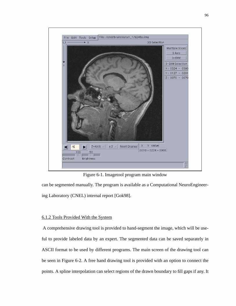
96
can be segmented manually. The program is available as a Computational NeuroEngineer-
ing Laboratory (CNEL) internal report [Gok98].
6.1.2 Tools Provided With the System
A comprehensive drawing tool is provided to hand-segment the image, which will be use-
ful to provide labeled data by an expert. The segmented data can be saved separately in
ASCII format to be used by different programs. The main screen of the drawing tool can
be seen in Figure 6-2. A free hand drawing tool is provided with an option to connect the
points. A spline interpolation can select regions of the drawn boundary to fill gaps if any. It
Figure 6-1. Imagetool program main window

97
is possible to paint inside the boundary provided the boundary is a closed curve. When the
boundary is drawn across several slices, then a 3-D view of the boundary is possible. To
correct the errors made during drawing, an UNDO/REDO function is provided up to the
starting point. The boundary can be saved, or a saved boundary can be loaded to view/
modify.
To increase the efficiency of the data analysis several different viewers are provided. The
Axis Viewer displays (Figure 6-3) all three axis at the same time, where the Multiple
Slices Viewer displays several slices at the same time (Figure 6-4). Finally the 3-D Viewer
of any selected region helps to visualize the data structure.
The 3-D Viewer (Figure 6-5) is useful to visualize the data and it is possible to view
not just the data itself but also the segmented data. The displayed image can be rotated
using the slide buttons. The Figure 6-5 is obtained by selecting the whole data set.
Figure 6-2. Drawing tool

98
Figure 6-3. Axis viewer
Figure 6-4. Multiple slices viewer

99
6.2 Testing on MR Images
6.2.1 Feature Extraction
If we don’t have a good feature set, even the most powerful algorithm won’t help us to
identify different brain tissues. Although the topic of this thesis is not feature extraction,
the following feature set was found to be very useful during simulations. The first feature
is the brain image itself. The second feature is calculated by taking a 2x2 square regions
starting from every point in the brain image and by calculating the Renyi’s entropy of
these regions. Notice that since the starting point is at every pixel, the regions are overlap-
Figure 6-5. 3-D viewer

100
ping. This calculation will give us more information about the edges and an illustration
can be seen in the Figure 6-6. Another important property of the calculation is the mea-
surement of smoothness of the brain tissue. We propose this feature extraction method as a
new edge detector, although properties of the detector should be investigated further.
6.2.2 Test Image
A small test image is used to see the power of the algorithm which is given in Figure 6-
7. We selected a small region of size 30x30 from a brain MRI image given in Figure 6-12,
and calculated a 2-dim feature set using entropy of 2x2 blocks and the image itself. The
entropy of the blocks can be seen in Figure 6-10.(a). We used the Renyi’s entropy derived
before with Gaussian kernels using a variance of 20.0. The feature set created using
entropy of the blocks enhances the edges between tissues. The feature set has a low value
Figure 6-6. Entropy calculation
Entropy of 2x2 block
original image feature set

101
only on the edges. In order to differentiate between tissue classes we multiply the feature
set with the image itself. To our surprise the multiplication of the feature set with the
image itself increases the contrast of the brain image which can be seen in Figure 6-10.(b).
This may be due to the fact that the smoothness of the gray and white matter differ. The
variance of the kernel used in the clustering procedure is 5.0 and the algorithm reached a
Figure 6-7. Test image
Figure 6-8. Histogram of the original image

102
minimum point of . We can see the difference in the histograms in the origi-
nal image and the enhanced image in Figure 6-8 and Figure 6-9.
The rest of the image is classified using the results obtained above. After generating
the feature set, the distance of each pixel to each of the classes found using the small test
Figure 6-9. Histogram of the enhanced image
Figure 6-10. Entropy of the blocks and second feature set
2.08 107–×
(a) (b)

103
image, is measured using the distance measure CEF developed in CHAPTER 4. The pixel
is assigned to the closest class. This type of clustering, where clustering is done on a small
set of the data, and the rest of the data just reclassified without running the clustering algo-
rithm, is preferred because of highly computational calculation of the minimization func-
tion. After classifying all the pixels, the clustering algorithm can be run with a very small
group size (i.e. 1 or 2) to check further improvements. The full brain image can be seen in
Figure 6-12 and the output of the clustering algorithm is shown in Figure 6-13. The white
matter seems to be clustered very smoothly, except for a couple of discontinuous pixels.
The CSF seems to be broken in many areas, but since the gray matter folds and touches
other gray matter, this is no surprise. The algorithm missed a spot at the top of the brain,
where the structure looks like white matter, but it is classified as gray matter. Running the
algorithm on one slice has an influence on the results. Including more than one slice in
feature extraction and reclassification of the rest of the pixels will definitely change the
results because of improved estimation of the probability density estimation. One way of
achieving this is to take a 3-D block during the calculation of features. For example, we
Figure 6-11. Input test image and output of clustering algorithm
(a) (b)

104
can use a 2x2x2 size blocks to calculate the feature vector which is generated by measur-
ing the entropy of each block.
6.3 Validation
To visual inspection of the segmented brain images, the results appear to be good, but
we need a quantitative assessment. We adapted the validation method explained in Chap-
ter 1, using the fact that the percentage of the gray matter decreases with age, and the per-
centage of white matter increases with age. The total cerebral volume is not changed
significantly after age 5, but the percentage of white matter and gray matter change by a
both 1 percent per year [Rei96]. Detecting this change should be a good measure of the
quality of the segmentation algorithm, although validation of the individual structures can
not be done using this method. We tested our algorithm on MR images of two children
scanned at two year interval with different ages ranging from 5 to 10 years. Scan
Figure 6-12. Full brain image (single slice)

105
sequences were acquired in a 1.5T Siemens Magnetom using a quadrature head coil: a
gradient echo volumetric acquisition "Turboflash" MP Rage sequence (TR= 10 ms, TE = 4
ms, FA = 10o, 1 acquisition, 25 cm field of view, matrix=130x256) that was reconstructed
into a gapless series of 128 1.25-mm thick images in the sagittal plane.
6.3.1 Brain Surface Extraction
Since we would like to measure the change of the gray and white matter of the brain
only, we removed the skull and the remaining tissues using a “Automated Brain Surface
Extraction Program” called BSE [San96] [San97], developed at the University of Southern
California. The algorithm in this package uses a combination of non-linear smoothing,
edge-finding and morphologic processing. The details can be found in [San97]. An exam-
ple can be seen in Figure 6-14. The correct filter parameters are found by trial and error,
since there is no universal way of setting the parameters. The extraction program usually
Figure 6-13. Output of clustering algorithm

106
has difficulty removing the bottom part of the brain. This can be seen in Figure 6-15,
where the algorithm couldn’t removed the bottom part of the head. Setting the parameters
to remove the bottom part usually results in holes in the brain itself. Since we don’t want
to compromise the brain structure, we applied the images from top to bottom where an
example can be seen in Figure 6-16.
6.3.2 Segmentation
The algorithm is applied to MR images of two different children of ages 5 years and 8
years at first scan, and 7.5 years and 10.2 years at second scan. Because of the large data
Figure 6-14. Brain extraction sample 1
Figure 6-15. Brain extraction sample 2

107
set, the algorithm is applied to a small section of the brain, and afterwards the rest of the
pixels are reclassified by measuring the CEF value between the unclassified pixels and the
labeled pixels. The feature extraction is performed by using 2x2x2 blocks, calculating the
entropy and mean of each block, and by multiplying the entropy values with the image
itself creating a contrast enhanched image, used as a feature. The mean of each block
becomes another feature.
The values of the features are between 0 and 400.0. The variance of the kernel should
not be too small, where the distributions loose their smoothness, and it should not be too
large to cause over-smoothed distributions. The selected value for the variance is between
15.0-20.0. Selection of the variance is one particular aspect of the clustering algorithm,
that needs to be improved further. The group size is selected as N/3, where N is the total
number of points in the training data set. The group size can be selected between 1 and N.
The bigger the group size, the better the chance of escaping from local minima. Of course
the price is increased computation time.
Figure 6-16. Brain extraction sample

108
6.3.3 Segmentation Results
Figure 6-17. Original, enhanced and segmented MR images (5.5 years, slice 50)
Figure 6-18. Original, enhanced and segmented MR images (5.5 years, slice 60)
Figure 6-19. Original, enhanced and segmented MR images (5.5 years, slice 65)

109
Figure 6-20. Original, enhanced and segmented MR images (5.5 years, slice 70)
Figure 6-21. Original, enhanced and segmented MR images (5.5 years, slice 80)
Figure 6-22. Original, enhanced and segmented MR images (7.5 years, slice 50)

110
Figure 6-23. Original, enhanced and segmented MR images (7.5 years, slice 60)
Figure 6-24. Original, enhanced and segmented MR images (7.5 years, slice 70)
Figure 6-25. Original, enhanced and segmented MR images (7.5 years, slice 75)

111
Figure 6-26. Original, enhanced and segmented MR images (7.5 years, slice 80)
Figure 6-27. Original, enhanced and segmented MR images (8 years, slice 60)
Figure 6-28. Original, enhanced and segmented MR images (8 years, slice 70)

112
Figure 6-29. Original, enhanced and segmented MR images (8 years, slice 75)
Figure 6-30. Original, enhanced and segmented MR images (8 years, slice 80)
Figure 6-31. Original, enhanced and segmented MR images (8 years, slice 85)

113
Figure 6-32. Original, enhanced and segmented MR images (10.2 years, slice 60)
Figure 6-33. Original, enhanced and segmented MR images (10.2 years, slice 70)
Figure 6-34. Original, enhanced and segmented MR images (10.2 years, slice 75)

114
6.4 Results
After all the images are segmented, the percentages of white matter, gray matter and
CSF w.r.t. the cerebral volume are calculated and given in Table 6-1. The percentage vol-
ume of white matter to the cerebral volume is increased, whereas the percentage volume
of gray matter to the cerebral volume is decreased. The results are in good aggrement with
the published results in [Rei96], which is given in Figure 6-37 and Figure 6-381. We
embedded our results in the figures as big black dots. The comparison shows that the clus-
tering algorithm successfully segmented the brain image.
Figure 6-35. Original, enhanced and segmented MR images (10.2 years, slice 80)
Figure 6-36. Original, enhanced and segmented MR images (10.2 years, slice 85)
1. The Figure 6-37 and Figure 6-38 are reprinted with the permission of Oxford University Press.

115
Figure 6-37. Change of gray matter
Figure 6-38. Change of white matter

116
Table 6-1. Percentages of brain matter
white gray CSF
5.5 years %31.45 %57.97 %10.56
7.5 years %33.37 %55.73 %10.89
8 years %36.39 %54.21 %9.39
10.2 years %37.60 %50.87 %11.51

117
CHAPTER 7CONCLUSIONS AND FUTURE WORK
We would like to summarize the contributions made in this dissertation. The initial
goal is to develop a better clustering algorithm which can be used to cluster nonlinearly
separable clusters. Second order statistics are not sufficient for use on nonlinearly separa-
ble clusters. In order to achieve this goal, we developed a cost function which can be used
to measure the cluster separability and which can be used for nonlinearly formed clusters.
The cost function can be easily computable which decreases the normally high computa-
tional requirements of clustering algorithms. The cost function is developed using infor-
mation theoretic distance measures between probability density functions, and the relation
of different measures to the clustering algorithm is investigated. The cost function is basi-
cally a valley seeking algorithm, where the distance measure is calculated from the data
without requiring numerical integration. It is a data driven method. An optimization proce-
dure which is efficient and simple is also developed to be used with the proposed method,
although the usage of the optimization algorithm is not limited to the method proposed in
this dissertation. We also find out that certain distance measures are not suitable for use in
our clustering algorithm. In the second part of the dissertation, we applied the algorithm
for the segmentation of MR images. The segmentation was found to be very succesful.
There are certain areas where the algorithm can be improved further. It is possible to
adapt the kernel shape dynamically according to the data. Having a fixed circular shape
may not be suitable for all data sets. Instead of fixing the shape, we can change the shape

118
of the kernel using the samples around the pixel. We can use the samples already found
during our grouping algorithm, and fit a gaussian kernel to each group of pixels whenever
the grouping is changed. This may improve the result of our clustering algorithm. The suc-
cess of the algorithm depends on the estimation of the probability density function of each
cluster generated during iterations, which is controlled to some degree by the variance of
the kernel used. A more systematic way should be developed to adjust the variance of the
kernel. This is a problem related to probability density estimation and it is more general
than the clustering problem.
The algorithm can be used only in batch mode in the current form. This is an area
which can be improved with an online optimization algorithm. This will help the cases
where not all the data is available at the same time for batch learning.
Running the algorithm with large data sets is very time-consuming. This is an area
which needs to be improved. Clustering the data into a more compact data clusters will
help to improve the efficiency of the method, although that brings into question how to
adjust the compact cluster sizes.

119
REFERENCES
[Aar90] Aarts, E., Simulated Annealing and Boltzmann Machines, John Wiley& Sons, New York, 1990.
[Ama77] Amari, S.I., “Neural theory of association and concept-formation,” Bio-logical Cybernetics, V26, p175-185, 1977.
[Ash90] Ashtari, M., Zito, J.L., Gold, B.I., Lieberman, J.A., Borenstein, M.T.,Herman, P.G., “Computerized volume measurement of brain structure,”Invest Radiology, V25, p798-805, 1990.
[Bea92] Bealy, D.M., Weaver, J.B., “Two applications of wavelet transforms inmagnetic resonance imaging,” IEEE Transactions in Information The-ory, V38, p840-860, 1992.
[Ben66] Benson, Russell V., Euclidean Geometry and Convexity, McGraw-Hill,New York, 1966.
[Ben94a] Benes, F.M., Turtle, M. , Khan, Y. , and Farol, P., “Myelination of a keyrelay zone in the hippocampal formation occurs in the human brainduring childhood, adolescence, and adulthood,” Archives of GeneralPsychiatry V51, p477-484, 1994.
[Ben94b] Bensaid, A.M., Hall, L.O., Bezdek, J.C., Clarke, L.P., “ Fuzzy clustervalidity in magnetic resonance images,” Proceedings of SPIE, V2167,p454-464, 1994.
[Bez93] Bezdek, J. C., “Review of MRI Image Segmentation techniques usingpattern recognition,” Medical Physics, V20, N4, p1033-1048, 1993.
[Bha43] Bhattacharya, A., “ On a measures of divergence between two statisti-cal populations defined by their probability distributions,” Bull. Cal.Math. Soc., V35, p99-109, 1943.

120
[Bis95] Bishop, C., Neural Networks for Pattern Recognition, Oxford Univer-sity Press, New York, 1995.
[Bit84] Bittoun, J.A., “A computer algorithm for the simulation of any nuclearmagnetic resonance imaging method,” Journal of Magnetic ResonanceImaging, V2, p113-120, 1984.
[Bom90] Bomans, M., Hohne, K.H., Tiede, U., Riemer, M., “3-D segmentationof MR images of the head for 3-D display,” IEEE Transactions on Med-ical Imaging, V9, p177-183, 1990.
[Bou94] Bouman C.A., “A multiscale random field model for bayesian imagesegmentation,” IEEE Transactions on Image Processing, V3, p162-176,1994
[Bra93] Bradley, W.G., Yuh, W.T.C., Bydder, G.M., “Use of MR imaging con-trast agents in the brain,” Journal of Magnetic Resonance Imaging, V3,p199-232, 1993.
[Bra94] Brandt, M.E., Bohan, T.P., Kramer, L.A., Fletcher, J.M., “Estimation ofCSF, white and gray matter volumes in hydrocephalic children usingfuzzy clustering of MR images,” Computational Medical Imaging,V18, p25-34, 1994.
[Bro87] Brody, B.A., Kinney, H.C. , Kloman, A.S. and Gilles, F.H., “Sequenceof central nervous system myelination in human infancy.I. An autopsystudy of myelination,” Journal of Neuropathology & ExperimentalNeurology V46, p283-301, 1987.
[Bro90] Bronen, R.A., Sze, G., “Magnetic resonance imaging contrast agents:Theory and application to the central nervous system,” Journal of Neu-rosurgery, V73, p820-839, 1990.
[Bru93] Brummer, M.E., Eisner, R.L., “Automatic Detection of Brain Contoursin MRI Data Sets,” IEEE Trans. on Med. Imag., V12, N2, p152-166,1993.
[Buc91] Buchbinder, B.R., Belliveau, J.W., McKinstry, R.C., Aronen, H.J.,Kennedy, M.S., “Functional MR imaging of primary brain tumors withPET correlation,” Society of Magnetic Resonance in Medicine, V1,1991.

121
[Car88] Carpenter G.A., Grossberg, S., "Art of adaptive recognition by a self-organizing neural network," Computer, V21, N3, p77-88, March 1988.
[Car87a] Carpenter, G.A., Grossberg, S., “A massively parallel architecture for aself-organizing neural pattern recognition machine,” Computer Vision,Graphics, and Image Processing, V37, p54-115, 1987.
[Car87b] Carpenter, G.A., Grossberg, S., “ART2: Self-organization of stable cat-egory recognition codes for analog input patterns,” Applied Optics,V26, p4919-4930, 1987.
[Car90] Carpenter, G.A., Grossberg, S., “ART3: Hierarchical search usingchemical transmitters in self-organizing pattern recognition architec-tures,” Neural Networks, V3, p129-152, 1990.
[Car91a] Carpenter, G.A., Grossberg, S., “ART2-A: An adaptive resonance algo-rithm or rapid category learning and recognition,” Neural Networks,V4, p493-504, 1991.
[Car91b] Carpenter, G.A., Grossberg, S., “ARTMAP: Supervised real-time learn-ing and classification of nonstaionary data by a self-organizing neuralnetwork,” Neural Networks, V4, p565-588, 1991.
[Che52] Chernoff, H., “A measure of asymptotic efficiency for tests of a hypoth-esis based on a sum of observations,” Ann. Math. Stat., V23, p493-507,1952.
[Cla93] Clarke, L.P., Velthuizen, R.P., Phuphanich, S., Shellenberg, J.D., Arri-gnton, J.A., “Stability of three supervised segmentation techniques,”Magnetic Resonance Imaging, V11, p95-106, 1993.
[Cli87] Cline, H.E., Dumoulin, C.L., Hart, H.R., “3D reconstruction of thebrain from magnetic resonance images using a connectivity algorithm,”Magnetic Resonance Imaging, V5, p345-352, 1987.
[Cli91] Cline, H.E., Lorensen, W.E., Souza, S.P., Jolesz, F.A., Kikinis, R.,Gerig, G., Kennedy, T.E., “3D surface rendered MR images of the brainand its vasculature,” Computer Assisted Tomogrophy, V15, p344-351,," 1991.

122
[Chr81] Christensen, R., Entropy Minimax Sourcebook, V1, Entropy Ltd., Lin-coln, MA, 1981.
[Coh91] Cohen, L., “On active contour models and balloons,” Computer Vision,Graphics and Image Processing, V53, p211-218, 1991.
[Cov91] Cover T.M., Thomas, J.A., Elements of Information Theory, Wiley,New York, 1991.
[Dav96] Davatzikos, C., Bryan, R.N., “Using a Deformable Surface Model toObtain a Shape Representation of the Cortex,” Technical Report, JohnsHopkins University, Baltimore, 1996.
[Daw91] Dawant, B.M., Ozkan, M., Zijdenbos, A., Margolin, R., “A computerenvironment for 2D and 3D quantitation of MR images using neuralnetworks,” Proceedings of the 13th IEEE Engineering in Medicine andBiology Society, V13, p64-65, 1991.
[Del91a] Dellepiane, S., “Image segmentation: Errors, sensitivity and uncertan-ity,” Proceedings of the 13th IEEE Engineering in Medicine and Biol-ogy Society, V13, p253-254, 1991.
[Del91b] Dellepiane, S., Venturi, G., Vernazza, G., “A fuzzy model for the pro-cessing and recognition of MR pathologic images,” Information Pro-cessing in Medical Imaging, p444-457, 1991.
[Dem77] Demspter, A.P., “Maximum likelihood from incomplete data via theEM algorithm,” Journal of the Royal Statistic Society, Series B 39, p1-38, 1977.
[Dud73] Duda, R.O., Hart P.E., Pattern Classification and Scene Analysis, Wiley,New York, 1973.
[Eil90] Eilbert, J.L., Gallistel, C.R., McEachron, D.L., “The variation in userdrawn outlines on digital images,” Computational Medical Imaging,V14, p331-339, 1990.
[Fug70] Fugunaga, K., Koontz, W.L.G., “A criterion and analgorithm for group-ing data,” Transactions of IEEE Computers, V19, p917-923, 1970.

123
[Fug90] Fugunaga, K., Introduction to Statistical, Pattern Recognition, Aca-demic Press, New York, 1990.
[Gal93] Galloway, R.L., Maciunas, R.J., Failinger, A.L., “Factors affecting per-ceived tumor volumes in magnetic resonance imaging,” Annals of Bio-medical Engineering, V21, p367-375, 1993.
[Ger82] Gersho, A., “On the structure of vector quantizers,” IEEE Transactionson Information Theory, V28, p157-166, 1982.
[Ger92a] Gersho, A., Gray, R.M., Vector Quantization and Signal Compression,Kluwer Norwell, MA, 1992.
[Ger92b] Gerig, G., Martin, J., Kikinis, R., Kubler, O., Shenton, M., Jolesz, F.A.,“Unsupervised tissue type segmentation of 3D dual-echo MR headdata,” Image Vision Computing, V10, p349-360, 1992.
[Gie99] Giedd J.N., Blumental J., Jeffries N.O., Castellanos F.X., Liu H.,Zijdenbos A., Paus T., Evans A.C., Rapoport J.L, “Brain developmentduring childhood and adolescense: a longitudinal MRI study,” NatureNeuroscience, V2, p861-863, 1999.
[Gok98] Gokcay, E. “A pvwave interface to visualize brain images: Imagetool,”CNEL internal report, University of Florida, 1998.
[Gok00] Gokcay E., Principe J., “A new clustering evaluation function usingRenyi’s information potential,” ICASSP 2000, Istanbul, Turkey, 2000.
[Gra84] Gray, R.M., “Vector quantization,” IEEE ASSP Magazine, V1, p4-29,1984.
[Gra90] Gray, R.M., Entropy and Information Theory, Springer-Verlag, NewYork, 1990.
[Gre74] Greenberg, M.J., Euclidean and non-Euclidean Geometries: Develop-ment and History, W. H. Freeman, San Francisco, 1974.
[Gro69] Grossberg, S., “On learning and energy-entropy dependence in recur-rent and nonrecurrent signed networks,” Journal of Statistical Physics,V1, p319-350, 1969.

124
[Gro76a] Grossberg, S., “Adaptive pattern classification and universal recording:I. Paralel development and coding of neural feature detectors,” Biologi-cal Cybernetics, V23, p121-134, 1976.
[Gro76b] Grossberg, S., “Adaptive pattern classification and universal recording:II. Feedback, expectation, olfaction, and illusions,” Biological Cyber-netics, V23, p187-202, 1976.
[Gui97] Guillemaud, R., Brady, M., “Estimating the bias field of MR images,”IEEE Trans. on Med. Imag., V16, N3, p238-251, 1997.
[Hal92] Hall, L.O., Bensaid, A.M., Clarke, L.P., Velthuizen, R.P., Silbiger,M.S., Bezdek, J.C., “A comparison of neural network and fuzzy clus-tering techniques is segmenting magnetic resonance images of thebrain,” IEEE Transactions on Neural Networks, V3, p672-682, 1992.
[Har85] Haralick, R.M., Shapiro, L.G., “Image segmentation techniques,”Com-puter Vision, Graphics, and Image Processing, V29, p100-132, 1985.
[Har75] Hartigan, J., Clustering Algorithms, Wiley, New York, 1975.
[Has95] Hassoun, M.H., Fundamentals of Artificial Neural Networks, MIT,Cambridge, MA, 1995.
[Hay94] Haykin, S., Neural Networks, IEEE Press, New Jersey, 1994.
[Heb49] Hebb, D.O., The Organization of Behaviour:A NeuropsychologicalTheory, New York, Wiley, 1949.
[Hec89] Hecht-Nielsen R., Neurocomputing, Addison-Wesley, Reading, MA,1989.
[Hei93] Heine, J.J., “Computer simulations of magnetic resonance imaging andspectroscopy,” MS Thesis, University of South Florida, Tampa, 1993.
[Hen93] Hendrick, R.E., Haacke, E.M., “Basic Physics of MR contrast agents inthe brain,” Journal of Magnetic Resonance Imaging, V3, p137-156,1993.

125
[Hil93] Hill, D.L.G., Hawkes, D.J., Hussain, Z., Green, S.E.M., Ruff, C.F.,Robinson, G.P., “Accurate combination of CT and MR data of thehead:Validation and applications in surgical and therapy planning,”Comput. Medical Imaging Graph., V17, p357-363, 1993.
[Hog65] Hogg, R.V., Craig, A.T., Introduction to Mathematical Statistics, Mac-millan, New York, 1965.
[Hu90] Hu, X.P., Tan, K.K., Levin, D.N., Galhotra, S., Mullan, J.F., Hekmat-panah, J., Spire, J.P.,”Three-dimensional magnetic resonance images ofthe brain: Application to neurosurgical planning,” Journal of Neurosur-gery, V72, p433-440, 1990.
[Jac90] Jack, C.R., Bentley, M.D., Twomey, C.K., Zinsmeister, A.R., “MRImaging-based volume measurement of the hippocampal formation andanterior temporal lobe,” Radiology, V176, p205-209, 1990.
[Jac93] Jackson, E.F., Narayana, P.A., Wolinksy, J.S., Doyle, T.J., “Accuracyand reproducibility in volumetric analysis of multiple sclerosislesions,” Journal of Computer Assisted Tomogrophy, V17, p200-205,1993.
[Jai89] Jain, A.K., Fundamentals of Digital Image Processing, Prentice Hall,Englewood Cliffs, NJ, 1989.
[Jay57] Jaynes, E.T., “Information theory and statistical mechanics, I, II,” Phys-ical Review, V106, p620-630, V108, p171-190, 1957.
[Kam93] Kamada, K., Takeuchi, F., Kuriki, S., Oshiro, O., Houkin, K., Abe, H.,“Functional neurosurgical simulation with brain surface magnetic reso-nance imaging and magnetoencephalograpy,” Neurosurgery, V33,p269-272, 1993.
[Kap92] Kapur, J.N., Kesavan, H.K., Entropy Optimization Principles withApplications, Academic Press, Boston, 1992.
[Kap95] Kapur, T., “Segmentation of brain tissue from magnetic resonanceimages,”Technical Report, MIT, Cambridge, 1995.

126
[Kar94] Karhunen, J., “Optimization criteria and nonlinear PCA neural net-works,” IEEE International Conference on Neural Networks, V2,p1241-1246, 1994.
[Kars90] Karssemeijer, N., “A statistical method for automatic labeling of tissuesin medical images,” Machine Vision and Applications, V3, p75-86,1990.
[Kaz90] Kazakos D., Kazakos Papantoni P., Detection and Estimation, Com-puter Science Press, New York, 1990.
[Kir83] Kirkpatrick S., Gelatt, C.D., Vecchi, M.P., "Optimization by simulatedannealing," Science, V220, p671-680, 1983.
[Koh91] Kohn, M.I., Tanna, N.K., Herman, G.T., Resnick, S.M., Mozley, P.D.,Gur, R.E., Alavi, A., Zimmerman, R.A., Gur, R.C., “Analysis of brainand cerebrospinal fluid volumes with MR imaging:Part1. Methods, reli-ability and validation,” Radiology V178, p115-122, 1991.
[Koh95] Kohonen, T., Self-Organizing Maps, Springer, New York, 1995.
[Kul59] Kullback, S., Information Theory and Statistics, John Wiley, New York,1959.
[Lia93] Liang, Z., “Tissue classification and segmentation of MR images,”IEEE Eng. Med. Biol., V12, p81-85, 1993.
[Lia94] Liang, Z., Macfall, J.R., “Parameter estimation and tissue segmentationfrom multispectral MR images,” IEEE Trans. on Med. Imag., V13,N3, p441-449, 1994.
[Lin80] Linde, Y., Buzo, A., Gray, R.M., “An algorithm for vector quantizerdesign,” IEEE Transactions on Communications, V28, p84-95, 1980.
[Lin88] Linsker, R., “Self-organization in a perceptual network,” Computer,p105-117, March 1988.
[Lip87] Lippman, R.P., “An introduction to computing with neural nets,” IEEEMagazine on Accoustics, Signal, and Speech Processing, V4, p4-22,1987.

127
[Lip89] Lippman, R.P., “Review of neural networks for speech recognition,”Neural Computation, V1, p1-38, 1989.
[Mal73] Malsberg, V.D. , “Self-organizing of orientation sensitive cells in thestriate cortex,” Kybernetick, V14, p85-100, 1973.
[Mar80] Marr, D., Hilderth, E., “Theory of edge detection,” Proceedings of theRoyal Society of London, V207, p187-217, 1980.
[Mcc94] McClain, K.J., Hazzle. J.D., “MR image selection for segmentation ofthe brain,” Journal of Magnetic Resonance Imaging, V4, 1994.
[Mcl88] McLachlan, G.J., Basford, K.E., Mixture Models: Inference and Appli-cations to Clustering, Marcel Dekker, Inc., New York, 1988.
[Mcl96] McLachlan, G.J., Krishnan, T., The EM algorithm and extensions, JohnWiley & Sons, Inc., New York, 1996.
[Mit94] Mittchell, J.R., Karlik, S.J., Lee, D.H., Fenster, A.,”Computer-assistedidentification and quantification of multiple sclerosis lesions in MRimaging volumes in the brain,” Journal of Magnetic Resonance Imag-ing, V4, p197-208, 1994.
[Moo89] Moore, B., “ART1 and pattern clustering,” Proceedings of the 1988Connectionists Models Summer Schools, p174-185, 1989.
[Odo85] O’Donnel, M., Edelstein, W.A., “NMR imaging inthe presence of mag-netic field inhomogeneities and gradient field nonlinearities,” MedicalPhysics, V12, p20-26, 1985.
[Oja82] Oja, E., “A simlified neuron model as a principal componet analyzer,”Journal of Mathematical Biology, V15, p267-273, 1982.
[Oja83] Oja, E., “Neural networks, principal components, and subspaces,”International Journal of Neural Systems, V1, p61-68, 1983.
[Oja85] Oja, E., Karhunen, J., “On stochastic approximation of the eigenvectorsof the expectation of a random matrix,” Journal of Mathematical Anal-ysis and Applications, V106, p69-84, 1985.

128
[Oja91] Oja, E., “Data compression, feature extraction, and autoassociation infeedforward neural networks,” Artificial Neural Networks, V1, p737-745, 1991.
[Ozk93] Ozkan, M., Dawant, B.M., “Neural-Network Based Segmentation ofMulti-Modal Medical Images,” IEEE Transactions on Med. Imag.,V12, N3, p534-544, 1993.
[Pal93] Pal, N.R., Pal, S.K., “A review on image segmentation techniques,” Pat-tern Recognition, V26, N9, p1277-1294, 1993.
[Pao89] Pao, Y.H., Adaptive Pattern Recognition and Neural Networks, Addi-son-Wesley, Reading, MA, 1989.
[Pap65] Papoulis, A., Probability, Random Variables and Stochastic Processes,McGraw-Hill, New York, 1965.
[Par62] Parzen E., "On estimation of a probability density function and mode,"Annals of Mathematical Statistics, V33, p1065-1076, 1962.
[Pec92] Peck, D.J., Windham, J.P., Soltanian-Zadeh, H., Roebuck, J.R., “A fastand accurate algorithm for volume determination in MRI,” MedicalPhysics, V19, p599-605, 1992.
[Pel82] Peli T., Malah, D., “A study of edge detection algorithms,” ComputerGraphics and Image Processing, V20, p1-21, 1982.
[Pet93] Peterson, J.S., Christoffersson, J.O., Golman, K., “MRI simulationusing k-space formalism,” Magnetic Resonance Imaging, V11, p557-568, 1993.
[Phi95] Phillips, W.E., Velhuizen, R.P., Phuphanich, S., Vilora, J., Hall, L.O.,Clarke, L.P., Silbiger, M.L., “ Application of fuzzy segmentation tech-niques for tissue differentation in MR images of a hemorrhagic glio-blastoma multiforme,” Magnetic Resonance Imaging, V13, p277-290,1995.
[Pri90] Principe, J.C., Euliano, N.R., Lefebvre, W.C., Neural and AdaptiveSystems: Fundamentals Through Simulations, John Wiley & Sons,New York, 2000.

129
[Pri00] Principe, J., Xu D., and Fisher, J.,”Information theoretic learning,” inUnsupervised Adaptive Filtering, Ed. S. Haykin, John Wiley & Sons,New York, 2000.
[Puj93] Pujol, J., Vendrell, P., Jungue, C., Marti-Vilalta, J.L., Capdevila,A.,”When does human brain development end? Evidence of corpus cal-losum growth up to adulthood,” Annals or Neurology, V34, p71-75,1993.
[Raf90] Raff, U., Newman, F.D., “Lesion detection in radiologic images usingan autoassociative paradigm,” Medical Physics, V17, p926-928, 1990.
[Rei96] Reiss A., Abrams M., Singer H., Ross J., Denckla M., “Brain develop-ment, gender and IQ in children: A volumetric imaging study,” Brain,V119, p1763-1774, 1996.
[Ren60] Renyi A., "On measures of entropy and information," Proceedings ofthe 4th Berkeley Symposium on Mathematics, Statistics and Probabil-ity, p547-561, 1960.
[Rit87a] Ritter, G.X., Wilson, J.N., “Image algebra: A unified approach to imageprocessing,” SPIE Proc. on Medical Imaging, Newport Beach, CA,1987.
[Rit87b] Ritter, G.X., Shrader-Frechette, M., Wilson, J.N., “Image algebra: Arigorous and translucent way of expressing all image processing opera-tions,” Proc. SPIE Southeastern Technical Symposium on Optics, Elec-tro-Optics and Sensors, Orlando, FL, p116-121, 1987.
[Rit96] Ritter, G.X., Wilson, J.N., Handbook of Computer Vision Algorithmsin Image Algebra, CRC Press, Boca Raton, FL, 1996.
[Rub89] Rubner, J., Tavan, P., “A self-organizing network for principal-compo-nent analysis,” Europhysics Letters, V10, p693-698, 1989.
[Rum85] Rumelhart, D.E., Zipser, D., “Feature discovery by competitive learn-ing,” Cognitive Science, V9, p75-112, 1985.
[Run89] Runge, V.M., Enhanced Magnetic Resonance Imaging, C.V. MosbyCompany, St. Louis, 1989.

130
[Rob94] Robb, R.A., Visualization methods for analysis of multimodalityimages,” Functional Neuroimaging: Technical Foundations, Orlando,FL, Academic Press, p181-190, 1994.
[Sah88] Sahoo, P.K., Soltani, S., Wong, K.C., “A survey of thresholding tech-niques,” Computer Vision, Graphics and Image Processing, V41, p233-260, 1988.
[San96] Sandor S. R., Leahy R. M., Timsari B., "Generating cortical constraintsfor MEG inverse procedures using MR volume data,” ProceedingsBIOMAG96, Tenth International Conference on Biomagnetism, SantaFe, New Mexico, Feb. 1996.
[San97] Sandor, S., Leahy, R.M., "Surface-based labeling of cortical anatomyusing a deformable database," IEEE Transactions on Medical Imag-ing, V16, N1, p41-54, February 1997.
[San89] Sanger, T.D., “Optimal unsupervised learning in a single layer linearfeedforward neural network,” Neural Networks, V2, p459-473, 1989.
[Sha48] Shannon, C.E., “A mathematical theory of communications,” Bell Sys-tem Technical Journal, V27, p370-423, 1948.
[Sha62] Shannon, C.E., Weaver, W., The Mathematical Theory of Communica-tion, The University of Illinois Press, Urbana, 1962.
[Sch94] Schwartz, M.L., Sen, P.N., Mitra, P.P., “Simulations of pulsed field gra-dient spin-echo measurements in porous media,” Magnetic ResonanceImaging, V12, p241-244, 1994.
[Sum86] Summars, R.M., Axel, L., Israel, S., “A computer simulation of nuclearmagnetic resonance,” Magnetic Resonance Imaging, V3, p363-376,1986.
[Tay93] Taylor, J.G., Coombes, S., “Learning higher order correlations,” NeuralNetworks, V6, p423-427, 1993.

131
[Tju94] Tjuvajev, J.G., Macapinlac, H.A., Daghighian, F., Scott, A.M., Ginos,J.Z., Finn, R.D., Kothari, P., Desai, R., Zhang, J., Beattie, B., Graham,M., Larson, S.M., Blasberg, R.G., “Imaging of brain tumor prolifera-tive activity with Iodine-131-Iododeoxyuridine,” Journal of NuclearMedicine, V35, p1407-1417, 1994.
[Vai00] Vaidyanatkan, M., Clarke, L.P., Velthuizen, R.P., Phuphanich, S., Ben-said, A.M, Hall, L.O., Silbiger, M.L., “Evaluation of MRI segmentationmethods for tumor volume determination,” Magnetic Resonance Imag-ing (in press).
[Van88] Vannier, M.W., Speidel, C.M., Rickman, D.L., “Magnetic resonanceimaging multispectral tissue classification,” News Physiol. Sci., V3,p148-154, 1988.
[Van91a] Vannier, M.W., Pilgram, T.K., Speidel, C.M., Neumann, L.R.,”Valida-tion of magnetic resonance imaging multispectral tissue classification,”Comput. Med. Imaging Graph., V15, p217-223, 1991.
[Van91b] Van der Knaap, M.S., et al., “Myelination as an expression of the func-tional maturity of the brain,” Developmental Medicine and Child Neu-rology, V33, p849-857, 1991.
[Vel94] Vellhuizen, R.P., Clarke, L.P., “An interface for validation of MR imagesegmentations,” Proceedings of IEEE Engineering in Medicine andBiology Society, V16, p547-548, 1994.
[Wal92] Wallace, C.J., Seland, T.P., Fong, T.C., “Multiple sclerosis: The impactof MR imaging,” AJR, V158, p849-857, 1992.
[Wan98] Wang, Y., Adali, T., “Quantification and segmentation of brain tissuesfrom MR images: A probabilistic neural network approach,” IEEETrans. on Image Processing, V7, N8, p1165-1180, 1998.
[Wel96] Wells, W.M., Grimson, W.E.L., “Adaptive segmentation of MRI data,”IEEE Trans. on Med. Imag., V15, N4, p429-442, 1996.
[Wit88] Witkin, A., Kass, M., Terzopoulos, D., “Snakes:Active contour mod-els,” International Journal of Computer Vision,V4, p321-331, 1988.

132
[Xu94] Xu, L., “Theories of unsupervised learning: PCA and its nonlinearextensions,” IEEE International Conference on Neural Networks, V2,p1252-1257, 1994.
[Xu98] Xu D., Principe J., “Learning from examples with quadratic mutualinformation,” Neural Networks for Signal Processing - Proceedings ofthe IEEE Workshop, IEEE, Piscataway, NJ, USA. p155-164, 1998.
[Zad92] Zadech, H.S., Windham, J.P., “A comparative analysis of several trans-formations for enhancement and segmentation of magnetic resonanceimage scene sequences,” IEEE Trans. on Med. Imag., V11, N3, p302-318, 1992.
[Zad96] Zadech, H.S., Windham, J.P., “Optimal linear transformation for MRIfeature extraction,” IEEE Trans. on Med. Imag.,V15, N6, p749-767,1996.
[Zha90] Zhang, J., ”Multimodality imaging of brain structures for stereoacticsurgery,” Radiology, V175, p435-441, 1990.
[Zij93] Zijdenbos, A.P., Dawant, B.M., Margolin, R., “Measurement reliabilityand reproducibility in manual and semi-automatic MRI segmentation,”Proceedings of the IEEE-Engineering in Medicine and Biology Soci-ety, V15, p162-163, 1993.

133
BIOGRAPHICAL SKETCH
Erhan Gokcay was born in Istanbul,Turkey, on January 6, 1963. He attended “Istanbul
Erkek Lisesi” High School in Istanbul, Turkey, from 1974 through 1981. In 1981, he
began undergraduate studies at the Middle East Technical University in Ankara, Turkey,
graduating with a B.S. in electrical and electronic engineering in 1986. In 1986, he began
graduate studies at the Middle East Technical University in Ankara, Turkey, graduating
with a M.S. degree in electrical and electronic engineering in 1991, and continued the
graduate studies for a PhD in computer engineering at the same university. In 1993 he was
accepted to the University of Florida and continued his PhD studies in the Computer and
Information Sciences and Engineering Department at the University of Florida, in Gaines-
ville, Florida. He worked as an application programmer in ASELSAN Military Electron-
ics and Telecommunications Company, in Ankara, Turkey, and as a system programmer in
STFA Enercom Computer Center, in Ankara, Turkey, from 1986 to 1990. He worked as
the Technical Manager in Tulip Computers in Ankara, Turkey, until 1991, and he was
responsible from the installation and maintenance of the computer systems and training
the technical support team. He worked as a network administrator and hardware supervi-
sor in Bilkent University, in Ankara, Turkey, from 1991 to 1993, where he was responsible
from the installation, maintenance and support for the computer systems and campus-wide
network. He was working as a system administrator in the CNEL and BME labs from
1993 until graduation at University of Florida, in Gainesville, Florida.

I certify that I have read this study and that in my opinion it conforms to acceptable standards ofscholarly presentation and is fully adequate, in scope and quality, as a dissertation for the degree ofDoctor of Philosophy.
_________________________________________________Jose C. Principe, ChairmanProfessor of Electrical and Computer Engineering
I certify that I have read this study and that in my opinion it conforms to acceptable standards ofscholarly presentation and is fully adequate, in scope and quality, as a dissertation for the degree ofDoctor of Philosophy.
_________________________________________________John G. HarrisAssociate Professor of Electrical and Computer Engineering
I certify that I have read this study and that in my opinion it conforms to acceptable standards ofscholarly presentation and is fully adequate, in scope and quality, as a dissertation for the degree ofDoctor of Philosophy.
_________________________________________________Christiana M. LeonardProfessor of NeuroScience
I certify that I have read this study and that in my opinion it conforms to acceptable standards ofscholarly presentation and is fully adequate, in scope and quality, as a dissertation for the degree ofDoctor of Philosophy.
_________________________________________________Joseph N. WilsonAssistant Professor of Computer and Information Sciencesand Engineering
I certify that I have read this study and that in my opinion it conforms to acceptable standards ofscholarly presentation and is fully adequate, in scope and quality, as a dissertation for the degree ofDoctor of Philosophy.
_________________________________________________William W. EdmonsonAssistant Professor of Electrical and Computer Engineering

This dissertation was submitted to the Graduate Faculty of the College of Engineering and to theGraduate School and was accepted as partial fulfillment of the requirements for the degree ofDoctor of Philosophy.
August 2000 _________________________________________________M. Jack OhanianDean, College of Engineering
_________________________________________________Winfred M. Phillips
Dean, Graduate School