A Monte Carlo assessment of Eulerian flow and transport perturbation models

WATER RESOURCES RESEARCH, VOL. 34, NO. 5, PAGES 1143-1163, MAY 1998

A Monte Carlo assessment of Eulerian flow and transport perturbation models Ahmed E. Hassan •

School of Civil Engineering, Purdue University, West Lafayette, Indiana

John H. Cushman

Center for Applied Mathematics, Purdue University, West Lafayette, Indiana

Jacques W. Delleur School of Civil Engineering, Purdue University, West Lafayette, Indiana

Abstract. Monte Carlo studies of flow and transport in two-dimensional synthetic conductivity fields are employed to evaluate first-order flow and Eulerian transport theories. Hydraulic conductivity is assumed to obey fractional Brownian motion (fBm) statistics with infinite integral scale or to have an exponential covariance structure with finite integral scale. The flow problem is solved via a block-centered finite difference scheme, and a random walk approach is employed to solve the transport equation for a conservative tracer. The model is tested for mass conservation and convergence of computed statistics and found to yield accurate results. It is then used to address several issues in the context of flow and transport. The validity of the first-order relation between the fluctuating velocity covariance and the fluctuating log conductivity is examined. The simulations show that for exponential covariance, this approximation is justified in the mean flow direction for log conductivity variance, rr•, of the order of unity. However, as rr• increases, the relation for the transverse velocity component deviates from the fully nonlinear Monte Carlo results. Eulerian transport models neglect triplet correlation functions that appear in the nonlocal macroscopic flux. The relative importance of the triplet correlation term for conservative chemicals is examined. This term appears to be small relative to the convolution flux term in mildly heterogeneous media. As rr• increases or the integral scale grows, the triplet correlation becomes significant. In purely ' convective transport the triplet correlation term is significant if the heterogeneity is evolving. The exact nonlocal macroscale flux for the purely convective case significantly differs from that of the convective-dispersive transport. This is in agreement with recent theoretical analysis and numerical studies, and it suggests that neglecting local-scale dispersion may lead to large errors. Localization errors in the flux term are evaluated using Monte Carlo simulations. The nonlocal in time model significantly differs from the fully nonlocal model. For small variance and integral scale there is a slight difference between the fully localized flux and the fully nonlocal convolution flux. This is also in agreement with recent theories that suggest that moments through the second for the two models are nearly identical for conservative tracers. The fully localized model does not perform well in the purely convective cases.

1. Introduction

It has been known for many years that natural variability in geologic media controls the evolution and spreading of con- taminants in groundwater systems. The main physical property which exhibits large-scale spatial variability is the hydraulic conductivity, which has been known to vary by several orders of magnitude in some cases. Consequently, researchers usually regard the conductivity variability as the main factor controlling flow and transport processes in heterogeneous media, and

1Now at Desert Research Institute, Water Resources Center, Uni- versity System of Nevada, Las Vegas.

Copyright 1998 by the American Geophysical Union.

Paper number 98WR00011. 0043-1397/98/98 WR-00011 $09.00

because of uncertainty in this field (see work by Dagan [1989] or Gelhar [1993] for exhaustive references) it is generally considered random. Therefore it is commonly assumed that the log conductivity field of a heterogeneous porous medium is a random space function (RSF) that is statistically homoge- neous. Statistical homogeneity implies that the ensemble mean of the log conductivity is the same everywhere in space and that the two-point covariance function depends only on the separation vector between the two points and not on their absolute position. If statistical isotropy is assumed, then only the magnitude of the separation vector is relevant to the covariance.

In general, the full description of the random In K field requires that the joint probability density function (pdf) between all points in space be known. However, if the random In K field is Gaussian, then only the first two moments, mean and covariance, are sufficient. Thus the detailed spatial distribution

1143

1144 HASSAN ET AL.: MONTE CARLO ASSESSMENT

of In K is conventionally reduced to a few statistical parameters, for example, mean, variance, and correlation scale. Be- cause of the many uncertainties associated with these and other flow and transport parameters, stochastic approaches are usually used to study flow and transport in natural porous formations. Stochastic theories involve the description of the local porous medium structure using a statistical model that requires a small number of parameters to be identified from field measurements. Subsequently, .large-scale mean balance equations can be developed by upscaling the local equations which yield effective coefficients for the controlling parameters [e.g., Desbarats, 1992; Dykaar and Kitanidis, 1992; Neumann and Orr, 1993] or nonlocal governing laws [e.g., Koch and Brady, 1987; Naff, 1990; Deng et al., 1993; Cushman and Ginn, 1993; Neuman, 1993].

One can distinguish between the analytical and quasi- analytical methods [Gelhar and Axness, 1983; Dagan, 1989; Neuman and Zhang, 1990; Deng et al., 1993; Cushman and Ginn, 1993] and the numerical grid-based methods [e.g., Ab- abou et al., 1989; Tompson and Gelhar, 1990; Chin and Wang, 1992; Bellin et al., 1992a]. Analytical methods provide closed form solutions that give insight about the studied problem, but they are limited by simplifying assumptions employed to close equations. On the other hand, numerical approaches, although computationally demanding, provide a powerful tool to analyze the transport problems in complex geometry and highly heterogeneous systems. In contrast with the infinite domain assumption inherent in many stochastic theories, numerical methods do not require such an assumption and a finite domain is usually used for computations. Numerical constraints such as grid resolution, domain size, discretized time step, and convergence issues have to be considered.

Large-scale numerical simulations are being used with increasing frequency to complement, examine validity and sen- sitivity, and investigate limiting issues and assumptions of theoretical and experimental studies. Various numerical studies have been undertaken to show the applicability of analytical approaches and to demonstrate the behavior of dispersing plumes in heterogeneous media [e.g., Graham and McLaugh- lin, 1989; Rubin, 1990, 1991; Tompson and Gelhar, 1990; Bellin et al., 1992a; Chin and Wang, 1992]. Graham and McLaughlin [1989] used a Monte Carlo technique to compare simulations in two dimensions to perturbation results. Rubin [1990] derived the velocity pdf and used it to generate random velocity realizations and perform particle-tracking experiments to model the transport equation. He then studied the temporal and spatial evolution of the macrodispersion coefficients. Chin and Wang [1992] performed Monte Carlo simulations in three dimensions to investigate the accuracy of first-order stochastic flow and dispersion theories. Bellin et al. [1992a] used two- dimensional Monte Carlo simulations for flow and transport in heterogeneous systems to investigate the validity of first-order

As mentioned earlier, it is common to assume that the log conductivity field is stationary and characterized by its mean and covariance. With this assumption the steady head and velocity covariances have been derived through a popular first- order approximation [Bakr et al., 1978; Mizell et al., 1982; Gelhar and Axness, 1983; Dagan, 1989; Rubin, 1990, 1991; Ru- bin and Dagan, 1992]. For example, by assuming a small variance for the fluctuating log conductivity, Gelhar and Axness [1983] relate the Fourier-transformed velocity covariance to that of the fluctuating log conductivity:

t/i•(k) = (•___)2( klki•- klkjN" •il- k 2 • ( ajl --•-Jff(k) (1) where f is the fluctuating log conductivity (ln K = F + f, with F constant),?i is the fluctuating velocity component in the ith direction, v7--b7•(k) is the Fourier-transformed fluctuating velocity covariance, K G = e r is the geometric mean of hydraulic conductivity, J is the mean head gradient along the mean flow direction, n is the •edium porosity, k is the magnitude of the wave vector, and if(k) is the Fourier-transformed fluctuating log conductivity covariance. For a more detailed discussion on this result and higher order corrections to it refer to work by Cushman [1983], Dagan and Neuman [1991], and Deng and Cushman [1995]. In particular, Deng and Cushman's [1995] study presents a derivation of a second-order expression for the velocity covariance in anisotropic porous media. These authors explored the accuracy of the first-order approximation and reported that for rrfi << 1, second-order corrections to the velocity covariance are unimportant, but as o-• approaches unity they become significant. It is one objective of this study to evaluate the robustness of the first-order approximation for the velocity covariance, equation (1), and to compare the results of this first-order approximation and others to Monte Carlo simulations for a variety of heterogeneous systems.

Nonlocal theories of transport have recently attracted the attention of many researchers [see Koch and Brady, 1987; Cushman, 1991; Cushman and Ginn, 1993; Deng et al., 1993; Neuman, 1993; Cushman et al., 1994; Hu et al., 1995, 1997]. Deng et al. [1993] developed a nonlocal Eulerian stochastic theory for transport of conservative chemicals in saturated heterogeneous porous media. Nonlocality is usually manifest in higher-order derivatives and spatial and temporal integrals. It implies that the solution for the dependent variable at point x in space at time t depends on the solution at all other points in space at all previous times. The main assumption employed in this theory is that the triplet correlation terms involving the fluctuating velocities and fluctuating concentration are insignificant as compared to the flux terms that contain doublet correlations. These correlation terms appear in the nonlocal macroscale flux expressions that are used to close the mass balance equation for the mean concentration. As it is mathe- matically unclear whether these triplet correlation terms are

theories and the convergence of numerical computations.' really insignificant or not, a numerical approach is used to Their findings reveal that over 1000 Monte Carlo iterations are required to stabilize second-order moments even for relatively mild heterogeneity. Bellin et al. [1994] used a random field generator (RFG) for the velocity field and tried to correctly reproduce the velocity statistics and satisfy mass balance without solving the flow equation. Other numerical studies have been performed in the past two decades and we summarize some of these in Table A1. There, we highlight the main features and numerical aspects of each study and compare them to the present study.

explore this issue. Localized models, when used to solve the transport prob-

lems, induce some errors in the resulting solution. Cushman et al. [1995] presented comparisons between the fully nonlocal, the nonlocal in time, and the fully localized models. They compared the spatial moments and the concentration contours resulting from the three models. Localization errors in the macroscale flux were not addressed, and it is another purpose of this study to evaluate these errors.

Following a major body of literature, in this paper we em-

HASSAN ET AL.: MONTE CARLO ASSESSMENT 1145

ploy a Monte Carlo simulation in two-dimensional horizontal domains. The aim of the study is not to create an efficient numerical scheme, but rather to contribute to the ongoing efforts to understand the effects of nonlinear terms on flow

and transport in heterogeneous systems. It represents another link in the growing chain of literature on this topic. Following numerous other studies, as depicted in Table A1 we assume that naturally occurring heterogenous conductivity fields are statistically representable by the exponential covariance model or a self-similar model. A Monte Carlo technique is used to solve the stochastic boundary value problem by repetitively solving a set of deterministic flow problems, each of which is an equally probable representation of the response of the real heterogenous medium [Smith and Freeze, 1979]. The flow problem is solved by employing a block-centered finite difference scheme, and then a random walk particle-tracking algorithm is used to solve the transport equation. Realized solutions are averaged to get the fluctuating log conductivity covariance, velocity covariances and mean concentrations. The accuracy of the flow model is tested by comparing Monte Carlo results to first-order flow theories and by satisfying the mass conservation requirements. Additionally, by using Monte Carlo realizations the triplet correlation term in the conservative theory is computed and compared to the convolution flux term that is kept in the nonlocal formulation. Localization errors in the macroscale flux are also computed with the Monte Carlo simulation. The computations are performed for both convective-dispersive and purely convective transport.

2. Monte Carlo Simulation

As mentioned earlier, we intend to study the behavior of fluids and solutes as they migrate through heterogeneous media. Two common numerical approaches may be employed. The first uses a large, highly resolved, single realization of the domain and postulates ergodicity so that ensemble averaging employed in theoretical analyses can be replaced by spatial averaging [e.g.,Ababou et al., 1989; Tompson and Gelhar, 1990; Valocchi, 1990; Tompson, 1993]. The other approach is Monte Carlo, which relies on generating a large number of indepen- dent conductivity realizations, solving the flow and transport equations for each of them, and employing ensemble averaging over all realizations [e.g., Smith and Freeze, 1979; Smith and Schwartz, 1980; Graham and McLaughlin, 1989; Quinodoz and Valocchi, 1990; Rubin, 1991; Bellin et al., 1992a, b; Chin and Wang, 1992]. We employ the second approach here since it is more realistic and consistent with theory.

Of major concern is convergence of the Monte Carlo scheme. Bellin et al. [1992a] generated realizations until the ensemble statistics (mean trajectory of particles and second- order moments) showed negligible variation with increase in realizations. They required up to 1500 realizations to stabilize second-order moments. On the other hand, Burr et al. [1994] compared simulation results of 5 Monte Carlo realizations to those of 25 realizations with no significant differences in the first two spatial moments, which contradicts the findings of Bellin et al. [1992a]. We will touch on this issue later in this paper and show some convergence plots.

As can be seen from Table A1, most numerical simulations in three dimensions are performed either within a single- realization study or within a limited Monte Carlo analysis involving small numbers of realizations. Detailed Monte Carlo simulations, in which accurate ensemble statistics are needed,

are usually performed in two-dimensional domains because of computational limitations. One can legitimately argue that two-dimensional simulations are poor approximations to natural three-dimensional systems. However, two-dimensional models are of value when studying problems at the regional scale [Dagan, 1986]. The regional scale is defined for aquifers whose planar dimension is much larger than the aquifer thickness. In this case formation properties are averaged over depth and are regarded as functions of the horizontal dimension only [Rubin, 1990]. Steady, uniform, and two-dimensional flow pre- vail at the natural gradient tracer experiment in the sand aquifer that Was carried out at the Borden site [Mackay et al., 1986; Freyberg, 1986; Roberts et al., 1986; Curtis et al., 1986; Sudicky, 1986]. Freyberg [1986] found that the motion of the plume and its center of mass is essentially horizontal. Barry et al. [1988] also found the assumption of two-dimensional flow to yield good results. In the other commonly cited natural tracer test, performed at the Cape Cod site, LeBlanc et al. [1991] found that the plume centroid moved vertically downward for a small distance which enabled Deng et al. [1993] to reproduce the field spatial moments using a two-dimensional stochastic model. The Columbus site [Boggs et al., 1992] has a horizontal dimension about 10-100 times larger than the aquifer thickness. Thus it can be considered two-dimensional. Moltyaner et al. [1993] investigated the effect of dimensionality on transport at the Twin Lakes natural gradient test. They found that over the first 40 m along the mean flow path, the three-dimensional model does not reproduce the plume migration any better than the two-dimensional simulation.

On the basis of the above discussion we argue that two- dimensional models can be very useful tools to study and predict contaminant behavior in natural aquifers. Also for the purpose of testing and validating stochastic theories, ensemble statistics must be computed over a large number of Monte Carlo realizations, usually more than 1000, a task that is computationally very demanding and may not be feasible for three- dimensional domains even with powerful supercomputers.

The first step in the Monte Carlo approach is to choose a statistical model that represents the aquifer heterogeneity, mainly the In K variability. Usually the simulated domain is divided into square blocks or cells, Ax• = Ax2 = A, which can be represented by nodes at their centers (Figure la) to which the cell properties such as the conductivity K are assigned. The exponential covariance model of heterogeneity with finite integral scale X is commonly used in theoretical [e.g., Gelhar and Axness, 1983; Gelhar, 1986; Dagan, 1984, 1988, 1989, 1994] as well as numerical (see Table A1) works. The justification for using this model is based on the geostatistical data obtained from several sites [Sudicky, 1986]. In addition, the macrodis- persivities measured from tracer tests agree approximately with the stochastic theory results based on the exponential model. However, as pointed out by Zhan and Wheatcraft [1996], the field hydraulic conductivity measurements are limited, have large uncertainty and have been carried out for relatively small scales (at most-a kilometer). If the measurements are available at a much larger scale, conductivity values may remain correlated at that large scale and may give rise to fractal distributions [Hewett, 1986; Wheatcraft and Cushman, 1991; Adler, 1991; Kemblowski and Chang, 1993; Kemblowski and Wen, 1993; Chang and Kemblowski, 1994] with infinite correlation scale. Hewett [1986] noted that vertical property distributions in geologic formations behave like fractional Gaussian noise (fGn) and horizontal distributions exhibit the


(A)

Computational grid

(dotted lines)

Conductivity blocks

(solid lines)

which the spectrum can be truncated. Ababou and Gelbar [1990] and Hassan et al. [1997] also used an upper cutoff (maximum k) for representing the spatial structure of the log conductivity field. The idea is to let the low wave number cutoff be proportional to the inverse of the size of the domain of interest while the upper cutoff is set proportional to the inverse of the measurement spacing or possibly the grid size used for the numerical simulations. For wave numbers k < kmi n and k > kma x the conductivity spectrum is considered negligible. Consequently the above equation, after evaluating the propor- tionality constant A in terms of the fractal dimension and the conductivity variance, is modified to

- 3) if(k) = 2D-6 k. 2D-6]k;8-2D kmin < Ikl < kmax w[kmax -

(B)

q3

ql • • q2

q4

Figure 1. (a) Domain discretization and (b) mass balance considerations.

properties of fBm. Robin et al.'s [1991] analysis of In K data from the Borden site indicates that a fGn model is appropriate for horizontal variability and vertical variations are well described by a fBm model. Rajaram and Gelbar [1995] argued that self-similar random field models are not appropriate in such cases. However, when Rajaram and Gelbar [1995] fitted In K data at the Cape Cod site to three variograms, a two-scale exponential model and two different self-similar models, they found it difficult to argue that any of the three fits is superior to the other two. Therefore we can safely assume that in two-dimensional horizontal domains, both fBm and exponential models may suffice.

In this study we use both a fBm distribution with infinite correlation length and an exponential model with finite integral scale. The fBm distribution has the power law spectrum [Hewett, 1986] given by

if(k) =Alkl -• (2)

where )• (k) is the spectral density function, A is a proportion- ality constant, and the power/3 is equal to 2H + E t where H is the Hurst exponent and E t is the Euclidean dimension of the space modeled. This exponent can be related to the fractal dimension D of the conductivity distribution through the relation H = 3 - D. It is cle•ar that this spectrum has a singular point at the origin, since ff (k) --> o• when k --> 0. Since k is inversely proportional to the length scale l, the singular point implies that the porous medium is infinitely large [Zhan and Wheatcraft, 1996]. As the real flow domain is .usually finite, there exists a maximum length scale (minimum k) beyond

(3) if(k) - 0 elsewhere

Zhan and Wheatcraft [1996] used a lower wave number cutoff only as determined by a maximum length scale. Their spectrum is given by

ñ try(6- 2D) ff(k) = ,, ,_2D-6,_8-2D (4)

Z qTKmi n K

Our spectrum, (3), reduces to the Zhan and Wheatcraft [1996] spectrum in the limit kma x • 00.

An isotropic exponential covariance structure of the form

ff (u) = cr/e -"/• (5)

is also used to generate realizations of the hydraulic conductivity. Here u is the isotropic spatial lag at which the correlation is estimated and ,k is the correlation length or the so-called integral scale. The same random field generator can be used for this distribution. The two-dimensional spectrum in this case [Mantoglou and Wilson, 1982] is

• O'•X 2 if(k) = 2w(1 + •.2k2)3/2 (6)

The above spectra are used in conjunction with a random field generator based on a spectral method, described in detail by Voss [1988], to generate realizations of random numbers having the statistics of a fBm process or with an exponential covariance structure. Bellin et al. [1992a] found that the fast Fourier transform (FFT)-based method [Gutjahr, 1989] yields small spatial variations of the reconstructed In K covariance with respect to the turning bands method [Mantoglou and Wil- son, 1982], and as such we choose a similar FFT method [Voss, 1988]. In all cases studied the hydraulic conductivity is generated as In K(x) = F + f(x), where F is set to unity and f(x) is a spatially correlated random field of zero mean, variance crf, and a spectrum given by (3) or (6).

It is important at this point to test the RFG and its ability to reproduce the input covariance structure for the exponential model. The conductivity values are generated over a two- dimensional grid for which the two-point covariance function can be estimated. Two estimates can be used to compute the covariance. The first estimate assumes that stationarity is strictly satisfied and a single spatial mean (equivalent to the ensemble mean for ergodic conditions) can be utilized. In this case the covariance estimate in the/th direction R• for any random parameter W is given by


1 M N-u Rl(U) = N x M • •'• (W(i, j) - {W))(W(i + u, j) - {W))

j=l i=1

(7)

where (W) is the spatial average of W, u is the lag at which the estimate is obtained, W(i, j) is the value of W at node (i, j) (Figure la), N is the number of columns in the domain, and M is the number of rows. For consistency we use the angle brack- ets to denote spatial averaging and the ovdrbar to denote ensemble averaging. A second estimate was suggested by Mc- Cuen and Snyder [1986] for lags exceeding 10% of the record length and was used by Chin and Wang [1992] to estimate the velocity covariances. This estimate accounts for the differing mean and variance of the lagged quantities, thereby providing a more accurate estimate of the autocorrelation function [Mc- Cuen and Snyder, 1986]. The suggested autocorrelation estimate is

M N-u Rl(U) = • • (W(i, j) - (W(j)),)(W(i + u, j) - (W(j)),+u) j=l

M N-u ß • •'• [W(i,j) - (W(/))i] 2 j=l i=1

M N-u } -1 ß • • [W(i + u, j) -(W(j))i+u] 2 /=1 i=1

(8)

where (W(j)) i and (W(j))i+, are the mean of the first and last N - u values of W in row j, respectively. To estimate the covariance function from the above equation, we multiply it by its denominator evaluated at zero lag and divided by the total number of nodes N x M.

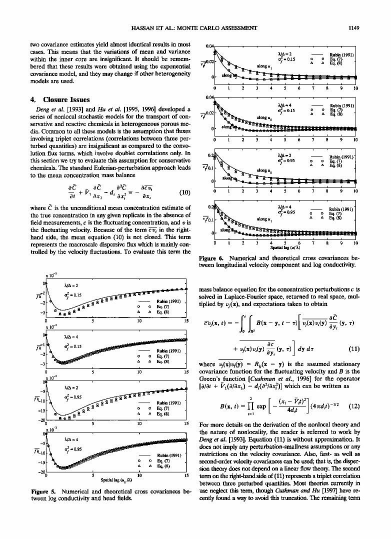
Both of the two estimates are used to evaluate the log conductivity covariance, •(u), which is obtained by ensemble averaging over all realizations. Figure 2 shows the comparison between the analytical covariance, (5), and the numerical covariances estimated using (7) and (8). The simulations are performed for •r• = 0.15 and 0.95 with two and four grid points per integral scale in each case (the issue of grid resolution will be discussed later). Also, the two covariance estimates are employed along the mean flow direction; u = (u•, 0), and normal to it, u = (0, u2). It is clear that the finer grid gives identical results to the analytical covariance. Nevertheless, the coarse grid (A/A = 2) does a good job in reproducing the input covariance except for minor deviations at small lags. Figure 2 also indicates that the first estimate, (7), is better than the second one, (8), in terms of matching the analytical curve. Comparing Figure 2 to Bellin et al.'s [1992a] results, which test RFGs based on turning bands and FFT methods, shows that our RFG is reproducing the analytical covariance much more closely than Bellin et al.'s results using both methods.

Having established the accuracy of our RFG, the Monte Carlo technique can be employed. First, the random conductivity field is generated as described above with a predefined spectrum. Second, the flow equation can be deterministically solved with the appropriate boundary conditions. Third, a particle-tracking technique is employed to obtain the concentration distribution for each realized flow field. Finally, Monte Carlo iterations are repeated for the first three steps, and ensemble averaging is used to obtain the statistics of concern.

0 1 2 3 4 5 6 7 8 9 10

0.1 •A=4

f7 0.11 • o•=0.15

00 0 1 2 3 4 5 6 7 8 ; 10

1• .... k/A = 2 .....

i i i i i i

0 1 2 3 4 5 6 7 8

.... •,/a = 4 .....

4 5 6 7 8 9 10 Spatial lag (ufk)

Figure 2. Comparison between reproduced log conductivity covariance with the analytical expression.

We present in the appendix the details of the solutions to the flow and transport equations. We discuss the finite difference solution to the flow equation and the numerical implementa- tion issues associated with the solution. The accuracy of the flow model is established through a mass balance check using different grid resolutions. We also show the boundary effects on the head and velocity variability and establish the stationarity of the head and velocity fields. We then present some details about the random walk particle-tracking approach used for solving the transport equation and the basis for choosing the parameters of the transport model.

3. Comparison With First-Order Flow Theories The convergence of the flow model is confirmed in the

appendix. Here we compare the velocity covariance, and its cross covariance with the head and the log conductivity, to linear perturbation results. Equation (1) is an example of such a linearization. This theory, as well as many others, assumes that the log conductivity variance o-• is sufficiently smaller than unity. The main result of all flow theories is the functional relation between the velocity covariance and the log conductivity field. Unlike authors of previous studies [Salandin and Rinaldo, 1990; Bellin et al., 1992a; Chin and Wang, 1992; Bellin et al., 1994], we do not restrict our attention to the velocity covariance only. We hope to provide more insight into the robustness of the linear theory and draw a clear picture of which truncation has the most effect; the truncation in computing the heads or in computing the velocity via Darcy's law.

Gelhar and Axness [1983] obtain (1), and Rubin [1990, 1991]


15 x 10 -3 ........ 1• •A=2 ' . Rubin (1990) J -I '%,-"•_ . o2.=0.15 --- G&A(1983)

v_--_--• • along u 1 o o •. (7) ]

I along u; -5, , , , , , , , , , I 0 1 2 3 4 5 6 7 8 9 10

15 X 10 -3 ......... l• • MA=4 - Rubin (19•)J

'[ •_ g2 = 0 15 G&A (1983) / v• -[ • • alongu I f o o •.(7) /

0 1 2 3 4 6 7 8 9

MA=2

005•- 0•=0.95 Rubin (1990)I G&A (1983) / v• ß o o •. (7)

0• along• a • • • • • • • • • • a a I I i I i i I ..... • • [ ' • ' 0 1 2 3 4 S 6 7 9 10

0,1 .........

• M•: 4 Rubin (19•) G&A

o o

• I I

0 1 2 3 4 5 6 7 8 9 10

Spatial lag (u/•)

Figure 3. Numerical and theoretical longitudinal veloci• covariances.

gives the velocity covariance as well as the cross covariances between velocity, head, and conductivity iri real space. In all the comparisons that follow we employ both covariance estimates, (7) and (8), using the exponential model with o-• - 0.15 and 0.95 and grid resolution A/A = 2 and 4. Also, where applicable, we compare the covariances along the mean flow direction and normal to it. All Monte Carlo covariances are

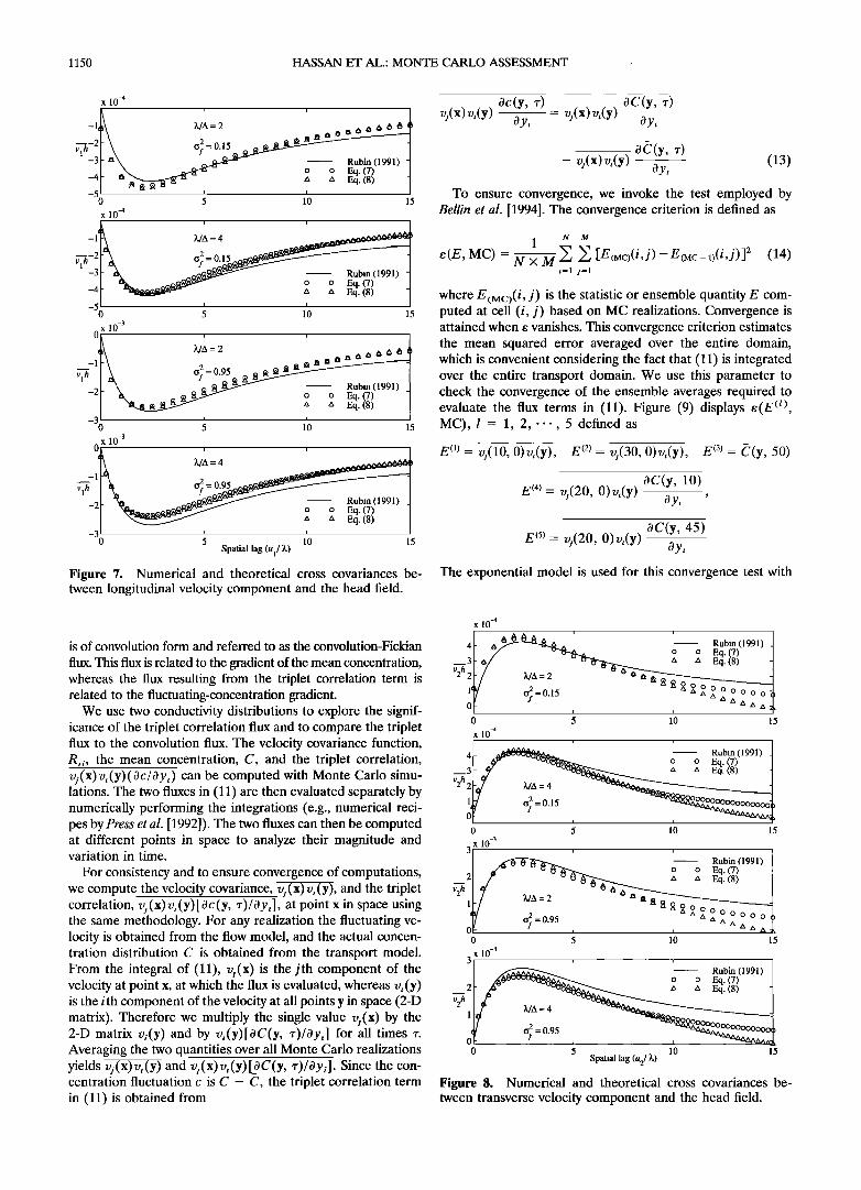
obtained by averaging within the inner core that is not affected by the boundaries. That core is determined by excluding a region of width 3A from each side of the domain [Bellin et al., 1992a]. Figure 3 shows the longitudinal velocity covariance, vx v•. Equation (1) of Gelhar andAxness [1983], abbreviated as G&A, is inverted to real space and essentially matches Rubin's [1990] result. Figure 3 shows that the longitudinal velocity covariance is anisotropic although the input In K covariance is isotropic. This is due to the effect of the mean head gradient J, which leads to larger velocity correlation length in the mean flow direction as opposed to the transverse direction. Gener- ally all the numerical covariances match the theoretical values. Minor differences exist for the coarse grid, especially at small lags. Also, (7) is closer to the analytical values than (8). Figure 4 shows the isotropic covariance of the transverse velocity component. It confirms the results of Figure A2 that the linear theory underestimates the variance and the covariance at small lags. These two figures reveal a picture that is different from that of Bellin et al. [1992a]. They show that both covariances deviate from the linear theory at small lags as o-• increases and exceeds unity. That is true for our transverse velocity, but not so for the longitudinal. This good agreement between linear

theory and fully nonlinear Monte Carlo results is consistent with those of Dagan [1985; 1993] and Tompson and Gelhar [1990], who have suggested for isotropic formations that the first-order approximation is quite accurate for both the head and velocity covariances up to a log conductivity variance of the order of unity.

In Figure 5 the In K cross covariance with the head field along the mean flow direction is shown. The grid effect is significant in this case, and again the first estimate is closer to the theory than the second. The linear theory of Rubin [1991] matches the numerical results very well for the fine grid case. The velocity In K cross covariance, v•f, is shown in Figure 6, which shows the deviation of the linear theory as o-] approaches unity. The two covariance estimates are almost identical along u2, but they differ along u x, with the second estimate matching the theory better. The cross covariance between the velocity components and the head is shown in Figures 7 and 8. In both figures the grid refinement improves the comparison with the theoretical covariance. However, significant deviations exist as o-] increases. The deviations at large lags with o-] = 0.15 can be due to the decreasing accuracy of the numerical estimate as the lag increases.

The main conclusions in this section are that v• v•, t/2t/2, and fh obtained from first-order flow theory are very close to the Monte Carlo simulations even with o-] approaching 1.0. Other theoretical covariances, vd', v•h, and v2h, deviate from Monte Carlo results as o-] increases. Grid refinements seem to improve the prediction in most cases; however, the difference between MA = 2 and 4 is not very significant. In addition, the

x 10 -3 ! , i ! ! i i ! !

MA = 2 Rubin (1990) o•f= 0.15 G&A (1983) o o Eq. (7)

v2v2 •x •x Eq. (8)

01 , - ,- _-'-c•_ _ _• _:._ • _• I i I I I

0 I 2 3 4 5 6 7 8 9 I0

x I0 -3

i Rubin (1990) Eq. (7) Eq. (8)

I

9

•i i i i i | i i i i 0.0 k/A = 2 Rubin (1990) 0.02• NxO o• G&A (1983) v?: I 'xx : 0.95 o o Eq. (7) a a Eq. (8)

I -%._ øl- , ,-:-,---,---, ,

0 1 2 3 4 5 6 7 8 9

•]• i i i i i I i i l 0.0 )h/A = 4 Rubin (1990) 0.02•- N,a of/= 0.95 G&A (1983) vB o o Eq. (7) 0.01[ • a a Eq.(8)

øI , --"-,-'-----,---,---,--- 0 1 2 3 4 5 6 7 8 9 10

Spatial lag (u/•,)

Figure 4. Numerical and theoretical transverse velocity covariances.


two covariance estimates yield almost identical results in most cases. This means that the variations of mean and variance

within the inner core are insignificant. It should be remembered that these results were obtained using the exponential covariance model, and they may change if other heterogeneity models are used.

4. Closure Issues

Deng et al. [1993] and Hu et al. [1995, 1996] developed a series of nonlocal stochastic models for the transport of conservative and reactive chemicals in heterogeneous porous media. Common to all these models is the assumption that fluxes involving triplet correlations (correlations between three perturbed quantities) are insignificant as compared to the convolution flux terms, which involve doublet correlations only. In this section we try to evaluate this assumption for conservative chemicals. The standard Eulerian-perturbation approach leads to the mean concentration mass balance

.... (10) Ot + •/• • di 0 xi 2 0 x i where C is the unconditional mean concentration estimate of

the true concentration in any given replicate in the absence of field measurements, c is the fluctuating concentration, and v is the fluctuating velocity. Because of the term • in the right- hand side, the mean equation (10) is not closed. This term represents the macroscale dispersive flux which is mainly con- trolled by the velocity fluctuations. To evaluate this term the

x 10 -3

ø• x/a = 2 ' ' -2•- • •S • a- - - Rub• (1991)

i • • • - o o •. -3 , • a •. (8)

0 5 10 15

x 10 -3

• Ma =4 ' ' ' • d=015 fh f ' i •Rub• (1991) -- I I

0 5 10 15

x 10 -3

• Ma = 2 ' ' [•10[k [ - ••- - - •ub•(1991)

•125 • aa••a : : •:((:••- o ••(7)) 0 5 10 15

x 10 -•

1250• •n- ' • : •:'":)) •5 5 10

Spatial lag (u• fk)

Figure 5. Numerical and theoretical cross covariances between log conductivity and head fields.

0'04•x• .... MA'=2 ' ' ' Rubin'(1991) l --0 02• • o•: 0.15 o o Eq. (7) |

I a a ,Sq. (8) ] I , , -7'7-7 .... I I I I I

0 1 2 3 4 5 6 7 8 9 10

0,04 i i i ! i i i i i

--0 02• xhat• q = 0.15 o o Eq. (7) 1

0 I 2 3 4 5 6 7

i i i i i i i i i 0.2• k/A = 4 l •x o• = 0.95 Rubin (1991) o o Eq. (7) /

, • • i I 0 1 2 3 4 5 6 7 8 9 10

Spatial lag (ul •)

Figure 6. Numerical and theoretical cross covariances between longitudinal velocity component and log conductivity.

mass balance equation for the concentration perturbations c is solved in Laplace-Fourier space, returned to real space, mul- tiplied by vi(x ), and expectations taken to obtain

_ B(x- y, t- ,r) vj(x)vi(y) •ii (y' ,r)

oc ] + v•(x)v,(y) •/(y, ,) ay a, (11) where •5.(x)vi(y) = Rii(x - y) is the assumed stationary covariance function for the fluctuating velocity and B is the Green's function [Cushman et al., 1996] for the operator [O/Ot + P•(O/Ox•) - di(O2/Oxi2)] which can be written as

2 I (Xi • --•rit) 2] (4*rdit)-'/2 (12) B(x, t) = 1-[ exp - 4dit i=1

For more details on the derivation of the nonlocal theory and the nature of nonlocality, the reader is referred to work by Deng et al. [1993]. Equation (11) is without approximation. It does not imply any perturbation-smallness assumptions or any restrictions on the velocity covariance. Also, first- as well as second-order velocity covariances can be used; that is, the dispersion theory does not depend on a linear flow theory. The second term on the right-hand side of (11) represents a triplet correlation between three perturbed quantities. Most theories currently in use neglect this term, though Cushman and Hu [1997] have recently found a way to avoid this truncation. The remaining term


x 10 -4

-It[ X/A=2 - ,, O •I

-3[- • • •• - - Rubin (1991)

, t 0 5 10 15

x 10-4

0 5 10 15

x 10 -3

X,/A = 2

-1 2= q •1• ¾1 h Of 0.9..,• • •1 a a a • n• I -X a •• - - Rubin (1991)

o 5 lO 15

o x lO -3 , ,

-3 -• , • a Eq.(8) 0 5 10 15

Spatial lag (Ul/

Figure 7. Numerical and theoretical cross covariances between longitudinal velocity component and the head field.

is of convolution form and referred to as the convolution-Fickian

flux. This flux is related to the gradient of the mean concentration, whereas the flux resulting from the triplet correlation term is related to the fluctuating-concentration gradient.

We use two conductivity distributions to explore the signif- icance of the triplet correlation flux and to compare the triplet flux to the convolution flux. The velocity covariance function, Rii, the mean concentration, •, and the triplet correlation, vi(x)vi(y)(Oc/Oy•) can be computed with Monte Carlo simulations. The two fluxes in (11) are then evaluated separately by numerically performing the integrations (e.g., numerical recipes by Press et al. [1992]). The two fluxes can then be computed at different points in space to analyze their magnitude and variation in time.

For consistency and to ensure convergence of computations, we compute the velocity covariance, vi(x)v•(y), and the triplet correlation, v:(x)v•(y)[Oc(y, r)/Oy•], at point x in space using the same methodology. For any realization the fluctuating velocity is obtained from the flow model, and the actual concentration distribution C is obtained from the transport model. From the integral of (11), vj(x) is the jth component of the velocity at point x, at which the flux is evaluated, whereas vi(y) is the ith component of the velocity at all points y in space (2-D matrix). Therefore we multiply the single value vj(x) by the 2-D matrix v•(y) and by v•(y)[OC(y, r)/Oy•] for all times r. Averaging the two quantities over all Monte Carlo realizations yields vj(x)v•(y) and v•(x)vi(y)[_OC(y, r)/Oy•]. Since the concentration fluctuation c is C - C, the triplet correlation term in (11) is obtained from

Oc(y, r) OC(y, r) v•(x) v•(y) -- = v•(x) v•(y) Oyi

OC(y, r) vj(x) v,(y) Oy, (13)

To ensure convergence, we invoke the test employed by Bellin et al. [1994]. The convergence criterion is defined as

1 N M e(E, MC): N x M ]• • [E(Mo(i'J) --E(Mc-•)(i,j)]2

i=1 j=l

(14)

where E (•o(i, j) is the statistic or ensemble quantity E computed at cell (i, j) based on MC realizations. Convergence is attained when e vanishes. This convergence criterion estimates the mean squared error averaged over the entire domain, which is convenient considering the fact that (11) is integrated over the entire transport domain. We use this parameter to check the convergence of the ensemble averages required to evaluate the flux terms in (11). Figure (9) displays e(E ©, MC), l - 1, 2, --., 5 defined as

E (•) = vj(10, 0)v,(y), E © = v;(30, 0)v•(y), E © = •(y, 50)

E ©: v:(20, O)v•(y) OC(y, 10)

Oyi '

E © = vj(20, O)v,(y) OC(y, 45)

Oy,

The exponential model is used for this convergence test with

x 10-4

4[ 6 O• . ' '- Rubin (1991)

1

0 5 10 15

x 10 •

4• •• ' '. aubin(1991) J • • •o• o o •.(7) /

0 5 10 15

x 10 -3

• Rubin (1991 ) ,,/ •g'• - '• • • o o Eqi(7)

v2h

0 5 10 15

x 10 -3 3 , ,

. a/-'••-'•;•....,• Rubin (1991) • / ,40 .... o•8•,,•----•,,•. o o •. (7) /

v2h

0 • , •• 0 5 10 15

Spatial lag (u2/•)

Figure 8. Numerical and theoretical cross covariances be- •een transverse veloci• component and the head field.


Table 1. Input Parameters for the Cases Studied

Parameter Value

Fractal dimension of f D 2.2 Upper cutoff kma x Lower cutoff kmi n 2z'/128 f variance tr] varies Integral scale for exponential h 1.0 Mean head gradient J 0.06162 Mean velocity •z• 0.4786 Longitudinal dispersivity a/• = d•/IVl 0.5 Transverse dispersivity arH: d2/lvI 0.05 Mean log conductivity F 1.0 Initial concentration mass M 4.2 Initial concentration box 6.0 x 2.0

Initial source location (x•, x2) (0.0, 0.0) Computational grid Ax• X •X 2 0.25 x 0.25 Time step At 0.25 Point of flux computation (x•, x2) (10.0, 0.0), (20.0, 0.0),

(30.0, 0.0)

variance rr• = 0.4 and other parameters as shown in Table 1. It is obvious in Figure 9 that all convergence parameters are very small after 100 iterations and they decay quickly as the number of realizations increases from 100 to 600. In order to

assure proper convergence, we perform 1200-2400 Monte Carlo iterations depending on the degree of heterogeneity rr• and the integral scale k.

Figure 10a shows the results with a fBm conductivity and • = 0.05. The two fluxes are computed 10, 20, and 30 m downstream from the initial source location. Since the convolution flux (solid line) is proportional to the gradient of the mean concentration, it

becomes zero when t = x•/P•, where x• is the point at which the flux is computed. This can be seen by examining the nature of the convolution term in (11) and the Green's function B(x, t) given in (12). It is clear from (12) that B(x, t) is a dispersing function which propagates and spreads in space with a velocity equal to V• as t increases. The nature of the convolution flux dictates that the

mean concentration plume and the function B(x, t) move in the same direction with velocity V• as the time integration parameter ß changes from zero to t. By choosing t = x•/•z• the peak of the function B always coincides with the centroid of the mean plume as the integration is performed over ß whereas the peak of the covariance function, Rii, remains at x•. The Green's function B is symmetric, whereas the gradient of the mean concentration is asymmetric. Also, the stationary velocity covariance is symmetric aboutxv As a result, the spatial integration of the convolution flux vanishes for any ß between zero and t = x•/•z•. Therefore the temporal integration will lead to a zero flux at this time.

The behavior of the triplet flux is also as expected, and may be interpreted as follows. Bellin et al. [1994] showed that the estimation of the concentration is the most error prone during the passage of either the leading or trailing edges of the plume. During passage of the plume centroid, the concentration becomes more predictable with small uncertainty. Rubin [1991] showed that the prediction of the low concentration at the periphery of the plume is subject to the largest uncertainty, while that along the mean plume centroid is quite reliable. On the periphery of the plume the appearance of a single particle is very significant and entails a considerable variability; however, as the center of the plume is approached, the concentration varies in space more smoothly and hence is easier to

œ(E, MC) 1

4

œ(E ©, MC)

x 10 -6

0 100

x 10 -8

>

200 300 400 500

x 10 -6 1.5

- 1.0

0.5

0.0

600

0 100 200 300 400 500 600

x 10 -9 8 i i i i

6

œ(E, MC) 4

>

1 O0 200 300 400 500 MC

1(• -9 5

3

1

0.0

600

Figure 9. Convergence of computations for the velocity covariance, mean concentration, and triplet correlation estimates.


x 10 -3

-4 • 0 10 20 30 40 50

X 10 -3 4

!

o

2 x 10 -3 10 20 30 40 50

0.02 I (b) J

0.01 •-

o/ -0.01 [

0

11 10-3 o

o

X 10 -3

10 2o 30 40 50

10 20 30 40 50

-1 0 10 20 30 40 50 0 10 '20 30 40 50

Time (days) Time (days.)

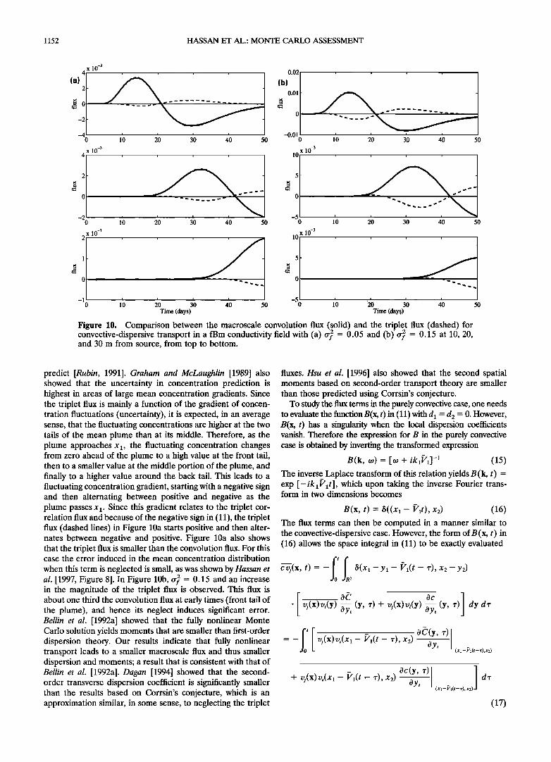
Figure 10. Comparison between the macroscale convolution flux (solid) and the triplet flux (dashed) for convective-dispersive transport in a fBm conductivity field with (a) o-• = 0.05 and (b)' trf = 0.15 at 10, 20, and 30 m from source, from top to bottom.

predict [Rubin, 1991]. Graham and McLaughlin [1989] also showed that the uncertainty in concentration prediction is highest in areas of large mean concentration gradients. Since the triplet flux is mainly a function of the gradient of concentration fluctuations (uncertainty), it is expected, in an average sense, that the fluctuating concentrations are higher at the two tails of the mean plume than at its middle. Therefore, as the plume approaches x•, the fluctuating concentration changes from zero ahead of the plume to a high value at the front tail, then to a smaller value at the middle portion of the plume, and finally to a higher value around the back tail. This leads to a fluctuating concentration gradient, starting with a ne, gative sign and then alternating between positive and negative as the plume passes x2. Since this gradient relates to the triplet correlation flux and because of the negative sign in (t 1), the triplet flux (dashed lines) in Figure 10a starts positive and then alter- nates between negative and positive. Figure 10a also shows that the triplet flux is smaller than the convolution flux. For this case the error induced in the mean concentration distribution

when this term is neglected is small, as was shown by Hassan et al. [1997, Figure 8]. In Figure 10b, crf = 0.15 and an increase in the magnitude of the triplet flux is observed. This flux is about one third the convolution flux at early times (front tail of the plume), and hence its neglect induces significant error. Bellin et al. [1992a] showed that the fully nonlinear Monte Carlo solution yields moments that are smaller than first-order dispersion theory. Our results indicate that fully nonlinear transport leads to a smaller macroscale flux and thus smaller dispersion and moments; a result that is consistent with that of Bellin et al. [1992a]. Dagan [1994] showed that the second- order transverse dispersion coefficient is significantly smaller than the results based on Corrsin's conjecture, which is an approximation similar, in some sense, to neglecting the triplet

fluxes. Hsu et al. [1996] also showed that the second spatial moments based on second-order transport theory are smaller than those predicted using Corrsin's conjecture.

To study the flux terms in the purely convective case, one needs to evaluate the function B(x, t) in (11)with d• = d 2 - 0. However, B(x, t) has a singularity when the local dispersion coefficients vanish. Therefore the expression for B in the purely convective case is obtained by inverting the transformed expression

B(k, 6o) = [6o + ik,P,]-' (15) The inverse Laplace transform of this relation yields B(k, t) = exp [-ik• V•t], which upon taking the inverse Fourier transform in two dimensions becomes

B(x, t) = tS((x•- V•t), x2) (16)

The flux terms can then be computed in a manner similar to the convective-dispersive case. However, the form of B (x, t) in (16) allows the space integral in (11) to be exactly evaluated

cvj(x, t) = - 13(x• - y• - V•(t - r), x2 - Y2) 2

oC oc ] ß vj(x)v(y) (y, r) + vj(x)vi(y) • (y, r) dy dr

ot[ - Uj(X)Vi(X 1 -- V•(t- r), x2) 0 •7(y, r)

Oyi (Xl-•"l(t-z),x2)

q- Uj(X)•i(X 1 -- P•(t •- r), x2) oc(y,

(Xl--Pl(t--•'),x2)] dr (17)


0.04 / 0.02[

0 '

0 021 -- .

0 10 20 30 50

0.02

0.01

-0.01

-0.02 0 10

x 10 -3 6

- - - Triplet corr. Total flux

20 30 40

I I

-20 10 20 30 40 50 Time (days)

Figure 11. Comparison between the macroscale convolution flux (solid) and the triplet flux (dashed) for purely, convective transport in a fBm conductivity field with o-• = 0.15, and the net (total) fluxes (dashed-dotted).

The two terms in (17) are numerically evaluated at the same points as for the previous case. For o-• = 0.15 the triplet flux (Figure 11, dashed line), though smaller, is comparable in magnitude to the convolution flux (solid line), and therefore neglecting this term may lead to large errors. Figure 11 also shows the total flux, that is, the convolution flux added to the triplet flux.

A similar analysis can be performed with exponential covariance for the fluctuating log conductivity. Figure 12a shows the results for o-• = 0.15 and X = 1.0 m with local-scale dispersion. The triplet flux is insignificant relative to the convolution flux. When local dispersion is not included, the triplet flux increases (Figure 12b) but not as much as for the fractal conductivity distribution. Therefore the error induced by neglecting this term is much smaller for the exponential covariance than for the fractal conductivity with the same variance. This is attributed to the long (theoretically infinite) correlation scale of the fractal distributions. The total flux for this pure convective case is plotted in Figure 12b.

To further elaborate and shed more light on the importance of local-scale dispersion, we plot in Figure 13 the exact nonlocal fluxes (both terms in (11)) for several values of dispersivity. The longitudinal dispersivity az• is taken as 0.0, 0.01, 0.05, and 0.5, and the transverse horizontal dispersivity a Tr• is taken as aL/10. The last value of a lies in the upper range of the values determined by Klotz et al. [1980]. Clearly, the dispersivity has a significant influence on the magnitude of the total flux. The purely convective case differs from the convective-dispersive cases, even for small dispersivity values of az• =

5

(a)

•o

-5 0

x 10 -s

10 20 30 40 50

0.04 I {b) /

0.02•

o/ _ -o.o! ;o 20

x 10 -s 4

2

0 '

0.02

0.01

-0.02 20 30 40 50 1'0 0 1'0 2• 3; 4'0

10

-5 0

x 10 -4 0.01

0.005

---- Conv. flux

- - - Triplet corr. ..... Total flux

50

Figure 12. Comparison between the macroscale convolution flux (solid) and the triplet flux (dashed) for exponential conductivity covariance with o-] = 0.15 and it = 1.0 m: (a) convective-dispersive transport and (b) purely convective transport, with the dashed-dotted lines indicating the total flux.

0 10 20 30 40 50 0 10 20 30 40 50

Time (days) Time (days)


o.o2[ = 0.0•[ • -0.01 I

-0.02• o ,'o 3'o i0 so

0'02 ø'ø10

-O.Ol I

0 10 20 30 40 50

6 x 10 -3 .... I -- O•L=O•TH =0.0

4 t • O'L=0'01 & O'T/-/=0'001 • / ..... O'L=0'05 & O'TH--0'005 / I • 2 t - - - 0tL=0'5 & 0iT/-/=0'05 .ty J

0 10 20 30 40 50

Time (days)

Figure 13. Comparison between the exact nonlocal macroscale flux for different dispersivity values.

0.05 and a Ti-i = 0.005. As expected, for a L = 0.01 and a T/-/ = 0.001 the convective-dispersive flux approaches that of the purely convective. When local dispersivity increases, the difference between the purely convective flux and the convective- dispersive flux increases.

Because dispersivity grows with the scale of observation, there is a fundamental difficulty defining "local scale" and hence in choosing a rational nonambiguous dispersivity. But in any case, these plots show that it should not be neglected in transport theories. These numerical results are in agreement with recent theoretical discussions by Hu et al. [1995] and Fiori [1996]. In the context of numerical simulations, Jussel et al. [1994] found that neglecting local dispersion in transport simulations in a real aquifer underestimated the mean cloud velocity by 7%. Graham and McLaughlin [1989] reported that low values of local dispersivity produce steeper, less dispersed mo- ment distributions, which is similar to the pattern observed in Figure 13.

We next examine the interplay between o-f and )t a little more closely using an exponential covariance. Figure 14a shows the results for o-f = 0.4 and )t = 1.0 m. Even for this variance the ratio of the triplet flux to the convolution flux is still smaller than in Figure 10b for the fBm conductivity where o-f = 0.15. Again the long range correlation is affecting the magnitude of the triplet flux. This can also be seen in Figure 14b where o-f = 0.15 and )t - 5.0 m. The grid size for this case is kept at 0.5 m so that MA = 10. Increasing the correlation length increases the magnitude of the triplet flux, which causes large errors in the concentration distribution. This can be explained by noting that large integral scale may cause large velocity deviations (rrv = f( o-f, /•)) from the mean which are likely to persist over greater distances. This effect increases variability between plumes across the ensemble, leading to greater concentration uncertainty [Graham and McLaughlin, 1989]. Increasing the concentration fluctuations (uncertainty) leads to a stronger correlation with the velocity components and hence a higher triplet flux effect.

In summary, the errors induced in Eulerian theories which

0.02 I (a) /

o.o1•

o/ -O.Ol {

o

x 10 -3

5

0

x 10 -3 4

0

,'0 do 3'0 io

•0.02 [ ,

0 10 20 30 40 50

10 20 30 40 50

x 10 -3 lO

o

x 10 -3

10 20 30 40 50

10 2'0 30 40 50 0 Time (days)

Figure 14. Comparison between the macroscale convolution flux (solid) and the triplet correlation flux (dashed) for a convective-dispersive transport in a conductivity field with exponential covariance: (a) o-f = 0.40, )t = 1.0 m and (b) o-• = 0.15, )t = 5.0 m.

10 20 30 40 50 Time (days)


neglect triplet correlations are small for mildly heterogeneous media with short correlation scales. When either the conduc-

tivity variance o-f or its correlation scale X increases, the error increases and seems significant. Also in purely convective transport the resulting errors are higher than in the convective- dispersive case.

5. Flux Localization Errors

Cushman et al. [1995] argue that media which are either nonperiodic (e.g., media with evolving heterogeneity) or peri- odic viewed on a scale wherein a unit cell is discernible must

display nonlocality in the mean. They suggest that owing to the scarcity of information on natural scales of heterogeneity and on scales of observation associated with an instruments win-

dow, constitutive theories for the mean concentration should at the outset of any modeling effort be nonlocal. If the scale of observation turns out to be large relative to the heterogeneity scale, the process can be considered local. However, nothing will be lost in using the nonlocal constitutive theory since it will reduce to its correct local counterpart. The fully nonlocal theory can be localized in space or time alone or it can be localized in both space and time, resulting in a fully localized theory. To see what types of errors might be induced in the convolution flux by various localizations, we will follow the lead of Cushman et al. [1995] and make comparisons between the fluxes resulting from the fully nonlocal (FNL) model, the nonlocal in time (NLT) model, and the fully localized (FL) model.

The two-dimensional convolution flux Qi(x, t) in (11) is

Qj(x, t) = - B(x- y, t - ,) 2

ß vj(x)v,(y) •/(y, ,) dy d, (18) To localize this equation in space one needs to factor the mean concentration gradient out of the integral and integrate the remaining part of the integrand with respect to x:

•0 ! 0• Q;(x, t) = - Bji(x , t- ,) • (x, ,) d, (19)

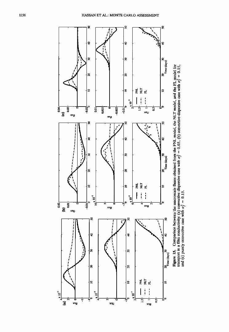
models. Conductivity realizations are again generated either from a fBm distribution or with exponential covariance. Figure 15a shows the results for a fBm conductivity with o-• = 0.05. Clearly the FL model works reasonably well. Consistent with Cushman et al. [1995], the NLT model markedly deviates from the other two models. When o-• is increased to 0.15, the FL model starts to deviate from the FNL model but still works

much better than the NLT model (Figure 15b). In this latter case for purely convective transport the fully localized model produces significant errors (Figure 15c).

Figure 16a shows results for an exponential conductivity covariance with o-• = 0.15 and X = 1.0 m. The NLT model works better in this case than in the fractal case. However, it is very different from the FNL model. The FL results compare reasonably well with the FNL, although there are some dis- crepancies. The same case but without the inclusion of local dispersion is shown in Figure 16b. The FL results are better here than in the fractal case, but they still significantly differ from the FNL results. The NLT model remains in large error. When o-f increases to 0.4, the NLT model shows large errors while the FL model has small errors (Figure 17a). The NLT results become even worse when the integral scale X increases to 5.0 m while tr• = 0.15, as shown in Figure 17b. The FL model shows larger errors in this case. The irregular pattern of the FL model in the previous cases is due to the fine grid resolution, which enhances the localization effect, and the fact that the solution is only a function of small neighborhood around the point.

In the light of the above results it can be seen that the nonlocal in time model is not accurate when applied to heterogeneous media with evolving scales of heterogeneity nor even in the media with a short correlation scale. For large conductivity variance and/or large integral scale, the fully localized model deviates from the fully nonlocal model. These errors increase when local dispersion is not included, especially when heterogeneity is evolving. It should be remembered that localization errors were examined for only the convolution flux, which is the first term in the right-hand side of (11). A better comparison would have been made with both terms in (11). However, it is not possible to localize the second term (triplet correlation) on the right-hand side of (11), so such a comparison cannot be made.

where

Bji(x, t- ,) = IR B(x - y, t- ,)vj(x)v,(y) dy (20) 2

Equation (19) is nonlocal in time alone and denoted NLT. A similar localization procedure can be applied to time and leads to

Qj(x, t) = -B'/i(x , t) • (x, t) (21)

f0 t BS'i(x, t) = Bj,(x, t- ,) d, (22)

Equations (18), (19), and (21) represent the FNL, NLT, and the FL models, respectively. These equations are evaluated using Monte Carlo simulations. A numerical integration procedure is applied to compute the flux Qi(x, t) in the three

6. Summary and Conclusions Monte Carlo simulations of flow and transport in heteroge-

neous media are employed to investigate several issues related to flow and transport in such media. The validity of first-order relations for the velocity covariance is examined. Monte Carlo simulations were used to construct the velocity covariance from the conductivity covariance. These results were then compared to the velocity covariance obtained from first-order flow theories. It is found that these theories predict the longitudinal velocity covariance very accurately up to o-• of the order of unity. However, the linear transverse velocity covariance deviates from the fully nonlinear Monte Carlo results as o-• approaches unity.

The closure issue associated with the nonlocal transport model of Deng et al. [1993] is addressed to explore the extent to which the assumptions underlying this issue hold. Triplet fluxes that are usually neglected in the derivation of the transport equations induce small errors that can be neglected in cases when the porous medium has mild heterogeneity with


I• , , ,i , i

xn U


(a)1ø /

6 x 10 -3

x 10 -3

I'

• 2

-2 0

x 10 -3 3

2

• FNL

..... NLT

_0'.021 0

-0.01 [ -0.02 /

0

6 x 10 -3 l

4

0

'lb

,%

l 10 20 30 40 50

i I I i 11 I ' I

i, i i I 1'0 ' 20 30 40 50 2'0 3'0 Time (days) Time (days)

..... I I l

i II

40 50

Figure 16. Comparison between the macroscale fluxes obtained from the FNL model, the NLT model, and the FL model for transport in a conductivity field with exponential covariance: (a) convective-dispersive case with o-• = 0.15, A = 1.0 m and (b) purely convective case with o-• = 0.15, A = 1.0 m.

small integral scale. When either the log conductivity variance or its integral scale is increased, the triplet flux becomes important and should not be neglected. Also, for the purely convective transport in a fractal conductivity field, the mac-

roscale flux resulting from the triplet correlation is large and comparable to the convolution flux. This triplet flux is not as large in purely convective transport in a log conductivity field with an exponential covariance structure.

0.02 , 0.021 . , , , , . la) lb) /

t• 0.01 • • 0.01 • .•,.. 0

-0 01 ' -0'010 l'O 2'0 3•0 i0 50 ' 0 10 20 310 40 50

10 x 10 -3

• -

........ ....

i10 10 20 30 40 50

x 10 -3 10 ....

- lb ;0 3'0 40 50 X 10 -3 x 10 -3

i

• FNL

..... NLT

I0 i i i i 0 i 0 1 20 30 40 50 0 1 20

Time (days)

, , , ,

I i i

3• 40 50 Time (days)

Figure 17. As in Figure 11: (a) convective-dispersive case with rr• = 0.40, X = 1.0 m and (b) convective- dispersive case with o-• = 0.15, X = 5.0 m.


Localization errors in the macroscale flux are studied. The

fully nonlocal macroscale convolution flux is first localized in space and then in time to give the fully localized model. Re- sults show that the nonlocal in time model differs significantly from the fully nonlocal model and there is a lesser difference between the fully localized model and the fully nonlocal model. This result is consistent with the findings of Cushman et al. [1995] for conservative transport. It is also found that the fully localized model works reasonably well when tr• and ,k are small, but gives large errors when local-scale dispersion is switched off. The exact macroscale flux is computed for transport with different dispersivity values. It is found that neglecting local-scale dispersion can lead to large errors in the total macroscale flux. This is in agreement with the theoretical results of Hu et al. [1995] and Fiori [!996] and numerical simulations of Jussel et al. [1994] and Graham and McLaughlin [1989].

Appendix A1. Summary of Numerical Studies

We summarize in Table A1 several numerical studies of flow

and transport in heterogeneous porous formations. The main features, such as solution methodology, models used, and computational aspects, are presented. The missing data in Table A1 are either not mentioned in the study or are not applicable in the present context. Some of the studies combine a numerical simulation with analytical approach.

A2. Flow Model

We consider steady flow of groundwater in a two-dimensional, horizontal, saturated, incompressible porous medium with physical heterogeneity represented by spatially varying conductivity. We further assume that the mean flow is uniform and in the x• direction, [/• = V = constant, and [/2 = fz3 = 0. This is achieved by fixing the hydraulic head at the left and right boundaries and keeping the top and bottom boundaries impervious.

Steady state groundwater flow is described by

V-q(x) = V-(-K(x)V4)(x)) = 0 (A1)

where q(x) is the Darcy flux relative to the solid matrix and 4)(x) is the hydraulic head. This flow equation is discretized by employing a block-centered finite difference scheme using the domain shown in Figure 1. This yields a system of linear equations that can be directly or iteratively solved for the nodal heads. We solve the system of equations directly using an efficient Gauss elimination algorithm. In order to compute the flux components at the interfaces between adjacent blocks (Figure lb), the interblock conductivities are obtained by harmonic averaging of adjacent conductivity values. This form of averaging ensures continuity of the head field and conservation of mass flux across block boundaries [Aziz and Settari, 1979]. The head gradient at the interface between adjacent blocks is approximated by centered differencing utilizing the two adjacent nodal heads. Darcy's law can then be applied to obtain the flux components and accordingly, the velocity components using the assumed constant porosity value. Some computational considerations are worth mentioning here.

To obtain an accurate solution to the flow problem, the simulation domain should be much larger than the conductivity integral scale ,k, and the grid size in any direction, Axi, should be smaller than ,k i. As a rule of thumb based on scaling and

statistical arguments, reasonable grid resolution can be achieved by satisfying the inequality MAx _> (1 + try) [Ab- abou et al., 1989]. Bellin et al. [1992a] show that MAx = 4 is appropriate for heterogeneity level of up to trf = 1.6. As pointed out by Tompson and Gelhat [1990], a fully three- dimensional problem with ,ki/Ax i --• 4 and Li/,k i '" 25 would need as many as 10 6 nodes. Since the multiple-realization Monte Carlo approach we pursue here requires solving a system of linear equations for the nodal heads for each realization, a fully three-dimensional simulation with highly resolved and large enough domain would be very time consuming and may impose some limitations on the number of realizations considered. That is another reason we restricted ourselves to

two-dimensional simulations.

We check the accuracy of our flow model using a coarse grid with the least acceptable resolution of two points per integral scale (,k/A = 2) and refine the grid to a maximum of four points per integral scale (,k/A = 4). In doing so we rely on the specific indication of Bellin et al. [1992a], that results of flow and transport solutions are not affected by refinements of the grid size involving more than four points per integral scale for mildly heterogeneous media.

The solution of the mass balance equation coupled with Darcy's law is subject to an error that depends on the grid resolution and the degree of heterogeneity. In the finite difference method the error in the discretization of the differen-

tial operators is coupled with error stemming from computation of interblock conductivities [Goode, 1990]. However, these errors can be reduced by using a fine grid and taking the harmonic mean as a representative of the interblock conductivities. The mass balance test we perform here is a two-fold check, local mass balance and global mass balance. For the local mass balance the local error for any cell (Figure lb) is

e(i, j) = •qin(i, j) -- •qout(i, j) (A2)

and from the notation of Figure lb, e(i, j) = q• + q3 -- q2 -- q4. As discussed by Bellin et al. [1994], e is a RSF because it is derived from the random velocity field, and therefore, it can be characterized by its spatial mean, (e) = (1/N x M) E N E M (i, j) denoted by Bellin et al. [1994] as the local i=1 j=l e , closure error, and its variance, Se 2 = (1/N x M - 1) EiN__ [e(i, j) - (e)] 2 We computed the two estimates for each realization and ensemble averaged over 1500 realizations to obtain (e) and Se 2 as well as their ensemble variance, tr•e> and O2se 2. For all the cases we studied using the exponential covariance, we obtained the ensemble mean and variance of the closure error of the order of about 10 -•2 and 10 -8, respectively. This is to be compared to 10 -6 in Bellin et al.'s [1994] study. They, however, generated the random velocity field by a geostatistical model without solving the flow equation, as we do in this study. The reason we have that small local error is probably because we solve the linear system of equations for the nodal heads directly and not iteratively, so error tolerance for the solution is essentially zero. This result indicates that local mass is satisfactorily conserved in our simulations.

The other mass balance check we perform is the global mass balance, which can be defined [Chin and Wang, 1992] as e a = [system outflow - system inflow]/system inflow x 100. Similar to the local closure error, the global error can be expressed by its ensemble mean e a and variance 0 -2 These global error e•7ø

statistics computed with reference to 1500 realizations are summarized in Table A2 for different heterogeneity levels and grid resolutions. Table A2 shows that the magnitude of the


o

1160 HASSAN ET AL.' MONTE CARLO ASSESSMENT

Table A2. Global Error Statistics

X / A 0-• e a 0 -2 N10 eg

2 0.15 -0.006 0.365 0 2 0.95 -0.031 3.472 5 2 1.6 -0.063 8.193 17 4 0.15 0.012 0.092 0 4 0.95 0.014 0.850 2 4 1.6 0.001 1.982 2

mean global error, e a, is always less than 0.1%. Figure A1 2 from Table A2 compares the variance of the global error, O'eg,

to the results of Chin and Wang [1992] and that of Bellin et al. [1994]. Although the results of Chin and Wang [1992] seem much better than the other two cases in Figure A1 at small the rate of the error-variance growth with o-• does not seem correct or consistent, which casts some doubts about the accuracy and consistency of their results. Bellin et al. [1994] had a plot similar to our Figure A1 but when they compiled the data from Chin and Wang's [1992] study, they plotted the standard deviation instead of the variance. The better performance of Bellin et al.'s [1994] model may be attributed to the different boundary conditions used and to the fact that they generate the velocity field directly to conserve mass and reproduce the covariance. However, the overall values of the mean global error and its variance indicate a good accuracy for our flow model. Another statistic shown in Table A2 is the number of realiza-

tions, out of 1500, that have global error greater than 10%, N10. The number increases as o-• increases, but it decreases dramatically with refining the grid. With MA = 2, Chin and Wang [1992] obtained N10 = 2 for rr• = 1.44 and N10 = 8 for o-• = 1.6 9 where their total number of realizations was 92. So, the percentage of the number of realizations having error greater than 10% is about 2.2% and 8.7% for the two variances in Chin and Wang's [1992] study, while our percentage for o-• = 1.6 is about 1.1%. We conclude from the mass balance

analysis and the comparisons with other numerical studies that our flow model accurately produces the velocity field and sat- isfies mass balance requirements.

10 2

101

10 ø

132 0-1 el g

10 -2

10 -3

Pre'sent Study ' Chin. and Wang (1992)

Bellin et al. (1994) ...

71' I'

I

I

I

I

1 ß

, X/ix= 2_ _ _.

......•

......'"

i i i 0.5 1 1.5

MA=4

A3. Boundary Effects and Stationarity of the Head and Velocity Fields

Rubin and Dagan [1988, 1989] show that the presence of boundaries influences the head and velocity variabilities along a zone of width 3A normal to the boundaries. They also report that for distances larger than A normal to the boundary, the effects of the boundaries on the head and velocity spatial variabilities diminish considerably, and variations behave as if the domain were infinite. This indicates that there is a need for

an inner core region to which all other estimates and transport simulations should be limited. Salandin and Rinaldo [1990] and Bellin et al. [1992a] showed the boundary effects on the velocity variance and identified the inner core that is unaffected by the boundaries where transport simulations Were carried out. Sim- ilar to these studies, we plot in Figure A2 the variances of the two velocity components, and we add the variance of the head field. The exponential model is used with different o-• and grid resolution. Some important observations about Figure A2 are highlighted here. The head spatial variability is affected by the boundaries for a distance larger than 3A and it increases with o-•. Beyond this effect, the head variance is invariant in space. It is also observed that grid refinement affects the results more significantly as o-• increases; the finer the grid, the lower the head variability even though the In K variance and integral scale are preserved in both cases. On the other hand, the velocity variability increases as the grid is refined. This can be explained by the fact that head variations can be smoothed over a fine grid, but since the velocity is directly proportional to

0.01

0.008

2 0.006

0.004

0.002

0 ' (A) 0 10

0.2

0.15

2

i./ 2 /! _ o• = 0.95 I/If.-- ...... -.-.- -•--

ß

!•' 2 7 _13f• = 0.15

2'0 30 4'0 5'0 60 x IfK

13 2 Vl 0.1

0.05

0.06

132 0.04 V 2

13• = 0.15 10 20 30 40 50 60

Xlf)•

(B)

313.•V2/8

0.02

i 10-40 2 2.5 O0

Figure A1. Ensemble variance of the global mass balance error computed with 1500 Monte Carlo iterations.

Figure A2. effects.

Head and velocity variances showing boundary

HASSAN ET AL.' MONTE CARLO ASSESSMENT 1161

K, the finer grid captures more heterogeneity at the small scale leading to higher variability in the velocity field. Figure A2 also shows that the variance of the longitudinal velocity behaves differently than that of Salandin and Rinaldo [1990] and Bellin et al. [1992a], which behaves similar to the head variance in our case. Different boundary conditions are used in these studies. We employ fixed head boundaries which yield minimum head variabilities and maximum velocity variations along the boundaries, whereas Salandin and Rinaldo [1990] and Bellin et al. [1992a] assume unit specific discharge across the boundaries yielding minimum velocity variance and maximum head variability at the boundaries. They, however, did not show the head plots. The finer-grid results for the longitudinal velocity variance match the linear theory value of (3/8)o-•V 2 extremely well for the three cases considered. However, that is not the case for the transverse component where the theoretical variance deviates from the numerical one as tr] increases. The mean head gradient in the x • direction is the dominating factor in determining the longitudinal velocity component and it is completely captured by the linear theory. On the other hand, the transverse component is mainly affected by the conductivity fluctuations, and the resulting random head field, which make it sensitive to the truncation of the higher order terms in the flow equation. Figure A2 shows the linear theory is under- estimating the transverse velocity variance. This is consistent with the findings of Bellin et al. [1992a, Figure 6b].

Figure A2 ensures that sufficiently well developed head and flow fields are established in the inner core of the simulation

domain. The flow field can therefore be considered second

order stationary with constant mean velocity V and a spatially invariant variance within this inner region.

A4. Transport Model

Several numerical approaches can be used to solve the transport equation for the concentration distribution, for example, finite differences, finite elements, and random walk particle- tracking methods. The Peclet number Pe associated with the traditional finite difference and finite element solution of the

transport equation can be approximated by the ratio (V/Xx •)/ (aLV) -- (Ax•)/(aL). Pe should be kept less than unity and thus a very fine grid is needed for small dispersivity, a•. This can lead to severe computational limitations in terms of stor- age and processing time. The random walk method provides a suitable alternative that does not suffer from the above restric-

tion and that is also computationally very efficient. In addition, numerical dispersion is a common problem with finite difference and finite element methods for the solution of the advec-

tion-dispersion equation [Kinzelbach, 1988]. Moltyaner et al. [1993, Figure 12] have shown that the random walk method completely eliminates numerical dispersion. For this reason and following the majority of studies (Table A1) we use a random walk particle-tracking approach to simulate the movement and evolution of conservative tracers in random velocity fields. We replace the injected areal solute pulse with a large number of particles NP of equal mass rn and trace these particles in the space-time domain. The initial concentration Co, considered to be deterministic and constant, is given by C O = (NP rn)/(nll), where 12 is the area of the initial solute pulse. Ahlstrom et al. [1977] suggest that 103-104 particles may be sufficient for a one-component model. We use 2500 particles in all the transport simulations that follow. At each time step the concentration distribution is approximated as

C(x, t) = Z m(Xnp(t), t)T/(x- Xnp(t)) (m3) np•NP

where np = 1, 2, 3, ..., NP is the particle index; NP is the total number of particles used to simulate the continuous solute mass; Xnp(t ) is the position of the np'th particle at time t, which was initially at Xnp(0); m(Xnp , t) is the mass associated with that particle; and ,t(x) projects the contribution of all particles in a small neighborhood around point x to the concentration value at that point. The most simple choice for *t is a box function with value 1/a inside an area a centered at x and

zero otherwise. The positions of the particles are updated at each time step according to the random walk equation [Kin- zelbach, 1988; Tompson and Gelhat, 1990]

Xt+At = X t q- [V(Xt, t) + V. d(V(Xt, t))]At

+ [2d(V(Xt, t))At] •/2' Z (A4)

where Xt + at is the updated position of the particle that was at X t in the previous time step, V(X t, t) is the velocity vector at the old position at time t, d is the local scale dispersion tensor, At is the time step, and Z is a vector of normally distributed random numbers of zero mean and unit variance. The term

involving V-d in (A4) is dropped. We do so because the stochastic theory of Deng et al. [1993], which we investigate here, assumes that the velocity-dependent pore-scale dispersion coefficient can be replaced by a constant. The particle velocity needed in (A4) is obtained by using a bilinear interpolation utilizing the four velocity values surrounding the particle position. This linear velocity interpolation yields smooth velocity variations within each cell. This approach is quite unlike that of Tompson and Gelhar [1990] who assume the velocity is constant within each cell [Chin and Wang, 1992].

In practice At is chosen such that the fraction of the cell's length traversed by a particle in a single time step is much smaller than one. Rubin [1990] reported that results of simulations were insensitive to the size of the time step for average step size in the x• direction less or equal to 0.5X. Rubin [1991] found that stable results for the particle trajectory were obtained when VAt < 0.5 X. Bellin et al. [1992a] chose At to avoid particles bypassing one or more cells in a single time step. To be consistent, we choose the time step At to be 0.25 days for A = 0.25 m and X = 1.0 m, and 0.5 days for A = 0.5 m and X = 5.0 m, where the mean velocity in all cases is 0.4786 m/d.

The particle-tracking experiments are performed in the inner zone of the flow domain that is not affected by the boundaries. Therefore our initial pulse is released within this inner core, and the simulation is terminated before the plume begins to exit this region. Concentrations can be obtained at any time by employing (A3). Ensemble averaging is then performed to get the mean concentration and triplet correlation terms.

Acknowledgments. This work was sponsored by the U.S. ARMY/ WES under contract DACA39-95-K-0056.

References

Ababou, R., and L. W. Gelhat, Self-similar randomness and spectral conditioning: Analysis of scale effects in subsurface hydrology, in Dynamics of Fluids in Hierarchical Porous Media, edited by J. H. Cushman, Academic, San Diego, Calif., 1990.

Ababou, R., D. McLaughlin, L. W. Gelhat, and A. F. B. Tompson, Numerical simulation of three-dimensional saturated flow in ran-

domly heterogeneous porous media, Transp. Porous Media, 4, 549- 565, 1989.


Adler, P.M., Fractal porous media, in Transport Processes in Porous Media, part 4, edited by J. Bear and M. Y. Corapcioglu, pp. 723-743, Kluwer Acad., Norwell, Mass., 1991.

Ahlstrom, S. W., H. P. Foote, R. C. Arnett, C. R. Cole, and R. J. Serne, Multicomponent mass transport model: Theory and numerical im- plementation (discrete-parcel-random walk version), Rep. BNWL- 2127, Battelle Pac. Northwest Lab., Richland, Wash., 1977.

Aziz, K., and A. Settari, Petroleum Reservoir Simulation, 476 pp., Appl. Sci., London, 1979.

Bakr, A. A., L. W. Gelhar, A. L. Gutjahr, and J. R. MacMillan, Stochastic analysis of spatial variability in subsurface flow, 1, Com- parison of one- and three-dimensional flows, Water Resour. Res., 14(2), 263-271, 1978.

Barry, D. A., J. Coves, and G. Sposito, On the Dagan model of solute transport in groundwater: Application to the Borden site, Water Resour. Res., 24(10), 1805-1817, 1988.

Bellin, A., Y. Rubin, and A. Rinaldo, Eulerian-Lagrangian approach for modeling of flow and transport in heterogeneous geological formations, Water Resour. Res., 30(11), 2913-2924, 1994.

Bellin, A., P. Salandin, and A. Rinaldo, Simulation of despersion in heterogeneous porous formations: Statistics first-order theories, convergence of computions, Water Resour. Res., 28(9), 2211-2227, 1992a.

Bellin, A., A. Rinaldo, W. J.P. Bosma, and S. E. A. T. M. van der Zee, A study on transport of reactive solutes in heterogenous porous media, in Computational Methods in Water Resources IX, vol. 2, Mathematical Modeling in Water Resources, edited by T. Russell et al., pp. 147-153, Comput. Mech., Billerica, Mass., 1992b.

Bellin, A., M. Pannone, A. Fiori, and A. Rinaldo, On transport in porous formations characterized by heterogeneity of evolving scales, Water Resour. Res., 32(12), 3485-3496, 1996.

Boggs, J. M., S. T. Young, L. M. Beard, L. W. Gelhar, K. R. Rehfeldt, and E. E. Adams, Field study in a heterogeneous aquifer, 1, Over- view and site description, Water Resour. Res., 28(12), 3218-3291, 1992.

Bosma, W. J.P., A. Bellin, S. E. A. T. M. van der Zee, and A Rinaldo, Linear equilibrium adsorbing solute transport in physically and chemically heterogeneous porous formations, 2, Numerical results, Water Resour. Res., 29(12), 4031-4043, 1993.

Burr, D. T., E. A. Sudicky, and R. L. Naff, Nonreactive and reactive solute transport in three-dimensional heterogeneous porous media: Mean displacement, plume spreading and uncertainty, Water Resour. Res., 30(3), 791-815, 1994.

Chang, C.-M., and M. W. Kemblowski, Unsaturated flows in soils with self-similar hydraulic conductivity distribution, Stochastic Hydrol. Hydraul., 8, 281-300, 1994.

Chin, D. A., and T. Wang, An investigation of the validity of first-order stochastic despersion theories in isotropic porous media, Water Re- sour. Res., 28(6), 1531-1542, 1992.

Curtis, G. P., P. V. Roberts, and M. Reinhard, A natural gradient experiment on solute transport in a sand aquifer, 4, Sorption of organic solutes and its influence on mobility, Water Resour. Res., 22(13), 2059-2068, 1986.

Cushman, J. H., Comment on "Three-dimensional stochastic analysis of macrodispersion in aquifers" by L. W. Gelhar and C. L. Axness, Water Resour. Res., 19(6), 1641-1642, 1983.

Cushman, J. H., On diffusion in fractal porous media, Water Resour. Res., 27(4), 643-644, 1991.

Cushman, J. H., and T. R. Ginn, Non-local dispersion in media with continuously evolving scales of heterogeneity, Transp. Porous Media, 13, 123-138, 1993.

Cushman, J. H., and B. Hu, Solutions to the stochastic transport problem of O(o-•) for conservative solutes, Stochastic Hydrol. Hy- draul., 11, 297-302, 1997.

Cushman, J. H., B. X. Hu, and T. R. Ginn, Nonequilibrium statistical mechanics of preasymptotic dispersion, J. $tat. Phys., 75, 859-878, 1994.

Cushman, J. H., B. X. Hu, and F.-W. Deng, Nonlocal reactive transport with physical and chemical heterogeneity: Localization errors, Water Resour. Res., 31 (9), 2219-2237, 1995.

Cushman, J. H., B. X. Hu, and F.-W. Deng, Comparison of Eulerian to Lagrangian expected spatial moments for transport in a heterogeneous porous medium with deterministic linear nonequilibrium sorption, Chem. Eng. Com., 148-150, 5-21, 1996.

Dagan, G., Solute transport in heterogeneous pours formations, J. Fluid Mech., 154, 151-177, 1984.

Dagan, G., A note on higher-order corrections to the head covariances in steady aquifer flow, Water Resour. Res., 21 (4), 573-578, 1985.

Dagan, G., Statistical theory of ground water flow and transport: Pore to laboratory, laboratory to formation, and formation to regional scale, Water Resour. Res., 22(9), 120S-134S, 1986.

Dagan, G., Time-dependent macrodispersion for solute transport in anisotropic heterogeneous aquifers, Water Resour. Res., 24(9), 1491- 1500, 1988.

Dagan, G., Flow and Transport in Porous Formation, Springer-Verlag, New York, 1989.

Dagan, G., Higher-order correction of effective permeability of heterogeneous isotropic formations of lognormal conductivity distribution, Transp. Porous Media, 12, 279-290, 1993.

Dagan, G., An exact nonlinear correction to transverse macrodispersivity for transport in heterogeneous formations, Water Resour. Res., 30(10), 2699-2705, 1994.

Dagan, G., Comment on "Nonreactive and reactive solute transport in three-dimensional heterogeneous porous media: Mean displacement, plume spreading and uncertainty" by D. T. Burr, E. A. Su- dicky, and R. L. Naff, Water Resour. Res., 31(5), 1439-1441, 1995.

Dagan, G., and S. P. Neuman, Nonasymptotic behavior of a common Eulerian approximation for transport in random velocity fields, Wa- ter Resour. Res., 27(12), 3249-3256, 1991.

Deng, F.-W., and J. H. Cushman, On higher-order corrections to the flow velocity covariance tensor, Water Resour. Res., 31(7), 1659- 1672, 1995.

Deng, F.-W., J. H. Cushman, and J. W. Delleur, A Fast Fourier transform stochastic analysis of the contaminant transport problem, Water Resour. Res., 29(9), 3241-3247, 1993.

Desbarats, A. J., Spatial averaging of transmissivity in heterogeneous fields with flow toward a well, Water Resour. Res., 28(3), 757-767, 1992.

Dykaar, B. B., and P. K. Kitanidis, Determination of the effective hydraulic conductivity for heterogeneous porous media using a numerical spectral approach, 2, Results, Water Resour. Res., 28(4), 1167-1178, 1992.

Fiori, A., Finite Peclet extensions of Dagan's solutions to transport in anisotropic heterogeneous formations, Water Resour. Res., 32(1), 193-198, 1996.

Freyberg, D. L., A natural gradient experiment on solute transport in a sand aquifer, 2, Spatial moments and the advection and dispersion of nonreactive tracers, Water Resour. Res., 22(13), 2031-2046, 1986.

Gelhar, L. W., Stochastic Subsurface Hydrology, Prentice-Hall, Engle- wood Cliffs, N.J., 1993.

Gelhar, L. W., and C. L. Axness, Three-dimensional stochastic analysis of macrodispersion in aquifers, Water Resour. Res., 19(1), 161-180, 1983.

Gelhar, L. W., Stochastic subsurface hydrology: From theory to applications, Water Resour. Res., 22(9), 135S, 1986.

Goode, D. J., Particle velocity interpolation in block-centered finite difference groundwater flow models, Water Resour. Res., 26(5), 925- 940, 1990.

Graham, W. D., and D. McLaughlin, Stochastic analysis of nonstationary subsurface solute transport, 1, Unconditional moments, Water Resour. Res., 25(2), 215-232, 1989.

Gutjahr, A. L., Fast Fourier transform for random field generation, project report, contract 4-RS of Los Alamos National Laboratory, N.M. Inst. of Min. and Technol., Socorro, 1989.

Hassan, A. E., J. H. Cushman, and J. W. Delleur, Monte Carlo studies of flow and transport in fractal conductivity fields: Comparison with stochastic perturbation theory, Water Resour. Res., 33(11), 2519- 2534, 1997.

Hewett, T. A., Fractal distribution of reservoir heterogeneity and their influence on fluid transport, paper presented at the 1986 SPE An- nual Technical Conference and Exhibition, Soc. of Pet. Eng., New Orleans, La., 1986.

Hsu, K., D. Zhang, and S. P. Neuman, Higher-order effects on flow and transport in randomly heterogeneous porous media, Water Re- sour. Res., 32(3), 571-582, 1996.

Hu, B. X., F.-W. Deng, and J. H. Cushman, Nonlocal reactive transport with physical and chemical heterogeneity: Linear nonequilibrium sorption with random Kd, Water Resour. Res., 31(9), 2239- 2252, 1995.

Hu, B. X., F.-W. Deng, and J. H. Cushman, Nonlocal reactive transport with physical and chemical heterogeneity: Linear nonequilibrium sorption with random rate coefficients, in Recent Advances in Subsurface Stochastic Hydrology, edited by G. Dagan and S. P. Neu- man, UNESCO, Cambridge, England, 1997.


Jussel, P., F. Stauffer, and T. Dracos, Transport modeling in heterogeneous aquifers, 2, Three-dimensional transport model and stochastic numerical tracer experiments, Water Resour. Res., 30(6), 1819-1831, 1994.

Kemblowski, M. E., and C. M. Chang, Infiltration in soils with fractal permeability distribution, Groundwater, 3•(2), 187-192, 1993.

Kemblowski, M. W., and J. C. Wen, Contaminant spreading in strat- ified soils with fractal permeability distribution, Water Resour. Res., 29(2), 419-425, 1993.

Kinzelbach, W., The random walk method in pollutant transport simulation, in Groundwater Flow and Quality Modeling, edited by E. Custodio et al., pp. 227-246, D. Reidel, Norwell, Mass., 1988.

Kinzelbach, W., and P. Ackerer, Modelisation du transport de contaminant dans un champ d'ecoulement non-permanent, Hydrogeolo- gie, 2, 197-206, 1986.

Klotz, D., K. P. Seiler, H. Moser, and F. Neumaier, Dispersivity and velocity relationships from laboratory and field experiments, J. Hy- drol., 45, 169-184, 1980.

Koch, D. L., and J. F. Brady, A nonlocal description of advection diffusion with application to dispersion in porous media, Chem. Eng. Sci., 42, 1377, 1987.

LeBlanc, D. R., S. P. Garabedian, K. H. Hess, L. W. Gelhar, R. D. Quadri, K. G. Stollenwerk, and W. W. Wood, Large-scale natural gradient tracer test in sand and gravel, Cape Cod, Massachusetts, 1, Experimental design and observed tracer movement, Water Resour. Res., 27(5), 895-910, 1991.

Mackay, D. M., D. L. Freyberg, P., V. Roberts, and J. A. Cherry, A natural gradient experiment on solute transport in a sand aquifer, 1, Approach and overview of plume movement, Water Resour. Res., 22(13), 2017-2029, 1986.

Mantoglou, A., and J. L. Wilson, The turning bands method for simulation of random fields using line generation by a spectral method, Water Resour. Res., •8(5), 1370-1394, 1982.

McCuen, R. H., and W. M. Snyder, Hydrological Modeling: Statistical Methods and Applications, Prentice-Hall, Englewood Cliffs, N.J., 1986.

Mckinney, D.C., and D. P. Loucks, Uncertainty analysis methods in groundwater modeling, in Computational Methods in Subsurface Hy- drology, edited by G. Gambolati et al., pp. 479-485, Springer- Verlag, New York, 1990.

Mizell, S. A., A. L. Gutjahr, and L. W. Gelhar, Stochastic analysis of spatial variability in two-dimensional steady groundwater flow assuming stationary and nonstationary heads, Water Resour. Res., •8(4), 1053-1067, 1982.

Moltyaner, G. L., M. H. Klukas, C. A. Wills, and W. D. Killey, Numerical simulation of Twin Lake natural-gradient tracer tests: A comparison of methods, Water Resour. Res., 29(10), 3433-3452, 1993.

Naff, R. L., On the nature of the dispersive flux in saturated heterogeneous porous media, Water Resour. Res., 26, 1013-1026, 1990.

Neuman, S. P., Eulerian-Lagrangian theory of transport in space-time nonstationary velocity fields: Exact nonlocal formalism by conditional moments and weak approximation, Water Resour. Res., 29(3), 633-645, 1993.

Neuman, S. P., and S. err, Prediction of steady state flow in nonuni- form geologic media by conditional moments: Exact nonlocal formalism, effective conductivities, and weak approximation, Water Re- sour. Res., 29(2), 341-364, 1993.

Neuman, S. P., and Y. K. Zhang, A quasi-linear theory of non-Fickian and Fickian subsurface dispersion, 1, Theoretical analysis with application to isotropic media, Water Resour. Res., 26(5), 887-902, 1990.

Neuman, S. P., S. err, e. Levin, and E. Paleologos, Theory and high-resolution finite element analysis of 2-D and 3-D effective permeabilities in strongly heterogeneous porous media, in Mathe- matical Modeling in Water Resources, vol. 2, edited by T. F. Russel et al., pp. 118-136, Elsevier Sci., New York, 1992.

Press, W. H., S. A. Teukolsky, W. T. Vetterling, and B. P. Flannery, Numerical Recipes in Fortran: The Art of Scientific Computing, Cam- bridge Univ. Press, New York, 1992.

Quinodoz, H. A.M., and A. J. Valocchi, Macrodispersion in heterogeneous aquifers: Numerical experiments, in Transport and Mass Processes in Sand and Gravel Aquifers: Field Modeling Studies, edited by G. Moltyaner, pp. 455-468, At. Energy Agency of Can., Chalk River, Ont., 1990.

Rajaram, H., and L. W. Gelhar, Plume-scale dependent dispersion in aquifers with a wide range of scales of heterogeneity, Water Resour. Res., 31(10), 2469-2482, 1995.

Roberts, P. V., M. N. Go!tz, and D. M. Mackay, A natural gradient

experiment on solute transport in a sand aquifer, Retardation estimates and mass balances for organic solutes, Water Resour. Res., 22(13), 2047-2058, 1986.

Robin, M. J. L., E. A. Sudicky, R. W. Gilham, and R. G. Kachanoski, Spatial variability of stronium distribution coefficients and their correlation with the hydraulic conductivity in the Canadian Forces Base Borden aquifer, Water Resour. Res., 27, 2619-2632, 1991.

Robin, M. J. L., A. L. Gutjahr, E. A. Sudicky, and J. L. Wilson, Cross-correlated random filed generation with the direct Fourier transform method, Water Resour. Res., 29(7), 2385-2397, 1993.

Rubin, Y., Stochastic analysis of macrodispersion in heterogeneous porous media, Water Resour. Res., 26(1), 133-141, 1990. (Correction, Water Resour. Res., 26(10), 2631, 1990.)

Rubin, Y., Prediction of tracer plume migration in disordered porous media by the method of conditional probabilities, Water Resour. Res., 27(6), 1291-1308, 1991.

Rubin, Y., and G. Dagan, Stochastic analysis of boundary effects on head spatial variability in heterogeneous aquifers, 1, Constant head boundary, Water Resour. Res., 24(10), 1689-1697, 1988.

Rubin, Y., and G. Dagan, Stochastic analysis of boundary effects on head spatial variability in heterogeneous aquifers, 2, Impervious boundaries, Water Resour. Res., 25(4), 707-712, 1989.

Rubin, Y., and G. Dagan, A note on head and velocity covariance in three-dimensional flow through heterogeneous anisotropic porous media, Water Resour. Res., 28(5), 1463-1470, 1992.

Salandin, P., and A. Rinaldo, Numerical experiments on dispersion in heterogeneous porous media, in Computational Methods in Subsur- face Hydrology, edited by G. Gambolati et al., pp. 495-501, Springer- Verlag, New York, 1990.

Schwartz, F. W., Macroscopic dispersion in porous media: The controlling factors, Water Resour. Res., •3(4), 743-752, 1977.

Smith, L., and R. A. Freeze, Stochastic analysis of steady state groundwater flow in a bounded domain, 2, Two-dimensional simulations, Water Resour. Res., •5(6), 1543-1559, 1979.

Smith, L., and F. W. Schwartz, Mass transport, 1, A stochastic analysis of macroscopic dispersion, Water Resour. Res., •6(2), 303-313, 1980.

Sudicky, E. A,., A natural gradient experiment on solute transport in a sand aquifer: Spatial variability of hydraulic conductivity and its role in dispersion process, Water Resour. Res., 22(13), 2069-2082, 1986.

Sudicky, E. A., The Laplace transform Galerkin technique: A time- continuous finite element theory and application to mass transport in groundwater, Water Resour. Res., 25(8), 1833-1846, 1989.

Sudicky, E. A., The Laplace transform Galerkin technique for efficient time-continuous solution of solute transport in double porosity media, Geoderma, 46, 209-232, 1990.

Tompson, A. F. B., Numerical simulation of chemical migration in physically and chemically heterogeneous porous media, Water Re- sour. Res., 29(11), 3709-3726, 1993.

Tompson, A. F. B., and L. W. Gelhar, Numerical simulation of solute transport in three-dimensional, randomly heterogeneous porous media, Water Resour. Res., 26(10), 2541-2562, 1990.

Valocchi, A. J., Numerical simulation of the transport of adsorbing solutes in heterogeneous aquifers, in Computational Methods in Sub- surface Hydrology, edited by G. Gambolati et al., pp. 373-382, Springer-Verlag, New York, 1990.

Voss, R. F., Fractals in nature: From characterization to simulation, in The Science of Fractal Images, edited by H. Peitgen and D. Saupe, Springer-Verlag, New York, 1988.

Wheatcraft, S. W., and J. H. Cushman, Hierarchical approaches to transport in heterogeneous porous media, U.S. Natl. Rep. Int. Union Geod. Geophys. 1987-1990, Rev. Geophys., 29, 263-269, 1991.

Zhan, H., and S. Wheatcraft, Macrodispersivity tensor for nonreactive solute transport in isotropic and anisotropic fractal porous media: Analytical solutions, Water Resour. Res., 32(12), 3461-3474, 1996.

J. H. Cushman, Center for Applied Mathematics, Purdue Univer- sity, West Lafayette, IN 47907. (e-mail: [email protected])

J. W. Delleur, School of Civil Engineering, Purdue University, West Lafayette, IN 47907.

A. E. Hassan, Desert Research Institute, Water Resources Center, University System of Nevada, Las Vegas, NV 89132.

(Received July 25, 1997; revised December 29, 1997; accepted December 30, !997.)

A Monte Carlo assessment of Eulerian flow and transport perturbation models

Documents

Transcript of A Monte Carlo assessment of Eulerian flow and transport perturbation models