A Monetary Model of Factor Utilisation

Katharine S. Neiss✝ Evi Pappa♣

Bank of England Universitat Pompeu Fabra

Original Version: October 2000

This Version: December 2001

Abstract:

We investigate the propagation mechanism of monetary shocks in an otherwise

standard sticky price model, modified to incorporate factor hoarding in the form of

variable capital utilisation rates and labour effort. In contrast to previous studies, we

find that real effects of monetary shocks can be generated at relatively low degrees of

nominal rigidity. Factor hoarding enriches the propagation mechanism by flattening

the marginal cost responses to monetary shocks. The assumption of labour hoarding is

crucial for generating persistence, while the assumption of variable capital utilisation

allows us to generate realistic investment volatility without having to introduce capital

adjustment costs.

JEL Classification: E51,E22

Keywords: Factor hoarding, propagation of monetary shocks, persistence

We thank Mark Astley, Larry Ball, Jordi Gali, Jens Larsen, Ed Nelson and FergalShortall for helpful discussions. We are particularly indebted to Ed Nelson for hishelp in coding stochastic simulations.

✝ Analyst, Structural Economic Analysis Division, Monetary Analysis, Bank ofEngland, Threadneedle Street, London EC2R 8AH, United Kingdom.Tel: +44 20 7601 4588 Fax: +44 20 7601 5018Email: katharine.neiss@bankofengland.co.uk

♣Department of Economics, London School of Economics and Political Science,Houghton Street, London WC2A AE, United KingdomTel: +44 20 7955 7584 Fax: +44 20 7955 1840Email: p.pappa@lse.ac.uk

2

1 Introduction

The current workhorse for the study of monetary policy is a sticky-price dynamic

stochastic general equilibrium model.1 Calvo (1983) and Rotemberg (1997) provide

the theoretical background for introducing nominal price rigidities within a tractable,

representative firm framework. As shown by Roberts (1995), this framework implies

a Phillips curve, known as the ‘New Keynesian’ Phillips curve, that has become

standard in sticky price models (McCallum, 1997). A central component of ‘New

Keynesian’ models is that monetary shocks have real effects. Recent work by Kiley

(1998) and Chari, Kehoe and McGrattan (2000), however, has shown that the

predictions regarding persistence in the Calvo, partial price adjustment model do not

generally carry over to more realistic models of Taylor - type (1979) price

staggering.2 Moreover, they argue that the only way to induce protracted effects of

monetary policy on real variables is to assume a high degree of price stickiness. This

is a rather unsatisfying mechanism given the controversy surrounding the existence of

price adjustment costs. And even if there is agreement that these costs exist, there is

no agreed framework for modelling the costs that firms face for changing their price.3

One way to address these criticisms is to reduce the model’s reliance on nominal

rigidities for the propagation of shocks, and assume a low degree of nominal rigidity.

In doing so, however, the propagation mechanism to monetary shocks in a standard

model is essentially eliminated. In a seminal paper, Ball and Romer (1990) suggest

that real rigidities have a crucial role in amplifying nominal rigidities and the non-

neutrality of shocks. Indeed these arguments are echoed in work by Romer (1996),

Christiano, Eichenbaum, and Evans (1997), Kiley (1998), and Chari, Kehoe, and

McGrattan (2000). The hope is that real rigidities, coupled with small nominal

rigidities, are enough to induce non-neutral effects of monetary policy shocks. In

addition, real rigidities have the added benefit of bringing the predictions of a partial

price adjustment model closer in line with more realistic, but cumbersome, staggered

price setting models as noted by Kiley (1998).

A related issue is the importance of fluctuations in investment in the transmission

mechanism of monetary policy. Many New Keynesian sticky price models assume an 1 See for example Rotemberg and Woodford (1997) and McCallum and Nelson (1999).2 See for example Jeanne (1997).3 For example, a recent paper by Mankiw and Reis (2001) looks at sluggish price adjustment in a modelwhere there are costs to acquiring information. Mankiw (2000) reviews some more general

3

exogenous capital stock (Rotemberg and Woodford, 1997, McCallum and Nelson,

1999). The behaviour of these models with endogenous capital formation has been a

key area of recent research (King and Watson 1996, King and Wolman 1996, Yun

1996, Woodford 2000, Casares and McCallum 2000). A problem with sticky price

models with capital, however, is that output becomes excessively responsive to

monetary shocks if capital can be costlessly adjusted. However, Chari, Kehoe, and

McGrattan (2000) note that the introduction of capital nevertheless reinforces the lack

of persistence in staggered pricing and partial price adjustment models. In order to

generate realistic dynamics, sticky price models typically introduce a real rigidity in

the form of capital adjustment costs-- in essence, making these models behave

similarly to sticky price models with no capital.

This paper investigates the persistence properties of a sticky-price variant of Burnside

and Eichenbaum’s (1996) model with capital and time-varying factor utilisation.4

Burnside and Eichenbaum’s seminal paper showed that i.i.d. shocks to productivity

growth generate persistence in a real business cycle model with time-varying factor

utilisation. That paper was motivated in part by criticisms of the RBC literature,

notably by Cogley and Nason (1995), that they lack internal propagation mechanisms.

We investigate whether the persistence properties of the model carry over to nominal

shocks in a sticky-price environment. We find that the introduction of time varying

factor utilisation can generate a real and persistent response to monetary policy

shocks, even at relatively low levels of nominal rigidity.5 Unlike sticky-price models

with capital, time-varying factor utilisation elicits an even greater response of

investment to policy shocks, and as such allows for a reduction in the assumed degree

of price rigidity without sacrificing the persistence properties of the model. In

addition, at low levels of nominal rigidity, we are able to generate realistic investment

volatility without having to introduce capital adjustment costs.

weaknesses associated with the New Keynesian Phillips curve, such as the counter-intuitive predictedrelationship between expected inflation and output as noted by Ball (1994).4 Fagnart, Licandro, and Portier (1999) investigate the implications of capacity utilisation in a modelwith explicit micro-foundations, and find that capacity utilisation is an important mechanism for thepropagation of technology shocks. Although the depreciation through use assumption in the BE modelis a crude way of modelling capacity utilisation, the authors find that it generates similar predictions tothose based on a more micro-founded approach.5 A related paper by Cook (1999) looks at the propagation mechanism of a real business cycle modelwith time varying factor utilisation and dynamic complementarities in a limited participation model.He finds that a transitory liquidity shock has a persistent effect on real output, and that time varyingfactor utilisation plays an important role in augmenting the propagation mechanism.

4

We compare our results to sticky-price models with capital to explore more generally

the relationship between nominal price rigidity and firms’ ability to adjust capital

services. The introduction of variable capital utilization and capital hoarding

substantially decreases the instantaneous responsiveness of real marginal costs to

changes in output. In standard models with variable labour input and predetermined

capital, firms face sharply rising short-run marginal costs. Since prices and capital are

predetermined, firms increase output by hiring more labour in response to

unanticipated shocks, which in turn drives up real wages and hence marginal cost. As

a result, real marginal costs are highly responsive to changes in output. In a model of

variable factor utilization, firms can increase both capital and labour services in

response to unanticipated shocks. Although, wages rise to reflect the increase in

labour, the marginal increase in production by varying capital utilization is higher

than the marginal cost of increasing the effective capital input, because firms hoard

capital in equilibrium. As a result, output increases are much larger than the increases

in real marginal costs. This is the mechanism that a model of time varying factor

utilisation exploits to generate real effects of monetary shocks. In addition, the effect

of utilization on the depreciation of capital coupled with the assumption of labour

hoarding enables us to generate persistence at low degrees of nominal rigidity.

In a related paper, Christiano, Eichenbaum and Evans (2001) use staggered wage

contracts and variable capital utilisation to generate both output persistence and

inflation inertia. Labour market rigidities coupled with variable capital utilisation in

their model and in the one presented here introduces a strong internal propagation

mechanism. In our model, labour market ‘rigidities’ are represented by labour

hoarding (i.e. firms cannot adjust employment in heads instantaneously), whereas

Christiano et. al (2001) assume staggered wage contracts. Their model includes

additional departures from the standard general equilibrium model, such as habit

persistence in consumption and investment adjustment costs, in order to account for

the response of consumption and investment to a monetary policy shock. For a small

degree of price rigidity, the prediction of our model for the behaviour of output and

investment in response to a nominal shock coincides with theirs. However, unlike

Christiano et al. (2001), we are unable to generate inertia in inflation. This is due to

the assumption of wage flexibility in our model.

The paper is organised as follows. In Section 2 we describe our benchmark model,

Section 3 discusses the calibration and impulse responses, Section 4 considers other

5

sticky-price models both with and without capital, Section 5 compares the various

model statistics, Section 6 explores the mechanisms that generate persistence in our

benchmark model, and Section 7 concludes.

2 A model of time-varying factor utilisation

This section describes a sticky-price variant of Burnside and Eichenbaum’s (1996)

model with capital formation and time-varying effort and capital utilisation rates.

The economy consists of infinitely-lived agents, firms, and a government sector.

Households and firms optimise intertemporally and have rational expectations. As is

usually assumed in the New Keynesian literature, monopolistic firms set their price to

maximise profits, but cannot always adjust them instantaneously in response to

changing economic conditions. Nominal price stickiness is modelled as in Calvo’s

(1983) specification of partial price adjustment. Firms produce a continuum of

differentiated goods, which are aggregated to produce a single composite good that

can be used for consumption and investment. Households derive utility from the

transactions services provided by real balances, and the economy is subject to shocks

to real productivity, government spending and the nominal money stock. The key

feature of the model is factor hoarding by firms. Following Burnside and

Eichenbaum, we assume that the technology for producing differentiated goods

depends on capital and labour services. The latter is defined as labour effort times

total hours worked. The former is defined as capital utilisation times the existing

physical stock of capital. The rate at which capital depreciates is assumed to be a

function of the capital utilisation rate. Moreover, the equilibrium amount of labour

units employed (measured in heads) in production is assumed to be chosen prior to the

realisation of period t shocks. As a result, in equilibrium, firms may over- or under-

utilise (e.g. hoard) capital and labour.

6

2.1 Households

Households consume a continuum of differentiated goods indexed by [ ]0,1i ∈ . The

composite consumption good ( tC ), which is defined by a Dixit-Stiglitz aggregate over

a multiplicity of goods, and price index ( tP ) are defined as:

( )1 11

0t tC c i di

ρρρ

ρ−−� �

= � �� �� (1.1)

and

( )1

1 11

0t tP p i di

ρ ρ− −� �= � �� �� �� (1.2)

where the elasticity of substitution between differentiated goods, ρ , is assumed to be

greater than one.

The economy is inhabited by a large number of households, each of which has

preferences defined over the composite consumption good ( tC ), real money balances

(dt

t

MP ), and leisure. Following Hansen (1985) and Rogerson (1988), we assume that

agents face a lottery, which determines whether or not they will be employed. The

probability of employment in time t is given by ( tN ). The proportion (1 tN− ) of the

population not currently employed derive leisure from their total time endowmentτ .

Those who are currently employed work a fixed shift length h , and incur a fixed cost

of commuting χ out of their total time endowment. Whether time spent at work

contributes to leisure depends on the level of effort ( te ) expended. Effective hours of

leisure for the fraction of the population currently employed are thus given by

theτ χ− − .

The proportion of the population currently employed, tN , is assumed to be

predetermined. Following Burnside, Eichenbaum, and Rebelo (1993), this

formulation introduces labour-hoarding and captures the notion that employment in

7

heads cannot be immediately adjusted in response to unanticipated shocks, and that

firms must make employment decisions conditional on their view about the future

state of demand and technology.

The representative household chooses a sequence of consumption, effort, nominal

money balances and one-period bond holdings ( 1tB + ), capital ( 1tK + ), utilisation ( tU ),

and employment ( 1tN + ), to maximise lifetime utility:

( ) ( ) ( )1

0

1ln ln 1 ln1

dt jj

t t j t j t j t jj t j

ME C N he N

P

ε

β θ τ χ θ τε

−∞

++ + + +

= +

� �� �� �+ − − + − + � �� �−� � � �

�

(1.3)

subject to a series of period budget constraints:

( )1 1 11d dt j t j t j t j t j t j t j t j t j t j t j t j t j t j t j t j t j t j t jP C P I M B P w N e P r U K M R B V+ + + + + + + + + + + + + + + − + − + + + ++ + + = + + + + + +Γ

(1.4)

0,1,...,j∀ = ∞ , where 0θ > , 0ε > , and ( )0,1β ∈ . In the budget constraint,

1t jR − + denotes the net nominal interest rate, t jr + denotes the rental rate on capitalservices, and jtV + and t j+Γ denote lump sum firm profits and government transfers,respectively. Investment ( t jI + ) is related to the capital stock by:

( )1 1t j t j t j t jI K U Kφδ+ + + + += − − (1.5)

Following Greenwood, Hercowitz and Huffman (1988) the evolution of capital

assumes that using capital more intensively increases the rate at which capital

depreciates, where [ )0,1δ ∈ and 1φ > . The parameter φ is negatively related to the

responsiveness of utilisation to shocks, and is interpreted as the elasticity of

depreciation with respect to utilisation. For very large values of φ , the negative

effects of utilisation on depreciation dominate the positive effects of utilisation on

output, and firms choose to keep utilisation constant.

The first order conditions for the representative household are given in Appendix 1.

8

2.2 Firms

There is a continuum of monopolistically competitive firms, indexed by [ ]0,1i ∈ .Each firm i chooses its factor inputs, labour services ( t tN e ) and capital services

( t tK U ), in order to minimise costs of producing a given level of output ( tY ):

t t t t t tw N e r K U+ (1.6)

subject to its technological constraint on production:6

( ) ( )1t t t t t tY K U N he Xα α−≤ , (1.7)

where 0 1α< < . The process for the level of technology is assumed to follow a

logarithmic random walk with drift:

( )1 expt t tX X vγ−= + (1.8)

where ( )0,t Av iid σ� . The firm chooses labour and capital services such that:

t tt

t t

Y mcwN e

α= (1.9)

( )1 t tt

t t

Y mcr

K Uα−

= (1.10)

where tmc denotes the unit cost function, or real marginal cost.

As described in King and Wolman (1996) and Yun (1996), each firm i is allowed to

reset its price ( itP ) according to a stochastic time-dependent rule that depends on

receiving a signal at a constant random rate (1 η− ). The parameter η governs the

degree of nominal price rigidity: as η approaches 0, prices become perfectly flexible;

as η approaches 1, firms charge a fixed price. Producers face an idiosyncratic risk

6 An alternative model of factor hoarding, due to Bils and Cho (1994), relates capital utilisation directlyto effort in the production function. This specification has perhaps greater intuitive appeal in thatincreases in total hours worked automatically raises the degree to which the existing physical capitalstock is utilised. However, Burnside and Eichenbaum note that the propagation mechanism of thisalternative model of factor hoarding is much weaker. Although the specification adopted in the presentpaper does not mechanically link utilisation to effort, they will nevertheless move together in responseto shocks since they are assumed to be complements in production.

9

due to the uncertainty of price adjustment. The probability that the price set at time t

still prevails at t j+ is given by jη . Each firm with an opportunity to change its price

will choose it to maximise profits, taking aggregate output ( tY ), the aggregate price

level ( tP ), and nominal marginal cost ( itMC ) as given:

�,

0

ij i itt t t j t j t j

jE P MC Yη

∞

+ + +=

� �Λ −� �� �� (1.11)

subject to demand for its good ( itY ):

, 0,1,...,i

i tt j t j

t

PY Y jP

ρ−

+ +

� �= ∀ = ∞� �� �

(1.12)

The solution to this problem yields the firm’s optimal price ( �itP ), which is given by:

�

,0

,0

1

j i it t t j t j t j

i jt

j it t t j t j

j

E Y mcP

E Y

ηρ

ρ η

∞

+ + +=

∞

+ +=

� �Λ � �=

− Λ

�

�(1.13)

In the above relationship, 1

ρρ −

is the steady state mark-up, or the inverse of the

steady state real marginal cost. Equation (1.13) illustrates that the optimal price

depends on current and expected future demand and real marginal cost ( itmc ).

Intuitively, firms know that the price they set today may also apply in future periods,

so the expected state of the economy influences the price they choose today.

Given the pricing decisions of each firm i , the aggregate price index evolves

according to:

( ) �1

1 111 1 tt tP P P

ρ ρρη η− −−

−� �= + −� �� �

. (1.14)

10

The aggregate price level is therefore a weighted average of prices set in 1t − , to

reflect the fact that some firms cannot change their price in period t , and the optimal

period t price, to reflect the fact that the remaining firms can reset their price.

2.3 Government

Real government purchases of goods and services are modelled as an exogenous

stochastic process:

( )expt t tG X g= , (1.15)

where ( ) 11t g g t gtg gµ ρ ρ ε−= − + + , with | | 1gρ < , and ( )0,gt giidε σ� .7 Shocks to

government expenditure serves as a second source of uncertainty in the model.

The nominal money supply process is assumed to follow: 8

1s st t tM Mµ −= , (1.16)

where 1log logt t tµ µµ ρ µ ε−= + , with | | 1µρ < , and ( )0,t iidµ µε σ� . Shocks to the

growth rate of the nominal money supply introduce a third source of uncertainty in the

model.

The government finances its expenditures and lump sum transfers to the

representative household through seignorage. It must satisfy its budget constraint,

which is given by:

sjt

sjtjtjtjt MMGP +−++++ −=Γ+ 1 , (1.17)

for all 0,1,....,j = ∞ .

7 This assumption simplifies adjusting the model to account for steady state growth.8 McGrattan (1999) shows that the response of real variables with respect to productivity andgovernment spending shocks is affected by the choice of monetary policy rule. Since our mainobjective is to focus on the propagation mechanism of monetary shocks, we do not consider moregeneral policy feedback rules in the benchmark economy. However, in Section 6, we evaluate ourresults under the case in which monetary policy is described by a Taylor Rule.

11

2.4 Market clearing

Finally, the economy is subject to the following resource constraint:

t j t j t j t jY C I G+ + + += + + . (1.18)

In the money market, the equilibrium quantity of nominal money demanded mustequal supply:

d st j t jM M+ += . (1.19)

2.5 Equilibrium

An equilibrium for this economy is a collection of allocations for: consumers { tC , te ,

1tN + , tU , 1tK + , tM , 1tB + }; and producers { tY , tK , tN , te , tU }; together with prices

{ tw , tr , 1tR − , tP and � itP for [ ]0,1i ∈ } that satisfy the following conditions: (a) taking

prices as given, consumer allocations solve the consumer’s problem, (b) taking all

prices but their own as given, producer allocations satisfy the producer’s problem, (c)

factor markets clear, and (d) the resource constraint holds.

In order to investigate the dynamics of the model, we log-linearise the equilibrium

conditions around the steady state. The system of log-linear equations is presented in

Appendix 2.

2.6 Shocks

There are three types of shocks in this model: two real shocks (technology and

government spending), and a nominal money supply shock. Each shock is assumed to

follow an AR(1) process:

Productivity1t tA Atv vρ ε−= +� � (1.20)

Government Spending

� �1g gtt tg gρ ε−= + (1.21)

Money

� �1 tt tµ µµ ρ µ ε−= + (1.22)

12

where Atε , gtε , and tµε are mutually independent white noise, normally distributedprocesses.

3 Benchmark model

3.1 Calibration

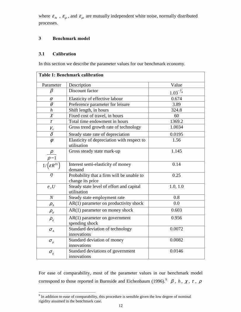
In this section we describe the parameter values for our benchmark economy.

Table 1: Benchmark calibration

Parameter Description Valueβ Discount factor 1

41.03−

α Elasticity of effective labour 0.674θ Preference parameter for leisure 3.89h Shift length, in hours 324.8χ Fixed cost of travel, in hours 60τ Total time endowment in hours 1369.2

xγ Gross trend growth rate of technology 1.0034δ Steady state rate of depreciation 0.0195φ Elasticity of depreciation with respect to

utilisation1.56

1ρ

ρ −Gross steady state mark-up 1.145

( )1/ SSRε Interest semi-elasticity of moneydemand

0.14

η Probability that a firm will be unable tochange its price

0.25

e ,U Steady state level of effort and capitalutilisation

1.0, 1.0

N Steady state employment rate 0.8Aρ AR(1) parameter on productivity shock 0.0

µρ AR(1) parameter on money shock 0.603

gρ AR(1) parameter on governmentspending shock

0.956

Aσ Standard deviation of technologyinnovations

0.0072

µσ Standard deviation of moneyinnovations

0.0082

gσ Standard deviations of governmentinnovations

0.0146

For ease of comparability, most of the parameter values in our benchmark model

correspond to those reported in Burnside and Eichenbaum (1996).9 β , h , χ , τ , ρ

9 In addition to ease of comparability, this procedure is sensible given the low degree of nominalrigidity assumed in the benchmark case.

13

and ε are not estimated. The discount factor is calibrated such that the steady state

annualised real interest rate is equal to 3%. The parameter h , the number of hours

worked by an employed person, is calibrated so that the steady state level of effort

equals one. The time spent commuting per quarter, χ , is set to 60.10 This value falls

in the middle of the range reported by Burnside and Eichenbaum (1996). The total

quarterly time endowment τ is fixed at 1,369.2 hours.

In the model, the indivisibility of labour assumption makes aggregation easier, and

implies a within period employment elasticity of zero, in line with empirical estimates

indicating that labour supply elasticities are quite small. The elasticity of effort

supply, however, is given by t

t

hehe

τ χ− − , which in steady state takes a value of

approximately 3. Blanchard and Fischer (1989), Ball, Mankiw, and Romer (1988)

and Blanchard (1990) note that although very elastic labour supply in a model of

sticky prices can generate large nominal rigidities, actual labour supply elasticities

have been estimated to be fairly small. In order to evaluate the impact of labour-

hoarding on the persistence properties of our model, Section 6 considers more general

preferences that do not have these features.

The calibrated value for the parameter ρ implies a steady-state markup of 14.5%, and

the interest semi-elasticity of money demand, 1/εRss, is calibrated to take on a value of

0.14. This value is consistent with the values estimated in Stock and Watson (1993).11,12

The parameters α ,θ , xγ , δ , φ , Aρ , gρ , Aσ , and gσ take the estimated values given

in Burnside and Eichenbaum (1996). The persistence µρ and variance µσ of the

monetary policy shock are taken from the estimation in Yun (1996).

10 This amounts to commuting approximately 1 hour per day.11 The consumption elasticity of money demand equals σ ε . In order to maintain comparability with

Burnside and Eichenbaum, we set 1σ = in the benchmark specification. However, our results hold formore plausible values of the consumption elasticity of money demand. Specifically, when

5σ = (implying a consumption elasticity of 0.7), our results with respect to a monetary disturbance donot change.12 See also Mankiw and Summers (1986), and Lucas (1988).

14

The remaining key parameter values of the model are φ , the parameter governing the

degree to which firms will choose to vary capital utilisation in response to shocks, and

η the degree of nominal rigidity. As discussed in Burnside and Eichenbaum (1996),

the estimate of φ depends on the mean of the depreciation series δ , which is

estimated to take on a value of 0.0195. Normalising the steady state rate of capital

utilisation to 1 then implies that 1.56φ = .

In standard sticky-price models, η often takes the value of around 0.75, indicating

that firms change their price on average once a year. Estimates of this parameter vary

from 0.75 in Gali and Gertler (1999), to 0.5 in Gali, Gertler, Lopez-Salido (2001). 13

Our benchmark value of 0.25η = assumes a lower degree of nominal rigidity. This is

discussed further below.

3.2 Impulse responses

In this section we report the impulse response of the benchmark model to a

productivity, government spending, and money shock.

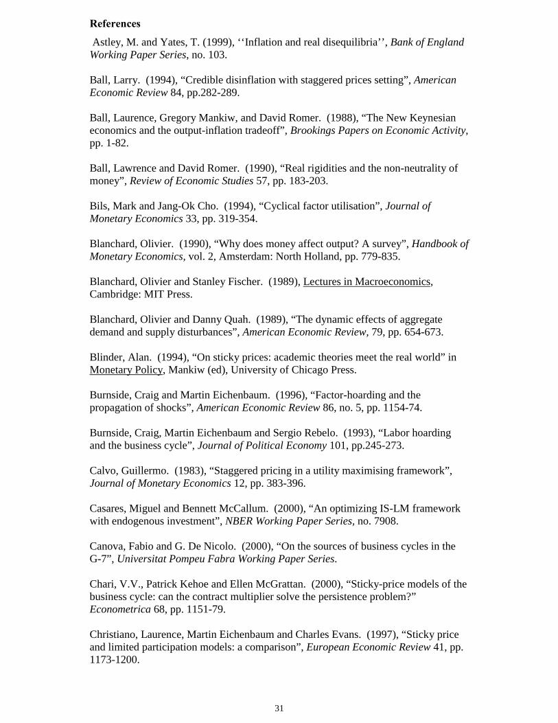
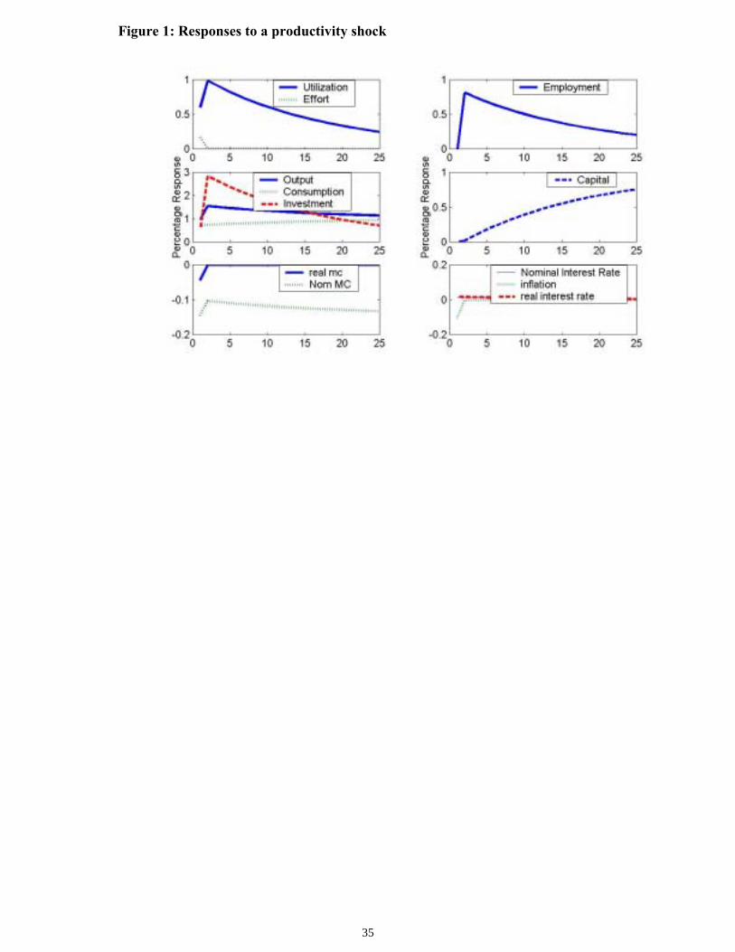
Figure 1 plots the responses of the endogenous variables to a 1% i.i.d. shock to

productivity growth. Because the assumed degree of nominal rigidity is very low in

the benchmark model (the average frequency of price adjustment is a little over once

per quarter), the impulse responses reported here essentially replicate those in

Burnside and Eichenbaum (1996). The key finding of that paper is that variable factor

utilisation magnifies the impact of a real shock. In addition, despite the fact that

productivity growth shocks are assumed to be white noise, the real effect of the shock

is highly persistent. This is because both labour and capital services can vary

immediately in response to shocks. Firms would like to increase their factor inputs to

fully exploit the temporarily higher growth rate of productivity. In a standard two-

factor input model with predetermined capital, the increased demand for labour

services is dampened somewhat by the short-run rigidity of capital, which causes the

marginal productivity of labour to decline quite sharply. With variable factor

utilisation, firms can increase capital as well as labour services. In doing so, their

action magnifies the impact effect of the productivity shock on output.

13 See Blinder (1994), Sbordone (1998) for empirical evidence of nominal price rigidities in the US.

15

The effect of the shock is persistent because of the combined effect of utilisation on

depreciation and hence the capital stock, and the assumption of labour hoarding. In

periods following the shock, the physical capital stock is relatively low. Output must

remain high to finance investment and build up the capital stock. Utilisation and

employment remain above steady state to generate the higher output needed to bring

the capital stock up to its new steady state. The transition path of the capital stock to

its new steady state is relatively slow, however, since higher utilisation rates along

this path dampen the rate at which capital accumulates. In addition to this

mechanism, the assumption that it is costless to adjust employment in the period after

the shock leads to an immediate response of effort in the impact period. In the period

following the shock, employment responds by relatively more, leading to a hump-

shaped response in output.

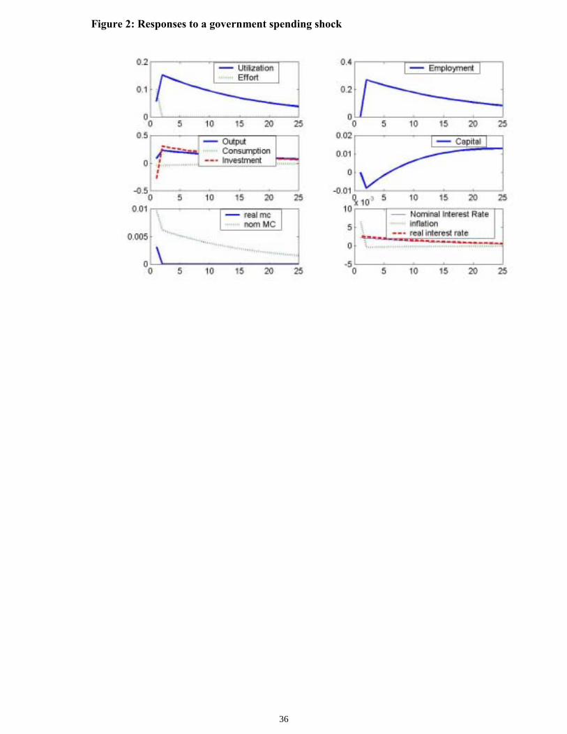
Figure 2 plots the model impulse responses to a temporary increase in the growth rate

of government spending. The effect of a demand shock is also similar to that found in

Burnside and Eichenbaum’s original model. Utilisation and effort increase on impact

to satisfy temporarily higher demand. Higher utilisation in turn temporarily reduces

the capital stock. Output remains high in subsequent periods, reflected in utilisation

and employment rates above steady state, to satisfy the temporarily higher demand

and finance investment in order to restore the capital stock to it steady state level.

Figure 3 plots the impulse responses to a shock to the money supply. Despite the low

degree of nominal rigidity assumed, the response of the real variables to the shock is

on par with the effect of real shocks on the economy. The increase in output is driven

by a surge in investment, with consumption remaining relatively flat.14 In the impact

period of the shock, output increases by almost the same amount as effort. Since the

rise in capital utilisation is associated with additional costs in the form of

depreciation, while the rise in effort is not, the marginal product of effective capital

rises by more than the marginal product of effective labour. The surge in investment is

in response to the increased marginal productivity of effective capital.

Real marginal costs increase on impact, but by only 1/3 of the change in output. This

is due to the assumption of capital hoarding. Since firms hoard capital in equilibrium,

14 Christiano, Eichenbaum and Evans (2001) are able to dampen the response of investment andincrease the response of consumption by introducing investment adjustment costs.

16

the marginal benefits of an increase in utilization on output are larger than the

marginal costs.

The effect of the shock is quite persistent in subsequent periods, with variables

returning to steady state in approximately five quarters—somewhat longer than the

period over which prices are assumed to be fixed at just over one quarter. The hump-

shaped response in output arises for the same reason as in the case of a productivity

shock: employment in the period after the shock rises by more than the

contemporaneous response of effort.

The persistent output response is in contrast with the immediate price level response.

Prices react quickly to a monetary shock, mainly reflecting the large proportion (75%)

of firms that are allowed to reset their price each period and also because of the effect

of the monetary shock on future inflation. Given the positive slope of the real

marginal costs curve, when a firm gets a signal it will adjust its price by a higher

percentage than the change in the money supply.

The nominal interest rate increases in response to a monetary expansion. The model is

therefore unable to generate a liquidity effect. This is a common feature of sticky

price models of the business cycle and is due to the increase of expected inflation after

a monetary shock. Expected inflation is high because a positive shock to the money

supply increases the long run price level, whereas prices cannot adjust in the short

run. Finally the movements in expected inflation and nominal interest rates leave the

real interest rate fairly unaffected.

4 Other sticky-price models

This section considers alternative sticky-price models with the aim of comparing our

benchmark model with time-varying factor utilisation to models without capital, and

models with capital and capital adjustment costs.

We first consider a model with no capital. Such a model has a similar structure to the

one presented above, but with a fixed level of capital services and employment, where

variations in effort are now interpreted as variations in labour supply.

17

We also consider a standard two-factor input model.15 This corresponds to our model

of time-varying factor utilisation under the condition of constant capital utilisation and

employment, so that variations in the capital stock and effort are now simply

interpreted as variations in capital and labour. Standard two-factor input models with

endogenous capital typically introduce capital adjustment costs in order to reduce the

response of real variables to a money shock (see King and Watson, 1996, Chari,

Kehoe and McGrattan, 2000, and Casares and McCallum 2000, Woodford 2000). To

facilitate comparison purposes across the different capital adjustment costs found in

the literature, we adopt a simple quadratic specification that takes the form:

( ) ( ) ( )2

11

11 1

2t j t j

t j t j t j x t jt j

K KbI K K KK

δδ γ δ+ + +

+ + + + ++

� �− −= − − + − − +� �

� �� �, (1.23)

where the parameter b determines the size of the capital adjustment cost. As owners

and suppliers of the capital stock, these adjustment costs are borne by the household.

In the standard one- and two-factor input model, effort is interpreted as labour

supply.16 As is common in the literature, its steady state value is calibrated to 13 .

The adjustment cost parameter, b , takes on a value of 19.4, and governs the response

of investment to changes in the real return of the asset.17 When there are no capital

adjustment costs ( 0b = ), then the response of investment is unconstrained, and in the

case of money shocks leads to unrealistically large responses in investment and

output.18 For this reason, the parameter indexing the size of adjustment costs is a

crucial parameter governing the response of sticky-price models with capital. Our

benchmark value for b is calibrated in a similar way to that in Casares and McCallum

15 The calibrated parameter values for the model variants are reported in Table 2 in the appendix. Onlyparameter values that take on a different value from those reported in Table 1 are included below.

16 In this case, the elasticity of labour supply is given by 1 t

t

ee−

, which for our calibration implies a

steady state value of around 2, somewhat lower than the typical value assumed in the RBC literature.

17 If adjustment costs are described generically by the function t

t

IK

φ� �� �� �

, where 1' t

t

IK

φ � �� �� �

is

interpreted as Tobin’s q, then adjustment costs affect the second derivative '' t

t

IK

φ� �� �� �

. When

adjustment costs are zero, the second derivative is zero. The higher the adjustment cost parameter b,the larger the second derivative, and the smaller the response of the investment-to-capital ratio tovariations in Tobin’s q.18 See Casares and McCallum (2000) and Ellison and Scott (2001).

18

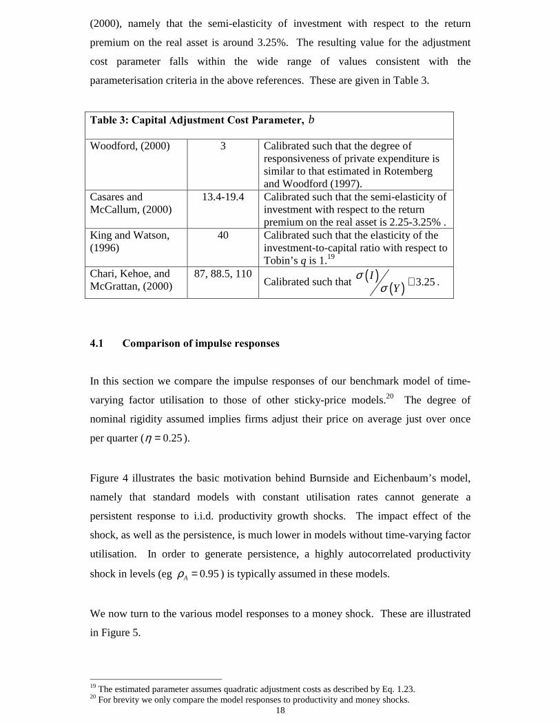
(2000), namely that the semi-elasticity of investment with respect to the return

premium on the real asset is around 3.25%. The resulting value for the adjustment

cost parameter falls within the wide range of values consistent with the

parameterisation criteria in the above references. These are given in Table 3.

Table 3: Capital Adjustment Cost Parameter, b

Woodford, (2000) 3 Calibrated such that the degree ofresponsiveness of private expenditure issimilar to that estimated in Rotembergand Woodford (1997).

Casares andMcCallum, (2000)

13.4-19.4 Calibrated such that the semi-elasticity ofinvestment with respect to the returnpremium on the real asset is 2.25-3.25% .

King and Watson,(1996)

40 Calibrated such that the elasticity of theinvestment-to-capital ratio with respect toTobin’s q is 1.19

Chari, Kehoe, andMcGrattan, (2000)

87, 88.5, 110Calibrated such that ( )

( ) 3.25IY

σσ ≅ .

4.1 Comparison of impulse responses

In this section we compare the impulse responses of our benchmark model of time-

varying factor utilisation to those of other sticky-price models.20 The degree of

nominal rigidity assumed implies firms adjust their price on average just over once

per quarter ( 0.25η = ).

Figure 4 illustrates the basic motivation behind Burnside and Eichenbaum’s model,

namely that standard models with constant utilisation rates cannot generate a

persistent response to i.i.d. productivity growth shocks. The impact effect of the

shock, as well as the persistence, is much lower in models without time-varying factor

utilisation. In order to generate persistence, a highly autocorrelated productivity

shock in levels (eg 0.95Aρ = ) is typically assumed in these models.

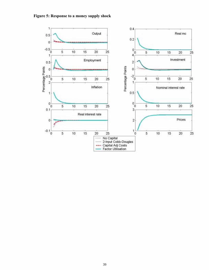
We now turn to the various model responses to a money shock. These are illustrated

in Figure 5.

19 The estimated parameter assumes quadratic adjustment costs as described by Eq. 1.23.20 For brevity we only compare the model responses to productivity and money shocks.

19

In models with constant factor utilisation, the low degree of nominal rigidity is

reflected in a very small response of real variables. For reasons discussed above,

however, our benchmark sticky-price model with factor utilisation has a relatively

large impact and persistent response to a money shock.

An interesting feature of Figure 5 is the implied relationship between output, real

marginal cost and nominal variables across the different models. The response of real

marginal costs, inflation and nominal interest rates is coincident across models,

whereas the response of output and real interest rates is quite different. Although real

marginal costs rise by the same amount in response to a monetary policy expansion,

the output response under factor utilisation is three times larger than in sticky price

models with capital adjustment costs and no capital. Woodford (2000) finds similar

cyclical variation in real marginal costs for standard models both with and without

capital, which he attributes to relatively small cyclical variation in the capital stock. 21

A thorough look at the impulse responses of the factor inputs in Figure 5 reveals that

in all the models labour moves almost one-to-one with output. However, this is not

true for the movements in investment. In the standard sticky price model with capital

adjustment costs, investment moves one-for-one with output and labour, whereas in

the factor hoarding model, the reaction of investment is four times larger than the

reaction of output and labour, and in the sticky price model with no capital adjustment

costs it is three times larger. The different responses of investment across the different

models also explains the different behaviour of real interest rates. On the other hand,

the similarities in the reaction of the real marginal costs explain the similarities in the

reaction of the nominal variables across the different model specifications. Since

inflation is mainly determined by the path of real marginal costs, the behaviour of

actual and expected inflation across the models is also similar.

5 Model simulations

5.1 Model statistics

In this section we investigate simulated statistics in order to assess the performance of

the factor utilisation model relative to the data as well as across the different model

variants.22 We allow for both productivity and nominal and real policy shocks, the

21 This relation is further discussed in Section 5.2.22 Each simulation is made up of 500 observations, and is repeated 500 times. The reported samplestatistics represent averages across simulation experiments.

20

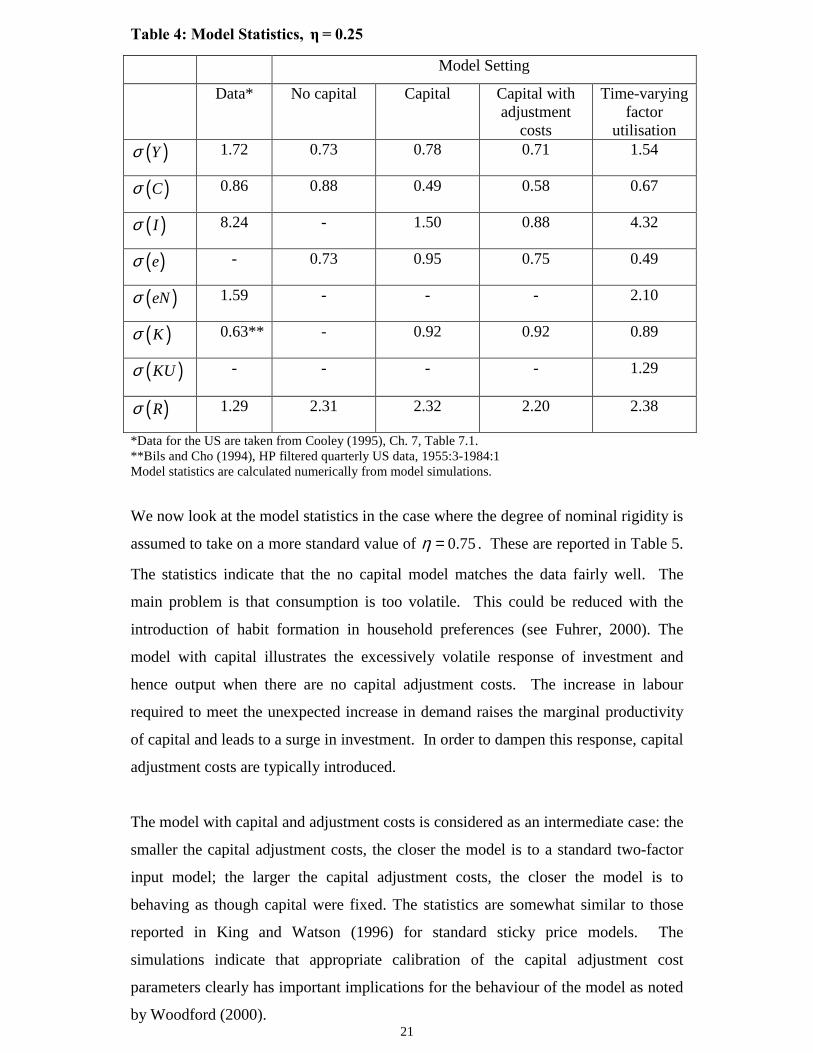
standard deviations of which are calibrated as reported in Table 1. In Table 4 we first

compare model statistics across the sticky-price model variants assuming our

benchmark low degree of nominal rigidity. The relatively low standard deviations for

output in the no capital, capital, and capital with adjustment costs cases reflect the

limited amount of response in those models to both white noise productivity growth

shocks and money shocks in an environment of low nominal rigidity.23 The statistics

of the factor utilisation model match the data better. Despite the absence of capital

adjustment costs, investment does not vary too much, but by more than in a standard

sticky-price model with capital. The increased variability of investment is a

consequence of the depreciation-through-use assumption and the desire by firms to

invest such that the capital stock comes on line with employment. As in Burnside,

Eichenbaum, and Rebelo (1993), the standard deviation of effort accounts for

approximately 1/5 of the standard deviation of effective labour supply. By contrast,

the standard deviation of capital services is dominated by the standard deviation in

utilisation, estimated at 2.22%.

When we consider conditional moments, we find that all shocks have a substantial

role in explaining the variance of the real variables for the factor utilisation model. In

particular, 56% of the variability of output is due to productivity shocks, while 27% is

due to monetary shocks. Real supply and real demand shocks account for 61% of the

variability of investment and the remaining 39% is due to monetary shocks. By

comparison, in the no capital model, most of the variability of the real variables is due

to real shocks and monetary shocks have a very small overall effect. This is in

accordance with models with capital where fluctuations in real variables are

dominated by supply shocks when the assumed degree of nominal rigidity is fairly

low. In particular, 72% of the fluctuations in output are due to productivity shocks,

while money shocks account for only 14% of these fluctuations. In the model with

capital adjustment costs, these values become 71% and 9%, respectively. Again,

money has a relatively small role on explaining business cycle fluctuations because

the degree of nominal rigidity assumed is very low.

23 The statistics reported here for the model variants do not reflect the better fit of real business cyclemodels, such as the indivisible labour model of Hansen (1985).

21

Table 4: Model Statistics, η = 0.25

Model Setting

Data* No capital Capital Capital withadjustment

costs

Time-varyingfactor

utilisation( )Yσ 1.72 0.73 0.78 0.71 1.54

( )Cσ 0.86 0.88 0.49 0.58 0.67

( )Iσ 8.24 - 1.50 0.88 4.32

( )eσ - 0.73 0.95 0.75 0.49

( )eNσ 1.59 - - - 2.10

( )Kσ 0.63** - 0.92 0.92 0.89

( )KUσ - - - - 1.29

( )Rσ 1.29 2.31 2.32 2.20 2.38

*Data for the US are taken from Cooley (1995), Ch. 7, Table 7.1.**Bils and Cho (1994), HP filtered quarterly US data, 1955:3-1984:1Model statistics are calculated numerically from model simulations.

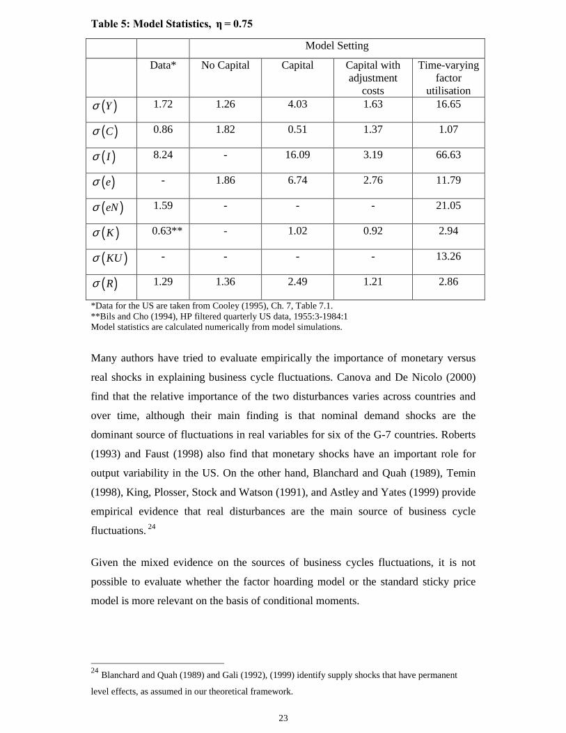
We now look at the model statistics in the case where the degree of nominal rigidity is

assumed to take on a more standard value of 0.75η = . These are reported in Table 5.

The statistics indicate that the no capital model matches the data fairly well. The

main problem is that consumption is too volatile. This could be reduced with the

introduction of habit formation in household preferences (see Fuhrer, 2000). The

model with capital illustrates the excessively volatile response of investment and

hence output when there are no capital adjustment costs. The increase in labour

required to meet the unexpected increase in demand raises the marginal productivity

of capital and leads to a surge in investment. In order to dampen this response, capital

adjustment costs are typically introduced.

The model with capital and adjustment costs is considered as an intermediate case: the

smaller the capital adjustment costs, the closer the model is to a standard two-factor

input model; the larger the capital adjustment costs, the closer the model is to

behaving as though capital were fixed. The statistics are somewhat similar to those

reported in King and Watson (1996) for standard sticky price models. The

simulations indicate that appropriate calibration of the capital adjustment cost

parameters clearly has important implications for the behaviour of the model as noted

by Woodford (2000).

22

Comparing the last two columns illustrates that introducing factor utilisation

exacerbates the volatility of investment and hence output. This is because firms can

now meet the increase in demand not just through higher labour inputs, but higher

capital utilisation as well. This raises the marginal productivity of physical capital

even more, leading to an even greater surge in investment than in the standard two-

factor input model with no capital adjustment costs. The introduction of factor

utilisation, therefore, worsens the dynamic properties of the model by increasing the

sensitivity of investment with respect to monetary shocks. But it is precisely the

increased sensitivity of investment that allows for a reduction in the degree of nominal

rigidity in a model with time-varying factor utilisation, without sacrificing its

response to policy shocks.

This point is better illustrated by considering the conditional moments of the shocks.

In the factor hoarding model with a high degree of nominal rigidity (and also in the

model with capital and no adjustment costs), the magnitude of the response of real

variables with respect to monetary shocks is huge. As a result, monetary shocks are

the dominant source of fluctuations in real variables in this case. For example,

monetary shocks account for 86% of the fluctuations in output, while productivity

disturbances account for just 11% of these fluctuations. Nominal shocks are the main

source of fluctuations in the no capital model as well, although the absence of

investment dynamics moderates the magnitude of the responses of real variables with

respect to monetary disturbances in this case.

23

Table 5: Model Statistics, η = 0.75

Model Setting

Data* No Capital Capital Capital withadjustment

costs

Time-varyingfactor

utilisation( )Yσ 1.72 1.26 4.03 1.63 16.65

( )Cσ 0.86 1.82 0.51 1.37 1.07

( )Iσ 8.24 - 16.09 3.19 66.63

( )eσ - 1.86 6.74 2.76 11.79

( )eNσ 1.59 - - - 21.05

( )Kσ 0.63** - 1.02 0.92 2.94

( )KUσ - - - - 13.26

( )Rσ 1.29 1.36 2.49 1.21 2.86

*Data for the US are taken from Cooley (1995), Ch. 7, Table 7.1.**Bils and Cho (1994), HP filtered quarterly US data, 1955:3-1984:1Model statistics are calculated numerically from model simulations.

Many authors have tried to evaluate empirically the importance of monetary versus

real shocks in explaining business cycle fluctuations. Canova and De Nicolo (2000)

find that the relative importance of the two disturbances varies across countries and

over time, although their main finding is that nominal demand shocks are the

dominant source of fluctuations in real variables for six of the G-7 countries. Roberts

(1993) and Faust (1998) also find that monetary shocks have an important role for

output variability in the US. On the other hand, Blanchard and Quah (1989), Temin

(1998), King, Plosser, Stock and Watson (1991), and Astley and Yates (1999) provide

empirical evidence that real disturbances are the main source of business cycle

fluctuations. 24

Given the mixed evidence on the sources of business cycles fluctuations, it is not

possible to evaluate whether the factor hoarding model or the standard sticky price

model is more relevant on the basis of conditional moments.

24 Blanchard and Quah (1989) and Gali (1992), (1999) identify supply shocks that have permanent

level effects, as assumed in our theoretical framework.

24

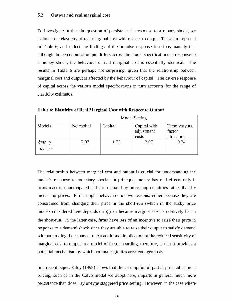
5.2 Output and real marginal cost

To investigate further the question of persistence in response to a money shock, we

estimate the elasticity of real marginal cost with respect to output. These are reported

in Table 6, and reflect the findings of the impulse response functions, namely that

although the behaviour of output differs across the model specifications in response to

a money shock, the behaviour of real marginal cost is essentially identical. The

results in Table 6 are perhaps not surprising, given that the relationship between

marginal cost and output is affected by the behaviour of capital. The diverse response

of capital across the various model specifications in turn accounts for the range of

elasticity estimates.

Table 6: Elasticity of Real Marginal Cost with Respect to Output

Model Setting

Models No capital Capital Capital withadjustmentcosts

Time-varyingfactorutilisation

mc yy mc

∂∂

2.97 1.23 2.07 0.24

The relationship between marginal cost and output is crucial for understanding the

model’s response to monetary shocks. In principle, money has real effects only if

firms react to unanticipated shifts in demand by increasing quantities rather than by

increasing prices. Firms might behave so for two reasons: either because they are

constrained from changing their price in the short-run (which in the sticky price

models considered here depends on η ), or because marginal cost is relatively flat in

the short-run. In the latter case, firms have less of an incentive to raise their price in

response to a demand shock since they are able to raise their output to satisfy demand

without eroding their mark-up. An additional implication of the reduced sensitivity of

marginal cost to output in a model of factor hoarding, therefore, is that it provides a

potential mechanism by which nominal rigidities arise endogenously.

In a recent paper, Kiley (1998) shows that the assumption of partial price adjustment

pricing, such as in the Calvo model we adopt here, imparts in general much more

persistence than does Taylor-type staggered price setting. However, in the case where

25

the elasticity of marginal cost with respect to output is small (eg less than one), the

implications of the two types of price setting are equivalent. Our finding that

marginal cost is relatively insensitive to changes in output suggests that the persistent

output response to a monetary shock with relatively low price rigidity and time-

varying factor utilisation holds more generally in staggered price setting models. This

finding differs from that of Chari, Kehoe and McGrattan (2000), who conclude that

output persistence cannot be rationalised within a standard business cycle model with

staggered price setting without appealing to implausibly large nominal rigidities. In a

model with factor utilisation, it seems, small degrees of nominal rigidity can lead to

real and persistent response of output by flattening the marginal cost curve.

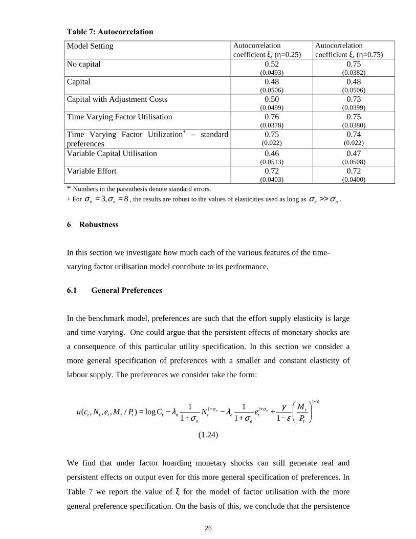
5.3 Persistence

We estimate the conditional autocorrelation coefficient, ξ , of the simulated output

response to money shocks in order to evaluate the persistence of each of the model

variants. The values of ξ are reported in Table 7. The greater the autocorrelation

coefficient, the more persistent is the response of output.

Table 7 shows that the introduction of variable capital utilisation and effort in a

sticky-price model increases the persistence of output relative to standard models

despite the low degree of nominal rigidity assumed. This is because of the effect of

utilisation on depreciation, and of labour hoarding. Labour hoarding prolongs the

response of effective labour input, which in turn propagates the response of real

variables. On the contrary, models with capital generate less persistence for a low

degree of price stickiness. This reflects a lack of strong propagation mechanism in one

and two- factor input models. The results in Table 7 are also consistent with the

findings of Chari, Kehoe and McGrattan (2000), namely that the introduction of

capital in a model where nominal rigidities provide another source of propagation

reduces persistence by providing agents with a mechanism for smoothing

unanticipated nominal shocks over time.

26

Table 7: Autocorrelation

Model Setting Autocorrelationcoefficient ξ, (η=0.25)

Autocorrelationcoefficient ξ, (η=0.75)

No capital 0.52(0.0493)

0.75(0.0382)

Capital 0.48(0.0506)

0.48(0.0506)

Capital with Adjustment Costs 0.50(0.0499)

0.73(0.0399)

Time Varying Factor Utilisation 0.76(0.0378)

0.75(0.0380)

Time Varying Factor Utilization+ – standardpreferences

0.75(0.022)

0.74(0.022)

Variable Capital Utilisation 0.46(0.0513)

0.47(0.0508)

Variable Effort 0.72(0.0403)

0.72(0.0400)

* Numbers in the parenthesis denote standard errors.+ For 3, 8n eσ σ= = , the results are robust to the values of elasticities used as long as e nσ σ>> .

6 Robustness

In this section we investigate how much each of the various features of the time-

varying factor utilisation model contribute to its performance.

6.1 General Preferences

In the benchmark model, preferences are such that the effort supply elasticity is large

and time-varying. One could argue that the persistent effects of monetary shocks are

a consequence of this particular utility specification. In this section we consider a

more general specification of preferences with a smaller and constant elasticity of

labour supply. The preferences we consider take the form:

11 11 1( , , , / ) log

1 1 1n e t

t t t t t t n t e tn e t

Mu c N e M P C N eP

εσ σ γλ λ

σ σ ε

−+ + � �

= − − + � �+ + − � �

(1.24)

We find that under factor hoarding monetary shocks can still generate real and

persistent effects on output even for this more general specification of preferences. In

Table 7 we report the value of ξ for the model of factor utilisation with the more

general preference specification. On the basis of this, we conclude that the persistence

27

results in a model of factor hoarding are robust to alternative preference

specifications, and are not due to the indivisible labour supply assumption. As we

have seen in the benchmark factor utilisation model, an unanticipated shock invokes

changes in effort in the impact period, because of labour hoarding. In order to

generate a hump-shaped response of effective labour, employment needs to increase

by more in the second period than the impact response of effort. In the specification of

Eq (1.24), this happens when the effort supply elasticity is lower than the employment

supply elasticity ( 1 1

e nσ σ<< ).25

6.2 Variable Capital Utilisation

This section investigates whether our results on persistence are driven by the

assumption of capital utilisation. Thus, we consider a two-factor input model with

variable capital utilisation. Such a model has a similar structure to the two-factor input

model presented of Section 4 with the additional feature that capital utilisation is time-

varying. The calibrated values for this model are therefore the same as those reported

in Table 2, except that 1.56φ = .26

Our estimates indicate that variable capital utilisation alone cannot account for the

persistent response of output to monetary shocks (see Table 7), although it does

increase the impact effect of the response of real variables to unanticipated shocks

compared to a two-factor input model without time-varying capital utilisation. It is

still the case that we can generate realistic investment volatility without having to

assume capital adjustment costs at relatively low degrees of nominal rigidity. On the

basis of these results we conclude that in order to generate persistence of real

variables with respect to nominal shocks, variable capital utilisation must be

combined with ‘real rigidities’ such as labour hoarding or wage rigidities as in

Christiano, Eichenbaum, and Evans (2001).

6.3 Variable Labour Effort

If we alternatively consider a model in which there is no capital utilisation, and effort

is the only contemporaneously variable factor input, then the impact effect of a

25 We investigate the behaviour of the model over a range of parameter values, 1 , 10N eσ σ< < .26 See appendix 3 for a complete description of the parameter values.

28

monetary shock on real variables is persistent but relatively small at low degrees of

nominal rigidity. The model we consider is similar to the one in Burnside,

Eichenbaum and Rebelo (1993), and corresponds with our benchmark model of

Section 2 with 10000φ = . An increase in the degree of nominal rigidity raises the

impact effect of a nominal shock on real variables, but at the cost of unrealistic

investment volatility given that there are no constraints on adjusting capital.

The above analysis suggests that both capital and labour hoarding are important for

generating large impact as well as persistent responses of real variables to nominal

shocks at low degrees of nominal rigidity.

6.4 Endogenous Monetary Policy

In the preceding discussion we have focussed our attentions on equilibria in which

monetary policy is exogenous. However, the empirical literature has demonstrated

that policy movements are largely due to reactions in the state of the economy. In this

section, we analyse whether the persistence properties of our model change when the

money supply rule of equation (1.16) is replaced by a Taylor (1993) interest rate rule

that responds to changes in the state of the economy. Such a rule has been shown to

match the behaviour of interest rates quite well.27 In its most generic form, this rule

takes the form:

t t y t tR b b yππ µ= + +

where 1.5bπ = and 0.5yb = , as in Taylor’s (1993) original specification, and tµ

represents a policy shock as before.

Our findings can be summarised as follows. First, for a low degree of nominal

rigidity, the benchmark model of time-varying factor utilisation generates more

persistence in output than the other sticky price model variants we investigate.

Second, the response of real variables following a real shock remains essentially

unchanged relative to the responses under a money rule. McGrattan (1999) shows

that the response of real variables to real shocks is affected by the policy rule

specification. In our case, however, this is not the case when 0.25η = . This is

because for low degrees of nominal rigidity the systematic component of monetary

27 See Clarida, Gali, Gertler (1998, 2000) for a recent empirical analysis of Taylor rules.

29

policy has almost no effect on real variables and the economy behaves as if it had

flexible prices when hit by real shocks.

7 Conclusions

Recent debate has focussed on the failure of standard general equilibrium sticky-price

models to generate business cycle fluctuations unless an extreme degree of price

stickiness is assumed. This paper investigates the propagation mechanism of

monetary shocks in an otherwise standard general equilibrium sticky-price model,

modified to incorporate factor hoarding in the form of variable capital utilisation rates

and labour effort. In contrast to previous studies, we find that real and persistent

effects of monetary shocks can be generated at a relatively low degree of nominal

rigidity.

In addition, we show that our model can generate realistic variances of capital and

investment without having to assume capital adjustment costs. Contrary to standard

sticky-price models with capital, the introduction of capital in our framework does not

reduce persistence in response to nominal shocks. Indeed, the increased sensitivity of

investment allows for a reduction in the assumed degree of nominal rigidity without

sacrificing the model’s response to policy shocks.

Finally, we compare the predictions of our model with standard sticky-price models

both with and without capital in order to gain insight in the relationship between

nominal price rigidity and a firm’s ability to adjust capital and labour services. The

sensitivity of marginal cost to output is closely related to a firm’s ability to adjust its

inputs. A model of variable factor utilisation introduces an additional margin by

which firms can respond to unanticipated shocks, reducing the effect of output on

marginal cost. In other words, variable capital utilisation results in a flattening of the

marginal cost schedule thereby introducing the possibility of endogenous price

stickiness. On the other hand, standard sticky-price models both with and without

capital are subject to increasing short-run marginal costs, which in turn dampens the

response of output. The real effect of monetary shocks on output in such models is

consequently weak, and can only be accomplished by assuming a relatively high

degree of nominal rigidity.

30

Although our model generates substantial persistence in output, it cannot generate

persistence in inflation. Variable factor utilization breaks the link between variations

in output and in real marginal costs, through movements in capital utilization.

However, the behaviour of marginal costs does not change dramatically across the

model variants considered here, and as a result the inflation dynamics do not change

either. In order to generate persistent responses of inflation to changes in the money

supply one has to incorporate an additional real rigidity in the model, such as real

wage rigidities, as in Christiano Eichenbaum and Evans (2001). Real wage rigidities

have the effect of delaying the response of real marginal cost to changes in output,

and as a result introduce persistence in inflation.

31

References

Astley, M. and Yates, T. (1999), ‘‘Inflation and real disequilibria’’, Bank of EnglandWorking Paper Series, no. 103.

Ball, Larry. (1994), “Credible disinflation with staggered prices setting”, AmericanEconomic Review 84, pp.282-289.

Ball, Laurence, Gregory Mankiw, and David Romer. (1988), “The New Keynesianeconomics and the output-inflation tradeoff”, Brookings Papers on Economic Activity,pp. 1-82.

Ball, Lawrence and David Romer. (1990), “Real rigidities and the non-neutrality ofmoney”, Review of Economic Studies 57, pp. 183-203.

Bils, Mark and Jang-Ok Cho. (1994), “Cyclical factor utilisation”, Journal ofMonetary Economics 33, pp. 319-354.

Blanchard, Olivier. (1990), “Why does money affect output? A survey”, Handbook ofMonetary Economics, vol. 2, Amsterdam: North Holland, pp. 779-835.

Blanchard, Olivier and Stanley Fischer. (1989), Lectures in Macroeconomics,Cambridge: MIT Press.

Blanchard, Olivier and Danny Quah. (1989), “The dynamic effects of aggregatedemand and supply disturbances”, American Economic Review, 79, pp. 654-673.

Blinder, Alan. (1994), “On sticky prices: academic theories meet the real world” inMonetary Policy, Mankiw (ed), University of Chicago Press.

Burnside, Craig and Martin Eichenbaum. (1996), “Factor-hoarding and thepropagation of shocks”, American Economic Review 86, no. 5, pp. 1154-74.

Burnside, Craig, Martin Eichenbaum and Sergio Rebelo. (1993), “Labor hoardingand the business cycle”, Journal of Political Economy 101, pp.245-273.

Calvo, Guillermo. (1983), “Staggered pricing in a utility maximising framework”,Journal of Monetary Economics 12, pp. 383-396.

Casares, Miguel and Bennett McCallum. (2000), “An optimizing IS-LM frameworkwith endogenous investment”, NBER Working Paper Series, no. 7908.

Canova, Fabio and G. De Nicolo. (2000), “On the sources of business cycles in theG-7”, Universitat Pompeu Fabra Working Paper Series.

Chari, V.V., Patrick Kehoe and Ellen McGrattan. (2000), “Sticky-price models of thebusiness cycle: can the contract multiplier solve the persistence problem?”Econometrica 68, pp. 1151-79.

Christiano, Laurence, Martin Eichenbaum and Charles Evans. (1997), “Sticky priceand limited participation models: a comparison”, European Economic Review 41, pp.1173-1200.

32

Christiano, Laurence, Martin Eichenbaum and Charles Evans. (2001), “Nominalprice rigidities and the dynamic effects of a shock to monetary policy”, workingpaper, Northwestern University.

Clarida, Richard, Jordi Gali, and Mark Gertler. (1999), “The science of monetarypolicy: a New Keynesian perspective”, Journal of Economic Literature 37, pp. 1661-1707.

Cogley, Timothy, and James Nason. (1995), “Output dynamics in real-business cyclemodels”, American Economic Review 83, pp. 492-511.

Cook, David. (1999), “Real propagation of monetary shocks: dynamiccomplementarities and capital utilisation”, Macroeconomic Dynamics 3, pp. 368-383.

Cooley, Thomas and Gary Hansen. (1995), “Money and the business cycle”, inFrontiers of Business Cycle Research, T. Cooley (ed.), Princeton University Press.

Ellison, Martin and Andrew Scott. (2001), “Sticky-prices and volatile output”, Bankof England Working Paper Series, no. 127.

Fagnart, Jean-Louise, Omar Licandro, and Franck Portier. (1999), “Firmheterogeneity, capacity utilisation, and the business cycle”, Review of EconomicDynamics vol. 2, pp. 433-455.

Faust, John. (1998), “On the robustness of the identified VAR conclusions aboutmoney”, Carnegie-Rochester Conference Series on Public Policy 49, pp. 207-244.

Fuhrer, Jeffrey, (2000), “Habit formation in consumption and its implications formonetary policy models”, American Economic Review 90, pp. 367-90.

Gali, Jordi. (1992), “Does the IS-LM model fit US postwar data?” Quarterly Journalof Economics CVII, pp. 708-738.

Gali, Jordi. (1999), “Technology, employment and the business cycle: do technologyshocks explain aggregate fluctuations?” American Economic Review 89, pp. 249-271.

Gali, Jordi and Mark Gertler. (1999), “Inflation dynamics: a structural econometricanalysis”, Journal of Monetary Economics 44, pp.195-222.

Gali, Jordi, Mark Gertler, and J. David Lopez-Salido. (2001), “European inflationdynamics”, forthcoming European Economic Review.

Greenwood, Jeremy, Zvi Hercowitz, and Gregory Huffman. (1988), “Investment,capacity utilization, and the real business cycle”, American Economic Review 78,pp.402-17.

Hansen, Gary. (1985), “Indivisible labour and the business cycle”, Journal ofMonetary Economics 16, pp. 309-28.

Jeanne, Olivier (1997), “Generating real persistent effects of monetary shocks: howmuch rigidity do we really need?’’ NBER Working Paper Series, no. 6258.

33

Kiley, Michael. (1998), “Partial adjustment and staggered price setting”, mimeo,Federal Reserve Board.

King, Robert, Charles Plosser, James Stock and Mark Watson. (1991), “Stochastictrends and economic fluctuations”, American Economic Review 81, pp.819-40.

King, Robert and Mark Watson. (1996), “Money, prices, and interest rates and thebusiness cycle”, Review of Economics and Statistics 78, pp. 35-53.

King, Robert and Alex Wolman. (1996), “Inflation targeting in a St. Louis model ofthe 21st century”, Federal Reserve Bank of St. Louis Review.

Lucas Robert (1988). “Money demand in the US: a quantitative review”, CarnegieRochester Series on Public Policy 29, pp. 137-167.

Mankiw, Gregory, (2000), “The inexorable and mysterious trade-off betweeninflation and unemployment”, NBER Working Paper Series, no. 7884.

Mankiw, Gregory and Ricardo Reis. (2001), “Sticky information vs sticky prices: aproposal to replace the New Keynesian Phillips curve”, NBER Working Paper Series,no. 8290.

Mankiw, Gregory and Lawrence Summers (1986). “Money Demand and the Effectsof Fiscal Policy”, Journal of Money, Credit and Banking 18, pp. 415-429.

McCallum , Bennett. (1997), “Comment”, in NBER Macroeconomics Annual,Bernanke and Gertler (eds). Cambridge, MA: MIT Press, pp. 355-359.

McCallum, Ben and Edward Nelson. (1999), “An optimising IS-LM specification formonetary policy and business cycle analysis”, Journal of Money, Credit, and Banking,31, pp. 296-316.

McGrattan, Ellen (1999). “Predicting the effects of Federal Reserve Policy in asticky-price model: an analytical approach”, Federal Reserve Bank of MinneapolisWorking Paper Series, no. 598.

Roberts, John M. (1993), “The sources of business cycles: a monetaristinterpretation”, International Economic Review, 34, pp. 923-934.

Roberts, John M. (1995), “New Keynesian economics and the Phillips curve”,Journal of Money, Credit, and Banking 27, pp. 975-984.

Rogerson, Richard. (1988), “Indivisible labour, lotteries and equilibrium”, Journal ofMonetary Economics, vol.21, no. 1, pp. 71-89.

Romer, David. (1996), Advanced Macroeconomics, New York: McGraw-Hill.

Rotemberg, Julio. (1987), “The New Keynesian microfoundations” in NBERMacroeconomics Annual, S. Fischer (ed.). Cambridge, MA: MIT Press, pp. 69-104.

Rotemberg, Julio and Michael Woodford. (1997), “An optimisation-basedeconometric framework for the evaluation of monetary policy”, in B.S. Bernanke and

34

J.J. Rotemberg (eds.), NBER Macroeconomics Annual 1997. Cambridge: MIT Press,pp.297-346.

Sbordone, Argia. (1998), “Price and unit labor cost: a new test of price rigidity”,Institute for International Economic Studies, Stockholm University Seminar Paper,no. 653.

Stock, John and Mark Watson. (1993), “A simple estimator of cointegrating vectorsin higher order integrated systems”, Econometrica 61, pp. 783-820.

Taylor, John. (1979), “Staggered contracts in a macro model”, American EconomicReview 69, pp.108-13.

Taylor, John. (1993), “Discretion versus policy rules in practise”, Carnegie-Rochester Conference Series on Public Policy 39, pp. 195-214.

Temin, Peter. (1998), “The causes of American business cycles: an essay ineconomic historiography”, NBER Working Paper Series, no. 6692.

Woodford, Michael. (2000), “A neo-Wicksellian framework for the analysis ofmonetary policy” Chapter 4 of Interest and Prices, manuscript, Princeton University.

Yun, Tack. (1996), “Nominal price rigidity, money supply endogeneity, and businesscycles”, Journal of Monetary Economics 37, pp. 345-370.

35

Figure 1: Responses to a productivity shock

36

Figure 2: Responses to a government spending shock

37

Figure 3: Responses to a money supply shock

38

Figure 4: Response to a productivity shock

39

Figure 5: Response to a money supply shock

40

Appendices

These appendices collect the derivation of the equations used in the paper. They are

included to facilitate the work of the referees but they are not intended for publication.

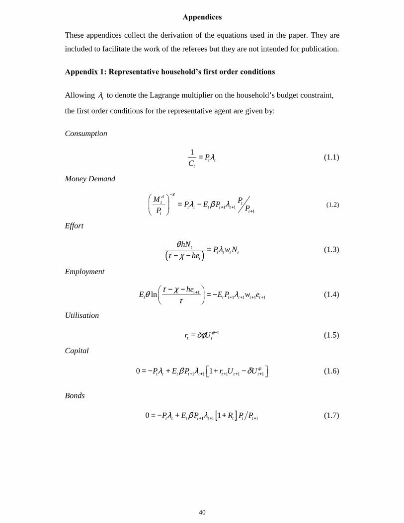
Appendix 1: Representative household�s first order conditions

Allowing tλ to denote the Lagrange multiplier on the household’s budget constraint,

the first order conditions for the representative agent are given by:

Consumption

1t t

t

PC

λ= (1.1)

Money Demand

1 11

dt t

t t t t ttt

M PP E P PP

ε

λ β λ−

+ ++

� �= −� �

� �(1.2)

Effort

( )t

t t t tt

hN P w Nhe

θ λτ χ

=− −

(1.3)

Employment

11 1 1 1ln t

t t t t t theE E P w eτ χθ λ

τ+

+ + + +− −� � = −� �

� �(1.4)

Utilisation

1t tr U φδφ −= (1.5)

Capital

1 1 1 1 10 1t t t t t t t tP E P r U U φλ β λ δ+ + + + +� �= − + + −� � (1.6)

Bonds

[ ]1 1 10 1t t t t t t t tP E P R P Pλ β λ+ + += − + + (1.7)

41

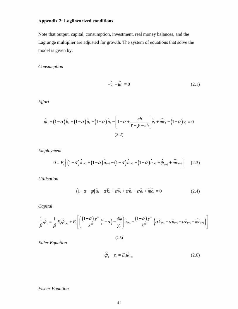
Appendix 2: Loglinearized conditions

Note that output, capital, consumption, investment, real money balances, and the

Lagrange multiplier are adjusted for growth. The system of equations that solve the

model is given by:

Consumption

� 0t tc ψ− − =� (2.1)

Effort

� ( ) � ( ) � ( ) � � ( )1 1 1 1 1 0t t t t t ttehk u n e mc v

ehψ α α α α α

τ χ� �

+ − + − − − − − + + − − =� �− −� �

�

(2.2)

Employment

( ) � ( ) � ( ) � ( ) � �1 1 1 1 110 1 1 1 1t t t t tt tE k u n e mcα α α α ψ+ + + + ++

� �= − + − − − − − + +� �

� (2.3)

Utilisation

( ) � � � �1 0t t t t t tu k v n e mcα φ α α α α− − − + + + + =� � (2.4)

Capital

� � ( ) ( ) � ( ) � � �( )1 1 1 1 11

1 11 1 1ss ss

t t t t tt tt t ss ssx

y yE E u k n e mc

k kα αδφψ ψ α α α α

β β γ+ + + + ++

� �� �− −= + − − − − − −� �� �

� � � �

�

(2.5)Euler Equation

� �1t tt tz Eψ ψ +− = (2.6)

Fisher Equation

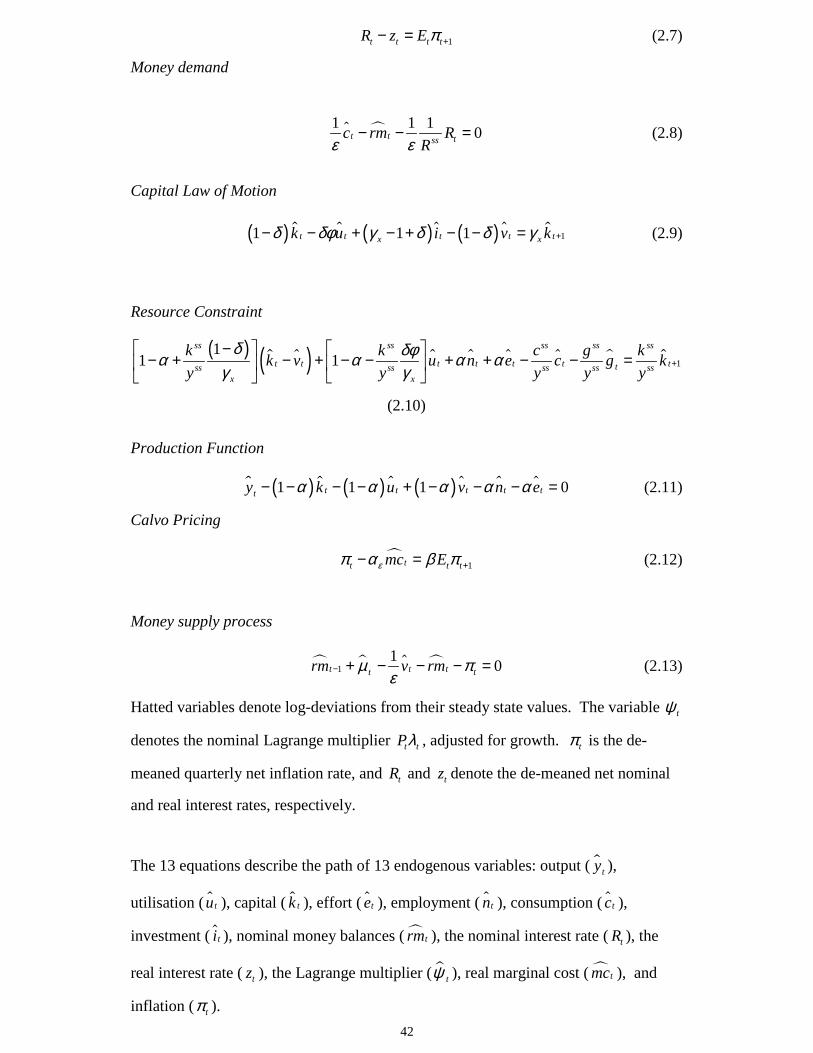
42

1t t t tR z Eπ +− = (2.7)

Money demand

�1 1 1 0t t tssc rm RRε ε

− − =� (2.8)

Capital Law of Motion

( ) � � ( ) ( ) �11 1 1t t t t tx xk u i v kδ δφ γ δ δ γ +− − + − + − − =� � (2.9)

Resource Constraint

( ) �( ) � � � �1

11 1

ss ss ss ss ss

t t t t t t ttss ss ss ss ssx x

k k c g kk v u n e c g ky y y y y

δ δφα α α αγ γ

+−� � � �

− + − + − − + + − − =� � � �� �� �

� � �

(2.10)

Production Function

� ( ) � ( ) � ( ) �1 1 1 0t t t t tty k u v n eα α α α α− − − − + − − − =� � (2.11)

Calvo Pricing

�1tt t tmc Eεπ α β π +− = (2.12)

Money supply process

� � �1

1 0t t t ttrm v rmµ πε

− + − − − =� (2.13)

Hatted variables denote log-deviations from their steady state values. The variable tψ

denotes the nominal Lagrange multiplier t tPλ , adjusted for growth. tπ is the de-

meaned quarterly net inflation rate, and tR and tz denote the de-meaned net nominal

and real interest rates, respectively.

The 13 equations describe the path of 13 endogenous variables: output ( � ty ),

utilisation ( � tu ), capital ( � tk ), effort ( te� ), employment ( � tn ), consumption ( tc� ),

investment ( ti� ), nominal money balances ( � trm ), the nominal interest rate ( tR ), the

real interest rate ( tz ), the Lagrange multiplier ( � tψ ), real marginal cost ( � tmc ), and

inflation ( tπ ).

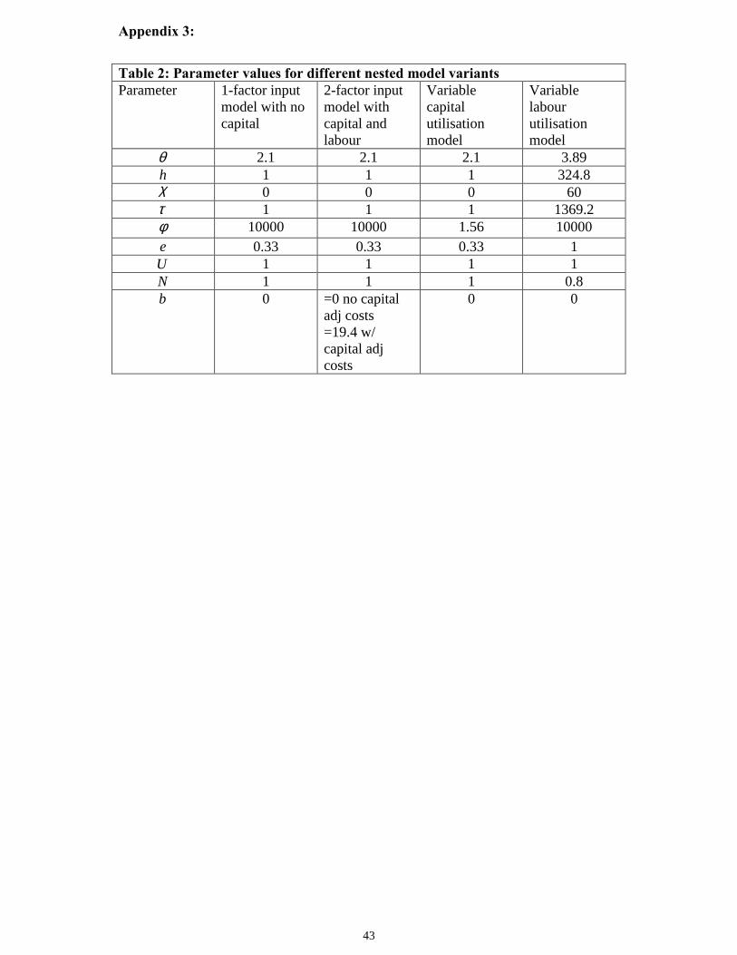
43

Appendix 3:

Table 2: Parameter values for different nested model variantsParameter 1-factor input

model with nocapital

2-factor inputmodel withcapital andlabour

Variablecapitalutilisationmodel

Variablelabourutilisationmodel

θ 2.1 2.1 2.1 3.89h 1 1 1 324.8χ 0 0 0 60τ 1 1 1 1369.2φ 10000 10000 1.56 10000e 0.33 0.33 0.33 1U 1 1 1 1N 1 1 1 0.8b 0 =0 no capital

adj costs=19.4 w/capital adjcosts

0 0