arX

iv:1

105.

6329

v1 [

q-bi

o.M

N]

31

May

201

1

A modular synthetic device to calibrate promoters

D. Gamermanna,b, A. Montagudb, P. Aparicioc, E. Navarrod, J. Trianae, F.R. Villatorod, J. F. Urchueguıab, P. Fernandez de Cordobab

aCatedra Energesis de Tecnologıa Interdisciplinar, Universidad Catolica de Valencia SanVicente Martir,

Guillem de Castro 94, E-46003, Valencia, Spain.bInstituto Universitario de Matematica Pura y Aplicada, Universidad Politecnica de

Valencia,Camino de Vera 14, 46022 Valencia, Spain.

cDepartament de Quımica Fısica i Inorganica,Universitat Rovira i Virgili, 43007, Tarragona, Spain.

dDepartamento de Lenguajes y Ciencias de la Computacin,E.T.S.I Industriales, Universidad de Malaga,Campus El Ejido, S/n 29013, Malaga, Spain.

eDepartamento de Quımica,Universidad Pinar del Rıo “Hermanos Saız Montes de Oca”,

Martı 270, 20110, Pinar del Rıo, Cuba.

Abstract

In this contribution, a design of a synthetic calibration genetic circuit to char-acterize the relative strength of different sensing promoters is proposed andits specifications and performance are analyzed via an effective mathematicalmodel. Our calibrator device possesses certain novel and useful features likemodularity (and thus the possibility of being used in many different biolog-ical contexts), simplicity, being based on a single cell, high sensitivity andfast response. To uncover the critical model parameters and the correspond-ing parameter domain at which the calibrator performance will be optimal,a sensitivity analysis of the model parameters was carried out over a givenrange of sensing protein concentrations (acting as input). Our analysis sug-gests that the half saturation constants for repression, sensing and differencein binding cooperativity (Hill coefficients) for repression are the key to theperformance of the proposed device. They furthermore are determinant forthe sensing speed of the device, showing that it is possible to produce de-

Email address: daniel.gamermann@ucv.es (D. Gamermann)

Preprint submitted to Elsevier January 9, 2014

tectable differences in the repression protein concentrations and in turn inthe corresponding fluorescence in less than two hours. This analysis pavesthe way for the design, experimental construction and validation of a newfamily of functional genetic circuits for the purpose of calibrating promoters.

Keywords: synthetic genetic circuits, synthetic biology, calibration, genepromoter, effective modeling of gene circuits, parameter analysis

1. Introduction

One of the fundamental principles of synthetic biology is the constructionof biological standardized parts and devices which are interchangeables. Aproper characterization of these parts and devices appears as a key issue inorder to make them reusable in a predictive way. In the recent past scien-tists have witnessed several initiatives towards the design and fabrication ofsynthetic biological components and systems as a promising way to explore,understand and obtain beneficial applications from nature. For instance, inthe post genomic era one of the most fascinating challenges scientists arefacing is to understand how the phenotypic behaviour of living cells arise outof the properties of their complex network of signalling proteins. While theinteracting biomolecules perform many essential functions in these systems,the underlying design principles behind the functioning of such intracellu-lar networks still remain poorly understood [3, 13]. Several initiatives havebeen reported in this line of thought to uncover some key working principlesof such genetic regulatory networks via quantitative analysis of some rel-atively simple, experimentally well characterized, artificial genetic circuits.It has been shown that custom made gene-regulatory circuits with any de-sired property can be constructed from simple regulatory elements [4]. Theseproperties include bistability, multistability or oscillatiory behaviour of ge-netic circuits in various microorganisms such as bacteriophage switch [5] orthe cyanobacterium circadian oscillator [6]. As one example, the genetic tog-gle switch, a synthetic, bi-stable gene-regulatory network in Escherichia coli,was shown to provide a simple theory that uncovers the conditions necessaryfor bi-stability [11, 12]. Further, artificial positive feedback loops (PFLs)have been used as genetic amplifiers in order to enhance the responses ofweak promoters and in the creation of eukaryotic gene switches [14]. Sayutet al. demonstrated the construction and directed evolution of two PFLsbased on the LuxR transcriptional activator and its cognate promoter, Pluxl

2

[8]. These circuits may have application in metabolic engineering or genetherapy that requires inducible gene expressions [9, 10].

The desired performance of these synthetic networks and in turn theresultant phenotype is strongly dependent on the expression level of the cor-responding genes, which is further controlled by several factors such as pro-moter strength, cis- and trans-acting factors, cell growth stage, the expressionlevel of various RNA polymerase-associated factors and other gene-level reg-ulation characteristics [11, 13]. Thus, one important ingredient to elucidategene function and genetic control on phenotype would be to have access towell-characterized promoter libraries. These promoter libraries would be inturn useful for the design and construction of novel biological systems. Therehave been several initiatives to control gene expression through the creationof promoter libraries [2, 7]. Alper et al., [1] have reported a methodology todevelop a completely characterized, homogeneous, broad-range, functionalpromoter library with the demonstration of its applicability to analysis ofgenetic control.

Since Miller published [16] a proposal for a measurement standard forβ-galactosidase assays, yet much work has been done with no conclusivestandard being established [17, 18, 19]. The main goal in calibration is mea-suring a query value up to an established standard. A good device shouldbe unique, reliable and easy to use; additionally it should circumvent, toall possible extent, any noise that could alter the measurement. Recently amethodology [20] has been reported to characterize the activity of promotersby using two different cell strains. In the present study we propose the useof a synthetic gene regulatory network as a framework to characterize dif-ferent promoter specifications by using a single-cell strategy. In this contextcharacterization stands for evaluating the parameters of a query promoter ascompared to a standard promoter acting as a scale. The proposed device,the promoter calibrator, works on the principle of comparing a specific inputsignal which will be sensed by promoters of different sensing strengths and,as an output, produces fluorescence of specific colours which allows quanti-fying the relative strength of the promoters. Analyses were carried out inorder to find out relevant model parameters and the corresponding range ofmodel parameter values which are compatible with the performance of thiscalibrating biological design over a spectrum of given input .

This contribution is organized as follows: in the first part, “Design”, thestructure and working principle are explained and the mathematical modelresulting from the construction is established. In section 3, “Numerical Anal-

3

SensingProtein

Input

RFP

GFP

x

y

Pdev Px

Pqry Py

Figure 1: Design of the proposed promoter calibrator. It is composed of two promoters(with two parts each: a sensing and a repressed domain) one of the sensing promotersis the device promoter and the other is the query promoter. The repressed domains arecontroled by the two repressors proteins (x and y). Each promoter is inhibited by therepressor which is transcribed from the opposing promoter. Fluorescence proteins levelswill be proportional to repressor protein levels, which, in turn, will be promoted by thesensing promoters.

ysis of the System”, we analyze the dynamics of the model equations in regardto its stability, functional parameter regions and sensitivity or robustness vs.the change in certain key parameter values. In the following section, a proofof concept design is proposed in order to choose the right parameters to actu-ally perform the experimental validation of our concepts and have a systemthat gives a clear and stable signal that can be interpreted. Finally, theconclusions resulting from our paper are exposed.

2. Design

2.1. Biological principles

Our promoter calibrator is composed of two promoters (each with twoparts: a sensing and a repressed domain), two repressors proteins and twofluorescent protein outputs (see Fig. 1). Each promoter is inhibited bythe repressor, transcription of which is promoted by the opposing promoter.Fluorescence protein levels will be directly related to repressor protein lev-els, activated in turn by their sensing promoters. Hence, different sensingstrengths will cause a difference in the expression of the fluorescence pro-teins, detectable by means of single cell fluorescence as changes in the colorpatterns of the individual cell or cell sample.

In our scheme, one of the sensing promoters acts as the device promoterto which the strength of a given query promoter is quantitatively compared.

4

The main use of this device is to characterize different promoter specifications(sensing affinities and cooperativities) compared to some standard. One ofthe main usefulness of this design lies in the potential modularity of the sys-tem: by changing the sensing part of the promoters, other sensing promoterscould be calibrated; this change can be carried out by a simple, straight-forward cloning step. Modularity also boasts the potential of this device asit can be implemented in a potentially unlimited set of systems.

2.2. Mathematical model

The behaviour of the proposed promoter calibrator can be understoodvia an effective mathematical model. The model is considered to be effectiveas transcription and translation have been modeled as a lumped reaction.The separation of transcription and translation otherwise involves a responsedelay. We seek to classify dynamic behaviors depending upon the change inmodel parameters and determine which experimental parameters should befine-tuned in order to obtain a satisfactory performance of our device.

The time dependent changes in repressor and sensing protein (input) con-centrations is shown in equations (1-3). Subsequent to the biological design,reporter protein concentrations are directly related to repressor protein con-centrations.

dx

dt= α1

(

psk1

)n1

1 +(

psk1

)n1

1

1 +(

yky

)ny− βxx+ γx, (1)

dy

dt= α2

(

psk2

)n2

1 +(

psk2

)n2

1

1 +(

xkx

)nx− βyy + γy, (2)

dpsdt

= −βpsps. (3)

The device and query promoters activate the production of repressor pro-tein x and y, respectively, and their concentration is related directly to theconcentration of fluorescence proteins. Thus these variables will be treated asequivalent from the modelling point of view. Parameters α1 and α2 representthe effective rate of synthesis of repressor proteins x and y, respectively; α isa lumped parameter that takes into account the net effect of various activ-ities such as RNA polymerase binding, RNA elongation and termination of

5

transcript, ribosome binding and polypeptide elongation and will be modi-fied by repression and sensing effects. The βx, βy and βps are the degradationconstants of repressor protein x, repressor protein y and sensing protein ps,respectively. The sensing protein concentration ps will depend on the sensedinput, will be easy to change in a given experiment and is used as the maininput variable in our calibrator experiments. It is important to note that aslow rate of degradation is assumed for the sensing protein, implying a nearlyconstant level over a reasonable experimental time interval. Basal level ratesof synthesis of proteins x and y are denoted by γx and γy, respectively.

Repressor and sensing responses are assumed to follow Hill equation dy-namics: promoter-binding monomers form multimers by positive allosterismand attach to its cognate promoter with saturating behaviour. Binding coop-erativities are described by Hill coefficients nx and ny for repressor domainscorresponding to x and y respectively, and n1 and n2 for sensing domainscorresponding to device and query promoter respectively. The extent of thesaturation rate is described by half saturation constants or Michaelis con-stants, denoted by parameter kx and ky for repressor domains correspondingto x and y respectively and k1 and k2 for sensing domains corresponding todevice and query promoter respectively. The total number of promoter sitesis assumed to be conserved and the total concentration of both promoters ischosen to be identical.

In our construction, the crossrepressing part will be kept unchanged whiledifferent sensing domains may be attached to it. The aim is to establisha protocol to accurately quantify differences between the sensing promoterparameters (α1,2, k1,2). Crossrepression parameters (kx,y, βx,y and nx,y) arestructural parameters that must be chosen in such a way that the fluorescenceresponse of the system gives us stable, sensitive and robust indication aboutthe quantitative relations between the sensing promoter parameters. Thedynamic analysis of the system will help us to take the right decisions onwhich are the most appropriate values for these structural parameters. Thenext sections are devoted to the dynamical analysis in order to determine thesensitivity and robustness of the system for different ranges of the structuralparameters.

The commercial software package Mathematica (Wolfram), was used formodel development and simulation. In the numerical calculations we haveused the following dimensionless variables:

6

X =x

kx(4)

Y =y

ky(5)

τ = tβx (6)

α1,2 =α1,2

βxkx,y(7)

γx,y =γx,yβxkx,y

(8)

therefore, the units in the plots of the figures in this work are given in unitsof kx or ky for the x and y repressor proteins concentrations and time in unitsof 1

βx

. For the adimensional variables, Equations (1-2) take the form:

dX

dτ= α1

(

psk1

)n1

1 +(

psk1

)n1

1

1 + Y ny

−X + γx, (9)

dY

dτ= α2

(

psk2

)n2

1 +(

psk2

)n2

1

1 +Xnx

− RY + γy, (10)

where R is the ratio βy

βx

.

3. Numerical analysis of the system

The simplifying assumption of considering sensing proteins for which thedegradation constant βps is much smaller than the rest (βps ≪ βx, βy) wasmade in order to classify the possible dynamic scenarios of our model. Giventhis assumption, in a first order of approximation we have,

dpsdt

= −βpsps ≈ 0. (11)

In such approach, the concentration of sensing protein ps is constantduring the evolution time of the rest of the internal variables of the system.This assumption leads to a system of two autonomous coupled non-linear

7

ordinary differential equations dependent on the variables x and y, eqs. (9-10), in which ps is fixed although it can be easily changed within a givenexperiment. This is not true for the rest of parameters which are moredifficult to modify in a given experiment. This approximation transformsthe system into:

dX

dτ= α′

1

1

1 + Y ny

−X + γx, (12)

dY

dτ= α′

2

1

1 +Xnx

−RY + γy. (13)

where the new parameters α′

i (effective transcription factors) are given bythe following expression:

α′ = α

(

psk

)n

1 +(

psk

)n . (14)

In the limit in which the constants kx,y, βx,y, γx,y are equal, this equationsdescribe the biological equivalent of an electronic comparator, that is, a devicewhich compares two voltages or currents and switches its output to the largersignal. In the biological equivalent, our comparator would select for the largerof the two α’s, as exemplified in Fig. 2, which represent the evolution of thesystem for the cases in which the query promoter has a higher and lowereffective transcription factor compared to the device promoter, respectively.

In any case, our aim is to construct a device, termed a calibrator, whichnot only selects the stronger affinity but also allows quantifying the rela-tive strength of both promoters. Although the comparator is a fundamentalpart of this device, a deeper understanding of the dynamics of the system isrequired for its application as a calibrator device in real biological environ-ments.

3.1. Dynamic analysis of the calibrator

The dynamical analysis of the system given by Eqs. (12-13) requires thedetermination of its steady state solutions and their linear stability. Thesteady states (xss, yss) are given by the intersection of the null clines:

F1(X, Y ) = α′

1

1

1 + Y ny

−X + γx = 0, (15)

8

0 2 4 6 8 10 12Τ @units of ΒxD

0.5

1.0

1.5

2.0

2.5

3.0

X,Y @units of Kx and KyD

0 2 4 6 8 10 12Τ @units of ΒxD

0.5

1.0

1.5

2.0

2.5

3.0

X,Y @units of Kx and KyD

Figure 2: Typical response of the proposed promoter calibrator. In the upper figure theconcentration of the x protein (solid line) in the steady state is higher while in the figurebelow the concentration of the y protein (dashed line) is higher.

and

F2(X, Y ) = α′

2

1

1 +Xnx

− RY + γy = 0. (16)

The analytical solution of Eqs. (15-16) cannot be obtained, hence nu-merical methods must be used. The linear stability of the steady states isdetermined by the sign of the eigenvalues of the Jacobian matrix,

M =

(

∂F1

∂X∂F1

∂Y∂F2

∂X∂F2

∂Y

)

X=Xss,Y=Yss

(17)

which are given by

λ± = −1 +R

2± 1

2

√

(R− 1)2 + 4∆, (18)

∆ =nxny(Xss − γx)(α

′

1 + γx −Xss)(YssR− γy)(α′

2 + γy − YssR)

α′

1α′

2XssYss.(19)

9

From the analysis of the previous equations (15-16), we deduce that, forthe positive steady state solutions (Xss > 0 and Yss > 0), the followingmathematical constraints hold: α′

1 > Xss − γx > 0 and α′

2 > YssR − γy > 0,respectively. Thus, taking into account (18-19), we observe that ∆ > 0 andλ− is always negative. However, λ+ can be either negative, for ∆ > R,or positive, for ∆ < R, resulting in either stable nodes (sinks) or unstablesaddles, respectively. The condition ∆ = R is satisfied at certain criticalvalues of the parameters at which precisely one of the steady state solutionsof the system changes its stability.

In order to highlight the specific aspects of the calibrator dynamics, wewill in the following sections consider a number of special cases. Specificallywe will examine the (fully) symmetrical calibrator, α′

1 = α′

2 = α′, nx = ny =n, kx = ky = k, βx = βy ⇒ R = 1 and γx = γy = γ, and the partiallysymmetrical calibrator, with the same specifications except that α′

1 and α′

2

may differ. At the end of the section some general considerations aboutdynamics of the system in the most general case will made.

3.2. The fully symmetrical calibrator (α′

1 = α′

2 = α′)

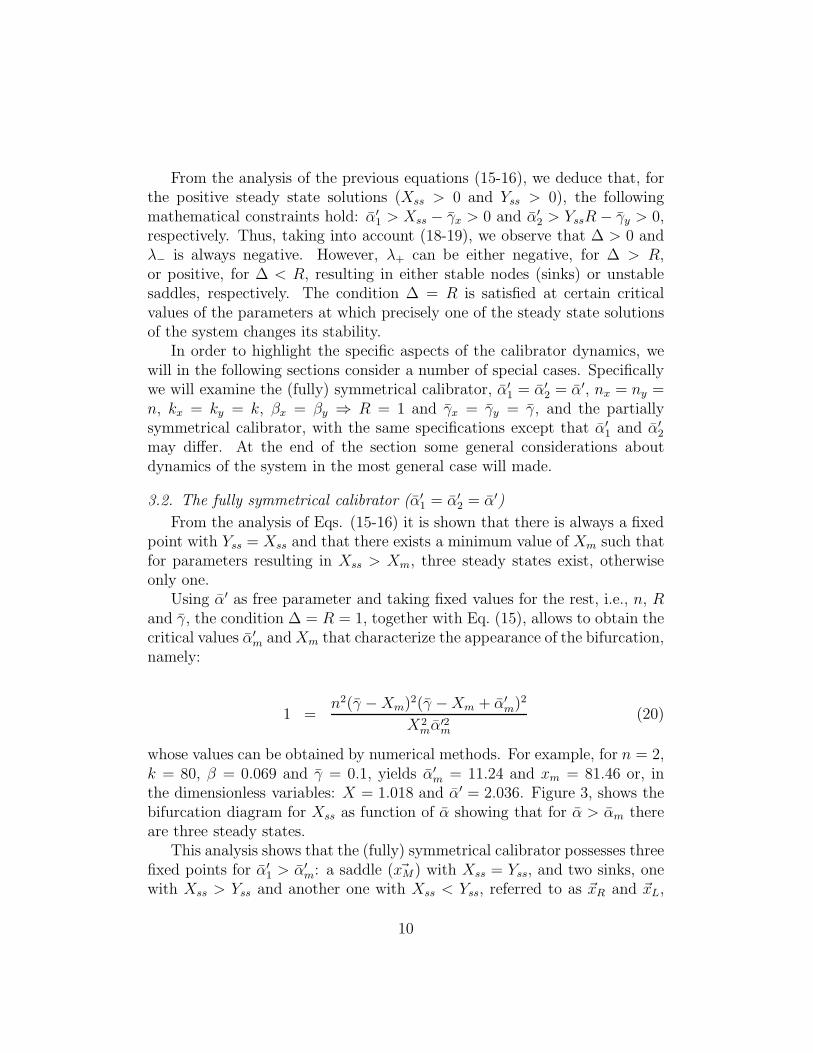
From the analysis of Eqs. (15-16) it is shown that there is always a fixedpoint with Yss = Xss and that there exists a minimum value of Xm such thatfor parameters resulting in Xss > Xm, three steady states exist, otherwiseonly one.

Using α′ as free parameter and taking fixed values for the rest, i.e., n, Rand γ, the condition ∆ = R = 1, together with Eq. (15), allows to obtain thecritical values α′

m andXm that characterize the appearance of the bifurcation,namely:

1 =n2(γ −Xm)

2(γ −Xm + α′

m)2

X2mα

′2m

(20)

whose values can be obtained by numerical methods. For example, for n = 2,k = 80, β = 0.069 and γ = 0.1, yields α′

m = 11.24 and xm = 81.46 or, inthe dimensionless variables: X = 1.018 and α′ = 2.036. Figure 3, shows thebifurcation diagram for Xss as function of α showing that for α > αm thereare three steady states.

This analysis shows that the (fully) symmetrical calibrator possesses threefixed points for α′

1 > α′

m: a saddle ( ~xM) with Xss = Yss, and two sinks, onewith Xss > Yss and another one with Xss < Yss, referred to as ~xR and ~xL,

10

0

0.5

1

1.5

2

2.5

3

0 0.5 1 1.5 2 2.5 3

Xss

αx

Figure 3: Bifurcation diagram for Xss.

respectively. This behaviour is typical of the occurrence of a (supercritical)pitchfork bifurcation and bistable behaviour.

Regarding the possible trajectories of the dynamic variables, Figure 4illustrates the phase plane of Eqs. (12-13), where the steady states are locatedat the intersection of the null clines eqs.(15-16) represented by dashed lines.The solid lines are the stable (W S) and unstable (WU) manifolds of thesaddle fixed point ~xM . The stable manifold W S divides the phase planein two regions, the first and second octants corresponding to the attractionbasins of the sinks ~xR and ~xL, respectively. Different possible trajectories inthe phase plane are depicted for a given number of initial conditions, wherethe arrows indicate the flow direction.

In a calibrator experiment the initial value of the repressor protein con-centrations x and y would be zero and hence the phase plane trajectorieswould depart from the origin in Figure 4. For values of α′ larger than α′

m,the system becomes unpredictable, as small perturbations in the trajectorieswould potentially push the system into any of the attraction basins of thesinks ~xR and ~xL.

3.3. The partially symmetrical calibrator

We consider now the more general scenario in which α′

1 and α′

2 may differbeing the rest of variables equal (nx = ny = n, kx = ky = k, βx = βy = βand γx = γy = γ). The condition ∆ = R which characterizes the occurrenceof the pitchfork bifurcations now reads:

11

Figure 4: Phase plane, showing the unstable equilibrium point (the point where the twodashed lines touch in the center) and the two steady state solutions (points where thedashed lines touch close to each axis). The arrows show the path the system would dostarting from any point in the phase space.

1 =n2(γ −Xss)(γ − Yss)(γ −Xss + α′

1)(γ − Yss + α′

2)

XssYssα′xα

′y

(21)

that shall be solved together with Eqs. (15-16) for the fixed points of thesystem.

Fig. 5 shows the result of the numerical simulation of the resulting systemof equations (with initial conditions X = Y = 0) by slightly changing thevalue of α′

2 with respect to α′

1. The figure shows the results of differentsimulations for α′

1 =3.0, n = 3 and α′

2 = ǫα′

1 with ǫ =0.5, 0.6, 0.7, ..., 1.0, ...,1.5. The results for ǫ < 1 are the points in the right down corner of the plot.One can see that these points positions are very insensitive to the value ofα′

2. There is only one point in the center of the plot, which corresponds toα′

1 = α′

2, it is the unstable saddle, and small perturbations in the system willdrive the system away from this solution to either of the other two steadystate solutions. Once ǫ > 1, the system goes to the solutions where Yss > Xss

which are represented by the points in the upper left corner. For these pointsthe maximum value of α′ is growing and one can observe that the solution

12

0 0.5

1 1.5

2 2.5

3 3.5

4 4.5

5

0 0.5 1 1.5 2 2.5 3 3.5

Yss

Xss

Figure 5: Results for the simulation of the partially symmetric calibrator. On the right,close to the x-axis (α′

2< α′

1for these points), there are many points at the same posi-

tion, showing that, for the parameter region where a bifurcation happens, the solution isinsensitive to the value of the weakest between the two α′s.

is sensitive to this value. So the steady state solution into which the systemfalls is only sensitive to the bigger value between α′

1 and α′

2 and changes inthe smaller among these two parameters has no sensible effect in the finalsolution.

For the case in which the calibrator falls within the region of bistability,if α′

2 < α′

1 the orbits departing from the origin of Fig. 5 would fall within theattraction basin of solution ~xR. It is nevertheless observed that ~xR is quiteinsensitive to the actual α′

2/α′

1 ratio. In consequence, the system would showa stable but rather insensitive response to different query promoters. On theother hand, if α′

1 < α′

2, the orbits departing from the origin would fall withinthe attraction basin of solution ~xL, which changes appreciably as a functionof the α′

2/α′

1 ratio. Thus the system would not only be stable, but also rathersensitive to changes in the effective query promoter affinity. It should be keptin mind that the sensing protein concentration, ps, can be used to modifyα′

1, α′

2, which changes from unity to α1,2 as ps changes from zero to infinityand therefore the ratio α′

2/α′

1 changes with ps.We can also define the fluorescence ratio as the ratio of X/Y if X < Y

and Y/X if Y > X . This will be the intensity ratio of the two fluorescencesonce the system reaches stability. In Fig. 6 we show a plot of this ratio for

13

different values of α′

2/α′

1. This ratio grows until it reaches its maximum whenα′

2 = α′

1 and then it decreases. Another observation about this parameteris that the bigger α′

1 is, the less sensible to the ratio α′

2/α′

1 the fluorescenceratio will be.

3.4. The calibrator dynamics in the general case

The theorem of Andronov and Pontryagin [21] states that Eqs. (12-13)in the symmetrical case are structurally stable, since every fixed point is hy-perbolic (its eigenvalues have a non-null real part) and there are no orbitsconnecting two saddles (since there is only one). Structural stability im-plies that the phase plane topology is preserved under small perturbationsof the parameters. Hence, the phase plane of Eqs. (12-13) in the case thatα′

x ≈ α′

y, nx ≈ ny, kx ≈ ky, βx ≈ βy and γx ≈ γy, is topologically equiv-alent to that shown in Fig. 4, meaning that there is a continuous function(homeomorphism) between both phase planes.

Changing the ratio of other structural parameters of the calibrator hassimilar results as in the partially symmetrical case. For a given range closeto the value 1 for the ratio of each parameter ratio (nx/y, βx/y, ...) thebifurcation appears while far from the value 1 the bifurcation cannot beseen. The range is usually bigger, the bigger the values for α′

1,2 are. In Fig. 7we show, as an example, the range where the bifurcation appears for differentvalues of βx/βy.

If R < 1 the orbits departing from the origin (X = Y = 0) would fallwithin the attraction basin of solution ~xL, on the other hand if R > 1 theorbits departing from the origin would fall within the attraction basin ofsolution ~xR.

3.5. Calibrator performance analysis: robustness and response time

In order to use this system to measure the relative strength between twopromoters, one should keep in mind two factors. The first important factoris the right choice for the parameters of the repressor proteins and devicepromoter in order to have a robust system, that gives a stable response thatcan be easily interpreted. Second, is the time response of the device, thatmeans, how long does the system needs to reach its steady state solution.

When the equations are written in the dimensionless form, the parameterskx and ky do not appear explicitly, see eqs. (9-10). These parameters appearimplicit in the definition of the variables X and Y and in the γ parameters(which have small influence in the dynamics of the system). By choosing

14

0

0.05

0.1

0.15

0.2

0.25

0.3

0.2 0.4 0.6 0.8 1 1.2 1.4 1.6 1.8

Flu

ores

cenc

e R

atio

α’y/α’x

X>YX<Y

0 0.1 0.2 0.3 0.4 0.5 0.6 0.7 0.8 0.9

1

0.2 0.4 0.6 0.8 1 1.2 1.4 1.6 1.8

Flu

ores

cenc

e R

atio

α’y/α’x

α’x=2α’x=3α’x=4

Figure 6: Upper plot: Fluorescence ratio for different values of α′

y/α′

x(α′

x=2.5). The blue

points are solutions where X > Y and in the red points Y > X . Lower plot: Fluorescenceratio for different values of α′

y/α′

xand for different values of α′

x(Solid line:α′

x=2, dashed

line:α′

x=3, dotted line:α′

x=4).

15

0 0.5

1 1.5

2 2.5

3 3.5

4

0 0.2 0.4 0.6 0.8 1 1.2 1.4 1.6 1.8 2

Xss

β’y/β’x

α’x=2α’x=3α’x=4

Figure 7: (Color online) Position of Xss for different values of βy/βx. In the black curveα′

x= α′

y=2, in the blue curve α′

x= α′

y=3 and in the red one α′

x= α′

y=4.

kx = ky the results will be easier to interpret since the fluorescence is directlyrelated to the concentrations of the proteins x and y and, by setting kx =ky, the fluorescence intensity ratio (X/Y and Y/X) and the fluorescenceintensity difference (|X−Y |) will be directly proportional to these parametercalculated with the real protein concentrations.

An experiment made with the calibrator would consist of cloning a plas-mid with the calibrator genetic circuit assembled with the device promoter(whose parameters one have to choose) among known ones and with a querypromoter whose parameters are unknown. The plasmid should be insertedin cells in solutions of the signaling protein at different concentrations ps.Each promoter is modeled through two parameters, α1/2 and k1/2, 1/2 standfor device/query promoter. While at low ps concentrations both promotersare weak and give a weak fluorescence response, at high ps concentrations,both promoters are saturated and their strength is maximal. From the flu-orescence intensities at these high concentrations of the signaling protein itis possible to establish the relative strength of the two promoters α2/α1. Infigures 8 and 9 we show plots of the fluorescence difference defined as |X−Y |and the fluorescence ratio X/Y for three different values of α1 and varyingα2 at high signaling protein concentrations (the effective strength of bothpromoters is maximum).

16

0 1 2 3 4 5 6 7 8 9

10

0 2 4 6 8 10

|X-Y

|

α2

α1=1α1=2α1=3

Figure 8: (Color online) The fluorescence difference for different values of α1 as a functionof α2. Note that for values of α2 sufficiently higher than α1 the fluorescence differenceincreases linearly with the value of α2.

The first thing to note from figures 8 and 9 is that, if the query pro-moter is stronger than the device one, the device fluorescence (X) will bestrongly suppressed, and the fluorescence intensity coming from the querypromoter is proportional to its strength (the response of the system is lin-ear). That means, choosing a weak device promoter, one can establish therelative strength of other promoters by a simple proportionality law given bythe linear response plotted in figure 8.

At each different ps concentration, the effective strength of the device andquery promoters is different, see eq. (14). The parameter that distinguishestwo promoters, with respect to the ps concentration, is their Michaelis con-stants, k1,2. The parameters k1,2 mark the rhythm at which the effectivestrength of each promoter grows. If a promoter has a small value of k, at lowps concentrations of the signaling protein, the promoter is already acting atfull strength, while for high values of k the promoter saturates only at highvalues of ps. We have already established to choose a small value for thedevice promoter α1, so we expect the query promoters to have α2 > α1. Ifk2 < k1, the effective strength of the query promoter is always bigger thanthe relative strength of the device one, and in the experiment one observesthat the luminosity associated with the query promoter is stronger for anyvalue of the signaling protein concentration ps. On the other hand, if one

17

0 5

10 15 20 25 30 35 40

0 0.5 1 1.5 2 2.5 3

X/Y

α2/α1

α1=3α1=2α1=1

0 0.1 0.2 0.3 0.4 0.5 0.6 0.7 0.8 0.9

1

1.2 1.4 1.6 1.8 2 2.2 2.4 2.6 2.8 3

X/Y

α2/α1

α1=3α1=2α1=1

Figure 9: (Color online) Upper plot: the fluorescence ratio X/Y as a function of α2/α1

for different values of α1. One can clearly see that for similar values of α1 and α2, whenthe bifurcation occurs, the system goes to a state where the repressor protein of thestronger promoter completely dominates the system. Lower plot: Detail of the regionwhere α2 > α1.

18

chooses a small value for k1, already at low ps concentrations the strength ofthe device promoter saturates, and if k1 is small enough it saturates beforethe effective strength of the query promoter reaches a value bigger than α1.In this situation one would observe at low concentrations of ps the lumi-nosity of the device promoter stronger than the one coming from the querypromoter. Then, at some critical value of ps = psc both strength are equaland for ps > psc the stronger fluorescence is the one from the query promoter.For n1 = n2, the value of k2 given in units of k1 as a function of psc (also inunits of k1) is given by:

k2 = n

√

pnsc

(

α2

α1

− 1

)

− α2

α1

, (22)

psc = n

√

(

kn2 − α2

α1

)(

α1

α2 − α1

)

. (23)

In figure 10 we show a few examples of results one might expect fordifferent values of k2.

So, the construction of the calibrator device, as we present it, would bethe following: first one chooses a very weak promoter which has a smallMichaelis constant to act as the device promoter in the calibrator. Secondstep is to define a standard, to choose a known promoter, clone the calibratordevice with it as query promoter and perform a measurement of the fluores-cence intensity of this standard promoter at high ps concentrations. Thisfluorescence intensity is the standard one, to which we can compare otherpromoters. Now performing the experiment with another promoter actingas query promoter one obtains another value for the luminosity that we cancompare with the standard one. The higher or lower this luminosity is withrespect to the standard, the stronger or weaker the promoter is comparedwith the standard, so one can establish the value of α2. Knowing α2 one canperform the same measurement for different ps concentrations in order toestablish the critical value of ps where the query fluorescence becomes higherthan the device one. Knowing the value of psc it is possible to establish thevalue of k2 by means of eq. 22 (assuming both promoters have the same n).

Now that we have established the ideal parameters for the device promoter(weak strength and small Michaelis constant) and set kx = ky and βx = βy

the last important factor is the time response of the system.

19

In figure 11 we show plots for the tf , the time the systems needs toreach its steady state1 for different values of α1. One observes that the timeresponse of the system has a peak with the maximum around 30β−1

x whenthe effective strength of both promoters is equal and then it goes to a ratherstable value close to 7β−1

x . For a realistic value of βx like 0.069 min−1 the peakvalue for tf is 7 hours, while for most of the measurements (the calibrator atdifferent ps concentrations) this time should be around two hours.

4. Conclusions

In the present study we have proposed a biological device that works as apromoter calibrator in which the strength of a collection of query promoterscan be measured against the strength of a device promoter. Some of the keyfeatures of the proposed design are its single cell character, high modular-ity and handy construction: a unique molecular cloning permits the changeof the promoter ready to be calibrated. The designed performance of theproposed biological device has been demonstrated by means of an effectivemathematical model. The sensitivity analysis of the model shows that thereis a sensible relation between the relative promoter strengths and the finalsteady fluorescences measured by the system.

Furthermore, a response time analysis shows that the device can producea large difference in the repression protein concentrations and in turn in thecorresponding fluorescence in approximately two hours.

Finally our promoter calibrator principle may lead to an improvement inthe modeling and characterizations of systems in Synthetic Biology, whichfrequently rely on arbitrarily characterized, or even non-characterized, pro-moters.

acknowledgements

This work has been funded by MICINN TIN2009-12359 project ArtBio-Com, the Spanish Ministerio de Educacin y Ciencia through the programJuan de la Cierva, the FPI grant program of the Generalitat Valenciana andthe Beca de recerca predoctoral from the Universitat Rovira i Virgili.

1The system actually goes asymptotically to its steady state without really reaching it.What we have calculated is the time needed so that the sum of the absolute values of thederivatives of X and Y reach a small value (0.01).

20

The authors would also like to thank the Valencia iGEM 2007 team andEnrique O’Connor for useful discussions.

References

[1] Alper et al., Tuning genetic control through promoter engineering.,PNAS. 102 (36), 12678-12683 (2005).

[2] Kumar A and Snyder M., Genome-Wide Transposon Mutagenesis inYeast., Current Protocols in Molecular Biology., 13, 13.3 (2001).

[3] Elowitz MB and Leibler S., A synthetic oscillatory network of transcrip-tional regulators., Nature, 403, 335-338 (2000).

[4] Monod, J. and Jacob, General conclusions: teleonomic mechanismsin cellular metabolism, growth and differentiation., Cold spring Harb.Symp. Quant. Biol., 26, 389-401 (1961).

[5] Ptashne, M., A genetic switch: phage λ and Higher Organisms. (1992).

[6] Ishiura, M et al., Expression of gene cluster kaiABC as a circadian feed-back process in cyanobacteria., Science, 281, 1519-1523 (1998)

[7] Santos CN and Stephanopoulos G., Combinatorial engineering of mi-crobes for optimizing cellular phenotype., Current Opinion in ChemicalBiology., 12, 168-176 (2008)

[8] Sayut DJ, Niu Y, and Sun L., Construction and Engineering of PositiveFeedback Loops., JACS chemical Biology., 1(11), 692-696 (2006)

[9] Weber, W., and Fussenegger, M., Pharmacologic transgene control sys-tems for gene therapy, J. Gene Med., 8, 535556 (2006).

[10] Walz, D., and Caplan, S. R., Chemical oscillations arise solely fromkinetic nonlinearity and hence can occur near equilibrium, Biophys. J.,69, 16981707 (1995).

[11] Gardner T, Cantor CR and Collins JJ., Construction of genetic toggleswitch in Escherichia coli., Nature., 403, 339-342 (2000).

[12] J. Stricker et. al., A fast, robust and tunable synthetic gene oscillator.,Nature., 456, 516-519 (2008).

21

[13] Becskei A and Serrano L., Engineering stability in gene networks byautoregulation., Nature 405, 590-593 (2000).

[14] Becskei A, Seraphin B and Serrano L., Positive feedback in eukaryoticgene networks: cell differentiation by graded to binary response conver-sion., The EMBO Journal, 20(10), 2528-2535 (2001).

[15] Cox, Surette, Elowitz., Programming gene expression with combinato-rial promoters., Mol Syst Biol., 3, 145(2007).

[16] J. Miller., Experiments in molecular genetics, Cold Spring Harbor Lab-oratory (1972).

[17] Liang et al., Activities of Constitutive Promoters in Escherichia coli., JMol Biol., 292, 19-37, (1999).

[18] Smolke & Keasling., Effect of Gene Location, mRNA Secondary Struc-tures, and RNase Sites on Expression of Two Genes in an EngineeredOperon., Biotech Bioeng., 80, 762-776 (2002).

[19] Khlebnikov et al., Modulation of gene expression from the arabinose-inducible araBAD promoter., J Ind Microb Biotec., 29, 34-37 (2002).

[20] J. R. Kelly et. al., Measuring the activity of BioBrick promoters usingan in vivo standard., Journal of Biological Engineering, 3, 1-13 (2009).

[21] Guckenheimer, J., and Holmes, P., Nonlinear oscillations, dynamicalsystems, and bifurcations of vector fields., Springer Berlin (1990).

22

0 0.2 0.4 0.6 0.8

1 1.2 1.4 1.6 1.8

2

0 2 4 6 8 10

X,Y

ps [k1]

XY

0 0.2 0.4 0.6 0.8

1 1.2 1.4 1.6 1.8

0 2 4 6 8 10

X,Y

ps [k1]

XY

0 0.2 0.4 0.6 0.8

1 1.2 1.4 1.6 1.8

0 2 4 6 8 10

X,Y

ps [k1]

XY

Figure 10: In all plots α1=k1=1 and α2=2. In the upper plot k2=2, in the center k2=3and in the bottom plot k2=4. The values for psc are respectively:

√2,

√7 and

√14.

23

0

5

10

15

20

25

30

35

0 2 4 6 8 10

t f

α2/α1

α1=1α1=2α1=3

Figure 11: Response time of the system for different values of α1 and α2. For values ofthe α′s that the system presents a bifurcation, the response time can be large because thesystem spend time in its non-equilibrium solution.

24