A Model of Double-Directional Indoor Channels for Multiterminal Communications
14
A Model of Double-Directional Indoor Channels for Multi-Terminal Communications Puji Handayani, Gamantyo Hendrantoro Department of Electrical Engineering, Institut Teknologi Sepuluh Nopember, Surabaya 60111, Indonesia [email protected], [email protected] In this paper, we propose a model of double-directional indoor non line of sight (NLOS) channels for multi-terminal communications. We derive a simple channel matrix that describes input-output relationship for such channels. The multi-terminal systems may consist of several terminals that act as amplify-and-forward (AF) relays, where source, relays and destination have arbritrary number of antennas. We complete our model by characterizing the parameters of double-directional channel impulse response of such channels through measurements in indoor environment using 3-D synthetic array antenna at 2.5 GHz band. To find out the relation between spatial characteristic of channels in each hop, we observe direction of arrival (DOA) and direction of departure (DOD) of multipath component signals at the terminal that acts as relay. We find that there are several closely matched azimuth of DOAs and azimuth of DODs which follow uniform distribution in the range of –180° to 180° for elevation around the broadside direction of vertical omni-directional elements of arrays. Index Terms—double directional indoor channel, multi-terminal communication, statistical characterization. 1. Introduction The significant improvements in spectral efficiency and system reliability through spatial multiplexing-diversity trade off promised by the multiple-input multiple-output (MIMO) transmission techniques have triggered their adoption in various broadband wireless systems. Multi-terminal communication systems may involve terminals equipped with multi-antennas, which are known as multi user MIMO. Further, these systems grow up by incorporating other terminals as relays between source and destination, in the form of multi-hop communication. The evaluation of such systems needs a channel model that describes statistically the actual physical phenomenon of radio waves propagation with sufficient accuracy. The standard MIMO channel models are being developed, as within the European Cooperation in the field of Scientific and Technical Research (COST), and the 3-rd Generation Partnership Project (3GPP) which then followed by Wireless world Initiative New Radio (WINNER) project. On the other hand, works on multiple-link indoor channel characterization are reported in some literatures, e.g., in [1], where the authors examined the correlation of dual-link MIMO channel matrices between a mobile transmitter and two receivers by studying the similarity in the eigenspace of correlation matrix of those two channel matrices, might only partially be applicable to the multi-hop modeling problem at hand. Works reported in [2] and [3] were carried out for characterization of indoor multi- link large scale fading parameters. In [2] the authors further investigated the correlation of channel matrices of two-hop MIMO channels. They expressed the channel matrix between source and destination that consists of two MIMO hops as the Kronecker product of the two MIMO channel matrices, so that their expression is restricted to the condition that scatterers around the first and second hops are uncorrelated. However, the uncorrelated scattering condition is given without further insight into the multipath phenomenon that actually occurs in radio channels in a multi-hop system. Also, works reported in [1]-[3] have not considered a general model of multi-hop channels, i.e., channels with arbitrary number of hops and antennas at each node, and joint characterization of spatial- temporal parameters of the channels. An analytical result in [4] showed that radio wave propagation over MIMO amplify-and-forward relay channel is influenced by the propagation of radio wave in individual hops and the responses of the relays. However, the model assumes that the array responses of transmitter and receiver of a relay are orthogonal, which does not hold for arrays with isotropic or omnidirectional elements. Furthermore, no verification was attempted to the assumption by field measurement. Likewise, a recent literature [5] proposed a unified channel model for multi-link cooperative MIMO. Based on geometry-based stochastic modeling, the model can be applied to many cooperative scenarios by adjusting its parameters. The paper also derived spatial correlation between any two links. However the channel gains and their spatial correlations obtained is determined by the type of links in a multi-link scenario where the parameters have been adjusted according to the physical properties of the local scatterers around each end node of the links, which still needs further investigations. Our contribution includes firstly the derivation of a simple expression of channel matrix that describes input-output relationship of indoor multi-hop communication involving amplify-and-forward (AF) relays as illustrated in Figure 1, assuming there is no direct link between the source and the destination. The expression is general in that the number of relays as well as the numbers of antennas at the source (S), relays (R) and the destination (D) are arbitrary. It also incorporates any correlation between model parameters that may exist in the channel. The model is similar with that reported in [4], but in our expression we include the expression of delays as well as that of DOD and DOA of MPCs in each hop of the channel and does not consider any assumptions for the array response at relay.
-
Upload
independent -
Category
Documents
-
view
3 -
download
0
Transcript of A Model of Double-Directional Indoor Channels for Multiterminal Communications
A Model of Double-Directional Indoor Channels for Multi-Terminal Communications Puji Handayani Gamantyo Hendrantoro Department of Electrical Engineering Institut Teknologi Sepuluh Nopember Surabaya 60111 Indonesia pujieeitsacid gamantyoeeitsacid In this paper we propose a model of double-directional indoor non line of sight (NLOS) channels for multi-terminal communications We derive a simple channel matrix that describes input-output relationship for such channels The multi-terminal systems may consist of several terminals that act as amplify-and-forward (AF) relays where source relays and destination have arbritrary number of antennas We complete our model by characterizing the parameters of double-directional channel impulse response of such channels through measurements in indoor environment using 3-D synthetic array antenna at 25 GHz band To find out the relation between spatial characteristic of channels in each hop we observe direction of arrival (DOA) and direction of departure (DOD) of multipath component signals at the terminal that acts as relay We find that there are several closely matched azimuth of DOAs and azimuth of DODs which follow uniform distribution in the range of ndash180deg to 180deg for elevation around the broadside direction of vertical omni-directional elements of arrays Index Termsmdashdouble directional indoor channel multi-terminal communication statistical characterization 1 Introduction The significant improvements in spectral efficiency and system reliability through spatial multiplexing-diversity trade off promised by the multiple-input multiple-output (MIMO) transmission techniques have triggered their adoption in various broadband wireless systems Multi-terminal communication systems may involve terminals equipped with multi-antennas which are known as multi user MIMO Further these systems grow up by incorporating other terminals as relays between source and destination in the form of multi-hop communication The evaluation of such systems needs a channel model that describes statistically the actual physical phenomenon of radio waves propagation with sufficient accuracy
The standard MIMO channel models are being developed as within the European Cooperation in the field of Scientific and Technical Research (COST) and the 3-rd Generation Partnership Project (3GPP) which then followed by Wireless world Initiative New Radio (WINNER) project On the other hand works on multiple-link indoor channel characterization are reported in some literatures eg in [1] where the authors examined the correlation of dual-link MIMO channel matrices between a mobile transmitter and two receivers by studying the similarity in the eigenspace of correlation matrix of those two channel matrices might only partially be applicable to the multi-hop modeling problem at hand Works reported in [2] and [3] were carried out for characterization of indoor multi-link large scale fading parameters In [2] the authors further investigated the correlation of channel matrices of two-hop MIMO channels They expressed the channel matrix between source and destination that consists of two MIMO hops as the Kronecker product of the two MIMO channel matrices so that their expression is restricted to the condition that scatterers around the first and second hops are uncorrelated However the uncorrelated scattering condition is given without further insight into the multipath phenomenon that actually occurs in
radio channels in a multi-hop system Also works reported in [1]-[3] have not considered a general model of multi-hop channels ie channels with arbitrary number of hops and antennas at each node and joint characterization of spatial-temporal parameters of the channels
An analytical result in [4] showed that radio wave propagation over MIMO amplify-and-forward relay channel is influenced by the propagation of radio wave in individual hops and the responses of the relays However the model assumes that the array responses of transmitter and receiver of a relay are orthogonal which does not hold for arrays with isotropic or omnidirectional elements Furthermore no verification was attempted to the assumption by field measurement Likewise a recent literature [5] proposed a unified channel model for multi-link cooperative MIMO Based on geometry-based stochastic modeling the model can be applied to many cooperative scenarios by adjusting its parameters The paper also derived spatial correlation between any two links However the channel gains and their spatial correlations obtained is determined by the type of links in a multi-link scenario where the parameters have been adjusted according to the physical properties of the local scatterers around each end node of the links which still needs further investigations
Our contribution includes firstly the derivation of a simple expression of channel matrix that describes input-output relationship of indoor multi-hop communication involving amplify-and-forward (AF) relays as illustrated in Figure 1 assuming there is no direct link between the source and the destination The expression is general in that the number of relays as well as the numbers of antennas at the source (S) relays (R) and the destination (D) are arbitrary It also incorporates any correlation between model parameters that may exist in the channel The model is similar with that reported in [4] but in our expression we include the expression of delays as well as that of DOD and DOA of MPCs in each hop of the channel and does not consider any assumptions for the array response at relay
In a two-hop link the first and the second hops that share a
common node ie a relay in Figure 1 which can be a base station or access point in multi user MIMO might also share the same interacting objects surrounding the relay This situation might lead to the appearance of multipath component signals (MPCs) that arrive at and depart from relay at the same directions which might cause an extent of correlation between the hops The common assumption as taken in [2] that the first and second hop channel matrices are uncorrelated still needs to be verified Our second contribution in this work is an investigation into the spatial characteristics at a relay We observe how DOA and DOD at a relay are related to each other to obtain a clear understanding about the correlation between the two hops described above
To complete our model we derive statistical characterization of model parameters based on the results of a measurement campaign conducted in our laboratory building Although several statistical characteristic of channel parameters have been reported in the literature eg in [6]-[8] according to the best of our knowledge the joint statistical characterization of all double-directional indoor channel parameters have not been reported yet By using a 3-D array antenna at the transmitter and at the receiver instead of using a linear or planar array we could estimate completely directional parameters at both sides ie azimuth and elevation from -180deg to 180deg and 0deg to 180deg respectively without any ambiguity in elevation 3-D cube geometry with isotropic elements theoretically has isotropic array factor desired for better DOD and DOA estimation [9] Although we use omni-directional antennas as array elements the better estimation results compared to those obtained by using linear or planar arrays should still be achieved By applying a high resolution channel parameter estimation first proposed in [10] we could obtain the directions delays and powers contained in MPCs simultaneously so that we could observe the relation among parameters simultaneously too Thus our third contribution is a new joint statistical characterization of channel parameters and channel power spectra that would be meaningful to gain more complete and accurate statistical model particularly for the 25 GHz band NLOS indoor environment
The paper is organized in the following way In Section 2 we derive double-directional multi-hop channel model Section 3 describes the measurement system and measurement environment followed by signal processing technique used to
estimate channel parameters in Section 4 In Section 5 we discuss the statistical characteristics of model parameters including a look into the relation between DOA and DOD at relays In Section 6 we presents the power spectra of the channels Finally some concluding remarks are given in Section 7
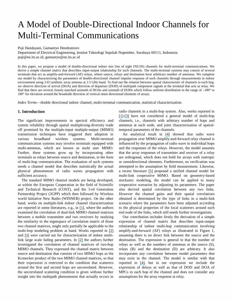
2 Multi-hop Channel Model The multi-hop channel considered in this paper is illustrated in Figure 1 where source S and destination D employ M and K antennas respectively The channel consists of Q parallel relays each of which consists of P serial relays so that the number of relays is QP in total This relay structure is general so that simple arrangement of serial or parallel relays can be derived from it Each relay has gain of gp and is equipped with Np antennas Each hop in Figure 1 generally represents a MIMO link On link (a11) if 퐱[푖] represents output discrete time signal vector of S where 퐱[푖] isin 퐶 times and i represents time index then following the description in [11] received signal vector at relay R11 퐲 [푖] isin 퐶 times can be expressed as
퐲 [푖] = sum 퐇( ) 퐱[푖 minus 휏 ] + 퐕 [푖]
(1)
In (1) 퐿 denotes the number of MPCs at link (a11) 휏 is delay of the l-th MPC wrt to the first MPC where the delay of the first MPC is 0 ns 퐕 [푖] isin 퐶 times is noise vector at R11 antennas and 퐇( ) isin 퐶 times is MIMO channel matrix that consists of complex channel gain between all possible transmit-receive antenna pairs encountered by the l-th MPC in link (a11) and can be written as
퐇( ) =ℎ hellip ℎ ⋮ ⋱ ⋮
ℎ hellip ℎ
(2)
where N11 is the number of antenna at R11
According to [12] the double directional impulse response at link (a11) can be written as
ℎ 휑 휃 휏휑 휃
= 훼 훿(휏 minus 휏 )
times 훿 휑 minus 휑 휃 minus휃
times 훿 휑 minus 휑 휃 minus 휃
(3)
where 휑 휃 휑 and 휃 are azimuth and elevation variable wrt R11 receiver and S array respectively and τ is delay variable Also 휑 휃 휏 휑 and 휃 are azimuth and elevation of DOA at R11 receiver delay and azimuth and elevation of DOD at S of the l-th MPC respectively while 훼 is complex amplitude of the l-th MPC The definition of elevation and azimuth variable at any transmitter and receiver array in a single-hop MIMO channel
FIGURE 1 Multi-hop AF relay channel
and the example of azimuth and elevation DOD and DOA of the l-th MPC related to array orientation is depicted in Figure 3
The matrix elements in (2) can be obtained by computing double-directional channel impulse response at each pair of S and R11 receiver antenna given by (4) assuming that array at S and R11 is narrowband and all MPCs incident to array are plane waves In (4) 푓 (휃휑) denotes radiation pattern of the n-th element of array 퐫 represents the position vector of the n-th element of array wrt array mass center k is wave number vector given by
퐤 = (2휋 휆frasl )[푠푖푛휃푐표푠휑 푠푖푛휃푠푖푛휑 푐표푠휃] (5)
where 휆 is wavelength at the center frequency of radio wave and [∙] stands for transpose operation Meanwhile 퐤
and 퐤 are wave number vectors at R11 receiver and S related to the l-th MPC respectively
If the complex steering vector of any array containing N elements for the l-th MPC is denoted by 퐚 = [푎 푎 hellip 푎 ] and 푎 = 푓 (휃휑)exp(minus푗퐫 ∙ 퐤 ) for n=1 hellipN then (2) can be expressed as
퐇( ) = 훼 훿(휏 minus 휏 )퐚( ) 퐚( ) (6)
where 퐚( ) and 퐚( ) are complex steering vectors of the lth MPC at R11 receiver and S respectively
The complete expression of channel matrix of link (a11) that combines all MPCs and includes all MPCs parameters is simply
퐇 ( ) = 퐚( )퐝 퐚( ) (7)
where 퐚( ) isin 퐶 times and 퐚( ) isin 퐶 times are complex steering matrices at R11 receiver and S respectively Parameter 퐝 is 퐿 times 퐿 diagonal matrix that represents complex amplitude and delay factors of MPCs at link (a11) and is expressed as
퐝 =훼 훿(휏 minus 휏 ) hellip 0
⋮ ⋱ ⋮0 hellip 훼 훿(휏 minus 휏 )
(8)
Using (7) and by dropping time index i to simplify the
expression input-output relationship in (1) can be written as
퐲 = 퐇 ( )퐱 + 퐕 = 퐚( )퐝 퐚( ) 퐱+ 퐕 (9)
On the the second hop of the first serial relay in Figure 1 the signal vector radiated by R11 transmitter is 퐳 =푔 퐲 = 푔 퐇 ( )퐱+ 퐕 If this second hop channel is denoted by (a12) the signal vector received by relay R12 is 퐲 = 퐇 ( ) 푔 퐇 ( )퐱 + 퐕 + 퐕 where 퐕 the is noise vector at R12 receiver Then 퐲 can be written as
퐲 = 푔 퐇 ( )퐇 ( )퐱 + 퐕 (10)
where V is the accumulated noise The combined two-hop channel matrix is
퐇 ( )퐇 ( ) = 퐇
= 푔 퐚( )퐝 퐚( ) 퐚( )퐝 퐚( ) (11)
If we suppose that the number of MPCs on link (a12) is L12
and the number of antennas at relay R12 is N12 then 퐚( ) isin 퐶 times and 퐚( ) isin 퐶푁11times퐿12 are complex steering matrices at R12 receiver and R11 transmitter respectively Parameter 퐝 is 퐿 times 퐿 diagonal matrix that represents complex amplitude and delay factors of MPCs at link (a12)
Following this derivation if the number of such serially arranged relays is P then the matrix of (P+1)-hop channel is
퐇 = 푔 hellip푔 퐚( )퐝 퐚( ) hellip 퐚( )퐝 퐚( ) (12)
where 퐚( ) isin 퐶 times and 퐝 are complex steering matrices at D and 퐿 times 퐿 is diagonal matrix that represents complex amplitude and delay factors of MPCs at link (a1P+1) respectively while L1P+1 is the number of MPCs on that link The channel matrix in (12) is generic in that every (P+1)-hop channel can be considered as an extension of P-hop channel by inserting a matrix factor similar in shape to (7) into (12) to represent the additional relay
Then the signal vector received at D from these serial relays can be written as
퐲ퟏ = 퐇 퐱+ 퐕 (13)
ℎ 휃 휑 휏휃 휑
= 훼 훿(휏 minus 휏 ) times 푓 휃 휑 times훿 휃 minus 휃 휑 휑 times exp(minus푗퐫 ∙ 퐤)푑휃 푑휑
times 푓 (휃 휑 ) times훿 휃 minus 휃 휑 minus휑 times exp(minus푗퐫 ∙ 퐤)푑휃 푑휑
= 훼 훿(휏 minus 휏 ) times 푓 휃 휑 exp(minus푗퐫 ∙ 퐤 ) times 푓 휃 휑 exp(minus푗퐫 ∙ 퐤 )
(4)
where V1 is the accumulated noise in the first serial relays The other sets of serial relays have the same expression as
(12) Therefore the matrix of multi-hop channel with relay structure depicted in Figure 1 can be written as
퐇 =퐇⋮
퐇
(14)
and signal vector received at D is
퐘 =퐇⋮
퐇퐱
(15)
While expression in (12) and (14) can be applied to m ulti-
hop links involving AF relays with any number of hops the statistical characteristics of any single link in the following sections apply also for multi-hop links with detect and forward (DF) relays
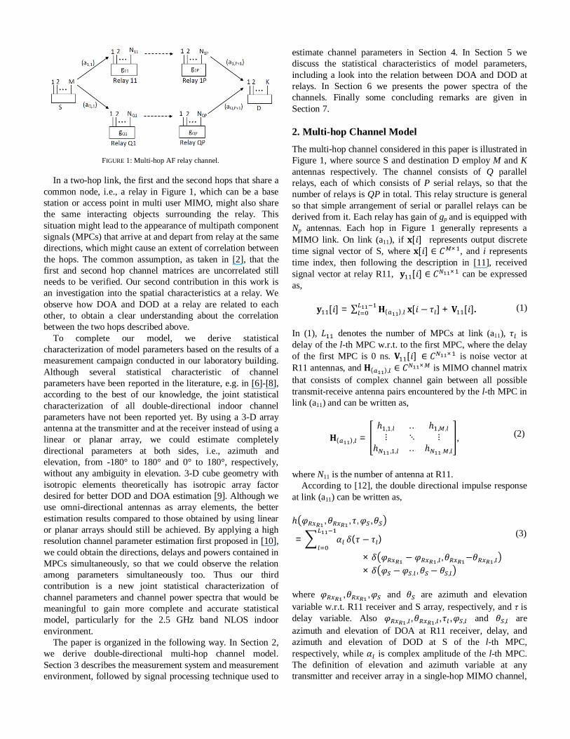
3 Measurement System and Environment The measurement system is based on vector network analyzer (VNA) focusing at 217-25 GHz band and comprising 201 points of frequency [13] with the measurement configuration as depicted in Figure 2 We use a 3-D cube shaped synthetic array antenna at both transmitter and receiver Each of the eight elements is a wideband bi-conical type antenna with 3-dB elevation beam-width of 60ordm and mounted vertically at the cube corners Measurements in anechoic chamber have shown that the antenna pattern in azimuth and elevation variable did not change significantly over the measured frequency band The standard deviations of normalized power measured in all frequency points averaged over the azimuth and elevation samples are 004 and 009 respectively which prove the statement above The distance between array elements is 6 cm and is equal to half wavelength of the upper frequency to avoid spatial aliasing caused by spatial under-sampling over the array The resulting dimension of the array fulfills the requirement of narrowband array so that there is no significant delay difference experienced by an MPC when it arrives at the array elements
The cube array orientation and the definition of azimuth and elevation for transmitter and receiver in a single-hop link are depicted in Figure 3 where the l-th MPC departs from transmitter at azimuth and elevation of (휑 휃 ) and arrives at receiver at (휑 휃 ) As shown in Figure 3 the reference direction of 0deg azimuth of DOD and DOA are in line to their respective x axes when the arrays are facing each other
The measurement floor plan is depicted in Figure 4 There are two measurement scenarios The first is conducted to obtain statistical characteristics of double-directional channel parameters This scenario consists of single-hop double-direc- tional channel measurement where the transmitter and receiver in each hop are described in Table I and the numbers
indicate transmitter and receiver locations in Figure 4
The second scenario is conducted to investigate the relation between DOA and DOD at a relay in a two-hop channel Source relay and destination in each of the two-hop channel are described in Table 2 The two-hop channel is composed of two one-hop channel measured in sequence where the ldquoRelayrdquo serves as a receiver and a transmitter in the first and second hop respectively The relation between DOA and DOD at relay in the two-hop channel can be used to describe the relation between DOA and DOD at any relay in a multi-hop channel This is because a multi-hop channel can be decomposed into several two-hop channels and any additional relay or hop can be represented by a matrix factor as in (7)
This second measurement scenario concerns the spatial characteristics at each relay of a multi-hop channel with an arbitrary number of hops For example in the measurement realizations depicted in Table 2 and referring to Figure 4 the three-hop channel consisting of nodes 1-2-3-4 is decomposed into two two-hop channels ie 1-2-3 and 2-3-4 and also measurement realizations of four-hop channel consists of nodes 5-6-7-8-9 is decomposed into three two-hop channels ie 5-6-7 6-7-8 and 7-8-9
From the scenario in Table 2 we obtain seven two-hop double-directional channel transfer functions In all measurement realizations the distances between transmitter and receiver and those between transmitter or receiver and wall glass door or metal cupboard are kept in far field region to fulfill the requirement of plane wave measurement
FIGURE 2 Measurement system configuration
FIGURE 3 Transmitter and receiver cube array orientation and the definition
of elevation and azimuth
The environment under consideration is a laboratory room which represents a small lab or office with its furniture and equipments of any shapes sizes and materials The common furniture materials are wood plastic and glass while the common equipment material is metal There are also some glass windows and doors in the environment Transmitter and receiver arrayrsquos height are 80 cm above the floor to approximately represent usersrsquo equipment or access pointrsquos height In all measurement scenarios transmitter and receiver are in different rooms separated by brick wall or in the same room but obstructed by metal cupboards in between
The use of synthetic array antenna requires that the environment should be kept static during one double- directional measurement of each single-hop channel in the first measurement scenario Meanwhile in the second scenario the static condition must be fulfilled during multi-hop channel measurements described above This is achieved by doing the measurement activities in the evening or during weekends In addition by using synthetic arrays the measured channel transfer functions are free from mutual coupling effect To avoid interference from any wireless local area network signals we turn off access points around measurement locations during the measurement activities and by using a spectrum analyzer assure that there is only noise in the measurement band when the system is turned off
Measurement using cube shaped synthetic array antenna is carried out by placing an array element on a corner of the transmitter cube and placing another array element on a corner of the receiver cube The element of transmitter array and that
of receiver array are connected to VNA at port 1 and port 2 respectively and then the channel transfer function is measured This measurement is repeated by moving the element of receiver array to the other cube corners sequentially so that we obtained eight channel transfer function between the first element of transmitter array and each element of the receiver array To obtain one double directional channel transfer function this procedure is repeated for the other transmitter array element positions The results is arranged in a matrix of 64 times 201 size that represents 201-frequency point channel transfer function between 8 times 8 pairs of transmitter and receiver antennas
4 Data Post Processing There are some methods that can be used to estimate channel parameters from measured data such as the Frequency-Domain Space Generalized Expectation-Maximization (FD-SAGE) [14] FD-SAGE was developed for estimating single-input multiple-output (SIMO) channel parameters from data measured in the frequency domain It was based on previous work reported in [10] and [15] where [10] discussed general SAGE algorithm and [15] studied the implementation of [10] for multipath channel parameter estimation
The computational load in FD-SAGE depends on the number of MPCs assumed to exist in the channel and the number of parameters of each MPC that have to be estimated In an indoor environment naturally there are many MPCs Modeling MIMO channels relates to the larger number of MPC parameters that have to be estimated when compared to that in SIMO channels As indicated in (3) the set of parameters of the l-th MPC is 휃 = 훼 휏 휑 휃 휑 휃 Accordingly we modify some procedures in FD-SAGE to achieve less computational load In order to do so while maintaining the accuracy we divide our procedure into two stages ie the IFT stage and FD-SAGE stage We call this method as IFT-FD-SAGE
The first step in IFT-FD-SAGE consists of applying window and inverse Fourier transform (IFT) The result of this process is a delay domain impulse response of a channel between the n-th and m-th antenna at receiver and transmitter respectively For a pair of transmitter-receiver with N and M antennas respectively we obtain NM impulse responses A threshold is then applied to those impulse responses where the components below it which are considered as noise are removed In this work the threshold is set to 3 dB above the
FIGURE 4 Measurement floor plan
TABLE 1 Measurement scenario for channel characterization
Transmitter (Tx) Receiver (Rx) 1 2 2 3 8 20 21 22 23 19 11 18 3 4 5 6 6 7 10 7 8 8 9 12 13 13 14 10 11 17 16 5 15
TABLE 2 Measurement scenario for the investigation of DOA and DOD at relay
Source (S) Relay (R) Destination (D) 1 2 3 2 3 4 5 6 7 6 7 8 7 8 9 12 13 14 6 10 11
highest side-lobe level of the window used which is Hamming window
Further we use the first criterion in [16] to determine if an MPC is not a spike noise ie all of NM impulse responses are examined for consistent emergence of an MPC Inconsistent spikes are considered as noise and removed from the MPCs set The emergence of a spike is considered as consistent if it is greater than or equal to p of the NM impulse responses where in our procedure we choose 75 of 64 impulse responses Then the power of MPCs is calculated as the mean of the corresponding power values in all NM impulse responses By completing the first stage we have estimated the number of MPCs the delay of each MPC and its power
In the second stage we apply FD-SAGE to estimate four parameters that have not been estimated yet ie 휃 =휑 휃 휑 휃 Because we have determined the number of MPCS through thresholding in the first stage unlike in [14] we do not any longer require MPC removal after FD-SAGE is finished
We verify our method by comparing the results of the method when it is applied to the measured data made in one of the rooms in floor plan of Figure 4 ie the room in the middle that contains measurement points 2 7 and 10 with their counterparts obtained from a simple 2-D ray tracing in a room with the same layout as the actual room The results are depicted in Figure 5 There are five paths obtained from IFT-FD-SAGE and those obtained from ray tracing that closely matched These paths consist of the direct single-reflection and double-reflection paths The other paths which encounter more reflections are not considered in the ray tracing so that the results of the algorithm which have longer delay cannot be confirmed In Figure 5 we can see that path 2 and path 6 have larger error (defined herein as absolute difference between the value of parameter obtained from ray tracing and that obtained from the algorithm) compared to the other paths This is mainly because the delay difference between path 2 and path 6 is below the delay resolution ie 3 ns according to the measurement bandwidth whereas based on ray tracing calculation the delay of path 2 and path 6 are 392 ns and 418 ns respectively
On the other hand we also perform simulations to observe the performance of the method and its capability to estimates parameters of a sufficiently large number of MPCs For example in case of estimating the parameters of twenty MPCs the method works well if the SNR is high enough ie 20 dB in our simulations Following this simulation result we keep the minimum SNR at 20 dB in all measurement realizations except one measurement whose the maximum SNR achieved is 18 dB
By using the SAGE based method the angular resolution can be set high enough although the number of array elements is limited In this work we set it at 1deg
5 Statistical Characteristic of Channel Parameters It was introduced in [17] that the channel statistic depends on the product of probability density function (pdf) of the channel
parameters and power spectral density of the channel In this section we present pdfs of channel parameters whereas power spectral density of the channel will be discussed in Section 6
From the first measurement scenario described in Section 3 we obtain 23 single-hop double-directional channel transfer functions in total The number of MPCs and their parameters in each hop were obtained by applying IFT-FD-SAGE algorithm described in Section 4 to these channel transfer functions Based on these results we characterize statistical distribution of channel parameters described in (3)
51 Marginal Distribution of Parameters Marginal distribution of parameters obtained by applying Kolmogorov-Smirnov (K-S) goodness of fit (GOF) test at significance level α of 005 to the empirical cumulative distribution functions (cdfs) of parameters The results are listed in Table 3 where in the table micro and σ are mean and standard deviation of parameters respectively dmax is the maximum distance between empirical cdf and theoretical cdf cnα is the value of K-S statistic at significance level of α and n is the number of samples within the range of parameter values used to calculate the empirical and theoretical cdf The empirical data are well fitted to a certain theoretical distribution if dmax is lower than cnα [18]
We observe that many strong MPCs arrive at the array around the azimuth of 0deg There is also another group of weaker MPCs arriving around 180deg These two groups appear to be separated by the even weaker powers at around 120deg and 240deg as can be seen in Figure 6 We also observe that the departure characteristic of MPCs is similar with their arrival characteristic above These results indicate that in the measured environment many MPCs whose powers are higher than those coming to or depart from around 120deg and 240deg seem to come to or depart from the front of and behind the array At the receiver site these MPCs are likely to come from the direct path through the wall diffracted by objects or building structures near the direct path and then penetrate the wall and some of them whose powers are lower and arrive
FIGURE 5 The results of IFT-FD-SAGE when applied to the measured data
compared to their counterparts obtained from 2-D ray tracing 1 is the direct path 2 3 and 4 are the single-reflection paths and 6 is the double-
reflection path (a) is for the DOAs and (b) is for the DODs
behind the array may come then after reflected by objects behind the arrays On the other hand the small number of MPCs around 120deg and 240deg indicates that the MPCs reflected or diffracted by object or building structures in those directions may experience longer propagation path and have lower power than the others
Therefore in order to properly characterize DOA and DOD azimuth we divide those parameters into intervals of ndash120deg to 120deg and 120deg to 240deg for the array orientation depicted in Figure 3 In those two intervals DOD and DOA follow a curtailed Gaussian distribution Each of DOD and DOA azimuth has mean value around 0deg and 180deg for the two interval described above This give a new understanding that MPCs actually are not distributed uniformly although transmitter and receiver are surrounded by objects and the radio links are NLOS This results are different from those reported in [7] where for NLOS environment DOA azimuth of inter-cluster MPCs are distributed uniformly in ndash180deg to 180deg We compare this result with inter-cluster azimuth in [7] although we do not model MPCs as clusters for the reason that will be discussed in Section 6
We also observed statistics of the number of MPCs contained in the two intervals We found that on average the number of MPCs in each hop is 25 while the number of MPCs in front of the array ie in the range of ndash120deg to 120deg is almost four-times that of behind the array ie in the range of 120deg to 240deg In these two intervals they follow Gaussian distribution
Statistics of those six normally distributed parameters are
listed in Table 3 and their marginal pdf can be written as
푓 (푥) =radic
exp(minus(푥 minus 휇 ) 2휎 ) for 푎 lt 푥 lt 푏 (16)
where X can be one of the above described parameters 휇 and 휎 are the mean and standard deviation respectively a and b are the lower and upper bounds value of parameter X
On the other hand DOA and DOD elevations are better fitted to asymmetric Laplace than to Gaussian distribution although the two are accepted according to their K-S statistics Their pdfs can be expressed as
푓 (휃) =1
2훽 exp(minus|휃 minus 휇 |훽) (17)
where θ can be θ or θ ie DOD or DOA elevation and also 휇 can be 휇 or 휇 ie mean DOD or DOA elevation 훽 = 휎 radic2 where 휎 can be 휎 or 휎 ie standard deviation of DOD or DOA elevation Figure 7 depicts the empirical pdf of DOA and DOD elevation superimposed with their theoretical Laplace pdf
As described in Section 3 we use vertical biconical antennas for array elements and we set the same height for transmitter and receiver antennas Accordingly most of the MPCs should depart from or arrive at the antenna from broadside direction of the array element The Laplace pdf with the mean value around 75deg and small standard deviation suggests that most of MPCs are scattered by objects whose positions are higher than the array eg lamp shades the top of metal cupboards equipments in high shelves etc We see from Figure 7 that MPCs depart to or come from elevation below the broadside direction of the array element are few This gives information that MPCs which are resulted from reflections at the floor are few
Time of arrival or delay of MPCs is measured relative to that of the first MPC which is 0 ns Result of K-S GOF test confirms that delay distribution fits to exponential distribution
TABLE 3 Marginal distribution of parameters
Parameter Interval micro σ Distri-bution
K-S Statisic
Number of MPCs ldquoArdquo
11 to 32 20 ns 5 ns Gaussian dmax=05 cnα=034 n=11
Number of MPCs ldquoBrdquo
0 to 16 40 ns 4 ns Gaussian dmax=01 cnα=026 n=21
Delay 0 to 127 ns 40 ns 28 ns Expo-nential
dmax=015 cnα=021 n=43
Elevation DOD
10deg to 170deg 76deg 12deg Laplace dmax=008 cnα=021 n=33
Azimuth DOD
-120deg to 120deg
-15deg 56deg Gaussian dmax=005 cnα=026 n=25
120deg to 240deg
176deg 32deg Gaussian dmax=006 cnα=026 n=25
Elevation DOA
10deg to 170deg 77deg 16deg Laplace dmax=003 cnα=021 n=33
Azimuth DOA
-120deg to 120deg
-11deg 58deg Gaussian dmax=005 cnα=026 n=25
120deg to 240deg
177deg 28deg Gaussian dmax=009 cnα=026 n=25
Number of MPCs ldquoArdquo and ldquoBrdquo are the number of MPCs in azimuth range of -120deg to 120deg and 120deg to 240deg respectively
The Gaussian distribution stands for a curtailed Gaussian in the certain range described in the table
FIGURE 6 1 is the power of MPCs that arrive at certain azimuth in ndash120deg to to 240deg where the total power in the range is 1 2 is the probability of MPCs arrive from the related azimuth where the total probability in the
range is 1
The pdf is expressed as
푓 (휏) = (1휇)푒 ( ) (18)
where 휇 is mean of delay and the value can be seen in Table 3 The delay distribution of MPCs cluster reported in [7] for NLOS environment is also exponential with mean 53 ns
52 DOA and DOD Relation at Relay Our second contribution is the investigation of DOA and DOD relation at relay It was based on the idea that any relay in multi-hop communication may be surrounded by objects that will produce the same direction to the wave coming to the relay or leaving it This gives an insight into the presence of scatterers around relay common to the incoming and outgoing waves and about the physical properties of scatterers around the relay As channel matrices correlation between incoming and outgoing hop of a relay should depend on the common scatterers of the incoming and outgoing waves the spatial characteristics discussed below relates to correlation between those channel matrices The investigation was performed by measuring the channel with the second measurement scenario described in Section 3
As was described in Section 51 when considered in elevation variable most of MPCs arrive at or depart from array near the broadside direction of the array elements This fact motivates us to focus the investigation of the closely equal DODs and DOAs only on MPCs with elevation of DODs and that of DOAs around this direction By applying this procedure we neglect elevation variable and the investigation of DOA and DOD at relays is carried out only in azimuth variable The closely matched azimuths are defined as the DODs and DOAs azimuth that have magnitude of difference value below or equal to 2ordm
In reference to Figure 3 closely matched DOAs and DODs azimuth at R represent the same directions wrt array at R MPCs in those directions arise as radio wave scattered to R by any objects and those same objects scatter radio wave from R
According to K-S GOF test at the significance level α of 005 closely matched DOAs and DODs azimuth are uniformly distributed in the range of ndash180deg to 180deg with an average of -6ordm and standard deviation of 109deg This result indicates that in the environment considered any objects will
act as the same scatterer around R for the incoming and outgoing MPCs with the same probability
From seven two-hop links considered we found that the number of closely matched DOAs and DODs azimuth are uniformly distributed in the range of 2 to 6 with an average of 4 and standard deviation of 2 It suggests that on average 4 of 25 MPCs arrive at relay after scattered by some objects and then depart from the relay to the same objects and then scattered again by these objects to the direction of destination The different pairs of arriving and departing waves with closely matched azimuth DOAs and azimuth DODs observed originate from different scatterers as indicated by their values The low average number of these pairs indicates the low correlation between channel matrix of incoming hop and that of outgoing hop of a relay in the multi-hop channel considered However the statistics reported in this section needs more measurements to confirm because we only observe 7 pairs of dual-hop link
53 Joint Distribution of Parameters By using the FD-SAGE based algorithm we obtain all parameters of MPCs ie 휑 휃 휏 휑 휃 and 훼 simultaneously for 푙 =0 hellip 퐿 minus 1 There is no assumption that these parameters are independent to each other and hence we investigate the dependence between any pair x and y out of the five parameters above Since the random parameters evaluated are not necessarily Gaussian we therefore resort to the least-squares independence test (LSIT) [19] rather than evaluating the correlation coefficients The test is performed on parameters of 23 single hop measured channels The results are depicted in Table 4 where we divide azimuth of DOD and that of DOA into two intervals as in Section 51 However an azimuth of DOD in front of the Tx array may form a pair with an azimuth of DOA in front of or behind the Rx array and also one behind the Tx array may form a pair with another in front of or behind the Rx array so that the sample space of DODs and DOAs in those two intervals are not the same and we cannot define any joint distributions between those parameters Accordingly we suggest considering them independent to each other We choose a reasonable significance level α of 01 to reject the null hypothesis that x and y are independent where the p-value of LSIT is listed in Table 4
The joint pdf of DOD and DOA elevation whose the marginal pdf are asymmetric Laplace is a bivariate asymmetric Laplace expressed as [20]
푓 Ө(훉) = (훉푻횺 퐦)|횺| 퐾 (2 +퐦 횺 퐦)(훉푻횺 훉) (19)
where 훉 = [휃 휃 ] 퐦 = [휇 휇 ] 횺 is covariance matrix of 휃 and 휃 and [middot]-1 denotes inverse operation 퐾 (푣) is the third kind of Bessel function of zero-th order The value of 휇 and 휇 are depicted in Table 3 The covariance matrix 횺 can be constructed if correlation coefficient between
FIGURE 7 Pdf of DOA and DOD elevation
휃 and 휃 and standard deviation 휎 and 휎 are known Correlation coefficients between 휃 and 휃 calculated from all measured channels appear to be random in the range of -05 to 05 following a Gaussian distribution with mean of 013 and standard deviation of 025 Meanwhile the value of 휎 and 휎 can be seen in Table 3
Following the derivation in [7] the joint distribution of DOD elevation and delay and that of DOA elevation and delay are expressed as conditional pdf ie pdf of DOD elevation and that of DOA elevation conditioned on a specific delay interval Tk where 푘∆휏 le 푇 lt (푘 + 1)∆휏 for k=0 1 K-1 and K is the number of delay steps of ∆휏 width The relation between τ intervals and Tk is described in Table 5 The pdf of elevation θ which can be DOD elevation θ or DOA elevation θ conditioned on delay τ is expressed as
푓 | (휃|휏) = sum 푓 | (휃|푇 ) (20)
A set of empirical DOA elevation pdfs conditioned on Tk
are depicted in Figure 8 where ∆휏=20 ns is chosen to obtain a moderate interval in the 0 to 120 ns range of delay All of the empirical pdfs in Figure 8 are well fitted to Laplace pdf according to K-S GOF test The average of means is 78deg in agreement with the mean of DOA elevation marginal distribution The standard deviations tend to decay with increasing Tk which implies that they tend to decay with increasing delay The pdfs of DOD elevation conditioned on Tk have similar characteristics The conditional pdf plots are not shown here but the results in general are similar to those for the DOA given in Figure 8 Figure 9 shows the variation of standard deviations of DOA and DOD elevation pdfs conditioned on Tk
Pdfs of DOD and DOA elevation conditioned on Tk can be written as 푓 | (휃|푇 ) = exp minus 휃 minus 휇 훽 (21)
where 훽 = 휎 radic2 휇 and 휎 are respectively the mean and standard deviation of DOD and DOA elevation for
delay interval centered at Tk The variation of standard deviation on delay can be approximated by the functions
휎 (휏) = 225exp(minus001휏) and
휎 (휏) = 154exp(minus0008휏) (22)
The expression in (20) now can be written as
TABLE 4 P-value of LSIT of channel parameters
Parameter x Parameter y P-value Independence DOA Elevation DOA Azimuth ldquoArdquo 025 Independent DOA Elevation DOA Azimuth ldquoBrdquo 032 Independent DOA Elevation Delay 006 Dependent DOA Elevation DOD Elevation 003 Dependent DOA Elevation DOD Azimuth ldquoArdquo 04 Independent DOA Elevation DOD Azimuth ldquoBrdquo 033 Independent
DOA Azimuth ldquoArdquo Delay 054 Independent DOA Azimuth ldquoBrdquo Delay 014 Independent DOA Azimuth ldquoArdquo DOD Elevation 015 Independent DOA Azimuth ldquoBrdquo DOD Elevation 019 Independent
Delay DOD Elevation 001 Dependent Delay DOD Azimuth ldquoArdquo 019 Independent Delay DOD Azimuth ldquoBrdquo 036 Independent
DOD Elevation DOD Azimuth ldquoArdquo 027 Independent DOD Elevation DOD Azimuth ldquoBrdquo 039 Independent
DOA and DOD azimuth ldquoArdquo and ldquoBrdquo are those in azimuth range of -120deg to 120deg and 120deg to 240deg respectively
TABLE 5 The definition of delay interval for elevation pdf conditioned on delay
k τ interval (ns) Tk (ns) 0 0 le τ le 20 10 1 20 le τ le 40 30 hellip hellip
K-1 20(K-1) le τ le 20K 20K-10
(a)
(b)
(c)
(d)
(e)
(f)
FIGURE 8 Set of DOA elevation pdf conditioned on (a) 0leτlt20 ns (b) 20leτlt40 ns (c) 40leτlt60 ns (d) 60leτlt80 ns (e) 80leτlt100 ns (f) 100leτlt120 ns
푓 | (휃|휏) = sum exp minus 휃 minus 휇 훽 (23) where the value of 휇 can be approximated by the mean of θ in Table 3
Because DOD and DOA elevation are dependent and are expressed as joint pdf in (19) then joint pdf of DOA elevation and DOD elevation and delay is expressed as joint DOD and DOA pdf conditioned on certain delay interval as follows
푓Ө| (훉|휏)
=exp(훉푻횺 ퟏ퐦)휋|횺 | 퐾 (2 +퐦 횺 ퟏ퐦)(훉푻횺 ퟏ훉)
(24)
where now 횺 is covariance matrix of DOD and DOA elevation at Tk obtained by calculating standard deviation of DOD and DOA elevation at Tk in (19) and correlation coefficient as described before
The decreasing standard deviation of elevation pdfs as a function of delay indicates that the MPCs which arrive with longer delay most probably are not caused by multiple reflections by objects which the position is higher or lower than the array The MPCs that depart to or arrive from objects above or below the arrays most probably present in the delay below 40 ns as indicated by Figure 7
Then joint pdf of all parameters can be expressed as 푓 Ө Ө (휏휃 휃 휑 휑 )
= 푓 (휑 )푓 (휑 )푓Ө| (훉|휏)푓 (휏) (25)
where 푓 (휑 ) and 푓 (휑 ) are described in (16) for each azimuth interval 푓Ө| (훉|휏) as in (24) and 푓 (휏) as in (18) The expression in (25) completely describes joint pdf of all double-directional parameters appearing in (3)
6 Channel Power Spectra
Power spectra of the channel are considered separately at transmitter and receiver sides This is because in each side they represent the total power spread in the delay-angular domain Power spectrum in delay-angular variable considered at transmitter and receiver sides can be expressed as
푃 (휏 휃 휑 ) = 퐸|ℎ(휏 휃 휑 )|
and 푃 (휏휃 휑 ) = 퐸|ℎ(휏 휃 휑 )|
(26)
respectively The operator E and || denote expectation and absolute value respectively Those two power spectra are related to each other by the delay variable and satisfy
푃 (휏 휃 휑 )푑휏푑휃 푑휑
= 푃 (휏휃 휑 )푑휏푑휃 푑휑
= 1
(27)
Power spectrum considered in any certain variable could be
obtained by integrating (26) over other variables For example power spectrum considered in delay variable ie power delay spectrum (PDS) is calculated by
푃(휏) = 푃 (휏휃 휑 )푑휃 푑휑
= ∬푃 (휏휃 휑 )푑휃 푑휑 (28)
In the following we investigate two kinds of power spectra
The first is power spectra of single variables defined in (28) namely empirical power delay spectrum (PDS) departure and arrival power elevation spectrum (DPES and APES) and departure and arrival power azimuth spectrum (DPAS and APAS)
However those power spectra do not describe the relation between power spectrum in a certain variable and that in another Therefore we need a complete description of power spectrum involving all variables ie delay elevation and azimuth defined in (26) which is called power delay-angular spectrum Recalling the results of LSIT to the double directional parameters in Section 53 the only dependencies are between DOA elevation and delay DOD elevation and delay and between DOA and DOD elevation Because the power spreading in the double directional variables depends on the probability of the emergence of MPCs in those variables ie their pdfs the power spreading should also consider the known dependencies above Hence to obtain power delay-angular spectrum in the following we only investigate power delay-elevation spectrum and consider that the departure and arrival power azimuth spectra are independent to delay This is the second power spectra that will be discussed
In this work the expectation in (26) is estimated by averaging the 23 single hop double directional impulse responses obtained previously This is because the desired power spectra are those that represent the characteristic of the
FIGURE 9 Standard deviation of empirical DOD (1) and DOA (3)
elevation considered in certain delay interval 2 and 4 are their exponential fit respectively
measured environment not those that represent a local averaging over a certain area of radius about several wave lengths
61 Power Delay Spectrum (PDS) Empirical PDS is calculated as follows
푃 =1푁 푝 (29)
where 푃 represents the average power of l-th MPC 푁 is the number of measurements and 푝 is the power of l-th MPC in the n-th measurement The empirical PDS should satisfy sum 푃 = 1 as in (27)
The obtained empirical PDS is depicted in Figure 10 It fits to an exponential function expressed as
푃(휏) = exp(minus휏휎 ) (30)
Parameter 휎 is delay spread and defined as the square root of the second central moment of P(τ) The estimated value of 휎 is 25 ns
In [6] and [21] PDS of clusters and rays inside clusters are modeled by decaying exponential function Although in this work we do not consider MPCs cluster generally our model agrees with those results because PDS of clusters is the envelope of PDS of rays inside clusters In the cluster based model the center of cluster is MPC whose power is the highest If we could observe rays inside a cluster its power should not be higher than the cluster center According to this we believe that the PDS in (25) is more relevant to compares to the PDS of clusters Also the comparison of pdf of delay and that of DOA and DOD azimuth in Section 51 with those reported in [7] is based on the same reason above
62 Departure and Arrival Power Elevation Spectrum (DPES and APES) DPES and APES are power elevation spectra considered at transmitter and receiver sides respectively The calculation procedure of empirical DPES and APES is similar to that used for empirical PDS
The obtained empirical APES is depicted in Figure 11 The empirical DPES is not shown however its shape is similar to the empirical APES The empirical APES and also empirical DPES follow asymmetric Laplace function expressed as
푃(휃) =
radicexp(minus|휃 minus 휇 |훽) (31)
where θ may denote θTx or θRx ie DOD or DOA elevation 훽 = 휎 radic2 and 휎 can be 휎 or 휎 ie departure or arrival elevation spread which is defined as the square root of second central moment of DPES or APES respectively and also 휇 can be 휇 or 휇 ie the central moment of DPES and APES The value of 휇 and 휇 are 75deg and 77deg respectively whereas the value of 휎 and 휎 are 14deg and
17deg respectively In (31) the factor 1radic2 is normalization constant to satisfy (27)
These results show that much of the power distribution in elevation is concentrated in narrow region which is slightly higher above broadside direction of the array element in agreement with the result in Section 51 where the elevation departure and arrival of MPCs are mostly in these directions
63 Departure and Arrival Power Azimuth Spectrum (DPAS and APAS) Empirical APAS can be seen in Figure 6 whereas empirical DPAS has similar shape to it As described in Section 51 visually we can see that there are two groups of MPCs ie having DOD and DOA around 0deg and 180deg which tend to have higher power then MPCs groups having DOD and DOA around 120deg and 240deg Based on these results we do not consider that DPAS and APAS are uniform in ndash180deg to 180deg Instead we divide the interval of DPAS and APAS into -120deg to 120deg and 120deg to 240deg and fit the empirical DPAS and APAS with Gaussian function
The Gaussian fit shows much lower sum of square error (SSE) than uniform fit and accordingly we model DPAS 푃 (휑 ) and APAS 푃 (휑 ) as follows
FIGURE 10 Power delay spectrum
FIGURE 11 Empirical APES and its Laplace fit
푃(휑)
=
⎩⎪⎨
⎪⎧ 1radic2
exp minus휑 minus 휇
2휎 minus120deg le 휑 le 120deg
1휋radic2
exp minus휑 minus 휇
2휎 121deg lt 휑 lt 239deg
(32)
where φ can be φTx or φRx ie DOD or DOA azimuth respectively whereas 휇 and 휇 can be 휇 or 휇 and 휇 or 휇 ie the central moment of DPAS or APAS in -120deg to 120deg and in 121deg to 239deg respectively Their values are -15deg -15deg 176deg and 177deg respectively Also 휎 and 휎 can be 휎 or 휎 and 휎 or 휎 ie departure or arrival azimuth spread in the two intervals above respectively the values of which are 55deg 56deg 31deg 30deg The constants 1radic2 and 1휋radic2 in (32) are required to fulfill int 푃(휑)푑휑 = 1deg
deg These results are different from the power azimuth
spectrum reported in [7] where inter-cluster APAS in NLOS environment is uniform in ndash180deg to 180deg Our results can be understood when we recall that in LOS environment the power azimuth spectrum in several literatures eg [4] and [5] is modeled by Laplace function When the links are obstructed or separated by wall the Laplace function may not become uniform function directly but part of power which is higher than the others may still fill the region in front of the arrays and one which is lower than the first fill the region behind the arrays where the mechanism of filling those regions have been discussed in Section 51 64 Departure and Arrival Power Elevation-Delay Spectrum Following the method in [22] departure and arrival power elevation-delay spectra are expressed as partial departure and arrival power elevation spectrum (PDPES and PAPES) at certain delay interval and are given by
푃(휃|푇 ) = int 푃(휃 휏)∆
∆ 푑휏 (33)
where 푇 relates to specific delay interval defined in Table 5 A series of empirical PAPES is shown in Figure 12 Empirical PDPES is not shown here but its shape is similar to that of PAPES Figures 12 shows that PAPES on all specified delay intervals 푇 could be approximated by asymmetric Laplace function However the elevation spreads seems to decrease when 푇 increase As in (31) asymmetric Laplace function is now used to model PAPES as follows
푃(휃|푇 ) prop exp(minus 휃 minus 휇 훽 ) (34)
where as before 휃 might represent 휃 or 휃 while 휇 denotes the central moment of PDPES or PAPES at interval Tk 휇 does not vary significantly with k and can be approximated by the central moment of PDPES or PAPES described in Section 62 훽 = 휎 radic2 where 휎 denotes
the departure or arrival elevation spread at Tk In (34) the notation a propb means that a is propotional to b The variation of 휎 on k implies that 휎 varies according to τ and is shown in Figure 13 They can be approximated by exponential functions expressed as
휎 (휏) = 218exp(minus001휏) and
휎 (휏) = 154exp(minus0007휏) (35)
for PAPES and PDPES respectively To obtain a complete description of power delay-elevation
spectrum we observe the variation of power contained in each delay interval Tk as a function of k As can be seen in Figure 12 the total power contained in each delay interval seems to vary which fits an exponential function well in Figure 10
From these results we can model power delay-elevation spectrum (PDES) from (30) and (34) as follows
FIGURE 12 Empirical PAPES at (a) T0) (b) T1 (c) T2 (d) T3 (e) T5 (f) T6
푃(휃 휏) = exp(minus휏휎 )exp(minus|휃 minus 휇 |훽(휏)) (36) where 훽(휏) varies according to the variation of 휎 (휏) in (35) The values of 휎 is given in Section 61 65 Channel Power Delay-Angular Spectrum (PDAS) In this section the results of the previous power spectra are used to describe the general power delay-angular spectrum of the channel The power delay-angular spectrum in (26) can be expressed as partial power angular spectrum at certain delay interval given by
푃(휃휑|푇 ) = int 푃(휃휑 휏)푑휏∆
∆ (37)
where Tk has been described in Section 53 and as before 휃 may denote 휃 or 휃 and similarly 휑 may be 휑 or 휑
Examined at either receiver or transmitter channel power angular spectrum is given by
푃(휃휑) = int푃(휃휑 휏)푑휏 (38)
Because 푃(휑) and 푃(휃) are independent therefore 푃(휃휑) = 푃(휃)푃(휑) and partial power angular spectrum becomes 푃(휃휑|푇 ) = 푃(휃|푇 )푃(휑|푇 ) However 푃(휑|푇 ) =푃(휑) Hence partial power angular spectrum can be written as
푃(휃휑|푇 ) = 푃(휑)푃(휃|푇 ) (39)
Since 푃(휃|푇 ) implicitly describes the variation of power elevation spectrum on delay as in (36) therefore (39) also describes power angular-delay spectrum and can be expressed as
푃(휃휑 휏) = 푃(휑)푃(휃 휏) (40)
where 푃(휑) and 푃(휃 휏) are given by (32) and (36) respectively Equation (40) expresses completely power angular-delay spectrum of the channel In Table 6 we present the summary of the channel power spectra discussed in Section 6
7 Conclusion An expression for channel matrix that describes input-output relationship of double-directional indoor multi-terminal communication involving AF relays has been presented The expression is general in that the number of relays and the number of antennas at transmitter relay and receiver are arbitrary If there is any correlation between model parameters in each hop or in multi-hop channel the correlation can be incorporated in the expression
The spatial characteristics at a relay of multi-terminal communication have been described by closely matched DOA and DOD azimuth at the relay Based on measurement results we found that there are some closely matched azimuth of DOAs and that of DODs which follow uniform distribution in ndash180deg to 180deg for elevation around broadside of the vertical omni-directional array element The number of closely matched azimuth of DOAs and that of DODs are uniformly distributed in the range of 2 to 6 with an average of 4
We present new statistical characteristics of double-directional channel model parameters and channel power spectra The statistical characteristics are based on intensive measurements using cube synthetic array antenna so that the double-directional angular parameters obtained consist of elevation without ambiguity The proposed statistical characteristics of channel parameters and channel power spectra are expressed by including their variation on delay
The proposed delay distribution is exponential which agrees with delay distribution proposed before in the literatures The marginal distribution of DOD and DOA elevation are asymmetric Laplace with mean of about 75deg and standard deviation of about 15deg They are dependent to each other and be modeled by bivariate asymmetric Laplace pdf characterized by their covariance matrix Further the DOD
FIGURE 13 Empirical elevation spread as a function of delay interval Tk
TABLE 6 The model of channel power spectra and their parameters
Power Spectrum
Theoretical fit (equation) Parameter RMSE
푃(휏) PDS Exponential
(30) 휎 =246 ns 휏 =127 ns 004
APAS ldquoArdquo 푃(휑 ) Gaussian (32) 휇 = -15ordm 휎 =56ordm 018
APAS ldquoBrdquo 푃(휑 ) Gaussian (32) 휇 =177ordm 휎 =30ordm 009
DPAS ldquoArdquo 푃(휑 ) Gaussian (32) 휇 = -15ordm 휎 =55ordm 021
DPAS ldquoBrdquo 푃(휑 ) Gaussian (32) 휇 =176ordm 휎 =31ordm 014
APES 푃(휃 )
Laplace (31)
휇 =77ordm 훽 =휎 radic2 휎 =17ordm
010
DPES 푃(휃 )
Laplace (31)
휇 =75ordm 훽 =휎 radic2 휎 =14ordm
019
APDES 푃(휃 휏) (36)
휎 (휏)= 218exp(minus001휏) 102
DPDES 푃(휃 휏) (36)
휎 (휏)
= 154exp(minus0007휏)
168
PDAS 푃(휃휑 휏) (40) - -
and DOA elevation are dependent to delay so that their joint distribution is characterized into partial joint pdf ie joint pdf considered in specific delay interval where their standard deviation decrease with increasing delay Meanwhile DOD and DOA azimuth follow Gaussian distribution for the direction in front of and behind the array with means near 0deg and 180deg
Each of channel power spectra considered at transmitter and receiver is expressed as the multiplication of its power delay-elevation spectrum and power azimuth spectrum The power delay-elevation spectrum considered is modeled by Laplace function whose magnitude and elevation spread varies with delay meanwhile the power azimuth spectrum is modeled by Gaussian function in the region in front of and behind the array
References [1] V Kolmonen K Haneda T Hult J Poutanen F Tufvesson P
Vainikainen ldquoMeasurement-based evaluation of interlink correlation for indoor multiuser MIMO channelsrdquo IEEE Antennas and Wireless Propagation Letters vol 9 pp 311-314 2010
[2] P Wang Y Zhou X Yin X Huang F Liu ldquoMeasurement and analysis of relay channels in indoor environmentsrdquo in Procedings of International Conference on Wireless Communications Networking and Mobile Computing (WiCOM) Chengdu China pp 1-5 Sept 23-25 2010
[3] J Poutanen K Haneda V Kolmonen J Salmi P Vainikainen ldquoAnalysis of correlated shadow fading in dual-link indoor radio wave propagationrdquo IEEE Antenna and Wireless Propagation Letters vol 8 pp 1190-1193 2009
[4] X Yin S X Lu B-J Kwak H K Chung F Liu ldquoPropagation Channel Characterization for amplify-and-forward MIMO-relaying systemsldquo IEEE Vehicular Technology Conference Fall 2010 pp 1-5 Sept 2010
[5] X Cheng C-X Wang H Wang X Gao X-H You D Yuan B Ai Q Huo L-Y Song B-L Jiao ldquoCooperative MIMO channel modeling and multi-link spatial correlation propertiesrdquo IEEE Journal on Selected Areas in Communications vol 30 pp 368-395 Feb 2012
[6] Q H Spencer B D Jeffs M A Jensen A L Swindlehurst ldquoModeling the statistical time and angle of arrival characteristics of an indoor multipath channelrdquo IEEE Journal on Selected Areas in Communications vol 18 pp 347-360 March 2000
[7] C C Chong C M Tan D I Laurenson S McLaughlin M A Beach A R Nix ldquoA new statistical wideband spatio-temporal channel model fo 5-GHz band WLAN systemsrdquo IEEE Journal on Selected Areas in Communications vol 21 pp 139-150 Feb 2003
[8] K Yu Q Li M H ldquoMeasurement investigation of tap and cluster angular spreads at 52 GHzrdquo IEEE Transactions on Antennas and Propagation vol 53 pp 2156-2160 July 2005
[9] U Baysal R L Moses ldquoOn the geometry of isotropic arrayrdquo IEEE Transactions on Signal Processing vol 51 pp 1469-1478 June 2003
[10] J A Fessler A O Herordquo Space-alternating generalized expectation-maximization algorithmrdquo IEEE Transactions on Signal Processing vol 42 pp 2664-2677 Oct 1994
[11] N Costa S Haykin Multiple-input multiple-output channel models John Wiley amp Sons 2010 p 33
[12] M Steinbauer A F Molisch E Bonek ldquoThe double-directional radio channelrdquo IEEE Antennas and Propagation Magazine vol 43 pp 51-63 Aug 2001
[13] P Handayani G Hendrantoro ldquoCharacterization of DOD and DOA correlation among converging indoor radio links by applying reciprocity principleldquo In Procedings of International Conference on ICT Convergence (ICTC) 2011 Seoul Korea pp 90-94 2011
[14] C C Chong D I Laurenson C M Tan S McLaughlin M A Beach A R Nix ldquoJoint detection-estimation of directional channel parameters using 2-D frequency domain SAGE algorithm with serial interference cancellationrdquo In Procedings of International Conference on Communication (ICC) pp 906-910 vol 2 2002
[15] B H Fleury M Tschudin R Heddergott D Dahlhaus K I Pedersen ldquoChannel parameter estimation in mobile radio environments using the SAGE algorithmrdquo IEEE Journal on Selected Areas in Communications vol 17 pp 434-450 March 1999
[16] E S Sousa V M Jovanovic C Daigneault rdquoDelay spread measurement for the digital cellular channel in Torontordquo IEEE Transactions on Vehicular Technology vol 43 pp 837-847 Nov 1994
[17] M Bengtsson B Volker ldquoOn the estimation of azimuth distributions and azimuth spectrardquo in Proceedings of Vehicular Technology Conference vol 3 pp 1612-1615 Oct 2001
[18] T T Soong Fundamentals of probability and statistics for engineers John Wiley amp Sons 2004
[19] M Sugiyama T Suzuki ldquoLeast-squares independence testrdquo IEICE Transactions on Information and System vol E94-D no 6 pp 1333-1336 2011
[20] S Kotz T J Kozubowski K Podgoacuterski ldquoAn asymmetric multivariate Laplace distributionrdquo Technical Report 367 Department of Statistics and Applied Probabilities University of Carolina Santa Barbara USA 2000
[21] A A M Saleh R A Valenzuela ldquoA statistical model for indoor multipath propagationldquo IEEE Journal on Selected Areas in Communications vol 5 pp 128-137 Feb 1987
[22] A Algans K I Pedersen P E Mogensen ldquoExperimental analysis of joint statistical properties of azimuth spread delay spread and shadow fadingrdquo IEEE Journal on Selected Areas in Communications vol 20 pp 523-531 April 2002
In a two-hop link the first and the second hops that share a
common node ie a relay in Figure 1 which can be a base station or access point in multi user MIMO might also share the same interacting objects surrounding the relay This situation might lead to the appearance of multipath component signals (MPCs) that arrive at and depart from relay at the same directions which might cause an extent of correlation between the hops The common assumption as taken in [2] that the first and second hop channel matrices are uncorrelated still needs to be verified Our second contribution in this work is an investigation into the spatial characteristics at a relay We observe how DOA and DOD at a relay are related to each other to obtain a clear understanding about the correlation between the two hops described above
To complete our model we derive statistical characterization of model parameters based on the results of a measurement campaign conducted in our laboratory building Although several statistical characteristic of channel parameters have been reported in the literature eg in [6]-[8] according to the best of our knowledge the joint statistical characterization of all double-directional indoor channel parameters have not been reported yet By using a 3-D array antenna at the transmitter and at the receiver instead of using a linear or planar array we could estimate completely directional parameters at both sides ie azimuth and elevation from -180deg to 180deg and 0deg to 180deg respectively without any ambiguity in elevation 3-D cube geometry with isotropic elements theoretically has isotropic array factor desired for better DOD and DOA estimation [9] Although we use omni-directional antennas as array elements the better estimation results compared to those obtained by using linear or planar arrays should still be achieved By applying a high resolution channel parameter estimation first proposed in [10] we could obtain the directions delays and powers contained in MPCs simultaneously so that we could observe the relation among parameters simultaneously too Thus our third contribution is a new joint statistical characterization of channel parameters and channel power spectra that would be meaningful to gain more complete and accurate statistical model particularly for the 25 GHz band NLOS indoor environment
The paper is organized in the following way In Section 2 we derive double-directional multi-hop channel model Section 3 describes the measurement system and measurement environment followed by signal processing technique used to
estimate channel parameters in Section 4 In Section 5 we discuss the statistical characteristics of model parameters including a look into the relation between DOA and DOD at relays In Section 6 we presents the power spectra of the channels Finally some concluding remarks are given in Section 7
2 Multi-hop Channel Model The multi-hop channel considered in this paper is illustrated in Figure 1 where source S and destination D employ M and K antennas respectively The channel consists of Q parallel relays each of which consists of P serial relays so that the number of relays is QP in total This relay structure is general so that simple arrangement of serial or parallel relays can be derived from it Each relay has gain of gp and is equipped with Np antennas Each hop in Figure 1 generally represents a MIMO link On link (a11) if 퐱[푖] represents output discrete time signal vector of S where 퐱[푖] isin 퐶 times and i represents time index then following the description in [11] received signal vector at relay R11 퐲 [푖] isin 퐶 times can be expressed as
퐲 [푖] = sum 퐇( ) 퐱[푖 minus 휏 ] + 퐕 [푖]
(1)
In (1) 퐿 denotes the number of MPCs at link (a11) 휏 is delay of the l-th MPC wrt to the first MPC where the delay of the first MPC is 0 ns 퐕 [푖] isin 퐶 times is noise vector at R11 antennas and 퐇( ) isin 퐶 times is MIMO channel matrix that consists of complex channel gain between all possible transmit-receive antenna pairs encountered by the l-th MPC in link (a11) and can be written as
퐇( ) =ℎ hellip ℎ ⋮ ⋱ ⋮
ℎ hellip ℎ
(2)
where N11 is the number of antenna at R11
According to [12] the double directional impulse response at link (a11) can be written as
ℎ 휑 휃 휏휑 휃
= 훼 훿(휏 minus 휏 )
times 훿 휑 minus 휑 휃 minus휃
times 훿 휑 minus 휑 휃 minus 휃
(3)
where 휑 휃 휑 and 휃 are azimuth and elevation variable wrt R11 receiver and S array respectively and τ is delay variable Also 휑 휃 휏 휑 and 휃 are azimuth and elevation of DOA at R11 receiver delay and azimuth and elevation of DOD at S of the l-th MPC respectively while 훼 is complex amplitude of the l-th MPC The definition of elevation and azimuth variable at any transmitter and receiver array in a single-hop MIMO channel
FIGURE 1 Multi-hop AF relay channel
and the example of azimuth and elevation DOD and DOA of the l-th MPC related to array orientation is depicted in Figure 3
The matrix elements in (2) can be obtained by computing double-directional channel impulse response at each pair of S and R11 receiver antenna given by (4) assuming that array at S and R11 is narrowband and all MPCs incident to array are plane waves In (4) 푓 (휃휑) denotes radiation pattern of the n-th element of array 퐫 represents the position vector of the n-th element of array wrt array mass center k is wave number vector given by
퐤 = (2휋 휆frasl )[푠푖푛휃푐표푠휑 푠푖푛휃푠푖푛휑 푐표푠휃] (5)
where 휆 is wavelength at the center frequency of radio wave and [∙] stands for transpose operation Meanwhile 퐤
and 퐤 are wave number vectors at R11 receiver and S related to the l-th MPC respectively
If the complex steering vector of any array containing N elements for the l-th MPC is denoted by 퐚 = [푎 푎 hellip 푎 ] and 푎 = 푓 (휃휑)exp(minus푗퐫 ∙ 퐤 ) for n=1 hellipN then (2) can be expressed as
퐇( ) = 훼 훿(휏 minus 휏 )퐚( ) 퐚( ) (6)
where 퐚( ) and 퐚( ) are complex steering vectors of the lth MPC at R11 receiver and S respectively
The complete expression of channel matrix of link (a11) that combines all MPCs and includes all MPCs parameters is simply
퐇 ( ) = 퐚( )퐝 퐚( ) (7)
where 퐚( ) isin 퐶 times and 퐚( ) isin 퐶 times are complex steering matrices at R11 receiver and S respectively Parameter 퐝 is 퐿 times 퐿 diagonal matrix that represents complex amplitude and delay factors of MPCs at link (a11) and is expressed as
퐝 =훼 훿(휏 minus 휏 ) hellip 0
⋮ ⋱ ⋮0 hellip 훼 훿(휏 minus 휏 )
(8)
Using (7) and by dropping time index i to simplify the
expression input-output relationship in (1) can be written as
퐲 = 퐇 ( )퐱 + 퐕 = 퐚( )퐝 퐚( ) 퐱+ 퐕 (9)
On the the second hop of the first serial relay in Figure 1 the signal vector radiated by R11 transmitter is 퐳 =푔 퐲 = 푔 퐇 ( )퐱+ 퐕 If this second hop channel is denoted by (a12) the signal vector received by relay R12 is 퐲 = 퐇 ( ) 푔 퐇 ( )퐱 + 퐕 + 퐕 where 퐕 the is noise vector at R12 receiver Then 퐲 can be written as
퐲 = 푔 퐇 ( )퐇 ( )퐱 + 퐕 (10)
where V is the accumulated noise The combined two-hop channel matrix is
퐇 ( )퐇 ( ) = 퐇
= 푔 퐚( )퐝 퐚( ) 퐚( )퐝 퐚( ) (11)
If we suppose that the number of MPCs on link (a12) is L12
and the number of antennas at relay R12 is N12 then 퐚( ) isin 퐶 times and 퐚( ) isin 퐶푁11times퐿12 are complex steering matrices at R12 receiver and R11 transmitter respectively Parameter 퐝 is 퐿 times 퐿 diagonal matrix that represents complex amplitude and delay factors of MPCs at link (a12)
Following this derivation if the number of such serially arranged relays is P then the matrix of (P+1)-hop channel is
퐇 = 푔 hellip푔 퐚( )퐝 퐚( ) hellip 퐚( )퐝 퐚( ) (12)
where 퐚( ) isin 퐶 times and 퐝 are complex steering matrices at D and 퐿 times 퐿 is diagonal matrix that represents complex amplitude and delay factors of MPCs at link (a1P+1) respectively while L1P+1 is the number of MPCs on that link The channel matrix in (12) is generic in that every (P+1)-hop channel can be considered as an extension of P-hop channel by inserting a matrix factor similar in shape to (7) into (12) to represent the additional relay
Then the signal vector received at D from these serial relays can be written as
퐲ퟏ = 퐇 퐱+ 퐕 (13)
ℎ 휃 휑 휏휃 휑
= 훼 훿(휏 minus 휏 ) times 푓 휃 휑 times훿 휃 minus 휃 휑 휑 times exp(minus푗퐫 ∙ 퐤)푑휃 푑휑
times 푓 (휃 휑 ) times훿 휃 minus 휃 휑 minus휑 times exp(minus푗퐫 ∙ 퐤)푑휃 푑휑
= 훼 훿(휏 minus 휏 ) times 푓 휃 휑 exp(minus푗퐫 ∙ 퐤 ) times 푓 휃 휑 exp(minus푗퐫 ∙ 퐤 )
(4)
where V1 is the accumulated noise in the first serial relays The other sets of serial relays have the same expression as
(12) Therefore the matrix of multi-hop channel with relay structure depicted in Figure 1 can be written as
퐇 =퐇⋮
퐇
(14)
and signal vector received at D is
퐘 =퐇⋮
퐇퐱
(15)
While expression in (12) and (14) can be applied to m ulti-
hop links involving AF relays with any number of hops the statistical characteristics of any single link in the following sections apply also for multi-hop links with detect and forward (DF) relays
3 Measurement System and Environment The measurement system is based on vector network analyzer (VNA) focusing at 217-25 GHz band and comprising 201 points of frequency [13] with the measurement configuration as depicted in Figure 2 We use a 3-D cube shaped synthetic array antenna at both transmitter and receiver Each of the eight elements is a wideband bi-conical type antenna with 3-dB elevation beam-width of 60ordm and mounted vertically at the cube corners Measurements in anechoic chamber have shown that the antenna pattern in azimuth and elevation variable did not change significantly over the measured frequency band The standard deviations of normalized power measured in all frequency points averaged over the azimuth and elevation samples are 004 and 009 respectively which prove the statement above The distance between array elements is 6 cm and is equal to half wavelength of the upper frequency to avoid spatial aliasing caused by spatial under-sampling over the array The resulting dimension of the array fulfills the requirement of narrowband array so that there is no significant delay difference experienced by an MPC when it arrives at the array elements
The cube array orientation and the definition of azimuth and elevation for transmitter and receiver in a single-hop link are depicted in Figure 3 where the l-th MPC departs from transmitter at azimuth and elevation of (휑 휃 ) and arrives at receiver at (휑 휃 ) As shown in Figure 3 the reference direction of 0deg azimuth of DOD and DOA are in line to their respective x axes when the arrays are facing each other
The measurement floor plan is depicted in Figure 4 There are two measurement scenarios The first is conducted to obtain statistical characteristics of double-directional channel parameters This scenario consists of single-hop double-direc- tional channel measurement where the transmitter and receiver in each hop are described in Table I and the numbers
indicate transmitter and receiver locations in Figure 4
The second scenario is conducted to investigate the relation between DOA and DOD at a relay in a two-hop channel Source relay and destination in each of the two-hop channel are described in Table 2 The two-hop channel is composed of two one-hop channel measured in sequence where the ldquoRelayrdquo serves as a receiver and a transmitter in the first and second hop respectively The relation between DOA and DOD at relay in the two-hop channel can be used to describe the relation between DOA and DOD at any relay in a multi-hop channel This is because a multi-hop channel can be decomposed into several two-hop channels and any additional relay or hop can be represented by a matrix factor as in (7)
This second measurement scenario concerns the spatial characteristics at each relay of a multi-hop channel with an arbitrary number of hops For example in the measurement realizations depicted in Table 2 and referring to Figure 4 the three-hop channel consisting of nodes 1-2-3-4 is decomposed into two two-hop channels ie 1-2-3 and 2-3-4 and also measurement realizations of four-hop channel consists of nodes 5-6-7-8-9 is decomposed into three two-hop channels ie 5-6-7 6-7-8 and 7-8-9
From the scenario in Table 2 we obtain seven two-hop double-directional channel transfer functions In all measurement realizations the distances between transmitter and receiver and those between transmitter or receiver and wall glass door or metal cupboard are kept in far field region to fulfill the requirement of plane wave measurement
FIGURE 2 Measurement system configuration
FIGURE 3 Transmitter and receiver cube array orientation and the definition
of elevation and azimuth
The environment under consideration is a laboratory room which represents a small lab or office with its furniture and equipments of any shapes sizes and materials The common furniture materials are wood plastic and glass while the common equipment material is metal There are also some glass windows and doors in the environment Transmitter and receiver arrayrsquos height are 80 cm above the floor to approximately represent usersrsquo equipment or access pointrsquos height In all measurement scenarios transmitter and receiver are in different rooms separated by brick wall or in the same room but obstructed by metal cupboards in between
The use of synthetic array antenna requires that the environment should be kept static during one double- directional measurement of each single-hop channel in the first measurement scenario Meanwhile in the second scenario the static condition must be fulfilled during multi-hop channel measurements described above This is achieved by doing the measurement activities in the evening or during weekends In addition by using synthetic arrays the measured channel transfer functions are free from mutual coupling effect To avoid interference from any wireless local area network signals we turn off access points around measurement locations during the measurement activities and by using a spectrum analyzer assure that there is only noise in the measurement band when the system is turned off
Measurement using cube shaped synthetic array antenna is carried out by placing an array element on a corner of the transmitter cube and placing another array element on a corner of the receiver cube The element of transmitter array and that
of receiver array are connected to VNA at port 1 and port 2 respectively and then the channel transfer function is measured This measurement is repeated by moving the element of receiver array to the other cube corners sequentially so that we obtained eight channel transfer function between the first element of transmitter array and each element of the receiver array To obtain one double directional channel transfer function this procedure is repeated for the other transmitter array element positions The results is arranged in a matrix of 64 times 201 size that represents 201-frequency point channel transfer function between 8 times 8 pairs of transmitter and receiver antennas
4 Data Post Processing There are some methods that can be used to estimate channel parameters from measured data such as the Frequency-Domain Space Generalized Expectation-Maximization (FD-SAGE) [14] FD-SAGE was developed for estimating single-input multiple-output (SIMO) channel parameters from data measured in the frequency domain It was based on previous work reported in [10] and [15] where [10] discussed general SAGE algorithm and [15] studied the implementation of [10] for multipath channel parameter estimation
The computational load in FD-SAGE depends on the number of MPCs assumed to exist in the channel and the number of parameters of each MPC that have to be estimated In an indoor environment naturally there are many MPCs Modeling MIMO channels relates to the larger number of MPC parameters that have to be estimated when compared to that in SIMO channels As indicated in (3) the set of parameters of the l-th MPC is 휃 = 훼 휏 휑 휃 휑 휃 Accordingly we modify some procedures in FD-SAGE to achieve less computational load In order to do so while maintaining the accuracy we divide our procedure into two stages ie the IFT stage and FD-SAGE stage We call this method as IFT-FD-SAGE
The first step in IFT-FD-SAGE consists of applying window and inverse Fourier transform (IFT) The result of this process is a delay domain impulse response of a channel between the n-th and m-th antenna at receiver and transmitter respectively For a pair of transmitter-receiver with N and M antennas respectively we obtain NM impulse responses A threshold is then applied to those impulse responses where the components below it which are considered as noise are removed In this work the threshold is set to 3 dB above the
FIGURE 4 Measurement floor plan
TABLE 1 Measurement scenario for channel characterization
Transmitter (Tx) Receiver (Rx) 1 2 2 3 8 20 21 22 23 19 11 18 3 4 5 6 6 7 10 7 8 8 9 12 13 13 14 10 11 17 16 5 15
TABLE 2 Measurement scenario for the investigation of DOA and DOD at relay
Source (S) Relay (R) Destination (D) 1 2 3 2 3 4 5 6 7 6 7 8 7 8 9 12 13 14 6 10 11
highest side-lobe level of the window used which is Hamming window
Further we use the first criterion in [16] to determine if an MPC is not a spike noise ie all of NM impulse responses are examined for consistent emergence of an MPC Inconsistent spikes are considered as noise and removed from the MPCs set The emergence of a spike is considered as consistent if it is greater than or equal to p of the NM impulse responses where in our procedure we choose 75 of 64 impulse responses Then the power of MPCs is calculated as the mean of the corresponding power values in all NM impulse responses By completing the first stage we have estimated the number of MPCs the delay of each MPC and its power
In the second stage we apply FD-SAGE to estimate four parameters that have not been estimated yet ie 휃 =휑 휃 휑 휃 Because we have determined the number of MPCS through thresholding in the first stage unlike in [14] we do not any longer require MPC removal after FD-SAGE is finished
We verify our method by comparing the results of the method when it is applied to the measured data made in one of the rooms in floor plan of Figure 4 ie the room in the middle that contains measurement points 2 7 and 10 with their counterparts obtained from a simple 2-D ray tracing in a room with the same layout as the actual room The results are depicted in Figure 5 There are five paths obtained from IFT-FD-SAGE and those obtained from ray tracing that closely matched These paths consist of the direct single-reflection and double-reflection paths The other paths which encounter more reflections are not considered in the ray tracing so that the results of the algorithm which have longer delay cannot be confirmed In Figure 5 we can see that path 2 and path 6 have larger error (defined herein as absolute difference between the value of parameter obtained from ray tracing and that obtained from the algorithm) compared to the other paths This is mainly because the delay difference between path 2 and path 6 is below the delay resolution ie 3 ns according to the measurement bandwidth whereas based on ray tracing calculation the delay of path 2 and path 6 are 392 ns and 418 ns respectively
On the other hand we also perform simulations to observe the performance of the method and its capability to estimates parameters of a sufficiently large number of MPCs For example in case of estimating the parameters of twenty MPCs the method works well if the SNR is high enough ie 20 dB in our simulations Following this simulation result we keep the minimum SNR at 20 dB in all measurement realizations except one measurement whose the maximum SNR achieved is 18 dB
By using the SAGE based method the angular resolution can be set high enough although the number of array elements is limited In this work we set it at 1deg
5 Statistical Characteristic of Channel Parameters It was introduced in [17] that the channel statistic depends on the product of probability density function (pdf) of the channel
parameters and power spectral density of the channel In this section we present pdfs of channel parameters whereas power spectral density of the channel will be discussed in Section 6
From the first measurement scenario described in Section 3 we obtain 23 single-hop double-directional channel transfer functions in total The number of MPCs and their parameters in each hop were obtained by applying IFT-FD-SAGE algorithm described in Section 4 to these channel transfer functions Based on these results we characterize statistical distribution of channel parameters described in (3)
51 Marginal Distribution of Parameters Marginal distribution of parameters obtained by applying Kolmogorov-Smirnov (K-S) goodness of fit (GOF) test at significance level α of 005 to the empirical cumulative distribution functions (cdfs) of parameters The results are listed in Table 3 where in the table micro and σ are mean and standard deviation of parameters respectively dmax is the maximum distance between empirical cdf and theoretical cdf cnα is the value of K-S statistic at significance level of α and n is the number of samples within the range of parameter values used to calculate the empirical and theoretical cdf The empirical data are well fitted to a certain theoretical distribution if dmax is lower than cnα [18]
We observe that many strong MPCs arrive at the array around the azimuth of 0deg There is also another group of weaker MPCs arriving around 180deg These two groups appear to be separated by the even weaker powers at around 120deg and 240deg as can be seen in Figure 6 We also observe that the departure characteristic of MPCs is similar with their arrival characteristic above These results indicate that in the measured environment many MPCs whose powers are higher than those coming to or depart from around 120deg and 240deg seem to come to or depart from the front of and behind the array At the receiver site these MPCs are likely to come from the direct path through the wall diffracted by objects or building structures near the direct path and then penetrate the wall and some of them whose powers are lower and arrive
FIGURE 5 The results of IFT-FD-SAGE when applied to the measured data
compared to their counterparts obtained from 2-D ray tracing 1 is the direct path 2 3 and 4 are the single-reflection paths and 6 is the double-
reflection path (a) is for the DOAs and (b) is for the DODs
behind the array may come then after reflected by objects behind the arrays On the other hand the small number of MPCs around 120deg and 240deg indicates that the MPCs reflected or diffracted by object or building structures in those directions may experience longer propagation path and have lower power than the others
Therefore in order to properly characterize DOA and DOD azimuth we divide those parameters into intervals of ndash120deg to 120deg and 120deg to 240deg for the array orientation depicted in Figure 3 In those two intervals DOD and DOA follow a curtailed Gaussian distribution Each of DOD and DOA azimuth has mean value around 0deg and 180deg for the two interval described above This give a new understanding that MPCs actually are not distributed uniformly although transmitter and receiver are surrounded by objects and the radio links are NLOS This results are different from those reported in [7] where for NLOS environment DOA azimuth of inter-cluster MPCs are distributed uniformly in ndash180deg to 180deg We compare this result with inter-cluster azimuth in [7] although we do not model MPCs as clusters for the reason that will be discussed in Section 6
We also observed statistics of the number of MPCs contained in the two intervals We found that on average the number of MPCs in each hop is 25 while the number of MPCs in front of the array ie in the range of ndash120deg to 120deg is almost four-times that of behind the array ie in the range of 120deg to 240deg In these two intervals they follow Gaussian distribution
Statistics of those six normally distributed parameters are
listed in Table 3 and their marginal pdf can be written as
푓 (푥) =radic
exp(minus(푥 minus 휇 ) 2휎 ) for 푎 lt 푥 lt 푏 (16)
where X can be one of the above described parameters 휇 and 휎 are the mean and standard deviation respectively a and b are the lower and upper bounds value of parameter X
On the other hand DOA and DOD elevations are better fitted to asymmetric Laplace than to Gaussian distribution although the two are accepted according to their K-S statistics Their pdfs can be expressed as
푓 (휃) =1
2훽 exp(minus|휃 minus 휇 |훽) (17)
where θ can be θ or θ ie DOD or DOA elevation and also 휇 can be 휇 or 휇 ie mean DOD or DOA elevation 훽 = 휎 radic2 where 휎 can be 휎 or 휎 ie standard deviation of DOD or DOA elevation Figure 7 depicts the empirical pdf of DOA and DOD elevation superimposed with their theoretical Laplace pdf
As described in Section 3 we use vertical biconical antennas for array elements and we set the same height for transmitter and receiver antennas Accordingly most of the MPCs should depart from or arrive at the antenna from broadside direction of the array element The Laplace pdf with the mean value around 75deg and small standard deviation suggests that most of MPCs are scattered by objects whose positions are higher than the array eg lamp shades the top of metal cupboards equipments in high shelves etc We see from Figure 7 that MPCs depart to or come from elevation below the broadside direction of the array element are few This gives information that MPCs which are resulted from reflections at the floor are few
Time of arrival or delay of MPCs is measured relative to that of the first MPC which is 0 ns Result of K-S GOF test confirms that delay distribution fits to exponential distribution
TABLE 3 Marginal distribution of parameters
Parameter Interval micro σ Distri-bution
K-S Statisic
Number of MPCs ldquoArdquo
11 to 32 20 ns 5 ns Gaussian dmax=05 cnα=034 n=11
Number of MPCs ldquoBrdquo
0 to 16 40 ns 4 ns Gaussian dmax=01 cnα=026 n=21
Delay 0 to 127 ns 40 ns 28 ns Expo-nential
dmax=015 cnα=021 n=43
Elevation DOD
10deg to 170deg 76deg 12deg Laplace dmax=008 cnα=021 n=33
Azimuth DOD
-120deg to 120deg
-15deg 56deg Gaussian dmax=005 cnα=026 n=25
120deg to 240deg
176deg 32deg Gaussian dmax=006 cnα=026 n=25
Elevation DOA
10deg to 170deg 77deg 16deg Laplace dmax=003 cnα=021 n=33
Azimuth DOA
-120deg to 120deg
-11deg 58deg Gaussian dmax=005 cnα=026 n=25
120deg to 240deg
177deg 28deg Gaussian dmax=009 cnα=026 n=25
Number of MPCs ldquoArdquo and ldquoBrdquo are the number of MPCs in azimuth range of -120deg to 120deg and 120deg to 240deg respectively
The Gaussian distribution stands for a curtailed Gaussian in the certain range described in the table
FIGURE 6 1 is the power of MPCs that arrive at certain azimuth in ndash120deg to to 240deg where the total power in the range is 1 2 is the probability of MPCs arrive from the related azimuth where the total probability in the
range is 1
The pdf is expressed as
푓 (휏) = (1휇)푒 ( ) (18)
where 휇 is mean of delay and the value can be seen in Table 3 The delay distribution of MPCs cluster reported in [7] for NLOS environment is also exponential with mean 53 ns
52 DOA and DOD Relation at Relay Our second contribution is the investigation of DOA and DOD relation at relay It was based on the idea that any relay in multi-hop communication may be surrounded by objects that will produce the same direction to the wave coming to the relay or leaving it This gives an insight into the presence of scatterers around relay common to the incoming and outgoing waves and about the physical properties of scatterers around the relay As channel matrices correlation between incoming and outgoing hop of a relay should depend on the common scatterers of the incoming and outgoing waves the spatial characteristics discussed below relates to correlation between those channel matrices The investigation was performed by measuring the channel with the second measurement scenario described in Section 3
As was described in Section 51 when considered in elevation variable most of MPCs arrive at or depart from array near the broadside direction of the array elements This fact motivates us to focus the investigation of the closely equal DODs and DOAs only on MPCs with elevation of DODs and that of DOAs around this direction By applying this procedure we neglect elevation variable and the investigation of DOA and DOD at relays is carried out only in azimuth variable The closely matched azimuths are defined as the DODs and DOAs azimuth that have magnitude of difference value below or equal to 2ordm
In reference to Figure 3 closely matched DOAs and DODs azimuth at R represent the same directions wrt array at R MPCs in those directions arise as radio wave scattered to R by any objects and those same objects scatter radio wave from R
According to K-S GOF test at the significance level α of 005 closely matched DOAs and DODs azimuth are uniformly distributed in the range of ndash180deg to 180deg with an average of -6ordm and standard deviation of 109deg This result indicates that in the environment considered any objects will
act as the same scatterer around R for the incoming and outgoing MPCs with the same probability
From seven two-hop links considered we found that the number of closely matched DOAs and DODs azimuth are uniformly distributed in the range of 2 to 6 with an average of 4 and standard deviation of 2 It suggests that on average 4 of 25 MPCs arrive at relay after scattered by some objects and then depart from the relay to the same objects and then scattered again by these objects to the direction of destination The different pairs of arriving and departing waves with closely matched azimuth DOAs and azimuth DODs observed originate from different scatterers as indicated by their values The low average number of these pairs indicates the low correlation between channel matrix of incoming hop and that of outgoing hop of a relay in the multi-hop channel considered However the statistics reported in this section needs more measurements to confirm because we only observe 7 pairs of dual-hop link
53 Joint Distribution of Parameters By using the FD-SAGE based algorithm we obtain all parameters of MPCs ie 휑 휃 휏 휑 휃 and 훼 simultaneously for 푙 =0 hellip 퐿 minus 1 There is no assumption that these parameters are independent to each other and hence we investigate the dependence between any pair x and y out of the five parameters above Since the random parameters evaluated are not necessarily Gaussian we therefore resort to the least-squares independence test (LSIT) [19] rather than evaluating the correlation coefficients The test is performed on parameters of 23 single hop measured channels The results are depicted in Table 4 where we divide azimuth of DOD and that of DOA into two intervals as in Section 51 However an azimuth of DOD in front of the Tx array may form a pair with an azimuth of DOA in front of or behind the Rx array and also one behind the Tx array may form a pair with another in front of or behind the Rx array so that the sample space of DODs and DOAs in those two intervals are not the same and we cannot define any joint distributions between those parameters Accordingly we suggest considering them independent to each other We choose a reasonable significance level α of 01 to reject the null hypothesis that x and y are independent where the p-value of LSIT is listed in Table 4
The joint pdf of DOD and DOA elevation whose the marginal pdf are asymmetric Laplace is a bivariate asymmetric Laplace expressed as [20]
푓 Ө(훉) = (훉푻횺 퐦)|횺| 퐾 (2 +퐦 횺 퐦)(훉푻횺 훉) (19)
where 훉 = [휃 휃 ] 퐦 = [휇 휇 ] 횺 is covariance matrix of 휃 and 휃 and [middot]-1 denotes inverse operation 퐾 (푣) is the third kind of Bessel function of zero-th order The value of 휇 and 휇 are depicted in Table 3 The covariance matrix 횺 can be constructed if correlation coefficient between
FIGURE 7 Pdf of DOA and DOD elevation
휃 and 휃 and standard deviation 휎 and 휎 are known Correlation coefficients between 휃 and 휃 calculated from all measured channels appear to be random in the range of -05 to 05 following a Gaussian distribution with mean of 013 and standard deviation of 025 Meanwhile the value of 휎 and 휎 can be seen in Table 3
Following the derivation in [7] the joint distribution of DOD elevation and delay and that of DOA elevation and delay are expressed as conditional pdf ie pdf of DOD elevation and that of DOA elevation conditioned on a specific delay interval Tk where 푘∆휏 le 푇 lt (푘 + 1)∆휏 for k=0 1 K-1 and K is the number of delay steps of ∆휏 width The relation between τ intervals and Tk is described in Table 5 The pdf of elevation θ which can be DOD elevation θ or DOA elevation θ conditioned on delay τ is expressed as
푓 | (휃|휏) = sum 푓 | (휃|푇 ) (20)
A set of empirical DOA elevation pdfs conditioned on Tk
are depicted in Figure 8 where ∆휏=20 ns is chosen to obtain a moderate interval in the 0 to 120 ns range of delay All of the empirical pdfs in Figure 8 are well fitted to Laplace pdf according to K-S GOF test The average of means is 78deg in agreement with the mean of DOA elevation marginal distribution The standard deviations tend to decay with increasing Tk which implies that they tend to decay with increasing delay The pdfs of DOD elevation conditioned on Tk have similar characteristics The conditional pdf plots are not shown here but the results in general are similar to those for the DOA given in Figure 8 Figure 9 shows the variation of standard deviations of DOA and DOD elevation pdfs conditioned on Tk
Pdfs of DOD and DOA elevation conditioned on Tk can be written as 푓 | (휃|푇 ) = exp minus 휃 minus 휇 훽 (21)
where 훽 = 휎 radic2 휇 and 휎 are respectively the mean and standard deviation of DOD and DOA elevation for
delay interval centered at Tk The variation of standard deviation on delay can be approximated by the functions
휎 (휏) = 225exp(minus001휏) and
휎 (휏) = 154exp(minus0008휏) (22)
The expression in (20) now can be written as
TABLE 4 P-value of LSIT of channel parameters
Parameter x Parameter y P-value Independence DOA Elevation DOA Azimuth ldquoArdquo 025 Independent DOA Elevation DOA Azimuth ldquoBrdquo 032 Independent DOA Elevation Delay 006 Dependent DOA Elevation DOD Elevation 003 Dependent DOA Elevation DOD Azimuth ldquoArdquo 04 Independent DOA Elevation DOD Azimuth ldquoBrdquo 033 Independent
DOA Azimuth ldquoArdquo Delay 054 Independent DOA Azimuth ldquoBrdquo Delay 014 Independent DOA Azimuth ldquoArdquo DOD Elevation 015 Independent DOA Azimuth ldquoBrdquo DOD Elevation 019 Independent
Delay DOD Elevation 001 Dependent Delay DOD Azimuth ldquoArdquo 019 Independent Delay DOD Azimuth ldquoBrdquo 036 Independent
DOD Elevation DOD Azimuth ldquoArdquo 027 Independent DOD Elevation DOD Azimuth ldquoBrdquo 039 Independent
DOA and DOD azimuth ldquoArdquo and ldquoBrdquo are those in azimuth range of -120deg to 120deg and 120deg to 240deg respectively
TABLE 5 The definition of delay interval for elevation pdf conditioned on delay
k τ interval (ns) Tk (ns) 0 0 le τ le 20 10 1 20 le τ le 40 30 hellip hellip
K-1 20(K-1) le τ le 20K 20K-10
(a)
(b)
(c)
(d)
(e)
(f)
FIGURE 8 Set of DOA elevation pdf conditioned on (a) 0leτlt20 ns (b) 20leτlt40 ns (c) 40leτlt60 ns (d) 60leτlt80 ns (e) 80leτlt100 ns (f) 100leτlt120 ns
푓 | (휃|휏) = sum exp minus 휃 minus 휇 훽 (23) where the value of 휇 can be approximated by the mean of θ in Table 3
Because DOD and DOA elevation are dependent and are expressed as joint pdf in (19) then joint pdf of DOA elevation and DOD elevation and delay is expressed as joint DOD and DOA pdf conditioned on certain delay interval as follows
푓Ө| (훉|휏)
=exp(훉푻횺 ퟏ퐦)휋|횺 | 퐾 (2 +퐦 횺 ퟏ퐦)(훉푻횺 ퟏ훉)
(24)
where now 횺 is covariance matrix of DOD and DOA elevation at Tk obtained by calculating standard deviation of DOD and DOA elevation at Tk in (19) and correlation coefficient as described before
The decreasing standard deviation of elevation pdfs as a function of delay indicates that the MPCs which arrive with longer delay most probably are not caused by multiple reflections by objects which the position is higher or lower than the array The MPCs that depart to or arrive from objects above or below the arrays most probably present in the delay below 40 ns as indicated by Figure 7
Then joint pdf of all parameters can be expressed as 푓 Ө Ө (휏휃 휃 휑 휑 )
= 푓 (휑 )푓 (휑 )푓Ө| (훉|휏)푓 (휏) (25)
where 푓 (휑 ) and 푓 (휑 ) are described in (16) for each azimuth interval 푓Ө| (훉|휏) as in (24) and 푓 (휏) as in (18) The expression in (25) completely describes joint pdf of all double-directional parameters appearing in (3)
6 Channel Power Spectra
Power spectra of the channel are considered separately at transmitter and receiver sides This is because in each side they represent the total power spread in the delay-angular domain Power spectrum in delay-angular variable considered at transmitter and receiver sides can be expressed as
푃 (휏 휃 휑 ) = 퐸|ℎ(휏 휃 휑 )|
and 푃 (휏휃 휑 ) = 퐸|ℎ(휏 휃 휑 )|
(26)
respectively The operator E and || denote expectation and absolute value respectively Those two power spectra are related to each other by the delay variable and satisfy
푃 (휏 휃 휑 )푑휏푑휃 푑휑
= 푃 (휏휃 휑 )푑휏푑휃 푑휑
= 1
(27)
Power spectrum considered in any certain variable could be
obtained by integrating (26) over other variables For example power spectrum considered in delay variable ie power delay spectrum (PDS) is calculated by
푃(휏) = 푃 (휏휃 휑 )푑휃 푑휑
= ∬푃 (휏휃 휑 )푑휃 푑휑 (28)
In the following we investigate two kinds of power spectra
The first is power spectra of single variables defined in (28) namely empirical power delay spectrum (PDS) departure and arrival power elevation spectrum (DPES and APES) and departure and arrival power azimuth spectrum (DPAS and APAS)
However those power spectra do not describe the relation between power spectrum in a certain variable and that in another Therefore we need a complete description of power spectrum involving all variables ie delay elevation and azimuth defined in (26) which is called power delay-angular spectrum Recalling the results of LSIT to the double directional parameters in Section 53 the only dependencies are between DOA elevation and delay DOD elevation and delay and between DOA and DOD elevation Because the power spreading in the double directional variables depends on the probability of the emergence of MPCs in those variables ie their pdfs the power spreading should also consider the known dependencies above Hence to obtain power delay-angular spectrum in the following we only investigate power delay-elevation spectrum and consider that the departure and arrival power azimuth spectra are independent to delay This is the second power spectra that will be discussed
In this work the expectation in (26) is estimated by averaging the 23 single hop double directional impulse responses obtained previously This is because the desired power spectra are those that represent the characteristic of the
FIGURE 9 Standard deviation of empirical DOD (1) and DOA (3)
elevation considered in certain delay interval 2 and 4 are their exponential fit respectively
measured environment not those that represent a local averaging over a certain area of radius about several wave lengths
61 Power Delay Spectrum (PDS) Empirical PDS is calculated as follows
푃 =1푁 푝 (29)
where 푃 represents the average power of l-th MPC 푁 is the number of measurements and 푝 is the power of l-th MPC in the n-th measurement The empirical PDS should satisfy sum 푃 = 1 as in (27)
The obtained empirical PDS is depicted in Figure 10 It fits to an exponential function expressed as
푃(휏) = exp(minus휏휎 ) (30)
Parameter 휎 is delay spread and defined as the square root of the second central moment of P(τ) The estimated value of 휎 is 25 ns
In [6] and [21] PDS of clusters and rays inside clusters are modeled by decaying exponential function Although in this work we do not consider MPCs cluster generally our model agrees with those results because PDS of clusters is the envelope of PDS of rays inside clusters In the cluster based model the center of cluster is MPC whose power is the highest If we could observe rays inside a cluster its power should not be higher than the cluster center According to this we believe that the PDS in (25) is more relevant to compares to the PDS of clusters Also the comparison of pdf of delay and that of DOA and DOD azimuth in Section 51 with those reported in [7] is based on the same reason above
62 Departure and Arrival Power Elevation Spectrum (DPES and APES) DPES and APES are power elevation spectra considered at transmitter and receiver sides respectively The calculation procedure of empirical DPES and APES is similar to that used for empirical PDS
The obtained empirical APES is depicted in Figure 11 The empirical DPES is not shown however its shape is similar to the empirical APES The empirical APES and also empirical DPES follow asymmetric Laplace function expressed as
푃(휃) =
radicexp(minus|휃 minus 휇 |훽) (31)
where θ may denote θTx or θRx ie DOD or DOA elevation 훽 = 휎 radic2 and 휎 can be 휎 or 휎 ie departure or arrival elevation spread which is defined as the square root of second central moment of DPES or APES respectively and also 휇 can be 휇 or 휇 ie the central moment of DPES and APES The value of 휇 and 휇 are 75deg and 77deg respectively whereas the value of 휎 and 휎 are 14deg and
17deg respectively In (31) the factor 1radic2 is normalization constant to satisfy (27)
These results show that much of the power distribution in elevation is concentrated in narrow region which is slightly higher above broadside direction of the array element in agreement with the result in Section 51 where the elevation departure and arrival of MPCs are mostly in these directions
63 Departure and Arrival Power Azimuth Spectrum (DPAS and APAS) Empirical APAS can be seen in Figure 6 whereas empirical DPAS has similar shape to it As described in Section 51 visually we can see that there are two groups of MPCs ie having DOD and DOA around 0deg and 180deg which tend to have higher power then MPCs groups having DOD and DOA around 120deg and 240deg Based on these results we do not consider that DPAS and APAS are uniform in ndash180deg to 180deg Instead we divide the interval of DPAS and APAS into -120deg to 120deg and 120deg to 240deg and fit the empirical DPAS and APAS with Gaussian function
The Gaussian fit shows much lower sum of square error (SSE) than uniform fit and accordingly we model DPAS 푃 (휑 ) and APAS 푃 (휑 ) as follows
FIGURE 10 Power delay spectrum
FIGURE 11 Empirical APES and its Laplace fit
푃(휑)
=
⎩⎪⎨
⎪⎧ 1radic2
exp minus휑 minus 휇
2휎 minus120deg le 휑 le 120deg
1휋radic2
exp minus휑 minus 휇
2휎 121deg lt 휑 lt 239deg
(32)
where φ can be φTx or φRx ie DOD or DOA azimuth respectively whereas 휇 and 휇 can be 휇 or 휇 and 휇 or 휇 ie the central moment of DPAS or APAS in -120deg to 120deg and in 121deg to 239deg respectively Their values are -15deg -15deg 176deg and 177deg respectively Also 휎 and 휎 can be 휎 or 휎 and 휎 or 휎 ie departure or arrival azimuth spread in the two intervals above respectively the values of which are 55deg 56deg 31deg 30deg The constants 1radic2 and 1휋radic2 in (32) are required to fulfill int 푃(휑)푑휑 = 1deg
deg These results are different from the power azimuth
spectrum reported in [7] where inter-cluster APAS in NLOS environment is uniform in ndash180deg to 180deg Our results can be understood when we recall that in LOS environment the power azimuth spectrum in several literatures eg [4] and [5] is modeled by Laplace function When the links are obstructed or separated by wall the Laplace function may not become uniform function directly but part of power which is higher than the others may still fill the region in front of the arrays and one which is lower than the first fill the region behind the arrays where the mechanism of filling those regions have been discussed in Section 51 64 Departure and Arrival Power Elevation-Delay Spectrum Following the method in [22] departure and arrival power elevation-delay spectra are expressed as partial departure and arrival power elevation spectrum (PDPES and PAPES) at certain delay interval and are given by
푃(휃|푇 ) = int 푃(휃 휏)∆
∆ 푑휏 (33)
where 푇 relates to specific delay interval defined in Table 5 A series of empirical PAPES is shown in Figure 12 Empirical PDPES is not shown here but its shape is similar to that of PAPES Figures 12 shows that PAPES on all specified delay intervals 푇 could be approximated by asymmetric Laplace function However the elevation spreads seems to decrease when 푇 increase As in (31) asymmetric Laplace function is now used to model PAPES as follows
푃(휃|푇 ) prop exp(minus 휃 minus 휇 훽 ) (34)
where as before 휃 might represent 휃 or 휃 while 휇 denotes the central moment of PDPES or PAPES at interval Tk 휇 does not vary significantly with k and can be approximated by the central moment of PDPES or PAPES described in Section 62 훽 = 휎 radic2 where 휎 denotes
the departure or arrival elevation spread at Tk In (34) the notation a propb means that a is propotional to b The variation of 휎 on k implies that 휎 varies according to τ and is shown in Figure 13 They can be approximated by exponential functions expressed as
휎 (휏) = 218exp(minus001휏) and
휎 (휏) = 154exp(minus0007휏) (35)
for PAPES and PDPES respectively To obtain a complete description of power delay-elevation
spectrum we observe the variation of power contained in each delay interval Tk as a function of k As can be seen in Figure 12 the total power contained in each delay interval seems to vary which fits an exponential function well in Figure 10
From these results we can model power delay-elevation spectrum (PDES) from (30) and (34) as follows
FIGURE 12 Empirical PAPES at (a) T0) (b) T1 (c) T2 (d) T3 (e) T5 (f) T6
푃(휃 휏) = exp(minus휏휎 )exp(minus|휃 minus 휇 |훽(휏)) (36) where 훽(휏) varies according to the variation of 휎 (휏) in (35) The values of 휎 is given in Section 61 65 Channel Power Delay-Angular Spectrum (PDAS) In this section the results of the previous power spectra are used to describe the general power delay-angular spectrum of the channel The power delay-angular spectrum in (26) can be expressed as partial power angular spectrum at certain delay interval given by
푃(휃휑|푇 ) = int 푃(휃휑 휏)푑휏∆
∆ (37)
where Tk has been described in Section 53 and as before 휃 may denote 휃 or 휃 and similarly 휑 may be 휑 or 휑
Examined at either receiver or transmitter channel power angular spectrum is given by
푃(휃휑) = int푃(휃휑 휏)푑휏 (38)
Because 푃(휑) and 푃(휃) are independent therefore 푃(휃휑) = 푃(휃)푃(휑) and partial power angular spectrum becomes 푃(휃휑|푇 ) = 푃(휃|푇 )푃(휑|푇 ) However 푃(휑|푇 ) =푃(휑) Hence partial power angular spectrum can be written as
푃(휃휑|푇 ) = 푃(휑)푃(휃|푇 ) (39)
Since 푃(휃|푇 ) implicitly describes the variation of power elevation spectrum on delay as in (36) therefore (39) also describes power angular-delay spectrum and can be expressed as
푃(휃휑 휏) = 푃(휑)푃(휃 휏) (40)
where 푃(휑) and 푃(휃 휏) are given by (32) and (36) respectively Equation (40) expresses completely power angular-delay spectrum of the channel In Table 6 we present the summary of the channel power spectra discussed in Section 6
7 Conclusion An expression for channel matrix that describes input-output relationship of double-directional indoor multi-terminal communication involving AF relays has been presented The expression is general in that the number of relays and the number of antennas at transmitter relay and receiver are arbitrary If there is any correlation between model parameters in each hop or in multi-hop channel the correlation can be incorporated in the expression
The spatial characteristics at a relay of multi-terminal communication have been described by closely matched DOA and DOD azimuth at the relay Based on measurement results we found that there are some closely matched azimuth of DOAs and that of DODs which follow uniform distribution in ndash180deg to 180deg for elevation around broadside of the vertical omni-directional array element The number of closely matched azimuth of DOAs and that of DODs are uniformly distributed in the range of 2 to 6 with an average of 4
We present new statistical characteristics of double-directional channel model parameters and channel power spectra The statistical characteristics are based on intensive measurements using cube synthetic array antenna so that the double-directional angular parameters obtained consist of elevation without ambiguity The proposed statistical characteristics of channel parameters and channel power spectra are expressed by including their variation on delay
The proposed delay distribution is exponential which agrees with delay distribution proposed before in the literatures The marginal distribution of DOD and DOA elevation are asymmetric Laplace with mean of about 75deg and standard deviation of about 15deg They are dependent to each other and be modeled by bivariate asymmetric Laplace pdf characterized by their covariance matrix Further the DOD
FIGURE 13 Empirical elevation spread as a function of delay interval Tk
TABLE 6 The model of channel power spectra and their parameters
Power Spectrum
Theoretical fit (equation) Parameter RMSE
푃(휏) PDS Exponential
(30) 휎 =246 ns 휏 =127 ns 004
APAS ldquoArdquo 푃(휑 ) Gaussian (32) 휇 = -15ordm 휎 =56ordm 018
APAS ldquoBrdquo 푃(휑 ) Gaussian (32) 휇 =177ordm 휎 =30ordm 009
DPAS ldquoArdquo 푃(휑 ) Gaussian (32) 휇 = -15ordm 휎 =55ordm 021
DPAS ldquoBrdquo 푃(휑 ) Gaussian (32) 휇 =176ordm 휎 =31ordm 014
APES 푃(휃 )
Laplace (31)
휇 =77ordm 훽 =휎 radic2 휎 =17ordm
010
DPES 푃(휃 )
Laplace (31)
휇 =75ordm 훽 =휎 radic2 휎 =14ordm
019
APDES 푃(휃 휏) (36)
휎 (휏)= 218exp(minus001휏) 102
DPDES 푃(휃 휏) (36)
휎 (휏)
= 154exp(minus0007휏)
168
PDAS 푃(휃휑 휏) (40) - -
and DOA elevation are dependent to delay so that their joint distribution is characterized into partial joint pdf ie joint pdf considered in specific delay interval where their standard deviation decrease with increasing delay Meanwhile DOD and DOA azimuth follow Gaussian distribution for the direction in front of and behind the array with means near 0deg and 180deg
Each of channel power spectra considered at transmitter and receiver is expressed as the multiplication of its power delay-elevation spectrum and power azimuth spectrum The power delay-elevation spectrum considered is modeled by Laplace function whose magnitude and elevation spread varies with delay meanwhile the power azimuth spectrum is modeled by Gaussian function in the region in front of and behind the array
References [1] V Kolmonen K Haneda T Hult J Poutanen F Tufvesson P
Vainikainen ldquoMeasurement-based evaluation of interlink correlation for indoor multiuser MIMO channelsrdquo IEEE Antennas and Wireless Propagation Letters vol 9 pp 311-314 2010
[2] P Wang Y Zhou X Yin X Huang F Liu ldquoMeasurement and analysis of relay channels in indoor environmentsrdquo in Procedings of International Conference on Wireless Communications Networking and Mobile Computing (WiCOM) Chengdu China pp 1-5 Sept 23-25 2010
[3] J Poutanen K Haneda V Kolmonen J Salmi P Vainikainen ldquoAnalysis of correlated shadow fading in dual-link indoor radio wave propagationrdquo IEEE Antenna and Wireless Propagation Letters vol 8 pp 1190-1193 2009
[4] X Yin S X Lu B-J Kwak H K Chung F Liu ldquoPropagation Channel Characterization for amplify-and-forward MIMO-relaying systemsldquo IEEE Vehicular Technology Conference Fall 2010 pp 1-5 Sept 2010
[5] X Cheng C-X Wang H Wang X Gao X-H You D Yuan B Ai Q Huo L-Y Song B-L Jiao ldquoCooperative MIMO channel modeling and multi-link spatial correlation propertiesrdquo IEEE Journal on Selected Areas in Communications vol 30 pp 368-395 Feb 2012
[6] Q H Spencer B D Jeffs M A Jensen A L Swindlehurst ldquoModeling the statistical time and angle of arrival characteristics of an indoor multipath channelrdquo IEEE Journal on Selected Areas in Communications vol 18 pp 347-360 March 2000
[7] C C Chong C M Tan D I Laurenson S McLaughlin M A Beach A R Nix ldquoA new statistical wideband spatio-temporal channel model fo 5-GHz band WLAN systemsrdquo IEEE Journal on Selected Areas in Communications vol 21 pp 139-150 Feb 2003
[8] K Yu Q Li M H ldquoMeasurement investigation of tap and cluster angular spreads at 52 GHzrdquo IEEE Transactions on Antennas and Propagation vol 53 pp 2156-2160 July 2005
[9] U Baysal R L Moses ldquoOn the geometry of isotropic arrayrdquo IEEE Transactions on Signal Processing vol 51 pp 1469-1478 June 2003
[10] J A Fessler A O Herordquo Space-alternating generalized expectation-maximization algorithmrdquo IEEE Transactions on Signal Processing vol 42 pp 2664-2677 Oct 1994
[11] N Costa S Haykin Multiple-input multiple-output channel models John Wiley amp Sons 2010 p 33
[12] M Steinbauer A F Molisch E Bonek ldquoThe double-directional radio channelrdquo IEEE Antennas and Propagation Magazine vol 43 pp 51-63 Aug 2001
[13] P Handayani G Hendrantoro ldquoCharacterization of DOD and DOA correlation among converging indoor radio links by applying reciprocity principleldquo In Procedings of International Conference on ICT Convergence (ICTC) 2011 Seoul Korea pp 90-94 2011
[14] C C Chong D I Laurenson C M Tan S McLaughlin M A Beach A R Nix ldquoJoint detection-estimation of directional channel parameters using 2-D frequency domain SAGE algorithm with serial interference cancellationrdquo In Procedings of International Conference on Communication (ICC) pp 906-910 vol 2 2002
[15] B H Fleury M Tschudin R Heddergott D Dahlhaus K I Pedersen ldquoChannel parameter estimation in mobile radio environments using the SAGE algorithmrdquo IEEE Journal on Selected Areas in Communications vol 17 pp 434-450 March 1999
[16] E S Sousa V M Jovanovic C Daigneault rdquoDelay spread measurement for the digital cellular channel in Torontordquo IEEE Transactions on Vehicular Technology vol 43 pp 837-847 Nov 1994
[17] M Bengtsson B Volker ldquoOn the estimation of azimuth distributions and azimuth spectrardquo in Proceedings of Vehicular Technology Conference vol 3 pp 1612-1615 Oct 2001
[18] T T Soong Fundamentals of probability and statistics for engineers John Wiley amp Sons 2004
[19] M Sugiyama T Suzuki ldquoLeast-squares independence testrdquo IEICE Transactions on Information and System vol E94-D no 6 pp 1333-1336 2011
[20] S Kotz T J Kozubowski K Podgoacuterski ldquoAn asymmetric multivariate Laplace distributionrdquo Technical Report 367 Department of Statistics and Applied Probabilities University of Carolina Santa Barbara USA 2000
[21] A A M Saleh R A Valenzuela ldquoA statistical model for indoor multipath propagationldquo IEEE Journal on Selected Areas in Communications vol 5 pp 128-137 Feb 1987
[22] A Algans K I Pedersen P E Mogensen ldquoExperimental analysis of joint statistical properties of azimuth spread delay spread and shadow fadingrdquo IEEE Journal on Selected Areas in Communications vol 20 pp 523-531 April 2002
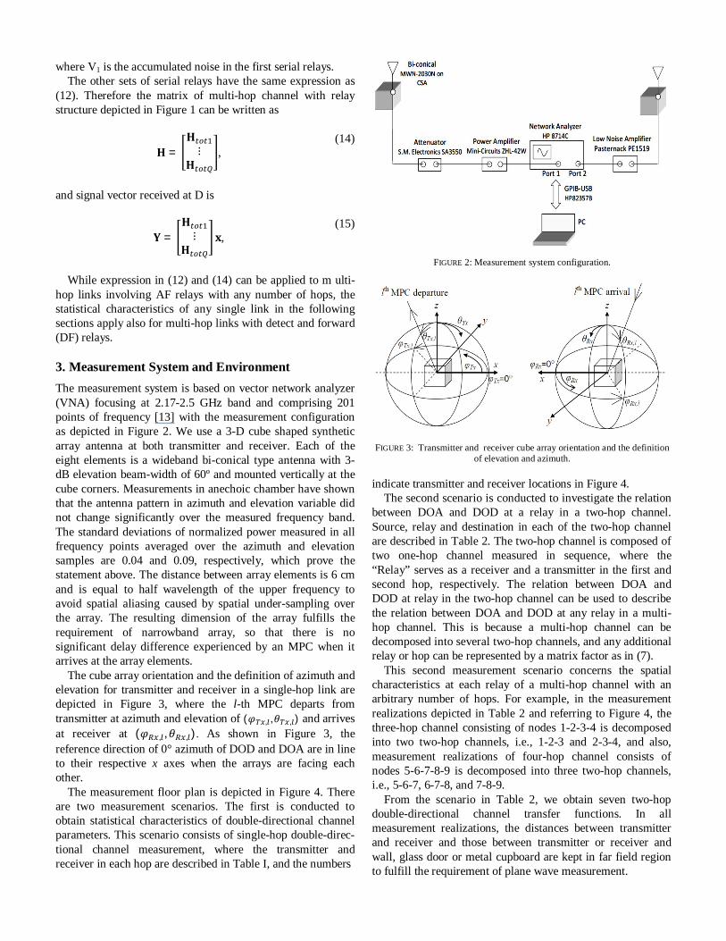
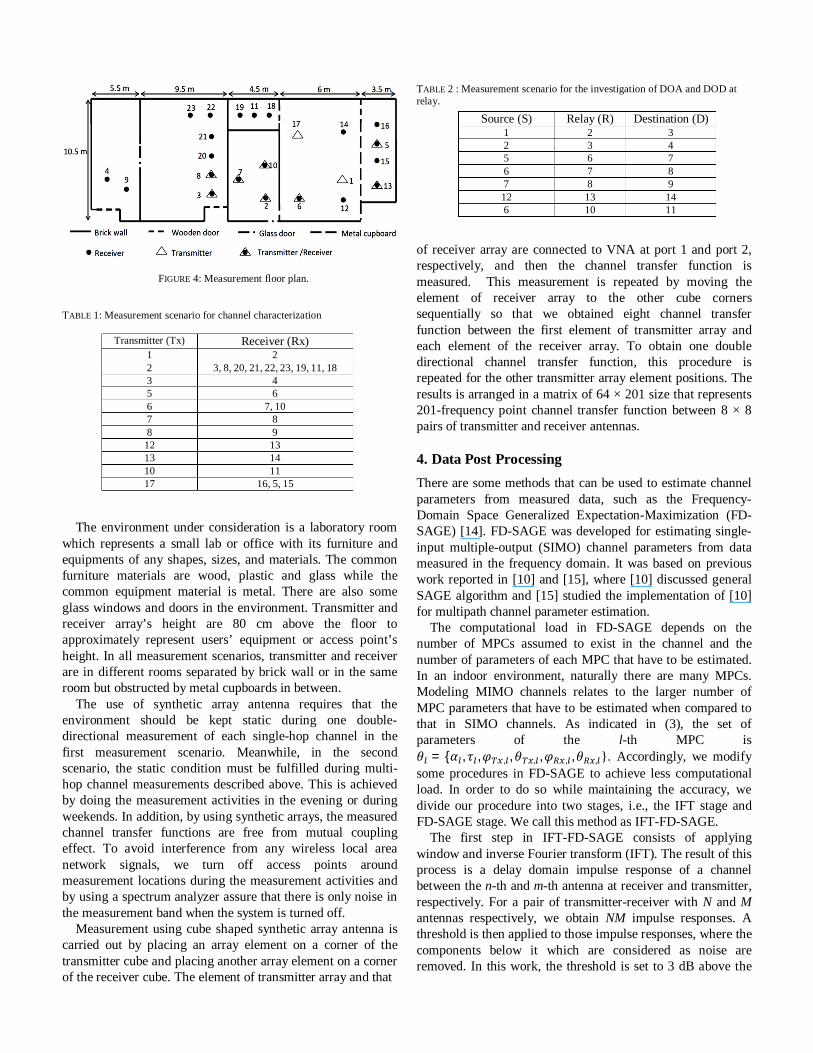
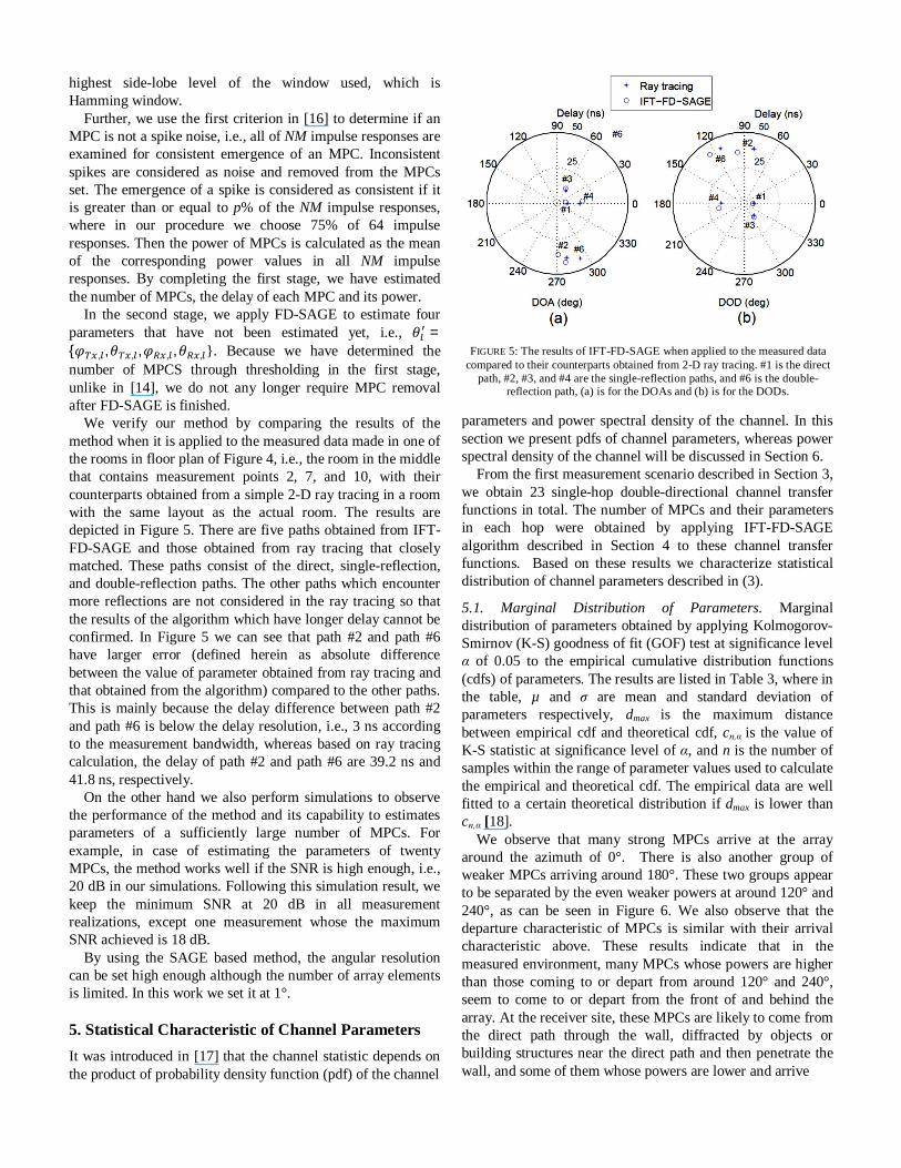
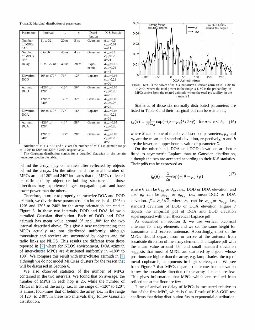
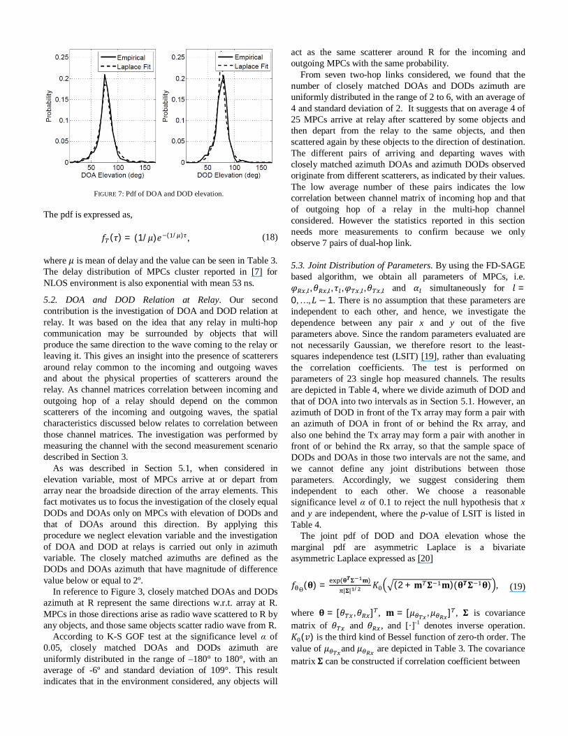
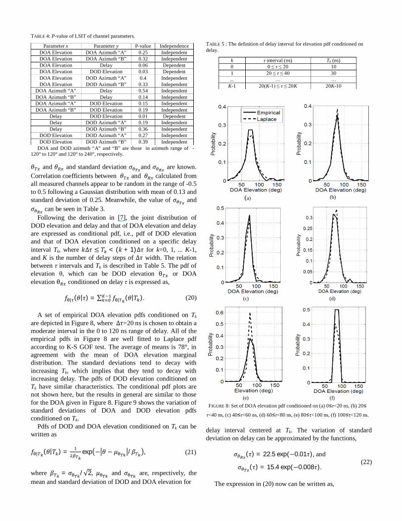
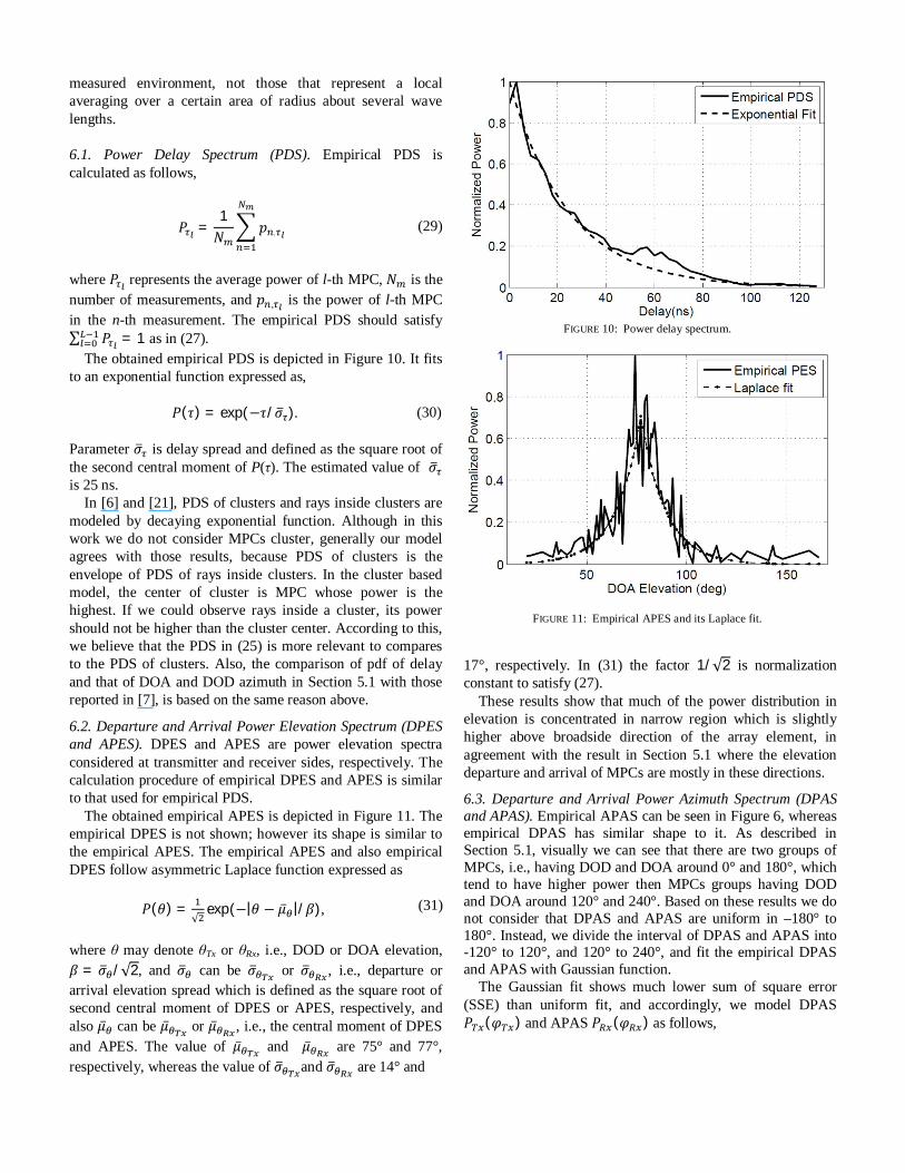
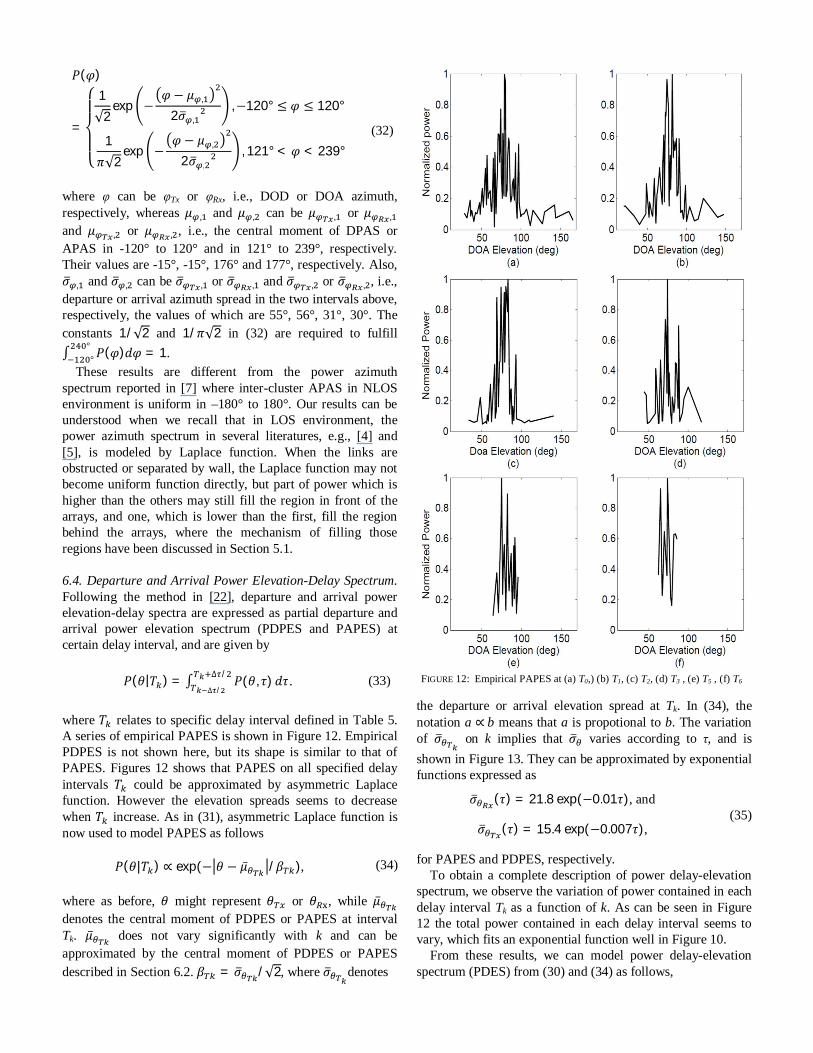
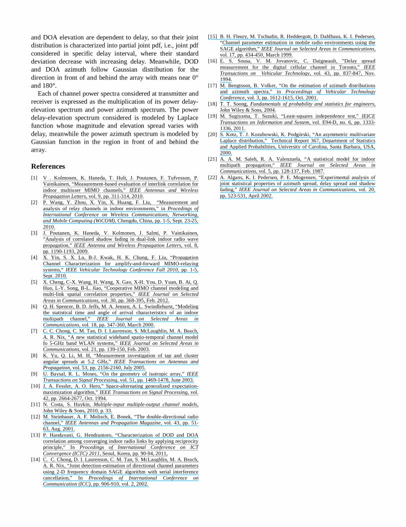