A model for the assessment of habitat conservation status in ...

Report EUR 26186 EN

2 0 1 3

Joachim Maes

A model for the assessment of habitat conservation status in the EU

European Commission

Joint Research Centre

Institute for Environment and Sustainability

Contact information

Joachim Maes

Address: Joint Research Centre, Via Enrico Fermi 2749, TP 270, 21027 Ispra (VA), Italy

E-mail: [email protected]

Tel.: +39 0332 78 9148

http://ies.jrc.ec.europa.eu/

http://www.jrc.ec.europa.eu/

Cover photo by J. Maes, flower field in the national park of the Sibillini mountains in Italy

This publication is a report by the Joint Research Centre of the European Commission.

Legal Notice

Neither the European Commission nor any person acting on behalf of the Commission

is responsible for the use which might be made of this publication.

Europe Direct is a service to help you find answers to your questions about the European Union

Freephone number (*): 00 800 6 7 8 9 10 11

(*) Certain mobile telephone operators do not allow access to 00 800 numbers or these calls may be billed.

A great deal of additional information on the European Union is available on the Internet.

It can be accessed through the Europa server http://europa.eu/.

JRC 84824

EUR 26186 EN

ISBN 978-92-79-33253-1 (pdf)

ISSN 1831-9424 (online)

doi: 10.2788/27866

Luxembourg: Publications Office of the European Union, 2013

© European Union, 2013

Reproduction is authorised provided the source is acknowledged.

Printed in Ispra, Italy

http://ies.jrc.ec.europa.eu/

http://www.jrc.ec.europa.eu/

1 | P a g e

Contents

1. Introduction ........................................................................................................................................ 3

2. Article 17 reporting on the conservation status of habitats ............................................................... 5

3. Methods and data sources.................................................................................................................. 7

3.1. General approach ........................................................................................................................ 7

3.2. Article 17 data.............................................................................................................................. 7

3.3. Frequency analysis of pressures versus habitat conservation status.......................................... 9

3.4. Drivers of change of biodiversity ............................................................................................... 11

3.5. Statistical analysis ...................................................................................................................... 13

3.5.1 Analysis of variance ............................................................................................................. 13

3.5.2 Single response models ....................................................................................................... 13

3.5.3. Multivariate response models ........................................................................................... 14

3.6. Mapping habitat conservation status across Europe ................................................................ 14

4. Results ............................................................................................................................................... 15

4.1. Average response of habitat conservation status to different drivers of change ..................... 15

4.2. Single response models ............................................................................................................. 17

4.3. Multivariate response of conservation status to drivers .......................................................... 21

4.3.1. Model 1. Continuous predictors only ................................................................................. 21

4.3.2. Model 2. Binary and continuous predictors ....................................................................... 22

4.3.2. Model 3. Continuous predictors and ecosystem types ...................................................... 25

4.4. Mapping conservation status .................................................................................................... 26

4.5. Uncertaintly assessment ........................................................................................................... 30

5. Discussion and final remarks............................................................................................................. 34

References ............................................................................................................................................ 35

Supplement tables ................................................................................................................................ 36

Supplement text: Mathematical solution of equation 1 ...................................................................... 45

2 | P a g e

3 | P a g e

1. Introduction

The Habitats Directive, together with the Birds Directive, forms the cornerstone of the nature

conservation policy in the European Union. The directive aims to maintain or restore vulnerable

natural habitats and threatened species of wild fauna and flora to favourable conservation status.

The directive established the Natura 2000 network of protected areas to achieve this goal. With over

26 thousand sites and covering 17.5% of the EU, this network is the largest ecological network in the

world.

Under Article 17 of the Habitats Directive, Member States of the EU must submit information on

how the Directive is being implemented every six years. For the reporting period 2001 to 2006, 25

Member States provided, for the first time, detailed assessments on the conservation status of each

of the habitat types and species listed in the directive and found on their territory or different bio-

geographical regions therein. The results of the 2001-2006 assessment reports show that for many

of the habitats and species listed under the directive, favourable conservation status has not been

achieved either at national or bio-geographic regional level. In fact, only 17% of all the habitat

assessments and 17% of the species assessments yielded a favourable conservation status. In

particular wetlands, grasslands and coastal habitats suffer from continuing degradation.

The EU Biodiversity Strategy to 2020 aims to halt the deterioration in the status of all species and

habitats covered by EU nature legislation. In particular target 1 has the ambition to achieve a

significant and measurable improvement in conservation status of habitats and species so that, by

2020, compared to current assessments 100% more habitat assessments and 50% more species

assessments show an improved conservation status. A first milestone to measure the progress of

meeting this target will be presented in 2014 when the next Art. 17 assessment reports will be made

available.

This report presents a model based approach to assess how conservation status may change in the

future. This approach is based on the available assessments and simulates the probability that a

habitat assessment results in a favourable conservation status as a function of drivers of change.

Such a modelling approach to habitat conservation status has several advantages. Importantly, it

allows different biodiversity policy scenarios or measures to be analysed to see whether or not the

target of increasing the number of favourable assessments will be met. Furthermore, this analysis is

an input to Action 5 of the Biodiversity Strategy which aims to map and assess ecosystems and their

services. By downscaling the results of the national Art. 17 assessments to a finer resolution, this

model may help define the status of Europe’s ecosystems. Such information is useful to determine

whether or not healthy ecosystems contribute more than average to the delivery of key ecosystem

services and to help define priority areas for restoring degraded ecosystems.

A first analysis of the relation between ecosystem services, biodiversity and habitat conservation

status was presented by Maes et al. (1). Using multinomial regression models, they showed that

habitats in good conservation status have a higher potential to deliver regulating and cultural

ecosystem services and that conservation status was related to Mean Species Abundance, a global

indicator for biodiversity. The authors presented evidence to support the hypothesis that actions

which target the restoration of ecosystems, and the maintenance of the services they provide, are

likely to have positive effects on habitat and species conservation status. This information is indeed

4 | P a g e

of importance in identifying regions in which measures are likely to result in cost-effective progress

towards both target 1 (nature conservation) and target 2 (restoring ecosystems and maintaining

ecosystem services) of the Biodiversity Strategy.

This report uses the same methodology as outlined in (1) to model habitat conservation status as a

function of drivers of change of biodiversity. The model is built on the assumption that across

Europe, habitats show an average response to pressures such as land use change, nitrogen loading,

pollution or poor management of the land. This assumption is necessary because it was not possible

to achieve a fully harmonized assessment of European habitats and species throughout all Member

States. This resulted in two main problems with the Art. 17 data: (i) the use of a different baseline to

assess conservation status of habitats and (ii) differences in spatial accuracy of the data. By assuming

an average response of habitats to either degradation or restoration, we argue that these

differences are, to some extent, levelled when considering the data at European scale.

The objective of this report is thus to present a model to assess habitat conservation status in

Europe, based on the reporting under Art. 17 of the Habitats Directive. The present work is limited

to habitats and does not consider species. Modelling species conservation status requires a different

approach, in particular for mobile species and vertebrates which respond differently to declining

area or pollution.

5 | P a g e

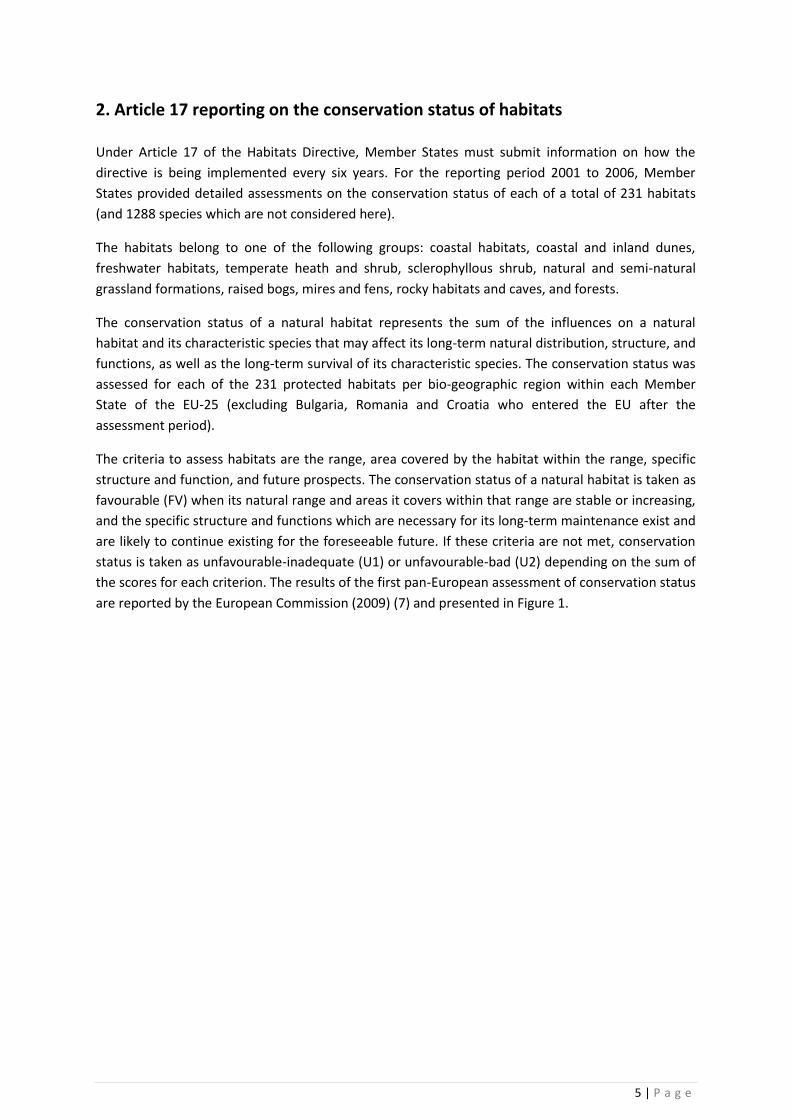
2. Article 17 reporting on the conservation status of habitats

Under Article 17 of the Habitats Directive, Member States must submit information on how the

directive is being implemented every six years. For the reporting period 2001 to 2006, Member

States provided detailed assessments on the conservation status of each of a total of 231 habitats

(and 1288 species which are not considered here).

The habitats belong to one of the following groups: coastal habitats, coastal and inland dunes,

freshwater habitats, temperate heath and shrub, sclerophyllous shrub, natural and semi-natural

grassland formations, raised bogs, mires and fens, rocky habitats and caves, and forests.

The conservation status of a natural habitat represents the sum of the influences on a natural

habitat and its characteristic species that may affect its long-term natural distribution, structure, and

functions, as well as the long-term survival of its characteristic species. The conservation status was

assessed for each of the 231 protected habitats per bio-geographic region within each Member

State of the EU-25 (excluding Bulgaria, Romania and Croatia who entered the EU after the

assessment period).

The criteria to assess habitats are the range, area covered by the habitat within the range, specific

structure and function, and future prospects. The conservation status of a natural habitat is taken as

favourable (FV) when its natural range and areas it covers within that range are stable or increasing,

and the specific structure and functions which are necessary for its long-term maintenance exist and

are likely to continue existing for the foreseeable future. If these criteria are not met, conservation

status is taken as unfavourable-inadequate (U1) or unfavourable-bad (U2) depending on the sum of

the scores for each criterion. The results of the first pan-European assessment of conservation status

are reported by the European Commission (2009) (7) and presented in Figure 1.

6 | P a g e

favourable (FV)

unfavourable-inadequate (U1)

unfavourable-bad (U2)

unknown (XX)

Bio-geographical regions ALP: Alpine ATL: Atlantic BOR: Boreal CON: Continental MAC: Macaronesian MATL: Marine Atlantic MBAL: Marine Baltic MED: Mediterranean MMAC: Marine Macaronesian MMED: Marine Mediterranean PAN: Pannonian

Figure 1. Pie chart: summary of the conservation status of Annex I habitats (the percentage relates to the number of assessments made). Upper bar chart: summary of the conservation status of habitat types in the different bio-geographical regions (numbers in brackets refer to the number of assessments). Lower bar chart: assessment of conservation status of habitats by habitat group (the number in brackets refers to the number of assessments carried out for each group).

7 | P a g e

3. Methods and data sources

3.1. General approach

The probability that habitats are in a favourable conservation status was statistically modelled as a

function of different positive and negative drivers of biodiversity change. Positive drivers of

biodiversity were the location of Natura 2000 sites as well as the network of green infrastructure.

Negative drivers of change or pressures are the transition of land for development and agriculture,

nitrogen enrichment, air pollution, but also management practises such as drainage or abandoning

traditional agricultural practises.

The probability of favourable conservation status ranged, evidently, between 0 and 1 depending on

the combination of drivers that are exerted on habitats. A probability of 0.3 means that there is a

30% chance that a habitat in an assessment would receive a favourable conservation status.

Consequently, the probability that the same habitat has an unfavourable conservation status is 70%.

The choice to include pressures to the model depended on a frequency analysis of pressures that

Member States had to report when submitting their habitat assessments. The 20 most reported

pressures of a list of 170 were selected for further analysis. From this selection, those pressures

were identified for which harmonized data is available at EU scale, e.g. air pollution, land use,

eutrophication or cultivation. For other pressures, e.g. grazing, drainage or invasion by alien species,

quantitative data may be available but they do not cover Europe completely. Still, these pressures

were included in the model albeit as a binary variable with two possible outcomes (present, absent).

In next step, the average response of conservation status to each driver of change was calculated

over habitat conservation status. We excluded pressures from further analysis in cases where

habitat conservation status responded positively to increasing pressures. The rationale is that in

some cases, but in particular for air pollution, distributional effects lead to increment of pollutant

concentrations in rural and natural areas relative to industrial and urban sites. In a next step, the

probability of conservation status was modelled, first using single response models, and secondly

using multivariate models.

Finally, the regression results were used to map habitat conservation status at 10 km resolution

across the EU.

3.2. Article 17 data

This EU wide assessment assigned favourable (FV), unfavourable-inadequate (U1), unfavourable-bad

(U2), or unknown (XX) conservation status to 231 different habitats across 25 Member States

covering seven terrestrial and four marine bio-geographical regions (totalling 2759 habitat

assessments). All national assessments were collected by the European Topic Centre on Biological

Diversity (ETC/BD) and are available in a geospatial database reporting habitat conservation status

on a 10 km grid covering the EU-251. From the dataset including 2759 habitat assessments, the

following assessments were removed (1) all the assessments of offshore coastal and marine

1 http://www.eea.europa.eu/data-and-maps/data/article-17-database-habitats-directive-92-43-eec

8 | P a g e

habitats, (2) all the assessments that resulted in an unknown conservation status, (3) all the

assessments of freshwater habitats (lakes, rivers and streams). Assessments of the following broad

habitat types were included (with in brackets the corresponding MAES ecosystem typology, see (2)):

coastal and inland dunes habitats (sparsely vegetated habitats) , temperate heath and shrub (heath

and shrubland), sclerophyllous shrub (heath and shrubland), natural and semi-natural grassland

formations (grassland), raised bogs, mires and fens (wetland), rocky habitats and caves (sparsely

vegetated habitats), and forests (forest and woodland). This final dataset included 1482 habitat

assessments. Each assessment can be identified by a unique polygon which covers the area where

the habitat is found for each bio-geographic region within every Member State. Figure 2 illustrates

the Art. 17 information that is available for habitat 4030: European dry heath. It also demonstrates

the data quality issues that come with the Art. 17 assessments. The most obvious difference

between member states is the spatial resolution of the assessment. Some countries like France,

Ireland and Poland mapped the distribution of habitat 4030 while other countries mapped the

presence of heath on a grid, albeit at different spatial resolution. Some countries, in this case Spain,

Estonia and Lithuania have reported an unknown status.

Figure 2. Data issues with the Art. 17 assessment. Left: Assessment conclusion for habitat 4030 (European dry heath); Right: The ratio (as a percentage) between the number of favourable habitat assessments and the total number of assessments on a standard 10 km resolution grid covering the EU.

A second issue is the different outcome between the national assessments of conservation status. In

the Atlantic region of Germany, European dry heath was assessed at favourable conservation status

(FV) while in all surrounding countries but also in the continental region of Germany, this habitat

received an unfavourable-bad (U2) assessment. Although this report does not question the quality

of the assessments, it is still possible, and even likely, that different references have been used

across MS to assess conservation status. This is further evidenced by Figure 2 which also plots the

number of favourable conservation assessments as a percentage of all the assessments (excluding

9 | P a g e

unknowns). The differerences between countries are now more apparent. While large portions of

Belgium, France, The Netherlands, UK and Ireland have a low number of assessments with habitats

in favourable conservation status, other countries and most notably Italy and Greece, score

remarkedly better. The possible use of different references against which conservation status has

been assessed can be observed when visually inspecting the percentage of favourable assesments in

the Baltic or Scandinavian countries. Note also that Spain has delivered mainly unknown

assessments.

Clearly, these data quality issues must be considered as they are likely to influence the outcome of

this modelling exercise. The final regression parameters that were derived based on Art. 17 data

were thus subjected to an uncertainty analysis which will be detailed later. Figure 2 also illustrates

why it is important to assume that conservation status exhibits an average response to drivers of

biodiversity change across Europe and across all habitats lised under Annex I of the directive.

The European Commission provides a guidance document to assist Member States in their

assessments. Member States’ reports included maps of range and distribution of these habitats. The

European Topic Centre on Biological Diversity (ETC/BD) collected all national assessments and made

them available in a geospatial database reporting habitat conservation status on a 10 km resolution

grid covering the EU-25. The database and shapefiles of Article 17 reporting are available at:

http://www.eea.europa.eu/data-and-maps/data/article-17-database-habitats-directive-92-43-eec

3.3. Frequency analysis of pressures versus habitat conservation status

Member States (MS) were asked to add information on the pressures on habitats. MS had to

indicate the presence of threats and pressures. The list of main pressures and threats is given in

Appendix E of the Explanatory Notes of the Natura 2000 Standard Data Form2. They are grouped

into nine major impacts and activities that influence conservation status: (1) Agriculture, forestry

and animal breeding; (2) Fishing, hunting and collecting; (3) Mining and extraction of materials; (4)

Urbanisation, industrialisation and similar activities; (5) Transportation and communication; (6)

Leisure and tourism; (7) Pollution and other human impacts/activities; (8) Human induced changes in

hydraulic conditions; (9) Natural processes (biotic and abiotic). We used the Art. 17 database to

cross tabulate the frequency of each pressure over conservation status (FV, U1 or U2). The most

frequent pressures were than selected for possible inclusion in the statistical model.

The results of this analysis are presented table S1 in the Annex (including all pressures) and in Figure

3 (including the most important pressures). A total of 14 856 pressures is observed in the Article 17

habitat assessments, of which 2 459 (or 16%) are assigned to assessments with a favourable

conservation status while 12 397 are assigned to assessments with an unfavourable conservation

status. The most frequently observed pressures on habitats in Europe were the abandonment of

pastoral systems, eutrophication, the so-called modification of hydrographic functioning (which is

physically modifying the course of water), grazing (which can, however, be beneficial for

biodiversity, see also later), drainage, water and air pollution, urbanization and invasion by species.

2 http://ec.europa.eu/environment/nature/legislation/habitatsdirective/docs/standarddataforms/notes_en.pdf

http://www.eea.europa.eu/data-and-maps/data/article-17-database-habitats-directive-92-43-eec

10 | P a g e

Figure 3 also shows the relative frequencies for each type of assessment conclusion. Clearly, the

frequency of many pressures increases with decreasing conservation status or, put another way,

habitats to which an unfavourable conservation status was assigned have to cope with more

pressures than habitats in a favourable conservation status. This conclusion may sound obvious but

this evidence is a first and important piece of information that can be derived from the Art. 17

assessments and it forms the basis of the analysis in this report. The observed relation between

pressures and conservation status provides the evidence that increasing pressure on habitats is

more likely to result in an unfavourable conservation status than in a favourable conservation status

and it is precisely this observation that has been modelled using multinomial logistic regression

models.

Figure 3. Break down of the most frequently occurring pressures over habitat conservation status (FV: Favourable; U1: Unfavourable – Inadequate; U2: Unfavourable – Bad).

11 | P a g e

3.4. Drivers of change of biodiversity

Based on the analysis of pressure frequencies, the following predictor variables for the habitat

conservation status were selected: the proportion of artificial and agricultural land cover, the

density of the road network, nitrogen deposition and exceedance of nitrogen critical loads, fertilizer

input, and exposure of ecosystems to ozone (Table 1). The year 2006 was used as reference year for

the collection of data.

The proportion of artificial land was estimated using the refined version of the Corine Land Cover

data set for the year 2006 (3), which incorporates land use/cover information present in finer

thematic maps available for Europe. Artificial land includes continuous urban fabric, discontinuous

urban fabric (two classes in the refined version), industrial or commercial units, road and rail

networks and associated land, port areas, airports, mineral extraction sites, dump sites, construction

sites.

Also for estimating the proportion of arable land and pasture, the same dataset was used. Arable

land includes non-irrigated arable land, permanently irrigated land, and rice fields.

The road network fragments habitats in small pieces and destroys connectivity. Spatial data

representing Europe’s road network were used to calculate the average length of major roads per

km2.

Ozone is the most important air pollutant in Europe for forest ecosystems. The ozone impact on

vegetation can be calculated using the AOT40 indicator which is the accumulated exposure over a

threshold of 40 ppb. AOT is expressed in μg m-3 × hour.

Excessive nitrogen loading is a leading cause of biodiversity loss, mainly as a result of increased

nitrogen fixation for the production of artificial fertilizers and through the combustion of fossil fuels.

The latter process releases nitrogen to the atmosphere and part of this atmospheric nitrogen is

deposited on earth. Nutrient poor ecosystems contain more biodiversity whereas nitrogen

deposition adds nutrients, which results in loss of plant species. Three possible indicators for

nitrogen loading were considered: total annual nitrogen deposition; the average accumulated

exceedance of nitrogen critical loads, and total annual fertilizer input on cropland.

To this list of pressures, we included also drivers of change that were assumed to positively influence

habitat conservation status: the proportion of land covered by Natura 2000 sites and by green

infrastructure elements.

Several of the pressures on habitats in Europe are not captured by data that reflect land use change,

air pollution or nitrogen enrichment but relate to the poor management of ecosystems. From table

S1, we included the most important pressures to the model as categorical predictor variables with

two possible outcomes (yes: the pressure is present; no: the pressure is absent). Included drivers

were the modification of hydrographic functioning, drainage, grazing, the abandonment of the

pastoral system, and the invasion of alien species.

12 | P a g e

Table 1. Major drivers of biodiversity used in the habitat conservation status model.

Driver Type A priori direction of

change

Reference

Land use change Proportion of artificial land

use including urban and industrial land use (%)

C - Corine Land Cover 2006 refined; European Environment Agency; (3)

Proportion of arable land use (%)

C -

Proportion of pasture (%) C - Road density (km ha

-1) C - ESRI data and maps

Nitrogen enrichment Nitrogen deposition (mg m

-2) C - EMEP model 2006

http://www.emep.int/mscw/index_mscw.html Average accumulated

exceedance of nutrient critical loads (equivalent ha

-1)

C - Coordination Centre for Effects (CCE), (4)

Fertilizer input on arable land (kg ha

-1)

C - GREEN model; (5)

Air pollution Ozone AOT40 for forests C - European Environment Agency; Interpolated air

quality data.

Land management Modification of hydrographic

functioning, general (Frequency)

B - European Environment Agency; Art. 17 database

Grazing (Frequency) B + European Environment Agency; Art. 17 database Abandonment of pastoral

systems B - European Environment Agency; Art. 17 database

Drainage (Frequency) B - European Environment Agency; Art. 17 database

Invasive alien species Invasion by a species

(Frequency) B - European Environment Agency;Art. 17 database

Protected areas and green infrastructure

Green Infrastructure - Proportion of nodes (%)

C + (6)

Green Infrastructure - Proportion of links (%)

C + (6)

Proportion of area covered by Natura 2000 (%)

C + European Environment Agency; Natura 2000 data.

C: continuous data B: binary data (yes, no)

13 | P a g e

3.5. Statistical analysis

The Art. 17 assessments of conservation status have a spatial component: the presence of each

habitat has been mapped at 10 km resolution (although some MS have mapped the range instead of

the presence of habitats, see Figure 2). Each of these habitat maps was intersected with the spatial

information of the drivers of change listed in Table 1. This data set, containing 1482 habitat

assessments, was used in all statistical analyses. The resulting dataset thus contains for each

assessed habitat the assessment conclusion with three possible outcomes (FV, U1, U2), average

values for each continuous driver of change, the presence or absence of invasive alien species, and

the presence of absence of 4 types of land management (Table 1).

3.5.1 Analysis of variance

Analysis of Variance (ANOVA) was used to calculate the average value of continuous predictor

variables for each of three assessment conclusions across Europe.

3.5.2 Single response models

A single response model expresses the probability that habitats are in favourable (or unfavourable)

conservation status as a function of a single driver of change. Since there are 3 possible outcomes

for conservation status (FV, U1 and U2), the appropriate statistical model is a multinomial logistic

regression. This procedure is an extension of the binary logistic regression model and allows for

more than two categories of the dependent or outcome variable.

In a multinomial logistic regression model, the estimates for the parameters can be identified

compared to a baseline category. In this study the probability of membership in the categories U1

and U2 was compared to the probability of membership in a reference category (FV). The

multinomial logistic regression model with reference category FV can be expressed as follows:

xFVP

iPii 21

)(

)(log

(1)

where P(i) is the probability of class membership in the categories U1 or U2, P(FV) is the probability

of class membership in the reference category FV; x is the independent or predictor variable (e.g.

the proportion of artificial land cover) and β1i and β2i are the regression coefficients that were

estimated using maximum likelihood. The mathematical solution of equation 1 is given in the

Supplement.

The left term of equation 1 is by statisticians referred to as the log odds. The odds ratio is the

quotient of two probabilities, here for instance the probability that a habitat is in an unfavourable

status over the probability that a habitat is in a favourable conservation status. One unit of

increment in the independent variable x will increase the log odds with β2. A negative slope means

that, following an increase of x, it is more likely that a habitat will be in favourable status than in an

unfavourable status. Vice versa, a positive slope tells that a one unit increase in x increases the odds

of an unfavourable conservation status.

14 | P a g e

3.5.3. Multivariate response models

A multivariate response model expresses the probability that habitats are in favourable (or

unfavourable) conservation status as a function of a combination of multiple drivers of change. The

same statistical model was used. The difference with equation 1 is that there are more independent

predictor variables which each have a separate regression coefficient.

Only a selection of the drivers was included in the multivariate response model. The relationship

between drivers of change and habitat conservation status was defined a priori. Table 1 presents the

a priori defined relationships with a + indicating a positive relationship and a – for a negative

relationship. Variables for which this relation was rejected, were not considered in the final models.

Three different models were considered. Model 1 predicts habitat conservation status as a function

of continuous drivers only (Table 1). Model 2 uses the same predictor variables as model 1 but

includes the drivers binary values as well. Model 3 uses the same predictor variables as model 1 but

includes a grouping variable that assigns the different habitats to the MAES ecosystem typology,

which enables to model habitat conservation status separately for forests and woodlands, wetlands,

grasslands, heathlands and shrub, and sparsely vegetated ecosystems.

3.6. Mapping habitat conservation status across Europe

In a last step, the models were used to map the probability of a favourable conservation status

across Europe on a grid with resolution 10 km. For each grid cell, the value for each predictor

variable was calculated. Next, the equations of model 1 and model 3 were applied so as to obtain a

European wide map.

15 | P a g e

4. Results

4.1. Average response of habitat conservation status to different drivers of change

Table 2 shows the average values and frequencies of the both continuous and categorical drivers of

change on habitat conservation status. Table 2 largely corroborates the earlier made observation

that assessments with an unfavourable conservation status are subject to stronger pressures than

assessments which resulted in a favourable conservation status.

The proportion of artificial land, arable land and pasture increases, on average, with decreasing

conservation status. Artificial and agricultural land use almost doubles in assessments with an

unfavourable bad status relative to assessments with a favourable status. Habitats in favourable

conservation status also have a significantly lower density of roads.

The effect of nitrogen enrichment on conservation status is less evident. On average, nitrogen

deposition rates did not differ substantially between the three assessment conclusions and lowest

values were observed for the unfavourable inadequate status. Both fertilizer input and the

exceedance of critical nitrogen load increased, on average, with decreasing conservation status. The

case of nitrogen deposition certainly relates to problems of resolution of both the Art. 17 data (> 10

km) as well as of the EMEP air quality model domain (50 km). In this case, zonal statistics are

expected to level any differences, particularly in areas where some habitats are in favourable status

while others are assessed as unfavourable. Apart from data issues, it needs to be stressed that

nitrogen deposition, and air pollution in general, is a wide-spread environmental pressure impacting

almost every place on earth, even areas remote from emission sources with a supposedly high

conservation status. The assessment of fertilizer is based on data with finer spatial resolution while

the data for critical nitrogen loads are available for the EMEP modelling domain but consider only

the portion of EUNIS habitats in each grid cell.

Accumulated ozone exposure followed the opposite trend. Ozone AOT40 levels increased, on

average, with increasing conservation status contrasting the a priori assumed relationship between

habitat conservation status and pressure (Table 1). Distributional effects of emission patterns and

chemistry between ozone and its precursors exclude the use of ozone AOT as an appropriate

predictor for conservation status. Ozone concentrations are higher in rural areas relative to cities

where it reacts with NO (and other substances), released by traffic, to form NO2 and O2. In rural

areas, with less traffic, the opposite reaction takes place and ozone is produced. This process is

enhanced in summer months.

16 | P a g e

Table 2. Average response of drivers of change per assessment conclusion.

Driver of change Conclusion of the assessment

ANOVA results

FV U1 U2 F p

Continuous drivers Proportion artificial land (%) 3.42 4.98 6.27 53.6 <0.01 Proportion arable land (%) 11.27 15.90 23.65 87.2 <0.01 Proportion pasture (%) 5.23 7.20 9.49 33.7 <0.01 Nitrogen deposition (mg m

-2) 607.64 601.81 656.56 5.8 <0.01

Average accumulated exceedance of nutrient critical loads (equivalent ha

-1)

232.80 254.87 292.38 16.9 <0.01

Road density (km ha-1

) 0.95 1.20 1.40 34.5 <0.01 Fertilizer input on arable land (kg ha

-1) 54.98 65.43 89.99 75.2 <0.01

Ozone AOT on forests 42 846.23 36 227.26 31 592.81 95.5 <0.01 Green Infrastructure - Proportion of nodes (%) 51.34 36.14 25.90 106.9 <0.01 Green Infrastructure - Proportion of links (%) 3.16 3.98 5.02 24.9 <0.01 Proportion of area covered by Natura 2000 (%) 33.87 24.19 17.76 126.8 <0.01

Categorical (binary) drivers Modification of hydrographic functioning, general (Frequency)

78 182 195

Grazing (Frequency) 132 156 157 Abandonment of pastoral systems 85 144 254 Drainage (Frequency) 56 150 221 Invasion by a species (Frequency) 38 144 220

Habitats in favourable conservation status had, on average, a higher proportion of coverage by

Natura 2000 sites than habitats in unfavourable conservation status and this difference was

significant. It is still remarkable that, on average, habitat assessments yielding an unfavourable

status are for 17% covered by the Natura 2000 network. This could lead to the conclusion that at EU

scale, the present coverage of the Natura 2000 network is not sufficient to warrant a favourable

conservation status. We refer to the single and multivariate response models as well as to the

uncertainty analysis for a more in depth discussion on this conclusion.

Conservation status exhibited a mixed response to increasing proportions of land covered by green

infrastructure elements. Assessments with a favourable conservation status are, on average, better

covered by nodes, which constitute the core elements of green infrastructure, while assessments

with an unfavourable status contain, on average, more links, which bridge the different core

elements.

The frequency of 5 categorical drivers, measured as presence or absence, increased with decreasing

conservation status (table 2). Modification of hydrographic functioning, grazing, and abandonment

of the pastoral systems, drainage and invasion by species were all observed at higher frequencies for

assessments with an unfavourable conservation status. This was especially evident for invasive

species.

Two essential conclusions were derived from this first analysis of the average response of

conservation status to drivers of biodiversity change. Firstly, the a priori formulated relations with

conservation status (Table 1) were respected for most drivers i.e. habitats in unfavourable status

undergo, on average, a higher pressure than habitats in favourable status. This was not the case for

17 | P a g e

air quality, for nitrogen deposition and for green infrastructure links, and these predictors for habitat

conservation status were therefore not considered any longer in the statistical models. Secondly, the

coarse spatial resolution of the Art. 17 assessments causes the within group assessment average to

move to the overall, between-group assessment average. This can be illustrated using the example

of artificial land use. In Europe, about 5% of the land is claimed for residential and industrial uses.

This figure is based on the relative coverage of artificial land in the Corine dataset. This percentage is

almost equal for areas assessed as unfavourable inadequate (Table 2). The proportion of artificial

land increases for areas assessed as unfavourable bad (6.3%) and decreases for areas assessed as

favourable (3.4%) (table 2). It is likely that (future) assessments at a finer spatial resolution will cause

these latter two values to drift away from the average and will yield a lower percentage in case of

favourable conservation status and an equal or higher percentage in case of unfavourable bad

conservation status. In part, this explains also why assessments in unfavourable conservation have

relatively high proportions of coverage by green infrastructure nodes and Natura 2000 sites.

4.2. Single response models

Instead of considering the average response of habitat conservation status to drivers of change, this

section examines how conservation status changes along a continuous or discrete gradient of

change. Figure 4 depicts the probability that an assessment results in a particular conservation

status along single gradients of pressure. The regression coefficients and model diagnostics are given

in table S2.

The probability of a favourable assessment decreases sharply with increasing proportions of artificial

and agricultural land use and with an increasing density of the road network. Evidently, the relation

between these variables and the probability of an unfavourable bad conservation status has an

opposite pattern, while the probability of an unfavourable inadequate status follows a bell shaped

curve with positive skew (a tail to the right). While these probabilities clearly differ at the extremes

(land which is completely artificial has a very high probability of unfavourable status and a very low

probability of favourable status), the intercepts at the origin do not differ much. So the probability of

a favourable conservation status if land is not taken for any kind of development is only 0.43,

suggesting that other factors play a role in determining conservation status. The relative

contributions of different pressures will be examined in the next section. But it also reflects to some

extent the mosaic structure of Europe at the landscape scale with patchy patterns of urbanisation,

agriculture, forests and semi-natural areas.

18 | P a g e

Figure 4. Single response models. The probability of habitat conservation status as a function of different drivers of change.

19 | P a g e

Figure 4. Continued. Single response models. The probability of habitat conservation status as a function of different drivers of change.

Nitrogen stress on habitat conservation status is expressed using three variables: nitrogen

deposition, exceedance of the critical nitrogen load and fertilizer input. All pressures but the first

one yielded significant regression coefficients (table S3).

Importantly, conservation status responded strongly to increasing protection (Natura 2000 network)

or increasing green infrastructure (% of nodes in the GI network). The probability of favourable

conservation status increases sharply with increasing coverage of protected areas or nodes in the GI

network. Note also the difference with other models at the origin. In absence of protected areas or

of green infrastructure core elements, the probability of a favourable conservation status is quite

low (around 0.1) and certainly much lower than the probability of an unfavourable status.

Multinomial regression models can also be used when the predictor variables have discrete

outcomes. Here we examine the effect of presence or absence of five pressures on habitat

conservation status, based on the Art. 17 reports. Each predictor variable was encoded with a 1 if

the pressure was reported (present) and with a 0 if the pressure was unreported (absent). The

results of the statistical model are presented in Figure 5 and are quite interesting.

20 | P a g e

Figure 5. Single response models. The probability of habitat conservation status as a function of different drivers of change.

A striking observation concerns the direction of change. The probability of a favourable conservation

status decreases when a pressure is present in all models but one, grazing. The impact of alien

species is quite pronounced. Habitat assessments where invasion of alien species is reported as

pressure have a much higher probability of an unfavourable status than habitat assessments where

this pressure is not reported. Similar observations were made for abandonment of pastoral systems

as well as water stress (two pressures). Interestingly, grazing, which was reported as pressure,

results in an opposite pattern. Grazing is associated with favourable conservation status and, if

reported, it actually increases the probability of the favourable conservation status.

21 | P a g e

The significance of these conclusions, even based on qualitative information based on reporting by

MS, cannot be underestimated. The assessment of pressures demonstrates that management

practises have a profound impact on conservation status. In particular, the physical modification of

the hydrology of watersheds by lowering the water table (drainage) or by restructuring waterways,

the abandonment of traditional agricultural management, and the invasion of alien species were

assessed as the most important threats to habitat conservation status.

The added value of including these binary variables in the model is that we can now simulate the

impact of restoration of ecosystem management on conservation status. Provided that location

specific data are available, we can model the absence of each pressure which corresponds to either

restoration measures (e.g. rewetting, removing alien species) or to appropriate management

(extensive grazing, traditional agricultural practise). These options will be discussed in the next

section where the impact of combined pressures on conservation status are analysed.

4.3. Multivariate response of conservation status to drivers

Multivariate regression models were used to predict the response of conservation status when

exposed to multiple drivers of change. Three combinations of predictor variables were tested and

used for analysis and mapping of conservation status (see section 4.4). The first combination

included only continuous predictors: four land use variables, two nitrogen enrichment variables that

resulted in significant models, Natura 2000 and green infrastructure nodes. For reasons explained

above, air quality (ozone AOT40) and the proportion of green infrastructure links were not

considered any more in the statistical models. A second combination added to this first set the five

binary predictor variables. The third combination added to the first set an extra categorical variable

that assigns each habitat assessment to one of the following MAES ecosystem types (forests and

woodlands, wetlands, grasslands, sparsely vegetated ecosystems, and heathlands and shrubs). No

habitats were assigned to cropland or urban ecosystems while freshwater and marine ecosystems

were excluded from this analysis.

All regression coefficients and model diagnostics are available in the supplement to this report.

4.3.1. Model 1. Continuous predictors only

A first run including only continuous predictor variables delivered in first instance results that were

opposed to the single model responses (Figure 4). In particular, the probability of a favourable

conservation status increased with increasing values of road density and fertilizer input and

decreased with increasing values of green infrastructure nodes, contrasting with the a priori signs

set in Table 1. Typically, multi-collinearity in the predictor data set causes regression coefficients

which flip sign after including other predictors. Multi-collinearity refers to correlated predictor

variables. The density of the road network is correlated to artificial land use; fertilizer input is

correlated to arable land use and exceedance of critical loads; the green infrastructure nodes are

related to the Natura 2000 coverage. A common method to avoid collinearity is principal component

analysis on the predictor data set after which the principal components are further used as

predictors in the regression models. Here, we decided to simply exclude these three variables from

22 | P a g e

the analysis. It follows that all final models are based on the following combination of continuous

drivers of change: artificial land use, arable land use, pasture, exceedance of the nitrogen critical

load and the proportion of coverage by Natura 2000. This combination yields a set of regression

coefficients that observe the a priori assumed direction of change (positive or negative) of Table 1.

The final model to predict conservation status can be calculated using the following equations:

AAE0.0001N0.0190-L0.0174L0.0080L0.05920.3210)(

)1(log 2000pastarabarti1

F

FVP

UP (2)

AAE0.0005N0.0433-L0.0386L0.0313L0.06630.0183)(


F

FVP

UP (3)

)exp()exp(1

1

21 FFFVp

(4)

)exp()exp(1

)exp(1

21

1

FF

FUp

(5)

)exp()exp(1

)exp(2

21

2

FF

FUp

(6)

where P(FV) is the probability that an assessment returns a favourable conservation status, p(U1) is

the probability that an assessment returns a unfavourable inadequate conservation status, P(U2) is

the probability that an assessment returns a unfavourable bad conservation status, Larti is the

proportion of artificial land use (%), Larab is the proportion of arable land use (%), Lpast is the

proportion of pasture (%), N2000 is the proportion of land covered by Natura 2000 and AAE is the

annual average exceedance of the critical load for nitrogen (eq ha-1).

The regression coefficients including their standard error and level of significance are repeated in

Table S2. In case of a dependent variable that has continuous values, linear regression results in an

explained variance, which measures the proportion to which a regression model accounts for the

variation. An explained variance cannot be calculated using a maximum likelihood method but the

analysis can deliver an estimate of the correct classification of all cases. So the equation is used to

calculate the probability of each observation in the data and compares this probability with the

observed assessment conclusion. These results are provided in table S6 and can be used to interpret

to some extent the variance that is explained by the model. The percentage of correct classifications

for model 1 was 43% for assessment conclusion FV, 46% for assessment conclusion U1 and 62% for

assessment conclusion U2.

4.3.2. Model 2. Binary and continuous predictors

A second model includes the 5 continous variables that were retained in model 1 and adds variables

that contain data on the presence or absense of drivers (or pressures). Model results and diagnostics

are given in Tables S3 and S6 of the supplement. Importantly, the percentage or correctly classified

cases increased, in particular for the FV conclusion assessment. Model 2 successfully predicts 54% of

23 | P a g e

the FV assessments, 44 % of the U1 assessments and almost 65% of the U2 assessments. The

equations of model 2 are as follows:

AAE0.0002N0.0192-L0.0088L0.0010-L0.0720

M0.5169M0.2180M0.1652M0.0228-M0.16201.2149)(

)1(log

2000pastarabarti

543211

F

FVP

UP

(7)

AAE0.0004N0.0421-L0.0254L0.0167L0.0885

M0.7460M0.5082M0.5125M0.0524M0.05611.3147)(

)2(log

2000pastarabarti

543212

F

FVP

UP

(8)

where, in addition to previous set of equations (model 1) M1 stands for modification of the

hydrographic functioning, M2 for grazing, M3 for abandonment of the pastoral system, M4 for

drainage and M5 of invasion of alien species. The Mi variables can only have two possible values: 1

means that the driver is present and -1 which means that the driver is absent3. So these categorical

variables essentially increase or decrease the intercepts of the model. Substituting equations (7) and

(9) in equations (4), (5) and (6) yields the probalities for conservation status.

It is possible to examine the interaction effects between discrete and continous drivers of change,

for example, between the presence and absence of grazing and the proportion of land covered by

pasture. The assumption is then that habitat status responds differently to increasing coverage of

pasture at different levels of grazing. However, such interaction effects violate the initial

asssumption of a single, average reponse of conservation status to drivers of change across all

habitats. They also complicate to some extent the interpretation of the model coefficients.

Table 3 illustrates the resulting probabilities of a favourable conservation status given hypothetical4

combinations of continous and discrete drivers. The rows contain four different scenarios with

respect to the continous predictors and may represent values that typically refer to intensively used

land, an agriculture mosaic, rural pasture and and a natural landscape, respectively. The columns

contain different combinations of the categorical drivers expressend as present (yes) or absent (no).

Back ground colours indicate which conservation status has the highest probability. Arguably, the

probability of a favourable conservaton status increases with decreasing pressures from left to right

and from the top to the bottom. It demonstrates that achieving favourable conservation status is

challenging, in particular in areas with an intensive land use. By no means can this table be used to

argue that achieving a good conservation status in such areas is impossible. It is sufficient to inspect

Figure 4 again and observe the strongly positive relation between green infrastructure nodes and

favourable status. Whereas green infrastructure was not included in the final multivariate models,

Figure 4 provides evindence that increasing green infrastucture elements in agricultural and urban

land may result in a positive impact on habitat conservation status. This stresses the need for better

and more detailed data on small landscape elements in agricultural and urbanised areas.

Table 3 can also be used to focus some of the ongoing restoration efforts on good ecosystem

management which includes combatting invasive alien species, rewetting, restoring rivers, extensive

grazing and reinstalling tradional land management. Table 3 provides some insight in how

3 This is the typical coding for sigma-restricted models.

4 The table has only illustrative value; some combinations of drivers are unlikely to occur.

24 | P a g e

management at local or landscape scale can substantially improve conservation status, keeping

constant the pressures that operate at broader geographical scales, such as land use change and

nitrogen deposition. It also demonstrates well the benefits of the Natura 2000 network in achieving

good conservation status as required by the Habitats Directive.

Table 3. Probability of favourable conservation status for hypothetical combinations of drivers. Background colours represent the conservation status that has the highest probability (red: unfavourable bad, orange: unfavourable inadequate, green: favourable).

Modified hydrographic functioning yes no no no no no

Grazing no no yes yes yes yes

Abandonment of the pastoral system yes yes yes no no no

Drainage yes yes yes yes no no

Invasion of alien species yes yes yes yes yes no

Urban and agriculture development

20% artificial, 35% arable, 5% pasture

5% Natura2000, 300 eq. ha-1

AAE

0.003 0.004 0.004 0.01 0.02 0.08

Agricultural mosaic


17% Natura2000, 250 eq. ha-1

AAE

0.02 0.02 0.02 0.06 0.12 0.32

Rural pasture


50% Natura2000, 50 eq. ha-1

AAE 2%

0.10 0.11 0.12 0.21 0.32 0.60

Nature


100% Natura2000, 50 eq. ha-1

AAE

0.35 0.41 0.43 0.54 0.66 0.85

25 | P a g e

4.3.2. Model 3. Continuous predictors and ecosystem types

The last statistical model used the same predictor variables as model 1 but included a categorical

variable that groups every habitat assessment into one of the MAES ecosystem types. The aim of

this model is to contribute information that can be used for mapping the status of ecosystems. Table

S5 lists the regression coefficients along with the other model diagnostics. Also this model has an

increased performance with respect to correct classification of FV assessments relative to model 1

(Table S6).

Similarly as in model 2, the effect of including ecosystem typology is an increase or a decrease of the

model interceps while keeping the slopes homogenous. The equations to solve p(FV) are as follows:

AAE0.0001N0.0182-L0.0122L0.0071L0.0721)(


F

FVP

UP (9)

AAE0.0003N0.0437-L0.0321L0.0305L0.0802)(


F

FVP

UP (10)

intercepts β1 β2 wetlands 0.9812 0.6753 grasslands 0.5608 1.0563 heathlands and shrub -0.0182 -0.0437 forests and woodlands 0.0361 -0.0496 sparsely vegetated ecosystems -0.2102 -0.0697

where, similar as in models 1 and 2, Larti is the proportion of artificial land use (%), Larab is the

proportion of arable land use (%), Lpast is the proportion of pasture (%), N2000 is the proportion of land

covered by Natura 2000 and AAE is the annual average exceedance of the critical load for nitrogen

(eq ha-1).

The relative value of the intercepts tells something about the relative vulnerability of the considered

ecosystem types. Recall that positive intercepts increase the odds of unfavourable status while

negative intercepts increase the odds of favourable status. Keeping everything else constant,

wetlands are thus the most vulnerable habitats according to the analysis, followed by grasslands,

heathlands and shrub, forests and woodlands, and finally sparsely vegetated habitats. This

corresponds with Figure 1 which depicts the relative frequencies of habitat groups considered in the

Habitats Directive. For three out of five groups, we used a one to one relation between the MAES

typologies and the broad habitats defined under the Habitats Directive. This is not the case for

heathlands and shrub and for sparsely vegetated habitat. The latter MAES ecosystem type contains

both dunes and rocky habitats which respond quite differently to pressures. Consequently, the

coefficients for sparsely vegetated habitats will overestimate the probability of a favourable

conservation status of coastal dunes given land use change, nitrogen deposition and coverage by the

Natura 2000 network.

26 | P a g e

4.4. Mapping conservation status

The statistical models can be used to map conservation status, or at least, the probability that

habitats will be assessed as having favourable or unfavourable status. As an example, we mapped

the probability of favourable conservation status on a 10 km resolution grid which covers the EU

based on the regression coefficients by model 1 and model 3. Recall that model 1 used only

continuous variables to predict conservation status while model 3 included five terrestrial MAES

ecosystem types.

Using the regression coefficients of equations (2-6), Figure 6 maps the probability of a favourable

conservation status across all habitats based on the proportion of artificial land use, arable land use,

pasture, Natura 2000 sites, and the exceedance of critical nitrogen loads for every grid cell. This map

should be interpreted as the average probability of habitats to be assessed at favourable

conservation status, given a combination of land uses and nitrogen deposition. As can be expected,

probabilities are low in areas with intensive land use and high rates of nitrogen deposition whereas

they are high in Scandinavia, the Iberian Peninsula, and Europe’s major mountain chains. Note also

the impact that the Natura 2000 network has on conservation status, which is well well-illustrated

by the vast Natura 2000 site of Sologne in the heart of France.

Figure 6 can be compared in a straightforward manner with Figure 2. Whereas Figure 6 maps a

probability between 0 and 100%, Figure 2 maps the relative frequency of a favourable conservation

status based on the Art. 17 reports. Also these frequencies are presented between 0 and 100%.

Comparing both figures demonstrates well the advantages of this particular statistical analysis which

was made under the assumption of an average response of habitats to pressures and drivers of

change. The regression models effectively allow to gap fill and downscale the Art. 17 assessment

data and to provide more special detail.

Figures 7 and 8 map the probability of a favourable conservation status based on the regression

coefficients of equations (9-10). Firstly, the percentage of each MAES ecosystem type was calculated

per grid cell making use of the cross walk between the MAES ecosystem typology and the corine

land cover classes (2). Ecosystem types that cover more than or equal to 20% of the surface area of

each 10 km grid cell were mapped.

27 | P a g e

Figure 6. Modelled probability of favourable conservation status in the EU-27 based on the results of Model 1.

28 | P a g e

Figure 7. Modelled probability of favourable conservation status in the EU-27 based on the resuls of Model 3.

29 | P a g e

Figure 8. Modelled probability of favourable conservation status in the EU-27 based on the resuls of Model 3.

30 | P a g e

4.5. Uncertaintly assessment

The Article 17 reporting on habitat and species conservation status constituted an unparalleled

assessment involving hundreds of people in national and regional administrations and research

institutes from 25 EU Member States (7). However, it was not realistic to assess European habitats

using a harmonized approach throughout all Member States. This resulted in two main problems

which were already pinpointed in the introduction of this report: (i) the use of a different baseline to

assess conservation status of habitats and (ii) differences in spatial accuracy of the data. The

European Topic Centre on Biological Diversity provides a detailed report on the completeness,

quality and coherence of the data (8).

We used a Monte Carlo analysis to test the robustness of the regression coefficients obtained from

the first multinomial logit model, which predicts conservation status based on a combination of

artifical land cover, arable land cover, pasture, coverage by the Natura 2000 network and

exceedance of critical nitrogen loading. The Monte Carlo analysis addressed the following question:

how well does model 1 predict the probability of a favourable conservation status if the regression

coefficients are based on a subsample of only 200 instead of 1482 assessments. Figure 9 contains a

flowchart that demonstrates the general idea of the Monte Carlo procedure to test data uncertainty.

Figure 9. Flow chart of the Monte Carlo assessment on the regression models.

We thus randomly resampled 200 habitat assessments out of a total of 1482 habitat assessments

used in this study and recalculated the regression coefficients. We repeated this procedure 1000

times. This resulted in a distribution representing the uncertainty in each regression coefficient,

which is explained by a normal distribution characterized by an average and a standard deviation.

Table 4 presents the results of this analysis and compares the regression coefficients obtained from

a nominal model run (and corresponding to the regression coefficients of equations 2and 3) with the

31 | P a g e

average coefficients based on 1000 models, each using 200 resampled assessment conclusions.

Table 4 shows that both sets of coefficients are virtually the same.

Furthermore, the direction of change of each regression coefficient based on the Monte Carlo

models was compared with the a priori assumed direction of change in Table 1. These results are

also reported in Table 4. Let’s examine the Natura 2000 coverage as predictor for habitat

conservation status. In table 1, we assumed that the Natura 2000 network positively influenced the

favourable conservation status. This hypothesis was accepted by the nominal regression model

based on all 1482 habitat assessments. Following model 1, every unit of increase of the natura 2000

network decreases the odds of an unfavourable status. Put another way, it increases the probability

of a favourable status. The Monte Carlo analysis corroborates this observation. Only 2 models out of

1000 models flipped the sign of this relationship and resulted in higher probability of the

unfavourable status for every increment of the Natura 2000 network. The other 998 models

confirmed the a priori direction of change as well as the positive relation between the network and

favourable conservation status.

In general, the conclusion is that the relationships we observed between drivers of change included

in the statistical model and favourable habitat conservation status reflect a meaningful and robust

statistical pattern which is present in the Art. 17 data.

Figure 10 shows the distribution of probabilities that were obtained for 1000 model runs, given

average values for the predictor variables.

32 | P a g e

Table 4. Uncertainty assessment on model 1. A comparision of the nominal model coefficients with the average regression coefficients based on 1000 Monte Carlo (MC) runs. The last column presents the number of Monte Carlo models that correctly prediced the a-priori sign of the reponse of each predictor variable.

Regression coefficients

Level of response

Nominal model

coefficients

Average coefficient of

1000 MC runs

Standard deviation of 1000 MC runs

Number of models with a correct a priori

sign

Intercept U1 0.321 0.352 0.497

% Artificial land use U1 0.059 0.067 0.054 908

% Arable land use U1 0.008 0.008 0.014 717

% Pasture U1 0.017 0.019 0.032 725

% Natura 2000 coverage

U1 -0.019 -0.021 0.012 979

Exceedance of the critical nitrogen loads

U1 0.0001 0.0001 0.001 538

Intercept U2 -0.018 -0.004 0.623

% Artificial land use U2 0.066 0.074 0.057 912

% Arable land use U2 0.031 0.032 0.015 979

% Pasture U2 0.039 0.043 0.032 934

% Natura 2000 coverage

U2 -0.043 -0.047 0.017 998


U2 0.001 0.001 0.001 665

0.10 0.15 0.20 0.25 0.30 0.35 0.40 0.45 0.50

Probability of a favourable conservation status

0

50

100

150

200

250

300

350

400

450

500

550

Freq

uenc

y

Figure 10. Uncertainty assessment on model 1. Distribution of probabilities of favourable conservation status based on 1000 Monte Carlo models using the following values for the predictor variables artificial land use: 3.42%; arable land use: 11.27%, pasture: 5.23%, Natura 2000: 17%; AAE: 232.80 eq. ha

-1). The nominal

probability based on model 1 is 0.27.

33 | P a g e

A second question follows from the Monte Carlo assessment: What is the lowest number of

assessments that we need to extract at random from the Art. 17 data to still produce a robust

model. In the first Monte Carlo procedure, we reproduced the results 1000 times, each time based

on 200 randomly drawn habitat assessments from the 1482 assessments that are available in the

Art. 17 reports and that were considered in this study. So what would happen if we took only 100

assessments at random, or 50, or only 20? Figure 11 provides some insight in the minimum number

of habitat assessments that are needed to reproduce a reliable model that predicts the probability

of a favourable conservation status as a function of drivers of change. The figure plots the number of

sub samples taken in 7 Monte Carlo procedures against the coefficient of variation which is the ratio

between the standard deviation and the average probability calculated using 1000 models. The

bottom line is that with relatively few habitat assessments conservation status can be modelled

across Europe. It supports again the observation that Art. 17 habitat assessments provide a powerful

dataset to simulate conservation status in the EU.

Figure 11. Uncertainty analysis. The number of sub samples that are randomly taken from the Art. 17 assessments versus the coefficient of variation of the probability of a favourable conservation status

34 | P a g e

5. Discussion and final remarks

Habitat conservation status constitutes a policy relevant indicator to assess the state of

ecosystems and biodiversity in Europe and to measure progress to the biodiversity targets.

The indicator is expressed as a probability between 0 and 100% that habitats are assessed at

a favourable conservation status, which allows a straightforward interpretation.

A first test of the model will be the Art. 17 status reports that will become available in 2014.

These reports can be used to validate the model predictions against a new set of status data

and will allow us to improve the model performance.

The Habitats Directive aims to bring vulnerable and threatened habitats in the EU at

favourable conservation status. Using the models presented in this report can support

achieving this policy goal. In particular, scenarios on land use change, nitrogen deposition,

and protected areas in combination with local management can explore how policy

measures can increase or decrease the probability of a favourable conservation status. This

model can thus be used to assess under which scenarios target 1 of the EU Biodiversity

Strategy can be achieved.

The combination of drivers of change which operate at a large spatial scale with pressures

that act on local to regional scale is a promising approach and warrants further research.

There is certainly a need for more and better data on the management of ecosystems.

The Art. 17 database contains much information on species protected under the Habitats

directive. Modelling species requires, however, a different approach than the one addressed

in this study since many species are mobile. Such an assessment should include predictor

variables that describe the climatic suitability of species and connectivtiy between suitable

habitats.

35 | P a g e

References

1. Maes J, Paracchini MP, Zulian G, & Alkemade R (2012) Synergies and trade-offs between ecosystem

service supply, biodiversity and habitat conservation status in Europe. Biological Conservation 155:1-12.

2. Maes J, et al. (2013) Mapping and Assessment of Ecosystems and their Services. An analytical

framework for ecosystem assessments under action 5 of the EU biodiversity strategy to 2020. Publications

office of the European Union, Luxembourg.

3. Batista e Silva F, Lavalle C, & Koomen E (2012) A procedure to obtain a refined European land

use/cover map. Journal of Land Use Science:1-29.

4. Posch M, Hettelingh JP, & De Smet PAM (2001) Characterization of critical load exceedances in

Europe. Water, Air, and Soil Pollution 130(1-4 III):1139-1144.

5. Grizzetti B, Bouraoui F, & De Marsily G (2008) Assessing nitrogen pressures on European surface

water. Global Biogeochemical Cycles 22(4).

6. Mubareka S, Maes J, Lavalle C, & de Roo A (2013) Estimation of water requirements by livestock in

Europe. Ecosystem Services.

7. European Commission (2009) Composite Report on the Conservation Status of Habitat Types and

Species as required under Article 17 of the Habitats Directive. COM(2009) 358 final. Brussels

8. European Topic Centre on Biological Diversity (2008) Data completeness, quality and coherence. Paris

36 | P a g e

Supplement tables Table S1. Frequency analysis of pressures versus habitat conservation status. For each presssure, the frequency of occurrence in the Art. 17 database is given as well as the break-down (as a percentage) over three assessment conclusions (FV: Favourable conservation status; U1: Unfavourable inadequate conservation status, U2: Unfavourable bad conservation status). Pressures were ranked in decreasing order of frequency.

Rank Pressure Frequency FV U1 U2

1 abandonment of pastoral systems 483 17.6 29.8 52.6

2 eutrophication 470 9.1 31.7 59.1

3 Modification of hydrographic functioning, general 455 17.1 40.0 42.9

4 Grazing 445 29.7 35.1 35.3

5 Drainage 427 13.1 35.1 51.8

6 water pollution 425 10.4 42.4 47.3

7 Urbanised areas, human habitation 425 12.2 42.8 44.9

8 invasion by a species 402 9.5 35.8 54.7

9 General Forestry management 402 26.6 34.3 39.1

10 Biocenotic evolution 391 22.0 40.4 37.6

11 Fertilisation 363 7.4 33.9 58.7

12 forest planting 319 12.5 32.6 54.9

13 Trampling, overuse 310 17.4 50.0 32.6

14 air pollution 273 21.6 28.9 49.5

15 modification of cultivation practices 260 11.2 37.3 51.5

16 artificial planting 255 14.9 35.7 49.4

17 Cultivation 247 8.5 38.1 53.4

18 Communication networks 245 18.4 47.3 34.3

19 Landfill, land reclamation and drying out, general 212 8.5 34.0 57.5

20 Sand and gravel extraction 194 13.4 35.1 51.5

21 paths, tracks, cycling tracks 192 24.5 44.3 31.3

22 management of water levels 189 8.5 41.8 49.7

23 Agriculture and forestry activities not referred to above 183 22.4 33.9 43.7

24 Sport and leisure structures 175 11.4 49.7 38.9

25 removal of dead and dying trees 173 21.4 32.9 45.7

26 roads, motorways 169 20.7 40.2 39.1

27 Other natural processes 168 14.9 46.4 38.7

28 Discharges 168 11.9 38.1 50.0

29 walking, horse-riding and non-motorised vehicles 163 28.2 39.3 32.5

30 competition 158 14.6 39.9 45.6

31 Other pollution or human impacts/activities 157 17.2 53.5 29.3

32 Erosion 155 23.9 40.6 35.5

33 Outdoor sports and leisure activities 154 20.8 35.7 43.5

34 Dykes, embankments, artificial beaches, general 152 13.8 37.5 48.7

35 Other human induced changes in hydraulic conditions 151 10.6 48.3 41.1

36 quarries 143 38.5 34.3 27.3

37 forestry clearance 140 20.7 37.1 42.1

38 mountaineering, rock climbing, speleology 132 56.1 30.3 13.6

39 modifying structures of inland water courses 131 20.6 42.0 37.4

40 Canalisation 130 11.5 35.4 53.1

41 dispersed habitation 129 17.1 52.7 30.2

42 forest replanting 124 12.9 37.9 49.2

43 motorised vehicles 123 19.5 46.3 34.1

44 continuous urbanisation 123 9.8 38.2 52.0

45 Burning 119 16.8 37.8 45.4

46 drying out / accumulation of organic material 117 10.3 37.6 52.1

47 Drying out 113 7.1 39.8 53.1

48 infilling of ditches, dykes, ponds, pools, marshes or pits 106 17.0 34.9 48.1

49 Peat extraction 106 11.3 33.0 55.7

50 sea defense or coast protection works 103 19.4 47.6 33.0

51 nautical sports 102 18.6 40.2 41.2

52 Removal of sediments (mud...) 98 14.3 40.8 44.9

53 management of aquatic and bank vegetation for drainage purposes 97 21.6 43.3 35.1

54 damage by game species 97 24.7 36.1 39.2

55 Use of pesticides 94 8.5 21.3 70.2

56 Other leisure and tourism impacts not referred to above 93 25.8 49.5 24.7

57 Pollution 93 18.3 33.3 48.4

37 | P a g e

58 skiing complex 93 46.2 38.7 15.1

59 acidification 91 4.4 34.1 61.5

60 Industrial or commercial areas 86 1.2 34.9 64.0

61 soil pollution 84 9.5 36.9 53.6

62 Restructuring agricultural land holding 83 7.2 26.5 66.3

63 stock feeding 80 7.5 11.3 81.3

64 discontinuous urbanisation 78 5.1 35.9 59.0

65 camping and caravans 78 19.2 39.7 41.0

66 Fish and Shellfish Aquaculture 74 8.1 35.1 56.8

67 reclamation of land from sea, estuary or marsh 74 9.5 67.6 23.0

68 disposal of household waste 73 12.3 46.6 41.1

69 Silting up 72 18.1 30.6 51.4

70 Leisure fishing 70 10.0 31.4 58.6

71 Taking / Removal of flora, general 66 18.2 47.0 34.8

72 Interspecific floral relations 66 30.3 47.0 22.7

73 Shipping 66 22.7 30.3 47.0

74 Hunting, fishing or collecting activities not referred to above 65 9.2 46.2 44.6

75 fire (natural) 64 40.6 43.8 15.6

76 Dumping, depositing of dredged deposits 58 19.0 34.5 46.6

77 collapse of terrain, landslide 55 30.9 41.8 27.3

78 Professional fishing 54 7.4 50.0 42.6

79 removal of beach materials 54 13.0 48.1 38.9

80 other patterns of habitation 54 18.5 42.6 38.9

81 port areas 52 15.4 44.2 40.4

82 removal of forest undergthreatth 50 8.0 38.0 54.0

83 disposal of inert materials 50 14.0 46.0 40.0

84 golf course 50 8.0 16.0 76.0

85 mowing / cutting 48 12.5 37.5 50.0

86 other forms or mixed forms of interspecific floral competition 43 4.7 18.6 76.7

87 Flooding 42 9.5 35.7 54.8

88 Vandalism 42 23.8 50.0 26.2

89 Mining and extraction activities not referred to above 41 22.0 36.6 41.5

90 Animal breeding 38 18.4 39.5 42.1

91 forest exploitation without replanting 38 15.8 44.7 39.5

92 Other urbanisation, industrial and similar activities 37 18.9 51.4 29.7

93 antagonism arising from introduction of species 37 16.2 35.1 48.6

94 other outdoor sports and leisure activities 36 41.7 38.9 19.4

95 Other discharges 36 8.3 69.4 22.2

96 Military manouvres 36 13.9 27.8 58.3

97 storm, cyclone 36 27.8 50.0 22.2

98 Improved access to site 35 11.4 62.9 25.7

99 mechanical removal of peat 35 8.6 31.4 60.0

100 Mines 34 50.0 38.2 11.8

101 pillaging of floristic stations 34 14.7 47.1 38.2

102 introduction of disease 33 6.1 66.7 27.3

103 disposal of industrial waste 33 24.2 51.5 24.2

104 Irrigation 31 6.5 41.9 51.6

105 modification of marine currents 31 9.7 35.5 54.8

106 trawling 30 6.7 40.0 53.3

107 skiing, off-piste 29 37.9 37.9 24.1

108 electricity lines 29 13.8 41.4 44.8

109 Agricultural structures 27 29.6 48.1 22.2

110 inundation 26 15.4 46.2 38.5

111 hand cutting of peat 26 3.8 38.5 57.7

112 Energy transport 25 8.0 52.0 40.0

113 removal of hedges and copses 25 4.0 32.0 64.0

114 Hunting 25 0.0 36.0 64.0

115 other forms or mixed forms of pollution 24 25.0 20.8 54.2

116 railway lines, TGV 24 25.0 20.8 54.2

117 open cast mining 22 68.2 13.6 18.2

118 other sport / leisure complexes 22 13.6 50.0 36.4

119 Taking / Removal of fauna, general 20 10.0 45.0 45.0

120 other forms or mixed forms of interspecific faunal competition 20 15.0 25.0 60.0

121 other communication networks 20 15.0 35.0 50.0

122 airport 19 5.3 57.9 36.8

123 bridge, viaduct 19 15.8 57.9 26.3

124 polderisation 18 0.0 22.2 77.8

38 | P a g e

125 Submersion 18 22.2 33.3 44.4

126 Natural catastrophes 17 11.8 52.9 35.3

127 bait digging 16 6.3 25.0 68.8

128 Storage of materials 16 0.0 31.3 68.8

129 sports pitch 14 0.0 7.1 92.9

130 avalanche 13 38.5 46.2 15.4

131 pipe lines 13 0.0 23.1 76.9

132 other industrial / commercial areas 12 0.0 50.0 50.0

133 lack of pollinating agents 12 0.0 66.7 33.3

134 genetic pollution 11 9.1 45.5 45.5

135 Interspecific faunal relations 11 9.1 27.3 63.6

136 fixed location fishing 10 0.0 40.0 60.0

137 Salt works 10 0.0 20.0 80.0

138 factory 10 0.0 40.0 60.0

139 drift-net fishing 8 0.0 25.0 75.0

140 collection (insects, reptiles, amphibians.....) 7 14.3 57.1 28.6

141 gliding, delta plane, paragliding, ballooning 7 14.3 57.1 28.6

142 industrial stockage 7 0.0 42.9 57.1

143 other forms of taking fauna 7 0.0 71.4 28.6

144 circuit, track 6 16.7 0.0 83.3

145 Interpretative centres 6 16.7 83.3 0.0

146 Exploration and extraction of oil or gas 5 0.0 0.0 100.0

147 Other forms of transportation and communication 5 40.0 60.0 0.0

148 other natural catastrophes 5 60.0 20.0 20.0

149 parasitism 5 20.0 20.0 60.0

150 trapping, poisoning, poaching 5 20.0 40.0 40.0

151 aerodrome, heliport 4 0.0 50.0 50.0

152 other forms of energy transport 4 25.0 75.0 0.0

153 tidal wave 4 0.0 25.0 75.0

154 tunnel 4 50.0 25.0 25.0

155 attraction park 3 0.0 66.7 33.3

156 earthquake 3 66.7 33.3 0.0

157 Noise nuisance 2 0.0 0.0 100.0

158 antagonism with domestic animals 2 0.0 0.0 100.0

159 competition (example: gull/tern) 2 50.0 50.0 0.0

160 stadium 2 50.0 0.0 50.0

161 hippodrome 1 0.0 0.0 100.0

162 taking from nest (falcons) 1 0.0 0.0 100.0

163 volcanic activity 1 100.0 0.0 0.0

39 | P a g e

Table S2. Regression results. Regression coefficients and model diagnostics based on univariate multinomial regression with conservation status as dependent variable (equation 1).

Regression coefficient Estimate Standard error Wald statistic Significance level

% Artificial land use

β1,U1 -0.255 0.0999 6.5 0.01

β2,U1 0.145 0.0207 49.0 <0.01

β1,U2 -0.625 0.1044 35.9 <0.01

β2,U2 0.198 0.0208 91.2 <0.01

% Arable land use

β1,U1 0.022 0.0835 0.1 0.79

β2,U1 0.023 0.0045 27.6 <0.01

β1,U2 -0.586 0.0932 39.5 <0.01

β2,U2 0.051 0.0045 129.8 <0.01

% Pasture

β1,U1 0.086 0.0811 1.1 0.29

β2,U1 0.041 0.0093 19.5 <0.01

β1,U2 -0.210 0.0846 6.2 0.01

β2,U2 0.068 0.0091 55.6 <0.01

% Green infrastructure (nodes)

β1,U1 1.047 0.1095 91.4 <0.01

β2,U1 -0.016 0.0020 64.8 <0.01

β1,U2 1.392 0.1090 163.0 <0.01

β2,U2 -0.030 0.0023 172.2 <0.01

% Natura2000 coverage

β1,U1 1.114 0.1146 94.4 <0.01

β2,U1 -0.027 0.0034 64.8 <0.01

β1,U2 1.738 0.1241 196.2 <0.01

β2,U2 -0.061 0.0046 177.8 <0.01

Nitrogen deposition

β1,U1 0.375 0.1346 7.8 0.01

β2,U1 0.000 0.0002 0.1 0.75

β1,U2 -0.064 0.1400 0.2 0.65

β2,U2 0.001 0.0002 6.7 0.01

Road density

β1,U1 -0.114 0.1053 1.2 0.28

β2,U1 0.424 0.0837 25.7 <0.01

β1,U2 -0.482 0.1092 19.5 <0.01

β2,U2 0.652 0.0833 61.2 <0.01

Fertilizer input

β1,U1 -0.010 0.1046 0.0 0.93

β2,U1 0.006 0.0015 15.8 <0.01

β1,U2 -0.792 0.1149 47.5 <0.01

β2,U2 0.015 0.0015 106.6 <0.01

40 | P a g e

Table S2. Continued.

Regression coefficient Estimate Standard error Wald statistic Significance level

Exceedance of the critical load for nitrogen

β1,U1 0.138 0.1063 1.7 0.19

β2,U1 0.001 0.0004 4.7 0.03

β1,U2 -0.270 0.1124 5.8 0.02

β2,U2 0.002 0.0004 30.7 <0.01

Modification of hydrographic functioning

β1,U1 0.540 0.0822 43.2 <0.01

β2,U1 0.314 0.0822 14.6 <0.01

β1,U2 0.522 0.0817 40.9 <0.01

β2,U2 0.422 0.0817 26.7 <0.01

Grazing

β1,U1 0.251 0.0760 10.9 <0.01

β2,U1 -0.140 0.0760 3.4 0.07

β1,U2 0.134 0.0790 2.9 0.09

β2,U2 -0.205 0.0790 6.7 0.01

Abandonment of the pastoral system

β1,U1 0.420 0.0797 27.8 <0.01

β2,U1 0.130 0.0797 2.6 0.10

β1,U2 0.519 0.0761 46.5 <0.01

β2,U2 0.492 0.0761 41.7 <0.01

Drainage

β1,U1 0.598 0.0892 45.0 <0.01

β2,U1 0.372 0.0892 17.4 <0.01

β1,U2 0.677 0.0864 61.3 <0.01

β2,U2 0.684 0.0864 62.6 <0.01

Invasion of alien species

β1,U1 0.838 0.1177 50.7 <0.01

β2,U1 0.619 0.1177 27.6 <0.01

β1,U2 0.974 0.1141 73.0 <0.01

β2,U2 0.983 0.1141 74.3 <0.01

41 | P a g e

Table S3. Regression results of model 1. Regression coefficients and model diagnostics based on a multivariate multinomial regression with conservation status as dependent variable.

Regression coefficient Level of response

Estimate Standard error

Wald statistic

Significance level

Intercept U1 0.3210 0.1990 2.60 0.11

% Artificial land use U1 0.0592 0.0215 7.61 0.01

% Arable land use U1 0.0080 0.0058 1.92 0.17

% Pasture U1 0.0174 0.0101 2.97 0.08

% Natura 2000 coverage U1 -0.0190 0.0041 21.04 <0.01


U1 0.0001 0.0004 0.08 0.77

Intercept U2 -0.0183 0.2244 0.01 0.93

% Artificial land use U2 0.0663 0.0217 9.37 <0.01

% Arable land use U2 0.0313 0.0059 28.33 <0.01

% Pasture U2 0.0386 0.0101 14.49 <0.01



U2 0.0005 0.0005 1.26 0.26

42 | P a g e




Wald statistic

Significance level

Intercept U1 1.2149 0.2728 19.83 <0.01


% Arable land use U1 -0.0010 0.0061 0.03 0.87

% Pasture U1 0.0088 0.0104 0.72 0.40


Exceedance of the critical nitrogen loads U1 0.0002 0.0004 0.14 0.71

Modification of hydrographic functioning U1 0.1620 0.1090 2.21 0.14

Grazing U1 -0.0228 0.0845 0.07 0.79

Abandonment of pastoral systems U1 0.1652 0.0865 3.65 0.06

Drainage U1 0.2180 0.1094 3.97 0.05

Invasion by a species U1 0.5169 0.1292 16.00 <0.01

Intercept U2 1.3147 0.2982 19.44 <0.01


% Arable land use U2 0.0167 0.0063 7.03 0.01

% Pasture U2 0.0254 0.0108 5.59 0.02


Exceedance of the critical nitrogen loads U2 0.0004 0.0005 0.64 0.42

Modification of hydrographic functioning U2 0.0561 0.1171 0.23 0.63

Grazing U2 -0.0524 0.0999 0.28 0.60

Abandonment of pastoral systems U2 0.5125 0.0896 32.73 <0.01

Drainage U2 0.5082 0.1129 20.27 <0.01

Invasion by a species U2 0.7460 0.1313 32.28 <0.01

43 | P a g e




Wald statistic

Significance level

Intercept U1 0.2260 0.2780 0.66 0.42


% Arable land use U1 0.0071 0.0059 1.44 0.23

% Pasture U1 0.0122 0.0102 1.44 0.23


Exceedance of the critical nitrogen loads U1

-0.0001 0.0004 0.07 0.80

Wetlands U1 0.7552 0.2779 7.38 0.01

Sparse vegetated areas U1 -0.2823 0.2303 1.50 0.22

Forests U1 0.0290 0.2292 0.02 0.90

Grasslands U1 0.5486 0.2506 4.79 0.03

Heathland and shrub U1 0

Intercept U2 -0.2313 0.3193 0.52 0.47


% Arable land use U2 0.0305 0.0061 25.21 <0.01

% Pasture U2 0.0321 0.0104 9.60 <0.01


Exceedance of the critical nitrogen loads U2

0.0003 0.0005 0.44 0.51

Wetlands U2 0.9065 0.3126 8.41 <0.01

Sparse vegetated areas U2 -0.1499 0.2710 0.31 0.58

Forests U2 -0.0801 0.2661 0.09 0.76

Grasslands U2 1.0242 0.2805 13.33 <0.01

Heathland and shrub U2 0

44 | P a g e

Table S6. Model diagnostics. Correct classifications based the difference between observed and predicted

frequencies of each assessment conclusions for models 1, 2 and 3.

Predicted: FV

Predicted: U1

Predicted: U2

Percentage correct classifications

Model 1

Observed: FV

185 161 80 43.4

Observed: U1

106 249 190 45.7

Observed: U2

32 161 318 62.2

Model 2

Observed: FV

231 129 66 54.2

Observed: U1

123 242 180 44.4

Observed: U2

31 151 329 64.4

Model 3

Observed: FV

208 141 77 48.8

Observed: U1

145 213 187 39.1

Observed: U2

42 151 318 62.2

45 | P a g e

Supplement text: Mathematical solution of equation 1 This supplement describes the solution for the multinomial regression model, which is expressed as

xFVP

iPii 21

)(

)(log

(1)

where P(i) is the probability of class membership in the categories U1 or U2, P(FV) is the probability of class

membership in the reference category FV; x is the independent or predictor variable (e.g. the proportion of

artificial land cover) and β1i and β2i are the regression coefficients. Solving equation (1) for P(FV), P(U1) and

P(U3) requires solving a systems of the following three equations:

xFVP

UPUU 2211exp

)(

)1( (2)

xFVP

UPUU 2221exp

)(

)2( (3)

1)2()1()( UPUPFVP (4)

The solutions for P(FV), P(U1) and P(U3) follows from substituting equations (2) and (3) into equations (4).

xx

FVpUUUU 22212211 expexp1

1

(5)

xx

xUp

UUUU

UU

22212211

2211

expexp1

exp1

(6)

xx

xUp

UUUU

UU

22212211

2221

expexp1

exp2

(7)

European Commission

EUR 26186– Joint Research Centre – Institute for Environment and Sustainability

Title: A model for the assessment of habitat conservation status in the EU

Author: Joachim Maes

Luxembourg: Publications Office of the European Union

2013 – 45 pp. – 21.0 x 29.7 cm

EUR – Scientific and Technical Research series – ISSN 1831-9424 (online)

ISBN 978-92-79-33253-1 (pdf)

doi: 10.2788/27866

Abstract

Under Article 17 of the Habitats Directive, Member States of the EU must submit information on how the Habitats Directive is

being implemented every six years. For the reporting period 2001 to 2006, 25 Member States provided, for the first time, detailed

assessments on the conservation status of each of the habitat types and species listed in the directive and found on their territory or

different bio-geographical regions therein. This report presents a model based approach to assess how conservation status may

change in the future. This approach is based on the available assessments and simulates the probability that a habitat assessment

results in a favourable conservation status as a function of drivers of change.

z

As the Commission’s in-house science service, the Joint Research Centre’s mission is to provide EU

policies with independent, evidence-based scientific and technical support throughout the whole policy

cycle.

Working in close cooperation with policy Directorates-General, the JRC addresses key societal

challenges while stimulating innovation through developing new standards, methods and tools, and

sharing and transferring its know-how to the Member States and international community.

Key policy areas include: environment and climate change; energy and transport; agriculture and food

security; health and consumer protection; information society and digital agenda; safety and security

including nuclear; all supported through a cross-cutting and multi-disciplinary approach.

LB

-NA

- 2618

6 -E

N-N

A model for the assessment of habitat conservation status in ...

Documents

Transcript of A model for the assessment of habitat conservation status in ...