Electronic copy available at: http://ssrn.com/abstract=1579630

1

A model for estimating how variability of biological parameters affects economic

factors in an integrated turkey farm

Gregory Yom Dina,b,*, Shaike Gilad

c, Zinaida Zugman

a

a Golan Research Institute, University of Haifa, Katzrin 12900, Israel

b Department of Management and Economics, The Open University of Israel,

Raanana 43104, Israel

c Agro Technology Ltd., Beer Tuvia 70996, Israel

*Corresponding author. Telephone: +972 4 6961330; fax: +972 4 6961930.

E-mail address: rres102@research.haifa.ac.il (Gregory Yom Din).

ABSTRACT

Turkey meat is marketed as a healthier alternative to red meat but the necessary

investment in integrated turkey projects is 65% higher than for similar broiler

projects. This explains the importance of rigorous evaluation of new turkey farms,

including their sensitivity to biological parameters. We present a method of evaluating

poultry projects that takes simultaneous variability of several biological parameters

into account, using a bio-economic model, stochastic simulation, and an integrated

turkey farm in Russia as a real-life example. The algorithm based on the Cholesky

decomposition of the covariance matrix was used to generate a multivariate normal

random vector of biological parameters. The bio-economic model takes into account

simultaneous variability of major input biological parameters related to all stages of

an integrated poultry farm: survival, hatchability, ratio of carcass weight to live

weight, and number of eggs per layer. The variability of the output economic indices

was indicated by coefficients of variation (CV) which were 100-108% of the CV of

the biological parameter, for production cost, and 163-168% for project profitability.

Such an estimation can be used to analyze a project’s economic risks, i.e., variability

in production cost and profitability.

Keywords:

Bio-economic model, Integrated poultry farm, Stochastic simulation, Variability, Risk

1. Introduction

The poultry industry is characterized by frequent turnover of flock (high flock

dynamics) and a relatively short payback period that is sensitive to biological

Electronic copy available at: http://ssrn.com/abstract=1579630

2

parameters. In Russia, domestic poultry production is expected to increase 8.8% in

2009 while production of turkey is expected to increase 12.5%. Turkey meat is

marketed as a healthier alternative to red meat. Nevertheless, as much as 65% of the

turkey meat consumed in Russia is still imported. This reason, and the fact that turkey

retail prices are 30-50% higher than those of broiler meat, explain the initiation of

many projects to increase domestic production capacity (Eratalar, 2007; USDA, 2008,

2009). At the same time, the needed investment for an integrated turkey project is

65% higher per kg live weight than for a similar broiler project, as found in studies

prepared by the authors in Russia and the former Soviet republics in 2007-2009. This

explains the importance of rigorous evaluation of new turkey production projects

including their sensitivity to major biological parameters.

Deterministic and stochastic bio-economic models enable linking biological

parameters with economic indices, a feature that makes such models a useful

instrument for evaluating investments in commercial poultry projects. One of the first

deterministic models for economic evaluation of broiler production was described by

Groen et al. (1998). The model distinguishes between four production stages:

multiplier breeder, hatchery, commercial grower, and processor. By changing

exogenous parameters (biological, feed, prices), the model can be used to analyze the

profitability of other poultry production projects, such as for turkey. In Menge et al.

(2005), a deterministic model was developed to evaluate biological and economic

variables that characterize indigenous chicken production systems in Kenya. The

model uses a modified Gompertz function (derived from the economic processes of

diffusion and growth; Hernes, 1976) to predict live weights at different ages for

different categories of chicken. Input parameters are divided into four categories:

animal traits, management, nutrition, and economic variables. The deterministic

model described in Yom Din and Gilad (2008) was used to evaluate an integrated

turkey farm project.

McAinsh and Kristensen (2004) used a stochastic model to simulate dynamics

of a chicken flock at the smallholder level. Output includes number of chickens

produced and net return after entering the biological parameters: hatchability, egg

production, growth, and survival. Alvarez and Hocking (2007) developed a stochastic

model to simulate egg production of broiler breeders.

A bio-economic model of an integrated poultry farm includes input biological

parameters related to the breeding, hatching, growing, and fattening stages. Deviation

3

of these biological parameters from the means, and variability in production

conditions, lead to variability of profitability and that can influence an investor’s

opinion of the project’s economic gains. The aim of this study was to propose a

method of evaluating integrated poultry projects that takes simultaneous variability of

several biological parameters into account. For this purpose we used a bio-economic

model and stochastic simulation that includes the following steps: (a) presentation of a

bio-economic model that includes relevant biological parameters and equations for

simulation; (b) generation of random vectors of the biological parameters; and (c)

multiple runs of the simulation to estimate stochastic characteristics of the economic

indices.

To input relevant biological parameters and possible variations, we surveyed

research and industrial data from recently published poultry studies. Oblakova (2007)

reported that the coefficient of variation (CV) for live body weight in Big-6 turkeys

ranged 11.2–20.4% in different weeks while the 95% confidence interval of the turkey

weight at four weeks was as great as 6.2% of the mean weight. Alvarez and Hocking

(2007) found that the CV of the body weight of broiler breeders for initial model

development was 9% (taken from the management manual of Aviagen Turkey) and

that the CV of the probability of multiple ovulation was 10%.

Our model was applied to a real-life example in one of the European regions

of Russia in 2007-2008, an integrated turkey farm with a yearly production of 15,000

tons live weight, supervised by Agro Technology Ltd.

2. Empirical model of an integrated turkey farm

2.1. General aspects

The farm was planned to breed and grow 1.2 million turkeys yearly, producing

15,000 tons of turkey meat (live weight). The heavy breeding turkey strain, Big-6,

was chosen to supply 1-day-old chicks. This strain is well suited for the value-added

product strategy (Aviagen Turkey) identified as preferable for the Russian market;

i.e., production of more expensive meat products rather than frozen and chilled

turkeys.

The following biological inputs were chosen for use in the simulation: number

of eggs laid per layer per week (E), hatchability of eggs (H), survival of commercial

(as opposed to breeding) turkeys (S), and ratio of carcass weight to live weight (CW),

4

parameters that are among the most important for poultry farms (Arthur and Albers,

2003, table 1.2). In livestock models, it is common to simplify the normal multivariate

distribution of major biological parameters (Park et al., 2002; de Maturana et al.,

2009). In our model, we assumed there is variability in the reproduction material

(number of one-day-old chicks, determined by E and H) and in the growing and

feeding conditions.

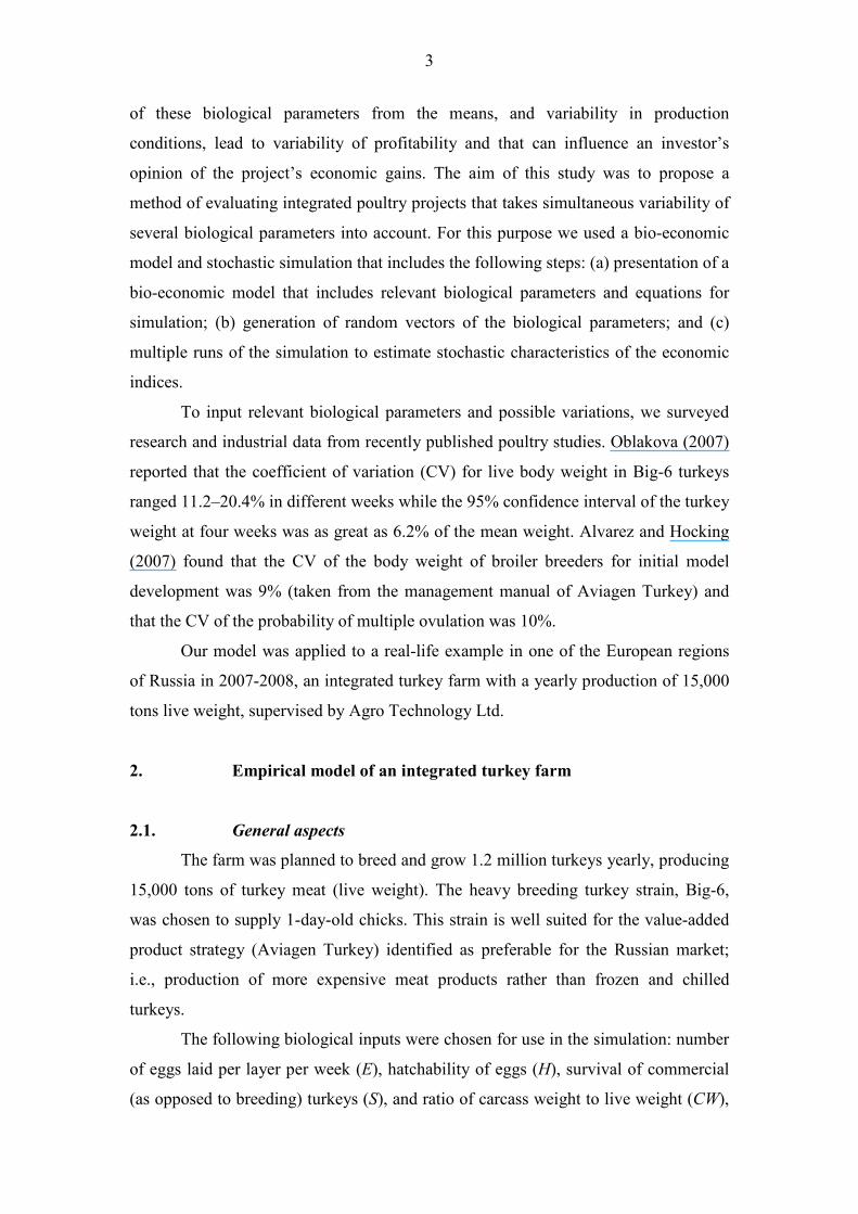
The bio-economic model was developed on an Excel worksheet with Visual

Basic modules for simulation (Fig. 1). Data tables were used to describe egg-laying

rates and feed demand during the growing and fattening periods (example: NRC,

1994). These biological processes were not linear (Fig. 2). Feeds contained about

twenty components, and the farm’s feed mill was planned for their production. Linear

programming was used to determine optimal (minimal cost) rations for breeders, for

turkeys aged 1-6 weeks, and for older turkeys. Survival was assumed to be 99.1% for

the first six weeks and 99.3% for older turkeys. The farm was planned to produce only

value-added meat products.

Two output indices were chosen to analyze the economic side of the model:

the cost of producing the turkey meat in Euro/kg, and the profitability of the

investment in percent. The cost, C, is defined as the sum of the current expenses and

depreciation of the farm divided by the quantity, Q, of meat sold:

( ) QondepreciatiexpensescurrentC /+= , (1)

Profitability, Prof, is defined as profit related to the project investment:

[ ] investmentQCpriceProf /)( −= . (2)

Quantity (Q) in Eq. (1) depends on the biological parameters. The number of

eggs laid and their hatchability determine the number of one-day-old turkeys that

leave the hatchery for the growing facilities. Survival determines the number of

turkeys that reach the meat factory. The ratio of carcass weight to live weight defines

the quantity of meat products produced from one bird. Therefore, it follows from Eq.

(1) and Eq. (2) that economic indices, production cost and profitability, depend on the

input biological parameters.

2.2. Flock dynamics and equations for simulation

The production and movement dynamics of the turkey flocks are as follows. One-day-

old chicks are purchased every ten weeks and raised for 29 weeks to produce

5

breeders. The breeders produce eggs for 27 weeks. The eggs are moved to the

hatchery for four weeks of incubation and one-day-old chicks are moved out of the

hatchery for six weeks of brooding and growing (these are ‘commercial’ chicks as

opposed to ‘breeder’ chicks). Fattening of commercial chicks lasts 13 weeks for males

and 9 weeks for females. For three units for each of the stages of breeders rearing,

eggs production, and commercial chicks brooding, there are five units for fattening

males and four for fattening females. Sanitation periods between crops last 1-3 weeks.

An integrated farm purchases breeders five times each year. We assumed that

the biological parameters of such a farm have a stochastic distribution and, for

example, a 10-year period lead to a random sample size of 50. Each realization of this

sample includes a set of input biological parameters that are stochastic by assumption,

and a set of output economic indices that are stochastic by the equations that link them

to the biological parameters. Thus, we used stochastic simulation (the method of

Monte-Carlo) to estimate mean values and standard deviations of the output economic

indices.

By running the bio-economic model many times (N runs) and obtaining values

x1,x2, …,xN of the economic index X, the usual Monte-Carlo estimates were applied:

NxxxXE N /)...()( 21 +++= for the mean value (a simple case of the law of large

numbers), and 22 ))(()()( XEXEXStDev −= for the standard deviation (Sobol,

1994, Section 1).

Simulated data from the above biological parameters were used to determine

the following: (a) production of one-day-old commercial chicks

4+=⋅⋅ ttt hicksHeadsOneDayOldCHEadsBreedersHe (3)

(b) flock dynamics for commercial turkeys

19,...,1,1 =⋅=+ tSHeadsHeads ttt (4)

and (c) production of meat products by male and female

CWesHeadsFemaloductsMeat

CWHeadsMalesoductsMeat

⋅=

⋅=

15

19

Pr

Pr (5)

where t is the number of weeks, S is survival, H is hatchability, CW is the ratio of

carcass weight to live weight, and E is the number of eggs per layer per week.

Initial values were assumed to be as follows: S = 99.1% for the first six weeks

of growing commercial turkeys and 99.3% for older turkeys, H = 80%, CW = 65%,

6

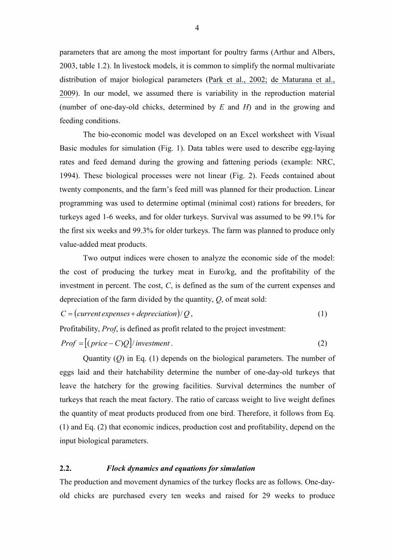
and E = 4-5 eggs for most of the period of breeders use (Fig. 2).

In every run of the computer program, the vector of coefficients

))(),(),(),(( ECoefCWCoefHCoefSCoefCoef = was generated as a multivariate

normal vector when the expected value of each of the four components equaled 1:

1))(())(())(())(( ==== ECoefECWCoefEHCoefESCoefE . Biological

parameters were simulated as follows: (a) hatchability

1)1(),( =>⋅= HTHENHIFHCoefHH init (6)

(b) number of eggs

)(, ECoefEE inittt ⋅= (7)

(c) survival

))(2()1(1 tinitt SCoefSS −⋅−−= (8)

and (d) ratio of carcass weight to live weight

)(CWCoefCWCW init ⋅= (9)

It follows from Eq. (7), Eq. (8), and Eq. (9) that expected values of Et, St, and

CW are equal their initial values. H can be less than its initial value because of the

condition added in (6), obviously, hatchability cannot be greater than 100%. In

practice, the expected H is as close to 1 as are the other parameters: for the assumed

variability of the parameters the number of runs with H >1 is too small.

2.3. Simulating vector of coefficients

To generate a multivariate normal random vector of the biological parameters we used

the algorithm based on the Cholesky decomposition of the covariance matrix (Press et

al., 1992). This algorithm has been applied in livestock industry models to simulate

joint distributions of several biological parameters. Leon-Velarde and Quiroz (2001)

used this technique to simulate lactation curves of individual cows and herds. In a

model of cattle feeding, Lambert (2008) used a similar approach to simulate how

changes in traits affected carcass value. In our study the algorithm was modeled in

three stages as follows, where the random vector of the coefficients for the four input

biological parameters was ))(),(),(),(( ECoefCWCoefHCoefSCoefCoef = .

Stage 1. The components of vector Coef are dependent variables. We have no

empirical data of their covariance matrix Σ, but this is of little importance to the

formulated question of variability in profitability resulting from simultaneous changes

7

in the biological parameters. We assumed several levels of parameter variability in

terms of matrix Σ, and tested the profitability variability for each level. Thus, for the

element 4,...1,, =jiijσ of Σ, we assumed:

4,...1,2

))(())(())(())((1

==

=+++⋅= ∑=

i

ECoefECWCoefEHCoefESCoefEn

k

ii

α

ασ (10)

For other elements of matrix Σ we assumed:

jijiiiij ≠== ,4,...1,,βσσ . (11)

Five levels of parameter variability were tested: α = 0.01, 0.025, 0.05, 0.075, and 0.1.

β = 0.75 was chosen in the model calibration as the value that leads to reasonable

variability of the biological parameters for tested α values.

Stage 2. Four independent standard normal random variables were generated

and their values comprise vector γ.

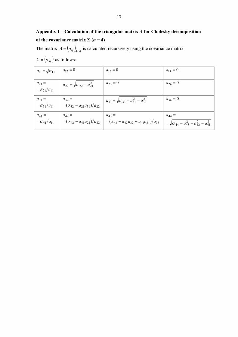
Stage 3. The covariance matrix Σ is positive-semidefinite and therefore the

Cholesky decomposition was Σ = AAT where A is a lower triangular matrix. The

elements of A can be calculated recursively using the elements of Σ (Appendix 1) and

the following expression can be used to generate vector Coef:

γγ AACoefECoef T +=+= )1,1,1,1()( (12)

3. Results and discussion

The bio-economic model was run 5000 times for every assumed value of α. In every

run, a coefficients vector (8) was generated and used in the bio-economic model to

calculate random biological parameters. For all four parameters and five levels, the

mean simulated values were very close to the initial values; the maximum deviation

was less than 0.4%. Arranging the CVs in columns enabled us to translate the chosen

variability levels into usual measures of variability (Table 1). As should follow from

Eq. (10), the CV for every biological parameter increased proportionally to level α.

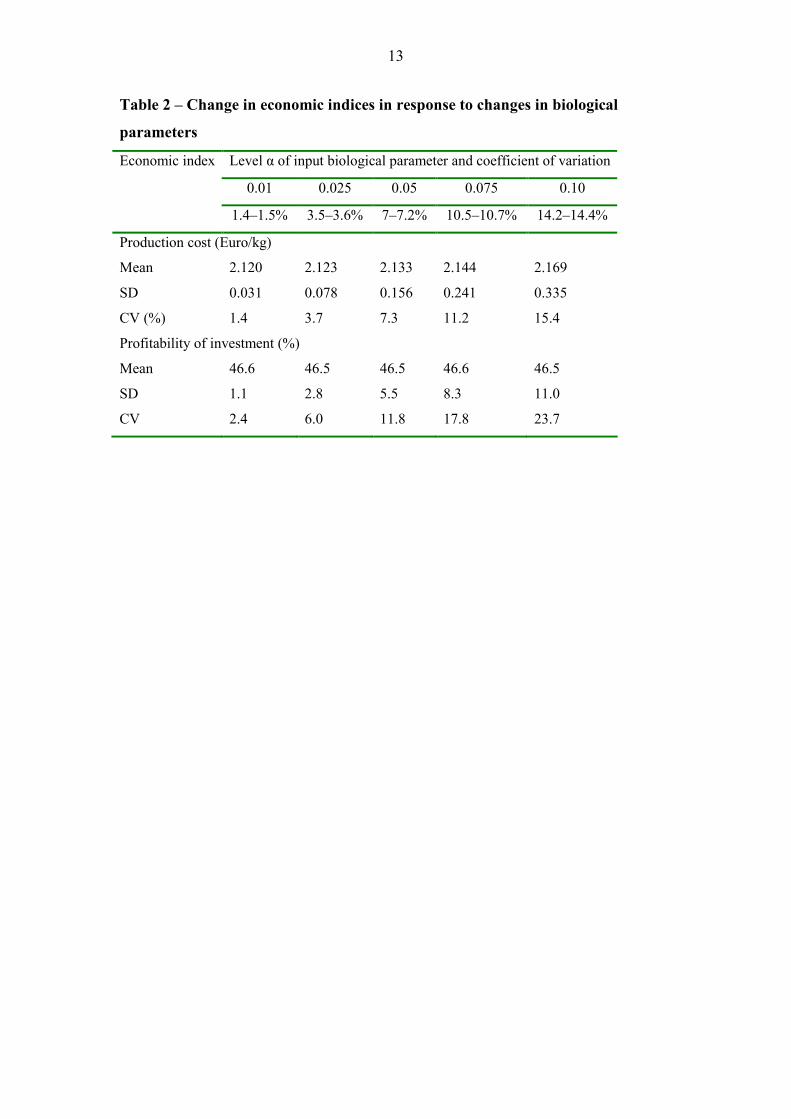
Economic indices were also close to their initial values: production cost was

2.12 Euro/kg and profitability 47% (Table 2). Changes in biological parameters led to

only slight decreases in mean cost (1-2%) and practically no change in mean

profitability. The variability of the economic indices was strongly influenced by the

variability of the biological parameters. For production cost, the CV was 100-108% of

the CV of the biological parameter; for profitability it was 163-168%. This means that

8

the variability of the economic indices, particularly profitability (a major index for

decision-making), can be much higher than the variability of the input biological

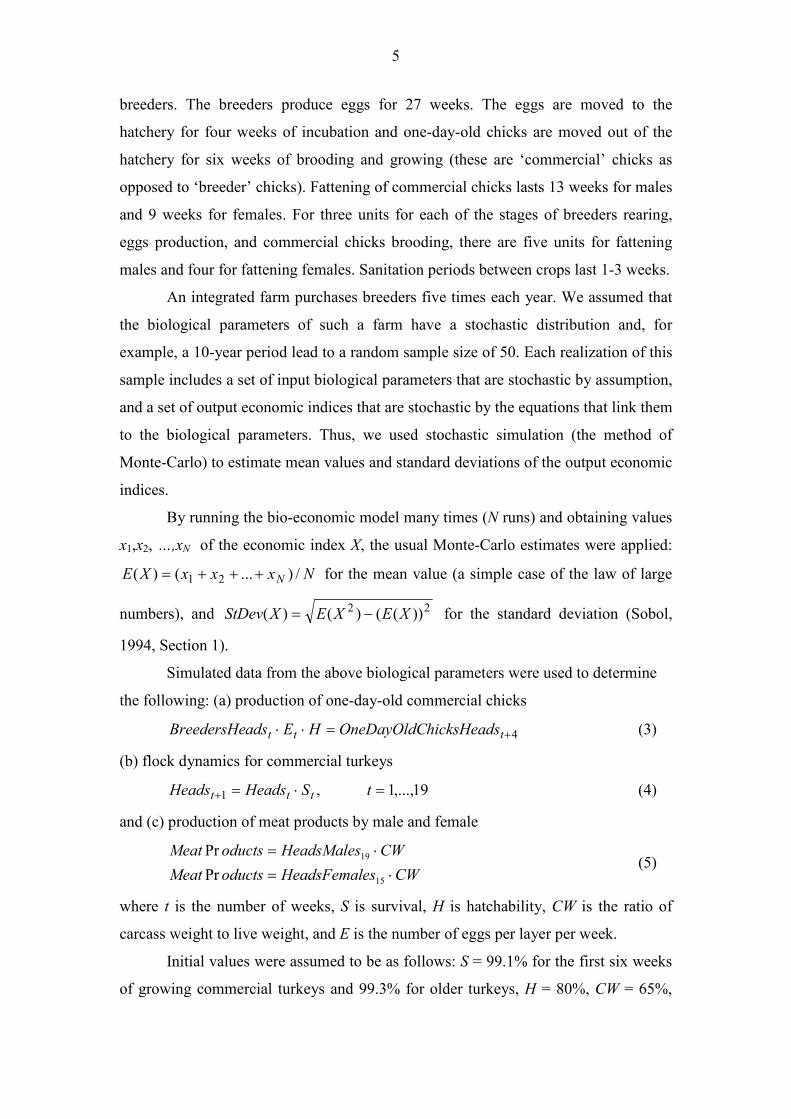
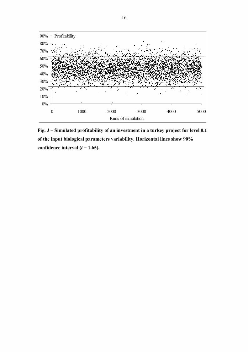
indices. The simulated profitability distribution for level 0.1 of the biological

parameters is shown in Fig. 3.

What can decision-makers conclude from Table 1 and Fig. 3 regarding project

profitability? CVs of the biological parameters account for 10.5-10.7% at the level α =

0.075. A standard deviation of 8.3% for profitability corresponds to such variability in

the biological parameters. This means that the average profitability of the project in

the evaluation period can drop below 33% ( %3.865.1%5.46 ⋅− ) with a probability of

5% at the level α = 0.075. This should be compared to the initial profitability value of

47% which does not take variability of input biological parameters into account. For

level α = 0.1 (standard deviation of the reproduction material was 14.2–14.4%), the

average profitability can drop below 28% ( %1165.1%5.46 ⋅− ) with a probability of

5%. In this way, estimates obtained from the bio-economic model can be used to

analyze economic risks in poultry projects.

Kulak et al. (2003) measured risks in a beef production model and found that

variance of profit and risk aversion attitudes of livestock producers define the

quantitative measure of risk. The main source of risk in their model was variability of

beef prices. The authors concluded that accounting for risk represents a better model

for real life; otherwise profit is overestimated. This finding is consistent with the

results of our model.

An important element of the project's evaluation is its location. In Russia, most

turkey is imported and sold as frozen turkeys. Under this condition, the high rate of

change in the business environment and insufficient producers' knowledge of the

market may discourage investment in facilities (Lorentz, 2008). Presentation of the

potential variability of economic indices can be helpful for emerging markets like that

in Russia.

4. Conclusions

A method of evaluating poultry projects that takes simultaneous variability of

input biological parameters into account is described. The bio-economic model

includes major input biological parameters related to all stages of an integrated

poultry farm, flock dynamics, equations for simulation, and a flow-chart of the

stochastic simulation algorithm. Simulation of biological parameters based on their

9

assumed multivariate normal distribution and covariance matrix enables estimation of

the variability of the output economic indices, production cost and profitability.

The method was applied to an integrated turkey farm in Russia. The variability

of the output economic indices resulting from the variability of biological parameters

was estimated: the CV of production cost was 100-108% of the CV of the input

biological parameters, and the CV of project profitability was 163-168%. Such

estimates can be used to analyze economic risks (variability in cost and profitability)

of the project.

Acknowledgements

The authors wish to thank the agricultural technologist and agronomist Ilan Sela of

Agro Technology Ltd. for useful consultation on the production methods in integrated

turkey farms.

REFERENCES

Alvarez, R., Hocking, P.M., 2007. Stochastic model of egg production in broiler

breeders. Poult. Sci. 86, 1445–1452.

Arthur, J.A., Albers, G.A.A., 2003. Industrial perspective on problems and issues

associated with poultry breeding. In: Muir, W.M., Aggrey, S.E. (Eds.), Poultry

Genetics, Breeding and Biotechnology. CABI Publishing, Wallingford, UK,

pp. 1–12.

Aviagen Turkey.

http://www.aviagen.com/output.aspx?sec=3761&con=3771&siteId=7

de Maturana, E.L., Xiao-Lin, W., Gianola, D., Weigel, K.A., Rosa, G.J.M., 2009.

Exploring biological relationships between calving traits in primiparous cattle

with a Bayesian recursive model. Genetics 181, 277–287.

Eratalar, S.A., 2007. Turkey production in Turkey. In: Hafez, H.M. (Ed.), Turkey

Production: Current Challenges. Mensch – Buch – Verlag: 8–18.

Groen, A.F., Jiang, X., Emmerson, D.A., Vereijken, A., 1998. A deterministic model

for the economic evaluation of broiler production systems. Poult. Sci. 77, 925–

933.

10

Hernes, G., 1976. Diffusion and growth: the non-homogeneous case. Scand. J. Econ.

78, 427–436.

Kulak, K., Wilton, J., Fox, G., Dekkers, J., 2003. Comparisons of economic values

with and without risk for livestock trait improvement. Livest. Prod. Sci. 79,

183–191.

Lambert, K.D., 2008. The expected utility of genetic information in beef cattle

production. Agric. Syst. 99, 44–52.

León-Velarde, C.U., and Quiroz, R. 2001. Modeling cattle production systems:

integrating components and their interactions in the development of simulation

models. In: Proceedings - Third International Symposium on Systems

Approaches for Agricultural Development, SAAD III International Potato

Center (CIP), Lima Peru. 8pp.

Lorentz, H., 2008. Production locations for the internationalising food industry: case

study from Russia. Br. Food J. 110, 310–334.

McAinsh, C.V, Kristensen, A.R., 2004. Dynamic modelling of a traditional African

chicken production system. Trop. Anim. Health Prod. 36, 609–626.

Menge, E.O., Kosgey I.S., Kahi1, A.K., 2005. Bio-economic model to support

breeding of indigenous chicken in different production systems. Int. J. Poult.

Sci. 4, 827–839.

NRC, 1994, National Research Council. Nutrient Requirements of Poultry. 9th Rev.

ed. National Academy Press, Washington, DC.

Oblakova, M., 2007. Weigth [sic] development and body configuration of turkey-

broiler parents BIG-6. Trakia J. Sci. 5, 33–39.

Park, B., Lawrence, K.C., Windham, W.R., Chen, Y.-R., Chao, K., 2002.

Discriminant analysis of dual-wavelength spectral images for classifying

poultry carcasses. Computers Electronics Agric. 33, 219–231.

Press, W.H., Flannery, B.P., Teukolsky, S.A., Vetterling, W.T., 1992. Numerical

Recipes in Pascal: The Art of Scientific Computing, 2nd ed. Cambridge

University Press. p. 350.

Sobol, I.M., 1994. A Primer for the Monte Carlo Method. CRC Press.

USDA, 2008. Livestock and Poultry, World Markets and Trade. Circular Series

DL&P 1-08, Foreign Agricultural Service, U.S. Department of Agriculture.

http://www.fas.usda.gov/dlp/circular/2008/livestock_poultry_04-2008.pdf.

11

USDA, 2009. Russian Federation - Poultry and Products - Poultry Semi-Annual

Report. GAIN Report - RS9016, Foreign Agricultural Service, U.S.

Department of Agriculture.

http://www.fas.usda.gov/gainfiles/200903/146347613.pdf.

Yom Din, G., Gilad, S., 2008. Operational Model to Support Investment Decisions in

Turkey Agribusiness. http://ssrn.com/abstract=1156756.

12

Table 1 – Statistical summary of input simulated biological parameters

Biological

parameter

Level α of input biological parameter

0.01 0.025 0.05 0.075 0.10

Mean CV* Mean CV Mean CV Mean CV Mean CV

Survival 99.22% 1.4% 99.18% 3.5% 99.19% 7.0% 99.20% 10.5% 98.84% 14.2%

Hatchability 80.01% 1.5% 80.01% 3.6% 79.88% 7.2% 79.95% 10.7% 79.90% 14.4%

Carcass wt/live

wt

65.01% 1.4% 64.99% 3.6% 64.91% 7.1% 65.03% 10.7% 64.91% 14.2%

Eggs/layer/week 4.521 1.4% 4.52 3.5% 4.516 4.2% 4.521 10.6% 4.514 14.3%

* - coefficient of variation

13

Table 2 – Change in economic indices in response to changes in biological

parameters

Economic index Level α of input biological parameter and coefficient of variation

0.01 0.025 0.05 0.075 0.10

1.4–1.5% 3.5–3.6% 7–7.2% 10.5–10.7% 14.2–14.4%

Production cost (Euro/kg)

Mean 2.120 2.123 2.133 2.144 2.169

SD 0.031 0.078 0.156 0.241 0.335

CV (%) 1.4 3.7 7.3 11.2 15.4

Profitability of investment (%)

Mean 46.6 46.5 46.5 46.6 46.5

SD 1.1 2.8 5.5 8.3 11.0

CV 2.4 6.0 11.8 17.8 23.7

14

Rearing

breedersBreeders

Output of the

model

Incubation

Brooding

and growingFattening

Feed & other

balancesProduction

Cash flowSensitivity

analysis

Flock

dynamics

Material

balances and

production

Financial

analysis for

project

evaluation

Meat

factory

S

H, S

CW

ERearing

breedersBreeders

Output of the

model

Incubation

Brooding

and growingFattening

Feed & other

balancesProduction

Cash flowSensitivity

analysis

Flock

dynamics

Material

balances and

production

Financial

analysis for

project

evaluation

Meat

factory

S

H, S

CW

E

Fig. 1 – Flow-chart of the bio-economic model. Input biological parameters

include number of eggs laid per layer per week (E), survival (S), hatchability (H),

and ratio of carcass weight to live weight (CW).

15

0

5

30 35 40 45 50 55Week

Eggs

Breeders

0

5

0 5 10 15 20

Week

Fee

d (kg)

females

males

Commercial turkeys

Fig. 2 – Number of eggs laid by breeders and feed demand for growing and

fattening commercial (not breeder) turkeys.

16

0%

10%

20%

30%

40%

50%

60%

70%

80%

90%

0 1000 2000 3000 4000 5000

Runs of simulation

Profitability

Fig. 3 – Simulated profitability of an investment in a turkey project for level 0.1

of the input biological parameters variability. Horizontal lines show 90%

confidence interval (t = 1.65).

17

Appendix 1 – Calculation of the triangular matrix A for Cholesky decomposition

of the covariance matrix Σ (n = 4)

The matrix ( )44×

= ijaA is calculated recursively using the covariance matrix

( )ijσ=Σ as follows:

1111 σ=a 012 =a 013 =a 014 =a

1121

21

a

a

σ=

=

2212222 aa −= σ 023 =a 024 =a

1131

31

a

a

σ=

=

22312132

32

)( aaa

a

−=

=

σ

232

2313333 aaa −−= σ 034 =a

1141

41

a

a

σ=

=

22214142

42

)( aaa

a

−=

=

σ

333141324243

43

)( aaaaa

a

−−=

=

σ

241

242

24344

44

aaa

a

−−−=

=

σ

18

Appendix 2 – Flow chart for the computer program of simulation

Start

End

Input: level α of

biological parameters

variability

Number of

run n = 1

Simulate random vector

Coef from Eq. 12

Run bio-

economic model

n = n+1

n < 5000

k < 5

number of level k = k+1

Number of

level k = 1

Output: economic

indices, their

characteristics

Yes

No

No

Yes

StartStart

EndEnd

Input: level α of

biological parameters

variability

Input: level α of

biological parameters

variability

Number of

run n = 1

Number of

run n = 1

Simulate random vector

Coef from Eq. 12

Simulate random vector

Coef from Eq. 12

Run bio-

economic model

Run bio-

economic model

n = n+1n = n+1

n < 5000n < 5000

k < 5k < 5

number of level k = k+1 number of level k = k+1

Number of

level k = 1

Number of

level k = 1

Output: economic

indices, their

characteristics

Output: economic

indices, their

characteristics

Yes

No

No

Yes